The Southern Westerlies during the last glacial maximum in PMIP2 simulations

The Southern Westerlies during the last glacial maximumin PMIP2 simulations

Maisa Rojas Æ Patricio Moreno Æ Masa Kageyama ÆMichel Crucifix Æ Chris Hewitt Æ Ayako Abe-Ouchi ÆRumi Ohgaito Æ Esther C. Brady Æ Pandora Hope

Received: 3 October 2007 / Accepted: 7 May 2008

� Springer-Verlag 2008

Abstract The Southern Hemisphere westerly winds are

an important component of the climate system at hemi-

spheric and global scales. Variations in their intensity and

latitudinal position through an ice-age cycle have been

proposed as important drivers of global climate change due

to their influence on deep-ocean circulation and changes in

atmospheric CO2. The position, intensity, and associated

climatology of the southern westerlies during the last gla-

cial maximum (LGM), however, is still poorly understood

from empirical and modelling standpoints. Here we analyse

the behaviour of the southern westerlies during the LGM

using four coupled ocean-atmosphere simulations carried

out by the Palaeoclimate Modelling Intercomparison

Project Phase 2 (PMIP2). We analysed the atmospheric

circulation by direct inspection of the winds and by using a

cyclone tracking software to indicate storm tracks. The

models suggest that changes were most significant during

winter and over the Pacific ocean. For this season and

region, three out four models indicate decreased wind

intensities at the near surface as well as in the upper tro-

posphere. Although the LGM atmosphere is colder and the

equator to pole surface temperature gradient generally

increases, the tropospheric temperature gradients actually

decrease, explaining the weaker circulation. We evaluated

the atmospheric influence on the Southern Ocean by

examining the effect of wind stress on the Ekman pumping.

Again, three of the models indicate decreased upwelling in

a latitudinal band over the Southern Ocean. All models

indicate a drier LGM than at present with a clear decrease

in precipitation south of 40�S over the oceans. We identify

M. Rojas (&)

Department of Geophysics,

University of Chile Blanco Encalada,

2002 Santiago, Chile

e-mail: [email protected]

M. Rojas � P. Moreno

Institute of Ecology and Biodiversity, Santiago, Chile

P. Moreno

Department of Ecological Sciences, University of Chile,

Las Palmeras, 3425 Santiago, Chile

M. Kageyama

LSCE/IPSL, UMR CEA-CNRS-UVSQ 1572, CE Saclay,

L’Orme des Merisiers Bat. 701, 91191 Gif-sur-Yvette Cedex,

France

M. Crucifix

Institut d’Astronomie et de Geophysique G. Lemaitre,

Universite catholique de Louvain, Chemin du Cyclotron,

2, 1348 Louvain-la-Neuve, Belgium

C. Hewitt

Met Office, FitzRoy Road, Exeter, Devon EX1 3PB, UK

A. Abe-Ouchi

Center for Climate System Research,

The University of Tokyo, 5-1-5 Kashiwanoha,

Kashiwa 277-8568, Japan

R. Ohgaito

Frontier Research Center for Global Change,

Japan Agency for Marine-Earth Science and Technology,

Showa-machi 3173-25, Kanazawa-ward, Yokohama,

Kanagawa 236-0001, Japan

E. C. Brady

Climate Change Research National Center for Atmospheric

Research, 1850 Table Mesa Drive, P.O. Box 3000, Boulder,

CO 80307, USA

P. Hope

Bureau of Meteorology Research Centre, GPO Box 1289,

Melbourne, VIC 3001, Australia

123

Clim Dyn

DOI 10.1007/s00382-008-0421-7

important differences in precipitation anomalies over the

land masses at regional scale, including a drier climate over

New Zealand and wetter over NW Patagonia.

1 Introduction

The behaviour of the southern westerlies and the adjacent

Southern Ocean during the last glacial maximum (LGM

21 kyr, Kyr = 1,000 calendar years before present) and the

last glacial–interglacial transition (LGIT, *18–11 kyr) is

still poorly understood despite its fundamental role on

modern hemispheric and global climate. A conceptual

palaeoclimate model by Imbrie et al. (1992) suggested that

the wind stress imparted by the westerlies on the Southern

ocean at and south of the latitude of Drake Passage (50�–

60�S) may greatly influence the global thermohaline cir-

culation during glacial terminations. They proposed that

the northward flow of surface waters forced by the stress of

the westerly winds help drive deep thermohaline currents

into the Antarctic region. Variations in this mechanism

through an ice-age cycle would be linked to the intensity

and latitudinal position of the southern westerlies (Imbrie

et al. 1992). More recently, Toggweiler et al. (2006)

developed an idealised general circulation model of the

ocean’s deep circulation and atmospheric CO2 fluxes that

addresses some key elements of glacial-interglacial tran-

sitions. Among those are CO2 cycles, the tight correlation

between atmospheric CO2 and Antarctic temperatures, the

lead of Antarctic temperatures over CO2 at terminations,

and inter-hemispheric alternations in the ocean’s d13C

minimum values. Toggweiler et al. (2006) hypothesised

that these transitions occur through a positive feedback that

involves the mid-latitude westerly winds in the Southern

Hemisphere, the mean temperature of the atmosphere, and

the overturning of southern deep water. In this scenario,

extreme glacial conditions are coupled with an equator-

ward shift of the westerlies, allowing more respired CO2 to

accumulate in the deep ocean. The opposite state, warm

interglacial climates, would be associated with a poleward

shift of the westerlies that would trigger a release of

respired CO2 out of the deep ocean via surface wind stress

(Ekman divergence) imparted by the westerlies on the

surface of the Southern ocean. Hence, tracking the ice-age

history of the southern westerlies is of fundamental

importance for understanding the origin and propagation of

palaeoclimate signals, the coupling of the ocean–atmo-

sphere in the extra-tropics, and the interaction of low- and

high-latitude climate controls on hemispheric and global

climate.

The exact timing of variations of the southern westerlies

during the LGIT, as well as the magnitude of these

variations, are a subject of active discussion (Heusser et al.

1999; Lamy et al. 1998, 1999; Moreno et al. 1999; Valero-

Garces et al. 2005), and there are important differences

between and within terrestial and marine archives.

1.1 Palaeoclimate proxies

There are a number of palaeoclimate proxies that directly

or indirectly tell us about wind speed and past precipitation

regimes. Direct proxy of wind intensity are dust records

and oceanic upwelling, whereas pollen records and varia-

tions in terrigenous supply to offshore environments could

be considered indirect proxies of wind speed. Wind

intensity affects precipitation, and in the southern hemi-

sphere extratropics the precipitation is mainly produced in

winter by fronts and low-pressure systems embedded in the

prevailing westerly circulation (e.g. Garreaud 2007). In

addition orographic rainfall is an important component of

the total precipitation in New Zealand and the southern

Andes. In these regions the existing mountain ranges exert

strong east–west dry-wet gradients. Therefore during

periods of reduced westerly flow, these east–west contrasts

may be reduced.

A recent synthesis of Palaeoclimate records from

Australia (Turney et al. 2006) spanning between 30 and

8 kyr, indicates colder conditions (DT: 9–11�C), wide-

spread desiccation of lakes, and more intense aeolian

activity during the LGM. Likewise, New Zealand records

of stalagmites are interpreted as indicative of colder and

relatively drier conditions (Williams et al. 2005) during

the LGM, contemporaneous with maximum glacial extent

in South Island (Schaefer et al. 2006), and stronger-than-

present surface wind speeds are deduced from the

enhanced deposition of aeolian Quartz (Alloway et al.

1992). A synthesis by Shulmeister et al. (2004) concludes

that the LGM was a period of enhanced westerlies

between 36� and 43�S over the Australasian sector. That

synthesis incorporates a large number of palaeoclimate

proxies, including terrestial and marine dust, upwelling,

glacial advances, ice cores and vegetation changes. Dust

records from southern Australia and New Zealand sug-

gest maximum wind speeds during the LGM, with a

modest equatorward deflection of 3�. This is of similar

magnitude to modern variability associated to ENSO

events. Around the New Zealand region there is wide-

spread evidence for increased upwelling at the LGM.

Shulmeister et al. (2004) further reports that pollen

records in southern Australia indicate colder and drier

conditions compared to present. Pollen records in New

Zealand (South Island) indicate grassland and shrubland

vegetation east of the southern Alps during the LGM,

this type of land cover are most likely linked to frost,

drought and high winds.

M. Rojas et al.: The Southern Westerlies during the last glacial maximum in PMIP2 simulations

123

In South America, the majority of palaeoclimate records

north of 42�S in the SE Pacific sector estimate an increase

and/or northward shift of the westerly belt relative to

modern conditions sometime during the LGIT. Lake cores

suggest wetter than present conditions during the LGM

(Valero-Garces et al. 2005). Twice as much precipitation

and 6�–7� colder conditions compared to present day are

inferred from a pollen records at 41�S by Moreno et al.

(1999) and Heusser et al. (1999). Proxy analysis of ter-

rigenous material found in offshore sediment cores from

central Chile (27�–33�S) (Lamy et al. 1998, 1999) suggest

increased rainfall brought by equatorward-shifted wester-

lies throughout the LGM.

Latitudinal shifts in the zone of maximum precipitation

associated with the southern westerlies in the South

American sector have been invoked as a possible cause for

the apparent mismatch in the timing and extent of glacial

advances during the LGM in different sectors of Patagonia

(39�–54�S) (Denton et al. 1999; Douglass et al. 2005;

Moreno and Leon 2003; Sugden 2005). Therefore, mod-

elling the geographic and temporal variations of the

southern westerlies during the LGM and LGIT are critical

for assessing the meaning and implications of paleocli-

matic data for reconstructing past climate dynamics at

regional and hemispheric scales.

1.2 Previous modelling studies

As described above, a consensus is emerging from the

paleoclimatic records for enhanced westerly wind speeds

and its effect on the precipitation in the SH midlatitudes,

and this evidence has helped to develop various conceptual

models for palaeoclimate change during glacial–intergla-

cial transitions (Toggweiler et al. 2006; Williams and

Bryan 2006). Yet the climate modelling studies still have

not converged into a clear picture of how and why the

changes in the westerly circulation occurred.

Most of the earlier modelling studies aimed towards

understanding the palaeoclimate evolution in the Southern

Hemisphere were carried out under the Paleoclimate

Intercomparison Project framework (PMIP1, Joussaume

et al. 1999). The experimental design of the PMIP1 sim-

ulations, for the LGM climate, included atmospheric global

circulations models forced with reduced CO2 concentra-

tion, Peltier’s (1994) ice-sheet reconstructions, and changes

in orbital parameters. For the sea-surface temperatures

(SSTs) two alternatives were given: (1) prescribed SSTs,

taken from the CLIMAP dataset (CLIMAP 1981), or (2)

computed SSTs from a slab ocean model with a prescribed

ocean heat transport.

Valdes (2000) summarised PMIP1 simulations for var-

ious time intervals (21, 15, 9 and 6 kyr) for South America.

The paper discusses several difficulties of the Paleo climate

simulations arising from this experimental design. For

South America that study mentions a caveat in PMIP1

simulations related to the inadequate representation of the

Andes Cordillera, which affects a correct treatment of

atmospheric circulation in this region. The prescribed SST

experiments showed only moderate cooling over the con-

tinents and, in particular, anomalously low temperatures,

compared to observations, over the southern tip of the

continent which would have resulted from the apparent

overestimation of sea-ice cover around Antarctica. The

models also showed a weak increase of precipitation over

the southern tip of South America, but the inter-model

variability was very large. Past changes in the westerly

circulation and the embedded storm tracks, both in the

Northern and Southern Hemispheres have been discussed

in various papers. Kageyama et al. (1999) showed that

coarse resolution models cannot represent storm tracks in

an accurate manner. Valdes (2000) reported that, for the

LGM simulations, most models showed a poleward shift of

the mean westerlies. This is consistent with results from a

higher-resolution GCM simulation by Wyrwoll et al.

(2000) that also showed a general poleward shift of the

Southern Hemisphere storm tracks. Their results, however,

show substantial regional differences, with a conspicuous

poleward shift over the Australian sector, and an equator-

ward shift in the westerlies storm tracks in the vicinity of

South America. More recent studies carried out with cou-

pled AOGCMs still show ambiguous results with respect to

the Southern Hemisphere westerly circulation, Kitoh et al.

(2001) and Shin (2003) indicate a poleward shift in the

surface westerlies, whereas a study by Kim et al. (2003)

displays an equatorward shift. Results of a newer version of

the CCSM3 model (Otto-Bliesner et al. 2006) indicates no

shift in the position of the maximum westerlies during the

LGM, but an increase in the intensity of the westerly cir-

culation, as expressed by the surface wind stress.

In this paper we present results from four simulations

conducted in the framework of the second phase of the

Palaeoclimate Modelling Intercomparison Project

(PMIP2), with identical forcings applied to all models.

These simulations were carried out by state-of-the-art

coupled GCMs, that include a dynamic ocean component,

so that the responses of sea-ice, ocean and atmosphere are

dynamically consistent, and hence it is expected that many

of the problems in the previous generation of Palaeoclimate

experiments will be addressed more appropriately. The aim

of this paper is to report on the simulated changes in these

state-of-the-art models and advance in the knowledge of a

number of basic unanswered questions that linger in the

palaeoclimate literature. These questions include: (1) Did

the southern westerlies intensify/abate their velocity during

the LGM?. (2) Did the westerlies widened, narrowed, or

shifted latitudinally during the LGM?. (3) Did the storm


123

tracks embedded in the westerlies change during the

LGM?. (4) Were changes in latitude and speed of the winds

symmetrical over the major ocean basins of the southern

Hemisphere?

Although we carried out analysis for the complete

Southern Hemisphere and the four seasons, the discussion

in the paper focuses on the summer (DJF) and winter (JJA)

seasons.

2 Models and experiments

In this study we analyse four PMIP2 (Braconnot et al.

2007) coupled ocean–atmosphere models: the Hadley

Centre HadCM3 model, the Japanese Model for Interdis-

ciplinary Research on Climate MIROC3.2.2, the National

Center for Atmospheric Research (NCAR) Community

Climate System Model version 3 (CCSM3) model, and the

Institute Pierre Simon Laplace Climate System Model,

IPSL-CM4.

All models are fully coupled and include at least the

following components: atmosphere, ocean, land surface and

sea-ice. The HadCM3 model includes the MOSES II land

surface scheme with 9 different possible surface types, a

vegetation and a sea-ice model (for more details see Hewitt

et al. 2003). The NCAR CCSM3 is a climate model whose

atmospheric component (CAM3) is a spectral model, solved

at T42 horizontal resolution. The land model uses the same

grid as the atmospheric model and specified but multiple

sub-grid land cover types (five types) and seven primary

plant functional types. The ocean component (POP model)

and the sea ice model use the same resolution, and includes

sub-grid scale ice thickness (more information about

CCSM3 can be found in Collins et al. 2006). We analysed

the medium resolution MIROC3.2.2 model, which is a fully

coupled model with the four aforementioned main compo-

nents, in addition it has a river routing model, for more

information see http://www.ccsr.u-tokyo.ac.jp/kyosei/

hasumi/MIROC/tech-repo.pdf. Finally, the IPSL-CM4

uses the LDMZ atmospheric component and ORCA for its

ocean component, it also includes a three layer sea-ice

model (snow and 2 ice layers) and a land vegetation model

with 12 plant functional types (for more information in:

http://dods.ipsl.jussieu.fr/omamce/IPSLCM4/DocIPSLCM4/

FILES/DocIPSLCM4. pdf). Table 1 gives some general

characteristics of the atmospheric and oceanic components

of these models. Results from other coupled GCMs run by

PMIP2 for the LGM, with the required data, were not

available for us at the time of this analysis.

We assessed the performance of all models using a control

period, defined as Pre Industrial (PI) climate conditions, and

LGM boundary conditions. The PMIP2 forcing of the LGM

simulations includes the following three sources: changes in

orbital parameters, differences in greenhouse gases con-

centrations, as well as different to present continental ice-

sheet distribution, coastlines and topography. The ICE-5G

ice-sheet reconstruction by Peltier (2004) is used as bound-

ary condition with the corresponding changes in land-sea

mask. However, vegetation remains unchanged relative to

the control simulation. More information on the basic setup

for these experiments can be found on the PMIP2 webpage

(http://pmip2.lsce.ipsl.fr/).

The simulations for both experiments were run for

long enough to allow the atmosphere and oceans reach

quasi-equilibrium state to the specified boundary condi-

tions and for trends to become small. For the LGM

simulations HadCM3 started from the cold state of a

previous coupled LGM simulation, whereas MIROC3.2.2

was initialised from modern conditions. CCSM3 uses a

PI state to start the atmospheric component, whereas the

ocean is initialised by applying the anomalies from a

previous LGM simulation. IPSL-CM4 started from the

Levitus conditions of a number of parameters (tempera-

ture, salinity, oxygen, etc) for the ocean (Levitus 1994

World Ocean Atlas) and an atmospheric state from a

previous atmospheric GCM experiment. In this simula-

tion, the deep ocean has not achieved complete

equilibrium but the atmosphere and upper ocean char-

acteristics are stable. We analysed the final 30–100 years

of each simulation.

All variables used in this paper were monthly mean data,

except for the evaluation of the storm tracks. For this we

used daily sea level pressure data. Several indicators are

commonly used to evaluate synoptic variability and asso-

ciated storm tracks. In this study, we use a cyclone-tracking

software that follows surface low pressure systems. The

cyclone-tracking scheme was developed and implemented

by Simmonds and Keay (2000), and references therein. In

this scheme latitude–longitude data are transformed to a

polar stereographic array centred around the pole (South

Table 1 PMIP2 coupled

ocean–atmosphere models

employed in this analysis

Model name Atmosphere

res lon 9 lat

Vertical

levels

Ocean

lon 9 lat

Vertical

levels

Years used

in analysis

HadCM3M2 3.75 9 2.5 19 1.25 9 1.25 19 100

MIROC3.2.2 2.8 9 2.8 20 1.4 9 1.4 43 30

CCSM3.0 ver beta14 1.4 9 1.4 26 *1 9 1 40 30

IPSL-CM4v1 3.75 9 2.5 19 2.4 9 2.4 cos/ 31 100


123

http://www.ccsr.u-tokyo.ac.jp/kyosei/hasumi/MIROC/tech-repo.pdf.

http://www.ccsr.u-tokyo.ac.jp/kyosei/hasumi/MIROC/tech-repo.pdf.

http://dods.ipsl.jussieu.fr/omamce/IPSLCM4/DocIPSLCM4/FILES/DocIPSLCM4. pdf

http://dods.ipsl.jussieu.fr/omamce/IPSLCM4/DocIPSLCM4/FILES/DocIPSLCM4. pdf

http://pmip2.lsce.ipsl.fr/

Pole in this case). The low-finding routine tries to locate

the position of the associated pressure minimum by itera-

tive approximations. Full details are discussed in

Simmonds and Murray (1999) and Simmonds et al. (1999).

3 Results

In this section we evaluate simulated temperature, sea level

pressure, circulation, storm tracks, and precipitation. First,

we assess the models performance against present day

atmospheric reanalysis data (1961–1990 mean), and then

we present differences between the LGM and control

simulations. Although the control simulations were forced

with PI greenhouse gas concentration, we will evaluate

these runs with present day climatology for the remainder

of the paper.

3.1 Temperature

Seasonal mean summer and winter surface air temperatures

were compared with those from the NCEP/NCAR reanal-

ysis (Kalnay et al. 1996), and shown in Fig. 1. All models

show a cold bias over most grid points of the southern

a

b

c

d

e

f

g

h

i

j

Fig. 1 Present day seasonal mean surface temperature fields for summer (left column) and winter (right column). From reanalysis (top row) and

four models


123

oceans (ranging from 1� to 5�) in both seasons. Over the

land masses the biases are less uniform and are season

dependent, for example in summer (DJF) all models exhibit

a cold bias over most of Australia (-2� to -3�) and Ant-

arctica (-5� to -8�). Over South America, HadCM3 and

IPSL simulate warmer temperatures (over 3�). In winter all

models have a considerable warm bias over Antarctica (5�–

8�), the western coast of South America (3�–5�) and parts

of southern Africa (3�–5�), whereas Australia is well sim-

ulated. Although all models have biases in the surface

temperatures, CCSM3 simulates largest and most uni-

formly colder temperatures compared to reanalysis over the

southern ocean in summer and winter.

The above atmospheric surface temperature biases

reflect similar biases in the underlying SSTs. Modelled

SSTs were compared with a climatological SST dataset

(Reynolds and Smith 1994, not shown). In summer and

winter three models (except HadCM3) show a negative

SST bias over most of the oceans, north of 50�S, and a

positive bias at the western coast of Africa and South

America, indicating that the upwelling regions are not well

captured by the models. In summer all models, except

CCSM3, simulate warmer SSTs around Antarctica. Overall

HadCM3 tends to simulate a warmer Southern Ocean

compared to observations.

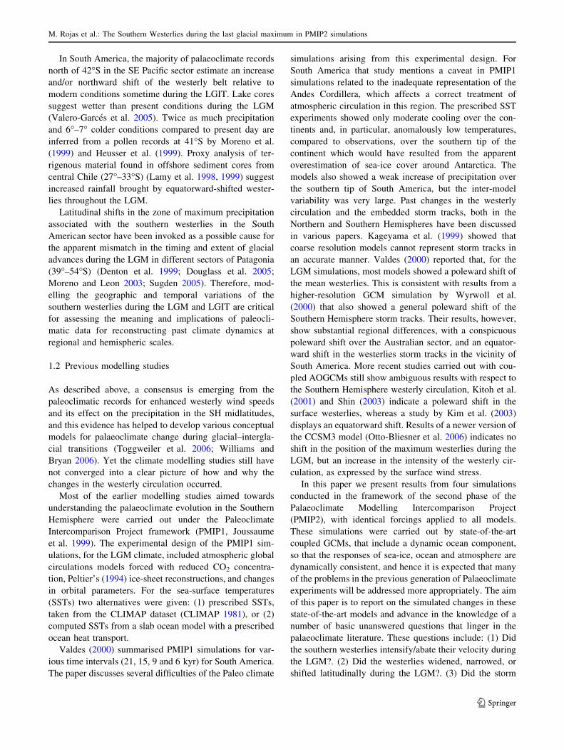
The geographic distribution of the seasonal mean sur-

face temperature changes between the LGM and present

are shown in Fig. 2. For each model the seasonal differ-

ences between the LGM and PI simulations of summer and

winter are shown. As expected, all models simulate, to

different degrees, a colder climate for all seasons. The red

and blue lines on the figures indicate the position of the

area covered by 80% of sea-ice for PI and LGM, respec-

tively. Next to each panel of temperature difference are

profiles of the zonal mean meridional temperature gradient

from 80�N to 80�S. Largest cooling is seen in the winter

season over Antarctica and the surrounding oceans, which

were covered by extensive sea-ice during the LGM (see

blue lines in Fig. 2). Of the four models, CCSM3 produces

the largest cooling, ranging from 3� to 5�C over the con-

tinents (Australia and Southern South America) to over

15�C over Antarctica. IPSL simulates the least cooling, and

mainly over the continents, similar to MIROC3.2.2. The

surface temperature and sea-ice changes are consistent.

From the four models, CCSM3 simulates the largest sea-ice

cover extent during the LGM, and IPSL the minimum.

a

b

c

d

e

f

g

h

a

Fig. 2 Seasonal mean surface temperature changes LGM-PI for

summer (left panels) and winter (right panels) of the four models. The

red and blue lines represents the position of the 80% sea-ice cover

during PI and LGM, respectively. The profiles at the right of each

panel correspond to the zonal mean meridional surface temperature

gradient, from 80�N to 80�S. Red line for PI and blue for LGM


123

Temperature changes are strongest at high latitude over

land or sea-ice, but there is much less polar amplification of

the cooling than for the northern hemisphere (Braconnot

et al. 2007). In fact, over much of the ocean the tempera-

ture changes are rather homogeneous (except for CCSM3).

So, the meridional temperature gradients that are a driver

of the atmospheric circulation should not change a lot

(compared to the northern hemisphere), as seen in the

profiles of Fig. 2, except south of about 70�S and hence the

circulation main structures should be quite stable. Finally, a

large sensitivity in the sea-ice response, in an already cold

CCSM3 model, can probably partly explain the large

temperature and sea-ice cover response to the LGM forc-

ings in this model.

3.2 Sea level pressure

We found considerable changes in sea level pressure

(SLP), associated to changes in surface temperature and

sea-ice cover during the LGM. Figure 3 shows the seasonal

mean SLP for summer (DJF) and winter (JJA) from

reanalysis (top panels) and the PI simulations of the four

models. In general terms, the subtropical anticyclones are

well simulated in their intensity and position in all four

a

b

c

d

e

f

g

h

i

j

Fig. 3 Present day seasonal mean sea level pressure fields for summer (left column) and winter (right column). From reanalysis (top row) and

four models


123

models. HadCM3, MIROC3.2.2 and CCSM3 simulate a

more intense circumpolar trough between 40� and 50�S

with larger SLP gradients. IPSL simulates a weaker and

less circumpolar trough and exhibits anomalously high

pressure fields over Antarctica compared to reanalysis.

HadCM3 simulates weaker anticyclones in all seasons

(about 5 hPa lower).

For the LGM, HadCM3, MIROC3.2.2 and IPSL simu-

late higher SLP values in all seasons over the Southern

Hemisphere, with the largest differences occurring during

summer over Antarctica. CCSM3 shows the opposite pat-

tern, with a large decrease in SLP over the southern oceans

and Antarctica (not shown).

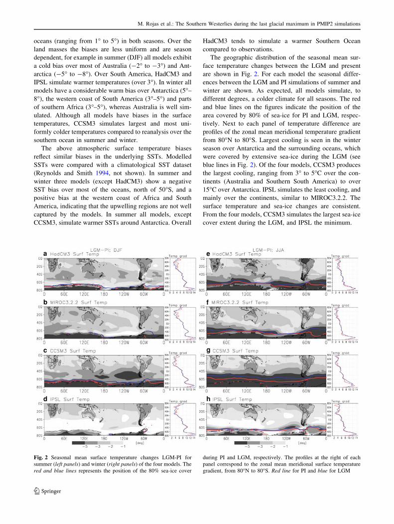
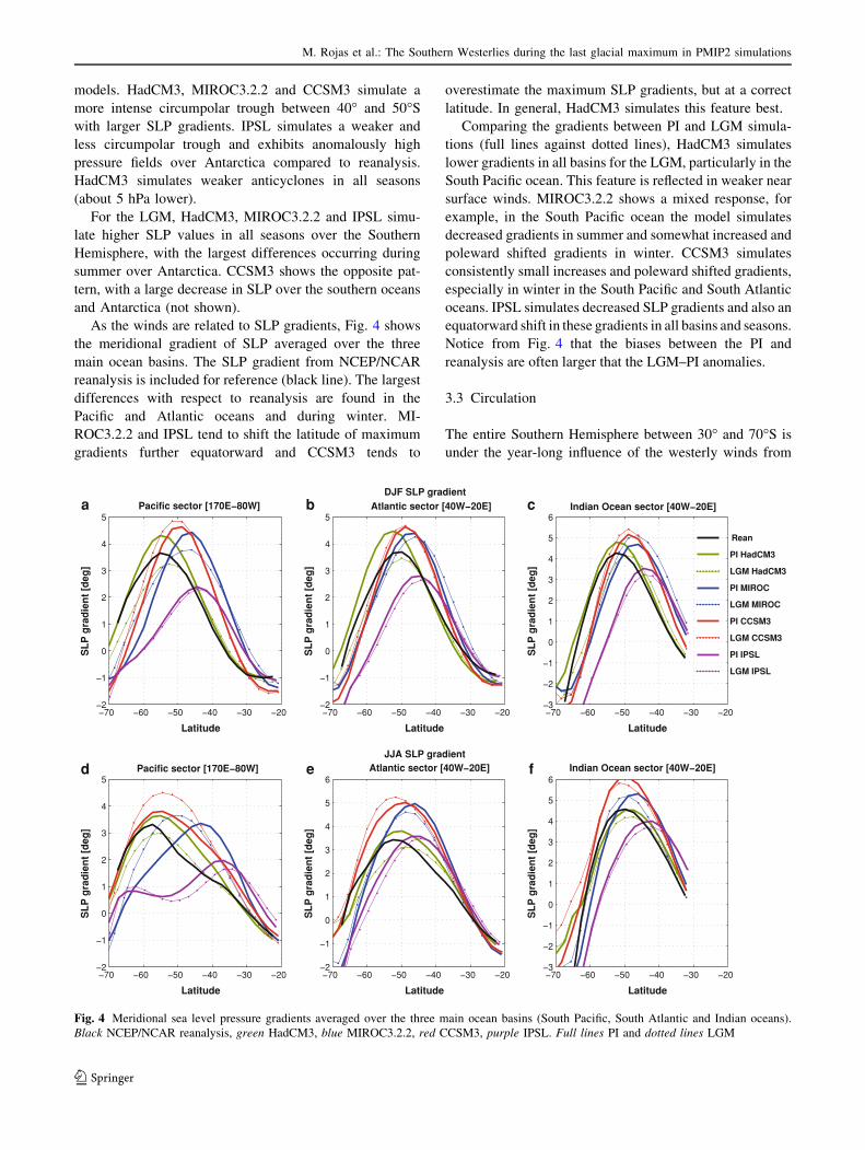
As the winds are related to SLP gradients, Fig. 4 shows

the meridional gradient of SLP averaged over the three

main ocean basins. The SLP gradient from NCEP/NCAR

reanalysis is included for reference (black line). The largest

differences with respect to reanalysis are found in the

Pacific and Atlantic oceans and during winter. MI-

ROC3.2.2 and IPSL tend to shift the latitude of maximum

gradients further equatorward and CCSM3 tends to

overestimate the maximum SLP gradients, but at a correct

latitude. In general, HadCM3 simulates this feature best.

Comparing the gradients between PI and LGM simula-

tions (full lines against dotted lines), HadCM3 simulates

lower gradients in all basins for the LGM, particularly in the

South Pacific ocean. This feature is reflected in weaker near

surface winds. MIROC3.2.2 shows a mixed response, for

example, in the South Pacific ocean the model simulates

decreased gradients in summer and somewhat increased and

poleward shifted gradients in winter. CCSM3 simulates

consistently small increases and poleward shifted gradients,

especially in winter in the South Pacific and South Atlantic

oceans. IPSL simulates decreased SLP gradients and also an

equatorward shift in these gradients in all basins and seasons.

Notice from Fig. 4 that the biases between the PI and

reanalysis are often larger that the LGM–PI anomalies.

3.3 Circulation

The entire Southern Hemisphere between 30� and 70�S is

under the year-long influence of the westerly winds from

−70 −60 −50 −40 −30 −20−2

−1

0

1

2

3

4

5

SL

P g

rad

ien

t [d

eg]

Latitude

a

−70 −60 −50 −40 −30 −20−2

−1

0

1

2

3

4

5

SL

P g

rad

ien

t [d

eg]

Latitude

b DJF SLP gradient

−70 −60 −50 −40 −30 −20−3

−2

−1

0

1

2

3

4

5

6S

LP

gra

die

nt

[deg

]

Latitude

c

Rean

PI HadCM3

LGM HadCM3

PI MIROC

LGM MIROC

PI CCSM3

LGM CCSM3

PI IPSL

LGM IPSL

−70 −60 −50 −40 −30 −20−2

−1

0

1

2

3

4

5

SL

P g

rad

ien

t [d

eg]

Latitude

d

−70 −60 −50 −40 −30 −20−2

−1

0

1

2

3

4

5

6

SL

P g

rad

ien

t [d

eg]

Latitude

e JJA SLP gradient

−70 −60 −50 −40 −30 −20−3

−2

−1

0

1

2

3

4

5

6

SL

P g

rad

ien

t [d

eg]

Latitude

f

Pacific sector [170E−80W]

Pacific sector [170E−80W] Atlantic sector [40W−20E]

Atlantic sector [40W−20E] Indian Ocean sector [40W−20E]

Indian Ocean sector [40W−20E]

Fig. 4 Meridional sea level pressure gradients averaged over the three main ocean basins (South Pacific, South Atlantic and Indian oceans).

Black NCEP/NCAR reanalysis, green HadCM3, blue MIROC3.2.2, red CCSM3, purple IPSL. Full lines PI and dotted lines LGM


123

the surface to the tropopause. In the upper troposphere, the

westerlies structure around the subtropical jet stream (STJ)

and the subpolar jet stream (SPJ), both with distinct sea-

sonal evolution in extent and strength, as well as vertical

structure. Figure 5 shows the seasonal mean zonal winds at

the near surface (925 hPa) for summer (left panels) and

winter (right panels) from NCEP/NCAR reanalysis (top

row) and the four models, for reference, the blue line

represent the latitude of maximum wind speed of the

NCEP/NCAR reanalysis.

Reanalysis DJF

0 60E 120E 180 120W 60W 0 80S

60S

40S

20S

EQReanalysis JJA

u−wind at 925hPaa

b

c

d

e

f

g

h

i

j

0 60E 120E 180 120W 60W 080S

60S

40S

20S

EQ

HadCM3 DJF PI

0 60E 120E 180 120W 60W 0 80S

60S

40S

20S

EQHadCM3 JJA PI

0 60E 120E 180 120W 60W 080S

60S

40S

20S

EQ

MIROC3.2.2 DJF PI

0 60E 120E 180 120W 60W 0 80S

60S

40S

20S

EQMIROC3.2.2 JJA PI

0 60E 120E 180 120W 60W 080S

60S

40S

20S

EQ

CCSM3 DJF PI

0 60E 120E 180 120W 60W 0 80S

60S

40S

20S

EQCCSM3 JJA PI

0 60E 120E 180 120W 60W 080S

60S

40S

20S

EQ

IPSL DJF PI

0 60E 120E 180 120W 60W 0 80S

60S

40S

20S

EQIPSL JJA PI

[m/s]

0 60E 120E 180 120W 60W 080S

60S

40S

20S

EQ

6 99 1212 15

Fig. 5 Zonal winds at 925 hPa. Top rows from NCEP/NCAR reanalysis, following rows of the four models, during summer (left panels) and

winter (right panels). Black line latitude of maximum wind speed, blue line latitude of maximum wind speed from NCEP/NCAR reanalysis


123

Near surface westerly winds are present between 30�and 70�S, with strongest winds centred at around 50�S.

This band of the westerly winds corresponds to the near

surface extent of the SPJ that has its core region at higher

altitudes. Strongest winds are present over the South

Atlantic and Indian oceans and weakest over the South

Pacific ocean. The annual cycle over the South Atlantic and

Indian oceans is marked by a maximum in autumn (SON)

and winter (JJA) and minimum during summer (DJF). Over

the Pacific ocean the maximum occurs in spring (SON) and

summer (DJF) and the minimum in winter (JJA).

Figure 6 shows the same as Fig. 5, but for 200 hPa. The

upper tropospheric winds are dominated by both the STJ

and SPJ streams. The core region of the STJ is located over

a Reanalysis DJF

0 60E 120E 180 120W 60W 0 80S

60S

40S

20S

EQf Reanalysis JJA

u−wind at 200hPa

0 60E 120E 180 120W 60W 080S

60S

40S

20S

EQ

b HadCM3 DJF PI

0 60E 120E 180 120W 60W 0 80S

60S

40S

20S

EQg HadCM3 JJA PI

0 60E 120E 180 120W 60W 080S

60S

40S

20S

EQ

c MIROC3.2.2 DJF PI

0 60E 120E 180 120W 60W 0 80S

60S

40S

20S

EQh MIROC3.2.2 JJA PI

0 60E 120E 180 120W 60W 080S

60S

40S

20S

EQ

d CCSM3 DJF PI

0 60E 120E 180 120W 60W 0 80S

60S

40S

20S

EQi CCSM3 JJA PI

0 60E 120E 180 120W 60W 080S

60S

40S

20S

EQ

e IPSL DJF PI

0 60E 120E 180 120W 60W 0 80S

60S

40S

20S

EQj IPSL JJA PI

[m/s]

0 60E 120E 180 120W 60W 080S

60S

40S

20S

EQ

20 3030 4040 50

Fig. 6 Same as Fig. 5 but for 200 hPa


123

Australia and the western South Pacific ocean. The STJ has

a marked annual cycle, having its maximum strength in

JJA and almost disappearing in DJF. In contrast the annual

cycle of the SPJ exhibits more modest changes, it is most

intense and circumpolar in summer, when it is the domi-

nant jet in the Southern Hemisphere, and weakened during

winter and spring. As to the longitudinal extent, its core

region is over the South Atlantic and Indian oceans at

*50�S. During winter, when the STJ intensifies north of

the SPJ the well known double jet structure in the upper

troposphere develops over the Indian and South Pacific

oceans.

In Fig. 5 three models, except HadCM3, simulate the

position of the maximum wind speed further equatorward

than reanalysis, especially during winter (right panels).

Additionally, the intensity is overestimated by the models,

except IPSL, especially over the Indian ocean. At 200 hPa

(Fig. 6) MIROC3.2.2, CCSM3 and IPSL fail to reproduce

the double jet structure over the Pacific ocean in winter,

underestimating the subpolar jet. The simulation of the

subtropical jet is well captured by the models, IPSL

overestimates the jet speed. In summer all models over-

estimate the SPJ and all, except HadCM3, shift the core of

the jet further equatorward (40�–45�S instead of 50�S).

HadCM3 reproduces the near surface and upper tropo-

spheric circulation the best.

With respect to the circulation biases in the models, we

note that for instance the equatorward bias in maximum

near surface winds in the models are consistent with the

equatorward shift in the maximum SLP gradients seen in

Fig. 4. The biases in the upper level circulation can be

explained by the tropospheric thermal structure in the

models. Through the thermal wind equation the vertical

wind gradient (i.e. jets) is related to the meridional tem-

perature gradients. The Southern Hemisphere tropospheric

temperatures, as seen in reanalysis, show strong gradients

south of 70�S all year long (not shown). In addition,

maximum gradients are found throughout the troposphere

between 30� and 50�S. The maximum gradients vary

throughout the year and, depending on the region, in a

similar way as the already described evolution of the SPJ

and STJ. Inspection of the temperature structure in the

models and comparison with reanalysis (not shown) show a

clear correspondence between the position and intensity of

the temperature gradients, and the position and intensity of

the SPJ and STJ.

When comparing the PI and LGM simulations in Figs. 7

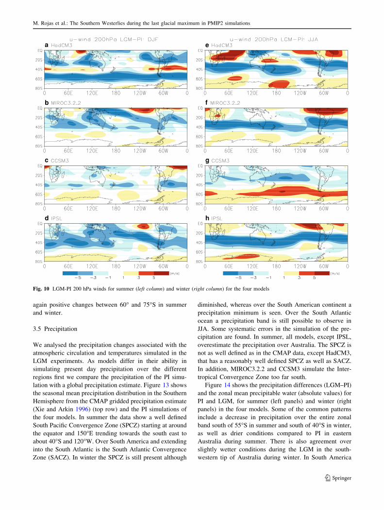
and 8 (as well as in Figs. 9, 10, that show the difference

fields), it is evident that the overall position and annual

cycle of the maximum wind speeds do not change signif-

icantly. Only HadCM3 shows a modest general

equatorward shift at the LGM in summer at both levels

(compare black against red lines), and IPSL simulates a

slight equatorward shift at the near surface in both seasons

and a poleward shift in the upper troposphere over the

south Pacific ocean.

Figures 9 and 10 show the differences between the

LGM and PI simulations of the seasonal mean near sur-

face and upper level zonal winds for the four models,

respectively. In winter, these figures show that, three out

of four models, indicate a decrease in the strength of the

winds at 200 hPa (SPJ and STJ), as well as at the near

surface. The exception is CCSM3, that shows a intensi-

fication of the SPJ and winds at the near surface. For the

summer season the observed changes are smaller, but

with a clear weakening of the SPJ. The stronger winds in

CCSM3 are coherent with the larger SLP gradients sim-

ulated by the model in this region (Fig. 4) and the larger

surface temperature and sea-ice response to LGM condi-

tions. These features produce a larger meridional

temperature gradient than in the other models (see profiles

in Fig. 2). The other three models simulate decreased SLP

gradients that are consistent with a weakened near surface

circulation. Again, inspection of the tropospheric tem-

perature reveals that, although there is an overall cooling

of the troposphere in the models, this cooling does not

increase the temperature gradients, as seen in zonal pro-

files of Fig. 2. HadCM3, MIROC3.2.2 and IPSL illustrate

this point by showing a decrease in SLP gradients and

weakened atmospheric circulation. One exception is the

atmosphere south of 70�S, where the already large tem-

perature gradients in the PI simulations are further

enhanced in all LGM simulations.

Most noticeable in Fig. 9 is that the magnitude of the

observed changes in near surface circulation are larger in

winter than in summer, except in HadCM3, that shows

significant differences in both seasons. During winter there

are important regional heterogeneities, so that largest

changes occur over the Pacific ocean. More specifically, for

the winter season, HadCM3, MIROC3.2.2 and IPSL show

similar patterns in the difference fields. The zonal band

between 40� and 60�S shows decreased westerly winds in

the LGM compared to PI, especially in the South Pacific

region, and stronger winds north of 35�S in the same

region. CCSM3 simulates the opposite pattern. In summer,

HadCM3 shows a very longitudinally homogeneous band

between 45� and 60�S of decreased westerly winds, and

stronger winds north of this band. This is also seen, to a

lesser degree in IPSL. The other models show less zonally

symmetric patterns. MIROC3.2.2 and CCSM3 indicate

somewhat stronger winds in a zonal band between 50� and

70�S.

At 200 hPa (Fig. 10) in summer, HadCM3 simulates a

zonal band of weaker winds in the SPJ region (50�–60�S)

and a narrow band of stronger winds north and south of

this latitude. The other models show a less clear pattern,


123

with somewhat stronger winds from about 60� to 70�S

and weaker north of this latitude. For winter HadCM3,

MIROC3.2.2 and IPSL tend to agree, as for the low level

winds, with decreased westerly flow in the zonal band 20�and 50�S, CCSM3, shows decreased winds north of 40�S

and a strong increase south of this latitude, especially

over the Pacific ocean. We note that the patterns of the

difference fields arises from a general decrease or increase

of wind strength rather than a significant shift (either

equator or poleward) of the core of the jet streams or

latitude of maximum wind speeds, as discussed

previously.

a HadCM3 DJF LGM

0 60E 120E 180 120W 60W 0 80S

60S

40S

20S

EQe HadCM3 JJA LGM

u−wind at 925hPa

0 60E 120E 180 120W 60W 080S

60S

40S

20S

EQ

b MIROC3.2.2 DJF LGM

0 60E 120E 180 120W 60W 0 80S

60S

40S

20S

EQf MIROC3.2.2 JJA LGM

0 60E 120E 180 120W 60W 080S

60S

40S

20S

EQ

c CCSM3 DJF LGM

0 60E 120E 180 120W 60W 0 80S

60S

40S

20S

EQg CCSM3 JJA LGM

0 60E 120E 180 120W 60W 080S

60S

40S

20S

EQ

d IPSL DJF LGM

0 60E 120E 180 120W 60W 0 80S

60S

40S

20S

EQh IPSL JJA LGM

[m/s]

0 60E 120E 180 120W 60W 080S

60S

40S

20S

EQ

6 99 1212 15

Fig. 7 LGM zonal winds at 925 hPa of the four models during summer (left panels) and winter (right panels). Black line latitude of maximum

wind speed from PI simulation. Red line latitude of maximum wind speed of LGM simulation


123

3.4 Storm tracks

Atmospheric variability responsible for much of the

weather in the midlatitudes arises primarily from the pas-

sage of cyclones and anticyclones and their associated

frontal systems. Consequently, past changes in the westerly

storm tracks bear on precipitation changes during the

LGM, as most of the winter precipitation in midlatitudes is

of frontal origin. This is the case in western South America,

the southern limit of Australia, and New Zealand in winter.

In addition, orographic features enhance the precipitation

in western Patagonia and the western slopes of New Zea-

land’s south Island. In the Southern Hemisphere these

systems are embedded in the westerly flow, and they are

a HadCM3 DJF LGM

0 60E 120E 180 120W 60W 0 80S

60S

40S

20S

EQe HadCM3 JJA LGM

u−wind at 200hPa

0 60E 120E 180 120W 60W 080S

60S

40S

20S

EQ

b MIROC3.2.2 DJF LGM

0 60E 120E 180 120W 60W 0 80S

60S

40S

20S

EQf MIROC3.2.2 JJA LGM

0 60E 120E 180 120W 60W 080S

60S

40S

20S

EQ

c CCSM3 DJF LGM

0 60E 120E 180 120W 60W 0 80S

60S

40S

20S

EQg CCSM3 JJA LGM

0 60E 120E 180 120W 60W 080S

60S

40S

20S

EQ

d IPSL DJF LGM

0 60E 120E 180 120W 60W 0 80S

60S

40S

20S

EQh IPSL JJA LGM

[m/s]

0 60E 120E 180 120W 60W 080S

60S

40S

20S

EQ

20 3030 4040 50

Fig. 8 Same as Fig. 7 but for 200 hPa


123

expected to differ between the LGM and present, as a

consequence of changes in the mean westerly circulation

discussed in the previous section.

First, we used daily sea level pressure data to track

cyclones during the 30 year period of the control simula-

tions and compared those results with the cyclone density

found in NCEP/NCAR reanalysis sea level pressure. Fig-

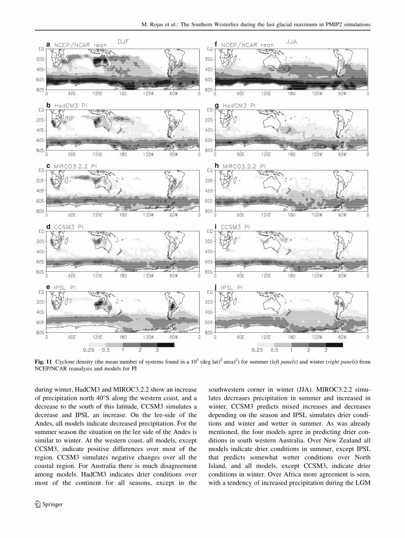
ure 11 shows the seasonal mean cyclone density (the mean

number of systems found in a 103 (deg lat)2 area) for the

Southern Hemisphere found by the tracking software in

30 years of daily SLP data, for summer (left panels) and

winter (right panels) from the NCEP/NCAR reanalysis (top

row) and the four models. The figure shows the well known

maximum density at high latitudes. In winter, when zonal

asymmetries are largest, a secondary storm track at mid-

latitudes is especially pronounced in the Pacific sector. The

top row of this figure can be compared with Fig. 4 from

Simmonds and Keay (2000), where they used 6-hourly

ERA-40 data.

Comparing the models with the observations in Fig. 11,

the first we observe is that the models simulate smaller

cyclone density than the observations. Disregarding this

bias, we see that HadCM3 annual density as well as the

seasonal densities compares best with the NCEP/NCAR

reanalysis. The highest density is found around Antarctica

with maximum values in the Atlantic and Indian oceans.

The density by seasons also reproduce the more symmetric

summer activity (DJF) and the more zonally asymmetric

winter season (JJA) with higher cyclone activity in the

midlatitudes of the Australian and Pacific ocean sectors.

The other three models tend to underestimate the second-

ary, midlatitude storm track present during winter over

the Pacific ocean. Additionally, IPSL simulates the

primary circumpolar storm track further equatorward than

reanalysis.

After this first analysis we applied the cyclone tracking

procedure to calculate the cyclone tracks for the LGM

simulations. The differences between LGM and PI system

density are shown in Fig. 12. Overall there are not many

common patterns in the difference field. Except over the

Pacific ocean, where we see positive changes between 30�and 45�S, negative changes between 50� and 60�S, and

a e

f

g

h

b

c

d

Fig. 9 LGM-PI 925 hPa winds for summer (left column) and winter (right column) for the four models


123

again positive changes between 60� and 75�S in summer

and winter.

3.5 Precipitation

We analysed the precipitation changes associated with the

atmospheric circulation and temperatures simulated in the

LGM experiments. As models differ in their ability in

simulating present day precipitation over the different

regions first we compare the precipitation of the PI simu-

lation with a global precipitation estimate. Figure 13 shows

the seasonal mean precipitation distribution in the Southern

Hemisphere from the CMAP gridded precipitation estimate

(Xie and Arkin 1996) (top row) and the PI simulations of

the four models. In summer the data show a well defined

South Pacific Convergence Zone (SPCZ) starting at around

the equator and 150�E trending towards the south east to

about 40�S and 120�W. Over South America and extending

into the South Atlantic is the South Atlantic Convergence

Zone (SACZ). In winter the SPCZ is still present although

diminished, whereas over the South American continent a

precipitation minimum is seen. Over the South Atlantic

ocean a precipitation band is still possible to observe in

JJA. Some systematic errors in the simulation of the pre-

cipitation are found. In summer, all models, except IPSL,

overestimate the precipitation over Australia. The SPCZ is

not as well defined as in the CMAP data, except HadCM3,

that has a reasonably well defined SPCZ as well as SACZ.

In addition, MIROC3.2.2 and CCSM3 simulate the Inter-

tropical Convergence Zone too far south.

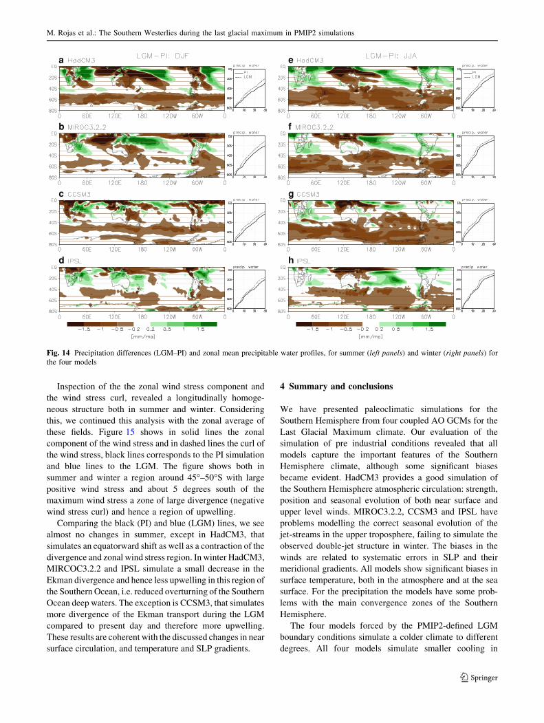
Figure 14 shows the precipitation differences (LGM–PI)

and the zonal mean precipitable water (absolute values) for

PI and LGM, for summer (left panels) and winter (right

panels) in the four models. Some of the common patterns

include a decrease in precipitation over the entire zonal

band south of 55�S in summer and south of 40�S in winter,

as well as drier conditions compared to PI in eastern

Australia during summer. There is also agreement over

slightly wetter conditions during the LGM in the south-

western tip of Australia during winter. In South America

a

b

c

d

e

f

g

h

Fig. 10 LGM-PI 200 hPa winds for summer (left column) and winter (right column) for the four models


123

during winter, HadCM3 and MIROC3.2.2 show an increase

of precipitation north 40�S along the western coast, and a

decrease to the south of this latitude, CCSM3 simulates a

decrease and IPSL an increase. On the lee-side of the

Andes, all models indicate decreased precipitation. For the

summer season the situation on the lee side of the Andes is

similar to winter. At the western coast, all models, except

CCSM3, indicate positive differences over most of the

region. CCSM3 simulates negative changes over all the

coastal region. For Australia there is much disagreement

among models. HadCM3 indicates drier conditions over

most of the continent for all seasons, except in the

southwestern corner in winter (JJA). MIROC3.2.2 simu-

lates decreases precipitation in summer and increased in

winter. CCSM3 predicts mixed increases and decreases

depending on the season and IPSL simulates drier condi-

tions and winter and wetter in summer. As was already

mentioned, the four models agree in predicting drier con-

ditions in south western Australia. Over New Zealand all

models indicate drier conditions in summer, except IPSL

that predicts somewhat wetter conditions over North

Island, and all models, except CCSM3, indicate drier

conditions in winter. Over Africa more agreement is seen,

with a tendency of increased precipitation during the LGM

a

b

c

d

e

f

g

h

i

j

Fig. 11 Cyclone density (the mean number of systems found in a 103 (deg lat)2 area)2) for summer (left panels) and winter (right panels) from

NCEP/NCAR reanalysis and models for PI


123

compared to pre industrial conditions, especially in winter.

In summer HadCM3, MIROC3.2.2 and IPSL simulate

increased and CCSM3 decreased precipitation.

Some of the precipitation changes described above over

the land masses reflect shifts and changes of the conver-

gence zones during the LGM. In summer MIROC3.2.2 and

HadCM3 simulate a stronger SACZ and a westward shift of

the SPCZ. In winter the SPCZ is stronger than PI and

displaced further to the west. CCSM3 and IPSL tend to

simulate diminished convergence zones in the South

Pacific as in the South Atlantic oceans.

In the midlatitudes, in general the precipitation changes

are consistent with circulation changes, in the sense that

regions with increased near surface winds coincide with

regions of increased precipitation and vice-versa. This is

the case in HadCM3, MIROC3.2.2 and IPSL. CCSM3

however, simulates large regions of increased zonal winds

and decreased precipitation. Presumably, a factor

responsible for the decreased precipitation is the overall

drying of the atmosphere during the LGM, as seen in

latitudinal profiles of precipitable water in Fig. 14.

Atmospheric precipitable water was roughly 50% less

than PI south of 70�S, 50–70% less south of 60�S and 80–

90% less in midlatitudes (larger drying is found during

winter).

3.6 Atmospheric influence on the Southern Ocean

As stated in the introduction, Toggweiler et al. (2006)

discussed the role of the midlatitude westerlies in glacial-

interglacial transitions, arguing that equatorward-shifted

westerlies and diminished surface wind-stress during gla-

cials would influence dissolved and atmospheric CO2

concentrations and reduced ocean overturning in the

Southern Ocean. Sigman and Boyle (2000) proposed that a

decrease in the polar upwelling of CO2- and nutrient-

enriched deep waters, in conjunction with expanded sea-ice

would lead to increased stratification of the glacial South-

ern Ocean. This physical mechanism, in conjunction with a

biological mechanism that involves higher nutrient

a

b

c

d

e

f

g

h

Fig. 12 Model cyclone density LGM-PI for summer (left panels) and winter (right panels)


123

utilisation of upwelled intermediate waters, and mediated

by increased deposition of iron-rich dust on the surface of

the sub-antarctic ocean, have the potential of lowering CO2

concentrations of the glacial atmosphere.

Caring out a complete analysis of the ocean circulation

is outside the scoop of the paper. However, in order to gain

insight into the atmospheric influence on the Southern

Ocean circulation we have calculated the vertical move-

ments in the upper layer as exerted by the surface wind

stress.

Using surface winds when available and lowest level

wind otherwise, we computed the wind stress for the four

models. The vertical velocity at the bottom of the Ekman

layer is related to the curl of the wind stress by the fol-

lowing equation:

xEð0Þ ¼ �curlsqf

� �ð1Þ

where xE(0) is the vertical velocity at the bottom of the

Ekman layer, s the wind stress, q the ocean density and f

the Coriolis parameter.

Therefore, in the Southern Hemisphere (where f is

negative), a positive (negative) curl of the wind stress

indicates zones of convergence (divergence) of the Ekman

transport, and therefore downward (upward) motion in the

ocean.

a

b

c

d

e

f

g

h

i

j

Fig. 13 Seasonal mean precipitation comparison for summer (left panels) and winter (right panels), from CMAP gridded analysis (top row) and

the four models


123

Inspection of the the zonal wind stress component and

the wind stress curl, revealed a longitudinally homoge-

neous structure both in summer and winter. Considering

this, we continued this analysis with the zonal average of

these fields. Figure 15 shows in solid lines the zonal

component of the wind stress and in dashed lines the curl of

the wind stress, black lines corresponds to the PI simulation

and blue lines to the LGM. The figure shows both in

summer and winter a region around 45�–50�S with large

positive wind stress and about 5 degrees south of the

maximum wind stress a zone of large divergence (negative

wind stress curl) and hence a region of upwelling.

Comparing the black (PI) and blue (LGM) lines, we see

almost no changes in summer, except in HadCM3, that

simulates an equatorward shift as well as a contraction of the

divergence and zonal wind stress region. In winter HadCM3,

MIRCOC3.2.2 and IPSL simulate a small decrease in the

Ekman divergence and hence less upwelling in this region of

the Southern Ocean, i.e. reduced overturning of the Southern

Ocean deep waters. The exception is CCSM3, that simulates

more divergence of the Ekman transport during the LGM

compared to present day and therefore more upwelling.

These results are coherent with the discussed changes in near

surface circulation, and temperature and SLP gradients.

4 Summary and conclusions

We have presented paleoclimatic simulations for the

Southern Hemisphere from four coupled AO GCMs for the

Last Glacial Maximum climate. Our evaluation of the

simulation of pre industrial conditions revealed that all

models capture the important features of the Southern

Hemisphere climate, although some significant biases

became evident. HadCM3 provides a good simulation of

the Southern Hemisphere atmospheric circulation: strength,

position and seasonal evolution of both near surface and

upper level winds. MIROC3.2.2, CCSM3 and IPSL have

problems modelling the correct seasonal evolution of the

jet-streams in the upper troposphere, failing to simulate the

observed double-jet structure in winter. The biases in the

winds are related to systematic errors in SLP and their

meridional gradients. All models show significant biases in

surface temperature, both in the atmosphere and at the sea

surface. For the precipitation the models have some prob-

lems with the main convergence zones of the Southern

Hemisphere.

The four models forced by the PMIP2-defined LGM

boundary conditions simulate a colder climate to different

degrees. All four models simulate smaller cooling in

a

b

c

d

e

f

g

h

Fig. 14 Precipitation differences (LGM–PI) and zonal mean precipitable water profiles, for summer (left panels) and winter (right panels) for

the four models


123

Australia than paleoclimatic estimates (DT = 2–5� vs. DT =

6–10�, Turney et al. 2006). Over southern South America

and Antarctica the cooling is more in agreement with

proxies (DT = 8–10� and DT = 10–15�, respectively, Mo-

reno et al. 1997; Heusser et al. 1999; Stenni et al. 2001).

With respect to the atmospheric circulation, results dif-

fer among seasons. In summer changes are small with little

common patterns. In winter some clearer patterns of

change emerge. Additionally, changes are larger in the

Pacific Ocean than in the other basins. Three out of the four

models (HadCM3, MIROC3.2.2, and IPSL) simulate

weaker winds in winter at 925 and 200 hPa, these are

related to decreased SLP gradient and decreased mid-tro-

pospheric temperature gradients, respectively. Therefore,

although for the LGM the pole to equator surface tem-

perature gradient increases, the gradient at mid-

tropospheric levels actually decreases, with the conse-

quence of a weaker atmospheric circulation. CCSM3 is the

exception, apart from a weaker SPJ in winter, this model

simulates a more vigorous atmospheric circulation during

the LGM. This can be understood by the large temperature

and sea-ice response to LGM forcings in the model.

Although none of the models simulate significant

changes in the latitudinal position of the jet streams and the

maximum wind speed regions, HadCM3, MIRCO3.2.2 and

IPSL simulate a narrower STJ, apparently related to

reduced midlatitude baroclinic zones in the LGM simula-

tions relative to the present day; and weaker wind speeds at

the near surface. As a result of these changes, at the near

surface the region between 20� and 35�S shows stronger

winds than PI in winter and weaker winds between 35� and

50�S. We observe diminished winds from 20� to 60�S at

200 hPa in summer and winter in these models.

Regarding the storm tracks, indicated by the cyclone

density over a certain region, all models indicate increased

storm activity in winter in midlatitudes (25�–45�S) and

south of 60�S over the Pacific ocean. But, as with the

atmospheric circulation, no significant shifts in the regions

of maximum storm tracks are evident. Over the Pacific

ocean there is a significant increase in storms during

summer and winter. Although models simulate more

storms at some longitudes south of about 60�S in the LGM,

this increase is not accompanied by an increase in precip-

itation in the region. This is probably a consequence of

lower precipitable water at these latitudes during the LGM.

The changes in precipitation patterns in all models

indicate a general decrease south of 40�S. Agreement is

found especially over the oceans, with some discrepancies

over land. As a summary of the changes over the Pacific

ocean, Fig. 16 shows the zonal mean profiles of winds,

storm tracks and precipitation of the four models. From this

summary figure there seems to be no direct link between

the change in storm tracks and change in atmospheric

winds. As discussed above, there are no large displace-

ments in the position of zonal winds themselves where

these cyclones are embedded in. Because storm tracks

a

b

c

d

e

f

g

h

Fig. 15 Zonal mean profiles of curl of wind stress (solid lines) and

zonal wind stress (dashed lines). Black lines PI simulation, blue linesLGM simulations


123

reflect the atmospheric baroclinicity they might also be

influenced by other variables, such as changes in the SST

gradients.

The relation between changes in the SST gradients and

their influence on the Southern Hemisphere storm tracks is

analysed and discussed in Inatsu and Hoskins (2004). They

performed a number of experiments changing the SST

gradients in the tropics as well as in the midlatitudes and

evaluated their effect on the upper-level and low-level

storm Track. They found that a reduction in the meridional

SST gradient in the midlatitudes (south of 35�S) induces a

decrease in the the low-level storm track in this region

(measured as the meridional temperature gradient at 850

hPa in their case).

When comparing the SST gradients between LGM and

PI, we find that the models simulate an important decrease

of the SST gradient south of 50�, especially in winter. In

summer only HadCM3 and CCSM3 show this feature.

MIROC3.2.2 and IPSL simulate much smaller changes in

the SST gradients, this is probably due to the smaller

changes in sea-ice cover and is also reflected in small

surface temperature changes over the oceans in these

models (see Fig. 2). In winter there is an increase of the

SST gradient between 40 and 45�S, coinciding with the

region of increased storms.

Bengtsson et al. (2006) examined the causes of storm

tracks changes in the Southern Hemisphere according

ECHAM5 simulational for present day versus climate

−10 0 10 20 30−80

−60

−40

−20

latit

ude

a HadCM3 DJFZonal mean over Pacific: 180−280W

−10 0 10 20 30 40 50−80

−60

−40

−20

latit

ude

e HadCM3 JJA precip PD

precip LGM

u925 PD

u925 LGM

u200 PD

u200 Rean

ST den PD

ST den LGM

−10 0 10 20 30−80

−60

−40

−20

latit

ude

b CCSM3 DJF

−10 0 10 20 30 40 50−80

−60

−40

−20

latit

ude

f CCSM3 JJA

−10 0 10 20 30−80

−60

−40

−20

latit

ude

c MIROC DJF

−10 0 10 20 30 40 50−80

−60

−40

−20la

titud

eg MIROC JJA

−10 0 10 20 30−80

−60

−40

−20

latit

ude

d IPSL DJF

−10 0 10 20 30 40 50−80

−60

−40

−20

latit

ude

h IPSL JJA

Fig. 16 Zonal mean profiles over the Pacific Ocean: 180–280�W of 925 and 200 hPa winds (m/s), storm track density and Precipitation (mm/

mo) of all four models. Black lines PI simulation, blue lines LGM simulations


123

change simulations (the IPCC SRES A1B scenario). They

found systematic poleward shifts of the Southern Hemi-

sphere storm tracks, and in the zone of maximum SST

gradient. The results of Bengtsson et al. (2006) are further

validated by Yin (2005), who reported on a consistent

poleward shift of the Southern Hemisphere storm tracks by

analysing climate change simulations (from the SRES A1B

scenario) in 15 models. In that paper the storm tracks are

represented by the vertically integrated 2–8 day Eddy

Kinetic Energy. We note that these conclusions, based on

‘‘greenhouse’’ or ‘‘extreme interglacial’’ conditions have

the opposite effect on the atmosphere-ocean interphase at

mid- to high latitudes, than our findings on the PMIP2

simulations based on glacial boundary conditions.

The results reported in this paper, based on four coupled

GCMs, do not find a definite ‘‘shift’’ in the westerly cir-

culation, but suggest a general decrease in surface wind

speeds in the Southern Ocean and sub-Antarctic sectors.

This decline, in practise, could induce a similar effect as

the hypothesised equatorward shift of the southern margin

of the southern westerlies. We also found decreased

upwelling over a longitudinal homogeneous region of the

Southern Ocean, due to reduced near surface wind speeds.

This change, coupled with a notable expansion in modelled

sea-ice, lend support to the scenario proposed by Tog-

gweiler et al. (2006) and Sigman and Boyle (2000) to

account for oceanographic conditions and glacial/intergla-

cial variations in atmospheric carbon dioxide. These GCM

simulations might be sufficient to support Toggweiler’s

hypothesis, but a more complete analysis of the ocean

circulation should be carried out.

We have analysed four models in this study, and this has

shown us that despite the identical forcing applied to the

four models we detect diverse, even opposite responses.

The models also show regional heterogeneities, contribut-

ing to the view, only more recently acknowledged, of a less

zonally symmetric Southern Hemisphere (e.g. general

drying south of 40�S, but wetter NW Patagonia). In par-

ticular larger changes are found during winter and over the

Pacific ocean.

We found that the cooling of the atmosphere during the

LGM is not accompanied by an increase in tropospheric

baroclinicity, as measured by the meridional temperature

gradients. In fact, although at the surface the models sim-

ulate increased temperature gradients in winter (in summer

changes are not significant), at higher levels, the midlati-

tude baroclinic zones are reduced, inducing a weakened

atmospheric circulation, except at latitudes south of 70�S.

There the temperature gradients are steeper at the surface

as well as throughout the troposphere. Therefore, coming

back to the questions enounced in the introduction, results

of our analysis suggest that: (1) Three out of four models

simulate a less baroclinic atmosphere and hence abated

westerly circulation. (2) We do not see any significant shift

in the westerly circulation during the LGM, however

decreased wind speeds are found at the surface and the

upper troposphere, with a narrower Subtropical Jet. (3) The

LGM storm tracks did not exhibit either a significant lati-

tudinal shifts. (4) Mayor circulation changes occur in

winter and over the Pacific ocean.

Another interesting finding is that, despite regional

heterogeneities and inter-model divergences, there seems

to be a climate boundary between the mid- and high-lati-

tudes of the Southern Hemisphere during the LGM. This

discontinuity, which develops north and south of the zone

of maximum wind speeds at 45–50�S is well expressed in

several diagnostic features (maximum SLP gradient, SSTs,

near-surface wind speeds, precipitation, cyclone density).

We can only speculate that this transition might reflect the

interface between regions dominated by an ‘‘Antarctic’’

versus a ‘‘rest of the world’’ palaeoclimate pattern during

the LGM (Blunier and Brook 2001; Broeckner 1998;

Denton et al. 1999; Moreno et al. 2001; Sugden et al.

2005).

Acknowledgments We acknowledge the international modelling

groups for providing their data for analysis, the Laboratoire des

Sciences du Climat et de l’Environnement (LSCE) for collecting and

archiving the model data. The PMIP2/MOTIF Data Archive is sup-

ported by CEA, CNRS, the EU project MOTIF (EVK2-CT-2002-

00153) and the Programme National d’Etude de la Dynamique du

Climat (PNEDC). The analyses were performed using version mm-

dd-yyyy of the database. More information is available on

http://pmip2.lsce.ipsl.fr/ and http://motif.lsce.ipsl.fr. This investiga-

tion was supported by the FONDECYT grant # 1050416 and Institute

of Ecology and Biodiversity, IEB. M. Rojas also thanks the ACT19

project. Disussion with Aldo Montecino on the ocean analysis and

comments of two anonymous reviewers contributed greatly to the

final version of the paper.

References

Alloway BV, Stewart RB, Neall VE, Vucetich CG (1992) Climate of

the last glaciation in New Zealand, based on aerosolic quartz

influx in an andesitic terrain. Quat Res 38:170–179

Bengtsson L, Hodges K, Roeckner E (2006) Storm tracks and climate

change. J Clim 19:3518–3543

Blunier T, Brook EJ (2001) Timing of millennial-scale climate

change in Antarctica and Greenland during the last glacial

period. Science 291:109–112

Braconnot P, Otto-Bliesner B, Harrison S , Joussaume S, Peterschmitt

J-Y, Abe-Ouchi A, Crucifix M, Driesschaert E, Fichefet Th,

Hewitt CD, Kageyama M, Kitoh A, Laine A, Loutre M-F, Marti

O, Merkel U, Ramstein G, Valdes P, Weber SL, Yu Y, Zhao Y

(2007) Results of PMIP2 coupled simulations of the mid-

Holocene and last glacial maximum—Part 1: experiments and

large-scale features. Clim Past 3:261–277

Broecker WS (1998) Paleocean circulation during the last deglaci-

ation: a bipolar seesaw? Paleoceanography 13:119–121

CLIMAP (1981) Seasonal reconstructions of the earth’s surface at the

last glacial maximum. Map Chart Series MC-36. Geological

Society of America, Boulder, CO


123

http://pmip2.lsce.ipsl.fr/

http://motif.lsce.ipsl.fr

Collins WD, Bitz CM, Blackmon ML, Bonan GB, Bretherton CS,

Carton JA, Chang P, Doney SC, Hack JJ, Henderson TB, Kiehl

JT, Large WG, McKenna DS, Santer BD, Smith RD (2006) The

community climate system model Version 3 (CCSM3). J Clim

19:2122–2143

Denton GH, Lowell TV, Moreno PI, Andersen BG, Schlucher C

(1999) Interhemispheric linkage of palaeoclimate during the last

glaciation. Geogr Ann Ser A Phys Geogr 81A:107–153

Douglass DC, Singer BS, Kaplan MR, Ackert RP, Mickelson DM,

Caffee MW (2005) Evidence of early Holocene glacial advances

in southern South America from cosmogenic surface-exposure

dating. Geology 33:237–240

Garreaud R (2007) Precipitation and circulation covariability in the

extratropics. J Clim 20:4789–4797

Heusser CJ (1989) Southern westerlies during the last glacial

maximum. Quat Res 31:423–425

Heusser CJ, Heusser LE, Lowell TV (1999) Paleoecology of the

southern Chilean Lake District–Isla Grande de Chiloe during

middle–late Llanquihue glaciation and deglaciation. Geogr Ann

Ser A Phys Geogr 81:231–284

Hewitt CD, Stouffer RJ, Broccoli AJ, Mitchell JFB, Valdes PJ (2003)

The effect of ocean dynamics in a coupled GCM simulation of

the last glacial maximum. Clim Dyn 20:203–218. doi:

10.1007/s00382-002-0272-6

Imbrie J, Boyle EA, Clemens SC, Duffy A, Howard WR, Kukla G,

Kutzbach J, Martinson DG, McIntyre A, Mix AC, Molfino B,

Morley JJ, Peterson LC, Pisias NG, Prell WL, Raymo ME,

Schackleton NJ, Toggweiler JR (1992) On the structure and

origin of major glaciation cycles 1. Linear responses to

Milankovitch forcing. Paleoceanography 7:701–738

Inatsu M, Hoskins BJ (2004) The zonal asymmetry of the Southern

Hemisphere winter storm track. J Clim 17:4882–4892

Joussaume S, Taylor KE, Braconnot P, Mitchell JFB, Kutzbach JE,

Harrison SP, Prentice IC, Broccoli AJ, Abe-Ouchi A, Bartlein

PJ, Bonfils C, Dong B, Guiot J, Herterich K, Hewitt CD, Jolly D,

Kim JW, Kislov A, Kitoh A, Loutre MF, Masson V, McAvaney

B, McFarlane N, de Noblet N, Peltier WR, Peterschmitt JY,

Pollard D, Rind D, Royer JF, Schlesinger ME, Syktus J,

Thompson S, Valdes P, Vettoretti G, Webb RS, Wyputta U

(1999) Monsoon changes for 6000 years ago: results of 18

simulations from the Palaeoclimate Modeling Intercomparison

Project (PMIP). Geophys Res Lett 26:859–862

Kageyama M, Valdes P, Ramstein G, Hewitt C, Wyputta U (1999)

Northern Hemisphere storm tracks in present day and Last

Glacial Maximum climate simulations: a comparison of the

European PMIP models. J Clim 12:742–760

Kalnay E, Coauthors (1996) The NCEP/NCAR 40-Year reanalysis

project. Bull Am Meteor Soc 77:437–471

Kim SJ, Flato GM, Boer GJ (2003) A coupled climate simulation of

the Last Glacial Maximum, Part2: approach to equilibrium. Clim

Dyn 20:635–661

Kitoh A, Murakami S, Kiode H (2001) A simulation of the last glacial

maximum with a coupled atmosphere–ocean GCM. Geophys

Res Lett 28:2221–2224

Lamy F, Hebbeln D, Wefer G (1998) Late quaternary precessional

cycles of terrigenous sediment input off the Norte Chico, Chile

(27.5 degrees S) and palaeoclimatic implications. Palaeogeogr

Palaeoclimatol Palaeoecol 140:233–244

Lamy F, Hebbeln D, Wefer G (1999) High-resolution marine record of

climatic change in mid-latitude Chile during the last 28,000 years

based on terrigenous sediment parameters. Quat Research 51:83–93

Levitus S (1994) NOAA Atlas NESDIS, World Ocean Atlas, U.S.

Govt. Printing Office

Moreno PI (1997) Vegetation and climate change near Lago

Llanquihue in the Chilean Lake District between 20,200 and

9500 14C yr B.P. J Quat Sci 12:434–441

Moreno PI, Leon A (2003) Abrupt vegetation changes during the last

glacial to Holocene transition in mid-latitude South America. J

Quat Sci 18:787–800

Moreno PI, Jacobson GL, Andersen B, Lowell TV, Denton GH

(1999) Abrupt vegetation and climate changes during the last

glacial maximum and the last Termination in the Chilean Lake

District: A case study from Canal de la Puntilla (418S).

Geografiska Annaler Series A-Physical Geography 81A:285–311

Moreno PI, Jacobson GL, Lowell TV, Denton GH (2001) Interhemi-

spheric climate links revealed from a late-glacial cool episode in

southern Chile. Nature 409:804–808

Otto-Bliesner B, Brady E, Clauzet G, Thomas R, Levis S, Kothavala

Z (2006) Last glacial maximum and Holocene climate in

CCSM3. J Clim 19:2526–2544

Peltier WR (1994) Ice age paleotopography. Sci 265:195–201

Peltier WR (2004) Global glacial isostasy and the surface of the ice-

age Earth: the ICE-5G (VM2) model and GRACE. Ann Rev

Earth Planet Sci 32:111-149

Reynolds RW, Smith TM (1994) Improved global sea surface

temperature analyses using optimum interpolation. J Clim

7:929-948

Schaefer JM, Denton GH, Barrell DJA, Ivy-Ochs S, Kubik PW,

Andersen BG, Phillips FM, Lowell TV, Schluchter C (2006)

Near-synchronous interhemispheric termination of the last

glacial maximum in mid-latitudes. Science 312:1510–1513

Shin SI, Lui Z, Otto-Bliesner B, Brady EC, Kutzback JE, Harrison SP

(2003) A simulation of the last glacial maximum climate using

the NCAR-CCSM. Clim Dyn 20:127-151. doi:10.1007/

s00382-002-0260-x

Shulmeister J, Goodwin I, Renwick J, Harle K, Armand L, McGlone

MS, Cook E, Dodson J, Hesse PP, Mayewski P, Curran M (2004)

The Southern Hemisphere westerlies in the Australasian sector

over the last glacial cycle: a synthesis. Quat Int 118–119:23–53

Sigman DM, Boyle EA (2000) Glacial/interglacial variations in

atmospheric carbon dioxide. Nature 407:859–865

Simmonds I, Keay K (2000) Mean Southern Hemisphere extratropical

cyclone behaviour in the 40-year NCEP-NCAR reanalysis. J

Clim 13:973–885

Simmonds I, Murray RJ (1999) Southern extratropical cyclone

behaviour in ECMWF analysis during the FROST Special

Observing Periods. Wea Forecasting 14:878–891

Simmonds I, Murray RJ, Leighton RM (1999) A refinement of

cyclone tracking methods with data from FROST. Aust Meteor

Antarctic Mag Special Issue, pp 35–49

Stenni B, Masson-Delmotte V, Johnson S, Jouzel J, Longinelli A,

Monnin E, Rothlisberger R, Selmo E (2001) An oceanic

cold reversal during the last deglaciation. Science 293:2074–

2077

Sugden DE, Bentley MJ, Fogwill CJ, Hulton NRJ, Mcculloch RD,

Purves RS (2005) Late-glacial glacier events in Southernmost

South America: A blend of ‘Northern’ and ’Southern’ Hemi-

spheric climate signals? Geogr Anna Ser A Phys Geogr 87:273–

288

Toggweiler JR, Russel J, Carson SR (2006) Midlatitude westerlies,

atmospheric CO2, and climate change during the ice ages.

Paleooceonography 21:PA2005. doi:10.1029/2005PA001154

Turney CSM, Gaberle S, Fink D, Kershaw AP, Barbetti M, Barrows

TT, Black M, Cohen TJ, Correge T, Hesse PP, Hua Q, Johnston

R, Morgan V, Moss P, Nanson G, Van Ommen T, Rule S,

Williams NJ, Zhao J-X, D’Costa D, Feng Y-X, Gagan M,

Mooney S, Xia Q (2006) Integration of ice-core, marine and

terrestrial records for the Australian last glacial maximum and

termination: a contribution from the OZINTIMATE group.

J Quat Sci 21(7):751–761

Valdes PJ (2000) South American paleoclimate model simulations:

how reliable are the models? J Quat Sci 15:357–368


123

http://dx.doi.org/10.1007/s00382-002-0272-6

http://dx.doi.org/10.1007/s00382-002-0260-x

http://dx.doi.org/10.1007/s00382-002-0260-x

http://dx.doi.org/10.1029/2005PA001154

Valero-Garces BL, Jenny B, Rondanelli M, Delgado-Huertas A,

Burns SJ, Veit H, Moreno A (2005) Palaeohydrology of Laguna

de Tagua Tagua (34� 30’S) and moisture fluctuations in Central

Chile for the last 46 000 yr. J Quat Sci 20:625–641

Williams GP, Bryan K (2006) Ice age winds: an aquaplanet model. J

Clim 19:1706–1715

Williams PW, Kingb DNT, Zhaoc J-X, Collerson KD (2005) Late

Pleistocene to Holocene composite speleothem 18O and 13C

chronologies from South Island, New Zealand-did a global

Younger Dryas really exist? Earth Planet Sci Lett 230:301–317

Wyrwoll K-H, Dong B, Valdes P (2000) On the position of southern

westerlies at the last glacial maximum: an outline of AGCM

simulation results and evaluation of their implications. Quat Sci

Rev 19:881–898

Xie P, Arkin PA (1996) Analyses of global monthly precipitation

using gauge observations, satellite estimates, and numerical

model predictions. J Clim 9:840–858

Yin JH (2005) A consistent poleward shift of the storm tracks in

simulations of 21st century climate. Geophys Res Lett

32:L18701. doi:10.1029/2005GL023684


123

http://dx.doi.org/10.1029/2005GL023684

The Southern Westerlies during the last glacial maximum in PMIP2 simulations

Documents

Transcript of The Southern Westerlies during the last glacial maximum in PMIP2 simulations