Eastern equatorial Pacific cold tongue during the Last Glacial

Maximum as seen from alkenone paleothermometry

Nathalie Dubois,1 Markus Kienast,1 Claire Normandeau,1 and Timothy D. Herbert2

Received 14 April 2009; revised 24 July 2009; accepted 13 August 2009; published 6 November 2009.

[1] We present new alkenone-based sea surface temperature (SST) estimates from the eastern equatorial Pacific(EEP) for the last 30 kyr. By combining these new results with recently published records from the region, wereconstruct the spatial pattern of changes in SST during the Last Glacial Maximum (LGM). Alkenone-basedSST estimates show a greater glacial cooling in the upwelling environment of the cold tongue than in siteslocated further north in the equatorial front and eastern Pacific Warm Pool. This result agrees with the paradigmof stronger glacial winds, increased upwelling, steeper zonal thermocline tilt, and stronger advection of coldwater in the Peru Current. Furthermore, we investigate possible changes in glacial surface hydrography by usingthe alkenone-based SST reconstructions to correct planktonic foraminifera d18O for the temperature effect. Afteradditional correction for the global ice volume effect, the residual changes in seawater d18O show a clearlatitudinal pattern that would be consistent with a southward shift of the Intertropical Convergence Zone. Wethus suggest that changes in sea surface salinities could explain contrasting SST reconstructions based onplanktonic foraminifera d18O, which implied a weakening of the cold tongue. The controversial LGM dynamicsof the EEP reconstructed by different proxies, i.e., a weakening or a strengthening of the cold tongue, highlightthe necessity to better assess the influence of various biases on these proxies.

Citation: Dubois, N., M. Kienast, C. Normandeau, and T. D. Herbert (2009), Eastern equatorial Pacific cold tongue during the Last

Glacial Maximum as seen from alkenone paleothermometry, Paleoceanography, 24, PA4207, doi:10.1029/2009PA001781.

1. Introduction

[2] The equatorial Pacific plays an important role inEarth’s climate. Present-day perturbations to the ocean-atmosphere system of the tropical Pacific (i.e., theEl Nino–Southern Oscillation (ENSO) phenomenon) affectclimate throughout the globe [Trenberth et al., 1998]. Basedon this evidence, the tropical Pacific has been proposed asthe instigator, amplifier and/or mediator of past globalclimate change on timescales ranging from interannual toglacial-interglacial [Cane, 1998]. Knowledge of the paststate of the tropical Pacific is crucial for understanding thepossible role it played in global climate changes. But themagnitude and spatial pattern of tropical cooling duringthe Last Glacial Maximum (LGM, 19–23 kyr B.P.) havebeen debated extensively since the sea surface temperature(SST) reconstructions of CLIMAP [1981].[3] As themost complex region of the tropical Pacific, with

large seasonal and interannual variations and strong climaticasymmetries, the eastern equatorial Pacific (EEP) representsa sensitive diagnostic of coupled ocean-atmosphere dynam-ics across the entire Pacific basin. Small changes in thePacific ocean-atmosphere system will have a larger effect inthe eastern than in the central or western part of the

equatorial Pacific. The region north of the equator (theeastern Pacific Warm Pool (EPWP)) is characterized bywarm SSTs and intense rainfall due to the overlyingIntertropical Convergence Zone (ITCZ) [Mitchell andWallace, 1992; Li and Philander, 1996; Xie et al., 2005].Centered at 1�S, a tongue of cold water is caused byupwelling favorable southeasterly trade winds blowingyear-round across the equator and into the ITCZ. Horizontaladvection of cool water upwelled along the coast of Perucontributes to this cold tongue that extends west from thecoast of Peru to the date line [Wyrtki, 1981]. The equatorialfront, between the cold tongue and EPWP, features one ofthe world’s steepest SST gradients [Deser and Wallace,1990]. The cold tongue and equatorial front complexintensify during boreal summer, when the ITCZ is in itsnorthernmost position, and diminishes or vanishes duringboreal winter, when the ITCZ is in its southernmost position[Li and Philander, 1996]. The seasonal cycle created bythese latitudinal shifts of the convergence zone is dominatedby upwelling-driven SST variations in the cold tongue, ascompared to precipitation-driven salinity variations in theEPWP [Koutavas and Lynch-Stieglitz, 2003]. In summary,EEP SSTs are affected both by variable advection of watermasses from the Peru Current and equatorial upwellingdynamics, including the rate of upwelling and the temper-ature of the source waters.[4] Two opposite states have been reconstructed for the

last glacial in the EEP: both a strengthened and a weakenedcold tongue have been suggested. SST estimates based onradiolaria and planktonic foraminifera assemblages suggesta relatively large cooling in the equatorial divergence driven

PALEOCEANOGRAPHY, VOL. 24, PA4207, doi:10.1029/2009PA001781, 2009ClickHere

for

FullArticle

1Department of Oceanography, Dalhousie University, Halifax, NovaScotia, Canada.

2Department of Geological Sciences, Brown University, Providence,Rhode Island, USA.

Copyright 2009 by the American Geophysical Union.0883-8305/09/2009PA001781$12.00

PA4207 1 of 12

by increased advection of colder waters from the PeruCurrent [Pisias and Mix, 1997; Mix et al., 1999; Feldbergand Mix, 2002; Martınez et al., 2003]. At the same time, theoxygen isotopic composition of surface compared to sub-thermocline planktonic foraminifera suggest a less stratifiedupper water column and a steeper thermocline [Patrick andThunell, 1997]. These authors therefore attributed the gla-cial cooling to an increase in upwelling driven by strongertrade winds. A similar result of enhanced Walker circulationwas obtained from foraminiferal transfer functions, whichindicate a steeper glacial thermocline tilt [Andreasen andRavelo, 1997] and from foraminiferal Mg/Ca paleother-mometry, which suggests a larger zonal SST gradient [Leaet al., 2000].[5] In contrast, other SST reconstructions based on plank-

tonic d18O and Mg/Ca suggest a reduced eastern Pacificcross-equatorial gradient during the LGM [Koutavas et al.,2002; Koutavas and Lynch-Stieglitz, 2003]. These authorssuggested that the small cold tongue cooling that theyreported implies a southward shift of the ITCZ, weakenedHadley and Walker circulations, and a persistent El Nino–like pattern in the tropical Pacific.[6] Recently, MARGO Project Members [2009] (Multi-

proxy approach for the reconstruction of the glacial oceansurface) presented a synthesis of LGM SST reconstructionsthat included estimates from 20 EEP sediment records basedon planktonic foraminifera transfer functions (12 estimates),alkenones (3 estimates) and Mg/Ca (5 estimates). Thesedata show rather limited consistency of absolute SSTreconstructions between techniques and different cores.This may in part be due to the low confidence of many ofthe reconstructions from the region due to poor age control,lack of analogs (foraminifera assemblages) or the effect ofdissolution (Mg/Ca) [Kucera et al., 2005]. As a result, theglacial SST pattern reconstructed is not robust. The limitednumber of records of sufficient quality is not adequate toresolve the complex EEP oceanography.[7] In order to address these inconclusive and controver-

sial results from a new perspective, we present a reconstruc-tion of the pattern of SST distribution based on alkenoneunsaturation thermometry from 5 new and 12 previouslypublished records. This study is the first regional compila-tion of alkenone records from the EEP. As synthesized inMARGO, the vast majority of SST reconstructions from thisparticular region is based on foraminiferal assemblages andMg/Ca.

2. Materials and Methods

[8] We present new records of alkenone-based SST of5 cores from the EEP covering the last 30 kyr. Sedimentcores ME0005A-27JC and ME0005A-43JC were recoveredduring the ME0005A expedition aboard the R/V Melville in2000. Sediment cores TR163-19, TR163-22 and TR163-31Pwere recovered during the cruise 163 aboard the R/V Tridentin 1975. Core locations and water depths can be found inTable 1. Cores ME-27, ME-43 and TR-31 were analyzed foralkenone unsaturation at Dalhousie University followingstandard laboratory procedures detailed by Kienast et al.[2006], whereas cores TR-19 and TR-22 where analyzed at

Brown University following similar laboratory proceduresdetailed by Herbert et al. [1998]. The age models for thesecores were adopted as published in earlier studies (Table 1).[9] These records are supplemented by 12 previously

published alkenone-based SST reconstructions also summa-rized in Table 1, which represent all the records availablefrom the region investigated (i.e., 10�N–10�S and 77�W–97�W). This approach allows every EEP oceanographicprovince (cold tongue, equatorial front, eastern PacificWarm Pool, Galapagos Island) to be represented by anumber of cores (see Table 1 and Figure 1a). The alkenoneunsaturation records and age models were adopted as pub-lished by the respective authors. It is worth noting that allthese cores have robust age models: 14 of the 17 cores weuse have been radiocarbon dated, while the chronology inthe 3 cores that have not been radiocarbon dated is based ond18O stratigraphy (JPC32, ODP-846, TR163-31P). In orderto assess the reliability of the various records, we assignedquality flags following theMARGO Project Members [2009]approach (see Table 1). The mean reliability index (q) iscomputed from three semiquantitative flags: (1) the qualitylevel of the age model (qstr), as defined by Mix et al. [2001];(2) the number of samples per core on which the LGM SSTreconstruction is based (qnum); and (3) the SST reconstruc-tion reliability (qrel), which incorporates the uncertainty dueto the stationarity through time and in space of the calibra-tion error. The ‘‘mean reliability index’’ q is computed in thefollowing way [cf. MARGO Project Members, 2009]: q =(0.75*qstr + qnum + qrel). The value of q ranges from 1 to 3.27,with 1 indicating the highest reliability.[10] The alkenone unsaturation index UK037 is calculated

as UK037 = (C37:2)/(C37:3 + C37:2), where (C37:2) and(C37:3) are concentrations of the diunsaturated and triunsa-turated C37 methyl alkenones. For conversion into temper-ature estimates, we used the culture calibration of Prahl etal. [1988] (UK037 = 0.034T + 0.039), which has beenvalidated by a global core top compilation [Muller et al.,1998]. Replicate analyses of selected samples indicate ananalytical precision of about ±0.01 UK037 units (�0.3�C).The standard error of SST estimation using the global coretop calibration is estimated at ±1.5�C [Muller et al., 1998].

3. Results

3.1. SST Distribution During the LGM DerivedFrom Alkenones

[11] In order to estimate the pattern of surface coolingduring the LGM we computed the mean LGM-HoloceneSST difference (DSST) in the 17 EEP UK037 recordsavailable. We decided not to use the MARGO ProjectMembers [2009] approach, which compares reconstructedLGM SST directly with present-day World Ocean Atlas(WOA) values, because of the relatively large calibrationuncertainty with respect to the small signal observed. Asshown in Table 1, the offset between the ‘‘core top’’ and theWOA value is within the calibration error (±1.5�C) exceptfor V19-27 and MD-29. Because of lack of evidence to thecontrary, we assume that this offset is site specific andstationary through time. This assumption is supported byrelatively constant temperature differences between sites

PA4207 DUBOIS ET AL.: GLACIAL ALKENONE SST OF THE EAST PACIFIC

2 of 12

PA4207

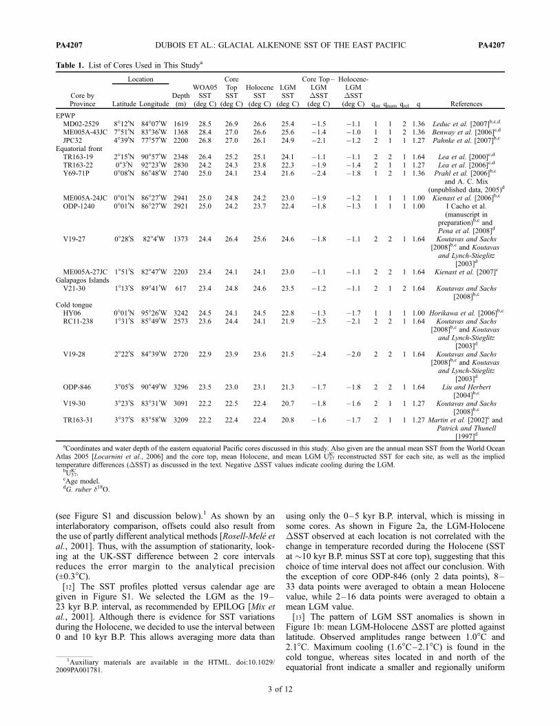
(see Figure S1 and discussion below).1 As shown by aninterlaboratory comparison, offsets could also result fromthe use of partly different analytical methods [Rosell-Mele etal., 2001]. Thus, with the assumption of stationarity, look-ing at the UK-SST difference between 2 core intervalsreduces the error margin to the analytical precision(±0.3�C).[12] The SST profiles plotted versus calendar age are

given in Figure S1. We selected the LGM as the 19–23 kyr B.P. interval, as recommended by EPILOG [Mix etal., 2001]. Although there is evidence for SST variationsduring the Holocene, we decided to use the interval between0 and 10 kyr B.P. This allows averaging more data than

using only the 0–5 kyr B.P. interval, which is missing insome cores. As shown in Figure 2a, the LGM-HoloceneDSST observed at each location is not correlated with thechange in temperature recorded during the Holocene (SSTat �10 kyr B.P. minus SST at core top), suggesting that thischoice of time interval does not affect our conclusion. Withthe exception of core ODP-846 (only 2 data points), 8–33 data points were averaged to obtain a mean Holocenevalue, while 2–16 data points were averaged to obtain amean LGM value.[13] The pattern of LGM SST anomalies is shown in

Figure 1b: mean LGM-Holocene DSST are plotted againstlatitude. Observed amplitudes range between 1.0�C and2.1�C. Maximum cooling (1.6�C–2.1�C) is found in thecold tongue, whereas sites located in and north of theequatorial front indicate a smaller and regionally uniform

Table 1. List of Cores Used in This Studya

Core byProvince

Location

Depth(m)

WOA05SST

(deg C)

CoreTopSST

(deg C)

HoloceneSST

(deg C)

LGMSST

(deg C)

Core Top–LGMDSST(deg C)

Holocene-LGMDSST(deg C) qstr qnum qrel q ReferencesLatitude Longitude

EPWPMD02-2529 8�120N 84�070W 1619 28.5 26.9 26.6 25.4 �1.5 �1.1 1 1 2 1.36 Leduc et al. [2007]b,c,d

ME005A-43JC 7�510N 83�360W 1368 28.4 27.0 26.6 25.6 �1.4 �1.0 1 1 2 1.36 Benway et al. [2006]c,d

JPC32 4�390N 77�570W 2200 26.8 27.0 26.1 24.9 �2.1 �1.2 2 1 1 1.27 Pahnke et al. [2007]b,c

Equatorial frontTR163-19 2�150N 90�570W 2348 26.4 25.2 25.1 24.1 �1.1 �1.1 2 2 1 1.64 Lea et al. [2000]c,d

TR163-22 0�30N 92�230W 2830 24.2 24.3 23.8 22.3 �1.9 �1.4 2 1 1 1.27 Lea et al. [2006]c,d

Y69-71P 0�080N 86�480W 2740 25.0 24.1 23.4 21.6 �2.4 �1.8 1 2 1 1.36 Prahl et al. [2006]b,c

and A. C. Mix(unpublished data, 2005)d

ME005A-24JC 0�010N 86�270W 2941 25.0 24.8 24.2 23.0 �1.9 �1.2 1 1 1 1.00 Kienast et al. [2006]b,c

ODP-1240 0�010N 86�270W 2921 25.0 24.2 23.7 22.4 �1.8 �1.3 1 1 1 1.00 I Cacho et al.(manuscript in

preparation)b,c andPena et al. [2008]d

V19-27 0�280S 82�40W 1373 24.4 26.4 25.6 24.6 �1.8 �1.1 2 2 1 1.64 Koutavas and Sachs[2008]b,c and Koutavasand Lynch-Stieglitz

[2003]d

ME005A-27JC 1�510S 82�470W 2203 23.4 24.1 24.1 23.0 �1.1 �1.1 2 2 1 1.64 Kienast et al. [2007]c

Galapagos IslandsV21-30 1�130S 89�410W 617 23.4 24.8 24.6 23.5 �1.2 �1.1 2 1 2 1.64 Koutavas and Sachs

[2008]b,c

Cold tongueHY06 0�010N 95�260W 3242 24.5 24.1 24.5 22.8 �1.3 �1.7 1 1 1 1.00 Horikawa et al. [2006]b,c

RC11-238 1�310S 85�490W 2573 23.6 24.4 24.1 21.9 �2.5 �2.1 2 2 1 1.64 Koutavas and Sachs[2008]b,c and Koutavasand Lynch-Stieglitz

[2003]d

V19-28 2�220S 84�390W 2720 22.9 23.9 23.6 21.5 �2.4 �2.0 2 2 1 1.64 Koutavas and Sachs[2008]b,c and Koutavasand Lynch-Stieglitz

[2003]d

ODP-846 3�050S 90�490W 3296 23.5 23.0 23.1 21.3 �1.7 �1.8 2 2 1 1.64 Liu and Herbert[2004]b,c

V19-30 3�230S 83�310W 3091 22.2 22.5 22.4 20.7 �1.8 �1.6 2 1 1 1.27 Koutavas and Sachs[2008]b,c

TR163-31 3�370S 83�580W 3209 22.2 22.4 22.4 20.8 �1.6 �1.7 2 1 1 1.27 Martin et al. [2002]c andPatrick and Thunell

[1997]d

aCoordinates and water depth of the eastern equatorial Pacific cores discussed in this study. Also given are the annual mean SST from the World OceanAtlas 2005 [Locarnini et al., 2006] and the core top, mean Holocene, and mean LGM U37

K0 reconstructed SST for each site, as well as the impliedtemperature differences (DSST) as discussed in the text. Negative DSST values indicate cooling during the LGM.

bU37K0 .

cAge model.dG. ruber d18O.

1Auxiliary materials are available in the HTML. doi:10.1029/2009PA001781.

PA4207 DUBOIS ET AL.: GLACIAL ALKENONE SST OF THE EAST PACIFIC

3 of 12

PA4207

cooling of 1�C–1.3�C. Cores V21-30 and Y69-71P bothstand out as exceptions. As will be discussed in x4.3, coreV21-30, a shallow water site that lies close to one of theGalapagos Islands, is possibly influenced by local upwell-ing: the ‘‘island effect’’ described by Feldberg and Mix[2003]. Indeed, in the MARGO Project Members [2009]study, foraminiferal assemblages from this core suggest aLGM cooling of �10.5�C while Mg/Ca SST reconstruc-tions suggest a cooling of 1.5�C only.[14] Core Y69-71P from the equatorial front records a

cooling of 1.8�C as opposed to a cooling of only 1.2�C and1.3�C for ME-24 and ODP-1240, respectively. These threecores share almost the same location (see Table 1). Al-though the difference between those cores is within theaccepted calibration error, based on the very good agree-ment from the two high-resolution cores nearby this dis-crepancy is more likely due to the lower resolution of therecord from site Y69-71P (4 and 6 data points in theHolocene and LGM, respectively). In fact, the discrepancybetween the nearby sites ME-24 and Y69-71P goes beyondSST reconstructions (e.g., flux estimates [Kienast et al.,2007] and clay and foraminiferal content (F. Mekik, per-sonal communication, 2009)) and is the subject of ongoingstudies (M. Kienast and F. Prahl, unpublished data, 2009).This interpretation is also in line with the close agreementbetween TR-31 and V19-30, which are located closetogether, or that of MD-29 and ME-43.

3.2. Magnitude of Glacial Cooling Reported by UK037Records

[15] Because UK037-SST records from the EEP show awarming trend during the course of the Holocene (seeFigure S1), comparing mean SST during the LGM andthe entire Holocene will give a smaller temperature anomalythan the actual full glacial-interglacial range. We thereforealso include in Table 1 the SST difference between the coretop and the LGM. The mean glacial–core top SST changein the EEP reported by these UK037 reconstructions is1.7�C, ranging from 1.1�C to 2.5�C.[16] Interestingly, recent UK037-SST estimates from the

western Pacific Warm Pool (WPWP) indicate a glacial-interglacial DSST of 1.3�C [de Garidel-Thoron et al.,2007]. Because the alkenone index is at or near saturationduring the late Holocene in the WPWP, this is likely aminimum estimate. When merged with the data presentedhere, this western estimate would suggest a glacial coolingof the whole Pacific, as indicated by alkenone paleother-mometry, of around �1.5�C, with possibly a somewhat

Figure 1. (a) Locations of the cores in the easternequatorial Pacific: solid circles represent cores analyzedin the present study, and open squares represent cores fromprevious studies. The background SST distribution corre-sponds to mean annual conditions from the World OceanAtlas 2005 [Locarnini et al., 2006]. (b) LGM-Holocenetemperature difference (DSST) plotted versus latitude,using the Prahl et al. [1988] calibration. Negative DSSTvalues reflect cooling during the LGM. (c) LGM-Holocenetemperature difference (DSST) plotted versus latitude,using the Conte et al. [2006] nonlinear calibration.

4 of 12

PA4207PA4207 DUBOIS ET AL.: GLACIAL ALKENONE SST OF THE EAST PACIFIC

greater cooling in the cold tongue. Previous alkenonereconstructions summarized by Sonzogni et al. [1998]suggest a �1.0�C ± 0.4�C glacial-modern DSST in theequatorial Pacific.

4. Discussion

4.1. Assessment of the Potential Geographic Biases

[17] The cores compiled in this study come from a varietyof EEP oceanographic environments. These diverse settingsmay cause a number of biases in the UK037 records. Herewe assess the impact of the two main potential biases:(1) different sedimentation rates between core sites and thecomplications associated with it and (2) the effect of thewarm limit of the alkenone method, in particular withregards to the cores located in the EPWP.[18] Sedimentation rates in the cores from the present

study range from 3 to 30 cm/kyr. As pointed out in previousstudies, bioturbation at sites with low sedimentation ratescan lead to a smaller glacial-interglacial SST difference [deGaridel-Thoron et al., 2007, and references therein]. InFigure 2b we show that there is no relationship betweensedimentation rate and the LGM-Holocene DSST. We cantherefore exclude any significant impact of bioturbation onthe LGM-Holocene DSST amplitude at sites with lowsedimentation rates. Similarly, there is no correlation (r2 =0.10) between the number of data points used to calculate theaverage SST and the LGM-HoloceneDSST reported at eachlocation, excluding a possible bias resulting from differentsampling resolution in and outside of the cold tongue.[19] The second possible artifact arises from SSTs in the

EPWP being close to the limit of the UK037 method. Awater column study in the WPWP suggested that UK037cannot be used as an accurate paleothermometer above26.4�C [Bentaleb et al., 2002]. With mean annual SSTsbetween 26.5�C and 28.6�C (WOA05), four cores from thiscompilation would be above this threshold limit (TR-19,JPC-32, ME-43, MD-29 (see Table 1)). However, Pelejeroand Calvo [2003] subsequently argued against this partic-ular upper temperature limit, suggesting that the UK037index value should not be reported as unity when C37:3 isundetected, as done in the study by Bentaleb et al. [2002].In the core top sample of ME-43, we have been able toreliably measure an UK037 index of 0.960 (i.e., 27�C), withthe C37:3 being above the limit of detection.[20] A second aspect of this warm end problem is the

actual shape of the calibration curve. It has been suggested

Figure 2. (a) LGM-Holocene temperature difference(DSST) as a function of the change in SST occurringduring the Holocene (here computed as the SST at 10 kyrB.P. minus the core top SST). (b) LGM-Holocenetemperature difference (DSST) as a function of sedimenta-tion rate (here computed as the average sedimentation ratefor the last 23 kyr). Note that no dampening of the glacial toHolocene SST difference is observed in the cores with thelower sedimentation rates. (c) LGM-Holocene temperaturedifference (DSST) as a function of the deviation of the coretop UK037 SST reconstruction from WOA05, using thePrahl et al. [1988] calibration.

5 of 12

PA4207PA4207 DUBOIS ET AL.: GLACIAL ALKENONE SST OF THE EAST PACIFIC

that the relationship between UK037 and SST is moresigmoidal than linear, i.e., that the linear regression slopesflatten toward the cold and warm ends of the temperaturerange (see the reviews by Pelejero and Calvo [2003] andConte et al. [2006]). Using a ‘‘global’’ linear calibrationwould lead to an underestimation of the Holocene SST inthe warmer sites, and, as a consequence, to a smaller LGM-Holocene DSST. The evidence we find is contradictory:Although the core top UK037 SST reconstructions from thetwo northern sites (MD-29 and ME-43) underestimate meanannual SSTs at those sites (WOA05) by �1.5�C, the thirdwarm site from the EPWP (JPC-32) overestimates slightlythe modern mean annual SST (see Table 1). In addition,4 cores located further south (i.e., in colder SSTs) alsoreport a significant underestimation of the modern meanannual SST as in the warmest cores. At this point, it is worthmentioning that the results from our compilation do notrepresent true surface sediments, but piston core tops, whenavailable. With the exception of JPC32, the results wepresent as core tops are in reality the topmost samples inthe core analyzed for alkenones, and have dates rangingfrom 0.1 to 5.4 kyr B.P. Consequently the direct comparisonwith present-day SST is far from ideal. And although thereis a weak correlation between the core top deviation fromthe mean annual WOA05 value and the absolute SST ateach site (r2 = 0.42), there is no correlation between the coretop deviation from the mean annual WOA05 value and theLGM-Holocene DSST (r2 = 0.016 (Figure 2c)). We arethus confident that the possible flattening of the UK037-temperature relationship at warmer temperatures does notaffect our main conclusion.[21] The linear equation by Prahl et al. [1988] is based on

cultures of E. huxleyi, between 10�C and 25�C, and thusmight not be suitable for the high SSTs of the EPWP. On theother hand, extrapolating Prahl’s linear equation to the limitof the UK037 index (i.e., 1) gives a theoretical maximumSST of 28.3�C. We decided to use the Prahl et al. [1988]calibration because it gives the best fit (smallest root meansquare error (RMSE)) between the core tops and the meanannual SSTs at each location, as compared to the calibra-tions of Muller et al. [1998], the nonlinear calibration ofConte et al. [2006] and the warm temperature calibration ofSonzogni et al. [1997] (Table 2). As shown in Figure 1c, thenonlinear Conte et al. [2006] calibration results in a similargeographic distribution of LGM-Holocene DSST as thePrahl et al. [1988] calibration (Figure 1b).

4.2. Significance of the Results

[22] The RMSE of the absolute temperature calibration isabout 1�C for the Prahl et al. [1988] equation versus meanannual SST (Table 2). However, the reader should keep in

mind that the top most samples used in this calibration arenot surface sediments (with the exception of JPC32).Therefore, some deviation from modern WOA values is tobe expected.[23] In addition, our strategy does not rely on absolute

temperature determination, but on computation of relativedowncore changes. With the assumption that the UK037-SST relationship and any site/lab systematic offset remainsconstant through time, the uncertainty in the DSST wereconstruct is defined only by the uncertainties in themean Holocene and mean LGM SST. Thus sDSST =p(sLGM-SST

2 + sHolocene-SST2 ). The measurement uncertainty

equals s = 0.3�C. Consequently, sDSST =p(2 � 0.32) =

0.42�C. The signal we observe, an average temperaturedifference between the two regions (cold tongue versusequatorial front and further north) of 0.7�C is thereforelarger than the uncertainty. In addition, the geographiccoherence given by the numerous cores also supports anonrandom result (Figure 1b).[24] Finally, the standard deviation within each region is

significantly smaller than the temperature difference be-tween these two regions (0.1�C for the northern region and0.2�C for the cold tongue environment). A t test indicatesthat the difference between the two regions is extremelystatistically significant (P < 0.0001, df = 13, t = 6.89).

4.3. Comparison With Previous Studies

[25] Although the LGM-core top DSST (1.1�C–2.5�C) islarger than the LGM-Holocene DSST (1.0�C–2.1�C) inmost of the cores (see Table 1), the magnitude of glacial-interglacial cooling recorded by some of the UK037 recordsremains somewhat smaller than the 2�C–3�C suggested bythe MARGO Project Members [2009]. However, this com-monly accepted glacial-interglacial SST range for the EEP isbased mainly on Mg/Ca ratios (�2.5�C) and faunal assemb-lages (0.5�C–10.5�C) [e.g., Lea et al., 2000; Martınez etal., 2003]. EEP data from the MARGO synthesis are givenin Table 3 and plotted as single points in a map in Figure 3a(MARGO data are available at http://www.glacialoceanatlas.org/). As shown by the mean reliability index q, a majorityof the EEP data available in the MARGO synthesis is ofpoor quality. The average q for the MARGO data is 2.27(Table 3), while the average q presented in this study is1.41. In Figure 3b, we have plotted only the reliableMARGO data with a q < 2. These data are comparable toour Holocene-LGM DSST reconstruction, which is shownin Figure 3c. In particular, the faunal SST reconstructionssuggest a glacial cooling between 1�C and 1.5�C, verysimilar to our LGM-Holocene UK037-DSST. Mg/Ca SSTreconstructions on the other hand, suggest a slightly largercooling. Using a MARGO approach (LGM �WOADSST)

Table 2. Root Mean Square Error Between the Calibrations of the Core Tops and WOA05 Mean Values

Equation Annual Spring Summer Fall Winter

Prahl et al. [1988] E. huxleyi culture calibration 1.02 1.26 1.69 1.31 1.88Muller et al. [1998] global core top compilation 1.13 1.13 2.08 1.69 1.48Conte et al. [2006] nonlinear global surface water calibration 1.11 1.14 2.05 1.65 1.48Conte et al. [2006] linear global surface sediments calibration 1.02 1.18 1.82 1.43 1.72Sonzogni et al. [1997] high-temperature range (24�C–30�C) calibration 1.42 1.63 1.61 1.42 2.51Sonzogni et al. [1997] global core top compilation 1.32 1.20 2.33 1.94 1.36

PA4207 DUBOIS ET AL.: GLACIAL ALKENONE SST OF THE EAST PACIFIC

6 of 12

PA4207

for the alkenone records presented here, the pattern becomesless clear (Figure 3d) and is complicated by the calibrationuncertainty (see above).[26] Every SST proxy is affected by various biases. The

UK037 proxy might be complicated by nonthermal effects,such as light or nutrient stress, changes in the season ordepth of production with time [e.g., Prahl et al., 2003;MARGO Project Members, 2009]. Mg/Ca can be affectedby dissolution problems [Kucera et al., 2005; Lea et al.,2006; Mekik et al., 2007]. Following the MARGO qualityflag labeling, all the EEP Mg/Ca records, with the exceptionof MD-29 and ME-43 [Leduc et al., 2007; Benway et al.,2006], have a reliability index (qrel) of only 2 because ofwater depths greater than 2000 m. In addition, Mg/Ca hasbeen recently shown to be affected by changes in salinity[Ferguson et al., 2008; Kisakurek et al., 2008] and by thepresence of volcanic shards [Lea et al., 2005]. Faunalmethods, on the other hand, are complicated by the no-analog problem [Mix et al., 1999] and systematic largeerrors at the oceanic temperatures extremes [Morey et al.,2005].[27] However, researchers now attempt to correct for

those biases whenever possible [e.g., Lea et al., 2005;Mix et al., 1999]. For example, the disagreements in theamplitude and/or timing of SST changes between alkenoneand planktonic foraminiferal Mg/Ca estimates during thedeglaciation have recently been suggested to result fromdifferences in seasonality of the planktonic foraminiferaG. ruber and alkenone-producing algae [Steinke et al.,2008; Sachs, 2008; Timmermann and Timm, 2008]. Sachs[2008] suggested that E. huxleyi (the primary alkenone

producer) is most abundant in winter in the cold tongueprovince, whereas G. ruber appears to be most abundant insummer, though the data are limited and the specificecologic niche of E. huxleyi is not known. However, theseasonal distribution of insolation was the same during theLGM and the late Holocene and thus cannot account forthe discrepancy of glacial-interglacial SST differencesreported by these two proxies. In addition, independent ofthe UK037 calibration equation used, the core top values arestatistically closer (smallest RMSE) to the WOA05 meanannual SST value than to the mean boreal winter value ateach site (Table 2).[28] In conclusion, it seems that when the various biases

affecting SST proxies are taken into account and onlyreliable records are used, a relatively consistent pictureemerges for the EEP, at least in terms of magnitude of theglacial cooling.

4.4. Glacial Hydrographic Changes in the EEP

[29] The alkenone-based spatial pattern of SST distribu-tion during the LGM we present here seems to be at oddswith recent Mg/Ca and d18O studies. In the EEP, Mg/CaSSTs indicate a �2.6�C cooling north of the equatorial front[Lea et al., 2000], a �1.9�C cooling just south of theequatorial front [Lea et al., 2006] and a relatively smallcooling (�1�C) within the cold tongue [Koutavas et al.,2002]. Based on these results, Koutavas et al. [2002]inferred a reduced meridional SST gradient during theLGM, in a pattern consistent with ‘‘El Nino–like’’ con-ditions. However, the site used in the Koutavas et al. [2002]study (V21-30) is located very close to the Galapagos

Table 3. List of Cores Used by MARGO Project Members [2009]a

Core by Proxies

Location WOA98SST

(deg C)

LGMSST

(deg C)

WOA-LGMDSST(deg C) qstr qnum qrel q ReferencesLatitude Longitude

Mg/CaTR163-18 2�490N 89�510W 26.32 23.3 �3.02 2 3 2 2.36 Lea et al. [2000]TR163-19 2�260N 90�950W 26.04 23.3 �2.74 3 2 1 1.91 Lea et al. [2000]TR163-20B 0�470N 93�510W 23.78 21.1 �2.68 2 3 2 2.36 Lea et al. [2000]TR163-22 0�310N 92�240W 23.28 22.3 �0.98 2 3 2 2.36 Lea et al. [2000]V21-30 1�220S 89�680W 22.80 21.3 �1.50 2 1 2 1.64 Koutavas et al. [2002]

UK037138-846B 3�050S 90�490W 22.91 24.2 1.29 2 3 1 2.00 Emeis et al. [1995]138-847_Site 0�190N 95�320W 23.80 20.8 �3.00 2 2 1 1.64 K.-C. Emeisb

GIK16969-1 9�060N 85�630W 27.56 25.6 �1.96 2 2 1 1.64 K.-C. Emeisb

Foram assemblages111-677B 1�200N 83�740W 25.40 24.14 �1.26 2 1 1 1.27 Martınez et al. [2003]138-846B 3�050S 90�490W 22.91 21.86 �1.05 2 1 2 1.64 Martınez et al. [2003]70-506B 0�610N 86�090W 24.84 23.83 �1.01 2 1 1 1.27 Martınez et al. [2003]RC13-110 0�100N 95�650W 23.74 23.38 �0.37 4 3 1 2.55 A. C. Mixb

TR163-11 6�450N 85�820W 27.66 26.43 �1.23 3 3 1 2.27 Martınez et al. [2003]TR163-33 1�910S 82�570W 22.55 21.91 �0.64 2 1 3 2.00 Martınez et al. [2003]V19-29 3�580S 83�930W 22.05 15.80 �6.25 4 3 3 3.27 A. C. Mixb

V21-30 1�220S 89�680W 22.80 12.21 �10.59 4 3 2 2.91 A. C. Mixb

V21-33 3�800S 92�080W 23.25 20.24 �3.02 4 3 3 3.27 A. C. Mixb

Y69-106P 2�980N 86�550W 26.70 24.27 �2.43 4 3 2 2.91 A. C. Mixb

Y69-71P 0�100N 86�480W 24.38 22.25 �2.14 4 3 2 2.91 A. C. Mixb

Y71-03-02 7�170N 85�150W 27.83 25.57 �2.26 4 3 3 3.27 A. C. Mixb

aCoordinates of the eastern equatorial Pacific cores presented in the MARGO synthesis. Also given are the annual mean SST from the World Ocean Atlas1998 [Antonov et al., 1998] and the mean LGM reconstructed SST for each site, as well as the implied temperature differences (DSST) to WOA. NegativeDSST values indicate cooling during the LGM.

bUnpublished data as cited by Kucera et al. [2005].

PA4207 DUBOIS ET AL.: GLACIAL ALKENONE SST OF THE EAST PACIFIC

7 of 12

PA4207

Islands and might be influenced by ‘‘island dynamics’’[Feldberg and Mix, 2003]. In addition, the Mg/Ca measure-ments in this study were conducted on G. sacculifer, whichhas been shown to record a thermocline signature during thelast glacial period in the EEP and therefore not to be anappropriate sea surface proxy carrier [Spero et al., 2003]. Incontrast, the two sites located across the equatorial front donot report an obvious glacial-interglacial pattern of changein the meridional SST gradient [Lea et al., 2006]. A reduced

glacial gradient was, however, also deduced by Koutavasand Lynch-Stieglitz [2003] from SST reconstructions basedon planktonic d18O. These authors inferred that the coldtongue cooled by only �1.5�C while further north SSTsdecreased by 2.5�C–3�C (Figure 4a). UK037-SST estimateson 4 of the cores used in the d18O-based reconstruction,however, show the opposite pattern than the d18O results,with the coldest temperature in the cold tongue [Koutavasand Sachs, 2008]. As pointed out by the authors themselves,

Figure 3. Comparison of the MARGO Project Members [2009] synthesis with the alkenone results fromthis study (squares) in a map view. MARGO data are separated by proxy: stars are for alkenones,triangles are for Mg/Ca, and circles are for foraminiferal fauna. (a) Location and LGM SST anomaliesfrom the cores presented in the MARGO Project Members [2009] synthesis. (b) Same as in Figure 3a, butonly the reconstructions from cores with a mean reliability index q < 2 are shown. (c) Results fromthis study, using the Holocene-LGM DSST. (d) LGM SST anomalies using the MARGO approach(LGM minus WOA).

PA4207 DUBOIS ET AL.: GLACIAL ALKENONE SST OF THE EAST PACIFIC

8 of 12

PA4207

the LGM planktonic foraminifera d18O might be compli-cated by the carbonate ion effect [Spero et al., 1997] andsalinity variations, which the authors do not account for. Asouthward shift of the ITCZ during the LGM, as suggestedby Koutavas and Lynch-Stieglitz [2003], should increase seasurface salinity (SSS) in the EPWP and thereby enrichforaminiferal d18O, leading to an underestimation of theSST and therefore a larger LGM-Holocene DSST.[30] We investigate the possible salinity bias on the d18O-

based SST records by correcting the LGM-Holocene Dd18Ofor ice volume (0.95 ± 0.09% [Adkins and Schrag, 2001])and temperature effect, using the UK037 LGM-HoloceneDSST from the same cores and the Bemis et al. [1998] low-light paleotemperature equation (see Table 1 for references).Figure 4b shows the location of the cores for which bothG. ruber d18O and UK037 records are available. Usingalkenone SST reconstructions to deconvolve planktonicd18O records does not take into account any seasonal ordepth difference in the growth of algae versus planktonicforaminifera. As discussed in x4.3, the UK037 index corre-lates best with mean annual SST, whereas G. ruber is mostabundant during the summer season in the surface mixedlayer [Sachs, 2008]. Thus we acknowledge that somedifferences in amplitude and timing of the two signalsmay result from ecological differences. As shown byKoutavas and Lynch-Stieglitz [2003], the present-day EEPdoes not experience large seasonal differences in SSSdespite the seasonal shifts in ITCZ-linked precipitation.Therefore, the main bias would result from the summer(G. ruber d18O) versus annual (UK037) SST recorded. Weassume that this bias is unlikely to show significant geo-graphic differences across the EEP. Furthermore, as reportedby Otto-Bliesner et al. [2009], MARGO data and PMIP2model estimates suggest little summer versus winter differ-ences in SST cooling in the Pacific Ocean.[31] Because of the large systematic errors in paleosalinity

estimates based on analyses of fossil shells [e.g., Rohling,2000], we do not attempt here to present a reconstruction ofabsolute LGM salinities. Rather, we present a qualitativeapproximation of possible hydrologic changes which couldhave affected the planktonic d18O records, thus leading toconflicting SST reconstructions. The residual Dd18Oobtained after temperature and ice volume correction rep-resents the change in oxygen isotopic composition ofsurface waters (d18Osw) between the LGM and the Holocenetime period. The Dd18Osw shows a clear latitudinal trend

Figure 4. (a) Figure taken from Koutavas and Lynch-Stieglitz [2003], presenting LGM to late Holocene SSTanomalies based on d18O (G. ruber in gray and G. sacculiferin black). Mg/Ca SST reconstructions are underlined.(b) Eastern equatorial Pacific cores for which bothGlobigerinoides ruber d18O and U37

K0 SST data exist. Thebackground SSS distribution corresponds to mean annualconditions from the World Ocean Atlas 2005 database.(c) Latitudinal plot of the estimated LGM-Holoceneseawater d18O change (Dd18Osw), after subtraction of theice volume effect and correction for changes in temperatureas reported by alkenone paleothermometry.

PA4207 DUBOIS ET AL.: GLACIAL ALKENONE SST OF THE EAST PACIFIC

9 of 12

PA4207

(Figure 4c). The pattern of heavier LGM d18Osw north of theequator and lighter LGM d18Osw south of the equator isconsistent with a southward displacement of the ITCZ.However, changes in d18Osw may also reflect changes inthe relative contributions of distant (Caribbean and/or largestorms) versus local (Pacific) freshwater sources [Benwayand Mix, 2004]. In either case, evidence presented herestrongly suggests that regional changes in the d18O ofseawater in the surface EEP at the LGM have to beconsidered in addition to the global ice volume effect whenusing planktonic d18O as a paleothermometer.[32] Using Mg/Ca SST to correct the d18O records of

EPWP cores MD-29 and ME-43, both Benway et al. [2006]and Leduc et al. [2007] do not report a significant glacialchange in SSS. However, since recent studies show asalinity effect on foraminiferal Mg/Ca, it could be worthinvestigating how this bias affects the SSS reconstructions[Ferguson et al., 2008; Kisakurek et al., 2008]. In contrast,Pahnke et al. [2007] infer reduced rainfall in and around thePanama Basin during the last glacial period, using recordsof hydrogen isotope ratios of alkenones in core JPC32 as ahydrologic proxy. In addition, Schmidt et al. [2004] report alarge glacial increase in salinity (2.3–2.7 psu) in theCaribbean, just to the east of the EPWP on the other sideof the Panama Isthmus. Both these studies call on asouthward shift of the mean position of the ITCZ. Thishypothesis, however, implies that the modern seasonalvariations in the cold tongue–ITCZ complex, which arecharacterized by small changes in salinity and a weaker coldtongue (less upwelling) when the ITCZ is further south [Liand Philander, 1996], is not an analog for longer-termvariations in the past.

4.5. Glacial EEP Oceanographic Changes

[33] The stronger glacial cooling within the cold tonguethat we reconstruct from alkenone unsaturation agrees withprevious studies based on faunal assemblages and thermo-cline reconstructions [e.g., Pisias and Mix, 1997; Patrickand Thunell, 1997; Martınez et al., 2003]. Comparison toLGM reconstructions preceding EPILOG [Mix et al., 1999]is risky because these studies used the 18 kyr B.P. level asthe LGM. However, major reorganizations in the structureof the EEP are not likely to have occurred between theLGM and the 18 kyr B.P. level, but rather during thedeglaciation [e.g., Anderson et al., 2009]. Both an increasein equatorial upwelling and a stronger flow of the PeruCurrent have been proposed previously to explain thecooling in the equatorial region [e.g., Feldberg and Mix,2002; Kienast et al., 2006]. The spatial pattern of SSTdistribution during the LGM indicated by alkenone recordsdoes not permit distinguishing between the upwelling oradvection mechanisms. However, the glacial southwardshift of the ITCZ previously suggested and corroboratedby our d18O versus UK037 reconciliation would be inconflict with the upwelling-driven cooling mechanism. Atpresent, equatorial upwelling is caused by the southeasterlytrade winds crossing the equator when the ITCZ is in itsnorthernmost position. One could hypothesize that duringthe LGM, equatorial upwelling was driven by the north-easterly trade winds crossing the equator to reach the

southward shifted ITCZ. But this speculation would implya complete oceanographic reorganization of the EEP. Wethus suggest that the most probable cause of the largerglacial cooling in the cold tongue is the advection of colderwater in the Peru Current, though we cannot rule out theupwelling of colder water in the equatorial divergence as apossible mechanism.[34] The advection mechanism is supported by greater

glacial cooling toward the pole in the southeast Pacific.Alkenone reconstructions report a glacial decrease in SSTsof 3�C at 16�S [Prahl et al., 2006] and of 6�C–7�C at30�S–40�S [Kim et al., 2002; Kaiser et al., 2005]. SSTchanges in this region have been suggested to be closelyassociated with variations in the position of the SouthernPacific Westerlies and northward advection of cold Antarc-tic Circumpolar Current (ACC) waters. Kaiser et al. [2005]indeed suggest that a northward widening of the westerliesduring the last glacial displaced the ACC northward,increased the advection of cold water masses into themidlatitudes and extended the cold tongue westward.[35] Otto-Bliesner et al. [2009] recently compared the

data synthesis of MARGO with the Paleoclimate ModelingIntercomparison Project, Phase 2 (PMIP2) predictions. ThePMIP2 compares the response of different coupled atmo-sphere-ocean models to a common set of forcings andboundary conditions for the LGM [Braconnot et al.,2007]. Here we briefly discuss how the PMIP2 predictedLGM cooling compares with our UK based LGM-HoloceneDSST. The PMIP2 models estimate an annual averagecooling in the glacial EEP in the range of 1�C–3�C(LGM to pre-Industrial), which compares well to theHolocene-LGM DSST estimates from this study. In addi-tion, the majority of the models simulate a larger cooling inthe cold tongue environment, with respect to the regionnorth of the equator. The PMIP2 multimodel mean SSTanomaly clearly shows the presence of a cold tongueanomaly of �2�C to �3�C, whereas north and south of itthe anomaly is estimated at �1�C to �2�C [see Otto-Bliesner et al., 2009, Figure 3]. Interestingly, modeled depthprofiles along the equator suggest a larger cooling in EEPsurface waters (<30 m) than in subsurface waters (30–150 m). This vertical structure of glacial temperatureanomaly lends support to the advection mechanism as acause of surface cooling in the glacial EEP.[36] Finally, although some previous studies reporting an

intensified cold tongue during the LGM have suggested amean glacial state analogous to present-day La Nina–likecondition [Martınez et al., 2003], we prefer not to invokeany ENSO-like state for the glacial EEP based solely on ourUK037 SST.

5. Conclusion

[37] We present new SST records from the EEP based onalkenone unsaturation and combine them with recentlypublished UK037 records to reconstruct the geographicpattern of SSTs during the LGM. Cold tongue SST isfound to have experienced a larger decrease (1.6�C–2.1�C)during the LGM compared to sites further north (1�C–1.3�C). This UK037-based SST pattern resembles previous

PA4207 DUBOIS ET AL.: GLACIAL ALKENONE SST OF THE EAST PACIFIC

10 of 12

PA4207

reconstructions based on foraminiferal and radiolarian fauna,though the amplitude of cooling reported by alkenones issmaller.[38] However, the LGM SST pattern reconstructed from

alkenone paleothermometry directly contradicts the spatialSST pattern estimated from planktonic foraminifera d18Oand Mg/Ca. The EEP Mg/Ca records available are affectedby various problems: dissolution, use of inadequate speciesand the ‘‘(Galapagos) island effect.’’ Their scarcity does notpermit to unambiguously reconstruct the LGM cold tonguedynamics. With regard to the discrepancy between d18O andUK037 SST records, we suggest that it arises from theinfluence of salinity variations on the d18O record, causedby a southward shift of the ITCZ and its rainfall belt. Thisclimatic interpretation leads us to suggest that strongeradvection of cold waters in the Peru Current is responsiblefor the colder SST reconstructed in the cold tongue envi-ronment during the LGM. It would indeed be difficult to

reconcile an increase in equatorial upwelling with a meanlocation of the ITCZ further south.[39] To conclude, we acknowledge that the alkenone

proxy is not devoid of bias, with possible aliasing due tolight or nutrient stress, changes in productive season ordepth of the temperature reflected. Further investigation isrequired to assess the influence of various biases on thedifferent SST proxies and to reconcile the dynamics of thecold tongue during the LGM as well as the magnitude ofglacial cooling.

[40] Acknowledgments. Core material was kindly and generouslyprovided by the Core Repositories of Oregon State University (supportedby NSF grant OCE97-12024) and the University of Rhode Island (sup-ported by NSF grant OCE-9102410). We gratefully acknowledge L. Penaand I. Cacho for sharing unpublished data (ODP-1240). We are also gratefulfor constructive comments made by David Piper, Figen Mekik, twoanonymous reviewers, and the Associate Editor on the original version ofthis paper. This work was supported by NSERC Canada, NSF, and theCanadian Institute for Advanced Research (CIFAR; M.K.).

ReferencesAdkins, J. F., and D. P. Schrag (2001), Pore fluidconstraints on deep ocean temperature andsalinity during the Last GlacialMaximum,Geo-phys. Res. Lett., 28, 771–774, doi:10.1029/2000GL011597.

Anderson, R. F., S. Ali, L. I. Bradtmiller, S. H. H.Nielsen, M. Q. Fleisher, B. E. Anderson, andL. H. Burckle (2009), Wind-driven upwellingin the Southern Ocean and the deglacial rise inatmospheric CO2, Science, 323, 1443–1448,doi:10.1126/science.1167441.

Andreasen, D. J., and A. C. Ravelo (1997),Tropical Pacific Ocean thermocline depthreconstructions for the Last Glacial Maximum,Paleoceanography, 12, 395–413, doi:10.1029/97PA00822.

Antonov, J., S. Levitus, T. P. Boyer,M. Conkright,T. O’Brien, and C. Stephens (1998), WorldOcean Atlas 1998, vol. 2, Temperature of thePacific Ocean, NOAA Atlas NESDIS, vol. 28,166 pp., NOAA, Silver Spring, Md.

Bemis, B. E., H. J. Spero, J. Bijma, and D. W.Lea (1998), Reevaluation of the oxygen isoto-pic composition of planktonic foraminifera:Experimental results and revised paleotem-perature equations, Paleoceanography, 13,150–160, doi:10.1029/98PA00070.

Bentaleb, I., M. Fontugne, and L. Beaufort(2002), Long-chain alkenones and U37

K0 varia-bility along a south – north transect in thewestern Pacific Ocean, Global Planet.Change, 34, 173–183, doi:10.1016/S0921-8181(02)00113-3.

Benway, H. M., and A. C. Mix (2004), Oxygenisotopes, upper-ocean salinity, and precipita-tion sources in the eastern tropical Pacific,Earth Planet. Sci. Lett., 224, 493 – 507,doi:10.1016/j.epsl.2004.05.014.

Benway, H. M., A. C. Mix, B. A. Haley, andG. P. Klinkhammer (2006), Eastern PacificWarm Pool paleosalinity and climate variability:0 – 30 kyr, Paleoceanography, 21, PA3008,doi:10.1029/2005PA001208.

Braconnot, P., et al. (2007), Results of PMIP2coupled simulations of the mid-Holocene andLast Glacial Maximum—Part 1: Experimentsand large-scale features,Clim. Past, 3, 261–277.

Cane, M. A. (1998), A role for the tropicalPacific, Science, 282, 59–61, doi:10.1126/science.282.5386.59.

CLIMAP (1981), Seasonal reconstructions of theEarth’s surface at the Last Glacial Maximum,Tech. Rep. MC-36, Geol. Soc. of Am.,Boulder, Colo.

Conte, M. H., M.-A. Sicre, C. Ruhlemann, J. C.Weber, S. Schulte, D. Schulz-Bull, andT. Blanz (2006), Global temperature calibra-tion of the alkenone unsaturation index (U37

K0)in surface waters and comparison with surfacesediments, Geochem. Geophys. Geosyst., 7,Q02005, doi:10.1029/2005GC001054.

de Garidel-Thoron, T., Y. Rosenthal, L. Beaufort,E. Bard, C. Sonzogni, and A. C. Mix (2007), Amultiproxy assessment of the western equator-ial Pacific hydrography during the last 30 kyr,Paleoceanography, 22, PA3204, doi:10.1029/2006PA001269.

Deser, C., and J. M. Wallace (1990), Large-scaleatmospheric circulation features of warm andcold episodes in the tropical Pacific, J. Clim.,3, 1254–1281, doi:10.1175/1520-0442(1990)003<1254:LSACFO>2.0.CO;2.

Emeis, K.-C., H. Doose, A. C. Mix, andD. Schulz-Bull (1995), Alkenone sea-surfacetemperatures and carbon burial at Site 846(eastern equatorial Pacific Ocean): The last1.3 M.Y., Proc. Ocean Drill. Program Sci.Results, 138, 605–613.

Feldberg, M. J., and A. C. Mix (2002), Sea-surface temperature estimates in the southeastPacific based on planktonic foraminiferal spe-cies: Modern calibration and Last GlacialMaximum, Mar. Micropaleontol., 44, 1 –29,doi:10.1016/S0377-8398(01)00035-4.

Feldberg, M. J., and A. C. Mix (2003), Plank-tonic foraminifera, sea surface temperatures,and mechanisms of oceanic change in the Peruand south equatorial currents, 0–150 ka BP,Paleoceanography, 18(1), 1016, doi:10.1029/2001PA000740.

Ferguson, J. E., G. M. Henderson, M. Kucera,and R. E. M. Rickaby (2008), Systematicchange of foraminiferal Mg/Ca ratios across astrong salinity gradient, Earth Planet. Sci.Lett., 265, 153–166, doi:10.1016/j.epsl.2007.10.011.

Herbert, T. D., J. D. Schuffert, D. Thomas,C. Lange, A. Weinheimer, A. Peleo-Alampay,and J.-C. Herguera (1998), Depth and season-ality of alkenone production along the Califor-

nia margin inferred from a core top transect,Paleoceanography, 13, 263–271.

Horikawa, K., M. Minagawa, M. Murayama,Y. Kato, and H. Asahi (2006), Spatial and tem-poral sea-surface temperatures in the easternequatorial Pacific over the past 150 kyr,Geophys. Res. Lett., 33, L13605, doi:10.1029/2006GL025948.

Kaiser, J., F. Lamy, and D. Hebbeln (2005), A70-kyr sea surface temperature record offsouthern Chile (Ocean Drilling Program Site1233), Paleoceanography, 20, PA4009,doi:10.1029/2005PA001146.

Kienast, M., S. S. Kienast, S. E. Calvert, T. I.Eglinton, G. Mollenhauer, R. Francois, andA. Mix (2006), Eastern Pacific cooling andAtlantic overturning circulation during thelast deglaciation, Nature, 443, 846 – 849,doi:10.1038/nature05222.

Kienast, S. S., M. Kienast, A. C. Mix, S. E.Calvert, and R. Francois (2007), Thorium-230 normalized particle flux and sedimentfocusing in the Panama Basin region duringthe last 30,000 years, Paleoceanography, 22,PA2213, doi:10.1029/2006PA001357.

Kim, J.-H., R. R. Schneider, D. Hebbeln, P. J.Muller, and G. Wefer (2002), Last deglacialsea-surface temperature evolution in the south-east Pacific compared to climate changes onthe South American continent, Quat. Sci.Rev., 21, 2085 – 2097, doi:10.1016/S0277-3791(02)00012-4.

Kisakurek, B., A. Eisenhauer, F. Bohm, D. Garbe-Schonberg, and J. Erez (2008), Controls onshell Mg/Ca and Sr/Ca in cultured planktonicforaminiferan, Globigerinoides ruber (white),Earth Planet. Sci. Lett., 273, 260 – 269,doi:10.1016/j.epsl.2008.06.026.

Koutavas, A., and J. Lynch-Stieglitz (2003),Glacial-interglacial dynamics of the easternequatorial Pacific cold tongue– IntertropicalConvergence Zone system reconstructed fromoxygen isotope records, Paleoceanography,18(4), 1089, doi:10.1029/2003PA000894.

Koutavas, A., and J. P. Sachs (2008), Northerntiming of deglaciation in the eastern equatorialPacific from alkenone paleothermometry,Paleoceanography, 23, PA4205, doi:10.1029/2008PA001593.

PA4207 DUBOIS ET AL.: GLACIAL ALKENONE SST OF THE EAST PACIFIC

11 of 12

PA4207

Koutavas, A., J. Lynch-Stieglitz, T. M. MarchittoJr., and J. P. Sachs (2002), El Nino-like patternin ice age tropical Pacific sea surface tempera-ture, Science, 297, 226 – 230, doi:10.1126/science.1072376.

Kucera, M., A. Rosell-Mele, R. Schneider,C. Waelbroeck, and M. Weinelt (2005), Multi-proxy approach for the reconstruction of theglacial ocean surface (MARGO), Quat. Sci.Rev., 24, 813–819.

Lea, D. W., D. K. Pak, and H. J. Spero (2000),Climate impact of late quaternary equatorialPacific sea surface temperature variations,Science, 289, 1719 – 1724, doi:10.1126/science.289.5485.1719.

Lea, D. W., D. K. Pak, and G. Paradis (2005),Influence of volcanic shards on foraminiferalMg/Ca in a core from the Galapagos region,Geochem. Geophys. Geosyst., 6, Q11P04,doi:10.1029/2005GC000970.

Lea, D. W., D. K. Pak, C. L. Belanger, H. J.Spero, M. A. Hall, and N. J. Shackleton(2006), Paleoclimate history of Galapagos sur-face waters over the last 135,000 yr, Quat. Sci.Rev., 25, 1152–1167, doi:10.1016/j.quascirev.2005.11.010.

Leduc, G., L. Vidal, K. Tachikawa, F. Rostek,C. Sonzogni, L. Beaufort, and E. Bard(2007), Moisture transport across CentralAmerica as a positive feedback on abrupt cli-matic changes, Nature, 445 , 908 – 911,doi:10.1038/nature05578.

Li, T., and S. G. H. Philander (1996), On theannual cycle of the eastern equatorial Pacific,J. Clim., 9, 2986–2998, doi:10.1175/1520-0442(1996)009<2986:OTACOT>2.0.CO;2.

Liu, Z., and T. D. Herbert (2004), High-latitudeinfluence on the eastern equatorial Pacific cli-mate in the early Pleistocene epoch, Nature,427, 720–723, doi:10.1038/nature02338.

Locarnini, R. A., A. V. Mishonov, J. I. Antonov,T. P. Boyer, and H. E. Garcia (2006), WorldOcean Atlas 2005, vol. 1, Temperature, NOAAAtlas NESDIS, vol. 61, edited by S. Levitus,182 pp., NOAA, Silver Spring, Md.

MARGO Project Members (2009), Constraintson the magnitude and patterns of ocean coolingat the Last Glacial Maximum, Nat. Geosci., 2,127–132, doi:10.1038/ngeo411.

Martin, P. A., D. W. Lea, Y. Rosenthal, N. J.Shackleton, M. Sarnthein, and T. Papenfuss(2002), Quaternary deep sea temperaturehistories derived from benthic foraminiferalMg/Ca, Earth Planet. Sci. Lett., 198, 193–209,doi:10.1016/S0012-821X(02)00472-7.

Martınez, I., L.Keigwin, T. T.Barrows,Y.Yokoyama,and J. Southon (2003), La Nina– like condi-tions in the eastern equatorial Pacific and astronger Choco jet in the northern Andes dur-ing the last glaciation, Paleoceanography,18(2), 1033, doi:10.1029/2002PA000877.

Mekik, F., R. Francois, and M. Soon (2007), Anovel approach to dissolution correction ofMg/Ca–based paleothermometry in the tropi-cal Pacific, Paleoceanography, 22, PA3217,doi:10.1029/2007PA001504.

Mitchell, T. P., and J. M. Wallace (1992), Theannual cycle in equatorial convection and seasurface temperature, J. Clim., 5, 1140–1156,doi:10.1175/1520-0442(1992)005<1140:TACIEC>2.0.CO;2.

Mix, A. C., A. E. Morey, N. G. Pisias, and S. W.Hostetler (1999), Foraminiferal faunal esti-mates of paleotemperature: Circumventing

the no-analog problem yields cool ice age tro-pics, Paleoceanography, 14 , 350 – 359,doi:10.1029/1999PA900012.

Mix, A. C., E. Bard, and R. Schneider (2001),Environmental processes of the ice age: Land,oceans, glaciers (EPILOG), Quat. Sci. Rev.,20, 627 –657, doi:10.1016/S0277-3791(00)00145-1.

Morey, A. E., A. C. Mix, and N. G. Pisias(2005), Planktonic foraminiferal assemblagespreserved in surface sediments correspond tomultiple environment variables, Quat. Sci.Rev., 24, 925–950, doi:10.1016/j.quascirev.2003.09.011.

Muller, P. J., G. Kirst, G. Ruhland, I. von Storch,and A. Rosell-Mele (1998), Calibration of thealkenone paleotemperature index UK37 basedon core-tops from the eastern South Atlanticand the global ocean (60�N–60�S), Geochim.Cosmoch im . Ac t a , 62 , 1 757 – 1772 ,doi:10.1016/S0016-7037(98)00097-0.

Otto-Bliesner, B. L., et al. (2009), A comparisonof PMIP2 model simulations and the MARGOproxy reconstruction for tropical sea surfacetemperatures at Last Glacial Maximum, Clim.Dyn., 32, 799–815, doi:10.1007/s00382-008-0509-0.

Pahnke, K., J. P. Sachs, L. Keigwin, A. Timmermann,and S.-P. Xie (2007), Eastern tropical Pacifichydrologic changes during the past 27,000 yearsfrom D/H ratios in alkenones, Paleoceanogra-phy, 22, PA4214, doi:10.1029/2007PA001468.

Patrick, A., and R. C. Thunell (1997), TropicalPacific sea surface temperatures and upperwater column thermal structure during the LastGlacial Maximum, Paleoceanography, 12,649–657, doi:10.1029/97PA01553.

Pelejero, C., and E. Calvo (2003), The upper endof the U37

K0 temperature calibration revisited,Geochem. Geophys. Geosyst., 4(2), 1014,doi:10.1029/2002GC000431.

Pena, L. D., I. Cacho, P. Ferretti, and M. A. Hall(2008), El Nino –Southern Oscillation– likevariability during glacial terminations andinterlatitudinal teleconnections, Paleoceanogra-phy, 23, PA3101, doi:10.1029/2008PA001620.

Pisias, N. G., and A. C. Mix (1997), Spatial andtemporal oceanographic variability of theeastern equatorial Pacific during the latePleistocene: Evidence from radiolaria micro-fossils, Paleoceanography, 12, 381 – 393,doi:10.1029/97PA00583.

Prahl, F. G., L. A. Muehlhausen, and D. L.Zahnle (1988), Further evaluation of long-chain alkenones as indicators of paleoceano-graphic conditions, Geochim. Cosmochim.Acta, 52, 2303 – 2310, doi:10.1016/0016-7037(88)90132-9.

Prahl, F. G., M. A. Sparrow, and G. V. Wolfe(2003), Physiological impacts on alkenonepaleothermometry, Paleoceanography, 18(2),1025, doi:10.1029/2002PA000803.

Prahl, F. G., A. C. Mix, and M. A. Sparrow(2006), Alkenone paleothermometry: Biologi-cal lessons from marine sediment records offwestern South America, Geochim. Cosmo-chim. Acta, 70, 101 – 117, doi:10.1016/j.gca.2005.08.023.

Rohling, E. J. (2000), Paleosalinity: Confidencelimits and future applications, Mar. Geol., 163,1–11, doi:10.1016/S0025-3227(99)00097-3.

Rosell-Mele, A., et al. (2001), Precision of thecurrent methods to measure the alkenoneproxy U37

K0 and absolute alkenone abundance

in sediments: Results of an interlaboratorycomparison study, Geochem. Geophys. Geo-syst., 2(7), 1046, doi:10.1029/2000GC000141.

Sachs, J. P. (2008), Divergent trends in HoloceneSSTs derived from alkenones and Mg/Ca inthe equatorial Pacific, Eos Trans. AGU,89(53), Fall Meet. Suppl., Abstract PP23C-1486.

Schmidt, M. H., H. J. Spero, and D. W. Lea(2004), Links between salinity variation inthe Caribbean and North Atlantic thermohalinec i r cu l a t i on , Nature , 428 , 160 – 163 ,doi:10.1038/nature02346.

Sonzogni, C., E. Bard, F. Rostek, D. Dollfus,A. Rosell-Mele, and G. Eglinton (1997), Tem-perature and salinity effects on alkenone ratiosmeasured in surface sediments from the IndianOcean, Quat. Res., 47, 344–355, doi:10.1006/qres.1997.1885.

Sonzogni, C., E. Bard, and F. Rostek (1998),Tropical sea-surface temperatures during thelast glacial period: A view based on alkenonesin Indian Ocean sediments, Quat. Sci. Rev., 17,1185 – 1201, doi:10.1016/S0277-3791(97)00099-1.

Spero, H. J., J. Bijma, D. W. Lea, and B. E.Bemis (1997), Effect of seawater carbonateconcentration on foraminiferal carbon andoxygen isotopes, Nature, 390, 497 – 500,doi:10.1038/37333.

Spero, H. J., K. M. Mielke, E. M. Kalve, D. W.Lea, and D. K. Pak (2003), Multispeciesapproach to reconstructing eastern equatorialPacific thermocline hydrography during thepast 630 kyr, Paleoceanography, 18(1), 1022,doi:10.1029/2002PA000814.

Steinke, S., M. Kienast, J. Groeneveld, L.-C. Lin,M.-T. Chen, and R. Rendle-Buehriung (2008),Proxy dependence of the temporal pattern ofdeglacial warming in the tropical South ChinaSea: Toward resolving seasonality, Quat. Sci.Rev., 27, 688–700, doi:10.1016/j.quascirev.2007.12.003.

Timmermann, A., and O. Timm (2008), Mechan-isms for deglacial temperature rise in the tro-pical Pacific, Eos Trans. AGU, 89(53), FallMeet. Suppl., Abstract PP22A-08.

Trenberth, K. E., G. W. Branstator, D. Karoly,A. Kumar, N.-C. Lau, and C. Ropelewski(1998), Progress during TOGA in understand-ing and modeling global teleconnections asso-ciated with tropical sea surface temperatures,J. Geophys. Res., 103, 14,291 – 14,324,doi:10.1029/97JC01444.

Wyrtki, K. (1981), An estimate of equatorialupwelling in the Pacific, J. Phys. Oceanogr.,11, 1205–1214, doi:10.1175/1520-0485(1981)011<1205:AEOEUI>2.0.CO;2.

Xie, S.-P., H. Xu, W. S. Kessler, and M. Nonaka(2005), Air-sea interaction over the easternPacific Warm Pool: Gap winds, thermoclinedome, and atmospheric convection, J. Clim.,18, 5–20, doi:10.1175/JCLI-3249.1.

�������������������������N. Dubois, M. Kienast, and C. Normandeau,

Department of Oceanography, Dalhousie Uni-versity, Halifax, NS B3H 4J1, Canada. (nathalie.dubois@dal.ca)T. D. Herbert, Department of Geological

Sciences, Brown University, Providence, RI02912, USA.

PA4207 DUBOIS ET AL.: GLACIAL ALKENONE SST OF THE EAST PACIFIC

12 of 12

PA4207