Ventilation of the North Atlantic Ocean during the Last Glacial Maximum: A comparison between...

Ventilation of the North Atlantic Ocean during the

Last Glacial Maximum: A comparison between

simulated and observed radiocarbon ages

K. J. Meissner, A. Schmittner, and A. J. WeaverSchool of Earth and Ocean Sciences, University of Victoria, Victoria, British Columbia, Canada

J. F. AdkinsGeological and Planetary Sciences, California Institute of Technology, Pasadena, California, USA

Received 28 January 2002; revised 27 September 2002; accepted 22 October 2002; published 8 April 2003.

[1] The distribution of radiocarbon during simulations of the Last Glacial Maximum with a coupled ocean-atmosphere-sea ice model is compared with sediment core measurements from the equatorial Atlantic CearaRise, Blake Ridge, Caribbean Sea, and South China Sea. During these simulations we introduce a perturbationof North Atlantic freshwater fluxes leading to varying strengths of the Atlantic meridional overturning. The bestfit with the observations is obtained for an overturning weakened by 40% compared with today. Further, wesimulate the phenomenon of an ‘‘age reversal’’ found in deep sea corals, but we suggest that this indicates rathera sudden interruption of deep water formation instead of an increase in ventilation, which was suggestedearlier. INDEX TERMS: 4860 Oceanography: Biological and Chemical: Radioactivity and radioisotopes; 4255 Oceanography:

General: Numerical modeling; 4532 Oceanography: Physical: General circulation; 4267 Oceanography: General: Paleoceanography;

KEYWORDS: Last Glacial Maximum, thermohaline circulation, radiocarbon, climate modeling

Citation: Meissner, K. J., A. Schmittner, A. J. Weaver, and J. F. Adkins, Ventilation of the North Atlantic Ocean during the Last

Glacial Maximum: A comparison between simulated and observed radiocarbon ages, Paleoceanography, 18(2), 1023,

doi:10.1029/2002PA000762, 2003.

1. Introduction

[2] From the interpretation of different marine sedimentdata it is widely believed that the deep water ventilation inthe North Atlantic was substantially reduced during the LastGlacial Maximum (21,000 years before present) comparedto the present day. The evidence on which this interpretationis based comprises proxy data, such as d13C and cadmium,for nutrient distribution, as well as radioactive tracers likeradiocarbon (see Boyle [1995] for a review).[3] Lynch-Stieglitz et al. [1999] utilize oxygen-isotope

ratios of benthic foraminifera, which lived along the oceanmargins along the Florida Current during the Last GlacialMaximum (LGM), to infer that the overturning cell wasindeed weaker during glacial times. On the other hand, Yu etal. [1996] deduce only a relatively small decrease in theoceanic large-scale overturning motion based on 231Pa/230Thratios in sediment cores. Rutberg et al. [2000] point out thatenhanced biological activity along the North Atlantic con-tinental and ice margins could reduce the signal in theradiochemical data, hiding a glacial-interglacial reorganiza-tion of the thermohaline circulation [see also Boyle andRosenthal, 1996]. Moreover,Marchal et al. [2000] show thatdue to the large scatter in the 231Pa/230Th data a reduction ofthe circulation cannot be ruled out.

[4] Previous investigations with coupled ocean-atmos-phere-sea ice models [Meissner and Gerdes, 2002; Weaveret al., 1998], as well as the ocean modeling studies ofFichefet et al. [1994] and Duplessy et al. [1996] driven byLGM data [CLIMAP Project Members, 1981], all find aweakening of the thermohaline circulation. This view of theglacial circulation, however, has been criticized recently.Wunsch [2003] applies an inverse model to the observedradiocarbon distribution and suggests that higher windstresses during the LGM would have led to higher massfluxes and that a reduced circulation is thus difficult torationalize. He also points out that the data base is inad-equate to assess mass flux (or ventilation) rates on thegrounds of the radiocarbon observations alone.[5] An alternative method to infer past ventilation rates is

through detailed simulations of the glacial circulation includ-ing the distribution of those tracers measured in the sedi-ments. The comparison of modeled and observed tracerdistributions can then be used to estimate past ocean ven-tilation rates, which is precisely the objective of the presentstudy. For the LGM, detailed distributions of nutrient tracershave been simulated with a coupled ocean-carbon cyclemodel [Winguth et al., 1999]. The results from this studyindicate that an overturning circulation in the Atlantic with ashallower and 50% weaker flow is most consistent with theobservations. Since the nutrient distribution is determined bythe marine biology, large uncertainties in its modeling com-plicate the interpretation of the results. Another recent studyalso inferred reduced ventilation rates by comparing simu-

PALEOCEANOGRAPHY, VOL. 18, NO. 2, 1023, doi:10.1029/2002PA000762, 2003

Copyright 2003 by the American Geophysical Union.0883-8305/03/2002PA000762$12.00

1 - 1

lated sea surface properties with reconstructions [Schmittneret al., 2002a]. However, sea surface properties are onlyindirectly related to the ventilation.[6] More direct proxies for ventilation of the deep waters

are unstable isotopes like radiocarbon (14C). Since 14Cdecays with a half-life of 5730 years, waters which havebeen isolated from the surface for a long time containconsiderably lower amounts of 14C than freshly ventilatedwaters. Measurements of the 14C/12C ratio in coexistingbenthic and planktonic foraminifera shells from deep seasediment cores provide a 14C age difference between sur-face and bottom waters (hereinafter called ‘‘top to bottomage difference’’) [Broecker et al., 1990b]. This top tobottom age difference can give us direct insight in pastocean ventilation rates. Several data sets of top to bottomage differences exist in the North and equatorial Atlantic aswell as in the South China Sea for the LGM [Broecker et al.,1990b; Keigwin and Schlegel, 2002].[7] Here we introduce radiocarbon as a radioactive tracer

in a coupled ocean-atmosphere-sea ice model. We vary thehydrological budget in the North Atlantic as considerableuncertainties are associated with both its simulation andreconstructions. This leads to different simulated ventilation

rates. The modeled top to bottom age differences are thencompared to observations in order to find the glacial Atlanticocean’s conveyor circulation in best agreement with deep seasediment core data. Additionally, we will test the hypothesiswhereby age reversals found in deep sea corals from theNorth Atlantic have been attributed to an abrupt resumptionof North Atlantic deep water formation [Adkins et al., 1998].

2. Model Description and Experimental Setup

[8] We use the UVic Earth System Climate Model(ESCM), which consists of an ocean general circulationmodel (Modular Ocean Model, version 2) [Pacanowski,1995] coupled to a vertically integrated, two-dimensionalenergy-moisture balance model of the atmosphere and adynamic-thermodynamic sea ice model [Bitz et al., 2001].All the subcomponents of the model have the same reso-lution of 1.8� � 3.6�. The vertical resolution of the oceanmodel varies from 50 m at the surface to 500 m at 5 kmdepth. The model version used here is described byWeaver etal. [2001]. It is driven by seasonal variations in solarinsolation at the top of the atmosphere and seasonallyvarying wind stress at the ocean surface [Kalnay et al.,1996]. Boundary conditions for the Last Glacial Maximum(LGM) simulations are the same as in the work of Weaver etal. [1998]. Weuse elevated topographybasedona reconstruc-tion of Northern Hemisphere ice sheets [Peltier, 1994]. Theplanetary albedo is raised by 0.18 over continental ice sheets,the orbital parameters are set to 21 kyr BP values and the levelof atmospheric CO2 is lowered to 220 ppm. All experimentspresented here are computed with near surface advection of

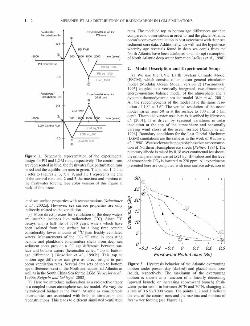
Figure 1. Schematic representation of the experimentaldesign for PD and LGM runs, respectively. The control runsare represented in blue, the freshwater flux perturbation runsin red and the equilibrium runs in green. The points 1, 2 and3 refer to Figures 2, 3, 7, 8, 9, and 11; 1 represents the endof the control runs and 2 and 3 the maxima and minima ofthe freshwater forcing. See color version of this figure atback of this issue.

Figure 2. Hysteresis behavior of the Atlantic overturningmotion under present-day (dashed) and glacial conditions(solid), respectively. The maximum of the overturningmotion is shown as a function of a linearly decreasing(upward branch) or increasing (downward branch) fresh-water perturbation in between 50�N and 70�N, changing ata rate of 0.6 Sv/1000 years. The points 1, 2 and 3 indicatethe end of the control runs and the maxima and minima offreshwater forcing (see Figure 1).

1 - 2 MEISSNER ET AL.: DISTRIBUTION OF RADIOCARBON IN LGM SIMULATIONS

specific humidity as described by Weaver et al. [2001]. Thewind stress at the ocean surface as well as the wind fieldsused for moisture advection are the same for present-day andLGM runs, respectively. Diffusion occurs along and acrossisopycnals and a parameterization of the effect of mesoscaleeddies on the tracer distribution is included [Gent andMcWilliams, 1990]. Mixing parameters are the same forLGM and PD simulations. The location and rates of deepwater formation are realistic in our model as has been

validated with CFC concentrations [Saenko et al., 2002]. Ageneral overview of efforts to validate and diagnose oceanmodels by incorporating geochemical tracers as prognosticvariables is given by England and Maier-Reimer [2001].[9] Radiocarbon is introduced as a passive tracer in the

ocean model with a half-life of 5730 years [Toggweiler etal., 1989]. During a present-day (PD) and an LGM controlrun the atmospheric 14C/12C ratio (called 14Catm/12C here-after) is held fixed to the preindustrial standard ratio. The

Figure 3. Top to bottom age difference (in years) as a function of the maximum strength of themeridional overturning (in Sv) for experiment PD FWP and the three equilibrium runs, compared to datafrom cores Vema 28-122 (a), Sonne 50-37KL (b), Knorr 110-82GGC (c), Knorr 110-66GGC (d), Knorr110-50GGC (e) and Knorr 140-39GGC (f). Model results are annual means and plotted every tenintegration years (red crosses for experiment PD FWP, green circles for the equilibrium runs). The blackdiamonds indicate the model results at points 1, 2 and 3 (end of the control run and maximum andminimum of freshwater forcing, respectively; see Figure 1). The results of the control run and the threeequilibrium runs are represented by black stars. The sediment core data for the Holocene (core tops) arerepresented by the thick blue line (Broecker et al. [1990b], Caribbean Sea (a), South China Sea (b), CearaRise (c, d, e) and [Keigwin and Schlegel, 2002], Blake Ridge (f)). The black dashed line indicates aninterpolation between the three equilibrium runs and the PD control run. Its intersection with sedimentcore data shows the overturning strength in the model which fits best with observations (vertical lines; forSouth China Sea and Blake Ridge, the vertical line indicates the minimum distance between theinterpolation and observations). See color version of this figure at back of this issue.

MEISSNER ET AL.: DISTRIBUTION OF RADIOCARBON IN LGM SIMULATIONS 1 - 3

air-sea exchange of radiocarbon is parameterized as in thework Stocker and Wright [1996, equation (A2)] with arestoring time t equal to 5 years [see Stocker and Wright,1996, and references therein].[10] The two control experiments are then integrated for

3000 years to reach a quasi-equilibrium. At the end of thecontrol runs, we diagnose the 14Catm production rates at thetop of the atmosphere needed to keep the 14Catm/12C ratioconstant for the PD and the LGM scenarios, respectively.This procedure yields a production rate of 1.31 atoms/(cm2s) for the PD run and 1.27 atoms/(cm2s) for theLGM run. These production rates lie within the order ofmagnitude of other model-based estimates; Masarik andBeer [1999] simulate a present-day production rate varyingspatially between 0.83 and 4.55 atoms/(cm2s) (their globalaverage amounts to 2.02 atoms/(cm2s)).[11] In order to simulate different overturning rates, pertur-

bations of the surface freshwater fluxes in the North Atlanticare used. In these perturbation experiments (Exp PDFWPandLGM FWP), we apply the 14Catm production rates diagnosedat the end of the control runs to the atmosphere.[12] We introduce a perturbation of freshwater fluxes into

the North Atlantic (between 50�N and 70�N) at a rate of 0.6Sv per 1000 years as in the work of Schmittner et al.[2002b]. The 14Catm/12C ratio is then calculated prognosti-cally and can respond to changes in the oceanic circulationand in the oceanic radiocarbon uptake due to the freshwaterperturbation. By introducing the freshwater perturbation, thedistribution of oceanic 14C/12C ratio (called 14Cocn/12Chereafter) can be studied for various strengths of the NorthAtlantic overturning. We use these simulations to infer ifage reversals are simulated in the deep ocean as observed byAdkins et al. [1998].

[13] In order to assess the overturning rate during the LastGlacial Maximum three additional experiments are con-ducted for LGM and PD boundary conditions, respectively(PD eq_1500, PD eq_1700, PD eq_1900 and LGM eq_500,LGM eq_700, LGM eq_900), during which the freshwaterperturbation is kept constant for 1500 years in order tosimulate near equilibrium distributions of radiocarbon fordifferent rates of overturning (Figure 1). This approach isconsistent with the notion that the overturning during theLGM was near equilibrium.

3. Results for Present-Day Simulations

[14] The introduction of a freshwater flux perturbation(experiments PD FWP and LGM FWP) in the northernNorth Atlantic leads to a hysteresis behavior of the meri-dional overturning, which is shown in Figure 2. Comparingthe two hysteresis curves it can be seen that the LGM curveis narrower than the PD curve, indicating that the over-turning is less stable under LGM than under PD conditions,consistent with earlier findings [Schmittner et al., 2002b;Ganopolski and Rahmstorf, 2001].[15] The evolution of the top to bottom age differences

during the PD FWP and the three PD equilibrium runs arecompared with sediment data at six locations in Figure 3. Asthe ocean model, with a resolution of 1.8� � 3.6�, has anecessarily coarse topography, we interpolated our data tothe six locations and depths of sediment data for thecomparative study. At all locations, the top to bottom agedifference increases for a decreasing overturning (betweenpoints 1 and 2; red crosses in Figure 3). When the fresh-water perturbation starts to decrease (after point 2; seeFigure 1), the ocean does not react immediately, and thetop to bottom age differences continue to increase while theoverturning motion continues to decrease. A rapid transitiontoward smaller top to bottom age differences can be seenafter the onset of the North Atlantic Deep Water (NADW)formation (before point 3), except in the China Sea where itis slower. The transient response of the modeled 14C/12C isthe consequence of changes in the water masses whichoccupy the particular sites. As younger NADW is replacedby older Antarctic Bottom Water (AABW), the top tobottom age differences increase and vice versa.[16] In order to get an idea about the 14C/12C distributions

in an equilibrium state, we run three additional equilibriumruns (PD eq_1500, PD eq_1700, PD eq_1900) during whichthe freshwater forcing was kept constant for 1500 years (seeFigure 1). Time series of the maximum meridional over-turning in the North Atlantic as well as of the top to bottomage difference in the six studied locations can be seen inFigures 4 and 5, respectively. The results of these equili-brium runs are also reported as green circles in Figure 3; thefinal results after 1500 years of integration are marked byblack stars. We then interpolate a response between the fourequilibrium results (PD control run, PD eq_1500, PDeq_1700, PD eq_1900, all represented by black stars). This‘‘equilibrium response’’ (represented by the black dashedline) shows a similar behavior in all locations except for theCaribbean Sea. Considering its slope, we can see that thesensitivity of radiocarbon to overturning is highly nonlinear.

Figure 4. Time series of the maximum of the overturningmotion for the equilibrium runs PD eq_1500 (blue dashed),PD eq_1700 (red dashed), PD eq_1900 (green dashed),LGM eq_500 (blue solid), LGM eq_700 (red solid) andLGM eq_900 (green solid) (see Figure 1). See color versionof this figure at back of this issue.


The top to bottom age difference varies more for highoverturning rates (>20 Sv) than for intermediate overturningrates (<20 Sv). At the two shallower locations at the CearaRise as well as at the Blake Ridge, the top to bottom agedifference varies less for very high overturning rates (whenthe advective time scale is very small; between PD eq_1500and PD eq_1700). For the locations at the Ceara Rise, wecan also see that the sensitivity at very high overturningrates increases with depth.[17] The intersection of the ‘‘equilibrium response’’

(black dashed line) with the blue line (observations for theHolocene; core tops) gives the meridional overturningstrength in best agreement with observations. The best fitwith observations for the 5 locations in the North Atlantic isgiven for a meridional overturning strength between 22.3and 25.3 Sv (23.8 Sv for the Caribbean Sea, 22.3 Sv, 24 Svand 24.6 Sv for the Ceara Rise at 2800 m depth, 3500 mdepth and 4000 m depth, respectively, and 25.3 Sv for theBlake Ridge). Schmitz and McCartney [1993] report athermohaline transport of 18 Sv at 24�N. As ’6 Sv

recirculate within the North Atlantic in our model, 22–25Sv is in excellent agreement with observed values of thepresent-day overturning.[18] This success represents an independent validation

of our method of finding the circulation strength from the14C distribution. Only the location in the South China Seagets the best results for an overturning strength of 15.75Sv. As the 14Cocn/12C distribution in the Pacific is domi-nated by diffusion [Toggweiler et al., 1989], the results inthe South China Sea are not very relevant to measure themeridional overturning in the North Atlantic and mightrather indicate errors in the value for the vertical diffu-sivity in the model.[19] Out of the four equilibrium runs, PD eq_1700 with an

overturning strength of 22.7 Sv is in best agreement with thesediment core data. A comparison between the 14Cocn/12Cratio in PD eq_1700 and observed 14C data from the Geo-chemical Ocean Sections Study (GEOSECS) (available athttp://ingrid.ldgo.columbia.edu/SOURCES/.GEOSECS/) isshown in Figure 6. Contamination of oceanic waters by

Figure 5. Time series of the top to bottom age differences (in years) at each of the six locations for theequilibrium runs PD eq_1500 (blue dashed), PD eq_1700 (red dashed) PD eq_1900 (green dashed),LGM eq_500 (blue solid), LGM eq_700 (red solid) and LGM eq_900 (green solid) (see Figure 1). Seecolor version of this figure at back of this issue.


the Suess effect and bomb 14C were taken into account byprescribing a variable atmospheric 14C/12C ratio between1840 and 1973 based on the industrial record [Orr et al.,1999]. The simulated AABW in our PD equilibrium run hasslightly higher 14C/12C ratios (’140 per mil) than observed(’160 per mil). This could lead to an underestimation of ourtop to bottom age differences in locations where youngerwater masses are replaced by AABW. NADW is wellrepresented except for the deep Greenland Sea, where notrace of bomb 14C can be seen. Overall, the simulated large

scale structure of 14C/12C distribution shows the imprints ofyoung NADW and the inflow of AABW similar to theobserved data.

4. Results for Last Glacial MaximumSimulations

[20] The top to bottom age differences from LGM runsare shown in Figure 7. Starting with high age differences(point 1) the top to bottom age differences decrease with

Figure 6. Distribution of the 14C/12C ratio (per mil) along the Atlantic sections of GEOSECS. Theupper panel shows the location of data points, the middle panel observations (interpolation between thetwo sections), the lower panel model results from the PD eq_1700 run averaged over the years 1972–1973 (interpolation between the same grid points as for the observations). See color version of this figureat back of this issue.


increasing overturning (between point 1 and point 2, redcrosses) during our LGM FWP run. When the freshwaterperturbation in the North Atlantic starts to increase again(point 2), the overturning strength decreases. However, theadvection of NADW is still strong enough to lead to afurther decrease of top to bottom age differences at everylocation (after point 2). Finally, the overturning strengthdecreases enough to cause an increase in top to bottom age

differences (before point 3). As in the present-day run thesetransient changes are caused by water masses of differentradiocarbon concentrations flushing the sites.[21] As for Figure 3, the results of our equilibrium runs

(LGM control run, LGM eq_500, LGM eq_700 and LGMeq_900; see also Figures 4 and 5) are represented by blackstars in Figure 7 and used to find the ‘‘equilibriumresponse’’ of the system (black dashed line). The intersec-

Figure 7. Top to bottom age difference (in years) as a function of the maximum strength of themeridional overturning (in Sv) for experiment LGM FWP and the three equilibrium runs compared todata from cores Vema 28-122 (a), Sonne 50-37KL (b), Knorr 110-82GGC (c), Knorr 110-66GGC (d),Knorr 110-50GGC (e) and Knorr 140-39GGC (f). Model results are annual means and plotted every tenintegration years (red crosses for experiment LGM FWP, green circles for the equilibrium runs). Theblack diamonds indicate the model results at points 1, 2 and 3 (end of the control run and minimum andmaximum freshwater forcing, respectively; see Figure 1). The results of the control run and the threeequilibrium runs are represented by black stars. The sediment core data for the LGM are represented bythe thick blue line, error bars by thin blue lines (Broecker et al. [1990b], Caribbean Sea (a), South ChinaSea (b), Ceara Rise (c, d, e) and [Keigwin and Schlegel, 2002], Blake Ridge (f)). The black dashed lineindicates an interpolation between the three equilibrium runs and the LGM control run. Its intersectionwith the sediment core data (vertical lines) and its error bars (dash-dotted vertical lines) shows the rangeof overturning strength in the model which fits best with observations (yellow shaded). See color versionof this figure at back of this issue.


tion of the ‘‘equilibrium response’’ with the measured datafor the LGM (thick horizontal blue line), as well as with itserror bars (thin horizontal blue lines), gives us an estimateof the overturning which is in best agreement with obser-vations (yellow shaded area). The results for the CaribbeanSea and the three locations on the Ceara Rise are remark-ably consistent; all indicate a very high overturning in bestagreement with sediment data. Sediment data from SouthChina Sea and Blake Ridge fit best with model results for aweakened overturning motion (�15 Sv).[22] Measuring paleoocean ventilation by dating pairs of

benthic and planktonic foraminifera requires a large numberof specimens for analysis. Bioturbation [Broecker et al.,1999] or sample contamination may lead to underestimatesof the ventilation age where the sedimentation rates are low[Broecker et al., 1999; Keigwin and Schlegel, 2002]. Veryhigh sedimentation rates as well as dated peaks in flux ofbenthic foraminifera make data from the Blake Ridge morereliable than data from other sites in the North Atlantic. Bythis logic, we find the best agreement between model results

and sediment data for an overturning between 12.7 and 18.3Sv (Blake Ridge).[23] The traditional calculation method for benthic-plank-

tonic ventilation ages can be biased by changes in theatmospheric 14C/12C ratio. Adkins and Boyle [1997] developa projection age method to avoid this problem. Using areconstruction of atmospheric 14C/12C ratios, age differencesbased on bottom 14C and atmospheric 14C can be calculated.A 400-year reservoir age correction is introduced to accountfor the difference between atmospheric and surface ocean14C/12C ratios [Broecker et al., 1990a; Adkins and Boyle,1997]. Sediment data from the Blake Ridge [Keigwin andSchlegel, 2002] are recalculated with this method. For thepresent study, we also redate the data from the Ceara Rise andthe Caribbean Sea using this method. Data from the SouthChina Sea are already redated by Adkins and Boyle [1997].Model results compared with redated sediment data (andassuming a 400-year reservoir age correction) are shown inFigure 8. For the Atlantic cores, the most likely overturningstrength is slightly weaker than for the comparison with

Figure 8. As Figure 7. Simulated top to bottom age difference (in years) are compared with redated data[Adkins and Boyle, 1997] assuming a reservoir age of 400 years. See color version of this figure at backof this issue.


conventional top to bottom ages (Figure 7). At the BlakeRidge, the best fit indicates overturning strengths between2.7 and 15.8 Sv.[24] Surface 14C/12C distributions in the present ocean are

not homogeneous. The assumption that the glacial oceanwas characterized by a fixed reservoir age can be debated.As atmospheric 14C/12C ratios are calculated prognosticallyin our model runs, we complete our analysis with a thirdcomparison between redated data (without reservoir agecorrection) and simulated atmospheric to bottom age differ-ences. The results can be seen in Figure 9. Overall, theyellow areas indicate a further weakening of the most likelyglacial circulation (0 to 12.1 Sv for the Blake Ridge).[25] The simple parameterization of gas exchange

between atmosphere and ocean in our model as well asthe assumption of a fixed reservoir age leads to importantuncertainties in the last two comparisons (Figures 8 and 9).On the other hand, redated ventilation ages for LGM andolder events are highly uncertain because the INTCAL 98calibration curve extends only to �16.6 kyr BP. Beyond that

there are only a few pairs of dates on early deglacial andLGM corals [Bard et al., 1998; Keigwin and Schlegel,2002]. The large error envelope around the calibration lineleads to a further uncertainty of ±390 years (not included inFigures 8 and 9). The projection age method used in thepresent study [Adkins and Boyle, 1997] is also only appli-cable for one unmixed water mass.[26] Following these arguments, our first analysis com-

paring conventional top to bottom age differences withmodel results (Figure 7) is probably the most reliable.

5. Ventilation of the Glacial North Atlantic

[27] Although 4 out of 5 North Atlantic sediment coresindicate a high overturning motion (�17 Sv; Caribbean Seaand Ceara Rise; see Figure 7) as the most likely circulation,sediment data from the Blake Ridge are characterized byhigher sedimentation rates and seem to be more reliablethan data from other locations in the North Atlantic. Weconclude that the distribution of radiocarbon obtained with

Figure 9. As Figure 7. Simulated atmospheric to bottom age difference (in years) are compared withredated data [Adkins and Boyle, 1997] (without reservoir age correction). See color version of this figureat back of this issue.


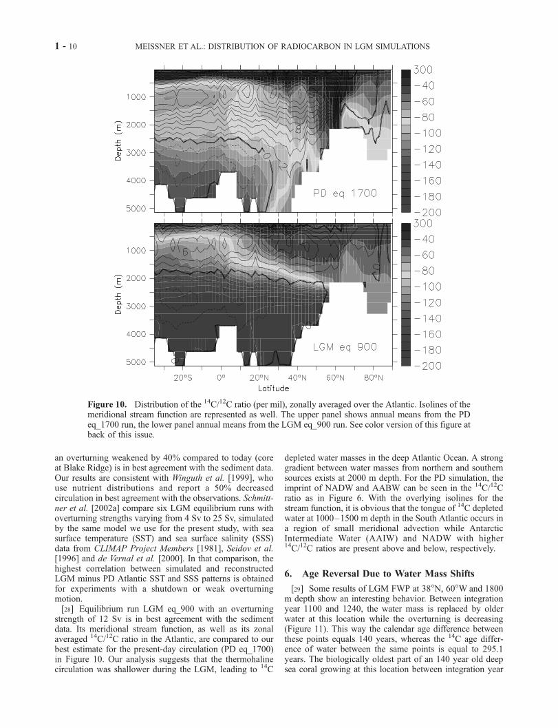
an overturning weakened by 40% compared to today (coreat Blake Ridge) is in best agreement with the sediment data.Our results are consistent with Winguth et al. [1999], whouse nutrient distributions and report a 50% decreasedcirculation in best agreement with the observations. Schmitt-ner et al. [2002a] compare six LGM equilibrium runs withoverturning strengths varying from 4 Sv to 25 Sv, simulatedby the same model we use for the present study, with seasurface temperature (SST) and sea surface salinity (SSS)data from CLIMAP Project Members [1981], Seidov et al.[1996] and de Vernal et al. [2000]. In that comparison, thehighest correlation between simulated and reconstructedLGM minus PD Atlantic SST and SSS patterns is obtainedfor experiments with a shutdown or weak overturningmotion.[28] Equilibrium run LGM eq_900 with an overturning

strength of 12 Sv is in best agreement with the sedimentdata. Its meridional stream function, as well as its zonalaveraged 14C/12C ratio in the Atlantic, are compared to ourbest estimate for the present-day circulation (PD eq_1700)in Figure 10. Our analysis suggests that the thermohalinecirculation was shallower during the LGM, leading to 14C

depleted water masses in the deep Atlantic Ocean. A stronggradient between water masses from northern and southernsources exists at 2000 m depth. For the PD simulation, theimprint of NADW and AABW can be seen in the 14C/12Cratio as in Figure 6. With the overlying isolines for thestream function, it is obvious that the tongue of 14C depletedwater at 1000–1500 m depth in the South Atlantic occurs ina region of small meridional advection while AntarcticIntermediate Water (AAIW) and NADW with higher14C/12C ratios are present above and below, respectively.

6. Age Reversal Due to Water Mass Shifts

[29] Some results of LGM FWP at 38�N, 60�W and 1800m depth show an interesting behavior. Between integrationyear 1100 and 1240, the water mass is replaced by olderwater at this location while the overturning is decreasing(Figure 11). This way the calendar age difference betweenthese points equals 140 years, whereas the 14C age differ-ence of water between the same points is equal to 295.1years. The biologically oldest part of an 140 year old deepsea coral growing at this location between integration year

Figure 10. Distribution of the 14C/12C ratio (per mil), zonally averaged over the Atlantic. Isolines of themeridional stream function are represented as well. The upper panel shows annual means from the PDeq_1700 run, the lower panel annual means from the LGM eq_900 run. See color version of this figure atback of this issue.


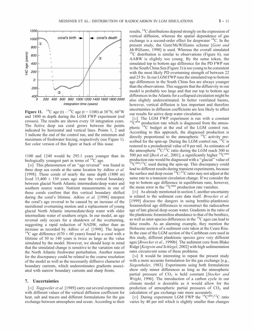
1100 and 1240 would be 295.1 years younger than itsbiologically youngest part in terms of 14C age.[30] This phenomenon of an ‘‘age reversal’’ was found in

three deep sea corals at the same location by Adkins et al.[1998]. These corals of nearly the same depth (1800 m)lived 15,400 ± 150 years ago near the vertical boundarybetween glacial North Atlantic intermediate/deep water andsouthern source water. Nutrient measurements in one ofthese corals confirm that this vertical boundary shiftedduring the coral’s lifetime. Adkins et al. [1998] interpretthe coral’s age reversal to be caused by an increase of themeridional overturning motion and a replacement of youngglacial North Atlantic intermediate/deep water with olderintermediate water of southern origin. In our model, an agereversal only occurs for a shutdown of the overturning,suggesting a rapid reduction of NADW, rather than anincrease as recorded by Adkins et al. [1998]. The largest14C age difference (670 ± 60 years) found in a coral with alifetime of 30 to 140 years is twice as large as the valuesimulated by the model. However, we should keep in mindthat the simulated change is sensitive to the variation rate ofthe North Atlantic freshwater perturbation. Another reasonfor the discrepancy could be related to the coarse resolutionof the model as well as the necessarily diffusive character ofboundary currents, which underestimates gradients associ-ated with narrow boundary currents and sharp fronts.

7. Uncertainties

[31] Toggweiler et al. [1989] carry out several experimentswith different values of the vertical diffusion coefficient forheat, salt and tracers and different formulations for the gasexchange between atmosphere and ocean. According to their

results, 14C distributions depend strongly on the expression ofvertical diffusion, whereas the spatial dependence of gasexchange is a second-order effect for deepwater 14C. In thepresent study, the Gent/McWilliams scheme [Gent andMcWilliams, 1990] is used. Whereas the overall simulated14C distribution is similar to observations (Figure 6), ourAABW is slightly too young. By the same token, thesimulated top to bottom age difference for the PD FWP runin the South China Sea (Figure 3) is too young to be consistentwith the most likely PD overturning strength of between 22and 25 Sv. In our LGMFWP runs the simulated top to bottomage differences in the South China Sea are always youngerthan the observations. This suggests that the diffusivity in ourmodel is probably too large and that our top to bottom agedifferences in the Atlantic for a collapsed circulation might bealso slightly underestimated. In better ventilated basins,however, vertical diffusion is less important and thereforeuncertainties in diffusion coefficients are less likely to affectour results for active deep water circulation.[32] The LGM FWP experiment is run with a constant

14Catm production rate which is diagnosed from the atmos-pheric 14C budget at the end of the LGM control run.According to this approach, the diagnosed production isdirectly proportional to the atmospheric 14C activity pre-scribed for the spin-up. During the LGM control run, 14C isrestored to a preindustrial value of 0 per mil. As estimates ofthe atmospheric 14C/12C ratio during the LGM reach 300 to500 per mil [Beck et al., 2001], a significantly higher 14Catm

production rate would be diagnosed with a ‘‘glacial’’ value of14Catm/12C used during the spin-up. This discrepancy couldlead to different results during transient experiments, becausethe surface and deep ocean 14C/12C ratio may not adjust at thesame rate to a transient circulation change. If we consider thetop to bottom age difference in equilibrium runs, however,the mean error in the 14Catm production rate vanishes.[33] As alreadymentioned in section 3, another uncertainty

is related to the sediment core data itself. Broecker et al.[1999] discuss the dangers in using benthic-planktonicforaminiferal age differences to reconstruct the radiocarbonage of late glacial deep ocean water. Gradients in the ratio ofthe planktonic foraminifera abundance to that of the benthics,as well as inter-species differences in the 14C ages can lead tofalse results. As an alarming example, they mention theHolocene section of a sediment core taken at the Ceara Rise.In the case of the LGM section of the Caribbean core used inthis study, different planktonic species gave very differentages [Broecker et al., 1990b]. The sediment core from BlakeRidge [Keigwin and Schlegel, 2002] with high sedimentationrates circumvent some of these problems.[34] It would be interesting to repeat the present study

with a more accurate formulation for the gas exchange [e.g.,Siegenthaler, 1983]. Experiments using both formulationsshow only minor differences as long as the atmosphericpartial pressure of CO2 is held constant [Stocker andWright, 1996]. The introduction of a carbon cycle in ourclimate model is desirable as it would allow for theprediction of atmospheric partial pressures of CO2 andcalculation of gas exchange rate more accurately.[35] During experiment LGM FWP the 14Catm/12C ratio

varies by 40 per mil which is slightly smaller than changes

Figure 11. 14C age (t) �14C age (t = 1100) at 38�N, 60�Wand 1800 m depth during the LGM FWP experiment (redcrosses). The results are shown every 10 integration years.The fictive deep sea coral grows between the pointsindicated by horizontal and vertical lines. Points 1, 2 and3 indicate the end of the control run, and the minimum andmaximum of freshwater forcing, respectively (see Figure 1).See color version of this figure at back of this issue.


found in sediment cores (e.g., 50–70 per mil at the onset ofthe Younger Dryas) [Hughen et al., 1998]. However, thevariability of the 14Catm production rate, as well as changesin the carbon uptake of the biosphere, both not consideredhere, can have a crucial influence on the 14Catm/12C ratio[Marchal et al., 2001].[36] Our study is limited by the small number of measure-

ments available and would benefit greatly from a morespatially extensive proxy record. Particularly, more meas-urements from intermediate levels in the North Atlanticwould be useful to determine the ventilation at shallowerdepths [Marchitto et al., 1998]. According to our simula-tions, the largest impact on glacial top to bottom agedifferences due to changing overturning rates can beexpected in sediments located west of the Mid-AtlanticRidge in the Sargasso Sea, near the Bermuda Rise and asfar north as the Labrador Sea (see Figure 12).

8. Conclusion

[37] Measured 14C age differences between surface anddeep waters provide powerful constraints on past oceanventilation rates. In conjunction with simulations it ispossible to estimate deep water formation rates, a quantity

which is very difficult to infer with other methods. Ourstudy suggests that deep water formation rates in the NorthAtlantic reduced by about 40% compared to the present areconsistent with available deep sea radiocarbon ages. How-ever, we cannot exclude other circulation patterns (like anincrease in AABW) to account for the observed radiocarbondistribution as suggested by Wunsch [2003]. We have alsoshown that age reversals in the North Atlantic found in deepsea corals [Adkins et al., 1998] are simulated in our experi-ments. Contrary to the original interpretation of theseobservations by Adkins et al. [1998], however, our studysuggests an abrupt reduction in deep water ventilation as thecause of the age reversal, rather than a rapid resumption ofdeep water production.

[38] Acknowledgments. We would like to thank Lloyd D. Keigwinfor providing his submitted manuscript and for his useful comments aboutthe interpretation of his data. Two anonymous reviewers and MatthewEngland were extraordinarily helpful with an earlier version of this paper.Furthermore, we would like to thank Carl Wunsch for many useful com-ments on an earlier version of this manuscript. Michael Eby’s technicalsupport was very appreciated. We are grateful for research grant supportunder the NSERC Operating, Strategic, CSHD and CFCAS research grantprograms. Daithı A. Stone is gratefully acknowledged for editing Englishgrammar.

Figure 12. Difference between two extreme states (LGM control run (weak overturning) minus LGMeq_500 (strong overturning)) of the top to bottom age difference. The locations of the sea sediment coresand the deep sea coral are represented as well. See color version of this figure at back of this issue.

ReferencesAdkins, J. F., and E. A. Boyle, Changing atmo-spheric D

14C and the record of deep waterpaleoventilation ages, Paleoceanography,12(3), 337–344, 1997.

Adkins, J. F., H. Cheng, E. A. Boyle, E. R. M.Druffel, and R. L. Edwards, Deep-sea coralevidence for rapid change in ventilation ofthe deep North Atlantic 15,400 years ago,Science, 280, 725–728, 1998.

Bard, E., M. Arnold, B. Hamelin, N. Tisnerat-Laborde, and G. Cabioch, Radiocarbon cali-bration by means of mass spectrometric230Th/234U and 14C ages of corals: An updated

database including samples from Barbados,Mururoa and Tahiti, Radiocarbon, 40, 1085–1092, 1998.

Beck, J. W., et al., Extremely large variations ofatmospheric 14C concentration during the lastglacial period, Science, 292, 2453 – 2458,2001.

Bitz, C. M., M. M. Holland, A. J. Weaver, andM. Eby, Simulating the ice-thickness distribu-tion in a coupled climate model, J. Geophys.Res., 106, 2441–2464, 2001.

Boyle, E., Last-Glacial-Maximum North AtlanticDeep Water: On, off or somewhere in-be-

tween?, Philos. Trans. R. Soc. London, 348,243–253, 1995.

Boyle, E., and Y. Rosenthal, Chemical hydrogra-phy of the South Atlantic during the Last Gla-cial Maximum: Cd vs. d13C, in The SouthAtlantic: Present and Past Circulation, editedby G. Wefer et al., pp. 423–443, Springer-Verlag, New York, 1996.

Broecker, W. S., M. Klas, E. Clark, S. Trumbore,G. Bonani, W. Wolfli, and S. Ivy, Acceleratormass spectrometric measurements on forami-nifera shells from deep sea cores, Radiocar-bon, 32, 119–133, 1990a.


Broecker, W. S., T.-H. Peng, S. Trumbore,G. Bonani, and W. Wolfli, The distribution ofradiocarbon in the glacial ocean, Global Bio-geochem. Cycles, 4, 103–106, 1990b.

Broecker, W. S., K. Matsumoto, E. Clark,I. Hajdas, and G. Bonani, Radiocarbon agedifferences between coexisting foraminiferalspecies, Paleoceanography, 14(4), 431–436,1999.

CLIMAP Project Members, Seasonal reconstruc-tions of the earth’s surface at the Last GlacialMaximum, Map Chart Ser. MC-36, Geol. Soc.Am., Boulder, Colo., 1981.

de Vernal, A., C. Hillaire-Marcel, J.-L. Turon,and J. Matthiessen, Reconstruction of sea-sur-face temperature, salinity and sea ice cover inthe northern North Atlantic during the LastGlacial Maximum based on dinocyst assem-blages, Can. J. Earth Sci., 37, 725 – 750,2000.

Duplessy, J. C., L. Labeyrie, M. Paterne, S. Ho-vine, T. Fichefet, J. Duprat, and M. Labrach-erie, High latitude deep water sources duringthe Last Glacial Maximum and the intensity ofglobal ocean circulation, in The South Atlantic:Present and Past Circulation, edited byG. Wefer et al., pp. 445–460, Springer-Verlag,New York, 1996.

England, M. H., and E. Maier-Reimer, Usingchemical tracers to assess ocean models, Rev.Geophys., 39, 29–70, 2001.

Fichefet, T., S. Hovine, and J. C. Duplessy, Amodel study of the atlantic thermohaline circu-lation during the Last Glacial Maximum, Nat-ure, 372(6503), 252–255, 1994.

Ganopolski, A., and S. Rahmstorf, Rapid changesof glacial climate simulated in a coupled cli-mate model, Nature, 409, 153–158, 2001.

Gent, P. R., and J. C. McWilliams, Isopycnalmixing in ocean circulation models, J. Phys.Oceanogr., 20, 150–155, 1990.

Hughen, K. A., J. T. Overpeck, S. J. Lehman,M. Kashgarian, J. Southon, L. C. Peterson, R.Alley, and D. M. Sigman, Deglacial changes inocean circulation from an extended radiocar-bon calibration, Nature, 391, 65–68, 1998.

Kalnay, E., et al., The NCEP/NCAR 40-year re-analysis project, Bull. Am. Meteorol. Soc., 77,437–471, 1996.

Keigwin, L. D., and M. A. Schlegel, Ocean ven-tilation and sedimentation since the glacialmaximum at 3 km in the western North Atlan-tic, Geochem. Geophys. Geosyst., 3(6), 1034,doi:10.1029/2001GC000283, 2002.

Lynch-Stieglitz, J., W. B. Curry, and N. Slowey,Weaker Gulf Stream in the Florida Straits dur-

ing the Last Glacial Maximum, Nature,402(6762), 644–648, 1999.

Marchal, O., R. Francois, T. F. Stocker, andF. Joos, Ocean thermohaline circulation andsedimentary 231Pa/230Th ratio, Paleoceanogra-phy, 15, 625–641, 2000.

Marchal, O., T. F. Stocker, and R. Muscheler,Atmospheric radiocarbon during the YoungerDryas: Production, ventilation, or both?, EarthPlanet. Sci. Lett., 185, 383–395, 2001.

Marchitto, T. M., Jr., W. B. Curry, and D. L.Oppo, Millenial-scale changes in North Atlan-tic circulation since the last glaciation, Nature,393, 557–561, 1998.

Masarik, J., and J. Beer, Simulation of particlefluxes and cosmogenic nuclide production inthe Earth’s atmosphere, J. Geophys. Res.,104(D10), 12,099–12,111, 1999.

Meissner, K. J., and R. Gerdes, Coupled climatemodelling of ocean circulation changes duringice age inception, Clim. Dyn., 18, 455–473,2002.

Orr, J. C., R. Najjar, C. L. Sabine, and F. Joos,Abiotic-HOWTO, Internal OCMIP Rep., 25pp., Lab. des Sci. de Clim. et l’Environ.,Comm. a l’Energie Atom., Saclay, Gif-sur-Yv-ette, France, 1999.

Pacanowski, R. C., MOM 2 Documentation,User’s Guide and Reference Manual, Tech.Rep. 3, Geophys. Fluid Dyn. Lab. OceanGroup, Princeton, N. J., 1995.

Peltier, W. R., Ice age paleotopography, Science,265, 15–21, 1994.

Rutberg, R. L., S. R. Hemming, and S. L. Gold-stein, Reduced North Atlantic Deep Water fluxto the glacial Southern Ocean inferred fromneodymium isotope ratios, Nature, 405(6789),935–938, 2000.

Saenko, O. A., A. Schmittner, and A. J. Weaver,On the role of wind-driven motion on oceanventilation, J. Phys. Oceangr., 32(12), 3376–3395, 2002.

Schmittner, A., K. J. Meissner, M. Eby, and A. J.Weaver, Forcing of the deep ocean circulationin simulations of the Last Glacial Maximum,Paleoceanography, 17(2), 1015, doi:10.1029/2001PA000633, 2002a.

Schmittner, A., M. Yoshimori, and A. J. Weaver,Instability of glacial climate in a model of theocean-atmosphere-cryosphere system, Science,295, 1489–1493, 2002b.

Schmitz, W. J., and M. S. McCartney, On theNorth Atlantic circulation, Rev. Geophys., 31,29–49, 1993.

Seidov, D., M. Sarnthein, K. Stattegger, R. Prien,and M. Weinelt, North Atlantic ocean circula-

tion during the Last Glacial Maximum andsubsequent meltwater event: A numericalmodel, J. Geophys. Res., 101, 16,305 –16,332, 1996.

Siegenthaler, U., Uptake of excess CO2 by anoutcrop-diffusion model of the ocean, J. Geo-phys. Res., 88, 3599–3608, 1983.

Stocker, T. F., and D. G. Wright, Rapid changesin ocean circulation and atmospheric radiocar-bon, Paleoceanography, 11(6), 773 – 795,1996.

Toggweiler, J. R., K. Dixon, and K. Bryan, Si-mulations of radiocarbon in a coarse-resolutionworld ocean model, 1, Steady state prebombdistributions, J. Geophys. Res., 94(C6), 8217–8242, 1989.

Weaver, A. J., M. Eby, A. F. Fanning, and E. C.Wiebe, Simulated influence of carbon dioxide,orbital forcing and ice sheets on the climate ofthe Last Glacial Maximum, Nature, 394, 847–853, 1998.

Weaver, A. J., et al., The Uvic Earth SystemClimate Model: Model description, climatol-ogy, and applications to past, present and fu-ture climates, Atmos. Ocean, 4, 361 – 428,2001.

Winguth, A. M. E., D. Archer, J. C. Duplessy,E. Maier-Reimer, and U. Mikolajewicz, Sen-sitivity of paleonutrient tracer distributionsand deepsea circulation to glacial boundaryconditions, Paleoceanography, 14, 304–323,1999.

Wunsch, C., Determining paleoceanographic cir-culations, with emphasis on the Last GlacialMaximum, Quat. Sci. Rev., 22, 371 – 385,2003.

Yu, E. F., R. Francois, and M. P. Bacon, Similarrates of modern and last-glacial ocean thermo-haline circulation inferred from radiochemicaldata, Nature, 379, 689–694, 1996.

��J. F. Adkins, Geological and Planetary

Sciences, California Institute of Technology,MS 100-23 1200, E. California Blvd., Pasadena,CA 91125, USA. ([email protected])K. J. Meissner, A. Schmittner, and A. J.

Weaver, School of Earth and Ocean Sciences,University of Victoria, PO Box 3055, Stn CSC,Victoria, BC V8W 3P6, Canada. ([email protected]; [email protected];[email protected])


Figure 1. Schematic representation of the experimental design for PD and LGM runs, respectively. Thecontrol runs are represented in blue, the freshwater flux perturbation runs in red and the equilibrium runsin green. The points 1, 2 and 3 refer to Figures 2, 3, 7, 8, 9, and 11; 1 represents the end of the controlruns and 2 and 3 the maxima and minima of the freshwater forcing.

MEISSNER ET AL.: DISTRIBUTION OF RADIOCARBON IN LGM SIMULATIONS

1 - 2

Figure 3. Top to bottom age difference (in years) as a function of the maximum strength of themeridional overturning (in Sv) for experiment PD FWP and the three equilibrium runs, compared to datafrom cores Vema 28-122 (a), Sonne 50-37KL (b), Knorr 110-82GGC (c), Knorr 110-66GGC (d), Knorr110-50GGC (e) and Knorr 140-39GGC (f). Model results are annual means and plotted every tenintegration years (red crosses for experiment PD FWP, green circles for the equilibrium runs). The blackdiamonds indicate the model results at points 1, 2 and 3 (end of the control run and maximum andminimum of freshwater forcing, respectively; see Figure 1). The results of the control run and the threeequilibrium runs are represented by black stars. The sediment core data for the Holocene (core tops) arerepresented by the thick blue line (Broecker et al. [1990b], Caribbean Sea (a), South China Sea (b), CearaRise (c, d, e) and [Keigwin and Schlegel, 2002], Blake Ridge (f)). The black dashed line indicates aninterpolation between the three equilibrium runs and the PD control run. Its intersection with sedimentcore data shows the overturning strength in the model which fits best with observations (vertical lines; forSouth China Sea and Blake Ridge, the vertical line indicates the minimum distance between theinterpolation and observations).


1 - 3

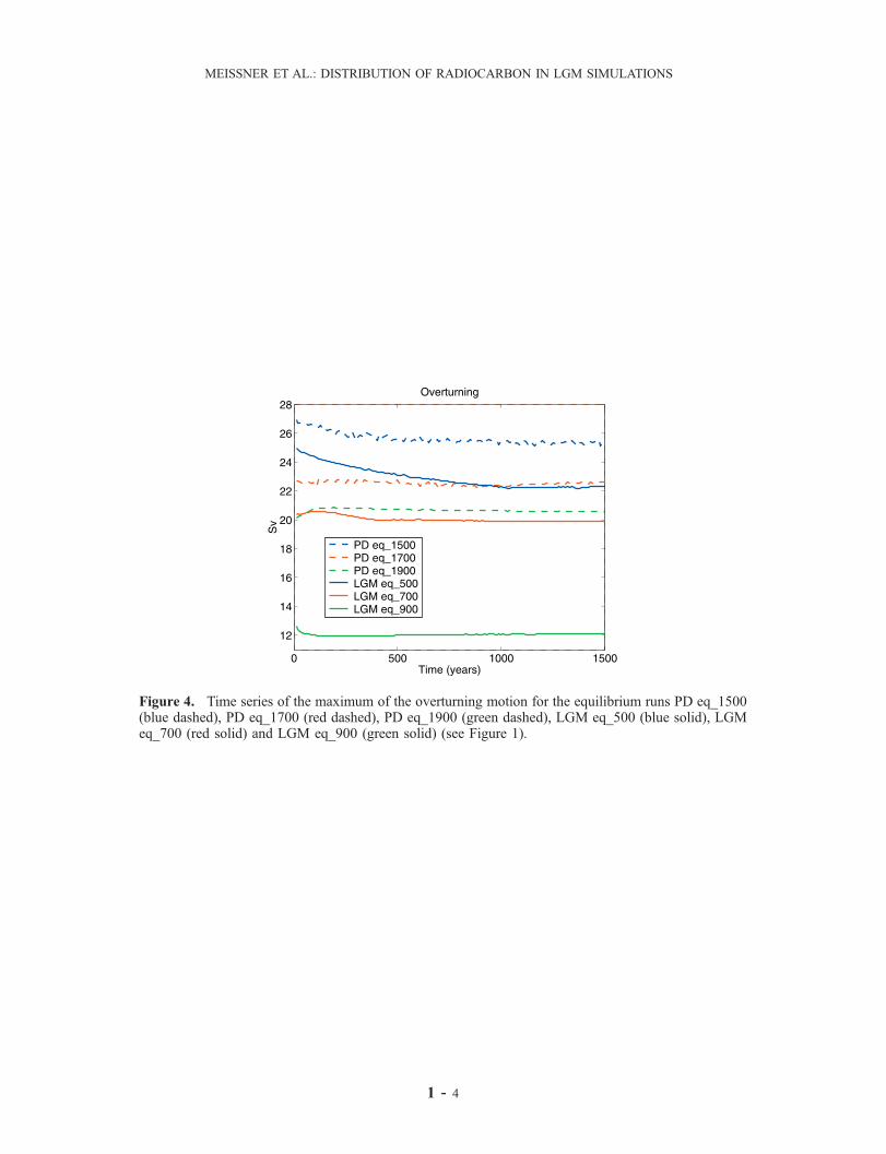
Figure 4. Time series of the maximum of the overturning motion for the equilibrium runs PD eq_1500(blue dashed), PD eq_1700 (red dashed), PD eq_1900 (green dashed), LGM eq_500 (blue solid), LGMeq_700 (red solid) and LGM eq_900 (green solid) (see Figure 1).


1 - 4

Figure 5. Time series of the top to bottom age differences (in years) at each of the six locations for theequilibrium runs PD eq_1500 (blue dashed), PD eq_1700 (red dashed) PD eq_1900 (green dashed),LGM eq_500 (blue solid), LGM eq_700 (red solid) and LGM eq_900 (green solid) (see Figure 1).


1 - 5

Figure 6. Distribution of the 14C/12C ratio (per mil) along the Atlantic sections of GEOSECS. Theupper panel shows the location of data points, the middle panel observations (interpolation between thetwo sections), the lower panel model results from the PD eq_1700 run averaged over the years 1972–1973 (interpolation between the same grid points as for the observations).


1 - 6

Figure 7. Top to bottom age difference (in years) as a function of the maximum strength of themeridional overturning (in Sv) for experiment LGM FWP and the three equilibrium runs compared todata from cores Vema 28-122 (a), Sonne 50-37KL (b), Knorr 110-82GGC (c), Knorr 110-66GGC (d),Knorr 110-50GGC (e) and Knorr 140-39GGC (f). Model results are annual means and plotted every tenintegration years (red crosses for experiment LGM FWP, green circles for the equilibrium runs). Theblack diamonds indicate the model results at points 1, 2 and 3 (end of the control run and minimum andmaximum freshwater forcing, respectively; see Figure 1). The results of the control run and the threeequilibrium runs are represented by black stars. The sediment core data for the LGM are represented bythe thick blue line, error bars by thin blue lines (Broecker et al. [1990b], Caribbean Sea (a), South ChinaSea (b), Ceara Rise (c, d, e) and [Keigwin and Schlegel, 2002], Blake Ridge (f)). The black dashed lineindicates an interpolation between the three equilibrium runs and the LGM control run. Its intersectionwith the sediment core data (vertical lines) and its error bars (dash-dotted vertical lines) shows the rangeof overturning strength in the model which fits best with observations (yellow shaded).


1 - 7

Figure 8. As Figure 7. Simulated top to bottom age difference (in years) are compared with redated data[Adkins and Boyle, 1997] assuming a reservoir age of 400 years.


1 - 8

Figure 9. As Figure 7. Simulated atmospheric to bottom age difference (in years) are compared withredated data [Adkins and Boyle, 1997] (without reservoir age correction).


1 - 9

Figure 10. Distribution of the 14C/12C ratio (per mil), zonally averaged over the Atlantic. Isolines of themeridional stream function are represented as well. The upper panel shows annual means from the PDeq_1700 run, the lower panel annual means from the LGM eq_900 run.


1 - 10

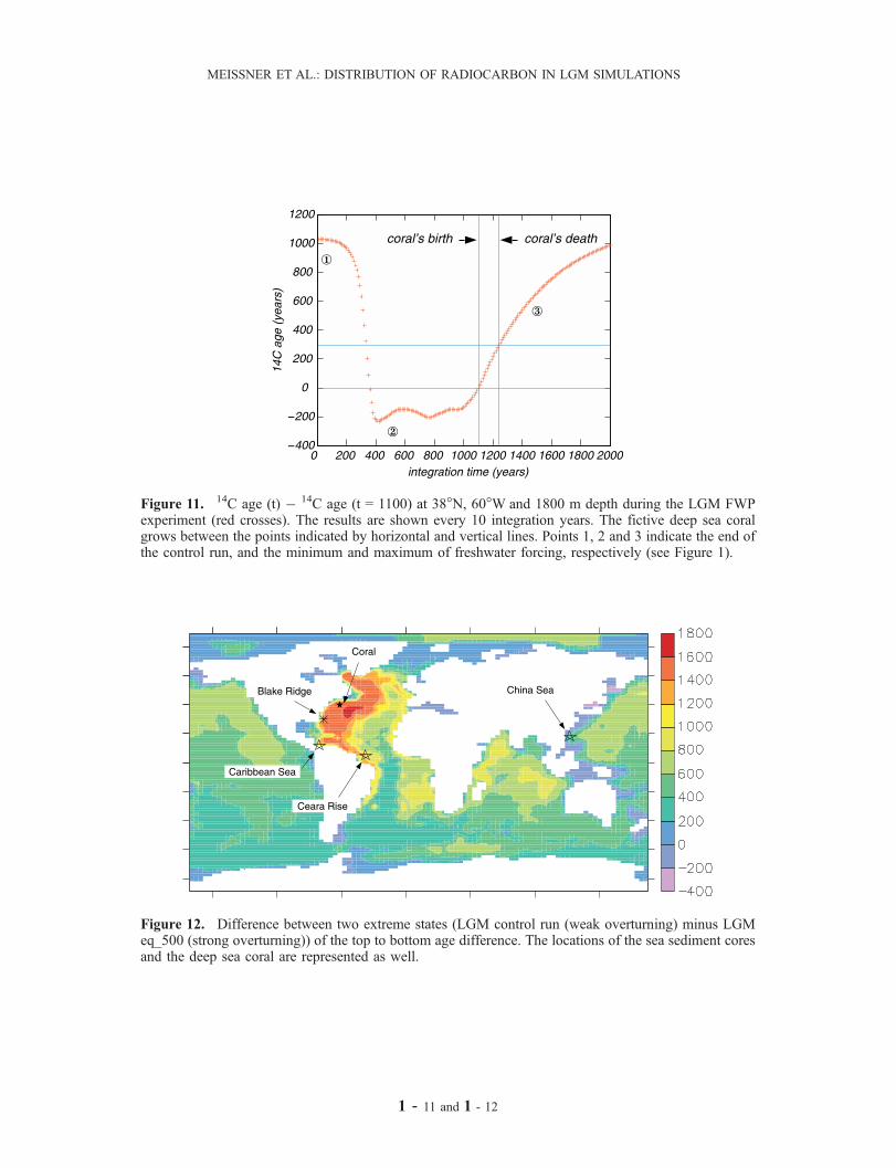
Figure 11. 14C age (t) � 14C age (t = 1100) at 38�N, 60�W and 1800 m depth during the LGM FWPexperiment (red crosses). The results are shown every 10 integration years. The fictive deep sea coralgrows between the points indicated by horizontal and vertical lines. Points 1, 2 and 3 indicate the end ofthe control run, and the minimum and maximum of freshwater forcing, respectively (see Figure 1).

Figure 12. Difference between two extreme states (LGM control run (weak overturning) minus LGMeq_500 (strong overturning)) of the top to bottom age difference. The locations of the sea sediment coresand the deep sea coral are represented as well.


1 - 11 and 1 - 12

Ventilation of the North Atlantic Ocean during the Last Glacial Maximum: A comparison between...

Documents

Transcript of Ventilation of the North Atlantic Ocean during the Last Glacial Maximum: A comparison between...