Developments in radiocarbon calibration for archaeology

Res

earc

h

Developments in radiocarboncalibration for archaeologyChristopher Bronk Ramsey1, Caitlin E. Buck2, Sturt W. Manning3,Paula Reimer4 & Hans van der Plicht5

This update on radiocarbon calibration results from the 19th International RadiocarbonConference at Oxford in April 2006, and is essential reading for all archaeologists. The wayradiocarbon dates and absolute dates relate to each other differs in three periods: back to 12 400 calBP, radiocarbon dates can be calibrated with tree rings, and the calibration curve in this formshould soon extend back to 18 000 cal BP. Between 12 400 and 26 000 cal BP, the calibrationcurves are based on marine records, and thus are only a best estimate of atmospheric concentrations.Beyond 26 000 cal BP, dates have to be based on comparison (rather than calibration) with avariety of records. Radical variations are thus possible in this period, a highly significant caveatfor the dating of middle and lower Paleolithic art, artefacts and animal and human remains.

Keywords: Dating, radiocarbon, calibration, varves, ice-cores, speleothems

IntroductionRadiocarbon dating underpins most of the chronologies used in archaeology for the last50 000 years. However, it is universally acknowledged that the radiocarbon ‘ages’ themselves(usually expressed in terms of 14C years BP – because they are measured relative to thestandard which corresponds to AD 1950) are not an accurate reflection of the true age(in calendar years) of samples, because the proportion of radiocarbon in the atmospherehas fluctuated in the past and because the half-life used for the calculation of radiocarbonages is not correct. For this reason, where possible, radiocarbon dates are calibrated againstmaterial of known age (giving ages expressed in terms of cal AD, cal BC or cal BP – whichis absolute relative to AD 1950). For recent periods (in practice, the Holocene) this is nowstandard practice amongst archaeologists. However, as we seek to extend the timescale overwhich calibration is possible, it is important to be aware of the diverse nature of calibrationdatasets and the limits to their reliability. It is also worth considering some of the reasonsbehind the controversy over the term ‘calibration’ (van Andel 2005).

1 Research Laboratory for Archaeology and the History of Art, University of Oxford, UK2 Department of Probability and Statistics, University of Sheffield, UK3 Department of Classics and The Malcolm and Carolyn Wiener Laboratory for Aegean and Near Eastern

Dendrochronology, Cornell University, USA; School of Human and Environmental Sciences, University of Reading,UK

4 14CHRONO Centre for Climate, the Environment and Chronology, Queen’s University Belfast, Belfast, NorthernIreland

5 Centre for Isotope Research, Rijksuniversiteit Groningen, Netherlands; Faculty of Archaeology, Leiden University,Netherlands

Received: 28 June 2006; Accepted: 6 September 2006; Revised: 12 September 2006

antiquity 80 (2006): 783–798

783

Developments in radiocarbon calibration

Data for radiocarbon calibration

Until recently the main data that have been employed to generate the estimates of theradiocarbon calibration curve have been measurements of the radiocarbon concentration ofwood which has been dendro-chronologically dated to the nearest year. This is ideal fromthe point of view of archaeologists since the wood in trees is laid down with carbon takenfrom the atmosphere. The same can be said for most plant fragments, and, through thefood chain, for terrestrial animals. So, for the vast majority of archaeological material, thecarbon in the samples should have a radiocarbon concentration very close to that ofthe tree rings used to generate the calibration curve. Only when there are samples frommarine or fluvial environments, or other unusual situations (for example depleted 14CO2

from volcanic sources, or significant oceanic upwelling in some coastal situations) do we haveto worry about reservoirs of carbon with radiocarbon concentrations that are substantiallydifferent to those in the atmosphere.

Over the last couple of decades the extent of tree ring records available has been greatlyexpanded. In 1986 the firmly dated sections of the calibration curve extended back to about7300 cal BP (Stuiver 1986), although floating sections could be used to infer its form backover the full extent of the Holocene. When the IntCal04 calibration curve (Reimer et al.2004) was constructed the tree ring data extended back to about 12 400 cal BP. This recordis in most places duplicated many times over, both in terms of the dendro-chronologyand with dates measured at a number of different high-precision laboratories. This lendsgreat strength to our conviction that, within the uncertainty quoted on IntCal04, thetree ring section of the IntCal04 curve closely represents a true record for the atmosphereof the mid-latitude Northern Hemisphere (see Figures 1 & 2). The 2004 estimate of thecalibration curve for the past 1000 years from the Southern Hemisphere, which has a slightlydifferent radiocarbon concentration (this difference equates to no more than c . 100 14Cyears in this time period), is also available in the form of the SHCal04 curve (McCormacet al. 2004) (see also Figure 2). Furthermore, more data are always being added to thiscorpus and floating sections of wood from Germany now extend well back into the lateglacial. This will almost certainly allow us to extend the terrestrial calibration curve backfurther in time. Equally interesting is the fact that kauri trees from New Zealand are foundwith ages that extend right out beyond the range of radiocarbon and are currently beingdated in the age range 25-55 000 BP (oral presentation by Chris Turney at the nineteenthInternational Radiocarbon Conference, Oxford). These do not, and perhaps never will,provide a continuous chronology that can be linked together to provide a chronology likethe one we have for the Holocene. However, it is likely to give us insight into the way inwhich the radiocarbon concentration in the atmosphere fluctuated in the past.

In order to calibrate samples older than the extant tree-ring-based calibration curve, weneed to make use of different kinds of records, and this is where things become morecomplicated (see Table 1). The reasons for these complications are obvious. Ideal calibrationrelates measurements of atmospheric radiocarbon (14C years BP) to the absolute calendartimescale, and according to the strict definition, only the dendro-chronological recordqualifies for this. Beyond the tree ring data, most radiocarbon samples in ‘known-age’records are derived from non-terrestrial reservoirs, such as marine deposits and speleothems

784

Res

earc

h

Christopher Bronk Ramsey et al.

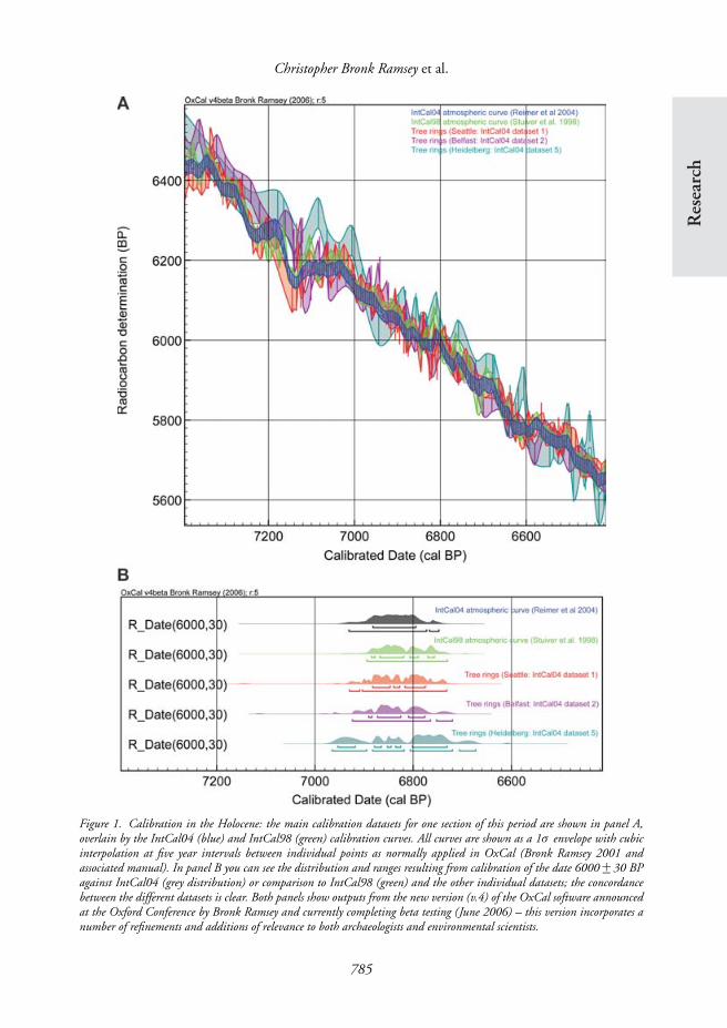
Figure 1. Calibration in the Holocene: the main calibration datasets for one section of this period are shown in panel A,overlain by the IntCal04 (blue) and IntCal98 (green) calibration curves. All curves are shown as a 1σ envelope with cubicinterpolation at five year intervals between individual points as normally applied in OxCal (Bronk Ramsey 2001 andassociated manual). In panel B you can see the distribution and ranges resulting from calibration of the date 6000 +− 30 BPagainst IntCal04 (grey distribution) or comparison to IntCal98 (green) and the other individual datasets; the concordancebetween the different datasets is clear. Both panels show outputs from the new version (v.4) of the OxCal software announcedat the Oxford Conference by Bronk Ramsey and currently completing beta testing (June 2006) – this version incorporates anumber of refinements and additions of relevance to both archaeologists and environmental scientists.

785


Figure 2. Comparison AD 1510-1900 of (i) single year northern hemisphere 14 C data (black circles with 1σ errors shownby the grey bars; uwsy98 dataset from Stuiver, Reimer & Braziunas 1998), versus (ii) a moving 5-year average of thesingle-year data of (i) in magenta, versus (iii) a moving 10-year average of the single-year data of (i) in red, versus (iv) theIntCal98 northern hemisphere calibration curve (Stuiver, Reimer, Bard et al. 1998) shown as a 1σ envelope in green, versus(v) the IntCal04 northern hemisphere calibration curve (Reimer et al. 2004) shown as a 1σ envelope in blue, versus (vi) theSHCal04 southern hemisphere calibration curve (McCormac et al. 2004) shown as a 1σ envelope in brown. We may note:(a) that annual variability/noise in the (non-replicated) single-year data lies closely around the longer-term 5-year or 10-yeartrend of the standard much-replicated calibration curves, with the 10-year moving average of the single-year data (red line)conforming very closely to the IntCal04 1σ envelope (blue lines); (b) the similarity of the IntCal98 and IntCal04 curves;(c) that IntCal04 picks up the short-term variability slightly better compared to IntCal98 where the underlying data have aresolution finer than the 5-year interpolated points of the IntCal04 curve – as the case AD 1511 and later where we haveunderlying 1-year resolution.

(mineral cave deposits), and are therefore subject to reservoir effects. The ‘known-ages’ inthese records also depend on deposition models and measurement errors. All of these issueslead to varying degrees of uncertainty, depending on the nature of the dataset, as discussedbelow (see also the list of ‘pros and cons’ given by van der Plicht et al. 2004).

First of all we have the different kinds of sample that can be used for measurements.The main samples that have been used for this kind of study are: wood, plant remains,foraminifera, corals and speleothems. The first two of these reflect atmospheric radiocarbonconcentration and so are potentially ideal for calibration purposes. However foraminiferaand corals are marine organisms, and so reflect the radiocarbon concentration in particularregions of the ocean. We know the radiocarbon concentration of the surface oceans today,but there is increasing evidence that the difference between the oceans and the atmospherehas varied (and perhaps very considerably if we look at the late glacial and earlier periods).

786

Research

Christopher

Bronk

Ram

seyetal.

Table 1. Summary of different calibration records showing the sample types and the methods used to assess independently the (calendar) ages; theexamples given are not intended to be an exhaustive list

Sample material

Plant fragments Foraminifera Speleothems tufas,(terrestrial; (oceanic; depth etc. (mixed

Independent assumed young Corals (surface depends on terrestrial anddating method Wood (terrestrial) on deposition) ocean) species) geological carbon)

Tree rings(accurate to theyear)

Tree ring records(see main recordsin Reimer et al.2004)

Uranium series(quality dependson samples)

Coral records (e.g.Bard et al. 1998;Chiu et al. 2006;Cutler et al.2004; Fairbankset al. 2005)

Speleothems andTufa records (e.g.Beck et al. 2001;Stein et al. 2004;Vogel & Kronfeld1997)

Ice cores (subjectto modelling orcounting errors)

Ocean sedimentrecords (e.g.Bard et al. 2004;Hughen et al.2004b)

Varved sediments(susceptible tomissing varvesand countingerrors)

Varved lakerecords (e.g.Kitagawa & vander Plicht 1998)

Varved oceansediments(Hughen et al.2004b)

787


This should not surprise us since one of the main phenomena of the glacial fluctuations inclimate is major change in ocean circulation (Dansgaard et al. 1993). Speleothem recordsare even more complex: they contain a mixture of carbon from the atmosphere and fromground water, which is likely to have a component of carbon from geological deposits thatare essentially free of radiocarbon.

Secondly, we have different methods of estimating the true age of the samples that areto be used for calibration. In the Holocene we have the luxury of tree ring dates that areaccurate usually to the exact year. We do not have this in earlier periods and so we mustuse other methods, the main ones being varve counting, ice-core timescales and uraniumseries dating. Varve counting of lakes (such as Lake Suigetsu, Japan) is susceptible to errorfor a number of reasons – although such sequences do usually provide a fairly good relativechronology. Ice-core timescales are either based on direct counting of ice layers (as in thecase of the GISP2 chronology and the new NGRIP chronology back to c . 40 000 BP) orbased on age/depth models (as in the case of GRIP and GISP2 beyond 40 000 BP). Inprinciple, these records suffer some of the same problems as varved lakes (for one discussionof problems in the chronology of the well-known GISP2 ice core, see Southon 2004) butdue to the concentration of effort in these records and the degree of duplication they are,at their best, considerably better than varves (presentation of J.P. Steffensen at the OxfordRadiocarbon Conference). They also have the benefit of being the timescale against whichmuch palaeoclimate data are generated, and so, even if the absolute ages are not correct, therelationships to these data will be. However, one further complication is that in order touse these timescales it is necessary to make assumptions about the synchronicity of globalclimate signals that may not be fully justified. Finally, we have uranium series dating, in thiscase either of corals or speleothems. This is a very precise and accurate technique if correctlyapplied. However, it does require very careful analysis to ensure that the samples datedhave not suffered from detrital contamination or post-depositional re-crystallisation. Thesecaveats aside, the timescale derived is independent and so provides a very useful method forradiocarbon calibration, when proven absolute (Chiu et al. 2006).

So we can see that all of the records we might use for calibration of earlier timescales dohave their problems – often complicated and often interwoven. There is some strength in thediversity of the methods employed and this is why for the IntCal04 calibration curve someof these records were used to extend the calibration curve back to 26 000 cal BP on the basisthat there was sufficiently good agreement between the different datasets (see Figure 3).However, it should be stressed that beyond the tree ring data this curve is essentiallybased on marine data and therefore relies on assumptions about the relationship betweenthe radiocarbon concentration of the oceans and the atmosphere. Thus, this part of theatmospheric calibration curve is ‘marine derived’. Further back in time the records, in partbecause of the various problems outlined above, showed poor agreement when IntCal04was compiled (see Figure 4). Research in this area is, however, very active and the situationis changing rapidly. Research programmes and investigations in different areas are bringingthe marine calibration datasets into much closer agreement. For example, the Cariaco basindata (Hughen et al. 2004a; Hughen et al. 1998; Hughen et al. 2004c), for which the initialcalendar ages were based on the GISP2 timescale, agrees much better with the coral data ifeither the new NGRIP chronology is used or the chronology from Hulu Cave (Wang et al.

788

Res

earc

h


Figure 3. Calibration at around 15 000 14 C years BP. Panel A shows the main calibration datasets for this period andinterpolated as for Figure 1A. The plots are overlain by the IntCal04 curve (blue) and the IntCal98 curve (green). In panel Byou can see the distribution and ranges resulting from calibration of the date 15 000 +− 75 BP against IntCal04 (greydistribution) or comparison to IntCal98 (green) and the other individual datasets. There is reasonable concordance with themarine datasets although the Lake Suigetsu data (which is terrestrial and not used in IntCal) suggests slightly younger ages.This may be due to the uncertainties in the Suigetsu timescale or because of slightly larger than expected oceanic reservoir effects.

789


Figure 4. Comparison against datasets at around 31 000 14 C years BP (approximate radiocarbon age of samples fromChauvet: Valladas et al. 2001). Panel A shows the main radiocarbon datasets for this period and interpolated as for Figure 1A.In panel B you can see the distribution and ranges resulting from comparison of the date 31 000 +− 300 BP to the individualdatasets. There is virtually no overlap between the results of any of the analyses. The concordance between the two marinedatasets plotted here is better although even this becomes significantly worse earlier than 38 000 cal BP, probably largelybecause of the problems with the GISP2 timescale. The terrestrial records, which are more directly applicable to archaeologicalsamples, show very substantial offsets. Thus, at present, considerable caution is appropriate when estimating any calendar agerange for examples like this.

790

Res

earc

h


2001). Other records are also being revised as new data and methods become available (suchas that of Beck et al. 2001) and it looks as if it will not be long before a marine calibrationcurve can be constructed for the last 40 000 (or even 50 000-55 000) years – as evident inpresentations by both Konrad Hughen and Richard Fairbanks at the Oxford RadiocarbonConference.

However, other discrepancies remain. These probably arise from three major factors:

� Increasing uncertainty in the calendar age estimates for the samples undergoingradiocarbon dating. Ice-core timescales become increasingly uncertain with increasingage because of thinning of the annual layers and concatenation of errors through therecord. Correlation with the oxygen isotope records also becomes more complicated insome periods. Uranium series dates are in principle still very precise over this time rangebut there is increasing chance of post-depositional change and complications of changing(or unknown) environmental conditions.

� Increasing difficulty in measuring the radiocarbon concentration of the samples accurately,especially as the records get back before 30 000 14C years BP, where the corrections formodern contamination in processing and more recent environmental contamination inthe samples are issues which can be difficult to resolve fully (at this age only about2 per cent of the radiocarbon remains in the sample and even low levels of contaminationbecome significant).

� Increasing difficulty in assessing the state of the global carbon cycle, including particularlythe ocean circulation, deep ocean ventilation and the radiocarbon production rate in theseperiods.

Of greatest significance are indications in some of the terrestrial (but not atmospheric)records (such as the Bahamas speleothem; Beck et al. 2001) that there may be someconsiderable offsets between the atmosphere and the oceans at particular periods andpossibly major age inversions at or just before 40 000 cal BP which may be related tomajor geomagnetic excursions such as the Laschamp event. If this is the case, then cautionwill still be needed in using marine records for the calibration of terrestrial samples.

What is calibrationMuch debate centres on the use of the word calibration. There are of course many uses ofthe word ‘calibrate’ in the English language, but the sense in which it is most often used inscience is ‘to set an instrument so that readings taken from it are absolute rather than relative’(Simpson & Weiner 1989). The mathematical methods employed by radiocarbon calibrationprograms such as BCal (Buck et al. 1999), CALIB (Stuiver & Reimer 1993), CalPal (Joris& Weninger 1998), the Groningen radiocarbon calibration program (WinCal25/Cal25;van der Plicht 1993), or OxCal (Bronk Ramsey 2001) are essentially methods for mappingradiocarbon ages and their associated laboratory uncertainties through a mathematicalfunction with its own uncertainty (often known as a calibration curve) onto the calendarscale. It is the view of many in the radiocarbon community that this mapping process shouldreally only be called ‘calibration’ if the mathematical function or calibration curve we use is

791


derived in such a way that we can be fairly sure that by using it we are putting our samples(with a known degree of accuracy) onto an absolute timescale.

The reason for this caution is essentially in order to prevent too much confusion inthe disciplines served by radiocarbon dating. Archaeology has suffered too much over thelast five decades from ‘radiocarbon revolutions’ without having to experience further onesevery time a new ‘calibration’ record emerges. For this reason it seems sensible to base ourestimates of calibration curves solely on data that are well corroborated and to avoid datawhich (although potentially useful for other purposes) are currently seen as provisionalfor calibration purposes. In this respect it would also seem sensible to draw a semanticdistinction between ‘calibration’ as such and ‘comparison’ of radiocarbon dates to particularrecords. The same kinds of mathematical method can be used to undertake both ‘calibration’and ‘comparison’ and the data are almost always made freely available by the scientificcommunity, so there is no question of curtailing freedom as suggested by van Andel (2005).We simply urge everyone to make it clear whether they are undertaking true calibration ora comparison and draw their readers’ attention to the difference between the two.

There is an argument that ‘calibration’ need not be very precise and that even a roughcalibration may be useful. This is certainly true. However, if the calibration is to be usefulit must have a statement of uncertainty attached to it and this must accurately reflect thetrue uncertainty in the absolute age estimate generated. Herein lies a problem. Each groupof researchers who provide data with potential utility for radiocarbon calibration curveestimation do their best to quantify their own internal sources of error and uncertainty andto report these in a standard form. What they do not and cannot do is to allow for sources oferror or uncertainty that they are completely unaware of. If we look at the currently availabledata for the pre-tree-ring timescale we find that there are substantial uncertainties that havesimply not been quantified. Buck and Blackwell (2004) provide a statistical method toestimate the scale of unquantified uncertainties that must be present if all of the recordsthey considered relate to the same underlying radiocarbon calibration record and foundoffsets as large as 2500 years (van der Plicht et al. 2004). Given this (and other observationsabout the data), the IntCal group felt that they could not provide a reliable estimate of theradiocarbon calibration curve beyond 26 000 cal BP in 2004.

In the absence of an internationally agreed calibration curve beyond 26 000 cal BP, it isnatural for researchers to compare one record to another (exactly as the IntCal team did). Indoing this, however, it is wise to avoid use of the term ‘calibration’ since this does suggest anabsolute scale, and instead use alternatives, for example ‘comparison’ as proposed previously(Richards & Beck 2001; van der Plicht 2000; van der Plicht et al. 2004).

Implications for archaeologistsSo how should archaeologists treat the data that are currently available? The data are there tobe used and studied and no-one wishes to stifle speculation about what those data mean forvery important archaeological issues. Indeed, the calendar timescale created by radiocarbonlargely shapes a number of questions and debates in the later Palaeolithic period. It is thusnot realistic to assume that those working in the area will wait until the research is completebefore starting to look at such issues (as for example in Mellars 2006 and the discussion with

792

Res

earc

h


Turney et al. 2006). However, it is important that the archaeological community is awareof the different nature of the radiocarbon records.

Back to around 12 400 cal BP, the period for which we have multiple records that arein good agreement, including tree rings, it seems very likely that the calibration curve willnot change significantly as new data come to light and calibration can in most cases be usedas a tool in studying archaeological chronology even in a fairly fine-grained manner (seeFigure 1). This period of relative certainty is likely to reach back to about 18 000 cal BPonce the new work extending the tree ring record reported by Mike Friedrich at the OxfordRadiocarbon Conference is (eventually) completed. In this time period there are some minorissues that are still to be sorted out for very high precision work. These centre on how thedifferent calibration sets are compiled into a single curve. Such a compilation is undoubtedlythe best policy since it ensures that no one dataset, with its inevitable possible faults, is giventoo much weight. All of the indications are that within any one hemisphere there are nosignificant regional effects although some very minor differences between records have beenattributed to differences in growth seasons (Kromer et al. 2001) or proximity to oceanupwelling regions (Stuiver & Braziunas 1998). Probably more significant is the fact thatmost of the calibration data are measured on ten- or twenty-year sections of wood andtherefore average out shorter-term to annual variations (see Figure 2 – this visible noise willusually in effect cancel itself out over even a few years and especially within the range of manytypical radiocarbon measurements and their associated errors – minor exceptions may occurat times of major peaks or troughs in the radiocarbon record – e.g. AD 1788-92 – but itshould also be remembered that this single-year record is not replicated and clearly containssubstantial noise as well as signal). There are also questions over what the best statisticalmethods are for combining the datasets; the IntCal04 curve (Buck & Blackwell 2004;Reimer et al. 2004) uses a statistical model which introduces a small amount of smoothingto the data (though no more than is apparently justified by the expected random noise –and indeed this model better reflects underlying data when we have annual scale input whencompared to IntCal98 – see Figure 2). Since such methods cannot distinguish betweenrandom outliers and real extreme values there are some real short-term fluctuations thatmay be attenuated in this compilation (especially when the underlying data are only decadalor bidecadal). There is scope for further work to refine these statistical methods. However,from the point of view of a user of calibration, IntCal04 provides the most comprehensiveand up-to-date estimate of the Northern Hemisphere calibration curve and should alwaysbe the first choice for calibration. Comparison of the results with those obtained againstthe IntCal98 (Stuiver, Reimer, Bard et al. 1998) calibration curve, which used a simplebinning and weighted average of the data then available, can be valuable as can comparisonagainst individual datasets. Such a degree of complexity is however only really warrantedin large-scale Bayesian models (when the results are usually insensitive to such changes) orwiggle-matching of tree ring sequences (where differences are occasionally significant if thematch relies predominantly on one or two fluctuations in radiocarbon levels). For normalcalibration the IntCal04 curve is all that is required.

Between 12 400 and 26 000 cal BP, the current situation is slightly different. Here thecalibration curve is based on multiple records in good agreement, but these are all marinerecords and therefore represent our best estimate of the atmospheric concentration. There

793


may however be changing marine reservoir offsets that could mean the curve in some sectionsof this time period is out by as much as 250 14C years BP (Bondevik et al. 2006; Kromeret al. 2004). It is very unlikely to be worse than this given the agreement of IntCal04 withother records not used in the calibration curve, such as the terrestrial macrofossil recordfrom Lake Suigetsu (Kitagawa & van der Plicht 2000). In this time range calibration forarchaeological purposes is possible. However, such calibration is more provisional and therecould be some minor changes as new data accumulate, particularly from terrestrial records,which might be significant in certain contexts (see Figure 3).

Further back than 26 000 cal BP, the situation is radically different. Here the recordsare neither based on purely terrestrial material, nor do they agree with one another (seeFigure 4). As stated above, some of these discrepancies are being addressed actively andwithin a couple of years the situation is likely to be much better. However, the possiblemajor discrepancies between the marine and atmospheric data need to be viewed withparticular caution as they imply that even with consistent marine records we may still notunderstand how to interpret the records in the context of terrestrial archaeological samples.Given this, it is clear why the radiocarbon community does not think that calibrationas such is possible in this time range, since it is not clear which, if any, of the presentrecords provide a good indication of the atmospheric radiocarbon concentration. Thusfar there is only one record that represents true atmospheric 14C measurements (LakeSuigetsu); however, this record stands alone in the sense that it is not confirmed byothers. We know for the period in which we do have an atmospheric record that thereare many short-term fluctuations, which are missing from the marine record. This is likelyto be even more significant in periods where the climate is much less stable, there may bemajor magnetic excursions, and the resolution of the marine measurements we do have ispoorer.

The highest resolution record in this time range, that from the Cariaco basin (Hughen,Lehman et al. 2004), illustrates many of these points clearly and also shows what can andcannot be done with the current data. The samples for this record are marine, and they areabsolutely dated by matching changes in the characteristics of the sediments to changes inthe climate as recorded by the Greenland ice cores, in this case GISP2. This means that thetimescale used is the GISP2 timescale, which is based on a model of ice accumulation beyond41 000 cal BP. Recent work on the NGRIP core (presentation of J.P. Steffensen at the OxfordRadiocarbon Conference) suggests that the GISP2 timescale has non-linear errors, whichmeans that not only are the absolute ages wrong, but that rates of change estimated fromthis timescale may be significantly incorrect too. This in turn then significantly impactsarchaeological assessments made using the 2004 Cariaco record (as in Mellars 2006). Asreported at the Oxford Radiocarbon Conference, this particular problem is likely to beaddressed by linking to other absolutely dated records, most likely that at Hulu Cave(Wang et al. 2001). However, the uncertainty in the difference between the atmosphericand marine radiocarbon concentration will not be so easily addressed. Even though thesedifferences seem to be fairly well behaved in the late glacial we cannot assume that this isalways the case. That said, comparison of radiocarbon dates to this record can undoubtedlybe valuable, particularly if what is of interest is how the dates lie in relation to the changesin climate as recorded in the GISP2 δ18O record – but where this is done it should always

794

Res

earc

h


be made clear that the comparison is made against this record and is on the GISP2 orNGRIP timescale (as discussed in Gravina et al. 2005).

Other records are also valuable for archaeologists. Coral data, although also marine, linkinto a more absolute uranium-series-based chronology. This is better from the point-of-viewof absolute ages – though not as useful if you wish to compare them to the oxygen isotoperecords of the Greenland ice cores. Furthermore, the coral-based records such as that ofFairbanks et al. (2005), are not continuous records, since they are based on chance finds ofcorals; nor is it likely that they are an entirely random sample since formation factors linkingto climate and environmental changes are likely to bias the recovered sample set. Thus anycurve generated from such datasets looks smooth. But we must remember that absence ofevidence is not evidence of absence and such a curve almost certainly fails to show even thescale of fluctuations in the radiocarbon concentration of the oceans, let alone the levels ofvariability in the atmosphere. Available climate indicators suggest similar (e.g. Roig et al.2001) or greater (e.g. Bond & Lotti 1995; Dansgaard et al. 1993) periods and cycles ofchange for the later Pleistocene compared to the Holocene (e.g. Bond et al. 2001). Thesewould be reflected in an atmospheric 14C record giving at least as many, and very likely more,variations and cyclical features than for the record available for the Holocene. At presentwe are largely lacking such information for the periods before terrestrial tree-based records,and measurement errors on very old radiocarbon ages will anyway tend to mask some of theexpected century-scale variation. The record for Lake Suigetsu is potentially very useful as itis purely terrestrial, but it lacks a good absolute timescale. The speleothem records are partlyterrestrial and so also provide useful information on the possible scale of differences betweenthe radiocarbon concentration of the surface oceans and the terrestrial groundwater. No onerecord is right in all respects but all give information that is potentially useful. Because theirproblems are all different it is also potentially misleading to compile them into a compositecurve for calibration since this merely serves to mask the underlying complications. Thisis the reason for the ironically named NOTCal curve (van der Plicht et al. 2004), and thecriticisms levelled at aspects of the CalPal program referred to by van Andel (2005).

So what should the archaeological researcher working in this period do? Ignoring theproblem, either by assuming that radiocarbon ages in this period can be treated as someapproximate proxy for age, or by using some ad hoc compilation of data into a ‘comparison’curve as if it were a ‘calibration’ curve cannot be regarded as good scholarship. It is almostbound to result in conclusions and assertions which will have to be changed (and quitepossibly significantly) within a very few years – indeed often before the research is physicallypublished. The uncertainties need to be fully acknowledged. The correct approach willdepend very much on the application. In many cases it may be appropriate to compare datesto a number of different specific records – unless there are very particular reasons for onerecord being most appropriate. The timescale to which the comparison has been made (forexample Uranium Series or NGRIP ice core) should be made explicit and the ages deducedwould be better referred to as ‘estimated’ rather than ‘calibrated’ dates. Most crucially allshould be aware that these estimates may well change significantly as our understandingof the Earth’s system during the last glaciation improves. If absolute ages are the primaryinterest then there is not really much of a substitute for comparison against all of the mainrecords since this demonstrates the range of possible true ages depending on which of the

795


records most closely reflect the relevant reality. As the datasets improve, this exercise willhopefully provide a narrower and narrower range of possibilities.

ConclusionsThere has been considerable progress in recent years in the level of information available forassessing the past radiocarbon concentration of the atmosphere and oceans. This informationis very valuable for archaeologists since it helps them to interpret their radiocarbon dates interms of absolute chronology. However, the cost of this progress is increasing complexity inthe nature of the data, and this means that archaeologists need to have a critical understandingof what sort of analyses the data can and cannot support.

Back to about 12 400 cal BP, the data are fairly robust and the IntCal04 calibrationcurve should provide accurate calibration for most purposes. Where very high precision isrequired, with large Bayesian models or wiggle-matching of tree ring sequences, it may alsobe valuable to compare the results of such analyses against the IntCal98 curve because it iscompiled differently (even though it does have known deficiencies), or against individualdatasets (such as Irish oak in the case of British sites, for example).

In the period between 12 400 and 26 000 cal BP any calibration is more provisional sincethe data used for construction of the calibration curve are marine-derived. However, giventhe level of agreement between records in this region, such calibration is likely to be fairlyaccurate and for most purposes the IntCal04 calibration curve can be used as it is. In somecritical applications, it may also be useful to compare such calibration to estimates fromindividual records.

Beyond 26 000 cal BP, there is no accepted calibration curve simply because of thedisparity in the records we have for this time period as of June 2006, and so comparisonshould be made to a range of individual records to estimate ages on the timescale relevantto the specific records. The records used for such comparisons will depend on the detailsof the application. If climatic correlations are important, then records that link to climaticdata will be most useful. On the other hand, if absolute ages are the main issue, then thefull range of datasets should be considered to see the range of possibilities.

In order to prevent confusion, it makes a lot of sense to reserve the terms ‘calibration’and ‘calibrated dates’ for analyses based on the recognised calibration curves (IntCal04,SHCal04 & Marine04). In the periods covered by these curves it may also be useful tomake a ‘comparison’ against other records. The term ‘estimated dates’ for the results of suchanalyses seems most appropriate. Where calibration is not yet possible, ‘comparison’ againstthe different records now available may still be useful but the provisional nature of suchanalyses should be fully appreciated. As with the paper by Mellars (2006), speculation aboutthe implications of the data as they emerge are entirely appropriate but the caveat at the endof that piece is important to keep fully in mind: ‘A final, definitive calibration curve for thistime range will depend on the results of new calibration studies, at present being pursuedin several different laboratories. The full implications of these studies for the interpretationof the human archaeological and evolutionary record will need to be kept under active andvigilant review’. If we always remember this, we should avoid the inevitable disappointmentwhen new facts emerge to overturn a beautiful and elegant hypothesis constructed on thebasis of preliminary data.

796

Res

earc

h


ReferencesBard, E., M. Arnold, B. Hamelin,

N. Tisnerat-Laborde & G. Cabioch. 1998.Radiocarbon calibration by means of massspectrometric Th-230/U-234 and C-14 ages ofcorals: An updated database including samples fromBarbados, Mururoa and Tahiti. Radiocarbon 40(3):1085-92.

Bard, E., F. Rostek & G. Menot-Combes. 2004.Radiocarbon calibration beyond 20 000 C-14 yr BPby means of planktonic foraminifera of the IberianMargin. Quaternary Research 61(2): 204-14.

Beck, J.W., D.A. Richards, R.L. Edwards, B.W.Silverman, P.L. Smart, D.J. Donahue,S. Hererra-Osterheld, G.S. Burr, L. Calsoyas,A.J.T. Jull & D. Biddulph. 2001. Extremely largevariations of atmospheric C-14 concentrationduring the last glacial period. Science 292(5526):2453-58.

Bond, G., B. Kromer, J. Beer, R. Muscheler, M.N.Evans, W. Showers, S. Hoffmann,R. Lotti-Bond, I. Hajdas & G. Bonani. 2001.Persistent solar influence on north Atlantic climateduring the Holocene. Science 294(5549): 2130-36.

Bond, G.C. & R. Lotti. 1995. Iceberg Discharges intothe North-Atlantic on Millennial Time Scalesduring the Last Glaciation. Science 267(5200):1005-10.

Bondevik, S., J. Mangerud, H.H. Birks,S. Gulliksen & P. Reimer. 2006. Changes inNorth Atlantic radiocarbon reservoir ages duringthe Allerod and Younger Dryas. Science 312(5779):1514-17.

Bronk Ramsey, C. 2001. Development of theradiocarbon calibration program OxCal.Radiocarbon 43(2A): 355-63.

Buck, C.E. & P.G. Blackwell. 2004. Formalstatistical models for estimating radiocarboncalibration curves. Radiocarbon 46(3): 1093-1102.

Buck, C.E., J.A. Christen & G.N. James. 1999.BCal: an on-line Bayesian radiocarbon calibrationtool. Internet Archaeology 7:http://intarch.ac.uk/journal/issue7/buck index.html.

Chiu, T.C., R.G. Fairbanks, R.A. Mortlock,L. Cao, T.W. Fairbanks & A.L. Bloom. 2006.Redundant 230Th/234U/238U, 231Pa/235U and 14Cdating of fossil corals for accurate radiocarbon agecalibration. Quaternary Science Reviews 25(17-18):2431-40.

Cutler, K.B., S.C. Gray, G.S. Burr, R.L. Edwards,F.W. Taylor, G. Cabioch, J.W. Beck, H. Cheng& J. Moore. 2004. Radiocarbon calibration andcomparison to 50 kyr BP with paired C-14 andTh-230 dating of corals from Vanuatu and PapuaNew Guinea. Radiocarbon 46(3): 1127-60.

Dansgaard, W., S.J. Johnsen, H.B. Clausen, D.Dahljensen, N.S. Gundestrup, C.U. Hammer,C.S. Hvidberg, J.P. Steffensen, A.E.Sveinbjornsdottir, J. Jouzel & G. Bond. 1993.Evidence for General Instability of Past Climatefrom a 250-Kyr Ice-Core Record.Nature 364(6434): 218-20.

Fairbanks, R.G., R.A. Mortlock, T.C. Chiu,L. Cao, A. Kaplan, T.P. Guilderson, T.W.Fairbanks, A.L. Bloom, P.M. Grootes & M.J.Nadeau. 2005. Radiocarbon calibration curvespanning 0 to 50 000 years BP based on pairedTh-230/U-234/U-238 and C-14 dates on pristinecorals. Quaternary Science Reviews 24(16-17):1781-96.

Gravina, B., P. Mellars & C. Bronk Ramsey. 2005.Radiocarbon dating of interstratified Neanderthaland early modern human occupations at theChatelperronian type-site. Nature 438(7064): 51-6.

Hughen, K.A., M.G.L. Baillie, E. Bard, J.W. Beck,C.J.H. Bertrand, P.G. Blackwell, C.E. Buck,G.S. Burr, K.B. Cutler, P.E. Damon, R.L.Edwards, R.G. Fairbanks, M. Friedrich, T.P.Guilderson, B. Kromer, G. McCormac,S. Manning, C. Bronk Ramsey, P.J. Reimer,R.W. Reimer, S. Remmele, J.R. Southon,M. Stuiver, S. Talamo, F.W. Taylor, J. van derPlicht & C.E. Weyhenmeyer. 2004a. Marine04marine radiocarbon age calibration, 0-26 cal kyr BP.Radiocarbon 46(3): 1059-86.

Hughen, K.A., S. Lehman, J. Southon, J. Overpeck,O. Marchal, C. Herring & J. Turnbull. 2004b.C-14 activity and global carbon cycle changes overthe past 50 000 years. Science 303(5655): 202-7.

Hughen, K.A., J.T. Overpeck, S.J. Lehman, M.Kashgarian & J.R. Southon. 1998. A new C-14calibration data set for the last deglaciation basedon marine varves. Radiocarbon 40(1): 483-94.

Hughen, K.A., J.R. Southon, C.J.H. Bertrand,B. Frantz & P. Zermeno. 2004c. Cariaco basincalibration update: Revisions to calendar and C-14chronologies for core PL07-58PC. Radiocarbon46(3): 1161-87.

Joris, O. & B. Weninger. 1998. Extension of theC-14 calibration curve to ca. 40 000 cal BC bysynchronizing Greenland O-18/O-16 ice corerecords and North Atlantic foraminifera profiles:A comparison with U/Th coral data. Radiocarbon40(1): 495-504.

Kitagawa, H. & J. van der Plicht. 1998.Atmospheric radiocarbon calibration to 45 000 yrBP: Late glacial fluctuations and cosmogenicisotope production. Science 279(5354): 1187-90.

–2000. Atmospheric radiocarbon calibration beyond11 900 cal BP from Lake Suigetsu laminatedsediments. Radiocarbon 42(3): 369-80.

797


Kromer, B., M. Friedrich, K.A. Hughen, F. Kaiser,S. Remmele, M. Schaub & S. Talamo. 2004. Lateglacial C-14 ages from a floating, 1382-ring pinechronology. Radiocarbon 46(3): 1203-9.

Kromer, B., S.W. Manning, P.I. Kuniholm, M.W.Newton, M. Spurk & I. Levin. 2001. Regional(CO2)-C-14 offsets in the troposphere: Magnitude,mechanisms, and consequences. Science 294(5551):2529-32.

McCormac, F.G., A.G. Hogg, P.G. Blackwell, C.E.Buck, T.F.G. Higham & P.J. Reimer. 2004.SHCal04 Southern Hemisphere calibration,0-11.0 cal kyr BP. Radiocarbon 46(3): 1087-92.

Mellars, P. 2006. A new radiocarbon revolution andthe dispersal of modern humans in Eurasia.Nature 439(7079): 931-5.

Reimer, P.J., M.G.L. Baillie, E. Bard, A. Bayliss,J.W. Beck, C.J.H. Bertrand, P.G. Blackwell,C.E. Buck, G.S. Burr, K.B. Cutler, P.E. Damon,R.L. Edwards, R.G. Fairbanks, M. Friedrich,T.P. Guilderson, A.G. Hogg, K.A. Hughen,B. Kromer, G. McCormac, S. Manning,C. Bronk Ramsey, R.W. Reimer, S. Remmele,J.R. Southon, M. Stuiver, S. Talamo, F.W.Taylor, J. van der Plicht & C.E.Weyhenmeyer. 2004. IntCal04 terrestrialradiocarbon age calibration, 0-26 cal kyr BP.Radiocarbon 46(3): 1029-58.

Richards, D.A. & J.W. Beck. 2001. Dramatic shiftsin atmospheric radiocarbon during the last glacialperiod. Antiquity 75(289): 482-5.

Roig, F.A., C. Le-Quesne, J.A. Boninsegna, K.R.Briffa, A. Lara, H. Grudd, P.D. Jones &C. Villagran. 2001. Climate variability50 000 years ago in mid-latitude Chile asreconstructed from tree rings. Nature 410(6828):567-70.

Simpson, J.A. & E.S.C. Weiner. 1989. The OxfordEnglish dictionary. 2nd ed. 20 vols. Oxford:Clarendon Press.

Southon, J. 2004. A radiocarbon perspective onGreenland ice-core chronologies: Can we use icecores for C-14 calibration? Radiocarbon 46(3):1239-59.

Stein, M., C. Migowski, R. Bookman & B. Lazar.2004. Temporal changes in radiocarbon reservoirage in the dead sealake Lisan system. Radiocarbon46(2): 649-55.

Stuiver, M. 1986. Proceedings of the 12thInternational Radiocarbon Conference – Held atTrondheim Norway 24-28 June 1985. Radiocarbon28(2B): R2-R2.

Stuiver, M. & T.F. Braziunas. 1998. Anthropogenicand solar components of hemispheric C-14.Geophysical Research Letters 25(3): 329-32.

Stuiver, M. & P.J. Reimer. 1993. Extended C-14Data-Base and Revised Calib 3.0 C-14 AgeCalibration Program. Radiocarbon 35(1): 215-30.

Stuiver, M., P.J. Reimer, E. Bard, J.W. Beck, G.S.Burr, K.A. Hughen, B. Kromer, G. McCormac,J. Van der Plicht & M. Spurk. 1998.INTCAL98 radiocarbon age calibration,24 000-0 cal BP. Radiocarbon 40(3): 1041-83.

Stuiver, M., P.J. Reimer & T.F. Braziunas. 1998.High-precision radiocarbon age calibration forterrestrial and marine samples. Radiocarbon 40(3):1127-51.

Turney, C.S.M., R.G. Roberts & Z. Jacobs. 2006.Progress and pitfalls in radiocarbon dating.Nature 443: E3-E4.

Valladas, H., J. Clottes, J.M. Geneste, M.A.Garcia, M. Arnold, H. Cachier &N. Tisnerat-Laborde. 2001. Palaeolithicpaintings – Evolution of prehistoric cave art. Nature413(6855): 479.

van Andel, T.H. 2005. The ownership of time:approved C-14 calibration or freedom of choice?Antiquity 79(306): 944-8.

van der Plicht, J. 1993. The Groningen RadiocarbonCalibration Program. Radiocarbon 35(1):231-7.

–2000. Introduction: The 2000 Radiocarbonvarve/comparison issue. Radiocarbon 42(3): 313-22.

van der Plicht, J., J.W. Beck, E. Bard, M.G.L.Baillie, P.G. Blackwell, C.E. Buck,M. Friedrich, T.P. Guilderson, K.A. Hughen,B. Kromer, F.G. McCormac, C. Bronk Ramsey,P.J. Reimer, R.W. Reimer, S. Remmele, D.A.Richards, J.R. Southon, M. Stuiver & C.E.Weyhenmeyer. 2004. NotCal04 – Comparison/calibration C-14 records 26-50 cal kyr BP.Radiocarbon 46(3): 1225-38.

Vogel, J.C. & J. Kronfeld. 1997. Calibration ofradiocarbon dates for the late Pleistocene usingU/Th dates on stalagmites. Radiocarbon 39(1):27-32.

Wang, Y.J., H. Cheng, R.L. Edwards, Z.S. An,J.Y. Wu, C.C. Shen & J.A. Dorale. 2001.A high-resolution absolute-dated Late Pleistocenemonsoon record from Hulu Cave, China. Science294(5550): 2345-8.

798

Developments in radiocarbon calibration for archaeology

Documents

Transcript of Developments in radiocarbon calibration for archaeology