Engineering, 2022, 14, 185-216 https://www.scirp.org/journal/eng

ISSN Online: 1947-394X ISSN Print: 1947-3931

DOI: 10.4236/eng.2022.146018 Jun. 30, 2022 185 Engineering

The Solving of the Inverse Thermal Conductivity Problem for Study the Short Linear Heat Pipes

Arkady Vladimirovich Seryakov

LLC “Rudetransservice”, Veliky Novgorod, Russia

Abstract The results of studies by solving the inverse thermal conductivity problem of the heat capacity of evaporator of the short linear heat pipes (HP’s) with a Laval nozzle-liked vapour channel and intended for cooling spacecraft and sa-tellites with strict take-off mass regulation are presented. Mathematical for-mulation of the inverse problem for the HP’s thermal conductivity in one- dimensional coordinate system is accompanied by the measurement results using the monotonic heating method in a vacuum adiabatic calorimeter the HP’s surface temperatures along the longitudinal axis over the entire temper-ature load range, thermal resistance, and arrays of thermal power data on the evaporator Qev and vortex flow calorimeter Qcond for the condensation surface allow us to estimate the average value of the evaporator heat capacity Cev by solving the inverse thermal conductivity problem in the HP’s evaporator re-gion. Since at the beginning of working fluid boiling for a certain time inter-val, the temperature of the capillary-porous evaporator remains close to con-stant, and with the continuation of heating and by solving the inverse thermal conductivity problem, it becomes possible to calculate the heat capacity of the working evaporator and the evaporation specific heat of the boiling working fluid and compare it with the table values.

Keywords Short Linear HP’s, The Inverse Problem of Thermal Conductivity, The Monotonic Heating Method, Thermal Resistance and Heat Capacity

1. Introduction

The current development level of the computer technology and computing tech-nologies allows us to significantly expand the class of applied problems to be

How to cite this paper: Seryakov, A.V. (2022) The Solving of the Inverse Thermal Conductivity Problem for Study the Short Linear Heat Pipes. Engineering, 14, 185-216. https://doi.org/10.4236/eng.2022.146018 Received: April 11, 2022 Accepted: June 27, 2022 Published: June 30, 2022 Copyright © 2022 by author(s) and Scientific Research Publishing Inc. This work is licensed under the Creative Commons Attribution International License (CC BY 4.0). http://creativecommons.org/licenses/by/4.0/

Open Access

A. V. Seryakov

DOI: 10.4236/eng.2022.146018 186 Engineering

solved. Those scientific and technical problems of the HP’s heat transfer that have traditionally been tried to be considered analytically are increasingly being ana-lysed and solved with the help of numerical methods using specialized software for engineering calculations. We are talking about the application of computa-tional programs for solving inverse problems of thermal conductivity of solids in one-dimensional formulation and the use of the obtained methods for analysing the operation of short HP’s with a Laval nozzle-liked vapour channel and a large amount of working fluid in the capillary-porous insert and evaporator. Numeri-cal methods have received the greatest application due to a number of specific advantages, the main of which is their relatively simple implementation on com-puters [1] [2] [3].

Inverse problems are characterized by instability of their solutions, which ma-nifests itself in the occurrence of large numerical changes in the solution with small changes in the initial data.

Tasks of this type are called incorrectly assigned tasks or ill-posed problems [4] [5] [6] [7] [8]. A large section of ill-posed problems consists of inverse problems that arise in cases where the necessary initial and boundary data for the formula-tion of a direct correct problem, for example, the direct heat conduction prob-lem, are not available, but there is some additional information about the solu-tion that allows us to formulate the inverse problem. Such problems include in-verse problems of thermal conductivity (IPTC) [9] [10] [11].

The general nonlinear problem of non-stationary HP’s thermal conductivity can be considered as a set of three nonlinear problems: a problem in which the nonlinearity arises due to the temperature dependence of the coefficients of the main equation; a problem in which the boundary conditions are nonlinear, for example, due to evaporation or boiling of the working fluid in the evaporator; and a problem in which the nonlinearity arises due to the temperature depen-dence of internal heat sources (sinks). The boundaries between these problems are very conditional, since some transformations allow you to switch from one type of nonlinearity to another, which sometimes simplifies the use of certain methods for solving nonlinear problems.

The main difficulty in the approximate solution of ill-posed problems is the choice of regularization parameters to achieve the stability of the solution. To determine it, the following approaches are most widely used [12] [13] [14] [15]: the choice of the regularization parameter by the remainder in the different func-tional; the use of the variational method with the calculation of the Lagrange function (Lagrangian); an iterative method in which the regularization parame-ter is the number of iterations corresponding to the error of the input data [15]. This latter well-known methodology of solving inverse heat transfer problems is quite effective and is widely used in space technology, military science, aviation, but its implementation requires a large amount of computational work [12] [13].

When solving inverse problems for equations of mathematical physics, gra-dient iterative methods are widely used in the variational formulation of the in-

A. V. Seryakov

DOI: 10.4236/eng.2022.146018 187 Engineering

verse problem [13]. In this paper, we consider the simplest gradient iterative me-thod for approximate solution of the retrospective (with inverse time) inverse problem of the evaporator heat capacity of short HP’s with a vapour channel similar to a Laval nozzle with a known value of thermal resistance RHP or ther-mal conductivity coefficient λHP. In addition, in our inverse problem, the initial condition is iteratively refined, i.e., at each iteration, the usual boundary value problem for the heat equation is solved.

In addition the heat source in the HP’s evaporator depends only on the time τ, and the temperature field T(z) in the entire geometric space of the HP inside the adiabatic calorimeter is experimentally determined using copper-constantan surface thermocouples. These measurements guarantee that the inverse problem has an unambiguous solution, but this solution is unstable; therefore, additional regularization and the use of the variational method [14] [15] with Lagrange mul-tipliers to determine the optimal values of the parameters in the different func-tional are necessary to solve the problem. This method gives rapidly converging successive approximations of the exact solution.

A simple algorithm for the numerical solution of a one-dimensional inverse problem by the coefficient of thermal conductivity for calculating the heat ca-pacity of a short HP’s evaporator with a boiling working fluid has been devel-oped and implemented in the FORTRAN system for a PC. In this case, an im-portant factor is the temperature of the external surface of the capillary-porous HP’s evaporator, which is close to a constant value. With further heating, the level of boiling working fluid in the HP’s evaporator slowly decreases, and the temperature of the external surface also slowly decreases. And this allows us to calculate the extreme behavior of the evaporator heat capacity and estimate the specific heat of working fluid boiling in them.

In addition, our simple algorithm is convenient for its implementation in the measuring scheme of an adiabatic vacuum calorimeter for the study of short HP’s. The capabilities of this algorithm are illustrated by solving several specific problems for calculating the heat capacity of short solids under monotonic heating at moderate temperatures, including a model problem with the evaporation of diethyl ether and, consequently, with variable initial conditions.

Thus, the main purpose of this work is to expand the research capabilities of HP heat pipes, solve inverse problems of thermal conductivity with their help and clarify the thermophysical characteristics of working fluids when boiling occurs in an HP capillary-porous evaporator. The proposed new application of the developed mathematical ideas makes it possible to significantly increase the scope of HP and raise the depth and vastness of the results obtained.

HP’s Thermophysical Analysis

When analyzing short HP’s, the thermophysical characteristics are represented by the so-called effective properties, and the process of heat transfer along the vertically oriented z coordinate is described by the thermal conductivity equa-

A. V. Seryakov

DOI: 10.4236/eng.2022.146018 188 Engineering

tion:

( ) ( )( )HP eff HP HP effTС T L F T Tρ λτ∂

= ∇ ∇∂

. (1)

The specific heat capacity of the HP’s is determined additively by the formula (2) when the components and materials are characterized by the absence of chemical interaction between them.

( ) ( )HP j jjC T C Tψ= ∑ . (2)

where ψj is the mass fractions of the HP’s components, Cj is their heat capacity’s. The effective thermal conductivity λeff as an additive sum thermophysical cha-racteristics of the components can be presented only in simple cases, in particu-lar for HP’s in a non-working state.

During the phase transformation of the fluid component, for example, during the working fluid boiling process in the HP’s evaporator, Equation (1) must be supplemented with an additional source function:

( ) ( ) ( )j jHP j HP j

TY T r T r TT

ψ ψρ ρ

τ τ∂ ∂ ∂

= =∂ ∂ ∂

. (3)

where rj(T) is the specific heat of the phase transformation of the j – th compo-nent.

Taking into account (2), Equation (1) can also be used in the presence of phase transformations in the HP with a new average heat capacity:

( ) ( ) ( )HP eff spC T С T r T= − .

The heat conduction equation in one-dimensional Cartesian coordinate sys-tem for calculating the heat propagation in a vertically oriented short linear HP’s with a cylindrical body along the longitudinal z-axis, during monotonic heating in an adiabatic calorimeter without heat losses through the side walls is written as follows:

( ) ( ) ( )( )

( ) ( )

,1 1, ;

.

HP v HP HP HP HPHP

HPHP

HP HP

t zС T L F T z L F

z z R T zLR TT F

τρ τ

λ

∂∂=

∂ ∂

=

(4)

The process of heating and heat transfer using HP’s is endothermic process, parameter Y(T) has a negative value, Y(T) ≤ 0, which implies the principle of maximum and the uniqueness of the thermal conductivity equation solution [4] [5]. However, if the parameter Y(T) is positive, Y(T) > 0 in general case it may turn out that the heat capacity cv(T) in some temperature range is negative, cv(T) < 0, which may lead to instability of the numerical solution and incorrectness of the direct problem for Equation (4).

The measurement part of our method consists in a system for measuring the thermal power entering to the evaporator, the thermal power entering in the vortex flow calorimeter and the temperature distribution of the HP’s surface in-side the adiabatic calorimeter. In the case of using a vacuum adiabatic calorime-

A. V. Seryakov

DOI: 10.4236/eng.2022.146018 189 Engineering

ter with slow monotonous heating, the temperature distribution along the HP’s body makes it possible to distinguish characteristic areas (zones) of the HP’s, for example, the zone of the evaporator, the temperature in which, under a high temperature load, is close to constant for a fairly long boiling time (several tens of minutes), the time when the level of the working fluid in the capillary-porous evaporator decreases from the initial value h = 3.5 mm to the final value h = 0.02 – 0.01 mm and even less than this value.

The monotonic heating mode is extremely informative for the study of the short HP’s with the phase transformation (boiling) of the working fluid in the evaporator [3] [6], since it maintains the temperature difference required by the monotonicity conditions between the evaporator and the condensation surface inside the HP and, in addition, contains the thermophysical characteristics of the HP in an implicit inverse form.

At the working fluid boiling beginning during a certain time interval, the tem-perature of the capillary-porous evaporator remains close to constant and with the continuation of heating and by solving the inverse problem of thermal con-ductivity, it becomes possible to calculate the heat capacity of the working eva-porator and the heat of evaporation.

The mathematical description of the monotone heating mode contains and implies several simplifying assumptions, which as a result lead to analytical rela-tions for the direct calculation of the IPTC.

Heating mode contains and implies several simplifying assumptions, which as a result lead to analytical relations for the direct calculation of the IPTC. How-ever, it is necessary to introduce some specific adjustments to take into account several interfering factors. It is necessary to take into account the final longitu-dinal dimensions of the HP, which lead to a distortion of the HP’s temperature field due to the heat exchange of the condensation end surface and the nearby side section with the cooling running water in the calorimeter, while analytical expressions imply the one-dimensionality of the temperature field in the HP.

The relatively large noticeable temperature differences within the HP during the boiling of the working fluid in the evaporator also require certain adjust-ments to the calculations. The values of the corrections will (can) be estimated in a special way.

The direct problem of the HP thermal conductivity is to find the HP’s tem-perature (surface temperature for the thin HP’s in a one-dimensional model of heat propagation in an adiabatic calorimeter) that satisfies the differential equa-tion of thermal conductivity and has the specified boundary and initial condi-tions of unambiguity [9] [10] [11].

The solution of the direct problem for the HP’s evaporator in the case of large temperature load and the boiling process beginning in the temperature region of the working fluid phase transition is accompanied by a nonlinear dependence of the intrinsic properties (heat capacity CHP and thermal resistance RHP) to tem-perature and leads to large error as the averaged results and the ambiguity of the resulting solutions.

A. V. Seryakov

DOI: 10.4236/eng.2022.146018 190 Engineering

At the same time, the average values of the obtained heat capacity results CHP are not of great interest and make it absolutely necessary to isolate the zone of the HP’s evaporator at the working fluid boiling beginning, thereby allocating the heat capacity Cev of the HP’s evaporative fragment.

The inverse problem of thermal conductivity (IPTC) in this case is to deter-mine the parameters of internal heat transfer also in a one-dimensional model of heat propagation in an adiabatic calorimeter, the thermal resistance RHP (or thermal conductivity λHP) and the heat capacity Cev of a short linear HP’s evapo-rator at high thermal loads and the working fluid boiling beginning.

IPTC is an incorrect problem in the sense of Hadamard [3] [4] [5] [6] [7], i.e. one whose numerical solution is unstable. This instability manifests itself in a significant and abrupt change in the solution itself with a small change in the in-itial conditions. To solve such problems, regularization methods have been de-veloped and sustainable solutions have been proposed [9]-[13].

Formulation and solution of coefficient inverse problems of heat conduction in a one-dimensional coordinate system with one-dimensional temperature field are the theoretical basis of the main experimental methods for the evaporator’s heat capacity study of short linear HP’s (HP’s evaporative fragment), using the re-sults of thermal resistance measurement and the transferred heat power qev along the longitudinal axis to reflect a decrease in transmitted power due to losses on internal friction and heat transfer losses due to the nonabsolute adiabatic mode in the calorimeter [11] [12] [13] [14].

Thus, we have a coefficient inverse problem of thermal conductivity, when the known experimental data on the thermal resistance RHP and the side surface temperature THP in adiabatic conditions, as well as the measured heat flow on the surface of the evaporator Qev (and condensation Qcond), it is possible to re-store the values of the heat capacity Cev of the evaporative fragment depending on the temperature load δt.

2. Method and Materials

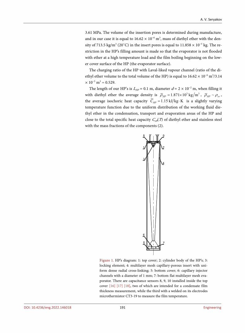
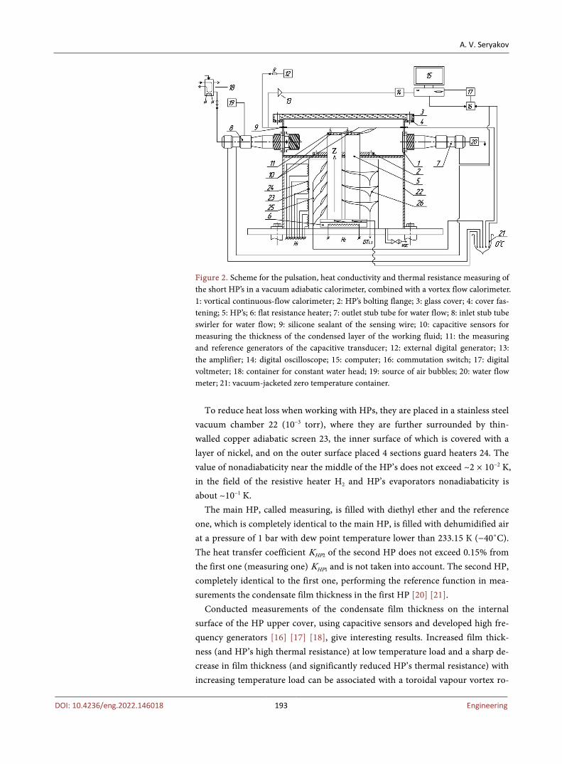
To conduct the experimental studies of the linear HP’s thermal characteristics, we used previously developed and used in many previous studies short stainless steel HP’s with a Laval nozzle-shaped vapour channel, the detailed description of which was repeatedly given in previous publications [16] [17] [18]. A schematic diagram of the experimental test setup is shown in Figure 1. In the upper cover capacitive sensors are installed to measure the working fluid condensate film thickness and temperature [19] [20] [21].

The capillary-porous evaporator 7 together with insert 4 forming a unified hydraulic working fluid delivery system, are made of layers of a thin stainless steel mesh with 0.07 mm thick each layer, with a cell size of 0.04 mm. The diethyl ether C4H10O is used as the working fluid, which has the boiling temperature under the atmospheric pressure of TB = 308.65 K (35.5˚C), freezing temperature TF = 156.95 K (−116.2˚C) and critical parameters TC = 466.55 K (193.4˚C), PC =

A. V. Seryakov

DOI: 10.4236/eng.2022.146018 191 Engineering

3.61 MPa. The volume of the insertion pores is determined during manufacture, and in our case it is equal to 16.62 × 10−6 m3, mass of diethyl ether with the den-sity of 713.5 kg/m3 (20˚С) in the insert pores is equal to 11.858 × 10−3 kg. The re-striction in the HP’s filling amount is made so that the evaporator is not flooded with ether at a high temperature load and the film boiling beginning on the low-er cover surface of the HP (the evaporator surface).

The charging ratio of the HP with Laval-liked vapour channel (ratio of the di-ethyl ether volume to the total volume of the HP) is equal to 16.62 × 10−6 m3/3.14 × 10−5 m3 = 0.529.

The length of our HP’s is LHP = 0.1 m, diameter d = 2 × 10−2 m, when filling it with diethyl ether the average density is 3 31.871 kg m10HPρ = × , ~HP evρ ρ , the average isochoric heat capacity 1.15 kJ kg KHPC = ⋅ is a slightly varying temperature function due to the uniform distribution of the working fluid die-thyl ether in the condensation, transport and evaporation areas of the HP and close to the total specific heat capacity Ceff(T) of diethyl ether and stainless steel with the mass fractions of the components (2).

Figure 1. HP’s diagram: 1: top cover; 2: cylinder body of the HP’s; 3: locking element; 4: multilayer mesh capillary-porous insert with uni-form dense radial cross-linking; 5: bottom cover; 6: capillary injector channels with a diameter of 1 mm; 7: bottom flat multilayer mesh eva-porator. There are capacitance sensors 8, 9, 10 installed inside the top cover [16] [17] [18], two of which are intended for a condensate film thickness measurement, while the third with a welded on its electrodes microthermistor CT3-19 to measure the film temperature.

A. V. Seryakov

DOI: 10.4236/eng.2022.146018 192 Engineering

The defining parameter of the entire capillary-porous insert and the evapora-tor is a small longitudinal interlayer gap (clearance) between layers of the metal mesh, which does not exceed 0.007 mm, and developed by a porous system the capillary pressure, which is sufficient for the HP’s work when the external iner-tial effects.

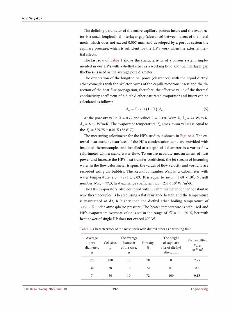
The last row of Table 1 shows the characteristics of a porous system, imple-mented in our HP’s with a diethyl ether as a working fluid and the interlayer gap thickness is used as the average pore diameter.

The orientation of the longitudinal pores (clearances) with the liquid diethyl ether coincides with the skeleton wires of the capillary-porous insert and the di-rection of the heat flux propagation, therefore, the effective value of the thermal conductivity coefficient of a diethyl ether-saturated evaporator and insert can be calculated as follows:

( )1ev l scλ λ λ= Π ⋅ + −Π ⋅ . (5)

At the porosity value П = 0.72 and values λl = 0.136 W/m K, λsc = 24 W/m∙K, λev = 6.82 W/m∙K. The evaporator temperature Tev (maximum value) is equal to the Tev = 329.75 ± 0.01 K (56.6˚C).

The measuring calorimeter for the HP’s studies is shown in Figure 2. The ex-ternal heat exchange surfaces of the HP’s condensation zone are provided with insulated thermocouples and installed at a depth of 1 diameter in a vortex flow calorimeter with a stable water flow. To ensure accurate measurement of heat power and increase the HP’s heat transfer coefficient, the jet stream of incoming water in the flow calorimeter is spun, the values of flow velocity and vorticity are recorded using air bubbles. The Reynolds number Recal in a calorimeter with water temperature Tcal = (293 ± 0.03) K is equal to Recal = 3.68 × 103, Nusselt number Nucal = 77.3, heat exchange coefficient acal = 2.4 × 103 W /m2∙K.

The HPs evaporators, also equipped with 0.1 mm diameter copper constantan wire thermocouples, is heated using a flat resistance heater, and the temperature is maintained at δТ, K higher than the diethyl ether boiling temperature of 308.65 K under atmospheric pressure. The heater temperature is stabilized and HP’s evaporators overheat value is set in the range of δТ = 0 ÷ 20 К, herewith heat power of single HP does not exceed 200 W.

Table 1. Characteristics of the mesh wick with diethyl ether as a working fluid.

Average pore

diameter, μ

Cell size, μ

The average diameter

of the wire, μ

Porosity, %

The height of capillary

rise of diethyl ether, mm

Permeability, Kwick,

10−10 m2

120 400 15 78 8 7.25

30 30 10 72 81 0.2

7 30 10 72 400 0.15

A. V. Seryakov

DOI: 10.4236/eng.2022.146018 193 Engineering

Figure 2. Scheme for the pulsation, heat conductivity and thermal resistance measuring of the short HP’s in a vacuum adiabatic calorimeter, combined with a vortex flow calorimeter. 1: vortical continuous-flow calorimeter; 2: HP’s bolting flange; 3: glass cover; 4: cover fas-tening; 5: HP’s; 6: flat resistance heater; 7: outlet stub tube for water flow; 8: inlet stub tube swirler for water flow; 9: silicone sealant of the sensing wire; 10: capacitive sensors for measuring the thickness of the condensed layer of the working fluid; 11: the measuring and reference generators of the capacitive transducer; 12: external digital generator; 13: the amplifier; 14: digital oscilloscope; 15: computer; 16: commutation switch; 17: digital voltmeter; 18: container for constant water head; 19: source of air bubbles; 20: water flow meter; 21: vacuum-jacketed zero temperature container.

To reduce heat loss when working with HPs, they are placed in a stainless steel

vacuum chamber 22 (10−3 torr), where they are further surrounded by thin- walled copper adiabatic screen 23, the inner surface of which is covered with a layer of nickel, and on the outer surface placed 4 sections guard heaters 24. The value of nonadiabaticity near the middle of the HP’s does not exceed ~2 × 10−2 K, in the field of the resistive heater H2 and HP’s evaporators nonadiabaticity is about ~10−1 K.

The main HP, called measuring, is filled with diethyl ether and the reference one, which is completely identical to the main HP, is filled with dehumidified air at a pressure of 1 bar with dew point temperature lower than 233.15 К (−40˚С). The heat transfer coefficient KHP2 of the second HP does not exceed 0.15% from the first one (measuring one) KHP1 and is not taken into account. The second HP, completely identical to the first one, performing the reference function in mea-surements the condensate film thickness in the first HP [20] [21].

Conducted measurements of the condensate film thickness on the internal surface of the HP upper cover, using capacitive sensors and developed high fre-quency generators [16] [17] [18], give interesting results. Increased film thick-ness (and HP’s high thermal resistance) at low temperature load and a sharp de-crease in film thickness (and significantly reduced HP’s thermal resistance) with increasing temperature load can be associated with a toroidal vapour vortex ro-

A. V. Seryakov

DOI: 10.4236/eng.2022.146018 194 Engineering

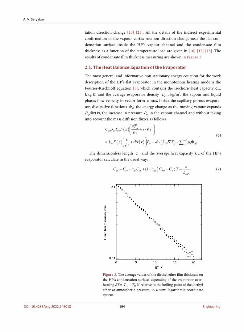
tation direction change [20] [21]. All the details of the indirect experimental confirmation of the vapour vortex rotation direction change near the flat con-densation surface inside the HP’s vapour channel and the condensate film thickness as a function of the temperature load are given in [16] [17] [18]. The results of condensate film thickness measuring are shown in Figure 3.

2.1. The Heat Balance Equation of the Evaporator

The most general and informative non-stationary energy equation for the work description of the HP’s flat evaporator in the monotonous heating mode is the Fourier-Kirchhoff equation [5], which contains the isochoric heat capacity Cev, J/kg∙K, and the average evaporator density evρ , kg/m3, the vapour and liquid phases flow velocity in vector form v, m/s, inside the capillary-porous evapora-tor, dissipative functions Φdf, the energy change as the moving vapour expands Pvpdiv(v), the increase in pressure Pev in the vapour channel and without taking into account the mass diffusion fluxes as follows:

( )

( ) ( ) ( ) 12

evev ev ev

ei

v ev HP i dfii

TC L F T

L F div P diz v T

zρτ

λ µτ =

=

∂+ ⋅ ∂

∂ = + + + Φ ∂ ∑

v

v

∇

∇

. (6)

The dimensionless length z and the average heat capacity Cev of the HP’s evaporator calculate in the usual way:

( )1 ;ev sc ev vp ev fev wHP

zC C x C x zC CL

= + + − + = . (7)

Figure 3. The average values of the diethyl ether film thickness on the HP’s condensation surface, depending of the evaporator over-heating δT = Tev − TB, K relative to the boiling point of the diethyl ether at atmospheric pressure, in a semi-logarithmic coordinate system.

A. V. Seryakov

DOI: 10.4236/eng.2022.146018 195 Engineering

With an increase in the temperature load in the initial heating period of a ca-pillary-porous HP’s mesh evaporator the wetting of the grid frame with diethyl ether deteriorates sharply, since the wetting angle increases with an increase in temperature. This effect is thermosensitive and already with a relatively small increase in temperature δT = Tev – TB ~ (3 - 5) K wetting deteriorates, the level of diethyl ether in the grid evaporator decreases and further HP’s heating δT = Tev – TB ≥ 10 K through the flat surface of the bottom cover occurs in a thin layer of boiling diethyl ether.

The thickness of the diethyl ether layer decreases from ~3.5 mm at the heating beginning to the most intense boiling, while the vapour flow becomes stationary, and the thickness of the ether micro-layer does not exceed (1 - 2) × 10−2 mm. This fact greatly simplifies the conduct of assessments and the maximum achievable result in our conditions is as follows:

( ) ( )

22 2 2

0

21 118.4 W.

Hev H H H ev

fevc wevH fev ev

c w fev ev

z

TQ E C T

T T F z

zλ

δδ δλ λ λ α

=

∂ = − = − ∂

= − + + + =

(8)

( )

5.4 K, 18.8 K,

35 0.55 K.

ev c ev wc wev

c ev w ev

ev fevfev

fev ev

Q QT T

F FQ

TF

δ δλ λ

δλ

∆ = = ∆ = =

∆ = = … (9)

The equation of the thermal energy of a working HP’s evaporator in a mono-tonic heating mode in the approximation of small heat losses ( )sh

HP HP shelk T T− in the adiabatic calorimeter can be represented using enthalpy equation as fol-lows:

( ) ( ) ( )21

i shev ev i dfi HP HP sheliQ H k T Tτ τ µ=

== + Φ + −∑ . (10)

and the actual enthalpy equation of an evaporator in a monotonous heating mode also can be represented using this thermodynamic equation:

( ) ( ) ( ) ( ) ( ) ( ) ( )ev vp B vp vp ev sc l pl ev fevH G r T G С T T G C T Tτ τ τ τ= + − + − . (11)

The expression for the thermal energy released in the HP’s condensation re-gion is written similarly using the heat balance equation:

( ) ( ) ( ) ( )

( )

2

2

21

dd d1 1

d d d.

fevev sccond vp B vp ev vp sc ev ev

i shi dfi HP HP sheli

Tx TQ G r T G x C F z L

k T Tz z z

λ

µ=

=

= + − + −Π

− Φ − −∑ (12)

The performed measurements and calculations make it possible to estimate the heat transfer coefficient in the vortex flow calorimeter αcal = 2.3 × 103 W/m2∙K, αcond ≥ 5 × 103 W/m2∙K, and the final expression for the maximum val-ue of the condensation heat in our HP is the follows:

( ) 1 1 115.4 Wfcond wcond fcond cal cond

l w cal cond

Q T T Fδ δλ λ α α

= − + + + =

.(13)

A. V. Seryakov

DOI: 10.4236/eng.2022.146018 196 Engineering

The thickness parameters in parentheses are equal to the following values:

( )

1 3

3 2 3 2

10 -10 mm, 1 mm,

2.4 10 W m K , 5 -10 10 W m K.fcond w

cal cond

δ δ

α α

− −= =

= × ⋅ ≥ × ⋅

To solve the complex Fourier-Kirchhoff Equation (6), it is necessary first to determine the velocity field of the liquid and vapour phases in a capillary-porous evaporator using the Navier-Stokes equations. The results of this study will be presented later in a separate report.

To simplify all subsequent calculations, the average cross-section HP’s tem-perature at any point at altitude i i HPz z L= inside the vapour channel can be considered equal to the surface temperature of the HP, measured at this height ( ),i sur

T z τ in the vacuum chamber of the adiabatic calorimeter:

( ) ( ) ( ) ( )1 dHP i HP i HPsurT F T

Fz z z

zT= =∫ . (14)

The vapour flow can be estimated according to the interphase mass transfer gives in case of small departures from equilibrium by the Hertz-Knudsen equa-tion [22] [23]:

1 222 2

fcondevvp

fev fcond

PPMGR T T

ξξ

= − − π . (15)

where the diethyl ether C4H10O, selected as the working fluid has a molar mass M = 74.1216 g/mol, R is the universal gas constant and ξ is the condensation coefficient, ξ ≤ 1, defined as the ratio of the number of vapour molecules con-densing over the total number of molecules which strikes the liquid film surface.

There is a redistribution of the liquid mass of diethyl ether inside the HP, while the heat capacity of the evaporator increases due to the liquid film boiling. In this case, the temperature Tfev of the diethyl ether layer and its dependence on time are determined using external thermocouples that control the temperature of the HP external surface inside the vacuum chamber. The results of the ther-mocouple measurements are shown in Figure 4 and Figure 5 in section 2.2.

2.2. Temperature Distribution Inside the Vapour Channel

Earlier calculations of the flow velocity and vapour density of diethyl ether using the Navier Stokes equation system in a short HP’s vapour channel similar to the Laval nozzle [16] [18], allow us to calculate the temperature distribution in this channel. The ratio between the pressure, density and temperature of the con-densing vapor in the first approximation can be given by the equation of state of an ideal gas in the following form [19] [20] [21]:

( )

1

12 2 2 2

;

.

; ~ ;

1 112 2

kmixvpmix

vp v fcondv v

k k

v v

v v

P P P PRT P

u u v vP kP k RT m

ρρ

ρ−

= =

− −−= + +

(16)

where k = 1.31 is the value of the adiabatic index of diethyl ether vapour.

A. V. Seryakov

DOI: 10.4236/eng.2022.146018 197 Engineering

Figure 4. Comparison of the experimental values of the HP’s surface tem-perature along the generatrix, and the calculated diethyl ether vapour tem-perature inside the Laval nozzle-liked formed vapour channel. A: is the up-per part of the Figure 4. 1: black dots, the experimental values of the HP’s surface temperature Tsur with a vapour channel made in the Laval nozzle- liked form, K; 2: the solid curve, the calculated temperature values T, K, in the Laval nozzle-liked formed HP’s vapour channel. B: is the lower part of the Figure 4, which shows the half part of the vapour channel cross section along the longitudinal axis Oz.

Figure 5. The experimental values of the HP’s surface temperature of the evaporator with maximum filling by the diethyl ether at the boiling begin-ning on a large scale. It is clearly visible the weak evaporator temperature drop (<1 K) and a sharp drop of the vapour temperature inside the Laval nozzle-liked formed vapour channel above the evaporator, coinciding with the calculated vapour temperature values.

A. V. Seryakov

DOI: 10.4236/eng.2022.146018 198 Engineering

Calculations of moving vapour temperature in a short HP’s vapour channel, made in the form of Laval nozzle, were performed using the program code ANSYS\CFD Fluent 6.3.26 -20090623 [24] and using Equation (16) and other more complete calculation equations given in [19] [20] [21]. Taking into ac-count the tabular values [25] [26] [27] of the diethyl ether vapour pressure at the humidity coefficient γdr = 0.2, the temperature distribution inside the vapour channel along the longitudinal z axis was obtained at the beginning of boiling in the HP evaporator, as shown in Figure 4 and Figure 5 during overheating δt = Tev – TB = 11 K:

( )1k k

vv

PT TP

−

=

. (17)

The calculated values of the vapour temperature along the longitudinal axis of the HP vapour channel at the temperature of lower layer of the diethyl ether in the evaporator ( )329.75 K 56.6 CfevT = . The calculation error is 0.3%, the measurement error of the HP’s surface temperature is less than 0.1 K. Heating and all calculations were carried out in the temperature range of the evaporator (298 - 348) K (25˚C - 75˚C).

The outer surface of the HP’s body in the region of a 3.5 mm high multilayer mesh evaporator, filled with boiling diethyl ether is characterized by a close to constant temperature under monotonous heating, which is clearly seen in Fig-ure 4 and Figure 5. With further heating, the thickness of the diethyl ether layer in the evaporator and, accordingly, the width of the constant temperature region decreases.

Inside the vapour channel, the temperature decreases sharply, the temperature drop reaches ΔT = 35 K, due to the cooling in the condensation region and the influence of the Laval nozzle shape of the vapour channel. The results of the ex-perimental analysis of the HP’s surface temperature distribution along the gene-ratrix also confirmed the nonlinear nature of the temperature distribution as a function of the channel length in the Laval-liked vapour channel.

Experimental data shows a close to constant temperature of the evaporator when diethyl ether boils in it, a weak nonlinearity in the confuser part of the nozzle, and a strong nonlinearity in the behavior of the temperature near the HP’s condensation surface. With a further increase in the heat load, the length of the constant temperature region in the evaporator is reduced.

The results of numerical analysis of the vapour axial temperature distribution inside the Laval-liked HP’s vapour channel of compressible moist vapour at high heat loads confirm the nonlinear character of the temperature distribution as function of the channel length, which is due to the joint influence of the channel shape in the form of a Laval-liked nozzle and a sharp gradient vortex formation near the HP’s condensation surface, taking into account an additional tempera-ture decrease inside the vortex ring of the condensing vapour [18] [21], which makes it extremely difficult to solve the heat equation for our HP’s.

A. V. Seryakov

DOI: 10.4236/eng.2022.146018 199 Engineering

2.3. Thermal Resistance Results

Experimental values in the stationary state of the thermal resistance RHP of a short HP’s are defined as the thermophysical characteristic of the heat transfer device as a whole [28], at a constant value of the temperature load (pressure) on the evaporator δt = Tev – TB and calculated using formula (18) and a vacuum adiabatic calorimeter, Figure 2, in which all parameters of the working HP, in-cluding temperature and transmitted thermal power, are measured using ther-mocouples.

The full temperature load on the evaporator δt = Tev – TB = (0 - 20) K [16] (relative to the boiling point of ether at atmospheric pressure) is set and main-tained using a precision temperature controller with a temperature step of δt = 0.5 K, the long-term instability does not exceed 1 × 10−2 K.

Experimental values of thermal resistance RHP obtained during monotonic heating of the HP’s evaporator with a speed close to linear in time 3 × 10−3 K/s using a special precision temperature controller and a system of computer- controlled switches, surface thermocouples, heater power measurements form arrays of data on HP surface temperatures in a vacuum adiabatic calorimeter, condensation surface, heater power EH2 and heat flows Qev and Qcond for solving thermal conductivity equations and calculating thermal resistance according to formula (18) from [28]:

( ) ev condHP

ev

T TR t

Q−

= . (18)

The small size and the low heating rates ensured that the measurements of the RHP were carried out under homogeneity conditions and local thermal equili-brium. The obtained values of the thermal resistance RHP, K/W in the conti-nuous heating mode refer to the direction of the heat flow that coincides with heat flow direction in the stationary states measurements.

The polynomial Equation (19) describing in dimensionless form the experi-mental values of the thermal resistance RHPk for a time moment τk of the short HP with a Laval nozzle-liked vapour channel, depending on the overheating value of the evaporator δt: 0 ≤ δt ≤ 20 (and also in dimensionless form) looks like this:

( ) ( )( ) ( )( ) ( )

( ) ( )

11

7 68 6

5 45 4

3 2

2.0795621 10 1.6029662 10

4.9921411 10 8.0489929 10

0.0071936 0.036334060.1113127 0.2702057, 8

R inHPk HPkii

R

R t R t

t t

t t

t tt n

δ δ

δ δ

δ δ

δ δδ

−

=

− −

− −

=

= − × + ×

− × + ×

− +

− + ≤

∑

(19)

Standard deviation σ = 0. 0024929, Fisher criterion R2 = 0.9980243. The obtained experimental results of thermal resistance at temperature load

δt > 10 K allow us to estimate the characteristic total thickness of the diethyl ether film on the evaporator surface (boiling in the evaporator) and the conden-

A. V. Seryakov

DOI: 10.4236/eng.2022.146018 200 Engineering

sation surface of short HP’s with a Laval nozzle-liked vapour channel and flat upper and lower covers as follows (without the thermal resistance of covers):

2 2 4 2

6

~

4 10 K W 0.136 W m K 3.14 10 m

1.7 10 m.

ev cond HP lR Fδ δ λ− −

−

+

= × × × ×

≤ ×

⋅

From the analysis of Figure (6), it follows that the film thickness on the eva-porator is close to a constant value in the range of thermal loads δT = (10 - 20) K, and with a further increase in the temperature load δT, the evaporator begins to dry out and there is a sharp increase in the thermal resistance RHP.

In addition, when the HP’s evaporator is monotonically heated, the diethyl ether layer thickness inside the evaporator δfev(τ) also decreases monotonically and within the range of the coordinate z:

0 < z < Lev = 0.035∙LHP limited by the longitudinal dimensions of the evapora-tor Lev, the functional dependence of the thermal resistance RHP on the coordi-nate z: RHP = RHP(z) is of practical interest, and has a positive sign:

1

0; 0 0.035HP HP HPev HP

R R Rt z z L Lz t z t t

−∂ ∂ ∂∂ ∂ = = > ≤ < = ⋅ ∂ ∂ ∂ ∂ ∂ . (20)

The distributions of the experimental values of the HP’s surface temperature shown in Figure 4 and Figure 5 ((∂t/∂z) < 0) at the diethyl ether boiling begin-ning in a saturated evaporator under the monotonic heating, and the decreasing values of the thermal resistance on a global evaluation between evaporator and condenser ((∂RHP/∂t) < 0) in Figure 6, show a positive value of the derivative in Equation (21). And this authorizes the hypothesis that the thermal resistances RHP associated with each z position 0 < z < Lev confirms the dependence on RHP = RHP(z) and apply it in the thermal conductivity equation. The same can be said or concluded about the heat capacity of the evaporator.

3. Mathematical Model of the Inverse Thermal Conductivity Problem

Let’s formulate a mathematical statement of the inverse problem of restoring the heat capacity of working HP’s. Let there be a vertically oriented HP with the length LHP = 100 mm and diameter of 20 mm, DHP/LHP ≤ 0.2 and the temperature field inside can be viewed in one-dimensional axisymmetric mode and located at the bottom of HP the capillary-porous evaporator with a thickness of Lev = 0.035∙LHP. At the lower end of the HP the evaporator is supplied with a flow of heat ( )0evQ z = from a flat heater H2, Figure 2. At the upper end of the eva-porator there is a heat exchange ( )0.035evQ z = and at the upper HP’s end there is a heat exchange ( )1ev condQ Qz = = with an external fluid with a con-stant temperature Tcal.

The classical equation of spatial thermal conductivity for the linear HP’s as a solid rod (solid body) is looks like this [4] [5] [6]:

( ) ( ) ( )HP v HP HPz Tс t L F div grad Tρ λτ∂

=∂

. (21)

A. V. Seryakov

DOI: 10.4236/eng.2022.146018 201 Engineering

Figure 6. Thermal resistance RHP, depending on the evaporator overheating δt = Tev – TB relative to the boiling point of diethyl eth-er at atmospheric pressure. 1: black dots, experimental stationary RHP values of short HP’s with a vapour channel made in the Laval nozzle-liked form; 2: solid lines, the experimental values of the thermal resistance RHP of the same HP obtained in the continuous heating mode with close to linear in time speed of 3 × 10−3 K/s.

In a working HP with monotonous heating the heat capacity Cev of the evapo-

rator can be considered and analyzed only as the heat capacity of the HP’s lower fragment ( )0.035ev HP zС С= = with a thickness of Lev = 0.035∙LHP and thermal resistance ( )0.035ev HP zR R= = .

The distribution of the one-dimensional axisymmetric temperature field ( )HP i sur

t z and ( ), k surt z τ along the longitudinal dimensionless z -axis of a

short linear HP’s is used to solve the heat conduction Equation (22) for the eva-porator fragment without internal sources [4]:

( )( ) ( ) ( )

,1 1 , ; 0.035evev HP

t zС tz

z zz z

tt zR L

ττ

∂∂= = ≤

∂ ∂ . (22)

The thermal resistance of the evaporator (evaporative HP fragment) is an integral part of the thermal resistance RHP of the entire HP, and the value of the thermal resistance of the evaporator during the diethyl ether boiling at tempera-ture load (pressure) > 11 K can be estimated using the experimental results pre-sented in Figure 6. Given the close thicknesses of diethyl ether films in the eva-porator and on the condensation surface of HP ~ev condδ δ during film boiling, the thermal resistance of the evaporator (evaporative fragment) will be no more then Rev ≤ 0.02 K/W.

Energy losses due to friction in the vapour channel and non-absolute calori-meter adiabaticity lead to the fact that the thermal power of Qev and Qcond differ from each other:

A. V. Seryakov

DOI: 10.4236/eng.2022.146018 202 Engineering

( ) 2.6%ev cond evQ Q Q− ≤ .

And the heat power becomes a function of the dimensionless vertical coordi-nate z and time with monotonous heating:

( ),ev evQ Q z τ= . (23)

One of the possible formulations of the coefficient inverse problem (CIP) for Equation (23) consists in setting redefined boundary conditions, with the help of which the definition unicity of three functions – temperature ( ),sur kt z τ , heat capacity ( ),ev kC z τ and thermal resistance ( ),ev kR z τ (or thermal conductiv-ity ( ),ev kzλ τ ), moreover all functions must be analytical functions, for exam-ple, represented as polynomials or piecewise smooth spline functions. For expe-rimentally determined boundary conditions, the inverse heat conduction prob-lem for Equation (22) is usually incorrect in the classical sense [9] [10] [11]. To bring it to a conditionally correct formulation, we restrict the class of acceptable solutions to a set of piecewise regular approximating dependencies and apply the step – by step principle of natural regularization for IPTC solution [6] [9].

The temperature distribution of the cylindrical HP’s housing inside the va-cuum chamber with an adiabatic shell near the flat resistive heater is symmetric-al:

( ) ( )0 0

, ,0

z z

z zt tx yτ τ

= =

∂ ∂ = = ∂ ∂

. (24)

The initial boundary conditions [29] [30] [31]:

( ) ( ) ( ) ( )0, ev ev c w fev evt t T R R R Qτ τ τ≡ = − + + . (25)

( ) ( ) 30 00,0 ; 0, 3 10 K sk kt t t tτ τ −× ×= = + . (26)

( ) ( ) ( ) ( ),HP k cond cond k cal w fcond cond cond kt L t T R R R R Qτ τ τ≡ = + + + + . (27)

( ) ( )2 20, ,ev k H H ev kQ E C Tz zτ τ= = − . (28)

The Qcond energy transmitted by HP to the vortex flow calorimeter during va-pour condensation is determined using the experimental stand shown in Figure 2 and Equation (13).

We write down the dimensional equation of thermal conductivity to estimate the heat capacity of a capillary-porous evaporator with a finite height of 0.035∙LHPi in the following standard form:

( ) ( ) ( ) ( )( ),

, ; 0.035kHPevk k

HP HP

t zL zzС t t zz R t F z z L

ττ

∂∂= ≤ ∂ ∂

. (29)

And we introduce a general expression for the heat flow ( ), kq z τ inside the short HP along the longitudinal z axis:

( ) ( ) ( ) ( )2 2

, ,, ,HP k HP kHP

k HP H H ev kHP HP

T z T zLq z z z E C T zz R F zτ τ

τ λ τ∂ ∂

= = = −∂ ∂

.(30)

In the first approximation, in which the heat flow is determined only by the

A. V. Seryakov

DOI: 10.4236/eng.2022.146018 203 Engineering

HP’s capillary-porous evaporator without taking into account heat losses, the heat propagation equation in the vapour channel using the thermal resistance RHP of a short HP’s as a whole can be written in the following form:

( )( )

( ) ( ) ( )2

2

,

dd d1

d.

d d

HP kHP

HP ev

fevev scvp B vp vp sc ev ev

TLzR t F

Tx TG r T G

zz

z zC F z L

z

τ

λ

∂

∂

= + + −Π

(31)

The solution of the Equations (29) and (31) is possible only with positive val-ues of time τk and heat capacity ( )evkC T :

( )0; 0k evkC Tτ > >

To simplify all subsequent calculations, it is possible to take the initial tem-perature value equal to zero:

( ),0 0t z =

Equations (30) and (29) of the heat flow propagation ( ), kq z τ can be rewrit-ten in the dimensionless form ( ),ev kq z τ as the heat flow of the evaporator (without taking into account heat losses) along the z-axis at time moment τk and presented as a system of two energy equations for calculating the heat capacity Cevk(t) and the heat flow of the evaporator ( ),ev kq z τ , the value of which is re-lated to the thermal resistance RHP of a short HP’s as a whole and for the time τk can be represented as follows:

( ) ( ),0ev k

evk

qtzC t

zzτ∂

+ =∂

. (32)

( )( ) ( )

,, 0HP

ev kHP

t zz

z zLz q

R Fτ

τ∂

+ =∂

. (33)

The values of the variable thermal power ( ),ev kq z τ on the lower HP’s flat borders, on the upper boundary of the flat evaporator and on the upper flat bor-ders are equal to:

( ) ( ) ( )0.0350, ; 0.035, ; 1,ev k ev ev k ev k condq Q q Q q Qτ τ τ= = = . (34)

and Equation (33) for determination the transmitted thermal power by the HP’s capillary-porous evaporator at a height of z = 0.035∙LHP is made using the HP’s surface temperature distribution in the adiabatic calorimeter:

( ) ( )( )

( )( )

0.035

2

0.035

,0.035,

,0.035 .

HPev k

HP

HP

zHP

z

zz

tLq zR F

tLR F

z z

zz z

ττ

τ=

=

∂ = = − ∂

∂ = − ∂

(35)

The heat capacity of the evaporator allows us to evaluate the work of the HP. To calculate the

HP’s evaporator heat capacity Cevk, the heat output in the evaporator volume can be considered as reduced by the temperature reduce from the Equation (31)

A. V. Seryakov

DOI: 10.4236/eng.2022.146018 204 Engineering

and (35), and an illustration of the experimental temperature distribution data from Figure 4 and Figure 5:

( ) ( )0.035

,0.035 k

ev

z

k

zqC t t

zτ

=

∂= − ∂ . (36)

Figure 4 and Figure 5 show the close to the constant experimental tempera-ture distribution inside the evaporator with boiling diethyl ether at a high heat load and further temperature drop in the HP’s Laval nozzle-liked vapour chan-nel up to the condensation surface.

3.1. Performing Calculations of the Inverse Thermal Conductivity Problem

The inverse thermal conductivity problem (ITCP) solution for the HP’s evapo-rator is a method of stepwise continuation of the known solution, for example equal to zero at the initial moment, for the next time interval Δτk = (τk, τk+1) and the corresponding temperature interval tk = (tk, tk+1) to calculate the heat capacity of a capillary-porous evaporator with a height (thickness) of 0.03·LHP.

The solution of the equations system (32) and (33) is carried out using expe-rimentally determined surface temperature values ( ), kt z τ in the range HP0.03 = (τk, τk+1) × (0, 0.035∙LHP), experimental thermal resistance values ( ),HP kR z τ in the range HP1 = (τk, τk+1) × (0, 1∙LHP), and calculated values of the evaporator volumetric heat capacity Cevk(δt) in the range (τk, τk+1) × (0, 0.035∙LHP) and satis-fying the thermal conductivity equations (22) and additional conditions (25) - (28), provided that the thermal resistance defined in stationary states is known as a polynomial (19).

Crank-Nicholson calculation scheme, Figure 7 with temperature averaging on the previous calculation layer and taking into account the temperature depen-dence of the thermal conductivity coefficient can be used to improve the calcula-tions accuracy. The equation for the Crank-Nicholson scheme calculation of the evaporator heat capacity is as follows:

1 1 1 1 11 1 1 1

2 2

2 22 2 2

n n n n n n n n n ni i i i i i i i i i

evi evi eviT T T T T T T T T T

Ch h

ρ λτ

+ + + + +− + − + − + − + − +

= + ∆

.(37)

Figure 7. A six-point difference scheme in which three points are taken from the next (new) time layer n + 1, and three from the old (previous) time layer n.

A. V. Seryakov

DOI: 10.4236/eng.2022.146018 205 Engineering

The coefficient λevi of the evaporator thermal conductivity can be estimated by the Equation (5).

Experimental temperature tk at time τk inside the HP’s vapour channel with monotonous heating relative to the boiling point tB of diethyl ether at atmos-pheric pressure is determined as follows:

( ) ( ) ( ), , ; ,k k k B k k k Bt t t t t tz z z t tτ δ τ δ δ τ= = + = = − . (38)

At the initial time moment τk and at the initial temperature value tk, we should consider that the HP’s evaporator heat capacity Cevk(δt) with the initial temper-ature load value ( ), kt zδ τ are known and is equal zero, so the heat capacity from now on further heating can be represented as a polynomial with a variable (δt):

( ) ( ) ( ) 11 ; 10.c in

evk evki CiC t C t nφ ξ δ −

== ⋅ ≤∑ (39)

Approximation function Φ(ξ) is a mandatory regularizing parameter in the form of monotone increasing function, Φ(ξ) = ξ, or maybe exp(ξ). The value of numerical parameter Φ(ξ) determines the stability and the range of acceptable heat capacity properties, and smoothes out non-linearity’s in a blurred thermal transformation in the HP’s evaporator. With the change from linear to an expo-nential dependence, the error in calculating the heat capacity decreases markedly, especially when the polynomial heat capacity function leaves the peak, see Fig-ure 8. This is due to the fact that exp(ξ) provides a limit on the range of HP’s permissible properties in a positive value with Cevk and RHPi(λHPi) > 0, and the solution for Cevk is significantly much improved, especially at the exit from the heat capacity peak, corresponding to the blurred phase transition at the boiling beginning in the HP’s evaporator. In the case of Φ(ξ) = ξ, the error in the heat capacity recovery in the temperature range (298 - 348) K (25˚С - 75˚С) reaches 25%, and when replaced by exp(ξ) falls to 2%.

The temperature time derivative is a constant value for time values τ > τk and is a coordinating (synchronizing) parameter of all measurements in a time in-terval Δτk:

30

3

0, 0, , 2, ; 3 10 K s;

3 10 K s.i k k k

k k

t i t t

t

τ τ τ

τ

−

−

> = > = + × ×

∆ = ∆ × ×

(40)

The experimental distribution of the HP’s surface temperature tk at time τk along the HP’s body is known, are positive and can be written as follows:

( ) ( ) ( ) ( )( ) ( )

0 0.035 0

1 0

0 0; 0.035 0;

1 0.ev k k k k

k k

t t z z

z

t t

t t

τ τ

τ

= = > = = >

= = > (41)

The accounting and synchronization of the thermal resistance RHPk equili-brium values (33) in a linear slow heating process to the moments of time mea-surements τk is performed using the value of the temperature load δtk from (38) and (40)-(41). The thermal power from the Equation (30) is calculated as fol-lows:

( ) ( ) ( )0 0.035 0.035 1: ; ;z z z zk k ev k k condQ Q Q q q Qτ τ τ τ τ= = = => = = = . (42)

A. V. Seryakov

DOI: 10.4236/eng.2022.146018 206 Engineering

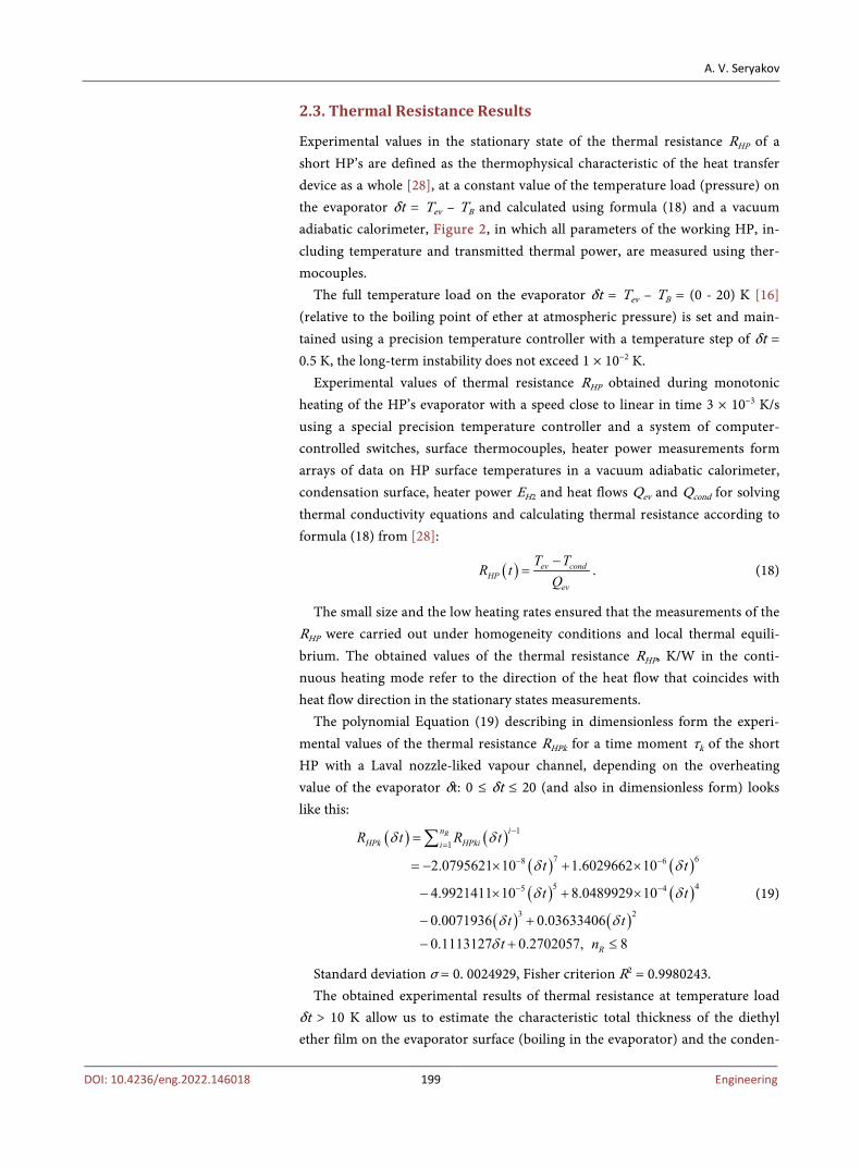
Figure 8. The calculated values of the HP’s evaporator heat capacity Cev/Cev0: Cev, the heat capacity of the diethyl ether-saturated evaporator, J/K; Cev0, the heat capacity of the reference HP evaporator filled with dried air, J/K. 1-black dots, values of the relative heat capacity of the HP’s evaporator with a Laval nozzle-shaped vapour channel, obtained by solving the inverse problem using Equation (44) with a temperature step of 0.5 K. δt = Tev-TB, when the diethyl ether boiling process begins; 2-a polynomial function of the tenth degree for smoothing the ob-tained points of the evaporator heat capacity.

When the ITCP problem at time τk is solved and the temperature at time τk+1

of the evaporator 0z = : ( ) ( )0 0ev k kt t zτ = = , at a height 0.035z = : ( ) ( )0.035 0 0.035k kt t zτ = = and the temperature of the HP condensation surface

1z = : ( ) ( )1 0 1k kt t zτ = = becomes measured and known, this solution be-comes the temperature and thermal power initial distribution at transition to the next τk+1 time interval, Δτk+1 = (τk+1, τk+2). From the solution of the problem on the time interval Δτk+1, the function Ck+1(t) is determined on the temperature in-terval tk+1 = (tk+1, tk+2).

To reduce the number of Ck+1 parameters, defined at each time interval Δτk+1, the crosslink should be performed with the polynomial (39) from the previous calculation at the boundary point of the temperature tk by the function and its derivatives, this greatly simplifies all calculations.

The total number of equations for crosslinking Nc = 2 (heat capacity and tem-perature derivative of heat capacity), and the maximum degree of the polynomi-al nc = 10 are primarily the main regularizing parameters of calculation, and were determined in accordance with the estimated accuracy of the heat capacity and experimental error of the temperature measuring.

In addition, the method of numerical solution of ITCP for short linear HP’s using a polynomial expansion of the heat capacity, the size of each time Δτk step is an important regularizing parameter [12] [13] [14] [15] [32] [33]. The optimal

A. V. Seryakov

DOI: 10.4236/eng.2022.146018 207 Engineering

time step size Δτk is the determining parameter of the calculations accuracy, de-pends on many HP’s parameters, and it was chosen experimentally. The charac-teristic time of all measuring sensors survey of the experimental stand, Figure 2 is Δτmeas = 21 s, so the time step Δτk in the area of boiling beginning of the die-thyl ether in the HP evaporator changed from Δτk = 30 s up to Δτk = 60 s, and the temperature step reached the value of Δtk ≤ 0.2 K. In the initial heating re-gion the temperature step could be greater and reached the value of Δtk ≤ 0.5 K.

The program that controls the operation of the measuring stand, Figure 2, has two operating modes: “control” and “measurement”. In the “control” mode, all sensors are cycled, including thermocouples, thermistors, capacitive sensors, controls the power of the main resistive heater and protective heaters of the adiabatic calorimeter system, the regime of “zero heating” mode of the HP’s evaporator is specified, the measurement results are processed and output on the display screen.

In this mode, the parameters of the control program are specified such as the duration of the sensors readings measurement, the measurement times of digital voltmeters, oscilloscopes, frequency meters, etc. After the HP evaporator and the vortex flow calorimeter reach stationary isothermal states, the program switches to the “measurement” mode.

The main resistive heater H2 and control system are switched on, and the li-near time heating of the HP’s evaporators begins, the adiabatic system and all measuring sensors start working. In this mode, the temperatures distribution on the outer surface of the measuring HP, the evaporator heat power, the condensa-tion surface temperature, the heat output of the adiabatic system and all other thermal characteristics, including the heat transfer characteristics of the HP, are measured. The obtained experimental data arrays are saved and a measurement library is formed.

3.2. Performing Calculations of the Evaporator Heat Capacity

We analyze the case when the thermal resistance RHP, Equation (19) of the entire HP as a whole is known, have a positive value and it is necessary to calculate the heat capacity of a capillary-porous evaporator with a height of 3.5 mm and satu-rated with diethyl ether. We integrate Equation (22) with respect to z and, taking into account the experimental boundary conditions (25), (26), (27) and (28) we obtain a nonlinear integral equation for calculating the evaporator heat capacity at the time moment τk:

( ) ( ) ( )0.035

0, d 0.035 ,evk k ev kz zC t t qz zτ τ=∫ . (43)

To solve such integral equations, the finite difference method is used, based on replacing the derivatives with their approximate values expressed in terms of the functions differences at individual discrete points (nodes) of the finite-difference grid, Equation (37).

We will solve the functional Equation (43) by the iterative method, for which

A. V. Seryakov

DOI: 10.4236/eng.2022.146018 208 Engineering

it is necessary to proceed to the variational formulation of this task. We define the target functional as the discrepancy, corresponding to the difference between the left and right sides of Equation (43), and the calculation problem for each time interval Δτk will look like the task of minimizing the discrepancy function-al:

( ) ( ) ( ) ( )

( )

120.035

0

1 , d 0.035 d2inf .

k

kevk evk k ev kk k

ievk

C t C t t q

С t

z z zτ

τδ τ τ τ+ = −

=

∫ ∫∑ ∑

(44)

The most suitable way to minimize the functional is the conjugate gradient method [34] [35] [36]. To calculate the gradient components of the functional (44) (Frechet derivatives) at the points of minimizing sequence, the method of the optimal process control theory [35] [36] is used, described by partial diffe-rential equations [35]. In this method, an important role is played by the so-called conjugate boundary value problems corresponding to the original optimal con-trol problem.

The Lagrange functional L for minimization the problem (44) with additional conditions (22), (25), (26) and with the values of the heat flow at the boundaries of the evaporator (32), (36) is as follows:

( ) ( ) ( )

( ) ( )( )

1

1

0

0

0.035

0.035

,d d

,, d d .

k

k

k

k

evk kkevk k

i

HPev k k

HP

zz z

z

zz z

z

C t qC t t

c

ztLq z

R F

τ

τ

τ

τ

δ τη τ

τχ τ τ

+

+

∂ ∂= + + ∂ ∂

∂+ + ∂

∫

∫

∑∫

∫

L

(45)

where the domain of variables τk and ( ),ev kq z τ is kept the same as HP0.035 and HP1, and η and χ are Lagrange multipliers corresponding to the first and second Equations (32) and (33).

To obtain the gradient expression of the functional L [35], Lagrange multip-liers and formulate the conjugate task of calculating the heat capacity, we present a variation of the Lagrange function with respect to the variables τk and

( ),ev kq z τ and the heat capacity parameters ( )ievkС t , and taking into account

the boundary conditions (25) and (26) and the initial conditions (32), (33), (40) and expressions for the heat flow (30), (35):

( ) ( )

( ) ( )

( ) ( )

( )

1

1

1

0

20.035

20.035

0.035 0 035

0

.

0

2

0

d d

d d

, d d d

k

k

k

k

k

k

i HPevk i ki

HP

i HPevk k

HP

iev k k evk

HP

HP

LС t gR F

L bС t tR

z zz

z z zF

q С t t

L

z z

z z z z zz

zR Fz

τ

τ

τ

τ

τ

τ

δ χ δ τ

η δ τ

η χ δ τ τ η δ

+

+

+

=

∂− + ∂

∂ − − + ∂

+

∑ ∫

∫

∫

∫

∫

∫ ∫

L

( ) ( ) ( )1 0.03

0

5, d 0.03 d .k

k

ievk k ev k kz t zС t q tz

τ

τη τ τ δ τ+

− −

∫∫

(46)

where the value gk denotes the derivative of the heat capacity components in the

A. V. Seryakov

DOI: 10.4236/eng.2022.146018 209 Engineering

following form:

( )( )

( )( )

( )1 0 5

0

.03,; , d d

, ,k

k

evkevk k ki k i ki i

evk k k

C tC tg

tzt z g

С t Сτ

τ

δτη τ τ

τ τ+∂∂ = = ∂ ∂ ∫ ∫

∑ . (47)

where η, is the solution of the conjugate problem completely corresponding to the original problem (22), (25) and (27). In the reverse time, τ = τk+1 – τk the conjugate problem is written using Equations (32) and (33) and the HP’s ther-mal conductivity coefficient ak:

( )( ) ( ) ( )

1;, ,

kk k k HPk

evk k evk k HPk

La aC t C t zR

zz

z Fzη λ

ητ τ

∂ ∂ ∂= = =

∂. (48)

Both the initial and boundary conditions of the conjugate task are written in the usual way, and at the upper boundary of the evaporator, the conjugate value is equal to the caloric residual from the square brackets in the Equation (44):

( ) ( ),0 0; 0, 0kzη η τ= = .

( ) ( ) ( ) ( ) ( )20.035

0 10.035, , d 0.035k evk k ev k kC t t qz z z zη τ τ τ τ τ+ = = − − ∫ . (49)

the inverse problem for the heat capacity ( ),evk kC t τ at each k-th interval is re-duced to finding the minimum of the functional by the method of conjugate gradients.

The solution of the HP’ evaporator thermal conductivity inverse problem (32), (37) and (46) and the solution of the integral Equation (44) for determining the evaporator heat capacity was carried out using the developed program in Fortran [3] [4] [5].

In the conjugate gradient method, one-dimensional minimization in the per-missible direction was carried out using the interpolation-extrapolation method [35]. The described algorithm for determining the piecewise function Cevk(δt) with a known thermal resistance function RHP(t) was previously tested on several classical models of the inverse problems in thermal conductivity. The obtained results of these problems solving show that the heat capacity function Cevk(δt) can be restored in all cases with an error of less than 5%. Table 2 shows the re-sults of solving the inverse problem of thermal conductivity for two cylindrical samples, a measuring sample with conductive heat transfer and a model sample with a local phase transition, with the same sample length of 3 × 10−3 m. The heat capacity is C0 = 1 × 106 J/m3∙K, thermal resistance Rsample = 0.25 × 102 K/W, the heat of evaporation Qvp = 345 kJ/kg (C4H10O ) at the evaporator temperature Tev = 328.75K (55.6˚C) and pressure 5~ 6.13 10 PaP × , Qev = 210 W, heating velocity 3 × 10−3 K/s.

For a measuring sample with conductive heat transfer, all details are from Equation (22). For a model sample, the boundary conditions are given below in Equations (50) and (51):

:ev condTL Qzz

λ ∂= =∂

. (50)

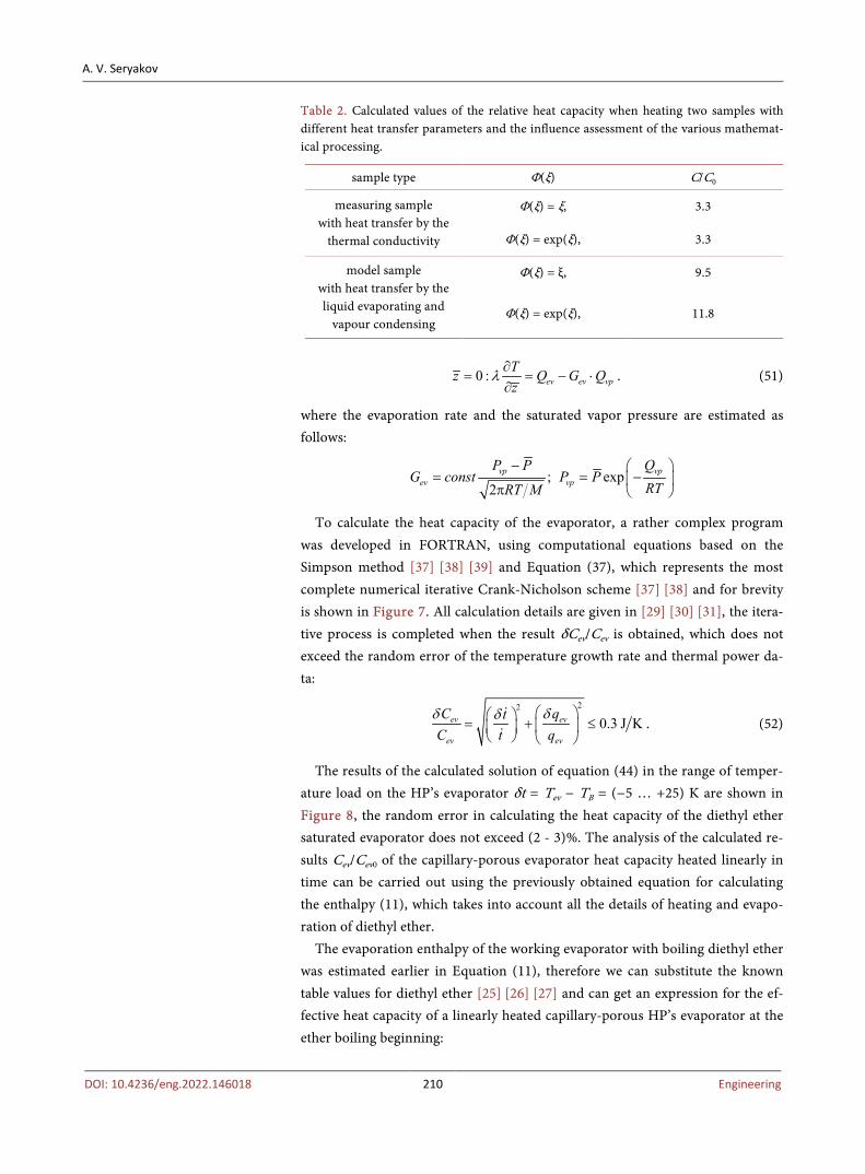
A. V. Seryakov

DOI: 10.4236/eng.2022.146018 210 Engineering

Table 2. Calculated values of the relative heat capacity when heating two samples with different heat transfer parameters and the influence assessment of the various mathemat-ical processing.

sample type Φ(ξ) C/C0

measuring sample with heat transfer by the

thermal conductivity

Φ(ξ) = ξ, 3.3

Φ(ξ) = exp(ξ), 3.3

model sample with heat transfer by the liquid evaporating and

vapour condensing

Φ(ξ) = ξ, 9.5

Φ(ξ) = exp(ξ), 11.8

0 : ev ev vpT Q Gzz

Qλ ∂= = −∂

⋅ . (51)

where the evaporation rate and the saturated vapor pressure are estimated as follows:

; exp2

vp vpev vp

P P QG const P P

RTRT M

− = = −

π

To calculate the heat capacity of the evaporator, a rather complex program was developed in FORTRAN, using computational equations based on the Simpson method [37] [38] [39] and Equation (37), which represents the most complete numerical iterative Crank-Nicholson scheme [37] [38] and for brevity is shown in Figure 7. All calculation details are given in [29] [30] [31], the itera-tive process is completed when the result δCev/Cev is obtained, which does not exceed the random error of the temperature growth rate and thermal power da-ta:

22

0.3 J Kev ev

ev ev

C qtC t qδ δδ = + ≤

. (52)

The results of the calculated solution of equation (44) in the range of temper-ature load on the HP’s evaporator δt = Tev − TB = (−5 … +25) K are shown in Figure 8, the random error in calculating the heat capacity of the diethyl ether saturated evaporator does not exceed (2 - 3)%. The analysis of the calculated re-sults Cev/Cev0 of the capillary-porous evaporator heat capacity heated linearly in time can be carried out using the previously obtained equation for calculating the enthalpy (11), which takes into account all the details of heating and evapo-ration of diethyl ether.

The evaporation enthalpy of the working evaporator with boiling diethyl ether was estimated earlier in Equation (11), therefore we can substitute the known table values for diethyl ether [25] [26] [27] and can get an expression for the ef-fective heat capacity of a linearly heated capillary-porous HP’s evaporator at the ether boiling beginning:

A. V. Seryakov

DOI: 10.4236/eng.2022.146018 211 Engineering

( ) 4

3

345 kJ kg 1.75 kJ kg K 11 K 2.34 kJ kg K 16 K 1.57 10 kg s3 10 K s

21.02 kJ K.

evev

HС

t−

−

=

+ ⋅ × + ⋅ × × ×=

×=

(53)

The ratio of the heat capacity of the evaporator with diethyl ether to the dry evaporator Cev/Cev0 taking into account the heat capacity of the resistive heater CH2 = 1.2 kJ/K at the diethyl ether boiling beginning is as follows:

0

0 0 0

21.02 1.21 18.51.2

ev ev ev ev

ev ev ev

С С H t H tС С С

+ += = + = =

. (54)

which is very close to the maximum numerical value of the heat capacity of the HP’s evaporator.

Equations (53) and (54) confirm the correspondence of the experimental and calculated thermophysical characteristics of diethyl ether located in the evapo-rator at a high temperature load.

4. Conclusions

1) The measurements of the surface temperature of short linear HP’s with li-near heating of the evaporator in time make it possible to unambiguously record an uneven drop in surface temperature. The HP’s surface temperature values around the evaporator, which are close to constant, allow us to estimate a small drop in the transmitted thermal power in the HP’s vapour channel. The con-stancy of the surface temperature around the evaporator also allows us to apply the method of solving the inverse problem of thermal conductivity (IPTC), and numerically obtain the extreme value of the heat capacity of the area (fragment) of the HP’s evaporator. This calculated result was obtained for the first time.

2) The HP’s external surface temperature of the capillary-porous evaporator, which is close to a constant value with monotonous heating, confirms the boil-ing process beginning and allows us to estimate the complex thermophysical pa-rameters of diethyl ether in the evaporator.

3) With step-by-step regularization of the inverse problem solution of the HP’s thermal conductivity and piecewise smooth polynomial approximation of unknown coefficients, it is possible to minimize the error in restoring the eva-porator heat capacity using a polynomial-exponential approximation function that restricts the range of acceptable heat capacity values by only positive values.

Acknowledgements

The author expresses gratitude to Tsvetkov Oleg Borisovich, Professor of ITMO, St. Petersburg, for his active participation in the discussion of this article at the Institute’s conferences. The author expresses special gratitude to the manage-ment of “RUDETRANSSERVICE”, Veliky Novgorod, for providing instruments and equipment for conducting experimental determination of thermal characte-ristics of heat pipes with heating close to linear in time.

A. V. Seryakov

DOI: 10.4236/eng.2022.146018 212 Engineering

Conflicts of Interest

The author declares no conflicts of interest regarding the publication of this pa-per.

References [1] Brebbia, C.A. and Dominguez, J. (1998) Boundary Elements: An Introductory Course.

WIT Press & Computational Mechanics Publication, Boston & Southampton, 325 p.

[2] Nakayama, A. and Kuwanara, F. (2008) A General Bioheat Transfer Model Based on the Theory of Porous Media. International Journal of Heat and Mass Transfer, 51, 3190-3199. https://doi.org/10.1016/j.ijheatmasstransfer.2007.05.030

[3] Beck, J., Blackwell, B. and Clair, C. (1985) Inverse Heat Conduction Ill Posed Prob-lems. Wiley & Sons, New York, 308 p.

[4] Carslaw, H.S. and Jaeger, J.C. (1986) Conduction of Heat in Solids. Oxford Univer-sity Press, Oxford, 510 p.

[5] Lykov, A.V. (1967) Theory of Thermal Conductivity. Higher School, Moscow, 600 p.

[6] Platunov, E. (1973) Thermophysical Measurements in a Monotonic Mode. Energy, Moscow, 144 p. (In Russian)

[7] Isachenko, V.P., Osipova, V.A. and Sukomel, A.S. (1981) Heat Transfer. Energoiz-dat, Moscow, 416 p. (In Russian)

[8] Kutateladze, S.S. (1979) Fundamentals of the Heat Transfer Theory. 5th Edition, Atomizdat, Moscow, 416 p. (In Russian)

[9] Denisov, A.M. (1994) Introduction to the Theory of Inverse Problems. MU, Mos-cow, 208 p. (In Russian)

[10] Tikhonov, A.M. (1963) On the Solution of Incorrectly Set Tasks and the Method of Regularization. DAN USSR, 151, 501-504.

[11] Tikhonov, A.N. and Arsenin, V.Ya. (1979) Methods for Solving Incorrect Problems. Science, Moscow, 284 p. (In Russian)

[12] He, J.-H. (1999) Variational Iteration Method—A Kind of Non-Linear Analytical Technique: Some Examples. International Journal of Non-Linear Mechanics, 34, 699-708. https://doi.org/10.1016/S0020-7462(98)00048-1

[13] He, J.-H. (2006) Some Asymptotic Methods for Strongly Nonlinear Equations. In-ternational Journal of Modern Physics B, 20, 1141-1199. https://doi.org/10.1142/S0217979206033796

[14] Lu, J. (2007) Variational Iteration Method for Solving Two-Point Boundary Value Problems. Journal of Computational and Applied Mathematics, 207, 92-95. https://doi.org/10.1016/j.cam.2006.07.014

[15] Yan, L., Fu, C.-L. and Yang, F.L. (2008) The Method of Fundamental Solutions for the Inverse Heat Source Problem. Engineering Analysis with Boundary Elements, 32, 216-222. https://doi.org/10.1016/j.enganabound.2007.08.002

[16] Seryakov, A.V. (2018) Intensification of Heat Transfer Processes in the Low Tem-perature Short Heat Pipes with Laval Nozzle Formed Vapour Channel. American Journal of Modern Physics, 7, 48-61. https://doi.org/10.11648/j.ajmp.20180701.16

[17] Seryakov, A.V., Shakshin, S.L. and Alekseev, P. (2017) The Droplets Condensate Centering in the Vapour Channel of Short Low Temperature Heat Pipes at High Heat Loads. Journal of Physics: Conference Series, 891, Article ID: 012123. https://doi.org/10.1088/1742-6596/891/1/012123

A. V. Seryakov

DOI: 10.4236/eng.2022.146018 213 Engineering

[18] Seryakov, A.V. (2019) Computer Modeling of the Vapour Vortex Orientation Changes in the Short Low Temperature Heat Pipes. International Journal of Heat and Mass Transfer, 140, 243-259. https://doi.org/10.1016/j.ijheatmasstransfer.2019.04.123

[19] Seryakov, A.V. (2016) Characteristics of Low Temperature Short Heat Pipes with a Nozzle-Shaped Vapour Channel. Journal of Applied Mechanics and Technical Physics, 57, 69-81. https://doi.org/10.1134/S0021894416010089

[20] Seryakov, A.V. (2017) The Study of Condensation Processes in the Low-Temperature Short Heat Pipes with a Nozzle-Shaped Vapour Channel. Engineering, 9, 190-240. https://doi.org/10.4236/eng.2017.92010

[21] Seryakov, A.V. (2019) Numerical Modeling of the Vapour Vortex. Journal of High Energy Physics, Gravitation and Cosmology, 5, 218-234. https://doi.org/10.4236/jhepgc.2019.51013

[22] Fowler, R.H. (1936) Statistical Mechanics. 2nd Edition, Cambridge University Press, London.

[23] Chapman, S. and Cowling, T.G. (1953) The Mathematical Theory of Non-Uniform Gases. Cambridge University Press, London, 447 p.

[24] CFdesign 10.0 2009. Version 10.0-20090623. User’s Guide.

[25] Mackay, D., Shiu, W., Ma, K. and Lee, S. (2006) Handbook of Physical-Chemical Properties and Environmental Fate for Organic Chemicals. Vol. III. Oxygen Con-taining Compounds. Taylor and Francis, Abingdon-on-Thames.

[26] (1976) Tables of Physical Values. Guide under the ed. of Kikoin I.K. Atomizdat, Moscow. 1008 p.

[27] Vargaftic, N.B. (1972) Handbook of Thermophysical Properties of Gases and Liq-uids. Publishing House of Physics and Mathematical Literature, Moscow, 721 p.

[28] Faghri, A. (1995) Heat Pipe Science and Technology. Taylor and Francis, Washing-ton DC.

[29] Seryakov, A.V. and Alekseev, A.P. (2020) A Study of the Short Heat Pipes by the Monotonic Heating Method. Journal of Physics: Conference Series, 1683, Article ID: 022051. https://doi.org/10.1088/1742-6596/1683/2/022051

[30] Seryakov, A.V. and Alekseev, A.P. (2020) Investigation of Short Heat Pipes by the Method of Monotonous Heating. III International Conference “Modern Problems of Thermophysics and Energy”, Moscow, 19-23 October 2020, 270-272.

[31] Seryakov, A.V. and Alekseev, A.P. (2020) Investigation of Short Linear Heat Pipes by Solving the Inverse Problem of Thermal Conductivity. Reshetnev Readings. Ma-terials of the XXIV International Scientific and Practical Conference Dedicated to the Memory of the General Designer of Rocket and Space Systems, Krasnoyarsk, 10-13 November 2020, Part 1, 144-146.

[32] Odibat, Z.M. and Momani, S. (2006) Application of Variational Iteration Method to Nonlinear Differential Equations of Fractional Order. International Journal of Non-linear Sciences and Numerical Simulation, 7, 27-34. https://doi.org/10.1515/IJNSNS.2006.7.1.27

[33] Farcas, A. and Lesnic, D. (2006) The Boundary-Element Method for the Determina-tion of a Heat Source Dependent on One Variable. Journal of Engineering Mathe-matics, 54, 375-388. https://doi.org/10.1007/s10665-005-9023-0

[34] Elsholts, L.E. (2008) Calculus of Variations: A Textbook for Physical and Physical- Mathematical Faculties of Universities. Moscow Publishing House, Moscow, 205 p. (In Russian)

A. V. Seryakov

DOI: 10.4236/eng.2022.146018 214 Engineering

[35] Elsholts, L.E. (1969) Differential Equations and Calculus of Variations. Nauka, Mos-cow. (In Russian)

[36] Tslaf, L.Y. (2005) Calculus of Variations and Integral Equations: A Reference Guide. 3rd Edition, St. Petersburg Publishing House, St. Petersburg, 192 p. (In Russian)

[37] Marchuk, G.I. (1980) Methods of Computational Mathematics. Nauka, Moscow, 536 p. (In Russian)

[38] Tikhonov, A.N. and Samarsky, A.A. (1966) Equations of Mathematical Physics. Nauka, Moscow, 724 p. (In Russian)

[39] Kalitkin, N.N. (1978) Numerical Methods. Nauka, Moscow, 512 p. (In Russian)

A. V. Seryakov

DOI: 10.4236/eng.2022.146018 215 Engineering

Nomenclature

a = λ/CP∙RHP—coefficient of HP’s thermal diffusivity; ak = k-th calculated component of the thermal diffusivity coefficient, m2/s; Ceff: effective heat capacity of the HP, J/K; CHP(t)—HP’s heat capacity as a whole, J/K; cv(t)—HP’s volume heat capacity, J/m3∙K; cv(T)—HP’s specific isochoric heat capacity, J/kg∙K; Cev0—heat capacity of the dry evaporator, J/K; Cev—heat capacity of the evaporator with diethyl ether, J/K; Cev—calculated heat capacity of the evaporator, J/K; Cl—diethyl ether heat capacity, J/kg∙K; Cvp—heat capacity of diethyl ether moist vapour, J/kg∙K; Cfev—heat capacity of diethyl ether on the evaporator surface, J/kg∙K; EH2—thermal power of the resistive heater, W; FHP(sz)—HP’s cross-sectional area, m2; Gl—mass flow rate of diethyl ether liquid phase in the evaporator, kg/s; Gmix—mass flow of the moist saturated vapour over the evaporator, kg/s; Gvp—mass flow rate of dry saturated vapour over the evaporator, kg/s; (1 – xev) = G’/(G’ + G) —the degree of moisture vapour in the evaporator; gk—the derivative of the heat capacity components; Hev—enthalpy of the HP’s evaporator, W; LHP—HP’s length, m; Lev—the thickness of the capillary porous evaporator, m; P —the average pressure in the vapour channel, Pa; Pev—pressure above the evaporator, Pa; Pfcond—pressure on the condensation surface, Pa; Pv—the vapour pressure inside the toroidal vortex, close to the condensation pressure Pfcond; Pr—the Prandtl number of the diethyl ether vapour; Qev—heat input to the evaporator, W; Qcond—heat of condensation, W; Rc—thermal resistance of the lubricant layer, K/W; Rev—thermal resistance of the evaporator, K/W; Rw—thermal resistance of the metal cover, K/W; RHP(T)—HP’s thermal resistance, K/W; r(TB) —specific heat of evaporation of diethyl ether, kJ/kg; TB—boiling point of the diethyl ether, K; Tcal—the temperature of the flowing water in the vortex calorimeter; Tcond—condensation surface temperature T, K;

fcondT —the average temperature of the diethyl ether film on the HP’s condensa-tion surface, K;

fevT —the average temperature of diethyl ether boiling microlayer on the HP’s lower cover surface, K;

A. V. Seryakov

DOI: 10.4236/eng.2022.146018 216 Engineering

( )HPT z —the temperature inside the HP’s vapour channel at a height of z above the evaporator, K; Tev—stationary temperature of the grid evaporator saturated with the diethyl ether, K; Tsc—stationary temperature of the evaporator metal mesh, K; Tv—he vapour temperature inside the toroidal vapour vortex, K; t—temperature growth rate, K/s; v—vapour (and liquid) phases flow velocity inside the capillary-porous evapo-rator, m/s; xev—the degree of vapour moisture in the evaporator; Y—parameter of the additional source function, J;

HPz z L= —dimensionless longitudinal coordinate; uv, vv—axial and tangential components of the vortex velocity in the HP’s vapour channel, m/s; Greek αcal—heat transfer coefficient in the vortex flow calorimeter, W/m2∙K; αcond—heat transfer coefficient in the HP’s condensation region, W/m2∙K; δfcond—the average thickness of the diethyl ether film on the condensation sur-face, m; δw—the thickness of the flat metal bottom cover, m; η—Lagrange multiplier; λeff—effective thermal conductivity, W/m·K;

HPλ —effective thermal conductivity of the HP, W/m∙K; λl—thermal conductivity of diethyl ether, W/m∙K; λ(t)—HP thermal conductivity coefficient, W/m∙K; λsc—thermal conductivity coefficient of metal mesh evaporator frame, W/m∙K; λw—thermal conductivity coefficient of metal top and bottom covers, W/m∙K; μi—friction coefficients; ξ—condensation coefficient defined as the ratio of the number of vapour mole-cules condensing over the total number of molecules which strikes the surface; Π—the porosity of the evaporator and insert (wick) in the HP’s vapour channel; ρHP—HP’s density, kg/m3;

mixvpρ —the density of moist vapour inside the vapour channel, kg/m3;

ρv—the vapour density inside the toroidal vortex, kg/m3;

evρ , kg/m3—average evaporator density, kg/m3; τ—time, s; Δτk—time step for calculations and measurements, s; Φdf—dissipative functions; χ—Lagrange multiplier; ψ—the mass fractions of the HP’s components;