Comput Mech (2014) 54:711–722DOI 10.1007/s00466-014-1023-3

ORIGINAL PAPER

The morphing method as a flexible tool for adaptivelocal/non-local simulation of static fracture

Yan Azdoud · Fei Han · Gilles Lubineau

Received: 4 September 2013 / Accepted: 31 March 2014 / Published online: 19 April 2014© Springer-Verlag Berlin Heidelberg 2014

Abstract We introduce a framework that adapts local andnon-local continuum models to simulate static fracture prob-lems. Non-local models based on the peridynamic theory arepromising for the simulation of fracture, as they allow dis-continuities in the displacement field. However, they remaincomputationally expensive. As an alternative, we develop anadaptive coupling technique based on the morphing methodto restrict the non-local model adaptively during the evolu-tion of the fracture. The rest of the structure is described bylocal continuum mechanics. We conduct all simulations inthree dimensions, using the relevant discretization scheme ineach domain, i.e., the discontinuous Galerkin finite elementmethod in the peridynamic domain and the continuous finiteelement method in the local continuum mechanics domain.

Keywords Non-local elasticity · Coupling · Peridynamics ·Static fracture · DGFEM · Anisotropy · Morphing

1 Introduction

Recent advances in non-local continuum mechanics havegreatly improved the simulation of discontinuous processesby allowing accurate mathematical representations of singu-larities and discontinuities. Models based on this paradigmand notably based on peridynamics, yield promising resultson the simulation of fractures [6,10,11]. The internal lengthscale allows these models to address localization problemsoften encountered in classical damage mechanics simula-tions. Despite these advances, challenges remain in easing

Y. Azdoud · F. Han · G. Lubineau (B)COHMAS Laboratory, Physical Science and Engineering Division,King Abdullah University of Science and Technology (KAUST),Thuwal 23955-6900, Saudi Arabiae-mail: gilles.lubineau@kaust.edu.sa

the implementation, as well as in extending the capabilitiesof this approach to include various constitutive behaviors,such as plasticity, damage mechanics, or complex heteroge-neous geometries [7,8]. This study has two aims. First, wepresent an adaptive approach that couples local and non-localcontinua to reduce the computational cost of peridynamics-based fracture simulations. Second, we present a variationaldiscretization method for peridynamics.

We address the cost-reduction requirement by restrictingthe domain of the non-local model in the structure, whileapplying a classic local continuum model elsewhere. This isachieved using a non-local-to-local coupling approach. Onerequirement is that this coupling approach has to be suffi-ciently flexible to follow the quasi-static evolution of cracksin a simple and robust manner. Several methods have beendeveloped for non-local-to-local coupling. Han and Lubineau[9] developed a coupling method based on the Arlequinmethod. Seleson et al. [16] introduced a force conservation-based technique in one dimension. Liu and Hong [12] intro-duced two coupling techniques (so-called CT and VL cou-pling) based on force partitioning at the discretized level. Themorphing method [13] was developed based on the conser-vation of the strain energy density in a hybrid local/non-localmodel over an overlapping coupling region. We propose touse the morphing method because of its robustness in threedimensions and its ability to define the coupling area by asimple mapping function, called the morphing parameter. Wenote that this coupling technique is performed at the consti-tutive equation level and that it does not depend on the cho-sen discretization scheme. Because cracks propagate withinthe structure, it is essential to define an adaptive method toextend the non-local zone during the evolution of cracks. Wedemonstrate here how the morphing parameter introduced inthe morphing technique can be used as a very flexible toolfor making the hybrid local/non-local description adaptive.

123

712 Comput Mech (2014) 54:711–722

We are also careful to introduce a suitable conformingdiscretization scheme for the peridynamic framework. Theperidynamic theory does not require the displacement field tobe continuous. Mathematically, the displacement field has theminimal requirement of being in the space of quadraticallyintegrable functions (the L2 space), while in classical con-tinuum models, it is contained within the space of derivablefunctions (the H1 space). Thus, the discontinuous Galerkinfinite element method (DGFEM) is used for the non-localcontinuum.

This communication is organized as follows. First, afterdescribing the non-local model, we introduce a hybrid modeldefined by the morphing method. Then, we derive the dis-cretized problem using the Galerkin method. Second, wepresent the adaptive algorithm used to implement the frac-ture simulation. Third, we focus on the convergence of themethod relative to the space and time discretization for afixed non-local/local partition. Finally, we implement a three-dimensional compact tension (CT) fracture test to assess thequality of the adaptive mapping algorithm.

2 A non-local framework for simulation of staticfracture: a bond-based peridynamic model

2.1 Overview of a simple peridynamic model

Peridynamics has been developed as a non-local formula-tion to allow the representation of discontinuities in the dis-placement field, with the central focus being the simulationof fractures. For this study, we employ a bond-based model[17,19], which is based on a simple rendering of the peridy-namic theory. This model is developed around central non-local interactions between material points within the domainof study, and it is defined by an integral form of the equilib-rium equation.

Say Ω is a continuum where material points interact witheach other via long-range forces (see Fig. 1) such that theequilibrium equation at point x for a quasi-static problem isas follows:

∫

Hδ(x)

f (p → x)dVp + b = 0 ∀x ∈ Ω (1)

where f (p → x) is the action of point p over point x . δ

is the cut-off radius, which limits the long-range interactionof x with the material points in its neighborhood, Hδ(x),also called the horizon (Fig. 1). b are the prescribed externalbody forces. For simplicity, we introduce the concept of abond ξ = p − x .

The model is fully defined by the following set of equa-tions:

Fig. 1 The non-local continuum Ω: Hδ(x) is the horizon of x depend-ing on the characteristic range of long-range forces. Bonds are definedby x and p, where p is in the horizon of x

• Kinematic admissibility and compatibility:

ηξ (p − x) = uξ (p) − uξ (x) ∀x, p ∈ Ω (2)

• Static admissibility:∫

Hδ(x)

f (p → x)dVp + b = 0 ∀x ∈ Ω (3)

• Constitutive equation:

f (p → x) = c[x](ξ) + c[p](ξ)

2ηξ (p − x)eξ ∀x, p ∈ Ω

(4)

where eξ = ξ/‖ξ‖ and uξ (p) is the projection of the dis-placement at point p over the bond (i.e., uξ (p) = u(p) · eξ ).

The micromodulus, c[x](ξ), defines the stiffness parame-ters at point x relative to the bond, ξ . c[x](ξ) can vary withthe orientation of ξ to introduce some degree of anisotropy[3]. In the reminder of this paper, we focus solely on homo-geneous isotropic models defined by:

c[x](ξ) = c(‖ξ‖) (5)

where ‖ξ‖ is the Euclidean norm of ξ .

2.2 A bond-based fracture law

We use a simple failure criterion based on the critical stretchof the bond. This model has been introduced in [18] and hasbeen extensively used to study static and dynamic fractures[6,10,15].

123

Comput Mech (2014) 54:711–722 713

Bond force density (N.m-6)

Stretchscrit

Fig. 2 The force density in relation to the bond stretch in a perfectlybrittle case. The bond is elastic up to scri t at which point it experiencesan irreversible brittle failure

Fig. 3 The reference case to estimate the link between the criticalenergy release rate and the bond stretch to calculate the energy of bondscrossing a crack

We assign to every bond a critical stretch, scri t , abovewhich the bond is broken. This breakage of the bond is irre-versible. The force density of the bond relative to its stretchis given in Fig. 2 for a constant micromodulus. It is possibleto link the critical stretch, scri t , to the critical energy releaserate, Gc, as denoted in [18]. In the case when a crack goesthrough complete horizons (Fig. 3), the relation between scri t

and Gc is given by Eq. 6:

Gc =

1

2

δ∫

0

2π∫

0

δ∫

z

arccos(z/ξ)∫

0

c(‖ξ‖)ξ4s2cri t sin(ϕ)dϕdξdθdz

(6)

This relation estimates Gc as being the energy dissipationissued from breaking all the bonds that cross a unit cracksurface. We refer the reader to Silling and Askari [18] for thederivation of a similar equation.

Of course, this relation is modified when the horizons arenot complete, which is the case when the crack is close to theedge of the structure. The relation is then locally dependanton the geometry. In the reminder of this paper, we assumethat the peridynamic parameter for fracture, i.e., the criticalstretch, scri t , is constant throughout the structure. The equiv-alent critical energy release rate, Gc, is calculated accordingto scri t and according to the geometry of the structure inSects. 5 and 6.

2.3 Remarks on the discretization of a peridynamic model

Different approaches may be taken to discretize peridynamicmodels. Most such approaches are based on a particle-likemodel in which every node is weighted by the area of its cor-responding Voronoi cell [2,19]. Other approaches rely on thefinite element method (FEM) [3,13,14,20]. Nodal methodsare effective only for regular grids, as the Voronoi partitionfor an irregular grid introduces local integration errors. Thislimits their usage to simple structures. Moreover, the poorestimation of the integral over the horizon, Hδ(x), leads toa sub-optimal convergence rate (inferior to O(N ), where Nis the number of nodes). On the other hand, FEM has a highconvergence rate, although it was designed for continuousmedia. Thus, its use is inappropriate if the fields of interestare not sufficiently regular. In FEM, the displacement fieldis assumed to be differentiable, i.e., in the H1 space. Thisregularity of the field of interest is not possible in simula-tions in which fracture is assumed, making FEM unsuitablefor non-local models with fracture.

Nevertheless, we would like to use a high convergencerate discretization scheme in which the fields of interest areonly quadratically integrable (in the L2 space), such as theDGFEM. A convergence study by Chen and Gunzburger [4]demonstrated the potential of DGFEM for peridynamics ina one-dimensional problem. The DGFEM is a discretizationscheme based on the variational formulation of a mechani-cal problem. It allows discontinuities to exist at the interfacebetween finite elements. In that sense, it is interesting to notethat the nodal method is the DGFEM of level 0. In local mod-els, DGFEM is difficult to apply because it allows approxi-mated solutions to be in the L2 space. Thus, a flux constrainthas to be applied over the boundaries of the elements [1].Such an issue does not exist for a non-local model: DGFEMis conforming because the approximate solution and the ana-lytical solution are in the same space (the L2 space).

3 Hybrid modeling by the morphing method

Our final objective here is to design a technique capable ofhandling an adaptive hybrid description of the structure. At agiven increment, the fracture lies within a non-local (peridy-namic) domain, which is itself embedded in a classical localcontinuum model to reduce the computation cost. This par-tition should then evolve to track the extension of the crack.

3.1 The morphing method

The morphing method [3,13] was designed to couple localand non-local continua. We propose to use this method toconstrain the non-local domain around discontinuities suchas cracks. The morphing method is described by the follow-

123

714 Comput Mech (2014) 54:711–722

ing set of equations that represents a hybrid local/non-localcontinuum model:

• Kinematic admissibility and compatibility:

ε(x) = 1

2

(∇ · u(x) +t ∇ · u(x)

)∀x ∈ Ω (7)

ηξ (p − x) = uξ (p) − uξ (x) ∀x, p ∈ Ω (8)

u = u ∀x ∈ Su (9)

• Static admissibility:

divσ +∫

Hδ(x)

f (p → x)dVp = −b ∀x ∈ Ω (10)

σ · n = T ∀x ∈ ST (11)

• Constitutive equations:

σ = C[x] : ε ∀x ∈ Ω (12)

f (p → x) = (α(x) + α(p))c(‖ξ‖)2

ηξ (p − x)eξ

∀x, p ∈ Ω (13)

where C[x] is the stiffness of the local continuum at any point

x , and u and T are respectively the displacement and the forceboundary conditions, applied on the respective boundaries,Su and ST (see Fig. 4). σ and ε are the Cauchy stress tensorand the linearized strain tensor, respectively.

Following Lubineau et al. [13], passage between local andnon-local models is guaranteed by the morphing function,α(x). The relationship between the local stiffness operatorand the micromodulus at every point x is given by an energydensity conservation constraint that leads to the followingequation:

C[x] = (1 − α[x])Co

+∫

Hδ(x)

c(‖ξ‖) (α[x] − α[p])2

ξ ⊗ ξ ⊗ ξ ⊗ ξ

2‖ξ‖2 dVp

(14)

where Co is the fourth-order stiffness tensor that describes

the elasticity of the material when only the local continuummodel is used. When subjected to locally uniform strain load-ing (cf. [13]), Co is given by the following equation:

Co =∫

Hδ(x)

c(‖ξ‖) ξ ⊗ ξ ⊗ ξ ⊗ ξ

2‖ξ‖2 dVp (15)

=1

0< <1

=01

Su

bST LOCAL

NON LOCAL

c

2

Fig. 4 Description of a hybrid domain. Ω2, the non-local region, isembedded in the local region, Ω1. The coupling is ensured by the vari-ation of the coupling parameter, α(x), in the coupling zone, Ωc. δ is thenon-local cut-off radius

Note that the parameter α(x) in Eq. 14 is a mapping func-tion over the domain Ω that completely defines if the modelis local, non-local or hybrid at each and every material point.Figure 4 shows a choice of α(x). Note that for any point x inthe domain Ω2, which is purely non-local, we have:

α(p) = 1 ∀p ∈ Hδ(x) (16)

and in the domain Ω1, which is purely local, we have:

α(p) = 0 ∀p ∈ Hδ(x) (17)

α(x) varies in Ωc to couple both local and non-local regionssmoothly. Ωc, the coupling domain, is the part of the structurewhere both descriptions (local and non-local) coexist. Thecore of the Ωc domain is made of a region over which 0 <

α < 1 (light grey in Fig. 4). There are, however, layers ofthickness δ at the boundaries of the coupling domain whereboth local and non-local descriptions exist but over whichα is constant (equal to 1 and 0, respectively). Indeed, fromEq. 14, a point x is strictly local if α = 0 for all p such that|x − p| < δ, and a point x is strictly non-local if α = 1 for allp such that |x − p| < δ. The strength of this approach is thatthe coupling is done at the level of the constitutive equation.That makes it very easy to define and modify this couplingmethod from an algorithmic point of view.

3.2 Discretization of the hybrid local/non-local model

In this section, we discretize the hybrid local/non-local modelin the configuration presented in Fig. 4. In Sect. 2.3, we dis-cussed the appropriate discretization method for the non-local model relative to the regularity of the displacement field.Here, the strategy is to apply the appropriate discretization(FEM or DGFEM) in relation with the regularity of the con-sidered sub-domain. In Fig. 4, we partitioned the domain Ω

into three subdomains: the domain Ω2, where fracture canexist, i.e., where the displacement field is in the L2 spacebut not in the H1 space, and the domains Ω1 and Ωc, where

123

Comput Mech (2014) 54:711–722 715

there is no fracture, i.e., where the displacement field can beassumed in the H1 space. From a modeling standpoint, wedefine a purely non-local model in the domain Ω2 to repre-sent fracture, a purely local model in the domain Ω1 for itslow computational cost and a transition domain Ωc to ensurecoupling. Thus, we apply DGFEM in the domain Ω2 andFEM in the remainder of the structure. This is a conformingdiscretization approach.

3.2.1 The Galerkin formulation

We define the Galerkin variational formulation of the modelproposed in Sect. 3.1. The weak primal formulation of thehybrid problem can be written as:

Find u ∈ W | ∀v ∈ W o a(u, v) = l(v) (18)

where v is a virtual displacement field and with W and W o

being the admissible displacement fields space and the spaceof admissible virtual fields, respectively, such that:

W = {u ∈ L2(Ω) ∪ H1(Ω1 ∪ Ωc); u = u ∀x ∈ Su} (19)

W o ={v ∈ L2(Ω) ∪ H1(Ω1 ∪ Ωc); v=0 ∀x ∈ Su} (20)

Similarly to Di Paola et al. [5], we can find the bilinearand linear forms a(•, •) and l(•), respectively, for our hybridproblem. It yields:

a(u, v) =∫

Ω

σ(u) : ε(v)dΩ

+1

2

∫ ∫

Ω

c(‖ξ‖) (α[x] + α[p])2

ηξ [u](x, ξ)

ηξ [v](x, ξ)d pdx

∀(u, v) ∈ W × W o (21)

l(v) =∫

Ω

b · vdΩ +∫

ST

T · vd ST ∀v ∈ W o (22)

with ηξ [v](x, ξ) = vξ (p) − vξ (x) and ξ = p − x . Thisformulation is valid over the entire domain Ω because thechange from a local to a non-local model is defined by themapping function α(x). The derivation of similar linear andbilinear forms can be found in Di Paola et al. [5].

It should be noted that the originality of the approach liesin defining the spaces W and W o such that the degree ofregularity is varying in space.

3.2.2 Discretization and Gauss quadrature

Section 3.2.1 provided the variational formulation of thehybrid model. We apply a first-order discretization in eitherFEM or DGFEM. DGFEM discretization is applied only inthe non-local zone. As we do not apply the DGFEM to the

local model, the problem is simplified since no jump con-straint between elements has to be specified. A Gauss quadra-ture scheme is retained to estimate the integrals within theelements.

Let {ei } be a polygonal element partition of Ω . Let {φik} be

a nodal basis for an element, ei , and {v(xk)}be the nodal valueof a function, v(x). φk is the nodal basis for the whole domainΩ . We denote by v(x) = ∑

k v(xk)φk(x) the interpolant ofv(x) on Ω .

The weak formulation can then be rewritten as

a(u, v) =∑

i

∫

ei

ε(v) : C(x) : ε(u)dx

+1

2

∑i

∫

ei

∑j

∫

e j

α(x) + α(p)

2

·c(‖ξ‖)(ηξ [v](x, ξ))(eξ ⊗ eξ )(ηξ [u](x, ξ))d pdx

(23)

and

l(v) =∑

i

∫

ei

b · vdx +∑

i

∫

SiT

T · vd SiT . (24)

From this formulation, we can derive the linear system to besolved in the following form:

[K ]{u} = {F} (25)

with

u(x) = [Φ(x)]{u} (26)

and

[Φ(x)

]=⎡⎣φ1(x) 0 0 · · · φn(x) 0 0

0 φ1(x) 0 · · · 0 φn(x) 00 0 φ1(x) · · · 0 0 φn(x)

⎤⎦

(27)

where 3n is the total degrees of freedom (DoFs) of our prob-lem, and the components of {u} are the value of the displace-ment for those DoFs.

The stiffness matrix is then given by:

[K ] =∑

i

∫

ei

([H ][Φ(x)])T [C(x)][H ][Φ(x)]dx

+∑

i

∑j

∫

ei

∫

e j

α(x) + α(p)

2c(‖ξ‖)[Φ(x)]T

[G][Φ(x)]d pdx (28)

123

716 Comput Mech (2014) 54:711–722

1

Su

bST LOCAL

NON LOCAL

c

2FEM

DGFEM

=1

0< <1

=0

Fig. 5 The Discretized domain. DGFEM is applied to elementsembedded in the domain Ω2, while FEM is applied in the remainder ofthe structure

−∑

i

∑j

∫

ei

∫

e j

α(x) + α(p)

2c(‖ξ‖)[Φ(x)]T

[G][Φ(p)]d pdx

where [H ] is a matrix of differential operators and [G] =eξ ⊗ eξ .

The load vector {F} is given by:

{F} =∑

i

∫

ei

[Φ(x)]T {b}dx +∑

i

∫

SiT

[Φ(x)]T {T }d SiT (29)

Integrals are estimated using a high-order Gauss–Legen-dre quadrature method (4×4×4 Gauss points per element)for a better approximation of the micro-modulus integration.Note that the discretized forms for FEM and for DGFEM areidentical. The difference between these two methods residesin the type of shape functions used. In the case of DGFEM,neighboring elements do not share nodes. Shape functionsare therefore discontinuous on the nodes. We apply lineardiscontinuous shape functions in Ω2, where the model ispurely non-local and fracture is allowed. Linear continuousshape functions are used in the remainder of the structure.The discretized domain is illustrated in Fig. 5.

4 A computational solution for the hybridlocal/non-local model

In Sect. 3, we describe the structure of the hybrid model at agiven increment. The challenge is now to make this descrip-tion evolve in space such that it naturally tracks the evolu-tion of the cracking process. Optimization of the code is notdescribed, but a C++ implementation has been conductedin parallel using OpenMP 3.0 with in-house sparse matrixsolvers.

4.1 Structure of the implicit fracture algorithm

We choose an implicit algorithm for the study of fracture.External loading is specified as Ni progressive increments,

Di=1 ; Ni ; {F} ; [K]

{F i }= i / Ni * {F}

Solve [K]{u} = {F i }

Break bonds for s > scrit

Bond broken ?

Is i = Ni ?

Store broken bonds

Update [K]

Run adaptive algorithm ; update i

Yes

No

Yes

No

End fracture algorithm

Start fracture algorithm

Fig. 6 Flowchart of the iterative implicit fracture algorithm

i . At each increment, the linear elastic problem, [K ]{u} ={Fi }, is solved. The calculated displacement field is then usedto test the bond stretch criterion. Bond breakage induces aloss of stiffness denoted by the update of the stiffness matrix,[K ]. The linear elastic problem is iteratively calculated untilno bond is broken at the current loading increment beforepassing to the adaptive algorithm. When the last increment isreached, the simulation ends. The flowchart in Fig. 6 summa-rizes the different steps of the fracture algorithm. The adap-tive process is described in the following section.

4.2 An adaptive criterion for non-local mapping updating

We use a simple adaptive criterion that ensures that the frac-ture zone always remains far enough away from the limitsof the non-local zone, i.e., that any broken bond is at least ata distance d = δ from the limits of the non-local zone. Ourapproach takes advantage of the morphing parameter, α(x),that defines the non-local mapping.

Two possible strategies can be used to update α(x),either between increments or between iterations. The lat-ter allows us to follow the cracking process without makingassumptions about the number of increments, the mesh sizeor the stability of the fracture process but dramatically reduc-ing the computational performance. Updating α(x) betweenincrements, on the other hand, supposes that the crack exten-sion during an increment is smaller than δ but has a lowimpact on the computational performance. We therefore pro-pose to update α(x) at each increment to follow the crack.

Updating α(x) for every single bond loss would be com-putationally expensive. Rather, at each increment, we updateα(x) at the scale of the elements by identifying elementsin which bonds were broken. For every new damaged ele-ment, a spherical region centered on the centroid of this

123

Comput Mech (2014) 54:711–722 717

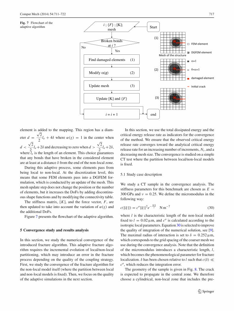
Fig. 7 Flowchart of theadaptive algorithm

element is added to the mapping. This region has a diam-

eter d =√

2

2le + 4δ where α(x) = 1 in the center when

d <

√2

2le +2δ and decreasing to zero when d >

√2

2le +2δ,

where le is the length of an element. This choice guaranteesthat any bonds that have broken in the considered elementare at least at a distance δ from the end of the non-local zone.

During this adaptive process, some elements pass frombeing local to non-local. At the discretization level, thismeans that some FEM elements pass into a DGFEM for-mulation, which is conducted by an update of the mesh. Thismesh update step does not change the position or the numberof elements, but it increases the DoFs by adding discontinu-ous shape functions and by modifying the connectivity table.

The stiffness matrix, [K ], and the force vector, F , arethen updated to take into account the variation of α(x) andthe additional DoFs.

Figure 7 presents the flowchart of the adaptive algorithm.

5 Convergence study and results analysis

In this section, we study the numerical convergence of theintroduced fracture algorithm. This adaptive fracture algo-rithm requires the incremental evolution of local/non-localpartitioning, which may introduce an error in the fractureprocess depending on the quality of the coupling strategy.First, we study the convergence of the fracture algorithm forthe non-local model itself (where the partition between localand non-local models is fixed). Then, we focus on the qualityof the adaptive simulations in the next section.

In this section, we use the total dissipated energy and thecritical energy release rate as indicators for the convergenceof the method. We ensure that the observed critical energyrelease rate converges toward the analytical critical energyrelease rate for an increasing number of increments, Ni , and adecreasing mesh size. The convergence is studied on a simpleCT test where the partition between local/non-local modelsis fixed.

5.1 Study case description

We study a CT sample in the convergence analysis. Thestiffness parameters for this benchmark are chosen as E =300 GPa and ν = 0.25. We define the micromodulus in thefollowing way:

c(‖ξ‖) = co‖ξ‖2e− ‖ξ‖l N m−7 (30)

where l is the characteristic length of the non-local modelfixed to l = 0.02 µm, and co is calculated according to theisotropic local parameters. Equation 30 is selected to improvethe quality of integration of the numerical solution, see [9].The maximal radius of interaction is set to δ = 0.252 µm,which corresponds to the grid spacing of the coarser mesh weuse during the convergence analysis. Note that the definitionof the micromodulus introduces a characteristic length, l,which becomes the phenomenological parameter for fracturelocalization. δ has been chosen relative to l such that c(δ) co, which reduces the integration error.

The geometry of the sample is given in Fig. 8. The crackis expected to propagate in the central zone. We thereforechoose a cylindrical, non-local zone that includes the pre-

123

718 Comput Mech (2014) 54:711–722

=1

0< <1

=0

Pre-crack

S1

S2

L w

h

ud

-ud

Fig. 8 Geometry, mapping of α(x) and boundary conditions for thecracked plate example. The dimensions of the sample are w = 2δ,h = 8δ and L = 12δ

crack tip. We prescribe for S1 (respectively S2) the followingboundary conditions: u · z = ud (respectively u · z = −ud ) =45δ, and σxy = σxz = 0 (see Fig. 8). The boundary conditionsare applied as a ramp of displacement from 0 to ud in Ni

increments. The bond fracture stretch criterion is fixed atscri t = 1.10. Due to the geometry of the sample, the criticalenergy corresponding to this critical stretch is calculated tobe Gc = 530.74 J m−2 on average throughout the thicknessof the sample using Eq. 6.

5.2 Convergence study

We propose to study the numerical convergence of the modelaccording to discretization parameters, such as the number oframp increments, Ni , and the mesh density (with the numberof elements, Ne). All data (geometry and material parame-ters) are similar to those introduced in Sect. 5.1.

5.2.1 Ni -convergence

We set the number of elements for this simulation to Ne =648. Figure 9 shows the maps of dissipated energy at aprescribed displacement of 5

6 ud , with different choices of

Fig. 10 Total dissipated energy versus imposed displacement for 6(green), 60 (blue) and 600 (red) increments

(a) (b)

Fig. 11 Absolute (a) and relative (b) difference of 6 and 60 incrementsrelative to 600 increments, for increasing imposed displacements

Ni (Ni = 6, 60, 600). The morphology of the fracture is iden-tical. Figure 10 presents the total dissipated energy relativeto the imposed displacement. We note that the dissipation

Fig. 9 a, b and c, maps of dissipated energy for Ni = 6, 60 and 600, respectively, at the imposed displacement of 5/6ud . D denotes the value ofenergy dissipated per element (×10−6 J)

123

Comput Mech (2014) 54:711–722 719

Fig. 12 a, b and c, maps of dissipated energy for 648, 1,536 and 3,000 elements, respectively, at 50 increments. D denotes the value of energydissipated per element (×10−6 J)

0.4 0.5 0.6 0.7 0.8 0.9 10

0.1

0.2

0.3

0.4

0.5

0.6

0.7

0.8

0.9

1

192 elements648 elements1536 elements3000 elements

0 0.2 0.4 0.6 0.8 10

50

100

150

200

250

300194 elements648 elements1536 elements3000 elements

0.10.150.20.250.3102

103

104

(a) (b) (c)

Fig. 13 a Total dissipated energy versus imposed displacement for the different mesh densities. b Estimation of the crack length in relation to theimposed displacement for different mesh densities. c Convergence of the norm max ‖Gc − Gc‖∞ in relation to the mesh size

-ud

S1

S2

L w

h

ud

=1

0< <1

=0

Pre-crack

Fig. 14 Geometry, non-local seed and boundary conditions for thecracked plate adaptive mesh example. The dimensions of the sampleare w = 2δ, h = 8δ and L = 12δ

remains similar even at a low number of increments. A lownumber of increments can result in some bonds reaching thecritical stretch, scri t , contrary to the expected solution. As aresult, the total dissipated energy should be overestimated bythe implicit algorithm when too few increments are used. Thisis estimated by comparing the dissipated energy for differ-ent Ni at common imposed displacement, as seen in Fig. 11.

Fig. 15 Evolution of the total dissipated energy in relation to theimposed displacement of the adaptive model (blue curve), comparedto a fixed mesh solution (green curve)

Figure 11 shows the difference in total dissipated energy forNi = 6 and Ni = 60 relative to Ni = 600. Figure 11a revealsa cumulative error that decreases when Ni increases. Simi-

123

720 Comput Mech (2014) 54:711–722

Fig. 16 The evolution of the mapping function, α(x) (first column),mesh partition (second column) and dissipated energy map (third col-umn) for increasing increments (1 increment in the first line, 30 incre-ments in the second line and 50 increments in the third line). We note

that the evolution of the mapping function follows the crack propaga-tion. DGFEM, denoted by square elements, is embeded in the evolvingnon-local zone of the structure

larly, the relative error (Fig. 11b) decreases to a low constantvalue (under 1 %). This suggests that Ni has a low impact onthe quality of the approximation for this simulation. Thus,for the reminder of this paper, we use Ni = 60.

5.2.2 Ne-convergence

We set the number of increments to Ni = 60 and we study themesh convergence on the example presented in Sect. 5.1, witha varying number of elements (192, 648, 1,536 and 3,000).

We calculate analytically the critical energy release rate, Gc,and propose to estimate the convergence using the max norm‖Gc − Gc‖∞, where Gc is the approximate critical energyrelease rate, calculated as the ratio between the dissipatedelastic energy and the estimated surface of the crack.

Figure 12 shows the map of dissipated energy for differentmesh densities with the same boundary conditions. Qualita-tively, we notice that localization is independent of the meshdensity, as the fracture mechanism is guided by the charac-teristic length of the non-local model. Figure 13a displaysthe total dissipated energy relative to the imposed displace-

123

Comput Mech (2014) 54:711–722 721

ment. Global evolution of the dissipated energy is similarregardless of mesh size, though increasing the mesh densitydecreases the height of the jumps and smooths the evolu-tion of the dissipated energy. We notice that the jumps in thedissipated energy curve occur when an interface betweentwo elements is totally broken. With this, we can evalu-ate the crack length and derive the apparent critical energyrelease rate, Gc. For this purpose, we evaluate the relationbetween crack length and imposed displacement in Fig. 13b,based on the estimation of the actual crack length at thejumps. It is straightforward to estimate Gc during the frac-ture process with this estimated crack length and the relateddissipated energy. We graph ‖Gc − Gc‖∞ by the elementsize le on a log–log scale in Fig. 13c. The rate of con-vergence is estimated to be of O(l2

e ). This result suggeststhat the convergence toward a smooth fracture process ofour model is proportional to the crack surface resolutionfor a fixed number of steps, Ni . Note that when DGFEMis used, cracks can propagate only at interfaces between ele-ments. In all those examples, the mesh is compatible withthe expected crack location. Examples where the mesh is notcompatible might reduce the convergence rate of the expectedsolution.

6 Application of the adaptive algorithm: a simple CTtest

We study the same sample as for the CT example in Sect. 5.1with similar boundary conditions. The purpose of this studyis to test the quality of the adaptability of the non-local-to-local mapping. An initial non-local seed is positionedat the crack tip (see Fig. 14). The evolution of the map-ping function follows the mapping criterion introduced inSect. 5.

Figure 16 shows the damage map at 1, 30 and 50 incre-ments and the evolution of the mapping of the coupling para-meter α(x). As expected, we can see that the mapping fol-lows the crack propagation. The crack propagation is simi-lar to the test in Sect. 5.1, which suggests that the fractureprocess is not affected by the introduction of the adaptivemapping. This result is correlated with the evolution of thetotal dissipated energy (Fig. 15). The dissipated energy graphreveals that more bonds are broken in the adaptive scheme,but it remains consistent with the results of the non-evolvingmesh. The computational CPU time is lower for the adap-tive model compared to a non-evolving mesh generated withthe same final mapping, α(x) (by an order of magnitude of30 % for this example). Additionally, this method would bea powerful tool in the study of more complex structures, inwhich crack propagation is unknown.

7 Conclusion

In this paper, we proposed an algorithm to simulate an evolv-ing hybrid local and non-local model for non-local static frac-ture. Three main results emerge from this study:

– coupled simulation captures the fracture process pre-cisely, even when the non-local model is restricted tothe crack evolution region.

– DGFEM can easily be used for a three-dimensional simu-lation of the non-local model, with the advantage of beinga conforming approach with a high convergence rate.

– the simple adaptive algorithm does not introduce spu-rious effects on the fracture process while reducing thecomputational expense.

Future studies need to be conducted to generalize this methodto more complex models and fracture laws and to developautomatic criteria for the introduction of non-local seeds asneeded.

Acknowledgments The authors gratefully acknowledge the financialsupport received from KAUST baseline and the Boeing Company forthe completion of this work.

References

1. Arnold D, Brezzi F, Cockburn B, Marini L (2002) Unified analysisof discontinuous galerkin methods for elliptic problems. SIAM JNumer Anal 39(5):1749–1779

2. Askari E, Xu J, Silling S (2006) Peridynamic analysis of dam-age and failure in composites. In: 44th AIAA aerospace sciencesmeeting and exhibit. Reno, Nevada

3. Azdoud Y, Lubineau G, Han F (2013) A morphing framework tocouple non-local and local anisotropic continua. Int J Solids Struct50(9):1332–1341

4. Chen X, Gunzburger M (2011) Continuous and discontinuous finiteelement methods for a peridynamics model of mechanics. ComputMethods Appl Mech Eng 200:1237–1250

5. Di Paola M, Failla G, Zingales M (2010) The mechanically-basedapproach to 3d non-local linear elasticity theory. Int J Solids Struct47(18–19):2347–2358

6. Ha YD, Boharu F (2010) Studies of dynamic crack propagationand crack branching with peridynamics. Int J Fract 162:229–244

7. Han F, Azdoud Y, Lubineau G (2014) Computational modelingof elastic properties of carbon nanotube/polymer composites withinterphase regions. Part 1: Micro-structural characterization andgeometric modeling. Comput Mater Sci 81:641–651

8. Han F, Azdoud Y, Lubineau G (2014) Computational modelingof elastic properties of carbon nanotube/polymer composites withinterphase regions. Part II: Mechanical modeling. Comput MaterSci 81:652–661

9. Han F, Lubineau G (2012) Coupling of non-local and local contin-uum models by the arlequin approach. Int J Numer Methods Eng89(6):671–685

10. Hu W, Ha Y, Bobaru F (2012) Peridynamic model for dynamic frac-ture in unidirectional fiber-reiforced composites. Comput MethodsAppl Mech Eng 217–220:247–261

123

722 Comput Mech (2014) 54:711–722

11. Killic B, Madenci E (2009) Prediction of crack paths in a quenchedglass plate by using peridynamic theory. Int J Fract 156:165–177

12. Liu W, Hong JW (2012) A coupling approach of discretized peridy-namics with finite element method. Comput Methods Appl MechEng 245–246:163–175

13. Lubineau G, Azdoud Y, Han F, Rey C, Askari A (2012) A morphingstrategy to couple non-local to local continuum. J Mech Phys Solids60(6):1088–1102

14. Macek R, Silling S (2007) Peridynamics via finite elements analy-sis. Finite Elem Anal Des 43:1169–1178

15. Oterkus E, Madenci E, Weckner O, Silling S, Bogert P, Tessler A(2012) Combined finite elements and peridynamic analyses for pre-dicting failure in a stiffened composite curved panel with a centralslot. Compos Struct 94(3):839–850

16. Seleson P, Beneddine S, Prudhomme S (2013) A force-based cou-pling scheme for peridynamics and classical elasticity. ComputMater Sci 66:34–49

17. Silling S (2000) Reformulation of elasticity theory for discontinu-ities and long-range forces. J Mech Phys Solids 48:175–209

18. Silling S, Askari E (2005) A meshfree method based on the peridy-namic model of solid mechanics. Comput Struct 83(17–18):1526–1535

19. Silling S, Bobaru F (2005) Peridynamic modeling of membranesand fibers. Int J Non-linear Mech 40:395–409

20. Zingales M, DiPaola M, Inzerillo G (2011) The finite elementmethod for the mechanically based model of non-local continuum.Int J Numer Methods Eng 86:1558–1576

123