A Morphing framework to couple non-local and local anisotropic continua

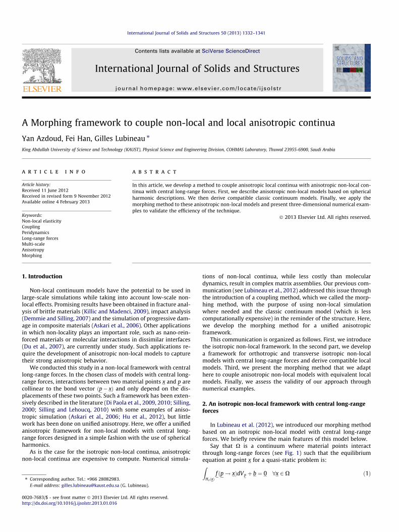
International Journal of Solids and Structures 50 (2013) 1332–1341

Contents lists available at SciVerse ScienceDirect

International Journal of Solids and Structures

journal homepage: www.elsevier .com/locate / i jsolst r

A Morphing framework to couple non-local and local anisotropic continua

Yan Azdoud, Fei Han, Gilles Lubineau ⇑King Abdullah University of Science and Technology (KAUST), Physical Science and Engineering Division, COHMAS Laboratory, Thuwal 23955-6900, Saudi Arabia

a r t i c l e i n f o

Article history:Received 11 June 2012Received in revised form 9 November 2012Available online 4 February 2013

Keywords:Non-local elasticityCouplingPeridynamicsLong-range forcesMulti-scaleAnisotropyMorphing

0020-7683/$ - see front matter � 2013 Elsevier Ltd. Ahttp://dx.doi.org/10.1016/j.ijsolstr.2013.01.016

⇑ Corresponding author. Tel.: +966 28082983.E-mail address: [email protected] (G. Lu

a b s t r a c t

In this article, we develop a method to couple anisotropic local continua with anisotropic non-local con-tinua with central long-range forces. First, we describe anisotropic non-local models based on sphericalharmonic descriptions. We then derive compatible classic continuum models. Finally, we apply themorphing method to these anisotropic non-local models and present three-dimensional numerical exam-ples to validate the efficiency of the technique.

� 2013 Elsevier Ltd. All rights reserved.

1. Introduction tions of non-local continua, while less costly than molecular

Non-local continuum models have the potential to be used inlarge-scale simulations while taking into account low-scale non-local effects. Promising results have been obtained in fracture anal-ysis of brittle materials (Killic and Madenci, 2009), impact analysis(Demmie and Silling, 2007) and the simulation of progressive dam-age in composite materials (Askari et al., 2006). Other applicationsin which non-locality plays an important role, such as nano-rein-forced materials or molecular interactions in dissimilar interfaces(Du et al., 2007), are currently under study. Such applications re-quire the development of anisotropic non-local models to capturetheir strong anisotropic behavior.

We conducted this study in a non-local framework with centrallong-range forces. In the chosen class of models with central long-range forces, interactions between two material points x and p arecollinear to the bond vector ðp� xÞ and only depend on the dis-placements of these two points. Such a framework has been exten-sively described in the literature (Di Paola et al., 2009, 2010; Silling,2000; Silling and Lehoucq, 2010) with some examples of aniso-tropic simulation (Askari et al., 2006; Hu et al., 2012), but littlework has been done on unified anisotropy. Here, we offer a unifiedanisotropic framework for non-local models with central long-range forces designed in a simple fashion with the use of sphericalharmonics.

As is the case for the isotropic non-local continua, anisotropicnon-local continua are expensive to compute. Numerical simula-

ll rights reserved.

bineau).

dynamics, result in complex matrix assemblies. Our previous com-munication (see Lubineau et al., 2012) addressed this issue throughthe introduction of a coupling method, which we called the morp-hing method, with the purpose of using non-local simulationwhere needed and the classic continuum model (which is lesscomputationally expensive) in the reminder of the structure. Here,we develop the morphing method for a unified anisotropicframework.

This communication is organized as follows. First, we introducethe isotropic non-local framework. In the second part, we developa framework for orthotropic and transverse isotropic non-localmodels with central long-range forces and derive compatible localmodels. Third, we present the morphing method that we adapthere to couple anisotropic non-local models with equivalent localmodels. Finally, we assess the validity of our approach throughnumerical examples.

2. An isotropic non-local framework with central long-rangeforces

In Lubineau et al. (2012), we introduced our morphing methodbased on an isotropic non-local model with central long-rangeforces. We briefly review the main features of this model below.

Say that X is a continuum where material points interactthrough long-range forces (see Fig. 1) such that the equilibriumequation at point x for a quasi-static problem is:Z

HdðxÞf ðp! xÞdVp þ b ¼ 0 8x 2 X ð1Þ

http://dx.doi.org/10.1016/j.ijsolstr.2013.01.016

mailto:[email protected]

http://dx.doi.org/10.1016/j.ijsolstr.2013.01.016

http://www.sciencedirect.com/science/journal/00207683

http://www.elsevier.com/locate/ijsolstr

Fig. 1. The non-local continuum X : HdðxÞ is the horizon of x depending on thecharacteristic range of long-range forces.

Y. Azdoud et al. / International Journal of Solids and Structures 50 (2013) 1332–1341 1333

where f ðp! xÞ is the action of point p over point x. d is the cut-offradius, which limits the long-range interaction of x with the mate-rial points in its neighborhood, HdðxÞ (Fig. 1). b are the prescribedexternal body forces.

To ensure the balance of the linear momentum, an antisymmet-ric form (with respect to x and p) of the interactions is prescribed(see Silling et al., 2007; Warren et al., 2009). The choice is:

f ðp! xÞ ¼ f̂ ½x�hp� xi � f̂ ½p�hx� pi ð2Þ

where f̂ ½x�hp� xi (respectively f̂ ½p�hx� pi) is the partial interactiondue to the action of point p over point x (respectively of point x overpoint p). We introduce the bond vector n ¼ p� x.

If infinitesimal displacements and linear elasticity are assumed,a possible constitutive model is (Silling, 2010; Silling and Lehoucq,2010):

f̂ ½x�hp� xi ¼ c½x�2

unðpÞ � unðxÞn o

en ð3Þ

where en ¼ n=knk and unðpÞ is the projection of the displacement atpoint p over the bond (i.e. unðpÞ ¼ uðpÞ � en). In this approach, thepartial bond behaves as a spring with elementary stiffness, c½x� (aso-called micromodulus in peridynamics). This leads to the set ofequations that describes this model over the continuum X:

� Kinematic admissibility and compatibility

gnðp� xÞ ¼ unðpÞ � unðxÞ 8ðx;pÞ 2 X ð4Þ

� Static admissibility
ZHdðxÞ
f ðp! xÞdVp þ b ¼ 0 8x 2 X ð5Þ

� Constitutive equation

f ðp! xÞ

¼c½x�ðknkÞ þ c½p�ðknkÞ

2unðpÞ � unðxÞn o

en 8x;p 2 X ð6Þ

Let us introduce the gradient of the transformation, F, defined asF ¼ @x

@X, where X is a vector in the reference configuration and xits image in the deformed configuration. In case F is locally uni-form, i.e.:

Fig. 2. The bond’s spherical coordinates.

Fðx0Þ � FðxÞ ¼ �F 8x0 2 HdðxÞ ð7Þ

It has been shown (see Lubineau et al., 2012) that a local model canbe defined that is equivalent to a non-local model in an energeticsense. The key-idea is to define the stiffness operator of the local

model in such a way that the local and non-local models bear thesame strain energy density for any locally uniform strain.

Provided that we consider only small displacements and anhomogeneous material (c½x�ðknkÞ ¼ cðknkÞ), this equivalent localmodel is defined by a 4th-order stiffness operator C such that:

C ¼Z

HdðxÞcoðknkÞ

n� n� n� n

2knk2 dVp ð8Þ

From Eq. (8), it is clear that the assumption of central forces resultsin an additional symmetry of the stiffness tensor, C (on top of theclassical major and minor symmetries):

Cijkl ¼ Cilkj ð9Þ

This symmetry implies that some stiffness coefficients areequal. A classic result is that a three-dimensional isotropic contin-uum can have only one material parameter (the Young’s modulus,E), whereas the Poisson’s ratio is fixed to m ¼ 1

4. This is also a classicresult in atomistic modeling, in which a material represented by asingle pair interaction cannot be fully general (Anderson and Dem-arest, 1971).

Multiple techniques have been developed to tackle this issueand develop totally generic anisotropic models (Gerstle et al.,2007; Silling, 2010; Zhang and Ge, 2005). An overview of thosemethods is given in Appendix A. Considering that our couplingframework applies to central forces, we develop anisotropic mod-els based only on central forces. In the next section, we present themost general anisotropic description that can be obtained assum-ing that long-range interactions are central, i.e. parallel to thebond.

3. An anisotropic non-local framework with central long-rangeforces

3.1. Anisotropy of the micromodulus: notation

In this section, we build an anisotropic model with the restric-tion of central long-range forces. We start from the isotropicframework presented in Eqs. (1)–(6).

In the isotropic form of Eq. (3), c½x� is a local material parameterat point x that does not depend on the bond orientation. In order todescribe anisotropic behaviors, one possible choice is to expressc½x� as explicitly depending on the bond’s spherical coordinates(h;/; knk, see Fig. 2) such that:

c½x� ¼ c½x�ðh;/; knkÞ ð10Þ

1334 Y. Azdoud et al. / International Journal of Solids and Structures 50 (2013) 1332–1341

Rewriting Eq. (6) leads to:

f ðp! xÞ ¼c½x�ðh;/; knkÞ þ c½p�ðp� h;pþ /; knkÞ

2unðpÞ � unðxÞn o

en

ð11Þ

In the case of an homogeneous material (i.e.c½x�ðh;/; knkÞ ¼ c½p�ðh;/; knkÞ ¼ cðh;/; knkÞ), we introduce a bond-wise micromodulus �c, so that:

f ðp! xÞ ¼ �cðh;/; knkÞgnðp� xÞ ð12Þ

with

�cðh;/; knkÞ ¼cðh;/; knkÞ þ cðp� h;pþ /; knkÞ

2ð13Þ

Provided that f ðp! xÞ derives from a potential xðgnðp� xÞ; nÞ suchthat:

f ðp! xÞ ¼@xðgnðp� xÞ; nÞ@gnðp� xÞ ð14Þ

the strain energy density of the non-local model at a point x can bewritten:

WnlðxÞ ¼ 12

ZHdðxÞ

xðgnðp� xÞ; nÞdVp ð15Þ

WnlðxÞ ¼ 14

ZHdðxÞ

�cðh;/; knkÞ unðpÞ � unðxÞn o2

dVp ð16Þ

where the factor 1=2 in Eq. (16) relates the bond energy partitionbetween x and p.

We emphasize that �c has to be centrosymmetric to ensure theconservation of the linear momentum, a property that is met forany choice of c (see the proof in Appendix B). For simplicity andwithout losing generality, we choose c to be centrosymmetric:

cðh;/; knkÞ ¼ cðp� h;pþ /; knkÞ ð17Þ

This naturally leads to �c ¼ c. We then drop the bar for convenience.

3.2. Using spherical harmonics to describe the anisotropy

Under the assumption of uniform or smooth strain fields (seeEq. (7)), we can show that an equivalent local model can be derivedfrom the non-local model presented here. Such a model wouldhave a stiffness tensor,C, defined as follows:

C ¼Z

HdðxÞcðh;/; knkÞ

n� n� n� n

2knk2 dVp ð18Þ

We propose to define c in order to have the most general level ofanisotropy under the restriction of central forces. Without any lossof generality we use a real spherical harmonic expansion to de-scribe it:

cðh;/;knkÞ¼ cnðknkÞ a00þXþ1k¼1

Xk

m¼0

Pmk ðcosðhÞÞðakmcosðm/Þþbkmsinðm/ÞÞ

" #" #

ð19Þ

where a00; akm and bkm are real parameters, Pmk are the associated

Legendre functions and cn is a weight function that depends onlyon knk. This technique is a powerful way to represent generalthree-dimensional (3D) surfaces (see Thiagarajan et al. (2004) fora description of its application to anisotropy in a virtual bondframework, or Morris et al. (2005) for an application to 3D surfacemodeling in bioengineering).

3.3. Application to orthotropy and transverse isotropy

3.3.1. An orthotropic modelIn the case of an orthotropic material, the model should exhibit

three planes of symmetry. Let ðe1; e2; e3Þ be our reference basis. Ifðe1; e2; e3Þ is also orthotropic, then c has to satisfy the followingrelations:

cðh;/; knkÞ ¼ cðp� h;/; knkÞ ¼ cðh;p� /; knkÞ¼ cðh;/þ p; knkÞ ð20Þ

These symmetries lead to the following properties for theequivalent orthotropic stiffness matrix:

Cijkl¼Cijlk¼Cjikl¼Cklijclassical minor and major symmetries ð21ÞCijkl¼Cilkjcentral symmetry ð22Þ

CPðijklÞ ¼0 if i – ðj;k; lÞby antisymmetry of the integrand in Eq:ð18Þ ð23Þ

where Pð�Þ is the permutation operator. A proof of Eq. (23) is givenin Appendix C. This leads to the following shape for the stiffnessoperator using Voigt’s notation in the basis ðe1; e2; e3Þ:

ð24Þ

As a result, only six independent coefficients are available in anorthotropic model based on central long-range forces, whereas aclassical orthotropic material would have nine independent coeffi-cients. We run the model up to the 4th order for Eq. (19) to findthose coefficients:

cðh;/;knkÞ¼ cnðknkÞ a00þX4

k¼1

Xk

m¼0

Pmk ðcosðhÞÞðakmcosðm/Þþbkmsinðm/ÞÞ

" #" #

ð25Þ

Due to the symmetry conditions (Eqs. (17) and (20)) and to thesymmetry properties of the associated Legendre functions, it isstraightforward to demonstrate that all the coefficients, akm andbkm, vanish, except for six of them that do not affect the symmetryproperties:

a00; a20; a22; a40; a42; a44½ � – 0 ð26Þ

Thus, a 4th-order development of the micromodulus surface pro-vides exactly six material parameters to represent the most generalorthotropic materials possible in the framework of central long-range forces. Higher orders of development would not add moregenerality. The micromodulus surface can be written:

cðh;/; knkÞ ¼ cnðknkÞ½a00 þ a20P02ðcosðhÞÞ

þ a22cosð2/ÞP22ðcosðhÞÞ þ a40P0

4ðcosðhÞÞ

þ a42cosð2/ÞP24ðcosðhÞÞ þ a44cosð4/ÞP4

4ðcosðhÞÞ� ð27Þ

for which the associated Legendre functions are described inAppendix D. Introducing (27) into (18) and performing the neces-sary integrations provide the relations between the six componentsof the stiffness tensor and the six parameters of the micromodulussurface:


a00¼5ðC1111þ2C1122þ2C1133þC2222þ2C2233þC3333Þ

2d5pð28Þ

a20¼�25ðC1111þ2C1122�C1133þC2222�C2233�2C3333Þ

4d5pð29Þ

a22¼25ðC1111þC1133�C2222�C2233Þ

8d5pð30Þ

a40¼45ð3C1111þ6C1122�24C1133þ3C2222�24C2233þ8C3333Þ

16d5pð31Þ

a42¼�15ðC1111�6C1133�C2222þ6C2233Þ

16d5pð32Þ

a44¼15ðC1111�6C1122þC2222Þ

128d5pð33Þ

Eqs. (28)–(33) define the mapping between the local stiffnessparameters and the spherical harmonic coefficients for an ortho-tropic model. Note that those results are valid for cnðknkÞ ¼ 1 ifknk < d, and cnðknkÞ ¼ 0 otherwise.

3.3.2. A transverse isotropic modelA classical transverse isotropic model would have five indepen-

dent coefficients. Due to centrosymmetry, our non-local transverseisotropic model has only three coefficients.

Transverse isotropy can be defined by an axisymmetry around thereference direction of the material (here selected as e3), which corre-sponds to the constraints on the micromodulus given in Eq. (34):

cðh;/; knkÞ ¼ cðh; knkÞ; cðh; knkÞ ¼ cðp� h; knkÞ ð34Þ

Note that the resulting micromodulus is independent of the an-gle /. We can then, preserving generality, represent the micromod-ulus as a development on circular harmonics:

cðh; knkÞ ¼ cnðknkÞX1i¼0

aiP0i ðcos hÞ ð35Þ

At maximum, a central transverse isotropic model leads to threeindependent coefficients (Eq. (37)). We limit the circular harmon-ics development to the minimal expression with three indepen-dent coefficients, which is obtained at the 4th order:

cðh; knkÞ ¼ cnðknkÞ a0 þ a2P02ðcos hÞ þ a4P0

4ðcos hÞh i

ð36Þ

ð37Þ

Note that there are four symbols in this matrix: C1122 as repre-sented by actually depends on the other coefficients.

Using Eq. (36), it leads to

a0 ¼5ð8C1111 þ 12C1133 þ 3C3333Þ

6d5pð38Þ

a2 ¼ �25ð4C1111 � 3C1133 � 3C3333Þ

6d5pð39Þ

a4 ¼45ðC1111 � 6C1133 þ C3333Þ

2d5pð40Þ

The coefficient C1122 is defined as:

C1122 ¼13

C1111 ð41Þ

Note that these results are valid for cnðknkÞ ¼ 1 if knk < d andcnðknkÞ ¼ 0 otherwise.

We have thereby completely defined anisotropic non-localmodels and their equivalent local models under the assumptionof homogeneous transformation. The next step, presented in Sec-tion 4, is to generalize the morphing method developed in Lubi-neau et al. (2012) to perform a natural coupling between thenon-local and local models.

4. The morphing technique for anisotropic non-local to localcoupling

4.1. The morphing framework

We extend the technique proposed by Lubineau et al. (2012).Specifically, we seek to model a continuum, X, where, because ofmodeling considerations, central long-range forces are required.We use the non-local model only in a sub-domain, X2, which re-quires a refined description where non-local effects are predomi-nant while, for the remainder of the structure (sub-domain X1),the equivalent local model can be employed. The coupling methodis employed in the bridging domain, Xm (Fig. 3). The non-localmodel is defined by the micromodulus coðh;/; knkÞ and its equiva-lent local model by Co½x�.

We assume that @X � @X1. The non-local sub-domain, X2, isconsequently totally embedded within the local one. Xm meetsthe following requirements:

X ¼ X1 [Xm [X2; X1 \Xm ¼ ;; X2 \Xm ¼ ; ð42Þ

The coupling is then defined as a simple evolution of the mate-rial properties characterizing each model, which leads to the fol-lowing system of equations:


eðxÞ ¼ 12r � uðxÞþtr � uðxÞ� �

8x 2 X ð43Þ

gnðp� xÞ ¼ unðpÞ � unðxÞ 8ðx;pÞ 2 X ð44Þ

u ¼ �u 8x 2 S�u ð45Þ


divrþZ

HdðxÞf̂ ½x�hp�xi� f̂ ½p�hx�pin o

dVpþb¼0 8x2X ð46Þ

r �n¼ �T 8x2 S�T ð47Þ

� Constitutive equations

r ¼ C½x� : e 8x 2 X ð48Þ

f̂ ½x�hp� xi ¼cðh;/; knkÞ

2gnðp� xÞen 8x 2 X ð49Þ

Fig. 3. The domain X ¼ X1 [Xm [X2.


C½x� characterizes the stiffness of the local continuum at any

point x. cðh;/; knkÞ is the non-local constitutive parameter at pointx. Using coðh;/; knkÞ as references, we define cðh;/; knkÞ by intro-ducing a weighting scalar function, a, such that:

c½x�ðh;/; knkÞ ¼ aðxÞcoðh;/; knkÞ ð50Þ

We note that, based on Eq. (46), (Fig. 4):

� a point x strictly belongs to the local model (i.e. x 2 X1) if andonly if:

Fig. 4.needs t

C½x� ¼ Co and aðpÞ ¼ 0 8p 2 HdðxÞ ð51Þ

� a point x strictly belongs to the non-local model (i.e. x 2 X2) ifand only if:

C½x� ¼ 0 and aðpÞ ¼ 1 8p 2 HdðxÞ ð52Þ

4.2. Defining the morphing: a and C

The function a is set to define the interface of the sub-domainX2 as a user parameter. We apply an energy density constraint todefine the stiffness tensor C. At any point x 2 Xm, the strain energydensity can be written as:

WðxÞ ¼ 12eðxÞ : CðxÞ : eðxÞ

þZ

HdðxÞcoðh;/; knkÞ

aðxÞ þ aðpÞ2

unðpÞ � unðxÞn o2

4dVp ð53Þ

Under a quasi-uniform strain field (Eq. (55)), we can assumethat the energy density of the coupling zone is equivalent to theenergy density of a fully local model. This is written as:

WðxÞ ¼ 12eðxÞ : CoðxÞ : eðxÞ ð54Þ

FðpÞ � FðxÞ ¼ �F 8p 2 HdðxÞ ð55Þ

This naturally leads to a general relation between the stiffnessoperators:

C½x� ¼ ð1� a½x�ÞCo þZ

HdðxÞcoðh;/; knkÞ

ða½x� � a½p�Þ2

n� n� n� n

2knk2 dVp ð56Þ

The general shape of the morphing function a. The solid lines are the initial requiro be defined. Xs is a frontier of Xm over which a has to be prescribed as either 0

Then, provided that the non-local region is fully located by thechoice of the morphing function a, the local material parameter C

can be estimated at every point using Eq. (56). This makes the ap-proach very easy to use as it relies only on the definitions of thechanging material parameters across space.

5. Numerical benchmarks and examples

The purpose of this section is to illustrate the accuracy of thecoupling method for anisotropic models with three dimensions.We consider two cases. First, we apply the morphing method toan homogeneous orthotropic block under boundary conditionsthat guarantee uniform strain to evaluate the strain error of themethod. As a reference, the same problem is treated as an isotropicmodel. Second, we study the case of a cracked bulk material undertraction and shear using a transverse isotropic model.

In our calculations, we assume the micromodulus cðh;/; knkÞ ¼

cnðknkÞch;/ðh;/Þ to be chosen such that cnðknkÞ ¼ n2e�knk

l , where l isan intrinsic length. cn is chosen in such a way as to avoid disconti-nuities of the bond force (Eq. (46)) at n ¼ 0 (with the term n2) andto be small when knk ¼ d (with the exponential term). Numericalimplementation of the method is conducted using the FiniteElement framework. All elements are eight-node hexahedral ele-ments arranged in a regular grid. The grid size is chosen as0:02 lm, the intrinsic length is l ¼ 0:0024 lm and the horizon dis 0:06 lm. l can be seen either as a material or phenomenologicalparameter. Then d is chosen such that cnðknkP dÞ ’ 0 and the ratioof 3 elements per radius d has been chosen as a compromisebetween good convergence and calculation time.

Note that the choice of the characteristic length l will not influ-ence elastic characteristics in case of low strain gradients, butrather can be seen as a relevant parameter for other physical ef-fects: at nano-scale, it can approximate Van der Waals forces; infracture mechanics, it will influence the localization of cracks.

5.1. Example 1: uniform strain of a block

This example aims at presenting an accurate depiction of thecoupling effects of an anisotropic non-local bulk in three dimen-sions. We consider an homogeneous cube subjected to tractionand shear conditions. Fig. 5(a) shows the dimensions of this cube.The non-local model is found in the spherical zone X2 colored darkgray in the center of the bulk. The light-gray spherical zone Xm is themorphing domain over which the weighting function a varies. Therest of this structure is defined with the local continuum model.

ements in X1 and X2 (Eqs. (51) and (52)). The dashed line is a free evolution of a thator 1 (see Eqs. (51) and (52)).

(a) (b) (c)

Fig. 5. Dimensions and boundary conditions of a cube (unit of length: lm).


We show the kinematic boundary conditions for the tractioncase in Fig. 5(b). uz ¼ 0:5 lm is the imposed displacement on thetop surface of the cube. The displacement is fully prescribed to zeroat the origin o (bottom left corner), and the z-component of the dis-placement is prescribed to zero for all the points over the bottomsurface. In a classical local continuum, this would lead to an homo-geneous tensile strain field. In Fig. 5(c), the bulk is under pure sheardeformation and the kinematic boundary conditions are set by Eq.(57) on all surfaces of the cube:

ux ¼ 0:25yþ 0:25z

uy ¼ 0:25xþ 0:25z

uz ¼ 0:25xþ 0:25y

8><>: ð57Þ

The equivalent local orthotropic stiffness coefficients for thisexample are estimated by Eq. (18), and set to Ex ¼ 60 GPa;Ey ¼ 90 GPa; Ez ¼ 150 GPa and mxy ¼ 0:3; myz ¼ 0:2; mxz ¼ 0:1. Thereference isotropic stiffness coefficients are E ¼ 90 GPa andm ¼ 0:25.

Fig. 6 shows the relative error of the strain components, ezz, ob-

tained for the traction test. The relative error is defined by ezz�eAzz

eAzz

,

where eAzz is the average value of strain components ezz. Fig. 6(a)

and (c) display the isosurfaces of the relative error in the strainat þ0:05% and �0:05% in a three-dimensional deformed bulk.These isosurfaces limit the regions in which the relative errors inthe strain are larger than 0:05%. This reveals that the strain fieldis quasi-uniform in most of the deformed bulk. We extracted slicesperpendicular to the y-axis in which the maximal error is reached(y ¼ 0:5lm), as shown in Fig. 6(b) and (d). Thus, we can clearly seethat the spurious effects occur near the upper and lower bound-aries of the morphing domain, but, overall, the error in the strain

Fig. 6. Isosurfaces (a), (c) and contour slices (b), (d) of the relative error of the strain comand with the orthotropic stiffness models (c), (d).

remains at values under 0:3%. In Fig. 6, we compare the result ob-tained with an isotropic model (a) and (b) with the result obtainedwith an orthotropic model (c) and (d). The error map is qualita-tively the same for both models, demonstrating that the accuracyof the morphing method does not depend of the anisotropic propri-ety of the model in the case of traction.

The results for the pure shear boundary conditions are shown inFig. 7. The relative error in eyz shares similar characteristics withthe relative error shown in the traction examples in Fig. 6.Fig. 7(a) and (c) display the isosurfaces set at relative errors of0:02% and �0:06%, respectively. We show slices on a plane definedby the z-axis and the line x ¼ y on the deformed bulk. This planehas been chosen as it displays the maximal range of the relative er-ror on eyz. The error range is smaller than in the traction examplesin Fig. 6. Again, the anisotropy does not seem to influence the errorin the strain induced by the coupling method.

Overall, these two benchmarks demonstrate that the error re-mains localized to the coupling zone, that the range of error re-mains small for practical choices of the coupling zone and thecoupling function a, and that anisotropy does not qualitativelyinfluence the accuracy of the morphing method.

5.2. Example 2: a cracked block

The benchmark results from previous examples illustrate thequality of the coupling technique. Let us now consider an applica-tion. This example is designed to show the performance of themorphing-based coupling technique for representing local phe-nomena such as those induced by a crack. A cracked bulk is repre-sented in Fig. 8. It is subjected to both traction and shear boundaryconditions. The bottom surface of this bulk is completely fixed and

ponents ezz for a 3D bulk under traction with the isotropic stiffness models (a), (b)

Fig. 7. Isosurfaces (a), (c) and contour slices (b), (d) of the relative error of the strain components eyz for a 3D bulk under shear with the isotropic stiffness models (a), (b) andwith the orthotropic stiffness model (c), (d).

Fig. 8. Dimensions and boundary conditions of a cracked bulk (unit of length: lm).

Fig. 9. The strain components exx calculated by (a) the classical continuum mo

Fig. 10. The contour slices of strain components exx calculated by (a) the classical contin


the values of the boundary displacements on the top surface are gi-ven by:

ux ¼ 0lm

uy ¼ 0:5lm

uz ¼ 0:5lm

8><>: ð58Þ

The non-local continuum model is used in the vicinity of the crackin X2, while classical continuum mechanics is employed in X1. Xm,displayed in light gray (Fig. 8), is the domain where the weightingfunction a varies. The bulk is modeled as a transverse isotropicmaterial. The stiffness coefficients for the local continuum modelare Ex ¼ Ey ¼ 60 GPa; Ez ¼ 150 GPa and mxy ¼ 0:3; mxz ¼ myz ¼ 0:1.

For comparison purposes, the static simulation is run three times,with the classical continuum model, the morphing-based couplingmodel and the non-local continuum model, respectively. Thecontour plots of the strain component exx are displayed in Fig. 9.

del, (b) the morphing-based coupling model, and (c) the non-local model.

uum model, (b) the morphing-based coupling model, and (c) the non-local model.


The strain resulting in Fig. 9(a) is obtained by the local contin-uum model. Its crack shape is different from the others as there isno non-local interaction. Fig. 9(b) shows the solution of the morp-hing-based coupling model. It has to be compared with results inFig. 9(c) from the non-local continuum solution.

We plot the slices of the strain component exx perpendicular tothe y-axis at y ¼ 0:75lm in Fig. 10 to compare the three models.The results in Fig. 10(b) and (c) indicate similarity, and they differfrom the result obtained by the classical continuum model shownin Fig. 10(a). The solutions in Fig. 10(b) and (c) agree, except closeto the boundary. This is due to the fact that points near of the sur-face do not have a complete neighborhood, HdðxÞ. This mismatch isthus inherent to the differences between local and non-localboundary conditions and is not related to the coupling technique.

This application example shows the adaptability of the morp-hing method to practical cases, effectively reducing the calculationcost of a non-local simulation while preserving non-locality whereit is needed.

6. Conclusion

In this paper, we extended the application field of the morphingmethod to anisotropic models. The morphing method is a simple androbust method to couple a continuous non-local model with anequivalent local model through a single uniform model defined overthe whole structure. We developed the anisotropic model and de-rived compatible local models in a non-local framework with centrallong-range forces. A key point of this development is the usage ofspherical harmonics to describe the non-local micromoduli. Numer-ical examples have been provided to demonstrate the efficiency ofthe method in three dimensions. The morphing method has beenshown to be as accurate under anisotropy as under isotropy.

Two main directions are clear for future research. The first is todevelop the morphing method for fully generalized anisotropyusing considerations presented in Appendix A. The second is to ex-tend the scope of this technique by solving practical mechanicalproblems using the morphing method.

Fig. 11. The point q interacts indirectly with x because p is in the horizon of both xand q.

Appendix A. An overview of anisotropy for long-range-forcenon-local models

Several methods have emerged to tackle the issue of the centralsymmetry in large-range interactions based non-local models. Itappears that a simple bond consisting of a pair of potentials thatdepend only on the length of the bond would not be enough to takeinto account the shear effects. An initial way to circumvent this is-sue is to take into account multibody interactions: potentials thatdepend on at least two bonds can introduce a relative rotation. Thissolution has been chosen, for instance, in the state-based theory(see Silling, 2010). Another way is to further develop the bond-based representation of forces by adding an extra rotational degreeof freedom to the material point. This solution is applied in someform to the virtual internal bond method (VIB) (see Zhang andGe, 2005) and in the work of Gerstle et al. (2007) who uses a Coss-erat micro-moduli representation. We describe these methods andevaluate their benefits.

A.1. Multibody interactions

Using multibody interactions to eliminate this symmetry has al-ready been applied in atomistics. Generally, in atomistics, theinteraction between particles derives from a potential energy U de-fined as a function of the position of the particles xi : Uðx1; . . . ; xnÞ.For instance, a potential energy that depends on the length of pair-wise bonds can be written:

U ¼ 12

Xi;j

Uðkxi � xjkÞ ðA:1Þ

where U is the potential of the bond ði; jÞ. It is clear that Eq. (A.1) re-fers to the stretching energy of the bonds and does not allocate anyenergy to their relative angular motion. However, if we introducethree-body term potentials, such as the Stillinger–Weber potentials(Stillinger and Weber, 1985), we introduce a relative rotation:

U ¼ 12

Xi;j

Uðkxi � xjkÞ þ13!

Xi;j;k

Vðkxi � xjk; kxj � xkk; hijkÞ ðA:2Þ

where hijk is the angle between the bond ði; jÞ and the bond ðj; kÞ.This process can be extended to more than three particles, but it re-mains unclear where to truncate the multibody interaction (Volokhand Gao, 2005). A similar point of view is taken for continuum non-local models in the state-based theory by Silling (2010). The modelpresented by Silling respects the following equations:


gðx; pÞ ¼ uðpÞ � uðxÞ 8x;p 2 X ðA:3Þ

ZX
T½x�hp� xi � T½p�hx� pidVp þ b ¼ 0 8x 2 X ðA:4Þ

T½x�hni ¼ 0 if knkP d 8x 2 X ðA:5Þ

� Constitutive equation

T½x�hp� xi ¼Z

XK½x�hp� x; q� xigðx; qÞdVq 8x; p

2 X ðA:6Þ

K½x�hn; fi ¼ 0 if knk; kfkP d 8x 2 X ðA:7Þ

where T½x�hp� xi is the force state applied at point x relative to thebond p� x and K½x�hp� x; q� xi is the modulus state that holds thestiffness parameters at point x relative to the bonds p� x and q� x.This system of equations defines the force state T½x�hp� xi as theassociation of the direct effects of points x and p and the indirecteffect of their neighborhoods on the bond p� x (see Fig. 11). Inthe case of an homogeneous material and under homogeneousdeformation, the author gives an equivalent local model in a cho-sen basis of reference:

Cijkl ¼Z

Hd

ZHd

Kikhn; finjfldV fdVn ðA:8Þ

where Cijkl are the equivalent stiffness coefficients and Hd is a sphereof radius d in the body X. The modulus state K is a symmetric tensor.


The symmetries of the stiffness tensor C are then the major and

minor symmetries. Any classical anisotropy can be reproduced inthe non-local framework of the state-based theory.

The evident downside of this method is the high calculationcost that comes from an additional level of integration.

A.2. The Cosserat model

Using an additional set of equations to evaluate the angularbehavior of the bond has been applied in the modified virtual inter-nal bond method (Zhang and Ge, 2005), where an additional R-bond is introduced. This bond depends on the rotation of a pairwisebond. Another method is introduced in the micropolar peridynam-ic model presented by Gerstle et al. (2007), based on a Cosseratmodel. Here, we present the micropolar peridynamic model.

The micropolar peridynamic model relies on a Cosserat contin-uum extrapolated to a non-local model. The Cosserat model is acontact force model built around the introduction of couples andangles as additional static and, respectively, kinematic variables.Static equilibrium is given by:

rji;j þ bi ¼ 0 ðA:9Þmji;j þ �ijkrjk þ ci ¼ 0 ðA:10Þ

where r is the Cosserat stress tensor, m is the Cosserat couple, �ijk isthe permutation tensor, bi is the body force and ci is the body coupleforce. Cosserat constitutive relations are given by:

rij ¼ Dijklekl ðA:11Þmij ¼ Mijkljkl ðA:12Þ

where D and M are 4th-order stiffness tensors, e is the strain oper-

ator and j is the curvature operator. e and j are coupled, linkedthrough the relation:

jij ¼ ��ijkelj;k ðA:13Þ

The author took advantage of this model to create a Cosserat-like peridynamics approach. It increases the size of the system byadding equations on moments in the equilibrium:Z

HdðxÞf ðp! xÞdVp þ b ¼ 0 8x 2 X ðA:14ÞZ

HdðxÞmðp! xÞdVp þ c ¼ 0 8x 2 X ðA:15Þ

where f ðp! xÞ (respectively mðp! xÞ) is the force (respectively thecouple) of p over x.

In three dimensions, a force vector, Fx;p ¼ ½f x;mx; f p;mp�, and akinematic vector, Ux;p ¼ ½ux; hx; up; hp�, are associated with eachbond, ðx; pÞ, where ux and hx are the displacement and rotation ofnode x, respectively. The constitutive equation is then given by:

Fx;p ¼ Kx;pUx;p ðA:16Þ

The stiffness tensor Kx;p is symmetric and depends on parameters ofthe bond such as its direction, length, effective section and qua-dratic moment of inertia. Despite the difficulty in associating aphysical meaning while choosing these parameters, this modelhas enough independent variables to completely represent anisot-ropy in an equivalent Cosserat continuum.

Appendix B. Centrosymmetry of the micromodulus

This section proves that any choice of c leads to a centrosym-metric �c. To satisfy the conservation of linear momentum and un-der the choice of a centered force, �c has to be centrosymmetric.

Indeed, in a central force representation, the conservation of linearmomentum is obtained when:

f ðp! xÞ ¼ �f ðx! pÞ ðB:1Þ

Using Eqs. (11) and (13), it leads to:

�cðh;/; knkÞ ¼ �cðp� h;pþ /; knkÞ ðB:2Þ

Eq. (B.2) being the definition of the centrosymmetry of �c.By construction, �c defined as:

�cðh;/; knkÞ ¼cðh;/; knkÞ þ cðp� h;pþ /; knkÞ

2ðB:3Þ

is centrosymmetric.

Proof. Let cðh;/; knkÞ be an arbitrary periodical C1 function.cðh;/; knkÞ can be written as the sum of a centrosymmetricfunction and a centroantisymmetric function:

cðh;/; knkÞ ¼ csðh;/; knkÞ þ caðh;/; knkÞ ðB:4Þ

where

csðh;/; knkÞ ¼ csðp� h;pþ /; knkÞ ðB:5Þ

and

caðh;/; knkÞ ¼ �caðp� h;pþ /; knkÞ ðB:6Þ

Using Eqs. (B.3) and (B.4) yields:

�cðh;/; knkÞ ¼ csðh;/; knkÞ ðB:7Þ

�cðh;/; knkÞ is then always centrosymmetric for any choice ofcðh;/; knkÞ.

As a result, if we choose a centrosymmetric cðh;/; knkÞ, we endup with �cðh;/; knkÞ ¼ cðh;/; knkÞ, the choice that we assume forsimplification throughout this paper.

Appendix C. Null coefficients in C

The symmetry property of the integrand of Eq. (18) leads to thenull coefficient in the stiffness tensor C. If we work in a specific ba-

sis ð1;2;3Þ, Eq. (18) can then be written as:

Cijkl ¼Z

HdðxÞcðh;/; knkÞ ninjnknl

2knk2 dVp 8i; j; k; l 2 ð1;2;3Þ ðC:1Þ

It appears that any permutation of a specific choice of ði; j; k; lÞ doesnot change the result of the integrand. Given that there are onlythree orthogonal directions (namely ð1;2;3Þ), we can distinguishthree major cases that are not affected by these permutations.

i ¼ j ¼ k ¼ l; i ¼ j – k ¼ l; i – ðj; k; lÞ ðC:2Þ

In the third case (i – ðj; k; lÞ), it is possible to identify that thesymmetry property of the integrand will lead to null coefficientsof C. Indeed, the function cðh;/; knkÞ is centrosymmetric and the

domain of integration is spherical, centered on x, which leads to:

– If j – k ¼ l, nknl is a centrosymmetric term, nj and ni are anti-symmetric and orthogonal, the integrand is antisymmetric:the resulting integral is null.– If j ¼ k ¼ l, nknlnj and ni are antisymmetric and orthogonal, theintegrand is antisymmetric: the resulting integral is also null.

As a result, we obtain Eq. (23):

CPðijklÞ ¼ 0 if i – ðj; k; lÞ 8 Pði; j; k; lÞ permutations of ði; j; k; lÞðC:3Þ

Fig. 12. Spherical harmonics used for the generation of non-local anisotropic models. (a) S22 with a22 ¼ 1 and b22 ¼ 0, (b) S42 with a42 ¼ 1 and b42 ¼ 0, (c) S44 with a44 ¼ 1 andb44 ¼ 0, (d) S20 with a20 ¼ 1, (e) S40 with a40 ¼ 1, (f) S00 with a00 ¼ 1.


Appendix D. Spherical harmonics

Spherical harmonics are built using generalized Legendre poly-nomials (see Eqs. (D.2)–(D.6)) to create an orthogonal base of func-tion. The base of spherical harmonics Sij (see Fig. 12) is constructedas follows:

Sij ¼ PjiðcosðhÞÞðaijcosðj/Þ þ bijsinðj/ÞÞ i; j 2 N ðD:1Þ

P02ðcosðhÞÞ ¼ 1

41þ 3cosð2hÞð Þ ðD:2Þ

P22ðcosðhÞÞ ¼ 3sinðhÞ2 ðD:3Þ


649þ 20cosð2hÞ þ 35cosð4hÞð Þ ðD:4Þ


45þ 7cosð2hÞð ÞsinðhÞ2 ðD:5Þ

P44ðcosðhÞÞ ¼ 105sinðhÞ4 ðD:6Þ

References

Anderson, O., Demarest, H., 1971. Elastic constants the central force model for cubicstructures: polycrystalline aggregates and instabilities. Journal of GeophysicalResearch 76, 1349–1369.

Askari, E., Xu, J., Silling, S. 2006. Peridynamic analysis of damage and failure incomposites. In: 44th AIAA Aerospace Sciences Meeting and Exhibit, Reno,Nevada.

Demmie, P., Silling, S., 2007. An approach to modeling extreme loading of structuresusing peridynamics. Journal of Mechanics of Materials and Structures 2, 1921–1945.

Di Paola, M., Failla, G., Zingales, M., 2009. Physically-based approach to themechanics of strong non-local linear elasticity theory. Journal of Elasticity 97,103–130.

Di Paola, M., Failla, G., Zingales, M., 2010. The mechanically-based approach to 3Dnon-local linear elasticity theory: Long-range central interactions. InternationalJournal of Solids and Structures 47, 2347–2358.

Du, J., Bai, J., Cheng, H., 2007. The present status and key problems of carbonnanotube based polymers. Express Polymer Letters 1, 253–273.

Gerstle, W., Sau, N., Aguilera, E. 2007. Micropolar peridynamic constitutive modelfor concrete. In: SMiRT 19.

Hu, W., Ha, Y., Bobaru, F., 2012. Peridynamic model for dynamic fracture inunidirectional fiber-reinforced composites. Computer Methods in AppliedMechanics and Engineering, 247–261.

Killic, B., Madenci, E., 2009. Prediction of crack paths in a quenched glass plate byusing peridynamic theory. International Journal of Fracture 156, 165–177.

Lubineau, G., Azdoud, Y., Han, F., Rey, C., Askari, A., 2012. A morphing strategy tocouple non-local to local continuum. Journal of the Mechanics and Physics ofSolids 60, 1088–1102.

Morris, R., Najmanovich, R., Karahman, A., Thrnton, J., 2005. Real spherical harmonicexpansion coefficients as 3d shape descriptors for protein binding pocket andligand comparisons. Bioinformatics 21, 2347–2355.

Silling, S., 2000. Reformulation of elasticity theory for discontinuities and long-range forces. Journal of the Mechanics and Physics of Solids 48, 175–209.

Silling, S., 2010. Linearized theory of peridynamic states. Journal of Elasticity 99,85–111.

Silling, S., Lehoucq, R., 2010. Peridynamic theory of solid mechanics. Advances inApplied Mechanics 44, 73–168.

Silling, S., Epton, M., Weckner, O., Xu, J., Askari, E., 2007. Peridynamic states andconstitutive modeling. Journal of Elasticity 88, 151–184.

Stillinger, F., Weber, T., 1985. Computer-simulation of local order in condensedphases of silicon. Physical Review B, 5262–5271.

Thiagarajan, G., Hsia, K., Huang, Y., 2004. Finite element implementation of virtualinternal bond model for simulating crack behavior. Engineering FractureMechanics, 401–423.

Volokh, K., Gao, H., 2005. On the modified virtual internal bond method. Journal ofApplied Mechanics 72, 969–971.

Warren, T., Silling, S., Askari, A., Weckner, O., Epton, M., Xu, J., 2009. A non-ordinarystate-based peridynamic method to model solid material deformation andfracture. International Journal of Solids and Structures 46, 1186–1195.

Zhang, Z., Ge, X., 2005. Micromechanical consideration of tensile crack behaviorbased on virtual internal bond in contrast to cohesive stress. Theoretical andApplied Fracture Mechanics 43, 342–359.

A Morphing framework to couple non-local and local anisotropic continua

Documents

Transcript of A Morphing framework to couple non-local and local anisotropic continua