The measurable heat flux that accompanies active transport by Ca2+-ATPase

The measurable heat flux that accompanies active transport

by Ca2+

-ATPase

Dick Bedeauxw and Signe Kjelstrupw

Received 18th June 2008, Accepted 9th September 2008

First published as an Advance Article on the web 29th October 2008

DOI: 10.1039/b810374g

We present a new mesoscopic basis which can be used to derive flux equations for the forward

and reverse mode of operation of ion-pumps. We obtain a description of the fluxes far from

global equilibrium. An asymmetric set of transport coefficients is obtained, by assuming that the

chemical reaction as well as the ion transports are activated, and that the enzyme has a

temperature independent of the activation coordinates. Close to global equilibrium, the

description reduces to the well known one from non-equilibrium thermodynamics with a

symmetric set of transport coefficients. We show how the measurable heat flux and the heat

production under isothermal conditions, as well as thermogenesis, can be defined. Thermogenesis

is defined via the onset of the chemical reaction or ion transports by a temperature drop.

A prescription has been given for how to determine transport coefficients on the mesocopic level,

using the macroscopic coefficient obtained from measurements, the activation enthalpy, and a

proper probability distribution. The method may give new impetus to a long-standing unsolved

transport problem in biophysics.

1. Introduction

Active transport is transport of a constituent (an ion) against its

chemical or electrochemical potential by means of a spontaneous

chemical reaction. Active transport in biological systems has

been described in several ways. Most common is to picture the

various enzyme states in a so-called Post-Albers cycle, and give the

kinetic constants for the various steps in the cycle, see e.g. Peinelt

and Appell.1,2 Hill3 devised a combinatorial method based

on reaction kinetics, that was able to account for alternative

parallel pathways, that are not necessarily included in a

Post-Albers cycle.

In order to include temperature differences as driving forces for

transport, kinetic methods are not enough. A thermodynamic

method is needed. The central theory in this context is non-

equilibrium thermodynamics, and the efforts over the years in

this field have been large, see books by Katchalsky and Curran;4

Caplan and Essig;5,6 Westerhoff and van Dam;7 Demirel;8–10 and

references therein. The most recent books on non-equilibrium

thermodynamics applied to biological systems,6,10 do not describe

the possibility of having a thermal driving force, however. On the

other hand, de Meis and coworkers11–14 have documented, by a

series of measurements, that the heat production in active trans-

port is significant and varies. These authors studied the active

transport of Ca2+ across a vesicle membrane by means of the

Ca2+-ATPase (the calcium pump). A long-standing problem with

the classical theory of non-equilibrium thermodynamics (NET)

has also been its linear flux-force relations,5–7,9,15 which are unable

to describe chemical reactions.

With the extension of classical non-equilibrium thermo-

dynamics to the mesocopic level, see de Groot and Mazur16

pages 226–232, the problem of linearity seems solvable in a well

defined, simple manner. By writing flux-force relations on the

mesoscopic level, non-linear flux-force relations become standard

for chemical reactions. This development has motivated us to

search for a new basis for a thermodynamic description of active

transport in terms of mesoscopic non-equilibrium thermo

dynamics (MNET). In earlier articles17,18 we described the energy

dissipation during active transport of Ca2+ by the Ca2+-ATPase,

using a model where the hydrolysis of adenosine triphosphate

(ATP) was an activated reaction. The purpose was to make a

quantitative connection between the aforementioned experimen-

tal results11–14 and the energy dissipation in the pump. Some

assumptions were made at the time, which were not optional,

however. We did not, for instance, take the transport of ions to be

activated, in spite of the experiments of Peinelt and Apell1,2 which

show that it is. The flux-force relations were therefore linear in the

conjugate driving force for ion transport. Furthermore, we did

not write the flux equations with the measurable heat flux. In that

way, we did not relate the set of flux equations directly to heat flux

measurements.

We shall see here how these assumptions can be lifted, and

that a more general framework and basis can be obtained.

This then leads to a more transparent description. A

direct prescription for the determination of the transport

coefficients for the pump, including those that relate ATP

hydrolysis or synthesis to thermal effects, becomes possible.

We can thus give a quantitative description of, say, thermo-

genesis, but shall postpone a detailed analysis of the experi-

mental result of this theory, to a paper that follows the

present one.

Centre for Advanced Study at Norwegian Academy of Science andLetters, Oslo, NO-0271, Norway.E-mail: [email protected] On leave from: Department of Chemistry, Faculty of NaturalScience and Technology, Norwegian University of Science and Tech-nology, Trondheim, 7491-Norway and Department of Process andEnergy, TU Delft, 2628EV, The Netherlands.

7304 | Phys. Chem. Chem. Phys., 2008, 10, 7304–7317 This journal is �c the Owner Societies 2008

PAPER www.rsc.org/pccp | Physical Chemistry Chemical Physics

The purpose of the present work is to provide a theoretical

basis for transport in biological systems, starting with a statis-

tical description of enzyme states, taking again active transport

of Ca2+ by the Ca2+-ATPase as an example. The paper is

organized as follows. After a description of the system and its

three subsystems in section 2, we focus on the central one, the

membrane, in section 3. The events in and around the

membrane are treated on the mesoscopic level in general terms

in section 4, before thermodynamic variables are introduced in

section 5. The model is next presented in section 6. The model

for the conservation equations leads to the entropy production

of the system on the mesoscopic level, a quantity which can be,

and is, checked for consistency by the theory. Once the entropy

production is obtained, the flux-force relations follow directly in

section 7 on the mesoscopic level. By integration we find explicit

relations between the transport coefficients on the mesoscopic

and macroscopic level, an important result of the derivations. In

section 9 we discuss how the description simplifies close to

global equilibrium. The measurable heat flux is introduced in

section 8. The method is discussed in section 10. Conclusions

and perspectives are given in the last section.

2. The system

We consider again the well studied19 active transport of Ca2+,

across a membrane by means of its ATPase. The enzyme has

been shown to work in vesicles made from sarcoplasmic or

endoplasmic reticulum (SERCA). The transport process

divides the system we are looking at into three parts: the

external phase (denoted i), the membrane phase (denoted s)

and the vesicle internal phase (denoted o), see Fig. 1. The

transport obtains energy from the hydrolysis of ATP on the

membrane surface:

ATP(s) + H2O(s) " ADP(s) + Pi(s) (1)

Here ADP means adenosine diphosphate, while Pi means

inorganic phosphate. The binding site for ATP is indicated.

The charge numbers of reactants and products have been

omitted, as is common in biology.20 The reaction Gibbs energy

of the hydrolysis refers to a given pH, pMg and concentrations

used. It is �57 kJ mol�1 for 298 K, pH = 7.0, 10 mM MgCl2,

Pi = 10 mM and [ATP]/[ADP] = 103:19

DrGs ¼ msPi þ msADP � msATP � msH2O

ð2Þ

Calcium ions are transported across the membrane, often

against a chemical potential difference, from the external

phase (i) to the internal phase (o) via the membrane (s), see

Fig. 1. Obara et al.21 reasoned from structural considerations,

that 2–3 H+ are likely to move in the direction opposite to

Ca2+, possibly also with water(s) attached. The ion transports

that are coupled to the reaction,1 may thus not be electro-

neutral, see also Peinelt et al.1,2 The pump is then electrogenic.

The overall processes that take place may still be electro-

neutral, because there can be leak pathways for protons.22,23

Because of this, and because net charge build-up is unlikely in

the absence of red/ox reactions, we propose that there is

an exchange of ions, through one or more pathways,

according to:

Ca2+(i) + 2H+(o) " Ca2+(o) + 2H+(i) (3)

The ratio JCa/r gives the number of Ca2+ ions transported per

turnover of ATP. The maximum ratio is 2, because there are

two binding sites (see Fig. 1), but uncoupling occurs and

makes the ratio smaller. It is characteristic of each SERCA

Ca2+-ATPase. The Gibbs energy change of the exchange

reaction is:

DGCa/2H = moCa+ 2miH � miCa � 2moH (4)

The rate of transport can be large, up to 8� 10�8 mol s�1 mg,19

because the ATPase density in the membrane is high.1,2 Rates

are given per mg of protein. The change in ion concentrations

on the vesicle exterior (i) or interior (o), may also lead to further

reactions with buffers and chelators.

It would be interesting to describe the electrogenic part of

the process seperately. The main problem is then that all ion

densities involved are needed as variables. This increases the

number of variables and leads to a substantially more

complicated description.

The disappearance of water from the external phase in

reaction (1) plus the accompanying increase in solute concen-

tration must lead to water re-equilibration across the vesicle

membrane. We assume that water exchange via the ATPase or

the lipid part of the membrane is rapid (i.e. within milliseconds)

H2O(i) " H2O(o) (5)

and that the difference in the chemical potential of water

between the two sides becomes zero on the time scale of the

pump operation.

DGw = miw � mow = 0 (6)

The overall process has a very high activation energy,

93 kJ mol�1, attributed to the enzyme conformational changes

that are required for the transport.1,2 The ion exchange processes

are slow and also show a high activation energy barrier.

Fig. 1 The Ca2+-ATPase in the membrane phase (s) surrounded by

the external phase i, and the internal phase o. The chemical potentials

of calcium ion and the temperatures on the two sides of the membrane

can differ.

This journal is �c the Owner Societies 2008 Phys. Chem. Chem. Phys., 2008, 10, 7304–7317 | 7305

3. Membrane excess variables

The external and internal solutions in Fig. 1 form the boundary

conditions for transport experiments. A thermodynamic

description can therefore focus on the membrane, the transition

zone between the two solutions. The membrane consists of the

phospholipid bilayer and the protein embedded in this layer,

plus adsorbed water, ions, reactants and products, see Fig. 1. We

aim to give a stochastic description of the events that take place

in and just outside the membrane, but need to discuss first how

the thermodynamic variables should be defined.

The membrane is regarded as a separate thermodynamic

system, for which we can define excess thermodynamic

variables, as was done by Gibbs for interface layers between

the phases, see Kjelstrup and Bedeaux.24 The total energy of

the membrane interface is then the total energy of the system

minus the energy of the adjacent phases. The excess densities

are the total membrane interface values divided by the

membrane area. The Gibbs equation for the excess densities

of the membrane is here:

dss ¼ 1

Tsdus � msATP

TsdcsATP �

msH2O

TsdcsH2O

� msADP

TsdcsADP �

msPiTs

dcsPi �msCaTs

dcsCa �msHTs

dcsH ð7Þ

where ss is the excess entropy density in J m�2 K�1, Ts the

temperature of the membrane interface, us the excess energy

density in J m�2, msj and csj the chemical potential in J mol�1

and the excess density in mol m�2 of the membrane interface

of component j. In the experiment all densities or concentra-

tions are given per mg of protein. With knowledge of the

average interface area of the vesicles per mg protein, one can

calculate the densities per m2. As membrane interface, or

membrane for short, we mean the membrane described in

terms of excess densities.

A comment is needed on the determination of the extensive

variables. The ensemble of enzymes in all vesicles that are

present in the solution, contains enzymes which are in different

states of progress in the enzyme cycle. X-Ray crystallographic

data have recently shown that there are four different major

states,24 and it is likely that all four, and possibly more, are

present in the ensemble at the same time. The value of, say, the

internal energy density is then an integral of the energy over all

possible states.

We now introduce two assumptions, which are critical for

progress in the theoretical derivation. We assume that:

1. The entropy density of the membrane as well as of the

i-phase is unaltered if the components j are moved from the

i-phase to the s-phase and back at constant internal energy.

This means that there is partial equilibrium for adsorption or

desorption on the time scale of the measurement at the i-side.

The assumption of isentropy means that the Planck potentials

are constant:

msjTs¼

mijTi

ð8Þ

For open systems this is the equilibrium condition, cf.

de Groot and Mazur,16 ch. 15. We return to the variation of

thermodynamic properties in Fig. 4 and 5.

2. Internal energy can be moved from the membrane to the

o-phase and back, without moving ions, and without altering

the entropy. This implies that

Ts = To (9)

The assumption means that the temperature of the interior

dominates the temperature of the membrane interface, or vice

versa. The external solution is, however, in thermal contact

with the surroundings, so its temperature might well differ

from that of the vesicle interior during heat transport.

The driving force of the chemical reaction eqn (2) can then

conveniently be referred to the i-phase, rather than to the

s-phase:

DrGs

Ts¼

miADP þ miPi � miATP � miH2O

Ti¼ DrG

i

Tið10Þ

The quantity DrGi is used by others in descriptions of active

transport.5–7,15 It can be calculated with information about

concentrations of the reactants and products in the solution.

The driving force, �DrGs/Ts, cannot be found so easily.

4. The excess entropy production of the membrane

The excess entropy production for the membrane interface, ss,shall be determined in the normal way,16,26 by substituting the

first law and the mass balances into the Gibbs equation, and

comparing the result with the entropy balance:

dss

dt¼ �Jos þ Jis þ ss ð11Þ

Here Jis and Jos are entropy fluxes into and out of the membrane

interface from the i-phase and to the o-phase, respectively. The

entropy flux is composed of the measurable heat flux divided

by the temperature plus the entropy carried by all components,

or alternatively by the total heat flux (the energy flux) minus

the chemical potentials carried by the components, both terms

divided by the temperature:

Js ¼J0qTþXi

JiSi ¼1

TJq �

Xi

Jimi

!ð12Þ

Biological organelles operate normally at constant temperature.

It is nevertheless known that a drop in the temperature outside

the organelle, can promote a reaction that triggers heat

production.11 In order to be able to describe such coupling of

fluxes, we need eqn (12), even if the system is close to being

isothermal. The energy flux is the sum of the measurable heat

flux and the partial molar enthalpies,Hlk, carried along with the

components.16 An equivalent relation is the sum of the

temperature times the entropy flux and the chemical potentials

carried along with the components:

Jlq ¼ J0lq þ

Xk

HlkJ

lk ¼ TlJls þ

Xk

mlkJlk ð13Þ

where k refers to all components and l = i or o.

We will see in the next chapter that, because of the activated

nature of the reaction and the calcium transport, the system is


quasi stationary. As a consequence both the calcium ion flux

and the energy flux (the total heat flux) are constant.

JiCa = JoCa = JCa and Jiq = Joq = Jq (14)

Fig. 2 illustrates the calcium ion flux and the energy flux. The

measurable heat flux into the membrane from the i-phase is

different from the measurable heat flux out of the membrane

into the o-phase; this is also illustrated in Fig. 2.

The excess entropy production of the membrane

becomes:18,24,26

ss ¼ �rDrGi

Ti� JCa

moCa=2HTo

�miCa=2HTi

!

þ Jq1

To� 1

Ti

� �ð15Þ

where r is the reaction rate. We have used mlCa/2H = mlCa � 2mlHfor l = i and o. Using eqn (13) one may show that:24

ss ¼ �rDrGiðToÞTo

� JCa1

ToðmoCa=2HðToÞ � miCa=2HðToÞÞ

þ J0iq

1

To� 1

Ti

� �ð16Þ

The first form, eqn (15), uses the energy flux, Jq, through the

membrane. The second form, eqn (16), uses the measurable

heat flux into the membrane interface from the i-phase, J0iq.

The third driving force is the same in both formulations and is

referred to as the thermal driving force. The change in the

choice of the heat flux, has an impact on the driving forces

conjugate to r and JCa, the first and the second term to the

right. These driving forces shall be called the chemical and

the osmotic driving forces. In order to be precise, one has to

state which heat flux is used in ss.All expressions on a finer level of description, i.e. a meso-

copic level, must integrate to give eqn (15) or eqn (16). In

active transport, the second term in the entropy production

rate is negative, because the internal calcium ion concentration

is high, while the first term containing the reaction Gibbs

energy is positive and larger than the value of the second

term.18 The relative size of the last term is as yet unknown.

5. Thermodynamic variables for the mesoscopic

level

Eqns (15) or (16) are not detailed enough for our purpose, so

we proceed to give a finer description for ss valid at the

mesoscopic or stochastic level. When we leave the macroscopic

thermodynamic level, the basic set of variables is no longer

sufficient to describe the system. It must be expanded. The

additional variables are necessarily of a new type. They can no

longer be controlled from the outside, and are thus called

internal variables.16,27

In order to address the distribution of Ca2+-ATPase over

the states associated with the chemical reaction, it is natural to

use the reaction coordinate for the ATP reaction, gr, as an

internal variable. This variable was first introduced by Eyring

and Eyring.28 The ion exchange may follow a similar

pattern,1,2 so a sensible next step is to introduce a similar

internal coordinate, gd, for the transport of calcium ions from

the i-phase to the o-phase. Both processes are then activated.

In our previous analysis17,18 we did not treat the ion transport

as being activated, while this is indicated by the data of Peinelt

and Apell.1,2

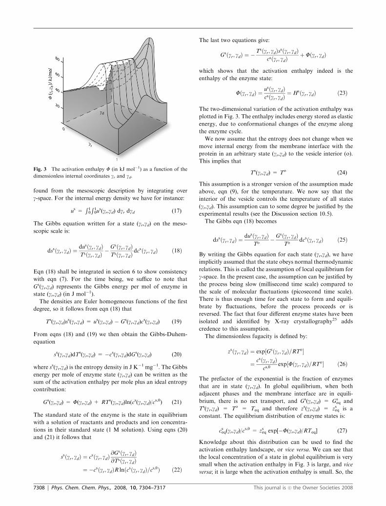
The two-dimensional activation enthalpy barrier, F(gr,gd)(in kJ mol�1), that we obtain in this manner, is illustrated in

Fig. 3. The figure shows a hypothetical variation in F(gr,gd) asa function of the dimensionless variables gr and gd. For furtherdefinition, see eqn (23) below. As is normal, the reaction

coordinate gr is 0 when the reaction starts (the reactants come

together). It is 1 when the reaction is completed (products have

been formed). The function F(gr,gd) shows the familiar peak at

a transition state value, gtr(gd). The dependence on gd gives a

ridge in the two-dimensional landscape. Similarly, the coordi-

nate gd for the transport of calcium ions is 0 when the ion

enters the membrane interface from the i-phase and 1 when the

ion leaves to the o-phase. For gd = 0 the function F(gr,gd) firstdecreases to a value where two calcium ions are bound to their

membrane site and then increases sharply. For gr = 1 the

variation along the gd-coordinate has a peak, to prevent Ca2+

from sliding backwards. A probable trajectory for ion trans-

port from (0,0) to (1,1) in the two-dimensional landscape

formed within these boundaries, may look like crossing a

mountain pass, see Fig. 3.

The concentration of enzymes in state (gr,gd), refers to the

reaction being in state gr and the calcium ions being in state gd.The concentration is denoted cs(gr,gd) and is given in mol mg�1.

By dividing this value by the integrated enzyme concentration,

we obtain the fraction of states at position (gr,gd) in the internal

coordinate space or, alternatively, the normalized probability of

that state. The integrated enzyme concentration is equal to the

inverse molar weight in mg mol�1. We will continue to use the

concentration cs(gr,gd) in mol mg�1, as these are the units used

in the experiments. Aside from a trivial normalisation factor

cs(gr,gd) is a probability distribution, and we will refer to it as

such when appropriate. The entropy and internal energy of the

enzyme in state (gr,gd) are, accordingly, ss(gr,gd) in J mg�1 K�1

and us(gr,gd) in J mg�1, respectively. All excess variables are

Fig. 2 The fluxes passing the Ca2+-ATPase in the membrane phase

(s). The ion flux and the total energy flux are constant in stationary

state, while the measurable heat flux on the i-side differ from that on

the o-side.


found from the mesoscopic description by integrating over

g-space. For the internal energy density we have for instance:

us =R10

R10u

s(gr,gd) dgr dgd (17)

The Gibbs equation written for a state (gr,gd) on the meso-

scopic scale is:

dssðgr; gdÞ ¼dusðgr; gdÞTsðgr; gdÞ

� Gsðgr; gdÞTsðgr; gdÞ

dcsðgr; gdÞ ð18Þ

Eqn (18) shall be integrated in section 6 to show consistency

with eqn (7). For the time being, we suffice to note that

Gs(gr,gd) represents the Gibbs energy per mol of enzyme in

state (gr,gd) (in J mol�1).

The densities are Euler homogeneous functions of the first

degree, so it follows from eqn (18) that

Ts(gr,gd)ss(gr,gd) = us(gr,gd) � Gs(gr,gd)c

s(gr,gd) (19)

From eqns (18) and (19) we then obtain the Gibbs-Duhem-

equation

ss(gr,gd)dTs(gr,gd) = �cs(gr,gd)dGs(gr,gd) (20)

where ss(gr,gd) is the entropy density in J K�1 mg�1. The Gibbs

energy per mole of enzyme state (gr,gd) can be written as the

sum of the activation enthalpy per mole plus an ideal entropy

contribution:

Gs(gr,gd) = F(gr,gd) + RTs(gr,gd)ln(cs(gr,gd)/c

s,0) (21)

The standard state of the enzyme is the state in equilibrium

with a solution of reactants and products and ion concentra-

tions in their standard state (1 M solution). Using eqns (20)

and (21) it follows that

ssðgr; gdÞ ¼ csðgr; gdÞ@Gsðgr; gdÞ@Tsðgr; gdÞ

¼ �csðgr; gdÞR lnðcsðgr; gdÞ=cs;0Þ ð22Þ

The last two equations give:

Gsðgr; gdÞ ¼ �Tsðgr; gdÞssðgr; gdÞ

csðgr; gdÞþ Fðgr; gdÞ

which shows that the activation enthalpy indeed is the

enthalpy of the enzyme state:

Fðgr; gdÞ ¼usðgr; gdÞcsðgr; gdÞ

¼ Hsðgr; gdÞ ð23Þ

The two-dimensional variation of the activation enthalpy was

plotted in Fig. 3. The enthalpy includes energy stored as elastic

energy, due to conformational changes of the enzyme along

the enzyme cycle.

We now assume that the entropy does not change when we

move internal energy from the membrane interface with the

protein in an arbitrary state (gr,gd) to the vesicle interior (o).

This implies that

Ts(gr,gd) = To (24)

This assumption is a stronger version of the assumption made

above, eqn (9), for the temperature. We now say that the

interior of the vesicle controls the temperature of all states

(gr,gd). This assumption can to some degree be justified by the

experimental results (see the Discussion section 10.5).

The Gibbs eqn (18) becomes

dssðgr; gdÞ ¼dusðgr; gdÞ

To� Gsðgr; gdÞ

Todcsðgr; gdÞ ð25Þ

By writing the Gibbs equation for each state (gr,gd), we have

implicitly assumed that the state obeys normal thermodynamic

relations. This is called the assumption of local equilibrium for

g-space. In the present case, the assumption can be justified by

the process being slow (millisecond time scale) compared to

the scale of molecular fluctuations (picosecond time scale).

There is thus enough time for each state to form and equili-

brate by fluctuations, before the process proceeds or is

reversed. The fact that four different enzyme states have been

isolated and identified by X-ray crystallography25 adds

credence to this assumption.

The dimensionless fugacity is defined by:

zsðgr; gdÞ ¼ exp½Gsðgr; gdÞ=RTo�

¼ csðgr; gdÞcs;0

exp½Fðgr; gdÞ=RTo� ð26Þ

The prefactor of the exponential is the fraction of enzymes

that are in state (gr,gd). In global equilibrium, when both

adjacent phases and the membrane interface are in equili-

brium, there is no net transport, and Gs(gr,gd) = Gseq and

Ts(gr,gd) = To = Teq and therefore zs(gr,gd) = zseq is a

constant. The equilibrium distribution of enzyme states is:

cseq(gr,gd)/cs,0 = zseq exp[�F(gr,gd)/RTeq] (27)

Knowledge about this distribution can be used to find the

activation enthalpy landscape, or vice versa. We can see that

the local concentration of a state in global equilibrium is very

small when the activation enthalpy in Fig. 3 is large, and vice

versa; it is large when the activation enthalpy is small. So, the

Fig. 3 The activation enthalpy F (in kJ mol�1) as a function of the

dimensionless internal coordinates gr and gd.


probability of finding a state populated, is smaller, the higher

the value of F. In the absence of global equilibrium, the value

of cs(gr,gd) may be smaller or larger than cseq(gr,gd). The

gradient of the fugacity zs(gr,gd) will, as we shall see later,

define the driving forces in the two directions gr and gd of thesystem. Using eqn (27), it follows from eqn (26) that

zsðgr; gdÞzseq

¼ expGsðgr; gdÞ � Gs

eq

RTo

� �¼ csðgr; gdÞ

cseqðgr; gdÞð28Þ

The balance equation for entropy along the (gr,gd)-co-ordinates is

dssðgr; gdÞdt

¼ ssðgr; gdÞ �@

@grJs;rðgr; gdÞ

� @

@gdJs;dðgr; gdÞ þ Jisðgr; gdÞ � Jos ðgr; gdÞ ð29Þ

The entropy change is equal to the entropy production minus

the 2-D divergence of a 2-D entropy flux (Js,r(gr,gd),Js,d(gr,gd))in the (gr,gd)-coordinate plane, plus the entropy flux into the

membrane interface from the i-side, Jis(gr,gd), minus the entropy

flux from the membrane interface to the o-side, Jos (gr,gd).Eqn (29) is the most general form of a balance equation in

the (gr,gd)-coordinate plane. When an enzyme changes its

state (gr,gd), entropy is not only produced, but also carried

along, as reflected in the second and the third term on the

right hand side of the equation. The two last terms reflect

that internal energy, and therefore the entropy, can go from

an enzyme in the state (gr,gd) directly into the i- or the

o-phase and vice versa. We shall see from eqn (37) below, that

eqn (29) can be integrated out to give the entropy production

of eqn (15).

All excess densities of the membrane interface are given

by integrals of the corresponding densities along the

(gr,gd)-coordinates. For the excess entropy of the mem-

brane interface and the excess entropy production we

therefore have

ss =R10

R10s

s(gr,gd)dgr dgd and

ss =R10

R10s


6. A consistent thermodynamic model

We have so far introduced certain assumptions in the basic

thermodynamic equations, eqns (8), (9) and (24). These

assumptions constitute a part of our view of the process, or

the process model. In order to complete the model, we give the

conservation equations for the mesoscopic level.

Enzymes in the state (gr,gd) change their state by a reaction

flux and by the transport of calcium ions. Conservation of

enzymes means that:

dcsðgr; gdÞdt

¼ � @rðgr; gdÞ@gr

� @JCaðgr; gdÞ@gd

ð31Þ

where the first term on the right hand side gives the change due

to the reaction rate and the second the change due to the

transport of the calcium ions. The internal energy is also

conserved. In terms of energy fluxes, this can be expressed by:

dusðgr; gdÞdt

¼ Jiqðgr; gdÞ � Joqðgr; gdÞ ð32Þ

The equation says that the energy flux Jiq(gr,gd) can be directed

from the i-phase into the membrane to any state (gr,gd).Similarly, an energy flux Joq(gr,gd) can leave the membrane

interface into the o-phase with the enzyme in an arbitrary state

(gr,gd). We have assumed that there is no internal energy flux in

the (gr,gd)-coordinate plane.

Expressions (8, 9, 24, 31 and 32) give a completely solvable

model. Equations (31, 32) are introduced into Gibbs eqn (25),

and we find:

dssðgr; gdÞdt

¼ 1

ToJiqðgr; gdÞ � Joqðgr; gdÞ� �

þ Gsðgr; gdÞTo

@rðgr; gdÞ@gr

þ @JCaðgr; gdÞ@gd

� �

¼ Jisðgr; gdÞ � Jos ðgr; gdÞ þ@

@grrðgr; gdÞ

Gsðgr; gdÞTo

� �

þ @

@gdJCaðgr; gdÞ

Gsðgr; gdÞTo

� �

þ Jiqðgr; gdÞ1

To� 1

Ti

� �� rðgr; gdÞ

@

@gr

Gsðgr; gdÞTo

� JCaðgr; gdÞ@

@gd

Gsðgr; gdÞTo

ð33Þ

By comparing this expression with the balance eqn (30) for the

entropy, we can identify the net entropy fluxes

Js;rðgr; gdÞ ¼ �rðgr; gdÞGsðgr; gdÞ

To;

Js;dðgd; gdÞ ¼ �JCaðgd; gdÞGsðgr; gdÞ

To

Jisðgr; gdÞ ¼ Jiqðgr; gdÞ=Ti; Jos ðgr; gdÞ ¼ Joqðgr; gdÞ=To ð34Þ

and the entropy production in the (gr,gd)-coordinate plane

ssðgr; gdÞ ¼ �rðgr; gdÞ@

@gr

Gsðgr; gdÞTo

� JCaðgr; gdÞ@

@gd

Gsðgr; gdÞTo

þ Jiqðgr; gdÞ1

To� 1

Ti

� �ð35Þ

This is the expression for the entropy production on the meso-

scopic level for the model. This is the main result of

the mesoscopic analysis of this paper. It helps us to define correct

flux-force relations on this level, from which all properties on the

macroscopic level can be derived in the following sections.

In order to integrate eqn (35) and check the model for

consistency with the macroscopic description, we need to specify

the boundary conditions at the beginning and the end of the

(gr,gd)-coordinates. We discuss this at the end of this section.

We now follow Kramers’ analysis from 1940 (ref. 29) to give

a statement on the fluxes: because the common activation

enthalpy barrier is high (see Fig. 3), the progress of the


reaction as well as the flux of the calcium ion are determined

by the small probability of the transition state, see the discus-

sion below eqn (27). Both transport processes can therefore be

regarded as quasi-stationary, in the sense that dcs(gr,gd)/dt isnegligible. As the heat flux finds its origin in the reaction and

the calcium ion flux, also this process is quasi-stationary. As a

consequence also dus(gr,gd)/dt is negligible. It follows from

eqns (31) and (32) that

@rðgr; gdÞ@gr

þ @JCaðgd; gdÞ@gd

¼ 0

Jiqðgr; gdÞ ¼ Joqðgr; gdÞð36Þ

In our model we will, consistent with these conditions, choose

the reaction rate, the calcium ion and the energy fluxes

independent of the (gr,gd)-coordinates:

r(gr,gd) = r (37)

JCa(gr,gd) = JiCa = JoCa = JCa (38)

Jiq(gr,gd) = Joq(gr,gd) = Jq (39)

The boundary conditions for the Planck potentials, chemical

potentials and Gibbs energies of the reactants and the

products, as well as the temperature are illustrated in Fig. 4.

The reactants in phase i enter the membrane phase and return

to phase i. The axis shows the progress of the reaction in terms

of the reaction coordinate gr. The temperature of the

membrane is constant according to eqn (24) and differs from

that of the i-phase, as indicated in the upper part of the figure.

Continuity in the Planck potential at the interface according to

eqn (8) and the drop at the transition state value (at gtr)lead to the variation that is illustrated for Gs(gr,gd)/T

o.

The values of this function at the boundaries are Gs(0,gd)/To =

(miATP + miH2O)/Ti and Gs(1,gd)/T

o = (miADP + miPi)/Ti.

Continuity in the Planck potential at the boundary means

that there is a jump in the corresponding chemical potential.

With a drop in temperature, the jump must be downwards.

The shape of the curve between the boundaries is the same as

that of the curve above, given the constant membrane

interface temperature.

In Fig. 5, we illustrate the variation of the thermodynamic

variables of Ca2+ and H+ with the gd-coordinate, which spans

the membrane. The temperature drops again, as we are passing

from the i-phase to the membrane, but it maintains its level into

the o-phase eqn (24). The difference in Gibbs energy by

the exchange of Ca2+ by protons in the i-phase divided by the

temperature of this phase, varies in a continuous fashion. At the

i-side of the membrane interface, Gs(gr,0)/To = (miCa � 2miH)/T

i,

while at the o-side, Gs(gr,1)/To = (moCa � 2moH)/T

o. The

corresponding chemical potentials jump at the interfaces, due

to the jump in temperature, giving e.g. Gs(gr,1) = (moCa � 2moH)at the end of the gd-coordinate. The variation along the

gd-coordinate is pictured as less dramatic than along the

gr-coordinate.Fig. 4 and 5 show that the temperature drops from the i

phase to the membrane phase, while it remains constant going

from the membrane to the o phase. The figures apply when

calcium ions are pumped into the o phase. The increase of the

calcium ion density in the o phase leads to a decrease of

the entropy of the o phase. Such a decrease implies that there is

a heat flux out of the o phase to the membrane and as a

consequence out of the membrane to the i phase. This cools

the membrane and the o phase relative to the i phase, as is

indicated in Fig. 4 and 5. The dissipated heat is not sufficient to

compensate for this.

We shall now verify that integration of eqn (35) with these

boundary values gives eqn (15). This shows that our set of

assumptions presents a model that is consistent with the

Fig. 4 The thermodynamic variables of the products and reactants in

the external phase and the membrane phase for Ca2+-uptake condi-

tions as a function of the gr coordinate. The Gibbs energy of the

ensemble has, for a given gd, rapid drop around the transition ridge

(gr,gd).

Fig. 5 The thermodynamic variables of the Ca2+ and H+ in across

the membrane phase for Ca2+-uptake conditions as a function of the

gd coordinate. The Gibbs energy of the ensemble has, for a given gr, arelatively smooth increase from side i to side o.


second law of thermodynamics. Using eqns (37)–(39) it follows

from eqn (35) that

ss ¼Z 1

0

Z 1

0

ssðgr; gdÞdgrdgd

¼ �rZ 1

0

Z 1

0

@

@gr

Gsðgr; gdÞTo

dgrdgd

� JCa

Z 1

0

Z 1

0

@

@gd

Gsðgr; gdÞTo

dgrdgd

þ Jq

Z 1

0

Z 1

0

1

To� 1

Ti

� �dgrdgd

¼ �rDrGi

Ti� JoCa

moCa=2HTo

�miCa=2HTi

!

þ Jq1

To� 1

Ti

� �ð40Þ

which thus verifies eqn (15). For the difference in the entropy

fluxes on the i- and the o-side we have:

Jis � Jos ¼Z 1

0

Z 1

0

Jisðgr; gdÞ � Jos ðgr; gdÞ �@

@grJs;rðgrÞ

�

� @

@gdJs;dðgdÞ

�dgrdgd

¼Z 1

0

Z 1

0

Jiqðgr; gdÞTi

�Joqðgr; gdÞ

Toþ @

@grrGsðgr; gdÞ

To

� �"

þ @

@gdJCa

Gsðgr; gdÞTo

� ��dgrdgd

¼ Jq

Tiþ r

DrGi

Ti� JCa

miCa=2HTi

!� Jq

To� JCa

moCa=2HTo

� �

ð41Þ

where we again used the boundary conditions. This expression

agrees with eqn (12). This means that the expression for the

entropy production (35) can be used to define fluxes and

forces in the system on the mesocopic level; i.e. in the

(gr,gd)-coordinate space.

7. The forces and fluxes on the mesoscopic level

The linear force-flux relations that follow from eqn (35) on the

mesoscopic level are with eqns (37)–(39):

r ¼ �lrrðgr; gdÞ@

@gr

Gsðgr; gdÞTo

� lrdðgr; gdÞ@

@gd

Gsðgr; gdÞTo

þ lrqðgr; gdÞ1

To� 1

Ti

� �

JCa ¼ �ldrðgr; gdÞ@

@gr

Gsðgr; gdÞTo

� lddðgr; gdÞ@

@gd

Gsðgr; gdÞTo

þ ldqðgr; gdÞ1

To� 1

Ti

� �

Jq ¼ �lqrðgr; gdÞ@

@gr

Gsðgr; gdÞTo

� lqdðgr; gdÞ@

@gd

Gsðgr; gdÞTo

þ lqqðgr; gdÞ1

To� 1

Ti

� �ð42Þ

The matrix was constructed following Onsager30,31 who used

generalized fluctuating variables in his analysis. These

variables compare well to the ones used here. The equations

contain thermodynamic forces, defined from the entropy

production in the proper manner, meaning that the Onsager

relations are valid, lij(gr,gd) = lji(gr,gd), see in this context also

Prigogine and Mazur,27 and Meixner.32 The coefficients are

independent of the forces.

The emphasis of this paper is on the derivation of the non-

linear relations between the reaction rate, the calcium flux and

the measurable heat flux to the Gibbs energy of the reaction

DrGi and the chemical potential difference of the calcium ion

and proton exchange DmCa/2H, as well as a linear coupling to

the temperature difference across the membrane. The formal-

ism presented makes it possible to address fluctuations. We

show in the Appendix how the Smoluchowski equation for

diffusion along the reaction coordinate given by Kramers29

follows from the material presented above but shall not go

into further details.

We can rewrite the driving forces of the chemical reaction

and the calcium ion transport, using the dimensionless

fugacity defined in eqn (26)

@

@gk

Gsðgr; gdÞTo

¼ Rcs;0

csðgr; gdÞexp �Fðgr; gdÞ

RTo

� �@

@gkzsðgr; gdÞ

for k ¼ r; d ð43Þ

Substituting this into eqn (42) results in

r ¼� drr exp �Fðgr; gdÞRTo

� �@

@grzsðgr; gdÞ

� drd exp �Fðgr; gdÞRTo

� �@

@gdzsðgr; gdÞ

� drqcsðgr; gdÞRTics;0

1� Ti

To

� �

JCa ¼� ddr exp �Fðgr; gdÞRTo

� �@

@grzsðgr; gdÞ

� ddd exp �Fðgr; gdÞRTo

� �@

@gdzsðgr; gdÞ

� ddqcsðgr; gdÞRTics;0

1� Ti

To

� �

Jq ¼� dqr exp �Fðgr; gdÞRTo

� �@

@grzsðgr; gdÞ

� dqd exp �Fðgr; gdÞRTo

� �@

@gdzsðgr; gdÞ

� dqqcsðgr; gdÞRTics;0

1� Ti

To

� �ð44Þ

where we introduced

dij ¼ lijðgr; gdÞRcs;0

csðgr; gdÞð45Þ

It follows from the construction and from the Onsager

relations that:


dij = dji (46)

This rewriting is similar to what is done on the macro-

scopic level, when one wants to replace the thermodynamic

transport law with Fick’s law for diffusion. One is also then

introducing a diffusion coefficient equal to a phenomeno-

logical coefficient divided by the concentration. The Onsager

coefficients are in good approximation proportional to the

density. We will therefore assume that the coefficients dij are

constant.

The particular choice that we made for the activation

enthalpy (that it is a function of two internal variables) led

to a common prefactor of the chemical and osmotic driving

forces in eqn (44). This makes the next step transparent. We

multiply both sides of eqn (44) with exp[F(gr,gd)/RTo].

Integration of eqn (44) then gives:

r ¼ �Drr 1� exp �DrGi

RTi

� �� þDrd 1� exp D

mCa=2HRT

� �h i� Drq

RTi1� Ti

To

� �

JCa ¼ �Ddr 1� exp �DrGi

RTi

� �� þDdd 1� exp D

mCa=2HRT

� �h i� Ddq

RTi1� Ti

To

� �

Jq ¼ �Dqr 1� exp �DrGi

RTi

� ��

þDqd 1� exp DmCa=2HRT

� �h i�Dqq 1� Ti

To

� �ð47Þ

where Dij are transport coefficients on the macroscopic level,

and we have used D(mCa/2H/RT)� (moCa/2H/RTo)� (miCa/2H/RT

i).

In the expressions for the elements of the Dij-matrix we

used the activation energy Fact. The enthalpy F(gr,gd)has a sharp maximum along the gr coordinate, cf. Fig. 3. Theintegral over exp[F(gr,gd)/RT

o] is dominated by this maxi-

mum. We then find the following expression for the activation

energy:

exp[Fact/RTo] =

R10

R10exp[F(gr,gd)/RT

o]dgr dgd (48)

The integration procedure gives several explicit relations

between the transport coefficients on the macroscopic level,

Dij, and their mesoscopic counterparts, dij. We have:

Djr = djr exp[�Fact/RTo] exp((miADP + miPi)/RT

i)

for j = r,d,q

Djd = djd exp[�Fact/RTo] exp(miCa/2H/RT

i) for j = r,d,q

Djq = djq exp[�Fact/RTo]R10

R10z

s(gr,gd) dgr dgd for j = r,d

Dqq = RTidqq exp[�Fact/RTo]R10

R10z


As can be seen, the D-matrix, unlike the d-matrix, is not

symmetric. While the six coefficients Drr, Drd, Ddr, Ddd, Drq,

Ddq can be determined by experiments, the remaining three

coefficients can not, because Jq is not measurable. In order to

have a practical flux-force set we need to introduce the

measurable heat flux.

In a sensitivity analysis, it is beneficial that the diffusion

coefficients are comparable in size. In order to make Djr

comparable to Djd, we chose the particular form of eqns (47).

Other choices are possible, but lead to transport coefficients

that differ by orders of magnitude.18

8. A set of fluxes that include the measurable heat

flux

For interpretation of data it is crucial to use the measurable

heat flux rather than the energy flux. The relevant flux is

the measurable heat flux in the external phase. This measur-

able heat flux is given by

J0iq = Jq + DrHir � (Hi

Ca � 2HiH)JCa (50)

The measurable heat flux is an absolute quantity. It bears the

name

’’

measurable’’ because it can be registered by measuring

the temperature variation at a location. With knowledge of the

local heat capacity and the temperature change, one can find

the measurable heat flux. With knowledge of the remaining

terms in eqn (50), one can then calculate the total heat flux.

Eqn (50) contains the enthalpies of the ions. These enthalpies

are not absolute quantities, unlike DrH, but depend on the

choice for the state of reference. A choice should be made so

that the combination HCa � 2HH = HCa/2H is measurable.

If water transport accompanies the ion transport, a contribu-

tion from water must be added. The same applies if buffer

equilibria in the external solution are shifted by the transports.

We assume now that such corrections can be made20 so that

J0iq and next Jq can be found, once the calorimetric experiment

has been done.

From eqn (47) it follows that

J0iq ¼ �D00qr 1� exp �DrG

i

RTi

� ��

þD00qd 1� exp DmCa=2HRT

� �h i�D00qq 1� Ti

To

� �ð51Þ

The coefficients with double prime have been used as’’

intermediate-step coefficients’’

D00qj = Dqj + DrHiDrj � Hi

Ca/2HDdj for j = r,d

D00qq ¼ Dqq þDrH

i

RTiDrq �

HiCa=2H

RTiDdq ð52Þ

For r and JCa we can still use eqn (47). All the forces

that appear are then unchanged, they are �Dr(Gi/RTi),

D(mCa/2H/RT) and 1 � Ti/To. These forces are not conjugate

to the new choice of the fluxes, however. The correct

conjugate forces follow from eqn (16) for the excess

entropy production in terms of the measurable heat flux.

Below we will therefore transfer to the correct conjugate

forces.

We expand for this purpose the present chemical and

osmotic forces to linear order in the temperature difference.


This assumption is not necessary, but it serves to prove the

point (below we will also give the result for the case we do

not make this approximation). For the chemical force,

we have:

1� exp �DrGiðTiÞ

RTi

� �¼ 1� exp �DrG

iðToÞRTo

� �

� exp �DrGiðTiÞ

RTiþ DrG

iðToÞRTo

� �

¼ 1� exp �DrGiðToÞ

RTo

� �

� 1� DrGiðTiÞ

RTiþ DrG

iðToÞRTo

� �


RTo

� �

� 1� DrHiðToÞ

RTi1� Ti

To

� ��


RTo

� �

þ DrHi

RTi1� Ti

To

� �

ð53Þ

In the last identity, we took DrGi(To) = 0 and To = Ti in the

prefactor of (1 � Ti/To).

For the osmotic force we similarly have

1� exp DmCa=2HRT

� �¼ 1� exp

DmCa=2HðToÞRTo

� �

� exp �miCa=2HðTiÞ

RTiþmiCa=2HðToÞ

RTo

!

¼ 1� expDmCa=2HðToÞ

RTo

� �

� 1�miCa=2HðTiÞ

RTiþmiCa=2HðToÞ

RTo

" #


RTo

� �

� 1�Hi

Ca=2HðToÞRTi

1� Ti

To

� �" #


RTo

� �

þHi

Ca=2H

RTi1� Ti

To

� �ð54Þ

where we defined DmCa/2H(To) � moCa/2H(T

o) � miCa/2H(To). In

the last identity we took miCa/2H(To) = moCa/2H(T

o) and To = Ti

in the prefactor of (1 � Ti/To).

Substituting eqns (53) and (54) into eqns (47a,b) and (51),

we obtain the main result of this section; the flux equations

that can be used to describe experiments on active transport:

r ¼ �Drr 1� exp �DrGiðToÞ

RTo

� ��

þDrd 1� expDmCa=2HðToÞ

RTo

� ��

D0rqRTi

1� Ti

To

� �

JCa ¼ �Ddr 1� exp �DrGiðToÞ

RTo

� ��

þDdd 1� expDmCa=2HðToÞ

RTo

� ��

D0dqRTi

1� Ti

To

� �

J0iq ¼�D0qr 1� exp �DrG

iðToÞRTo

� ��

þD0qd 1� expDmCa=2HðToÞ

RTo

� ��

�D0qq 1� Ti

To

� �ð55Þ

This is the set of equations we need to describe measurements

on active transport on the macroscopic level, as will be

clarified in the rest of this paper. The equations contain fluxes

and forces which can all be determined from experiment, as

will be used in the paper to follow this one.

The fluxes and forces in the matrix are properly conjugate,

compared with eqn (16), and the set of equations are therefore an

alternative to eqn (47). We have now obtained two sets of fluxes

and forces; one set that contains the energy flux, and one set that

contains the measurable heat flux. Due to the quasi-stationary

nature of the process the energy flux was constant, which made it

possible to integrate over the internal variable space. We have not

found an equivalent procedure using the measurable heat flux.

The link between the macroscopic and the mesoscopic level is

therefore provided by the energy flux. The thermodynamic

description must ultimately be able to describe the experimental

results, however, so the measurable heat flux must be introduced.

We take advantage of the energy balance, eqn (50), and the

invariance eqn (15) of the entropy production on the macroscopic

level to accomplish this. While the set (47) took advantage of the

constant energy flux, assumption (38), the set (55) is able to make

a direct description of the measurable heat flux. One may say that

the set eqn (55) is the mesoscopically based analogue of what was

called

’’

A practical set of fluxes and forces’’ in classical non-

equilibrium thermodynamics by Kedem and Katchalsky (33).

We see now some interesting properties of the system.

1. Active transport is described by the coefficient Ddr which

links Ca2+ uptake to a nonzero chemical driving force.

2. Synthesis of ATP can be accomplished with energy from

the osmotic driving force, through the coefficient Drd.

3. It is possible to have ATP hydrolysis or synthesis, by

exposing the vesicle at equilibrium to a thermal driving force.

This follows from the coefficient D0rq.

4. It is likewise possible to have Ca2+ uptake or active

transport by a thermal driving force through D0dq.


5. It is possible to have a heat flux to the external solution,

even if the temperatures inside and outside the vesicles are the

same. This heat production is caused by the chemical and

the osmotic driving forces. It is a reversible heat production, in

the sense that a change in the direction of the driving force will

change the direction of the heat flux. This can be understood

from the terms containing D0qr and D0qd in eqn (55)c. This can

be used to define non-shivering thermogenesis.

Only the first two properties were described before. We shall

elaborate on available experiments and confirm the other

properties in a paper to follow. We continue now to comment

on the properties of the equations.

Through the relations of the fluxes in eqn (50) and forces in

eqns (53) and (54), we can calculate one set of transport

coefficients once we know the other. The transport coefficients

to be found from the experiments are given by eqn (55). We

note that four of the phenomenological coefficients are the same

as in the original D-matrix and the other five are given by:

D0qj = D00qj = Dqj + DrHiDrj � Hi

Ca/2HDdj for j = r,d

D0jq = Djq + DrHiDjr � Hi

Ca/2HDjd for j = r,d

D0qq ¼ Dqq þDrH

i

RTiðDrq þDqrÞ �

HiCa=2H

RTiðDdq þDqdÞ ð56Þ

The equations relate the coefficients obtained with the measur-

able heat flux to those obtained with the energy flux.

For convenience we have also given the relation to the

intermediate-step coefficients D00ij.

Finally, if we do not make the simplification in the last line

of eqns (53) and (54), we also obtain eqn (55), but the

phenomenological coefficients change to:

D0qj = D00qj = Dqj + DrHi(Ti)Drj � Hi

Ca/2H(Ti)Ddj for j = r,d

D0jq ¼Djq þ DrHiðToÞ exp �DrG

iðToÞRTo

� �Djr

�HiCa=2HðToÞ exp

DmCa=2HðToÞRTo

� �Djd for j ¼ r; d

D0qq ¼Dqq þDrH

iðTiÞRTi

Drq �Hi

Ca=2HðTiÞRTi

Ddq

þ DrHiðToÞ

RTiexp �DrG

iðToÞRTo

� �Dqr

�Hi

Ca=2HðToÞRTi

expDmCa=2HðToÞ

RTo

� �Dqd

ð57Þ

This set can be used instead of eqn (56) if a higher precision is

needed in the calculation. The experimental errors that are

typical in biological systems, are probably going to make the

set (56) sufficient for most purposes.

9. The coefficient matrix near global equilibrium

Some experiments start with the system in equilibrium. The

system is next perturbed, by adding a reagent or by changing

the variables, for instance the pH. The change induces a driving

force, and subsequently fluxes of some sort. In this situation, the

driving force may be small, and the whole experiment may be

said to work close to global equilibrium. A linear description is

then enough. This is certainly the case, when a system in

equilibrium is exposed to a temperature drop. It is then possible

to expand on the chemical and osmotic forces, and use only

the first term of the expansion. The flux–force relationships

become the classical ones, where the upper left corner of two

fluxes and two forces can be found in classical books:5,6

r ¼ �DrrDrG

iðToÞRTo

�Drd

DmCa=2HðToÞRTo

�D0rqRTi

1� Ti

To

� �

JCa ¼ �DdrDrG

iðToÞRTo

�Ddd

DmCa=2HðToÞRTo

�D0dqRTi

1� Ti

To

� �

J0 iq ¼ �D0qr

DrGiðToÞ

RTo�D0qd

DmCa=2HðToÞRTo

�D0qq 1� Ti

To

� � ð58Þ

while the driving forces obey

|DrGi(To)| { RTo and |DmCa/2H(T

o)| { RTo (59)

Near equilibrium we may use

|miADP + miPi| { RTi, |

miCa/2H| { RTi and zs(gr,gd) C 1 (60)

As a consequence the D-matrix given in eqn (49) reduces to

Dij = dij exp[�Fact/RTo] when ij a qq

Dqq = RTidqq exp[�Fact/RTo] (61)

and the coefficient matrix is again symmetric. The corresponding

D0-matrix is given in terms of the D-matrix by eqn (56)

and is also, as a consequence of this, symmetric. This shows that

the solution we found for transport processes which take place far

from equilibrium, obeys the proper near-equilibrium behavior.

10. Discussion

10.1 Thermodynamic basis for equations describing active

transport

As mentioned in the Introduction, it has been a long-standing

problem in non-equilibrium thermodynamics to find a

statistical basis for coupled non-linear flux-force relations. Such

relations are observed in various contexts where chemical reac-

tions are involved; in particular in biological transport problems.

Also, one has not earlier devised a method for biological systems

that puts the heat flux of a system on a quantitative and

thermodynamic footing. We think that our efforts in this direc-

tion are promising. A possible solution has been found to both

these problems. The solution should now be tested experimen-

tally or computationally, and also tried out in similar systems.

The essential steps in the solution method was to first write

thermodynamic equations and conservation equations for the

mesoscopic level. Flux equations were next obtained for this


level of description. These then had to be integrated, in order

to be able to relate the equations to observables.

The distribution function on the mesoscopic level, given by

the concentration cs(gr,gd) in mol mg�1 times the molar mass

of the proteins in mg mol�1, was crucial for the derivations. By

using the probability function on this level, we rely on the well-

proven assumption of Gibbs, that the thermodynamic entropy

is equal to the Boltzmann entropy. We further assumed that

the entropy in internal coordinate space is the ideal, statistical

one (see eqn (22)). The remaining contribution to the fugacity,

the activation enthalpy function F(gr,gd) in Fig. 3 is interesting.

It can be further examined by other methods. Activation

energy calculations have been performed in quantum

mechanics, and this should also be feasible here.

A special choice was made for the distribution function: we

chose to use the population of all enzymes as the basis, and

detail the distribution of enzymes in reaction coordinate space

(gr) as well as in transport coordinate space (gd). In this manner,

a two-dimensional distribution was obtained of the activation

enthalpy landscape of Fig. 3. This made it possible to find an

integrable form of the flux equations, because a common factor

was obtained in the transport equations for the chemical and

the osmotic force. The results obtained rests on this choice.

The present method of analysis of biological transport

problems can deal with more variables than Post–Albers or

Hill-kinetic diagrams. Whenever the temperature or heat pro-

duction plays a role, one needs a thermodynamically based

method, to quantify the relation of these variables to the others.

10.2 A practical set of flux equations

We have been able to arrive at a set of transport equations that

relate observable fluxes to driving forces that can be deter-

mined from experiments. The equation set can thus be termed’’

practical’’ in the sense first used by Kedem and Katchalsky.33

Experimental consequences shall be discussed in depth in a

paper to follow, since this is a big topic of its own. We

continue to discuss the theoretical aspects of the solution.

On a mesocopic level, we were only able to write flux

equations with the energy flux as the flux conjugate to the

thermal force. We needed to take advantage of this flux being

constant in the integration to the macroscopic level. This then

led to a rearrangement on the macroscopic level, to include as

preferred heat flux the measurable heat flux. The rearrange-

ment involved some algebra, but no further assumption. In the

end we were able to relate directly to measurements.

10.3 Transport coefficients and their relations

It is interesting that explicit formulae have been obtained which

are linking the transport coefficients, determined by experi-

ments, to the transport coefficient on the molecular level. It is

an important outcome of the derivations; that the coeffi-

cients Dij or D0ij can be linked to the coefficients on the

mesoscopic scale, dij. Points in the activation energy landscape

in the future may be accessible through quantum mechanical

calculations. The exponential functions that contain the

chemical potentials are calculable, when the distribution func-

tions are known. With knowledge of Dij one can then find dij.

Calculations of the latter may yield insight in the process on the

molecular scale.

The possible symmetry of the matrix of transport coeffi-

cients far away from global equilibrium is a topic that has

concerned many scientists over the years. Caplan and Essig5,6

introduced the concept of proper pathways to extend the use

of linear flux–force relations. The apparent linear range was

used by Waldeck et al.34 to describe the performance of the

Ca2+-ATPase. In their model, the proton transport was

independent from the Ca2+ transport, and the system was

isothermal. The present analysis avoids the introduction of

proper pathways, and is also able to include heat transport.

We find that the solution for large driving forces does not

have a symmetric matrix of transport coefficients. The reason

for this is that the phenomenological coefficients lij on the

mesoscopic level, which satisfy the Onsager reciprocal

relations,27,32 are proportional to the density. This leads to a

driving force in terms of the gradient in the fugacity. A

non-linear flux–force relationship on the macroscopic level

with an asymmetric transport coefficient matrix followed.

We have, however, been able to prove in the limit of global

equilibrium, that the macroscopic coefficients Dij, D0ij become

symmetric. This shows that the method is in full agreement

with Onsager.30,31 The matrix of coefficients is thus symmetric

on the mesocopic level, and becomes asymmetric upon

integration to macroscopic level when we are far from global

equilibrium. But we can approach the limit of symmetric

coefficients on the macroscopic level, by reducing the driving

forces. The procedures of Caplan and Essig5,6 who proposed

proper pathways and linear flux–force relations far from

global equilibrium, is thus not needed.

We have chosen to present the flux equations with dimen-

sionless driving forces, in order to be able to compare them in

equivalent units, and in order to give the coefficients the dimen-

sion of their corresponding flux. This choice need not be done,

and one is free to make other choices. In our earlier analysis of

the problem,17,18 where we only included one activated path, this

lead to coefficients that varied by orders of magnitude, which

was rather unpractical. In the present case, the coefficients will

be of a comparable order of magnitude.

10.4 The assumption of local equilibrium in c-space

A legitimate question to ask is, of course, whether it is possible

at all to write thermodynamic equations on a mesocopic level.

Some arguments have already been given, namely that the

pumping of ions is a relatively slow process (millisecond scale),

so that there is time for internal equilibration of vibrational

and rotational modes of the protein. In this context, we may

mention work on nanometer thick interfaces between vapor

and liquid. We have found, using molecular dynamics simula-

tions, that the equation of state for the interface was unper-

turbed by the thermal or chemical driving force that it was

exposed to (ref. 35 and 36). In stationary state calculations,

not many particles are needed to find time averages that obey

thermodynamic relations. Hafskjold and Ratkje37 found that

around 16 particles were sufficient for this in a control volume

of few (nm)3. These results were not obtained for paths along

internal coordinates, however. In this respect the assumption


made here of local equilibrium along the path in internal

coordinate space seems new. It was however introduced

already a long time ago for chemical reactions by Kramers,29

and has since then been used in reaction kinetics and electrode

kinetics for the degree of advancement of a chemical or

electrochemical reaction.

10.5 Assumptions on the Planck potentials and the temperature

In the derivation of the entropy production on a mesoscopic

level, it was essential to first make the assumption that the

Planck potentials were equal, msj/Ts = mij/T

i, and that

the membrane interface temperature was that of its inside,

Ts = To, see eqns (8) and (9).

The assumption about the Planck potentials is not a radical

one, as many authors have used DrGi for the Gibbs energy of the

hydrolysis reaction already, see i.e. Caplan and Essig.5,6 The

assumption requires that the binding of reactants and debinding

of products to the protein binding site is relatively rapid com-

pared to the slowest step in the overall process. This is probably

true for ATP, ADP, Pi, and Ca2+. Discussion exists on whether

proton debinding is a relatively slow step, however.1,2

Assumption (9) and its follow-up Ts(gr,gd) = To in eqn (24)

about the temperature is more uncertain, since nothing is

known about the temperature in internal variable space. A

temperature different from the temperature of the external

solution is necessary to obtain a thermal driving force. This

driving force is probably not going to be large.38 Nevertheless

it is crucial to explain thermally induced effects such as, for

instance, thermogenesis. More work is needed to substantiate

this point.

11. Conclusions and perspectives

We have presented above a new description of the phenomena

that can be accomplished by the forward and reverse mode of

operation of ion-pumps. An important improvement over

earlier work is that both the reaction and the transport of

calcium ions are now treated as activated processes. We have

described the operation far from global equilibrium with an

asymmetric set of transport coefficients, and shown that the

problem reduces to the well known symmetric set close to

equilibrium. The description accounts for the effects of

temperature differences and of the heat flux. A further

improvement over earlier work is that the description now

uses the measurable heat flux rather than the energy flux. This

makes an analysis of experimental data possible. In particular

we have been able to describe the measurable heat flux and its

conjugate force; heat production under isothermal conditions;

and thermogenesis as defined by the onset of the reaction and

calcium ion transport due to a temperature drop. A prescrip-

tion was given for how to determine transport coefficients on

the mesocopic level, from the macroscopic coefficient, the

activation enthalpy, and a proper probability distribution.

On the mesoscopic level it was possible to formulate the

Onsager reciprocal relations.

We shall next see how the equations can be used to under-

stand experimental results that are reported in the literature,

and propose experiments which can be carried out to test

the model.

12. Appendix

As it is not the aim of this paper to give a detailed analysis of

the fluctuations, we restrict this appendix to the case of a

reaction. There are therefore no calcium ion and energy fluxes.

Furthermore the temperature is constant. Eqn (31) then

reduces to

dcsðgrÞdt

¼ � @rðgrÞ@gr

ð62Þ

The linear force flux relation (42) becomes

r ¼ � lrrðgrÞT

@GsðgrÞ@gr

ð63Þ

For Gs(gr) we can use eqn (21)

Gs(gr) = F(gr) + RT ln(cs(gr)/cs,0) (64)

Substituting this relation into eqn (63) we find

r ¼� lrrðgrÞT

@

@gr½FðgrÞ þ RT lnðcsðgrÞ=cs;0Þ�

¼ � lrrðgrÞT

@

@grFðgrÞ �

RlrrðgrÞcsðgrÞ

@csðgrÞ@gr

ð65Þ

Table 1 Symbols

cj Concentration of ATP, ADP or Pi, mol mg�1

protein or mol m�2 interface areacr(gr,gd)/c

0 Probability distribution for enzyme statescs(gr,gd)/c

s,0 Probability distribution for enzyme statesdij Mobility coefficient, assumed constant in internal

coordinate spaceDij Mobility coefficient, integrated over internal

coordinate spaceeq Denotes the state of global equilibriumGs(gr,gd) Gibbs energy of ensemble in state gr,gdDrG Gibbs energy of reaction/J mol�1

h Heat transfer coefficient/J mol�1 K�1

Hk Partial molar enthalpy of k/J mol�1

Hs(gr,gd) Enthalpy of ensemble in state gr,gdDH Enthalpy of reaction/J mol�1

i Phase i, left of the membraneJk Flux of component k/mol s�1 mgJ0q Flux of sensible (measurable) heat/J s�1 mg�1

Jq Total heat flux/J s�1 mg�1Js Flux of entropy/J s�1 mg�1lij(gr,gd) General phenomenological coefficient in internal

coordinate spacen Number of componentso Phase o, right of the membraner Reaction rate, mol s�1 mgs Phase s, the membrane phasess Entropy density of the membrane/J K�1 mg�1

Sk Partial molar entropy/J K�1 mol�1

T Temperature/Kus Internal energy density of membrane/J mg�1

zs Dimensionless fugacity of ensemble of enzymestates

gr Dimensionless internal coordinate for the reactiongd Dimensionless internal coordinate for ion

transportgtr(gd) Position of the transition stateF(gr,gd) Activation enthalpy barrier, or enthalpy of

enzyme state (gr,gd)/J mol�1

mk Chemical potential of k/J mol�1

ss Entropy production of the membrane/J K�1 mg�1


Defining the diffusion constant by

D � RlrrðgrÞcsðgrÞ

ð66Þ

and the force by

K � � 1

R

@

@grFðgrÞ ð67Þ

The reaction flux can be written as

r ¼ DK

TcsðgrÞ �D

@csðgrÞ@gr

ð68Þ

Substituting this expression into eqn (62) we obtain

dcsðgrÞdt

¼ � @

@gr

DK

TcsðgrÞ �D

@csðgrÞ@gr

� �ð69Þ

In eqn (11) in Kramers’ paper29 the spacial coordinate q is the

reaction coordinate gr, D is T/Z and cs(gr) is s. This shows thatthe expression we find is the Smoluchowski equation for

diffusion along the reaction coordinate given already by

Kramers.

Acknowledgements

The Center for Advanced Studies at the Norwegian Academy of

Science and Letters is thanked for support of extraordinary

sabbaticals of D.B and S.K. We are grateful to the referees for

their constructive comments, which made us clarify the proba-

bilistic nature of the mesoscopic description and the relation to the

Smoluchowski equation for diffusion in the paper by Kramers.

References

1 C. Peinelt and H. J. Apell, Time-resolved charge movements in thesarcoplasmatic reticulum Ca-ATPase, Biophys. J., 2004, 86, 815–824.

2 C. Peinelt and H. J. Apell, Time-resolved charge movements in thesarcoplasmatic reticulum Ca-ATPase, Biophys. J., 2005, 89, 2427–2433.

3 T. L. Hill, Free energy transduction and biochemical cycle kinetics,Springer Verlag, New York, 1989.

4 A. Katchalsky and P. Curran, Nonequilibrium thermodynamics inbiophysics, Harvard University Press, Cambridge, Massachusetts, 1975.

5 S. R. Caplan and A. Essig, Bioenergetics and linear nonequilibriumthermodynamics. The steady state, Harvard University Press,Cambridge, Massachusetts, 1983.

6 S. R. Caplan and A. EssigBioenergetics and linear nonequilibriumthermodynamics. The steady state, Harvard University Press,Cambridge, Massachusetts, 3rd edn, 1999.

7 H. V. Westerhoff and K. van Dam, Thermodynamics and controlof biological free-energy transduction, Elsevier, Amsterdam, 1987.

8 Y. Demirel, Non-equilibrium thermodynamics. Transport and rateprocesses in physical, chemical and biological systems, Elsevier,Amsterdam, 2002.

9 Y. Demirel and S. I. Sandler, Nonequilibrium Thermodynamics inEngineering and Science, J. Phys. Chem. B, 2004, 108, 31–43.

10 Y. Demirel, Non-equilibrium thermodynamics. Transport and rateprocesses in physical, chemical and biological systems, Elsevier,Amsterdam, 2nd edn, 2007.

11 L. de Meis, Uncoupled ATPase activity and heat production by thesarcoplasmic reticulum Ca2+-ATPase, J. Biol. Chem., 2001, 276,25078–25087.

12 L. de Meis, Ca2+-ATPases (SERCA): energy transduction and heatproduction in transport ATPases, Membr. Biol., 2002, 188, 1–9.

13 L. de Meis, Brown Adipose Ca2+-ATPase tissue, J. Biol. Chem.,2003, 278, 41856–41861.

14 A. P. Arruda, W. da Silva, D. Carvalho and L. de Meis,Hyperthyroidism increases the uncoupled ATPase activity andheat production by the sarcoplasmic reticulum Ca2+-ATPase,Biochem. J., 2003, 375, 375–753.

15 D. Walz, Biothermokinetics of processes and energy conversion,Biochim. Biophys. Acta, 1990, 1019, 171–224.

16 S. R. de Groot and P. Mazur, Non-equilibrium thermodynamics,Dover, New York, 1984.

17 S. Kjelstrup, J. M. Rubi and D. Bedeaux, Active transport: Kineticdescription on thermodynamics grounds, J. Theor. Biol., 2005, 234,7–12.

18 S. Kjelstrup, J. M. Rubi and D. Bedeaux, Energy dissipation in slippingbiological pumps, Phys. Chem. Chem. Phys., 2005, 7, 4009–4018.

19 M. C. Berman, Slippage and uncoupling in P-type cation pumps;implications for energy transduction mechanisms and regulation ofmetabolism, Biochim. Biophys. Acta, 2001, 1513, 95–121.

20 R. A. Alberty, Thermodynamics of the hydrolysis of adenosinetriphosphate as a function of temperature, pH, pMg, and ionicstrength, J. Phys. Chem. B, 2003, 107, 12324–12330.

21 K. Obara, N. Miyashita, C. Xu, I. Toyashima, Y. Sugita, G. Inesiand C. Toyoshima, Structural role of countertransport revealed inCa2+ pump crystal structure in the absence of Ca2+, Proc. Natl.Acad. Sci. U. S. A., 2005, 41, 14489–14496.

22 F. Tadini-Buoninsegni, G. Bartolommei, M. R. Moncelli,R. Guidelli and G. Inesi, Pre-steady state electrogenic events ofCa2+/H+ exchange and transport by the Ca2+-ATPase, J. Biol.Chem., 2006, 281, 37720–37727.

23 E. L. Karjalainen, K. Hauser and A. Barth, Proton paths in thesarcoplasmic reticulum Ca2+-ATPAse, Biochim. Biophys. Acta,2007, 1767, 1310–1318.

24 S. Kjelstrup, D. Bedeaux, Non-equilibrium thermodynamics ofheterogeneous systems, Series on Advances in StatisticalMechanics, World Scientific, Singapore, 2008, vol. 16.

25 C. Olesen, M. Picard, A. M. LundWinther, C. Gyrup, J. P. Morth,C. Oxvig, J. V. Møller and P. Nissen, The structural basis ofcalcium transport by the calcium pump, Nature, 2007, 450,1036–1042.

26 A. M. Albano and D. Bedeaux, Non-equilibrium electro-thermo-dynamics of polarizable multicomponent fluids with an interface,Physica A, 1987, 147, 407–435.

27 I. Prigogine and P. Mazur, Sur l’extension de la thermodynamiqueaux phenomenes irreversibles lies aux degres de liberte internes,Physica, 1953, 19, 241–254.

28 H. Eyring and E. Eyring,Modern Chemical Kinetics, Chapman andHall, London, 1965.

29 H. A. Kramers, Brownian motion in a field of force and thediffusion model of chemical reactions, Physica, 1940, 7, 284–304.

30 L. Onsager, Reciprocal relations in irreversible processes I, Phys.Rev., 1931, 37, 405–426.

31 L. Onsager, Reciprocal relations in irreversible processes II, Phys.Rev., 1931, 38, 2265–2279.

32 J. Meixner, Zur statischtischen Thermodynamik irreversibler,Proz. Z. Phys., 1957, 149, 624–646.

33 O. Kedem and A. Katchalsky, Thermodynamic analysis of thepermeability of biological membranes to non-electrolytes, Biochim.Biophys. Acta, 1958, 27, 229–246.

34 A. R. Waldeck, K. van Dam, J. Berden and P. W. Kuchel, A non-equilibrium thermodynamics model of reconstituted Ca2+-ATPase,Eur. Biophys. J., 1998, 27, 255–262.

35 J. Xu, S. Kjelstrup, D. Bedeaux, A. Røsjorde and L. Rekvig,Verification of Onsager’s reciprocal relations for evaporation andcondensation using non-equilibrium molecular dynamics simula-tions, J. Colloid Interface Sci., 2006, 299, 452–463.

36 A. Røsjorde, D. W. Fossmo, S. Kjelstrup, D. Bedeaux andB. Hafskjold, Non-equilibrium molecular dynamics simulationsof steady-state heat and mass transport in condensation. I. Localequilibrium, J. Colloid Interface Sci., 2000, 232, 178–185.

37 B. Hafskjold and S. Kjelstrup Ratkje, Criteria for local equilibriumin a system with transport of heat and mass, J. Stat. Phys., 1995,78, 463–494.

38 M. Suzuki, V. Tseeb, K. Oyama and S. Ishiwata, Microscopicdetection of thermogenesis in a single HeLa cell, Biophys. J., 2007,92, L46–L48.


The measurable heat flux that accompanies active transport by Ca2+-ATPase

Documents

Transcript of The measurable heat flux that accompanies active transport by Ca2+-ATPase