arX

iv:a

stro

-ph/

0307

015v

2 1

6 D

ec 2

003

THE LUMINOSITY–SIZE AND MASS–SIZE RELATIONS OF

GALAXIES OUT TO z ∼ 31

IGNACIO TRUJILLO2, GREGORY RUDNICK3, HANS–WALTER RIX2, IVO LABBE4,

MARIJN FRANX4, EMANUELE DADDI5, PIETER G. VAN DOKKUM6, NATASCHA

M. FORSTER SCHREIBER4, KONRAD KUIJKEN4, ALAN MOORWOOD5, HUUB

ROTTGERING4, ARJEN VAN DE WEL4, PAUL VAN DER WERF4, LOTTIE VAN

STARKENBURG4

ABSTRACT

The luminosity–size and stellar mass–size distributions of galaxies out to z∼3

is presented. We use very deep near–infrared images of the Hubble Deep Field

South in the Js, H, and Ks bands, taken as part FIRES at the VLT, to follow the

evolution of the optical rest–frame sizes of galaxies. For a total of 168 galaxies

with Ks,AB ≤23.5, we find that the rest–frame V–band sizes re,V of luminous

galaxies (<LV >∼2×1010h−2L⊙) at 2<z<3 are 3 times smaller than for equally

luminous galaxies today. In contrast, the mass–size relation has evolved relatively

little: the size at mass <M⋆>∼2×1010h−2M⊙, has changed by 20(±20)% since

z∼2.5. Both results can be reconciled by the fact that the stellar M/L ratio is

lower in the luminous high z galaxies than in nearby ones because they have

young stellar populations. The lower incidence of large galaxies at z∼3 seems to

reflect the rarity of galaxies with high stellar mass.

Subject headings: galaxies: fundamental parameters, galaxies: evolution, galax-

ies: high redshift, galaxies: structure

1Based on observations collected at the European Southern Observatory, Paranal, Chile (ESO LP 164.O–

0612). Also, based on observations with the NASA/ESA Hubble Space T elescope, obtained at the Space

Telescope Science Institute, which is operated by AURA Inc, under NASA contract NAS 5–26555.

2Max-Planck-Institut fur Astronomie, Konigstuhl 17, 69117 Heidelberg, Germany

3Max-Planck-Institut fur Astrophysik, Postfach 1317, D-85748, Garching, Germany

4Leiden Observatory, P.O. Box 9513, NL–2300 RA, Leiden, The Netherlands

5European Southern Observatory, D–85748, Garching, Germany

6Department of Astronomy, Yale University, P.O. Box 208101, New Haven, CT 06520-8101, USA

– 2 –

1. INTRODUCTION

The size evolution of galaxies with redshift serves as an important constraint on models

of galaxy evolution. In the current standard cosmology (ΩM=0.3, ΩΛ=0.7), hierarchical

models of galaxy formation predict a strong increase in the characteristic size of galaxies

since z∼3 (Baugh et al. 1998; Mao, Mo & White 1998; Avila–Reese & Firmani 2001;

Somerville, Primack & Faber 2001). This, however, has not yet been extensively tested

by observations. Early studies using ground–based telescopes (Smail et al. 1995) and the

Hubble Space Telescope (HST; Casertano et al. 1995) showed that at magnitudes of I ≈ 22

and R ≈ 26, where the expected median redshift is greater than 0.5, the dominant field

population is formed by very small systems with a mean scale length of ∼ 0.′′2 − 0.′′3. These

objects are more compact than one would expect by assuming a fixed intrinsic physical

size (Smail et al. 1995). Subsequent studies (Roche et al. 1998) at fainter magnitudes

(22 < I < 26) suggested that most size evolution occurs at z > 1.5.

The study of galaxy properties at larger redshifts (z > 2) was dramatically improved

by the identification of a large population of star–forming galaxies (Steidel et al. 1996).

These Lyman–Break galaxies (LBGs) are identified by the redshifted break in the far UV

continuum caused by intervening and intrinsic neutral hydrogen absorption. Sizes of galaxies

at z ∼3 have been measured for LBGs (Giavalisco, Steidel & Maccheto 1996; Lowenthal et al.

1997; Ferguson et al. 2003), but in the rest–frame UV part of their spectra. In the UV these

galaxies appear compact (r ∼ 0.′′2 − 0.′′3, ∼1.5–3 h−1 kpc), in good qualitative agreement

with the predictions for the build–up of stellar mass from hierarchical formation scenarios

(Mo, Mao & White 1999). However, the selection technique and the observed rest–frame

wavelength raises the following question: are the galaxies selected (Lyman–break galaxies)

and the sizes measured (UV sizes) representative of the radial stellar mass distribution of the

luminous high–z galaxy population? Put differently, is the radial extent of the instantaneous,

relatively unobscured star formation, which is measured by the rest–frame far UV light,

indicative of the radial extent of the stellar mass distribution?

To properly test the model predictions one would ideally like to trace the size evolution

of galaxies in the optical (rather than UV) rest–frame at every redshift. Any observed

size evolution would then reflect true evolutionary changes not subject to the changing

appearance of galaxies in different bandpasses, an effect known as the morphological k-

correction. Most of the past studies using constant rest–frame bands have been limited to

modest redshifts (z.1; e.g. Lilly et al. 1998) due to the dearth of very deep near infrared

images which allow one to reach the rest–frame optical.

To map the size evolution of the stellar body of galaxies it is necessary to conduct an

analysis at wavelengths at least as red as the rest–frame optical. At z & 0.8 this implies

– 3 –

selecting and analyzing galaxies from very deep near–infrared images. In this paper we

use data for the Hubble Deep Field South from the Faint InfraRed Extragalactic Survey

(FIRES; Franx et al. 2000) to address this issue7. We use these data to constrain the size

evolution, i.e. we test whether for a given rest–frame luminosity, or a given stellar mass, the

sizes of the high–z population are equal to or different from those of nearby galaxies? To

assess the degree of evolution, if any, it is crucially important that good local calibrating

data be available. With the advent of large local surveys (e.g. the Sloan Digital Sky Survey

(SDSS); York et al. 2000), we now have complete samples of local galaxies with accurate

measurements of fundamental properties such as luminosity or size to use as low redshift

reference points.

This paper is organized as follows: the data and the measurement technique are de-

scribed in §2; in §3 we present the luminosity–size and mass–size relation of the high–z

galaxies and discuss how selection effects play a role in interpreting the observed trends; §4describes simulations of how the local galaxy population (as provided by the SDSS data)

would appear at high–z. By comparing with the FIRES data, we constrain the size evolution

for the galaxies in our sample. Finally, in Sect. 5 we discuss our results.

2. OBSERVATIONS, DATA, AND SIZE DETERMINATIONS

2.1. Data and catalog construction

Ultradeep near–infrared images of the Hubble Deep Field South were obtained as part

of the FIRES survey and the data processing and photometry are discussed in detail by

Labbe et al. (2003)8. Briefly, using ISAAC (Moorwood 1997; field of view of 2.5′×2.5′ and

pixel scale 0.′′119)9 on the VLT the HDF–S was imaged for 33.6 hours in Js, 32.3 hours in

H, and 35.6 hours in Ks. The effective seeing in the reduced images is approximately 0.′′47

in all bands. The depth (3σ) reached was 26.8 mag in Js, 26.2 mag in H, and 26.2 mag in

Ks for point sources. All magnitudes in this paper are given in the AB system unless stated

explicitly otherwise. Some examples of galaxies in these ultra–deep images are presented in

Fig. 1. Combining these near infrared data with deep optical HST/WFPC2 imaging (version

7The size properties of galaxies in the MS1054–03 FIRES field (Forster Schreiber et al. in preparation)

will be discussed in a forthcoming paper.

8The catalog and reduced images are available at http://www.strw.leidenuniv.nl/∼fires

9The ISAAC pixel scale is actually 0.′′147, however we resampled the ISAAC pixels to 3x3 blocked HDF-S

WFPC2 pixels.

– 4 –

2; Casertano et al. 2000), we assembled a Ks–selected catalogue containing 833 sources, of

which 624 have seven–band photometry, covering 0.3–2.2µm. Stars were identified, and

removed from the catalog, if their spectral energy distributions (SEDs) were better fitted

by a single stellar template than by a linear combination of galaxy templates. Four of the

stellar candidates from this color classification were obviously extended and were reidentified

as galaxies. Two bright stars were not identified by their colors because they are saturated

in the HST images and were added to the list by hand. Photometric redshifts were estimated

for the catalogued galaxies following Rudnick et al. (2001) (see also Section 3).

The sample of galaxies is selected in the Ks–band. For z.3 this filter reflects galaxy flux

at wavelengths redward than the rest–frame V–band and so selects galaxies in a way that is

less sensitive to their current unobscured star formation rate than selection in the rest-frame

UV. To select galaxies with reliable photometry, we exclude the much less exposed borders

of our combined Ks “dithered” image (see Labbe et al. 2003), taking only those galaxies

whose fractional exposure time is ≥35% of the maximum. To ensure sufficient signal-to-noise

for the subsequent size determinations, we limit ourselves to the 171 objects with Ks ≤ 23.5

and with ISAAC and WFPC2 coverage.

2.2. Measuring sizes

The multiband imaging allows us to make a homogeneous comparison of the rest–frame

optical size for all sample galaxies at redshift z.3. We measure the sizes of galaxies at all

redshifts consistently by fitting the profile of each galaxy in the band–pass which corresponds

most closely to the rest–frame V–band at that redshift: for 0<z<0.8 we fit the I814–band,

for 0.8<z<1.5 the Js–band, for 1.5<z<2.6 the H–band, and for 2.6<z<3.2 the Ks–band.

At high redshift the angular sizes of typical galaxies in our sample are comparable to

the size of the seeing (∼ 0.′′47). Consequently, the intrinsic structure and size of the galaxies

must be obtained by adopting a surface brightness (SB) model and convolving it with the

image PSF. This approach is well tested and successful at fitting low–z galaxies.

We seek a flexible parametric description of the galaxies’ SB distribution, without re-

sorting to multi–component models. The population of galaxies at any redshift is likely a

mixture of spirals, ellipticals and irregular objects. Elliptical galaxies (from dwarfs to cDs)

are well fitted by a Sersic model r1/n (Sersic 1968), as demonstrated by a number of authors

(see e.g. Trujillo, Graham & Caon 2001 and references therein). The Sersic model is given

by:

I(r) = I(0) exp−bn(r/re)1/n

, (1)

– 5 –

where I(0) is the central intensity and re the effective radius, enclosing half of the flux from

the model light profile. The quantity bn is a function of the radial shape parameter n –

which defines the global curvature in the luminosity profile – and is obtained by solving the

expression Γ(2n)=2γ(2n, bn), where Γ(a) and γ(a, x) are respectively the gamma function

and the incomplete gamma function.

The disks of spiral galaxies are also well described by a Sersic model with n=1, corre-

sponding to an exponential profile. The Sersic model (with its free shape parameter n) is

flexible enough to fit the radial profiles of nearly every galaxy type10. For this reason and

for its simplicity, we decided to use it for measuring the sizes of galaxies in our data.

Both the intrinsic ellipticities of the galaxies and the effects of the seeing on the images

were taken into account when fitting the model. Details of the particular model fitting

method are given in Trujillo et al. (2001) and Aguerri & Trujillo (2002).

We start by measuring the SB and ellipticity profiles along the major radial axis by

fitting isophotal ellipses to the sample object images, using the task ELLIPSE within IRAF11.

The fits extend down to 1.5 times the standard deviation of the sky background of the images.

Some examples of the model fits to our sample galaxies are presented in Fig. 2. A Levenberg–

Marquardt non–linear fitting algorithm (Press et al. 1992) was used to determine the set

of free parameters which minimizes χ2. To do this, we fit simultaneously the observed 1D

and ellipticity profiles using a PSF convolved model for each. In what follows, we refer to

the circularized effective radius of the fitted model, i.e. re = ae

√

(1 − ǫ), as the size of

the galaxies; here ae is the semi–major effective radius and ǫ the projected ellipticity of the

galaxy model. We checked that the estimate of the intrinsic ellipticity of our sources, and

hence the conversion to circularized effective radius, was not systematically affected by the

seeing, by searching for trends with z or the Ks apparent magnitude (Fig. 3). No significant

trends were found.

The PSF was estimated for every band by fitting a Moffat function to star profiles.

We find the following β and FWHM (Full at Width Half Maximum) as our best fitting

stellar parameters: β=2.5, FWHM=0.′′147 (I814–band); β=3, FWHM=0.′′46 (Js–band); β=3,

FWHM=0.′′49 (H–band), and β=3, FWHM=0.′′47 (Ks–band). When fitting objects close to

the resolution limit, it is crucial to have an accurate measure of the PSF. To test the robust-

ness of our size measurements against slight errors in our PSF determination we compared

10Even early–type spirals composed by a bulge plus a disk can be fitted by a single Sersic model (Saglia

et al. 1997).

11IRAF is distributed by the National Optical Astronomical Observatories, which are operated by AURA,

Inc. under contract to the NSF.

– 6 –

our sizes to those determined using a completely independent fitting algorithm (GALFIT;

Peng et al. 2002). This code uses the 2D profiles of the stars themselves to convolve the

models with the seeing. In Fig. 4 we show the relative error between the size estimates using

both our code and GALFIT. The difference between the sizes does not show any clear trend

with z or the apparent Ks magnitude. The agreement between these two different algorithms

(∼68% of the galaxies have a size difference less than 35%) corroborates the robustness of the

size determination. One reason for this is that our very deep NIR data allows us to sample

the profiles out to approximately 2 effective radii, providing ample constraints for the fit.

For the smallest objects, our bright total magnitude limit (Ks=23.5) has the effect that the

measured SB profile extends over 5 magnitudes and is therefore very well characterized. The

size errors of each galaxy are taken into account in the subsequent analysis.

There are 3 galaxies where the size estimation is ill defined because they have a close

companion. These galaxies represent only ∼ 1.5% of the total and are all at z<1.15. The

final sample is composed of 168 galaxies. The sizes of these galaxies are shown in Table 1.

One way to test the quality of our model fits is to compare the model magnitude with

an aperture isophotal magnitude (Labbe et al. 2003) (see Fig. 5). The total luminosity, LT ,

associated with an r1/n profile extended to infinity can be written as

LT = I(0)r2e

2πn

b2nn

Γ(2n) (2)

As expected for an extrapolation to infinity, the total model magnitude is almost always

equal or brighter than the model–independent determination. In general, there is relatively

good agreement between the two measures: a magnitude difference <0.2 mag for 75% of the

sample. The difference between the two estimators is largest for objects with the highest

n values, as expected because of the large amounts of light at large radii in these models

(Trujillo, Graham & Caon, 2001). Galaxies, however, certainly do not extend to infinity and

the model extrapolation is likely unphysical, especially for high-n values. For this reason we

choose the total luminosity from Labbe et al. (2003) in the following analysis.

3. THE OBSERVED LUMINOSITY/MASS V S SIZE RELATIONS AT

HIGH-Z

We now present the relations between stellar luminosity, or stellar mass, and the rest–

frame V–band size over a wide range of redshift. Throughout, we will assume ΩM=0.3,

ΩΛ=0.7 and H0=100h km s−1 Mpc−1. We convert our measured angular sizes to physical

– 7 –

sizes using the photometric redshift determined for each object12. These redshifts, and the

rest-frame optical luminosities, were estimated by fitting a linear combination of nearby

galaxy SEDs and model spectra to the observed flux points (Rudnick et al. 2001, 2003a).

The accuracy derived from 39 available spectroscopic redshifts is very good, with |zphot −zspec|/(1 + zspec) ≈ 0.05 for z > 1.4. A plot of the zspec versus zphot for the present sample is

shown in Labbe et al. (2003; Figure 6). We neglect the photometric redshift uncertainties in

our analysis since a redshift error of even ±0.5 at z = 1.5 correspond to size errors of . 5%.

On the other hand, our photometric redshift uncertainties equate to .35% luminosity errors.

For a first analysis step, we have split our sample into a z≤1.5 and a z>1.5 bin and plot the

rest–frame optical effective radius (the size estimated in the rest–frame band filter) versus

the total luminosity in the rest–frame V–band in Fig. 6.

We also have explored the relation between stellar mass and size for our sample (see

Fig. 6). The stellar mass-to-light ratios (M/L) and hence stellar masses for the individual

galaxies were estimated by Rudnick et al. (2003b) from their rest–frame colors and SEDs,

using a technique similar to that of Bell & de Jong (2001). Briefly, this approach exploits

the relation between color and stellar mass-to-light ratio (M/L), which exists over a wide

range of monotonic star formation histories, and which is rather robust against the effects of

age, dust extinction, or metallicity. Errors in the derived masses will occur in the presence

of bursts. In practice, we derive the M/L from the rest-frame (B − V ) color using the

models presented in Bell & de Jong (2001). We take into account the photometric redshift

probability distribution and the scatter in the (B − V ) – M/L relation when calculating our

uncertainties (Rudnick et al. 2003b).

3.1. Selection Effects

For studying galaxy size evolution from Fig. 6, we must understand the selection effects

at play in our sample. Redshift–dependent observational biases can mimic real evolutionary

changes in the galaxy population, both through biases in the selection of galaxies and through

the measurement of their sizes. Knowing the selection effects is also crucial in creating mock

high redshift catalogs from low redshift surveys.

For a given flux limit (in our case Ks=23.5) there is a corresponding threshold in the rest-

frame luminosity, which increases with redshift. This is well illustrated in the LV –z diagram

(Fig. 7) and demonstrates that our high–z sample represents only the most luminous fraction

12For 25% of the galaxies in our sample z was determined spectroscopically. When a zspec determination

is available, this is the value used.

– 8 –

of the galaxy population. The absence of bright galaxies at low redshift is largely due to the

small volume of the HDF–S over this redshift range.

The detectability of an object, however, depends not only on its apparent magnitude,

but also on its morphology and mean SB: for a given apparent magnitude, very extended, and

hence low–SB, objects will have a lower signal-to-noise than a compact source. In practice,

any image presents a SB limit beyond which the sample will be incomplete. For a given

flux limit, the SB limit translates, therefore, into an upper limit on the size for which an

object can still be detected. To determine the completeness of the FIRES K–band image

we created 100,000 artificial galaxies with intrinsic exponential profiles and with structural

parameter values covering the ranges 18<Ks<24, 0.′′03 < re < 3.′′0 and 0<i<9013. The

model images were randomly placed, 20 at a time, into the Ks–band image, and SExtractor

was run using the same parameters that were used to detect the real galaxies. Fig. 8 shows

the fraction of galaxies successfully detected by SExtractor at each input value (Ks, re).

Superimposed in Fig. 8, we show the Ks–band size and apparent magnitude for our sample

objects. Also shown are lines of constant central SB for exponential models (n=1). Even

for the conservative assumption of an exponential profile, we are complete over almost the

entire range spanned by our sample galaxies. This can be understood simply because our

NIR images are so deep. Our sample selection threshold is ∼ 3 magnitudes brighter than

the 3-sigma detection limit.

The exact SB limit for real distributions of galaxies is more complex, as galaxies have

a range of profile shapes, with different Sersic indices n and hence different central SBs.

Indeed, the data show no clearly defined threshold. Nonetheless, as a conservative estimate

of our completeness limit we adopt a threshold at a central SB of µK(0)=23.5 mag/arcsec2,

for which we are 90% complete for an exponential model. Objects with this µK(0) that are

more concentrated than an exponential would be detected with even more completeness than

90%. We have also found that, at the SB limit, we can retrieve the sizes to within ∼ 20% of

objects with n=1. However, for exponential objects near our SB limit, we underestimate the

magnitude by a median of 0.25 mag (and >0.4 mag for 25% of these objects). This has to do

with the way SExtractor measures magnitudes, which depends on apparent SB. We have also

checked for possible incompleteness effects around the observed Ks=23.5 magnitude limit,

because of small systematic underestimates of measured magnitudes, but find that they are

13Galaxies with values of n bigger than 1 are more centrally concentrated that an exponential and, hence,

are easier to detect at a given total magnitude. Therefore, our choice of n = 1 is a conservative one. We do

note, however, that objects with n < 1 will be harder to detect at a given total magnitude; such objects are

found to be dwarf (faint) galaxies in the local universe and we assume that they will not be observed in our

high–z sample.

– 9 –

not significant. The corrections to total magnitudes for observed galaxies near the SB limit

are, however, uncertain. To be conservative we choose not to correct the flux at the SB limit

and note that the application of any correction for missed flux would simply increased the

derived luminosities of our galaxies.

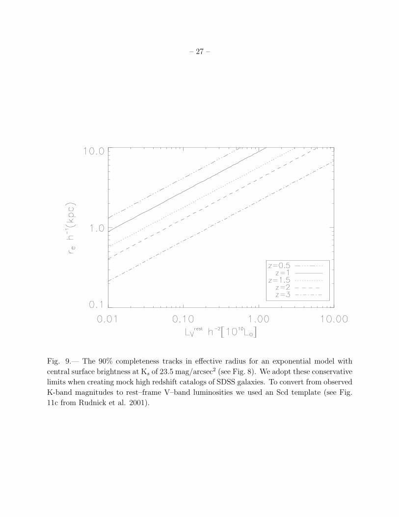
In Fig. 9 we show how our conservative SB limit translates into the 90% completeness

track in parameter plane of re and LV,rest. For a given redshift, we are less than 90% complete

for exponential galaxies with an effective radius larger than the corresponding line in Fig. 9.

Due to (1+z)4 SB dimming, redshift plays a very large role in this detectability. Similarly,

for a given luminosity the maximal disk size to which we are complete will decrease with

increasing redshift.

4. ANALYSIS

The selection effects will affect the distribution of points in Fig. 6 and make it impos-

sible to read–off any size evolution, or lack thereof, without careful modelling. We explore

evolutionary trends in the distribution of the galaxies in the above diagrams, by taking a

z=0 luminosity-size (and mass-size) relation and by drawing a mock high redshift catalogs

from these relations, subject to the redshift–dependent selection effects.

4.1. Simulating the local luminosity/mass vs. size relations at high redshifts

The Sloan Digital Sky Survey (SDSS, York et al. 2000) is providing an unprecedented

database of ∼ 106 nearby galaxies with spectroscopic redshifts and multi-band photometry.

In particular, it has been used to derive the size distribution of present–epoch galaxies

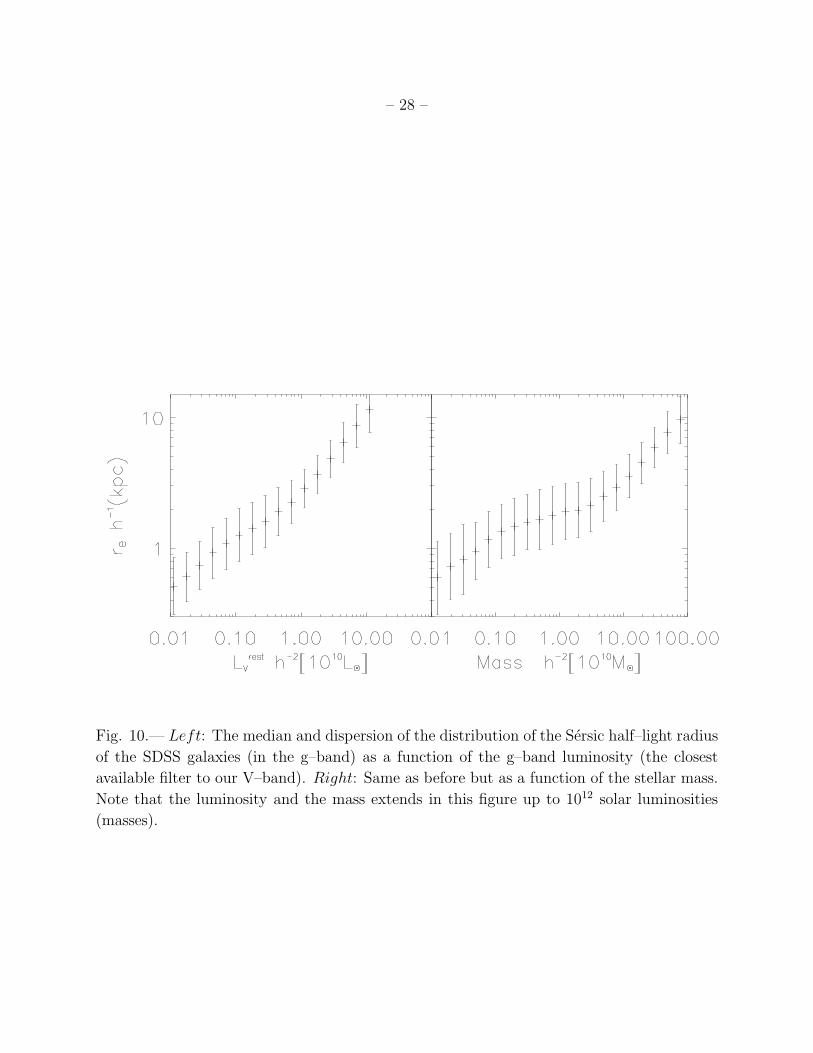
versus their luminosities and stellar masses (Shen et al. 2003). Shen et al. show the

median and dispersion of the distribution of Sersic half–light radius (Blanton et al. 2003)

for different bands as a function of the luminosity and of the stellar mass. We have used

their g–band (the closest available filter to our V–band) size distributions (S. Shen, 2003,

private communication) as a local reference of the size distribution of galaxies in the nearby

universe. We note that whereas Shen et al. show separately the distribution of early and

late–type galaxies, we use their combination of these two subsamples into one, to make a

direct comparison with our sample. For nearby galaxies of a given luminosity, Shen et al.

propose the following size log–normal distribution with median re and logarithmic dispersion

σ:

– 10 –

f(re|re(L), σ(L)) =1√

2πσ(L)e−

ln2(re/re(L))

2σ2(L)dre

re

, (3)

illustrated in Fig. 10.

The SDSS relations are used to test the null hypothesis, i.e., that the luminosity–size or

mass–size relations do not change with redshift. It is important to note that this does not

imply that the galaxies themselves do not change; they could certainly evolve ‘along’ such

a relation. To test the null hypothesis, we construct distributions of SDSS galaxies as they

would be observed at high redshift, mimicking our observations as follows: every simulated

distribution of galaxies contains the same number of objects than our FIRES sample (i.e.

168). We pick a luminosity and redshift pairs at random from our observed sample. For this

luminosity L, we evaluate a size at random from the local size sample distribution provided

by the SDSS data (Eq. 3), by solving the following implicit equation:

F (re|L) =1

2

1 − Φ( ln(re/re(L))√

2σ(L)

)

; (4)

where Φ is the error function and F(re|L) is randomly distributed in [0,1].

For every effective radius drawn from Eq. 4 we analyze if this galaxy (characterized by

re, L, z) would be observed within the completeness limit of Fig. 9. If it is larger, it is not

taken into account in our simulated distribution. The process for selecting a new galaxy is

repeated until we have a mock sample with the same number of objects as galaxies observed.

This procedures assures that the simulated galaxy distribution follows the same redshift

and luminosity distribution as the observed sample and also is affected by the same selection

effects. An analogous procedure is repeated in the case of the size–mass relation replacing

L with M⋆ in Eqs. 3 and 414. At this time, to account for the selection effects, we select a

(M/L, L, z) triplet at random from the observed distribution.

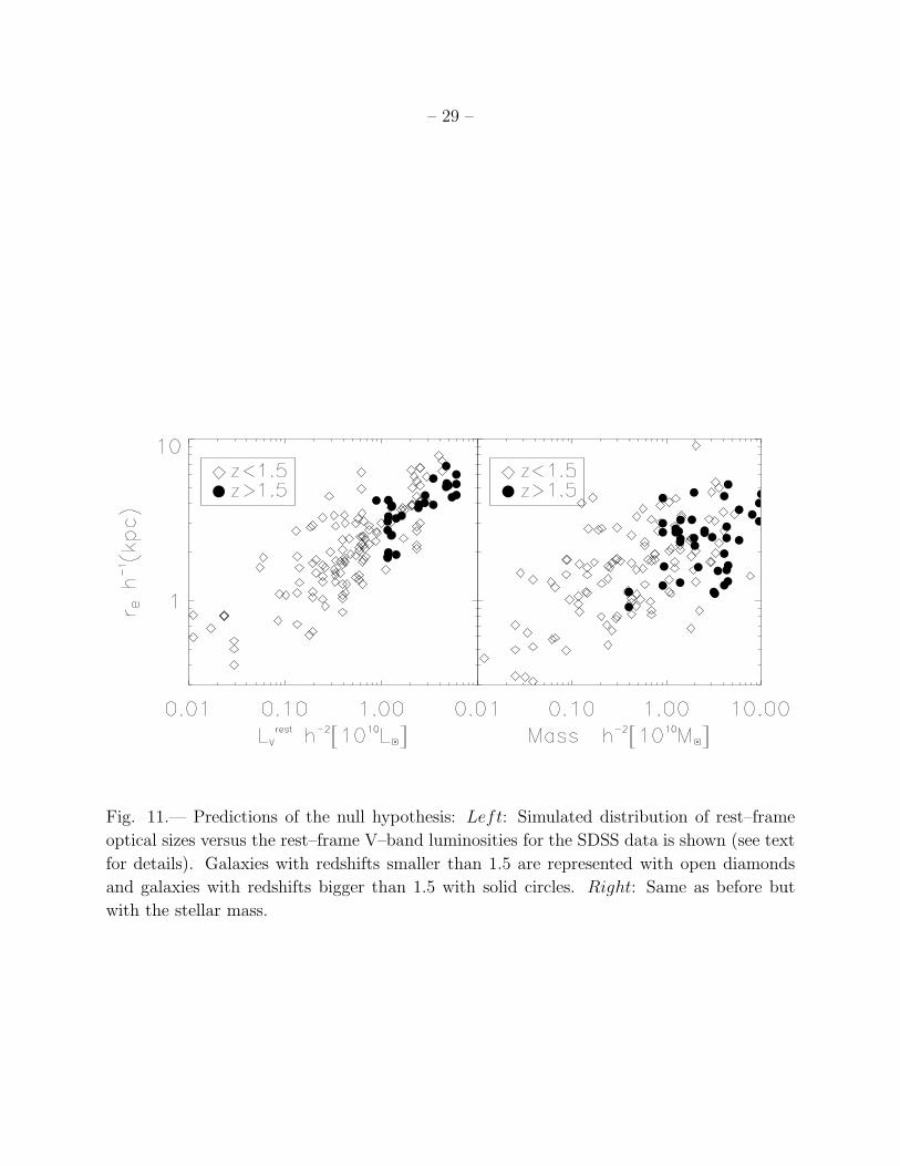
Fig. 11 shows an example of how the SDSS galaxies would be distributed in the size

diagrams with the same luminosity, mass and redshift distribution as the galaxies observed

in FIRES. A comparison of Fig. 6 and 11 shows that the simulated SDSS data have a

luminosity–size and a mass-size relation that is tighter than the observed FIRES relations.

If the luminosity–size relation from SDSS remained unchanged with increasing z, we would

14Shen et al. use also a log–normal distribution for the size–mass relation. Their mass evaluation rests in

the Kroupa (2001) IMF (Initial Mass Function). The stellar mass modelling of the FIRES data, however,

uses a Salpeter IMF. In our simulations we have followed the procedures suggested in Kauffmann et al.

(2003) of using MassIMF,Salpeter=2×MassIMF,Kroupa to transform from SDSS data to our data.

– 11 –

not expect to find small and luminous objects at high redshift, however these objects are

present in the FIRES observations (see Fig. 6).

To quantify if these qualitative differences between the observed distributions and the

simulated null hypothesis are significant, we ran the generalization of the Kolmogorov–

Smirnov (K–S) test to two–dimensional distributions (Fasano & Franceschini 1987). We

create 1000 SDSS realizations (both for luminosity and mass). For all the simulations the

rejection probability is bigger than 99.9%. Consequently, we conclude that neither the

luminosity–size nor the mass–size observed relations satisfy the null hypothesis.

To account for measurement errors in the size estimates of the FIRES galaxies, we also

create mock “FIRES” data point distributions. To create these distributions we randomly

vary every observed effective radius using a normal distribution with standard deviation equal

to the size error measured for each galaxy. We make 1000 mock “FIRES” and compare for

each the rejection probability between the SDSS and the mock “FIRES” data. The rejection

probability for all mock samples is again more than 99.9% in the luminosity and the mass

relations. So, the intrinsic dispersion of our measurements are unable to explain the difference

with the SDSS simulated data.

We also explored the sensibility of the adopted FIRES selection limits through simu-

lations: we have evaluated the SDSS DF including different central SB limit ranging from

23 to no restrictions at all. We do not find any significant difference in our results. As we

expected due to the depth of our images, uncertainties in the selection effects do not affect

our analysis.

4.2. Testing the hypothesis of evolution

The no–evolution hypothesis, that the size relations for all galaxies are redshift inde-

pendent, can be rejected both for the LV –re and M⋆–re relations. To quantify and constrain

the evolution of these relations with redshift, we need to devise an evolution model. In the

absence of clear–cut theoretical predictions, we have resorted to a heuristic parameterization

that draws on the observed local distribution. We have assumed that the log–normal size

distribution (Eq. 3) applies at all redshifts, but with evolving parameters:

re(L, z) = re(L, 0)(1 + z)−α (5)

σ(L, z) = σ(L, 0)(1 + z)β . (6)

Here, re(L, 0) and σ(L, 0) are the median size and dispersion provided at z=0 by the Shen

et al. (2003) data, and α and β describe the redshift evolution. Note that Eq. 5 and Eq 6

– 12 –

imply the same size evolution for all the galaxies independently of their luminosity. We also

assume an analogous parameterization for the masses. Both for LV –re and M⋆–re we explore

the ranges between [-2,3] for α and between [-2,2] for β.

As for the null hypothesis, we generate simulated galaxy distributions for every pair

(α, β) and we ran K–S test between these simulations and the observed data. Neither

for LV –re nor for M⋆–re could we produce evolutionary scenarios (α, β) whose distribution

functions are in agreement with what we see in the FIRES data. However, one must bear

in mind that not all the luminosities can be observed over the full redshift range (see Fig.

7). To understand better what possible evolution our data imply and to avoid luminosity

dependent redshift ranges we decided to create more homogeneous subsamples by splitting

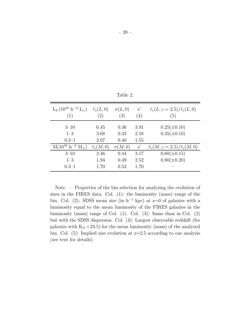
our sample in three different luminosity (mass) bins. Both our luminosity–size and mass–

size observed distributions have been divided in three luminosity (mass) bins as detailed

in Table 215. The splitting of our sample into these intervals avoids that low luminosity

(mass) galaxies at low redshift dominate the results of our analysis. The mean redshifts for

the low/intermediate/high luminosity (mass) bins are 1.0, 1.6 and 2.0, respectively. These

different sets measure evolution in a different luminosity (mass) range and a different redshift

range, and splitting them helps to make this clear.

We now can check whether the observed FIRES relations can be explained if the evo-

lutionary parameters α and β depend on the luminosity (mass), and write out the new

distribution function explicitly, combining Eqs. 5 and 6 with Eq. 3:

g(re|re, σ, z) =1√2πσ

dre

re

dz

(1 + z)βe−

ln2(re/re(1+z)α)

2σ2(1+z)2β (7)

The expression in Eq. 7 is a probability density and we use this to evaluate α and β

using a Maximum Likelihood Method. For each luminosity/mass subsample we show in Fig.

12 the likelihood contours (1σ and 2σ) in the plane of α and β. We have also included as a

reference the point α=0 and β=0 which indicates the case of no–evolution at this plane. The

top row shows the evolution of the size distribution at a given luminosity. The mean size

at a given luminosity changes significantly for luminous galaxies: at <LV >∼2×1010h−2L⊙

galaxies were typically three times smaller at z∼2.5 than now, and 4 times smaller for

LV >3×1010h−2L⊙. A luminosity independent model (α and β independent of L) is less likely

15The lowest luminosity (mass) galaxies with L<0.3×1010 L⊙ (M⋆<0.3×1010 M⊙) are not presented in

this analysis. These galaxies have z.1 and, consequently, the results coming from this subsample are largely

affected by the cosmic variance associated with the small volume enclosed in the HDF-S over this redshift

range.

– 13 –

than our luminosity dependent model, justifying our choice of three subsamples. For the sizes

at a given stellar mass the picture is qualitatively different: there is no evidence for significant

evolution of the re–M⋆ relation, except for the most massive bin, M⋆>3×1010h−2M⊙. At

<M⋆>∼2×1010h−2M⊙ the relation may only have changed by 20% since z∼2.5. The implied

size evolution at z=2.5 in each luminosity (mass) bin is summarized in Table 2. Note that

in all cases the evidence for an evolving scatter of the LV ,M⋆–re relations is marginal.

In Fig. 13, we visualize these results in a different way: we show the ratio between

the present epoch mean size for every luminosity (mass) bin and the expected mean size

as a function of redshift using the α values derived from the FIRES data (i.e. we show

re(L, z)/re(L, 0)=(1+z)−α). The same is done for the mass. This figure shows the region

enclosed by the 1σ level confidence contours. The lines stop at the limiting redshift z′ we

are able to explore for the different luminosity (mass) bins.

Again, Fig. 13 shows that high–z galaxies (most luminous bin) at z∼2.5 are more

compact (a factor of 4) than the nearby equally luminous galaxies. On the other hand,

high–z galaxies differ only slightly in size at a given mass from the present–epoch. In the

middle luminosity (mass) bin the evolution with z appears to be less important. For the LV –

re relations the dispersion of the high–z population increases in all the cases. This increase

is, however, relatively moderate (a factor of 1.2–2.). We discuss how we can understand

these results in the following section.

5. DISCUSSION

Using the observed nearby SDSS size relations (Shen et al. 2003) as the correct lo-

cal references, the observed FIRES size–luminosity and mass–size distributions at high–z

show a very different degree of evolution. The mass–size relation has remained practically

unchanged whereas, the size–luminosity has evolved significantly: there are many more com-

pact luminous objects at high–z than now. How can we re–concile these two observational

facts?

In absence of M/L evolution with time, a change in the size–luminosity relation with

z would imply the same degree of evolution in the mass–size relation. However, the mean

M/L ratio decreases with increasing z. In the nearby universe, most galaxies have large

M/L ratios (see Fig. 14 of Kauffmann et al. 2003). In contrast, FIRES galaxies at z>2,

at all luminosities, have M/L ratios of the order ∼1 (Rudnick et al. 2003b). Consequently,

although we observe a strong evolution in the luminosity–size relation, the decrease of M/L

avoids a significant change in the observed mass–size relation.

– 14 –

We can therefore characterize our observed high–z galaxy population as follows: small

to medium size objects (effective radius ∼1.5 h−1 kpc) not very massive (∼3×1010h−2M⊙)

but often very luminous (∼3×1010h−2L⊙) in the V–band. The above picture does not mean

that large galaxies can not be found at high z (Labbe et al. 2003b), but that they are

relatively rare.

Traditionally the high–z population has been selected by the Lyman Break selection

technique (Steidel & Hamilton 1993) known to select luminous unobscured star–forming

galaxies. However, dust obscured or UV–faint galaxies may have been missed. The galaxies

in FIRES are selected from very deep near infrared Ks–band imaging, and consequently,

are expected to be less affected by this problem and give a more complete mass census of

the high–z universe. In fact, the population of galaxies under study consists in part of a

red population (Franx et al. 2003), which would be largely missed by the Lyman Break

technique, but whose volume number density is estimated to be half that of LBGs at z∼3.

Hierarchical models for structure formation in a Λ dominated universe predict that LBGs

have typical half–light radii of ∼2 h−1 kpc (Mo, Mao & White 1999) in good agrement to

the size of the galaxies we are measuring and to the observed sizes for LBGs of other authors

(Giavalisco, Steidel & Macchetto 1996, Lowenthal et al. 1997). Interestingly, other authors

have observed LBGs using optical filters and, consequently, these sizes are UV sizes. The fact

that their measures and ours (which are in the optical rest–frame) do not differ significantly

could be evidence that the star formation of the LBGs is extended over the whole object16.

In fact, if we select in our sample those galaxies with LV >2×1010h−2L⊙ and z>2.5, 1/2 of

this subsample would be considered as LBGs following the Madau et al. (1996) color criteria.

We will explore the relation of UV and optical sizes in a forthcoming paper.

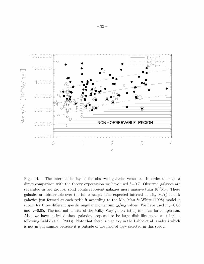
“High–redshift disks are predicted to be small and dense, and could plausibly merge

together to form the observed population of elliptical galaxies” (Mo, Mau & White 1998).

We have made a simplistic comparison between the above prediction and our data in Fig.

14. The lines represent the expected internal mass density M/r3e of disks galaxies just formed

at each redshift for three different values of the specific angular momentum. These lines are

evaluated combining the Eqs. (4) and (12) of Mo et al. (1998) and assume a constant fraction

of the mass of the halo which settles into the disk, md=0.05, and a constant spin parameter

of the halo λ=0.05. With these two assumptions the internal mass density increases with z

as the square of the Hubble constant H(z).

Galaxies more massive than 1010M⊙ are observable over the complete range in redshift.

16There is some evidence that the LBGs morphology depends not much on the wavelength, remaining

essentially unchanged from the far-UV to the optical window (Giavalisco 2002 and references therein).

– 15 –

The measured mean internal density for this galaxy population appears to evolve only slightly

with z, in agreement with the lack of strong evolution in the size–mass relation. If all the

galaxies present in Fig. 14 were disks, their distribution would not be compatible with the

theoretical expectation. However, we must take into account that we are observing a mix

of galaxy types and not only disk galaxies. In order to address this point we have made

a visual galaxy classification of all the objects with z<1.5 and mass larger than 1010M⊙.

We can do that because of the high–resolution of the HST images in the I814–band filter.

This examination showed that the dense objects (M/r3e >1010M⊙/kpc3) with z<1.5 appear

to be all ellipticals and that the late type fraction appears to increase as one moves to lower

density objects. Unfortunately, we cannot make a similar analysis for z>1.5 and the question

of whether the high density objects we observe there are disk dominated remains unsolved.

However, it is highly tempting to propose that our high z dense population could be the

progenitors of the nearby dense elliptical galaxies.

Independently of the nature of the LBGs and of the red population it is clear that in

order to reach the mass and sizes of the nearby galaxies an evolutionary process must be

acting on the high–z population. Recently, Shen et al. have proposed, for the early–type

galaxies, a simple model of mass and size evolution based on subsequent major mergers.

This model explains the observed relations for these kind of galaxies between mass and size

in the SDSS data, i.e. R∝M0.56. In the Shen et al. picture two galaxies with the same mass

(M1=M2) and radius (R1=R2) merge forming a new galaxy with mass M=2M1 and radius

R=20.56R1. If this process is repeated p times: M=2pM1 and R=20.56pR1. If we take a galaxy

at z=3 (following our mass and size estimates) with M1=3×1010h−2M⊙ and R1=1.5h−1 kpc

this implies that after 3 major mergers M=24×1010h−2M⊙ and R=4.8 h−1 kpc, in excellent

agreement to the values we see in nearby galaxies (M=24×1010h−2M⊙ and R=5 h−1 kpc, see

Fig. 10). These numbers may suggest that the massive and dense high–z population can be

understood as the progenitors of the bright and massive nearby early type galaxies.

6. SUMMARY

Using ultra–deep near–infrared images of the HDF-S we have analyzed the rest–frame

optical band sizes of a sample of galaxies selected down to Ks=23.5. This has allowed us to

measure the evolution of the luminosity–size and mass–size relation out to z∼3. This is the

first time that the rest–frame V–band sizes of such distant galaxies have been systematically

analyzed as a function of stellar luminosity and stellar mass.

We compared our observed luminosity–size and mass–size relations to those measured

in the nearby universe by the SDSS data (Shen et al. 2003). For this comparison we have

– 16 –

analyzed in detail the detectability effects that high–z observations impose on the observed

relations. From this comparison, assumming the Shen et al. distributions are correct, we

found:

1. The size–luminosity relation has evolved since z∼2.5. Luminous objects (LV ∼3×1010h−2L⊙)

at z∼2.5 are 4 times smaller than equally luminous galaxies today.

2. The size–stellar mass relation has remained nearly constant since z∼2.5: for <M⋆>∼2×1010h−2M⊙

the change is 20(±20)%; for stellar masses larger than 3×1010h−2M⊙ the characteristic

mean size change is 40(±15)%.

The above results are reconciled by the fact the M/L values of high–z galaxies are lower

than nowadays <M/L>∼1 (Rudnick et al. 2003b). Consequently, the brightest high–z

galaxies are a group composed of a high internal luminosity density population but with

a mean internal stellar mass density not much higher than found in the nearby universe.

The observed small sizes of distant galaxies found here and in previous studies for LBGs

(Giavalisco, Steidel & Maccheto 1996; Lowenthal et al. 1997; Ferguson et al. 2003) are in

agreement with the small evolution of the mass–size relation because the typical masses of

z=3 galaxies are substantially smaller than those at low redshift.

We are happy to thank Shiyin Shen for providing us with the Sloan Digital Sky Survey

data used in this paper and Boris Haußler for running GALFIT. We thank the staff at ESO

for the assistance in obtaining the FIRES data and the the Lorentz Center for its hospitality

and support. We also thank the anonymous referee for useful comments.

Funding for the creation and distribution of the SDSS Archive has been provided by

the Alfred P. Sloan Foundation, the Participating Institutions, the National Aeronautics

and Space Administration, the National Science Foundation, the US Department of En-

ergy, the Japanese Monbukagakusho, and the Max-Planck Society. The SDSS Web site

is http://www.sdss.org. The SDSS is managed by the Astrophysical Research Consortium

(ARC) for the Participating Institutions. The Participating Institutions are the University

of Chicago, Fermilab, the Institute for Advanced Study, the Japan Participation Group,

Johns Hopkins University, Los Alamos National Laboratory, the Max-Planck-Institut fur

Astronomie (MPIA), the Max-Planck-Institut fur Astrophysik (MPA), New Mexico State

University, University of Pittsburgh, Princeton University, the US Naval Observatory, and

the University of Washington.

– 17 –

REFERENCES

Aguerri, J.A.L. & Trujillo, I., 2002, MNRAS, 333, 633

Avila–Reese, V & Firmani, C., 2001, RevMexAA, 10, 97

Baugh, C. M., Cole, S., Frenk, C. S., & Lacey, C. G. 1998, ApJ, 498, 504

Blanton, M. et al., 2003, ApJ, 592, 819

Bell, E. F. & de Jong, R. S., 2001, ApJ, 550, 212

Casertano, S., Ratnatunga, K. U., Griffiths, R. E., Im, M., Neuschaefer, L. W., Ostrander,

E. J. & Windhorst, R. A., 1995, ApJ, 453 ,599

Casertano, S. et al. 2000, AJ, 122, 2205

Franx, M. et al., ”FIRES at the VLT: the Faint Infrared Extragalactic Survey”, The Mes-

senger 99, pp. 20–22, 2000

Franx, M. et al., 2003, ApJL, 587, L79

Fasano, G.& Franceschini, A., 1987, MNRAS, 225, 155

Ferguson et al. 2003, ApJL, in press

Giavalisco, M., Steidel C.C. & Macchetto, F.D., 1996, ApJ, 470, 189

Giavalisco, M.,2002, ARA&A, 40, 579

Kauffmann, G., et al., 2003, MNRAS, 341, 33

Kroupa, P., 2001, MNRAS, 322, 231

Labbe, I.F.L. et al., 2003, AJ, 125, 1107

Labbe, I.F.L. et al., 2003b, ApJ, 591, L95

Lilly, S. et al. 1998, ApJ, 500, 75

Lowenthal, J.D., Koo, D.C., Guzman, R., Gallego, J., Phillips, A.C., Faber, S.M., Vogt,

N.P., Illingworth G.D., 1997, ApJ, 481, 67

Madau, P., Ferguson, H.C., Dickinson, M.E., Giavalisco, M., Steidel, C.C. & Fruchter, A.,

1996, MNRAS, 283, 1388

Mao, S., Mo, H. J.& White, S.D.M., 1998, MNRAS, 297, L71

Mo, H. J., Mao, S. & White, S.D.M., 1999, MNRAS, 304, 175

Moorwood, A. F. 1997, Proc. SPIE, 2871, 1146

Peng, C.Y., Ho, L.C., Impey, C.D. & Rix, H.W., 2002, AJ, 124, 266

– 18 –

Press, W.H., Teukolsky, S.A., Vetterling, W.T. & Flannery, B.P., 1992, Numerical Recipes

(Cambridge: Cambridge Univ. Press)

Roche, N., Ratnatunga, K., Griffiths, R. E., Im, M. & Naim, A., 1998, MNRAS, 293, 157

Rudnick, G. et al., 2001, AJ, 122, 2205

Rudnick, G. et al., 2003a, ApJ, in press, astro-ph/0307149

Rudnick, G. et al., 2003b, in preparation

Saglia, R. P., Bertschinger, E., Baggley, G., Burstein, D., Colless, M., Davies, R. L., McMa-

han, R. K., Wegner, G. 1997, ApJS, 109, 79

Sersic, J.-L. 1968, Atlas de Galaxias Australes (Cordoba: Ob servatorio Astronomico)

Shen, S., Mo, H.J., White, S.D.M., Blanton, M.R., Kauffmann, G., Voges, W., Brinkmann,

J. & Csabai, I., MNRAS, 2003, 343, 978

Smail, I., Hogg, D. W., Yan, L, Cohen, J. G., 1995, ApJ, 449, L105

Somerville, R. S., Primack, J. R., & Faber, S. M. 2001, MNRAS, 320, 504

Steidel, C.C. & Hamilton, D., 1993, AJ, 105, 2017

Steidel C.C., Giavalisco, M., Pettini, M., Dickinson, M., & Adelberger, K. L., 1996, ApJ,

462, L17

Trujillo, I., Aguerri, J.A.L., Gutierrez, C.M., & Cepa, J., 2001, AJ, 122, 38

Trujillo, I., Graham, A. W., & Caon, N., 2001, MNRAS, 326, 869

York D. et al., 2000, AJ, 120, 1579

This preprint was prepared with the AAS LATEX macros v5.0.

– 19 –

Fig. 1.— A mosaic of similar rest–frame V–band luminosities galaxies at different redshifts.

The apparent K-band magnitude decreases towards the bottom. The luminosities are given

in 1010 solar luminosities. The galaxies are shown in four different filters.

– 20 –

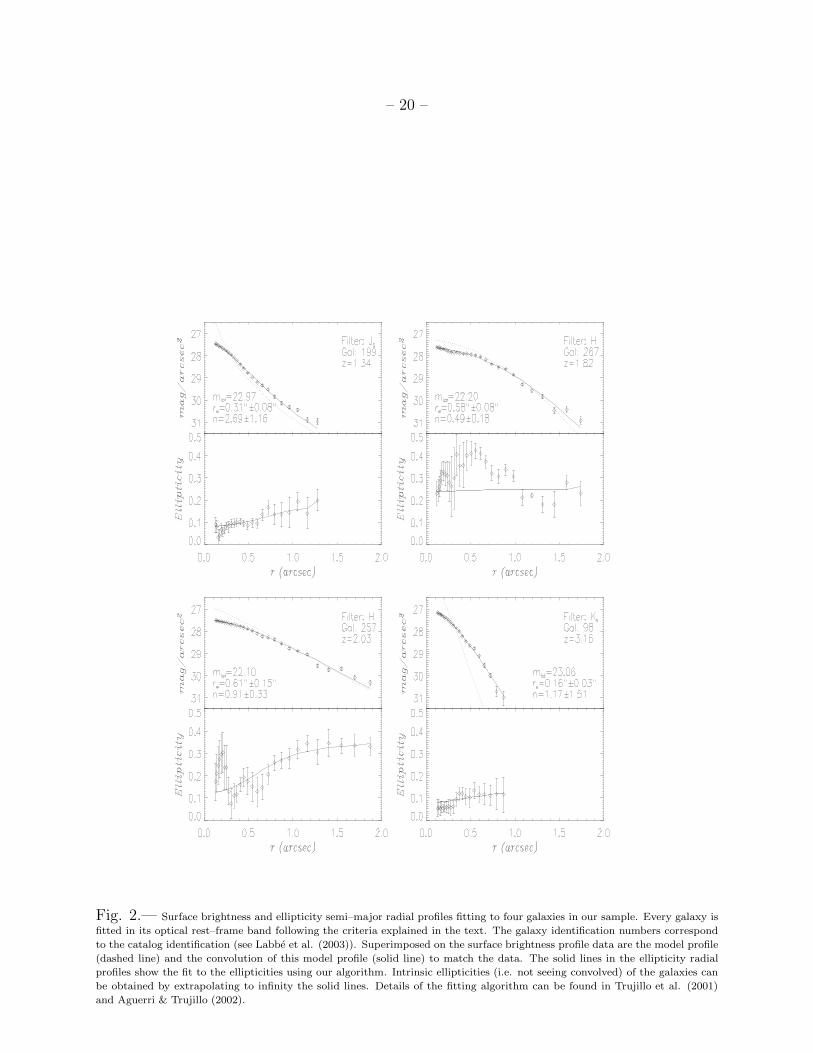
Fig. 2.— Surface brightness and ellipticity semi–major radial profiles fitting to four galaxies in our sample. Every galaxy is

fitted in its optical rest–frame band following the criteria explained in the text. The galaxy identification numbers correspond

to the catalog identification (see Labbe et al. (2003)). Superimposed on the surface brightness profile data are the model profile

(dashed line) and the convolution of this model profile (solid line) to match the data. The solid lines in the ellipticity radial

profiles show the fit to the ellipticities using our algorithm. Intrinsic ellipticities (i.e. not seeing convolved) of the galaxies can

be obtained by extrapolating to infinity the solid lines. Details of the fitting algorithm can be found in Trujillo et al. (2001)

and Aguerri & Trujillo (2002).

– 21 –

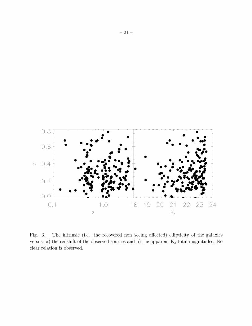
Fig. 3.— The intrinsic (i.e. the recovered non–seeing affected) ellipticity of the galaxies

versus: a) the redshift of the observed sources and b) the apparent Ks total magnitudes. No

clear relation is observed.

– 22 –

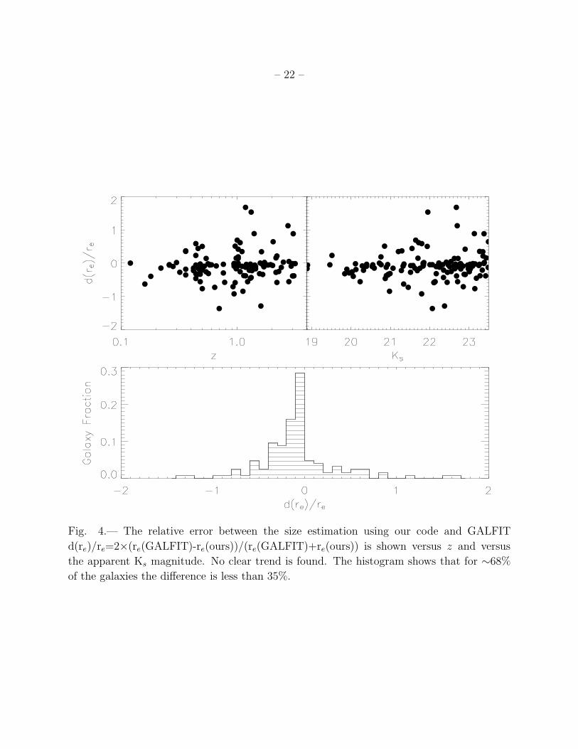
Fig. 4.— The relative error between the size estimation using our code and GALFIT

d(re)/re=2×(re(GALFIT)-re(ours))/(re(GALFIT)+re(ours)) is shown versus z and versus

the apparent Ks magnitude. No clear trend is found. The histogram shows that for ∼68%

of the galaxies the difference is less than 35%.

– 23 –

Fig. 5.— The total magnitude retrieved from the model fitting is compared to the total

magnitude measured in a model independent way for the galaxies analyzed in this paper.

Galaxies with n<1.5 are represented with solid circles and galaxies with n>1.5 with open

diamonds.

– 24 –

Fig. 6.— Left: The distribution of rest–frame optical sizes versus the rest–frame V–band

luminosities is shown. Galaxies with redshifts smaller than 1.5 are represented with open

diamonds and galaxies with redshifts bigger than 1.5 with solid circles. Right: Same as

before but with the stellar mass. For clarity error bars are not shown. The mean size

relative error is 35%.

– 25 –

Fig. 7.— The LV –z diagram for the objects selected in our sample with Ks <23.5. The track

represent the values of LrestV for a Scd template spectra (see Rudnick et al. (2001); Figure

11c) normalized at each redshift to Ks,AB=23.5.

– 26 –

Fig. 8.— A completeness map for detecting galaxies with exponential profiles in the FIRES

K–band data. The horizontal and vertical axis represent the input values. Overplotted is

the Ks–band size versus the apparent Ks magnitude for the objects in our sample (open

points). We have also shown exponential models (n=1) with central surface brightness of 23

and 24 mag/arcsec2 (dotted lines). The solid line represents the central surface brightness

(µK(0)=23.5 mag/arcsec2) at which we are 90% complete.

– 27 –

Fig. 9.— The 90% completeness tracks in effective radius for an exponential model with

central surface brightness at Ks of 23.5 mag/arcsec2 (see Fig. 8). We adopt these conservative

limits when creating mock high redshift catalogs of SDSS galaxies. To convert from observed

K-band magnitudes to rest–frame V–band luminosities we used an Scd template (see Fig.

11c from Rudnick et al. 2001).

– 28 –

Fig. 10.— Left: The median and dispersion of the distribution of the Sersic half–light radius

of the SDSS galaxies (in the g–band) as a function of the g–band luminosity (the closest

available filter to our V–band). Right: Same as before but as a function of the stellar mass.

Note that the luminosity and the mass extends in this figure up to 1012 solar luminosities

(masses).

– 29 –

Fig. 11.— Predictions of the null hypothesis: Left: Simulated distribution of rest–frame

optical sizes versus the rest–frame V–band luminosities for the SDSS data is shown (see text

for details). Galaxies with redshifts smaller than 1.5 are represented with open diamonds

and galaxies with redshifts bigger than 1.5 with solid circles. Right: Same as before but

with the stellar mass.

– 30 –

Fig. 12.— Likelihood contours representing the evolution in size and dispersion in the α–β

plane. The top (bottom) row shows the evolution of the luminosity–size (mass–size) relation.

Solid line represents the 1σ confidence level contour, dashed line the 2σ confidence level.

The cross shows the position of no–evolution in this plane. Positive values of α represent

decreasing values of the size with redshift. Positive values of β represent increasing the

instrinsic dispersion σ of the population with redshift. Both the luminosity and the mass

are in units of 1010 solar value. Both the no evolution model and a luminosity independent

evolution model are less likely than the luminosity dependent model.

– 31 –

Fig. 13.— The ratio between the SDSS mean size and the expected mean size as a function

of z is shown both for the luminosity and for mass relations. Both the luminosity and the

mass are in units of 1010 solar value. Equal style lines enclose the 1σ variation.

– 32 –

Fig. 14.— The internal density of the observed galaxies versus z. In order to make a

direct comparison with the theory expectation we have used h=0.7. Observed galaxies are

separated in two groups: solid points represent galaxies more massive than 1010M⊙. These

galaxies are observable over the full z range. The expected internal density M/r3e of disk

galaxies just formed at each redshift according to the Mo, Mau & White (1998) model is

shown for three different specific angular momentum jd/md values. We have used md=0.05

and λ=0.05. The internal density of the Milky Way galaxy (star) is shown for comparison.

Also, we have encircled those galaxies proposed to be large disk–like galaxies at high–z

following Labbe et al. (2003). Note that there is a galaxy in the Labbe et al. analysis which

is not in our sample because it is outside of the field of view selected in this study.

– 33 –

Table 1.

Galaxy X Y Ks,tot re ǫ LV (1010 h−2 L⊙) M(1010 h−2 M⊙) z Filter

793 3538.3 3496.9 21.33 0.04 0.10 0.01 0.01 0.140 I814244 2272.6 1587.5 20.71 0.40 0.67 0.06 0.09 0.173a I814283 2063.5 1660.1 23.34 0.51 0.62 0.01 0.01 0.180 I814314 2741.5 1815.3 21.61 0.24 0.08 0.02 0.02 0.220 I814288 501.6 1633.9 23.23 0.39 0.09 0.01 0.02 0.280 I814464 943.0 2017.5 20.76 0.30 0.44 0.11 0.20 0.280 I814227 1393.0 1430.0 21.51 0.60 0.35 0.12 0.17 0.320 I814184 626.9 1387.0 18.89 0.55 0.21 0.75 1.92 0.340a I814446 2417.6 2080.2 20.05 0.56 0.36 0.39 1.11 0.364a I814528 2478.4 3018.5 20.53 0.71 0.64 0.28 0.42 0.365a I81453 2954.6 522.7 23.26 0.14 0.23 0.02 0.03 0.380 I814663 3106.0 3832.1 21.28 0.17 0.08 0.19 0.26 0.414a I814763 1258.2 3079.6 19.89 0.76 0.15 0.56 0.96 0.415a I814138 3709.8 1029.9 19.83 0.14 0.40 0.48 4.08 0.420 I814189 1678.4 1190.2 23.00 0.64 0.56 0.06 0.07 0.420 I814256 1619.2 1632.0 21.84 0.54 0.26 0.17 0.16 0.423a I814307 3037.7 1762.6 21.79 0.43 0.29 0.15 0.27 0.440 I814374 1205.1 2466.3 22.80 0.13 0.22 0.03 0.16 0.440 I81429 3817.2 486.8 20.58 0.34 0.24 0.64 0.48 0.460 I81475 2162.5 727.1 23.14 0.94 0.05 0.08 0.06 0.460 I814708 2656.4 3737.6 21.27 0.75 0.20 0.35 0.30 0.460 I814292 781.1 1876.3 18.88 0.86 0.48 1.15 4.03 0.464a I81487 459.7 700.5 23.26 0.29 0.30 0.05 0.05 0.480 I81495 3873.2 715.5 23.33 0.11 0.30 0.05 0.03 0.480 I814344 3579.9 2599.2 22.78 0.42 0.50 0.10 0.07 0.480 I814415 2401.5 2278.5 21.34 0.30 0.21 0.18 0.56 0.480 I814442 3236.2 2130.7 22.46 0.54 0.34 0.12 0.11 0.480 I814459 3410.0 2059.1 23.14 0.19 0.17 0.08 0.03 0.480 I814544 1405.0 2923.0 21.51 0.51 0.63 0.16 0.32 0.480 I814673 2131.5 3486.8 22.87 0.24 0.49 0.09 0.06 0.480 I814758 2271.3 3535.7 20.12 0.24 0.23 0.47 2.57 0.480 I814

– 34 –

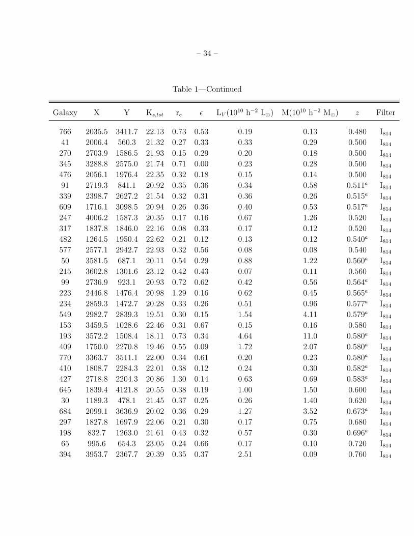
Table 1—Continued

Galaxy X Y Ks,tot re ǫ LV (1010 h−2 L⊙) M(1010 h−2 M⊙) z Filter

766 2035.5 3411.7 22.13 0.73 0.53 0.19 0.13 0.480 I81441 2006.4 560.3 21.32 0.27 0.33 0.33 0.29 0.500 I814270 2703.9 1586.5 21.93 0.15 0.29 0.20 0.18 0.500 I814345 3288.8 2575.0 21.74 0.71 0.00 0.23 0.28 0.500 I814476 2056.1 1976.4 22.35 0.32 0.18 0.15 0.14 0.500 I81491 2719.3 841.1 20.92 0.35 0.36 0.34 0.58 0.511a I814339 2398.7 2627.2 21.54 0.32 0.31 0.36 0.26 0.515a I814609 1716.1 3098.5 20.94 0.26 0.36 0.40 0.53 0.517a I814247 4006.2 1587.3 20.35 0.17 0.16 0.67 1.26 0.520 I814317 1837.8 1846.0 22.16 0.08 0.33 0.17 0.12 0.520 I814482 1264.5 1950.4 22.62 0.21 0.12 0.13 0.12 0.540a I814577 2577.1 2942.7 22.93 0.32 0.56 0.08 0.08 0.540 I81450 3581.5 687.1 20.11 0.54 0.29 0.88 1.22 0.560a I814215 3602.8 1301.6 23.12 0.42 0.43 0.07 0.11 0.560 I81499 2736.9 923.1 20.93 0.72 0.62 0.42 0.56 0.564a I814223 2446.8 1476.4 20.98 1.29 0.16 0.62 0.45 0.565a I814234 2859.3 1472.7 20.28 0.33 0.26 0.51 0.96 0.577a I814549 2982.7 2839.3 19.51 0.30 0.15 1.54 4.11 0.579a I814153 3459.5 1028.6 22.46 0.31 0.67 0.15 0.16 0.580 I814193 3572.2 1508.4 18.11 0.73 0.34 4.64 11.0 0.580a I814409 1750.0 2270.8 19.46 0.55 0.09 1.72 2.07 0.580a I814770 3363.7 3511.1 22.00 0.34 0.61 0.20 0.23 0.580a I814410 1808.7 2284.3 22.01 0.38 0.12 0.24 0.30 0.582a I814427 2718.8 2204.3 20.86 1.30 0.14 0.63 0.69 0.583a I814645 1839.4 4121.8 20.55 0.38 0.19 1.00 1.50 0.600 I81430 1189.3 478.1 21.45 0.37 0.25 0.26 1.40 0.620 I814684 2099.1 3636.9 20.02 0.36 0.29 1.27 3.52 0.673a I814297 1827.8 1697.9 22.06 0.21 0.30 0.17 0.75 0.680 I814198 832.7 1263.0 21.61 0.43 0.32 0.57 0.30 0.696a I81465 995.6 654.3 23.05 0.24 0.66 0.17 0.10 0.720 I814394 3953.7 2367.7 20.39 0.35 0.37 2.51 0.09 0.760 I814

– 35 –

Table 1—Continued

Galaxy X Y Ks,tot re ǫ LV (1010 h−2 L⊙) M(1010 h−2 M⊙) z Filter

610 1674.7 3067.4 19.95 0.84 0.28 1.66 3.46 0.760a I814768 2591.1 3492.9 23.36 0.30 0.67 0.13 0.08 0.760 I814774 2782.2 3544.1 22.43 0.39 0.43 0.33 0.19 0.800 I814777 1520.1 3463.8 22.06 0.34 0.24 0.60 0.25 0.800 I814306 1129.4 1783.3 22.85 0.43 0.70 0.42 0.20 0.940 Js

337 3929.8 2643.0 21.82 0.39 0.08 1.08 0.74 0.940 Js

638 2661.3 4089.3 23.02 0.28 0.42 0.24 0.12 0.940 Js

795 1214.5 3434.2 23.37 0.24 0.32 0.21 0.10 0.940 Js

64 2166.0 660.9 22.25 0.28 0.10 0.54 0.48 0.960 Js

268 1288.8 1574.3 22.10 0.09 0.15 0.37 1.83 0.960 Js

367 3558.3 2506.5 23.23 0.60 0.16 0.27 0.18 0.960 Js

429 581.0 2211.8 21.79 0.75 0.73 0.82 0.68 0.970a Js

97 3335.8 784.7 20.85 0.10 0.02 2.08 5.25 0.980 Js

301 1390.5 1700.6 23.15 0.22 0.26 0.24 0.14 0.980 Js

326 1654.8 2678.6 22.16 0.19 0.11 0.40 1.77 0.980 Js

420 2836.4 2263.4 21.69 0.15 0.14 0.61 3.02 0.980 Js

691 3374.1 3822.9 22.63 0.24 0.23 0.39 0.39 0.980 Js

608 3122.9 4270.2 22.18 0.41 0.22 0.61 0.42 1.000 Js

665 2535.8 3888.0 21.64 0.44 0.42 0.70 3.58 1.000 Js

224 2397.5 1376.9 21.82 0.24 0.24 0.56 1.08 1.020 Js

753 2850.8 3602.0 22.89 0.22 0.17 0.41 0.29 1.020 Js

10008 342.7 1274.3 22.32 0.19 0.38 0.32 1.05 1.040 Js

152 1123.2 994.5 23.00 0.40 0.35 0.43 0.31 1.060 Js

241 2508.8 1585.0 21.71 0.46 0.36 0.74 1.56 1.060 Js

79 3159.3 746.3 21.48 0.46 0.44 1.24 1.38 1.080 Js

18 1361.7 404.4 21.20 0.30 0.11 1.09 3.28 1.100 Js

249 2222.5 1495.3 22.59 0.55 0.28 0.29 0.63 1.100 Js

565 2534.7 2935.8 20.75 0.47 0.32 2.31 2.92 1.114a Js

686 2474.7 3767.0 21.06 0.33 0.19 1.57 2.82 1.116a Js

493 271.4 1901.0 20.97 0.74 0.40 1.60 2.02 1.120 Js

45 3166.5 573.0 20.89 0.28 0.01 2.04 4.08 1.140 Js

– 36 –

Table 1—Continued

Galaxy X Y Ks,tot re ǫ LV (1010 h−2 L⊙) M(1010 h−2 M⊙) z Filter

206 3136.3 1280.3 22.71 0.36 0.25 0.67 0.33 1.152a Js

276 2216.7 1691.8 20.89 0.27 0.20 2.00 6.13 1.160 Js

644 3261.3 3967.9 22.67 0.21 0.00 0.40 2.24 1.160 Js

669 2412.0 3968.5 23.27 0.47 0.06 0.46 0.23 1.200 Js

404 3693.2 2330.4 22.75 0.41 0.26 0.65 0.59 1.220 Js

27 956.2 585.7 20.22 1.07 0.08 4.25 8.05 1.230a Js

251 765.4 1492.1 22.79 0.30 0.77 0.54 0.70 1.240 Js

254 2579.9 1701.3 20.31 0.27 0.13 4.96 7.81 1.270a Js

101 1314.3 781.9 22.23 0.35 0.35 1.21 1.43 1.280 Js

149 2849.3 951.4 23.18 0.23 0.16 0.29 0.74 1.280 Js

470 2606.8 1988.5 20.39 0.52 0.03 3.93 6.13 1.284a Js

502 1804.0 1838.1 23.20 0.46 0.66 0.33 0.47 1.300 Js

771 3494.8 3469.8 22.85 0.58 0.43 0.45 0.69 1.300 Js

145 1432.7 983.2 22.34 0.71 0.32 0.74 1.00 1.320 Js

395 2926.7 2377.6 22.65 0.24 0.13 0.90 0.85 1.320 Js

637 2746.6 4100.2 21.94 0.27 0.48 1.68 1.81 1.320 Js

199 1544.7 1257.0 21.68 0.31 0.18 1.29 6.27 1.340 Js

791 2767.9 3454.1 22.97 0.33 0.47 0.58 0.58 1.360 Js

437 3508.0 2173.2 23.15 0.51 0.52 0.58 0.58 1.380 Js

201 3955.7 1215.0 22.96 0.32 0.18 0.99 0.64 1.400 Js

408 1297.5 2325.2 23.08 0.17 0.20 0.75 0.56 1.400 Js

785 3438.1 3196.3 21.57 0.43 0.23 2.16 3.33 1.400 Js

751 2004.1 3687.6 23.13 0.21 0.13 0.69 0.80 1.420 Js

302 770.9 1799.8 21.55 0.94 0.10 2.94 3.36 1.439a Js

61 3804.3 592.7 23.02 0.34 0.25 0.58 0.68 1.440 Js

783 2674.2 3530.1 22.50 0.26 0.19 0.86 1.21 1.440 Js

10001 2954.3 782.1 21.53 0.59 0.24 2.50 3.16 1.440 Js

781 1304.1 3494.1 22.72 0.53 0.53 1.08 0.75 1.480 Js

620 1876.8 3623.2 22.16 0.29 0.12 2.27 1.48 1.558a H

628 3265.9 4251.8 22.37 0.13 0.10 1.15 3.18 1.580 H

675 1836.0 3395.8 22.22 0.32 0.18 1.61 2.17 1.600 H

– 37 –

Table 1—Continued

Galaxy X Y Ks,tot re ǫ LV (1010 h−2 L⊙) M(1010 h−2 M⊙) z Filter

724 2272.9 3717.9 23.34 0.17 0.37 0.56 0.75 1.620 H

583 3745.2 3064.7 22.90 0.12 0.19 0.88 4.36 1.640 H

349 1064.0 2559.4 23.17 0.40 0.28 1.06 0.51 1.680 H

233 1148.6 1369.4 23.38 0.07 0.44 1.03 0.70 1.720 H

754 2616.4 3525.4 23.16 0.26 0.36 0.73 1.80 1.760 H

267 966.0 1628.1 21.83 0.58 0.26 3.42 3.39 1.820 H

810 3062.8 3348.3 22.80 0.14 0.12 1.17 2.69 1.920 H

600 1843.5 3658.4 22.32 0.52 0.33 2.94 3.49 1.960 H

500 2364.1 1852.0 23.24 0.15 0.54 0.89 1.91 2.020 H

290 696.4 1684.2 21.95 0.27 0.11 4.66 2.54 2.025a H

257 3011.6 1696.2 22.10 0.61 0.43 3.75 2.27 2.027a H

21 2416.4 406.0 23.49 0.20 0.54 1.15 0.39 2.040 H

96 375.0 716.1 23.35 0.30 0.57 1.40 0.56 2.060 H

776 3562.4 3421.4 22.44 0.21 0.16 2.82 1.96 2.077a H

173 572.9 1026.0 23.23 0.35 0.23 1.41 0.86 2.140 H

496 373.2 1877.0 22.40 0.21 0.13 2.40 4.49 2.140 H

729 3327.2 3768.1 22.73 0.38 0.31 2.51 0.91 2.140 H

143 779.7 969.2 23.37 0.48 0.34 1.41 0.94 2.160 H

242 1139.5 1425.8 23.43 0.25 0.17 1.25 0.55 2.160 H

219 3888.0 1291.8 23.35 0.35 0.62 1.27 1.35 2.200 H

375 1210.7 2405.4 22.79 0.47 0.21 2.01 3.14 2.240 H

767 3297.6 3622.1 22.54 0.17 0.41 3.06 10.1 2.300 H

161 2577.8 985.6 23.42 0.10 0.40 1.30 5.55 2.340 H

591 3936.8 3251.8 19.56 0.18 0.16 1.49 0.94 2.400 H

176 722.5 1089.1 22.92 0.46 0.24 2.79 4.11 2.500 H

363 537.5 2521.3 22.41 0.78 0.24 4.72 2.00 2.500 H

10006 3127.6 985.8 23.32 0.18 0.23 2.43 1.41 2.652a Ks

656 2535.7 4060.5 22.69 0.68 0.21 4.21 15.2 2.740 Ks

452 567.0 2083.6 22.84 0.31 0.57 4.13 3.06 2.760 Ks

806 3266.3 3256.9 22.67 0.26 0.30 4.91 1.76 2.789a Ks

807 3305.0 3263.3 22.70 0.45 0.14 4.86 1.86 2.790a Ks

– 38 –

Table 1—Continued

Galaxy X Y Ks,tot re ǫ LV (1010 h−2 L⊙) M(1010 h−2 M⊙) z Filter

657 3370.9 4068.2 22.53 0.57 0.26 5.94 3.51 2.793a Ks

294 382.4 1662.5 23.34 0.49 0.10 2.81 1.95 2.820 Ks

453 3945.9 2085.7 23.27 0.24 0.12 2.99 8.15 2.900 Ks

534 3452.7 2959.4 22.78 0.28 0.31 5.35 4.52 3.000 Ks

494 2562.2 1910.4 22.99 0.93 0.31 4.47 2.28 3.000 Ks

465 360.7 2029.8 23.37 0.14 0.71 3.13 3.27 3.040 Ks

397 2460.0 2379.0 23.41 0.32 0.46 3.17 5.91 3.080 Ks

448 2508.9 2111.6 23.46 0.16 0.41 2.78 1.25 3.140 Ks

622 3299.0 4292.6 23.07 0.24 0.37 3.90 1.95 3.140 Ks

98 4055.0 718.8 23.09 0.16 0.16 4.65 9.66 3.160 Ks

624 3738.7 4243.9 23.19 0.21 0.16 4.22 9.01 3.160a Ks

813 2779.1 3315.0 23.31 0.29 0.43 3.14 1.39 3.240 Ks

80 2926.6 703.1 22.71 0.40 0.11 8.88 3.71 3.840 Ks

Note. — Col. (1): Catalog identification numbers (see Labbe et al. 2003). Col. (2) and (3): X

and Y pixel coordinate positions in the HDF–S mosaic. Col (4): Ks–band total magnitudes. Col. (5):

Circularized restframe half–light radii (arcsec). The typical uncertainty on the size determination is

35%. Col (6): intrinsic (i.e. the recovered non–seeing affected) ellipticity. Col (7): Restframe V–band

luminosity. The typical uncertainty on the luminosity determination is 30%. Col (8): Stellar mass.

Col (9): redshift (the index a mean spectroscopic z). Col (10): Filter used to measure the size of the

galaxies

– 39 –

Table 2.

LV (1010 h−2 L⊙) re(L, 0) σ(L, 0) z’ re(L, z = 2.5)/re(L, 0)

(1) (2) (3) (4) (5)

3–10 6.45 0.36 3.91 0.25(±0.10)

1–3 3.68 0.33 2.58 0.35(±0.10)

0.3–1 2.07 0.40 1.55 –

M(1010 h−2 M⊙) re(M, 0) σ(M, 0) z’ re(M, z = 2.5)/re(M, 0)

3–10 2.46 0.44 3.17 0.60(±0.15)

1–3 1.94 0.49 2.52 0.80(±0.20)

0.3–1 1.70 0.52 1.70 –

Note. — Properties of the bin selection for analyzing the evolution of

sizes in the FIRES data. Col. (1): the luminosity (mass) range of the

bin. Col. (2): SDSS mean size (in h−1 kpc) at z∼0 of galaxies with a

luminosity equal to the mean luminosity of the FIRES galaxies in the

luminosity (mass) range of Col. (1). Col. (3): Same than in Col. (2)

but with the SDSS dispersion. Col. (4): Largest observable redshift (for

galaxies with KS <23.5) for the mean luminosity (mass) of the analyzed

bin. Col. (5): Implied size evolution at z=2.5 according to our analysis

(see text for details).