Effect of primordial non-Gaussianities on the far-UV luminosity function of high-redshift galaxies:...

MNRAS 446, 3235–3252 (2015) doi:10.1093/mnras/stu2280

Effect of primordial non-Gaussianities on the far-UV luminosity functionof high-redshift galaxies: implications for cosmic reionization

Jacopo Chevallard,1‹ Joseph Silk,1,2 Takahiro Nishimichi,1 Melanie Habouzit,1

Gary A. Mamon1 and Sebastien Peirani11UPMC-CNRS, UMR7095, Institut d’Astrophysique de Paris, F-75014 Paris, France2Department of Physics and Astronomy, The Johns Hopkins University, Baltimore, MD 20218, USA

Accepted 2014 October 28. Received 2014 September 19; in original form 2014 July 31

ABSTRACTUnderstanding how the intergalactic medium (IGM) was reionized at z � 6 is one of the bigchallenges of current high-redshift astronomy. It requires modelling the collapse of the firstastrophysical objects (Pop III stars, first galaxies) and their interaction with the IGM, whileat the same time pushing current observational facilities to their limits. The observational andtheoretical progress of the last few years have led to the emergence of a coherent picturein which the budget of hydrogen-ionizing photons is dominated by low-mass star-forminggalaxies, with little contribution from Pop III stars and quasars. The reionization history ofthe Universe therefore critically depends on the number density of low-mass galaxies at highredshift. In this work, we explore how changes in the cosmological model, and in particular inthe statistical properties of initial density fluctuations, affect the formation of early galaxies.Following Habouzit et al. (2014), we run five different N-body simulations with Gaussianand (scale-dependent) non-Gaussian initial conditions, all consistent with Planck constraints.By appealing to a phenomenological galaxy formation model and to a population synthesiscode, we compute the far-UV galaxy luminosity function down to MFUV = −14 at redshift7 ≤ z ≤ 15. We find that models with strong primordial non-Gaussianities on � Mpc scalesshow a far-UV luminosity function significantly enhanced (up to a factor of 3 at z = 14) in low-mass galaxies. We adopt a reionization model calibrated from state-of-the-art hydrodynamicalsimulations and show that such scale-dependent non-Gaussianities leave a clear imprint onthe Universe reionization history and electron Thomson scattering optical depth τ e. Althoughcurrent uncertainties in the physics of reionization and on the determination of τ e still dominatethe signatures of non-Gaussianities, our results suggest that τ e could ultimately be used toconstrain the statistical properties of initial density fluctuations.

Key words: galaxies: high-redshift – intergalactic medium – galaxies: luminosity function,mass function – dark ages, reionization, first stars.

1 IN T RO D U C T I O N

Most baryons in the Universe exist in the form of ionized gas(mainly hydrogen and helium) in the intergalactic medium (IGM;e.g. Fukugita, Hogan & Peebles 1998; Cen & Ostriker 2006). TheIGM plays the role of a gas reservoir by feeding dark matter haloeswith fresh gas available for star formation, in this way connectingthe properties of large-scale structures to those of single haloes andgalaxies. At very early times (z � 20), gas in the IGM is neutral,and it remains neutral until the appearance of the first sources ofionizing radiation, namely metal-free Population III (Pop III) stars,

� E-mail: [email protected]

early galaxies and quasars. These sources can potentially provideenough photons to almost fully ionize the IGM by redshift ∼6 (e.g.Fan, Carilli & Keating 2006).

Although the details of Universe ‘reionization’ are still uncer-tain, the last decade has seen an impressive improvement of ourknowledge of this phase thanks to large observational and mod-elling efforts. On the one hand, very deep multiwavelength imageshave allowed the detection of � 1500 galaxy candidates at (photo-metric) redshift z > 6 (e.g. Oesch et al. 2013; Bouwens et al. 2014).This has allowed the first statistical studies of galaxy populationsat high redshift, e.g. the accurate determination of the ultravioletgalaxy luminosity function up to z = 8 (Bouwens et al. 2014). Onthe other hand, state-of-the-art hydrodynamic simulations are ex-ploring, with improved resolution and refined physical recipes, the

C© 2014 The AuthorsPublished by Oxford University Press on behalf of the Royal Astronomical Society

by guest on January 5, 2015http://m

nras.oxfordjournals.org/D

ownloaded from

mailto:[email protected]

http://mnras.oxfordjournals.org/

3236 J. Chevallard et al.

formation of the first galaxies and their contribution to the reion-ization process (e.g. So et al. 2014; Wise et al. 2014). At present,there is broad agreement on Universe reionization being driven byUV radiation emitted by hot, massive stars born in the first galaxies.The low number density of quasars at high redshift (z � 6) maketheir contribution to reionization negligible (e.g. Hopkins, Richards& Hernquist 2007; Faucher-Giguere et al. 2009), while many com-putations have shown that the contribution from metal-free, Pop IIIstars is also of secondary importance (e.g. Paardekooper, Khochfar& Dalla Vecchia 2013; Wise et al. 2014). This means that a crucialingredient for any reionization model is the number of ionizing pho-tons emitted by early galaxies. This number depends, among otherfactors, on the number density of galaxies emitting UV radiation atdifferent redshifts, that is on the evolution with time of the far-UVgalaxy luminosity function. Several works so far have explored theeffect on cosmic reionization of assumptions about the far-UV lu-minosity function of galaxies, such as the minimum mass of a haloable to sustain star formation and the shape of the faint-end of theluminosity function, assuming a fixed cosmological model.

In this work, we adopt a different approach, exploring the effectof varying the cosmological model, and in particular the statisti-cal properties of initial density perturbations. These perturbations,usually described by a Gaussian random field, evolve with timecausing the collapse of dark matter particles, and at later times ofbaryons, into haloes. The assumption of Gaussian initial densityperturbations is supported, at large scales, by the measurements ofthe temperature fluctuation of the cosmic microwave background(CMB) radiation. In particular, the recent analysis by the Plancksatellite puts a stringent constraint on the magnitude of a possi-ble departure from Gaussianity using multipoles � < 2500, whichcorresponds to k � 0.18 Mpc−1 in comoving wavenumber (PlanckCollaboration XVI 2014a).

There is still, however, room for significant non-Gaussianitieson smaller scales beyond the reach of CMB observations. Someinflationary models indeed predict the presence of scale-dependentnon-Gaussian initial density perturbations (e.g. Dirac–Born–Infeldinflation: Alishahiha, Silverstein & Tong 2004; Silverstein & Tong2004; Chen 2005). It is possible for these models to pass theCMB constraints, while leaving a significant impact on structureformation relevant to fluctuations on smaller scales. Although pre-vious theoretical work has shown that the scale dependence ofnon-Gaussianities can alter the abundance and clustering of col-lapsed objects, these studies mainly focus on the high-mass end ofthe mass function and at late times (Lo Verde et al. 2008; Becker,Huterer & Kadota 2011; Shandera, Dalal & Huterer 2011), with theexception of the work by Crociani et al. (2009), which focused onthe reionization epoch. Given the already tight constraints on pri-mordial non-Gaussianities on large scales, their imprint on smallerobjects that formed at an earlier stage would be a complementaryprobe for understanding the statistical properties of the initial cos-mic perturbations over a wider dynamic range.

Habouzit et al. (2014, hereafter Paper I) have recently consid-ered the effects of scale-dependent non-Gaussianity on the haloand stellar mass functions of galaxies. For this, four cosmologicalN-body simulations were run, each with different spectra for thescale dependence of the local non-Gaussianity, plus an additionalone with Gaussian initial conditions, all with the same phases.The level of non-Gaussianity was high on Galactic scales, but lowenough to be consistent with the CMB constraints from the Planckmission on cluster scales and larger. A simple galaxy formationmodel was applied to the halo merger trees run forward in time:this was based on the redshift-dependent stellar to halo mass rela-

tion of Behroozi, Wechsler & Conroy (2013), which was modifiedto prevent stellar masses from decreasing in time. Paper I con-cludes that the stellar mass function is significantly altered if thenon-Gaussianity varies very strongly with scale.

In this work, we analyse the same cosmological simulations as inPaper I, extending the analysis of Paper I in several ways. We appealto the simple, physically motivated, galaxy formation model ofMutch, Croton & Poole (2013) to compute the stellar mass assemblyin each dark matter halo. Next, we adopt the Bruzual & Charlot(2003) stellar population synthesis code to compute the far-UVluminosity function of galaxies in the redshift range 7 ≤ z ≤ 15.Finally, we consider a ‘standard’ reionization model and computethe reionization history of the Universe, exploring the impact of thedifferent scale-dependent non-Gaussianities on reionization.

In Section 2 below, we describe the cosmological simulationsalong with the algorithms used to generate the non-Gaussian initialconditions, to identify haloes and build merger trees. We also presentthe simple galaxy formation model of Mutch et al. (2013), as wellas our additions to and modifications of the model. In Section 3, weshow the effect of different scale-dependent non-Gaussianities onthe halo and stellar mass functions, and on the far-UV luminosityfunction of galaxies at redshift 7 ≤ z ≤ 15. In Section 4, we presentthe reionization model that we later adopt to compute the reioniza-tion history of the Universe. In Section 5, we quantify the impact ofdifferent levels of non-Gaussian initial density perturbations on theUniverse reionization history and on the optical depth of electronsto Thomson scattering. In Section 6, we discuss the assumptionsof our reionization model and the possible sources of uncertainty.Finally, we discuss in Section 7 the implications of our findings onUniverse reionization, and we highlight how more accurate mea-surements of the electron Thomson scattering optical depth can beused to constrain the level of primordial non-Gaussianities.

2 MO D EL

We start by presenting the simulation setup, i.e. the algorithm weused to generate the (Gaussian and non-Gaussian) initial densityperturbations and the N-body code adopted to compute their timeevolution. We also introduce the codes we employ to identify thedark matter haloes at each time-step of the simulations and to buildthe merger trees. We end this section by introducing the analyticgalaxy formation model of Mutch et al. (2013), along with ourmodification on the efficiency of baryon conversion into stars andaddition of a prescription for the chemical evolution of galaxies,and the Bruzual & Charlot (2003) population synthesis code.

2.1 Non-Gaussian initial density perturbations

The statistical properties of the initial density perturbations dependon the high-energy physics adopted at the very first instants ofthe Universe. Assuming the inflationary paradigm, this means thatthese density perturbations are linked to the details of the adoptedinflationary model. The simplest model of inflation, a single slowlyrolling scalar field, predicts nearly Gaussian initial density pertur-bations, while more complicated models lead to non-Gaussianitiesof different shapes, amplitudes and scale dependences.

If the initial density perturbations are purely Gaussian, the densityfield can be fully described by the two-point correlation function(i.e. the power spectrum in Fourier space), since all higher ordermoments are zero. The three-point correlation function (i.e. the‘bispectrum’ in Fourier space) is the lowest order statistic affected

MNRAS 446, 3235–3252 (2015)



ownloaded from


Primordial non-Gaussianities and reionization 3237

Table 1. Parameters defining the non-Gaussian term in theinitial density perturbations (see equation 2) at the pivotwavenumber k0 = 100 h Mpc−1, and number of haloes(excluding satellites) identified by ADAPTAHOP at the final stepof our simulations (z = 6.5).

Simulation f 0NL γ Haloes at z = 6.5

Gaussian – – 331 139Non-Gaussian 1 82 1/2 324 181Non-Gaussian 2 103 4/3 337 388Non-Gaussian 3 7.357 × 103 2 374 653Non-Gaussian 4 104 4/3 491 577

by the presence of non-Gaussianities. It can be measured by consid-ering triangles in the Fourier space, and the shape of the triangles,i.e. the relative magnitude of the wave vectors, is linked to thephysical mechanism creating such non-Gaussianities.

In this work, we consider non-Gaussianities of ‘local’ type, cor-responding to ‘squeezed’ triangles in which two wave vectors havesimilar magnitudes and are much larger than the third one (k1 �k2 � k3). This type of primordial non-Gaussianity originates frominflationary models whose non-linearities develop on superhorizonscales (e.g. ‘curvaton’ models, multifield inflation, see Yadav &Wandelt 2010).

To compute the impact of primordial non-Gaussianities on earlystructure formation, we first generate the non-Gaussian initial con-ditions at z = 200 using a parallel non-Gaussian code developedand updated in Nishimichi et al. (2009), Valageas & Nishimichi(2011) and Nishimichi (2012). This code is based on second-orderLagrangian perturbation theory (e.g. Scoccimarro 1998; Crocce,Pueblas & Scoccimarro 2006) with pre-initial particles placed on aregular lattice. We consider the phenomenological model for scale-dependent non-Gaussianities of Becker et al. (2011, i.e. generalizedlocal ansatz)

ζ (x) = ζG(x) + 3

5

[fNL ∗ (

ζ 2G − 〈ζ 2

G〉)] (x) , (1)

where ζ denotes the curvature perturbation, ζ G a Gaussian randomfield and fNL the scale-dependent amplitude of non-Gaussianity.The convolution is defined in Fourier space as a multiplication by ascale-dependent coefficient

fNL(k) = f 0NL

(k

k0

)γ

, (2)

where f 0NL indicates the magnitude of non-Gaussianity at the scale

k = k0.This model is a generalization of the so-called local-type non-

Gaussianity (Komatsu & Spergel 2001). It has two parameters, f 0NL

and γ , that determine the amplitude and the slope of the functionfNL(k), respectively. We recover the (scale-independent) local non-Gaussianity by setting γ = 0. The parameters of the models usedin this work are taken from Paper I, listed in Table 1 and plotted inFig. 1. We also show in Fig. 1 the constraint on fNL(k) by PlanckCollaboration XVI (2014a) as a grey shaded region. We considermodels with γ > 0 such that the magnitude of non-Gaussianity islarge on galactic scales, while being below the observational upperlimit on the scales probed by Planck observations. Also, the signconvention for fNL is chosen such that a positive fNL leads to apositive skewness in the initial matter fluctuations.

-3 -2 -1 0 1 2

-2

0

2

4non-G 1

non-G 2

non-G 3

non-G 4

Planck 2013

log k [Mpc 1]

logfl

ocal

NL

Figure 1. Level of non-Gaussianity of local type at different scales for thedifferent models adopted in this work, parametrized with a power law as inequation (2). The red line indicates the non-Gaussian model 1 (f 0

NL = 82and γ = 1/2); blue the non-Gaussian model 2 (f 0

NL = 103 and γ = 4/3);dark-green the non-Gaussian model 3 (f 0

NL = 7357 and γ = 2) and orangethe non-Gaussian model 4 (f 0

NL = 104 and γ = 4/3). The hatched regionshows the allowed region of f 0

NL at scales k � 0.18 Mpc−1 (68 per centcredible interval) from Planck Collaboration XVI (2014a).

2.2 Dark matter simulations

Previous studies have shown, analytically and by means of N-body simulations, the effect of scale-invariant primordial non-Gaussianities on the halo mass function and halo power spectrum(Nishimichi et al. 2010; Nishimichi 2012). In this work. we ap-peal to the N-body simulations presented in Paper I, which webriefly summarize below, to study how scale-dependent initial non-Gaussianities affect structure formation at redshift 7 ≤ z ≤ 15.

We adopt the smoothed particle hydrodynamics code GAD-GET2 (Springel, Yoshida & White 2001; Springel 2005) to runthe N-body simulations. We fix the cosmological parameters tothe values obtained by the Planck mission (see last column‘Planck+WP+highL+BAO’ in table 5 of Planck CollaborationXXIV 2014b), namely �� = 0.693, �m = 0.307, h = 0.678 andσ 8 = 0.829. We perform all the simulations in a periodic box ofside 50 h−1Mpc with 10243 particles; the mass of each dark matterparticle is therefore ∼9.9 × 106 h−1 M

We run a set of five different N-body simulations, startingeach simulations at z = 200 and evolving it till z = 6.5, takingsnapshots every ∼40 Myr. We identify dark matter haloes andsubhaloes by means of ADAPTAHOP (Aubert, Pichon & Colombi2004), a (sub)structure finder based on the identification of saddlepoints in the (smoothed) density field, fixing the density thresh-old δρ/ρc = 180, where ρc is the critical density of the Uni-verse. We consider only haloes containing >20 particles (Mhalo �2.9 × 108 M) and build the merger trees by means of TREEMAKER

(Tweed et al. 2009).

2.3 The Mutch et al. (2013) galaxy formation model

Many approaches have been adopted to describe the assemblyof stellar mass in dark matter haloes. Semi-analytic models (e.g.Kauffmann, White & Guiderdoni 1993; Cole et al. 2000; Crotonet al. 2006; Lu et al. 2011) are multiparameters models whichadopt analytic relations to describe the baryonic processes (e.g. gasaccretion, galaxy interactions, stellar and active galactic nuclei

MNRAS 446, 3235–3252 (2015)



ownloaded from



(AGN) feedback) that regulate star formation and chemical enrich-ment in galaxies. Halo occupation distribution models (HOD) aredefined in terms of the statistical properties of dark matter haloes,i.e. of the probability of a halo of given mass to host a given numberof galaxies, without any explicit connection to the physical pro-cesses acting in galaxies (e.g. Berlind & Weinberg 2002; Berlindet al. 2003; Zheng et al. 2005). Halo abundance matching (HAM) isanother statistical approach in which the cumulative mass functionsof haloes and galaxies are matched under the assumption of a mono-tonic relation between stellar and halo masses (i.e. more massivehaloes contains more massive galaxies) (e.g. Conroy, Wechsler &Kravtsov 2006; Moster, Naab & White 2013).

In spite of the variety of these approaches, they all suffer fromlimitations which do not make them suitable for our purposes. Semi-analytic models suffer from the presence of many adjustable param-eters (usually � 10) that can be partially constrained by observa-tions in the Local Universe (e.g. Lu et al. 2011; Henriques et al.2013), but remain largely unconstrained at higher redshift. Statisti-cal approaches such as HOD and HAM consider only the averageproperties of haloes of given mass, therefore not accounting forthe stochasticity that is inherent to the hierarchical growth of darkmatter haloes.

These reasons have motivated over the last years the emergence ofanother kind of galaxy formation model in which the complexity ofthe baryonic physics is subsumed and simplified into a few analyticfunctions (e.g. Behroozi et al. 2013; Mutch et al. 2013; Tacchella,Trenti & Carollo 2013). The advantage of these phenomenologicalmodels is that they do not suffer from the presence of multiple,unconstrained parameters typical of semi-analytic models, whileallowing one to link the evolution of stellar mass in dark matterhaloes to physical quantities, and not just to the average statisticalproperties of haloes.

Among the various available phenomenological models, weadopt the galaxy formation model of Mutch et al. (2013, here-after M13), since it allows us to compute the stellar mass assemblyassociated with the hierarchical growth of individual dark matterhaloes, hence accounting for the stochasticity of stellar mass growthin galaxies (e.g. see fig. 1 of M13). In practice, the model of M13relates the stellar mass growth in dark matter haloes to two analyticfunctions: a ‘growth’ function, describing the amount of baryonsavailable for star formation, and a ‘physics’ function, which deter-mines the fraction of available baryons actually converted into stars.The variation of the stellar mass of a halo is therefore described bythe following relation:

dM∗dt

= Fgrowth Fphys , (3)

where the growth function Fgrowth is defined as

Fgrowth = fbdMhalo

dt, (4)

where fb = 0.17 is the universal fraction of baryons. The previousrelation implies that the rate of change in the amount of availablebaryons is proportional to the rate of change in the virial mass ofthe halo, with the constant of proportionality being fb.

We adopt a log-Cauchy function of halo mass to describe the‘physics’ function, unlike M13 who adopt a log-normal function.The reason is that our study focuses on haloes of lower mass thanthose considered by M13, and the log-normal function proposed byM13 decays very rapidly far from the peak, implying an unphysicallow efficiency of star formation at low halo masses. We therefore

describe the ‘physics’ function as

Fphys = εσ 2

(log Mhalo − log Mpeak

vir

)2 + σ 2, (5)

and fix log(Mpeakvir /M) = 11.8, σ = 1 and ε = 0.07, all independent

of redshift, to match the observed far-UV luminosity function ofBouwens et al. (2014) at z = 7 (see Section 3.3). Equation (5)implies an efficiency of baryons conversion into stars ∼0.04 atlog(Mhalo/M) = 11, and ∼0.008 at log(Mhalo/M) = 9.

Equations (3)–(5) allow us to compute the star formation his-tory from redshift 20 to 6.5 for all haloes identified in the Gaus-sian and non-Gaussian simulations. However, the M13 model doesnot include any prescription for the chemical evolution of galax-ies, as they assume a constant value for the metallicity, 1/3 of thesolar value, at all ages and galaxy masses. Unlike M13, we asso-ciate a value for the metallicity [Fe/H](t) drawn from the mass–metallicity relation for dwarf galaxies of Kirby et al. (2013, see theirequation 4).

[Fe/H](t) = −1.69 + 0.3[log(M∗/M) − 6] , (6)

assuming solar-scaled abundance rations and a dispersion of 0.17dex around this mean relation. This relation implies a metallic-ity [Fe/H] = −1.54 at log(M∗/M) = 6.5 and [Fe/H] = −0.79 atlog(M∗/M) = 9.

2.4 Spectral evolution model

To compute the light emission from galaxies, we combine the starformation and chemical enrichment histories obtained with the M13model with the population synthesis code of Bruzual & Charlot(2003). We adopt the Galactic-disc stellar initial mass function ofChabrier (2003), with lower and higher mass cut-offs at 0.1 and100 M, respectively.1

3 R ESULTS

In the previous section, we have described the different N-body sim-ulation we have run with Gaussian and non-Gaussian initial condi-tions, and the tools we have used to identify the dark matter haloesand build the merger trees. We have also described the M13 galaxyformation model, which we have used to compute the assembly ofstellar mass with time in the dark matter haloes previously iden-tified. Finally, we have introduced the BC03 population synthesiscode, which we adopted to calculate the spectral energy distributionof each galaxy in the catalogues. With these tools, we can computethe halo and stellar mass functions, and the far-UV luminosity func-tion at different redshifts and for the different N-body simulation.In this section, we will show the results of these computations,showing the redshift evolution of these quantities for the Gaussiansimulation, and the differences introduced by the primordial non-Gaussianities as a function of redshift and halo mass. Results onthe halo and stellar mass functions, and associated constraints, havebeen previously presented in Paper I, although assuming a differentgalaxy formation model.

1 The catalogues of halo masses, galaxy stellar masses and spectral energydistributions computed from the different Gaussian and non-Gaussian sim-ulations in the redshift range 15 ≤ z ≤ 7 are available upon request from thecorresponding author.

MNRAS 446, 3235–3252 (2015)



ownloaded from



9 10 11

-4

-2

0 z = 7z = 8z = 9z =10z =12z =14

log Mhalo [ M ]

log

[Mpc

3M

1]

Figure 2. Halo mass function at different redshifts for the simulation withGaussian initial conditions. Open circles indicate the mass function mea-sured from our halo catalogue, while solid lines are a Schechter functionfitted to the points. Solid black lines are power laws (M) ∝ 10(M−M�)(1+α)

with α equal to the value obtained at z = 7 and scaled to match the computedmass functions at log(Mhalo/M) = 9, and are meant to highlight the evolu-tion of the low-mass slope of the halo mass function with redshift. Error-barsare computed assuming independent Poisson distributions in each mass bin,and are plotted only when greater than the size of circles.

3.1 Halo mass function

We show in Fig. 2 the evolution with redshift of the halo massfunction obtained from the simulation with Gaussian initial con-ditions (see also Paper I). The open circles of different coloursrepresent the halo mass function at different redshifts measuredfrom our simulation. To compute the halo mass function, we dividethe halo catalogue in logarithmic mass bins of 0.05 dex width inthe halo mass range 8.9 ≤ log(Mhalo/M) ≤ 11.4, and then con-sider the number of haloes within each bin and divide this numberby the simulation volume and bin width.2 The limited volume ofour simulations makes massive haloes rare, therefore increasing thePoisson noise at large halo masses. To reduce this noise, we mergeadjacent bins until reaching ≥10 objects in each bin. Error-barsare computed assuming Poisson noise. The solid lines in Fig. 2 areobtained by fitting the binned luminosity function with a Schechter(1976) function of the form

(M) = ln(10) � 10(M−M�)(1+α) exp(−10M−M�

), (7)

where M = log(Mhalo/M), α is the slope of the power law at lowmasses, M� = log(M�

halo/M) is the characteristic mass and � thenormalization. We adopt a Markov Chain Monte Carlo (MCMC)to find the combination of parameters M�, α and � that best re-produce our measurements, choosing as best-fitting values the me-dian of the posterior marginal distribution of each parameter. Theadoption of an MCMC also allows us to derive reliable estimateson the uncertainties of the Schechter function parameters. To easethe comparison of the low-mass slope of the halo mass function,

2 We do not include satellite haloes in the computation of the halo mass func-tion and in the successive computations. However, we note that the numberof satellites at these redshifts is small, so the choice of including/neglectingthem would not influence our results.

we also overplot with black lines in Fig. 2 a power law of theform (M) ∝ 10(M−M�)(1+α) fixing α to the value obtained with theSchechter function fit at redshift z = 7 and normalizing the functionto match the measured mass function at log(Mhalo/M) = 9.

Fig. 2 indicates that the number density of haloes decreases withincreasing redshift, at fixed halo mass, as expected in the hierarchi-cal growth of structures in a � cold dark matter (�CDM) Universe.The characteristic halo mass also decreases with increasing redshift,from M� = 10.78 ± 0.05 at z = 7 to M� = 9.39 ± 0.12 at z = 14.The low-mass slope of the halo mass function also evolves with red-shift, becoming steeper with increasing redshift, from α = −2.19 ±0.02 at z = 7 to α = −2.35 ± 0.1 at z = 10. At higher redshift, thesmaller values of the characteristic halo mass M� combined withthe resolution of our simulation do not allow us to properly mea-sure the slope of the low-mass end of the halo mass function, asthe exponential cut-off of the mass function makes the fitted valueα unreliable. The behaviour obtained for the halo mass function isexpected in a �CDM Universe in which structures grow hierarchi-cally from low to high masses, since merging increases, as the ageof the Universe increases, the relative number of high-mass haloeswith respect to the low-mass ones, thereby flattening the low-massend of the mass function, while increasing the characteristic massand number density of haloes.

We show in Fig. 3 the difference between the halo log-massfunction computed from each simulation with non-Gaussian initialdensity perturbations and the simulation with Gaussian perturba-tions as a function of halo mass, for different redshifts (see alsoPaper I). To accomplish this, we divide, at each redshift, the cata-logue of halo masses of each simulation in 10 logarithmic bins inthe range 8.9 ≤ log(Mhalo/M) ≤ 11.4. We then divide the numberof haloes in each bin by the simulation volume and bin width,obtaining the halo number density, and compute the differenceδφ = (log φnon-G − log φG) between the halo number density foreach non-Gaussian simulation and the Gaussian one as a functionof halo mass. We only consider bins with ≥20 objects, and calculatethe error in each bin by summing in quadrature the relative errors inthe halo number density for the Gaussian and non-Gaussian simu-lation, which are in turn computed assuming a Poisson distribution.The different colours in Fig. 3 refer to different redshifts, and thewidth of the coloured regions reflects the error associated with eachbin.

Fig. 3(a) indicates that the shallow spectrum (γ = 1/2), with alow normalization (f 0

NL = 82), used to generate the non-Gaussianinitial conditions for the simulation non-G 1 produces a halo massfunction which is statistically consistent with that obtained from theGaussian simulation, at all redshift and halo masses.

Fig. 3(b) indicates that the steeper slope (γ = 4/3) and largernormalization (f 0

NL = 103) adopted to generate the initial condi-tions for the non-G 2 simulation produces marginally larger dif-ferences in the halo mass function than those obtained for thenon-G 1 model. These differences are <0.1 dex at all redshift andhalo masses here considered, and are more significant at low halomasses (log(Mhalo/M) � 9.5) because of the higher number oflow- than high-mass haloes. We note also that the effect of initialnon-Gaussianities increases with increasing redshift, at fixed halomass.

Fig. 3(c) shows that the non-G 3 model (γ = 2 and f 0NL =

7.357 × 103), which has stronger initial non-Gaussianities thenthe non-G 1 and 2 models, produces statistically significant vari-ations in the halo mass function (up to 0.2 dex) with respectto the Gaussian simulation, at all redshifts and both at low andhigh masses. At fixed redshift, the non-G 3 halo mass function

MNRAS 446, 3235–3252 (2015)



ownloaded from



0.0

0.2

0.4

0.6

z =14

z =12

z =10

z = 9

z = 8

z = 7(a)

non-G 1

(b)

non-G 2

9 10 11

0.0

0.2

0.4

0.6(c)

non-G 3

9 10 11

(d)

non-G 4

log Mhalo [ M ]

log

non-

Glo

gG

[Mpc

3M

1]

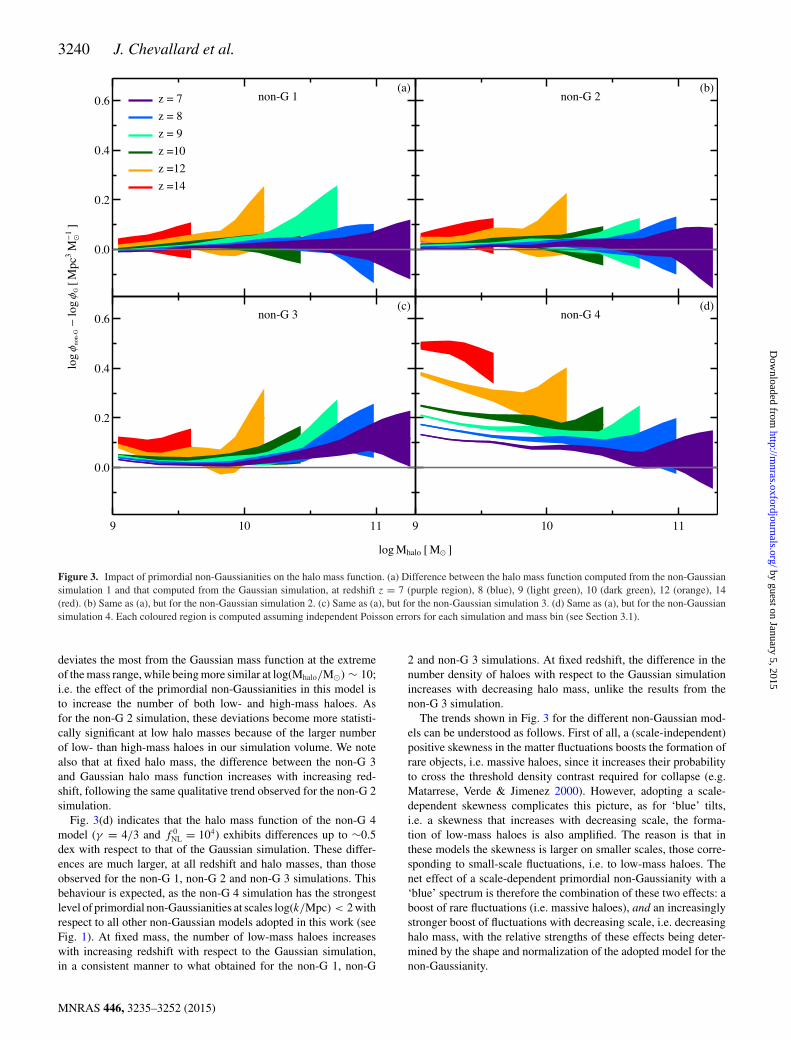
Figure 3. Impact of primordial non-Gaussianities on the halo mass function. (a) Difference between the halo mass function computed from the non-Gaussiansimulation 1 and that computed from the Gaussian simulation, at redshift z = 7 (purple region), 8 (blue), 9 (light green), 10 (dark green), 12 (orange), 14(red). (b) Same as (a), but for the non-Gaussian simulation 2. (c) Same as (a), but for the non-Gaussian simulation 3. (d) Same as (a), but for the non-Gaussiansimulation 4. Each coloured region is computed assuming independent Poisson errors for each simulation and mass bin (see Section 3.1).

deviates the most from the Gaussian mass function at the extremeof the mass range, while being more similar at log(Mhalo/M) ∼ 10;i.e. the effect of the primordial non-Gaussianities in this model isto increase the number of both low- and high-mass haloes. Asfor the non-G 2 simulation, these deviations become more statisti-cally significant at low halo masses because of the larger numberof low- than high-mass haloes in our simulation volume. We notealso that at fixed halo mass, the difference between the non-G 3and Gaussian halo mass function increases with increasing red-shift, following the same qualitative trend observed for the non-G 2simulation.

Fig. 3(d) indicates that the halo mass function of the non-G 4model (γ = 4/3 and f 0

NL = 104) exhibits differences up to ∼0.5dex with respect to that of the Gaussian simulation. These differ-ences are much larger, at all redshift and halo masses, than thoseobserved for the non-G 1, non-G 2 and non-G 3 simulations. Thisbehaviour is expected, as the non-G 4 simulation has the strongestlevel of primordial non-Gaussianities at scales log(k/Mpc) < 2 withrespect to all other non-Gaussian models adopted in this work (seeFig. 1). At fixed mass, the number of low-mass haloes increaseswith increasing redshift with respect to the Gaussian simulation,in a consistent manner to what obtained for the non-G 1, non-G

2 and non-G 3 simulations. At fixed redshift, the difference in thenumber density of haloes with respect to the Gaussian simulationincreases with decreasing halo mass, unlike the results from thenon-G 3 simulation.

The trends shown in Fig. 3 for the different non-Gaussian mod-els can be understood as follows. First of all, a (scale-independent)positive skewness in the matter fluctuations boosts the formation ofrare objects, i.e. massive haloes, since it increases their probabilityto cross the threshold density contrast required for collapse (e.g.Matarrese, Verde & Jimenez 2000). However, adopting a scale-dependent skewness complicates this picture, as for ‘blue’ tilts,i.e. a skewness that increases with decreasing scale, the forma-tion of low-mass haloes is also amplified. The reason is that inthese models the skewness is larger on smaller scales, those corre-sponding to small-scale fluctuations, i.e. to low-mass haloes. Thenet effect of a scale-dependent primordial non-Gaussianity with a‘blue’ spectrum is therefore the combination of these two effects: aboost of rare fluctuations (i.e. massive haloes), and an increasinglystronger boost of fluctuations with decreasing scale, i.e. decreasinghalo mass, with the relative strengths of these effects being deter-mined by the shape and normalization of the adopted model for thenon-Gaussianity.

MNRAS 446, 3235–3252 (2015)



ownloaded from



7 8 9 10

-4

-2

z = 7z = 8z = 9z =10z =12z =14

log M [ M ]

log

[Mpc

3M

1]

Figure 4. Galaxy stellar mass function at different redshifts for the simula-tion with Gaussian initial conditions. Open circles indicate the stellar massfunction computed form our simulation, while solid coloured lines are fittedto the points with a Schechter function. Solid black lines are power laws (M) ∝ 10(M−M�)(1+α) with α equal to the value obtained at z = 7 andscaled to match the computed mass functions at log(M∗/M) = 6.7. Error-bars are computed assuming independent Poisson distributions in each massbin, and are plotted only when greater than the size of circles.

In the next section, we will show how the effect of primordial non-Gaussianities on the number density of haloes at different redshiftsaffects the redshift evolution of the galaxy stellar mass function.

3.2 Galaxy stellar mass function

We have shown that the adoption of non-Gaussian initial densityperturbations produces measurable differences in the halo massfunction for the non-Gaussian simulations 2, 3 and 4, i.e. for thosesimulations with strong enough initial non-Gaussianities. We there-fore expect a similar behaviour for the galaxy stellar mass function,as it depends on the halo merger history (see equations 3–5).

We show in Fig. 4 the galaxy stellar mass function obtained byapplying the galaxy formation model of M13 (see Section 2.3) on thedark matter simulation with Gaussian initial conditions. The opencircles of different colours indicate the mass function at differentredshifts. We compute the galaxy stellar mass function in the sameway as we do for the halo mass function (see Section 3.1), butadopting logarithmic mass bins of 0.1 dex width in the range 6.5 ≤log(M∗/M) ≤ 10. The solid, coloured lines in Fig. 4 are obtainedby fitting a Schechter function to the our measured points (seeequation 7 and Section 3.1 for details). The solid black lines inFig. 4 are power laws of the form (M) ∝ 10(M−M�)(1+α) with α

equal to the value obtained with the Schechter function fit at redshiftz = 7, and normalized to match the measured stellar mass functionat log(M∗/M) = 6.7.

Fig. 4 shows that, as for the halo mass function of Fig. 2,the number density of galaxies decreases with increasing red-shift, at fixed stellar mass. The characteristic stellar mass also de-creases with increasing redshift, from M� = 9.03 ± 0.12 at z = 7to M� = 6.90 ± 0.36 at z = 14, indicating that the typical stellarmass of galaxies decreases with increasing redshift. The low-massend of the mass function steepens with increasing redshift, fromα = −2.03 ± 0.02 at z = 7 to α = −2.23 ± 0.07 at z = 10.As we already noted for the halo mass function, at higher redshiftthe low values of the characteristic stellar mass combined with the

resolution of the N-body simulation makes the exponential cut-offimportant at all stellar masses here considered, therefore affectingthe value of α obtained with the Schechter function fit. The likelyexplanation for the flattening of the low-mass end of the stellar massfunction from high to low redshift is merging, as we already notedfor the halo mass function. We note also that at a given redshift,the low-mass slope of the stellar mass function is flatter than thehalo mass function (αhalo − αstar ∼ 0.15 at z = 7–10). This is dueto the increasing efficiency of baryon conversion into stars withincreasing halo mass in the galaxy formation model adopted in thiswork, for the halo mass ranges here considered (see Section 2.3 andequation 5). This causes high mass haloes to have, on average, largerstellar-to-halo mass ratios (M∗/Mhalo) than haloes with lower mass,thus increasing the relative number of high- to low-mass galaxies,i.e. flattening the stellar mass function with respect to the halo massfunction.

We show in Fig. 5 the effect of non-Gaussian initial density per-turbations on the galaxy stellar mass function as a function of stellarmass. We compute the stellar mass function for the Gaussian sim-ulation and each non-Gaussian simulation in the same way as wedo for the halo mass function (see Section 3.1), adopting 10 loga-rithmic bins in the range 6.5 ≤ log(M∗/M) ≤ 10, and consideringonly bins with ≥20 objects.

Fig. 5(a) displays the difference between the galaxy stel-lar mass function computed from the non-G 1 simulation andthat computed from the Gaussian simulation. As for the halomass function [see Fig. 3(a)], the stellar mass function obtainedfrom the non-G 1 model is consistent, within the errors, withthat computed from the Gaussian simulation, at all redshift andmasses.

Fig. 5(b) indicates that, unlike the galaxy stellar mass function ofthe non-G 1 simulation, that of the non-G 2 simulation exhibits, atlow (log(M∗/M) � 8) masses, small (<0.1 dex) but statisticallysignificant differences with the mass function of the Gaussian sim-ulation. In particular, the number of low-mass galaxies is increasedwith respect to the Gaussian simulation. Also, this effect increaseswith increasing redshift, at fixed stellar mass, as already noted forthe halo mass function (Section 3.1).

Fig. 5(c) shows that the primordial non-Gaussianities adoptedin the non-G 3 simulation, stronger than those in the non-G 1 andnon-G 2 simulations, produce even more statistically significant dif-ferences with respect to the stellar mass function of the Gaussiansimulation, both at low and high stellar masses. At each redshift,the number density of low- and high-mass galaxies is increasedwith respect to the Gaussian simulation, but, unlike the correspond-ing figure for the halo mass function (Fig. 3c), the effect is morepronounced for high-mass galaxies. We can explain this behaviourby appealing to the decreasing efficiency of baryon conversion intostars, i.e. the decrease of the stellar-to-halo mass ratio, with decreas-ing halo mass, which reduces the differences between the non-G 3and Gaussian simulations at low stellar masses. At fixed stellarmass, the effect of primordial non-Gaussianities on the galaxy stel-lar function increases with increasing redshift, as we already notedfor the non-G 2 simulation.

Fig. 5(d) indicates that the non-G 4 simulation, which has thestrongest level of primordial non-Gaussianities among all simula-tions, produces the strongest deviations in the galaxy stellar massfunction with respect to the Gaussian simulation, as already notedfor the halo mass function in Fig. 3(d). At all redshift and masses,the number density of galaxies is larger in the non-G 4 simula-tion than in the Gaussian simulation. This difference increases,at fixed stellar mass, with increasing redshift, reaching δφ ∼ 0.4

MNRAS 446, 3235–3252 (2015)



ownloaded from



0.0

0.2

0.4

0.6

z =14

z =12

z =10

z =9

z =8

z =7(a)

non-G 1

(b)

non-G 2

7 8 9

0.0

0.2

0.4

0.6(c)

non-G 3

7 8 9

(d)

non-G 4

log M [ M ]

log

non-

Glo

gG

[Mpc

3M

1]

Figure 5. Impact of primordial non-Gaussianities on the galaxy stellar mass function. (a) Difference between the galaxy stellar mass function computed fromthe non-Gaussian simulation 1 and that computed from the Gaussian simulation, at redshift z = 7 (purple region), 8 (blue), 9 (light green), 10 (dark green), 12(orange), 14 (red). (b) Same as (a), but for the non-Gaussian simulation 2. (c) Same as (a), but for the non-Gaussian simulation 3. (d) Same as (a), but for thenon-Gaussian simulation 4. Each coloured region is computed assuming independent Poisson errors for each simulation and mass bin.

at z = 14 and log(M∗/M) = 6.5. We note that this value islower than that observed in the halo mass function [δφ ∼ 0.5,see Fig. 3(d)], and that, even though at fixed redshift the differencebetween the non-Gaussian and Gaussian mass functions increaseswith decreasing galaxy stellar mass, this trend is weaker (i.e. flatter)that that for the halo mass function. This is in qualitative agreementto what we noted for the non-G 3 simulation and likely relatedto the same explanation: the decreasing baryon conversions effi-ciency with decreasing halo mass reduces the differences betweenthe non-Gaussian simulations and the Gaussian one at low stellarmasses.

Our results on the effects of non-Gaussianity on the galaxy stellarmass function are qualitatively very similar to those found in Paper I,despite the different galaxy formation models used (see fig. 3 ofPaper I).

In the next section, we will show by means of the Bruzual &Charlot (2003) population synthesis code how the differences in thegalaxy stellar mass function between the non-Gaussian and Gaus-sian simulations reflect into different far-UV luminosity functionsat different redshifts.

3.3 UV luminosity function

In the previous sections, we have illustrated the effect of primordialnon-Gaussianities on the halo and stellar mass functions computedfrom our N-body simulation and the M13 galaxy formation model.By means of the galaxy chemical evolution prescription presentedin Section 2.3 (see equation 6) and the Bruzual & Charlot (2003)population synthesis code, we now show the effect of non-Gaussianinitial density perturbations on the redshift evolution of the far-UVluminosity function.

Fig. 6 shows the far-UV luminosity function computed from theGaussian simulation. The open circles of different colours indicatethe far-UV luminosity function at different redshifts, which wecompute in the same way as we do for the halo mass function (seeSection 3.1), but adopting bins of far-UV absolute magnitudes 0.2dex width in the range −22 ≤ MFUV ≤ −14. The solid, colouredlines in Fig. 6 are computed by fitting with the same method outlinedin Section 3.1, a Schechter function of the form

φ(M) = 0.4 ln(10) φ� 10−0.4(M−M�)(1+α) exp(−10−0.4(M−M�)), (8)

MNRAS 446, 3235–3252 (2015)



ownloaded from



-14 -16 -18 -20 -22

-4

-2

Bouwens 2014 (z=7)Bouwens 2014 (z=8)

MFUV [ AB mag ]

log

[Mpc

3m

ag1

]

z 7z 8z 9z 10z 12z 14

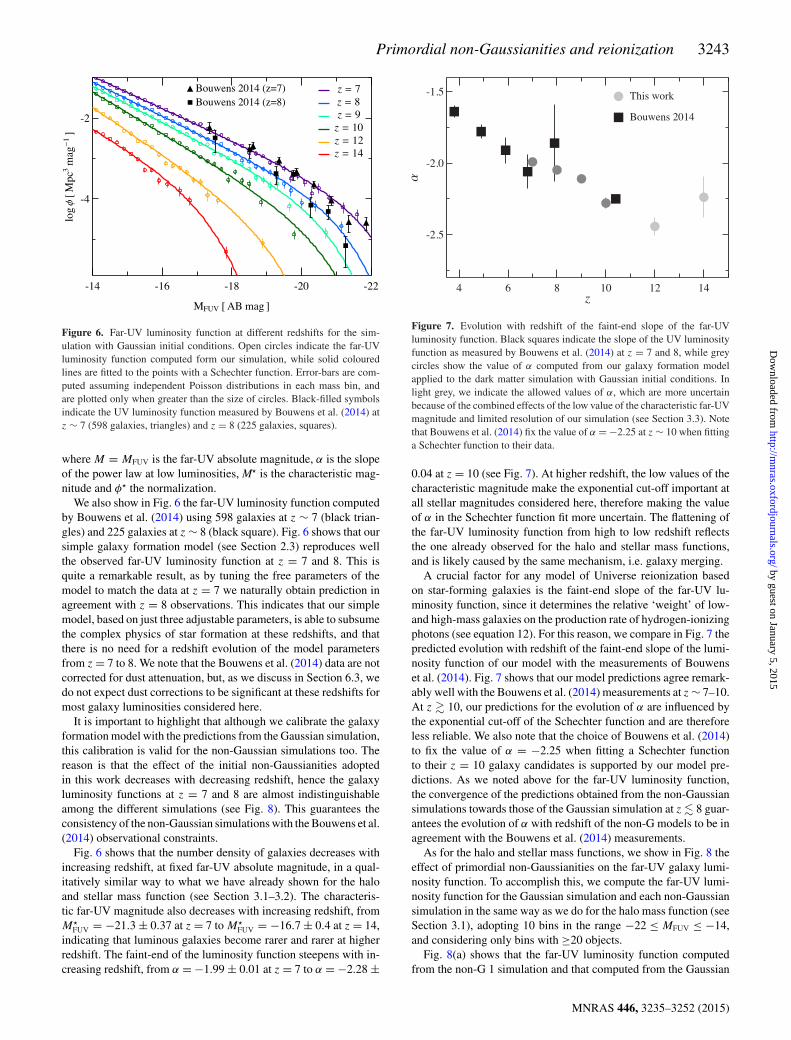
Figure 6. Far-UV luminosity function at different redshifts for the sim-ulation with Gaussian initial conditions. Open circles indicate the far-UVluminosity function computed form our simulation, while solid colouredlines are fitted to the points with a Schechter function. Error-bars are com-puted assuming independent Poisson distributions in each mass bin, andare plotted only when greater than the size of circles. Black-filled symbolsindicate the UV luminosity function measured by Bouwens et al. (2014) atz ∼ 7 (598 galaxies, triangles) and z = 8 (225 galaxies, squares).

where M = MFUV is the far-UV absolute magnitude, α is the slopeof the power law at low luminosities, M� is the characteristic mag-nitude and φ� the normalization.

We also show in Fig. 6 the far-UV luminosity function computedby Bouwens et al. (2014) using 598 galaxies at z ∼ 7 (black trian-gles) and 225 galaxies at z ∼ 8 (black square). Fig. 6 shows that oursimple galaxy formation model (see Section 2.3) reproduces wellthe observed far-UV luminosity function at z = 7 and 8. This isquite a remarkable result, as by tuning the free parameters of themodel to match the data at z = 7 we naturally obtain prediction inagreement with z = 8 observations. This indicates that our simplemodel, based on just three adjustable parameters, is able to subsumethe complex physics of star formation at these redshifts, and thatthere is no need for a redshift evolution of the model parametersfrom z = 7 to 8. We note that the Bouwens et al. (2014) data are notcorrected for dust attenuation, but, as we discuss in Section 6.3, wedo not expect dust corrections to be significant at these redshifts formost galaxy luminosities considered here.

It is important to highlight that although we calibrate the galaxyformation model with the predictions from the Gaussian simulation,this calibration is valid for the non-Gaussian simulations too. Thereason is that the effect of the initial non-Gaussianities adoptedin this work decreases with decreasing redshift, hence the galaxyluminosity functions at z = 7 and 8 are almost indistinguishableamong the different simulations (see Fig. 8). This guarantees theconsistency of the non-Gaussian simulations with the Bouwens et al.(2014) observational constraints.

Fig. 6 shows that the number density of galaxies decreases withincreasing redshift, at fixed far-UV absolute magnitude, in a qual-itatively similar way to what we have already shown for the haloand stellar mass function (see Section 3.1–3.2). The characteris-tic far-UV magnitude also decreases with increasing redshift, fromM�

FUV = −21.3 ± 0.37 at z = 7 to M�FUV = −16.7 ± 0.4 at z = 14,

indicating that luminous galaxies become rarer and rarer at higherredshift. The faint-end of the luminosity function steepens with in-creasing redshift, from α = −1.99 ± 0.01 at z = 7 to α = −2.28 ±

4 6 8 10 12 14

-2.5

-2.0

-1.5 This work

Bouwens 2014

z

Figure 7. Evolution with redshift of the faint-end slope of the far-UVluminosity function. Black squares indicate the slope of the UV luminosityfunction as measured by Bouwens et al. (2014) at z = 7 and 8, while greycircles show the value of α computed from our galaxy formation modelapplied to the dark matter simulation with Gaussian initial conditions. Inlight grey, we indicate the allowed values of α, which are more uncertainbecause of the combined effects of the low value of the characteristic far-UVmagnitude and limited resolution of our simulation (see Section 3.3). Notethat Bouwens et al. (2014) fix the value of α = −2.25 at z ∼ 10 when fittinga Schechter function to their data.

0.04 at z = 10 (see Fig. 7). At higher redshift, the low values of thecharacteristic magnitude make the exponential cut-off important atall stellar magnitudes considered here, therefore making the valueof α in the Schechter function fit more uncertain. The flattening ofthe far-UV luminosity function from high to low redshift reflectsthe one already observed for the halo and stellar mass functions,and is likely caused by the same mechanism, i.e. galaxy merging.

A crucial factor for any model of Universe reionization basedon star-forming galaxies is the faint-end slope of the far-UV lu-minosity function, since it determines the relative ‘weight’ of low-and high-mass galaxies on the production rate of hydrogen-ionizingphotons (see equation 12). For this reason, we compare in Fig. 7 thepredicted evolution with redshift of the faint-end slope of the lumi-nosity function of our model with the measurements of Bouwenset al. (2014). Fig. 7 shows that our model predictions agree remark-ably well with the Bouwens et al. (2014) measurements at z ∼ 7–10.At z � 10, our predictions for the evolution of α are influenced bythe exponential cut-off of the Schechter function and are thereforeless reliable. We also note that the choice of Bouwens et al. (2014)to fix the value of α = −2.25 when fitting a Schechter functionto their z = 10 galaxy candidates is supported by our model pre-dictions. As we noted above for the far-UV luminosity function,the convergence of the predictions obtained from the non-Gaussiansimulations towards those of the Gaussian simulation at z � 8 guar-antees the evolution of α with redshift of the non-G models to be inagreement with the Bouwens et al. (2014) measurements.

As for the halo and stellar mass functions, we show in Fig. 8 theeffect of primordial non-Gaussianities on the far-UV galaxy lumi-nosity function. To accomplish this, we compute the far-UV lumi-nosity function for the Gaussian simulation and each non-Gaussiansimulation in the same way as we do for the halo mass function (seeSection 3.1), adopting 10 bins in the range −22 ≤ MFUV ≤ −14,and considering only bins with ≥20 objects.

Fig. 8(a) shows that the far-UV luminosity function computedfrom the non-G 1 simulation and that computed from the Gaussian

MNRAS 446, 3235–3252 (2015)



ownloaded from



0.0

0.2

0.4

0.6

z =14

z =12

z =10

z = 9

z = 8

z = 7(a)

non-G 1

(b)

non-G 2

-16 -20

0.0

0.2

0.4

0.6(c)

non-G 3

-16 -20

(d)

non-G 4

MFUV [ AB mag ]

log

non-

Glo

gG

[Mpc

3m

ag1

]

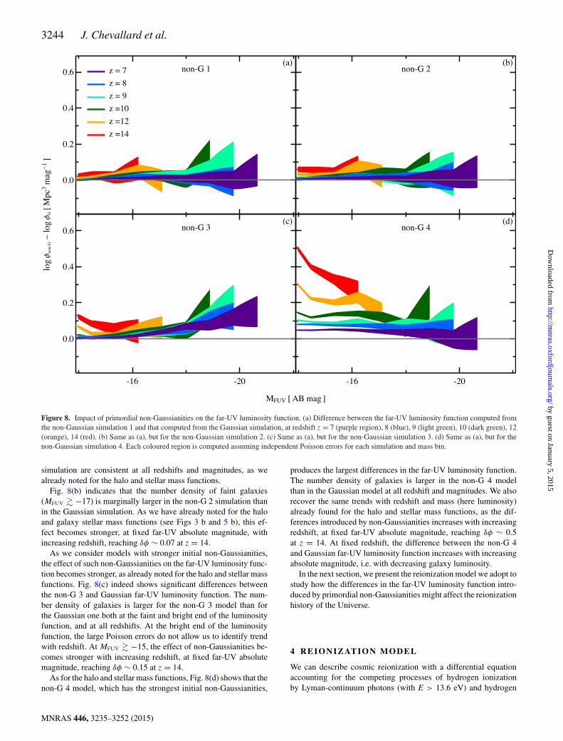
Figure 8. Impact of primordial non-Gaussianities on the far-UV luminosity function. (a) Difference between the far-UV luminosity function computed fromthe non-Gaussian simulation 1 and that computed from the Gaussian simulation, at redshift z = 7 (purple region), 8 (blue), 9 (light green), 10 (dark green), 12(orange), 14 (red). (b) Same as (a), but for the non-Gaussian simulation 2. (c) Same as (a), but for the non-Gaussian simulation 3. (d) Same as (a), but for thenon-Gaussian simulation 4. Each coloured region is computed assuming independent Poisson errors for each simulation and mass bin.

simulation are consistent at all redshifts and magnitudes, as wealready noted for the halo and stellar mass functions.

Fig. 8(b) indicates that the number density of faint galaxies(MFUV � −17) is marginally larger in the non-G 2 simulation thanin the Gaussian simulation. As we have already noted for the haloand galaxy stellar mass functions (see Figs 3 b and 5 b), this ef-fect becomes stronger, at fixed far-UV absolute magnitude, withincreasing redshift, reaching δφ ∼ 0.07 at z = 14.

As we consider models with stronger initial non-Gaussianities,the effect of such non-Gaussianities on the far-UV luminosity func-tion becomes stronger, as already noted for the halo and stellar massfunctions. Fig. 8(c) indeed shows significant differences betweenthe non-G 3 and Gaussian far-UV luminosity function. The num-ber density of galaxies is larger for the non-G 3 model than forthe Gaussian one both at the faint and bright end of the luminosityfunction, and at all redshifts. At the bright end of the luminosityfunction, the large Poisson errors do not allow us to identify trendwith redshift. At MFUV � −15, the effect of non-Gaussianities be-comes stronger with increasing redshift, at fixed far-UV absolutemagnitude, reaching δφ ∼ 0.15 at z = 14.

As for the halo and stellar mass functions, Fig. 8(d) shows that thenon-G 4 model, which has the strongest initial non-Gaussianities,

produces the largest differences in the far-UV luminosity function.The number density of galaxies is larger in the non-G 4 modelthan in the Gaussian model at all redshift and magnitudes. We alsorecover the same trends with redshift and mass (here luminosity)already found for the halo and stellar mass functions, as the dif-ferences introduced by non-Gaussianities increases with increasingredshift, at fixed far-UV absolute magnitude, reaching δφ ∼ 0.5at z = 14. At fixed redshift, the difference between the non-G 4and Gaussian far-UV luminosity function increases with increasingabsolute magnitude, i.e. with decreasing galaxy luminosity.

In the next section, we present the reionization model we adopt tostudy how the differences in the far-UV luminosity function intro-duced by primordial non-Gaussianities might affect the reionizationhistory of the Universe.

4 R E I O N I Z AT I O N M O D E L

We can describe cosmic reionization with a differential equationaccounting for the competing processes of hydrogen ionizationby Lyman-continuum photons (with E > 13.6 eV) and hydrogen

MNRAS 446, 3235–3252 (2015)



ownloaded from



-14 -16 -18 -20 -22

25.4

25.6

25.8

26.0

z = 7z = 8z = 9z = 10z = 12z = 14

MFUV [AB mag]

log

ion

[erg

1H

z]

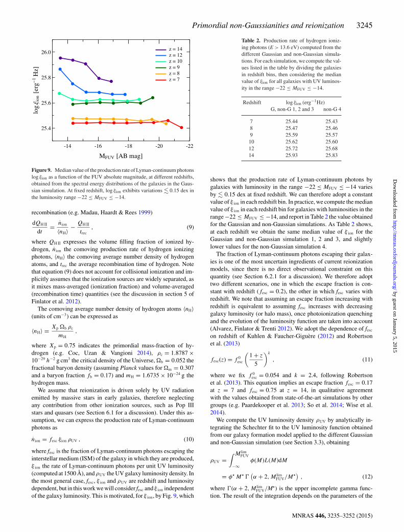
Figure 9. Median value of the production rate of Lyman-continuum photonslog ξion as a function of the FUV absolute magnitude, at different redshifts,obtained from the spectral energy distributions of the galaxies in the Gaus-sian simulation. At fixed redshift, log ξion exhibits variations � 0.15 dex inthe luminosity range −22 ≤ MFUV ≤ −14.

recombination (e.g. Madau, Haardt & Rees 1999)

dQH II

dt= nion

〈nH〉 − QH II

trec, (9)

where QH II expresses the volume filling fraction of ionized hy-drogen, nion the comoving production rate of hydrogen ionizingphotons, 〈nH〉 the comoving average number density of hydrogenatoms, and trec the average recombination time of hydrogen. Notethat equation (9) does not account for collisional ionization and im-plicitly assumes that the ionization sources are widely separated, asit mixes mass-averaged (ionization fraction) and volume-averaged(recombination time) quantities (see the discussion in section 5 ofFinlator et al. 2012).

The comoving average number density of hydrogen atoms 〈nH〉(units of cm−3) can be expressed as

〈nH〉 = Xp �b ρc

mH,

where Xp = 0.75 indicates the primordial mass-fraction of hy-drogen (e.g. Coc, Uzan & Vangioni 2014), ρc = 1.8787 ×10−29 h−2 g cm3 the critical density of the Universe, �b = 0.052 thefractional baryon density (assuming Planck values for �m = 0.307and a baryon fraction fb = 0.17) and mH = 1.6735 × 10−24 g thehydrogen mass.

We assume that reionization is driven solely by UV radiationemitted by massive stars in early galaxies, therefore neglectingany contribution from other ionization sources, such as Pop IIIstars and quasars (see Section 6.1 for a discussion). Under this as-sumption, we can express the production rate of Lyman-continuumphotons as

nion = fesc ξion ρUV , (10)

where fesc is the fraction of Lyman-continuum photons escaping theinterstellar medium (ISM) of the galaxy in which they are produced,ξ ion the rate of Lyman-continuum photons per unit UV luminosity(computed at 1500 Å), and ρUV the UV galaxy luminosity density. Inthe most general case, fesc, ξ ion and ρUV are redshift and luminositydependent, but in this work we will consider fesc and ξ ion independentof the galaxy luminosity. This is motivated, for ξ ion, by Fig. 9, which

Table 2. Production rate of hydrogen ioniz-ing photons (E > 13.6 eV) computed from thedifferent Gaussian and non-Gaussian simula-tions. For each simulation, we compute the val-ues listed in the table by dividing the galaxiesin redshift bins, then considering the medianvalue of ξion for all galaxies with UV luminos-ity in the range −22 ≤ MFUV ≤ −14.

Redshift log ξion (erg−1Hz)G, non-G 1, 2 and 3 non-G 4

7 25.44 25.438 25.47 25.469 25.59 25.57

10 25.62 25.6012 25.72 25.6814 25.93 25.83

shows that the production rate of Lyman-continuum photons bygalaxies with luminosity in the range −22 ≤ MFUV ≤ −14 variesby � 0.15 dex at fixed redshift. We can therefore adopt a constantvalue of ξ ion in each redshift bin. In practice, we compute the medianvalue of ξ ion in each redshift bin for galaxies with luminosities in therange −22 ≤ MFUV ≤ −14, and report in Table 2 the value obtainedfor the Gaussian and non-Gaussian simulations. As Table 2 shows,at each redshift we obtain the same median value of ξ ion for theGaussian and non-Gaussian simulation 1, 2 and 3, and slightlylower values for the non-Gaussian simulation 4.

The fraction of Lyman-continuum photons escaping their galax-ies is one of the most uncertain ingredients of current reionizationmodels, since there is no direct observational constraint on thisquantity (see Section 6.2.1 for a discussion). We therefore adopttwo different scenarios, one in which the escape fraction is con-stant with redshift (fesc = 0.2), the other in which fesc varies withredshift. We note that assuming an escape fraction increasing withredshift is equivalent to assuming fesc increases with decreasinggalaxy luminosity (or halo mass), once photoionization quenchingand the evolution of the luminosity function are taken into account(Alvarez, Finlator & Trenti 2012). We adopt the dependence of fesc

on redshift of Kuhlen & Faucher-Giguere (2012) and Robertsonet al. (2013)

fesc(z) = f 0esc

(1 + z

5

)k

, (11)

where we fix f 0esc = 0.054 and k = 2.4, following Robertson

et al. (2013). This equation implies an escape fraction fesc = 0.17at z = 7 and fesc = 0.75 at z = 14, in qualitative agreementwith the values obtained from state-of-the-art simulations by othergroups (e.g. Paardekooper et al. 2013; So et al. 2014; Wise et al.2014).

We compute the UV luminosity density ρUV by analytically in-tegrating the Schechter fit to the UV luminosity function obtainedfrom our galaxy formation model applied to the different Gaussianand non-Gaussian simulation (see Section 3.3), obtaining

ρUV =∫ M lim

FUV

−∞φ(M)L(M)dM

= φ� M� �(α + 2, M lim

FUV/M�)

, (12)

where �(α + 2, M limFUV/M�) is the upper incomplete gamma func-

tion. The result of the integration depends on the parameters of the

MNRAS 446, 3235–3252 (2015)



ownloaded from



Schechter function φ�, M� and α, which we derive by means of anMCMC fitting of equation (8) to the binned luminosity functionof each simulation at each redshift, and on the minimum galaxyluminosity M lim

FUV.The minimum galaxy luminosity is also an uncertain ingredient

of any reionization model, as current observations of high-redshiftgalaxies probe only the bright end of the UV luminosity function(see Section 6.2.2 for a discussion). This value depends on theminimum mass of a halo able to cool down the gas to the tem-peratures required for star formation, and therefore on the highlyuncertain physics of high-redshift dwarf galaxy formation models(e.g. effects of cooling from molecular hydrogen and metal lines,UV background, stellar feedback; see Wise et al. 2014). As for theescape fraction, we have to rely on simulations and previous work.We therefore fix M lim

FUV = −12 (AB magnitude), which is, for in-stance, similar to the preferred value of Robertson et al. (2013), andconsistent with the recent simulations of Wise et al. (2014), in whichgalaxies down to M lim

FUV ∼ −5 are formed. Since our model galaxiesof MFUV = −14 correspond to haloes of 109 M, adopting a lim-iting far-UV magnitude of −12 is equivalent to considering halomasses down to ∼108 M, assuming a fixed mass-to-light ratio inthis mass range. Note that, unlike Robertson et al. (2013), we do notadopt a single metallicity to compute the spectral energy distributionof our model galaxies, since we adopt the mass–metallicity relationfor dwarf galaxies of Kirby et al. (2013) to calculate the chemicalevolution of all galaxies in our simulations (see Section 2.3).

The last quantity entering equation (9) is the average recombina-tion time of ionized hydrogen atoms in the IGM, which is

trec = [αB(T )ne]−1

= [CH IIαB(T )fe〈nH〉(1 + z)3

]−1, (13)

where αB is the hydrogen recombination coefficient, ne =fe〈nH〉(1 + z)3 the number density of free electrons at redshift z, fe

the fraction of free electrons per hydrogen nucleus in the ionizedIGM and CH II the ‘clumping factor’, which accounts for inhomo-geneities in the reionization process. We adopt an electron tempera-ture of T = 20 000 K and adopt the case B recombination coefficientαB = 2.52 × 10−13 cm3 s−1.3 Assuming that helium is doubly ion-ized at z < 4 and singly ionized at higher redshift (e.g. Kuhlen &Faucher-Giguere 2012), we can express the number of free electrons

per hydrogen nucleus as fe ={

1 + Yp/2Xp at z ≤ 4 ,

1 + Yp/4Xp at z > 4 ,where

Xp and Yp = 1 − Xp indicate the primordial mass fraction of hydro-gen and helium, respectively.

The clumping factor that enters the recombination time allowsone to account for the effect of inhomogeneities in the density, tem-perature and ionization fields of the IGM. As for the escape fraction,one has to rely on simulations, since there are no observational con-straints on the quantities determining the recombination rate of theIGM at high redshift (see Section 6.2.3 for a discussion). We adoptfor CH II the analytic expression of Finlator et al. (2012), which isbased on state-of-the-art hydrodynamical simulations which includethe effect of stellar feedback, photoheating from a UV backgroundand self-shielding on the IGM:

CH II = 9.25 − 7.21 log (1 + z) , (14)

3 Assuming an IGM temperature of T = 10 000 K would imply a case Brecombination coefficient αB = 2.59 × 10−13, therefore a difference of �3 per cent with respect to our choice.

which implies a clumping factor that increases from 0.77 at z = 14to 3.16 at z = 6. Note that equation (14) is in excellent agreementto that found by Wise et al. (2014) in their recent hydrodynamicalsimulations.

An important constraint on cosmic reionization comes from theoptical depth of electrons to Thomson scattering, which can beexpressed as

τe =∫ ∞

0dz

c (1 + z)2

H (z)QH II(z) σT 〈nH〉 fe , (15)

where c is the speed of light, H(z) the Hubble parameter, QH II theionization fraction at redshift z, σ T the cross-section of electrons toThomson scattering, 〈nH〉 the comoving average number density ofhydrogen atoms and fe the fraction of free electrons per hydrogennucleus in the ionized IGM.

5 IM P L I C AT I O N S FO R C O S M I CR E I O N I Z AT I O N

We have shown in Section 3 that introducing non-Gaussianities inthe initial density perturbations which are then evolved by means ofan N-body code produces measurable effects on the halo mass func-tion, galaxy stellar mass function and far-UV luminosity function.These effects are marginally significant for the non-G 1 and non-G2 models, while being stronger in the non-G 3 and non-G 4 simula-tions. This is caused by the different level of non-Gaussianities in thedifferent models, as stronger deviations from purely Gaussian ini-tial conditions produce stronger effects on the quantities consideredhere. Two general features are shared by all non-Gaussian modelsconsidered in this work: the effect of primordial non-Gaussianitieson the halo and stellar mass function and on the far-UV luminosityfunction increases with increasing redshift from z = 7 to 14; thiseffect becomes stronger at low halo and stellar masses, and thus infaint galaxies (except for the non-G 3 simulation, which show thesame level of deviations at low and high masses). This is relevantto the Universe reionization history, since faint galaxies, i.e. galax-ies which are currently unobservable because of their distance andlow luminosity, are thought to be the primary source of ionizingradiation at high redshift.

In this section, we will therefore explore the impact of differentlevels of primordial non-Gaussianities on the reionization historyof the Universe and on the optical depth of electrons to Thomsonscattering. This depends on the time-integral of the reionizationhistory, and can be directly measured by CMB observations. Wewill also show how the emissivity rate of ionizing photons of ourmodels is consistent with recent observations at 2 ≤ z ≤ 5. Toexplore the effect of different assumptions about the reionizationmodel on our results, we consider three different models, labelled‘A’, ‘B’ and ‘C’, in which we vary the escape fraction and limitingUV magnitude. Table 3 summarizes our choices for fesc and M lim

FUV

for the three models: model A has fesc = 0.2 at all redshifts andM lim

FUV = −12; model B has the same M limFUV as model A, but fesc

that increases with redshift following equation (11); model C hasthe same fesc as model B, but a larger M lim

FUV = −7, i.e. it includesfainter galaxies than model A and B. Note that to compute theUV luminosity density for model C (see equation 12), we adopt atwo-piece luminosity function: we consider a Schechter function tillMFUV = −12, then a constant function in the range −12 ≤ MFUV ≤−7. This is suggested by the recent hydrodynamic simulation ofWise et al. (2014), in which they show that the low efficiency

MNRAS 446, 3235–3252 (2015)



ownloaded from



Table 3. Different reionization models adopted in this work. Weadopt for all models the clumping factor of Finlator et al. (2012,see equation 14), while we vary the escape fraction and limiting UVmagnitude. Note that for model C, we consider a limiting magnitudeof −7, but adopting a constant number density of galaxies in the range−12 ≤ MFUV ≤ −7, equal to the density at MFUV = −12.

Reionization model fesc M limFUV

A 0.2 −12B increasing with z (see equation 11) −12C increasing with z (see equation 11) −7

of baryons conversion into stars in low-mass (log(Mhalo/M) � 8)haloes flattens the UV luminosity function at faint luminosities.

5.1 Reionization history of the Universe

We compute the reionization history of the Universe for the dif-ferent reionization models and both Gaussian and non-Gaussiansimulations by numerically integrating equation (9). For the fixedreionization model, the only quantity that varies in equation (9)among the Gaussian and non-Gaussian simulations is the produc-tion rate of ionizing photons, since it depends on ξ ion, the rate ofLyman-continuum photons per unit UV luminosity, and on ρUV,the UV galaxy luminosity density. This in turns depends on the far-UV galaxy luminosity function through equation (12), which weintegrate analytically assuming for the parameters of the Schechterfunction φ�, M� and α the median of the posterior marginal distri-butions obtained by an MCMC fitting of the ‘numerical’ luminosityfunction at each redshift (see Section 3.3).

We show in Fig. 10 the results of the numerical integration ofequation (9), i.e. the fraction of ionized volume of the Universe asa function of redshift. Lines of different colours correspond to thedifferent Gaussian and non-Gaussian simulations; solid lines referto the reionization model A, dashed lines to model B and dot–dashedlines to model C. The solid lines in Fig. 10 indicate that the reion-ization histories obtained for the Gaussian, non-Gaussian 1, 2 and3 simulations for the reionization model A show small differenceswith one another. This is a direct consequence of the similarity ofthe far-UV luminosity functions among the Gaussian, non-Gaussian1, 2 and 3 simulations at redshift z � 12, and therefore at most times(see Fig. 8). On the other hand, Fig. 10 shows significant differencesamong the reionization history of the non-G 4 simulation and theother simulations. At a given redshift, the fraction of the IGM ion-ized is larger for the non-G 4 simulation, being QH II = 0.08 (0.53)at redshift z = 12 (8), to be compared with QH II ∼ 0.04 (0.45) at thesame redshifts for the other simulations. This difference is a directconsequence of the larger number of low-mass galaxies formed inthe non-G 4 simulation with respect to the other simulations (seeFig. 8 d), which, at each redshift, increases the number of photonsavailable for hydrogen ionization.

The dashed lines in Fig. 10 show the reionization histories forthe different simulations obtained assuming the reionization modelB, which, unlike model A, has an escape fraction that increaseswith increasing redshift. This makes the fraction of ionized IGMto increase more rapidly at high z, because of the larger number ofphotons available for hydrogen ionization at high redshift in modelB than in model A. As for model A, the reionization histories ofthe Gaussian simulation and non-Gaussian simulation 1, 2 and 3show smaller differences than that of the non-G 4 simulation. Wenote, however, that the dashed lines in Fig. 10 are more separated

6 8 10 12 140.00

0.25

0.50

0.75

1.00 Gnon-G 1non-G 2non-G 3non-G 4

Model AModel BModel C

z

QH

II

Figure 10. Ionization fraction of the Universe as a function of redshift ob-tained by applying the different reionization models of Table 3 to the differentGaussian and non-Gaussian simulations. Different colours indicate differentsimulations: Gaussian (black), non-Gaussian 1 (red), non-Gaussian 2 (blue),non-Gaussian 3 (dark green) and non-Gaussian 4 (orange). Solid lines referto the reionization model A (fesc = 0.2 and M lim

FUV = −12), dashed linesto model B (fesc increasing with z as in equation 11 and M lim

FUV = −12),dot–dashed lines to model C (fesc increasing with z as in equation 11 andM lim

FUV = −7). For clarity, for this latter model, we just plot the results forthe Gaussian and non-Gaussian 3 simulations.

than the solid ones, indicating that a model with an escape fractionthat increases with redshift boosts the effect of primordial non-Gaussianities on the Universe reionization history. The reason isthat in such a model the ionizing radiation emitted by higher red-shift galaxies can escape the ISM more easily, hence increasing thecontribution to Universe reionization of galaxies at high z, thosemost affected by primordial non-Gaussianities.

In Fig. 10, we show as dot–dashed lines QH II for model C, whichhas a higher (fainter) M lim

FUV than models A and B. For clarity, we justplot QH II for the Gaussian and non-Gaussian 3 simulations. Fig. 10shows that considering fainter galaxies than those considered inmodels A and B makes QH II increase faster at z � 10, while atsame time increasing the difference between the Gaussian and non-Gaussian model 3. The explanation is similar to that given above formodel B, but it appeals to the increasing effect of non-Gaussianitieswith decreasing galaxy luminosity, as adopting higher values ofM lim

FUV increases the weight of very faint galaxies, those most affectedby non-Gaussianities, towards reionization.

5.2 Electron Thomson scattering optical depth

Direct measurements of the Universe ionized fraction through Lyα

absorption from background quasars are effective up to neutralfractions (1 − QH II) ∼ 10−3, since at higher values of (1 − QH II)the resonance introduced by Lyα scattering makes ionizing pho-tons almost completely absorbed by neutral hydrogen in the IGM.This situation may change in the future through measurements ofthe 21 cm emission from the hyperfine transition of neutral hydro-gen, since this quantity directly depends on the hydrogen reioniza-tion history (e.g. see the review of Morales & Wyithe 2010). Fornow, one of the most important constraints on cosmic reionizationcomes from the optical depth of electrons to Thomson scattering τe,since this quantity depends on the (integrated) ionization fraction at

MNRAS 446, 3235–3252 (2015)



ownloaded from



6 8 10 12 140.00

0.04

0.08

0.12

G

non-G 1

non-G 2

non-G 3

non-G 4

Model A

Model B

Model C

z

e

Figure 11. Optical depth of electrons to Thomson scattering as a func-tion of redshift obtained by numerically integrating equation (15). Thedark-grey solid line indicates the ‘best-fitting’ value of τ e along with the68 per cent confidence limits (grey hatched region), obtained by Planck Col-laboration XXIV (2014b, see their table 5, first column). Lines of differ-ent colours refer to different simulations: Gaussian (black), non-Gaussian 1(red), non-Gaussian 2 (blue), non-Gaussian 3 (dark green) and non-Gaussian4 (orange). Solid lines refer to the reionization model A (fesc = 0.2 andM lim

FUV = −12), dashed lines to model B (fesc increasing with z as in equa-tion 11 and M lim

FUV = −12), dot–dashed lines to model C (fesc increasingwith z as in equation 11 and M lim

FUV = −7). For clarity, for this latter model,we just plot the results for the Gaussian and non-Gaussian 3 simulations.

different redshifts (see equation 15) and can be measured throughCMB photons.

We show in Fig. 11 the optical depth of electrons to Thomsonscattering for the different reionization models, for the Gaussianand non-Gaussian simulations, obtained by numerically integratingequation (15). As in Fig. 10, different colours refer to differentsimulations, solid lines to the reionization model A, dashed lines tomodel B and dot–dashed lines to model C.

As for the reionization history shown in Fig. 10, solid lines inFig. 11 indicate that the values of τ e obtained from the Gaussian andnon-Gaussian simulation 1, 2 and 3 show small differences whenassuming a reionization model with constant escape fraction. As inFig. 10, the non-G 4 simulation produces the largest difference inthis quantity. This is not surprising, since the only term which variesin the computation of the electron optical depth is the fraction ion-ized at each redshift (see equation 15), which shows large variationsbetween the non-G 4 simulation and the other simulations. Fig. 10shows also that assuming a constant escape fraction fesc = 0.2 pro-duces an optical depth τ e lower than the values currently allowedby Planck observations, for all models. This suggests that a higherescape fraction and/or a fainter limiting UV magnitude are requiredto reionize earlier the Universe and obtain τ e in agreement withPlanck constraints.

The dashed lines in Fig. 11 show τ e for model B, in which theescape fraction increases with increasing redshift. Unlike model A,this one produces values of τ e within the Planck constraints forall Gaussian and non-Gaussian simulations. As we have alreadyhighlighted for the reionization history, this model boosts the effectof primordial non-Gaussianities, increasing the differences in theThomson scattering optical depth among all simulations. This isa direct consequence of the different reionization histories, and ofthe increased ‘weight’ that an increasing fesc with redshift gives

to high-redshift galaxies, those most affected by primordial non-Gaussianities.

The dot–dashed lines in Fig. 11 show the effect of increasingthe limiting UV magnitude from −12 to −7 for the Gaussian andnon-Gaussian 3 simulations. This increases, at a given redshift, thevalue of τ e with respect to models A and B, while at the same timeboosting the differences between the G and non-G 3 models. As wealready noted for QH II, the cause is the increased weight of veryfaint galaxies to reionization, that is of the galaxies most affectedby non-Gaussianities.

5.3 Ionizing emissivity

We have shown in Fig. 11 that our models with variable escapefraction (models B and C) predict values of τ e within Planck con-straints. However, this does not guarantee our models to be con-sistent with the (comoving) ionizing emissivity rate measured fromthe IGM opacity to Lyα photons. We therefore compute the ion-izing emissivity rate of our reionization models, for the Gaussianand non-Gaussian simulations, and compare our results with themeasures by Becker & Bolton (2013) of the ionizing emissivity at2 ≤ z ≤ 5. Note that in order to compare our predictions with theBecker & Bolton (2013) data, we have to extrapolate the predictedfar-UV luminosity function to lower redshift, as our simulationsstop at z = 6.5. We therefore consider the relations between the freeparameters of the Schechter function (φ�, M� and α) and redshift,and note that these relations are linear in the range 6.5 ≤ z ≤ 9.We therefore adopt a linear extrapolation to compute the far-UVluminosity function and ionizing emissivity rate down to z = 5.

We show in Fig. 12 as shaded areas the emissivities predictedby the reionization models A (dark grey), B (grey), and C (black),while we indicate with black circles Becker & Bolton (2013) data.

Model C

Model B

Model A

2 4 6 8 10 12 14-1.0

-0.5

0.0

0.5

1.0Becker & Bolton 2013

z

logn i

on[1

051s

1M

pc3]

Figure 12. Ionizing emissivity as a function of redshift for the differentreionization models adopted in this work. Black circles indicate the ionizingemissivity measured by Becker & Bolton (2013) at 2 ≤ z ≤ 5. The shadedregions refer to different reionization models: model A (dark grey shadedregion, fesc = 0.2 and M lim

FUV = −12), model B (grey shaded region, fesc

increasing with z as in equation 11 and M limFUV = −12); model C (black

shaded region, fesc increasing with z as in equation 11 and M limFUV = −7).

Note that the width of each shaded region reflects, for the fixed reionizationmodel, the range spanned by the different Gaussian and non-Gaussian sim-ulations, without accounting for other sources of errors (e.g. uncertaintiesin the luminosity function fitted with a Schechter function, uncertainties inthe free parameters of the reionization model).

MNRAS 446, 3235–3252 (2015)



ownloaded from



The width of the shaded areas at each redshift reflects the rangeof emissivities of the different Gaussian and non-Gaussian simula-tions. Fig. 12 shows that at high redshift, our reionization modelsspan a wide range of ionizing emissivities, while at z = 5 the predic-tions of all models agree with Becker & Bolton (2013) observations.Fig. 12 also shows that the relative emissivities of models A, B andC are mainly driven by the adopted relation between escape fractionand redshift: at z � 8, the escape fraction is larger in models B andC than in model A, and so is the emissivity, while at z � 7 thesituation is reversed, as the escape fraction of model A becomeslarger than that of models B and C.

6 U N C E RTA I N T I E S IN T H E R E I O N I Z AT I O NM O D E L

The model of cosmological reionization that we have adopted de-pends on several assumptions, which we will discuss in this section.We first address our choice of neglecting the contribution of AGNand Pop III stars to cosmological reionization. Then, we discussour assumptions about the adjustable parameters of the reioniza-tion model, namely the escape fraction, limiting UV magnitude andclumping factor. Finally, we justify our choice of not including dustattenuation in our model.

6.1 Contribution of AGN and Pop III to hydrogen reionization

In our model of cosmic reionization, we have ignored the contri-bution of AGN and Pop III stars to the hydrogen ionizing budget;within our model, the only sources of ionizing radiations are metal-enriched stars residing in galaxies.

AGN do not contribute significantly to hydrogen reionization be-cause their number density rapidly decreases at z � 3 (e.g. Hopkinset al. 2007; Ross et al. 2013), and therefore they add few UV pho-tons to those produced by massive stars (e.g. Faucher-Giguere et al.2009). Nevertheless, Volonteri & Gnedin (2009) have pointed outthat secondary ionization from X-ray emission could boost AGNcontribution to reionization up to 50–90 per cent at z � 8. However,Grissom, Ballantyne & Wise (2014) have recently re-addressedthis question, reaching a different conclusion. They consider themost recent constraints on the AGN X-ray luminosity function, andadopt a conservative model in which AGN accrete at the maximum(Eddington) rate and are unobscured. They consider primary andsecondary ionization from X-ray photons, and find that the AGNcontribution to Universe reionization is � 14 per cent at all redshifts6 ≤ z ≤ 14 (see their fig. 3).

Metal-free ‘Pop III’ stars form from pristine gas which has notyet been enriched by previous generation of stars. The absenceof metals and dust grains suggest that fragmentation of molecularclouds is less efficient, and simulations have indeed shown that thefirst stars form with an initial mass function richer in high-massstars than what observed in the Local Universe (e.g. McKee & Tan2008; Clark et al. 2011), even though no observational constraintson their masses currently exist. Pop III stars are therefore thoughtto be massive and short-lived, and, despite their hot temperaturesand hard-radiation spectrum, to give little contribution to the totalbudget of hydrogen ionizing photons (e.g. see fig. 1 2 of Wiseet al. 2014 and fig. 2 of Paardekooper et al. 2013). We note alsothat the chemical abundances of the IGM measured from dampedLyα systems at z � 6 suggests a low contribution of Pop III starsto Universe reionization, as the yields of massive Pop III stars

would leave peculiar imprints, which are not observed, on theseabundances (e.g. Becker et al. 2012; Kulkarni et al. 2014).

6.2 Effect of changes in the adjustable parameters of thereionization model

The reionization model we have presented in Section 4 depends onthree adjustable parameters: the escape fraction of ionizing photons,limiting UV magnitude and clumping factor. These parameters arepoorly constrained at high redshift by current observations, andtherefore they are the major sources of uncertainty in modellingcosmological reionization. In this section, we discuss our choicesfor these three adjustable parameters, and how their variation willaffect our results.

6.2.1 Escape fraction

The fraction of ionizing (Lyman-continuum) photons escaping theISM of the galaxies in which they are produced alters the amount ofphotons available for hydrogen ionization, therefore affecting thereionization history of the Universe (see equations 9 and 10). Obser-vations can accurately constrain fesc only in the Local Universe, e.g.the (angle-averaged) Milky Way escape fraction is 〈fesc〉 ∼ 0.02(Bland-Hawthorn & Maloney 1999). Adopting such a low valuefor the escape fraction would make Universe reionization by star-forming galaxies alone very challenging. At higher redshift con-straints on fesc are more uncertain, however data suggest that theescape fraction at z ∼ 3 is ∼0.05–0.07 for Lyman-break galax-ies, and ∼0.1–0.3 for (fainter) Lyman-alpha emitters (Nestor et al.2013, see also Jones et al. 2013), pointing towards an increase ofthe escape fraction with increasing redshift.

Local constraints on fesc are of limited use at high redshift, sincethe escape fraction depends, among other parameters, on galaxymorphologies, stellar feedback, and more in general on the inter-play between galaxies and the IGM, while the available observa-tional constraints at high redshift are still very uncertain. This hasmotivated in the last few years the development of extensive simu-lations to study how the escape fraction varies in dwarf galaxies athigh redshift.

Different groups have found consistent trends in their sophisti-cated hydrodynamical simulations of star-bursting dwarf galaxies(Wise & Cen 2009; Paardekooper et al. 2013; Kimm & Cen 2014;So et al. 2014; Wise et al. 2014). They find fesc in these high-redshiftdwarf galaxies to be higher than in local disc galaxies (fesc > 0.1for high-z dwarf), and to be tightly correlated to their star forma-tion rate. Moreover, they find systematically larger escape fractionswith decreasing halo mass. They explain these trends as follows:the irregular morphology of high-z dwarf galaxies boosts fesc withrespect to local discs since star formation is not confined along theequatorial disc of the galaxies, hence UV radiation escaping star-forming regions is less likely to be absorbed during its travel alongthe disc. Dwarf galaxies are also more affected by stellar feedback(i.e. ionization fronts, winds, shocks from supernovae) because oftheir shallower potential wells and irregular morphology. This alsoexplains the trend they observe with halo mass, as feedback in lowermass haloes is more efficient in removing gas and creating cavitiesalong which the ionizing radiation can escape. The dependence offesc on the star formation rate is also caused by stellar feedback, as aburst of star formation clears out the gas from the galaxy, allowingphotons to escape more easily and increasing fesc.

MNRAS 446, 3235–3252 (2015)



ownloaded from



To summarize, hydrodynamical simulations from differentgroups consistently show that the escape fraction is larger in high-zdwarf galaxies than in low-z discs; fesc in high-z galaxies is time-and space-dependent since it depends on the interplay between stel-lar feedback and gas in the ISM; fesc increases with decreasing halomass. Our choice of a constant escape fraction fesc = 0.2 at all halomasses and redshift is therefore conservative, while our model withfesc increasing with redshift is based upon the above results, since, asthe average halo mass decreases with increasing redshift, we expectthe escape fraction to increase. This, as shown by the dashed lines inFigs 10–11, increases the effect of primordial non-Gaussianities onthe Universe reionization history, since a larger fraction of the pho-tons emitted by high-redshift (z � 10) galaxies, those most affectedby primordial non-Gaussianities, becomes available for hydrogenionization.

6.2.2 Limiting UV magnitude

The limiting UV magnitude affects the UV luminosity density (viathe integral of equation 12), and therefore the reionization history ofthe Universe (see equations 9 and 10). This quantity depends on theminimum mass of a halo able to cool down the gas and sustain starformation. Constraining this quantity with data requires observingthe faintest galaxies at high redshift, a task which will be very diffi-cult even with the next generation of telescopes such as JWST (e.g.see fig. 1 5 of Wise et al. 2014). This means that, as for the escapefraction, we have to rely on simulations to constrain the limiting UVmagnitude.

For a long time, it has been thought that only haloes hostingatomic hydrogen (i.e. with Tvir > 104 K, or log(Mhalo/M) � 8)can cool gas down to the temperatures required for stars to form(e.g. Bromm & Loeb 2003). The reason is that earlier modelsoverpredicted the efficiency of UV background (Lyman–Werner)radiation in dissociating hydrogen molecules, hence preventingthem from being an effective gas coolant. In the past few years,however, several groups (e.g. Wise & Abel 2007; O’Shea &Norman 2008) have shown by means of sophisticated hydrody-namical simulations that hydrogen molecules can survive evenin the presence of an extreme UV background, and that theycan therefore act as an effective coolant in haloes with masseslog(Mhalo/M) � 8. In particular, Wise et al. (2014) show thathaloes with masses as low as log(Mhalo/M) ∼ 6.5, correspond-ing to MFUV ∼ 5.5, can host dense molecular gas able to formstars. The same authors find however an almost constant numberdensity of faint galaxies (MFUV � −12), unlike what one wouldexpect by extrapolating the galaxy luminosity function to very faintluminosities.

In our model, we have chosen a limiting UV magnitude M limFUV =

−12, similar to what has been assumed in previous works (e.g.Robertson et al. 2013) and in agreement with the Wise et al. (2014)predictions for an extrapolation of the luminosity function at faintmagnitudes. We have also explored that the effect of increasingM lim

FUV on the Universe reionization history: assuming M limFUV > −12

increases the ‘weight’ of low-mass galaxies to the reionizationbudget, thus boosting the effect of non-Gaussianities in a qual-itatively similar way to what we observed for the escape frac-tion (see Fig. 11). On the other hand, considering M lim

FUV < −12would reduce the effect of primordial non-Gaussianities on cos-mological reionization, although in this case, other sources ofionizing radiation would be required to match Planck constraintson τ e.

6.2.3 Clumping factor

The clumping factor accounts for inhomogeneities in the den-sity, temperature and ionization fields of the IGM. These inhomo-geneities make the recombination rate computed assuming a densityand temperature averaged over the whole Universe different fromthat computed from averaging over H II regions, since this rate de-pends on the local temperature and density of electrons and protons.A clumping factor CH II > 1 reduces the recombination time (seeequation 13), delaying reionization with respect to a case in whichCH II ≤ 1. As for the escape fraction and limiting UV magnitude, theclumping factor too can only be studied only through simulations,since there are no observations of this quantity at the redshifts ofinterest for reionization.

A common definition of the clumping factor in simulations in-volves only the gas density CH II = 〈ρ2〉IGM/〈ρ〉2, where ρ indicatesthe baryon density and brackets refer to a volume-average overthe recombining IGM and over the whole Universe. By adoptingsuch a definition, early simulations obtained large clumping fac-tors CH II ∼ 30 (e.g. Gnedin & Ostriker 1997), which would makereionization hard to achieve with star-forming galaxies alone. Morerecent works consider a density threshold in order to separate gas inthe ISM from gas in the IGM, accounting also for photoionizationby a UV background. This lowers the clumping factor by almost anorder of magnitude (CH II ∼ 3 at z = 6), and predicts a decreasingCH II with increasing redshift (Pawlik, Schaye & van Scherpenzeel2009). However, a limitation of the model of Pawlik et al. (2009) isthat it assumes an optically thin IGM, therefore not accounting forself-shielding in overdense regions.

This limitation has been overcome in the recent simulation ofFinlator et al. (2012), in which they include a subgrid model forthe self-shielding of overdense regions in the IGM. They find thatthe density threshold for self-shielding evolves with redshift, as itdepends on both the UV background and gas temperature, which inturns varies with z. Their main result is that accounting for both self-shielding and fluctuations in the IGM temperature further reducesthe clumping factor with respect to Pawlik et al. (2009) values (seefig. 3 of Finlator et al. 2012). We therefore adopt equation 8 ofFinlator et al. (2012), which is valid in the redshift range 5 ≤ z ≤15, to describe the evolution with redshift of the clumping factorin our reionization model. This equation predicts a clumping factorwhich decreases with increasing redshift (see fig. 11 of Wise et al.2014 for a similar prediction), i.e. a larger recombination time athigh redshift with respect to a model in which CH II is constant withredshift (e.g. as in Robertson et al. 2013). Similarly to the effect of anescape fraction that increases with redshift, this boosts the effect ofprimordial non-Gaussianities on cosmological reionization, since alower clumping factor at high redshift increases the recombinationtime (see equations 9 and 13), hence enhancing the efficiency ofhigh (z � 10) galaxies, those most affected by non-Gaussianities,in ionizing hydrogen.

6.3 Dust attenuation

Simulations have shown that dust in high-z galaxies has little effecton fesc, as the absorption cross-section of Lyman-continuum pho-tons to dust is much smaller than to neutral hydrogen (e.g. Gnedin,Kravtsov & Chen 2008; Paardekooper et al. 2011). We have alsoneglected dust attenuation when matching our predictions for thefar-UV luminosity function with the Bouwens et al. (2014) observa-tions at z = 7 and 8. This is supported by the recent work of Wilkinset al. (2013), who consider the UV continuum slope of a large

MNRAS 446, 3235–3252 (2015)



ownloaded from



sample of star-forming galaxies at z � 5. They estimate the amountof UV attenuation affecting their sample by considering differentattenuation and extinction curves, so as to minimize the model de-pendence of their results. They find that UV attenuation decreaseswith increasing redshift, at fixed UV luminosity, so that at z ∼ 6the mean far-UV attenuation of galaxies with MFUV ∼ −21.5 isin the range 0.5–1.5, decreasing to 0.5–1 at z = 7, with the exactvalues depending on the adopted curve. They also find that AFUV

decreases with decreasing UV luminosity, at fixed redshift, so thatat z = 7 the far-UV attenuation is in the range 0–0.5 for galaxieswith MFUV � −20.3. This suggests that dust corrections are notimportant for most galaxy luminosities and redshifts considered inthis work.

7 C O N C L U S I O N S

Understanding the details of cosmological reionization is one ofthe big challenges of current high-redshift astronomy. Observationshave established that at high redshift (z � 6), low-mass galaxies out-numbered high-mass galaxies more than at lower redshift, i.e. thatthe UV luminosity function becomes steeper with increasing red-shift (e.g. Bouwens et al. 2014). This, combined with the observeddecline of the AGN number density at z � 3 and the predicted neg-ligible contribution to the ionizing budget of Pop III stars, suggeststhat dwarf galaxies at z � 6 are likely responsible for cosmologicalreionization.

In this work, we have extended the analysis of Paper I on theimpact of scale-dependent non-Gaussianities by considering theireffects on the UV galaxy luminosity function and on the reionizationhistory of the Universe. Specifically, we have run five cosmologi-cal N-body simulations with identical power spectra, but differentscale-dependent primordial non-Gaussianities, all consistent withPlanck constraints. As in Paper I, we have shown that models withstronger initial non-Gaussianities produce larger effects (up to a fac-tor of 3) on the halo mass function, and that this effect increases withincreasing redshift, at fixed halo mass. We find in all simulations ex-cept the one with the steepest scale-dependent non-Gaussianity thatthe effect of such primordial non-Gaussianities is more significantin low- than high-mass haloes, at fixed redshift.

By combining the halo merger trees obtained from simulationswith different initial conditions together with a modified versionof the galaxy formation model of M13 and the Bruzual & Charlot(2003) population synthesis code, we have then matched the mostrecent determination of the far-UV galaxy luminosity function atz = 7 and 8. We have also shown that the prediction of our model forthe evolution of the faint-end slope of the far-UV galaxy luminosityfunction is in excellent agreement with observations at z = 6–10.This demonstrates that a phenomenological galaxy formation modelwhich subsumes the complex baryonic physics in a few analyticfunctions is accurate enough to predict the observed properties ofthe galaxy population at high redshift.

Having calibrated in such a way the galaxy formation model, weapply it to the different simulations with non-Gaussian initial con-ditions, showing that the effects introduced by non-Gaussianitieson the distribution of halo masses propagate to the galaxy stellarmass function and far-UV luminosity function. In particular, theinitial non-Gaussianities considered in this work increase the num-ber density of faint galaxies (up to a factor of 3), and this effectbecomes stronger with increasing redshift, at fixed UV magnitudeand similarly to what noted for the halo mass function.

Finally, we have appealed to an analytic reionization modelto quantify the effect of primordial non-Gaussianities on the

reionization history of the Universe. We find that the effect of suchnon-Gaussianities depends on the adopted reionization model, andin particular on the adopted values for the ionizing escape fractionand limiting UV magnitude. For a given set of parameters describ-ing the far-UV luminosity function, these two quantities, along withthe clumping factor, determine the relative contribution to Universereionization of galaxies at different redshifts, and hence the impactof primordial non-Gaussianities, as their effect is strongly redshift-dependent.

We find that adopting a (redshift-dependent) ionizing escapefraction and clumping factor, as predicted by state-of-the-art hy-drodynamical simulations, boosts the imprint of primordial non-Gaussianities on the reionization history of the Universe and onthe electron Thomson scattering optical depth. The same quali-tative effect is produced by decreasing the limiting UV luminos-ity, i.e. by considering stars residing in ‘mini-haloes’ (down tolog(Mhalo/M) ∼ 6, as in Wise et al. 2014). We also find that ourreionization models with ionizing escape fraction increasing withredshift produce τ e in agreement with Planck constraints, while atthe same time allowing us to match the ionizing emissivity ratemeasured at z ∼ 5. Although current uncertainties on the physicsof reionization and on the determination of τ e dominate the signalof non-Gaussianities, more accurate measurements of this quantity,combined to a better understanding of the ingredients of reioniza-tion models, have the potential to constrain the shape of primordialdensity fluctuations, and may eventually be used to narrow downthe allowed model-space of inflation.

AC K N OW L E D G E M E N T S

We thank the anonymous referee for insightful comments whichhelped improving the paper. We are grateful to Kristian Finlatorand Stephane Charlot for their comments on an early draft of thispaper, which helped us improving the work. JC acknowledges thesupport of the European Research Council via Advanced Grantno. 267117 (DARK, P.I. Joseph Silk) and via Advanced Grant no.321323 (NEOGAL, P.I. Stephane Charlot). TN is supported by theJapan Society for the Promotion of Science (JSPS) PostdoctoralFellowships for Research Abroad.

R E F E R E N C E S

Alishahiha M., Silverstein E., Tong D., 2004, Phys. Rev. D, 70, 123505Alvarez M. A., Finlator K., Trenti M., 2012, ApJ, 759, L38Aubert D., Pichon C., Colombi S., 2004, MNRAS, 352, 376Becker G. D., Bolton J. S., 2013, MNRAS, 436, 1023Becker A., Huterer D., Kadota K., 2011, J. Cosmol. Astropart. Phys., 1, 6Becker G. D., Sargent W. L. W., Rauch M., Carswell R. F., 2012, ApJ,

744, 91Behroozi P. S., Wechsler R. H., Conroy C., 2013, ApJ, 770, 57Berlind A. A., Weinberg D. H., 2002, ApJ, 575, 587Berlind A. A. et al., 2003, ApJ, 593, 1Bland-Hawthorn J., Maloney P. R., 1999, ApJ, 510, L33Bouwens R. J. et al., 2014, preprint (arXiv:1403.4295)Bromm V., Loeb A., 2003, ApJ, 596, 34Bruzual G., Charlot S., 2003, MNRAS, 344, 1000Cen R., Ostriker J. P., 2006, ApJ, 650, 560Chabrier G., 2003, PASP, 115, 763Chen X., 2005, Phys. Rev. D, 72, 123518Clark P. C., Glover S. C. O., Klessen R. S., Bromm V., 2011, ApJ, 727, 110Coc A., Uzan J.-P., Vangioni E., 2014, J. Cosmology Astropart. Phys., 10,

50Cole S., Lacey C. G., Baugh C. M., Frenk C. S., 2000, MNRAS, 319, 168Conroy C., Wechsler R. H., Kravtsov A. V., 2006, ApJ, 647, 201

MNRAS 446, 3235–3252 (2015)



ownloaded from

http://arxiv.org/abs/e-prints



Crocce M., Pueblas S., Scoccimarro R., 2006, MNRAS, 373, 369Crociani D., Moscardini L., Viel M., Matarrese S., 2009, MNRAS, 394, 133Croton D. J. et al., 2006, MNRAS, 365, 11Fan X., Carilli C. L., Keating B., 2006, ARA&A, 44, 415Faucher-Giguere C.-A., Lidz A., Zaldarriaga M., Hernquist L., 2009, ApJ,

703, 1416Finlator K., Oh S. P., Ozel F., Dave R., 2012, MNRAS, 427, 2464Fukugita M., Hogan C. J., Peebles P. J. E., 1998, ApJ, 503, 518Gnedin N. Y., Ostriker J. P., 1997, ApJ, 486, 581Gnedin N. Y., Kravtsov A. V., Chen H.-W., 2008, ApJ, 672, 765Grissom R. L., Ballantyne D. R., Wise J. H., 2014, A&A, 561, A90Habouzit M., Nishimichi T., Peirani S., Mamon G. A., Silk J., Chevallard

J., 2014, MNRAS, 445, L129 (Paper I)Henriques B. M. B., White S. D. M., Thomas P. A., Angulo R. E., Guo Q.,

Lemson G., Springel V., 2013, MNRAS, 431, 3373Hopkins P. F., Richards G. T., Hernquist L., 2007, ApJ, 654, 731Jones T. A., Ellis R. S., Schenker M. A., Stark D. P., 2013, ApJ, 779, 52Kauffmann G., White S. D. M., Guiderdoni B., 1993, MNRAS, 264, 201Kimm T., Cen R., 2014, ApJ, 788, 121Kirby E. N., Cohen J. G., Guhathakurta P., Cheng L., Bullock J. S., Gallazzi

A., 2013, ApJ, 779, 102Komatsu E., Spergel D. N., 2001, Phys. Rev. D, 63, 063002Kuhlen M., Faucher-Giguere C.-A., 2012, MNRAS, 423, 862Kulkarni G., Hennawi J. F., Rollinde E., Vangioni E., 2014, ApJ, 787, 64Lo Verde M., Miller A., Shandera S., Verde L., 2008, J. Cosmol. Astropart.

Phys., 4, 14Lu Y., Mo H. J., Weinberg M. D., Katz N., 2011, MNRAS, 416, 1949McKee C. F., Tan J. C., 2008, ApJ, 681, 771Madau P., Haardt F., Rees M. J., 1999, ApJ, 514, 648Matarrese S., Verde L., Jimenez R., 2000, ApJ, 541, 10Morales M. F., Wyithe J. S. B., 2010, ARA&A, 48, 127Moster B. P., Naab T., White S. D. M., 2013, MNRAS, 428, 3121Mutch S. J., Croton D. J., Poole G. B., 2013, MNRAS, 435, 2445 (M13)Nestor D. B., Shapley A. E., Kornei K. A., Steidel C. C., Siana B., 2013,

ApJ, 765, 47Nishimichi T., 2012, J. Cosmol. Astropart. Phys., 8, 37Nishimichi T. et al., 2009, PASJ, 61, 321

Nishimichi T., Taruya A., Koyama K., Sabiu C., 2010, J. Cosmol. Astropart.Phys., 7, 2

O’Shea B. W., Norman M. L., 2008, ApJ, 673, 14Oesch P. A. et al., 2013, ApJ, 773, 75Paardekooper J.-P., Pelupessy F. I., Altay G., Kruip C. J. H., 2011, A&A,

530, A87Paardekooper J.-P., Khochfar S., Dalla Vecchia C., 2013, MNRAS, 429, L94Pawlik A. H., Schaye J., van Scherpenzeel E., 2009, MNRAS, 394, 1812Planck Collaboration XVI, 2014a, A&A, 571, A16Planck Collaboration XXIV, 2014b, A&A, 571, A24Robertson B. E. et al., 2013, ApJ, 768, 71Ross N. P. et al., 2013, ApJ, 773, 14Schechter P., 1976, ApJ, 203, 297Scoccimarro R., 1998, MNRAS, 299, 1097Shandera S., Dalal N., Huterer D., 2011, J. Cosmol. Astropart. Phys., 3, 17Silverstein E., Tong D., 2004, Phys. Rev. D, 70, 103505So G. C., Norman M. L., Reynolds D. R., Wise J. H., 2014, ApJ, 789, 149Springel V., 2005, MNRAS, 364, 1105Springel V., Yoshida N., White S. D. M., 2001, New Astron., 6, 79Tacchella S., Trenti M., Carollo C. M., 2013, ApJ, 768, L37Tweed D., Devriendt J., Blaizot J., Colombi S., Slyz A., 2009, A&A,

506, 647Valageas P., Nishimichi T., 2011, A&A, 527, A87Volonteri M., Gnedin N. Y., 2009, ApJ, 703, 2113Wilkins S. M., Bunker A., Coulton W., Croft R., Matteo T. D., Khandai N.,

Feng Y., 2013, MNRAS, 430, 2885Wise J. H., Abel T., 2007, ApJ, 671, 1559Wise J. H., Cen R., 2009, ApJ, 693, 984Wise J. H., Demchenko V. G., Halicek M. T., Norman M. L., Turk M. J.,

Abel T., Smith B. D., 2014, MNRAS, 442, 2560Yadav A. P. S., Wandelt B. D., 2010, Adv. Astron., 2010Zheng Z. et al., 2005, ApJ, 633, 791

This paper has been typeset from a TEX/LATEX file prepared by the author.

MNRAS 446, 3235–3252 (2015)



ownloaded from


Effect of primordial non-Gaussianities on the far-UV luminosity function of high-redshift galaxies:...

Documents

Transcript of Effect of primordial non-Gaussianities on the far-UV luminosity function of high-redshift galaxies:...