A NEW SPIN ON PRIMORDIAL HYDROGENRECOMBINATION

and

A REFINED MODEL FOR SPINNING DUST RADIATION

Thesis by

Yacine Ali-Haımoud

In Partial Fulfillment of the Requirements

for the Degree of

Doctor of Philosophy

California Institute of Technology

Pasadena, California

2011

(Defended May 9, 2011)

ii

c© 2011

Yacine Ali-Haımoud

All Rights Reserved

iii

A Djeddi, pour m’avoir tire les oreilles en me disant “il faut bien travailler”.

A Papi, pour m’avoir montre les plaisirs simples de la vie.

A Mane et Mami pour leur douceur.

iv

Acknowledgements

Despite the seriousness of the topics addressed in this thesis, most of the “work” that I have been

doing during these years was actually a lot of fun. I would therefore like to start by thanking my

fellow taxpayers for giving me the opportunity to have a hobby as my job.

It is a rare privilege to be able to see beauty in an equation or an idea, and this taste could

only be acquired and educated with the help of many patient teachers, more than I could list here.

In particular, Professors Castaing and Mercier, if you ever read these lines, I thank you for your

communicative passion and dedication to teaching.

I was extremely lucky during my stay at Caltech to be advised by Prof. Christopher Hirata, who

has set an example for me in many ways. The vastness of Chris’ knowledge is only equaled by his

great humility and the patience with which he would share his wisdom with anyone who needs an

explanation. Ever since his first description of the Fokker-Planck equation at the Red Door Cafe,

Chris’ regular impromptu blackboard derivations have enlightened my years of graduate school. He

has assigned me interesting and important problems to work on, and has guided me through their

solutions. Above all, I would like to thank him for being always available, supportive and kind. I

am honored and proud to be Chris’ first official graduate student.

Other professors have been very helpful during these few years. I thank Prof. Clive Dickinson

for patiently mentoring me during my first year of graduate school and Prof. Anthony Readhead for

giving me the opportunity to spend a few weeks at the Cosmic Background Imager in Chile. I also

thank Prof. Marc Kamionkowski for initiating me to “quick and dirty” theoretical astrophysics and

giving me advice when I needed it, as well as warm encouragements. I recently had the pleasure to

work with Prof. Yanbei Chen, who has introduced me to the interesting field of gravity theory.

I started by mentioning the fun of being a graduate student. Often, the fun part comes after

long and not-so-fun weeks or months of hard work. Luckily, my office has always been a welcoming

place. My long-term officemates and now friends, Nate, Dan and Anthony, have created a warm

and relaxed atmosphere — they even laughed at my jokes, sometimes — while still scientifically

stimulating.

My well being and balance has been greatly helped by my friends and family. Being far away

from home for such a long time is not always easy (and not only because of the lack of good cheese).

v

Several people have come across my path, that brought me solace, or even just an attentive ear and

kind words when needed. You who recognize yourselves, I thank you for being kind to me.

My final words will be for my parents. You have always given me unconditional love and support

and taught me things that no book nor school can teach. Thanks to you, my childhood dreams have

become a reality. Maman, Papa, my debt to you is far beyond what I could ever give back. All I

can hope for is to make you proud.

Standard acknowledgements

This thesis has been funded in part by the U.S. Department of Energy (Contract No. DE-FG03-92-

ER40701) and the National Science Foundation (Contracts No. AST-0607857 and AST-0807337). I

have also benefitted from a fellowship of the Carnot Foundation.

Remerciements

Malgre le serieux des sujets traites dans cette these, la plupart du “travail” que j’ai fait pendant ces

annees m’a procure beaucoup de plaisir. J’aimerais donc commencer par remercier les contribuables

qui m’ont donne l’opportunite d’avoir un hobby en guise d’emploi.

C’est un privilege rare que de pouvoir voir de la beaute dans une equation ou une idee. Je

n’aurais pu acquerir et eduquer ce gout sans l’aide de nombreux enseignants devoues, dont la liste

est trop longue pour etre detaillee ici. J’aimerais tout particulierement remercier Messieurs Castaing

et Mercier pour leur passion communicative et leur devouement pour l’enseignement.

J’ai eu la grande chance d’avoir effectue ma these sous la direction de Professeur Christopher

Hirata, dont je suis honore et fier d’etre officiellement le premier etudiant. L’etendue des connais-

sances de Chris n’a d’egale que sa grande humilite et la patience sans fin avec laquelle il partage

son savoir. Depuis notre premiere discussion au Red Door Cafe, les lecons improvisees de Chris au

tableau ont rythme et illumine mes annees de these. Chris m’a donne des problemes interessants

et importants sur lesquels travailler, et m’a guide avec sagesse pour les resoudre. Par dessus tout,

j’aimerais le remercier d’avoir toujours ete disponible et comprehensif, et pour sa grande gentillesse.

D’autres professeurs ont ete d’une grande aide pendant ces annees a Caltech. Je remercie Pro-

fesseur Clive Dickinson d’avoir ete un mentor patient pendant ma premiere annee, et Professeur

Anthony Readhead de m’avoir donne l’opportunite de passer quelques semaines au Cosmic Back-

ground Imager au Chili. J’aimerais aussi remercier Professeur Marc Kamionkowski de m’avoir

initie a l’astrophysique theorique “quick and dirty”, m’avoir donne de bons conseils lorsque j’en

avais besoin, et de m’avoir encourage et montre son appreciation. J’ai recemment eu le plaisir de

collaborer avec Professeur Yanbei Chen, qui m’a introduit au sujet passionant de la theorie de la

vi

gravite.

J’ai commence par evoquer le plaisir d’etre un thesard. Souvent, le plaisir et la satisfaction ne

viennent qu’apres de longues semaines voire longs mois de travail penible et frustrant. Heureusement,

mon bureau a toujours ete un endroit accueillant. Mes collegues de bureau de longue date, et a

present amis, Nate, Dan et Anthony, ont su creer une atmosphere chaleureuse et detendue — ils

ont meme ri a mes jeux de mots douteux, parfois — tout en restant stimulante scientifiquement.

Mon bien-etre et equilibre a ete beaucoup aide par mes amis et proches. Etre loin de chez soi

pour si longtemps n’est pas toujours facile (et pas seulement a cause du manque de bon fromage).

Vous, qui vous reconnaıtrez, je vous remercie de m’avoir apporte du reconfort, ou tout simplement

une oreille attentive quand j’ai avais besoin.

Mes dernieres pensees iront a mes parents. Vous m’avez toujours donne un amour et un soutien

inconditionnels et enseigne des choses que l’on ne trouve pas dans les livres. Grace a vous, mes

reves d’enfant sont devenus realite. Maman, Papa, je vous dois bien plus que je ne pourrai jamais

vous rendre. Tout ce que je peux esperer, c’est de vous rendre fiers.

vii

Abstract

This thesis describes theoretical calculations in two subjects: the primordial recombination of the

electron-proton plasma about 400,000 years after the Big Bang and electric dipole radiation from

spinning dust grains in the present-day interstellar medium.

Primordial hydrogen recombination has recently been the subject of a renewed attention because

of the impact of its theoretical uncertainties on predicted cosmic microwave background (CMB)

anisotropy power spectra. The physics of the primordial recombination problem can be divided into

two qualitatively different aspects. On the one hand, a detailed treatment of the non-thermal radi-

ation field in the optically thick Lyman lines is required for an accurate recombination history near

the peak of the visibility function. On the other hand, stimulated recombinations and out-of equilib-

rium effects are important at late times and a multilevel calculation is required to correctly compute

the low-redshift end of the ionization history. Another facet of the problem is the requirement of

computational efficiency, as a large number of recombination histories must be evaluated in Markov

chains when analyzing CMB data. In this thesis, an effective multilevel atom method is presented,

that speeds up multilevel atom computations by more than 5 orders of magnitude. The impact

of previously ignored radiative transfer effects is quantified, and explicitly shown to be negligible.

Finally, the numerical implementation of a fast and highly accurate primordial recombination code

partly written by the author is described.

The second part of this thesis is devoted to one of the potential galactic foregrounds for CMB

experiments: the rotational emission from small dust grains. The rotational state of dust grains is

described, first classically, and assuming that grains are rotating about their axis of greatest inertia.

This assumption is then lifted, and a quantum-mechanical calculation is presented for disk-like

grains with a randomized nutation state. In both cases, the probability distribution for the total

grain angular momentum is computed with a Fokker-Planck equation, and the resulting emissivity

is evaluated, as a function of environmental parameters. These computations are implemented in a

public code written by the author.

viii

Contents

Acknowledgements iv

Abstract vii

List of Figures xiv

List of Tables xvi

1 General introduction and summary 1

I Primordial hydrogen recombination 4

2 Introduction 5

2.1 Motivations: an improved prediction for CMB anisotropy . . . . . . . . . . . . . . . 5

2.2 Hydrogen recombination: overview . . . . . . . . . . . . . . . . . . . . . . . . . . . . 9

2.2.1 The effective three-level atom model . . . . . . . . . . . . . . . . . . . . . . . 9

2.2.2 Hydrogen recombination phenomenology . . . . . . . . . . . . . . . . . . . . . 14

2.2.3 Validity of the assumptions made . . . . . . . . . . . . . . . . . . . . . . . . . 15

2.3 Outline of Part I . . . . . . . . . . . . . . . . . . . . . . . . . . . . . . . . . . . . . . 18

3 Effective multilevel atom method for primordial hydrogen recombination 19

3.1 Introduction . . . . . . . . . . . . . . . . . . . . . . . . . . . . . . . . . . . . . . . . . 19

3.2 Network of bound-bound and bound-free transitions . . . . . . . . . . . . . . . . . . 21

3.2.1 Recombination to and photoionization from the excited states . . . . . . . . . 21

3.2.2 Transitions between excited states . . . . . . . . . . . . . . . . . . . . . . . . 22

3.2.3 Transitions to the ground state . . . . . . . . . . . . . . . . . . . . . . . . . . 22

3.3 The standard multilevel atom method . . . . . . . . . . . . . . . . . . . . . . . . . . 23

3.4 New method of solution: the effective multilevel atom . . . . . . . . . . . . . . . . . 24

3.4.1 Motivations and general formulation . . . . . . . . . . . . . . . . . . . . . . . 25

3.4.2 Equivalence with the standard MLA method . . . . . . . . . . . . . . . . . . 28

ix

3.4.3 Choice of interface states . . . . . . . . . . . . . . . . . . . . . . . . . . . . . 31

3.4.4 Further simplification: the effective four-level atom . . . . . . . . . . . . . . . 32

3.5 Implementation and results . . . . . . . . . . . . . . . . . . . . . . . . . . . . . . . . 36

3.5.1 Computation of the effective rates . . . . . . . . . . . . . . . . . . . . . . . . 36

3.5.2 Ultrafast EMLA code . . . . . . . . . . . . . . . . . . . . . . . . . . . . . . . 38

3.5.3 Results and code comparison . . . . . . . . . . . . . . . . . . . . . . . . . . . 38

3.6 Conclusions and future directions . . . . . . . . . . . . . . . . . . . . . . . . . . . . . 40

3.A Appendix: Proofs of relations involving effective rates . . . . . . . . . . . . . . . . . 42

3.A.1 Preliminaries . . . . . . . . . . . . . . . . . . . . . . . . . . . . . . . . . . . . 42

3.A.2 Invertibility of the system defining the P iK , PeK . . . . . . . . . . . . . . . . . 42

3.A.3 Proof of the complementarity relation∑i P

iK + P eK = 1 . . . . . . . . . . . . 43

3.A.4 Detailed balance relations . . . . . . . . . . . . . . . . . . . . . . . . . . . . . 44

3.A.5 Proof of Eq. (3.51) . . . . . . . . . . . . . . . . . . . . . . . . . . . . . . . . . 45

3.A.6 Expression of XK in terms of xi, xe . . . . . . . . . . . . . . . . . . . . . . . 45

3.B Appendix: Computation of the effective rates . . . . . . . . . . . . . . . . . . . . . . 46

3.B.1 Sparse matrix technique for the evaluation of the P iK . . . . . . . . . . . . . . 46

3.B.2 Extrapolation of the effective rates to nmax =∞ . . . . . . . . . . . . . . . . 47

4 Radiative transfer effects in primordial hydrogen recombination 48

4.1 Introduction . . . . . . . . . . . . . . . . . . . . . . . . . . . . . . . . . . . . . . . . . 48

4.2 Radiative transfer in the Lyman lines . . . . . . . . . . . . . . . . . . . . . . . . . . 49

4.2.1 Basic notation . . . . . . . . . . . . . . . . . . . . . . . . . . . . . . . . . . . 49

4.2.2 Line processes . . . . . . . . . . . . . . . . . . . . . . . . . . . . . . . . . . . 50

4.2.2.1 True absorption and emission . . . . . . . . . . . . . . . . . . . . . . 51

4.2.2.2 Coherent scattering . . . . . . . . . . . . . . . . . . . . . . . . . . . 53

4.2.2.3 The radiative transfer equation . . . . . . . . . . . . . . . . . . . . . 54

4.2.3 Net decay rate in the Lyman-n line . . . . . . . . . . . . . . . . . . . . . . . . 57

4.2.4 The Sobolev approximation . . . . . . . . . . . . . . . . . . . . . . . . . . . . 58

4.3 The Lyman alpha line . . . . . . . . . . . . . . . . . . . . . . . . . . . . . . . . . . . 59

4.3.1 Thomson scattering in Lyman-α . . . . . . . . . . . . . . . . . . . . . . . . . 60

4.3.2 Interaction with the Deuterium Lyman-α line . . . . . . . . . . . . . . . . . . 63

4.3.2.1 Motivations . . . . . . . . . . . . . . . . . . . . . . . . . . . . . . . . 63

4.3.2.2 Spectral distortions caused by deuterium . . . . . . . . . . . . . . . 64

4.3.2.3 Analytic estimate for the number of spectral distortion photons . . 65

4.4 Higher-order, non-overlapping Lyman lines (2 ≤ n ∼< 23) . . . . . . . . . . . . . . . . 69

4.4.1 List of efficient Lyman transitions . . . . . . . . . . . . . . . . . . . . . . . . 69

x

4.4.2 Resonant scattering in the low-lying Lyman lines . . . . . . . . . . . . . . . . 70

4.5 Overlap of the high-lying Lyman lines (n ∼> 24) . . . . . . . . . . . . . . . . . . . . . 71

4.5.1 Motivations . . . . . . . . . . . . . . . . . . . . . . . . . . . . . . . . . . . . . 71

4.5.2 Photoionization and recombination from and to the ground state . . . . . . . 73

4.5.3 The radiative transfer equation in the presence of multiple overlapping lines,

and photoionization and recombination from and to the ground state . . . . . 74

4.5.4 Generalized escape probability formalism . . . . . . . . . . . . . . . . . . . . 76

4.5.4.1 Preliminaries . . . . . . . . . . . . . . . . . . . . . . . . . . . . . . . 76

4.5.4.2 Interline transition probabilities . . . . . . . . . . . . . . . . . . . . 77

4.5.4.3 Net decay rate in the Ly-i transition . . . . . . . . . . . . . . . . . . 78

4.5.4.4 Net rate of recombinations to the ground state . . . . . . . . . . . . 79

4.5.4.5 Rate of change of the ground state population . . . . . . . . . . . . 80

4.5.5 Evaluation of the overlap-induced transition rates . . . . . . . . . . . . . . . 81

4.5.6 Results . . . . . . . . . . . . . . . . . . . . . . . . . . . . . . . . . . . . . . . 83

4.6 Population inversion . . . . . . . . . . . . . . . . . . . . . . . . . . . . . . . . . . . . 84

4.7 Conclusions . . . . . . . . . . . . . . . . . . . . . . . . . . . . . . . . . . . . . . . . . 84

4.A Appendix: Notation used in this chapter . . . . . . . . . . . . . . . . . . . . . . . . . 86

4.B Appendix: Resonant scattering in a Doppler core dominated line . . . . . . . . . . . 88

4.B.1 The radiative transfer equation in the presence of partial frequency redistribution 88

4.B.2 Escape probability . . . . . . . . . . . . . . . . . . . . . . . . . . . . . . . . . 90

4.B.3 Hermite polynomial expansion of the scattering kernel . . . . . . . . . . . . . 91

4.B.4 Solution of the steady-state radiative transfer equation with scattering . . . . 93

5 A fast and highly accurate primordial hydrogen recombination code 97

5.1 Introduction . . . . . . . . . . . . . . . . . . . . . . . . . . . . . . . . . . . . . . . . . 97

5.2 Two-photon processes: formal description . . . . . . . . . . . . . . . . . . . . . . . . 98

5.2.1 Overview . . . . . . . . . . . . . . . . . . . . . . . . . . . . . . . . . . . . . . 98

5.2.2 Two-photon decays and Raman scattering . . . . . . . . . . . . . . . . . . . . 99

5.2.3 Resonant scattering in Lyman-α . . . . . . . . . . . . . . . . . . . . . . . . . 100

5.2.4 The radiative transfer equation . . . . . . . . . . . . . . . . . . . . . . . . . . 102

5.2.5 Inclusion in the effective multilevel atom rate equations . . . . . . . . . . . . 102

5.2.5.1 Formal two-photon decay rates . . . . . . . . . . . . . . . . . . . . . 102

5.2.5.2 Decomposition into “1+1” transitions and non-resonant contributions 102

5.2.5.3 “1+1” Resonant contribution . . . . . . . . . . . . . . . . . . . . . . 103

5.2.5.4 “Pure two-photon” non-resonant contribution . . . . . . . . . . . . 105

5.3 Numerical solution of the radiative transfer equation . . . . . . . . . . . . . . . . . . 105

xi

5.3.1 Discretization of the radiative transfer equation . . . . . . . . . . . . . . . . . 105

5.3.2 Solution of the discretized radiative transfer equation . . . . . . . . . . . . . 107

5.3.3 Populations of the excited states . . . . . . . . . . . . . . . . . . . . . . . . . 109

5.3.4 Evolution of the coupled system of level populations and radiation field . . . 110

5.3.5 Implementation, convergence tests and results . . . . . . . . . . . . . . . . . . 111

5.4 Conclusions . . . . . . . . . . . . . . . . . . . . . . . . . . . . . . . . . . . . . . . . . 113

5.A Appendix: Numerical integration of the recombination ODE . . . . . . . . . . . . . . 116

5.A.1 Post-Saha expansion at early phases of hydrogen recombination . . . . . . . . 116

5.A.2 Explicit numerical integration at later times . . . . . . . . . . . . . . . . . . . 116

5.B Appendix: Stable numerical radiative transfer equations . . . . . . . . . . . . . . . . 117

6 Prospects for detection of heavy elements present at the epoch of primordial

recombination 118

6.1 Introduction . . . . . . . . . . . . . . . . . . . . . . . . . . . . . . . . . . . . . . . . . 118

6.2 Effect of neutral metals on the Lyman-α decay rate . . . . . . . . . . . . . . . . . . . 120

6.2.1 Continuum opacity in Lyα due to photoionization of neutral metals . . . . . 120

6.2.2 Ionization state of metals and results . . . . . . . . . . . . . . . . . . . . . . . 122

6.3 The Bowen resonance-fluorescence mechanism for oxygen . . . . . . . . . . . . . . . 123

6.4 Additional free electrons due to ionized metals . . . . . . . . . . . . . . . . . . . . . 126

6.5 Conclusions . . . . . . . . . . . . . . . . . . . . . . . . . . . . . . . . . . . . . . . . . 126

II Spinning dust radiation 128

7 Introduction 129

7.1 Motivations . . . . . . . . . . . . . . . . . . . . . . . . . . . . . . . . . . . . . . . . . 129

7.2 Outline of Part II . . . . . . . . . . . . . . . . . . . . . . . . . . . . . . . . . . . . . . 130

8 A refined model for spinning dust radiation 132

8.1 Introduction . . . . . . . . . . . . . . . . . . . . . . . . . . . . . . . . . . . . . . . . . 132

8.2 Electric dipole radiation . . . . . . . . . . . . . . . . . . . . . . . . . . . . . . . . . . 133

8.3 Dust grain properties . . . . . . . . . . . . . . . . . . . . . . . . . . . . . . . . . . . . 134

8.3.1 Grain shapes . . . . . . . . . . . . . . . . . . . . . . . . . . . . . . . . . . . . 134

8.3.2 Size distribution . . . . . . . . . . . . . . . . . . . . . . . . . . . . . . . . . . 134

8.3.3 Dipole moments . . . . . . . . . . . . . . . . . . . . . . . . . . . . . . . . . . 136

8.3.4 Grain charge . . . . . . . . . . . . . . . . . . . . . . . . . . . . . . . . . . . . 137

8.4 The Fokker-Planck equation . . . . . . . . . . . . . . . . . . . . . . . . . . . . . . . . 137

8.4.1 Form of the equation in spherical polar coordinates . . . . . . . . . . . . . . . 137

xii

8.4.2 Normalized damping and excitation coefficients . . . . . . . . . . . . . . . . . 140

8.5 Collisional damping and excitation . . . . . . . . . . . . . . . . . . . . . . . . . . . . 141

8.5.1 General considerations: spherical grain . . . . . . . . . . . . . . . . . . . . . . 142

8.5.1.1 Computation of Pesc . . . . . . . . . . . . . . . . . . . . . . . . . . . 143

8.5.1.2 Computation of K(θ) . . . . . . . . . . . . . . . . . . . . . . . . . . 143

8.5.1.3 Damping and excitation rates . . . . . . . . . . . . . . . . . . . . . 144

8.5.1.4 Evaporation temperature Tev . . . . . . . . . . . . . . . . . . . . . . 145

8.5.2 Collision with neutral H atoms: neutral grain, general grain shape . . . . . . 148

8.5.3 Collisions with neutral atoms: charged grains . . . . . . . . . . . . . . . . . . 149

8.5.4 Collisions with ions: charged grains . . . . . . . . . . . . . . . . . . . . . . . 150

8.5.5 Collisions with ions, neutral grain . . . . . . . . . . . . . . . . . . . . . . . . 153

8.6 Plasma drag . . . . . . . . . . . . . . . . . . . . . . . . . . . . . . . . . . . . . . . . . 156

8.6.1 Charged grain . . . . . . . . . . . . . . . . . . . . . . . . . . . . . . . . . . . 156

8.6.2 Neutral grain . . . . . . . . . . . . . . . . . . . . . . . . . . . . . . . . . . . . 160

8.7 Infrared emission . . . . . . . . . . . . . . . . . . . . . . . . . . . . . . . . . . . . . . 163

8.8 Photoelectric emission . . . . . . . . . . . . . . . . . . . . . . . . . . . . . . . . . . . 166

8.9 Random H2 formation . . . . . . . . . . . . . . . . . . . . . . . . . . . . . . . . . . . 167

8.10 Resulting emissivity and effect of various parameters . . . . . . . . . . . . . . . . . . 168

8.10.1 General shape of the rotational distribution function . . . . . . . . . . . . . . 168

8.10.2 Emissivity . . . . . . . . . . . . . . . . . . . . . . . . . . . . . . . . . . . . . . 170

8.10.3 Effect of the intrinsic dipole moment . . . . . . . . . . . . . . . . . . . . . . . 171

8.10.4 Effect of number density . . . . . . . . . . . . . . . . . . . . . . . . . . . . . . 173

8.10.5 Effect of the gas temperature . . . . . . . . . . . . . . . . . . . . . . . . . . . 175

8.10.6 Effect of the radiation field intensity . . . . . . . . . . . . . . . . . . . . . . . 176

8.10.7 Effect of the ionization fraction . . . . . . . . . . . . . . . . . . . . . . . . . . 177

8.10.8 Concluding remarks . . . . . . . . . . . . . . . . . . . . . . . . . . . . . . . . 178

8.11 Conclusion . . . . . . . . . . . . . . . . . . . . . . . . . . . . . . . . . . . . . . . . . 178

8.A Appendix: numerical evaluation of I(ωbv , e, Zg) . . . . . . . . . . . . . . . . . . . . . 183

8.A.1 Positively charged grains . . . . . . . . . . . . . . . . . . . . . . . . . . . . . 183

8.A.2 Negatively charged grains . . . . . . . . . . . . . . . . . . . . . . . . . . . . . 183

9 Spinning and wobbling dust: Quantum-mechanical treatment 185

9.1 Introduction . . . . . . . . . . . . . . . . . . . . . . . . . . . . . . . . . . . . . . . . . 185

9.2 Rotation of a disk-like grain . . . . . . . . . . . . . . . . . . . . . . . . . . . . . . . . 185

9.2.1 General description . . . . . . . . . . . . . . . . . . . . . . . . . . . . . . . . . 186

9.2.2 Rotational configuration . . . . . . . . . . . . . . . . . . . . . . . . . . . . . . 186

xiii

9.2.3 Angular momentum distribution . . . . . . . . . . . . . . . . . . . . . . . . . 188

9.2.4 Form of the principle of detailed balance . . . . . . . . . . . . . . . . . . . . . 188

9.3 Quantum mechanical expressions for spontaneous transition rates . . . . . . . . . . . 190

9.3.1 Transition frequencies . . . . . . . . . . . . . . . . . . . . . . . . . . . . . . . 190

9.3.2 Decay rates . . . . . . . . . . . . . . . . . . . . . . . . . . . . . . . . . . . . . 190

9.4 Electric dipole emission and radiative damping . . . . . . . . . . . . . . . . . . . . . 192

9.4.1 Spontaneous decay rates . . . . . . . . . . . . . . . . . . . . . . . . . . . . . . 193

9.4.2 Radiated power . . . . . . . . . . . . . . . . . . . . . . . . . . . . . . . . . . . 193

9.4.3 Radiation-reaction torque with a nonzero CMB temperature . . . . . . . . . 195

9.5 Plasma excitation and drag . . . . . . . . . . . . . . . . . . . . . . . . . . . . . . . . 199

9.6 Infrared excitation and damping . . . . . . . . . . . . . . . . . . . . . . . . . . . . . 203

9.7 Collisions . . . . . . . . . . . . . . . . . . . . . . . . . . . . . . . . . . . . . . . . . . 206

9.8 Results . . . . . . . . . . . . . . . . . . . . . . . . . . . . . . . . . . . . . . . . . . . . 206

9.8.1 Angular momentum distribution . . . . . . . . . . . . . . . . . . . . . . . . . 206

9.8.2 Change in emissivity . . . . . . . . . . . . . . . . . . . . . . . . . . . . . . . . 209

9.8.3 Sensitivity to dipole moment orientation . . . . . . . . . . . . . . . . . . . . . 209

9.9 Discussion . . . . . . . . . . . . . . . . . . . . . . . . . . . . . . . . . . . . . . . . . . 211

9.A Appendix: Evaluation of the plasma excitation and drag coefficients . . . . . . . . . 215

Bibliography 216

xiv

List of Figures

2.1 Rates of Lyman-α decays and two-photon decays as a function of redshift . . . . . . . 13

2.2 Peebles C-factor and population of the first excited state during hydrogen recombination 14

3.1 Schematic representation of the effective multilevel atom method . . . . . . . . . . . . 26

3.2 Schematic representation of the simplified effective multilevel atom method . . . . . . 35

3.3 “Exact fudge factor”, AB(Tm, Tr)/αB(Tm) as a function of redshift . . . . . . . . . . . 37

3.4 Fraction of effective recombinations that lead to the 2s state . . . . . . . . . . . . . . 37

3.5 Recombination histories for several maximum number of shells nmax, up nmax = 500 . 39

3.6 A comparison of our ultrafast code to RecSparse . . . . . . . . . . . . . . . . . . . . 40

3.7 Effect of accounting for high-n transitions on the recombination history . . . . . . . . 41

4.1 Characteristic widths W and S for the Lyman-α line as a function of redshift . . . . . 57

4.2 Characteristic strength and region of influence of Thomson scattering in Lyman-α . . 61

4.3 Changes to the recombination history due to Thomson scattering. Figure provided by

Christopher Hirata. . . . . . . . . . . . . . . . . . . . . . . . . . . . . . . . . . . . . . 63

4.4 Schematic representation of the deuterium problem . . . . . . . . . . . . . . . . . . . 69

4.5 Number of distortion photons per deuterium atom . . . . . . . . . . . . . . . . . . . . 70

4.6 Effect of feedback between Lyman lines on the recombination history . . . . . . . . . 70

4.7 Differential optical depth in the overlapping high-lying Lyman lines . . . . . . . . . . 81

4.8 Decrease in the escape probability due to partial frequency redistribution . . . . . . . 95

4.9 Normalized photon occupation number as a function of frequency . . . . . . . . . . . 96

5.1 Sparsity pattern of the matrix equations solved by HyRec . . . . . . . . . . . . . . . 110

5.2 Changes in the recombination history due to two-photon decays and Raman scattering 113

5.3 Changes in the recombination history due to frequency diffusion in Lyman-α . . . . . 114

5.4 Comparison of HyRec to other recombination codes with radiative transfer . . . . . 114

6.1 Neutral fraction of beryllium, boron and silicon as a function of redshift . . . . . . . . 124

6.2 Minimum abundance of metals required to affect radiative transfer in Lyman-α . . . . 124

xv

8.1 Effect of assumptions on grain shape on the spinning dust spectrum . . . . . . . . . . 135

8.2 Evaporation temperature as a function of grain size . . . . . . . . . . . . . . . . . . . 146

8.3 Effect of the evaporation temperature model on the spinning dust spectrum . . . . . . 147

8.4 Normalized damping and excitation rates for collisions of a neutral grain with ions . . 155

8.5 Contour levels of the function I(ωbv , e, Zg) used in the plasma drag calculation . . . . 161

8.6 Normalized rotational excitation rate due to interactions with the plasma . . . . . . . 163

8.7 Infrared emission damping and excitation coefficients in CNM conditions . . . . . . . 166

8.8 Rotational distribution function for a grain radius a = 7 A, in CNM conditions . . . . 169

8.9 Characteristic rotation rate as a function of grain radius for CNM conditions . . . . . 171

8.10 Power radiated by one grain of radius a = 3.5 A in CNM conditions . . . . . . . . . . 172

8.11 Spinning dust emissivity for CNM environment . . . . . . . . . . . . . . . . . . . . . . 172

8.12 Effect of the intrinsic electric dipole moment on spinning dust spectrum . . . . . . . . 174

8.13 Effect of various environmental parameters on the spinning dust spectrum . . . . . . . 179

8.14 Spinning dust spectra for several environmental conditions . . . . . . . . . . . . . . . 180

9.1 Power radiated per unit frequency by a disklike dust grain, for a given Ω = ~J/I3 . . 196

9.2 Dimensionless plasma excitation and drag coefficients, for NC = 54 in the WIM . . . . 203

9.3 Probability distribution function for the parameter Ω = L/I3 for a 5 A grain . . . . . 207

9.4 Power radiated by a grain of radius a = 5 A in WIM conditions . . . . . . . . . . . . . 208

9.5 Spinning dust emissivity in WIM environment. . . . . . . . . . . . . . . . . . . . . . . 208

9.6 Spinning dust spectra for several environments, accounting for grain wobbling . . . . 210

9.7 Effect of the ratio of in-plane to total dipole moment on the peak frequency . . . . . . 212

9.8 Effect of the ratio of in-plane to total dipole moment on the total power . . . . . . . . 213

xvi

List of Tables

4.1 Notation used in Chapter 4 . . . . . . . . . . . . . . . . . . . . . . . . . . . . . . . . . 86

9.1 Characteristic timescales for UV photons absorption and rotational damping for ideal-

ized interstellar phases . . . . . . . . . . . . . . . . . . . . . . . . . . . . . . . . . . . . 187

1

Chapter 1

General introduction and summary

This thesis treats two seemingly very different topics: the recombination of the primordial plasma

when the Universe was about 400,000 years old and composed almost exclusively of hydrogen and

helium, and the physics of rotation of dust grains (or complex molecules) in the interstellar medium

(ISM) today, 13.6 billion years after the Big Bang. These two subjects, however, share several

common points, besides being interesting physics problems.

First, from a cosmologist point of view, both studies are motivated by improving our predictions

and measurements of the cosmic microwave background (CMB) anisotropy. After its serendipitous

discovery by Penzias and Wilson in 1965 [1, 2], the CMB became one of the cornerstones of the

hot Big Bang model. The measurement of its tiny anisotropies to greater and greater accuracy,

starting with COBE1 and culminating with the WMAP mission2, propelled cosmology into the era

of high-precision. A standard cosmological model is now firmly established, and its free parameters

are measured to an excellent accuracy: the Universe is filled with a black-body radiation with

temperature T0 = 2.73 K [3], it is nearly spatially flat, and its energy content is shared between

the rest-mass of standard “baryonic” matter (about 5%), a dark matter component (about 23%)

that only interacts gravitationally, and a mysterious “dark energy” component (about 72%) that

has a negative pressure and causes today’s acceleration of the universal expansion [4]. Moreover,

the Universe is believed to have undergone a period of inflation soon after the Big Bang, during

which density perturbations were seeded with a nearly scale-invariant power spectrum, the imprint

of which is visible in the CMB anisotropy power spectrum.

So what would we gain from measuring the parameters of the standard model to yet another

decimal place? Part of the answer lies in the very denomination of the majority of the components of

the present Universe, which remain dark areas of our knowledge. Whereas a few particle candidates

for dark matter have been suggested, our understanding of dark energy remains rudimentary. This

component remains best described by a simple — maybe too simple — cosmological constant, the

1http://lambda.gsfc.nasa.gov/product/cobe/2http://lambda.gsfc.nasa.gov/product/map/current/

2

value of which is uncomfortably low compared to what can be obtained from a naive dimensional

analysis estimate. Inflation is another mostly unknown part of the Universe’s history, and a plethora

of models exist that do fit the current data, strengthening the case for their general features, but

allowing for a large variety of possible scenarios. More accurate CMB data will help measure qualita-

tive features that cannot be currently detected, or, in other words, measure additional parameters of

an extended standard cosmological model, such as an evolving equation of state for dark energy, or

a running spectral index for the primordial power spectrum. Such measurements will help theorists

to better understand the fundamental physical processes that underlie dark energy and inflation.

With these motivations, ESA’s Planck mission3 has started measuring the CMB anisotropy

to an unprecedented accuracy. In fact, Planck ’s sensitivity is so high that theoretical predictions

need to be made more accurate so that their errors do not lead to a biased interpretation of the

data [5]. This theoretical accuracy requirement is what motivates the first part of this thesis,

concerned with improving the computation of the primordial recombination history, on which the

predicted CMB anisotropy depends critically. The drawback of a higher accuracy is in general an

increased computational burden. An important contribution of this thesis is to introduce a method

that greatly simplifies the most computationally expensive aspect of the recombination problem,

without any approximation. The final product of this work is a highly accurate and fast primordial

recombination code, HyRec4, co-written by the author and C. Hirata, which will hopefully be used

for future CMB data analysis.

Whereas the first part of this thesis deals, to some extent, with the cosmological signal, the second

part is concerned with one of the potential noise sources that may hinder its detection. Electric

dipole radiation from spinning dust grains (most likely, Polycyclic Aromatic Hydrocarbons or PAHs)

is a possible mechanism for the “anomalous microwave emission” (AME) that seems omnipresent

in our Galaxy (a statement which has recently been strengthened by Planck ’s early results [6]).

Some foreground removal methods require the knowledge of the spectral characteristics of Galactic

foregrounds, and it is therefore important to understand them as precisely as possible. The second

part of this thesis revisits the theory of spinning dust radiation, first introduced by Draine & Lazarian

[7, 8] as a candidate for the AME. Here also, the final product is a public code, SpDust5, that has

very recently been used by the Planck team to test the spinning dust hypothesis with the first data

release.

In addition to their motivations form a cosmologist point of view, the two subjects treated in the

remainder of this thesis share very similar characteristics and make use of a common set of physics

tools. First, in both cases, we are dealing with similar physical environments: partially ionized gases

with densities of a few tenths to a few thousands particles per cubic centimeter and temperatures of a

3http://www.esa.int/SPECIALS/Planck/index.html4HyRec is available for download at http://www.tapir.caltech.edu/∼yacine/hyrec/hyrec.html5SpDust is available for download at http://www.tapir.caltech.edu/∼yacine/spdust/spdust.html

3

few tens to a few thousands of Kelvins. Both the primordial plasma and the ISM are mostly composed

of hydrogen and helium. However, the metal-enriched ISM allows for more complex physics (with the

drawback that one can compute fewer things from first principles), in particular the physics of dust

grains. Both environments, due to their extremely low densities, are out of equilibrium, which leads

to non-thermal distributions — whether it is for the population of excited states in hydrogen atoms

or dust grains, or the radiation field generated by hydrogen recombination or dust grain transitions.

A very important physicist’s tool, the fluctuation-dissipation theorem, or the principle of detailed

balance (both arise from the same microscopic physics), is used repeatedly throughout this work.

In both studies, we will come across some basic radiative transfer calculations, in homogeneous and

isotropic media, as well as elementary quantum mechanical problems. We believe that the topics

treated in this thesis are not only interesting for their cosmological implications, but also for the

richness of the physical processes involved, which however remain simple enough that relatively

robust predictions can be made from first principle calculations.

The remainder of this thesis is organized as follows. Part I studies the recombination of the

primordial electron-proton plasma. We first motivate the study and review the the basics of cosmo-

logical recombination in Chapter 2. Chapter 3 describes the effective multilevel atom method that

alleviates the computational burden associated with the highly excited states of hydrogen. Chapter 4

considers radiative transfer effects in primordial hydrogen recombination. Two-photon processes and

the numerical method of solution for the radiative transfer equation used in HyRec are presented in

Chapter 5. Finally, Chapter 6 assesses whether the high-sensitivity of Planck to the recombination

history can be used to constrain the abundance of heavy elements at the surface of last scatter. Part

II is devoted to improving Draine & Lazarian’s model for spinning dust radiation. In Chapter 8, we

revisit their classical computations for a grain rotating around its axis of greatest inertia. Finally,

Chapter 9 contains the largest portion of unpublished work. There, we treat the rotation of dust

grains quantum-mechanically, and study the effect of rotation around a non-principal axis of inertia.

4

Part I

Primordial hydrogen

recombination

5

Chapter 2

Introduction

2.1 Motivations: an improved prediction for CMB anisotropy

The first measurements of the cosmic microwave background (CMB) spectrum [9] and temperature

anisotropies [10] changed cosmology from a qualitative to a robust and predictive science. Since

then our picture of the Universe has become more and more accurate. Observations of high-redshift

type Ia supernovae [11, 12] have made it clear that nearly three fourths of the energy budget of

our Universe is a non-clustering “dark energy” fluid with a negative pressure. In the last decade,

the measurements of the temperature and polarization anisotropies in the CMB by the Wilkinson

Microwave Anisotropy Probe (WMAP) [4] have confirmed this picture and propelled cosmology into

the era of high precision. Combined with other CMB measurements (for example, BOOMERANG

[13], CBI [14], ACBAR [15], QUaD [16]) and large-scale structure surveys (2dF [17], SDSS [18]),

WMAP results have firmly established the ΛCDM model as the standard picture of our Universe.

What has also emerged from this high-precision data is our ignorance of the large majority of

the constituents of the Universe. Only ∼ 5% of our Universe is in the form of known matter (most

of which is not luminous), the rest is in the form of an unknown clustering “dark matter” (∼ 23%)

or the even more disconcerting “dark energy” (∼ 72%). In addition, it is now widely believed

that the Universe underwent an inflationary phase early on that sourced the nearly scale-invariant

primordial density perturbations, which led to the large-scale structure we observe today. Inflation

requires non-standard physics, and at present there is no consensus on the mechanism that made the

Universe inflate, and only few constraints on the numerous inflationary models are available from

observations.

The Planck satellite, launched in May 2009, will measure the power spectrum of temperature

anisotropies in the CMB, CTT` , with a sub-percent accuracy, up to multipole moments ` ∼ 2500

[19, 20]. It will also measure the power spectrum of E-mode polarization anisotropies up to ` ∼ 1500.

With this unprecedented ultra-high-precision data, cosmologists will be in a position to infer cos-

mological parameters accurate to the sub-percent level. The high resolution of Planck observations

6

will provide a lever arm to precisely measure the spectral index of scalar density perturbations nS

and their running αS, therefore usefully constraining models of inflation. The polarization data

will help break degeneracies of cosmological parameters with the optical depth to the surface of

last scattering τ , giving us a better handle on the epoch of reionization. This wealth of upcoming

high-precision data from Planck, as well as that from ongoing experiments (ACT [21], SPT [22]) or

possible future space-based polarization missions (CMBPol [23]), can be fully exploited only if our

theoretical predictions of CMB anisotropies are at least as accurate as the data.

The physics of CMB anisotropy generation is now well understood, and public Boltzmann codes

are available (CMBFast [24], CAMB [25], CMBEasy [26]), which evolve the linear equations of

matter and radiation perturbations and output highly accurate CMB temperature and polarization

angular power spectra, for a given ionization history [27]. The dominant source of systematic

uncertainty in the predicted C`s is the recombination history [5]. Not only the peak and width

of the visibility function are important, but the precise shape of its tails is also critical at the

sub-percent level of accuracy, in particular for the Silk damping tail [28] of the anisotropy power

spectrum (for a quick overview of these concepts, see Box 1 below). This has motivated Seager et

al. [29, 30] to revise the seminal work of Peebles [31] and Zeldovich et al. [32] and extend their

effective three-level atom model to a multilevel atom (MLA) calculation. Their recombination code,

RecFast, is accurate to the percent level, and is a part of the Boltzmann codes routinely used for

current day CMB data analysis. While sufficiently accurate for WMAP data, RecFast does not

satisfy the level of accuracy required by Planck [33, 34].

In the last few years, significant work has been devoted to further understanding the rich physics

of cosmological hydrogen recombination. On the one hand, accurate recombination histories need

to account for as large a number as possible of excited states of hydrogen. This is particularly

important at late times, z ∼< 800–900, when the free electron abundance becomes very low and the

slow recombinations to the excited states become the “bottleneck” of the recombination process.

In these conditions, it is important to precisely account for all possible recombination pathways

by including a large number of excited states in MLA calculations. Since the recombination rates

strongly depend on the angular momentum quantum number l, an accurate code must resolve the

angular momentum substates [35, 36] and lift the statistical equilibrium assumption previously made.

The standard MLA approach requires solving for the population of all the excited states accounted

for, which is computationally expensive and has limited recent high-n computations [37, 38] to only a

few points in parameter space. Recently, we have introduced a new effective MLA (EMLA) method

[39], which makes it possible to account for virtually infinitely many excited states, while preserving

the computational efficiency of a simple few-level atom model. The EMLA approach consists in

factoring the effect of the “interior” excited states (states which are not connected to the ground

state) into effective recombination and photoionization coefficients and bound bound transition rates

7

for the small number of “interface” states radiatively connected to the ground state, i.e., 2s, 2p and

the low-lying p states.

Another important aspect of the recombination problem is that of radiative transfer in the vicinity

of the Lyman lines, in particular Lyman-α. In its early stages, hydrogen recombination is mostly

controlled by the slow escape (via redshifting) of photons from the Lyman-α line and the rate of two-

photon decays from the 2s state. Accurate values for these rates require treatments of the radiation

field that go beyond the simple Sobolev approximation [29, 40]. Important corrections include

feedback from higher-order lines [41, 42], time-dependent effects in Ly-α [43], and frequency diffusion

due to resonant scattering [44, 45, 46]. An accurate 2s − 1s two-photon decay rate also requires

following the radiation field to account for stimulated decays [47] and absorption of non-thermal

photons [48, 49]. Dubrovich & Grachev [50] suggested that two-photon transitions from higher

levels may have a significant effect on the recombination history. Later computations confirmed

this idea [51], and provided an accurate treatment of radiative transfer in the presence of two-

photon transitions, as well as a solution for the double-counting problem (which arises for resonant

two-photon transitions, already included in the one-photon treatment as “1+1” transitions) [49, 52].

The accuracy requirement is less stringent for primordial helium recombination, as it is completed

by z ∼ 1700, much earlier than the peak of the visibility function. Corrections at the percent level

are still important, and several works have been devoted to the problem [53, 54, 5, 29, 50, 55, 56,

57, 58, 59, 60]. The most important effect is continuum opacity in the He I 21P o − 11S line due to

photoionization of neutral hydrogen, which requires a detailed radiative transfer analysis [55, 56, 59].

The inclusion of the intercombination line He I] 23P o − 11S is also significant.

Several other processes have been investigated and shown not to be significant for CMB anisotropies,

for example the effects of the isotopes D and 3He [58, 42, 40], lithium recombination [61], quadrupole

transitions [37], high-order Lyman line overlap [40], and Thomson scattering [46, 40]. Collisional

processes are negligible for helium recombination [58]; for hydrogen recombination, collisional cor-

rections appear to be small [38], but whether they are truly negligible is still under investigation.

After a decade of being placed under scrutiny, primordial recombination now seems to be un-

derstood to a sufficient level of accuracy for Planck data analysis (with the possible exception of

the effect of collisional transitions). The final goal of all these studies, and one of the main thrusts

of this thesis, is to provide a recombination model including all the important physics, and im-

plement it in a complete and fast recombination code. In the first part of this thesis, we present

our contributions to the detailed recombination theory that has emerged from this series of works

and describe the computational methods used in the implementation of HyRec, a fast and highly

accurate primordial hydrogen and helium recombination code. We will only discuss the physics of

hydrogen recombination and refer the reader to Refs. [56, 62] and references therein for an account

of helium recombination physics.

8

Box 1: The visibility function and Silk damping

Changes in the recombination history xe(z) affect the CMB anisotropy in two ways: through the visibility

function and Silk damping. We only give a brief explanation of these concepts here, and refer the interested

reader to standard cosmology textbooks for a more complete treatment, for example Ref. [63].

• The visibility function

The optical depth for Thomson scattering (cross-section σT) between the time t and today (time t0) is

τ =

∫ t0

tne(t

′)cσTdt′ =

∫ z

0

ne(z′)cσT

H(z′)

dz′

1 + z′. (2.1)

The probability for a photon to be scattered while traveling through an infinitesimal optical depth dτ is just dτ .

And the probability of survival (i.e., non-scattering) of a photon while traveling through a finite optical depth

τ is e−τ . Therefore, the probability that a photon was last scattered in the interval [τ, τ + dτ ] is e−τdτ . The

visibility function is the probability distribution for last scattering of photons in redshift domain:

g(z) ≡ e−τ(z) dτ

dz=

ne(z)cσT

(1 + z)H(z)e−τ(z). (2.2)

We plot the visibility function in the left panel below. It peaks at z ≈ 1080 and has a long low-redshift

“tail”, which is also important for high-precision CMB measurements. As an example, a correct MLA treatment

(Chapter 3) lowers g(z) at low-z in comparison to Peebles’ model (Section 2.2.1). This leads to an enhanced

predicted CMB anisotropy as photons are less rescattered at low redshifts.

• Silk damping

Prior to their last scattering at redshift zrec ≈ 1080, photons go through a random walk as they scatter off

free electrons. At redshift z > zrec, their mean free path is (in physical length)

Lmfp(z) ≈ 1

ne(z)σT. (2.3)

The variance of the comoving length travelled prior to last scattering is then

λ2D ≡ 〈∆x2〉 ≈

∫ trec

0

(Lmfp(z)

a

)2 cdt

Lmfp(z)=

∫ ∞zrec

c(1 + z)dz

H(z)ne(z)σT. (2.4)

Any perturbation with wavelength λ ∼< λD is therefore damped (photons from hot spots and cool spots can

efficiently mix before last scattering). For the standard cosmology, we find λD ∼ 20 Mpc with the simple

estimate (2.4). A more accurate treatment would give a ∼ 3 times larger length, which subtends an angle of

∼ 10′. We can see on the plot below (right panel; adapted from Fig. 2.8 of Ref. [19]) that anisotropies are

indeed exponentially damped for multipole moments ` ∼> `D ∼ 1000.

100 1000z

0.0001

0.0010

0.0100

0.1000

1.0000

10.0000

(1+

z)g

(z)

PeeblesEffective MLA

2.3 Cosmological Parameters from Planck 33

FIG 2.8.—The left panel shows a realisation of the CMB power spectrum of the concordance !CDM model (redline) after 4 years of WMAP observations. The right panel shows the same realisation observed with the sensitivityand angular resolution of Planck.

since the fluctuations could not, according to this naive argument, have been in causal contactat the time of recombination.

Inflation o"ers a solution to this apparent paradox. The usual Friedman equation for theevolution of the cosmological scale factor a(t) is

H2 =

!a

a

"2

=8!G

3" ! k

a2, (2.5)

where dots denote di"erentiation with respect to time and the constant k is positive for a closeduniverse, negative for an open universe and zero for a flat universe. Local energy conservationrequires that the mean density " and pressure p satisfy the equation

" = !3

!a

a

"(" + p). (2.6)

Evidently, if the early Universe went through a period in which the equation of state satisfiedp = !", then according to Equation 2.6 " = 0, and Equation 2.5 has the (attractor) solution

a(t) " exp(Ht), H # constant. (2.7)

In other words, the Universe will expand nearly exponentially. This phase of rapid expansionis known as inflation. During inflation, neighbouring points will expand at superluminal speedsand regions which were once in causal contact can be inflated in scale by many orders ofmagnitude. In fact, a region as small as the Planck scale, LPl $ 10!35 m, could be inflatedto an enormous size of 101012

m—many orders of magnitude larger than our present observableUniverse ($ 1026 m)!

As pointed out forcefully by Guth (1981), an early period of inflation o"ers solutions tomany fundamental problems. In particular, inflation can explain why our Universe is so nearlyspatially flat without recourse to fine-tuning, since after many e-foldings of inflation the cur-vature term (k/a2) in Equation 2.5 will be negligible. Furthermore, the fact that our entireobservable Universe might have arisen from a single causal patch o"ers an explanation of theso-called horizon problem (e.g., why is the temperature of the CMB on opposite sides of thesky so accurately the same if these regions were never in causal contact?). But perhaps moreimportantly, inflation also o"ers an explanation for the origin of fluctuations.

!

Adapted from the Planck blue book

Planck simulated data

Silk damping tail

9

2.2 Hydrogen recombination: overview

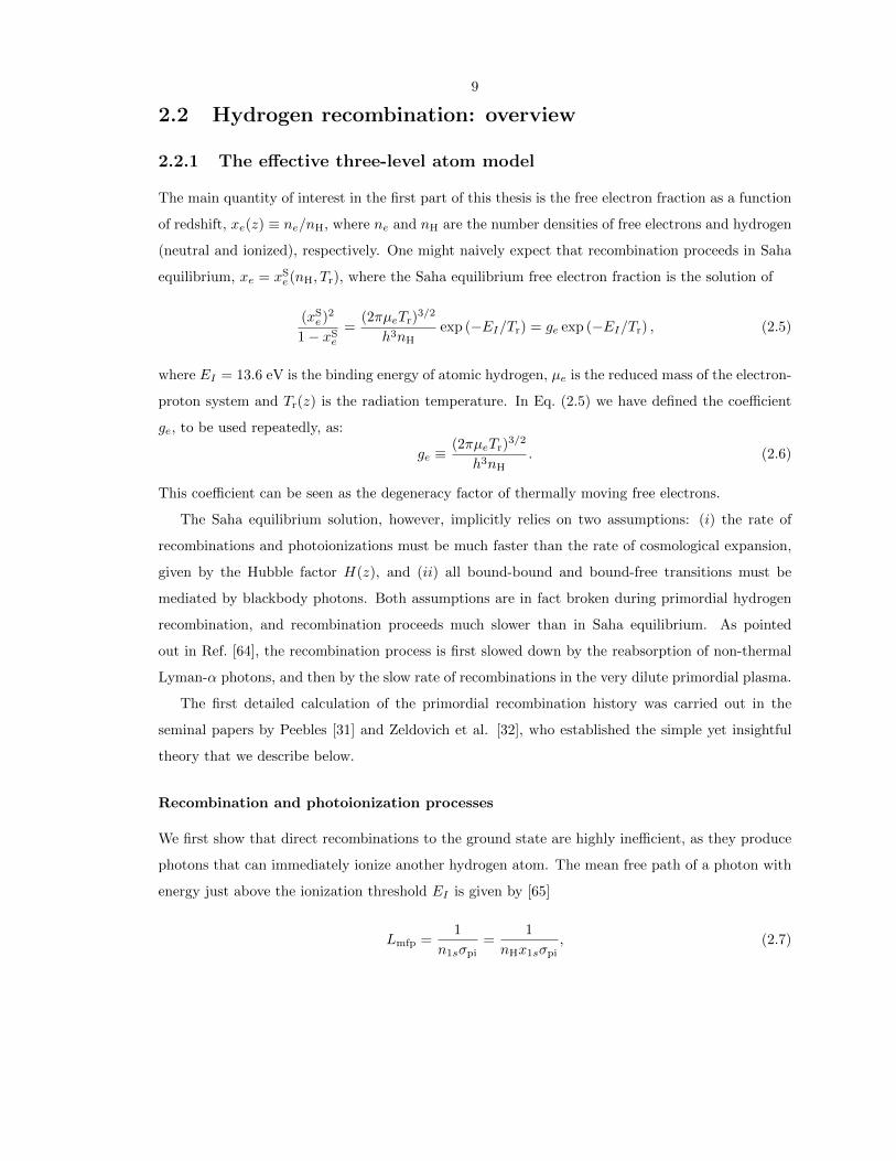
2.2.1 The effective three-level atom model

The main quantity of interest in the first part of this thesis is the free electron fraction as a function

of redshift, xe(z) ≡ ne/nH, where ne and nH are the number densities of free electrons and hydrogen

(neutral and ionized), respectively. One might naively expect that recombination proceeds in Saha

equilibrium, xe = xSe(nH, Tr), where the Saha equilibrium free electron fraction is the solution of

(xSe)2

1− xSe

=(2πµeTr)

3/2

h3nHexp (−EI/Tr) = ge exp (−EI/Tr) , (2.5)

where EI = 13.6 eV is the binding energy of atomic hydrogen, µe is the reduced mass of the electron-

proton system and Tr(z) is the radiation temperature. In Eq. (2.5) we have defined the coefficient

ge, to be used repeatedly, as:

ge ≡(2πµeTr)

3/2

h3nH. (2.6)

This coefficient can be seen as the degeneracy factor of thermally moving free electrons.

The Saha equilibrium solution, however, implicitly relies on two assumptions: (i) the rate of

recombinations and photoionizations must be much faster than the rate of cosmological expansion,

given by the Hubble factor H(z), and (ii) all bound-bound and bound-free transitions must be

mediated by blackbody photons. Both assumptions are in fact broken during primordial hydrogen

recombination, and recombination proceeds much slower than in Saha equilibrium. As pointed

out in Ref. [64], the recombination process is first slowed down by the reabsorption of non-thermal

Lyman-α photons, and then by the slow rate of recombinations in the very dilute primordial plasma.

The first detailed calculation of the primordial recombination history was carried out in the

seminal papers by Peebles [31] and Zeldovich et al. [32], who established the simple yet insightful

theory that we describe below.

Recombination and photoionization processes

We first show that direct recombinations to the ground state are highly inefficient, as they produce

photons that can immediately ionize another hydrogen atom. The mean free path of a photon with

energy just above the ionization threshold EI is given by [65]

Lmfp =1

n1sσpi=

1

nHx1sσpi, (2.7)

10

where n1s is the abundance of ground state hydrogen, x1s ≡ n1s/nH and σpi ≈ 6× 10−18 cm2 is the

photoionization cross-section at threshold. The total number density of hydrogen is given by

nH(z) = 250 cm−3

(1 + z

1100

)3Ωbh

2

0.022

1− YHe

0.76, (2.8)

where we have normalized the baryon abundance Ωbh2 and the helium mass fraction YHe to their

current best estimates [4, 66]. Photons just above the ionization threshold are therefore absorbed

by neutral hydrogen atoms in a characteristic time

tabs =Lmfp

c≈ 2× 104

x1ssec

(1 + z

1100

)−3

. (2.9)

Therefore, as soon as a tiny fraction of hydrogen has recombined (x1s ∼> 10−9), ionizing photons

are absorbed, or re-absorbed, in a time much shorter than the characteristic expansion time texp ∼300, 000 years, i.e., nearly instantaneously.

Electrons and protons can therefore recombine efficiently only to the excited states of hydrogen.

This situation is familiar in the study of the interstellar medium: it is referred to as “case-B”

recombination (see e.g. Ref. [67]). Once they have recombined to one of the excited states of

hydrogen, electrons “cascade down” to the n = 2 shell, on a much shorter timescale than the overall

recombination timescale. Recombinations to the excited states nl (with coefficient αnl) can therefore

effectively be accounted for as recombinations to the n = 2 shell with the case-B recombination

coefficient,

αB ≡∑

n≥2

αnl. (2.10)

The effective rate of recombinations is then

xe∣∣rec

= −x2

∣∣rec

= −nHx2eαB(Tm), (2.11)

where x2 ≡ nH(n=2)/nH is the fractional abundance of hydrogen in the first excited state and Tm

is the matter temperature, locked to the radiation temperature Tr by Thomson scattering at most

times during recombination. The reverse process, photoionizations from the excited states, must

also be accounted for, and has a rate

xe∣∣ion

=∑

n≥2

xnlβnl(Tr), (2.12)

where xnl is the fractional abundance of hydrogen in the state nl and βnl is the photoionization

rate from that state. It depends on the radiation temperature as photoionizations are caused by

11

blackbody photons, and is related to the corresponding recombination coefficient by detailed balance:

βnl(Tr) =gegl

eEn/TrnHαnl(Tm = Tr), (2.13)

where ge was defined in Eq. (2.6), En ≡ −EI/n2 is the energy of the n-th shell, and gl ≡ 2l + 1 is

the degeneracy of the state nl. We can now simplify Eq. (2.12) with the additional assumption that

excited states are in Boltzmann equilibrium with the first excited state, i.e.,

xnl = x2gl4

exp

(E2 − En

Tr

). (2.14)

Inserting Eqs. (2.13) and (2.14) into Eq. (2.12), we can rewrite the rate of photoionizations from the

excited states (which can effectively be seen as photoionizations from the n = 2 state) as

xe∣∣ion

= −x2

∣∣ion

= x2βB(Tr), (2.15)

where the effective photoionization rate is related to the case-B recombination coefficient by

βB(Tr) =ge4

eE2/TrnHαB(Tm = Tr). (2.16)

Transitions to the ground state

Once they have reached the n = 2 shell, electrons can reach the ground state by emitting a Lyman-α

photon from the 2p state. Due to the very high optical depth of the Lyman-α transition, emitted

photons will however almost certainly be reabsorbed by another atom. This is similar to the case

of ionizing photons which are immediately reabsorbed, but atoms in the 2p state have no other

option to decay to the ground state, unlike free electrons that can be captured in an excited state,

so computing the very small net decay rate is important.

The way out of this Lyman-α “bottleneck” is for photons to redshift below the Lyα resonant

frequency due to cosmological expansion. We denote fν the photon occupation number at frequency

ν [for a blackbody at temperature T , we would have fν =(ehν/kT − 1

)−1]. Simple phase-space

considerations give us the number of photons per frequency interval per hydrogen atom, Nν =

8πν2

c3nHfν . The rate at which photons redshift across a frequency ν due to cosmological expansion,

per hydrogen atom, is then given by HνNν . The net decay rate in the Lyman-α line, per hydrogen

atom, is then given by the difference between the rate at which photons produced in the line redshift

out of the line and the rate at which photons from the blue side redshift into the line. On the blue

side of the line, the photon occupation number can be approximated by a blackbody. Since the

12

energy of Lyα photons is ∼ 40 times larger than Tr, we have

f+νLyα

≈ e−E21/Tr , (2.17)

where E21 = E2 − E1 = 34EI is the energy of Lyα photons. The line being optically thick, the

photon occupation number equilibrates with the 2p to 1s ratio, and, just redward of the line, we

have

f−νLyα=

x2p

3x1s=

x2

4x1s, (2.18)

where in statistical equilibrium x2p = 34x2. The net rate of Lyman-α decays is then given by

x1s

∣∣Lyα

= −x2

∣∣Lyα

= HνLyα

(N−νLyα

−N+νLyα

)= RLyα

(3

4x2 − 3x1se

−E21/Tr

), (2.19)

where we have defined the rate of escape of Lyα photons per atom in the 2p state,

RLyα ≡8πH

3nHx1sλ3Lyα

. (2.20)

Eqs. (2.19–2.20) can also be derived in the Sobolev approximation, in the limit of large Sobolev

optical depth; we will do so in Chapter 4. We show the rate RLyα as a function of redshift in

Fig. 2.1. We see that at all relevant times during primordial recombination, 3RLyα is of the order

of a few to a few tens of net decays per second. This extremely slow net Lyman-α decay rate is

comparable to the rate of two-photon decays from the 2s state, Λ2s,1s ≈ 8.22 s−1 [68, 69]. The

latter therefore significantly contribute to the recombination dynamics, and should be accounted

for as a transition channel from the first excited state to the ground state [31, 32] (in fact, in the

late sixties, it was believed that Ωb = 1 and RLyα was thought to be even lower; Refs. [31, 32] had

therefore concluded that the large majority of decays to the ground state proceeded through two-

photon decays; using modern estimates for cosmological parameters, Ref. [70] find that ∼ 57% of

ground state hydrogen is formed following a two-photon decay). The net rate of two-photon decays

from the 2s state is:

x1s

∣∣2γ

= −x2

∣∣2γ

= Λ2s,1s

(x2s − x1se

−E21/Tr

)= Λ2s,1s

(x2

4− x1se

−E21/Tr

), (2.21)

where the second term accounts for two-photon absorptions and can be obtained by a detailed

balance argument.

Population of the excited state and recombination rate

We now have all the relevant rates to solve for the free-electron fraction. The last simplification is

to realize that the atomic rates, even for the slow 2s → 1s decays or the slow escape out of the

13

200 400 600 800 1000 1200 1400 1600z

1

10

100

Rate

(sec

-1)

!Ly "

#2s,1s

3RLy!

Figure 2.1: Rate of Lyman-α escape per atom in the 2s state, 3RLyα, where RLyα is given byEq. (2.20) (evaluated with the modern value of Ωbh

2), compared to the spontaneous two-photondecay rate from 2s, Λ2s,1s, as a function of redshift, for a standard recombination history.

Lyα resonance, are many orders of magnitude larger than the overall recombination rate, which is

of the order of (10 times) the Hubble expansion rate, that is ∼ 10−13 − 10−12 s−1. The population

of the n = 2 shell can therefore be obtained to high accuracy in the steady-state approximation, i.e.,

assuming that the net rate of recombinations to the n = 2 shell equals the net rate of transitions to

the ground state:

x2 = x2

∣∣rec

+ x2

∣∣ion

+ x2

∣∣Lyα

+ x2

∣∣2γ≈ 0. (2.22)

We can therefore solve for x2 and obtain:

x2 = 4nHx

2eαB + (3RLyα + Λ2s,1s)x1se

−E21/Tr

4βB + 3RLyα + Λ2s,1s. (2.23)

From Eqs. (2.11) and (2.15) we then obtain the rate of change of the free electron fraction:

xe = xe∣∣rec

+ xe∣∣ion

= −C(nHx

2eαB − 4x1sβBe−E21/Tr

), (2.24)

where the Peebles C-factor is given by

C ≡ 3RLyα + Λ2s,1s

4βB + 3RLyα + Λ2s,1s. (2.25)

As noted by Peebles, this factor represents the probability that an atom initially the n = 2 shell

reaches the ground state before being photoionized. Note that we could have obtained the same

equation starting from xe = −x1s = −(x1s|2p + x1s|2s) (this is because we have set x2 = 0).

14

200 400 600 800 1000 1200 1400 1600z

0.001

0.010

0.100

1.000

Peebles C-factorx2/x2(Saha)

Figure 2.2: Peebles C-factor [Eq. (2.25)] and ratio of the population of the n = 2 shell to its valuein Saha equilibrium with the continuum, as a function of redshift.

At all relevant times during the epoch of hydrogen recombination, x2 1, and therefore x1s =

1 − xe. If matter and radiation temperatures are set to be equal, Eq. (2.24) is therefore a simple

ordinary differential equation for xe, that can be easily integrated. A simple improvement is to also

explicitly follow the matter temperature evolution, which is determined by the Compton evolution

equation:

Tm = −2HTm +8σTarT

4r xe(Tr − Tm)

3(1 + fHe + xe)mec, (2.26)

where σT is the Thomson cross section, ar is the radiation constant, me is the electron mass and

fHe is the He:H ratio by number of nuclei.

2.2.2 Hydrogen recombination phenomenology

We show in Fig. 2.2 the evolution of the Peebles C-factor and the population of the n = 2 shell

relative to its value in Saha equilibrium with the continuum, x2|Saha ≡ 4ge

e−E2/Tx2e. We can see

that there are two distinct regimes.

Early times

At early times (z ∼> 900), electrons in the n = 2 shell have a high probability of being photoionized,

and the C-factor is much smaller than unity, C 1. As a consequence, the population of the n = 2

shell is very close to Saha equilibrium with the continuum, as can be seen by rewriting Eq. (2.23)

in the form

x2 = (1− C)4

gee−E2/Tx2

e + C 4x1se−E21/T , (2.27)

15

where we have assumed Tr = Tm = T and used Eqs. (2.16) and (2.25). During that period,

the recombination rate is therefore virtually independent of the exact value of the recombination

coefficient, and is entirely determined by the small net decay rate from the n = 2 shell to the ground

state:

xe(z ∼> 900) = −x1s ≈ (3RLyα + Λ2s,1s)

[x2|Saha

4− x1se

−E21/T

]. (2.28)

The recombination rate is of order ∼ CnHx2eαB ∼ 10−13 sec−1 (using Eq. (2.8), αB ∼ 10−13 cm−3

and C ∼ 10−2), which is of the same order as the Hubble expansion rate. Saha equilibrium with the

ground state can therefore not be maintained and the free electron fraction quickly becomes orders

of magnitude larger than the Saha equilibrium prediction. Since x2 ≈ x2(Saha), this means that

the excited states becomes over-populated with respect to Boltzmann equilibrium with the ground

state. This situation is usually referred to as the “n = 2 bottleneck”.

Late times

At late times (z ∼< 800), C ≈ 1, and the n = 2 shell is no longer in Saha equilibrium with the

continuum (note that it is not in Boltzmann equilibrium with the ground state either, as the rate

of recombinations to the n = 2 shell dominates over the net rate of two-photon or Ly-α absorptions

from the ground state). The free electron fraction is now many orders of magnitude above the value

it would have in Saha equilibrium. In that case, the second term in Eq. (2.24) is negligible and the

evolution of the free electron fraction becomes:

xe(z ∼< 800) ≈ −nHx2eαB. (2.29)

As we can see, the evolution of the free electron fraction is then virtually independent of the rate

of decays to the ground state from the n = 2 shell, but is highly sensitive to the exact value of the

effective recombination coefficient.

2.2.3 Validity of the assumptions made

The simple yet insightful effective three-level atom model presented in Section 2.2.1 provides a good

approximation for the recombination problem and remained essentially unaltered for several decades.

However, this simple theory relies on many simplifying assumptions, the validity of which we assess

now.

Steady-state approximation for the excited states X

The formal way to assess the validity of the steady-state approximation is to compute the eigenvalues

of the transition matrix in a multilevel calculation (to be described soon). This was done in Ref. [37],

16

where it was found that the minimum eigenvalue of the rate matrix is ∼ 1 sec−1. This could be

expected as the rate of Ly-α decays per atom in the 2p state is RLyα, which has a minimum of ∼ 1

sec−1 at z ≈ 1100 (see Fig. 2.1). This minimum rate is ∼ 12 orders of magnitude larger than the

recombination rate. The steady-state approximation was also checked explicitly in Ref. [38] where

the solution of the time-dependent problem was computed (i.e., solving coupled ordinary differential

equations for xe and the populations of the excited states). There again, it was found to be very

accurate. Note that this approximation also underlies the use of the case-B recombination coefficient,

as electrons captured in excited states are assumed to “cascade down” instantaneously to the first

excited shell.

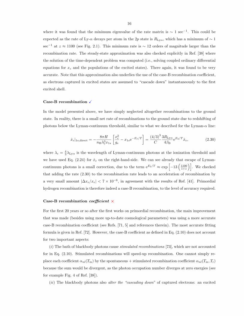
Case-B recombination X

In the model presented above, we have simply neglected altogether recombinations to the ground

state. In reality, there is a small net rate of recombinations to the ground state due to redshifting of

photons below the Lyman-continuum threshold, similar to what we described for the Lyman-α line:

xe|1s,direct = − 8πH

nHλ3cx1s

[x2e

ge− x1se

−EI/T]

=(4/3)

3

C

3RLyα

4βBeE2/T xe, (2.30)

where λc = 43λLyα is the wavelength of Lyman-continuum photons at the ionization threshold and

we have used Eq. (2.24) for xe on the right-hand-side. We can see already that escape of Lyman-

continuum photons is a small correction, due to the term eE2/T ≈ exp[−13

(11001+z

)]. We checked

that adding the rate (2.30) to the recombination rate leads to an acceleration of recombination by

a very small amount |∆xe/xe| < 7 × 10−6, in agreement with the results of Ref. [41]. Primordial

hydrogen recombination is therefore indeed a case-B recombination, to the level of accuracy required.

Case-B recombination coefficient ×

For the first 20 years or so after the first works on primordial recombination, the main improvement

that was made (besides using more up-to-date cosmological parameters) was using a more accurate

case-B recombination coefficient (see Refs. [71, 5] and references therein). The most accurate fitting

formula is given in Ref. [72]. However, the case-B coefficient as defined in Eq. (2.10) does not account

for two important aspects:

(i) The bath of blackbody photons cause stimulated recombinations [73], which are not accounted

for in Eq. (2.10). Stimulated recombinations will speed-up recombination. One cannot simply re-

place each coefficient αnl(Tm) by the spontaneous + stimulated recombination coefficient αnl(Tm, Tr)

because the sum would be divergent, as the photon occupation number diverges at zero energies (see

for example Fig. 4 of Ref. [38]).

(ii) The blackbody photons also alter the “cascading down” of captured electrons: an excited

17

atom may be photoionized before decaying to the first excited state. The sum in Eq. (2.10) should

therefore be weighted by the probabilities to actually reach the first excited state.

(iii) At late times, when the intensity of the blackbody radiation field decreases, excited states

cannot be maintained in Boltzmann equilibrium with each other. This is especially true for 2s and

2p, and one should split the case-B recombination coefficient appropriately between the two states.

From the discussion in Section 2.2.2, we can anticipate that these considerations may be impor-

tant at late times.

Lyman-α escape rate ×

The treatment of the Lyman-α presented in Section 2.2.1 is very simplistic: the radiation field is

just assumed to be a step function. Since ∼ 43% of recombinations proceed through a Lyman-α

decay [70], a more sophisticated radiative transfer calculation is required. Moreover, higher-order

Lyman lines also need to be considered. We can anticipate that more accurate calculations of the

Ly-α decay rate and decays in the higher-order Lyman lines will affect the peak of the visibility

function (see Section 2.2.2).

Two-photon decay rate ×

The majority of decays to the ground state proceed through the two-photon channel. The simple

expression for decay rate given in Eq. (2.21) does not account for two processes:

(i) Stimulated two-photon decays, particularly important when one of the two photons has energy

of the order of or less than Tr [47].

(ii) Absorption of non-thermal photons emitted in the Lyman-α line [48].

In addition, two-photon decays from higher-order excited states are also important [50]. Since

the bulk of these decays are near resonance with a Lyman line (i.e., the higher-energy photon is

close to a Lyman frequency), this also requires a radiative transfer treatment. Again, we expect

such corrections to be mostly important at early times z ∼> 900 and affect the peak of the visibility

function.

From the above discussion, we see that corrections to the recombination model can be subdivided

into two distinct categories:

(i) Radiative transfer calculations, mainly in the Lyman-α line, and also in higher-order lines.

These calculations must also properly account for two-photon decays from 2s and the higher-order

states. Corrections to the simple decay rates Eqs. (2.19) and (2.21) are expected to mostly affect

the early time recombination history z ∼> 900. Since the visibility function peaks at z ≈ 1100, small

corrections to the net decay rates may have important consequences on the C`’s and even a priori

small effects should be considered.

18

(ii) Multilevel atom calculations, that properly account for all transitions between excited states

of hydrogen and generalize the effective three-level atom model. Such modifications will mostly

affect the low redshift tail of the visibility function, and the accuracy requirement is somewhat lower

than for (i).

2.3 Outline of Part I

In the remainder of this part, we describe our work on both the radiative transfer and the multilevel

aspects of primordial hydrogen recombination. We first consider the late-time corrections due to the

multilevel structure of hydrogen. Chapter 3 is devoted to the description of the network of transitions

in hydrogen, and to the exposition of the effective multilevel atom method, suggested in Y. Ali-

Haımoud & C. M. Hirata, Phys. Rev. D 82, 063521 (2010). This method leads to a considerable

speedup of multilevel atom recombination computations. Chapter 4 is adapted from Y. Ali-Haımoud,

D. Grin & C. M. Hirata, Phys. Rev. D 82, 123502 (2010). In this work, we quantify the impact

of several previously neglected radiative transfer effects on the recombination history. Chapter 5

describes the implementation of HyRec, a fast and highly accurate recombination code that the

author developed with C. Hirata. This chapter is adapted from the first part of Y. Ali-Haımoud

& C. M. Hirata, Phys. Rev. D 83, 043513 (2011). It does not include C. Hirata’s contribution

on helium recombination, but the reader is encouraged to read the paper for a description of this

equally interesting problem. Finally, Chapter 6 is a reproduction of Y. Ali-Haımoud, C. M. Hirata

& M. Kamionkowski, Phys. Rev. D 83, 083508 (2011). In this chapter, slightly different from

the main line of research developed in the remainder of this part, we consider whether the high

sensitivity of future CMB experiments on the recombination history can be used to detect eventual

heavy elements present at the epoch of last scatter. All the mentioned published papers are fully or

partially reproduced here with permission, copyright (2010, 2011) by the American Physical Society.

Acknowledgements

I would like to thank Christopher Hirata for directing me to work on such an interesting topic, and

for his contributions to the research described here. I also thank Marc Kamionkowski for suggesting

the study of the effect of heavy elements at the surface of last scatter and his contributions to

this work. I have enjoyed discussing and collaborating with Daniel Grin on various aspects of

the recombination problem. Finally, I thank the participants of the July 2009 Paris Workshop

on Cosmological Recombination, in particular Jens Chluba, for many conversations on primordial

hydrogen recombination. Jens Chluba and I are currently running a detailed code comparison of

our respective recombination codes, CosmoRec and HyRec, which has unfortunately not yet been

completed at the time of submission of this thesis.

19

Chapter 3

Effective multilevel atom methodfor primordial hydrogenrecombination1

3.1 Introduction

We saw in Section 2.2.2 that the effective three-level atom (TLA) model [31, 32] cannot fully capture

the effect of the bath of blackbody photons on the recombination process: stimulated recombinations

must also be accounted for, as well as bound-bound transitions among excited states and photoion-

izations events that impede some of the “cascading” electrons to reach the first excited states. Such

processes will essentially affect the low-redshift tail of the ionization history, but are still important

given the sensitivity of upcoming CMB experiments.

One way to account exactly for these processes is to solve simultaneously for the free electron

fraction and the populations of all (or at least, a large number of) excited states. This method of

solution, which we refer to as the standard multilevel atom (MLA) method, is commonly used in the

study of emission lines in the interstellar medium. In fact, it was first used in the context of primordial

recombination to compute the spectrum of emitted lines [74, 75]. After it was understood that non-

equilibrium of excited states and stimulated recombinations may have an effect on the recombination

history itself [5], the first detailed MLA calculations were carried by Seager et al. [29, 30]. In

practice, one cannot account for an infinite number of excited states and must impose a cutoff in

MLA computations, i.e., discard states with principal quantum number higher than a given nmax.

Refs. [29, 30] computed recombination histories including up to nmax = 300 excited states, assuming

that angular momentum substates within a given energy shell are in statistical equilibrium. They

1The material in this chapter was mostly adapted from the paper Ultrafast effective multilevel atom methodfor primordial hydrogen recombination, Y. Ali-Haımoud & C. M. Hirata, Phys. Rev. D 82, 063521 (2010), withthe exception of Section 3.4.4, which is an exerpt from the paper HyRec: A fast and highly accurate primordialhydrogen recombination code, Y. Ali-Haımoud & C. M. Hirata, Phys. Rev. D 83, 043513 (2011). Reproduced herewith permission, copyright (2010, 2011) by the American Physical Society.

20

found that the residual ionization fraction at low redshift is decreased by approximately 10% with

respect to the TLA prediction. It was later shown that the desired sub-percent accuracy can only

be reached when explicitly resolving the out-of-equilibrium angular momentum substates [35, 36],

which requires the MLA codes to follow Nlevel = nmax(nmax + 1)/2 individual states. Moreover,

the ordinary differential equations (ODEs) describing the level populations are stiff, requiring the

solution of large Nlevel×Nlevel systems of equations at each integration time step. This problem has

been solved by several authors [36, 37, 38]; however, these standard MLA codes take hours to days

to compute a single recombination history.

Eventually, it is necessary to be able to produce not only accurate but also fast recombination

histories, to be included in Markov Chain Monte Carlo (MCMC) codes for cosmological parameter

estimation. The MCMC requires CMB power spectra (and hence recombination histories) to be gen-

erated at each proposed point in cosmological parameter space, with a typical chain sampling O(105)

points [76]. Furthermore, dozens of MCMCs are often run with different combinations of observa-

tional constraints and different parameter spaces. This makes it impractical to include recombination

codes that run for more than a few seconds in the MCMC. One solution is to precompute recombina-

tion histories xe(z|H0, TCMB,Ωmh2,Ωbh

2, YHe, Nν) on a grid of cosmological parameters, and then

use elaborate interpolation algorithms to evaluate the recombination history for any cosmology [77],

or to construct fitting functions [30, 78]. However, such procedures need to be re-trained every time

additional parameters are added, and are rather unsatisfying regarding their physical significance.

In this chapter, we present a new2, effective multilevel atom method (hereafter EMLA), that

is a simple generalization of Peebles’ TLA model presented in Section 2.2.1, but accounts exactly

for the multilevel structure of hydrogen, and allows for the inclusion of virtually infinitely many

excited states of hydrogen and all relevant bound-bound and bound-free transitions. The improved

recombination equations are exactly equivalent to the standard MLA equations, but have the same

computational cost as the TLA model (for an equal treatment of radiative transfer), while being

much more accurate. The basic idea is that the vast majority of the excited hydrogen levels are

populated and depopulated only by optically thin radiative transitions (bound-bound and bound-

free) in a bath of thermal photons; we show that their effect can be “integrated out” leaving only a

few functions of the matter and radiation temperatures Tm and Tr (this list would include the free

electron density ne if we incorporated collisions), which can be pre-tabulated. These functions are

just the generalization of the case-B recombination coefficient. In an actual call to the recombination

code from an MCMC, it is then only necessary to solve an effective MLA with a smaller number of

levels, which eliminates the computationally difficult Nlevel×Nlevel system solution in the traditional

MLA. [The idea is similar in spirit to the line-of-sight integral method for the computation of the

2It has recently been brought to my attention that this method was independently suggested by M. S. Burgin[79, 80]. Due to translation delays, this work only became known in the Western world several months after thepublication of our paper.

21

CMB power spectrum [24], which eliminated a large number of independent variables from the

cosmological perturbation theory system of ODEs (the high-order moments of the radiation field,

Θ` for ` 1) in favor of pretabulated spherical Bessel functions.] Our method achieves a speed-up

of the recombination calculation by 5 to 6 orders of magnitude.

This chapter is organized as follows. In Section 3.2 we review the general picture of hydrogen

recombination, and the bound-bound and bound-free transition rates involved in the calculation.

In Section 3.3 we describe the standard MLA method. We present our new EMLA method in

Section 3.4 and demonstrate its equivalence with the standard MLA formulation. We describe our

numerical implementation and results in Section 3.5, and conclude in Section 3.6. Appendix 3.A

gives mathematical proofs for various relations satisfied by the effective rates. Appendix 3.B gives

the details of our numerical evaluation of the effective rates.

3.2 Network of bound-bound and bound-free transitions

Here we give explicit expressions for the bound-bound and bound-free rates discussed above. Sub-

scripts nl refer to the bound state of principal quantum number n and angular momentum quantum

number l. We denote αfs the fine structure constant, µe ≡ memp/(me + mp) the reduced mass of

the electron-proton system, EI the ionization energy of hydrogen, and En ≡ −EIn−2 the energy of

the nth shell. Finally, we denote by fBB(E, Tr) ≡ (eE/Tr − 1)−1 the photon occupation number at

energy E in the blackbody radiation field at temperature Tr.

3.2.1 Recombination to and photoionization from the excited states

We have justified in Section 2.2.3 that direct recombinations to the ground state can be neglected,

and we only need to consider recombinations to the excited states. The recombination coefficient to

the excited state nl, including stimulated recombinations, is denoted αnl(Tm, Tr) (it has units of cm3

s−1). The photoionization rate per atom in the state nl is denoted βnl(Tr). Both can be expressed

in terms of the bound-free radial matrix elements g(n, l, κ, l′) [81]. Defining

γnl(κ) ≡ 2

3n2α3

fs

EIh

(1 + n2κ2)3 ×∑

l′=l±1

max(l, l′)g(n, l, κ, l′)2, (3.1)

where κ denotes the momentum of the outgoing electron in units of ~/a0 (where a0 is the reduced-

mass Bohr radius), the recombination coefficient is given by [81]:

αnl(Tm, Tr) =h3

(2πµeTm)3/2×∫ +∞

0

e−EIκ2/Tmγnl(κ)× [1 + fBB (Eκn, Tr)] d(κ2), (3.2)

22

where Eκn ≡ EI(κ2 + n−2). The photoionization rate only depends on the radiation temperature

and can be obtained by detailed balance considerations from the recombination coefficient:

βnl(Tr) =(2πµeTr)

3/2

(2l + 1)h3eEn/Trαnl(Tm = Tr, Tr). (3.3)

3.2.2 Transitions between excited states

We denote Rnl,n′l′ the transition rate from the excited state nl to the excited state n′l′. It has units

of sec−1 per atom in the initial state. Transitions among excited states can be either radiative or

collisional:

Rnl,n′l′ = Rradnl,n′l′(Tr) +Rcoll

nl,n′l′(Tm, ne), (3.4)

where ne = np is the abundance of free electrons or free protons. In this work, we follow exclusively

the radiative rates. These are given by

Rradnl,n′l′ =

Anl,n′l′ [1 + fBB(Enn′ , Tr)] if En > En′

gl′gl

e−En′n/TrRradn′l′,nl if En < En′ ,

(3.5)

where Enn′ ≡ En − En′ is the energy difference between the excited levels, gl ≡ 2l + 1 is the

degeneracy of the state nl, and Anl,n′l′ is the Einstein A-coefficient for the nl, n′l′ transition, which

may be obtained from the radial matrix element Rnln′l′ [82]:

Anl,n′l′ =2π

3α3

fs

EIh

(1

n′2− 1

n2

)3max(l, l′)

2l + 1|Rnln′l′ |2. (3.6)

An important underlying assumption of Eq. (3.5) is that transitions between excited states are

optically thin. The maximum Sobolev optical depth (to be defined in Chapter 4) in these transitions

is indeed at most 5.5×10−4 [49]. The consequence is that bound-bound transitions between excited

states only depend on the radiation temperature.

3.2.3 Transitions to the ground state

Transitions to the ground state require a more subtle treatment than optically thin transitions

between excited states. Their rates have in general complicated dependences, not only on the

radiation temperature but also on cosmology. To remain general, we denote the net i → 1s decay

rate in the form

x1s

∣∣i

= −xi∣∣1s

= xiRi,1s − x1sR1s,i, (3.7)

where the notation R is meant to emphasize the complicated (not necessarily analytical) functional

form. The equations presented in this chapter are general and can accommodate any particular form

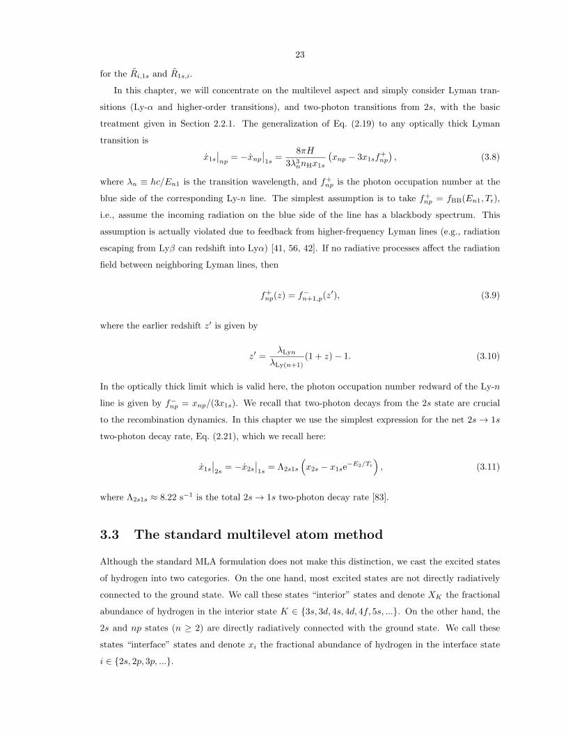
23

for the Ri,1s and R1s,i.

In this chapter, we will concentrate on the multilevel aspect and simply consider Lyman tran-

sitions (Ly-α and higher-order transitions), and two-photon transitions from 2s, with the basic

treatment given in Section 2.2.1. The generalization of Eq. (2.19) to any optically thick Lyman

transition is

x1s

∣∣np

= −xnp∣∣1s

=8πH

3λ3nnHx1s

(xnp − 3x1sf

+np

), (3.8)

where λn ≡ hc/En1 is the transition wavelength, and f+np is the photon occupation number at the

blue side of the corresponding Ly-n line. The simplest assumption is to take f+np = fBB(En1, Tr),

i.e., assume the incoming radiation on the blue side of the line has a blackbody spectrum. This

assumption is actually violated due to feedback from higher-frequency Lyman lines (e.g., radiation

escaping from Lyβ can redshift into Lyα) [41, 56, 42]. If no radiative processes affect the radiation

field between neighboring Lyman lines, then

f+np(z) = f−n+1,p(z

′), (3.9)

where the earlier redshift z′ is given by

z′ =λLyn

λLy(n+1)(1 + z)− 1. (3.10)

In the optically thick limit which is valid here, the photon occupation number redward of the Ly-n

line is given by f−np = xnp/(3x1s). We recall that two-photon decays from the 2s state are crucial

to the recombination dynamics. In this chapter we use the simplest expression for the net 2s→ 1s

two-photon decay rate, Eq. (2.21), which we recall here:

x1s

∣∣2s

= −x2s

∣∣1s

= Λ2s1s

(x2s − x1se

−E2/Tr

), (3.11)

where Λ2s1s ≈ 8.22 s−1 is the total 2s→ 1s two-photon decay rate [83].

3.3 The standard multilevel atom method

Although the standard MLA formulation does not make this distinction, we cast the excited states

of hydrogen into two categories. On the one hand, most excited states are not directly radiatively

connected to the ground state. We call these states “interior” states and denote XK the fractional

abundance of hydrogen in the interior state K ∈ 3s, 3d, 4s, 4d, 4f, 5s, .... On the other hand, the

2s and np states (n ≥ 2) are directly radiatively connected with the ground state. We call these

states “interface” states and denote xi the fractional abundance of hydrogen in the interface state

i ∈ 2s, 2p, 3p, ....

24

In the standard MLA formulation, the free electron fraction xe(z) is evolved by solving the

hierarchy of coupled differential equations: for the interior states,

XK = x2enHαK +

∑

L

XLRL,K +∑

j

xjRj,K −XK

(βK +

∑

L

RK,L +∑

j

RK,j

); (3.12)

for the interface states,

xi = x2enHαi +

∑

L

XLRL,i +∑

j

xjRj,i + x1sR1s,i − xi(βi +

∑

L

Ri,L +∑

j

Ri,j + Ri,1s

); (3.13)

and for the free electrons and ground state,

xe = −x1s = x1s

∑

i

R1s,i −∑

i

xiRi,1s. (3.14)

The radiative rates between excited states are many orders of magnitude larger than the rate at

which recombination proceeds, which is of the order of the Hubble rate. Even the relatively small

net rates out of the interface states (Λ2s,1s and RLyα) are still more than 12 orders of magnitude

larger than the Hubble rate. The populations of the excited states can therefore be obtained to high

accuracy in the steady-state approximation (this approximation is ubiquitous in many problems and

has long been used in the context of cosmological recombination [31, 49, 37], where its accuracy

has been tested explicitly [38]). Setting XK and xi to zero in Eqs. (3.12) and (3.13), we see that

the problem amounts to first solving a system of linear algebraic equations for the XK , xi, with an

inhomogeneous term depending on xe, and then using the populations xi in Eq. (3.14) to evolve the

free electron fraction. The solution of the system of equations (3.12), (3.13) needs to be done at

every time step, since the inhomogeneous term of the equation depends on the ionization history,

which explicitly depends on time as well as on the cosmological parameters. Recent work [37, 38]

has shown that to compute sufficiently accurate recombination histories, one needs to account for

excited states up to a principal quantum number nmax ∼ 100, resolving the angular momentum

substates. This requires solving an O(104 × 104

)system of equations at each time step, which, even

with modern computers, is extremely time consuming.

3.4 New method of solution: the effective multilevel atom

We now give a computationally efficient method of solution for the primordial recombination prob-

lem. We factor the effect of the numerous transitions involving interior states in terms of effective

transitions into and out of the much smaller number of interface states. Once the rates of these

effective transitions are tabulated, the cosmological evolution of the free electron fraction can be

25

obtained from a simple effective few-level atom calculation. We describe the method in Section 3.4.1

and give the proof of its exact equivalence to the standard MLA method in Section 3.4.2. In the

subsequent Section 3.4.3, we consider which states should be treated as interface states. Finally, Sec-

tion 3.4.4 provides a further simplification of the problem, which is reduced to an effective four-level

atom calculation.

3.4.1 Motivations and general formulation

We first note that the only quantity of importance for CMB power spectrum calculations is the

free electron fraction as a function of redshift, xe(z). The populations of the excited states are

calculated only as an intermediate step — if they are desired (for example, to calculate Hα scattering

features [84] or the recombination spectrum [74, 75, 35]), the populations of the excited states can be

obtained by solving Eqs. (3.12, 3.13) once the free electron fraction is known. Furthermore, only the

“interface” states 2s and np (and ns, nd when accounting for two-photon processes from higher-order

states) are directly connected to the ground state and directly appear in the evolution equation for

the free electron fraction Eq. (3.14). All other (“interior”) excited states are only connected with

other excited states or with the continuum, through optically thin radiative transitions (and to a

lesser extent through collisions [36]). Interior states are only transitional states: an electron in

the “interior” rapidly transitions through spontaneous and stimulated decays or absorptions caused

by the blackbody radiation field (or collisions with free electrons and protons), until it is either

photoionized, or reaches an interface state. There can be a very large number of transitions before

any of these outcomes occurs, but the passage through the “interior” is always very short compared

to the overall recombination timescale, and can be considered as instantaneous (for the same reason

that the steady-state approximation is valid in the standard MLA formulation).

Instead of computing the fraction of hydrogen in each interior state K, one can rather evaluate

the probabilities that an atom initially in the interior state K ultimately reaches one of the interface

states or gets photoionized. Of course, after reaching an interface state, the atom may perfectly

transition back to an interior state, or get photoionized. However, we consider the probability of

first reaching a given interface state before any other one, which is uniquely defined. For an atom

in the interior state K, we denote by P iK the probability of ultimately reaching the interface state i,

and P eK the probability of ultimately being photoionized. An excited atom initially in the interior

state K has a probability RK,i/ΓK to directly decay to the interface state i, where ΓK is the total

width (or inverse lifetime) of the state K:

ΓK ≡∑

L 6=KRK,L +

∑

j

RK,j + βK . (3.15)

The atom may also first decay or get excited to another interior state L 6= K, with a probabil-

26

P eK

K

P iK

i

e! + p+

H(1s)

“interior”states

“interface” states

Figure 3.1: Schematic representation of the formulation of the recombination problem adopted inthis work. Dotted arrows represent possibly numerous fast transitions within the “interior”.

ity RK,L/ΓK , from which it may then eventually reach the interface state i with probability P iL.

Mathematically, these various paths translate into the following system of linear equations for the

probabilities P iK :

P iK =∑

L 6=K

RK,LΓK

P iL +RK,iΓK

. (3.16)

Similarly, the P eK must satisfy the self-consistency relations:

P eK =∑

L 6=K

RK,LΓK

P eL +βKΓK

, (3.17)

We show in Appendix 3.A.2 that these linear systems are invertible and therefore uniquely determine

P iK and P eK . In Appendix 3.A.3 we prove the complementarity relation,

∑

i

P iK + P eK = 1, (3.18)

which has the simple physical interpretation that an atom in the Kth interior state eventually reaches

an interface state or is photoionized with unit probability.

Once these probabilities are known, it is possible to describe the large number of transitions

between all the states in a simplified manner, in terms of effective rates into and out of the interface

states. To clarify the explanation, we illustrate in Figure 3.1 the processes described below.

An electron and a proton can effectively recombine to the interface state i either through a direct

recombination (with coefficient αi), or following a recombination to an interior state K (with coef-

ficient αK), from which a sequence of interior transitions may ultimately lead to the interface state

27

i with probability P iK . The effective recombination coefficient to the interface state i is therefore:

Ai ≡ αi +∑

K

αKPiK . (3.19)

Conversely, an atom in the interface state i may effectively be ionized either through a direct

photoionization (with rate βi), or after being first excited to an interior state K (with rate Ri,K),

from which the atom may ultimately be photoionized after a series of interior transitions with

probability P eK . The effective photoionization rate from the interface state i is therefore:

Bi ≡ βi +∑

K

Ri,KPeK . (3.20)

Finally, atoms can effectively transition from an interface state i to another interface state j, either

through a direct transition if it is allowed, or after first transitioning through the interior. The

effective transfer rate between the ith and jth interface states is therefore:

Ri,j ≡ Ri,j +∑

K

Ri,KPjK (j 6= i). (3.21)

The rate of change of the population of the interface state i is therefore:

xi = x2enHAi +

∑

j 6=ixjRj,i + x1sR1s,i − xi

(Bi +

∑

j 6=iRi,j + Ri,1s

), (3.22)

where we have included the effective transitions described above, as well as transitions from and to

the ground state.

The system of equations (3.16–3.22) is exactly equivalent to the standard MLA formulation, as

we shall show in Section 3.4.2 below. Moreover, we will show that the rate of change of the free

electron fraction, Eq. (3.14), can also be written in the equivalent form

xe = −∑

i

(nHx

2eAi − xiBi

). (3.23)

Let us now consider the dependences of the effective rates. In the purely radiative case, the prob-

abilities P iK and P eK only depend on the radiation temperature Tr, since transitions between excited

states and photoionizations only depend on the locally thermal radiation field. As a consequence,

the effective recombination rates Ai (Tm, Tr) are only functions of matter and radiation tempera-

tures and the effective photoionization and bound-bound rates Bi (Tr) and Ri,j (Tr) are functions

of the radiation temperature only. When including collisional transitions, all effective rates become

functions of the three variables Tr, Tm and ne. In all cases, effective rates can be easily tabulated

once and for all and interpolated when needed for a recombination calculation.

28

Intuitively, we would expect that Ai, Bi, and Ri,j satisfy the detailed balance relations,

gie−Ei/TrRi,j(Tr) = gje

−Ej/TrRj,i(Tr) (3.24)

and

gie−Ei/TrBi(Tr) =

(2πµeTr)3/2

h3Ai(Tm = Tr, Tr). (3.25)

We show in Appendix 3.A.4 that these equations are indeed valid. This means that we only need to

tabulate half of the Ri,j [the other half can be obtained from Eq. (3.24)] and all the Ai [the Bi can

be obtained from Eq. (3.25); in particular, we do not need to solve for the P eK ].

We note that the probabilities P iK , PeK are a generalization of the cascade matrix technique

introduced by Seaton [85]. Seaton’s calculation assumed a vanishing ambient radiation field, so

that electrons can only “cascade down” to lower energy states. In the context of the recombination

of the primeval plasma, one cannot ignore the strong thermal radiation field, and electrons rather

“cascade up and down,” following spontaneous and stimulated decays or photon absorption events.

The spirit of our method is however identical to Seaton’s cascade-capture equations [85], where the

“cascading” process is decoupled from the particular process populating the excited states, or from

the depopulation of the interface states.

We emphasize that the method presented here is a simple generalization of the effective TLA

model, with the case-B recombination coefficient being replaced by the effective recombination co-

efficients, which are computed individually for each interface state 2s, 2p, 3p, ....

3.4.2 Equivalence with the standard MLA method

This section is dedicated to proving the equivalence of the EMLA equations, Eqs. (3.16–3.22), with

the standard MLA equations, Eqs. (3.12, 3.13), in the steady-state limit for the interior states

(i.e., where we set XK ≈ 0). The steady-state approximation does not need to be made for the

interface states to demonstrate the equivalence of the two formulations (but we do use it for practical

computations since it is valid to very high accuracy).

We denote by N the number of interior states and n∗ the number of interface states (we will

address in Section 3.4.3 the issue of which states need to be considered as interface states).

We begin by defining the N ×N rate matrix M with elements

MKL ≡ δKLΓK − (1− δKL)RK,L. (3.26)

We also define the n∗ + 1 length-N vectors Pi,Pe, the components of which are the probabilities

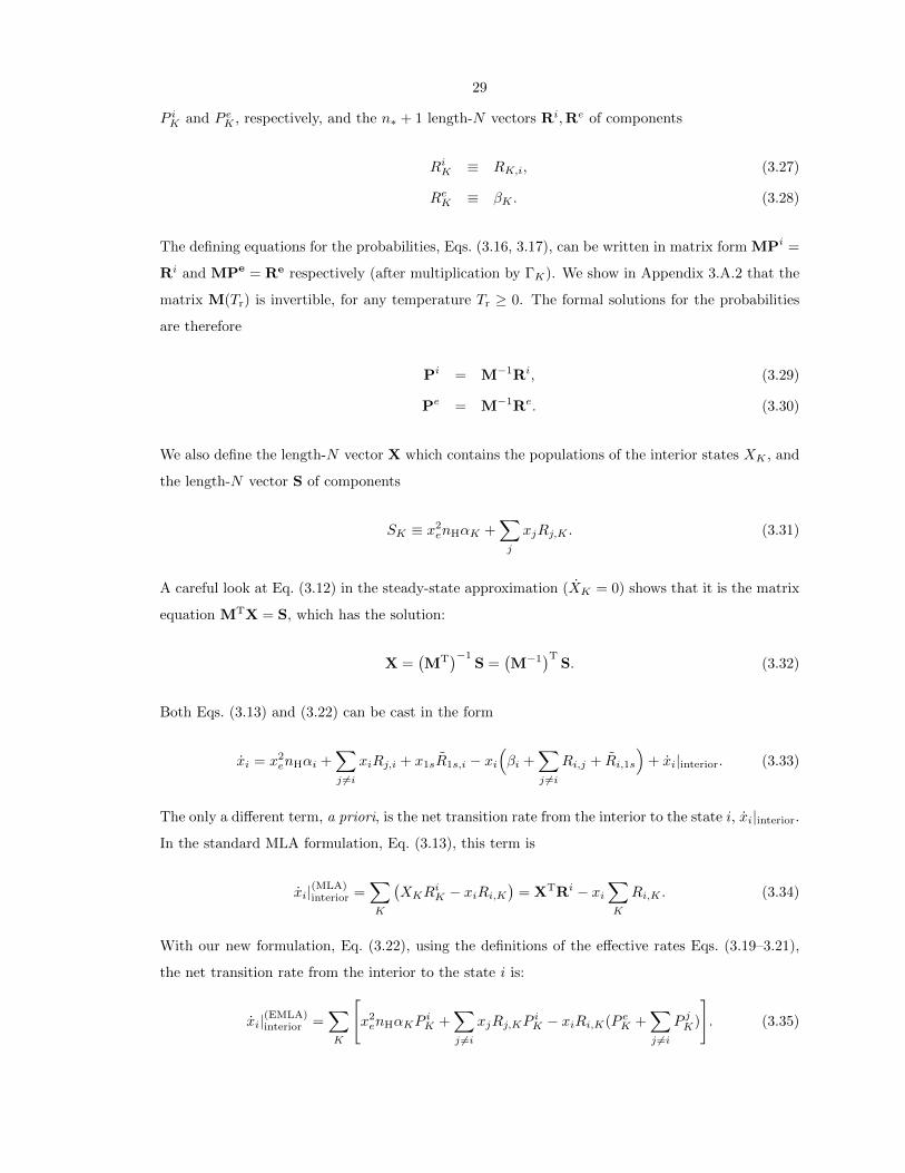
29

P iK and P eK , respectively, and the n∗ + 1 length-N vectors Ri,Re of components

RiK ≡ RK,i, (3.27)

ReK ≡ βK . (3.28)

The defining equations for the probabilities, Eqs. (3.16, 3.17), can be written in matrix form MPi =

Ri and MPe = Re respectively (after multiplication by ΓK). We show in Appendix 3.A.2 that the

matrix M(Tr) is invertible, for any temperature Tr ≥ 0. The formal solutions for the probabilities

are therefore

Pi = M−1Ri, (3.29)

Pe = M−1Re. (3.30)

We also define the length-N vector X which contains the populations of the interior states XK , and

the length-N vector S of components

SK ≡ x2enHαK +

∑

j

xjRj,K . (3.31)

A careful look at Eq. (3.12) in the steady-state approximation (XK = 0) shows that it is the matrix

equation MTX = S, which has the solution:

X =(MT

)−1S =

(M−1

)TS. (3.32)

Both Eqs. (3.13) and (3.22) can be cast in the form

xi = x2enHαi +

∑

j 6=ixiRj,i + x1sR1s,i − xi

(βi +

∑

j 6=iRi,j + Ri,1s

)+ xi|interior. (3.33)

The only a different term, a priori, is the net transition rate from the interior to the state i, xi|interior.

In the standard MLA formulation, Eq. (3.13), this term is

xi|(MLA)interior =

∑

K

(XKR

iK − xiRi,K

)= XTRi − xi

∑

K

Ri,K . (3.34)

With our new formulation, Eq. (3.22), using the definitions of the effective rates Eqs. (3.19–3.21),

the net transition rate from the interior to the state i is:

xi|(EMLA)interior =

∑

K

[x2enHαKP

iK +

∑

j 6=ixjRj,KP

iK − xiRi,K(P eK +

∑

j 6=iP jK)

]. (3.35)

30

Using the complementarity relation Eq. (3.18), we rewrite P eK +∑j 6=i P

jK = 1 − P iK . We then

recognize that the common factor of P iK is just the K-th component of the vector S, Eq. (3.31), so

we can rewrite Eq. (3.35) as

xi|(EMLA)interior = STPi − xi

∑

K

Ri,K . (3.36)

From the formal solution for the populations of the interior states Eq. (3.32), we have

XTRi = STM−1Ri = STPi, (3.37)

where the second equality is obtained from the formal solution for the probabilities P iK , Eq. (3.29).

We therefore see from Eqs. (3.34) and (3.36) that

xi|(MLA)interior = xi|(EMLA)

interior , (3.38)

and hence the two formulations are exactly equivalent. They only differ by the order in which the

bilinear product STM−1Ri is evaluated.

Finally, we show that Eq. (3.23) correctly gives the rate of change of the free electron fraction.

In the standard MLA formulation, the rate of change of the free electron fraction can be written as:

xe = −∑

K

[nHx

2eαK −XKβK

]−∑

i

[nHx

2eαi − xiβi

]. (3.39)

This formula is never used in standard MLA codes, as it requires a summation over a large number

of nearly canceling terms, and MLA codes use instead xe = −x1s to compute the rate of change

of the free electron fraction. Eq. (3.39) remains however formally correct. Using Eqs. (3.32) and

(3.30), we rewrite:

∑

K

XKβK =∑

K,L

βK(M−1

)LK

[nHx

2eαL +

∑

i

xiRi,L

]=∑

L

P eL

[nHx

2eαL +

∑

i

xiRi,L

]

=∑

L

nHx2eαL − nHx

2e

∑

i

∑

L

αLPiL +

∑

i

xi∑

L

Ri,LPeL, (3.40)

where in the last equality we have used the complementarity relation∑i P

iK + P eK = 1. Inserting

this result into Eq. (3.39), and using the definitions of the effective recombination coefficients and

photoionization rates Eqs. (3.19) and (3.20), we immediately recover Eq. (3.23).

31

3.4.3 Choice of interface states

If one naively includes all np states up to n = nmax = O(100) in the list of interface states, the

interpolation of effective rates can become somewhat cumbersome as it involves O(104)

functions

of one to three variables. However, only the lowest few of these states actually have significant

transition rates to the ground state; indeed, most of the decays to the ground state proceed through

either 2s (two-photon decay) or 2p (Lyα escape), as anticipated in the earliest studies [31, 32].

The rate of Lyman line escape is dominated by the lowest few lines. For example, if the relative

populations of the excited states were given by the Boltzmann ratios (which is a good approximation

until late times) then the net decay rate in the np→ 1s transition (not accounting for feedback from

the next line) would be proportional to

xnp→1s ∝ (1− n−2)3e−En/Tr . (3.41)

This relation would imply that the Lyβ escape rate is < 1% of the Lyα escape rate, and the higher-

order Lyman lines contribute even less. Previous computations of the escape rates (e.g., Ref. [49])

agree with this expectation. These considerations imply that for n ≥ 3, x1s|np x1s|2p in Eq. (3.14).

Moreover, an atom in the np state with n ≥ 3 is much more likely to spontaneously decay to n′s

or n′d, with 2 ≤ n′ < n, than to emit a Lyman-n photon that successfully escapes the line. This

implies that∣∣∣xnp|1s

∣∣∣∣∣∣xnp

∣∣∣ in Eq. (3.13).

In addition to a very low net decay rate out of the np states for n ≥ 3, feedback between

neighboring lines further suppresses their efficiency as interface states. The few photons that escape

the Ly(n+ 1) line will be reabsorbed almost certainly in the next lower line, after a redshift interval

∆z = zem − zab = (1 + zab)

(En+1,1

En1− 1

). (3.42)

Feedback between the lowest-lying lines is not instantaneous: ∆z/(1 + zab) = 0.185 for Lyβ →Lyα

feedback, 0.055 for Lyγ →Lyβ, and 0.024 for Lyδ →Lyγ. However, for higher-order lines, feedback

rapidly becomes nearly instantaneous as ∆z/(1 + zab) ∼ 2/n3. Thus the effect of the higher Lyman

lines is even weaker than Eq. (3.41) would suggest. Recent work [42] has shown that including lines

above Lyβ results in a fractional error |∆xe|/xe of at most ≈ 3× 10−4.

We therefore conclude that very accurate recombination histories can be obtained by only includ-

ing 2s and the low-lying p-states as interface states and neglecting higher-order Lyman transitions

altogether (we will show below that accounting for Lyα Lyβ and Lyγ and feedback between them

is sufficient). In addition, when considering two-photon transitions from higher levels, one should in

principle add the ns and nd states as “interface” states. However, only two-photon transitions from

2s, 3s and 3d, are important (and 4s, 4d at the level of a few 10−4), see Chapter 5 and Refs. [49, 52].

32

The number of efficient “interface” states, which we denote n∗, is therefore small (n∗ = 8 is sufficient

from the above discussion).

We can now see that our formulation in terms of effective transition rates and interface states is

much better adapted for a fast recombination calculation that the standard MLA formulation. To

compute accurate recombination histories, explicitly accounting for high-n shells of hydrogen, one

first needs to tabulate a few functions Ai and Ri,j on temperature grids. The computation of

the effective rates is the time-consuming part of the calculation; however, since they are independent

of the cosmological parameters, this can be done once, and not repeated for each cosmology. When

considering n∗ interface states, the free electron fraction can then be computed very quickly for

any given cosmology by solving the n∗ + 1 equations (3.22) and (3.14) or (3.23), interpolating the

effective rates from the pre-computed tables. Note that Eq. (3.22) is a simple n∗ × n∗ system of

linear algebraic equations in the steady-state approximation. In the following section we show that

we can simplify the the problem even further by reducing it to an effective four-level atom model.

3.4.4 Further simplification: the effective four-level atom

If we wish to follow n∗ “interface” states, then the system of equations (3.22), in the steady-state

approximation, is an n∗×n∗ system. Moreover, one needs to interpolate n∗ functions of 2 variables

(the effective recombination coefficients — the effective photoionization rates are obtained by detailed

balance), and n∗(n∗−1)/2 functions of 1 variable (half of the effective bound-bound rates, the other

half being obtained by detailed balance). Here we show how this system can be further reduced to

a 2× 2 system involving only 2s and 2p, requiring only 2 functions of 2 variables and 1 function of

1 variable, with virtually no loss of accuracy.

For now on we use the general index K for all states with principal quantum number n ≥ 3.

Even if some of the states with n ≥ 3 are radiatively connected to the ground state, one can still

formally define the effective transition rates Eqs. (3.19), (3.20) and (3.21) for the 2s and 2p states

because of the near-instantaneity of transitions out of the excited states. However, these coefficients

do not have a simple temperature dependence anymore, and are therefore not well suited for fast

interpolation. Indeed, the probabilities P iK and P eK , where i = 2s, 2p, are still defined by Eqs. (3.16)

and (3.17), but the inverse lifetime of the state K, Eq. (3.15), should now account for the net

downward transition rate to the ground state, and one should make the replacement:

ΓK → ΓK ≡ ΓK(Tr) + RK,1s, (3.43)

where we define ΓK(Tr) as the inverse lifetime of the K-th interface state when transitions to the

ground state are not included. In addition, we need to define additional effective transition rates

33

with the ground state. For i = 2s, 2p, we define:

Ri,1s ≡ Ri,1s +∑

K

Ri,K P1sK (3.44)

and

R1s,i ≡ R1s,i +∑

K

R1s,KPiK , (3.45)

where the probabilities P 1sK must satisfy the self-consistency relations:

P 1sK =

∑

L 6=K

RK,L

ΓKP 1sL +

RK,1s

ΓK. (3.46)

The standard MLA equations, in the steady-state approximation for the excited states with n ≥ 3,

can then be shown to be exactly equivalent to the following set of equations: for the net rate of

production of 2s,

x2s = x2enHA2s + x2pR2p,2s + x1sR1s,2s − x2s

(B2s +R2s,2p + R2s,1s

); (3.47)

for the net rate of production of 2p,

x2p = x2enHA2p + x2sR2s,2p + x1sR1s,2p − x2p

(B2p +R2p,2s + R2p,1s

); (3.48)

and for either the net recombination rate or the net rate of generation of H(1s),

xe =∑

i=2s,2p

[xiBi − x2

enHAi]

(3.49)

=∑

i=2s,2p

[x1sR1s,i − xiRi,1s

]. (3.50)

The proof of equivalence is exactly the same as that of Section 3.4.2 and we do not reproduce it

here. Note that we use the same notation for the effective rates independently of the number of

“interface” states considered, but they obviously have a different meaning that should be clear from

the context.

The coefficients in the above system are in principle not simple functions of temperature anymore

if one wishes to account for the transitions to the ground state from excited states with n ≥ 3. We can

nevertheless simplify their expressions with some minimal approximations. We start by noticing that

for excited states nl with n ≥ 3, the rate of spontaneous decays to the n′, l±1 states with 1 < n′ < n

is much larger than the net decay rate to the ground state. For the 3p state for example, we find that

in the Sobolev approximation for Lyβ decays, R3p,1s/A3p,2s < 8 × 10−6 for 200 < z < 1600, where

34

A3p,2s is the Einstein A-coefficient of the 3p → 2s transition. Therefore, to an excellent accuracy

(with relative errors of order RK,1s/ΓK), one can neglect RK,1s in Eq. (3.43), and simply use ΓK(Tr)

instead of ΓK wherever the latter appears. With this approximation, the rate coefficients A2s/2p,

B2s/2p and R2s,2p are simply the usual effective rates computed in the case that only 2s and 2p are

considered as interface states, and depend only on matter and radiation temperatures. We explain

in Appendix 3.B.2 how we obtain effective rates extrapolated to nmax =∞.

We show in Appendix 3.A.5 that using ΓK ≈ ΓK(Tr) in Eq. (3.46), we can rewrite Eq. (3.44) as:

Ri,1s = Ri,1s +∑

K

RK,1sgKgi

e−EK2/TrP iK(Tr), (3.51)

where gK , gi are the statistical weights of the states K, i and EK2 ≡ EK−E2 is the energy difference

between the state K and the n = 2 shell.

In addition, the populations of the “weak” interface states XK are sometimes required — for

example the photon occupation number depends on the populations of the s and d states, see Section

5.3.2. We show in Appendix 3.A.6 that the following relation is verified for Tm = Tr:

XK

∣∣Tm=Tr

=gKge

e−EK/TrP eK(Tr)x2e +

∑

i=2s,2p

gKgi

e−EK2/TrP iK(Tr)xi. (3.52)

In fact, Tm < Tr and the coefficient of x2e in the above equation should be slightly higher. In practice

though, |Tm/Tr−1| < 1% for z ∼> 500, and for lower redshifts P eK 1 and transitions to the ground

state are unimportant anyway, so the above equation is very accurate at all times.

We therefore only need to tabulate the additional 2(n∗ − 2) functions P 2sK (Tr) and P 2p

K (Tr) to

account for n∗− 2 “weak” interface states in addition to 2s and 2p (note that P eK = 1−P 2sK −P 2p

K ).

In practice, we can further reduce the computational load by simply using P 2sns = P 2s

nd = P 2pnp =

0, P 2pns = P 2p

nd = P 2snp = 1. This amounts to assuming that for n ≥ 3, ns and nd states are in

Boltzmann equilibrium with 2p, whereas np states are in Boltzmann equilibrium with 2s — see

Eq. (3.52), and rewriting transitions from n ≥ 3 states as transitions from the n = 2 state to which

they are tightly coupled. This is extremely accurate at all times when accurate transition rates to the

ground state are required. The validity of this statement is somewhat weaker for the n = 4 states,

which are somewhat in between equilibrium with the 2s state and the 2p state (because allowed

transitions connect them to both states). However, as decays from 4p, 4s and 4d only marginally

affect recombination anyway (at the level of a few 10−4), and 2s and 2p are very close to equilibrium

at the relevant times, this approximation is still very accurate. We explicitly checked that using the

approximate values for the P iK instead of their exact values in Eqs. (3.45), (3.51) and (3.52) leads

to maximum errors on the recombination history |∆xe|/xe < 3× 10−5.

We illustrate the simplification to an effective four-level atom in Fig. 3.2.

35

1s

2s 2p

3s 3p 3d

e- + p+

“interior” states

“weak

interface”

states

“interface” states

Figure 3.2: Schematic representation of the hydrogen atom, with the nomenclature used in this work.Slow transitions from the “weak interface” states to the ground state are counted as transitions fromthe n = 2 state with which they are in equilibrium. The problem reduces to an effective four-levelatom calculation.

The system of equations (3.47), (3.48) and (3.49) is just the extension of Peebles effective three-

level atom to an effective four-level atom, properly accounting for the nonzero radiation field, the

nearly instantaneous multiple transitions between excited states, the fact that 2s and 2p are out

of Boltzmann equilibrium, and possibly additional radiative transfer effects and decays from higher

shells through the appropriate coefficients R. Making the usual steady-state assumption for the

excited states, we can first solve for x2s and x2p and then evolve xe. When using the simple 2p↔ 1s

and 2s ↔ 1s transition rates of Section 2.2.1, the system is simple enough that we may write the

function xe explicitly as an illustration:

xe = −C2s

(nHx

2eA2s − x1sB2se

−E21/Tr

)− C2p

(nHx

2eA2p − 3x1sB2pe

−E21/Tr

), (3.53)

where the C-factors are given by

C2s ≡Λ2s,1s +R2s,2p

RLyα

Γ2p

Γ2s −R2s,2pR2p,2s

Γ2p

, (3.54)

and

C2p ≡RLyα +R2p,2s

Λ2s,1s

Γ2s

Γ2p −R2p,2sR2s,2p

Γ2s

, (3.55)

36

where RLyα was defined in Eq. (2.20) and we have used the effective inverse lifetimes:

Γ2s ≡ B2s +R2s,2p + Λ2s,1s and

Γ2p ≡ B2p +R2p,2s +RLyα. (3.56)

The variation of the factors C2s and C2p as a function of redshift is very similarly to that of the

Peebles C-factor, see Fig. 2.2.

3.5 Implementation and results

Here we give some details on the implementation of our EMLA code. Section 3.5.1 describes the

computation of the effective rates (the computationally expensive part of the calculation, which

needs to be done only once). Section 3.5.2 describes the implementation of the ultrafast effective

few-level atom calculation. We show our recombination histories and compare our results with the

existing standard MLA code RecSparse [37] in Section 3.5.3.

3.5.1 Computation of the effective rates

We have implemented the calculation of the effective rates in the purely radiative case. Bound-free

rates were computed by numerically integrating Eq. (3.2) using an 11-point Newton-Cotes method,

where the radial matrix elements g(n, l, κ, l′) were obtained using the recursion relation given by

Burgess [81]. Einstein A-coefficients were computed by using the recursion relations obtained by

Hey [86] for the radial matrix elements Rnln′l′ . Finally, we obtained the probabilities P iK using a

sparse matrix technique similar to that of Ref. [37] when solving Eq. (3.16) (see Appendix 3.B.1

for details). We accounted explicitly for all excited states up to a principal quantum number nmax,

resolving angular momentum substates. We tabulated the effective rates Ai(Tm, Tr) on a grid of 100

log-spaced points in Tr from 0.004 to 0.4 eV and 40 linearly spaced points in Tm/Tr from 0.1 to 1.0,

and Ri,j(Tr) on the grid of points in Tr. We tabulated the effective rates for several values of nmax,

up to nmax = 600, and extrapolated them to nmax =∞ (see details in Appendix 3.B.2).

Figure 3.3 shows the total effective recombination coefficientAB(Tm, Tr) ≡ A2s(Tm, Tr)+A2p(Tm, Tr),

normalized to the case-B recombination coefficient αB(Tm). Note that αB(Tm) is just AB(Tm, Tr = 0)

with our notation; indeed, for Tr = 0, βK = 0 and therefore P eK = 0 for all K so∑i P

iK = 1 and

hence∑iAi =

∑i αi +

∑K αK =

∑nl αnl, where the last sum is over all excited states.

In Fig. 3.4, we show the ratio A2s(Tm, Tr)/AB(Tm, Tr), which is the fraction of recombinations

to the n = 2 shell that are to the 2s level. This fraction is in general different from the intuitive

value of 1/4, and its exact value depends on temperature.

37

100 1000

z

1.08

1.10

1.12

1.14

1.16

1000Tr

50 500

3000300

AB(T

m,T

r)/!

B(T

m)

0.88

Tm/Tr = constant1

0.77

0.65

0.54

0.42

Tr(K)

Figure 3.3: “Exact fudge factor” AB(Tm, Tr)/αB(Tm), where we use the fit of Ref. [72] for the case-B recombination coefficient αB(Tm). The solid thick line shows the evolution of this quantity asa function of redshift, for Tm(z) computed by our recombination code (see text for details). Wehave overlaid contours of constant Tm/Tr as dotted lines, as a function of Tr (the value of Tm/Tr isindicated below each line). For comparison, the code Recfast uses a constant fudge factor F = 1.14to mimic the effect of high-n states.

50 500

3000300

Tm/Tr = constant

1

0.42

100 1000

z

0.15

0.20

0.25

0.30

1000TrTr(K)

A2s

AB

Figure 3.4: Fraction of the effective recombinations to the n = 2 shell that lead to atomic hydrogenin the 2s state (as opposed to the 2p state). This fraction differs from the naive expectation of 1/4and depends on temperature. The solid thick line shows the evolution of this quanity as a functionof redshift, for Tm(z) computed by our recombination code (see text for details). We have overlaidcontours of constant Tm/Tr as dotted lines, as a function of Tr (same values as in Fig. 3.3, but noticethat here the upper curve corresponds to Tm/Tr = 1).

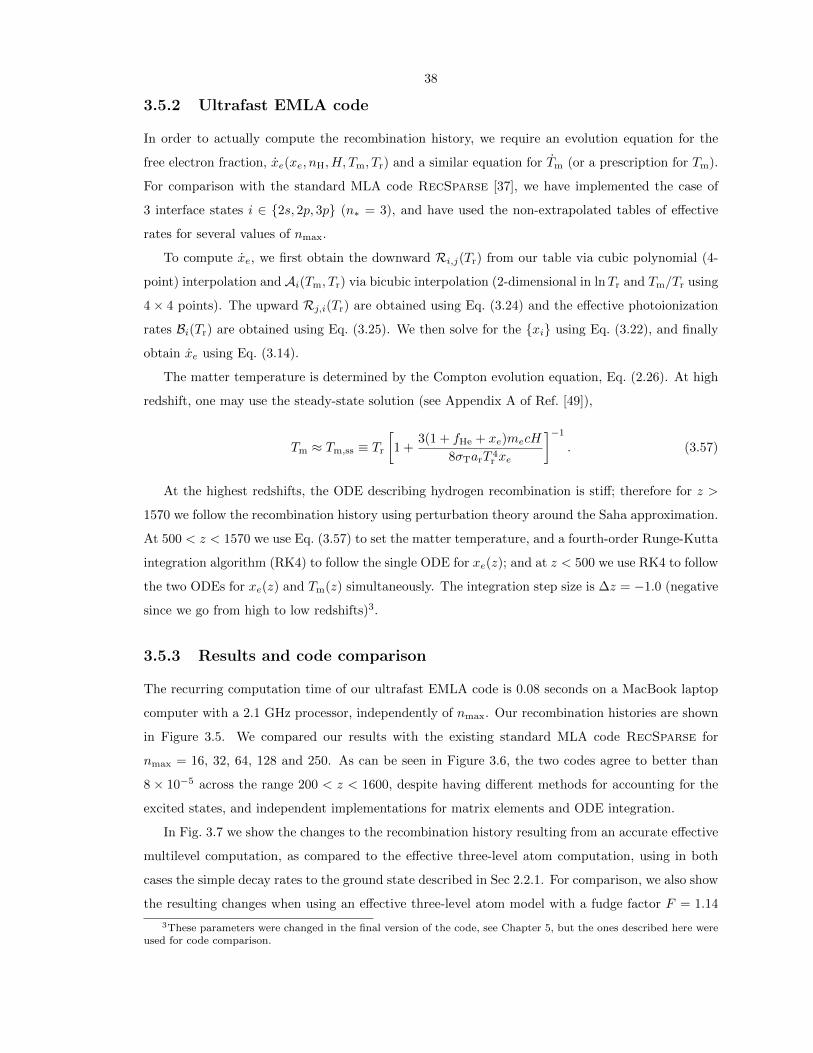
38

3.5.2 Ultrafast EMLA code

In order to actually compute the recombination history, we require an evolution equation for the

free electron fraction, xe(xe, nH, H, Tm, Tr) and a similar equation for Tm (or a prescription for Tm).

For comparison with the standard MLA code RecSparse [37], we have implemented the case of

3 interface states i ∈ 2s, 2p, 3p (n∗ = 3), and have used the non-extrapolated tables of effective

rates for several values of nmax.

To compute xe, we first obtain the downward Ri,j(Tr) from our table via cubic polynomial (4-

point) interpolation and Ai(Tm, Tr) via bicubic interpolation (2-dimensional in lnTr and Tm/Tr using

4× 4 points). The upward Rj,i(Tr) are obtained using Eq. (3.24) and the effective photoionization

rates Bi(Tr) are obtained using Eq. (3.25). We then solve for the xi using Eq. (3.22), and finally

obtain xe using Eq. (3.14).

The matter temperature is determined by the Compton evolution equation, Eq. (2.26). At high

redshift, one may use the steady-state solution (see Appendix A of Ref. [49]),

Tm ≈ Tm,ss ≡ Tr

[1 +

3(1 + fHe + xe)mecH

8σTarT 4r xe

]−1

. (3.57)

At the highest redshifts, the ODE describing hydrogen recombination is stiff; therefore for z >

1570 we follow the recombination history using perturbation theory around the Saha approximation.

At 500 < z < 1570 we use Eq. (3.57) to set the matter temperature, and a fourth-order Runge-Kutta

integration algorithm (RK4) to follow the single ODE for xe(z); and at z < 500 we use RK4 to follow

the two ODEs for xe(z) and Tm(z) simultaneously. The integration step size is ∆z = −1.0 (negative

since we go from high to low redshifts)3.

3.5.3 Results and code comparison

The recurring computation time of our ultrafast EMLA code is 0.08 seconds on a MacBook laptop

computer with a 2.1 GHz processor, independently of nmax. Our recombination histories are shown

in Figure 3.5. We compared our results with the existing standard MLA code RecSparse for

nmax = 16, 32, 64, 128 and 250. As can be seen in Figure 3.6, the two codes agree to better than

8 × 10−5 across the range 200 < z < 1600, despite having different methods for accounting for the

excited states, and independent implementations for matrix elements and ODE integration.

In Fig. 3.7 we show the changes to the recombination history resulting from an accurate effective

multilevel computation, as compared to the effective three-level atom computation, using in both

cases the simple decay rates to the ground state described in Sec 2.2.1. For comparison, we also show

the resulting changes when using an effective three-level atom model with a fudge factor F = 1.14

3These parameters were changed in the final version of the code, see Chapter 5, but the ones described here wereused for code comparison.

39

-3.5

-3

2.5

200 400 600 800 1000 1200 1400 1600

-5

-4.5

-4

-3.5

-3

-2.5

-2

-1.5

-1

200 400 600 800 1000 1200 1400 1600

log

10 (

|!x

e|/x

e)

z

nmax = 32 vs 6464 vs 128

128 vs 250250 vs 500

!"#$

!"

!%#$

!%

!&#$

!&

!'#$

('

(%'' ()'' (*'' (+'' (&''' (&%'' (&)'' (&*''

,-.&'(/0

123/(4($''

!$

!)#$

!)

!"#$

!"

!%#$

!%

!&#$

!&

(%'' ()'' (*'' (+'' (&''' (&%'' (&)'' (&*''

,-.&'(56/067/08

9

123/(4("%(:;(((*)*)(:;(&%+&%+(:;(%$'%$'(:;($''

9

!

Figure 3.5: Top panel : Relative differences between recombination histories computed with suc-cessively more accurate effective rates. Bottom panel : Recombination history for effective ratescomputed with nmax = 500, i.e., accounting explicitly for 125,250 states of the hydrogen atom.Figures provided by Christopher Hirata.

40

-8

-6

-4

-2

0

2

4

200 400 600 800 1000 1200 1400 1600

10

5!

xe/x

e

z

nmax

= 16

64

250

Figure 3.6: A comparison of our ultrafast code to RecSparse [37], for different values of nmax.The vertical axis is the fractional difference in free electron abundance rescaled by 105 (positiveindicating that RecSparse gives a larger xe). We see that the maximum fractional deviation is< 8 × 10−5. The feature around z = 1540 is due to a time-step change in RecSparse. Figureprovided by Christopher Hirata and data from RecSparse computations provided by Daniel Grin.

as in the code RecFast [30]. We checked that it is not possible to reproduce the correct effective

MLA computation with a constant fudge factor in an effective three-level atom. We find that the

best fitting fudge factor would be F = 1.126, with relative errors reaching 0.2 %. In any case, the

effective MLA computation is so simple and computationally efficient that the need for non-physical

fudge factors does not arise.

3.6 Conclusions and future directions

We have shown that the computation of primordial hydrogen recombination can be factored into

two independent calculations. On the one hand, most excited states are not directly radiatively

connected to the ground state, and undergo transitions caused by the thermal bath of blackbody

photons at the relevant frequencies, as well as the thermal electrons and protons. One can account

for these numerous transitions with effective transition rates into and out of the “interface” states

which are connected to the ground state. The computationally intensive aspect of a recombination

calculation in fact resides in the evaluation of these effective rates, which are functions of matter and

radiation temperature only, and are a generalization of the case-B recombination coefficient. This

calculation being independent of cosmological parameters, it can be done prior to any recombination

calculation, once and for all. A simple effective few-level atom can then be evolved for any set of

cosmological parameters, without any need for “fudge factors” or approximations.

Collisional transitions were not included in our computations. They may be particularly impor-

tant for the high-n states. The effective rates computed here are therefore only approximating the

correct rates in the limit of zero density. Our formalism is general and collisions can be included as

41

200 400 600 800 1000 1200 1400 1600z

-0.12

-0.10

-0.08

-0.06

-0.04

-0.02

0.00

! x

e/x

e

RecFast vs PeeblesEMLA (2s-2p) vs Peebles

Figure 3.7: Fractional changes in the ionization history relative to the effective three-level atommodel. The “RecFast” model is an effective three-level atom with the case-B recombination coeffi-cient multiplied by a fudge factor F = 1.14. The same prescription for the evolution of the mattertemperature is used in all cases, see Section 5.3.5.

soon as accurate rates are available (the main change would be that the interpolation tables would

require lnne as an additional independent variable).

The formalism developed in this chapter is general and can accommodate any form of the tran-

sition rates to the ground state. In the subsequent chapters, we shall dwell on the radiative transfer

effects, which are constitute a conceptually more challenging aspect of primordial recombination.

42

3.A Appendix: Proofs of relations involving effective rates

3.A.1 Preliminaries

The purpose of this appendix is to prove some relations involving effective rates and give some details

regarding their numerical evaluation.

We recall that in our notation, capital indices K,L refer to “interior” excited states, and lower-

case indices i, j refer to “interface” excited states. We have previously defined the rate matrix M(Tr)

with coefficients:

MKL = δKLΓK − (1− δKL)RK,L, (3.58)

where RK,L(Tr) is the rate of K → L transitions and ΓK(Tr) is the inverse lifetime of the interior

state K. In Section 3.4.2, we have shown that the populations of the interface states are given by:

XK =∑

L

(M−1

)LK

[nHx

2eαL +

∑

i

xiRi,L

]. (3.59)

We also showed that the probabilities P iK and P eK are given by

P iK =∑

L

(M−1

)KL

RL,i, (3.60)

and

P eK =∑

L

(M−1

)KL

βL. (3.61)

3.A.2 Invertibility of the system defining the P iK, P

eK

In this section we show that the matrix M(Tr) defined in Eq. (3.58) is non-singular, for any value

of the radiation temperature Tr ≥ 0.

Let us consider the eigenvalue equation Mb = 0 and select a particular K1 such that |bK1| ≥ |bL|

for all L. The eigenvalue equation implies

0 =∣∣MK1K1bK1 +

∑

L 6=KMK1LbL

∣∣

≥ MK1K1

∣∣bK1

∣∣−∑

L 6=K1

∣∣MK1L

∣∣∣∣bL∣∣, (3.62)

where we have used the inverse triangle inequality. The matrix M is diagonally dominant, i.e.,

∀K, MKK = ΓK ≥∑

L 6=KRK,L =

∑

L 6=K|MKL|. (3.63)

43

Using the inequality (3.63) for K = K1 in Eq. (3.62), we obtain

0 ≥∑

L 6=K1

∣∣MK1L

∣∣ (|bK1| − |bL|) . (3.64)

For any interior state K1, there always exists a sequence of transitions that ultimately leads to

some interface state i, K1 → K2 → ... → Kn → i, for any temperature Tr ≥ 0. (i.e., there are

no “dead end” interior states). In particular,∣∣MK1K2

∣∣ = RK1,K2> 0. For Eq. (3.64) to hold,

it is therefore necessary that |bK1| = |bK2

|. Repeating the above reasoning recursively leads to

|bK1 | = |bK2 | = ... = |bKn |.For the last interior state of this sequence, Kn, the inequality (3.63) is strict since RKn,i > 0.

The eigenvalue equation projected on Kn leads to Eq. (3.62) for Kn:

0 ≥MKnKn

∣∣bKn∣∣−

∑

L 6=Kn

∣∣MKnL

∣∣∣∣bL∣∣. (3.65)

If b 6= 0, then |bKn | > 0 and the strict inequality (3.63) for K = Kn used in Eq. (3.65) implies the

contradictory result

0 >∑

L 6=Kn

∣∣MKnL

∣∣ (|bKn | − |bL|) ≥ 0. (3.66)

As a consequence, Mb = 0 implies that b = 0 necessarily. This proves that M(Tr) is nonsingular,

for any Tr ≥ 0.

3.A.3 Proof of the complementarity relation∑i P

iK + P e

K = 1

We define the length-N vector V ≡ (1, 1, ..., 1)T, and note that

(MV)K =∑

L

MKL =∑

j

RK,j + βK (3.67)

(the RK,L terms cancel). In matrix form, this reads:

MV =∑

j

Rj + Re = M

∑

j

Pj + Pe

. (3.68)

The matrix M being invertible, this implies∑j Pj + Pe = V, which once projected on each com-

ponent K is just the complementarity relation Eq. (3.18).

44

3.A.4 Detailed balance relations

This appendix is dedicated to proving the detailed balance relations for Ri,j and Bi. We denote

gK the statistical weight of state K. Defining the contributions of individual states to the partition

function,

QK ≡ gKe−EK/Tr (3.69)

and similarly for Qi, we make use of the standard principle of detailed balance for rates connecting

individual states,

QKRK,L = QLRL,K , (3.70)

and similarly QKRK,i = QiRi,K .

We begin by defining the N × N nonsingular diagonal matrix F that is proportional to the

equilibrium abundances,

FKL ≡ QKδKL. (3.71)

Then Eq. (3.70) combined with the definition Eq. (3.26) implies that FM is symmetric. It therefore

follows that its matrix inverse M−1F−1 is symmetric, and hence that

(M−1)KLQL

=(M−1)LK

QK. (3.72)

The transition rate, Eq. (3.21), can be expanded using Eq. (3.29) as

Ri,j = Ri,j +∑

K,L

(M−1)KLRi,KRL,j . (3.73)

We then see that:

QiRi,j = QiRi,j +∑

K,L

Qi(M−1)KLRi,KRL,j = QiRi,j +

∑

K,L

QK(M−1)KLRK,iRL,j

= QjRj,i +∑

K,L

QL(M−1)LKRK,iRL,j = QjRj,i +∑

K,L

Qj(M−1)LKRK,iRj,L

= QjRj,i, (3.74)

where we have used Eq. (3.70) twice and in the third equality used Eq. (3.72). This proves Eq. (3.24).

We may also relate the effective recombination and photoionization rates. To do so, we consider

the case of Tm = Tr and define

q ≡(

2πµeTr

h2

)3/2

. (3.75)

45

Then Eq. (3.3) can be written as Qnlβnl = qαnl. Using Eq. (3.30), we see that

QiBi = Qiβi +∑

K,L

QiRi,K(M−1)KLβL = qαi +∑

K,L

QKRK,i(M−1)KLβL

= qαi +∑

K,L

QLRK,i(M−1)LKβL = qαi +

∑

K,L

qRK,i(M−1)LKαL = qAi, (3.76)

where in the last equality we have used Eq. (3.19) with the P iK determined by Eq. (3.29). This

proves Eq. (3.25).

3.A.5 Proof of Eq. (3.51)

Consider Eq. (3.46) with ΓK ≈ ΓK(Tr). The formal solution for the P 1sK is given by:

P 1sK =

∑

L

(M−1

)KL

RL,1s. (3.77)

Therefore one may rewrite Eq. (3.44), for i = 2s, 2p:

Ri,1s = Ri,1s +∑

K

λi,K(Tr)RK,1s, (3.78)

where we have defined

λi,K(Tr) ≡∑

L

Ri,L(M−1

)LK

=∑

L

Ri,LQKQL

(M−1

)KL

=∑

L

RL,iQKQi

(M−1

)KL

=gKgi

e−EKi/TrP iK(Tr), (3.79)

where in the second equality we used Eq. (3.72), in the third equality we used the detailed balance

relation verified by Ri,L and RL,i, and in the last line we used the formal solution for P iK , Eq. (3.60).

We therefore obtain Eq. (3.51).

3.A.6 Expression of XK in terms of xi, xe

Taking Tm = Tr and using the detailed balance relation qαL = QLβL, we rewrite Eq. (3.59) as

follows:

XK = q−1nHx2e

∑

L

QL(M−1

)LK

βL +∑

i

xi∑

L

(M−1

)LK

QLQi

RL,i

= q−1nHx2eQK

∑

L

(M−1

)KL

βL +∑

i

xiQKQi

∑

L

(M−1

)KL

RL,i, (3.80)

46

where in the last equality we have used Eq. (3.72). Using the formal solutions for the probabilities

Eqs. (3.60), (3.61), we see that we recover Eq. (3.52).

3.B Appendix: Computation of the effective rates

3.B.1 Sparse matrix technique4 for the evaluation of the P iK

In order to compute the probabilities P iK , one needs to solve the linear large linear system given in

Eq. (3.16), truncated to only account for states with principal quantum number n ≤ nmax. Because

of selection rules, the system is very sparse and we can solve it efficiently using a sparse matrix

approach similar to that of Grin & Hirata [37].

We separate the interior states in groups of identical angular momentum l. For each interface

state i, we define the nmax + 1 vectors ~P il , with 0 ≤ l ≤ lmax ≡ nmax − 1, such that ~P il has nmax − lnon-vanishing elements P il [n] ≡ P inl for n ≥ l + 1. We also define the matrices Ml,l±1 of elements

given by:

Ml,l±1[n][n′] =Rn,l,n′,l±1

Γnl, (3.81)

and the source vectors ~sil of elements

sil[n] =Rnl,iΓnl

. (3.82)

The system to be solved, Eq. (3.16), can be rewritten in the form:

~P i0 −M0,1~P i1 = ~si0 (3.83)

−Ml,l−1~P il−1 + ~P il −Ml,l+1

~P il+1 = ~sil for 1 ≤ l < lmax, (3.84)

−Mlmax,lmax−1~P ilmax−1 + ~P ilmax

= ~silmax. (3.85)

Note that a simplification from the case of Ref. [37] is that the only non-vanishing source vectors (for

interface states 2s and np) are ~s np0 , ~s 2s1 and ~s np2 . We now define the matrices Gl by the recursion

relation:

Glmax≡ Mlmax,lmax−1 (3.86)

(1−Ml,l+1Gl+1)Gl ≡ Ml,l−1 for 1 ≤ l < lmax (3.87)

and the vectors ~Si2,~Si1 such that:

(1−M2,3G3)~Si2 ≡ ~si2 (3.88)

(1−M1,2G2)~Si1 ≡ ~si1 + M1,2~Si2. (3.89)

4The material presented in this section is unpublished.

47

Once all these matrix equations have been solved, the solution to the system is obtained as follows:

(1−M0,1G1)~P i0 = ~si0 + M0,1~Si1 (3.90)

~P i1 = G1~P i0 + ~Si1 (3.91)

~P i2 = G2~P i1 + ~Si2 (3.92)

~P il = Gl~P il−1, 3 ≤ l ≤ lmax. (3.93)

3.B.2 Extrapolation of the effective rates to nmax =∞

We have tabulated the effective rates A2s(Tm, Tr),A2p(Tm, Tr) and R2s,2p(Tr), including all excited

states up to the principal quantum number nmax, for several values of nmax up to 600, over the

temperature range 0.004 eV ≤ Tr ≤ 0.4 eV, 0.1 ≤ Tm/Tr ≤ 1. This range of temperatures corre-

sponds to 20 < z < 1650 for a wide range of cosmologies. For every pair (Tm, Tr), we have fitted the

effective rates by the following functional form:

Ai(Tm, Tr;nmax) = Ai(Tm, Tr;∞)

(1− κ

(nmax)γ

), (3.94)

and similarly for R2s,2p, where κ and γ depend on Tm and Tr as well as on the coefficient being

fitted. This allows us to extrapolate the effective rates to nmax → ∞. Of course, this is only a

formal extrapolation, as for n larger than a few thousands, the excited states of hydrogen are no

more well defined (see Ref. [87] for a discussion). The extrapolated rates are still more accurate than

those computed with a a finite number of states. The residuals of the fit have a maximum relative

amplitude of 5 × 10−4 over the whole range of temperature considered, for 200 ≤ nmax ≤ 600, and

more than an order of magnitude smaller on the restricted range Tr ≥ 0.04 eV, Tm/Tr ≥ 0.8 which

corresponds to z ∼> 200 (note that neglecting the overlap of the high-lying Lyman lines leads to er-

rors in the effective rates of similar amplitude [40]). For reference, the maximum relative difference

between the effective rates computed with nmax = 600 and their extrapolation at nmax =∞ is 0.05

over the whole range of temperature considered, and 0.002 over the restricted range corresponding

to z ∼> 200. We checked that our method recovers the correct case-B recombination coefficient

αB(Tm) ≡ ∑i=2s,2pAi(Tm, Tr = 0;∞). Our extrapolated αB agrees with the fit of Ref. [72] to

better than 0.2 % for Tm > 40 K, which is the accuracy claimed by the authors of Ref. [72].

48

Chapter 4

Radiative transfer effects inprimordial hydrogenrecombination1

4.1 Introduction

In the previous chapter we have considered one of the two aspects of the recombination problem, the

multilevel atom and the “high-n” problem. The second facet of the problem is to properly model the

transitions from the “interface” states to the ground state, of particular importance at early times

when the overall recombination rate is controlled by the so called “n = 2 bottleneck”. Hydrogen

atoms in the n = 2 shell can reach the ground state either through emissions of single photons

from the 2p state, which slowly escape the optically thick Lyman-α transition through cosmological

redshifting, or from the 2s state, through forbidden two-photon decays. Previous studies have

examined a series of effects that may affect these transition rates, including but not limited to

stimulated 2s→ 1s two-photon decays and non-thermal 1s→ 2s two-photon absorptions [47, 48, 49],

feedback between neighboring lines of the optically thick Lyman series [41, 42], time-dependent

effects in the Lyman-α line [43, 49], two-photon decays from higher excited states [50, 51, 49, 52],

and diffusion in the Lyman-α line [44, 46, 45].

The purpose of this chapter is mainly to assess the importance of several radiative transfer effects

in the Lyman lines, that have not been investigated yet, or not in sufficient detail (we defer a detailed

discussion of radiative transfer in the presence of two-photon decays to Chapter 5). In Section 4.2,

we review the theory of radiative transfer in the vicinity of a resonant line in an expanding Universe.

We then turn to the Lyman-α line, for which we study the effect of Thomson scattering (Section

4.3.1) and the interaction with the Lyα line of deuterium (Section 4.3.2). In Section 4.4, we quantify

1The material in this chapter was adapted from the paper Radiative transfer effects in primordial hydrogenrecombination, Y. Ali-Haımoud, D. Grin & C. M. Hirata, Phys. Rev. D 82, 123502 (2010). Reproduced here withpermission, copyright (2010) by the American Physical Society.

49

the importance of the high-lying, non-overlapping Lyman transitions. Section 4.5 is devoted to the

overlapping high-lying Lyman lines. We also explore the possibility of a cosmological recombination

maser in Section 4.6. We summarize and discuss our results in Section 4.7. Appendix 4.A summarizes

the notation used in this chapter and Appendix 4.B describes the computation of the modified escape

probability in a Doppler-dominated line with partial frequency redistribution.

4.2 Radiative transfer in the Lyman lines

4.2.1 Basic notation

In this section, we present the basic quantities and notation used throughout this chapter. We

summarize our notation in Table 4.1.

The photon occupation number at frequency ν is denoted fν . In the case of a black body

spectrum with temperature T , fν =(ehν/kT − 1

)−1. We will also make use of the number of

photons per hydrogen atom per unit frequency,

Nν ≡8πν2

c3NHfν , (4.1)

where NH is the number density of hydrogen atoms. The population of a species X relative to the

total abundance of hydrogen is denoted xX ≡ NX/NH. The fractional abundance of hydrogen in the

state [n, l] is denoted xnl. For the low l states, we use the spectroscopic notation s, p, d, ..., so the

ground state is denoted 1s and the [n, l = 1] states are denoted np.

This work will be concerned primarily with the np → 1s transitions, which will be referred to

as the Lyman-n (or Ly-n) transitions. The Ly-2 transition therefore designates, in that convention,

the Lyman-α (Lyα) transition. We denote the resonant Ly-n transition frequency

νn ≡4

3

(1− 1

n2

)νLyα =

(1− 1

n2

)νc, (4.2)

where νLyα ≈ 2.47×1015 Hz is the Lyman α frequency, and νc = 43νLyα is the Lyman-limit frequency.

The spontaneous emission rate (Einstein A-coefficient) in the Ly-n transition is [82]:

Anp,1s =213π3

32n3

(1− 1

n

)2n−5

(1 + 1

n

)2n+5

ν3n

c2αa2

0 (4.3)

∼n1

213π3

32 exp(4)

1

n3

ν3c

c2αa2

0, (4.4)

where α is the fine-structure constant and a0 is the Bohr radius.

50

We define the ratio

fneq ≡xnp3x1s

, (4.5)

which is the equilibrium value of the photon occupation number at the Ly-n transition frequency.

The Sobolev optical depth for the hydrogen Ly-n transition is [75, 29]:

τn =3c3NHx1s

8πHν3n

Anp,1s

(1− xnp

3x1s

), (4.6)

where H(z) is the Hubble expansion rate. In all that follows, we will neglect stimulated emission in

the Lyman lines, as the photon occupation number near Ly-n is of order fneq 1 (the largest value

is for n = 2 and is less than 10−11 for z < 1600). In particular, we can neglect the last term2 in the

expression for the Sobolev optical depth Eq. (4.6).

Finally, we will refer to the matter temperature as Tm and the radiation temperature as Tr. In

practice, the matter temperature is locked to the radiation temperature through Thomson scattering,

and the relative difference between the two is below a percent until redshift z ≈ 500 [29, 56].

4.2.2 Line processes

Consider an excited hydrogen atom in the np state; it has two mutually exclusive fates.

The first possibility is that it reaches another excited state n′s or n′d, with n′ 6= 1, either through

a spontaneous or stimulated decay if n′ < n or following the absorption of a CMB photon if n′ > n.

It can also be photoionized by a CMB photon.

The second possibility is that the atom spontaneously decays to the ground state, emitting a

Ly-n photon. In principle, this decay can also be stimulated. However, even when accounting for

non-thermal distortions to the radiation field, the photon occupation number at Lyman frequencies

is extremely small, and stimulated emission in the Lyman lines can be neglected.

The probabilities of these two complementary fates are denoted pnab and pnsc, respectively (the

justification of the notation will become clearer in the next paragraph). Given the width (or inverse

lifetime) Γnp of the np state (the sum of the rates of all transitions depopulating this state), they

are given by:

pnsc =Anp,1s

Γnp= 1− pnab. (4.7)

If we now assume that the considered atom was initially in the ground state and reached the np state

after the absorption of a resonant Ly-n photon, the two fates mentioned above can be described in

a two-photon picture.

First, if the atom reaches another excited state n′ < n, the overall reaction H(1s) + γ(Ly-n) →2When dealing with the possibility of cosmological masers in Section 4.6, we will of course explicitly account

for this term and use the appropriate expression for the Sobolev optical depth in a general (not necessarily Lyman)transition.

51

H(n′l) + γ′ is a (possibly stimulated) Raman scattering event. If the atom absorbs a CMB photon

and reaches a higher excited state n′ > n (or gets photoionized), the overall reaction H(1s) + γ(Ly-

n) + γ′ → H(n′l) (or → e−+ p+) is a two-photon absorption (or two-photon photoionization) event.

In these cases we will refer to the absorption of the Ly-n photon as a true absorption event, in the

sense that the photon is destroyed in the process. The emission of a Ly-n photon following the

inverse reaction chain will be referred to as a true emission event.

Secondly, if the atom decays back to the ground state, the overall reaction H(1s) + γ(Ly-n) →H(1s) +γ(Ly-n) is a Rayleigh scattering event (which in what follows we will refer to as a scattering

event for short). In that case the incoming and outgoing photons have the same frequency in the

atom’s rest frame. Their frequencies in the comoving frame (frame in which the CMB appears

isotropic) are Doppler-shifted with respect to the atom’s rest frame frequencies. Since the Doppler

shift depends on the relative orientation of the photon propagation direction and the atom’s velocity,

the frequencies of the incoming and outgoing photons in the comoving frame are in general different.

They are however statistically correlated, as will be described in Section 4.2.2.2.

4.2.2.1 True absorption and emission

The rate of true emission of resonant Ly-n photons at frequency ν, per H atom, per frequency

interval, is given by [56, 45]:

Nν∣∣em

=

∑

(n′ 6=1),l

xn′lRn′l→np + xexpNHαnp

× pnsc ϕn(ν). (4.8)

In the above equation, Rn′l→np is the radiative transition rate per hydrogen atom from the n′l state

to the np state, including stimulated transitions, αnp is the direct recombination coefficient to the

np state, including stimulated recombinations, and ϕn(ν) is the line profile, which has the Voigt

shape3:

ϕn(ν) =1

νn∆HφV

(ν − νnνn∆H

; an

), (4.9)

where

φV(x; a) ≡ a

π3/2

∫ +∞

−∞

e−t2

a2 + (x− t)2dt, (4.10)

is the dimensionless Voigt profile,

∆H ≡√

2kTm

mHc2≈ 2.35× 10−5

(1 + z

1100

Tm

Tr

)−1/2

(4.11)

3The Voigt profile can be derived quantum-mechanically, in the two-photon picture, when one neglects the variationof multiplicative factors ν/νn across the line and uses the resonance approximation. See e.g. Ref. [45] for fits to thecorrect profile in the case of the Lyman α line. We will consider the correct two-photon profiles in Chapter 5.

52

is the dimensionless Doppler width and

an =Γnp

4πνn∆H=

1

pnsc

Anp,1s4πνn∆H

(4.12)

is the dimensionless Voigt parameter of the line.

For small Voigt parameters a 1, which is the case in all Lyman lines at the epoch of recom-

bination, the Voigt profile has the well known asymptotic behaviors in the line center and in the

damping wings:

φV(x; a) ≈

1√π

e−x2

if x ∼< xa,

aπx2 if x ∼> xa,

(4.13)

where the transition scale xa is the solution of [88]:

x2ae−x

2a =

a√π. (4.14)

In general, for a 1, xa ∼ 3.

Following Ref. [56], we define

fn(em) ≡∑

(n′ 6=1),l xn′lRn′l→np + xexpNHαnp

3x1sΓnppnab

, (4.15)

so that the true emission rate per H atom per frequency interval can be rewritten as:

Nν∣∣em

= pnab 3x1sAnp,1sϕn(ν)fn(em). (4.16)

The rate of true absorption of resonant photons is simply the total rate of absorption times the

true absorption probability. The absorption profile differs from the emission profile by a factor

eh(ν−νn)/(kT ), where T = Tr in the wings (because the low-energy photon of the two-photon process

comes from a black-body distribution and the excited states of hydrogen are near Boltzmann equi-

librium with each other at temperature Tr [49, 45]), and T = Tm in the Doppler core, where atomic

recoil tends to equilibrate the radiation field with the atoms’ thermal velocity distribution. The rate

of true absorption of resonant Ly-n photons at frequency ν, per H atom, per frequency interval, is

therefore given by:

Nν∣∣ab

= −pnab3x1sAnp,1sϕn(ν)eh(ν−νn)kT fν . (4.17)

The net (uncompensated) rate of true emission of resonant Ly-n photons at frequency ν, per H

atom, is therefore:

Nν∣∣em,ab

= pnab 3x1sAnp,1sϕn(ν)×[fn(em) − e

h(ν−νn)kT fν

]. (4.18)

53

It will be useful in what follows to cast this expression into a different but equivalent form, which

can be done with the following considerations.

The rate of change in the population of the np state is:

xnp =∑

n′,l

xn′lRn′l→np + xexpNHαnp − xnpΓnp

= 3x1sΓnppnabf

n(em) + x1sR1s→np − xnpΓnp. (4.19)

The radiative rates (of order ∼ 108 s−1) are many orders of magnitude larger than the overall

recombination rate, which is of order the Hubble rate H ∼ 10−13 s−1. The population of the excited

states can therefore be obtained to an excellent accuracy by using the steady-state approximation

and setting xnp = 0 in the above equation. Setting the left-hand side of Eq. (4.19) to zero, we can

solve for fn(em):

fn(em) =1

3x1sΓnppnab

[xnpΓnp − x1sR1s→np] . (4.20)

The total (including both true absorptions and absorptions leading to a scattering) 1s→ np (forward

only) excitation rate per H atom is given by:

x1sR1s→np = 3x1sAnp,1s

∫ϕn(ν)e

h(ν−νn)kT fνdν. (4.21)

This finally gives us the following relation for fn(em) [43]:

pnabfn(em) = fneq − pnsc

∫ϕn(ν)e

h(ν−νn)kT fνdν. (4.22)

We can now rewrite the net rate of true emission of resonant Ly-n photons at frequency ν, per H

atom, in a form exactly equivalent to Eq. (4.18):

Nν∣∣em,ab

= 3x1sAnp,1sϕn(ν)

fneq − e

h(ν−νn)kT fν + pnsc

[eh(ν−νn)kT fν −

∫ϕn(ν′)e

h(ν′−νn)kT fν′dν

′]

.

(4.23)

4.2.2.2 Coherent scattering

The rate at which resonant scattering removes photons from the line, at frequency ν, (in photons

per second per H atom per frequency interval) is the total absorption rate times the scattering

probability:

Nν∣∣sc,− = −pnsc3x1sAnp,1sϕn(ν)e

h(ν−νn)kT fν . (4.24)

54

The rate at which resonant scattering injects photons in the line, at frequency ν, depends on the

absorption at all other frequencies, since incoming and outgoing photon frequencies are correlated:

Nν∣∣sc,+

= pnsc3x1sAnp,1s ×∫pn(ν|ν′)ϕn(ν′)e

h(ν′−νn)kT fν′dν

′, (4.25)

where pn(ν|ν′) is the probability that the outgoing photon has frequency ν in the comoving frame

given that the incoming photon had frequency ν′. It accounts for the random thermal motions of

the scattering atoms (at temperature Tm) and depends on the angular probability distribution of a

scattering event. It is normalized:

for all ν′,∫pn(ν|ν′)dν = 1, (4.26)

and to respect detailed balance, must satisfy

pn(ν|ν′)ϕn(ν′) = pn(ν′|ν)ϕn(ν). (4.27)

The scattering redistribution kernel

Rn(ν, ν′) ≡ pn(ν|ν′)ϕn(ν′)eh(ν′−νn)

kT (4.28)

is calculated in Ref. [89] (in which, however, atomic recoil during a scattering event is not accounted

for).

The most general form for the rate of change of the photon field through resonant scattering is

given by Eqs. (4.24) and (4.25). However, in the case where the radiation field is smooth on the

scale of a characteristic frequency shift in a scattering 〈∆ν2〉1/2 = νn∆H, one can approximate the

integral operator by a second-order differential operator. The rate of change of Nν due to scattering

is then given by a Fokker-Planck equation [90, 91, 92, 44, 45, 46], accounting for scattering as a

diffusive process in frequency space, with a systematic shift (or drift) due to recoil and Doppler

boosting:

Nν∣∣FP

sc= pnsc3x1sAnp,1s

∂

∂ν

ν2∆2

H

2ϕn(ν)

[∂fν∂ν

+h

kTmfν

]. (4.29)

4.2.2.3 The radiative transfer equation

In the vicinity of the Ly-n line, the photon occupation number evolves under the influence of the

resonant processes described above, as well as eventual non resonant processes that may act in the

vicinity of the line. The time-dependent radiative transfer equation (the Boltzmann equation for

55

the photon fluid) can be written in the general form:

dfνdt≡ ∂fν

∂t−Hν ∂fν

∂ν= fν

∣∣em,ab,sc

+ fν∣∣nr, (4.30)

where d/dt is the derivative along a photon trajectory, and fν |nr groups all processes that are not

resonant with the considered line (these could include absorption and emission from neighboring

lines for example). The contribution of resonant processes is obtained with the conversion:

fν∣∣em,ab,sc

=c3NH

8πν2Nν∣∣em,ab,sc

. (4.31)

Neglecting the variation of multiplicative factors ν/νn across the line, and using the definition of τn,

Eq. (4.6), as well as Eq. (4.23), the most general expression for the resonant term can be written:

− 1

Hνfν∣∣em,ab,sc

= τnϕn(ν)[eh(ν−νn)kT fν − fneq

]

+ pnscτn

∫ [ϕn(ν)ϕn(ν′)e

h(ν′−νn)kT −Rn(ν, ν′)

]fν′dν

′. (4.32)

The radiative transfer equation, Eq. (4.30), with fν |em,ab,sc given by Eq. (4.32), is therefore, in the

general case, a time-dependent, partial integro-differential equation. As a result, it is computation-

ally expensive to solve without further approximations.

If the radiation field varies on a frequency scale large compared to a Doppler width, then we can

use the Fokker-Planck operator for the scattering term, and the above term can be approximated

by:

− 1

Hνfν∣∣em,ab,sc

≈ pnabτnϕn(ν)[eh(ν−νn)kT fν − fn(em)

]− pnscτn

∂

∂ν

ν2∆2

H

2ϕn(ν)

[∂fν∂ν

+h

kTmfν

].

(4.33)

More insight can be gained by considering some characteristic scales of the problem. Using the

asymptotic expansion for the wings of the Voigt profile, Eq. (4.13), we obtain the total optical depth

for true absorption in each damping wing:

τab,wingn = pnabτn

anπxan

. (4.34)

If τab,wingn 1, the damping wings are optically thin to true absorption, and one can use the Doppler

core approximation to the Voigt profile in the radiative transfer equation. If τab,wingn 1, then the

wings are optically thick for true absorption up to a detuning from the line center:

Wn ≡ pnabτnanπνn∆H νn∆H. (4.35)

56

In that case, the radiation field is near its equilibrium value fν ≈ fn(em)e−h(ν−νn)/kT within a detuning

from the line center |ν − νn| ∼<Wn.

One can similarly define the optical depth for resonant scattering in each damping wing, τ sc,wingn .

If τ sc,wingn 1, we can see using dimensional analysis that resonant scattering, when described with

a Fokker-Planck operator, is effective up to a characteristic detuning from the line center

Sn ≡(pnscτn

an2π

)1/3

νn∆H. (4.36)

The physical meaning of this quantity can be understood as follows. A photon with initial frequency

ν can diffuse (in frequency space) to the line center in a characteristic time

∆tdiff ∼(ν − νn)2

(νn∆H)2

1

cx1sNHσn(ν), (4.37)

where σn(ν) is the cross section for resonant scattering:

σn(ν) ≡ pnsc3

8π

c2

ν2n

Anp,1sϕn(ν). (4.38)

The time it takes for the photon to redshift from ν to νn (if ν > νn, or from νn to ν in the opposite

case) is

∆tredshift =|ν − νn|νnH

. (4.39)

Using the damping wings approximation for ϕn(ν) Eq. (4.13), the definition of the Sobolev optical

depth Eq. (4.6), and Eq. (4.36), we obtain:

∆tdiff

∆tredshift∼( |ν − νn|Sn

)3

. (4.40)

Therefore the radiation field will reach the equilibrium spectrum fν ∝ e−hν/kTm within a detuning

from the line center |ν − νn| ∼< Sn, due to the very fast redistribution of photon frequencies through

resonant scattering.

As an illustration, we show in Fig. 4.1 the parameters W2,S2 for the Lyman-α line, extracted

from the MLA code described in Ref. [49]. We see that for z ∼> 800, S2 ≥ W2 > νLyα∆H and at all

relevant times S2 νLyα∆H. According to the above discussion, the radiation field in the vicinity

of Lyα is therefore smooth on a frequency scale ∆ν ∼ S2 around line center, and the use of the

Fokker-Planck operator for resonant scattering is well justified.

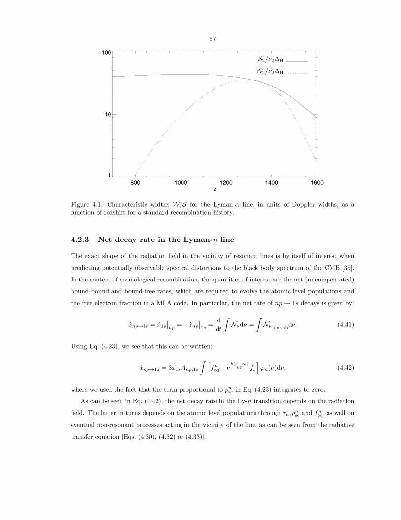
57

800 1000 1200 1400 1600

z

1

10

100

S2/!2!H

W2/!2!H

800 1000 1200 1400 1600

z

1

10

100

Figure 4.1: Characteristic widths W,S for the Lyman-α line, in units of Doppler widths, as afunction of redshift for a standard recombination history.

4.2.3 Net decay rate in the Lyman-n line

The exact shape of the radiation field in the vicinity of resonant lines is by itself of interest when

predicting potentially observable spectral distortions to the black body spectrum of the CMB [35].

In the context of cosmological recombination, the quantities of interest are the net (uncompensated)

bound-bound and bound-free rates, which are required to evolve the atomic level populations and

the free electron fraction in a MLA code. In particular, the net rate of np→ 1s decays is given by:

xnp→1s = x1s

∣∣np

= −xnp∣∣1s

=d

dt

∫Nνdν =

∫Nν∣∣em,ab

dν. (4.41)

Using Eq. (4.23), we see that this can be written:

xnp→1s = 3x1sAnp,1s

∫ [fneq − e

h(ν−νn)kT fν

]ϕn(ν)dν, (4.42)

where we used the fact that the term proportional to pnsc in Eq. (4.23) integrates to zero.

As can be seen in Eq. (4.42), the net decay rate in the Ly-n transition depends on the radiation

field. The latter in turns depends on the atomic level populations through τn, pnsc and fneq, as well on

eventual non-resonant processes acting in the vicinity of the line, as can be seen from the radiative

transfer equation [Eqs. (4.30), (4.32) or (4.33)].

58

4.2.4 The Sobolev approximation

Equations (4.30) and (4.32) give the most general form4 of the radiative transfer equation, in a

homogeneous expanding Universe. It has no analytic solution, because of its complexity and since

it requires the values of the level populations, which in turn depend on the radiation field. It can

however be simplified and decoupled under some approximations, for which an analytic solution

exists. The Sobolev approximation [75, 29] relies on the following assumptions:

(i) No non-resonant processes act in the vicinity of the line (fν |nr = 0 in Eq. (4.30)).

(ii) Steady-state: the time it takes a photon to redshift across the line is of order w/Hνn, where

w is the characteristic line width. If the line is very narrow, w νn, then this time is much smaller

than the Hubble time, therefore physical quantities, such as nH, Tr, Tm, H, xe, xnl vary very little

during the time it takes a photon to redshift through the line. As a consequence, one can neglect

the time dependence in Eq. (4.30).

(iii) Equal absorption and emission profile. This assumption also derives from the assumption

of an infinitesimally thin line, in which case one can take the exponential factors to be unity in

Eq. (4.17).

(iv) Complete redistribution of emitted photons. Mathematically, this means that pn(ν|ν′) is

independent of ν′ in Eq. (4.25). Because of assumption (iii), it is also assumed that pn(ν|ν′) = ϕn(ν),

i.e., the scattered photons are completely redistributed over the line profile. This implies that

Rn(ν, ν′) = ϕn(ν)ϕn(ν′), and therefore the integral in Eq. (4.32) vanishes (taking the exponential

to be unity).

The radiative transfer equation, under these assumptions, becomes the much simpler ordinary

differential equation:dfνdν

= τnϕn(ν)(fν − fneq

). (4.43)

It has the analytic solution

fν = fneq + (fn+ − fneq) exp

[−τn

∫ +∞

ν

ϕn(ν′)dν′], (4.44)

where fn+ is the photon occupation number at the blue side of the line. The photon occupation

number at the red side of the line is therefore

fn− = fneq + (fn+ − fneq)e−τn . (4.45)

4We neglected the variation of phase-space factors ν/νn across the line, as well as stimulated emission andstimulated scatterings.

59

Integrating Eq. (4.43) from −∞ to +∞ gives

fn+ − fn− = τn

∫ [fν − fneq

]ϕn(ν)dν. (4.46)

This, combined with Eqs. (4.42) and (4.45) finally gives us the standard Sobolev expression for the

net decay rate in the line:

xnp→1s = 3x1sAnp,1sPS,n

[fneq − fn+

], (4.47)

where

PS,n ≡1− e−τn

τn(4.48)

is the Sobolev escape probability. In the case of Lyman transitions, τn 1, and PS,n ≈ 1/τn. The

net decay rate becomes, using Eq. (4.6):

xnp→1s =8πHν3

n

c3NH

[fneq − fn+

], (4.49)

which is simply the rate at which distortion photons redshift across the line, which we derived

heuristically in Section 2.2.1.

The Sobolev approximation provides relatively accurate net decay rates, despite the multiple

assumptions that it relies on, and recombination histories currently used for CMB analysis [29, 30],

which use this approximation, are accurate at the percent level. The level of precision required by

upcoming CMB experiments has motivated recent work to obtain more accurate solutions to the

radiative transfer equation and net bound-bound rates in the optically thick Lyman lines. In this

work we investigate previously ignored radiative transfer effects, and quantify as much as possible

the errors made by the inevitable approximations that still need to be made.

4.3 The Lyman alpha line

The Lyman-α transition is one of the bottlenecks of hydrogen recombination. Electrons recombine

to the excited states of hydrogen, from which they eventually cascade down to the n = 2 state.

They can then reach the ground state either by a two-photon decay from the 2s state, with rate

Λ2s1s ≈ 8.22 s−1, or from the 2p state, by redshifting out of the Lyman-α resonance, with rate

A2p1sPesc, where Pesc is the escape probability. Due to its substantial impact on the recombination

history (see for example Fig. 11 in Ref. [43]), the net decay rate, or equivalently the escape probability

in Lyα has been studied extensively, including time-dependent effects [90, 43], two-photon processes

[49, 52], resonant scattering [93, 94, 44, 46, 45], and Thomson scattering [46]. In this section we

consider two additional effects: the non-local aspect of Thomson scattering (Section 4.3.1), and a

quantitative estimate of the effect of deuterium on hydrogen recombination (Section 4.3.2).

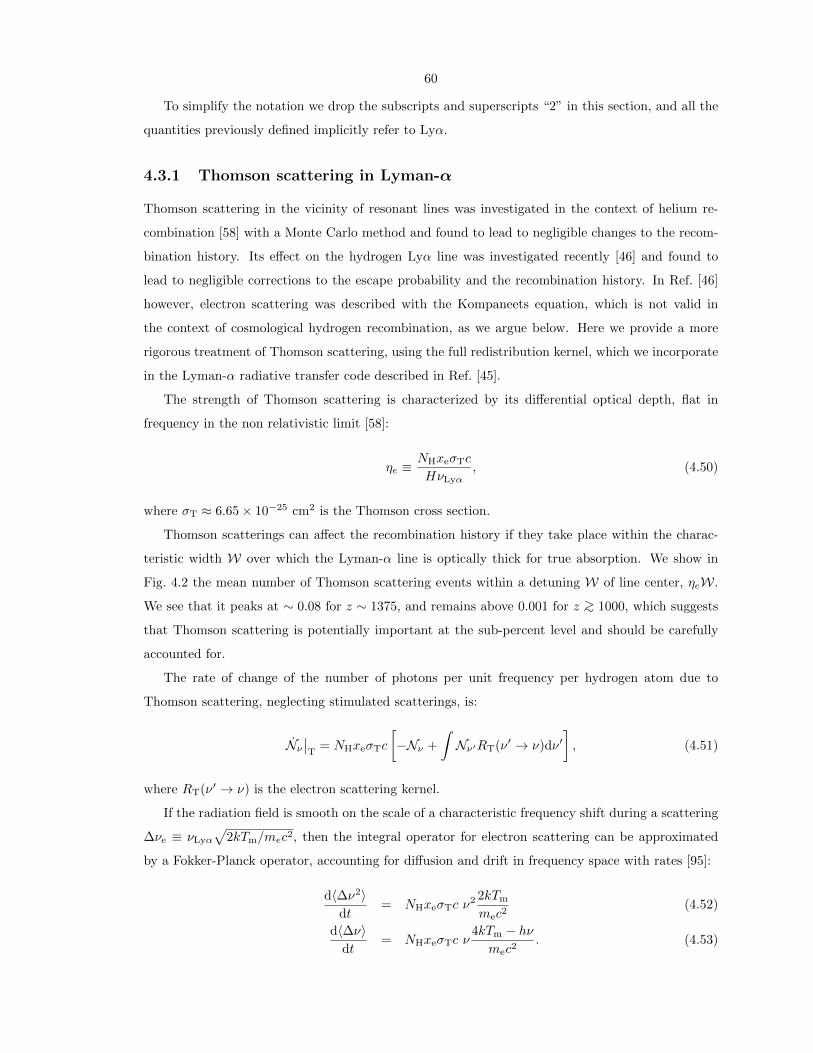
60

To simplify the notation we drop the subscripts and superscripts “2” in this section, and all the

quantities previously defined implicitly refer to Lyα.

4.3.1 Thomson scattering in Lyman-α

Thomson scattering in the vicinity of resonant lines was investigated in the context of helium re-

combination [58] with a Monte Carlo method and found to lead to negligible changes to the recom-

bination history. Its effect on the hydrogen Lyα line was investigated recently [46] and found to

lead to negligible corrections to the escape probability and the recombination history. In Ref. [46]

however, electron scattering was described with the Kompaneets equation, which is not valid in

the context of cosmological hydrogen recombination, as we argue below. Here we provide a more

rigorous treatment of Thomson scattering, using the full redistribution kernel, which we incorporate

in the Lyman-α radiative transfer code described in Ref. [45].

The strength of Thomson scattering is characterized by its differential optical depth, flat in

frequency in the non relativistic limit [58]:

ηe ≡NHxeσTc

HνLyα, (4.50)

where σT ≈ 6.65× 10−25 cm2 is the Thomson cross section.

Thomson scatterings can affect the recombination history if they take place within the charac-

teristic width W over which the Lyman-α line is optically thick for true absorption. We show in

Fig. 4.2 the mean number of Thomson scattering events within a detuning W of line center, ηeW.

We see that it peaks at ∼ 0.08 for z ∼ 1375, and remains above 0.001 for z ∼> 1000, which suggests

that Thomson scattering is potentially important at the sub-percent level and should be carefully

accounted for.

The rate of change of the number of photons per unit frequency per hydrogen atom due to

Thomson scattering, neglecting stimulated scatterings, is:

Nν∣∣T

= NHxeσTc

[−Nν +

∫Nν′RT(ν′ → ν)dν′

], (4.51)

where RT(ν′ → ν) is the electron scattering kernel.

If the radiation field is smooth on the scale of a characteristic frequency shift during a scattering

∆νe ≡ νLyα

√2kTm/mec2, then the integral operator for electron scattering can be approximated

by a Fokker-Planck operator, accounting for diffusion and drift in frequency space with rates [95]:

d〈∆ν2〉dt

= NHxeσTc ν2 2kTm

mec2(4.52)

d〈∆ν〉dt

= NHxeσTc ν4kTm − hνmec2

. (4.53)

61

-7

-6

-5

-4

-3

-2

-1

800 1000 1200 1400 1600

z

0

1

2

3

4

5

log10(!

eW

)!! e

/S

Figure 4.2: Top panel : characteristic number of electron scatterings within the region where the Lyαline is optically thick for true absorption. Bottom panel : ratio of the characteristic frequency shiftduring a Thomson scattering event to the characteristic width over which the Lyα line is smoothedout by frequent resonant scatterings.

The corresponding Fokker-Planck equation is known as the Kompaneets equation:

Nν∣∣FP

T= NHxeσTc

kTm

mec2∂

∂ν

ν4

[∂

∂ν

(Nνν2

)+

h

kTm

Nνν2

]. (4.54)

This is the approximation that was made in Ref. [46]. However, due to the small mass of the

electron, the characteristic frequency shift during an electron scattering event ∆νe can be larger

than the characteristic width over which the radiation field changes in the vicinity of the line. This

characteristic width is of order S (which is ∼>W at all times, see Fig. 4.1), set by frequency diffusion

due to resonant scattering near line center (see end of Section 4.2.2.3). We see from Fig. 4.2 that

∆νe ≥ S at all times, and therefore electron scattering cannot be considered as a diffusive process

and the Kompaneets equation is not valid in this context.

We have implemented the correct integral scattering kernel given by Eq. (4.51) in the Lyman-α

transfer code developed in Ref. [45]. Accurate approximate expressions of the electron scattering

62

kernel RT(ν′ → ν) are given in Ref. [95]. For the purpose of our calculation, we only need the kernel

calculated in the non-relativistic limit adequate here, for a dipolar angular distribution [96]. We set

RT(ν′ → ν) +RT(ν → ν′) =2

∆νeR(ν − ν′∆νe

), (4.55)

where the dimensionless kernel R is given by5 [96, 95]:

R(β) =1

10√π

[11 + 4β2 +

1

2β4

]exp

(−β

2

4

)− 1

4

[3 + β2 +

1

10β4

]|β| erfc

( |β|2

). (4.56)

We moreover require that detailed balance is satisfied, i.e., that the Planck spectrumNν ∝ ν2e−hν/(kTm)

(in the limit hν kTm valid here) is preserved by imposing:

RT(ν → ν′)RT(ν′ → ν)

=ν′2

ν2exp

[h(ν − ν′)kTm

]. (4.57)

When evolving the number of photons per H nucleus per frequency bin in the ith frequency bin,

Ni = Nνiνi∆ ln ν, the radiative transfer code uses a backward Euler method which requires inverting

the matrix equation:

Mij(t+ ∆t)Nj(t+ ∆t) = Ni(t). (4.58)

The matrix to be inverted, M, is tridiagonal in the case where only absorption, emission, and

resonant scattering (described by a Fokker-Planck operator) are present. Thomson scattering breaks

this tridiagonality, which renders the system prohibitively time-consuming to invert (M is a 801×801

matrix in our lowest resolution run). However, we can use the fact that Thomson scattering is only

a perturbation to the radiative transfer equation. Therefore, M = M0 + δM, where M0 is an easily

invertible tridiagonal matrix, and the perturbation δM due to Thomson scattering is such that its

eigenvalues are always small compared to those of M0. We can therefore invert the perturbed matrix

using the expansion:

(M0 + δM)−1

= M−10 −M−1

0 (δM)M−10 + M−1

0 (δM)M−10 (δM)M−1

0 − ... . (4.59)

We find that the second order of the expansion is usually sufficient, with a maximum change of the

net decay rate in the line of 1.5× 10−5 between the first and second order.

We show the resulting changes in the free electron fraction in Fig. 4.3. We can see that at early

times, z ∼> 1350, Thomson scattering delays recombination. Indeed, the relatively large frequency

changes during electron scatterings allow photons to be moved from the red side of the line to the

blue side of the line, and vice versa. Because of the large jump in photon occupation number across

the line, the net photon flux is from the red side to the blue side. As a consequence, some escaping

5There is a typo in Ref. [96]: erf should be erfc.

63

-8

-6

-4

-2

0

2

4

6

8

700 800 900 1000 1100 1200 1300 1400 1500 1600

10

5 !

xe/x

e

z

Effect of Thomson scattering on Recombination History

MatrixFokker-Planck

Full scattering kernel

Kompaneets equation

Figure 4.3: Changes to the recombination history due to Thomson scattering. Figure provided byChristopher Hirata.

photons are re-injected into the line, where they can be absorbed, which decreases the escape rate

and delays recombination. At later times, this effect is not so important as the radiation profile

becomes smoother (∆νe ∼ S, see Fig. 4.2). The systematic frequency loss during scattering events

due to electron recoil starts to dominate, and Thomson scattering helps photons escaping out of the

line and speeds up recombination.

For comparison, we have also implemented the Kompaneets equation (4.54), in a similar fashion

as resonant scattering (see Ref. [45] for details on the implementation). We can see that using

the Kompaneets equation does not represent accurately the physics of Thomson scattering, as it

cannot capture the large frequency shifts at early times. The error in the correction is of order the

correction itself, and it has the wrong sign at early times. However, the basic conclusion reached in

Ref. [46] remains valid: Thomson scattering can indeed be safely ignored during cosmic hydrogen

recombination, since it leads to corrections to the ionization fraction of at most ∆xe/xe ∼ ±3×10−5.

4.3.2 Interaction with the Deuterium Lyman-α line

4.3.2.1 Motivations

A second radiative transfer effect associated with the Lyman-α transition is the interaction of the

hydrogen and deuterium lines. Due to the slightly larger reduced mass of deuterium, the Lyman-

α frequency in deuterium νD ≡ νLyα(D) is shifted to a higher frequency than that of hydrogen,

64

νH ≡ νLyα(H). The relative shift, to first order in me/mp, and with mD+ ≈ 2mp, is:

νD − νH

νH≈ me

2mp≈ 2.7× 10−4. (4.60)

This separation is ∼ 10 times the Doppler width of the hydrogen line so the D Ly-α line center lies

in the blue damping wing of the H Ly-α line. Despite the tiny fractional abundance of primordial

deuterium xD = 2.87+0.22−0.21 × 10−5 [97], the D Ly-α line is still optically thick during cosmological

hydrogen recombination, τD,Lyα ≈ xDτH,Lyα ∼ 102−104. This has motivated the authors of Ref. [42]

to consider the possible screening of radiation incoming into the H Lyα line by the optically thick,

bluer D Lyα line. Ref. [42] pointed out that the deuterium line lies in the optically thick part of the

H Lyα wings (|νD − νH| ∼<W,S, see Fig. 4.1) and concluded, without further justification, that the

screening was absent. Here we explain in detail how the two lines interact and explicitly compute the

effect of deuterium on the recombination history. We show that the effect is completely negligible,

independently of the fact that |νD − νH| ∼<W,S (which does, however, indeed lead to an additional

suppression).

4.3.2.2 Spectral distortions caused by deuterium

Our first step is to understand the physical mechanism of deuterium recombination. The rates of D

and H recombination are tied together via the charge-exchange reaction

D+ + H(1s)↔ D(1s) + H+, (4.61)

which has a forward rate coefficient of order ∼ 10−9 cm3 s−1 [98]; at recombination-era densities

of ∼ 500 cm−3 this implies an equilibrium timescale of ∼ 2 × 106 s, i.e., six orders of magnitude

shorter than the recombination timescale itself. Thus to a very good approximation, the deuterium

ionization fraction tracks that of hydrogen:

xD+

xD(1s)≈ xH+

xH(1s)e−

∆EIkTm ≈ xe

1− xee−

∆EIkTm ≈ xe

1− xe, (4.62)

where the difference in ionization energies of deuterium and hydrogen, ∆EI/k ≈ 41 K, is small

compared to the matter temperature during recombination. Using the last approximation, we obtain

xD+ ≈ xDxe, (4.63)

xD(1s) ≈ xDxH(1s). (4.64)

Note, however, that the populations of the excited states do not, satisfy such a relation, i.e.,, a

priori, xD(2p) 6= xDxH(2p).

65

Like hydrogen, deuterium may recombine radiatively and reach the ground state either via 2s→1s two-photon decay or Lyα escape; the net rate of recombinations (H+D) is simply the sum of

the two rates, and charge exchange [Eq. (4.61)] distributes the bound electrons between H and D.

It is clear that the absolute rate of transitions to the ground state via the optically thin 2s → 1s

transition will be much smaller for D than H because of its lower abundance; however for the Lyα

channel in principle the rates could be comparable because the Lyα(D) optical depth is smaller

than the Lyα(H) optical depth by a factor of ∼ xD, and hence the escape probability is enhanced

by a factor of x−1D . However, since Lyα(D) is located blueward of Lyα(H), all photons emitted in

Lyα(D) will be re-absorbed in Lyα(H); and all photons absorbed in the Lyα(D) transition would

have been absorbed anyway had the deuterium not been present. Thus the net (integrated over

time) number of recombinations that proceed via Lyα(D) escape is zero. However, the re-absorption

of the D photons is not instantaneous, so at any given time the presence of deuterium causes an

additional distortion to the radiation field (on top of the distortion to the blackbody spectrum due

to H(2p)→ H(1s) decays in the blue wing of H Lyα). The number of additional distortion photons

per hydrogen atom is

U =

∫8πν2

c3NH[f (H+D)ν − f (H)

ν ] dν, (4.65)

where f(H)ν is the photon occupation number when only hydrogen is present, and f

(H+D)ν is its value

when the presence of deuterium is accounted for.

Note that U(t)→ 0 at both early times (because the radiation field is thermal independently of

the presence of deuterium) and late times (since after recombination is over, there are no more Lyα

photons produced).

The correction to the rate of formation of ground-state atoms through the (H+D) 2p → 1s

channel is then equal to the rate of creation of distortion photons:

∆x1s|Lyα(D) = −∆xe|Lyα(D) = U . (4.66)

4.3.2.3 Analytic estimate for the number of spectral distortion photons6

We now compute the number of spectral distortion photons. We will treat the deuterium line in

the Sobolev approximation, i.e., assuming that its profile is a delta-function. This approximation is

well justified since the deuterium line is dominated by its Doppler core: the damping wings are only

marginally optically thick, and the differential optical depth in the deuterium wings is always much

smaller than that of hydrogen anyway (see for example Fig. 7 of Ref. [42]). In this case complete

redistribution is a good approximation since both partial and complete redistribution have a similar

6This section is not part of the published paper [40], where the interested reader will find a more elaboratetreatment that accounts for frequency diffusion. Here I have opted for a simpler and less complete, but hopefullymore enlightening calculation.

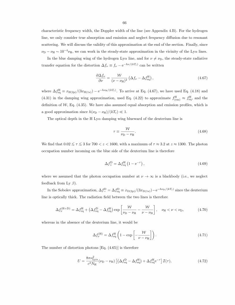
66

characteristic frequency width, the Doppler width of the line (see Appendix 4.B). For the hydrogen

line, we only consider true absorption and emission and neglect frequency diffusion due to resonant

scattering. We will discuss the validity of this approximation at the end of the section. Finally, since

νD − νH ∼ 10−4νH, we can work in the steady-state approximation in the vicinity of the Lyα lines.

In the blue damping wing of the hydrogen Lyα line, and for ν 6= νD, the steady-state radiative

transfer equation for the distortion ∆fν ≡ fν − e−hν/(kTr) can be written

∂∆fν∂ν

=W

(ν − νH)2

(∆fν −∆fH

eq

), (4.67)

where ∆fHeq ≡ xH(2p)/(3xH(1s))− e−hνH/(kTr). To arrive at Eq. (4.67), we have used Eq. (4.18) and

(4.31) in the damping wing approximation, used Eq. (4.22) to approximate fH(em) ≈ fH

eq, and the

definition of W, Eq. (4.35). We have also assumed equal absorption and emission profiles, which is

a good approximation since h(νD − νH)/(kTr) 1.

The optical depth in the H Lyα damping wing blueward of the deuterium line is

τ ≡ WνD − νH

. (4.68)

We find that 0.02 ∼< τ ∼< 3 for 700 < z < 1600, with a maximum of τ ≈ 3.2 at z ≈ 1300. The photon

occupation number incoming on the blue side of the deuterium line is therefore

∆fD+ = ∆fH

eq

(1− e−τ

), (4.69)

where we assumed that the photon occupation number at ν → ∞ is a blackbody (i.e., we neglect

feedback from Ly β).

In the Sobolev approximation, ∆fD− = ∆fD

eq ≡ xD(2p)/(3xD(1s))−e−hνD/(kTr) since the deuterium

line is optically thick. The radiation field between the two lines is therefore

∆f (H+D)ν = ∆fH

eq +(∆fD

eq −∆fHeq

)exp

[ WνD − νH

− Wν − νH

], νH < ν < νD, (4.70)

whereas in the absence of the deuterium line, it would be

∆f (H)ν = ∆fH

eq

(1− exp

[− Wν − νH

]). (4.71)

The number of distortion photons [Eq. (4.65)] is therefore

U =8πν2

Lyα

c3NH(νD − νH)

[(∆fD

eq −∆fHeq

)+ ∆fH

eqe−τ]I(τ), (4.72)

67

where we have defined

I(τ) ≡ τeτ∫ ∞

τ

e−udu

u2. (4.73)

We find that the function I(τ) is fit to better than 2% accuracy over the range of interest 0.02 <

τ < 3.3 by the simple formula

I(τ) ≈ 1

1 + 1.5 τ0.8. (4.74)

Using Eq. (4.69) and the definition of RLyα (the rate of Lyα escape per atom in the 2p state),

Eq. (2.20), we can rewrite Eq. (4.72) in the form

U = H−1 νD − νH

νHI(τ)RLyα3xH(1s)

[∆fD

eq −∆fD+

]. (4.75)

We now need to estimate the population of the excited state in deuterium in order to obtain the

difference ∆fDeq−∆fD

+ . The population of the n = 2 shell of deuterium is controlled by net recombi-

nations to the excited states and Lyman-α decays (as mentioned earlier, decays to the ground state

through the Lyman-α channel are dominant over two-photon decays from the 2s state because of

the relatively low optical depth of the D Lyα line). We can obtain the contribution of the former

with a Peebles-like estimate [31]:

xD(2p)

∣∣rec

=3

4αBNHxexD+ − βBxD(2p) =

3

4αBNHxDx

2e − βBxD(2p), (4.76)

where αB(Tm) is the case-B recombination coefficient, and we have used xD+ ≈ xDxe in the second

equality. The net rate of Lyα decays in the deuterium line is, in the Sobolev approximation:

xD(2p)

∣∣Lyα

=8πHν3

Lyα

c3NH

(∆fD

+ −∆fDeq

)= 3RLyαxH(1s)

(∆fD

+ −∆fDeq

), (4.77)

where RLyα is the rate of escape of Lyα photons per atom in the 2p state and was defined in

Eq. (2.20). We can now solve for the the population of the excited state, in the steady-state

approximation:

xD(2p)

∣∣rec

+ xD(2p)

∣∣Lyα≈ 0, (4.78)

from which we obtain [recalling that ∆fDeq ≡ xD(2p)/(3xD(1s))− e−hνD/(kTr)]

∆fDeq −∆fD

+ =14αBNHx

2e − βBxH(1s)e

−hνH/(kTr) − βBxH(1s)∆fD+

xH(1s)

(βB +

RLyα

xD

) . (4.79)

We can simplify Eq. (4.79) with the following considerations. First, we can simplify the denominator

since RLyα ∼> 10−3βB xDβB (i.e., the rate of Lyα escape is much larger than the rate of pho-

toionizations from the excited state in deuterium). Secondly, using Eq. (4.69) we can simplify the

68

numerator. Thirdly, assuming Boltzmann equilibrium between excited states of hydrogen (which is

a good approximation whenever radiative transfer effects are important), we arrive at

∆fDeq −∆fD

+ =1

4

xD

RLyαxH(1s)

[αBNHx

2e − βBxH(n=2) + e−τβB

(xH(n=2) − 4xH(1s)e

−hνH/(kTr))].

(4.80)

Finally, using again a simple Peebles’ estimate for hydrogen (see Section 2.2.1), we arrive at

∆fDeq −∆fD

+ = xD3RLyα + Λ2s,1s

4RLyα

[1 + e−τ

4βB

3RLyα + Λ2s,1s

]∆fH

eq, (4.81)

or, equivalently,

∆fDeq −∆fD

+ = −1

4

xD

RLyαxH(1s)

[1 + e−τ

4βB

3RLyα + Λ2s,1s

]xe, (4.82)

and our final estimate for the number of distortion photons is

U =3

4H−1xD

νD − νH

νHI(τ)

[1 + e−τ

4βB

3RLyα + Λ2s,1s

]|xe|. (4.83)

We show the number of distortion photons per deuterium atom, U/xD, as a function of redshift,

in Fig. 4.5. We see that this number is already relatively small at all times, and since xD ∼ 10−5,

we conclude that the effect of deuterium on the recombination history is completely negligible (for

comparison, two-photon decays and Raman scattering events, which represent a ∼ 1% correction to

the recombination history, lead to a distortion U2γ ∼ 0.01, see Fig. 9 of Ref. [49]).

To summarize the essential points, the distortion is very small because

(i) the separation between the lines is very small (νD − νH)/νH 1 and there is just not much

space (in the frequency domain) that can be filled with distortion photons, see Eq. (4.75) or Fig. 4.4,

(ii) the optical depth in the deuterium Lyα line is low enough (although still 1) that Lyα escape

dominates over photoionizations from the excited states and therefore the excited state population

equilibrates such that ∆fDeq −∆fD

+ ∼ xD∆fHeq, see Eq. (4.81), and

(iii) even if (i) and (ii) are already sufficient to largely suppress any distortion, the fact that the

damping wing of hydrogen is marginally optically thick (τ ∼> 1) adds an additional suppression (see

Fig. 4.5), through I(τ) < 1 and the exponential factor e−τ in Eq. (4.81), because the the radiation

field is already nearly in equilibrium with the H Lyα line at the D Lyα frequency.

Finally, we have not considered the effect of frequency diffusion here. We treat this case in

Ref. [40], where we find that frequency diffusion suppresses the distortion even more, essentially

by enhancing effect (iii). The reason is that the deuterium line lies with the diffusion-dominated

region, (νD − νH)3 S3.

69

!!H !D

fD+fDeqfHeq

f!

Figure 4.4: Schematic representation of the deuterium problem: the distortion induced by thepresence of the deuterium line is shown as the hatched area.

4.4 Higher-order, non-overlapping Lyman lines (2 ≤ n ∼< 23)

4.4.1 List of efficient Lyman transitions

One of the strengths of the EMLA formulation is that it only requires the computations of effective

transition rates for a small set of “interface” states. These “interface” states should in principle be

2s, 2p, and all the higher lying p states. However, as we saw in Section 3.4.3, only the lowest few

Lyman transitions significantly contribute to the overall recombination rate, and one can neglect

higher-order Lyman transitions without loss of accuracy. The aim of this section is to verify this

statement quantitatively.

In Fig. 4.6 we show the effect of adding higher-order Lyman transitions and feedback between

them. This initially speeds up recombination by adding more decay paths to the ground state, then

slows it down due to delayed reabsorptions of Lyβ photons in the Lyα line. Our results are similar

to those of Ref. [42]. We checked that it is sufficient to include Lyman transitions up to Lyγ, and

that including higher-order Lyman transitions leads to relative changes to the recombination history

of at most 10−5. This statement was also confirmed with the MLA code RecSparse [37].

4.4.2 Resonant scattering in the low-lying Lyman lines

The Lyman-α line has a particularly high resonant scattering probability, as atoms in the 2p state

can leave the state only through spontaneous Ly-α decay, or through absorption of a CMB photon

(typically, pab ∼ 10−4 at z = 1100, see Fig. 1 of Ref. [52]). There is no lower energy state to

spontaneously decay to other than the ground state. For higher-order Lyman transitions, though,

70

U

xD

Number of distortion photons per deuterium atom

800 1000 1200 1400

z

10-6

10-5

10-4

10-3

10-2

10-1

100

U/x

D

! = 0

with correct !

Figure 4.5: Number of distortion photons per deuterium atom (in the limit RLyα xDβB).The dotted line shows the corresponding distortion if we set τ = 0, i.e., treat the H Lyα line as adelta-function. Multiplying by xD ∼ 3 × 10−5, we see that the number of distortion photons perhydrogen atom is minuscule.

there are multiple allowed channels out of the np state, np → n′l, with 1 < n′ < n and l = 0, 2.

Therefore the scattering probability defined in Eq. (4.7) becomes comparable to the absorption

probability, pnsc ∼ pnab (in vacuum, pLyβab ≈ 0.12 and pLyγ

ab ≈ 0.16). From Eqs. (4.35) and (4.36), we

can see that in that case ( Snνn∆H

)3

∼ Wn

νn∆H. (4.84)

The wings of the Lyβ and Lyγ lines are optically thick for true absorption (this is the case for all

Ly-n lines with n ∼< 13). This implies (see Eq. (4.35) and corresponding discussion):

1 Wn

νn∆H( Wn

νn∆H

)3

, (4.85)

where the the second inequality is a consequence of the first one. From Eq. (4.84), we therefore

obtain that for the low-lying Lyman lines above Lyα, (Sn/Wn)3 1. This means that frequency

diffusion is efficient only on a small fraction of the width over which the line is optically thick to

true absorption.

There is not a simple relationship between the ratio (Sn/Wn)3

and the impact of frequency

diffusion on the Ly-n decay rate. However, the effect of frequency diffusion clearly increases with

this ratio. Radiative transfer computations including frequency diffusion were carried out for the

Lyman-α line, which showed that frequency diffusion leads to corrections of a few percents to the

net decay rate in Lyα [45, 46]. As shown in Fig. 4.1, (S2/W2)3 1 at most times for the Lyα

line, in contrast with what we just showed for the higher-order lines. Therefore, we can expect that

frequency diffusion would lead to corrections of much less than a percent to the net decay rate in

71

200 400 600 800 1000 1200 1400 1600z

-0.0005

0.0000

0.0005

0.0010

0.0015

0.0020

0.0025

! x

e/x

e

Ly", # + feedbackLy", #, $ + feedback

Figure 4.6: Fractional changes in the ionization history when including higher-order Lyman transi-tions and feedback between them, compared to the effective multilevel atom model with 2s and 2ponly. Adding lines above Lyγ has a negligible effect.

the Lyβ and Lyγ lines. Since Lyβ decays themselves contribute of the order of a percent only to the

overall recombination rate, sub-percent corrections to their rate can therefore be safely neglected at

the level of accuracy required.

As a conclusion, resonant scattering in Lyβ and higher-order Lyman lines does not affect the

recombination dynamics to any significant level.

4.5 Overlap of the high-lying Lyman lines (n ∼> 24)

4.5.1 Motivations

In the previous section we have shown that Lyman transitions above Lyγ do not affect the recom-

bination history to a significant level and can be ignored. However, this relied on using the Sobolev

approximation for the net decay rate out of the optically thick Lyman lines. As we show below, high-

lying Lyman lines overlap with each other, or even with the continuum, which breaks assumption (i)

of the Sobolev approximation that each line is isolated. In this section we address the consequences

of this feature.

For n ∼> 13, the Lyman lines are dominated by their Doppler core (the damping wings become

optically thin). The condition for the two neighboring Ly-(n+1) and Ly-n lines to overlap is therefore

that their separation νn+1 − νn ∼ 2νc/n3 becomes of order the Doppler width of an individual line,

νn∆H ∼ νc∆H. Overlap therefore occurs for

n ∼> nov ≡(

2

∆H

)1/3

≈ 44

(Tm

3000 K

)−1/6

. (4.86)

72

For even higher-order lines, the separation with the continuum νc−νn = νc/n2 becomes of the order

of a Doppler width. This occurs for

n ∼> nov,c ≡ ∆−1/2H ≈ 206

(Tm

3000K

)−1/4

. (4.87)

Intuitively, one can expect that line overlap amounts to adding new transitions R(ov)np→n′p between

high-lying p states, as photons emitted in the np → 1s transition can be re-absorbed immediately

in a neighboring 1s → n′p transition. More importantly, overlap with the continuum provides an

additional recombination pathway. Direct recombinations to the ground state are usually considered

as highly inefficient as the resulting emitted photons can immediately ionize neutral hydrogen atoms

in their ground state. We have considered the possibility of continuum escape (similar to Lyman-α

escape) in Section 2.2.3, where we showed that it leads to negligible corrections to the ionization

history ∆xe/xe ∼ 10−6 (see also Ref. [41]). If overlap of the highest Lyman lines with the continuum

is accounted for, it becomes possible for free electrons and protons to successfully recombine to the

ground state of hydrogen, if the emitted photon subsequently excites another atom to a high-lying

p state rather that ionizing it. The recombination event e− + p → 1s + γ immediately followed by

the absorption event 1s + γ → np thus corresponds to an additional, indirect recombination event

to the np state, to which a coefficient α(ov)np can be associated. The reverse process corresponds to

an additional photoionization rate, β(ov)np .

Modern recombination codes account for the excited states of hydrogen up to extremely high

principal quantum number nmax ∼> 200 [37, 38], and recently up to nmax = 500 [39]. It is therefore

important to quantify the impact of line overlap on the recombination history. In what follows we

develop a formalism that generalizes the Sobolev escape probability method, and accounts for the

overlap of the high-lying Lyman lines.

We start by evaluating the effect of photoionization and recombinations from and to the ground

state on the radiation field and providing the relevant equations.

4.5.2 Photoionization and recombination from and to the ground state

The frequency-dependent photoionization cross section from the ground state is, in the atom’s rest

frame:

σ(ν) = σ0 g

(ν

νc

), (4.88)

where

σ0 ≡29π2

3 exp(4)αa2

0 ≈ 6.3× 10−18 cm2 (4.89)

is the photoionization cross section at threshold and the function g(κ) is such that g(κ < 1) = 0,

g(1) = 1, and varies on a scale ∆κ ∼ 1 for κ > 1 [82]. The Doppler-averaged cross section is

73

therefore:

σ(ν;Tm) =

∫ +∞

−∞σ(ν[1− u∆H])

e−u2

√π

du = σ0

∫ ν−νcν∆H

−∞g

(ν

νc[1− u∆H]

)e−u

2

√π

du. (4.90)

In what follows we use the distance to the Lyman limit in Doppler width units:

x ≡ ν − νc

νc∆H. (4.91)

The Doppler-averaged cross section can be rewritten as

σ(ν;Tm) =

∫ x1+x∆H

−∞g ([1 + x∆H][1− u∆H])

e−u2

√π

du. (4.92)

For frequencies within a few Doppler widths from the Lyman limit (|x| ∼ a few), the argument of g

in the integral is 1 +O(∆H). Since g varies very little on a scale ∆H, we can set it to its threshold

value in the integral, g ≈ 1. We therefore obtain the Doppler-averaged photoionization cross section,

for frequencies within a few Doppler widths of the ionization threshold:

σ(ν;Tm) ≈ σ0

[1− 1

2erfc(x)

]≡ σ0φc(x), (4.93)

where the last equality defines the dimensionless profile φc(x).

The rate of photoionizations from the ground state per hydrogen atom per frequency interval

(for the photoionizing photon) is then:

Nν∣∣phot

= −cσ(ν;Tm)NHx1sNν . (4.94)

Detailed balance considerations show that the differential recombination coefficient to the ground

state, per frequency interval for the outgoing photon (in units of cm3s−1Hz−1) is given by:

dα1s

dν=

8πν2

c2σ(ν;Tm)e−

h(ν−νc)kTm

(2π~2

mekTm

)3/2

. (4.95)

The rate of recombinations to the ground state per hydrogen atom per frequency interval (for the

emitted photon) is then

Nν∣∣rec

= NHx2e

dα1s

dν. (4.96)

We define the continuum equilibrium occupation number:

f ceq ≡NHx

2e

x1s

(2π~2

mekTm

)3/2

. (4.97)

74

The rate of change of the photon occupation number due to photoionizations and recombinations

from and to the ground state, neglecting stimulated recombinations, can then be written as:

fν∣∣c

= −cσ(ν;Tm)NHx1s

[fν − e−

h(ν−νc)kTm f ceq

]. (4.98)

4.5.3 The radiative transfer equation in the presence of multiple overlap-

ping lines, and photoionization and recombination from and to the

ground state

The time-dependent radiative transfer equation for the photon occupation number fν , Eqs. (4.30)

and (4.32), in the presence of multiple lines, is (if one line is considered as the fiducial line, then the

other lines and continuum absorption and emission constitute the “non-resonant” processes in that

equation):

− 1

Hν

∂fν∂t

+∂fν∂ν

=∑

n

τnϕn(ν)[eh(ν−νn)kTm fν − fneq

]+cσ(ν)NHx1s

Hν

[fν − e−

h(ν−νc)kTm f ceq

]

+∑

n

pnscτn

∫ [ϕn(ν)ϕn(ν′)e

h(ν′−νn)kTm −Rn(ν, ν′)

]fν′dν

′. (4.99)

Since line overlap is expected to be a small correction to the recombination history, we can neglect

“corrections to the correction” and make some approximations to simplify the calculations. As the

potentially important effect is the violation of assumption (i) of the Sobolev approximation, we will

lift this assumption, but keep the other three assumptions on which it relies, as we justify below.

First, as we are considering the radiation field over a characteristic frequency width a few Doppler

widths, which corresponds to changes in the scale factor ∆a/a ∼ 10−4, we can make the usual steady-

state approximation by neglecting the time derivative. We also approximate the exponentials by

unity since their exponents are of order ∼ ∆Hhνc

kTm∼ 10−3. In addition, we approximate the Doppler

width of the Ly-n line νn∆H ≈ νc∆H, neglecting corrections of order O(n−2). Finally, we will

assume complete redistribution for resonant scattering. The validity of the latter approximation is

more difficult to precisely quantify, but it can be justified with the following arguments. Firstly, the

resonant scattering probability pnsc rapidly decreases as n increases due to the abundance of low-

energy photons that can easily photoionize atoms in the np state or cause transitions to neighboring

excited states. We find, for Tm = 3000 K, p25sc = 0.44, p50

sc = 0.28, p100sc = 0.17 and p200

sc = 0.09.

Secondly, for a Doppler-dominated line, partial redistribution is close to complete redistribution,

in the sense that both distributions have a similar characteristic width, of the order of a Doppler

width. We explicitly compute the change in escape probability in a single Doppler-dominated line

with partial frequency redistribution in Appendix 4.B. There we show that the escape probability

is changed by at most a few percent with respect to the complete redistribution case. This contrasts

75

with the Lyα line, where complete redistribution can change photon frequencies by many Doppler

widths due to the optical thickness of the Damping wings, and the distinction between the two types

of redistribution is important.

We work with the dimensionless frequency x defined in Eq. (4.91). We define the optical depth

for continuum absorption, per unit Doppler width:

Φc(x) ≡ τcφc(x), (4.100)

where

τc ≡ ∆Hcσ0NHx1s

H. (4.101)

We further define:

xn ≡ νn − νc

νc∆H= − 1

n2∆H(4.102)

Φn(x) ≡ τnφn(x) ≡ τn1√π

e−(x−xn)2

(4.103)

Φ(x) ≡∑

n

Φn(x) + Φc(x). (4.104)

The steady-state radiative transfer equation for f(x) becomes, with the approximations justified

above:df

dx=∑

n

Φn(x)[f(x)− fneq

]+ Φc(x)

[f(x)− f ceq

](4.105)

Since the continuum is optically thick, we set the boundary condition to f(+∞) = f ceq. Note that

our treatment does not allow for any continuum escape in the absence of high-lying Lyman lines

(the total optical depth for continuum absorption is infinite in our approximation). However, this

has been shown to be negligible and lead to corrections to the ionization history ∆xe/xe ∼ 10−6

[41].

4.5.4 Generalized escape probability formalism

4.5.4.1 Preliminaries

Let us consider the probability distribution Πν of photons injected with a total rate Γinj and a profile

ϕinj(ν) (normalized to unity), that then undergo line and continuum absorption. The evolution of the

probability distribution is given by an equation similar to the radiative transfer equation Eq. (4.99)

(assuming complete redistribution and taking the exponential terms to unity):

dΠν

dt=∂Πν

∂t−Hν ∂Πν

∂ν= Γinjϕinj(ν)−Hν

∑

n

τnϕn(ν)Πν − cσ(ν)NHx1sΠν . (4.106)

76

The rate at which these photons are absorbed in the Ly-n transition is then Hντn∫ϕn(ν)Πνdν, and

the rate at which they are absorbed by the continuum is∫cσ(ν)NHx1sΠνdν. Finally, these photons

may also escape the set of overlapping lines by redshifting below their resonant frequencies. If we only

consider lines above a given frequency νlow (below which lines can be considered as isolated), then

the escape rate is HνlowΠνlow. In practice, νlow is many Doppler widths below νc (so xlow −1),

but still close enough to νc that we can approximate the escape rate by HνcΠν(x→ −∞).

Now in steady state, the sum of all these rates must equal the injection rate (there are no other

possible fates than those described above for the injected photons). This can be checked explicitly

by integrating Eq. (4.106) from νlow to +∞ in the steady-state limit (with boundary condition

Π(+∞) = 0 since no photons are injected at infinity). Therefore, the steady-state probability that

injected photons are absorbed in the Ly-n line is

P (inj→ n) =HνcΓinj

τn

∫ϕn(ν)Πνdν, (4.107)

the probability that they cause a photoionization is

P (inj→ c) =1

Γinj

∫cσ(ν)NHx1sΠνdν, (4.108)

and the probability that they escape without being absorbed is

P (inj→ esc) =HνcΓinj

Πν(x→ −∞). (4.109)

In what follows, we apply this idea to develop a formalism for interline transition probabilities.

4.5.4.2 Interline transition probabilities

Taking advantage of the linearity of Eq. (4.105), we can decompose f(x) on a set of basis functions:

f(x) =∑

j

f jeqτjvj(x) + f ceq

∫ +∞

−∞Φc(y)G(x, y)dy, (4.110)

where the functions vj(x) satisfy the linear inhomogeneous differential equations:

dvjdx

= Φ(x)vj(x)− φj(x), (4.111)

with boundary conditions vj(+∞) = 0, and the Green’s function G(x, y) satisfy a similar equation:

dG

dx= Φ(x)G(x, y)− δ(x− y), (4.112)

77

with boundary condition G(+∞, y) = 0. The asymptotic behavior of G(x, y) at x 1 is:

G(x, y) ≈x1

0 if x > y,

eτc(x−y) if x < y,

(4.113)

where we used Φ(+∞) = Φc(+∞) = τc. We therefore recover the appropriate boundary condition

for f(x) at +∞:

f(x 1) ≈ f ceq

∫ +∞

x

τceτc(x−y)dy = f ceq. (4.114)

We can now use the results from the previous section. Using Πν = vj(x)/(νc∆H), ϕinj(ν) =

φj(x)/(νc∆H), and Γinj = H/∆H, we see that Eq. (4.111) is the steady-state version of Eq. (4.106).

Therefore the steady-state probabilities that a photon emitted in the Ly-j line is later absorbed in

a Ly-i transition, or subsequently photo-ionizes an atom in its ground state are, respectively:

P (j → i) =

∫Φi(x)vj(x)dx, (4.115)

P (j → c) =

∫Φc(x)vj(x)dx. (4.116)

The probability that a photon emitted in the Ly-j line escapes at x = −∞ without being reabsorbed

in any line or causing a photoionization is given by

P (j → esc) = vj(−∞). (4.117)

Clearly, the probability of escape from the whole set of overlapping lines is vanishingly small, except

possibly for photons emitted from the lowest lying line considered as “overlapping”. The region of

line overlap blends smoothly into the region of quasi-instantaneous feedback between neighboring

Lyman lines, for n ∼< 20–30. Therefore, even for photons emitted from the lowest line considered as

“overlapping” with the next higher line, there is still a near-unity probability of being reabsorbed

quasi instantaneously in the next lower transition. Therefore, in practice, we have P (j → esc) = 0

for all lines considered as overlapping, or simply close enough that feedback is quasi-instantaneous.

Integrating Eq. (4.111) from −∞ to +∞, we can see that these probabilities are complementary,

as they should:∑

i

P (j → i) + P (j → c) = 1. (4.118)

The Green’s function G(x, y) can similarly be interpreted as the steady-state number distribution

for continuum photons initially injected at the frequency y. The probabilities that a photon emitted

at frequency y is absorbed in the Ly-i transition, absorbed by the continuum, or escapes at −∞ are,

78

respectively:

P (y → i) =

∫Φi(x)G(x, y)dx (4.119)

P (y → c) =

∫Φc(x)G(x, y)dx (4.120)

P (y → esc) = G(−∞, y). (4.121)

Again, the probability for photons emitted in the continuum to escape the whole set of high-lying

overlapping lines is vanishingly small, which means that in practice we have P (y → esc) = 0.

Finally, one can check that these probabilities are indeed complementary by integrating Eq. (4.112)

between −∞ and +∞:∑

i

P (y → i) + P (y → c) = 1. (4.122)

4.5.4.3 Net decay rate in the Ly-i transition

From Eq. (4.42), the net decay rate in the Ly−i line is

xip→1s = 3x1sAip,1s

∫ [f ieq − f(x)

]φi(x)dx = Aip,1sxi − 3x1s

Aip,1sτi

∫f(x)Φi(x)dx. (4.123)

Using the expansion (4.110) for f(x) and the definitions for the interline transition probabilities, we

rewrite

xip→1s = Aip,1sxip −Aip,1sτi

∑

j

τjxjpP (j → i)− 3x1sAip,1sτi

f ceq

∫ +∞

−∞Φc(y)P (y → i)dy. (4.124)

We notice that Aip,1s/τi × τj = Ajp,1s (approximating νi ≈ νj ≈ νc). Also, using Eqs. (4.6), (4.95)

and (4.101), we obtain that

3x1sAip,1sτi

f ceqΦc(y) = NHx2e

dα1s

dy, (4.125)

where dα1s

dx ≡ νc∆Hdα1s

dν is the differential recombination coefficient to the ground state per unit

Doppler width. Using the complementarity relation (4.118), we can now rewrite the net decay rate

in the Ly-i transition as:

xip→1s = xip

∑

j 6=iR

(ov)ip→jp + β

(ov)ip

−

∑

j 6=ixjpR

(ov)jp→ip −NHx

2eα

(ov)ip , (4.126)

where we have defined the overlap-induced transition rates

R(ov)ip→jp ≡ Aip,1sP (i→ j), (4.127)

79

and the overlap-induced recombination coefficients and photoionization rates:

α(ov)ip ≡

∫dα1s

dyP (y → i)dy, (4.128)

β(ov)ip ≡ Aip,1sP (i→ c). (4.129)

4.5.4.4 Net rate of recombinations to the ground state

The net rate of recombinations to the ground state, per hydrogen atom, is

xc→1s =8πν2

c

c2x1s

∫σ(ν)

[e−

h(ν−νc)kTm f ceq − fν

]dν

≈ 8πν2c

c2x1sνc∆Hσ0

∫φc(x)

[f ceq − f(x)

]dx, (4.130)

where in the second line we took e−h(ν−νc)kTm ≈ 1 in the vicinity of the Lyman limit. Using again the

decomposition (4.110) and the definitions of the interline transition probabilities, we get:

xc→1s =8πν2

c

c2x1sνc∆Hσ0f

ceq × Γc −

8πν3c

3c2∆Hσ0

∑

j

xjpτjτcP (j → c), (4.131)

where we have defined

Γc ≡∫φc(x)

[1−

∫Φc(y)G(x, y)dy

]dx

=

∫dx φc(x)

∫dy

[δ(y − x)−

∫Φc(y)G(x, y)

]

=

∫dy

∫dx φc(x)

[δ(y − x)−

∫Φc(y)G(x, y)

]

=

∫φc(y) [1− P (y → c)] dy =

∫φc(y)

∑

j

P (y → j), (4.132)

where we have used the definition (4.120) of P (y → c) in the fourth equality, and in the last equality

we have used the complementarity relation (4.122).

After some algebraic manipulations, we can cast the net rate of recombinations to the ground

state in the following form:

xc→1s =∑

j

[NHx

2eα

(ov)jp − xjpβ

(ov)jp

], (4.133)

where the overlap-induced recombination coefficients and photoionization rates have been defined in

Eqs. (4.128) and (4.129).

80

Ly-30 Ly-40 Ly-50

Figure 4.7: Differential optical depth per unit Doppler width, Φ(x), for fiducial values τLyα = 6×108

and Tm = 3000 K. The dashed line is the contribution from Lyman lines, the dot-dashed line is thecontribution from photoionization from the ground state, and the solid line is their sum. The positionof the Lyman-30 to 100 resonant frequencies (spaced by ∆n = 10) is shown.

4.5.4.5 Rate of change of the ground state population

Adding Eqs. (4.126) and (4.133), we see that the net rate of change for the ground state population

due to decays from the overlapping lines and recombination to the ground state is zero:

x(ov)1s = −x(ov)

e =∑

j, ov

xjp→1s + xc→1s = 0. (4.134)

This can be understood intuitively since any photon emitted from one of the overlapping lines is

bound to be reabsorbed in a neighboring line or photoionize an atom from the ground state; similarly,

a photon emitted after a recombination to the ground state will almost certainly be reabsorbed in a

high-lying Lyman line, or cause a subsequent photoionization. In other words, no escape is possible

from the series of high-lying lines, and the net decay rate to the ground state therefore vanishes.

Line overlap can therefore only influence the recombination history indirectly, through changing the

populations of the excited states.

We now turn to the numerical evaluation of the overlap-induced transition rates.

4.5.5 Evaluation of the overlap-induced transition rates

We show in Fig. 4.7 the optical depth per unit Doppler width, Φ(x). It can be seen that for x ∼> xnov ,

Φ(x) is nearly constant. This can be explicitly derived as follows. From Eqs. (4.3), (4.6), (4.89) and

81

(4.101), we can show that

τn ∼n1

2

∆Hn3τc. (4.135)

Moreover, the separation between two neighboring high-lying lines has the asymptotic expression

xn+1 − xn ∼2

∆Hn3. (4.136)

For x ∼> xnov(such that the separation between neighboring lines becomes small compared to unity),

we can approximate the sum of optical depths due to Lyman transitions as a Riemann integral:

∑

n

τnφn(x) ≈ τc∑

n

(xn+1 − xn)1√π

e−(x−xn)2

≈ τc1√π

∫ 0

−∞e−(x−u)2

du =τc2

erfc(x) = τc − τcφc(x). (4.137)

Thus, we obtain, using the definition (4.104):

Φ(x ∼> xnov) ≈ τc. (4.138)

Equation (4.111) therefore has an analytic solution:

vj(x) =1

2e−(x−xj)2

erfc(x− xj +

τc2

)e(x−xj+ τc

2 )2

≈ 1

τc

e−(x−xj)2

√π

, (4.139)

where in the second line we used τc 1 (τc ∼> 102 at all times). We therefore obtain:

P (j → i) ≈ τiτc

1√2π

e−12 (xi−xj)2 ≈ 2

∆Hi31√2π

e−12 (xi−xj)2

(4.140)

P (j → c) ≈ 1− 1

2√π

∫ +∞

−∞erfc(x)e−(x−xi)2

dx = 1− 1

2erfc

(xj√

2

), (4.141)

where the integral can be evaluated after differentiating with respect to xi. The overlap-induced

transition rates R(ov)ip→jp and photoionization rates β

(ov)jp can then be obtained from Eqs. (4.127) and

(4.129).

Similarly, the function vc(x) ≡∫φc(y)G(x, y)dy satisfies the following differential equation:

dvcdx

= Φ(x)vc(x)− φc(x), (4.142)

which has the solution, valid to lowest order in 1/τc:

vc(x) ≈ 1

τc

[1− 1

2erfc(x)

]. (4.143)

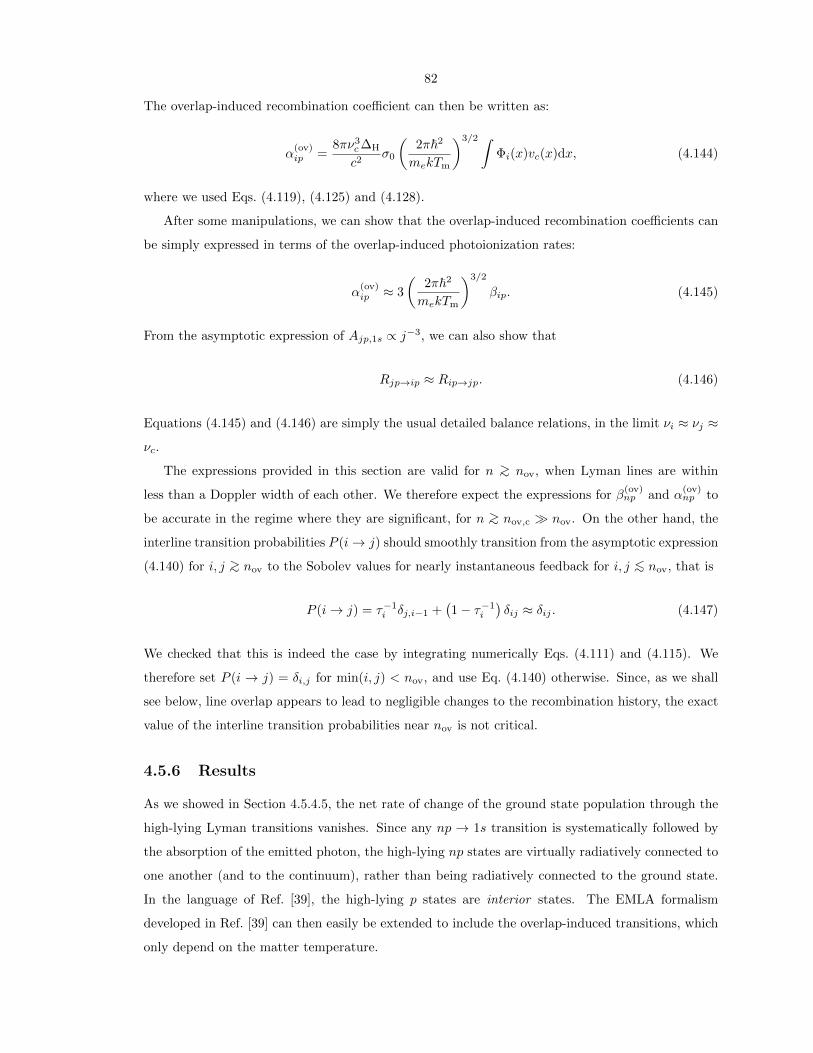
82

The overlap-induced recombination coefficient can then be written as:

α(ov)ip =

8πν3c∆H

c2σ0

(2π~2

mekTm

)3/2 ∫Φi(x)vc(x)dx, (4.144)

where we used Eqs. (4.119), (4.125) and (4.128).

After some manipulations, we can show that the overlap-induced recombination coefficients can

be simply expressed in terms of the overlap-induced photoionization rates:

α(ov)ip ≈ 3

(2π~2

mekTm

)3/2

βip. (4.145)

From the asymptotic expression of Ajp,1s ∝ j−3, we can also show that

Rjp→ip ≈ Rip→jp. (4.146)

Equations (4.145) and (4.146) are simply the usual detailed balance relations, in the limit νi ≈ νj ≈νc.

The expressions provided in this section are valid for n ∼> nov, when Lyman lines are within

less than a Doppler width of each other. We therefore expect the expressions for β(ov)np and α

(ov)np to

be accurate in the regime where they are significant, for n ∼> nov,c nov. On the other hand, the

interline transition probabilities P (i→ j) should smoothly transition from the asymptotic expression

(4.140) for i, j ∼> nov to the Sobolev values for nearly instantaneous feedback for i, j ∼< nov, that is

P (i→ j) = τ−1i δj,i−1 +

(1− τ−1

i

)δij ≈ δij . (4.147)

We checked that this is indeed the case by integrating numerically Eqs. (4.111) and (4.115). We

therefore set P (i → j) = δi,j for min(i, j) < nov, and use Eq. (4.140) otherwise. Since, as we shall

see below, line overlap appears to lead to negligible changes to the recombination history, the exact

value of the interline transition probabilities near nov is not critical.

4.5.6 Results

As we showed in Section 4.5.4.5, the net rate of change of the ground state population through the

high-lying Lyman transitions vanishes. Since any np → 1s transition is systematically followed by

the absorption of the emitted photon, the high-lying np states are virtually radiatively connected to

one another (and to the continuum), rather than being radiatively connected to the ground state.

In the language of Ref. [39], the high-lying p states are interior states. The EMLA formalism

developed in Ref. [39] can then easily be extended to include the overlap-induced transitions, which

only depend on the matter temperature.

83

We added the overlap-induced H(np)↔ H(n′p) and H(np)↔ e− + p transitions to our effective

rates code. We computed the change in the effective recombination coefficients A2s, A2p and effective

2p → 2s transition rate R2p→2s when the states 2s, 2p are considered as the only interface states

(i.e., cutting off the Lyβ transition and above for simplicity; the effect of overlap is independent of

that simplification). We find that the relative changes in each of the effective coefficients are at most

a few times 10−5. As a comparison, the change in total effective recombination coefficient between

nmax = 100 and nmax = 200 is of order 0.3 to 2% over the temperature range considered; from

nmax = 200 to nmax = 400, this change is of order 0.08 to 0.6%. Therefore, the effect of overlap is

a few orders of magnitude smaller than the mere error due to the necessary truncation of the high

energy shells when computing the effective rates. Since previous work [37, 38] have shown that MLA

computations with nmax ∼ 100 already reach the desired level of accuracy, we conclude that line

overlap can be safely ignored.

4.6 Population inversion7

The populations of the 2p and 2s states are strongly out of equilibrium towards the end of the epoch

of primordial recombination, with the ratio x2p/3x2s reaching values as large as ∼ 3 for z ∼ 500−600.

Although we do not track the populations of the 2p3/2 and 2p1/2 states separately, the overlap of

the 1s1/2 − 2p1/2 and 1s1/2 − 2p3/2 Lyα doublet ensures that they are in statistical equilibrium, so

x2p3/2/2x2s1/2 = x2p/3x2s. It is therefore a priori possible for the 11 GHz 2p3/2 → 2s1/2 transition

to be amplified. We checked however that the largest negative optical depth in this transition is

τ ∼ −10−7 for z ∼ 1100, and therefore the population inversion does not lead to any significant

amplification.

4.7 Conclusions

In this chapter, we have evaluated the impact of several radiative transfer effects on cosmological

hydrogen recombination:

• Thomson scattering in the Ly-α line was shown to be negligible, with corrections to the re-

combination history |∆xe/xe| ∼< 3× 10−5. We showed that at early times, z ∼> 1300, the dominant

effect was a delay of recombination, due to the reinjection of photons from the red side of the line

back into the blue side of the line during large angle scattering events. That effect can only be

properly accounted for with a full kernel approach, since scattered photons are redistributed on

frequency scales larger than the characteristic scale over which the radiation field changes. At lower

7I have removed the part of this section addressing population inversion in the high-n states, which is DanielGrin’s work and can be found in the published paper [40], as well as in Daniel Grin’s thesis [87].

84

redshifts, recoil becomes dominant and Thomson scattering accelerates recombination by helping

photons escape from the Lyα line.

• Distortions from the deuterium Ly-α line were shown to be negligible. Indeed, the very fast

D(2p)→ D(1s) transition rate, due to the relatively small optical depth in the deuterium line, brings

the deuterium 2p to 1s ratio close to equilibrium with the incoming radiation field on the D Lyα

line. Moreover, any distortions are further washed out due to the very large frequency diffusion rate

caused by resonant scattering by neutral hydrogen. Accounting for deuterium therefore leads to

changes of at most O(10−5) to the recombination history due to the small change in the expansion

history and the ambiguity in defining xe.

• The high-lying, non-overlapping Lyman transitions above Lyγ (strictly) can be artificially cut

off without loss of accuracy. Only the 2s, 2p, 3p and 4p states therefore need to be considered as

“interface” states in an EMLA computation [39]. Diffusion in Lyβ and higher lines can be neglected.

• Overlap of the high-lying Lyman lines, as well as overlap of the extremely high-lying lines with

the continuum, was shown to lead to O(10−5) changes to the effective transition rates. This change

is a few orders of magnitude smaller than the mere truncation error in the effective transition rates

computed with nmax ∼ 100 energy shells. The effect of line overlap is therefore negligible.

• Cosmological hydrogen masers are shown not to arise in this purely radiative treatment.

The goal of the ongoing work in the field is to develop a complete theory for hydrogen recombi-

nation, with a well understood error budget. In this chapter, we have evaluated the impact of some

radiative transfer effects that had not been previously addressed. While it is possible that some

effects have not been considered yet, we believe that most of the radiative transfer effects relevant in

primordial hydrogen recombination are now well understood. The picture is less clear for the effect

of collisional processes [38], for which the rates are relatively poorly known. Ultimately, we need a

recombination code that is not only accurate, but also fast, in order to be included in Markov chains

for cosmological parameter estimation; this will be the subject of the next chapter.

85

4.A

Ap

pen

dix

:N

ota

tion

use

din

this

chap

ter

Tab

le4.

1:N

otat

ion

use

din

this

chap

ter.

Un

its

of

“1”

mea

ns

the

qu

anti

tyis

dim

ensi

on

less

.

Sym

bol

Un

its

Des

crip

tion

Equ

atio

nAnp,1s

s−1

Ein

stei

nA

-coeffi

cien

tfo

rth

esp

onta

neo

us

dec

aynp→

1s

Eq.

(4.3

)an

1d

imen

sion

less

Voig

tp

ara

met

erfo

rth

eL

y-n

tran

siti

on

an

=Γnp/(4πν n

∆H

)f ν

1p

hot

onocc

up

ati

on

nu

mb

erat

freq

uen

cyν

fn eq

1eq

uilib

riu

mva

lue

off ν

nea

rL

y-n

fn eq

=xnp/(

3x

1s)

fn (e

m)

1eq

uil

ibri

um

valu

eoff ν

nea

rL

y-n

,w

ith

true

ab

sorp

tion

an

dem

issi

on

on

lyE

q.

(4.1

5)

Hs−

1H

ub

ble

exp

an

sion

rate

NH

cm−

3to

tal

num

ber

den

sity

of

hyd

rogen

nu

clei

NX

cm−

3nu

mb

erden

sity

of

spec

ies

X

Nν

Hz−

1nu

mb

erof

ph

oton

sp

erhyd

rogen

ato

mp

eru

nit

freq

uen

cyNν

=8πν

2

c3N

Hf ν

pn sc

1fr

acti

onof

ph

oton

ab

sorp

tion

sin

Ly-n

resu

ltin

gin

asc

att

erin

gpn sc

=Anp,1s/Γ

np

pn ab

1fr

acti

onof

tru

ep

hoto

nab

sorp

tion

sin

Ly-n

pn ab

=1−pn sc

Rn′ l→np

s−1

rad

iati

vetr

ansi

tion

raten′ l→np

per

hyd

rogen

ato

min

the

[n′ ,l]

state

Rn(ν,ν′ )

Hz−

2re

son

ant

scatt

erin

gre

dis

trib

uti

on

kern

elin

Ly-n

Eq.(

4.28)

RT

(ν→ν′ )

Hz−

1T

hom

son

scatt

erin

gke

rnel

Eq.

(4.5

1)

R(δ

)1

dim

ensi

onle

ssT

hom

son

scatt

erin

gke

rnel

Eq.

(4.5

6)

S nH

zw

idth

over

wh

ich

reso

nant

scatt

erin

gis

effec

tive

inL

y-n

Eq.

(4.3

6)

SH

zw

idth

over

wh

ich

reso

nant

scatt

erin

gis

effec

tive

inL

yα

S=S 2

S1

dim

ensi

onle

ssw

idth

over

wh

ich

reso

nant

scatt

erin

gis

effec

tive

inL

yα

S=

(hS/

(kT

r))

3

Tm,T

rK

mat

ter

an

dra

dia

tion

tem

per

atu

res

Wn

Hz

wid

thov

erw

hic

hth

eL

y-n

win

gs

are

op

tica

lly

thic

kfo

rtr

ue

ab

sorp

tion

Eq.

(4.3

5)

WH

zw

idth

over

wh

ich

the

Lyα

win

gs

are

op

tica

lly

thic

kfo

rtr

ue

ab

sorp

tion

W=W

2

W1

dim

ensi

onle

ssw

idth

over

whic

hL

yα

isop

tica

lly

thic

kfo

rtr

ue

ab

sorp

tion

W=hW/(kT

r)

86

Tab

le4.1

(conti

nu

ed)

Sym

bol

Un

its

Des

crip

tion

Equ

ati

on

xD

1ab

un

dan

ceof

deu

teri

um

rela

tive

toto

tal

hyd

rogen

nu

clei

xD

=N

D/N

H

xnl

1fr

act

ion

of

hydro

gen

inth

est

ate

[n,l

]xnl

=N

H(n,l

)/N

H

xe

1ab

un

dan

ceof

free

elec

tron

sre

lati

ve

toto

tal

hyd

rogen

nu

clei

xe

=Ne/N

H

x1

det

unin

gfr

om

lin

ece

nte

r(w

hen

con

sid

erin

ga

sin

gle

lin

e),

x=

(ν−ν n

)/(νn∆

H)

orfr

omν c

(wh

enco

nsi

der

ing

lin

eov

erla

p),

inD

op

ple

ru

nit

sx

=(ν−ν c

)/(νc∆

H)

xn

1d

etu

nin

gb

etw

een

Ly-n

an

dL

y-c

onti

nu

um

freq

uen

cies

inD

op

ple

rw

idth

sxn

=(νn−ν c

)/(νc∆

H)

y1

sam

easx

OR

det

un

ing

from

the

Lyα

freq

uen

cyin

un

its

ofkT

r/h

y=h

(ν−ν L

yα

)/(kT

r)

Γnp

s−1

wid

th(o

rin

vers

eli

feti

me)

of

thenp

state

∆X

1d

imen

sion

less

Dop

ple

rw

idth

for

asc

att

erin

gsp

ecie

sof

massm

X∆

X=√

2kT

m/(m

Xc2

)∆ν e

Hz

rms

freq

uen

cysh

ift

du

rin

gan

elec

tron

scatt

erin

gev

ent

nea

rL

yα

∆ν e

=ν L

yα

∆e

η eH

z−1

diff

eren

tial

opti

cal

dep

thfo

rT

hom

son

scatt

erin

gn

ear

Lym

an

-αE

q.

(4.5

0)

ν Lyα

(νH,ν

D)

Hz

Lym

an-α

reso

nan

tfr

equ

ency

(in

hyd

rogen

or

deu

teri

um

spec

ifica

lly)

ν cH

zL

ym

an

-lim

itfr

equ

ency

ν c=

4 3ν L

yα

ν nH

zL

ym

an

-nre

son

ant

freq

uen

cyν n

=(1−n−

2)νc

σT

cm2

Th

om

son

cross

sect

ion

σ0

cm2

ph

otoi

oniz

atio

ncr

oss

sect

ion

from

the

gro

un

dst

ate

,at

thre

shold

Eq.

(4.8

9)

τ n1

Sob

olev

op

tica

ld

epth

inth

eL

ym

an

-nre

son

an

celi

ne

Eq.

(4.6

)τ L

yα

1S

obole

vop

tica

ld

epth

inth

eL

ym

an

-αli

ne

τ Lyα

=τ 2

τ c1

Lym

anco

nti

nu

um

op

tica

ld

epth

per

Dop

ple

rw

idth

nea

rth

resh

old

Eq.

(4.1

01)

ϕn(ν

)H

z−1

lin

ep

rofi

lefo

rth

eL

y-n

tran

siti

on

φV

(x;a

)1

dim

ensi

on

less

Voig

tp

rofi

le,

wit

hV

oig

tp

ara

met

era

Eq.

(4.1

0)

φn(x

)1

dim

ensi

onle

ssD

op

ple

rp

rofi

lece

nte

red

at

the

Ly-n

freq

uen

cyφn(x

)=π−

1/2e−

(x−xn

)2

φc(x

)1

non

-nor

mal

ized

dim

ensi

on

less

pro

file

for

conti

nu

um

ab

sorp

tion

nea

rth

resh

old

Eq.

(4.9

3)

87

4.B Appendix: Resonant scattering in a Doppler core dom-

inated line8

We showed in Section 4.4.1 that only Lyα, Lyβ and Lyγ decays affect recombination to a significant

level. The exact value of the escape probability in higher-order lines is therefore irrelevant to the

problem of primordial recombination. It may however be important in other environments, such

as the interstellar medium or stellar atmospheres, to compute the change in escape probability

due to partial frequency redistribution in resonant scattering events. This appendix provides a

generalization of the Sobolev escape probability for Doppler core dominated optically thick lines

(i.e., with optically thin damping wings) with partial frequency redistribution. We also develop a

method of solution based on expansion of the radiative transfer equation on the Hermite polynomials

basis. We do not consider stimulated emission nor stimulated scattering.

4.B.1 The radiative transfer equation in the presence of partial frequency

redistribution

In the absence of non-resonant processes, the most general radiative transfer equation in the vicinity

of a resonant line was given in Eq. (4.32). We consider a line (with resonant frequency ν0) with

optically thin damping wings. We can use the Doppler core approximation for the line profile:

φ(ν) =1√π∆νD

exp

[−(ν − ν0

∆νD

)2], (4.148)

where ∆νD ≡ ν0

√2kT/(mc2) is the Doppler width of the line, m being the mass of the scatterers.

Provided hν0 √mc2kT , we can neglect approximate the exponential factors by unity in Eq. (4.32).

The scattering redistribution kernel Rn(ν, ν′) = φn(ν′)pn(ν|ν′) can be taken to be the RI kernel for

zero natural line width [89]. Finally, as long as the line is narrow (∆νD ν0, always true if the

scatterers are non-relativistic), one can make the steady-state approximation and neglect the time

dependence in this problem. Making the change of variables

x ≡ ν − ν0

∆νD, (4.149)

the time-steady radiative transfer equation for the photon occupation number f(x) becomes:

df

dx= τφ(x) [f(x)− feq] + psc τ

∫[φ(x)φ(x′)−RI(x, x

′)] f(x′)dx′, (4.150)

8This work is unpublished.

88

where φ(x) ≡ 1√π

e−x2

is the dimensionless Doppler profile and RI(x, x′) is the dimensionless scat-

tering kernel for zero natural width. It is symmetric in in its arguments when recoil is ignored, and

satisfies∫RI(x, x

′)dx′ = φ(x). The scattering kernel is a combination of the kernel for isotropic

scattering RI−A and the one for dipolar scattering RI−B, given in Eqs. (3.11.3) and (3.11.5) of

Ref. [89]:

RI(x, x′) = (1− χ)RI−A(x, x′) + χRI−B(x, x′), (4.151)

with χ ∈ [0, 1]. The value of χ depends on the angular probability distribution of scattering directions

in the atom’s rest frame, g(n′|n), where n and n′ are the direction of propagation of the incoming

and outgoing photons respectively. It can be found by decomposing g on the basis:

g(n′|n) = (1− χ)giso(n′|n) + χgdip(n′|n) (4.152)

≡ (1− χ)1

4π+ χ

3

16π

(1 + (n · n′)2

). (4.153)

The value of χ depends in general on the fine and hyperfine splitting of the levels of the considered

transition. The boundary condition for f is f(+∞) = f+. Using the linearity of the equation, and

the relation∫

[φ(x)φ(x′)−R(x, x′)] dx′ = 0, we can simplify Eq. (4.150) further by defining:

ξ(x) ≡ f(x)− f+

feq − f+, (4.154)

which satisfies the equation:

dξ

dx= τ φ(x) [ξ(x)− 1] + τ psc

∫[φ(x)φ(x′)−R(x, x′)] ξ(x′)dx′, (4.155)

with boundary condition ξ(+∞) = 0.

Let us now try to qualitatively understand what we expect to happen when accounting for

partial frequency redistribution. The differential probability for a scattered photon to have frequency

x′ given that the incoming photon had frequency x is p(x′|x) = φ(x′) in the case of complete

redistribution, and p(x′|x) = R(x, x′)/φ(x) in the case of partial frequency redistribution. This

allows us to compute the mean and variance of the frequency of the scattered photon frequency, as

a function of that of the incoming photon. In the case of complete redistribution, we have

〈x′〉CR = 0, 〈x′2〉CR =1

2, (4.156)

independently of the frequency of the incoming photon. In the case of partial frequency redistri-

bution, one can show either using the expressions given by Hummer [89] or the expansion derived

89

below, Eq. (4.175), that

〈x′〉PR = 0, 〈x′2〉PR =1

3

[(1 +

χ

5

)x2 + 1− χ

10

]. (4.157)

The mean outgoing photon frequency vanishes because forward (x′ = x) and backward (x′ = −x)

scattering events are equally probable. The variance of the scattered photon frequency, however,

increases with the distance of the incoming photon frequency from the resonant frequency. Near line

center, 〈x′2〉PR < 〈x′2〉CR so we expect photons to “pile up” a little more near line center. Several

Doppler widths away from line center, 〈x′2〉PR > 〈x′2〉CR so we expect photons in the wings to be

re-scattered towards line center. Since the photon occupation number on the red side of the line is

much larger (for an optically thick line) than that on the blue side, we therefore expect a net flux

of photons from the red side of the line to the line center. In other words, partial redistribution will

re-inject photons from the blue side of the line back into the line center where they are more likely

to be absorbed, and therefore decrease the escape probability. Note, finally, that the effect will be

more pronounced for isotropic scattering due to the enhanced probability of backward (and forward)

scattering.

We now compute the change in escape probability. We will see that the qualitative features

described above are indeed recovered in the exact solution (see Figs. 4.8 and 4.9).

4.B.2 Escape probability

From Eq. (4.42), the net decay rate in the line is

xu→l =guglxlAu,l

∫φ(x)[feq − f(x)]dx =

guglxlAu,l

∫φ(x)[1− ξ(x)]dx× [feq − f+]

≡ Pesc(τ, psc)Au,l

[xu −

guglxlf+

], (4.158)

where u and l denote the upper and lower levels. The last line defines the escape probability:

Pesc(τ, psc) ≡ 1− ξ =ξ(−∞)

τ, (4.159)

where ξ ≡∫φ(x)ξ(x)dx and we integrated Eq. (4.155) from −∞ to +∞ to obtain the second

equality. When psc = 0 (complete redistribution), Eq. (4.155) is a simple ODE that can be solved

analytically; in that case ξ(−∞) = 1− e−τ and we recover the standard Sobolev escape probability.

In the general case, Eq. (4.155) is an integro-differential equation, which does not have any analytic

solutions, and therefore requires solving by a numerical method.

Before explaining our method of solution, we first relate our expression for the escape probability

to that derived by Switzer & Hirata [56] in the context of helium recombination. In the absence of

90

continuum absorption, Switzer & Hirata define the function

ξSH ≡ f − f+

f(em) − f+, (4.160)

where f(em) was defined in Eq. (4.15) [this definition was given for a Lyman transition in hydrogen

but can be easily generalized to any resonant line]. We showed in Section 4.2.2.1 that when the rate

of expansion is much smaller than the inverse lifetimes of the excited states, the following relation

was satisfied [see Eq. (4.22)]: (1− psc)f(em) = feq− pscf . This allows us to express the function ξSH

as a function of our function ξ:

ξSH =(1− psc)ξ

1− pscξ. (4.161)

The expression derived in Ref. [56] for the escape probability

P SHesc =

(1− psc)(1− ξSH)

1− psc(1− ξSH)

(4.162)

can then be shown to be exactly equivalent to our expression, Eq. (4.159). The advantage of our

formulation (besides a simpler expression for the escape probability) is that our function ξ is always

strictly positive, even when psc → 1, whereas ξSH → 0 when psc → 1 and the escape probability as

given by Ref. [56] is the ratio of two small numbers in that limit.

4.B.3 Hermite polynomial expansion of the scattering kernel

Explicit expressions for the angle averaged scattering redistribution kernel are given in [89]. It is

however easier to start off with the angle-dependent scattering kernel, which in the case of zero

natural line width is [99, 89]:

RI(x,n, x′,n′) =

g(n′|n)

4π2 sin γe−x

′2−(x−x′ cos γ)2 csc2 γ , (4.163)

where γ is the angle between n and n′, which are the directions of propagation of the incoming and

outgoing (scattered) photon respectively, and g(n′|n) is the probability distribution of n′ given n

(s.t.∫g(n′|n)dn′ = 1).

We define the sequence:

un(x′) ≡ 1√π

∫ +∞

−∞e−(x−x′ cos γ)2 csc2 γHn(x)dx, (4.164)

where Hn is the n-th Hermite polynomial. Using the recursion relation

Hn(x) = 2xHn−1(x)− 2(n− 1)Hn−2(x), (4.165)

91

integrating by parts and using the property

H ′n−1(x) = 2(n− 1)Hn−2(x), (4.166)

we obtain the recursion relation:

un(x′) = 2x′ cos γ un−1(x′)− 2(n− 1) cos2 γ un−2(x′). (4.167)

This is the recursion relation satisfied by cosn γ Hn(x′). Since u0(x′) = sin γH0(x′) and u1(x′) =

sin γ cos γH1(x′), we conclude that

un(x′) = sin γ cosn γHn(x′). (4.168)

We therefore obtain the relation:

1√π

∫RI(x,n, x

′,n′)Hn(x)dx =g(n′|n)

4π2cosn γe−x

′2Hn(x′). (4.169)

From the orthogonality relation of the Hermite polynomials

1√π

∫ +∞

−∞e−x

2

Hn(x)Hm(x)dx = δnm2nn!, (4.170)

we deduce the decomposition of RI(x,n, x′,n′) on the Hermite basis:

RI(x,n, x′,n′) =

g(n′|n)

4π2e−x

2

e−x′2

+∞∑

n=0

cosn γ

2nn!Hn(x)Hn(x′). (4.171)

The angle-averaged redistribution kernel can be obtained by integrating over angles n,n′ [89]:

RI(x, x′) = 8π2

∫ π

0

RI(x,n, x′,n′) sin γdγ (4.172)

=e−x

2

e−x′2

π

+∞∑

p=0

1

22p(2p)!

∫ 1

−1

2πg(µ)µ2pdµ H2p(x)H2p(x′),

where we used the fact that g(n′|n) is a function of the dot product n ·n′ = cos γ only, and therefore

all its odd moments vanish.

For an isotropic angular distribution, giso(µ) = 14π , we have:

∫ 1

−1

2πgiso(µ)µ2pdµ =1

2p+ 1, (4.173)

92

whereas for the dipolar angular distribution, gdip(µ) = 316π (1 + µ2), we have:

∫ 1

−1

2πgdip(µ)µ2pdµ =3(p+ 1)

(2p+ 1)(2p+ 3). (4.174)

With g = (1− χ)giso + χgdip, we obtain the decomposition of the scattering kernel on the Hermite

polynomial basis:

RI(x, x′) = φ(x)φ(x′)

+∞∑

p=0

(1 +

χ p

2p+ 3

)H2p(x)H2p(x

′)22p(2p+ 1)!

. (4.175)

Such a decomposition was already worked out in Refs. [100, 101] in the case of isotropic scattering

(with a missing factor of 1/(2p+ 1) in Ref. [100]).

4.B.4 Solution of the steady-state radiative transfer equation with scat-

tering

Given the quite simple decomposition of the scattering kernel on the Hermite polynomial basis de-

rived above, we suggest a method of solution to the time-steady radiative transfer equation including

scattering, Eq. (4.155).

The Hermite polynomials form an orthonormal basis, and we can decompose the function ξ on

that basis:

ξ =

+∞∑

n=0

anHn(x). (4.176)

Using the decomposition (4.175) and the orthogonality relation (4.170), the radiative transfer equa-

tion Eq. (4.155) therefore reads:

dξ

dx= τ φ(x)

[a0 − 1 +

+∞∑

n=1

anHn(x)− psc

+∞∑

p=1

(1 +

χp

2p+ 3

)a2p

2p+ 1H2p(x)

]. (4.177)

The formal solution to this equation is:

ξ(x) = −∫ +∞

x

dξ

dx′dx′. (4.178)

Using the defining relation for Hermite polynomials,

Hn(x) = ex2

(−1)nd

dxn

(e−x

2), (4.179)

93

we can easily show that, for n > 0,

∫ +∞

x

φ(x′)Hn(x′)dx′ = φ(x)Hn−1(x). (4.180)

The formal solution is therefore:

ξ(x) = τ (1− a0)1

2erfc(x) + τ φ(x)

[−

+∞∑

n=1

anHn−1(x) + psc

+∞∑

p=1

(1 +

χp

2p+ 3

)a2p

2p+ 1H2p−1(x)

].

(4.181)

To close the system we need to make sure that the coefficients of ξ on the Hermite basis are those

we started with:

an =1√π2nn!

∫ +∞

−∞e−x

2

Hn(x)ξ(x)dx. (4.182)

We need to establish some preliminary results first. We define the sequence:

vp ≡ 1√π

∫ +∞

−∞e−2x2

H2p(x)dx (4.183)

= u2p

(x′ = 0; γ =

π

4

), (4.184)

where un(x′; γ) was defined in Eq. (4.164). From Eq. (4.168), we have

vp =1√2

1

2pH2p(0) = (−1)p

1√2

(2p)!

2pp!, (4.185)

from the well known values of the Hermite numbers H2p(0). We can show the following relations:

1√π

∫ +∞

−∞e−x

2

H2q(x)erfc(x)dx = δq0 (4.186)

1√π

∫ +∞

−∞e−x

2

H2q+1(x)erfc(x)dx = − 2√πvq (4.187)

1√π

∫ +∞

−∞e−2x2

H2q+1(x)H2p(x)dx = 0 (4.188)

1√π

∫ +∞

−∞e−2x2

H2q(x)H2p(x)dx = vp+q (4.189)

1√π

∫ +∞

−∞e−2x2

H2q+1(x)H2p−1(x)dx = −vp+q. (4.190)

We finally obtain the system of equations satisfied by the coefficients an:

a2q =1

2τ(1− a0)δq0 −

τ

22q(2q)!√π

+∞∑

p=0

vp+qa2p+1, (4.191)

a2q+1 =τ/√π

22q+1(2q + 1)!

− (1− a0)vq +

+∞∑

p=1

[1− psc

2p+ 1

(1 +

χ p

2p+ 3

)]vp+qa2p

.(4.192)

94

1 10 100 1000!

-0.12

-0.10

-0.08

-0.06

-0.04

-0.02

0.00

" P

esc/P

esc

dipolar, # = 1isotropic, # = 0

!

psc = 1

psc = 0.66

psc = 0.33

!Pesc

Pesc

Figure 4.8: Decrease in the escape probability due to partial frequency redistribution [the quantityplotted is ∆Pesc/Pesc ≡ Pesc(τ, psc)/Pesc(τ, psc = 0)− 1]. The effect is more pronounced for dipolarscattering than isotropic scattering due to the higher probability of backward scattering.

This is in principle an infinite system of linear equations with an infinite number of unknowns. Our

approximation of order N consists in truncating it to the N + 1 unknowns a0, ..., aN, i.e., solving

the system (4.191), (4.192) where we set an = 0 for n > N .

Once we obtain the coefficients a0, ..., aN, we use the expression (4.181) for ξ(x) to compute

ξ(−∞) rather than the initial decomposition (4.176), which, when truncated at a finite N , is infinite

at x→ ±∞. We therefore obtain the desired escape probability:

Pesc =ξ(−∞)

τ= 1− a0. (4.193)

We check the convergence of our method with the known analytic solution in the case psc = 0:

Pesc(τ, psc = 0) =1− e−τ

τ≈ 1

τ, τ 1. (4.194)

We find that the approximation has converged to the analytic solution with a relative accuracy of

10−4 for N ∼> 30 log10(τ).

We show the resulting change in escape probability as function of the optical depth and psc in

Fig. 4.8. We see that partial redistribution leads to a systematic decrease of the escape probability,

as we had anticipated (see discussion at the end of Section 4.B.1). The magnitude of the relative

decrease is no larger than ∼ 10%, reached for τ ∼ 50, psc = 1 and χ = 1. We also show the function

ξ(x) in Fig. 4.9 as an illustration of the qualitative argument given in Section 4.B.1.

95

-3 -2 -1 0 1 2 3x

0.0

0.2

0.4

0.6

0.8

1.0

!!

psc = 1psc = 0.5psc = 0

" = 45, # = 1

x

!(x)

psc = 0psc = 0.5psc = 1

! = 45, " = 1

Figure 4.9: Normalized photon occupation number ξ as defined in Eq. (4.154) as a function offrequency in Doppler width units, for Sobolev optical depth τ = 45 and dipolar scattering. Partialredistribution during resonant scattering events re-injects photons from the red side of the line backinto line center, where they get absorbed.

96

Chapter 5

A fast and highly accurateprimordial hydrogen recombinationcode1

5.1 Introduction

Previous works have all concentrated on one or a few aspects of the primordial recombination

problem. Producing a complete and fast recombination code has so far been hindered by the com-

putational burden previously associated with the high-n problem. Given that this problem is now

solved, and that it seems that the main radiative transfer effects have now all been identified, it

is timely to deliver a single code that computes an accurate hydrogen and helium recombination

history and incorporates all the relevant physics. The purpose of this chapter is to introduce our

new recombination code, HyRec, which is publicly available2, and can compute a highly accurate

recombination history (with errors at the level of a few times 10−3 for helium recombination and a

few times 10−4 for hydrogen recombination) in only ∼ 2 seconds on a standard laptop. Our code does

not account for collisional transitions in hydrogen, as their rates are poorly known. When accurate

rates are available and if collisional transitions are shown to significantly impact recombination, we

will update our code with the appropriate effective rates.

Recently, a similar work has been carried out by Chluba & Thomas [102], also relying on the

effective MLA method presented in Chapter 3. The code they present includes the same physics

as ours. The main difference is the treatment of radiative transfer. In Ref. [102], an “order zero”

recombination history is first computed, with a simple treatment of radiative transfer. The radiative

transfer equation is then solved, given this order zero history. Corrections to the net decay rates

1This chapter is adapted from the paper HyRec: A fast and highly accurate primordial hydrogen and heliumrecombination code, Y. Ali-Haımoud & C. M. Hirata, Phys. Rev. D 83, 043513 (2011). The section on heliumrecombination was not included as it is Christopher Hirata’s work but the reader is encouraged to read it in thepublished paper. Reproduced here with permission, copyright (2011) by the American Physical Society.

2HyRec is available for download at the following url: http://www.tapir.caltech.edu/∼yacine/hyrec/hyrec.html.

97

to the ground state are then evaluated, and used to compute a corrected recombination history.

This procedure can in principle be iterated, but because the corrections are small, it is essentially

converged after one or two iterations. Our solution, on the other hand, is non-perturbative, in the

sense that we solve simultaneously for the radiation field and the recombination history. A detailed

code comparison is in progress, and a full error budget will be presented once it is completed.

In Chapter 4 we briefly evoked the connection between resonant line processes and two-photon

transitions. We considered line profiles in the resonant approximation near resonances, since we

were mainly studying other (non-resonant) processes that turned out to be negligible. At the level

of precision required by Planck, two-photon processes must be treated accurately, with correct

profiles and a full time-dependent radiative transfer calculation [49, 51, 52].

This chapter is organized as follows. Two-photon processes and frequency diffusion are formally

described in Section 5.2. In Section 5.3, we present our numerical solution for the radiative transfer

equation. We use a new method of solution, extending that of Ref. [49] to account for frequency

diffusion, that allows to solve for the atomic populations and the radiation field simultaneously. We

conclude in Section 5.4. Appendix 5.A describes our ordinary differential equation (ODE) integrator

and Appendix 5.B lists the numerically stable radiative transfer equations used in the latest version

of HyRec3.

Throughout this chapter we use a flat background ΛCDM cosmology with T0 = 2.728 K, Ωbh2 =

0.022, Ωmh2 = 0.13, ΩΛh

2 = 0.343, YHe = 0.24 and Nν,eff = 3.04.

5.2 Two-photon processes: formal description

5.2.1 Overview

It is well known since the first works on primordial recombination that 2s→ 1s two-photon decays

significantly contribute to the recombination dynamics [31, 32]. Even with a relatively low decay rate,

the forbidden 2s→ 1s decays are indeed comparable in efficiency to the highly self-absorbed Lyman-

α transition; in fact, more than half of hydrogen atoms have formed through the 2s → 1s channel

[70]. This process was traditionally accounted for with the total 2s → 1s decay rate in vacuum,

Λ2s,1s ≈ 8.22 s−1, with a two-photon absorption rate obtained by detailed balance considerations.

For the level of accuracy required for future CMB experiments, one needs to account for stimulated

two-photon decays [47] and non-thermal absorptions [48, 49].

Recently, it was suggested that two-photon decays from higher lying ns and nd states may also

lead to percent level corrections to the recombination history [50]. Inclusion of such decays presents

an additional conceptual difficulty which was not present for the 2s → 1s decays: the problem

of double-counting. Indeed, there is no fundamental difference between a sequence of two allowed

3I will upload this version online within the next few days.

98

one-photon transitions nl → n′p, n′p → 1s, with 1 < n′ < n, and a two-photon decay from the nl

state near resonance (i.e., where the energy of the two photons are near Enn′ and En′1 respectively).

Approximate solutions were presented in Refs. [50, 103, 51] (for a review, see Ref. [49]). The double-

counting problem as well as the reabsorption problem were resolved with a numerical approach,

solving the radiative transfer equations for the photon field in Ref. [49], which also provided analytic

approximations to check the validity of the numerical result. In this work, we will use the same

numerical method as in Ref. [49], which we extend to account for frequency diffusion near the Lyα

line. In this section, we review the formalism presented in Ref. [49] and how to solve the double

counting problem. In Section 5.3 we will describe our numerical method for solving simultaneously

the radiative transfer equation and the evolution of the atomic level populations.

5.2.2 Two-photon decays and Raman scattering

We start by defining the coefficient:

dΛnldν≡ α6

fsν3ν′3

108(2l + 1)E6I

|M(ν)|2, (5.1)

where the matrix element M(ν) is given by Eq. (B5) of Ref. [49], and ν′ ≡ |ν − νn1|, where νn1 is

the frequency of the Ly-n transition. For ν < νn1, dΛnl/dν is the rate of spontaneous two-photon

decays from nl per frequency interval. For ν > νn1, dΛnl/dν×fν′ (where fν is the photon occupation

number at frequency ν) is the rate of spontaneous Raman scatterings per frequency interval per atom

initially in nl (in the notation of Ref. [49], dΛnl/dν = dKnl/dν for ν > νn1). The function dΛnl/dν

is continuous across ν = νn1, where it vanishes.

We can now write the net rate of nl ↔ 1s two-photon transitions per frequency interval per

hydrogen atom, for which the highest energy photon has frequency ν < νn1:

∆nl(ν < νn1) =dΛnldν

[xnl(1 + fν′)(1 + fν)− gnl

g1sx1sfν′fν

]. (5.2)

For ν > νn1, the appropriate rate is that of Raman scattering events:

∆nl(ν > νn1) =dΛnldν

[xnlfν′(1 + fν)− gnl

g1sx1s(1 + fν′)fν

], (5.3)

In both cases, we can assume that the photon occupation number for the low-energy photons is

that of a blackbody, since the optical depth for two-photon absorption of the low-energy photons is

tiny (for a discussion, see Ref. [49]). We therefore set fν′ = (ehν′/Tr − 1)−1. Moreover, the photon

occupation number for frequencies ν > νLyα/2 is much smaller than unity: fν 1. This means that

we can neglect stimulated emission by the high-energy photons in Eqs. (5.2) and (5.3). Given these

considerations, the net rate of two-photon transitions can be written in the following form, valid for

99

both ν < νn1 and ν > νn1:

∆nl(ν) =dΛnldν

∣∣eh(ν−νn1)/Tr − 1∣∣−1[xnl −

gnlg1s

x1seh(ν−νn1)/Trfν

]. (5.4)

5.2.3 Resonant scattering in Lyman-α

We now consider pure scattering events,

H(1s) + γ → H(1s) + γ. (5.5)

In the low-frequency limit this corresponds to the familiar Rayleigh scattering phenomenon; the cross

section however has resonances at the Lyman-series lines, which correspond to resonant Rayleigh

scattering.

Rayleigh scattering events conserve the photon frequency in the atom’s rest frame. In the co-

moving frame (frame in which the CMB appears isotropic), the frequency of the scattered photon

appears shifted due to the thermal motions of the scatterers. The frequencies of the incoming and

outgoing photons are however statistically correlated. Mathematically, there is a definite probability

distribution p(ν, ν′), such that p(ν, ν′)dν′ is the probability that the outgoing photon has frequency

in [ν′, ν′+dν′] given that the incoming photon had frequency ν, and this function generally depends

on both ν and ν′. For Tm hν, which is the case near the Lyman lines, the variance of the frequency

shifts imparted by thermally moving atoms is given by:

〈δν2〉 ≡∫

(ν′ − ν)2p(ν, ν′)dν′ =2Tm

mHc2ν2. (5.6)

The rate of injection of photons per frequency interval at frequency ν, due to resonant Rayleigh

scattering in Ly-α, can be written in the general form (neglecting stimulated scatterings):

∆1s(ν) = x1s

[∫fν′R(ν′, ν)dν′ −

∫fνR(ν, ν′)dν′

], (5.7)

where R(ν, ν′) = dΛ1s

dν p(ν, ν′) is the differential rate of scatterings per hydrogen atom in the ground

state, per unit frequency interval for both the incoming and outgoing photons (it has units of

s−1Hz−2). The scattering kernel must respect detailed balance:

R(ν, ν′)e−hν/Tm = R(ν′, ν)e−hν′/Tm . (5.8)

To be fully general one should compute the scattering kernel from first principles. However, simpli-

fications can be easily made in various regimes.

Far from any resonance, the rate of redshifting due to the Hubble expansion is much larger than

100

the rate of frequency diffusion due to scattering (see for example the discussion in Section 4.2.2.3).

We can neglect Rayleigh scattering there, and set ∆1s(ν) = 0.

Near Lyman resonances, we have

dΛ1s

dν(ν ≈ νn1) ≈ 3Anp,1sp

nscφV,n(ν), (5.9)

where pnsc = Anp,1s/Γnp is the scattering probability in the Lyman-n line (the complementary events

being two-photon absorptions and two-photon photoionizations), and φV,n(ν) is the Voigt profile

for the Ly-n line. In the Doppler core, we can approximate the partial redistribution induced

by scattering events by a complete redistribution, i.e., approximate p(ν, ν′) ≈ φV,n(ν) ≈ φD,n(ν),

independent of ν′, where φD is the Doppler profile. This approximation is valid because in the

Doppler core, complete redistribution recovers the correct rms frequency shift during scattering

events, Eq. (5.6) (if one averages over the frequencies of absorbed photons).

In the damping wings of Lyman resonances above Lyα, the rate of scattering events is of the same

order as the rate of two-photon absorptions. Each scattering event shifts the photon frequency by a

very small amount compared to the width over which the radiation field varies (δνrms/ν ∼ 2.5×10−5).

Partial redistribution is therefore essentially coherent in the comoving frame, i.e., p(ν, ν′) ≈ δ(ν′−ν),

which implies ∆1s(ν) ≈ 0. For a more quantitative argument, see Section 4.4.2.

The only frequency regime where Rayleigh scattering affects the radiation field in a non-trivial

way is in the damping wings of Lyα. In this line, indeed, scattering events are much more frequent

than two-photon absorption events (by a factor of ∼ 104). Resonant scattering therefore leads to

a significant diffusion in frequency. Because the frequency shifts are small compared to the width

over which the radiation field varies, the integral scattering operator can be approximated by a

second-order differential operator — a Fokker-Planck operator [92, 90, 45, 46]. For the purpose of

numerical implementation, the relevant properties are (i) the fact that this operator is nearly local

(it only connects neighboring bins in frequency), (ii) it must respect detailed balance, and (iii) the

diffusion rate must be correct. We will explain our numerical method for the implementation of

Lyman-α diffusion in Section 5.3.1.

We note that a number of analytic treatments of Lyman-α scattering in the recombination

epoch have been proposed in the past [104, 93, 94, 105, 90]. However, since two-photon emission

and absorption act on the same region of frequency space, and since both processes involve high

optical depth, an accurate recombination history can only be obtained by considering all processes

simultaneously.

101

5.2.4 The radiative transfer equation

The radiative transfer equation for the photon occupation number is:

∂fν∂t−Hν ∂fν

∂ν=c3nH

8πν2

∑

n≥2,l

∆nl(ν) + ∆1s(ν)

, (5.10)

where the left-hand side is the derivative of the photon occupation number along a photon trajectory

in the expanding universe, and the prefactor on the right-hand side converts the number of photons

per unit frequency per hydrogen atom to the photon occupation number (see Section 4.2).

5.2.5 Inclusion in the effective multilevel atom rate equations

5.2.5.1 Formal two-photon decay rates

As mentioned earlier, including two-photon decays from states with n > 2 and Raman scattering

events poses a double-counting problem. In principle, to avoid this double counting issue, one should

discard “1+1” decays (or decays following an absorption event, which is like a Raman scattering

event on resonance) altogether. If one were to pursue this idea, one should not consider the p states

at all anymore (as they are formally only intermediate states in two-photon processes), but consider

all s and d states as “interface states” and allow for two-photon recombinations to the ground state.

The two-photon nl↔ 1s transition rates would then become:

xnl∣∣(2γ)

1s= −x1s

∣∣(2γ)

nl= x1sR

total1s,nl − xnlRtotal

nl,1s, (5.11)

where the formal transition rates are given by:

Rtotal1s,nl ≡

∫dΛnldν

gnlg1s

∣∣eh(νn1−ν)/Tr − 1∣∣−1

fνdν (5.12)

and

Rtotalnl,1s ≡

∫dΛnldν

∣∣eh(ν−νn1)/Tr − 1∣∣−1

dν, (5.13)

where the integrals run from νn1/2 to νc. In principle Eq. (5.11)–(5.13), can be included in a standard

or effective multilevel atom code, provided one solves simultaneously for the radiation field, using

the radiative transfer equation Eq. (5.10).

5.2.5.2 Decomposition into “1+1” transitions and non-resonant contributions

Two-photon decays from higher excited states constitute, however, a correction to the recombination

history computed in the standard “1+1” picture, and we would like to implement it as such. We

start by formally separating the integrals in Eqs. (5.12) and (5.13) in two contributions: the resonant

102

pieces, for ν ≈ νn′1, and a non-resonant piece, for frequencies far enough from any resonance. We

therefore rewrite, formally:

Rtotal1s,nl =

∑

n′

R(n′p)1s,nl + R1s,nl and

Rtotalnl,1s =

∑

n′

R(n′p)nl,1s + Rnl,1s, (5.14)

where the resonant contributions R(n′p)1s,nl and R

(n′p)nl,1s are defined in a similar manner as in Eqs. (5.12)

and (5.13), but with the integration being carried over a narrow range ∆ν near νn′1, and R1s,nl and

Rnl,1s are the non-resonant pieces required to complete the total rates. So far the separation is just

formal and we have not made any approximation.

5.2.5.3 “1+1” Resonant contribution

We now notice that near a resonance ν ≈ νn′1, the two-photon differential decay rate dΛnl/dν takes

on the following form (if n > n′):

dΛnldν

∣∣∣ν≈νn′1

≈ 1

4π2

Anl,n′pAn′p,1s(ν − νn′1)2 + (Γn′p/4π)2

= Anl,n′pAn′p,1s

Γn′pφL(ν − νn′1; Γn′p), (5.15)

where Γn′p is the total inverse lifetime of the state n′p, and the Lorentzian profile is given by

φL(∆ν; Γ) ≡ Γ/(4π2)

∆ν2 + (Γ/4π)2. (5.16)

For n < n′, the first coefficient in Eq. (5.15) should be gn′p/gnl × An′p,nl instead of Anl,n′p. When

accounting for the thermal motions of atoms, the Lorentzian profile should be replaced by a Voigt

profile. We can now approximate the resonant pieces with the following expressions, valid for both

n < n′ and n > n′:

R(n′p)1s,nl ≈ 3An′p,1sfνn′1

Rn′p,nlΓn′p

(5.17)

and

R(n′p)nl,1s ≈ Rnl,n′p

An′p,1sΓn′p

, (5.18)

where fνn′1 is the photon occupation number averaged over the Voigt profile near the resonance

ν ≈ νn′1. Eqs. (5.17) and (5.18) are exactly what one would obtain in the “1+1” picture after

“factoring out” the p states (with a procedure similar to what is used to get rid of the “interior”

states in the EMLA method). Having these resonant rates is exactly equivalent to having optically

thin one-photon transitions between the nl and n′p states, with rates Rnl,n′p(Tr) and Rn′p,nl(Tr),

103

and optically thick Lyman transitions, with net rate:

xn′p∣∣1s

= −x1s

∣∣n′p

= An′p,1s

(3x1sfνn′p − xn′p

). (5.19)

To obtain the net decay rates in the Lyman transitions, one then needs to solve for the radiation

field in the immediate vicinity of Lyman resonances. If the frequency region for which two-photon

transitions are considered as “resonant” is narrow enough, this can be done in the Sobolev approxi-

mation. Indeed, all the relevant conditions are met (see also discussion in Ref. [49]; for more details

on the Sobolev approximation, see Section 4.2.4):

First, the two-photon absorption and emission profiles can both be approximated by the same

resonance profile Eq. (5.15). This relies on the assumption that the blackbody radiation field varies

little across the “resonant” region, and requires for its width to satisfy ∆ν Tr/h.

Secondly, we argued in Section 5.2.3 that one could assume complete frequency redistribution

for resonant scattering near the Doppler core of Lyman resonances. The “resonant” region should

therefore not exceed a few Doppler widths.

Finally, if we consider regions in frequency narrow enough around the resonances, we can use

the steady-state approximation. This requires ∆ν/ν 1.

We can see that considering the “resonant” region around each Lyman resonance to be a few

Doppler widths wide meets all the requirements.

An additional assumption required here is that excited states are near Boltzmann equilibrium,

which is very accurate at redshifts for which two-photon processes are important. In the Sobolev

approximation, and in the limit of large Sobolev optical depth, Eq. (5.19) becomes the standard

Lyman decay rate Eq. (3.8), where f+np is the photon occupation number incoming on the resonance,

preprocessed by two-photon processes and diffusion in the blue damping wing of the line.

The Sobolev approximation is probably the least accurate for Lyα decays where partial redistri-

bution due to resonant scattering is important. However, the large optical depth to two-photon ab-

sorptions in the Lyman-α blue damping wing, in conjunction with frequent scattering events, drive

the radiation field to the equilibrium value fν = xn′p/(3x1s)e−h(ν−νn′1)/Tm over several Doppler

widths (of the order of 40 Doppler widths, see Fig. 4.1 and accompanying discussion in Section 4.2).

As a consequence the net decay rate in the core of the resonance is very small anyway. We checked

that in the presence of two-photon transitions and frequency diffusion, even setting xn′p∣∣1s

= 0

instead of the expression given by Eq. (5.19) leads to relative changes to the recombination history

of at most 7 × 10−4. Given that frequency diffusion leads to corrections of a few percent at most

to the decay rate in Lyα when radiative transfer is treated carefully even at the line center [45], we

can be confident that using the Sobolev approximation for the resonant contributions of two-photon

decays is accurate to better than 10−4.

104

5.2.5.4 “Pure two-photon” non-resonant contribution

In the previous section we discussed how two-photon decays within a few Doppler widths of Lyman

resonances can in fact be accounted for in the standard “1+1” picture. To evaluate the non-resonant

pieces, R1s,nl and Rnl,1s, we need to solve the radiative transfer equation, Eq. (5.10), to obtain the

photon occupation number. The subject of Section 5.3 is to describe our numerical method of

solution.

Note that choosing the “resonant” regions to be a few Doppler widths has an additional advan-

tage. Since a Doppler width is ∼ 103 times wider than the natural width of Lyman lines, it is not

necessary to account for the pole displacements in the computation of the differential two-photon

decay rates in the non-resonant region. In addition, the fraction of two-photon decays that are

considered non-resonant will be small (of the order of Γnp/(4π2)/∆ν, where ∆ν is the width of the

“resonant” region). For ∆ν of a few Doppler widths, this fraction is ∼ 10−4. This means that the

“pure” two-photon decay rates Rnl,1s are much smaller than the total inverse lifetime of the nl state,

Γnl, which is required to simplify the effective MLA model to an effective four-level atom model as

we discussed in Section 3.4.4.

As a final note, we want to emphasize why the final result is independent of the exact boundary

between “resonant” and “non-resonant” regions, so long as the resonant regions are a few Doppler

widths wide. If one were to increase the width of the “resonant” region, then the “pure” two-photon

transition rates Rnl,1s and R1s,nl would decrease, mainly because of the change of the integration

region in the blue wings of the resonance – in the red wing, the radiation field has reached near

equilibrium with the line and the net rate of decays immediately blueward of line center is very small

anyway. This decrease would be nearly exactly compensated by the increase of what is considered as

“1+1” decays, as the photon occupation number incoming on the Lyman resonances, f+np, would be

decreased due to the smaller optical depth due to “pure” two-photon absorptions in the blue wing.

Hirata (2008) checked the independence of the result from the exact value chosen for the width of

the “resonant” region, and found that even changing this width by a factor of 9 lead to relative

changes of at most 4× 10−4 in the recombination history.

5.3 Numerical solution of the radiative transfer equation

5.3.1 Discretization of the radiative transfer equation

To solve the radiative transfer equation [Eq. (5.10)] numerically in the “non-resonant” frequency

region, we follow the method of Hirata (2008), and extend it to also account for frequency diffusion.

We will consider the radiation field in the vicinity of N frequency “spikes” νb, for b = 1, 2, ... N .

Each spike has an associated width ∆νb (which is just the separation between consecutive spikes if

105

they are linearly spaced, for example).

We use the discretized differential two-photon rate:

dΛnldν

∣∣∣used

=∑

b

Anl,bδε(ν − νb), (5.20)

where we use the coefficients

Anl,b ≡∫

∆νb

dΛnldν

dν, (5.21)

where the integral is carried over the frequency region associated with the spike ∆νb. The function

δε(ν − νb) in Eq. (5.20) should be understood as a sharp profile centered at νb, which integrates to

unity, and has support in [νb−ε, νb+ε]. The solution we derive is in the limit ε→ 0, for which δε → δ,

the Dirac delta function. Doing so, we are simply approximating the optical depth as concentrated

in discrete frequencies instead of being a smooth function.

The main new contribution of the present work is the discretization method for the scattering

operator. We use the discretized scattering kernel

R(ν, ν′)∣∣∣used

=∑

b,b′

Rb,b′δε(ν − νb)δε(ν′ − νb′). (5.22)

We enforce detailed balance:

Rb,b′e−hνb/Tm = Rb′,be

−hνb′/Tm . (5.23)

We moreover use the diffusion approximation for resonant scattering. This allows us to assume that

the numerical scattering kernel Rb,b′ is non-vanishing only for neighboring bins, b′ = b± 1. In order

to obtain the correct diffusion rate, we set

(νb+1 − νb)2Rb,b+1 + (νb−1 − νb)2Rb,b−1 = 3A2

2p,1s

4π2(ν − νLyα)2∆νb

2Tm

mHc2ν2

Lyα, (5.24)

where we used the damping wing approximation for the absorption profile (and approximate ν2b ≈

ν2Lyα in the multiplicative factor).

As boundary conditions, we assume a vanishing photon flux due to diffusion at the boundaries

of our domain, i.e.,, formally, R1,0 = RN,N+1 = 0 (in fact we set these conditions at the boundaries

of the diffusion domain, smaller than the entire frequency domain considered). Using Eq. (5.24), we

then obtain R1,2 and RN,N−1. Using iteratively Eqs. (5.23) and (5.24), we can then obtain all the

coefficients of the numerical diffusion kernel, starting from the boundaries, and up to line center.

Denoting b1 the highest bin below Ly-α and b1 +1 the first bin above Ly-α, we obtain all coefficients

up to RbLyα,b1 on the red side of Ly-α, and up to RbLyα,b1+1 on the blue side (we do not follow the

radiation field at the central bin bLyα but can still define these coefficients). Note that with this

106

method we cannot ensure that the diffusion rate at the central bin is correct. However, the exact

value of the diffusion rate at line center does not matter, as long as it is high enough to ensure that

the photon occupation number reaches the equilibrium spectrum fν ∝ e−hν/Tm .

5.3.2 Solution of the discretized radiative transfer equation

To simplify the notation, we define the following rate coefficients:

Rnl,b ≡ dΛnldν

∣∣∣νb

∣∣eh(νb−νn1)/Tr − 1∣∣−1

∆νb and

Rb,nl ≡gnlg1s

eh(νb−νn1)/TrRnl,b. (5.25)

This coefficients can be thought of as transition rates between bound states and a set of “virtual”

levels with associated energies Eb = hνb [49]. We define the total Sobolev optical depth in the b-th

frequency spike:

∆τb ≡c3nHx1s

8πν3bH

(∑

nl

Rb,nl +∑

b′=b±1

Rb,b′

). (5.26)

We also define the average photon occupation number near νb:

fνb ≡∫ νb+ε

νb−εδε(ν − νb)fνdν. (5.27)

Finally, we define the equilibrium photon occupation number at the b-th frequency spike:

f eqνb≡∑nl xnlRnl,b + x1s

∑b′ fνb′Rb′,b

x1s (∑nlRb,nl +

∑b′ Rb,b′)

. (5.28)

In the vicinity of νb, the discretized radiative transfer equation becomes:

1

Hνb

∂fν∂t− ∂fν

∂ν= ∆τbδε(ν − νb)

[f eqνb− fν

]. (5.29)

In the limit that the support of the delta function becomes vanishingly small, ε→ 0, the discretized

radiative transfer equation can be solved in the steady-state approximation, and one can neglect the

time derivative. This is similar to the commonly used Sobolev approximation, except that we are

now making this approximation in the vicinity of an artificially introduced spike (as opposed to a

true resonance line), for the purposes of numerical resolution. Another conceptual difference is that

the equilibrium photon occupation number also depends on the averaged value of the radiation field

at neighboring bins, because of frequency diffusion. Given the photon occupation number at the blue

edge of the b-th spike, fνb+ε, this equation has a well-known solution fν . The quantities of interest

for us are the photon occupation number at the red edge of the spike fνb−ε and the average photon

occupation number in the spike fνb . They are given by the following expressions (for a derivation,

107

see Section 4.2.4):

fνb−ε = fνb+εe−∆τb + f eq

νb

(1− e−∆τb

), (5.30)

and

fνb = Πbfνb+ε + (1−Πb)feqνb, (5.31)

where Πb is the Sobolev escape probability from the b-th spike:

Πb ≡1− e−∆τb

∆τb. (5.32)

We now use the variables

xb ≡ x1sfνb . (5.33)

As explained in Ref. [49], xb can be interpreted as the population of the virtual level b. One should

however keep in mind that this is is just a convenient rewording for the radiation field intensity.

Using the definition of f eqνb

, Eq. (5.28), we can rewrite Eq. (5.31) in the form:

Tb,bxb =∑

nl

xnlRnl,b +∑

b′=b±1

xb′Rb′,b + sb, (5.34)

where we have defined:

Tb,b ≡ 1

1−Πb

(∑

nl

Rb,nl +∑

b′=b±1

Rb,b′

)and

sb ≡ Πbx1sfνb+εTb,b. (5.35)

We only follow two-photon decays in the damping wings of resonances, but we should still account

for frequency diffusion between line center and the neighboring bins. At the Lyman-α line center,

the radiation field is in equilibrium with the 2p/1s ratio: fνLyα = x2p/(3x1s). If b1 is the highest

frequency bin below Ly-α, (and b1 + 1 is the first bin above Ly-α), we therefore define the transition

rates with 2p:

R2p,b1 =1

3RbLyα,b1 and R2p,b1+1 =

1

3RbLyα,b1+1. (5.36)

Provided that we set Rb1,b1+1 = Rb1+1,b1 = 0, Eq. (5.34) remains valid for b = b1, b1 + 1. Adding

these transitions with the central frequency bin will ensure that the photon occupation number is

driven to its equilibrium value near line center, f eqν = x2p/(3x1s)e

−h(ν−νLyα)/Tm .

We now use Eq. (3.52) for the populations xnl with n ≥ 3. We define the coefficients, for

i = 2s, 2p:

Tb,i ≡ −Ri,b −∑

n≥3,l

gnlgi

e−En2/TrP inl(Tr)Rnl,b. (5.37)

108

We define the new source vector:

Sb ≡ sb + x2e

∑

n≥3,l

gnlge

e−En/TrP enl(Tr)Rnl,b. (5.38)

In practice, we use Sb = sb as we approximate P enl = 0 (see discussion in Section 3.4.4). We also

define the coefficients

Tb,b±1 ≡ −Rb±1,b. (5.39)

The discretized radiative transfer equation then takes the final form:

Tb,2sx2s + Tb,2px2p +

b+1∑

b′=b−1

Tb,b′xb′ = Sb. (5.40)

5.3.3 Populations of the excited states

Given the radiation field, we can now compute the two-photon transition rates. Using Eqs. (5.12)

and (5.13) limited to the “non-resonant” frequency region, we obtain, after discretization:

Rnl,1s =∑

b

Rnl,b and R1s,nl =∑

b

fνbRb,nl. (5.41)

The effective transition rates from the i = 2s and 2p states to the ground state are therefore,

according to the discussion in Section 3.4.4, and using the definition of Tb,i Eq. (5.37):

Ri,1s = −∑

b

Tb,i +∑

n

gnpgiRLyne−En2/TrP inp(Tr), (5.42)

where the first term accounts for two-photon transitions and the second term for escape from Lyman

lines, where RLyn = (νn/ν2)3RLyα and RLyα was defined in Eq. (2.20) (it is understood that P 2s2p = 0

and P 2p2p = 1; also, in practice for n ≥ 3 we use P 2s

ns = 1 − P 2pns = 0, P 2s

np = 1 − P 2pns = 1, P 2s

nd =

1− P 2pnd = 0, see discussion in Section 3.4.4). The effective transition rate for the reverse process is

given by:

R1s,i = −∑

b

Ti,bfνb + 3∑

n

RLynPinp(Tr)f

+np, (5.43)

where we have defined the coefficients, for i = 2s, 2p:

Ti,b ≡gig1s

eh(νb−ν21)/TrTb,i. (5.44)

For a given radiation field and free electron fraction, we can now obtain an equation for the popu-

lations of the excited states 2s, 2p. We do so in the steady-state approximation, i.e., setting xi = 0

109

0

0

2s2p

diffusion region

2s 2p b = 1 2 N

b = 12

N

Figure 5.1: Sparsity pattern of the linear system solved for evolving simultaneously the level popu-lations and the radiation field, in the presence of two-photon transtions and frequency diffusion.

for i = 2s, 2p in Eqs. (3.47) and (3.48). We first define the 2× 2 matrix of elements

Ti,i ≡ Bi +Ri,j + Ri,1s and

Ti,j ≡ −Ri,j , j 6= i. (5.45)

We also define the source vector of elements

Si ≡ nHx2eAi + 3

∑

n≥2

RLynPinp(Tr)f

+np. (5.46)

The steady-state equation for each state i translates into the linear equation:

∑

j=2s,2p

Ti,jxj +∑

b

Ti,bxb = Si, i = 2s, 2p. (5.47)

5.3.4 Evolution of the coupled system of level populations and radiation

field

We now have all the necessary pieces to evolve simultaneously the level populations and the radiation

field, and compute the free electron fraction. In this section we summarize the procedure and recall

the main equations. We start with an initially thermal radiation field, fν = e−hν/Tr . At each time

step, we do the following computations:

1. We obtain the photon occupation number incoming on each bin b assuming free streaming

110

between frequency spikes:

fνb+ε(z) = fνb+1−ε

(z′ = (1 + z)

Eb+1

Eb− 1

). (5.48)

We also obtain in the same way the incoming photon occupation number at the Ly-n transi-

tions, f+np.

2. We solve for the populations of the 2s and 2p states and the average photon occupation number

at each frequency spike fνb = xb/x1s simultaneously by solving the coupled linear system given

by Eqs. (5.40) and (5.47). Even with a large number of bins for the radiation field (N = 311

in our fiducial case), this system is easily solved because the matrix of coefficients Tb,b′ is

tridiagonal and the overall system has the particular sparsity pattern shown in Fig. 5.1. Such

a sparse system can be solved in O(N) operations (specifically, we can solve the system in

∼ 16N operations).

3. We update the photon occupation number at the red side of each spike, fνb−ε, using Eq. (5.30).

At the red side of Lyman resonances, we use f−np = xnp/(3x1s), valid in the optically thick

limit, where the np state is assumed to be in Boltzmann equilibrium with 2s for n ≥ 3.

4. After step #2, we can obtain the function xe(z, xe) through Eq. (3.49) or4 (3.50). This allows

us to evolve the free electron fraction to the next time-step.

Note that for numerical stability at early times, it is better to implement the above equations in

terms of photon distortion and deviations from Boltzmann equilibrium. We present the appropriate

equations in Appendix 5.B.

5.3.5 Implementation, convergence tests and results

We evolve the free electron fraction during hydrogen recombination in several phases. We use even

steps in ln a (where a = (1 + z)−1 is the scale factor), with ∆ ln a = 8.5 × 10−5. We describe our

ODE integrator in Appendix 5.A.

• We checked that hydrogen and helium recombination never overlap and can be followed sep-

arately (to an accuracy of a few times 10−4). We therefore start computing the hydrogen

recombination history once helium is completely recombined. Quantitatively, we start hydro-

gen recombination once the fractional abundance of He+ ions is less than 10−4 relative to

hydrogen. If this criterion is met earlier than z = 1650 we only switch on the hydrogen recom-

4Eq. (3.49) contains near exact cancellations but Eq. (3.50) contains a large number of terms for which numericalroundoff errors can add up. We checked that both equations give the same result within numerical roundoff errors.We use Eq. (3.49) in the final code simply because it is more compact.

111

bination computation at z = 1650. We checked that at this redshift the exact free electron

fraction differs from the Saha equilibrium value by no more than a few times 10−4 anyway.

• In the first phases of hydrogen recombination, we use the post-Saha expansion described in

Appendix 5.A.1. We do so as long as the free electron fraction differs from the Saha value

by ∆xe < 5 × 10−5. We checked that explicitly integrating the ODE for xe instead (with

a much smaller time-step, as the ODE is stiff at early times) leads to maximum changes of

∆xe/xe ∼< 3× 10−4.

• From then on and until z = 700 we solve simultaneously for the level populations and radiative

transfer with two photon processes and diffusion as described in this section.

• For z < 700, we use the simple EMLA equations, with simple decay rates from 2s and 2p

only (i.e., not accounting for higher order Lyman lines and radiative transfer effects). We

checked that moving the last switch to z = 400 instead of 700 leads to maximum changes

|∆xe|/xe < 10−4.

• For the matter temperature evolution, we use the asymptotic solution of Hirata [49] [it can be

obtained by setting Tm = −HTm in Eq. (2.26)] as long as 1− Tm/Tr < 5 × 10−4. Depending

on cosmology, this corresponds to 750 < z < 950. After that we switch to solving for xe and

Tm simultaneously by using Eq. (2.26).

All the checks mentioned above were made for a wide range of cosmological parameters.

Our fiducial parameters for the numerical solution of radiative transfer are N = 311 frequency

bins extending from νLyα/2 to νLyγ , and a diffusion region with 80 bins extending to ∆ν/νLyα =

±1.7 × 10−2. The minimal spacing between bins is min[ln(νb+1/νb)] = 8.5 × 10−5, which sets the

largest step in ln a that we can take (this is also half of the width ∆ν/ν of the “resonant” region

around Lyα). We checked (for the fiducial cosmology only) that reducing the diffusion region to

∆ν/νLyα = ±1 × 10−2 leads to changes |∆xe|/xe < 6 × 10−6. Reducing the diffusion region to

∆ν/νLyα = ±5×10−3 leads to changes |∆xe|/xe < 4×10−5. We checked that using a 10 times finer

frequency grid in the diffusion region (and a 10 times smaller time-step) leads to maximum changes

|∆xe|/xe ≈ 1.5× 10−4 at z ≈ 900.

We are therefore confident that our numerical treatment is converged at the level of a few parts

in 104.

We show in Fig. 5.2 the changes in the recombination history due to two-photon processes. We

find that including two-photon transitions from the initial states 2s, 3s, 3d, 4s and 4d is sufficient for

the level of accuracy required — we checked that including two-photon transitions from 5s and 5d

leads to a maximum change ∆xe/xe ∼ 8 × 10−5 at z ∼ 1200 and can therefore be neglected. The

effect of frequency diffusion in the Lyα line is shown in Fig. 5.3.

112

200 400 600 800 1000 1200 1400 1600z

-0.02

-0.01

0.00

0.01

0.02

! x

e/x

e

2s, 3s, 3d, 4s, 4d2s, 3s, 3d2s

Figure 5.2: Changes in the recombination history when including two-photon decays and Ramanscattering (no diffusion), compared to our “base” model. The line labeled “2s” shows the changesin xe when one properly accounts for stimulated 2s→ 1s decays, as well as absorptions of distortionphotons and Raman scattering from 2s. The other lines show the cumlative correction when addingtwo-photon transitions from higher levels.

We compared our results to the two-photon MLA code of Hirata [49], as well as to the results of

Hirata & Forbes [45] for frequency diffusion. For this comparison, we use nmax = 30. The result of

the comparison is shown in Fig. 5.4. The maximum difference between the codes for 700 < z < 1600

is |∆xe|/xe = 0.0005. The increase of the relative difference at late times is most likely due to small

differences in the bound-free rates, which are computed with different methods (we use the recursion

relations of Ref. [81] whereas Hirata (2008) directly integrates the products of wave functions to

compute matrix elements). This difference remains even when switching off two-photon processes.

The ∼ 3×10−5 kink at z ∼ 1570 is a startup transient due to switching from the post-Saha solution

to solving the full ODE. The kink at z = 1350 is due to the Lyβ photons emitted at z = 1600

starting to redshift into Lyα. Overall, the agreement is excellent (|∆xe|/xe < 10−4 for z > 900),

even though the codes use different methods to compute atomic rates and different approaches for

solving the MLA problem and treating Lyα frequency diffusion.

5.4 Conclusions

We have presented a complete treatment of primordial hydrogen and helium recombination (see

description in Ref. [62]), including all the effects that have been shown to be important so far. Our

computation accounts for the multilevel character of hydrogen and the non-equilibrium of angular

momentum substates, radiative feedbacks, two-photon transitions, and frequency diffusion in Lyα

for hydrogen recombination. For helium recombination, we account for HI continuum opacity in the

He I 21P o − 11S line, decays in the 23P o − 11S intercombination line, and feedback between these

113

200 400 600 800 1000 1200 1400 1600

z

-0.005

-0.004

-0.003

-0.002

-0.001

0.000

! x

e/x

e

Figure 5.3: Changes in the recombination history when including frequency diffusion in Lyman-α,compared to a model with two-photon transitions but no diffusion.

-0.0006

-0.0004

-0.0002

0

0.0002

0.0004

700 800 900 1000 1100 1200 1300 1400 1500 1600

xe(H

yR

ec)/

xe(s

low

) -

1

z

Comparison of HyRec to Previous Codes

Hirata (2008) 2!Hirata+Forbes (2009) 2! + Ly" diff

Figure 5.4: Comparison of HyRec with the MLA+two-photon code of Hirata (2008) and to theresults of Hirata & Forbes (2009) who account for Lyα diffusion. See text for comments. Figureprovided by Christopher Hirata.

114

lines. We have implemented all these effects in a single recombination code, HyRec, which can

compute a recombination history in ∼ 2 seconds on a standard laptop for a given set of cosmological

parameters. Provided collisional transitions can be neglected (which remains to be established), we

estimate the errors of our computation to be a few times 10−3 during helium recombination and a

few times 10−4 during hydrogen recombination, including both numerical errors and errors due to

the assumptions and approximations made for physical effects. If collisional transitions are shown

to have a significant effect on recombination, our code can be easily updated to account for them

with very little loss of computational efficiency.

It has been argued that corrections to the recombination history due to radiative transfer effects

are relatively independent of cosmology [106], and that one could therefore compute them once and

use the resulting correction function to account for them for any given cosmology. Alternatively, one

might run a grid of recombination histories for different cosmologies and construct a fitting function

[33, 77]. Our point of view here is that the physics of primordial recombination is simple enough,

and an exact calculation from first principles is now fast enough that there should be no reason

to use fudge factors and approximate correction functions. This is especially relevant if one wishes

to extend the standard recombination calculation by introducing “exotic” new physics. We would

like to emphasize that the fast computation presented here, using the EMLA method, is very well

adapted for the computation of the recombination history, but that the standard MLA approach and

fast interpolation methods may still be useful for the computation of the recombination spectrum.

We believe our code is accurate enough (aside from neglecting collisional transitions) and has

a sufficiently small runtime to be incorporated in Monte Carlo Markov chains for upcoming CMB

data analysis from the Planck mission.

115

5.A Appendix: Numerical integration of the recombination

ODE

5.A.1 Post-Saha expansion at early phases of hydrogen recombination

At the highest redshifts, the ODE describing hydrogen recombination is stiff, and we follow the

recombination history using perturbation theory around the Saha approximation, which we describe

here. The free electron fraction is very close to the Saha equilibrium value: xe = xSe + ∆xe, with

(xSe)2

1− xSe

= s ≡ gee−EI/T , (5.49)

where ge was given in Eq. (2.6) and T = Tm = Tr at early times. We can therefore Taylor-expand

the derivative of the free-electron fraction:

xe(xe, z) ≈ xe(xSe , z) + ∆xe

∂xe∂xe

∣∣∣xSe

. (5.50)

Note that in Ref. [39], we used the Peebles ODE at early times, which has xe(xSe , z) = 0. However,

for a better accuracy, we account for two-photon processes and radiative transfer even at early times

in HyRec. In that case, the small distortion developed by the radiation field renders xe(xSe , z)

nonzero. We now approximate the left-hand side by d(xSe)/dt, which allows us to obtain an estimate

of the departure from Saha equilibrium:

∆xe ≈[d(xS

e)

dt− xe(xS

e , z)

]/∂xe∂xe

∣∣∣xSe

. (5.51)

The first term in the numerator in Eq. (5.51) can be obtained analytically by differentiating Eq. (5.49):

d(xSe)

dt= −H(EIT − 3

2 )(xSe)2

2xSe + s

. (5.52)

For the denominator in Eq. (5.51), we numerically differentiate the derivative xe obtained when

accounting for two-photon processes and diffusion, using a one-sided finite difference with ∆xe =

0.01(1− xSe).

We use the post-Saha expansion until the departure from Saha equilibrium reaches ∆xe =

5× 10−4, after which we switch to the numerical integration of the recombination ODE.

5.A.2 Explicit numerical integration at later times

For the sake of computational efficiency, we use a second-order ODE integrator that uses derivatives

computed at previous time-steps. This allows us to evaluate derivatives only once at each time-step.

116

Explicitly, to numerically solve the equation y′(x) = f(x, y), we use evenly spaced steps ∆x, and

obtain the solution at the (i+ 1)th step as follows:

yi+1 = yi + ∆x[1.25y′i − 0.25y′i−2

], (5.53)

where y′i = f(xi, yi) is stored at each time-step for later use. For the case of interest, we have

x = ln a, y = xe and f = xe/H.

5.B Appendix: Stable numerical radiative transfer equations

The equations presented in this chapter for the photon occupation number and the excited level

populations are prone to numerical instability at early times, when the radiation field and the level

populations are nearly thermal, and the source terms are nearly canceling. This is not an important

issue for the recombination history itself, but HyRec could also potentially be used to compute

the spectral distortion in the Lyman lines, for which such numerical errors can be important. Here

we give the equivalent of the equations of Chapter 5 for the photon distortion ∆fν ≡ fν − e−hν/Tr

and the deviations from Boltzmann equilibrium ∆xi ≡ xi − gig1a

e−E21/Tr , and the deviation of the

free electron fraction from the Saha value [defined in Eq. (2.5)], ∆xe ≡ xe − xSe . We also define

∆xb ≡ xb−x1se−hνb/Tr , ∆x1s ≡ x1s−xSaha

1s = −∆xe and ∆Ai ≡ Ai(Tm, Tr)−Ai(Tm = Tr, Tr). The

nearly canceling terms can be eliminated analytically, and we obtain the following new equations:

• The discretized radiative transfer equation Eq. (5.40) becomes

Tb,2s∆x2s + Tb,2s∆x2p +

b+1∑

b′=b−1

Tb,b′∆xb = Πbx1s∆fνb+εTb,b. (5.54)

• The rate equation for each state i = 2s, 2p Eq. (5.47) becomes

∑

j

Ti,j∆xj +∑

b

Ti,b∆xb = ∆Si, where (5.55)

∆Si ≡ nH

[∆Ai(xS

e)2 +Ai∆xe(2xSe + ∆xe)

]− gig1s

∆x1sBie−E21/Tr + 3∑

n≥2

RLynPinp∆f

+np.(5.56)

• Finally, the rate of change of the free electron fraction Eq. (3.49) becomes

∆xe = −∑

i

nH

[∆Ai(xS

e)2 +Ai∆xe(2xSe + ∆xe)

]− gig1s

∆x1sBie−E21/Tr −∆xiBi. (5.57)

117

Chapter 6

Prospects for detection of heavyelements present at the epoch ofprimordial recombination1

6.1 Introduction

Big-bang nucleosynthesis (BBN) is one of the pillars of the hot standard cosmological model. Com-

parison of BBN theoretical predictions to observed abundances of the lightest nuclei (D, 3He, 4He

and 7Li) uniquely determines the only free parameter of standard BBN, the baryon-to-photon ratio

η = (5.7±0.3)×10−10, or equivalently, given the cosmic microwave background (CMB) temperature

today T0 = 2.73 K, the baryon abundance Ωbh2 = 0.021 ± 0.001 (see, e.g., Ref. [107]). The latest

results from CMB anisotropy measurements by the WMAP satellite are in excellent agreement, with

Ωbh2 = 0.02249+0.00056

−0.00057 [4].

In the standard BBN scenario, elements heavier than lithium are only produced with trace

abundances [108]. It has been shown, however, that significant amounts of heavy elements may be

produced in inhomogeneous BBN (IBBN) models [109, 110, 111]. IBBN may take place if some

non-standard mechanism leads to large baryon-abundance inhomogeneities on small scales, which

are allowed by current observations. It is possible to adjust the IBBN parameters to reproduce the

observed abundances of light elements, while producing heavier elements with abundances as large

as those in the Sun [111, 112]. More generally, it cannot be excluded that some unknown processes

may lead to a significant production of metals heavier than lithium. It may therefore be profitable

to inquire what empirical constraints to primordial metals might be possible.

Standard methods to constrain metal abundances at high redshifts rely on line emission or

absorption measurements, and therefore require some sources to have already formed (typically,

1The material in this chapter was reproduced from Metals at the surface of last scatter, Y. Ali-Haımoud, C. M. Hi-rata & M. Kamionkowski, Phys. Rev. D 83, 083508 (2011). Reproduced here with permission, copyright (2011) bythe American Physical Society.

118

high-redshift quasars). The intergalactic medium (IGM) is therefore already partially enriched by

metals produced in the first stars, and extracting limits on the primordial abundances relies on

understanding the complex physics of galactic outflows and gas mixing and correctly modeling the

ambient radiation field. It would be of great interest to be able to probe the abundance of metals

before the formation of Population III stars that enriched the IGM. A few ideas were put forward to

probe the metallicity during the dark ages: Ref. [113] suggested using resonant scattering of CMB

photons off neutral lithium atoms (later shown to be unobservable because lithium is kept ionized

by redshifted Lyman-α photons emitted during primordial hydrogen recombination [114]); Ref. [115]

studied the effect of fine-structure transitions of heavy elements in atomic or ionized states on CMB

anisotropies; Ref. [116] considered the spectral signatures of carbon and oxygen. In this chapter we

assess whether heavy elements present during primordial recombination could be detectable from

upcoming CMB experiments.

Primordial recombination has recently been the subject of a renewed interest, due to the impact of

uncertainties in the standard theory on the predicted CMB temperature and polarization anisotropy

power spectrum. Errors in the free-electron fraction xe(z) as small as a few tenths of a percent near

the peak of the visibility function at redshifts z ∼ 1100 would induce biases of several standard devi-

ations for cosmological parameters estimated from Planck data [19, 106]. This accuracy requirement

has motivated abundant work on radiative transfer in the Lyman lines, in particular Lyman-α (see

for example Refs. [49, 52, 45, 40] and references therein). The tails of the visibility function are

less important, but an accuracy of about a percent is still needed, which required implementing an

accurate multilevel–atom formulation of the recombination problem [36, 37, 38, 39]. Such a high

sensitivity to the recombination history can be turned into an asset and serve to probe unusual

physics taking place during the recombination history as, for example, the presence of primordial

heavy elements. In this chapter, we explore this idea, and quantify the impact of neutral metals

on the Lyα and Lyβ net decay rates, and of ionized metals on the low-redshift tail of the visibility

function.

Below we consider three effects of metals on the recombination history and thus on the CMB

visibility function: (1) The removal of Lyman-α photons (and thus acceleration of recombination)

by photoionization of metals (Section 6.2); (2) the degradation of Lyman-β photons (and thus

acceleration of recombination) by the Bowen resonance-fluorescence mechanism (Section 6.3); and

(3) the contribution to the free-electron abundance at late times by low-ionization metals (Section

6.4). We find that effects (2) and (3) provide the biggest impact on CMB power spectra. However,

the effects are visible in Planck only if the primordial metal abundance is at least a few hundredths

of solar for (2) and a few tenths of solar for (3). Given that the Lyman-alpha forest [117] and ultra-

metal-poor halo stars [118] constrain the primordial metal abundance to be at least a few orders

of magnitude smaller than solar, we conclude that Planck will be unable to improve upon current

119

constraints to the primordial metal abundance or, alternatively, that the standard CMB predictions

for Planck are robust to primordial metals at the levels allowed by current empirical constraints.

6.2 Effect of neutral metals on the Lyman-α decay rate

All metals (in the proper chemical sense of the term, i.e., not including noble gases, halogens and

other nonmetals) have a first ionization energy below 10.2 eV, which corresponds to the Lyα transi-

tion in hydrogen. This means that neutral metals can provide continuum opacity in the vicinity of

the Lyα line by absorbing Lyα photons in photoionization events. Since the photoejected electrons

rapidly thermalize their energy, this results in a net loss of resonant Lyα photons, which would have

otherwise been reabsorbed by ground-state hydrogen atoms. The presence of metals can therefore

speed up hydrogen recombination by increasing the net rate of Lyman-α decays. A similar process

was investigated for primordial helium recombination [55, 57]: in that case the presence of neutral

hydrogen leads to continuum opacity in the He I 21P o− 11S line. To estimate the impact of contin-

uum opacity on the Lyman-α line, we use the analytic treatment presented for He I recombination

in Ref. [62].

6.2.1 Continuum opacity in Lyα due to photoionization of neutral metals

The radiative-transfer equation in the vicinity of Lyα for the photon occupation number fν , including

only true absorptions and emissions (i.e., neglecting resonant scatterings) and continuum opacity is

1

HνLyα

∂fν∂t− ∂fν

∂ν= τabsφ(ν)

(x2p

3x1s− fν

)+ ηc

(e−hν/Tm − fν

), (6.1)

where we approximated ν ≈ νLyα in the prefactor on the left-hand side, τabs is the Sobolev optical

depth for true absorption in the Lyα line, φ(ν) is the line profile, and ηc is the continuum differential

optical depth, given by

ηc ≡nM0cσpi(νLyα)

HνLyα. (6.2)

In Eq. (6.2), nM0 is the abundance of neutral metal M0, and σpi(ν) is the photoionization cross

section of M0 at frequency ν. We have assumed that σpi varies slowly over the Lyα resonance

(specifically, over the region which is optically thick for true absorption, which corresponds to a

few tens of Doppler widths [49]), so we can approximate σpi(ν) ≈ σpi(νLyα). Note that Eq. (6.1)

assumes that the ionization state of M0 is given by the Saha equilibrium equation (this translates

in a ratio of continuum emission to absorption rates equal to e−hν/Tm/fν), even though this is not

strictly correct (see Section 6.2.2).

120

The net rate of 2p→ 1s decays is then obtained as follows:

x2p→1s =8πν2

Lyα

c3nH

∫Hντabsφ(ν)

(x2p

3x1s− fν

)dν, (6.3)

where the prefactor converts photon occupation numbers to photons per unit frequency per hydrogen

atom, and we have approximated ν ≈ νLyα in the multiplicative factor. Ref. [62] showed that the

net decay rate in Lyman-α can be written in the following form:

x2p→1s = E × x2p→1s

∣∣std, (6.4)

where

x2p→1s

∣∣std

=8πHν3

Lyα

c3nH

(x2p

3x1s− e−hνLyα/Tr

)(6.5)

is the standard net decay rate in Lyα, in the Sobolev approximation, for a large optical depth

and assuming an incoming blackbody radiation field, and E is a correction factor accounting for

continuum absorption in the line. The correction factor E(τc) depends on the single parameter

τc ≡τabsΓ2pηc

4π2, (6.6)

where Γ2p is the total inverse lifetime of the 2p state. The dimensionless parameter τc can be

interpreted as the continuum optical depth within the part of the Lyα line which is optically thick

for true absorption. For τc → 0, E(τc) → 1, and for τc > 0, E(τc) > 1, which is what one would

expect as continuum opacity increases the net rate of decays in the line, as explained above. For

τc 1, we have the following approximate expansion (see Eq. (117) of Ref. [62]):

E ≈ 1 + 13τc , τc 1. (6.7)

In order for primordial metals to change the net decay rate in Lyα by ∼ 1% (which is roughly the

level detectable by Planck), we therefore need τc ∼ 0.001 near the peak of the visibility function.

Extracting the relevant parameters from the multilevel atom code of Hirata [49], we obtain, for

z = 1100,

τc ≈ 0.7× 10−3 σpi(νLyα)

10−17cm2

xM0

10−9, (6.8)

where xM0 = nM0/nH is the abundance of neutral metals relative to hydrogen. We see that for

a characteristic photoionization cross section σpi = 10−17 cm2, a fractional abundance of neutral

metals per hydrogen atom as low as ∼ 10−9 would be potentially detectable.

121

6.2.2 Ionization state of metals and results

We now turn to the evaluation of the fraction of neutral metals fM0 ≡ nM0/nM. As a first approxi-

mation we use the Saha equilibrium value:

(1− fM0)

fM0

∣∣∣Saha

= SM ≡gM+gegM0

(2πmeTr)3/2

neh3e−χM/Tr , (6.9)

where χM is the ionization energy of M0, ne is the free electron abundance, and the g’s are the

degeneracy factors for each species2. For a standard recombination history, at z = 1100, Eq. (6.9)

gives (taking the ratio of degeneracy factors to be unity) fM0 = 5×10−3, 10−4, 2×10−6 and 5×10−8

for χM = 10, 9, 8 and 7 eV, respectively, and we can anticipate that only metals with χM ∼> 8 eV

may have some impact on Lyα.

Saha equilibrium assumes that the ionizing radiation field is thermal. During hydrogen recom-

bination, the radiation field develops large distortions in the vicinity of the Lyα line, due to the

slow escape of Lyα photons (in fact, thermalization of these distortions is so inefficient that they

survive until today [31]). These non-thermal photons increase the ionization rate with respect to

its thermal value, and the neutral fraction of metals is therefore smaller than predicted by the Saha

equation (see for example Ref. [114] for the case of lithium). The ionization state of the metal M

is therefore rather determined by the balance of recombinations and photoionizations (this assumes

the steady-state limit, valid so long as the photoionization rate is much larger than the Hubble

expansion rate, which is a very good approximation around the peak of the visibility function)

nM+neαM = nM0βM, (6.10)

where αM is the M+ →M0 recombination coefficient and βM is the M0 →M+ photoionization rate.

From Eq. (6.10), we obtain the neutral fraction,

fM0 =

(1 +

βM

neαM

)−1

. (6.11)

The photoionization rate βM = βCMB + βdist comprises a thermal part, due to photoionizations by

CMB photons (from the ground state and excited states), which is related to the recombination

coefficient through the detailed balance relation

βCMB = SMneαM, (6.12)

2Here the degeneracy factor ge is to be understood as the degeneracy of a single electron (i.e.,, 2).

122

and a non-thermal part, due to photoionizations from the ground state by distortion photons,

βdist =

∫ ∞

νM

σpi(ν)8πν2

c3∆fν dν, (6.13)

where νM ≡ χM/h and ∆fν = fν − f(CMB)ν is the non-thermal distortion to the photon occu-

pation number. The Lyman-α distortion peaks around z ∼ 1400. We can therefore expect that

distortions may start significantly affecting the ionization state of the metal M around redshift

z ∼ 1400 χM/(10.2 eV). As a consequence, we expect the Saha equilibrium approximation to be

quite accurate around z ∼ 1100 for metals with ionization threshold lower than ∼ 8 eV. For the

more interesting metals with χM ∼> 8 eV, however, spectral distortions will lower the neutral fraction

with respect to the Saha value at z ∼ 1100, making their detection more difficult through the effect

considered here (we will consider the effect of additional free electrons due to the presence of ionized

metals in Section 6.4).

We have computed the neutral fraction of several metals with atomic number Z ≤ 26, using the

fits of Ref. [119] for the photoionization cross sections, and the chianti database for the recombi-

nation coefficients [120, 121]. We have extracted the Lyα distortion3 from the two-photon code of

Hirata [49]. We show the ionization state of beryllium (χBe = 9.32 eV), boron (χB = 8.30 eV) and

silicon (χSi = 8.15 eV) as a function of redshift, for a standard recombination history, in Fig. 6.1.

We show in Fig. 6.2 the minimal abundance of metals detectable through its effect on Lyα (i.e.,

such that τc ≥ 0.001 at redshift 1100). We see that the smallest detectable abundance would be

xBe ∼ 3 × 10−4. Due to lack of data, we have not treated the case of other metals with χM > 9

eV, such as zinc (χZn = 9.39), arsenic (χAs = 9.79) and gold (χAu = 9.23), but do not expect

significantly lower detectability thresholds unless they have unusually high photoionization cross

sections.

6.3 The Bowen resonance-fluorescence mechanism for oxy-

gen

There is an accidental coincidence between the hydrogen Lyβ line at 1025.72 A and the O I 2p4 3P2−2p33d 3Do

3 line at 1025.76 A. Lyβ photons may therefore excite neutral oxygen instead of being

reabsorbed in the hydrogen line. Neutral oxygen in the 2p33d 3Do3 state can then either directly

decay back to the ground state or first decay to the 2p33p 3P2 state by emitting an infrared photon

at 1.13 µm, and subsequently cascade down to the ground state (in principle, atoms in the 2p33d 3Do3

state can also be excited or photoionized, but there are very few thermal photons energetic enough

3In principle, to be self-consistent, one should account for the continuum optical depth due to metal photoionizationabove Lyα and between νM and νLyα. Given that we find that this effect should not be detectable anyway, we havenot implemented a more subtle treatment.

123

800 1000 1200 1400 1600

z

10-8

10-6

10-4

10-2

100

f M0

Be

B

Si

Figure 6.1: Neutral fraction of beryllium, boron and silicon as a function of redshift. Thin linesrepresent the Saha equilibrium value given by Eq. (6.9). Thick lines represent a more accurateestimate accounting for distortions to the ambient blackbody field near Lyman-α.

Li

BeB

Na

Mg

Al

Si

Ca

Fe

atomic number

xM

Detectability thresholds

0 5 10 15 20 25 30

10-4

10-2

100

102

104

with distortions

Saha

Figure 6.2: Minimum abundance of metals relative to hydrogen needed to result in a continuumoptical depth in Lyα τc ≥ 0.001 at z = 1100.

124

to do so). The probability of the latter series of events (neglecting stimulated decays) is p1.13µm =

A1.13µm/(A1.13µm + A1025.76) ≈ 0.3. Direct decays of excited oxygen to the ground state do not

affect radiative transfer in the Lyβ line, as they do not change the number of Lyβ photons. On the

other hand, absorptions in the 1025.76 A line followed by emission of infrared photons degrade Lyβ

photons that would otherwise have been reabsorbed by neutral hydrogen. This effect is similar to

the continuum opacity in Lyα discussed in Section 6.2, except that this is now a resonant process.

The escape4 probability in the Lyβ line is enhanced by the probability that a Lyβ photon is

absorbed by O I (and then degraded) rather than by H I:

∆Pesc ≈79nOI A1025.76 p1.13µm

3nHIA3p,1s≈ 0.2

nOI

nHI, (6.14)

where the multiplicative factors are the ratios of the degeneracy factors of the excited levels to those

of the ground states. Note that the photon occupation number redward of Lyβ is slightly decreased

by this process: f− = x3p/(3x1s) (1−∆Pesc). However, as long as ∆Pesc 1 this has no detectable

impact on radiative transfer redward of Lyβ.

As oxygen and hydrogen have very similar ionization energies, we can assume that they have

the same recombination history. More specifically, the ratio of ionized to neutral oxygen rapidly

equilibrates to the corresponding ratio for hydrogen because the continuum above the ionization

threshold is optically thick. We therefore have nOI/nOII ≈ 98nHI/nHII [the 9/8 comes from properly

accounting for degeneracy factors, see Eq. (6.9)] and as a result we obtain nOI/nHI ≈ xO/(1−xe/9) ≈xO.

As long as xOI ∼< 10−3 the damping wings of the O I 1025.76 A line are optically thin, and the

Bowen mechanism can only affect the net decay rate in the Doppler core of the Lyβ line. The latter

is very small anyway as the radiation field is very close to equilibrium with the 3p-1s ratio over many

Doppler widths near line center. We have modified the escape probability from the Doppler core

of Lyβ in the recombination code HyRec [62] according to Eq. (6.14), and found that a minimal

abundance of oxygen xO ≈ 10−5 is required to affect the recombination history at a potentially

detectable level ∆xe/xe ≈ 0.2% at z ≈ 1100. Note that this would correspond to an enhancement

by a factor ∼ 200 from the standard escape probability in the Lyβ Doppler core. This stems from

the fact that only a tiny fraction of Lyβ decays occur in the Doppler core of the line, whereas most

of them take place in the damping wings. The recombination history is therefore highly insensitive

to the exact decay rate in the core.

4The term “escape” is somewhat misleading in this situation: photons near the Lyβ frequency do not actuallyescape more from the resonant region (in fact, their overall escape rate is even lower due to a slightly higher opticaldepth). They rather only “escape” reabsorption by neutral hydrogen.

125

6.4 Additional free electrons due to ionized metals

If metals remain ionized, they can contribute an additional residual free-electron fraction at late

times, ∆xe ∼ xM+ . In fact we have ∆xe = 12xM+ , as we show below. At late times the evolution of

the free-electron fraction is given by

xe ≈ −nHαBxexp = −nHαBxe(xe − xM+). (6.15)

Eq. (6.15) is valid because the free electron fraction is many orders of magnitude above the Saha

equilibrium value at late time (for a discussion, see Section 2.2.2). If x0e is the unperturbed free

electron fraction (i.e., obtained with xM+ = 0) and xe = x0e + ∆xe, we obtain

˙∆xe = −nHαBx0e (2∆xe − xM+) , (6.16)

which asymptotes to ∆xe = 12xM+ . The Planck satellite will be sensitive to fractional changes

∆xe/xe ∼ 1% at late times. Since xe ≈ 0.3 − 1 × 10−3 for 200 ∼< z ∼< 700, we conclude that a

potential detection by Planck requires a fractional abundance of metals xM ∼> 10−5 (in the case that

metals remain fully ionized). Note that for a given Ωb, the presence of metals also modifies the total

abundance of hydrogen, nH, throughout the recombination history. However these modifications

are degenerate with a mere change of Ωb of YHe at the level of a few times 10−5 and are therefore

undetectable.

6.5 Conclusions

We have investigated whether a primordial metal content could sufficiently affect the recombination

history to be detectable in upcoming CMB data from Planck. We first considered the effect of

photoionization of neutral metals by Lyα photons. We showed that although a very small abundance

of neutral metals would be enough to significantly affect the net decay rate in Lyα, metals with

ionization threshold below Lyα are mostly ionized at z ∼ 1100, and therefore undetectable. We also

considered the Bowen resonance-fluorescence mechanism if primordial oxygen is present. This effect

leads to an enhanced escape rate of Lyβ photons and a speed up of recombination. We showed

that it could lead to detectable changes for a primordial oxygen abundance of a couple hundredths

of solar xO ∼ 10−5. Finally, we pointed out that metals that stay ionized until late times provide

additional free electrons and therefore change the late-time Thomson scattering optical depth. A

fractional abundance xM ∼ 10−5 of primordial metals could be detectable through this effect. As a

reference, the most abundant metal in the solar photosphere is oxygen (xO = 4.9× 10−4), followed

by carbon (xC = 2.7 × 10−4), neon (xNe = 8.5 × 10−5), nitrogen (xN = 6.8 × 10−5), magnesium

126

(xMg = 3.4× 10−5), silicon (xSi = 3.2× 10−5), iron (xFe = 3.2× 10−5) and sulfur (xS = 1.3× 10−5).

Other metals have fractional abundances xM < 10−5 in the Sun [122]. As carbon, nitrogen, oxygen

and neon are neutral at late times (due to their high ionization potential), we conclude that Planck

could potentially detect primordial metals with an abundance at least a few tenths of solar. This is

moreover an optimistic estimate, as the effect of metals is likely to be degenerate with the redshift

of reionization or other cosmological parameters.

Given that Lyman-alpha-forest measurements and ultra-metal-poor halo stars suggest a primor-

dial metallicity much smaller than one hundredth solar, we conclude that the CMB can unfortunately

not usefully constrain the abundance of primordial metals. At the same time, we also conclude that

the CMB predictions for the Planck satellite are robust to a primordial metallicity allowed by current

empirical constraints.

127

Part II

Spinning dust radiation

128

Chapter 7

Introduction

7.1 Motivations

Observational cosmology has entered an era of high precision, exemplified by the most recent temper-

ature results from sensitive cosmic microwave background (CMB) experiments [123, 124, 125, 126].

However, foreground separation and removal remains a major challenge for any CMB measure-

ment (see e.g. Refs. [127, 128]). In addition to the standard Galactic foregrounds, free-free, syn-

chrotron and thermal dust emission (for a description see Box 2 below), an unknown “anomalous”

dust-correlated emission has been observed over the last decade, in the microwave region of the

spectrum. The anomalous emissions was first interpreted as free-free emission from shock-heated

gas in Ref. [129], but Draine & Lazarian [7] showed that this would require an extremely high

plasma temperature and a corresponding unrealistic energy injection rate. They proposed instead

two possible mechanisms to explain the anomalous microwave emission. One of them is the mag-

netic dipole emission from thermal fluctuations in the magnetization of interstellar dust grains [130].

The other possible mechanism, on which the present work focuses, is electric dipole radiation from

the smallest carbonaceous grains, described in Ref. [8], hereafter DL98b. The physical principle is

quite straightforward: dust grains are presumably asymmetric, and thus will have a nonzero elec-

tric dipole moment. These grains will spin due to interaction with the ambient interstellar medium

(ISM) and radiation field, and thus radiate electromagnetic waves due to the rotation of their electric

dipole moment. To get the electric dipole radiation spectrum, one thus needs three ingredients: the

quantity of small grains, then their dipole moment, and finally their rotation rates.

Although the observational interest in electric dipole radiation from spinning dust grains has

only grown in the last decade, there is a long standing history of theoretical work on the subject.

Ref. [131] was the first to consider the possibility that rotating dust grains could be the source of

non-thermal radio-noise. Ref. [132] showed that this process was dominated by grains with radius

a ∼< 10−6 cm and could lead to radio emission around 10 GHz. Ref. [133] estimated the spinning

dust emissivity for thermally rotating grains. The first work to provide a detailed treatment of

129

rotational excitation of small grains was Ref. [134], where the effect of collisions with gas atoms and

absorption and emission of radiation were considered. Ref. [135] evaluated the effect of collisions

with ions and “plasma drag” (torques due to the electric field of passing ions).

DL98b provided the first comprehensive study of the rotational dynamics of small grains, in-

cluding all the previous effects. They evaluated, as a function of grain radius and environmental

conditions, rotational damping and excitation rates through collisions, “plasma drag”, infrared emis-

sion, emission of electric dipole radiation, photoelectric emission and formation of H2 molecules.

The spectra they provided are now widely used in interpreting ISM microwave emission (see for

example Refs. [136, 137, 138, 139, 140, 141, 142, 143]) and for CMB foreground analyses (e.g.

Refs. [144, 145, 146, 147, 148]). Given that the DL98b models are now a decade old, and the recent

surge in interest in anomalous emission, it is timely to revisit the theory of spinning dust emission,

including the approximations made in DL98b. This is the purpose of the second part of this thesis.

7.2 Outline of Part II

The remainder of this part is divided into two chapters. Chapter 8 is a reproduction of Y. Ali-

Haımoud, C. M. Hirata & C. Dickinson, Mon. Not. Roy. Astron. Soc. 395, 1055 (2009), where we

describe our formalism for the computation of the grain rotation rate probability distribution, and

calculate improved rotational excitation and damping rates for the various processes introduced by

Draine & Lazarian. In Chapter 9, the rotation of disk-like grains around a non-principal axis of

inertia is considered. This chapter contains mostly unpublished work, and re-derives the results of

the paper K. Silsbee, Y. Ali-Haımoud & C. M. Hirata, Mon. Not. Roy. Astron. Soc. 411, 2750 (2011)

with a quantum mechanical treatment, rather than using classical calculations. Some sections of the

published paper are reproduced. All the mentioned papers are fully or partially reproduced with

permission, copyright (2009, 2011) by the Royal Astronomical Society.

Acknowledgements

I would like to thank Clive Dickinson for initiating this project and helping me understand the basics

of spinning dust physics. I also thank Christopher Hirata for his important contributions to the work

presented here. Finally, I would like to thank Anthony Readhead for giving me the opportunity to

participate in observation runs at the Cosmic Background Imager in the Atacama desert in Chile,

during the summer of my first year when this work was started.

130

Box 2: Standard Galactic foregrounds

Radio emission for the Milky Way is one of the major contaminants for observations of the CMB anisotropy.

Here we give a short overview of the physical origin and spectral characteristics of the standard Galactic microwave

foregrounds.

• Thermal free-free emission (Bremsstrahlung)

Charged particles scatter off each other in the ISM, and in this process, radiate electromagnetic waves.

Being the lightest charged particles, free electrons get the largest accelerations and are the primary emitters of

free-free radiation. The free-free emissivity in a thermal electron-proton plasma is given by (for a derivation, see

Ref. [149])

jffν =24e6

3m3/2e c3

√2π

3kTnenpe−hν/(kT )gff(T, ν), (7.1)

where gff(T, ν) is the velocity averaged Gaunt factor, which is of order unity for most cases of astrophysical

interest. Tabulated velocity-averaged Gaunt factors can be found in Ref. [150]. The essential property of the

free-free spectrum is that it is nearly flat up to the cutoff νmax = kT/h, after which it decays exponentially.

• Synchrotron radiation

Relativistic electrons circling around the magnetic field lines also radiate energy as they are accelerated. If free

electrons have a power-law distribution in energy dNe ∝ E−pdE, as is generally expected for Fermi acceleration

in shocks, then the spectrum of synchrotron radiation is also a power law in frequency (for a derivation, see

Ref. [149])

jsynchν ∝ ν−s, s =

p− 1

2. (7.2)

The typical spectral index for Galactic synchrotron radiation is s ≈ 1.

• “Thermal” (vibrational) dust emission

Dust grains in the ISM absorb the visible and ultraviolet starlight, which “heats them up”, i.e., puts them

in excited vibrational states. The grains then spontaneously decay from the excited states and emit infrared

radiation. Grains large enough to reach a steady-state configuration emit as modified blackbodies at temperature

Td ∼ 15− 20 K (smaller grains undergo thermal spikes), and the far infrared dust emissivity has the form

jdustν ∝ νβBν(Td) ∝ νβ+2, hν kTd. (7.3)

The spectral index β is measured to be β ≈ 1.8 [151, 152].

Below we show the characteristic antenna temperature [Tν ≡ Iνc2/(2kν2), where Iν is the specific intensity]

of the standard Galactic foregrounds (figure reproduced from Ref. [153]).

K Ka Q V W

CMB Anisotropy

Frequency (GHz)

( er

utar

ep

me

T a

nn

etn

A)

smr ,

K

1

10

100

10020 6040 80 200

85%Sky (Kp2)no

rtor

hcny

S

eerf-

eerF tsuDno

rtor

hcny

S

77%Sky (Kp0)

Figure from Bennet et al., 2003

131

Chapter 8

A refined model for spinning dustradiation1

8.1 Introduction

In this chapter, we revisit and update the model of Draine & Lazarian (DL98b) for electric dipole

radiation from spinning dust grains. Following DL98b, we consider either spherical grains or disk-like

grains rotating about their axis of greatest inertia, leaving the discussion of non-uniformly rotating

grains to the next chapter. We concentrate on the rotation rate of the grains; the size distribution has

been reconsidered by other authors, and the grain dipole moment distribution should be regarded as

a model parameter since one cannot compute it from first principles. We first review the calculation

of DL98b for rotational excitation and damping rates. We modify the rotational excitation and

damping rates by collisions with neutral species, such that it respects detailed balance in the case

where the evaporation temperature is equal to the gas temperature. We include the electric dipole

potential when evaluating the effect of collisions with ions. Full hyperbolic trajectories and rotating

grains are used when computing the effect of plasma drag. We correct the infrared emission damping

rate which was underestimated for a given infrared spectrum. Finally, we use these excitation and

damping rates to calculate the grain rotational distribution function by solving the Fokker Planck

equation. Updated grain optical properties and size distribution are used throughout this analysis.

An Interactive Data Language (IDL) code implementing the formulas in this chapter, SpDust, is

available on the web2, and will hopefully allow for a more thorough exploration of the parameter

space, as well as model fitting to observations.

This chapter is organized as follows. In Section 8.2 we remind the reader of the electric dipole

radiation formula and give the resulting expected emissivity. In Section 8.3 we discuss the size

1The work presented in this chapter was reproduced from the paper A refined model for spinning dust radiation,Y. Ali-Haımoud, C. M. Hirata & C. Dickinson, Mon. Not. Roy. Astron. Soc. 395, 1055 (2009). Reproduced withpermission, copyright (2009) by the Royal Astronomical Society.

2SpDust is available for download at http://www.tapir.caltech.edu/∼yacine/spdust/spdust.html.

132

distribution and dipole moments, along with other grain properties. We then turn to the main

thrust of this study, which is the computation of the angular velocity distribution function. The

theoretical formalism is exposed in Section 8.4, which presents the Fokker-Planck equation. Sections

8.5–8.9 discuss the various rotational damping and excitation processes: collisions with ions and

neutral species, plasma drag, infrared emission, photoelectric emission, and random H2 formation.

The reader interested primarily in the predicted emission may wish to proceed directly to Section

8.10, where we present the resulting emissivity and the effect of various parameters and environment

conditions. Our conclusions are given in Section 8.11. Appendix 8.A presents the techniques used to

numerically evaluate integrals of rapidly oscillating functions involved in the plasma drag calculation.

8.2 Electric dipole radiation

The power radiated by a dust grain spinning with an angular velocity ω, of electric dipole moment

µ, with component µ⊥ perpendicular to ω, is

P =2

3

µ2⊥ ω

4

c3. (8.1)

This power is emitted at the frequency ν = ω/2π.

To get the emissivity of electric dipole radiation per H atom, in erg s−1 sr−1 (H atom)−1, one

needs several ingredients:

• The grain size distribution function: n−1H dngr/da, which gives the number of dust grains per

unit size per H atom.

• The electric dipole moments as a function of grain size a: µ(a).

• The angular velocity distribution function, fa(ω), which depends upon the grain radius and

environmental conditions. It depends on the angular velocity modulus only in a perfectly

isotropic environment, with no strong electromagnetic fields forcing the dipole moments to

align in some particular direction.

One then readily gets the emissivity of spinning dust grains per H atom:

jνnH

=1

4π

∫ amax

amin

da1

nH

dngr

da4πω2fa(ω) 2π

2

3

µ2a⊥ω

4

c3, (8.2)

where ω = 2πν.

133

8.3 Dust grain properties

8.3.1 Grain shapes

The grains are characterized by their volume-equivalent radius a, such that the grain volume is

4πa3/3. The radius a is in fact a measure of the number of C atoms in the grain, which we assume

to be

NC =4πa3ρC

3mC≈ 468 a3

−7 (8.3)

where ρC = 2.24g cm−3 is the density of ideal graphite and a−7 ≡ a/(10−7 cm).

We follow Ref. [154], hereafter DL01, for the number NH of H-atoms in the grains [see their

Eq. (8)]. Following DL98b, we account for the fact that the smallest grains may be sheet-like3,

as expected for polycyclic aromatic hydrocarbons (PAHs). We assume that this is the case for

a < a2 = 6 A (this corresponds to NC ≈ 100 carbon atoms, the size of a large PAH). We model them

as disks of thickness d = 3.35 A, the interlayer separation in graphite. In many cases, these grains

will be rotating primarily around the axis of largest moment of inertia [155], which is perpendicular

to the plane of the grain — we will lift this assumption in Chapter 9. When computing various rates,

we will usually assume a spherical geometry, with a “surface-equivalent” radius as or a “cylindrical

excitation-equivalent” radius acx, defined as :

4πa2s ≡

∮dS and 4πa4

cx ≡3

2

∮ρ2dS, (8.4)

where ρ ≡ r sin θ is the distance to the axis of symmetry and dS is the surface area element.

Although the assumption of cylindrical grains for a < a2 is not critical, it does have an effect on

the spectrum, which is shown in Fig. 8.1.

8.3.2 Size distribution

Following Ref. [156], we adopt the following size distribution for carbonaceous dust, for grain radii

amin = 3.5 A< a < amax = 100A:

1

nH

dngr

da= D(a) +

C

a

(a

at

)αF (a;β, at)×

1, amin < a < at

e−[(a−at)/ac]3 , a > at, (8.5)

where

F (a;β, at) =

1 + βa/at, β ≥ 0

(1− βa/at)−1, β < 0. (8.6)

3DL98b allow for a possible population of linear grains, although they do not actually use them.

134

10 100! (GHz)

10-20

10-19

10-18

10-17

j !/n

H (

Jy s

r-1 c

m2 p

er H

) Cylindrical if a < a2 = 6.10-8 cmAll spherical

Figure 8.1: Effect of relaxing the assumption of cylindrical grains on the spectrum, for a fiducial coldneutral medium environment [CNM, defined in Eq. (8.176)]. At equal radius, spherical grains havea smaller moment of inertia than the cylindrical ones, which are rotating primarily about their axisof largest moment of inertia. They will thus radiate at slightly higher frequencies. For the CNM,we find an increase of peak frequency ∆νpeak/νpeak ≈ 6%. The high-frequency tail of the spectrumis due to the smallest dipole moments of the assumed Gaussian distribution for the intrinsic dipolemoments (see Section 8.3.3 and Fig. 8.10). For a spherical distribution of dipole moments, there arefewer grains with a low dipole than for a planar distribution. This explains the decrease in power athigh frequencies. For the CNM, this results in a decrease of total emitted power ∆jtot/jtot ≈ −16%.

The function D(a) describes truncated (at 3.5 A) lognormal grain populations,

D(a) =

2∑

i=1

Bia

exp− 1

2

[ ln(a/a0,i)

σ

]2, (8.7)

with the normalizations Bi defined to place a total number bC,i of carbon atoms per hydrogen

nucleus in the ith lognormal population. Here bC,1 = 0.75bC, bC,2 = 0.25bC, bC being the total

carbon abundance per hydrogen nucleus in the lognormal populations, a0,1 = 3.5 A, a0,2 = 30 A,

and σ = 0.4. This size distribution has a total of six adjustable parameters (bC , C, at, ac, α, β). For

a given choice of bC , the other five parameters can be found in Ref. [157], Table 1.

We consider only carbonaceous grains in this work. The abundance of small silicate grains in

the diffuse phases is indeed limited by the absence of the 10 µm band in emission, as discussed

in Ref. [157]. Note, however, that Ref. [158] found that as much as ∼ 10% of the interstellar

silicate mass could be in the form of ultra-small particles (a ∼< 15A) without violating any existing

observational constraints. While consistent with observations, our assumption is thus not required

by them.

135

8.3.3 Dipole moments

Although only the component of the dipole moment perpendicular to ω is of importance for the

electric dipole emission, the total dipole moment will be needed in coming calculations. In case

of spherical grains, we assume the dipole moment and rotation axis are randomly oriented. For

cylindrical grains, the dipole moment is mainly oriented in the plane of the grain, perpendicular to

the rotation axis.

The dipole moments have two components. First, an intrinsic part µi, which results from the

addition of dipole moments from individual molecular bonds. For a given grain radius, we assume a

multivariate Gaussian distribution, with variance proportional to the number of atoms in the grain,

Nat = NC +NH:

P (µi) ∝

µ2i e−3µ2

i /2〈µ2i 〉 spherical grains

µie−µ2

i /〈µ2i 〉 disklike grains

, (8.8)

with

〈µ2i 〉 = Natβ

2. (8.9)

These are appropriate assumptions if the dipole moments of bonds add in a random-walk fashion,

although we caution that this need not be the case. Counterexamples could include dipole moments

dominated by a single feature, e.g. a PAH with a single OH group. The formula given above is

in that case intended to give an estimate of the total dipole moment, with the value of β tuned to

reproduce approximately observed dipole moments for laboratory molecules (see e.g. DL98b, Table

3).

The rms dipole moment per atom, β, is poorly known. Following DL98b, we will take β =

0.38 Debye as a fiducial value, corresponding to

〈µ2i 〉|a=10−7 cm = (9.3 Debye)2. (8.10)

In addition, for grains with charge Ze, a displacement d between charge centroid and center of

mass (e.g. due to asymmetric grain shape or isotopic substitution) may add another, uncorrelated

component. We assume that the displacement is proportional to the excitation equivalent radius:

d = εacx, where ε = 0.01 (DL98b). In most cases this is negligible compared to the intrinsic

component, so we model it as a single value for the sake of simplicity. The total dipole moment is

thus given by

µ2 = µ2i + (εZqeacx)2, (8.11)

where qe is the elementary charge.

136

8.3.4 Grain charge

The rotational damping and excitation rates will be dependent on the grain charge. DL98b showed

that the characteristic timescale for changes in charge is much shorter than the characteristic rota-

tional damping time. We will therefore average the damping and excitation rates over grain charges,

as well as the electric dipole moment when computing the power radiated. We therefore need the

charge distribution function4 of the grains as a function of their radius and environmental conditions,

fa(Z).

There are three main processes contributing to grain charging: collisional charging by electrons

and ions, which rates we denote Je(Z, a) and Ji(Z, a), respectively, and photoelectric emission of

electrons caused by the impinging radiation, which rate is Jpe(Z, a). For every grain radius, the

steady state charge distribution function is obtained by solving recursively the following equations:

[Ji(Z, a) + Jpe(Z, a)] fa(Z) = Je(Z + 1, a)fa(Z + 1). (8.12)

We use the equations of Ref. [159] for collisional processes, updated with the electron sticking

coefficients of Ref. [157], for Ji and Je. The photoelectric emission rate is computed according to

Ref. [157]. The radiation field is taken to be a multiple χ of the average interstellar radiation field

uISRF, as estimated in Refs. [160, 161].

8.4 The Fokker-Planck equation

8.4.1 Form of the equation in spherical polar coordinates

The stationary angular velocity distribution function fa(ω) (such that fa(ω)d3ω is the probability

of the grain’s angular velocity being ω within d3ω) is determined from the stationary Fokker-Planck

equation. We differ here from DL98b who assumed the distribution was Maxwellian and calculated

its approximate rms grain rotation rate < ω2 >1/2. The Fokker-Planck equation is valid in the limit

of continuous torques, i.e., if every interaction changing the rotation rate of the grain does so by a

small amount δω ω. This is, therefore, accurate for the largest grains, which have large moments

of inertia. But it fails to describe precisely the smallest ones (a ∼< 7 A), for which DL98b showed

that impulsive torques are important (see their Section 7 and Fig. 7). However, we believe that the

actual distribution function would differ from the one we calculate only at very high frequencies,

where the dust emissivity is dominated by the vibrational emission. Indeed, the occasional impulsive

torques on the grains enhance the distribution function for high values of the rotation rate, where

the solution of the Fokker-Planck equation predicts an exponential cutoff, as we shall see later. The

4We use the same notation for different distribution functions. The context and their argument should make theirmeaning unambiguous.

137

peak of the distribution will not be affected significantly, as the variations of the rotation rate of a

grain within the peak are not impulsive.

The stationary Fokker-Planck equation is given by (see for example Ref. [162])

∂

∂ωi[Di(ω)fa(ω)

]+

1

2

∂2

∂ωi∂ωj[Eij(ω)fa(ω)

]= 0. (8.13)

The coefficients are defined as:

Di(ω) ≡ − limδt→0

〈δωi〉δt

and Eij(ω) ≡ limδt→0

〈δωiδωj〉δt

. (8.14)

We assume that the medium is isotropic, and there are no physical processes that allow for a

preferred direction, such as a magnetic field. As a consequence, the rotational distribution function

only depends upon the magnitude ω of ω. Moreover, in a local orthonormal frame (eω, eθ, eφ),

where ω, θ and φ are the usual spherical polar coordinates defining ω, the excitation coefficient takes

up the following form:

Eωω = E‖(ω) (8.15)

accounts for fluctuations along ω, and

E θθ = Eφφ = E⊥(ω) (8.16)

accounts for fluctuations perpendicular to ω. The components in the coordinate basis are thus:

Eωω = E‖(ω), Eθθ =E⊥(ω)

ω2, Eφφ =

E⊥(ω)

ω2 sin2 θ. (8.17)

Moreover, we assume there are no systematic torques, so the damping coefficient is directed along

ω and we have

D(ω) = D(ω)eω. (8.18)

In the spherical polar coordinate basis, the Fokker-Planck equation then becomes:

1

ω2

d

dω

[ω2D(ω)fa(ω)

]+

1

2ω2

d2

dω2

[ω2E‖(ω)fa(ω)

]− 1

ω2

d

dω[ω E⊥(ω)fa(ω)] = 0. (8.19)

Integrating once, we get the following first-order differential equation:

dfadω

+ 2D

E‖fa = 0, (8.20)

where

D ≡ D +1

ω(E‖ − E⊥) +

1

2

dE‖dω

. (8.21)

138

Note that D is simply equal to D if the fluctuations are isotropic and independent of ω.

The coefficients D, E‖, E⊥, and therefore D from various independent rotational damping and

excitation processes are additive.

A given process is said to respect detailed balance, when, if that process were the only one

taking place, the grain would rotate thermally, i.e., fa(ω) ∝ exp(−Iω2/2kT ). As one can see from

the Fokker-Planck equation, this implies that this process must satisfy :

D =Iω

2kTE‖. (8.22)

Excitation rates are often easier to calculate than damping rates, since they are positive definite

and do not rely on near-cancellation of processes that increase versus decreasing ω. Thus in some

cases, we will make use of detailed balance (i.e., the fluctuation-dissipation theorem), to obtain the

damping rate, knowing the excitation rate.

We can also derive Eq. (8.20) with simpler arguments5. The change of the magnitude of ω can

be obtained as follows:

δω ≡ δ|ω| = ω(t+ δt)− ω(t) =√

(~ω(t) + δ~ω)2 − ω(t) = ω

[√1 + 2

~ω.δ~ω

ω2+δ~ω2

ω2− 1

]

= ω

[~ω.δ~ω

ω2+

1

2

δ~ω2

ω2− 1

8

(2~ω.δ~ω

ω2

)2

+O(δω3)

]= δ~ω.eω +

δω2⊥

2ω+O

(δω3

ω2

). (8.23)

We therefore obtain, after averaging and taking the time derivative (with E⊥(ω) ≡ 12 limδt→0

δω2⊥

δt ):

limδt→0

〈δω〉δt

= −D(ω) +E⊥(ω)

ω, (8.24)

limδt→0

〈δω2〉δt

= E||(ω). (8.25)

If we now consider the one-dimensional probability distribution for ω, F(ω) [such that F(ω)δω is

the probability that the rotation rate is ω within δω], it satisfies the one-dimensional stationary

Fokker-Planck equation:d

dω

[(D − E⊥

ω

)F]

+1

2

d2

dω2

[E||F

]= 0, (8.26)

which, integrated once, gives (assuming F(ω) and its derivative vanish at infinity):

(D − E⊥

ω

)F +

1

2

d

dω

[E||F

]= 0. (8.27)

If we know rewrite F(ω) = 4πω2fa(ω), we directly obtain Eq. (8.20).

5This paragraph is not part of the published paper.

139

8.4.2 Normalized damping and excitation coefficients

We will see in the next section that for collisions with neutral H atoms, at a temperature T , for

a spherical dust grain at the same temperature T , the damping and parallel excitation coefficients

have the following form:

DH =ω

τHand E||,H = E⊥,H =

2kT

IτH, (8.28)

where

τH ≡[nHmH

(2kT

πmH

)1/24πa4

cx

3I

]−1

(8.29)

is the characteristic rotational damping timescale for collisions with neutral H atoms. Note that

they respect the detailed balance condition.

We normalize the damping and excitation coefficients of each process to those of collisions with

H atoms. Taking DL98b notation, we define, for each process X :

FX(ω) ≡ τHωDX (8.30)

GX(ω) ≡ IτH2kT

E‖,X(ω). (8.31)

A special case is made of the rotational damping through electric dipole radiation (subscript ed),

because of its specific ω3 dependence:

d

dt

(1

2Iω2

)∣∣∣∣ed

=2

3

µ2⊥ω

4

c3, (8.32)

sodω

dt

∣∣∣∣ed

= −Ded(ω) = −2

3

µ2⊥ω

3

Ic3= − Iω

3

3kT

1

τed. (8.33)

Here we define, following DL98b:

τed ≡I2c3

2kTµ2⊥

(8.34)

Using Eqs. (8.30), (8.31) and (8.33) in Eq. (8.20), the final equation for the distribution function is

dfadω

+

[Iω

kT

F

G+τHτed

1

3G

I2ω3

(kT )2

]fa = 0, (8.35)

where

F ≡∑

X

FX and G ≡∑

X

GX . (8.36)

One can see that the conditions to get a thermal, Maxwellian distribution fa(ω) ∝ exp(−Iω2/2kT )

are:

F = G andτHGτed

→ 0. (8.37)

140

Otherwise, the general solution to this equation is :

fa(ω) ∝ exp

−∫ ω

0

dω′[Iω′

kT

F (ω′)G(ω′)

τH3τedG(ω′)

I2ω′3

(kT )2

]. (8.38)

If all FX ’s and GX ’s are constant, this has a simple form :

fa(ω) ∝ exp

[−FG

Iω2

2kT− τHτed

1

3G

( Iω2

2kT

)2]. (8.39)

Note that the damping through electric dipole radiation causes the distribution to be non-Maxwellian.

In the general case, some FX ’s and GX ’s may depend upon ω and one has to compute numerically

the resulting distribution function, using Eq. (8.38).

We now turn to the calculation of the various damping and excitation coefficients, due to col-

lisions, plasma drag, infrared emission, photoelectron emission, and random H2 formation. In the

following microphysics sections that form the heart of the calculations, we compute excitation and

damping coefficients as a function of grain radius and environmental conditions. We evaluate them

numerically for a fiducial cold neutral medium (CNM) environment, defined explicitly in Eq. (8.176).

8.5 Collisional damping and excitation

In this section we correct the results of DL98b, Appendix B, which did not take into account the

fact that not all neutrals escape the grain surface when computing the damping rate.

The microphysics of collisions is complex and beyond the scope of this study (for a discussion of the

physics and chemistry of PAHs and their relation with the interstellar gas see for example Ref. [163]).

We therefore use the following simplifying assumptions:

• The grain is in a stationary state: the rate at which species collide with it is equal to the rate

at which they leave its surface.

• We assume that all species (neutrals and ions) colliding with the grain stick and that they

depart the grain as neutrals. In extremely dense environments, the colliding species may

bounce off the grain surface instead of sticking. This case is discussed at the end of Section

8.5.1.4.

• Even if the impacting species may not collide equiprobably everywhere on the grain’s surface

(e.g. if the grain is non spherical or if it has a dipole moment), we assume they somehow get

re-distributed on the grain surface and leave it equiprobably from any point.

• We assume, as in DL98b, that neutrals leave the grain surface with a thermal velocity dis-

tribution in the grain’s frame, with a temperature Tev of the order of the infrared emission

141

characteristic temperature. Unlike DL98b, we estimate Tev as a function of grain radius and

ambient radiation field (see Section 8.5.1.4).

Using those assumptions, one can compute the rate of collisional damping and excitation. We will

perform the calculations for a spherical grain in the general case. To find the relevant equivalent

radius to use for a cylindrical grain, we will carry out the explicit calculation in the case of collisions

of a neutral grain with neutral H atoms. Note that as pointed out in DL98b, the rotational excitation

in case of collisions has two origins: the random excitation by incoming particles (superscript (in)),

as well as the random excitation by “evaporating” neutrals (superscript (ev)).

8.5.1 General considerations: spherical grain

We use the usual spherical polar coordinates around the spherical grain, taking the rotation axis as

a reference. The local phase-space density at the grain surface is:

fev(v, θ) = K(θ) exp[− m(v − v0)2

2kTev

](8.40)

with the local velocity

v0 ≡ ω × r = aω sin θeφ. (8.41)

The normalization constant K(θ) is found by imposing that, locally, the flux of evaporating (and

escaping) particles is equal to the flux of colliding particles. Except for the case of ions interacting

with the electric dipole of the grain, the flux of colliding particles will be homogenous on the grain

surface. If it is not the case, we approximate the local flux by the total rate of collisions dNcoll/dt

divided by the grain area:

1

4πa2

dNcolldt

= K

∫vr exp

[−m(v − v0)2

2kTev

]Pesc d3v, (8.42)

where Pesc = 1 for velocities at the grain surface leading to escape, and 0 otherwise.

All particles evaporating from the grain are neutrals. They interact with the grain through the

induced dipole potential (we neglect the dipole-induced dipole interaction with the dipole moment

of the grain):

U(r) = −1

2αZ2gq

2e

r4, (8.43)

where α is the polarizability of the escaping neutral and qe is the elementary charge. The polariz-

ability of hydrogen is a standard result in non-relativistic quantum mechanics and is 92a

30 = 0.67 A3

where a0 is the Bohr radius [164]. We also take α = 0.20A3 for helium6 [165], and α = 1.54A3 for

carbon [166], which is important since C+ is often the dominant ion if the hydrogen is self-shielded.

6We assume that all the helium is neutral and nHe/nH = 1/12.

142

For molecular hydrogen H2, we take α = 0.79A3 [167].

8.5.1.1 Computation of Pesc

The radial coordinate of the escaping neutral is the solution of the following equation:

r2 + Veff(r) ≡ r2 +a2

r2v2‖ −

a4

r4v2a =

2E

m, (8.44)

where v‖ is the modulus of the tangential velocity at the grain surface and

v2a ≡

Z2gq

2eα

ma4. (8.45)

The effective potential has a maximum at the radius

ra =√

2 avav‖

; Veff (ra) =v4‖

4v2a

. (8.46)

To escape, a neutral needs to have either a > ra or 2E/m > Veff(ra). These two conditions can be

combined to get:

Pesc = 1 if

vr > va

or

0 < vr < va and v‖ >√

2va(va − vr), (8.47)

where vr is the radial velocity at the grain surface.

8.5.1.2 Computation of K(θ)

Following DL98b, we define ε2e ≡ mv2a/2kTev, which describes whether the typical evaporating atom

has enough energy to overcome the induced dipole attraction to the grain (εe < 1) or not (εe > 1).

We also define the ratio of rotational velocity to thermal velocity at the grain surface, which is small

compared to unity:

Ω ≡ aω√

m

2kTev∼( m

mgrain

Trot

Tev

)1/2

1. (8.48)

In terms of those dimensionless quantities, we can find the normalization constant K. The right-hand

side of Eq. (8.42) can be expanded using the substitution

(vr, vθ, vφ) =

√2kTevm

(ur, u cosψ, u sinψ) (8.49)

143

to yield

1

4πa2

dNcoll

dt= K

(2kTevm

)2π

2

×[

e−ε2e + e−(Ω sin θ)2

∫ εe

0

2urdur e−u2r

∫ ∞√

2εe(εe−ur)

2udu e−u2

I0(2uΩ sin θ)

], (8.50)

where

I0(X) =1

2π

∫ 2π

0

eX sinψdψ = 1 +1

4X2 +O(X3) (8.51)

is a modified Bessel function of the first kind. Expanding to second order in Ω, we get:

K =

(2kTevm

)−22

π

eε2e

e−ε2e +√πεe erf (εe)

1

4πa2

dNcoll

dt(8.52)

up to corrections of order O(Ω2).

8.5.1.3 Damping and excitation rates

Each escaping neutral particle takes away an angular momentum

L = ma(vθeφ − vφeθ). (8.53)

As Pesc is an even function of vθ, the average of vθ vanishes. The loss of angular momentum along

the z-direction per unit time per unit area is given by

dLzdtdS

= −ma sin θ K

∫vrvφ exp

[−m(v − v0)2

2kTev

]Pesc dvr dvθ dvφ. (8.54)

Here we differ from DL98b as we take into account the fact that not all particles escape from the

grain. Expanding in Ω and using the expression for K we get, up to corrections of order O(Ω2):

dLzdtdS

= − 1

4πm sin2 θ

e−ε2e + 2ε2e

e−ε2e +√πεe erf εe

dNcoll

dtω. (8.55)

Integrating over the whole grain surface, we find the damping rate

D(ω) = −1

I

dLzdt

=e−ε

2e + 2ε2e

e−ε2e +√πεe erf εe

2ma2

3I

dNcoll

dtω. (8.56)

A similar calculation leads to the excitation rate through evaporating particles:

E‖(ev)(ω) =

1

I2

d∆L2z

dt

(ev)

=e−ε

2e + 2ε2e

e−ε2e +√πεe erf εe

2ma2

3I2

dNcoll

dtkTev =

kTevIω

D(ω), (8.57)

144

up to terms quadratic in Ω.

This implies the remarkable relation

G(ev)coll =

Tev2T

Fcoll. (8.58)

Physically, this occurs because if Tev = T then the collisions with neutrals satisfy detailed balance,

Eq. (8.22). The factor of 2 arises since in this case there is an equal contribution to the excitation

from incoming and evaporating particles.

We derive a stronger damping rate due to evaporating atoms than DL98b: for εe 1 this results

in no change, but for εe 1 we find much stronger damping. The physical origin of this is that

atoms that evaporate with prograde velocities relative to the local grain surface (vφ > v0φ) typically

have more angular momentum than atoms that evaporate with retrograde velocities. Therefore the

centrifugal potential helps them to escape the grain. DL98b neglected this effect, but for εe 1 it

is dominant.

The excitation rate through incoming particles will be calculated for each case.

8.5.1.4 Evaporation temperature Tev

DL98b assume that the evaporating temperature is a constant, independent of grain size. This ac-

curately describes the largest grains, for which the temperature may be approximated as a constant,

obtained from equating the absorbed and emitted energy (DL98b):

Tc =hc

k

[ 〈Q〉∗u∗8πhcQ0λα0 Γ(α+ 4)ζ(α+ 4)

]1/(α+4)

(8.59)

where in the infrared the grain absorption efficiency is assumed to be a power-law

Qν = Q0

(ν

ν0

)α, λ0 =

c

ν0(8.60)

with typically α = 2 and 〈Q〉∗u∗ ≡∫

dνQνuν . Note that we have Tc ∝ χ1/6 and a weak dependence

on grain radius as the absorption efficiencies cancel out.

However, the smallest grains undergo sudden thermal spikes after each photon absorption, fol-

lowed by long intervals during which the grain drops to its vibrational ground state. The neutrals

or ions that have stuck to the grain after a collision cannot be thermally ejected from a grain in the

ground state so we assume ejection during thermal spikes. A simple assumption is that in this case

ejection occurs after a photon absorption and thermalization of the photon’s energy. We take

Eγ =

∫Qνuνdν∫Qν

uνhνdν

(8.61)

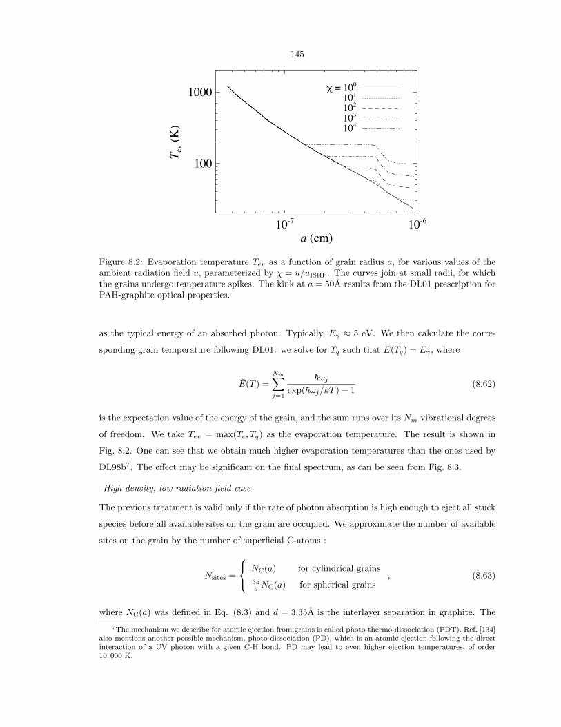
145

10-7

10-6

a (cm)

100

1000

Tev (

K)

! = 100

101

102

103

104

Figure 8.2: Evaporation temperature Tev as a function of grain radius a, for various values of theambient radiation field u, parameterized by χ = u/uISRF. The curves join at small radii, for whichthe grains undergo temperature spikes. The kink at a = 50A results from the DL01 prescription forPAH-graphite optical properties.

as the typical energy of an absorbed photon. Typically, Eγ ≈ 5 eV. We then calculate the corre-

sponding grain temperature following DL01: we solve for Tq such that E(Tq) = Eγ , where

E(T ) =

Nm∑

j=1

~ωjexp(~ωj/kT )− 1

(8.62)

is the expectation value of the energy of the grain, and the sum runs over its Nm vibrational degrees

of freedom. We take Tev = max(Tc, Tq) as the evaporation temperature. The result is shown in

Fig. 8.2. One can see that we obtain much higher evaporation temperatures than the ones used by

DL98b7. The effect may be significant on the final spectrum, as can be seen from Fig. 8.3.

High-density, low-radiation field case

The previous treatment is valid only if the rate of photon absorption is high enough to eject all stuck

species before all available sites on the grain are occupied. We approximate the number of available

sites on the grain by the number of superficial C-atoms :

Nsites =

NC(a) for cylindrical grains

3da NC(a) for spherical grains

, (8.63)

where NC(a) was defined in Eq. (8.3) and d = 3.35A is the interlayer separation in graphite. The

7The mechanism we describe for atomic ejection from grains is called photo-thermo-dissociation (PDT). Ref. [134]also mentions another possible mechanism, photo-dissociation (PD), which is an atomic ejection following the directinteraction of a UV photon with a given C-H bond. PD may lead to even higher ejection temperatures, of order10, 000 K.

146

10 100! (GHz)

10-20

10-19

10-18

10-17

j ! /n

H (

Jy s

r-1 c

m2 p

er H

) This workTev = 20 K

Figure 8.3: Effect of the evaporation temperature model on the spinning dust spectrum for thecold neutral medium [CNM, Eq. (8.176)]. Our prescription results in a much higher evaporationtemperature for the smallest grains, compared to DL98b, who assume a constant Tev = 20 K forall grain sizes. This leads to a decreased damping rate (see discussion at the end of Section 8.5.1.3)and an increased excitation rate through collisions, and therefore increases the peak frequency ofthe spectrum.

ratio of collision rate to photon absorption rate is given by :

Rcoll/abs =nH

√8kT/πmH∫

Qνuνhνdν c

≈ 0.1× nH

30cm−3T

1/22 χ−1a−1

−7. (8.64)

In most environments, Rcoll/abs Nsites so there is no accumulation of stuck species. In very

dense and dark clouds however, the rate of collisions may become so high compared to the rate of

photon absorption that all the sites are occupied. In that case, the assumption that incoming species

stick to the grain is no more valid. They will instead bounce off the irregular grain surface. From

the fluctuation-dissipation theorem, one expects that, for collisions with neutral species, Fn = Gn.

Thus, we set the effective evaporation temperature equal to the gas temperature in that case (see

Eq. (8.79) and discussion below):

Tev = T if Rcoll/abs > Nsites. (8.65)

The actual transition from sticking to elastic collisions should of course be smooth, unlike the

discontinuous step we assume here. Our treatment should approximately reflect the physics of

collisions except near the transition regime Rcoll/abs ∼ Nsites.

147

8.5.2 Collision with neutral H atoms: neutral grain, general grain shape

We assume that the grain is neutral, and has no dipole moment, so there is no interaction whatsoever

between the grain and the neutral H atoms (purely geometric cross section). The phase-space density

of incoming H atoms at the grain surface is simply

fin(v) = nH

( mH

2πkT

)3/2

e−mHv2/2kT , (8.66)

from which one can easily get the excitation rate through incoming particles :

d∆L2z

dtdS

(in)

=

∫vn(mHρvφ)2fin(v)d3v (8.67)

where vn is the component of the velocity normal to the grain surface. This evaluates to

d∆L2z

dtdS

(in)

= nHm2Hρ

2π

4

(2kT

πmH

)3/2

. (8.68)

Integrating over the grain surface, we get

d∆L2z

dt

(in)

= kTnHmH

(2kT

πmH

)1/24πa4

cx

3, (8.69)

where acx was defined in Eq. (8.4). For a spherical grain, acx = a. For a disk-like grain of thickness

d and radius b, spinning around its axis of symmetry, we have

acx =

[3

8b3 (2d+ b)

]1/4

. (8.70)

We can write the excitation rate by incoming H atoms as

E(in)‖,H =

kT

IτH, (8.71)

where τH was defined in equation (8.29).

The case of evaporating particles is very similar. Assuming the grain surface is at the same

temperature T as the gas, the phase-space density of evaporating particles is

fev(v) = nH

( mH

2πkT

)3/2

exp

(−mH(v − v0)2

2kT

). (8.72)

In that case Pesc = 1 for all outgoing particles. The same calculation therefore leads to

E(ev)‖,H =

kT

IτH, (8.73)

148

up to terms of order O(Ω2), which comes from the fact that we did not take into account the slight

change of ω after the particle has collided (we assumed the same ω for the incoming and the outgoing

particle). Detailed balance ensures that

DH =ω

τH. (8.74)

Therefore, for non-spherical grains, we will compute collision rates assuming a spherical geometry

with radius acx. We just showed that this is an exact result for collisions with neutral H atoms. The

collision rates are indeed proportional to the area of the grain, but the angular momentum gained

depends on 〈ρ2〉, so acx will approximately reflect both dependencies.

8.5.3 Collisions with neutral atoms: charged grains

In that case, the incoming neutrals interact with the same potential as the outgoing particles:

U(r) = −1

2αZ2gq

2e

r4. (8.75)

We use the same notation as DL98b and define

εn ≡√mv2

a

2kTand b0(v) ≡ a

√2vav, (8.76)

where va was defined in Eq. (8.45).

We recall, from DL98b, that a trajectory with impact parameter b and velocity at infinity v leads

to a collision if

b ≤ bmax(v) =

b0(v) if v ≤ vaa√

1 + v2a/v

2 if v ≥ va. (8.77)

We compute the collision rate

dNcoll

dt= nn

∫ ∞

0

dv 4πv3πb2max(v)( mn

2πkT

)3/2

e−mv2/2kT

= nn2πa2

(2kT

πm

)1/2 [e−ε

2n +√πεn erf εn

]. (8.78)

We can now get the normalized damping and excitation rates for collisions with neutrals:

Fn =nnnH

√mn

mH

e−ε2n +√πεn erf εn

e−ε2e +√πεe erf εe

(e−ε

2e + 2ε2e

),

G(ev)n =

Tev2T

Fn, and

G(in)n =

nn2nH

√mn

mH

(e−ε

2n + 2ε2n

), (8.79)

149

where the result for G(in)n is identical to that of DL98b. Note that when T = Tev, G

(ev)n = G

(in)n =

Fn/2 so the principle of detailed balance holds. Moreover, in the case of a neutral grain, if the only

rotational excitation and damping process were collisions with neutral species, then the rotational

distribution function would be a Maxwellian. In that case the rotational temperature would be given

by Trot = Gn/Fn × T = 12 (T + Tev), the arithmetic mean of the gas and evaporation temperatures,

as was already shown in Ref. [155].

This is the contribution of an individual neutral, for a given grain charge. To get the total

contribution, one must average over all grain charges (DL98b showed that the charging timescale

is much shorter than the collision timescale) and sum over all neutral species, which we take to be

atomic and molecular hydrogen, and helium8 (with nHe/nH = 1/12).

8.5.4 Collisions with ions: charged grains

The ion interacts with the grain through the Coulomb, electric dipole, and “image charge” potentials.

The latter dominates over the Coulomb potential only in the immediate vicinity of the grain surface,

so we will neglect it for charged grains. Properly accounting for it would result in a slight increase

in both damping and excitation rates as this is an attractive potential. The general solution for this

problem, with a rotating electric dipole moment, is still not analytical. Thus, for simplicity, we will

only consider the case where the electric dipole moment can be considered as non-rotating, i.e., when

the timescale of the collision is short compared to the rotation period of the grain. This is justified

as, when the ion reaches the vicinity of the grain surface, the ratio of collision timescale to rotation

timescale is approximately ωa/v ∼√mi/mgr 1. We will assume that the grain is spherical, so

that the electric dipole moment is randomly oriented relative to the rotation axis (for cylindrical

grains this is not the case but we will assume so for simplicity). Note that when the grain rotates

rapidly, the component of the dipole moment perpendicular to the rotation axis averages out, but

not the parallel component. Although this problem will be different in nature as this alignment

creates anisotropic excitation by collisions, the magnitude of the non-rotating part of the dipole

moment will remain of the same order (a factor 1/√

3 smaller only), so our approximation should

give a decent idea of what the effect of the dipole moment is on the trajectory.

We assume a spherical geometry with radius acx. Taking µ as the polar axis for spherical polar

coordinates, the interaction potential of the ion in the Coulomb and dipole field of the grain is given

by

V (r, θ) =ZgZiq

2e

r+Ziqeµ cos θ

r2. (8.80)

The motion in this potential has two obvious constants: the energy E and the angular momentum

8Collisions with neutral helium have little effect on the spectrum: the helium contribution dominates Fn and Gnonly in the case where the medium is strongly ionized, i.e., when the dominant rotational excitation and dampingmechanisms are rather collisions with ions or plasma drag. We include them for completeness.

150

along the z-axis (along µ), Lz. For this special potential, however, there exists a third constant of

the motion. The torque L exerted on the ion comes entirely from the second term in the potential

and is

L = −r ×∇V (r) =Ziqeµ sin θ

r2eφ. (8.81)

Since the azimuthal component of angular momentum is L · eφ = mr2θ, we can then determine the

overall rate of change of the angular momentum,

d

dt(L2) = 2miZiqeµ sin θ θ = −2miZiqeµ

d

dtcos θ. (8.82)

Therefore we find the constant of the motion9

A ≡ L2 + 2miZiqeµ cos θ. (8.83)

Its value can be determined by taking the incoming trajectory at infinity with approach angle θ∞,

A = (mibv)2 + 2miZiqeµ cos θ∞. (8.84)

The energy of the trajectory is1

2mir

2 + Veff(r) = E (8.85)

where Veff(r) is the sum of the potential V (r, θ) and the tangential kinetic energy L2/2mir2:

Veff(r) ≡ ZgZiq2e

r+mi(bv)2 + 2Ziqeµ cos θ∞

2r2. (8.86)

It is easier to work with the following dimensionless parameters

ψ ≡ ZgZiq2e

acxkT, µ ≡ Ziqeµ

a2cxkT

. (8.87)

Their physical meaning is as follows : |ψ| 1 when the thermal energy of the ion dominates over the

electrostatic interaction energy, and |ψ| 1 when the electrostatic interaction dominates. The sign

determines whether the interaction is attractive (ψ < 0) or repulsive (ψ > 0). µ is the equivalent

quantity for the dipole interaction. Note that we consider only positively charged ions so µ > 0. We

also work with the dimensionless variables

c =b

acx, u =

√mi

2kTv. (8.88)

9This may also be derived by the Hamilton-Jacobi method in spherical polar coordinates.

151

The effective potential can now be written

Veff(r) = kT

[ψacxr

+(u2c2 + µ cos θ∞

) (acxr

)2]. (8.89)

A study of this potential leads to the following condition for collision:

cos θ∞ < Xmax(c, u) ≡ µ−1(u2 − u2c2 − ψ

). (8.90)

Note that if Xmax < −1, then there is never collision, for any angle. If Xmax > 1, then all angles

lead to a collision. We define

X(c, u) ≡ max −1,min [1, Xmax(c, u)] . (8.91)

Now, we can compute the collision rate

dNcoll

dt= ni

∫2πv3dv 2πbdb

( mi

2πkT

)3/2

e−miv2/2kT (X + 1)

= 2ni

√2πkT

mia2cx

∫2u3e−u

2

du 2c dcX + 1

2. (8.92)

We can also get the excitation rate by incoming ions

d∆L2z

dt= ni

∫(mbv)2

32πv3dv 2πbdb

( mi

2πkT

)3/2

e−miv2/2kT (X + 1)

=2nim

2i a

4cx

3π

(2πkT

mi

)3/2 ∫u5e−u

2

du 4c3dcX + 1

2. (8.93)

These integrals can be evaluated explicitly and one then gets, for the charged grains Zg 6= 0

Fi(Zg 6= 0) =ninH

√mi

mH

e−ε2i + 2ε2i

e−ε2i +√πεi erf εi

g1(ψ, µ),

G(ev)i (Zg 6= 0) =

Tev2T

Fi(Zg 6= 0), and

G(in)i (Zg 6= 0) =

ni2nH

√mi

mHg2(ψ, µ), (8.94)

where we have defined g1(ψ, µ) =

1− ψ ψ < 0

e−ψ sinh µ/µ ψ > 0, µ ≤ |ψ|

1− e−(ψ+µ) + µ− ψ + 12 (µ− ψ)2

2µ, µ > |ψ|, (8.95)

152

and g2(ψ, µ) =

1− ψ + ψ2/2 + µ2/6 ψ < 0

e−ψ sinh µ/µ ψ > 0, µ ≤ |ψ|

1− e−(ψ+µ) + µ− ψ + 12 (µ− ψ)2 + 1

6 (µ− ψ)3

2µ, µ > |ψ|. (8.96)

Note that these functions coincide with the functions g1(ψ), g2(ψ) defined in DL98b for µ = 0. We

also defined ε2i ≡ Z2gq

2eαi/2a

4kTev (here αi is the polarizability of species i after it neutralizes on

the grain surface, e.g. when considering collisions with the C+ ion we take the polarizability of the

neutral C atom). Note that even when Tev = T , Fi 6= Gi as the incoming and outgoing particles are

in different ionization states; detailed balance does not apply since realistic ISM phases are not in

Saha equilibrium. Numerically, one has (with T2 ≡ T/100K)

ψ ≈ 170 Zg a−1−7 T

−12 (8.97)

µ ≈ 30〈µ2〉1/2|10−7cm

9.3 Debyea−1/2−7 T−1

2 . (8.98)

From these values, one can see that in general the effect of the dipole moment cannot be neglected

a priori, as µ is not small compared to unity. However, in general µ < |ψ|. This implies that, for

negatively charged grains, the dipole moment has little or no effect on the excitation and damping

rate. For positively charged grains, the damping and excitation rate are both increased by the huge

factor sinh µ/µ, but still remain extremely small due to the Coulomb repulsion, which shows in the

factor e−ψ.

We therefore conclude that DL98b approximation of neglecting the effect of the electric dipole

moment on the trajectory of ions, is essentially valid in the case of collisions with charged grains. It

only has a significant effect for positively charged grains, for which the Coulomb repulsion implies an

extremely small rate of collisions with ions anyway. We still account for the electric dipole moment

for the sake of completeness.

8.5.5 Collisions with ions, neutral grain

In that case the Coulomb potential vanishes, and the “image charge” potential has to be taken into

account. We carry the calculation using the same assumptions as in the previous section: slowly

rotating spherical grain, with radius acx. Taking µ as the polar axis for spherical polar coordinates,

the interaction potential of the ion in the dipole and induced dipole field of the grain is given by

V (r, θ) = − Z2i q

2ea

3cx

2r2(r2 − a2cx)

+Ziqeµ cos θ

r2. (8.99)

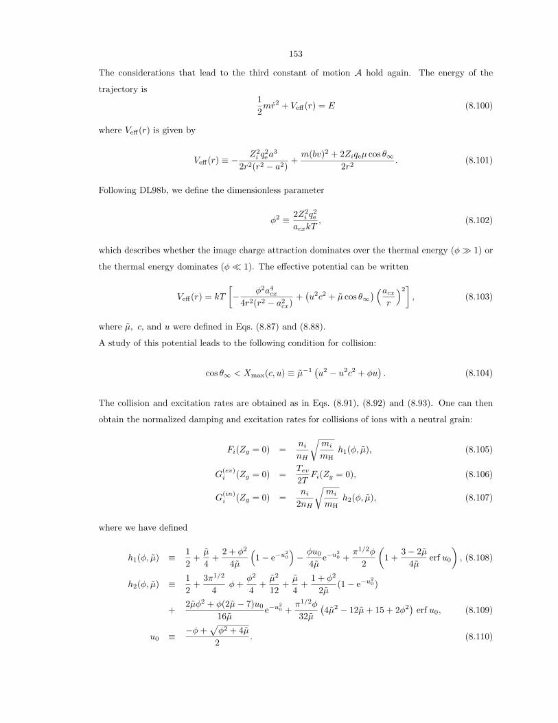
153

The considerations that lead to the third constant of motion A hold again. The energy of the

trajectory is1

2mr2 + Veff(r) = E (8.100)

where Veff(r) is given by

Veff(r) ≡ − Z2i q

2ea

3

2r2(r2 − a2)+m(bv)2 + 2Ziqeµ cos θ∞

2r2. (8.101)

Following DL98b, we define the dimensionless parameter

φ2 ≡ 2Z2i q

2e

acxkT, (8.102)

which describes whether the image charge attraction dominates over the thermal energy (φ 1) or

the thermal energy dominates (φ 1). The effective potential can be written

Veff(r) = kT

[− φ2a4

cx

4r2(r2 − a2cx)

+(u2c2 + µ cos θ∞

) (acxr

)2], (8.103)

where µ, c, and u were defined in Eqs. (8.87) and (8.88).

A study of this potential leads to the following condition for collision:

cos θ∞ < Xmax(c, u) ≡ µ−1(u2 − u2c2 + φu

). (8.104)

The collision and excitation rates are obtained as in Eqs. (8.91), (8.92) and (8.93). One can then

obtain the normalized damping and excitation rates for collisions of ions with a neutral grain:

Fi(Zg = 0) =ninH

√mi

mHh1(φ, µ), (8.105)

G(ev)i (Zg = 0) =

Tev2T

Fi(Zg = 0), (8.106)

G(in)i (Zg = 0) =

ni2nH

√mi

mHh2(φ, µ), (8.107)

where we have defined

h1(φ, µ) ≡ 1

2+µ

4+

2 + φ2

4µ

(1− e−u

20

)− φu0

4µe−u

20 +

π1/2φ

2

(1 +

3− 2µ

4µerf u0

), (8.108)

h2(φ, µ) ≡ 1

2+

3π1/2

4φ+

φ2

4+µ2

12+µ

4+

1 + φ2

2µ(1− e−u

20)

+2µφ2 + φ(2µ− 7)u0

16µe−u

20 +

π1/2φ

32µ

(4µ2 − 12µ+ 15 + 2φ2

)erf u0, (8.109)

u0 ≡ −φ+√φ2 + 4µ

2. (8.110)

154

10-7 10-6

a (cm)

0.01

0.10

Fi(

Zg =

0)

µi(10-7 cm)/9.3 debye = 0 0.51.02.0

10-7 10-6

a (cm)

0.1

1.0

Gi(

Zg =

0)

Figure 8.4: Fi(Zg = 0) (left panel) and Gi(Zg = 0) (right panel) for several values of the electricdipole moment, in CNM conditions, Eq. (8.176).

Note that in the limit µ→ 0 we recover DL98b result, as

h1(φ, µ→ 0) = 1 +π1/2

2φ+O(µ3), (8.111)

h2(φ, µ→ 0) = 1 +3π1/2

4φ+

φ2

2+O(µ2). (8.112)

However, the parameter µ is not small in general, as we saw in Eq. (8.98), so the effect of the dipole

moment on the trajectory cannot be neglected. Note that we also have φ ≈ 18 a−1/2−7 T

−1/22 . The

net effect of the dipole moment is to increase the collision and excitation rates, as can be seen from

Fig. 8.4. In contrast to the case of charged grains, the electric dipole moment does have a significant

effect and cannot be discarded.

The effect of the dipole moment is always to increase both the collision and excitation rates,

for both charged and neutral grains. This can be understood as follows. When the dipole moment

vanishes, ions with a given velocity at infinity v collide with the grain if their impact parameter

is such that b < bmax(v). The effect of the dipole moment is to make a smooth transition from

non-colliding to colliding trajectories: all ions with impact parameter b < b1(v) collide with the

grain, a fraction (X(b, v) + 1)/2 of those for which b1(v) < b < b2(v) do collide, and none of the ions

with b > b2(v) collide. b1 and b2 are such that b1 < bmax < b2. As a result, a fraction of trajectories

for which b1(v) < b < bmax(v) do not lead to collision anymore (compared to the vanishing dipole

case), and a fraction of trajectories bmax(v) < b < b2(v) now lead to collision. The suppressed

colliding trajectories have a lower rate of collision and angular momentum than the added colliding

trajectories. Thus the net effect of the dipole moment is to increase the collision and rotational

excitation rates.

155

8.6 Plasma drag

DL98b computed the effect of torques from passing ions on the electric dipole moments of the dust

grains, which they named “plasma drag”. They computed this effect for straight-line trajectories (the

“Born approximation”). Here we include the full hyperbolic trajectory in the case of charged grains.

We also account for the rotation of the grain explicitly. Moreover, we do not include trajectories

leading to collisions, as they will give away their entire angular momentum through collision, which

we already accounted for. A precise calculation is important because plasma drag is one of the major

excitation processes in some environments.

We will find that the straight-line approximation usually overestimates the plasma drag. In the

case of positively charged grains, there is a range of impact parameters where the ion trajectory

is deflected away from the grain, thereby suppressing angular momentum transfer. For negatively

charged grains, ions can be focused by electrostatic attraction. Ref. [135] argued that this is not

a significant correction because the increased torque during close approach balances the shorter

interaction time since the ion gains kinetic energy as it is attracted to the grain; however, we will

see that in these cases there is a cancellation of angular momentum transfer in different parts of

the trajectory that leads to reduced drag. For very special cases, the grain can corotate with the

ion during close approach leading to an enhancement of the plasma drag, but this occurs for only a

narrow range of impact parameters and does not compensate for the reduction of plasma drag that

we find in other regimes.

As in DL98b, we find it easiest to directly compute the plasma excitation Gp and use the

fluctuation-dissipation theorem to infer Fp = Gp.

8.6.1 Charged grain

We consider the trajectories of positively charged ion (charge Zi > 0) in the electric potential of a

charged dust grain (charge Zg 6= 0). The trajectories are not strictly hyperbolic due to the presence

of the electric dipole potential (see Section 8.5.4). However, we saw that it has little influence on

collisions and we will neglect its effect on the trajectory here, assuming they are hyperbolic and

determined by the Coulomb potential only. The eccentricity of the hyperbolic trajectory of the ion

will be denoted e (as opposed to the elementary charge qe).

Let the ion trajectory (a hyperbola) be in the (ey, ez) plane, symmetric about the ey axis. The

ion position is given by

r = rer = r(α) (cosα ey + sinα ez) . (8.113)

The hyperbolic trajectory of impact parameter b and velocity at infinity v can be described in polar

156

coordinates as

r(α) =p

e cosα− 1α ∈ (−αe, αe) (Zg > 0),

r(α) =p

1− e cosαα ∈ (αe, 2π − αe) (Zg < 0); (8.114)

the eccentricity and semilatus rectum of the trajectory are

e =

√1 +

(mibv2

ZiZgq2e

)2

and p = b√e2 − 1. (8.115)

The range of longitudes α of the trajectory are determined by the limiting case

αe ≡ arccos1

e. (8.116)

The longitude can be related to the true anomaly f familiar from planetary dynamics by α = f for

repulsive (Zg > 0) cases and α = π + f for attractive (Zg < 0) cases. We will need the following

expression for the time t(α), valid in both cases (for the case of an attractive potential, see e.g.

Ref. [168], Eq. (2.4.12)):

t(α) =b

v

1

e+ 1

[√e+ 1

e− 1ln

∣∣∣∣∣∣

tan α2 +

√e−1e+1

tan α2 −

√e−1e+1

∣∣∣∣∣∣− 2e tan α

2

tan2 α2 − e−1

e+1

]. (8.117)

In order to characterize the torque on the grain, we must first take the unit vector in the direction

of grain rotation,

eω = sin θ cosφ ex + sin θ sinφ ey + cos θ ez, (8.118)

so that ω = ωeω. We use (θ, φ) to parameterize the (general) direction of rotation. We define the

other two axes:

eθ = cos θ cosφ ex + cos θ sinφ ey − sin θ ez (8.119)

and eφ = − sinφ ex + cosφ ey. (8.120)

In this system the electric dipole moment of the grain is

µ = µ‖eω + µ⊥ [cos(ωt+ χ)eθ + sin(ωt+ χ)eφ] , (8.121)

where t = 0 is taken to be the time when the ion is at the closest approach (i.e., r ‖ ey) and

χ ∈ [0, 2π) is the random angle that µ⊥ makes with eθ at that time.

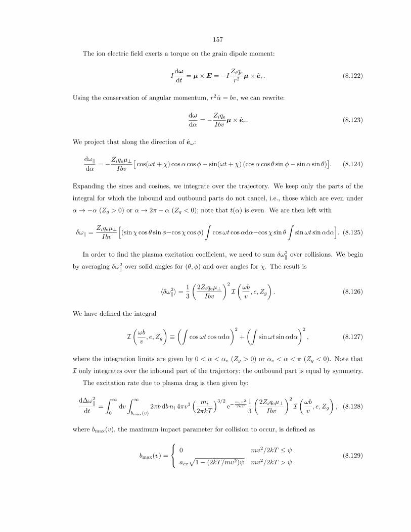
157

The ion electric field exerts a torque on the grain dipole moment:

Idω

dt= µ×E = −I Ziqe

r2µ× er. (8.122)

Using the conservation of angular momentum, r2α = bv, we can rewrite:

dω

dα= −Ziqe

Ibvµ× er. (8.123)

We project that along the direction of eω:

dω‖dα

= −Ziqeµ⊥Ibv

[cos(ωt+ χ) cosα cosφ− sin(ωt+ χ) (cosα cos θ sinφ− sinα sin θ)

]. (8.124)

Expanding the sines and cosines, we integrate over the trajectory. We keep only the parts of the

integral for which the inbound and outbound parts do not cancel, i.e., those which are even under

α→ −α (Zg > 0) or α→ 2π − α (Zg < 0); note that t(α) is even. We are then left with

δω‖ =Ziqeµ⊥Ibv

[(sinχ cos θ sinφ−cosχ cosφ)

∫cosωt cosαdα−cosχ sin θ

∫sinωt sinαdα

]. (8.125)

In order to find the plasma excitation coefficient, we need to sum δω2‖ over collisions. We begin

by averaging δω2‖ over solid angles for (θ, φ) and over angles for χ. The result is

〈δω2‖〉 =

1

3

(2Ziqeµ⊥Ibv

)2

I(ωb

v, e, Zg

). (8.126)

We have defined the integral

I(ωb

v, e, Zg

)≡(∫

cosωt cosαdα

)2

+

(∫sinωt sinαdα

)2

, (8.127)

where the integration limits are given by 0 < α < αe (Zg > 0) or αe < α < π (Zg < 0). Note that

I only integrates over the inbound part of the trajectory; the outbound part is equal by symmetry.

The excitation rate due to plasma drag is then given by:

d∆ω2‖

dt=

∫ ∞

0

dv

∫ ∞

bmax(v)

2πbdb ni 4πv3( mi

2πkT

)3/2

e−miv

2

2kT1

3

(2Ziqeµ⊥Ibv

)2

I(ωb

v, e, Zg

), (8.128)

where bmax(v), the maximum impact parameter for collision to occur, is defined as

bmax(v) =

0 mv2/2kT ≤ ψacx√

1− (2kT/mv2)ψ mv2/2kT > ψ(8.129)

158

where ψ = ZgZiq2e/acxkT .

Note that technically the integration over impact parameters should stop at the Debye length

λD =

√kT

4πneq2e

≈ 398

(T2

ne/0.03cm−3

)1/2

. (8.130)

We will see below, however, that the integrand vanishes exponentially for

b > v/ω ≈ 4.5× 10−6a5/2−7

√mH

mi

v

vth

ωth

ωcm (8.131)

which is much smaller than the Debye length. Converting this into an excitation coefficient, we find

Gp =ninH

√mi

mH

(Ziqeµ⊥a2cxkT

)2

× gp(ψ,

√mia2

cx

2kTω

), (8.132)

where

gp (ψ,Ω) ≡∫ ∞

0

2ue−u2

du

∫ ∞bmaxacx

dc

cI(

Ωc

u, e, Zg

), (8.133)

where the eccentricity is given by

e =

√1 +

(2cu2

ψ

)2

. (8.134)

Note that we recover DL98b result10 in the limit I = 1.

This expression has to be averaged over the grain charge and summed over all present ions.

Straight line limit for I

In the limit e→∞, it is easier to express the integrals as a function of time, using

cosα =y√

y2 + z2=

b√b2 + (vt)2

, (8.135)

sinα =v t√

b2 + (vt)2, and (8.136)

dα =1

1 +(vtb

)2v

bdt. (8.137)

In this case, the first integral for I reduces to

∫cosωt cosα dα =

v

b

∫ ∞

0

cosωtdt

[1 + (vt/b)2]3/2=ωb

vK1

(ωb

v

), (8.138)

10DL98b include a term due to the parallel component of µ which is not relevant as it only leads to excitationperpendicular to ω.

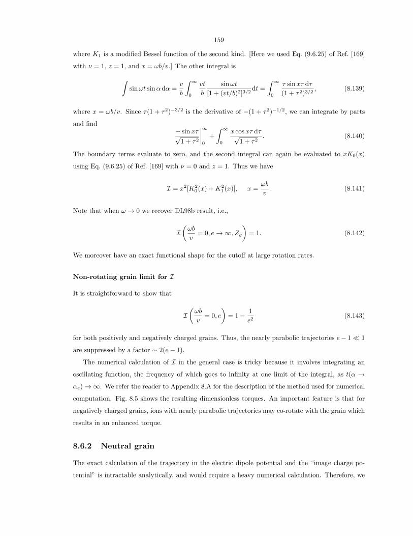
159

where K1 is a modified Bessel function of the second kind. [Here we used Eq. (9.6.25) of Ref. [169]

with ν = 1, z = 1, and x = ωb/v.] The other integral is

∫sinωt sinα dα =

v

b

∫ ∞

0

vt

b

sinωt

[1 + (vt/b)2]3/2dt =

∫ ∞

0

τ sinxτ dτ

(1 + τ2)3/2, (8.139)

where x = ωb/v. Since τ(1 + τ2)−3/2 is the derivative of −(1 + τ2)−1/2, we can integrate by parts

and find− sinxτ√

1 + τ2

∣∣∣∣∞

0

+

∫ ∞

0

x cosxτ dτ√1 + τ2

. (8.140)

The boundary terms evaluate to zero, and the second integral can again be evaluated to xK0(x)

using Eq. (9.6.25) of Ref. [169] with ν = 0 and z = 1. Thus we have

I = x2[K20 (x) +K2

1 (x)], x =ωb

v. (8.141)

Note that when ω → 0 we recover DL98b result, i.e.,

I(ωb

v= 0, e→∞, Zg

)= 1. (8.142)

We moreover have an exact functional shape for the cutoff at large rotation rates.

Non-rotating grain limit for I

It is straightforward to show that

I(ωb

v= 0, e

)= 1− 1

e2(8.143)

for both positively and negatively charged grains. Thus, the nearly parabolic trajectories e− 1 1

are suppressed by a factor ∼ 2(e− 1).

The numerical calculation of I in the general case is tricky because it involves integrating an

oscillating function, the frequency of which goes to infinity at one limit of the integral, as t(α →αe)→∞. We refer the reader to Appendix 8.A for the description of the method used for numerical

computation. Fig. 8.5 shows the resulting dimensionless torques. An important feature is that for

negatively charged grains, ions with nearly parabolic trajectories may co-rotate with the grain which

results in an enhanced torque.

8.6.2 Neutral grain

The exact calculation of the trajectory in the electric dipole potential and the “image charge po-

tential” is intractable analytically, and would require a heavy numerical calculation. Therefore, we

160

I(! b / v, e, Zg > 0)

10-6 10-4 10-2 100 102 104 106

! b / v

10-6

10-4

10-2

100

102

104e

- 1

0.3

0.3

0.60

.9

Slowly rotating grain

Straight line trajectory

Slowly rotating grain

Parabolic trajectory

Rapidly rotating grain

I(! b / v, e, Zg < 0)

10-6 10-4 10-2 100 102 104 106

! b / v

10-6

10-4

10-2

100

102

104

e -

1

0.5

0.5

0.5

0.5

1.0

1.0

1.0

1.0

1.5

1.5

Slowly rotating grain

Straight line trajectory

Slowly rotating grain

Parabolic trajectory

Corotation regime

Figure 8.5: Contour levels of I(ωbv , e, Zg > 0) (top panel) and I(ωbv , e, Zg < 0) (bottom panel). Bothshow that I goes to unity for slowly rotating grain, straightline trajectories, and vanishes for rapidlyrotating grains or nearly parabolic trajectory. In the case of negatively charged grains, though, thereis a visible co-rotation regime, where e− 1 1 and ωb/v(e− 1) ∼ 1, for which the ion and the grainapproximately co-rotate, enhancing the torque given to the grain.

161

will make the following simplifications. First, we neglect the effect of the electric dipole moment on

the trajectory. This assumption is somewhat cavalier, as we saw previously that the electric dipole

moment may significantly affect the ion trajectory in the case of a neutral grain. Furthermore, al-

though trajectories in the “image charge potential” will be curved in general, we will consider them

to be straight lines. Thus, we will approximate the torque given to the grain by Eq. (8.126), where

I is given by Eq. (8.141). Colliding trajectories should not be taken into account for the plasma

drag excitation rate. Thus, we integrate the torque only over trajectories with impact parameter

b > bmax(v), with

bmax = acx

√1 +

φ

u(8.144)

(see DL98b Eq. (B24) and the definition of φ Eq. (8.102)). Therefore, in the case of neutral grains,

we have

Gp(Zg = 0) =ninH

√mi

mH

(Ziqeµ⊥a2cxkT

)2

× gp(φ,

√mia2

cx

2kTω

), (8.145)

where

gp (φ,Ω) ≡∫ ∞

0

2ue−u2

du

∫ ∞bmaxacx

dc

cI(

Ωc

u, e→∞

). (8.146)

The inner integral can in fact be evaluated analytically, and Eq. (8.146) can be simplified to11

gp (φ,Ω) = 2Ω

∫ ∞

0

√1 +

φ

uK0

(Ω

u

√1 +

φ

u

)K1

(Ω

u

√1 +

φ

u

)e−u

2

du. (8.147)

Eq. (8.147) does not have a simple analytic form in the general case. We can however get simple

analytic estimates in limiting cases. We first notice that φ ≈ 18a−1/2−7 T

−1/22 1, and therefore for

the smallest grains, we have:

gp (φ,Ω) ≈ 2Ω√φ

∫ ∞

0

1√uK0

(Ω√φ

u3/2

)K1

(Ω√φ

u3/2

)e−u

2

du. (8.148)

We then obtain that

gp(Ω√φ 1) ≈ ln

(2

Ω√φ

)− 7

4γ, (8.149)

where γ ≈ 0.5774 is Euler’s gamma constant, and

gp(Ω√φ 1) ≈ 6.7(Ω

√φ)2/7e−2.9(Ω

√φ)4/7

. (8.150)

We therefore see that rotational excitation by the plasma is exponentially suppressed for grains with

rotation rate larger than ωmax ∼√

2kT/(mia2φ) ∼ 3× 1011 T3/22 a

−3/4−7 sec−1.

The normalized excitation rate for plasma drag for cold neutral medium conditions, Eq. (8.176),

11This simplification is not present in the published paper.

162

10-7 10-6

a (cm)

0.001

0.010

0.100

1.000

10.000

Gp(!

th)

1-1

Zg = 0

Figure 8.6: Normalized excitation rate due to plasma drag Gp(ωth) for a neutral grain, a positivelycharged grain, and a negatively charged grain in CNM conditions [Eq. (8.176)], evaluated at the

thermal rotation rate ωth = (2kT/I)1/2

. All of them are lower than estimated by DL98b. It is clearthat the positively charged grains are much less excited than the neutral and negatively chargedgrains. The kink at 6A is due to the change of grain shape.

is shown in Fig. 8.6.

8.7 Infrared emission

A dust grain absorbs visible and ultraviolet light and re-emits it in the infrared. A rotating grain

will also radiate angular momentum, which damps its rotation. DL98b compute this damping rate

by modeling the grain as composed of six rotating dipoles. We give here a more accurate calculation,

using the correlation functions of the dipole moment in the grain frame. Our result is a factor of

two greater than that of DL98b. We present a classical calculation in this section.

The rates of emission of energy and of angular momentum by a varying electric dipole moment:

E =2

3c3p2 and L =

2

3c3p× p. (8.151)

We denote the coordinates of the dipole moment in the frame co-rotating with the grain with

unprimed indices, and the ones in the “lab frame” with primed indices. Take a grain rotating

around the z-axis, without precession, with angular frequency ω. We have

px′ = cosωt px − sinωt py, (8.152)

py′ = sinωt px + cosωt py, (8.153)

pz′ = pz. (8.154)

163

A straightforward calculation leads to the following expressions in the lab frame :

p2 = p2x + p2

y + p2z + 4ω (pxpy − pypx) + ω2

[4(p2x + p2

y

)− 2 (pxpx + pypy)

]

+ 4ω3 (pxpy − pypx) + ω4(p2x + p2

y

)(8.155)

and

(p× p)z = pxpy − pypx + ω[2(p2x + p2

y

)− (pxpx + pypy)

]+ 3ω2 (pxpy − pypx) + ω3

(p2x + p2

y

).

(8.156)

Since we are interested in the statistical properties of the emission, we define the unequal-time

dipole moment correlation function in grain coordinates,

Cij(τ) ≡⟨(pi(t)− 〈pi〉)(pj(t+ τ)− 〈pj〉)

⟩, (8.157)

where 〈pi〉 = µi is just the constant dipole moment of the grain. We further assume statistical

spherical symmetry of the dipole moment in the grain coordinates, i.e., Cij = Cδij . (For a planar

grain, the values of the correlation functions depend on the in-plane or out-of-plane character of the

vibrational modes and may be anisotropic. However if the infrared emission arises during thermal

spikes when the grain is not rotating around its axis of greatest angular momentum, we expect the

isotropic analysis to be a good approximation.) The average values of the previous formulae then

become12

〈p2〉 = 3C ′′′′(0)− 12ω2C ′′(0) + 2ω4C(0) (8.158)

and

〈p× p〉z = −6ωC ′′(0) + 2ω3C(0), (8.159)

where ′ denotes the derivative of the correlation function with respect to τ .

The Wiener-Khintchine Theorem relates the correlation functions to the spectral density Sν ,

C(τ) =∫∞

0Sν cos(2πντ)dν (see for example Ref. [162]). Plugging back into Eqs. (8.158) and

(8.159), we get

〈p2〉 =

∫ ∞

0

[3(2πν)4 + 12ω2(2πν)2 + 2ω4

]Sν dν (8.160)

and

〈p× p〉z =

∫ ∞

0

[6ω(2πν)2 + 2ω3

]Sν dν. (8.161)

Now making use of the assumption that the grain rotates slowly, i.e., that νrot ≡ ω/2π ν0 ≡typical frequency of emission, in the infrared, we get, at the lowest order in νrot/ν0, the average

12Expectation values of derivatives such as 〈p2x〉 can be expressed in terms of correlation functions via integration

by parts. In this case, 〈p2x〉 = 〈 d

dt(pxpx)〉 − 〈pxpx〉. The first term vanishes for a stationary process, and the second

is −C′′(0).

164

total power and average total rate of radiation of angular momentum:

⟨dE

dt

⟩=

2

3c3〈~p2〉 =

2

c3

∫ ∞

0

(2πν)4Sν dν (8.162)

and ⟨dLzdt

⟩=

2

3c3〈p× p〉z =

4ω

c3

∫ ∞

0

(2πν)2Sν dν. (8.163)

If one knows the infrared power radiated per steradian per frequency interval Fν , such that

⟨dE

dt

⟩= 4π

∫ ∞

0

Fν dν, (8.164)

one can deduce the rate of angular momentum loss through infrared emission:

⟨dLzdt

⟩=

2ω

π

∫ ∞

0

Fνν2

dν. (8.165)

This result is twice as big as the one given in DL98b. [The difference occurs because DL98b modeled

the dipole fluctuations with six uncorrelated rotating dipoles, one rotating each direction in the xy,

yz, and xz planes. They counted the radiated power from all six of these, but only considered the

angular momentum loss from two of them (in the xy plane). The dipoles rotating in the xz and

yz planes containing the rotation axis also emit net angular momentum however, and if they are

considered one recovers the factor of 2.]

This classical treatment does not predict the rotational excitation from the recoil given by indi-

vidual photons, which is a quantum effect. Each photon has a rotational quantum number J = 1,

which corresponds to an angular momentum squared L2γ = ~2J(J + 1) = 2~2. We therefore have13

⟨d∆L2

dt

⟩= 3

⟨d∆L2

z

dt

⟩=

dNphot

dt2~2 =

2h

π

∫ ∞

0

Fνν

dν. (8.166)

The normalized damping and excitation rates are then

FIR =2τHπI

∫ ∞

0

Fνν2

dν and

GIR =h

3πI

τHkT

∫ ∞

0

Fνν

dν. (8.167)

We calculate the infrared emissivity of PAHs and small carbonaceous grains using the“thermal

continuous” approximation, described in DL01. They indeed show that this treatment leads to

spectra very close to those predicted by the exact statistical treatment, and has the advantage of

being computationally much faster. We obtain the steady-state energy distribution function and

then get the infrared emissivity, as explained in DL01.

13This factor of 2 was not included in the original paper and was pointed out in Ref. [170].

165

10-7

10-6

a (cm)

1

10

FIR

This work2*DL98

10-7

10-6

a (cm)

0.1

1.0

GIR

This workDL98

1 2

Figure 8.7: Infrared emission damping and excitation coefficients FIR, GIR, in CNM conditions [Eq.(8.176)], compared with the result of DL98b. The difference is mainly due to differences in grainabsorption efficiencies and the calculation of the infrared spectrum. We used absorption efficienciesfrom Ref. [171] and the model of DL01 to compute the infrared emissivity. The kink at 50 A in ourresult is due to a change in optical properties of dust grains. The kink around 50 A in the DL98bresult is due to the change from constant temperature limit (larger grains) to thermal spikes limit(smaller grains). The fact that they coincide is purely chance, and would not be necessarily the casefor other environmental conditions. The discontinuity at 6A is due to the change in grain shape.Note: we have plotted 1

2GIR = GIR,old, which is the result initially used in the paper before wepointed out the missing factor of 2 in Ref. [170]. The correct GIR is now used in the code.

We checked numerically that we recover the result of DL98b for low values of the radiation field

intensity: FIR, GIR ∝ χ. However, their result for high values of the radiation field (FIR ∝ χ2/3,

GIR ∝ χ5/6) relies on the fact that the absorption efficiency Qν ∝ ν2 at the characteristic frequencies

of infrared emission. This is not valid anymore for intense radiation fields, which offset the emission

spectrum to higher frequencies, where the absorption efficiency has not a simple dependence on

frequency anymore. We show the resulting infrared emission and damping coefficients in Fig. 8.7.

8.8 Photoelectric emission

An electron ejected from the grain carries away an angular momentum along the rotation axis

(z-axis) equal to:

∆Lz = meρ(v′φ − ρω

), (8.168)

where v′φ is its tangential velocity in the grain frame. From this we deduce that

Fpe =me

mH

Jpe

2πa2snH

√2kT/πmH

, (8.169)

where Jpe is the photoemission rate and was described in Section 8.3.4. The excitation rate can be

obtained by first noticing that the rotational velocity is much smaller than the velocity of ejected

166

electrons:

aω v′φ (8.170)

so that we have, up to small corrections

∆L2z = m2

eρ2v′2φ . (8.171)

We assume a cosine-law directional distribution for escaping electrons, so that 〈v′2φ 〉 = 14v

2e , where

we denote ve the average velocity of the electron at the grain surface. The latter satisfies

1

2mev

2e −

(Zg + 1)q2e

as= Epe, (8.172)

where Epe is the average energy at infinity of the photoejected electron. We finally get

〈∆L2z〉 = m2

e

2

3

a4cx

a2s

1

4v2e =

me

3

a4cx

a2s

[Epe +

(Zg + 1)q2e

as

]. (8.173)

So the normalized excitation rate is

Gpe =me

4nH (8πmHkT )1/2

a2skT

[Γpe +

(Zg + 1)q2e

asJpe

], (8.174)

where Γpe is the heating rate due to photoemission of electrons, obtained from Ref. [157].

8.9 Random H2 formation

DL98b showed that the random formation of H2 molecules on the grain surface does not make a

major contribution to rotational excitation. We use their result:

GH2=γ

4(1− y)

EfkT

[1 +〈J(J + 1)〉~2

2mHEfa2x

], (8.175)

where γ is the efficiency of H2 formation, y = 2nH2/nH, Ef ≈ 0.2eV is the average translational

kinetic energy of the nascent H2, and 〈J(J + 1)〉 ≈ 102 gives its average angular momentum.

167

8.10 Resulting emissivity and effect of various parameters14

Throughout this section and unless otherwise stated, we will take as a fiducial environment the CNM

parameters specified by

nH = 30 cm−3, T = 100 K, xH ≡n(H+)

nH= 10−3, xC ≡

n(C+)

nH= 3× 10−4, χ ≡ u

uISRF= 1, γ = 0.

(8.176)

We also take the rms intrinsic dipole moment to be

〈µ2i 〉1/2

(a = 10−7cm

)= 9.3 Debye. (8.177)

For the size distribution parameters, we use those given by Ref. [156] for a ratio of visual extinction

to reddening RV = 3.1, and a carbon abundance in the log-normal distributions bC = 6× 10−5.

This section is intended to give some intuition into the effect of various parameters on the

spinning dust spectrum. However, the reader should keep in mind that environment parameter

space is many-dimensional, and changing several parameters at once may lead to modifications that

are not superpositions of the effects described here.

8.10.1 General shape of the rotational distribution function

The rotational distribution function is obtained as described in Section 8.4. We remind the reader

that the Fokker-Planck equation is not strictly valid for the smallest grains, for which impulsive

torques are important. It however still describes their rotational distribution function with more ac-

curacy than a simple Maxwellian. Moreover, DL98b showed that impulsive torques may be neglected

for grain radii a ≥ 7A. In Fig. 8.8, we show that the rotational distribution function obtained by

the Fokker-Planck equation differs significantly from a Maxwellian. It has a sharper cutoff at high

frequencies due to the proper accounting for rotational damping through electric dipole radiation.

In what follows we will analyze the effect of various parameters on the spinning dust emissivity.

As can be seen from Eq. (8.38) and the expressions derived next for the normalized damping and

excitation rates, the rotational distribution function has complex dependencies on all grain and

environmental parameters. To get some intuition on the physics of spinning dust and the influence

of each parameter, we will rely on a simplified expression for the rotational distribution function in

the following sections:

fa(ω) ∝ exp

(−FG

Iω2

2kT− τH

3Gτed

(Iω2

2kT

)2), (8.178)

where we approximate the plasma drag excitation rate (which is in principle a function of ω) by the

14The results shown in this section use the initial estimate for GIR, which was too low by a factor of 2. This doesnot change any of the results qualitatively (and only very little quantitatively), and we have therefore not reproducedthe whole analysis with the correct GIR.

168

1 10

! /2 " (GHz)

0.0

0.2

0.4

0.6

0.8

1.0

1.2

4 "

!3 fa(!

)

This workMaxwellian (DL98b)

Figure 8.8: Rotational distribution function for a grain radius a = 7 A, in CNM conditions, fora single value of the dipole moment µi(10−7cm) = 9.3 Debye. The plot compares the solutionof the Fokker-Planck equation with the DL98b Maxwellian approximation (DL98b Eq. (57) usedwith our F , G). Note that DL98b prescription gives (< ω2 >)1/2 = 2π × 10.7 GHz, which is inexcellent agreement with the value we get, (< ω2 >)1/2 = 2π × 10.9 GHz. However, the shape ofthe distribution function is significantly different.

constant

Gp ≈ Gp(ωth) , ωth ≡(

3kT

I

)1/2

. (8.179)

In our analysis we will also neglect the charge-displacement-induced dipole moment, as it has a minor

contribution. Of course the actual rotational distribution function and emissivity are computed using

the exact equations developed in this chapter.

For a given grain radius a and intrinsic electric dipole moment µi, the power radiated is Pν (a;µi) ∝ν6fa(2πν;µi). It is straightforward, from Eq. (8.178), to show that the peak frequency is given by

νpeak ≈(

2

1 +√

1 + ξ

G

F

)1/21

2π

√6kT

I, (8.180)

where we defined the parameter

ξ ≡ 8G

F 2

τHτed

, (8.181)

which denotes the non-Maxwellian character of the distribution function.

For ξ 1, the distribution is nearly Maxwellian,

fa(ω) ∝ exp

(−FG

Iω2

2kT

), (8.182)

169

and the peak frequency is given by

νpeak ≈(G

F

)1/21

2π

√6kT

I(ξ 1). (8.183)

Moreover, the total power emitted by a single grain ja ∝ µ2∫ω6fa(ω)dω has the following depen-

dence:

ja ∝ µ2

(G

F

)2

T 2 (ξ 1). (8.184)

For ξ 1 the distribution is strongly non-Maxwellian15,

fa(ω) ∝ exp

(− τH

3Gτed

(Iω2

2kT

)2), (8.185)

and the peak frequency is given by

νpeak ≈(Gτed

2τH

)1/41

2π

√6kT

I(ξ 1). (8.186)

The total power is then given by

ja ∝ µ2 Gτed

τHT 2 (ξ 1). (8.187)

In Fig. 8.9 we show the rms rotation rate < ω2 >1/2 as a function of grain radius. As can

be expected, the smallest grains are rotating with the greatest angular velocity, as they have the

smallest moment of inertia. Consequently, they radiate at the highest frequencies, and constitute

the peak of the spectrum. Therefore, we will use Eqs. (8.178) to (8.187) for a grain of radius

amin = 3.5 A to evaluate the effect of various parameters on the emissivity.

We finally remind the reader with the dependencies of characteristic timescales:

τH ∝ n−1H T−1/2 , τed ∝ µ−2T−1. (8.188)

8.10.2 Emissivity

Once the rotational distribution function is known, as a function of the intrinsic electric dipole

moment, fa(ω;µi), one can get the power radiated by a grain of radius a by averaging over the

intrinsic dipole moments Gaussian distribution P (µi) defined in Eq. (8.8). One gets:

Pν(a) =

∫dµiP (µi)

2

3

µ2⊥ω

6

c32π fa(ω;µi) (8.189)

15Interestingly, Ref. [131] had already obtained a result similar to Eq. (8.185) with a Fokker-Planck equation.

170

10-7

10-6

a (cm)

0.01

0.10

1.00

10.00

100.00

!rm

s/ 2"

(G

Hz)

Thermal rotationThis work

Figure 8.9: rms rotation rate ωrms ≡< ω2 >1/2 as a function of grain radius a, for CNM conditions.The rotation rate the grain would achieve if it were rotating thermally (in that case ωrms =

√3kT/I)

is also shown. It can be seen that the grains rotate sub-thermally. The kink at 6 A is due to thechange in grain geometry.

where µ2⊥ = 2

3µ2 for spherical grains, and µ2

⊥ = µ2 for cylindrical grains.

The overall effect of averaging over the dipole moments distribution is to broaden the spectrum,

as can be seen in Fig. 8.10. The peak frequency remains approximately equal to that of Pν(µi =

〈µ2i 〉1/2). We will discuss the effect of the rms intrinsic dipole moment in Section 8.10.3.

The emissivity per H atom is then obtained by integrating the power radiated by each grain

over the grain size distribution function, described in Section 8.3.2. The emissivity for the CNM

environment is shown in Fig. 8.11. Note that the grain size distribution directly weights the spectrum,

and thus needs to be known with accuracy, which is not quite the case yet for the very small grains.

8.10.3 Effect of the rms intrinsic dipole moment 〈µ2i 〉1/2

Varying the rms intrinsic dipole moment affects the spectrum in three main ways. First, it affects the

total power radiated, as Pν ∝ µ2. Then, it affects the non-Maxwellian character of the distribution

function, as τed ∝ µ2. Finally, it affects the rotational damping and excitation rates essentially

through plasma drag, which has Gp ∝ µ2 (the effect on Gi is not as important). Throughout the

range of values considered,

1 Debye < µi(10−7 cm) < 100 Debye, (8.190)

171

1 10 100! (GHz)

10-42

10-40

10-38

10-36

10-34

10-32

P! (

erg

s-1

sr-1

Hz-1

)

!i / !0 = 0.0050.03

0.21.02.0

total

a = 3.5 x 10-8 cm

Figure 8.10: Power radiated by one grain of radius a = 3.5 A in CNM conditions. The dottedand dashed lines show the contributions of various values of the intrinsic dipole moment, which isassumed to have a gaussian distribution with rms value µ0 ≡< µ2

i >1/2 (a). The solid line is the

total power.

10 100! (GHz)

10-21

10-20

10-19

10-18

10-17

10-16

j ! /n

H (

Jy s

r-1 c

m2 p

er H

) CNMa-7 = 0.37

0.460.580.720.901.13

Figure 8.11: Spinning dust emissivity for CNM environment. Contributions from grains of varioussizes are shown [a−7 ≡ a/(10−7 cm)]. The grain size distribution parameters are taken from Ref. [156]with RV = 3.1 and bc = 6× 10−5.

172

and in CNM conditions, the distribution function remains strongly non-Maxwellian: ξ ∼> 60. There-

fore, we can use the strongly non-Maxwellian limit Eq. (8.186) to evaluate the peak frequency.

Low dipole moment limit

For low values of the electric dipole moment, plasma drag has little effect on both the rotational

damping and excitation. Therefore, F and G are roughly independent of µ, and, from Eqs. (8.186),

(8.187) and τed ∝ µ2, we get

νpeak (µi → 0) ∝ µ−1/2i , (8.191)

j/nH (µi → 0) → constant. (8.192)

One can see in Fig. 8.12 that Eq. (8.192) is quite accurately satisfied. The total power has a weak

dependence on µi for low values of the intrinsic dipole moment, but is not strictly independent

of it, which comes from the multiple approximations made in this analysis (neglecting the charge-

displacement-induced dipole moment, and using Eq. (8.187) for the total power, after integration

over the size distribution, instead of the total power radiated by a single grain).

High dipole moment limit

For high values of the electric dipole moment, plasma drag dominates both rotational damping and

excitation. Therefore, G ≈ Gp ∝ µ2 so we get

νpeak (µi →∞) → constant, (8.193)

j/nH (µi →∞) ∝ µ2i , (8.194)

which describe approximately the behavior observed in Fig. 8.12.

8.10.4 Effect of number density nH

The main effects of the number density are:

• Changing the relative contribution of gas-induced and radiation-induced rotational damping

and excitation. For very low number densities, FIR and GIR ∝ τH ∝ n−1H dominate over other

rotational damping and excitation rates. For high densities, plasma drag and collisions are

dominant. Note that the charge distribution is also modified as the higher the density, the more

important is collisional charging compared to photoemission. As a consequence, the grains are

positively charged at low densities, and tend to be negatively charged at high densities, due

to the higher rate of collisions with electrons.

173

1 10 100!i(10-7 cm) (debye)

10

100

!p

eak (

GH

z)

1 10 100µi(10-7 cm) (debye)

10-7

10-6

10-5

j/n

H (

Jy c

m2 s

r-1 H

z per

H)

Figure 8.12: Effect of the intrinsic electric dipole moment on the peak frequency and the totalspinning dust emission. Environment parameters are set to CNM conditions defined in equation(8.176). Increasing the electric dipole moment decreases the peak frequency and increases the totalpower radiated.

• Influencing the non-Maxwellian character of the rotational distribution function. The higher

the number density, the closer is the distribution function to a Maxwellian. Numerical cal-

culation shows that starting from CNM conditions and varying only nH, we transition to the

Maxwellian regime (ξ ∼< 1) if nH ∼> 105 cm−3.

Low density limit

For very low number densities, the distribution is highly non-Maxwellian and we can use Eqs.

(8.186) and (8.187), with G = GIR, to estimate the peak frequency and total power. As GIR/τH is

independent of nH, both the number density and total power should asymptote to a constant value.

We can estimate numerically the peak frequency in CNM conditions and get:

νpeak (nH → 0) ≈ 13 GHz, (8.195)

j/nH (nH → 0) → constant, (8.196)

which is in good agreement with Fig. 8.13.

Intermediate densities

Over the range 102 cm−3 ∼< nH ∼< 104 cm−3, gas processes are dominant over infrared emission, so

F , G are roughly independent of nH. In addition, the distribution is still strongly non-Maxwellian.

Using Eqs. (8.186) and (8.187), we thus find

νpeak

(102 cm−3 ∼< nH ∼< 104 cm−3

)∝ n

1/4H , (8.197)

j/nH

(102 cm−3 ∼< nH ∼< 104 cm−3

)∝ nH. (8.198)

174

The kink around nH ∼ 3 × 103 cm3 is due to our discontinuous treatment of the evaporation

temperature for high densities (see Section 8.5.1.4), and to the replacement of the integration over

all grain radii by a discrete summation when numerically computing the spectrum. Therefore the

spectra should not be considered as very accurate in that region.

High density limit

For very high number densities, the excitation and damping is dominated by gas processes, and

the electric dipole damping becomes negligibly small, so that the rotational distribution function is

actually a Maxwellian, although not thermal. Using Eqs. (8.183) and (8.184), we find

νpeak (nH →∞) ≈ 150 GHz, (8.199)

j/nH (nH →∞) → constant. (8.200)

8.10.5 Effect of the gas temperature T

Temperature has a less obvious effect on the spectrum and we need to analyze in detail every

damping and excitation process. It turns out the charge distribution of the smallest grains varies

very little over the range of temperature considered 1 K < T < 105 K and they remain mostly

neutral throughout this interval. The distribution remains strongly non-Maxwellian for T greater

than a few K.

Low temperature limit

At very low temperatures, the dominant excitation process is collisions with ions. Indeed, the grains

being mostly neutral, the ions interact strongly with the electric dipole potential. As µ ∝ T−1

and φ ∝ T−1/2, one can see from Eqs. (8.107) and (8.109) that Gi ∝ T−2. Plasma drag has also

Gp ∝ T−2 in principle but this becomes a shallower power law at low temperatures as the interaction

timescale becomes longer than the rotation timescale. We find numerically, though, that roughly

G ∝ T−1.5 as G is not strictly equal to Gi (collisions with neutrals are also significant at low

temperatures). Using Eqs. (8.183), (8.184), and (8.188) we find

νpeak

(3 K ∼< T ∼< 102 K

)≈ 35 GHz, (8.201)

j/nH

(3 K ∼< T ∼< 102 K

)≈ constant. (8.202)

175

Note that for extremely low temperatures, the distribution would become Maxwellian, and one would

get, according to Eqs. (8.186) and (8.187),

νpeak (T → 0) ∝ T 1/2, (8.203)

j/nH (T → 0) ∝ T 2, (8.204)

which can be guessed at the extreme low temperature end of Fig. 8.13. Temperatures below ∼ 3 K

are of course unphysical, but for other environmental conditions than those of Eq. (8.176), the

behavior discussed above could take place at higher, observed temperatures.

High temperature limit

At very high temperatures, collisions with neutrals are the dominant damping and excitation process.

The CNM environment being mostly neutral, Fn → 1 and Gn → 1/2 at high temperatures (G(ev)n ∝

Tev/T → 0). Moreover, the distribution becomes strongly non-Maxwellian, as ξ ∝ T 1/2. We

therefore obtain

νpeak(T →∞) ≈ 200 T3/85 GHz, (8.205)

j/nH (T →∞) ∝ T 3/2. (8.206)

Fig. 8.13 shows that these power laws describes the behavior of the peak frequency and total power

with very good accuracy.

8.10.6 Effect of the radiation field intensity χ

The radiation field affects the spectrum through only two ways. First of all, it changes the charge

distribution of the grains as an increased radiation implies a higher photoemission rate. Second

of all, it affects the rate of damping and excitation through infrared emission (and photoelectric

emission, but this is subdominant).

Low radiation intensity limit

In a low radiation field, Frad and Grad become negligible. The photoemission charging rate becomes

insignificant compared with collisional charging, and the charge distribution function depends only

on other environment parameters. Thus, one expects the spectrum to reach an asymptotic shape for

very low radiation fields. The distribution is strongly non-Maxwellian, and the dominant excitation

mechanism is collisions with ions, whereas the dominant damping mechanisms are plasma drag and

176

collisions with neutrals. Thus, we find

νpeak(χ→ 0) ≈ 35 GHz, (8.207)

j/nH (χ→ 0)→ constant. (8.208)

The kink around χ ∼ 2 × 10−2 is due to our discontinuous treatment of the evaporation temper-

ature for low intensities of the radiation field. Around χ ≈ 1 − 10, the grain becoming more and

more positively charged, collisions with ions start being less efficient, even though they remain the

dominant excitation mechanism. This results in a slight decrease in both νpeak and j/nH.

High radiation intensity limit

In a high radiation field, F ≈ FIR, and G ≈ GIR. Both FIR and GIR are approximately (although

not strictly) linear in χ, as shown in DL98b for the thermal spikes limit [see their Eqs. (31) and

(44)]. Thus, ξ ∼ χ−1 so the distribution becomes Maxwellian. The peak frequency and total emitted

power are then given by Eqs. (8.183) and (8.184), which imply that

νpeak(χ→∞) ≈ constant, (8.209)

j/nH (χ→∞) ≈ constant. (8.210)

These asymptotic forms are not strictly valid because FIR and GIR are not strictly linear in χ, and

do not have a simple dependence on that parameter.

8.10.7 Effect of the ionization fraction xH

The hydrogen ionization fraction affects the charge distribution by modifying the contribution from

collisions with protons. It also changes the contribution of collisions with ions and neutrals, and

plasma drag. Characteristic timescales are left invariant, and ξ 1 for any ionization fraction in

otherwise CNM conditions.

Low ionization fraction limit

In that limit the rotational distribution function reaches an asymptotic form where collisions with

protons and plasma drag due to protons can be neglected. However, there are still C+ ions in the

gas, so collisions with ions and plasma drag may still be important, although the dominant excitation

process is collisions with neutrals. We find

νpeak (xH → 0) ≈ 30GHz, (8.211)

j/nH (xH → 0) → constant. (8.212)

177

High ionization fraction limit

In that case collisions with ions are the dominant excitation process. Using Eqs. (8.186) and (8.187)

along with G ≈ Gi ∝ xH, we find

νpeak(xH → 1) ≈ 90(xH/0.1)1/4GHz, (8.213)

j/nH (xH → 1) ∝ xH. (8.214)

8.10.8 Concluding remarks

We remind the reader that all the estimates in the previous section were given by assuming that

the peak frequency of the spinning dust spectrum is determined by that of the smallest grains, and

that the total power follows the same dependence upon environmental parameters as the power

emitted by the smallest grains. Therefore they should be taken as an aid to understand the physics

of spinning dust, but not as an accurate description, which requires numerical calculations.

The overall conclusion of this section is that varying a single environmental parameter may change

the peak frequency by up to an order of magnitude, and the total emitted power by several orders

of magnitude. There is therefore a very large range of possible peak frequencies and total powers

that can be produced by spinning dust radiation. Multiphase environments, in particular, could

emit very broad spinning dust spectra. Deducing the environment parameters from an observed

spectrum could therefore be a difficult task.

We show the spinning dust spectrum for various environments and compare them to the results

of DL98b in Fig. 8.14.

8.11 Conclusion

We have presented a detailed analysis of the rotational excitation and damping of small carbonaceous

grains. We have refined the calculations of DL98b in the case of collisions, accounting properly for

the centrifugal potential which increases the net damping rate. In the case of collisions with ions,

we accounted for the effect of the electric dipole potential on the collision cross section. We found

that this is a small effect in the case of charged grains, but that it may significantly increase the

damping and excitation rates in the case of neutral grains. We evaluated the contribution of “plasma

drag” by considering hyperbolic trajectories and rotating grains in the case of charged grains, and

straight lines in the case of neutral grains. We corrected the results of DL98b for the damping

through infrared emission. Finally, we calculated the rotational distribution function by solving the

Fokker-Planck equation.

178

10-2 100 102 104 106

nH (cm-3)

10

100!

pea

k (

GH

z)

10-2 100 102 104 106

nH (cm-3)

10-8

10-7

10-6

10-5

10-4

j/n

H (

Jy c

m2 s

r-1 H

z p

er H

)

100 101 102 103 104 105

T (K)

10

100

!pea

k (

GH

z)

100 101 102 103 104 105

T (K)

10-8

10-7

10-6

10-5

10-4

j/n

H (

Jy c

m2 s

r-1 H

z per

H)

10-2 100 102 104 106

!

10

100

"pea

k (

GH

z)

10-2 100 102 104 106

!

10-8

10-7

10-6

10-5

10-4

j/n

H (

Jy c

m2 s

r-1 H

z p

er H

)

10-5 10-4 10-3 10-2 10-1 100

xH

10

100

!p

eak (

GH

z)

10-5 10-4 10-3 10-2 10-1 100

xH

10-8

10-7

10-6

10-5

10-4

j/n

H (

Jy c

m2 s

r-1 H

z p

er H

)

Figure 8.13: Effect of various environmental parameters on the peak frequency and the total spin-ning dust emission. When one parameter is varied, other environment parameters are set to CNMconditions defined in Eq. (8.176). See Sections 8.10.4 to 8.10.7 for a detailed description.

179

10-20

10-19

10-18

10-17

j ! /n

H (

Jy s

r-1 c

m2 p

er H

)

CNM

WNM

WIM

1 10 100! (GHz)

10-20

10-19

10-18

10-17

j ! /n

H (

Jy s

r-1 c

m2 p

er H

)

MC

1 10 100! (GHz)

DC

1 10 100! (GHz)

RN

Figure 8.14: Spinning dust spectra for several environmental conditions: cold neutral medium(CNM), warm neutral medium (WNM), warm ionized medium (WIM), molecular cloud (MC), darkcloud (DC) and reflection nebula (RN). The environments are defined in DL98b, Table 1. The thinsolid line is the result of our calculation, the dotted line being DL98 prediction, and the dashed lineis the free-free emission (the free-free gaunt factor was taken from Ref. [150]). The parameters forthe grain size distribution are: RV = 3.1, bC = 6 × 10−5 for the diffuse CNM, WNM and WIMenvironments, and RV = 5.5, bC = 3 × 10−5 for the dense MC, DC and RN environments. Theapparent systematic increase of power around the peak frequency for our result is mainly due tothe grain size distribution we use, which has an increased number of small grains compared to thatused by DL98 (compare e.g. Fig. 2 from Ref. [156] with Fig. 8 from DL98b). Note that for the DCenvironment, for which rotational excitation and damping is dominated by collisions with neutralspecies (mainly H2 molecules), DL98 prediction largely overestimates the peak frequency and totalpower because they underestimate the damping rate (see Eq. (8.58) and subsequent discussion).

180

We believe our model provides a much more accurate description of the spinning dust spectrum

than previous work. However, we would like to remind the reader of its uncertainties and limitations.

First, our model only computes the total intensity of the emitted radiation and not the polarization,

which would require an additional study of the alignment mechanisms for PAHs. Secondly, the dust

grains properties are poorly known:

• The size distribution and abundance of the smallest grains is uncertain, and in particular the

nature of the cutoff at small grain sizes a ∼ amin can have a large effect on the spectrum.

• The permanent electric dipole moments of dust grains are not directly constrained by other

dust observables. Given that it cannot be computed from first principles, one may regard it

as a free parameter (or parameters) of the spinning dust model.

Thirdly, we made some simplified calculations in some cases, as an accurate calculation would have

been intractable numerically or substantially complicated the code:

• We used the Fokker-Planck approximation, which starts to break down for our smallest grains

because a single collision suffices to change the rotational state. We expect that the main

consequence of a full treatment would be a tail in the emission spectrum extending to high

frequencies, because impulsive collisions would be able to increase the rotation velocities of

the grains to > 2νpeak before dissipative forces had time to act (an effect missed by the

Fokker-Planck treatment). Therefore one should not place too much confidence in the many-

order-of-magnitude falloff at ∼ 100 GHz seen in most of our models. (In many cases this will

be unimportant observationally since at high frequencies the vibrational dust contribution is

dominant.)

• In the plasma drag calculation, we neglected the electric dipole potential when evaluating

the trajectory of ions, taking the straight-line (neutral grain) or hyperbolic (charged grain)

approximation. Relying on the study of collisions with ions, we may expect the dipole moment

to have a small effect in the case of a charged grain. On the other hand, its effect in the case of

a neutral grain may be more important, as in that case the electric dipole potential provides

the dominant interaction.

• We assumed the evaporation temperature for the smallest grains was the “temperature” of the

grain just after it has absorbed a UV photon. This is a physically motivated assumption but

its validity is not established. The evaporation temperature can have a significant effect on

the spectrum, as can be seen from Fig. 8.3 and one should be aware of the uncertainty in this

parameter. Also, we assumed that collisions transition from being sticking to elastic, as the

density exceeds a given threshold. Our model is therefore inaccurate in the transition region.

181

• When calculating the infrared emission spectrum of dust grains, we used the DL01 “thermal

continuous” approximation, which is not very accurate to describe the low energy part of the

spectrum. Whereas these uncertainties are not important if one only wants the spectrum Fν

in the mid-infrared, they may lead to significant errors when calculating the corresponding

damping and excitation rates, which are proportional to∫ν−2Fνdν and

∫ν−1Fνdν, respec-

tively.

• We ignored systematic torques, although this may not be a major omission for the smallest

dust grains.

Despite these uncertainties, we believe that this model is the most complete thus far, and will be

a useful tool for comparison to observations and testing the spinning dust hypothesis for anomalous

microwave emission in various ISM phases.

In this chapter, we have assumed that the smallest, disk-like grains always rotate about their

axis of greatest inertia. In the next chapter, we shall see that this assumption is in fact not correct,

and that grains are more likely to have their nutation state randomized by frequent absorptions of

ultraviolet photons.

182

8.A Appendix: numerical evaluation of I(ωbv, e, Zg)

The numerical evaluation of I [defined in Eq. (8.127)] is tricky because it involves integrating an

oscillating function which frequency goes to infinity at one limit of the integral, as t(α→ αe)→∞.

Here we describe our implementation for both the positive and negative grain charges.

8.A.1 Positively charged grains

We first make the change of variable

z =√γ cot

α

2, (8.215)

where γ = (e− 1)/(e+ 1). The expression for the time is now:

ωt(z) =ωb

v

1√e2 − 1

(lnz + 1

z − 1+ 2e

z

z2 − 1

). (8.216)

The I-integral is then

I = 4γ

[<∫ ∞

1

eiωt(z)z2 − γ

(z2 + γ)2dz

]2

+ 16γ2

[=∫ ∞

1

eiωt(z)z

(z2 + γ)2dz

]2

. (8.217)

The functions inside the integrals are analytical on the complex plane, deprived from the branch cut

[−1, 1] on the real axis and the two poles ±i√γ. The integrands are at least O(z−2) as |z| → ∞.

Moreover, for y → 0+,

< [iωt(1− iy)] ∝ <[i ln

(−1 +

2i

y

)− e

y

]< 0. (8.218)

Thus, using the fact that the integral over the lower right part of the complex plane vanish, we can

replace our integrals by integrals over the axis

z = 1− iy, 0 < y < +∞. (8.219)

Note that for e→ 1, I = O(e−1), as one may expect from almost parabolic trajectories if the grain

repels the ion. Also, in the limit ωb/v → 0, I → (e2 − 1)/e2.

8.A.2 Negatively charged grains

This time we make the change of variable

z =1√γ

tanα

2. (8.220)

183

The expression for the time is now

ωt(z) =ωb

v

1√e2 − 1

(lnz + 1

z − 1− 2e

z

z2 − 1

). (8.221)

And we have:

I = 4γ

[<∫ ∞

1

eiωt(z) 1− γz2

(1 + γz2)2dz

]2

+ 16γ2

[=∫ ∞

1

eiωt(z) z

(1 + γz2)2dz

]2

. (8.222)

The functions inside the integrals are analytical on the complex plane, deprived from the branch cut

[−1, 1] on the real axis and the two poles ±i/√γ. This time <(iωt) is negative for z close to 1 when

=z > 0. Moreover, the two poles tend to infinity when e → 1 so to avoid integrating too close to

the poles, we integrate over the line

z = 1 + eiπ/4y, 0 < y < +∞. (8.223)

In that case, the integrals are not simply bounded anymore for nearly parabolic trajectories. One

can show, by making the previous change of variables, that

I(ωb

v, e, Zg < 0

)= exp

2πωb

v√e2 − 1

I(ωb

v, e, Zg > 0

). (8.224)

This expression is ill behaved for nearly parabolic trajectories, as the exponential factor diverges

whereas the I-integral vanishes. In order to avoid numerical problems, in the case of nearly parabolic

trajectories, we make the change of variables

u =(

tanα

2

)−1

. (8.225)

The expression for the I-integral is then, for e− 1 1:

I ≈ 4

∫ √ 2e−1

0

cos

[ωb

v(e− 1)(u+

u3

3)

]u2 − 1

(u2 + 1)2du

2

+ 16

∫ √ 2e−1

0

sin

[ωb

v(e− 1)(u+

u3

3)

]u

(u2 + 1)2du

2

(8.226)

Note that in terms of the true anomaly f we have u = − tan f/2 and the expression for the time

can be found in Ref. [168], Eq. (2.3.9). Here again we integrate along u = eiπ/6y, 0 < y <∞, which

cancels the O(u3) real part of the time and maximizes its positive imaginary part at infinity. Notice

that for very small eccentricities, this is mainly a function of (ωb/v)(e− 1).

184

Chapter 9

Spinning and wobbling dust:Quantum-mechanical treatment 1

9.1 Introduction

In the previous chapter, following DL98b, we assumed that dust grains were either spherically sym-

metric, or rotating about their axis of greatest inertia if they are non-spherical. Refs. [170, 172]

however showed that in general ISM conditions, the rotational state of grains will be randomized

due to rapid energy transfer between vibrational and rotational degrees of freedom following absorp-

tion of ultraviolet photons. Not only the emission spectrum is modified for a given total angular

momentum, but also the rotational excitation and damping rates and consequently the angular mo-

mentum distribution must be re-evaluated. This is the subject of this chapter, where we compute the

rotational excitation and damping rates quantum-mechanically (except for collisions). Since DL98b

showed that even the smallest grains can be considered as classical rotators (their characteristic

angular momentum is much larger than ~), we will take the classical limit of the rates obtained

quantum-mechanically.

9.2 Rotation of a disk-like grain

Here we review the formalism to describe the rotation of a general axisymmetric grain, and the

physics that determines the nutation angle distribution.

1This chapter follows the same idea as the paper Spinning dust emission: the effect of rotation around a non-principal axis, K. Silsbee, Y. Ali-Haımoud & C. M. Hirata, Mon. Not. Roy. Astron. Soc. 411, 2750 (2011). Most ofthe calculations presented in this chapter are original, unpublished work, and reproduce the results of the publishedpaper using quantum-mechanical arguments, rather than a classical treatment. Sections 9.8 and 9.9 are reproducedfrom the published paper with permission, copyright (2011) by the Royal Astronomical Society.

185

9.2.1 General description

We focus here on the case of an oblate axisymmetric dust grain, i.e., one with principal moments of

inertia I1 = I2 < I3. For a planar grain, which is a reasonable model for a PAH, one has I3 = 2I1.

In free solid-body rotation, the conserved quantities are the total angular momentum L, and the

total rotational energy Erot. As a consequence, the the projection of the angular momentum on the

grain symmetry axis is also conserved. The energy eigenstates are determined by three quantum

numbers: J [a non-negative integer such that the square of the angular momentum is ~2J(J + 1)],

K (|K| ≤ J , the projection of L on the symmetry axis is ~K) and M (|M | ≤ J , the projection of

the angular momentum on a given reference axis is ~M). The rotational energy corresponding to

the eigenstate |J,K,M〉 is

EJK =~2

2I1J(J + 1)− ~2

2

(1

I1− 1

I3

)K2. (9.1)

Note that in the large J limit, the nutation angle θ (angle between the direction of the angular

momentum L and the grain axis of symmetry) is given by cos θ ≈ K/J . To simplify upcoming

calculations, it will be useful to introduce the characteristic frequencies

ν1 ≡ ~4πI1

, (9.2)

ν13 ≡ ~4π

(1

I1− 1

I3

), (9.3)

so that we can rewrite the rotational energy in the eigenstate |J,M,K〉 as

EJK = hν1J(J + 1)− hν13K2. (9.4)

9.2.2 Rotational configuration

For large grains, we expect that energy dissipation will bring the grain to the state of lowest energy

at fixed total angular momentum, i.e., a state where the grain is rotating about the axis of greatest

inertia, with K = ±J [see Eq. (9.1)]. For the smallest grains, however, the physics is different. Small

grains are stochastically heated to large temperatures (because they have few degrees of freedom) by

occasional absorption of ultraviolet photons (see Fig. 8.2). As they cool down by emitting infrared

ro-vibrational photons, a rapid energy transfer occurs between rotational and vibrational degrees

of freedom. Since the characteristic temperature of the grain (corresponding to IR frequencies)

is much larger than the characteristic energy difference between rotational states (corresponding to

microwave frequencies), the rotational state of the grain is completely randomized after each thermal

spike. It is then important to consider how the time between thermal spikes τabs compares to the

timescale for changes in grain angular momentum τrot. The characteristic timescale between UV

186

Table 9.1: Characteristic timescales for UV photons absorption and rotational damping for idealizedinterstellar phases. The rotational damping time is shown for grains rotating about their axis ofgreatest inertia (“case 1”, as assumed in DL98b and Ref. [173] — see Chapter 8), and for grainswhich are randomly oriented with respect to their angular momentum (“case 2”, the subject of thepresent work). All values are for the smallest grains (a = 3.5 A or NC = 20).

Phase DC MC CNM WNM WIM RN PDRτabs (sec) 2.0× 1011 2.0× 109 2.0× 107 2.0× 107 2.0× 107 2.0× 104 6.6× 103

τrot (sec) [case 1] 1.6× 107 9.5× 107 1.9× 108 2.8× 108 2.1× 108 7.0× 106 1.4× 106

τrot (sec) [case 2] 1.4× 107 4.1× 107 8.2× 107 1.2× 108 9.0× 107 6.9× 106 1.1× 106

photon absorptions for a grain of volume-equivalent radius a is

τabs =

[πa2c

∫Qabs(a; ν)

uνhν

dν

]−1

, (9.5)

where uν = χuν,ISRF is the ambient radiation field and πa2Qabs is the absorption cross section.

The characteristic rotational damping (or excitation, in steady-state) timescale for such a grain is

τrot ≡ L∣∣dL

dt

∣∣−1, where L is the characteristic angular momentum of the grain and dL

dt is the rotational

damping rate evaluated at L. Evaluating τrot requires an analysis of the rotational dynamics. The

analysis of Chapter 8 suggests

τrot ≈ min

[τHF,(τHτed

G

)1/2], (9.6)

where F and G are the normalized damping and excitation rates; and τH and τed are the ideal-

ized characteristic damping timescales through collisions with hydrogen atoms and electric dipole

radiation, respectively (see Section 8.4.2 and the next section for their precise definitions; and note

that τed is defined for thermally rotating grains, but that the actual dipole damping time varies

depending on whether rotation is sub- or super-thermal).2

Since the smallest grains rotate fastest and determine the peak of the spinning dust spectrum,

we evaluate the above timescales at the smallest grain size a = 3.5 A, for the idealized interstellar

environments defined in DL98b, Table 1. We show these timescales in Table 9.1, for both the case

of θ = 0 (Chapter 8) and for randomized θ (using the formulae in this chapter).

In the diffuse ISM phases (CNM, WNM, WIM), thermal spikes occur with a rate at least ∼ 4

to 6 times higher than the processes that change the grain angular momentum. The rate difference

is even more pronounced in regions of high radiation intensity (RN, PDR), where the small grains

can absorb several hundreds of photons during the time it takes to change their angular momentum.

Therefore we expect an isotropic distribution P (K|J) = 1/(2J + 1) in these phases. Note that this

2In Eq. (9.6) the damping time is typically τH/F when linear drag processes dominate. When electric dipoledamping dominates, e.g. in the WIM, the angular velocity is typically (Gτed/τH)1/4 times the thermal angularvelocity ωth = (kT/I3)1/2 (see Section 8.10.1). Since electric dipole emission torque scales as ω3 instead of ω, theactual timescale for electric dipole damping is then τed(ω/ωth)−2, or (τHτed/G)1/2.

187

is not true of regions of lower radiation density (DC, MC), where thermal spikes occur every few

hundreds to thousands of years and τabs τrot. In such cases, other processes will dominate the

distribution of K and the result may be in between complete isotropization (as assumed here) and

perfect rotation around the I3 axis (|K| = J ; assumed in DL98b and Chapter 8).

9.2.3 Angular momentum distribution

The angular velocity vector ω is no longer conserved for a non-spherical grain. The proper variable

to follow is rather the total angular momentum L. In the classical limit J 1, we can see L

as a continuous stochastic variable, and use the Fokker-Planck equation to compute its probability

distribution. In order to maintain a simple connection with previous work, we define the variable

Ω ≡ L

I3, (9.7)

which would be the angular velocity of the grain if if were rotating about its axis of greatest inertia.

The Fokker-Planck equation for fa(Ω) then takes the same form as that described in Section 8.4.1

for ω and we will not repeat it here. The only subtlety is that the drift and diffusion coefficients

must be averaged over the orientation of the grain:

Di(Ω) = −⟨

limδt→0

〈δΩi〉δt

⟩K≡ − 1

2J + 1

∑

K

limδt→0

〈δΩi〉δt

(Ω,K), (9.8)

and similarly Eij(Ω) = 〈Eij(Ω,K)〉K .

We also define the dimensionless damping and excitation coefficients, for each process X:

FX(Ω) ≡ τHΩDX(Ω), (9.9)

GX(Ω) ≡ I3τH2kT

E||,X(Ω), (9.10)

where the characteristic damping time-scale τH is given by Eq. (8.29) with the replacement I → I3

and D was defined in Eq. (8.21).

9.2.4 Form of the principle of detailed balance

In Section 8.4.1, we showed that a simple relation must be satisfied between the drift and diffusion

rates due to a thermal process X with characteristic temperature TX . One must be careful when

deriving such a relation in the case of grains for which the nutation state is constantly randomized.

The detailed derivation is given in Ref. [170], and we simply outline it here.

Consider the microscopic transition rates ΓX(J,K → J ′,K ′) associated with a process X. If the

process is thermal with temperature TX , the transition rates must preserve the thermal probability

188

distribution for J and K:

P (J,K;TX) ∝ (2J + 1) exp

[− ~2

2I1kTXJ(J + 1)

]exp

[~2

2kTX

(1

I1− 1

I3

)K2

], (9.11)

i.e., we must have the following relation between backward and forward transition rates:

P (J,K;TX)ΓX(J,K → J ′,K ′) = P (J ′,K ′;TX)ΓX(J ′,K ′ → J,K). (9.12)

In the classical limit (J, |K| 1) and for non-impulsive torques (|∆J | = |J ′ − J | J, |∆K| =

|K ′−K| |K|), we can Taylor-expand this relation in ∆J/J,∆K/K. This then allows us to relate

the mean rate of change of J ,

DJ ≡d〈∆J〉

dt=

∑

∆J,∆K

∆J ΓX(J,K → J + ∆J,K + ∆K), (9.13)

in which contributions from ∆J and −∆J nearly cancel each other, to the rates of diffusion in

J-space and K-space,

EJJ ≡ d〈∆J2〉dt

=∑

∆J,∆K

∆J2 ΓX(J,K → J + ∆J,K + ∆K), (9.14)

EJK ≡ d〈∆J∆K〉dt

=∑

∆J,∆K

∆J∆K ΓX(J,K → J + ∆J,K + ∆K). (9.15)

The relation obtained is [170]:

DJ =

(1

2J− ~2J

2I1kTX

)EJJ +

~2K

2kTX

(1

I1− 1

I3

)EJK +

1

2

∂EJJ∂J

+1

2

∂EJK∂K

. (9.16)

The next step is to relate these rates to the coefficients appearing in the Fokker-Planck equation.

We recall that in the large-J limit, Ω ≡ |Ω| = ~J/I3. Using Eqs. (8.24) and (8.25), we obtain

D(Ω,K) = − ~I3DJ +

E⊥(Ω,K)

Ω, (9.17)

E||(Ω,K) =~2

I23

EJJ . (9.18)

The final step is to average the obtained relations over K. The final result is [170]:

D =I3Ω

2kTX

[I3I1E‖ −

(I3I1− 1

)⟨KJ

~2EJKI23

⟩K

], (9.19)

where D was defined in Eq. (8.21). This relation will be useful when computing the damping rate

due to interaction of the passing ions with the electric dipole moment of the grain (“plasma drag”).

189

9.3 Quantum mechanical expressions for spontaneous tran-

sition rates3

9.3.1 Transition frequencies

Consider a decay from the state |J,K,M, v〉 to the state |J ′,K ′,M ′, v′〉, where v and v′ are the

vibrational quantum numbers of the grain in the initial and final states. In the absence of vibration-

rotation interactions, the energy of the photon associated with the transition is just ∆E = ∆Evib +

∆Erot, where ∆Evib ≡ Ev − Ev′ , and the change in rotational energy ∆Erot ≡ EJ,K − EJ′,K′ ≡∆E(∆J,∆K) can be obtained from Eq. (9.4):

∆E(∆J,∆K) = −(1 + ∆J + 2J)∆J hν1 + (∆K + 2K)∆K hν13 (9.20)

≈ −2J∆J hν1 + 2K∆K hν13, (9.21)

where ∆J ≡ J ′ − J , ∆K ≡ K ′ −K, and the second line is valid in the large-J and large-K limit.

9.3.2 Decay rates

The spontaneous transition rate from the state |J,K,M, v〉 to the state |J ′,K ′,M ′, v′〉 is given by

the standard electric dipole formula (see for example Ref. [174])

AJ,K,M,v→J′,K′,M ′,v′ =4(∆E)3

3~4c3|〈J ′,K ′,M ′, v′|µ|J,K,M, v〉|2, (9.22)

where µ is the electric dipole moment operator and ∆E ≡ E(J,K,M, v) − E(J ′,K ′,M ′, v′) is the

energy difference between the initial and final states. The square of the dipole matrix element can

be rewritten as

|〈J ′,K ′,M ′, v′|µ|J,K,M, v〉|2 ≡1∑

m=−1

|〈J ′,K ′,M ′, v′|µm|J,K,M, v〉|2, (9.23)

where, following Ref. [175], we have used

µ0 ≡ µz, µ± ≡∓µx + iµy√

2. (9.24)

We can relate the components of µ in the rotating grain frame [superscript (g)] to those in the “lab”

frame (i.e., the frame of reference in which the state |J,K,M〉 corresponds to an angular momentum

3This section is a generalization of Appendix B of Ref. [173].

190

~M along the z-axis):

µ(g)m′ =

1∑

m=−1

D(1)m,m′(χ)µm, (9.25)

where D(j)m,m′ ≡ 〈j,m(“lab”)|j,m′(grain)〉 is the rotation matrix in the spin-j representation [175],

and χ represents the set of three Euler angles. The inverse of Eq. (9.25) is just

µm =

1∑

m′=−1

D(1)∗m′,m(χ)µ

(g)m′ , (9.26)

where we have used the fact that D(j) is unitary. In the absence of rotation-vibration interactions, the

electric dipole operator only acts on the vibrational degrees of freedom of the grain, when expressed

in the frame of the rotating grain, so we have

〈J ′,K ′,M ′, v′|µm|J,K,M, v〉 =

1∑

m′=−1

〈v′|µ(g)m′ |v〉

∫Ψ∗J′,K′,M ′(χ)D(1)∗

m′,m(χ)ΨJ,K,M (χ)d3χ, (9.27)

where we have written the state |J,K,M, v〉 as a tensor product of a wave function describing the

rotational configuration ΨJ,K,M (χ) and a vibrational eigenstate |v〉. The rotational wave functions

can be expressed in terms of the rotation matrix elements [175]:

ΨJ,K,M (χ) =

√2J + 1

8π2D(J)M,K(χ). (9.28)

The integrand in Eq. (9.27) is therefore a product of three rotation matrix elements. Using the

symmetries of the rotation matrices and Eq. (4.6.2) of Ref. [175], we obtain

〈J ′,K ′,M ′, v′|µm|J,K,M, v〉 =√

(2J ′ + 1)(2J + 1)(−1)M′+K′+m

J ′ 1 J

−M ′ −m M

×1∑

m′=−1

(−1)m′〈v′|µ(g)

m′ |v〉

J ′ 1 J

−K ′ −m′ K

. (9.29)

We then obtain the following expression for the spontaneous decay rate:

AJ,K,M,v→J′,K′,M ′,v′ =4(∆E)3

3~4c3(2J + 1)(2J ′ + 1)

1∑

m=−1

J ′ 1 J

−M ′ −m M

2

×∣∣∣∣∣

1∑

m′=−1

(−1)m′〈v′|µ(g)

m′ |v〉

J ′ 1 J

−K ′ −m′ K

∣∣∣∣∣

2

. (9.30)

Each sum of 3j symbols in Eq. (9.30) in fact reduces to a single element, with m = −∆M ≡M−M ′

and m′ = −∆K ≡ K −K ′, respectively. From a basic property of the 3j symbol, we see that the

191

∆K = 0 transitions are induced by the component of the permanent dipole moment which is parallel

to the grain’s axis of symmetry, whereas the ∆K = ±1 transitions are induced by the perpendicular

component of the permanent dipole moment. Explicitly, we have

AJ,K,M,v→J′,K′,M ′,v′ =4(∆E)3

3~4c3(2J+1)(2J ′+1)|〈v′|µ(g)

−∆K |v〉|2fJM (∆J,∆M)fJK(∆J,∆K), (9.31)

where we have defined

fJM (∆J,∆M) ≡

J + ∆J 1 J

−(M + ∆M) ∆M M

2

. (9.32)

Using Table 2 of Ref. [175], we obtain the following explicit values for the function f :

fJM (+1,±1) =(J ±M + 1)(J ±M + 2)

(2J + 1)(2J + 2)(2J + 3)≈ 1

8J

(1± M

J

)2

, (9.33)

fJM (−1,±1) =(J ∓M − 1)(J ∓M)

(2J − 1)(2J)(2J + 1)≈ 1

8J

(1∓ M

J

)2

, (9.34)

fJM (±1, 0) =J2> −M2

J>(2J> − 1)(2J> + 1)≈ 1

4J

(1− M2

J2

), (9.35)

fJM (0,±1) =(J ±M + 1)(J ∓M)

2J(J + 1)(2J + 1)≈ 1

4J

(1− M2

J2

), (9.36)

fJM (0, 0) =M2

J(J + 1)(2J + 1)≈ 1

2J

M2

J2, (9.37)

where J> ≡ max(J, J + ∆J) and we have given both the exact values and approximate expressions

in the large-J and large-M limit.

To simplify the computations, we are always free to orient the “lab” frame in such a way that

the grain angular momentum is aligned with the z-axis, and M = J . We can see from inspection of

Eqs. (9.33)–(9.37) that in the large-J limit fJJ(∆M = ∆J) ≈ 1/(2J) independently of ∆J . In the

large-J limit, we therefore have, for transitions with ∆J = ∆M :

AJ,K,J,v→J′,K′,J′,v′ ≈8(∆E)3

3~4c3|〈v′|µ(g)

−∆K |v〉|2JfJK(∆J,∆K). (9.38)

Moreover, we see that transitions with ∆M 6= ∆J are suppressed by a factor ∼ 1/J |∆M−∆J| with

respect to transitions with ∆M = ∆J .

9.4 Electric dipole emission and radiative damping

In the case where the grain is assumed to rotate about its axis of greatest inertia, the electric dipole

emission is monochromatic, at frequency ω/(2π), where ω is the angular velocity of the grain. For

192

a disk-like grain that wobbles, the emission spectrum, for a given total angular momentum, is more

complicated, and we will see that the grain radiates at four different frequencies.

9.4.1 Spontaneous decay rates

Here we consider the purely rotational transitions, i.e., those for which the vibrational state is

unchanged (v′ = v). There are four allowed transitions for spontaneous decay, corresponding to four

possible frequencies of emission ν(∆J,∆K) = 1h∆E(∆J,∆K):

∆J = −1, ∆K = 0 : ν(−1,0) = 2Jν1 ≈I3I1

Ω

2π, (9.39)

∆J = −1, ∆K = ±1 : ν(−1,±1) = 2Jν1 ± (2K ± 1)ν13 ≈[I3I1±(I3I1− 1

)K

J

]Ω

2π, (9.40)

∆J = 0, ∆|K| = +1 : ν(0,±1) = (2|K|+ 1)ν13 ≈(I3I1− 1

) |K|J

Ω

2π, (9.41)

where ν1 and ν13 were defined in Eqs. (9.2) and (9.3) and we recall that Ω ≈ ~J/I3 in the large-J

limit. We see that in the case of a spherical grain (I1 = I3 ≡ I, ν13 = 0), there is only one emitted

frequency, ν = Ω2π . Also, if we assume that the grain is initially rotating about its axis of greatest

inertia (K = J), then only the transition ∆J = ∆K = −1 is allowed (as K ′ must be between −J ′

and J ′), and it also has frequency ν = Ω2π in the large-J limit.

We can now use the formalism developed in Section 9.3 to compute the spontaneous decay rates.

To simplify the notation, we first define the in-plane (ip) and out-of-plane (op) components of the

permanent electric dipole moment

µ2op ≡ |〈v|µ(g)

0 |v〉|2, µ2ip ≡ |〈v|µ(g)

1 |v〉|2 + |〈v|µ(g)−1|v〉|2 = 2|〈v|µ(g)

±1|v〉|2. (9.42)

Using Eq. (9.38) and Eqs. (9.33)-(9.37), we obtain the spontaneous decay rate for purely rotational

transitions, in the large-J limit:

A∆J=∆M=−1,∆K=0 ≈(I3I1

)3(1− K2

J2

)2µ2

opΩ3

3~c3, (9.43)

A∆J=∆M=−1,∆K=±1 ≈[I3I1±(I3I1− 1

)K

J

]3(1∓ K

J

)2 µ2ipΩ3

6~c3(9.44)

A∆J=∆M=0,∆|K|=1 ≈(I3I1− 1

)3( |K|J

)3(1− K2

J2

)µ2

ipΩ3

3~c3. (9.45)

9.4.2 Radiated power

In the case that the grain is initially rotating along the axis of greatest inertia (K = J), we see that

only the transition ∆J = ∆K = −1 is allowed. The power radiated in this transition is obtained by

193

multiplying the spontaneous transition rate, Eq. (9.44), by ∆E = ~Ω. In the large-J limit, we find

P (K = J) =2µ2

ipΩ4

3c3, (9.46)

independently of the ratio I3/I1. This is the same expression as what was obtained classically from

the electric dipole formula, Eq. (8.1).

Let us now turn to the case where the orientation of the grain is randomized and K is uniformly

distributed in [−J, J ]. In the large-J limit, we can replace discrete averaging over K by integrals:

1

2J + 1

J∑

K=−JF (K/J) −→

J1

1

2

∫ 1

−1

F (x)dx. (9.47)

For a given a value of J , the transitions ∆J = −1, ∆K = 0 all radiate at ν = I3I1

Ω2π , independently

of the initial value of K. Averaging over grain orientation, the power radiated per unit frequency in

these transitions is then

dP

dν

∣∣∣(∆J=−1

∆K=0 )=

(I3I1

)3 4µ2opΩ4

9c3δ

(ν − I3

I1

Ω

2π

). (9.48)

Let us now consider the ∆J = −1,∆K = ±1 transitions. They emit power in the frequency interval

Ω

2π< ν <

(2I3I1

+ 1

)Ω

2π. (9.49)

Since K is uniformly distributed in [−J, J ], we obtain that the power radiated by these transitions

per unit frequency is

dP

dν

∣∣∣(∆J=−1∆K=+1)

=dP

dν

∣∣∣(∆J=−1∆K=−1)

=

(I3I1− 1

)−3 [2I3I1− 1− 2πν

Ω

]22π

Ω

µ2ip(2πν)4

12c3, (9.50)

where we have made the replacement K/J = ±(I3I1− 1)−1 [

2πνΩ − I3

I1

]. A similar reasoning applied

to the ∆J = 0,∆|K| = 1 gives us

dP

dν

∣∣∣( ∆J=0∆|K|=1)

=

(I3I1− 1

)−3 [I3I1− 1− 2πν

Ω

]22π

Ω

µ2ip(2πν)4

3c3, 0 < ν <

(I3I1− 1

)Ω

2π. (9.51)

Note that the total power radiated through the latter transition is much smaller than the total power

radiated in ∆J = −1,∆K = ±1 transitions: in the case I3 = 2I1 we obtain

P( ∆J=0∆|K|=1)

/[P(∆J=−1

∆K=+1)+ P(∆J=−1

∆K=−1)

]=

1

174. (9.52)

The total power radiated in ∆J = −1,∆K = ±1 transitions is of the same order as that radiated

194

in ∆J = −1,∆K = 0 transitions:

[P(∆J=−1

∆K=+1)+ P(∆J=−1

∆K=−1)

]/P(∆J=−1

∆K=0 ) =261

560

µ2ip

µ2op

. (9.53)

The total emitted spectrum is then the sum of the 4 components, Eqs. (9.48–9.51), considered only

within their respective range of validity. In the case of I1 = 12I3, we obtain:

dP

dν(ν|Ω) = 2π

ω4

c3

µ2

ip

6Ω

(3− ω

Ω

)2

1Ω<ω<3Ω +µ2

ip

3Ω

(1− ω2

Ω2

)1ω<Ω +

4

9µ2

opδ(ω − 2Ω)

, (9.54)

where ω = 2πν and the truth function 1 is 1 if the subscripted inequality holds and 0 otherwise. We

show the power radiated by one grain, for a given angular momentum, in Fig. 9.1. The total power

emitted per grain is then (for I3 = 2I1):

Ptot =2Ω4

3c3

(5µ2

ip +32

3µ2

op

). (9.55)

This should be compared to 2Ω4µ2ip/(3c

3) for the case of a grain rotating around it axis of greatest

inertia; for an in-plane dipole moment (µop = 0) the emitted power is 5 times higher, whereas for an

isotropically distributed dipole moment (µ2ip : µ2

op = 2 : 1) the emitted power is ∼ 10 times higher.

The emissivity per H atom jν (units of erg s−1 Hz−1 sr−1 per H atom) can then be obtained by

integrating over the probability distribution for Ω and the grain size distribution:

jν =1

4π

∫da

1

nH

dngr

da

∫dΩ

dP

dν(ν|Ω)4πΩ2fa(Ω) =

ω4

c3

∫da

1

nH

dngr

da×

µ2

op

9πω2fa

(ω2

)+µ2

ip

3

∫ ω

ω3

dΩ

Ω

(3− ω

Ω

)2

πΩ2fa(Ω) +2µ2

ip

3

∫ ∞

ω

dΩ

Ω

(1− ω2

Ω2

)πΩ2fa(Ω)

, (9.56)

where ω = 2πν. This expression should in addition be averaged over magnitudes and orientations

of dipole moments.

9.4.3 Radiation-reaction torque with a nonzero CMB temperature

In the previous chapter, we have only accounted for spontaneous rotational decays and hence consid-

ered electric dipole radiation as a pure damping process. In practice, however, the ISM is permeated

by CMB photons, which can also cause stimulated decays or be absorbed by dust grains. The char-

acteristic frequencies of emission of spinning dust grains are in the range 10 GHz ∼< ν ∼< 100 GHz,

which is of the order of the characteristic CMB frequency ν0 ≡ kT0/h ≈ 57 GHz, where T0 ≈ 2.73

K is the CMB temperature. This implies that the mean occupation number of CMB photons at the

frequencies of interest is of order unity, and the rates of stimulated emissions and absorptions are

comparable to the spontaneous decay rates. The main effect is to lead to an additional rotational

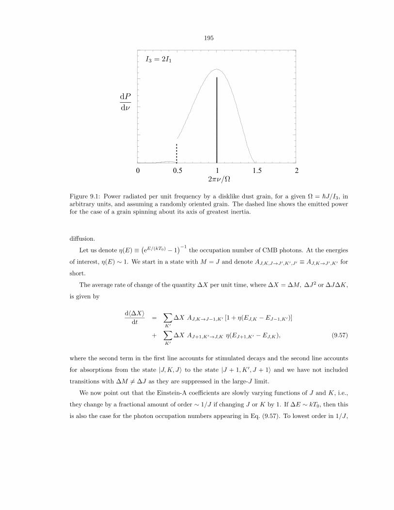
195

2!"/!0 0.5 1 1.5 2

dP

d!

I3 = 2I1

Figure 9.1: Power radiated per unit frequency by a disklike dust grain, for a given Ω = ~J/I3, inarbitrary units, and assuming a randomly oriented grain. The dashed line shows the emitted powerfor the case of a grain spinning about its axis of greatest inertia.

diffusion.

Let us denote η(E) ≡(eE/(kT0) − 1

)−1the occupation number of CMB photons. At the energies

of interest, η(E) ∼ 1. We start in a state with M = J and denote AJ,K,J→J′,K′,J′ ≡ AJ,K→J′,K′ for

short.

The average rate of change of the quantity ∆X per unit time, where ∆X = ∆M, ∆J2 or ∆J∆K,

is given by

d〈∆X〉dt

=∑

K′

∆X AJ,K→J−1,K′ [1 + η(EJ,K − EJ−1,K′)]

+∑

K′

∆X AJ+1,K′→J,K η(EJ+1,K′ − EJ,K), (9.57)

where the second term in the first line accounts for stimulated decays and the second line accounts

for absorptions from the state |J,K, J〉 to the state |J + 1,K ′, J + 1〉 and we have not included

transitions with ∆M 6= ∆J as they are suppressed in the large-J limit.

We now point out that the Einstein-A coefficients are slowly varying functions of J and K, i.e.,

they change by a fractional amount of order ∼ 1/J if changing J or K by 1. If ∆E ∼ kT0, then this

is also the case for the photon occupation numbers appearing in Eq. (9.57). To lowest order in 1/J ,

196

we therefore obtain

d〈∆M〉dt

≈ −∑

∆K

AJ,K→J−1,K′ , (9.58)

d〈∆J2〉dt

≈∑

∆K

AJ,K→J−1,K′ [1 + 2η(EJ,K − EJ−1,K′)] , (9.59)

d〈∆J∆K〉dt

≈ −∑

∆K

∆K AJ,K→J−1,K′ [1 + 2η(EJ,K − EJ−1,K′)] . (9.60)

We see that there is not only rotational damping, but also diffusion associated with electric dipole

radiation, even at zero CMB temperature. In the case of a grain rotating about its axis of greatest

inertia, we find

Ded(Ω;K = J) ≡ ~I3

d〈∆M〉dt

=2

3

µ2ipΩ3

I3c3(9.61)

E||,ed(Ω;K = J) ≡ ~2

I23

d〈∆J2〉dt

=~I3Ded(Ω) [1 + 2η(~Ω)] . (9.62)

The damping rate is identical to that found in Chapter 8. Note that Eq. (9.62) resembles closely

the generalized Nyquist theorem [176, 162]. In the limit ~Ω kT0, we obtain the form derived in

Chapter 8 for the fluctuation-dissipation theorem, E||,ed = 2kT0/(I3Ω)Ded.

For a randomly oriented grain, we must evaluate the average of Eqs. (9.58) and (9.59) over K.

For I3 = 2I1, we obtain

Ded(Ω) =32

9

µ2opΩ3

I3c3+

82

45

µ2ipΩ3

I3c3(9.63)

E||,ed(Ω) =32

9

~Ω3

I23c

3µ2

op [1 + 2η(2~Ω)] +~Ω3

3I23c

3µ2

ip

[82

15+ G

(~Ω

kT0

)], (9.64)

where we have defined

G(λ) ≡∫ 1

−1

(2− x)3(1 + x)2

e(2−x)λ − 1dx. (9.65)

Moreover, we can evaluate the following quantity, which appears in the principle of detailed balance

for a randomly oriented grain, Eq. (9.19):

⟨~2

I23

K

J

d〈∆J∆K〉dt

⟩K

=~Ω3

3I23c

3µ2

ip

[104

105+H(λ)

], (9.66)

where we have defined

H(λ) ≡∫ 1

−1

x(2− x)3(1 + x)2

e(2−x)λ − 1dx. (9.67)

One can easily check that in the limit ~Ω kT0, the principle of detailed balance as previously

derived is indeed satisfied in the form of Eq. (9.19) with T = T0. We now explain why the form (9.19)

197

is not recovered for a general value of ~Ω/(kT0). One expects that in the absence of any interactions

besides absorptions and emissions of microwave photons, the probability distribution of rotational

quantum number should reach thermal equilibrium with a temperature T0. In that case, the ratio

of the population of two neighboring levels is of order XJ+1/XJ ∼ e−~Ω/(kT0). For ~Ω kT0,

we see that this ratio is close to unity and one can treat the population of rotational states as a

smoothly varying function, which is an underlying assumption of the Fokker-Planck equation. For

~Ω ∼> kT0, however, the population of rotational states would be a rapidly decreasing function, and

a Fokker-Planck treatment would not be valid if no other processes were present ; in that case one

should rather solve a coupled rate equation in a matrix form. Due to other rotational excitation and

damping processes, however, the characteristic rotation temperature is much larger than the CMB

temperature and the level populations are indeed slowly varying with J around the peak of the

spectrum. The Fokker-Planck treatment is therefore valid, but one cannot expect the form (9.19) of

detailed balance to be satisfied for excitation and damping by emission and absorption of microwave

photons. Note, finally, that for all other processes considered, the temperature is much larger than

the characteristic emission frequency and the generalized Nyquist theorem takes the form of the

standard dissipation-fluctuation theorem.

Normalized damping and excitation rates

In Chapter 8 we had only considered electric dipole radiation as a rotational damping process, which

we characterized by the characteristic timescale τed. Here we have shown that there is an associated

rotational excitation rate. The corresponding dimensionless damping and excitation rates defined

in Eqs. (9.9) and (9.10) are given by

Fed(Ω;K = J) = τH2

3

µ2ipΩ2

I3c3, (9.68)

Ged(Ω;K = J) =~Ω

kT

[1

2+ η(~Ω)

]Fed(Ω), (9.69)

when the grain is rotating about its axis of greatest inertia, and

Fed(Ω;K random) = τH

[32

9µ2

op +82

45µ2

ip

]Ω2

I3c3, (9.70)

Ged(Ω;K random) =1

2

~Ω

kTFed(Ω) + τH

~Ω

kT

[32

9µ2

opη(2~Ω) +1

6µ2

ipG(

~Ω

kT0

)]Ω2

I3c3, (9.71)

when the grain’s orientation is randomized.

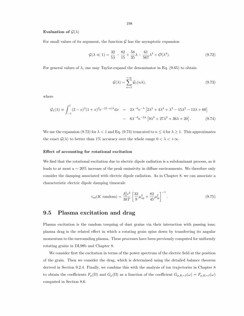
198

Evaluation of G(λ)

For small values of its argument, the function G has the asymptotic expansion

G(λ 1) =32

5λ− 82

15+

58

35λ− 61

567λ3 +O(λ4). (9.72)

For general values of λ, one may Taylor-expand the denominator in Eq. (9.65) to obtain

G(λ) =

+∞∑

n=1

G1(nλ), (9.73)

where

G1(λ) ≡∫ 1

−1

(2− x)3(1 + x)2e−(2−x)λdx = 2λ−6e−λ[2λ5 + 4λ4 + λ3 − 15λ2 − 12λ+ 60

]

− 6λ−6e−3λ[9λ3 + 27λ2 + 36λ+ 20

]. (9.74)

We use the expansion (9.72) for λ < 1 and Eq. (9.73) truncated to n ≤ 4 for λ ≥ 1. This approximates

the exact G(λ) to better than 1% accuracy over the whole range 0 < λ < +∞.

Effect of accounting for rotational excitation

We find that the rotational excitation due to electric dipole radiation is a subdominant process, as it

leads to at most a ∼ 20% increase of the peak emissivity in diffuse environments. We therefore only

consider the damping associated with electric dipole radiation. As in Chapter 8, we can associate a

characteristic electric dipole damping timescale

τed(K random) =I23c

3

3kT

[32

9µ2

op +82

45µ2

ip

]−1

. (9.75)

9.5 Plasma excitation and drag

Plasma excitation is the random torquing of dust grains via their interaction with passing ions;

plasma drag is the related effect in which a rotating grain spins down by transferring its angular

momentum to the surrounding plasma. These processes have been previously computed for uniformly

rotating grains in DL98b and Chapter 8.

We consider first the excitation in terms of the power spectrum of the electric field at the position

of the grain. Then we consider the drag, which is determined using the detailed balance theorem

derived in Section 9.2.4. Finally, we combine this with the analysis of ion trajectories in Chapter 8

to obtain the coefficients Fp(Ω) and Gp(Ω) as a function of the coefficient Gp,K=J(ω) = Fp,K=J(ω)

computed in Section 8.6.

199

Perturbation theory predicts the transition rate Γn→k for a perturbation depending on time V (t)

(see e.g. Ref. [164])

Γn→k =1

~2PVkn(νkn) , (9.76)

where hνkn ≡ |Ek − En| and PV (ν) is the power spectrum of the perturbation:

PVkn(ν) ≡ limT→∞

1

T

∣∣∣∣∣

∫ T

0

e2πiνtVkn(t)dt

∣∣∣∣∣

2

. (9.77)

In the case of a rotating dust grain in a fluctuating electric field, the perturbation operator is given

by

V = −µ.E , (9.78)

where µ is the electric dipole operator of the grain and E is the stochastic electric field produced by

the passing ions. Using Eq. (9.26), we rewrite the perturbation as

V = −1∑

m=−1

(−1)mµmE−m = −1∑

m=−1

(−1)mE−m1∑

m′=−1

D(1)∗m′m(χ)µ

(g)m′ , (9.79)

where we rewrote the components of the dipole moment in the lab frame as a function of those in

the grain frame. The matrix element of the perturbation between two states can then be evaluated:

〈J ′,K ′,M ′, v′|V |J,K,M, v〉 = −1∑

m=−1

(−1)mE−m1∑

m′=−1

〈v′|µ(g)m′ |v〉〈J ′,K ′,M ′|D1∗

m′m(χ)|J,K,M〉

= (−1)K′+M ′

√(2J ′ + 1)(2J + 1)

1∑

m=−1

E−m

J ′ 1 J

−M ′ −m M

×1∑

m′=−1

(−1)m′〈v′|µ(g)

m′ |v〉

J ′ 1 J

−K ′ −m′ K

. (9.80)

The transition rate induced by the perturbation is therefore

ΓJ,K,M,v→J′,K′,M ′,v′ =(2J ′ + 1)(2J + 1)

~2limT→∞

1

T

∣∣∣∣∣1∑

m=−1

J ′ 1 J

−M ′ −m M

∫ T

0

ei ∆Eh tE−m(t)dt

×1∑

m′=−1

(−1)m′〈v′|µ(g)

m′ |v〉

J ′ 1 J

−K ′ −m′ K

∣∣∣∣∣

2

. (9.81)

If we now assume that the x, y, z components of the electric field are uncorrelated, the terms mixing

different values of m in the modulus squared vanish, we obtain, using Eq. (9.30) for the spontaneous

200

decay rates4:

ΓJ,K,M,v→J′,K′,M ′,v′ =3~2c3

4(∆E)3PE(

∆E

h

)×AJ,K,M,v→J′,K′,M ′,v′ , (9.82)

where we used the power spectrum of the electric field, which we assumed to be isotropic :

PE(ν) ≡ PEx(ν) + PEy (ν) + PEz (ν). (9.83)

Before proceeding further, we should emphasize a subtlety regarding the meaning of the electric

field power spectrum. The stochastic electric field arises from ions passing nearby the grain. Ions

that collide with the grain, however, should not be accounted for, as we already include them in

the collisional excitation and damping rates. Therefore only ions which have an impact parameter b

large enough not to collide with the grain (typically b ∼> a) should be accounted for when evaluating

the power spectrum PE . With this knowledge, we can estimate the characteristic cutoff frequency

νmax of the power spectrum: νmax ∼ vth/a ∼√

2kT/(mpa2) ∼ 1012 T1/22 a−1

−7 Hz. We therefore see

that transitions between different vibrational states will be largely suppressed as they correspond to

infrared frequencies νIR ∼ 1013−1014 Hz for the smallest grains. We therefore only need to consider

purely rotational transitions with v′ = v.

We choose the reference z-axis so that the grain is initially in the state M = J . There are in

principle 18 possible transitions, ∆J = 0,±1, ∆M ≤ ∆J , ∆K = 0,±1. We saw in Section 9.3 that

transitions with ∆M < ∆J are suppressed with respect to those with ∆M = ∆J in the large J

limit. We are left with 8 transitions that change J and/or K. Transitions with ∆J = 0 do not

appear in calculations of the diffusion rates d〈∆J2〉/dt or d〈∆J∆K〉/dt. We therefore only need to

consider the 6 transitions ∆J = ∆M = ±1,∆K = 0,±1.

In the large-J limit, we find that the transition rates are given by:

Γ∆J=±1,∆K=0 =µ2

op

2~2PE(I3I1

Ω

2π

)(1− K2

J2

), (9.84)

Γ∆J=±1,∆K=±1 =µ2

ip

8~2PE(ν)

(1 + ∆J∆K

K

J

)2

=µ2

ip

8~2PE(ν)

(I3I1− 1

)−2(2I3I1− 1− 2πν

Ω

)2

, (9.85)

where in the last line we have used ν ≡(I3/I1 −∆J∆K (I3/I1 − 1) KJ

)Ω/(2π). We can now obtain

4Einstein-A coefficients are only defined when the final state has a lower energy than the initial state. HereAJ,K,M,v→J′,K′,M′,v′ should just be understood as a compact notation for the right-hand side of Eq. (9.30), whichis always well defined.

201

the diffusion rates

EJJ(J,K) ≡ d〈∆J2〉dt

=∑

∆J,∆K

(∆J)2Γ∆J,∆K , (9.86)

EJK(J,K) ≡ d〈∆J∆K〉dt

=∑

∆J,∆K

∆J∆K Γ∆J,∆K . (9.87)

Let us first consider the case where the grain is rotating about its axis of greatest inertia, K = J .

In this case the ∆K = 0 and ∆K = −∆J transitions are suppressed and we find

EJJ(J, J) = EJK(J, J) =µ2

ip

~2PE(

Ω

2π

). (9.88)

We have already computed the rate of angular momentum diffusion in this case in Section (8.6). We

can therefore relate the electric field power spectrum to the dimensionless diffusion rate Gp,K=J(ω):

PE(ν) =2kTI3τHµ2

ip

Gp,K=J(2πν). (9.89)

Note that Gp,K=J ∝ µ2ip so this quantity is well defined even for µip = 0.

For a randomly oriented dust grain, we need to evaluate the averages 〈EJJ〉K and 〈(K/J)EKJ〉K .

In the large-J limit, we can change the discrete sums over K to integrals, and we obtain, for I3 = 2I1:

~2〈EJJ〉(Ω) =2

3µ2

opPE(

Ω

π

)+µ2

ip

4

∫ 3Ω

Ω

PE( ω

2π

)(3− ω

Ω

)2 dω

Ω, (9.90)

and therefore

Gp(Ω) =2

3

µ2op

µ2ip

Gp,K=J(2Ω) +1

4

∫ 3Ω

Ω

(3− ω

Ω

)2

Gp,K=J(ω)dω

Ω. (9.91)

The rates we have derived are symmetric and do not properly account for the fact that the total

angular momentum of the system grain + ions should be conserved. In principle there should be

a slight asymmetry in the ∆J = +1 and ∆J = −1 rates, translating the fact that a supra-thermally

rotating grain will be systematically slowed down by transferring its angular momentum to the bath

of thermal ions. To obtain the net damping rate one should therefore not use the face values of the

rates computed here, but rather derive it from the diffusion rate through the principle of detailed

balance, which takes the form of Eq. (9.19). We therefore obtain the normalized damping rate

Fp(Ω) =4

3

µ2op

µ2ip

Gp,K=J(2Ω) +1

4

∫ 3Ω

Ω

ω

Ω

(3− ω

Ω

)2

Gp,K=J(ω)dω

Ω. (9.92)

Notice that Gp < Fp < 3Gp. We describe our numerical implementation of the plasma excitation

and drag coefficients in Appendix 9.A.

We show the plasma excitation and drag coefficient for a grain containing NC = 54 carbon atoms

202

Figure 9.2: Dimensionless plasma excitation and drag coefficients, for NC = 54 in the WIM. Thecurve labelled “θ = 0” corresponds to a grain rotating around its axis of greatest inertia as assumedin Chapter 8; the curves labelled “θ random” correspond to grains with a randomized nutation anglediscussed in this chapter.

(equivalent radius a ≈ 5A), in WIM conditions (as defined in DL98b) in Fig. 9.2.

9.6 Infrared excitation and damping

Dust grains in the ISM get excited by absorbing ultraviolet photons, which they then degrade into a

large number of infrared photons, emitted in ro-vibrational transitions. Because of the (∆E)3 factor

in the spontaneous rates, for given initial and final vibrational states, transitions with ∆J = −1

have slightly larger rates than transitions with ∆J = +1, and the emission of infrared photons

tends to systematically damp out the grain’s rotation. This damping is accompanied by a stochastic

excitation as infrared photons carry quanta of angular momentum with random projections. We

have already computed the damping rate for a grain rotating about its axis of greatest inertia with a

classical approach in Section 8.7. In this section, we generalize the quantum treatment of Appendix

B of Ref. [173] for randomly oriented disk-like grains.

As in the previous section, we choose a reference frame such that the grain is initially in theM = J

rotational state. As for the plasma drag calculation, only the 6 cases ∆J = ∆M = ±1,∆K = 0,±1

need to be considered in the large-J limit.

We consider the ro-vibrational transition v → v′ with change in the rotational configuration

∆J,∆K. The energy of the emitted photon is ∆E = ∆Evib+∆Erot ≡ hνvib+∆E(∆J,∆K). Rotational

transition energies (typically in the microwaves) are much smaller than vibrational transition energies

203

(typically in the infrared). We can therefore expand the (∆E)3 term in Eq. (9.30) to lowest order

in ∆E(∆J,∆K)/∆Evib. The Einstein-A coefficients for the J-changing ro-vibrational transitions are

then, in the large-J limit:

Av→v′;∆J=∆M=±1,∆K=0 ≈2µ2||

3~c3(2πνvib)3

(1− K2

J2

)(1− 3∆J

I3I1

Ω

2πνvib

), (9.93)

Av→v′;∆J=∆M=±1,∆K=±1 ≈ µ2⊥

6~c3(2πνvib)3

(1 + ∆J∆K

K

J

)2

×

1 + 3Ω

2πνvib

[−∆J

I3I1

+ ∆KK

J

(I3I1− 1

)], (9.94)

where we have defined

µ2|| ≡ |〈v′|µ

(g)0 |v〉|2, µ2

⊥ ≡ |〈v′|µ(g)1 |v〉|2 + |〈v′|µ(g)

−1|v〉|2 = 2|〈v′|µ(g)±1|v〉|2. (9.95)

Note that these differ form µ2ip and µ2

op as we are now considering matrix elements between different

vibrational states. Classically, they correspond to the power spectrum of the stochastic dipole

moment of the grain at the relevant transition frequency (see Section 8.7).

The slight asymmetry between the rates of ∆J = +1 and ∆J = −1 transitions causes a net loss

of z-angular momentum, with rate (recalling that transitions with ∆M 6= ∆J are suppressed in the

large-J limit):

d〈∆Lz〉dt

(J,K) = ~d〈∆M〉

dt= ~

∑

∆J,∆K

∆J Av→v′;∆J=∆M,∆K

= − 4

c3(2πνvib)2Ω

I3I1µ2||

(1− K2

J2

)+

I32I1

µ2⊥

(1− K2

J2

)+ µ2

⊥K2

J2

. (9.96)

We would like to compare this quantity to the rate of energy loss. For that, we also need the rate

of ∆J = ∆M = 0 ro-vibrational transitions, which, to lowest order in ∆Erot/∆Evib, are given by:

Av→v′;∆J=∆M=0,∆K=0 =4µ2||

3~c3(2πνvib)3K

2

J2, (9.97)

Av→v′;∆J=∆M=0,∆K=±1 =µ2⊥

3~c3(2πνvib)3

(1− K2

J2

). (9.98)

We can then evaluate the rate of energy loss:

E(J,K) = −hνvib

∑

∆J,∆K

Av→v′;∆J,∆K = −4

3

(2πνvib)4

c3

(µ2|| + µ2

⊥). (9.99)

We can now relate the rate of angular momentum loss to the rate of energy loss. In the case K = J ,

204

we see that only the last term in Eq. (9.96) contributes and we obtain

d〈∆Lz〉dt

(K = J) = − 4

c3(2πνvib)2µ2

⊥Ω =3µ2⊥

µ2|| + µ2

⊥

Ω

(2πνvib)2E. (9.100)

In the case where the grain orientation is randomized, one must average over K. For I3 = 2I1, we

obtain:

d〈∆Lz〉dt

(K = random) = − 4

c3(2πνvib)2

[4

3µ2|| + µ2

⊥

]Ω =

3µ2⊥ + 4µ2

||µ2|| + µ2

⊥

Ω

(2πνvib)2E. (9.101)

We see that we obtain an increase in the damping rate by a factor (1+ 43

µ2||µ2⊥

) in comparison to the case

K = J . In principle one should specify the character of each transition (in-plane, or perpendicular, if

µ2|| = 0; out-of-plane, or parallel, if µ2

⊥ = 0). For simplicity we assume the isotropic case, µ2|| = 1

2µ2⊥.

In that case, we obtain

FIR =10τH3πI

∫ ∞

0

Fνν2

dν, (9.102)

where Fν ≡ 14π

dEdν .

We can now also obtain the rotational excitation rate. Using Eqs. (9.93) and (9.94) to lowest

order in Ω/(2πνvib), we obtain

d〈∆L2z〉

dt(J,K) =

2~3c3

(2πνvib)3

2µ2||

(1− K2

J2

)+ µ2

⊥

(1 +

K2

J2

). (9.103)

In the case that the grain rotates around its axis of greatest inertia, we have

d〈∆L2z〉

dt(K = J) =

~2

hνvib

µ2⊥

µ2|| + µ2

⊥E =

1

3

2~2

hνvibE, (9.104)

where in the last equality is valid in the isotropic case. When the grain’s nutation state is randomized,

we obtaind〈∆L2

z〉dt

(K random) =1

3

2~2

hνvibE, (9.105)

regardless of the character of the transition. As was explained in Chapter 8, this result can be

intuitively understood as follows: each photon carries and angular momentum squared L2γ = 2~2. If

photons are isotropically emitted, then 1/3 of this quantity leads to a diffusion of the grain’s angular

momentum along its initial direction.

205

9.7 Collisions

A quantum mechanical treatment of collisions would be much more complex than that of plasma

drag or infrared emission, and we have not carried it. For completeness, we just state the results

of Ref. [170], where these rates were derived classically, and we refer the reader to the paper for a

complete discussion. For the case of neutral grains and neutral impactors, we have:

Fn(Zg = 0) =5

3Fn,K=J and Gn(Zg = 0) = Gn,K=J. (9.106)

For charged grains and neutral impactors, the normalized damping rate was found to be:

F (in)n (Zg 6= 0) =

1 +

2

3

[1 +

(rc

acx

)2]−1

Fn,K=J, where rc ≡

4

√Z2gq

2eα

3kT. (9.107)

rc is the critical separation at which the induced dipole attraction overwhelms the thermal energy

of the gas. The normalized excitation rate is

Gn(Zg 6= 0) = Gn,K=J. (9.108)

The case of ion impacts is left unchanged from Chapter 8.

9.8 Results

To avoid lengthy repetitions, we will refer to the case where grains are spinning around their axis of

greatest inertia (as treated by DL98b and in Chapter 8) by “case 1” (or “θ = 0” in figures), and to

the case where the relative orientation of the grain and the angular momentum is randomized (as

discussed in the present chapter) by “case 2” (or “θ random” in figures).

9.8.1 Angular momentum distribution

We saw in Section 9.4.2 that, at equal angular momentum, the total power radiated by a disk-like

grain in case 2 was 5 times (in the case µop = 0) to ∼ 10 times (µ2ip : µ2

op = 2 : 1) higher than the

power radiated in case 1. This ratio goes even higher as one increases the µ2op : µ2

ip ratio. However,

the angular momentum distribution is different in each case, and, as P ∝ L4, the ratio of the total

power emitted will really bePcase2

Pcase1≈ 10

〈L2〉2case2

〈L2〉2case1

. (9.109)

In what follows we show that 〈L2〉case2 < 〈L2〉case1.

First of all, we showed in earlier sections that the damping rates are generally higher for grains

206

5 2010

Figure 9.3: Probability distribution function for the parameter Ω = L/I3, for a grain of radiusa = 5 A, in WIM conditions, with µ2

ip : µ2op = 2 : 1, and with dipole moment per atom β = 0.38

Debye.

spinning around a non-principal axis of inertia. This can be understood heuristically as follows:

for a given angular momentum L = ~J , the rotational energy Erot(J,K) was given in Eq. (9.1).

Averaging over the nutation angle (i.e., averaging over K), we find that

〈Erot〉(J) =L2

2I1− 1

3

L2

2

(I−11 − I−1

3

). (9.110)

In the case of a disk-like grain, (I3 = 2I1) this is

〈Erot〉(J) =5

3

L2

2I3=

5

3Erot(J,K = J). (9.111)

Therefore, we may expect that, when in contact with a bath of a characteristic energy, grains with a

randomly oriented rotation axis will have an rms angular momentum of the order of ∼√

3/5 ≈ 0.77

that of grains rotating around their axis of greatest inertia. This is indeed what we found in the

case of collisions of neutral grains with neutral impactors, or emission of infrared photons, for which

we showed that G was unchanged but F was increased by a factor of 5/3. We also showed that the

normalized plasma damping and excitation rates satisfied 1 < Fp/Gp < 3.

More importantly, the characteristic radiation-reaction damping time τed was found to be shorter

in case 2. We haveτed(case 2)

τed(case 1)=

µ2ip

4115µ

2ip + 16

3 µ2op

. (9.112)

In the case where radiation-reaction is the dominant rotational damping mechanism, which is the

207

Figure 9.4: Power radiated by a grain of radius a = 5 A, in WIM conditions, with µ2ip : µ2

op = 2 : 1,and with dipole moment per atom β = 0.38 Debye.

Figure 9.5: Spinning dust emissivity in WIM environment.

208

case for the smallest grains in diffuse phases of the ISM, we showed in Section 8.10.1 that the rms

angular momentum is proportional to τ1/4ed . Numerically, we have

τ1/4ed (case 2)

τ1/4ed (case 1)

≈

0.78 µop = 0,

0.66 µ2ip : µ2

op = 2 : 1.(9.113)

From these considerations, we therefore expect that in the same environment, the characteristic

angular momentum in case 2 will be ∼ 0.66–0.78 times the one in case 1.

We show in Fig. 9.3 the angular momentum distribution for a grain of volume equivalent radius

a = 5 A, in WIM conditions, with µ2ip : µ2

op = 2 : 1, and with dipole moment per atom β = 0.38

Debye. The rms angular momentum in case 2 is ∼ 0.67 times the one in case 1.

9.8.2 Change in emissivity

At a given angular momentum, the power radiated in case 2 peaks at a frequency approximately

twice higher than the power radiated in case 1 (see discussion in Section 9.4.2).

Therefore, and in view of the preceding section, we expect that the total power radiated in

case 2 will peak at a frequency ∼ 2 × 0.7 ∼ 1.4 times higher and will integrate to a total power

∼ 10 × (0.7)4 ∼ 2 times the power radiated in case 1. This is indeed what we find, as can be seen

in Fig. 9.4.

The overall spinning dust emissivity follows the same trends, as can be seen in Fig. 9.5 for the

WIM, and in Fig. 9.6 for other interstellar environments.

9.8.3 Sensitivity to dipole moment orientation

It is not clear what is the correct assignment for the direction of the grain permanent dipole moment

relative to the principal axes. Here we analyze the effect of the dipole moment orientation on the

spinning dust spectrum; it appears to make only a minor difference in the WIM environment.

For the smallest grains where radiation-reaction damping is most important, we expect 〈Ω2〉1/2 ∝τ

1/4ed so

〈Ω2〉1/2 ∝

µ−1/2ip (case 1),

µ−1/2(

8039 −

µ2ip

µ2

)−1/4

(case 2).(9.114)

In case 1 the rotation rate is very sensitive to the orientation of the dipole moment (only the in-

plane component contributes to the power and the radiation reaction damping). Eventually, when

the in-plane component becomes small enough, radiation-reaction damping becomes subdominant

and the rms angular momentum will depend only on interactions with gas or infrared photons. In

case 2 however the dependence on µ2ip/µ

2 is quite weak, as the out-of-plane component contributes

to the power and angular momentum loss. We show the normalized rms angular momenta in case 1

209

Figure 9.6: Spinning dust spectra for several environmental conditions: dark cloud (DC), molecularcloud (MC), cold neutral medium (CNM), warm neutral medium (WNM), reflection nebula (RN) andphotodissociation region (PDR). The environments are defined in DL98b, table 1. The parametersfor the grain size distribution are RV = 3.1, bC = 6× 10−5 for the diffuse CNM and WNM phases,and RV = 5.5, bC = 3×10−5 for the dense DC, MC, RN and PDR. The dashed line is for a spectrumcalculated assuming case 1 (θ = 0), whereas the solid line is for case 2 (isotropic θ). The shift tohigher frequencies and increase in emissivity in case 2 is systematic for all environments. We expectthat case 2 should be a better approximation in the diffuse and high radiation intensity phases(WIM, CNM, WNM, RN, PDR).

210

and 2 in Fig. 9.7. Figure 9.7 also shows an estimate of the peak frequency of the emitted power in

both cases.

The total power radiated by one grain, at a given angular momentum, was given in Eq. (9.55)

for case 2. Taking Ω ∼ 〈Ω2〉1/2, and using the above results, we obtain

P ∝

constant (case 1)(3217 −

µ2ip

µ2

)/(8039 −

µ2ip

µ2

)(case 2).

(9.115)

Thus in both cases the total power is very nearly independent of µ2ip/µ

2. In case 1, when µ2ip/µ

2 → 0,

radiation-reaction damping becomes subdominant and the power becomes proportional to µ2ip. These

features are shown in Fig. 9.8.

9.9 Discussion

The purpose of this chapter was to revisit the assumption of Refs. [8, 173] that PAHs rotate about

their axis of main inertia. The motivation in doing so is that thermal spikes following the absorption

of UV photons randomize the orientation of the grain with respect to the angular momentum axis.

These absorption events happen frequently enough (i.e., on timescale shorter than the timescale

for significant changes in the total angular momentum) that we expect such a randomization to be

effective in most environments. Thus we expect the results from this work (“case 2”) to be a better

approximation to diffuse or high-radiation environments (CNM, WNM, WIM, PDR, and RN) than

those from Chapter 8, which assumed rapid dissipation of the nutational energy (θ = 0 or “case 1”).

However, the new release of SpDust allows the user to choose either case; for example, one may

wish to explore the range of cases in dark cloud environments where thermal spikes are infrequent,

or what happens if an as-yet-unidentified dissipational process is active and restores θ = 0.

In this chapter, we showed that, for a given angular momentum, the power radiated by a grain

in case 2 is ∼ 10 times higher than that radiated by a grain in case 1. This is because in case 2,

the grain emits at higher frequencies, including above the one corresponding to the instantaneous

angular velocity, as it is not rotating around the axis of greatest inertia.

We evaluated the rotational excitation and damping rates in case 2 as a function of grain size

and environment conditions, and the resulting angular momentum distribution. We showed that in

a given environment, grains in case 2 have a lower rms angular momentum than those in case 1, by

a factor of ∼ 0.7. This is due to larger damping rates, in particular radiation-reaction damping, in

case 2.

The combination of these results leads to a spinning dust spectrum peaking at slightly higher

frequencies in case 2, and a total power approximately twice as large as that emitted in case 1.

Finally, we showed that the spectrum in case 2 is only weakly sensitive to the precise value of the

211

Figure 9.7: Top panel: normalized rms angular momentum 〈Ω2〉1/2 as a function of the ratio ofin-plane to total dipole moment. Bottom panel: estimate of the peak frequency

∫ν(dP/dν)dν

/P ,

as a function of this ratio. Both are for a dust grain of radius a = 5 A and dipole moment per atomβ = 0.38 Debye, in WIM conditions.

212

Figure 9.8: Total power emitted by a dust grain of radius a = 5 A and dipole moment per atomβ = 0.38 Debye, in WIM conditions, as a function of the ratio of in-plane to total dipole moment.

µ2ip : µ2

op ratio.

Ref. [143] found a tension between theoretical results and microwave observations of the WIM:

the theory was a factor of ∼ 3 larger than the observations, and the peak frequency of the spinning

dust and its amplitude could not be simultaneously reconciled by changing β (the normalization

of the dipole moment). By increasing the theoretical emissivity and moving its peak to higher

frequencies, our results may worsen this tension. This seems likely to strengthen the empirical

case for depletion of the PAH population in the WIM phase, however there are other conceivable

explanations for this discrepancy. The random walk model for the dipole moment may not apply

well to the smallest grains (e.g. one could imagine that some of the small PAHs have symmetries

that guarantee µ = 0 exactly), or one could imagine extra low-frequency internal degrees of freedom

which allow the grain to relax to a state where it rotates around the axis of greatest moment of

inertia. A detailed exploration of the parameter space (as was done in Ref. [143]) is beyond the

scope of this work.

As a final note, we present some of the remaining issues in the treatment of the rotational physics

of the smallest dust grains:

• Triaxiality: Many PAHs have triaxial moment of inertia tensors (e.g. ovalene C32H14, circum-

pyrene C42H16, and their derivatives). This case was not treated in the present work due to

its much greater complexity.

• Impulsive torques: Some of the sources of torque, such as ion impacts, impart large but in-

frequent changes in angular momentum. This could in principle lead to “rotational spikes”

213

analogous to the well-known thermal spikes in the grains’ internal energy, and would not be

treated correctly by the Fokker-Planck equation (which is a diffusive approximation).5

• Ancillary data: We have not fully quantified the uncertainties in the ancillary data, such as

evaporation temperatures, the emissivity in the lowest-frequency vibrational modes, and the

grain charging model (photoelectric and electron/ion impact). However, our hope in making

the SpDust code publicly available is to provide users the flexibility to explore deviations

from default or fiducial parameters.

5This issue is treated in Ref. [172]; they find that the principal effect on the spinning dust spectrum is the existenceof a “tail” to high frequencies resulting from transient spin-up of the grains.

214

9.A Appendix: Evaluation of the plasma excitation and drag

coefficients

In this appendix we describe our implementation of the plasma drag coefficients Fp(Ω) and Gp(Ω),

in SpDust. These are integrals over the function Gp,AHD(ω), which is itself time-consuming to

compute.

If we wish to calculate the integral∫w(x)g(x)dx, where w(x) is a known weighing function

which properties will be discussed later, and the function g(x) is smooth enough on the interval of

integration that it can be approximated by a quadratic polynomial g(x) ≈ a + bx + cx2, then we

may approximate ∫w(x)g(x)dx ≈ A [g(x+) + g(x−)] , (9.116)

where A ≡ 12

∫w(x)dx, and x+, x− are the solutions of the second-order system

x+ + x− = A−1∫xw(x)dx,

x2+ + x2

− = A−1∫x2w(x)dx.

(9.117)

We now turn our attention to the specific cases of Gp(Ω) and Fp(Ω). With x = ω/Ω and the

weighing function w(x) = (3− x)2, we get

Gp(Ω) ≈ 2µ2op

3µ2ip

Gp,AHD(2Ω) +1

3[Gp,AHD(Ω+) +Gp,AHD(Ω−)] , (9.118)

where

Ω± =3±

√3/5

2Ω ≈ 1.11Ω, 1.89Ω. (9.119)

Similarly, with the weighing function w(x) = x(3− x)2, we get

Fp(Ω) ≈ 4µ2op

3µ2ip

Gp,AHD(2Ω) +1

2

[Gp,AHD(Ω+) +Gp,AHD(Ω−)

], (9.120)

where

Ω± =8±

√13/3

5Ω ≈ 1.18Ω, 2.02Ω. (9.121)

We have tested the accuracy of the approximate integrator and found that the error was less than

1% in the regime where Fp, Gp have significant values, i.e., for Ω ∼< Ωth =√

3kT/I3. More precisely,

we checked that|∆Fp(Ω)|Fp(Ω)

×min

(1,

Fp(Ω)

Fp(Ωth)

)< 0.01 (9.122)

for grain radii a = 4, 5, 6 A, gas temperatures T = 50, 500, 5000 K and grain charge Z = −1, 0, 1,

and similarly for Gp.

215

Bibliography

[1] R. H. Dicke, P. J. E. Peebles, P. G. Roll, and D. T. Wilkinson, ApJ, 142, 414 (1965).

[2] A. A. Penzias and R. W. Wilson, ApJ, 142, 419 (1965).

[3] D. J. Fixsen, E. S. Cheng, J. M. Gales, J. C. Mather, R. A. Shafer, and E. L. Wright, ApJ,

473, 576 (1996).

[4] E. Komatsu et al., ApJS, 192, 18 (2011).

[5] W. Hu, D. Scott, N. Sugiyama, and M. White, Phys. Rev. D, 52, 5498 (1995).

[6] The Planck Collaboration, arXiv:1101.2031 (2011).

[7] B. T. Draine and A. Lazarian, ApJL, 494, L19 (1998).

[8] [DL98b], B. T. Draine, and A. Lazarian, ApJ, 508, 157 (1998).

[9] J. C. Mather et al., ApJL, 354, L37 (1990).

[10] G. F. Smoot et al., ApJL, 396, L1 (1992).

[11] A. G. Riess et al., Astron. J., 116, 1009 (1998).

[12] S. Perlmutter et al., ApJ, 517, 565 (1999).

[13] C. B. Netterfield et al., ApJ, 571, 604 (2002).

[14] T. J. Pearson et al., ApJ, 591, 556 (2003).

[15] C. L. Kuo et al., ApJ, 600, 32 (2004).

[16] P. Ade et al., ApJ, 674, 22 (2008).

[17] E. Hawkins et al., MNRAS, 346, 78 (2003).

[18] K. N. Abazajian et al., ApJS, 182, 543 (2009).

[19] The Planck Collaboration, arXiv:astro-ph/0604069 (2006).

216

[20] J. A. Tauber et al., A&A, 520, A1 (2010).

[21] The ACT Collaboration, ApJ, 722, 1148 (2010).

[22] J. Ruhl et al., SPIE Conference Series, 5498, 11 (2004).

[23] D. Baumann et al., AIP Conference Series, 1141, 10 (2009).

[24] U. Seljak and M. Zaldarriaga, ApJ, 469, 437 (1996).

[25] A. Lewis, A. Challinor, and A. Lasenby, ApJ, 538, 473 (2000).

[26] M. Doran, JCAP, 10, 11 (2005).

[27] U. Seljak, N. Sugiyama, M. White, and M. Zaldarriaga, Phys. Rev. D, 68, 083507 (2003).

[28] W. Hu and M. White, ApJ, 479, 568 (1997).

[29] S. Seager, D. D. Sasselov, and D. Scott, ApJS, 128, 407 (2000).

[30] S. Seager, D. D. Sasselov, and D. Scott, ApJL, 523, L1 (1999).

[31] P. J. E. Peebles, ApJ, 153, 1 (1968).

[32] Y. B. Zeldovich, V. G. Kurt, and R. A. Syunyaev, Sov. Phys. JETP, 28, 146 (1969).

[33] A. Lewis, J. Weller, and R. Battye, MNRAS, 373, 561 (2006).

[34] J. A. Rubino-Martın, J. Chluba, W. A. Fendt, and B. D. Wandelt, MNRAS, 403, 439 (2010).

[35] J. A. Rubino-Martın, J. Chluba, and R. A. Sunyaev, MNRAS, 371, 1939 (2006).

[36] J. Chluba, J. A. Rubino-Martın, and R. A. Sunyaev, MNRAS, 374, 1310 (2007).

[37] D. Grin and C. M. Hirata, Phys. Rev. D, 81, 083005 (2010).

[38] J. Chluba, G. M. Vasil, and L. J. Dursi, MNRAS, 407, 599 (2010).

[39] Y. Ali-Haımoud and C. M. Hirata, Phys. Rev. D, 82, 063521 (2010).

[40] Y. Ali-Haımoud, D. Grin, and C. M. Hirata, Phys. Rev. D, 82, 123502 (2010).

[41] J. Chluba and R. A. Sunyaev, A&A, 475, 109 (2007).

[42] E. E. Kholupenko, A. V. Ivanchik, and D. A. Varshalovich, Phys. Rev. D, 81, 083004 (2010).

[43] J. Chluba and R. A. Sunyaev, A&A, 496, 619 (2009).

[44] S. I. Grachev and V. K. Dubrovich, Astron. Lett., 34, 439 (2008).

217

[45] C. M. Hirata and J. Forbes, Phys. Rev. D, 80, 023001 (2009).

[46] J. Chluba and R. A. Sunyaev, A&A, 503, 345 (2009).

[47] J. Chluba and R. A. Sunyaev, A&A, 446, 39 (2006).

[48] E. E. Kholupenko and A. V. Ivanchik, Astron. Lett., 32, 795 (2006).

[49] C. M. Hirata, Phys. Rev. D, 78, 023001 (2008).

[50] V. K. Dubrovich and S. I. Grachev, Astron. Lett., 31, 359 (2005).

[51] J. Chluba and R. A. Sunyaev, A&A, 480, 629 (2008).

[52] J. Chluba and R. A. Sunyaev, A&A, 512, A53 (2010).

[53] T. Matsuda, H. Sato, and H. Takeda, Progress of Theoretical Physics, 42, 219 (1969).

[54] T. Matsuda, H. Sato, and H. Takeda, Progress of Theoretical Physics, 46, 416 (1971).

[55] E. E. Kholupenko, A. V. Ivanchik, and D. A. Varshalovich, MNRAS, 378, L39 (2007).

[56] E. R. Switzer and C. M. Hirata, Phys. Rev. D, 77, 083006 (2008).

[57] C. M. Hirata and E. R. Switzer, Phys. Rev. D, 77, 083007 (2008).

[58] E. R. Switzer and C. M. Hirata, Phys. Rev. D, 77, 083008 (2008).

[59] J. A. Rubino-Martın, J. Chluba, and R. A. Sunyaev, A&A, 485, 377 (2008).

[60] E. E. Kholupenko, A. V. Ivanchik, and D. A. Varshalovich, Astron. Lett., 34, 725 (2008).

[61] E. R. Switzer and C. M. Hirata, Phys. Rev. D, 72, 083002 (2005).

[62] Y. Ali-Haımoud and C. M. Hirata, Phys. Rev. D, 83, 043513 (2011).

[63] S. Dodelson, Modern Cosmology, Academic Press (2003).

[64] I. D. Novikov and Y. B. Zeldovic, ARAA, 5, 627 (1967).

[65] C. M. Hirata, Lecture notes on primordial recombination, unpublished (2008).

[66] G. Steigman, Annual Review of Nuclear and Particle Science, 57, 463 (2007).

[67] D. E. Osterbrock and G. J. Ferland, Astrophysics of gaseous nebulae and active galactic nuclei,

2nd. ed., CA: University Science Books (2006).

[68] M. Goppert-Mayer, Annalen der Physik, 401, 273 (1931).

218

[69] L. N. Labzowsky, A. V. Shonin, and D. A. Solovyev, Journal of Physics B Atomic Molecular

Physics, 38, 265 (2005).

[70] J. Chluba and R. A. Sunyaev, A&A, 458, L29 (2006).

[71] B. J. T. Jones and R. F. G. Wyse, A&A, 149, 144 (1985).

[72] D. Pequignot, P. Petitjean, and C. Boisson, A&A, 251, 680 (1991).

[73] S. Sasaki and F. Takahara, PASJ, 45, 655 (1993).

[74] Y. E. Lyubarsky and R. A. Sunyaev, A&A, 123, 171 (1983).

[75] I. P. dell’Antonio and G. B. Rybicki, ASP Conference Series, 51, 548 (1993).

[76] D. Larson et al., ApJS, 192, 16 (2011).

[77] W. A. Fendt, J. Chluba, J. A. Rubino-Martın, and B. D. Wandelt, ApJS, 181, 627 (2009).

[78] W. Y. Wong, A. Moss, and D. Scott, MNRAS, 386, 1023 (2008).

[79] M. S. Burgin, Bulletin of the Lebedev Physics Institute, 36, 110 (2009).

[80] M. S. Burgin, Bulletin of the Lebedev Physics Institute, 37, 280 (2010).

[81] A. Burgess, Mem. R. Astr. Soc. , 69, 1 (1965).

[82] H. A. Bethe and E. E. Salpeter, Quantum Mechanics of One- and Two-Electron Atoms, New

York: Academic Press (1957).

[83] S. P. Goldman, Phys. Rev. A, 40, 1185 (1989).

[84] C. Hernandez-Monteagudo, J. A. Rubino-Martın, and R. A. Sunyaev, MNRAS, 380, 1656

(2007).

[85] M. J. Seaton, MNRAS, 119, 90 (1959).

[86] J. D. Hey, Journal of Physics B Atomic Molecular Physics, 39, 2641 (2006).

[87] D. Grin, Ph.D. thesis, California Institute of Technology (2010).

[88] D. G. Hummer, Mem. R. Astr. Soc. , 70, 1 (1965).

[89] D. G. Hummer, MNRAS, 125, 21 (1962).

[90] G. B. Rybicki and I. P. dell’Antonio, ApJ, 427, 603 (1994).

[91] C. M. Hirata, MNRAS, 367, 259 (2006).

219

[92] G. B. Rybicki, ApJ, 647, 709 (2006).

[93] J. H. Krolik, ApJ, 338, 594 (1989).

[94] J. H. Krolik, ApJ, 353, 21 (1990).

[95] S. Y. Sazonov and R. A. Sunyaev, ApJ, 543, 28 (2000).

[96] D. G. Hummer and D. Mihalas, ApJL, 150, L57 (1967).

[97] F. Iocco, G. Mangano, G. Miele, O. Pisanti, and P. D. Serpico, Phys. Rep., 472, 1 (2009).

[98] P. C. Stancil, S. Lepp, and A. Dalgarno, ApJ, 509, 1 (1998).

[99] R. N. Thomas, ApJ, 125, 260 (1957).

[100] W. Unno, ApJ, 129, 375 (1959).

[101] A. G. Nikogosian, Akademiia Nauk SSSR Doklady, 235 (1977).

[102] J. Chluba and R. M. Thomas, MNRAS, 412, 748 (2011).

[103] W. Y. Wong and D. Scott, MNRAS, 375, 1441 (2007).

[104] S. I. Grachev, Astrophysics, 30, 211 (1989).

[105] S. I. Grachev and V. K. Dubrovich, Astrophysics, 34, 124 (1991).

[106] J. A. Rubino-Martın, J. Chluba, W. A. Fendt, and B. D. Wandelt, MNRAS, 403, 439 (2010).

[107] F. Iocco et al., Phys. Rep., 472, 1 (2009).

[108] F. Iocco, G. Mangano, G. Miele, O. Pisanti, and P. D. Serpico, Phys. Rev. D, 75, 087304

(2007).

[109] K. Jedamzik, G. M. Fuller, G. J. Mathews, and T. Kajino, ApJ, 422, 423 (1994).

[110] S. Matsuura, S. I. Fujimoto, S. Nishimura, et al., Phys. Rev. D, 72, 123505 (2005).

[111] S. Matsuura, S. I. Fujimoto, M. A. Hashimoto, et al., Phys. Rev. D, 75, 068302 (2007).

[112] R. Nakamura, M. A. Hashimoto, S. I. Fujimoto, et al., arXiv:1007.0466 (2010).

[113] A. Loeb, ApJ, 555, L1 (2001).

[114] E. R. Switzer and C. M. Hirata, Phys. Rev. D, 72, 083002 (2005).

[115] K. Basu, C. Hernandez-Monteagudo, and R. A. Sunyaev, a, 416, 447 (2004).

[116] M. Harwit and M. Spaans, ApJ, 589, 53 (2003).

220

[117] A. M. Wolfe, E. Gawiser, and J. X. Prochaska, ARAA, 43, 861 (2005).

[118] T. C. Beers and N. Christlieb, ARAA, 43, 531 (2005).

[119] D. A. Verner, G. J. Ferland, K. T. Korista, and D. G. Yakovlev, ApJ, 465, 487 (1996).

[120] K. P. Dere et al., Astron. Astrophys. Supp. Ser., 149 (1997).

[121] K. P. Dere et al., Astron. Astrophys. Supp. Ser., 498, 915 (2009).

[122] M. Asplund, N. Grevesse, A. J. Sauval, and P. Scott, ARAA, 47, 481 (2009).

[123] C. Dickinson et al., MNRAS, 353, 732 (2004).

[124] A. C. S. Readhead et al., ApJ, 609, 498 (2004).

[125] C. L. Kuo et al., ApJ, 664, 687 (2007).

[126] G. Hinshaw et al., ApJS, 180, 225 (2009).

[127] H. K. Eriksen, J. B. Jewell, C. Dickinson, et al., ApJ, 676, 10 (2008).

[128] S. M. Leach et al., A&A, 491, 597 (2008).

[129] E. M. Leitch, A. C. S. Readhead, T. J. Pearson, and S. T. Myers, ApJL, 486, L23 (1997).

[130] B. T. Draine and A. Lazarian, ApJ, 512, 740 (1999).

[131] W.C. Erickson, ApJ, 126, 480 (1957).

[132] F. Hoyle and N. C. Wickramasinghe, Nature, 227, 473 (1970).

[133] A. Ferrara and R.-J. Dettmar, ApJ, 427, 155 (1994).

[134] D. Rouan, A. Leger, A. Omont, and M. Giard, A&A, 253, 498 (1992).

[135] N. Anderson and W. D. Watson, A&A, 270, 477 (1993).

[136] D. P. Finkbeiner, ApJ, 614, 186 (2004).

[137] R. A. Watson, R. Rebolo, J. A. Rubino-Martın, et al., ApJL, 624, L89 (2005).

[138] S. Casassus, G. F. Cabrera, F. Forster, et al., ApJ, 639, 951 (2006).

[139] S. Casassus, L.-A. Nyman, C. Dickinson, and T. J. Pearson, MNRAS, 382, 1607 (2007).

[140] S. Casassus et al., MNRAS, 391, 1075 (2008).

[141] C. Dickinson, R. D. Davies, L. Bronfman, et al., MNRAS, 379, 297 (2007).

221

[142] C. Dickinson et al., ApJ, 690, 1585 (2009).

[143] G. Dobler, B. T. Draine, and D. P. Finkbeiner, ApJ, 699, 1374 (2009).

[144] A. J. Banday, C. Dickinson, Davies, et al., MNRAS, 345, 897 (2003).

[145] R. D. Davies et al., MNRAS, 370, 1125 (2006).

[146] A. Bonaldi, S. Ricciardi, S. Leach, et al., MNRAS, 382, 1791 (2007).

[147] S. R. Hildebrandt, R. Rebolo, J. A. Rubino-Martın, et al., MNRAS, 382, 594 (2007).

[148] B. Gold et al., ApJS, 180, 265 (2009).

[149] G. B. Rybicki and A. P. Lightman, Radiative processes in Astrophysics, Wiley-VCH Verlag

GmbH & Co. KGaA. Weinheim (2004).

[150] R. S. Sutherland, MNRAS, 300, 321 (1998).

[151] E. L. Wright et al., ApJ, 381, 200 (1991).

[152] The Planck Collaboration, arXiv:1101.2036 (2011).

[153] C. L. Bennett et al., ApJS, 148, 97 (2003).

[154] [DL01], Draine B. T., and A. Li, ApJ, 551, 807 (2001).

[155] E. M. Purcell, ApJ, 231, 404 (1979).

[156] J. C. Weingartner and B. T. Draine, ApJ, 548, 296 (2001).

[157] J. C. Weingartner and B. T. Draine, ApJ, 134, 263 (2001).

[158] A. Li and B. T. Draine, ApJ, 550, L213 (2001).

[159] B. T. Draine and B. Sutin, ApJ, 320, 803 (1987).

[160] P. G. Mezger, J. S. Mathis, and N. Panagia, A&A, 105, 372 (1982).

[161] J. S. Mathis, P. G. Mezger, and N. Panagia, A&A, 128, 212 (1983).

[162] R. D. Blandford and K. S. Thorne, Applications of Classical Physics, unpublished (2008).

[163] A. Omont, A&A, 164, 159 (1986).

[164] L. D. Landau and E. M. Lifshitz, Quantum Mechanics, Butterworth Heinemann (1997).

[165] M. A. Thomas and J. W. Humbertson, J. Phys. B, 5, L229 (1972).

[166] J. H. Miller and H. P. Kelly, Phys. Rev. A, 5, 516 (1972).

222

[167] W. C. Marlow, Proc. Phys. Soc., 86, 731 (1965).

[168] F. T. Geyling and H. R. Westerman, Introduction to orbital mechanics, Addison-Wesley

Aerospace Series (1971).

[169] Abramowitz M. and I. Stegun, Handbook of Mathematical Functions, New York: Dover (1972).

[170] K. Silsbee, Y. Ali-Haımoud, and C. M. Hirata, MNRAS, 411, 2750 (2011).

[171] A. Li and B. T. Draine, ApJ, 554, 778 (2001).

[172] T. Hoang, B. T. Draine, and A. Lazarian, ApJ, 715, 1462 (2010).

[173] Y. Ali-Haımoud, C. M. Hirata, and C. Dickinson, MNRAS, 395, 1055 (2009).

[174] D. P. Craig and T. Thirunamachandran, Molecular Quantum Electrodynamics, Dover Publi-

cations, INC, Mineola, NY (1998).

[175] A. R. Edmonds, Angular Momentum in Quantum Mechanics, Princeton University Press,

Princeton, NJ (1996).

[176] H. B. Callen and T. A. Welton, Phys. Rev., 83, 34 (1951).