arX

iv:a

stro

-ph/

0407

644v

1 3

0 Ju

l 200

4

Preprint typeset using LATEX style emulateapj v. 11/12/01

THE LUMINOSITY FUNCTION OF EARLY-TYPE FIELD GALAXIES AT Z ≈ 0.75

N.J.G. Cross1, R.J. Bouwens2, N. Benıtez1, J.P. Blakeslee1, F. Menanteau1, H.C. Ford1,T. Goto1, B. Holden2, A.R. Martel1, A. Zirm3, R. Overzier3, C. Gronwall4, N.

Homeier1, D.R. Ardila1, F. Bartko5, T.J. Broadhurst6, R.A. Brown7, C.J. Burrows7,E.S. Cheng8, M. Clampin8, P.D. Feldman1, M. Franx3, D.A. Golimowski1, G.F. Hartig7,G.D. Illingworth2, L. Infante9 R.A. Kimble8, J.E. Krist7, M.P. Lesser10, G.R. Meurer1,G.K. Miley3, M. Postman1,7, P. Rosati11, M. Sirianni7, W.B. Sparks7, H.D. Tran12, Z.I.

Tsvetanov13, R.L. White1,7 & W. Zheng1

ABSTRACT

We measure the luminosity function of morphologically selected E/S0 galaxies from z = 0.5 to z = 1.0using deep high resolution Advanced Camera for Surveys imaging data. Our analysis covers an area of48

′ (8× the area of the HDF-N) and extends 2 magnitudes deeper (I ∼ 24 mag) than was possible inthe Deep Groth Strip Survey (DGSS). Our fields were observed as part of the ACS Guaranteed TimeObservations. At 0.5 < z < 0.75, we find M∗

B − 5 log h0.7 = −21.1 ± 0.3 and α = −0.53 ± 0.2, and at0.75 < z < 1.0, we find M∗

B − 5 log h0.7 = −21.4 ± 0.2, consistent with 0.3 magnitudes of luminosityevolution (from 0.5 < z < 0.75). These luminosity functions are similar in both shape and number densityto the luminosity function using morphological selection (e.g., DGSS), but are much steeper than theluminosity functions of samples selected using morphological proxies like the color or spectral energydistribution (e.g., CFRS, CADIS, or COMBO-17). The difference is due to the ‘blue’, (U − V )0 < 1.7,E/S0 galaxies, which make up to ∼ 30% of the sample at all magnitudes and an increasing proportionof faint galaxies. We thereby demonstrate the need for both morphological and structural information toconstrain the evolution of galaxies.

We find that the ‘blue’ E/S0 galaxies have the same average sizes and Sersic parameters as the ‘red’,(U − V )0 > 1.7, E/S0 galaxies at brighter luminosities (MB < −20.1), but are increasingly differentat fainter magnitudes where ‘blue’ galaxies are both smaller and have lower Sersic parameters. Wefind differences in both the size-magnitude relation and the photometric plane offset for ‘red’ and ‘blue’E/S0s, although neither ‘red’ nor ‘blue’ galaxies give a good fit to the size magnitude relation. Fits ofthe colors to stellar population models suggest that most E/S0 galaxies have short star-formation timescales (τ < 1 Gyr), and that galaxies have formed at an increasing rate from z ∼ 8 until z ∼ 2 afterwhich there has been a gradual decline.

Subject headings: galaxies: elliptical and lenticular, evolution, fundamental parameters, luminosityfunction

1. introduction

The luminosity function of galaxies is the number den-sity of galaxies as a function of absolute magnitude. Theshape of the luminosity function can be used to constraingalaxy formation models. The luminosity function is of-ten described by three numbers: M∗, the magnitude atwhich the number of bright galaxies rapidly decreases; φ∗,the space density at M∗, and the faint end slope α whichcharacterizes the ratio of dwarf galaxies to giant galaxies.Models of galaxy formation and evolution must be able toaccount for these parameters, which vary with galaxy type.

Over the past few years, the luminosity function of highredshift (z > 0.5) galaxies have been studied extensivelythrough the use of deep, wide-area surveys. Some of themore notable efforts include the Canada-France RedshiftSurvey (CFRS, Lilly et al. 1995), the Canadian Networkfor Observational Cosmology Field Galaxy Redshift Sur-vey (CNOC2, Lin et al 1999), the Calar Alto Deep Imag-ing Survey (CADIS, Fried et al. 2001), the Deep GrothStrip Survey (DGSS, Im et al. 2002), the Subaru DeepSurvey (Kashikawa et al. 2003), the Classifying Objectsby Medium Band Observations (COMBO-17, Wolf et al.

1 Department of Physics and Astronomy, Johns Hopkins University, 3400 North Charles Street, Baltimore, MD 21218.2 UCO/Lick Observatory, University of California, Santa Cruz, CA 95064.3 Leiden Observatory, Postbus 9513, 2300 RA Leiden, Netherlands.4 Department of Astronomy and Astrophysics, The Pennsylvania State University, 525 Davey Lab, University Park, PA 16802.5 Bartko Science & Technology, P.O. Box 670, Mead, CO 80542-0670.6 Racah Institute of Physics, The Hebrew University, Jerusalem, Israel 91904.7 STScI, 3700 San Martin Drive, Baltimore, MD 21218.8 NASA Goddard Space Flight Center, Laboratory for Astronomy and Solar Physics, Greenbelt, MD 20771.9 Departmento de Astronomıa y Astrofısica, Pontificia Universidad Catølica de Chile, Casilla 306, Santiago 22, Chile.10 Steward Observatory, University of Arizona, Tucson, AZ 85721.11 European Southern Observatory, Karl-Schwarzschild-Strasse 2, D-85748 Garching, Germany.12 W. M. Keck Observatory, 65-1120 Mamalahoa Highway, Kamuela, Hawaii 96743.13 NASA Headquarters, Washington, DC 20546-0001.

1

2

2003) and from a combination of Hubble Space Telescope(HST) and Very Large Telescope (VLT) images, Poli et al.(2003). Most of these use deep, ground-based images withspectroscopic or photometric redshifts to construct the lu-minosity function, but do not have the spatial resolutionto measure the structural properties of galaxies at higherredshifts.

Without information on the structural properties,ground-based surveys have resorted to using color infor-mation as a proxy for morphologies, whether this informa-tion comes in the form of a best-fit spectral energy dis-tribution (e.g. Wolf et al. 2003), or a rest-frame colorcut (e.g. Lilly et al. 1995). This can result in apparentdiscrepant results. For example, Wolf et al. (2003) foundthat the elliptical/S0 (E/S0) galaxies that produce ∼ 50%cent of the current B-band luminosity density only con-tributed ∼ 5% at z = 1. By contrast, using morphologicalclassification, van den Bergh (2001) found that the frac-tion of elliptical galaxies has remained constant at ∼ 17%,0.25 < z < 1.2, implying that either the luminosity ofellipticals has increased over time relative to other typesof galaxies or that the differences in color-selection andmorphological-selection have produced apparently incon-sistent results between these surveys.

Surveys using the Hubble Space Telescope (HST) suchas the DGSS (Im et al. 2002; Simard et al. 2002) andthe Medium Deep Survey (Griffiths et al. 1994) havebeen able to reliably morphologically classify and mea-sure structural parameters for galaxies with IAB < 22mag, but over much smaller areas of sky than the deepground based surveys. These HST surveys have discov-ered a population of 0.3 < z < 1 blue E/S0 galaxies (e.g.Menanteau et al. 1999, Im et al. 2001, Gebhardt et al.2003) that have similar luminosities to standard red E/S0galaxies. Im et al. (2001) find these make up ∼ 15% of theE/S0 sample whereas Menanteau et al. (1999) find a muchhigher fraction: 30 − 50% of the sample. Objects such asthese demonstrate the inherent weakness of using color asa proxy for morphology. At low redshifts, almost all of thebright E/S0 galaxies are red, with blue ellipticals (dwarfellipticals) many magnitudes fainter. From the work ofMenanteau et al. (2004) and Im et al. (2001) it appearsthat most of these blue E/S0 galaxies have blue cores andred exteriors, with the exteriors having the same colors asred E/S0 galaxies, which have constant colors at all radii.Im et al. (2001) concluded that these blue E/S0 galaxieswere less massive than the red E/S0 galaxies based on thedynamical masses calculated from the velocity dispersions.However, because the velocity dispersions were measuredmuch closer to the core of the galaxy for the low redshiftred ellipticals, the high redshift blue ellipticals may bemore massive than the measurements suggest. Even if themeasurements give accurate dynamical masses, the blueE/S0 galaxies have masses equivalent to the lower massred E/S0s, so they may still yet evolve into high mass redE/S0s through a combination of luminosity evolution thatreddens the stellar population over time and mergers thatincrease the mass.

Luminosity evolution occurs when there is new star-formation, or when the stellar population ages, and doesnot necessarily imply any change in the mass or number ofstars in a galaxy. Structural parameters such as the size

and shape are better indicators of the morphological evo-lution, since they are only weakly dependent on the ageof the stellar population and are mainly determined bydynamical characteristics such as total mass and angularmomentum. Within the half-light radius of a giant ellip-tical galaxy the dynamical time-scale is very short, lessthan 108 years, so dynamical equilibrium is reached veryquickly. The size and shape of the galaxy will not changesignificantly unless mass is added via mergers or accre-tion; a close encounter changes the angular momentum;tidal forces disrupt the outer layers. Small changes in theapparent shape and size do occur when star-formation islocalized in the center, in bars, rings or spiral arms, butthese are much weaker changes than the variation in SEDor color. Therefore morphology is a more robust indicatorof the nature of a galaxy, but it requires good resolutionto use.

Previous studies have differed in the way they haveutilized size information to make inferences about evolu-tion. Several surveys have assumed that galaxy size andshape are constant with redshift. Schade, Barrientos &Lopez-Cruz (1997) showed that cluster ellipticals evolveas ∆ M = −2.85 log10(1 + z), assuming they maintain aconstant size, and Schade et al. (1999) demonstrated thatfield ellipticals show a similar evolution. Using a sampleof 44 galaxies with z < 2 Roche et al. (1998) discoveredthat ellipticals show significant luminosity evolution butlittle size evolution from z = 1.0 to z = 0.2. They foundthat most size evolution appears to happen at z > 1.5.Graham (2002) compared the scatter in the ‘photomet-ric plane’ which only requires parameters measured fromgalaxy images, to the scatter in the ‘fundamental plane’which requires dispersion velocities measured from highresolution spectra. Graham showed that the photomet-ric plane could be used to constrain distances to ellipticalgalaxies.

In Cross et al. (2001) and Cross & Driver (2002), theeffects of surface brightness selection on the z = 0 galaxyluminosity function were discussed. In this paper we lookat the LF of morphological early types at 0.5 < z ≤ 1. Wethen examine the effect that color selection has on this lu-minosity function. Finally, we use structural parametersto test whether blue E/S0 galaxies are progenitors of redE/S0 galaxies and what evolution has taken place fromz = 1 to z = 0.5.

The Advanced Camera for Surveys (ACS, Ford et al.2002) significantly improves on WFPC2 in terms of sen-sitivity (a factor of 5), field of view (a factor of 2) andresolution (a factor of 2), giving well sampled PSFs in thei and z bands. This leads to significant improvements inboth the accuracy of the size measurements and the overallsample size.

In this paper we use data from 5 fields observed aspart of the ACS GTO program. The total area is over 8times the HDFN. These fields were selected to observe verynearby (z < 0.03) galaxies or very distant (z > 4) galaxies,so galaxies in the redshift range 0.5 < z < 1.0 should berepresentative of the universe at that redshift. The fieldsare in various parts of the sky, sampling a large volumein each redshift range (∼ 1.6 × 104 Mpc3 0.5 < z < 0.75and ∼ 2.4 × 104 Mpc3 0.75 < z < 1.0) so the effects ofcosmic variance should be much smaller than in the Hub-

3

ble Deep Fields. In fact, the relative independence of ourfields makes this survey more competitive with larger sur-veys than one might think based upon the areal coveragealone. We express all magnitudes in the AB system anduse a ΩM = 0.3, Λ = 0.7 cosmology with H0 = 70 km s−1

Mpc−1. We define h0.7 = H0/70.

2. data

The data were extracted from 5 fields observed by theACS Wide Field Camera (WFC) between April 2002 andJune 2003. The fields were selected to give accurate pho-tometric redshifts (3 or more filters), to not have any pri-mary targets in the range 0.5 < z < 1.0 and to not containany clusters at lower redshifts. While the Hubble DeepField North (HDFN) was only imaged in two ACS bands(F775W and F850LP), it has been imaged extensively in 7optical and near infrared bands and has a large amount ofspectroscopic follow-up. The combined area of these fieldsis 47.9

′, over 8 times the area of the Hubble Deep FieldNorth. The extinction values, E(B-V), are taken from theSchlegel, Finkbeiner & Davis (1998) dust maps, and thetotal extinction in each filter, A(filter), is calculated us-ing the method described in Schlegel, Finkbeiner & Davis(1998). A summary of the data properties in each field isgiven in Table 1 which lists the ACS filters, field-of-view,I-band exposure time, E(B-V), I-band extinction, I-bandzeropoint and the number of E/S0 galaxies in our sample.

2.1. NGC 4676

NGC 4676 is a low redshift pair of merging spiral galax-ies and was observed as part of the ACS “Early ReleaseObservations” (ERO) program (Ford et al. 2002). Wemask out NGC 4676 and use galaxies in the backgroundfield. It was observed for 6740s in the F475W (g) filter,4000s in the F606W (V) filter and 4070s in the F814W(I) filter. The area remaining after masking out the twoprominent foreground galaxies is 7.8

′.

2.2. UGC 10214

UGC 10214 is a low redshift spiral galaxy that is merg-ing with a much smaller dwarf galaxy and has an extendedtidal tail as a result (Tran et al. 2003). As with NGC4676 it was selected as part of the ERO program. Wemask out UGC 10214 and use galaxies in the backgroundfield (see Benıtez et al. 2004). It was observed in 2 sep-arate pointings giving a combined exposure of 13600s inF475W (g), 8040s in F606W (V) and 8180s in F814W (I).The area remaining after masking out the prominent fore-ground galaxy is 10.7

′.

2.3. TN1338

TN J1338 −1942 (TN1338) is a radio galaxy at z = 4.1that was observed as part of our ACS/GTO program tostudy proto-clusters around high-redshift radio galaxies(see Miley et al. 2004, Overzier et al., in prep). It wasobserved for 9400s in F475W (g), 9400s in F625W (r),11700s in F775W (i) and 11800s in F850LP (z). The totalobserved area is 11.7

′.

2.4. TN0924

TN J0924 −2201 (TN0924),a radio galaxy at z = 5.2,was also observed as part of the high-redshift radio galaxyproto-cluster program (Overzier et al., in prep). It was ob-served for 9400s in F606W (V), 11800s in F775W (i) and11800s in F850LP (z). The total observed area is 11.7

′.

2.5. HDFN

The Hubble Deep Field North (HDFN) was observedwith the ACS to find supernovae and test the ACS Grism(Blakeslee et al. 2003a). It was observed for 5600s in theF775W (i) filter and 10300s in the F850LP (z) filter. Weuse the ACS i-band for measurements of the structuralparameters, but we do not have enough ACS filters foraccurate photometric redshifts. However there is a deep7-filter data available for the portion of the ACS image al-ready observed by WFPC2 (Williams et al. 1996). We usethe photometric catalog from Fernandez-Soto, Lanzetta &Yahil (1999, FLY99), which has very deep F300W (U),F450W (B), F606W (V), F814W (I) WFPC2 and KittPeak National Observatory (KPNO) J,H,K band photom-etry. There are 146 spectroscopic redshifts from Cohen etal. (2000). We only use ACS data coincident with thedeep WFPC2 image and take our photometric redshiftsand colors from the FLY99 data. The observed area is5.8

′.

2.6. Catalogs

Each set of images was run through the ACS ScienceData Analysis Pipeline (Blakeslee et al. 2003b). The datain each field were selected from the detection images pro-duced from combining the filter images, weighted by theinverse noise squared. This aids in the detection of ex-tremely faint objects by combining the signal from thedifferent filters to produce a more significant detection.Source Extractor (Bertin & Arnouts 1996) was run firston the detection image and then in dual mode on the de-tection image and each filter image, to produce catalogsof the same objects, with photometry in matched aper-tures. We use these source catalogs as the starting pointfor selecting our sample and measuring the photometricproperties.

3. measurements

3.1. Photometric Redshifts

We use the Bayesian Photometric Redshift code (BPZ,Benıtez 2000) to calculate the photometric redshifts ofgalaxies in the fields of NGC 4676, UGC 10214, TN1338and TN0924. This takes advantage of both the color in-formation and a magnitude prior to constrain the redshift.The magnitude prior distinguishes nearby red galaxies(e.g. giant ellipticals) from distant, redshifted blue galax-ies, which while having similar colors when seen through asmall set of filters, will have very different magnitudes. Weuse the template spectra described in Benıtez et al. (2004),which are based upon a subset of the templates from Cole-man, Wu & Weedman (1980) and Kinney et al. (1996).The template set is: ‘El’, ‘Sbc’, ‘Scd’, ‘Im’, ‘SB3’ and‘SB2’. These represent the typical spectral energy distri-butions (SED) of elliptical, early/intermediate type spiral,late type spiral, irregular and two types of starburst galax-ies. These templates have been modeled using Chebyshevpolynomials to remove differences between the predicted

4

colors and those of real galaxies. The final “calibrated”templates have been found to give better BPZ results onthe HDFN (Benıtez et al. 2004). We use extinction-corrected isophotal magnitudes to maximize the signal-to-noise on the color input to BPZ. In each case, the apertureis the same for each filter. The magnitude prior is basedon the Hubble Deep Field North database (Williams etal. 1996) which uses deep (∼ 27 mag arcsec−2) isophotalmagnitudes.

3.2. Testing BPZ

To test our photometric redshift catalogs for complete-ness, contamination, and systematic and random errors wecompare them to spectroscopic data in the HDFN and tosimulations. Fig. 1 shows the spectral energy distributionof an elliptical galaxy against the throughput of the filtersused. The lower panel shows the HDFN filter set, con-sisting of the UBVI WFPC2 filters and the JHK KPNOfilters. The ‘El’ SED is plotted 3 times, at z = 0.5 (dot-ted line), at z = 0.75 (short dashed line), and at z = 1.0(long dashed line). The main feature of this spectrum isthe 4000A break, which is indicated by the bold arrow ateach of these redshifts. The 4000 A break is prominentin galaxies where there is very little ultraviolet radiationproduced by hot, young stars, compared to the optical fluxproduced by an older stellar population. This break fallswithin the V or I filters at every redshift in the range thatwe use. The drop in flux per wavelength from one side ofthe break to the other side produces a significant changein magnitude from one filter to the next, leading to anaccurate measurement of the photometric redshift.

The lower-middle panel shows the same plot for the ACSg, V and I filters used in the UGC10214 and NGC4676fields. The upper-middle panel shows the g,r,i and z filtersused in the TN1338 field. The top panel shows the V,i andz filters used in the TN0924 field.

We use the HDFN photometric and spectroscopic red-shifts to estimate the errors for 3-color BPZ measurementsof real galaxies seen through the WFPC2 filters and thenuse simulations to determine any biases in the BPZ mea-surements through ACS filters at the noise limits of ourdata. The g, V and I filters used in the UGC10214 andNGC4676 fields are similar in wavelength coverage to theB, V and I filters used in the HDFN dataset. Thereforewe can test the accuracy of the photometric redshifts inthese fields by calculating 3-color photometric redshifts forellipticals in the HDFN. In the upper panel of Fig. 2, weplot the 3-color photometric redshifts calculated using theB, V and I filters against the 7 color photometric red-shifts. The offset, z3BP Z−z7BPZ

1+z7BPZ= 0.010±0.074, is low and

there are no outliers. We calibrate the 7-color photometricredshift to the spectroscopic sample and find a deviationz7BP Z−zspec

1+zspec= −0.045 ± 0.026, shown in the middle panel

of Fig. 2. There is one outlier, a galaxy with zBPZ = 0.87and zspec = 0.67. As expected from the poor fit, this ob-ject has (V −I) colors which are much redder and (B−V )colors which are slightly bluer than one would expect foran elliptical galaxy at this redshift. The bottom panelshows the 3-color photometric redshifts corrected for thisoffset. The correction is described at the end of this sec-tion. The quoted error in the above cases and for futureBPZ measurements is for a single galaxy, so this offset is

significant. Cohen et al. (2000) show that the errors inthe spectroscopic data are ∆ v = 200 km s−1, implying∆ z = 0.0007. The final error is consistent with the typ-ical scatter found in the overall analysis of all HDF red-shifts (∆ z/(1 + z) = 0.06). The offset between BPZ andspectroscopic redshifts, implies some evolution in ellipti-cal galaxies from z = 0.2 (the redshift of the calibrationcluster) and z ∼ 0.75.

Given that all of the HDFN ellipticals have good 3-band photometric redshifts, we expect that ellipticals inNGC4676 and UGC10214 should also have good photo-metric redshifts. However, the noise in these fields aresomewhat greater than the HDFN, so there may be somemissing objects.

We test the reliability of BPZ in each of the fields us-ing Bouwens’ Universe Construction Set (BUCS, Bouwens,Magee & Illingworth, in preparation; Bouwens, Broad-hurst & Illingworth 2003; Bouwens et al. 2004) simula-tions of r1/4 elliptical galaxies with three different SEDs:‘El’, ‘Sbc’ and ‘Scd’ (Benıtez et al. 2004). These simu-lations are designed to have the same noise characteris-tics as the observed ACS datasets and are processed inthe same way as the data (§ 2.6). Therefore, the UGC10214 simulation, with double the exposure time, has 1.4×the signal-to-noise of the NGC 4676 simulation. We usethe 3 SEDs to test the reliability of redshifts for early-type galaxies with a range of colors. All the simula-tions are made up of galaxies with elliptical morphologies(β = 4) and a Schechter luminosity function with param-eters φ∗ = 0.00475, M∗ = −20.87 and α = −0.48. Thedensity of galaxies was increased by a factor of 5 over thenormal elliptical galaxy density to give a large sample ofgalaxies at each redshift. In these simulations ellipticalgalaxies are placed at random in 4 fields, each 2000×2000pixels. Each of these fields is approximately the area of asingle amplifier on the Wide Field Camera.

Once the images had been processed we compared thesimulation input catalog and the catalog of detected ob-jects. The results are shown in Fig. 3. In each of thefields we find small differences between the measured red-shift and the input redshift. The only major differencesoccur in the NGC4676 and UGC 10214 simulations, in thezsimulation = 0.95 bin. In both cases zdetection is over esti-mated. Fig. 1 shows that at this redshift, the 4000A breakis in the middle of the F814W filter with no redder filterto compare to. This is also the redshift range at whichthere is increased scatter in 3-band photometric redshiftsin the HDFN, which had a similar combination of filters.The offsets are due to the increased scatter and are not asystematic effect. We find that the TN1338 simulation hasa mean scatter σz = 0.023, TN0924 has σz = 0.028, NGC4676 has σz = 0.045 and UGC 10214 has σz = 0.046. Sincethe HDFN has similar filters to NGC 4676 and UGC10214and is deeper, we would expect σz to be lower. The ad-ditional noise is due to the real galaxy spectral energydistributions varying from the ideal templates used in oursimulations. There is a large increase in the scatter forall galaxy types in the HDFN, UGC 10214 and NGC 4676fields at z > 0.85, with the rms in the HDFN increasingfrom σz = 0.029 (z < 0.85) to σz = 0.068 (z > 0.85) andthe rms in the UGC 10214 and NGC 4676 fields increasingfrom σz = 0.036 (z < 0.85) to σz = 0.050 (z > 0.85).

5

We can use the simulations to check for incompleteness.All of the galaxies with Bz=0 ≤ 24.5 mag (Bz=0 ≤ 24.0mag at z > 0.75) were detected apart from one or twogalaxies close to the edge of each image, one or two witha nearby neighbor or a few galaxies at z > 1.2 in TN0924.At fainter magnitudes the errors become very large forgalaxies in NGC4676 in particular. Altogether 15% of0.5 < z < 1.0 objects have −0.06 < ∆ z/(1+z) > 0.06 andonly 6% have −0.12 < ∆ z/(1 + z) > 0.12. There is alsoaround 2% contamination from lower or higher redshifts(z < 0.3 and z > 1.2).

We correct the BPZ redshift estimates to account forthe difference between the spectroscopic and BPZ mea-surements for elliptical galaxies:

zbest =zBPZ + 0.045

(1 − 0.045)(1)

zbest is plotted against zspec in the lower panel of Fig.2.

This changes the input BPZ redshift range to 0.43 <zBPZ < 0.91. It also reduces the errors associated withzBPZ > 0.85 galaxies in UGC 10214 and NGC 4676considerably. We use the Benıtez et al. (2004) errors(σz = 0.06) for our BPZ measurements. We find thata few (7) of our objects have significantly broader prob-ability density functions. The width of these PDFs areadded in quadrature to the initial σz = 0.06. The objectsin UGC 10214 and NGC 4676 with zBPZ > 0.85 are givenan uncertainty σz = 0.09. This takes into account bothtemplate error (errors related to mismatches between thereal and assumed templates) and random errors (due tothe noise).

In summary, our final sample contains 72 galaxies, 10 ofwhich have spectroscopic redshifts. The completeness isexpected to be in excess of 95% (.3-4 missing galaxies),with a contamination of less than 2-3 galaxies (from red-shift uncertainties). We list the properties of all our galax-ies in Table 2, in two redshift intervals (0.5 < z ≤ 0.75,0.75 < z ≤ 1.0). Within each interval they are listed inorder of increasing restframe (U − V )0 color (see Section5.1).

3.3. Measuring the Half-light Radius and TotalMagnitude

We calculate the half-light radius re of each galaxy us-ing GALFIT (Peng et al. 2002). In each case we assumea single Sersic profile (see Eqn. 2) and allow the Sersicparameter (β) to vary between 0 and 10.

I(r) = Ireexp

−k

[

(

r

re

)β

− 1

]

(2)

where Ireis the surface brightness at the half-light radius,

re, and k ∼ 1.9992β−0.3271 (Capaccioli et al. 1989). Thehalf-light radius is defined along semi-major axis. Sincethe shape and size of the galaxy can be strongly affectedby the background, we force the sky to the value calculatedby Source Extractor.

An alternative way of measuring the half-light radiusis through the growth curve. The growth curve analysisuses a maximum likelihood fit to the measured flux in 14circular apertures to estimate the Sersic parameter and

half-light radius. We find that the correction from circu-lar half-light radius to elliptical half-light radius is well fitby a Moffat profile, rell

e = rcire (1+( 1

a )2)b/(1+(φa )2)b, where

the φ is the ratio of semiminor axis to semimajor axis andthe Moffat parameters a and b are only weakly dependenton the Sersic profile. The best fit parameters for an expo-nential profile (β = 1) are a = 0.38 and b = 0.28, whereasa de Vaucouleur’s profile (β = 4) is well fit by a = 0.24 and

b = 0.21. Therefore, if φ = 0.8,rell

e

rcire

= 1.11 andrell

e

rcire

= 1.09

for β = 1 and β = 4 respectively, and if φ = 0.6,rell

e

rcire

= 1.26

andrell

e

rcire

= 1.22 respectively. These two examples demon-

strate the weak dependency on β. Once the best fit pa-rameters are found, a new total flux is calculated and theprocess is iterated until the new flux is no longer largerthan the old flux.

We use the output from GALFIT for the rest of ouranalysis since it is corrected for the PSF, which is impor-tant for galaxies with re < 0.4′′, but use the growth curveto identify outliers. The scatter in the two measurementsis linear with size:

∆ re = 0.25re − 0.013 (3)

Outliers are objects where the difference between thegrowth curve and GALFIT is greater than 2.0 times thestandard error at that size. The few outliers found hadnearby neighbors that affected the growth curve analysisor GALFIT. In each case the size was checked manually.In most cases GALFIT gave the best fit, but for the largestobject (number 30, in Table 2), we found that neither thegrowth curve or GALFIT yielded a good fit. We used theELLIPROF task in Vista to get an ellipse fit model andIRAF PHOT procedure to continue the growth curve outto larger apertures. Both methods give an elliptical halflight radius re = 1.75′′ compared to re = 1.34′′ for theoriginal growth curve method and re = 2.05′′ for GAL-FIT. Once we got our best fit half-light radius, we ranGALFIT with this fixed half-light radius to get the Sersicparameter and total magnitude.

We convert the apparent half-light radius (in arcsec) tothe intrinsic half-light radius (in kpc) using:

Re = 4.85 × 10−3 re da(z, Ωm, Λ, H0) (4)

where da is the angular-size distance (in Mpc) calculatedfrom the redshift and cosmology.

3.4. The Rest-frame B-band magnitude.

The rest-frame Johnson B band has a mean wavelength∼ 4400A which translates to ∼ 7700A at z = 0.75. Thisputs it into either the F775W-band or F814W-band, avail-able for our datasets. Most of the rest-frame B flux fallswithin these bands, so the k-corrections from these bandsshould be the smallest and most accurate, and similarlyfor the structural parameters. For convenience, we let theI-band refer to either F775W or F814W throughout thissection. Converting from these filters to the z = 0 JohnsonB removes any differences particular to the passband. Cor-recting to total magnitudes removes any differences par-ticular to the depth. Once these corrections have beenmade the data from all fields should be homogeneous and

6

the only differences should come from cosmic variance andthe field-of-view.

The rest-frame B-band magnitude is calculated usingthe k-correction of the best fit BPZ SED from the I bandto the z=0 Johnson B-band.

Bz=0,iso = Iiso + k(SED, I, zBPZ, B, 0) (5)

where the k-correction k(SED, I, zBPZ, B, 0) is the differ-ence in magnitude between the integrated flux through anI-band filter at zBPZ and the B-band filter at z = 0. TheSEDs fit our colors best at zBPZ rather than zbest, so wemust use the zBPZ to calculate the k-correction. Bz=0,iso

and Iiso are the restframe B band and measured I bandisophotal magnitudes, which have a strong dependence onthe surface brightness limit and the redshift (Cross et al.2001), so a correction must be made for the missing flux.GALFIT calculates the total flux of each galaxy in theI-band, which we then trivially convert to a total I-bandmagnitude IT . We can transform this to the total rest-frame B magnitude, Bz=0,T .

Bz=0,T = Bz=0,iso + IT − Iiso (6)

The total magnitude is between 0.1 and 0.7 mag brighterthan the isophotal magnitude, with a mean aperture cor-rection of 0.34 mag. Finally we convert to absolute mag-nitudes. Since we have already k-corrected and extinctioncorrected the data, the equation is simply:

MB,T,z=0 = Bz=0,T − 5 log(dL) − 25. (7)

where the luminosity distance dL is in Mpc. The effectivesurface brightness of the galaxy is defined as the mean sur-face brightness within the half-light radius. The intrinsiceffective surface brightness is calculated from the absolutemagnitude and half-light radius to remove the (1 + z)4

redshift dependence:

µe = MB + 5 log10 Re + 38.57 (8)

where the constant converts from magnitudes per kpc tomag arcsec−2.

4. sample selection

We select elliptical and S0 (E/S0) galaxies on the basisof morphology to a rest-frame B magnitude limit that givesus the largest sample with reliable redshifts and morpholo-gies. We select over a redshift range 0.5 < zbest < 1.0 sincethe 4000 A break is outside our range of filters for z < 0.25and z > 1.25. For redshifts close to these limits it will beincreasingly difficult to estimate an accurate photometricredshift. The k-corrections between I-band and rest-frameB-band have a very weak dependence on the SED acrossthis range and have the weakest dependence at z = 0.75.At z < 0.5, the errors in the k-correction increase (thestandard deviation across the range of SEDs is 0.16 magat z = 0.5 and 0.28 mag at z = 0.3), and the additionalvolume over which galaxies can be seen is relatively small.For z > 1.0, the errors in the k-corrections increase, andthe range of absolute magnitudes that can be sampled de-creases. At z = 1, it is possible to see MB < −20.1 galax-ies, by z = 1.2, the combination of distance modulus and

k-correction reduces the range to MB < −21.6, so only thevery brightest galaxies ∼ M∗

B will be sampled.Initially, galaxies are selected with 0.5 ≤ z < 1.0 and

Bz=0,iso ≤ 25.5 mag. Stars are removed by selectingand removing objects with the SExtractor stellaricity flag> 0.8. This sample was morphologically classified usinga semi-automated method. The first part of the classi-fication was by eye. For an object to be selected as anearly-type galaxy, it had to be axi-symmetrical, centrallyconcentrated and must not have any spiral features. Thisremoves spiral galaxies, chain galaxies, mergers, irregularsand most starbursts. The galaxies that were selected asearly types were then run through GALFIT as describedabove to determine the half-light radius, Sersic parameterand total magnitude. Objects with β < 2 or re < 0.1were removed from the sample. The β & 2 criterion iseffective at removing any residual irregular or starburstgalaxies which were not caught by the first test. Remov-ing re < 0.1 galaxies, eliminates those objects where theerrors on re and β will be large, dominated by the seeingand pixel scale. These objects may not really be E/S0galaxies, even if we measure β > 2. We find that morpho-logical classification is easy for I < 24 mag, but becomesprogressively more difficult at fainter magnitudes until itbecomes almost impossible at I > 25 mag.

Since we are interested in the rest-frame B-band proper-ties of our galaxies, our magnitude limit should be the to-tal rest-frame B magnitude. The main criterion for sampleselection is the magnitude at which photometric redshiftsand morphological classification become unreliable.

Fig. 5 shows the difference between the total rest-frameBz=0,T magnitude and the Iiso magnitude. For z < 0.75,there is a fairly constant offset Bz=0,T − Iiso = 0.61 magwith a scatter of 0.2 mag, and the offset for z ≥ 0.75 isBz=0,T − Iiso = 0.17 mag with a scatter of 0.3 mag. Usinga limit Bz=0,T = 24.5 mag at z < 0.75 is equivalent to alimit of Iiso = 23.89 and Bz=0,T = 24.0 mag at z > 0.75is equivalent to a limit of Iiso = 23.83.

The data can be used to test these limits, using the oddsvalue that is calculated in BPZ. The odds value is the inte-gration of the probability density function (PDF) between2 standard deviations of the Bayesian redshift.

Odds =

∫ zBPZ+2σ

zBPZ−2σ

pdf(z)dz (9)

Benıtez et al. (2004, in preparation) determined thestandard deviation to be σ = (1 + z)σz where σz = 0.06.Thus a galaxy with a well-defined PDF, a single peakwith a small standard deviation should have an odds value≥ 0.95. 75% of galaxies of zbest ≤ 0.75 and 85% ofzbest > 0.75 have odds ≥ 0.95. If the magnitude limits areincreased by 0.5 mag, only 67% of the new 0.5 ≤ z < 0.75galaxies have odds ≥ 0.95 and only 33% of the new0.75 ≤ z < 1.0 have odds ≥ 0.95. Both the BPZ re-sults from the simulations and the data suggest the bestlimits are Bz=0,T < 24.5 for z < 0.75 and Bz=0,T < 24.0for z ≥ 0.75, both roughly equivalent to Iiso < 24.0.

In summary, the final selection criteria are: Mor-phologically elliptical galaxies, defined by a centrally-concentrated, axisymmetric profile with re ≥ 0.1′′ andβ ≥ 2. Objects in our lower redshift sample 0.5 < z < 0.75have a rest-frame B-band magnitude limit of 24.5 mag

7

(observed I . 23.5) while objects in our higher redshiftsample 0.75 < zbest ≤ 1.0 have a B-band magnitude limitof 24.0 mag (observed I . 23.5)

The 0.5 ≤ z < 0.75 sample contains 32 galaxies and the0.75 ≤ z < 1.0 sample contains 40 galaxies. Since oursamples are morphologically selected rather than color orSED selected we will be able to study the color evolutionof the galaxies. In Fig. 6 we show all of the galaxies in ourdata set. These are ordered in the same way as Table 2.

4.1. Errors

The final redshift errors are calculated from the BPZ ofBenıtez et al. (2004). This gives ∆ z = 0.06(1 + z) as thefinal photometric redshift errors that we use. The errors inthe spectroscopic redshifts are ∆ z = 0.0007 from Cohenet al. (2000). The error bars in absolute magnitude, half-light radius and surface brightness are calculated from theerrors in magnitude, half-light radius and redshift:

∆ MB =

√

(∆ B)2 + (∂ M

∂ z∆ z)2 (10)

∆ Re = Re

√

(∆ re

re)2 + (

∂ da

∂ z∆ z)2 (11)

∆ µe =

√

(∆ B)2 + (4.3∆ z

(1 + z))2 + (

2.2∆ re

re)2 (12)

where ∆ B is the final error in the restframe B-band mag-nitude. This includes the measured error in the F775W orF814W magnitude calculated in the ACS pipeline, whichranges from ∆m = 0.002 mag to ∆ m = 0.08 mag, theerror in the k-correction from the F775W/F814W to rest-frame B (∆ k ∼ 0.05 mag), the uncertainty in the zeropoint(∆ zp ∼ 0.02 mag) and the uncertainty in the isophotal tototal magnitude correction (∆mtot ∼ 0.05 mag). For ob-jects with photometric redshifts, the errors are dominatedby the redshift error.

5. properties of early type galaxies

5.1. Colors of Early Type Galaxies

An unbiased look at the colors of E/S0 galaxies is im-portant, not only for understanding their star formationhistory, but also for understanding the role that color selec-tion has in isolating large samples of these objects at highredshift. Such color (or SED) selections have already beenemployed in the CFRS, CADIS, and COMBO-17 surveysand are relatively cheap to perform, requiring only ground-based imaging over large areas of the sky. Morphologiesand structural properties are, by contrast, much more ex-pensive to acquire, requiring the unique high resolutioncapabilities of HST. But, the cheaper route may not bethe best route as selecting by color can result in contam-ination from particularly red later types (non-E/S0s) orincompleteness to blue E/S0s.

Fig. 7 plots the absolute B-band magnitude against therest-frame (U − V )z=0 (AB) color. This is calculated inthe same way as the rest-frame B magnitude:

(U − V )z=0 = [mF1 + k(SED, F1, zBPZ, U, 0)]

− [mF2 + k(SED, F2, zBPZ, V, 0)](13)

where mF1 and mF2 are the magnitudes in the closest fil-ters (Filter1 and Filter2) to the redshifted rest-frame Uand V filters. Filter1 and Filter2 are defined in Table 3for each field. The SED is the best-fit SED (or linear com-bination of SEDs) from BPZ and k(SED, mF1, zBPZ, U, 0)is the k-correction between the observed filter at zBPZ andthe Johnson U band filter at z = 0.

We find a significant range in colors of early-type galax-ies, with the majority having (U − V )0 > 1.7. Those with(U − V )0 > 1.9 have colors similar to the classic red el-lipticals that form the red sequence seen in both clusters(Blakeslee et al. 2003c) and the field (Bell et al. 2004).The red colors are consistent with an old coeval popu-lation of stars. While there is a slight color magnituderelationship for (U − V )0 > 1.9 galaxies, the red sequenceis blurred by a combination of the wide redshift range anderrors in the photometric redshift. For the remainder ofthe paper we define galaxies with (U − V )0 > 1.7 as ‘red’and galaxies with (U − V )0 < 1.7 as ‘blue’.

There is a set of early-type galaxies with (U − V )0 <1.7. These have a broad color distribution, implying awide range in age or metallicity, with some ongoing star-formation. There is also a wide range in absolute magni-tude for (U − V )0 > 1.1, −22.5 < MB < −18. The lowerpanel of Fig. 8 shows the reliability of the redshift withcolor.

The redshift odds are good for more than 80% of thegalaxies with a small dependence on color (see §4, Eqn 9).The fraction of galaxies with just a single peak or a nar-row dominant peak (total probability greater than 90%)in the probability density function is shown by the solidhistogram in the middle panel of Fig. 8. The fraction is> 85% for all but the bluest, (U − V )0 < 1.12, galaxieswhere it is reduced to ∼ 60%. Some of these galaxies havea slightly wider probability density function with a fewnearby peaks that overlap. These can be used, but have alarge uncertainty in their photometric redshifts. We alsohave two galaxies with a secondary peak at z ∼ 4. In thetop panel of Fig. 8 we show the uncertainty as determinedfrom the PDF. The open squares denote the galaxies witha dominant narrow peak and the filled squares representthose with overlapping peaks. The filled circles are themean uncertainty calculated in the simulations for the 3different SEDs. Galaxies with 1.4 < (U − V )0 < 1.9 havethe lowest uncertainties and the greatest chance of havinga single peaked probability distribution function. Bluergalaxies have larger uncertainties and greater chance of amultipeaked distribution. We take into account the in-creased uncertainty resulting from the broader probabilitydistributions.

We will use the (U − V )0 colors calculated here to testthe effect of color selection on the luminosity function andstructural properties, but note that one color by itself isnot enough to put constraints on both the age and star-formation timescale of these galaxies.

To estimate the ages of galaxies, we use the methodologyof Menanteau, Abraham & Ellis (2001) to fit exponentiallydecaying starburst models to the colors of early type galax-ies. But instead of fitting to the radial variations in color,we use a simpler method, fitting to the overall colors. Weuse the Bruzual & Charlot (2003) models to calculate the

8

expected colors for a set of exponentially decaying continu-ous starburst models. These models assume a Salpeter Ini-tial Mass Function and solar metallicity. The time scalesfor the exponential decay (τ) were allowed to have thefollowing values: 0.1, 0.2, 0.4, 1.0, 2.0, 5.0, 9.0 Gyr. Ellip-tical galaxies are generally expected to have very shorttimescales (τ ≤ 1 Gyr), while late-type galaxies are ex-pected to have much longer timescales (τ > 2 Gyr). Themodels calculate the expected magnitudes in each filter ata given redshift for a variety of galaxy ages (T ). For eachfield we produced the models for redshifts from 0.4 to 1.1at intervals of 0.05.

Using the set of models where the redshift most closelymatches our redshift estimate zbest for each object, themodel colors were compared to the measured colors, afterconverting from Vega to AB magnitudes. We calculatedthe maximum likelihood for the different values of τ and(T ) using the following equation:

lnL =∑

i

[

ln(2πσ2C,i) +

(

Cmod,i(τ, T ) − Ci

σC,i

)2]

+ ln(p)

(14)where Ci are the measured colors (e.g. [g-V] and [V-I] inthe case of NGC4676), σC,i are the errors in the measuredcolors and Cmod,i(τ, T ) are the model colors, a function ofthe timescale τ and the age T . A prior p is used such thatthe combination of age and lookback-time does not exceedthe age of the universe in the adopted cosmology.

p = 1; tfrm < Tuni − 1.0 Gyr

=(Tuni − tfrm − 0.5 Gyr)

(0.5 Gyr); 0.5 Gyr < Tuni − tfrm < 1.0 Gyr

= 0; tfrm > Tuni − 0.5 Gyr(15)

where tfrm = T + t[z, (ΩM , Λ, H0)] is the formation time ofthe galaxy and Tuni = 13.5 Gyr is the age of the universein the adopted cosmology.

We used the following combinations of adjacent filtersfor each field. UGC10214 / NGC4676: (g − V ), (V − I);TN0924: (V − i), (i− z); TN1338: (g − r), (r− i), (i− z);HDFN: (U − B), (B − V ), (V − I). In Fig. 9 we plotthe star formation timescale (τ) against the galaxy age(bottom left hand panel), against the lookback time (bot-tom middle hand panel) and formation time (bottom righthand panel) as square points (both open and filled). Thetop panels show the histogram of galaxy age, lookbacktime and formation time. The error bars are calculatedusing a Monte Carlo simulation assuming Gaussian errorsin the redshift and colors.

Most galaxies have τ ≤ 1 Gyr suggesting an intense pe-riod of star formation that then rapidly decreased. We seea strong peak in galaxy ages of 2 Gyrs, but a wide spreadwith T < 1 Gyr and T > 7 Gyr in some cases. The for-mation times show a peak at 1.5 < z < 2 (8.5 < tfrm < 10Gyr), consistent with the star formation history seen inHeavens et al. (2004), with a rapid falloff at high redshiftand a lower limit at the lookback time of our sample.

Fig. 7 also shows the expected evolutionary tracksof galaxies with different masses and decay timescales.Galaxies undergoing pure luminosity evolution with an

exponentially decaying star-formation rate as describedabove will move along these tracks from blue to red.The tracks show that these galaxies, regardless of thedecay timescale reach a maximum B-band luminosity at(U − V )0 < 0.7 and then they gradually fade as they red-den. The Bruzual-Charlot models are calculated for a 1stellar mass object, so the evolutionary tracks are calcu-lated by scaling Mz=0

B by 1011 and 1012. While most of the(U − V )0 > 1.7 E/S0s have M > 1011M⊙ and some haveM > 1012M⊙, the bluer E/S0s, 1.2 < (U − V )0 < 1.7,have 1010 < M < 1011M⊙ and those with (U −V )0 < 1.2have only M < 1010M⊙. Note that these results shouldbe treated with caution given their obvious dependence onour simple exponentially decaying model. The very bright-est of the blue E/S0s will end up amongst the red sequencethat has already formed, but most will end up extendingthe sequence to fainter absolute magnitudes, given pureluminosity evolution. For reference, the expected color ofa ‘red’ elliptical at z = 0 is (U − V )0 = 2.18 assumingthe Coleman, Wu & Weedman (1980) SED, so even thereddest galaxies in the sample will undergo an additional0.1 − 0.2 magnitudes of reddening to z = 0.

Galaxies at lower redshifts can be seen to fainter lumi-nosities, so it is best to compare objects over a volume lim-ited sample (i.e., where all objects are seen over the sameabsolute magnitude and intrinsic size ranges). The dashedhistograms and filled points in Fig. 9 show galaxies withMB < −20.1 mag and Re > 0.8 kpc. The peak formationage is slightly higher at 2 < z < 2.5 (10 < tfrm < 11 Gyr).This is consistent with the Heavens et al. (2004) resultsthat show that more massive galaxies form earlier.

It is useful to compare the rest-frame (U − V )0 colorsto the Bruzual & Charlot (2003) model results since thesewere calculated using very different methods. In Fig. 10we plot (U − V )0 against the number of decay timescales(Nτ = T/τ). As expected, there is a strong correlationbetween these numbers over the range 1 < Nτ < 10.

The strong correlation between the (U − V )0 color andthe more complicated modeling that leads to age and decaytimescale indicates that many past surveys for early-typegalaxies (e.g., CFRS, COMBO-17 and CADIS) will pref-erentially miss the younger versions of these galaxies. ForCOMBO-17 and CADIS, the (U − V )0 > 1.7 selectioneliminated objects that have undergone star-formationfor less than 7 decay timescales, and for the CFRS, the(U − V )0 > 1.38 selection eliminated objects at less than4 decay timescales.

Early-type galaxies must have gone through a period ofhigh star-formation, and the youngest of these galaxies arebeing systematically missed by ground-based surveys thatselect by color or SED, rather than morphology.

Menanteau et al. (2004) looked at the color gradients ofgalaxies in the UGC10214 field and showed that 30− 40%of field ellipticals are from 0.3 < z < 1.2 are blue andthat the blue colors occur preferentially in the cores. Wefind that 39% of all our galaxies have (U − V )0 < 1.7 and33% of our volume limited sample have (U −V )0 < 1.7, incomplete agreement. The Menanteau et al. (2004) resultsshow that the ongoing star-formation is localized to thecore.

5.2. Structural Properties

9

When we look at the structural properties of galaxies itis important to understand the selection effects. Fig. 11shows the distribution of galaxies in absolute magnitudeand surface brightness, the Bivariate Brightness Distribu-tion (BBD, Cross et al. 2001). Galaxies that are in theunshaded region meet the selection criteria (in magnitude,half-light radius and surface brightness) at all redshifts inthe ranges prescribed. In this plot and most of the fol-lowing plots, we use shading to highlight the visibility ofgalaxies. No shading is used when objects have the maxi-mum visibility, i.e. they can be seen right across the red-shift range. Cross-hatching is used when, given our selec-tion criteria, no galaxies can be seen (visibility is zero).Light shading denotes parts of parameter space where agalaxy can be seen at the minimum redshift but not allthe way to the maximum redshift. The visibility functionshows us when a correlation is real or is due to a selectioneffect. It also helps us to properly weight our data.

The absolute selection limits are calculated from the ap-parent z, re, Bz=0 and µapp

lim selection limits, using Eqns 4,7and µlim = µapp

lim − 10 log10(1+ z). The low surface bright-ness boundary is the limit at which the mean surfacebrightness of a galaxy within the half-light radius is lowerthan the threshold of the shallowest survey (i.e. NGC4676,µapp

lim,I = 25.2 mag arcsec−2) and so it becomes difficultto accurately measure the half-light radius. The follow-ing absolute selection limits are used: 0.5 < z < 0.75range (z = 0.5), Mz=0

B = −17.8 mag, µlim,B = 23.9mag arcsec−2, Re = 0.61 kpc; 0.5 < z < 0.75 range(z = 0.75), Mz=0

B = −18.8 mag, µlim,B = 23.3 magarcsec−2, Re = 0.73 kpc; 0.75 < z < 1.0 range (z = 0.75),Mz=0

B = −19.3 mag, µlim,B = 22.8 mag arcsec−2, Re =0.73 kpc; 0.75 < z < 1.0 range (z = 1.0), Mz=0

B = −20.1mag, µlim,B = 22.2 mag arcsec−2, Re = 0.80 kpc.

The 0.5 < z < 0.75 sample has a narrow range in surfacebrightness (18.5 < µe < 21 mag arcsec−2), with one out-lier. This is the galaxy found earlier to have re = 1.75′′,corresponding to Re = 11.0 kpc. The 0.75 < z < 1.0 sam-ple has a wider range in surface brightness (17.5 < µe <21.5 mag arcsec−2).

In the unshaded region where galaxies can be seen overthe whole range of redshifts, the volume over which agalaxy can be seen is constant, and so the space densityis proportional to the number of galaxies. This ’volume-limited’ sample is useful for comparing galaxies over arange of magnitudes. To compare galaxies within each red-shift range, we use a sample that is volume-limited from0.5 < z ≤ 1.0, with MB ≤ −20.1 mag and Re > 0.8 kpc.Only 20 of the 32 galaxies from the 0.5 < z < 0.75 sub-sample makes it into this volume-limited sample, and 34of the 40 galaxies in the 0.75 < z < 1.0 subsample (Ta-ble 2). The ratio of galaxies in these two samples is 1 : 1.7(20:34), which is very similar to the ratio of comoving vol-ume: 1 : 1.5.

In Fig. 12 we compare the histogram of the Sersic pa-rameters in each redshift range. The lower panel showsthe 0.5 < z ≤ 0.75 sample and the upper panel shows the0.75 < z ≤ 1.0 sample. The long-dashed line representsthe full distribution at each redshift and the solid line rep-resents the equivalent volume limited samples, selected atMB ≤ −20.1 mag and Re ≥ 0.8 kpc. To compare eachdistribution we calculate the biweight and biweight-scale

(Beers, Flynn & Gebhardt 1990). These are equivalent tothe mean and standard deviation in the case of a Gaus-sian distribution and a large number of data points. Thebiweight is more robust in the case of a non-Gaussian dis-tribution with small-number statistics. The biweight andbiweight-scale values of β in the volume limited sample aretabulated in Table 4, for both redshift ranges and for ‘red’galaxies, (U −V ) > 1.7, and ‘blue’ galaxies (U −V ) < 1.7.The biweight, < β >∼ 4.4 for the present sample anddoes not vary significantly with redshift or color. The(U − V ) > 1.7 have slightly lower values, closer to the deVaucouleur’s value (β = 4.0), and the bluer galaxies havelarger values on average, although with a larger biweight-scale, indicating a wider range of values. The larger val-ues of β are consistent with the bluer galaxies having astarburst in the cores: the central regions will be slightlybrighter, making the galaxies appear more concentrated.However, at fainter luminosities −20.1 < MB < −18.8,the distributions become significantly different. There isa significant increase in the number of low β, ‘blue’ galax-ies, leading to a biweight of < β >= 2.7 compared to< β >= 4.1 for the ‘red’ galaxies. Kolmogorov-Smirnovtests demonstrate that the ‘blue’ and ‘red’ galaxies withMB ≤ −20.1 mag and Re ≥ 0.8 kpc are equivalent to eachother at 85% and 55% confidence in the redshift ranges0.5 < z < 0.75 and 0.75 < z < 1.0, respectively. At faintermagnitudes (MB ≥ −18.8 mag), this probability decreasesto 1%, thus implying a split in the properties between ‘red’and ‘blue’ early-type galaxies. This latter comparison isonly possible in our lower redshift slice 0.5 < z < 0.75, forobjects with Re ≥ 0.73 kpc.

Fig. 13 shows the histogram of half-light radii. The re-sults for the volume limited sample are summarised in Ta-ble 4. The distribution of Re appears uneven, consideringthe smooth distribution of β. Again there is no change be-tween the two redshift ranges with the biweight size ∼ 2.6kpc and there is no significant difference in the biweightsizes of red or blue early-types in either redshift range. TheKolmogorov-Smirnov test gives high probabilities 73% and79% that the ‘red’ and ‘blue’ galaxies have equivalent sizedistributions with MB ≤ −20.1 mag and Re ≥ 0.8 kpc atz < 0.75 and z ≥ 0.75, respectively. At lower luminosities,the biweight size is lower, and the difference between the‘red’ and ‘blue’ distributions is greater with a K-S proba-bility of 52%. However the discrepancy is much lower thanwith the Sersic parameters.

Comparing samples in the same luminosity range canbe misleading, since ellipticals are expected to show lu-minosity evolution simply as a result of passive evolu-tion in the stars. Ideally one would like to compareobjects of the same mass, but without dynamical infor-mation we compare the luminosity of objects of a sim-ilar size, since size is expected to change more slowly.Schade et al. (1999) looked at the relationship betweenhalf-light radius and B-band absolute magnitude of fieldellipticals. They used 17 ellipticals in the range 0.5 <z ≤ 0.75 (15 had spectroscopic redshifts) and 20 in therange 0.75 < z ≤ 1.0 (11 had spectroscopic redshifts).We have a larger sample, which extends to fainter abso-lute magnitudes, but fewer spectroscopic redshifts (4 outof 32 and 6 out of 40, respectively, for our two subsam-ples). Schade et al. (1997) find that cluster ellipticals are

10

fit well by MB = −3.33 log(Re) − 18.65 + ∆ MB where∆ MB = s log(1 + z) and in Schade et al. (1999) theyshow that ∆MB = −0.56± 0.3 for ellipticals in the range0.5 < z ≤ 0.75 and ∆MB = −0.97 ± 0.14 for ellipticalsin the range 0.75 < z ≤ 1.0. In Fig. 14 we measure therelationship between M and Re for our galaxies. Schadeet al. (1999) used a cosmology with ΩM = 1.0, Λ = 0.and H0 = 50 km s−1 Mpc−1. Converting to the cos-mology used in this paper, we now have the relationshipMB = −3.33 log(Re)−18.56+∆ MB at 0.5 < z ≤ 0.75 andMB = −3.33 log(Re) − 18.60 + ∆ MB at 0.75 < z ≤ 1.0.The results are tabulated in Table 4.

The solid lines in Fig. 14 show our best fit resultsfor ∆MB in the volume limited sample (i.e the param-eter space not shaded). We find ∆MB = −0.78 ± 0.07(χ2

ν = 3.0) for galaxies in the range 0.5 < z ≤ 0.75 and∆ MB = −1.32 ± 0.06 (χ2

ν = 2.4) for E/S0s in the range0.75 < z ≤ 1.0. Since the χ2

ν values are so high, the fitsare poor. We find poor fits for both red and blue galaxiesand both redshift ranges. Furthermore, there is no obvi-ous correlation between the half-light radius and absolutemagnitude. We find many more compact luminous E/S0galaxies (both red and blue) than Schade found. As withthe Sersic parameter, we find a significant change in ∆MB

for fainter ‘blue’ galaxies and a much greater variance in∆ MB for ‘blue’ galaxies. One effect that is difficult totake into account is the ‘color-selection effect’. The mostrapidly evolving ‘blue’ galaxies at 0.75 < z < 1.0 will be-come ‘red’ at 0.5 < z < 0.75. This could increase theevolution seen amongst red galaxies and decrease the evo-lution seen amongst ‘blue’ galaxies.

While we find a poor fit to the magnitude size rela-tionship, we find a much better fit to the photometricplane. Graham (2002) demonstrated that the ‘photomet-ric plane’ variables Re, µe, β are correlated with an rmsscatter of 0.170, compared to the ‘fundamental plane’ vari-ables Re, µe, σ0 which are correlated with an rms scatterof 0.137 for a selection of elliptical and S0 galaxies in theFornax and Virgo clusters. Marquez et al. (2001) demon-strate that the photometric plane naturally emerges forrelaxed Sersic profile systems as a scaling relation betweenpotential energy and mass. The photometric plane:

log(Re) = a(log(β) + 0.26µe) + b (16)

is plotted in Fig. 15 and compared to the Graham (2002)result. The two redshift samples are fit by constraining theslope such that a = 0.86, the same as in Graham (2002)and then the offset b is found. We use ∆β = 0.5 in our er-ror assessment. This is the scatter found when comparingthe β from GALFIT to the β from the growth curve anal-ysis. The values of b for each of the samples are tabulatedin Table 4. There is a significant shift in the offset fromthe Graham (2002) result (b = −4.85) to our results sug-gesting evolution in the photometric plane. There is alsoa small but insignificant change in offset between the dif-ferent colored galaxies, and the fits for the (U −V )0 > 1.7galaxies are better for brighter galaxies. The increasedvariance in the ‘blue’ galaxies at MB < −20.1 is consis-tent with earlier results. Since the earlier results showedthat there is no significant variation in < Re > or < β > atMB < −20.1 with redshift, the shift is caused by a changein surface brightness.

At fainter absolute magnitudes, the offset changesslightly. The offset for ‘blue’ galaxies with MB < −20.1at z < 0.75 is similar to that of ‘red’ galaxies withMB < −18.8 at z < 0.75. Unfortunately the differencesare not significant so this does not demonstrate evolution.

Solving the photometric plane equation for µe, we findthe evolution in surface brightness (for MB < −20.1)and compare our results to the change in surface bright-ness found in ellipticals in the Sloan Digital Sky Survey(Bernardi et al. 2003) from z = 0.06 to z = 0.2 and inSchade et al. (1999), at z = 0.35 and z = 0.78. Theseare shown in the top panel of Fig. 15. The variationis linear with redshift, ∆µ = −1.74z. Using the funda-mental plane results for E/S0 galaxies in the DGSS, Geb-hardt et al. (2003) find an evolution in surface brightness∆µe = −3.38z + 4.97z2 − 4.011z3. Our results are consis-tent with both the DGSS and the SDSS results.

No evolution is apparent in the structural properties ofearly-type galaxies over the redshift interval 0.5 < z ≤ 1.0,as shown by the lack of variation in the biweight andbiweight-scale of β and Re at MB < −20.1 with redshift(Table 4). There are also no significant differences betweenthe sizes of ‘red’ and ‘blue’ galaxies. There is however someindication that the Sersic parameter is slightly larger forbright (MB < −20.1) ‘blue’ galaxies with a wider dis-persion (as demonstrated by the larger biweight-scale), aswell as increased variance found in the size-magnitude andphotometric plane measurements for ‘blue’ galaxies. Whenfainter galaxies (−20.1 < MB < −18.8) are added into thesample at z < 0.75, a significant decrease is found in theβ values of ‘blue’ galaxies and Re values for both samples,as well as a small decrease in β for the ‘red’ sample.

The fainter ‘blue’ galaxies have a significant effect onthe offset measured in the size-magnitude relation relativeto ‘red’ E/S0 galaxies, but they do not significantly effectthe offset in the photometric plane.

The weaker correlations amongst bluer galaxies couldbe due to three different effects: the bluer galaxies havelarger photometric variations; the bluer galaxies haven’treached dynamical equilibrium; the errors in photometricredshifts are greater for the bluer galaxies. While there isa small color dependency on redshift, it only affects thevery bluest ((U − V )0 < 1.2) galaxies and these are notparticularly abundant at MB < −20.1. The dynamicaltime for elliptical galaxies is very low: even if ‘blue’ E/S0galaxies are 10 times less massive than ‘red’ E/S0 galaxiesas suggested by Im et al. (2001) the dynamical time wouldonly be a few times 108 yrs, much lower than the formationtimescales and estimated ages. The surface brightness inthese galaxies is not as tied to the Sersic parameter andhalf-light radii as it is for the ‘red’ E/S0s.

We recalculated the above results using the geometricmean half-light radius instead of the semi-major axis, andfind that this makes no significant difference to our con-clusions.

6. the space density of e/s0 galaxies

We calculate the space density over the BBD (seeFig. 11) using the bivariate (in MB and µe) StepwiseMaximum Likelihood (SWML) method of Sodre & La-hav (1993), modified to incorporate photometric redshifterrors using the method of Chen et al. (2003). The bivari-

11

ate SWML takes into account limits in both magnitudeand size, and outputs the correctly weighted space densityof galaxies as a function of both absolute magnitude andeffective surface brightness (Cross et al. 2001). The lumi-nosity function can be calculated by summing this distri-bution in the surface brightness direction. Our limits areB < 24.5 mag, re ≥ 0.1′′, µapp

e = 25.7 mag arcsec−2 for0.5 < z < 0.75 and B < 24.0 mag, re ≥ 0.1′′, µapp

e = 25.2mag arcsec−2 for 0.75 < z < 1.0. SWML is found tobe give unbiased results even in very inhomogeneous sam-ples (Willmer 1997; Takeuchi, Yoshikawa & Ishii 2000).SWML gives the shape of the luminosity function, butneeds to be normalized independently. We normalize bycalculating the number of galaxies in each magnitude bin(after distributing each galaxy by the probability densityfunction in redshift) in the volume limited region of theluminosity function and dividing by the known volume.This is divided by the luminosity function calculated bythe SWML method to give a normalization factor in eachbin and the mean is found.

6.1. The Luminosity Function of E/S0 Galaxies

Fig. 16 shows the luminosity functions of both sam-ples, calculated by summing the two-dimensional spacedensity produced above along the surface brightness di-rection. The bottom panel shows the full morphologicallyselected luminosity functions for both redshift ranges andthe middle and top panels show the (U − V ) > 1.38 andthe (U − V ) > 1.7 luminosity functions respectively. Thesquare points and solid error bars show the luminosityfunction for the 0.5 < z < 0.75 sample and the triangularpoints and dashed error bars show the 0.75 < z < 1.0sample. The solid and dashed lines show the best fitSchechter function to each redshift range respectively.Since we cannot determine the luminosity function of the0.75 < z < 1.0 fainter than MB = −19.3 mag, the faintend slope cannot be properly constrained. Therefore we fitthe Schechter function using the faint end slope calculatedfrom the 0.5 < z < 0.75 sample in each case. The best fitparameters for all the Schechter functions are tabulated inTable 5.

For the 0.5 < z < 0.75 sample, we find φ∗ = (1.61 ±0.18)×10−3h3

0.7 Mpc−3mag−1, M∗−5 log h0.7 = (−21.1±0.3) mag and α = −0.53 ± 0.17 and we find that the0.75 < z < 1.0 sample has φ∗ = (1.90 ± 0.16) × 10−3h3

0.7Mpc−3mag−1, M∗ − 5 log h0.7 = (−21.4 ± 0.2)mag andα = −0.53 (fixed). The evolution in the luminosity func-tion can be accounted for by a decrease in luminosity of0.36±0.36 mag from 0.75 < z < 1.0 to 0.5 < z < 0.75 anda decrease of (15 ± 12)% in the number density.

In the 0.5 < z < 0.75 range, removing the (U − V )0 <1.38 galaxies significantly reduces the number of low lu-minosity galaxies, changing the faint end slope from α =−0.53 to α = 0.24. M∗ for the 0.5 < z < 0.75 sample is0.26 ± 0.5 mag fainter and has decreased in space densityby (39 ± 11)% compared to the 0.75 < z < 1.0 sample.The MB − 5 log h0.7 = −20 point in the 0.75 < z < 1.0sample suggests a steeper faint end slope for this popula-tion. However, the present data are not deep enough toproperly constrain it. The (U − V )0 > 1.7 population issimilar in character to the (U − V )0 > 1.38 population,with an evolution of 0.22 ± 0.5 mag in luminosity and a

(34 ± 12)% decrease in number densityIn Fig. 17 we compare the 0.5 < z < 0.75 LFs with

each other and with other rest-frame B luminosity func-tions for early-type galaxies in this redshift range. Ineach case, we have converted from the given cosmologyto ΩM = 0.3, Λ = 0.7, H0 = 70 km s−1Mpc−1. In the caseof the COMBO-17 data (Wolf et al. 2003) we have con-verted from Vega to AB magnitudes by subtracting 0.13mag (Johnson-B band). All the results are summarised inTable 5. The points with errorbars are those for the mor-phologically selected luminosity function. The solid linesshow our ACS LF, with the thick line showing the fullcolor range, the medium line showing the (U −V )0 > 1.38sample and the thin line showing the (U −V )0 > 1.7 sam-ple. The main difference is between the morphologically-selected sample and the color-selected sample, with littledifference between the (U − V )0 > 1.38 sample and the(U −V )0 > 1.7 sample. This difference occurs at the faintend, where most of the very blue galaxies are. The thinlines with long dashes and short dashes show the COMBO-17 LFs (Wolf et al. 2003) at z = 0.5 and z = 0.7, respec-tively, while the thin dotted line shows the CADIS LF(Fried et al. 2001). The medium thick long-dashed linerepresents the CFRS (Lilly et al. 1995) LF, and the thicklong-dashed line shows the DGSS (Im et al. 2002) lumi-nosity function. The COMBO-17 and CADIS LFs are forobjects classified as E-Sa from SED templates and shouldbe best matched to the (U−V )0 > 1.7 sample. The CFRSshould be best matched to the (U−V )0 > 1.38 sample andthe DGSS is morphologically selected and so can be com-pared to the full sample. Fig. 18 shows the equivalent plotfor 0.75 < z ≤ 1.0.

The present study has somewhat different parametersfrom the DGSS, with a fainter M∗

B and higher φ∗, butthe luminosity functions are similar, see Fig. 17, with themain differences due to the correlations between M∗

B andα. At MB = −21.1 (M∗

B), our 0.5 < z ≤ 0.75 LF hasa space density that is 33% larger. There is closer agree-ment at other magnitudes. Our LF at 0.75 < z ≤ 1.0does not have such close agreement. At MB = −21.4(M∗

B), our LF has a space density that is 89% larger. TheDGSS was not able to constrain the faint end slope, sothey used a value α = −1.0, based on the morphologi-cally selected low redshift luminosity functions calculatedfrom the Second Southern Sky Redshift Survey (SSRS2,Marzke et al. 1998) and the Nearby Optical Galaxy Sam-ple (NOG, Marinoni et al. 1999). Our sample goes almost2 magnitudes deeper than the DGSS and hence we are ableto constrain the faint end slope: α = −0.53± 0.17 is shal-lower than the DGSS LF, but is much steeper than thecolor-selected luminosity functions. We can achieve thisgreater depth (I ∼ 24 vs I ∼ 22) due to a combinationof improved pixel scale / point spread function and im-ages that are 1− 1.5 mag deeper, giving higher resolutionimages with better signal-to-noise than the DGSS.

When we compare the samples selected with (U−V )0 >1.38, we find that the CFRS is not a good match tothe ACS LF. While both have similar values of M∗, andthe values of α are consistent given the shallow depth ofthe CFRS, the space density is about twice as high inthe CFRS as our measurement. In the higher redshiftrange, the CFRS luminosity function is a closer match for

12

MB < −21 mag, but again overestimates the number ofgalaxies for lower luminosities. This suggests some con-tamination by late-type galaxies such as Sa/Sbc spiralswhich the morphological selection removes, as well miss-ing the bluer early-type galaxies.

The 0.5 < z ≤ 0.75 CADIS LF and 0.4 < z ≤ 0.6COMBO-17 LF both closely resemble the ACS 0.5 < z ≤0.75, (U −V )0 > 1.7 LF, with offsets of ∼ 0.25 magnitudeseither way, which is well within the errors. However the0.6 < z ≤ 0.8 COMBO-17 LF has a much lower space den-sity, which is also much lower than the ACS 0.75 < z ≤ 1.0,(U−V )0 > 1.7 LF. In fact all of the SED selected luminos-ity functions in the 0.75 < z ≤ 1.0 range find a much lowerspace density than the ACS 0.75 < z ≤ 1.0, (U−V )0 > 1.7LF. The ACS 0.75 < z ≤ 1.0 LFs have much better agree-ment with the DGSS and the CFRS surveys.

The 0.75 < z ≤ 1.04 CADIS LF, the 0.8 < z ≤ 1.0COMBO-17 LF and the ACS 0.75 < z ≤ 1.0, (U − V )0 >1.7 LF all have a mean redshift < z > of ∼ 0.9, soit is expected that the luminosity functions should bethe same. At MB = −21.1 (M∗ for the ACS LF), thespace density measured in the CADIS LF is 0.43 thatof the ACS LF and the space density measured in theCOMBO-17 is only 0.13 that of the ACS LF. It ap-pears that many more E/S0 galaxies are missing fromthe high redshift COMBO-17 and CADIS luminosity func-tions than expected even considering the color selection in(U − V )0. However, there is an additional color selectionfor COMBO-17, which is the R-band selection. Galaxieswere initially selected to have R < 24, so the selectionis in the rest-frame UV at z > 0.75. Finally we calcu-late the luminosity function for our blue E/S0 galaxies.Since we have fewer blue, (U − V )0 < 1.7, E/S0 galaxies,we combine all the Bz=0 ≤ 24 mag galaxies together tocalculate a LF from 0.5 < z ≤ 1.0, see Fig. 19. It hasa much steeper faint end slope than the red E/S0 withM∗ − 5 log h0.7 = (−22.1 ± 0.4) and α = −1.19 ± 0.15.

These results show that there is a wide variation in theluminosity functions reported and that selection effectshave a systematic effect on the results. In particular, forall color-selected samples, we noted a significant underesti-mate of the faint end slope compared with morphologicallyselected samples. The space density of M∗ galaxies alsovaried greatly from survey to survey.

6.2. The Surface Brightness Distribution

The luminosity function of galaxies can be calculated asabove by summing the space density in the surface bright-ness direction, as long as there are not any galaxies missingfrom the sample due to surface brightness dependent selec-tion criteria (see Cross et al. 2001, Cross & Driver 2002).Fig. 11 demonstrates that we are not missing a significantpopulation of low surface brightness ellipticals. However,the compact (re < 0.1′′) E/S0 galaxies that we removedfrom the sample do affect the faint end of the luminosityfunction.

The surface brightness distribution for galaxies with0.5 < z ≤ 0.75 is shown in Fig. 20, for all the galaxiesand galaxies in different luminosity ranges. It is apparentthat the surface brightness distribution peaks at µe = 20mag arcsec−2 for bright galaxies and that any effects ofmissing galaxies are negligible for MB < −20 mag and

small for −20 < MB < −19 mag. However they are im-portant for MB > −19. We estimate the effects by addingin all galaxies with re < 0.1, regardless of β, since β willbe difficult to accurately measure for such compact ob-jects. At z < 0.75 there are three additional objects, withMB = −19.8,−19.3,−18.6. The new luminosity functionparameters are shown in Table 5. The faint end slope issteeper, with α = −0.75. M∗

B is slightly brighter and φ∗

is slightly reduced, but these effects are due to the de-pendency of M∗

B on α. It must be emphasized that theadditional compact objects may not meet the selectioncriterion β > 2 if observed by a telescope with better res-olution, so this new luminosity function is an upper limit.

Fig. 21 shows the surface brightness distributions ofthe 0.75 < z ≤ 1.0 sample. At bright MB the surfacebrightness distribution peaks at µe ∼ 19.5 mag arcsec−2,brighter than the 0.5 < z ≤ 0.75 sample by 0.5 magarcsec−2. This is consistent with the change in surfacebrightness measured in Fig. 15. The surface brightnessdistributions suggest that there are no missing compactgalaxies with MB < −21. There are likely to be some miss-ing galaxies in the range −21 < MB < −20, but these onlymake up a small fraction of the total. For MB > −20, themissing fraction is likely to be significant. Amongst galax-ies that were discarded, there are two additional galaxies(MB = −20.8, −20.2) that have re < 0.1 arcsec. Thiscould increase the space density at MB = −20 by up to10%. The low surface brightness limit also becomes im-portant at MB > −20. However since this is the limitwhere our measurements of the half-light radius begins tobreak down, rather than a detection limit (E/S0 have veryhigh central surface brightnesses), it is unlikely that we aremissing any LSBGs.

7. discussion

We find that ‘blue’ E/S0 galaxies make up 30 − 50% ofMB < −20.1 E/S0 galaxies at 0.5 < z < 0.75 and 20−40%of MB < −20.1 E/S0 galaxies at 0.75 < z < 1.0. Our re-sults are consistent with both the Menanteau et al. (1999)sample which found similar numbers to these depths andthe Im et al. (2001) sample which found only ∼ 15%. Il-lustrating this agreement with the latter sample requiresthat we select galaxies to I < 22 using the Im et al. (2001)(V − I) color criteria (Figure 1 from that paper). For thepresent sample this works out to a blue fraction of 23± 11per cent, consistent with the above numbers.

From the analysis of the colors and structural proper-ties of E/S0 galaxies at 0.5 < z < 1.0, it is apparentthat bright (MB < −20.1), ‘blue’ (U − V )0 < 1.7 E/S0galaxies are not significantly different from bright ‘red’(U − V )0 > 1.7 E/S0 galaxies in terms of their struc-tural parameters. When the stellar population has aged,these galaxies will be only slightly less luminous than thecurrent ‘red’ galaxies, and there will be significant overlap,see Fig. 7. They just have higher current star-formationrates, as measured by the Nτ from the Bruzual & Char-lot (2003) models. However, these same models indicatethat (U − V )0 < 1.7 E/S0 galaxies are less massive than(U − V )0 > 1.7 galaxies at the same luminosity. Fainter(MB > −20.1) ‘blue’ E/S0 galaxies are smaller with lowerSersic parameters than their ‘red’ counterparts. Thesegalaxies often have extremely blue colors (U − V )0 < 1.2

13

and are likely to be less massive. The evolution tracksFig. 7 suggests that these will fade by ∼ 3 mag as their stel-lar populations age. This is consistent with these galaxiesbecoming present day dwarf ellipticals.

The best fits to these models give an increasing rate offormation from z ∼ 8 all the way down to z ∼ 2 with ashort star-formation timescale τ ≤ 1 Gyr. There are onlya few objects with longer timescales. The caveat in thismodeling is that we have used simple, exponentially de-caying star-formation models at a fixed metallicity, withno internal dust corrections since we are comparing obser-vations in only 3 or 4 filters. With 3 broadband filters,there are only 2 color constraints that one can apply tothe models, so it is impossible to test for anything beyonda simple variation in age and timescale. Observations ofmassive ellipticals at low redshifts and modeling supporta single main burst, with a short timescale 0.1 < τ < 0.3and a Salpeter IMF (Pipino & Matteucci 2004).

While there is not enough data to find the best fit so-lution for a range of metallicities and dust models, it isinstructive to estimate the effect that different metallici-ties or dust will have on the result. As a test for these ef-fects, we recalculated the ages and timescales using metal-licities Z = 0.008 and Z = 0.05 to contrast with theresults obtained with the solar metallicities (Z = 0.02).For each of these metallicities we calculated the ages andstar-formation timescales with no dust and using the dustmodel of Charlot & Fall (2000) assuming a V-band opticaldepth, τV = 1 and the fraction of light contributed by the‘ambient’ interstellar medium µ = 0.3. These values arethe default values used in the Bruzual & Charlot (2003)code, and are close to the “standard” values discussed inCharlot & Fall (2000) and Bruzual & Charlot (2003) forobjects with T > 107 yr. We recalculated models for star-formation timescales of τ = 0, 1, 0.4, 2.0 only. We foundthat the addition of this dust model reduces the averageage of each galaxy by ∼ 10%, depending on the metallicity.Since both age and dust tend to redden a galaxy, the samecolors can reflect an old, dust free galaxy or a young dustygalaxy. Age increases with decreasing metallicity and vice-versa due to the absorption of blue light by metals in theatmospheres of stars. We find that ( ∂ ln t

∂ ln Z ) ∼ −0.4, lower

than the Worthey (1994) value ( ∂ ln t∂ ln Z ) ∼ −1.5. The lower

value may be due to the different assumptions. Wortheyassumed a single-burst model, whereas we have a contin-uous exponentially decaying star-formation rate. If thesegalaxies do have a lower metallicity (as one might expectfor intrinsically fainter, likely less massive, bluer galaxies:Tremonti et al. 2003), then they may be older than weestimate.

While the structural properties (Re and β) of bright‘red’ or ‘blue’ E/S0s do not change significantly withredshift, there is a change in the photometric plane off-set, the size-magnitude relation and the luminosity func-tions demonstrating significant luminosity evolution (∼0.4 mag) from 0.75 < z < 1.0 to 0.5 < z < 0.75. Thereare some variations in structural properties between ‘red’and ‘blue’ galaxies with the ‘red’ galaxies having a smallervariance in the Sersic parameter than ‘blue’ galaxies.

The luminosity evolution measured from the size-magnitude relation is 0.6 mag for ‘red’ galaxies and 0.3mag for ‘blue’ galaxies. However, there is only a 0.1 mag

change in the M∗ point for the luminosity function of‘red’ galaxies and 0.3 mag overall. While these values arequite different, the size-magnitude relation does not give agood fit, so one should be careful with the interpretation.(U − V )0 = 2.0 galaxies are expected to fade by ∼ 0.25mag, regardless of the star-formation timescale, over the∼ 1.5 Gyr time span that separates the median redshift ineach bin. Over this same time, (U − V )0 = 1.8 galaxiesare expected to fade by ∼ 0.55 mag, so ∼ 0.4 mag of evo-lution is expected. To complicate matters, some objectsthat were previously considered to be ‘blue’ will have agedsufficiently to be classified as ‘red’. The lower variation inthe M∗ point may relate to the smaller variation amongstthe very reddest galaxies ((U − V )0 = 2.0), which are alsogenerally the brightest. The expected variation of ‘blue’galaxies is much wider ranging 0.2 < ∆ M < 1.5, andshows a much greater dependence on the star-formationtimescale, so any offset is difficult to predict, especiallygiven that ‘blue’ galaxies will eventually evolve to become‘red’ galaxies and other new ‘blue’ galaxies may form.Since the evolutionary tracks on Fig 7 suggest that theredder galaxies are more massive than the bluer galaxies,the luminosity evolution is particularly difficult to predict,as more massive ‘blue’ galaxies will become ‘red’. Indeedthe galaxies with the most rapid evolution in the restframeMB magnitude will also redden the most rapidly, so thereis a selection effect operating that will reduce the apparentluminosity evolution observed.

There is a decrease in number density for (U − V )0 >1.38 E/S0 galaxies of (40±10%) from z = 0.89 to z = 0.64,which is very small compared to the factor 3 increase seenin the COMBO-17 and CADIS LFs over the same redshiftrange. This argues against hierarchical merging being animportant evolutionary driver between z = 1 and z = 0.5,although it could be an important feature at higher red-shifts or in lower luminosity objects.

Using deep high resolution optical data we are able tomeasure the morphological E/S0 luminosity function al-most 2 magnitudes deeper than the DGSS and constrainthe faint end slope of the 0.5 < z ≤ 0.75 LF. We finda fairly flat faint end slope α = −0.75 ± 0.13, slightlyshallower than low redshift luminosity functions for mor-phologically selected E/S0s but much steeper than color-selected samples. Our values for M∗

B are consistent withthe DGSS but our φ∗ is larger by ∼ 40%. This couldbe due to cosmic variance since both samples are smallor due to the differences in morphological selection. Toaddress the latter point, we note that the DGSS sampleis selected using the the bulge-to-total ratio (B/T > 0.4)and the residual parameter (R < 0.06). Fig. 9 of Im et al.(2002) demonstrates that varying the selection criteria alittle (B/T > 0.3, R < 0.08) can increase the sample sizeby 50%. Changing our selection criteria to β < 2.5 reducesour sample size by 15%. These changes are expected tohave more of an effect at faint absolute magnitudes, wheregalaxies have flatter (i.e. lower Sersic number) profiles(Graham & Guzman 2003). Thus different morphologicalselection criteria could explain the variation seen.

Using purely photometric information (color, SED) toselect the galaxy sample misses the bluer early types, andmay lead to contamination from Sa/Sbc spiral galaxies orother red galaxies. As shown in Figs 17 & 18 there is a

14

large variation in the measurement of the luminosity func-tion. Indeed using the COMBO-17 results, one would bedrawn to the conclusion that there were very few faintearly-types (α = 0.52) and that there is strong numberevolution in the luminosity function, suggesting that manyspiral or other galaxies must have become ellipticals overtime, e.g. via a high merger rate. The COMBO-17 lu-minosity functions only sample the brightest luminositiesat z ∼ 1, while the ACS and CADIS LFs reach 1.5 magdeeper.

The luminosity function of blue E/S0s is steeper (α =−1.19±0.15) with a bright M∗

B −5 log h0.7 = −22.1±0.4,but a much lower space density φ∗ = 2.5± 0.5× 10−4 h3

0.7Mpc−3mag−1. Low luminosity systems have a greater pro-portion of young star-forming systems, suggesting that themore massive galaxies formed earlier or underwent more

rapid star-formation, so they now contain only older stars.These results provide a good fit to the models of Pipino &Matteucci (2004).

8. acknowledgements

ACS was developed under NASA contract NAS5-32865and this research has been supported by NASA grantNAG5-7697. The STScI is operated by AURA Inc., underNASA contract NAS5-26555. We are grateful to Ken An-derson, Jon McCann, Sharon Busching, Alex Framarini,Sharon Barkhouser, and Terry Allen for their invaluablecontributions to the ACS project at JHU. We thank JonMcCann for his general computing support, including thedevelopment of FITSCUT, that we used to produce thecolor images. We would like to thank the anonymous ref-eree for his/her useful comments.

REFERENCES

Abraham R.G. 2003, ApJ, 586, 745.Beers T., Flynn K., Gebhardt K. 1990, AJ, 100, 32Benıtez N. 2000, ApJ, 536, 571Benıtez N. et al. (ACS Team) 2004, ApJS, 150, 1Bell E.F. et al. (GEMS Team) 2004, ApJL, 600, 11Bernardi M. et al. 2003, AJ, 125, 1849Bertin E., Arnouts S. 1996, A&AS, 117, 393Blakeslee, J.P et al. (ACS Team) 2003a, ApJ, 589, 693Blakeslee, J.P, Anderson, K.R., Meurer, G.R., Benıtez, N., Magee,

D. 2003b, ASP Conf. Ser., Astronomical Data Analysis Softwareand Systems XII, ed. H. Payne, R. Jedrzejewski, R. Hook, 257.

Blakeslee, J.P et al. (ACS Team) 2003c, ApJL, 596, 143Bouwens R., Broadhurst, T., Illingworth G. 2003, ApJ, 593, 640Bouwens R., Broadhurst, T., Illingworth G., Meurer G., Blakeslee

J.P., Franx M., Ford H.C., 2004, ApJ, submittedCapaccioli M. 1989, in Corwin H.G., Bottinelli L. eds, The World of

Galaxies, Springer-Verlag, Berlin, p.208Charlot S., Fall S.M. 2000, ApJ, 539, 718Chen H-W, Marzke R.O., McCarthy P.J., Martini P., Carlberg R.G.,

Persson S.E., Bunker A., Bridge C.R. 2003, ApJ, 586, 745Cohen J.G. Hogg D.W., Blandford R., Cowie L.L., Hu E., Songaila

A., Shopbell P., Richberg K. 2000, ApJ, 538, 29Coleman G.D., Wu, C.-C., Weedman, D.W. 1980, ApJS, 43, 393Cross N.J.G., Driver S.P. 2002, MNRAS, 329, 579Cross N.J.G. et al. 2001, MNRAS, 324, 879de Jong R., Lacey C. 2000, ApJ, 545, 781Fernandez-Soto A., Lanzetta K.M., Yahil A. 1999, ApJ, 513, 34

(FLY99)Ford H. et al. (ACS Team) 2002, BAAS, 200, 2401Fried J.W. et al. 2001, A&A, 367, 788Gebhardt K. et al. 2003, ApJ, 597, 239Graham A.W., 2002, MNRAS, 334, 859Graham A.W., Guzman, R. 2003, AJ, 125, 2936Griffiths R. 1994, ApJL, 435, 19Heavens A., Panter B., Jimenez R., Dunlop J. 2004, Nature, in press

Im M. et al. 2001, AJ, 122, 750Im M. et al. 2002, ApJ, 571, 136Kashikawa N., et al. 2003, ApJ, 125, 53Kinney A.L., Calzetti D. Bohlin R.C., McQuade K. Storchi-

Bergmann T., Schmitt H.R. 1996, ApJ, 467, 38Lilly S.J., Tresse L., Hammer F., Crampton D., Le Fevre O. 1995,

ApJ, 455, 108Lin H., Yee H.K.C., Carlberg R.G., Morris S.L., Savicki M., Patton

D.R., Wirth G. Shepherd C.W. 1999, ApJ, 518, 533Lupton R.H., Blanton M.R., Fekete G., Hogg D.W., O’Mullane W.,

Szalay A.S., Wherry N. 2004, PASP, 116, 133Marquez I., Lima Neto G.B., Capelato H., Durret F., Lanzoni B.,

Gerbal D. 2001, A&A, 379, 767Menanteau F., Ellis R.S., Abraham R.G., Barger A.J., Cowie L.L.

1999, MNRAS, 309, 208Menanteau F., Abraham R.G., Ellis R.S. 2001, MNRAS, 322, 1Menanteau F. et al. (ACS Team) 2004, ApJ, submittedMiley G.K. et al. (ACS Team) 2004, Natur, 427, 47Peng C. Y., Ho L. C., Impey C. D., Rix H.-W., 2002, AJ, 124, 266Pipino A., Matteucci F. 2004, MNRAS, 347, 968Poli F. et al. 2003, ApJ, 593, 1Roche N., Ratnatunga K., Griffiths R.E., Im M., Naim A. 1998,

MNRAS, 293, 157Schade D., Barrientos L.F., Lopez-Cruz O. 1997, ApJ, 477, L17Schade D. et al. 1999, ApJ, 525, 31Schlegel D. Finkbeiner D., Davis M. 1998, ApJ, 500, 525Sodre L.Jr., Lahav O. 1993, MNRAS, 260, 285Takeuchi T.T, Yoshikawa K.,Ishii T.T., 2000, ApJS, 129, 1Tran H.D., et al. (ACS Team) 2003, ApJ, 585, 750van den Bergh S. 2001, AJ, 122, 621Williams R.E., et al. 1996, AJ, 112, 1335Willmer C.N.A. 1997, AJ, 114, 898Wolf C., Meisenheimer K., Rix H.-W., Borch A., Dye S.,

Kleinheinrich M. 2003, A&A, 401, 73Worthey G. 1994, ApJS, 95, 107

15

Table 1

Summary of data from different fields.

Field Filters Area (′

) Texp,I(s)a E(B-V) A(I)a ZP(I)ab N(E/S0)

NGC4676 g,V,I 7.8 4070 0.017 0.030 25.947 12UGC10214 g,V,I 10.7 8180 0.009 0.017 25.947 17TN1338 g,r,i,z 11.7 11700 0.096 0.193 25.655 14TN0924 V,i,z 11.7 11800 0.057 0.115 25.655 19HDFN i+FLY99 5.8 5600 0.012 0.024 25.655 10

aThe exposure time, extinction and zeropoint are given for the F775W or F814W filter,since this was used for measurements of the structural parameters.

bThis is the zeropoint for a 1s exposure.

16

Table 2

Summary of galaxy properties for all 72 E/S0s in the sample. The galaxies in bold are those in the volumelimited sample MB < −20.1, Re > 0.8 kpc. The horizontal line separates those with 0.5 < z ≤ 0.75 from those with

0.75 < z ≤ 1.0. Within each redshift range they are in order of their (U − V )0 color.

No RA Dec za MB (U − V )0 β Re / kpc

01 16 06 16.9 55 26 53.4 0.65 -19.14 0.61 2.56 0.9602 16 06 06.5 55 26 50.9 0.66 -18.88 0.75 2.57 1.4603 09 24 19.1 -22 01 28.1 0.73 -20.44 0.83 2.09 2.88

04 16 06 16.5 55 23 44.2 0.52 -19.26 0.84 2.61 1.6305 12 46 18.1 30 42 53.5 0.66 -20.75 0.84 7.18 2.09

06 13 38 30.0 -19 44 20.0 0.61 -19.36 0.96 3.50 0.7407 09 24 27.4 -22 01 37.9 0.72 -18.81 0.97 2.38 1.1508 09 24 21.4 -22 01 15.9 0.73 -20.30 1.16 5.18 1.92

09 09 24 25.4 -22 02 46.9 0.73 -19.33 1.17 2.32 1.4510 12 46 14.7 30 45 32.7 0.72 -18.83 1.17 2.39 1.6311 16 06 14.9 55 26 52.8 0.53 -20.51 1.22 2.19 1.36

12 09 24 23.2 -22 03 04.3 0.71 -20.32 1.27 2.25 2.47

13 12 46 18.3 30 43 25.5 0.63 -21.26 1.29 5.26 4.04

14 09 24 17.4 -22 01 38.5 0.73 -19.55 1.40 4.86 1.6115 09 24 20.0 -22 03 15.2 0.69 -20.23 1.40 9.01 2.08

16 12 46 12.3 30 45 21.2 0.70 -22.83 1.41 5.03 3.30

17 12 46 08.6 30 41 52.7 0.66 -20.75 1.42 4.29 2.89

18 13 38 31.5 -19 45 05.7 0.66 -20.97 1.71 5.25 1.44

19 09 24 24.5 -22 00 42.3 0.70 -21.37 1.74 4.01 2.49

20 09 24 15.7 -22 01 33.4 0.71 -21.73 1.74 6.47 2.07

21 16 06 02.0 55 24 51.3 0.59 -20.97 1.76 3.22 2.91

22 12 36 57.1 62 12 10.8 0.67a

-21.18 1.93 4.34 2.72

23 13 38 21.8 -19 44 31.7 0.66 -19.62 1.94 10.00 1.4324 12 46 17.3 30 42 28.2 0.55 -19.40 1.96 3.40 0.8825 12 46 15.2 30 43 57.4 0.53 -20.45 1.97 3.00 2.96

26 09 24 19.2 -22 03 00.2 0.64 -21.77 1.98 2.73 6.36

27 12 37 00.2 62 12 35.0 0.56a

-20.32 1.99 3.16 2.07

28 13 38 22.0 -19 44 38.7 0.68 -20.00 1.99 5.13 1.2929 12 36 46.2 62 11 51.4 0.50a -19.43 2.00 3.24 0.8830 09 24 20.1 -22 03 11.4 0.53 -21.30 2.00 6.59 11.03

31 12 46 17.8 30 43 38.7 0.55 -20.87 2.01 3.14 1.48

32 12 36 49.9 62 12 46.0 0.68a

-21.08 2.02 5.86 4.40

33 16 06 18.0 55 25 03.2 0.89 -19.80 1.23 2.33 2.0634 16 06 20.3 55 24 44.2 0.99 -21.68 1.24 3.66 1.56

35 13 38 20.7 -19 43 30.9 0.97 -21.23 1.30 5.35 1.74

36 09 24 21.9 -22 02 54.8 0.76 -21.21 1.39 2.02 1.32

37 09 24 16.3 -22 01 17.1 0.77 -20.52 1.39 9.42 2.42

38 09 24 26.1 -22 03 31.0 0.88 -20.47 1.40 2.16 2.77

39 12 36 45.8 62 12 46.7 0.90a

-21.52 1.46 6.17 2.79

40 09 24 20.9 -22 03 08.2 0.75 -20.99 1.55 4.49 3.45

41 16 06 03.6 55 24 54.0 0.84 -19.78 1.56 4.79 3.4242 13 38 22.4 -19 42 52.8 0.90 -20.94 1.58 2.73 4.68

43 13 38 24.4 -19 41 34.0 1.00 -21.17 1.66 8.75 2.55

44 13 38 30.5 -19 42 44.1 0.97 -22.12 1.70 7.13 7.46

45 13 38 31.4 -19 44 36.8 0.94 -21.21 1.72 4.29 1.66

46 16 06 04.6 55 24 44.5 0.84 -21.52 1.74 2.64 2.92

47 13 38 21.5 -19 44 39.8 0.85 -20.07 1.74 9.86 0.9248 13 38 27.6 -19 42 12.6 0.98 -20.35 1.81 2.04 3.79

49 13 38 30.1 -19 44 14.7 0.93 -20.68 1.86 3.21 1.53

50 09 24 27.3 -22 02 54.3 0.90 -21.39 1.91 6.33 1.81

51 16 06 01.0 55 24 57.6 0.82 -21.52 1.93 5.00 3.33

52 13 38 25.4 -19 43 33.3 0.96 -21.00 1.96 3.05 1.42

53 09 24 16.4 -22 01 11.6 0.85 -21.52 1.97 5.21 3.96

17

Table 2—Continued

No RA Dec za MB (U − V )0 β Re / kpc

54 16 05 59.4 55 26 16.0 0.81 -22.47 1.97 8.38 5.18

55 16 06 13.5 55 24 45.8 0.84 -19.68 1.99 2.43 1.5056 16 06 08.6 55 26 04.0 0.79 -20.52 1.99 2.52 1.52

57 16 06 14.9 55 27 12.7 0.84 -20.78 1.99 4.29 1.06

58 09 24 28.0 -22 01 38.2 0.98 -20.11 1.99 4.82 1.43

59 12 46 17.1 30 44 09.0 0.86 -20.25 2.01 2.73 3.03

60 12 46 20.5 30 42 54.8 0.88 -21.00 2.01 2.81 4.15

61 12 36 54.8 62 13 03.9 0.95a

-20.26 2.01 2.98 0.89

62 16 06 00.7 55 24 59.5 0.76 -19.93 2.02 2.90 2.4263 12 46 07.7 30 44 41.7 0.86 -20.03 2.02 3.28 1.2164 16 06 11.3 55 27 45.3 0.86 -22.38 2.02 5.56 3.72

65 12 36 42.8 62 12 42.3 0.85a

-21.64 2.03 4.49 2.35

66 09 24 26.7 -22 01 01.7 0.97 -20.40 2.04 4.19 2.03

67 12 46 16.6 30 44 48.2 0.79 -20.13 2.04 4.93 1.64

68 12 36 55.1 62 13 11.5 0.97a

-21.90 2.05 3.90 3.82

69 12 36 56.3 62 12 20.4 0.93a

-21.39 2.06 5.38 3.48

70 13 38 31.0 -19 44 41.9 0.79 -21.47 2.06 6.36 3.67

71 12 36 43.5 62 11 43.0 0.77a

-22.09 2.07 5.15 3.55

72 16 05 59.5 55 26 13.3 0.88 -20.43 2.08 3.28 1.27

aThe redshifts are zbest in all cases apart from those marked which are spectro-scopic redshifts in the HDFN (RA ∼ 189.2, DEC ∼ 62.2).

Table 3

Summary of closest band to rest-frame U and rest-frame V. These bands are used to give the best estimate ofthe restframe (U − V )0, which is used to compare to the color or SED selected samples of CFRS, CADIS and

COMBO-17.

Field Band1 (z < 0.75) Band2 (z < 0.75) Band1 (z ≥ 0.75) Band2 (z ≥ 0.75)

UGC10214 F475W F814W F606W F814WNGC4676 F475W F814W F606W F814WTN1338 F475W F850LP F625W F850LPTN0924 F606W F850LP F606W F850LPHDFN F450W F814W F606W JKPNO

18

Table 4

Comparison of structural properties of early-type galaxies.

Sample < β >a < Re >b Re vs MBc χ2

ν Re vs (log(β) + 0.26µe)d χ2

ν

M < −20.1, Re > 0.8z < 0.75 all 4.4 ± 0.4 2.5 ± 0.2 −0.78 ± 0.07 3.0 −4.56± 0.03 1.2z < 0.75 red 4.2 ± 0.5 2.5 ± 0.4 −0.74 ± 0.08 4.1 −4.54± 0.04 0.6z < 0.75 blue 4.7 ± 0.8 2.5 ± 0.3 −0.96 ± 0.17 1.8 −4.60± 0.06 1.9z > 0.75 all 4.4 ± 0.3 2.6 ± 0.2 −1.32 ± 0.06 2.4 −4.49± 0.03 0.9z > 0.75 red 4.3 ± 0.3 2.7 ± 0.3 −1.34 ± 0.06 2.3 −4.47± 0.03 0.6z > 0.75 blue 4.7 ± 1.0 2.5 ± 0.3 −1.29 ± 0.12 3.0 −4.55± 0.05 1.7M < −18.8, Re > 0.73z < 0.75 all 3.7 ± 0.3 2.0 ± 0.2 −0.72 ± 0.06 2.3 −4.63± 0.03 1.4z < 0.75 red 4.1 ± 0.4 2.0 ± 0.3 −0.76 ± 0.08 2.8 −4.61± 0.04 1.6z < 0.75 blue 2.7 ± 0.4 1.8 ± 0.2 −0.60 ± 0.12 1.8 −4.67± 0.04 1.1

aβ is the Sersic parameter, see Eqn 2. The average in this case is the biweight and the error is thebiweight-scale.

bRe is the intrinsic half-light radius in kpc. The average in this case is the biweight and the erroris the biweight-scale.

cThe offset in the size-magnitude relation compared to z = 0.

dThe offset in the photometric plane at z = 0 is −4.85.

Table 5

Summary of B-band luminosity function Schechter parameters for early type galaxies. All values have beencorrected to Ωm = 0.3, Λ = 0.7 and H0 = 70 km s−1Mpc−1.

Sample Selection Redshift M∗B − 5 log h0.7 φ∗ / 10−4h3

0.7 α

ACS Morph 0.5 < z < 0.75 −21.1± 0.3 16.1 ± 1.8 −0.53 ± 0.17ACS Morph 0.75 < z < 1.0 −21.4± 0.2 18.9 ± 1.6 −0.53DGSS Morph 0.6 < z < 1.2 −21.75± 0.15 7.7 ± 2.2 −1.0ACS (U − V ) > 1.38 0.5 < z < 0.75 −20.6± 0.5 12.9 ± 1.5 +0.24 ± 0.49ACS (U − V ) > 1.38 0.75 < z < 1.0 −20.8± 0.2 21.2 ± 1.8 +0.24CFRS (U − V ) > 1.38 0.5 < z < 0.75 −20.74 31.5 −0.37CFRS (U − V ) > 1.38 0.75 < z < 1.0 −22.84 1.9 −2.01ACS (U − V ) > 1.7 0.5 < z < 0.75 −20.6± 0.5 10.3 ± 1.4 +0.35 ± 0.59ACS (U − V ) > 1.7 0.75 < z < 1.0 −20.7± 0.2 15.5 ± 1.5 +0.35COMBO-17 SED (E+Sa) 0.4 < z < 0.6 −20.69± 0.16a 9.8 ± 4.1 +0.52COMBO-17 SED (E+Sa) 0.6 < z < 0.8 −21.10± 0.16a 4.6 ± 1.2 +0.52COMBO-17 SED (E+Sa) 0.8 < z < 1.0 −20.96± 0.21a 1.6 ± 1.4 +0.52CADIS SED (E+Sa) 0.5 < z < 0.75 −20.65± 0.27 10.8 ± 1.1 −0.05 ± 0.22CADIS SED (E+Sa) 0.75 < z < 1.04 −20.48± 0.32 4.9 ± 1.0 +0.63 ± 0.58ACS (U − V ) < 1.7 0.5 < z < 1.0 −22.1± 0.4 2.5 ± 0.5 −1.19 ± 0.15ACS SB Corr 0.5 < z < 0.75 −21.3± 0.3 13.9 ± 1.8 −0.75 ± 0.13ACS SB Corr 0.75 < z < 1.0 −21.6± 0.2 16.7 ± 0.5 −0.75

aThe COMBO-17 magnitudes have been corrected by -0.13 to convert MB(Vega) to MB(AB).

19

Fig. 1.— The filter sets used in these observations. The top panel shows the three filters used in TN0924, V iz, the upper-middle panelshows the griz filters used in TN1338, the lower-middle panel shows the gV I filters used in UGC10214 and NGC4676 and the bottom panelshows the HDFN, with 7-bands from U to K. The dotted, short-dashed and long-dashed curves show the ‘El’ SED (Benıtez et al. 2004, inpreparation) at z = 0.5, 0.75, 1.0 respectively. The arrows mark the position of the 4000 A break at these three redshifts. The 4000 A breakis well within our filter coverage at all redshifts.

20

0.3 0.4 0.5 0.6 0.7 0.8 0.9 1 1.1 1.20

0.5

1

1.5

z [BPZ (UBVIJHK)]

E/S0 galaxiesAll galaxies I<25

0

0.5

1

1.5E/S0 galaxies All galaxies I<25

0.3 0.4 0.5 0.6 0.7 0.8 0.9 1 1.1 1.20

0.5

1

1.5

z [SPECTROSCOPIC]

E/S0 galaxies All galaxies I<25

Fig. 2.— The errors in BPZ derived from the HDFN. In the top panel we show the 3-color BPZ redshifts plotted against the 7-color BPZredshifts for all IAB < 25 galaxies with 0.3 < z < 1.2. The squares surround the galaxies which are morphological elliptical galaxies and have0.5 < zspec < 1.0 or 0.5 < zBPZ < 1.0 in the 7-color BPZ catalog. There are no outliers in our sample and the systematic offset and error inthe redshift each galaxy are small: ∆ z/(1 + z) = 0.010 and σ(∆ z/(1 + z)) = 0.074 respectively. We then compare 7-color BPZ photometricredshifts to the smaller sample of objects with spectroscopic redshifts in the middle panel. We find that there is a significant offset betweenthe 7-color BPZ and the spectroscopic redshifts. We correct for this offset, see Eqn 1 and calculate zbest, which is plotted in the lower panel.

21

0.4 0.6 0.8 1

-0.1

0

0.1

0.2

z [SIMULATION]

TN0924 SIMULATION

0.4 0.6 0.8 1

z [SIMULATION]

TN1338 SIMULATION

-0.1

0

0.1

0.2

NGC4676 SIMULATION UGC10214 SIMULATION

Fig. 3.— The 4 panels show the results of the 4 simulations, TN0924, TN1338, NGC4676 and UGC10214 as labeled. The y axis is thedifference in the redshift, (zdetection−zsimulation)/(1+zsimulation). The open squares represent objects with an ‘El’ SED, the crosses representobjects with a ‘Sbc’ SED and the filled triangles represent objects with a ‘Scd’ SED. The circles with errorbars represent the 3 − σ clippedmean for the ‘El’ and ‘Sbc’ SEDs. The dotted lines mark out the samples at z = 0.5, 0.75, 1.0. The dashed lines show the expected meanand standard deviations based on the measurements against spectroscopic data (Benıtez et al. 2004, in preparation). There are no significantsystematic errors, but galaxies in UGC 10214 and NGC 4676 have large random errors for z > 0.85.

22

0 0.2 0.4 0.6 0.8 1 1.2 1.4 1.6 1.8 20

0.2

0.4

0.6

0.8

1

1.2

1.4

1.6

1.8

2

Fig. 4.— This shows a comparison of the half-light radius obtained via a growth curve analysis and the 2-D fitting program GALFIT (Penget al. 2002) for the ellipticals that we have selected. The PSF correction becomes important for re < 0.4′′. The typical error is ∆ re ∼ 0.05′′

for each galaxy, comparable to the pixel size. The much larger errors at re = 0.55′′ are largely the result of nearby neighbors that affect thephotometry. All large outliers were checked manually to see if GALFIT or the growth curve was the source of error. All necessary changeswere made.

23

0.5 0.6 0.7 0.8 0.9 1

-0.5

0

0.5

1

z

Fig. 5.— This plot shows the generalized k-correction from the measured IF814W or iF775W band magnitude to the total rest-frame Bmagnitude for early type galaxies in our sample. Objects in the interval 0.5 ≤ z < 0.75 have an approximate k-correction (Bz=0,T − Iiso) of0.6 while for objects in the range 0.75 ≤ z < 1.0, the k-correction is closer to 0.2.

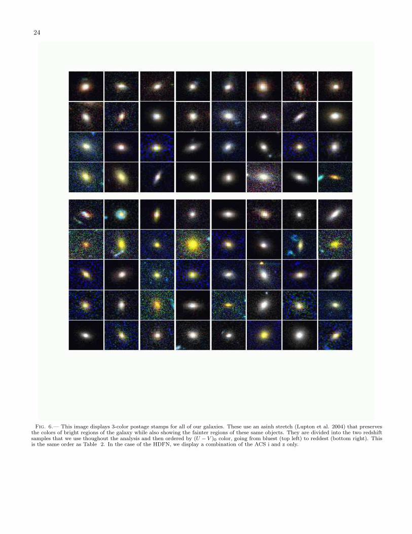
24

Fig. 6.— This image displays 3-color postage stamps for all of our galaxies. These use an asinh stretch (Lupton et al. 2004) that preservesthe colors of bright regions of the galaxy while also showing the fainter regions of these same objects. They are divided into the two redshiftsamples that we use thoughout the analysis and then ordered by (U − V )0 color, going from bluest (top left) to reddest (bottom right). Thisis the same order as Table 2. In the case of the HDFN, we display a combination of the ACS i and z only.

25

-24 -23 -22 -21 -20 -19 -180.4

0.5

0.6

0.7

0.8

0.9

1

1.1

1.2

1.3

1.4

1.5

1.6

1.7

1.8

1.9

2

2.1

2.2

0 5 10 15 20

Number of Galaxies

Fig. 7.— The left-hand panel shows the distribution of rest-frame (U − V )0 color against Mz=0B

for early-type galaxies with 0.5 < z ≤ 0.75

(squares) and 0.75 < z ≤ 1.0 (crosses). The dotted lines represent the Bruzual & Charlot (2003) evolutionary tracks for a 1011M⊙ galaxywith solar metallicity and an exponentially decaying star-formation rate with decay timescales τ = 0.1, 0.2, 0.4, 1.0, 2.0, 5.0, 9.0 Gyr, from leftto right. The filled circles represent the age of the galaxy in these models going from 1 Gyr (largest circle) to 7 Gyr (smallest circle) in stepsof 2 Gyr. The short dashed lines represent the same tracks for a 1012M⊙ galaxy. The tracks allow us to compare the masses of blue galaxiesand red galaxies. The long dashed lines represent the selection criteria used to mimic different color selections employed in the literature.One subsample has (U − V )z=0 > 1.38, to match the CFRS selection and the other has (U − V )z=0 > 1.7 to mimic the selections by theCOMBO-17 and CADIS (Fried et al. 2001) surveys. The right-hand panel shows the histogram in color for the combined sample. Note thesignificant number of E/S0s that are bluer than any of the color selections shown.

26

0.6 0.8 1 1.2 1.4 1.6 1.8 2 2.20

0.2

0.4

0.6

0.8

1

0.2

0.4

0.6

0.8

1

0.02

0.04

0.06

0.08

0.1

0.12

Fig. 8.— This plot shows how the redshift reliability depends on color. The lower panel shows the odds calculated from BPZ against therest-frame (U − V )0 color (see §4, Eqn 9 for a definition of the odds). The squares represent z < 0.75 galaxies and the crosses representz > 0.75 galaxies. This shows that 80% of our objects have good odds, and that the reliability of the redshift does not vary significantly withcolor or redshift. The middle panel splits the distribution into 8 bins of equal number and plots the number of objects with a single peakin the probability density function (dashed histogram); the solid histogram represents those with one narrow dominant peak (i.e one peakmakes up > 90% of the integrated probability) and the dotted histogram includes those with multiple overlapping peaks that are in effect awider peak with > 90% of the integrated probability. While the bluer galaxies have more of the wider peaks objects with a single dominantpeak make up almost 90% of objects for (U − V )0 > 1.2. In the top panel we show the widths of the peaks in the pdf. The open squaresshow the single narrow peaks, the filled squares show the multiple dominant peaks and the filled circles show the mean from the simulationsfor an elliptical (U − V )0 = 1.99, an Sbc (U − V )0 = 1.40 and an Scd (U − V )0 = 1.12.

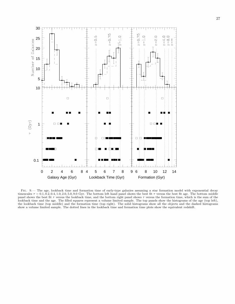
27

0 2 4 6 8

0.1

1

10

Galaxy Age (Gyr)

5

10

15

20

25

30

4 5 6 7 8 9

Lookback Time (Gyr)

6 8 10 12 14

Formation (Gyr)

Fig. 9.— The age, lookback time and formation time of early-type galaxies assuming a star formation model with exponential decaytimescales τ = 0.1, 0.2, 0.4, 1.0, 2.0, 5.0, 9.0 Gyr. The bottom left hand panel shows the best fit τ versus the best fit age. The bottom middlepanel shows the best fit τ versus the lookback time, and the bottom right panel shows τ versus the formation time, which is the sum of thelookback time and the age. The filled squares represent a volume limited sample. The top panels show the histograms of the age (top left),the lookback time (top middle) and the formation time (top right). The solid histograms show all the objects and the dashed histogramsshow a volume limited sample. The dotted lines in the lookback time and formation time plots show the equivalent redshift.

28

1 10 100

0.5

1

1.5

2

Fig. 10.— This plot compares the rest-frame (U − V )0 color to the number of decay timescales (Nτ = T/τ) derived from the Bruzual &Charlot (2003) models. For 1 < Nτ < 10, there is a strong correlation with (U − V )0 = 1.59 log (Nτ ) + 0.38. For Nτ > 10, (U − V )0 ∼ 2.0,the rest-frame color of the ‘El’ template from Benıtez et al. 2004. The long-dashed line indicates the best fit linear correlation (from a simpleleast squares calculation). The dotted lines indicate the color cuts for CFRS ((U −V )0 = 1.38) and COMBO-17 and CADIS ((U −V )0 = 1.7).

29

-23 -22 -21 -20 -19 -18

23

22

21

20

19

18

17

23

22

21

20

19

18

17

Fig. 11.— The distribution of galaxies in the absolute magnitude and surface brightness plane. The size and magnitude limits are shownat both the low and high redshift end of each sample. All objects in the unshaded area are seen over the same volume. All objects in thecross-hatched area are outside the limits of the survey. The singly shaded region denotes parameter space where galaxies cannot be seen tothe maximum redshift. The lower plot shows the 0.5 < z ≤ 0.75 sample and the upper plot shows the 0.75 < z ≤ 1.0 sample. The blueE/S0s are circled. They are not separated from the red E/S0s in MB, µe space.

30

1 2 3 4 5 6 7 8 9 100

2

4

6

8

10

12

14

0

2

4

6

8

10

12

14

Fig. 12.— We plot the distribution in the Sersic parameter β for each sample (dashed histogram). The solid histogram in each panel is thedistribution for equivalent volume limited samples. The distribution of β does not change significantly with redshift. The dotted histogramis the distribution of the ‘blue’ E/S0s. The thick arrow in each panel marks the mean β.

31

0 1 2 3 4 5 6 7 8 9 10 11 120

2

4

6

8

10

12

14

0

2

4

6

8

10

12

14

Fig. 13.— The Sersic parameter β distribution for each sample (dashed histogram). The solid histogram is the distribution of the volumelimited samples and the dotted histogram is the distribution of the ‘blue’ E/S0s. The thick arrow shows the mean value of Re.The shadingrepresents the selection limits in half light radius: the single shading begins at the high-redshift limit of the sample and the cross-hatchingbegins at the low-redshift limit.

32

-0.2 0 0.2 0.4 0.6 0.8 1-23

-22

-21

-20

-22

-21

-20

Fig. 14.— This plot shows the distribution of absolute magnitude (MB) versus the logarithm of half-light radius for both E/S0 subsamplesconsidered in this study. The light shading represents the parts of the parameter space where galaxies cannot be seen out to the maximumredshift, and the heavy shading represents the parameter space where galaxies cannot be seen at all. The dotted line is the z = 0 relationshipfrom Schade et al. (1997) corrected to our cosmology. The dashed line is the expected fit from Schade et al. (1999) for each sample and thesolid line is our best fit in the volume limited region. The circles mark the positions of blue early-type galaxies. Neither type of galaxy showsstrong evidence for a size-magnitude relationship.

33

5 5.5 6 6.5

0

0.5

1

z=0 (Graham 2002)

0 0.2 0.4 0.6 0.8 11

0.5

0

-0.5

-1

-1.5

-2

-2.5

-3

Redshift

Fig. 15.— The lower panel of this plot shows the photometric plane for elliptical galaxies in our fields. The squares denote the 0.5 < z ≤ 0.75sample and the crosses represent the 0.75 < z ≤ 1.0 sample. Our best fit lines are the solid one for 0.75 < z ≤ 1.0 and the long-dashed for0.5 < z ≤ 0.75. The z = 0 fit from Graham (2002) is shown by the short dashed line. The blue galaxies are marked by circles. We find goodfits to the photometric plane although there are a few outliers amongst the blue E/S0 galaxies. In the top panel, we show the variation insurface-brightness with redshift, calculated from this plot. Our points are marked by the squares ringed by large circles. The Schade et al.(1999) results are marked by crosses, the Bernardi et al. (2003) results are marked by squares and the Graham (2002) result is marked withthe triangle. The solid line shows our best fit to these results, and the dashed line is the Gebhardt et al. (2003) best fit.

34

-23 -22 -21 -20 -19 -18

0.0001

0.001

0.01

0.75<z<1.0 LF 0.5<z<0.75 LF

ALL

0.0001

0.001

0.01

0.75<z<1.0 LF 0.5<z<0.75 LF

(U-V)>1.38

0.0001

0.001

0.01

0.75<z<1.0 LF 0.5<z<0.75 LF

(U-V)>1.7

Fig. 16.— The luminosity functions of the 0.5 < z < 0.75 (squares with solid error bars) and the 0.75 < z < 1.0 (triangles dashed error bars)samples. The bright ends are normalized to the volume limited samples and the lines show the Schechter function fits to each set of points.The single shaded hatching denotes the magnitude limit of the 0.75 < z < 1.0 sample and the criss-cross hatching denotes the magnitude limitof the 0.5 < z < 0.75 sample. The lower panel shows the morphologically selected samples, the middle panel shows the two (U − V )0 > 1.38color selected samples and the upper panel shows the two (U − V )0 > 1.7 color selected samples.

35

-23 -22 -21 -20 -19 -18

0.0001

0.001

ACS (0.5<z<0.75) LF

DGSS (0.6<z<1.2) LF

CFRS (0.5<z<0.75) LF

COMBO-17 (0.4<z<0.6) LF

COMBO-17 (0.6<z<0.8) LF

CADIS (0.5<z<0.75) LF

Fig. 17.— The luminosity functions of our 0.5 < z < 0.75 early-types compared to that from previous surveys. The ACS LFs are plottedwith solid lines, with the thickest showing the morphologically selected LF, the medium thick showing the (U − V )0 > 1.38 LF and thethin line the (U − V )0 > 1.7 LF. The points and errorbars are for the morphologically selected sample. The thick dashed line shows themorphologically selected DGSS LF, the medium thick dashed line shows the (U −V )0 > 1.38 selected CFRS LF and the thin dotted or dashedlines show the SED selected COMBO-17 and CADIS LFs. All the luminosity functions have been converted to a Λ-CDM cosmology withH0 = 70 km s−1 Mpc−1.

36

-23 -22 -21 -20 -19

0.0001

0.001

ACS (0.75<z<1.0) LF

DGSS (0.6<z<1.2) LF

CFRS (0.75<z<1.0) LF

COMBO-17 (0.6<z<0.8) LF

COMBO-17 (0.8<z<1.0) LF

CADIS (0.75<z<1.04) LF

Fig. 18.— The luminosity functions of our 0.75 < z < 1.0 early-types compared to that from previous surveys. Otherwise, the same asFig. 17.

37

-23 -22 -21 -20 -19 -18

0.0001

0.001

Fig. 19.— The luminosity functions of our (U − V )0 < 1.7 galaxies. The 0.5 < z < 1.0 LF is shown by square points with the solid linerepresenting the best fit Schechter function, see Table 5.

38

17 18 19 20 21 22 23

0.0001

0.001

0.01

All

17 18 19 20 21 22 23

M<-22

0.0001

0.001

0.01

-22<M<-21 -21<M<-20

0.0001

0.001

0.01

-20<M<-19 -19<M<-18

Fig. 20.— This plot shows the surface brightness distributions as a function of absolute magnitude for the 0.5 < z < 0.75 sample. Thebottom left hand plot shows the surface brightness distribution summed to MB = −18, close to the magnitude limit of the survey. The other5 plots show the surface brightness distribution in small ranges of absolute magnitude. The shading represents the limits at the midpointof all these magnitude ranges. The light shading is the region where the sample volume decreases from the maximum and the dark shadingshows where there sample volume is zero.

39

17 18 19 20 21 22 23

0.0001

0.001

0.01

All

17 18 19 20 21 22 23

M<-22

0.0001

0.001

0.01

-22<M<-21 -21<M<-20

0.0001

0.001

0.01

-20<M<-19

Fig. 21.— This plot shows the surface brightness distributions as a function of absolute magnitude for the 0.75 < z < 1.0 sample. Thebottom left hand plot shows the surface brightness distribution summed to MB = −19. Otherwise, the same as Fig. 20.