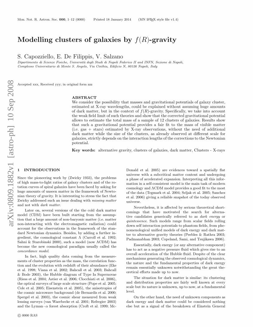
arX

iv:0

809.

1882

v1 [

astr

o-ph

] 1

0 Se

p 20

08Mon. Not. R. Astron. Soc. 000, 1–12 (0000) Printed 18 January 2014 (MN LATEX style file v1.4)

Modelling clusters of galaxies by f(R)-gravity

S. Capozziello, E. De Filippis, V. SalzanoDipartimento di Scienze Fisiche, Universita degli Studi di Napoli Federico II and INFN, Sezione di Napoli,

Complesso Universitario di Monte S. Angelo, Via Cinthia, Edificio N, 80126 Napoli, Italy

Accepted xxx, Received yyy; in original form zzz

ABSTRACT

We consider the possibility that masses and gravitational potentials of galaxy cluster,estimated at X-ray wavelengths, could be explained without assuming huge amountsof dark matter, but in the context of f(R)-gravity. Specifically, we take into accountthe weak field limit of such theories and show that the corrected gravitational potentialallows to estimate the total mass of a sample of 12 clusters of galaxies. Results showthat such a gravitational potential provides a fair fit to the mass of visible matter(i.e. gas + stars) estimated by X-ray observations, without the need of additionaldark matter while the size of the clusters, as already observed at different scale forgalaxies, strictly depends on the interaction lengths of the corrections to the Newtonianpotential.

Key words: alternative gravity, clusters of galaxies, dark matter, Clusters - X-rays

1 INTRODUCTION

Since the pioneering work by (Zwicky 1933), the problemsof high mass-to-light ratios of galaxy clusters and of the ro-tation curves of spiral galaxies have been faced by asking forhuge amounts of unseen matter in the framework of Newto-nian theory of gravity. It is interesting to stress the fact thatZwicky addressed such an issue dealing with missing matter

and not with dark matter.

Later on, several versions of the the cold dark mattermodel (CDM) have been built starting from the assump-tion that a large amount of non-baryonic matter (i.e. matternon-interacting with the electromagnetic radiation) couldaccount for the observations in the framework of the stan-dard Newtonian dynamics. Besides, by adding a further in-gredient, the cosmological constant Λ (Carroll et al. 1992;Sahni & Starobinski 2000), such a model (now ΛCDM) hasbecome the new cosmological paradigm usually called theconcordance model.

In fact, high quality data coming from the measure-ments of cluster properties as the mass, the correlation func-tion and the evolution with redshift of their abundance (Ekeet al. 1998; Viana et al. 2002; Bahcall et al. 2003; Bahcall& Bode 2003), the Hubble diagram of Type Ia Supernovae(Riess et al. 2004; Astier et al. 2006; Clocchiati et al. 2006),the optical surveys of large scale structure (Pope et al. 2005;Cole et al. 2005; Eisenstein et al. 2005), the anisotropies ofthe cosmic microwave background (de Bernardis et al. 2000;Spergel et al. 2003), the cosmic shear measured from weaklensing surveys (van Waerbecke et al. 2001; Refregier 2003)and the Lyman -α forest absorption (Croft et al. 1999; Mc-

Donald et al. 2005) are evidences toward a spatially flatuniverse with a subcritical matter content and undergoinga phase of accelerated expansion. Interpreting all this infor-mation in a self-consistent model is the main task of moderncosmology and ΛCDM model provides a good fit to the mostof the data (Tegmark et al. 2004; Seljak et al. 2005; Sanchezet al. 2006) giving a reliable snapshot of the today observeduniverse.

Nevertheless, it is affected by serious theoretical short-comings that have motivated the search for alterna-tive candidates generically referred to as dark energy orquintessence. Such models range from scalar fields rollingdown self interaction potentials to phantom fields, from phe-nomenological unified models of dark energy and dark mat-ter to alternative gravity theories (Peebles & Rathra 2003;Padmanabhan 2003; Copeland, Sami, and Tsujikawa 2006).

Essentially, dark energy (or any alternative component)has to act as a negative pressure fluid which gives rise to anoverall acceleration of the Hubble fluid. Despite of the clearmechanisms generating the observed cosmological dynamics,the nature and the fundamental properties of dark energyremain essentially unknown notwithstanding the great the-oretical efforts made up to now.

The situation for dark matter is similar: its clusteringand distribution properties are fairly well known at everyscale but its nature is unknown, up to now, at a fundamentallevel.

On the other hand, the need of unknown components asdark energy and dark matter could be considered nothingelse but as a signal of the breakdown of Einstein General

c© 0000 RAS

2 S. Capozziello, E. De Filippis, V. Salzano

Relativity at astrophysical (galactic and extragalactic) andcosmological scales.

In this context, Extended Theories of Gravity could be,in principle, an interesting alternative to explain cosmic ac-celeration without any dark energy and large scale struc-ture without any dark matter. In their simplest version, theRicci curvature scalar R, linear in the Hilbert-Einstein ac-tion, could be replaced by a generic function f(R) whose trueform could be ”reconstructed” by the data. In fact, there isno a priori reason to consider the gravitational Lagrangianlinear in the Ricci scalar while observations and experimentscould contribute to define and constrain the ”true” theoryof gravity. For a discussion on this topic, see (Capozziello& Francaviglia 2008; Nojiri & Odintsov 2007; Sotiriou &Faraoni2008).

In a cosmological framework, such an approach lead tomodified Friedmann equations that can be formally writ-ten in the usual form by defining an effective curvature fluid

giving rise to a negative pressure which drives the cosmic ac-celeration (Capozziello 2002; Capozziello, Carloni and Troisi2003; Carroll et al. 2004; Capozziello & Francaviglia 2008).Also referred to as f(R) theories, this approach is recentlyextensively studied both from the theoretical and the ob-servational point of view (see e.g. (Capozziello et al. 2003;Capozziello, Cardone and Francaviglia 2006; Borowiec, God-lowski and Szydlowski 2006)). Moreover, this same approachhas been also proposed, in early cosmology, as a mechanismgiving rise to an inflationary era without the need of anyinflaton field (Starobinsky 1980).

All this amount of work has been, essentially, concen-trated on the cosmological applications and have convinc-ingly demonstrated that extended theories of gravity (in par-ticular f(R) gravity) are indeed able to explain the cosmicspeed up and fairly fit the available data-sets and, hence,represents a viable alternative to the dark energy models(Capozziello, Cardone and Troisi 2005).

Changing the gravity sector could have consequencesnot only at cosmological scales, but also at the galactic andcluster scales so that it is mandatory to investigate the lowenergy limit of such theories. A strong debate is open withdifferent results arguing in favor (Dick 2004; Sotiriou 2006;Cembranos 2006; Navarro & van Acoleyen 2005; Allemandiet al. 2005; Capozziello & Troisi 2005) or against (Dolgov &Kawasaki2003; Chiba 2003; Olmo 2005) such models. It isworth noting that, as a general result, higher order theoriesof gravity cause the gravitational potential to deviate fromits Newtonian 1/r scaling (Stelle 1978; Kluske & Schmidt1996; Schmidt 2004; Clifton & Barrow 2005; Sobouti 2007;Mendoza & Rosas-Guevara 2007) even if such deviationsmay be vanishing.

In (Capozziello, Cardone and Troisi 2007), the Newto-nian limit of power law f(R) = f0R

n theories has been in-vestigated, assuming that the metric in the low energy limit(Φ/c2 << 1) may be taken as Schwarzschild - like. It turnsout that a power law term (r/rc)

β has to be added to theNewtonian 1/r term in order to get the correct gravitationalpotential. While the parameter β may be expressed analyti-cally as a function of the slope n of the f(R) theory, rc setsthe scale where the correction term starts being significant.A particular range of values of n has been investigated sothat the corrective term is an increasing function of the ra-dius r thus causing an increase of the rotation curve with

respect to the Newtonian one and offering the possibility tofit the galaxy rotation curves without the need of furtherdark matter components.

A set of low surface brightness (LSB) galaxies with ex-tended and well measured rotation curves has been consid-ered (de Blok & Bosma 2002; de Blok 2005). These systemsare supposed to be dark matter dominated, and successfullyfitting data without dark matter is a strong evidence in fa-vor of the approach (see also (Frigerio Martins & Salucci2007) for an independent analysis using another sample ofgalaxies). Combined with the hints coming from the cos-mological applications, one should have, in principle, thepossibility to address both the dark energy and dark matterproblems resorting to the same well motivated fundamen-tal theory (Capozziello, Cardone and Troisi 2006; Koivisto2007; Lobo 2008). Nevertheless, the simple power law f(R)gravity is nothing else but a toy-model which fail if onetries to achieve a comprehensive model for all the cosmolog-ical dynamics, ranging from the early universe, to the largescale structure up to the late accelerated era (Capozziello,Cardone and Troisi 2006; Koivisto 2007).

A fundamental issue is related to clusters and superclus-ters of galaxies. Such structures, essentially, rule the largescale structure, and are the intermediate step between galax-ies and cosmology. As the galaxies, they appear dark-matterdominated but the distribution of dark matter componentseems clustered and organized in a very different way withrespect to galaxies. It seems that dark matter is ruled bythe scale and also its fundamental nature could depend onthe scale. For a comprehensive review see (Bahcall 1996).

In the philosophy of Extended Theories of Gravity, theissue is now to reconstruct the mass profile of clusters with-

out dark matter, i.e. to find out corrections to the Newtonpotential producing the same dynamics as dark matter butstarting from a well motivated theory. This is the goal ofthis paper.

As we will see, the problem is very different with respectto that of galaxies and we need different corrections to thegravitational potential in order to consistently fit the clustermass profiles.

The paper is organized as follows. In Section 2, also re-ferring to other results, we discuss the weak field limit off(R)-gravity showing that an f(R) theory is, in principle,quite fair to address the cluster problem (Lobo 2008). InSection 3, starting from the corrected potential previouslyderived for a point-like masses, we generalize the results toextended spherically symmetric systems as required for wellshaped cluster models of the Bautz and Morgan classifica-tion (Bautz 1970). Section 4 is devoted to the description ofthe general properties of galaxy clusters. In Section 5, thesample of galaxy clusters which we are going to fit is dis-cussed in details. Results are presented in Section 6, whileSection 7 is devoted to the discussion and the conclusions.

2 F (R)-GRAVITY

Let us consider the general action :

A =

∫

d4x√−g [f(R) + XLm] , (1)

c© 0000 RAS, MNRAS 000, 1–12

Modelling clusters of galaxies by f(R)-gravity 3

where f(R) is an analytic function of the Ricci scalar R, g

is the determinant of the metric gµν , X =16πG

c4is the cou-

pling constant and Lm is the standard perfect-fluid matterLagrangian. Such an action is the straightforward general-ization of the Hilbert-Einstein action of GR obtained forf(R) = R. Since we are considering the metric approach,field equations are obtained by varying (1) with respect tothe metric :

f ′Rµν − 1

2fgµν − f ′

;µν + gµνf ′ =X2

Tµν . (2)

where Tµν = −2√−g

δ(√

−gLm)δgµν is the energy momentum tensor

of matter, the prime indicates the derivative with respect toR and = ;σ

;σ. We adopt the signature (+,−,−,−).

As discussed in details in (Capozziello, Stabile andTroisi 2008a), we deal with the Newtonian and the post-Newtonian limit of f(R) - gravity on a spherically sym-metric background. Solutions for the field equations can beobtained by imposing the spherical symmetry (Capozziello,Stabile and Troisi 2007b):

ds2 = g00(x0, r)dx02

+ grr(x0, r)dr2 − r2dΩ (3)

where x0 = ct and dΩ is the angular element.

To develop the post-Newtonian limit of the theory, onecan consider a perturbed metric with respect to a Minkowskibackground gµν = ηµν +hµν . The metric coefficients can bedeveloped as:

gtt(t, r) ≃ 1 + g(2)tt (t, r) + g

(4)tt (t, r)

grr(t, r) ≃ −1 + g(2)rr (t, r)

gθθ(t, r) = −r2

gφφ(t, r) = −r2 sin2 θ

, (4)

where we put, for the sake of simplicity, c = 1 , x0 = ct → t.We want to obtain the most general result without imposingparticular forms for the f(R)-Lagrangian. We only consideranalytic Taylor expandable functions

f(R) ≃ f0 + f1R + f2R2 + f3R

3 + ... . (5)

To obtain the post-Newtonian approximation of f(R) - grav-ity, one has to plug the expansions (4) and (5) into the fieldequations (2) and then expand the system up to the ordersO(0), O(2) and O(4) . This approach provides general re-sults and specific (analytic) Lagrangians are selected by thecoefficients fi in (5) (Capozziello, Stabile and Troisi 2008a).

If we now consider the O(2) - order of approximation,the field equations (2), in the vacuum case, results to be

f1rR(2) − 2f1g

(2)tt,r + 8f2R

(2),r − f1rg

(2)tt,rr + 4f2rR

(2) = 0

f1rR(2) − 2f1g

(2)rr,r + 8f2R

(2),r − f1rg

(2)tt,rr = 0

2f1g(2)rr − r[f1rR

(2)

−f1g(2)tt,r − f1g

(2)rr,r + 4f2R

(2),r + 4f2rR

(2),rr] = 0

f1rR(2) + 6f2[2R

(2),r + rR

(2),rr] = 0

2g(2)rr + r[2g

(2)tt,r − rR(2) + 2g

(2)rr,r + rg

(2)tt,rr] = 0

(6)

It is evident that the trace equation (the fourth in the sys-tem (6)), provides a differential equation with respect to theRicci scalar which allows to solve the system at O(2) - order.One obtains the general solution :

g(2)tt = δ0 − 2GM

f1r− δ1(t)e−r

√−ξ

3ξr+ δ2(t)er

√−ξ

6(−ξ)3/2r

g(2)rr = − 2GM

f1r+

δ1(t)[r√

−ξ+1]e−r√

−ξ

3ξr− δ2(t)[ξr+

√−ξ]er

√−ξ

6ξ2r

R(2) = δ1(t)e−r√

−ξ

r− δ2(t)

√−ξer

√−ξ

2ξr

(7)

where ξ.=

f1

6f2, f1 and f2 are the expansion coefficients

obtained by the f(R)-Taylor series. In the limit f → R,for a point-like source of mass M we recover the standardSchwarzschild solution. Let us notice that the integrationconstant δ0 is dimensionless, while the two arbitrary time-functions δ1(t) and δ2(t) have respectively the dimensionsof lenght−1 and lenght−2; ξ has the dimension lenght−2.As extensively discussed in (Capozziello, Stabile and Troisi2008a), the functions δi(t) (i = 1, 2) are completely arbitrarysince the differential equation system (6) depends only onspatial derivatives. Besides, the integration constant δ0 canbe set to zero, as in the standard theory of potential, sinceit represents an unessential additive quantity. In order toobtain the physical prescription of the asymptotic flatnessat infinity, we can discard the Yukawa growing mode in (7)and then the metric is :

ds2 =

[

1 − 2GM

f1r− δ1(t)e

−r√

−ξ

3ξr

]

dt2

−[

1 +2GM

f1r− δ1(t)(r

√−ξ + 1)e−r√

−ξ

3ξr

]

dr2

− r2dΩ . (8)

The Ricci scalar curvature is

R =δ1(t)e

−r√

−ξ

r. (9)

The solution can be given also in terms of gravitationalpotential. In particular, we have an explicit Newtonian-liketerm into the definition. The first of (7) provides the secondorder solution in term of the metric expansion (see the defini-

tion (4)). In particular, it is gtt = 1+2φgrav = 1+g(2)tt and

then the gravitational potential of an analytic f(R)-theoryis

c© 0000 RAS, MNRAS 000, 1–12

4 S. Capozziello, E. De Filippis, V. Salzano

φgrav = −GM

f1r− δ1(t)e

−r√

−ξ

6ξr. (10)

Among the possible analytic f(R)-models, let us considerthe Taylor expansion where the cosmological term (theabove f0) and terms higher than second have been discarded.We rewrite the Lagrangian (5) as

f(R) ∼ a1R + a2R2 + ... (11)

and specify the above gravitational potential (10), generatedby a point-like matter distribution, as:

φ(r) = −3GM

4a1r

(

1 +1

3e−

rL

)

, (12)

where

L ≡ L(a1, a2) =(

−6a2

a1

)1/2

. (13)

L can be defined as the interaction length of the problem⋆

due to the correction to the Newtonian potential. We havechanged the notation to remark that we are doing only aspecific choice in the wide class of potentials (10), but thefollowing considerations are completely general.

3 EXTENDED SYSTEMS

The gravitational potential (12) is a point-like one. Now wehave to generalize this solution to extended systems. Let usdescribe galaxy clusters as spherically symmetric systemsand then we have to extend the above considerations to thisgeometrical configuration. We simply consider the systemcomposed by many infinitesimal mass elements dm each onecontributing with a point-like gravitational potential. Then,summing up all terms, namely integrating them on a spher-ical volume, we obtain a suitable potential. Specifically, wehave to solve the integral:

Φ(r) =

∫ ∞

0

r′2dr′∫ π

0

sin θ′dθ′∫ 2π

0

dω′ φ(r′) . (14)

The point-like potential (12)can be split in two terms. TheNewtonian component is

φN(r) = −3GM

4a1r(15)

The extended integral of such a part is well-known (apartfrom the numerical constant 3

4a1) expression. It is

ΦN (r) = − 3

4a1

GM(< r)

r(16)

where M(< r) is the mass enclosed in a sphere with radiusr. The correction term

φC(r) = −GM

4a1

e−rL

r(17)

considering some analytical steps in the integration of theangular part, give the expression

⋆ Such a length is function of the series coefficients, a1 and a2,and it is not a free independent parameter in the following fitprocedure.

ΦC(r) = −2πG

4· L∫ ∞

0

dr′r′ρ(r′) · e−|r−r′ |

L − e−|r+r′|

L

r(18)

The radial integral is numerically estimated once the massdensity is given. We underline a fundamental difference be-tween such a term and the Newtonian one: while in the lat-ter, the matter outside the spherical shell of radius r doesnot contribute to the potential, in the former, external mat-ter takes part to the integration procedure. For this reasonwe split the corrective potential in two terms:

• if r′ < r:

ΦC,int(r)=−2πG

4· L∫ r

0

dr′r′ρ(r′) · e−|r−r′|

L − e−|r+r′|

L

r

=−2πG

4· L∫ r

0

dr′r′ρ(r′) · e−r+r′

L

(

−1 + e2r′

L

r

)

• if r′ > r:

ΦC,ext(r)=−2πG

4· L∫ ∞

r

dr′r′ρ(r′) · e−|r−r′|

L − e−|r+r′|

L

r=

=−2πG

4· L∫ ∞

r

dr′r′ρ(r′) · e−r+r′

L

(

−1 + e2rL

r

)

The total potential of the spherical mass distribution will be

Φ(r) = ΦN (r) + ΦC,int(r) + ΦC,ext(r) (19)

As we will show below, for our purpose, we need the gravi-tational potential derivative with respect to the variable r;the two derivatives may not be evaluated analytically so weestimate them numerically, once we have given an expres-sion for the total mass density ρ(r). While the Newtonianterm gives the simple expression:

−dΦN

dr(r) = − 3

4a1

GM(< r)

r2(20)

the internal and external derivatives of the corrective poten-tial terms are more involved. We do not give them explicitlyfor sake of brevity, but they are integral-functions of theform

F(r, r′) =

∫ β(r)

α(r)

dr′ f(r, r′) (21)

from which one has:

dF(r, r′)

dr=

∫ β(r)

α(r)

dr′df(r, r′)

dr+

−f(r, α(r))dα

dr(r) + f(r, β(r))

dβ

dr(r) (22)

Such an expression is numerically derived once the integra-tion extremes are given. A general consideration is in orderat this point. Clearly, the Gauss theorem holds only for theNewtonian part since, for this term, the force law scales as1/r2. For the total potential (12), it does not hold anymoredue to the correction. From a physical point of view, this isnot a problem because the full conservation laws are deter-mined, for f(R)-gravity, by the contracted Bianchi identitieswhich assure the self-consistency. For a detailed discussion,see (Capozziello, Cardone and Troisi 2007; Capozziello &Francaviglia 2008; Sotiriou & Faraoni2008).

c© 0000 RAS, MNRAS 000, 1–12

Modelling clusters of galaxies by f(R)-gravity 5

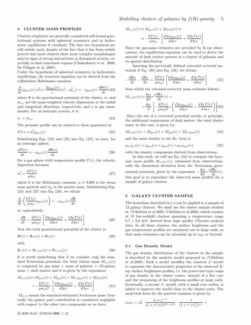
4 CLUSTER MASS PROFILES

Clusters of galaxies are generally considered self-bound grav-itational systems with spherical symmetry and in hydro-static equilibrium if virialized. The last two hypothesis arestill widely used, despite of the fact that it has been widelyproved that most clusters show more complex morphologiesand/or signs of strong interactions or dynamical activity, es-pecially in their innermost regions (Chakrabarty et al. 2008;De Filippis et al. 2005).Under the hypothesis of spherical symmetry in hydrostaticequilibrium, the structure equation can be derived from thecollisionless Boltzmann equation

d

dr(ρgas(r) σ2

r)+2ρgas(r)

r(σ2

r −σ2θ,ω) = −ρgas(r)·

dΦ(r)

dr(23)

where Φ is the gravitational potential of the cluster, σr andσθ,ω are the mass-weighted velocity dispersions in the radialand tangential directions, respectively, and ρ is gas mass-density. For an isotropic system, it is

σr = σθ,ω (24)

The pressure profile can be related to these quantities by

P (r) = σ2rρgas(r) (25)

Substituting Eqs. (24) and (25) into Eq. (23), we have, foran isotropic sphere,

dP (r)

dr= −ρgas(r)

dΦ(r)

dr(26)

For a gas sphere with temperature profile T (r), the velocitydispersion becomes

σ2r =

kT (r)

µmp(27)

where k is the Boltzmann constant, µ ≈ 0.609 is the meanmass particle and mp is the proton mass. Substituting Eqs.(25) and (27) into Eq. (26), we obtain

d

dr

(

kT (r)

µmpρgas(r)

)

= −ρgas(r)dΦ

dr

or, equivalently,

−dΦ

dr=

kT (r)

µmpr

[

d ln ρgas(r)

d ln r+

d lnT (r)

d ln r

]

(28)

Now the total gravitational potential of the cluster is:

Φ(r) = ΦN (r) + ΦC(r) (29)

with

ΦC(r) = ΦC,int(r) + ΦC,ext(r) (30)

It is worth underlining that if we consider only the stan-dard Newtonian potential, the total cluster mass Mcl,N (r)is composed by gas mass + mass of galaxies + cD-galaxymass + dark matter and it is given by the expression:

Mcl,N (r)=Mgas(r) + Mgal(r) + MCDgal(r) + MDM (r)

=− kT (r)

µmpGr

[

d ln ρgas(r)

d ln r+

d ln T (r)

d ln r

]

(31)

Mcl,N means the standard estimated Newtonian mass. Gen-erally the galaxy part contribution is considered negligiblewith respect to the other two components so we have:

Mcl,N(r) ≈ Mgas(r) + MDM (r) ≈

≈ −kT (r)

µmpr

[

d ln ρgas(r)

d ln r+

d lnT (r)

d ln r

]

Since the gas-mass estimates are provided by X-ray obser-vations, the equilibrium equation can be used to derive theamount of dark matter present in a cluster of galaxies andits spatial distribution.

Inserting the previously defined extended-corrected po-tential of Eq. (29) into Eq. (28), we obtain:

−dΦN

dr− dΦC

dr=

kT (r)

µmpr

[

d ln ρgas(r)

d ln r+

d ln T(r)

d ln r

]

(32)

from which the extended-corrected mass estimate follows:

Mcl,EC(r)+4a1

3Gr2 dΦC

dr(r) =

=4a1

3

[

− kT (r)

µmpGr

(

d ln ρgas(r)

d ln r+

d ln T (r)

d ln r

)]

(33)

Since the use of a corrected potential avoids, in principle,the additional requirement of dark matter, the total clustermass, in this case, is given by:

Mcl,EC(r) = Mgas(r) + Mgal(r) + MCDgal(r) (34)

and the mass density in the ΦC term is

ρcl,EC(r) = ρgas(r) + ρgal(r) + ρCDgal(r) (35)

with the density components derived from observations.In this work, we will use Eq. (33) to compare the bary-

onic mass profile Mcl,EC(r), estimated from observations,with the theoretical deviation from the Newtonian gravi-

tational potential, given by the expression −4a1

3Gr2 dΦC

dr(r).

Our goal is to reproduce the observed mass profiles for asample of galaxy clusters.

5 GALAXY CLUSTER SAMPLE

The formalism described in § 4 can be applied to a sample of12 galaxy clusters. We shall use the cluster sample studiedin (Vikhlinin et al.2005; Vikhlinin et al.2006) which consistsof 13 low-redshift clusters spanning a temperature range0.7 ÷ 9.0 keV derived from high quality Chandra archivaldata. In all these clusters, the surface brightness and thegas temperature profiles are measured out to large radii, sothat mass estimates can be extended up to r500 or beyond.

5.1 Gas Density Model

The gas density distribution of the clusters in the sampleis described by the analytic model proposed in (Vikhlininet al.2006). Such a model modifies the classical β−modelto represent the characteristic properties of the observed X-ray surface brightness profiles, i.e. the power-law-type cuspsof gas density in the cluster center, instead of a flat coreand the steepening of the brightness profiles at large radii.Eventually, a second β−model, with a small core radius, isadded to improve the model close to the cluster cores. Theanalytical form for the particle emission is given by:

npne = n20 · (r/rc)

−α

(1 + r2/r2c )3β−α/2

· 1

(1 + rγ/rγs )ǫ/γ

+

c© 0000 RAS, MNRAS 000, 1–12

6 S. Capozziello, E. De Filippis, V. Salzano

+n2

02

(1 + r2/r2c2)

3β2(36)

which can be easily converted to a mass density using therelation:

ρgas = nT · µmp =1.4

1.2nemp (37)

where nT is the total number density of particles in the gas.The resulting model has a large number of parameters, someof which do not have a direct physical interpretation. Whilethis can often be inappropriate and computationally incon-venient, it suits well our case, where the main requirementis a detailed qualitative description of the cluster profiles.In (Vikhlinin et al.2006), Eq. (36) is applied to a restrictedrange of distances from the cluster center, i.e. between aninner cutoff rmin, chosen to exclude the central tempera-ture bin (≈ 10 ÷ 20 kpc) where the ICM is likely to bemulti-phase, and rdet, where the X-ray surface brightnessis at least 3σ significant. We have extrapolated the abovefunction to values outside this restricted range using thefollowing criteria:

• for r < rmin, we have performed a linear extrapolationof the first three terms out to r = 0 kpc;

• for r > rdet, we have performed a linear extrapolation ofthe last three terms out to a distance r for which ρgas(r) =ρc, ρc being the critical density of the Universe at the clusterredshift: ρc = ρc,0 · (1 + z)3. For radii larger than r, the gasdensity is assumed constant at ρgas(r).

We point out that, in Table 1, the radius limit rmin is almostthe same as given in the previous definition. When the valuegiven by (Vikhlinin et al.2006) is less than the cD-galaxy ra-dius, which is defined in the next section, we choose this lastone as the lower limit. On the contrary, rmax is quite differ-ent from rdet: it is fixed by considering the higher value oftemperature profile and not by imaging methods.We then compute the gas mass Mgas(r) and the total massMcl,N (r), respectively, for all clusters in our sample, sub-stituting Eq. (36) into Eqs. (37) and (31), respectively; thegas temperature profile is described in details in § 5.2. Theresulting mass values, estimated at r = rmax, are listed inTable 1.

5.2 Temperature Profiles

As stressed in § 5.1, for the purpose of this work, we needan accurate qualitative description of the radial behavior ofthe gas properties. Standard isothermal or polytropic mod-els, or even the more complex one proposed in (Vikhlinin etal.2006), do not provide a good description of the data at allradii and for all clusters in the present sample. We hence de-scribe the gas temperature profiles using the straightforwardX-ray spectral analysis results, without the introduction ofany analytic model.X-ray spectral values have been provided by A. Vikhlinin(private communication). A detailed description of the rela-tive spectral analysis can be found in (Vikhlinin et al.2005).

5.3 Galaxy Distribution Model

The galaxy density can be modelled as proposed by (Bahcall1996). Even if the galaxy distribution is a point-distribution

100 150 200 300 500 700 1000 1500

R H Kpc L

1. ´ 1012

1. ´ 1013

1. ´ 1014

MH

ML

Figure 1. Matter components for A478: total Newtonian dynam-ical mass (continue line); gas mass (dashed line); galactic mass(dotted-dashed line); cD-galaxy mass (dotted line).

instead of a continuous function, assuming that galaxies arein equilibrium with gas, we can use a β−model, ∝ r−3, forr < Rc from the cluster center, and a steeper one, ∝ r−2.6,for r > Rc, where Rc is the cluster core radius (its value istaken from Vikhlinin 2006). Its final expression is:

ρgal(r) =

ρgal,1 ·[

1 +(

rRc

)2]− 3

2

r < Rc

ρgal,2 ·[

1 +(

rRc

)2]− 2.6

2

r > Rc

(38)

where the constants ρgal,1 and ρgal,2 are chosen in the fol-lowing way:

• (Bahcall 1996) provides the central number density ofgalaxies in rich compact clusters for galaxies located within a1.5 h−1Mpc radius from the cluster center and brighter thanm3 + 2m (where m3 is the magnitude of the third brightestgalaxy): ngal,0 ∼ 103h3 galaxies Mpc−3. Then we fix ρgal,1

in the range ∼ 1034 ÷ 1036 kg/kpc3. For any cluster obeyingthe condition chosen for the mass ratio gal-to-gas, we assumea typical elliptical and cD galaxy mass in the range 1012 ÷1013M⊙.

• the constant ρgal,2 has been fixed with the only require-ment that the galaxy density function has to be continuousat Rc.

We have tested the effect of varying galaxy density in theabove range ∼ 1034 ÷ 1036 kg/kpc3 on the cluster with thelowest mass, namely A262. In this case, we would expectgreat variations with respect to other clusters; the result isthat the contribution due to galaxies and cD-galaxy gives avariation ≤ 1% to the final estimate of fit parameters.The cD galaxy density has been modelled as described in(Schmidt 2006); they use a Jaffe model of the form:

ρCDgal =ρ0,J

(

rrc

)2 (

1 + rrc

)2(39)

where rc is the core radius while the central density is ob-

tained from MJ =4

3πR3

cρ0,J . The mass of the cD galaxy

has been fixed at 1.14 × 1012 M⊙, with rc = Re/0.76, withRe = 25 kpc being the effective radius of the galaxy. Thecentral galaxy for each cluster in the sample is assumed tohave approximately this stellar mass.

c© 0000 RAS, MNRAS 000, 1–12

Modelling clusters of galaxies by f(R)-gravity 7

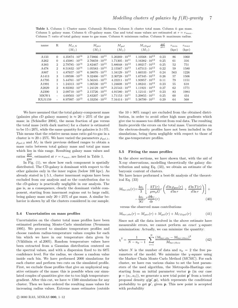
Table 1. Column 1: Cluster name. Column2: Richness. Column 3: cluster total mass. Column 4: gas mass.Column 5: galaxy mass. Column 6: cD-galaxy mass. Gas and total mass values are estimated at r = rmax.Column 7: ratio of total galaxy mass to gas mass. Column 8: minimum radius. Column 9: maximum radius.

name R Mcl,N Mgas Mgal McDgalgalgas

rmin rmax

(M⊙) (M⊙) (M⊙) (M⊙) (kpc) (kpc)

A133 0 4.35874 · 1014 2.73866 · 1013 5.20269 · 1012 1.10568 · 1012 0.23 86 1060A262 0 4.45081 · 1013 2.76659 · 1012 1.71305 · 1011 5.16382 · 1012 0.25 61 316A383 2 2.79785 · 1014 2.82467 · 1013 5.88048 · 1012 1.09217 · 1012 0.25 52 751A478 2 8.51832 · 1014 1.05583 · 1014 2.15567 · 1013 1.67513 · 1012 0.22 59 1580A907 1 4.87657 · 1014 6.38070 · 1013 1.34129 · 1013 1.66533 · 1012 0.24 563 1226A1413 3 1.09598 · 1015 9.32466 · 1013 2.30728 · 1013 1.67345 · 1012 0.26 57 1506A1795 2 5.44761 · 1014 5.56245 · 1013 4.23211 · 1012 1.93957 · 1012 0.11 79 1151A1991 1 1.24313 · 1014 1.00530 · 1013 1.24608 · 1012 1.08241 · 1012 0.23 55 618A2029 2 8.92392 · 1014 1.24129 · 1014 3.21543 · 1013 1.11921 · 1012 0.27 62 1771A2390 1 2.09710 · 1015 2.15726 · 1014 4.91580 · 1013 1.12141 · 1012 0.23 83 1984MKW4 - 4.69503 · 1013 2.83207 · 1012 1.71153 · 1011 5.29855 · 1011 0.25 60 434

RXJ1159 - 8.97997 · 1013 4.33256 · 1012 7.34414 · 1011 5.38799 · 1011 0.29 64 568

We have assumed that the total galaxy-component mass(galaxies plus cD galaxy masses) is ≈ 20 ÷ 25% of the gasmass: in (Schindler 2004), the mean fraction of gas versusthe total mass (with dark matter) for a cluster is estimatedto be 15÷20%, while the same quantity for galaxies is 3÷5%.This means that the relative mean mass ratio gal-to-gas in acluster is ≈ 20÷25%. We have varied the parameters ρgal,1,ρgal,2 and MJ in their previous defined ranges to obtain amass ratio between total galaxy mass and total gas masswhich lies in this range. Resulting galaxy mass values and

ratiosgal

gas, estimated at r = rmax, are listed in Table 1.

In Fig. (1), we show how each component is spatiallydistributed. The CD-galaxy is dominant with respect to theother galaxies only in the inner region (below 100 kpc). Asalready stated in § 5.1, cluster innermost regions have beenexcluded from our analysis and so the contribution due tothe cD-galaxy is practically negligible in our analysis. Thegas is, as a consequence, clearly the dominant visible com-ponent, starting from innermost regions out to large radii,being galaxy mass only 20÷ 25% of gas mass. A similar be-havior is shown by all the clusters considered in our sample.

5.4 Uncertainties on mass profiles

Uncertainties on the cluster total mass profiles have beenestimated performing Monte-Carlo simulations (Neumann1995). We proceed to simulate temperature profiles andchoose random radius-temperature values couples for eachbin which we have in our temperature data given by(Vikhlinin et al.2005). Random temperature values havebeen extracted from a Gaussian distribution centered onthe spectral values, and with a dispersion fixed to its 68%confidence level. For the radius, we choose a random valueinside each bin. We have performed 2000 simulations foreach cluster and perform two cuts on the simulated profile.First, we exclude those profiles that give an unphysical neg-ative estimate of the mass: this is possible when our simu-lated couples of quantities give rise to too high temperature-gradient. After this cut, we have ≈ 1500 simulations for anycluster. Then we have ordered the resulting mass values forincreasing radius values. Extreme mass estimates (outside

the 10 ÷ 90% range) are excluded from the obtained distri-bution, in order to avoid other high mass gradients whichgive rise to masses too different from real data. The resultinglimits provide the errors on the total mass. Uncertainties onthe electron-density profiles have not been included in thesimulations, being them negligible with respect to those ofthe gas-temperature profiles.

5.5 Fitting the mass profiles

In the above sections, we have shown that, with the aid ofX-ray observations, modelling theoretically the galaxy dis-tribution and using Eq. (33), we obtain an estimate of thebaryonic content of clusters.We have hence performed a best-fit analysis of the theoret-ical Eq. (33)

Mbar,th(r)=4a1

3

[

− kT (r)

µmpGr

(

d ln ρgas(r)

d ln r+

d ln T (r)

d ln r

)]

+

− 4a1

3Gr2 dΦC

dr(r) (40)

versus the observed mass contributions

Mbar,obs(r) = Mgas(r) + Mgal(r) + MCDgal(r) (41)

Since not all the data involved in the above estimate havemeasurable errors, we cannot perform an exact χ-squareminimization: Actually, we can minimize the quantity:

χ2 =1

N − np − 1·

N∑

i=1

(Mbar,obs − Mbar,theo)2

Mbar,theo(42)

where N is the number of data and np = 2 the free pa-rameters of the model. We minimize the χ-square usingthe Markov Chain Monte Carlo Method (MCMC). For eachcluster, we have run various chains to set the best param-eters of the used algorithm, the Metropolis-Hastings one:starting from an initial parameter vector p (in our casep = (a1, a2)), we generate a new trial point p′ from a testedproposal density q(p′, p), which represents the conditionalprobability to get p′, given p. This new point is acceptedwith probability

c© 0000 RAS, MNRAS 000, 1–12

8 S. Capozziello, E. De Filippis, V. Salzano

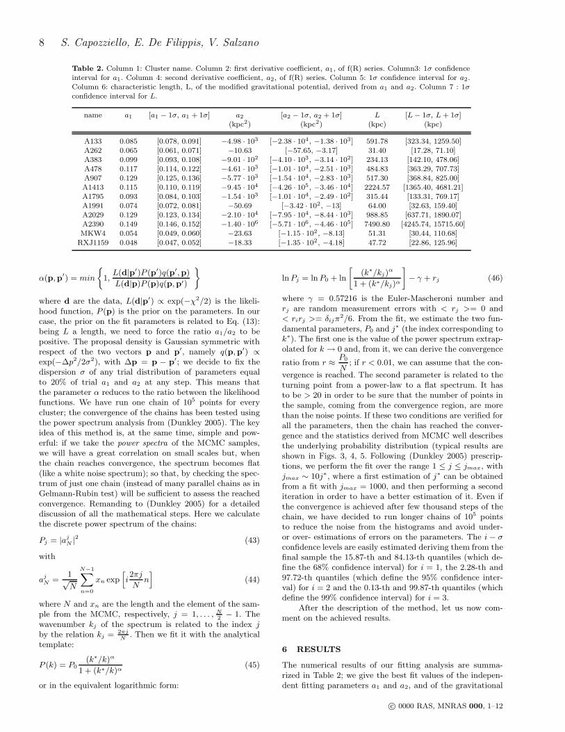
Table 2. Column 1: Cluster name. Column 2: first derivative coefficient, a1, of f(R) series. Column3: 1σ confidenceinterval for a1. Column 4: second derivative coefficient, a2, of f(R) series. Column 5: 1σ confidence interval for a2.Column 6: characteristic length, L, of the modified gravitational potential, derived from a1 and a2. Column 7 : 1σconfidence interval for L.

name a1 [a1 − 1σ, a1 + 1σ] a2 [a2 − 1σ, a2 + 1σ] L [L − 1σ, L + 1σ](kpc2) (kpc2) (kpc) (kpc)

A133 0.085 [0.078, 0.091] −4.98 · 103 [−2.38 · 104, −1.38 · 103] 591.78 [323.34, 1259.50]A262 0.065 [0.061, 0.071] −10.63 [−57.65, −3.17] 31.40 [17.28, 71.10]A383 0.099 [0.093, 0.108] −9.01 · 102 [−4.10 · 103, −3.14 · 102] 234.13 [142.10, 478.06]A478 0.117 [0.114, 0.122] −4.61 · 103 [−1.01 · 104, −2.51 · 103] 484.83 [363.29, 707.73]A907 0.129 [0.125, 0.136] −5.77 · 103 [−1.54 · 104, −2.83 · 103] 517.30 [368.84, 825.00]A1413 0.115 [0.110, 0.119] −9.45 · 104 [−4.26 · 105, −3.46 · 104] 2224.57 [1365.40, 4681.21]A1795 0.093 [0.084, 0.103] −1.54 · 103 [−1.01 · 104, −2.49 · 102] 315.44 [133.31, 769.17]A1991 0.074 [0.072, 0.081] −50.69 [−3.42 · 102, −13] 64.00 [32.63, 159.40]A2029 0.129 [0.123, 0.134] −2.10 · 104 [−7.95 · 104, −8.44 · 103] 988.85 [637.71, 1890.07]A2390 0.149 [0.146, 0.152] −1.40 · 106 [−5.71 · 106, −4.46 · 105] 7490.80 [4245.74, 15715.60]MKW4 0.054 [0.049, 0.060] −23.63 [−1.15 · 102, −8.13] 51.31 [30.44, 110.68]

RXJ1159 0.048 [0.047, 0.052] −18.33 [−1.35 · 102, −4.18] 47.72 [22.86, 125.96]

α(p,p′) = min

1,L(d|p′)P (p′)q(p′,p)

L(d|p)P (p)q(p,p′)

where d are the data, L(d|p′) ∝ exp(−χ2/2) is the likeli-hood function, P (p) is the prior on the parameters. In ourcase, the prior on the fit parameters is related to Eq. (13):being L a length, we need to force the ratio a1/a2 to bepositive. The proposal density is Gaussian symmetric withrespect of the two vectors p and p′, namely q(p,p′) ∝exp(−∆p2/2σ2), with ∆p = p − p′; we decide to fix thedispersion σ of any trial distribution of parameters equalto 20% of trial a1 and a2 at any step. This means thatthe parameter α reduces to the ratio between the likelihoodfunctions. We have run one chain of 105 points for everycluster; the convergence of the chains has been tested usingthe power spectrum analysis from (Dunkley 2005). The keyidea of this method is, at the same time, simple and pow-erful: if we take the power spectra of the MCMC samples,we will have a great correlation on small scales but, whenthe chain reaches convergence, the spectrum becomes flat(like a white noise spectrum); so that, by checking the spec-trum of just one chain (instead of many parallel chains as inGelmann-Rubin test) will be sufficient to assess the reachedconvergence. Remanding to (Dunkley 2005) for a detaileddiscussion of all the mathematical steps. Here we calculatethe discrete power spectrum of the chains:

Pj = |ajN |2 (43)

with

ajN =

1√N

N−1∑

n=0

xn exp[

i2πj

Nn]

(44)

where N and xn are the length and the element of the sam-ple from the MCMC, respectively, j = 1, . . . , N

2− 1. The

wavenumber kj of the spectrum is related to the index jby the relation kj = 2πj

N. Then we fit it with the analytical

template:

P (k) = P0(k∗/k)α

1 + (k∗/k)α(45)

or in the equivalent logarithmic form:

ln Pj = ln P0 + ln

[

(k∗/kj)α

1 + (k∗/kj)α

]

− γ + rj (46)

where γ = 0.57216 is the Euler-Mascheroni number andrj are random measurement errors with < rj >= 0 and< rirj >= δijπ

2/6. From the fit, we estimate the two fun-damental parameters, P0 and j∗ (the index corresponding tok∗). The first one is the value of the power spectrum extrap-olated for k → 0 and, from it, we can derive the convergence

ratio from r ≈ P0

N; if r < 0.01, we can assume that the con-

vergence is reached. The second parameter is related to theturning point from a power-law to a flat spectrum. It hasto be > 20 in order to be sure that the number of points inthe sample, coming from the convergence region, are morethan the noise points. If these two conditions are verified forall the parameters, then the chain has reached the conver-gence and the statistics derived from MCMC well describesthe underlying probability distribution (typical results areshown in Figs. 3, 4, 5. Following (Dunkley 2005) prescrip-tions, we perform the fit over the range 1 ≤ j ≤ jmax, withjmax ∼ 10j∗, where a first estimation of j∗ can be obtainedfrom a fit with jmax = 1000, and then performing a seconditeration in order to have a better estimation of it. Even ifthe convergence is achieved after few thousand steps of thechain, we have decided to run longer chains of 105 pointsto reduce the noise from the histograms and avoid under-or over- estimations of errors on the parameters. The i − σconfidence levels are easily estimated deriving them from thefinal sample the 15.87-th and 84.13-th quantiles (which de-fine the 68% confidence interval) for i = 1, the 2.28-th and97.72-th quantiles (which define the 95% confidence inter-val) for i = 2 and the 0.13-th and 99.87-th quantiles (whichdefine the 99% confidence interval) for i = 3.

After the description of the method, let us now com-ment on the achieved results.

6 RESULTS

The numerical results of our fitting analysis are summa-rized in Table 2; we give the best fit values of the indepen-dent fitting parameters a1 and a2, and of the gravitational

c© 0000 RAS, MNRAS 000, 1–12

Modelling clusters of galaxies by f(R)-gravity 9

length L, considered as a function of the previous two quan-tities. In Figs. 3- 5, we give the typical results of fitting, withhistograms and power spectrum of samples derived by theMCMC, to assess the reached convergence (flat spectrum atlarge scales).

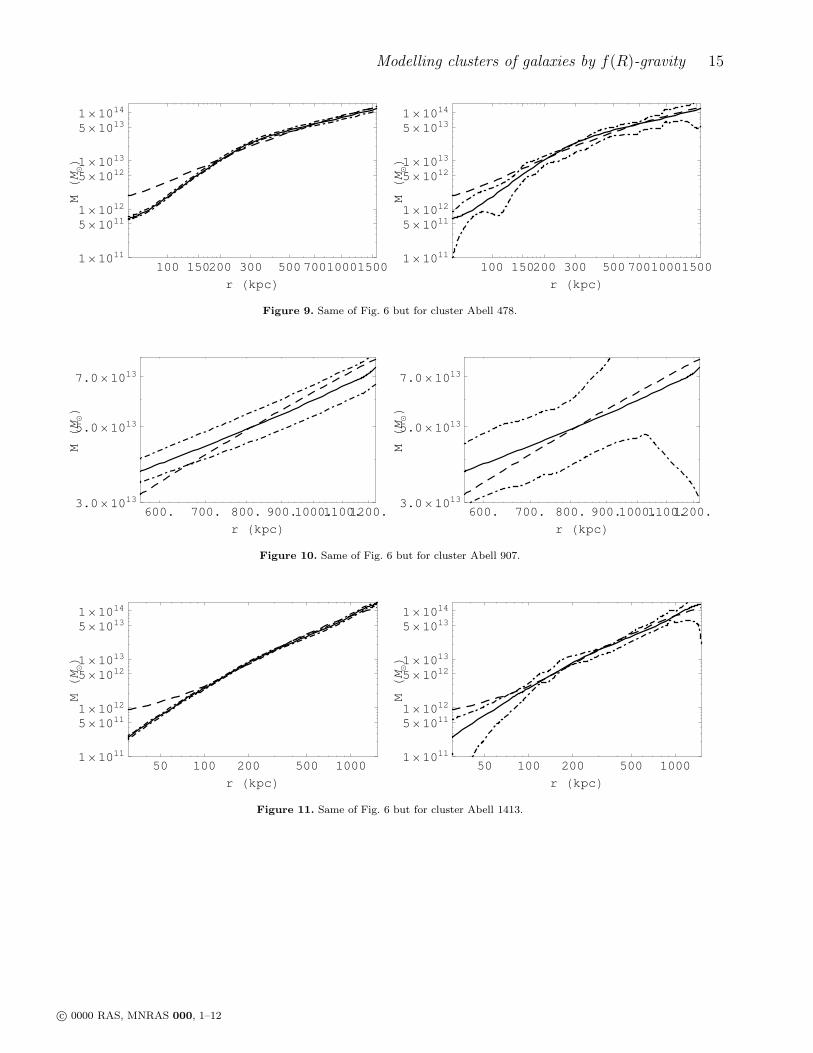
The goodness and the properties of the fits are shown inFigs. 6- 17. The main property of our results is the presenceof a typical scale for each cluster above which our modelworks really well (typical relative differences are less than5%), while for lower scale there is a great difference. It ispossible to see, by a rapid inspection, that this turning-pointis located at a radius ≈ 150 kpc. Except for extremely richclusters, it is clear that this value is independent of the clus-ter, being similar for all clusters in our sample.

There are two main independent explanations thatcould justify this trend: limits due to a break in the state ofhydrostatic equilibrium or limits in the series expansion ofthe f(R)-models.

If the hypothesis of hydrostatic equilibrium is not cor-rect, then we are in a regime where the fundamental relationsEqs. (23)- (28), are not working. As discussed in (Vikhlininet al.2005), the central (70 kpc) region of most clusters isstrongly affected by radiative cooling and thus its physicalproperties cannot directly be related to the depth of thecluster potential well. This means that, in this region, thegas is not in hydrostatic equilibrium but in a multi-phasestate. In this case, the gas temperature cannot be used as agood standard tracer.

We have also to consider another limit of our modelling:the requirement that the f(R)-function is Taylor expand-able. The corrected gravitational potential which we haveconsidered is derived in the weak field limit, which means

R − R0 <<a1

a2(47)

where R0 is the background value of the curvature. If thiscondition is not satisfied, the approach does not work (see(Capozziello, Stabile and Troisi 2008a) for a detailed discus-sion of this point). Considering that a1/a2 has the dimensionof length−2 this condition defines the length scale where ourseries approximation can work. In other words, this indicatesthe limit in which the model can be compared with data.

For the considered sample, the fit of the parameters a1

and a2, spans the length range 19; 200 kpc (except for therichest clusters). It is evident that every galaxy cluster hasa proper gravitational length scale. It is worth noticing thata similar situation, but at completely different scales, hasbeen found out for low surface brightness galaxies modelledby f(R)-gravity (Capozziello, Cardone and Troisi 2007).

Considering the data at our disposal and the analy-sis which we have performed, it is not possible to quantifyexactly the quantitative amount of these two different phe-nomena (i.e. the radiative cooling and the validity of theweak field limit). However, they are not mutually exclusivebut should be considered in details in view of a more refinedmodelling †.

† Other secondary phenomena as cooling flows, merger and asym-metric shapes have to be considered in view of a detailed mod-elling of clusters. However, in this work, we are only interested toshow that extended gravity could be a valid alternative to darkmatter in order to explain the cluster dynamics.

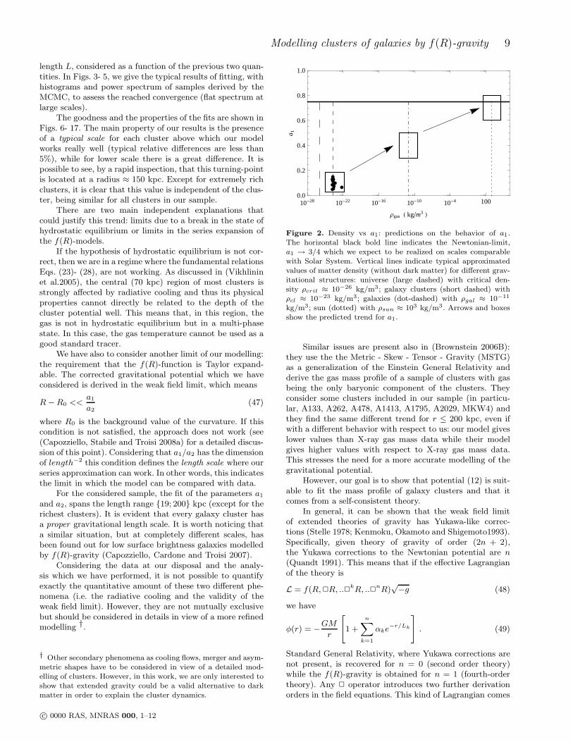
10-28 10-22 10-16 10-10 10-4 1000.0

0.2

0.4

0.6

0.8

1.0

Ρgas H kgm3 L

a 1

Figure 2. Density vs a1: predictions on the behavior of a1.The horizontal black bold line indicates the Newtonian-limit,a1 → 3/4 which we expect to be realized on scales comparablewith Solar System. Vertical lines indicate typical approximatedvalues of matter density (without dark matter) for different grav-itational structures: universe (large dashed) with critical den-sity ρcrit ≈ 10−26 kg/m3; galaxy clusters (short dashed) withρcl ≈ 10−23 kg/m3; galaxies (dot-dashed) with ρgal ≈ 10−11

kg/m3; sun (dotted) with ρsun ≈ 103 kg/m3. Arrows and boxesshow the predicted trend for a1.

Similar issues are present also in (Brownstein 2006B):they use the the Metric - Skew - Tensor - Gravity (MSTG)as a generalization of the Einstein General Relativity andderive the gas mass profile of a sample of clusters with gasbeing the only baryonic component of the clusters. Theyconsider some clusters included in our sample (in particu-lar, A133, A262, A478, A1413, A1795, A2029, MKW4) andthey find the same different trend for r ≤ 200 kpc, even ifwith a different behavior with respect to us: our model giveslower values than X-ray gas mass data while their modelgives higher values with respect to X-ray gas mass data.This stresses the need for a more accurate modelling of thegravitational potential.

However, our goal is to show that potential (12) is suit-able to fit the mass profile of galaxy clusters and that itcomes from a self-consistent theory.

In general, it can be shown that the weak field limitof extended theories of gravity has Yukawa-like correc-tions (Stelle 1978; Kenmoku, Okamoto and Shigemoto1993).Specifically, given theory of gravity of order (2n + 2),the Yukawa corrections to the Newtonian potential are n(Quandt 1991). This means that if the effective Lagrangianof the theory is

L = f(R, R, ..kR, ..nR)√−g (48)

we have

φ(r) = −GM

r

[

1 +

n∑

k=1

αke−r/Lk

]

. (49)

Standard General Relativity, where Yukawa corrections arenot present, is recovered for n = 0 (second order theory)while the f(R)-gravity is obtained for n = 1 (fourth-ordertheory). Any operator introduces two further derivationorders in the field equations. This kind of Lagrangian comes

c© 0000 RAS, MNRAS 000, 1–12

10 S. Capozziello, E. De Filippis, V. Salzano

out when quantum field theory is formulated on curvedspacetime (Birrell & Davies1982). In the series (49), G isthe value of the gravitational constant considered at infin-ity, Lk is the interaction length of the k-th component ofthe non-Newtonian corrections. The amplitude αk of eachcomponent is normalized to the standard Newtonian term;the sign of αk tells us if the corrections are attractive or re-pulsive (see (Will1993) for details). Moreover, the variationof the gravitational coupling is involved. In our case, we aretaking into account only the first term of the series. It is thethe leading term. Let us rewrite (12) as

φ(r) = −GM

r

[

1 + α1e−r/L1

]

. (50)

The effect of non-Newtonian term can be parameterized byα1, L1 which could be a useful parameterisation whichrespect to our previous a1, a2 or Geff , L with Geff =3G/(4a1). For large distances, where r ≫ L1, the exponen-tial term vanishes and the gravitational coupling is G. Ifr ≪ L1, the exponential becomes 1 and, by differentiatingEq.(50) and comparing with the gravitational force mea-sured in laboratory, we get

Glab = G[

1 + α1

(

1 +r

L1

)

e−r/L1

]

≃ G(1 + α1) , (51)

where Glab = 6.67 × 10−8 g−1cm3s−2 is the usual New-ton constant measured by Cavendish-like experiments. Ofcourse, G and Glab coincide in the standard Newtonian grav-ity. It is worth noticing that, asymptotically, the inversesquare law holds but the measured coupling constant differsby a factor (1 + α1). In general, any correction introduces acharacteristic length that acts at a certain scale for the self-gravitating systems as in the case of galaxy cluster which weare examining here. The range of Lk of the kth-componentof non-Newtonian force can be identified with the mass mk

of a pseudo-particle whose effective Compton’s length canbe defined as

Lk =h

mkc. (52)

The interpretation of this fact is that, in the weak energylimit, fundamental theories which attempt to unify gravitywith the other forces introduce, in addition to the masslessgraviton, particles with mass which also carry the gravita-tional interaction (Gibbons & Whiting1981). See, in particu-lar, (Capozziello et al.2008b) for f(R)-gravity. These massesare related to effective length scales which can be parame-terized as

Lk = 2 × 10−5(

1 eV

mk

)

cm . (53)

There have been several attempts to experimentally con-strain Lk and αk (and then mk) by experiments on scalesin the range 1 cm < r < 1000 km, using different tech-niques (Fischbach et al. 1986; Speake & Quinn1988; Eck-hardt1993). In this case, the expected masses of particleswhich should carry the additional gravitational force are inthe range 10−13eV < mk < 10−5 eV. The general outcomeof these experiments, even retaining only the term k = 1,is that geophysical window between the laboratory and theastronomical scales has to be taken into account. In fact, therange

|α1| ∼ 10−2 , L1 ∼ 102 ÷ 103 m , (54)

is not excluded at all in this window. An interesting sug-gestion has been given by Fujii (Fujii1988), which proposedthat the exponential deviation from the Newtonian standardpotential could arise from the microscopic interaction whichcouples the nuclear isospin and the baryon number.

The astrophysical counterparts of these non-Newtoniancorrections seemed ruled out till some years ago due to thefact that experimental tests of General Relativity seemed topredict the Newtonian potential in the weak energy limit,”inside” the Solar System. However, as it has been shown,several alternative theories seem to evade the Solar Systemconstraints (see (Capozziello et al.2008b) and the referencetherein for recent results) and, furthermore, indications of ananomalous, long–range acceleration revealed from the dataanalysis of Pioneer 10/11, Galileo, and Ulysses spacecrafts(which are now almost outside the Solar System) makesthese Yukawa–like corrections come again into play (An-derson et al.1998). Besides, it is possible to reproduce phe-nomenologically the flat rotation curves of spiral galaxiesconsidering the values

α1 = −0.92 , L1 ∼ 40 kpc . (55)

The main hypothesis of this approach is that the additionalgravitational interaction is carried by some ultra-soft bosonwhose range of mass is m1 ∼ 10−27 ÷ 10−28eV. The actionof this boson becomes efficient at galactic scales without therequest of enormous amounts of dark matter to stabilize thesystems (Sanders1990).

Furthermore, it is possible to use a combination of twoexponential correction terms and give a detailed explana-tion of the kinematics of galaxies and galaxy clusters, againwithout dark matter model (Eckhardt1993).

It is worthwhile to note that both the spacecrafts mea-surements and galactic rotation curves indications comefrom ”outside” the usual Solar System boundaries used upto now to test General Relativity. However, the above re-sults do not come from any fundamental theory to explainthe outcome of Yukawa corrections. In their contexts, theseterms are phenomenological.

Another important remark in this direction deserves thefact that some authors (McGaugh2000) interpret also the ex-periments on cosmic microwave background like the experi-ment BOOMERANG and WMAP (de Bernardis et al. 2000;Spergel et al. 2003) in the framework of modified Newtonian

dynamics again without invoking any dark matter model.All these facts point towards the line of thinking that

also corrections to the standard gravity have to be seriouslytaken into account beside dark matter searches.

In our case, the parameters a1,2, which determinethe gravitational correction and the gravitational coupling,come out ”directly” from a field theory with the only re-quirement that the effective action of gravity could be moregeneral than the Hilbert-Einstein theory f(R) = R. Thismain hypothesis comes from fundamental physics motiva-tions due to the fact that any unification scheme or quan-tum field theory on curved space have to take into ac-count higher order terms in curvature invariants (Birrell &Davies1982). Besides, several recent results point out thatsuch corrections have a main role also at astrophysical andcosmological scales. For a detailed discussion, see (Nojiri &Odintsov 2007; Capozziello & Francaviglia 2008; Sotiriou &Faraoni2008).

c© 0000 RAS, MNRAS 000, 1–12

Modelling clusters of galaxies by f(R)-gravity 11

With this philosophy in mind, we have plotted the trendof a1 as a function of the density in Fig.2. As one can see,its values are strongly constrained in a narrow region of theparameter space, so that a1 can be considered a ”tracer” forthe size of gravitational structures. The value of a1 rangebetween 0.8 ÷ 0.12 for larger clusters and 0.4 ÷ 0.6for poorer structures (i.e. galaxy groups like MKW4 andRXJ1159). We expect a particular trend when applying themodel to different gravitational structures. In Fig. 2, we givecharacteristic values of density which range from the biggeststructure, the observed Universe (large dashed vertical line),to the smallest one, the Sun (vertical dotted line), throughintermediate steps like clusters (vertical short dashed line)and galaxies (vertical dot-dashed line). The bold black hori-zontal line represents the Newtonian limit a1 = 3/4 and theboxes indicate the possible values of a1 that we obtain byapplying our theoretical model to different structures.

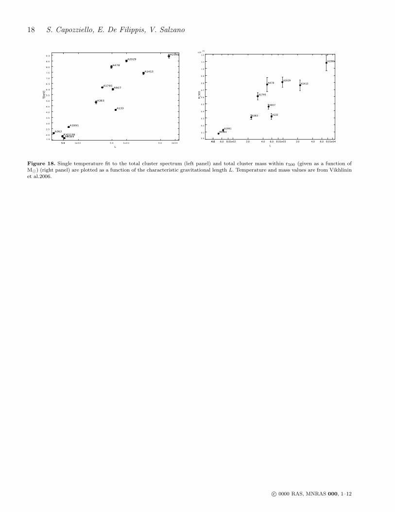
Similar considerations hold also for the characteristicgravitational length L directly related to both a1 and a2.The parameter a2 shows a very large range of variation−106 ÷−10 with respect to the density (and the mass) ofthe clusters. The value of L changes with the sizes of grav-itational structure (see Fig. 18), so it can be considered,beside the Schwarzschild radius, a sort of additional grav-itational radius. Particular care must be taken when con-sidering Abell 2390, which shows large cavities in the X-raysurface brightness distribution, and whose central region,highly asymmetric, is not expected to be in hydrostatic equi-librium. All results at small and medium radii for this clustercould hence be strongly biased by these effects (Vikhlinin etal.2006); the same will hold for the resulting exceptionallyhigh value of L. Fig. 18 shows how observational proper-ties of the cluster, which well characterize its gravitationalpotential (such as the average temperature and the totalcluster mass within r500, plotted in the left and right panel,respectively), well correlate with the characteristic gravita-tional length L.

For clusters, we can define a gas-density-weighted and agas-mass-weighted mean, both depending on the series pa-rameters a1,2. We have:

< L >ρ = 318 kpc < a2 >ρ= −3.40 · 104

< L >M = 2738 kpc < a2 >M= −4.15 · 105 (56)

It is straightforward to note the correlation with the sizesof the cluster cD-dominated-central region and the ”grav-itational” interaction length of the whole cluster. In otherwords, the parameters a1,2, directly related to the first andsecond derivative of a given analytic f(R)-model determinethe characteristic sizes of the self gravitating structures.

7 DISCUSSION AND CONCLUSIONS

In this paper we have investigated the possibility that thehigh observational mass-to-light ratio of galaxy clusterscould be addressed by f(R)- gravity without assuming hugeamounts of dark matter. We point out that this proposalcomes out from the fact that, up to now, no definitive can-didate for dark-matter has been observed at fundamentallevel and then alternative solutions to the problem shouldbe viable. Furthermore, several results in f(R)-gravity seemto confirm that valid alternatives to ΛCDM can be achieved

in cosmology. Besides, as discussed in the Introduction, therotation curves of spiral galaxies can be explained in theweak field limit of f(R)-gravity. Results of our analysis goin this direction.

We have chosen a sample of relaxed galaxy clustersfor which accurate spectroscopic temperature measurementsand gas mass profiles are available. For the sake of simplic-ity, and considered the sample at our disposal, every clus-ter has been modelled as a self bound gravitational sys-tem with spherical symmetry and in hydrostatic equilib-rium. The mass distribution has been described by a cor-rected gravitational potential obtained from a generic ana-lytic f(R)-theory. In fact, as soon as f(R) 6= R, Yukawa-like exponential corrections emerge in the weak field limitwhile the standard Newtonian potential is recovered onlyfor f(R) = R, the Hilbert-Einstein theory.

Our goal has been to analyze if the dark-matter contentof clusters can be addressed by these correction potentialterms. As discussed in detail in the previous section and howit is possible to see by a rapid inspection of Figs. 6- 17, allthe clusters of the sample are consistent with the proposedmodel at 1σ confidence level. This shows, at least qualita-

tively, that the high mass-to-light ratio of clusters can beexplained by using a modified gravitational potential. Thegood agreement is achieved on distance scales starting from150 kpc up to 1000 kpc. The differences observed at smallerscales can be ascribed to non-gravitational phenomena, suchas cooling flows, or to the fact that the gas mass is not agood tracer at this scales. The remarkable result is that wehave obtained a consistent agreement with data only usingthe corrected gravitational potential in a large range of radii.In order to put in evidence this trend, we have plotted thebaryonic mass vs radii considering, for each cluster, the scalewhere the trend is clearly evident.

In our knowledge, the fact that f(R)-gravity could workat these scales has been only supposed but never achievedby a direct fitting with data (see (Lobo 2008) for a review).Starting from the series coefficients a1 and a2, it is possi-ble to state that, at cluster scales, two characteristic sizesemerge from the weak field limit of the theory. However, atsmaller scales, e.g. Solar System scales, standard Newtoniangravity has to be dominant in agreement with observations.

In conclusion, if our considerations are right, gravita-tional interaction depends on the scale and the infrared limit

is led by the series coefficient of the considered effectivegravitational Lagrangian. Roughly speaking, we expect thatstarting from cluster scale to galaxy scale, and then downto smaller scales as Solar System or Earth, the terms of theseries lead the clustering of self-gravitating systems besideother non-gravitational phenomena. In our case, the New-tonian limit is recovered for a1 → 3/4 and L(a1, a2) ≫ rat small scales and for L(a1, a2) ≪ r at large scales. In thefirst case, the gravitational coupling has to be redifined, inthe second G∞ ≃ G. In these limits, the linear Ricci termis dominant in the gravitational Lagrangian and the New-tonian gravity is restored (Quandt 1991). Reversing the ar-gument, this could be the starting point to achieve a theorycapable of explaining the strong segregation in masses andsizes of gravitationally-bound systems.

c© 0000 RAS, MNRAS 000, 1–12

12 S. Capozziello, E. De Filippis, V. Salzano

8 ACKNOWLEDGMENTS

We warmly thank V.F. Cardone for priceless help in compu-tational work. We acknowledge A. Stabile and A. Troisi forcomments, discussions and suggestions on the topic and M.Paolillo for hints and suggestions in cluster modelling. Weare indebted with A. Vikhlinin which kindly gave us dataon cluster temperature profiles.

REFERENCES

Allemandi, G., Francaviglia, M., Ruggiero, M., Tartaglia, A. 2005,Gen. Rel. Grav., 37, 1891

Anderson J.D., et al., 1998, Phys. Rev. Lett. 81, 2858.

Astier, P. et al. 2006, A&A, 447, 31Bahcall N. A., 1996, in ”Formation of structure in the universe,

1995, Jerusalem Winter School”, astro-ph/9611148,

Bahcall, N.A. et al. 2003, ApJ, 585, 182Bahcall, N.A., Bode, P. 2003, ApJ, 588, 1

Bautz, L. P., Morgan, W. W., 1970, ApJ, 162, L149Birrell, N.D. and Davies, P.C.W., 1982, Quantum Fields in

Curved Space, Cambridge Univ. Press, Cambridge

Borowiec, A., Godlowski, W., Szydlowski, M. 2006, Phys. Rev.D, 74, 043502

Brownstein, J. R., Moffat, J. W., 2006, MNRAS, 367, 527

Capozziello, S. 2002, Int. J. Mod. Phys. D, 11, 483

Capozziello, S., Cardone, V.F., Carloni, S., Troisi, A. 2003, Int.J. Mod. Phys. D, 12, 1969

Capozziello, S., Cardone, V.F., Francaviglia, M. 2006, Gen. Rel.Grav., 38, 711

Capozziello, S., Cardone, V.F., Troisi, A. 2005, Phys. Rev. D, 71,043503

Capozziello, S., Cardone, V.F., Troisi, A. 2006, JCAP, 0608, 001

Capozziello, S., Cardone, V. F., Troisi, A., 2007, MNRAS, 375,1423

Capozziello, S., Stabile A., Troisi, A., 2007, Class. quant. grav.,24, 2153

Capozziello, S., Stabile, A., Troisi, A., 2008, Physical Review D,76, 104019

Capozziello, S., De Laurentis, M., Nojiri, S., Odintsov, S.D., 2008,arXiv:0808.1335 [hep-th]

Capozziello, S., Carloni, S., Troisi, A. 2003, Rec. Res. Devel. As-tronomy. & Astrophys., 1, 625, astro - ph/0303041

Capozziello S. and Francaviglia M., 2008, Gen. Rel. Grav.: SpecialIssue on Dark Energy 40, 357.

Capozziello, S., Troisi, A. 2005, Phys. Rev. D, 72, 044022

Carroll, S.M., Duvvuri, V., Trodden, M., Turner, M.S. 2004, Phys.Rev. D, 70, 043528

Carroll, S.M., Press, W.H., Turner, E.L. 1992, ARA&A, 30, 499

Cembranos, J.A.R. 2006, Phys. Rev. D, 73, 064029Chakrabarty, D., de Filippis, E.,& Russell, H. 2008, A&A, 487,

75

Chiba, T. 2003, Phys. Lett. B, 575, 1Clifton, T., Barrow, J.D. 2005, Phys. Rev. D, 72, 103005

Clocchiati, A. et al. 2006, APJ, 642, 1Cole, S. et al. 2005, MNRAS, 362, 505

Copeland E.J., Sami M., Tsujikawa S., 2006, Int. Jou. Mod. Phys.D 15, 1753

Croft, R.A.C., Hu, W., Dave, R. 1999, Phys. Rev. Lett., 83, 1092de Bernardis, P. et al. 2000, Nature, 404, 955

de Blok, W.J.G., Bosma, A. 2002, A&A, 385, 816de Blok, W.J.G. 2005, ApJ, 634, 227

De Filippis, E., Sereno, M., Bautz, Longo G., M. W., 2005, ApJ,625, 108

Dick, R. 2004, Gen. Rel. Grav., 36, 217

Dolgov, A.D., Kawasaki, M. 2003, Phys. Lett. B, 573, 1

Dunkley, J., Bucher, M., Ferreira, P. G., Moodley, K., Skordis,

C., 2005, MNRAS, 356, 925Eckhardt, D.H., 1993 Phys. Rev. 48 D, 3762.Eisenstein, D. et al. 2005, ApJ, 633, 560Eke, V.R., Cole, S., Frenk, C.S., Petrick, H.J. 1998, MNRAS, 298,

1145Sotiriou, T.P. and Faraoni, V., 2008, arXiv:0805.1726 [gr-qc]E. Fischbach, E., Sudarsky, D., Szafer, A., Talmadge, C. and Aro-

son, S.H., 1986, Phys. Rev. Lett. 56, 3Frigerio Mar-

tins C. and Salucci P., 2007, Mon.Not.Roy.Astron.Soc. 381,1103

Y. Fujii, Y., 1988, Phys. Lett. B 202, 246G.W. Gibbons, G.W. and Whiting, B.F., 1981, Nature 291, 636M. Kenmoku, M., Okamoto, Y. and Shigemoto, K., 1993, Phys.

Rev. 48 D, 578.Kluske, S., Schmidt, H.J. 1996, Astron. Nachr., 37, 337Koivisto T., 2007, Phys.Rev.D76, 043527Lobo F.S.N., arXiv: 0807.1640[gr-qc] (2008).McDonald, P. et al. 2005, ApJ, 635, 761S.S. McGaugh, 2000, Ap. J. Lett. 541, L33Mendoza S. and Rosas-Guevara Y.M., 2007, Astron. Astrophys.

472, 367.Navarro, I., van Acoleyen, K. 2005, Phys. Lett. B, 622, 1Neumann., D. M., Bohringer, H., 1995, Astron. Astrophys., 301,

865Nojiri S. and Odintsov S.D. 2007, Int. J. Geom. Meth. Mod. Phys.

4, 115.Olmo, G.J. 2005, Phys. Rev. D, 72, 083505Padmanabhan, T. 2003, Phys. Rept., 380, 235Peebles, P.J.E., Rathra, B. 2003, Rev. Mod. Phys., 75, 559Pope, A.C. et al. 2005, ApJ, 607, 655Quandt, I., Schmidt H. J., 1991, Astron. Nachr., 312, 97Refregier, A. 2003, ARA&A, 41, 645Riess, A.G. et al. 2004, ApJ, 607, 665Sahni, V., Starobinski, A. 2000, Int. J. Mod. Phys. D, 9, 373Sanchez, A.G. et al. 2006, MNRAS, 366, 189Sanders, R.H., 1990, Ann. Rev. Astr. Ap. 2, 1Schindler, S., 2004, Astrophys.Space Sci., 28, 419Schmidt, H.J. 2004, Lectures on mathematical cosmology, gr -

qc/0407095Schmidt, R. W., Allen S. W., 2007 MNRAS 379, 209Seljak, U. et al. 2005, Phys. Rev. D, 71, 103515Sobouti, Y. 2007, A & A, 464, 921Sotiriou, T.P. 2006, Gen. Rel. Grav., 38, 1407Speake, C.C. and Quinn, T.J., 1988, Phys. Rev. Lett. 61, 1340Spergel, D.N. et al. 2003, ApJS, 148, 175

Starobinsky, A.A. 1980, Phys. Lett. B, 91, 99Stelle, K., 1978, Gen. Relat. Grav., 9, 353Tegmark, M. et al. 2004, Phys. Rev. D, 69, 103501van Waerbecke, L. et al. 2001, A&A, 374, 757Viana, P.T.P., Nichol, R.C., Liddle, A.R. 2002, ApJ, 569, 75Vikhlinin, A., Markevitch, M., Murray, S. S., Jones, C., Forman,

W., Van Speybroeck, L., 2005, ApJ, 628, 655Vikhlinin, A., Kravtsov, A., Forman, W., Jones, C., Markevitch,

M., Murray, S. S., Van Speybroeck, L., 2006, ApJ, 640, 691Will C.M., 1993, Theory and Experiments in Gravitational

Physics, Cambridge Univ. Press, Cambridge.Zwicky, F., 1933, Helv. Phys. Acta, 6, 110

c© 0000 RAS, MNRAS 000, 1–12

Modelling clusters of galaxies by f(R)-gravity 13

0.09 0.10 0.11 0.12

0

20

40

60

80

a1

freq

-9 -8 -7 -6 -5

0

2

4

6

8

10

k

PHkL

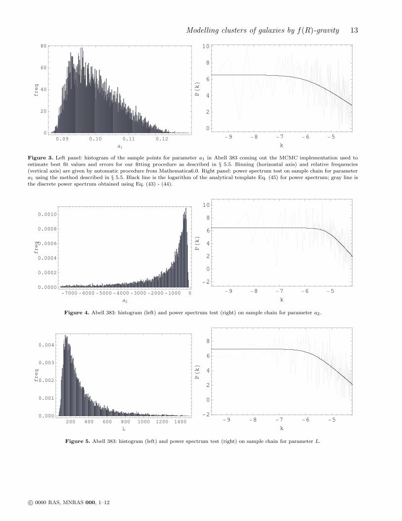
Figure 3. Left panel: histogram of the sample points for parameter a1 in Abell 383 coming out the MCMC implementation used toestimate best fit values and errors for our fitting procedure as described in § 5.5. Binning (horizontal axis) and relative frequencies(vertical axis) are given by automatic procedure from Mathematica6.0. Right panel: power spectrum test on sample chain for parametera1 using the method described in § 5.5. Black line is the logarithm of the analytical template Eq. (45) for power spectrum; gray line isthe discrete power spectrum obtained using Eq. (43) - (44).

-7000 -6000 -5000 -4000 -3000 -2000 -1000 0

0.0000

0.0002

0.0004

0.0006

0.0008

0.0010

a2

freq

-9 -8 -7 -6 -5

-2

0

2

4

6

8

10

k

PHkL

Figure 4. Abell 383: histogram (left) and power spectrum test (right) on sample chain for parameter a2.

200 400 600 800 1000 1200 1400

0.000

0.001

0.002

0.003

0.004

L

freq

-9 -8 -7 -6 -5-2

0

2

4

6

8

k

PHkL

Figure 5. Abell 383: histogram (left) and power spectrum test (right) on sample chain for parameter L.

c© 0000 RAS, MNRAS 000, 1–12

14 S. Capozziello, E. De Filippis, V. Salzano

100 1000500200 300150 7001 ´ 1011

5 ´ 10111 ´ 1012

5 ´ 10121 ´ 1013

5 ´ 1013

r HkpcL

MHML

100 1000500200 300150 7001 ´ 1011

5 ´ 10111 ´ 1012

5 ´ 10121 ´ 1013

5 ´ 1013

r HkpcL

MHML

Figure 6. Baryonic mass vs radii for Abell A133. Dashed line is the experimental-observed estimation Eq. (41) of baryonic mattercomponent (i.e. gas, galaxies and cD-galaxy); solid line is the theoretical estimation Eq. (40) for baryonic matter component. Dottedlines are the 1-σ confidence levels given by errors on fitting parameters in the left panel; and from fitting parameter plus statistical errorson mass profiles as discussed in § 5.4 in the right panel.

10 20 50 100 2001 ´ 1011

5 ´ 10111 ´ 1012

5 ´ 10121 ´ 1013

5 ´ 1013

r HkpcL

MHML

10 20 50 100 2001 ´ 1011

5 ´ 10111 ´ 1012

5 ´ 10121 ´ 1013

5 ´ 1013

r HkpcL

MHML

Figure 7. Same of Fig. 6 but for cluster Abell 262.

100 500200 300150 7001 ´ 1011

5 ´ 10111 ´ 1012

5 ´ 10121 ´ 1013

5 ´ 1013

r HkpcL

MHML

100 500200 300150 7001 ´ 1011

5 ´ 10111 ´ 1012

5 ´ 10121 ´ 1013

5 ´ 1013

r HkpcL

MHML

Figure 8. Same of Fig. 6 but for cluster Abell 383.

c© 0000 RAS, MNRAS 000, 1–12

Modelling clusters of galaxies by f(R)-gravity 15

100 1000500200 300150 15007001 ´ 1011

5 ´ 10111 ´ 1012

5 ´ 10121 ´ 1013

5 ´ 10131 ´ 1014

r HkpcL

MHML

100 1000500200 300150 15007001 ´ 1011

5 ´ 10111 ´ 1012

5 ´ 10121 ´ 1013

5 ´ 10131 ´ 1014

r HkpcL

MHML

Figure 9. Same of Fig. 6 but for cluster Abell 478.

600. 700. 800. 900.1000.1100.1200.

5.0 ´ 1013

3.0 ´ 1013

7.0 ´ 1013

r HkpcL

MHML

600. 700. 800. 900.1000.1100.1200.

5.0 ´ 1013

3.0 ´ 1013

7.0 ´ 1013

r HkpcL

MHML

Figure 10. Same of Fig. 6 but for cluster Abell 907.

50 100 200 500 10001 ´ 1011

5 ´ 10111 ´ 1012

5 ´ 10121 ´ 1013

5 ´ 10131 ´ 1014

r HkpcL

MHML

50 100 200 500 10001 ´ 1011

5 ´ 10111 ´ 1012

5 ´ 10121 ´ 1013

5 ´ 10131 ´ 1014

r HkpcL

MHML

Figure 11. Same of Fig. 6 but for cluster Abell 1413.

c© 0000 RAS, MNRAS 000, 1–12

16 S. Capozziello, E. De Filippis, V. Salzano

100 1000500200 300150 7001 ´ 1012

2 ´ 1012

5 ´ 1012

1 ´ 1013

2 ´ 1013

5 ´ 1013

r HkpcL

MHML

100 1000500200 300150 7001 ´ 1012

2 ´ 1012

5 ´ 1012

1 ´ 1013

2 ´ 1013

5 ´ 1013

r HkpcL

MHML

Figure 12. Same of Fig. 6 but for cluster Abell 1795.

20 50 100 200 5001 ´ 1011

2 ´ 1011

5 ´ 1011

1 ´ 1012

2 ´ 1012

5 ´ 1012

1 ´ 1013

r HkpcL

MHML

20 50 100 200 5001 ´ 1011

2 ´ 1011

5 ´ 1011

1 ´ 1012

2 ´ 1012

5 ´ 1012

1 ´ 1013

r HkpcL

MHML

Figure 13. Same of Fig. 6 but for cluster Abell 1991.

50 100 200 500 1000

1 ´ 10122 ´ 1012

5 ´ 10121 ´ 10132 ´ 1013

5 ´ 10131 ´ 10142 ´ 1014

r HkpcL

MHML

50 100 200 500 1000

1 ´ 10122 ´ 1012

5 ´ 10121 ´ 10132 ´ 1013

5 ´ 10131 ´ 10142 ´ 1014

r HkpcL

MHML

Figure 14. Same of Fig. 6 but for cluster Abell 2029.

c© 0000 RAS, MNRAS 000, 1–12

Modelling clusters of galaxies by f(R)-gravity 17

100 1000500200 300150 1500700

2 ´ 1012

5 ´ 1012

1 ´ 1013

2 ´ 1013

5 ´ 1013

1 ´ 1014

2 ´ 1014

r HkpcL

MHML

100 1000500200 300150 1500700

2 ´ 1012

5 ´ 1012

1 ´ 1013

2 ´ 1013

5 ´ 1013

1 ´ 1014

2 ´ 1014

r HkpcL

MHML

Figure 15. Same of Fig. 6 but for cluster Abell 2390.

20 50 100 2001 ´ 1011

5 ´ 1011

1 ´ 1012

5 ´ 1012

1 ´ 1013

r HkpcL

MHML

20 50 100 2001 ´ 1011

5 ´ 1011

1 ´ 1012

5 ´ 1012

1 ´ 1013

r HkpcL

MHML

Figure 16. Same of Fig. 6 but for cluster MKW4.

20 50 100 200 5001 ´ 1011

5 ´ 1011

1 ´ 1012

5 ´ 1012

1 ´ 1013

r HkpcL

MHML

20 50 100 200 5001 ´ 1011

5 ´ 1011

1 ´ 1012

5 ´ 1012

1 ´ 1013

r HkpcL

MHML

Figure 17. Same of Fig. 6 but for cluster RXJ1159.

c© 0000 RAS, MNRAS 000, 1–12

18 S. Capozziello, E. De Filippis, V. Salzano

Figure 18. Single temperature fit to the total cluster spectrum (left panel) and total cluster mass within r500 (given as a function ofM⊙) (right panel) are plotted as a function of the characteristic gravitational length L. Temperature and mass values are from Vikhlininet al.2006.

c© 0000 RAS, MNRAS 000, 1–12