MNRAS 453, 868–878 (2015) doi:10.1093/mnras/stv1650

Structure and dynamics of the supercluster of galaxies SC0028-0005

Ana Laura O’Mill,1,2‹ Dominique Proust,3 Hugo V. Capelato,4,5 Mirian Castejon,1

Eduardo S. Cypriano,1 Gastao B. Lima Neto1 and Laerte Sodre Jr1

1Departamento de Astronomia, Instituto de Astronomia, Geofısica e Ciencias Atmosfericas da USP, Rua do Matao 1226, Cidade Universitaria, 05508-090Sao Paulo, Brazil2Instituto de Astronomıa Teorica y Experimental, CONICET-UNC, Laprida 922, X5000BGR Cordoba, Argentina3Observatoire de Paris-Meudon, GEPI, F-92195 Meudon, France4Divisao de Astrofısica, INPE/MCT, 12227-010 Sao Jose dos Campos, Sao Paulo, Brazil5Nucleo de Astrofısica Teorica, Universidade Cruzeiro do Sul, Rua Galvao Bueno, 868, CEP 01506-000 Sao Paulo, Brazil

Accepted 2015 July 20. Received 2015 July 13; in original form 2014 December 9

ABSTRACTAccording to the standard cosmological scenario, superclusters are objects that have justpassed the turn-around point and are collapsing. The dynamics of very few superclusters havebeen analysed up to now. In this paper, we study the supercluster SC0028-0005, at redshift0.22, identify the most prominent groups and/or clusters that make up the supercluster, andinvestigate the dynamic state of this structure. For the membership identification, we have usedphotometric and spectroscopic data from Sloan Digital Sky Survey Data Release 10, findingsix main structures in a flat spatial distribution. We have also used a deep multiband observationwith MegaCam/Canada–France–Hawaii Telescope to estimate de mass distribution throughthe weak-lensing effect. For the dynamical analysis, we have determined the relative distancesalong the line of sight within the supercluster using the Fundamental Plane of early-typegalaxies. Finally, we have computed the peculiar velocities of each of the main structures. The3D distribution suggests that SC0028-005 is indeed a collapsing supercluster, supporting theformation scenario of these structures. Using the spherical collapse model, we estimate thatthe mass within r = 10 Mpc should lie between 4 and 16 × 1015 M�. The farthest detectedmembers of the supercluster suggest that within ∼60 Mpc the density contrast is δ ∼ 3 withrespect to the critical density at z = 0.22, implying a total mass of ∼4.6–16 × 1017 M�, mostof which in the form of low-mass galaxy groups or smaller substructures.

Key words: galaxies: clusters: general – galaxies: kinematics and dynamics – cosmology:theory.

1 IN T RO D U C T I O N

In the hierarchical paradigm of structure formation, the smalleststructures are the first to collapse and virialize. They later getcollected into progressively larger structures, each of which goesthrough the same stages of collapse and virialization. At present,the largest collapsed structures are clusters of galaxies, whereassuperclusters are expected to be in the stage of gravitational col-lapse, at least in their inner tens of Mpc (Reisenegger et al. 2000;Batiste & Batuski 2013; Merluzzi et al. 2015). In the currentlyfavoured cosmological scenario, dominated by a cosmological con-stant or another form of ‘dark energy’, superclusters are startingto recede from each other at an accelerated rate, which will notallow them to get collected into even larger structures. Therefore,they are the largest structures that will ever collapse and virialize

� E-mail: anaomill@gmail.com

(e.g. Busha et al. 2003; Nagamine & Loeb 2003; Dunner et al.2006, 2007; Proust et al. 2006; Rines et al. 2013). If this sce-nario is correct, present superclusters play a pivotal role in ourunderstanding of the evolution of the universe. Thus, it is very im-portant to determine their quantitative properties such as masses,sizes, and densities reliably, as well as testing this scenario as bestas possible. Since superclusters have not yet collapsed and virial-ized, they do not stand out against the background density field asclearly as individual galaxies or even clusters of galaxies (in terms ofmass, optical light or X-ray emission), and equilibrium techniquesused to determine the masses of clusters (hydrostatic equilibriumof the gas and virial equilibrium of the galaxies) do not applyto them.

The study of superclusters has a long history, beginning withworks such as the identification of our own Virgo supercluster(de Vaucouleurs 1953) and the statistical description of ‘cluster-ing of second order’ (which are known nowadays as the superclus-ters; Neyman, Scott & Shane 1956). Other studies addressed the

C© 2015 The AuthorsPublished by Oxford University Press on behalf of the Royal Astronomical Society

Dow

nloaded from https://academ

ic.oup.com/m

nras/article/453/1/868/1751475 by guest on 16 March 2022

Structure and dynamics of the supercluster of galaxies SC0028-0005 869

identification, distribution and characterization of these objects (e.g.Joeveer, Einasto & Tago 1978; Einasto et al. 1984, 1994; Tago,Einasto & Saar 1984; Zucca et al. 1993), establishing that theyare separated by large voids and clusters inside them are usuallyorganized in chain-like structures.

Some studies considered the morphology of superclusters, basedon the spatial distribution of their galaxies. Einasto et al. (2007,2011) analysed a sample drawn from Sloan Digital Sky Survey DataRelease 7 (SDSS-DR7), finding two main morphological types: fil-aments and others with a more complex, multibranch fine structure.The wide morphological variety of superclusters let Einasto et al.(2011) to suggest that their evolution have been dissimilar. Costa-Duarte, Sodre & Durret (2011) used a kernel-based density fieldmethod to identify the superclusters and Minkowski Functionals toquantify their shape. They found that filaments and pancakes repre-sent distinct morphological classes of superclusters in the Universe.The filaments tend to be richer, more luminous and larger than pan-cakes. It is then plausible to think that pancakes evolve towardsfilaments.

While there is plenty of morphological analysis, dynamical stud-ies of galaxy superclusters are more scarce. In the hierarchical modelof structure formation we expect that galaxy clusters form throughaccretion of galaxies and groups or merger with other clusters inthe environment of superclusters. In the case of a supercluster withseveral clusters, it is possible that massive clusters grow through thegravitational collapse of the central parts of superclusters. There-fore, superclusters are still far from equilibrium today. The collapsescenario predicts that, among the clusters in a supercluster, thosewith higher observed redshifts are falling in to the centre from thefront side (and thus are closer to us), while those with lower ob-served redshifts are falling in from the back (and are therefore moredistant). Consequently, in the gravitationally collapsing region, theHubble relation is reversed. This effect is indeed present in the coreof the Shapley Supercluster (Proust et al. 2006; Ragone et al. 2006;Dunner et al. 2007), at z � 0.04. Batiste & Batuski (2013) made adynamical analysis of the Corona Borealis supercluster at z � 0.07using data from the SDSS. They find this supercluster has brokenfrom the Hubble flow and, based on dynamical simulations, con-clude that a significant fraction of mass should reside outside theclusters comprising the supercluster. Recently, Tully et al. (2014)have used peculiar velocities to identify and describe a large andmassive structure, Laniakea, comprising most of the galaxies in thelocal universe.

The picture of gravitationally collapsing central parts of super-clusters is required by the present cosmological model, but it hasbeen tested only at low redshifts. Indeed, previous dynamical stud-ies, as those described above and in Section 5, dealt with super-clusters below z = 0.1. In this work, we analyse the superclusterSC0028-0005, at z = 0.22, in order to test the collapse scenariofor structures at intermediate redshift. This paper is organized asfollows. In Section 2, we describe what is known about this su-percluster and what is the data that we will analyse in this paper.In Section 3, we present an identification of the supercluster mem-bers. Section 4 contains a weak-lensing analysis of the substructuresfound in the supercluster. In Section 5, we show that the dynamicalbehaviour of the supercluster components is consistent with a col-lapsing scenario. For this analysis, we use the Fundamental Plane(FP) of early-type galaxies to obtain relative distances and peculiarvelocities of these components. Finally, our results are summarizedin Section 6. Throughout this paper we adopt, when necessary, a �

cold dark matter (�CDM) cosmological model with �M = 0.30,�� = 0.70 and H0 = 70 h70 km s−1 Mpc−1.

Table 1. CFHT Imaging characteristics.

Band Exposure Seeing Completness(h) (arcsec) (AB mag)

g 1.5 0.52 24.5r 3.3 0.45 24.6i 2.5 0.45 24.3

2 T H E S U P E R C L U S T E R S C 0 0 2 8 - 0 0 0 5

In this study, we focus on the galaxy supercluster SC0028-0005(hereafter SC0028 for simplicity) at α = 00h28m and δ = −00◦05′

(J2000.0). It is in the catalogue of Basilakos (2003), obtainedfrom the Sloan Digital Sky Survey (SDSS) ‘Cut & Enhance’ clus-ter catalogue (Goto et al. 2002) by applying a percolation radiusRpc = 26 h−1 Mpc. Among the 57 superclusters of this catalogue,SC0028 is the number 38, with an assigned redshift z = 0.197,and is classified as a filament by using the shape finder estimatorof Basilakos (2003). This structure was chosen for this study be-cause it was not too complex in the Goto et al. (2002) catalogue,containing only three galaxy clusters with relative distances of 4–10 h−1 Mpc between them, what was suggestive of the presence ofstrong peculiar motions.

2.1 Spectroscopic and photometric samples

We selected from the Data Release 10 of Sloan Digital Sky Survey1

(SDSS-DR10) a sample of galaxies with spectroscopic and photo-metric data within an area of radius 1.◦2, centred on the supercluster.

SDSS DR10 covers an additional 3100 deg2 of sky over theprevious release and includes spectra obtained with the new spec-trographs APOGEE and BOSS, whose sky coverage includes theregion of SC0028.

The spectroscopic and photometric data sets were extracted fromthe SpecObjAll and PhotoObj tables of the CasJobs2 data base.From the PhotoObj table we downloaded the objID, the coordi-nates, the model g and r magnitudes, the Galaxy extinction values,the effective radii derived from the de Vaucouleurs profile fit, aswell as model magnitudes and axial ratios of the de Vaucouleursfits, and the photometric redshifts. From the SpecObjAll table,we downloaded the spectroscopic redshifts and the galaxy centralvelocity dispersions plus the respective errors.

From this data, we selected two galaxy samples. The first samplecomprises 4921 galaxies with spectroscopic redshift. This sample isemployed to identify the supercluster members and substructures,as well as in the dynamical analysis of Section 5.

The second sample contains 35 757 galaxies with photometricredshifts (including the galaxies of the previous spectral sample),selected from the PhotoObj table. This sample allowed an anal-ysis of the photometric properties of the substructures identifiedspectroscopically and is also useful for their detection.

2.2 CFHT Imaging

The supercluster field was observed with Canada–France–HawaiiTelescope (CFHT)/MegaCam in imaging mode, mostly for theweak-lensing analysis described in Section 4. We got deep, goodquality g, r, i images, whose main features are shown in Table 1.

1 https://www.sdss3.org/dr10/2 http://skyserver.sdss3.org/CasJobs/

MNRAS 453, 868–878 (2015)

Dow

nloaded from https://academ

ic.oup.com/m

nras/article/453/1/868/1751475 by guest on 16 March 2022

870 A. L. O’Mill et al.

Figure 1. Redshift distribution within an area of 1.◦2 radius centred on SC0028. Left-hand panel: spectroscopic redshift distribution. The inset shows theredshift distribution of galaxies in the �z < 0.02 interval around the supercluster mean redshift, as well as a Gaussian fit of this distribution. Right-handpanel: photometric redshifts. The grey histogram correspond to the redshift sample, reported here for easy comparison. In both panels, the dashed vertical linescorrespond to the supercluster mean redshift and the magenta dotted lines show the galaxies within a redshift interval around the mean of �z < 0.02 for theS1 sample and �zphot < 0.04 for the S2 sample.

The whole data processing (bias and overscan subtraction, flat-fielding and sky subtraction), image combination and catalogueextraction with SEXTRACTOR (Bertin & Arnouts 1996) has been doneby the Terapix3 team, using the procedures described in Bertin et al.(2002).

The total integrations were obtained with a series of ∼10 minexposures per filter, with small position offsets, for the coverage ofthe cap between the camera CCDs. As a result, the final combinedimage in each band covers an area slightly smaller than 1 deg2

(MegaCam’s full field of view).

3 ID E N T I F Y I N G T H E SU P E R C L U S T E RMEMBERS

3.1 Selecting galaxies

With the aim of selecting galaxies which are members of the super-cluster, we start by defining �z as the absolute difference betweena given redshift and the supercluster mean redshift. For galaxieswith spectroscopic redshifts we consider as members those with�z < 0.02. We call this sample S1. For those with photometric red-shifts only, due to the larger uncertainties, we adopted �zphot < 0.04(about twice the SDSS photometric redshift standard deviation).This we call the S2 sample.

Left- and right-hand panels of Fig. 1 show the resulting redshiftdistribution of the galaxies in the spectroscopic and photometricsamples (Section 2.1), respectively. The peak around z � 0.22 inthese figures corresponds to the supercluster.

We selected galaxies from the spectroscopic sample which are su-percluster members using the following approach. We pre-selectedall galaxies in the range 0.195 < z < 0.245, a redshift intervallarge enough to not exclude possible members, and small enoughto avoid most fore/background galaxies. We fitted a Gaussian tothe resulting redshift distribution, obtaining an average redshift ofz = 0.220 ± 0.001. Around this value we selected the spectroscopic

3 http://terapix.iap.fr/

sample, S1, using �z < 0.02, resulting in a total of 271 galaxies.For the photometric sample we adopted �zphot < 0.04, obtaining3549 galaxies. In both panels of Fig. 1 the magenta dotted linesbracket the membership ranges.

3.2 Identifying substructures

In order to identify substructures in our spectroscopic sample, wepresent a density map of the S1 sample in the upper-left panelof Fig. 2. This map was made by counting the number of galax-ies in equal size square cells with 15 arcsec on a side. We foundnine well-defined peaks in this density distribution which are mostlikely galaxy groups or clusters candidate members of SC0028. Thebrightest galaxy in each peak was taken as the group/cluster centre,and all galaxies in the sample within a 2.5 h−1

70 Mpc radius (∼11.7 ar-cmin) of this centre were considered as group/cluster members. Inthis panel, the circles show the region around each peak ascribedto a certain group or cluster. Table 2 presents the identification,coordinates and mean redshift of each of these substructures. Notethat they may be groups or galaxy clusters, but hereafter we willcall them substructures.

The upper-right panel of Fig. 2 is similar to the left-hand panel,but uses the larger S2 sample (the photometric one) instead of theS1 sample.

The light map (Fig. 2, lower-left panel) was made by stronglysmoothing the S2 sample of galaxies by a bidimensional Gaus-sian with intensity proportional to the galaxy luminosity and widthproportional to their half-luminosity radius, σ = 100R50. In thisway, we can take into account the different apparent sizes of thegalaxies. This luminosity field was then binned in a 2D grid with15 × 15 arcsec2 cells, producing an image. Since the mean R50 is∼1.1 arcsec, the typical galaxy luminosity was spread in a radius of∼7 pixel (1σ ), which we found adequate to describe the substruc-tures in the light distribution. This map is in qualitative agreementwith the S1 density map, as there are peaks in most regions previ-ously identified (solid line circles in Fig. 2).

The bottom-right panel of Fig. 2 shows the weak-lensing recov-ered projected mass distribution (see Section 4). The same structures

MNRAS 453, 868–878 (2015)

Dow

nloaded from https://academ

ic.oup.com/m

nras/article/453/1/868/1751475 by guest on 16 March 2022

Structure and dynamics of the supercluster of galaxies SC0028-0005 871

Figure 2. Substructures in the supercluster. Top-left: surface density map of supercluster members in the S1 (spectroscopic) sample. Top-right: surface densitymap of supercluster members in the S2 (photometric) sample. Bottom-left: projected light distribution of the galaxies within photometric redshift �z < 0.04 ofthe supercluster mean spectroscopic redshift, z = 0.22. Bottom-right: weak-lensing recovered mass distribution (See Section 4 for details). The green squarecorresponds to the 1 deg2 MegaCam/CFHT field of view. In all panels, the red circles (R = 11.7 arcmin) correspond to maximum projected density regions(based on the S1 sample), recentred at the location of the corresponding brightest galaxy in each maximum density box. The circles with solid lines are thesubstructures that will be considered in this study (see text for details).

identified in the previous maps are also present in this mass map,within the CFHT field of view (green square in the figure). Thisre-assures that these substructures are not projection effects, butrather actual mass concentrations. Substructure 3 is the only ex-ception, since it is detected in redshift space, upper-left panel, butnot clearly visible in any of the others. This probably means thatsubstructure 3 is the least massive region of them all.

In Fig. 2, we can see that areas 5 and 6 overlap. After analysingthe photometric redshifts of the six galaxies in the area in common,we decided to consider them as a part of group/cluster 5.

Some of those substructures might be due to projection effectsand, to obtain a sample of more reliable physical structures, we haveinvestigated their red galaxy content, since it is well know that thepresence of a red sequence is conspicuous in large physical groupsand clusters (e.g. Oemler 1974; Dressler 1980; Postman & Geller1984).

We present in Fig. 3 the (g − r) versus r colour–magnitudediagram for galaxies in sample S2. This figure shows a clear con-centration of red galaxies. In order to make an inventory of red

objects, we have divided our sample in two using (g − r) = 1.1 as acutoff based on the typical colours of galaxies at redshift z = 0.2 asgiven by Fukugita, Shimasaku & Ichikawa (1995): ellipticals (g −r) = 1.31, lenticulars (g − r) = 1.13, Sab galaxies (g − r) = 1.01.

The fraction of red galaxies, by this definition, is shown in Table 2for each identified structure.

Based on this information we decided to remove substructures7, 8 and 9 from our subsequent analysis, as they all have a frac-tion of red galaxies smaller than 50 per cent. We suspect that thesesubstructures may not be bona fide bound groups and/or clustersof galaxies. We thus kept, for the present study, six groups/clusterswhich we considered dense and red enough to be safely consideredas substructures of SC0028. Note that structure 3 appears strong inthe spectroscopic redshift map (Fig. 2), while in the photometricredshift and light maps it appears diluted. We have considered thisstructure significant, since more than 50 per cent of its galaxies arered.

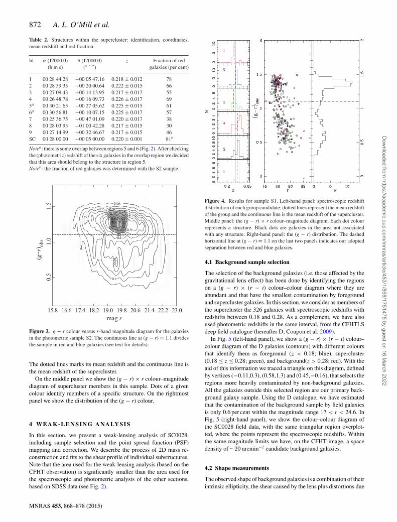
Fig. 4 presents results for the spectroscopic sample, S1. In the left-hand panel, we show the redshift distribution for each substructure.

MNRAS 453, 868–878 (2015)

Dow

nloaded from https://academ

ic.oup.com/m

nras/article/453/1/868/1751475 by guest on 16 March 2022

872 A. L. O’Mill et al.

Table 2. Structures within the supercluster: identification, coordinates,mean redshift and red fraction.

Id α (J2000.0) δ (J2000.0) z Fraction of red(h m s) (◦ ′ ′′) galaxies (per cent)

1 00 28 44.28 −00 05 47.16 0.218 ± 0.012 782 00 28 59.35 +00 20 00.64 0.222 ± 0.015 663 00 27 09.43 +00 14 13.95 0.217 ± 0.017 554 00 26 48.78 −00 16 09.73 0.226 ± 0.017 695a 00 30 21.65 −00 27 05.62 0.225 ± 0.015 616a 00 30 56.81 −00 10 07.15 0.225 ± 0.017 577 00 25 36.75 +00 47 01.09 0.220 ± 0.017 388 00 28 03.93 −01 00 42.28 0.217 ± 0.015 309 00 27 14.99 +00 32 46.67 0.217 ± 0.015 46SC 00 28 00.00 −00 05 00.00 0.220 ± 0.001 81b

Notea: there is some overlap between regions 5 and 6 (Fig. 2). After checkingthe (photometric) redshift of the six galaxies in the overlap region we decidedthat this area should belong to the structure in region 5.Noteb: the fraction of red galaxies was determined with the S2 sample.

Figure 3. g − r colour versus r-band magnitude diagram for the galaxiesin the photometric sample S2. The continuous line at (g − r) = 1.1 dividesthe sample in red and blue galaxies (see text for details).

The dotted lines marks its mean redshift and the continuous line isthe mean redshift of the supercluster.

On the middle panel we show the (g − r) × r colour–magnitudediagram of supercluster members in this sample. Dots of a givencolour identify members of a specific structure. On the rightmostpanel we show the distribution of the (g − r) colour.

4 W EAK-LENSING ANALYSIS

In this section, we present a weak-lensing analysis of SC0028,including sample selection and the point spread function (PSF)mapping and correction. We describe the process of 2D mass re-construction and fits to the shear profile of individual substructures.Note that the area used for the weak-lensing analysis (based on theCFHT observation) is significantly smaller than the area used forthe spectroscopic and photometric analysis of the other sections,based on SDSS data (see Fig. 2).

Figure 4. Results for sample S1. Left-hand panel: spectroscopic redshiftdistribution of each group candidate; dotted lines represent the mean redshiftof the group and the continuous line is the mean redshift of the supercluster.Middle panel: the (g − r) × r colour–magnitude diagram. Each dot colourrepresents a structure. Black dots are galaxies in the area not associatedwith any structure. Right-hand panel: the (g − r) distribution. The dashedhorizontal line at (g − r) = 1.1 on the last two panels indicates our adoptedseparation between red and blue galaxies.

4.1 Background sample selection

The selection of the background galaxies (i.e. those affected by thegravitational lens effect) has been done by identifying the regionson a (g − r) × (r − i) colour–colour diagram where they areabundant and that have the smallest contamination by foregroundand supercluster galaxies. In this section, we consider as members ofthe supercluster the 326 galaxies with spectroscopic redshifts withredshifts between 0.18 and 0.28. As a complement, we have alsoused photometric redshifts in the same interval, from the CFHTLSdeep field catalogue (hereafter D; Coupon et al. 2009).

In Fig. 5 (left-hand panel), we show a (g − r) × (r − i) colour–colour diagram of the D galaxies (contours) with different coloursthat identify them as foreground (z < 0.18; blue), supercluster(0.18 ≤ z ≤ 0.28; green), and background(z > 0.28; red). With theaid of this information we traced a triangle on this diagram, definedby vertices (−0.11,0.3), (0.58,1.3) and (0.45,−0.16), that selects theregions more heavily contaminated by non-background galaxies.All the galaxies outside this selected region are our primary back-ground galaxy sample. Using the D catalogue, we have estimatedthat the contamination of the background sample by field galaxiesis only 0.6 per cent within the magnitude range 17 < r < 24.6. InFig. 5 (right-hand panel), we show the colour–colour diagram ofthe SC0028 field data, with the same triangular region overplot-ted, where the points represent the spectroscopic redshifts. Withinthe same magnitude limits we have, on the CFHT image, a spacedensity of ∼20 arcmin−2 candidate background galaxies.

4.2 Shape measurements

The observed shape of background galaxies is a combination of theirintrinsic ellipticity, the shear caused by the lens plus distortions due

MNRAS 453, 868–878 (2015)

Dow

nloaded from https://academ

ic.oup.com/m

nras/article/453/1/868/1751475 by guest on 16 March 2022

Structure and dynamics of the supercluster of galaxies SC0028-0005 873

Figure 5. Left-hand panel: colour–colour diagram identifying the regions that encompasses the galaxies of D catalogue (contours) and galaxies. Superclustergalaxies (0.18 ≤ z ≤ 0.28) are in green, foreground ones (z < 0.18) in blue, and background galaxies (z > 0.28) in red. The yellow triangle encloses theregion where most foreground and supercluster galaxies lie. Right-hand panel: colour–colour diagram for galaxies in the field of the supercluster SC0028 withspectroscopic redshifts (points).

to the atmosphere and the telescope+instrument optics (the PSF).The latter can be mapped through the observed shapes of stars (pointsources in practice), and we can use it to deconvolve galaxy images.

We measured galaxy and PSF shapes using the IM2SHAPE software(Bridle et al. 2002), which estimates the ellipticity of astronomicalobjects by modelling them as a sum of Gaussians with ellipticalbases. Stars are modelled as a single Gaussian whereas galaxiesrequire a sum of two of those components, however keeping thecentroid (xc, yc) and ellipticity (ε1, ε2) of both components as thesame. The remaining parameters are the amplitudes (A) and a pa-rameter related to the area of the base ellipse (ab).

We selected 1944 stars based on the FWHM (∼0.45 arcsec) oftheir PSF in the range (18 < r < 22), where they have good signalto noise, are easily separable from galaxies, and show no signs ofsaturation. From this sample, we can estimate the PSF at any pointof the image. We did that by smoothing the spatial variation of therelevant PSF parameters (ε1, ε2 and ab) with a Gaussian filter

PSFpar =∑

i wiPSFpar,i∑i wi

, with wi = exp

(−d2i

2σ 2

), (1)

where PSFpar represents one of the relevant parameters at a givenpoint of the image and di is the projected distance from the pointto the star. The free parameter here is σ . We found a best value of110 arcsec by minimizing the variance between predicted (interpo-lated) values with the actual values measured from the stars (SeeFig. 6).

Next, we applied IM2SHAPE to the galaxies, tuning it to perform aPSF deconvolution using the predicted values for each galaxy posi-tion. We then excluded all the galaxies with a composed ellipticityerror σ 2

ε1+ σ 2

ε2> 0.45, ending up with a sample of 54 187 galaxies

(∼15 gal. arcmin−2).

4.3 Mass map

We reconstruct the 2D density map from the shear information usingthe LENSENT2 algorithm (Bridle et al. 1998; Marshall et al. 2002),which creates a convergence (κ) map through a maximum entropymethod from the ellipticity components of each background galaxyε1 and ε2 and their respective uncertainties. To prevent overfitting,the resultant mass distribution is convolved with a Gaussian kernel.

Figure 6. Values of components of ellipticity, ε1 and ε2, before(pink) and after (purple) the correction described in the text, where〈ε1〉 = 10.10 × 10−5, σε1 = 7.32 × 10−3, 〈ε2〉 = 2.14 × 10−5 andσε2 = 5.21 × 10−3.

For that we choose an scale of 150 arcsec that yields a significantresult, as estimated using the Bayesian evidence, without compro-mising too much the spatial resolution.

The convergence is translated in to a physical mass density bymultiplying it with the critical lensing surface mass density

�crit = c2

4πG

Ds

DlDls

, (2)

where Dl, Ds and Dls are the angular diameter distances from theobserver to the lens, from the observer to the source, and from thelens to the source.

Using the photometric redshift of the deep CFHTLS catalogues,we estimated an average ratio 〈Ds/Dls〉 of 1.39 (See Cypriano et al.2004, for a description of the procedure). Therefore, we obtained�crit = 3.28 × 1015 M� Mpc−2 = 0.685 g cm−2. The resultantmass distribution is shown in the lower-right panel of Fig. 2.

MNRAS 453, 868–878 (2015)

Dow

nloaded from https://academ

ic.oup.com/m

nras/article/453/1/868/1751475 by guest on 16 March 2022

874 A. L. O’Mill et al.

Table 3. Weak-lensing masses ofSC0028 substructures with the CFHTimaging field.

ID M200 (1014 M�)

1 0.65 ± 0.402 2.04 ± 0.584 1.21 ± 0.535 1.82 ± 0.88

4.4 Individual masses

We determined the masses of each substructure in the superclus-ter by fitting NFW (Navarro, Frenk & White 1996, 1997) modelpredictions to their shear profiles up to a radius of 10 arcmin cen-tred in each optically identified structure. Other values for radiushave been tested, however the estimated masses remain unchangedwithin the statistical errors. The analytical expressions for the radialdependence of the shear of the NFW model can be seen in Wright& Brainerd (2000).

The NFW profile can be completely defined by two parameters:the mass inside a region with density 200 times the critical density,M200, and a concentration parameter c. The latter is poorly con-strained by our data and thus we fix it at the value of c = 6.79,which is appropriate for 1014 M� haloes at z = 0.2 (Prada et al.2012).

We obtain the masses by minimizing the standard statistical misfitbetween data and model:

χ2 =∑

i

(εt,i − gt,i)2

σ 2ell + σ 2

m,i

, (3)

where εt,i is the measured tangential component of the ellipticitywith respect to the substructure centre for the ith galaxy and gt,i isthe model prediction. σ ell is an error related to the intrinsic ellipticityof the galaxies, for which we measured a value of ∼0.3, and σ m,i isassociated with the measurement error of ellipticities. The latter isestimated as

σm =√

σ 2ε1

+ σ 2ε2

2, (4)

where σε1 and σε2 are the uncertainties in both components of theellipticity estimated by IM2SHAPE in the fitting process.

In Table 3, we show the masses of the four identified substructureswhich are in the CFHT imaging field. The mass of region 3 isconsistent with zero so it does not appear in this table. Region 6does not appear either because its centre lies outside the CFHTimage.

5 DY NA M I C A L A NA LY S I S

In this section, we verify if the dynamical behaviour of the substruc-tures identified in the supercluster are consistent with the collapsescenario described in the Introduction. For this, we first determinethe relative distances and peculiar velocities of these substructures.We also examine our results with a simple dynamical model.

5.1 Scaling relations: the FP

In this section, we determine the FP of early-type galaxies to obtain,in the next section, estimates of the distances to the substructuresidentified in the supercluster.

The FP is an empirical relation between the central velocity dis-persion (σ 0), the physical effective radius (R0) and the mean surfacebrightness (μe) within the effective radius (Terlevich et al. 1981;Djorgovski & Davis 1987; Dressler et al. 1987). The FP can berepresented as

log10(R0) = a log10(σ0) + b log10(Ie) + c , (5)

where Ie is the mean effective surface brightness in linear unities,μe = −2.5 log10(Ie).

If the FP is to be used as a distance estimator, it is convenient toadopt a direct fit for the coefficients (Bernardi et al. 2003), because itminimizes the dispersion in the physical radius R0. Another optionis by applying orthogonal fits, but this approach is more usefulfor the study of the global properties of elliptical galaxies or toconstrain their underlying physics. Hence, we use here a direct fitfor the calibration of the FP to use it as a distance indicator.

Following Bernardi et al. (2003) and Hyde & Bernardi (2009),we first renormalized the effective radii from the SDSS data (rsdss)using the ratio of the minor and major galaxy semi-axes (qAB) toaccount for the ellipticities of the galaxies in our sample.

Thus, we adopted as our galaxy radius:

r = rsdss√

qAB. (6)

This was done to avoid a bias due to the distribution of ellipticities(Bernardi et al. 2003).

Since the SDSS uses a fixed fibre size, the fibres cover differentgalaxy physical areas at different distances. Therefore, we need totake this into consideration and correct the velocity dispersion forthe spectroscopic galaxies in our sample.

The aperture corrections for early-type galaxies were calculatedby Jørgensen, Franx & Kjaergaard (1995) and Wegner et al. (1999)as follows:

σ0 = σsdss(rfibre

r)0.04 , (7)

where r is the corrected radius (see above) and rfibre is 1 arcsec (Ahnet al. 2012).

Finally, the surface brightness in a circle of radius r is defined as

μ0 = m + 2.5 log10(2πr2) , (8)

where m is the apparent magnitude corrected by extinction and k-correction. In this work, k-corrections were calculated using thepublicly available software K-CORRECT v4.2 of Blanton & Roweis(2007). The effective radius R0 is in physical units of h−1

70 kpc.In this subsection and in the next, we work with the S1 sample.

Since we are interested here in early-type galaxies, we consideronly red galaxies, those with (g − r) > 1.1.

We verified that the resulting sample is consistent with the mor-phological classification of GalaxyZoo (Lintott et al. 2011), avail-able for 52 out of the 57 galaxies of our sample. We used for thisend the assigned probabilities of being ellipticals (P(E)). For the 52galaxies we found that 49 have P(E) > 0.8, 2 P(E) > 0.71 and 1 hasP(E) ∼ 0.2. Additionally, the distribution of apparent axial-ratios isconsistent with that of bona fide elliptical galaxies extracted fromthe Third Reference Catalogue of Bright Galaxies (RC3) by G. deVaucouleurs, A. de Vacouleurs, H.G. Corwin, R.J. Buta, P. Fouqueand G. Paturel (Corwin, Buta & de Vaucouleurs 1994). We found∼10 per cent of our galaxies having (b/a) < 0.6, where a and b arethe apparent major and minor axis, similar to the RC3 sample. Weconclude that our sample of galaxies should be less than 10 per centcontaminated by non-elliptical galaxies, with no impact on the FPfitting.

MNRAS 453, 868–878 (2015)

Dow

nloaded from https://academ

ic.oup.com/m

nras/article/453/1/868/1751475 by guest on 16 March 2022

Structure and dynamics of the supercluster of galaxies SC0028-0005 875

Figure 7. The FP relation. Black box symbols correspond to all red galax-ies ((g − r) > 1.1) within �z < 0.02 of the supercluster mean, whereasred symbols show galaxies belonging to the supercluster substructures. Thedotted and dashed lines are the best linear fittings to the black and red sym-bols, respectively. The fittings are almost identical, making the distinctionof the two lines difficult. The rms dispersions are 0.094 and 0.079 for theblack and red dots, respectively.

Fig. 7 shows the best FP fit. The black box dots represent the 123red galaxies of the spectroscopic sample with reliable central ve-locity dispersion measurements and within �z < 0.02 of the meansupercluster redshift. The red dots represent 57 galaxies within thesix substructures we identified. The best-fitting parameters for thewhole supercluster and for galaxies in the substructures are virtuallyindistinguishable, with a = 1.035 ± 0.036, and b = −0.775 ± 0.031and a rms scatter of 0.0941 and 0.0787 for the whole and sub-structure samples, respectively. These values agree well with thoseobtained by Saulder et al. (2013) for the SDSS-DR8.

5.2 Determination of distances and peculiar velocities

In this section, we first estimate relative distances to each substruc-ture and, together with mean radial velocities, we estimate theirpeculiar radial velocities. Since we have on average only 10 galax-ies in the S1 sample per substructure (see Table 4), we do not use theFP to directly measure distances to the supercluster components;instead, the zero-point offset of each sustructure with respect tothe overall fit can be used to find relative distances between them,keeping the coefficients a and b of equation (5) fixed. The values ofthe fitting coefficients are shown in Table 4, for the supercluster asa whole and for the substructures.

Following Pearson, Batiste & Batuski (2014) and Batiste &Batuski (2013), we assume that the structures are, on average, at restwith respect to the CMB. Specifically, we do not assume any pecu-liar motion for the supercluster centroid. Individual substructuresoffsets are shown in Table 4.

The error of individual galaxy distances estimated from the FP is� = ln (10) × rms; since the dispersion of the FP relation is ∼0.079(Table 4), � is around 18 per cent, in agreement with the valuesobtained by Pearson et al. (2014) and Batiste & Batuski (2013).For individual distances, the error percentage is reduced, assuming

Table 4. Results for the best fit of the FP for the superclusteras a whole and the substructures. Column (1) shows theidentification of the structure in consideration. Column (2)presents the FP coefficients (see text for more details), witherrors calculated via a bootstrapping procedure. Column (3)is the rms dispersion in the fits for the supercluster as awhole and the substructures. Column (4) gives the numberof galaxies used for the FP fitting.

Sample id rms N

SC a = 1.035 ± 0.036 0.0787 57b = −0.775 ± 0.031c = −9.105 ± 0.006

1 c = −9.108 ± 0.015 0.055 112 c = −9.103 ± 0.012 0.061 103 c = −9.098 ± 0.014 0.062 84 c = −9.127 ± 0.014 0.064 95 c = −9.127 ± 0.012 0.056 106 c = −9.101 ± 0.017 0.065 9

Table 5. FP mean redshifts and peculiarvelocities for each substructure. Column (1)gives the identification of the substructures.Column (2) gives the cluster redshift deter-mined from the FP and Column (3) givesthe derived peculiar velocity. Column (4)gives the error in the distances determinedfrom the rms dispersion of the global fit andthe number of objects in each substructure.

Id zFP Vp(km s−1) err(per cent)

1 0.219 −489.810 42 0.217 1025.577 43 0.215 269.444 54 0.228 −611.016 55 0.228 −815.231 46 0.216 2036.244 4

a Poissonian distribution, by �/√

N (where N is the number ofgalaxies in the substructure) and is typically 6 per cent.

The comoving distances were calculated using the difference ofzero-points and converted to redshift by the approximation (Peebles1993):

D = cz

H0(1 − z

1 + q0

2) ≈ 4283(1 − 0.225z) zh−1

70 Mpc , (9)

which is appropriate at z ∼ 0.22. We assume q0 = −0.55. Thepeculiar velocities, vp, were measured for each substructure usingthe difference between the redshift obtained with the FP (zFP) andthe mean spectroscopic redshift of the supercluster (zm):

vp = c

(zm − zFP

1 + zFP

). (10)

A negative velocity indicates that the substructure moves towardsus, while a positive velocity indicates that it moves away from us.

A summary of the main results of this section is given in Table 5.

5.3 SC0028 as a collapsing structure

Now we test whether or not the substructures we identified are in aprocess of collapse towards the supercluster barycentre. The mostidentifiable feature of the process is a simple redshift space dis-tortion. Substructures which are physically closer to the observer

MNRAS 453, 868–878 (2015)

Dow

nloaded from https://academ

ic.oup.com/m

nras/article/453/1/868/1751475 by guest on 16 March 2022

876 A. L. O’Mill et al.

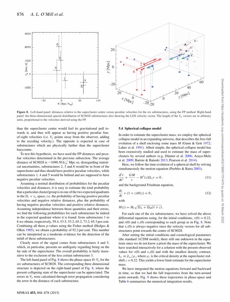
Figure 8. Left-hand panel: distances relative to the supercluster centre versus peculiar velocities for the six substructures, using the FP method. Right-handpanel: the three-dimensional spacial distribution of SC0028 substructures also showing the LOS velocity vector. The length of the Vp vectors are in arbitraryunits, proportional to the velocities derived using the FP.

than the supercluster centre would feel its gravitational pull to-wards it, and thus will appear as having positive peculiar line-of-sight velocities (i.e. Vp points away from the observer, addingto the receding velocity.). The opposite is expected in case ofsubstructures which are physically farther than the superclusterbarycentre.

To test this hypothesis, we have used the FP distances and pecu-liar velocities determined in the previous subsection. The averagedistance of SC0028 is ∼1090.50 h−1

70 Mpc so, disregarding statisti-cal uncertainties, substructures 2, 3 and 6 would be in front of thesupercluster and thus should have positive peculiar velocities, whilesubstructures 1, 4 and 5 would be behind and are supposed to havenegative peculiar velocities.

Assuming a normal distribution of probabilities for the peculiarvelocities and distances, it is easy to estimate the total probabilitythat a particular cluster/group is in one of the two expected quadrantsin the Dr × vp space, i.e. the probability of having positive peculiarvelocities and negative relative distances, plus the probability ofhaving negative peculiar velocities and positive relative distances.Assuming independence between those quantities and their errors,we find the following probabilities for each substructure be indeedin the expected quadrant where it is found: from substructure 1 to6 we obtain, respectively, 59.4, 53.5, 53.2, 65.2, 73.2, 65.3 per cent.Combining all these p-values using the Fisher method (Hedges &Olkin 1985), we obtain a probability of 92.2 per cent. This numbercan be interpreted as a moderate evidence for the detection of theinfall of these substructures.

Clearly most of the signal comes from substructures 4 and 5,which, in particular, presents no ambiguity regarding being on thefar side of the supercluster. The overall probability is fairly insen-sitive to the exclusion of the less certain substructure 3.

The left-hand panel of Fig. 8 shows the phase-space D–Vp for thesix substructures of SC0028. The corresponding three dimensionalstructure is depicted on the right-hand panel of Fig. 8, where thepresent collapsing state of the supercluster can be appreciated. Theerrors in Vp were calculated through error propagation consideringthe error in the distance of each substructure.

5.4 Spherical collapse model

In order to estimate the supercluster mass, we employ the sphericalcollapse model in an expanding universe, that describes the free-fallevolution of a shell enclosing some mass M (Gunn & Gott 1972;Lahav et al. 1991). Albeit simple, the spherical collapse model hasbeen extensively studied and used to estimate the mass of super-clusters by several authors (e.g. Dunner et al. 2006; Araya-Meloet al. 2009; Batiste & Batuski 2013; Pearson et al. 2014).

Here, we follow the time evolution of a spherical shell by solvingsimultaneously the motion equation (Peebles & Ratra 2003),

d2r

dt2+ GM

r− H 2(z)��r = 0 , (11)

and the background Friedman equation,

dz

dt+ (1 + z)H (z) = 0 , (12)

with

H (z) = H0

√�� + �M(1 + z) .

For each one of the six substructures, we have solved the abovedifferential equations using, for the initial conditions, z(0) = 0.22,and r(0) and vr(0) corresponding to each group as in Fig. 8. Notethat vr(0) is always negative since the velocity vectors for all sub-structures point towards the centre of SC0028.

After setting the initial conditions and cosmological parameters(the standard �CDM model), there still one unknown in the equa-tions since we do not know a priori the mass of the supercluster. Wehave searched interactively for a solution with the present observedvalues for r(0) and vr(0) and with the smallest density contrast,δsc ≡ ρsc/ρc, where ρc is the critical density at the supercluster red-shift z = 0.22. This yields a lower limit estimate for the superclustermass.

We have integrated the motion equations forward and backwardin time, so that we had the full trajectories from the turn-aroundpoint onwards. Fig. 9 shows these trajectories in phase-space andTable 6 summarizes the numerical integration results.

MNRAS 453, 868–878 (2015)

Dow

nloaded from https://academ

ic.oup.com/m

nras/article/453/1/868/1751475 by guest on 16 March 2022

Structure and dynamics of the supercluster of galaxies SC0028-0005 877

Figure 9. Free-fall trajectories for the six substructures in SC0028 in phase-space. The initial conditions are marked as large dots, with the correspondingnumbers.

Table 6. Initial conditions, r(0) and vr(0), and results of the integrationof the spherical collapse equation. δsc is the mean density contrast ofthe supercluster with respect to the critical density. tTA and rTA are thetime of turn-around and the radial distance at that time.

Obj. r(0) vr(0) δsc M[ < r(0)] tTA rTA

Id (Mpc) (km s−1) (1015 M�) (Gyr) (Mpc)

1 10.0 −490 6.1 4.3 −5.7 11.12 5.5 −1026 21.6 2.6 −6.5 8.03 14.1 −269 3.6 7.2 −5.5 14.64 61.0 −611 2.8 445 −3.6 61.95 60.0 −815 3.2 489 −5.7 61.06 9.8 −2036 24.9 16.4 −7.4 14.7

Fig. 9 shows that substructures 1, 2, 3 and 6 have nearby trajec-tories in phase-space, while substructures 4 and 5 have very similartrajectories, but distinct from the other four. The latter pair seems tohave about the same turn-around radius, compatible with an enclos-ing total mass of ∼4.5–4.9 × 1017 M�. This large mass, however,corresponds to a mean density contrast of only ∼3 above the criticalbackground density at z = 0.22.

The case of substructures 1, 2, 3 and 6 is more complex. Objects 2and 6 suggest a high-density contrast, ∼22–25, while objects 1 and3 suggest a low-density contrast, in agreement with substructures 4and 5 (between δsc ∼ 4 and 6). On the other hand, substructures 3and 6 have almost the same turn-around radius, rTA ∼ 14 Mpc.

Given the uncertainties in the distance determination and ourlack of information on the transverse component of the substructurespeculiar velocities – we have used the line-of-sight peculiar velocityas a rough estimate of the radial peculiar velocity, vr – we can onlyhave an order of magnitude estimate on the supercluster mass. At aradius of 10 Mpc, the free-fall motion suggests that mass should liebetween ∼4 and 16 × 1015 M�.

The weak-lensing masses of the individual substructures are ofthe order of 1–2 × 1014 M� (see Table 3). Within 10 Mpc from thesupercluster centre, there are 3–4 of such substructures that addsup to about ∼3 × 1014 (without substructure 6, which lies outsidethe footprint of CFHT). Therefore, most of this supercluster massbudget should be in the form of lower than ∼5 × 1013 M� galaxygroups. That is below our detectable level with the present data.

6 SU M M A RY A N D C O N C L U S I O N S

In this work, we have analysed the gravitational dynamics of thesupercluster SC0028 with spectroscopic and photometric data fromSDSS-DR10. This supercluster was selected from the superclustercatalogue of Basilakos (2003), where it was classified as a filamen-tary structure.

We have chosen an area of 1.2 deg2 around the supercluster andproceeded to identify substructures using density maps and red-sequence analysis. We identified nine substructures throughout thearea, but three of them were discarded because their fraction of redgalaxies was less than 50 per cent.

To test the collapse scenario for supercluster evolution, we havedetermined the distances and peculiar velocities for each substruc-ture in the supercluster. In order to study the dynamics of thesesubstructures, the FP was used as a distance indicator. For the spec-troscopic sample, each substructure has, on average, 10 galaxies.This number is too small to determine the local FP parameters.Instead we have used the globally fitted slopes and then estimatedzero-point offsets for each of the six substructures.

In order to obtain the individual distances and peculiar velocities,we considered that the supercluster’s centroid does not have peculiarmovements and, knowing the supercluster’s distance beforehand,we computed the individual distances for each structure.

The resulting picture for SC0028 is of three substructures ap-proaching the supercluster barycentre from the far side and threefrom the near side, based on the computed empirical relations withphotospectroscopic data. The spatial distribution and peculiar veloc-ities of the detected members of SC0028 support the collapsing su-percluster scenario. Assuming that the dynamics may be describedby a simple free-fall spherical collapse model, the overall densitycontrast is δ ∼ 3 inside a radius of 60 Mpc. In the inner region, inside10 Mpc, the mass should be 4–16 × 1015 M�. Most of this shouldbe in the form of low-mass (M � 5 × 1013 M�) substructures.

AC K N OW L E D G E M E N T S

We acknowledge financial support form CONICET/CofecubFrench-Brazilian cooperation, CNPq, FAPESP, Castejon2013/14817-9, Cypriano 2014/13723-3, Lima Neto and Sodre Jr.2012/00800-4 and O’Mill 2011/09565-5.

Funding for SDSS-III has been provided by the Alfred P. SloanFoundation, the Participating Institutions, the National ScienceFoundation, and the US Department of Energy Office of Science.The SDSS-III web site is http://www.sdss3.org/.

SDSS-III is managed by the Astrophysical Research Consor-tium for the Participating Institutions of the SDSS-III Collabora-tion including the University of Arizona, the Brazilian ParticipationGroup, Brookhaven National Laboratory, Carnegie Mellon Uni-versity, University of Florida, the French Participation Group, theGerman Participation Group, Harvard University, the Instituto deAstrofisica de Canarias, the Michigan State/Notre Dame/JINA Par-ticipation Group, Johns Hopkins University, Lawrence BerkeleyNational Laboratory, Max Planck Institute for Astrophysics, MaxPlanck Institute for Extraterrestrial Physics, New Mexico State Uni-versity, New York University, Ohio State University, PennsylvaniaState University, University of Portsmouth, Princeton University,the Spanish Participation Group, University of Tokyo, Universityof Utah, Vanderbilt University, University of Virginia, Universityof Washington and Yale University.

MNRAS 453, 868–878 (2015)

Dow

nloaded from https://academ

ic.oup.com/m

nras/article/453/1/868/1751475 by guest on 16 March 2022

878 A. L. O’Mill et al.

This work is partially based on CFHT observations (IDs 10BB07and 10BB97) which have been processed at the TERAPIX datacenter located at the Institut d’Astrophisique de Paris.

R E F E R E N C E S

Ahn C. P. et al., 2012, ApJS, 203, 21Araya-Melo P. A., Reisenberg A., Meza A., van de Weygaert R., Dunner R.,

Quintana H., 2009, MNRAS, 399, 97Basilakos S., 2003, MNRAS, 344, 602Batiste M., Batuski D. J., 2013, MNRAS, 436, 3331Bernardi M. et al., 2003, AJ, 125, 1882Bertin E., Arnouts S., 1996, A&AS, 117, 393Bertin E., Mellier Y., Radovich M., Missonnier G., Didelon P., Morin B.,

2002, in Bohlender D. A., Durand D., Handley T. H., eds, ASP Conf.Ser. Vol. 281, Astronomical Data Analysis Software and Systems XI.Astron. Soc. Pac., San Francisco, p. 228

Blanton M. R., Roweis S., 2007, AJ, 133, 734Bridle S. L., Hobson M. P., Lasenby A. N., Saunders R., 1998, MNRAS,

299, 895Bridle S., Kneib J.-P., Bardeau S., Gull S. F., 2002, in Natarajan P., ed.,

Proc. Yale Cosmology Workshop “The Shapes of Galaxies and TheirDark Matter Halos”, Bayesian galaxy shape estimation in The Shapesof Galaxies and Their Dark Halos. World Scientific, Singapore, p. 38,available at: http://www.sarahbridle.net/im2shape/yale.pdf

Busha M. T., Adams F. C., Wechsler R. H., Evrard A. E., 2003, ApJ, 596,713

Corwin H. G., Jr, Buta R. J., de Vaucouleurs G., 1994, AJ, 108, 2128Costa-Duarte M. V., Sodre L., Jr, Durret F., 2011, MNRAS, 411, 1716Coupon J. et al., 2009, A&A, 500, 981Cypriano E. S., Sodre L. J., Kneib J.-P., Campusano L. E., 2004, ApJ, 613,

95de Vaucouleurs G., 1953, AJ, 58, 30Djorgovski S., Davis M., 1987, ApJ, 313, 59Dressler A., 1980, ApJ, 236, 351Dressler A., Lynden-Bell D., Burstein D., Davies R. L., Faber S. M.,

Terlevich R., Wegner G., 1987, ApJ, 313, 42Dunner R., Araya P. A., Meza A., Reisenegger A., 2006, MNRAS, 366, 803Dunner R., Reisenegger A., Meza A., Araya P. A., Quintana H., 2007,

MNRAS, 376, 1577Einasto J., Klypin A. A., Saar E., Shandarin S. F., 1984, MNRAS, 206, 529Einasto M., Einasto J., Tago E., Dalton G. B., Andernach H., 1994, MNRAS,

269, 301Einasto M. et al., 2007, A&A, 476, 697

Einasto M., Liivamagi L. J., Tago E., Saar E., Tempel E., Einasto J., MartnezV. J., Heinamaki P., 2011, A&A, 532, A5

Fukugita M., Shimasaku K., Ichikawa T., 1995, PASP 107, 945Goto T. et al., 2002, AJ, 123, 1807Gunn J. E., Gott J. R., III, 1972, ApJ, 176, 1Hedges L., Olkin I., 1985, Statistical Methods for Meta-Analysis. Academic

Press, San DiegoHyde J. B., Bernardi M., 2009, MNRAS, 396, 1171Joeveer M., Einasto J., Tago E., 1978, MNRAS, 185, 357Jørgensen I., Franx M., Kjaergaard P., 1995, MNRAS, 276, 1341Lahav O., Lilje P. B., Primack J. R., Rees M. J., 1991, MNRAS, 251, 128Lintott C. et al., 2011, MNRAS, 410, 166Marshall P. J., Hobson M. P., Gull S. F., Bridle S. L., 2002, MNRAS, 335,

1037Merluzzi P. et al., 2015, MNRAS, 446, 803Nagamine K., Loeb A., 2003, New Astron., 8, 439Navarro J. F., Frenk C. S., White S. D. M., 1996, ApJ, 462, 563Navarro J. F., Frenk C. S., White S. D. M., 1997, ApJ, 490, 493Neyman J., Scott E. L., Shane C. D., 1956, in Jerzy Neyman, ed.,Proceedings

of the Third Berkeley Symp. on Mathematical Statistics and ProbabilityVol. 3, University of California Press, Berkeley, CA 75

Oemler A., Jr, 1974, ApJ, 194, 1Pearson D. W., Batiste M., Batuski D. J., 2014, MNRAS, 441, 1601Peebles P. J. E., 1993, Principles of Physical Cosmology. Princeton Univ.

Press, Princeton, NJPeebles P. J. E., Ratra B., 2003, Rev. Mod. Phys., 75, 559Postman M., Geller M. J., 1984, ApJ, 281, 95Prada F., Klypin A. A., Cuesta A. J., Primark J., 2012, MNRAS, 423, 3018Proust D. et al., 2006, The Messenger, 124, 30Ragone C. J., Muriel H., Proust D., Reisenegger A., Quintana H., 2006,

A&A, 445, 819Reisenegger A., Quintana H., Carrasco E. R., Maze J., 2000, AJ, 120, 523Rines K., Geller M. J., Diaferio A., Kurtz M. J., 2013, ApJ, 767, 15Saulder C., Mieske S., Zeilinger W., Chilingarian I., 2013, A&A, 557, id.A21Tago E., Einasto J., Saar E., 1984, MNRAS, 206, 559Terlevich R., Davies R. L., Faber S. M., Burstein D., 1981, MNRAS, 196,

381Tully R. B., Courtois H., Hoffman Y., Pomarede D., 2014, Nature, 513, 71Wegner G., Colless M., Saglia R. P., McMahan R. K., Davies R. L., Burstein

D., Baggley G., 1999, MNRAS, 305, 259Zucca E., Zamorani G., Scaramella R., Vettolani G., 1993, ApJ, 407, 470

This paper has been typeset from a TEX/LATEX file prepared by the author.

MNRAS 453, 868–878 (2015)

Dow

nloaded from https://academ

ic.oup.com/m

nras/article/453/1/868/1751475 by guest on 16 March 2022