
Imaging structure and dynamics using controlled molecules
163
Imaging structure and dynamics using controlled molecules Dissertation zur Erlangung des Doktorgrades an der Fakult¨ at f¨ ur Mathematik, Informatik und Naturwissenschaften, Fachbereich Physik der Universit¨ at Hamburg vorgelegt von Thomas Kierspel aus Bergisch Gladbach Hamburg 2017
-
Upload
khangminh22 -
Category
Documents
-
view
0 -
download
0
Transcript of Imaging structure and dynamics using controlled molecules

Imaging structure and
dynamics using controlled molecules
Dissertation
zur Erlangung des Doktorgrades
an der Fakultat fur Mathematik, Informatik und Naturwissenschaften,
Fachbereich Physik
der Universitat Hamburg
vorgelegt von
Thomas Kierspel
aus Bergisch Gladbach
Hamburg
2017

Gutachter der Dissertation: Prof. Dr. Jochen Kupper
Dr. Oriol Vendrell
Zusammensetzung der Prufungskommission: Prof. Dr. Jochen Kupper
Dr. Oriol Vendrell
Prof. Dr. Henry N. Chapman
Dr. Oliver D. Mucke
Prof. Dr. Caren Hagner
Datum der Disputation: 3. Marz 2017
Vorsitzender des Prufungsausschusses: Prof. Dr. Caren Hagner
Vorsitzender des Promotionsausschusses: Prof. Dr. Wolfgang Hansen
Dekan der Fakultat fur Mathematik,
Informatik und Naturwissenschaften: Prof. Dr. Heinrich Graener

Eidesstattliche Versicherung
Hiermit versichere ich an Eides statt, dass ich die Inanspruchnahme fremder Hilfen aufgefuhrt habe, sowie,
dass ich die wortlich oder inhaltlich aus anderen Quellen entnommenen Stellen als solche kenntlich gemacht
habe. Weiterhin versichere ich an Eides statt, dass ich die Dissertation selbst verfasst und keine anderen
als die angegebenen Hilfsmittel benutzt habe.
Thomas Kierspel

Abstract
Folding, isomerization, and dissociation of molecules, i. e., bond breaking and bond formation, is happening
on ultrafast time scales. Femtoseconds (1 fs = 10−15 s) are the time scale on which atoms move. Hence,
the observation of a chemical process on that time scale allows not only to measure the reactants and
products of a chemical reaction, but also allows to observe the systems far from equilibrium. Within this
dissertation several complementary measurements are presented, which are designed to measure chemical
reactions of controlled gas-phase molecules at synchrotrons, high-harmonic generation based radiation
sources, and the 4th generation x-ray light sources, x-ray free-electron lasers.
Gas-phase molecular ensembles are cooled in molecular beams and purified by either spatial separation
of different rotational isomers, or size-selection of molecular clusters to provide a clean sample for the
experiments. Furthermore, control is gained by the alignment of the initially isotropically distributed
molecular sample to the laboratory frame. The controlled molecular samples, or their fragments, are
imaged by several techniques, ranging from one-dimensional ion time-of-flight measurements, over two-
dimensional velocity-map imaging of electrons and ions, to the measurement of scattered x-ray photons by
an x-ray camera.
At first it is demonstrated that the cis- and trans-conformer of 3-fluorophenol can be purified in the
interaction region to more than 90 % via spatial separation, and thus providing an ideal sample to study
isomerization dynamics (chapter 3). The sample was chosen such that it is possible measure the ultrafast
isomerization dynamics via photoelectron diffraction by using a free-electron laser.
In addition to the spatial control of the molecular beam, the alignment of the gas-phase molecular sample
is demonstrated at the full repetition rate of a free-electron laser by the use of an in-house Ti:Sapphire
laser system (chapter 4). Since most facilities have synchronized Ti:Sapphire laser systems at their
corresponding end stations, this approach is demonstrating an alignment technique which can be easily
implemented in most experiments.
The controlled gas-phase molecules were probed by hard x-ray photons to determine their structure via
diffractive imaging (chapter 5). Diffractive imaging of gas-phase molecules at free-electron lasers is a highly
promising approach to image ultrafast molecular dynamics of gas-phase molecules. The alignment of the
molecular sample does have the advantage that, providing the molecules are perfectly aligned (or more
general perfectly oriented), its diffraction pattern is equal to the diffraction pattern of a single molecule,
which allows for the reconstruction of bond distances and bond angles of the molecule.
Furthermore, the x-ray photophysics of indole and indole-water clusters measured at a synchrotron are
presented in chapter 6 and chapter 7. Indole and microsolvated indole-water clusters were spatially
separated and both locally ionized by soft x-ray radiation. The ionic fragments as well as emitted electrons
were recorded in coincidence. The fragmentation patterns of both species are compared to learn about the
influence of the hydrogen-bonded water on the fragmentation of indole. This experiment was aiming at
v

the difference between isolated molecules and molecules in solvation, and also to study hydrogen bonds
which are of universal importance in chemistry and biochemistry.
The potential use of a high-harmonic generation based radiation as a further source–next to the established
accelerator-based facilities–for extreme ultraviolet photons is demonstrated in section 8.1 to study ultrafast
dynamics of gas-phase molecules. Moreover, the sample preparation of the amino acid glycine is shown in
section 8.2 for future studies of ultrafast charge migration in conformer-selected molecular samples by the
use of attosecond pulses generated by higher harmonics.
vi
Zusammenfassung
Faltung, Isomerisierung oder die Dissoziation von Molekulen findet auf der Zeitskala von Femtosekunden
(1 fs = 10−15 s) statt. Experimente mit einer Zeitauflosung im Bereich von fs machen es somit moglich,
nicht nur den Anfangs- und Endzustand einer chemischen Reaktion zu beobachten, sondern erlauben
es auch ein Bild von der Chemie weit entfernt vom Gleichgewichtszustand des jeweiligem System zu
bekommen. In dieser Arbeit werden mehrere Experimente prasentiert, welche konzipiert sind um zukunftig
verschiedenen ultraschnelle chemische Prozesse in kontrollierten Molekulen in der Gasphase mit verschiede-
nen Strahlungsquellen (Laser oder hohere harmonische eines Lasers, Synchrotron, Freie-Elektronen-Laser)
zu messen.
Die Kontrolle der Molekule wurde auf zwei unterschiedliche Weisen realisiert. Zum einen wurden ver-
schiedene molekulare Spezies (Isomere und molekulare Cluster) durch inhomogene statische elektrische
Felder raumlich voneinander getrennt. Zum anderen wurde die raumliche Ausrichtung der Molekule durch
Laserpulse kontrolliert. Die kontrollierten Molekule wurden anschließend mit verschiedenen Strahlungen
(Infrarot-Laser, Ultraviolett-Laser, weiche und harte Rontgenstrahlung) vermessen. Die Resultate der
Interaktion wurden durch Ionen-Flugzeitmassenspektrometer, “Velocity-Map Imaging“-Spektrometer, oder
einer Rontgenkamera abgebildet.
Im ersten gezeigten Experiment wird die raumliche Trennung des cis und trans-Konformer von 3-
Fluorphenol demonstriert (Kapitel 3). Hierbei wird gezeigt, dass es moglich ist eine nahezu reine Probe
von beiden Konformeren zu erhalten, welche dazu genutzt werden konnen Isomerisierungsdynamiken in
der Gasphase zu untersuchen.
Anschließend wird die raumliche Ausrichtung von Molekulen in der Gasphase bei voller Repetitionsrate
von einem Freie-Elektronen-Laser demonstriert (Kapitel 4). Dies ist eine wichtige Demonstration, da die
eingesetzten Laser an nahezu jeder Messstation von Freie-Elektronen-Lasern vorhanden sind, wodurch es
vielen Experimentatoren ermoglicht wird ohne großen experimentellen Aufwand Molekule in der Gasphase
auszurichten.
Die ausgerichteten Molekule wurden genutzt um mittels Rontgenbeugung die atomare Struktur des einzel-
nen Molekuls zu bestimmen (Kapitel 5). Durch die ultrakurzen Rontgenblitze von Freie-Elektronen-Lasern
ist es namlich moglich Strukturen sowie Strukturanderugen mit einer Zeitauflosung von Femtosekunden
zu messen und somit einen direkten Einblick in the Femtochemie zu bekommen. Das Ausrichten der
Molekulen erlaubt es dabei viele einzelne Bilder aufzunehmen, deren Summe dann–im Fall von perfekt
ausgerichteten Molekulen (oder allgemeiner perfekt orientieren Molekulen)–gleich dem Bild des einzelnen
Molekuls ist.
Anschließend wird die Photophysik von Indol sowie Indol-Wasser-Clustern untersucht (Kapitel 6, Kapi-
tel 7). Dabei wurden beide Spezies raumlich voneinander getrennt und lokal am Indol-Molekul ionisiert.
vii

Die ionischen Fragmente und Elektronen wurden in Koinzidenz gemessen. Die unterschiedlichen Frag-
mentationskanale wurden verglichen um den Einfluss des gebunden Wassers auf die Fragmentation vom
Indol-Monomer zu untersuchen.
Zusatzlich wurde eine laborbasierte Laserquelle genutzt um die Fragmentation von Iodmethan durch
lokalisierte Innerschalenionisation zu messen (Abschnitt 8.1). Dafur wurden hohere Harmonische des
Lasers erzeugt, welche Iodmethan lokal ionisiert haben. Auch hier wurden die emittierten Elektronen
und die ionischen Fragmente in Koinzidenz gemessen. Das Experiment wird in den Zusammenhang mit
ahnlichen Experimenten gesetzt, welche an beschleunigerbasierten Photonenquellen durchgefuhrt wurden,
um das Potential laborbasierter Messung im Bereich der extrem ultravioletten Strahlung zu demonstrieren.
Anschließend wird die mogliche Separation der Konformere von Glycin in einem Molekulstrahl diskutiert.
Ziel des Experiments ist es konformerenabhangige Ladungsmigration in Glycin mittels hoherer harmonischer
eines Laser zu messen (Abschnitt 8.2).
viii

Contents
1 Introduction 1
1.1 Sample preparation . . . . . . . . . . . . . . . . . . . . . . . . . . . . . . . . . . . . . . . . 2
1.2 X-ray diffractive imaging . . . . . . . . . . . . . . . . . . . . . . . . . . . . . . . . . . . . . 3
1.3 X-ray photophysics and coincident measurements . . . . . . . . . . . . . . . . . . . . . . . 4
1.4 Outline of the thesis . . . . . . . . . . . . . . . . . . . . . . . . . . . . . . . . . . . . . . . 5
2 Fundamental concepts 7
2.1 Performed experiments . . . . . . . . . . . . . . . . . . . . . . . . . . . . . . . . . . . . . . 7
2.2 Molecules in electric fields . . . . . . . . . . . . . . . . . . . . . . . . . . . . . . . . . . . . 10
2.3 Adiabatic alignment of molecules . . . . . . . . . . . . . . . . . . . . . . . . . . . . . . . . 12
2.4 X-ray matter interaction . . . . . . . . . . . . . . . . . . . . . . . . . . . . . . . . . . . . . 14
2.4.1 X-ray absorption and relaxation . . . . . . . . . . . . . . . . . . . . . . . . . . . . 15
2.4.2 X-ray diffraction . . . . . . . . . . . . . . . . . . . . . . . . . . . . . . . . . . . . . 17
3 Conformer separation of gas-phase molecules 21
3.1 Introduction . . . . . . . . . . . . . . . . . . . . . . . . . . . . . . . . . . . . . . . . . . . . 21
3.2 Experimental details . . . . . . . . . . . . . . . . . . . . . . . . . . . . . . . . . . . . . . . 22
3.3 Results and discussions . . . . . . . . . . . . . . . . . . . . . . . . . . . . . . . . . . . . . 23
3.4 Conclusions . . . . . . . . . . . . . . . . . . . . . . . . . . . . . . . . . . . . . . . . . . . . 25
4 Alignment at 4th generation light source 27
4.1 Introduction . . . . . . . . . . . . . . . . . . . . . . . . . . . . . . . . . . . . . . . . . . . . 27
4.2 Experimental Setup . . . . . . . . . . . . . . . . . . . . . . . . . . . . . . . . . . . . . . . 28
4.3 Results from experiments at LCLS . . . . . . . . . . . . . . . . . . . . . . . . . . . . . . . 31
4.4 Results from experiments at CFEL . . . . . . . . . . . . . . . . . . . . . . . . . . . . . . . 32
4.5 Discussion . . . . . . . . . . . . . . . . . . . . . . . . . . . . . . . . . . . . . . . . . . . . . 33
4.6 Summary . . . . . . . . . . . . . . . . . . . . . . . . . . . . . . . . . . . . . . . . . . . . . 36
5 X-ray diffractive imaging of controlled molecules 39
5.1 Introduction . . . . . . . . . . . . . . . . . . . . . . . . . . . . . . . . . . . . . . . . . . . . 39
5.2 Experimental setup . . . . . . . . . . . . . . . . . . . . . . . . . . . . . . . . . . . . . . . . 41
5.3 Simulations . . . . . . . . . . . . . . . . . . . . . . . . . . . . . . . . . . . . . . . . . . . . 42
5.4 CSPAD data handling . . . . . . . . . . . . . . . . . . . . . . . . . . . . . . . . . . . . . . 48
5.5 Experimental results . . . . . . . . . . . . . . . . . . . . . . . . . . . . . . . . . . . . . . . 50
5.6 Discussion . . . . . . . . . . . . . . . . . . . . . . . . . . . . . . . . . . . . . . . . . . . . . 57
5.7 Conclusion and outlook . . . . . . . . . . . . . . . . . . . . . . . . . . . . . . . . . . . . . 60
ix

6 X-ray photophysics of indole 63
6.1 Introduction . . . . . . . . . . . . . . . . . . . . . . . . . . . . . . . . . . . . . . . . . . . . 63
6.2 Experimental setup . . . . . . . . . . . . . . . . . . . . . . . . . . . . . . . . . . . . . . . . 64
6.3 Coincidence spectra . . . . . . . . . . . . . . . . . . . . . . . . . . . . . . . . . . . . . . . 66
6.4 Photoelectron spectrum . . . . . . . . . . . . . . . . . . . . . . . . . . . . . . . . . . . . . 72
6.5 Discussion . . . . . . . . . . . . . . . . . . . . . . . . . . . . . . . . . . . . . . . . . . . . . 73
6.6 Conclusion . . . . . . . . . . . . . . . . . . . . . . . . . . . . . . . . . . . . . . . . . . . . 76
7 X-ray photophysics of indole-water clusters 79
7.1 Introduction . . . . . . . . . . . . . . . . . . . . . . . . . . . . . . . . . . . . . . . . . . . . 79
7.2 Experimental setup . . . . . . . . . . . . . . . . . . . . . . . . . . . . . . . . . . . . . . . . 80
7.3 Ion coincidence spectra . . . . . . . . . . . . . . . . . . . . . . . . . . . . . . . . . . . . . . 81
7.4 Electrons . . . . . . . . . . . . . . . . . . . . . . . . . . . . . . . . . . . . . . . . . . . . . 86
7.5 Discussion . . . . . . . . . . . . . . . . . . . . . . . . . . . . . . . . . . . . . . . . . . . . . 88
7.6 Summary and outlook . . . . . . . . . . . . . . . . . . . . . . . . . . . . . . . . . . . . . . 89
8 Applications of HHG photon sources 91
8.1 HHG source for coincidence ion imaging of gas-phase molecules . . . . . . . . . . . . . . . 91
8.1.1 Introduction . . . . . . . . . . . . . . . . . . . . . . . . . . . . . . . . . . . . . . . 92
8.1.2 High-repetition-rate and high-photon-flux XUV source . . . . . . . . . . . . . . . . 93
8.1.3 Coherently combined femtosecond fiber chirped pulse amplifier . . . . . . . . . . . 93
8.1.4 Nonlinear compression . . . . . . . . . . . . . . . . . . . . . . . . . . . . . . . . . . 94
8.1.5 High photon flux source at 68.6 eV . . . . . . . . . . . . . . . . . . . . . . . . . . . 96
8.1.6 Coincidence detection of CH3I ionization fragments . . . . . . . . . . . . . . . . . . 99
8.1.7 Photon flux estimate . . . . . . . . . . . . . . . . . . . . . . . . . . . . . . . . . . . 102
8.1.8 Conclusion and outlook . . . . . . . . . . . . . . . . . . . . . . . . . . . . . . . . . 103
8.2 Toward charge migration in conformer-selected molecular samples . . . . . . . . . . . . . . 104
8.2.1 Simulations: Stark curves and deflection profile . . . . . . . . . . . . . . . . . . . . 105
8.2.2 Experiment . . . . . . . . . . . . . . . . . . . . . . . . . . . . . . . . . . . . . . . . 108
8.2.3 Conclusion and outlook . . . . . . . . . . . . . . . . . . . . . . . . . . . . . . . . . 110
9 Summary 111
9.1 Sample preparation . . . . . . . . . . . . . . . . . . . . . . . . . . . . . . . . . . . . . . . . 111
9.2 X-ray diffractive imaging . . . . . . . . . . . . . . . . . . . . . . . . . . . . . . . . . . . . . 112
9.3 X-ray photophysics and coincident measurements . . . . . . . . . . . . . . . . . . . . . . . 112
10 Conclusion and outlook 115
Bibliography 117
x

Appendix 135
A Supplementary information chapter 5 135
A.1 Molecular properties of 2,5-diiodothiophene . . . . . . . . . . . . . . . . . . . . . . . . . . 135
A.2 Diffractive imaging – ADU gate optimization . . . . . . . . . . . . . . . . . . . . . . . . . 136
B Supplementary information chapter 6 and 7 139
B.1 Molecular beam reconstruction . . . . . . . . . . . . . . . . . . . . . . . . . . . . . . . . . 139
B.2 Coincidence spectrum (PIPICO) . . . . . . . . . . . . . . . . . . . . . . . . . . . . . . . . 140
B.3 Mass spectrum calibration . . . . . . . . . . . . . . . . . . . . . . . . . . . . . . . . . . . . 141
B.4 Ion VMI calibration . . . . . . . . . . . . . . . . . . . . . . . . . . . . . . . . . . . . . . . 141
B.5 Electron VMI calibration . . . . . . . . . . . . . . . . . . . . . . . . . . . . . . . . . . . . 145
Acknowledgment 149
List of Publications 151
xi


1 Introduction
Images of nature, animals, humans, or the night sky can not only look really nice but they can also be
intellectually appealing. Consider, for example, images of Antarctica. Most people have not yet visited
Antarctica but thanks to the images most people have an image in their mind about Antarctica and the
animals that live there. Additionally, the images provide us, at least those of us who have not yet been
there, a glimpse on what living in Antarctica would be like: very cold, half of the year pretty dark, no
big supermarkets or bars. At least the beer won’t get warm. The point is, images can tell us something
about a place or a person even though we might never have seen or experienced the place or have never
talked to the person. The experiments presented in this dissertation show the imaging of controlled
molecules in the gas-phase. Images were recorded to study their structure as well as to learn about
the response of gas-phase molecules and molecular clusters to localized ionization. Unlike the cameras
which were used to make photos of Antarctica, the applied scientific cameras are optimized to image tiny
molecules in the gas-phase. Imaging is here also not only restricted to the detection of photons, but it
is also covering the imaging of electrons and ions with techniques like an ion-time-of-flight (TOF, 1D
image) [1], or velocity-map imaging (VMI, 2D image) [2–5] of electrons and ions. Additionally, the images
were taken of controlled cold molecular samples. Control encompasses the spatial separation of different
molecular species, such as isomers or size-selection of molecular clusters, as if one would first sort the
penguins in Antarctica by hand according to species, or by the size of their family before the pictures
are shot. Furthermore, control is gained by aligning the controlled molecules in the gas-phase, which
would otherwise typically have a random orientation in space, i. e., making sure that the penguins are all
standing on their feet or head, instead of sitting or lying.
The presented experiments can be divided into three sections, namely sample preparation, x-ray diffraction
imaging and the x-ray photophysics of gas-phase molecules and clusters. The common (future) goal of
these experiments is to study structural changes of the molecules on femtosecond timescales, i. e., to get
a closer insight into the femtochemistry (1 femtosecond = 1 fs = 10−15 s) of gas-phase molecules. In
general, femtosecond(s) is the timescale of atomic motion within a molecule. Femtochemistry allows the
study of not only the educts and products, but also the evolution between them, i. e., the structure and
properties of the systems far from an equilibrium point. The field covers, for instance, bond breaking,
bond formation, folding and isomerization dynamics, as well as proton transfer or dissociation dynamics.
A pioneer in this field was Ahmed H. Zewail whom was awarded the Nobel Prize in 1999 for his studies of
the transition states of chemical reactions using femtosecond spectroscopy [6]. The presented experiments
image the static structure of molecules/molecular clusters as well as their product states. This was partly
due to the fact that most experiments were designed such that ultrashort x-ray laser pulses delivered by
x-ray free-electron lasers (FEL) are required to probe the femtochemistry, and hence beamtime has to be
approved.
1

1. Introduction
1.1 Sample preparation
Molecules in the gas-phase have the advantage that they can be treated as isolated systems, whereby the
intrinsic properties can be studied without influence from the environment. The focus of this dissertation
is to probe various aspects of controlled gas-phase molecules and to image their structure or fragmentation
pattern. To maximize the control over the molecules it is necessary to start with a cold (few Kelvin)
molecular beam, which was achieved by a supersonic expansion [7]. The control of the molecules covered
the spatial separation of different species present in the molecular beam as well as the alignment of the
isotropic distributed molecules in space.
The different species in the molecular beam are due to different conformers of the gas-phase molecule
or due to different molecular clusters. In general, different conformers of complex molecules often exist
in a molecular beam even at low temperatures [8]. The number of different conformers, the relative
population of these conformers, and the experimental observables can lead to a much higher complexity in
the extracted data or can make it simply impossible to interpret the experimental findings correctly. In
experiments focussing on molecular clusters, a similar problem arises. The cluster formation relies on the
collision between the various species present in the molecular beam in the early phase of the supersonic
expansion. The overall size and cluster distribution can be controlled by the relative amount of sample
present in the gas-phase prior the supersonic expansion. However, there will always be various clusters
present in the molecular beam in addition to the desired cluster size to study. Spatial separation of the
different clusters helps to reduce the complexity and ensures that the desired cluster size dominates or
is at least enhanced. Thus, spatial separation is important to have a well defined starting point for the
imaging of structural dynamics in the molecules. The spatial separation was achieved by a device called
the deflector [9–13], which consists of two closely spaced electrodes generating a strong inhomogeneous
direct current (DC) electric field. In analogy to the Stern-Gerlach deflector [14], where inhomogeneous
magnetic fields were used to deflect silver atoms, the strong inhomogeneous DC electric fields were used
to spatially separate molecular species according to their effective dipole moments. Thus, the spatial
separation of conformers works best if they have a large difference in their effective dipole moment. For
clusters, the effective dipole moment to mass ratio is the important factor.
In addition to the control of molecules via spatial separation, the control of the alignment of a molecular
ensemble in space was utilized in the presented experiments. The orientation of molecules in the gas-phase
is typically isotropic. Experiments, which aim at the study of molecular frame dependent properties such
as the molecular frame photo-angular distribution (MFPAD) [15], or experiments, which aim at structure
determination by MFPAD [16–20], recoil-frame photo angular distributions (RFPAD) [19, 21–23], or
structure determination via diffractive imaging with x-rays as well as electrons (chapter 5) [24–32], require
the alignment of the gas-phase molecules or it can be highly advantageous. For example, MFPAD as
well as RFPAD experiments simply require access to the molecular frame to measure molecular-frame
dependent properties. For x-ray and electron diffraction experiments, the alignment of the molecular
2

1.2 X-ray diffractive imaging
ensemble has practical and scientific advantages. Due to the low density in a molecular beam the scattering
signal is typically very weak (for x-ray diffraction less than one photon per FEL pulse [25], chapter 5).
The practical advantage is that the alignment of the molecules can locally increase the signal to noise ratio
on the detector. Scientifically, the alignment has the advantage that it ensures to always diffract from
molecules in the same orientation. Thus, it is possible to integrate the diffraction images and be able to
reconstruct an image as if the photons have been scattered from a single object. This allows reconstructing
bond lengths and bond angles from the diffraction image, where the latter one is typically hidden for an
isotropically distributed molecular sample. The alignment can be done in several ways, ranging from DC
electric fields by so-called brute force orientation [33, 34], by laser alignment [35–38], or a combination
of both called mixed-field orientation [38, 39]. The difference between alignment and orientation is that
aligned molecules can still have an up-down symmetry (penguins standing on their feet or their head),
which is broken in the case of orientation. Laser alignment is sensitive to the polarization anisotropy in
the molecule, which leads to an alignment of the most-polarizable axis of the molecule along the major
axis of the alignment laser polarization ellipse [38]. It can be separated into adiabadic, non-adiabatic, and
intermediate regime, which are quantified by the rising (falling) times of the envelope of the laser pulse
and the rotational period of the molecule [35, 37]. For the presented experiments, the laser alignment
was conducted in the intermediate regime. An alternative to brute fore orientation or laser alignment is
the reconstruction of the molecular axis a posteriori. This can be achieved if the probe pulse induces a
Coulomb explosion in the molecule, the recoil of the ions is well defined in the molecular frame, and all
momenta of the ions are measured in coincidence [19, 21–23].
1.2 X-ray diffractive imaging
Within the context of the dissertation, x-ray diffraction was applied to aligned gas-phase molecules to
image their structure. But why does one need x-rays to image small structures? Considering a standard
camera first, the reason why it (or the human eye) can make an image of something is also related to
the wavelength λ of visible light (λ ≈ 400-800 nm), which is orders of magnitude smaller than the size
of the objected typically imaged. In 1873 Ernst Karl Abbe formulated that the resolution limit of a
microscope is in the order of the wavelength used to illuminate the sample [40]. Considering that criteria,
the imaging of viruses (≈ 100 nm), proteins (≈ 10 nm), or molecules (≈ 1 nm) with atomic resolution (≈
0.1 nm) is not possible with visible light. In 1895 Wilhelm Conrad Rontgen discovered a type new type of
radiation, which he gave the german name X-strahlen (Rontgen’sche Strahlen, Rontgenstrahlen) [41], or
in english x-rays. X-rays are a form of electromagnetic radiation and, depending on the definition, cover
a wavelength region ranging from a few nm to a few pm [42–44]. Consequently, x-rays fulfill the Abbe
criteria to image structure with atomic resolution. X-ray diffractive imaging in crystalline samples is still
today a really successful approach to probe structures of, e. g., bacteria, viruses, or proteins. It lead to
the discovery of the structure of the benzene ring [45] and the structure of the DNAs’ double-helix [46].
The structure determination of viruses of bacteria lead, among many other things, to the development
3

1. Introduction
of structural based drug design [47]. Also, several Nobel prizes have already been awarded to structural
biology, with the most recent one in 2009 for unraveling the structure of the ribosome [48]. Most of the
experiments were conducted at synchrotrons, which provided until the year 2009 the most powerful x-ray
photon sources. In 2009 the era of x-ray free-electron lasers (FELs) started with the Linac Coherent Light
Source (LCLS) at the SLAC National Accelerator Laboratory being the first to go in user mode. FELs are
nowadays the brightest x-ray sources in the world and provide coherent x-ray pulses with pulse durations
in the order of femtoseconds. The short pulses of the free-electron lasers have the advantage that they can
outrun the radiation damage induced by the x-rays in the sample [49, 50], i. e., the photons diffract off the
sample before the structure of interest is destroyed. Additionally, they provide the time-resolution to study
ultrafast dynamics in gas-phase molecular samples. Thus, FELs are a highly promising photon source to
image the structure of gas-phase molecules and, more importantly, to image structural changes of the
molecule on ultrafast timescales. In a scattering and diffraction type of experiment this has already been
demonstrated for gas-phase molecules in a gas-cell [51, 52]. In the environment of a cold molecular beam
only static diffraction images have been recorded so far [24–26]. This is due to the orders of magnitude
lower density of molecules in a molecular beam compared to the density achievable in a gas-cell. The
experiment conducted in the scope of this dissertation was performed at a much shorter wavelength
compared to [24–26], which allowed consequently for a higher spatial resolution.
1.3 X-ray photophysics and coincident measurements
X-rays are not only very suitable for diffraction experiments but can also be used for localized ionization
of a molecular sample due to their element selectivity [42, 43]. Site-specific ionization within a molecule as
a starting point for controlled dynamics is a key to gain even more control about the triggered dynamics
or the probe pulse. Site-specific ionization is typically not achievable with femtosecond lasers since, in
that case, the ionization process relies on multiphoton or tunnel ionization, where the exact knowledge of
where the ionization in the molecule has happened is hidden from the experimentalist. Ionization by soft
x-ray photons has been used in a variety of experiments to observe, for instance, charge rearrangement in
dissociating molecules [53, 54], relaxation of highly exited states by observation of Auger electrons [55–57],
or fragmentation of the molecule following (site) specific ionization [22, 58–61] with the common goal to
get a closer insight into the world of femtochemistry.
Within the context of the dissertation, soft x-ray radiation was used to study the photofragmentation of
gas-phase molecules and molecular clusters upon localized core-shell ionization. The experiments were
aiming at two goals. First, the photofragmentation of indole and indole-water clusters was studied in
detail to understand the influence of the hydrogen-bonded water on the fragmentation of indole. The
localized ionization at the indoles’ nitrogen using soft x-ray radiation played a key role to guarantee that
the fragmentation was always triggered in the same way. These molecular systems allowed thus to study
hydrogen bonding, which is of universal importance in chemistry and biochemistry. In the second case,
the photon source was a laboratory-based high-harmonic generation (HHG) source, which was used for
4

1.4 Outline of the thesis
site-specific ionization of iodomethane molecule. The experiment was conducted to put HHG sources in
the realm of accelerator-based light sources, and to demonstrate the potential of the laboratory based
studies. In all cases the measurements were performed in a coincident mode, meaning that the ionic
fragments as well as electrons were recorded in coincidence. This allowed in all cases a 3D momentum
reconstruction of the ionic fragment and a 2D momentum reconstruction of the photo- and Auger electrons.
Coincidence measurements do have the strength that they help to understand the fragmentation of the
molecule upon inner-shell ionization [17, 21–23, 58, 59, 61, 62]. Also, the coincidence measurements do
allow to measure RFPADs of the molecules [19, 21–23] with the possibility to image the molecules upon
fragmentation, and to get thus an even closer insight into the femtochemical reaction.
1.4 Outline of the thesis
In chapter 2 the fundamental concepts of the dissertation are described, covering the generation of a
molecular beam, the fundamentals to spatially separate different conformers/clusters (possibly) present in
the molecular beam, and the alignment of gas-phase molecules. Also, the fundamental concepts of x-ray
matter interaction are shortly described, ranging from the relaxation following core-shell ionization to an
insight into x-ray diffraction.
In chapter 3 the spatial separation of the cis and trans conformer 3-fluorophenol is demonstrated by
making use of the strong inhomogeneous electric fields generated within the deflector. It demonstrates
for the first time that it is was possible to purify (> 90 %) the conformer with the lower effective dipole
moment, which was additionally less populated in the molecular beam. The aim was to provide a pure
molecular sample to study isomerization dynamics.
In chapter 4 the alignment of molecules in the gas-phase at the full FEL repetition rate is shown. It
demonstrates a universal preparation of molecules tightly fixed in space by the use of the available in-house
laser system at the coherent x-ray imaging (CXI) beamline at the Linac Coherent Light Source. The
molecules were aligned for structure determination via diffractive imaging.
Chapter 5 shows the diffractive imaging part of chapter 4. The results show evidence for the measurement
of a 1D diffraction image. The 2D diffractive imaging data cannot confirm the experimental findings
in the 1D diffraction image, also due to the experimental background, which was much higher than the
diffraction signal of the molecules. This chapter gives an outline for diffractive imaging off controlled
gas-phase molecules and discusses about improvements for future experiments.
Chapter 6 shows a detailed photofragmentation study of indole–the chromophore of the amino acid
tryptophan–triggered by inner-shell ionization. Photo- and Auger electrons as well as ionic fragments have
been measured in coincidence. The results show that indole is primarily fragmenting in three fragments,
where only two of them are ionized. The data also show coincidences, which are primarily present if the
indole monomer is localized ionized at its nitrogen atom. This experiment was conducted to understand
the photofragmentation of indole and provide thus a foundation for the photofragmentation study of
indole-water cluster.
5

1. Introduction
Chapter 7 shows the photofragmentation of indole-water clusters upon localized ionization at the indole-
part of the cluster. The indole-water clusters have been spatially separated from the indole monomer and
higher clusters. The spatial separation allowed to determine the fragmentation signature of indole-water,
which primarily showed a charge and proton transfer to the hydrogen-bonded water. Furthermore, it
showed that the generation of, in total, three ionic fragments is much more likely in the case of indole-water
compared to the indole monomer.
Chapter 8 is devided into two experiments. Section 8.1 shows the potential use of a HHG source to
measure the photophysics upon localized ionization by a table-top laser system. The experiment compares
the outcome with comparable experiments conducted at FELs and synchrotrons. Section 8.2 shows an
early stage of sample preparation of glycine for a conformer-selected attosecond pump-probe experiment to
measure conformer-specific charge migration. It provides simulations that show the possibility to spatially
separate/purify different conformers. Additionally, it shows that a molecular beam of glycine could not be
generated by the use of the pulsed Even-Lavie valve. Alternative evaporation sources like laser-desorption
or laser-induced acoustic desorption were used to demonstrate the measurement on an ion-TOF spectra of
glycine in the gas-phase.
6
2 Fundamental concepts
This chapter provides at first a general step-by-step overview, starting with the generation of a molecular
beam, followed by the control of molecules in the gas-phase using DC and alternating current (AC) electric
fields. Finally, the different probing schemes and detection techniques, which were applied in the context
of the dissertation, are described. A more detailed description of some of the fundamental concepts is
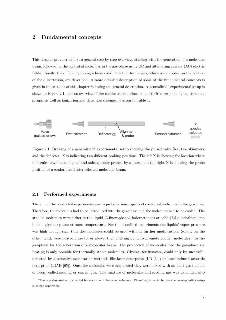
given in the sections of this chapter following the general description. A generalized∗ experimental setup is
shown in Figure 2.1, and an overview of the conducted experiments and their corresponding experimental
setups, as well as ionization and detection schemes, is given in Table 1.
Valve(pulsed or cw) First skimmer Deflector or Second skimmer
species selected
probe
x
Alignment& probe
x
Figure 2.1: Drawing of a generalized∗ experimental setup showing the pulsed valve [63], two skimmers,
and the deflector. X is indicating two different probing positions. The left X is showing the location where
molecules have been aligned and subsequently probed by a laser, and the right X is showing the probe
position of a conformer/cluster selected molecular beam.
2.1 Performed experiments
The aim of the conducted experiments was to probe various aspects of controlled molecules in the gas-phase.
Therefore, the molecules had to be introduced into the gas-phase and the molecules had to be cooled. The
studied molecules were either in the liquid (3-fluorophenol, iodomethane) or solid (2,5-diiodothiophene,
indole, glycine) phase at room temperature. For the described experiments the liquids’ vapor pressure
was high enough such that the molecules could be used without further modification. Solids, on the
other hand, were heated close to, or above, their melting point to promote enough molecules into the
gas-phase for the generation of a molecular beam. The promotion of molecules into the gas-phase via
heating is only possible for thermally stable molecules. Glycine, for instance, could only by successful
detected by alternative evaporation methods like laser desorption (LD [64]) or laser induced acoustic
desorption (LIAD [65]). Once the molecules were evaporated they were mixed with an inert gas (helium
or neon) called seeding or carrier gas. The mixture of molecules and seeding gas was expanded into
∗The experimental setups varied between the different experiments. Therefore, in each chapter the corresponding setup
is shown separately.
7

2. Fundamental concepts
vacuum either via a pulsed valve [63] (valve shown in Figure 2.1) or a continuous nozzle to generate a
supersonic expansion. Due to collisions between the seeding gas and molecules in the early phase of the
expansion a cooling of the molecules’ vibrational and rotational states is achieved such that only the
vibrational ground state and the lowest rotational states were significantly populated afterwards [7]. The
cold molecular beam was subsequently skimmed by the first skimmer (Figure 2.1). The skimmer was used
for differential pumping between the valve and the deflector/interaction chamber, to select the coldest
part of the molecular beam, and to reduce the size of the beam such that fewer collisions between the
beam and the deflector (Figure 2.1) occur, which lead to a warmer molecular beam.
The control of the cold molecular beam was achieved either by spatial separation of the different species
present in the molecular beam [9–11], or by alignment of the isotropically distributed molecules in space [35].
The spatial separation of the different molecular species was achieved by the deflector (Figure 2.1), and
performed to probe primarily the species of interest, i. e., a certain conformer or a certain cluster size. In
short, the deflector consists of two closely spaced electrodes (a cross section is shown in Figure 2.2 c))
generating a strong inhomogeneous electric DC field. The inhomogeneous electric field is required to exert
a force on the different molecular species, which is proportional to the effective dipole moment of the
molecules. Due to the effective dipole moment, which is dependent on the molecules rovibronic state, and
which is also typically dependent on the species, different states and species will experience a different
force which leads to a spatial separation after the deflector. A second skimmer (Figure 2.1) after the
deflector was used as differential pumping stage before the molecular beam was entering the probe section
of the experimental setup. A more detailed description of the concept of molecular deflection is given
in section 2.2.
In addition to the control of molecules via spatial separation, the control of the molecules was achieved by
laser-alignment of the isotropically orientated molecules in space [35]. The alignment was performed to
measure the structure of molecules via x-ray diffraction. The alignment of the molecular ensemble has the
experimental advantage of a local increase of the signal-to-noise ratio on the detector [24–26]. Scientifically
its advantage is that the diffraction image of a perfectly aligned (or more general oriented) molecular
ensemble is equal to the diffraction image of a single molecule [24–26]. In these experiments, alignment
and probing was conducted after the first skimmer, as it is indicated in Figure 2.1. In short, a linear
polarized laser pulse induces a dipole moment in the molecule which is dependent on the molecular-frame
polarizability. The molecular axis with the highest polarizability will align along the alignment laser
polarization. A more detailed description is given in section 2.3.
The probe pulses applied for the presented experiments are ranging from infrared to hard x-ray photons.
Sorted by increasing photon energy, an infrared (IR) femtosecond (fs) laser pulse was applied to probe the
molecules via strong-field ionization. Probing molecules by a fs-laser pulse is a general approach applicable
to a large range of molecules and observation parameters. It was used to measure an ion TOF spectrum,
and it was used to trigger a Coulomb explosion of the molecules to measure their degree of alignment via
velocity map imaging. An ultraviolet (UV) laser was used to probe different conformers of a molecule by
8

2.1 Performed experiments
resonant enhanced multi-photon ionization (REMPI). Among others, REMPI has the advantage of being
conformer specific, i. e., it can used to probe different structural isomers of the same molecule. This was
done to prove that different conformers could be spatially separated. Not all molecules do have suitable
REMPI transitions and hence it is only applicable to a limited amount of molecules. XUV and soft x-ray
radiation was used for localized ionization of the molecule from inner-shell orbitals. Localized ionization
has the advantage that it is a much cleaner probe pulse compared to, for instance, strong field ionization
since the ionization will primarily happen at the same/at a few known positions within the molecule.
Finally, hard x-ray photons were primarily used to image the structure of molecules.
In most of the experiments molecular ions as well as there ionic fragments were used as observables. The
simplest form of imaging was measuring a 1 dimensional (1D) TOF spectrum in a Wiley-McLaren [1]
type of spectrometer. It was used to determine the mass spectrum of the probed molecules, and thus to
measure the molecular species present in the molecular beam. 2 dimensional (2D) imaging of electrons
and ions was performed by a VMI spectrometer [2–5]. Velocity-map imaging is an imaging technique
which allows to determine the velocity components of the ions or electrons parallel to the detector surface.
For the case of aligned molecules, VMI was used to determine the degree of alignment of these molecules.
Further more, it was used to measure kinetic energies of electrons and ionic fragments to get an insight
into the dissociation processes of a molecule. In addition to electron and ion imaging, an x-ray camera
was used to detect scattered photons from the molecular sample which contain information about the
molecular structure.
Table 1: Overview of the experimental setups
Chapter Molecule Valve Deflector Alignment Probe Detector
chapter 3 3-fluorophenol pulsed conformer – REMPI TOF
chapter 4 2,5-diiodothiophene pulsed – laser fs, x-ray VMI
chapter 5 2,5-diiodothiophene pulsed – laser x-ray x-ray camera
chapter 6 indole pulsed – – x-ray TOF and VMI
chapter 7 indole-Water pulsed cluster – x-ray TOF, VMI
section 8.1 iodomethane cont. – – XUV (HHG) TOF, VMI
section 8.2 glycine pulsed — — fs TOF
9

2. Fundamental concepts
2.2 Molecules in electric fields
The deflector was used to spatially separate different conformers as well as different molecular clusters
according to their effective dipole moment [9–11]. In the following it is described how the molecular
Hamiltonian is modified in the presence of an external electric field, what the effective dipole moment is,
and how it that can be used to spatially separate the different species.
The energy W of a molecule in quantum mechanics can be obtained by solving the Schordinger equation
WΨ = H Ψ, where Ψ are the wavefunctions, and H is the molecular Hamiltonian [66–69]. If the molecules
are in the presence of an external electric field the Hamiltonian can be modified by
Hrot,ε = Hrot + HStark, (1)
where Hrot,ε is the Hamiltonian of the molecule in the external electric field, Hrot is a simplified molecular
Hamiltonian †, and HStark is the Hamiltonian describing the interaction between the molecule and the
electric DC field, which is also known as the Stark effect [71]. Hrot is given by
Hrot = HRigid + Hd (2)
, where HRigid is the simplified Hamiltonian† of the rigid rotor molecule, and Hd compensates for the
centrifugal distortions of the molecule†. HStark is given by
HStark = −µ · ε = −εZ∑
g=a,b,c
µgφZg (3)
where µ is the permanent dipole moment, and ε is the electric field vector in the laboratory frame.
Commonly Z is chosen for the electric field direction in the laboratory frame. µg is the dipole moment
along the molecules principal inertial axes, and φZg is projection of different molecular axis (direction
cosine) onto the field direction Z. This formula gives thus directly the connection between the molecular
dipole moment and the change of the molecular Hamiltonian in the presence of the electric field. The
eigenvalues of the Hamiltonian are found by matrix diagonalization in the basis of the symmetric-top
wavefunctions and were calculated throughout the presented work by the CMIStark code [70].
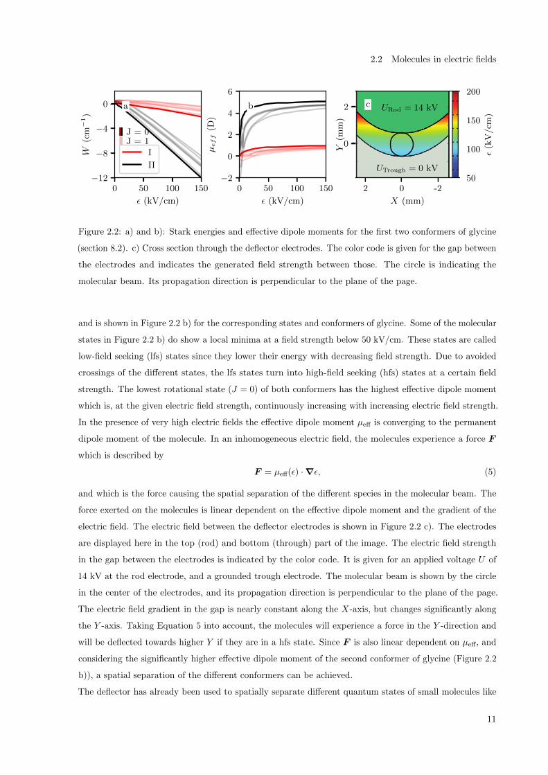
Figure 2.2 a) shows exemplarily the calculated Stark curves (energy W of a rotational state in dependence
of the electric field strength ε) for the two lowest rotational states of the first two conformers (red and
black) of glycine (section 8.2). All presented states do change their energy in the presence of the electric
field, with a global trend towards lower energy for an increased field strength. Conformer II shows a
bigger change in energy than conformer I due to its higher dipole moments (Equation 3, section 8.2). The
effective dipole moment µeff from a single molecular state can be derived by
µeff = −∂W/∂ε, (4)
†The Hamiltonian and the energies of the molecules in the external field were calculated throughout the dissertation by
using the CMIStark code [70] which also specifies the simplifications taken into account.
10
2.2 Molecules in electric fields
2 0 -2
X (mm)
2
0
Y(m
m)
c URod = 14 kV
UTrough = 0 kV50
100
150
200
ε(k
V/cm
)
0 50 100 150
ε (kV/cm)
0
−4
−8
−12
W(c
m−
1)
J = 0J = 1
a
I
II
0 50 100 150
ε (kV/cm)
−2
0
2
4
6
µeff
(D)
b
Figure 2.2: a) and b): Stark energies and effective dipole moments for the first two conformers of glycine
(section 8.2). c) Cross section through the deflector electrodes. The color code is given for the gap between
the electrodes and indicates the generated field strength between those. The circle is indicating the
molecular beam. Its propagation direction is perpendicular to the plane of the page.
and is shown in Figure 2.2 b) for the corresponding states and conformers of glycine. Some of the molecular
states in Figure 2.2 b) do show a local minima at a field strength below 50 kV/cm. These states are called
low-field seeking (lfs) states since they lower their energy with decreasing field strength. Due to avoided
crossings of the different states, the lfs states turn into high-field seeking (hfs) states at a certain field
strength. The lowest rotational state (J = 0) of both conformers has the highest effective dipole moment
which is, at the given electric field strength, continuously increasing with increasing electric field strength.
In the presence of very high electric fields the effective dipole moment µeff is converging to the permanent
dipole moment of the molecule. In an inhomogeneous electric field, the molecules experience a force F
which is described by
F = µeff(ε) ·∇ε, (5)
and which is the force causing the spatial separation of the different species in the molecular beam. The
force exerted on the molecules is linear dependent on the effective dipole moment and the gradient of the
electric field. The electric field between the deflector electrodes is shown in Figure 2.2 c). The electrodes
are displayed here in the top (rod) and bottom (through) part of the image. The electric field strength
in the gap between the electrodes is indicated by the color code. It is given for an applied voltage U of
14 kV at the rod electrode, and a grounded trough electrode. The molecular beam is shown by the circle
in the center of the electrodes, and its propagation direction is perpendicular to the plane of the page.
The electric field gradient in the gap is nearly constant along the X-axis, but changes significantly along
the Y -axis. Taking Equation 5 into account, the molecules will experience a force in the Y -direction and
will be deflected towards higher Y if they are in a hfs state. Since F is also linear dependent on µeff, and
considering the significantly higher effective dipole moment of the second conformer of glycine (Figure 2.2
b)), a spatial separation of the different conformers can be achieved.
The deflector has already been used to spatially separate different quantum states of small molecules like
11
2. Fundamental concepts
OCS [72], nuclear-spin isomers [73], conformers (chapter 3) [10, 11, 13], or to spatially separate molecular
clusters (chapter 7) [12, 13].
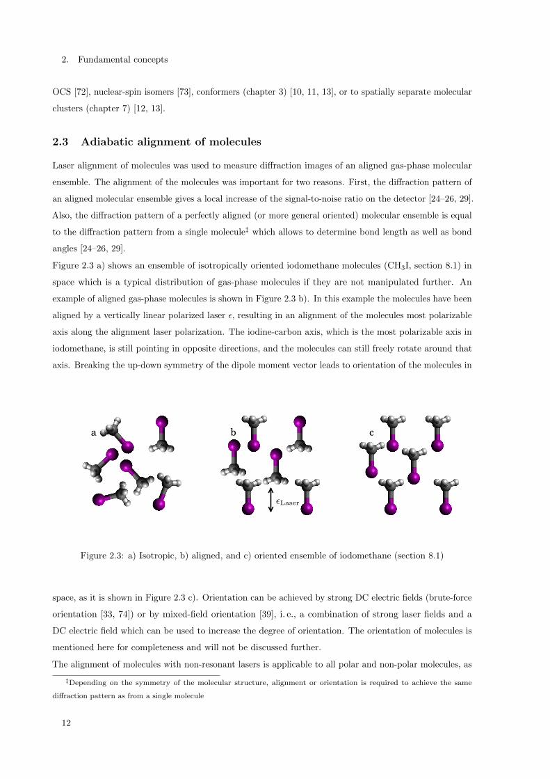
2.3 Adiabatic alignment of molecules
Laser alignment of molecules was used to measure diffraction images of an aligned gas-phase molecular
ensemble. The alignment of the molecules was important for two reasons. First, the diffraction pattern of
an aligned molecular ensemble gives a local increase of the signal-to-noise ratio on the detector [24–26, 29].
Also, the diffraction pattern of a perfectly aligned (or more general oriented) molecular ensemble is equal
to the diffraction pattern from a single molecule‡ which allows to determine bond length as well as bond
angles [24–26, 29].
Figure 2.3 a) shows an ensemble of isotropically oriented iodomethane molecules (CH3I, section 8.1) in
space which is a typical distribution of gas-phase molecules if they are not manipulated further. An
example of aligned gas-phase molecules is shown in Figure 2.3 b). In this example the molecules have been
aligned by a vertically linear polarized laser ε, resulting in an alignment of the molecules most polarizable
axis along the alignment laser polarization. The iodine-carbon axis, which is the most polarizable axis in
iodomethane, is still pointing in opposite directions, and the molecules can still freely rotate around that
axis. Breaking the up-down symmetry of the dipole moment vector leads to orientation of the molecules in
a
εLaser
b c
Figure 2.3: a) Isotropic, b) aligned, and c) oriented ensemble of iodomethane (section 8.1)
space, as it is shown in Figure 2.3 c). Orientation can be achieved by strong DC electric fields (brute-force
orientation [33, 74]) or by mixed-field orientation [39], i. e., a combination of strong laser fields and a
DC electric field which can be used to increase the degree of orientation. The orientation of molecules is
mentioned here for completeness and will not be discussed further.
The alignment of molecules with non-resonant lasers is applicable to all polar and non-polar molecules, as
‡Depending on the symmetry of the molecular structure, alignment or orientation is required to achieve the same
diffraction pattern as from a single molecule
12

2.3 Adiabatic alignment of molecules
long as they do have a polarizability anisotropy. It is typically separated into three different cases [35],
quantified by the rising and falling times of the laser pulse intensity τLaser, and the rotational period τRot
of the molecule.
If τLaser τRot the molecules are adiabatically aligned, i. e., the population of states in the molecule
is equal before and after the laser pulse; the eigenstates of the field-free molecular Hamiltonian will be
transferred to field-dressed pendular states in the presence of the slowly rising laser field intensity. If
τLaser τRot rotational states are coherently coupled and the molecule experiences a periodic field-free
alignment after the laser pulse. If τLaser ≈ τRot, the molecules are aligned in the presence of the laser
field (similar to adiabatic alignment), and do experience a periodic field-free alignment after the laser
pulse (similar to non-adiabatic alignment). The experiments presented in chapter 4 and chapter 5 were
conducted in this intermediate regime; the molecules were probed at the peak of the alignment laser pulse
and no focus was put on the field free alignment after the laser pulse. Hence, the following discussion is
focussing on adiabatic alignment of molecules in the gas-phase. A more detailed description can be found
for instance in [35, 36, 75].
The period of the electric field of a laser with a central wavelength of 800 nm is (in vacuum) 2.7 fs, which
is orders of magnitude shorter than the rotational period of molecules. The comparable fast oscillations of
the laser field lead to a suppression of the Stark effect (section 2.2), because the molecules effective dipole
moment cannot follow the fast oscillations within the laser field. But the laser field can induce a dipole
moment µInd within the molecule. In simple words, the laser field induces electron oscillations within the
molecule on the frequency of the laser field; the heavy nuclei cannot follow the field that fast, leading to a
relative charge displacement, i. e., an induced dipole moment. The induced dipole moment does depend
on the polarizability tensor αij of the molecule, the electric field strength ε, and the angle between αij
and the polarization of the laser field. For an asymmetric top molecule the induced potential by a linear
polarized laser can be described by
VInd(t) = − (E0ε(t))2
4(sin2θ(αxxcos2χ+ αyysin2χ) + αzzcos2θ) (6)
where E0 is the electric field strength and ε(t) is the laser pulse envelope. αxx, αyy, and αzz are the
polarizability tensor components with respect to the molecular frame, θ is polar Euler angle between the
laser field polarization and the molecular axis, and χ is the azimuthal Euler angle about the molecules
z-axis.
The experimental realization of the measurement of the degree of alignment is shown in Figure 2.4. A
molecule is aligned along the alignment laser polarization εLaser (Figure 2.4 a)). The angle between
εLaser and the molecular axis is θ. In the presented experiments (chapter 4, chapter 5) the degree of
alignment was probed via a second laser pulse which triggered a Coulomb explosion of the molecule.
This is illustrated by the broken bond between the iodine+ and the CH3+ part of the molecule. Ideally,
the ionic fragments recoil along the intramolecular axis. The angle θ can be measured for an ensemble
of molecules and can be used to quantify the degree of alignment⟨cos2θ
⟩. Depending on how well the
13

2. Fundamental concepts
εLaser
θθ
αXX
a b
VMI
+
+
Figure 2.4: a) A single molecule aligned along the laser polarization axis. The broken bond indicates the
Coulomb explosion of the fragmenting molecule. b) Drawing of a possible VMI image of aligned molecules
gated on a specific fragment.
molecules are aligned,⟨cos2θ
⟩can take values between 1/3 and 1 for an isotropically and a perfectly
aligned molecular ensemble respectively. In the presented experiment the degree of alignment is measured
by mapping the 3 dimensional (3D) velocity distribution of a certain ionic fragment of the molecule onto
the detector via velocity-map imaging [2–5] (Figure 2.4 b)). However, velocity-map imaging allows only to
determine the velocity components parallel to the detector surface. Thus, only the 2D projection of the
polar Euler angle θ is measured.⟨cos2θ2D
⟩can be between 0.5 and 1 for an isotropically and a perfectly
aligned molecular ensemble respectively. Among others,⟨cos2θ
⟩can be reconstructed by a rotation of the
laser polarization, such that it is perpendicular to the detector surface and measuring again⟨cos2θ2D
⟩from that second angle.
2.4 X-ray matter interaction
In the presented experiments x-ray radiation was used to image the structure of controlled gas-phase
molecules. Also, x-rays have been used for localized ionization of controlled gas-phase molecules and
molecular cluster, to learn about their photophysics and charge-rearrangement upon core-shell ionization.
The x-ray spectrum can be classified into the regime of soft and hard x-ray photons for low and high
energetic photons respectively [42, 43]. The photon energies are not strictly defined. Here, the definition
given in [44] is used, which puts the soft x-ray photons between the electron 1s binding energies of a
carbon and an argon atom, i. e., the spectrum is ranging from 284 eV to 3.2 keV. Photon energies on
the order of several keV are considered as hard x-rays, and photon energies in the region of MeV are
considered as gamma rays.
In the experiments presented in chapter 6 and chapter 7 soft x-ray radiation (420 eV) was used for
14

2.4 X-ray matter interaction
side-specific ionization in the molecular sample. Additionally, the experiment shown in section 8.1 was
conducted in the XUV region, i. e., at a photon energy of 70 eV, also for side-specific ionization in the
molecular sample. Side-specific ionization is achieved by tuning the photon energy on, or slightly above, the
core-resonances of the atom(s) within the molecule, and increasing thus the probability of photoabsorption
in that atom(s). If the photon energy is higher than the binding energy of electron in the core, the
sample can be core-shell ionized. The excited atoms or molecules can relax via, for instance, emission of a
further electron (Auger decay, chapter 4, chapter 6, chapter 7, section 8.1) or emission of a photon (x-ray
fluorescence, chapter 5). The x-ray photoabsorption and the following relaxation mechanisms are shortly
described in subsection 2.4.1.
In addition to photoabsorption, the x-ray radiation can also scatter off the atoms/molecules which can be
used for structure determination (chapter 5). To achieve atomic resolution hard x-ray photons are required,
since their wavelength is short enough to image small structures, i. e., shorter than the intramolecular
distances. The scattering process can be coherent (elastic) or incoherent (inelastic), where the coherent
part of the scattering process is containing the structure information of the molecular sample. The
incoherent part is considered as background radiation in diffractive imaging experiments. Both processes
are described in more detail in subsection 2.4.2.
A collection of cross sections for the different interactions can be found in [76–78]. A good overview about
the theoretical treatment of the x-ray matter interaction is given in [42, 43] as well as by the tutorial [44]
and references therein.
2.4.1 X-ray absorption and relaxation
Figure 2.5 a) show a schematic drawing of the lowest energy states of an atom. The incident x-ray photon
hν is absorbed by a K-shell electron and ionizes the sample. The kinetic energy of the photoelectron Ekin
is given by the difference of incident photon energy and the binding energy. The absorption cross section
scales approximately with the atomic number Z4 [43]. For a constant Z, the photoabsorption cross section
scales with the photon energy E−3Ph . The total absorption cross sections σTot for a carbon and a nitrogen
atom are exemplarily shown in Figure 2.6 [76]. The cross section for nitrogen is generally higher than the
carbon cross section (ZN > ZC) and both decrease with increasing photon energy. At a photon energy
of ≈ 284 and 410 eV the cross sections for carbon and nitrogen do increase by more than one order of
magnitude. The sudden increase of the cross section is here due to the photon energy which is exceeding
the ionization potentials for the 1s orbitals [78].
After ionization the atom is left in a highly core-excited state. Relaxation can happen via, for instance, an
Auger decay (non-radiative decay) (Figure 2.5 b)) or via fluorescence (Figure 2.5 c)). The Auger decay is
the dominant relaxation process for ≈ Z < 18 [44]. In this example, the created K-hole is filled from an
electron of the L-shell, and an electron is emitted from the L-shell, leaving the atom in a dicationic state.
15

2. Fundamental concepts
a Ekin
IP
L2/3
L1
K
hν
b Ekin
IP
L2/3
L1
K
cIP
L2/3
L1
K
hν
Figure 2.5: Illustration of a) x-ray photoionization, b) the Auger decay, and c) decay via x-ray fluorescence
in an atom. K, L1, L2/3 are illustrating the corresponding atomic levels, which are occupied by electrons
(blue dots). The blue circles indicate the generated core-hole by the x-ray photon hν and IP is illustrating
the ionization potential of the atom.
102 103
EPh (eV)
10−2
10−1
100
σT
ot(1
0−
22m
2)
C(1s) N(1s)
CarbonNitrogen
Figure 2.6: Absorption cross sections for carbon and nitrogen in dependence of the photon energy [76]
The kinetic energy of the Auger electrons energy EAug is given by [79]
EAug ≈ EA − EB − E′C ≈ EA − EB − EC(Z + 1), (7)
where EA and EB are the ionization energies of the shells from the generated vacancy and from the less
tightly bound electron which is filling the vacancy. E′C is the ionization energy of the emitted electron
for the case of a singly ionized atom. E′C can be approximated by E′C = EC(Z + 1) where EC is the
ionization energy of the neutral atom from which the Auger electron is emitted. The Auger electrons
are typically labeled according to their involved transitions. The Auger electron shown in Figure 2.5
would thus be labeled as KL1L2,3. In molecules the Auger electrons can originate from valence orbitals V,
16
2.4 X-ray matter interaction
which would be labeled as, for example, KLV or KVV Auger electron. In molecules and especially atomic
or molecular clusters, similar relaxation processes (relaxation and electron emission) like intermolecular
Coulombic decay (ICD) [80, 81] or electron-transfer mediated decay (ETMD) [82] play an important role.
In ICD a core hole is created which is filled by an electron from a higher state, but the electron is emitted
from a neighboring atom. In ETMD a created core hole is filled by an electron from a neighboring atom,
the electron is emitted from a third atom. X-ray fluorescence (Figure 2.5 c)) is the dominant relaxation
process for heavier atoms. The inner-shell vacancy is filled by an electron from a higher shell accompanied
by the emission of a x-ray photon. The photon energy is equivalent to the energy difference between
the two orbitals and is element specific. The transitions are labeled as, for example, Kα or Kβ if the
electron relaxes from a 2p or 3p orbital, respectively, into a K-shell vacancy. The fluorescence yield scales
approximately with Z4 [44] and a good overview of the different emission lines for the different atoms is
given in [78].
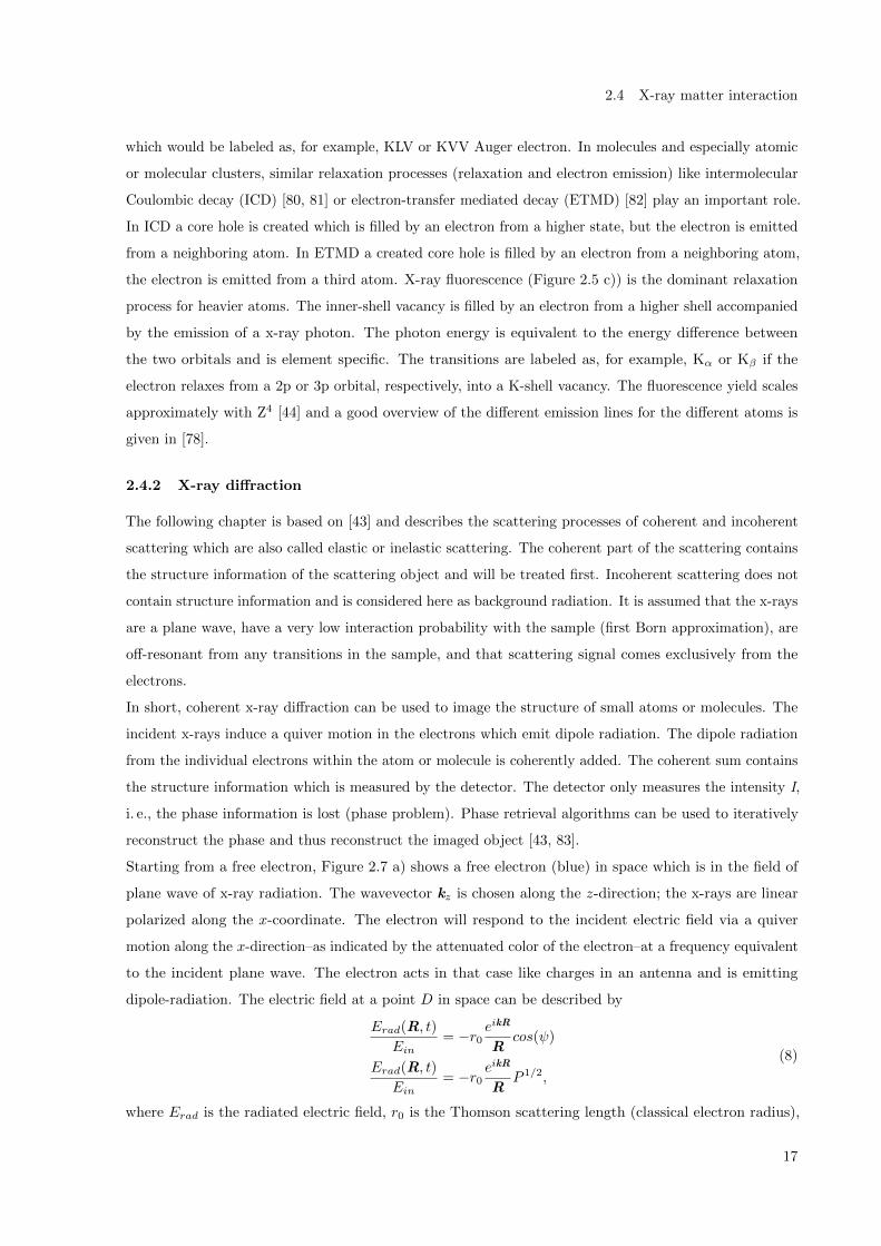
2.4.2 X-ray diffraction
The following chapter is based on [43] and describes the scattering processes of coherent and incoherent
scattering which are also called elastic or inelastic scattering. The coherent part of the scattering contains
the structure information of the scattering object and will be treated first. Incoherent scattering does not
contain structure information and is considered here as background radiation. It is assumed that the x-rays
are a plane wave, have a very low interaction probability with the sample (first Born approximation), are
off-resonant from any transitions in the sample, and that scattering signal comes exclusively from the
electrons.
In short, coherent x-ray diffraction can be used to image the structure of small atoms or molecules. The
incident x-rays induce a quiver motion in the electrons which emit dipole radiation. The dipole radiation
from the individual electrons within the atom or molecule is coherently added. The coherent sum contains
the structure information which is measured by the detector. The detector only measures the intensity I,
i. e., the phase information is lost (phase problem). Phase retrieval algorithms can be used to iteratively
reconstruct the phase and thus reconstruct the imaged object [43, 83].
Starting from a free electron, Figure 2.7 a) shows a free electron (blue) in space which is in the field of
plane wave of x-ray radiation. The wavevector kz is chosen along the z-direction; the x-rays are linear
polarized along the x-coordinate. The electron will respond to the incident electric field via a quiver
motion along the x-direction–as indicated by the attenuated color of the electron–at a frequency equivalent
to the incident plane wave. The electron acts in that case like charges in an antenna and is emitting
dipole-radiation. The electric field at a point D in space can be described by
Erad(R, t)
Ein= −r0
eikR
Rcos(ψ)
Erad(R, t)
Ein= −r0
eikR
RP 1/2,
(8)
where Erad is the radiated electric field, r0 is the Thomson scattering length (classical electron radius),
17

2. Fundamental concepts
a
Electron
xy
z
kz
ψ
D(x, z, y = 0)
b
Atom
kkk kkk′
rrr
kkk · rrr kkk′ · rrr
Figure 2.7: a) Scattering of an x-ray photon by an electron, where kz is the wavevector of the incident
x-ray radiation and D is an observation point in the x− z plane. b) Scattering of x-rays from an atom. k
is incident x-ray wavevector, k ’ is the scattered wavevector, |k| = |k′|, and r is the difference between a
wave scattered at the origin and a wave scattered at a position r. The images are adapted from [43].
R is the distance between the observation point D and the electron, ψ is the angle with respect the
incident beam, and Ein is the incident radiating field. cos(ψ) is describing the angular dependency due to
the linear motion of the electron within the linear polarized incident electric field. Thus, the radiated
electric field is maximized at ψ = 0 and minimized at ψ = 90 . This polarization dependency is also
commonly known as polarization factor P , which is for the given case cos2(ψ), and 1/2(1 + cos2(ψ)) for
an unpolarized light source.
Figure 2.7 b) shows the scattering of x-rays from an individual atom where k is defined here as the incident
plane wave, k′ is the scattered wave. For the case of elastic (coherent) scattering |k| = |k′|. All the
electrons within the atom respond to the electric field via a quiver motion. Thus, the contribution of the
individual electrons have to be added up coherently if electron-electron correlations are neglected. The
atom can be divided therefore into small sections which do have a certain charge density ρ(r). r is the
distance between a certain volume element and the origin of the atom, as it is indicated in Figure 2.7 b).
The phase difference ∆φ between the emitted wave of a volume element in the origin and at a point r can
be described by
∆φ = k · r − k′ · r
= (k− k′) · r
= Q · r,
(9)
where Q is the wavevector transfer. The integration over the different volume elements gives the atomic
18

2.4 X-ray matter interaction
scattering, which is also known as the atomic form factor f0(Q) with
− r0f0(Q) = −r0
∫ρ(r)eiQrdr. (10)
The integral over the different electron charge densities ρ(r) is equal to the number of electrons in the atom.
The atomic form factor is recognizable as a Fourier transformation connecting the density distribution
ρ(r) in real space with the momentum space or also know as reciprocal space§. Not taken into account are
the different energy levels in the atom. K-shell atoms are much stronger bounded to the nucleus than L or
M-shell electrons. If, for instance, the incident photon energy is much smaller than the binding energy of
the K-shell atoms, the quiver-motion of the electrons on this shell can be neglected and hence the total
scattering amplitude is reduced. The total atomic form factor can than be described by
f(Q, ~ω) = f0(Q) + f ′(~ω) + if ′′(~ω) (11)
, where f ′(~ω) is a damping factor and if ′′(~ω) is giving a phase correction between the electrons quiver
motion and the driving field.¶
The connection between the molecular form factor Fmol(Q) and atomic form factor is given by the
summation of the individual atomic form factors of the atoms within the molecule. It is important to
keep track of the distances r between the different atoms such that those are coherently added. Thus, the
molecular form factor can be written as
Fmol(Q) =∑rj
fj(Q)eiQ·rj . (12)
Taking Equation 8 into account, the scattering of the molecules can be described by
Erad(R,Q)
Ein= −r0 F
mol(Q)eikR
RP 1/2 (13)
For an experimentalist it is desirable to measure Fmol(Q) for sufficientQ-values to be able to reconstruct,
via fitting algorithms, the molecular structure.
In addition to elastic (coherent) scattering, x-rays can also inelastically (incoherent) scatter of the sample.
An inelastic scattering process is schematically shown in Figure 2.8. The incident x-ray photon has a
momentum p and is scattered off the electron at an angle θ. The momentum of the scattered photon is
p ′. In the case of an inelastic scattering process |k| 6= |k′|; the momentum difference is transferred to the
electron. The energy of the incoherent scattered photon E′inc can be described by
E′inc =1
1 + k(1− cos(θ))E (14)
where k = E/(me · c2), i. e., it is the incident photon energy E in units of the electron rest mass energy,
and θ the angle between incident and the scattered photon. The scattering of x-rays on a free-electron
§The atomic form factors can be parameterized. In [84] the parametrization consists of a sum of five weighted Gaussians
plus a constant which are listed for a large number of neutral and ionic atoms.¶[85] gives tabulated values for this correction.
19

2. Fundamental concepts
Electron
p = hkp′ = hk′
hq′
k
k′ q′
θ
θ
Figure 2.8: Inelastic scattering of an x-ray by an electron, where p and p′ are the momenta of the incident
and scattered photons, θ is the angle between the incident and the scattered photons, and ~q ′ is the
momentum transferred to the electron.
in relativistic quantum mechanics can be described by the Klein-Nishina formula [86]. Below a photon
energy of 100 keV, the Klein-Nishina formula can be approximated by [78]
dσKNdΩ
=r2eP
(1 + k(1− cos(θ))2
= r2eP |
E′incE|2
(15)
where P is the polarization factor. The Klein-Nishina formula is here expressed as the differential cross
section‖ where σKN is the Klein-Nishina cross section per solid angle Ω of the detector. The Klein-Nishina
formula can be multiplied by the incoherent scattering function S(Q, Z) to make the transformation from
a single electron to a single atom. S(Q, Z) is thus comparable to the atomic form factor and tabulated
values can be found in [87]. The incoherent scattering can then described by
P (k,Q) =dσKNdΩ
· S(Q, Z) (16)
where P (k,Q) is the angular and energy distribution of the scattered photon. During the course of the
dissertation the incoherent scattering was implemented within the CMIDiffract code [24, 25, 29] which is
used to simulated diffraction pattern of molecules.
‖Differential cross sections are derived by normalization of the scattered intensity by the incident photon flux and the
solid angle of the detector ∆Ω
20

3 Conformer separation of gas-phase molecules∗
The following chapter is based on the publication [11] and demonstrates the spatial separation of the
cis-, and trans conformer of 3-fluorophenol (C6H5OF, 3FP) utilizing their individual effective dipole
moments. It starts with an introduction (section 3.1), which puts the spatial separation of conformer
into context with novel, upcoming experiments and highlights the importance of conformer-separated
molecular samples. The experimental setup and results are shown in section 3.2 and section 3.3. The
experiment shows the first demonstration of the spatial separation of the least polar conformer, which is
additionally less populated in the molecular beam.
3.1 Introduction
Complex molecules often exhibit different structural isomers (conformers), even under the conditions
of a cold molecular beam [8]. For a variety of upcoming novel experiments like photoelectron [16, 18],
electron [32, 88], and x-ray diffraction [25, 27] imaging of gas-phase molecules, for conformer-specific
chemical reaction studies [89], or for mixed-field orientation experiments [35, 38, 90], pure species-selected
molecular samples with all molecules in the lowest-energy rotational states are highly advantageous or
simply necessary. Using strong inhomogeneous electric fields it is possible to spatially separate individual
conformers [10, 91], specific molecular clusters [12], as well as the individual quantum states of neutral
polar molecules [92–94]. While the electric deflector was exploited for the spatial separation of individual
conformers [10] and for the generation of highly polar samples of single-conformer molecules [38], it was not
a priory clear whether it would be possible to create pure samples of the most polar low-rotational-energy
states of any conformer but the most polar one.
Here, we demonstrate the generation of conformer-selected and very polar ensembles of both conformers of
3FP. 3FP is a prototypical large molecule with two stable conformers that differ by their orientation of the
OH functional group. Conformer-selected and three-dimensionally oriented [97] ensembles of 3FP are good
candidates for the investigation of conformer-interconversion reactions in an ultrafast laser pump, x-ray
probe experiment, in which structural information would be accessible through photoelectron holography
following F(1s) ionization [16, 18].
The structures of cis and trans 3FP are shown in Figure 3.1, together with calculated energies of their
lowest rotational states in an electric field [70]. At relevant electric field strengths, all states are high-field
∗This chapter is based on the paper Spatially separated polar samples of the cis and trans conformers of 3-fluorophenol,
T. Kierspel, D. Horke, Y.-P. Chang, and J. Kupper, Chemical Physics Letters 591, 130–132 (2014).
I conducted the measurements together with D. Horke. I conducted the data analysis and the simulations. Together with
the other authors, I discussed the results and I wrote the published article.
21

3. Conformer separation of gas-phase molecules
cis-3FP
trans-3FP
J = 0
J = 1
J = 2
A = 3790 MHz
B = 1795 MHz
C = 1218 MHz
µ = 0.82 D
A = 3749 MHz
B = 1798 MHz
C = 1215 MHz
µ = 2.64 D
0 20 40 60 80 100 120 140
0
-1
-3
-2
-5
-4
-6
Figure 3.1: Stark-energies for the lowest rovibronic quantum states (J < 3) of the cis- (red) and trans-
conformer (black) of 3FP as a function of the electric field strength. The inset shows the molecular
structures, the rotational constants [95, 96], and the calculated dipole moments of these conformers.
seeking.† Due to the different electric dipole moments of µ = 0.82 D and 2.64 D for cis and trans,
respectively, the energy dependence of the molecular eigenstates as a function of electric field strength
is quite different for the two conformers. The projection of the molecule-fixed dipole moment onto the
electric field axis is the effective dipole moment µeff = −∂W/∂ε. The force exerted by an electric field on a
polar molecule is ~F = µeff(ε) · ~∇ε ‡. Thus, for a given inhomogeneous electric field trans-3FP is deflected
more than cis-3FP. Moreover, the lowest energy rotational states are generally more polar, i. e., have a
larger effective dipole moment µeff, than higher-energy rotational states [38] and, therefore, are deflected
more.
3.2 Experimental details
Figure 3.2 shows a schematic of the experimental setup [93]. In brief, 3FP was placed in a room-temperature
Even-Lavie valve [63]. The molecules are coexpanded into the vacuum chamber at a repetition rate
of 20 Hz in 50 bar of helium or 25 bar of neon, resulting in a supersonic expansion with a rotational
temperature of the molecules of 1.5 K and 1 K, respectively. The molecular beam was collimated by two
skimmers with diameters of 2 mm and 1 mm that were placed 5.5 cm and 21.5 cm downstream of the
valve. Behind the second skimmer the molecular beam entered the electric deflector that provided an
inhomogeneous electric field to disperse the molecular beam. A third skimmer with 1.5 mm diameter was
placed directly behind the deflector. A time-of-flight mass-spectrometer was placed 30 cm downstream the
†Molecules in high-field seeking states have a negative Stark energy shift, i. e., their potential energy decreases with
electric field strength. Thus, they have positive effective dipole moments (vide infra). Therefore, they orient along the
electric field and they are attracted to regions of stronger electric field in order to minimize their energy.‡The formula was mistakingly published with a wrong algebraic sign which has been corrected for.
22

3.3 Results and discussions
Valve
Skimmers
Deflector
TOF electrodes
MCP
Probe laser
15.4 cm
30.2 cm
y
x
+14 kV
0 kV−2 −1 0 1 2
−2
−1
0
1
2
3
−2−1
0123
x (mm)−2−1 0 1 2
50
100
200
150
Figure 3.2: Schematic of the experimental setup consisting of a pulsed molecular beam source, a deflector,
and a time-of-flight mass spectrometer. The inset shows a cut through the deflector and depicts the
generated electric field.
deflector. A tunable pulsed dye laser (Fine Adjustment Pulsare Pro) provided approximately 400 µJ per
pulse in a soft focus at the electronic origin transitions of 36623 cm−1 and 36830 cm−1 for cis and trans,
respectively [98]. Individual conformers were selectively detected through resonance-enhanced two-photon
ionization (R2PI) mass spectrometry. For the measurements of spatial molecular beam profiles the laser is
sampled by moving the focusing lens in steps of 200 µm in the y-direction.
Ab initio calculations (B3LYP/aug-cc-pVTZ) predict the trans conformer to be about 55 cm−1 more stable
than the cis conformer, in agreement with the 85 cm−1 energy difference derived from a one-dimensionally
torsional potential based on far-infrared spectroscopy [99]. The corresponding expected relative abundances
of the trans and cis conformers in the molecular beam of approximately 2:1 agree with the experimentally
obtained R2PI signal levels.
3.3 Results and discussions
Figure 3.3 shows the vertical molecular beam profile for trans-3FP seeded in helium for different voltages
applied to the deflector. The height of the undeflected molecular beam (0 kV) is 2 mm, defined by the
mechanical apertures of the deflector and the skimmers. When a voltage of 5 kV is applied to the deflector
the beam is deflected upwards by approximately 0.4 mm for the trans-conformer. Increasing the voltage to
10 kV and 14 kV, the deflection increases to 0.8 mm and 1.4 mm, respectively. Solid lines show simulated
spatial profiles obtained using the libcolmol package [93]. Only a single free parameter, the peak intensity
of the undeflected beam, was adjusted to the experiment.
Figure 3.4 a) shows the deflection profiles of both conformers of 3FP seeded in helium for applied voltages of
0 V and 14 kV to the deflector. The cis-conformer was deflected significantly less than the trans-conformer.
This leads to a spatial separation of the trans-conformer from the cis-conformer and from the original
beam, e. g., the seed gas. The purity of the trans sample at various heights is shown in Figure 3.4 b).
23

3. Conformer separation of gas-phase molecules
Figure 3.3: Spatial profiles for trans-3FP seeded in helium for different voltages applied to the deflector.
The solid lines indicate simulated deflection profiles, the symbols are experimental values and the depicted
ranges are their 1σ standard deviation.
b
a
Figure 3.4: a) Field-free (0 kV) and deflected (14 kV) spatial beam profiles for the cis and the trans
conformers of 3FP seeded in helium. b) The fractional population of the trans isomer in the beam.
Assuming similar excitation and ionization cross-sections for the two conformers, a beam of trans-3FP
with a purity >95 % was obtained in the range of 2.5 mm to 3.5 mm. Around y = −0.8 mm a nearly pure
beam of cis-3FP was obtained, similar to previous measurements [10]. However, these samples correspond
to high-energy rotational states that are not suited for the envisioned novel orientation and imaging
24

3.4 Conclusions
b
a
Figure 3.5: a) Field-free (0 kV) and deflected (14 kV) spatial beam profiles for the cis and the trans
conformers of 3FP seeded in neon. b) The fractional population of the cis isomer in the beam.
experiments. Moreover, these molecules were still immersed in the atomic seed gas. In order to create a
pure beam of low-energy rotational states of cis-3FP we increased the deflection by seeding the molecules
in neon, resulting in a molecular beam with a speed of 900 m/s, half the speed of the helium expansion.
The doubled interaction time resulted in a stronger deflection, as shown in Figure 3.5 a. For an applied
voltage of 14 kV both conformers were strongly deflected. For the originally very cold molecular beam the
deflection of trans-3FP was so strong that most molecules crash into the rod electrode and are lost from
the beam. For the cis conformer, however, a strong deflection out of the seed gas beam was observed. For
y = 1.5–2.5 mm a beam of cis-3FP with a purity >90 % with all molecules in the lowest-energy rotational
states was obtained, see Figure 3.5 b, even though this conformer was less abundant in the original beam
(vide supra). The remaining signal strength at position 1.5 mm was 40 % of the maximum of the field-free
case. The amplitudes for each conformer are normalized to the laser intensity. The remaining contribution
from trans-3FP for y < 2 mm is attributed to warm molecules that diffuse into the detection region after
colliding with the deflector rod.
3.4 Conclusions
In summary, we have demonstrated the spatial separation of the cis and trans conformers of 3FP
and the generation of cold, low-energy rotational state samples of both conformers of 3FP. These
results demonstrate the feasibility to create pure samples of both conformers of this prototypical large
25

3. Conformer separation of gas-phase molecules
molecule using the electric deflector, allowing for strong three-dimensional alignment and mixed-field
orientation [97]. These samples will allow direct molecular-frame imaging experiments on all structural
isomers to disentangle the structure-function relationship for the conformer interconversion. This could be
investigated through molecular frame photoelectron angular distributions and electron or x-ray diffraction
experiments [15, 18, 25, 27, 28, 32].
26

4 Alignment at 4th generation light source∗
The following chapter is based on the publication [100] and shows the preparation of aligned molecular
samples at the full repetition rate of free-electron lasers (FELs) utilizing a commercial Ti:Sapphire laser
(TSL) system. The chapter starts with the introduction, putting the experiment into context with other
experiments and motivates why alignment at high repetition rates is important for FEL experiments,
followed by a short description of the experimental setup section 4.2. The results of laser-alignment at
the FEL and laboratory based results are presented in section 4.3 and section 4.4, showing an measured
degree of alignment of⟨cos2θ2D
⟩= 0.85 respectively
⟨cos2θ2D
⟩= 0.94. Both experiments were performed
under similar alignment laser conditions but with different experimental setups concerning the molecular
beam, leading to a warmer beam in the former case, which is discussed in section 4.5. A summary and
outlook for future experiments is presented in section 4.6.
4.1 Introduction
Imaging the structural dynamics of gas-phase molecules using approaches such as photoelectron imaging in
the molecular frame [15, 18, 101], high-harmonic-generation spectroscopy [102, 103], laser-induced electron
diffraction [104, 105], electron diffraction [32, 88], or x-ray diffraction [25, 27, 106] is much improved or is
only possible by fixing the molecules in space [25, 27, 28, 32, 35, 106]. Various approaches to align or orient
molecules have been demonstrated, ranging from state-selection [92] over brute-force orientation [107] to
laser alignment [35]. Generally, laser alignment has been implemented in two different regimes, namely,
using short laser pulses to “impulsively” create coherent rotational wavepackets that generate alignment
some time after the laser pulse [108, 109] or using long laser pulses to “adiabatically” create pendular
states that are strongly aligned during the laser pulse [110]. In the former approach, pulses from standard
commercial TSL systems can be utilized at repetition rates up to several kilohertz, whereas in the latter
approach, traditionally, injection seeded Nd:YAG lasers were employed, with hundreds of millijoules of
pulse energy, limited to a few 10 Hz. Through the addition of weak dc electric fields, strong orientation
can be achieved in both scenarios [38, 90, 93]. Three-Dimensional (3D) alignment or orientation was also
demonstrated [38, 93, 111–114]. It was shown that the degree of alignment necessary for molecular-frame
diffractive imaging is very high [27, 28, 115] and, for complex molecules, could not be achieved with
impulsive alignment approaches. Generally, the degree of alignment can be improved through higher
∗This chapter is based on the paper Strongly aligned gas-phase molecules at free-electron lasers, T. Kierspel, J. Wiese, T.
Mullins, J. Robinson, A. Aquila, A. Barty, R. Bean, R. Boll, S. Boutet, P. Bucksbaum, H. Chapman, L. Christensen, A.
Fry, M. Hunter, J. Koglin, M. Liang, V. Mariani, A. Morgan, A. Natan, V. Petrovic, D. Rolles, A. Rudenko, K. Schnorr, H.
Stapelfeldt, S. Stern, J. Thøgersen, C. Yoon, F. Wang, S. Trippel, J. Kupper, Journal Of Physics B-Atomic Molecular And
Optical Physics 48, 204002 (2015).
I was conducting the experiments jointly with the other authors, and was primarily responsible for the molecular beam. I
discussed the results with the other authors together, and I wrote the published article.
27

4. Alignment at 4th generation light source
laser-field intensities, limited by the onset of ionization, or colder samples [116], possibly achieved through
state selection [38, 90, 93].
The intermediate-pulse-duration regime, for which the alignment laser pulse duration is shorter than the
lowest rotational period of the molecule, but cannot be considered impulsive anymore, had previously
been analyzed theoretically [37, 117, 118]. While the laser pulse is still on, the molecules act similar to
the adiabatic alignment case, whereas after the pulse periodic revivals can be observed [37]. Recently, this
mesobatic regime was explored experimentally and it was realized that degrees of alignment comparable
to the adiabatic limit can be achieved with much shorter and weaker laser pulses, e. g., from commercial
chirped-pulse-amplified (CPA) TSL systems [119, 120]. While the nonadiabatic interaction creates
interesting dynamic phenomena such as the observation of pendular motion [120], this approach does
provide strongly aligned samples of complex molecules [119]. Moreover, it requires only moderately long
pulses on the order of 100 ps with moderate pulse energies, i. e., a few mJ, which are available as output
from the standard laser systems available at x-ray laser facilities.
Here, we demonstrate the successful implementation of intermediate-pulse-duration regime, strong align-
ment of the prototypical asymmetric rotor molecule 2,5-diiodothiophene (C4H2I2S) in a molecular beam
at the Coherent X-ray Imaging (CXI) [121, 122] endstation of the Linac Coherent Light Source (LCLS) at
the SLAC National Accelerator Laboratory (SLAC). Previous experiments with fixed-in-space molecules
at FELs have exploited both, impulsive and adiabatic alignment, for instance, in ion imaging [52, 123],
electron imaging [17, 18, 20, 124], or x-ray diffraction experiments [25, 26]. Our approach allows one
to combine the strong alignment achieved in adiabatic alignment approaches [17, 18, 20, 25, 26] with
the utilization of x-ray pulses at the full repetition rate of the LCLS [52, 124]. This allowed to perform
experiments at 120 Hz, comparable to previously demonstrated intermediate regime alignment at 1 kHz
in table-top experiments [119]. For comparison, we also provide measurements for the degree of alignment
from experiments conducted in our laboratory at the Center for Free-Electron Laser Science (CFEL) [119]
during the beam time preparation.
4.2 Experimental Setup
Figure 4.1 shows a sketch of the experimental setup at LCLS. A trace of 2,5-diiodothiophene was
coexpanded in 80 bar helium into the vacuum by a pulsed valve [63], operated at and at a repetition rate
of 120 Hz synchronized to the LCLS. The molecular beam was skimmed 8 cm downstream the nozzle
using a 3-mm-diameter skimmer. This resulted in a 5.2 mm molecular beam (full width at half maximum,
FWHM) in the interaction zone.
Near-infrared (IR) laser pulses were produced in a CPA TSL system (Coherent) with a central wavelength
of 800 nm. The laser system is operated at and synchronized to the repetition rate of LCLS. The chirped
pulses out of the regenerative amplifier were split using a beam splitter with a reflectivity of 90 %. The
reflected pulses, which were used to align the molecules [119, 120], had a pulse energy of 3.3 mJ and a
28

4.2 Experimental Setup
Pulsed valve
Skimmer
Overlap mirror
Alignment laserFEL
MCP and phosphor screen
CCD camera
TOF/VMI electrodes
Z X
Y
X
Figure 4.1: Sketch of the experimental setup showing the pulsed molecular beam valve, the laser beam
path of the alignment laser (red) and the free-electron laser (cyan), and a holey mirror to collinearly
overlap both beams. The detection system consists of an ion-imaging setup for time-of-flight measurements
and velocity-map imaging onto a micro-channel plate, phosphor screen, and a CCD camera. In the inset
the definition of θ is depicted, it is the angle between the laser polarization, i. e., the X axis, and the most
polarizable axis of the molecule, i. e., the iodine-iodine axis.
pulse duration of 94 ps (FWHM). The transmitted pulses were compressed using a standard grating-based
compressor to a pulse duration of 55 fs (FWHM) at a pulse energy of 250 µJ. The compressed pulses
multiply ionize the molecules through strong-field ionization, resulting in Coulomb explosion; in all
experiments these compressed pulses were linearly polarized, with the polarization perpendicular to the
long axis of polarization of the alignment laser pulses (vide infra). Both arms were spatially and temporally
recombined before entering the vacuum system. This, in combination with ion imaging (vide infra), allows
to characterize and optimize the degree of alignment without the FEL beam.
The short pulses were also utilized to measure the pulse duration of the alignment laser pulses through
spectral interference. The frequency components of the chirped pulse arrive sequentially, whereas all fre-
quencies in the compressed pulse are temporally overlapped. At finite spectrometer resolution, interference
in the combined spectrum is only visible at those wavelength components of the alignment pulse that are
temporally overlapped, or nearly overlapped, with the compressed pulse. The strongest interference is
visible at the wavelength that temporally coincides with the compressed pulse. A delay line was used to
change the relative timing between the chirped alignment and the compressed pulses. Thus, monitoring
the spectrum in dependence of the delay between these two pulses provided information on the pulse
duration of the chirped pulse.
To reach sufficiently high intensities to align the molecules, a telescope was used to expand both beams by
a factor of three before being focused into the chamber with a 1-m-focal-length lens. A holey mirror was
29

4. Alignment at 4th generation light source
used to spatially overlap the TSL pulses with the FEL beam path, losing 20 % of the near-infrared laser
power. The hole had a diameter of 2 mm and the FEL beam was guided through the hole to achieve a
collinear propagation of both beams. The alignment laser focus size was 45 µm (FWHM) leading to an
estimated peak intensity at the focus on the order of 1·1012 W/cm2. The FEL beam size was estimated to
12 µm in the horizontal and 3 µm in the vertical axis. The different beam diameters made the setup more
stable against beam pointing imperfections and ensured that only well aligned molecules were probed with
the FEL. The alignment laser pulse and the FEL/TSL pulses were spatially and temporally overlapped in
order to maximize the degree of alignment; the exact timing was not critical [119].
The alignment laser beam was elliptically polarized with an aspect ratio of 3:1 in order to obtain 3D
alignment. The major axis was parallel to the micro-channel plate (MCP) and phosphor screen surface.
That way the most polarizable axis of 2,5-diiodothiophene, i. e., the iodine–iodine axis, was confined to the
X axis as can be seen in Figure 4.1. The degree of alignment was probed using x-ray pulses with a pulse
duration of approximately 70 fs (FWHM), a photon energy of 9.5 keV, and a pulse energy of approximately
0.64 mJ (4.2 · 1011 photons, beam line transmission 80 %, focussing mirror transmission 40 %) in the
interaction zone. X-ray absorption is largely localized at one of the iodine atoms, followed by Auger
cascades and intramolecular charge redistribution leading to Coulomb explosion of the molecule. The ions
were accelerated by the electric field of the spectrometer (Figure 4.1) towards a position sensitive detector
consisting of a MCP and a phosphor screen (Photonis). A CCD camera (Adimec Opal), operating at the
FEL repetition rate, recorded single-shot ion distributions visible as light spots on the phosphor screen.
A real time online monitoring software, implementing a peak finding [125] and centroiding [126, 127]
algorithm, was used to identify and localize single ion hits on the detector. By measuring the transverse
velocity distribution of the iodine cations, the degree of alignment is evaluated by determining⟨cos2θ2D
⟩†,
where θ is defined as indicated in Figure 4.1 and θ2D is defined as indicated in Figure 4.3.
The detection system allowed to switch between a time-of-flight (TOF) [1] mode to determine the various
fragment masses and a velocity map imaging (VMI) [2] mode to determine the ion angular distribution.
In the VMI mode, a fast high-voltage switch (Behlke) was used to gate the phosphor screen on a single
iodine charge state determined from the TOF mass spectrum (MS).
The experimental details for the comparison measurement performed at the CFEL are described in
reference 119. In short, the molecular beam was triply skimmed before it entered a VMI spectrometer
where it was crossed by the alignment and probe laser pulses. The distance from the valve to the interaction
zone was approximately a factor of 3.5 longer than at the LCLS. The sample reservoir was heated to
40 C and a stagnation pressure of 90 bar helium was applied. The alignment and probe laser pulses were
provided by splitting the output of an amplified femtosecond TSL system into two parts. The alignment
pulses were stretched, or, more accurately, overcompressed. This resulted in negatively chirped pulses
with a duration of 485 ps (FWHM) and focused to a beam waist of 36 µm times 39 µm (FWHM). At
†The two-dimensional degree of alignment is defined as⟨cos2θ2D
⟩=∫ π0
∫ vmaxvmin
cos2(θ2D) f(θ2D, v2D) dv2Ddθ2D, where
f(θ2D, v2D) is the normalized 2D projection of the probability density.
30

4.3 Results from experiments at LCLS
time (µs)2 3 4 5 6 7
ions
(ion
s/bi
n/s)
4
2
6
C+
O+
S+2 I+4
S+
8
I+5
Ne+
I+3 I+2 I+
Figure 4.2: Time-of-flight mass spectrum of the ionic fragments produced in the Coulomb explosion of
2,5-diiodothiophene following absorption of a 9.5 keV x-ray photon. The gray areas indicate the gating
windows for the VMI spectrometer used to determine the angular distribution for each fragment in
Figure 4.3.
a maximum pulse energy of 7.4 mJ a focus peak intensity of 9.6·1011 W/cm2 can be estimated. The
temporal profile of the alignment pulse had a trapezoid-like shape, i. e., fast rising time (100 ps), longer
plateau (400 ps), and fast falling time (100 ps). The alignment laser was elliptically polarized with an
aspect ratio of 3:1. The probe pulses were compressed to 30 fs and focused to 27× 28 µm2 (FWHM).
4.3 Results from experiments at LCLS
Following the absorption of a 9.5 keV x-ray photon the 2,5-diiodothiophene molecules charge up and
fragment through Coulomb explosion. Figure 4.2 shows a time-of-flight (TOF) mass spectrum (MS) build
up as a histogram of events from several thousand single-shot mass spectra. Clearly separated peaks for
singly to triply charged iodine ions are visible, while the peaks for higher charge states of iodine ions
overlap with other fragments. Based on this TOF spectrum, we have recorded angular distributions of the
I+, I+2, and I+3 fragments with the VMI spectrometer by gating the detector for the appropriate arrival
times, as indicated by the gray areas in Figure 4.2.
In Figure 4.3 a sum of several thousand individually-processed VMI images for several iodine cation
fragments of 2,5-diiodothiophene upon ionization with a 9.5 keV x-ray photon are shown. When the
alignment laser was blocked, the image, Figure 4.3 a, shows a practically isotropic velocity distribution for
triply charged iodine ions obtained from Coulomb explosion of randomly oriented molecules. As expected
for the isotropic sample the measured degree of alignment is⟨cos2θ2D
⟩= 0.50. Figure 4.3 b–d show the
corresponding velocity distributions for triply, singly and doubly charged iodine fragments received from
aligned molecules. The majority of detected ions is located at two distinct spots around θ2D = 0 and π.
The non-isotropic ion fragment distribution is a clear indication that the molecules are aligned along the
X axis, the major axis of the polarization ellipse of the alignment laser. The velocity distributions show
additional structure due to different fragmentation channels of 2,5-diiodothiophene upon x-ray ionization,
but only the areas between the inner and outer white circles were used to determine the degree of alignment.
31

4. Alignment at 4th generation light source
b I+3
I+c I+2d
v X (km
/s)
I+3a
X
Z-4
0-2
2
6
-6
4
-4
0-2
2
6
-6
4
v X (km
/s)
-2
0-1
1
3
-3
22
0
-2
-4
4
6420-2-4-6vZ (km/s)
6420-2-4-6
3210-1-2-3vZ (km/s)
210-1-2vZ (km/s)
vZ (km/s)
inte
nsity
(fra
ctio
n of
det
ecte
d io
ns/b
in)
1.5
0.0
3.0
4.5
6.0
7.5
9.0
10.5
Figure 4.3: VMI images for (a) isotropic and (b–d) aligned iodine cations. The area between the inner and
outer circle was used to determine the degree of alignment. The laboratory framework and the definition
of the angle θ2D is shown in a). The dark spot in the left middle is due to a damaged area on the MCP,
but it has no significant influence on our results; see text for details.
This corresponds to the fastest observed ion fragment for each iodine charge state. These fragments are a
good measure of the degree of alignment since they are produced from molecules undergoing the fastest
fragmentation, thus exhibiting the most-axial recoil. We point out that non-axial recoil would result in a
smaller measured degree of alignment than actually exists and, therefore, that the measurements provide
a lower limit for the actual degree of alignment. The resulting degrees of alignment for triply, doubly, and
singly charged iodine cations are⟨cos2θ2D
⟩= 0.85,
⟨cos2θ2D
⟩= 0.84, and
⟨cos2θ2D
⟩= 0.82, respectively.
The dark spot in the left part of the images, best visible in Figure 4.3 a, is due to a damaged area on the
MCP. It has no significant influence on the measured degree of alignment as the velocity distribution of
the ions, from aligned molecules, is peaked at θ2D = 0 and π. The tilt of the I+n ion distributions in the
VMIs is attributed to imperfect imaging due to a off-center ionization.
4.4 Results from experiments at CFEL
Figure 4.4 shows 2D momentum distributions for singly charged iodine (side view, vertical plane) and
sulfur fragments (top view, horizontal plane) upon near-infrared (NIR) strong-field ionization (SFI) of 3D
aligned molecules. The major (minor) axis of the alignment laser polarization ellipse was set along the
X axis (Y axis). The corresponding spatial orientation of 3D aligned 2,5-diiodothiophene is indicated
by the two molecules. For singly charged iodine ions three major Coulomb fragmentation channels are
visible by the three maxima in the transverse velocity. The velocity distribution of the fragmentation
channel with the highest kinetic energy (indicated by the white circles) was used to determine the degree
32

4.5 Discussion
θ2D
Sulfur
Iodine
vS (km/s)
v I (k
m/s
)
2
1
0
-1
-2
-4-2
02
4+
+
-4-2
02
4
vS (km/s)+
21
0-1
-2
vI (km/s)+
Figure 4.4: VMI images for singly charged iodine (side view, vertical plane) and sulfur (top view, horizontal
plane) measured upon near-infrared strong field ionization. The two molecules sketch the 3D alignment.
The area between the inner and outer white circles was used to determine the degree of alignment.
Background from low-energy fragmentation channels were removed in the sulfur VMI. The color scale is
the same as for Figure 4.3. The white arrows in the images depict the angles θ2D and φ2D.
of alignment as⟨cos2θ2D
⟩= 0.94, reflecting the very strong alignment of the iodine-iodine axis. For the
sulfur ions, two major fragmentation channels are observed. The slow channel, located in the center
of the image, is significantly stronger in signal and has been removed to increase the contrast for the
fast channel. The degree of alignment obtained from the velocity distribution of the fast sulfur ions
is⟨cos2φ2D
⟩= 0.79, reflecting the additional strong alignment of the molecular plane to the plane of
polarization of the alignment laser.
In Figure 4.5 the degree of alignment of the iodine-iodine axis is shown as a function of the laser pulse
energy, obtained from I+ momentum images. The typical power dependence of the degree of alignment
for a cold beam is observed. The highest degree of alignment of⟨cos2θ2D
⟩= 0.94 is obtained at a peak
intensity of 9.6 · 1011 W/cm2, but above 7 · 1011 W/cm2 no significant change of the degree of alignment
can be seen, indicating the saturation of the degree of alignment.
4.5 Discussion
The principal aim of the experiment performed at LCLS was to record the x-ray diffraction patterns of
isolated gas phase molecules, similar to previous experiments [25, 26], which will be reported elsewhere.
The experiments at CFEL were performed in preparation of that beamtime. Since in the diffractive
33

4. Alignment at 4th generation light source
0 2 4 6 8 10Imax (1011 W/cm2)
0.5
0.6
0.7
0.8
0.9
Figure 4.5: The degree of alignment for singly charged iodine as a function of the peak intensity of the
alignment laser using a pulse duration of 485 ps (FWHM). This experiment was conducted at CFEL.
imaging experiment the amount of scattered photons scales linearly with the density of the molecules
in the molecular beam, the experimental setup was designed such that the pulsed valve was located
as close as possible to the interaction region for a collimated, dense, cold molecular beam. A density
estimation of the molecular beam can be derived from the mass spectrum, Figure 4.2. To obtain a
lower boundary for the molecular beam density it was assumed that all ionized molecules show two ionic
iodine fragments and that the total ion-detection efficiency is 50 %. This led to an average of 8.6 ionized
molecules per x-ray pulse. X-ray photons mainly interact with inner shells electrons and therefore the
total molecular photo-absorption cross section is approximated by the sum of the individual atomic
photo-absorption cross sections. At a photon energy of 9.5 keV the atomic photo-absorption cross sections
are 3.86 · 10−20 cm2 for iodine, 3.05 · 10−21 cm2 for sulfur, and 4.88 · 10−23 cm2 for carbon [24, 128]. The
interaction length is given by the FWHM of the molecular beam. This results in a molecular beam density
of 1 · 109 molecules per cm−3.
To determine the degree of alignment it was assumed that the iodine ions recoil along the most polarizable
axis of the molecules, which is parallel to the iodine–iodine axis. This lead to an underestimation of the
degree of alignment since positive charges can also be created at different locations in the molecule, for
instance at the sulfur atom, leading to a non-axial recoil of the iodine ions. The difference in the degree of
alignment between I+, I+2, I+3 can be explained by the stronger Coulomb repulsion for higher charge
states, resulting in faster fragmentation. This provided a more instantaneous mapping of the molecular
orientation. Thus a more accurate, less underestimated, value for the degree of alignment is measured for
higher charged states.
For the 3D alignment measurement conducted at CFEL, the difference in alignment of the two different
molecular axes (⟨cos2θ2D
⟩vs.
⟨cos2φ2D
⟩) is due to the fact that the most polarizable axis, the iodine-
iodine axis, aligns along the long axis of the laser polarization, resulting in the strongest interaction. The
second-most polarizable axis of the molecule aligns along the short axis of laser polarization, resulting
in a somewhat weaker interaction. For the rigid molecule investigated here, the third axis can safely be
34

4.5 Discussion
assume to be fixed with respect to the two others, and thus shows the same degree of alignment as the
secondary axis. We note that all degrees of alignment are specified as projections on the experimental
screen, as is typically done in experiments on comparably large and complex molecules [38, 119, 129, 130].
The difference between the measured degree of alignment at LCLS and CFEL can be understood as
follows: The major factors that affect the achievable degree of alignment are the peak intensity of the
alignment laser pulse, the rise time of the alignment laser pulse, and the rotational temperature of the
molecules. Moreover, different probing schemes can influence the observed degree of alignment. Here, the
alignment laser pulses, at LCLS and CFEL, are not expected to cause this big discrepancy. Generally, for
a given laser peak intensity, the degree of alignment decreases with decreasing adiabaticity. To account for
the non-adiabaticity of the molecular alignment, the rise time of the laser pulses and the peak intensities
have to be examined. Both laser pulses had a comparable peak intensities in the focus. The rise times at
LCLS and CFEL were 70 and 100 ps, respectively. Considering that the largest classical rotation period
of the molecule is about 2 ns, it is expected that the alignment dynamics during the rising edges of the
laser pulses at both experiments are similar. This is supported by the observed saturation of the degree of
alignment for a cold molecular beam, at CFEL, for the investigated peak intensities.
An analysis of the degree of alignment of (complex) molecules in dependence of the pulse duration has
not yet been performed, but from other experiments we have learned that the degree of alignment is
nearly independent of the pulse duration for a given pulse energy, over a wide range of intermediate-
regime durations, as long as ionization is avoided [120]. Generally, for complex molecules it will be most
practical to obtain the optimal pulse duration, for maximum alignment, experimentally and corresponding
experiments are forthcoming, especially in preparation of future campaigns at FELs.
The different probing schemes, i. e., single photon x-ray probe at LCLS and IR strong field ionization at
CFEL, should both be reliable probing schemes and not cause the discrepancy in the measured degree of
alignment. This was confirmed by NIR strong field ionization experiments at LCLS to probe the degree of
alignment while no x-rays were available. Here, no significant changes in the degree of alignment compared
to the one obtained by the single photon x-ray probe were observed under otherwise identical experimental
conditions. Therefore, we conclude that the rotational temperature of the molecular ensemble causes
the significant difference in the measured degree of alignment, an effect that was described in detail
elsewhere [38, 116]. The temperature of the pulsed valve was approximately 35 C higher at LCLS than
at CFEL, which leads to a somewhat higher initial rotational temperature in the supersonic expansion. In
addition the stagnation pressure of the helium seed gas was lower at LCLS than at CFEL, leading to a
less efficient cooling in the expansion. Moreover, at LCLS the pulsed valve was only 18 cm away from
the interaction zone, which is likely too short a distance to get a molecular beam without any collisions
between the contained atoms and molecules [131], i. e., the molecular beam could not have reached its
terminal temperature.
The achieved degree of alignment is slightly lower than the⟨cos2θ2D
⟩= 0.89 previously obtained at LCLS
for a molecule with a similar polarizability anisotropy [25]. This can be attributed to the colder molecular
35

4. Alignment at 4th generation light source
beam achieved in that experiment and the fully adiabatic alignment in the 10-ns-duration pulses provided
by a 30 Hz Nd:YAG laser system. However, while the Nd:YAG laser system needed to be user supplied and
required a special setup with significant technical challenges and safety implications, TSLs are generally
available at FEL facilities for pump-probe experiments and typically support the full XFEL repetition
rates.
Furthermore, the elliptically polarized laser pulses were expected to 3D align the molecules. The 3D
alignment was not independently measured by ion-imaging at LCLS, but demonstrated by the experiments
at CFEL using the same alignment laser polarization ellipticity. However, due to the warmer molecular
beam at LCLS, the molecules are also expected to be less confined in 3D. The final analysis of the x-ray
diffraction data will provide more details on this.
The described experiment should be directly extensible to larger (bio)molecules, such as the building
blocks of life or small model peptides. These systems often have a polarizability anisotropy comparable to,
or even larger than, the current sample and scalar polarizabilities that essentially scale with mass. The
main obstacle for the molecular-frame investigation of such systems at FELs is the generation of cold
ensembles with sufficient density. Related resolution limits of diffraction experiments had previously been
discussed [132].
4.6 Summary
We have shown that it is possible to use the direct output from the regenerative amplifier of the in-house
TSL at the CXI beamline at LCLS to strongly align molecules at the full LCLS repetition rate. We
have measured a degree of alignment of⟨cos2θ2D
⟩= 0.85. We reasoned that the degree of alignment was
limited by the intrinsic temperature of the molecular beam, which was optimized for increased diffraction
signal, rather than by the alignment-laser parameters. We have presented evidence for 3D-alignment of
our molecular sample. This allows to directly observe bond length and angles in the molecule in an x-ray
diffraction experiment.
The demonstrated technique is advantageous to, for instance, Nd:YAG-laser-based alignment as it allows
to utilize the full repetition rate of current FELs. Experiments at those facilities are expensive and by
adapting this approach one makes optimal use of the limited beam time. Current FEL facilities already
have synchronized TSL systems making the implementation of our setup fast, convenient, and, arguably,
easy. Moreover, considering more complex experiments in a fs-laser-pump x-ray-probe scheme, or vice
versa, it is possible to use different beams of the same optical laser source as alignment, pump, and probe
pulses. This reduces the amount of lasers to be synchronized, the amount of possible sources of errors,
and, therefore, makes the experiment overall more stable. Our approach will also allow to utilize a very
large fraction, if not all, of the nearly 27 000 pulses per second at the upcoming European XFEL or the
one million pulses of LCLS-II, solely depending on the availability of a synchronized high-repetition-rate
millijoule-level near-infrared laser system at these facilities. We point out that our method does not
rely on the presence of a well-defined molecular recoil-frame and, thus, has advantages over coincidence
36

4.6 Summary
techniques [133] for molecular-frame investigations of complex molecules, even at high repetition rates.
Furthermore, the alignment approach allows for multiple isolated molecules in the interaction volume.
Providing stretched pulses of high-power amplified TSL systems, for instance, with pulse energies on
the order of 10 mJ and durations of ∼1 ns, would allow for investigations of strongly-aligned very large
molecules, for instance, through coherent diffractive imaging.
37


5 X-ray diffractive imaging of controlled molecules
The following chapter describes an experiment were an ensemble of aligned gas-phase molecules was
probed by hard x-ray photons, aiming at the structure determination of the molecules via x-ray diffraction.
The experiment was conducted at the Coherent X-ray Imaging (CXI) [121, 122] endstation of the Linac
Coherent Light Source (LCLS) at the SLAC National Accelerator Laboratory. The first part of the
experiment, i. e., the long-pulse alignment of molecules at the full Free-Electron Laser (FEL) repetition
rate is described in detail in chapter 4. The current chapter focusses on the diffraction signal recorded
from that experiment. It starts with the motivation (section 5.1) and puts the concept of x-ray diffraction
of isolated aligned gas-phase molecules into the context of other experiments. The experimental setup is
briefly described section 5.2 with a focus on measurement of the diffraction signal, building up on chapter 4.
Next, the simulated diffraction pattern of the molecules and the seeding gas is described in section 5.3,
followed by an explanation of the data processing of the diffraction images recorded by the Cornell-SLAC
pixel array detector (CSPAD) [134] (section 5.4). The recorded diffraction images are shown in section 5.5
and the results are discussed in section 5.6. The chapter closes in section 5.7 with a discussion of the
current state of diffractive imaging of controlled gas-phase molecules and provides an outlook of the
possibilities to study structural dynamics of controlled gas-phase molecules as well as the potential of
using x-ray diffractive imaging to probe the structure of small biomolecules.
5.1 Introduction
Diffractive imaging of gas-phase molecules is a promising tool to unravel the intrinsic structural dynamics
of gas-phase molecules on ultrafast timescales [27, 28]. Approaches like photoelectron imaging in the
molecular frame [15, 18, 101], high-harmonic-generation spectroscopy [102, 103], laser-induced electron
diffraction [104, 105], electron diffraction [32, 88], or x-ray diffraction [24, 25, 27, 51] are nowadays applied
to probe the dynamics of dilute gas-phase molecular samples.
The development of ultrashort and intense hard x-ray laser pulses generated by FELs opens the possibility
to conduct x-ray diffraction experiments on gas-phase molecules [25, 51, 135]. The pulse durations in
the femtoseconds range allow one to study ultrafast structural dynamics and can outrun the radiation
damage caused by the probing x-rays in the sample [49]. Radiation damage is induced in the sample via
absorption of the x-ray photons, which lead to a destruction of the sample while it is still being probed by
the x-ray pulse. If the fragmentation of the structure of interest within the sample is slower than the FEL
pulse duration, the diffraction pattern still contains the structure of interest, which is termed ‘diffraction
before destruction’ [49, 50].
In contrast to diffractive imaging of crystalline samples [50], gas phase molecules have a much lower
density, are isotropically oriented in space and do have no fixed distances among each other. Thus, Bragg
39

5. X-ray diffractive imaging of controlled molecules
peaks, which do locally strongly increase the coherent part of the diffraction signal in crystallography,
are not measurable. Instead, the signal measured by the detector is an incoherent sum of the molecule’s
individual diffraction pattern. Measuring or controlling the molecules orientation in space while the
diffraction pattern is recorded is highly advantageous or simply necessary to retrieve the three-dimensional
structure of the molecule. Ideally, the orientation of each molecule and their individual contribution
to the diffraction image is known. In principle this could be done by probing single molecules [49] and
subsequently determining their orientation from the diffraction pattern [136–139] or, if their diffraction
signal is too weak, by a simultaneously measurement of the ions’ time-of-flight and velocity distribution in
space. In the latter case it is possible to reconstruct the molecules’ 3D orientation in their recoil frame
as shown in chapter 6. This knowledge could be used to sum up the individual diffraction images by
taking the molecules orientation into account. However, it is ultimately limited by the signal to noise
ratio, and becomes impractical for small gas-phase molecules since their diffraction signal is too weak.
Alternatively, measuring the molecules diffraction pattern can be achieved by probing an aligned ensemble
of molecules [25, 26]. In that case the diffraction patterns of the individual molecules are incoherently
added in a common alignment. The signal is thus amplified due to the many particles in the beam (as in
crystallography), but without the interference between Bragg peaks, which leads to the measurement of
the entire reciprocal space of the molecule [140].
Electron diffractive imaging is conceptually very close to x-ray diffraction. Utilizing electrons instead of
x-rays for a diffraction experiment has the advantage of orders of magnitude higher coherent scattering
cross sections at a comparable spatial resolution. Also, the generation of electrons with a short de Broglie
wavelength is comparatively easy, considering that electrons with an energy of 150 eV already have a
de Broglie wavelength of 0.1 nm (equivalent to an x-ray photon energy of 12.4 keV). This lead to the
development of small laboratory based electron diffraction setups, such as those developed within the
CMI group [141]. The drawbacks of electron diffractive imaging are the Coulomb forces between the
electrons, which lead to a temporal and spatial broadening of the electron pulse, and therefore limit the
number of electrons per pulse [142]. Further, a velocity mismatch between an electron and a laser pulse in
a pump-probe experimental scheme does limit the temporal resolution due to the electrons velocity, which
is always slower than the speed of light [143]. Both problems can be partially suppressed by the use of
relativistic electrons, which are now available at larger electron facilities [144, 145]. In general, electron
diffractive imaging is sensitive to full Coulomb potential within a molecule, whilst x-ray diffraction is
sensitive mostly to the electron density within a molecule. Both are thus complementary experimental
approaches.
In the presented experiment 2,5-diiodothiophene (C4H2I2S) molecules were seeded in 80 bar helium and
expanded into vacuum. The molecules were aligned by an uncompressed laser pulse generated by an
Ti:Sapphire laser system. The molecular degree of alignment was probed by velocity map imaging [2–5],
which is in detail explained in chapter 4 [100]. The aligned ensemble of molecules and the carrier gas were
probed by hard x-ray photons at a photon energy of 9.5 keV (λ = 130 pm) and diffraction images were
40

5.2 Experimental setup
Pulsed valve
FEL
Alignment laser
ApertureVMI electrodes
Camera
MCP+Phosphor screen
CSPADcamera
Fluorescence
Holey mirror
Skimmer
Holey mirror
Figure 5.1: Sketch of the experimental setup showing the pulsed valve, skimmer and the molecular beam
axis indicated by the green line, which is crossed by the FEL (cyan) and the alignment laser (red). The
FEL and alignment lasers were spatially overlapped by a holey mirror and transmitted through a hole in
the CSPAD camera, which was used to record the diffraction pattern of the molecules. The ion detection
system consisting of VMI electrodes, an MCP and phosphor screen and a camera were used to measure
the degree of alignment of the molecules. Fluorescence photons, indicated by the half-sphere, were induced
in the aperture by photons from the beamline.
recorded by the Cornell-SLAC pixel array detector (CSPAD) [134]. The diffraction image consists of a
incoherent sum of the molecules’ and the helium diffraction pattern, where the latter one is considered
as background. The goal of the experiment was to measure 2D slices through the diffraction volume of
2,5-diiodothiophene.
5.2 Experimental setup
The experimental setup is shown in Figure 5.1 [100]. It is the same setup as described in detail in
section 4.2, but it shows additional elements such as the aperture, the Cornell-SLAC pixel array detector
(CSPAD) [134] and the out-coupling mirror.
A trace of 2,5-diiodothiophene molecules was placed within the sample reservoir of a pulsed valve [63] and
heated to a temperature of 75 C. The molecules were seeded in 80 bar helium and expanded into vacuum
at a repetition rate of 120 Hz, matched to the repetition rate of the FEL. The molecular beam was singly
skimmed at a distance of 8 cm from the pulsed valve with a 3-mm-diameter skimmer, which resulted in a
41

5. X-ray diffractive imaging of controlled molecules
5.2 mm molecular beam (FWHM) in the interaction zone.
The FEL was operating at a photon energy of 9.5 keV (λ = 130 pm) with a pulse energy of approximately
0.64 mJ (4.2 · 1011 photons, beamline transmission 80%, focussing mirror transmission 40%), a pulse
duration of approximately 70 fs (FWHM), and a repetition rate of 120 Hz. It was transmitted through the
hole of a holey mirror, which was used to spatially overlap the FEL with the alignment laser (Coherent
CPA TSL system, pulse energy 3.3 mJ, pulse duration 94 ps (FWHM), Figure 5.1 [100] ) and, thus, to
collinearly propagate both beams toward the interaction zone. The FEL was placed temporally in the
center of the alignment laser pulse. An iron aperture with a central hole was placed before the interaction
zone to reduce background photons from the beamline on the detector. The background photons induced
unwanted fluorescence in the iron aperture. These fluorescence photons were emitted at a photon energy
of 7 keV and are indicated by the spherical wave originating from the aperture. After passing the aperture,
the molecules were aligned by the 94 ps long alignment laser pulse and their structure was probed by the
FEL. The alignment of the molecules was probed via velocity map imaging [136–139] of certain fragments
of the molecule, corresponding details can be found in chapter 4 [100]. Diffracted photons were recorded
with the CSPAD camera, which was placed ≈ 8 cm downstream of the interaction zone. The detector
consisted of 2.3 megapixel in total, is built up of 64 application-specific integrated circuits (ASICs) with a
resolution of 185 · 194 pixel each, and has a read-out speed of 120 frames per second. The FEL beam
was transmitted through a hole in the center of the detector and was guided toward a beam dump. The
alignment laser was guided through the same hole of the detector and sent outside of the vacuum chamber
via a holey mirror to reduce the number of back-scattered photons on the detector.
5.3 Simulations
The simulations for this experiment were carried out using the CMIDiffract code, which was developed
within the CMI group to simulate the diffraction of x-rays/electrons off gas-phase molecules [24–26, 29].
The molecular cross section can be approximated by the sum of the atomic cross sections [24–26, 43].
Hence, the cross sections for all relevant atoms in this experiment are shown in Table 2 [128] for a photon
energy of 9.5 keV. The incoherent scattering cross section (σinc) for hydrogen as well as helium is bigger
than the coherent scattering cross section (σcoh), and comparable in the case of carbon. For heavier
atoms like sulfur or iodine coherent scattering is the dominant process. The photoelectric absorption cross
sections (σabs) are shown here for comparison and will be discussed again in section 5.6. From Table 2
it is evident, that the photoelectric absorption is the dominant process for heavier atoms. In the case
of 2,5-diiodothiophene, the total ratio of coherent and incoherent cross section is 31, i. e., scattering is
dominated by the coherent scattering. In contrast, the ratio for helium is only 0.4. Since helium was the
seeding gas of the molecules, and no deflector was used to separate molecules and helium [28], it was much
more abundant in the interaction zone and can therefore not be neglected. Figure 5.2 shows the simulated
42

5.3 Simulations
Table 2: Atomic and molecular cross sections at a photon energy of 9.5 keV for coherent and incoherent
scattering as well as photoelectric absorption [128]
Atom/Molecule σcoh(10−24cm2/atom) σinc(10−24cm2/atom) σabs(10−24cm2/atom)
Hydrogen 0.04520 0.5965 0.0054
Helium 0.4267 1.043 0.2306
Carbon 3.431 2.653 48.82
Sulfur 40.73 5.451 3045
Iodine 619.5 12.13 38560
2,5-diiodothiophene 1293.5 41.52 80360
diffraction pattern of 2,5-diiodothiophene for a) an unaligned (⟨cos2θ2D
⟩∗ = 0.5), b) well aligned
(⟨cos2θ2D
⟩= 0.81), c) a perfectly aligned ensemble of molecules (
⟨cos2θ2D
⟩= 1). The color code is
given in photons per pixel. The degree of alignment chosen in Figure 5.2 b) is equivalent to the measured
degree of alignment before and in between the diffraction measurements recorded of 2,5-diiodothiophene
(section 5.5). The insets of the molecules show a sketch of the aligned molecules ensemble, neglecting
the misalignment in the third dimension (perpendicular to the x − y plane), and the rotation of the
molecule around the alignment laser polarization. In the experiment the molecules were 3D aligned with
an elliptically polarized laser, see chapter 4 [100]. The angle α (Figure 5.2 c) is defined between the
polarization of the FEL and the major axis of the alignment laser polarization and was set to 66 .
The simulations were performed based on experimentally determined parameters (chapter 4) such as a
molecular beam density of 1·109 molecules per cm−3, and a molecular beam diameter of 5.2 mm in the
interaction zone. Also included is the polarization of the FEL, visible by the vertically (horizontally)
stretched (squeezed) diffraction pattern in Figure 5.2 a), the 4.2·1011 photons per FEL pulse at a photon
energy of 9.5 keV, and the geometry and distance of the CSPAD camera. Additionally, the simulations
are multiplied by the number of shots acquired during the experiments (section 5.5). The structure for
2,5-diiodothiophene was calculated using the GAMESS-US MP2/6-311G** level of theory, and can be
found in section A.1.
The strongest contribution in the diffraction pattern is due to interference between the two iodine atoms
of the molecule, as expected due to the high coherent scattering cross section for iodine (Table 2). Thus,
the diffraction pattern is dominated by two-point interference, similar to diffraction from a double-slit.
For unaligned molecules, this diffraction pattern expresses itself as rings of constructive and destructive
interference around the center of the image. The stronger the molecules are aligned, the more pronounced
will be the interference fringes. The tilt of the double-slit like interference pattern arises from the alignment
∗The two-dimensional degree of alignment is defined as⟨cos2θ2D
⟩=∫ π0
∫ vmaxvmin
cos2(θ2D) f(θ2D, v2D) dv2Ddθ2D, where
f(θ2D, v2D) is the normalized 2D projection of the probability density.
43

5. X-ray diffractive imaging of controlled molecules
−500 0 500
−500
0
500
Pix
ely
a
10−2
10−1
100
Pho
tons
(pho
tons
/pix
el)
−500 0 500
b
−500 0 500
Pixel x
−500
0
500
Pix
ely
c
α
εFEL
εLaser
−1000 −500 0 500 1000
PixelεLaser
0
250
500
750
Pho
tons
(pho
tons
/pix
el)
I-I 1.
2.
3.
4.
I-S
1.
2.
0.d
Figure 5.2: Simulated diffraction pattern of 2,5-diiodothiophene for a) an unaligned, b) strongly aligned
and c) a perfectly aligned ensemble of molecules. d) A projection of c) perpendicular to the alignment
axis of the molecule (blue). The green and red curve show the contribution of the iodine-iodine and
iodine-sulfur interference term to the diffraction pattern.
of the molecules at 66 with respect to the FEL polarization. The distance between maximum/minimum
is in linear relationship to the distance of the iodines within the coordinate space of the Ewald sphere.
The increasing distance between the interference fringes (best visible in Figure 5.2 c) and d)) is due to the
projection of the Ewald’s sphere onto the flat detector. This projection explains as well the increasing
bend of the interference fringes best visible in Figure 5.2 c). The color code is indicating that only the
pixel in the central part do have a high probability of detecting more than one photon. Experimentally,
the signal can be extracted by adding up several pixels, which reduces on one hand the resolution but, on
the other hand, can drastically increase the number of photons per pixel area (section 5.5) [25, 26].
In Figure 5.2 d) a 1D diffraction pattern of Figure 5.2 c), projected onto the alignment laser polarization,
is shown in blue. The iodine-iodine interference term contribution to the interference pattern is shown
in the left part of the image, indicated by the green color. According to these simulations the first four
44

5.3 Simulations
−500 0 500
Pixel x
−500
0
500
Pix
ely
10−2
10−1
100
Pho
tons
(pho
tons
/pix
el)
−500 0 500
Pixel x
Pix
ely
10−2
10−1
100
Pho
tons
(pho
tons
/pix
el)
Figure 5.3: Simulated diffraction pattern of helium separated in its coherent (left) and incoherent (right)
contributions to the diffraction signal.
orders of the constructive interference would be measurable with the detector under these experimental
conditions. The iodine-sulfur interference pattern is the second strongest contributor to the diffraction
pattern and is indicated by the red color in the right part of the graph. Their distance is roughly half
of the iodine-iodine distance, and tilted by approximately 12 degrees with respect to the iodine-iodine
axis (section A.1). In this case only the first two constructive interference maximum are expected to be
measurable with this detector configuration.
The simulated diffraction pattern for helium, i. e., the seeding gas, is shown in Figure 5.3, separated
by its coherent and incoherent contributions to the diffraction image. The simulation for the coherent
(incoherent) diffraction is shown in the left (right), displayed with a logarithmic color scale. The FEL
polarization dependent scattering is visible in both patterns as a modulation in the scattering intensity
with the azimuthal component of the scattering angle, with a maximum along the vertical axis (at x = 0)
and a minimum along the horizontal axis (at y = 0).
In the latter case a minimum is found in the center of the detector, i. e., in the case of forward scattering.
This is a well known characteristic of inelastically scattered photons. A shift in photon energy corresponds
to a shift in the momentum vector of the photon. If there is no shift in the energy of the scattered photon
there will be no incoherent scattering and hence the photon is not incoherently scattered (section 2.4).
The ratio between coherent and incoherent photons on the detector is approximately 0.51. It is slightly
higher than the ratio for the coherent and incoherent cross section of helium (vide supra), which can be
explained by the limited size of the detector.
The sum of the simulated diffraction patterns for helium (coherent and incoherent scattering) and for the
molecular diffraction pattern, with a degree of alignment given by⟨cos2θ2D
⟩= 0.81 (see Figure 5.2 b)), is
shown in Figure 5.4 a). The central part of the diffraction image has been suppressed to enhance the
contrast in the rest of the image; the labels Q1-Q4 indicate the four different quadrants of the detector.
The ratio between the number of helium and 2,5-diiodothiophene molecules was assumed to be between
45

5. X-ray diffractive imaging of controlled molecules
−500 0 500
Pixel x
−500
0
500
Pix
ely
Q1
Q4
Q2
Q3
a
10−1
100
Pho
tons
(pho
tons
/pix
el)
0 400 800 1200
Radius (pixel)
−4
−2
0
2
∆ph
oton
s(1
000
phot
ons)
1.
2. 3. 4.
b
8000:180000:1
Figure 5.4: a) Sum of diffraction patterns of the molecule and the coherent and incoherent scattering of
helium for a ratio of helium to molecule of 8000:1. The labels Q1-Q4 indicate the four different quadrants
of the detector. b) Radial plot for (Q1R + Q3R)− (Q2R + Q4R) for two different He:Molecule ratios
8000:1 and 80000:1, with the former case shown in the simulated diffraction image. This ratio is based on
the assumption, that the vapour pressure of 2,5-diiodothiophene is between 1 and 10 mbar at a temperature
of 75 C under an atmosphere of 80 bar helium. At the lower boundary, i. e., at a ratio of 8000:1, the
simulations suggest that approximately 1.2·106 scattered photons (≈ 0.52 photons/FEL pulse) in the
diffraction pattern originate from helium, compared to 2.15·105 scattered photons (≈ 0.1 photons/FEL
pulse) from the molecule. It is evident that the molecular diffraction pattern in Figure 5.4 a) is barely
visible by eye. This is a typical situation for diffraction experiments with molecular beams.
There are several ways to extract the molecular interference pattern from the 2D diffraction image. The
following discussion will focus first on the 1D reconstruction of the molecular diffraction pattern, which
utilizes the symmetry of the diffraction pattern, and was also the first step in the data analysis. The
advantage of the 1D reconstruction is an increased signal to noise ratio per bin due to the collection of
several thousand pixel into a single bin.
In Figure 5.2 it was shown that alignment of the molecular ensemble enhances the number of photons in
top right (Q1) and lower left (Q3) part of the image. In contrast, the molecular scattering signal must be
reduced in Q2 and Q4. The contribution of the carrier gas in the diffraction pattern is independent of
the alignment laser and is thus equal in all quadrants. This can be utilized to generate differential plots
between the quadrants, which is shown in Figure 5.4 b). The red curve shows the differential radial plot for
(Q1R + Q3R)− (Q2R + Q4R), where QXR is the radial plot of a single quadrant. The error bars are given
as the statistical error per bin; the line, which is connecting the different points, is simply given as visual
aid. The four maxima of the iodine-iodine interference term are now clearly visible and are highlighted by
the numbers 1-4. The strongest contribution to the differential radial plots of the molecular interference
pattern is given by the second maximum; the first maximum is suppressed due to a strong contribution in
46

5.3 Simulations
0 90 180 270 360
Angle (deg)
0
200
400
600
800
1000
1200R
adiu
s(p
x)
Q1 Q2 Q3 Q4
a
0
10
20
30
40
50
0 90 180 270 360
Angle (deg)
Q1 Q2 Q3 Q4
b
0
40
80
120
160
200
0 45 90
Angle (deg)
c
Q1,3 −Q∗2,4
−30
−15
0
15
30
Pho
tons
(pho
tons
per
bin)
Figure 5.5: Diffraction images displayed in a polar coordinates. a) Molecular diffraction pattern for a
molecular degree of alignment of⟨cos2θ2D
⟩= 0.81. b) Same as a) including the coherent and incoherent
contribution of the helium diffraction. c) Differential images of b), where (Q2+Q4) is added, and reversed
in the x−axis before it is subtracted from (Q1+Q4)
the central part of the diffraction image, which falls into quadrant one and three, visible, for instance,
in Figure 5.2. The black error bars are given for a helium to molecule ratio of 80000:1. The increased
amount of helium does not influence the shape of the molecular interference pattern but increases the
error bars due to the higher number of background photons per pixel.
The symmetry of the diffraction image can also be utilized to extract a 2D diffraction image, which is
shown in Figure 5.5. For those images the coordinate system has been changed from a Cartesian into
a polar coordinate system. The angle is determined from the center of Figure 5.2 a) in a mathematical
sense and different pixels were integrated, which lead to a 2D histogram with a resolution of 60 times
200. The different quadrants have been labeled, and the color code is given in photons per bin. In
Figure 5.5 a) the polar plot of Figure 5.2 b) is shown, i. e., the molecular diffraction pattern for a molecular
degree of alignment of⟨cos2θ2D
⟩= 0.81. Similar to the 1D diffraction image in Figure 5.4 b) the second
maxima shows here the strongest contribution, visible by the increased signal in Q1 and Q3 at a radius of
approximately 350 pixel. The molecular diffraction pattern in Q1 and Q3, as well as in Q2 and Q4 is
the same for symmetry reasons. Figure 5.5 b) shows additionally the contribution from the coherent and
incoherent diffraction of helium. Visible are two strong maxima at an angle of 90 and 270 degree and a
radius of approximately 500-900 pixel. These maxima are due to the polarization dependent scattering.
As discussed in the case of the 1D diffraction pattern the helium contribution is symmetric around the
borders of Q1/Q2 and Q3/Q4, which can be utilized to subtract the helium background. Both, Q1 and Q3
as well as Q2 and Q4 do have the same diffraction image and can thus be added up to Q1,3 and Q2,4 to
increase the statistics. To cancel out the contribution of the helium diffraction pattern the x−axis (angle)
has to be reversed in, for example, Q2,4, which is than subtracted from Q2,4. This is shown in Figure 5.5
47

5. X-ray diffractive imaging of controlled molecules
c), where Q∗2,4 is indicating the reversed x−axis of Q2,4. The second maxima is now clearly visible at an
angle of 66 and a radius of approximately 350 pixel.
The presented 1D and 2D reconstructions of the diffraction image are not the ideal solutions because
they rely on the symmetry of the background radiation. As will be discussed in the experimental results
in section 5.5, the background radiation from the beamline, and the observed fluorescence signal was
asymmetric. Typically, diffraction images of aligned and unaligned molecules are recorded and their
difference is displayed [25, 26, 31]. This was not possible for the presented experiment due to the lack of
recorded data as discussed in section 5.5.
5.4 CSPAD data handling
Before the scattering signal from 2,5-diiodothiophene could be analyzed the raw data from the CSPAD
camera had to be converted into x-ray photons. The signal from the CSPAD camera is provided by a so
called ADU (analog-to-digital-unit) value, which is simply the electronically measured signal in each pixel
per frame. Considering the 2.3 megapixel of the detector, it was providing 2.3 · 106 ADU values per frame.
The camera was operating at 120 frames per second, and 5.2 hours of diffraction image as well as 1.76
hours of background measurement were acquired (section 5.5). Thus, in total 7 · 1012 ADU values were
analyzed for the presented experiment. To convert an ADU count into a photon, the DC offset was first
subtracted from each pixel (dark field calibration), than the gain of each pixel was calibrated via a flat
field measurement (white field correction). Subsequently a pixel based ADU histogram was generated, and
corrected by a DC shift to correct for the relative ADU offset between the pixel, followed by a calibration
for the photon energy response of the CSPAD by filtering over the desired ADU range.
−20 0 20 40
ADU
104
106
108
1010
Cou
nts
−500 0 500
Pixel x
−500
0
500
Pix
ely
0
20
40
60
Pho
tons
(pho
tons
/pix
el)
Figure 5.7: CSPAD detector image (left) and corresponding sum of corrected, pixel-based ADU histograms
(right). The CSPAD image shows the shadow of the VMI electrodes and holding posts (three vertical
lines) if it is gated on the fluorescence photons in the ADU range highlighted by the blue area in the right
graph.
48

5.4 CSPAD data handling
−30 −20 −10 0 10 20 30 40 50
ADU
105
106
107
108
109
1010
1011
Cou
nts
ADU hist.Fit 0-photonFit 7 keVFit 9.5 keV
Figure 5.6: Sum of the corrected pixel-based ADU histograms for all pixels (blue). The black, green, and
red plots show fits of the estimated ADU photon distribution, which were obtained according to [146].
The dark field calibration was applied to the data by recording for ≈ 30 minutes dark images. The
averaged ADU value in each pixel was subsequently subtracted from the pixel-based ADU value. The
gain correction was applied next. The gain per pixel can be explained by the amount of generated
charges within a pixel upon interaction with a x-ray photon. The amount of generated charge is, to a
first approximation, linearly dependent on the photon energy per pixel. To quantify the gain per pixel, a
calibration measurement was used for which a copper plate was placed in the interaction zone (center of
the VMI) and irradiated by the FEL. The FEL induced Kα fluorescence in the copper, which uniformly
illuminated the detector. These monochromatic x-ray photons had a photon energy of 8 keV and allowed
thus for the generation of a pixel-based gain map. In the next step the single frames for the signal and
background measurement have been integrated. The integration was done by a pixel based histogram of
the offset and gain corrected ADU values. The amount of entries within the histogram of a pixel was
thus equal to the number of FEL shots integrated. Before the data could be used for data analysis, the
maximum of the pixel based ADU histograms where shifted to a common value. Assuming that the
highest peak in each pixel-based histogram corresponds to their offset value, i. e., assuming that most of
the time no photon has been detected. The shift leads thus to an additional pixel based offset correction.
Figure 5.6 shows a sum of all individual pixel based histograms of the CSPAD detector in the blue graph.
The main peak in the histogram is at zero ADU, which corresponds to the zero-photon peak, i. e., when
no photon has been measured. Two peaks are visible in the tail of the zero-photon peak at around 21.5
and 30 ADU. These two peaks correspond to photon energies of 7 and 9.5 keV, resulting from the iron
49

5. X-ray diffractive imaging of controlled molecules
fluorescence and elastic scattering respectively. Despite their separation of 8.5 ADU, both peaks strongly
overlap, which can be explained by the following consideration. If a photon at a certain energy would
always create the same ADU value in a pixel, its minimum ADU width would be determined by the ADU
value generated by the photon and its convolution with the background measurement of that pixel. The
FWHM of the background measurement is 7 ADU; the peak separation between the photon energies is
8.5 ADU. This broadening and the too close lying photon energies results in this big overlap, for which
the two peaks are impossible to distinguish. The dashed black, green and red curve show a fit to the
expected ADU photon distributions for a photon energy of 0, 7, and 9.5 keV [146]. One can see that
the shape of the ADU distributions for 7 and 9.5 keV photons do have a double peak structure. The
peak at the lower ADU value is due to the photon sharing effect. The sharing effect is due to photons,
which hit in between two pixels, or close to the edge of a pixel. In that case the charge created by the
photon will be shared between the pixels, resulting in the detection of two ADU values for one photon.
The sum of the ADU values is corresponding again to the ADU value, which the single photon would
create in a single pixel. After gating on the desired photon energy, the location of each pixel in space had
to be assigned. As mentioned already in section 5.2, the CSPAD consists of 64 ASICs with a resolution
of 185·194 pixel each. The images acquired by the CSPAD camera were provided in a single file with a
resolution of 1480 times 1552 pixels. A so called geometry file was used to assign each ASIC to its true
location and orientation in space as shown in the left part of Figure 5.7. The visible structure is a shadow
image of the VMI electrodes and their holding posts, see Figure 5.1. This image was recorded in the
early phase of the experiment and shows, on purpose, an example where the FEL was strongly clipped by
the aperture. It thus provides a visually strong contrast that shows the geometry of the CSPAD camera
and, more importantly, demonstrates the influence of the fluorescence radiation on the image, i. e., the
visible shadow of the VMI electrodes and holding posts. In the right graph, the ADU histogram for that
measurement is presented and the ADU range, which was accepted as signal is highlighted by the blue
area under the graph. The lack of 9.5 keV photons at 30 ADU highlights again that, almost exclusively,
fluorescent photons emitted from the aperture were detected.
5.5 Experimental results
An overview of the different diffraction and background datasets acquired is shown in Table 3. In
total 5.2 hours of diffraction of aligned molecules (signal measurement), and 1.75 hours of background
measurement have been acquired. Measurements are declared as signal measurements if the molecules
have been aligned at an angle of 66 degree and were probed by the FEL. The background measurements
can be divided into three categories and are here labelled as background 1, 2, and 3. They deviate by
the presence of the molecular beam and, if the molecular beam was probed, on the relative alignment of
these molecules. Background 1 contains background measurements of the FEL without molecules in the
interaction zone, or with the molecular beam being temporally delayed such that it was not probed by the
FEL. It thus provides a background measurement of the fluorescence photons, photons from the beamline,
50

5.5 Experimental results
Table 3: Data set overview used for the diffraction data analysis
Molecules Alignment laser Acquisition time (hrs)
Signal On On (66 degree) 5.2
Background 1 Off or delayed On/Off 1
Background 2 On On (zero degree) 0.53
Background 3 On Off 0.23
which hit the detector, and a small contribution from photon, which diffracted off the background gas
within the vacuum chamber. Background 2 contains diffraction measurements of 0 aligned molecules and
provides thus additional background from the seeding gas and signal from the molecules aligned under a
angle different than the signal measurements (chapter 4). These were originally acquired to determine the
−30 −20 −10 0 10 20 30 40 50
ADU
105
106
107
108
109
1010
1011
1012
Cou
nts
SignalBackgroundDifference
Figure 5.8: Summation of the pixel-based ADU histogram for the collected diffraction runs (blue), the
scaled background (Table 3, green) and their difference (red).
degree of alignment of the molecules before and in between signal measurements. Background 3 contains
diffraction measurements of unaligned molecules. Background measurement 2 and 3 were declared as
background measurements to improve the statistic for the background measurement 1. For symmetry
reasons, the molecular signal from an isotropic molecular sample, as well as from molecules, which are
aligned along the horizontal or vertical axis of the detector do not have an influence on the differential
radial plots shown in Figure 5.4. But they contribute to the size of the error bars, which is negligible here
51
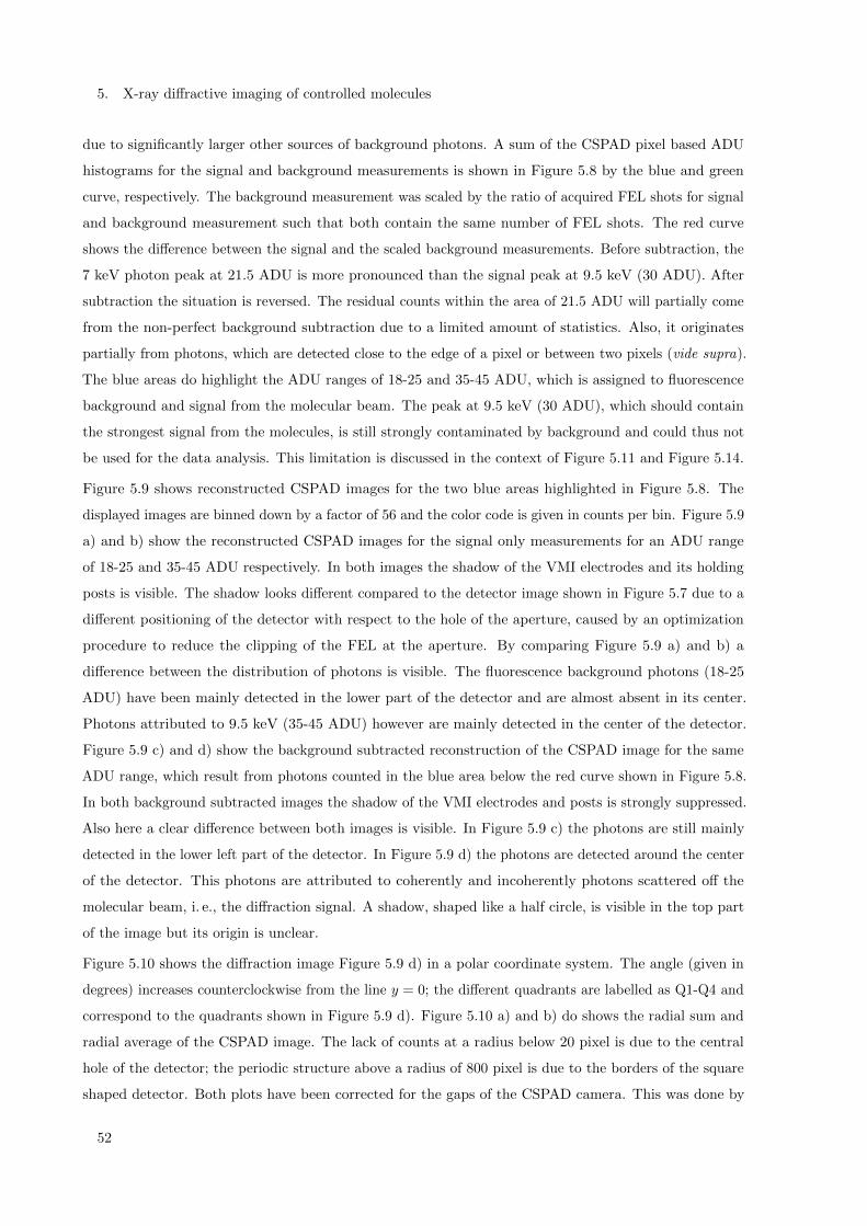
5. X-ray diffractive imaging of controlled molecules
due to significantly larger other sources of background photons. A sum of the CSPAD pixel based ADU
histograms for the signal and background measurements is shown in Figure 5.8 by the blue and green
curve, respectively. The background measurement was scaled by the ratio of acquired FEL shots for signal
and background measurement such that both contain the same number of FEL shots. The red curve
shows the difference between the signal and the scaled background measurements. Before subtraction, the
7 keV photon peak at 21.5 ADU is more pronounced than the signal peak at 9.5 keV (30 ADU). After
subtraction the situation is reversed. The residual counts within the area of 21.5 ADU will partially come
from the non-perfect background subtraction due to a limited amount of statistics. Also, it originates
partially from photons, which are detected close to the edge of a pixel or between two pixels (vide supra).
The blue areas do highlight the ADU ranges of 18-25 and 35-45 ADU, which is assigned to fluorescence
background and signal from the molecular beam. The peak at 9.5 keV (30 ADU), which should contain
the strongest signal from the molecules, is still strongly contaminated by background and could thus not
be used for the data analysis. This limitation is discussed in the context of Figure 5.11 and Figure 5.14.
Figure 5.9 shows reconstructed CSPAD images for the two blue areas highlighted in Figure 5.8. The
displayed images are binned down by a factor of 56 and the color code is given in counts per bin. Figure 5.9
a) and b) show the reconstructed CSPAD images for the signal only measurements for an ADU range
of 18-25 and 35-45 ADU respectively. In both images the shadow of the VMI electrodes and its holding
posts is visible. The shadow looks different compared to the detector image shown in Figure 5.7 due to a
different positioning of the detector with respect to the hole of the aperture, caused by an optimization
procedure to reduce the clipping of the FEL at the aperture. By comparing Figure 5.9 a) and b) a
difference between the distribution of photons is visible. The fluorescence background photons (18-25
ADU) have been mainly detected in the lower part of the detector and are almost absent in its center.
Photons attributed to 9.5 keV (35-45 ADU) however are mainly detected in the center of the detector.
Figure 5.9 c) and d) show the background subtracted reconstruction of the CSPAD image for the same
ADU range, which result from photons counted in the blue area below the red curve shown in Figure 5.8.
In both background subtracted images the shadow of the VMI electrodes and posts is strongly suppressed.
Also here a clear difference between both images is visible. In Figure 5.9 c) the photons are still mainly
detected in the lower left part of the detector. In Figure 5.9 d) the photons are detected around the center
of the detector. This photons are attributed to coherently and incoherently photons scattered off the
molecular beam, i. e., the diffraction signal. A shadow, shaped like a half circle, is visible in the top part
of the image but its origin is unclear.
Figure 5.10 shows the diffraction image Figure 5.9 d) in a polar coordinate system. The angle (given in
degrees) increases counterclockwise from the line y = 0; the different quadrants are labelled as Q1-Q4 and
correspond to the quadrants shown in Figure 5.9 d). Figure 5.10 a) and b) do shows the radial sum and
radial average of the CSPAD image. The lack of counts at a radius below 20 pixel is due to the central
hole of the detector; the periodic structure above a radius of 800 pixel is due to the borders of the square
shaped detector. Both plots have been corrected for the gaps of the CSPAD camera. This was done by
52

5.5 Experimental results
−500 0 500
−500
0
500
Pix
ely
a
18-25 ADU
0
15
30
45
60
Pho
tons
(pho
tons
/bin
)
−500 0 500
−500
0
500 b
35-45 ADU
0.0
1.5
3.0
4.5
6.0
Pho
tons
(pho
tons
/bin
)
−500 0 500
Pixel x
−500
0
500
Pix
ely
c
0
1
2
3
4
5
Pho
tons
(pho
tons
/bin
)
−500 0 500
Pixel x
−500
0
500 d Q1
Q4
Q2
Q3
0.0
0.8
1.6
2.4
3.2
4.0
Pho
tons
(pho
tons
/bin
)
Figure 5.9: a) and b): CSPAD detector images for the signal measurements, gated on an ADU range of
18-25 (left) and 35-45 (right). Bottom: Reconstructed CSPAD detector images for the signal measurements
subtracted by the scaled background measurements, gated on an ADU range of 18-25 (left) and 35-45
(right)
further reducing the image size 36 · 25 bins, as it is shown in Figure 5.10. Subsequently the ratio of ‘pixels
per bin for a gapless detector’ to ‘pixel per bin for the CSPAD camera’ was used as a scaling factor. The
half circled shadow with unknown origin (vide supra) is visible between 45 and 120 degree at a radius of
600 to 900 pixels. Both plots show maxima at an angle of 90 and 270 degree, which is explained by the
polarization dependent scattering of the linear polarized x-rays on the sample.
The diffraction signal within a single quadrant in Figure 5.10 a) can be reduced to a 1D diffraction
signal by summing up the different angular contributions within a single quadrant. This leads to four
1D diffraction signals (Q1, Q2, Q3, Q4), which are the radial sums of the diffraction pattern within each
quadrant. These four 1D diffraction images can be used do generate radial difference plots equivalent
to the one presented in the simulations in Figure 5.4. This is shown in Figure 5.11 for three different
ADU acceptance ranges, namely 35-45 ADU, 36-41 ADU, and 31-41 ADU for a), b) and c). The ADU
53

5. X-ray diffractive imaging of controlled molecules
0 100 200 300
Angle (degree)
0
200
400
600
800
1000
Rad
ius
(pix
el)
Q1 Q2 Q3 Q4
a
0
1
2
3
4
Pho
tons
(100
0ph
oton
s/pi
xel)
0 100 200 300
Angle (degree)
Q1 Q2 Q3 Q4
b
0
5
10
15
20
Pho
tons
(pho
tons
/pix
el/r
adiu
s)
Figure 5.10: The CSPAD image of Figure 5.9 d) is illustrated here in a polar coordinate system, where
the angle (given in degrees) increases counterclockwise from the line y = 0 and the quadrants Q1-Q4
correspond to the quadrants shown in Figure 5.9 d) . a) and b) do show the radial sum and the radial
average of the CSPAD image respectively. Both plots have been corrected by the gaps of the CSPAD
camera.
range presented in a) is the one, which was used to generate the images in Figure 5.9 b) and d) as well as
Figure 5.11. Due to the high background contamination it is not obvious what the optimum ADU range
and ADU gate width is to retrieve the diffraction signal from the molecule. Hence, this three different
ADU ranges represent (relatively speaking) a) intermediate signal to noise ratio (SNR) and intermediate
number of photons, b) high SNR and low number of photons, and c) low SNR and high number of photons.
The determination of the 3 ADU ranges is described in section A.2.
Figure 5.11 a) shows in black simulated differential radial plot for (Q1+Q3)-(Q2+Q4). It is the same
as presented in Figure 5.4 but modified by the pixel grid of the CSPAD camera, i. e., including the gaps
of the detector. The simulated differential plot was generated by the same procedure that was used to
generate the radial profiles of the experimental data. The gray areas do highlight the expected locations
for the first, second and third maxima of the molecules’ iodine-iodine interference term. The red curves
in a), b) and c) are labeled as ∆all and show the radial difference between (Q1+Q3)-(Q2+Q4) for the
experimental data (Figure 5.10 a)). The green and blue graph show the differential radial plot of Q1-Q2
= ∆12 (upper half of the detector) and Q3-Q4 = ∆34 (lower half of the detector) respectively. The error
bars for ∆all, ∆12, and ∆34 are given as the Poisson noise per bin, the connection between the bins are
given as visual aid, and ∆12 and ∆34 have been scaled by a factor two for an easier comparison to ∆all.
In general, ∆12 and ∆34 have the same contribution of the diffraction pattern due to the symmetry of the
diffraction pattern. But, due to the asymmetry of the background radiation their shape can differ.
From the simulations in Figure 5.4 it was expected that the strongest signal of the molecules will be
visible at the location of the second maximum. In Figure 5.11 a) ∆all does show a local maximum at the
location of the second maximum. Decomposing ∆all into ∆12 and ∆34 shows that the local maximum
54
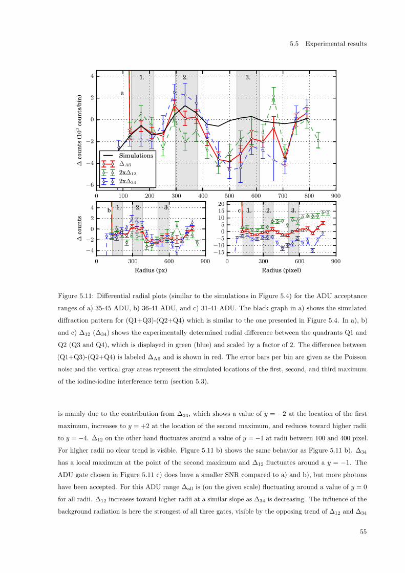
5.5 Experimental results
0 100 200 300 400 500 600 700 800 900
6
4
2
0
2
4
coun
ts(1
03
coun
ts/b
in) a
1. 2. 3.
SimulationsAll
2x12
2x34
0 300 600 900
Radius (px)
4
2
0
2
4
co
unts
1. 2. 3.b
0 300 600 900
Radius (pixel)
15105
05
101520
1. 2. 3.c
Figure 5.11: Differential radial plots (similar to the simulations in Figure 5.4) for the ADU acceptance
ranges of a) 35-45 ADU, b) 36-41 ADU, and c) 31-41 ADU. The black graph in a) shows the simulated
diffraction pattern for (Q1+Q3)-(Q2+Q4) which is similar to the one presented in Figure 5.4. In a), b)
and c) ∆12 (∆34) shows the experimentally determined radial difference between the quadrants Q1 and
Q2 (Q3 and Q4), which is displayed in green (blue) and scaled by a factor of 2. The difference between
(Q1+Q3)-(Q2+Q4) is labeled ∆All and is shown in red. The error bars per bin are given as the Poisson
noise and the vertical gray areas represent the simulated locations of the first, second, and third maximum
of the iodine-iodine interference term (section 5.3).
is mainly due to the contribution from ∆34, which shows a value of y = −2 at the location of the first
maximum, increases to y = +2 at the location of the second maximum, and reduces toward higher radii
to y = −4. ∆12 on the other hand fluctuates around a value of y = −1 at radii between 100 and 400 pixel.
For higher radii no clear trend is visible. Figure 5.11 b) shows the same behavior as Figure 5.11 b). ∆34
has a local maximum at the point of the second maximum and ∆12 fluctuates around a y = −1. The
ADU gate chosen in Figure 5.11 c) does have a smaller SNR compared to a) and b), but more photons
have been accepted. For this ADU range ∆all is (on the given scale) fluctuating around a value of y = 0
for all radii. ∆12 increases toward higher radii at a similar slope as ∆34 is decreasing. The influence of the
background radiation is here the strongest of all three gates, visible by the opposing trend of ∆12 and ∆34
55

5. X-ray diffractive imaging of controlled molecules
and considering that the contribution from the diffraction signal of the molecules as well as the helium
should be the same in ∆12 and ∆34. Interesting to note is the peak at the location of the second maximum
for ∆34 is now strongly suppressed compared to Figure 5.11 a) and b). This would not be expected for a
peak originating from the background radiation, indicating therefore a true molecular feature.
0 20 40 60 80
Angle (degree)
0
200
400
600
800
1000
Rad
ius
(Pix
el)
Data
−8
−4
0
4
8
0 20 40 60 80
Angle (degree)
0
200
400
600
800
1000
2nd max.
Simulations
−2
−1
0
1
2
0 20 40 60 80
Angle (degree)
0
200
400
600
800
1000Smoothed data
−8
−4
0
4
8
∆ph
oton
s(1
00ph
oton
s/pi
xel)
Figure 5.12: Differential images of quadrant 3 and 4 for the experimental data (left), simulations (center),
and smoothed experimental data (right). The angular coordinate of quadrant 4 has been reversed prior
the subtraction to compensate for the polarization dependent scattering effect. The location of the second
maximum is highlighted by the oval shaped circle.
∆34 in Figure 5.11 a) shows a distribution closest to the simulated data and hence it was used to generate
a 2D diffraction image, which is shown in Figure 5.12. It shows the subtraction of Q4 from Q3 in the polar
coordinate space as it is shown in Figure 5.10. The angular coordinates of Q4 have been reversed before
subtraction such that the 2D array of Q4 was ranging from 360 to 270 degree before it was subtracted
from Q3 ranging from 180-270 degree. This was done to cancel out the effect of the polarization dependent
scattering. The left image shows the difference from the experimental data shown in Figure 5.10 a), the
central image shows the simulations, and the right image shows again the experimental data convolved
by a Gaussian function with a sigma of 1.5 bins. The location of the second maximum is highlighted
in all images by the oval shaped circle. The simulation shows an area of constructive interference. The
experimental data do show no clear signature of a maximum at the location of the second maximum.
Figure 5.13 shows the statistical error and the signal to noise ratio (SNR) of the 2D diffraction image
shown in Figure 5.13. The statistical error is given by the square root of the contributions from the signal
and scaled background measurement in each bin of Q3 and Q4. The SNR 2D histogram shows the ratio
56

5.6 Discussion
0 20 40 60 80
Angle (degree)
0
200
400
600
800
1000
Rad
ius
(pix
el)
50
70
90
110
130
(Sig
nal+
Bac
kgro
und)
0.5
(pho
tons
/pix
el)
0 20 40 60 80
Angle (degree)
0.0
0.5
1.0
1.5
2.0
Sign
al/B
ackg
roun
d
Figure 5.13: Statistical error (left) and SNR (right) for the experimental data shown in Figure 5.12. The
circles show the location of the second maximum of the iodine-iodine interference term derived from the
simulation in Figure 5.12
between the (scaled) background subtracted signal and (scaled) background measurements. The circle
represents again the location of the second maximum derived by the simulations shown in Figure 5.12. It
can be seen that the statistical error in this region of this maximum is almost constant above 110 photons
per pixel. Also the SNR in this area is somewhat constant. At this statistical level the 2D representation
of the diffraction signal does neither confirm nor reject the attribution of the maxima detected in the 1D
diffraction diffraction pattern shown in Figure 5.11. In general it can be seen that, at radii bigger than
≈ 450 pixel, the SNR is getting lower, which can explain the discrepancy between data and simulations
shown in Figure 5.12. The statistical error shows an increase in the central right region, which is due to
the higher number of photons there, originating from the polarization dependent scattering.
5.6 Discussion
The recorded diffraction pattern in Figure 5.10 shows a clear signal of scattered photons, which is dependent
on the polarization of the FEL. The contribution from the rest gas in the chamber were compensated
by the background measurements; the fluorescence and beamline photons do have a different signature.
Therefore, these photons must originate to from the molecular beam (seeding gas, molecules).
From the simulations in Figure 5.4 it was expected that the second maxima of the iodine-iodine interference
is the strongest interference signal measurable in a 1D differential plot. The experimentally determined 1D
differential plots shown in Figure 5.11 a) and b) do show a maximum at the location of the second maxima
57
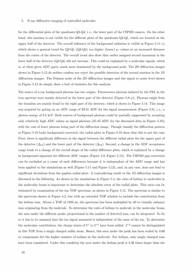
5. X-ray diffractive imaging of controlled molecules
for the differential plots of the quadrants Q3-Q4, i. e., the lower part of the CSPAD camera. On the other
hand, this maxima is not visible for the different plots of the quadrants Q2-Q1, which are located on the
upper half of the detector. The overall influence of the background radiation is visible in Figure 5.11 c),
which shows a general trend for Q2-Q1 (Q3-Q4) too higher (lower) y−values at an increased distance
from the center of the detector. The overall trend also show that earlier assigned second maximum in the
lower half of the detector (Q3-Q4) did not increase. This could be explained by a molecular signals, which
is, at these given ADU gates, much more dominated by the background peak. The 2D diffraction images
shown in Figure 5.12 do neither confirm nor reject the possible detection of the second maxima in the 1D
diffraction images. The Poisson noise of the 2D diffraction images and the signal to noise level shown
in Figure 5.13 do simply show a lack of statistics for this analysis.
The source of x-ray background photons has two origins. Fluorescence photons induced by the FEL in the
iron aperture were mainly detected in the lower part of the detector (Figure 5.9 a)). Photons origin from
the beamline are mainly found in the right part of the detector, which is shown in Figure 5.14. This image
was acquired by gating on an ADU range of 29-31 ADU for the signal measurement (Figure 5.8), i. e., a
photon energy of 9.5 keV. Both sources of background photons could be partially suppressed by accepting
only relatively high ADU values as signal photons (35-45 ADU for the discussed data in Figure 5.10),
with the cost of fewer photons being part of the diffraction image. Though visually the diffraction pattern
in Figure 5.10 looks background corrected, the radial plots in Figure 5.10 show that this is not the case.
First, there is significant difference in the signal between the different radial plots for the upper part of
the detector (∆12) and the lower part of the detector (∆34). Second, a change in the ADU acceptance
range leads to a change of the overall shape of the radial difference plots, which is explained by a change
in background signature for different ADU ranges (Figure 5.9, Figure 5.14). The CSPAD gap correction
can be excluded as a cause of such differences because it is independent of the ADU range and has
been applied to the simulations as well (Figure 5.11 and Figure 5.12), and ,in any case, does not lead to
significant deviations from the gapless radial plots. A contradicting result to the 1D diffraction images is
discussed in the following. As shown in the simulations in Figure 5.4, the ratio of helium to molecules in
the molecular beam is important to determine the absolute error of the radial plots. This ratio can be
estimated by examination of the ion TOF spectrum, as shown in Figure 5.15. The spectrum is similar to
the spectrum shown in Figure 4.2, but with an extended TOF window to include the contribution from
the helium ions. Above a TOF of 1950 ns, the spectrum has been multiplied by 20 to visually enhance
ions originating from the molecule. To determine the ratio of helium to molecule in the molecular beam,
the area under the different peaks, proportional to the number of detected ions, can be integrated. To do
so it has to be assumed that the ion signal measured is independent of the mass of the ion. To determine
the molecular contribution, the charge states of I+ to I+5 have been added. I+4 cannot be distinguished
in this TOF from a singly charged sulfur atom. Hence, this area under the peak has been scaled by 0.66
to compensate for the higher number of iodines in the molecule. For helium, only singly charged ions
have been considered. Under this condition the area under the helium peak is 2.36 times larger than the
58

5.6 Discussion
−500 0 500
Pixel x
−500
0
500
Pix
ely
0
2
4
6
8
10
Pho
tons
(pho
tons
/bin
)
Figure 5.14: Detected photons in the diffraction measurement for an ADU gate of 29-31 ADU, i. e., for
a photon energy of 9.5 keV. The highest photon count rate is visible in the upper right corner of the
detector, which origins from scattered photons from the beamline.
area under the iodine peaks, i. e., 2.36 times more helium atoms have been detected. With the additional
assumption that two ionic iodine fragments are always generated upon interaction with the x-rays, and
considering the detection efficiency of 50%, the ratio of helium to molecule is 4.72. Table 2 shows the
2000 4000 6000
TOF (ns)
0.0
0.5
1.0
1.5
Inte
grat
edam
plit
ude
×108
x20He+
I+I+2I+3I+4
S+
I+5S+2
O+
C+
Figure 5.15: Ion TOF spectrum of the molecular beam. For flight times higher than 1950 ns, the recorded
signal has been multiplied by a factor of 20.
59

5. X-ray diffractive imaging of controlled molecules
different photoelectric absorption cross sections for the helium and molecular atoms. Assuming that the
molecular cross section is equivalent to the sum of its individual atomic cross sections, its total cross
section is 80.360·10−24 cm2, compared to 0.2306·10−24 cm2 for helium. Hence, the probability of ionization
of a single molecule is ≈ 350.000 times higher. Considering that roughly 4.72 times more helium ions have
been detected the helium to molecule ratio in the molecular beam is 1.65 million to 1. This ratio is 20-200
times higher than it was expected to be beforehand and as it is shown in the simulations in Figure 5.4.
This estimation suggest that the maximums’ origin is due to the background rather than the molecular
interference pattern, supported by the statement that the maximum has only been observed in the lower
part of the detector. Additionally this estimation can also be used to determine the vapor pressure of the
molecule. Due to the good knowledge of the helium pressure in the pulsed valve, the molecule’s vapor
pressure can be calculate to be 0.05 mbar. This low vapor pressure for 2,5-diiodothiophene above its
melting point is highly unlikely and could be explained by the delay between FEL and molecular beam,
which has probed a temporally bad position of the molecular beam. Helium is typically a little bit faster
than the molecules and thus is more prominent at the front of the pulse. Also a partially clogged valve,
which predominantly transported helium to the interaction zone, or simply an empty molecular sample
could explain this ratio. During the experiment, a lot of precaution was taken into account to avoid any
of these possibilities and hence it is unclear, which, if not all, points are causing the strong deviations
from the expected helium to molecule ratio or if the estimation is based on wrong assumptions.
5.7 Conclusion and outlook
We have shown that we could retrieve a diffraction signal from the molecular beam despite the high
background generated by the beamline as well the used aperture. Whether or not the detected signal
from the molecules in the 1D diffraction image is due to the molecules or due to the background from the
beamline could not be conclusively answered. We have learned important lessens that show that the field
can make great progress in the next generation of FELs. The main challenges for this kind of experiment
are the low diffraction signal from the molecules, the resulting slow feedback from the experiment, and
the limited time available at a FEL facility. During this experiment 80% of the available time was spent
on the reduction of beamline background photons as well as on the reduction of secondary effects such as
fluorescence from the iron aperture. A different material for the aperture, like aluminum instead of iron,
could have helped to suppress fluorescence photons more efficiently by relying on the energy resolution of
the detector to filter the Kα and Kβ emission lines (which are well below the incident photon energy of
9.5 keV). Additionally, careful selection and placement of beamline apertures could have helped to protect
the detector from unwanted background, as it is shown, for instance, by the shadow-area of the VMI
electrodes (Figure 5.7). The background from the carrier gas, i. e. helium, can be conceptually suppressed
by the use of an electrostatic deflector [25] at the cost of a lower density in the molecular beam. Changing
the carrier gas to, for instance, neon is not useful despite the typically lower seeding pressure of 20 bar
and the consequent reduction in the number of atoms in the interaction zone. Drawbacks are the reduced
60

5.7 Conclusion and outlook
density of the molecular sample due to a slower molecular beam and the increase in the scattering cross
section (incoherent and coherent) of the carrier gas (≈ a factor of 20 and 200 respectively) leading to
producing higher background signal.
Beside the challenges presented, diffractive imaging is a highly promising experimental approach to deter-
mine molecular structure, and more importantly, to image molecular dynamics like folding, isomerization,
or photofragmentation with fs time resolution. The simulations in section 5.3 have shown that under
very good experimental conditions enough statistics for a static diffraction image of the molecule could
have been recorded within roughly 6 hours of integration time. The repetition rate of the upcoming
hard x-ray FELs, e. g., XFEL or LCLS II, is a few hundred to a few thousand times higher compared to
the 120 Hz, which were available for the presented experiment. At this high repetition rate it would be
possible to record the diffraction image of the molecule within minutes, and thus providing immediate
feedback from the experiment. The technology transfer to align molecules at FEL repetition rates [100] is
in principle capable of supporting any repetition rate, which is provided by the Ti:Sapphire laser available
at the different end stations, given that a few mJ per pulse are available. Additionally, intracavity laser
alignment of molecules, allowing for the alignment of molecules at arbitrary repetition rates, is currently
under development [147].
To measure the above mentioned molecular dynamics, the upcoming high-repetition rate FELs will play
a key-role. In a optical pump-probe experiment only 10-20 % of the molecules in the interaction zone
will be typically pumped by a laser; the FEL will probe the structure of all molecules. Thus up too 90 %
of the diffraction image will still be due to the static structure of the molecule. In first approximation
the integration time has to be 25-100 times longer to see a statistically relevant signal from the triggered
dynamics of the molecule. Not taken into account are, for instance, different dissociation channels and
different velocity distributions of the dissociation channels, which will further blur the structure. If a
‘well known’ molecular dynamics is the aim of the study, one can in principle beat the above mentioned
statement for the SNR and the stated modification of the integration time. Assuming the static diffraction
pattern of the molecule shows several minima and maxima on the detector (Figure 5.2), the triggered
dynamics could then be probed such that the maxima of the dynamical structure fall into the minima of
the static structure, and thus have locally a much lower background. One could measure the different time
steps within hours and would thus pave the way toward diffraction imaging of cold, controlled molecules
in the gas-phase.
The imaging of small biomolecules under controlled conditions in a cold molecular beam will be the next
challenging step. Tryptophan, for instance, is an α-amino acid with the chemical formula C11H12N2O2. It
consists of the chromophore indole and an α-amino group. It is chosen here exemplarily since both, the
indole chromophore and the α-amino group, were measured in the context of this thesis and are shown in
chapter 6, chapter 7 and section 8.2. The coherent scattering cross section of tryptophan is 63 ·10−24cm2.
For comparison, the coherent scattering cross section of 2,5-diiodothiophene is 1293 ·10−24cm2. Thus,
the probability of coherently scattering off tryptophan is only 5 % of the probability of scatting off
61

5. X-ray diffractive imaging of controlled molecules
2,5-diiodothiophene. Further, for lighter atoms the ratio of coherent to incoherent scattering cross sections
is reduced (Table 2). For tryptophan this ratio is only 1.28 compared to the earlier discussed ratio of 31
for 2,5-diiodothiophene. Thus, even if no background photons from the beamline and the seeding gas are
present, more than 40 % of the detected photons originate from incoherently scattered x-ray photons. The
shift in energy of the photon due to its elastic scattering (incoherent scatting) cannot be compensated by
a high energy resolution detector and subsequent gating on its ADU range since it is typically within the
bandwidth of the FEL [148].
A reduction of the photon energy can help in several ways. At a reduced photon energy, the FEL will
provide more photons, and the ratio of coherent to incoherent scattering will be much higher. The coherent
scattering cross section increase with decreasing photon energy, in contrast to the incoherent scattering,
which will be reduced at a lower photon energy. At a photon energy of 4 keV the photons still have
a wavelength of 0.31 nm, which will not provide atomic resolution, but can resolve (depending on the
molecule) inter-molecular distances.
62

6 X-ray photophysics of indole∗
The following chapter is describing the x-ray photophysics of gas-phase indole upon core-shell ionization.
Supplementary informations are given in Appendix B, covering the reconstruction of the molecular beam
profile (section B.1), a general explanation of the coincidence spectrum (section B.2), and the calibration
measurements for the ion TOF and VMI (section B.3, section B.4), as well as the electron VMI section B.5.
6.1 Introduction
Electronic relaxation dynamics, including charge-transfer and charge-migration processes, together with
the nuclear fragmentation dynamics after creation of one or several core-shell vacancies, play a crucial
role for our understanding of the interaction of x-rays with matter. Because of their element specificity,
x-rays can be efficiently employed to induce charge-transfer dynamics at specific and well-defined sites
via deep core level ionization of individual atoms inside the molecule. To unravel fundamental relaxation
processes, like interatomic coulombic decay (ICD) [80], small molecules and van-der-Waals hydrogen
bonded clusters [149, 150] in the gas-phase were widely studied by XUV and (soft) x-ray ionization
at various accelerator based facilities like synchrotrons or free electron lasers (FELs). The pioneering
experiments on ICD with van-der-Waals bonded Ne clusters were performed at synchrotrons at low
intensities below the threshold of photo double ionization for a single Ne site. The availability of FELs
with high radiation intensity allowed to study ultrafast charge rearrangement and nuclear dynamics
fragmentation subsequent to multiple innershell ionization [53, 54, 151, 152] revealing novel effects such
as double or multiple core-hole creation and frustrated x-ray absorption [153–155]. Furthermore, the
high temporal resolution of FELs provided access to dynamical studies such as electron transfer and
charge migration processes to trace the spatial localization of the charges as a function of time during
dissociation [156–160] and isomerization [161] reactions. Coincidence methods, where the momenta
of all charged particles are detected for a single event, play a crucial role to understand the complete
fragmentation and charge rearrangement dynamics in these experiments. Various techniques were developed
during the last years which include Photoion-Photoion Coincidence (PIPICO) [17, 62], Photoelectron-
Photoion-Photoion Coincidences (PEPIPICO) [21–23, 58, 59, 61], or Auger-Electron-Photoion-Photoion
Coincidences (AEPIPICO) [60] measurements. An extensive overview of the history and the current
state of different coincidence techniques is given in [162]. The accessibility of all momenta allowed in
addition to correlate the corresponding electron momenta with the recoil frame of the molecule resulting in
Recoil-Frame Photo Angular Distributions (RFPAD) [19, 21–23, 62]. These RFPADs allow in addition to
∗This chapter is based on a preliminary version of the manuscript: X-ray photophysics of indole, by T. Kierspel, M.
Di Fraia, J. Wiese, R. Boll, C. Bomme, D. Rolles, J. Viefhaus, J. Kupper, S. Trippel and others. I contributed to the
experimental part by pre-experiments in the laboratory. During the measurement I was responsible for the molecular beam.
I did the data analysis and I wrote the chapter supervised by S. Trippel and J. Kupper.
63

6. X-ray photophysics of indole
determine the structure of molecules and molecular dynamics in diffraction from within type of experiments.
Furthermore Molecular-Frame Photo Angular Distributions (MFPADs) experiments [16–20], where the
molecules are typically aligned, so fixed in space by a strong laser field [35], allow to unravel the dynamics
directly in the molecular frame.
Indole is the chromophore of the essential amino acid tryptophan, and as such also part of various proteins
and peptides. Indole itself was already in the focus of a variety of different experimental and theoretical
studies, ranging from microwave [163, 164] and optical spectroscopy [165, 166], over vibrationally [167]
and rotationally resolved electronic spectroscopy [168–172], to photoelectron spectroscopy [173–175]. The
lowest electronically excited states of indole are labeled as 1La and 1Lb (notation after [176]). The 1La state
is highly polar and, therefore, its energy is strongly influenced by the polarity of its solvent environment.
Already in small clusters like indole-water1 a shift in the electronic states and their corresponding dipole
moments is observed [167, 171, 172, 177, 178]. Tryptophan is used for the same reason in a variety of
experiments as an environment marker in proteins [179] (and references therein). The indole-water1
cluster has a well defined structure: the water is hydrogen bonded to indole at the nitrogen side of the
molecule [171]. These clusters are therefore well suited to study the nature of hydrogen bonds, which are
of universal importance in chemistry and biochemistry, via site specific core shell ionization.
Before studying the dynamics in clusters it is important to fully understand and characterize the photopysics
of the bare indole molecule especially focussing on the site specific ionization at the nitrogen atom. In
this study we present the photophysics of gas-phase indole by a single photon ionization primarily at the
carbon atomic 1s orbitals as well as by side specific ionization at the nitrogen atom. Photo- and Auger
electrons as well as the ionic fragments of indole were detected in coincidence in a double-sided velocity
map imaging (VMI) [2–5] spectrometer. Our work provides the basis for fragmentation studies of larger
molecules as well as molecular clusters. The experimental setup, described in the next chapter, was chosen
such that the photofragmentation of indole and indole-water clusters could be measured. Our findings for
the photopysics of indole-water1 clusters are discussed in chapter 7.
6.2 Experimental setup
The experimental setup is shown in Figure 6.1. The part that provides the molecular beam is similar to
the one described in [12]. A supersonic expansion of a few mbar of indole and a trace of water molecules
seeded in 60 bar of helium was provided by a pulsed Even-Lavie valve [63]. The valve was operated at a
repetition rate of 250 Hz, and was heated to a temperature of 110 C. Due to three-body collisions in the
early phase of the expansion indolem(H2O)n clusters are formed. The mixture can be spatially separated
using strong inhomogeneous electric fields generated by the electrostatic deflector [9]. From time of flight
(TOF) spectra obtained in characterization experiments using a compressed 50 fs laser pulse at 800 nm
we estimate a ratio R = 4 of indole molecules to indolem(H2O)n clusters. Due to the difference signature
of the fragmentation pattern of indole and indolem(H2O)n, we can estimate a purity of more than 95%
for indole on the data presented here. The data obtained from indolem(H2O)n clusters are discussed
64

6.2 Experimental setup
Pulsed valve (250 Hz)
Deflector
Ion detector
Electron detector
Soft x-ray(420 eV)
Time
Reconstructedmolecular pulse
Photoelectron detected:Record electrons and ions for 6 µs
200 µs
Skimmer Skimmer
VMI electrodes
synchrotron bunches(62.5 MHz)
Figure 6.1: Experimental setup showing the pulsed valve, skimmers, deflector, the double-sided VMI with
its corresponding delay line detectors to detect electrons and ions in coincidence, and the synchrotron
beam which crosses the molecular beam in the center of the VMI. A reconstructed molecular pulse is
shown in the top left part. Schematically indicated is the logical gate (red) synchronized to the molecular
beam. Multiple synchrotron pulses are crossing the molecular beam without interaction (black vertical
bars). A single interaction is indicated by the orange vertical bar.
in chapter 7. The molecular beam apparatus was mounted to the CAMP–CFEL-ASG Multi Purpose–end
station [180] which was connected to the synchrotron (Petra III, Variable Polarization Beamline P04 [181],
circular polarization (> 98%) †, 5·1013 photons/s, 480 bunches, 16 ns bunch period). The molecular
beam was crossed by the synchrotron radiation under an angle of 90 degree inside a double sided VMI
spectrometer ‡ for simultaneous electron and ion detection. The velocity of the molecular beam caused an
TOF dependent VMI offset of the detected ionic fragments due to an extraction of the ions perpendicular
to the molecular beam axis. Both, electrons and ions were detected with a hexanode (electrons) and
quadanode (ions) delay line detector (DLD, Roentek) respectively. Only two out of three electrodes within
the hexanode were working properly.
The pulse duration of the molecular beam in the interaction region was about 60 µs full width at half
maximum (FWHM). At the valve repetition rate of 250 Hz this resulted in a duty cycle of 1-2 %.
The electronic readout of the detectors was triggered by electrons detected on the electron side of the
†At the time of the experiment the only possible polarization‡The VMI images show the 2D-projection of the ions and electrons 3D velocity distribution onto the detector surface in
the laboratory frame coordinates.
65

6. X-ray photophysics of indole
spectrometer. In addition a logical gate was used to record data only in a 200 µs time window which was
synchronized to the arrival time of the molecular beam in the interaction zone (Figure 6.1). This resulted
in a reduction of the background signal created by the high repetition rate of the synchrotron. Once
triggered, electrons and ions were recorded for a time of 6 µs and marked as a single event which was
tagged with a timestamp (TS). The TS was the relative timing between the trigger of a single event and
the starting time of an individual measurement. The corresponding detected electrons/ions were saved in
a shot list and could be sorted subsequently according to their temporal position within the 200 µs time
window which was calculated by the modulus of TS/4 ms. A histogram of the modulus time for a single
measurement is exemplarily shown in blue in the top left part of Figure 6.1. The envelope represents
the temporal molecular profile plus a constant offset. Contributions at the beginning and the end of the
indicated temporal gate (red) are due to background events; the rise in the center is due to a higher event
rate when the molecular beam is in the interaction zone. The modulus time could be reconstructed to an
accuracy of less than 1 µs which was limited by a relative temporal drift within the electronics, but was
accurate enough for the conducted measurement. Further shown schematically is the pulse structure of
the synchrotron indicated by vertical black lines. The interaction probability of the synchrotron pulses
with the background/molecular beam is in the order of 0.005-0.01 %, indicated by the yellow bar. The
synchrotron was tuned to a photon energy of 420 eV (λ = 2.95 nm).
6.3 Coincidence spectra
The photofragmentation of indole was investigated via a coincidence measurement between the emitted
electrons and the corresponding ionic fragments. A background subtracted (PE)PIPICO spectrum [182,
183] of indole, ionized with a single photon at an energy of 420 eV, is shown in Figure 6.2 as a function of
the mass to charge ratio of the first and second detected ion, m1/q1 and m2/q2, respectively. The map
allows to disentangle different fragmentation channels of indole in the case of at least two detected ionic
fragments. The background correction was obtained by subtracting the signal outside the molecular pulse
from the data recorded inside the molecular pulse with an appropriate weight. If not stated otherwise, no
correction is applied to the presented data.
Visible are six main coincidence islands, labeled with 1-6. The coincidence islands 1-3 originate from the
fragmentation channels, C4H4−n + C4NH3−m or C3NH3−n + C5H4−m, C2NH3−m + C6H4−n or C3H3−m
+ C5NH4−n, and C7H5−n + CNH2 respectively. The indices m and n in the formulas account for the
loss of hydrogens or protons. The molecular structure of indole (atomic labeling according to [184])
as well as an expanded scale of these coincidence islands is shown by the insets of Figure 6.2. This is
visible as different diagonal lines within each of these PIPICO island, corresponding to a spacing of 1
u/e. The sum of the masses of all three islands is equal to the mass of indole, neglecting the loss of
hydrogen/protons. The fragmentation patterns show the strongest coincidence upon the emittance of two
or three hydrogens/protons in the case of island 1 (C4H4−n + C4NH3−m or C3NH3−n + C5H4−m) and
3 (C7H5−n + CNH2). PIPICO island 2 (C2NH3−m + C6H4−n or C3H3−m + C5NH4−n) shows only one
66
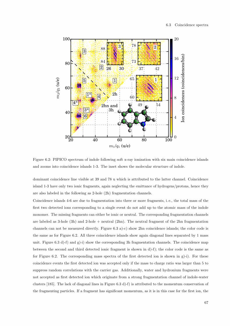
6.3 Coincidence spectra
20 40 60 80 100m1/q1 (u/e)
20
40
60
80
100
m2/q
2(u
/e)
2h
2hn and3h
1
2
3
4
5
63*
1*
4*
0
4
8
12
16
20
Ion
coin
cide
nces
(coi
ncid
ence
s/bi
n)
37 42
73
78 2
26 30
84
88 3
49 54
60
65 1
Figure 6.2: PIPICO spectrum of indole following soft x-ray ionization with six main coincidence islands
and zooms into coincidence islands 1-3. The inset shows the molecular structure of indole.
dominant coincidence line visible at 39 and 78 u which is attributed to the latter channel. Coincidence
island 1-3 have only two ionic fragments, again neglecting the emittance of hydrogens/protons, hence they
are also labeled in the following as 2-hole (2h) fragmentation channels.
Coincidence islands 4-6 are due to fragmentation into three or more fragments, i. e., the total mass of the
first two detected ions corresponding to a single event do not add up to the atomic mass of the indole
monomer. The missing fragments can either be ionic or neutral. The corresponding fragmentation channels
are labeled as 3-hole (3h) and 2-hole + neutral (2hn). The neutral fragment of the 2hn fragmentation
channels can not be measured directly. Figure 6.3 a)-c) show 2hn coincidence islands; the color code is
the same as for Figure 6.2. All three coincidence islands show again diagonal lines separated by 1 mass
unit. Figure 6.3 d)-f) and g)-i) show the corresponding 3h fragmentation channels. The coincidence map
between the second and third detected ionic fragment is shown in d)-f); the color code is the same as
for Figure 6.2. The corresponding mass spectra of the first detected ion is shown in g)-i). For these
coincidence events the first detected ion was accepted only if the mass to charge ratio was larger than 5 to
suppress random correlations with the carrier gas. Additionally, water and hydronium fragments were
not accepted as first detected ion which originate from a strong fragmentation channel of indole-water
clusters [185]. The lack of diagonal lines in Figure 6.3 d)-f) is attributed to the momentum conservation of
the fragmenting particles. If a fragment has significant momentum, as it is in this case for the first ion, the
67

6. X-ray photophysics of indole
36 39 42
48
51
54m
2/q 2
(u/e
) a
25 27 29
60
62
64 b
m(y−1)/q(y−1) (u/e)
25 27 29
36
38
40 c
48
51
54
m3/q 3
(u/e
) d
60
62
64 e
36
38
40 f
10 20 30 40
4
8
12
Ions
(100
ions
/bin
)
g
10 20 30
m1/q1 (u/e)
1
2
3
h
10 20 30
2
4
6
i
Figure 6.3: a-c: PIPICO islands 4-6 for the first against the second detected ion. d-f: Same PIPICO
islands for the second against the third detected ion. g-i: Corresponding m/q spectrum of the first detected
ion in case of a 3h fragmentation. The color code is the same as in Figure 6.2.
momenta of the two other ions are not opposed anymore, leading to a disappearance of the coincidence
lines [186]. The ion peak at 15 u/e in Figure 6.3 g)-i) is attributed to background ions since it does not
obey momentum conservation with the other ions detected in coincidence.
The total mass of the two ionic fragments of PIPICO island 4 (Figure 6.3 a)) is between 86 and 91 u.
The mass of the missing fragments ranges between 26 and 31 u which leaves 2C + xH (2 ≤ x ≤ 7) or
C + N + yH (0 ≤ y ≤ 5) as the only possible neutral fragments. The structure of the corresponding
3h fragmentation channel (Figure 6.3 d)) shows an additional enhancement of coincidences in the upper
right corner. This is attributed to a background contamination since these ions do not obey momentum
conservation. The mass spectrum of the first detected ion for this 3h channel is dominated by ions between
26 and 28 u/e which can be assigned to the ionic fragments C2Hx 2 ≤ x ≤ 4) or CNHy (0 ≤ y ≤ 2).
PIPICO island 5 (Figure 6.3 b)) consists of three distinct vertical coincidence islands with a mass to
charge ratio of 26-28 falling in coincidence with masses of 61-63. The total mass of these ionic fragments is
68

6.3 Coincidence spectra
0 90 180 270 360α12 (degree)
0
3
6
Coi
n.(1
03co
in.p
erbi
n) c
0 90 180 270 360α12 (degree)
0
2
4
d
29 31 33m1/q1 (u/e)
50
52
54
m2/q
2(u
/e)
a
26 28m1/q1 (u/e)
42
43
44 b
Figure 6.4: a) and b): Highlighted PIPICO islands 1* (left) and 3* (right). Dashed black lines show
a theoretical linear dependence with slopes corresponding to dicationic first (left) and second (right)
detected ions. The color code is the same as in Figure 6.2. c) and d) angle between the velocities v1 and
v2 for both coincidence islands. The dashed blue lines highlight a Gaussian fit. Gray areas indicate the
coincidences accepted for a) and b).
between 87 and 91 u. The mass of the neutral fragment ranges thus from 26 to 30 u. 2C + xH (2 ≤ x ≤ 6)
or C + N + yH (0 ≤ y ≤ 4) are hence the only possible fragments which are similar to the ones for
PIPICO island 4. The mass spectrum of the first detected ion (Figure 6.3 h)) shows a strong peak at 26 u
showing that only a single ionic fragment is detected in the case of a 3h fragmentation. The structure of
the corresponding PIPICO island for the second and third detected ion (Figure 6.3 e)) shows a shift of
the coincidence island toward higher masses. The shift in the 3h fragmentation channel can be explained
considering the fragmentation possibilities in this channel. The mass of the first detected ion in the
2hn fragmentation channel ((Figure 6.3 b)) is between 26 and 28 u. If both mentioned fragments are
ionic (Figure 6.3 h)) the lighter C2Hx fragment will always be detected first and its coincidence peak
consequently vanished in Figure 6.3 e). PIPICO island 6 is build up of four distinct vertical coincidence
islands with ions detected between 25-28 u/e falling in coincidence with ionic fragments between 37-39 u/e.
The enhancement of detected coincidences near the ionic fragments of 27 and 39 u/e is due to background
contamination since these coincidences do not fulfill momentum conservation. The total mass of the two
ionic fragments detected in PIPICO island 6 is between 62 and 67, leaving 50 to 55 u for the neutral
fragment(s), i. e., 4C + xH (2 ≤ x ≤ 7) or 3C + N + yH (0 ≤ y ≤ 5). The 3h coincidence spectrum in
69

6. X-ray photophysics of indole
-6 -3 0 3 6vX (km/s)
-6
-3
0
3
6
v Z(k
m/s
)
a
-6 -3 0 3 6vX (km/s)
b
0 180 360α12 (degree)
0
1
2
3
Coi
n.(1
03co
in.p
erbi
n)
c
Figure 6.5: a) and b) VMI images of the first and second detected ion contributing to the 2hn fragmentation
channel of coincident island 4. The color code is the same as in Figure 6.2 given in the unit of ions
(ions/bin). c) Histogram of the angle between the first and the second ion with a Gaussian fit indicated
by the dashed blue line.
Figure 6.3 f) is comparable in shape to the 2hn fragmentation channel. The mass spectrum of the first
detected ion (Figure 6.3 i)) shows a comparable amount of detected ions between 12-14 u/e (CHx, N) and
26-28 u (C2Hx or CNHx). Thus, this channel shows a fragmentation into at least 3 ionic fragments and a,
either neutral or ionic, fourth fragment.
Coincidence islands 1*, 3*, and 4* are shown in Figure 6.2 additionally. They are assigned to 3h
fragmentation channels of the coincidence island 1, 3, and 4, respectively. The islands 1* and 3* are
highlighted in Figure 6.4 a) and b); the color code is the same as in Figure 6.2. In both islands a strong
coincidence line is visible which is overlaid by a dashed black line. The slope s of a coincidence line can
be used to assign the charge state of the fragments. Typically, the PIPICOs’ are shown as a function
of the ions TOF, leading to a slope of s = −1 for equally charged fragments [186]. Here, the PIPICOs’
axis is converted into mass to charge ratio units to visually assign easier the fragments. Therefore the
slope is given by -√
(q1m2)/(q2m1) for the case of a fragmentation into two particles §. The dashed black
lines show the calculated slopes for the channels (C4H4)+ + (C4N)++ or (C3NH2)+ + (C5H2)++ in case
of island 1* and the channel (CNH2)+ + (C7H2)++ for island 3*, respectively.
Both are in good agreement with the experimental data. Both islands show the strongest coincidence at a
total mass of 114 u, as well as a dicationic state of the heavier fragment. For both spectra a filter was
applied such that only events which had opposed momenta are displayed. This was especially necessary
for Figure 6.4 b) where the PIPICO line is hidden without the filter. The histogram of the angular
distribution α12 of all ions without filter is shown in Figure 6.4 c) and d). α12 is defined by the angle
between the projected velocity vectors of the first and second detected ion as indicated by the indices. The
angle is determined in a mathematical sense starting from the first ion. Both graphs show a maximum at
§It is given by -√
(q2m1)/(q1m2) for PIPICOs displayed in the lower right half of the coincidence spectrum.
70

6.3 Coincidence spectra
-9
-6
0
6
9
v Z(k
m/s
)
a
-9 -6 0 6 9-9
-6
0
6
9
v Z(k
m/s
)
b
-9 -6 0 6 9vX (km/s)
-9
-6
0
6
9
v Z(k
m/s
)
c
0 90 180 270 360α21 (degree)
0
90
180
270
360
α23
(deg
ree)
d
Figure 6.6: a), b) and c) VMI images of the first, second and third detected ion contributing to the 3h
fragmentation channel of coincident island 4. d) 2D histogram of the angles between the second and first
as well as second and third detected ion. The color code is the same as in Figure 6.2 and for a), b) and c)
it is given in the unit of ions (ions/bin).
180 degrees which is expected for an axial recoil of both fragments. The dashed blue line is indicating a
Gaussian fit to the data. The RMS of these fits are σ = 9.8 and σ = 9.5 degrees for 1* and 3*, respectively.
For the coincidence spectra in Figure 6.4 a) and b) data in the gray area has been used. The width of the
grey area is equivalent to 4σ. The non-constant offset of the angular distributions is attributed to the
molecular beam velocity parallel to the detector surface and the background signal which is centered at
the absolute velocity point of origin.
Figure 6.5 and Figure 6.6 show exemplarily VMI images of the coincidence island 4 for the case of a 2hn
and a 3h fragmentation channel. The increased number of counts visible in all VMI images at vX = 0 and
vZ ≈ −1.5 is attributed to background from the carrier gas which is falsely detected at that corresponding
TOF and does not obey momentum conservation. The VMI images for the two ionic fragments detected
in the 2hn fragmentation channel are shown in Figure 6.5 a) and b); the color code is the same as shown
in Figure 6.2 given in the unit of ions per bin. The first detected ion shows a slightly higher velocity
compared to the second detected ion which is explained by its lower mass and the momentum conservation
of the fragmenting particles. Despite the neutral dissociating fragment, the two detected ions do still obey
strong axial recoil. This is shown by, for example, the diagonal coincidence lines for island 4 in Figure 6.3.
71

6. X-ray photophysics of indole
A closer insight is given in Figure 6.5 c) by the histogram of the angular relationship between both ionic
fragments, where α12 is defined as before. The dashed blue line is indicating a Gaussian fit to the data
with an corresponding RMS of σ = 18.4.
VMI images of the 3h fragmentation channel of PIPICO island 4 are shown in Figure 6.6 a)-c) for the first,
second and third detected ion; the color code given as the same as in Figure 6.2 in units of ions per bin. The
first detected ion shows the highest of all velocities due to its lighter mass and the momentum conservation
of the fragmentation process. The angular relationship between all fragments is visible in Figure 6.6 d);
the color code is the same as in Figure 6.2. Shown here is the angle α23 plotted against the angle α21. α21
and α23 are defined as before. Visible is a sand-timer like structure, rotated by approximately 45 . The
existence of this structure clearly shows that there is a angular relationship between these fragments. The
coincidences outside that structure are due to ions which do not fulfill momentum conservation.
6.4 Photoelectron spectrum
Figure 6.7 a) and b) show the electron velocity map in a cartesian and a polar coordinate systems
respectively. The labels Q1-Q4 correspond to the four different quadrants of the VMI image. The electrons
were detected in coincidence with PIPICO island 1-5, 1* and 3* (Figure 6.2). A background correction
was applied by accepting only events which obey momentum conservation. Islands 6 was not used due to
a high background contamination. The VMI images show four distinct electron velocities at 2.4, 7.1, 9.5,
and 11.2 · 106 m/s which correspond to electron energies of 16, 142, 258, and 358 eV. Additionally, slow
electrons are visible in the center of the cartesian VMI image which are assigned to background electrons.
The photoelectrons at a velocity of vr = 2.4 · 106 m/s (16 eV) are attributed to localized ionization at the
indoles’ nitrogen atom from the 1s orbital. The corresponding VMI images show an increased (decreased)
signal at 0 and 180 (90 and 270 ) which is due to ionization from a s-orbital with circular polarized
light polarized in the X-Z -plane. The angular dependence is best visible in the polar plot of the VMI
image. The electrons at an velocity of vr = 7.1 · 106 m/s (143 eV) are assigned to photoelectrons generated
by ionization of the indole monomer at a carbon 1s orbital. The anisotropy of the angular distribution is
attributed again to the s-orbital in combination with the circularly polarized synchrotron radiation. Auger
electrons are visible at higher electron velocities. The Auger electrons at a velocity of 9.5 · 106 m/s are due
to Auger electrons following the ionization out of a carbon 1s orbital and are isotropically distributed in
the laboratory frame. Higher electron velocities are attributed to Auger electrons following ionization at
the nitrogen part of the molecule. The electron energy spectrum shown in the bottom graph of Figure 6.7
was obtained from an inverse Abel transformation based on the BASEX algorithm [187]. The inverse
Abel transformation was performed by accepting only the second and third quadrant of the electrons VMI
image (Q2, Q3, Figure 6.7) due to distortions of the VMI image. These are best visible in the polar plot of
Figure 6.7 for Q1. The mean values of the photoelectron energies (vide supra) were determined by fitting
a Gaussian distribution to the four labeled peaks. The corresponding FWHM is determined to 10, 20, 33,
and 31 eV for the nitrogen and carbon 1s as well as Auger electrons. The correspondingly determined β
72

6.5 Discussion
−10 0 10
vX (106 m/s)
−10
0
10v Z
(106
m/s
)a
Q1Q2
Q3 Q4
0 90 180 270 360
Angle (deg)
0
5
10
v r(1
06m
/s)
Q1 Q2 Q3 Q4
b
N(1s)
C(1s)
C-Aug
N-Aug
100 101 102
Electrons (electrons/bin)
0 100 200 300 400
Energy (eV)
0
3
6
Inte
nsit
y(a
.u.)
N(1s) C(1s)C-Aug
N-Aug
c
Figure 6.7: Photoelectron VMI image of indole (top) in a cartesian (left) and polar (right) coordinate
system. Q1-Q4 indicate the four different quadrants of the VMI image. The photoelectron energy spectrum
(inverse Abel transformation of Q2 and Q3) is shown in the lower graph in black.
parameters (anisotropy parameters [67]) are -0.6 (0.1), -0.8 (0.0), -0.1 (0.0), and -0.1 (0.1) which were
calculated over for the FWHM of the corresponding peak. The numbers in the brackets indicate the
determined standard error. Figure 6.8 shows histograms of the electrons velocity spectrum shown in
Figure 6.7 sorted into the contributions of the ion fragmentation channels 2h (black), 2hn (red), 1* + 3*
(blue), and 3h (green). The histograms are normalized to the number of counts and the error bars are
given as the statistical error per bin. The connecting lines serve to guide the eye. The spectra for the
fragmentation channels 2h and 2hn (black and red) show a similar shape. Both show peaks at energies
which were assigned to nitrogen and carbon 1s photoelectrons and Auger electrons. The spectra for the
fragmentation channels 1* + 3* and 3h (blue and green) again show a similar distribution. Both deviate
from the 2h and 2hn electron spectra. The strongest peak of the spectrum is at electron velocities close to
the N(1s) photoline. It drops-off quasi continuously toward higher electron velocities, indicating that these
fragmentation channels are preferably populated upon side-specific ionization at the indoles’ nitrogen
atom. For these channels an inverse Abel transformation was not practical due to a low statistics.
6.5 Discussion
The photon energy of 420 eV is 10 eV above the atomic nitrogen 1s binding energy, leading to the highest
cross section for atomic nitrogen (0.6466· 10−22m2), followed by atomic carbon (0.4327·10−22m2) [76].
73

6. X-ray photophysics of indole
2.0 4.0 6.0 8.0 10.0 12.0vr (106 m/s)
0
10
20
Ele
ctro
ns(1
00el
ectr
ons/
bin)
2h0.5x 2hn4.6x *3.0x 3h
N(1s) C(1s) C-Aug N-Aug
Figure 6.8: Radial plot of the electron VMI image detected in coincidence with the PIPICO islands 1-3
(2h black), 4-5 (2hn, red), 4-5 (3h, green), and 1* and 3* (blue). The histograms have been normalized to
the number of counts.
In total, the indole monomer has eight carbons and one nitrogen, leading to a probability of 16 % that
the complex is locally ionized at the nitrogen 1s assuming that the atomic cross section do not differ
significantly from those within the molecule. The photoabsorption cross sections for hydrogen is 3000
times smaller than the nitrogen cross section and is therefore not considered in the following. The PIPICO
spectrum shown in Figure 6.2 is highlighting the fragmentation pattern of indole upon single photon core
hole ionization from the nitrogen and carbon 1s orbitals. Branching rations between the main islands from
the PIPICO spectrum can be estimated to 27, 60, and 13 % for 2h, 2hn and 3h fragmentation respectively,
taking the ion detection efficiency into account. The majority of indole molecules is therefore fragmenting
into three heavy fragments.
PIPICO island 3 and 3* are the only PIPICO islands in which the ionic fragments can be uniquely
assigned to the fragments C7H5−n + CNH2 of the molecule, if proton and hydrogen transfer processes
are neglected. PIPICO island 1 and 2 consist of a superposition of two fragmentation channels. These
channels are also not unique in terms of where the fragments are located inside the molecule. Considering,
for example, the fragmentation C3NH3−n + C5H4−m of PIPICO island 1. The carbons being part of the
nitrogen containing fragment could be due to the carbons (2,3,3a) or (2,3,7a) or (2,7,7a) or (6,7,7a) (see
notation in the inset of Figure 6.2). In the case of 2hn and 3h fragmentation channels (islands 4-6 shown
in Figure 6.3) the possible combination of ionic fragments is naturally increasing which leads to an even
lower probability to uniquely assigning the fragments inside the molecular structure. Exclusions are single
coincidence lines like C4H4 + C4NH3 (PIPICO island 1) whose mass sum is equivalent to the mass of the
indole molecule.
74

6.5 Discussion
A closer assignment of the neutral fragments of PIPICO island 4 and 5 (2C + xH or C + N + yH) is not
possible since the neutral fragments cannot be detected. We speculate that the missing masses are intact
fragments due to the following reasons. First, the ionic fragments dominantly stay intact in the case of a
3h fragmentation. Second, there is no dominant PIPICO island where only a single carbon is missing.
For the case of the 2h and 2hn fragmentation channels the ions recoil on average at 180 as shown
in Figure 6.4 c) and d) and Figure 6.5 c). The width of the angular distribution is dependent on the
fragmentation process. Island 1* and 3* have a RMS of σ = 9.8 and σ = 9.5, compared to σ = 18.4
for the 2hn fragmentation channel of PIPICO island 4. The corresponding analysis for the RMS of the
PIPICO islands 1-3 (2h) lead to σ = 12.7. The slightly smaller opening angle observed for island 1*
and 3* compared to the 2h fragmentation channel can be attributed by the stronger Coulomb repulsion
between the ionic fragments leading to a faster dissociation and a more instantaneous mapping of the
molecules orientation. The larger opening angle for the 2hn fragmentation channels is ascribed by the
momentum transfer to the neutral fragment.
The velocity of the neutral fragment of a 2hn fragmentation can be estimated as described in the following.
The momenta of the ionic fragments can be determined from the VMI images. The total momentum of
all fragments including electrons and photons has to be zero if energy conversion into internal energies
and rotations is neglected. In the case of the 2h fragmentation channels the RMS is broadened by the
momentum of the absorbed photon, the emitted electrons, and the emitted protons/hydrogens as these
particle momenta were not taken into account. The RMS of a 2hn fragmentation is additionally broadened
by the momentum taken up by the neutral fragment. Comparing the RMS distribution between the 2h
and 2hn channels provide the information on the momentum taken up by the neutral fragment. A velocity
of 0.5 km/s can be assigned to the momentum distribution of the neutral fragment of island 4 assuming a
single fragment with a mean mass of 27 u.
The recorded electron velocities spectra show a distortion which is visible in Figure 6.7 b) for electron
velocities in the order of 10 · 106 m/s. The distortions are attributed to a non-perfect setup of the VMI as
well as a non-working third electrode which is part of the hexanode DLD. Both limit the reconstruction of
the electron energy spectrum shown in Figure 6.7 c).
The mean electron energies are given by 16, 142, 258, and 358 eV for N(1s), C(1s) photoelectrons, and
the corresponding Auger electrons following core-hole ionization at the carbon and nitrogen atoms. The
atomic nitrogen and carbons photoelectron energies are 10.1, 135.8 eV [78]. They deviate both by about
6 eV. The observed C-Auger electron energies agree well with the experimentally observed lines in benzene
at 243-267 eV [188]. The nitrogen Auger lines agree well with the calculated energies of 356-377 eV [189].
The fitted Gaussian functions allow to determine the relative number of electrons for the specific peaks as
the match the spectrum well within the FWHM range of the individual peaks. The fit underestimates
the number of events below the mean of the N(1s) and C(1s) peak due to the shoulders present in the
spectrum. The shoulder at the N(1s) peak is attributed to the imperfect mapping of the electron velocities
as only a single photoelectron energy is present in that energy range. The estimated width of the 8 C(1s)
75

6. X-ray photophysics of indole
lines is in the order of 2 eV due to the chemical shift and thus much smaller than the measured RMS of
20 eV. The shoulder is therefore not attributed to the chemical shift of the C(1s) lines. In addition the
0.4 eV bandwidth of the synchrotron radiation can be neglected. The reconstructed beta parameters are
-0.6, -0.8, -0.1, and -0.1 for the corresponding electron energies. Beside the N(1s) peak, all determined
parameters are within 0.2 of the expectation of a beta parameter of -1 and 0 for photoelectron distributions
with |J,M〉 = |1, 1〉 and |J,M〉 = |0, 0〉. Comparing the relative number of electrons for the N(1s) and
C(1s) peak shows a 26.1 % probability for localized ionization at the nitrogen atom. A similar probability
of 24.8 % is obtained by comparing the Auger electrons. Both numbers slightly higher than the expected
probability of 16 % taking into account the atomic cross sections of C and N.
The 2D projections of the 3D electron velocity distribution are shown in Figure 6.8. The 2h and 2hn
fragmentation channels show clearly the four assigned electron energies. The relative peak heights between
these 2h and 2hn channels deviate slightly dependent on the photoelectron velocity. For the nitrogen 1s
photoelectrons and their corresponding Auger electrons, the 2hn fragmentation channel is stronger than
the 2h fragmentation channel. In contrast, for the carbon 1s photoelectrons and their corresponding Auger
electrons the 2h fragmentation channel is stronger than the 2hn fragmentation channel. This indicates
a higher probability for the 2hn fragmentation channel if the indole monomer is locally ionized at its
nitrogen atom. This can be qualitatively explained by considering the ionization state of indole. If indole
is locally ionized at the nitrogen atom the molecule has to redistribute ≈ 410 eV of energy, compared to
≈ 284 eV in the case of a carbon 1s ionization. Thus, a higher fragmentation of the molecule seem to
be more likely upon locally ionization of the nitrogen. This statement is additionally confirmed by the
electron spectra of the 3h fragmentation channels. They show a relatively higher number of counts for
photoelectrons origin from ionization at the nitrogen part of the molecule, and a suppression of the C(1s)
photoelectrons.
The presented data can in principle be used to reconstruct recoil-frame photo-angular distributions
(RFPAD) which contain information about the molecular structure or possibly the fragmentation process.
Photoelectron and Auger electron RFPAD images were reconstructed for the presented data, but the
limited amount of electron-ion coincidences (in the order of hundred events) did not show significant
asymmetries in the RFPAD distribution.
6.6 Conclusion
We have presented the photofragmentation of the indole monomer upon core-shell ionization by soft-x-ray
radiation at a photon energy of 420 eV. Both, electrons and ions, have been measured in coincidence via
velocity-map imaging. The PIPICO spectrum of indole has been discussed. It was found that the indole
monomer was primarily fragmenting into two ionic and a neutral fragment (neglecting the emittance
of hydrogens/protons). These fragments consist of at least two bounded carbon atoms if indole was
fragmenting in two or three fragments. The ionic fragments recoil on average with an angle of 180
if the fragmentation channel consisted of two ionic fragments or if a third neutral fragment is part of
76

6.6 Conclusion
the fragmentation channel. Fragmentation channels consisting of three ionic fragments also showed a
fixed angular relationship. The PIPICO spectrum additionally showed that the unique assignment of
a coincidence island to specific atoms within the molecule is rather the exception than the rule. We
presented the velocity distribution of selected fragmentation channels and discuss the velocity of a possible
neutral fragment.
The electron spectrum showed four electron energies which were assigned to photo- and Auger electrons
resulting from side-specific ionization at the indoles’ nitrogen as well as ionization at the carbon atoms. The
electron spectra have showed that some of the fragmentation channels of indole are primarily correlated
to side-specific ionization at the nitrogen part of the molecule. The presented data allowed to measure
RFPAD images of indole. Within our low statistics however no significant assymetries in the RFPAD
distribution were found.
Our work provides the basis for fragmentation studies of larger molecules as well as molecular clusters.
Comparison of the found fragmentation channels and dissociation energies will allow to study the role of
solvents on the photophysics of indole upon site specific x-ray ionization.
77

7 X-ray photophysics of indole-water clusters
The following chapter is describing the photophysics of indole(H2O) upon core-shell ionization by soft
x-ray radiation. The experiment was conducted along with the experiment described in chapter 6.
Thus, the experimental setup is the same, and a more detailed description is given in section 6.2. The
supplementary informations are given in Appendix B, covering the reconstruction of the molecular
beam profile (section B.1), a general explanation of an ion-coincidence spectrum (section B.2), and the
calibration measurements for the ion TOF and VMI (section B.3,section B.4), as well as the electron
VMI (section B.5). This chapter starts with a motivation and short description of the experimental setup
(section 7.2), followed by a comparison of the ion coincidence spectrum (section 7.3) and the recorded
electron spectrum (section 7.4). It is closing with the discussion (section 7.5) and a summary including
outlook (section 7.6).
7.1 Introduction
Properties of atoms and molecules are strongly dependent on their environment. Hydrogen bonds are of
universal importance in chemistry and biochemistry and it is, therefore, of great interest to bridge the
gap between single isolated molecules and molecules in solvation. Indole (C8H7N) is the chromophore
of the amino acid tryptophan. Indole and tryptophan have been intensively studied by a variety of
experiments (see section 6.1). This experiment is a follow-up experiment to the experiment presented
in chapter 6, and is focussing on the photofragmentation of indole(H2O) clusters upon localized ionization
at the indole-part of the molecule. The structure of indole(H2O) is already well known [171, 178], the
water is hydrogen-bonded to the nitrogen part of the indole as it is shown by the inset of Figure 7.2 [190].
The indole(H2O) cluster can be spatially separated from the other species in the molecular beam, such
as indole or higher clusters like indole(H2O)2 [12]. The well known structure and the purification of
the indole(H2O) in the molecular beam make indole(H2O) a good candidate to study hydrogen bonding.
Further, the localized ionization by the soft x-ray radiation leads to a well known starting point for the
study of the photophysics of indole(H2O). The aim of the study is to focus on the photofragmentation
of indole(H2O), and to learn about the influence of the hydrogen-bonded water on the fragmentation of
indole by comparison to the photofragmentation of the isolated indole monomer (chapter 6). Therefore,
indole(H2O) is ionized at its (atomic) carbon 1s orbitals, or site-specific ionization at the nitrogen 1s
orbital. VMI spectra of electrons and ions were recorded in coincidence. A coincidence map allowed to
disentangle the different fragmentation channels, and the VMI images allowed to get a deeper insight into
the fragmentation process.
79
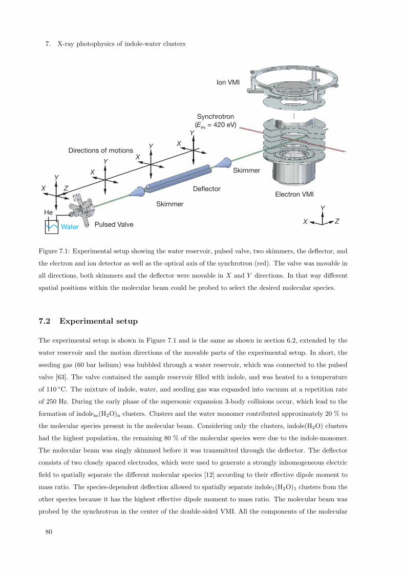
7. X-ray photophysics of indole-water clusters
Pulsed Valve
Skimmer
Skimmer
DeflectorElectron VMI
Ion VMI
...Synchrotron(EPh = 420 eV)
X Z
Y
XY
XY X
Y XY
Z
Directions of motions
He
Water
Figure 7.1: Experimental setup showing the water reservoir, pulsed valve, two skimmers, the deflector, and
the electron and ion detector as well as the optical axis of the synchrotron (red). The valve was movable in
all directions, both skimmers and the deflector were movable in X and Y directions. In that way different
spatial positions within the molecular beam could be probed to select the desired molecular species.
7.2 Experimental setup
The experimental setup is shown in Figure 7.1 and is the same as shown in section 6.2, extended by the
water reservoir and the motion directions of the movable parts of the experimental setup. In short, the
seeding gas (60 bar helium) was bubbled through a water reservoir, which was connected to the pulsed
valve [63]. The valve contained the sample reservoir filled with indole, and was heated to a temperature
of 110 C. The mixture of indole, water, and seeding gas was expanded into vacuum at a repetition rate
of 250 Hz. During the early phase of the supersonic expansion 3-body collisions occur, which lead to the
formation of indolem(H2O)n clusters. Clusters and the water monomer contributed approximately 20 % to
the molecular species present in the molecular beam. Considering only the clusters, indole(H2O) clusters
had the highest population, the remaining 80 % of the molecular species were due to the indole-monomer.
The molecular beam was singly skimmed before it was transmitted through the deflector. The deflector
consists of two closely spaced electrodes, which were used to generate a strongly inhomogeneous electric
field to spatially separate the different molecular species [12] according to their effective dipole moment to
mass ratio. The species-dependent deflection allowed to spatially separate indole1(H2O)1 clusters from the
other species because it has the highest effective dipole moment to mass ratio. The molecular beam was
probed by the synchrotron in the center of the double-sided VMI. All the components of the molecular
80

7.3 Ion coincidence spectra
beam could be moved such that it was possible to probe the different positions within the molecular
beam. The photon energy of the synchrotron was tuned to 420 eV∗, which is 10 eV higher than the
binding energy of the 1s electrons of atomic nitrogen [78]. The electron/ion detection system consisted
of a double-sided VMI to measure electrons and ions in coincidence. Each VMI was equipped with a
MCP and a hexanode/quadanode delay-line detector (DLD, Roentek) for the electron/ion side. Once an
electron was detected, the ions were recorded for a time of 6 µs. The detected electron(s) and ions were
written down in a shot-list and marked as a single event. A more detailed description of the setup is given
in section 6.2, and the calibrations used for the presented data are given in Appendix B.
7.3 Ion coincidence spectra
The photofragmentation of indole-water was investigated via a coincidence measurement between the
detected electrons and ions subsequent to core-shell ionization at the indole-part of the cluster. The
coincidence spectrum of two ions can be plotted in a so-called Photoion-Photoion Coincidence (PIPICO)
map (section B.2). This is shown in Figure 7.2 for the first (m1/q1) and second (m2/q2) detected ion of
all events. The PIPICO map has been corrected for the background by the same method as described
for Figure 6.2. The color scheme is given in coincidences per bin, and the insets show the molecular
structure of indole(H2O) [171, 178, 190], and a deflection profile of the molecular beam. The coincidence
spectrum shows a sum of all recorded coincidence spectra at various spatial positions in the molecular
beam. Highlighted are three areas by the blue square, and the red and green triangle. These are assigned
to fragmentation channels from indole(H2O), indole, and other clusters, respectively. Within the area of
the other clusters the summed mass of m1/q1 and m2/q2 is bigger than 135 u/e, i. e., they are heavier
than the indole(H2O) cluster. Thus they must originate from bigger clusters. The red triangle highlights
the fragmentation signature of indole, which is in detail described in section 6.3.
The blue area is assigned to fragmentation channels from indole(H2O), and is highlighted again in Figure 7.3.
This assignment of the blue are to indole(H2O) was done for the following reasons. At first, the first
detected ion has a mass to charge ratio 18 and 19 u/e, which can be assigned to the fragments H2O+
and H3O+. These channels are absent in the PIPICO of the indole-monomer (section 6.3). Further, the
deflection profile, which is shown in the inset of Figure 7.2, and discussed in the next paragraph, supports
the assignment of the blue are to indole(H2O) since it is much stronger deflected than, for example, the
higher clusters.
The deflection profile was recorded by moving the molecular beam (pulsed valve, skimmers and deflector)
over a distance of 3 mm in the Y -direction, which is equal to a scan of the vertical molecular beam
profile [12]. This has been done for an applied voltage difference of zero and 25 kV at the deflector electrodes.
The undeflected beam profile (0 V) is visible as a black line connecting the individual measurement points
(circles). The deflection profiles (25 kV) for indole, indole-water and higher-order clusters are highlighted
∗Petra III, Variable Polarization Beamline P04 [181], circular polarization (> 98%). At the time of the experiment the
only possible polarization.
81

7. X-ray photophysics of indole-water clusters
20 40 60 80 100 120
m1/q1 (u/e)
20
40
60
80
100
120m
2/q 2
(u/e
)
Indole
Cluster
Indole-H2O
0
4
8
12
16
20
Ion
coin
cide
nces
(coi
ncid
ence
s/bi
n)
−1 0 1 2
Y (mm)
0
1
2
3C
oin.
(arb
.u.)
Figure 7.2: Coincidence spectra between the mass to charge ratio of the first (m1/q1) and second detected
ion (m2/q2)) per event. The insets show the molecular structure of indole-water [171, 178, 190] as well as
the deflection profile extracted from the PIPICO map. The PIPICO map shows a sum of all coincidence
spectra recorded at the different spatial positions of the molecular beam and the color scheme is given in
coincidences per bin.
by their corresponding color scheme. For each species the (background corrected) counts within the
major coincidence islands were integrated. The undeflected beam profile shows a normalized sum of all
integrated coincidence islands (indole, indole(H2O), and cluster) for the case where the deflector was
switched off. The deflection profile for the different species are normalized to their individual undeflected
beam profiles. Additionally, each measurement has been normalized to the integration time to compensate
for the different recording times at each spatial position. It can be seen that indole and indole(H2O) are
stronger deflected than the clusters due to their higher effective dipole moment to mass ratio [12]. Though,
in contrast to [12], indole shows a similar deflection profile to indole(H2O).
The coincidence islands of indole(H2O) are highlighted in Figure 7.3; the color scheme is the same as
in Figure 7.2. The x and y-axes have been reversed such that the first (second) detected ion is now displayed
on the y-axis (x-axis). In all coincidence islands the hydronium fragmentation channel (m1/q1 = 19) is
82

7.3 Ion coincidence spectra
26 27 28
18
19
m1/q 1
(u/e
) a
36 37 38 39
b
50 51
c
57.5 58.0 58.5
d
61 62 63 64
m2/q2 (u/e)
18
19
m1/q 1
(u/e
) e
74 75 76
m2/q2 (u/e)
f
86 87 88 89 90
m2/q2 (u/e)
g
114 115 116 117
m2/q2 (u/e)
h
Figure 7.3: Highlighted coincidence islands of indole-water (blue square in Figure 7.2) for the first and
second ion detected. The color scheme is the same as given in Figure 7.2
dominant compared to the H2O+ (m1/q1 = 18) fragmentation channel. In Figure 7.3 e)-h) a coincidences
between H2O+ and the indole-fragments is not visible. This is only due to the given color scale and the
given binning of the PIPICO map. They are similar to the H3O+ fragmentation channels but simply have a
much lower population. Therefore those channels are not highlighted separately. Most coincidence islands
show an increased detection in the form of lines, which are signatures of an axial recoil of the detected
ionic fragments [186]. The second detected ions in Figure 7.3 a)-c) and e)-g) have all been detected in
the photofragmentation of the indole monomer (section 6.3). This is also clearly visible in Figure 7.2 by
comparing the second detected ion of indole and indole(H2O). Additional channels are given by Figure 7.3
d) and h). The latter one is a coincidence between H3O+ and the (indole-H)+, i. e., the ion of the indole
monomer, which donated a hydrogen/proton to the hydrogen-bonded water. Figure 7.3 d) shows in
principle the same channel, but this time singly charged H3O+ is in coincidence with doubly-charged
(indole-H), given thus in the mass to charge ratio 58 u/e instead of 116 u/e.
A coincidence map between the second and third detected ion is show in Figure 7.4 for which the first
detected ion was selected between 17.5 to 19.5 u/e, i. e., H2O+ and H3O+. Visible is the coincidence
structure of indole and higher clusters, highlighted by the red and green triangles as shown as well
in Figure 7.2. The existence of the indole fragmentation pattern confirms the findings in Figure 7.3 that
H2O+ and H3O+ are always found in coincidence with a fragment of indole. Also, it shows that there is a
probability of triple-ionization of the indole(H2O) cluster, where one charge is found on the hydrogen-
bonded water and two charges are left on the indole. Latter one is leading to a similar fragmentation
process of the indole-part compared to the indole monomer shown in Figure 6.2. The inset is highlighting
the washed out PIPICO island structure. The earlier mentioned diagonal lines within the PIPICO are not
83

7. X-ray photophysics of indole-water clusters
20 40 60 80 100 120
m2/q2 (u/e)
20
40
60
80
100
120
m3/q 3
(u/e
)
1
2
3
47 51 5558
62
66
Figure 7.4: PIPICO spectrum of the second and third detected ion. In order to produce this figure, a
gate was set for the mass to charge ratio of the first ion such that it was between 17.5 and 19.5 u/e, i. e.,
H2O+ and H3O+. The red and green triangles are the same as shown in Figure 7.2 and are corresponding
to the indole and cluster fragmentation patterns. The inset highlights a coincidence island of the indole
part. The labels 1-3 highlight PIPICO islands where m1/q1 +m2/q2 is equal to the mass of the indole
monomer, if proton loss is neglected.
present anymore, which is a common feature of a 3-body break up where all fragments carry significant
momentum. The labels 1-3 highlight PIPICO islands where m1/q1 +m2/q2 is equal to the mass of the
indole monomer if proton loss is neglected. The labeling of these islands is in accordance with the labels
given in chapter 6. In addition to the pure indole coincidences, there are also heavier fragments, which
are in coincidence with H2O+ and H3O+. This shows that the deflection profile shown in Figure 7.2 is
underestimating the deflection in indole(H2O), due to the contributions of these ions to the assigned blue
area.
The visible diagonal lines in Figure 7.3 and the washed-out structure shown in Figure 7.4 seem to be
contradicting results because if all fragments carry significant momentum, all coincidence lines should be
invisible. The contradiction can be explained by the existence of several fragmentation channels. In one
case, the indole monomer is singly ionized and recoils from singly ionized H2O+ and H3O+, which gives
rise to the diagonal lines visible in Figure 7.3. Since only one hole is located at the indole part of the
molecule it will not be shown in a coincidence spectrum between the second and third detected ion. In
the second case, two holes are located on the indole fragment and H2O+ and H3O+ are singly ionized. In
that case, the diagonal lines are washed out for all ions, which expressed itself in Figure 7.3 as an even
distributed background feature. This hypothesis is supported by the VMI images of H2O+ and H3O+
shown in Figure 7.5. The color scheme for the VMI images is the same as shown in Figure 7.2,
84
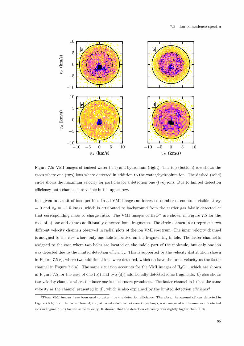
7.3 Ion coincidence spectra
−10
−5
0
5
10
v Z(k
m/s
)
a b
−10 −5 0 5 10
vX (km/s)
−10
−5
0
5
10
v Z(k
m/s
)
c
−10 −5 0 5 10
vX (km/s)
d
Figure 7.5: VMI images of ionized water (left) and hydronium (right). The top (bottom) row shows the
cases where one (two) ions where detected in addition to the water/hydronium ion. The dashed (solid)
circle shows the maximum velocity for particles for a detection one (two) ions. Due to limited detection
efficiency both channels are visible in the upper row.
but given in a unit of ions per bin. In all VMI images an increased number of counts is visible at vX
= 0 and vZ ≈ −1.5 km/s, which is attributed to background from the carrier gas falsely detected at
that corresponding mass to charge ratio. The VMI images of H2O+ are shown in Figure 7.5 for the
case of a) one and c) two additionally detected ionic fragments. The circles shown in a) represent two
different velocity channels observed in radial plots of the ion VMI spectrum. The inner velocity channel
is assigned to the case where only one hole is located on the fragmenting indole. The faster channel is
assigned to the case where two holes are located on the indole part of the molecule, but only one ion
was detected due to the limited detection efficiency. This is supported by the velocity distribution shown
in Figure 7.5 c), where two additional ions were detected, which do have the same velocity as the faster
channel in Figure 7.5 a). The same situation accounts for the VMI images of H3O+, which are shown
in Figure 7.5 for the case of one (b)) and two (d)) additionally detected ionic fragments. b) also shows
two velocity channels where the inner one is much more prominent. The faster channel in b) has the same
velocity as the channel presented in d), which is also explained by the limited detection efficiency†.
†These VMI images have been used to determine the detection efficiency. Therefore, the amount of ions detected in
Figure 7.5 b) from the faster channel, i. e., at radial velocities between ≈ 6-8 km/s, was compared to the number of detected
ions in Figure 7.5 d) for the same velocity. It showed that the detection efficiency was slightly higher than 50 %
85

7. X-ray photophysics of indole-water clusters
7.4 Electrons
Figure 7.6 shows the electron VMI spectrum detected in coincidence with the ionic fragments of indole(H2O).
The electrons were gated such that the highlighted coincidence islands shown in Figure 7.3 were accepted as
events. Further, for the channels where two ionic fragments have been detected in addition to H2O+/H3O+,
only the main coincidence islands within the area of the indole monomer (Figure 7.4) have been accepted.
Figure 7.6 a) and b) show the same electron VMI spectrum in a cartesian (a)) and polar (b)) coordinate
system. The different quadrants in the cartesian VMI spectrum are labeled as Q1-Q4, and are displayed
again in the polar spectrum. The electron VMI spectrum shows four main velocity channels at velocities
of 2.3, 7.1, 9.6, and 11.3·106 m/s, corresponding to electron energies of 14.8, 141.7, 260.7 and 364.9 eV.
These are assigned to the photoelectrons originating from localized ionization at the (atomic) nitrogen
and carbon 1s orbitals, as well as Auger electrons following carbon (CAug) and nitrogen (NAug) ionization
respectively. The radial anisotropy in the photoelectrons, which is best visible for the C(1s) electrons
in Figure 7.6, is due to the ionization from a s-orbital with circular polarized light; the Auger electrons are
isotropically distributed in the laboratory frame. In addition to the four detected photoelectron energies,
slow electrons in the center of the VMI are detected. These are best visible for Figure 7.6 a) and are
assigned to background electrons.
Figure 7.6 c) shows the inverse Abel transformation of the electrons VMI spectrum. The Abel transforma-
tion was performed based on the BASEX algorithm [187]. The black electron energy spectrum shows the
electrons detected in coincidence with indole(H2O), reconstructed from the second and third quadrant
of the electron VMI images. These quadrants were chosen because the electron VMI spectrum in these
quadrants is less distorted than, for instance, in Q1 (Figure 7.6 b)). The energy spectrum is overlaid
by the dashed red line, showing the electron energy spectrum of the indole monomer retrieved from the
same quadrants (Figure 6.7). Both spectra are comparable and show the four measured electron energies.
The electrons detected in coincidence with indole(H2O) show a higher offset value for energies below the
C(1s). This is attributed to a relatively higher background signal due to a lower density in the molecular
beam for indole(H2O) compared to indole. The energies of the peaks have been assigned by Gaussian
fits including an offset value evaluated in the vicinity of the peak. The area of the fits is proportional
to the number of electrons per electron energy. By comparing the photoelectrons and Auger electrons
separately, a contribution of 22.8 % and 16 % was attributed to localized ionization at the nitrogen part
of the molecule. The corresponding β parameters (anisotropy parameters [67]) were determined by the
mean value at the full-width at half maximum (FWHM) of the fitted Gaussian distribution and are
determined to be -0.44(0.08), -0.77(0.01), 0.03 (0.03), and -0.31 (0.02) for the N(1s), C(1s), C-Aug and
N-Aug respectively. The values in the brackets show the standard error of the β parameter.
Figure 7.7 shows a comparison of the photoelectrons in coincidence with one (black) or two holes (red)
detected on the indole-part of the molecule. The spectra are given as a histogram of the electrons radial
velocity vr. The connection lines between the point serve to guide the eye. The ion gating was applied
86

7.4 Electrons
−10 0 10
vX (106 m/s)
−10
0
10
v Y(1
06m
/s)
aQ1Q2
Q3 Q4
0 90 180 270 360
Angle (deg)
0
5
10
v r(1
06m
/s)
Q1 Q2 Q3 Q4
b
N(1s)
C(1s)
C-Aug
N-Aug
100 101 102
Electrons (electrons/bin)
0 100 200 300 400
Energy (eV)
0
3
6
Inte
nsit
y(a
.u.)
N(1s) C(1s)C-Aug
N-Aug
c
Figure 7.6: a) and b) VMI images in a cartesian and polar coordinate system for the electrons detected in
coincidence with the ionic fragments of indole(H2O). Q1-Q4 show the different quadrants of the VMI
image. c) The black curve shows the electron energy spectrum of indole-water calculated by an inverse
Abel transformation based on the BASEX algorithm [187] for the quadrants Q2 and Q3. The red dashed
line shows the energy spectrum obtained from the indole monomer (Figure 6.7) for comparison.
in the same way as for Figure 7.6. Additionally, for the case of two detected ions (H2O+/H3O+ and
one ionic fragment of indole), the coincidences have been gated on the angular relationship between the
ionic fragments (as described in the following) to suppress the influence from the faster three-ion channel
(H2O+/H3O+ and two ionic fragments of indole, Figure 7.5). The VMI images of the ionic fragments
allow one to determine the relative angle between two detected ions. If indole(H2O) fragments into two
ionic species, the ions must be detected on opposite directions in the VMI, i. e., their 3D velocity vectors
and their measured 2D projection must point in opposite directions to fulfill momentum conservation.
If a third fragment is part of the fragmentation process (neutral or ionic), the momentum sum between
all fragments must be zero, which leads to non-axial recoil between the fragments if all ions have some
momenta. For the case of indole (Figure 6.5) it was shown that the velocity vectors for two ions are still
pointing to a high degree in opposite directions if the third fragment is neutral. This is also the case for
indole(H2O). This was utilized to suppress the influence of the three-ion channel, by accepting only ionic
fragments whose velocity vectors were detected between an angle of 170 -190 .
The 2-ion channel shows an increase in detected electrons at radial velocities corresponding to the nitrogen
87

7. X-ray photophysics of indole-water clusters
2.0 4.0 6.0 8.0 10.0 12.0vr (106 m/s)
0
1
2
3
Ele
ctro
ns(1
00el
ectr
ons/
bin) 2 ions
3 ions
N(1s) C(1s) C-Aug N-Aug
Figure 7.7: Comparison of the electrons radial velocity distribution detected in coincidence with two
(H2O+/H3O+ and one ionic fragment of indole) and three (H2O+/H2O+ and two ionic fragments of
indole) ionic fragments of indole(H2O).
photoelectrons and the carbon photoelectrons as well as Auger electrons. The nitrogen Auger electrons are
suppressed, which is attributed to the distortion of the electron VMI which is best visible in Figure 7.6 b).
The 3-ion channel shows the most prominent peak at radial velocities attributed to nitrogen photoelectrons,
and a suppression of photoelectrons from the carbon 1s orbital compared to the 2-ion channel.
7.5 Discussion
The coincidence spectrum presented in Figure 7.3 gives an overview of the fragmentation pattern of indole
(red triangle), indole(H2O) (blue square), and higher clusters (green triangle) for two detected ions. The
higher clusters could be assigned by their mass sum m1/q1 +m2/q2, which is already bigger than the total
mass of indole(H2O). The red triangle is assigned to the fragmentation pattern of indole, as discussed
in chapter 6. Additionally, in Figure 7.4 it was shown that also fragments from indole(H2O) contribute to
this area in the coincidence spectrum. The blue square has been assigned to the fragmentation pattern of
indole(H2O). Also here, it was shown that fragmentations from higher clusters do partly contribute to
that assigned area (Figure 7.4). The deflection profile extracted from the PIPICO spectrum showed that
bigger clusters were less deflected than indole and indole(H2O). Indole(H2O) does not show a stronger
deflection than indole [12]. On the other hand, the deflection profile of indole(H2O) is underestimated
due to the contribution of higher clusters, and the deflection of indole could be overestimated due to
the contribution from indole(H2O). Though, the contribution from higher clusters in the indole area is
unknown.
The fragmentation of indole(H2O) showed a charge and mass transfer to the hydrogen bonded water.
88

7.6 Summary and outlook
The ratio between H2O+ and H3O+ is ≈ 1:2, if the ion detection efficiency is taken into account. The
formation of H2O+ and H3O+ could be triggered by, for instance, relaxation via interatomic coulombic
decay (ICD) [80], electron-transfer mediated decay (ETMD) [82], or proton transfer mediated charge
separation (PTM-CS) [191] of the highly excited indole(H2O) subsequent to core-shell ionization. Also,
secondary ionization of the water by the photoelectron cannot be excluded.
Both fragmentation channels (H2O+ and H3O+) could be separated further by the presence of one or two
holes on the indole-part of the cluster. The H2O+ fragmentation channels were detected in 60 % of the
cases with two ionic fragments of indole, compared to 50 % detection in the case of a H3O+ fragmentation
channel. For the indole monomer, the probability to create three ionic fragments is 13 %, and is thus
much lower than for indole(H2O). If two holes were present on the indole part of the molecule, the
coincidence pattern of the indole was comparable to the indole-monomer, but the branching ratios between
the channels not. In Figure 7.4 the islands 1-3 have branching ratio of 45 %, 27 %, and 28 %, compared
to nearly equal populations for the indole monomer.
VMI images presented in Figure 7.5 showed that the presence of one or two holes on the indole lead to two
different velocity channels for H2O+ and H3O+, which can be explained by a stronger Coulomb repulsion
of the fragmenting particles for the two holes located on indole.
The VMI images of the electrons have been recorded in coincidence with ionic fragments. The electron
energy spectrum for indole(H2O) is comparable to the electron energy spectrum of indole at the given
resolution. Nitrogen photo- and Auger electrons showed a contribution of 22.8 % and 16 % compared to the
ones detected for carbon. Taking the atomic cross section for the given photon energy into account (N =
0.6466 ·10−22m2, C = 0.4327 ·10−22 m2, O = 0.06023 ·10−22m2) [76], and neglecting the contribution from
the proton, the probabilities are 15.5 %, 83 %, and 1.5 % for localized ionization at the nitrogen, carbon
and oxygen, respectively. This discrepancy could be either explained by the non-perfect reconstruction of
the electron energy spectrum, or by alternative fragmentation channels of indole(H2O), which, on the
other hand, have not yet been observed in the data. The photoelectrons from the oxygen 2s orbital would
be expected at a photon energy 378.4 eV (11.5·106 m/s) [78] and are not observed. These electrons are
strongly overlapping with the nitrogen Auger electrons and hence could be hidden in the signal due to
their low contribution to the overall spectrum.
In Figure 7.7 it was shown that two holes on the indole-part of the cluster are primarily populated upon
localized ionization at the nitrogen end of the molecule. This has also been observed for the indole-monomer
in chapter 6, where three ionic fragments were primarily observed upon site-specific ionization at the
nitrogen end of the molecule.
7.6 Summary and outlook
This chapter presented the photophysics of indole(H2O) upon core-shell ionization primarily at the
indole-part of the cluster. VMI spectra of electrons and ions have been recorded in coincidence, and the
fragmentation pattern was displayed in a coincidence map. It was shown that a dominant relaxation
89

7. X-ray photophysics of indole-water clusters
process of indole(H2O) is a charge and mass transfer to the hydrogen-bonded water. The fragmentation
pattern of the indole-part of the molecule was comparable to the fragmentation of the indole-monomer.
Differences were found in the relative population of the fragmentation channels. The VMI images of H2O+
and H3O+ showed two velocity channels, which were assigned to the existence of one or two holes created
on the indole-part of the molecule.
The photoelectron spectrum of indole(H2O) was, at the given quality, comparable to the photoelectron
spectrum of the indole monomer. The photoelectron spectra revealed in both cases, that fragmentation
channels, which resulted in three ionic fragments, were primarily populated upon site-specific ionization.
The disentanglement of the different relaxation mechanisms, which lead to the charge-, and mass transfer
to the hydrogen-bonded water, will be part of future studies. Possible candidates are, e. g., interatomic
coulombic decay (ICD) [80], electron-transfer mediated decay (ETMD) [82], proton transfer mediated
charge separation (PTM-CSs) [191] , or also electron impact ionization of the water molecule by photo- or
Auger electrons emitted from the indole part of the molecule. The distance dependence of these processes
make indole(H2O) a very suitable system to study these processes, because indole(H2O) can be neutrally
dissociated upon absorption of a single UV photon. The VMI spectra of H2O+ and H3O+, and the relative
populations of the different channels, are most likely very sensitive probes dependent on the distance
between indole and water subsequent to UV absorption, as the H2O+ and H3O+ velocity depends on the
Coulomb repulsion between the fragments, and therefore on their distance. Additional information on the
relaxation process could be provided by high-resolution Auger electron spectroscopy.
90

8 Applications of HHG photon sources
The following chapter is separated into two parts. The first part is based on the publication [192] and
shows an experiment, which was utilizing XUV radiation to measure the photophysics of iodomethane
upon localized ionization within the molecule. The XUV radiation was generated by a laboratory based
high-harmonic (HHG) source. The experiment was aiming at the demonstration of a HHG source as
additional photon source along with accelerator based facilities, to measure the photophysics of gas-phase
molecules upon inner-shell ionization. The second part of the chapter is focussing on the conformer
separation of glycine in a cold-molecular beam with the aim to perform an (HHG-based) attosecond pump-
probe experiment with a conformer selected sample to study conformer-dependent charge migration [193].
Simulations are conducted to show how well the different conformers possibly can be separated in an
experiment. Additionally, the generation of a cold molecular beam of glycine is discussed.
8.1 HHG source for coincidence ion imaging of gas-phase molecules∗
Unraveling and controlling chemical dynamics requires techniques to image structural changes of molecules
with femtosecond temporal and picometer spatial resolution. Ultrashort-pulse x-ray free-electron lasers
have significantly advanced the field by enabling advanced pump-probe schemes. There is an increasing
interest in using table-top photon sources enabled by high-harmonic generation of ultrashort-pulse lasers
for such studies. We present a novel high-harmonic source driven by a 100 kHz fiber laser system, which
delivers 1011 photons/s in a single 1.3 eV bandwidth harmonic at 68.6 eV. The combination of record-high
photon flux and high repetition rate paves the way for time-resolved studies of the dissociation dynamics
of inner-shell ionized molecules in a coincidence detection scheme. First coincidence measurements on
CH3I are shown and it is outlined how the anticipated advancement of fiber laser technology and improved
sample delivery will, in the next step, allow pump-probe studies of ultrafast molecular dynamics with
table-top XUV-photon sources. These table-top sources can provide significantly higher repetition rates
than the currently operating free-electron lasers and they offer very high temporal resolution due to the
intrinsically small timing jitter between pump and probe pulses.
∗This chapter is based on the paper High-repetition-rate and high-photon-flux 70 eV high-harmonic source for coincidence
ion imaging of gas-phase molecules J. Rothhardt, S. Hadrich, Y. Shamir, M. Tschnernajew, R. Klas, A. Hoffmann, G.K.
Tadesse, A. Klenke, T. Gottschall, T. Eidam, J. Limpert, A. Tunnermann, R. Boll, C. Bomme, H. Dachraoui, B. Erk, M. Di
Fraia, D. Horke, T. Kierspel, T. Mullins, A. Przystawik, E. Savelyev, J. Wiese, T. Laarmann, J. Kupper, D. Rolles, Optics
Express 24, 16 (2016).
I contributed to the measurements and I was doing the data analysis for the part shown in subsection 8.1.6 and subsection 8.1.7,
which was focussing on the coincidence measurement of iodomethane and the photon flux estimation.
91

8. Applications of HHG photon sources
8.1.1 Introduction
The availability of ultrashort-pulse short-wavelength photon sources is an essential prerequisite to enable
studies of matter on atomic (picometer) length and (femtosecond) timescales. As such, they constitute an
indispensable tool for modern science, which is reflected by the growing number of free-electron lasers
(FELs) that are operating or being constructed at the moment [194–199]. These sources allow to address
many of the fundamental questions in areas as diverse as physics, chemistry, biology, material science and
medicine [200, 201]. Here, we will concentrate on ultrafast molecular dynamics imaging experiments [18,
25, 160] that aim, e.g., at tracing initial charge-transfer processes in space and time [157, 160], which can
be considered as a fundamental process in many photochemical reactions. Understanding these processes
has the potential to control, manipulate, and steer the reaction in a desired channel using ultrafast light. A
particularly powerful method for such studies is the coincident momentum imaging technique [133], which
yields multi-dimensional data sets that can provide kinematically complete, channel-resolved, and highly
differential measurements that contain a wealth of information, and, which allow studies in the molecular
reference frame [160]. However, it imposes the restriction of less than one ionization event per X-ray pulse
in the probed sample, on average, to unambiguously correlate the ionization fragments stemming from the
same molecule. Therefore, the acquisition of sufficient statistics is only feasible with high-repetition-rate
pump-probe sources, ideally with a multi-kHz repetition rate, which is beyond the capabilities of the current
FEL setups. Moreover, the x-ray pulses must be synchronized to optical pump pulses with femtosecond
precision, which is hindered by the long beam paths through the FEL machines and the intrinsic arrival
time jitter [202]. Nevertheless, pump-probe timing jitter at FELs has steadily been improved and sub 10 fs
timing jitter has already been demonstrated by a measure-and-sort method recently [203]. Complementary
table-top sources, realized via HHG of ultrashort-pulse lasers, have attracted significant attention with a
growing user community over the last years, since they are compact and highly accessible. The process
of HHG itself has been known for several decades already, but the repetition rate of the sources has
been mostly limited to the low kHz regime, which is dictated by the employed laser technology [204–208].
However, there is a strong demand for high repetition rate sources not only for coincidence experiments,
but also for many applications, e. g.in surface science [209, 210] or atomic [211] and molecular [212] physics.
The development of new high repetition rate HHG sources has seen rapid progress enabled by recent
advances in high average power femtosecond laser technology [213–219]. In that regard, fiber lasers in
combination with nonlinear compression have played a pivotal role, since these enabled high average power
ultrashort pulse laser sources [220, 221]. Additionally, the investigation of phase-matching aspects during
the frequency up-conversion for such rather low pulse energy lasers has finally led to efficient HHG using
fiber lasers [222, 223]. As a consequence, this approach produced a maximum photon flux of more than
1013 photons/s (100 µW of average power) in the XUV at 600 kHz repetition rate [224], or >109 photons/s
in the soft X-ray region at 100 kHz [225]. The repetition rate of these sources can even be pushed up to
10 MHz, still with 1013 photons/s [226], rendering novel applications in solid state and molecular physics
92

8.1 HHG source for coincidence ion imaging of gas-phase molecules
possible with fiber-laser-based HHG sources.
In this contribution, we present coincidence experiments for iodomethane (CH3I) that were conducted
with 68.6 eV photons from a laser-based 50/100 kHz repetition rate source. The XUV source was enabled
by a state-of-the-art chirped-pulse-amplification fiber-laser system that incorporates coherent combination
of two main amplifier channels to achieve 1 mJ, 300 fs pulses with 50/100 W of average power at a central
wavelength of 1030 nm. Subsequent spectral broadening in an argon-filled hollow-core fiber followed by
temporal compression via chirped mirrors supplied 0.6 mJ pulses with a duration of 35 fs. A part of
this pulse energy (up to 100 µJ) can be used for optical pumping of the molecular sample (CH3I) while
the remainder is used for high-harmonic generation. Particular optimization of the photon flux of the
57th harmonic yielded up to 6.8 · 1010 photons/s at a repetition rate of 50 kHz. This is not only the
highest achieved value in this spectral range, but it also allowed for the first successful demonstration of a
coincidence measurement on inner-shell ionized gas-phase molecules performed with table-top sources.
Previous coincidence experiments with HHG sources have been limited to valence ionization [227–233]
and only a few, non-coincident atomic inner-shell ionization experiments have been performed with HHG
sources to date [234–236]. Important aspects for future pump-probe experiments, such as finding the
temporal overlap between the pump and the probe pulses, increasing the density of the molecular beam,
and advances in laser technology to further increase the photon flux will be discussed, providing evidence
that time-resolved coincidence experiments on inner-shell ionized gas-phase molecules with high-order
harmonic sources are in reach. Since HHG sources can also provide attosecond pulses at high repetition
rates [237], such experiments are expected to access molecular dynamics at shortest timescales in the
future.
8.1.2 High-repetition-rate and high-photon-flux XUV source
The realization of a long-term-stable high-repetition-rate source of high harmonics inherently requires a
suitable high average power laser system. Here, a fiber chirped pulse amplifier was used that was operated
with two coherently combined main amplifier channels and that is described in subsection 8.1.3. The
pulses emerging from this laser were subsequently compressed in time utilizing a gas-filled hollow-core
fiber and chirped mirrors, as outlined in subsection 8.1.4. After the compression step, high harmonics
were generated in an argon gas jet with the generation process being particularly optimized for a photon
energy of 68.6 eV. The experimental characterization of the XUV source and details on selecting the
harmonic and focusing it onto the molecular target are described in subsection 8.1.5.
8.1.3 Coherently combined femtosecond fiber chirped pulse amplifier
The fiber chirped pulse amplification (FCPA) system is sketched in Figure 8.1. Its design is similar to
the laser system reported in [238], but incorporates only two instead of four main amplifier channels.
The frontend is a home-built femtosecond fiber oscillator that operates at 19 MHz repetition rate and
1030 nm central wavelength with a spectral bandwidth of ∼10 nm (FWHM). It is directly spliced to a first
93

8. Applications of HHG photon sources
fiber-integrated pre-amplifier, which increases the average power to 130 mW. Subsequently, the pulses are
stretched to ∼1.5 ns in duration by means of a dielectric grating based stretcher and then sent into a
spatial-light-modulator-based pulse shaper, which is used to compensate the residual linear and nonlinear
spectral phase for almost perfect pulse compression. The signal after this device is coupled to another
cascade of fiber-integrated pre-amplifiers that also include two acousto-optical modulators, which are used
to reduce the repetition rate to 1 MHz and then to the final value of 50 kHz or 100 kHz for the present
experiment; this yields a pulse energy of 0.5 µJ. This amplifier chain is followed by a first large pitch fiber
(LPF) with a mode field diameter of 55 µm, which delivers 20 µJ of pulse energy for seeding of the main
amplifiers. As shown in Figure 8.1 this signal is equally split into two spatial replicas by a polarizing
beam splitter cube and each of the beams is sent to a large pitch fiber amplifier with 80 µm mode-field
diameter. Before entering the main amplifiers, the linearly polarized signals are circularly polarized with a
quarter wave plate (QWP) to reduce the impact of nonlinearity [239]. After amplification and traversing
another QWP each channel delivers 750 µJ pulses with linear polarization, and recombination is done
with a thin film polarizer (TFP). After recombination a small portion of the beam (<1 %) is sent to a
Figure 8.1: Experimental setup of the coherently combined fiber chirped pulse amplification system
(CC-FCPA).
Hansch-Couillaud detector, that analyzes the polarization state of the recombined beam and uses this to
generate an error signal. This is fed-back to a piezo-driven mirror within the pre-amplifier section of the
laser system that adjusts the temporal delay between the two channels [217, 238]. Finally, the beam is
compressed to 300 fs duration in a dielectric grating based compressor. The compressed pulse energy is
1 mJ, corresponding to an average power of 50 W (100 W) at 50 kHz (100 kHz) repetition rate. Due to
the use of fiber amplifiers the spatial beam quality is excellent as verified by M2<1.4 measurements in
previous experiments [240, 241].
8.1.4 Nonlinear compression
As outlined in subsection 8.1.3, the pulses emerging from the coherently combined-fiber chirped-pulse-
amplification system (CC-FCPA) are 300 fs in duration, which is too long for efficient high harmonic
generation [206]. For that reason a nonlinear compression (NC) setup has been implemented that closely
94

8.1 HHG source for coincidence ion imaging of gas-phase molecules
follows the design presented in [221, 224]. A schematic setup of this NC stage together with the pump-
probe splitting is shown in Figure 8.2. The 1 mJ, 300fs pulses are coupled into an argon-filled (∼4.5 bar)
Figure 8.2: Experimental setup of the nonlinear compression stage and the pump and probe generation. As
mentioned in the text p-polarization refers to parallel and s-polarization to perpendicular polarization with
respect to the surface of the optical table. (HWP-half-wave plate, QWP-quarter-wave plate, TFP-thin
film polarizers, per.-periscope)
hollow-core fiber with an inner diameter of 250 µm and a length of 1 m. Propagation in this waveguide
leads to self-phase modulation resulting in spectral broadening. The imposed chirp is removed by a
chirped mirror compressor with a group delay dispersion (GDD) of -2000 fs2 leading to 35 fs pulses. The
pulse energy after the compressor is still as high as 0.6 mJ corresponding to an average power of 30 W
(60 W) at 50 kHz (100 kHz) repetition rate. The polarization used for the NC stage is parallel to the
optical table, which is ensured by a combination of a quarter and half-wave plate located before the
hollow-core fiber. In the following, we will refer to p-polarization (s-polarization) if the polarization is
parallel (perpendicular) to the surface of the optical table. A measurement of the polarization revealed
less than 1% of content in the perpendicular polarization state after the chirped mirror compressor. This
linearly polarized light is sent through another half-wave plate (HWP) and then impinges on a chicane
95

8. Applications of HHG photon sources
of two thin film polarizers (TFP), which are used to split part of the beam by rotating the polarization
with the HWP (Figure 8.2). The transmitted part with an energy of up to 100 µJ, which is p-polarized,
is sent through a delay line and can then be used as a pump pulse, initiating electronic and nuclear
dynamics in small molecular quantum systems. Although in the present experiment no time-dependent
molecular-dynamics were observed, robust methodologies for finding temporal overlap were established as
preparatory work, see supplementary online material for details. The main part of the beam with 0.5 mJ
of pulse energy and s-polarization is reflected off the TFPs, traverses another telescope to enlarge the
spatial beam diameter, is sent up on a periscope rotating back to p-polarization and then enters the high
harmonic generation chamber. The latter will be described in the following subsection 8.1.5 and provides
the XUV-probe beam at 68.6 eV used in present experiments.
8.1.5 High photon flux source at 68.6 eV
Using the 0.5 mJ, 35 fs pulses, which are available after splitting the pump beam (subsection 8.1.4), a high
harmonic source has been realized that is particularly optimized for operation at 68.6 eV. This photon
energy was chosen since it allows photo-ionizing the iodine 4d inner-shell electron in the CH3I molecule.
The experimental setup of the HHG source, including the selection of a single harmonic and the steering
Figure 8.3: Top view on the experimental setup used for high harmonic generation. The inset shows a
more detailed side-view of the separation of the harmonics from the fundamental driving laser, selection
of a single harmonic and focusing of the harmonic into the experiment. (GIP-grazing incidence plates,
M1/2-XUV mirrors at 68.6 eV, TP-turbo pumps, CAMP- CFEL-ASG Multi Purpose end station [180]
96

8.1 HHG source for coincidence ion imaging of gas-phase molecules
to the experimental chamber, is shown in Figure 8.3. The pulses are sent into a vacuum chamber and
are focused into an argon gas jet, which produced from a thin round orifice with 150 µm inner diameter.
Using a f = 300 mm focusing lens leads to a focal spot size (1/e2-intensity) of ∼90 µm and an intensity of
>2 · 1014 W/cm2. The generated high harmonics and the laser co-propagate and impinge on a chicane of
two grazing incidence plates (GIP) [242]. The latter are XUV-grade SiO2 substrates that are anti-reflection
coated for 930-1130 nm (s-polarization) used under 82 angle of incidence. As shown in the detailed
view in Figure 8.3, the two GIPs are used such that the XUV and infrared are s-polarized with respect
to the plane of incidence. Therefore, the XUV beam is changed in height, but maintains p-polarization
with respect to the optical table and the detector normal (see subsection 8.1.6). The reflectance of the
top layer of SiO2 is calculated to be 63 % (40 % after two reflections) of the 68.6 eV photon pulses,
whereas the reflection of the infrared laser is reduced to 10 % by the AR coating. Consequently, the
IR laser is suppressed to 1 % after two reflections, which is important to prevent subsequent aluminum
filters for complete reduction of NIR light from damage. In a first experimental campaign, a thorough
characterization of the high harmonic generation source was performed. For that purpose, the XUV beam
after the second reflection of the GIP was sent through two aluminum filters with a thickness of 200 nm
each, which were used to further suppress the 1030 nm driving laser and to attenuate the XUV in order to
prevent saturation of the following detector. A spatial-spectral analysis of the harmonics was done with a
flat-field grating spectrometer with an attached XUV CCD camera. The experimental conditions, i. e.,
intensity, gas jet position relative to the focus, and the gas pressure were optimized so as to maximize
the signal of H57 at ∼68.6 eV. Figure 8.4(a) shows the spatial-spectral distribution of the harmonic
signal between 55 eV and 75 eV at optimum conditions (7 bar backing pressure). Under these conditions,
spatially well-defined harmonics were generated with nearly Gaussian-like profiles [Figure 8.4(a) right
side]. Integration along the spatial direction yields the harmonic spectrum as shown by the blue curve
in Figure 8.4(b), which can then be used to obtain the number of photons per second by accounting
for the detection efficiency as described in [224]. Furthermore, absorption on the 90 cm beam path to
the detector has been taken into account. The rather high background pressure of 4 · 10−1 mbar in the
chamber results in a transmission of only T = 30 % at 68.6 eV. Note that additional corrections due
to clipping of the XUV beam at the detector, which is obvious in Figure 8.4(a), and at the diffraction
grating are taken into account for estimation of the photon flux. The corrected spectrum is displayed
in Figure 8.4 (b) (red curve). The resulting photon flux for the highest harmonic orders is obtained by
additional spectral integration across each individual harmonic line and summarized in Table 4. It should
be noted that this is a rather conservative analysis and resulting in a minimum value for the achieved
photon flux for the measured harmonics. It yields 6.8 · 1010 photons/s for harmonic 57 at 68.6 eV, which
constitutes at least an order of magnitude higher photon flux than previously reported in this spectral
region [243, 244]. However, the transmission of the Al filters, the diffraction efficiency of the grating
and the detection efficiency of the XUV CCD tend to degrade with time due to surface contamination.
Hence, the real photon flux might have been even higher than estimated above. As described below, an
97
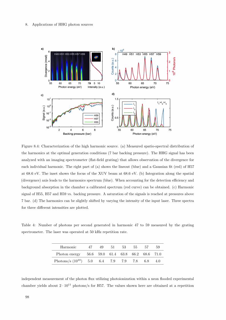
8. Applications of HHG photon sources
Figure 8.4: Characterization of the high harmonic source. (a) Measured spatio-spectral distribution of
the harmonics at the optimal generation conditions (7 bar backing pressure). The HHG signal has been
analyzed with an imaging spectrometer (flat-field grating) that allows observation of the divergence for
each individual harmonic. The right part of (a) shows the lineout (blue) and a Gaussian fit (red) of H57
at 68.6 eV. The inset shows the focus of the XUV beam at 68.6 eV. (b) Integration along the spatial
(divergence) axis leads to the harmonics spectrum (blue). When accounting for the detection efficiency and
background absorption in the chamber a calibrated spectrum (red curve) can be obtained. (c) Harmonic
signal of H55, H57 and H59 vs. backing pressure. A saturation of the signals is reached at pressures above
7 bar. (d) The harmonics can be slightly shifted by varying the intensity of the input laser. Three spectra
for three different intensities are plotted.
Table 4: Number of photons per second generated in harmonic 47 to 59 measured by the grating
spectrometer. The laser was operated at 50 kHz repetition rate.
Harmonic 47 49 51 53 55 57 59
Photon energy 56.6 59.0 61.4 63.8 66.2 68.6 71.0
Photons/s (1010) 5.0 6.4 7.9 7.9 7.8 6.8 4.0
independent measurement of the photon flux utilizing photoionization within a neon flooded experimental
chamber yields about 2 · 1011 photons/s for H57. The values shown here are obtained at a repetition
98

8.1 HHG source for coincidence ion imaging of gas-phase molecules
rate of 50 kHz, while part of the experiments subsection 8.1.6 has also been conducted with a repetition
rate of 100 kHz. Note that all other laser parameters such as pulse energy, pulse duration and focal spot
diameter remain unchanged. Hence, the XUV photon flux is expected to increase linearly with the laser
repetition rate [224] and >1011 photons/s could be generated in a single harmonic at 68.6 eV with the
presented system at 100 kHz.
Due to the use of grazing incidence reflections, the XUV beam still contains a broad spectrum of harmonics
after the GIPs. Selection of a single harmonic (H57) is done by two XUV mirrors that additionally are
used for collimation and re-focusing (Figure 8.3). Both are designed for reflection of 68.6 +/- 0.5 eV (R =
0.5), while the first mirror (f = 300 mm) collimates the XUV beam and the second one (f = 1200 mm)
focuses the XUV pulses onto the molecular beam of CH3I (Figure 8.3). The latter is located in the CAMP
end station. The inset of (Figure 8.4)(a) shows a nice and clean XUV focal spot with a diameter of ∼120
µm (1/e2-intensity). Fine tuning of the photon energy of the harmonic so as to match the mirror reflection
curve was possible by adapting the intensity of the driving laser. Three harmonic spectra for different
driving laser intensities are shown in Figure 8.4(d). The HHG chamber was separated from CAMP via a
differential pumping unit (Figure 8.3) and a sealed aluminum filter with 200 nm thickness that was placed
just in front of the differential pumping unit. This way, the pressure in CAMP stayed below 10−9 mbar,
while the pressure was 4·10−1 mbar in the HHG chamber when the gas jet was operated. As shown in
Figure 8.3, the XUV (probe) beam was focused into CAMP through a holey mirror while the infrared
pump was reflected of the same device with a focusing lens placed outside of the chamber. The temporal
delay was controlled by an additional delay line within the pump arm (see Figure 8.2). Note that the
employed 200 nm thick aluminum filter suppressed the average power of the HHG-driving IR beam to
<0.3 mW for the coincidence experiment.
8.1.6 Coincidence detection of CH3I ionization fragments
The coincidence experiment was performed in the CAMP instrument [180], a mobile multi-purpose
experimental station that was previously used, e. g., for electron and ion imaging experiments at the LCLS
and FLASH free-electron lasers [17, 18, 20, 25, 157, 158] and for electron-ion and ion-ion coincidence
experiments at the PETRA III synchrotron radiation source at DESY [245]. The current setup consists of a
doubly skimmed supersonic molecular beam (nozzle diameter: 30 µm, skimmer diameters: 200 and 400 µm,
distance nozzle to interaction region: roughly 70 cm) and a double-sided velocity map imaging (VMI)
spectrometer equipped with two microchannel plate (MCP) detectors with position-sensitive delay-line
anodes (Roentdek DLD80 for the ions and HEX80 for the electrons), as shown in Figure 8.5. The HHG
and/or NIR beams intersected with the molecular beam inside the VMI spectrometer, where a constant,
inhomogeneous electric field guided the electrons and ions created by the interaction of the photons with
the target molecules onto the position-sensitive detectors. Typical flight times of the ionic fragments were
on the order of 0.5 to 7 µs, while the electron time of flight was on the order of a few ns. The MCP
and position signals were recorded with a multi-hit time-to-digital converter (TDC) that was triggered
99

8. Applications of HHG photon sources
by the detection of an electron, and the data was stored event by event in a list-mode format that
allowed retrieving coincidences between the detected particles. With this detection scheme, it is possible
to record electron-ion coincidence data with up to MHz-repetition sources as long as the average time
between ionization events is considerably larger than the TDC acquisition window (for a 10 µs window,
this corresponds to an ionization rate of 100 kHz). Here, we only recorded events where at least one
electron and one ion was detected, which resulted in a typical event rate of about 900 Hz. For the data in
Figure 8.6(b), only those events were considered where two ionic fragments were detected in coincidence
with a photo- or Auger electron. This represents the most stringent coincident requirement one would
typically impose in such coincidence experiments and further reduced the count rate by more than a factor
of two. From the time of flight and the hit positions of the ions, the three-dimensional ion momenta
can be calculated, while the time of flight of the electrons is too short for a meaningful 3-D momentum
reconstruction such that only 2-D projections of the electron momentum distributions were measured.
For cylindrically symmetric electron distributions it is possible to retrieve the 3-D distributions through
inversion algorithms [246, 247].
Figure 8.5: Schematics of the coincidence apparatus with a supersonic molecular beam and a double-sided
velocity map imaging (VMI) spectrometer with MCP delay-line detectors for time- and position resolved
coincident electron and ion detection.
In the experiment described here, we recorded electron-ion-ion coincidence data for the photoionization of
CH3I molecules by photons from the HHG pulses. We chose CH3I as a target for this proof-of-principle
100

8.1 HHG source for coincidence ion imaging of gas-phase molecules
experiment since it is a prototypical polyatomic molecule whose UV- and NIR-induced dissociation and
ionization as well as XUV-induced inner-shell ionization are well-studied [157, 158, 248]. In particular, we
have recently investigated charge transfer dynamics in CH3I after inner-shell ionization in pump-probe
experiments at the LCLS and FLASH free-electron lasers [157, 158] and it is of enormous interest to
perform similar experiments with a significantly improved temporal resolution, e.g., on the order of some
10 fs.
At a photon energy of 68.6 eV, as chosen in the present experiment, the cross sections for both, valence
and inner-shell ionization, are roughly equal [248]. Thus, the CH3I molecules can either be valence ionized,
resulting predominantly in singly charged CH3I+ ions, or a I(4d) inner-shell electron can be removed,
which leads to a doubly or triply charged final state after the inner-shell vacancy relaxes via Auger decay.
The majority of these doubly or triply charged cations then break up into charged fragments as seen in the
ion time-of-flight mass spectrum shown in Figure 8.6(a). A plot of the ion-ion coincidences between CH+x
(x = 0, 1, 2, 3) fragments and I+ fragments is shown in Figure 8.6(b). Due to momentum conservation,
these coincidence events, which resulted from a (quasi-) two-body fragmentation–the neutral or charged
H+ fragments that may also be emitted carry very little momentum due to their light mass–can be clearly
identified by diagonal lines in the photoion-photoion coincidence (PIPICO) spectrum. The corresponding
detector images for I+, CH+x , and CH3I+ are shown in Figure 8.7. Combining the time-of-flight information
with the ion hit positions, the three-dimensional momentum of each fragment can be calculated and one
can determine the total kinetic energy release and three-dimensional angular distributions as well as
angular correlations between fragments, which, for the present data, agree with our previous measurements
on CH3I using synchrotron radiation [245]. Note that the results shown here were obtained from a single,
continuous, 20-hour long measurement during, which the laser system, the high harmonic generation,
and the coincidence apparatus were operated constantly and without interruption. This reliability and
long-term stability is an important prerequisite for coincidence measurements such as the one presented
here and, in particular, also for for future time-resolved experiments.
In order to demonstrate spatial and temporal overlap between the NIR-pump pulses and the XUV-probe
pulses, we removed the Al filter in front of the differential pumping section such as the NIR drive-laser
beam from the HHG chamber, which traveled collinear with the XUV pulses, could reach the interaction
region inside the CAMP chamber. Using a small Ce-doped YAG crystal that could be driven into the
interaction region on an xyz-manipulator and that could be viewed on a CCD camera through a long-
distance microscope, we first spatially overlapped the two NIR beams. Then we used a fast photodiode
that was also mounted on the xyz-manipulator to overlap the two laser pulses to within a few tens of
picoseconds. Finally, we scanned the delay stage in the pump arm until we observed interference fringes
on the Ce:YAG screen due to interferometric autocorrelation between the two NIR pulses, as shown by the
short movie that we recorded with the pnCCD camera attached to the microscope (see Visualization 1).
Thus, technically pump-probe experiments on femtosecond timescales would be feasible with the presented
setup.
101

8. Applications of HHG photon sources
Figure 8.6: (a) Ion time-of-flight mass spectrum of CH3I recorded at 68.6 eV photon energy. The CH3I+
parent ion as well as several ionic fragments can be seen along with several ions resulting from the
ionization of the residual background gas in the chamber. (b) Ion-ion coincidence spectrum of CH3I
zoomed in on the region containing the coincidences between CH+x (x = 0, 1, 2, 3) and I+ fragments. For
the data shown in panel (b), only those events were considered where two ionic fragments were detected
in coincidence with a photo- or Auger electron, which results in a quite low coincidence count rate of less
than one coincidence even per second in the selected coincidence channel; see text for details.
Figure 8.7: Two-dimensional ion momentum distributions (ion detector images) for three distinct ionic
fragments of CH3I: (a) I+, (b) CH+x , and (c) CH3I+.
8.1.7 Photon flux estimate
In order to obtain an experimental estimate of the actual XUV photon flux in the CAMP chamber,
we leaked 5.4 · 10−6 mbar of neon (as measured by a hot cathode ion gauge, taking into account the
appropriate correction factor) into the vacuum chamber through a needle valve and measured the count
102

8.1 HHG source for coincidence ion imaging of gas-phase molecules
rate of Ne+ ions with our VMI spectrometer described above. Using the formula
I = φσDδL (17)
where I = 2500 Hz is the Ne+ ion count rate, φ is the photon flux, σ = 6.1 Mbarn is the Ne photoionization
cross section at 69 eV [249] (which we consider to be constant over the bandwidth of the XUV pulses), D
= 0.5 is the detector efficiency, δ = 1.3 · 1011 cm−3 is the target density, and L = 2.0 cm the interaction
length inside the spectrometer, we can calculated the photon flux to be φ = 3.2 · 109 photons/s. Note
that the uncertainties connected to the ion gauge reading, the exact detector efficiency, and the effective
interaction length that is imaged by the spectrometer, result in an uncertainty of about a factor of two
for the absolute photon flux. When taking into account the estimated losses that occur on the path into
the CAMP chamber (EUV mirror reflectivity (R = 0.5)2 = 0.25; transmission of the aluminum filter of
0.5 and of the grazing incidence plates of 0.4; transmission through the HHG chamber due to absorption
because of the high background pressure of 0.3), we estimate a photon flux of about 2 · 1011 photons/s
that was generated by the HHG source. This even exceeds the photon flux measured with a grating
spectrometer as described in subsection 8.1.5.
8.1.8 Conclusion and outlook
In conclusion, we demonstrated coincidence experiments on gas phase-molecules after inner-shell ionization
with a table-top high harmonic source. This XUV source, based on a femtosecond fiber laser system,
provides a record high photon flux (> 4 · 1010 photons/s per harmonic) up to 71 eV at up to 100 kHz
repetition rate. The unprecedented combination of high photon flux, high repetition rate, and long
term stability enables photon-hungry experiments such as photoionization of gas-phase molecules with
coincidence detection of the fragments. We have performed molecular physics experiments with continuous
experimental runs up to 20 hours. Electron-ion-ion coincidence data were recorded for the photoionization
of CH3I molecules excited by HHG pulses at a photon energy of 68.6 eV. This first data is promising and
indicates that pump-probe experiments with such table-top sources are in reach. Since the pump pulse and
the XUV pulse are generated by the same laser and are, thus, inherently synchronized, it is technologically
possible to control their relative timing with sub-fs precision as demonstrated by attoseocond pump-probe
beamlines in many laboratories worldwide [250]. Note that a 600 kHz repetition rate attosecond source
has already been demonstrated [237], and laser technology is currently progressing towards much higher
average power for few-cycle driving lasers [225, 251].
However, for real pump-probe experiments, the count rate of the presented experiment has to be increased
by about two orders of magnitude. We expect to obtain at least an order of magnitude higher sample
density with a more compact molecular beam design that greatly reduces the distance between nozzle and
interaction region. The anticipated reduction in electron energy resolution due to space charge effects is
far less critical compared to the significant improvement in count rate, which would allow for pump-probe
scans with reasonable measurement times (few-hours). Furthermore, the experiments presented in this
103

8. Applications of HHG photon sources
manuscript have been performed with 25 W (50 W) of average power. Since more than 500 W of average
power have been demonstrated from a femtosecond fiber laser already [217] an order of magnitude higher
photon flux is expected to be available soon.
Finally, the combination of both improvements will enable ultrafast time-resolved imaging of charge
transfer processes with unprecedented time resolution on timescales, which are hard to be accessed by
todays FEL facilities.
8.2 Toward charge migration in conformer-selected molecular samples
Within the last decade the development of ultrashort laser pulses, and the growing interest in theoretical
physics to model electronic states of molecules and their correlation, opened the field of so-called attosecond
physics, with the idea of driving that field toward attosecond chemistry. The following, very basic
introduction into this field of science, is based on the review article [252] and references therein.
An attosecond is 10−18 s and is generally considered as the timescale in which it is possible to observe fast
electron dynamics. The first experiment, which was exploring ultrafast charge migration, was [253] where
neutral peptides of neutral amino acids where locally ionized on the C-terminal end, and the ion yield
related to the N-terminal end of the molecule was probed. The results were interpreted as charge migration
in ions. The term charge migration is used to describe purely electron correlated driven electronic motions,
fully decoupled and independent on the nuclear degrees of freedom. Contrary, and often mixed, is the
term charge transfer where the charge dynamics does depend on the nuclear coordinates and involves
dissipation of the electronic energy.
Charge migration can be triggered by coupling of electronic states within a molecule. This can be achieved
by ionization from delocalized orbitals of the molecule if the energy spacing between two electronic states
is smaller than the band-width of the laser. If the ionization process is additionally fast enough such that
rearrangement of the electronic structure during the course of ionization is negligible (prompt ionization),
these electronic states can be coherently coupled. The observation and understanding of the evolution of
this coherently coupled hole states, with also a possible aim of steering chemical reactions, is one principle
goal attosecond chemistry.
Experimentally, the observation of charge migration in a pump-probe experimental scheme is challenging.
To observe fast motion the laser pulses have to be sufficiently short, which results in a broad spectrum of
the laser pulse [254]. This spectral broadening leads to a higher probability of ionizing from more than
only the desired states to couple. Additionally, if the desired initially populated states are not the highest
occupied molecular orbitals (HOMO), but orbitals lower in energy, the laser pulses have always sufficient
energy to ionize higher lying orbitals. Thus, the molecular sample should have only few homo orbitals
in energy close by, with a big energy gap to the lower lying ones. Such conditions are also found in the
indole molecule [255].
Electron dynamics on ultrafast timescales have already been observed in the amino acid phenylalanine [256–
258]. In [257] phenylalanine was evaporated ”from a thin metallic foil heated by a continuous wave (CW)
104

8.2 Toward charge migration in conformer-selected molecular samples
laser” before the dynamics were pumped by an XUV pulse (pulse duration sub-300 as) and probed by an
IR laser pulse with a pulse duration of 4 fs. Due to the simple evaporation method, the retrieved signal
was averaged over the different conformers–in total 6 with relevant population under the experimental
conditions–though theoretical predictions show conformer-dependent electron dynamics.
We propose an experiment to probe charge migration in a conformer-selected, cold molecular sample
of glycine (C2H5NO2). Glycine is of particular interest because it is the smallest amino acid and a
building block of almost all proteins. It is thus of considerably importance for biology and chemistry. Its
observation in interstellar clouds [259], as well as its recent detection in the coma of a comet [260], has
had, and will have, profound impact onto the new field of astrobiology and -biochemistry. Furthermore,
glycine is a particularly good candidate to study charge migration since theoretical predictions of the most
abundant conformers suggest strong conformer-dependent charge migration with timescales of the hole
motion, which also vary strongly as a function of the prepared state of the pump pulse [193].
Further, the deflection profile of glycine can be used to address the question whether or not there exists
the IV conformer of glycine (conformer notation according to [261]), which has so far been predicted by
theory [261, 262] but could not yet been conclusively detected in experiments. This lack of detection could
be explained by an interconversion (IC) of this conformer into the first conformer during the course of the
free jet expansion [263], leading to a shift of the overall population.
8.2.1 Simulations: Stark curves and deflection profile
Table 5 shows the rotational constants and dipole moments for the first four conformers of glycine, which
are required to calculate the energies and Stark shifts of the rovibronic molecular states (section 2.2). The
corresponding Stark curves were calculated [70] up to a rotational state of J = 40, with an electric field
strength resolution of 1 kV/cm, and are shown in Figure 8.8 for the lowest rovibronic quantum states.
The Stark curves for conformer I and II/III and IV are shown in the left and right graph respectively.
The Stark energies are given in cm−1 in dependence of the electric field strength ε. Standing out here is
conformer II (black), which shows the most prominent Stark shift followed by conformer IV, III and I,
which do have a comparable shift in energy. The simulations of the deflection profiles–shown in Figure 8.9
and discussed in the corresponding paragraph–were done with an in-house developed particle tracing
software, which has already been used to simulate the deflection profiles in [11, 12]. The experimental
setup, i. e., the dimensions of the setup, skimmer sizes and deflector type, were taken from [12]. For the
simulated deflection profiles a molecular beam velocity of 1800 m/s and a molecular beam temperature of
1 K was assumed. Both are typically achieved under experimental conditions when the molecules are
seeded in helium. At this temperature, quantum states up to J = 6 are populated, where ”populated”
means that they contribute to more than 1 h to the overall population. The populations of the different
conformers in the molecular beam were taken from [262] and are shown in Table 6 in the left and middle
column for ’no IC’ and ’IC’ of the fourth conformer (vide supra). These populations are derived from the
105

8. Applications of HHG photon sources
Table 5: Rotational constants and dipole moments for the first four conformers of glycine (I and II [264],
III and IV [262, 265])
Conf. A (MHz) B (MHz) C (MHz) µA (D) µB (D) µC (D)
I 10.34 3.876 2.912 0.911 0.697 0.00
II 10.13 4.072 3.007 5.372 0.93 0.00
III 9.72 3.979 2.987 -0.156 1.691 -0.077
IV 10.26 3.971 2.962 -0.006 -1.552 1.436
0 20 40 60 80 100 120 140
ε (kV/cm)
−12
−10
−8
−6
−4
−2
0
2
W(c
m−
1)
J = 0J = 1J = 2
Conf. IConf. II
0 20 40 60 80 100 120 140
ε (kV/cm)
−12
−10
−8
−6
−4
−2
0
2
W(c
m−
1)
J = 0J = 1J = 2
Conf. IIIConf. IV
Figure 8.8: Left (right): Stark-energies for the lowest rovibronic quantum states of the first and second
(third and fourth) conformer of glycine as a function of the electric field strength.
simulations for a temperature of 385 K. Experimental determined populations [266] at this temperature
are shown in the right column of Table 6 simply for completeness.
Figure 8.9 shows smoothed simulated deflection profiles for a voltage of +/- 4 kV (top) and +/- 14 kV
(bottom) applied at the deflector electrodes. The different populations of the conformers for IC and no IC
of the fourth conformer are shown in the left and right graph respectively. The individual deflection profiles
of the different conformers are highlighted by their corresponding color visible in the legend in the upper
right graph. For comparison, an undeflected deflection profile is shown by the dashed black line. At an
applied voltage of +/- 4 kV, conformer II is already strongly deflected and fully separated from the other
conformers at a position of Y > 1.5 mm. All other conformers experience a much weaker deflection. At
an applied voltage of +/- 14 kV, the second conformer experience such a strong deflection that it collides
with the deflector rod and thus, on the scale of these simulations, is fully discriminated. Conformer IV
experiences the second strongest deflection, followed by conformer III and I. At Y > 2.5 conformer III
106
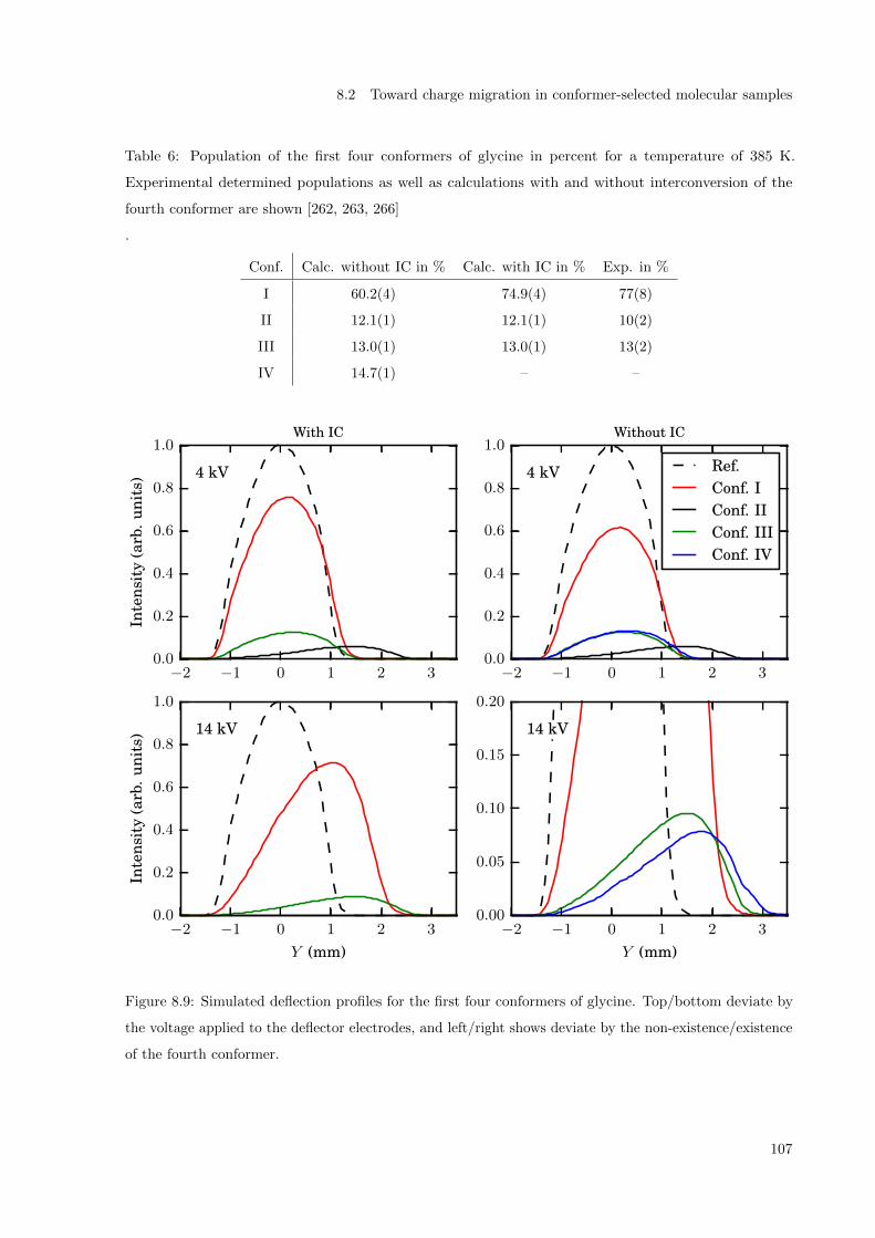
8.2 Toward charge migration in conformer-selected molecular samples
Table 6: Population of the first four conformers of glycine in percent for a temperature of 385 K.
Experimental determined populations as well as calculations with and without interconversion of the
fourth conformer are shown [262, 263, 266]
.
Conf. Calc. without IC in % Calc. with IC in % Exp. in %
I 60.2(4) 74.9(4) 77(8)
II 12.1(1) 12.1(1) 10(2)
III 13.0(1) 13.0(1) 13(2)
IV 14.7(1) – –
−2 −1 0 1 2 30.0
0.2
0.4
0.6
0.8
1.0
Inte
nsit
y(a
rb.u
nits
) 4 kV
With IC
−2 −1 0 1 2 30.0
0.2
0.4
0.6
0.8
1.0
4 kV
Without IC
Ref.Conf. IConf. IIConf. IIIConf. IV
−2 −1 0 1 2 3
Y (mm)
0.0
0.2
0.4
0.6
0.8
1.0
Inte
nsit
y(a
rb.u
nits
) 14 kV
−2 −1 0 1 2 3
Y (mm)
0.00
0.05
0.10
0.15
0.20
14 kV
Figure 8.9: Simulated deflection profiles for the first four conformers of glycine. Top/bottom deviate by
the voltage applied to the deflector electrodes, and left/right shows deviate by the non-existence/existence
of the fourth conformer.
107

8. Applications of HHG photon sources
and IV are separated from conformer I. Though the separation is not very strong, experimentally it would
be possible to probe at this position both conformers, and reduce thus strongly the influence of the first
conformer. Depending on the IC-factor, conformer I can be purified to >90 % (with IC) or > 82 %
(without IC) at a position between -1 < Y < 1.
8.2.2 Experiment
The experimental section can be separated into two parts, i. e., in the evaporation of glycine within a pulsed
valve [63] and two alternative evaporation techniques, namely laser desorption (LD) and laser-induced
acoustic desorption (LIAD) source. For the first part, the experimental setup was similar to section 6.2,
deviating only by the detection scheme, which was replaced by a time-of-flight mass spectrometer similar
to the one described in section 3.2. The molecules were seeded in 50-80 bar helium and the temperature of
the pulsed valve was varied between 110 and 170 C. Additional care was taken to the thermal insulation
of the pulsed valve such that the temperature gradient between the tip and the back of the valve (where
the sample reservoir was located) was not bigger than 20 C. The molecular beam was probed by a fs-laser
pulse at pulse energies varying from 50-250 µJ. The pulse duration was < 40 fs (FWHM for an Gaussian
temporal profile), and the laser pulse was focused with a 50 cm focussing lens. The recorded ion-mass
17 31 44 59 73
Mass (u/e)
−1
0
1
2
3
4
5
Am
plit
ude
(mV
)
x 0.1
Figure 8.10: Mass spectrum of glycine by thermal evaporation within a pulsed valve [63]. The spectrum
below a mass of 19 u has been scaled by 0.1.
108

8.2 Toward charge migration in conformer-selected molecular samples
spectra for the different experimental conditions looked similar. Exemplarily, a single mass spectrum is
shown in Figure 8.10. The spectrum has been recorded at a valve temperature of 155 C, with a backing
pressure of 50 bar helium, and a laser pulse energy of 150 µJ. The amplitude in left part of the spectrum
(< 19 u) was divided by a factor of 10. The spectrum is dominated by a peak at a mass of 17 u, e. g. OH+,
followed by singly ionized water at mass of 18 u. Smaller ion signals can be seen at masses of, for example,
59, 31 and 44 u. A very small signal is visible at a mass of 73 u, which is close to the parent ion of glycine
(75 u). The lack of parent ion and the very low count rate for ions above a mass of 19 u rose the question
whether or not intact glycine molecules do reach the interaction zone, and whether they are destroyed in the
former case by the fs-laser probe. Within the CMI-group (https://www.controlled-molecule-imaging.org)
alternative approaches to promote labile molecules into the gas-phase are currently under development by
graduate students. Nicole Teschmit is developing a LD supersonic-expansion source similar to [64], and a
LIAD source is being developed by Zhipeng Huang, which is similar to [65, 267]. Both experimental setups
were used to measure TOF-mass spectra of glycine. In the former case, the molecules were desorbed
in front of a pulsed valve, which used argon as carrier gas to transport the desorbed molecules into the
spectrometer. In the latter case, the molecules were placed on a modified repeller electrode of the TOF
spectrometer. The molecules have been probed by a fs-laser (vide supra) at a pulse energy of 170 µJ
0 10 20 30 40 50 60 70 80
Mass (u/e)
−0.2
0.0
0.2
0.4
0.6
0.8
1.0
Nor
mal
ized
ampl
itud
e
Gly+
CH4N+
Ar+
H2O+
LD
0 10 20 30 40 50 60 70 80
Mass (u/e)
−0.2
0.0
0.2
0.4
0.6
0.8
1.0
Gly+
CH4N+
H2O+
CO2H+
LIADEI
Figure 8.11: TOF mass spectra of glycine. Left (right): Glycine has been evaporated using a LD supersonic-
expansion source (LIAD). The spectra have been normalized and a spectrum of glycine recorded via
electron impact (EI) ionization is shown for comparison [268].
and their (normalized) recorded mass-spectra are shown in the left and right graph of Figure 8.11. Both
spectra show a similar structure with a dominant peak at 30 u, corresponding to a fragmentation of glycine
into an ionic CH4N fragment and a neutral carboxyl group. The emission of hydrogens from that ionic
109

8. Applications of HHG photon sources
fragment can lead to the small peaks visible at 27-29 u. The parent ion of glycine as well as ionic water
is visible in all cases. For comparison, a mass spectrum of glycine obtained from [268] and recorded via
electron impact (EI) ionization is shown in the right graph. Its amplitude is reversed has been normalized
-1. This spectrum looks comparable to the one acquired by LD and LIAD beside more prominent peak at
45 u, which is assigned to an ionic carboxyl group. †
8.2.3 Conclusion and outlook
The simulated deflection profiles in Figure 8.9 show that a conformer separation in glycine is possible.
Specifically, the second conformer of glycine is much stronger deflected than the other conformers and
should thus be ‘easily’ separated from the other conformers, even under non-perfect experimental conditions.
Conformer I, III and IV do have similar deflection profiles and, therefore, it will be challenging to get
a full separation of the latter ones under these experimental conditions. Though, deflection profiles at
different applied voltages, and possible conformer-dependent fragments in the TOF spectrum, could help
to disentangle the contribution of the individual conformers in the deflection profile, which could allow to
make statements about the existence/non-existence of the fourth conformer. Conformer I has the highest
population and can be purified to a high degree.
In the experimental section mass spectra for different evaporation methods have been compared. It can
be concluded that an evaporation within the pulsed valve leads to a fragmentation of the molecules. LD
and LIAD are promising approaches to evaporate glycine. The LD-approach additionally showed that a
subsequent cooling of the molecules with a seeding gas does not harm the molecules. Both approached are
designed such that they can be combined with the deflector, providing thus the potential to measure a
deflection profile of glycine, i. e., providing a conformer separated molecular beam.
†Mass-spectra recorded from glycine via XUV photon ionization do show a similar mass-spectrum [269]
110

9 Summary
The presented experiments covered the control of cold gas-phase molecules, x-ray diffractive imaging of
such controlled gas-phase molecules, and the x-ray photophysics and charge-rearrangement processes
of gas-phase molecules and molecular clusters. All experiments were designed such that they provided,
next to their results, a foundation for future experiments to study ultrafast structural changes or charge-
rearrangement processes by making use of x-ray free-electron lasers.
9.1 Sample preparation
The control of cold gas-phase molecules was covering the spatial separation of different species, such as
isomers or molecular clusters, to provide a strongly purified molecular sample as a starting point for
an experiment. In chapter 3 the spatial separation of the trans and cis conformer of 3-fluorophenol
was demonstrated. 3-fluorophenol is a prototypical large molecule, where the conformers differ by the
orientation of their OH functional group. The conformers have a relative abundance of 2:1 (trans:cis) in the
molecular beam, and the trans conformer has the higher permanent dipole moment. It was demonstrated
that both conformers could be purified to more than 90 %, and providing thus a strongly purified molecular
sample to study isomerization dynamics. 3-fluorophenol was chosen such that isomerization dynamics can
be studied by molecular-frame photo angular distribution (MFPAD) measurements of aligned gas-phase
molecules at a free electron lasers (FELs).
Simulations of the spatial separation of four different conformers of the smallest amino acid glycine were
presented in section 8.2. It was shown that the second conformer of glycine could be fully separated from
the other conformers. Additionally, it was shown that the first conformer can be purified to more than
90 %. The conformer separation of glycine is here in particular aiming at the study of conformer-dependent
charge migration, triggered by the creation of coherently coupled hole-states in the molecular sample.
The spatial separation of the indole(H2O) clusters from the indole monomer and other species present in
the molecular beam [12] was utilized in chapter 7. The experiment was aiming at the study of the x-ray
photophysics of the micro-solvated indole(H2O), where the spatial separation was an important factor for
the right interpretation of the data.
In addition to the separation of different conformers in the gas-phase, control of the molecules was
achieved by laser-alignment to gain control about the orientation of the molecules in space. Alignment
is necessary, or can be highly advantageous, for experiments aiming at the study of molecular frame
dependent properties such as MFPAD measurements, or x-ray diffraction experiments, which aim at the
structure determination small molecular samples in the gas-phase. In chapter 4 a general approach is
presented to strongly align gas-phase molecules at the full FEL repetition rate by utilizing an in-house
Ti:Sapphire laser system. Therefore, the compressor of the Ti:Sapphire laser system was bypassed, and the
111

9. Summary
direct output of the regenerative amplifier was used to strongly 3D align 2,5-diiodothiophene molecules. It
was shown that the achieved alignment of⟨cos2θ2D
⟩= 0.85 was limited by the warm molecular beam
rather than by the alignment laser pulse. Further, it was explained that the same laser system could
be used as a pump or probe laser in an ultrafast pump-probe experiment, and providing thus direct an
intrinsic synchronization between the alignment and the pump or probe laser.
9.2 X-ray diffractive imaging
Strongly aligned 2,5-diiodothiophene molecules were probed by hard x-ray photons to measure their
structure via x-ray diffraction (chapter 5). X-ray diffraction is a highly promising approach to image the
intrinsic structural changes of gas-phase molecules on ultrafast timescales. The alignment of the molecular
sample does have the advantage that, providing the molecules are perfectly aligned (or more generally
oriented), the diffraction pattern is equal to the diffraction pattern of the single molecule, which allows for
the reconstruction of bond-length and bond-angles of the molecule. The simulations showed the feasibility
to record 1D as well as 2D diffraction patterns of controlled gas-phase molecules within 6 hours at the
free-electron laser LCLS, if the molecules are probed at the full FEL repetition rate, and if the background
signal from the beamline is negligible. In the experimental section evidence for a 1D diffraction pattern
was presented, which, on the other hand, could not be confirmed by the 2D diffraction pattern. Also, it
was shown that the background signal from the beamline as well fluorescence background signal induced
by the FEL at an aperture, could be partially suppressed by making use of the ADU signature in the
x-ray camera. The experiment also showed that the upcoming high-repetition rate FELs like XFEL or
LCLS 2 are highly promising photon sources to image structural changes in controlled gas-phase molecules
via x-ray diffraction.
9.3 X-ray photophysics and coincident measurements
The x-ray photophysics of indole and indole water have been presented in chapter 6 and chapter 7.
In both cases, the indole molecule was core-shell ionized at the carbons as well as site-specific ionized
at its nitrogen atom by soft x-ray radiation. Electrons and ions have been recorded in coincidence.
The photofragmentation of indole showed that the indole monomer is primarily fragmenting into three
fragments, with two of them being ionic, and one being neutral. The recorded electron spectra showed
that some of the detected fragmentation channels were primarily populated upon site-specific ionization
at the nitrogen atom. The photofragmentation of indole(H2O) showed two main dissociation channels in
which charge and mass transfer to the hydrogen-bonded water was observed. It was shown that both
channels were accompanied by one or two holes located on the indole-site of the molecular cluster. In
both cases, the indole part of the molecule showed a similar fragmentation pattern compared to the indole
monomer. The indole(H2O) cluster is a highly promising sample to learn about the photofragmentation
and ultrafast relaxation processes like intermolecular Coulombic decay (ICD) or electron-transfer mediated
112

9.3 X-ray photophysics and coincident measurements
decay (ETMD) in hydrogen-bonded systems. FELs provide the required time resolution and, if a neutral
dissociation is triggered in the indole(H2O) system via a fs-UV laser pulse, these processes can be studied
with fs time resolution.
In addition to the photophysics studied at accelerator based facility, a laboratory based high harmonic
generation (HHG) source was used to study the photophysics of iodomethane upon site-specific ionization.
The HHG source was operating at a repetition rate up to 100 kHz, thereby generating more than 1010
photons/s per harmonic at a photon energy of up to 71 eV. It was possible to demonstrate that even
photon-hungry experiments such as photoionization of gas-phase molecules with coincidence detection of
the fragments could be performed with an HHG source. This experiment was conducted to demonstrate
the potential use of a laboratory based photon source as an alternative to accelerator based facilities.
113

10 Conclusion and outlook
Complementary experiments for imaging structure and molecular dynamics of controlled gas-phase
molecules have been presented. It was argued and demonstrated, that the control of gas-phase molecules
is often highly advantageous or simply necessary for various kinds of experiments.
Control was gained by laser alignment of an isotropically oriented ensemble of cold gas-phase molecules,
or by spatial separation of different species, e. g., conformers or molecular cluster, present in the molecular
beam. A high degree of alignment of a molecular ensemble is crucial for x-ray diffraction experiments,
because it increases locally the signal to noise ratio on the detector, and it allows to reconstruct the
structure of a single molecules, including bond-angles and atomic distances. The deflection profile of indole
and indole(H2O) was crucial for the disentanglement the photofragmentation pattern of both species,
and its separation from bigger clusters. Further, the spatial separation of the cis and trans conformer of
3-fluorophenol was demonstrated, providing an ideal sample for the study of isomerization dynamics.
Different imaging techniques such as diffractive imaging or velocity map imaging were used for structure
determination, or the study of the photofragmentation of isolated gas-phase molecules and cluster. The
structure of strongly-aligned molecules was measured via hard x-ray diffractive imaging. Evidence for
a 1D diffraction image has been presented, which could not be confirmed by the 2D diffraction image.
Background photons could be partially suppressed by making use of the ADU signature in the x-ray
camera. Electron-ion coincidence measurements have been used to study the photofragmentation of indole
and indole(H2O) upon localized core-shell ionization. Charge and mass transfer to the hydrogen-bonded
water was observed. The indole-part of the cluster was fragmenting in a similar way to the indole monomer,
though the population of the fragmentation channels differed.
The combination of the different presented experiments, or the extension of the experiments toward the
measurement of ultrafast dynamics, is feasible in various ways in a pump-probe experiment. Isomerization
dynamics of 3-fluorophenol could be measured at an FEL with a conformer-selected molecular beam,
aligned at full FEL repetition rate, and probed by x-ray diffraction or molecular-frame photoelectron
angular distribution. Indole(H2O) can be used to study charge transfer and relaxation processes like
interatomic coulombic decay (ICD), electron-transfer mediated decay (ETMD), or proton transfer mediated
charge separation (PTM-CS), by neutral dissociation of the cluster, and subsequent ionization at the
indole or water part of the cluster by localized ionization.
Coincidence measurements, which were performed at a high-repetition rate HHG source, showed the
potential use of laboratory based photon sources to perform pump-probe coincidence measurements by
making use of the XUV photons localized ionization in the sample. Laboratory based HHG sources allow
for long-term measurements, under typically more stable environments than provided at accelerator-based
facilities. The upcoming high repetition rate FELs like the European XFEL or LCLS II are promising
photon sources to measure intrinsic dynamics of molecules with various imaging techniques such as x-ray
diffraction, MFPAD, RFPAD, or Coulomb exploding imaging.
115


Bibliography
Bibliography
[1] Wiley W and Mclaren I 1955 Rev. Sci. Instrum. 26 1150–1157
[2] Eppink A T J B and Parker D H 1997 Rev. Sci. Instrum. 68 3477–3484 URL http://link.aip.org/link/
?RSI/68/3477/1
[3] Ashfold M N R, Nahler N H, Orr-Ewing A J, Vieuxmaire O P J, Toomes R L, Kitsopoulos T N, Garcia
I A, Chestakov D A, Wu S M and Parker D H 2006 Phys. Chem. Chem. Phys. 8 26–53 URL http:
//pubs.rsc.org/en/content/articlelanding/2006/cp/b509304j
[4] Chichinin A I, Gericke K H, Kauczok S and Maul C 2009 Int. Rev. Phys. Chem. 28 607–680 URL
http://www.tandfonline.com/doi/abs/10.1080/01442350903235045
[5] Stei M, von Vangerow J, Otto R, Kelkar A H, Carrascosa E, Best T and Wester R 2013 J. Chem. Phys. 138
214201
[6] Zewail A H 2000 Pure & Appl. Chem. 72 2219–2231 URL http://www.degruyter.com/view/j/pac.2000.
72.issue-12/pac200072122219/pac200072122219.xml
[7] Scoles G 1988 Atomic and Molecular Beam Methods (Oxford University Press)
[8] Rizzo T R, Park Y D, Peteanu L and Levy D H 1985 J. Chem. Phys. 83 4819–4820
[9] Chang Y P, Horke D A, Trippel S and Kupper J 2015 Int. Rev. Phys. Chem. 34(4) 557–590 (Preprint
1505.05632) URL http://dx.doi.org/10.1080/0144235X.2015.1077838
[10] Filsinger F, Kupper J, Meijer G, Hansen J L, Maurer J, Nielsen J H, Holmegaard L and Stapelfeldt H
2009 Angew. Chem. Int. Ed. 48 6900–6902 URL http://onlinelibrary.wiley.com/doi/10.1002/anie.
200902650/abstract
[11] Kierspel T, Horke D A, Chang Y P and Kupper J 2014 Chem. Phys. Lett. 591 130–132 ISSN 0009-2614
(Preprint 1312.4417) URL http://www.sciencedirect.com/science/article/pii/S0009261413014000
[12] Trippel S, Chang Y P, Stern S, Mullins T, Holmegaard L and Kupper J 2012 Phys. Rev. A 86 033202
(Preprint 1208.4935) URL http://pra.aps.org/abstract/PRA/v86/i3/e033202
[13] Horke D A, Trippel S, Chang Y P, Stern S, Mullins T, Kierspel T and Kup-
per J 2014 J. Vis. Exp. (83) e51137 URL http://www.jove.com/video/51137/
spatial-separation-of-molecular-conformers-and-clusters
[14] Gerlach W and Stern O 1922 Z. Phys. 9 349–352 URL http://dx.doi.org/10.1007/BF01326983
[15] Holmegaard L, Hansen J L, Kalhøj L, Kragh S L, Stapelfeldt H, Filsinger F, Kupper J, Meijer G, Dimitrovski
D, Abu-samha M, Martiny C P J and Madsen L B 2010 Nat. Phys. 6 428 (Preprint 1003.4634) URL
https://www.nature.com/articles/nphys1666
[16] Krasniqi F, Najjari B, Struder L, Rolles D, Voitkiv A and Ullrich J 2010 Phys. Rev. A 81 033411
[17] Boll R, Rouzee A, Adolph M, Anielski D, Aquila A, Bari S, Bomme C, Bostedt C, Bozek J D, Chapman H N,
Christensen L, Coffee R, Coppola N, De S, Decleva P, Epp S W, Erk B, Filsinger F, Foucar L, Gorkhover
T, Gumprecht L, Homke A, Holmegaard L, Johnsson P, Kienitz J S, Kierspel T, Krasniqi F, Kuhnel K U,
Maurer J, Messerschmidt M, Moshammer R, Muller N L M, Rudek B, Savelyev E, Schlichting I, Schmidt C,
Scholz F, Schorb S, Schulz J, Seltmann J, Stener M, Stern S, Techert S, Thøgersen J, Trippel S, Viefhaus J,
Vrakking M, Stapelfeldt H, Kupper J, Ullrich J, Rudenko A and Rolles D 2014 Faraday Disc. 171 57–80
(Preprint 1407.7782)
[18] Boll R, Anielski D, Bostedt C, Bozek J D, Christensen L, Coffee R, De S, Decleva P, Epp S W, Erk B,
117

Bibliography
Foucar L, Krasniqi F, Kupper J, Rouzee A, Rudek B, Rudenko A, Schorb S, Stapelfeldt H, Stener M, Stern
S, Techert S, Trippel S, Vrakking M J J, Ullrich J and Rolles D 2013 Phys. Rev. A 88 061402(R)
[19] Toffoli D, Lucchese R R, Lebech M, Houver J C and Dowek D 2007 J. Chem. Phys. 126 054307 URL
http://scitation.aip.org/content/aip/journal/jcp/126/5/10.1063/1.2432124
[20] Rolles D, Boll R, Adolph M, Aquila A, Bostedt C, Bozek J, Chapman H, Coffee R, Coppola N, Decleva
P, Delmas T, Epp S, Erk B, Filsinger F, Foucar L, Gumprecht L, Homke A, Gorkhover T, Holmegaard L,
Johnsson P, Kaiser C, Krasniqi F, Kuhnel K U, Maurer J, Messerschmidt M, Moshammer R, Quevedo W,
Rajkovic I, Rouzee A, Rudek B, Schlichting I, Schmidt C, Schorb S, Schroter C D, Schulz J, Stapelfeldt H,
Stener M, Stern S, Techert S, Thøgersen J, Vrakking M J J, Rudenko A, Kupper J and Ullrich J 2014 J.
Phys. B 47 124035
[21] Bomme C, Guillemin R, Marin T, Journel L, Marchenko T, Dowek D, Trcera N, Pilette B, Avila A, Ringuenet
H, Kushawaha R K and Simon M 2013 Rev. Sci. Instrum. 84 103104 URL http://scitation.aip.org/
content/aip/journal/rsi/84/10/10.1063/1.4824194
[22] Guillemin R, Bomme C, Marin T, Journel L, Marchenko T, Kushawaha R K, Trcera N, Piancastelli M N and
Simon M 2011 Phys. Rev. A 84 063425 URL http://link.aps.org/doi/10.1103/PhysRevA.84.063425
[23] Dowek D, Haouas A, Guillemin R, Elkharrat C, Houver J C, Li W B, Catoire F, Journel L, Simon M and
Lucchese R R 2009 Eur. Phys. J. Special Topics 169 85–93 URL http://link.springer.com/article/10.
1140/epjst/e2009-00977-8
[24] Stern S 2013 Controlled Molecules for X-ray Diffraction Experiments at Free-Electron Lasers Disserta-
tion Universitat Hamburg Hamburg, Germany URL http://www-library.desy.de/cgi-bin/showprep.pl?
desy-thesis-13-054
[25] Kupper J, Stern S, Holmegaard L, Filsinger F, Rouzee A, Rudenko A, Johnsson P, Martin A V, Adolph M,
Aquila A, Bajt S, Barty A, Bostedt C, Bozek J, Caleman C, Coffee R, Coppola N, Delmas T, Epp S, Erk B,
Foucar L, Gorkhover T, Gumprecht L, Hartmann A, Hartmann R, Hauser G, Holl P, Homke A, Kimmel
N, Krasniqi F, Kuhnel K U, Maurer J, Messerschmidt M, Moshammer R, Reich C, Rudek B, Santra R,
Schlichting I, Schmidt C, Schorb S, Schulz J, Soltau H, Spence J C H, Starodub D, Struder L, Thøgersen J,
Vrakking M J J, Weidenspointner G, White T A, Wunderer C, Meijer G, Ullrich J, Stapelfeldt H, Rolles D
and Chapman H N 2014 Phys. Rev. Lett. 112 083002 (Preprint 1307.4577)
[26] Stern S, Holmegaard L, Filsinger F, Rouzee A, Rudenko A, Johnsson P, Martin A V, Barty A, Bostedt
C, Bozek J D, Coffee R N, Epp S, Erk B, Foucar L, Hartmann R, Kimmel N, Kuhnel K U, Maurer J,
Messerschmidt M, Rudek B, Starodub D G, Thøgersen J, Weidenspointner G, White T A, Stapelfeldt H,
Rolles D, Chapman H N and Kupper J 2014 Faraday Disc. 171 393 (Preprint 1403.2553)
[27] Barty A, Kupper J and Chapman H N 2013 Annu. Rev. Phys. Chem. 64 415–435 URL http://dx.doi.org/
10.1146/annurev-physchem-032511-143708
[28] Filsinger F, Meijer G, Stapelfeldt H, Chapman H and Kupper J 2011 Phys. Chem. Chem. Phys. 13 2076–2087
(Preprint 1009.0871)
[29] Muller N L M 2016 Electron diffraction and controlled molecules Dissertation Universitat Hamburg Hamburg,
Germany
[30] Yang J, Beck J, Uiterwaal C J and Centurion M 2015 Nat. Commun. 6 8172
[31] Yang J, Guehr M, Vecchione T, Robinson M S, Li R, Hartmann N, Shen X, Coffee R, Corbett J, Fry A, Gaffney
118
Bibliography
K, Gorkhover T, Hast C, Jobe K, Makasyuk I, Reid A, Robinson J, Vetter S, Wang F, Weathersby S, Yoneda
C, Centurion M and Wang X 2016 Nat. Commun. 7 11232 URL http://dx.doi.org/10.1038/ncomms11232
[32] Hensley C J, Yang J and Centurion M 2012 Phys. Rev. Lett. 109 133202
[33] Loesch H J and Remscheid A 1990 J. Chem. Phys. 93 4779
[34] Friedrich B and Herschbach D R 1991 Z. Phys. D 18 153–161 URL http://dx.doi.org/10.1007/BF01437441
[35] Stapelfeldt H and Seideman T 2003 Rev. Mod. Phys. 75 543–557 URL http://link.aps.org/abstract/
RMP/v75/p543
[36] Friedrich B and Herschbach D 1995 Phys. Rev. Lett. 74 4623–4626
[37] Ortigoso J, Rodriguez M, Gupta M and Friedrich B 1999 J. Chem. Phys. 110 3870–3875 URL http:
//link.aip.org/link/?JCP/110/3870/1
[38] Holmegaard L, Nielsen J H, Nevo I, Stapelfeldt H, Filsinger F, Kupper J and Meijer G 2009 Phys. Rev. Lett.
102(2) 023001 (Preprint 0810.2307) URL http://dx.doi.org/10.1103/PhysRevLett.102.023001
[39] Friedrich B and Herschbach D 1999 J. Chem. Phys. 111 6157
[40] Abbe E 1873 Arch. Mikrosk. Anat. 9 413–418 ISSN 0176-7364 URL http://dx.doi.org/10.1007/BF02956173
[41] Rontgen W C 1898 Annalen der Physik 300 12–17 ISSN 1521-3889 URL http://dx.doi.org/10.1002/
andp.18983000103
[42] Attwood D 2000 Soft x-rays and extreme ultraviolet radiation: principles and applications (University of
California, Berkeley: Cambridge University Press) ISBN 0521652146
[43] Als-Nielsen J and McMorrow D 2001 Elements of Modern X-ray Physics (Chichester, West Sussex, United
Kingdom: John Wiley & Sons) ISBN 978-0-471-49858-2
[44] Santra R 2009 J. Phys. B 42 023001 URL http://iopscience.iop.org/article/10.1088/0953-4075/42/
2/023001
[45] Lonsdale K 1929 Proc. Royal Soc. London A 123 494–515 ISSN 0950-1207
[46] Watson J and Crick F 1953 Nature 171 737–738 URL http://dx.doi.org/10.1038/171737a0
[47] Anderson A C 2003 Chemistry & Biology 10 787–797 URL http://linkinghub.elsevier.com/retrieve/
pii/S1074552103001947
[48] Ramakrishnan V 2010 Angew. Chem. Int. Ed. 49 4355–4380 URL http://onlinelibrary.wiley.com/doi/
10.1002/anie.201001436/full
[49] Neutze R, Wouts R, van der Spoel D, Weckert E and Hajdu J 2000 Nature 406 752–757 URL http:
//dx.doi.org/10.1038/35021099
[50] Chapman H N, Fromme P, Barty A, White T A, Kirian R A, Aquila A, Hunter M S, Schulz J, Deponte D P,
Weierstall U, Doak R B, Maia F R N C, Martin A V, Schlichting I, Lomb L, Coppola N, Shoeman R L,
Epp S W, Hartmann R, Rolles D, Rudenko A, Foucar L, Kimmel N, Weidenspointner G, Holl P, Liang M,
Barthelmess M, Caleman C, Boutet S, Bogan M J, Krzywinski J, Bostedt C, Bajt S, Gumprecht L, Rudek
B, Erk B, Schmidt C, Homke A, Reich C, Pietschner D, Struder L, Hauser G, Gorke H, Ullrich J, Herrmann
S, Schaller G, Schopper F, Soltau H, Kuhnel K U, Messerschmidt M, Bozek J D, Hau-Riege S P, Frank M,
Hampton C Y, Sierra R G, Starodub D, Williams G J, Hajdu J, Timneanu N, Seibert M M, Andreasson J,
Rocker A, Jonsson O, Svenda M, Stern S, Nass K, Andritschke R, Schroter C D, Krasniqi F, Bott M, Schmidt
K E, Wang X, Grotjohann I, Holton J M, Barends T R M, Neutze R, Marchesini S, Fromme R, Schorb S, Rupp
D, Adolph M, Gorkhover T, Andersson I, Hirsemann H, Potdevin G, Graafsma H, Nilsson B and Spence J C H
119

Bibliography
2011 Nature 470 73 URL http://www.nature.com/nature/journal/v470/n7332/full/nature09750.html
[51] Minitti M P, Budarz J M, Kirrander A, Robinson J S, Ratner D, Lane T J, Zhu D, Glownia J M, Kozina M,
Lemke H T, Sikorski M, Feng Y, Nelson S, Saita K, Stankus B, Northey T, Hastings J B and Weber P M
2015 Phys. Rev. Lett. 114 255501 URL http://link.aps.org/doi/10.1103/PhysRevLett.114.255501
[52] Glownia J M, Cryan J, Andreasson J, Belkacem A, Berrah N, Blaga C I, Bostedt C, Bozek J, DiMauro L F,
Fang L, Frisch J, Gessner O, Guehr M, Hajdu J, Hertlein M P, Hoener M, Huang G, Kornilov O, Marangos
J P, March A M, McFarland B K, Merdji H, Petrovic V S, Raman C, Ray D, Reis D A, Trigo M, White J L,
White W, Wilcox R, Young L, Coffee R N and Bucksbaum P H 2010 Opt. Exp. 18 17620–17630
[53] Erk B, Rolles D, Foucar L, Rudek B, Epp S W, Cryle M, Bostedt C, Schorb S, Bozek J, Rouzee A,
Hundertmark A, Marchenko T, Simon M, Filsinger F, Christensen L, De S, Trippel S, Kupper J, Stapelfeldt
H, Wada S, Ueda K, Swiggers M, Messerschmidt M, Schroter C D, Moshammer R, Schlichting I, Ullrich J
and Rudenko A 2013 J. Phys. B 46 164031 URL http://iopscience.iop.org/0953-4075/46/16/164031/
pdf/0953-4075_46_16_164031.pdf
[54] Erk B, Rolles D, Foucar L, Rudek B, Epp S W, Cryle M, Bostedt C, Schorb S, Bozek J, Rouzee A,
Hundertmark A, Marchenko T, Simon M, Filsinger F, Christensen L, De S, Trippel S, Kupper J, Stapelfeldt
H, Wada S, Ueda K, Swiggers M, Messerschmidt M, Schroter C D, Moshammer R, Schlichting I, Ullrich J and
Rudenko A 2013 Phys. Rev. Lett. 110 053003 URL http://prl.aps.org/abstract/PRL/v110/i5/e053003
[55] McFarland B K, Farrell J P, Miyabe S, Tarantelli F, Aguilar A, Berrah N, Bostedt C, Bozek J D, Bucksbaum
P H, Castagna J C, Coffee R N, Cryan J P, Fang L, Feifel R, Gaffney K J, Glownia J M, Martinez T J,
Mucke M, Murphy B, Natan A, Osipov T, Petrovic V S, Schorb S, Schultz T, Spector L S, Swiggers M,
Tenney I, Wang S, White J L, White W and Guhr M 2014 Nat. Commun. 5 4235 URL http://www.nature.
com/doifinder/10.1038/ncomms5235
[56] Gessner O and Guhr M 2016 Acct. Chem. Res. 49 138–145 URL http://pubs.acs.org/doi/abs/10.1021/
acs.accounts.5b00361
[57] Sanchez-Gonzalez A, Barillot T R, Squibb R J, Kolorenc P, Agaker M, Averbukh V, Bearpark M J, Bostedt
C, Bozek J D, Bruce S, Montero S C, Coffee R N, Cooper B, Cryan J P, Dong M, Eland J H D, Fang
L, Fukuzawa H, Guehr M, Ilchen M, Johnsson A S, Liekhus-S C, Marinelli A, Maxwell T, Motomura K,
Mucke M, Natan A, Osipov T, Ostlin C, Pernpointner M, Petrovic V S, Robb M A, Sathe C, Simpson
E R, Underwood J G, Vacher M, Walke D J, Wolf T J A, Zhaunerchyk V, Rubensson J E, Berrah N,
Bucksbaum P H, Ueda K, Feifel R, Frasinski L J and Marangos J P 2015 J. Phys. B 48 234004 URL
http://iopscience.iop.org/article/10.1088/0953-4075/48/23/234004
[58] Levola H, Itala E, Schlesier K, Kooser K, Laine S, Laksman J, Ha D T, Rachlew E, Tarkanovskaja M, Tanzer K
and Kukk E 2015 Phys. Rev. A 92 063409 URL http://link.aps.org/doi/10.1103/PhysRevA.92.063409
[59] Kukk E, Ha D T, Wang Y, Piekarski D G, Diaz-Tendero S, Kooser K, Itala E, Levola H, Alcami M, Rachlew E
and Martın F 2015 Phys. Rev. A 91 043417 URL http://link.aps.org/doi/10.1103/PhysRevA.91.043417
[60] Ha D T, Wang Y, Alcami M, Itaelae E, Kooser K, Urpeainen S, Huels M A, Kukk E and Martın F 2014
J. Phys. Chem. A 118 1374–1383 URL http://eutils.ncbi.nlm.nih.gov/entrez/eutils/elink.fcgi?
dbfrom=pubmed&id=24517120&retmode=ref&cmd=prlinks
[61] Ha D T, Huels M A, Huttula M, Urpelainen S and Kukk E 2011 Phys. Rev. A 84 033419 URL http:
//link.aps.org/doi/10.1103/PhysRevA.84.033419
120

Bibliography
[62] Sugishima A, Nagaya K, Iwayama H, Yao M, Adachi J, Kimura Y, Yamazaki M and Yagishita A 2009 J.
Chem. Phys. 131 114309 URL http://scitation.aip.org/content/aip/journal/jcp/131/11/10.1063/1.
3224117
[63] Even U, Jortner J, Noy D, Lavie N and Cossart-Magos N 2000 J. Chem. Phys. 112 8068–8071 URL
http://dx.doi.org/10.1063/1.481405
[64] Meijer G, de Vries M S, Hunziker H E and Wendt H R 1990 Appl. Phys. B 51 395–403 ISSN 1432-0649
URL http://dx.doi.org/10.1007/BF00329101
[65] Lindner B and Seydel U 1985 Anal. Chem. 57 895–899 URL http://pubs.acs.org/doi/abs/10.1021/
ac00281a027
[66] Gordy W and Cook R L 1984 Microwave Molecular Spectra 3rd ed (New York, NY, USA: John Wiley &
Sons)
[67] Zare R N 1988 Angular Momentum (New York, NY, USA: John Wiley & Sons) ISBN 0471858927
[68] Bunker P R and Jensen P 2005 Fundamentals of Molecular Symmetry Series in Chemical Physics (Bristol,
UK: Institute of Physics Publishing)
[69] Demtroder W 2003 Molekuhlphysik, Theoretische Grundlagen und experimentelle Methoden (Oldenbourg
Verlag Munchen Wien)
[70] Chang Y P, Filsinger F, Sartakov B and Kupper J 2014 Comp. Phys. Comm. 185 339–49 (Preprint 1308.4076)
URL http://www.sciencedirect.com/science/article/pii/S0010465513003019
[71] Stark J and Wendt G 1914 Ann. Phys. 348 983–990 ISSN 1521-3889 URL http://dx.doi.org/10.1002/
andp.19143480703
[72] Kienitz J S, Trippel S, Mullins T, D lugo l ecki K, Gonzalez-Ferez R and Kupper J 2016 Chem. Phys. Chem.
17 3740–3746 (Preprint 1607.05615) URL http://dx.doi.org/10.1002/cphc.201600710
[73] Horke D A, Chang Y P, D lugo l ecki K and Kupper J 2014 Angew. Chem. Int. Ed. 53 11965–11968 (Preprint
1407.2056) URL http://onlinelibrary.wiley.com/doi/10.1002/anie.201405986/abstract
[74] Bulthuis J, Moller J and Loesch H J 1997 J. Phys. Chem. A 101 7684–7690
[75] Friedrich B and Herschbach D 1995 J. Phys. Chem. 99 15686
[76] 2017 Elettra Web Page atomic Calculation of Photoionization Cross-Sections and Asymmetry Parameters
URL https://vuo.elettra.eu/services/elements/WebElements.html
[77] Berger M J, Hubbell J H, Seltzer S M, Chang J, Coursey J S, Sukumar R, Zucker D S and Olsen K 2010
XCOM: Photon Cross Sections Database available at http://physics.nist.gov/xcom, National Institute of
Standards and Technology, Gaithersburg, MD URL http://physics.nist.gov/xcom
[78] Thompson A, Lindau I, Attwood D, Liu Y, Gullikson E, Pianetta P, Howells M, Robinson A, Kim K J,
Scofield J, Kirz J, Underwood J, Kortright J, Williams G and Winick H 2009 X-Ray Data Booklet (Center
for X-Ray Optics and Advanced Light Source, Lawrence Berkeley National Laboratory, Berkeley, CA) URL
http://xdb.lbl.gov/
[79] Burhop 1952 The Auger Effect and Other Radiationless Transitions (Cambridge University Press) ISBN
9781107641105
[80] Cederbaum L S, Zobeley J and Tarantelli F 1997 Phys. Rev. Lett. 79 4778–4781 URL https://doi.org/10.
1103/PhysRevLett.79.4778
[81] Zobeley J, Cederbaum L S and Tarantelli F 1998 J. Chem. Phys. 108 9737–9750 URL http://scitation.
121
Bibliography
aip.org/content/aip/journal/jcp/108/23/10.1063/1.476448
[82] Zobeley J, Santra R and Cederbaum L S 2001 J. Chem. Phys. 115 5076–5088 URL https://doi.org/10.
1063/1.1395555
[83] Rupp B 2009 Biomolecular Crystallography: Principles, Practice, and Application to Structural Biology 1st
ed (270 Madison Avenue, New York NY 10016, USA: Garland Science, Taylor & Francis Group)
[84] Waasmaier D and Kirfel A 1995 Acta Cryst. A 51 416–431 URL http://dx.doi.org/10.1107/
S0108767394013292
[85] Henke B, Gullikson E and Davis J 1993 Atomic Data and Nuclear Data Tables 54 181–342 ISSN 0092-640X
URL http://www.sciencedirect.com/science/article/pii/S0092640X83710132
[86] Klein O and Nishina Y 1929 Z. Phys. 52 853–868 URL http://link.springer.com/article/10.1007/
BF01366453
[87] Hubbell J H, Veigele W J, Briggs E A, Brown R T, Cromer D T and Howerton R J 1975 J. Phys. Chem. Ref.
Data 4 471–538 URL http://scitation.aip.org/content/aip/journal/jpcrd/4/3/10.1063/1.555523
[88] Sciaini G and Miller R J D 2011 Rep. Prog. Phys. 74 096101 URL http://iopscience.iop.org/0034-4885/
74/9/096101/
[89] Chang Y P, D lugo l ecki K, Kupper J, Rosch D, Wild D and Willitsch S 2013 Science 342 98–101 ISSN
0036-8075 (Preprint 1308.6538) URL http://dx.doi.org/10.1126/science.1242271
[90] Ghafur O, Rouzee A, Gijsbertsen A, Siu W K, Stolte S and Vrakking M J J 2009 Nat. Phys. 5 289–293
[91] Filsinger F, Erlekam U, von Helden G, Kupper J and Meijer G 2008 Phys. Rev. Lett. 100(13) 133003
(Preprint 0802.2795) URL http://dx.doi.org/10.1103/PhysRevLett.100.133003
[92] Reuss J 1988 State Selection by Nonoptical Methods Atomic and molecular beam methods vol 1 ed Scoles G
(New York, NY, USA: Oxford University Press) chap 11, pp 276–292 ISBN 0195042808
[93] Filsinger F, Kupper J, Meijer G, Holmegaard L, Nielsen J H, Nevo I, Hansen J L and Stapelfeldt H 2009 J.
Chem. Phys. 131 064309 (Preprint 0903.5413) URL http://scitation.aip.org/content/aip/journal/
jcp/131/6/10.1063/1.3194287
[94] Putzke S, Filsinger F, Haak H, Kupper J and Meijer G 2011 Phys. Chem. Chem. Phys. 13 18962 (Preprint
1103.5080)
[95] Jaman A I, Nandi R N and Ghosh D K 1981 J. Mol. Spec. 86 269–274 URL http://linkinghub.elsevier.
com/retrieve/pii/0022285281902794
[96] Dutta A and Jaman A I 1985 Pramana – J. Phys. 24 499–502 URL http://link.springer.com/10.1007/
BF02894850
[97] Nevo I, Holmegaard L, Nielsen J H, Hansen J L, Stapelfeldt H, Filsinger F, Meijer G and Kupper J 2009
Phys. Chem. Chem. Phys. 11 9912–9918 (Preprint 0906.2971)
[98] Fujimaki E, Fujii A, Ebata T and Mikami N 1999 J. Chem. Phys. 110 4238–4247
[99] Manocha A S, Carlson G L and Fateley W G 1973 J. Phys. Chem. 77 2094–2098 URL http://pubs.acs.
org/doi/abs/10.1021/j100636a013
[100] Kierspel T, Wiese J, Mullins T, Robinson J, Aquila A, Barty A, Bean R, Boll R, Boutet S, Bucksbaum
P, Chapman H N, Christensen L, Fry A, Hunter M, Koglin J E, Liang M, Mariani V, Morgan A, Natan
A, Petrovic V, Rolles D, Rudenko A, Schnorr K, Stapelfeldt H, Stern S, Thøgersen J, Yoon C H, Wang F,
Trippel S and Kupper J 2015 J. Phys. B 48 204002 (Preprint 1506.03650)
122

Bibliography
[101] Meckel M, Comtois D, Zeidler D, Staudte A, Pavicic D, Bandulet H C, Pepin H, Kieffer J C, Dorner R,
Villeneuve D M and Corkum P B 2008 Science 320 1478–1482 ISSN 0036-8075 URL http://science.
sciencemag.org/content/320/5882/1478
[102] Itatani J, Levesque J, Zeidler D, Niikura H, Pepin H, Kieffer J C, Corkum P B and Villeneuve D M 2004
Nature 432 867–871
[103] Worner H J, Bertrand J B, Kartashov D V, Corkum P B and Villeneuve D M 2010 Nature 466 604–607
[104] Zuo T, Bandrauk A D and Corkum P B 1996 Chem. Phys. Lett. 259 313–320
[105] Blaga C I, Xu J, DiChiara A D, Sistrunk E, Zhang K, Agostini P, Miller T A, DiMauro L F and Lin C D
2012 Nature 483 194–197 URL https://www.nature.com/articles/nature10820
[106] Stern S, Chapman H and Kupper J 2015 J. Phys. B In preparation for special issue on ”science at free-electron
lasers”
[107] Block P A, Bohac E J and Miller R E 1992 Phys. Rev. Lett. 68 1303–1306
[108] Normand D, Lompre L and Cornaggia C 1992 J. Phys. B 25 497–503
[109] Rosca-Pruna F and Vrakking M J J 2001 Phys. Rev. Lett. 87 153902 URL http://prola.aps.org/abstract/
PRL/v87/i15/e153902
[110] Sakai H, Safvan C P, Larsen J J, Hilligsøe K M, Hald K and Stapelfeldt H 1999 J. Chem. Phys. 110
10235–10238 URL http://link.aip.org/link/?JCP/110/10235/1
[111] Larsen J J, Hald K, Bjerre N, Stapelfeldt H and Seideman T 2000 Phys. Rev. Lett. 85 2470–2473
[112] Lee K F, Villeneuve D M, Corkum P B, Stolow A and Underwood J G 2006 Phys. Rev. Lett. 97 173001
URL http://link.aps.org/abstract/PRL/v97/e173001
[113] Ren X, Makhija V and Kumarappan V 2014 Phys. Rev. Lett. 112 173602
[114] Tanji H, Minemoto S and Sakai H 2005 Phys. Rev. A 72 063401
[115] Pabst S, Ho P J and Santra R 2010 Phys. Rev. A 81 043425 URL http://pra.aps.org/abstract/PRA/v81/
i4/e043425
[116] Kumarappan V, Bisgaard C Z, Viftrup S S, Holmegaard L and Stapelfeldt H 2006 J. Chem. Phys. 125
194309
[117] Torres R, de Nalda R and Marangos J P 2005 Phys. Rev. A 72 023420
[118] Owschimikow N, Schmidt B and Schwentner N 2011 Phys. Chem. Chem. Phys. 13(19) 8671–8680
[119] Trippel S, Mullins T, Muller N L M, Kienitz J S, D lugo l ecki K and Kupper J 2013 Mol. Phys. 111 1738
(Preprint 1301.1826) URL http://dx.doi.org/10.1080/00268976.2013.780334
[120] Trippel S, Mullins T, Muller N L M, Kienitz J S, Omiste J J, Stapelfeldt H, Gonzalez-Ferez R and Kupper J
2014 Phys. Rev. A 89 051401(R) (Preprint 1401.6897) URL https://journals.aps.org/pra/abstract/
10.1103/PhysRevA.89.051401
[121] Boutet S and Williams G 2010 New J. Phys. 12 035024
[122] Liang M, Williams G J, Messerschmidt M, Seibert M M, Montanez P A, Hayes M, Milathianaki D, Aquila
A, Hunter M S, Koglin J E et al. 2015 J. Synchrotron Rad. 22 514–519
[123] Johnsson P, Rouzee A, Siu W, Huismans Y, Lepine F, Marchenko T, Dusterer S, Tavella F, Stojanovic N,
Azima A, Treusch R, Kling M F and Vrakking M J J 2009 J. Phys. B 42 134017 URL http://www.iop.
org/EJ/abstract/0953-4075/42/13/134017/
[124] Cryan J P, Glownia J M, Andreasson J, Belkacem A, Berrah N, Blaga C I, Bostedt C, Bozek J, Buth C,
123

Bibliography
DiMauro L F, Fang L, Gessner O, Guehr M, Hajdu J, Hertlein M P, Hoener M, Kornilov O, Marangos J P,
March A M, McFarland B K, Merdji H, Petrovic V S, Raman C, Ray D, Reis D, Tarantelli F, Trigo M,
White J L, White W, Young L, Bucksbaum P H and Coffee R N 2010 Phys. Rev. Lett. 105 083004
[125] Barty A, Kirian R A, Maia F R N C, Hantke M, Yoon C H, White T A and Chapman H 2014 J. Appl.
Crystallogr. 47 1118––1131
[126] Kella D, Algranati M, Feldman H, Heber O, Kovner H, Malkin E, Miklazky E, Naaman R, Zajfman D,
Zajfman J and Vager Z 1993 Nucl. Instrum. Meth. A 329 440–452 ISSN 0168-9002
[127] Chang B Y, Hoetzlein R C, Mueller J A, D G J and Houston P L 1998 Rev. Sci. Instrum. 69(4) 1665–1670
[128] Berger M, Hubbell J, Seltzer S, Chang J, Coursey J, Sukumar R, Zucker D and Olsen K 2010 XCOM:
Photon Cross Section Database (version 1.5) URL http://physics.nist.gov/xcom
[129] Larsen J J, Sakai H, Safvan C P, Wendt-Larsen I and Stapelfeldt H 1999 J. Chem. Phys. 111 7774
[130] Hansen J L, Omiste J J, Nielsen J H, Pentlehner D, Kupper J, Gonzalez-Ferez R and Stapelfeldt H 2013 J.
Chem. Phys. 139 234313 (Preprint 1308.1216)
[131] Luria K, Christen W and Even U 2011 J. Phys. Chem. A 115 7362–7367 URL http://dx.doi.org/10.
1021/jp201342u
[132] Spence J C H, Schmidt K, Wu J S, Hembree G, Weierstall U, Doak R B and Fromme P 2005 Acta Cryst. A
61 237–245 URL http://dx.doi.org/10.1107/S0108767305002710
[133] Ullrich J, Moshammer R, Dorn A, Dorner R, Schmidt L P H and Schmidt-Bocking H 2003 Rep. Prog. Phys.
66 1463–1545 URL http://stacks.iop.org/0034-4885/66/1463
[134] Hart P, Boutet S, Carini G, Dubrovin M, Duda B, Fritz D, Haller G, Herbst R, Herrmann S, Kenney C,
Kurita N, Lemke H, Messerschmidt M, Nordby M, Pines J, Schafer D, Swift M, Weaver M, Williams G, Zhu
D, Van Bakel N and Morse J 2012 Proc. SPIE 8504 85040C–85040C–11 URL http://journals.iucr.org/
j/issues/2014/03/00/he5638/he5638.pdf
[135] Glownia J M, Natan A, Cryan J P, Hartsock R, Kozina M, Minitti M P, Nelson S, Robinson J, Sato T, van
Driel T, Welch G, Weninger C, Zhi D and Bucksbaum P H 2016 Phys. Rev. Lett. 117 153003 (Preprint
1608.03039)
[136] Loh N T D and Elser V 2009 Phys. Rev. E 80(2) 026705 URL http://link.aps.org/doi/10.1103/PhysRevE.
80.026705
[137] Loh N D 2014 Phil. Trans. R. Soc. B 369 20130328–20130328 URL http://rstb.royalsocietypublishing.
org/cgi/doi/10.1098/rstb.2013.0328
[138] Ayyer K, Geloni G, Kocharyan V, Saldin E, Serkez S, Yefanov O and Zagorodnov I 2015 Struct. Dyn. 2
041702 URL http://scitation.aip.org/content/aca/journal/sdy/2/4/10.1063/1.4919301
[139] Yefanov O M and Vartanyants I A 2013 J. Phys. B 46 164013 URL http://stacks.iop.org/0953-4075/
46/i=16/a=164013
[140] Yefanov O, Gati C, Bourenkov G, Kirian R A, White T A, Spence J C H, Chapman H N and Barty A 2014
Phil. Trans. R. Soc. B 369 20130333–20130333 URL http://rstb.royalsocietypublishing.org/cgi/doi/
10.1098/rstb.2013.0333
[141] Muller N L M, Trippel S, D lugo l ecki K and Kupper J 2015 J. Phys. B 48 244001 (Preprint 1507.02530)
[142] Siwick B J, Dwyer J R, Jordan R E and Miller R J D 2002 J. Appl. Phys. 92 1643–1648
[143] Dantus M, Scott B K, Williamson J C and Zewail A H 1994 J. Chem. Phys. 98 2782–2796 URL http:
124

Bibliography
//pubs.acs.org/doi/pdf/10.1021/j100062a011
[144] Manz S, Casandruc A, Zhang D, Zhong Y, Loch R A, Marx A, Hasegawa T, Liu L C, Bayesteh S, Delsim-
Hashemi H, Hoffmann M, Felber M, Hachmann M, Mayet F, Hirscht J, Keskin S, Hada M, Epp S W,
Flottmann K and Miller R J D 2015 Faraday Disc. 177 467–491
[145] Weathersby S P, Brown G, Centurion M, Chase T F, Coffee R, Corbett J, Eichner J P, Frisch J C, Fry
A R, Guhr M, Hartmann N, Hast C, Hettel R, Jobe R K, Jongewaard E N, Lewandowski J R, Li R K,
Lindenberg A M, Makasyuk I, May J E, McCormick D, Nguyen M N, Reid A H, Shen X, Sokolowski-Tinten
K, Vecchione T, Vetter S L, Wu J, Yang J, Durr H A and Wang X J 2015 Rev. Sci. Instrum. 86 073702
URL http://scitation.aip.org/content/aip/journal/rsi/86/7/10.1063/1.4926994
[146] Morgan A, Ayyer K, Barty A, Kupper J, Chapman H and et al A likelihood model for photon finding to be
published
[147] Deppe B, Huber G, Krankel C and Kupper J 2015 Opt. Exp. 23 28491 (Preprint 1508.03489)
[148] Slowik J M, Son S K, Dixit G, Jurek Z and Santra R 2014 New J. Phys. 16 073042 URL http://stacks.
iop.org/1367-2630/16/i=7/a=073042?key=crossref.2c232c97241e69fdf774cf23f17b54da
[149] Marburger S, Kugeler O, Hergenhahn U and Moller T 2003 Phys. Rev. Lett. 90 203401 URL http://link.
aps.org/doi/10.1103/PhysRevLett.90.203401
[150] Jahnke T, Sann H, Havermeier T, Kreidi K, Stuck C, Meckel M, Schoffler M, Neumann N, Wallauer R, Voss
S, Czasch A, Jagutzki O, Malakzadeh A, Afaneh F, Weber T, Schmidt-Bocking H and Dorner R 2010 Nat.
Phys. 6 139–142 URL http://www.nature.com/doifinder/10.1038/nphys1498
[151] Mertens K, Gerken N, Klumpp S, Braune M and Martins M 2016 J. Mod. Opt. 63 383–389 URL http:
//www.tandfonline.com/doi/full/10.1080/09500340.2015.1046521
[152] Motomura K, Kukk E, Fukuzawa H, Wada S i, Nagaya K, Ohmura S, Mondal S, Tachibanai T, Ito Y,
Koga R, Sakai T, Matsunami K, Rudenko A, Nicolas C, Liu X J, Miron C, Zhang Y, Jiang Y, Chen J,
Anand M, Kim D E, Tono K, Yabashi M, Yao M and Ueda K 2015 J. Phys. Chem. Lett. 6 2944–2949 URL
http://pubs.acs.org/doi/abs/10.1021/acs.jpclett.5b01205
[153] Young L, Kanter E P, Kraessig B, Li Y, March A M, Pratt S T, Santra R, Southworth S H, Rohringer
N, DiMauro L F, Doumy G, Roedig C A, Berrah N, Fang L, Hoener M, Bucksbaum P H, Cryan J P,
Ghimire S, Glownia J M, Reis D A, Bozek J D, Bostedt C and Messerschmidt M 2010 Nature 466 56 URL
http://dx.doi.org/10.1038/nature09177
[154] Hoener M, Fang L, Kornilov O, Geßner O, Pratt S T, Guhr M, Kanter E P, Blaga C, Bostedt C, Bozek J D,
Bucksbaum P H, Buth C, Chen M, Coffee R, Cryan J, DiMauro L, Glownia M, Hosler E, Kukk E, Leone
S R, McFarland B, Messerschmidt M, Murphy B, Petrovic V, Rolles D and Berrah N 2010 Phys. Rev. Lett.
104 253002 URL http://link.aps.org/doi/10.1103/PhysRevLett.104.253002
[155] Schorb S, Rupp D, Swiggers M L, Coffee R N, Messerschmidt M, Williams G, Bozek J D, Wada S i, Kornilov
O, Moller T and Bostedt C 2012 Phys. Rev. Lett. 108 233401 URL http://link.aps.org/doi/10.1103/
PhysRevLett.108.233401
[156] Schnorr K, Senftleben A, Schmid G, Rudenko A, Kurka M, Meyer K, Foucar L, Kuebel M, Kling M F, Jiang
Y H, Duesterer S, Treusch R, Schroeter C D, Ullrich J, Pfeifer T and Moshammer R 2014 Faraday Discuss.
171 41–56 URL http://xlink.rsc.org/?DOI=C4FD00031E
[157] Erk B, Boll R, Trippel S, Anielski D, Foucar L, Rudek B, Epp S W, Coffee R, Carron S, Schorb S, Ferguson
125

Bibliography
K R, Swiggers M, Bozek J D, Simon M, Marchenko T, Kupper J, Schlichting I, Ullrich J, Bostedt C, Rolles
D and Rudenko A 2014 Science 345 288–291
[158] Boll R, Erk B, Coffee R, Trippel S, Kierspel T, Bomme C, Bozek J D, Burkett M, Carron S, Ferguson
K R, Foucar L, Kupper J, Marchenko T, Miron C, Patanen M, Osipov T, Schorb S, Simon M, Swiggers
M, Techert S, Ueda K, Bostedt C, Rolles D and Rudenko A 2016 Struct. Dyn. 3 043207 URL http:
//scitation.aip.org/content/aca/journal/sdy/3/4/10.1063/1.4944344
[159] Rudenko A, Jiang Y H, Kurka M, Kuhnel K U, Foucar L, Herrwerth O, Lezius M, Kling M F, Schroter C D,
Moshammer R and Ullrich J 2010 Journal Of Physics B-Atomic Molecular And Optical Physics 43 194004
URL http://iopscience.iop.org/article/10.1088/0953-4075/43/19/194004
[160] Rudenko A and Rolles D 2015 J. Electron. Spectrosc. Relat. Phenom. 204 228–236 URL http://linkinghub.
elsevier.com/retrieve/pii/S0368204815001553
[161] Liekhus-Schmaltz C E, Tenney I, Osipov T, Sanchez-Gonzalez A, Berrah N, Boll R, Bomme C, Bostedt
C, Bozek J D, Carron S, Coffee R, Devin J, Erk B, Ferguson K R, Field R W, Foucar L, Frasinski
L J, Glownia J M, Guhr M, Kamalov A, Krzywinski J, Li H, Marangos J P, Martinez T J, McFarland
B K, Miyabe S, Murphy B, Natan A, Rolles D, Rudenko A, Siano M, Simpson E R, Spector L, Swiggers
M, Walke D, Wang S, Weber T, Bucksbaum P H and Petrovic V S 2015 Nat. Commun. 6 8199 URL
http://www.nature.com/ncomms/2015/150910/ncomms9199/full/ncomms9199.html
[162] Arion T and Hergenhahn U 2015 J. Electron. Spectrosc. Relat. Phenom. 200 222–231 URL http://
linkinghub.elsevier.com/retrieve/pii/S0368204815001310
[163] Suenram R D, Lovas F J and Fraser G T 1988 J. Mol. Spec. 127 472–480 URL https://doi.org/10.1016/
0022-2852(88)90135-X
[164] Caminati W and Di Bernardo S 1990 J. Mol. Struct. 240 253 ISSN 0022-2860 URL https://doi.org/10.
1016/0022-2860(90)80514-K
[165] Philips L A and Levy D H 1986 J. Chem. Phys. 85 1327–1332 URL https://doi.org/10.1063/1.451219
[166] Berden G, Meerts W L and Jalviste E 1995 J. Chem. Phys. 103 9596–9606 URL https://doi.org/10.
1063/1.469974
[167] Short K W and Callis P R 1998 J. Chem. Phys. 108 10189 URL https://doi.org/10.1063/1.476478
[168] Hager J and Wallace S C 1983 J. Phys. Chem. 87 2121–2127 URL https://doi.org/10.1021/j100235a019
[169] Brand C, Kupper J, Pratt D W, Meerts W L, Krugler D, Tatchen J and Schmitt M 2010 Phys. Chem. Chem.
Phys. 12 4968 URL http://dx.doi.org/10.1039/C001776K
[170] Kupper J, Pratt D W, Meerts L, Brand C, Tatchen J and Schmitt M 2010 Phys. Chem. Chem. Phys. 12
4980–4988 URL http://dx.doi.org/10.1039/C001778G
[171] Korter T M, Pratt D W and Kupper J 1998 J. Phys. Chem. A 102 7211–7216 URL http://dx.doi.org/10.
1021/jp982456x
[172] Kang C, Korter T M and Pratt D W 2005 J. Chem. Phys. 122 174301 URL https://doi.org/10.1063/1.
1883635
[173] Livingstone R, Schalk O, Boguslavskiy A E, Wu G, Therese Bergendahl L, Stolow A, Paterson M J and
Townsend D 2011 J. Chem. Phys. 135 194307 URL https://doi.org/10.1063/1.3659231
[174] Chrostowska A, Xu S, Maziere A, Boknevitz K, Li B, Abbey E R, Dargelos A, Graciaa A and Liu S Y 2014
J. Am. Chem. Soc. 136 11813–11820 URL http://pubs.acs.org/doi/abs/10.1021/ja5063899
126

Bibliography
[175] Godfrey T J, Yu H, Biddle M S and Ullrich S 2015 Phys. Chem. Chem. Phys. 17 25197–25209 URL
http://dx.doi.org/10.1039/C5CP02975A
[176] Platt J R 1949 J. Chem. Phys. 17 484–495
[177] Sobolewski A L, Domcke W, Dedonder-Lardeux C and Jouvet C 2002 Phys. Chem. Chem. Phys. 4 1093–1100
[178] Blanco S, Lopez J, Alonso J, Ottaviani P and Caminati W 2003 J. Chem. Phys. 119 880–886
[179] Vivian J T and Callis P R 2001 Biophys J 80 2093–2109
[180] Struder L, Epp S, Rolles D, Hartmann R, Holl P, Lutz G, Soltau H, Eckart R, Reich C, Heinzinger K,
Thamm C, Rudenko A, Krasniqi F, Kuhnel K, Bauer C, Schroeter C D, Moshammer R, Techert S, Miessner
D, Porro M, Haelker O, Meidinger N, Kimmel N, Andritschke R, Schopper F, Weidenspointner G, Ziegler A,
Pietschner D, Herrmann S, Pietsch U, Walenta A, Leitenberger W, Bostedt C, Moeller T, Rupp D, Adolph
M, Graafsma H, Hirsemann H, Gaertner K, Richter R, Foucar L, Shoeman R L, Schlichting I and Ullrich J
2010 Nucl. Instrum. Meth. A 614 483–496
[181] Viefhaus J, Scholz F, Deinert S, Glaser L, Ilchen M, Seltmann J, Walter P and Siewert F 2013 Nucl. Instrum.
Meth. A 710 151–154 URL http://www.sciencedirect.com/science/article/pii/S0168900212012831
[182] Eland J, Wort F S and Royds R N 1986 J. Electron. Spectrosc. Relat. Phenom. 41 297–309 URL http:
//linkinghub.elsevier.com/retrieve/pii/0368204886850101
[183] Frasinski L J, Stankiewicz M, Randall K J, Hatherly P A and Codling K 1986 J. Phys. B 19 L819–L824
[184] Moss G P 1998 Pure Appl. Chem. 70 143–216 URL http://dx.doi.org/10.1351/pac199870010143
[185] Kierspel T, Trippel S, Kupper J et al. 2017 In preparation
[186] Eland J H D 1987 Mol. Phys. 61 725–745 URL http://www.tandfonline.com/doi/abs/10.1080/
00268978700101421
[187] Dribinski V, Ossadtchi A, Mandelshtam V A and Reisler H 2002 Rev. Sci. Instrum. 73 2634 ISSN 00346748
URL http://scitation.aip.org/content/aip/journal/rsi/73/7/10.1063/1.1482156
[188] Tarantelli F, Sgamellotti A, Cederbaum L S and Schirmer J 1987 J. Chem. Phys. 86 2201–2206 URL
http://scitation.aip.org/content/aip/journal/jcp/86/4/10.1063/1.452118
[189] Thompson M, Hewitt P A and Wooliscroft D S 1976 Anal. Chem. 48 1336–1340 URL http://pubs.acs.
org/doi/abs/10.1021/ac50003a020
[190] Hanwell M D, Curtis D E, Lonie D C, Vandermeersch T, Zurek E and Hutchison G R 2012 Journal of
Cheminformatics 4 17 URL http://jcheminf.springeropen.com/articles/10.1186/1758-2946-4-17
[191] Slavıcek P, Kryzhevoi N V, Aziz E F and Winter B 2016 The Journal of Physical Chemistry Letters 7
234–243 URL http://pubs.acs.org/doi/10.1021/acs.jpclett.5b02665
[192] Rothhardt J, Hadrich S, Shamir Y, Tschnernajew M, Klas R, Hoffmann A, Tadesse G K, Klenke A,
Gottschall T, Eidam T, Limpert J, Tunnermann A, Boll R, Bomme C, Dachraoui H, Erk B, Di Fraia
M, Horke D A, Kierspel T, Mullins T, Przystawik A, Savelyev E, Wiese J, Laarmann T, Kupper J and
Rolles D 2016 Optics Express 24 18133–18147 URL http://www.osapublishing.org/viewmedia.cfm?uri=
oe-24-16-18133&seq=0
[193] Kuleff A I and Cederbaum L S 2007 Chem. Phys. 338 320–328 URL http://www.sciencedirect.com/
science/article/pii/S0301010407001413
[194] Shintake T, Tanaka H, Hara T, Tanaka T, Togawa K, Yabashi M, Otake Y, Asano Y, Bizen T, Fukui T,
Goto S, Higashiya A, Hirono T, Hosoda N, Inagaki T, Inoue S, Ishii M, Kim Y, Kimura H, Kitamura M,
127

Bibliography
Kobayashi T, Maesaka H, Masuda T, Matsui S, Matsushita T, Marechal X, Nagasono M, Ohashi H, Ohata
T, Ohshima T, Onoe K, Shirasawa K, Takagi T, Takahashi S, Takeuchi M, Tamasaku K, Tanaka R, Tanaka
Y, Tanikawa T, Togashi T, Wu S, Yamashita A, Yanagida K, Zhang C, Kitamura H and Ishikawa T 2008
Nat. Photon. 2 555–559 URL http://www.nature.com/doifinder/10.1038/nphoton.2008.134
[195] Feldhaus J 2010 J. Phys. B 43 194002 URL http://stacks.iop.org/0953-4075/43/i=19/a=194002?key=
crossref.f9eae7a79a592c26663ab12544e864d5
[196] Emma P, Akre R, Arthur J, Bionta R, Bostedt C, Bozek J, Brachmann A, Bucksbaum P, Coffee R, Decker F J,
Ding Y, Dowell D, Edstrom S, Fisher A, Frisch J, Gilevich S, Hastings J, Hays G, Hering P, Huang Z, Iverson
R, Loos H, Messerschmidt M, Miahnahri A, Moeller S, Nuhn H D, Pile G, Ratner D, Rzepiela J, Schultz D,
Smith T, Stefan P, Tompkins H, Turner J, Welch J, White W, Wu J, Yocky G and Galayda J 2010 Nat. Photon.
4 641–647 URL http://www.nature.com/nphoton/journal/vaop/ncurrent/abs/nphoton.2010.176.html
[197] Ishikawa T, Aoyagi H, Asaka T, Asano Y, Azumi N, Bizen T, Ego H, Fukami K, Fukui T, Furukawa Y,
Goto S, Hanaki H, Hara T, Hasegawa T, Hatsui T, Higashiya A, Hirono T, Hosoda N, Ishii M, Inagaki
T, Inubushi Y, Itoga T, Joti Y, Kago M, Kameshima T, Kimura H, Kirihara Y, Kiyomichi A, Kobayashi
T, Kondo C, Kudo T, Maesaka H, Marechal X M, Masuda T, Matsubara S, Matsumoto T, Matsushita T,
Matsui S, Nagasono M, Nariyama N, Ohashi H, Ohata T, Ohshima T, Ono S, Otake Y, Saji C, Sakurai
T, Sato T, Sawada K, Seike T, Shirasawa K, Sugimoto T, Suzuki S, Takahashi S, Takebe H, Takeshita K,
Tamasaku K, Tanaka H, Tanaka R, Tanaka T, Togashi T, Togawa K, Tokuhisa A, Tomizawa H, Tono K,
Wu S, Yabashi M, Yamaga M, Yamashita A, Yanagida K, Zhang C, Shintake T, Kitamura H and Kumagai
N 2012 Nat. Photon. 6 540–544 ISSN 1749-4885 URL http://dx.doi.org/10.1038/nphoton.2012.141
[198] Abela R, Witte K, Schwarz A, Redlin H, Eckoldt H J, Hartrott M, Floettmann K, Fajardo M, Katalev V,
Schilcher T, Tiedtke K, Baehr J, Singer W, Sombrowski E, Casalbuoni S, Hajdu J, Schneider J, Dipirro
G, Kim J W, Brinkmann R, Racky B, Chen J, Nienhaus A, Chapman H, Lierl H, Gadwinkel E, Gerth C,
Robinson I, Choroba S, Maslov M, Wenndorff R, Pagani C, Tallents G, Grabosch H J, Jaeschke E, Paparella
R, Seller P, Piot P, Tsakov I, Kraemer D, Winter A, Sachwitz M, Cianchi A, Weddig H, Sandner W, Schroer
C, Nunez T, Castro P, Napoly O, Kong Q, Simrock S, Gensch U, Thom H, Bratos S, Altucci C, Dobson B,
Masciovecchio C, Quack H, Kienberger R, Wendt M, Chergui M, Grimm O, Plech A, Obier F, Schmidt B,
Sytchev V, Rossbach J, Kozlov O, Kuhlmann M, Senf F, Wolf A, Vogel J, Prenting J, Stephan F, Syresin E,
Sertore D, Decking W, Baboi N, Vogel E, Juha L, Brandt A, Collet E, Filipov Y, Vartaniants I, Marangos
J, Golubeva N, Smith R, Techert S, Fateev A, Wulff M, Haenisch L, Huening M, Honkimaki V, Treusch
R, Ihee H, Prat S, Petrosyan B, Prat E, Tolan M, Honkavaara K, Tsakanov V, Ramert D, Ilday F O,
Schulte-Schrepping H, Moeller W D, Schuch R, Shabunov A, Sellmann D, Wark J S, Schafer J, Stulle F,
Nicolosi P, Castellano M, Trines D, Fominykh B, Ross M, Kim Y, McCormick D, Tschentscher T, Toral F,
Sytchev K, Reschke D, Anfinrud P, Will I, Toleikis S, Schlarb H, Bruck H, Monaco L, Ploenjes E, Johnson
S, Schmueser P, Aghababyan A, Krause B, Han J H, Tesch N, Klose K, Feldhaus J, Nagl M, Staack M,
Ischebeck R, Kocharyan V, Vuilleumier R, French M, Wittenburg K, Grubel G, Riemann S, Froehlich L,
Wochner P, Dehler M, Garcıa-Tabares L, Seidel M, Celik S, Lilje L, David C, Edwards H, Gel’mukhanov F,
Poletto L, Bostedt C, Wabnitz H, Bressler C, Delsim-Hashemi H, Kapitza H, Kostin D, Bohnet I, Lange R,
Richter D, Matheisen A, Kook W, Zambolin P, Griogoryan B, Hahn U, Wohlenberg T, Miltchev V, Schmitz
M, Petrosyan L, Schreiber S, Havlicek J, Roensch J, Saldin E, Gareta J J, Matzen O, Schrader S, Catani L,
128

Bibliography
Kammering R, Jablonka M, Lipka D, Ullrich F R, Blome C, Petersen B, Goerler M, Krasilnikov M, Loehl F,
Jensen J P, Proch D, Laich H, Balandin V, Tischer M, Charalambidis D, Garvey T, Luong M, Rybnikov V,
Minty M, Sinn H, Cavalleri A, Variola A, Moller T, Weiland T, Poplau G, Becker J, Yurkov M, Zeitoun
P, Bandelmann R, Pflueger J, Wanzenberg R, Larsson M, Steffen B, Lindenberg A, Riley D, Rehlich K,
Remde H, Michelato P, Hacker K, Krzywinski J, Pugachov D, Lee R W, Graeff W, Schneidmiller E, Noelle
D, Bolzmann A, Faatz B, Carneiro J P, Kollewe M, Meyners N, Gutt C, Weise H, Duesterer S, Petrov A,
Kaerntner F, Altarelli M, May H J, Brovko O, Schlott V, Ayvazyan V, Neubauer G, Frisch J, Kube G, van
Rienen U, Zagorodnov I, Sorokin A A, Clausen M, Bozhko Y, Stephenson B, Graafsma H, Maquet A, Zolotov
A, Schloesser M, Sekutowicz J, Matyushevskiy E, Koerfer M, Howells M R, Dohlus M, McNulty I, Oppelt
A, Rosmej F, Khodyachykh S, Wichmann R, Amatuni G, Wojtkiewicz J, Meulen P, Eckhardt A, Limberg
T, Mildner N, Krebs O, Reininger R, Koehler W, Hensler O, Staykov L, Schotte F, Jensch K, Ziemann V,
Springate E, Keil B, Audebert P, Pedersen H B, Danared H, Magne C, Leuschner A, Beutner B, Follath R,
Zapfe K, Hott T, Ludwig K and Richter M 2006 XFEL: The European X-Ray Free-Electron Laser - Technical
Design Report (DESY) ISBN 978-3-935702-17-1 URL https://bib-pubdb1.desy.de/record/77248#
[199] Schoenlein R W 2015 New science opportunities enabled by lcls-ii x-ray lasers URL https:
//portal.slac.stanford.edu/sites/lcls_public/Lists/Publications/DispForm.aspx?ID=1004&
ContentTypeId=0x0100D2D2C16F06384A44A845B10E6FC226F600DC7CB9184F2FB34484887A99919A7390
[200] McNeil B W J and Thompson N R 2010 Nat. Photon. 4 814–821 ISSN 1749-4885 URL http://dx.doi.org/
10.1038/nphoton.2010.239
[201] Bilderback D H, Elleaume P and Weckert E 2005 J. Phys. B 38 S773–S797 URL http://stacks.iop.org/
0953-4075/38/i=9/a=022?key=crossref.fff50e96d91376df49e03a0a29977070
[202] Schulz S, Grguras I, Behrens C, Bromberger H, Costello J T, Czwalinna M K, Felber M, Hoffmann M C,
Ilchen M, Liu H Y, Mazza T, Meyer M, Pfeiffer S, Pr edki P, Schefer S, Schmidt C, Wegner U, Schlarb H and
Cavalieri A L 2015 Nat. Commun. 6 5938 URL http://www.nature.com/doifinder/10.1038/ncomms6938
[203] Harmand M, Coffee R, Bionta M R, Chollet M, French D, Zhu D, Fritz D M, Lemke H T, Medvedev
N, Ziaja B, Toleikis S and Cammarata M 2013 Nat. Photon. 7 215–218 ISSN 1749-4885 URL http:
//dx.doi.org/10.1038/nphoton.2013.11
[204] Ferray M, L’Huillier A, Li X F, Lompre L A, Mainfray G and Manus C 1988 J. Phys. B 21 L31–L35 URL
http://stacks.iop.org/0953-4075/21/L31
[205] McPherson A, Gibson G, Jara H, Johann U and Luk T S 1987 J. Opt. Soc. Am. B 4 595–601 URL
http://www.opticsinfobase.org/abstract.cfm?URI=josab-4-4-595
[206] Popmintchev T, Chen M C, Arpin P, Murnane M M and Kapteyn H C 2010 Nat. Photon. 4 822–832 URL
http://www.nature.com/doifinder/10.1038/nphoton.2010.256
[207] L’Huillier A, Descamps D, Johansson A, Norin J, Mauritsson J and Wahlstrom C G 2003 Eur. Phys.
J. D 26 91–98 URL http://www.springerlink.com/openurl.asp?genre=article&id=doi:10.1140/epjd/
e2003-00072-2
[208] Schultze M, Wirth A, Grguras I, Uiberacker M, Uphues T, Verhoef A J, Gagnon J, Hofstetter M, Kleineberg
U, Goulielmakis E and Krausz F 2011 J. Electron. Spectrosc. Relat. Phenom. 184 68–77 URL http:
//linkinghub.elsevier.com/retrieve/pii/S0368204811000090
[209] Sudmeyer T, Marchese S V, Hashimoto S, Baer C R E, Gingras G, Witzel B and Keller U 2008 Nat. Photon.
129

Bibliography
2 599–604 URL http://www.nature.com/doifinder/10.1038/nphoton.2008.194
[210] Mathias S, Bauer M, Aeschlimann M, Miaja-Avila L, Kapteyn H C and Murnane M M 2010 Time-
resolved photoelectron spectroscopy at surfaces using femtosecond xuv pulses Dynamics at Solid State
Surfaces and Interfaces (Weinheim, Germany: Wiley-VCH Verlag GmbH & Co. KGaA) pp 499–535 URL
http://doi.wiley.com/10.1002/9783527633418.ch21
[211] Rothhardt J, Hadrich S, Demmler S, Krebs M, Winters D F A, Kuhl T, Stohlker T, Limpert J and Tunnermann
A 2015 Phys. Scr. T166 014030 URL http://iopscience.iop.org/article/10.1088/0031-8949/2015/
T166/014030/pdf
[212] Kling M F and Vrakking M J J 2008 Annu. Rev. Phys. Chem. 59 463–492 URL http://eutils.ncbi.nlm.
nih.gov/entrez/eutils/elink.fcgi?dbfrom=pubmed&id=18031218&retmode=ref&cmd=prlinks
[213] Russbueldt P, Mans T, Weitenberg J, Hoffmann H D and Poprawe R 2010 Opt. Lett. 35 4169–4171 URL
http://ol.osa.org/abstract.cfm?URI=ol-35-24-4169
[214] Saraceno C J, Emaury F, Heckl O H, Baer C R E, Hoffmann M, Schriber C, Golling M, Sudmeyer T and
Keller U 2012 Opt. Exp. 20 23535–23541
[215] Schulz M, Riedel R, Willner A, Dusterer S, Prandolini M J, Feldhaus J, Faatz B, Rossbach J, Drescher
M and Tavella F 2012 Opt. Exp. 20 5038–5043 URL http://www.opticsexpress.org/abstract.cfm?URI=
oe-20-5-5038
[216] Eidam T, Hanf S, Seise E, Andersen T V, Gabler T, Wirth C, Schreiber T, Limpert J and Tunnermann A
2010 Opt. Lett. 35 94–96 URL http://ol.osa.org/abstract.cfm?URI=ol-35-2-94
[217] Klenke A, Breitkopf S, Kienel M, Gottschall T, Eidam T, Hadrich S, Rothhardt J, Limpert J and Tunnermann
A 2013 Opt. Lett. 38 2283–2285 URL http://ol.osa.org/abstract.cfm?URI=ol-38-13-2283
[218] Emaury F, Saraceno C J, Debord B, Ghosh D, Diebold A, Gerome F, Sudmeyer T, Benabid F and Keller U
2014 Opt. Lett. 39 6843–6846 URL http://ol.osa.org/abstract.cfm?URI=ol-39-24-6843
[219] Negel J P, Loescher A, Voss A, Bauer D, Sutter D, Killi A, Ahmed M A and Graf T 2015 Opt. Exp. 23
21064–21077 URL https://www.osapublishing.org/abstract.cfm?URI=oe-23-16-21064
[220] Rothhardt J, Hadrich S, Carstens H, Herrick N, Demmler S, Limpert J and Tunnermann A 2011 Opt. Lett.
36 4605–4607 URL http://ol.osa.org/abstract.cfm?URI=ol-36-23-4605
[221] Hadrich S, Klenke A, Hoffmann A, Eidam T, Gottschall T, Rothhardt J, Limpert J and Tunnermann A
2013 Opt. Lett. 38 3866–3869 URL http://ol.osa.org/abstract.cfm?URI=ol-38-19-3866
[222] Heyl C M, Gudde J, L’Huillier A and Hofer U 2012 Journal of Physics B: Atomic, Molecular and Optical
Physics 45 074020 URL http://stacks.iop.org/0953-4075/45/i=7/a=074020
[223] Rothhardt J, Krebs M, Hadrich S, Demmler S, Limpert J and Tunnermann A 2014 New J. Phys. 16 033022
URL http://stacks.iop.org/1367-2630/16/i=3/a=033022
[224] Hadrich S, Klenke A, Rothhardt J, Krebs M, Hoffmann A, Pronin O, Pervak V, Limpert J and Tunnermann
A 2014 Nat. Photon. 8 779–783 URL http://www.nature.com/doifinder/10.1038/nphoton.2014.214
[225] Rothhardt J, Hadrich S, Klenke A, Demmler S, Hoffmann A, Gotschall T, Eidam T, Krebs M, Limpert J and
Tunnermann A 2014 Opt. Lett. 39 5224–5227 URL http://ol.osa.org/abstract.cfm?URI=ol-39-17-5224
[226] Hadrich S, Krebs M, Hoffmann A, Klenke A, Rothhardt J, Limpert J and Tunnermann A 2015 Light: Science
& Applications 4 e320 URL http://www.nature.com/doifinder/10.1038/lsa.2015.93
[227] Gagnon E, Ranitovic P, Tong X M, Cocke C L, Murnane M M, Kapteyn H C and Sandhu A S 2007 Science
130

Bibliography
317 1374–1378 URL http://www.sciencemag.org/cgi/doi/10.1126/science.1144920
[228] Sandhu A S, Gagnon E, Santra R, Sharma V, Li W, Ho P, Ranitovic P, Cocke C L, Murnane M M and Kapteyn
H C 2008 Science 322 1081–1085 URL http://www.sciencemag.org/cgi/doi/10.1126/science.1164498
[229] Cao W, De S, Singh K P, Chen S, Schoffler M S, Alnaser A S, Bocharova I A, Laurent G, Ray D, Zherebtsov
S, Kling M F, Ben-Itzhak I, Litvinyuk I V, Belkacem A, Osipov T, Rescigno T and Cocke C L 2010 Phys.
Rev. A 82(4) 043410 URL http://link.aps.org/doi/10.1103/PhysRevA.82.043410
[230] Zhou X, Ranitovic P, Hogle C W, Eland J H D, Kapteyn H C and Murnane M M 2012 Nat. Phys. 8 232–237
URL http://www.nature.com/doifinder/10.1038/nphys2211
[231] Ranitovic P, Hogle C W, Riviere P, Palacios A, Tong X M, Toshima N, Gonzalez-Castrillo A, Martin L,
Martın F, Murnane M M and Kapteyn H 2014 Proceedings of the National Academy of Sciences of the
United States of America 111 912–917 URL http://www.pnas.org/cgi/doi/10.1073/pnas.1321999111
[232] Fischer A, Sperl A, Corlin P, Schonwald M, Rietz H, Palacios A, Gonzalez-Castrillo A, Martın F, Pfeifer T,
Ullrich J, Senftleben A and Moshammer R 2013 Phys. Rev. Lett. 110 213002 URL http://link.aps.org/
doi/10.1103/PhysRevLett.110.213002
[233] Mansson E P, Guenot D, Arnold C L, Kroon D, Kasper S, Dahlstrom J M, Lindroth E, Kheifets A S,
L’Huillier A, Sorensen S L and Gisselbrecht M 2014 Nat. Phys. 10 207–211 URL http://www.nature.com/
doifinder/10.1038/nphys2880
[234] Drescher M, Hentschel M, Kienberger R, Uiberacker M, Yakovlev V, Scrinzi A, Westerwalbesloh T, Kleineberg
U, Heinzmann U and Krausz F 2002 Nature 419 803–807 URL http://www.nature.com/doifinder/10.
1038/nature01143
[235] Uiberacker M, Uphues T, Schultze M, Verhoef A J, Yakovlev V, Kling M F, Rauschenberger J, Kabachnik
N M, Schroder H, Lezius M, Kompa K L, Muller H G, Vrakking M J J, Hendel S, Kleineberg U, Heinzmann
U, Drescher M and Krausz F 2007 Nature 446 627–632 URL http://www.nature.com/doifinder/10.1038/
nature05648
[236] Uphues T, Schultze M, Kling M F, Uiberacker M, Hendel S, Heinzmann U, Kabachnik N M and Drescher M
2008 New J. Phys. 10 025009 URL http://stacks.iop.org/1367-2630/10/i=2/a=025009
[237] Krebs M, Hadrich S, Demmler S, Rothhardt J, Zair A, Chipperfield L, Limpert J and Tunnermann A 2013
Nat. Photon. 7 555–559 URL http://www.nature.com/doifinder/10.1038/nphoton.2013.131
[238] Klenke A, Hadrich S, Eidam T, Rothhardt J, Kienel M, Demmler S, Gottschall T, Limpert J and Tunnermann
A 2014 Opt. Lett. 39 6875–6878 URL http://ol.osa.org/abstract.cfm?URI=ol-39-24-6875
[239] Schimpf D N, Eidam T, Seise E, Hadrich S, Limpert J and Tunnermann A 2009 Opt. Exp. 17 18774–18781
URL http://www.opticsexpress.org/abstract.cfm?URI=oe-17-21-18774
[240] Stutzki F, Jansen F, Eidam T, Steinmetz A, Jauregui C, Limpert J and Tunnermann A 2011 Opt. Lett. 36
689–691 URL http://ol.osa.org/abstract.cfm?URI=ol-36-5-689
[241] Limpert J, Stutzki F, Jansen F, Otto H J, Eidam T, Jauregui C and Tunnermann A 2012 Light: Science &
Applications 1 e8 URL http://www.nature.com/doifinder/10.1038/lsa.2012.8
[242] Pronin O, Pervak V, Fill E, Rauschenberger J, Krausz F and Apolonski A 2011 Opt. Exp. 19 10232–10240
URL http://www.opticsexpress.org/abstract.cfm?URI=oe-19-11-10232
[243] Zhang X, Lytle A L, Popmintchev T, Zhou X, Kapteyn H C, Murnane M M and Cohen O 2007 Nat. Phys. 3
270–275 URL http://www.nature.com/doifinder/10.1038/nphys541
131

Bibliography
[244] Ding C, Xiong W, Fan T, Hickstein D D, Popmintchev T, Zhang X, Walls M, Murnane M M and Kapteyn H C
2014 Opt. Exp. 22 6194–6202 URL http://www.opticsexpress.org/abstract.cfm?URI=oe-22-5-6194
[245] Bomme C et al. 2018 No title to be published
[246] Vrakking M J J 2001 Rev. Sci. Instrum. 72 4084–4089 URL http://scitation.aip.org/content/aip/
journal/rsi/72/11/10.1063/1.1406923
[247] Garcıa G, Nahon L and Powis I 2004 Rev. Sci. Instrum. 75 4989–4996 URL http://rsi.aip.org/resource/
1/rsinak/v75/i11/p4989_s1
[248] Holland D M P, Powis I, Ohrwall G, Karlsson L and von Niessen W 2006 Chem. Phys. 326 535–550 URL
http://linkinghub.elsevier.com/retrieve/pii/S0301010406001595
[249] Samson J A R and Stolte W C 2002 J. Electron. Spectrosc. Relat. Phenom. 123 265–276 URL http:
//linkinghub.elsevier.com/retrieve/pii/S0368204802000269
[250] Frank F, Arrell C, Witting T, Okell W A, McKenna J, Robinson J S, Haworth C A, Austin D, Teng H,
Walmsley I A, Marangos J P and Tisch J W G 2012 Rev. Sci. Instrum. 83 071101 URL http://scitation.
aip.org/content/aip/journal/rsi/83/7/10.1063/1.4731658
[251] Hadrich S, Rothhardt J, Demmler S, Tschernajew M, Hoffmann A, Krebs M, Liem A, de Vries O, Plotner
M, Fabian S, Schreiber T, Limpert J and Tunnermann A 2016 Appl. Opt. 55 1636–1640 URL http:
//ao.osa.org/abstract.cfm?URI=ao-55-7-1636
[252] Lepine F, Ivanov M Y and Vrakking M J J 2014 Nat. Photon. 8 195–204 URL http://www.nature.com/
doifinder/10.1038/nphoton.2014.25
[253] Weinkauf R, Schanen P, Yang D, Soukara S and Schlag E W 1995 J. Phys. Chem. 99 11255–11265 URL
http://pubs.acs.org/doi/abs/10.1021/j100028a029
[254] Heisenberg W 1927 Z. Phys. 43 172–198 URL http://link.springer.com/article/10.1007/BF01397280
[255] Popova-Gorelova D, Kupper J and Santra R 2016 Phys. Rev. A 94 013412 URL https://doi.org/10.1103/
PhysRevA.94.013412
[256] Belshaw L, Calegari F, Duffy M J, Trabattoni A, Poletto L, Nisoli M and Greenwood J B 2012 J. Phys.
Chem. Lett. 3 3751–3754 URL http://pubs.acs.org/doi/abs/10.1021/jz3016028
[257] Calegari F, Ayuso D, Trabattoni A, Belshaw L, De Camillis S, Anumula S, Frassetto F, Poletto L, Palacios
A, Decleva P, Greenwood J B, Martın F and Nisoli M 2014 Science 346 336–339
[258] Calegari F, Ayuso D, Trabattoni A, Belshaw L, De Camillis S, Frassetto F, Poletto L, Palacios A, Decleva P,
Greenwood J B, Martın F and Nisoli M 2015 IEEE Journal of Selected Topics in Quantum Electronics 21
1–12 URL http://ieeexplore.ieee.org/document/7078880/
[259] Kuan Y J, Charnley S B and Huang H C 2003 Astrophys. J. 593 848–867 URL http://iopscience.iop.
org/article/10.1086/375637/meta
[260] Altwegg K, Balsiger H, Bar-Nun A, Berthelier J J, Bieler A, Bochsler P, Briois C, Calmonte U, Combi
M R, Cottin H, De Keyser J, Dhooghe F, Fiethe B, Fuselier S A, Gasc S, Gombosi T I, Hansen K C,
Haessig M, Jackel A, Kopp E, Korth A, Le Roy L, Mall U, Marty B, Mousis O, Owen T, Reme H,
Rubin M, Semon T, Tzou C Y, Hunter Waite J and Wurz P 2016 Science advances 2 e1600285 URL
http://advances.sciencemag.org/content/2/5/e1600285.abstract
[261] Hu C H, Shen M and Schaefer H F 1993 Journal Of The American Chemical Society 115 2923–2929 URL
http://pubs.acs.org/doi/abs/10.1021/ja00060a046
132

Bibliography
[262] Miller T F and Clary D C 2004 Physical Chemistry Chemical Physics 6 2563–2571
[263] Miller III T F, Clary D C and Meijer A J H M 2005 The Journal of Chemical Physics 122 244323 URL
http://scitation.aip.org/content/aip/journal/jcp/122/24/10.1063/1.1927527
[264] Lovas F J, KAWASHIMA Y, Grabow J U, Suenram R D, Fraser G T and HIROTA E 1995 Astrophys. J.
455 L201 URL http://stacks.iop.org/1538-4357/455/i=2/a=L201
[265] Meijer A J H M 2013 private communication
[266] Ivanov A Y, Sheina G and Blagoi Y P 1998 Spectrochimica Acta Part A 55 219–228 URL http://linkinghub.
elsevier.com/retrieve/pii/S1386142598002881
[267] Calvert C R, Belshaw L, Duffy M J, Kelly O, King R B, Smyth A G, Kelly T J, Costello J T, Timson D J,
Bryan W A, Kierspel T, Rice P, Turcu I C E, Cacho C M, Springate E, Williams I D and Greenwood J B
2012 Phys. Chem. Chem. Phys. 14 6289–6297 URL http://dx.doi.org/10.1039/c2cp23840c
[268] Linstrom P J and Mallard W G (eds) 2017 NIST Chemistry WebBook, NIST Standard Reference Database
Number 69 (Gaithersburg MD, 20899: National Institute of Standards and Technology) URL http://
webbook.nist.gov
[269] Lago A F, Coutinho L H, Marinho R R T, Naves de Brito A and de Souza G G B 2004 Chemical Physics
307 9–14 URL http://linkinghub.elsevier.com/retrieve/pii/S0301010404003465
133

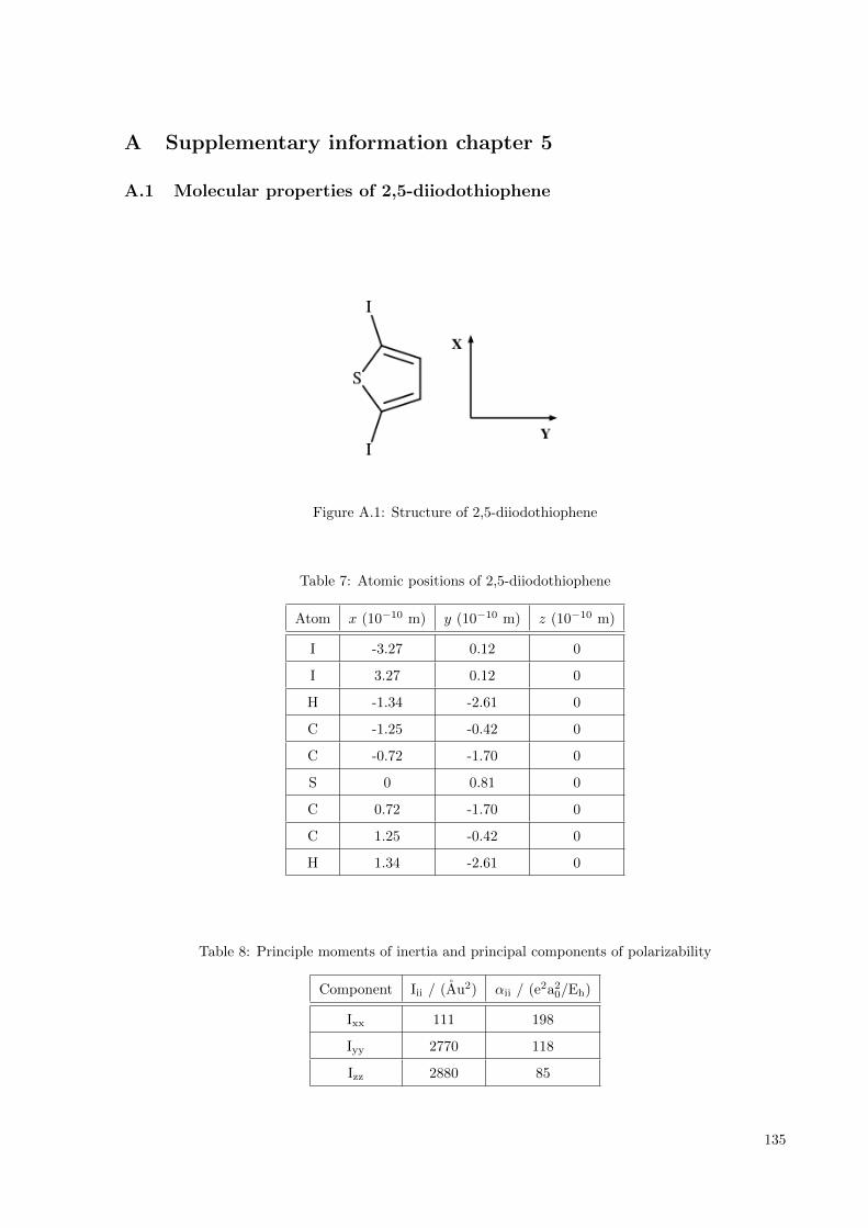
A Supplementary information chapter 5
A.1 Molecular properties of 2,5-diiodothiophene
Figure A.1: Structure of 2,5-diiodothiophene
Table 7: Atomic positions of 2,5-diiodothiophene
Atom x (10−10 m) y (10−10 m) z (10−10 m)
I -3.27 0.12 0
I 3.27 0.12 0
H -1.34 -2.61 0
C -1.25 -0.42 0
C -0.72 -1.70 0
S 0 0.81 0
C 0.72 -1.70 0
C 1.25 -0.42 0
H 1.34 -2.61 0
Table 8: Principle moments of inertia and principal components of polarizability
Component Iii / (Au2) αii / (e2a20/Eh)
Ixx 111 198
Iyy 2770 118
Izz 2880 85
135

A. Supplementary information chapter 5
A.2 Diffractive imaging – ADU gate optimization
The determination of the ADU gates shown in Figure 5.9 was done based on a signal to noise estimation.
Therefore, the recorded diffraction measurements (signal) and background measurement 1 (labeling
according to Table 3) were compared. The background measurement 1 was scaled such that it contains the
same number of FEL shots as the signal measurement; background measurements 2 and 3 were not taken
into account since they do also have contributions from the helium and molecular diffraction pattern. The
signal measurement contains thus signal from the helium, molecules and background from the beamline as
well as fluorescence photons. The background measurement contains only background photons from the
beamline and fluorescence photons.
Next, the number of photons detected within a certain ADU gate width have been integrated for both,
the signal and background measurements. By subtracting the number of photons within the background
measurement from the number of photons within the signal measurements results in the amount of detected
signal photons within that certain ADU gate width. Comparing the background subtracted signal photons
to the number of background photons provides an estimation of the signal-to-noise ratio (SNR). This has
been conducted for an (quasi arbitrary) chosen ADU gate width of 5 and 10 ADU. Shifting the ADU gate
over the full given ADU range allows to find an optimum ADU gate width and position. This is shown
in Figure A.2 and also explained again on two examples.
25 30 35 40 45
Position ADU gate high
0.0
0.5
1.0
1.5
2.0
2.5
3.0
Signal photonsSignal to noise
30 35 40 45 50
Position ADU gate High
0.0
0.5
1.0
1.5
2.0
2.5
3.0
Signal photonsSignal to noise
Figure A.2: Signal to noise ratio and total counts in the diffraction pattern for a ADU gate width of 5
(left) and 10 (right). The x-value shows the ADU upper value of the gate. The signal photons are given in
2·106 and 3·106 photons per ADU gate width.
In both plots of Figure A.2 the SNR (green) and the total number of diffracted photons (blue) is given
for the two different gate width of 5 (left) and 10 (right) ADU. The x-axis represents the location of the
136
A.2 Diffractive imaging – ADU gate optimization
upper gate position in ADU, i. e., if x is 25, the ADU gate used to integrate the photons is between 20-25
ADU for an ADU gate width of 5, and from 15-25 ADU for a ADU gate width of 10. Next, if x is 26, the
chosen ADU gate ranges are 21-26 ADU and 16-26 ADU, and so on. The ADU value for the 9.5 keV
signal photons was 30 ADU. For both plots shown in Figure A.2 the lower ADU gate position was chosen
between 20 and 40 ADU, leading to the displayed range of 25-45 ADU (30-50 ADU) for a chosen gate
width of 5 ADU (10 ADU).
Both graphs show at their maximum number of detected signal photons an SNR is below 1, meaning that
more background photons than signal photons have been detected. Contrary, the number of detected
photons decreases dramatically at a higher SNR value. Thus intermediate values have been used in the
analysis in section 5.5. The chosen gates shown in Figure 5.4 where a) 35-45 ADU, 2) 36-41, and 3) 31-41.
At this gate positions the SNR ratios are 2.1, 2.3, and 1.1 and the total number of diffracted photons in
the signal gate are 2.6, 1.7 and 6.8 million photons.
137


B Supplementary information chapter 6 and 7
B.1 Molecular beam reconstruction
To reconstruct the temporal molecular beam profile, the recoded events had to be sorted based on their
timestamp (TS). The TS for each event was recorded with respect to the beginning of an individual
measurement. Therefore, the TS does not directly provide the information at which relative time within
the logical set time window of 200 µs (Figure 6.1) a certain event has been occurred. The reconstruction
of the relative time trel can be done by
trel = TS − int(TS · fV alve)fV alve
, (18)
where int is the integer value of the numerator, and fV alve the frequency of the pulsed valve. The numerator
of the fraction can be interpreted as the pulse counter. If, for example, the recorded event has a TS of
2.0001 seconds, the numerator in Equation 18 is 500,025, and its integer value is 500. This means, that
the event has been recorded at the five-hundredth molecular pulse after the measurement has been started.
Dividing the integer value by the repetition rate of the valve gives a value of 2 seconds, i. e., the starting
time of the logical set time window. The difference between the TS and the starting time of the 200 µs
long time window results in the relative time for a certain event. Thus, trel should always be between 0
and 200 µs.
Figure B.1: a) Reconstructed relative timing and b) reconstructed molecular beam profile based on tEL
The reconstruction of trel based on the TS of one randomly selected measurement is shown in Figure B.1
a). The y-axis shows the time difference between the beginning of the logical set time window and the
time of the event within that window, and the x-axis shows the individual event number. Due to the
139

B. Supplementary information chapter 6 and 7
high number of events only the envelope of the reconstructed time is visible. Clearly visible is that the
blue graph has a relative time width of approximately 200 µs and expresses a linear, positive slope. This
can be explained by a timing drift between the pulse driver for the pulsed valve and the time-to-digital
converter (TDC). The green curve shows the same events corrected by a linear function
tEL = trel − c · EN, (19)
where c is a constant and EN is the event number. It can be seen that the reconstructed time is now
between a relative time of 0 and 200 µs, i. e., the chosen time window. The constant c was dependent
on the individual measurement due to, for instance, a higher event rate per second which resulted in a
different delay in the TDC unit. An algorithm was used to find for each measurement the constant by
variation of that constant until the difference between the minimum and maximum of the reconstructed
time was minimized. The difference between the maximum and minimum time of tEL was smaller than 200
+/- 1 µs for each measurement, which is accurate enough for the current experiment. The reconstructed
pulse structure is shown in Figure B.1 b), where the counts are given in counts per bin. The counts at the
beginning and at the end of the histogram with a constant value of approximately 2000 counts per bin are
background. The increased signal in the center of the image is due to an increased detection of ions while
the molecular beam is present in the interaction zone. From this reconstruction a pulse duration of 45 µs
FWHM is derived. The pulse duration varied depending on the spatial position in the deflected molecular
beam.
B.2 Coincidence spectrum (PIPICO)
An ion coincidence spectrum, as it is shown for instance in Figure 6.2, can be used to disentangle the
different fragmentation channels of a molecule. Requirements are the detection of two or more ionic
fragments from a single molecule, as well as (ideally) a maximum of one event per TOF spectrum.
Latter one is important for high repetition rate photon sources like synchrotrons, where the photon pulse
separation is typically in the order of ns, while the measurement of a TOF spectrum is typically in the
order of µs. Figure B.2 shows exemplarily a Coulomb exploding indole molecule for the three different
orientations a), b) and c). In this example the fragments 1 and 2 are ionic and are extracted toward
the detector, located in the upper part of Figure B.2. Fragment 2 is heavier than fragment 1 and will
thus always be detected as second ion. The TOF of the fragments will vary slightly depending on the
orientation of the molecule with respect to the detector. In a) fragment 1 will have an initial momentum
p1 in the opposite direction of the extracting field leading to a longer TOF compared to case b) and c).
On the other side, fragment 2, whose momentum p2 is in the direction of the extracting field, will have a
shorter TOF compared to case b) and c). Averaging over all different orientations of the molecule leads to
a diagonal line in the PIPICO spectrum as it is indicated in the right part of Figure B.2. The slope and
shape of a coincidence line is dependent on the charge state of the fragments as well as the angle between
their momentum vectors. A detailed description of the difference can be found for instance in [186] and
140
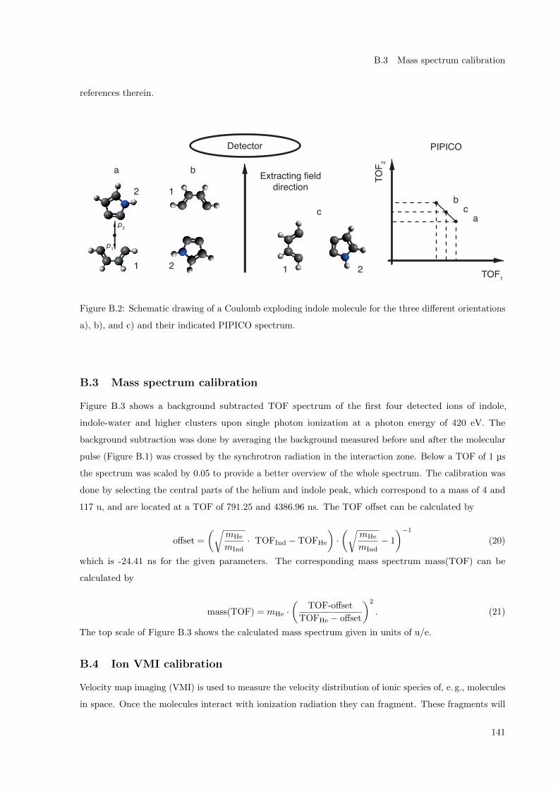
B.3 Mass spectrum calibration
references therein.
Extracting fielddirection
Detector PIPICO
TOF1
TOF 2
a
c
211
2
b
1
2
ca
b
p2
p1
Figure B.2: Schematic drawing of a Coulomb exploding indole molecule for the three different orientations
a), b), and c) and their indicated PIPICO spectrum.
B.3 Mass spectrum calibration
Figure B.3 shows a background subtracted TOF spectrum of the first four detected ions of indole,
indole-water and higher clusters upon single photon ionization at a photon energy of 420 eV. The
background subtraction was done by averaging the background measured before and after the molecular
pulse (Figure B.1) was crossed by the synchrotron radiation in the interaction zone. Below a TOF of 1 µs
the spectrum was scaled by 0.05 to provide a better overview of the whole spectrum. The calibration was
done by selecting the central parts of the helium and indole peak, which correspond to a mass of 4 and
117 u, and are located at a TOF of 791.25 and 4386.96 ns. The TOF offset can be calculated by
offset =
(√mHe
mInd· TOFInd − TOFHe
)·(√
mHe
mInd− 1
)−1
(20)
which is -24.41 ns for the given parameters. The corresponding mass spectrum mass(TOF) can be
calculated by
mass(TOF) = mHe ·(
TOF-offset
TOFHe − offset
)2
. (21)
The top scale of Figure B.3 shows the calculated mass spectrum given in units of u/e.
B.4 Ion VMI calibration
Velocity map imaging (VMI) is used to measure the velocity distribution of ionic species of, e. g., molecules
in space. Once the molecules interact with ionization radiation they can fragment. These fragments will
141

B. Supplementary information chapter 6 and 7
0 1 2 3 4 5 6
TOF (µs)
0
1
2
3
4
5
Ions
(10
4io
ns/b
in)
10 20 30 40 50 100 150Mass (u/e)
x 0.05
Figure B.3: Background subtracted TOF spectrum of indole, indole-water and higher clusters. The top
scale shows the corresponding mass spectrum.
have a certain 3D momentum distribution in space. For ionic fragments, the 3D velocity distribution can
be measured by a projection of this velocity distribution onto a 2D detector surface [2–5]. The position of
the ions on the detector can be described by
position = M · TOF · (vbeam + vion) + offset, (22)
where M is the magnification factor of the VMI, TOF is corresponding to the time of flight of a certain
fragment and is proportional to√
mass of the fragment, vbeam is the initial velocity of the molecules
with respect to the detector frame, vion is the velocity of the ions which they obey upon fragmentation,
and the offset is the shift of the VMI image of an ionic fragment with zero velocity with respect to an
arbitrary position on the detector, typically chosen as the center of the detector. The experimental setup
in Figure 6.1 illustrates that the molecular beam direction is in the plane of the detector. Thus, the
individual VMI spectra for single masses will have a TOF dependent shift of their mean position on the
detector. The presented data were corrected for this shift as it is described in the following. Figure B.4
a) shows a TOF spectra of the first detected ion. Highlighted is a single peak between 4.3 and 4.4 µs
which is corresponding to the mass of 117 u, i. e., the parent ion of indole. The corresponding VMI image
is shown in Figure B.4 b); the center of the detector is at X = 0 and Z = 0. Visible are two different
VMI distributions indicated by the two circles. The upper circle originates from indole ions which have at
142

B.4 Ion VMI calibration
1 2 3 4 5 6
TOF µs
0
2
4
6
8
10
12
Ions
(10
4io
ns/b
in) a
−20 0 20
X (arb. u.)
0
20
40
60
Z(a
rb.u
.)
Helium
Indole
b
0
60
120
180
240
Ions
(ion
s/bi
n)
Figure B.4: a) TOF spectra of the first detected ion. Highlighted in gray is the parent ion of indole.
b) VMI image of the parent ion of indole with the different contributions from background and indole
molecules. The arrow is indicating the axis of the molecular beam direction.
least two velocity channels; ‡ the lower circle originates from helium ions which are falsely detected at this
TOF. The center of gravity of both points (center of the indicated circles) is equivalent to the product of
the TOF of the ions and the velocity vector of the molecular beam in the detector frame. The connection
between both centers is indicated by the arrow and represents this product which is, in principle, enough
information to determine this product for all masses. Though, a more accurate determination is required.
Due to the helium contamination only a few specific ions, namely helium, water, hydronium and dicationic
indole, could be used to determine the molecular beam axis.
Additionally, one can use coincidences between ionic fragments to determine the product. From the
PIPICO spectrum shown in Figure 6.2 specific coincidence lines have been chosen. A single coincidence
line, i. e., a single dissociation channel, can be used to get in total three points for the determination.
These of the two individual ions detected in coincidence can be used to determine their specific central
VMI position (vide supra). Additionally, under the assumption that these ionic fragments do recoil in
opposite directions with parallel momentum vectors, the coincidence can be used to determine a third
point which is as well located on the molecular beam axis. This is schematically shown in Figure B.5 where
v1 (v2) is the velocity of the first (second) detected ion and TOF1 (TOF2) is the offset corrected TOF of
this fragment. The product of TOF and vbeam is again indicated by the arrow. The velocity vectors v1
and v2 are parallel due to the recoil in opposite directions, and the VMI images are indicated by the gray
circles. Due to momentum conservation of the fragmenting molecule v2 will always be smaller than v1
‡The slow ions visible in the center are due to slow ions which could origin from monomeric indole which relaxes via
emission of a photon subsequent to ionization. The faster ions are assigned to fragmentation of, e. g., indole-indole clusters
which experience Coulomb explosion after ionization
143

B. Supplementary information chapter 6 and 7
TOF • vbeam
TOF2
TOF1
v2
v1
Crossing point
Figure B.5: Illustration of the reconstruction of the crossing point which is used as additional point to
determine the product of TOF and vbeam.
since it has a higher TOF, i. e., higher mass. The linear connection between both fragments crosses the
molecular beam vector always at the same point, no matter where the ions from the molecular fragment
are detected in the VMI. The crossing point (CP) can be determined from the ions position and TOF via
CP(X,Z) = Ion1(X,Z) +
(1 +
TOF1
TOF2
)−1
· (Ion2(X,Z)− Ion1(X,Z)) , (23)
where Ion1(X,Z) and Ion2(X,Z) are the positions of the ions in the units of the detector, and TOF is the
offset corrected TOF of the ions determined as described in section B.3. The time of flight corresponding
to the crossing point TOFCP can be calculated by
TOFCP =TOF2
1 + TOF22
TOF1 + TOF2. (24)
The determined centers of the different TOF-specific VMI distributions, as well as the determined CPs, are
shown in Figure B.6 a) in red and blue respectively. The position X and Z is given in the detector units;
the error bars show the determined standard error. Note that the X and Z-axis do have different scales,
leading to a visually larger error in the X-direction. However, both error are comparable in numbers.
The gray line shows a linear fit to the data points corresponding to the product of vbeam · TOF, and has
a slope of -15.7 and a zero-crossing at 1.75 X. The center of gravity of the indole monomer (as shown
in Figure B.4 b)) is highlighted by the oval. The scaling of the TOF axis, and the determination of the
zero point, i. e., the point on the axis for TOF = 0 (X0 and Z0), was determined in the following way:
The TOF-dependent VMI centers as well as CPs (Figure B.6 a)) were projected in a right-angle onto
the determined product of vbeam · TOF. These points serve as a calibration for the TOF scale by the
individual TOF of the VMI centers as well as the determined TOF for the CPs (Equation 24). The zero
144

B.5 Electron VMI calibration
−2 0
X (arb. u.)
15
20
25
30
Z(a
rb.u
.)
a
0 5 10 15√Mass
0
10
20
Rad
ius
(arb
.u.)
b
Figure B.6: a) Overview of the determined points located on the velocity vector vbeam. The red data
points are determined from the TOF-dependent VMI distributions, the blue points correspond to CPs
(Equation 24), and the gray line shows the linear fit of vbeam ·TOF. b) Determination of the VMI positions
for a TOF = 0. The ellipse is highlighting the TOF-dependent center of the VMI for ionic indole shown
in Figure B.4
point was placed at a random position on the fitted line below the smallest determined TOF. The distance
between the zero point and the projected data can now be plotted against the TOF of the individual points
as it is shown in Figure B.6 b), where the red and blue points correspond again to the TOF dependent
VMI centers and CPs. The error bars were determined from Figure B.6 a) by considering the X - and Z
contributions on the projection, and the point corresponding to ionic indole is again highlighted by the
circle. If the zero position is at the appropriate location, the fitted line should cross the axis’s origin since
at a distance of 0 from the zero point the TOF is corresponding to zero. Thus, the zero point was varied
till the intercept was minimized. The corresponding zero point is X0 = -0.077 and Z0 = 6.121.
B.5 Electron VMI calibration
The electron VMI calibration has been done by photoelectrons originating from neon and helium ionized
at various photon energies. Figure B.7 a) shows exemplarily the sum of two spectra of neon ionized at 960
and 980 eV, resulting in photoelectrons with an energy of 89.9 and 109.8 eV (neon 1s = 870.2 eV [78]).
The corresponding radial integration (1D spectrum) is shown in the histogram in Figure B.7 c). The
diagonal lines in the VMI spectrum are caused by the hexanode where only two out of three electrodes
were working properly. Figure B.7 b) shows the inverse Abel transformation of Figure B.7 a) which was
145

B. Supplementary information chapter 6 and 7
calculated based on the BASEX algorithm [187]; the corresponding 1D spectrum is shown in the histogram
in Figure B.7 d). The 1D spectra obtained from the inverse Abel transformation were used as basis for a
Gaussian fit to determine the mean radius for a certain photoelectron velocity.
Additionally to neon, helium photoelectrons have been measured for ionization energies of 310 and 420 eV,
which correspond to a photoelectron energies of 285.4 and 395.4 eV. Figure B.8 shows the four determined
radii for the four measured photoelectron velocities. The red and orange crosses correspond here to the
measurement points for neon and helium respectively. The x-axis represents the radius in detector units,
the y-axis displays the velocity of the photoelectrons. The black circle is indicating the center of the VMI
images and the black graph is indicating a polynomial fit to the data which resulted in a slope of 0.9948,
crossing the origin at 0.
−8 −4 0 4 8
X (arb. u.)
−8
−4
0
4
8
Z(a
rb.u
.)
a
0
20
40
60
80
100
−8 −4 0 4 8
X (arb. u.)
b
0
2
4
6
8
10
Ele
c.(E
lec.
/bin
)
0 1 2 3 4 5 6 7
Radius (arb. u.)
0
4
8
12
16
Ele
c.(1
03E
lec.
/bin
) c
0 1 2 3 4 5 6 7
Radius (arb. u.)
0
4
8
12
16
Ele
c.(a
rb.u
.)
d
Figure B.7: a) Sum of two photoelectron spectra for neon ionized at a photonenergy of 960 and 980 eV.
The corresponding 1D spectrum is shown in c). b) shows the inverse Abel transformation of a) based on
the BASEX algorithm [187]. d) shows the 1D energy spectrum of b).
146

B.5 Electron VMI calibration
−5 0 5 10 15
Radius (detector units)
−5
0
5
10
15
v Rad
(10
6m
/s)
NeonHelium
Figure B.8: Electron velocity as a function of the distance to the origin of the VMI images. Neon and
helium is indicating the radii determined for the two different electron velocities of both atomic species.
The origin is labeled by the black circle and the black line shows a fit to the determined data points.
147


Acknowledgment
At first I would like to thank my group leader and Doktorvater Jochen Kupper for being my Doktorvater,
for the great experiments whom I was allowed to participate, for his continuously open ear for private as
well as work related discussions, his continuous advise, and of corse for given me the chance to conduct
the PhD in his group.
I would like to thank Oriol Vendrell for being the second examiner, and, despite the distance he has
currently to Hamburg, also to thank him for being part of my PhD defense committee.
Further, I would like to thank Henry Chapman, Oliver Mucke, the other members of my PhD defense
committee, and Caren Hagner, leader of my PhD defense committee, for not hesitating to join the
committee, and therefore also to accompany me by my last steps as a PhD student.
I would like to thank Sebastian Trippel for his great supervision of the indole and indole-water experiments.
Despite the time consuming work he had always an open ear, was giving always good advises, and was
always listen to counter-arguments(!)...until he found a good reason why that beautiful counter-argument
is not a good argument anymore!
I would like to thank Andrew Morgan for his awesome python skills, which he was willing to share with
me, and his continuous support in the data analysis of the x-ray diffraction experiment. Not to mention
countless discussions about everything one can imaging accompanied by a nice cold beer.
I would like to thank Daniel Horke and Yuan-Pin Chang. Both of them had the drawback of conducting
the first experiment with me. I was at the time a so-called laser person with no real experience in molecular
physics. They were at the front-end of my question marathon but were patient enough to keep me alive.
Along the same line I would like to thank Stephan Stern whom was my predecessor, and whom was really
patient with me, explained me everything necessary to conduct an experiment with his machine, which I
finally took over. I hope you appreciate that I kept that baby alive!
I would like to thank Mr. Mullins for being Mr. Mullins! Typically we were working together on beamtimes,
which were not always successful but at least we had fun! Not to mention here also his continuous support
and open ear.
Nele Muller and Jens Kienitz! A special thanks for the good time we had all the years, for all the fruitful
work related discussions, for all the good time after work! Without you the time would have been different,
Kolle Alaaf!
Joss Wiese, you smart guy! Thanks very much also to you for all your help and the great time!
Nicole Teschmit, another person whom won my heart! Thanks very much for ur help, discussions,
continuous smile, and the good time outside work!
My dear Italian friends Michele Di Fraia and Andrea Maria Trabattoni, my dear Scottish friend Ruth
Livingstone, one beamtime, several beers, thanks for the good time! Grazie mille! Thenk ye uncoly! And
the google-translated go raibh maith agat!
Karol D lugo l ecki and Lars Gumprecht! I think without you the machine would have been fallen apparat,

and modifications as well as technical drawings were on a level I do not dare to imaging. Thanks very
much to both of you!
Barbora Vagovic and Irmtraud Kleine, the glue of the group! Thanks very much for helping me and the
group to keep everything in order!
My dear PhD co-fighters Salah Awel, Helen Bieker, Bastian Deppe, Zhipeng Huang, Evangelos Karamatskos,
Nils Roth and Linda Thesing. My dear CMI co-workers Wilhelm Frisch, Daniel Gusa, Pau Gonzalez-
Caminal, Igor Rubinsky, Xiaoyan Sun, Lena Worbs, Lu Wu, .., my dear CMI colleagues and former
colleagues! We did not had too much work-related overlap during the time my PhD, but we still had
enough to giggle during, and off-time work! I really enjoyed being part of the group thanks to all of you!
From our collaborators I would like to explicitly mention the ”CAMP-crew” headed by Daniel Rolles, and
consisting (at this time) of Denis Anielski, Sadia Bari, Rebecca Boll, Cedric Bomme, Benjamin Erk, and
Evgeny Savelyev. Thank you very much for all the nice experiments, the support, the discussions, and
also the nice time off-work!
I would like to thank the Coherent Imaging Team headed by Henry Chapman, including Valerio Mariani
and Holger Fleckenstein. All of you where always really helpful, and also did not hesitate to borrow me/us
stuff for various experiments.
I would like to thank the people and groups around the beamlines where we have conducted the experiments,
namely the Variable Polarization Beamline P04 at Petra III headed by Jens Viefhaus, the CXI Beamline
at the LCLS headed by Sebastien Boutet, and the fiber and waveguide lasers group at the Friedrich-
Schiller-Univertitat Jena headed by Jens Limpert.
I would like to thank my colleagues and friends of the CFEL and DESY, including Frederike Ahr, Jonathan
Correa, Hauke Hoppner, Yannis La-Place, Francesca Moglia, and many more. All of you made it possible
that I really enjoyed my time as a PhD student!
Finally, I would like to thank my girlfriend for being so patient with me, and my parents and friends from
Bergisch Gladbach for supporting me all the time in Hamburg!
Peace, love, and rock ’n’ roll!

List of Publications
1. Charge transfer in dissociating iodomethane and fluoromethane molecules ionized by intense fem-
tosecond X-ray pulses
R. Boll, B. Erk, R. Coffee, S. Trippel, T. Kierspel, C. Bomme, J. Bozek, M. Burkett, S. Carron, K.
Ferguson, L. Foucar, J. Kupper, T. Marchenko, C. Miron, M. Patanen, T. Osipov, S. Schorb, M.
Simon, M. Swiggers, S. Techert, K. Ueda, C. Bostedt, D. Rolles, A. Rudenko
Structural Dynamics, 3, 4 (2016)
2. High-repetition-rate and high-photon-flux 70 eV high-harmonic source for coincidence ion imaging
of gas-phase molecules
J. Rothhardt, S. Hadrich, Y. Shamir, M. Tschnernajew, R. Klas, A. Hoffmann, G.K. Tadesse, A.
Klenke, T. Gottschall, T. Eidam, J. Limpert, A. Tunnermann, R. Boll, C. Bomme, H. Dachraoui,
B. Erk, M. Di Fraia, D. Horke, T. Kierspel, T. Mullins, A. Przystawik, E. Savelyev, J. Wiese, T.
Laarmann, J. Kupper, D. Rolles,
Optics Express 24, 16 (2016).
3. Strongly aligned gas-phase molecules at free-electron lasers
T. Kierspel, J. Wiese, T. Mullins, J. Robinson, A. Aquila, A. Barty, R. Bean, R. Boll, S. Boutet,
P. Bucksbaum, H. Chapman, L. Christensen, A. Fry, M. Hunter, J. Koglin, M. Liang, V. Mariani,
A. Morgan, A. Natan, V. Petrovic, D. Rolles, A. Rudenko, K. Schnorr, H. Stapelfeldt, S. Stern, J.
Thøgersen, C. Yoon, F. Wang, S. Trippel, J. Kupper
Journal Of Physics B-Atomic Molecular And Optical Physics 48, 204002 (2015).
4. Imaging Molecular Structure through Femtosecond Photoelectron Diffraction on Aligned and Oriented
Gas-Phase Molecules
R. Boll, A. Rouzee, M. Adolph, D. Anielski, A. Aquila, S. Bari, C. Bomme, C. Bostedt, J. D. Bozek,
H. N. Chapman, L. Christensen, R. Coffee, N. Coppola, S. De, P. Decleva, S. W. Epp, B. Erk, F.
Filsinger, L. Foucar, T. Gorkhover, L. Gumprecht, A. Homke, L. Holmegaard, P. Johnsson, J. S.
Kienitz, T. Kierspel, F. Krasniqi, K.-U. Kuhnel, J. Maurer, M. Messerschmidt, R. Moshammer, N.
L. M. Muller, B. Rudek, E. Savelyev, I. Schlichting, C. Schmidt, F. Scholz, S. Schorb, J. Schulz, J.
Seltmann, M. Stener, S. Stern, S. Techert, J. Thøgersen, S. Trippel, J. Viefhaus, M. Vrakking, H.
Stapelfeldt, J. Kupper, J. Ullrich, A. Rudenko and D. Rolles
Faraday discussions 171, 57 - 80 (2014)
5. Spatial Separation of Molecular Conformers and Clusters
D. A. Horke, S. Trippel, Y.-P. Chang, S. Stern, T. Mullins, T. Kierspel, and J. Kupper
J. Vis. Exp. 83, e51137 (2014)
6. Spatially separated polar samples of the cis and trans conformers of 3-fluorophenol
T. Kierspel, D. Horke, Y.-P. Chang, and J. Kupper
Chemical Physics Letters 591, 130–132 (2014).