arX

iv:a

stro

-ph/

0108

171v

2 8

Dec

200

1

The Las Campanas Infrared Survey. III. The H-band Imaging

Survey and the Near-Infrared and Optical Photometric Catalogs

HSIAO-WEN CHEN1, P. J. McCARTHY1, R. O. MARZKE1,3 J. WILSON1, R. G.

CARLBERG2, A. E. FIRTH4, S. E. PERSSON1, C. N. SABBEY4, J. R. LEWIS4, R. G.

McMAHON4, O. LAHAV4, R. S. ELLIS5, P. MARTINI1, R. G. ABRAHAM2, A.

OEMLER1, D. C. MURPHY1, R. S. SOMERVILLE4 M. G. BECKETT1,4, C. D.

MACKAY4

1Carnegie Observatories, 813 Santa Barbara St, Pasadena, CA 91101, U.S.A.

2Department of Astronomy, University of Toronto, Toronto ON, M5S 3H8 Canada

3Department of Astronomy and Physics, San Francisco State University, San Francisco, CA 94132-4163,

U.S.A.

4Institute of Astronomy, Cambridge CB3 OHA, England, UK

5Department of Astronomy, Caltech 105-24, Pasadena, CA 91125, U.S.A.

– 2 –

ABSTRACT

The Las Campanas Infrared Survey, based on broad-band optical and near-

infrared photometry, is designed to robustly identify a statistically significant and

representative sample of evolved galaxies at redshifts z > 1. We have completed

an H-band imaging survey over 1.1 square degrees of sky in six separate fields.

The average 5 σ detection limit in a four arcsecond diameter aperture is H ∼

20.8. Here we describe the design of the survey, the observation strategies, data

reduction techniques, and object identification procedures. We present sample

near-infrared and optical photometric catalogs for objects identified in two survey

fields. The optical images of the Hubble Deep Field South region obtained from

the literature reach 5 σ detection thresholds in a four arcsecond diameter aperture

of U ∼ 24.6, B ∼ 26.1, V ∼ 25.6, R ∼ 25.1, and I ∼ 24.2 magnitude. The

optical images of the Chandra Deep Field South region obtained from our own

observations reach 5 σ detection thresholds in a four arcsecond diameter aperture

of V ∼ 26.8, R ∼ 26.2, I ∼ 25.3, and z′ ∼ 23.7 mag. We perform object detection

in all bandpasses and identify ∼> 54,000 galaxies over 1,408 arcmin2 of sky in the

two fields. Of these galaxies, ∼ 14,000 are detected in the H-band and ∼ 2,000

have the colors of evolved galaxies, I − H ∼> 3, at z ∼> 1. We find that (1) the

differential number counts N(m) for the H-band detected objects has a slope

of d log N(m)/dm = 0.45 ± 0.01 mag−2 at H ∼< 19 and 0.27 ± 0.01 mag−2 at

H ∼> 19 with a mean surface density ≈ 7, 200 degree−2 mag−1 at H = 19. In

addition, we find that (2) the differential number counts for the H-band detected

red objects has a very steep slope, d log N(m; I − H ∼> 3)/dm = 0.84 ± 0.06

mag−2 at H ∼< 20 and 0.32± 0.07 mag−2 at H ∼> 20, with a mean surface density

≈ 3, 000 degree−2 mag−1 at H = 20. Finally, we find that (3) galaxies with red

optical to near-IR colors (I − H > 3) constitute ≈ 20% of the H-band detected

galaxies at H ∼< 21, but only ≈ 2% at H ∼< 19. We show that red galaxies

are strongly clustered, which results in a strong field to field variation in their

surface density. Comparisons of observations and predictions based on various

formation scenarios indicate that these red galaxies are consistent with mildly

evolving early-type galaxies at z ∼ 1, although with a significant amount of

on-going star formation as indicated by the large scatter in their V − I colors.

Subject headings: catalogs—cosmology: observations—galaxies: evolution—surveys

– 3 –

1. INTRODUCTION

Different galaxy formation scenarios provide distinct predictions for the space densities

and masses of evolved galaxies at redshifts beyond z = 1. In monolithic collapse scenarios,

massive galaxies form early over a dynamical time (e.g. Eggen, Lynden-Bell, & Sandage 1962)

and passively evolve to the present epoch. The co-moving space density of evolved galaxies

is therefore expected to remain constant and the intrinsic luminosities of these galaxies are

expected to increase gradually with increasing redshift. In hierarchical formation scenarios,

massive galaxies form later through mergers of low-mass galaxies over a significant fraction

of the Hubble time (White & Rees 1978). The bulk of star formation and mass assembly

occurs much later and the co-moving space density of evolved galaxies is expected to decline

steeply with redshift at z > 1. While various surveys have identified some luminous galaxy

populations at z > 2 (e.g. Steidel et al. 1999; Blain et al. 1999), the connection between

these galaxies and typical present-day galaxies is unclear. On the other hand, comparisons

of statistical properties of evolved high-redshift galaxies and local elliptical galaxies may

provide a direct means of discriminating between competing galaxy formation scenarios (e.g.

Kauffmann & Charlot 1998).

Evolved galaxies may be characterized by their intrinsically red colors due to the lack

of ongoing star formation that provides most of the UV light in typical galaxy spectral

energy distributions. At redshifts beyond unity, where the UV region of the spectrum is

redshifted to the visible, optical galaxy surveys are insensitive to evolved galaxies, because

of their steep UV spectra. Identifications of evolved high-redshift galaxies therefore rely

on observations carried out at near-infrared wavelengths. Various studies based on near-

infrared surveys have, however, yielded inconsistent measurements of the space density of

evolved galaxies (Kauffmann, Charlot, & White 1996; Totani & Yoshii 1997; Zepf 1997;

Franceschini et al. 1998; Benitez et al. 1999; Menanteau et al. 1999; Barger et al. 1999;

Schade et al. 1999; Broadhurst & Bouwens 2000; Daddi et al. 2000; Martini 2001a). Because

most of the existing deep, near-infrared surveys observe a sky area of only a few tens of

square arc-minutes, the discrepancy is likely due to significant field-to-field variation (e.g.

Daddi et al. 2000; McCarthy et al. 2001a,b). Furthermore, because evolved galaxies lack

prominent narrow-band spectral features in the UV spectral range, this discrepancy is also

likely due to selection biases (e.g. Totani & Yoshii 1997). Additional uncertainty may also

arise due to the presence of dusty star forming galaxies that exhibit red colors resembling

evolved high-redshift galaxies (e.g. Graham & Dey 1996; Smail, Ivison, & Blain 1997).

A complete survey of evolved galaxies over a large sky area is needed to address these

issues. Deep, wide-field near-infrared surveys have only recently become feasible due to

the advent of large format near-infrared cameras (Beckett et al. 1998; Elston 1998; Persson

– 4 –

et al. 2001). In addition, various groups have demonstrated that distant galaxies may be

accurately and reliably identified using photometric redshift techniques that incorporate op-

tical and near-infrared broad-band photometry (Connolly et al. 1997; Sawicki, Lin, & Yee

1997; Lanzetta, Fernandez-Soto, & Yahil 1998; Fernandez-Soto, Lanzetta, & Yahil 1999;

Fernandez-Soto et al. 2001). For galaxies lacking strong emission or absorption features, we

may still be able to estimate redshifts based on the presence/absence of spectral discontinu-

ities using photometric redshift techniques. Therefore, a wide-field optical and near-infrared

imaging survey, with sufficiently accurate colors to yield reliable photometric redshifts, of-

fers an opportunity to identify statistically significant and representative samples of evolved

galaxies at z > 1.

We initiated the Las Campanas Infrared (LCIR) Survey to obtain and analyze deep

near-infrared images and complementary optical images in the V , R, I, and z′ bandpasses

over one square degree of sky at high galactic latitudes (Marzke et al. 1999; McCarthy et

al. 2001a,b). The survey is designed to identify a large number of red galaxies at z > 1,

while securing a uniform sample of galaxies of all types to z ∼ 2 using broad-band optical

and near-infrared colors. In particular, this program utilizes one of the largest near-infrared

cameras available (CIRSI), which produces an image of 13′ × 13′ contiguous field of view in

a sequence of four pointings. The LCIR survey may serve to bridge the gap between very

wide field surveys (e.g. NOAO Deep-Wide; Jannuzi et al. 1998) and very deep, smaller field

near-infrared imaging surveys (e.g. ESO Imaging Survey, da Costa 2000; NTT Deep Field,

Moorwood, Cuby, & Lidman 1998).

The primary objectives of the program are (1) to examine the nature of the red galaxy

population and identify evolved galaxies at redshifts z > 1, (2) to study the space density

and luminosity evolution of evolved galaxies at redshifts z ∼< 2, and (3) to measure the

spatial clustering of evolved high-redshift galaxies (McCarthy et al. 2001a,b; Firth et al.

2001), thereby inferring merging rates of these galaxies for constraining theoretical models.

The galaxy catalog together with an accompanied photometric redshift catalog will also be

used (4) to assess luminosity and luminosity density evolution for galaxies of different types

over the redshift range between z = 0 to 2 (Chen et al. in preparation) and (5) to study the

bright-end luminosity functions for galaxies and QSOs at redshifts beyond z = 4.5. Finally,

galaxies identified in the survey will be compared with objects identified in a companion

VLA survey (6) to study the spatial distribution of weak radio sources (∼> 10 µJy; Yan et al.

in preparation).

To date we have completed an H-band imaging survey over 1.1 square degrees of sky

to a mean 5 σ detection limit in a four arcsecond diameter aperture of H ∼ 20.8. Here we

present sample optical and near-infrared photometric catalogs for galaxies identified in two

– 5 –

of our fields: the Hubble Deep Field South (HDFS) and Chandra Deep Field South (CDFS).

These are the two fields for which a complete set of near-infrared and optical images are

available. We have identified ∼ 24,000 galaxies over 847 arcmin2 in the HDFS region, of

which ∼ 6, 720 are detected in the H-band survey, and ∼ 30, 000 galaxies over 561 arcmin2

in the CDFS region, of which ∼ 7, 400 are detected in the H-band survey. Among the

H-detected galaxies in the two regions, ∼ 2, 000 have colors that match evolved galaxies,

I − H ∼> 3, at redshifts z ∼> 1. A complete near-infrared and optical photometric catalog

of the two fields may be accessed at http://www.ociw.edu/lcirs/catalogs.html. Catalogs for

the other survey fields will be released as they become available.

We describe the survey design and observation strategies in § 2 and data reduction

and image processing in § 3. The procedures for identifying objects in multi-bandpasses,

estimates of the completeness limits of the catalogs, and an assessment of the reliability of

the photometric measurements are presented in § 4. The format of the optical and near-

infrared photometric catalogs is described in § 5. Finally, we discuss statistical properties of

the H-band selected galaxies in § 6. An independent analysis based on objects identified in

the HDFS region is also presented in Firth et al. (2001). We adopt the following cosmology:

ΩM = 0.3 and ΩΛ = 0.7 with a dimensionless Hubble constant h = H0/(100 km s−1 Mpc−1)

throughout the paper.

2. Observations

2.1. Definition of the Las Campanas Infrared Survey

The goals of the LCIR survey are to robustly identify a statistically significant and

representative sample of evolved galaxies at redshifts z > 1, as well as to secure a uniform

sample of galaxies of all types at intermediate redshifts based on broad-band optical and

near-infrared colors.

To determine the image depths necessary to reach our goals, we estimated the expected

near-infrared brightness and optical and near-infrared colors of evolved high-redshift galaxies

using a series of evolutionary models. We considered a non-evolving model using an empirical

early-type galaxy template presented in Coleman, Wu, & Weedman (CWW, 1980) and two

evolving models for galaxies of solar metallicity formed in a single burst of 1 Gyr duration at

redshifts zf = 5 and zf = 10, respectively (Bruzual & Charlot 1993). We scaled these models

to have LH = LH∗

† at z = 0 (see also Marzke et al. 1999). Figure 1 shows the predicted

†We adopt MH∗= −22.9 + 5 log h from De Propris et al. (1998).

– 6 –

redshift evolution of the observed H-band magnitudes and optical and near-infrared colors

of evolved galaxies based on the three models. Adopting H0 = 70km s−1 Mpc−1, we found

that in the absence of dust an evolved L∗ galaxy may have an apparent H-band magnitude

between H = 19.5 and 20.3 and I − H ∼ 3 at redshift z ∼ 1, and an apparent H-band

magnitude between H = 20.7 and 22.5 and an I − H color between ∼ 4.5 and 5 at redshift

z ∼ 2. The color threshold I − H ∼> 3 therefore defines our selection criterion for evolved

galaxies at redshifts z > 1, which according to Figure 1 is similar to selections made based

on R − Ks ∼> 5. To identify a large number of the evolved galaxy population, we therefore

choose a target 5 σ survey depth of H ∼ 21, more than one magnitude fainter than an L∗

elliptical galaxy at z ∼ 1. We also require that the optical imaging survey reach consistent

depths based on the predicted optical and near-infrared colors. The actual depth that we

achieved varied from field-to-field and often fell somewhat short of our design goals.

To determine the survey area, we first estimated the number of evolved galaxies that are

required to obtain a significant signal in the clustering analysis. At a projected co-moving

correlation length rp = 1 Mpc, we found that a sample of ∼ 3000 galaxies are needed to reach

the 5 σ level of significance (Marzke et al. 1999). The surface density of galaxies satisfying

I − H ∼> 3 is, however, very uncertain. Different measurements based on K-band surveys

have been reported by several groups, ranging from 0.3 arcmin−2 to 3 arcmin−2 at Ks < 20

(Cowie et al. 1994; Elston et al. 1997; Barger et al. 1998). Adopting a median surface density

1 arcmin−2 and a mean near-infrared color H − Ks ∼ 1 for evolved galaxies at z > 1, we

concluded that one square degree of sky at a 5 σ limiting magnitude H ∼ 21 will yield ∼ 3000

red high-redshift galaxies.

The LCIR survey may serve to bridge the gap between the on-going NOAO Wide-Field

Survey that images 18 square degrees of sky at a shallower depth (Jannuzi et al. 1998) and

the existing deep, smaller field near-infrared imaging surveys such as the NTT Deep Field

(Moorwood, Cuby, & Lidman 1998). We have selected six distinct equatorial and southern

fields at high galactic latitudes distributed in right ascension. In Table 1, we list the fields,

their J2000 coordinates, and galactic latitudes.

2.2. Infrared Imaging Observations

The H-band imaging survey was carried out at the du Pont 2.5 m telescope at Las Cam-

panas using the Cambridge Infrared Survey Instrument (CIRSI). This instrument contains

a sparse mosaic of four 1024 × 1024 Rockwell Hawaii HgCdTe arrays (Beckett et al. 1998;

Persson et al. 2001). At the Cassegrain focus of the du Pont telescope, the plate scale of

the camera is 0.199 arcsec pixel−1. Some of the observations were made with a doublet field

– 7 –

corrector in front of the dewar window, which produced a plate scale of 0.196 arcsec pixel−1.

The spacing between each array is 90% of an array dimension. Therefore, one pass of four

pointings ∼ 192 arcsec apart in a square pattern is needed to fill in the spaces between the

arrays. A filled mosaic covers ∼ 13′×13′. This defines our unit field area, henceforth referred

to as a “tile”.

Observations of individual pointings were composed of nine sets of three to five exposures

35 to 45 s in duration with dither offsets of between 8 and 13 arcsec in a rectangular pattern.

For a typical H-band sky brightness of 14.7 magnitudes, we estimated that a total exposure

time of 80 minutes was needed to reach a 5 σ limiting magnitude of H ∼ 20.3 in a four arcsec

diameter aperture. The target integration time was achieved by making three passes on each

field. Because it was often impossible to complete three passes of a field within one night,

the observations of any given field area were spread over several nights. Standard stars from

Persson et al. (1998) were observed three to five times per night. Flat field observations were

made using a screen hung inside the dome and were formed from differences of equal length

exposures with the dome lamps on and off.

Most of our fields are composed of four contiguous tiles arranged to cover a roughly

25′ × 25′ field. The HDFS field contains seven tiles arranged in an H-shaped pattern to

avoid several very bright stars. The NTT Deep and 1511 fields contain tiles that are not

contiguous. This was because the optical data were obtained with the sparse-array geometry

Bernstein-Tyson Camera (BTC) on the 4-m telescope at CTIO. The journal of H-band

imaging observations is given in Table 2, in which columns (1) through (5) and column (8)

list the field, tile number, the 2000 coordinates of the tile centers, total exposure time, and

date of observation, respectively.

2.3. Optical Imaging Observations

Optical images of the LCIR survey fields were obtained either from our own observations

or from the literature using various large format CCDs at different telescopes. The journal of

optical imaging observations is given in Table 3, which lists the field, telescope, instrument,

plate scale, field of view (FOV), bandpasses, total exposure time, and date of observation.

A more detailed description of the optical imaging observations will be presented elsewhere

(Marzke et al. in preparation).

– 8 –

3. Image Processing

In this section, we describe the procedures of processing the near-infrared H-band images

of all six fields and summarize the qualities of the available optical images of the HDFS and

CDFS regions. In addition, we discuss astrometric and photometric calibration of these

images.

3.1. The H-band Images

The H-band images obtained with CIRSI were processed using two independent re-

duction packages, one developed by McCarthy, Wilson and Chen at Carnegie, the other by

Lewis, Sabbey, McMahon, and Firth at the Institute of Astronomy (IoA).

The Carnegie reduction pipeline proceeds as follows. First, loop-combined images were

formed by taking a mean of each loop of three to five exposures obtained without dithering

the telescope. A 5 σ rejection algorithm was applied to remove cosmic ray events, if there

were more than four exposures in a loop. Next, the loop-combined images were divided by

the normalized dome flats and grouped together according to their locations on the sky. The

use of a dome rather than dark-sky flat field image allows us to separate the pixel-to-pixel

gain variations from the additive sky fringes which are non-negligible for these Hawaii arrays.

The flat-field images have been normalized to remove the gain differences between the four

detectors. These are generally less than 5%, except in the case of chip #3 for which the gain

correction is ∼ 20%. Next, a bad pixel mask was generated for each night using the flat-

field exposures. Initial sky frames were constructed from medians of all frames for individual

arrays that lay within a given pointing position. These sky frames were subtracted from each

flat-field corrected image for the purpose of constructing an object mask for each image. The

sky-subtracted images were registered using the offsets derived from the centroids of 5 to 15

stars. All objects with peak intensities more than 10 σ above the sky noise were identified

and sorted into four categories according to their isophotal sizes. Mask frames were then

generated for each dithered exposure accordingly. Next, a sliding-median sky frame was

obtained by taking the median of the preceding and succeeding three to five images with

the bad pixel and object masks applied. After being scaled by the ratio of the modes in

the images, the median sky frame was subtracted from the appropriate flat-field-corrected

image to remove the fringes due to OH emission lines from the sky that are present in the

flat-field-corrected images. This latter scaling (typically ±1%) allowed us to remove non-

linear temporal variations in the sky level. Finally, the flat-field-corrected and sky-subtracted

images were registered and combined using a 5 σ rejection criterion, a bad pixel mask, and a

weight proportional to the inverse of the sky variance to form a final stacked image for each

– 9 –

pointing position.

The contiguous 13′×13′ tiles were assembled from the 16 stacked images corresponding

to the four arrays at four pointings of the telescope. The array boundaries were registered

using stars in the overlap region, which was typically 20 to 30 arcsec in extent. The four

arrays were not perfectly aligned with each other and a significant rotation (∼ 0.4) was found

necessary to bring one of the arrays into registration with the other three. The final image

was constructed by summing the 16 registered stacked images. A 5 σ rejection criterion and

a weighting determined from the sky variance were also applied in the vicinity of the array

boundaries. A 1 σ error image was formed simultaneously for each tile through appropriate

error propagation, assuming Poisson counting statistics.

The IoA based reduction pipeline is similar in conceptual design, although it is written

in a somewhat different architecture and contains a few operational differences (Sabbey et

al. 2001). The offsets between dithered images were derived via cross-correlations in the

IoA pipeline rather than from image centroiding. The object masks were derived from

segmentation maps produced by SExtractor (Bertin & Arnout 1996) rather than using a set

of five fixed object sizes as in the Carnegie pipeline. Finally, the assembly of the final tiles was

completed after the application of a world coordinate system derived from comparison with

the APM catalog. In the Carnegie pipeline the astrometry was derived for the completed

tiles using the USNO astrometric catalog, discussed in § 3.3.

The images of the first three tiles of the HDFS region, the first tile of the NTT field, and

the second tile of the 1511 field contained significant artifacts associated with instabilities

in the detector reset. These manifest themselves as low spatial frequency bias roll-offs that

change shape and amplitude on short timescales. Both the Carnegie and IoA pipelines deal

with this low frequency signal by fitting low order polynomials to sigma-clipped images on

a line-by-line and column-by-column basis. In the Carnegie pipeline this reset correction is

applied after the final sky subtraction, in the IoA pipeline it is applied before the flat-field

and sky corrections have been determined. New read-out electronics were implemented in

August 2000, which largely suppress the reset instability.

The full width at half maximum (FWHM) of a typical point spread function (PSF) and

the 5 σ detection threshold in a four arcsecond diameter aperture of each completed tile are

given in columns (6) and (7) of Table 2, respectively. The PSF was measured to vary by

no more than 10% across a tile, but the 5σ sky noise was found to vary by as much as 50%

across each tile. Figure 2 shows the distributions of the FWHM of a mean PSF (left) and

the 5 σ detection threshold estimated based on mean sky noise in a four arcsecond diameter

aperture (right) for each completed tile. Figure 3 shows an example of a completed tile in

the CDFS region from the Carnegie pipeline. The average PSF of this image has a FWHM

– 10 –

of ≈ 0.7 arcsec. The magnitudes of the two objects indicated by arrows are H = 19.4 and

21.3.

3.2. The Optical Images

The optical U , B, V , R, and I images of an 40′×40′ area around the HDFS region were

obtained and processed by a team at the Goddard Space Flight Center during the HDFS

campaign using the BTC (Teplitz et al. 2001). The spatial resolutions of the final combined

images were measured to range from FWHM ≈ 1.4 arcsec in the V band to ≈ 1.6 arcsec

in the B band, and the 5 σ detection thresholds in a four arcsecond diameter aperture were

measured to be U ∼ 24.6, B ∼ 26.1, V ∼ 25.6, R ∼ 25.1, and I ∼ 24.2 magnitudes using

the photometric zero points determined by the Goddard team.

The optical V , R, I, and z′ images of ≈ 36′×36′ around the CDFS region were obtained

using the MosaicII imager on the 4-m telescope at CTIO in November of 1999. Individual

images were processed following the standard mosaic image reduction procedures for data

obtained with the MosaicII imager, registered to a common origin, and coadded to form

final combined images (Marzke et al. in preparation). The spatial resolutions of the final

combined images were measured to range from FWHM ∼ 1.0 arcsec in the I and z′ bands

to ≈ 1.2 arcsec in the V band, and the 5 σ detection thresholds in a four arcsecond diameter

aperture were measured to be V ∼ 26.8, R ∼ 26.2, I ∼ 25.3, and z′ ∼ 23.7 mag.

3.3. Astrometry

Accurate astrometry is required for followup observations and for matching our cata-

log with observations at other wavelengths. The optical images of the HDFS region were

corrected for astrometric distortions with an RMS error of 0.16 pixels, corresponding to

0.07 arcsec (Teplitz et al. 2001). We adopted the World Coordinate System (WCS) solution

stored in the image headers to derive coordinates for objects identified in the images. To cor-

rect astrometric distortions for the MosaicII images of the CDFS region, we first re-sampled

images of individual exposures to a Cartesian grid before co-addition and derived a best-fit,

fourth-order polynomial for the WCS solution by matching stars in the U.S. Naval Observa-

tory catalog (USNO–A2.0) with stars identified in the images (Marzke et al. in preparation).

A total of 200 stars was included to obtain the best-fit astrometric solution. The goodness

of fit may be characterized by an RMS residual of ≈ 0.2 arcsec.

Astrometric solutions were also derived for the near-infrared images. We were able to

– 11 –

identify on average ∼ 150 unblended and unsaturated stars in each H-band tile. Using a

third order polynomial fit we were able to obtain solutions with rms residuals of between

0.25 and 0.35 arcsec.

4. Analysis

In this section, we describe the procedures for object detection in individual bandpasses

and object matching between frames taken through the various filters. We also examine the

completeness limits of our detection algorithm and the reliability of photometric measure-

ments in all bandpasses.

4.1. Object Detection

To obtain a uniform sample of distant galaxies of all types, it is crucial to identify

galaxies of a wide range of optical and near-infrared colors. To reach this goal, we performed

object detection using SExtractor for each bandpass in the regions where the H-band imaging

survey was carried out. To reliably identify all the faint objects in each of the optical images,

we set the SExtractor parameters by requiring that no detections be found in the negative

image. First, we set the minimum area according to the FWHM of a mean PSF. Next, we

adjusted the detection threshold to the lowest value that is consistent with zero detections

in the negative image. To aid in deblending overlapping objects, we first constructed a

“white light” image by co-adding all the registered optical images that had been scaled to

unit exposure time and filter throughput (see the next section for descriptions of image

registration). Next, we applied SExtractor to the white light image and determined object

extents based on their instrumental colors. Because the PSF varied between different optical

bandpasses by at most 10% in each field, we were able to reliably deblend overlapping

objects without erroneously splitting or blending individual objects in the white light image

due to a large variation in the PSFs of different bandpasses. This procedure takes into

account the intensity contrast between overlapping objects in all bandpasses instead of a

single bandpass, allowing a more accurate object deblending for overlapping objects with

different instrumental colors.

We adopted a different approach to reliably identify all the faint objects in the H-band

images. Because of a non-uniform noise pattern between individual arrays across a single tile,

in particular in the join regions between adjacent array images, the zero negative detection

criterion would force a significant underestimate of the survey depth in some areas. An

– 12 –

example to illustrate the noise pattern is given in Figure 4, which shows the associated 1 σ

noise image of the tile shown in Figure 3. We identified objects well into the noise in the H-

band images and used our subsequent calibration of the completeness limits and photometric

errors to set the faint magnitude limit of the H-band catalog.

Finally, to ensure accurate measurements of optical and near-infrared colors, we excluded

objects that lie within ≈ 2 arcsec of the edges of each tile.

4.2. Image Registration and Catalog Matching

The optical U , B, V , R, and I images of the HDFS region were registered to a common

origin by the Goddard team. The RMS dispersion in the object coordinates between different

bandpasses was measured to be within ≈ 0.2 BTC pixels (corresponding to 0.08 arcsec). The

optical V , R, I, and z′ images of the CDFS region were registered individually for each area

covered by a near-infrared tile, based on a solution determined using ∼ 200 common stars

identified in the tile. We applied standard routines to obtain the transformation solutions and

to transform the images. We were able to register the optical images of the CDFS tiles by a

simple transformation of low-order polynomials in the x and y directions without significantly

degrading the image quality. To assess image degradation after the transformation, we

measured the changes in the FWHM of the PSFs in transformed images and found an

increase of no more than 5%. The RMS dispersion in the object coordinates between different

bandpasses across an area spanned by a tile was measured to be within ∼ 0.3 MosaicII pixels

(corresponding to 0.08 arcsec). The dispersion was found to be the worst (as much as 0.5

MosaicII pixels or 0.13 arcsec) in the join area between adjacent arrays of the MosaicII

imager. To merge individual optical catalogs of each field, we stepped through each object

identified in the white light image, examined the presence/absence of object detections at the

location in individual bandpasses, and recorded the SExtractor measurements for detections

and placed null values for no detections in the combined optical catalog.

The H-band and optical catalogs were merged on the basis of astrometric position match-

ing, rather than by transforming the H images onto the same pixels as the optical images.

The large differences in pixel scales and in the PSFs of the optical and IR images result in

significant image degradation if one transforms the H images to match the optical images.

We derived a mapping between the H and optical coordinates from ∼ 150 common stars in

each tile. The RMS dispersion between the transformed optical coordinates and the H-band

coordinates was measured to be ≈ 0.2 CIRSI pixels (corresponding to 0.04 arcsec). Next, we

repeated the catalog merging procedure described above by examining the presence/absence

of object detections within a radius of two CIRSI pixels to the transformed object location

– 13 –

in the H-band image for all optically detected objects. The combined catalog was updated

accordingly throughout the procedure. Finally, we compared objects in the combined optical

catalog with those in the H-band catalog, identified those that appeared only in the H-band

catalog, and included them to form the final combined optical and near-infrared catalog for

each tile.

4.3. Survey Completeness

Because detection efficiencies vary significantly for objects of different intrinsic profiles

due to the strong surface brightness selection biases and because the noise patterns of the

H-band images vary across individual tiles, particularly at the edges of individual arrays,

it is crucial to understand the sensitivities and detection efficiencies of the LCIR survey in

order to ensure the reliability of future analyses. To understand the completeness limits of

the H-band images (similar analyses for the optical images will be presented in Marzke et al.

in preparation), we performed a series of simulations, the results of which were also adopted

for testing the photometric accuracy described in the next section. First, we generated test

objects of different brightness for various PSF-convolved model surface brightness profiles.

We adopted a Moffat (1969) profile to simulate the PSFs and considered (1) a point source

model, (2) a de Vaucouleurs’ r1/4 model characterized by a half-light radius re = 0.3 arcsec‡,

and (3) three exponential disk models characterized by scale radii of rs = 0.15, 0.3, and 0.6

arcsec, respectively. The upper boundary of the selected disk scale lengths was determined

according to the results of Schade et al. (1996) based on galaxies identified in the CNOC

survey. These authors found a mean scale length rs ∼ 0.6 arcsec for field galaxies at z ∼ 0.5.

Next, we placed the test objects of a given magnitude at 1000 random positions in an H tile

and repeated the object detection procedures using the same SExtractor parameters. Finally,

we measured the recovery rate of the test objects as a function of H-band magnitude.

The results of the completeness test are presented in Figure 5 for Tile 1 of the CDFS field.

Figure 5 shows that the 50% completeness limit of the image is ∼ 0.6 magnitudes fainter for

an exponential disk of rs = 0.3 arcsec than for the largest disk model of rs = 0.6 arcsec and is

an additional ∼ 0.6 magnitudes fainter for a point source. The large difference between the

completeness limits for objects of different intrinsic profiles makes an accurate incompleteness

correction of the survey very challenging, because in practice we have no prior knowledge

in the intrinsic profile of each source. It appears that under these circumstances correcting

for the incompleteness based on one of these curves becomes arbitrary and therefore less

‡One arcsec corresponds to a projected proper distance of 5.6 h−1kpc at z = 1.

– 14 –

accurate.

We repeated the simulations based on empirical surface brightness profiles determined

from the image itself to address this problem and obtain a more meaningful estimate of

the survey completeness. It is clear in Figure 5 that the completeness of an image is in

practice set by the limit at which we can identify the majority of extended sources and

that the survey for the largest disks in the image becomes incomplete at H at least 1.5

magnitudes brighter than the 50% completeness limit for point sources. First, we adopted

the stellarity index estimated by SExtractor, which according to Bertin & Arnouts (1996)

is nearly unity for a point source and zero for an extended object. We identified objects of

stellarity ∼> 0.95 and with an H-band magnitude between H = 17 and 18, and coadded the

individual images of these compact sources to form a high signal-to-noise empirical profile for

point sources. Next, we repeated the simulations using the empirical profile to construct a

completeness curve as a function of H for point sources. The results are shown as the thick,

solid curve in Figure 5. Next, we determined the 50% completeness limit H50 for point

sources and identified extended sources of stellarity ∼< 0.5 and with an H-band magnitude

between H = H50 − 2 and H50 − 1.5 (to include a large enough number of objects to form a

smooth image). We co-added the individual images of these extended sources to form a high

signal-to-noise empirical profile for extended sources. Finally, we repeated the simulations

using the empirical profile to construct a completeness curve as a function of H for extended

sources. The results are shown as the thick, dashed curve in Figure 5. The 95% completeness

is ≈ 0.5 magnitudes shallower for extended sources than for point sources. The completeness

curve for the empirical profile of an extended source falls between those of rs = 0.15 and 0.3

arcsec, suggesting that sources with a large extended disk do not constitute a large portion

of the faint population. We repeated this procedure for all H tiles.

4.4. Photometric Accuracy

Photometric calibrations of the optical U , B, V , R, and I images were obtained by fit-

ting a linear function, which included a zero-point, color, and extinction corrections, to the

Landolt standard stars (Landolt 1992) observed on the same nights. Photometric calibra-

tions of the z′ images were obtained using the Sloan Digital Sky Survey secondary standards

provided in Gunn et al. (2001), who adopted the AB magnitude system. We converted the

best-fit zero-point to the Vega magnitude system, using z′AB = z′ + 0.55 (Fukugita, Shi-

masaku, & Ichikawa, 1995), for calibrating photometry of our objects. The RMS dispersion

of the best-fit photometric solution was found to be ∼< 0.03 magnitudes in all optical images

of the CDFS field (a detailed discussion will be presented in Marzke et al. in preparation).

– 15 –

Photometric calibrations of the H-band images were obtained by fitting a constant term

that accounts for the zero-point correction to a number of faint near-infrared standard stars

(Persson et al. 1998) observed throughout every night. The RMS dispersion of the best-fit

photometric solution was found to be ∼< 0.02 mag. The zero-point was found to remain

stable between different nights with a scatter of ∼< 0.04 mag.

To cross check the photometric accuracy of objects identified in the HDFS and CDFS

regions, we first compared our photometry with that from the EIS project (da Costa et al.

1998) on an object-by-object basis. This clearly revealed an offset in the I-band photometry

for the HDFS. Next, we compared optical colors of bright, compact sources (which are likely

to be stars) with the UBV RI colors of sub-dwarfs presented in Ryan (1989). We found that

the stellar track agrees well with Ryan’s measurements in all colors for objects in the CDFS

region, but not for objects in the HDFS region in the U , V , and I bandpasses. Based on the

results of stellar track comparison, we concluded that adjustments of U = UGoddard + 0.3,

V = VGoddard + 0.1, and I = IGoddard + 0.27 may be needed in order to bring the stellar

colors into agreement, where UGoddard, VGoddard, and IGoddard are the photometric zero-points

published by the Goddard team at http://hires.gsfc.nasa.gov./˜ research/hdfs-btc/. This

also brought our photometry very close to the EIS photometry of the same objects in the

HDFS region.

Accurate photometry of faint galaxies is hampered by the unknown intrinsic surface

brightness profiles of the galaxies and because of strong surface brightness selection biases.

Accurate total flux measurements of distant galaxies are crucial not only for an accurate

assessment of galaxy evolution in luminosity function (e.g. Dalcanton 1998) but also for

comparing the observed number counts with theoretical predictions based on different cos-

mological models. Various approaches to measure the total fluxes of faint galaxies have been

proposed. For example, an “adapted” aperture magnitude, also known as a Kron magni-

tude, measures the integrated flux within a radius that corresponds to the first moment of

the surface brightness distribution of an object and corrects for the missing flux outside the

adopted aperture, which was found to be a constant fraction of the total flux for objects of

different surface brightness profiles (Kron 1980). A simpler way is to measure the integrated

flux within a fixed aperture and correct for the missing flux using a growth curve derived

from the PSF of the image.

To understand how well various approaches are able to recover the total flux for objects

identified in the survey, we performed a series of photometric tests for objects of different

brightness and intrinsic surface brightness profiles based on the same simulations as described

in § 4.3. First, we generated test objects of different brightness using a series of PSF-

convolved model surface brightness profiles. Next, we placed the test objects at 1000 random

– 16 –

positions in an H tile and ran SExtractor on the simulated object image using the same

photometric parameters. Finally, we compared various photometric measurements with the

model fluxes.

We present in Figure 6 comparisons of model fluxes and various photometric measure-

ments for objects of different intrinsic surface brightness profiles to the 90% completeness

limit of the image. The left most panel shows the test results for corrected isophotal mag-

nitudes provided by SExtractor, the center panel for aperture magnitudes within a four

arcsecond diameter, and the right panel for the “best” magnitudes estimated by SExtractor,

which are either Kron magnitudes or corrected isophotal magnitudes in cases of crowded

areas. The plotted points are the median residuals and the error bars indicate the 16th and

84th percentiles of the residuals in 1000 realizations. Three interesting points are illustrated

in Figure 6. First, the corrected isophotal magnitudes always underestimate the total flux at

faint magnitudes, irrespective of object intrinsic surface brightness profile. Second, the four

arcsecond diameter aperture photometry after a small, fixed aperture correction appears to

deliver accurate total flux measurements for all but the largest disk model at all magnitudes

to the 90% completeness limits. Third, the SExtractor “best” magnitudes appear to be able

to recover the total flux of every profile except for the largest disks at the faintest magni-

tudes, although it also appears that a small amount of “aperture” correction is needed to

bring the centroids of the residuals to zero. Because galaxies of scale length greater than 0.5

arcsec, corresponding to 0.8 arcsec half-light radius, appear to be rare (e.g. Yan et al. 1998),

we conclude that the corrected four arcsecond aperture magnitude provides the most accu-

rate estimate of the total object flux. Although the use of a relatively large aperture results

in reduced signal-to-noise ratios and hence a loss in depth, the loss in precision is offset by

the improved accuracy in both the total magnitude measurements and the determination of

colors from images with a wide range of seeing.

4.5. Star and Galaxy Separation

Stellar contamination of the final galaxy catalog from the LCIR survey is non-negligible,

particularly in the HDFS. An accurate separation of stars from the galaxy catalog is therefore

essential for subsequent statistical analysis. To identify stars in the survey fields, we can

either rely on morphological classification by comparing object sizes and shapes with the

PSF, or we can classify objects on the basis of their spectral shapes. Neither approach by

itself can robustly identify stars at all signal-to-noise levels.

To test the reliability of the stellarity index provided in SExtractor at different signal

levels, we measured the rate at which a point source has a measured stellarity index less

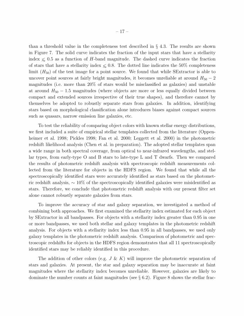
– 17 –

than a threshold value in the completeness test described in § 4.3. The results are shown

in Figure 7. The solid curve indicates the fraction of the input stars that have a stellarity

index ∼< 0.5 as a function of H-band magnitude. The dashed curve indicates the fraction

of stars that have a stellarity index ∼< 0.8. The dotted line indicates the 50% completeness

limit (H50) of the test image for a point source. We found that while SExtractor is able to

uncover point sources at fairly bright magnitudes, it becomes unreliable at around H50 − 2

magnitudes (i.e. more than 20% of stars would be misclassified as galaxies) and unstable

at around H50 − 1.5 magnitudes (where objects are more or less equally divided between

compact and extended sources irrespective of their true shapes), and therefore cannot by

themselves be adopted to robustly separate stars from galaxies. In addition, identifying

stars based on morphological classification alone introduces biases against compact sources

such as quasars, narrow emission line galaxies, etc.

To test the reliability of comparing object colors with known stellar energy distributions,

we first included a suite of empirical stellar templates collected from the literature (Oppen-

heimer et al. 1998; Pickles 1998; Fan et al. 2000; Leggett et al. 2000) in the photometric

redshift likelihood analysis (Chen et al. in preparation). The adopted stellar templates span

a wide range in both spectral coverage, from optical to near-infrared wavelengths, and stel-

lar types, from early-type O and B stars to late-type L and T dwarfs. Then we compared

the results of photometric redshift analysis with spectroscopic redshift measurements col-

lected from the literature for objects in the HDFS region. We found that while all the

spectroscopically identified stars were accurately identified as stars based on the photomet-

ric redshift analysis, ∼ 10% of the spectroscopically identified galaxies were misidentified as

stars. Therefore, we conclude that photometric redshift analysis with our present filter set

alone cannot robustly separate galaxies from stars.

To improve the accuracy of star and galaxy separation, we investigated a method of

combining both approaches. We first examined the stellarity index estimated for each object

by SExtractor in all bandpasses. For objects with a stellarity index greater than 0.95 in one

or more bandpasses, we used both stellar and galaxy templates in the photometric redshift

analysis. For objects with a stellarity index less than 0.95 in all bandpasses, we used only

galaxy templates in the photometric redshift analysis. Comparison of photometric and spec-

troscopic redshifts for objects in the HDFS region demonstrates that all 11 spectroscopically

identified stars may be reliably identified in this procedure.

The addition of other colors (e.g. J & K) will improve the photometric separation of

stars and galaxies. At present, the star and galaxy separation may be inaccurate at faint

magnitudes where the stellarity index becomes unreliable. However, galaxies are likely to

dominate the number counts at faint magnitudes (see § 6.2). Figure 8 shows the stellar frac-

– 18 –

tion in the HDFS and CDFS regions based on the results of the star and galaxy separation.

Closed circles indicate the mean surface density of galaxies observed in the two fields (see

§ 6.2 for a detailed discussion); stars indicate the surface density of stellar objects in the

HDFS region; and open triangles indicate the surface density of stellar objects in the CDFS

region. It shows that the star counts increase gradually with the H magnitude, while the

galaxy counts show a much steeper slope. The smooth, shallower slope of the star counts

suggests that stars do not contribute a significant fraction at H ∼> 19 in both HDFS and

CDFS fields.

5. The Catalogs

The H-band imaging survey presently covers 1.1 square degrees of sky to a mean 5 σ

detection limit in a four arcsecond diameter aperture of H ∼ 20.8. Here we present sample

near-infrared and optical photometric measurements for objects identified in the HDFS and

CDFS regions. We have performed object detection in all bandpasses and identified ∼ 24, 000

galaxies over 847 arcmin2 in the HDFS region, of which ∼ 6, 700 are detected in the H-band

survey, and ∼ 30, 000 galaxies over 561 arcmin2 in the CDFS region, of which ∼ 7, 400 are

detected in the H-band survey. Among the H-detected galaxies in the two regions, ∼ 2, 000

have I − H > 3 and are likely to be primarily evolved galaxies at redshifts z > 1.

The catalogs for each field is organized as follows: For each object we give an identifica-

tion number, x and y pixel coordinates in the optical images, α (J2000) & δ (J2000), the Kron

radius (in arcseconds) for each filter, the stellarity index determined by SExtractor, 2′′

and

4′′

diameter aperture magnitudes and their associated uncertainties, the corrected isophotal

magnitude, auto magnitude and the best magnitude and their assocaited uncertainties as pro-

vided by SExtractor for all the objects detected in each filter. We present an example of the

object catalog in Table 4 and an example of the photometric catalog in Table 5, which list the

first 50 objects identified in the CDFS region. Complete near-infrared and optical photomet-

ric catalogs of the two fields may be accessed at http://www.ociw.edu/lcirs/catalogs.html.

Catalogs for the remaining fields and their completeness limits will be posted at this address

as they become available.

6. Discussion

As we identify objects in each optical and near-infrared bandpass the catalogs contain

objects with a wide range of colors, ranging from the reddest objects, whether they be old

– 19 –

or dusty, to the most actively star forming systems. The full galaxy sample is therefore

representative of galaxies of a wide range of stellar properties and redshifts, and may be

used to address a variety of cosmological issues. Here we examine photometric properties

of the H-band selected objects and derive the number-magnitude relation for the H-band

selected galaxies as well as for red galaxies of different optical and near-infrared colors. We

compare our measurements with various model predictions and discuss the implications.

6.1. Distributions of Optical and Near-infrared Colors

We present the I−H versus H-band color–magnitude diagram for the ∼ 14, 000 H-band

selected galaxies identified in the HDFS and CDFS regions in Figure 9. Objects classified

as stars are not included. We show the 95% completeness limit of the H-band data in the

short dashed line and the 5 σ detection threshold over a four arcsecond diameter aperture for

the I-band images of the HDFS and CDFS regions in the dot-dashed lines. We also present

the expected color–magnitude evolution of an L∗ elliptical galaxy from z = 2 to the present

time under different evolution scenarios for h = 0.7. The curves trace the trajectories of

a non-evolving elliptical galaxy spectrum (blue), a passively evolving galaxy formed in a

single burst at z = 10 (red), and a galaxy formed at z = 30 with an exponentially declining

star formation rate (SFR ∼ exp(−t/τ)) for τ = 1 Gyr (green). The blue dashed curve

corresponds to a non-evolving 3 L∗ early-type galaxy.

Comparisons of measurements and model predictions show that the I − H colors of

galaxies with H ∼< 18 agree well with the expected colors at low redshifts. In addition, they

show that the median color becomes progressively bluer at fainter magnitudes, accompanied

by a tail of galaxies with very red colors (I − H ∼> 3). These red galaxies constitute a

negligible fraction of the total population at H ∼ 18, but become a significant constituent

by H ∼ 20. Similar trends are seen in B −K, R −K and I −K color–magnitude diagrams

based on smaller area surveys (Elston et al. 1988; Cowie et al. 1994; Ellis 1997; Cowie et al.

1997, Menanteau et al. 1999). Furthermore, the good agreements between observed colors

and model predictions suggest that these red galaxies are mildly evolving early-type galaxies

at z ∼ 1 sampled over the bright end of the luminosity function (∼ 1 − 5 L∗). The red

sequence observed in clusters with z ∼ 0.8−1.2 populate a similar range in the I −H vs. H

color–magnitude diagram, supporting the idea that the bulk of the red galaxies are evolved

early-type galaxies at intermediate redshifts (e.g. Stanford et al. 1997, 1998; Chapman,

McCarthy, & Persson 2000).

We present the V −I vs. I−H color–color distribution of the H-band detected objects in

the HDFS and CDFS regions in Figure 10. Stars that were classified according to the criteria

– 20 –

described in § 4.5, are indicated by crosses and galaxies are indicated by filled circles. Open

circles indicate galaxies that are not detected in V . The solid curves trace the trajectories of

different CWW spectral templates at redshifts from z = 2 to the present time: elliptical/S0

(yellow), Sab (green), Scd (cyan), and irregular (blue). The dotted curve shows the trajectory

of a passively evolving galaxy formed in a single burst at redshift zf = 10. The short and

long dashed curves trace the colors of galaxies formed at zf = 30 with exponentially declining

star formation rates for τ = 1 and 2 Gyr, respectively. The dash-dotted line corresponds to

a galaxy formed at zf = 30 with a constant star formation rate. Filled circles along each

curve indicate the corresponding redshifts, starting from z = 2 in the lower right corner,

evolving toward lower redshifts in steps of ∆z = 0.5, and ending at z = 0 in the lower left

corner.

The general agreement between distributions of various model predictions and measure-

ments of galaxies in our catalog, and the clear separation of the stellar sequence suggest that

most stars have been accurately identified in these two survey fields. A similar separation

is made in a B − I vs. I − K color–color diagram (e.g. Gardner 1992; Huang et al. 1997).

The large scatter in the V − I colors spanned by the galaxies reveals a wide range of star

formation histories for which our simple models provide only an idealized description. In

particular, the large scatter in the V − I colors for galaxies of I − H colors indicative of

redshifts z ∼ 1 suggest a significant amount of ongoing star formation in these galaxies.

Similar results are found in detailed studies of morphologically selected early-type galaxies

at intermediate redshifts that reveal a deficit of distant ellipticals with optical and UV colors

that match with expectations based on passively evolving galaxies formed at high redshifts

(e.g. Menanteau et al. 1999; Menanteau, Abraham, & Ellis 2001). In addition, the small

number (< 15%) of galaxies with I − H ∼> 3 and V − I ∼> 3 suggests that there are few

objects that may be adequately characterized as pure passively evolving systems formed at

high redshifts. The trajectories of the evolving galaxy models in the color–color diagram

suggests that these red galaxies span a significant range in redshift and that those of bluer

V − I colors largely arise at redshifts z ∼> 1.5. This is supported by their angular clustering

amplitude (McCarthy et al. 2001b) and photometric redshift measurements (Chen et al. in

preparation).

6.2. The H-band Number Counts

Galaxy number counts provide a diagnostic for distinguishing between different evolu-

tionary scenarios for galaxies of different colors (e.g. Metcalfe et al. 1996). Comparisons of

number count measurements from different surveys also allow us to examine the accuracy of

– 21 –

our photometric calibration. Figure 11 shows the H-band differential galaxy counts N(m)

derived from ∼ 14, 000 galaxies selected in the H-band survey toward the HDFS and CDFS

regions (filled circles). We applied incompleteness corrections down to the 95% completeness

level using the incompleteness curves determined for compact and extended sources in each

tile. According to the procedures described in § 4.3, we adopted the stellarity index deter-

mined in SExtractor for each object and corrected for the incompleteness at faint magnitudes

using the compact source incompleteness curve for objects of stellarity index greater than

0.5 and using the extended source incompleteness curve otherwise. The vertical bars indi-

cate the uncertainties in our measurements estimated using a variation of the “bootstrap”

resampling technique. The bootstrap resampling technique explicitly accounts for the sam-

pling error and for photometric uncertainties. We first resampled objects from the parent

catalog (allowing for the possibility of duplication) and added random noise (within the

photometric uncertainties) to the photometry. Then we estimated the H-band differential

number counts for the resampled, perturbed catalog. Finally, we repeated the procedures a

thousand times and determined the 1 σ uncertainties based on the 16th and 84th percentiles

of the distributions in each magnitude bin.

For comparison, we have also included in Figure 11 previous H-band measurements

reported by various groups. Our measurements span six magnitudes in H and nicely bridge

the gap between the existing measurements at the bright (open squares from Martini 2001b)§

and faint ends (Yan et al. 1998). The excellent agreements in both the slopes and the normal-

ization demonstrate not only the accuracy of our H-band photometry, but also the accuracy

in our star and galaxy separation. The best fitting power-law slopes, d log N(m)/dm, were

found to be 0.45 ± 0.01 mag−2 at H ∼< 19 and 0.27 ± 0.01 mag−2 at H ∼> 19 with a mean

surface density of ≈ 7, 200 degree−2 mag−1 at H = 19¶. The slope of the faint-end H-band

counts is in line with that of the faint-end K-band counts (Cowie et al. 1994; Djorgovski et

al. 1995; Bershady, Lowenthal, & Koo 1998; Metcalfe et al. 1996; McCracken et al. 2000).

The slope of the bright-end H-band counts (H ∼< 19) is slightly shallower than that of

the bright-end K-band counts reported by Huang et al. (1997) and Metcalfe et al. (1996),

although we note that our counts are not well determined at H < 16.

§Part of the apparent excess in the number count measurements by Martini (2001b) is due to an additional

aperture correction that the author applied in the galaxy photometry to account for missing light in the

wings of galaxy profiles, which was found to be between 0.1 and 0.2 mag.

¶We note that the uncertainties in the number count measurements due to random errors are small

given the large sample from our survey, but sysmatic errors are likely to dominate and more difficult to

measure. In particular, number count measurements at the faintest magnitude bins are more likely to be

overestimated due to photometric undertainties of the even fainter and more abundant populations. As a

result, the faint-end slope is likely to be overestimated.

– 22 –

To compare with simple model predictions, we considered a no-evolution model based

on an early-type galaxy template (the solid curve), a passive evolution scenario for galaxies

formed in a single burst at zf = 10 (the dotted curve), an exponentially declining star

formation for galaxies formed at zf = 30 (the short dashed curve), and a constant star

formation for galaxies formed at zf = 30 (the long dashed curve). We adopted the K-

band luminosity function derived by Gardner et al. (1997) and applied an H − K ≈ 0.22

color correction (Mobasher, Ellis, & Sharples 1986) to obtain an estimate for MH∗. This

is appropriate for galaxies of different type because the k-correction is nearly independent

of spectral type at near-infrared wavelengths. We find that all but the passive evolution

scenario (the dotted curve) agree well with the measurements.

6.3. Surface Density of Red Galaxies

In this section, we present surface density estimates of moderately red galaxies of I−H ∼>

3 and compare the measurements with those of extremely red objects (EROs) identified in

the survey. EROs are typically selected based on their extreme optical and near-infrared

colors R−K ∼> 6 (e.g. Elston, Rieke, & Rieke 1988; McCarthy, Persson, & West 1992; Hu &

Ridgway 1994). Here we selected EROs using R−H ∼> 5, which according to the simulations

presented in Figure 1 is equivalent to R − K ∼> 6 for high-redshift evolved populations.

Figure 12 shows the H-band differential number counts for galaxies of I −H ∼> 3 (filled

circles) and for galaxies of R − H ∼> 5 (squares) identified in the HDFS and CDFS regions.

Incompleteness corrections were applied at faint magnitudes and the uncertainties indicated

by the vertical bars were estimated following the same procedures described in § 6.2. The

slope of the red counts is quite steep, d log N(m)/dm = 0.84 ± 0.06 mag−2 for galaxies of

I − H ∼> 3 and 0.89 ± 0.24 mag−2 for galaxies of R − H ∼> 5 at H ∼< 20. The counts appear

to have shallower faint-end slopes for both of the red subsamples—between 0.17 and 0.32

mag−2—at H ∼> 20. While both subsamples show consistent slopes at the bright end, they

have a more steeply rising N(m) with the H magnitude than the total H-band detected

population. The steeper bright-end slope of the red galaxies indicates that most of the

foreground (z ∼< 1) galaxies have been effectively excluded from the red samples and that

the shape of the number counts reflects the shape of the bright-end luminosity function of the

red population. In addition, the consistent slopes between the two red subsamples suggest

that the underlying luminosity function is very similar.

For comparison, we also calculated the predicted differential number counts for red

galaxies with I − H ∼> 3 based on the no-evolution scenario and the exponentially declining

star formation scenario with τ = 1 Gyr that best fit the observed total H-band number

– 23 –

counts, as discussed in § 6.2. To model the intrinsic luminosity function of evolved galaxies,

we adopted the population ratio of elliptical galaxies in the local universe (e.g. Binggeli,

Sandage, & Tammann 1988). We first scaled the K-band luminosity function obtained by

Gardner et al. (1997) for the total galaxy population by M∗(red) = M∗(tot) − 0.2 and

φ∗(red) = 0.2 φ∗(tot) and then assumed a faint-end slope of α = 1. The curves indicate

the results of the calculations and are the same as those in Figure 11. It appears that both

scenarios fit the observations fairly well, but that the exponentially declining star formation

model predicts a sharp turnover in the differential number counts at H ∼> 21. The turnover

is due to the fact that at these faint magnitudes the evolved population is dominated by

those at redshifts z ∼> 2 where they would have bluer I − H colors under the exponentially

declining star formation scenario and would therefore be excluded based on the I − H ∼> 3

selection criterion (see Figure 9). Because of large uncertainties in the optical and H-band

photometry for galaxies at these faint magnitudes, we cannot rule out either of the scenarios.

The moderately good agreements between observations and model predictions, together with

the large scatter in the optical V − I color discussed in § 6.1, however suggest that there is

still some amount of star formation going on in the red population at redshifts z > 1.

In Figure 13 we plot the cumulative surface density measurements of galaxies with

I −H ∼> 3 (filled circles) and of R−H ∼> 5 (squares) as a function of H-band magnitude, in

comparison with those of the total H-band selected galaxies and with previous measurements

of EROs presented by Daddi et al. (2000; green squares), Yan et al. (2000; blue triangles),

and Thompson et al. (1999; red cross). Our surface density measurements of EROs span

two magnitudes in H and are consistent with those from previous surveys. In addition, we

find that red galaxies with I − H ∼> 3 constitute ≈ 20% of the H-band detected galaxies

at H ∼< 21, but only ≈ 2% at H ∼< 19. Specifically, we expect to observe on average ∼ 40

galaxies of I−H ∼> 3 and ∼ 8 galaxies of R−H ∼> 5 among ∼ 270 H-band detected galaxies

at H ∼< 21, but only ∼ 1 galaxy of I − H ∼> 3 and less than one of R − H ∼> 5 among ∼ 46

H-band detected galaxies at H ∼< 19 in a random 25-arcmin2 region.

On the other hand, because EROs and these moderately red galaxies are found to exhibit

strong angular clustering (Daddi et al. 2000; McCarthy et al. 2001b; Firth et al. 2001), a

large disperson in the surface density measurements is expected. To examine the accuracy

of the surface density measurements presented in Figure 13, we estimated the field to field

variation by measuring the surface density of galaxies of I − H ∼> 3 in a randomly selected

5 × 5 arcmin2 region in each tile and compared the measurements between different tiles.

We found that the total number of red galaxies of H ∼< 20.5 varies from ≈ 15 to ≈ 40 with

a mean surface density of ≈ 1 arcmin−2 and an rms dispersion of ≈ 0.4 arcmin−2. The

mean surface density estimated based on the randomly selected smaller areas is consistent

with the measurements presented in Figure 12 and the red counts over 0.62 square degrees

– 24 –

presented in McCarthy et al. (2001a,b), indicating that our surface density measurements

are not significantly affected by the cosmic variance due to clustering. In addition, following

Roche et al. (1999), we estimate an angular clustering amplitude of these red galaxies to be

A ≈ 4 at 1′′ (corresponding to a correlation angle of θ0 ≈ 5 arcsec), which indeed agrees

well with the results of an angular clustering analysis presented in McCarthy et al. (2001b).

We therefore conclude that a deep, wide-field survey is necessary not only to identify a large

number of red galaxies, but also to obtain accurate estimates of their statistical properties.

7. Summary

We present initial results from the Las Campanas Infrared Survey, which is a wide-

field near-infrared and optical imaging survey designed to reliably identify a statistically

significant and representative sample of evolved galaxies at redshifts z > 1 and to secure a

uniform sample of galaxies of all types at intermediate redshifts. We present sample near-

infrared and optical photometric catalogs for objects identified in two of the six survey fields,

surrounding the Hubble Deep Field South and Chandra Deep Field South regions. We have

identified ∼ 14,000 H-band detected galaxies over 1,408 arcmin2 of sky, ∼ 2,000 of which

are likely to be evolved galaxies at z ∼> 1 with I − H ∼> 3. Furthermore, we find that:

1. Red galaxies with I − H ∼> 3 are a significant constituent of galaxies with H ∼> 20

and are consistent with mildly evolving early-type galaxies at z ∼ 1. But there exists a large

scatter in the V − I colors spanned by the red galaxies, indicating a significant amount of

on-going star formation in these galaxies.

2. The differential number counts N(m) for the H-band detected objects has a slope of

d log N(m)/dm = 0.45 ± 0.01 mag−2 at H ∼< 19 and 0.27 ± 0.01 mag−2 at H ∼> 19 with a

mean surface density ≈ 7, 200 degree−2 mag−1 at H = 19.

3. The differential number counts for red objects (I − H ∼> 3) detected in the H-band

has a very steep slope, d log N(m; I − H ∼> 3)/dm = 0.84 ± 0.06 mag−2 at H ∼< 20 and

0.32 ± 0.07 mag−2 at H ∼> 20, with a mean surface density ≈ 3, 000 degree−2 mag−1 at

H = 20.

4. Red galaxies (I − H ∼> 3) constitute ≈ 20% of the H-band detected galaxies at

H ∼< 21, but only ≈ 2% at H ∼< 19. This suggests that foreground galaxies (z ∼< 1) may be

effectively excluded from the total H-band population by apply the I − H color selection

criterion and that the steep bright-end slope of red galaxy number counts reflects the shape

of the bright-end luminosity function of the red population.

– 25 –

5. Red galaxies are strongly clustered, producing strong field to field variation in their

surface density. We estimate a mean surface density of ≈ 1 arcmin−2 with an rms dispersion

of ≈ 0.4 arcmin−2 over 5× 5 arcmin2 sky regions for galaxies with H ∼< 20.5 and I −H ∼> 3,

implying an angular clustering amplitude of A ≈ 4 at 1′′ and a correlation angle of θ0 ≈ 5

arcsec.

We are grateful to Xiaohui Fan, Sandy Leggett, and Ben Oppenheimer for providing

various digitized stellar templates of M dwarfs, L dwarfs, and T dwarfs, and to Ken Lanzetta

for providing galaxy templates for the photometric redshift analysis. We appreciate the

expert assistance from the staffs of the Cerro Tololo Inter-American Observatory and Las

Campanas Observatory. This research was supported by the National Science Foundation

under grant AST-9900806. The CIRSI camera was made possible by the generous support

of the Raymond and Beverly Sackler Foundation.

– 26 –

REFERENCES

Barger, A. J., Cowie, L. L., Trentham, N., Fulton, E., Hu, E. M., Songaila, A., Hall, D. 1999,

AJ, 117, 102

Beckett, M. G., Mackay, C. D., McMahon, R. G., Parry, I. R., Ellis, R. S., Chan, S. J., &

Hoenig, M. 1998, in Infrared Astronomical Instrumentation, ed. Fowler, A.M., Proc.

SPIE, 3354, p. 14

Benitez, N., Broadhurst, T. J., Bouwens, R. J., Silk, J., & Rosati, P. 1999, ApJ, 515, L65

Bershady, M., Lowenthal, J., & Koo, D. C. 1998, ApJ, 505, 50

Bertin, E. & Arnouts, S. 1996, A&AS, 117, 393

Binggeli, B., Sandage, A., & Tammann, G. A. 1988, ARAA, 26, 509

Blain, A. W., Kneib, J.-P., Ivison, R. J., & Smail, I. 1999, ApJ, 512, 87

Broadhurst, T. J. & Bouwens, R. J. 2000, ApJ, 530, 53

Bruzual, A. G. & Charlot, S. 1993, ApJ, 405, 538

Chapman, S. C., McCarthy, P. J., & Persson, S. E. 2000, AJ, 120, 1612

Coleman, G. D., Wu, C. C., & Weedman, D. W. 1980, ApJS, 43, 393

Connolly, A. J., Szalay, A. S., Dickinson, M., Subbarao, M. U., & Brunner, R. J. 1997, ApJ,

486, L11

Cowie, L. L., Gardner, J. P., Hu, E. M., Songaila, A., Hodapo, K.-W., & Wainscoat, R. J.

1994, ApJ, 434, 114

Cowie, L. L., Songaila, A., Hu, E., Cohen, J. G. 1997, AJ, 112, 839

da Costa, L.N. 2001, in in ”VLT Opening Symposium”, eds, J. Bergeron and A. Renzini, p.

192

da Costa, L. Nonino, M., Rengelink, R. et al. 2001, A&A submitted (astro-ph/9812190)

Daddi, E., Cimmatti, A., Pozzetti, L., Hoekstra, H., Rottgering, H. J. A., Renzini, A.,

Zamorani, G., & Mannucci, F. 2000, A&A, 361, 535

Dalcanton, J. J. 1998, ApJ, 495, 251

De Propris, R., Eisenhardt, P. R., Stanford, S. A., & Dickinson, M. 1998, ApJ, 503, L45

Djorgovski, S., Soifer, B. T., Pahre, M. A., Larkin, J. E., Smith, J. D., Neugebauer, G.,

Smail, I., Matthews, K., Hogg, D. W., Blandford, R. D., Cohen, J., Harrison, W., &

Nelson, J. 1995, ApJ, 438, L13

Eggen, O. J., Lynden-Bell, D., & Sandage, A. R. 1962, ApJ, 136, 748

– 27 –

Ellis, R. S. 1997, ARA&A, 35, 389

Elston, R., Rieke, G. H., & Rieke, M. J. 1988, ApJ, 331, L77

Elston, R. 1998, in Infrared Astronomical Instrumentation, ed. Fowler, A.M., Proc. SPIE,

3354, p. 404

Fan, X. et al. 2000, AJ, 119. 928

Fernandez-Soto, A., Lanzetta, K. M., & Yahil, A. 1999, ApJ, 513, 34

Fernandez-Soto, A., Lanzetta, K. M., Chen, H.-W., Pascarelle, S. M., & Yahata, N. 2001,

ApJS, 135, 41

Firth, A. E., Somerville, R., & McMahon, R. G. et al. 2001, MNRAS submitted

Franceschini, A., Silva, L., Fasano, G., Granato, L., Bressan, A., Arnouts, S., & Danese, L.

1998, ApJ, 506, 600

Fukugita, M., Shimasaku, K., & Ichikawa, T. 1995, PASP, 107, 945

Gardner, J. P. 1992, PhD. Thesis, Univ. of Hawaii

Gardner, J. P., Sharples, R. M., Carrasco, B. E., & Frenk, C. S. 1996, MNRAS, 282, L1

Gardner, J. P., Sharples, R. M., Frenk, C. S., & Carrasco, B. E. 1997, ApJ, 480, L99

Graham, J. R. & Dey, A. 1996, ApJ, 471, 720

Gunn, J. E. et al. 2001, SDSS Early Release Catalog

Hu, E. M. & Ridgway, S. E. 1994, AJ, 107, 1303

Huang, J. -S., Cowie, L. L., Gardner, J. P., Hu, E. M., Songaila, A., & Wainscoat, R. J.

1997, ApJ, 476, 12

Jannuzi, B. & Dey, A. et al. 1998, http://www.noao.edu/noao/noaodeep/

Kauffmann, G., Charlot, S., & White, S. D. M. 1996, MNRAS, 283, 117

Kauffmann, G. & Charlot, S. 1998, MNRAS, 297, L23

Kron, R. G. 1980, ApJS, 43, 305

Landolt, A. U. 1992, AJ, 104, 340

Lanzetta, K. M., Fernandez-Soto, A., & Yahil, A. 1998, in “The Hubble Deep Field, Proceed-

ings of the Space Telescope Science Institute 1997 May Symposium,” ed. M. Livio, S.

M. Fall, & P. Madau (Cambridge: Cambridge University Press), P. 143

Leggett, S. K., Allard, F., Dahn, C., Hauschildt, P. H., Kerr, T. H., & Rayner, J. 2000, ApJ,

535, 965

– 28 –

Lin, H., Yee, H. K. C., Carlberg, R. G., Morris, S. L., Sawicki, M., Patton, D. R., Wirth,

G., & Shepherd, C. W. 1999, ApJ, 518, 533

Martini, P. 2001a, AJ, 121, 2301

Martini, P. 2001b, AJ, 121, 598

Marzke, R. O., McCarthy, P. J., & Persson, S. E. et al. 1999, in ”Photometric Redshifts and

High Redshift Galaxies”, eds. R. Weymann, L. Storrie-Lombardi, M. Sawicki, & R.

Brunner. A.S.P. Conf. Series vol. 191, p. 148

McCarthy, P. J., Persson, S. E. & West, S. C. 1992, ApJ, 386, 52

McCarthy, P. J., Carlberg, R. G., Marzke, R. O., & Chen, H.-W. et al. 2001a, in the

proceedings of the ESO/ECF/STScI workshop ”Deep Fields” (astro-ph/0011499)

McCarthy, P. J., Carlberg, R. G., Chen, H.-W., & Marzke, R. O. et al. 2001b, ApJL in press

McCracken, H.J., Metcalfe , N., Shanks, T., Campos, A., Gardner, J.P., Fong, R., 2000,

MNRAS, 311, 707

Menanteau, F., Ellis, R. S., Abraham, R. G., Barger, A. J., & Cowie, L. L. 1999, MNRAS,

309, 208

Menanteau, F., Abraham, R. G., & Ellis, R. S. 2001, MNRAS, 322, 1

Metcalfe, N., Shanks, T., Campos, A., Fong, R., & Gardner, J. P. 1996, Nature, 383, 236

Mink, D. J. 1999, in Astronomical Data Analysis Software and Systems VIII, eds. Dave

Mehringer, Ray Plante, & Doug Roberts, vol. 172, p. 498

Mobasher, B., Ellis, R. S., & Sharples, R. M. 1986, MNRAS, 223, 11

Moffat, A. F. J. 1969, A&A, 3, 455

Moorwood, A., Cuby, J. G., & Lidman, C. 1998, Messenger, 91, 9

Oppenheimer, B. R., Kulkarni, S. R., Matthews, K., & van Kerkwijk, M. H. 1998, ApJ, 502,

932

Persson, S. E., Murphy, D. C., Krzeminski, W., Roth, M., & Rieke, M. J. 1998, AJ, 116,

2475

Persson, S. E., Murphy, C. D., Gunnels, S., Birk, C., Bagish, A., & Koch, E. 2001, AJ

submitted

Pickles, A. J. 1998, PASP, 110, 863

Roche, N., Eales, S. A., Hippelein, H., & Willott, C. J. 1999, MNRAS, 306, 538

Ryan, S. G. 1989, AJ, 98, 1693

– 29 –

Sabbey, C. N., McMahon, R. G., Lewis, J. R., & Irwin, M. J. 2001, in Astronomical Data

Analysis and Software Systems X, ed. F. R. Harnden, Jr., F. A. Primini, & H. E.

Payne (San Francisco: ASP) (astro-ph/0101181)

Sawicki, M. J., Lin, H., & Yee, H. K. C. 1997, AJ, 113, 1

Schade, D., Carlberg, R. G., Yee, H. K. C., & Lopez-Cruz, O. 1996, ApJ, L103

Schade, D., Lilly, S. J., Crampton, D., Ellis, R. S., Le Fevre, O., Hammer, F., Brinchmann,

J., Abraham, R., Colles, M., Glazebrook, K., Tresse, L., & Broadhurst, T. 1999, ApJ,

525, 31

Smail, I., Ivison, R. J., & Blain, A. W. 1997, ApJ, 490, L5

Stanford, S. A., Elston, R., Eisenhardt, P. R., Spinrad, H., Stern, D., & Dey, A. 1997, AJ,

114, 2232

Stanford, S. A., Eisenhardt, P. R., & Dickinson, M. 1998, ApJ, 492, 461

Steidel, C. C., Adelberger, K. L., Giavalisco, M., Dickinson, M., & Pettini, M. 1999, ApJ,

519, 1

Teplitz, H., Hill, R. S., Malumuth, E. M., Collins, N. R., Gardner, J. P., Palunas, P., &

Woodgate, B. E. 2001, ApJ, 548, 127

Thompson, D., Beckwith, S. V. W., Fockenbrock, R., Fried, J., Hippelein, H., Huang, J.-

S., von Kuhlmann, B., Leinert, Ch., Meisenheimer, K., Phleps, S., Roser, H.-J.,

Thommes, E., Wolf, C. 1999, ApJ, 523, 100

Totani, T. & Yoshii, J. 1997, ApJ, 501, L177

White, S. D. M. & Rees, M. J. 1978, MNRAS, 183, 341

Yan, L., McCarthy, P. J., Storrie-Lombardi, L. J., & Weymann, R. J. 1998, ApJ, 503, L19

Yan, L., McCarthy, P. J., Weymann, R. J., Malkan, M. A., Teplitz, H. I., Storrie-Lombardi,

L. J., Smith, M., & Dressler, A. 2000, AJ, 120, 575

Zepf, S. E. 1997, Nature, 390, 377

This preprint was prepared with the AAS LATEX macros v4.0.

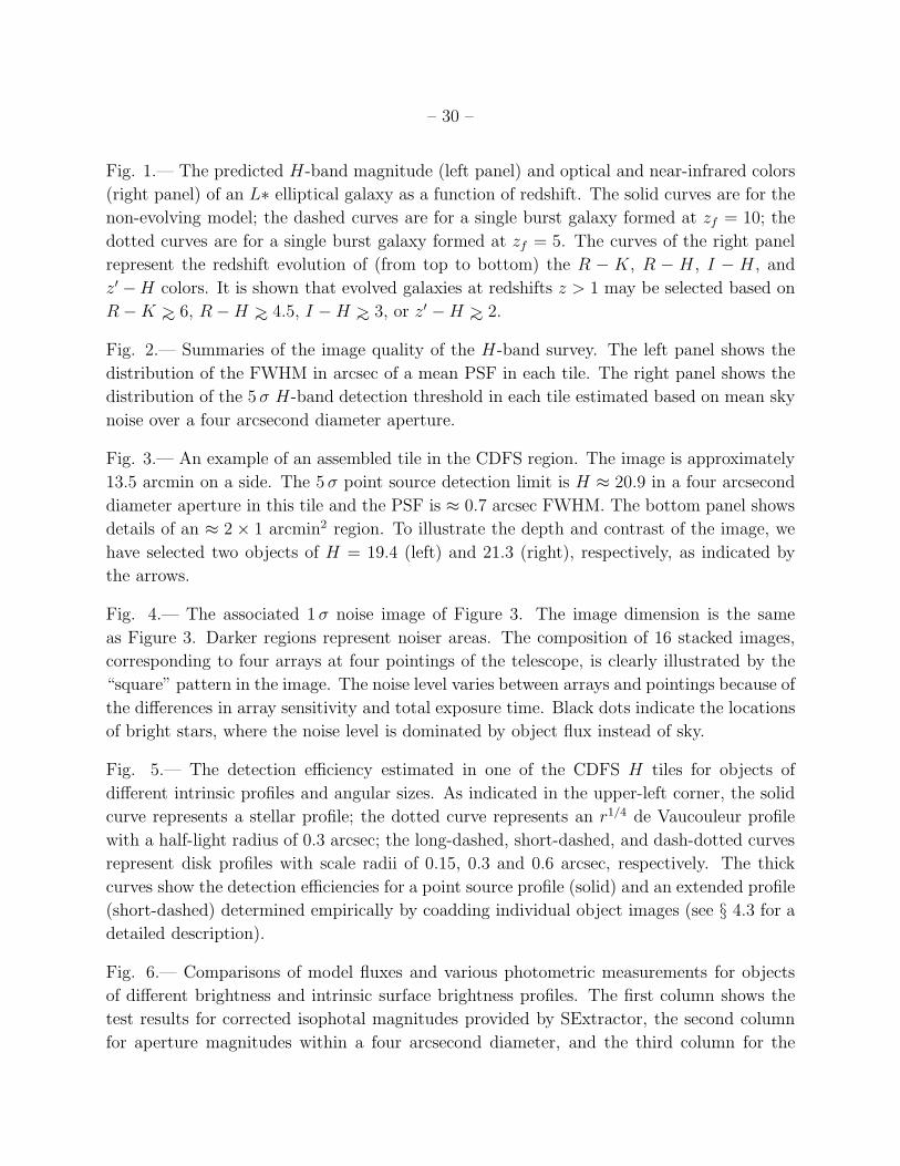
– 30 –

Fig. 1.— The predicted H-band magnitude (left panel) and optical and near-infrared colors

(right panel) of an L∗ elliptical galaxy as a function of redshift. The solid curves are for the

non-evolving model; the dashed curves are for a single burst galaxy formed at zf = 10; the

dotted curves are for a single burst galaxy formed at zf = 5. The curves of the right panel

represent the redshift evolution of (from top to bottom) the R − K, R − H , I − H , and

z′ −H colors. It is shown that evolved galaxies at redshifts z > 1 may be selected based on

R − K ∼> 6, R − H ∼> 4.5, I − H ∼> 3, or z′ − H ∼> 2.

Fig. 2.— Summaries of the image quality of the H-band survey. The left panel shows the

distribution of the FWHM in arcsec of a mean PSF in each tile. The right panel shows the

distribution of the 5 σ H-band detection threshold in each tile estimated based on mean sky

noise over a four arcsecond diameter aperture.

Fig. 3.— An example of an assembled tile in the CDFS region. The image is approximately

13.5 arcmin on a side. The 5 σ point source detection limit is H ≈ 20.9 in a four arcsecond

diameter aperture in this tile and the PSF is ≈ 0.7 arcsec FWHM. The bottom panel shows

details of an ≈ 2 × 1 arcmin2 region. To illustrate the depth and contrast of the image, we

have selected two objects of H = 19.4 (left) and 21.3 (right), respectively, as indicated by

the arrows.

Fig. 4.— The associated 1 σ noise image of Figure 3. The image dimension is the same

as Figure 3. Darker regions represent noiser areas. The composition of 16 stacked images,

corresponding to four arrays at four pointings of the telescope, is clearly illustrated by the

“square” pattern in the image. The noise level varies between arrays and pointings because of

the differences in array sensitivity and total exposure time. Black dots indicate the locations

of bright stars, where the noise level is dominated by object flux instead of sky.

Fig. 5.— The detection efficiency estimated in one of the CDFS H tiles for objects of

different intrinsic profiles and angular sizes. As indicated in the upper-left corner, the solid

curve represents a stellar profile; the dotted curve represents an r1/4 de Vaucouleur profile

with a half-light radius of 0.3 arcsec; the long-dashed, short-dashed, and dash-dotted curves

represent disk profiles with scale radii of 0.15, 0.3 and 0.6 arcsec, respectively. The thick

curves show the detection efficiencies for a point source profile (solid) and an extended profile

(short-dashed) determined empirically by coadding individual object images (see § 4.3 for a

detailed description).

Fig. 6.— Comparisons of model fluxes and various photometric measurements for objects

of different brightness and intrinsic surface brightness profiles. The first column shows the

test results for corrected isophotal magnitudes provided by SExtractor, the second column

for aperture magnitudes within a four arcsecond diameter, and the third column for the

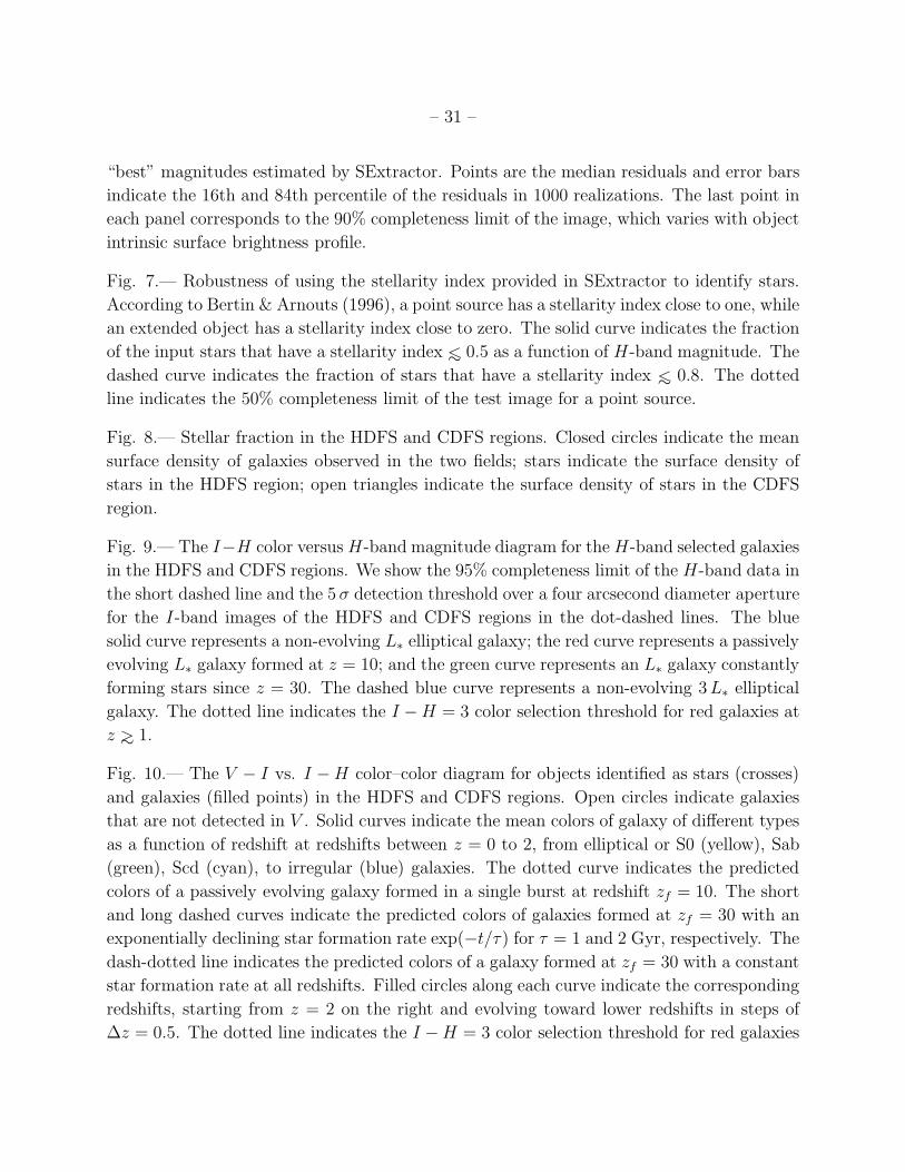
– 31 –

“best” magnitudes estimated by SExtractor. Points are the median residuals and error bars

indicate the 16th and 84th percentile of the residuals in 1000 realizations. The last point in

each panel corresponds to the 90% completeness limit of the image, which varies with object

intrinsic surface brightness profile.

Fig. 7.— Robustness of using the stellarity index provided in SExtractor to identify stars.

According to Bertin & Arnouts (1996), a point source has a stellarity index close to one, while

an extended object has a stellarity index close to zero. The solid curve indicates the fraction

of the input stars that have a stellarity index ∼< 0.5 as a function of H-band magnitude. The

dashed curve indicates the fraction of stars that have a stellarity index ∼< 0.8. The dotted

line indicates the 50% completeness limit of the test image for a point source.

Fig. 8.— Stellar fraction in the HDFS and CDFS regions. Closed circles indicate the mean

surface density of galaxies observed in the two fields; stars indicate the surface density of

stars in the HDFS region; open triangles indicate the surface density of stars in the CDFS

region.

Fig. 9.— The I−H color versus H-band magnitude diagram for the H-band selected galaxies

in the HDFS and CDFS regions. We show the 95% completeness limit of the H-band data in

the short dashed line and the 5 σ detection threshold over a four arcsecond diameter aperture

for the I-band images of the HDFS and CDFS regions in the dot-dashed lines. The blue

solid curve represents a non-evolving L∗ elliptical galaxy; the red curve represents a passively

evolving L∗ galaxy formed at z = 10; and the green curve represents an L∗ galaxy constantly

forming stars since z = 30. The dashed blue curve represents a non-evolving 3 L∗ elliptical

galaxy. The dotted line indicates the I −H = 3 color selection threshold for red galaxies at

z ∼> 1.

Fig. 10.— The V − I vs. I − H color–color diagram for objects identified as stars (crosses)

and galaxies (filled points) in the HDFS and CDFS regions. Open circles indicate galaxies

that are not detected in V . Solid curves indicate the mean colors of galaxy of different types

as a function of redshift at redshifts between z = 0 to 2, from elliptical or S0 (yellow), Sab

(green), Scd (cyan), to irregular (blue) galaxies. The dotted curve indicates the predicted

colors of a passively evolving galaxy formed in a single burst at redshift zf = 10. The short

and long dashed curves indicate the predicted colors of galaxies formed at zf = 30 with an

exponentially declining star formation rate exp(−t/τ) for τ = 1 and 2 Gyr, respectively. The

dash-dotted line indicates the predicted colors of a galaxy formed at zf = 30 with a constant

star formation rate at all redshifts. Filled circles along each curve indicate the corresponding

redshifts, starting from z = 2 on the right and evolving toward lower redshifts in steps of

∆z = 0.5. The dotted line indicates the I −H = 3 color selection threshold for red galaxies

– 32 –

at z ∼> 1.

Fig. 11.— Differential number counts for the H-band selected galaxies in the HDFS and

CDFS regions. The open symbles are previous measurements presented by Yan et al. (1998;

triangles) and Martini (2001b; squares). The curves are predictions based on various star

formation scenarios discussed in § 6.2.

Fig. 12.— Differential number counts for the H-band selected red galaxies in the HDFS

and CDFS regions. Points are for galaxies of I − H ∼> 3 and squares are for galaxies of

R − H ∼> 5. As shown in Figure 11, the solid curve indicates the prediction based on a

non-evolving scenario and the short-dashed curve indicates an exponentially declining star

formation scenario for galaxies formed at zf = 30. These models are described in § 6.3.

Fig. 13.— Cumulative surface densities of the total H-band detected galaxies (open circles)

and galaxies of I − H ∼> 3 (points) and of R − H ∼> 5 (squares) as a function of H-band

magnitude. The green squares are measurements presented by Daddi et al. (2000); the blue

triangles are from Yan et al. (2000); and the red cross is from Thompson et al. (1999; red

cross). The solid lines are the best-fit power laws to the cumulative counts.

– 33 –

– 34 –

– 35 –

– 36 –

– 37 –

– 38 –

– 39 –

– 40 –

– 41 –

– 42 –

– 43 –

Table 1. LCIR Survey Fields

Field RA (2000) DEC (2000) |b|

NOAO-Cetus 02h 10m −04 37′ 60

CDFS . . . . . . . . 03h 32m −27 38′ 54

NTT Deep . . . 12h 05m −07 27′ 52

1511 . . . . . . . . . 15h 24m +00 10′ 44

SSA22 . . . . . . . 22h 00m +00 21′ 40

HDFS . . . . . . . . 22h 33m −60 39′ 49

– 44 –

Table 2. Journal of H-band Imaging Observations

Exposure FWHM

Field Tile RA (2000) DEC (2000) (sec) (arcsec) H5 σa Date

(1) (2) (3) (4) (5) (6) (7) (8)

NOAO-Cetus 1 02:10:13.0 −04:33:00.0 4800 0.80 20.1 Oct 16–19 1999

2 02:09:22.0 −04:33:00.0 2430 0.70 20.2 Oct 09–09 2000

3 02:10:13.0 −04:45:48.0 3300 0.72 20.2 Oct 11–12 2000

4 02:09:22.0 −04:45:48.0 2320 0.68 20.3 Oct 09–09 2000

CDFS . . . . . . . . 1 03:32:36.0 −27:46:30.0 4420 0.66 21.3 Oct 07–09 2000

2 03:32:36.0 −27:33:53.0 4860 0.70 21.2 Oct 05–07 2000

3 03:31:39.0 −27:33:53.0 5535 0.69 21.2 Sep 15–16 2000

4 03:31:39.0 −27:46:30.0 6243 0.80 20.8 Dec 20–31 1999

NTT Deep . . . 1 12:05:57.8 −07:41:58.0 4700 0.80 20.5 Feb 13–16 1999

2 12:05:57.8 −07:21:52.0 4860 0.90 20.9 Jan 01–17 2000

3 12:04:36.6 −07:41:58.0 4691 0.80 20.6 Feb 13–16 2000

4 12:04:36.6 −07:21:52.0 5264 0.75 21.3 Dec 26–30 1999

1511 . . . . . . . . . 2 15:24:07.7 +00:20:16.0 3600 0.68 20.1 Feb 13–16 2000

SA22 . . . . . . . . . 1 22:18:00.0 +00:14:34.0 4321 0.66 20.1 Oct 16–24 1999

2 22:17:08.0 +00:14:34.0 3510 0.60 20.8 Oct 06–07 2000

3 22:18:00.0 +00:27:30.0 4620 0.77 20.8 Oct 04–06 2000

4 22:17:08.0 +00:27:30.0 3731 0.65 20.5 Oct 12–13 2000

HDFS . . . . . . . . 1 22:33:13.0 −60:39:27.0 4826 0.92 20.5 Oct 18–19 1999

2 22:34:56.0 −60:39:27.0 3645 0.90 20.5 Oct 20–29 1999

3 22:31:30.0 −60:39:27.0 4758 1.06 20.6 Oct 25–29 1999

4 22:34:56.0 −60:26:50.0 3645 0.84 21.3 Sep 07–07 2000

5 22:34:56.0 −60:49:50.0 4230 1.00 21.1 Sep 13–15 2000

6 22:31:30.0 −60:49:50.0 6986 0.85 21.2 Oct 04–11 2000

7 22:31:30.0 −60:26:00.0 4890 0.85 21.3 Oct 10–12 2000

aThe 5σ detection threshold was determined over a four arcsec diameter aperture using a mean sky

noise measured in each tile. The actual depth may vary, depending on the PSF, in each tile.

– 45 –

Table 3. Summary of Optical Imaging Data

Plate Scale FOV

Field Telescope Detector (arcsec/pixel) arcmin2 Bandpasses

NOAO-Cetus CTIO/4 m MosaicII 0.27 36×36 V

CFHT CFH12k 0.20 40×40 R, I, z′

CDFS . . . . . . . CTIO/4 m MosaicII 0.27 36×36 B,V,R, I, z′

NTT Deep . . CTIO/4 m BTC 0.43 29×29 V,R, I

CTIO/4 m MosaicII 0.27 36×36 B, z′

1511 . . . . . . . . CTIO/4 m BTC 0.43 29×29 V,R, I

CTIO/4 m MosaicII 0.27 36×36 B, z′

SA22 . . . . . . . . CTIO/4 m Mosaic 0.26 36×36 B,V,R, z′

CFHT CFH12k 0.20 40×40 I

HDFS . . . . . . . CTIO/4 m BTC 0.43 29×29 U,B, V,R, Ib

CTIO/4 m MosaicII 0.27 36×36 z′

bTeplitz et al. (2001).

This figure "f3.gif" is available in "gif" format from:

http://arXiv.org/ps/astro-ph/0108171v2

This figure "f4.gif" is available in "gif" format from:

http://arXiv.org/ps/astro-ph/0108171v2

Table 4: An Example of the Object Catalog of the CSDF Regionrk (pixels) S/GTile ID x y (J2000) (J2000) V R I z0 H V R I z0 H(1) (2) (3) (4) (5) (6) (7) (8) (9) (10) (11) (12) (13) (14) (15) (16)1 5001 2881 1474 03:32:30.34 27 : 45 : 23:70 ... 29:74 ... ... ... 1:00 0:00 1:00 1:00 1:001 5002 2296 1498 03:32:30.47 27 : 50 : 14:99 8:65 10:71 9:38 ... ... 0:21 0:52 0:57 1:00 1:001 5003 2416 1458 03:32:30.70 27 : 40 : 44:92 14:00 12:99 12:25 11:67 12:91 0:92 0:98 0:87 0:45 0:011 5004 2151 1510 03:32:31.15 27 : 51 : 11:24 8:21 9:68 ... ... ... 0:27 0:72 1:00 1:00 1:001 5005 130 1484 03:32:30.79 27 : 46 : 04:19 11:63 10:17 10:45 6:65 ... 0:12 0:45 0:55 0:63 1:001 5006 1360 1485 03:32:30.97 27 : 49 : 18:35 18:62 13:76 15:05 15:18 8:99 0:54 0:02 0:02 0:02 0:011 5007 273 1488 03:32:31.16 27 : 51 : 23:93 11:44 11:94 10:68 10:36 9:63 0:19 0:83 0:79 0:14 0:241 5008 2400 1505 03:32:30.09 27 : 51 : 00:03 11:10 8:22 9:07 ... ... 0:17 0:13 0:04 1:00 1:001 5009 63 1522 03:32:29.85 27 : 51 : 06:06 8:96 10:08 ... ... ... 0:69 0:11 1:00 1:00 1:001 5010 1209 1506 03:32:30.03 27 : 43 : 15:44 12:01 12:11 11:41 9:24 ... 0:18 0:17 0:08 0:53 1:001 5011 484 1514 03:32:31.21 27 : 50 : 53:82 10:43 9:66 10:01 ... ... 0:22 0:20 0:19 1:00 1:001 5012 16 1522 03:32:30.51 27 : 42 : 12:76 11:27 11:94 ... ... ... 0:09 0:63 1:00 1:00 1:001 5013 105 1469 03:32:30.07 27 : 43 : 19:06 30:56 23:06 16:37 14:21 10:92 0:04 0:04 0:07 0:05 0:181 5014 82 1457 03:32:30.96 27 : 47 : 54:05 23:24 30:94 16:80 ... ... 0:01 0:02 0:10 1:00 1:001 5015 1838 1471 03:32:30.59 27 : 51 : 21:64 17:06 14:14 11:91 13:99 ... 0:01 0:02 0:01 0:01 1:001 5016 128 1525 03:32:30.63 27 : 49 : 33:68 ... 7:58 ... ... ... 1:00 0:53 1:00 1:00 1:001 5017 2072 1495 03:32:30.98 27 : 41 : 21:14 10:64 10:99 16:99 13:42 ... 0:03 0:04 0:01 0:53 1:001 5018 1825 1472 03:32:31.02 27 : 42 : 36:66 21:70 22:05 18:76 13:04 12:29 0:04 0:04 0:03 0:06 0:011 5019 799 1514 03:32:30.75 27 : 43 : 45:52 11:39 8:13 11:09 ... ... 0:30 0:40 0:82 1:00 1:001 5020 24 1493 03:32:31.28 27 : 49 : 23:87 16:40 19:90 ... ... ... 0:04 0:01 1:00 1:00 1:001 5021 427 1497 03:32:30.75 27 : 43 : 17:42 22:85 24:37 11:38 ... ... 0:01 0:01 0:11 1:00 1:001 5022 2265 1519 03:32:31.11 27 : 47 : 58:48 ... 50:51 ... ... ... 1:00 0:03 1:00 1:00 1:001 5023 1983 1520 03:32:31.23 27 : 45 : 43:17 7:00 7:56 6:85 ... ... 0:11 0:04 0:13 1:00 1:001 5024 1726 1506 03:32:31.14 27 : 42 : 51:17 10:64 9:41 7:46 5:51 ... 0:91 0:95 0:14 0:69 1:001 5025 464 1529 03:32:30.05 27 : 39 : 46:29 14:98 9:01 ... ... ... 0:00 0:10 1:00 1:00 1:001 5026 1831 1506 03:32:31.08 27 : 49 : 51:10 17:71 10:29 10:36 10:08 8:47 0:02 0:35 0:03 0:02 0:021 5027 782 1521 03:32:30.53 27 : 40 : 30:33 18:03 11:39 ... ... ... 0:13 0:04 1:00 1:00 1:001 5028 1287 1529 03:32:31.00 27 : 40 : 30:80 7:80 12:53 12:34 ... ... 0:58 0:64 0:72 1:00 1:001 5029 1929 1526 03:32:31.46 27 : 50 : 15:44 11:60 5:53 ... ... ... 0:69 0:68 1:00 1:00 1:001 5030 2619 1474 03:32:30.67 27 : 47 : 41:70 22:74 14:05 9:98 ... ... 0:00 0:44 0:18 1:00 1:001 5031 362 1519 03:32:30.84 27 : 49 : 31:76 8:52 8:47 ... ... ... 0:20 0:84 1:00 1:00 1:001 5032 2455 1497 03:32:30.21 27 : 40 : 44:83 16:51 14:84 15:19 9:25 14:37 0:01 0:01 0:01 0:05 0:011 5033 2453 1520 03:32:30.98 27 : 43 : 05:89 12:53 12:53 11:71 ... ... 0:99 0:98 0:02 1:00 1:001 5034 271 1537 03:32:30.92 27 : 48 : 32:16 11:72 ... ... ... ... 0:88 1:00 1:00 1:00 1:001 5035 845 1500 03:32:31.37 27 : 46 : 03:55 22:63 18:73 9:35 7:56 ... 0:02 0:02 0:01 0:15 1:001 5036 434 1507 03:32:30.98 27 : 45 : 16:45 11:94 11:87 17:54 13:30 8:10 0:56 0:18 0:11 0:07 0:781 5037 2400 1481 03:32:30.89 27 : 42 : 26:52 23:00 19:50 25:50 22:93 13:33 0:00 0:00 0:01 0:00 0:001 5038 1874 1518 03:32:31.43 27 : 50 : 42:36 10:10 8:87 12:57 ... ... 0:36 0:89 0:13 1:00 1:001 5039 657 1511 03:32:30.72 27 : 46 : 17:22 9:38 10:72 7:46 ... ... 0:67 0:27 0:28 1:00 1:001 5040 1211 1536 03:32:31.21 27 : 43 : 10:45 ... 4:58 ... ... ... 1:00 0:49 1:00 1:00 1:001 5041 1387 1517 03:32:31.30 27 : 48 : 52:17 24:95 22:23 7:49 6:88 ... 0:03 0:03 0:13 0:60 1:001 5042 2021 1514 03:32:30.85 27 : 41 : 57:24 21:10 10:36 13:65 19:62 ... 0:01 0:04 0:09 0:09 1:001 5043 171 1536 03:32:30.70 27 : 50 : 24:73 5:44 ... ... ... ... 0:55 1:00 1:00 1:00 1:001 5044 1160 1503 03:32:31.21 27 : 50 : 34:58 14:02 11:44 12:59 12:11 8:32 0:02 0:02 0:02 0:01 0:001 5045 1857 1529 03:32:31.09 27 : 45 : 28:99 6:34 4:93 5:25 ... ... 0:78 0:59 0:74 1:00 1:001 5046 582 1531 03:32:31.18 27 : 45 : 07:05 9:85 7:43 ... ... ... 0:55 0:52 1:00 1:00 1:001 5047 2130 1512 03:32:30.80 27 : 40 : 04:30 9:66 10:50 11:65 7:90 6:34 0:89 0:88 0:70 0:43 0:331 5048 237 1500 03:32:30.79 27 : 46 : 37:40 14:30 12:95 11:94 9:06 ... 0:02 0:03 0:01 0:00 1:001 5049 200 1525 03:32:31.16 27 : 46 : 56:21 9:52 8:99 5:46 ... ... 0:30 0:75 0:44 1:00 1:001 5050 1340 1522 03:32:31.34 27 : 44 : 46:32 10:53 10:54 ... ... ... 0:63 0:68 1:00 1:00 1:0049

Table 5: An Example of the Near-Infrared and Optical Photometric Catalog of the CSDF RegionaAperture (400) BestTile ID x y V R I z0 H V R I z0 H(1) (2) (3) (4) (5) (6) (7) (8) (9) (10) (11) (12) (13) (14) (15) (16) (17) (18) (19) (20) (21) (22) (23) (24)1 5001 2881 1474 29.30 ... 24.65 0.07 28.03 ... 23.79 ... 23.76 ... 29.30 ... 24.55 0.07 28.03 ... 23.79 ... 23.76 ...1 5002 2296 1498 24.88 0.05 24.22 0.05 24.26 0.09 23.79 ... 23.76 ... 24.87 0.06 24.17 0.05 24.16 0.10 23.79 ... 23.76 ...1 5003 2416 1458 22.25 0.01 21.60 0.00 21.26 0.01 20.92 0.02 19.34 0.11 22.09 0.01 21.49 0.01 21.15 0.01 20.82 0.02 19.30 0.111 5004 2151 1510 25.57 0.11 24.91 0.09 27.84 ... 23.79 ... 23.76 ... 25.56 0.10 24.85 0.10 27.84 ... 23.79 ... 23.76 ...1 5005 130 1484 24.34 0.03 23.51 0.02 23.30 0.04 22.98 0.11 23.76 ... 24.22 0.03 23.41 0.02 23.27 0.05 23.03 0.09 23.76 ...1 5006 1360 1485 22.94 0.01 23.21 0.02 22.33 0.02 21.61 0.03 19.52 0.13 22.62 0.01 23.03 0.02 22.11 0.02 21.44 0.03 19.55 0.121 5007 273 1488 23.54 0.02 22.29 0.01 21.54 0.01 20.99 0.02 19.53 0.13 23.41 0.02 22.18 0.01 21.47 0.01 20.94 0.02 19.53 0.121 5008 2400 1505 24.95 0.06 24.60 0.06 24.20 0.09 23.79 ... 23.76 ... 24.94 0.07 24.62 0.06 24.24 0.10 23.79 ... 23.76 ...1 5009 63 1522 25.65 0.12 25.07 0.10 27.85 ... 23.79 ... 23.76 ... 25.91 0.10 25.30 0.10 27.86 ... 23.79 ... 23.76 ...1 5010 1209 1506 24.47 0.04 23.94 0.04 23.73 0.06 23.35 0.15 23.76 ... 24.40 0.05 23.86 0.04 23.64 0.06 23.34 0.16 23.76 ...1 5011 484 1514 24.58 0.04 24.52 0.06 23.96 0.07 23.79 ... 23.76 ... 24.53 0.05 24.53 0.06 23.90 0.08 23.79 ... 23.76 ...1 5012 16 1522 25.10 0.07 25.12 0.11 27.82 ... 23.79 ... 23.76 ... 24.90 0.07 25.19 0.09 27.81 ... 23.79 ... 23.76 ...1 5013 105 1469 23.34 0.01 22.08 0.01 21.02 0.01 20.41 0.01 18.85 0.09 22.80 0.02 21.69 0.01 20.76 0.01 20.21 0.01 18.84 0.091 5014 82 1457 24.40 0.04 23.78 0.03 23.68 0.05 23.79 ... 23.76 ... 23.86 0.04 23.11 0.03 23.20 0.06 23.79 ... 23.76 ...1 5015 1838 1471 24.01 0.03 23.36 0.02 23.23 0.04 22.69 0.08 23.76 ... 23.80 0.03 23.13 0.02 23.11 0.04 22.66 0.08 23.76 ...1 5016 128 1525 29.30 ... 25.44 0.13 28.03 ... 23.79 ... 23.76 ... 29.30 ... 25.29 0.10 28.03 ... 23.79 ... 23.76 ...1 5017 2072 1495 24.43 0.04 24.07 0.04 23.62 0.05 22.96 0.10 23.76 ... 24.31 0.04 24.00 0.05 23.03 0.06 22.51 0.11 23.76 ...1 5018 1825 1472 23.40 0.02 22.61 0.01 21.84 0.01 21.31 0.02 19.30 0.11 22.94 0.02 22.23 0.01 21.52 0.01 21.19 0.03 19.24 0.111 5019 799 1514 25.59 0.10 25.01 0.09 24.15 0.08 23.79 ... 23.76 ... 25.32 0.11 25.04 0.09 23.90 0.09 23.79 ... 23.76 ...1 5020 24 1493 25.32 0.09 24.48 0.06 27.83 ... 23.79 ... 23.76 ... 24.79 0.09 24.11 0.08 27.81 ... 23.79 ... 23.76 ...1 5021 427 1497 24.69 0.05 24.38 0.05 23.84 0.06 23.79 ... 23.76 ... 24.32 0.05 23.73 0.04 23.93 0.07 23.79 ... 23.76 ...1 5022 2265 1519 29.30 ... 21.99 0.01 28.03 ... 23.79 ... 23.76 ... 29.30 ... 20.92 0.01 28.03 ... 23.79 ... 23.76 ...1 5023 1983 1520 25.44 0.09 24.64 0.07 24.56 0.12 23.79 ... 23.76 ... 25.35 0.07 24.62 0.06 24.49 0.09 23.79 ... 23.76 ...1 5024 1726 1506 24.06 0.03 23.78 0.03 23.73 0.06 23.37 0.15 23.76 ... 23.94 0.03 23.67 0.03 23.74 0.05 23.36 0.10 23.76 ...1 5025 464 1529 24.36 0.04 24.69 0.07 27.78 ... 23.79 ... 23.76 ... 24.15 0.05 24.82 0.07 27.77 ... 23.79 ... 23.76 ...1 5026 1831 1506 23.53 0.02 23.23 0.02 22.38 0.02 21.90 0.04 20.80 0.26 23.30 0.02 23.26 0.02 22.35 0.02 21.77 0.04 20.55 0.201 5027 782 1521 25.04 0.07 24.65 0.07 27.82 ... 23.79 ... 23.76 ... 24.61 0.08 24.56 0.09 27.80 ... 23.79 ... 23.76 ...1 5028 1287 1529 25.85 0.13 24.80 0.08 24.22 0.08 23.79 ... 23.76 ... 26.10 0.11 24.90 0.07 24.07 0.09 23.79 ... 23.76 ...1 5029 1929 1526 25.53 0.10 25.28 0.12 27.84 ... 23.79 ... 23.76 ... 25.39 0.11 25.38 0.09 27.84 ... 23.79 ... 23.76 ...1 5030 2619 1474 25.23 0.07 24.69 0.07 24.22 0.09 23.79 ... 23.76 ... 24.61 0.09 24.44 0.09 24.20 0.10 23.79 ... 23.76 ...1 5031 362 1519 25.83 0.14 24.93 0.09 27.86 ... 23.79 ... 23.76 ... 25.80 0.14 24.83 0.07 27.86 ... 23.79 ... 23.76 ...1 5032 2455 1497 24.57 0.04 23.72 0.03 23.35 0.04 22.28 0.06 19.89 0.15 24.28 0.05 23.54 0.04 23.33 0.06 22.28 0.07 19.77 0.151 5033 2453 1520 20.75 0.00 20.47 0.00 23.92 0.08 23.79 ... 23.76 ... 20.69 0.00 20.43 0.00 24.10 0.08 23.79 ... 23.76 ...1 5034 271 1537 23.52 0.02 28.48 ... 27.74 ... 23.79 ... 23.76 ... 23.32 0.02 28.47 ... 27.73 ... 23.79 ... 23.76 ...1 5035 845 1500 23.79 0.02 23.38 0.02 23.20 0.04 22.76 0.09 23.76 ... 23.38 0.03 23.09 0.03 23.16 0.04 22.81 0.08 23.76 ...1 5036 434 1507 25.61 0.10 24.49 0.06 23.31 0.04 22.54 0.07 20.96 0.29 26.00 0.10 24.36 0.05 23.19 0.04 22.20 0.09 20.97 0.261 5037 2400 1481 24.84 0.05 23.83 0.03 22.72 0.02 21.91 0.04 20.01 0.16 24.26 0.05 23.17 0.03 22.21 0.03 21.43 0.06 19.94 0.161 5038 1874 1518 24.93 0.06 24.65 0.06 22.91 0.03 23.79 ... 23.76 ... 24.77 0.05 24.55 0.06 22.72 0.03 23.79 ... 23.76 ...1 5039 657 1511 24.13 0.03 23.78 0.03 23.58 0.05 23.79 ... 23.76 ... 24.12 0.03 23.71 0.04 23.58 0.05 23.79 ... 23.76 ...1 5040 1211 1536 29.30 ... 26.22 0.28 28.03 ... 23.79 ... 23.76 ... 29.30 ... 25.77 0.11 28.03 ... 23.79 ... 23.76 ...1 5041 1387 1517 21.72 0.00 20.92 0.00 23.53 0.05 23.26 0.14 23.76 ... 21.27 0.01 20.58 0.00 23.38 0.05 23.32 0.12 23.76 ...1 5042 2021 1514 24.31 0.03 24.15 0.04 23.73 0.06 22.72 0.08 23.76 ... 24.05 0.05 24.01 0.04 23.68 0.06 22.47 0.11 23.76 ...1 5043 171 1536 26.42 0.23 28.52 ... 27.89 ... 23.79 ... 23.76 ... 26.08 0.11 28.52 ... 27.87 ... 23.79 ... 23.76 ...1 5044 1160 1503 23.83 0.02 23.21 0.02 22.61 0.02 22.07 0.05 20.31 0.19 23.68 0.02 23.07 0.02 22.47 0.02 22.01 0.06 20.38 0.191 5045 1857 1529 25.70 0.11 25.87 0.20 24.68 0.13 23.79 ... 23.76 ... 25.59 0.08 25.47 0.09 24.71 0.09 23.79 ... 23.76 ...1 5046 582 1531 25.62 0.11 25.67 0.18 27.85 ... 23.79 ... 23.76 ... 25.97 0.10 25.99 0.11 27.87 ... 23.79 ... 23.76 ...1 5047 2130 1512 23.92 0.02 23.20 0.02 22.73 0.02 22.45 0.07 22.56 0.92 23.90 0.03 23.15 0.02 22.67 0.03 22.45 0.06 21.54 0.321 5048 237 1500 23.02 0.01 22.64 0.01 22.44 0.02 22.34 0.06 23.76 ... 22.86 0.02 22.53 0.02 22.29 0.02 22.30 0.06 23.76 ...1 5049 200 1525 24.34 0.04 24.14 0.04 24.49 0.12 23.79 ... 23.76 ... 24.37 0.04 24.17 0.05 24.31 0.07 23.79 ... 23.76 ...1 5050 1340 1522 25.63 0.11 25.14 0.11 27.85 ... 23.79 ... 23.76 ... 25.33 0.11 24.89 0.11 27.83 ... 23.79 ... 23.76 ...aMeasurements without associated errors indicate 1 upper limits over a two-arcsec diameter aperture.50

This figure "f10.gif" is available in "gif" format from:

http://arXiv.org/ps/astro-ph/0108171v2