Improving Infrared-Blocking Microwave Filters - Quantum ...
114
QUDE Semester Report Improving Infrared-Blocking Microwave Filters Graham J. Norris October 2, 2017 Supervisor : Dr. Sebastian Krinner Principal Investigator : Prof. Dr. Andreas Wallraff
-
Upload
khangminh22 -
Category
Documents
-
view
0 -
download
0
Transcript of Improving Infrared-Blocking Microwave Filters - Quantum ...

QUDE
Semester Report
Improving Infrared-BlockingMicrowave Filters
Graham J. Norris
October 2, 2017
Supervisor : Dr. Sebastian Krinner
Principal Investigator : Prof. Dr. Andreas Wallraff

Current Filter Specifications
There is currently one final filter design: the Low-Frequency Threaded End-Fill Eccosorb Filter (LF-TE). This filter is available in different lengths totune the attenuation for various applications (e.g. to use it for high-frequencydrive lines). However, due to the type of Eccosorb that we have, it is onlyimpedance-matched at low frequencies (below 1 GHz), and is most suited foruse in flux lines.
A typical example would be LF-TE10, which has an Eccosorb length ofapproximately 10 mm, pictured below in Figure 1. Physically, LF-TE10 hasan outer-diameter of 8 mm and a length of 36 mm (including the connectors).
The typical room-temperature electrical performance of LF-TE10 from0 GHz to 20 GHz is presented below in Figure 2. The reflected power asa function of frequency is plotted in blue; the predicted reflected power isplotted in gray; and the transmitted power is plotted in red and orange. Thereflected power beats theoretical expectations, always remaining below −9 dB,and, for frequencies below 1 GHz, remaining below −20 dB. Attenuationincreases linearly at 4.3 dB GHz−1, reaching 60 dB at 14 GHz. Attenuationis around 0.5 dB at 500 MHz and 20 dB at 5 GHz. More information onLF-TE10 can be found in section 3.1.4.
A second design, HF-TE, is planned for when we acquire a second type ofEccosorb that allows for impedance-matching in the 5 GHz to 8 GHz range.
Figure 1: Image of current low-frequency filter (LF-TE10 04). Body lengthof 15.0 mm, total length of 36 mm.
Semester Report iii

0.0 2.5 5.0 7.5 10.0 12.5 15.0 17.5 20.0Frequency [GHz]
60
50
40
30
20
10
0
|Sij|2 [
dB]
LF-TE10 04 S-Parameters (RT)
S11S22S12S21Sii (Pred.)
Figure 2: Room-temperature scattering parameters of LF-TE10 04 from0 GHz to 20 GHz at room temperature. Reflected power plotted in blueand light-blue; predicted reflected power plotted in gray; transmitted powerplotted in red and orange.
iv Graham Norris

Contents
Current Filter Specifications iii
1 Introduction 11.1 Purpose of Infrared-Photon Blocking Filters . . . . . . . . . . 11.2 Previous Infrared-Photon Blocking Filters . . . . . . . . . . . 21.3 Previous Infrared-Photon Blocking Filters in the Quantum
Device Laboratory . . . . . . . . . . . . . . . . . . . . . . . . 31.4 Goals . . . . . . . . . . . . . . . . . . . . . . . . . . . . . . . 5
2 Designing Eccosorb Filters 62.1 Computing Scattering Parameters for Coaxial Filters . . . . . 6
2.1.1 Impedance . . . . . . . . . . . . . . . . . . . . . . . . 62.1.2 Scattering Parameters . . . . . . . . . . . . . . . . . . 7
2.2 Computing Scattering Parameters for Different Grades ofEccosorb . . . . . . . . . . . . . . . . . . . . . . . . . . . . . . 82.2.1 Reflected Power as a Function of Cavity Size . . . . . 9
2.3 Eccosorb Selection . . . . . . . . . . . . . . . . . . . . . . . . 112.3.1 High-Frequency Filters . . . . . . . . . . . . . . . . . . 132.3.2 Low-Frequency Filters . . . . . . . . . . . . . . . . . . 13
3 Filter Specifications 143.1 Low-Frequency Filters . . . . . . . . . . . . . . . . . . . . . . 15
3.1.1 M/Y LF . . . . . . . . . . . . . . . . . . . . . . . . . . 153.1.2 LF-FS . . . . . . . . . . . . . . . . . . . . . . . . . . . 163.1.3 LF-PS . . . . . . . . . . . . . . . . . . . . . . . . . . . 173.1.4 LF-TE . . . . . . . . . . . . . . . . . . . . . . . . . . . 213.1.5 LF-TS . . . . . . . . . . . . . . . . . . . . . . . . . . . 25
3.2 High-Frequency Filters . . . . . . . . . . . . . . . . . . . . . . 263.2.1 HF-TE . . . . . . . . . . . . . . . . . . . . . . . . . . 26
4 Filter Measurements 274.1 VNA Parameters . . . . . . . . . . . . . . . . . . . . . . . . . 274.2 Low-Frequency Filters . . . . . . . . . . . . . . . . . . . . . . 274.3 Discussion . . . . . . . . . . . . . . . . . . . . . . . . . . . . . 40
Semester Report v

4.3.1 LF-FS . . . . . . . . . . . . . . . . . . . . . . . . . . . 404.3.2 LF-PS . . . . . . . . . . . . . . . . . . . . . . . . . . . 404.3.3 LF-TE . . . . . . . . . . . . . . . . . . . . . . . . . . . 414.3.4 LF-TS . . . . . . . . . . . . . . . . . . . . . . . . . . . 45
5 Discussion 465.1 Remarks . . . . . . . . . . . . . . . . . . . . . . . . . . . . . . 465.2 Conclusion . . . . . . . . . . . . . . . . . . . . . . . . . . . . 495.3 Outlook . . . . . . . . . . . . . . . . . . . . . . . . . . . . . . 49
A Filter Production Instructions 50A.1 Filter Body Machining . . . . . . . . . . . . . . . . . . . . . . 50A.2 Center Conductor Preparation . . . . . . . . . . . . . . . . . 52A.3 Filter Assembly . . . . . . . . . . . . . . . . . . . . . . . . . . 53
A.3.1 Labeling . . . . . . . . . . . . . . . . . . . . . . . . . . 53A.3.2 Preparation . . . . . . . . . . . . . . . . . . . . . . . . 53A.3.3 Cleaning . . . . . . . . . . . . . . . . . . . . . . . . . . 54A.3.4 Eccosorb Filling Preparation . . . . . . . . . . . . . . 55A.3.5 Eccosorb Filling . . . . . . . . . . . . . . . . . . . . . 55
B Filter Autopsies 60
C COMSOL Simulations 63C.1 Simulation Parameters . . . . . . . . . . . . . . . . . . . . . . 63C.2 Simulation Results . . . . . . . . . . . . . . . . . . . . . . . . 64
D Eccosorb Properties 66D.1 Physical Properties . . . . . . . . . . . . . . . . . . . . . . . . 66D.2 Electromagnetic Properties . . . . . . . . . . . . . . . . . . . 66D.3 Calculated Reflected Power versus Conductor Radius Ratio
for Different Grades of Eccosorb . . . . . . . . . . . . . . . . 69D.4 Calculated Optimal Reflected Power for Different Grades of
Eccosorb . . . . . . . . . . . . . . . . . . . . . . . . . . . . . . 74
E Thermal Photon Calculations 79E.1 Theory of Continuous Beamsplitter Model . . . . . . . . . . . 79
E.1.1 Temperature Calculations . . . . . . . . . . . . . . . . 79E.2 Continuous Beam Splitter Model . . . . . . . . . . . . . . . . 80
E.2.1 Black Body Photon Density . . . . . . . . . . . . . . . 81E.2.2 Coaxial Higher-Order TE and TM Modes . . . . . . . 83
E.3 Numerical Simulations . . . . . . . . . . . . . . . . . . . . . . 84E.3.1 Coaxial Cable Properties . . . . . . . . . . . . . . . . 84E.3.2 Cable Attenuation . . . . . . . . . . . . . . . . . . . . 85E.3.3 Coaxial Higher-Order Mode Minimum Frequencies . . 85E.3.4 Main Simulation . . . . . . . . . . . . . . . . . . . . . 88
vi Graham Norris

E.3.5 Summary of Assumptions . . . . . . . . . . . . . . . . 92E.3.6 Results . . . . . . . . . . . . . . . . . . . . . . . . . . 93
Semester Report vii

List of Figures
1 Current LF Filter Image . . . . . . . . . . . . . . . . . . . . . iii2 Current Low-Frequency Filter Scattering Parameters . . . . . iv
1.1 Mintu/Yves Eccosorb Filter Image . . . . . . . . . . . . . . . 31.2 Mintu/Yves High- and Low-Frequency Filter Scattering Pa-
rameters . . . . . . . . . . . . . . . . . . . . . . . . . . . . . . 4
2.1 Predicted Reflected Power versus CRR of Chosen EccosorbGrades . . . . . . . . . . . . . . . . . . . . . . . . . . . . . . . 10
2.2 Predicted Optimal Reflected Power of Chosen Eccosorb Grades 12
3.1 LF-FS36 01 Image . . . . . . . . . . . . . . . . . . . . . . . . 163.2 Modified LF-FS Connector . . . . . . . . . . . . . . . . . . . 173.3 LF-PS36 01 Image . . . . . . . . . . . . . . . . . . . . . . . . 183.4 Modified LF-PS36 Connector . . . . . . . . . . . . . . . . . . 193.5 LF-PS36 Misaligned Center Conductors . . . . . . . . . . . . 193.6 LF-PS03 01 Image . . . . . . . . . . . . . . . . . . . . . . . . 193.7 LF-PS03 Aligned Center Conductors . . . . . . . . . . . . . . 203.8 LF-TE35 01 Image . . . . . . . . . . . . . . . . . . . . . . . . 213.9 LF-TE10 01 Image . . . . . . . . . . . . . . . . . . . . . . . . 223.10 LF-TE10 04 Image . . . . . . . . . . . . . . . . . . . . . . . . 233.11 SMA Coupler Comparison Image . . . . . . . . . . . . . . . . 243.12 LF-TE06 02 Image . . . . . . . . . . . . . . . . . . . . . . . . 243.13 LF-TS35 01 Image . . . . . . . . . . . . . . . . . . . . . . . . 25
4.1 LF-FS36 01 Scattering Parameters . . . . . . . . . . . . . . . 294.2 LF-PS36 01 Scattering Parameters . . . . . . . . . . . . . . . 294.3 LF-PS36 02 Scattering Parameters . . . . . . . . . . . . . . . 304.4 LF-PS03 01 Scattering Parameters . . . . . . . . . . . . . . . 304.5 LF-PS03 02 Scattering Parameters . . . . . . . . . . . . . . . 314.6 LF-TE35 01 Scattering Parameters . . . . . . . . . . . . . . . 314.7 LF-TE10 01 Scattering Parameters . . . . . . . . . . . . . . . 324.8 LF-TE10 02 Scattering Parameters . . . . . . . . . . . . . . . 324.9 LF-TE10 03 Scattering Parameters . . . . . . . . . . . . . . . 33
viii Graham Norris

4.10 LF-TE10 04 Scattering Parameters . . . . . . . . . . . . . . . 334.11 LF-TE10 05 Scattering Parameters . . . . . . . . . . . . . . . 344.12 LF-TE10 06 Scattering Parameters . . . . . . . . . . . . . . . 344.13 LF-TE10 07 Scattering Parameters . . . . . . . . . . . . . . . 354.14 LF-TE10 08 Scattering Parameters . . . . . . . . . . . . . . . 354.15 LF-TE10 09 Scattering Parameters . . . . . . . . . . . . . . . 364.16 LF-TE10 10 Scattering Parameters . . . . . . . . . . . . . . . 364.17 LF-TE10 11 Scattering Parameters . . . . . . . . . . . . . . . 374.18 LF-TE10 12 Scattering Parameters . . . . . . . . . . . . . . . 374.19 LF-TE10 13 Scattering Parameters . . . . . . . . . . . . . . . 384.20 LF-TE06 01 Scattering Parameters . . . . . . . . . . . . . . . 384.21 LF-TE06 02 Scattering Parameters . . . . . . . . . . . . . . . 394.22 LF-TS35 01 Scattering Parameters . . . . . . . . . . . . . . . 394.23 LF-TE10 04 4 K Scattering Parameters . . . . . . . . . . . . . 434.24 LF-TE10 04 4 K Dipstick Attenuation Comparision . . . . . . 444.25 LF-TE10 04 S-Parameter Difference After Mechanical Stress 44
5.1 Attenuation Versus Eccosorb CR-124 Length . . . . . . . . . 47
A.1 LF-TE10 CAD Drawing . . . . . . . . . . . . . . . . . . . . . 51A.2 CEAM RG223 Center Conductor . . . . . . . . . . . . . . . . 52A.3 LF-TE06 Protruding Center Conductor . . . . . . . . . . . . 53A.4 Filter Assembly Preparation Image . . . . . . . . . . . . . . . 55A.5 Degassing Eccosorb . . . . . . . . . . . . . . . . . . . . . . . . 57A.6 Filling Eccosorb Filters . . . . . . . . . . . . . . . . . . . . . 58A.7 Filled Eccosorb Filters . . . . . . . . . . . . . . . . . . . . . . 58A.8 Curing Eccosorb Filters . . . . . . . . . . . . . . . . . . . . . 59
B.1 Overview Image of Filter Autopsies . . . . . . . . . . . . . . . 61B.2 LF-FS36 01 Autopsy Image . . . . . . . . . . . . . . . . . . . 61B.3 LF-PS36 01 Autopsy Image . . . . . . . . . . . . . . . . . . . 62B.4 LF-TE35 01 Autopsy Image . . . . . . . . . . . . . . . . . . . 62
C.1 COMSOL LF-FS36 Mesh . . . . . . . . . . . . . . . . . . . . 64C.2 COMSOL Calculated S-Parameters for LF-FS36 . . . . . . . 65C.3 COMSOL Calculated S-Parameters for LF-FS36 Without Side
Hole . . . . . . . . . . . . . . . . . . . . . . . . . . . . . . . . 65
D.1 Eccosorb MF Real Permittivity . . . . . . . . . . . . . . . . . 66D.2 Eccosorb MF Imaginary Permittivity . . . . . . . . . . . . . . 67D.3 Eccosorb MF Real Permeability . . . . . . . . . . . . . . . . . 67D.4 Eccosorb MF Imaginary Permeability . . . . . . . . . . . . . 68D.5 Eccosorb MF Attenuation . . . . . . . . . . . . . . . . . . . . 68D.6 Calculated Eccosorb MF-110 Reflected Power at Different CRRs 69D.7 Calculated Eccosorb MF-112 Reflected Power at Different CRRs 70
Semester Report ix

D.8 Calculated Eccosorb MF-114 Reflected Power at Different CRRs 70D.9 Calculated Eccosorb MF-116 Reflected Power at Different CRRs 71D.10 Calculated Eccosorb MF-117 Reflected Power at Different CRRs 71D.11 Calculated Eccosorb MF-124 Reflected Power at Different CRRs 72D.12 Calculated Eccosorb MF-175 Reflected Power at Different CRRs 72D.13 Calculated Eccosorb MF-190 Reflected Power at Different CRRs 73D.14 Calculated Eccosorb MF-110 Reflected Power at Optimal CRR 74D.15 Calculated Eccosorb MF-112 Reflected Power at Optimal CRR 75D.16 Calculated Eccosorb MF-114 Reflected Power at Optimal CRR 75D.17 Calculated Eccosorb MF-116 Reflected Power at Optimal CRR 76D.18 Calculated Eccosorb MF-117 Reflected Power at Optimal CRR 76D.19 Calculated Eccosorb MF-124 Reflected Power at Optimal CRR 77D.20 Calculated Eccosorb MF-175 Reflected Power at Optimal CRR 77D.21 Calculated Eccosorb MF-190 Reflected Power at Optimal CRR 78
E.1 Schematic of the Continuous Beam Splitter Model . . . . . . 80E.2 Coaxial Mode Number Plot . . . . . . . . . . . . . . . . . . . 87E.3 Rough Quadratic Number of Modes Picture . . . . . . . . . . 87E.4 Example Cable Temperature Profile . . . . . . . . . . . . . . 89E.5 Blackbody Photon FSD Method Comparison . . . . . . . . . 90E.6 Cable Photon FSD Method Comparison . . . . . . . . . . . . 91E.7 Stage 0 Photon FSD . . . . . . . . . . . . . . . . . . . . . . . 93E.8 Stage 1 Photon FSD . . . . . . . . . . . . . . . . . . . . . . . 94E.9 Stage 2 Photon FSD . . . . . . . . . . . . . . . . . . . . . . . 94E.10 Stage 3 Photon FSD . . . . . . . . . . . . . . . . . . . . . . . 95E.11 Stage 4 Photon FSD . . . . . . . . . . . . . . . . . . . . . . . 95E.12 Stage 5 Photon FSD . . . . . . . . . . . . . . . . . . . . . . . 96E.13 Stage 6 Photon FSD . . . . . . . . . . . . . . . . . . . . . . . 96
x Graham Norris

List of Tables
2.1 Predicted Attenuation for Different Eccosorb Grades at 500 MHzand 5 GHz . . . . . . . . . . . . . . . . . . . . . . . . . . . . . 11
3.1 Filter Naming Convention . . . . . . . . . . . . . . . . . . . . 143.2 M/Y LF Mechanical Properties . . . . . . . . . . . . . . . . . 153.3 LF-FS36 Mechanical Properties . . . . . . . . . . . . . . . . . 163.4 LF-PS36 Mechanical Properties . . . . . . . . . . . . . . . . . 183.5 LF-PS03 Mechanical Properties . . . . . . . . . . . . . . . . . 203.6 LF-TE35 Mechanical Properties . . . . . . . . . . . . . . . . . 213.7 LF-TE10 01–03 Mechanical Properties . . . . . . . . . . . . . 223.8 LF-TE10 04– Mechanical Properties . . . . . . . . . . . . . . 233.9 LF-TE06 Mechanical Properties . . . . . . . . . . . . . . . . . 243.10 LF-TS35 Mechanical Properties . . . . . . . . . . . . . . . . . 253.11 HF-TE Mechanical Properties . . . . . . . . . . . . . . . . . . 26
4.1 VNA Settings . . . . . . . . . . . . . . . . . . . . . . . . . . . 274.2 Measured Attenuation and Return Loss for Low-Frequency
Filters . . . . . . . . . . . . . . . . . . . . . . . . . . . . . . . 28
A.1 Filter Assembly Equipment . . . . . . . . . . . . . . . . . . . 54
E.1 Micro-Coax UT-085SS-SS Properties . . . . . . . . . . . . . . 85E.2 Numerical Simulation Stage Parameters . . . . . . . . . . . . 88E.3 Thermal Photon Number and Power . . . . . . . . . . . . . . 97
Semester Report xi

Acknowledgements
I thank Sebastian, Philipp, Paul, Simone, Johannes, and Yves for helpfuldiscussions and answering my plentiful questions. Adrian generously taughtme how to use the 4 K cryostat and dipstick. Melvin, Raphael, Karl, andJanis were indispensable for their advice and help in realizing the tangiblecomponents of this project.
xii Graham Norris

Chapter 1
Introduction
1.1 Purpose of Infrared-Photon Blocking Filters
Superconducting quantum circuits, where many electrons collectively exhibitmacroscopic quantum behavior, are extremely sensitive to environmentalperturbations [1]. One of these environmental perturbations is due to quasi-particles—broken Cooper pairs—in the superconductor, created by photonswith energies above the energy gap of the superconductor (2∆ in BCS theory)[2]. These quasiparticles may reduce the coherence time—roughly speaking,the time for which an object preserves quantum-mechanical properties likeenergy excitation or superposition—of our superconducting quantum circuits,limiting our ability to use them for quantum computation or simulation.
To protect the quantum circuit from environmental disturbances, we useextensive filtration on all cables that connect the quantum circuit to classicaldevices (such as microwave pulse generators and measurement equipment).In particular, to reduce the number of quasiparticles in the superconductor,we can use low-pass infrared-photon blocking filters, which I will discuss inthis Report.
The exact effect of quasiparticles on the coherence times of superconduct-ing quantum circuits, and in particular, the effect on the sort of quantumcircuit that we utilize—the transmon quantum bit (qubit)—is contested inthe literature. In the larger superconducting quantum circuit community,Kreikebaum et al. found that, without photon-blocking metal cans aroundtheir sample below the 2.7 K stage of their dilution refrigerator, the qualityfactor of their Al (but not their TiN) resonators was reduced, an effect theyattributed to quasiparticles producted by infrared photons [6]. Barends etal. showed that stray infrared light inside the sample area of their dilutionrefrigerator limited the resonator quality factor that they could achieve[7]. For capacitively shunted flux qubits, both Birenbaum and Yan et al.claim that quasiparticles are the predominant limiting factor on coherencetimes of this qubit design [8, 9]. Riste et al. investigated the timescales of
Semester Report 1

1.2. PREVIOUS INFRARED-PHOTON BLOCKING FILTERS
quasiparticle tunneling in transmon qubits and found them to be on theorder of one millisecond, meaning that quasiparticles are not the limitingfactor for transmon qubits with coherence times on the order of tens ofmicroseconds [3]. Sun et al. report that, while they could not claim thatquasiparticles were the dominant source of decoherence for their qubits, theirestimates of the quasiparticle tunneling rate would limit transmon qubitsto coherence times of approximately 100 µs [4]. Catelani et al. studied theissue of quasiparticle relaxation theoretically and found that, in order toreproduce experimental parameters, either thermal quasiparticles are notlimiting coherence times, or the quasiparticles are non-equilibrium in nature(either due to the quasiparticle population beging driven externally, or dueto the sample being an order of magnitude warmer than expected) [5].
Based on the above information reported in the literature, it is not clearwhether infrared-photon blocking filters for coaxial lines are needed for ourqubits. However, such filters can also be used to fulfill other requirements,such as attenuation and thermalization of the input signal. Typical experi-mental setups have approximately 60 dB of attenuation from the microwavesources to the sample, broken up into several stages of attenuation at succes-sively lower temperature stages in the dilution refrigerator. Vion et al. havedone extensive calculations on the optimal amount of attenuation dependingon the sample and filter temperatures [10]. This attenuation allows us tooperate the microwave sources in a power regime where the desired signaldominates over other noise in the source, such as Johnson–Nyquist noise,and reduces the signal to a level appropriate for the circuit [11]. Theseattenuation stages also help to thermalize the blackbody radiation that ispresent in the coaxial lines; each attenuator can be thought of as a beamsplitter that transmits some fraction of the incoming signal while addingthe remaining fraction of unity of noise photons at the temperature of theattenuator [12, p. 31].
1.2 Previous Infrared-Photon Blocking Filters
Aluminum and niobium, common superconductors used in our circuits, havesuperconducting energy gaps of 3.5× 10⁻⁴ eV and 30.5× 10⁻⁴ eV, respec-tively, corresponding to frequencies of 82 GHz and 737 GHz [2]. Frequenciesthis high are difficult to reach with LC or other lumped-element filters assmall stray capacitances or inductances cause such filters to become trans-parent at higher frequencies. Fortunately, infrared-blocking filters are neededin other fields studying cryogenic physics, and suitable designs have beenfound.
Bladh et al. list many of the relevant historical designs for cryogenic,infrared-photon blocking filters [13]. Importantly, powder filters, a predeces-sor of current filters, containing a spiraling central conductor surrounded by
2 Graham Norris

CHAPTER 1. INTRODUCTION
fine copper or stainless steel powder, were first mentioned in the context ofsuperconducting quantum systems by Martinis et al. [11]. Epoxy was some-times added to improve thermal conductivity and seal the filter, and Wollacket al. demonstrated a mixture of stainless steel particles and epoxy with athermal expansion coefficient that matches metals like copper or aluminum[14]. Santavicca and Prober switched to commercial magnetically loadeddielectric materials produced by Emerson & Cuming Microwave Products(now Laird Technologies, Inc.) [15]. These magnetically loaded, high-lossdielectrics go under the brand name ECCOSORB® (henceforth referred toas Eccosorb), and they come in several different types, depending on themagnetic material and support matrix. In 2015, Fang demonstrated theuse of Eccosorb CR in the production of high-performance, high-densityfilter blocks designed for attenuating and thermalizing many coaxial linessimultaneously [16].
1.3 Previous Infrared-Photon Blocking Filters inthe Quantum Device Laboratory
Eccosorb was initially investigated in the Qudev lab by Michael Petererin the form of coatings for the sample holder to reduce infrared radiation[17]. Available information points to the next use of Eccosorb being infrared-photon blocking filters by Mintu Mondal and Yves Salathe [18]. As is commonwhen designing such filters [16], two variants were produced: one version forthe flux bias lines (that I shall refer to as low-frequency, since the frequencyrange of interest is lower, from 0 MHz to 500 MHz); and a second versionfor the microwave drive lines (which I shall call high-frequency, since thefrequency range of interest is higher, approximately from 4 GHz to 8 GHz).These filters featured sub-miniature series A (SMA) connectors, for easyintegration with existing coaxial lines and other microwave filters.
Figure 1.1: Mintu/Yves low-frequency Eccosorb filter. Note that the leftconnector has completely broken off the filter but has been placed nearbyfor this image. Mechanical information about these filters can be found inTable 3.2.
Semester Report 3

1.3. PREVIOUS INFRARED-PHOTON BLOCKING FILTERS IN THEQUANTUM DEVICE LABORATORY
0.0 2.5 5.0 7.5 10.0 12.5 15.0 17.5 20.0Frequency [GHz]
60
50
40
30
20
10
0
|Sij|2 [
dB]
Mintu/Yves 03 S-Parameters (RT)
S11S22S12S21Sii (Pred.)
0.0 2.5 5.0 7.5 10.0 12.5 15.0 17.5 20.0Frequency [GHz]
60
50
40
30
20
10
0
|Sij|2 [
dB]
Mintu/Yves 07 S-Parameters (RT)
S11S22S12S21Sii (Pred.)
Figure 1.2: Room temperature scattering parameters Sij of the Mintu/Yvesfilters plotted for frequencies from 0 GHz to 20 GHz. The blue lines arereflected power, |Sii|2; the gray line is the reflected power predicted byimpedance calculations (see section 2.2); the orange-red lines are the trans-mitted power, |Sij |2. Top: filter designed for microwave drive-line. Eccosorblength of 3 mm Bottom: filter designed for flux-line. Eccosorb length of7 mm.
4 Graham Norris

CHAPTER 1. INTRODUCTION
The Mintu/Yves filter design is pictured above in Figure 1.1. These filtersoffered satisfactory electrical performance (see Figure 1.2) and were largelyconsistent between different samples. However, as evident in Figure 1.1,this design means that the soldered joint experiences strain every time aconnector is attached or removed, inevitably resulting in gross mechanicalfailure of the filter.
1.4 Goals
With previous filter designs, both within the Qudev group and elsewhere inmind, it is now possible to state the goals for this project. Replacements forboth the low-frequency and high-frequency filters are required that will showsufficient attenuation of infrared-photons without unduly attenuating therelevant signals. These filters should have the lowest possible reflected power(|Sii|2), should show consistent electrical performance, and should have goodmechanical strength. Ideally, the filters would be easy to manufacture andsmall because future experiments with larger number of qubits will requiremore control lines and space inside the dilution refrigerator is limited.
Semester Report 5

Chapter 2
Designing Eccosorb Filters
2.1 Computing Scattering Parameters for CoaxialFilters
2.1.1 Impedance
The characteristic impedance of a transmission line is given by the followingequation [19, p. 50]:
Z ≡
√R+ iωL
G+ iωC(2.1)
where R is the resistance of the line per unit length, L is the series inductanceof the line per unit length, G is the conductance of the line per unit length, Cis the series capacitance of the line per unit length, i ≡
√−1 is the imaginary
unit, and ω is the angular frequency ω = 2πν. For a coaxial line with complexpermittivity ε = ε′ − iε′′, permeability µ, surface resistance Rs, and an outerconductor of inner radius b and an inner conductor with an outer radius ofa, these parameters are [19, p. 54]:
R = Rs2π
(1a
+ 1b
)L = µ
2π log(b
a
)G = 2πωε′′
log(ba
)C = 2πε′
log(ba
)(2.2)
where log denotes the standard logarithm with base e.Plugging Equation 2.2 into Equation 2.1 and simplifying in the high-
frequency limit, where iωL R and iωC G, yields the following charac-teristic impedance for a coaxial line of possibly complex permittivity, ε∗, and
6 Graham Norris

CHAPTER 2. DESIGNING ECCOSORB FILTERS
possibly complex permeability, µ∗1:
Z = 12π
√µ∗
ε∗log
(b
a
). (2.3)
For a system with complex permittivity ε∗ = ε0(ε′r − iε′′r) and complexpermeability µ∗ = µ0(µ′r − iµ′′r ), we may write Equation 2.3 in terms of realand imaginary components of the relative permittivity and permeability
Z = Z02π
√µ′r − iµ′′rε′r − iε′′r
log(b
a
), (2.4)
where Z0 is the impedance of the vacuum√
µ0ε0≈ 377 Ω. Alternatively,
defining the magnetic loss tangent as tan(δm) ≡ µ′′rµ′r
and the dielectric losstangent as tan(δe) ≡ ε′′r
ε′r, we may write:
Z = Z02π
√µ′r[1− i tan(δm)]ε′r[1− i tan(δe)]
log(b
a
). (2.5)
2.1.2 Scattering Parameters
The voltage reflection coefficient, or, more simply, reflection coefficient, Γ, ofa transmission line is defined as [19, p. 57]:
Γ = V +
V −(2.6)
where V + is the amplitude of the incident voltage and V − is the amplitudeof the reflected voltage. For a system of two connected transmission lines ofdifferent impedances (or a transmission line connected to a coaxial filter),this can be reformulated as [19, p. 62]
Γ = Z − ZcZ + Zc
(2.7)
where Z is the impedance of the connected device or load, and Zc is thecharacteristic impedance of the feed transmission line. In this context, returnloss is defined as [19, p. 58]
Return Loss [dB] = −10 log10(|Γ|2) = −20 log10(|Γ|)
which is measured in decibels (dB). However, in order to facilitate easierplotting with other parameters, I will define return gain (or reflected power)as
Reflected Power [dB] = 20 log10(|Γ|). (2.8)1Note that ∗ in this case does not denote complex conjugation but is simply a label to
distinguish a complex permittivity or permeability from a real permittivity or permeability
Semester Report 7

2.2. COMPUTING SCATTERING PARAMETERS FOR DIFFERENTGRADES OF ECCOSORB
The scattering matrix or S matrix of a system of N ports is defined as[19, p. 178]:
V −1V −2
...V −N
=
S11 S12 · · · S1NS21 S22 · · · S2N
...... . . . ...
SN1 SN2 · · · SNN
V +
1V +
2...V +N
(2.9)
where V −i is the amplitude of reflected voltage at port i and V +i is the
amplitude of the incident voltage at port i. Comparing Equation 2.9 andEquation 2.6 reveals that each Sii is equivalent to Γ for port i. However, wealso have terms Sij with i 6= j which correspond to transmission coefficientsfrom port i to port j:
Sij = V −iV +j
.
These transmission coefficients may also be reformulated as attenuations forsignals travelling from port i to port j through
Attenuation [dB] = −20 log10 (|Sij |) .
Transmitted power has the same form as the above equation, but withoutthe minus sign.
More generally, the magnitude of the scattering matrix elements, Sij ,also referred to as S-parameters, can be expressed in terms of decibels as
|Sij |2 [dB] = 20 log10 (|Sij |) . (2.10)
2.2 Computing Scattering Parameters for Differ-ent Grades of Eccosorb
Laird Technologies, Inc., the manufacturer of Eccosorb, produces technicalbulletins for the different types of Eccosorb available that list the electro-magnetic properties (real and imaginary components of permittivity andpermeability, etc.) [20, 21]. Importantly, Equation 2.4 and Equation 2.5match the equations in the guide Laird published about designing productsusing their electromagnetic data [22].
Combining Equation 2.5, Equation 2.7, and Equation 2.8, it is possibleto compute the reflected power for different types of Eccosorb at differentfrequencies. Plots of the data provided by Laird are presented in Appendix D.Since these data are given only at select frequencies, linear interpolationof these data in linear frequency space was used when computing acrosscontinuous frequency ranges. This interpolation method was selected toprovide a balance between avoiding assumptions about the form of theelectromagnetic parameters, and physically reasonable interpolations of thedata that would accurately predict performance.
8 Graham Norris
CHAPTER 2. DESIGNING ECCOSORB FILTERS
As we have selected Eccosorb CR for our filters (which will be discussedin more detail in section 2.3), all of the plots below will refer to this typeof Eccosorb or to Eccosorb MF as Laird states that the electromagneticproperties of each grade of Eccosorb CR are equivalent to the matchinggrade of Eccosorb MF (e.g. Eccosorb CR-110 has equivalent electromagneticproperties to Eccosorb MF-110).
2.2.1 Reflected Power as a Function of Cavity Size
As evident in Equation 2.3, one of the ways of achieving a good impedancematch between a filter with given electromagnetic properties and the charac-teristic impedance of the coaxial lines to which the filter will be attached isto vary the outer-conductor inner-radius to center-conductor outer-radiusratio, referred to as the conductor radius ratio (CRR). However, the range ofpossible CRRs is limited by practical considerations. Many SMA microwaveconnectors are designed for a connector or hole diameter of between 200 milsand 210 mils (0.200 in to 0.210 in, 5.08 mm to 5.33 mm). As it is difficult tomachine a solid filter body with a cavity that expands in the middle, thissets an upper limit on the inner diameter of the outer conductor. Centerconductors smaller than 20 mils (0.51 mm) are available, but become moredifficult to physically handle, setting a lower bound on the center conductorouter diameter. Thus, the attainable range of CRRs is approximately from 1to 10.
Plots of reflected power versus CRR and frequency for the two chosengrades of Eccosorb are given in Figure 2.1 (More details as to why thesegrades were chosen are presented in section 2.3). Note that Eccosorb MF-110shows a region of good impedance matching (where the reflected power isbelow −30 dB) from 4 GHz to 10 GHz at conductor radius ratios of around4.2. Meanwhile, Eccosorb MF-124 shows worse impedance matching as thereis only a small region with a reflected power of less than −20 dB from 0 GHzto 2 GHz at conductor radius ratios between 6 and 10. Similar plots for allgrades of Eccosorb are available in section D.3. In general, only the “weaker”grades of Eccosorb (such as MF-110 and MF-112) can be properly impedancematched at practical conductor radius ratios, while the “stronger” grades(such as MF-124, MF-175, MF-190) can only be approximately impedancematched.
Plots of reflected power versus frequency at the “optimal” conductorradius ratio are presented in Figure 2.2 below. Optimal is this case meansthat the conductor radius ratio was selected to give the largest region oflow reflected power. For MF-110, this optimal ratio was 4.2 and this leadsto a calculated reflected power that is less than −30 dB from 2.5 GHz to12.5 GHz. For MF-124, there is no practical conductor radius ratio thatresults in ideal impedance matching, however a CRR of approximately 8results in a calculated reflected power that is generally less than −10 dB,
Semester Report 9

2.2. COMPUTING SCATTERING PARAMETERS FOR DIFFERENTGRADES OF ECCOSORB
2 4 6 8 10Frequency [GHz]
2
4
6
8
10Co
nduc
tor R
adiu
s Rat
io
-40-30
-30
-20
-20
-10
Predicted Eccosorb MF-110 Reflected Power
50
40
30
20
10
0
Refle
cted
Pow
er |S
ii|2 [dB
]
2 4 6 8 10Frequency [GHz]
2
4
6
8
10
Cond
ucto
r Rad
ius R
atio
-30-20
-10
Predicted Eccosorb MF-124 Reflected Power
50
40
30
20
10
0
Refle
cted
Pow
er |S
ii|2 [dB
]
Figure 2.1: Predicted reflected power versus conductor radius ratio calcu-lated for frequencies from 0 GHz to 10 GHz. Better performance indicatedby lighter colors. Top: Eccosorb MF-110, which shows a region of goodimpedance matching (reflected power below −30 dB, green and yellow-green)from 4 GHz to 10 GHz at an outer conductor inner diameter to inner conduc-tor outer diameter ratio of approximately 4.2. Bottom: Eccosorb MF-124,which shows a smaller region of impedance matching than MF-110, at con-ductor radius ratios between 8 and 10, and for frequencies below 1 GHz(green and blue-green region).
10 Graham Norris

CHAPTER 2. DESIGNING ECCOSORB FILTERS
reaching below −20 dB for frequencies below 1 GHz. Similar plots for allgrades of Eccosorb are presented in section D.4.
2.3 Eccosorb Selection
As our filter design involve filling cavities of arbitrary size, we need a castablemicrowave absorber. There are two Eccosorb products fitting this criterion:Eccosorb CR and Eccosorb CRS. Each grade of Eccosorb CRS is identicalto the corresponding grade of MFS, as Eccosorb CR is identical to EccosorbMF. Eccosorb MF shows a thermal expansion coefficient of 30× 10−6 K−1
while Eccosorb MFS shows a thermal expansion coefficient of 63× 10−6 K−1
[21, 23]. Thus, Eccosorb MF is better matched to copper, which has athermal expansion coefficient of 16.6× 10⁻⁶ K−1. Previous research in theQudev lab by Michael Peterer indicated that this mismatch of expansioncoefficients led to mechanical failure of Eccosorb CRS at low temperatures[17]. Eccosorb MF also shows better thermal conductivity than EccosorbMFS, at 1.44 W mK−1 compared to 0.865 W mK−1, which is important ifthe filters are also used to thermalize the coaxial lines. For these reasons, weselected Eccosorb CR as the lossy dielectric in our infrared-blocking filters.
Since the Eccosorb must simultaneously block the maximum number ofinfrared photons in the 80 GHz range while allowing the desired signal to passwith as little disturbance as possible, it is important to choose the correctgrade of Eccosorb MF (or CR) for each filter. The predicted attenuationper unit length of the different grades of Eccosorb MF are presented inTable 2.1. This table was prepared using the data in [21] along with linearinterpolation of the data at the frequencies of interest. Attenuation increaseswith increasing grade number.
Predicted Attenuation [dB cm−1]
Grade 500 MHz 5 GHzMF-110 0.046 0.881MF-112 0.082 2.13MF-114 0.288 5.27MF-116 0.628 10.7MF-117 1.39 23.5MF-124 3.16 35.4MF-175 4.31 38.6MF-190 6.32 42.4
Table 2.1: Predicted attenuation per centimeter at 500 MHz and 5 GHz fordifferent grades of Eccosorb MF.
Semester Report 11

2.3. ECCOSORB SELECTION
0.0 2.5 5.0 7.5 10.0 12.5 15.0 17.5 20.0Frequency [GHz]
60
50
40
30
20
10
0Re
flect
ed P
ower
|Sii|2 [
dB]
Predicted Eccosorb MF-110 Reflected Power (CRR: 4.2)
0.0 2.5 5.0 7.5 10.0 12.5 15.0 17.5 20.0Frequency [GHz]
60
50
40
30
20
10
0
Refle
cted
Pow
er |S
ii|2 [dB
]
Predicted Eccosorb MF-124 Reflected Power (CRR: 8.0)
Figure 2.2: Predicted reflected power for frequencies from 0 GHz to 10 GHzat conductor radius ratios chosen to minimize reflected power. Better perfor-mance indicated by lower numbers. Top: Eccosorb MF-110 at a conductorradius ratio of 4.2. This combination shows excellent performance, with acalculated reflected power of less than −30 dB from 2.5 GHz to 12.5 GHz.Bottom: Eccosorb MF-124 at a conductor radius ratio of 8.0, although CRRsbetween 8.0 to 10 show fairly similar results. Performance is worse thanMF-110, with reflected power less than −20 dB only for frequencies belowapproximately 1 GHz.
12 Graham Norris

CHAPTER 2. DESIGNING ECCOSORB FILTERS
2.3.1 High-Frequency Filters
High-frequency filters must, in the frequency range of interest (approximately4 GHz to 8 GHz), have low attenuation to avoid requiring higher drive powersthat would lead to higher thermal loads on the fridge. Ideally, they wouldalso have a flat frequency response, to avoid dephasing caused by attenuationof some drive frequencies more than others. At the same time, they shouldattenuate signals above 80 GHz by 60 dB or more to reduce quasiparticlepopulations. In addition to these attenuation properties, the filters shouldhave a low reflection coefficient so that they do not contribute to standingwaves that modify the local environmental impedance (or, equivalently,the environmental density of states) and generally complicate experimentalefforts. Looking at Table 2.1, 2 dB of attenuation at 5 GHz in a filter witha length of approximately 1 cm means using either Eccosorb MF-110 orMF-112. However, MF-110 shows a region of extremely low reflected powerbetween 4 GHz to 6 GHz while, for MF-112, this region is from 2 GHz to4 GHz, which is less convenient for our experiments (see Figure D.6 andFigure D.7). CR-110 was also used by Fang and showed good performance[16]. Therefore, CR-110 was selected for the high-frequency filter designs.
2.3.2 Low-Frequency Filters
In our experiments, low-frequency Eccosorb filters are used in conjunctionwith LC low-pass filters with a cutoff frequency of 780 MHz (Mini-CircuitsVLFX-780). However, as discusssed by Martinis, such filters become trans-parent at higher frequencies (in our case, approximately 20 GHz) due tostray capacitance in the filters [11]. Therefore, the low-frequency Eccosorbfilters need to have low attenuation at 500 MHz, but otherwise should havethe highest possible attenuation. Consulting Table 2.1, in order to achieveapproximately 2 dB of attenuation at 500 MHz in a filter length of around1 cm, either Eccosorb MF-117 or MF-124 would be suitable. As CR-124was already used for previous filters and provided good performance (seeFigure 1.2), we elected to use this for the low-frequency designs.
Semester Report 13
Chapter 3
Filter Specifications
Before I dive into the filter specifications, a brief note on the structureof the following chapters: In the following sections, I give the mechanicalspecifications of the different filters that were produced as a part of thisReport, including some discussion of manufacturing difficulties and whydifferent designs were tested. In chapter 4, I provide the electromagneticmeasurements of all the filters and a discussion of the merits and faultsof different versions. Finally, in chapter 5, I provide some more generaldiscussion of the filter performance along with an outlook for future designs.
Naming Convention
All of the filters produced during this project have a name that describesthe relevant properties and a unique serial number to distinguish them fromother filters of the same type.
Table 3.1: Naming convention for filters
Frequency - Connector Type Fill Type Length NumberLF, HF - F, P, T S, E 03-36 01-99
I have given a breakdown of the naming scheme in Table 3.1. Frequencyrefers to the frequency range for which the filter is impedance-matched. Thisis largely a function of the type of Eccosorb used as a fill. All current designsare “LF” as with Eccosorb CR-124, the only type that we currently have, wecan only achieve good impedance matching at low frequencies (below 1 GHz).In the future, once our Eccosorb CR-110 arrives, there will be “HF” modelsthat are impedance-matched from 4 GHz to 8 GHz. This label does not, forexample, preclude using LF filters for microwave drive lines, as long as thefilter meets the desired specifications. Connector type refers to the type ofconnector (in particular, to how it connects to the filter body). Current filtersuse either flanged connectors (“F”), press-fit connectors (“P”), or threaded
14 Graham Norris

CHAPTER 3. FILTER SPECIFICATIONS
connectors (“T”). Fill type refers to the method by which the filter is filledwith Eccosorb. Side filling (“S”) and end filling (“E”) are the two methodsused. Length refers to the Eccosorb fill length (in mm), to distinguish filtersof the same overall design but with different attenuations (and hence lengths).Finally, number is a unique number within each filter type and length so thatdifferent examples of the same design can be distinguished. This number isplaced after a space or on a separate line so that it can be distinguished fromthe length. All of these labels are also present on the filter body, with theaddition of labels “α ” and “β” to distinguish the two ports for measurementpurposes.
As an example, a low-frequency (Eccosorb CR-124), flanged connector,side-fill filter with a length of 36 mm would be called LF-FS36, and the firsttwo filters of this type would be LF-FS36 01 and LF-FS36 02.
3.1 Low-Frequency Filters
3.1.1 M/Y LF
Table 3.2: Mechanical properties of Mintu-Yves LF filter.
Property Value
Body Size 6.0 mm RoundBody Material OFHC CopperConnectors AEP Radiall 9402–1583–010 (Modified)Connector Type SolderCenter Conductor 0.085” Coaxial Cable Center ConductorCenter Conductor OD 0.51 mmCavity ID 4.2 mmConductor Radius Ratio 8.24Dielectric Fill Eccosorb CR-124Fill Mode Side Fill
The previous filter design in the QUDEV lab was due to Mintu and Yves.This design came in two variants: one shorter filter (body length of 5 mmand Eccosorb fill length of 2 mm) designed for use in microwave drive lines,and a longer filter (body length of 10 mm and fill length of 7 mm) designedfor use in flux lines. The remaining mechanical parameters for this designare presented in Table 3.2 and an image of the longer variant is presented inFigure 1.1.
Semester Report 15

3.1. LOW-FREQUENCY FILTERS
Figure 3.1: Image of LF-FS36 01. Body length of 36.0 mm.
Table 3.3: Mechanical properties of LF-FS36 filter.
Property Value
Body Length 36 mmFill Length 36 mmBody Size 12.0 mm SquareBody Material OFHC CopperConnectors RND 205–00498 (Modified)Connector Type Flange-MountCenter Conductor ConnectorsCenter Conductor OD 1.3 mmCavity ID 5.1 mmConductor Radius Ratio 3.92Dielectric Fill Eccosorb CR-124Fill Mode Side Fill
3.1.2 LF-FS
The first filter produced as part of this project was a low-frequency, flangedconnector, side-fill design—LF-FS, with the goal of testing connectors similarto those used by Fang [16] and determining if our Eccosorb still worked,three years after its stated expiration date. The chosen connectors wereflange-mount SMA connectors with an extended dieletric (RND 205–00498),modified to remove the extra dielectric from the center conductor (seeFigure 3.2). These connectors have a center-conductor outer-diameter of1.3 mm and attach to the filter body with a small screw in each corner of theflange. This provides high mechanical strength, but means that the filtersrequire more work to produce.
In order to use two of these connectors, the filter body is made out of12 mm square oxygen-free high-conductivity (OFHC) copper (ordered fromthe ETH D-PHYS shop), with a length of 36.0 mm and an outer-conductorinner-diameter of 5.1 mm and a body length of 36.0 mm. In order to solder
16 Graham Norris

CHAPTER 3. FILTER SPECIFICATIONS
Figure 3.2: Modified RND 205–00498 for use in LF-FS filter. Extendeddielectric (white) has been removed from the center conductor down to theflange of the filter.
the connectors together and fill the cavity with Eccosorb, a 5 mm hole wasdrilled from one face into the central cavity. This design results in anEccosorb length of 36 mm, leading to the full name of this model: LF-FS361),depicted in Figure 3.1.
With the ability to adjust the mounting of both connectors due to theflanges, it was easy to line up the two center conductors almost perfectlybefore soldering. Similarly, the large side hole made soldering and Eccosorbfilling easy.
A destructive autopsy of LF-FS36 01 revealed that the Eccosorb com-pletely filled the cavity, possibly with some smaller bubbles in the bulkEccosorb (see Figure B.2). This matches nicely with my observation ofaverage S-parameters (see Figure 4.1)
3.1.3 LF-PS
After LF-FS36 was tested to be working, the next step in replicating thework of Fang was to investigate press-fit connectors, leading to two LF-PSdesigns. These press-fit connectors should provide good mechanical strength,with the knurls on the press-fit section resisting torquing stresses, and alsobe easy to assemble (see Figure 3.4).
LF-PS36
The first variant, designed for flux-line use, featured extended center con-ductors (as in LF-FS36), resulting in the LF-PS36 filter (Figure 3.3 andTable 3.4). One of the only readily-available such connectors with an ex-tended center conductor (and dielectric, which is removed) is Johnson model
1Formerly known as LF-A, being the first design produced.
Semester Report 17
3.1. LOW-FREQUENCY FILTERS
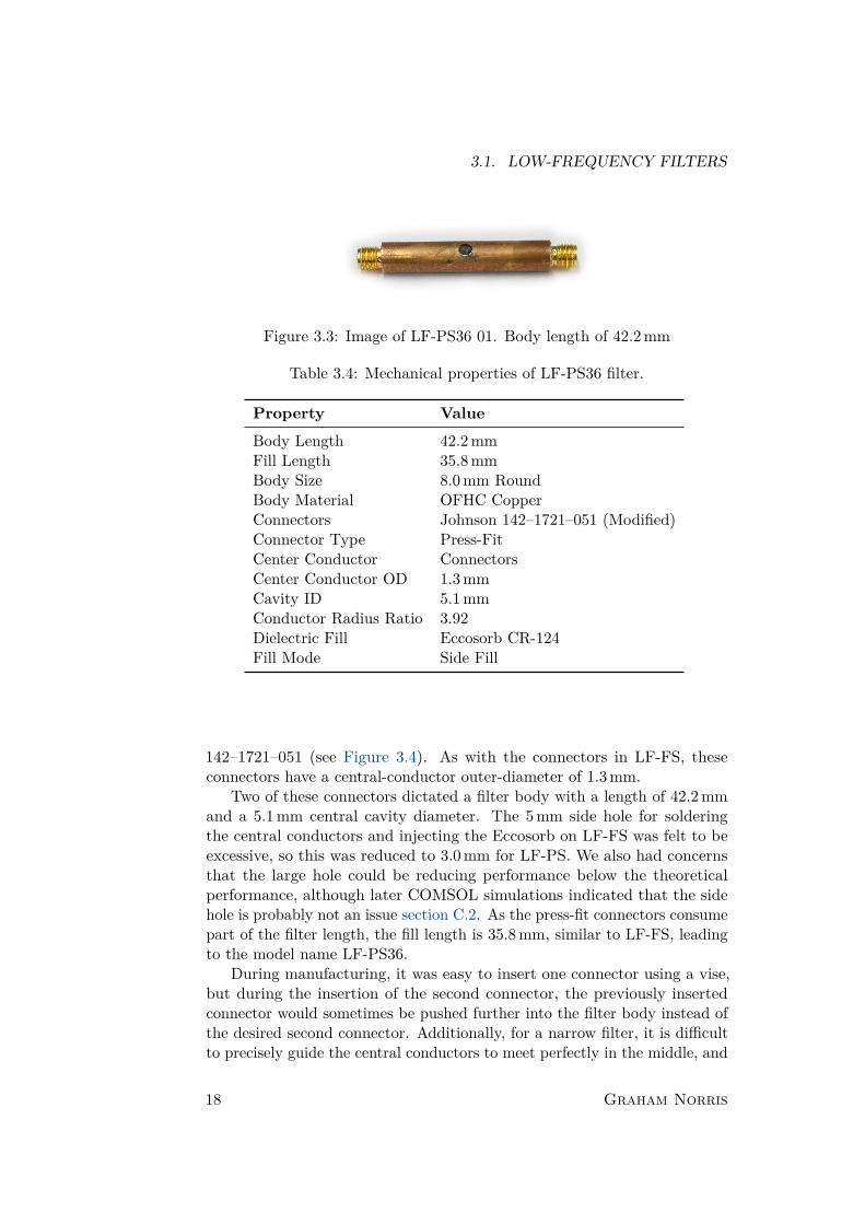
Figure 3.3: Image of LF-PS36 01. Body length of 42.2 mm
Table 3.4: Mechanical properties of LF-PS36 filter.
Property Value
Body Length 42.2 mmFill Length 35.8 mmBody Size 8.0 mm RoundBody Material OFHC CopperConnectors Johnson 142–1721–051 (Modified)Connector Type Press-FitCenter Conductor ConnectorsCenter Conductor OD 1.3 mmCavity ID 5.1 mmConductor Radius Ratio 3.92Dielectric Fill Eccosorb CR-124Fill Mode Side Fill
142–1721–051 (see Figure 3.4). As with the connectors in LF-FS, theseconnectors have a central-conductor outer-diameter of 1.3 mm.
Two of these connectors dictated a filter body with a length of 42.2 mmand a 5.1 mm central cavity diameter. The 5 mm side hole for solderingthe central conductors and injecting the Eccosorb on LF-FS was felt to beexcessive, so this was reduced to 3.0 mm for LF-PS. We also had concernsthat the large hole could be reducing performance below the theoreticalperformance, although later COMSOL simulations indicated that the sidehole is probably not an issue section C.2. As the press-fit connectors consumepart of the filter length, the fill length is 35.8 mm, similar to LF-FS, leadingto the model name LF-PS36.
During manufacturing, it was easy to insert one connector using a vise,but during the insertion of the second connector, the previously insertedconnector would sometimes be pushed further into the filter body instead ofthe desired second connector. Additionally, for a narrow filter, it is difficultto precisely guide the central conductors to meet perfectly in the middle, and
18 Graham Norris

CHAPTER 3. FILTER SPECIFICATIONS
Figure 3.4: Modified RND 205–00498 for use in LF-FS filter. Extendeddielectric (white) has been removed from the center conductor down to theflange of the filter.
in our case, the conductors ended up meeting side-on rather than head-on(see Figure 3.5). The 3 mm side hole meant that it was difficult to correctthis issue. The small side hole also made Eccosorb filling extremely difficult.
Figure 3.5: Misaligned center conductors on LF-PS36.
After this model showed poor S11 performance, a destructive autopsyof this filter model revealed that Eccosorb only partially filled the centercavity and confirmed that the center conductors did not meet head-on (seeFigure B.3).
LF-PS03
Figure 3.6: Image of LF-PS03 01. Body length of 9.0 mm.
The second variant featuring press-fit connectors, LF-PS03, was designedfor drive line use in parallel with LF-PS36 (see Figure 3.6). Delta RFmodel 1320–000–K911–32 connectors were used as these were available in
Semester Report 19

3.1. LOW-FREQUENCY FILTERS
Table 3.5: Mechanical properties of LF-PS03 filter.
Property Value
Body Length 9.0 mmFill Length 3.15 mmBody Size 10.0 mm RoundBody Material OFHC CopperConnectors Delta RF 1320–000–K911–32Connector Type Press-FitCenter Conductor ConnectorCenter Conductor OD 0.50 mmCavity ID 6.78 mmConductor Radius Ratio 13.56Dielectric Fill Eccosorb CR-124Fill Mode Side Fill
the QUDEV lab. The connectors dictate a cavity inner diameter of 6.78 mmand a total length of 9.0 mm. With a center pin diameter of 0.50 mm, theseconnectors result in a conductor radius ratio of 13.56. A 3.0 mm side holewas placed over the center of the filter for soldering and Eccosorb filling.
The hard stop present on the press-fit connectors solved the problem withLF-PS36, where the connector that was inserted first could be pushed pastthe ideal depth while inserting the second connector, and possibly helped toensure that the central conductors were parallel with the body cavity. Thecenter pins on each connector met perfectly end-to-end in the middle of thefilter cavity, although this is largely due to the short length of the pins (seeFigure 3.7).
Figure 3.7: Aligned center conductors on LF-PS03.
20 Graham Norris

CHAPTER 3. FILTER SPECIFICATIONS
Figure 3.8: Image of LF-TE35 01. Body length of 40.0 mm.
Table 3.6: Mechanical properties of LF-TE35 filter.
Property Value
Body Length 40.0 mmFill Length 35.2 mmBody Size 8.0 mm RoundBody Material OFHC CopperConnectors RND 205–00500Connector Type ThreadedCenter Conductor Silver-Plated Copper WireCenter Conductor OD 0.90 mmCavity ID 4.6 mmConductor Radius Ratio 5.11Dielectric Fill Eccosorb CR-124Fill Mode End Fill
3.1.4 LF-TE
LF-TE35
After the unsatisfactory performance of LF-PS, a new design was investigated.This model, LF-TE, replaced the push-fit connectors with threaded SMAfemale-to-female couplers (RND 205–00500) (see Figure 3.8). With theseconnectors, a separate center conductor with a diameter identical to that ofa SMA male pin (between 0.902 mm and 0.940 mm). In this case, a flexiblecoaxial cable with a solid 0.90 mm silver-plated copper center conductor wasused (Ceam M-17/84 RG223). In this design, the length was not fixed byconnectors, but was selected to be convenient and have a fill length compa-rable with previous filters. The fill length in this case is only approximate,including the length of the body cavity and the 1.93 mm of space in thethreaded couplers per the SMA standard. The threaded connectors alloweda maximum cavity size of 4.6 mm leading to a conductor radius ratio of 5.11.
Semester Report 21

3.1. LOW-FREQUENCY FILTERS
Due to the necessity of threading the filters with the uncommon 1/4”–36UNS 2B thread used by SMA connectors, this filter design was fabricated bythe ETH central workshop from OFHC copper stock. Great care was takenwhen sizing the center conductor with this filter design. The conductor wasinitially longer than required and gradually shortened until both connectorscould just barely thread to the stop. This ensured that the center conductorfully filled the connector at each end.
This design of filter also offered the advantage that the Eccosorb couldbe filled from one open side after a connector and the center conductor wereinserted. This should eliminate partial filling problems as the center cavityis large and, with the filter vertical on the sealed end, gravity assists infilling the filter from the bottom up. This intuition was supported by goodelectrical performance (see Figure 4.6), and by an autopsy of the filter, whichfound only a small air bubble at the end from which Eccosorb was filled (seeFigure B.4.
The mechanical strength of this design is quite good. Manually applyingsignificant torque (greater than specified for making proper SMA connections)to the connectors with a 5.5 mm wrench and pliers deformed the flat sectionson the coupler without the coupler unscrewing.
LF-TE10 01–03
Figure 3.9: Image of LF-TE10 01. Body length of 15.0 mm.
Table 3.7: Mechanical properties of LF-TE10 01–03 filters.
Property Value
Body Length 15.0 mmFill Length 10.2 mmRemaining See Table 3.6
During the redesign of LF-PS36 into LF-TE35 using threaded SMAfemale-to-female couplers, LF-PS03 was redesigned to become LF-TE10, ashorter variant of LF-TE35 (see Figure 3.9). The body length of this filterwas chosen to be a convenient length of 15.0 mm, leading to an estimated fill
22 Graham Norris

CHAPTER 3. FILTER SPECIFICATIONS
length of 10.2 mm. The center conductor for this filter was prepared in thesame way as for LF-TE35.
Although this filter was initially intended for microwave drive-line use,LF-TE10 01 was found to have sufficient attenuation for flux line use. Twoadditional filter bodies (LF-TE10 02 and 03) were produced. As bubbleformation was observed in both Eccosorb and Stycast (see Appendix B), theEccosorb was vacuum degassed for approximately two minutes after mixingbut before injection into the filter bodies.
LF-TE10 04–
Figure 3.10: Image of LF-TE10 04. Body length of 15.0 mm.
Table 3.8: Mechanical properties of LF-TE10 04– filters.
Property Value
Body Length 15.0 mmFill Length 10.2 mmConnectors Amphenol SMA7071A2-3GT50G-50Remaining See Table 3.6
The most recent variant of LF-TE10 is an updated version that useslarger SMA to SMA connectors that avoid the mechanical deformation issuesof the RND connectors (see Figure 3.11). This is the current design thatwill be used for all future flux-line filters, and which can also be used as amicrowave drive-line filter. Vacuum degassed Eccosorb was used for thesefilters.
After production, it was noticed that is was possible to partially unscrewone of the couplers (on the side that was initially facing down during Eccosorbfilling) from the body, although unscrewing and re-attaching the coupler didnot change the electrical performance. To fix this, filters from LF-TE10 06and onwards use Loctite 290 threadlocker on the α port.
Semester Report 23

3.1. LOW-FREQUENCY FILTERS
Figure 3.11: Comparison of threaded SMA female-female couplers. Left:RND 205–00500, right: Amphenol SMA7071A2-3GT50G-50. The Amphenolcoupler has a larger flat section that is separated from the threads, makingit easier to access with a wrench when the coupler is threaded into a filterbody.
Figure 3.12: Image of LF-TE06 02. Body length of 10.0 mm.
LF-TE06
After the good performance of LF-TE10 01, and with the adoption ofLF-TE10 as a flux-line filter, a shorter version was prepared to bring theattenuation in line with the ideal values for a high-frequency filter (seeFigure 3.12). This model also features vacuum degassed Eccosorb.
Table 3.9: Mechanical properties of LF-TE06 filter.
Property Value
Body Length 10.6 mmFill Length 5.8 mmRemaining See Table 3.6
24 Graham Norris

CHAPTER 3. FILTER SPECIFICATIONS
Figure 3.13: Image of LF-TS35 01. Body length of 40.0 mm.
Table 3.10: Mechanical properties of LF-TS35 filter.
Property Value
Body Length 40.0 mmFill Length 35.2 mmFill Mode Side FillRemaining See Table 3.6
3.1.5 LF-TS
LF-TS35
LF-TS35 is a variant of LF-TE35 that features two 3.0 mm side holes located6.82 mm from the ends of the filter for Eccosorb filling (see Figure 3.13). Thisdesign was produced in parallel with LF-TE35 in case the end-fill mechanismwas unsuccessful.
This filter does not have the same mechanical integrity of LF-TE35. Itis possible to unscrew one of the end connectors, although this was notexperienced during measurements of the filter, but rather when the strengthof the filter was investigated.
LF-TS10
LF-TS10 is a side-fill variant of LF-TE10 01 that was contemplated butnever produced, due to the good performance of LF-TE35 and LF-TE10 01and the lackluster mechanical strength of LF-TE35. This design has only asingle 3.0 mm fill hole centered in the filter body.
Semester Report 25

3.2. HIGH-FREQUENCY FILTERS
Table 3.11: Mechanical properties of HF-TE filter.
Property Value
Body Size 8.0 mm RoundBody Material OFHC CopperConnectors Amphenol SMA7071A2-3GT50G-50Connector Type ThreadedCenter Conductor SpC WireCenter Conductor OD 0.90 mmCavity ID 3.8 mmConductor Radius Ratio 4.2Dielectric Fill Eccosorb CR-110Fill Mode End Fill
3.2 High-Frequency Filters
3.2.1 HF-TE
HF-TE is a planned filter for our Eccosorb CR-110 once it arrives. This filteris designed for use in microwave drive lines, and has a smaller conductorradius ratio to better match the Eccosorb CR-110 (see Figure 2.1). Thelength will have to be determined after attenuation measurements can beperformed. All other properties should be identical to LF-TE10 06 (vacuumdegassed Eccosorb, thread locker, etc.).
26 Graham Norris

Chapter 4
Filter Measurements
4.1 VNA Parameters
All measurements below were performed on an Agilent N5230C VectorNetwork Analyzer (VNA) using the settings in Table 4.1 (except for themeasurements of LF-FS36, where an unknown IF bandwidth was used). Priorto measuring the scattering parameters of LF-FS36, manual calibration wasperformed using a Rhode and Schwarz ZV-Z32 calibration kit. Before alllater measurements, electronic calibration was performed using an AgilentN4433A electronic calibration module.
Table 4.1: VNA Settings
Property Value
Frequency Range 300.0 kHz to 20.0 GHzSweep Points 5000Power −8.0 dBmIF Bandwidth 10 kHzAveraging Factor 50
4.2 Low-Frequency Filters
The measured attenuation and averaged return-loss for the different low-frequency filters are presented in Table 4.2. The temperature at whichthe measurement was performed is listed, with RT corresponding to roomtemperature (approximately 298 K) and LN2 corresponding to liquid nitrogentemperature (approximately 77 K). The attenuation at the given frequencieswas computed from the measured data using linear interpolation to get theattenuation at the exact frequencies listed. Return losses were averagedover the listed frequency ranges as reflected power ratios (i.e. |Sij |2) before
Semester Report 27

4.2. LOW-FREQUENCY FILTERS
taking the logarithm to convert to decibels. This more accurately reflectsthe attenuation that a power source spread across those frequencies wouldexperience. The frequency regions for averaging were selected to correspondto the useful regions for both low-frequency (flux line) and high-frequency(microwave drive line) use cases.
Table 4.2: Measured Attenuation and Return Loss for Low-Frequency Filters
Attenuation [dB] Average Return Loss [dB]
Model T 500 MHz 5 GHz 0 MHz to 780 MHz 4 GHz to 8 GHzFS36 01 RT 2.14 67.2 18.3 9.61FS36 01 LN2 1.56 59.7 21.0 10.7PS36 01 RT 0.846 41.4 19.1 5.85PS36 02 RT 0.964 47.6 13.4 6.35PS03 01 RT 0.340 8.13 17.2 14.6PS03 02 RT 0.440 7.90 16.4 13.1TE35 01 RT 2.86 63.0 24.5 19.1TE10 01 RT 1.75 18.6 27.3 20.8TE10 02 RT 1.25 25.2 7.95 15.5TE10 03 RT 1.21 25.0 8.37 17.0TE10 04 RT 0.832 20.7 24.5 16.6TE10 05 RT 0.501 14.7 29.5 18.6TE10 06 RT 0.964 24.8 18.2 14.5TE10 07 RT 0.629 22.6 19.2 17.4TE10 08 RT 1.11 28.3 17.7 13.8TE10 09 RT 0.866 22.0 16.6 15.3TE10 10 RT 0.952 25.0 18.7 16.1TE10 11 RT 0.967 25.4 18.4 15.0TE10 12 RT 0.876 23.4 18.9 16.8TE10 13 RT 0.523 19.6 17.2 16.1TE06 01 RT 0.449 11.3 27.5 17.0TE06 02 RT 0.815 13.5 8.03 16.0TS35 01 RT 2.30 51.0 22.1 20.4M/Y 07 RT 0.853 16.1 16.3 19.4M/Y 03 RT 0.194 3.68 24.8 16.4
28 Graham Norris

CHAPTER 4. FILTER MEASUREMENTS
0.0 2.5 5.0 7.5 10.0 12.5 15.0 17.5 20.0Frequency [GHz]
60
50
40
30
20
10
0
|Sij|2 [
dB]
LF-FS36 01 S-Parameters (RT)
S11S22S12S21Sii (Pred.)
Figure 4.1: Room temperature scattering parameters, Sij , of LF-FS36 01from 300 kHz to 20 GHz. Reflected power plotted in blue, transmitted powerplotted in red-orange, and theoretical reflected power prediction plotted inlight gray.
0.0 2.5 5.0 7.5 10.0 12.5 15.0 17.5 20.0Frequency [GHz]
60
50
40
30
20
10
0
|Sij|2 [
dB]
LF-PS36 01 S-Parameters (RT)
S11S22S12S21Sii (Pred.)
Figure 4.2: Room temperature scattering parameters, Sij , of LF-PS36 01from 300 kHz to 20 GHz. Reflected power plotted in blue, transmitted powerplotted in red-orange, and theoretical reflected power prediction plotted inlight gray.
Semester Report 29

4.2. LOW-FREQUENCY FILTERS
0.0 2.5 5.0 7.5 10.0 12.5 15.0 17.5 20.0Frequency [GHz]
60
50
40
30
20
10
0|S
ij|2 [dB
]LF-PS36 02 S-Parameters (RT)
S11S22S12S21Sii (Pred.)
Figure 4.3: Room temperature scattering parameters, Sij , of LF-PS36 02from 300 kHz to 20 GHz. Reflected power plotted in blue, transmitted powerplotted in red-orange, and theoretical reflected power prediction plotted inlight gray.
0.0 2.5 5.0 7.5 10.0 12.5 15.0 17.5 20.0Frequency [GHz]
60
50
40
30
20
10
0
|Sij|2 [
dB]
LF-PS03 01 S-Parameters (RT)
S11S22S12S21Sii (Pred.)
Figure 4.4: Room temperature scattering parameters, Sij , of LF-PS03 01from 300 kHz to 20 GHz. Reflected power plotted in blue, transmitted powerplotted in red-orange, and theoretical reflected power prediction plotted inlight gray.
30 Graham Norris

CHAPTER 4. FILTER MEASUREMENTS
0.0 2.5 5.0 7.5 10.0 12.5 15.0 17.5 20.0Frequency [GHz]
60
50
40
30
20
10
0
|Sij|2 [
dB]
LF-PS03 02 S-Parameters (RT)
S11S22S12S21Sii (Pred.)
Figure 4.5: Room temperature scattering parameters, Sij , of LF-PS03 02from 300 kHz to 20 GHz. Reflected power plotted in blue, transmitted powerplotted in red-orange, and theoretical reflected power prediction plotted inlight gray.
0.0 2.5 5.0 7.5 10.0 12.5 15.0 17.5 20.0Frequency [GHz]
60
50
40
30
20
10
0
|Sij|2 [
dB]
LF-TE35 01 S-Parameters (RT)
S11S22S12S21Sii (Pred.)
Figure 4.6: Room temperature scattering parameters, Sij , of LF-TE35 01from 300 kHz to 20 GHz. Reflected power plotted in blue, transmitted powerplotted in red-orange, and theoretical reflected power prediction plotted inlight gray.
Semester Report 31

4.2. LOW-FREQUENCY FILTERS
0.0 2.5 5.0 7.5 10.0 12.5 15.0 17.5 20.0Frequency [GHz]
60
50
40
30
20
10
0|S
ij|2 [dB
]LF-TE10 01 S-Parameters (RT)
S11S22S12S21Sii (Pred.)
Figure 4.7: Room temperature scattering parameters, Sij , of LF-TE10 01from 300 kHz to 20 GHz. Reflected power plotted in blue, transmitted powerplotted in red-orange, and theoretical reflected power prediction plotted inlight gray.
0.0 2.5 5.0 7.5 10.0 12.5 15.0 17.5 20.0Frequency [GHz]
60
50
40
30
20
10
0
|Sij|2 [
dB]
LF-TE10 02 S-Parameters (RT)
S11S22S12S21Sii (Pred.)
Figure 4.8: Room temperature scattering parameters, Sij , of LF-TE10 02from 300 kHz to 20 GHz. Reflected power plotted in blue, transmitted powerplotted in red-orange, and theoretical reflected power prediction plotted inlight gray.
32 Graham Norris

CHAPTER 4. FILTER MEASUREMENTS
0.0 2.5 5.0 7.5 10.0 12.5 15.0 17.5 20.0Frequency [GHz]
60
50
40
30
20
10
0
|Sij|2 [
dB]
LF-TE10 03 S-Parameters (RT)
S11S22S12S21Sii (Pred.)
Figure 4.9: Room temperature scattering parameters, Sij , of LF-TE10 03from 300 kHz to 20 GHz. Reflected power plotted in blue, transmitted powerplotted in red-orange, and theoretical reflected power prediction plotted inlight gray.
0.0 2.5 5.0 7.5 10.0 12.5 15.0 17.5 20.0Frequency [GHz]
60
50
40
30
20
10
0
|Sij|2 [
dB]
LF-TE10 04 S-Parameters (RT)
S11S22S12S21Sii (Pred.)
Figure 4.10: Room temperature scattering parameters, Sij , of LF-TE10 04from 300 kHz to 20 GHz. Reflected power plotted in blue, transmitted powerplotted in red-orange, and theoretical reflected power prediction plotted inlight gray.
Semester Report 33

4.2. LOW-FREQUENCY FILTERS
0.0 2.5 5.0 7.5 10.0 12.5 15.0 17.5 20.0Frequency [GHz]
60
50
40
30
20
10
0|S
ij|2 [dB
]LF-TE10 05 S-Parameters (RT)
S11S22S12S21Sii (Pred.)
Figure 4.11: Room temperature scattering parameters, Sij , of LF-TE10 05from 300 kHz to 20 GHz. Reflected power plotted in blue, transmitted powerplotted in red-orange, and theoretical reflected power prediction plotted inlight gray.
0.0 2.5 5.0 7.5 10.0 12.5 15.0 17.5 20.0Frequency [GHz]
60
50
40
30
20
10
0
|Sij|2 [
dB]
LF-TE10 06 S-Parameters (RT)
S11S22S12S21Sii (Pred.)
Figure 4.12: Room temperature scattering parameters, Sij , of LF-TE10 06from 300 kHz to 20 GHz. Reflected power plotted in blue, transmitted powerplotted in red-orange, and theoretical reflected power prediction plotted inlight gray.
34 Graham Norris

CHAPTER 4. FILTER MEASUREMENTS
0.0 2.5 5.0 7.5 10.0 12.5 15.0 17.5 20.0Frequency [GHz]
60
50
40
30
20
10
0
|Sij|2 [
dB]
LF-TE10 07 S-Parameters (RT)
S11S22S12S21Sii (Pred.)
Figure 4.13: Room temperature scattering parameters, Sij , of LF-TE10 07from 300 kHz to 20 GHz. Reflected power plotted in blue, transmitted powerplotted in red-orange, and theoretical reflected power prediction plotted inlight gray.
0.0 2.5 5.0 7.5 10.0 12.5 15.0 17.5 20.0Frequency [GHz]
60
50
40
30
20
10
0
|Sij|2 [
dB]
LF-TE10 08 S-Parameters (RT)
S11S22S12S21Sii (Pred.)
Figure 4.14: Room temperature scattering parameters, Sij , of LF-TE10 08from 300 kHz to 20 GHz. Reflected power plotted in blue, transmitted powerplotted in red-orange, and theoretical reflected power prediction plotted inlight gray.
Semester Report 35

4.2. LOW-FREQUENCY FILTERS
0.0 2.5 5.0 7.5 10.0 12.5 15.0 17.5 20.0Frequency [GHz]
60
50
40
30
20
10
0|S
ij|2 [dB
]LF-TE10 09 S-Parameters (RT)
S11S22S12S21Sii (Pred.)
Figure 4.15: Room temperature scattering parameters, Sij , of LF-TE10 09from 300 kHz to 20 GHz. Reflected power plotted in blue, transmitted powerplotted in red-orange, and theoretical reflected power prediction plotted inlight gray.
0.0 2.5 5.0 7.5 10.0 12.5 15.0 17.5 20.0Frequency [GHz]
60
50
40
30
20
10
0
|Sij|2 [
dB]
LF-TE10 10 S-Parameters (RT)
S11S22S12S21Sii (Pred.)
Figure 4.16: Room temperature scattering parameters, Sij , of LF-TE10 10from 300 kHz to 20 GHz. Reflected power plotted in blue, transmitted powerplotted in red-orange, and theoretical reflected power prediction plotted inlight gray.
36 Graham Norris

CHAPTER 4. FILTER MEASUREMENTS
0.0 2.5 5.0 7.5 10.0 12.5 15.0 17.5 20.0Frequency [GHz]
60
50
40
30
20
10
0
|Sij|2 [
dB]
LF-TE10 11 S-Parameters (RT)
S11S22S12S21Sii (Pred.)
Figure 4.17: Room temperature scattering parameters, Sij , of LF-TE10 11from 300 kHz to 20 GHz. Reflected power plotted in blue, transmitted powerplotted in red-orange, and theoretical reflected power prediction plotted inlight gray.
0.0 2.5 5.0 7.5 10.0 12.5 15.0 17.5 20.0Frequency [GHz]
60
50
40
30
20
10
0
|Sij|2 [
dB]
LF-TE10 12 S-Parameters (RT)
S11S22S12S21Sii (Pred.)
Figure 4.18: Room temperature scattering parameters, Sij , of LF-TE10 12from 300 kHz to 20 GHz. Reflected power plotted in blue, transmitted powerplotted in red-orange, and theoretical reflected power prediction plotted inlight gray.
Semester Report 37

4.2. LOW-FREQUENCY FILTERS
0.0 2.5 5.0 7.5 10.0 12.5 15.0 17.5 20.0Frequency [GHz]
60
50
40
30
20
10
0|S
ij|2 [dB
]LF-TE10 13 S-Parameters (RT)
S11S22S12S21Sii (Pred.)
Figure 4.19: Room temperature scattering parameters, Sij , of LF-TE10 13from 300 kHz to 20 GHz. Reflected power plotted in blue, transmitted powerplotted in red-orange, and theoretical reflected power prediction plotted inlight gray.
0.0 2.5 5.0 7.5 10.0 12.5 15.0 17.5 20.0Frequency [GHz]
60
50
40
30
20
10
0
|Sij|2 [
dB]
LF-TE06 01 S-Parameters (RT)
S11S22S12S21Sii (Pred.)
Figure 4.20: Room temperature scattering parameters, Sij , of LF-TE06 01from 300 kHz to 20 GHz. Reflected power plotted in blue, transmitted powerplotted in red-orange, and theoretical reflected power prediction plotted inlight gray.
38 Graham Norris

CHAPTER 4. FILTER MEASUREMENTS
0.0 2.5 5.0 7.5 10.0 12.5 15.0 17.5 20.0Frequency [GHz]
60
50
40
30
20
10
0
|Sij|2 [
dB]
LF-TE06 02 S-Parameters (RT)
S11S22S12S21Sii (Pred.)
Figure 4.21: Room temperature scattering parameters, Sij , of LF-TE06 02from 300 kHz to 20 GHz. Reflected power plotted in blue, transmitted powerplotted in red-orange, and theoretical reflected power prediction plotted inlight gray.
0.0 2.5 5.0 7.5 10.0 12.5 15.0 17.5 20.0Frequency [GHz]
60
50
40
30
20
10
0
|Sij|2 [
dB]
LF-TS35 01 S-Parameters (RT)
S11S22S12S21Sii (Pred.)
Figure 4.22: Room temperature scattering parameters, Sij , of LF-TS35 01from 300 kHz to 20 GHz. Reflected power plotted in blue, insertion gainplotted in red-orange, and theoretical reflected power prediction plotted inlight gray.
Semester Report 39

4.3. DISCUSSION
4.3 Discussion
4.3.1 LF-FS
The scattering parameters of LF-FS36, plotted in Figure 4.1, reveal thatour Eccosorb CR-110, despite being thre years past its state expiration date,still functions as expected and that the actual filters perform similarly tothe theoretical expectations. This filter was thermally cycled down to liquidnitrogen temperatures and back to room temperature several times withoutany ill effects. Liquid nitrogen temperatures slightly reduced the attenuationand the average return loss.
4.3.2 LF-PS
LF-PS36
Both LF-PS36 01 (Figure 4.2) and LF-PS36 02 (Figure 4.3) display worsescattering parameters than LF-FS36 outside of very low frequencies. Thereflected power across much of the spectrum is above the theoretical expec-tations, and there is an asymmetry between the two ports. In addition, bothfilters showed nonlinear behavior of the attenuation with changing frequency(i.e. attenuation does not increase in an approximately linear fashion withincreasing frequency). At the very least, this design is consistently bad, withboth filters showing similar performance.
The degraded performance (relative to LF-FS36) was initially blamedon central conductors that did not line up perfectly end-to-end duringmanufacturing, but an autopsy of LF-PS36 01 revealed that the Eccosorbdid not fill the entire cavity, meaning that the filter is no longer evenapproximately impedance-matched to 50 Ω coaxial lines (see Appendix B).
LF-PS03
LF-PS03 01 (Figure 4.4) and LF-PS03 02 (Figure 4.5) show similar per-formance that is, unfortunately, not terribly better than that of LF-FS36.Compared to LF-PS36, the slope of the attenuation has increased, from ap-proximately −10 dB GHz−1 to −1.5 dB GHz−1, as expected, given the shorterlength of the filter. However, the reflected power performance, while slightlybetter than LF-PS36, is not great, averaging around −13 dB across much ofthe spectrum. Both filters (01 and 02) show some asymmetry between thetwo ports.
40 Graham Norris

CHAPTER 4. FILTER MEASUREMENTS
4.3.3 LF-TE
LF-TE35
LF-TE35 01 (Figure 4.6) demonstrated the potential of the threaded couplerdesign with end-filling. The attenuation is similar to LF-FS36 and LF-PS36,which is expected given that they have similar lengths. However, the reflectedpower is significantly better than either of those designs, with both portsbeating the theoretical expectations. Low-frequency performance is similarto the previous designs, with reflected power below −20 dB up to around1 GHz in both directions. One port has a reflected power that is below−30 dB for almost the entire range between 2 GHz to 7.5 GHz and is alwaysbelow −20 dB.
The cause for this super-theoretical performance was initially vexing.Swapping the cables in the VNA switched which port had better reflectedpower, so this is performance does not arise from an issue with one channelof the VNA. After the filter autopsies, a possible cause was revealed: LF-TE35 01 has an air bubble near one of the connectors (see Figure B.4). Myrecords from that period were not detailed enough to distinguish exactlywhich side corresponded to which port on the VNA measurement, however,I suspect that this bubble acted as an impedance matching region, much likean anti-reflective coating in optics or the angled lossy attenuators used inwaveguides. Unfortunately, this performance did not appear in other variantsof the LF-TE filter, but this is one area where a larger-scale project mightimprove on this design.
LF-TE35 01 was thermally cycled down to liquid nitrogen temperaturesand back to room temperature three times without significant change in themeasured performance.
LF-TE10
LF-TE10 01 (Figure 4.7) shows similar performance to LF-TE35 01 (theywere manufactured at the same time using the same procedures). Theattenuation is lower than the longer designs, approximately −4 dB GHz−1.The reflected power at both ports is consistently better than the theoreticalprediction. Again, as with LF-TE35 01, there is asymmetry between the twoports, with one port showing better performance and some sort of resonanceeffect in the reflected power. The exact reasons for this are unclear, but Isuspect either a bubble near the end of the filter, as with LF-TE35.
LF-TE10 02 (Figure 4.8) and 03 (Figure 4.9) show performance thatis worse than the previous LF-TE10 filters. The filters both have linearattenuation slopes of approximately −5.5 dB GHz−1, which is lower than the−5 dB GHz−1 and −4 dB GHz−1 of other LF-TE10s. For frequencies above2 GHz, the reflected power performance largely beats theoretical expectations.At low frequencies, however, these two filters show strange performance,
Semester Report 41

4.3. DISCUSSION
where the reflected power is rather large, starting at around 0 dB at 0 GHzand decreasing to −20 dB at around 2 GHz, rather than starting at betterthan −30 dB at very low frequencies. In addition to this, both filters showasymmetric reflected power, and one port shows some unusual peaking around11 GHz.
While all of these features are strange and undesirable, they are consistentfor the two filters, so this must come from some construction detail of thefilters. The major change that I recall from LF-TE10 01 to 02 and 03 wasthat less effort was used in sizing the center conductors to be the full lengthof the cavity plus the couplers. However, there is no clear physical motivationfor how an air gap in the back of the connector would increase the reflectedpower, given that the filters have DC conductivity. Therefore, the mostplausible explanation is that there is some unfilled region. The other possiblecause is a minor mistake in the Eccosorb recipe for these filters: 0.87 g ofPart B was added instead of 0.78 g. Unfortunately, due to limited time, anautopsy was not performed on these filters.
LF-TE10 04 (Figure 4.10) and 05 (Figure 4.11) largely remedied theissues with LF-TE10 02 and 03. Both filters demonstrate good low-frequencyreflected power, and in general beat the theoretical expectations across thespectrum. Attenuation is slightly reduced compared to LF-TE10 02 and 03,but is greater than LF-TE10 01 at approximately −5 dB GHz−1. For filter05, this attenuation is nonlinear with frequency, reducing the attenuation atlow frequencies, but still reaches greater than −60 dB for frequencies above12.5 GHz. LF-TE10 05 also displays some asymmetry between the two ports,and it is possible that this is linked to the nonlinear attenuation. It seemsthat with Eccosorb filters, although devices of the same design may performsimilarly, there is still the possibility of minor variations.
LF-TE10 04 was thermally cycled to liquid nitrogen temperatures withoutany major change in electrical performance. In this case, the filter was alsomeasured at 4 K temperatures in a liquid helium dipstick. The S-parametersat this temperature are presented in Figure 4.23, and a comparison of theattenuation at room temperature and 4 K is presented in Figure 4.24. Athrough coupler was measured at 4 K as a background for the attenuation.However, it was not possible to completely calibrate out the dipstick cables, soa direct comparison of the reflected power is not possible. At a minimum, thereflected power has not increased above the theoretical value for this design.The attenuation is reduced at low temperatures, going from approximately−5.5 dB GHz−1 at room temperature to approximately −4.8 dB GHz−1 at4 K.
During this thermal cycling, I noticed that it was possible to unscrewone of the threaded couplers from the filter body. Unscrewing this as far aspossible and then screwing it back on several times, I found no major changesin the scattering parameters. The difference between the initial and finalS-parameters are presented below in Figure 4.25. The largest differences are
42 Graham Norris

CHAPTER 4. FILTER MEASUREMENTS
in the scattering parameters of port 1, which is the port that was targetedin this testing. At worst, these changes resulted in an additional 2 dB inreflected power and a slight decrease in attenuation at around 10 GHz. Thelarge feature on the right is due to the attenuation reaching the noise floorof the VNA. In this sense, this filter design is very robust against mechanicaldamage.
0.0 2.5 5.0 7.5 10.0 12.5 15.0 17.5 20.0Frequency [GHz]
60
50
40
30
20
10
0
|Sij|2 [
dB]
LF-TE10 04 S-Parameters (4 K)
S11S22S12S21Sii (Pred.)
Figure 4.23: 4 K scattering parameters, Sij , of LF-TE10 04 from 300 kHzto 20 GHz. Reflected power plotted in blue, transmitted power plotted inred-orange, and theoretical reflected power prediction plotted in light gray.
LF-TE10 06–13 (Figure 4.12 through Figure 4.19) demonstrate the vari-ability of this design in mass production. In all of these plots, the oscillationsin S22 are due to either an issue calibrating the VNA for the dipstick cablesor the dipstick connectors themselves, as they are not present at room tem-perature or expected based on the simple nature of the filters. The filtersstill generally beat the theoretical expectation for reflected power.
LF-TE06
LF-TE06 01 (Figure 4.20) and 02 (Figure 4.21) are similar to LF-TE1002 and 03, with the exception that LF-TE06 01 has good low-frequencyperformance on both ports and a region of good reflected-power performanceon on port at around 7 GHz. The attenuation of this design is reduced to−2.9 dB GHz−1. Both filters have asymmetries of between the two ports andthe same resonance effects around 10 GHz seen in LF-TE10 02 and 03. The
Semester Report 43

4.3. DISCUSSION
0.0 2.5 5.0 7.5 10.0 12.5 15.0 17.5 20.0Frequency [GHz]
60
50
40
30
20
10
0|S
ij|2 [dB
]LF-TE10 04 Attenuation Comparison
RT S12RT S214 K S124 K S21
Figure 4.24: Comparison of attenuation for LF-TE10 04 at 4 K (blue) andat room temperature (red).
0.0 2.5 5.0 7.5 10.0 12.5 15.0 17.5 20.0Frequency [GHz]
4
2
0
2
4
|Sij|2 [
dB]
LF-TE10 04 S-Parameters Difference (RT)
S11S22S12S21
Figure 4.25: Difference in S-Parameters of LF-TE10 04 between initialtesting and after partially removing and then re-inserting one of the threadedcouplers several times.
44 Graham Norris

CHAPTER 4. FILTER MEASUREMENTS
main suspect for this poor performance is again some air bubble at one endof the filter.
4.3.4 LF-TS
LF-TS35 01 (Figure 4.22) shows performance that is largely comparable toLF-TE35 and LF-TE10. The attenuation is similar to LF-TE35 at around−11 dB GHz−1, and the reflected power is similar to the “normal” perfor-mance, slightly beating theoretical performance throughout the range, andwith very good performance at low frequencies. This design was discontinuedlargely because of the ease of end-filling and the boost to the mechanicalstrength provided by Eccosorb pressing into the threads of the coupler andfilter body.
Semester Report 45

Chapter 5
Discussion
5.1 Remarks
Attenuation
Although the attenuation of similar filters may differ (cf. Table 4.2), lookingat all of the filters, we can analyze the measured attenuation and compare itto the value provided for Eccosorb CR-124 by Laird. The attenuation of allof the filters produced during this project at 500 MHz and 5 GHz are plottedversus their Eccosorb fill length in Figure 5.1. Averaging these results revealsthat in our filter designs, we have 20.7 dB cm−1 of attenuation at 5 GHzand 0.88 dB cm−1 of attenuation at 500 MHz. Laird quotes 0.48 dB cm−1 at100 MHz, 6.5 dB cm−1 at 1 GHz, 20 dB cm−1 at 3 GHz, and 63 dB cm−1 at8.6 GHz for Eccosorb CR-124 (see Figure D.5), leading to a predicted at-tenuation of approximately 35 dB cm−1 at 5 GHz and 3 dB cm−1 at 500 MHz[21]. Thus, our filters have lower attenuation than predicted, possibly dueto the fact that the filters are small compared to the wavelength (especiallyat 500 MHz). While the electric field inside a coaxial cable is not uniformlyradially distributed, this should not affect the attenuation, as long as theattenuation remains constant at different input powers. One note is that,while some filters may have attenuation that varies from this average, theattenuation is usually similarly affected at 500 MHz and 5 GHz, i.e. only theslope of the attenuation is affected.
Assuming that a similar relation also holds for the attenuation of Ec-cosorb CR-110 in filters versus on the data sheet, the predicted values inTable 2.1 should be reduced to approximately 0.013 dB cm−1 at 500 MHzand 0.51 dB cm−1 at 5 GHz (and hence 0.013 dB at 500 MHz and 0.51 dB at5 GHz for a HF-TE10 filter). These values are similar to those given by Fangfor his “HF” filters that have an Eccosorb fill length of 9.5 mm [16].
In these experiments, I have only measured the attenuation of Eccosorbup to 20 GHz. While commercial VNAs that measure up to 100 GHz exist, Iwas not able to locate any at ETH. However, Eccosorb has been studied in
46 Graham Norris

CHAPTER 5. DISCUSSION
5 10 15 20 25 30 35Length [mm]
0
10
20
30
40
50
60
70
Atte
nuat
ion
[dB]
Attenuation Versus Eccosorb CR-124 Length5 GHz500 MHz
Figure 5.1: Attenuation of different filters versus the length of EccosorbCR-124 in the filter. Attenuation at 5 GHz plotted in blue; attenuation at500 MHz plotted in red-orange.
the far infrared, at millimeter and submillimeter wavelengths. Halpern et al.measured the absorption coefficient of Eccosorb CR-110 at 300 K, findingthat it increased linearly from 2 cm−1 at 75 GHz to 25 cm−1 at 900 GHz [24].Hemmati et al. extended this measurement out to 2700 GHz, finding that theattenuation of a 6.35 mm sample of CR-110 increased to 37 dB at 2700 GHz,with stronger grades of Eccosorb being even more attenuating [25]. Thus,although I was not able to measure out to extremely high frequencies, Iam confident that Eccosorb filters remain attenuating out to thousands ofgigahertz.
Labeling
Initially, I labeled filters with a unique number using a permanent marker.However, the marker is easily scratched off the filter by mechanical handlingand is dissolved by many solvents. Filters with asymmetric performancerevealed the need for labeling of the individual ports and tracking of thefilter orientation during manufacturing. With these points in mind, recentlabeling using the Arkograf has been largely successful. The only issue isthat the mechanical tightening of the filters using pliers can partially removethe shallow marks produced by the Arkograf. This might be improved by
Semester Report 47

5.1. REMARKS
using mechanical engraving or by adding the permanent labels after finalassembly and curing.
Thermalization
Eccosorb filters may also be used to improve the thermalization of thecenter conductor of coaxial cables. As previously mentioned, Eccosorbhas a thermal expansion coefficient that better matches metals like copper.In addition, at cryogenic temperatures, the thermal conductivity of theEccosorb is significantly greater than that of PTFE. Based on data fromWikus et al. Eccosorb CR-124 has a thermal conductivity of 4.0 W m−1 K−1
at 4 K and 0.38 W m−1 K−1 at 1 K [26]. Correspondingly, PTFE has thermalconductivities of 0.046 W m−1 K−1 at 4 K and 0.011 W m−1 K−1 at 1 K, basedon data from the NIST cryogenics database. An Eccosorb filter should thusprovide order of magnitude better thermalization of the center conductorthan simply clamping the coaxial cable and relying on thermal conductivitythrough the PTFE dielectric, especially for cables with a reduced density(foam) dielectric.
Thermal Photons
In order to measure the need for Eccosorb filters, one issue that becameinteresting during the progression of this project was how many thermalphotons at frequencies above the gap frequency are arriving at the sample.The coaxial cables themselves are attenuating for high frequency photons,but also have many modes available to extremely high frequency photons(>1000 GHz). To answer this question, numerical simulations were performed(as discussed in Appendix E). Based on this simulation, given our currentcabeling and attenuation configuration without Eccosorb filters, we expecton the order of 5.5× 10⁵ photons s−1 above the energy gap of aluminum andbelow the frequency at which the dielectric becomes strongly absorbing. Asdiscussed in Appendix E, this simulation makes many assumptions, so thisnumber is only a rough estimate. However, even assuming an additional 20or 30 dB of attenuation from the cables at high frequencies, quasiparticle-inducing photon numbers this large indicate that Eccosorb filters may berequired for experiments pursuing high coherence times.
Reflected Power
Bulk Eccosorb appears to behave reliably, handling thermal and mechanicalcycling without issue. However, the connectors are a different issue. It seemsthat the reflected power is sensitive to small changes in how connections areformed, with air bubbles at the β side of the filter as the most likely culprit.The β-side coupler is inserted after filling the body with Eccosorb, makingit difficult to guarantee that it is fully filled. Just as when trying to push
48 Graham Norris

CHAPTER 5. DISCUSSION
an inverted cup from air down into water, the coupler may force Eccosorbout through the threads without itself filling with Eccosorb. This could beremedied by pouring some Eccosorb into the empty space in the couplerbefore threading it into the filled body.
Another possibility would be that the reflected power depends on thesizing of the center wire. There is no clear reason why this would increasethe reflected power, but it could be tested by deliberately shortening a wireand measuring the performance.
Given all of this, it may be interesting to again consider a side-fill designusing a large side hole (5 mm). Since the COMSOL simulations showed nomajor difference between a LF-FS36 design with and without a hole, sidefilling should not negatively impact the electrical performance of the filters.For shorter lengths, uneven Eccosorb filling should not be a problem, evenunder the more difficult conditions of filter mass production.
5.2 Conclusion
After several variations, I have produced Eccosorb filters that demonstraterepeatable performance and beat the theoretical expectations. With someminor additional modifications, the LF-TE10 design should prove to bean ideal infrared-blocking filter for flux-line use. A future version, HF-TE,should provide similar performance for microwave drive-line use. These filtershave improved mechanical strength over previous designs, and are easier tomanufacture. Numerical simulations confirm the necessity of Eccosorb filtersor other infrared-blocking filters to block quasiparticle-inducing photons thatwould otherwise reach the sample under current attenuation schemes.
5.3 Outlook
If adding Eccosorb to the second coupler before attaching it does not improverepeatability or reduce the reflected power, then future designs might lookinto other connector types. There are a number of small flange-mount designsthat accept coaxial cable center conductors (some of which are made bySouthwest Microwave). Other options would be to investigate using hermeticlaunch pins so that the center conductor could be soldered to somethingdesigned to fit into the connector at each end.
Ideally, some company would produce Eccosorb filters for cryogenicuse. Several “miracle” filters showed extremely good performance, howeverthese were probably accidental, as subsequent filters have not shown similarperformance. With a bit more work, it would be possible to create someimpedance-transforming region at each end of the filter to achieve stellarreflected power performance.
Semester Report 49

Appendix A
Filter ProductionInstructions
A.1 Filter Body Machining
Filter production begins by selecting the desired properties of the filter, usu-ally its attenuation and frequency range. Once these are known, and a gradeof Eccosorb—which affects both parameters—is selected, the attenuation istuned by changing the length of the filter and the frequency range is tunedby changing the diameter of the hole in the filter body (see considerationsin chapter 2). After this design work, a CAD model and a drawing mustbe produced. In order to fit the threaded couplers, the interior threads atthe end of the filter body must match the SMA specifications. This dictates1/4”–36 UNS 2B interior threads and a stop lip with a depth of 4.3 mmand a diameter of 4.6 mm. The threads should be as deep as possible, butdo not need to be the full 4.3 mm deep (and this would be impossible orextremely difficult to physically machine). To specify this, the attribute“Norm Gewindehinterstich” can be applied to each of the threads to specifythat they should have the normal region carved out behind the end of thethreads, leaving a flat surface for the threaded coupler to press against. Notethat the filled Eccosorb length will be approximately 3.8 mm greater thanthe distance between the stops due to the female SMA connector (which hasmale threads) having approximately 1.9 mm of empty space between the endof the dielectric and the end of the metal rim. An example drawing, scaleddown, is presented in Figure A.1.
The filter bodies are ordered from the ETH central workshop by providinga complete drawing and specifying the material, quantity, and finish of thefilters. It is helpful to provide a previously made filter as an example and aSMA coupler as a test piece. The physics workshop lacks the necessary 1/4”–36 UNS tap. Project turnaround time for the central workshop is normally afew days, even for normal-priority projects. Costs for medium-sized batches
50 Graham Norris

APPENDIX A. FILTER PRODUCTION INSTRUCTIONS
lfte10.ipt
Weight
Designed
Checked
2016-12-07
Graham Norris
Rev.Description
Date Name
Quantity
12
A4
LF Threaded Endfill 10mm Eccosorb Filter
Part
1 of 1
Description
Page
Material
General Tolerances
ISO-2768-mH
Dimensions in [mm]
Linear Dimensions
>0.5
to
6
> 6
to
30
±0.1 ±0.5±0.3
3:1
>30
to
120
>400
to
1000
±0.8
>1000
to
2000
±1.2
>2000
to
4000
±2
Angular Dimensions
to
10
±1°
>10
to
50
±0°30'
>50
to
120
±0°20'
>120
to
400
>400
±0°10' ±0°5'
N/A
Projekt
>120
to
400
±0.2
Cost center
Phone nr.
03720
+41 44 633 22 92
Threaded Eccosorb Filters
OF Copper
06.11.2015 Melvin Frey
15
8
4,3
4,3
8
1/4-36 UNS - 2B
1/4-36 UNS - 2B
4,6
1/4-36 UNS - 2B
Norm Gewindehinterstich
Figure A.1: CAD drawing of LF-TE10 filter body. Scale in this case is 1.5:1rather than the 3:1 specified in the drawing.
Semester Report 51

A.2. CENTER CONDUCTOR PREPARATION
of filters bodies can be around 10 CHF per body, although this is determinedprimarily by labor costs, so it is beneficial to order a number of identicalfilter bodies at the same time.
SMA couplers can be ordered through Distrelec (and the D-PHYS Distr-elec omnibus order), but this also has a lead time of several days to a week,so it is advised to order the connectors (and wire, if needed) at the same timeas the filter bodies. Ordering multiple couplers also lowers the cost-per-filterdue to volume discounts.
A.2 Center Conductor Preparation
The center conductor of CEAM M-17/84 RG223, commercial RG223 flexiblecoaxial cable, is a perfect fit for the female socket of the SMA connector andis silver-plated for better conductivity. However, the fact that this wire ispart of a pre-existing cable means that we have to first extract the part thatwe want. First cut a section of wire that is longer than the filter body andconnectors. Then, remove the outer plastic insulation by slicing it with arazor blade and peeling it off. The two layers of stranded mesh conductorcan be removed by pressing inward at the two ends to enlarge the mesh andthen sliding it off, sort of like the solution to a “Chinese finger trap”. Theinner polyethylene dielectric is harder to remove. The easiest method that Ifound was to carve away the dielectric at one end of the wire using a knifeand then pull the center wire out using pliers while twisting the dielectric(see Figure A.2). Try not to bend the wire during this process.
Figure A.2: Center conductor and polyethylene dielectric from CEAM RG223coaixal cable.
Next, gently file and round the ends so that they fit—with some effort—into a SMA coupler. Insert the wire as far as possible into one coupler andthread this coupler into the filter body. The following steps are crucial tofilter performance, so go slowly! Insert the end of the wire into the othercoupler and try to thread the coupler into the body. If the coupler does notcome close at all to threading, trim off 1 mm, round the end, and try again.Once the filter begins threading onto the filter, trim in smaller increments.Once the coupler stops, to see whether this is due to the wire reaching theend of the socket in the coupler, or the coupler reaching the stop, unscrewthe other coupler slightly and then try to thread this coupler slightly farther.
52 Graham Norris

APPENDIX A. FILTER PRODUCTION INSTRUCTIONS
If, on the final iteration, the coupler reaches the stop before resistance oreffort is felt, start again. Wires of the correct length usually stick severalmm out of the filter body (see Figure A.3). Be wary of the wire getting“stuck” in one of the couplers, try to wiggle the wire to check that it is reallyinserted to the maximum depth. It is best to keep each filter body and itsmatching center conductor and couplers separate from the others in casethere are minor differences between these.
Figure A.3: Center conductor protruding out of LF-TE06 filter body.
A.3 Filter Assembly
A.3.1 Labeling
After manufacturing, all filter bodies are sanded to remove oxide coating andlabeled with their model name, a serial number, and port labels (α and β).Current labeling is done using an electric scribe, the “Arkograph”, presentin the central workshop. These markings survive subsequent cleaning steps,do not out-gas in a vacuum, and are generally more durable than permanentmarker labels. In the future, we may use a mechanical engraver to get deepermarks.
A.3.2 Preparation
When it is time to assemble the filters, the first step is to prepare the correctequipment. Table A.1 lists the equipment that is needed to assemble filtersusing the current procedure. Note that it is useful to have backups for itemslike syringes and paper towels in case of mistakes.
Semester Report 53

A.3. FILTER ASSEMBLY
Table A.1: Equipment used for filter assembly. n is the number of filters.Items above the middle line can be purchased in D-PHYS shop; items belowthe line should be in our workshop already.
Equipment Quantity1.2 mm by 40 mm Needle 11.5 mm by 5 mm NBR O-Rings 2n250 ml Plastic Beaker 1Plastic Tweezers 1Threaded SMA Covers n10 ml Syringe 12 ml Syringe 1Wooden Spatulas Several10 cm by 10 cm Aluminum Foil 1Aluminum U-Channel 1Glass Beaker 1Hotplate 1Paper Towels SeveralPliers 2Scale 1
Lay out paper towels to form a work space where the filters will be filledand assembled, usually next to the hotplate. Also place filters between thehotplate and the scale in case of spills. Remove the syringes from theirpackages and attach the needle to the 2 ml syringe. See Figure A.4 for anexample image.
A.3.3 Cleaning
Prior to assembly, all parts are cleaned to remove contaminants and enhancegalvanic contact between all parts. The copper filter bodies, which are usuallysomewhat oxidized, are soaked in a 10% citric acid solution for 5 min andthen rinsed in distilled (DI) water and isopropanol (IPA) and then set ona clean paper towel to dry. The silver-plated center conductor are usuallyprepared immediately before filter assembly and as such are not substantiallyoxidized. Thus, they and all remaining parts are cleaned of oils by rinsingin DI water and IPA. Keep each filter body and its center conductor andcouplers separate from all others.
54 Graham Norris

APPENDIX A. FILTER PRODUCTION INSTRUCTIONS
Figure A.4: Image of filter assembly preparation. Not all equipment listedabove is shown here. The object at the left edge of the frame is the hotplate.
A.3.4 Eccosorb Filling Preparation
After the filter parts have dried, don clean gloves and place an o-ring onone side of each coupler, between the threads and the center section. Insertthe center conductor into the o-ring side of the coupler, apply a drop ofthread locker (Loctite 240) to the threads on the o-ring side, and threadthis assembly into the α side of the filter body, wiping up any excess threadlocker. Place a SMA cap (Amphenol 132360) on the other end of the insertedcoupler. The o-ring is to direct any Eccosorb that leaks out between thecoupler and the filter body towards the sides rather than onto the threads.
A.3.5 Eccosorb Filling
According to the Eccosorb CR-124 specification sheet, parts A and B shouldbe mixed in a 100 : 2.6 ratio. In a convenient batch size, this amounts to 30 gof part A and 0.78 g of part B. Note that both parts A and B are slightlydangerous, so wear nitrile gloves, safety glasses, and a lab coat if possible.
Fill the glass beaker partially with water and begin heating this to 85 Con the hotplate. This is done to avoid uneven heating or melting the plasticbeaker. Extract 30 g of Eccosorb CR-124 Part A from the tin and place
Semester Report 55

A.3. FILTER ASSEMBLY
it in a plastic beaker. A plastic beaker is used because it is disposable;the cured Eccosorb is extremely tough and difficult to remove from mostmaterials. The cold part A is extremely viscous, so this will be difficult. Ihave found the best method to be a slow stirring or scooping motion with awooden spatula. Place the plastic beaker in the glass beaker with hot waterto begin warming the Eccosorb part A. Also place the partially-assembledfilters onto the hotplate, α (cap) side down, so that they begin warming upto the working temperature. The water bath is used here to protect theplastic beaker from any temperature swings of the hotplate and make surethat it does not melt. Pre-heating the filters helps keep the Eccosorb flowingwhen it contacts the filter body, otherwise, the large heat capacity of thefilter body quickly cools the Eccosorb, stopping any flow and resulting inpartially filled filters.
Once the Eccosorb part A is warm, which should greatly reduce itsviscosity, the next step is to add the part B. Part B, the activator, is alreadya liquid at room temperature, and the easiest way to add it is to use the 2 mlsyringe with a needle. Place the plastic beaker on the scale, zero it, drawapproximately 1 ml of part B into the syringe, and then slowly add it to theplastic beaker until it reads 0.78 g.
Before mixing, place the beaker back in the water bath for a minuteto re-warm the epoxy. Once the mixture has warmed up again, mix witha wooden spatula. The working time of the mixed epoxy varies based ontemperature, but is approximately 20 min.
To degas the mixture in order to reduce the chances of bubble formation,first open the vacuum chamber lid by applying lateral force. Place thealuminum foil on the bottom of the chamber to protect it against anyspillage, replace the lid, close any fill valves and open valves to the vacuumpump. Turn on the vacuum pump and observe the pressure decreasing inthe vacuum gauge. Allow the sample to de-gas for several minutes, notingthe foam that forms on the top of the mixture as bubbles are drawn out,before reversing the procedure above (see Figure A.5).
Return the plastic beaker to the water bath and allow it to warm againfor several minutes. In the meantime, move the filter bodies over to the workarea, still vertically aligned with the α side down. Gently mix the epoxy (toavoid mixing in extra air), tip the beaker slightly, and collect it in one side.Draw as much of the Eccosorb into the 10 ml syringe as possible and thenbegin filling the filter bodies (see Figure A.6). Go slowly, giving the Eccosorbtime to reach the bottom of the filter and spread out. Continue filling untilthe Eccosorb level is approximately 1 mm to 2 mm above the stop on theinside of the filter body (see Figure A.7). This is to ensure that there isenough Eccosorb to fill the empty space in the second conductor. Thread thesecond coupler, o-ring side first, into the filled filter as far as possible. Do notworry if it does not reach the stop at this point. Fill the remaining filters,
56 Graham Norris

APPENDIX A. FILTER PRODUCTION INSTRUCTIONS
Figure A.5: Image of Eccosorb that is being degassed in a vacuum chamber.Note the bubbles indicating that gas is removed from the Eccosorb.
remove the water bath from the hotplate, place the aluminum U-channel onthe hotplate, and increase the temperature to 120 C.
Place the filters in the U-channel to heat up to this curing temperature.The Eccosorb is initially very fluid at this temperature, so it may startseeping out around the threads, appearing between the o-ring and filter body.At this point, use the pliers to apply force and get the β coupler to threadcompletely into the filter body. Clean up any leaking Eccosorb with papertowels and replace in the U-channel (see Figure A.8). In 10 min, when theleaking has stopped, cut away the o-rings to prevent them from being gluedto the filter by small amounts of Eccosorb near the threads.
Allow the filters to cure at this temperature for two hours before removingthem and allowing them to cool. Check that the unused Eccosorb is curingand then throw this away in the lab trash. Clean up all other equipmentwhile the filters are curing.
Semester Report 57

A.3. FILTER ASSEMBLY
Figure A.6: Image of filters being filled with Eccosorb. Note that filter bodieshave just been removed from the hotplate and are still warm.
Figure A.7: Image of filter bodies filled with Eccosorb. Filters are sitting onthe hotplate to warm up the Eccosorb before attaching the second coupler.Note the glass beaker for the water bath and the plastic beaker containingthe Eccosorb mixture.
58 Graham Norris

APPENDIX A. FILTER PRODUCTION INSTRUCTIONS
Figure A.8: Image of filter bodies curing in an aluminum U-channel. O-ringshave not yet been removed, but the leaking Eccosorb has been wiped off ofthe filters.
Semester Report 59
Appendix B
Filter Autopsies
In order to check various hypotheses about the performance of the LF-FS36,LF-PS36, and LF-TE35 filters such as Eccosorb filling and center-conductorlocation, destructive autopsies of LF-FS36 01, LF-PS36 01 and LF-TE3501 were performed. The filters were placed on the bottom of a 136 mmby 71 mm by 32 mm polycarbonate sample holder box purchased from theD-PHYS shop. This size was larger than ideal, but the correct size samplecase was out of stock at the time.
In order to cover and support the filters, 192 g of Loctite Stycast 1266was prepared in the mixing ratio of 28 parts B compound to 100 parts Acompound. This was more than strictly necessary to cover the filters, butthis was not obvious when preparing the Stycast. No vacuum degassing wasperformed.
The Stycast was initially smooth and completely flat in the container.However, as indicated in the data sheet, masses above 100 g generate signifi-cant heat due to the exothermic reaction that occurs during epoxy curing.This heat warped the sample holder and, two hours after mixing the epoxy,was such that it was not possible to hold the sample holder for more than afew seconds. This heat did have the benefit of curing the epoxy in approxi-mately two hours rather than the 8 h to 16 h quoted for curing at 25 C onthe data sheet. The Stycast appears to have expanded slightly during curing,as part of the upper surface in the sample holder is raised, as are the corners.In addition, many bubbles appeared in the cured epoxy that were not visibleimmediately after pouring the mixed epoxy into the sample holder.
After waiting several more days, the milling was performed. The sampleholder was mounted inverted in the vise such that the bottom side facedupwards. This minimized the amount of Stycast or polycarbonate that hadto be milled before reaching the filter bodies. An approximately 8 mm wide,flat-bottomed milling bit was used to mill channels approximately 44 mmlong and between 5 mm and 8 mm deep, centered on the body cavity of thefilter. This length corresponds to the total length of the filter cavity and
60 Graham Norris

APPENDIX B. FILTER AUTOPSIES
part of the end connectors, and the depth was selected to reach the centralconductors of the different filters. Each channel was slowly milled down300 µm to 400 µm at a time while using cutting fluid. The block, with allthree slots and filters clearly visible is presented in Figure B.1.
Figure B.1: Block of Stycast with embedded Eccosorb filters. From left toright: LF-FS36 01, LF-PS36 01, LF-TE35 01.
Figure B.2: LF-FS36 01 autopsy image. Cavity is completely filled withEccosorb and the center conductors have met end-to-end.
LF-FS36 01 (see Figure B.2) appears completely filled with Eccosorb atthe current depth (with no bubbles or voids), although some air bubbles mayhave been observed while milling to this depth. Additionally, the two centralconductors have met almost perfectly end-to-end.
LF-PS36 01 (see Figure B.3) was only partially filled with Eccosorb,with the Eccosorb only occupying the central 1 cm to 1.5 cm near the fillhole. This was likely caused by the smaller side hole making filling moredifficult and possibly by a filter body that was not sufficiently heated to allowthe Eccosorb to flow freely. The remaining volume is empty. The central
Semester Report 61

Figure B.3: LF-PS36 01 autopsy image. Cavity is only partially filled withEccosorb and the center conductors have not met end-to-end (only oneconductor is visible in the middle of the filter).
conductors appear to have met side-to-side, as the center conductor fromone side is visible at the milled surface, but the other conductor is not. Fromthe empty space to the side, it appears that this second central conductor isbelow the first central conductor at the joining location.
Figure B.4: LF-TE35 01 autopsy image. Cavity almost completely filledwith Eccosorb (there is a small void near the left connector) and the centerconductors largely remained in the middle of the cavity.
LF-TE35 01 (see Figure B.4) has a bubble near the end from whichEccosorb was filled, but is otherwise filled. The central conductor showssome slight bending, but is still nicely mated to the one connector in whichit is visible.
62 Graham Norris

Appendix C
COMSOL Simulations
I pursued COMSOL simulations of the LF-FS36 filter in order to determinethe effect of side filling through a large hole on the scattering parameters ofthe filter.
C.1 Simulation Parameters
When preparing the COMSOL model, I matched the geometry of the modelto the LF-FS36 filter. The length of the model is 36 mm, the inner diameter is5.1 mm, and the diameter of the center conductor is 1.3 mm. The hole on theside of the model has a diameter of 5 mm. The center and outer conductorare specified as OFHC copper, while the space between the center conductorand the outer conductor, including the hole, is filled with a custom materialthat has dielectric data corresponding to Eccosorb CR-124. I imported theexact data points and then use linear interpolation between these points toget functions that are defined at all frequencies.
I performed the scattering parameters simulations within the “Electro-magnetic Waves, Frequency Domain” (emw) module. All surfaces on themodel that correspond to OFHC copper surfaces have an impedance match-ing boundary condition. The hole on the side of the model has a first-orderplane-wave scattering boundary condition. Then, the input and output portsare specified as 50 Ω coaxial cable lumped ports, with wave excitation onlyat the input port.
The mesh was automatically generated by COMSOL, however, I specifiedthe maximum element size as 3.33 mm and the minimum element size as64.8 µm, such that the elements are always much smaller than the wavelength.The maximum element growth rate was 1.5, the curvature factor was 0.6,and the resolution of narrow regions was 0.5. The mesh is pictured below inFigure C.1.
Semester Report 63

C.2. SIMULATION RESULTS
Figure C.1: COMSOL mesh for LF-FS36 filter including the hole. Due tohow the COMSOL simulations work, the copper body of the filter is simplyspecified as a boundary condition, as we do not care how the outside of thefilter interacts with far-field radiation.
C.2 Simulation Results
The primary metric I was interested in to compare a design with and withouta hole was the scattering parameters. It would not matter if there was somedifference in the electric field distribution between the filters as long as theiroverall performance was the same. I have given the scattering parameters ofthe design including the hole and the solid design without a side hole belowin Figure C.2 and Figure C.3.
These plots are quite different from the measured scattering parameters(cf. Figure 4.1), but the two plots are extremely similar to each other,indicating that the hole plays only a minor difference, and that removing thishole should not drastically improve the performance of the filter. Comparingthese plots to the measured data also reveals that most of the complexity inthe observed S-parameters cannot be explained by the geometry of the filteror the electromagnetic properties of the Eccosorb, although it is surprisingthat the COMSOL simulation does not produce results that are more similarto the theoretical predictions (see Figure D.19).
64 Graham Norris

APPENDIX C. COMSOL SIMULATIONS
0.0 2.5 5.0 7.5 10.0 12.5 15.0 17.5 20.0Frequency [GHz]
60
50
40
30
20
10
0
|Sij|2 [
dB]
LF-FS36 Hole COMSOL S-Parameters
S11S21
Figure C.2: COMSOL calculated scattering parameters for LF-FS36 includingthe side hole.
0.0 2.5 5.0 7.5 10.0 12.5 15.0 17.5 20.0Frequency [GHz]
60
50
40
30
20
10
0
|Sij|2 [
dB]
LF-FS36 Solid COMSOL S-Parameters
S11S21
Figure C.3: COMSOL calculated scattering parameters for LF-FS36 withoutthe side hole.
Semester Report 65

Appendix D
Eccosorb Properties
D.1 Physical Properties
D.2 Electromagnetic Properties
According to the Eccosorb CR Technical Bulletin, Eccosorb CR castableepoxies CR-XXX share electromagnetic properties with the machinable stockMF-XXX of the same number [20]. Therefore, all electromagnetic propertiesplotted below are listed for Eccosorb MF and derived from [21].
103 105 107 109
Frequency [Hz]
0
100
200
300
400
Re(
)
Eccosorb Real PermittivityMF-110MF-112MF-114MF-116MF-117MF-124MF-175MF-190
Figure D.1: Real component of permittivity of grades of Eccosorb fromMF-110 to MF-190
66 Graham Norris

APPENDIX D. ECCOSORB PROPERTIES
103 105 107 109
Frequency [Hz]
0
50
100
150
200
250
Im(
)
Eccosorb Imaginary PermittivityMF-110MF-112MF-114MF-116MF-117MF-124MF-175MF-190
Figure D.2: Imaginary component of permittivity of grades of Eccosorb fromMF-110 to MF-190
103 105 107 109
Frequency [Hz]
2
4
6
8
Re(
)
Eccosorb Real PermeabilityMF-110MF-112MF-114MF-116MF-117MF-124MF-175MF-190
Figure D.3: Real component of permeability of grades of Eccosorb fromMF-110 to MF-190
Semester Report 67

D.2. ELECTROMAGNETIC PROPERTIES
103 105 107 109
Frequency [Hz]
0
1
2
3
4
5
6Im
()
Eccosorb Imaginary PermeabilityMF-110MF-112MF-114MF-116MF-117MF-124MF-175MF-190
Figure D.4: Imaginary component of permeability of grades of Eccosorb fromMF-110 to MF-190
106 107 108 109 1010
Frequency [Hz]
10 2
10 1
100
101
102
Atte
nuat
ion
[dB
cm1 ]
Eccosorb AttenuationMF-110MF-112MF-114MF-116MF-117MF-124MF-175MF-190
Figure D.5: Attenuation in dB cm−1 of grades of Eccosorb from MF-110 toMF-190 across frequencies from 1 MHz to 20 GHz. Note the change in thescale of the mantissa relative to the preceding Eccosorb plots (done suchthat the different grades would appear distinct; the units are still dB). Noneof the grades of Eccosorb have any attenuation of frequencies below 1 MHz.
68 Graham Norris

APPENDIX D. ECCOSORB PROPERTIES
D.3 Calculated Reflected Power versus ConductorRadius Ratio for Different Grades of Eccosorb
The following figures were all calcualted using the data provided by Lairdalong with Equation 2.4 and Equation 2.7, following the general proceduresfrom that section.
2 4 6 8 10Frequency [GHz]
2
4
6
8
10
Cond
ucto
r Rad
ius R
atio
-40-30
-30
-20
-20
-10
Predicted Eccosorb MF-110 Reflected Power
50
40
30
20
10
0
Refle
cted
Pow
er |S
ii|2 [dB
]
Figure D.6: Calculated reflected power of Eccosorb MF-110 plotted againstouter-conductor inner-diameter to center-conductor outer-diameter ratiosfrom 1 to 10 and frequencies from 1 GHz to 10 GHz.
Semester Report 69

D.3. CALCULATED REFLECTED POWER VERSUS CONDUCTORRADIUS RATIO FOR DIFFERENT GRADES OF ECCOSORB
2 4 6 8 10Frequency [GHz]
2
4
6
8
10Co
nduc
tor R
adiu
s Rat
io
-40
-30
-20
-20
-10
Predicted Eccosorb MF-112 Reflected Power
50
40
30
20
10
0
Refle
cted
Pow
er |S
ii|2 [dB
]
Figure D.7: Calculated reflected power of Eccosorb MF-112 plotted againstouter-conductor inner-diameter to center-conductor outer-diameter ratiosfrom 1 to 10 and frequencies from 1 GHz to 10 GHz.
2 4 6 8 10Frequency [GHz]
2
4
6
8
10
Cond
ucto
r Rad
ius R
atio
-40-30
-20
-10
Predicted Eccosorb MF-114 Reflected Power
50
40
30
20
10
0Re
flect
ed P
ower
|Sii|2 [
dB]
Figure D.8: Calculated reflected power of Eccosorb MF-114 plotted againstouter-conductor inner-diameter to center-conductor outer-diameter ratiosfrom 1 to 10 and frequencies from 1 GHz to 10 GHz.
70 Graham Norris
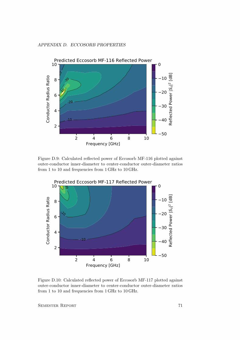
APPENDIX D. ECCOSORB PROPERTIES
2 4 6 8 10Frequency [GHz]
2
4
6
8
10
Cond
ucto
r Rad
ius R
atio
-40
-30
-20
-20
-10
Predicted Eccosorb MF-116 Reflected Power
50
40
30
20
10
0
Refle
cted
Pow
er |S
ii|2 [dB
]
Figure D.9: Calculated reflected power of Eccosorb MF-116 plotted againstouter-conductor inner-diameter to center-conductor outer-diameter ratiosfrom 1 to 10 and frequencies from 1 GHz to 10 GHz.
2 4 6 8 10Frequency [GHz]
2
4
6
8
10
Cond
ucto
r Rad
ius R
atio
-30
-20
-10
Predicted Eccosorb MF-117 Reflected Power
50
40
30
20
10
0
Refle
cted
Pow
er |S
ii|2 [dB
]
Figure D.10: Calculated reflected power of Eccosorb MF-117 plotted againstouter-conductor inner-diameter to center-conductor outer-diameter ratiosfrom 1 to 10 and frequencies from 1 GHz to 10 GHz.
Semester Report 71

D.3. CALCULATED REFLECTED POWER VERSUS CONDUCTORRADIUS RATIO FOR DIFFERENT GRADES OF ECCOSORB
2 4 6 8 10Frequency [GHz]
2
4
6
8
10Co
nduc
tor R
adiu
s Rat
io
-30-20
-10
Predicted Eccosorb MF-124 Reflected Power
50
40
30
20
10
0
Refle
cted
Pow
er |S
ii|2 [dB
]
Figure D.11: Calculated reflected power versus outer conductor inner di-ameter to inner conductor outer diameter ratio and frequency for EccosorbMF-124.
2 4 6 8 10Frequency [GHz]
2
4
6
8
10
Cond
ucto
r Rad
ius R
atio
-20
-10
Predicted Eccosorb MF-175 Reflected Power
50
40
30
20
10
0Re
flect
ed P
ower
|Sii|2 [
dB]
Figure D.12: Calculated reflected power of Eccosorb MF-175 plotted againstouter-conductor inner-diameter to center-conductor outer-diameter ratiosfrom 1 to 10 and frequencies from 1 GHz to 10 GHz.
72 Graham Norris

APPENDIX D. ECCOSORB PROPERTIES
2 4 6 8 10Frequency [GHz]
2
4
6
8
10
Cond
ucto
r Rad
ius R
atio
-20-10
Predicted Eccosorb MF-190 Reflected Power
50
40
30
20
10
0
Refle
cted
Pow
er |S
ii|2 [dB
]
Figure D.13: Calculated reflected power of Eccosorb MF-190 plotted againstouter-conductor inner-diameter to center-conductor outer-diameter ratiosfrom 1 to 10 and frequencies from 1 GHz to 10 GHz.
Semester Report 73

D.4. CALCULATED OPTIMAL REFLECTED POWER FORDIFFERENT GRADES OF ECCOSORB
D.4 Calculated Optimal Reflected Power for Dif-ferent Grades of Eccosorb
The following figures were all calcualted using the data provided by Lairdalong with Equation 2.4 and Equation 2.7, following the general proceduresfrom that section.
0.0 2.5 5.0 7.5 10.0 12.5 15.0 17.5 20.0Frequency [GHz]
60
50
40
30
20
10
0
Refle
cted
Pow
er |S
ii|2 [dB
]
Predicted Eccosorb MF-110 Reflected Power (CRR: 4.2)
Figure D.14: Calculated reflected power of Eccosorb MF-110 at a conductorradius ratio of 4.2 and frequencies from 1 GHz to 10 GHz.
74 Graham Norris

APPENDIX D. ECCOSORB PROPERTIES
0.0 2.5 5.0 7.5 10.0 12.5 15.0 17.5 20.0Frequency [GHz]
60
50
40
30
20
10
0
Refle
cted
Pow
er |S
ii|2 [dB
]
Predicted Eccosorb MF-112 Reflected Power (CRR: 5.1)
Figure D.15: Calculated reflected power of Eccosorb MF-112 at a conductorradius ratio of 5.1 and frequencies from 1 GHz to 10 GHz.
0.0 2.5 5.0 7.5 10.0 12.5 15.0 17.5 20.0Frequency [GHz]
60
50
40
30
20
10
0
Refle
cted
Pow
er |S
ii|2 [dB
]
Predicted Eccosorb MF-114 Reflected Power (CRR: 6.8)
Figure D.16: Calculated reflected power of Eccosorb MF-114 at a conductorradius ratio of 6.8 and frequencies from 1 GHz to 10 GHz.
Semester Report 75

D.4. CALCULATED OPTIMAL REFLECTED POWER FORDIFFERENT GRADES OF ECCOSORB
0.0 2.5 5.0 7.5 10.0 12.5 15.0 17.5 20.0Frequency [GHz]
60
50
40
30
20
10
0Re
flect
ed P
ower
|Sii|2 [
dB]
Predicted Eccosorb MF-116 Reflected Power (CRR: 7.1)
Figure D.17: Calculated reflected power of Eccosorb MF-116 at a conductorradius ratio of 7.1 and frequencies from 1 GHz to 10 GHz.
0.0 2.5 5.0 7.5 10.0 12.5 15.0 17.5 20.0Frequency [GHz]
60
50
40
30
20
10
0
Refle
cted
Pow
er |S
ii|2 [dB
]
Predicted Eccosorb MF-117 Reflected Power (CRR: 8.3)
Figure D.18: Calculated reflected power of Eccosorb MF-117 at a conductorradius ratio of 8.3 and frequencies from 1 GHz to 10 GHz.
76 Graham Norris

APPENDIX D. ECCOSORB PROPERTIES
0.0 2.5 5.0 7.5 10.0 12.5 15.0 17.5 20.0Frequency [GHz]
60
50
40
30
20
10
0
Refle
cted
Pow
er |S
ii|2 [dB
]
Predicted Eccosorb MF-124 Reflected Power (CRR: 8.0)
Figure D.19: Calculated reflected power of Eccosorb MF-124 at a conductorradius ratio of 8.0 and frequencies from 1 GHz to 10 GHz.
0.0 2.5 5.0 7.5 10.0 12.5 15.0 17.5 20.0Frequency [GHz]
60
50
40
30
20
10
0
Refle
cted
Pow
er |S
ii|2 [dB
]
Predicted Eccosorb MF-175 Reflected Power (CRR: 6.8)
Figure D.20: Calculated reflected power of Eccosorb MF-175 at a conductorradius ratio of 6.8 and frequencies from 1 GHz to 10 GHz.
Semester Report 77

D.4. CALCULATED OPTIMAL REFLECTED POWER FORDIFFERENT GRADES OF ECCOSORB
0.0 2.5 5.0 7.5 10.0 12.5 15.0 17.5 20.0Frequency [GHz]
60
50
40
30
20
10
0
Refle
cted
Pow
er |S
ii|2 [dB
]
Predicted Eccosorb MF-190 Reflected Power (CRR: 6.0)
Figure D.21: Calculated reflected power of Eccosorb MF-190 at a conductorradius ratio of 6.0 and frequencies from 1 GHz to 10 GHz.
78 Graham Norris
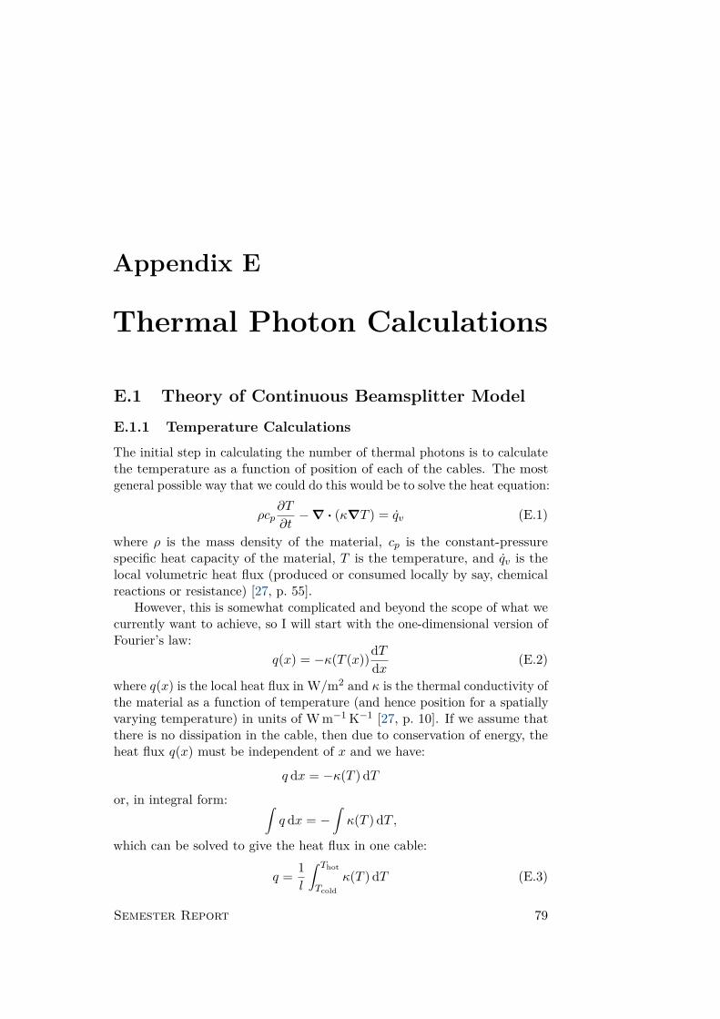
Appendix E
Thermal Photon Calculations
E.1 Theory of Continuous Beamsplitter Model
E.1.1 Temperature Calculations
The initial step in calculating the number of thermal photons is to calculatethe temperature as a function of position of each of the cables. The mostgeneral possible way that we could do this would be to solve the heat equation:
ρcp∂T
∂t−∇ · (κ∇T ) = qv (E.1)
where ρ is the mass density of the material, cp is the constant-pressurespecific heat capacity of the material, T is the temperature, and qv is thelocal volumetric heat flux (produced or consumed locally by say, chemicalreactions or resistance) [27, p. 55].
However, this is somewhat complicated and beyond the scope of what wecurrently want to achieve, so I will start with the one-dimensional version ofFourier’s law:
q(x) = −κ(T (x))dTdx (E.2)
where q(x) is the local heat flux in W/m2 and κ is the thermal conductivity ofthe material as a function of temperature (and hence position for a spatiallyvarying temperature) in units of W m−1 K−1 [27, p. 10]. If we assume thatthere is no dissipation in the cable, then due to conservation of energy, theheat flux q(x) must be independent of x and we have:
q dx = −κ(T ) dT
or, in integral form: ∫q dx = −
∫κ(T ) dT ,
which can be solved to give the heat flux in one cable:
q = 1l
∫ Thot
Tcoldκ(T ) dT (E.3)
Semester Report 79

E.2. CONTINUOUS BEAM SPLITTER MODEL
where l is the length of the cable in meters and Thot and Tcold are thetemperature of the hot and cold side of the cable in Kelvins.
Using the heat fluxes, calculated using the above equation, we can solveEquation E.2 for the temperature profile using numerical methods. Next, wemust address how the local temperature in the cable impacts the thermalphotons that are present in the cable.
E.2 Continuous Beam Splitter Model
a(x, ν)
Beam Splitterα(ν) dx a(x, ν)
(1− α(ν) dx)a(x, ν)
b(x, ν)
α(ν) dx b(x, ν)
a(x+ dx, ν)
Figure E.1: Schematic of the continuous beam splitter model. Incomingphotons in blue (a(x, ν)), black body photons in red (b(x, ν)), attenuatedphotons in gray (α(ν) dx a(x, ν)), output photons in both red and blue,reflecting the contribution of incoming and black body photons to the output.
I have provided the basic scheme of the continuous beam splitter model inFigure E.1 above. Focusing on an infinitesimal segment of cable of length dx,we model the cable as a beam splitter. On one input port, we have a(x, ν),the photons that have reached the distance x down the cable. Some fractionof these, α(ν) dx, are lost due to attenuation in this segment of the cable.The remaining fraction, (1− α(ν) dx), are transmitted to the output port.In addition to this, the cable produces local thermal black-body photons,b(x, ν). Due to the symmetry between absorption and emission, a fraction ofthese α(ν) dx are transmitted to the output port of the beam splitter. Inthis fashion, attenuation in the cable acts to “thermalize” the photons in thecable, reducing the number of photons produced by black body radiationelsewhere or intentionally added to the cable, replacing them with local blackbody photons.
By taking the output as the photon density at a position x+ dx, a(x+dx, ν), we can convert the scheme above into a differential equation for thephoton density,
a(x+ dx, ν) = a(x, ν) + [b(x, ν)− a(x, ν)]α(ν) dx.
80 Graham Norris

APPENDIX E. THERMAL PHOTON CALCULATIONS
Rearranging, we get
a(x+ dx, ν)− a(x, ν)dx = b(x, ν)− a(x, ν),
which, in the limit of dx→ 0 gives:
a′(x, ν) + a(x, ν) = b(x, ν),
a first-order inhomogeneous differential equation with the solution:
a(x, ν) = e−α(ν)x∫ x
0α(ν)eα(ν)yb(y, ν) dy + e−α(ν)xC(ν) (E.4)
where C(ν) is a constant function of position. Taking x = 0 reveals thatC(ν) = a0(ν), the photons arriving at the beginning of the cable.
Now, we must link experimental parameters to the parameters in Equa-tion E.4. The easiest way to do this is to ignore the black body photons.For a cable with an attenuation constant of 10 dB m−1 and a length of 1 m,ten percent of the input photons should reach the end of the cable, i.e.a(1, ν) = 1
10a0(ν). This gives:
110a0(ν) = e−α(ν)a0(ν)
or α(ν) = log 10. More generally, with an arbitrary attenuation in decibelsper meter, β(ν),
α(ν) = log 1010 β(ν)
revealing that α is the attenuation in units of nepers per meter and notdecibels per meter.
E.2.1 Black Body Photon Density
An important question when modeling the thermal photons of a coaxial cableis how to treat the black body photon density, in particular its dimensionality.In this case, because the electromagnetic modes of the coaxial cable arepredominantly confined in one dimension and the length of the cable is gen-erally long compared to the wavelength, I will treat the black body radiationdensity as a one-dimensional black body and treat the remaining degreeof freedom by considering the number of modes present at each frequency.Following the method presented in [28], let us begin by assuming that wehave a 1-D cavity of length L bounded by a perfectly conductive material.This boundary condition restricts the available wavelengths, requiring thatωn = 2πcn
2L where n indexes the available longitudinal modes. Treating eachmode as a harmonic oscillator, we have that the energy of each mode is equalto
Er =(r + 1
2
)hcn
2L
Semester Report 81

E.2. CONTINUOUS BEAM SPLITTER MODEL
where r is an integer that denotes the number of excitations in each mode.Following the usual statistical physics procedures, the probability of being inany of the excitation levels, Pr, is:
Pr = e−βEr
Z(β)
where β ≡ 1kBT
and Z(β) is the partition function:
Z(β) ≡∞∑r=0
e−βEr = e−β2hcn2L
1− e−β hcn2L.
for a single mode n.Denoting εn ≡ hcn
2L , the average energy in a mode n, is given by theformula:
〈En〉 = −∂ log(Z(β))∂β
= εn2 + εn
eεnβ − 1 ,
where the Bose–Einstein distribution appears on the right-hand side. If wemeasure the energy relative to the ground state (which is reasonable since wecan only ever measure energy differences), the total energy in the cavity is
U =∑
n〈En〉 −
εn2 .
As we take L→∞, the εn become continuous, and we can replace the sumabove with an integral,
U =∫ ∞
0
ε
eεβ − 1g(ε) dε
where g(ε) is the density of states, which allows us to exchange an integralover modes for an integral over energy. ε = hc
2Ln, so dn = 2Lhc dε and g(ε) = 2L
hc .Therefore, the total internal energy in this cavity of length L is
U = 2Lhc
∫ ∞0
ε
eεβ − 1 dε.
Per unit length, this becomes,
U
L= 2hc
∫ ∞0
ε
eεβ − 1 dε.
and so the spectral energy density, after converting the integral from energyto frequency, uν is given by:
uν(T ) = h2ν
hc
1
ehνkBT − 1
.
82 Graham Norris

APPENDIX E. THERMAL PHOTON CALCULATIONS
This light is emitted equally in both directions, and since we want to knowthe photons that pass through some imaginary surface in a given unit oftime, we must multiply by the speed of light and divide by the number ofdirections that the light can be emitted into. Thus, the spectral radiance is
Bν(T ) ≡ uν(T )c2 = hν
ehνkBT − 1
which has units of J s−1 Hz−1. Since for the calculations of the number ofthermal photons, we care about the number of photons and not the power,we must divide by the energy of a single photon, hν, to get
BPν (T ) = 1
ehνkBT − 1
,
the photon flux spectral density (Photon FSD or sometimes PFSD), in unitsof photons s−1 Hz−1. Again, in this one-dimensional case, the photon FSD isequivalent to the Bose–Einstein distribution.
To address the number of transverse modes that are available in thecoaxial lines, I will then define the coaxial black body photon flux spectraldensity as
b(ν, T ) ≡ n(ν)
ehνkBT − 1
(E.5)
where n(ν) is a function that gives the number of modes available in thecoaxial cable at frequency ν. This again has units of photons s−1 Hz−1.
E.2.2 Coaxial Higher-Order TE and TM Modes
We widely use coaxial cables to transmit microwave signals between two loca-tions because they are very easy to use; up to a frequency determined by thegeometry of the metal inner and outer conductors and the dielectric material,coaxial cables have only one mode, the TEM, or transverse electromagneticmode. Above this frequency (usually called the maximum frequency, modingfrequency, or higher-order mode cutoff frequency), however, coaxial cableshave a number of TE (transverse electric) and TM (transverse magnetic)modes. According to [29], the solutions of the TMnm modes are given by
Jn(ak)Yn(bk)− Jn(bk)Yn(ak) = 0 (E.6)
while the TEnm modes are given by
J ′n(ak)Y ′n(bk)− J ′n(bk)Y ′n(ak) = 0 (E.7)
where Jn is the n-th order Bessel function of the first kind, J ′n is its derivativewith respect to kx (x = a, b), Yn is the n-th order Bessel function of the
Semester Report 83

E.3. NUMERICAL SIMULATIONS
second kind and Y ′n is its derivative, k is the wavenumber, b is the inner radiusof the outer conductor, and a is the outer radius of the center conductor.The wavenumber solution is converted to frequency by
ν = kc
2π√εr
where c is the speed of light in a vacuum and εr is the relative dielectricconstant. In both equations above, the m portion of the mode comes fromtaking the m-th solution of Equation E.6 or Equation E.7.
For the TEnm modes, it is possible to describe the different modessomewhat intuitively. The n (azimuthal) parameter describes the number oftimes that the phase of the electric field winds around the center conductor.For example, for n = 0, the electric field will point inwards or outwards (butnot both at the same time), for n = 1, one semicircle will have the electricfield pointing inwards while the other semicircle will have the electric fieldpointing outwards. The m (radial) parameter describes the number of nodesin the electric field from the inner conductor to the outer conductor. Form = 0, the field points only in one direction radially, while for m = 1, theelectric field will switch directions once radially. For the TMnm modes, thissort of intuitive clarification is harder to give. The m parameter still describesthe number of nodes in the magnetic field radially, but the n parameter isharder to describe.
E.3 Numerical Simulations
All numerical simulations were performed using Wolfram Mathematica. Cur-rently, all simulation results are located in my USERS folder (Q: USERSGraham Mathematica Simulations Bluefors Thermal Noise Photons)
E.3.1 Coaxial Cable Properties
All information pertaining to the different types of coaxial cables that mightbe used in our lab are included in the coaxialCableProperties.m Mathe-matica library. This package depends on the group ThermalCalculationslibrary. Inside, two main data structures are defined: typeProperties andcableComponent. cableComponent is a function that builds an associationcorresponding to a single part of a coaxial cable. Thus, it has an innerradius, an outer radius, and a material. The radii are given in meters andthe materials are defined elsewhere in the document. typeProperties is afunction that builds an association corresponding to a single type of coax-ial cable. Thus, it has a name, a center conductor, a dielectric, an outerconductor, specified attenuation, specified higher-order mode frequencies,and a description. The cable names are based on manufacturer, cable type
84 Graham Norris

APPENDIX E. THERMAL PHOTON CALCULATIONS
(semirigid), nominal size, inner conductor material, dielectric material, andouter conductor material. cableComponents are used for the inner conductor,dielectric, and outer conductor. Importantly, the attenuation and higherorder mode frequencies are defined in the association as delayed-executionfunctions such that the data does not have to be available when the libraryis written, but is only required when the function is called for that specificcable type.
Materials within the coaxialCableProperties library are also associa-tions in which the materials are given whatever properties are defined forthem in ThermalCalculations, e.g. thermal conductivity, electrical resistiv-ity, linear thermal expansion coefficient, specific heat capacity, and density.Dielectrics have dielectric constants and cutoff frequencies, to be discussedbelow.
In this way, coaxialCableProperties is a flexible library that can beused for a variety of numerical simulations and programming tasks relatedto fridge thermal design.
E.3.2 Cable Attenuation
For the attenuation of the coaxial cables, there is no specific notebook orlibrary. Rather, the manufacturer specified attenuation of the cable typeis stored in the main directory as a csv file with a name that corresponsto the name of the cable type in coaxialCableProperties. Then theloadAttenuationData function of coaxialCableProperties, when it iscalled for this specific cable type, looks for this csv file and converts the datainto a piecewise function of attenuation in dB versus frequency in GHz withlinear interpolation between data points and a “clamping” of the attenuationat the highest (lowest) frequncy for all frequencies above (below) the limitvalue.
E.3.3 Coaxial Higher-Order Mode Minimum Frequencies
Table E.1: Micro-Coax UT-085SS-SS Properties
Parameter Value
Center Conductor Outer Radius 0.255 mmOuter Conductor Inner Radius 0.838 mmRelative Dielectric Constant 2.03
The data in Table E.1, included in coaxialCableProperties, are suf-ficient to compute the frequencies of different modes in this coaxial cable.However, the dielectric of our cables, PTFE (commonly known as Teflon),can interact with these modes, absorbing or attenuating transmissions at
Semester Report 85

E.3. NUMERICAL SIMULATIONS
different frequencies. Fortunately, PTFE is widely used, and there are anumber of studies of its properties in the far-infrared. Within this field,spectra are often presented in terms of the “spectroscopic” wavenumber,which is defined as ν ≡ 1
λ where λ is the wavelength and ν is expressed inunits of inverse cm. To convert to frequencies in Hz, the following formulacan be used:
ν = 100 · c · ν
where c is the vacuum speed of light in m s−1.Halpern et al. find that PTFE had negligible losses below 40 cm−1 (below
1200 GHz), the limits of their device [24]. Birch shows that, due to astrong absorption peak at 202 cm−1 (6060 GHz), PTFE becomes stronglyattenuating above approximately 190 cm−1 (5700 GHz), with an attenuationcoefficient greater than 20 cm−1 (without specifying if this is a Napierian ordecadic coefficient) [31]. McCarthy also found that the transmission of a1.6 mm sample of PTFE was negligible for wavenumbers between 190 cm−1
and 800 cm−1 (5700 GHz to 24 000 GHz) [32]. Therefore, I assume that thedielectric does not attenuate modes at all until 5700 GHz, when I assume thatthe absorption is so strong that no modes above this frequency propagate(hence I often refer to it as the dielectric cutoff frequency).
All calculations related to the number of higher order modes were per-formed in the coaxial_mode_calculations.nb notebook. The cutoff fre-quencies, the frequency at which a mode can begin propagating in the coaxialcable, of the different TM and TE modes were computed by numericallysolving Equation E.6 and Equation E.7 for different orders n and consideringall solutions up to frequencies beyond the upper limit set by the dielectric(thus including the different m modes). It was found to be important togive NSolve good bounds for the acceptable wavenumbers to reduce thetime spent looking for solutions, and solutions using ParallelTable couldstill take several hours to find all solutions up to 6000 GHz for 0.085”-classcables (smaller cables with greater mode spacing are faster). The TE modesrequired orders, n, up to 150, while the TM modes required orders up to70 to provide a buffer beyond the cutoff frequency of the dielectric. Thisnotebook exports the cutoff frequencies for TE and TM as separate text filesfor use by loadHigherOrderModeData in coaxialCableProperties.
Plotting the number of modes available at different frequencies (Fig-ure E.2) reveals quadratic behavior. This could be explained if, for example,the wavenumbers of different radial and azimuthal components are evenlyspaced. Then, as the total wavenumber, which could be divided betweenthese, increased, it would include quadratically more modes (see Figure E.3).Note: when fitting the number of modes, it is important to use a functionof aν2 + bν + 1 and not aν2 + bν + c, as there is always at least one modeavailable in the coaxial cable.
86 Graham Norris

APPENDIX E. THERMAL PHOTON CALCULATIONS
0 1000 2000 3000 4000 5000Frequency [GHz]
0
500
1000
1500
2000
2500
3000
3500
Num
ber o
f Mod
es
Micro Coax UT-085SS-SS Mode Spectrum
CalculatedQuadratic Fit
0 2500 5000Freq. [GHz]
0
1000
2000
No. M
odes
TETM
Figure E.2: Number of modes (TEnm and TMnm) available at differentfrequencies for a Micro-Coax UT-085SS-SS cable. Calculated data presentedin blue, quadratic fit of the form aν2 + bν + 1 presented in orange. Inset:Number of calculated TE (blue) and TM (orange) modes as a function offrequency. Both TE and TM modes show quadratic dependence on frequency.
kradial
kazimuthal
k
Figure E.3: Rough image of motivation for finding a quadratically increasingnumber of modes. Possible modes plotted as blue dots, available wavenumberrange plotted in red-orange.
Semester Report 87
E.3. NUMERICAL SIMULATIONS
E.3.4 Main Simulation
Table E.2: Stage parameters for numerical simulation. Cable length is fromthe previous stage to the current stage.
Stage Temperature [K] Cable Length [m] Attenuator
0 2931 45 0.2262 3 0.321 XMA 20 dB3 0.9 0.2804 0.100 0.199 XMA 20 dB5 0.010 0.1986 0.010 0.300 XMA 20 dB
The main simulation is contained in bluefors_coaxial_thermal_photons_simulation.nb and which relies heavily on the CoaxialThermalPhotonCalculations library. Here, the input data structure is a list of associationscalled stageParameters that has a temperature, cable length, cable type,and attenuator for each stage (included above in Table E.2). Importantly,cable length is the length from stage n − 1 to stage n (i.e. stage 0 is justpresent to provide the room temperature boundary condition). The cablelengths above were chosen to correspond to those predicted for the BlueForsXLD system and all cables are assumed to be Micro-Coax UT-085SS-SSsemi-rigid coaxial cable, which has the properties listed in Table E.1 [30].
In the beginning, I solve for the temperature profile of each of the cablesusing cableTemperatureSolution. This function first solves for the heatflux in each cable using Equation E.3 and NIntegrate (heatFlux). Then,it solves Equation E.2 using this flux (and assuming that it is the sameat all points in the cable, based on conservation of energy) with NDSolve(temperatureProfile). The temperature profile of the first cable fromstage 0 (293 K) to stage 1 (45 K) is plotted in Figure E.4. The calculatedtemperature profile is nonlinear because the thermal conductivity of 304stainless steel is not constant across this temperature range. Similarly non-linear results hold for all of the stages with a finite temperature difference.
With this data, I can finally solve for the photon densities at the differentstages using Equation E.4 and other equations from the continuous beamsplitter model section. From the temperature profile, I can calculate thelocal blackbody photon flux spectral density (blackbodyPhotonDensity),the photon FSD in a coaxial cable (cablePhotonDensity), and the photonFSD in an attenuator (attenuatorPhotonDensity). These functions arewrapped in a higher level function, stageCalculation, which automatesinserting the correct arguments and parsing coaxialCableProperties forthe correct parameters. Finally, stageCalculation itself is wrapped in
88 Graham Norris

APPENDIX E. THERMAL PHOTON CALCULATIONS
0.00 0.05 0.10 0.15 0.20Position [m]
0
50
100
150
200
250
300
Tem
pera
ture
[K]
First Stage Temperature ProfileCalculatedLinear Approx.
Figure E.4: Temperature profile for the cable from stage 0 (293 K) to stage1 (45 K). Calculated profile in blue, linear approximation in red-orange.Calculated profile is non-linear due to non-constant temperature dependenceof κ(T ) for 304 stainless steel.
the highest-level function, calculateStagePhotonDensities so that usersonly have to provide the stageParameters list in order to perform calcu-lations. For more information, look at the library usage information orcoaxial_tpc_testing.nb.
One note is that calculations using the calculated temperature profile,calculated number of modes, and specified attenuation are extremely slow(taking more than an hour just to plot the PFSD from 1 GHz to 5700 GHz).This is probably due to the fact that my current simulations are entirelyfunctional, always passing functions on, and thus the overhead of functioncalls rapidly builds up. However, in order to make the calculations faster,there is an approximate version that assumes constant attenuation, a lineartemperature profile between stages, and a quadratic form for the modespectrum. For the number of modes at a given frequency, the quadraticfit is quite close to the calculated data (see Figure E.2), with a regionwhere the quadratic fit overestimates the data somewhat between 800 GHzand 2000 GHz. The temperature profile shows the largest difference. Thenon-linear profile increases the average temperature of the calculated versusthe linear temperatures. For example, for the first cable, as shown inFigure E.4, the average calculated temperature is 185 K, while the average
Semester Report 89

E.3. NUMERICAL SIMULATIONS
linear temperature is 124 K. This means that the approximate calculationswill under-estimate the actual number of blackbody photons.
A comparison between the calculated and the approximate methods(temperature, attenuation, number of modes) is presented in Figure E.5.The approximate methods overestimate the photon FSD at frequencies upto 1800 GHz and then underestimate the photon FSD. The overestimate atintermediate frequencies may be due to the difference in the number of modesbetween the calculated values and the quadratic fit. At high frequencies,the underestimate is largely due to the difference in average temperaturesbetween the exact and approximate methods. The difference between thenormal and the approximate methods in the number of photons between thegap energy of aluminum and the cutoff frequency of the dielectric is roughly10%, well within the order-of-magnitude estimate that we are seeking.
0 1000 2000 3000 4000 5000Frequency [GHz]
0
200
400
600
800
1000
1200
1400
Phot
on F
SD [P
hoto
ns s
1 Hz
1 ]
Blackbody Photon FSD Method Comparison
CalculatedApproximate
Figure E.5: Comparison of calculated and approximate methods for producingthe blackbody photon flux spectral density. Temperature corresponds tothe temperature 10 cm into the first cable. Calculated results plotted inblue, approximate results plotted in red-orange. Vertical gray bars are thefrequencies corresponding to the gap energies of aluminum (left) and niobium(right).
The divergent photon flux spectral density at zero frequency visible inFigure E.5 (and other photon density plots below) is physical. Although, atlow frequencies, the interstage cable length may not be significantly greaterthan the wavelength, our cables are not shorted at the ends, but continue onor are 50 Ω terminated. Thus, we work in the semi-infinite cable regime, andthe cables are electrically long even at low wavelengths. This divergence in
90 Graham Norris

APPENDIX E. THERMAL PHOTON CALCULATIONS
photon comes purely from the one-dimensionality of the coaxial cable at lowfrequencies. However, since the power in these photons also scales as hν, aninfinite number of photons at 0 Hz corresponds to a fixed DC offset.
In Figure E.6, the photon FSD is plotted at the end of the cable fromstage 0 to stage 1, using the precise computed functions and the approximatefunctions, discussed above, for the number of modes, the temperature profileof the cable, and the attenuation of the cable. The photon FSD is reducedslightly compared to the blackbody plot above (Figure E.5), but the samegeneral features are present. The difference between the specified attenuationand the approximate attenuation should only matter for frequencies below50 GHz, which we ignore.
0 1000 2000 3000 4000 5000Frequency [GHz]
0
200
400
600
800
1000
1200
1400
Phot
on F
SD [P
hoto
ns s
1 Hz
1 ]
Cable Photon FSD Method Comparison (Stage 1)
CalculatedApproximate
Figure E.6: Comparison of photon flux spectral density at the end of thecable from stage 0 to stage 1 when using the computed and the approximatefunctions for the number of modes, temperature, and cable attenuation.Calculated results plotted in blue, approximate results plotted in red-orange.Vertical gray bars are the frequencies corresponding to the gap energies ofaluminum (left) and niobium (right).
Some stages also have XMA resistive attenuators. I currently assumethat they attenuate by the stated value at all frequencies. They are rated toat least 50 GHz, but it is not clear how they behave at higher frequencies.The resistive elements inside these filters (for an example discussing theconstruction of these cryogenic filters, see [33]) should continue to function,but stray capacitances might allow the filter to become transparent at highfrequencies.
Semester Report 91

E.3. NUMERICAL SIMULATIONS
E.3.5 Summary of Assumptions
These calculations have a number of limitations, so I think that it is good tobe very clear about the assumptions that I make in order to be clear aboutthe domain of validity of the simulation.
1. General Assumptions
(a) Coaxial cables are perfectly thermalized. Inner and outer conductorhave the same temperature, and the temperature at the ends ofthe cable corresponds to the stage temperatures.
(b) Local heat flux due to dissipation of signal photons can be ignored.Difficult to include in a general manner and this will mostly matterat high-temperature stages. The only sources of heat for the cableare the two stages to which it is connected.
(c) Coaxial cable only acts as 1D conductor. Needed to treat theblackbody photon density from a 1D object with a number ofmodes.
(d) Each TE and TM mode does not propagate at all below its cutofffrequency and propagates without loss above its cutoff frequency.The only source of attenuation is that specified by the cablemanufacturer.
(e) Coaxial cable is much longer than the wavelength. Required tomake the sum to integral transition. Usually fulfilled becuasesignal generators, etc. are all 50 Ω terminated, meaning that theyact as a semi-infinite cable.
(f) Attenuation of coaxial cable at high frequencies is equivalent toattenuation for highest specified frequency. Data beyond thisfrequency is unknown. Assuming that it remains constant appearsto be the safest option.
(g) Dielectric does not attenuate signal below its cutoff frequency andcompletely absorbs photons above its cutoff frequency.
(h) XMA attenuators are perfectly broadband. Performance outsidethe specified range is unknown
(i) Electric field couples equally at all points. No standing waves, etc.that would change how the blackbody photons are emitted intothe cable.
2. Performance Assumptions (Approximate Methods)
(a) Cable has equal attenuation at all frequencies. Used to speed upsimulation.
(b) Temperature profile can be approximated as linear. Used to speedup calculation.
92 Graham Norris

APPENDIX E. THERMAL PHOTON CALCULATIONS
(c) Number of modes can be approximated by a quadratic fit of theform aν2 + bν + 1. Used to speed up calculation.
E.3.6 Results
0 1000 2000 3000 4000 5000Frequency [GHz]
0.0
0.5
1.0
1.5
2.0
2.5
3.0
Phot
on F
SD [P
hoto
ns s
1 Hz
1 ]
1e3 Stage 0 Photon Flux Spectral Density
Figure E.7: Spectral density of photon flux at stage 0 (input to dilutionrefrigerator, 293 K). Vertical gray bars are the frequencies corresponding tothe gap energies of aluminum (left) and niobium (right).
The stage 0 photon flux spectral density, Figure E.7, shows the inputblackbody radiation photon density. Due to the one-dimensional nature ofthe system, the photon FSD diverges at low frequencies and then increaseswith a characteristic shape due to the interaction of the quadratic number ofmodes term with the exponential term in the denominator of Equation E.5.The photon FSD at this stage is in the thousands of photons s−1 Hz−1.
Cable attenuation brings the stage 1 photon FSD (Figure E.8) downto hundreds of photons s−1 Hz−1. However, the overall picture is similar tostage 0.
Stage 2 brings the first significant difference. With a 20 dB attenuatorpresent, this stage starkly reduces the number of photons present (to roughly1 % of the previous value) while adding black body photons at a temperatureof 3 K, causing the sharp peak of photon density to move from the left ofthe aluminum gap energy line to the right of it. The photon FSD is down tosingle photons s−1 Hz−1.
Stages 3 (Figure E.10), 4 (Figure E.11), 5 (Figure E.12), and 6 (Fig-ure E.13) largely display the same behavior as the stage 2 photon density,
Semester Report 93

E.3. NUMERICAL SIMULATIONS
0 1000 2000 3000 4000 5000Frequency [GHz]
0.0
0.2
0.4
0.6
0.8
1.0
1.2
1.4Ph
oton
FSD
[Pho
tons
s1 H
z1 ]
1e3 Stage 1 Photon Flux Spectral Density
Figure E.8: Spectral density of photon flux at stage 1 (45 K). Vertical graybars are the frequencies corresponding to the gap energies of aluminum (left)and niobium (right).
0 1000 2000 3000 4000 5000Frequency [GHz]
0.0
0.2
0.4
0.6
0.8
1.0
1.2
1.4
Phot
on F
SD [P
hoto
ns s
1 Hz
1 ]
Stage 2 Photon Flux Spectral Density
Figure E.9: Spectral density of photon flux at stage 2 (still, 3 K). Verticalgray bars are the frequencies corresponding to the gap energies of aluminum(left) and niobium (right).
94 Graham Norris

APPENDIX E. THERMAL PHOTON CALCULATIONS
0 1000 2000 3000 4000 5000Frequency [GHz]
0.00
0.05
0.10
0.15
0.20
0.25
0.30
Phot
on F
SD [P
hoto
ns s
1 Hz
1 ]
Stage 3 Photon Flux Spectral Density
Figure E.10: Spectral density of photon flux at stage 3 (0.9 K). Vertical graybars are the frequencies corresponding to the gap energies of aluminum (left)and niobium (right).
0 1000 2000 3000 4000 5000Frequency [GHz]
0.0
0.2
0.4
0.6
0.8
1.0
Phot
on F
SD [P
hoto
ns s
1 Hz
1 ]
1e 3 Stage 4 Photon Flux Spectral Density
Figure E.11: Spectral density of photon flux at stage 4 (100 mK). Verticalgray bars are the frequencies corresponding to the gap energies of aluminum(left) and niobium (right).
Semester Report 95
E.3. NUMERICAL SIMULATIONS
0 1000 2000 3000 4000 5000Frequency [GHz]
0.0
0.5
1.0
1.5
2.0
2.5Ph
oton
FSD
[Pho
tons
s1 H
z1 ]
1e 4 Stage 5 Photon Flux Spectral Density
Figure E.12: Spectral density of photon flux at stage 5 (base plate, 10 mK).Vertical gray bars are the frequencies corresponding to the gap energies ofaluminum (left) and niobium (right).
0 1000 2000 3000 4000 5000Frequency [GHz]
0.0
0.5
1.0
1.5
2.0
2.5
3.0
Phot
on F
SD [P
hoto
ns s
1 Hz
1 ]
1e 7 Stage 6 Photon Flux Spectral Density
Figure E.13: Spectral density of photon flux at stage 6 (sample, 10 mK).Vertical gray bars are the frequencies corresponding to the gap energies ofaluminum (left) and niobium (right).
96 Graham Norris

APPENDIX E. THERMAL PHOTON CALCULATIONS
but with ever-decreasing photon FSDs. By stage 6, the photon FSD has beenreduced to hundreds of nphotons s−1 Hz−1. Final photon number and photonpower calculations reveal that the total number of thermal photons betweenthe gap-energy frequency of aluminum and the cutoff frequency of the PTFEdielectric are in the order of 500 000 photons per second (see Table E.3).Based on this result, I can say that, assuming all of the assumptions madeabove hold, Eccosorb filters are crucial for rejecting thermal photons.
With these calculations it is also possible to test a more pessimisticexperimental setup. Assuming that the center conductor is not perfectlythermalized at the low temperature stages, but remains at 100 mK, this couldbe modeled by specifying the base-plate and sample temperature, as say50 mK. Simulations that encompassed these parameters showed an increasein the number of quasiparticle-inducing thermal photons from 5.2× 10⁵ s−1
previously to 5.3× 10⁵ s−1 in this case (approximate calculations). Therefore,the majority of the quasiparticle inducing photons arrive at the sample due toinsufficient attenuation rather than insufficient thermalization of the cables,at least, according to my results.
Table E.3: Number and power of photons between gap-energy frequency ofaluminum and cutoff frequency of PTFE dielectric
Stage Photon Number [photons s−1] Photon Power [W]
Input 7.9× 10¹⁵ 1.9× 10⁻⁵
Sample 5.5× 10⁵ 1.2× 10⁻¹⁵
In general, the approximate and “exact” methods produce similar finalresults. The approximate estimated the photon flux density at the sampleto within 6% of the value of the more rigorous calculations. However, the“exact” methods took 20 times longer to complete (5064 vs. 25 seconds to plotthe final stage photon FSD). Therefore, I recommend using the approximatemethods when possible, as this minor difference is well within the uncertaintydue to the other assumptions.
Semester Report 97
Bibliography
[1] M. H. Devoret, A. Wallraff, and J. M. Martinis. Superconducting Qubits:A Short Review. Version 1. Nov. 7, 2004. arXiv: cond-mat/0411174v1[cond-mat.mess-hall].
[2] Charles Kittel. Introduction to solid state physics. 7th ed. John Wiley& Sons, Inc., 1996. Chap. 12. isbn: 0-471-1181-3.
[3] D. Riste, C. C. Bultink, M. J. Tiggelman, R. N. Schouten, K. W.Lehnert, and L. DiCarlo. “Millisecond charge-parity flucuations andinduced decoherence in a superconducting transmon qubit”. In: NatureCommunications 4 (May 28, 2013), p. 1913. doi: 10.1038/ncomms2936.
[4] L. Sun, L. DiCarlo, M. D. Reed, G. Catelani, Lev S. Bishop, D. I.Schuster, B. R. Johnson, Ge A. Yang, L. Frunzio, L. Glazman, M. H.Devoret, and R. J. Schoelkopf. “Measurements of Quasiparticle Tun-neling Dynamics in a Band-Gap-Engineered Transmon Qubit”. In:Physical Review Letters 108 (June 8, 2012), p. 230509. doi: 10.1103/PhysRevLett.108.230509.
[5] G. Catelani, J. Koch, L. Frunzio, R. J. Schoelkopf, M. H. Devoret, andL. I. Glazman. “Quasiparticle Relaxation of Superconducting Qubits inthe Presence of Flux”. In: Physical Review Letters 106 (Feb. 18, 2011),p. 077002. doi: 10.1103/PhysRevLett.106.077002.
[6] J. M. Kreikebaum, A. Dove, W. Livingston, E. Kim, and I. Siddiqi.“Optimization of infrared and magnetic shielding of superconductingTiN and Al coplanar microwave resonators”. In: Superconductor Scienceand Technology 29 (Aug. 12, 2016). doi: 10.1088/0953-2048/29/10/104002.
[7] R. Barends, J. Wenner, M. Lenander, Y. Chen, R. C. Bialczak, J.Kelly, E. Lucero, P. O’Malley, M. Mariantoni, D. Sank, H. Wang, T. C.White, Y. Yin, J. Zhao, A. N. Cleland, John M. Martinis, and J. J. A.Baselmans. “Minimizing quasiparticle generation from stray infraredlight in superconducting quantum circuits”. In: Applied Physics Letters99 (Sept. 13, 2011), p. 113507. doi: 10.1063/1.3638063.
98 Graham Norris

BIBLIOGRAPHY
[8] Jeffrey Scott Birenbaum. “The C-Shunt Flux Qubit: A New Generationof Superconducting Flux Qubit”. PhD. Thesis. University of Califor-nia, Berkeley, 2014. eprint: http://eprints.cdlib.org/uc/item/3gg7j6rh.
[9] Fei Yan, Simon Gustavsson, Archana Kamal, Jeffrey Birenbaum, AdamP. Sears, David Hover, Ted J. Gudmundsen, Danna Rosenberg, GabrielSamach, S. Weber, Jonilyn L. Yoder, Terry P. Orlando, John Clarke,Andrew J. Kerman, and William D. Oliver. “The flux qubit revisitedto enhance coherence and reproducibility”. In: Nature Communications7 (Nov. 3, 2016), p. 12964. doi: 10.1038/ncomms12964.
[10] D. Vion, P. F. Orfila, P. Joyez, D. Esteve, and M. H. Devoret. “Minia-ture electrical filters for single electron devices”. In: Journal of AppliedPhysics 77 (Mar. 15, 1995), pp. 2519–2524. doi: 10.1063/1.358781.
[11] John M. Martinis, Michael H. Devoret, and John Clarke. “Experimentaltests for the quantum behavior of a macroscopic degree of freedom:The phase difference across a Josephson Junction”. In: Physical ReviewB 35 (Apr. 1, 1987), pp. 4682–4698. doi: 10.1103/PhysRevB.35.4682.
[12] Christopher Eichler. “Experimental Characterization of QuantumMicrowave Radiation and its Entanglement with a Superconduct-ing Qubit”. PhD. Thesis. ETH Zurich, 2013. eprint: http : / / e -collection.library.ethz.ch/view/eth:6886.
[13] K. Bladh, D. Gunnarsson, E. Hufeld, S. Devi, C. Kristoffersson, B.Smalander, S. Pehrson, T. Claeson, and P. Delsing. “Comparison ofcryogenic filters for use in single electronics experiments”. In: Reviewof Scientific Instruments 74 (Mar. 2003), pp. 1323–1327. doi: 10.1063/1.1540721.
[14] E. J. Wollack, D. J. Fixsen, R. Henry, A. Kogut, M. Limon, and P. Mirel.“Electromagnetic and Thermal Properties of a Conductively LoadedEpoxy”. In: Journal of Infrared, Millimeter, and Terahertz Waves 29(Oct. 27, 2007), pp. 51–61. doi: 10.1007/s10762-007-9299-4.
[15] D. F. Santavicca and D. E. Prober. “Impedance-matched low-passstripline filters”. In: Measurement Science and Technology 19 (June 30,2008), p. 087001. doi: 10.1088/0957-0233/19/8/087001.
[16] Michael Fang. “Development of Hardware for Scaling Up Supercon-ducting Qubits and Simulations of Quantum Chaos”. Bachelor’s HonorThesis. University of California, Santa Barbara, June 12, 2015.
[17] Michael Peterer. “Investigating the suppression of external sourcesof decoherence on transmon qubits”. Master’s Thesis. ETH Zurich,June 17, 2012.
[18] Mintu Mondal and Yves Salathe. “Impedance-matched coaxial low-passEccosorb filters”. Mar. 29, 2016.
Semester Report 99

BIBLIOGRAPHY
[19] David M. Pozar. Microwave Engineering. 4th ed. J. Wiley & Sons, Inc.,2012. isbn: 978-0-470-63155-3.
[20] Eccosorb CR. Two Part Castable Load Absorber Series. TechnicalBulletin. Laird Technologies, Inc. url: http://www.eccosorb.com/Collateral/Documents/English- US/CR.pdf (visited on Feb. 17,2017).
[21] Eccosorb MF. Lossy, Magnetically Loaded, Machinable Stock. TechnicalBulletin. Laird Technologies, Inc. url: http://www.eccosorb.com/Collateral/Documents/English- US/RFP- DS- MF%20092115.pdf(visited on Feb. 17, 2017).
[22] Eino J. Luoma. Energy propagation in dielectric and magnetic ma-terials. Laird Technologies, Inc. 1977. url: http://www.eccosorb.eu/energy- propagation- dielectric- and- magnetic- materials(visited on Feb. 20, 2017).
[23] Eccosorb MFS. High-Loss, Non-Rigid, Magnetically Loaded Stock. Tech-nical Bulletin. Laird Technologies, Inc. url: http://www.eccosorb.com/Collateral/Documents/English-US/RFP-DS-MFS%20100915.pdf (visited on Feb. 20, 2017).
[24] Mark Halpern, Herbert P. Gush, Edward Wishnow, and Vittorio DeCosmo. “Far infrared transmission of dielectrics at cryogenic androom temperatures: glass, Fluorogold, Eccosorb, Stycast, and vari-ous plastics”. In: Applied Optics 25.4 (Feb. 15, 1986), pp. 565–570. doi:10.1364/AO.25.000565.
[25] Hamid Hemmati, John C. Mather, and William L. Eichorn. “Sub-millimeter and millimeter wave characterization of absorbing mate-rials”. In: Applied Optics 24.24 (Dec. 15, 1985), pp. 4489–4492. doi:10.1364/AO.24.004489.
[26] Patrick Wikus, Kevin A. McCarthy, Scott A. Hertel, Yelena S. Bag-dasarova, Enectalı Figueroa-Feliciano, Steven W. Leman, John M.Rutherford, Sarah N. Trowbridge, and Scott W. Vasquez. “The spe-cific heat and thermal conductivity of Eccosorb CR-124 between 800mK and 6 K”. In: Cryogenics 49.8 (Aug. 2009), pp. 421–424. doi:10.1016/j.cryogenics.2009.06.002.
[27] John H. Lienhard IV and John H. Lienhard V. A Heat Transfer Textbook.4th ed. Cambridge, Massachusetts, U.S.A.: Phlogiston Press, Jan. 8,2017. url: http://ahtt.mit.edu (visited on Mar. 9, 2017).
[28] Planck’s Law. Wikimedia Foundation, Inc. url: https://en.wikipedia.org/wiki/Planck%27s_law (visited on Apr. 24, 2017).
[29] Stellan Ekberg. Mathematical analysis of coaxial cables. Goteborg:Elander, 1956.
100 Graham Norris

BIBLIOGRAPHY
[30] UT-085SS-SS Specifications. Revision B1. Micro-Coax, Inc. 206 JonesBlvd., Pottstown, PA 19464, U.S.A.
[31] J. R. Birch. “The far-infrared optical constants of polypropylene, PTFEand polystyrene”. In: Infrared Physics 33.1 (1992), pp. 33–38. doi:10.1016/0020-0891(92)90052-U.
[32] M. E. McCarthy. “Reflection and Transmission Measurements in theFar Infrared”. In: Applied Optics 10.11 (Nov. 1971), pp. 2539–2541.doi: 10.1364/AO.10.002539.
[33] Jen-Hao Yeh, Jay LeFebvre, Shavindra Premaratne, F. C. Wellstood,and B. S. Palmer. “Microwave attenuators for use with quantum devicesbelow 100 mK”. In: ArXiv e-prints (Mar. 3, 2017). arXiv: 1703.01285[physics.ins-det].
Semester Report 101

Colophon
This document was typeset in 11 point Latin Modern using LATEX2e, atypesetting system based on Leslie Lamport’s LATEX, which is a collection ofmacros to make working with Donald Knuth’s TEX typesetting and layoutengine easier. Compilation was performed with Han Th´e Thanh’s pdfLATEXwhich adds a large number of microtypographic improvements to the outputtext.
Figures were prepared using matplotlib version 2.0.0, python 3.4, andTableau’s Color Blind 10 color scheme or the Viridis color map included withmatplotlib.
102 Graham Norris