Infrared Solar Spectroscopic Measurements of Free Tropospheric CO, C2H6, and HCN

above Mauna Loa, Hawaii: Seasonal Variations and Evidence for Enhanced Emissions

from the Southeast Asian Tropical Fires of 1997-1998

C. P. Rinsland, l A. Goldman, 2 F. J. Murcray, 2 T. M. Stephen, 2 N. S. Pougatchev, 3 J.

Fishman, l S. J. David, 2 R. D. Blatherwick, 2 P. C. Novelli, 4 N. B. Jones, 5 and B.J.

Connor 5

INASA Langley Research Center, Hampton, VA

2Department of Physics, University of Denver, Denver, CO

3Department of Physics, Christopher Newport University, Newport News, VA4Climate Monitoring and Diagnostics Laboratory, National Oceanic and Atmospheric

Administration Boulder, CO

5National Institute of Water and Atmospheric Research, Lauder, New Zealand

UNIVERSITY of DENVER

Department of Physics

Phone (303) 871-3486 FAX (303) 778-0406

email: kamurcra@du.edu

July 13, 1999

NASA Center for AeroSpace Information

Parkway Center7121 Standard Drive

Hanover, MD 21076-1320

To Whom It May Concern,

Enclosed please one micro-reproducible copy of our research on NASA grant NSG

1432.

above.

If you need further information please feel free to contact me at the number(s) listed

Sincerely Yours,

K_kreen J.VMurcray

Research Office Manager

ERe.

2112 E Wesley Ave Denver Colorado80208-0202 303.871-2238 FAX# 303.871-4405

Tile J_ t'ersity of De.ver is an eqL.il opport.unity/atfirmative action institution

Abstract. High spectral resolution (0.003 cm -_) infrared solar absorption measurements

of CO, C2H6, and HCN have been recorded at the Network for the Detection of

Stratospheric Change station on Mauna Loa, Hawaii, (19.5°N, 155.6°W, altitude 3.4 kin).

The observations were obtained on over 250 days between August 1995 and February

1998. Column measurements are reported for the 3.4-16 km altitude region, which

corresponds approximately to the free troposphere above the station. Average CO

mixing ratios computed for this layer have been compared with flask sampling CO

measurements obtained in situ at the station during the same time period. Both show

asymmetrical seasonal cycles superimposed on significant variability. The first two years

of observations exhibit a broad January-April maximum and a sharper CO minimum

during late summer. The C2H6 and CO 3.4-16 km columns were highly correlated

throughout the observing period with the C2H6/CO slope intermediate between higher

and lower values derived from similar infrared spectroscopic measurements at 32°N and

45°S latitude, respectively. Variable enhancements in CO, C2H6, and particularly HCN

were observed beginning in about September 1997. The maximum HCN free

tropospheric monthly mean column observed in November 1997 corresponds to an

average 3.4-16 km mixing ratio of 0.7 ppbv (1 ppbv=10 "9 per unit volume), more than a

factor of 3 above the background level. The HCN enhancements continued through the

end of the observational series. Back-trajectory calculations suggest that the emissions

originated at low northern latitudes in southeast Asia. Surface CO mixing ratios and the

C2H6 tropospheric columns measured during the same time also showed anomalous

autumn 1997 maxima. The intense and widespread tropical wild fires that burned during

thestrongE1Nifio warmphaseof 1997-1998arethelikely sourceof theelevated

emissionproducts.

4

1. Introduction

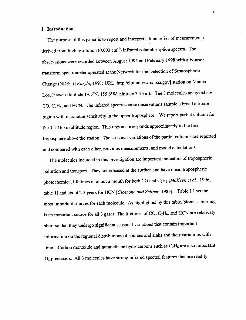
The purpose of this paper is to report and interpret a time series of measurements

derived from high resolution (0.003 cm l) infrared solar absorption spectra. The

observations were recorded between August 1995 and February 1998 with a Fourier

transform spectrometer operated at the Network for the Detection of Stratospheric

Change (NDSC) [Kurylo, 1991; URL: http:/climon.wwb.noaa.gov] station on Mauna

Loa, Hawaii (latitude 19.5°N, 155.6°W, altitude 3.4 km). The 3 molecules analyzed are

CO, C2H6, and HCN. The infrared spectroscopic observations sample a broad altitude

region with maximum sensitivity in the upper troposphere. We report partial column for

the 3.4-16 km altitude region. This region corresponds approximately to the free

troposphere above the station. The seasonal variations of the partial columns are reported

and compared with each other, previous measurements, and model calculations.

The molecules included in this investigation are important indicators of tropospheric

pollution and transport. They are released at the surface and have mean tropospheric

photochemical lifetimes of about a month for both CO and C2H6 [McKeen et al., 1996,

table 1] and about 2.5 years for HCN [Cicerone andZellner, 1983]. Table 1 lists the

most important sources for each molecule. As highlighted by this table, biomass burning

is an important source for all 3 gases. The lifetimes of CO, C2H6, and HCN are relatively

short so that they undergo significant seasonal variations that contain important

information on the regional distributions of sources and sinks and their variations with

time. Carbon monoxide and nonmethane hydrocarbons such as C2H6 are also important

03 precursers. All 3 molecules have strong infrared spectral features that are readily

measured by solar absorption spectroscopy [e.g., Rinsland et al., 1982, 1998a; Mahieu et

al., 1995, 1997; Notholt et al., 1999].

The Mauna Loa facility is a well-instrumented, high-altitude station for monitoring of

atmospheric constituents, aerosols, meteorological parameters, UV radiation, and solar

radiation [Climate Monitoring and Diagnostics Laboratory (CMDL), 1998]. Due to its

high elevation, Mauna Loa is located primarily in the free troposphere [Mendonca, 1969].

With the exception of the observations from Mauna Loa, the mid-Pacific region is data

sparse with few previous measurements of constituents in the free troposphere or time

series of observations. Trajectories arriving at MLO within 10 days originate mostly

from Asia during winter and spring with the station mostly isolated from Asian influence

during summer when some trajectories originate from over Central America within 10

days [CMDL, 1998; Kuniyuki et al., 1998]. Fall is a season of transition between easterly

trades and westerly flow [CMDL, 1998]. Transport of trace gases to the Mauna Loa

observatory have been discussed in several recent studies [e.g., Jaffe et al., 1997; Harris

et al., 1992, 1998]. Three important aircraft field campaigns have been conducted by

NASA's Global Tropospheric Experiment (GTE) to study tropospheric chemistry and

transport over the Pacific basin [Hoell et al., 1996, 1997, 1999]. Tropospheric remote

sensing measurements have also been obtained in this region during several shuttle flights

[Reichle et al., 1986, 1990, 1999; Connors et al., 1999; Rinsland et al., 1998a].

2. Infrared Spectroscopic Observations

The infrared solar absorption measurements at the Mauna Loa observatory (MLO)

were recorded with a modified Bruker model 120-HR Fourier transform spectrometer

(FTS)operatedatanunapodizedspectralresolutionof 0.0035cml (definedas0.9

dividedby themaximumopticalpathdifference).Theinstrument,installedin August

1995,is equippedwith a computer-controlledsolartrackerwith ahatchedweather-tight

enclosure.Thesystemonly requiresanoperatorto fill thedetectordewarswith liquid

nitrogenonceaday. Thesystemmonitorstheweatherconditionsandrecordssolar

spectrawhenconditionsarefavorable.Observationsarescheduledat sunrise and sunset

beginning on Monday afternoon through Saturday morning. Under favorable conditions,

the morning observations commence at 85 ° solar zenith angle with a total of 10

measurements recorded in 6 spectral bandpasses. Each observation is obtained from 2

complete interferograms recorded over a 4-minute time period. An additional 4 minutes

is required for computer evaluation and processing time of the observation. The database

analyzed here covers the August 1995 to February 1998, excluding time periods lost due

to instrumental problems. Most measurements were obtained in the morning because of

more frequent cloudiness in the afternoon.

Observations from the same site were also obtained between May 1991 and November

1995 with a Bomem model DA3.002 FTS operated typically at 0.005 cm "1resolution

[e.g., Goldman et al., 1992; David et al., 1994; Rinsland et al., 1994]. Additionally,

infrared spectra were recorded at 0.02 cm "1 resolution on 4 days in February 1987

[Rinsland et al., 1988]. Both sets of earlier measurements were obtained less frequently,

and they are generally of lower quality relative to the more recent measurements. Hence,

only the measurements recorded with the Bruker interferometer are included in the

present investigation.

3. Analysis Method and Assumptions

a. ) Retrieval Algorithm

The infrared solar spectra were analyzed with the SFIT2 algorithm, which has been

developed for the retrieval of molecular vertical profiles from ground-based infrared solar

absorption spectra. The profiles of one or two molecules are retrieved by simultaneously

fitting one or more narrow spectral intervals (microwindows) in one or more solar

spectra. The forward and inverse models in SFIT2 have been described previously

[Pougatchev et al., 1995; Rinsland et al. 1998b]. The algorithm includes a crude model

for simulating and fitting the absorption by solar CO lines [Rinsland et aL, 1998b, section

3.2.2]. The modeling of instrument performance-related parameters includes a parameter

to retrieve the wavelength shift between the measured and calculated spectra and a

parameter to fit for the slope of the background in each microwindow. The latter

parameter was required primarily because of uncertainties in modeling the absorption by

lines outside the fitted regions, particularly those of H20 and its continuum.

b.) A priori Profiles and Covariance Matrix Parameters

Below 12 km, a priori profiles for CO and C2H6 were derived by averaging aircraft in

situ profile measurements obtained near Mauna Loa during 3 GTE missions. The

measurements were obtained during the Pacific Exploratory Mission (PEM)-West, phase

A, conducted September-October 1991 [HoelI et al., 1996], PEM-West, phase B,

conducted during February-March 1994 [Hoell et al., 1997], and PEM-Tropics A

conducted between August-October 1996 [Hoell et al., 1999]. Prior CO in situ

measurements from Mauna Loa show considerable variability throughout the year. A

factor of two seasonal variation at the surface is indicated from time series of CMDL

observations [Novelli et al., 1992; 1998]. Similarly, a factor of two seasonal change was

indicated from C2H6 infrared total column measurements [Rinsland et al., 1994]. The

late winter GTE observations were obtained near maxima in both the CO and C2H6

seasonal cycles. We assumed the mean of the late winter and autumn profiles for both

molecules. Above 12 kin, the profiles were connected to averages of version 2 profiles

measured by the Atmospheric Trace MOlecule Spectroscopy (ATMOS) experiment

during the Atmospheric Laboratory for Applications and Science (ATLAS)-3 mission of

November 1994 [Gunson et al., 1996]. ATMOS measurements between latitudes of

15°1',1and 25°1'4 were averaged to derive the a priori profiles for CO and C2H6.

For HCN, a constant mixing ratio of 190 pptv (10 q2 per unit volume) was assumed

below 16 km. At higher altitudes a vertical distribution scaled to connect smoothly to the

reference profile given in Table III ofMahieu et al. [1995]. This profile is based on

retrievals from ground-based infrared solar spectra recorded at the U.S. National Solar

Observatory facility on Kitt Peak, Arizona (31.9°N latitude, 111.6°W longitude, altitude

2.09 kin) and the International Scientific Station of the Jungfraujoch (ISSJ) in the Swiss

Alps (46.6°N latitude, 8.0°E longitude, altitude 3.58 km) [Mahieu et al., 1995].

Vertical temperature profiles assumed in the analysis were taken from daily mean

National Centers for Environmental Prediction (NCEP) measurements. They were

smoothly connected to the 1976 U.S. Standard Atmosphere above 65 kin. A priori

volume mixing ratio profiles for interfering species were taken from reference

compilations (e.g., Smith [ 1982]).

c.) Spectroscopic Parameters and Microwindow Selections

Spectroscopic parameters adopted in the present study were taken from the 1996

HITRAN compilation [Rothman et al, 1998], except for the C2H6 parameters which were

replaced by improved values [Rinsland et al., 1998b, section 4.1] based on updates to the

work of Pine andStone [1996]. A line of HDO was added at 4274.81 cm "1to account for

an unassigned absorption feature [Rinsland et al., 1998b, section 4.2]. Absorption by this

transition is very weak because of the low H20 column abundance above the high-

altitude Mauna Loa station.

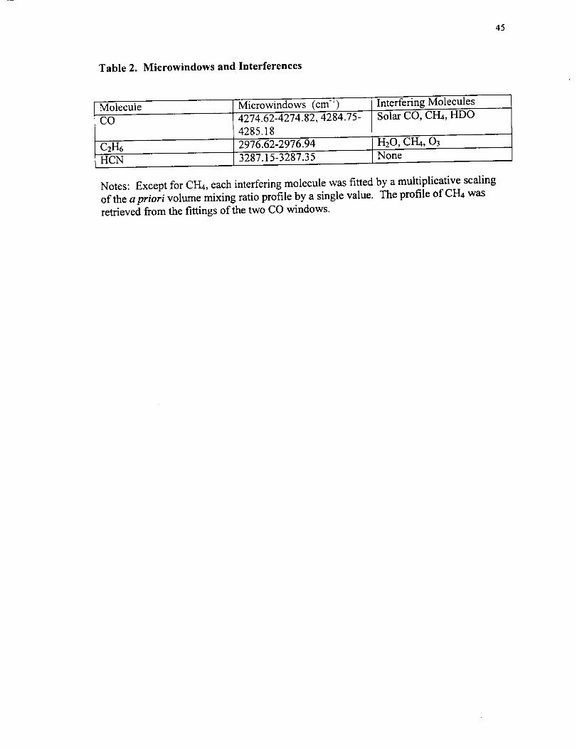
Table 2 lists the microwindows selected for the analysis of each molecule along with a

list of the interfering molecules that were fitted. The CO and C2H6 windows are identical

to those used in a previous investigation [Rinsland et al., 1998b]; simulations of the

atmospheric absorption by the individual molecules were displayed in Figs. 5 and 7 of

that paper. One of the two windows selected for retrieving profiles of CO contains the

strong CH4 line at 4285.1553 cm "l [Rinsland et al., 1998b, Fig. 7]. As in the previous

study, the profile of CH4 was also retrieved, though the results for this molecule are not

reported here.

The interval for retrieving HCN contains the v3 band P(8) line at 3287.2483 cm "1.

This transition is located in the far wings of the strong H20 lines at 3286.1689 and

3288.4829 cm "l with weak transitions of CO2 and several less significant absorbers

nearby [Rinsland et al., 1982]. Fits to the HCN v3 band P(4) line at 3299.5273 cm 1

simultaneously with the P(8) line showed minor inconsistencies. This problem was noted

previously by Mahieu et al. [1995]. Therefore, we decided not to include the P(4) line in

the analysis.

10

d.) Retrieval Characterization

Averaging kernels provide a direct assessment of the theoretical altitude sensitivity of

the observations in the absence of errors in the measurements and model parameters

[Rodgers, 1990, section 4]. They are a function of the retrieval intervals selected, the

spectral resolution of the observations, the assumed signal-to-noise of the measurements,

and the selections of the retrieval parameters, such as the apriori profile and its

covariance matrix. In this work, we assumed the covariance matrix is diagonal and

adopted a relative uncertainty equal to 0.5 times the a priori mixing ratio in each of the

29 layers in the atmospheric model extending from the surface (3.4 km) to 100 km.

Figure 1 shows the averaging kernels for CO, C2H6, and HCN. The kernels were

calculated for the spectral resolution of the measurements and the typical signal-to-noise

ratio of 200. Kernels are shown for 3.4-16.0 km and the total column. The boundary at

16 km corresponds to the approximate altitude of the annual mean tropopause above

Mauna Loa. As can be seen from this figure, the kernels for the 3.4-16.0 km layer are

broad for all 3 molecules with sensitivities that peak in the upper troposphere. The

altitudes of the peaks of the 3.4-16.0 km kernels are 11 km for CO, 11 krn for C2H6, and

13 km for HCN, respectively.

e.) Error Analysis

In Table 3, we report estimates of the uncertainties in the 3.4-16.0 km columns due to

both random and systematic sources of error. The approach used to estimate the

uncertainties is the same as adopted previously [Rinsland et al., 1998b].

The sources of random error considered are the temperature uncertainty, uncertainty

in the solar zenith angle, the effect of random instrumental noise, and errors in calculating

11

theabsorptionby interferinglines.We estimatedtheuncertaintydueto errorsin the

temperatureprofileby performedretrievalswith 2 K addedto theNCEPtemperatureat

eachaltitude. Changesin the 3.4-16km columnsareshownin thetable;thevalues

reportedfor temperaturearethemeanoffsetobtainedfrom retrievalsperformedwith 3

randomlyselectedspectraondifferentdays.Themaximumerrordueto temperature

profileuncertaintywasthevalueof 1.7%obtainedfor C2H6.

As already mentioned, each spectrum is generated from two coadded scans. The

airmass corresponding to the time of each zero path difference crossing is calculated and

the values averaged. Errors are introduced by the approximations used to estimate the

airmass of each spectrum and also by uncertainties in the time stamping of the individual

spectral files (up to 30 see). Calculations performed for a solar zenith angle of 75 °

indicate both effects combine to introduce an uncertainty in the calculated air mass of

about 1%.

The contribution of instrumental noise was evaluated by generating random numbers

with zero mean, a normal distribution, and a root-mean-square deviation equal to 0.005

times the maximum transmission in the spectral interval. The selected noise level is

typical of the Mauna Loa observations. Noise generated with 10 different seeds was

added to synthetic spectra calculated for a solar astronomical zenith angle of 60 °, and the

retrievals were repeated for each case. The mean difference between the 3.4-16 km

columns retrieved from the noisy spectra and the values obtained without noise is given

in the table. As we report only daily average partial columns, the error due to random

noise will be generally less than the value in table 3.

12

Estimatesfor therandomerrorsdueto interferingatmosphericlinesreflectthehigh

altitudeof MaunaLoa station. Previously,weestimateduncertaintiesof 7and2 % in the

troposphericcolumnsof C2H6 above Lauder, New Zealand (45.0°S latitude, 169.7°E

longitude, 0.37 km altitude) and Kitt Peak, respectively [Rinsland et al., 1998b, table 1].

The relatively high estimated uncertainties reflected the potential for error in the

calculation of the H20 absorption line overlapping the target C2H6 spectral feature at

2976.8 cm "l [Rinsland et al., 1998b, Fig. 5]. Hence, our calculated uncertainty due to

potential errors in calculating the overlapping interference by H20 absorption line is

significantly reduced.

Four sources of systematic error were considered: (1) errors in the assumed

spectroscopic line parameters, (2) uncertainties in the forward model, (3) errors in the a

priori profiles, and (4) errors in the instrument line shape function. The improvements in

the C2H6 spectroscopic parameters reduced the uncertainty in those retrievals from 10%

[Rinsland et al., 1994] to 5% [Rinsland et al., 1998b]. The forward model is also the

same as adopted previously, and hence the estimated systematic error due to its

limitations and approximations is unchanged [Rinsland et al., 1998b]. We estimated

the effect of uncertainty in knowledge of the instrument line shape function by generating

a synthetic spectrum for each molecule based on the instrument line shape function

assumed in the retrievals. We then performed a retrieval from the synthetic spectrum

with the coefficient of the "straight line" effective apodization coefficient [Park, 1983]

offset from the nominal value of 0.0 to -0.2. This calculation simulates an error in the

apodizing function with the error increasing from zero at the zero path difference to 20%

at the maximum path difference. Changes in the 0.4-16 km columns were at less than

13

0.4% for all 3 molecules. Hence, errors in modeling the instrument line shape function

introduce only a small error in the calculated 0.4-16 km columns. Narrow lines in the

solar spectra showed no evidence for phase errors.

4. Results

a.) Carbon Monoxide (CO)

Figure 2 presents typical spectral fits to the Mauna Loa solar absorption spectra in the

two windows used to measure atmospheric CO. The high quality of the Mauna Loa

measurements and the success in modeling the atmospheric and solar features can be

noted from the low residuals, which are displayed above the measured and best-fit

calculated spectra.

Figure 3 displays the time series of Mauna Loa CO measurements. The solid circles

show monthly mean mixing ratios (ppbv, 10 -9 per unit volume) calculated by dividing the

3.4-16 km CO column by the total air column in the same layer. Daily averages were

used in these calculations. Low signal-to-noise ratio observations and poor fits to the

spectral data have been excluded [Rinsland et al., 1998b, section 5.0]. The open circles

show monthly averages of preliminary CO mixing ratios from the CMDL cooperative

flask sampling network. The measurements were collected weekly from Mauna Loa and

are referenced to the CO CMDL scale [Novelli et al., 1991]. To avoid sampling

boundary layer air, the measurements are obtained in the morning before upslope flow

begins. Details of the sampling procedures and analytic methods can be found in Novelli

et al. [1992, 1998]. The flask measurements have been filtered to remove observations

subject to sampling errors, analytical problems, and non-background level measurements.

14

The vertical lines show standard deviations of the measurements. Absence of a vertical

marker denotes months when FTS measurements were recorded on a single day. Only

the CMDL observations obtained during the time period of the FTS measurements are

presented.

The 2.6 years of CO surface and FTS measurements presented in Fig. 3 show

significant short-term variations superimposed on a seasonal change of about a factor of

two. The August 1995-August 1997 measurements show very similar seasonal cycles

with a broad maximum in CO mixing ratio at the surface between January to April. The

seasonal variations at the surface are similar those reported for 1990-1995 by Novelli et

al. [1998, Fig. 4]. Near the peak of the cycle, the surface mixing ratio averaged 10-20%

higher than the mean value calculated from the integrated 3.4-16 km spectroscopic

columns. This difference implies that the free tropospheric CO mixing ratio profile

generally decreased with altitude, consistent with GTE PEM-West B mission CO

measurements obtained on February 7 and 8, 1994, near Hawaii [Hoell et al., 1997, table

1]. These measurements are available from the GTE data archive at NASA's Langley

Research Center (URL: http://www-gte.larc.nasa.gov). The CMDL surface and 3.4-16

km FTS column measurements both show a sharp minimum during late summer. While

many factors influence the seasonal variation of tropospheric CO, consistent with

previous studies [e.g., Novelli et al., 1998], we note that the seasonal CO maxima and

minima occur several months later the corresponding variations expected for OH from

seasonal changes in solar insulation. The late summer agreement between the FTS and

CMDL mixing ratios implies that the CO mixing ratio profile was on average nearly

constant with altitude in the free troposphere. This conclusion is also consistent with the

15

aircraftprofilesmeasuredin October1991closeto Hawaiiduring thePEM-WestA

mission[Hoell et al., 1996, table 2]. The September 1997-February 1998 time period

was anomalous in that the monthly averages showed maxima in surface CO (during

October) and free tropospheric CO (during November). The agreement between the two

sets of mixing ratios in late 1997 implies that the CO vertical mixing ratio profile was

nearly uniform in the free troposphere during this anomalous time period.

Pougatchev and Rinsland [1995] reported measurements of the CO seasonal variation

in two layers deduced from infrared solar spectra recorded between 1982 and 1993. The

observations were recorded from Kitt Peak located in Arizona, U.S.A., at 32°N latitude,

112°W, 2.09 km altitude. The lower layer extending from the surface to 400 mbar (-7

km altitude) sampled primarily the free troposphere. The upper layer extended from 400

mbar to the top of the atmosphere. The asymmetrical seasonal variations in both layers

are qualitatively similar to the variations indicated from the Mauna Loa surface and

infrared spectroscopic measurements. An average ratio of 2.2_-t:0.1 was derived from the

Kitt Peak measurements by dividing the average mixing ratio in the lower layer by the

average mixing ratio in the upper layer. This ratio implies that within the troposphere

there is a more rapid decrease with altitude above Kitt Peak than above Mauna Loa,

consistent with the continental location of Kitt Peak and its closer location to sources.

Very few measurements of the seasonal variation of CO in the tropical and subtropical

upper troposphere have been reported previously. Measurements of CO mixing ratios

have been obtained at altitudes of 8.5-13 km during commercial airline flights between

Japan and Australia from April 1993 to July 1996 roughly at 140°W longitude [Matsueda

et al., 1998a]. They provided unique measurements of CO variations as a function of

16

latitudeandtimein theuppertroposphereoverthewesternPacific. TheaverageCO

seasonalcyclefor this timeperiodin the15°N-20°Nlatitudeband[Matsuedaet al.,

1998a, Fig. 7] was derived by fitting the measurement time series with a linear function

combined with three harmonics [Matsueda et al., 1998a, Eq. 1]. The best-fit seasonal

component shows a minimum in mid-February with the peak amplitude of 10 ppbv and a

maximum at the beginning of May with a peak amplitude of 20 ppbv. Little seasonal

variation was observed at these heights during other times of the year [Matsueda et al.,

1998a, Fig. 7]. Our measurements of the peak-to-peak amplitude of the seasonal cycle

are generally consistent with the aircraft observations, though the times of the maxima

and minima are different in the two data sets. The CO late summer minimum apparent in

the Mauna Loa 3.4-16 km column measurement time series is not obvious in the aircraft

flask sampling observations. The differences in locations of the two sets of observations

and the limited samplings of both data sets are likely to contribute to these discrepancies.

To date, the only near global observations of tropospheric CO were obtained by a

nadir-viewing Measurement of Air Pollution from Satellites (MAPS) instrument that flew

onboard the U.S. Space Shuttle [Reichle et al., 1986, 1990, 1999; Connors et al., 1999].

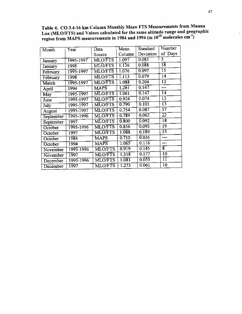
Table 4 presents the monthly mean 3.4-16 km CO columns derived from our FTS

measurements and values calculated from the MAPS observations. The measurements

are sorted by month. The number of days included in the calculations is listed in the

table. Values from the FTS observations are presented separately for the August 1995-

August 1997 and the September 1997-February 1998 time periods.

MAPS observations sample CO in the atmosphere [Pougatchev et al., 1998, Fig. 2]

with a vertical sensitivity very similar to our FTS solar observations (Fig. 1). Both sets of

17

observations are sensitive to changes in middle and upper tropospheric CO but have

practically no sensitivity to changes in boundary layer CO levels [Pougatchev et al.,

1998, Fig. 2]. In contrast, it should be noted that ground-based infrared measurements of

CO are usually performed from a strong CO line at 4.7 _tm, which samples the

atmosphere with a total column averaging kernel peaked at the surface, not in the upper

troposphere [Pougatchev et al., 1998, Fig. 2].

The MAPS instrument measured CO near Mauna Loa during shuttle flights in October

1984, April 1994, and October 1994. Average mixing ratios and standard deviations

were computed from a 1° x 1° gridded product (S. R. Nolf, private communication,

1999). Observations between 17°N and 21°N latitude and 150°W and 160°W longitude

were included. Averaging was performed because many of the MAPS grid points do not

have observational values due to the presence of clouds in the field of view or gaps in the

spatial coverage during the limited time period of the shuttle flights. This region is

located almost entirely over ocean.

We next used our Mauna Loa CO a priori profile to calculate a multiplicative factor

that relates the mean mixing ratio in the 3.4-16 km layer sampled by the FTS to a partial

column integrated over the same altitude range. The Mauna Loa CO a priori profile used

for the FTS retrievals was assumed. The derived conversion factor between mean CO

mixing ratio to the CO column in the 3.4-16 km layer is 1 ppbv = 1.196x1016 molecules

cm -2. This approach provides a quantitative correction for the reduced CO column

sampled by the FTS observations from the high-altitude Mauna Loa station. Because of

the close similarity between the FTS and MAPS averaging kernels and a priori profiles,

the error in our conversion of MAPS mixing ratio to equivalent 3.4-16 km CO column is

18

estimated as 3%, significantly less than the 10% accuracy of the MAPS CO observations

[Reichle et al., 1999]. Our approach for relating ground-based IR columns and MAPS

mixing ratios is consistent with the analysis of Pougatchev et al. [ 1998].

As shown in table 4, the FTS monthly average CO 3.4-16 km columns measured after

September 1997 are higher than values from the corresponding months of August 1995-

August 1997. The ratio of monthly averages from the two time periods peaked at

1.434-0.30. This value and uncertainty were calculated from monthly averages and

standard deviations for November 1997 relative to values for November 1995 and

November 1996. Monthly means of January 1998 and February 1998 FTS measurements

are only marginally higher than the corresponding values from the 1995-1997 time

period.

Tropospheric CO columns calculated from the MAPS measurements at the location

of Mauna Loa show significant variations that are both higher and lower than the FTS

averages. It is necessary to compare observations for the same months because of the

large seasonal variation in CO. Although no FTS measurements were recorded during

the month of April, we estimated a value for that month by averaging the FTS monthly

means from March and May of 1995-1997. The MAPS measurement from its April 1994

shuttle flight is higher than the calculated FTS mean by a factor of 1.17+0.24. The

MAPS column for October 1994 is also higher than the FTS value from October 1995

and October 1996 by a factor 1.244-0.19, but it was 0.98+0.20 times the FTS

measurements from October 1997.

value measured during that month.

The MAPS column from October 1984 is the lowest

The ratio of the MAPS October 1984 to the mean of

the Mauna Loa March and May measurements from 1995-1997 is 0.65+0.12.

19

b.) Ethane (C2H6)

The top panel of figure 4 illustrates a typical Mauna Loa spectrum and fit in the region

analyzed to retrieve the C2H6 profiles. The time series of 3.4-16 km columns shows a

distinct seasonal cycle that is very similar to the one observed for the 3.4-16 km CO

columns. This result is consistent with an analysis of Mauna Loa C2H6 observations

recorded between November 1991 and July 1993 [Rinsland et al., 1994], even though

the two sets of observations were recorded with different instruments, analyzed with

different sets of spectroscopic parameters, and different spectral fitting programs were

adopted. No significant long-term trend in the C2H6 column has been found from either

dataset.

Table 5 presents monthly averages of the C2H6 3.4-16 km columns from the 1995-

1998 series of measurements. As was done for CO, we report values separately for the

August 1995-August 1997 and the September 1997-February 1998 time periods. The

mean columns were systematically higher during October to December 1997 relative to

values for the same months in 1995 and 1996. As for CO, the maximum enhancement

was observed in November 1997 with an observed ratio of 1.43+0.41 relative to the

corresponding observations from 1995 and 1996. The January and February 1998

measurements show no obvious enhancements relative to the 1995-1997 observations

from the same months.

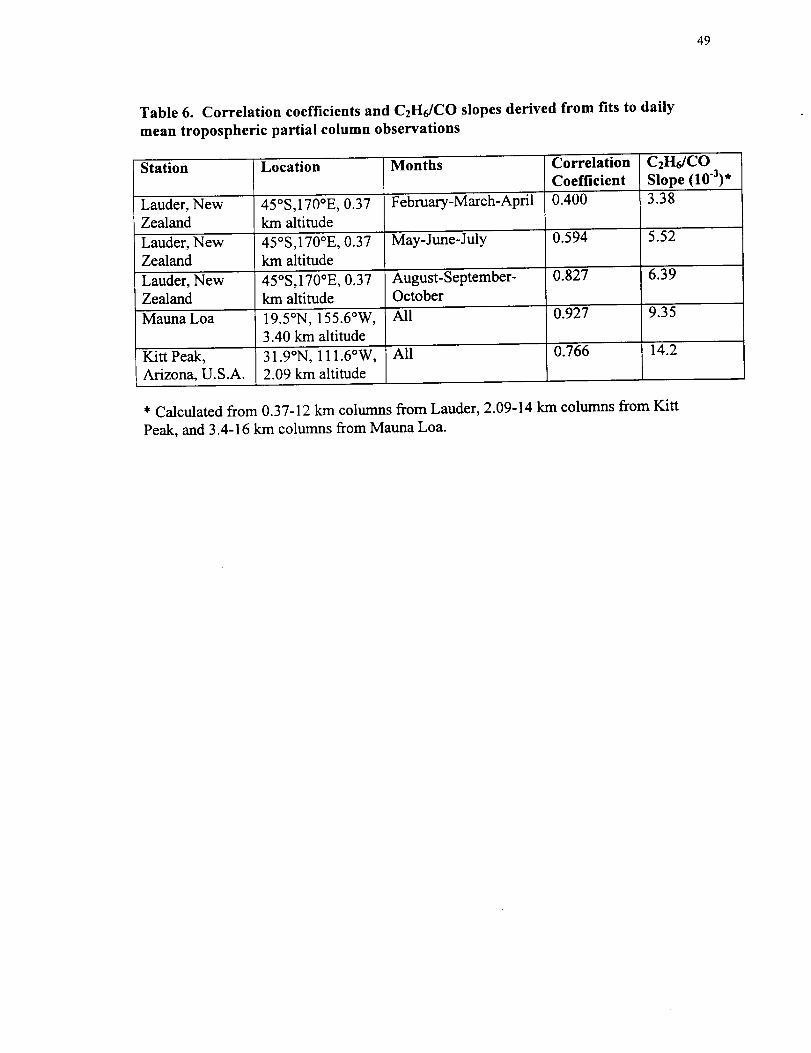
Figure 5 presents a plot of the daily average 3.4-16 km C2H6 vs. the daily average CO

3.4-16 km columns. Measurements from all seasons are included with the solid line

indicating a fit assuming a linear relation between the two sets of columns. Table 6

compares the correlation coefficients and C2H6/CO slope derived from the Mauna Loa

20

spectroscopic observations with previous tropospheric spectroscopic column

measurements. The previous measurements were obtained from Lauder and Kitt Peak

[Rinsland et al., 1998b]. The correlations between the integrated CO and C2H6

tropospheric columns are likely to reflect common principal sources for both molecules

(see Table 1) and their similar rates of reaction with OH [Rudolph, 1995]. Also, the

C2H6/CO emission factor of 0.0094 derived from biomass fire measurements [Yokelson et

al., 1997, Table 3] is very similar to the slope derived from the Lander infrared

observations during the southern hemisphere burning season. The best-fit Mauna Loa

C2H6/CO 3.4-16 km columns ratio of 0.00935 and the correlation coefficient of 0.927 are

also similar to values of 0.0073 and 0.92 deduced from C2H6 and CO mixing ratios

measured in situ in the western Pacific basin between 10°S and 25°N latitude and above 2

km altitude during February and March 1994 [Blake et al., 1997, Fig. 2].

We have also compared the Mauna Loa CO and C2H6 tropospheric columns with

monthly values calculated by integrating profiles predicted for the same location with a

global 3-D tropospheric model [Wang et al., 1998]. The model tropospheric columns (Y.

Wang, private communication, 1999) reproduce the spring maximum and autumn

minimum measured for both CO and C2H6 between August 1995 and August 1997. The

ratio of the monthly mean tropospheric columns to the corresponding model values has

been calculated for this time period. The mean and standard deviation are 1.06 and 0.08

for CO and 1.61 and 0.21 for C2H6, respectively. Hence, the model values are in very

good agreement with the measured CO tropospheric columns, but the model values are

systematically low for C2H6. The discrepancy for C2H6 is likely to reflect an

21

underestimationof C2H6 emissions from southeast Asia (Y. Wang, private

communications, 1999).

Both observational and theoretical evidence indicates that the tropospheric mixing

ratios of relatively long-lived hydrocarbons are determined by a combination of OH

photochemistry and turbulent mixing during transport [e.g., McKeen et aL, 1996]. In

general, these processes cannot be distinguished. Although the observed ratio of

C2H2/CO has proven to be a highly useful indicator of the combined effects of dynamical

mixing and photochemistry, the absorption by C2H2 lines is weak in the high-altitude,

low-latitude Mauna Loa solar spectra. Hence, it did not prove possible to measure C2H2

tropospheric columns throughout the year and use the C2H2 to CO ratio to classify air

masses, as has been done successfully during GTE field missions [e.g., Smyth et al.,

1996].

c.) Hydrogen Cyanide (HCN)

Figure 6 illustrates fits to the Mauna Loa spectra in the HCN window. The two

examples were selected to illustrate observations recorded during the month of November

at nearly the same solar zenith angle but with HCN 3.4-16 km column abundances that

differ by one order of magnitude.

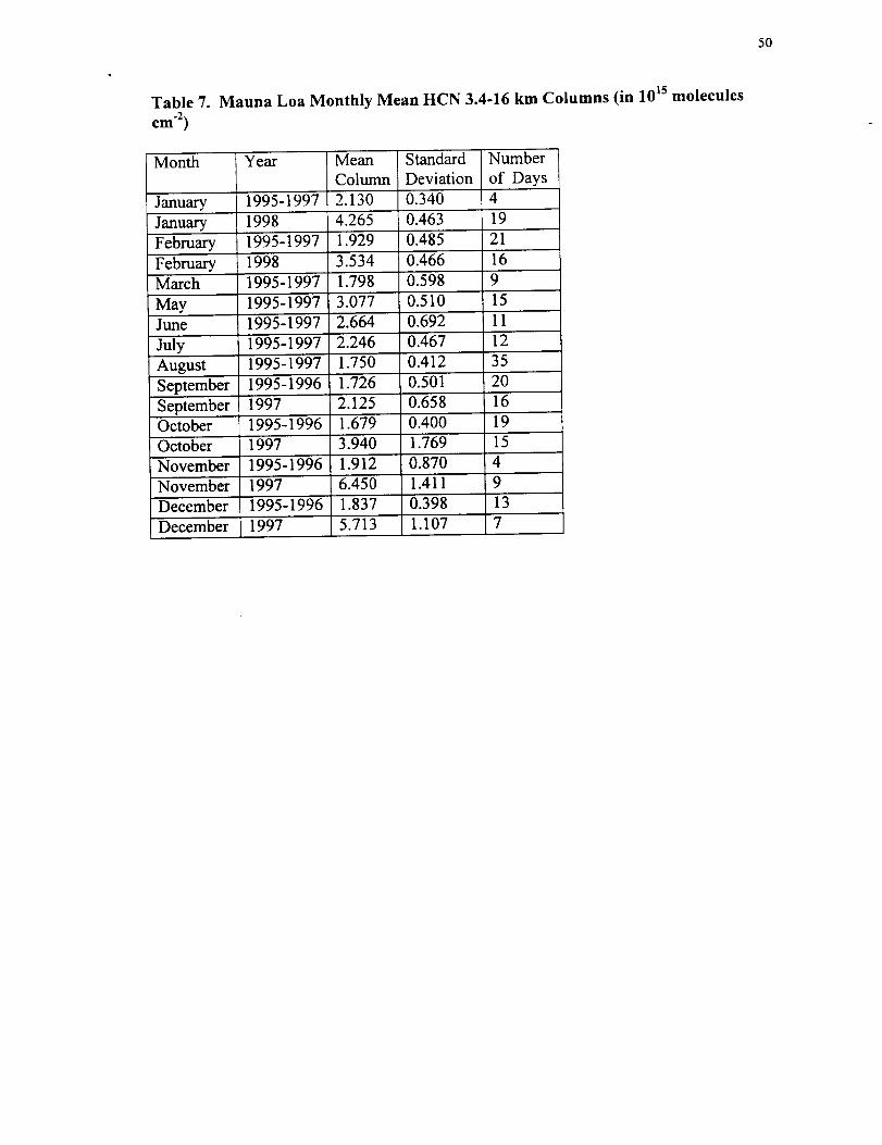
Figure 7 presents the measured time series of HCN 3.4-16 km partial columns derived

from the Mauna Loa measurements. Monthly averages and standard deviations are

reported in table 7. As for CO and C2H6, results are reported separately for the August

1995-August 1997 and September 1997-February 1998. As summarized in this table,

the variations in HCN are substantially larger than those measured for CO and C2H6.

22

HigherHCN 3.4-16km columnsweremeasuredthroughouttheOctober1997to

February1998timeperiodrelativeto thosefrom correspondingmonthsbetweenAugust

1995andAugust1997.A maximumratioof 3.37+1.70wascalculatedfrom themean

andstandarddeviationof theNovember1997monthlyaveragesandthecorresponding

valuesfrom bothNovember1995andNovember1996.

Solidcurvesin Fig. 7displaytheseasonalvariationandlong-termtrenddeducedfrom

thebest-fitsto themeasurements.Thelong-termtrendfit suggestsa factorof two

increasein the3.4-16km columnovertheobservationperiod. However,northern-

hemisphereground-basedtotalcolumns[Mahieu et al., 1995, 1997] and ATMOS lower

stratospheric mixing ratios from solar spectra from 1985 and 1994 [Rinsland et al., 1996]

show no evidence for a substantial change in HCN amounts at northern mid-latitudes

over multi-year time periods. The apparent trend in the HCN 3.4-16 km column above

Mauna Loa is due to the sharp increases observed after about September 1997.

There is now both direct and indirect evidence that HCN is less uniformly distributed

in the troposphere than indicated by an early assessment [Cicerone and Zellner, 1983].

Ground-based infrared spectroscopic measurements of HCN recorded from the

International Scientific Station of the Jungfraujoch (ISSJ) in the Swiss Alps and Kitt Peak

showed variable enhancements in the total column of up to factors of two and three

during spring, respectively [Mahieu et al., 1995, Figs. 3, 4; 1997]. The measured line

shapes indicated that the springtime HCN enhancements occurred near the surface, and

they were attributed to increased vegetative activity. Irtfrared solar occultation spectra

recorded by the Atmospheric Trace Molecule Spectroscopy (ATMOS) Fourier transform

spectrometer indicated variable enhancements of up to a factor of 5 in the November

23

1994 tropical and subtropical upper troposphere [Rinsland et al., 1998a, Fig. 2].

Ground-based measurements of HCN derived from IR solar spectra recorded during a

ship cruise between 60°N and 50°S on the central Atlantic also showed a pronounced

peak in the total column of HCN. The maximum was observed in the southern tropics

during October 1996 [Notholt et al., 1999]. The high HCN columns (corresponding to an

average tropospheric mixing ratio of >200 pptv) coincided with elevated levels of CO,

C2H6, and C2H2, which are well-known emission products ofbiomass fires [Yokelson et

al., 1996, 1997].

The HCN enhancements indicated by the ATMOS and cruise tropical observations

have been attributed to increased production of HCN in biomass fires [Rinsland et al.,

1998a; Notholt et al., 1999]. Evidence for this link originates primarily from emission

factors derived from laboratory fire studies [Lobert et aI., 1990, 1991 ; Hurst et al.,

1994a, b; Yokelsen et al., 1996, 1997]. Although production efficiencies are observed to

vary widely depending on the fuel type and burning phase, we note that from some

smoldering organic soils, HCN is the dominant detected nitrogen-containing biomass

emission relative to CO [Yokelson et al., 1997]. Usually NH3 is the major nitrogen-

containing emission detected from such fires [Yokelson et al., 1997]. Indirect evidence

for elevated HCN upper tropospheric levels has been inferred from the large

discrepancies between total reactive nitrogen (NOy) levels measured during GTE airborne

field campaigns and values calculated by summing the mixing ratios of the individual

components thought to comprise NOy [Bradshaw et al., 1998]. The observed differences

are largest in the middle to upper troposphere [Bradshaw et al., 1998].

24

Figure8 comparestheMaunaLoa CO, C2H6, and HCN 3.4-16 km partial columns for

the last half of 1997. As can be seen from this plot, the measurements of the 3 molecules

are highly correlated. The correlation coefficient between HCN and CO for this time

period is 0.95. Tropospheric columns of HCN prior to the beginning of October 1997

average 2 x 1015 molecules cm "1 with mean 3.4-16 km mixing ratios close to the typical

background level of 190 pptv in the free troposphere [Mahieu et aL, 1995]. However,

highly variable levels of all 3 molecules were observed, particularly during October and

November 1997. Sharp peaks in HCN were measured on Oct. 18 and Nov. 15 with the

mid-November maximum the larger of the two. The relative enhancements of HCN are

by far the largest observed for the three molecules with a maximum HCN 3.4-16 km

column of 9.14 x 1015 molecules cm "2 on November 15. This value corresponds to an

average free tropospheric HCN mixing ratio of 0.7 ppbv. After subtracting columns of

HCN and CO based on the 1995 and 1996 measurements, we calculate that the

November 1997 monthly mean correponded to an excess HCN/CO 3.4-16 km columns

ratio of 0.00982, well within the wide range of values measured from laboratory fires

(e.g. 0.00049-0.0581) [Lobert et al., 1991, Table 36.4]. The weekly Mauna Loa CMDL

surface CO measurements from October-November 1997 show no obvious evidence for

the sharp peaks detected in the infrared cohunn measurements.

5.) Trajectory Calculations and Discussion

The correlated variations of CO, C2H6, and HCN and unusual seasonal cycles

observed during the second half of 1997 suggest a common emission origin. The

averaging kernels and the observed broad widths of the spectral lines imply that the

25

enhancementswere located primarily in the upper troposphere. In an effort to identify

the origin of the high concentrations of the trace gases, we performed back-trajectory

calculations with the HYSPLIT4 (Hybrid Single Particle Lagrangian Integrated

Trajectory) model [Draxler and Hess, 1997]. Calculations were performed for two

altitudes above Mauna Loa, 7 and 11 km. The 6-hourly FLN archive data from the

NCEP operational model runs were adopted.

Calculations were performed for up to a 10-day period ending at 0 hr on each of 5

days before and 5 days after the HCN 3.4-16 km column maximum on November 15,

1997. Although there appears to be no consensus on the preferred methodology

[DraxIer, 1996], we performed runs based on the isentropic and the kinematic

assumptions, which should be more realistic in the free troposphere than calculations that

assume isobaric vertical motion.

Figure 9 displays the kinematic back trajectories ending at the two altitudes above

Mauna Loa.. The calculations were terminated shortly after land was encountered.

Although there were significant variations among the calculated altitudes and to a lesser

extent the geographic paths traversed by the back trajectories, essentially all of the

calculated trajectories arrived above Hawaii from the west. The plots show that the low

northern hemisphere tropical latitudes of Asia are the most likely origin of the enhanced

emissions. Intense and widespread forest fires occurred in tropical Asia during 1997 and

early 1998 and impacted a large portion of the population in that region [Liew et al.,

1998; Phadnis et al., 1998; UNEP, 1999]. Available satellite imagery and visual reports

confirm the existence of widespread biomass burning in southeast Asia [Liew et al.,

1998]. Most of our calculated trajectories pass north of Indonesia and Malaysia where

26

the most intense burning occurred. However, the calculated trajectories are subject to

errors in the thermodynamic and wind fields [Merrill, 1996]. Also, there is numerical

uncertainty due to the use of the gridded data to represent the continuous flow of air

[Draxler, 1996]. As demonstrated by previous studies [Merrill, 1996; Draxler, 1996],

the errors accumulate with time and can lead to large uncertainties for long-range

trajectory calculations, particularly over oceans where there are few soundings. Sample

tests performed by rerunning 10-day back trajectories forward in time from their end

point at an altitude of 11 km showed typical differences in calculated longitude and

latitude of 15 ° and 2 °, respectively.

Support for a connection between our observations of enhancements in tropospheric

CO, C2H6, and HCN columns and the tropical fires of 1997-1998 comes from the

measurements of CO observed in the tropical south Pacific during that time. Increased

CO levels were measured at the CMDL station on American Samoa (14.2°S, 170.6°E,

elevation 77m) and during shipboard transects between 5°S and 25°S latitude [Novelli.,

1998]. Relatively large annual mean CO values were also reported for 1997 from

shipboard measurements in the low latitudes of the South China Sea. They reflect the

very high CO levels observed during August, September, and October 1997 [CMDL,

1999, section 2.4.2 and table 2.9]. A unique seasonal cycle with an extremely enhanced

CO maximum throughout the southern hemisphere was also observed at 8-13 km altitude

during aircraft flights over the western Pacific in September and November 1997

[Matsueda et al., 1998b].

The observed enhancements and unusual seasonal variations in the free tropospheric

columns of CO, C2H6, and HCN observed above Marina Loa may be related to the

27

occurrence of ENSO (El Nifio/Southern Oscillation) events. ENSO events influence air

temperature and precipitation patterns [Ropelewski and Halpert, 1987; Halpert and

Ropelewski, 1992], which in turn effect the distribution, frequency, and intensity of

tropical biomass burning emissions. An index of spatially averaged sea surface

temperature anomalies calculated by the Japan Meteorological Agency (JMA) (URL:

http//www.coaps.fsu.edulpub/JMA_SST_Index/jma.gif) and a classification of ENSO

periods by the Center for Ocean-Atmospheric Prediction Studies (COAPS). (URL:

http//www.coaps.fsu.edu/-legler/jma_index 1.shtml) show the two most intense ENSO

events since 1970 took place in 1982-83 and 1997-98. Similar to 1997-98, large amounts

of burning took place in southeast Asia and New Guinea during drought conditions in

1982-83 [Malingreau et al., 1985] with elevated levels of tropospheric ozone observed in

that region [Fishman et al., 1990; Kim andNewchurch, 1998]. We note that high levels

of tropospheric 03 are often accompanied by enhancements in CO and other trace gases

[Browell et aI., 1996]. However, de-seasonalized weekly surface flask sampling

measurements of CO mixing ratios from Cape Kumukhai and Mauna Loa, Hawaii, and

Samoa (14.2°S, 170.6°E) show no obvious enhancements during 1982-83 [Khalil and

Rasmussen, 1988, Fig. 1]. These early CO flask sampling measurements may be

unreliable because of stability problems [Fraser et al., 1988; Mansbridge et al., 1988], or

possibly the prevailing winds did not transport the elevated CO emissions to Samoa or

Hawaii. Hence, although a good case can be made for elevated emissions and transport

of these emissions from southeast Asia to Mauna Loa in 1997-1998, to our knowledge,

no conclusive observational evidence exists for a similar connection during the intense El

Nifio of 1982-1983.

28

6. Summary and Conclusions

We have analyzed a time series of CO, C2H6, and HCN infrared solar measurements

obtained with the high spectral resolution FTS located at the NDSC primary station on

Mauna Loa, Hawaii. The measurements were recorded in solar absorption mode on over

250 days between August 1995 and February 1998. The observations sample a broad

altitude region with maximum sensitivity in the upper troposphere. Daily average 3.4-16

km columns are reported for all 3 molecules and compared with previous measurements

and model calculations. The comparisons include CO columns calculated for the same

altitude and geographic region from the MAPS shuttle measurements in April 1994,

October 1984, and October 1994, CMDL surface CO flask measurements from Mauna

Loa during the FTS observing period, and GTE aircraft measurements obtained near

Hawaii during several campaigns.

Both the FTS and CMDL CO data show significant variability superimposed on

changes by a factor of two with season. Prior to about September 1997, both sets of

observations show a broad maximum between January and April followed by a sharper

minimum in late summer. Differences of 10-20% between mean tropospheric mixing

ratios calculated from the FTS column data and measured CMDL surface mixing ratios

imply that the CO mixing ratio profile generally decreased with altitude in the

troposphere during the first third of the year. In contrast, the CO surface and mean

tropospheric mixing ratios agreed during late summer implying that on average

tropospheric profile of CO was nearly uniform with altitude during that time. Values

during other months are intermediate between these two extremes. Daily average partial

columns of CO and C2H6 are highly correlated during all seasons. The best-fit Mauna

29

LoaC2H6/COslopederivedfrom spectroscopiccolumnmeasurementsandtheCxH6-CO

correlation coefficient are similar to values derived from GTE measurements over the

western Pacific. The slope of C2H6 vs. CO correlation is intermediate between the lower

values derived from the station in Lauder, New Zealand (45°S), and the higher value

derived from solar spectra recorded at Kitt Peak in southern Arizona, U.S.A (32°N).

The 3.4-16 km columns of the 3 molecules were enhanced beginning in about

September 1997 with the highest levels observed during November 1997. The largest

variations relative to background were observed for HCN with values up to a factor of 3

above background. The observations also indicate that HCN remained elevated up to the

end of the observation period. Back-trajectory calculations performed for November

1997 show the low northern latitudes of Asia as the most likely source of the emissions,

though contributions from other low latitude areas in the northern hemisphere are

probable due to the relatively long lifetimes of all 3 molecules. As biomass burning is an

important source for all 3 molecules and widespread burning occurred throughout

southeast Asia at that time [Liew et al., 1998; UNEP, 1999; Levine, 1999], we attribute

the trace gas enhancements to those fires. Support for this hypothesis also comes from

the high CO levels and unusual seasonal cycles measured in the tropical south Pacific at

the surface [Novelli, 1998; CMDL, 1999, section 2.4.2] and at 8-13 km altitude

[Matsueda et al., 1998b] during the same time period. Additionally, our observations

provide further evidence for HCN as an important though highly fuel-composition-

dependent emission product of biomass burning [Lobert et al., 1990, 1991; Yokelsen et

al., 1996, 1997].

3O

Acknowledgments. Research at NASA Langley Research Center was funded by

NASA's Upper Atmosphere Research Program and the Atmospheric Chemistry

Modeling and Analysis Program. Research at Christopher Newport University was

funded by grants from NASA. Research at the NIWA was funded by the New Zealand

Foundation for Research, Science, and Technology (contract number CO 1221). We also

acknowledge the support of research at MLO-NASA Ames Research Center under NAG-

351 and help from the staff of the Mauna Loa observatory. We thank Linda Chiou of

Science Applications International Corporation for her assistance with the analysis of the

measurements and the preparation of the figures. The trajectory calculations were

performed with HYSPLIT4 (Hybrid Single Particle Lagrangian Integrated Trajectory)

model, 1997. Web address http//www.arl.noaa.gov/ready/hysplit4.html, NOAA Air

Resources Laboratory, Silver Spring, MD. We thank Henry Fuelberg of the Department

of Meteorology, Florida State University, Tallahassee, and Roland Draxler of the NOAA

Air Researches Laboratory, Sliver Spring, MD, for helpful discussions concerning the

interpretation of trajectory calculations. We also thank Scott R. Nolf of Computer

Sciences Corporation for providing the files of MAPS observations, and acknowledge

Joel S. Levine for discussions concerning the Indonesian wildfires of 1997-1998. We

are especially grateful to Yuhang Wang of Georgia Tech for making available C2H6 and

CO tropospheric columns calculated with the Harvard 3-D tropospheric model.

Suggestions from Jennifer Logan of Harvard University are acknowledged with thanks.

31

References

Blake, N. J., D. R. Blake, T.-Y. Chen, J. E. Collins, Jr., G. W. Sachse, B. E. Anderson,

and F. S. Rowland, Distribution and seasonality of selected hydrocarbons and

halocarbons over the western Pacific basin during PEM-West A and PEM-West B, J.

Geophys. Res., 102, 28,315-28,331, 1997.

Bradshaw, J., S. Sandholm, and R. Talbot, An update on reactive odd-nitrogen

measurements made during recent NASA global tropospheric experiment programs, J.

Geophys. Res., 103, 19,129-19,148, 1998.

Browell, E., M. A. Fenn, C. F. Butler, W. B. Grant, M. B. Clayton, J. Fishman, A. S.

Bachmeier, B. E. Anderson, G. L. Gregory, H. E. Fuelberg, J. D. Bradshaw, S. T.

Sandholm, D. R. Blake, B. G. Heikes, G. W. Sachse, H. B. Singh, and R. W. Talbot,

Ozone and aerosol distributions and air mass characteristics over the south Atlantic basin

during the burning season, J. Geophys. Res., 101, 24,043-24,068, 1996.

Cicerone, R. J., and R. Zellner, The atmospheric chemistry of hydrogen cyanide (HCN),

J. Geophys. Res., 88, 10,689-10,696, 1983.

Climate Monitoring and Diagnostics Laboratory (CMDL), Summary Report No. 24,

1996-1997, U.S. Department of Commerce, National Oceanic and Atmospheric

Administration, Environmental Research Laboratories, Boulder, CO, December 1998.

32

Connors, V. S., B. B. Gormsen, S. Nolf, and H. G. Reichle, Jr., Spaceborne observations

of the global distribution of carbon monoxide in the middle troposphere during April and

October 1994, J. Geophys. Res., in press, 1999.

David, S. J., F. J. Murcray, A. Goldman, C. P. Rinsland, and D. G. Murcray, The effect of

the Mr. Pinatubo aerosol on the HNO3 column over Mauna Loa, Hawaii, Geophys. Res.

LetL, 21,1003-1006,1994.

Draxler, R. R., Boundary layer isentropic and kinematic trajectories during the August

1993 north atlantic regional experiment intensive, d. Geophys. Res., 101, 29,255-29,268,

1996.

Draxler, R. R., and G. D. Hess, Description of the HYSPLIT_4 modeling system, NOAA

Tech. Memo. ERL ARL-224, 27 pp., Natl. Tech. Info. Serv., Springfield, Va, 1997.

Fishman, J., C. E. Watson, J. C. Larson, and J. Logan, Distribution of tropospheric ozone

determined from satellite data, J. Geophys. Res., 95, 3599-3617, 1990.

Fraser, P. J., R. A. Rasmussen, and M. A. K. Khalil, Atmospheric observations of

chlorofluorocarbons, nitrous oxide, carbon monoxide, methane, and hydrogen from the

Oregon Graduate Center flask sampling program, 1985-1986, in Baseline Atmospheric

Program 1986, edited by B. W. Forgan and G. O. Ayers, pp. 67-69, Australian

Government Department of Science and Technology, Canberra, Australia, 1988.

33

Goldman, A., F. J. Murcray, C. P. Rinsland, R. D. Blatherwick, S. J. David, F. H.

Murcray, and D. G. Murcray, Mt. Pinatubo SO2 column measurements from Mauna Loa,

Geophys. Res. Lett., 19, 183-186, 1992.

Gunson, M. R., M. M. Abbas, M. C. Abrams, M. Allen, L. R. Brown, T. L. Brown, A. Y.

Chang, A. Goldman, F. W. Irion, L. L. Lowes, E. Mahieu, G. L. Manney, H. A.

Michelsen, M. J. Newchurch, C. P. Rinsland, R. J. Salawitch, G. P. Stiller, G. C. Toon,

Y. L. Yung, and R. Zander, The Atmospheric Trace Molecule Spectroscopy (ATMOS)

experiment: Deployment on the ATLAS space shuttle missions, Geophys. Res. Lett., 23,

2333-2336, 1996.

Halpert, M. S., and C. F. Ropelewski, Surface temperature patterns associated with the

southern oscillation, J. Climate, 5, 577-593, 1992.

Harris, J. M., P. P. Tans, E. J. Dlugokencky, K. A. Masarie, P. M. Lang, S. Whittlestone,

and L. P. Steele, Variations in atmospheric methane at Mauna Loa observatory related to

long-range transport, J. Geophys. Res., 97, 6003-6010, 1992.

Harris, J. M., S. J. Oltmans, E. J. Dlugokencky, P. C. Novelli, B. J. Johnson, and T.

Mefford, An investigation into the source of the springtime tropospheric ozone maximum

at Mauna Loa observatory, Geophys. Res. Lett.,, 25, 1895-1898, 1998.

34

Hoell, J.M., D. D. Davis,S.C.Liu, R.Newell,M. Shipham,H. Akimoto, R. J.McNeal,

R. J.Bendura,andJ.W. Drewry,PacificExploratoryMission-WestA (PEM-WestA):

September-October1991,J. Geophys. Res., 101, 1641-1653, 1996.

Hoell, J. M., D. D. Davis, S. C. Liu, R. F. Newell, H. Akimoto, R. J. McNeal, and R. J.

Bendura, The Pacific Exploratory Mission-West phase B: February-March 1994, J.

Geophys. Res., 102, 28,223-28,239, 1997.

HoeU, J. M., D. D. Davis, D. J. Jacob, M. O. Rodgers, R. E. Newell, H. E. Fuelberg, R. J.

McNeal, J. L. Raper, and R. J. Bendura, The Pacific Exploratory mission in the Tropical

Pacific: PEM-Tropics A, August-September 1996, J. Geophys Res., in press, 1999.

Hurst, D. F., D. W. T. Griffith, J. N. Carras, D. J. Williams, and P. J. Fraser,

Measurements of trace gases emitted by Australian savanna fires during the 1990 dry

season, J. Atmos. Chem., 18, 33-56, 1994a.

Hurst, D. F., D. W. T. Griffith, and G. D. Cook, Trace gas emissions from biomass

burning in tropical Austrialian savannas, J. Geophys. Res., 99, 16,441-16,456, 1994b.

Jaffe, D., A. Mahura, J. Kelley, J. Atkins, P. C. Novelli, and J. Merrill, Impact of Asian

emissions on the remote north pacific atmosphere: Interpretation of CO data from

Shemya, Guam, Midway, and Mauna Loa, J. Geophys. Res., 102, 28,627-28,635, 1997.

35

Khalil, M. A. K., andR. A. Rasmussen,Carbonmonoxidein theEarth'satmosphere:

indicationsof aglobalincrease,Nature, 332, 242-245, 1988.

Kim, J. H., and M. J. Newchurch, Biomass-burning influence on tropospheric ozone over

New Guinea and South America, J. Geophys. Res., 103, 1455-1461, 1998.

Kuniyuki, D. T., R. C. Schnell, S. C. Ryan, and J. M. Harris, Transport of biomass

burning smoke from central America to Mauna Loa Observatory, Hawaii, July 1998,

EOS, 79, F101.

Kurylo, M. J., Network for the detection of stratospheric change, Proc. Soc. Photo. Opt.

Instrum. Eng., 1491, 169-174, 1991.

Levine, J. S., The 1997 fires in Kalimantan and Sumatra, Indonesia, Geophys. Res. Lett.,

26, 815-818, 1999.

Liew, S. C., O. K. Lim, L. K. Kwoh, and H. Lira, A study of the 1997 fires in South East

Asia using SPOT quicklook mosaics, paper presented at the 1998 International

Geoscience and Remote Sensing Symposium, July 6-10, Seattle, WA, 3 pp., 1998.

Lobert, J. M., D. H. Scharffe, W. M. Hao, and P. J. Crutzen, Importance of biomass

burning in the atmospheric budgets of nitrogen-containing gases, Nature, 346, 552-554,

1990.

36

Lobert,J.M., D. H. Scharffe,W.-M. Hao,T. A. Kuhlbusch,R. Seuwen,P.Warneck,and

P.J.Crutzen,Experimentalevaluationof biomassburningemissions:Nitrogenand

carboncontainingcompounds,in Global Biomass Burning: Atmospheric, Climatic and

Biospheric Implications, section IV, Biomass burning: Laboratory studies, pp. 289-304,

ed. J. S. Levine, MIT Press Cambridge, Mass., 1991.

Mahieu, E., C. P. Rinsland, R. Zander, P. Demoulin, L. Delbouille, and G. Roland,

Vertical column abundances of HCN deduced from ground-based infrared solar spectra:

Long-term trend and variability, J. Atmos. Chem., 20, 299-310, 1995.

Mahieu, E., R. Zander, L. Delbouille, P. Demoulin, G. Roland, and C. Servais, Observed

trends in total vertical column abundances of atmospheric gases from IR solar spectra

recorded at the Jungfraujoch, J. Atmos. Chem., 28, 227-243, 1997.

Malingreau, J. P., G. Stevens, and L. Fellows, Remote sensing of forest fires:

Kalimantan and north Borneo, Ambio, 14, 314-320, 1985.

Mansbridge, J. V., F. J. Robbins, and P. J. Fraser, Variations in measurements of

methane, carbon dioxide, and carbon monoxide from Cape Grim flask samples, in

Baseline Atmospheric Program 1986, edited by B. W. Forgan and G. O. Ayers, pp. 27-

35, Australian Government Department of Science and Technology, Canberra, Australia,

1988.

37

Matsueda,H., H. Y. Inoue,Y. Sawa,Y. Tsutsumi,andM. Ishii, Carbonmonoxidein the

uppertroposphereoverthewesternPacificbetween1993and1996,Jr.Geophys. Res.,

103, 19,093-19,110, 1998a.

Matsueda, H., H. I. Yoshikawa, and M. Ishii, Enhancement of trace gases in the upper

troposphere due to biomass burning in 1997 (abstract), Joint International Symposium on

Global Atmospheric Chemistry, University of Washington, Seattle, U.S.A., p. 27, 1998b.

McKeen, S. A.,S. C. Liu, E.-Y. Hsie, X. Lin, J. D. Bradshaw, S. Smyth, G. L. Gregory,

and D. R. Blake, Hydrocarbon ratios during PEM-WEST A: A model perspective, J.

Geophys. Res., 101, 2087-2109, 1996.

Mendonca, B. G., Local wind circulation on the slopes of Mauna Loa, J. Appl.

Meteorol., 8, 533-541, 1969.

Merrill, J. T., Trajectory results and interpretation for PEM-West A, J. Geophys. Res..

101, 1679-1690, 1996.

Notholt, J., G. Toon, C. P. Rinsland, N. Pougatchev, N. Jones, B. J. Connor, R. Weller,

M. Gautrois, and O. Schrems, Latitudinal variations of trace gas concentrations by solar

absorption spectroscopy during a ship cruise, 2. troposphere trace gases, J. Geophys.

Res., submitted, 1999.

38

Novelli, P. C., To what extent does biomass burning drive interannual variations in

tropospheric carbon monoxide?, Wengen '98 Workshop on Global Change Research,

Department of Geography, University of Fribourg,, proceedings of the workshop on

Biomass Burning and its Inter-Relationships with the Climate System, Sept. 28-Oct 2,

1998, p.9.

Novelli, P. C., J. W. Elldns, and L. P. Steele, The development and evaluation of a

gravimetric reference scale for measurements of atmospheric carbon monoxide, d.

Geophys. Res., 96, 13,109-13,121, 1991.

Novelli, P. C., L. P. Steele, and P. P. Tans, Mixing ratios of carbon monoxide in the

troposphere, d. Geophys. Res., 97, 20,731-20,750, 1992.

Novelli, P. C., K. A. Masarie, and P. M. Lang, Distributions and recent changes of carbon

monoxide in the lower troposphere, d. Geophys. Res., 103, 19,015-19,033, 1998.

Park, J. H., Analysis method for Fourier transform spectroscopy, Appl. Opt., 22, 835-

849, 1982.

Phadnis, G. R., P. K. Bhartia, G. R. Carmichael, J. R. Herman, and J. S. Levine, Regional

scale atmospheric impacts of the Indonesian fires of 1997, (Abstract) EOS Trans. A GU,

79, Fall Meet., F132, 1998.

39

Pine,A. S., and S. C. Stone, Torsional tunneling and AI-A2 splittings and air broadening

of the rQ0 and PQ3 subbranches of the v7 band of ethane, J. Mol. Spectrosc., 175, 21-30,

1996.

Pougatchev, N. S., and C. P. Rinsland, Spectroscopic study of the seasonal variation of

carbon monoxide vertical distribution above Kitt Peak, J. Geophys. Res., 100, 1409-1416,

1995.

Pougatchev, N. S., B. J. Connor, and C. P. Rinsland, Infrared measurements of the ozone

vertical distribution above Kitt Peak, Jr. Geophys. Res., 100, 16,689-16,697, 1995.

Pougatchev, N. S., N. B. Jones, B. J. Connor, C. P. Rinsland, E. Becker, M. T. Coffey, V.

S. Connors, P. Demoulin, A. V. Dzhola, H. Fast, E. I. Grechko, J. W. Hannigan, M.

Koike, Y. Kondo, E. Mahieu, W. G. Mankin, R. L. Mittermeier, J. Notholt, H. G.

Reichle, Jr., B. Sen, L. P. Steele, G. C. Toon, L. N. Yurganov, R. Zander, and Y. Zhao,

Ground-based infrared solar spectroscopic measurements of carbon monoxide during

1994 measurement of air pollution from space flights, J. Geophys. Res., 103, 19,317-

19,325,1998.

Reichle, H.G., Jr., V. S. Connors, J. A. Holland, W. D. Hypes, H. A. Wallio, J. C. Casas,

B. B. Gormsen, M. S. Saylor, and W. D. Hesketh, Middle and upper tropospheric carbon

40

monoxidemixing ratiosasmeasuredby a satellite-borneremotesensorduring 1981,J.

Geophys. Res., 91, 10,865-10,887, 1986.

Reichle, H. G., Jr., V. S. Connors, J. A. Holland, R. T. Sherrill, H. A. Wallio, J. C. Casas,

E. P. Condon, B. B. Gormsen, and W. Seiler, The distribution of middle tropospheric

carbon monoxide during early October 1994, J. Geophys. Res., 95, 9845-9856, 1990.

Reichle, H. G., Jr., B. Anderson, V. Connors, T. Denkins, D. Forbes, B. Gormsen, D.

Neil, S. Nolf, P. Novelli, N. Pougatchev, M. Roell, and P. Steele, Space shuttle based

global CO measurements during April and October 1994: MAPS instrument, data

reduction, and data validation, J. Geophys. Res., in press, 1999.

Rinsland, C. P., A. Goldman, F. J. Murcray, F. H. Murcray, R. D. Blatherwick, and D. G.

Murcray, Infrared measurements of atmospheric gases above Mauna Loa, Hawaii, in

February 1987, J. Geophys. Res., 93, 12,607-12,626, 1988.

Rinsland, C. P., A. Goldman, F. J. Murcray, S. J. David, R. D. Blatherwick, and D. G.

Murcray, Infrared spectroscopic measurements of the ethane (C2H6) total column

abundance above Mauna Loa, Hawaii - seasonal variations, J. Quant. Spectrosc. Radiat.

Transfer, 52, 273-279, 1994.

41

Rinsland, C. P., M. A. H. Smith, P. L. Rinsland, A. Goldman, J. W. Brault, and G. M.

Stokes, Ground-based spectroscopic measurements of atmospheric hydrogen cyanide, J.

Geophys. Res., 87, 11,119-11,125, 1982.

Rinsland, C. P., E. Mahieu, R. Zander, M. R. Gunson, R. J. Salawitch, A. Y. Chang, A.

Goldman, M. C. Abrams, M. M. Abbas, M. J. Newchurch, and F. W. Irion, Trends of

OCS, HCN, SF6, CHC1F2 (HCFC-22) in the lower stratosphere from 1985 and 1994

Atmospheric Trace Molecule Spectroscopy Experiment measurements near 30°N

latitude, Geophys. Res. Lett., 23, 2349-2352, 1996.

Rinsland, C. P., M. R. Gunson, P.-H. Wang, R. F. Arduini, B. A. Baum, P. Minnis, A.

Goldman, M. C. Abrams, R. Zander, E. Mahieu, R. J. Salawitch, H. A. Michelsen, F. W.

Irion, and M. J. Newchurch, ATMOS/ATLAS 3 infrared profile measurements of trace

gases in the November 1994 tropical and subtropical upper troposphere, J. Quant.

Spectrosc. Radiat. Transfer, 60, 891-901, 1998a.

Rinsland, C. P., N. B. Jones, B. J. Connor, J. A. Logan, N. S. Pougatchev, A. Goldman,

F. J. Murcray, T. M. Stephen, A. S. Pine, R. Zander, E. Mahieu, and P. Demoulin,

Northern and southern hemisphere ground-based infrared spectroscopic measurements of

tropospheric carbon monoxide and ethane, J. Geophys. Res., 103, 28,197-28,218, 1998b.

Rodgers, C. D., Characterization and error analysis of profiles retrieved from remote

sounding measurements, J. Geophys. Res., 95, 5587-5595, 1990.

42

Ropelewski, C. F., and M. S. Halpert, Global and regional scale precipitation patterns

associated with the E1Nifio/Southem Oscillation, Mon. Wea. Rev., 115, 1606-1626, 1987.

Rothman, L. S., C. P. Rinsland, A. Goldman, S. T. Massie, D. P. Edwards, J.-M. Flaud,

A. Perrin, C. Camy-Peyret, V. Dana, J.-Y. Mandin, J. Schroeder, A. McCann, R. R.

Gamache, R. B. Wattson, K. Yoshino, K. V. Chance, K. W. Jucks, L. R. Brown, V.

Nemtchinov, and P. Varanasi, The HITRAN molecular spectroscopic database and

HAWKS (HITRAN atmospheric workstation): 1996 edition, J Quant. Spectrosc.

Radiat. Transfer, 60, 665-710, 1998.

Rudolph, J., The tropospheric distribution and budget of ethane, J. Geophys. Res., I00,

11,369-11,381, 1995.

Seiler, W., and R. Conrad, Contribution of tropical ecosystems to the global budgets of

trace gases, especially CI-h, H2, CO and N20 in The Geophysiology of Amazonia, edited

by R. Dickirson, Chap. 9, pp.133-160, J. Wiley and Sons, New York, 1987.

Smith, M. A. H., Compilation of atmospheric gas concentration profiles from 0 to 50 krn,

NASA Tech. Memo., TM83289, 1982.

Smyth, S., J. Bradshaw, S. Sandholm, S. Liu, S. McKeen, G. Gregory, B. Anderson, R.

Talbot, D. Blake, S. Rowland, E. Browell, M. Fenn, J. Merrill, S. Bachmeier, G. Sachse,

43

J.Collins,D. Thomton,D. Davis,andH. Singh,Comparionsof freetroposphericwestern

Pacificair massclassificationschemesfor thePEM-WestA experiment,J. Geophys.

Res.,101,1743-1762,1996.

UNEP (United Nations Environment Programme), Levine, J. S., Bobbe, T., Ray, N.,

Singh, A., and R. G. Witt, Wildland Fires and the Environment: a Global Synthesis,

UNEP/DAIAEW/TR.99-1, 1999.

Wang, Y., D. J. Jacob, J. A. Logan, and C. F. Spivakovsky, Global simulation of

tropospheric 03- NO×-hydrocarbon chemistry, 1. Model formulation, J. Geophys. Res.,

103,10,713-10,726,1998.

Yokelson, D. W. T. Griffith, and D. E. Ward, Open-path Fourier transform infrared

studies of large scale laboratory biomass fires, J. Geophys. Res., 101, 21,067-21,080,

1996.

Yokelson, R. J., R. Susott, D. E. Ward, J. Reardon, and D. W. T. Griffith, Emissions from

smoldering combustion of biomass measured by open-path Fourier transform infrared

spectroscopy, J. Geophys. Res., 102, 18,865-18,877, 1997.

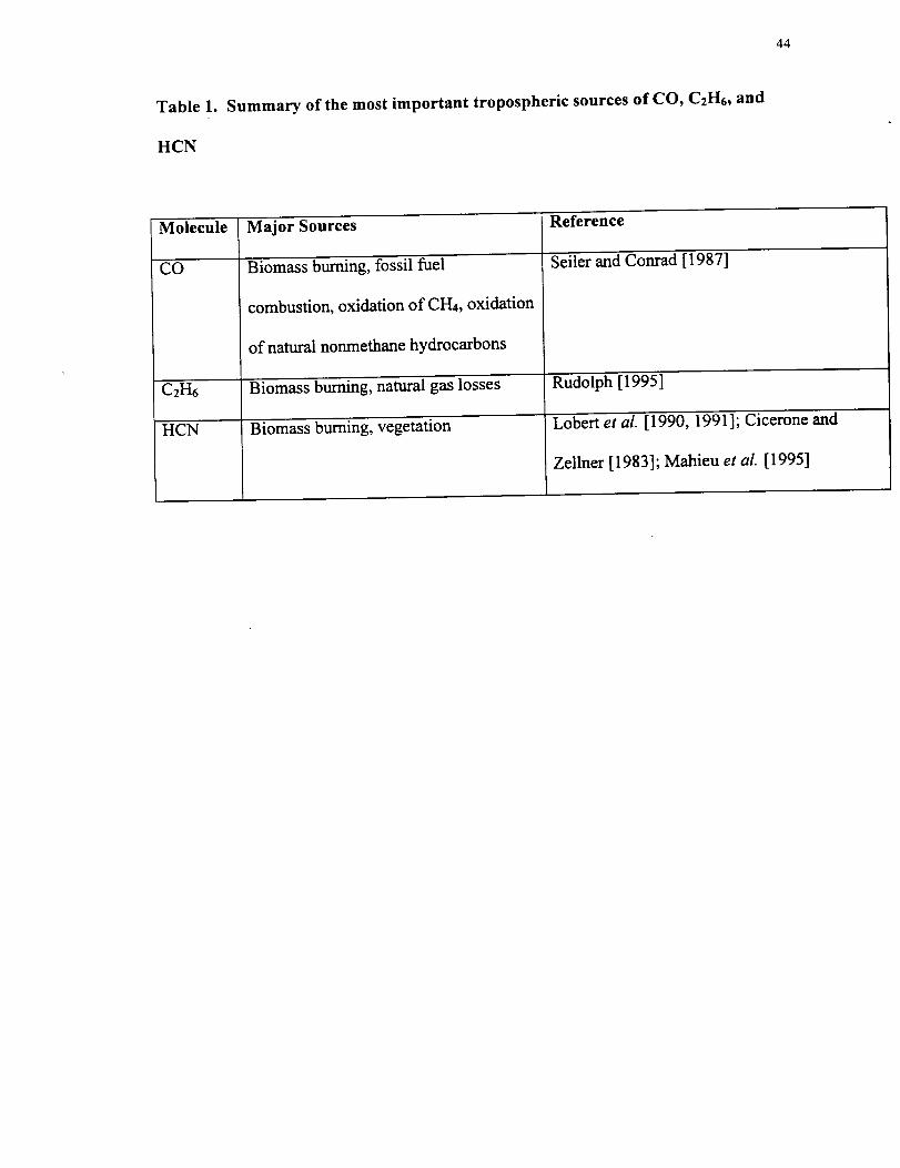
Table 1.

HCN

Summary of the most important tropospheric sources of CO, C2H6, and

44

Molecule

CO

C2H6

HCN

Major Sources

Biomass burning, fossil fuel

combustion, oxidation of CH4, oxidation

of natural nonmethane hydrocarbons

Biomass burning, natural gas losses

Biomass burning, vegetation

Reference

Seiler and Conrad [1987]

Rudolph [1995]

Lobert et al. [1990, 1991]; Cicerone and

Zellner [1983]; Mahieu et al. [1995]

45

Table 2. Microwindows and Interferences

Molecule Microwindows (cm -_)

CO 4274.62-4274.82, 4284.75-4285.18

C2H6 2976.62-2976.94

HCN 3287.15-3287.35

Interfering Molecules

Solar CO, CI-I4, HDO

H20, CI-I4, 03

None

Notes: Except for CH4, each interfering molecule was fitted by a multiplicative scaling

of the a priori volume mixing ratio profile by a single value. The profile of CH4 was

retrieved from the fittings of the two CO windows.

46

Table 3. CO, C2H6, and HCN 3.4-16 km Partial Column Measurement

Uncertainties

Random Error Budget

Error Source Relative Error, %

HCN

1

12

<1

CO CIH6

Temperature 1 2

Instrument 1 4

noise1 1Zenith angle

uncertainty

Interfering lines <1 <1 <1

RSS total 2 5 12

random error

Systematic Error Budget

Error Source Relative Error, %

CO C2H6

SpectroscopicParameters

A priori profileForward model

approximations¶

2 5

Instrument line < 1 < 1

shape function

RSS total systematic 5 5 3

error

HCN

2

<1

¶ Includes the estimated uncertainty in the retrieval due to errors in computing the

absorption by overlapping solar CO lines.

47

Table 4. CO 3.4-16 km Column Monthly Mean FTS Measurements from Mauna

Loa (MLO/FTS) and Values calculated for the same altitude range and geographic

region from MAPS measurements in 1984 and 1994 (in 10 Is molecules cm "2)

Month

January

January

February

FebruaryMarch

April

Year

July

1995-1997

1998

1995-1997

1998

1995-1997

1994

May 1995-1997June 1995-1997

1995-1997

Data

Source

MLO/FTS

MLO/FTS

MLO/FTS

MLO/FTS

MLO/FTS

MeanColumn

1.097

1.136

1.076

1.113

1.088

Standard

Devimion

0.083

0.088

0.097

0.079

0.204

Number

of Days

18

15

14

13

MAPS 1.261 0.147

MLO/FTS 1.061 0.147 14

MLO/FTS 0.924 0.074 13

MLO/FTS 0.790 0.101 13

37August 1995-1997 MLO/FTS 0.754 0.087

September 1995-1996 MLO/FTS 0.789 0.062 22

September 1997 MLO/FTS 0.800 0.092MLO/FTS

MLO/FTS

MAPS

MAPS

MLO/FTS

MLO/FTS

1995-1996

1997

1984

1994

1995-1996

1997

0.856

1.088

0.710

1.065

0.919

1.318

1.081

1.273

1995-1996

October

October

October

October

November

November

December

0.093

0.189

0.036

0.116

0.145

0.177

0.055

0.061December 1997

MLO/FTS

MLO/FTS

18

19

15

10

11

10

48

Table 5. Mauna Loa Monthly Mean C2H6 3.4-16 km Columns (in 10 Is molecules

cm -2)

Month Year

February

January 1995-1997

January 19981995-1997

FebruaryMarch

May

August

1998

1995-1997

1995-1997

1995-1997June

July 1995-19971995-1997

September

SeptemberOctober

October

November

December

1995-1996

1997

1995-1996

1997

1995-1996

_,/[ean

Column

Standard

Deviation

Number

of Days

9.101 1.049 9

9.278 1.124 21

9.343 1.039 21

9.287

9.458

18

9.550

0.942

1.521 12

1.272 16

8.194 1.225 15

6.698 1.184 15

5.916 0.689 44

5.730

5.983

6.595

8.590

0.433

0.823

1.273

1.977

2.247

1.182

0.434

1.076

8.064

November 1997 11.110

December 1995-1996 9.281

1997 11.452

21

19

21

17

7

10

14

12

49

Table 6. Correlation coefficients and C2H6/CO slopes derived from fits to daily

mean tropospheric partial column observations

Station Location Months Correlation C2H6/COCoefficient Slope (10"3) *

Lauder, New 45°S,170°E, 0.37 February-March-April 0.400 3.38

Zealand km altitude

Lauder, New 45°S, 170°E, 0.37 May-June-July 0.594 5.52

Zealand km altitude0.827 6.39Lauder, New

Zealand

Mauna Loa

Kitt Peak,

Arizona, U.S.A.

45°S,170°E, 0.37km altitude

19.5°N, 155.6°W,

3.40 km altitude

31.9°N, 111.6°W,

2.09 km altitude

August-September-October

All

All

0.927

0.766

9.35

14.2

* Calculated from 0.37-12 km columns from Lauder, 2.09-14 km columns from Kitt

Peak, and 3.4-16 km columns from Mauna Loa.

5O

Table 7. Mauna Loa Monthly Mean HCN 3.4-16 km Columns (in 10 Is molecules

cm -2)

Month

January

Year

1995-1997

Mean

Column

2.130

Standard

Deviation

0.340

Number

of Days

4

19January 1998 4.265 0.463

February 1995-1997 1.929 0.485 21

February 1998 3.534 0.466 16March 1995-1997 1.798 0.598 9

3.077

2.664

1995-1997

1995-1997

0.510

0.692

0.467

MayJune

2.246

15

11

12July 1995-1997

August 1995-1997 1.750 0.412 35

September 1995-1996 1.726 0.501 20

September 1997 2.125 0.658 16October 1995-1996 1.679 0.400 19

October 1997 3.940 1.769 15

November 1995-1996 1.912 0.870 4

November 1997 6.450 1.411 9

December 1995-1996 1.837 0.398 13

December 1997 5.713 1.107 7

51

Figure Captions

Figure 1. Averaging kernels calculated for CO, C2H6, and HCN.

merged layers, 3.4-16 km and the total column, 3.4-100 km.

Values are shown for

Figure 2. Sample spectrum and fits in the region of the CO (2-0) band R(3) and R(6)

lines at 4274.7047 and 4284.8911 cm "l. The measured spectrum was recorded on March

13, 1997. The spectrum has been normalized to the highest signal in each interval. The

astronomical zenith angle of the observation is indicated. Residuals (measured minus

calculated values) are shown on an expanded vertical scale above each spectral plot. The

measured 3.4-16 km CO column equals 9.99 x 1017 molecules cm "2.

Figure 3. Monthly average CO mixing ratios (ppbv) in the 3.4-16 km layer derived from

the infrared FTS measurements (solid circles) and corresponding values calculated from

preliminary CO mixing ratios measured at Mauna Loa by the CMDL cooperative flask

sampling network (open circles). Dashed and solid straight lines connect adjacent

CMDL and FTS monthly averages, respectively. Vertical lines indicate standard

deviations.

Figure 4. Example of a spectrum and the corresponding fit in the interval used to retrieve

profiles of C2H6. The results are shown in the same format as Fig. 2. The interval

contains the PQ3 Q branch of the C2H6 v7 band at 2976.8 cm l. The spectrum was

recorded on February 28, 1998. The astronomical zenith angle of the measurement is

indicated.

52

Figure 5. Daily average 3.4-16 km C2H6 vs. CO columns. Measurements from all

seasons are included. The solid line shows a fit to the observations assuming the two

quantities are linearly related with an extrapolation to a C2H6 3.4-16 km column of 0.0

shown as a dashed line. The slope, x-intercept, and correlation coefficient are reported.

Figure 6. Examples of spectra and least-squares best-fits in the microwindow used to

retrieve profiles of HCN. The two cases are shown in the same format as Fig. 2. They

were selected to illustrate similar airmass observations and the wide range in retrieved

HCN 3.4-16.0 km column amounts during the November time period. The upper

spectrum corresponds to a 3.4-16 km column of 9.14 x 101 s molecules cm 2 from

November 15, 1997, while the observation in the lower panel corresponds to a retrieved

3.4-16 km column of 8.78 x 1014 molecules cm "2. The spectrum was recorded on

November 2, 1996.

Figure 7. Measured HCN 3.4-16 km columns versus time. Daily averages are shown

with plus symbols. Corresponding approximate mean mixing ratios are shown on the

right vertical axis. Solid curves show least-squares best-fits to the daily-mean 3.4-16 km

columns with the seasonal variation and long-term trend displayed separately.

Figure 8. Time series of CO, C2H6, and HCN 3.4-16 km columns for the last half of

1997. Daily averages are shown. Approximate corresponding average mixing ratios for

the 3.4-16 km altitude region are shown on the right vertical axis.

53

Figure 9. Kinematic back-trajectories calculated for up to 10 days originating at Mauna

Loa between 10 November and 29 November 1997. Calculations are shown for ending

altitudes of 11 km (left) and 7 km (right).

54

Addresses of Authors

R. D. Blatherwick, S. J. David, A. Goldman, F. J. Murcray, T. M. Stephen, Departmem

of Physics, University of Denver, Denver, CO 80208 (email: blathe@meeker.ucar.edu;

Shelle@dove.uear.edu; goldman_acd.ucar.edu; murcray@ram.phys.du.edu;

tstephen@du.edu)

N. B. Jones and B. J. Connor, NIWA Climate, Private Bag 50061, Omakau, Lauder 9182,

New Zealand (email: jones@kea.lauder.cri.nz; connor@kea.lauder.cri.nz)

Paul C. Novelli, Climate Monitoring and Diagnostics Laboratory, National Oceanic and

Atmospheric Adminstration, 325 Broadway, Boulder, CO 80303 (email:

paul@hpsrv.cmdl.noaa.gov)

N. S. Pougatchev, Department of Physics, Christopher Newport University, Newport

News, VA (email: n.s.pougatchev@larc.nasa.gov)

C. P. Rinsland and J. Fishman, NASA Langley Research Center, Mail Stop 401A,

Hampton, VA 23681-2199 (email: c.p.rinsland@larc.nasa.gov;

j.fishman@larc.nasa.gov)

Fisure i

40_y-F-

7-

y-.---. _____ 30

._. _-

20

b-

b-,,.....l< 10

\

\

3.4-16 km3.4- I O0 km

O_ I I

-1.5 -I.0 -0.5

i I I

0.0 0.5 1.0

CO AVERAGING KERNELS

i

1.5 2.0

40

..--..

30

20-

[..

< 10

0

-1.5

3.4-16 km3.4-100 km

I I

-1.0 -0.5

• I I .... , , . , i

I

\

\

\

I L L

0.0 0.5 1.0

C2H _ AVERAGING KERNELS

2.0

40

30

20

[.-,[.-,

.< 10

\\

\

\

3.4-16 km3.4- 100 km

I , I

-I.0 -0.5

l

, i I J

0.0 0.5 1.0

HCN AVERAGING KERNELS

i

l

1.5 2.0

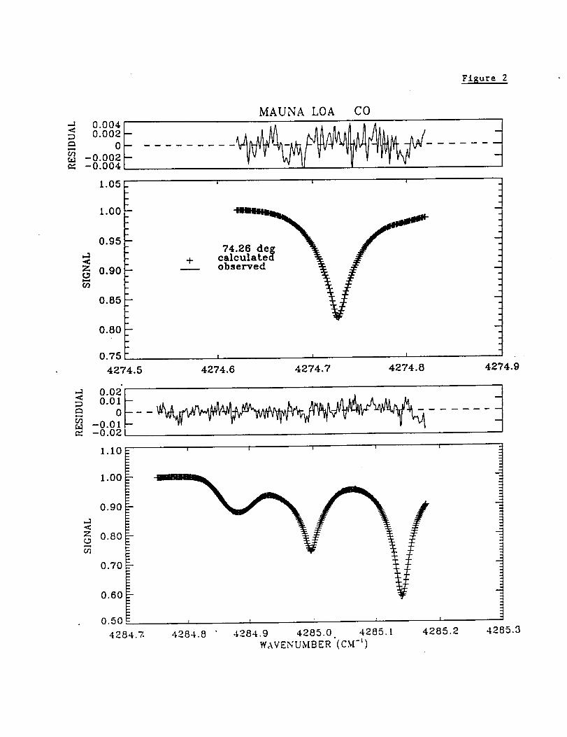
Figure 2

< 0"004 I

0.002 --

__. o-0.002

0.004

MAUNA LOA CO

1.05 I I I

+74.26 deg

calculatedobserved

I I I

4274.6 4274.7 4274.8 4274.9

.<Z

O3

1.10

1.00

0.90

0.80

0.70

0.60

0.50

4284.7.

I I

l

4284.8

| I I

4284.9 4285.0 4285.1

WAVENUMBER (CM-')

!

4285.2 4285.3

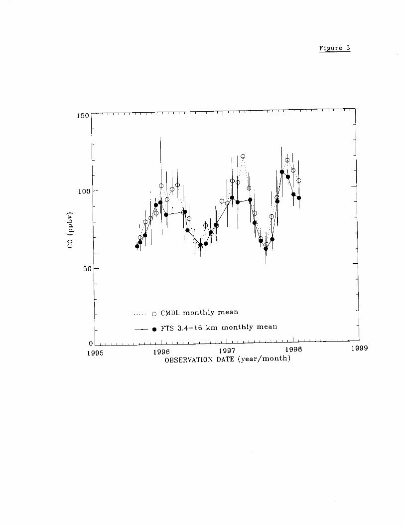
Fisure 3

150 ........... I ........... { ........... i ...........

>.Q

0o

I00

5O

..... © CMDL monthly mean

-- • FTS 3.4-16 km monthly mean

0 I I I I i I I I I l i { l i I I I I I i ' i i I i L I I I I l I i l I ] 1 I { I I 1 I i i } I

1995 1998 1997 1998 1999

OBSERVATION DATE (year/month)

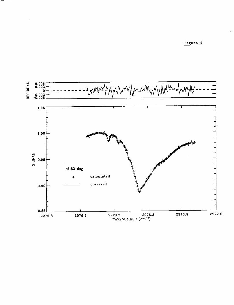
Fisure 4

'-J.,¢ 0.006 f

0.0030

-0.003-0.006

1.05 1 I I I 1

1.00

-0.95 "---

r"

i 75.63 deg

+

0.90 observed _

I I I0.85 I

2976.5 2976.6 2976.7 2976.8 2976.9WAVENUMBER (cm -1)

2977.0

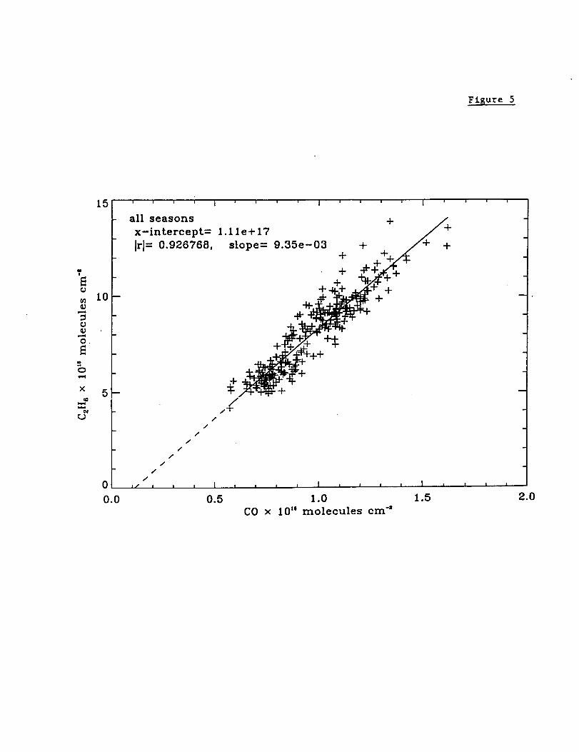
Figure 5

T

O

G0

O.

O

X

N

15

10

1

0

0.0

l a ! i

all seasons

I ' ' ' ' I ' ' ' ' I '

x-intercept= 1.11 e + 17 ++++__+//_+JrJ= 0.926768, slope= 9.35e-03 + +

+ _-++ +_+ _-

++

/

/

/

/

//

/

/

/,( , , , I , , , , I , , , , I J

0.5 1.0 1.5CO x 10 _' molecules era"

! ...

2.0

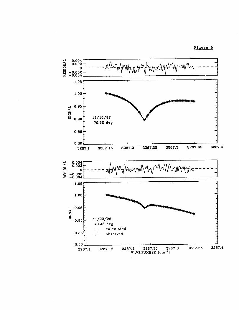
Fisure 6

_n

e-,

o_

0.004_

0.0020

-0.002-0.004

1.05

1.00

,,.= 0.95

Z

¢n 0.90

0.85

0.80

3287.1

t i i i J

70.82 deg

I I I I I

3287.15 3287.2 3287.25 3287.3 3287.35 3287.4

0.00_0.00

-0.002-0.004 [

1.05

1.00

..= 0.95

Z

¢n 0.90

0.85

l l a i b

11/o2/9870.4.3 deg

+ calculated__ observed

I I I I I

3287.t5 3287.2 3287.25 3287.3 3287.35WAVENUMBER (cm")

I

3287.4

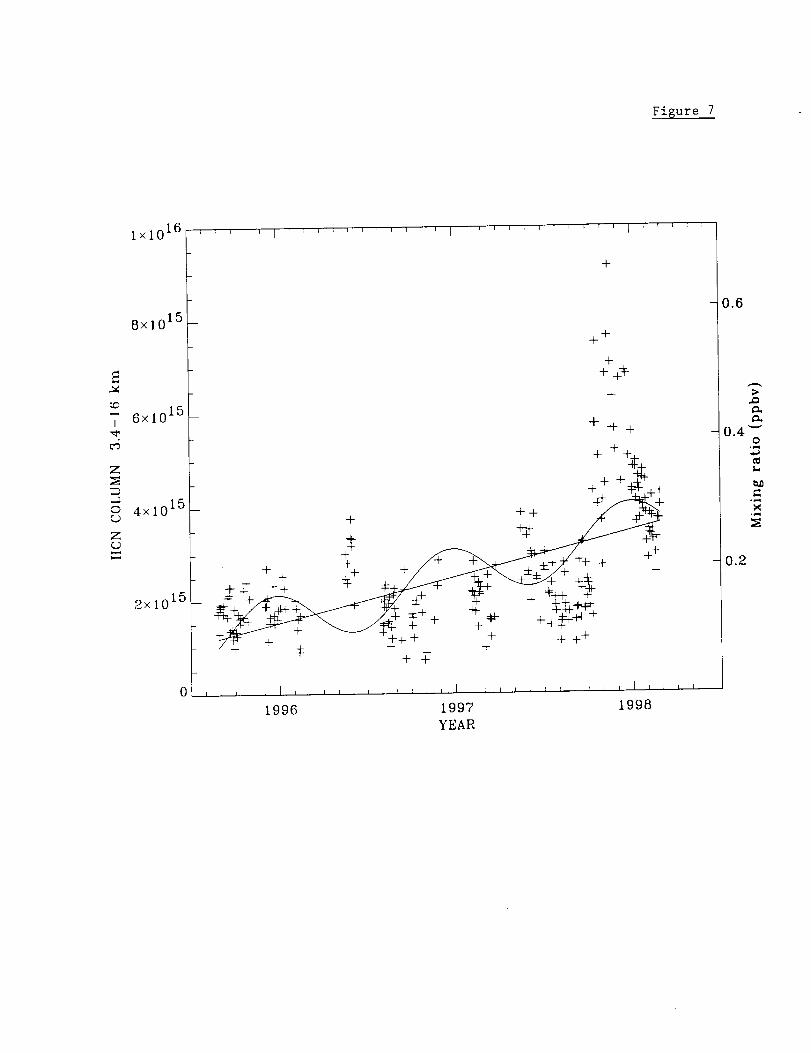
Fisure 7

1×1016 ..... t ........... I ........... i .....

8xi015

_D-- 6xlO 15

I

Z

-: 015o 4xl

Z

152xlO

+

++

+

÷

+q++

+_ _ __+

+ + _ '

f ___ + +

+++ + + + ++T +-F-

1996 1997 1998YEAR

0.6

>

=.

- 0.4_o

°.,,q

0.2

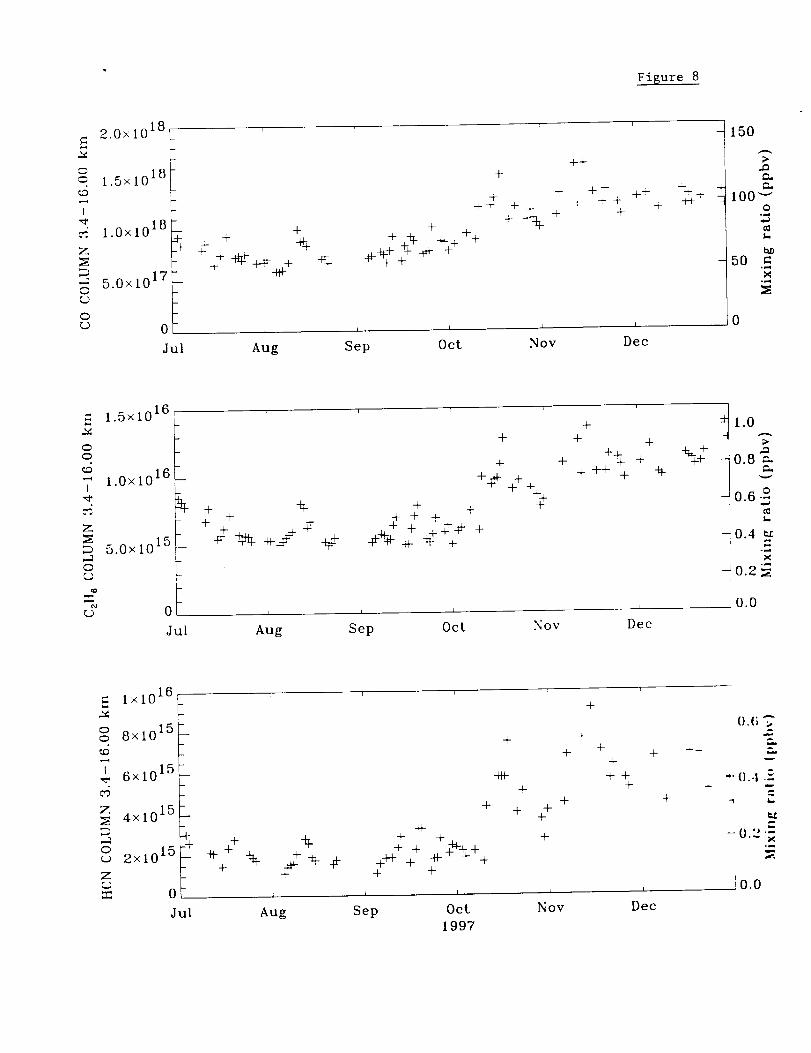
Fisure 8

18,2.0xlO

o a___ 1.5xlO 1

I

"_ 10181.OxZ

175.0x10

" f0

_ 0

Jul

i

4-

+ _+$- + -___ +

+

I

_+

I I

4-

Aug Sep Oct

4-+

4- 4--4-4- 4-4--

4- +

4-,-r+

_g.

_÷

I I

Nov Dec

- 150

>

00""o

°_

- 50 =

._.,q

0

_. 1.5xlO 16

oo

_0 161.0×10

I

_3

Z

155.0x 10

O{.D

0

T

+

4-

+# +++++% + +

.4-4-

+4=

4- + 4-4-

4-

4-

1.0

0.8 _

- 0.6-£

L

-'0.4._

X._

_0.2_

0.0

Jul Aug Sep Oct Nov Dec

16

I

Z

0G)

ZG_

lxl0

8x10 15

6xlO 15

4x1015

2x101510

Jul

+4+ + +_+ _ _ #

I

Aug

4-

444-

4-

4-+

4- 4- 4.-4-

-44-•4- 4-

+ 4- 44._+-_'++++H-+ +4- +

I I

4-

I

NovSep Oct1997

4-

++

+

4-.4-4-

+ -r .-,-

Dec

A

0.6

-, o.4 .£

I I.,

-0.2 -

',o.o

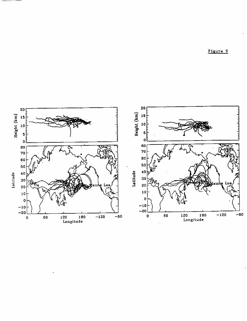
Figure 9

2oi 110

5

0

80

70

60

50

40

30

20

[0

0

-tO

-20

0

i

o

60 120 180 -120 -60

Longitude

20

E 15

-_ 10.=

t_

"_ 5

0

8O

70=

60

(P

..J

5O

40

3O

20

tO

0

-tO

-20

0

i i i |

/f.rLL.._ ' • _ -

. Loa .

60 120 180 -120 -60

Longitude

Northern and Southern Hemisphere Ground-Based Infrared Spectroscopic Measurements

of Tropospheric Carbon Monoxide and Ethane

z Jennifer A. Logan, 32 Brian J. Connor,Curtis P. Rinsland, I Nicholas B. Jones, 5Thomas M. Stephen, 5 AlanNikita S. Pougatchev, 4 Aaron Goldman, 5 Frank J. Murcray,

7 Emmanuel Mahieu 7, and Philippe Dem oulin7S. Pine, s Rodolphe Zander,

iAtmospheric Sciences Division, NASA Langley Research Center, Hampton, Virginia

2National Institute of Water and Atmospheric Research, Lauder, New Zealand

3Department of Earth and Planetary Sciences and Division of Applied Sciences,

Harvard University, Cambridge, Massachusetts

4Christopher Newport University, Newport News, VA

5Department of Physics, University of Denver, Denver, Colorado

SAlpine Technologies, Germantown, MD71nstitute of Astrophysics and Geophysics, University of Liege, Li_ge-Cointe,

Belgium

i

Abstract

Time series of CO and C2H 6 measurements have been derived from high resolution

infrared solar spectra recorded in Lauder, New Zealand (45.0 °S, 169.7°E, altitude

0.37 km) and at the U. S. National Solar Observatory (31. 9°N, III.60W, altitude

2.09 km) on Kitt Peak. Lauder observations were obtained between July 1993 and

November 1997 while the Kitt Peak measurements were recorded between May 1977

and December 1997. Both databases were analyzed with spectroscopic parameters

that included significant improvements for C2H 6 relative to previous studies.

Target CO and CzH 6 lines were selected to achieve similar vertical samplings

based on averaging kernels. These calculations show that partial columns from

layers extending from the surface to the mean tropopause and from the mean

tropopause to lOOk mare nearly independent. Retrievals based on a semiempirical

application of the Rodgers optimal estimation technique are reported for the

lower layer, which has a broad maximum in sensitivity in the upper troposphere.

The Lauder CO and C2H 6 partial columns exhibit highly asymmetrical seasonal

cycles with minima in austral autumn and sharp peaks in austral spring. The

spring maxima are the result of tropical biomass burning emissions followed by

deep convective vertical transport to the upper troposphere and long-range

horizontal transport. Significant year-to-year variations are observed for both

CO and C2H 6, but the measured trends, (+0.37±0.57)9 yr -I and (-0.64±0.79)_ yr -I,

I sigma, respectively, indicate no significant long-term changes. The Kitt Peak

data also exhibit CO and C2H s seasonal variations in the lower layer with trends

equal to (-0.27±0.17)9 yr -I and (-1.20±0.35)9 yr -I, i sigma, respectively. Hence,

a decrease in the Kitt Peak tropospheric CzH6 column has been detected, though

the CO trend is not significant. Both measurement sets are compared with

previous observations, reported trends, and three-dimensional model calculations.

2

i. Introduction

Carbon monoxide (CO) and ethane (C2H6) are important indicators of

tropospheric pollution and transport because they are emitted primarily by

anthropogenic sources [Logan et al., 1981; Rudolph, 1995], they have relatively

high tropospheric abundances [e.g., Novelli et al., 1992; Blake and Rowland,

1986], and moderately long tropospheric lifetimes. Hough [1991] used a two-

dimensional global tropospheric model to estimate mean annual globally averaged

tropospheric lifetimes of 52 and 59 days for CO and C2H 6, respectively. These

lifetimes are significantly shorter than that of CH 4 (7 years [Hough, 1991]), and

hence both gases are less well mixed throughout the troposphere than methane

[e.g., Reichle et al., 1986; Singh and Salas, 1982]. However, the lifetimes of

CO and CzH 6 are long enough for both gases to be possibly influenced by multiple

sources, over a large region, potentially with different emission fingerprints

[McKeen et al., 1996]. Dilution of emissions with "background" air during

transport from distant source regions (especially during vertical mixing) is an

important consideration for interpreting measurements at relatively unpolluted

locations [Singh and Zimmerman, 1992; McKenna et al., 1995; Smyth et al., 1996].

Both CO and C2H _ share a common initial, principal tropospheric sink, their

reaction with OH radicals [Levy, 1971; Crutzen and Gidel, 1983; Ehhalt et al.,

1986; Rudolph, 1995] and are convenient chemical species for remote sensing of

anthropogenic activity based on strong spectral signatures in the mid-infrared

[e.g., Wallace and Livingston, 1990; Zander et al. 1989; Ehhalt et al., 1991].

These absorptions are readily measured in ground-based solar spectra, even at

background conditions in the southern hemisphere [e.g., Goldman et al., 1988;

Rinsland et al., 1994a; Notholt et al., 1997a].

Nadir-viewing infrared measurements of CO were obtained from the U.S. Space

Shuttle in November 1981, October 1984, April 1994, and October 1994 by the

Measurement of Air Pollution from Satellite (MAPS) experiment [Reichle et al.,

1986; 1990; 1998; Novelli et al., 1998], and a few CO and C2H6 vertical profiles

have been derived from Atmospheric Trace Molecule Spectroscopy (ATMOS) Fourier

transform spectrometer (FTS) infrared solar occultation observations in May1985

[Rinsland et al., 1987] and November 1994 [Rinsland et al., 1998], also from the

U.S. shuttle. Because of the short duration of U.S. shuttle flights, these

observations provide "snapshots" of the CO and C2H6 atmospheric distributions

with only indirect information about transport, dilution, and the spatial and

temporal variations of CO and C2H s sources and sinks.

Seasonal variations of CO columns [e.g., Dianov-Klokov and Yurganov, 1989;

Zander et al., 1989; Wallace and Livingston, 1990; Pougatchev and Rinsland,

1995a; Yurganov et al., 1997; Notholt et al., 1997b] and C2H6 columns [e.g.,

Ehhalt et al., 1991; Rinsland et al., 1994a,b; Notholt et al., 1997b] have been

derived from ground-based infrared solar absorption spectra. These measurements

complement the spaceborne observations (cited above), airborne spectroscopic

column measurements [Coffey et al., 1985; Toon et al., 1992], and in sicu

aircraft measurements of CO and C2H6 [e.g. Blake et al., 1997; Talbot et al.,

1996; Matsueda et al., 1998] by providing databases covering longer time periods,

potentially with information on long-term trends free of drifts in calibration

standards [e.g., Mahieu et al., 1997]. Ground-based solar measurements sample

a broad altitude range. Hence, they measure plumes of pollution, uplifted by

deep convection from the surface to the upper troposphere and transported long

distances from sources by the prevailing winds [Dickerson et al., 1987;

Heintzenberg and Bigg, 1990; Chatfield et al., i996; Pickering et al., 1996;

Fuelberg et al., 1998; Matsueda et al., 1998]. Such plumes of pollution, located

aloft, are not measured by surface level in situ sampling.

Most of the surface emissions of CO and C2H6 originate at northern mid to

high latitudes [Logan et al., 1981; Khalil and Rasmussen, 1990; Kanakidou et

al., 1991; Rudolph, 1995; Manning et al., 1997]. Surface sources of CO in this

latitude range are mainly related to combustion, e.g. automobile exhaust

emissions, coal and oil burning, and natural gas losses. Ethane surface

emissions in these latitudes are primarily due to natural gas losses (see Rudolph

[1995] and the references cited therein).

Tropospheric measurements in the extratropical southern hemisphere (ETSH,

defined as 30°S-90 °S by Manning et al. [1997] and 35°S -900S by Rudolph [1995])

show large seasonal variations in both CO [Steele et al., 1996; Novelli et al.,

1998; Manning et al., 1997] and C2H 6 [Rudolph et al., 1989; Rudolph, 1995;

Clarkson et al., 1997]. The dominant cause of these variations is the long range

transport of tropical biomass burning surface emissions [e.g., Watson et al.,

1990; Heinzenberg and Bigg, 1990; Fishman et al., 1991]. Peak tropical biomass

burning north of 5°N usually occurs from March to June and south of the equator

between September and December [Hao and Liu, 1994]. In situ production of CO

from the oxidation of atmospheric CH4 during transport is also an important

source of CO in the ETSH [Manning et al., 1997], but the calculated yield is

quite uncertain [Manning et al., 1997; Conny and Currie, 1996]. Although the

tropospheric mixing ratios of CO and C2H6 are much higher in the northern

hemisphere than in the southern hemisphere [e.g., Logan et al., 1981, Fig. 9;

Rudolph, 1995, Fig. 4], the exchange between the hemispheres is limited by the

short lifetimes of CO and C2H _ in the tropics (about i month) relative to the

interhemispheric exchange time (i to 2 years) [Maiss et al., 1996; Geller et al.,

1997; Manning et al., 1997]. Biogenic emissions of C2H 6 may be important on a

relative basis in remote regions [Hough, 1991; Zimmerman et al., 1978; Singh and

Zimmerman, 1992; Rudolph, 1995].

The purpose of this paper is to report multiyear time series of CO and C2H s

measurements derived from high resolution infrared solar absorption spectra

recorded at two remote stations, both located at midlatitudes, one in the

northern hemisphere and the other in the southern hemisphere. A common set of

spectroscopic line parameters and analysis procedures were used so that the

results from the two sites are consistent. Significant improvements in the C2H s

spectroscopic parameters relative to those assumed in previous studies have been

incorporated. The observations have been analyzed and characterized with a

line-by-line, multilayer algorithm based on the semiempirical version of the

optimal estimation technique. The northern and southern hemisphere CO and C2H s

columns were derived for two nearly independent layers, the lower extending from

the surface to the altitude of the mean tropopause (12 km for Lauder, IA km for

Kitt Peak) and the upper layer extending from the altitude of the mean tropopause

to i00 km. Here we report and contrast the northern and southern hemisphere

results for the lower layer. The southern hemisphere measurements were obtained

with sufficient frequency over a 4.5-year period (1993-1997) to quantify the

interannual variability of both gases and comment on the suggestion that tropical

biomass burning may be either increasing [Watson et al., 1990; Houghton, 1991;

Hao and Liu, 1994; Kim and Newchurch, 1996, 1998] or decreasing [Khalil and

Rasmussen, 1994]. Rudolph [1995] highlighted C2Hs as a potentially useful gas

for that purpose. Owing to their similar lifetimes, the near simultaneous

observations of CO and CzH 6 provide a measure of seasonal changes in the relative

importance of surface emissions and in sicu photochemical CO production from CH 4

6

oxidation in the tropospheric column. This consideration is particularly

important for interpreting measurementsfrom the southern hemisphere, where the

seasonal cycles of C2Hs and COdestruction by OHare in phase with the seasonal

dependenceof biomass burning [Rudolph et al., 1989].

We start with a discussion of the observational database (section 2) and

the spectral analysis method (section 3). Section 4 describes the spectral

regions and line parameters adopted in the analysis. As reported in section 5,

after the initial retrievals were run, an objective procedure was used to remove

poor quality measurements from the database. Section 6 discusses the error

analysis and sensitivity studies. The time series of measurements from both

sites are reported and comparedwith previous observations and model calculations

in section 7. Finally, a brief summaryof the results is given in section 8.

2. Observations

Infrared observations were recorded at the two sites with different

instrumentation. Regular infrared observations from Lauder, NewZealand, were

obtained as part of a program dedicated to the Network for the Detection of

Stratospheric Change(NDSC)[Kurylo, 1991]. Lauder is a designated primary NDSC

station. Observations from Kitt Peak are recorded with a facility instrument,

which is used for laboratory, atmospheric, and astronomical observations in the

visible and infrared. Kitt Peak has been designated as a complementary NDSC

station.

2.1 Lauder database

The Lauder station (altitude 0.37 km, latitude 45.0 °S, longitude 169.7 °E)

is located in a small town (population -50) in the middle of the south island

of New Zealand in a region of minimal industrial activity. Local burnoffs occur

occasionally between about April and September with the majority in August-

October. Spectra recorded on days of particularly intense local burnoffs were

examined for the presence of spectral features characteristic of short-lived

gases emitted by biomass fires (for example, the enhanced IR features studied

in the fire spectra of Worden et al. [1997]). None were detected. Infrared

spectral features of NH 3 have been observed in the Lauder solar spectra with a

strong, positive correlation between the emissions and the local surface

temperature; the most likely source for these emissions is the release of animal

excretion at local farms during warm, dry surface conditions [Murcray et al.,

1989]. Hence, except for occasional local farming-related emissions, the Lauder

site is believed to be representative of background conditions at midlatitudes

of the southern hemisphere.

Broadband IR solar absorption spectra were first recorded from Lauder during

campaigns in 1985, 1986, and 1987 at a resolution of 0.02 cm -I [Murcray et al.,

1989]. These observations covered the 3-5 #m and 8-12 _m regions only, and hence

included measurements of CzH 6, but not CO. These relatively low resolution

measurements are not included in the present study. Regular high resolution IR

solar observations did not begin until September 1990. Initially, these

measurements were obtained with a Bruker model 120-HR FTS, which was replaced

in September 1992 with a Bruker model 120-M FTS. Observations covering both the

CO and C2H 6 regions began with the new instrument in July 1993. The 120-M

spectra are of significantly higher quality than the earlier data, and hence,

only the 120-Mmeasurementsrecorded through November1997 are reported here.

The Lauder 120-Msolar observations were recorded at unapodized resolutions

of 0.0035 or 0.007 cm-I (defined as 0.9 divided by the maximumoptical path

difference) with a liquid-nitrogen-cooled InSb detector and a KCI beamsplitter.

Optical filters were used to limit the spectral bandpasses to 1850-2100 cm-I (CO

fundamental band), 2400 to 3100 cm-I (C2H6v7 band), or 4000 to 4300 cm-I (CO

overtone band). The time required to record a single full resolution spectrum

was 104 s. The typical signal-to-noise ratio for full resolution Bruker 120-M

spectra was about 200:1 near 2000, 2900, and 4200 cm-I. Most of the spectra were

recorded between solar astronomical zenith angles of 45 and 85 = Boxcar

apodization was applied.

A major gap in the Lauder measurements occurred between September 1995

and January 1996 when the 120-M instrument was returned to the manufacturer for

upgrades and maintenance. Several observational gaps of 2 to 3 months also

resulted from failures of the HeNe laser, which measures the optical path

difference.

Instrumental performance varied at Lauder with minor phase errors observable

in most spectra. Comparisons of ozone lines in the spectra with simulations

based on correlative ozonesonde profiles [Rinsland et al., 1996] also indicate

that the instrument line shape function is broader at higher wavenumbers than

predicted from knowledge of the measurement parameters (maximum optical path

difference, applied apodization function, and internal field of view). Modeling

of both of these effects has been incorporated in the spectral analysis as

described in section 3.

2.2 Kitt Peak database

The McMath-Pierce l-m maximum optical path difference Fourier transform

spectrometer [Brault, 1978], on Kitt Peak in southeastern Arizona, U.S.A.

(altitude 2.09 km, 31.9°N, III.6°W), is located on a mountaintop in the Sonora

desert, a semiarid region with sparse population. The FTS is a modified

Michelson interferometer capable of observations in the 550-45000 cm -l range

using a selection of different beamsplitters, detectors, and optical bandpass

filters.

The measurements included in the analysis were recorded with maximum optical

path differences greater than 20 cm and solar astronomical zenith angles less

than 85 ° Liquid nitrogen cooled InSb detectors at the two output ports of the

FTS were used. Typical signal-to-noise ratios of full resolution spectra are

about 200:1, and 150:1 near 2900 and 4200 cm -I, respectively. The Kitt Peak

infrared atmospheric observations are recorded relatively infrequently, typically

4 runs per year totaling a dozen days, but the database spans 1977 to 1997 with

excellent uniformity in observational quality. Except for known problems, which

affect relatively few observations (all of which were eliminated from this

study), the measured instrument line shape function agrees with the function

predicted by theoretical calculations based on the instrumental settings.

3. Analysis Method

The Lauder and Kitt Peak spectra were analyzed with the SFIT2 algorithm,

which has been codeveloped at NASA Langley and NIWA Lauder for the retrieval of

vertical profiles of atmospheric gases from ground-based solar absorption

spectra. The profiles of one or more trace gases as well as the column

I0

abundances of interfering species are retrieved by simultaneously fitting one

or more microwindows in one or more solar spectra.

Analyses of IR solar spectra with SFIT2 have been reported by Pougatchev

et al. [1995b, 1996] and Connoret al. [1996]. The studies of Pougatchev et al.

[1995b, 1996] included comparisons of the SFIT2 ozone profile retrievals with

correlative ozonesonde measurements. Also, total columns of several gases

retrieved with SFIT [Rinsland et al., 1982a, 1984], which has the sameforward

model as SFIT2, have been comparedwith retrievals from the samespectra obtained

with independently developed NDSCalgorithms [Zander et al., 1993].

SFIT2 contains all the componentsrequired for retrieval of vertical volume

mixing ratio profiles from atmospheric datasets recorded with a ground-basedFTS

in solar absorption mode (refractive atmospheric ray tracing, forward line-by-

line radiative transfer model, FTSinstrument model, solar COabsorption model,

and the inverse model). Modeling of instrumental performance includes parameters

to simulate symmetric and asymmetric distortions of the instrumental line shape

function.

3.1 Forward Model

Monochromatic transmittances are calculated at a uniform grid spacing of

<0.0005 cm-I with a line-by-line model that assumesa Voigt shape [Drayson, 1976]

for lines in all atmospheric levels. Refractive ray tracing [Gallery et al.,

1983] is used to generate density weighted effective temperatures and pressures

for each of 29 layers with upper and lower model boundaries at the surface and

i00 km. Vertical layer thicknesses are set to 2 km up to an altitude of 50 km.

Higher altitude layer boundaries are at 60, 70, 80, and I00 km.

II

The FTS instrument response function is modeled by transforming the

calculated monochromatictransmittance spectrum to the Fourier domainwith a fast

Fourier transform. The model interferogram is then multiplied by the applied

apodization function and a function to simulate the decrease in fringe visibility

with optical path difference due to the finite solid angle of the instrument

internal field of view [e.g., Bell, 1972]. In the absence of instrumental

distortions, the synthetic spectrum is obtained from the inverse Fourier

transform of the model interferogram.

SFIT2 incorporates modeling of the combined effects of symmetric and

asymmetric distortions of the line shape function [Guelachvili, 1981]. Several

different functional forms have been implemented. Twoparameters were introduced

to model the Lauder data. One parameter is used to model the symmetric line

shape distortions with the straight-line approximation of the effective

apodization function [Park, 1983, Eq. 24]. A second parameter is used to model

the asymmetric line shape distortions assuming a constant phase error [Park,

1983, section 2B; Guelachvili, 1981, pp. 22]. The Lauder spectra were simulated

by Fourier transforming the model interferogram (including the simulated

distortion effects) back to the spectral domain.

Atmospheric spectroscopic parameters defined in the format of the HITRAN

database [Rothman et al., 1998, Table 3] are read by SFIT2. All are used

including the air pressure-shift coefficient and the coefficient of the

temperature dependence of the air-broadening coefficient. The isotope code

number is read to derive the isotopic massneeded to calculate the Doppler width

in each layer. Becauseof large fractionation effects in the atmosphere, HDO

is treated as a separate molecular species. The line intensity in each layer

is computed from the variations of the rotational and vibrational partition

12

functions of the molecule with temperature relative to the reference values at

296 K [Norton and Rinsland [1991, Eqs. 1-3]. An updated set of molecular

parameters based on Norton and Rinsland [1991, Table II] is assumed.

All telluric CO lines are overlapped by absorption from solar CO lines.

Additional solar COlines are observable in the solar spectrum because of the

high solar temperature and the high dissociation energy of CO. A single layer

at 4500 K is assumedto compute the solar COlines with the Minnaert empirical

formula [Kilston, 1975; Rinsland et al., 1982b], given by

I_/Rv = I/Re + I/(KvU)(1)

where R_ is the residual intensity (absorbed fraction of solar continuum

radiation), R= is the limiting residual intensity, Kv is the monochromatic

absorption coefficient at wavenumber v, and U is the solar CO column abundance.

Line parameters from HITRAN 1996 [Rothman et al., 1998] were assumed to calculate

the solar CO line list at 4500 K.

We further assume that all solar CO lines have a Voigt line shape with the

Doppler line width at 4500 K scaled by a multiplicative factor to account for

microturbulence in the solar atmosphere. The Lorentz width and the

microturbulence scale factor are taken to be the same for all solar CO lines.

A wavenumber shift parameter is included to account for the differential Doppler

shift of the solar lines with respect to the telluric lines. In summary, five

parameters are used in SFIT2 to model the absorption by solar CO lines. The

parameters are R=, U, the Doppler width multiplicative scale factor, the Lorentz

width, and the differential wavenumber shift. This model yields calculated solar

CO lines with absorbances that match the observed values to i5% or better.

13

3.2 Inverse model

The inverse method used in SFIT2 assumesthe optimal estimation formalism

of Rodgers [1976] modified on the basis of its semiempirical implementation for

NDSCmicrowave profiling of stratospheric 03 [Parrish et al., 1992; Connor et

al., 1995]. Following the nomenclature in these papers, an observing system

maybe defined conceptually by

y - F(x,b) + ey(2)

where y is the vector of measurements,F is the forward model that characterises

the measurementsin terms of x, the state vector of parameters to be retrieved,

b is the vector of model parameters which are assumed (not retrieved), and ey is

the vector of measurement errors, which are assumed to be normally distributed

with zero mean.

The optimal estimation method requires specification of the following 3

inputs for x: (I) x a, the a priori state vector; (2) Sa, the covariance of xa;

and (3) Se, the covariance of the measurement errors, ey. The parameters to be

retrieved simulate the target atmospheric absorptions, the interfering

atmospheric absorptions, and the solar CO absorptions. Parameters are also

included to model the instrumental performance.

In practice, the true a priori profile and its covariance are not known.

In the semiempirical approach to optimal estimation [Parrish et al., 1992; Connor

et al., 1995], the selections of the a priori mixing ratio profile is based on

the best available information. Simulations are then generated and the

covariance of the a priori state vector is adjusted empirically to yield the

desired performance, specifically, spectral fits to the noise level of the

measurements with minimal differences between the input vs. retrieved profiles

14

for the altitude range where the technique has sensitivity and avoidance of

nonphysical oscillations in the retrievals. The simulated data are usually based

on atmospheric observations, but ideally infinite resolution profiles with the

true mean profile and covariances are used.

An additional empirical modification to the method has been applied to set

the values for the measurement covariance matrix Se. As already noted, formally

the measurement errors are assumed to have a normal distribution. We further

assume that Se is diagonal; i.e. the measurement errors at each wavelength are

independent with the variance set for each spectral region on the basis of the

measurement signal-to-noise ratio.

3.2.1. Atmospheric state parameters. Modeling of the atmospheric state

requires specification of the target gas a priori mixing ratios in each of the

29 layers in the atmospheric model. Furthermore, all of the selected spectral

windows contain significant absorptions by interfering molecules, which were

individually modeled by either retrieving their vertical profile or by

multiplicatively scaling the a priori volume mixing ratio profile by a single

factor. Selections of intervals for the CzH s and CO retrievals are discussed

in sections 4.1 and 4.2, respectively.

The a priori atmospheric volume mixing ratio profiles for CO and CzH 6 were

obtained from several sources. For CO above Lauder, the vertical profile is

based on the average of aircraft flask air sample measurements obtained during

the months of April and October over Bass Strait and Cape Grim, Tasmania, and

analyzed by gas chromatography (L. P. Steele and R. L. Langenfelds, private

communication, 1997). These observations have been described by Langenfelds et

al. [1996] and Pak et al. [1996] and are reported in the NOAA/CMDL

gravimetrically derived CO scale [Novelli et al., 1991, 1998]. The two aircraft

15

profiles were extended above the highest measurementaltitude of 8 km on the

basis of the April-May 1985 ATMOSmeasurementsat 48°S [Gunson et al., 1990].

The two profiles are plotted in the paper by Pougatchev et al. [1998, Fig. 3].

The a priori profile for CzH6 above Lauder was taken as that described by

Rinsland et al. [1994a]. This profile below 14 km is based on a seasonal average

of the global two-dimensional model profiles calculated for the latitude of

Lauder [Kanakidou et al., 1991, Figure 7]. An exponential decline with a 3 km

scale height is assumedat higher altitudes based on stratospheric measurements

(e.g., Rinsland et al. [1987]).

The COa priori profile for the Kitt Peak analysis is based on an average

of tropospheric aircraft samplings at Carr, Colorado (40. 9°N, I04.8W) obtained

between November1992 and December1996 [Tans et al., 1996] and an average of

3 ATMOS/ATLAS3 profiles measuredat 32°N±I° latitude in November1994 [Gunson

et al., 1996]. The Carr measurements, also on the NOAA/CMDLgravimetrically

derived CO scale [Novelli et al., 1991, 1998], were used to define the CO a

priori profile from the surface to 10km. Observations marked as having analysis

or sample problems were excluded. The mean ATMOSmeasurement defines the a

priori profile between 16 to I00 km. A spline fit was used to smoothly connect

the two profiles in the intermediate altitude regime. The C2H6 a priori profile

above Kitt Peak was adopted from the reference listing of midlatitude northern

hemisphere profiles compiled by Smith [1982].

The mixing ratio of CO in the lower stratosphere is fairly constant because

of its production from the oxidation of CH 4 is balanced by OH reaction losses.

In contrast, there is a steep decline in the C2H 6 volume mixing ratio above the

tropopause because of reactions with both OH radicals and CI atoms [e.g., Goldman

et al., 1984; Rinsland et al., 1987].

16

Covariances for the CO and CzHe mixing ratio vectors were taken to be

diagonal. Additionally, we expressed the uncertainties relative to the a priori

mixing ratio in the layer. For CO, the diagonal elements in the Sa matrix were

calculated from sii = (klqai) 2 where qa± is the corresponding element of the CO a

priori profile and ki equals 0.2 for all layers. This value was tested by

generating synthetic spectra for a realistic set of atmospheric profiles and

performing retrievals on the synthetic observations. Figure I illustrates a

comparison for Kitt Peak of 2.09-14 km retrieved columns with the "true" columns.

The results are based on individual CO profiles from 82 aircraft flights from

Carr, Colorado during all 4 seasons. Each aircraft profile was extrapolated

above the flight altitude, as already described. The rms difference between the

"true" and retrieved CO 0.37-14 km columns is 2.735xi 01s molecules cm -2, 2% of the

0.37-14 km a priori column. As shown in the figure, there is no systematic bias

between the "true" and retrieved columns over the full factor of two range in

the measurements.

Unfortunately, there are no comparable sets of CzH 6 tropospheric profile

measurements appropriate for the Kitt Peak or Lauder analysis. We selected k i-

1.0 for all layers. This weak constraint yields a small relative contribution

of the a priori profile to the retrieval.

An a priori value of 1.0 and a variance of 0.3 were assumed for the factor

to multiplicatively scale the a priori mixing ratios to retrieve the total column

of each molecule with significant interfering absorption. As expected, tests

show that the a priori variance is a weak constraint (i.e., the relative

contribution of the a priori to the retrieval is small) provided that the

interfering molecule absorbs significantly in the measured spectrum.

17

3.2.2. Solar CO parameters. As described in section 3.1, 5 parameters

are required to model the absorption by solar CO lines with the a priori values

set on the basis of window-by-window fits to ATMOS exoatmospheric solar spectra,

except for the solar-atmospheric differential wavenumber shift, which was set

to zero. The parameter values were assumed uncorrelated (off-diagonal elements

equal to zero). Very small variances were assumed for R c and U, so that the a

priori values were adopted in the retrievals. The variances of the other

parameters were set large enough to make the retrieved values practically

independent of the a priori settings; hence, the information used in the

retrieval came almost entirely from the measured spectrum.

3.2.3. Instrument performance-related parameters. Model parameters

retrieved in the analysis are the wavelength scale calibration factor, the slope

of the background (100% transmission line) in each window, and the phase error

(Lauder data only). A priori values were set to realistic estimates (e.g., zero

for the background slope). The individual parameters were assumed to be

independent (coefficients of off-diagonal elements set to zero). Variances for

the individual parameters were set to large values to avoid underfitting the

measured spectrum. The phase error was assumed to be independent of wavenumber

in the analysis of the Lauder spectra.

As already mentioned, the Lauder spectra also show an instrument function

that is broader than the theoretical one with the discrepancy increasing at

higher wavenumbers. The coefficient of the straight line effective apodization

parameter used to model the symmetric broadening was assumed, not retrieved.

The value for the C2H 6 region was derived from spectral fits to strong, isolated

03 lines near the same wavelength with the vertical 03 profile distribution

constrained to agree with same day ozonesonde measurements [Rinsland et al.,

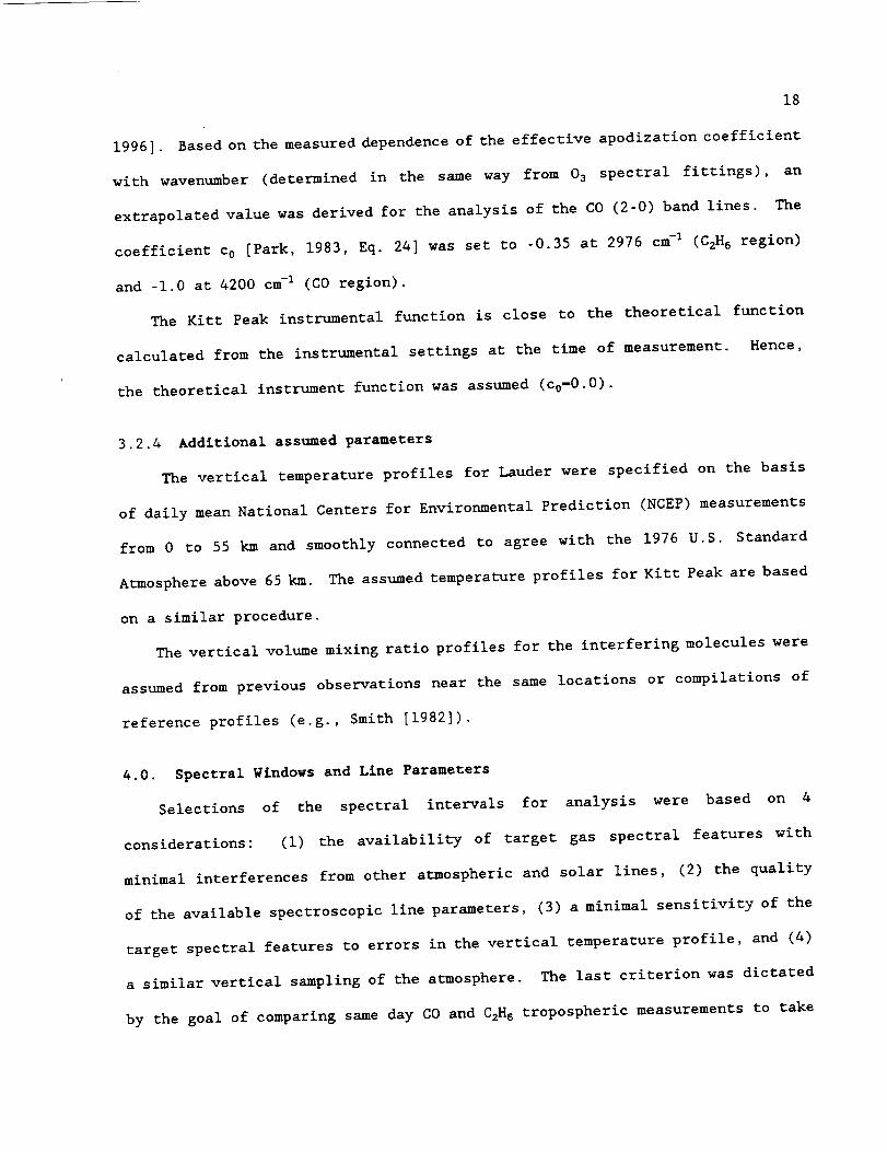
18

1996]. Based on the measured dependence of the effective apodization coefficient

with wavenumber (determined in the same way from 03 spectral fittings), an

extrapolated value was derived for the analysis of the CO (2-0) band lines. The

coefficient co [Park, 1983, Eq. 24] was set to -0.35 at 2976 cm-I (C2H6 region)

and -I.0 at 4200 cm-I (CO region).

The Kitt Peak instrumental function is close to the theoretical function

calculated from the instrumental settings at the time of measurement. Hence,

the theoretical instrument function was assumed (c0-O.0).

3.2.4 Additional assumed parameters

The vertical temperature profiles for Lauder were specified on the basis

of daily mean National Centers for Environmental Prediction (NCEP) measurements

from 0 to 55 km and smoothly connected to agree with the 1976 U.S. Standard

Atmosphere above 65 km. The assumed temperature profiles for Kitt Peak are based

on a similar procedure.

The vertical volume mixing ratio profiles for the interfering molecules were

assumed from previous observations near the same locations or compilations of

reference profiles (e.g., Smith [1982]).

4.0. Spectral Windows and Line Parameters

Selections of the spectral intervals for analysis were based on 4

considerations: (I) the availability of target gas spectral features with

minimal interferences from other atmospheric and solar lines, (2) the quality

of the available spectroscopic line parameters, (3) a minimal sensitivity of the

target spectral features to errors in the vertical temperature profile, and (4)

a similar vertical sampling of the atmosphere. The last criterion was dictated

by the goal of comparing same day CO and C2H B tropospheric measurements to take

19

advantage of their very similar tropospheric lifetimes with commonprincipal

destruction via reactions with OHradicals [e.g., Kanakidou et al., 1991, Fig.

4; Law and Pyle, 1993, Fig. I].

The selection of the spectral intervals was also constrain by the existence

of only relatively weak absorption features of C2H6 in ground-based infrared

solar absorption spectra. The most favorable ones for remote sensing are the

sharp PQ3and rQ0 subbranches of the v 7 perpendicular band at 3 _m [e.g., Ehhalt

et al., 1991; Rinsland et al., 1994a,b]. Lines of CO with a wide range of

absorption depths are present in ground-based solar spectra.

Averaging kernels provide a direct assessment of the theoretical altitude

sensitivity for an observing system in the absence of errors in the measurements

and the model parameters [Rodgers, 1990, section 4]. They show explicitly how

the true profile is smoothed in producing the retrieved profile. A perfect

measurement system would sample the intended altitude region uniformly with no

smoothing; put another way, the averaging kernel for each altitude would be a

6-function.

Figure 2 presents partial column averaging kernels for Lauder profile

retrievals of CzH 6 (top) and CO (bottom) obtained with the selected parameters.

The assumed a prior/ volume mixing ratio profiles, Sa covariance matrices,

spectral intervals, and spectroscopic parameters are described in sections 4.1

and 4.2. The calculated kernels also depend on the signal-to-noise ratio and

the spectral resolution of the measurements [Connor et al., 1996]. Typical

Lauder observation values of 200 and 0.0035 cm-I were assumed, respectively. The

kernels for partial columns were first generated for the 29 layer atmospheric

model, then combined to derive the curves for 0.37-12, 12-100, and the total

column, 0.37-100 km. The boundary at 12 kmwas selected to correspond with the

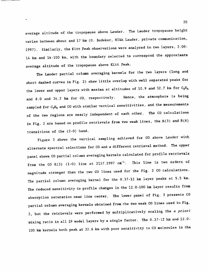
20

average altitude of the tropopause above Lauder. The Lauder tropopause height

varies between about and 17 km (G. Bodeker, NIWALauder, private communication,

1997). Similarly, the Kitt Peakobservations were analyzed in two layers, 2.09-

14 km and 14-100 km, with the boundary selected to correspond the approximate

average altitude of the tropopause above Kitt Peak.

The Lauder partial column averaging kernels for the two layers (long and

short dashedcurves in Fig. 2) show little overlap with well separated peaks for

the lower and upper layers with maximaat altitudes of 10.9 and 32.7 km for C2H6

and 8.0 and 34.2 km for CO, respectively. Hence, the atmosphere is being

sampled for CzH6 and COwith similar vertical sensitivities, and the measurements

of the two regions are nearly independent of each other. The COcalculations

in Fig. 2 are based on profile retrievals from two weak lines, the R(3) and R(6)

transitions of the (2-0) band.

Figure 3 shows the vertical sampling achieved for CO above Lauder with

alternate spectral selections for COand a different retrieval method. The upper

panel showsCOpartial columnaveraging kernels calculated for profile retrievals

from the COR(3) (I-0) line at 2157.2997 cm-I. This line is two orders of

magnitude stronger than the two COlines used for the Fig. 2 COcalculations.

The partial column averaging kernel for the 0.37-12 km layer peaks at 5.5 km.

The reduced sensitivity to profile changes in the 12.0-I00 km layer results from

absorption saturation near line center. The lower panel of Fig. 3 presents CO

partial column averaging kernels obtained from the two weak COlines used in Fig.

2, but the retrievals were performed by multiplicatively scaling the a priori

mixing ratio in all 29 model layers by a single factor. The 0.37-12 km and 12.0-

i00 kmkernels both peak at 32.6 kmwith poor sensitivity to COmolecules in the

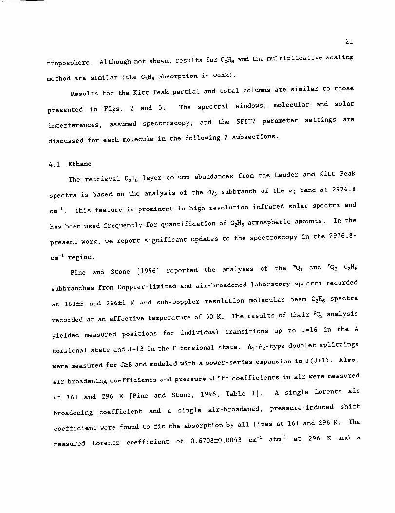
21

troposphere. Although not shown, results for CzH6 and the multiplicative scaling

method are similar (the C2H6 absorption is weak).

Results for the Kitt Peak partial and total columns are similar to those

presented in Figs. 2 and 3. The spectral windows, molecular and solar

interferences, assumed spectroscopy, and the SFIT2 parameter settings are

discussed for each molecule in the following 2 subsections.

4.i Ethane

The retrieval C2H8layer column abundances from the Lauder and Kitt Peak

spectra is based on the analysis of the PQ3subbranch of the v7 band at 2976.8

cm-I This feature is prominent in high resolution infrared solar spectra and

has been used frequently for quantification of C2H6 atmospheric amounts. In the

present work, we report significant updates to the spectroscopy in the 2976.8-

cm-I region.

Pine and Stone [1996] reported the analyses of the PQ3 and rQ0 C2H6

subbranches from Doppler-limited and air-broadened laboratory spectra recorded

at 161±5 and 296±1 K and sub-Doppler resolution molecular beam C2H6 spectra

recorded at an effective temperature of 50 K. The results of their PQ3analysis

yielded measured positions for individual transitions up to J=16 in the A

torsional state and J_13 in the E torsional state. A1_A2-typedoublet splittings

were measuredfor J_8 and modeledwith a power-series expansion in J(J+l). Also,

air broadening coefficients and pressure shift coefficients in air were measured

at 161 and 296 K [Pine and Stone, 1996, Table I]. A single Lorentz air

broadening coefficient and a single air-broadened, pressure-induced shift

coefficient were found to fit the absorption by all lines at 161 and 296 K. The

measured Lorentz coefficient of 0.6708±0.0043 cm-I atm-1 at 296 K and a

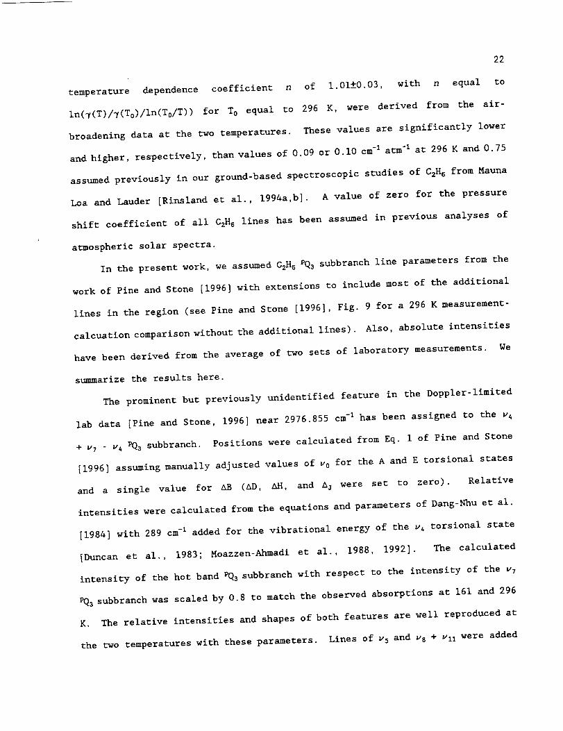
22

temperature dependence coefficient n of I. 01-+0.03, with n equal to

In(7(T)/v(T0)/In(T0/T)) for To equal to 296 K, were derived from the air-

broadening data at the two temperatures. These values are significantly lower

and higher, respectively, than values of 0.09 or 0.i0 cm -I arm -I at 296 K and 0.75

assumed previously in our ground-based spectroscopic studies of C2H 8 from Mauna

Loa and Lauder [Rinsland et al., 1994a,b]. A value of zero for the pressure

shift coefficient of all C2H 6 lines has been assumed in previous analyses of

atmospheric solar spectra.

In the present work, we assumed C2H 6 PQ3 subbranch line parameters from the

work of Pine and Stone [1996] with extensions to include most of the additional

lines in the region (see Pine and Stone [1996], Fig. 9 for a 296 K measurement-

calcuation comparison without the additional lines). Also, absolute intensities

have been derived from the average of two sets of laboratory measurements. We

summarize the results here.

The prominent but previously unidentified feature in the Doppler-limited

lab data [Pine and Stone, 1996] near 2976.855 cm -I has been assigned to the v4

+ v7 v4 PQ3 subbranch. Positions were calculated from Eq. i of Pine and Stone

[1996] assuming manually adjusted values of v0 for the A and E torsional states

and a single value for AB (AD, AH, and Aj were set to zero). Relative

intensities were calculated from the equations and parameters of Dang-Nhu et al.

[1984] with 289 cm -I added for the vibrational energy of the v4 torsional state

[Duncan et al., 1983; Moazzen-Ahmadi et al., 1988, 1992]. The calculated

intensity of the hot band PQs subbranch with respect to the intensity of the v7

PQ3 subbranch was scaled by 0.8 to match the observed absorptions at 161 and 296

K. The relative intensities and shapes of both features are well reproduced at

the two temperatures with these parameters. Lines of v5 and v8 + vll were added

23

to the linelist based on the positions and assignments of Pine and Lafferty

[1982, Table 2] and the intensity expressions and parameters of Dang-Nhuet al.

[1984]. The new linelist accounts for most of the absorptions observed in the

PQ3region at 161 and 296 K. Furthermore, it is apparent from plots of the

measuredversus calculated spectra that resonance mixing perturbs the positions

and intensities of several assigned lines in the interval. Figure 4 presents

comparisons of the measured and calculated Doppler-limited C2H6laboratory

spectra at temperatures of 161 and 296 K.

Absolute intensities were derived from an unweighted average of values

calculated from the intensity expressions and parameters of Dang-Nhu et al.

[198&] and a set of intensities inferred from the laboratory measurements of

Pine and Stone [1994]. The results from the more recent measurementsare 0.955

times the earlier ones. The discrepancy of the two intensity values primarily

reflects the uncertainties in the pressure measurements,at low temperatures in

the older study and at low pressure in the newer. The measurementsof Rinsland

et al. [1986] were not considered becauseof their low spectral resolution (0.06

cm -I ) •

The new C2H 6 spectroscopic parameters adopted here are a significant

improvement relative to those assumed in our previous atmospheric studies

[Rinsland et al., 1987; Rinsland et al., 1994a,b]. The previous model neglected

torsional tunneling and Az-A 2 splittings. Also, we previously assumed a 296 K

Lorentz broadening coefficient =30% larger than the value measured for PQ3 by

Pine and Stone [1996]. Further work to estimate the lower state energies of

unassigned lines in the vicinity of the PQ3 subbranch, obtain an improved

description of the intensity perturbations in the region, and calculate the

24

temperature dependent C2H 6 partition function with improved accuracy is in

progress.

Except for CzH 6, the spectroscopic parameters were taken from the 1996

HITRAN compilation [Rothman et al., 1998]. The weak temperature-sensitive

absorption by the H2180 line at 2976.7839 cm -I (lower state energy of 1574.679

cm -I) directly overlaps the PQ3 C2H6 subbranch. Parameters for this H21sO line

were added in HITRAN 1996 [Rothman et al., 1998]. Hence, no update was

necessary.

Figure 5 presents molecule-by-molecule simulations and a typical Lauder

spectrum in the region of the unresolved PQs subbranch. The C2H 6 retrievals

reported in this paper are based on the fits to the 2976.62-2976. 9A-cm-1 interval

shown in the figure. The importance of accurate modeling of the interferences,

particularly H20, at the low altitude of the Lauder station is evident, as was

noted previously [Rinsland et al., 1994a]. Four molecules were fitted in this

window: C2H6 ' H20 , CH4, and 03 . Only the profile of CzH s was retrieved; a

multiplicative a priori volume mixing ratio profile scaling factor was retrieved

for each of the other 3 gases. The phase error and zero absorption level were

also fitted in the Lauder spectra. A sample Lauder fit is presented in Figure

.

The PQ3 CzH6 region of the Kitt Peak spectra is similar to the sample Lauder

observations shown in Figs. 5 and 6. However, the interference by H20 is

significantly weaker because of the higher altitude of Kitt Peak. Columns of

CzH 6 obtained with the new line parameters are 13% less than values obtained with

the parameters assumed previously [Rinsland et al., 1994a,b].

25

4.2 Carbon Monoxide

The retrievals are based on spectral fittings of 2 intervals containing the

12C0 R(3) andR(6) (2-0) band lines at 4274.7047 and 4284.8911 cm -I, respectively.

Figure 7 illustrates the intervals for a sample Lauder spectrum along with

simulations for H20, HDO, CO, CH 4, and solar CO. The selected intervals avoid

CH 4 octad lines not included in HITRAN 1996 [Rothman et al., 1998] and yield

compatible simultaneous spectral fittings. An unpublished line list shows the

importance of the CH 4 lines missing from HITRAN 1996 [Rothman et al., 1998] in

other portions of the the 4200-4300 -cm-1 region (J.-C. Hilico, private

communication, 1997).

The HITRAN 1996 parameters [Rothman et al., 1998] adopted for the CO

analysis include CH 4 positions and intensities from Brown and Rothman [1982] with

accuracies for single, unblended lines of ±0.0005 cm-I and ±2%, respectively.

Air-broadening coefficients and pressure-shift coefficients at 296 K based on

the work of Malathy Devi et al. [1993] were assumed for CH 4 as given on HITRAN

1996 [Rothman et al., 1998]. A weak, unassigned absorption appears at 4274.81

cm -I in the Lauder and Kitt Peak spectra. A line of HDO was added at this

position. The retrievals satisfactorily reproduce this weak feature for the

range of observational conditions.

The R(3) (2-0) band terrestrial line in the 4274.62 -4274.82-cm-I spectral

interval is overlapped by absorption from the corresponding solar CO transition

with only minor interferences from other gases in the interval. The 4284.75-

4285.18 cm -I spectral interval contains the R(6) terrestrial CO line, several

solar CO lines, and the strong CH 4 line at 4285.1553 cm -I. The retrievals were

performed by fitting for the vertical profiles of both CO and CH 4. A

multiplicative a priori HDO volume mixing ratio profile scaling factor was also

26

retrieved to account for variations in the absorption by the 4274.81-cm-I line.

An example of a simultaneous fit to the two COwindows in a typical Kitt Peak

spectrum is presented in Fig. 8.

5.0 Measurement selection criteria

The quality control of retrieved profiles was based on a combination of

criteria that measure the goodness of fit and the relative strength of the target

absorption feature. The first criterion is the familiar root-mean-square error

(rms) between the measured and fitted spectra in the selected intervals. The

latter, called the signal strength ratio (ssr), is the observed depth of the

target absorption feature relative to the noise measured in a nearby window

region. It serves the purpose of identifying spectra in which the target feature

is too weak to be measured accurately. As illustrated in Fig. 9, a plot of rms

versus ssr produces a scatter plot with points that define an elbow-shaped curve.

Values for the maximum rms and minimum ssr are selected near the "elbow" of this

curve to weed out unreliable retrievals. As a final step, all profiles that pass

the rms/ssr criteria are displayed on a single plot, and any further profiles

that are clearly unacceptable (large negative mixing ratio excursions, for

example), are removed. This second step generally deletes only about 5% of the

remaining measurements, which for a variety of reasons, including poorly modelled

interferences, channel spectra, and unwanted instrumental artifacts, produce

instabilities in the retrieval process.

6.0 Error Analysis

In Table i, we report our estimates of the effects of both random and

systematic errors on the retrieved lower layer CO and CzH 6 partial columns. A

single value is given for the two stations where appropriate. We next describe

27

the procedures and assumptions used in generating the uncertainty estimates.

6.1. Temperature profile. As already noted, the analysis regions were

selected to contain target lines with intensities insensitive to temperature,

and all retrievals were performed assumingNCEPtemperature profiles calculated

for the date and location of the observations. We generated synthetic spectra

for 3 randomly selected days assuming the nominal temperature profile.

Retrievals were then performed by adding 2 K to the temperature at each altitude.

The magnitude of the mean difference between the true and retrieved partial

column is shown in the table; the errors are 1%or less for CzH6 and CO.

6.2. Noise. Random numbers with zero mean, a normal distribution, and a

root-mean-square deviation equal to 0.5% of the maximum transmission were added

to synthetic spectra generated for the C2H 6 and CO analysis regions. The

simulated noise is typical of the individual Lauder and Kitt Peak spectra. Ten

different seeds were chosen. The retrieved partial columns show no bias with

respect to the true partial columns. As shown in the table, the average

difference between the noisy and true partial columns range from 2 to 7%. Note

that daily averaging further reduces errors due to random instrument noise for

both Lauder and Kitt Peak.

6.3. Interfering atmospheric lines. As mentioned in section 4.1 and

illustrated in Fig. 5, HzO is an important interfering molecule with absorption

overlapping the target C2H 6 PQ3 v7 band subbranch. The two windows selected for

CO contain only minor absorptions by atmospheric molecules.

6.4. Spectroscopic parameters. We estimated a 2% uncertainty in the

retrievals due to spectroscopic parameters errors in the two microwindows

analyzed for CO. This small error estimate is based on the high quality of the

CO parameters in the HITRAN 1996 compilation [Rothman et al., 1998] and our

28

avoidance of intervals containing poorly-modeled, interfering CH_ lines. The

spectroscopic updates incorporated for C2H 6 in the present analysis are estimated

to reduce the errors in the C2H 6 retrievals from 10% [Rinsland et al., 1994a] to

5% with the main source of error the uncertainty in the laboratory pressure

measurements.

6.5. State vector of unknowns. The retrieval is a linear combination of

the true and a priori profiles with structures finer than the measurement

vertical resolution poorly determined [Connor et al., 1995]. Although we do not

know the true C2H 6 and CO atmospheric profiles on the dates of observation,

simulations based on correlative observations can be used to show the dependence

of the retrieval on the a priori profile and the assumed S a and S, covariances.

As illustrated in Fig. i, retrievals from synthetic spectra generated from a set

of correlative vertical profiles and the adopted settings yield partial columns

that track the values adopted in the simulations with no deviations from

linearity over the factor of two range in the CO 2.09-14 km a priori partial

columns. Based on these results, we estimate 1% as the error in the lower layer

partial column retrieval due the influence of the a priori profile and the other

state vector parameters.

6.6. Instrument line shape function. A synthetic spectrum was calculated

for the most common spectral resolution of the Lauder observations. The

theoretical instrument line shape function was assumed. A retrieval was

performed from this spectrum with the coefficient of the "straight line"

effective apodization coefficient [Park, 1983] decreased from the nominal value

of 0.0 to -0.i. This case simulates apodization function error that increases

linearly from zero at zero path difference to 10% at the maximum optical path

difference. Changes of 0.1% in the tropospheric layer partial columns of CO and

29

CzH 6 were obtained. The Kitt Peak instrument function is well determined so that

instrument function errors are negligible for both molecules. The Lauder CO and

C2H 6 0.37-12 km partial columns are much less sensitive to errors in the

instrument function than those derived for the Lauder 03 0.37-12 km column

[Pougatchev et al., 1996, Table i].

6.7. Forward model. The forward model in SFIT2 is essentially the same

as in SFIT and the algorithms developed at NASA Langley for the analysis of

infrared laboratory [Benner et al., 1995] and infrared solar spectra recorded

with Fourier transform spectrometers [Norton and Rinsland, 1991]. Based on

retrieval comparison exercises that have been performed for atmospheric and

laboratory studies [e.g. Zander et al., 1993], we estimate that errors in

simulated solar spectra generated with the SFIT2 forward model are unlikely to

introduce CzH 6 and CO lower layer partial column retrieval errors greater than

4% for CO and 2% for C2H 6. The larger value was assumed for CO because of the

additional uncertainty caused by errors in simulating the absorption by solar

CO lines in the windows.

7. Results and Discussion

For Lauder, 0.37-12 km partial vertical columns were calculated by

integrating the retrieved profiles. For Kitt Peak, the 2.09-14 km partial

columns were computed. Daily averages were generated assuming equal weights for

all observations; the number of observations per day ranged from I to 23 for

Lauder CzH 6, and the number of observations per day ranged from I to 25 for

Lauder CO. For Kitt Peak, the corresponding ranges of daily observations were

i to 13 and i to 14.

3O

The daily average partial columns Ct were fitted with the expression

Ct ffia0 + aI (t to) + a2 cos 2_ [(t - to) - tl](3)

where a0 is the mean value, t is the time of the observation in calendar years,

to is the time of the first observation in calendar years, aI is the long-term

trend, a2 is the amplitude of the seasonal cycle (assumed to be sinusoidal), and

tI is the fraction of the calendar year corresponding to the time of the seasonal

maximum.

7.1 Lauder C2H 6 and CO 0.37-12 km Time Series

The top and middle panels of Fig. I0 present the measured Lauder daily

average 0.37-12 km C2H 6 and CO partial columns between July 1993 to November

1997. The total number of measurement days are A07 for CzH 6 and 390 for CO. The

solid curves show the best-fits to the observations based on Eq. 3. This simple

model does a poor job in reproducing the observed highly asymmetrical C2H 6 and

CO seasonal cycles, which show sharp peaks during austral spring and deep minima

in austral autumn. Corresponding, peak column-average 0.37-12 km mixing ratios

(shown on the right vertical axis) exceeded 0.6 ppbv for CzH 6 and i00 ppbv for

CO. The maximum mixing ratios are as high as measurements in upper tropospheric

continental outflow regions between Brazil and Africa during September-October

1992 [Talbot et al, 1996, Tables 2 and 3]. Year-to-year differences are apparent

in the Lauder time series with particularly high 0.37-12 km partial CO and C2H 6

columns observed during October 1994, August 1995, and September-October 1997.

We attribute the sharp peaks to tropical biomass burning emissions lofted

to the upper troposphere by deep convection. In the upper troposphere, where

the present measurements have their highest sensitivity (Fig. 2), maximum wind

31

speeds exceeded A0 m s-I in the southern subtropical jet stream (~30°S latitude)

during the September-October 1996 Pacific Exploratory Mission-Tropics (PEM-T)

experiment [Fuelberg et al., 1998]. Although typical PEM-Tupper tropospheric

wind speeds were lower, calculations indicate that the strong, westerly upper

tropospheric winds were sufficient to transport southern hemisphere air parcels

thousands of km on a time scale of about a week during the mission [Fuelberg et

al., 1998]. Once lofted to the upper troposphere, only relatively minor

oxidative losses of COand C2H6 occur due to the rapid horizontal transport of

the emitted plumes.

No statistically significant long-term trend were detected from the Lauder

CzH6 or COmeasurementdatabases. The best-fit trends (aJa 0 of Eq. 3) for C2H6

and COfrom daily meansbetween July 1993 and November1997 are (-0.64±0.79)%

yr -I and (0.37±0.57)% yr -I, i sigma, respectively. Recently, Matsueda et al.

[1998] reported a series of upper tropospheric COmixing ratios measured in situ

during commericial aircraft flights at longitudes of 140°E to 152°E and latitudes

30°N to 30°S (Japan-Australia). A rate of COdecrease of about 5 ppbv yr -I was

derived from a fit to the 5°S to 30°S latitude observations during the 58

sampling flights between July 1994 and June 1996.

Ratios of the CzHJCO0.37-12 km daily averages are presented in the bottom

panel of Figure i0 for the 332 Lauder observation days in common. This plot

illustrates that larger relative seasonal changes are observed for C2H6 than for

COwith the seasonal variation of the C2H5/C00.37-12 km partial columns ratios

roughly in phase with the seasonal variations of both gases. The Lauder peak

CzHJCOcolumns ratio is close to the value of 6.0 × 10-3 measured directly over

(_ i km) active savanna fires in Brazil and Zambia during the same season

(September-October 1992 observations), but our peak value is significantly lower

32

than the enhanced, upper tropospheric ratio of 12.1 × I0 -s determined in the

upper troposphere over the south Atlantic basin during the same time period

[Talbot et al., 1996].

Time series of C2H6 and CO surface measurementsof clean marine air at

Baring Head, NewZealand (41.2°S, 174.5°E) have been reported recently [Clarkson

et al., 1997; Manning et al., 1997]. The Baring Head facility is a remote

station located on the edge of an 80-m cliff overlooking Cook Strait at the

southern tip of the North Island [Brenninkmeijer, 1993; Clarkson et al., 1997].

Wenext compare these in sicu measurements with mean 0.37-12 km mixing ratios

derived from our spectroscopic time series.

A sine curve fit to Baring Head C2H s monthly mean measurements collected

during southerly winds (to avoid local land sources of pollution) and from

measurements at Scott Base, Antarctica (77.5°S, 166.4 °E) between 1991 and 1996

yields a peak CzH 6 mixing ratio of about 0.4 ppbv in September and a minimum of

about 0.15 ppbv in March [Clarkson et al., 1997, Fig. 3a], though this curve does

not capture the relatively high measurements (0.4-0.6 ppbv) common in the Baring

Head data between January and May. The January-May peaks are not seen in the

Lauder spectroscopic data. The Baring Head surface C2H s measurements are

generally lower than the Lauder 0.37-12 kmcolumn average mixing ratios, and the

Baring Head measurements do not show the sharp peaks present in the September-

October Lauder spectroscopic observations.

The June 1989 to June 1995 monthly average CO mixing ratios at Baring Head

show median values ranging from 42 ppbv in March to 65 ppbv in October [Manning

et al., 1997, Fig. i]. The authors comment that while interannual variability

was observed, no statistically significant CO trend was detected. As for C2H 6,

the Lauder CO 0.37-12 kmcolumn-averaged mixing ratio show a seasonal cycle with

33

maxima and minima at times close to those inferred from the Baring Head in siru

data, but again, our spectroscopic 0.37-12 km daily mean CO mixing ratios show

sharp September-October peaks not present in the monthly-averaged surface

measurements from Baring Head.

Insight into differences between the Lauder and Baring Head measurements

can be obtained from a climatology of CO aircraft measurements obtained over

southeast Australia [Pak et al., 1996]. Although this location is quite far from

New Zealand, there are no major surface sources in either region, and long range

transport can be expected to bring gases originating at a similar set of distant

surface sites to these sites. The aircraft CO measurements show tropospheric

mixing ratios that increase with altitude throughout the year with the range of

the average seasonal cycles increasing with altitude. Increases in CO occur in

July and August prior to the observed mixing ratio peak [Pak et al., 1996]. The

range in the average CO seasonal cycle above Cape Grim is observed to increase

with altitude. The Lauder data do not show the secondary mixing ratio maximum

observed in March and April above Cape Grim in CO, CH 4, and N20 [Pak et al.,

1996].

Tables 2 and 3 list the Lauder monthly average 0.37-12 km CO and CzH e

columns calculated by averaging the 1993 to 1997 daily means. The listings give

the mean characteristics of the temporal variations over this time period, but

they do not capture the sharp peaks during austral spring nor do they show the

distinct year-to-year differences in the partial columns.

To our knowledge, the only correlative measurements were obtained by the

nadir-viewingMAPS gas correlation radiometer instrument [Reichle et al., 1990].

Measurements of CO obtained by the MAPS sensor in April and October 1994 have

been analyzed to derive equivalent CO total columns above sites performing

34

correlative observations, including the Lauder station [Pougatchev et al., 1998].

The MAPS measurements, which have an estimated accuracy of about ±10% [Pougatchev

et al., 1998] , correspond to total CO columns above Lauder in April and October

of 1.24 and 1.62 (in I0 _8 molecule cm-2), respectively. The averages of our

retrieved daily mean total CO columns from observations during the April and

October 1994 MAPS missions equal 0.95 and 1.30 (in 1018 molecule cm-2),

respectively. Our values average 0.78 times the corresponding MAPS values

despite the similarity of our total column averaging kernel (Fig. 2) to the MAPS

total column averaging kernel [Pougatchev et al., Fig. 2]. We note that our

April and October 1994 total columns are 0.92 and 0.94 times those deduced from

analysis of Lauder correlative solar spectral measurements of the 12C0 (i-0) band

R(3) line by Pougatchev et al. [1998], respectively. The averaging kernel for

spectroscopic measurements from this strong line (based on multiplicative scaling

of the CO a priori profile) decrease with altitude from a maximum of 1.5 at the

surface to 0.8 at 8 km [Pougatchev et al., 1998, Fig. 2]. The offsets between

the two independently-derived spectroscopic correlative total columns may reflect

inaccuraties in the spectroscopic parameters, errors in modeling the overlapping

solar CO lines (particularly for the weak lines analyzed in this study), and/or

the differences in the vertical sensitivities of the measurements at the moment

of the observations, as demonstrated by their averaging kernels. The cause of

the larger differences between the two sets of spectroscopic total columns and

the total columns inferred from the correlative MAPS measurements may reflect

the strong, irregular spatial and temporial variations of atmospheric CO above

Lauder (e.g. Fig. I0), and the differences in the times and locations of these

measurement sets.

35

7.2 Kltt Peak C2He and CO 2.09-14 km time series

Figure ii illustrates the time series of Kitt Peak 2.09-14 km C2H 5 and CO

daily average measurements between May 1977 and December 1997. The total number

of valid measurement days were 95 for C2H 6 and 150 for CO with the number of

measurements per day varying from i to 14 for CO and from I to 13 for CzH 6. The

results, displayed in the same format as Figure I0, show a distinct seasonal

cycle for both molecules with spring maxima and autumn minima. Significant

deviations from the best-fit curves were observed on several days. The trends

(aJa 0 of Eq. 3) determined from fitting the CzH 6 and CO daily mean 2.09-14 km

columns are (-1.20±0.35) and (-0.27±0.17)% yr -I, i sigma, respectively. Mean

Kitt Peak 2.09-14 km C2H 8 and CO mixing ratios are 1.08 and 103 ppbv,

respectively. Corresponding Lauder 0.37-12 km values from the 1993 to 1997

dataset are 0.32 and 57 ppbv. Hence, the mean C2H 6 and CO tropospheric mixing

ratios are higher in the northern hemisphere dataset relative to the southern

hemisphere dataset by factors of 3.4 and 1.8, respectively.

Table 4 and 5 list the monthly mean partial CO and C2H 6 columns for the

2.09-14 km layer. Unfortunately, the total number of measurement days is

significantly fewer than obtained from Lauder. A plot of the Kitt Peak monthly

averages from Table 5 shows the CO seasonal variation is asymmetrical with the

amplitude of the spring maximum larger than amplitude of the autumn minimum.

This conclusion is consistent with the results of Pougatchev and Rinsland

[1995a], who analyzed the Kitt Peak measurements with a different retrieval

method. The C2H 6 measurements show no clear evidence of an asymmetry in the

annual cycle. Note that only a single CzH 6 measurement was obtained during

August.

36

A substantial downwardtrend over this time period is indicated for C2H6,

but not for CO. In contrast, Ehhalt et al. [1991] reported C2H6 column

abundancesdeduced from the analysis of infrared solar spectra recorded at the

the International Scientific Station of the Jungfraujoch (ISSJ, 46.55°N, 7.98°E,

3580 m altitude). An exponential tropospheric C2H6 column increase rate of

(0.85±0.3)% yr -I was deduced by comparing 1984-1988 measurements with low

spectral resolution measurementsfrom March and April 1951. More recent (1985

to 1995) measurementsof C2HB total columns above the ISSJ indicate a mean

exponential trend equal to (-3.6±0.4)% yr "I, i sigma, which reduces to a trend

of (-2.7±0.3)% yr -I, i sigma, when fitting the observations with a model that

includes a sine function to account for the seasonal variations [Mahieu et al.,

1997].

Wallace and Livingston [1990] derived COtotal columns above Kitt Peak by

fitting two lines of the (2-0) band in solar spectra recorded between 1979 and

1985. A seasonal cycle with a spring maximumand autumn minimumwas observed

with no obvious long-term trend. No long-term CO trend was assumed in the

analysis of Kitt PeakCOobservations reported by Pougatchevand Rinsland [1995].

Although an average CO total column increase rate of about 1% yr -I has been

reported from infrared solar spectroscopic measurementsabovecentral Europe from

1950-1951 to 1985-1987 [Zander et al., 1989] and above Zvenigorod, Russia, for

1970-1995 [Yurganov et al., 1997], surface measurementsat remote sites in both

hemispheres show a shift from an upward COtrend during the 1980s to a downward

trend in the 1990s [Khalil and Rasmussen,1994]. The mean trend deduced from

the Kitt Peak 1977-1997 CO measurements is consistent with the northern

hemisphere 1987-1992 average linear trend of (-1.4±0.9)% yr -I reported from

surface in situ measurements [Khalil and Rasmussen, 1994, Table i]. More recent

37

surface measurementsfrom a global network of surface stations show an average

northern hemisphere CO surface trend of about -0.5 ppbv yr -I between 1994 and

April 1997 (M. A. K. Khalil, private communication, 1998). Fits derived from

April 1993 to March 1996 upper tropospheric COaircraft measurementsobtained

between Japan and Australia show a downward trend of about 2 ppbv yr -I at

northern hemisphere latitudes [Matsuda et al., 1998].

The features observed in the northern hemisphere CO surface and upper

tropospheric measurements, in particular the trend reversal since the late 1980s,

have been noticed in the COtotal columns monitored above the ISSJ between 1984

and 1995, i.e. a meanexponential rate of change of (-0.54±0.25)% yr -I, i sigma;

the negative rate is maintained but reduced to (-0.18±0.16)% yr -I when fitting

the observations with a function combining a sinusoidal and an exponential

component [Mahieu et al., 1997]. It should be noted that the COcolumn minima,

which occur above the ISSJ around mid-September, were record low in 1992 and

1993, i.e., during two years following the Mr. Pinatubo volcanic eruption of June

1991.

7.3 Correlations between CO and GzH 6

The number of Lauder observations is sufficient to examine the correlation

between CO with C2H 8 as a function of season. Table 7 presents correlation

coefficients and slopes derived by fitting the Lauder 1993-1997 CO and C2H s daily

mean 0.37-12 km partial column observations to the expression

[C2H_] = a + b [CO](4)

where [] denotes the daily-average value.

38

As expected from the bottom panel of Fig. i0, the minimumvalue of b is

measured early in the calendar year. This time period shows the lowest

correlation between the partial columns of the two species. Table 7 also reports

corresponding values derived by fitting all the Kitt Peak 2.09-14k m measurements

with Eq. 4. The correlation coefficient of 0.77 is only slightly less than the

peak seasonal value derived for Lauder while b is several times higher than the

corresponding value for Lauder.

Slopes derived from fits to Eq. 3 with model calculated columns computed

for the locations of Lauder and Kitt Peak (Y. Wang, private communication, 1998)

are also shown. The model slopes are lower than the observed values from both

sites. Model C2H6-CO correlation coefficients (not shown) derived from the model

columns are >0.9, significantly higher than indicated by the observations.

7.4 Comparisons of the observations with model calculations

Figure 12 presents comparisons of the Lauder and Kitt Peak monthly mean

tropospheric measurements with values calculated with a global 3-D tropospheric

model [Wang et al., 1998a]. The standard model calculations, which assumed 2.5

Tg C-I yr -I C2H6 emitted by biomass burning, are significantly lower than the

monthly average Lauder partial columns observed during all seasons. Also, the

September-October peak is broader in the model results than in the observations.

These differences are consistent with comparisons of the reported Lauder December

1992-March 1994 C2H 6 columns [Rinsland et al., 1994a] and the model results, as

displayed in Fig. 15 of Wang et al. [1998b]. The authors comment that the

agreement between the measured and calculated Lauder C2H 6 seasonal cycle is

improved with the biomass burning emission rate increased to 6 Tg C-I yr -I.

However, this emissions rate is also higher than the value of 2.7 Tg C-I yr -I

39

derived for the southern hemisphere by Clarkson et al. [1997], and it is outside

their estimated budget uncertainty (1.6-5.2 Tg yr-1). As pointed out by Wang et

al. [1998b], the cause of the CzH 6 model-measurement discrepancy is unclear

because the model calculations reproduce observations of the southern hemisphere

CO seasonal cycle very well (including the present data) and the C2H6/C0 biomass

burning emissions ratio is well determined from field emission measurements.

In contrast, calculations with the model of Wang et al. [1998a] are

significantly higher than the Kitt Peak CO tropospheric column observations

throughout the year, but the model reproduces the C2H _ measurements and their

seasonal variation quite well during all seasons. The cause of the Kitt Peak

CO model-measurement discrepancy is also unclear, but it is quite likely that

the difference is unrelated to the discrepancy noted for Lauder.

8. Summary

In this paper we have reported multi-year time series of high spectral

resolution infrared solar absorption CO and CzH 6 measurements from remote sites

at midlatitudes of the northern and southern hemispheres. Target lines were

selected to achieve similar vertical sensitivities based on averaging kernels.

The Lauder 1993-1997 CO and CzH 6 columns below 12 km (with peak sensitivities in

the upper troposphere) show highly asymmetrical seasonal cycles with a minimum

in about February, a maximum near September-October, and distinct year-to-year

differences in the seasonal variation. Sharp peaks are observed in the partial

columns of both gases near the seasonal maximum. The seasonal variation is

larger for C2H _ than from CO, which is also produced in si_u by the oxidation of

CH 4. The elevated values observed in austral spring likely result from the long

range transport of tropical biomass burning emissions, principally from Africa

40

and South America. Near the seasonal maximum, the peak column-average

tropospheric mixing ratios of CzH_ and CO above Lauder are similar to upper

tropospheric values observed in continental outflow regions between Brazil and

Africa during the sameseason. The peak Lauder partial columns are also similar

to the annual mean values observed above Kitt Peak. Although year-to-year

differences are apparent, no significant trend was detected for either molecule

above Lauder. The Kitt Peak 2.09-14 km partial columns also show distinct

seasonal cycles with spring peaks in the mixing ratios of the two gases and

larger relative seasonal variations for C2H6 than CO. An unexpected result of

this study is the observed, statistically significant downwardtrend in the Kitt

Peak C2H s tropospheric column. No significant long- term trend in the

tropospheric CO column was detected over the 20 year span of the Kitt Peak

spectroscopic observations.

Acknowledments. Special thanks to B. M. McNamara of NIWA, Claude Plymate, Jeremy

Wagner, and Michael Dulick of the National Solar Observatory (NSO) for recording

the high-resolution infrared solar spectra. The NSO is operated by the

Association of Universities for Research in Astronomy, Inc. (AURA) under a

cooperative agreement with the National Science Foundation (NSF). The McMath

FTS solar observations were partially supported by the U. S. Department of Energy

CO2 program, NASA, the Chemical Manufacturers Association, and NSF. Research at

the NIWA has been funded by the New Zealand Foundation for Research, Science,

and Technology (Contract number CO 1221). Research at NASA Langley has been

funded by NASA's Upper Atmosphere Reserach Program. Research at Christoper

Newport University is funded by a grant from NASA. The carbon monoxide aircraft

data obtained by the the CSIRO Division of Atmospheric Research GASLAB (version

41

l-release date Ii March 1997) were obtained by Paul Steele, Ray Langenfelds, and

coworkers of the CSIRODivision of Atmospheric Research, and we gratefully

acknowledge their use in this investigation. Research at the University of

Denver is supported by NASAand NSF. Research at the University of Liege was

partially supported by Belgian funds through the Office of Scientific, Technical,

and Cultural Affairs, Brussels. We thank Linda Chiou of Science Applications

International Corporation for her help with the analysis of the Kitt Peak solar

spectra and the preparation of the figures. Weare especially grateful to Yuhang

Wangof Georgia Tech for sending the Harvard model calculations. Jack Fishman

of NASALangley also provided helpful commentsduring the development of this

manuscript.

42

References

Bell, R. J., Introductory Fourier Transform Spectroscopy, Academic Press, New

York, 382 pp., 1972.

Benner, D. C., C. P. Rinsland, V. Malathy Devi, M. A. H. Smith, and D. Adkins,

A multispectrum nonlinear least squares fitting procedure, J. Quanc.

SpecCrosc. Radiac. Transfer, 53, 705-721, 1995.

Blake, D. R., and F. S. Rowland, Global atmospheric concentrations and source

strength of ethane, Nature, 321, 231-233, 1986.

Blake, N. J., Blake, D. R., J. E. Collins, Jr., G. W. Sachse, B. E. Anderson,

J. A. Brass, P. J. Riggan, and F. S. Rowland, Biomass burning emissions

of atmospheric methyl halide and hydrocarbon gases in the south atlantic

region, in Biomass Burning and Global Change, Vol. 2, Biomass Burning in

Sou_h America, Southeast Asia, and Temperate and Boreal Ecosystems, and

the 0il Fires of Kuwait, edited by J. S. Levine, pp. 576-594, MIT Press,

Cambridge, 1997.

Brault, J. W., Solar Fourier transform spectroscopy, in Proceedings of the JOSO

Workshop, Future Solar Optical Observations, Needs and Constraints,

Firenze, Italy, edited by G. Godoli, G. Noci, and A. Righin, pp. 33-52,

1978.

Brenninkmeijer, C. A. M., Measurement of the abundance of 14CO in the atmosphere

and the 13C/12C and 180/160 ratio of atmospheric CO with applications in New

Zealand and Antarctica, J. Geophys. Res., 98, 10,595-10,614, 1993.

Brown, L. R., and L. S. Rothman, Methane line parameters for the 2.3-pm region,

Appl. Opt., 21, 2425-2427, 1982.

43

Chatfield, R. B., J. A. Vastano, H. B. Singh, and G. Sachse, A general model of

how fire emissions and chemistry produce african/oceanic plumes (03, CO,

PAN, smoke) in TRACEA, J. Geophys. Res., i01, 24,279-24,306, 1996.

Coffey, M. T., W. G. Mankin, A. Goldman, C. P. Rinsland, G. A. Harvey, V. Malathy

Devi, and G. M. Stokes, Infrared measurements of atmospheric ethane (C2H 6)

from aircraft and ground-based solar absorption spectra in the 3000-cm -z

region, Geophys. Res. Left., 12, 199-202, 1985.

Clarkson, T. S., R. J. Martin, and J. Rudolph, Ethane and propane in the southern

marine troposphere, Atmos. Environ., 31, 3763-3771, 1997.

Connor, B. J., A. Parrish, J.-J. Tsou, and M. P. McCormick, Error analysis for

the ground-based microwave ozone measurements during STOIC, J. Geophys.

Res., i00, 9283-9291, 1995.

Connor, B. J., N. B. Jones, S. W. Wood, J. G. Keys, C. P. Rinsland, and F. J.

Murcray, Retrieval of HC2 and HNO 3 profiles from ground-based FTIR data

using SFIT2. Proc. XVIII Quadrennial 03 Symposium, Univ. L'Aquila, Italy,

1996.

Conny, J. M., and L. A. Currie, The isotopic characterization of methane, non-

methane hydrocarbons and formaldehyde in the troposphere, Armos. Environ.,

30, 621-638, 1996.

Crutzen, P. J., and L. T. Gidel, A two-dimensional photochemical model of the

atmosphere, 2, The tropospheric budgets of the anthropogenic chlorocarbons,

CO, CH 4, CH3C_ and the effects of various NO x sources on tropospheric

ozone, J. Geophys. Res., 88, 6641-6661, 1983.

Dang-Nhu, M., A. S. Pine, and W. T. Lafferty, Les intensit4s dans les bandes

ws, v 7 et v 8 + vzz de l'4thane, Can. J. Phys., 62, 512-519, 1984.

44

Dianov-Klokov, V. I., and L. N. Yurganov, Spectroscopic measurements of

atmospheric carbon monoxide and methane. 2: Seasonal variations and long-

term trends, J. A_mos. Chem., 8, 153-164, 1989.

Dickerson, R. R., G. J. Huffman, W. T. Luke, L. J. Nunnermacker, K. E. Pickering,

A. C. D. Leslie, C. G. Lindsey, W. G. Slinn, T. J. Kelly, P. H. Daum, A.

C. Delany, J. P. Greenberg, P. R. Zimmerman, J. F. Boatman, J. D. Ray, and

D. E. Stedman, Thunderstorms: An important mechanism in the transport of

air pollutants, Science, 235, 460-465, 1987.

Drayson, S. R., Rapid computation of the Voigt function, J. Quant. Specrrosc.

Radial. Transfer, 16, 611-614, 1976.

Duncan, J. L., R. A. Kelly, G. D. Nivellini, and F. Tullini, The empirical

general harmonic force field of ethane, J. Mol. Spec=rosc., 98, 87-110,

1983.

Ehhalt, D. H., J. Rudolph, and U. Schmidt, On the importance of light

hydrocarbons in multiphase atmospheric systems, in Chemistry of Mulriphase

Atmospheric Systems, NATO ASI Series G: Ecological Sciences, Vol. 6,

edited by W. Jaeschke, pp. 321-350, Springer-Verlag, New York, 1986.

Ehhalt, D. H., U. Schmidt, R. Zander, P. Demoulin, and C. P. Rinsland, Seasonal

cycle and secular trend of the total and tropospheric column abundance of

ethane above the Jungfraujoch, J. Geophys. Res., 96, 4985-4994, 1991.

Fishman, J., K. Fakhruzzaman, B. Cros, and D. Nganga, Identification of

widespread pollution in the southern hemisphere deduced from satellite

analyses, Science, 252, 1693-1696, 1991.

Fuelberg, H. E., R. E. Newell, S. P. Longmore, Y. Zhu, D. J. Westberg, and E.

V. Browell, A meteorological overview of the PEM-Tropics period, J.

Geophys. Res., in press, 1998.

45

Gallery, W. 0., F. X. Kneizys, and S. A. Clough, Air mass computer program for

atmospheric transmittance/radiance calculation: FSCATM,Environ. Res.

Pap. 828 (AFGL-TR-83-0065), 145 pp., Air Force Geophysics Lab., Bedford,

Mass., 1983.

Geller, L. S., J. W. Elkins, J. M. Lobert, A. D. Clarke, D. F. Hurst, J. H.

Butler, and R. C. Myers, Tropospheric SF6: Observed latitudinal

distribution and trends derived emissions and interhemispheric exchange

time, Geophys. Res. Le_r., 24, 675-678, 1997.

Goldman, A., C. P. Rinsland, F. J. Murcray, D. G. Murcray, M. T. Coffey, and W.

G. Mankin, Balloon-borne and aircraft infrared measurements of ethane

(C2H6) in the upper troposphere and lower stratosphere, J. Atmos. Chem.,

2, 211-221, 1984.

Goldman, A., F. J. Murcray, F. H. Murcray, D. G. Murcray, and C. P. Rinsland,

Measurements of several atmospheric gases above the south pole in December

1986 from high-resolution 3- to 4-_m solar spectra, J. Geophys. Res., 93,

7069-7074, 1988.

Guelachvili, G., Distortions in Fourier spectra and diagnosis, in Spectrometric

Techniques, Vol. II, pp. 1-62, Academic, New York, 1981.

Gunson, M. R., C. B. Farmer, R. H. Norton, R. Zander, C. P. Rinsland, J. H. Shaw,

and B.-C. Gao, Measurements of CH 4, NzO, CO, HzO and 03 in the middle

atmosphere by the atmospheric trace molecule spectroscopy experiment on

spacelab 3, J. Geophys. Res., 95, 13,867-13,882, 1990.

Gunson, M. R., M. M. Abbas, M. C. Abrams, M. Allen, L. R. Brown, T. L. Brown,

A. Y. Chang, A. Goldman, F. W. Irion, L. L. Lowes, E. Mahieu, G. L. Manney,

H. A. Michelsen, M. J. Newchurch, C. P. Rinsland, R. J. Salawitch, G. P.

Stiller, G. C. Toon, Y. L. Yung, and R. Zander, The Atmospheric Trace

46

Molecule Spectroscopy (ATMOS) experiment: Deployment on the ATLAS space

shuttle missions, Geophys. Res. Let_., 23, 2333-2336, 1996.

Hao, W. M., and M.-H. Liu, Spatial and temporal distribution of tropical biomass

burning, Global Biochem. Cycles, 8, 495-503, 1994.

Heintzenberg, J., and E. K. Bigg, Tropospheric transport of trace substances in

the southern hemisphere, Tellus, 42B, 355-363, 1990.

Hough, A., Development of a two-dimensional global tropospheric model: Model

chemistry, J. Geophys. Res., 96, 7325-7362, 1991.

Houghton, R. A., Biomass burning from the perspective of the global carbon cycle,

in Global Biomass BurninE Atmospheric, Climatic and Biospheric

Implications, edited by J. S. Levine, pp. 321-325, MIT Press, Cambridge,

1991.

Kanakidou, M., H. B. Singh, K. M. Valentin, and P. J. Crutzen, A two-dimensional

study of ethane and propane oxidation in the troposphere, J. Geophys. Res.

96, 15,395-15,413, 1991.

Khalil, M. A. K., and R. A. Rasmussen, The global cycle of carbon monoxide:

Trends and mass balance, Chemosphere, 20, 227-242, 1990.

Khalil, M. A. K., and R. A. Rasmussen, Global decrease in atmospheric carbon

monoxide concentrations, Nature, 370, 639-641, 1994.

Kilston, S., N-type carbon stars and the 3-a process, Pub. As_ron. Soc. Pacific,

87, 189-206, 1975.

Kim, J. H., and M. J. Newchurch, Climatology and trends of tropospheric ozone

over the eastern Pacific ocean, Geophys. Res. Left., 23, 3723-3726. 1996.

Kim, J. H., and M. J. Newchurch, Biomass-burning influence on tropospheric ozone

over New Guinea and South America, J. Geophys. Res., 103, 1455-1461, 1998.

47

Kurylo, M. J., Network for the detection of stratospheric change, Proc. Soc.

Photo. Opt. Instrum. Eng., 1491, 169-174, 1991.

Langenfelds, R. L., R. J. Francey, L. P. Steele, P. J. Fraser, S. A. Coram, M.

R. Hayes, D. J. Beardsmore, M. P. Lucarelli, and F. R. de Silva, Improved

vertical sampling of the trace gas composition of the troposphere above

Cape Grim since 1991, in Baseline Atmospheric Program (Australia) 1993,

edited by R. J. Francey, A. L. Dick, and N. Derek, pp. 45-56, Bureau of

Meteorology and CSIRO Division of Atmospheric Research, Melbourne,

Australia, 1996.

Law, K. S., and J. A. Pyle, Modeling trace gas budgets in the troposphere 2. CH 4

and CO, J. Geophys. Res., 98, 18,401-18,412, 1993.

Levy, H. II, Normal atmosphere: Large radical and formaldehyde concentrations

predicted, Science, 173, 141-143, 1971.

Logan, J. A., M. J. Prather, S. C. Wofsy, and M. B. McElroy, Tropospheric

chemistry: A global perspective, J. Geophys. Res., 86, 7210-7254, 1981.

Mahieu, E., R. Zander, L. Delbouille, P. Demoulin, G. Roland and C. Servais,

Observed trends in total vertical column abudances of atmospheric gases

from IR solar spectra recroded at the Jungfraujoch, J. Atmos. Chem., 28,

227-243, 1997.

Maiss, M., L. P. Steele, R. J. Francey, P. J. Fraser, R. L. Langenfelds, N. B.

A. Trivetts, and I. Levin, Sulfur hexafluoride-A powerful new atmospheric

tracer, A_mos. Environ., 30, 1621-1629, 1996.

Malathy Devi, V., D. C. Benner, M. A. H. Smith, and C. P. Rinsland, Measurements

of air-broadening and pressure-shifting of methane lines in the 2.3-_m

region, J. Mol. Spec_rosc., 157, 95-111, 1993.

48

Manning, M. R., C. A. M. Brenninkmeijer, and W. Allan, Atmospheric carbon

monoxide budget in the southern hemisphere: Implications of 13C/12C

measurements, J. Geophys. Res., 102, 10,673-10,682, 1997.

Matsueda, H., H. Y. Inoue, Y. Sawa, Y. Tsutsumi, and M. Ishii, Carbon monoxide

in the upper troposphere over the western Pacific between 1993 and 1996,

J. Geophys. Res., in press, 1998.

McKeen, S. A., S. C. Liu, E.-Y. Hsie, X. Lin, J. D. Bradshaw, S. Smyth, G. L.

Gregory, and D. R. Blake, Hydrocarbon ratios during PEM-WEST A: A model

perspective, J. Geophys. Res., I01, 2087-2109, 1996.

McKenna, D. S., C. J. Hord, and J. M. Kent, Hydroxyl radical concentrations and

Kuwait oil fire emission rates for March 1991, J. Geophys. Res., i00,

26,005-26,025, 1995.

Moazzen-Ahmadi, N., H. P. Gush, M. Halpern, H. Jagannath, A. Leung, and I. Ozier,

The torsional spectrum of CH3CH 3, J. Chem. Phys., 88, 563-577, 1988.

Moazzen-Ahmadi, N., A. R. W. McKellar, J. W. C. Johns, and I. Ozier, Intensity

analysis of the torsional spectrum of CH3CH 3, J. Chem. Phys., 97, 3981-3988

1992.

Murcray, F. J., A. Matthews, A. Goldman, P. Johnston, and C. P. Rinsland, NH 3

column abundances over Lauder, New Zealand, J. Geophys. Res., 94, 2235-

2238, 1989.

Norton, R. H., and C. P. Rinsland, ATMOS data processing and science analysis

methods, App1. Opt., 30, 389-400, 1991.

Notholt, J., G. C. Toon, R. Lehmann, B. Sen, and J.-F. Blavier, Comparison of

Arctic and Antarctic trace gas column abundances from ground-based FTIR

spectrometry, J. Geophys. Res., 102, 12,863-12,869, 1997a.

49

Notholt, J., G. C. Toon, F. Stordal, S. Solberg, N. Schmidbauer, E. Becker, A.

Meier, and B. Sen, Seasonal variations of atmospheric trace gases in the

high Arctic at 79°N, J. Geophys. Res., 102, 12,855-12,861, 1997b.

Novelli, P. C., J. W. Elkins, and L. P. Steele, The development and evaluation

of a gravimetric reference scale for measurements of atmospheric carbon

monoxide, J. Geophys. Res., 96, 13,109-13,121, 1991.

Novelli, P. C., L. P. Steele, and P. P. Tans, Mixing ratios of carbon monoxide

in the troposphere, J. Geophys. Res., 97, 20,731-20,750, 1992.

Novelli, P. C., V. S. Connors, H. G. Reichle, Jr., B. E. Anderson, C. A. M.

Brenninkmeijer, E. G. Brunke, B. G. Doddridge, V. W. J. H. Kirchoff, K.

S. Lam, K. A. Masarie, T. Matsuo, D. D. Parrish, H. E. Scheel. and L. P.

Steele, An internally consistent set of globally distributed atmospheric

carbon monoxide mixing ratios developed using results from an

intercomparison of measurements, J. Geophys. Res., in press, 1998.

Pak, B. C., R. L. Langenfelds, R. J. Francey, L. P. Steele, and I. Simmonds, A

climatology of trace gases from the Cape Grim overflights, 1992-1995, in

Baseline Atmospheric Program (Australia) 199_-5, edited by R. J. Francey,

A. L. Dik, and N. Derek, pp. 41-52, Bureau of Meteorology and CSIRO

Division of Atmospheric Research, Melbourne, Australia, 1996.

Park, J. H., Analysis method for Fourier transform spectroscopy, Appl. Opt. 22,

835-849, 1983.

Parrish, A., B. J. Connor, J. J. Tsou, I. S. McDermid, and W. P. Chu, Ground-

based microwave monitoring of stratospheric ozone, J. Geophys. Res., 97,

2541-2546, 1992.

Pickering, K. E., A. M. Thompson, Y. Wang, W.-K. Tao, D. P. McNamara, V. W. H.

Kirchhoff, B. G. Heikes, G. W. Sachse, J. D. Bradshaw, G. L. Gregory, and

50

D. R. Blake, Convective transport of biomass burning emissions over Brazil

during TRACEA, J. Geophys. Res., i01, 23,993-24,012, 1996.

Pine, A. S., and W. J. Lafferty, Torsional splittings and assignments of the

Doppler-limited spectrum of ethane in the C-H stretching region, J. Res.

Nat. Bur. Stand., 87, 237-256, 1982.

Pine, A. S., and S. C. Stone, Torsional tunneling and AI-A 2 splittings and air

broadening of the rQ 0 and PQ3 subbranches of the w 7 band of ethane, J. Mol.

Spec=rosc., 175, 21-30, 1996.

Pougatchev, N. S., and C. P. Rinsland, Spectroscopic study of the seasonal

variation of carbon monoxide distribution above Kitt Peak, J. Geophys.

Res., 100, 1409-1416, 1995a.

Pougatchev, N. S., B. J. Connor, and C. p. Rinsland, Infrared measurements of

the ozone vertical distribution above Kitt Peak, J. Geophys. Res., I00,

16,689-16,697, 1995b.

Pougatchev, N. S., B. J. Connor, N. B. Jones, and C. P. Rinsland, Validation of

ozone profile retrievals from infrared ground-based solar spectra, Geophys.

Res. Left., 23, 1637-1640, 1996.

Pougatchev, N. S., N. B. Jones, B. J. Connor, C. P. Rinsland, E. Becker, M. T.

Coffey, V. S. Connors, Ph. Demoulin, A. V. Dzhola, H. Fast, E. I. Grechko,

J. W. Hannigan, M. Koike, Y. Kondo, E. Mahieu, W. G. Mankin, R. L.

Mittermeier, J. Notholt, H. G. Reichle, Jr., B. Sen, L. P. Steele, G. C.

Toon, L. N. Yurganov, R. Zander, and Y. Zhao, Ground-based infrared solar

spectroscopic measurements of carbon monoxide during the 1994MAPS flights,

J. Geophys. Res., in press, 1998.

Reichle, H. G., Jr., V. S. Connors, J. A. Holland, W. D. Hypes, H. A. Wallio,

J. C. Casas, B. B. Gormsen, M. S. Saylor, and W. D. Hesketh, Middle and

51

upper tropospheric carbon monoxide mixing ratios as measured by a

satellite-borne remote sensor during November1981, J. Geophys. Res., 91,

10,865-10,887, 1986.

Reichle, H. G., Jr., V. S. Connors, J. A. Holland, R. T. Sherill, H. A. Wallio,

J. C. Casas, E. P. Condon, B. B. Gormsen, and W. Seller, The distribution

of middle tropospheric carbon monoxide during early October 1984, J.

Geophys. Res., 95, 9845-9856, 1990.

Reichle, H. G., B. Anderson, V. Connors, T. Denkins, D. Forbes, B. Gormsen, D.

Nell, S. Nolf, P. Novelli, N. Pougatchev, M. Roell, and P. Steele, Space

shuttle based global CO measurements during April and October 1994, MAPS

instrument, data reduction, and data validation, J. Geophys. Res., in

press, 1998.

Rinsland, C. P., M. A. H. Smith, P. L. Rinsland, A. Goldman, J. W. Brault, and

G. M. Stokes, Ground-based infrared spectroscopic measurements of

atmospheric hydrogen cyanide, J. Geophys. Res., 87, 11,119-11,125, 1982a.

Rinsland, C. P., A. Goldman, F. J. Murcray, D. G. Murcray, M. A. H. Smith, R.

K. Seals, Jr., J. C. Larsen, and P. L. Rinsland, Stratospheric NzO mixing

ratio profile from high-resolution balloon-borne solar absorption spectra

and laboratory spectra near 1880 cm -I, Appl. Opt., 21, 4351-4355, 1982b.

Rinsland, C. P., R. E. Boughner, J. C. Larsen, G. M. Stokes, and J. W. Brault,

Diurnal variations of atmospheric nitric oxide: Ground-based infrared

spectroscopic measurements and their interpretation with time-dependent

photochemical model calculations, J. Geophys. Res., 89, 9613-9622, 1984.

Rinsland, C. P., R. Zander, C. B. Farmer, R. H. Norton, and J. M. Russell III,

Concentration of ethane (CzH 6) in the lower stratosphere and upper

troposphere and acetylene (C2H z) in the upper troposphere deduced from

52

atmospheric trace molecule spectroscopy/spacelab 3 spectra, J. Geophys.

Res., 92, 11,951-11,964, 1987.

Rinsland, C. P., G. A. Harvey, V. Malathy Devi, K. B. Thakur, J. S. Levine, and

M. A. H. Smith, Q branches of the v 7 fundamental of ethane (C2H6):

Integrated intensity measurements for atmospheric measurement applications,

AppI. Opt., 25, 2872-2873, 1986.

Rinsland, C. P., R. Zander, C. B. Farmer, R. H. Norton, and J. M. Russell III,

Concentrations of ethane (C2H 6) in the lower stratosphere and upper

troposphere and acetylene (C2H z) in the upper troposphere deduced from

atmospheric trace molecule spectroscopy/spacelab 3 spectra, J. Geophys.

Res., 92, 11,951-11964, 1987.

Rinsland, C. P., N. B. Jones, and W. A. Matthews, Infrared spectroscopic

measurements of the total column abundance of ethane (C2H 6) above Lauder,

New Zealand, J. Geophys. Res., 99, 25,941-24,945, 1994a.

Rinsland, C. P., A. Goldman, F. J. Murcray, S. David, R. D. Blatherwick, and D.

G. Murcray, Infrared spectroscopic measurements of the ethane (C2H s) total

column above Mauna Loa, Hawaii, seasonal variations, J. Quant. Specrrosc.

RadiaC. Transfer, 52, 273-279, 1994b.

Rinsland, C. P., B. J. Connor, N. B. Jones, I. Boyd, W. Andrew Matthews, A.

Goldman, F. J. Murcray, D. G. Murcray, S. J. David, and N. S. Pougatchev,

Comparison of infrared and Dobson total ozone columns measured from Lauder,

New Zealand, Geophys. Res. Let_., 23, i025-i028, 1996.

Rinsland, C. P., M. R. Gunson, P. Wang, R. F. Arduini, B. A. Baum, P. Minnis,

A. Goldman, M. C. Abrams, R. Zander, E. Mahieu, R. J. Salawitch, H. A.

Michelsen, F. W. Irion, and M. J. Newchurch, ATMOS/ATLAS 3 infrared profile

53

measurements of trace gases in the tropical and subtropical upper

troposphere, J. Quan_. Specrrosc. Radiat. Transfer, accepted, 1998.

Rodgers, C. D., Retrieval of atmospheric temperature and composition from remote

measurements of thermal radiation, Rev. Geophys. Space Phys., 14, 609-624,

1976.

Rodgers, C. D., Characterization and error analysis of profiles retrieved from

remote sounding measurements, J. Geophys. Res., 95, 5587-5595, 1990.

Rothman, L. S., C. P. Rinsland, A. Goldman, S. T. Massie, D. P. Edwards, J.-M.

Flaud, A. Perrin, C. Camy-Peyret, V. Dana, J.-Y. Mandin, J. Schroeder, A.

McCann, R. R. Gamache, R. B. Wattson, K. Yoshino, K. V. Chance, K. W.

Jucks, L. R. Brown, V. Nemtchinov, and P. Varanasi, The HITRAN molecular

spectroscopic database and HAWKS (HITRAN atmospheric workstation): 1996

edition, J. Quanr. Spec_rosc. Radiat. Transfer, submitted, 1998.

Rudolph, J., A. Khedim, and Wagenbach, D., The seasonal variation of light

nonmethane hydrocarbons in the antarctic troposphere, J. Geophys. Res.,

94, 13,039-13,044, 1989.

Rudolph, J., and D. H. Ehhalt, Measurements of C2-C 5 hydrocarbons over the north

Atlantic, J. Geophys. Res., 86, 11,959-11,964, 1981.

Rudolph, J., The tropospheric budget and distribution of ethane, J. Geophys.

Res., i00, 11,369-11,381, 1995.

Singh, H. B., and L. J. Salas, Measurements of selected light hydrocarbons over

the Pacific Ocean, Geophys. Res. Le_t. 9, 842-845, 1982.

Singh, H. B., and P. B. Zimmerman, Atmospheric distribution and sources of

nonmethane hydrocarbons, in Gaseous Pollutan=s: Characterization and

Cycling, Edited by Jerome O. Nriagu (J. Wyle and Sons, pp. 177-235), 1992.

54

Smith, M. A. H., Compilation of atmospheric gas concentration profiles from 0

to 50 km, NASATech. Memo., TM 83289, 1982. (Available as NTIS 82N22822

from the Natl. Tech. Inf. Serv., Springfield, Va.)

Smyth, S., J. Bradshaw, S. Sandholm, S. Liu, S. McKeen,G. Gregory, B. Anderson,

R. Talbot, D. Blake, S. Rowland, E. Browell, M. Fenn, J. Merrill, S.

Bachmeier, G. Sachse, J. Collins, D. Thornton, D. Davis, and H. Singh,

Comparison of free tropospheric western pacific air mass classification

schemes for the PEM-West A experiment, J. Geophys. Res., I01, 1743-1762,

1996.

Steele, L. P., R. L. Langenfelds, M. P. Lucarelli, P. J. Fraser, L. N. Cooper,

D. A. Spencer, S. Chea, and K. Broadhurst, Atmospheric methane, carbon

dioxide, carbon monoxide, hydrogen and nitrous oxide from Cape Grim flask

air samples analyzed by gas chromatography, Baseline Atmospheric Program

(Australia) 1994-1995, edited by R. J. Francey, A. L. Dick, and N. Derek,

pp. 107-110, Bureau of Meteorology and CSIRO Division of Atmospheric

Research, Melbourne, Australia, 1996.

Talbot, R. W., J. D. Bradshaw, S. T. Sandholm, S. Smyth, D. R. Blake, N. R.

Blake, G. W. Sachse, J. E. Collins, B. D. Heikes, B. E. Anderson, G. L.

Gregory, H. B. Singh, B. L. Lefer, and A. S. Bachmeier, Chemical

characteristics of continental outflow over the tropical south atlantic

ocean from Brazil and Africa, J. Geophys. Res., i01, 24,187-24,202, 1996.

Tans, P. P., P. S. Bakwin, T. J. Conway, R. W. Dissly, E. J. Dlugokencky, L. S.

Geller, D. W. Guenther, D. F. Hurst, D. R. Kitzik, P. M. Lang, K. A.

Masarie, J. B. Miller, P. C. Novelli, C. Prostko-Bell, M. Ramonet, K. W.

Thoning, M. Troller, L. S. Waterman, N. Zhang, and C. Zhao, Carbon cycle,

in Climate Monitoring and DiaEnos_ics Laboratory Summary Report No. 23,

55

1994-1995, U. S. Department of Commerce, National Oceanic and Atmospheric

Administration Environmental Research Laboratories, pp. 45-47, 1996.

Toon, G. C., C. B. Farmer, P. W. Schaper, L. L. Lowes, and R. H. Norton,

Composition measurements of the 1989 Arctic winter stratosphere by airborne

infrared solar absorption spectroscopy, J. Geophys. Res., 97, 7939-7961,

1992.

Wallace, L., and W. Livingston, Spectroscopic observations of atmospheric trace

gases over Kitt Peak 2. Nitrous oxide and carbon monoxide from 1979 to

1985, J. Geophys. Res., 95, 16,383-16,390, 1990.

Wang, Y., D. J. Jacob, J. A. Logan, and C. S. Spivakovsky, Global simulation of

tropospheric 03-NOx-hydrocarb°n chemistry, i. Model formulation, J.

Geophys. Res., accepted, 1998a.

Wang, Y., J. A. Logan, and D. J. Jacob, Global simulation of tropospheric 03-

NOx-hydrocarbon chemistry, 2. Model evaluation and global ozone budget, J.

Geophys. Res., accepted, 1998b.

Watson, C. E., J. Fishman, and H. G. Reichle, Jr., The significance of biomass

burning as a source of carbon monoxide and ozone in the southern hemisphere

tropics: A satellite analysis, J. Geophys. Res., 95, 16,443-16,450, 1990.

Worden, H., R. Beer, and C. P. Rinsland, Airborne infrared spectroscopy of 1994

western wildfires, J. Geophys. Res., 102, 1287-1299, 1997.

Yurganov, L. N., E. I. Grechko, and A. V. Dzhola, Variations of carbon monoxide

density in the total atmospheric column over Russia between 1970 and 1995:

Upward trend and disturbances, attributed to the influence of volcanic

aerosols and forest fires, Geophys. Res. Left., 24, 1231-1234, 1997.

56

Zander, R., Ph. Demoulin, D. H. Ehhalt, U. Schmidt, and C. P. Rinsland, Secular

increase of the total vertical column abundance of carbon monoxide above

central Europe since 1950, J. Geophys. Res., 94, 11,021-11,028, 1989.

Zander, R., Ph. Demoulin, E. Mahieu, G. P. Adrian, C. P. Rinsland, and A.

Goldman, A., ESMOS II/NDSC - IR spectral fitting algorithms intercomparison

exercise, Proc. Atmospheric Spectroscopy Applications Workshop, Reims,

France, pp. 7-12, Sept. 8-10, 1993.

Zimmerman, M. R., R. B. Chatfield, J. Fishman, P. J. Crutzen, and P. L. Hanst,

Estimates of the production of CO and Hz from the oxidation of hydrocarbon

emissions from vegetation, Geophys. Res. Left., 5, 679-682, 1978.

57

Figure Captions

Figure i. Comparison of "true" and retrieved CO 2.09-14 km column amounts

(molecules cm-2). The "true" profiles are based on synthetic spectra generated

from 82 profiles created from merged aircraft tropospheric and ATMOS

measurements. The retrievals were obtained by fitting the synthetic spectra with

the a priori profile and retrieval algorithm settings described in the text.

Figure 2. Partial column averaging kernels for vertical profile retrievals of

C2H 6 (upper panel) and CO (lower panel) from Lauder observations and the spectral

intervals used in the present study. Kernels for merged layers of 0.37-12, 12-

i00, and 0.37-100 km (total column) are presented.

Figure 3. Examples of Lauder CO partial column averaging kernels for other

selections of spectral lines and retrieval methods. Upper panel: Kernels for

vertical profile retrievals from the strong CO (i-0) R(3) line at 2157.2997 cm -I.

Lower panel: Kernels for the same CO lines as in Fig. 2, but assuming

multiplicative scaling of the a priori mixing ratios by a single factor.

Figure 4. Comparison of measured and calculated Doppler-limited C2H 6 laboratory

spectra recorded in the region of the PQ3 subbranch of the v 7 band with a

difference-frequency laser spectrometer. The spectra were recorded at 296 K with

an absorption path of 69.7 cm (upper panel) and 161 K with an absorption path

of 8 m (lower panel). The measured and calculated absorbances are shown with

solid and dashed lines at top in each panel; calculated absorbances obtained for

58

A series, E series, and other lines, offset vertically for clarity, are shown

beneath.

Figure 5. Comparison of a Lauder solar absorption spectrum in the C2H6

measurementinterval and simulations of the principal absorbing molecules. The

molecule-by-molecule simulations are offset vertically for clarity. The Lauder

solar spectrum (bottom) was recorded at an astronomical zenith angle of 62.61°

on October 26, 1994, a spectral resolution of 0.006 cm-I, and a field of view of

2.95 mrad. An arrow marks the location of the unresolved CzH6 PQ3subbranch at

2976.8 cm-I. Note the overlapping absorption by a weak H20 line at 2976.7810

cm -1

Figure 6. Sample fit to a Lauder solar spectrum in the C2H 6 PQ3 microwindow.

The measured spectrum (lower panel), normalized to the peak amplitude in the

interval, was recorded at a resolution of 0.006 cm -I on June 3, 1997. Residuals

(measured minus calculated values) are shown on an expanded vertical scale in

the upper panel.

Figure 7. Molecule-by-molecule simulations of the absorptions by CO, CH 4, H20,

HDO, and solar CO, offset vertically for clarity, and a Lauder solar spectrum

in the 2 intervals used to analyze CO. The Lauder spectrum, normalized to the

peak signal in each interval, was recorded at an astronomical zenith angle of

78.05 ° on October 26, 1994, at a resolution of 0.006 cm -I. The (2-0) band CO

lines are identified beneath the measured spectrum.

59

Figure 8. Exampleof spectral fittings for the CO(2-0) band R(3) and R(6) lines

in a Kitt Peak solar spectrum. The observation was recorded on April 9, 1997,

at a spectral resolution of 0.01 cm-I. The measurementsin each interval are

normalized to the peak value in the interval. Measured minus calculated

residuals are plotted on an expanded scale.

Figure 9. Plot of Kitt Peak root mean square (rms) residual versus signal

strength ratio (ssr) for the C2H6 PQ3subbranch at 2976.8 cm -I. Observations with

ssr less than i0 and an rms residual greater than I were excluded from further

analysis.

Figure i0. Time series of Lauder 0.37-12 km daily average partial columns

(molecules cm -2) between July 1993 and November 1997. Plus symbols show the

observations; solid curves represent least-squares best-fits to the observations

with Equation 3. The best-fit, long-term trend with the seasonal variation

removed (a2=0 in Eq. 3) is shown with a dashed line. Results for CzH 6 and CO are

shown in the top and middle panels, respectively, with the corresponding,

approximate 0.37-12 km column average mixing ratios indicated on the right

vertical axis. Daily average 0.37-12 km C2H6/CO columns ratios are plotted in

the bottom panel.

Figure II. Time series of Kitt Peak 2.09-14 km daily average partial columns

(molecules cm -2) between May 1977 and December 1997 and the daily average 2.09-

14 km C2Hs/CO columns ratios displayed in the same format as in Fig. I0.

60

Figure 12. Comparisonof monthly average tropospheric partial columns of C2H e

and CO above Lauder and Kitt Peak (solid lines with open circles and error bars

showing standard deviations) and calculations (dotted lines and open triangles)

with the 3-dimensional tropospheric model of Wang et al. [1998a].

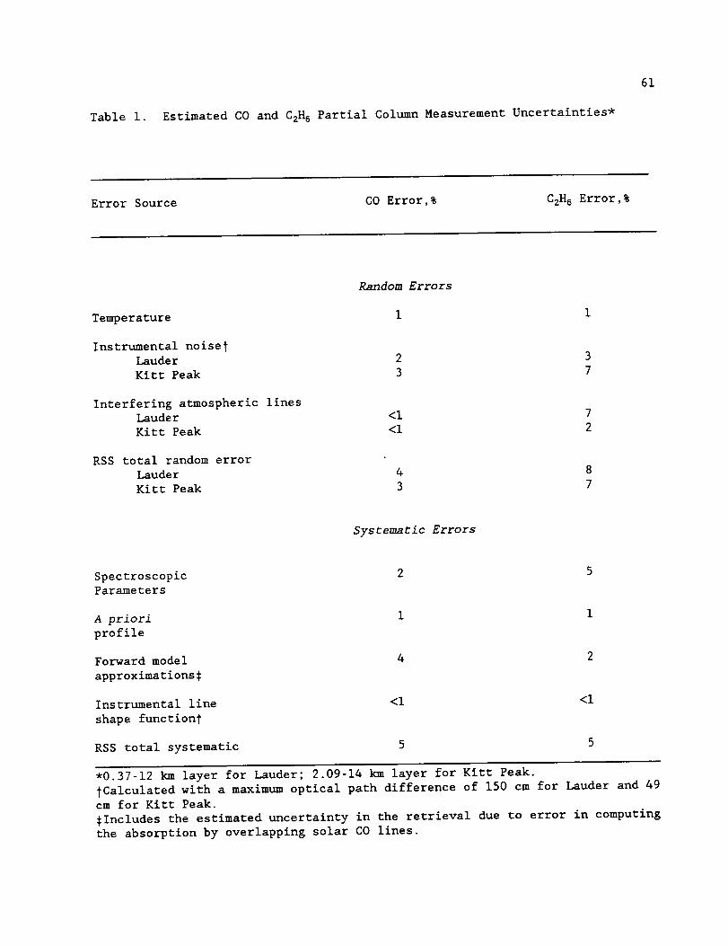
Table i. Estimated COand C2H5 Partial Column Measurement Uncertainties*

61

Error Source CO Error,% C2H 6 Error,%

Temperature

Random Errors

i

Instrumental noise%Lauder 2 3

Kitt Peak 3 7

Interfering atmospheric linesLauder

Kitt Peak

<I 7

<I 2

RSS total random error

Lauder 4 8

Kitt Peak 3 7

Systematic Errors

Spectroscopic 2 5

Parameters

A priori i i

profile

Forward model 4 2

approximations$

Instrumental line <I <i

shape function#

RSS total systematic 5 5

-0.37-12 km layer for Lauder; 2.09-14 km layer for Kitt Peak.

#Calculated with a maximum optical path difference of 150 cm for Lauder and 49

cm for Kitt Peak.

$1ncludes the estimated uncertainty in the retrieval due to error in computing

the absorption by overlapping solar CO lines.

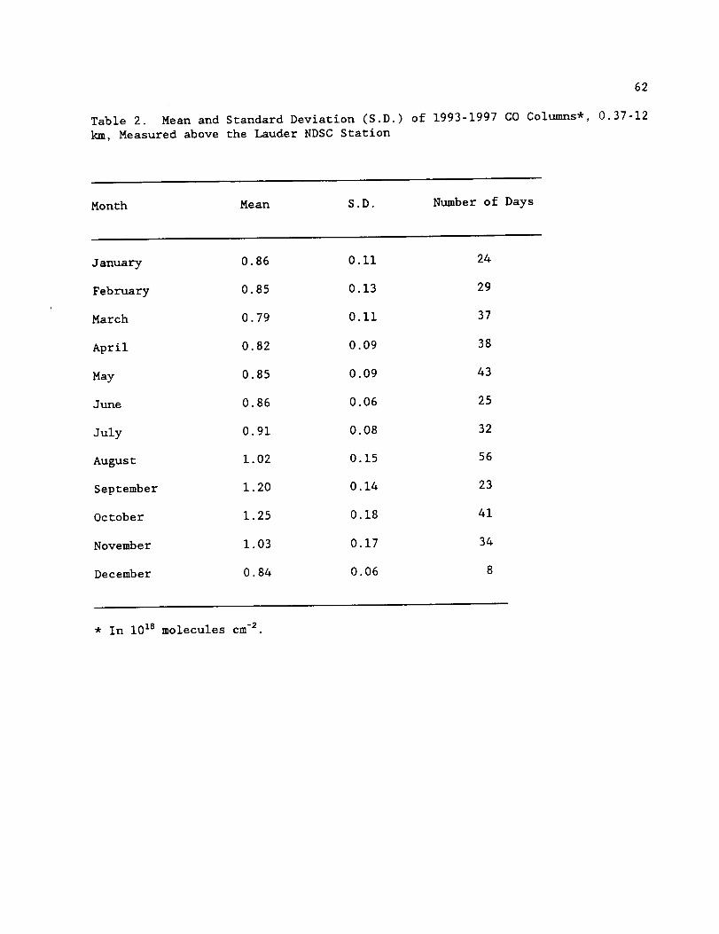
62

Table 2. Meanand Standard Deviation (S.D.) of 1993-1997 COColumns*, 0.37-12km, Measuredabove the Lauder NDSCStation

Month Mean S.D. Numberof Days

January

February

March

April

May

June

July

August

September

October

November

December

0.86

0 85

0 79

0 82

0.85

0.86

0.91

1.02

1 2O

1.25

1.03

0.84

0.Ii 24

0.13 29

0.ii 37

0.09 38

0.09 43

0.06 25

0.08 32

0.15 56

0.14 23

0.18 41

0.17 34

0.06 8

* In 1018 molecules cm-2.

63

Table 3. Mean and Standard Deviation (S.D.) of 1993-1997 C2H 6 Columns*, 0.37-

12 km, Measured above the Lauder NDSC Station

Month Mean S.D. Number of Days

January 3.78 0.68 19

February 4.12 0.79 21

March 3.70 0.71 33

April 4.12 0.69 36

May 4.51 0.64 43

June 5.05 0.58 37

July 5.59 0.76 41

August 6.30 1.26 63

September 7.64 1.35 30

October 7.49 1.37 45

November 5.56 1.23 29

December 4.19 0.59 13

* In 1015 molecules cm -2.

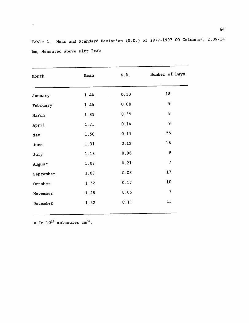
Table 4. Meanand Standard Deviation

km, Measured above Kitt Peak

(S.D.) of 1977-1997 COColumns*,

64

2.09-14

Month Mean S.D. Numberof Days

January 1.44 0.I0 18

February 1.44 0.08 9

March 1.85 0.35 8

April 1.71 0.14 9

May 1.50 0.15 25

June 1.31 0.12 16

July 1.18 0.08 9

August 1.07 0.21 7

September 1.07 0.08 17

October 1.32 0.17 i0

November 1.28 0.05 7

December 1.32 0.II 15

* In 1018molecules cm-2.

65

Table 5. Meanand Standard Deviation (S.D.) of 1977-1997 C2H 6 Columns*, 2.09-

14 km, Measured above Kitt Peak

Month Mean S.D. Number of Days

January 14.26 1.51 13

February 16.22 1.71 8

March 14.61 7.19 4

April 15.44 1.28 3

May 14.42 2.52 18

June 10.25 2.10 7

July 9.84 3.63 7

August 6.43 0.00 i

September 7.23 2.49 7

October 9.94 2.19 7

November 13.69 3.44 5

December 13.19 1.45 15

* In 1015 molecules cm -2.

66

Table 7. Correlation Coefficients and C2H6/C0Slopes derived from fits to daily

average Lauder and Kitt Peakpartial column measurementsand corresponding values

obtained with the Harvard model*

Station Months IRI b (I0 -3)

Measured Measured Model

Lauder Feb.-Mar.-Apr. 0.400 3.38 3.18

Lauder May-Jun.-Jul. 0.594 5.52 3.31

Lauder Aug.-Sep.-Oct. 0.827 6.39 4.44

Lauder Nov.-Dec.-Jan. 0.822 6.96 5.04

Kitt Peak All 0.766 14.2 13.2

*0.37-12 km column for Lauder, 1993-1997. 2.09-14kmcolumn for Kitt Peak, 1977-

1997.

Mailing Addresses

67

Ph. Demoulin, E. Mahieu, and R° Zander, Institute of Astrophysics and Geophysics,

University of Liege, 4000 Li_ge-Cointe, Belgium (email: zander@astro.ulg.ac.be)

A. Goldman, F. J. Murcray, and T. M. Stephen, Department of Physics, University

of Denver, Denver, CO 80208 (email: goldman@acd.ucar.edu;

fmucray@acd.ucar.edu; tstephen@du.edu)

Nicholas B. Jones and Brian J. Connor, NIWA Climate, Private Bag 50061, Omakau,

Lauder 9182, New Zealand (e-mail: jones@kea.lauder.cri.nz;

connor@kea.lauder.cri.nz)

J. A. Logan, Department of Earth and Planetary Sciences, Harvard University, 29

Oxford Street, Cambridge, MA 02138 (e-mail: jal@io.harvard.edu)

A. S. Pine, Alpine Technologies, 14401 Poplar Hill Road, Germantown, MD 20874

(alanpine@erols.com)

N. S. Pougatchev, Christopher Newport University, Newport News, VA 23606 (email:

nikita@riscbox.larc.nasa.gov)

C. P. Rinsland, Atmospheric Sciences Division, NASA Langley Research Center,

Mail Stop 401A, Hampton, VA 23681-2199 (e-mail: rinsland@riscbox.larc.nasa.gov)

68

Figure 1

2.0xlO 18 I l , , l j

.=q

I

.Q

oc.J

0¢.b

E--

1.5xi018

1.0×1018

5.0xlO 17

5.0xlO 17

0

0

0

I I I I I i

l.OxlO 18 l.SxlO 18

Retrieved CO Column (2.09-14 kin)

0

0

I I I

)

!

2.0xIO 18

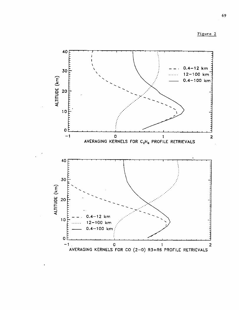
69

Fisure 2

4O

3O

E.x

,_ 20

.J

I0

0

-I

rI ...... " ' I .........

a

I

I

_\ --. 0.4--12 km !

\,,, _ ." ...... 12-100 km !

\_.. _...'" --_ 0.4-I00 krri

_. o"

* -_ o°- *% .

.-'" _ "

' ' i I i i i i , i i i i I . , . • i I

0 1 2

AVERAGING KERNELS FOR CzH s PROFILE RETRIEVALS

.¢0

3O

Ev

i,ic_ 20

k--

10

.%*%

-- -- . 0.4--12 km

...... 12-100 km

0.4--100 km

.... i i i i .

-1 0

I ......... ! " '

, J , . , , o I

1

AVERAGING KERNELS FOR CO (2-0) R3+R6 PROFILE RETRIEVALS

2

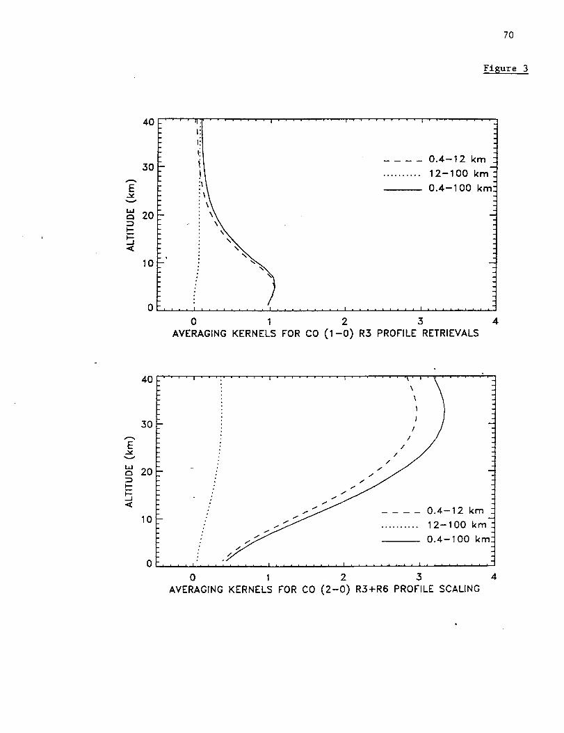
70

Figure 3

4O

3O

Ev

w,-', 20:3I--.-

I--._1.l{

10

0

'''''li ......... ' ......... , ......... , ........

I:_

li

, , , , I , , , ' .... I l I I I I I I I I I I I I I ' ' ' ' ' " I • , , , , , , , =

0 1 2 3

AVERAGING KERNELS FOR CO (1-0) R3 PROFILE RETRIEVALS

0.4-12 km

12-100 km :

0.4-100 kmi

4

4O

3O

EV

ILl,'-, 20:3I--I.-._1.,,:=:

10

0

• " ' ' I ' ' '_" ' .... I ...... ' ' ' I ..... ' ' "_ ' I ' _' ..... '

- ,' / .

; / /.

" /1

/ i I 0.4-12 km.

" ..._.._"/ .......... 12-1 O0 km:: .. _ 0.4-100 km

i ..... I , I I I I I I I i I I ........ I , n l l i l i l l I l ........

0 1 2 3 4

AVERAGING KERNELS FOR CO (2-0) R3+R6 PROFILE SCALING

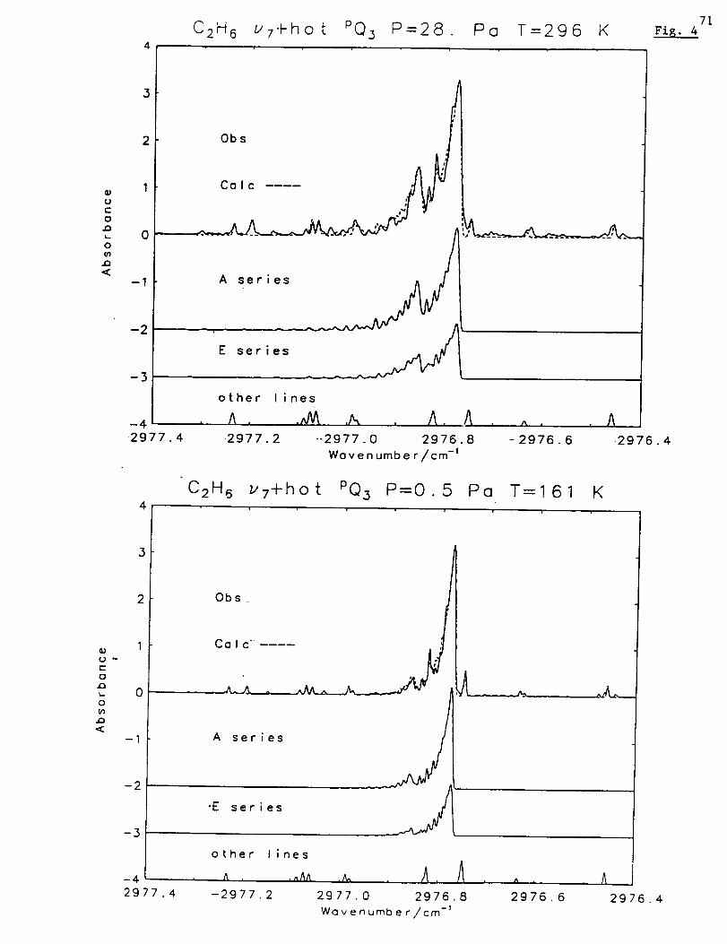
71C2H 6 u'7-kho t PQ5 P=28. Pa T=296 K m±_. 4

_D

U

0

..a

<

3

2

0

-1

-2

-3

Ob s :'

Calc

t e_

other Iines

, ^ , .,_ ._, , A.-2977.2

A , ^ , , A--2977.0 2976.8 -2976.6 .2976.4

Wovenumbe r/cm -1

C2H 6 _'7+ho t PQ3 P=O. 5 Pa T=I 6 1 K

3

U

0

33

; o(¢1

<

-1

-2

-3

-42977.4

Obs _

Colc-----

A series

-E series

other lines

^ ^_ ,_. A A-2977. 2 29 77.0 2976.8

-IWqvenumber/cm

^ , , A

2976.6 2976.4

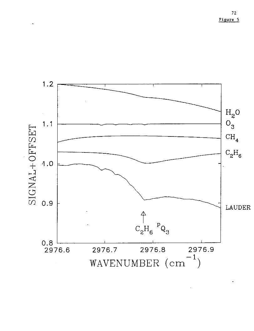
72

Figure 5

0+,._.q<Z

1.2 -------- I i I

-1.0

0.9

/

0.82976.6

f

fC2H6 PQ3

I I I

2976.7 2976.8 2976.9--1

WAVENUMBER (cm )

H20

0 3

CH 4

C2H 6

LAUDER

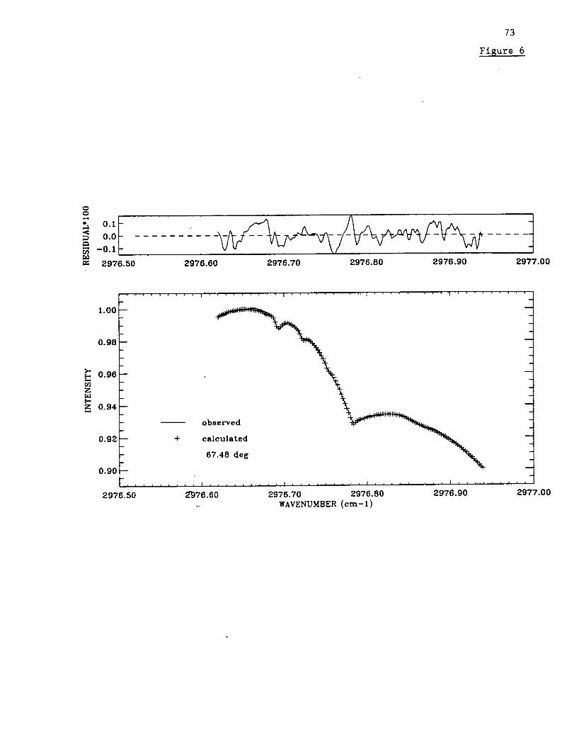
73

Fisure 6

OO

i 0.I0.0

-0.1

2976.50 2976.60 2976.70 2976.80 2976.90 2977.00

1.00

0.98

0.96

z

z 0.94

0.92

0.90

2976.60

r ......... I ' ' ' ' ..... i ....... '" i ......... i ' ' ' ' " ' ' ' '

ob

+ calculated '"_ -

\67.48 deg

i i i i i i • • • 1 .... , . , , , I J , ..... , . J , i , ...... I . , . , , . . • •

2"976.60 2976.70 2976.80 2976.90 2977.00

. WAVENUMBER (cm- 1)

1.2

E_

0 1.0

+

.,¢Z;t3,..4 0.8

0.6

I I I I

"T"co (2-o)R(s)

I I ! I

4274.65 4274.70 4274.75 4274.80

WAVENUI_BER (cm -I)

HzO

HD0

CH 4

74

Fisure 7

SOLAR C0C0

LAUDER

1.2

E_

_n 1.0

O

+

0.8

0.6

0.4

I I i I

j IHO

H_)OSOLAR C0

COf

CH 4

LAUDER

I I I I

4-284.8 4.284.9 ,t.285.0 4285.1

WAVENUMBER (cm-*)

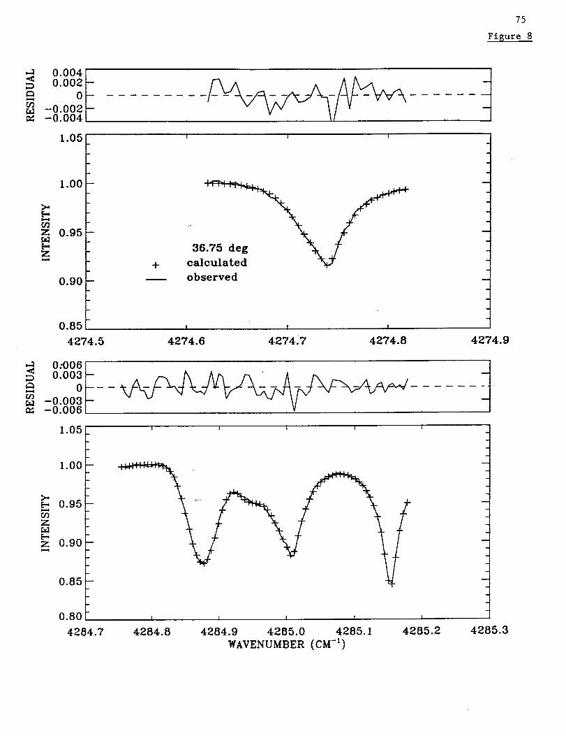
75

Figure 8

_:_ 0.004

0.002 -

oo']r_ -0.002

-0.004

1.05

1.00

>.

oQz 0.95

[-,z

0.90

0.85

4274.5

! | I

+ calculated

observed

I I I

4274.6 4274.7 4274.8 4274.9

1.05

1.00

>.,

E-_z_-0.95 iz 0.9O-

0.85

0.80

4284.7

I l | l i

r

I l I I I

4284.8 4284.9 4205.0 4285.1 4285.2 4285.3

WAVENUMBER (CM-')

76

Figure 9

120

100

8O

© 60

4O

2O

0

0.0

i ! i l [ i

0

0

O,000

0 0

o oo°co o

o ° o

° o_^ ° Oo

oO_O_ o

] I I I I I iO IO

0.5

Kitt Peaki i [ i i

0

0

0

00 o

0

0O0

I I O1_OO I

1.0

CZH6.rms(Z)

O

O oI I

' I

OO

O

t

1.5

OI

ooI I

OI

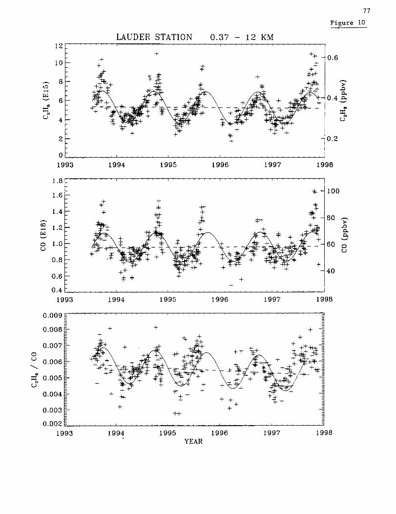
77

Figure i0

12

10

_- 8uo

Ld

v 6

£N

4

2

0

1993

LAUDER STATION 0.37 - 12 KM

+ %+

+ _ +++

+_ _*_ + _++

++. + + +

_ --,- __ . --

+ + _ 7%+ -0.2

1994 1995 1996 1997 1998

0.6

;>

0.4 _.

t_

1.8

1.6

1.4

er_.. 1.2

v

o 1.0

0.8 -

0.6 -

0.4 ....

1993

1+¢ • _ t-

_ , +

+ * + ֥ * ,+___ + _7-

+q_++ ÷ +

+

+

1994 1995 1996 1997 1998

100

80 ---

v

60 o¢.9

40

0.009

0.008

0.007

o0.006

.. 0.005q)

0.0O4

0.003

0.002

1993

J _ t i i

+ + + -

_+ -#" + +

+ . ÷+ _ + _+ + ++_-+_ _ +++_ + _i-. ,_-_++_

± ++ _#- , + . +., -,-

+ _-++

, I ......... I ......... i ......... _ .........

1994 1995 1996 1997 1998

YEAR

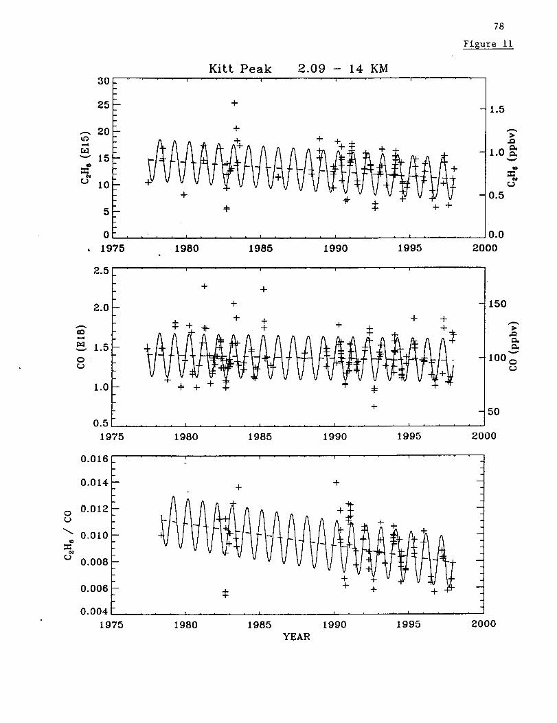
0

3O

25

.-. 2O

w_

_" 15

10

5

0 ,

, 1975

2.5

2.0

co

1.5

O

1.0

0.5 ,

1975

0.016

0.014 -

0.012

0.010

0.008

0.006

0.004 ,

1975

KiLt Peak 2.09 - 14 KMi i 1 D

+

+

v+vv vwvvv, _ ++

i h I m m . . ! m • i i l i . , i | i , ,

1980 1985 1990 1995

+ +

+

:_ + + + ÷+ 4t- + + ± +

+ +

+

, , I , , , , I , , * * I * , , , I i , ,

1980 1985 1990 1995

, i i i

78

Figure 11

- 1.5

>

- 1.0o.

- 0.5

, 0.0

2000

- 150

>

- 100 o

- 50

2000

++

+!

++

, ! * , * , I , , ° , I

1980 1985 1990

YEAR

+.

, i * i I

1995 2000

79

Figure 12

I0

8

6

4

2

020

15

10

5

C2H 6 Column (1 x 1017 moeclues cm "2)

0

JAN

L

_.°

Lauder(45 S, 169 E)

Kitt Peak -(32 N, 112 W)

APR JUL OCT

20

15

CO Column (1 x 1015 moeclues cm "2)

10

5

020

15

10

5

0

JAN

Lauder

(45 S, 169 E)

Kitt Peak

(32 N, 112 W)

APR JUL OCT

•_ _.i_ ¸ -.

_J

JOURNAL OF GEOPHYSICAL RESEARCH, VOL. 103, NO. D4, PAGES 3825-3846, FEBRUARY 27, i998

Measurements of the downward longwave radiation spectrum

over the Antarctic Plateau and comparisons with a line-by-line

radiative transfer model for clear skies

Von P. Walden

Space Science and Engineering Center, University of Wisconsin, Madison

Stephen G. Warren

Department of Atmospheric Sciences, University of Washington, Seattle

Frank J. Murcray

Department of Physics, University of Denver, Denver, Colorado

Abstract. A l-year field program was conducted at South Pole Station in 1992 to measure the

downward infrared radiance spectrum at a resolution of 1 cm "1 over the spectral range 550-1667

cm "l . The atmosphere over the Antarcuc PlarooUcSt_h: ' 300twinter,surface temperatures average aoour -or ,

p.m ofprecipitable water, and the clear-sky downward longwave flux is usually less than 80 W m "2.

Three clear-sky test cases are selected, one each for summer, winter, and spring, for which high-

quality radiance data are available as well as ancillary data to construct model atmospheres from

radiosondes, ozonesondes, and other measurements..The model atmospheres are used in

conjunction with the line-by-line radiative transfer model (LBLRTM) to compare model

• " with the s ectral radiance measurements. The high-resolution calculations ofcalculatmns P . -I • •LBLRTM (=0.001 cm "I) are matched to the lower-resolutmn measurements (1 cm ) by adjusting

their spectral resolution and by applying a correction for the finite field of view of theintefferometer. In summer the Uncertainties in temperature and water vapor profiles dominate the

radiance error in the LBLRTM calculations. In winter the uncertainty in viewing zenith angle

becomes important as well as the choice of atmospheric levels in the strong near-surface

temperature inversion. The spectral radiance calculated for each of the three test cases generally

agrees with that measured, to within twice the total estimated radiance error, thus validating

, " evel of accuracy for Antarctic conditions. However, the discrepancy exceedsBLRTM to th_s I .... -1Lt_Eice the estimated error in the gaps between spectral hnes m the regmn 1250-1500 cm , where

emission is dominated by the foreign-broadened water vapor continuum.

1. Introduction

The Antarctic Plateau covers large areas of East Antarctica

(above 2000 m) and West Antarctica (above 1500 m). In its long-

wave radiation budget this region differs from the katabatic wind

region [Yamanouchi and Kawaguchi, 1984, 1985] and the mari-

time Antarctic [Lubin, 1994]. For most of the year a near-surface

temperature inversion is present over the plateau, whose strength

increases with surface elevation as the atmosphere becomes thin-

ner and less absorptive to infrared radiation. Large radiation

losses to space occur throughout most of the year, with frontal

activity and the associated cloudiness temporarily reducing the

loss at the surface [e.g., Stone et al., 1989; Stone andKahl, 1991].

Continuous records of meteorological data from the East Ant-

arctic Plateau exist for three stations: 40 years at South Pole

(90%), 40 years at Vostok (78"S, 107*E), and 3 years at Plateau

(790S, 40°E). Since there is little regional variation in climate

Copyright 1998 by the American Geophysical Union.

Paper number 97JD02433.0145.0227/9g/97JD-02433509.00

across the plateau, data from one location can represent a large

geographical area. Thus, in the absence of data at other locations,

atmospheric conditions at South Pole Station may serve to repre-

sent the conditions over most of East Antarctica. Recent attempts

to model the climate of the Antarctic have met with some success

in comparing model output with existing observational data sets

[T:eng et al., 1993, 1994; Genthon, 1994]. For the purpose of this

paper the most important characteristic of the atmosphere over theAntarctic interior is that it is the coldest and driest on Earth and

thus represents an endpoint of terrestrial climate.

In the 1980s a project on Intercomparison of Radiation Codes

used in Climate Models (ICRCCM) was established to compare

radiative transfer models, ranging from detailed line-by-line codes

to highly parameterized band models [Luther et al., 1988; Elling-

son and Fouquart, 1991]. The results of clear-sky calculations for

shortwave models were summarized by Fouquart et al. [1991] and

those for Iongwave models by Ellingson et al. [1991]. The atmo-

spheres used in those comparisons were the five reference atmo-

spheres of the Air Force Geophysics Laboratory (AFGL)

[McClatchey et al., 1972] as well as isothermal atmospheres con-

taining only CO 2 or H20 as gaseous absorbers. One of the main

3825

3826 WALDENETAL: ANTARCTIC LONGWAVE RADIATION SPECTRUM

conclusions of the Iongwave study was that line-by-line radiative

transfer models, although they agree well with each other, do not

represent an absolute standard by which to judge less detailed

models. Their output must therefore be compared with data from

the real atmosphere. Spectral rather than broadband, and radiance

rather than flux measurements, would be most useful because the

causes of discrepancies between model and observation can be

more easily identified if angular and spectral averaging has not

been done. Specifically, the study concluded that spectral radi-

ance data of moderate resolution (about ! cm "1) would be particu-

larly valuable for comparison with a variety of radiation codes at

various spectral resolutions.

To resolve the differences among the most detailed radiation

models, the ICRCCM participants recommended that accurate

spectral radiance measurements be made coincidentally with the

atmospheric variables necessary to calculate radiance [Ellingson

et al., 1991]. Currently, data sets of this type exist for the follow-

ing locations: (1) Coffeyville, Kansas, where the Spectral Radi-

ance Experiment (SPECTRE) was performed [Ellingson and

Wiscombe, 1996], (2) the Southern Great Plains site of the Atmo-

spheric Radiation Measurement (ARM) program [Stokes and

Schwartz, 1994; Ellingson et al., 1995], (3) the California coast

[Clough et al., 1989a], and (4) the tropical Pacific Ocean [Lubin et

al., 1995]. ARM is now establishing a site on the North Slope of

Alaska.

The Antarctic Plateau is an ideal location for acquiring spectral

radiance data for testing radiative transfer models. Since the

atmosphere is so cold and dry (_<1 mm of precipitable water), the

overlap of the emission spectrum of water vapor with that of other

gases is greatly reduced. Therefore the spectral signatures of other

important infrared emitters, namely, CO2, O 3, CH4, and N20, are

quite distinct. In addition, the low atmospheric temperatures pro-

vide an extreme test case for testing models. Even in summer the

atmosphere is colder and drier than the sub-Arctic winter, the

coldest of the five AFGL model atmospheres. The radiation con-ditions at the surface of the Antarctic Plateau in winter are similar

to those at the tropopause at lower latitudes. Routine operations at

South Pole Station provide good ancillary data for characterizing

the atmosphere throughout the year. The South Pole Weather

Office (SPWO) launches radiosondes once or twice per day and

makes surface weather observations at least every 6 hours. The

Climate Monitoring and Diagnostics Laboratory (CMDL) of the

National Oceanic and Atmospheric Administration (NOAA) pro-

vides continuous near-surface concentrations of several radia-

tively active trace gases, as well as ozonesonde profiles once or

twice per week.

Many previous Antarctic field programs have reported mea-

surements of broadband radiation fluxes [Hanson, 1960; Hanson

and Rubin, 1962; Rusin, 1964; Kopanev, 1967; Kuhn et al., 1977;

Yamanouchi et al., 1982; Carroll, 1982; Yamanouchi and

Kawaguchi, 1984]. Such broadband measurements, however, are

not useful for identifying defects in radiative transfer models.

Here our focus is instead on how the radiance varies across the

infrared spectrum. In this paper we describe a data set taken at

South Pole Station throughout the year of 1992, consisting of

spectral infrared radiances together with observations from radio=

sondes and other instruments to characterize the atmosphere. Par-

ticular attention is given to the calibration and uncertainty

associated with the radiation measurements. The calibration pro-

cedure described here i_ an improvement over that of Van Allen et

al. [1996], which used the same instrument at South Pole Station.

Their experiment was designed to study stratospheric chemistry,

which did not require the level of accuracy needed here for

SPECTRE-D'pe comparisons.The uncertainties associated with characterizing the atmo-

sphere are also estimated, particularly with regard to temperature

and humidity variations in the near-surface layer. Three test cases

are constructed, using the highest-quality measurements from the

data set, representing the meteorological and infrared radiation

conditions in summer, winter, and spring under clear sky. These

test cases are used to compare the spectral infrared radiances with

calculations of the line-by-line radiative transfer model

(LBLRTM) [Clough et al., 1992]. A brief description of

LBLRTM is given below as it is applied to this work, including

how the model calculations were adjusted for instrumental effects,

so that the model results can be compared directly with the obser-

vations. The radiance error in the LBLRTM calculations induced

by uncertainties in the ancillary data is estimated; the majorsources of error are identified for summer and winter conditions.

The comparisons for our six test cases (two viewing angles on

each of 3 days) are shown, and portions of the spectrum are exam-

ined in detail.

2. Field Program

Spectral radiance was measured by a Fourier transform inter-

ferometer (FTIR), manufactured by Bomem, Inc., and modified at

the University of Denver (UD) for outdoor operation at South

Pole. It had been successfully operated through a previous winter

at South Pole for the purpose of determining concentrations of

atmospheric gases important to ozone chemistry [Murcray and

Heuberger, 1990, 1991, 1992]. The radiance spectrum was mea-

sured at viewing zenith angles of 45* and 75*, and also often at

60 °, every 12 hours throughout the year except during blizzard

conditions.

The state of the atmosphere is characterized by using various

sources of data. Visual sky observations were made by Warren

during each FTIR measurement, as well as routinely every 6 hours

by the SPWO observers. Vertical profiles of temperature, water

vapor, and ozone are constructed by using a combination of radio-

sonde data from SPWO and CMDL, plus satellite data from the

Upper Atmosphere Research Satellite (UARS) [Reber et al.,

1993]. Tropospheric concentrations of carbon dioxide, methane,

nitrous oxide, and chlorofluorocarbons were obtained from in situ

measurements made at the surface by CMDL, and stratospheric

concentrations were obtained from UARS.

3. Selection of Test Cases

Three days were selected for comparison of spectral radiance

measurements to radiative transfer models: January 17, 1992, May

1, 1992, and October 5, 1992. For each day the calibrated radi-

ances at viewing zenith angles of 45" and 75* are determined. The

three primary criteria for selection were clear skies with minimal

visually observed atmospheric ice crystals, well-calibrated spec-

tral radiance measurements, and time of year. The summer and

winter cases were chosen to span the full range of atmospheric

conditions over South Pole; the springtime case represents an

atmosphere with a depleted ozone profile. Secondary selection cri-

teria include availability of high-quality radiosonde and ozone-sonde information and minimal time between the radiosonde

launch and the spectral radiance measurements (Table 1). The

seasons at South Pole are defined by the annual cycle of surface

temperature [Schwerdtfeger, 1970; Warren, 1996]: summer

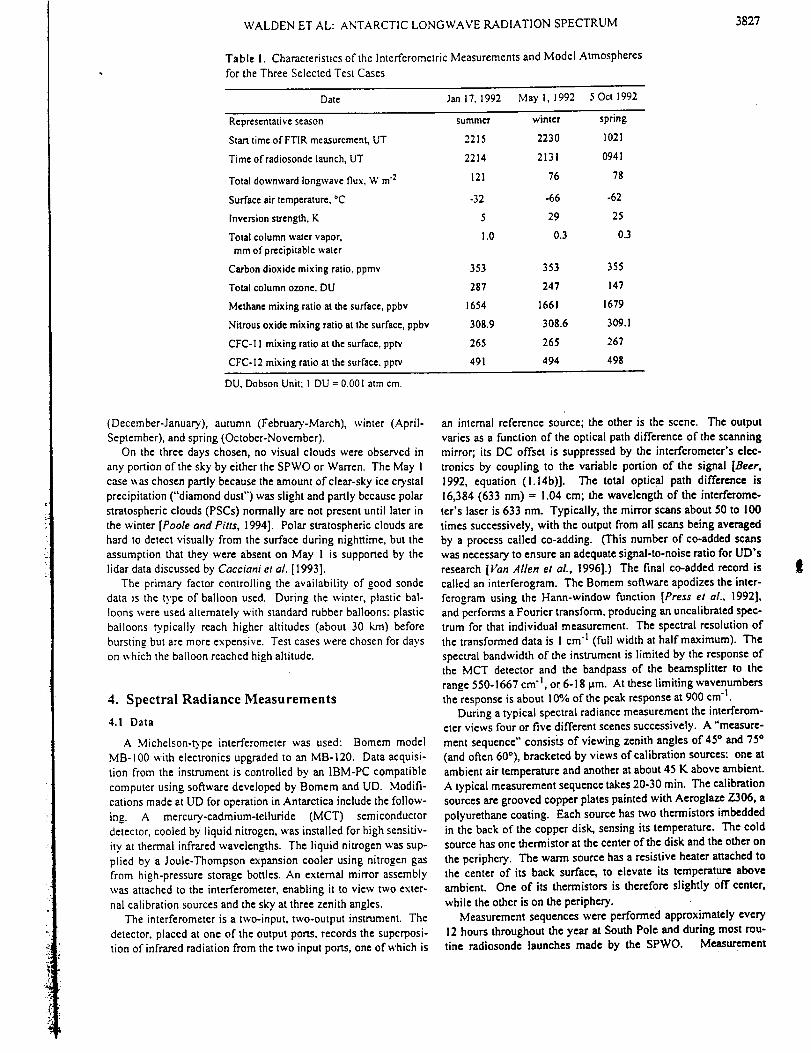
WALDENETAL:ANTARCTICLONGWAVERADIATIONSPECTRUM 3827

TableI. Characteristicsof the Intefferometric Measurements and Model Atmospheres

for the Three Selected Test Cases

Date Jan 17, 1992 May I, 1992 5 Oct 1992

Representativeseason summer winter spring

Start time of FTIR measurement, UT 2215 2230 1021

Time of radiosonde launch, UT 2214 2131 0941

Total downward Iongwave flux. W m":z 121 76 78

Surface air temperature, *C -32 -66 -62

Inversion strength, K 5 29 25

Total column water vapor, 1.0 0.3 0.3

mm of precipitable water

Carbon dioxide mixing ratio, ppmv 353 353 355

Total column ozone, DU 287 247 147

Methane mixing ratio at the surface, ppbv 1654 1661 1679

Nitrous oxide mixing ratio at the surface, ppbv 308.9 308.6 309A

CFC-I I mixing ratio at the surface, pptv 265 265 267

CFC-12 mixing ratio at the surface, pptv 491 494 498

DU, Dobson Unit; 1 DU= 0.001 atm cm.

(December-January), autumn (February-March), winter (April-

September), and spring (October-November).

On the three days chosen, no visual clouds were observed in

any portion of the sky by either the SPWO or Warren. The May I

case was chosen partly because the amount of clear-sky ice crystal

precipitation ("diamond dust") was slight and partly because polar

stratospheric clouds (PSCs) normally are not present until later in

the winter [Poole and Pitts, 1994]. Polar stratospheric clouds are

hard to detect visually from the surface during nighttime, but the

assumption that they were absent on May ! is supported by the

lidar data discussed by Cacciani et al. [1993].

The primary factor controlling the availability of good sonde

data is the type of balloon used. During the winter, plastic bal-

loons were used alternately with standard rubber balloons; plastic

balloons typically reach higher altitudes (about 30 km) before

bursting but are more expensive. Test cases were chosen for days

on which the balloon reached high altitude.

4. Spectral Radiance Measurements

4.1 Data

A Michelson-b'pe interferometer was used: Bomem model

MB-100 with electronics upgraded to an MB-120. Data acquisi-

tion from the instrument is controlled by an IBM-PC compatible

computer using software developed by Bomem and UD. Modifi-

cations made at UD for operation in Antarctica include the follow-

ing. A mercury-cadmium-telluride (MCT) semiconductor

detector, cooled by liquid nitrogen, was installed for high sensitiv-

ity at thermal infrared wavelengths. The liquid nitrogen was sup-

plied by a Joule-Thompson expansion cooler using nitrogen gas

from high-pressure storage bottles. An external mirror assembly

was attached to the interferometer, enabling it to view two exter-

nal calibration sources and the sky at three zenith angles.

The interferometer is a two-input, two-output instrument. The

detector, placed at one of the output ports, records the superposi-

tion of infrared radiation from the two input ports, one of which is

an internal reference source; the other is the scene. The output

varies as a function of the optical path difference of the scanning

mirror; its DC offset is suppressed by the interferometer's elec-

tronics by coupling to the variable portion of the signal [Beer,

1992, equation (I.14b)]. The total optical path difference is

16,384 (633 nm) == 1.04 cm; the wavelength of the interferome-

ter's laser is 633 nm. Typically, the mirror scans about 50 to 100

times successively, with the output from all scans being averaged

by a process called co-adding. (This number of co-added scans

was necessary to ensure an adequate signal-to-noise ratio for UD's

research [Van Allen et aL, 1996].) The final co-added record is

called an interferogram. The Bomem software apodizes the inter-

ferogram using the Hann-window function [Press et al., 1992],

and performs a Fourier transform, producing an uncalibrated spec-trum for that individual measurement. The spectral resolution of

the transformed data is 1 cm "1 (full width at half maximum). The

spectral bandwidth of the instrument is limited by the response of

the MCT detector and the bandpass of the beamsplitter to the

range 550-1667 cm "1, or 6-18 pm. At these limiting wavenumbers

the response is about 10% of the peak response at 900 cm "l.

During a typical spectral radiance measurement the intefferom-

eter views four or five different scenes successively. A "measure-

ment sequence" consisis of viewing zenith angles of 45* and 75*

(and often 60°), bracketed by views of calibration sources: one at

ambient air temperature and another at about 45 K above ambient.

A typical measurement sequence takes 20-30 rain. The calibration

sources are grooved copper plates painted with Aeroglaz¢ Z306, a

polyurethane coating. Each source has two thermistors imbedded

in the back of the copper disk, sensing its temperature. The cold

source has one thermistor at the center of the disk and the other on

the periphery. The warm source has a resistive heater attached to

the center of its back surface, to elevate its temperature above

ambient. One of its thermistors is therefore slightly off center,

while the other is on the periphery.

Measurement sequences were performed approximately every

12 hours throughout the year at South Pole and during most rou-

tine radiosonde launches made by the SPWO. Measurement

t

3828 WALDEN ET AL: ANTARCTIC LONGWAVE RADIATION SPECTRUM

sequences were taken more frequently when the sky was clear,

and special observations were made during some ozonesonde and

water vapor sonde launches. "Housekeeping" information was

recorded routinely during each sequence, consisting primarily of

temperature measurements of various parts of the interferometer.

These measurements were used to select test cases with good ther-

mal stability, in which the instrument temperature drifted by less

than 0. l K during the measurement sequence [Walden, 1995].

The interferometer was mounted atop the Skylab building at an

elevation of approximately I0 m above the upwind snow surface.

The instrument was housed in about 10 cm of styrofoam insula-

tion, while the external mirror assembly was exposed to the ambi-

ent temperature. Thus the internal temperature of the

interferometer varied only slowly as the ambient temperature

changed.

4.2 Calibration

The method of Revercomb et al. [1988] is used to calibrate

measurements of the sky. An uncalibrated spectrum, C', can be

written as a linear function of the measured radiance, L, as

C' = r[L+ L°ei#O]e i+, (1)

where r is the instrument response function of the interferometer,

L ° represents the spectral offset radiance from the instrument

itself, d_ is the phase response of the instrument due to optical and

electrical dispersion, and _o is any anomalous phase incorporated

into the offset radiance [Revercomb et aL, 1988]. All the variables

are functions of frequency. Subscripts w, c, and s are applied to C'

and L, referring to warm, cold, and sky (or scene). The uncali-

brated spectra for the warm and cold calibration sources, C w' and

Cc', are used to calibrate the measurements of the sky, Cs', by tak-

ing the real pan of the ratio of difference spectra and solving for

the scene radiance, L s, giving

where

Ls = y[L w-Lc]+L c, (2)

FCs'-Cc'q

Lw and L¢ are the radiances emitted and reflected from the calibra-tion sources:

Lj = cjB!Tj) +(1-ej)B(Tambicnt), (4)

where j is either w or c. B(T) represents the Planck radiance at a

particular frequency for a given temperature T, Tj is the tempera-

ture of the emitting surface of the source, cj is the spectral emissiv-ity of the source, and Tambien t is the temperature of the ambient

outside air.

There are implicit assumptions in equation (1). First, the out-

put from the interferometer's detector is assumed to be linearly

related to the input radiance into the interferometer. The possibil-

ity of nonlinearities in the detector is not considered in this study,

since any resulting bias is probably small compared with the over-

all radiance uncertainty discussed below.

In addition, the assumption of thermal stability means that the

offset radiance L°e i+° is constant within a measurement sequence,

so that it can be eliminated by the taking the difference of mea-

surements C, which results in the numerator and denominator of

equation (3). The maximum acceptable level of thermal drift of

the interferometer during measurement sequences to be used for

test cases was chosen such that any radiance errors resulting from

thermal drift are negligible compared with those from other error

sources. However, a procedure for adjusting measurement

sequences with lar3e thermal drift has been developed by Walden

[1995].

The radiances from the calibration sources, Lv, and Lc, must be

known accurately, independent of the measurements, for proper

calibration of atmospheric radiances. Thus the accuracy of the

final calibrated radiances depends on accurate specification of the

source temperature and emissivity. The uncenainties in these

temperatures and emissivities must also be assessed to estimate

the uncertainty in calibrated radiances. The source temperatures

and emissivities described below differ from those used by Van

Allen et al. [1996].

4.2.1 Temperature of the calibration sources. The tempera-

ture of each calibration source is measured by two thermistors that

were calibrated to a temperature reference of the National Institute

of Standards and Technology (NIST) by the manufacturer (Yellow

Springs Instruments, Inc., Yellow Springs, Ohio). The electronics

used to measure the source temperatures were checked by substi-

tuting four different high-precision resistors in place of each ther-

mistor. The resistors were chosen to represent a range of

temperatures far exceeding the range experienced at South Pole.

The voltage recorded by the electronics was convened back to a

resistance value, which was then compared with the value of the

precision resistors. Analysis of this cross-check procedure indi-cated that a small additional resistance needed to be added to the

inferred resistances to reconcile them with the actual values. In

the conversion of resistance to temperature this correction was sig-

nificant when the resistance being measured was small (less than

1000 ohms). The additional resistance ranged from 9 to 75 ohms

and varied from channel to channel within the data acquisition

system. Using the thermistor manufacturer's conversion from

resistance to temperature, we derived temperature corrections for

each thermistor. Figure I shows the corrections for the four ther-

mistors on the calibration sources over the range of temperature

values experienced by these sources at South Pole in 1992. The

corrections are significant at high temperatures, or low thermistor

resistance. The corrections are 0.6 K and 1.3 K for the cold source

thermistors at their maximum ),early temperature of-10°C, and0.3 K and 1.3 K for the warm source thermistors at +35°C.

Figure 2a shows the difference in temperature reported by the

two thermistors on the cold calibration source. Since the cold

source is at ambient outside temperature, the two thermistors

should agree. True temperature differences between the ther-

mistors would be due to random variation of environmental condi-

tions such as wind speed and direction, causing only random

scatter in the data. Figure 2a shows instead a consistent pattern of

deviation with small scatter; the deviation exceeds the manufac-

turer's tolerance limit at high temperatures. Figure 2b shows that

• after correcting for the thermistor electronics bias the cold source

temperatures agree well for the entire temperature range through-

out the year, thus validating the correction procedure. The true

cold source temperature, T c, is then estimated by averaging T4'

and T10', where the prime indicates that the correction for the elec-

tronics bias has been applied:

T 4'==T 4+ Ae4, (5}

where A_ is the temperature correction for the thermistor elec-

tronics bias of channel 4. A similar expression exists for TI0'.

A similar analysis of the warm source is not possible since tem-

perature gradients do exist within the heated plate, but the success

WALDENETAL:ANTARCTICLONGWAVERADIATIONSPECTRUM 3829

1.5

1.0

0.5o

E

0.0

I t I i I i I i I l

chart 1_1

ban 4/" /

Warm Source

Cold Source

I ' I ' I ' I ' I '-60 -40 -20 0 20

UncorrectedTemp_ature (oC)

40

Figure I. Thermistor electronics temperature bias (Ae) for theindividual thermistors in the infrared calibration sources. The

bias is shown for the range of temperatures experienced at South

Pole during 1992. The thermistors are designated by their house-

keeping channel number: channels 4 and I0 for the cold sourcethermistors and channels 5 and 11 for the warm source ther-

mistors. Channels 4, 10, and II are 300-ohm thermistors (YSI

44002); channel 5 is a 3000-ohm thermistor (YSI 44005). Allthermistors were manufactured by Yellow Springs Instruments,

Inc., Yellow Springs, Ohio.

of the electronics bias correction procedure for the cold source

argues for its validity in general. We therefore apply the electron-

ics bias correction to the warm source thermistors, Ts and T I 1.

However, for the warm source there is an additional correction

that must be applied due to thermal gradients within this source.

Figure 3a shows that there is a significant temperature differencebetween the two thermistors on the warm source, which increases

as the source temperature (e.g., T5') rises above ambient (To).

This behavior is expected because all thermal gradients in the

source should be proportional to the difference between its tem-

perature and ambient. Since the two thermistors are at different

temperatures, it was necessary to decide which sensor has better

accuracy. T( was chosen for two main reasons [Walden. 1995]: it

has better sensitivity over most of the range of temperatures expe-

rienced during 1992. and the thermistor electronics temperaturebias is much smaller for channel 5 than for channel 1 I (Figure I ).

In addilion to the radial temperature gradient between the ther-

mistors shown in Figure 3a, there is evidence of a temperature dif-

ference between T5' and the temperature of the emitting surface of

the warm source as viewed by the interferometer. Three indepen-

dent analyses described by Walden [1995, Appendix A] indicate

that the portion of the source viewed by the interferometer is aclu-

all',' warmer than Ts'. This higher temperature is due to the loca-

tion of the warm source's resistive heater in relation to its

thermistors mentioned above, assuming that the interferometer

views the center of the copper plate. The results from these analy-

ses are reproduced in Figure 3b. The temperature difference

increases as the warm source becomes increasingly warmer than

ambient.

A functional form for the thermal gradient temperature bias.

AC, was determined by performing a linear regression fit to thedata shown in Figure 3b. The fit was forced through the origin,

since no thermal gradients exist within the calibration source when

it is at ambient temperature. Our final estimate for the tempera-

ture of the viewed portion of the warm calibration source, Tw , is

then obtained by applying corrections for both the thermistor elec-

tronics (AeS) and thermal gradient biases, or

Tw-Ts'+A s = T s+AeS+A s . (6}

The larger of these two corrections is Ag. For the range of warm

source temperatures experienced during the year-long field exper-

iment, AS was in the range I-4 K, whereas Ae5 was at most 0.3 K.4.2.2 Emissivity of the calibrationsources. The spectral

emissivity of the UD calibration sources was not directly mea-

sured but was inferred from the measured emissivity of a similar

source built by Quantic Industries, Inc. (San Carlos, California)

while Walden worked there. Both the UD and Quantic sources are

grooved copper plates, coated with the same black paint, Aero-

glaze 7_.306. The emissivity of nongrooved plates (constructed

independently by Quantic and H. E. Revercomb's group at the

University of Wisconsin, but both painted with Aeroglaze) com-

pare well, indicating that perhaps the emissivity in the spectral

range 750-1300 cm "1 (the central portion of the interferometer's

bandwidth) is not highly sensitive to the paint thickness [Walden,

1995, Appendix A]. The emissivity of the Quantic grooved source

in this spectral region was the value used in deriving the thermal

gradient bias described above.

1.0

0.8

0.6

: 0.4

0.2

0.0

1.0

0.8

-o 0.6

' 0.4b."

0.2

0.0

ll. il.l,lmiil.

(a)

_co_t_ o_8

,'I'I'I'I'I'I'

llil,l,l,lil'

(b)co_ted

1

.I'I'I'I'I'I,'

-70 -60 -50 -40 -30 -20 -10 0

T4'(°C)

Temperature difference between the cold calibrationFigure 2.source thermistors (a) before and (b) after being corrected for the

thermistor electronics temperature bias. T 4 and TI0 are the uncor-

rected temperatures from two thermistors recorded in the house-

keeping Channels 4 and 10. T4' and T10' are the c6rresponding

corrected temperatures. The dashed line is the thermistor manu-facturer's interchangeability tolerance, defined as the maximum

difference that can occur when tw.o or more thermistors are used to

make the same measurement.

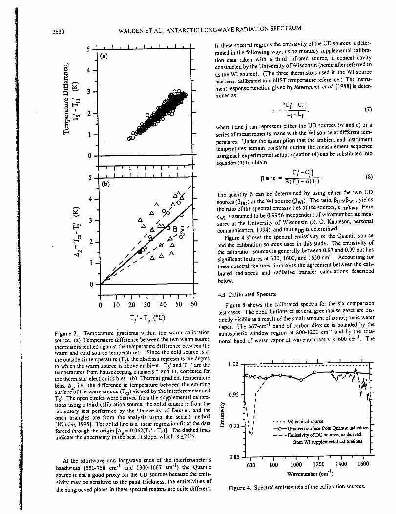
3830 WALDENETALeANTARCTICLONGWAVERADIATIONSPECTRUM

o"O

",,,,4

EO

I

II

4

3

2

0

2

, I , I l I , I , I ,

(a)

' I ' I ' I ' i ' I '

i I , I , I , I , I ,

Co) /

zx"A /

' I ' I ' I ' I ' I '

0 I0 20 30 40 50 60

T 5' - Tc (°C)

Figure 3. Temperature gradients within the warm calibration

source. (a) Temperature difference between the two warm source

thermistors plotted against the temperature difference between the

warm and cold source temperatures. Since the cold source is at

the outside air temperature (To), the abscissa represents the degreeto which the warm source is above ambient. T 5' and T 11' are the

temperatures from housekeeping channels 5 and 11, corrected forthe thermistor electronics bias. (b) Thermal gradient temperature

bias, Ag, i.e., the difference in temperature between the emittingsurface of the warm source (Tes) viewed by the interferometer and

TS'. The ol_en circles were derived from the supplemental calibra-

tions using a third calibration source, the solid square is from thelaboratory test performed by the University of Denver, and the

open triangles are from the analysis using the secant method

[Walden, 1995]. The solid line is a linear regression fit of the data

forced through the origin [Ag: 0.062(T 5' - T¢) ]. The dashed linesindicate the uncertainty in the best fit slope, which is +_.25%.

At the shortwave and longwave ends of the interferometer's

bandwidth (550-750 cm "l and 1300-1667 cm "1) the Quantic

source is not a good proxy for the UD sources because the emis-

sivity may be sensitive to the paint thickness; the emissivities of

the nongrooved plates in these spectral regions are quite different.

In these spectral regions the emissivity of the UD sources is deter-

mined in the following way, using monthly supplemental calibra-

tion data taken with a third infrared source, a conical cavity

constructed by the University of Wisconsin (hereinafter referred to

as the WI source). (The three thermistors used in the W! source

had been calibrated to a NIST temperature reference.) The instru-

ment response function given by Revercomb eta/. [1988] is deter-

mined as

IC?- c/l (7)r = _.

where i and j can represent either the UD sources (w and c) or a

series of measurements made with the wi source at different tem-

peratures. Under the assumption that the ambient and instrument

temperatures remain constant during the measurement sequence

using each experimental setup, equation (4) can be substituted into

equation (7) to obtain

IC;-C;l (8)13Ere = B(Ti )_B(Tj)

The quantity 13 can be determined by using either the two UD

sources (13UD) or the WI source (13Wl). The ratio, I_UD/13Wl, yields

the ratio of the spectral emissivities of the sources, cta_-Wl • Here

twi is assumed to be 0.9956 independent of wavenumber, as mea-

sured at the University of Wisconsin (R. O. Knuteson, personal

communication, 1994), and thus EUD is determined.

Figure 4 shows the spectral emissivity of the Quantic source

and the calibration sources used in this study. The emissivity of

the calibration sources is generally between 0.97 and 0.99 but has

significant features at 600, 1600, and 1650 cm'L Accounting for

these spectral features improves the agreement between the cali-

brated radiances and radiative transfer calculations described

below.

4.3 Calibrated Spectra

Figure 5 shows the calibrated spectra for the six comparison

test cases. The contributions of several greenhouse gases are dis-

tinctly visible as a result of the small amount of atmospheric water

vapor. The 667-cm "1 band of carbon dioxide is bounded by the

atmospheric window region at 800-1200 cm "t and by the rota-

tional band of water vapor at wavenumbers v < 600 cm "1. The

100 )... ,....I...,... L.. :...'.-.'... !.. :.- .L.

"It I .... VCIconical source0.90 -11 ! -.-O--Groov_l surface from Quantic Industries

_t - - -Emissivity of DU sources, as.deri.ved

0.85_

600 800 1000 1200 1400 1600

Wavenumber (era "t)

Figure 4. Spectral emissivities of the calibration sources.

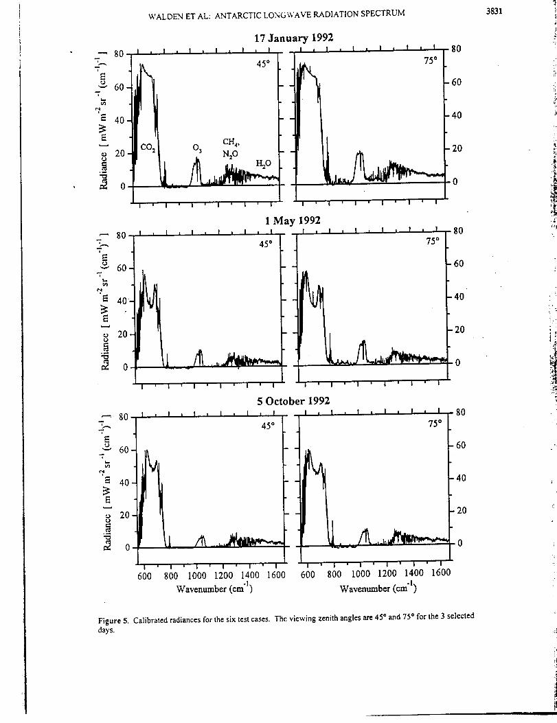
WALDEN ET AL: ANTARCTIC LONGWAVE RADIATION SPECTRUM 3831

17 January 1992

_ 0 -0

80 I , I , , , , , I , 1May1992 _o -80

6°1 I1 ,, _6o40 . ....i20 20

o t °

5 October 1992

6°1, I1 , I°°

14°1tt 111 ,4o°

600 800 1000 1200 1400 1600 600 800 1000 1200 1400 1600

Wavenumber (cm"l) Wavenumber (era'l)

Figure 5. Calibrated radiances for the six test cases. The viewing zenith angles are 45° and 75 ° for the 3 selecteddays.

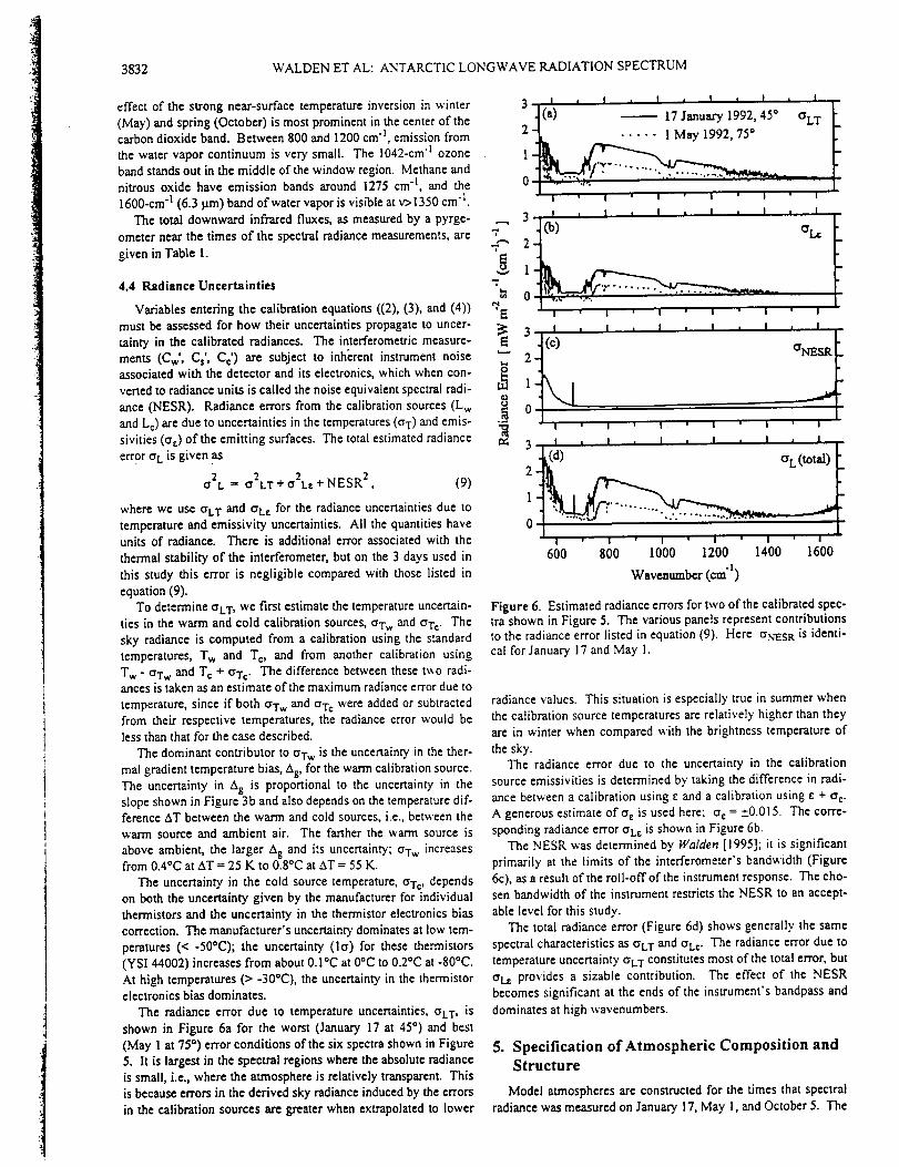
3832 WALDEN ET AL: ANTARCTIC LONGWAVE RADIATION SPECTRUM

effect of the strong near-surface temperature inversion in winter

(May) and spring (October) is most prominent in the center of thecarbon dioxide band. Between 800 and 1200 cm "l, emission from

the water vapor continuum is very small. The 1042-cm "1 ozone

band stands out in the middle of the window region. Methane and

nitrous oxide have emission bands around 1275 cm "l, and the

1600-cm "I (6.3 tam) band of water vapor is visible at v>1350 cm'k

The total downward infrared fluxes, as measured by a pyrge-

ometer near the times of the spectral radiance measurements, are

given in Table 1.

4.4 Radiance Uncertainties

Variables entering the calibration equations ((2), (3), and (4))

must be assessed for how their uncertainties propagate to uncer-

minD' in the calibrated radiances. The interferometric measure-

ments (Cw', Cs', Ce') are subject to inherent instrument noise

associated with the detector and its electronics, which when con-

vened to radiance units is called the noise equivalent spectral radi-

ance (NESR). Radiance errors from the calibration sources (Lw

and L c) are due to uncertainties in the temperatures (crT) and emis-

sivities (ere) of the emitting surfaces. The total estimated radiance

error crk is given .as

2o L = a2LT+ cr2t¢ +NESR 2, (9)

where we use CrLT and CrLc for the radiance uncertainties due to

temperature and emissivity uncertainties. All the quantities have

units of radiance. There is additional error associated with the

thermal stability of the interferometer, but on the 3 days used in

this study this error is negligible compared with those listed in

equation (9).

To determine CrLT,we first estimate the temperature uncertain-

ties in the warm and cold calibration sources, crTw and crTc The

sky radiance is computed from a calibration using the standard

temperatures, T w and T e, and from another calibration using

Tw- CrTw and Te + crTe" The difference between these two radi-ances is taken as an estimate of the maximum radiance error due to

temperature, since if both crTw and CrTcwere added or subtracted

from their respective temperatures, the radiance error would be

less than that for the case described.

The dominant contributor to craw is the uncertainty in the ther-

mal gradient temperature bias, Ag, for the warm calibration source.

The uncertainty in Ag is proportional to the uncertainty in the

slope shown in Figure 3b and also depends on the temperature dif-

ference AT between the warm and cold sources, i.e., between the

warm source and ambient air. The farther the warm source is

above ambient, the larger Ag and its uncertainty; crTw increasesfrom 0.4°C at AT = 25 K to 0.80C at t_T = 55 K.

The uncertainty in the cold source temperature, crT¢, depends

on both the uncertainty given by the manufacturer for individual

thermistors and the uncertainD" in the thermistor electronics bias

correction. The manufacturer's uncertainty dominates at low tem-

peratures (< -50°C); the uncertainty (lcr) for these thermistors

(YSI 44002) increases from about 0.1*C at 0*C to 0.20C at -80°C.

At high temperatures (> -30*C), the uncertainty in the thermistor

electronics bias dominates.

The radiance error due to temperature uncertainties, crLT, is

shown in Figure 6a for the worst (January 17 at 45*) and best

(May I at 75*) error conditions of the six spectra shown in Figure

5. It is largest in the spectral regions where the absolute radiance

is small, i.e., where the atmosphere is relatively transparent. This

is because errors in the derived sky radiance induced by the errors

in the calibration sources are greater when extrapolated to lower

C

"7

3 I , l , I , I , l i I

•I(a),...... . _ 17 January 1992, 45" I

2 _LT

01 . i ' I ' 'I ' I I I

3 "|)(b ' ' ' I , ' ' I , ' .

2

r° ' • "..-., --_ I

I I I I I ' I

aNESR

I ! ' I I ' I I

600 800 I000 1200 1400 1600

Wavenumber (cm" t)

Figure 6. Estimated radiance errors for two of the calibrated spec-tra shown in Figure 5. The various panels represent contributions

to the radiance error listed in equation (9). Here crNESR is identi-

cal for January 17 and May 1.

radiance values. This situation is especially true in summer when

the calibration source temperatures are relatively higher than they

are in winter when compared with the brightness temperature of

the sky.

The radiance error due to the uncertainty in the calibration

source emissivities is determined by taking the difference in radi-

ance between a calibration using E and a calibration using c + crc.

A generous estimate of crc is used here; crc = +__0.015. The corre-

sponding radiance error OLc is shown in Figure 6b.

The NESR was determined by Walden [1995]; it is significant

primarily at the limits of the interferometer's bandwidth (Figure

6c), as a result of the roll-off of the instrument response. The cho-

sen bandwidth of the instrument restricts the NESR to an accept-

able level for this study.

The total radiance error (Figure 6d) shows generally the same

spectral characteristics as CrLT and crL r. The radiance error due to

temperature uncertainty crLT constitutes most of the total error, but

crkt provides a sizable contribution. The effect of the NESR

becomes significant at the ends of the instrument's bandpass and

dominates at high wavenumbers.

5. Specification of Atmospheric Composition andStructure

Model atmospheres are constructed for the times that spectral

radiance was measured on January 17, May I, and October 5. The

WALDENETAL:ANTARCTICLONGWAVERADIATIONSPECTRUM 3833

trace gases included in our model atmospheres are water vapor.

carbon dioxide, ozone, methane, nitrous oxide, oxygen, CCI3F

(CFC-II). and CCI2F 2 (CFC-12). They are included either

because they are major infrared emitters in the atmosphere (water

vapor, carbon dioxide, ozone, methane, nitrous oxide) or because

their concentrations are readily available at South Pole Station

(CFC-] 1, CFC-12). The values are summarized in Table 1 along

with other information about the three selected test cases.

Detailed information on each model atmospheric profile and their

associated uncertainties is given by Walden [1995].

To select times when the sky conditions were most clear, we

consult the visual sky observations made by the SPWO and by

Warren. Clouds were detected at night when they were illumi-

nated by moonlight or, in the absence of moonlight, by their

obscuration of familiar stars. Slight diamond dust was observed

by Warren in the interferometer's field of view on May I but not

on January, 17 and October 5. Sunlight was available for the

observations on January 1 and October 5. Both the Sun and the

moon were below the horizon on May I.

5.1 Temperature

The temperature profiles in the near-surface layer, from the sur-

face (2.8 km above sea level) to 4 kin, were obtained from SPWO

radiosondes, corrected for thermal lag of the radiosonde's ther-

mistor by the method ofMahesh et al. [1997]. The uncertainty in

this correction depends upon how rapidly the temperature struc-

ture changes with altitude and is therefore greater in winter

(_+.0.6°C) than in summer (+_0.2°C). Another concern is the tempo-

ral constancy of the temperature within the inversion layer, since

the temperatures were not measured coincidentally with the spec-

tral radiances; the times of the FTIR measurement and the radio-

sonde launch are shown in Table I. For May I the uncertainty is

estimated to be 0.6°C, and 0.9°C for October 5 [Walden, 1995].

The total uncertainty in the near-surface temperature profile is

obtained by combining the two uncertainties discussed above with

the inherent temperature uncertainty (_+.0.5°C) given by the manu-

facturer of the sonde (Atmospheric Instrumentation Research.

Inc., Boulder. Colorado). For the near-surface layer these are

±0.5°C. -'__I.0°C. and +_1.2°C for January 17. May 1, and October

5.

The temperature profiles above 4 km are derived from the

SPWO radiosonde data and data from the co'ogenic limb array

etalon spectrometer (CLAES) and the Halogen Occultation Exper-

iment tHALOE) aboard the UARS [Roche et aL, 1993; Russell et

al., 1993: Hervig et al., 1995]. The radiosondes for our three case

studies reached altitudes of about 30 kin. The temperature uncer-

tainty betxseen 4 and 30 km is set to __.0.5°C, the manufacturer's

estimate. Temperatures between 30 km and 60 km v, ere obtained

from the UARS data archive at the Distributed Active Archive

Center (DA.AC) at Goddard Space Flight Center. The time refer-

ence data product (3AT) was used. The retrieved temperatures

from CLAES have better accuracy (1°-2°C) than those from

HALOE (2°-5°C) and are therefore used _'henever available.

Only data with positive quality values are used, meaning that the

data are based on actual atmospheric measurements rather than

climatology. Even though the UARS instruments view only to a

maximum southern latitude of 80°S, the temperatures from the

radiosondes generally agree with those from UARS, _'here they

overlap, to within the estimated uncertainties at the 2_ level. This

agreement is found as well for water vapor and ozone discussed

below.

The temperature profiles for the three model atmospheres are

shown in the first two columns of Figure 7; the second column

shows the near-surface layer with an expanded vertical scale. The

atmosphere is warmest at all altitudes on January 17. By May 1

the stratosphere has cooled as a result of the lack of sunlight. In

October the temperatures between 14 and 17 km are below 195 K,

cold enough for the formation of type I PSCs. The near-surface

temperature structure on January 17 shows a small surface-based

inversion, indicating that solar heating of the surface is not provid-

ing enough energy to compensate for the loss of Iongwave radia-

tion. On May i with no Sun, and October 5 with low Sun, the

surface-based inversion is well developed.

5.2 Water Vapor

Water vapor is an extremely important atmospheric constituent,

but it is the least well known of the gases measured at South Pole

and used in this study. The tethered kite experiments described by

Mahesh et al. [1997] are used to gain insight into the water vapor

content of the near-surface atmosphere. Despite the fact that the

carbon hygristors used for these tests were calibrated only down to

-40°C, the data suggest that the relative humidity with respect to

ice (R.H i) is close to saturation in the near-surface layer. In fact,

Schwerdtfeger [1970; 1984] took the frequent occurrence of dia-

mond dust ice crystals as evidence that the lower atmosphere must

be at least saturated with respect to ice. On the basis of the teth-

ered hygristor data we assume that the near-surface inversion layer

is saturated with respect to ice, and we bound the atmospheric rel-

ative humidity (with respect to ice) in this layer with a range of 90-

110%.

Tropospheric humidity was measured by three different instru-

ments: carbon hygristors used routinely by the SPWO, two frost-

point hygrometers launched by NOAA, and capacitive-type

Vaisala Humicaps that were packaged with the frost-point

hygrometers and ozonesondes. Like the carbon hygristors the

Humicaps are calibrated only down to -40°C. The frost-point

hygrometers are designed to measure stratospheric humidities and

thus are tuned for low absolute humidities (S. J. Oltmans, personal

communication, 1993).

On the basis of a small set of intercomparisons between these

various instruments it is impossible to draw firm conclusions

about the variability of tropospheric humidity. However, the data

suggest that the troposphere can be either near saturation or sub-

stantially subsaturated in the winter [Walden, 1995]. Because

there is no agreement between the SPWO carbon hygristor and the

Vaisala Humicap, some judgment is needed in specification of

humidity for the model atmospheres, taking into account the atmo-

spheric processes occurring over the Antarctic Plateau. For all

three of our model atmospheres, RMi from 4 to 7 km is assumed to

be 75% _+25%.

The microwave limb sounder (MLS) and HALOE instruments

from the UARS are used here to provide water vapor information

from about 30 to 60 km, or 100 to 0.1 mbar. Comparisons

between MLS data and the two NOAA-CMDL frost-point

hygrometers launched from South Pole in 1992 are very good

despite the fact that the UAR.S data are for lower latitudes

[Walden. 1995].

Figure 7 (right) shows the humidity profiles for the three model

atmospheres. In all cases the troposphere is more humid than the

upper atmosphere. The May and October cases have less water

vapor in the near-surface layer and the troposphere because of the

extreme low temperatures. The total column amount is i mm of

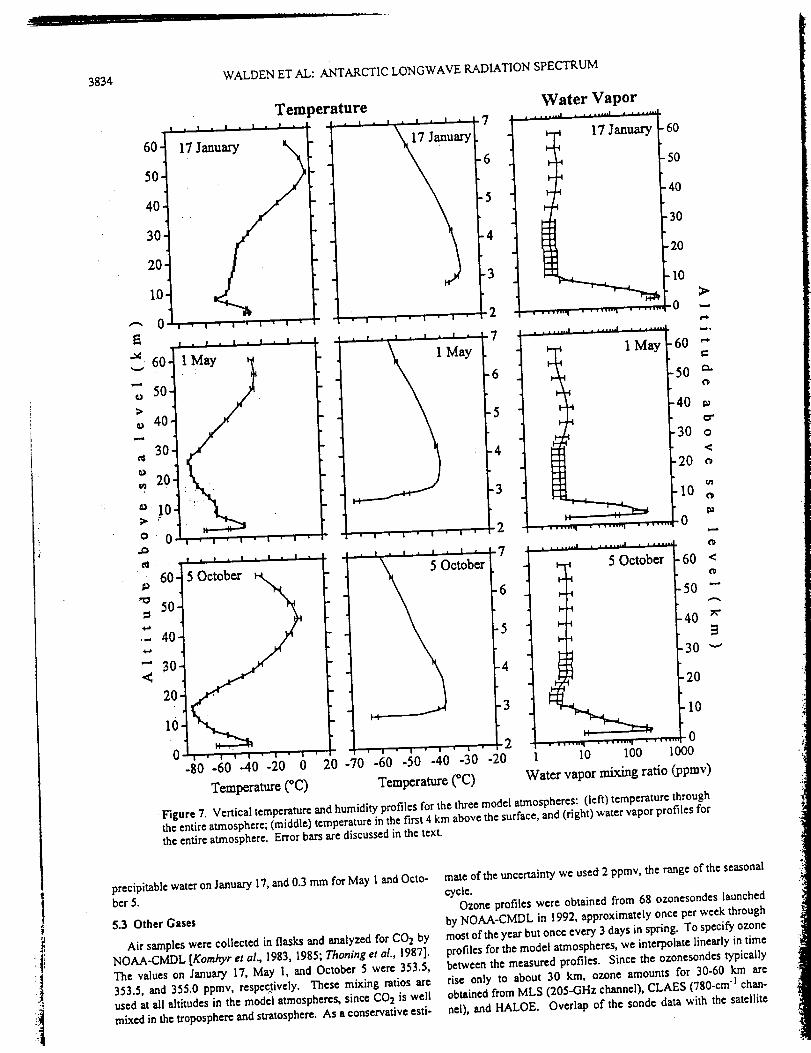
,ip

:ti

'1

3834WALDEN ET AL: ANTARCTIC LONGWAVE RADIATION SPECTRUM

Temperature

I I a I I a ! • I " I60 _ 17Jan

50 1.4

I

40

20

0 , 0 , , t

I • 0 a I • n , V • t"_ 60 1 May

o 50

40 _

30

20

O I I | t ° I

,.o

60

"_ 50

" 40 _.i,,e

ea

"-" 30<

20

IO

0

I I | I , I • !

o I I _ I '

,|,t,l'|"

i..I,l'la

5

.4

-3

_2

7

6

,5

-4

;-3

-2• I " i " I ' |

' ' ctober

14-

,[2'20 .70"-60"-50"-'_0'-30 -20

Water Vapor

17 JanuaryI--4-1

I._1

I.--I

f--

I• ,,..1 • • ,,-"1

,, ,,.,,I , • .....J

. .,,,,,.i , ,,,,,,"1 " "° .....

I • 'lo-,l

5 October

• , o ,,.,.| . ., ,,,,,| • ., ,,,,

10 100 1000

-60

-50

-40

-30

-20

-10

.... .. 0

, a i .....

1 May -60

50

.40

30

-20

10

0

-60

50

.40

-30

'2o

10

0

>

t.bo

¢:a,,,@

t_

o

<

('p

t_

0

t_

0

<

0

H

Temperature (*C) Temperature (*C) Water vapor mixing ratio (ppmv)

Figure 7. Vertical temperature and humidity profiles for the three model atmospheres: (left) temperature throughthe entire atmosphere; (middle) temperature in the first 4 km above the surface, and (right) water vapor profiles for

the entire atmosphere. Error bars are discussed in the text.

precipitable water on January 17, and 0.3 mm for May 1 and Octo-

ber 5.

5.3 Other Gases

Air samples were collected in flasks and analyzed for CO2 by

NOAA-CMDL [Komhyr et al., 1983, 1985; Thoning et al., 1987].

The values on January 17, May 1, and October 5 were 353.5,

353.5, and 355.0 ppmv, respe_ively. These mixing ratios are

used at all altitudes in the model atmospheres, since CO 2 is well

mixed in the troposphere and stratosphere. As a conservative csti-

mate of the uncertainty we used" 2 ppmv, the range of the seasonal

cycle.Ozone profiles were obtained from 68 ozonesondes launched

by NOAA-CMDL in 1992, approximately once per week through

most of the year but once every 3 days in spring. To specify ozone

profiles for the model atmospheres, we interpolate linearly in timebetween the measured profiles. Since the ozonesondes typically

rise only to about 30 kin, ozone amounts for 30-60 km are

obtained from MLS (205-GHz channel), CLAES (780-cm'1 chan-

nel), and HALOE. Overlap of the sonde data with the satellite

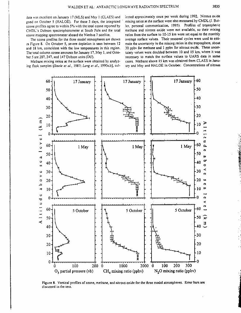
WALDEN ET AL: ANTARCTIC LONGWAVE RADIATION SPECTRUM 3835

data _vas excellent on January 17 (MLS) and May 1 (CLAES) and

good on October 5 (HALOE). For these 3 days, the integrated •

ozone profiles agree to within 5% with the total ozone reported by

CMDL's Dobson spectrophotometer at South Pole and the total

ozone mapping spectrometer aboard the Nimbus 7 satellite.

The ozone profiles for the three model atmospheres are shown

in Figure 8. On October 5, severe depletion is seen between 12

and 18 kin, coincident with the low temperatures in this region.

The total column ozone amounts for January i 7, May I, and Octo-

ber 5 are 287, 247, and 147 Dobson units (DU).

Methane mixing ratios at the surface were obtained by analyz-

ing flask samples {Steele et al., 1987; Lang et al., 1990a,b], col-

lected approximately once per week during 1992. Nitrous oxide

mixing ratios at the surface were also measured by CMDL (J. But-

ler, personal communication, 1995). Profiles of troposphericmethane and nitrous oxide were not available, so their mixing

ratios from the surface to 10-15 km were set equal to the monthly

average surface values. Their seasonal cycles were used to esti-

mate the uncertainty in the mixing ratios in the troposphere, about

30 ppbv for methane and 1 ppbv for nitrous oxide. These uncer-

tainty values were doubled between 10 and 15 krn, where it was

necessary to match the surface values to UARS data in somecases. Methane above 15 km was obtained from CLAES in Janu-

ary and May and HALOE in October. Concentrations of nitrous

¢3

;>

O

ra_

O

0

0

<

60

50

40

30

20

10

0

i ......... ! .........

......... i ........ •

a ......... i .........

60.

50-

40.

30.

2o2

1o£

i ......... i .........

i ......... i .........

5 October

?......... i .........

0 100 200

03 partial pressure (rib)

....... ! .........

17 January

I ......... I .... ' .... I

: ......... i .........

Y

i ......... i .........

: ......... i .........

er

; ........ 1"0'0"0....... 2"000

CH 4 mixing ratio (ppbv)

.i ......... ! ......... ! ......... i ....

Ii ......... i ......... I ......... i ....

i|i..._...i ......... I ......... i ....

1May

i ......... l ......... l ......... ¢ .... 0

! ......... | ......... i ......... I ....

"l 5 October

i ......... i ......... i ......... i ....

0 100 200 300

N20 mixing ratio (ppbv)

-60

_20

_I0 _

0 ..

-60

_40 o-o

_30 <0

_20 -O

_10

O

-60 ...

_50"-"

_40 _

I0

0

Figure 8. Vertical profiles of ozone, methane, and nitrous oxide for the three model atmospheres. Error bars arediscussed in the text.

]

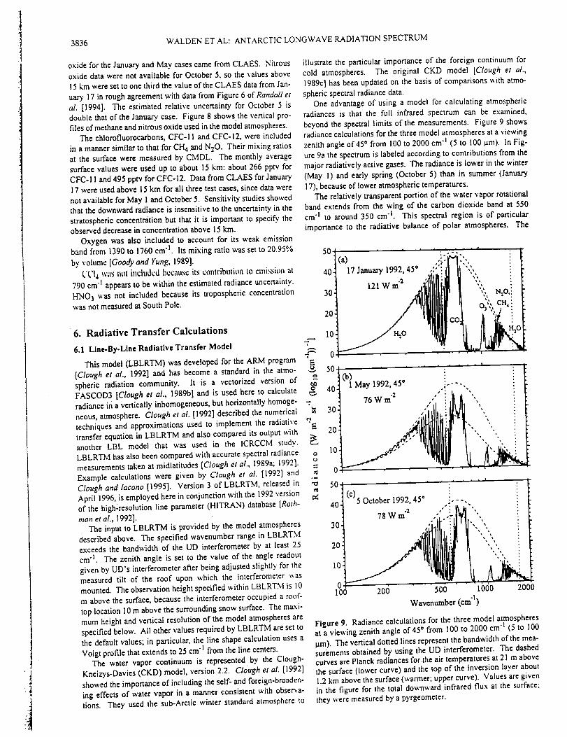
3836 WALDEN ET AL: ANTARCTIC LONGWAVE RADIATION SPECTRUM

oxide for the January and May cases came from CLAES. Nitrous

oxide data were not available for October 5, so the values above

15 km were set to one third the value ofthe CLAES data from Jan-

uary 17 in rough agreement with data from Figure 6 of Randall et

all [1994]. The estimated relative uncertainty for October 5 is

double that of the January case. Figure 8 shows the vertical pro-

files of methane and nitrous oxide used in the model atmospheres.

The chlorofluorocarbons, CFC-II and CFC-12, were included

in a manner similar to that for CH 4 and NzO. Their mixing ratios

at the surface were measured by CMDL. The monthly average

surface values were used up to about 15 km: about 266 pptv for

CFC-I 1 and 495 pptv for CFC-12. Data from CLAES for January

17 were used above 15 km for all three test cases, since data were

not available for May 1 and October 5. Sensitivity studies showed

that the downward radiance is insensitive to the uncertainty in the

stratospheric concentration but that it is important to specify the

observed decrease in concentration above 15 km.

Oxygen was also included to account for its weak emission

band from 1390 to 1760 cm "1. Its mixing ratio was set to 20.95%

by volume [Goody and Yung, 1989].

l,'L'l 4 was not included b¢catts¢ its contribution to emission at

790 cm "1 appears to be within the estimated radiance uncertainty.

HNO3 was not included because its tropospheric concentration

was not measured at South Pole.

6, Radiative Transfer Calculations

6.1 Line-By-Line Radiative Transfer Model

This model (LBLRTM) was developed for the ARM program

[Clough et al., 1992] and has become a standard in the atmo-

spheric radiation community. It is a vectorized version of

FASCOD3 [Clough et al., 1989b] and is used here to calculate

radiance in a vertically inhomogeneous, but horizontally homoge-

neous, atmosphere. Clough et al. [1992] described the numerical

techniques and approximations used to implement the radiative

transfer equation in LBLRTM and also compared its output with

another LBL model that was used in the ICRCCM study.

LBLRTM has also been compared with accurate spectral radiance

measurements taken at midlatitudes [Clough et al., 1989a; 1992].

Example calculations were given by Clough et al. [1992] and

Clough and lacono [1995]. Version 3 of LBLRTM, released in

April 1996, is employed here in conjunction with the 1992 version

of the high-resolution line parameter (HITRAN) database [Roth-

man et aL, 1992].

The input to LBLRTM is provided by the model atmospheres

described above. The specified wavenumber range in LBLRTM

exceeds the bandwidth of the UD interferometer by at least 25

cm "l. The zenith angle is set to the value of the angle readout

given by UD's interferometer after being adjusted slightly for the

measured tilt of the roof upon which the interferometer was

mounted. The observation height specified within LBLRTM is 10

m above the surface, because the interferometer occupied a roof-

top location 10 m above the surrounding snow surface. The maxi-

mum height and vertical resolution of the model atmospheres are

specified below. All other values required by LBLRTM are set to

the default values; in particular, the line shape calculation uses a

Voigt profile that extends to 25 cm "1 from the line centers.

The water vapor continuum is represented by the Clough-

Kneizys-Davies (CKD) model, version 2.2. Clough et al. [1992]

showed the importance of including the self- and foreign-broaden-

ing effects of water vapor in a manner consistent with observa-

tions. They used the sub-Arctic winter standard atmosphere to

illustrate the particular importance of lhe foreign continuum for

cold atmospheres. The original CKD model [Clough et al.,

1989c] has been updated on the basis of comparisons with atmo-

spheric spectral radiance data.

One advantage of using a model for calculating atmospheric

radiances is that the full infrared spectrum can be examined,

beyond the spectral limits of the measurements. Figure 9 showsradiance calculations for the three model atmospheres at a viewing

zenith angle of 45" from 100 to 2000 cm "1 (5 to 100 tam). In Fig-

ure 9a the spectrum is labeled according to contributions from the

major radiatively active gases. The radiance is lower in the winter

(May 1) and early spring (October 5) than in summer (January

17), because of lower atmospheric temperatures.

The relatively transparent portion of the water vapor rotational

band extends from the wing of the carbon dioxide band at 550

cm "l 1o around 350 cm "l. This spectral region is of particular

importance to the radiative balance of polar atmospheres. The

• o !

,o (.> ' ' o40 17 January 1992, 45 ::": 11 II "'_',

30 , lilllll,Ill l .., .,o.!i ., lll]llllll[ll It i

10 ._o

0

50 t .... :,

o_ 40: (b_ May 1992,45" , i-'", ::

_, 1": 76Win" ,'" i _ ["'i', i

'_ 0 .... "3 • ,,' : ', :

_'I_ 20. "" : "',, ", ::

0 • • '

0

"_ 50

40,

30

20.

10

(c)5 October 1992, 45*

.278Win

, , I

0 , , . • • i

100 206 500 1000 2000

Wavenumber (era "l)

Figure 9. Radiance calculations for the three model atmospheresat a viewing zenith angle of 45" from 100 to 2000 cm "t (5 to 100

pro). The vertical dotted lines represent the bandwidth of the mea-surements obtained by using the UD interferometer. The dashed

curves are Planck radiances for.the air temperatures at 21 m above

the surface (lower curve) and the top of the inversion layer about

1.2 km above the surface (warmer; upper curve). Values are given

in the figure for the total downward infrared flux at the surface:

they were measured by a pyrgeometer.

WALDENETAL:ANTARCTICLONGWAVERADIATION SPECTRUM

emission from _hc _ater vapor rotational bands at v < 350 cm "1

matches a Planck curve well in summer, but not in the winter and

spring because of the low water vapor amounts. This fact is some-_hat truc as _,.cll for the vibration-rotation band of v, ater vapor at

1,100 to 1600 cml Even though the atmosphere over the Antarc-

tic Plateau contains at most only I mm of precipitable water, and

thus emission from the water vapor continuum (between about

600 and 1000 cm l) is small, water vapor is still the primary emit-

let of thermal radiation to the surface [Walden and Warren, 1994].

contributing about t_vo thirds of the total downward flux to the

surface. The 667-cm'1 (15-pro) absorption band of carbon dioxide

is important because it is strong and is located near the peak of the

Planck function• The near-surface temperature inversion is stron-

gest in May and weakest in January; its effect on the carbon diox-ide band is evident. Emission from ozone at 1042 cm "1 is

maximum in January: it is lower in May because of low strato-

spheric temperatures, and even lower in October because of

reduced ozone abundance. The emission bands of methane and

nitrous oxide around 1100 to 1200 cm "1 are also visible. The N20

' band at 1168 cm "t contributes in the window region, while emis-

sion from both CH4 and N20 overlaps with water vapor between

1200 and 1300 cm "1. CH4 and N2 O are therefore relatively more

important in _inter. when emission from water vapor is weaker.

The importance of the near-surface air temperature and the var-

ious atmospheric window regions is seen by comparing the Planck

functions _ith the spectral radiance. Two Planck functions are

plotted: one for the surface air temperature at 2 m and the other for

the temperature at the top of the inversion. The peaks of the

Planck functions for the January case are centered on the carbon

dioxide band. _hereas in May and October, when the tempera-

tures are lower, the peaks are on the low-wavenumber side of the

band. The carbon dioxide band is relatively more important to the

surface energ.v budget in Antarctica than at other terrestrial loca-

tions both for this reason and also because emission from uater

vapor is small and therefore has little overlap with the CO2 band.

The radiance values between the verlical dotted lines in Figure

9 constitute the standard model calculations used throughout this

paper because this is the wavenumber region measured by theinterferomcter. The comparisons discussed below represent the

most variable and perhaps most interesting portion of the infrared

spectrum, but they do not provide a check on the emission from

_ater vapor at 1o_ (<550 cm "l) and high (>1667 cm d) wavenum-

hers.

6.2 Matching Calculations to Measurements

To compare spectral radiance observations with the results of a

high-spectral-resolution radiative transfer model such as

LBLRTM. it is necessary to account for the finite field of vie_

(FOV) of the intcrferometer and also to match the spectral resolu-tion of the calculations to that of the observations. Steel [1964]

and Bell [1972] discuss such corrections in general terms. The

discussions by CIough et al. [I 989a] and Smith et al. [1989] apply

this rheas' to comparisons of LBL calculations with interferomet-

ric measurements of atmospheric radiance and transmission. In

this study. LBLRTM calculations are converted to spectra suitable

for com;arisons with observed spectral radiances by using the fot-

lo_ing procedure. LBLRTM calculates a spectrum at its own

internal spectral resolution, which is about 0.001 cm l. An inter-

feropram is eenerated from the calculated spectrum, then apodized

by using the Hann-uindow function [Press et at.. 1992]. (This

apodization function was also applied to the measured interfero-

grams, and for proper comparisons it is necessary to apply the

same apodization function to the calculations•) This interferogram

is used to interpolate the spectrum to a wavenumber spacing of

0.01 cm "1, much finer than the wavcnumber grid of the trans-

formed apodized interferogram. This procedure is all done within

LBLRTM. The resulting calculated spectrum now matches the

spectral resolution of the radiance measurements. A FOV correc-

tion [Walden, 1995] is applied by using trapezoidal integration to

perform the integral over field of view,

L (V. d (lO)LLBL(V') --".a0 _ a\'_,)

where L a is the apodized version of the calculated spectrum. The

variable of integration, P, is the cosine of the angle 0 measured

from the center of the FOV. The outer limit of the FOV is at

= 8 m. The weight w(p) is set to the constant value of 1.0 from la

= 0.9996 (Bin = 1.5°) to g = i and set to zero elsewhere. Sensitiv-

ity studies show that the calculated spectra described in this studyare insensitive to reasonable assumptions about the shape of the

FOV and uncertainty in the choice of 0m- Finally, the oversam-

pied, field.of-view-corrected, calculated spectrum is linearly inter-

polated from its fine wavenumber grid to the coarser grid of the

measurements, allowing LLBL tO be directly compared to Ls from

equation (2).Before the correction was applied, there were large differences

between the observed spectra and the LBLRTM calculations

where the spectrum varied rapidly, notably in the wings of the

CO 2 band near 600 and 750 cm "f. The FOV correction greatly

reduced these differences.The radiances supplied to the ICRCCM project by Walden et

al. [1997] differ slightly from those reported here in two ways.

First, Walden et al. [1997] re-calibrated the radiance measure-

ments by adjusting the temperatures of the calibration sources

[Tw - n*a(T_) and T c+ n*a(Tc)], choosing a value of n as neces-

sary to eliminate most of the negative radiances in the atmospheric

window regions: n = +1 for Jan 17 (45°), 0 for Jan 17 (75°). +1 for

May 1 t45°). 0 for May I (75°). +1 for Oct 5 (45°), +2 for Oct 5

(75°). Second. Walden etal. [1997] chose to remove the effect of

the FC)V from the measurements rather than incorporate it into the

calculations. This was done by adjusting the wavenumber scale of

the original measurements, v, by v' = v / (cos0m)- This corrects

for the wavenumber shift caused by off-axis rays in the interfer-

ometer, but does not account for the slight spectral smearing; both

effects are described by Bell [1972].

7. Uncertainties in the Calculated Radiances

There are many possible sources of error in the LBLRTM cal-

culations. These include uncertainties in the specification of the

model atmosphere, the database of absorption line parameters

(HITRAN92). the model's numerical techniques, and the treat-

ment of the physics of infrared emission and absorption. EIling-

son et al. [1991] briefly discussed the three latter sources, finding

that LBL models agree well with each other where accurate spec-

troscopic data are available (e.g.. carbon dioxide), indicating that

the different numerical techniques used in the various models

were all adequate. However, large uncertainties persist where

there are deficiencies in the line parameter data. the theory of gas-

eous absorption, or the specification of the model atmosphere.

The purpose of the following error analysis is to place a lower

bound on the radiance error in the model calculations by consider-

ing only those sources of error induced by uncertainties in the

specification of the model atmosphere and in the viewing zenith

angle.

.r

3

3838 WALDEN ET AL: ANTARCTIC LONGWAVE RADIATION SPECTRUM

7.1 Maximum Height of the Model Atmosphere

The error in calculated radiance caused by truncating the model

atmosphere is determined by subtracting the radiance for a 60-kin

atmosphere from those truncated at 30, 40, or 50 kin. These radi-

ance differences are negative, since the emission from a truncated

atmosphere is less. The radiance errors for a 30-kin atmosphere

are significant, especially near the 1042-cm "1 ozone band, where

they exceed -0.8 mW m "2 sr "l (cm'l) "t. The errors are seen prima-

rily in spectral regions with weak absorption, where emission can

come from throughout the atmosphere. The difference in radiance

between a 50-kin atmosphere and a 60-kin atmosphere is very

small (less than -0.02 mW m"2 sr "l (cm'l) "l ), so we judge 60 km

to be adequate and use this as the maximum height in all further

calculations.

7.2 Vertical Resolution and Temperature Structure

in the Lowest 300 m

Ideally, an altitude grid can be chosen that adequately repre-

sents the near-surface temperature inversion over the plateau in

winter, when it is steepest. Model atmospheres with extreme

inversions and large zenith angles are most sensitive to changes in

the vertical resolution, so it is best to use such cases for choosing

the vertical resolution. We chose the October 5 atmosphere at a

zenith angle of 75*, since its temperature gradient in the lowest

100 m is the steepest of the three model atmospheres. Several dif-

ferent altitude grids between the surface (2.84 kin) and 3.15 km

are defined: grids with uniform spacings (10, 20, and 30 m) and a

variable grid with spacing varying from 5 to 100 m, increasing

with altitude. Between 3.15 and 60 km the grid spacing varies

from 150 m to 5 kin, gradually increasing with altitude, and is held

constant in these sensitivity studies. The appropriate vertical reso-

lution is chosen by successively decreasing the uniform altitude

spacing in the near-surface layer until the radiance differencebetween successive runs is smaller than a specified tolerance.

This tolerance is chosen as the radiance error induced by uncer-

tainties in the temperature profile, discussed below.The calculated radiance is sensitive to vertical resolution

mainly in spectral regions that are strongly absorbed; i.e., regions

in _hich most of the measured radiance originated in the inversion

layer. The 30-m grid causes significant differences, but the 10-m

and 20-m grids give almost identical results. Both still show a dif-

ference from the variable grid in the CO 2 band, but this difference

is small in comparison with radiance errors caused by the uncer-

tainty in the specification of the temperature profile, discussed

next. The calculations shown below use the variable grid.

7.3 Radiance Error Due to Uncertainty in Atmospheric

Temperature and Composition

With the vertical resolution and the height of the model atmo-

sphere chosen so that the), induce little error in the LBLRTM cal-

culations, the radiance error is now determined by performing

sensitivity studies by using the model atmosphere data and their

uncertainties. Standard spectral radiance calculations are produced

using the profile information presented in Figures 7 and 8. Radi-

ance errors are determined by perturbing, one at a time, an individ-

ual profile in the model atmosphere by adding its uncertainty.

LBLRTM is then run with this perturbed model atmosphere,

yielding a radiance spectrum. The radiance errors are found by

subtracting the standard radiance case from that obtained with the

perturbed atmosphere. The total radiance error is found by taking

the square root of the sum of the squares of the radiance differ-

ences due to the various profile perturbations.

The results for January 17 at 45 ° and May 1 at 75", represent-

ing the warmest and coldest atmospheres at South Pole, are shown

in Figure 10. These radiance errors represent the range of errors to

be expected for clear-sky calculations with LBLRTM for the Ant-

arctic Plateau. Only the four major sources of error are shown in

Figure ]0; the errors due to uncertainty in concentrations of car-

bon dioxide, methane, nitrous oxide, CFC-1 I, and CFC-12 are all

negligible in comparison with those shown. The radiance errorsfor October 5 are similar to those for May I. The total radiance

error in summer is dominated by uncertainties in the temperature

and water vapor profiles. In winter the uncenainty in zenith angle

(discussed below) is also a major contributor. The total error incalculated radiance for these cases is comparable to the error in

measured radiance shown in Figure 6. However. the spectral

structure is different. It should be emphasized that the error esti-

mates for the LBLRTM calculations assume the sky is clear. The

visual sky observations were initially used to identify clear test

cases, but subvisible clouds and aerosols may still have been

present in the actual atmosphere. This possibility is examined

below.

The uncertainty in zenith angle is due to many sources, some of

which are quantified here and some of which are estimated. The

angle readout for the interferometer's mirror assembly was accu-

rate to within a few millivolts, or roughly 0.1 °. The tilt of the roof

during 1992 was estimated as 0.4* +_0.1". Additional sources of

uncertainty included the interferometer being mounted in a non-

level position and inaccuracy in calibration of the angle readout

(which is ideally set to 0* when viewing vertically and 90*. when

viewing horizontally). One test indicated that the zenith angle was

actually 73.8 ° at the 75* mechanical mirror stop, an offset of 1.2"

if it is assumed that the angle readout was set to exactly the 75*

voltage during that test (R. Van Allen, personal communication,

1995). When all these sources of uncertainty are taken into

account, a generous estimate of the overall zenith angle uncer-

tainty is ___1.5*.

The radiance errors induced by the uncertainty in the zenith

angle are most significant in the wintertime. The largest contribu-

tions are primarily in regions where gases have intermediate

absorption, i.e., the wings of the carbon dioxide band, the weak

bands of carbon dioxide (975 cml) and nitrous oxide ( 1168 cm" I),

the ozone band, and methane, nitrous oxide, and water between

1200 and 1500 cm "l. Emission from these regions comes from a

long path length in the atmosphere and therefore comes on aver-

age from a great distance from the observation point. The farther

away the emission region, the greater the change in effective emit-

ling temperature due to a given change in zenith angle (if the tem-

perature varies with height). The radiance error is large in theozone band because most ozone emission comes from the upper

troposphere and lower stratosphere. The zenith angle uncertainty

induces much less error in summer because of weaker temperature

gradients; the error is confined to the wings of the carbon dioxide

band.

The uncertainty in the temperature profile produces radiance

errors in spectral regions where emission is from altitudes at

which the temperature is changing rapidly and where gases are

strongly absorbing. Most of the errors in both summer and winterare from emission within the inversion layer (carbon dioxide and

water vapor), but there is also a significant contribution in the

Ozone band.

The radiance errors due to water vapor and ozone are confined

to regions in which they emit radiation. The errors are largest

where the uncertainty in the individual profile is greatest. Thus,

for water vapor, the errors occur in spectral regions where emis-

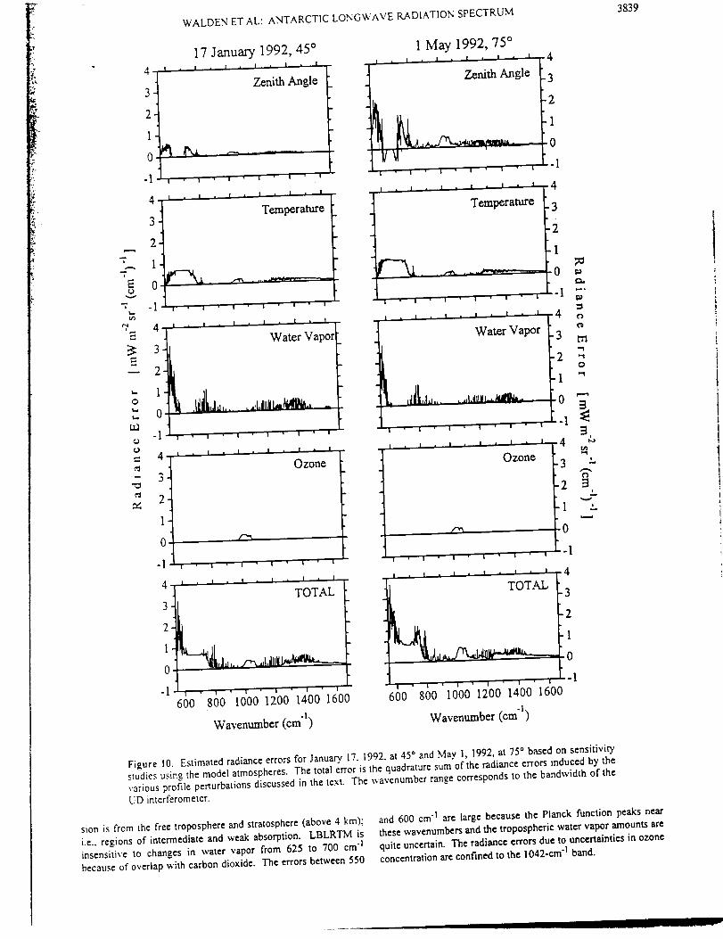
WALDENETAL:ANTARCTICLONGWAVERADIATIONSPECTRUM

17 January 1992, 45 o

4 , , ' • ' ' ' ' ' " 'Zenith Angle

3

2

1

o_ ..........

-1 | ' i ' I " I ' i ' I

4 I , I i I I I , I , I

Temperature3

' I ' I " I " I ' I

1 May 1992, 75 °_-4

Zenith Angle "3

'2

0

-1

, , , , , , , , , , , 4] Temperature [3-I

" 2

"1 1

f:a.

1 , , . , , , . , • , -I ;I i I , I , I i I * I 4 ¢,

2

- 1

_- 0

"v -1

4 I , I , I , I , I i I 1

Water Vapo3

=_.2

" 1 _ I_iko0 , ,,lu ..... ,I,lUll_t-, -

-I I ' I ' l ' I " I ' I

I i ' ' I

= 4 I , I , I ,

0 zone

• - 3

.-j

2

1

4.1 , I i I , I i I , I L

1"I l I ' I ' I ' I ' I ' I

600 800 1000 1200 1400 1600

Wavenumber (cm'l)

Water Vapor

al

I

71

]4

14

-I4

I

' I ' I ' I '

il,lilJ

I "-1' I ' l ' I ' I " I ' l

I , I , I , I , l , '[4

1

0

I I I " I ' ' L'I

600 800 1000 1200 1400 1600

Wavenumber (era"l)

t'rl,='1

2 "o

1

I ' I -1

I ' I -4 _,a

Ozone [ 3 "

-2i

1 '-.

0

3839

Figure 10. Estimated radiance errors for January. 17. 1992. at 45* and May !, 1992, at 75" based on sensitivitystudies using the model atmospheres. The total error is the quadrature sum of the radiance errors induced by the

various profile perturbations discussed in the text. The wavcnumber range corresponds to the bandwidth of the

UD interferometer.

sion is from the free troposphere and stratosphere (above 4 kin); and 600 cm "1 are large because the Planck function peaks near

i.e., regions of intermediate and weak absorption. LBLRTM is these wavenumbers and the tropospheric water vapor amounts are

insensitive to changes in water vapor from 625 to 700 cm "1 quite uncertain. The radiance errors due to uncertainties in ozone

because of overlap with carbon dioxide. The errors between 550 concentration are confined to the 1042-cm "1 band.

!

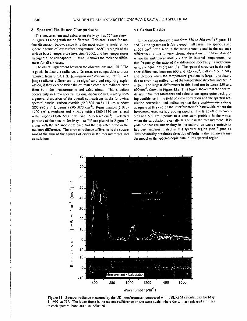
3840 WALDEN ET AL: ANTARCTIC LONGWAVE RADIATION SPECTRUM

8. Spectral Radiance Comparisons

The measurement and calculation for May I at 75 ° are shown

in Figure 11 along with their difference. This case is used for fur-

ther discussion below, since it is the most extreme model atmo-

sphere in terms of low surface temperature (-66°C), strength of the

surface-based temperature inversion (30 K), and low temperatures

throughout the atmosphere. Figure 12 shows the radiance differ-ences for all six cases.

The overall agreement between the observations and LBLRTM

is good. In absolute radiance, differences are comparable to those

reported from SPECTRE [Ellingson and Wiscombe, 1996]. We

judge radiance differences to be significant, and requiring expla-

nation, if they exceed twice the estimated combined radiance error

from both the measurements and calculations. This situation

occurs only in a few spectral regions, discussed below along witha general discussion of the overall comparisons in the following

spectral bands: carbon dioxide (550-800 cm'l), 1I-_m window

(800-990 cm'l), ozone (990-1070 cm'l), 9-_m window (1070-

1200 cm'l), methane and nitrous oxide (1200-1350 cm'l), and

water vapor (1350-1500 cm "l and 1500-1667 cm'I). Selected

portions of the spectra for May 1 at 75" are plotted in Figure 13

along with the radiance difference and the estimated error in the

radiance difference. The error in radiance difference is the square

root of the sum of the squares of errors in the measurements and

calculations.

8.1 Carbon Dioxide

In the carbon dioxide band from 550 to 800 cm "l (Figures I 1

and 12) the agreement is fairly good in all cases. The spurious lineat 667 cln "l often seen in the measurements and in the radiance

differences is due to very strong absorption by carbon dioxide

where the instrument mostly views its internal temperature. At

this frequency the ratio of the difference spectra, "/', is indetermi-

nate: see equations (2) and (3). The spectral structure in the radi-

ance differences between 600 and 725 cm "l, particularly in May

and October ,.,,'hen the temperature gradient is large, is probably

due to error in specification of the temperature structure and zenith

angle. The largest differences in this band are between 550 and

600 cm "1, shown in Figure 13a. This figure shows that the spectral

details in the measurements and calculations agree quite well, giv-

ing confidence in the field of view correction and the spectral res-olution correction, and indicating that the signal-to-noise ratio is

adequate at this end of the interferometer's bandwidth, where the

instrument response is dropping rapidly. The large offset between

570 and 600 cm "1 points to a consistent problem in the winter

when the calculation is usually larger than the measurement. It is

possible that the uncertainty in the calibration source emissivity

has been underestimated in this spectral region (see Figure 4).

This possibility precludes detection of faults in the radiative trans-

fer model or the spectroscopic data in this spectral region.

80-

70-

60-

5o-

E40-

"7

30-

E 20-

ElO-

o O-,j

e.

_0 -10-

•_ 10-

0-

-10[600 800 1000 1200 1400 1600

Wavenumber (cm "t)

Figure 11. Spectral radiance measured by the UD interferometer, compared with LBLRTM calculations for May1, 1992, at 75 °. The lower frame is the radiancedifference on the same scale, where the primary infrared emitters

in each spectral band arc also indicated.

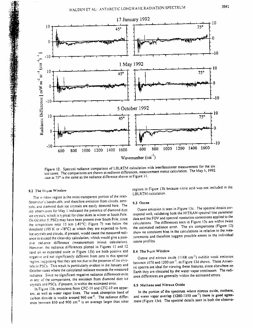
WALDENETAL:ANTARCTICLONGWAVERADIATIONSPECTRUM 3841

"7

E

"7L=.

¢xlJ

E

E

O

O

,.=.

a

10-

-10

10

0

-10

10

0

17 January 1992t , I m ' " _ -10

dl

1

75*

l ' I ' i ' I ' I I

1 May 1992

45*

5 October 1992

45*

-10600 800 1000 1200 1400 1600

I I ¢ I I I I • !

75*

600 ' 800 ' 10'00' 12'00" 14'00 ' 16'00

Wavenumber (cm"1)

.0

-I0

-10

.0

-10

10

0

-10

Figure 12. Spectral radiance comparison of LBLRTM calculation with interferometer measurement for the six

test cases. The comparisons are shown as radiance differences, measurement minus calculation. The May 1, 1992

case at 75* is the same as the radiance difference shown in Figure I I.

8.2 The ll-pm Window

The _ indow region is the most transparent portion of the inter-

ferometcrs band_vidth, and therefore emission from clouds, aero-

sols. and diamond dust ice crystals are easily detected here. The

sky obser_ ation for May I indicated the presence of diamond dust

ice crystals. _hicb is typical for clear skies in winter at South Pole.

On October 5. PSCs may have been present over South Pole, since

the temperature near 15 km (-81°C; Figure 7) was below the

threshold (195 K or -78°C) at which they are expected to form.

Ice crystals and clouds, if present, would cause the measured radi-

ance to exceed the clear-sky calculation, which would give a posi-

tive radiance difference (measurement minus calculation).

Ho_ve_er. the radiance differences plotted in Figures 11 and 12

land on an expanded scale in Figure 13b) are both positive and

negative and not significantly different from zero in this spectral

region.._usgcsting that they are not due to the presence of ice crys-

tals or PSCs. This result is particularly evident in the January. and

October cases where the calculated radiance exceeds the measured

radiance Since no significant negative radiance differences exist

in any of the comparisons, the emission from diamond dust ice

crystals and PSCs. if present, is within the estimated error.

In Figure 13b. emissions from CFC-I 1 and CFC-12 are appar-

ent. as well as water vapor lines. The weak absorption band of

carbon dioxide is visible around 960 cm "t. The radiance differ-

ence betx_een 850 and 900 cm "l is on average larger than other

regions in Figure 13b because nitric acid was not included in the

LBLRTM calculation.

8.3 Ozone

Ozone emission is seen in Figure 13c. The spectral details cor-

respond well. validating both the HITRAN spectral line parameterdata and the FOV and spectral resolution corrections applied to the

calculations. The differences seen in Figure 13c are within twice

the estimated radiance error. The six comparisons (Figure 12)

show no consistent bias in the calculations in relation to the mea-

surements and therefore suggest possible errors in the individual

ozone profiles.

8.4 The 9-pro Window

Ozone and nitrous oxide (1168 cm "1) exhibit weak emission

between 1070 and 1200 cm "1, as Figure 13d shows. These Antarc-

tic spectra are ideal for viewing these features, since elsewhere on

Earth they are obscured by the water vapor continuum. The radi-

ance differences are generally within the estimated errors.

8.5 Methane and Nitrous Oxide

In the portion of the spectrum where nitrous oxide, methane,

and water vapor overlap (1200-1350 cm "l) there is good agree-

ment (Figure 13e). The spectral details seen in both the observa-

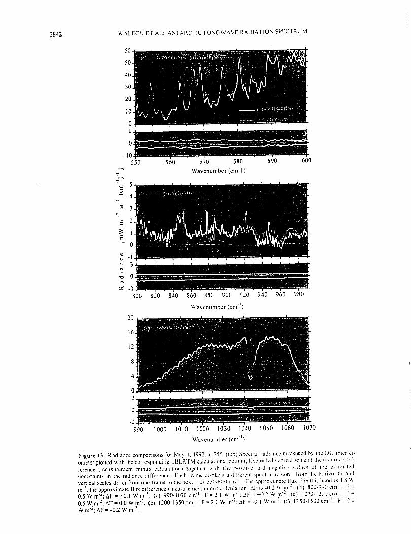
3842 WALDEN ET AL: ANTARCTIC I.ONGWAVE RADIATION SPECTRUM

60

50

40

30:

20

oilO-

560 570 580

Wavenumber (cm- l)

590 60O

-1'

3

0

-3

800 820 840 860 880 900 920 940

Wa,,enumber (cm "l)

960 980

-2

990 1000 1OI0 1020 1030 1040 1050 t060 1070

Wavenumber (crn "1)

Figure 13. Radiance comparisons for May I. 1992. :_t 75 °, (top) Spectral radiance measured b) It_c DI.; intcr_;,:a-

ometer plotted v, ith the corresponding LBL'RI'M calculation: (bottom) [i_,pandcd ', crtlcal scale of the rad_:mcc J_t'-fcrence (measurement minus calculalion) It_.cthcl _',llh the posni',¢ and nCgztti,,c ,.alucs t)l lh¢ C:-;tllllZtldd

uncertainty in the radiance dil'fcrcI_cc. I-_ach I?amc displa',s a diff,:rc_n ",r,cctrat rugmn Both the hori:/t_tllal amt

,,enical .,,calcs differ from one frame t_._the next. (a) 55t)-b(l() till "1 . lhc approxmlalc l]tlx l: if'l this hand i:-,48 \",

m2;theaDproxima_e flux difference (mcasurcmcnl minus calculation) Al: is "112 W m 2. (b) 80t)-99Ocm 1. F=0.5Wm'2:AF=*O.I Wm 2. (c) 990-1070crn 1. F =2 1 9,'m'2:..SF =-O.2 W m 2. (d) 1070-1200crn l. F

0.SWm'2;AF=0.0Wm "2. (e) 1200-1350cm "1. F=2.1 Wm'2:.SF=-().I Wm "2. (13 1350-1500cm 1, F=2()

W m'2; AF = -0.2 W m 2.

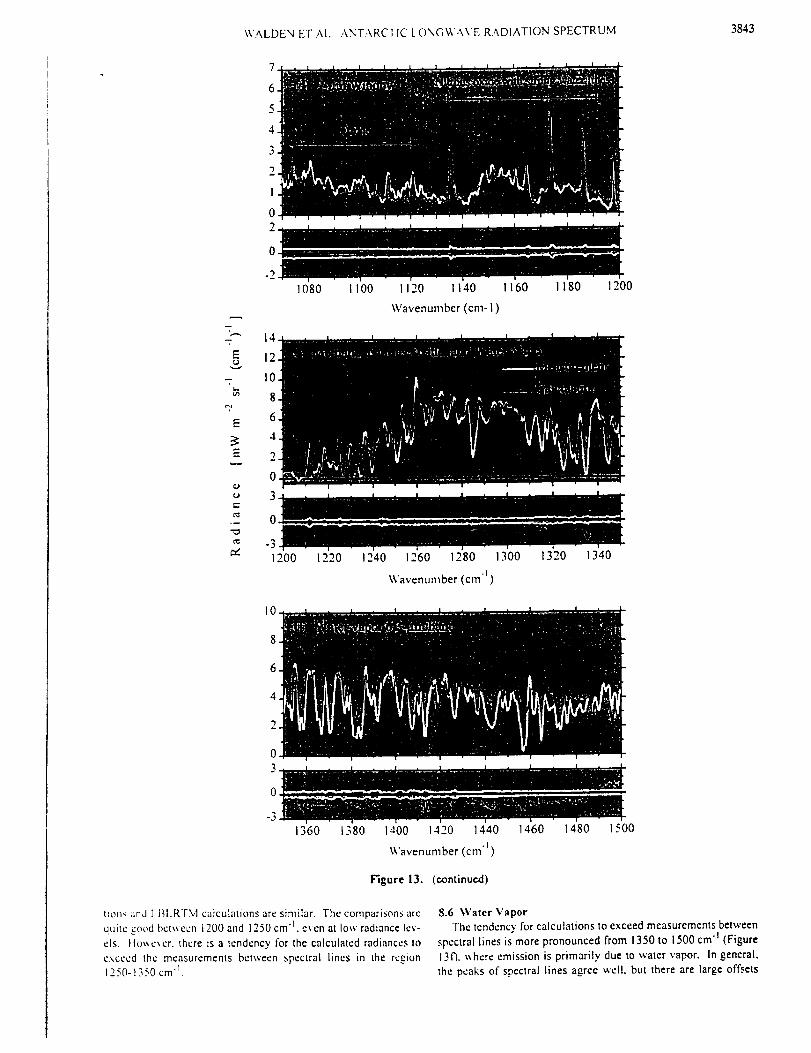
WALDENETAL:ANTARCIICLONGV_A",'ERADIATIONSPECTRUM

7.6_

3843

3:

2_

I

"7

"7

E

"7

E

=_

¢./

¢,-

,.¢

14

12

10

8

6

4

2

1080

0

3

0

-3

1200

1100

1220

1120 1140 1160

Wavenumber(cm-I)

1240 1260 1280 1300

Wavenumber(cm _ )

1180

1320

1200

I0

2

0"3

1360 1380 laO0 1420 1440

Wavenumber(cm "_)

1460 1480 1500

Figure 13. (continued)

tion:, and LI_,LRTM cutculations are similar. The comparisons are

quite good bct_ecn 1200 and 1250 cm "1. even at low radiance le,,-

els. Ftov.c_er. there is a lendency for the calculated radiances to

exceed the measurements betxveen spectral lines in the region1250-1350 cm 1

8.6 Water Vapor

The tendency for calculations to exceed measurements between

spectral lines is more pronounced from 1350 to 1500 cm "_ (Figure

1313. ,._hcre emission is primarily due to water vapor. In general.

the peaks of spectral lines agree well. but there are large offsets

3844 WALDENETAL:ANTARCTICLONGWAVERADIATIONSPECTRUM

betweenlineswith,insome cases, striking similarities in spectral

detail (for instance, around 1380 cm'l). Figure 12 shows the cal-

culation generally exceeding the radiance observation (negative

radiance differences) from 1250 to 1500 cm "1 for all six cases,

especially between strong water vapor emission lines. The radi-

ance differences exceed twice the estimated error in all the model

atmospheres, regardless of whether the residual calibration bias

seen in the measured window radiances is positive or negative.

Sensitivity studies were pert'on'ned on both the interferometric

calibration and the radiative transfer calculations in an attempt to

identify the cause of the discrepancies between 1250 and 1500

cm "L. First, the temperature of the warm calibration source was

adjusted to achieve bener agreement in this spectral region,

assuming the LBLRTM calculations were correct. The low values

of the measured radiance between spectral lines are more sensitive

to the calibration source radiance than are the peaks of the spectral

lines. Thus it is possible to fit the measured spectrum to the radi-

ance calculation by changing the warm source temperature. The

warm source temperature ,*'as chosen as a proxy for changes in the

calibration source radiance, since it is typically the largest source

of uncertainty in the measured radiances. To minimize the spec-

trolly averaged difference in radiance in this band, the warm

source temperature had to be decreased by about 6 K. This adjust-

ment provided a better match of the low radiances shown in Figure

13f, but it also increased unrealistically the radiance in other parts

of the spectrum, particularly the window regions. Furthermore, a

decrease in the warm source temperature of this magnitude would

imply that the intefferometer was viewing a source colder than

that repotted by the warm source thermistors, contrary to the evi-

dence from three different tests shown in Appendix A of Walden

[1995] and summarized in Figure 3b. Therefore miscalibration of

the measured radiances cannot explain all of the radiance differ-

ences between 1250 and 1500 cm "].

Second. sensitivity studies with LBLRTM were performed by

using different humidity profiles from the surface (2.8 km) to 7

km above sea level. As discussed above, the uncertainty in the

water vapor profiles is large. The calculated spectra are most sen-

sitive to humidity changes below 7 kin, since most of the "*'ater

`"apor is contained in the troposphere. The low radiance values

between spectral lines from 1250 to 1500 cm "1 are more sensitive

to humidity changes than are the peaks of lines, because the peaks

are saturated. Therefore the tropospheric humidity can be

adjusted to fit the radiance calculation to the measured spectrum.

As trial values, the tropospheric relative humidity with respect to

ice (RH i) "*'as set to 25%, 50%, 75%, and 100%. As RH i

decreases from 100% to 50%, the discrepancies between the cal-

culations and measurements also decrease. However, at RH i =

25% the peaks of the spectral lines become subsaturated, and the

agreement worsens. Therefore good agreement in both the peaks

and ",,alley's was impossible, but the best agreement "*as attained

for tropospheric RH i values of 25-50%. These low humidity val-

ues seem unreasonable, since ice crystal precipitation was

observed on every clear day in winter and on most clear days in

summer; the presence of precipitation implies saturated conditions

somewhere within the lower atmosphere.

Clougt, et al. [1992] and Th_riault et al. [1994] sho'*ed the

importance of the foreign-broadened water vapor continuum in

this spectral region, particularly in cold atmospheres where the

continuum increases the opacity between spectral lines. The oxy-

gen continuum is also important in cold and dry. atmospheres from

1400 cm "l to beyond the high-wavenumber limit of the interfer-

procter [Tiraofeyev and Tonkov. 1978; Rinsland et al., t989].

Revercomb et al. [1990] and Thdriault et al. [1994] found that cal-

culations using FASCODE (the predecessor of LBLRIM) and an

earlier version of the water vapor continuum model exceeded their

measurements, as we also find. Th_riault et al. [1994] calculated

radiance along horizontal paths at temperatures of -g_C to --4°C

and water vapor amounts of 0.6 to 1.2 g crn 2. They suggested that

perhaps either the foreign-broadened absorption coefficient has a

positive temperature dependence or the temperature dependence

of the strengths of nearby water vapor lines is in error. The for-

eign continuum absorption in the CKD model used here has a

slight temperature dependence through density, but the continuum

coefficients themselves do not depend on temperature (S. A.

Clough, personal communication, 1995).

The final spectral region considered here (1500-1667 cm t)

shows significant radiance differences (Figures I1 and 12), espe-

cially in January. This finding is surprising, since most of this

spectral region is strongly absorbed by "*'ater vapor and thus

should resemble a Planck curve, especially in January when the

lowest 2 km are nearly isothermal. Sensitivity studies show that

the choice of emissivity for the calibration sources has little effect

on the comparisons. It is possible that the noise equivalent spec-

tral radiance (Figure 6) was underestimated at these wavenum-

bets. However, since the errors are largest in Januar,.' and appear

to be a bias rather than noise, the radiance differences may be due

to slight water vapor variations within the warm and relatively

moist instrument during the measurement sequence that are not

accounted for in the calibration process. Errors of this t,,pe would

be most prevalent in spectral regions characterized by strong

absorption and emission, e.g., beyond 1500 cm 1.

9. Conclusions

A data set of downward Iongwave spectral radiance, measured

at South Pole Station in 1992. is augmented with ancillary data to

describe the atmosphere. An error analysis shows that the primary

source of uncertainty in the spectral radiances is the temperature

of the "*-arm calibration source; uncertainty in its emissi`' itv also

contributes significantly. The overall measurement error is largest

in spectral regions that are relatively transparent, particularly the

atmospheric window region (800-1250 cm'l). Three well-cali-

brated test cases are selected for clear-sky conditions.

The state of the atmosphere at the times of the test cases is con-

structed from radiosondes, water vapor sondes, and ozonesondes

and from surface measurements of carbon dioxide, methane.

nitrous oxide. CFC-1 I, and CFC-12 made at South Pole. Data

from the UARS satellite are used to describe the upper atmo-

sphere. Three model atmospheres have been constructed, includ-

ing estimated uncertainties in all profiles. These data represent thecoldest and driest test cases for radiative transfer models for ter-

restrial conditions.

The line-by-line radiative transfer model LBLRTM "*as used to

calculate spectral radiances, using the ancillary, data as input.

Before the measurements were compared, the calculations x_ere

adjusted for instrumental effects, namely, the spectral resolution

of the instrument and its finite field of view. Sources of error in

the calculations have been estimated; they are induced by uncer-

tainties in the viewing zenith angle and in the profiles of tempera-

ture and the principal radiatively active gases. The maior

contributors to this error are the uncertainties in the temperature

and water vapor profiles. The uncertainty in the yielding zenith

angle becomes important in ,.'inter. when a steep near-surface

temperature inversion persists over the Antarctic Plateau.

WALDEN ET ALe ANTARCTIC LONGWAVE RADIATION SPECTRUM 3845

The differences in radiance between the measurements and cal-

culations are generally within tv, ice the combined error in the

measurements and calculations. However. discrepancies exist at

both ends of the interferometer's bandwidth. Another region of

discrepancy is between spectral lines from 1250 to 1500 cm "_.

where emission is from the foreign-broadened water vapor contin-

uum. Sensitivity studies show that the discrepancies are probably

not solely due to errors in the spectral radiance calibration or to

inaccurate specification of the water vapor profiles and therefore

suggest errors in either the spectroscopic database or the model of

the foreign water vapor continuum, or both. Future field measure-

ments in the polar regions should concentrate on accurately deter-

mining temperature and water vapor within the boundary layer. In

addition, spectral radiance observations should be extended to

wavenumbers as low as 300 cm "t to fully measure the unsaturated

portion of the water vapor rotational band. These suggestions

apply in particular to the ARM site on the north slope of Alaska

and to the Surface Heat Budget of the Arctic Ocean (SHEBA)

experiment [Moritz and Perovich, 1996].

The spectral radiance measurements and their corresponding

model atmospheres are available to the modeling community

through ICRCCM [Walden et al., 1997].

Ackno,,,,ledgments. We thank Renate Van Allen and John Van Allen

of the Universit3, of Denver for preparing their interferometer so that it metour needs at South Pole. Kathryn Price helped maintain the interferometer

from November 1992 through January 1993. Henry Revercomb provided

a reference calibration blackbody, manufactured by his group at the Uni-

versity of Wisconsin. We had many helpful discussions about interferom-

etry with Gary Hansen (University of Hawaii), Robert Knuteson

(University of Wisconsin), Jeff Peterson (Carnegie Mellon University.),

Henry Revercomb, and Renate Van Allen. Kitl Hughes, Bob Koney, B. K.

Grant, and Peggy Klinedinst of the South Pole Weather Office provided uswith radiosonde data and helped us characterize the response time of the

radiosonde's thermistor. We thank Mike O'Neill and John Lowell of

NOAA-CMDL for coordinating their launches of water vapor sondes with

our interferometer measurements during 1990-1991. and Dale Tysor and

David Gaines (also of NOA.A-CMDL) for launching ozonesondes and

water vapor sondes during 1992. Denise Worthen (University of Wash-

ington) measured the tilt of the Skylab roof. We had helpful discussions

with R. O. Knuteson regarding field-of-view corrections. S. A. Clough

and P. Bro_vn of Atmospheric Environmental Research. Inc., supplied uswith the radiative transfer model, LBLRTM. and answered our questions

about ho,.,, Io use it with model atmospheres from the Antarctic. S.A.

Clough also provided many helpful comments through his review. Weacknowledge the Carbon Cycle, Acquisition and Data Management. and

Nitrous Oxide and Halocompounds divisions of NOAA-CMDL for pro-

riding data. We acknowledge the South Pole Station crews of 1990-1991and 1991-1992 for their help with our experiments. We thank the Upper

Atmosphere Research Satellite (UARS) project (code 916). and the Dis-tributed Active Archive Center (code 902.2) at the Goddard Space Flight

Center. Greenbelt. Maryland. for the production and distribution of the

UARS data. respectively. Their activities are sponsored by NASA's Mis-

sion 1o Planet Earth Program. This research was supported by NSF grants

DPP-88-18570, OPP-91-20380, and OPP-94-21096.

References

Beer. R.. Remote Sensing by Fourier Transform Spectroscopy, John

Wiley. New York. 1992.

Bell, R J . Introductory Fourier Transform Spectroscopy. 382 pp.. Aca-

demic. San Diego. Calif., 1972.Cacciani. M. P. di Girolamo, A. di Sarra. G. Fiocco, and D+ FuL Volcanic

aerosol la._ers observed by lidar at South Pole, September 1991 - June

1992. Geophys. Res. Lett., 20, 807-810, 1993.

Carroll. J.J.. Long-term means and short-term variability of the surface

energy balance components at the South Pole,./. Geophys. Res., 87,4277..4286, 1982.

Clough. S.A., and M.J. lacono, Calculations of atmospheric fluxes and

cooling rates. 2, Application to carbon dioxide, ozone, methane, nitrous

oxide, and the halocarbons. J. Oeophys. Res., 100, 16.519-16.535,

1995

Clough, S.A. RD. Worsham. WL. Smith. H.E. Revercomb. R.O. Knute-son. G.P. Anderson, M.L Hoke. and F.X. Kneizys, Validation of FAS-

CODE calculations with HIS spectral radiance measurements, in IRS

'88: Current Problems in Atmospheric Radiation edited by J. Lenoble

and J.F. Geleyn, pp. 376-279, A. Deepak, Hampton, Va., 1989a.

Clough, S.A., F.X. Kneizys, E.P. Shettle, and G.P. Anderson, FASCOD3:

Spectral simulation, in IRS '88: Current Problems in AtmosphericRadiation, edited by J. Lenoble and J.F. Geleyn, pp. 372-375, A.

Deepak, Hampton, Va., 1989b.

Clough, S.A., F. X. Kneizys, and R.W. Davies, Line shape and the water

vapor continuum, Atmos. Res..23, 229-241, 1989¢.

Clough, S.A., M.J. lacono, and J.L. Moncet, Line-by-line calculations of

atmospheric fluxes and cooling rates: Application to water vapor, ./.

Geophys. Res., 97, 15,761 -I 5,785, 1992.

Ellingson, R.G., and Y. Fouquart, The intercomparison of radiation codesused in climate models: An overview,,/. Geophys. Res., 96, 8925-

8927, 1991.

Ellingson, R.G., and WJ. Wiscombe, The spectral radiance experiment

(SPECTRE): Project description and sample results. Bull. Am. Meteo-roL Sot., 77, 1967-1985, 1996.

Ellingson, R.G., J. Ellis, and S. Fels, The intercomparison of radiationcodes used in climate models: Long wave results, ,L Geophys. Res.,

96, 8929-8953, 1991.

Ellingson, R.G., S. Shen, and J. Warner, Calibration of radiation codesused in climate models: Comparison of clear-sky calculations with

observations from the Spectral Radiance Experiment and the Atmo-

spheric Radiation Measurement program, in Proceedings of the Fourth

Atmospheric Radiation Measurement (ARM) Science Team Meeting,

28 February- 3 March 1994. Charleston, South Carolina. DOE

CONF-940277, 47-53, 1995.

Fouquart, Y., B. Bonnel, and V. Ramaswamy, Intercomp_ing shortwaveradiation codes for climate studies, .1. Geophys. Res., 96, 8955-8968,

1991.

Genthon, C., Antarctic climate modeling with general circulation models

of the atmosphere, ,I. Geophys. Res., 99, 12,953-12,961, 1994.

Goody, R.M., and Y.L. Yung, Atmospheric Radiation, Theormlcale_s,2nd ed., Oxford Univ. Press, New York, 1989.

Hanson, K.J., Radiation measurement on the Antarctic snowfiekl_ A pre-

liminary report, J. Geophys. Res., 65, 935-946, 1960.Hanson, K.J., and M.J. Rubin, Heat exchange at the snow-air interfaco at

the South Pole, .1. Geophys. Res., 67, 3415-3424, 1962.

Hervig, M.E., JM. Russell I11, L.L. Gordley, J. Daniels, S.R. Drayson, andJ.H. Park, Aerosol effects and corrections in the Halogen Occultation

Experiment, .1. Geophys. Re_, 100, 1067-79, 1995.Komhyr, W.D., L.S. Waterman, and WR. Taylor. Semiautomatic nondi$-

persive infrared analyzer apparatus for CO2, air sample analyses, J.

Geophys. Res.,88, 1315-1322, 1983.Komhyr, W.D., R.H. Gammon, T.B. Harris, L.S. Waterman, T.J. Conway,

W.R. Taylor, and K.W. Thoning, Global atmospheric CO:distribution

and variatio,ns from 1968-1982 NOA.AJGMCC CO2flask sample data.

.I. Geop_'s. Res., 90, 5567-5596, 1985.

Kopanev, I.D., The heat balance of the Antarctic continent, in Polar Mete-

orology, Tech. Note 87, pp. 189-195, World Meteorol. Org., Geneva,1967.

Kuhn, M., L.S. Kundla, and L.A. Stroschein, The radiation budget at Pla-

teau Station. Antarctica, 1966-1967, in Meteorological Studies at Pla-

teau Station, Antarct. Res. Ser., vol. 25, edited by J.A. Businger, pp.

41-73, AGU, Washington, D.C., 1977.

Lang, P.M., L.P. Steele, R.C. Martin, and K.A. Masarie, Atmospheric

methane data for the period 1983-1985 from the NOAA/GMCC global

cooperative flask sampling network, NOAA Tech. Memo., ERL

CMDL-1, 1990a.

Lang, P.M., L.P. Steele, and R.C. Martin, Atmospheric methane data for

the period 1986-1988 from the NOAAJCMDL global cooperative flask

sampling network, NOAA Tech. Memo., ERL CMDL-2, 1990b.Lubin, D., Infrared properties of the maritime Antarctic atmosphere, .1.

Clim., 7, 121-140, 1994.

Lubin, D., D. Cutchin, W. ConanL H. Grassl, U. Schmid, and W. Biselli,

Spectral Iongwave emission in the tropics: FTIR measurements at the

sea surface and comparison with fast radiation codes..1. Clim., 8, 286-

295, 1995.

Luther, F.M., R.G. Ellingson, Y. Fouquart, S. Fels, N. A. Scott, and W.J.

Wiscombe, Intercomparison of Radiation Codes used in Climate Mod-

3846 WALDENETAL:ANTARCTICLONGWAVERADIATIONSPECTRUM

els (ICRCCM): Longwave clear-sky results: A workshop summary.Bull. Am. Meteorol. Sue., 69, 40-48, 1988.

Mahesh, A., V.P. Walden, and S.G. Warren, Radiosonde temperature

measurements in strong inversions: Correction for thermal lag based

on an experiment at South Pole, J. Atmos. Oceanic. Technol., 14, 45-

53, 1997.

McClatchey, R.A., R.W. Fenn, J.E.A. Selby, F.E. Volz, and J S. Gating,

Optical properties of the atmosphere, 3rd ed., Rep. AFCRL-72-0497.

Air Force Geophys. Lab., Bedford, Mass., 1972.

Moritz, R.E. and D.K. Perovich (Eds.), Surface heat budget of the arctic

ocean science plan, ARCSS/OAH Rep. Number 5, 64 pp., Univ. of

Washington, Seattle, 1996.Murcray, F.J. and R. Heuberger, Infrared atmospheric absorption and

emission measurements, Antarctic J. U.S., 25(5), 244-246, 1990.

Murcray, F.J., and R. Heuberger, Year-round measurement of atmosphericinfrared emission at the South Pole, Antarct. J. U. S., 26(5), 278-281,

1991.

Murcray, F.J. and R. Heuberger, Extended observations of atmospheric

infrared absorption and emission, Antarct. J. U. S., 27(5), 278-279,1992.

Poole, L.R., and M.C. Pitts, Polar stratospheric cloud climatology based

on Stratospheric Aerosol Measurement 11 observations from 1978 to

1989, .I. Geophys. Rex, 99, 13,083-13,089, 1994.Press, W.H., B.P. Flannery, S.A. Teukolsky, and W.T. Vetterling, Numer-

ical Recapes: The Art of Scientific Computing, 2nd ed.. Cambridge

Univ. Press, New York, 1992.

Randall, W.J., B.A. Boville, .I.C. Gille, P.L. Bailey, S.T. Massie, J.B.

Kumer, J.L. Mergenthaler, and A.E. Roche, Simulation of stratospheric

N20 in the NCAR CCM2: Comparison with CLAES data and global

budget analysis, 3. Atmos. Sci., 51, 2834-2845, 1994.Reber, C.A, C.E. Trevathan, K.J. McNeal, and M.R. Luther, The Upper

Atmosphere Research Satellite (UARS) Mission, ,I. Geophys. Res., 98.

10,643-10,647, 1993.

Revercomb, H.E., H. Buijs, H.B. Howell, D.D. LaPorte, W.L. Smith, and

L.A. Sromovsky, Radiometric calibration of IR Fourier transform spec-

trometers: Solution to a problem with the high-resolution interferome-

ter sounder, Appl. Opt, 27, 3210 - 3218, 198g.Revercomb, H.E., R.O. Knuteson, W.L. Smith, H.M. Woolf, and H B.

Howell, Spectroscopic inference from HIS measurements of atmo-

spheric thermal emission, in Optical Remote Sensing of the Atmo-

sphere, Tech. Dig. Set., vol. 4, pp. 590-593, Opt. Soc. of Am.,

Washington, D. C., 1990.Rinsland, C.P., R. Zander, J.S. Namkumg, C.B. Farmer, and R.H. Norton.

Stratospheric infrared continuum absorption observed by the ATMOS

instrument, J. Geophys. Res., 94, 16,303-16,322, 1989.Roche, A.E., J.B. Kumer, JL. Mergenthaler, G.A. Ely, W.G. Uplinger,

J.F. Potter, T.C. James, and L.W. Stewart, The cryogenic limb array

etalon spectrometer (CLAES) on UARS: Experiment description and

performance, J. Geophys. Res., 98. 10,763-10,775, 1993.Rothman, L.S., et at., The HITRAN molecular database: Editions 1991

and 1992, J. Quant. Spectrosc. Radiat. Transfer, 48, 469-507, 1992.Rusin, N.P., Meteorological and Radiational Regime of Antarcttca., trans-

lated from Russian by the Israel Program for Scientific Translations,

U.S. Dep. of Commerce, Washington, D. C., 1964.

Russell, J.M., I11, L.L. Gordley, J.A. Park, S.R. Drayson, W.D. Hesketh,

R.J. Cicerone, A.F. Tuck, J.E. Frederick, J.E. Harries, and P.J. Crutzen,

The Halogen Occolation Experiment, ,/. Geophys. Res., 98, 10,777-

10,979, 1993.

Schwerdtfeger, W., The climate of the Antarctic, in World Survey of Cli-matology, edited by S. Orvig, vol. 14, pp. 253-355, Elsevier Sci., New

York, 1970.

Schwerdtfeger, W., Weather and Climate of the Antarctic, Elsevier Sci.,

New York, 1984.Smith, W.L., H.M. Woolf, H.B. Howell, H.-L. Huang, and HE. Rever-

comb, The simultaneous retrieval of atmospheric temperature and

water vapor profiles: Application to measurements with the high reso-

lution interferometer sounder (HIS), in RSRM "87: Advances in

Remote Sensing Retrieval Method_ edited by H.E. Fleming and J.S.

Theon, pp. 189-202, A. Deepak, Hampton, Va., 1989.

Steel, W H., Interferometers without collimation Jbr Fourier spectroscopy,

Appl. Opt., 54, 151-156, 1964.Steele, L.P., P.J. Fraser, R.A. Rasmussen, M.A.K. Khalil. T.J. Conway,

A.J. Crawford, R.H. Gammon, K.A. Masarie, and K.W. Thoning, The

global distribution of methane in the troposphere, ,I. Atmos. Chem., 5,

125-171, 1987.

Stokes, G.M., and S.E. Schwartz, The Atmospheric Radiation Measure-

ment (ARM) program: Programmatic background and design of theCloud and Radiation Test Bed. Bull. Am. Meteorol Soc.. -5. 1201-

1221, 1994.Stone, R.S., and .I.D. Kahl, Variations in boundary layer properties associ-

ated with clouds and transient weather disturbances at the south pole

during winter, J. Geophys. Rex, 96, 5137-5144, 1991.

Stone, R.S., E.G. Dutton, and J.J. DeLuisi, Surface radiation and tempera-ture variations associated with cloudiness at the South Pole, Antarct..I.

U. S., 2./(5), 230-232, 1989.Th_riault. J.-M., P.L. Roney, D. St.-Germaln, H.E. Revercomb, R.O.

Knuteson, and W.L. Smith, Analysis of the FASCODE model and its

H,O continuum based on long-path atmospheric transmission measure-

ments in the 4.5-11.5-pm region. Appl. Opt., 33, 323-333, 1994.

Thoning, K.W.. P. Tans. T.J. Conway, and L.S. Waterman, NOAAJGMCC

calibrations of CO2-in-air reference gases: 1979-1985. NOAA Tech.,_lemo £RL .-IRL-150, Environ. Res. Lab., Boulder, Colo., 1987.

Timofeyev, YM.. and M.V. Tonkov, Effect of the induced oxygen absorp-tion band on the transformation of radiation in the 6_m region in the

Earth's atmosphere, lay. Acad. Sci. USSR Atmos. Oceanic Phys.. Engl.

Transl., 14, 437-441, 1978.

Tzeng, KY., D.H. Bromwich, and T.R. Parish, Present-day Antarctic cli-

matology of the NCAR Community Climate Model version 1, J Clim.,

6, 205-226, 1993.

Tzeng, R.Y., DH. Bromwich, T.R. Parish, and B. Chen, NCAR CCM2simulation of the modem Antarctic climate, J. Geoph),s. Res., 99,

23,131-23,148, 1994.

Van Allen, R., F.J. Murcray, and X. Liu, Mid-infrared measurements of

the atmospheric emission over the South Pole using a radiometricallycalibrated Fourier transform spectrometer, Appl. Opt., 35. 1523-1530,

1996.

Walden, V.P., The downward Iongwave radiation spectrum over the Ant-

arctic Plateau, Ph.D. thesis, Univ. of Washington, Seattle, 1995.

Walden, V.P., and S.G. Warren, Atmospheric Iongwave radiation spec-trum and near-surface atmospheric temperature profiles at South Pole

Station, Antarct..I.U.S., 28(5), 269-271, 1994.

Walden, V.P., S.G. Warren, F.J. Murcray, and R.G. Ellingson, Infrared

radiance spectra for testing radiative transfer models in cold and dry

atmospheres: Test cases from the Antarctic Plateau. Bull Am ,_4eteo-

rol. Sue., 78, 2246-2247, 1997.

Warren, SG., .4ntarct_ca. in Encyclopedia of Weather and Climate.Oxford Univ. Press. New York, 32-39. 1996.

Yamanouchi, T.. and S. Ka_aguchi, Longwave radiation balance under a

strong surface inversion in the katabatic wind zone, Antarctica, J. Geo-

phys. Res.,89, 11,771-11,778, 1984.Yamanouchi, T., and S. Kawaguchi, Effects of driD, ing snow on surface

radiation budget in the katabatic wind zone, Antarctica, Ann. Glaciol.,

6, 238-241, 1985.Yamanouchi, T., M. Wada, S. Mac, S. Kawaguchi, and K. Kusunoki, The

radiation budget at Mizuho Station, Antarctica, 1979, Ann. GlacioL 3,

327-332, 1982.

F. J. Murcray, Department of Physics, University of Denver. 2112 E.

Wesley, Denver, CO 80210 (email: murcray@ram.physdu.edu)

V. P. Walden, Space Science and Engineering Center, University of

Wisconsin-Madison, 1225 W. Da>ton Street, Madison, "9,'1 53706 (email:

yon watden@ssec.wisc.edu)S. G. Warren, Department of Atmospheric Sciences, University of

Washington, Box 351640, Seattle, WA 98195-1640 (email:

sgw@atmos.washington.edu)

(Received October 7, 1996; revised April 23, 1997;

accepted August 18, 1997.)

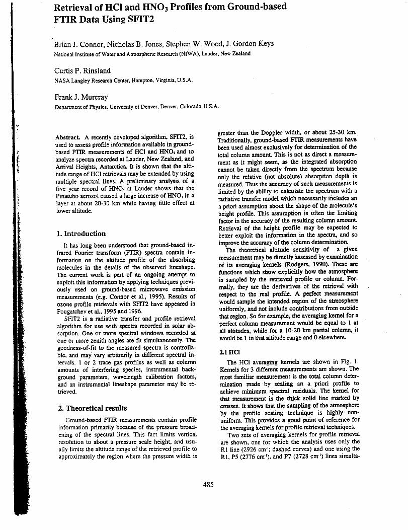
Retrieval of HCI and HNO3 Profiles from Ground-based

FTIR Data Using SFIT2

Brian J. Connor, Nicholas B. Jones, Stephen W. Wood, J. Gordon Keys

National Institute of Water and Atmospheric Research (NIWA), Lauder, New Zealand

Curtis P. Rinsland

NASA Langley Research Center, Hampton, Virginia, U.S.AI

Frank J. Murcray

Department of Physics, University of Denver, Denver, Colorado, U.S.A.

Abstract. A recently developed algorithm, SFXI2, isused to assess profile information available in ground-based FTIR measurements of HCI and HNO3 and to

analyze spectra recorded at Lauder, New Zealand, andArrival Heights, Antarctica. It is shown that the alti-

tude range of HCI retrievals may be extended by usingmultiple spectral lines. A preliminary analysis of afive year record of HNO_ at Lauder shows that thePinatubo aerosol caused a large increase of HNO_ in alayer at about 20-30 km while having little effect atlower altitude.

1. Introduction

It has long been understood that ground-based in-frared Fourier transform (FTIR) spectra contain in-formation on the altitude profile of the absorbingmolecules in the details of the observed lineshape.The current work is part of an ongoing attempt toexploit this information by applying techniques previ-ously used on ground-based microwave emissionmeasurements (e.g. Connor et al., 1995). Results ofozone profile retrievals with SFIT2 have appeared inPougatchev et ai., 1995 and 1996.

SFTF2 is a radiative transfer and profile retrievalalgorithm for use with spectra recorded in solar ab-sorption. One or more spectral windows recorded atone or more zenith angles are fit simultaneously. Thegoodness-of-fit to the measured spectra is controlla-ble, and may vary arbitrarily in different spectral in-tervals. 1 or 2 trace gas profiles as well as columnamounts of interfering species, instrumental back-ground parameters, wavelength calibration factors,and an instrumental lineshape parameter may be re-trieved.

2. Theoretical results

Ground-based FTIR measurements contain profileinformation primarily because of the pressure broad-ening of the spectral lines. This fact limits verticalresolution to about a pressure scale height, and usu-ally limits the altitude range of the retrieved profile toapproximately the region where the pressure width is

greater than the Doppler width, or about 25-30 kin.Traditionally, ground-based FTIR measurements havebeen used almost exclusively for determination of thetotal column amount. This is not as direct a measure-

ment as it might seem, as the integrated absorptioncannot be taken directly from the spectrum because

only the relative (not absolute) absorption depth ismeasured. Thus the accuracy of such measurements is

limited by the ability to calculate the spectrum with aradiative transfer model which necessarily includes an

a priori assumption about the shape of the molecule'sheight profde. This assumption is often the limitingfactor in the accuracy of the resulting column amount.Retrieval of the height profile may be expected tobetter exploit the information in the spectra, and soimprove the accuracy of the column determination.

The theoreticalaltitudesensitivityof a given

measurementmay bedirectlyassessedby examination

of itsaveragingkernels(Rodgers,1990).These am

functionswhich show explicitlyhow theatmosphere

issampledby theretrievedprofileor column. For-

maUy, they axe the derivatives of the retrieval withrespect to the real profile. A perfect measurementwould sample the intended region of the atmosphereuniformly, and not include contributions from outsidethat region. So for example, the averaging kernel for aperfect column measurement would be equal to 1 atall altitudes, while for a 10-20 km partial column, itwould be 1 in that altitude range and 0 elsewhere.

2.1 HCI

The HCI averaging kernels are shown in Fig. I.Kernels for 3 different measurements are shown. Themost familiar measurement is the total column deter-

mination made .by scaling an a priori profile toachieve minimum spectral residuals. The kernel forthat measurement is the thick solid line marked bycrosses.Itshows thatthesamplingoftheatmosphere

by the profilescalingtechnique is highly non-

uniform.Thisprovidesa good pointofreferencefortheaveragingkernelsforprofileretrievaltechniques.

Two setsof averagingkernelsforprofileretrievalam shown, one forwhich the analysisusesonlythe

RI line(2926cmt; dashedcurves)and one usingtheRI, P5 (2776cm't),and P7 (2728cm") linessimulta-

485

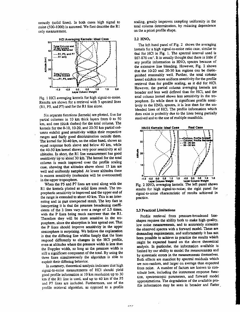
neously(solidlines). In both cases high signal tonoise (500-1000) is assumed. We first describe the R1only measurement.

HCI AveragingKernels: Ideal Case "so ........... ; .... ; 'i ........

I_--R1.PS, ImdP7 _ ._ [ ,_"

(

-1.0 .0.5 0.0 0.5 1.0 " 1_ .... 2.0

Layer Column Weight

Fig. I HCI averaging kernels for high signal-to-noise.Results are shown for a retrieval with 3 spectral lines

(Rl, P5, and I>7) and for the Rl line alone.

Six separate functions (kernels) are plotted, five forpartial columns in 10 km thick layers from 0 to 50km, and one (thick dashes) for the total column. Thekernels for the 0-10, 10-20, and 20-30 km partial col-umns exhibit good sensitivity within their respectiveranges and fairly good discrimination outside them.The kernel for 30-40 kin, on the other hand, shows an

equal response both above and below 40 kin, whilethe 40-50 km kernel shows very poor sensitivity at allaltitudes. In short, the Rt line measurement has good

semiti_,iW'iip to'aboiff 30 ]_.'The kei'r/ei for the totalcolumn is much improved over the profile scalingcase, showing that altitudes above about 15 km arewell and uniformly sampled. At lower altitudes thereis excess sensitivity (molecules will be overcounted)in the upper troposphere.

When the P5 and P7 lines are used along with the

R1 the kernels plotted as solid lines result. The tro-pospheric sensitivity is improved and the upper end ofthe range is extended to about 40 kin. This is an inter-esting and in part unexpected result. The key fact ininterpreting it is that the pressure broadening coeffi-cients of the 3-lines vary over a range of 2.5 awes,with the P lines being much narrower than the R1.

Therefore they will be more sensitive in the tro-

posphere,since the absorption is less spread out. Thatthe P lines should improve sensitivity in the upperstratosphere is surprising. We believe the explanationis that the differing line widths limply that the linesrespond differently to changes in the HCI profile,even at altitudes where the pressure width is less than

the Doppler width, so long as the pressure width isstill a significant component of the total. By using thethree lines simultaneously the algorithm is able to

exploit their differing behavior.In summary, theoretical analysis indicates that high

signal-to-noise measurements of HCI should yield

good profde information at I0 krn resolution up to 30krn if the RI line is used, and up to 40 km ff the P5and P7 lines are included. Furthermore, use of the

profile retrieval algorithm, as opposed to a profile

scaling, greatly improves sampling uniformity in thetotal column determination, by reducing dependence

on the a priori profde shape.

2.2 HNO)

The left hand panel of Fig. 2 shows the averagingkernels for a high signal-to-noise ratio case, similar tothat for HCI in Fig. 1. The spectral interval used is867-870 cm". It is usually thought that there is little ifany profile information in HNO) spectra because ofthe extensive line blending. However, Fig. 2 showsthat the 10-20 and 20-30 km regions can be distin-

guished reasonably well. Further, the total columnkernel exhibits more uniform sensitivity for the profileretrieval than for profile scaling, as it did for HCI.However, the partial column averaging kernels arebroader and less well def'med than for HCI, and thetotal column kernel shows less sensitivity in the tro-

posphere. So while there is significant profile sensi-tivity in the HNO3 spectra, it is less than for the un-blended lines of HC1. The profile information whichdoes exist is probably due to the lines being partiallyresolved and to the use of multiple manifolds.

HNO3 Kemele: Ideal Caae

4Oso....... ;.i',."'..../''''''''"...20 ".*'" .

10

0

ReelCase.... ,r.-., .... ,-- -,- --

+-_.,ol_nn, Profile•_ Column, Profile Re_'l_v_-- Io-2o Jan I/ T

//•1.0 -0.S 0.0 0.5 1.0 1.5 -0.5 0.0 0.5 1.0 1.5

Layer Column WqdgM Layer Coka.n Weight

Fig. 2 I-[HO) averaging kernels. The [eft panel showsresults for high signal-to-noise; the right panel forsignal-to-noise characteristic of results achieved in

practice.

2.3 Practical IJmRaflons

Profile retrieval from pressure-broadened line-

shapes requires the ability both to make high quality,low noise measurements, and to accurately simulate

the observed spectra with a forward model. These aredemanding requirements, and unfortunately it has notbeen possible to achieve in practice the results whichmight be expected based on the above theoreticalanalysis. In particular, the informationavailable islimited by our ability to model the measurements andby systematic errors in the measurements themselves.Both effects are manifest by spectral residuals whichare non-random, and larger on average than expectedfrom noise. A number of factors are known to con-

tribute here, including the instrument response func-

tion, spectroscopic parameters, and forward modelapproximations. The degradation of the available pro-file information may be seen in broader and flatter

averaging Ker-_els; ]mpl_ng less Glser;_ana,_on be-

tween layers and more influence of the a priori.

For HNO3 as measured at Lauder, the effective

si_gnal-to-noise (determined by the magnitude of the

spectral residuals) is about 200; the averaging kernels

for such measurements are shown on the right-hand

panel of Fig. 2. While the comparison to the high

signal-to-noise case in the left-hand panel is disap-

pointing, there is stiU some ability to distinguish the 2layers, and the total column kernel is stili better than

that for profile scaling. In the next section we will

show results which suggest that useful profile infor-

mation may be acquired from such measurements in

practice as well as in theory.

3. Atmospheric Measurements

Despite both theoretical and practical limitations,early results of profile retrievals on atmospheric dataare reasonably encouraging. We have made a prelimi-

nary analysis of the Lauder HNO3 data set, and ex-perimented with a small number of LauderHC1 meas-urements and HNO3 measurements from ArrivalHeights, Antarctica. It should be noted that this is

work-in-progress, and that further developments can

be expected.

HCl, Lauder, P7 Region PS Regionoo1,.0°_1°I _ .0.iilI1.021 h 1.051 -- m /

2727.70 2727.80 2775.65 2775.75

R1 Region HCI, 7 Sept 1993

-0.01 / l .f 30

._ 1.10-- :

1.00 ...i ! -oJot _ 1_ lo8:18[ 1 0

;nmtoo 1o" lO"_° lO"_ 1 4wmmuasNr (cm-1) mx_agm,eo

Fig. 3. An HCI retrieval from data of 7 September

1993 at Lauder, New Zealand. The 3 spectra shown

were fit simultaneously in retrieving the profile shown

in the lower right panel.

3.1 HCl

An example of an HC1 spectrum and profile meas-ured at Lauder is shown in Fig. 3. The spectral data

quality is excellent and the calculated spectrum fitsthe measurement to 1:500 on average. It is interesting

to note that all 3 spectral regions are fit reasonably

well, although small systematic features do dominate

the residuals, the most visible being in the P5 line

center. Despite this, while the retrieved profile is gen-erally reasonable, there is a significant discrepancy,

up to a factor 1.7, with HALOE HCI in the 20-30 inn

region. The cause of this is still being investigated. A

detailed algorithm comparison was recently carriedout (A. Goldman, private communication, 1996)

which would appear to role out the algorithm as the

principal source of this discrepancy.

487

3,2-H_U_ ................. : ....

Measurements have been made at Lander (45 S)

since 1990 at 0.0035 - 0.007 cm "t resolution. Fig. 4

shows partial columns in the 10-20 and 20-30 km

layers. The data are monthly averages. The solid lines

are regression fits to the daily data (not shown) before

the Pinatubo eruption and in 1994-95, including an-

nual, semi-annual, and secular terms. Fig 5 shows the

ratio of the partial columns. The data show a repeat-

able annual cycle and a clear response to the Mt. Pi-

natubo aerosol injection. Further, HNO3 behaves dif-

ferently in the two altitude regions. The annual cycle

differs in that the autumnal increase is later in the

lower layer. Also, the transient response to the Pi-

natubo aerosol was much greater in the upper layer.

1.2"1018!

1.0,10 TM

i &o.!ols

6,0.1018

&O*lO TM

2.0"101S

o

HNO3 Partial Columns at Lauder

...... , ......... t ........ , ......... , ......... , ......... , .........

1989 1990 1991 1992 1993 1094 1995 1996

Year

Fig. 4 A time series of HN03 in two layers at Lauder.The data points are monthly means. The solid line is a

regression fit to single measurements made before and

after the atmosphere was perturbed by the eruption ofMt. Pinatubo.

3.8

.J

]5 1.0

n. o,,c

HNO3 at Lauder

Rq...d=n _t _,'7 Ik=r_ly Data ,11

t!

191111 1990 1991 1992 1993 11194 1_16 1996

Year

Fig. 5. The ratio of the time series shown in Fig. 4.

HNO_ measurements are also made routinely at

Arrival Heights, Antarctica (78 S). Spectra are re-

corded at lower resolution (0.02 cm "t) than at Lmlder,

and ate genelally lower quality (Fig. 6). Nevertheless,

trials with the 1993 data show a fall to spring change

in profile shape roughly consistent with CLAES

measurements (Kumer et aL, 1996) in 1992, in that

the relative decrease in HNO3 is greater above 20 km

than below.

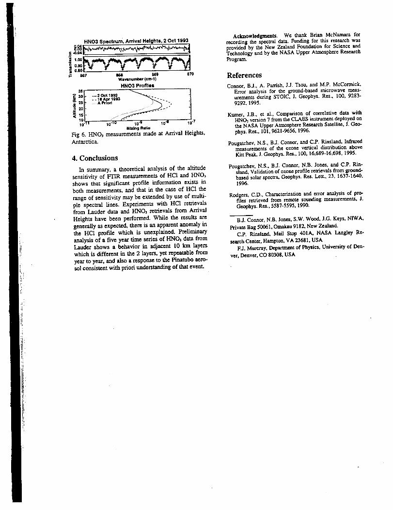
HNO3 Spectrum, Arrival Heights, 2 Oct 19938_8

: I.oo __o____0.90!0.80

)_ 867 s(_) u9 eTOWsvenumber (cm-1)

HNO3 Profiles

25

20

< 1510

..... A Priori _ "",

Mixing Rat|o

Fig 6. HNCh measurements made at Arrival Heights,

Antarctica.

4, Conclusions

In summary, a theoretical analysis of the altitude

sensitivity of FTIR measurements of HCI and HNO)

shows that significant profile information exists in

both measurements, and that in the case of HCI the

range of sensitivity may be extended by use of multi-

ple spectral lines. Experiments with HCI retrievalsfrom Lauder data and HNCh retrievals from Arrival

Heights have been performed. While the results are

generally as expected, there is art apparent anomaly in

the HCI profile which is unexplained. Preliminary

analysis of a five year time series of I-INCh data fromLauder shows a behavior in adjacent 10 km layers

which is different in the 2 layers, yet repeatable from

year to year, and also a response to the Pinambo aero-

sol consistent with priori understanding of that event.

Acknowledgments. We thank Brian McNamara forrecording the spectral data. Funding for this research wasprovided by the New Zealand Foundation for Science andTechnology and by the NASA Upper Atmosphere Research

Program.

References

Connor, BJ., A. Patrish, J.J. Tsou, and M.P. McCormick,Error analysis for the ground-based microwave meas-urements during STOIC, J. Geophys. Res., 100, 9283-

9292, 1995.

Kumer, J.B., et al., Comparison of correlative data withHNO3 version 7 from the CLAES instrument deployed onthe NASA Upper Atmosphere _ch Satellite, J. Geo-

phys. Res., 101, 9621-9656, 1996.

Pougatchev, N.S., BJ. Connor, and C.P. Rinsland, Infraredmeasurements of the ozone verticaldistributionaboveKitt Peak, J. Geophys. Res., 100, 16,689-16,698, 1995.

Pougatchev, N.S., B.J. Counor, N.B. Jones, and C.P. Rin-sland, Validation of ozone profile retrievals from ground-based solar spectra, Geophys. Res. Lett., 23, 1637-1640,1996.

Rodgers, C.D., Characterization and error analysis of pro-filesretrieved from remote sounding measurements,J.

Geophys. Res., 5587-5595, 1990.

B.J. Connor, N.B. Jones, S.W. Wood, J.G. Keys, NIWA,

Private Bag 50061, Omakau 9182, New Zealand.

C.P. Rinsland, Mall Stop 401A, NASA Langley Re-

search Centea', Hampton, VA 23681, USA

F.J. Mureray, Department of Physics, University of Den-

ver, Denver, CO 80308, USA

Retrieval of HCI and HNO3 Profiles from Ground-based

FTIR Data Using SFIT2

Brian J. Connor, Nicholas B. Jones, Stephen W. Wood, J. Gordon Keys

National Institute of Water and Atmospheric Research (NIWA), Lauder,New Zealand

Curtis P. Rinsland

NASA Langley Research Center,Hampton, Virginia, U.S.AI

Frank J. MurcrayDepartment of Physics, University of Denver, Denver, Colorado, U.S.A.

Abstract A recently developed algorithm, SFIT2, isused to assess profile information available in ground-based FTIR measurements of HCI and HNO3 and to

analyze spectra recorded at Lander, New Zealand, andArrival Heights, Antarctica. It is shown that the alti-tude range of HC1 retrievals may be extended by usingmultiple spectral lines. A preliminary analysis of afive year record of HNO3 at Lauder shows that thePinatubo aerosol caused a large increase of HNO_ in alayer at about 20-30 km while having little effect atlower altitude.

1. Introduction

It has long been understood that ground-based in-frared Fourier transform (FTIR) spectra contain in-formation on the altitude profile of the absorbingmolecules in the details of the observed lineshape.

The current work is part of an ongoing attempt toexploit this information by applying techniques previ-ously used on ground-based microwave emissionmeasurements (e.g. Cormor ct al., 1995). Results of

ozone profile retrievals with SH'I2 have appeared inPougatchev et al., 1995 and 1996.

SFIT2 is a radiative transfer and profile retrievalalgorithm for use with spectra recorded in solar ab-sorption. One or more spectral windows recorded atone or more zenith angles are fit simultaneously. Thegoodness-of-fit to the measured spectra is controlla-ble, and may vary arbitrarily in different spectral in-tervals. 1 or 2 trace gas profiles as well as columnamounts of interfering species, instrumental back-

ground parameters, wavelength calibration factors,and an instrumental lineshape parameter may be re-trieved.

2. Theoretical results

Ground-based FTIR measurements contain profile

information primarily because of the pressure broad-enmg of the spectral lines. This fact limits verticalresolution to about a pressure scale height, and usu-ally limits the altitude range of the retrieved profile toapproximately the region where the pressure width is

greater than the Doppler width, or about 25-30 kin.Traditionally, ground-based FTIR measurements havebeen used almost exclusively for determination of thetotal column amount. This is not as direct a measure-

ment as it might seem, as the integrated absorptioncannot be taken directly from the spectrum becauseonly the relative (not absolute) absorption depth ismeasured. Thus the accuracy of such measurements islimited by the ability to calculate the spectrum with aradiative transfer model which necessarily includes an

a priori assumption about the shape of the molecule'sheight profile. This assumption is often the limitingfactor in the accuracy of the resulting column amount.Retrieval of the height profile may be expected to

better exploit the information in the spectra, and soimprove the accuracy of the column determination.

The theoretical altitude sensitivity of a givenmeasurement may be directly assessed by examination

of its averaging kernels (Rodgers, 1990). These arefunctions which show explicitly how the atmosphere

is sampled by the retrieved profile or column. For-mally, they are the derivatives of the retrieval withrespect to the real profile. A perfect measurementwould sample the intended region of the atmosphereuniformly, and not include contributions from outsidethat region. So for example, the averaging kernel for a

perfect column measurement would be equal to 1 atall altitudes, while for a 10-20 km partial column, itwould be 1 in that altitude range and 0 elsewhere.

2.1HCi

The HCf averaging kernels are shown in Fig. 1.Kernels for 3 different measurements are shown. Themost familiar measurement is the total column deter-

ruination made .by scaling an a priori profile toachieve minimum spectral residuals. The kernel forthat measurement is the thick solid line marked by

crosses. It shows that the sampling of the atmosphere

by the profile scaling technique is highly non-uniform. This provides a good point of reference forthe averaging kernels for profile retrieval techniques.

Two sets of averaging kernels for profile retrievalare shown, one for which the analysis uses only theRI line (2926 cmt; dashed curves) and one using theRI, P5 (2776 cm'_), and P7 (2728 cm "_) lines simulta-

485

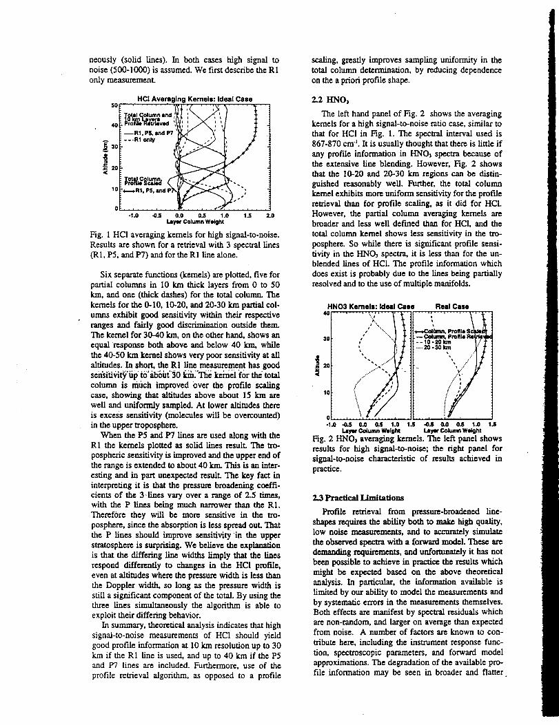
neously(solidlines).In bothcases high signal tonoise (500-1000) is assumed. We first describe the RIonly measurement.

50

40

30

2o(

10

HCfAveragingKernels:Ideal Case. . , .... , ...,

_'_tmlC;olumn mnd,

.--.R1 only

" ot I !

-1.0 -O`5 0.0

." L

. J

." I 1

0.5 1.0 1`5 2.0

Layer Column Weight

Fig. 1 HCI averaging kernels for high signal-to-noise.Results are shown for a retrieval with 3 spectral lines(R1, P5, and P7) and for the R1 line alone.

Six separate functions (kernels) are plotted, five forpartial columns in 10 km thick layers from 0 to 50kin, and one (thick dashes) for the total column. The

kernels for the 0-10, 10-20, and 20-30 km partial col-umns exhibit good sensitivity within their respectiveranges and fairly good discrimination outside them.The kernel for 30-40 kin, on the other hand, shows anequal response both above and below 40 kin, while

the 40-50 km kernel shows very poor sensitivity at allaltitudes. In short, the R1 line measurement has goodsen_iki_t_'iip' tb'ab_iK'30 ]_:ia:'Th_kemei for the totalcolumn is much improved Over the profile scalingcase, showing that altitudes above about 15 km arewell and uniformly sampled. At lower altitudes thereis excess sensitivity (molecules will be overcounted)in the upper troposphere.

When the P5 and 1>7 fines are used along with theR1 the kernels plotted as solid fines result. The tro-pospheric sensitivity is improved and the upper end ofthe range is extended to about 40 kin. This is an inter-esting and in part unexpected result. The key fact ininterpreting it is that the pressure broadening coeffi-cients of the 3-lines vary over a range of 2.5 times,with the P lines being much narrower than the R1.Therefore they will be more sensitive in the tro-

posphere, since the absorption is less spread out. Thatthe P lines should improve sensitivity in the upperstratosphere is surprising. We believe the explanationis that the differing line widths limply that the linesrespond differently to changes in the HCI profile,even at altitudes where the pressure width is less thanthe Doppler width, so long as the pressure width isstill a significant component of the total. By using thethree lines simultaneously the algorithm is able toexploit their differing behavior.

In summary, theoretical analysis indicates that highsignal-to-noise measurements of HCI should yieldgood profile information at I0 km resolution up to 30km if the R1 line is used, and up to 40 km if the P5and 1'7 lines are included. Furthermore, use of theprofile retrieval algorithm, as opposed to a profile

scaling, greatly improves sampling uniformity in thetotal colunm determination, by reducing dependenceon the a priori profile shape.

2.2 HNO_

The left hand panel of Fig. 2 shows the averagingkernels for a high signal-to-noise ratio case, similar tothat for HCI in Fig. I. The spectral interval used is867-870 cm "l. It is usually thought that there is little ifany profile information in HNO3 spectra because ofthe extensive line blending. However, Fig. 2 showsthat the 10-20 and 20-30 km regions can be distin-gnished reasonably well. Further, the total columnkernel exhibits more uniform sensitivity for the profileretrieval than for profile scaling, as it did for HCI.However, the partial column averaging kernels arebroader and less well defined than for HCI, and thetotal column kernel shows less sensitivity in the tro-

posphere. So while there is significant profile sensi-tivity in the HNO3 spectra, it is less than for the un-blended fines of HCI. The profile information which

does exist is probably due to the fines being partiallyresolved and to the use of multiple manifolds.

HNO3 Kernels: Ideal40 .... , .... I-:-,i-.-

// "°'-...

30 • "",

:

o _

_20 "" .........

10

:ase Real Case

i .... .r---, .... ,-- -, ..

_--l.Col_mn, Profile-- c,_mm,_ron_Re_l.--lo.ao_n l/"?

....Jl/..." • .:." tt"

_(ii'' "/,:............... /

1.5 -0.5 0,0 0`5 1.0 1`5

I._y_r Column Weight

0

-1.0 -O.S 0.0 0,5 1.0Llyw Column Weight

Pig. 2 HNO3 averaging kernels. The left panel showsresults for high signal-to-noise; the fight panel forsignal-to-noise characteristic of results achieved inpractice.

2.3 Practical Limitations

Profile retrieval from pressure-broadened line-

shapes requires the ability both to make high quality,low noise measurements, and to accurately simulate

the observed spectra with a forward model. These aredemanding requirements, and tmforttmately it has notbeen possible to achieve in practice the results whichmight be expected based on the above theoreticalanalysis. In particular, the information available islimited by our ability to model the measurements andby systematic errors in the measurements themselves.Both effects are manifest by spectral residuals whichare non-random, and larger on average than expectedfrom noise. A number of factors are known to con-

tribute here, including the instrument response func-tion, spectroscopic parameters, and forward modelapproximations. The degradation of the available pro-file information may be seen in broader and flatter.

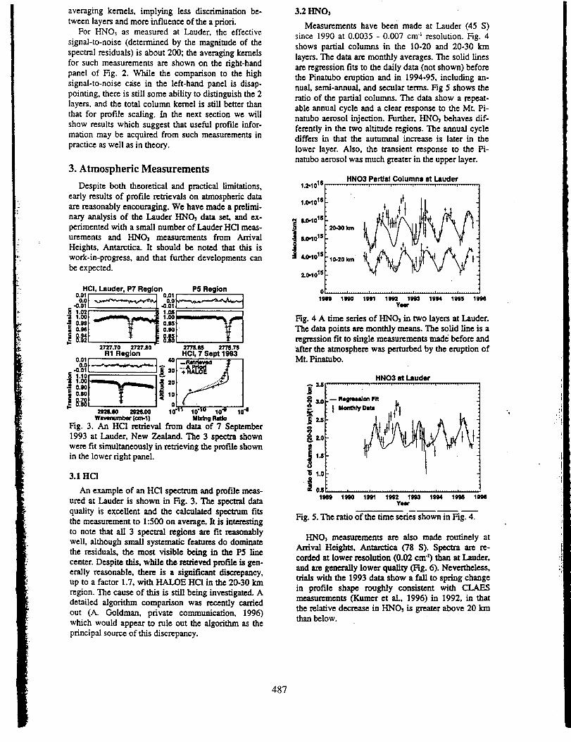
averaging kernels, implying less discrimination be-tween layers and more influence of the a priori.

For HNO3 as measured at Lauder, the effective

signal-to-noise (determined by the magnitude of thespectral residuals) is about 200; the averaging kernelsfor such measurements are shown on the right-handpanel of Fig. 2. While the comparison to the highsignal-to-noise case in the left-hand panel is disap-pointing, there is still some ability to distinguish the 2layers, and the total column kernel is still better than

that for profile scaling. In the next section we willshow results which suggest that useful profile infor-mation may be acquired from such measurements inpractice as well as in theory.

3. Atmospheric Measurements

Despite both theoretical and practical limitations,early results of profile retrievals on atmospheric dataare reasonably encouraging. We have made a prelimi-nary analysis of the Lauder HNO3 data set, and ex-perimented with a small number of Lauder HC! meas-urements and HNO3 measurements from ArrivalHeights, Antarctica. It should be noted that this is

work-in-progress, and that further developments canbe expected.

HCf, Lsuder, P7 Region PS Region

•o.G1i _ .o.G11 I1.051 , _

o..I -2727.70 2"_'.SO 27_.!_ 1"/'75.75

RI Region HCI, 7 Sept 1993

0.0_,'_ 4-O.01 1 I _[ 30

I 1.10r i1.00

| o.90t _f t g 18:t8t + 1"

_as.eo wae.oe Io"_ lohe 1(I"_ 1 4w_,._mm¢ (cm-l) U_ngm_o

Fig. 3. An HC] retrieval from data of 7 September1993 at Lauder, New Zealand. The 3 spectra shownwere fit simultaneously in retrieving the profile shownin the lower right panel.

3.1 HC1

An example of an HCI spectrum and profile meas-ured at Lauder is shown in Fig. 3. The spectral dataquality is excellent and the calculated spectrum fitsthe measurement to 1:500 on average. It is interestingto note that all 3 spectral regions are fit reasonablywell, although small systematic features do dominatethe residuals, the most visible being in the P5 linecenter. Despite this, while the retrieved profile is gen-erally reasonable, there is a significant discrepancy,up to a factor 1.7, with HALOE HCI in the 20-30 kmregion. The cause of this is still being investigated. Adetailed algorithm comparison was recently carriedout (A. Goldman, private communication, 1996)which would appear to rule out the algorithm as theprincipal source of this discrepancy.

487

3.2 HNO3

Measurements have been made at Lauder (45 S)

since 1990 at 0.0035 - 0.007 cm "_resolution. Fig. 4

shows partial columns in the 10-20 and 20-30 kinlayers. The data are monthly averages. The solid linesare regression fits to the dally data (not shown) beforethe Pinatubo eruption and in 1994-95, including an-nual, semi-annual, and secular terms. Fig 5 shows theratio of the partial columns. The data show a repeat-able annual cycle and a clear response to the Mt. Pi-natubo aerosol injection. Further, HNO3 behaves dif-ferently in the two altitude regions. The annual cyclediffers in that the autumnal increase is later in the

lower layer. Also, the transient response to the Pi-natubo aerosol was much greater in the upper layer.

HNO3 Partial Columnl at Lmuder1.2.1018 ......... , ......... , ......... , .................. , .......... . ........

+'7........................Fig. 4 A time series of HNO, in two layers at Lauder.The data points are monthly means. The solid line is aregression fit to single measurements made before andafter the atmosphere was perturbed by the eruption ofMt. Pinatubo.

"6 1.0

.I

HN03 at Lauder

;_ Regnm_an Fit L

Uo.mVO,,- ,_

n,, 0.5 ................ _ ..... - .........................................

19119 1990 19111 1992 1993 111114 111116 19911Yea"

Fig. 5. The ratio of the time series shown in Fig. 4.

HNO_ measurements are also made routinely atArrival Heights, Antarctica (78 S). Spectra are re-corded at lower resolution (0.02 cm") than at Lander,

and are generally lower quality (Fig. 6). Nevertheless,trials with the 1993 data show a fall to spring changein profile shape roughly consistent with CLAESmeasurements 0framer et eL, 1996) in 1992, in thatthe relative decrease in HNO_ is greater above 20 kinthan below.

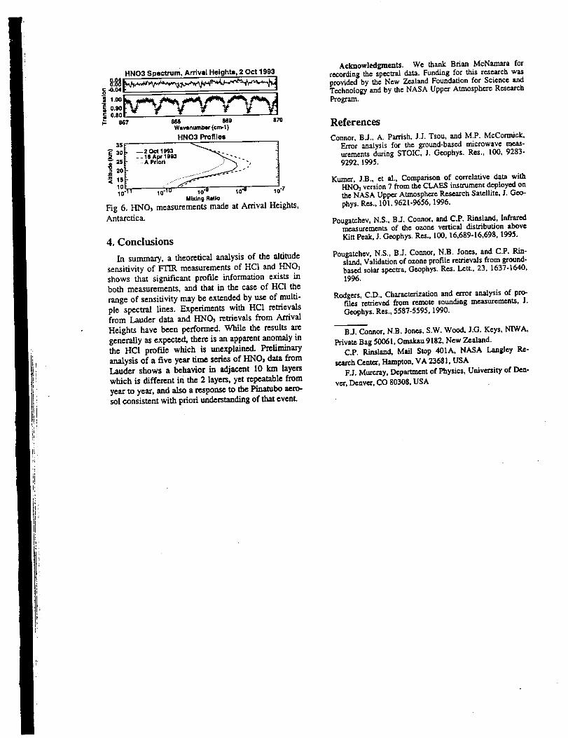
HNO3 Spectrum, Arrival Heights, 2 Oct 1993

-o:o4

1.00 I

0.80t,- 867

=( 1o10°11

_68 _9Wsvlnumb_"(cm-1)

HNO3 Profiles

87O

10-10 10 "g 10 .8

Mixing Ratio

Fig 6. HNO) measurements made at Arrival Heights,

Antarctica.

4. Conclusions

In summary, a theoretical analysis of the altitude

sensitivity of FITR measurements of HCI and HNO3

shows that significant prof'de information exists in

both measurements, and that in the case of HCI the

range of sensitivity may be extended by use of multi-

ple spectral lines. Experiments with HCl retrievalsfrom Lauder data and HNO3 retrievals from Arrival

Heights have been performed. While the results are

generally as expected, there is an apparent anomaly in

the HCI profile which is unexplained. Preliminary

analysis of a five year time series of I-INO) data fromLauder shows a behavior in adjacent 10 km layers

which is different in the 2 layers, yet repeatable from

year to year, and also a response to the Pinatubo aero-sol consistent with priori understanding of that event.

Acknowledgments. We thank Brian McNamara forrecording the spectral data. Funding for this research wasprovided by the New Zealand Foundation for Science andTechnology and by the NASA Upper Atmosphere ResearchProgram.

References

Connor, B.J., A. Parrish, J.J. Tsou, and M.P. McCormick,Error analysis for the ground-based microwave meas-urements during STOIC, J. Geophys. Res., 100, 9283-9292, 1995.

Kumer, J.B., et al., Comparison of correlative data withHNO_ version 7 from the CLAES instrument deployed onthe NASA Upper Atmosphere Research Satellite. J. Gco-

phys. Res., 101, 9621-9656, 1996.

Pougatchev, N.S., BJ. Coanor, and C.P. Rinsland, Infraredmeasurements of the ozone vertical distribution aboveKitt Peak, J. Geophys. Res., 100, 16,689-16,698, 1995.

Pougatchev, N.S., B.J. Cormor, N.B. Jones, and C.P. Rin-sland, Validation of ozone profile retrievals from ground-based solar spectra, Geophys. Res. LetL, 23, 1637-1640,1996.

Rodgers, C.D., Characterization and error analysis of pro-files retrieved from remote sounding measurements, J.

Geophys. Res., 5587-5595, 1990.

BJ. Coanor, N.B. Jones, S.W. Wood, J.G. Keys, NIWA,

Private Bag 50061, Omakan 9182, New Zealand.C.P. Rinsland, Mail Stop 401A, NASA Langley Re-

search Center, Hampton, VA 23681, USA

F.J. Mutcray, Department of Physics, University of Den-

ver, Denver, CO 80308, USA

® Pergamon

J. Quant. Spectrosc. RadJat. Transfer Vol. 60, No, 5, pp. 803-814, 1998Published by Elsevier Science Ltd

Printed in Great Britain

PII: S0022-4073(98)00083-1 0022--4073/98 519.00 + 0.00

SPECTROSCOPIC PARAMETERS FOR OZONE AND ITS

ISOTOPES: CURRENT STATUS, PROSPECTS FOR

IMPROVEMENT, AND THE IDENTIFICATION OF

160160170 AND 160170160 LINES IN INFRARED

GROUND-BASED AND STRATOSPHERIC SOLAR

ABSORPTION SPECTRA

C. P. RINSLAND,t* J.-M. FLAUD,_: A. GOLDMAN,§ A. PERRIN,,C. CAMY-PEYRET,¶ M. A. H. SMITH,t V. MALATHY DEVI,II D. C. BENNER,I[

A. BARBE,** T. M. STEPHEN§ and F. J. MURCRAY§tNASA Langley Research Center, Mail Stop 401A, Hampton, VA 23681-0001, U.S.A., _Laboratoire de

Photophysique Moleculaire, CNRS, BAt. 210, Universit6 Paris-Sud, Campus d'Orsay. 91405 Orsay Cedex,France, §Department of Physics, University of Denver, Denver, CO 80208, U.S.A., ¶Laboratoire dePhysique Moleculaire et Applications, CNRS, Boite 76, Universit_ Paris VI, 4 Place Jussieu, 75252 ParisCedex 05, France, IIDepartment of Physics, The College of William and Mary, Williamsburg. VA23187-8795. U.S.A. and **Groupe de Spectrometrie MolEculaire et Atmosphrrique, Universit_ de Reims,Equipe Associ_ au CNRS, UPRESA Q 6089 et ce n'est plus D 1434, UFR Sciences, B. P. 1039, 51687

Reims Cedex 2, France

(Receiped ._ June 1997)

Abstract--We describe the updates to the spectroscopic parameters of ozone and its isotopes

in the 1996 HITRAN compilation. Recent published studies not included in HITRAN are

also summarized. Finally, we report the identification of infrared lines of the v3 bands

of 160160170 and 160170160 in high-resolution solar spectra recorded by stratosphericballoon-borne and ground-based Fourier transform spectrometers. Published by ElsevierScience Ltd.

1. INTRODUCTION

Spectroscopic parameters of ozone are required for virtually all remote-sensing applicationsinvolving the chemistry of the troposphere and stratosphere. The vertical distribution of ozonealso influence the thermal structure of the atmosphere by absorbing and reemitting radiationin the 8-12 lam window. Hence, the knowledge of the 03 vertical distribution is needed forclimate research, z-4 For these reasons, numerous experimental and theoretical investigationshave focused on improving our knowledge of infrared, microwave, and electronic ozone spectro-scopy, s.6

The main purpose of this paper is to document the updates to the ozone spectroscopic parametersin the 1996 HITRAN compilation. 7 A total of 30 bands have been added and nine bands have beenmodified since the 1992 edition, s-t° extending the upper wave number limit of the compilation from3400 to 4100 cm-l. The updates include lines of the z60160170 and trOt 70 trO isotopic specieswhich appear in the microwave and infrared sections of the compilation for the first time. However,the new edition does not include the results of many recent studies, and in fact, presently, no

parameters are included for the near infrared, visible, and UV spectral regions. Therefore, asa second part of the paper, we provide a brief overview of recent laboratory and modeling work onozone and its isotopes and highlight areas in need of further investigation. Finally, we present theidentification of lines of v3 bands of 160160170 and 160170140 in high-resolution infrared

ground-based and stratospheric solar absorption spectra.

*To whom all correspondence should be addressed.

803

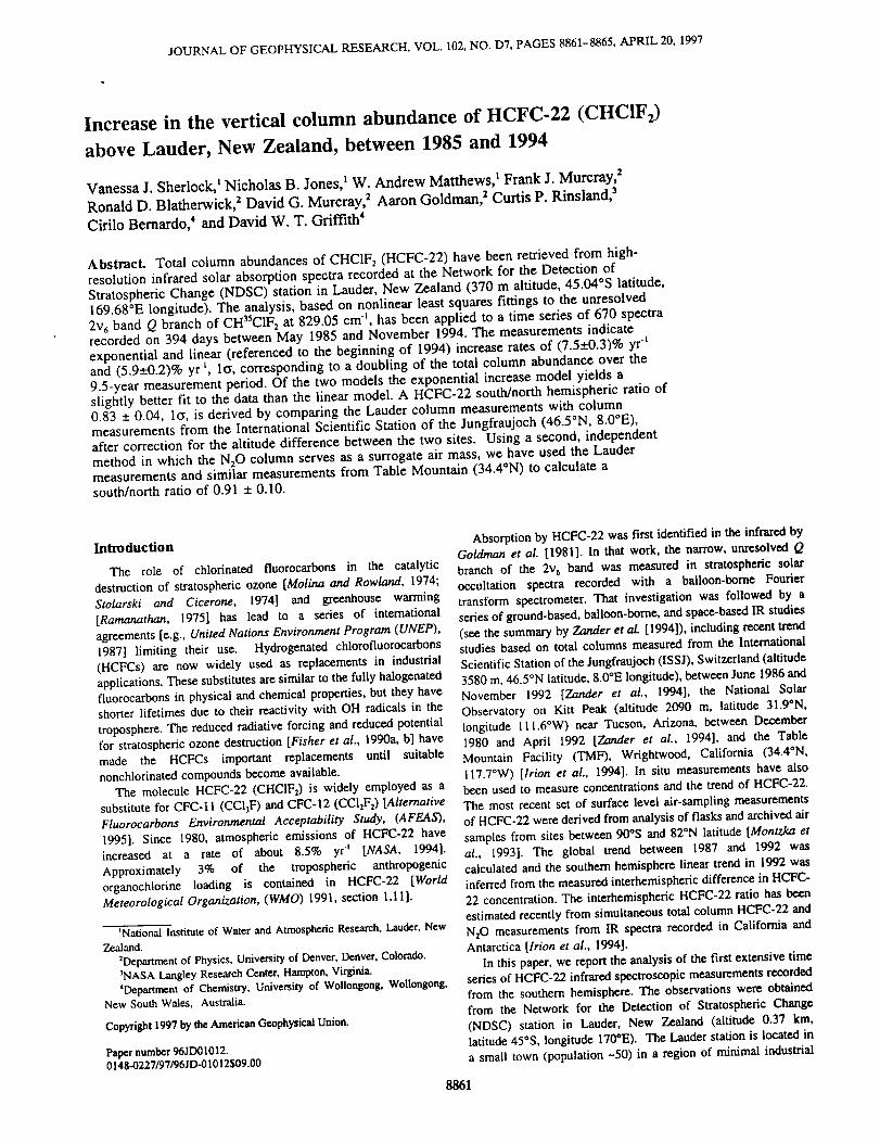
JOURNALOFGEOPHYSICALRESEARCH,VOL.102, NO. D7, PAGES 8861-8865, APRIL 20. 1997

Increase in the vertical column abundance of HCFC-22 (CHCIF2)

above Lauder, New Zealand, between 1985 and 1994

Vanessa J. Sherlock, I Nicholas B. Jones, t W. Andrew Matthews, t Frank J. Murcray, 2

Ronald D. Blatherwick, 2 David G. Murcray, 2 Aaron Goldman, 2 Curtis P. Rinsland, 3

Cirilo Bernardo, 4 and David W. T. Griffith _

Abstract. Total column abundances of CHC1F2 (HCFC-22) have been retrieved from high-

resolution infrared solar absorption spectra recorded at the Network for the Detection of

Stratospheric Change (NDSC) station in Lauder, New Zealand (370 m altitude, 45.04°S latitude,

169.68°E longitude). The analysis, based on nonlinear least squares fittings to the unresolved

2v6 band Q branch of CH35C1F2 at 829.05 cm l, has been applied to a time series of 670 spectra

recorded on 394 days between May 1985 and November 1994. The measurements indicate

exponential and linear (referenced to the beginning of 1994) increase rates of (7.5__.0.3)% yr t

and (5.9±0.2)% yr t, lo, corresponding to a doubling of the total column abundance over the

9.5-year measurement period. Of the two models the exponential increase model yields a

slightly better fit to the data than the linear model. A HCFC-22 south/north hemispheric ratio of

0.83 +-. 0.04, lc, is derived by comparing the Lauder column measurements with column

measurements from the International Scientific Station of the Jungfraujoch (46.5°N, 8.0°E),

after correction for the altitude difference between the two sites. Using a second, independent

method in which the N20 column serves as a surrogate air mass, we have used the Lauder

measurements and similar measurements from Table Mountain (34.4°N) to calculate a

south/north ratio of 0.91 ± 0.10.

Introduction

The role of chlorinated fluorocarbons in the catalytic

destruction of stratospheric ozone [Molina and Rowland, 1974;

Stolarski and Cicerone, 1974] and greenhouse warming

[Ramanathan, 1975] has lead to a series of international

agreements [e.g., United Nations Environment Program ( UNEP),

1987] limiting their use. Hydrogenated chlorofluorocarbons

(HCFCs) are now widely used as replacements in industrial

applications. These substitutes are similar to the fully halogenated

fluorocarbons in physical and chemical properties, but they have

shorter lifetimes due to their reactivity with OH radicals in the

troposphere. The reduced radiative forcing and reduced potentialfor stratospheric ozone destruction [Fisher et al., 1990a, b] have

made the HCFCs important replacements until suitable

nonchlorinated compounds become available.The molecule HCFC-22 (CHCIF2) is widely employed as a

substitute for CFC-I 1 (CCI3F) and CFC-12 (CClzFz) [Alternative

Fluorocarbons Environmental Acceptability Study, (AFEAS),

1995]. Since 1980, atmospheric emissions of HCFC-22 have

increased at a rate of about 8.5% yr "t [NASA, 1994].

Approximately 3% of the tropospheric anthropogenic

organochlorine loading is contained in HCFC-22 [WorldMeteorological Organization, (WMO) 1991, section 1.11].

_National Institute of Water and Atmospheric Research, Lauder, New

Zealand._Department of Physics, University of Denver, Denver, Colorado.

_NASA Langley Research Center, Hampton, Virginia.

4Departrnent of Chemistry, University of Wollongong, Wollongong,New South Wales, Australia.

Copyright 1997 by the American C-eophysieal Union.

Paper number 96JD01012.0148-0227/97/96JD-01012509.00

Absorption by HCFC-22 was first identified in the infrared by

Goldman et al. [1981]. In that work, the narrow, unresolved Q

branch of the 2v6 band was measured in stratospheric solar

occultation spectra recorded with a balloon-borne Fourier

transform spectrometer. That investigation was followed by a

series of ground-based, balloon-borne, and space-based IR studies

(see the summary by Zander et aL [1994]), including recent trendstudies based on total columns measured from the International

Scientific Station of the Jungfraujoch (ISSJ), Switzerland (altitude

3580 m, 46.5°N latitude, 8.0°E longitude), between June 1986 and

November 1992 [Zander et al., 1994], the National Solar

Observatory on Kitt Peak (altitude 2090 m, latitude 31.9°N,

longitude 111.6°W) near Tucson, Arizona, between December

1980 and April 1992 [Zander et al., 1994], and the Table

Mountain Facility (TMF), Wrightwood, California (34.4°N,

117.7°W) [Irion et al., 1994]. In situ measurements have also

been used to measure concentrations and the trend of HCFC-22.

The most recent set of surface level air-sampling measurements

of HCFC-22 were derived from analysis of flasks and archived air

samples from sites between 90°S and 82°N latitude [Montzka et

al., 1993]. The global trend between 1987 and 1992 was

calculated and the southern hemisphere linear trend in 1992 was

inferred from the measured interhemispheric difference in HCFC-

22 concentration. The interhemispheric HCFC-22 ratio has been

estimated recently from simultaneous total column HCFC-22 and

N20 measurements from IR spectra recorded in California and

Antarctica [lrion et al., 1994].

In this paper, we report the analysis of the first extensive time

series of HCFC-22 infrared spectroscopic measurements recorded

from the southern hemisphere. The observations were obtained

from the Network for the Detection of Stratospheric Change

(NDSC) station in Lauder, New Zealand (altitude 0.37 kin,

latitude 45*S, longitude 170*E). The Lauder station is located in

a small town (population -50) in a region of minimal industrial

8861

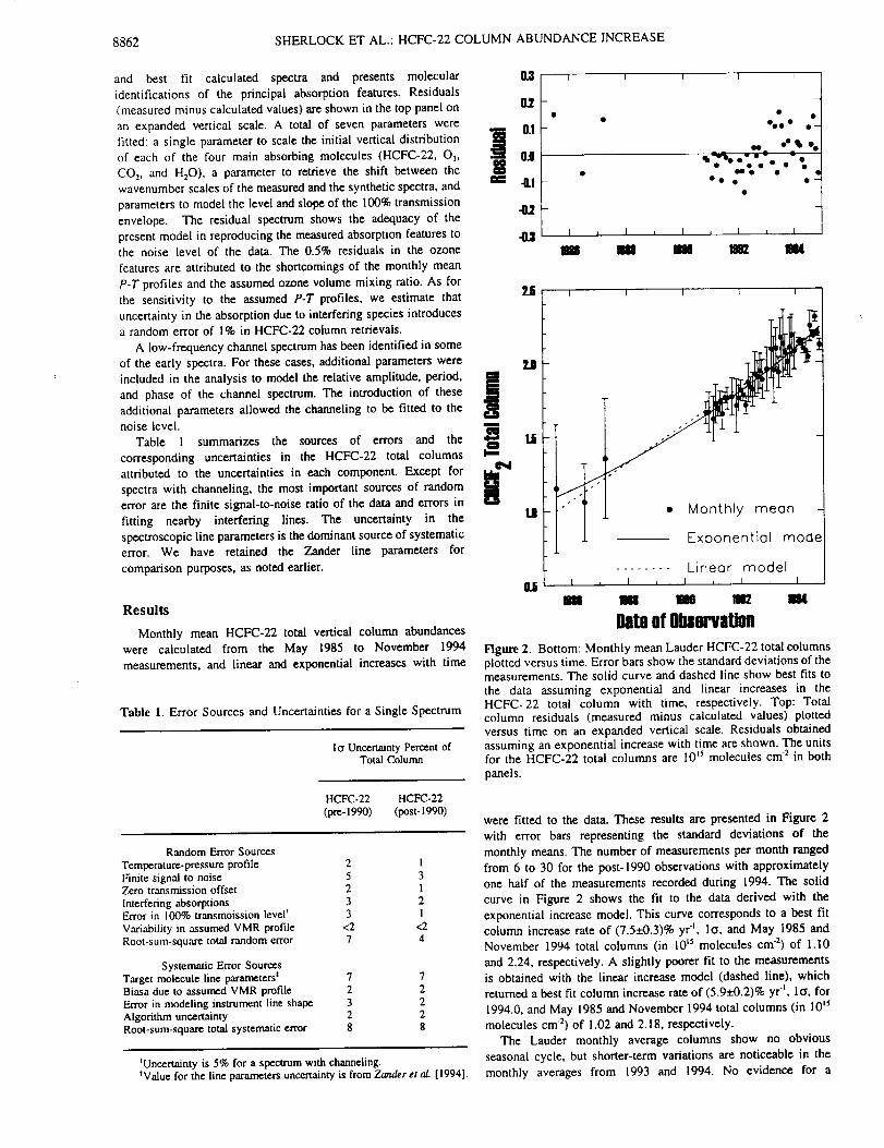
8862 SHERLOCK ET AL.: HCFC-22 COLUMN ABUNDANCE INCREASE

and best fit calculated spectra and presents molecular

identifications of the principal absorption features. Residuals

(measured minus calculated values) are shown in the top panel on 0"2

an expanded vertical scale. A total of seven parameters were _ [1fitted: a single parameter to scale the initial vertical distribution __

of each of the four main absorbing molecules (HCFC-22, 03, _1_ 011CO z, and H20), a parameter to retrieve the shift between thewavenumber scales of the measured and the synthetic spectra, and _1

parameters to model the level and slope of the 100% transmission 41envelope• The residual spectrum shows the adequacy of the

present model in reproducing the measured absorption features to -0.3

the noise level of the data. The 0.5% residuals in the ozone

features are attributed to the shortcomings of the monthly mean

P-T profiles and the assumed ozone volume mixing ratio. As for

the sensitivity to the assumed P-T profiles, we estimate that U

uncertainty in the absorption due to interfering species introducesa random error of 1% in HCFC-22 column retrievals.

A low-frequency channel spectrum has been identified in some

of the early spectra. For these cases, additional parameters were U

included in the analysis to model the relative amplitude, period, H

and phase of the channel spectrum. The introduction of these |additional parameters allowed the channeling to be fitted to the

noise level, im

Table I summarizes the sources of errors and the '_ tli

corresponding uncertainties in the HCFC-22 total columnsattributed to the uncertainties in each component. Except for

spectra with channeling, the most important sources of random Iterror are the finite signal-to-noise ratio of the data and errors in

fitting nearby interfering lines. The uncertainty in the

spectroscopic line parameters is the dominant source of systematic

error. We have retained the Zander line parameters for

comparison purposes, as noted earlier.

E--_Tq,.__

Results

Monthly mean HCFC-22 total vertical column abundances

were calculated from the May 1985 to November 1994

measurements, and linear and exponential increases with time

Table 1. Error Sources and Uncertainties for a Single Spectrum

Io Uncertamty Percent ofTotal Column

U I I I I I

• • 0000 O--

oo °°_°oqb_ O _ In, _O 7. •

• -, No • ,2

i I ] I• I J I i L

I m m

I I l I

tO • Monthly meon

Exponentiol mode

........ Lineor model

U I _ I , I L I _ I

Dateof Observation

Figure 2. Bottom: Monthly mean Lauder HCFC-22 total columnsplotted versus time. Error bars show the standard deviations of themeasurements. The solid curve and dashed line show best fits to

the data assuming exponential and linear increases in theHCFC-22 total column with time, respectively. Top: Totalcolumn residuals (measured minus calculated values) plotted

versus time on an expanded vertical scale. Residuals obtained

assuming an exponential increase with time are shown. The unitsfor the HCFC-22 total columns are 10 j5 molecules cm 2 in both

panels.

HCFC-22 HCFC-22

(pre- 1990) (post- 1990)

Random Error Sources

Temperature-pressure profile 2Finite signal to noise 5Zero transmission offset 2

Interfering absorptions 3Error in 100% transmoission level r 3

Variability in assumeA VMR profile <2Root-sum-square total random error 7

Systematic Error SourcesTarget molecule line parameters* 7Biasa due to assumed VMR profile 2Error in modeling instrument line shape 3Algorithm uncertainty 2Root-sum-square total systematic error g

I3I2I

<24

_Uncertainty is 5% for a spectrum with channeling.:Value for the Line parameters uncertainty is from Zanderet al. [1994]•

were fitted to the data. These results are presented in Figure 2

with error bars representing the standard deviations of the

monthly means. The number of measurements per month ranged

from 6 to 30 for the post-1990 observations with approximately

one half of the measurements recorded during 1994. The solid

curve in Figure 2 shows the fit to the data derived with the

exponential increase model. This curve corresponds to a best fit

column increase rate of (7.5!-0.3)% yr -1, 1_, and May 1985 and

November 1994 total columns (in 10 _5 molecules cm 2) of 1.10

and 2.24, respectively. A slightly poorer fit to the measurementsis obtained with the linear increase model (dashed line), which

returned a best fit column increase rate of (5.9:t-0.2)% yr t, 1o', for

1994.0, and May 1985 and November 1994 total columns (in 10 _5

molecules cm z) of 1.02 and 2.18, respectively.

The Lander monthly average columns show no obvious

seasonal cycle, but shorter-term variations are noticeable in the

monthly averages from 1993 and 1994. No evidence for a

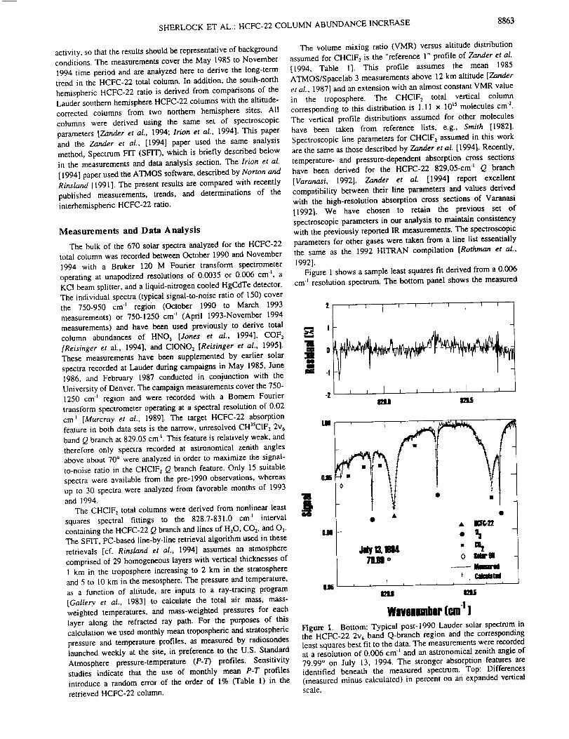
SHERLOCKETAL.:HCFC-22COLUMNABUNDANCEINCREASE8863

activity,sothattheresultsshouldberepresentativeofbackgroundconditions.ThemeasurementscovertheMay1985toNovember1994timeperiodandareanalyzedheretoderivethelong-termtrendintheHCFC-22totalcolumn.Inaddition,thesouth-northhemisphericHCFC-22ratioisderivedfromcomparisonsof theLandersouthernhemisphereHCFC-22columnswiththealtitude-correctedcolumnsfromtwonorthernhemispheresites.Allcolumnswerederivedusingthesamesetof spectroscopicparameters[Zanderet aL, 1994; lrion et al., 1994]. This paper

and the Zander et al., [1994] paper used the same analysis

method, Spectrum FIT (SFIT), which is briefly described below

in the measurements and data analysis section. The Irion et al.

[ 1994] paper used the ATMOS software, described by Norton and

Rinsland [ 1991 ]. The present results are compared with recently

published measurements, trends, and determinations of the

interhemispheric HCFC-22 ratio.

Measurements and Data Analysis

The bulk of the 670 solar spectra analyzed for the HCFC-22

total column was recorded between October 1990 and November

1994 with a Bruker 120 M Fourier transform spectrometer

operating at unapodized resolutions of 0.0035 or 0.006 cm t, a

KCI beam splitter, and a liquid-nitrogen cooled HgCdTe detector.

The individual spectra (typical signal-to-noise ratio of 150) cover

the 750-950 cm l region (October 1990 to March 1993

measurements) or 750-1250 cm t (April 1993-November 1994

measurements) and have been used previously to derive total

column abundances of HNO 3 [Jones et al., 1994], COF2

[Reisinger et al., 1994], and CIONOz [Reisinger et al., 1995].These measurements have been supplemented by earlier solar

spectra recorded at Lauder during campaigns in May 1985, June

1986, and February 1987 conducted in conjunction with the

University of Denver. The campaign measurements cover the 750-

1250 cm _ region and were recorded with a Bomem Fourier

translbrm spectrometer operating at a spectral resolution of 0.02

cm _ [Murcray et al., 1989]. The target HCFC-22 absorption

feature in both data sets is the narrow, unresolved CH35CIF2 2v6

band Q branch at 829.05 cm t. This feature is relatively weak, and

therefore only spectra recorded at astronomical zenith angles

above about 70 ° were analyzed in order to maximize the signal-

to-noise ratio in the CHCIFz Q branch feature. Only 15 suitable

spectra were available from the pre-1990 observations, whereas

up to 30 spectra were analyzed from favorable months of 1993

and 1994.

The CHCIF2 total columns were derived from nonlinear least

squares spectral fittings to the 828.7-831.0 cm t interval

containing the HCFC-22 Q branch and lines of H20, COy and 03.

The SFIT, PC-based line-by-line retrieval algorithm used in these

retrievals [cf. Rinsland et al., 1994] assumes an atmosphere

comprised of 29 homogeneous layers with vertical thicknesses of

I km in the troposphere increasing to 2 km in the stratosphere

and 5 to 10 km in the mesosphere. The pressure and temperature,

as a function of altitude, are inputs to a ray-tracing program

[Gallery. et al., 1983] to calculate the total air mass, mass-

weighted temperatures, and mass-weighted pressures for each

layer along the refracted ray path. For the purposes of thiscalculation we used monthly mean tropospheric and stratospheric

pressure and temperature profiles, as measured by radiosondes

launched weekly at the site, in preference to the U.S. Standard

Atmosphere pressure-temperature (P-T) profiles. Sensitivity

studies indicate that the use of monthly mean P-T profiles

introduce a random error of the order of 1% (Table l) in the

retrieved HCFC-22 column.

The volume mixing ratio (VMR) versus altitude distribution

assumed for CHC1F2 is the "reference 1" profile of Zander et al.

[1994, Table 1]. This profile assumes the mean 1985

ATMOS/Spacelab 3 measurements above 12 km altitude [Zander

et al., 1987] and an extension with an almost constant VMR value

in the troposphere. The CHC1F2 total vertical column

corresponding to this distribution is 1.11 × 10 _5 molecules cm z.

The vertical profile distributions assumed for other molecules

have been taken from reference lists, e.g., Smith [1982].

Spectroscopic line parameters for CHC1F2 assumed in this workare the same as those described by Zander et al. [1994]. Recently,

temperature- and pressure-dependent absorption cross sectionshave been derived for the HCFC-22 829.05-cm -t Q branch

[Varanasi, 1992]. Zander et al. [1994] report excellent

compatibility between their line parameters and values derived

with the high-resolution absorption cross sections of Varanasi

[1992]. We have chosen to retain the previous set of

spectroscopic parameters in our analysis to maintain consistency

with the previously reported IR measurements. The spectroscopic

parameters for other gases were taken from a line list essentially

the same as the 1992 HITRAN compilation [Rothraan et al.,

1992].

Figure l shows a sample least squares fit derived from a 0.006

cm _ resolution spectrum. The bottom panel shows the measured

W

Nml

' ' I ' ' ' ' 1 ' '

i i I , i _ , I , ,W

tOO

0.15

[m

tim

• ICIg-_

• %, c%

71111o O Saltml_Mmm/

+ Calmlatal

UU Ull

Wavnmnber(cmt )

Figure 1. Bottom: Typical post-1990 Lauder solar spectrum inthe HCFC-22 2V 6 band Q-branch region and the corresponding

least squares best fit to the data. The measurements were recordedat a resolution of 0.006 cm _ and an astronomical zenith angle of

79.99 ° on July 13, 1994. The stronger absorption features areidentified beneath the measured spectrum. Top: Differences

(measured minus calculated) in percent on an expanded vertical

scale.

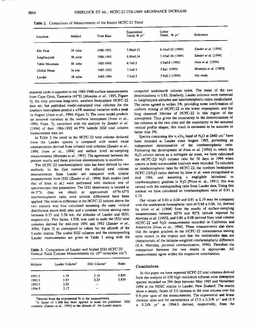
8864 SHERLOCKETAL.:HCFC-22COLUMNABUNDANCEINCREASE

Table2. ComparisonofMeasurementsoftheRecentHCFC-22Trend

Exponcntial LinearLocation Method Time Basc Trend, % yr"_ Trend, % yr.) Refcrenc_

Kin Peak IR solar 1980-1992 7.00x_.23 6.16i-0.20 (1989)

Jungfraujoch IR solar 1986-1992 6.99_-0.34 7.45±0.34 (1989)

Table Mountain IR solar 1985-1990 6.7±0.5 5.9x'-0.8 (1990)

Global Mean In situ 1987-1992 7.3-.t-0.3 5.8±1 (1992)

Lauder IR solar 1985-1994 7.5±0.3 5.9±0.2 (1994)

Zander et al. [1994]

_er et o2. [1994]

lrion et al. [1994]

Montzka et ol. [1993]

this study

seasonal cycle is apparent in the 1985-1988 surface measurements

from Cape Grim, Tasmania (41°S) [Montzka et al., 1993, Figure

3], the only previous long-term, southern hemisphere HCFC-22

data set, but published model-calculated total columns for the

southern hemisphere predict a ±3% seasonal variation with a peak

in August [lrion et al., 1994, Figure 3]. The same model predicts

no seasonal variation in the northern hemisphere [lrion et al.,

1994, Fiure. 3], consistent with the analysis by Zander et al.

[1994] of their 1986-1992 46.5°N latitude ISSJ total column

measurement data set.

In Table 2 the trend in the HCFC-22 total column deduced

from the Lauder spectra is compared with recent trend

measurements derived from infrared total columns [7_ander et al.,

1994; Irion et al., 1994] and surface level air-sampling

measurements [Montzlca et al., 1993]. The agreement between the

present results and these previous determinations is excellent.

The HCFC-22 interhemispheric ratio has been derived by two

methods. In the first method the infrared total column

measurements from Lauder are compared with similar

measurements from ISSJ [Zander et al., 1994]. Both studies (and

that of Irion et al.) were performed with identical sets of

spectroscopic line parameters. The ISSJ observatory is located at

46.5°N, thus we obtain an approximate 45°N-45°S

interhemispheric ratio, once altitude differences have been

applied. The relative difference in the HCFC-22 column above the

two stations was first calculated assuming the same vertical

distribution above both sites and a constant volume mixing ratio

between 0.37 and 3.58 km, the altitudes of Lauder and ISSJ,

respectively. This factor, 1.508, was used to scale the ISSJ total

columns derived for mid-year 1991 and 1992 [Zander et al.,

1994, Table 3] to correspond to values for the altitude of the

Lauder station. The scaled ISSJ columns and the corresponding

Lauder measurements are given in Table 3 along with the

Table 3. Comparison of Lauder and Scaled ISSJ HCFC-22Vertical Total Column Measurements (in 10 's molecules cm -z)

Midyear Lauder Column' ISSJ Column* Ratio

1991.5 1.74 2.10 0.829

1992.5 1.87 2.23 0.839

1993.5 2.02 --

1994.5 2.17 --

'Derived from the exponential fit to the measurements.*A factor of 1.508 has been applied to scale the published ISSJ

columns [Zander et al.. 1994] to the altitude of the Lauder station.

computed south/north column ratios. The mean of the two

determinations is 0.83. Similarly, Lauder columns were corrected

to Jungfraujoch altitudes and interhemispheric ratios recalculated.

The ratios agreed to within 2%, providing some confirmation of

uniform mixing of HCFC-22 in the lower troposphere, and the

long chemical lifetime of HCFC-22 in this region of the

atmosphere. Thus given the uncertainty in the determinations of

the columns at the two sites and the uncertainty in the assumed

vertical profile shapes, this result is estimated to be accurate to

better than 5%.

Spectra containing the vt+29 z band of N20 at 2440 cm" have

been recorded at Lauder since August 1993, permitting an

independent determination of the interhemispheric ratio.

Following the development of lrion et al. [1994] in which the

N20 column serves as a surrogate air mass, we have calculated

the HCFC-22/ NzO column ratio for 56 days in 1994 when

spectra in both wavenumber intervals were recorded. To calculate

an interhemispheric ratio for HCFC-22, the northern hemisphere

HCFC-22/NzO ratios derived by lrion et al. were extrapolated to

mid 1994, and assuming a negligible latitudinal or

interhemispheric gradient in N20 [Prinn et. at., 1991], this was

ratioed with the corresponding ratio from Lauder data. Using this

method we have calculated an interhemispheric ratio of 0.91 ±

0.10.

Our values of 0.83 ± 0.04 and 0.91 ± 0.10 may be compared

with the south/north hemispheric ratio of 0.88 ± 0.04, lff, derived

by lrion et al. [1994] from the results of surface-samplingmeasurements between 82°N and 90*S latitude reported by

Montzka et al. [1993], and 0.86 ± 0.08 derived from total column

HCFC-22 and N20 measurements recorded in California and

Antarctica [Irion et al., 1994]. These measurements also show

that the largest gradient in the HCFC-22 instantaneous mixing

ratio occurs in the tropics and that the midlatitudes data are

characteristic of the latitude-weighted interhemispheric difference

(S.A. Montzka, personal communication, 1996). Therefore the

comparison between the two results is appropriate. All

measurements agree within the respective uncertainties.

Conclusions

In this paper we have reported HCFC-22 total columns derived

from the analysis of 670 high-resolution infrared solar absorption

spectra recorded on 394 days between May 1985 and November1994 at the NDSC station in Lauder, New Zealand. The results

show a steady, factor of 2.0 increase in the total column over the

9.5-year span of the measurements. The exponential and linearincrease rates and lff uncertainties of (7.5 ± 0.3)% yrt and (5.9

± 0.2)% yr" at 1994.0 derived, respectively, from the

SHERLOCK ET AL.: HCFC-22 COLUMN ABUNDANCE INCREASE8865

measurements are in excellent agreement with previous

determinations of the trend through 1992 [Zander et al., 1994;

Montzka et al., 1993] and indicate that rapid accumulation of

HCFC-22 in the atmosphere continued during 1993 and 1994.

Comparisons of total columns measured at the Lauder station with

corresponding values measured at ISSJ [Zander et al., 1994]

indicate an instantaneous south/north hemispheric ratio of 0.83 ±

0.04. An independent calculation, based on the ratio of HCFC-22

and N20 columns gives an interhemispheric ratio of 0.91 4- 0.10

for HCFC-22. These results are in agreement within the

uncertainties with previous determinations based on surface air

sampling [Montzka et al., 1993] and infrared total column [Irion

et al., 1994] measurements.

Acknowledgments. Research at the NIWA is funded by the NewZealand Foundation for Research, Science, and Technology (contract CO

1221). Research at the University of Denver is funded by grants with theNational Aeronautics and Space Administration. The authors thank B. M.

McNamara for recording the high-resolution infrared solar spectra.

References

Alternative Fluorocarbons Environmental Acceptability Study, production,

(AFEAS), sales and atmospheric release of fluorocarbons through

1993, Washington, D. C., 1995.Fisher, D. A., C. H. Hales, D. L. Filkin, M. K. W. Ko, N. D. Sze, P. S.

Connell, D. J. Wuebbles, I. S. A. Isaksen, and F. Stordal, Modelcalculations of the relative effects of CFCs and replacements on

stratospheric ozone, Nature, 344, 508-512, 1990a.Fisher, D. A., C. H. Hales, W.-C. Wang, M. K. W. Ko, and N. D. Sze,

Model calculations of the relative effects of CFCs and their

replacements on global warming, Nature, 344, 513-516, 1990b.

Gallery, W. O., F. X. Kneizys, and S. A. Clough, Environ. Res. Pap. 828(AFGL-TR-83-O065), 145 pp., Air Force Geophys. Lab., Bedford,

Mass., 1983.Goldman, A., F. J. Murcray, R. J. Blatherwick, R. D. Bonomo, F. S.

Murcray, F. H. Murcray, and D. G. Murcray, Spectroscopicidentification of CHCIF, (F-22) in the lower stratosphere, Geophys.

Res. Lett., 8, 1012-1014, 1981.Irion, F. W., M. Brown, G." C. Toon, and M. R. Gunson, Increase in

atmospheric CHFzCI (HCFC-22) over southern California from 1985to 1990, Geophys. Res. Lett., 21, 1723-1726, 1994.

Jones, N. B., M. Koike, W. A. Mat'thews, and B. M. McNamara, Southern

hemisphere seasonal cycle in total column nitric acid, Geophys. Res.

Lett., 21,593-596, 1994.Molina, M. J., and F. S. Rowland, Stratospheric sink for

chlorofluoromethanes: Chlorine atom-catalysed destruction of ozone,

Nature, 249, 810-812, 1974.Montzka" S. A., R. C. Myers, J. H. Buffer, J. W. Elkins, and S. O.

Cummings, Global tropospheric distribution and calibration scale of

HCFC-22, Geophys. Res. Lett., 20, 703-706, 1993.

Murcray, F. J., W. A. Matthews, A. Goldman, P. V. Johnston, and C. P.Rinsland, NH3 column abundances over Lauder, New Zealand, J.

Geophys. Res., 94, 2235-2238, 1989.National Aeronautics and Space Administration (NASA), Present state of

knowledge of the upper atmosphere 1993: An assessment report, NASA

Re]i Publ. 1337, 1994.

Norton, R. H., and C. P. Rinsland, ATMOS data processing and science

analysis methods, Appl. Opt, 30, 389-400, 1991.Prinn, R., D. Cunnold, R. Rasmussen, P. Simmonds, F. Alyea, A.

Crawford, P. Fraser, and R. Rosen, Atmospheric emissions and trendsof nitric oxide deduced from ten years of ALE-GAGE data, J.

Geophys. Res., 95, 18369-18385, 1990.Ramanathan, V., Greenhouse effect due to chlorofluorocarbons: Climate

implications, Science, 190, 50-52, 1975.Reisinger, A., N. B. Jones, W. A. Matthews, and C. P. Rinsland, Southern

hemisphere ground-based measurements of carbonyl fluoride (COF_)

and hydrogen fluoride (HF): Partitioning between fluoride reservoir

species, Geophys. Res. Lett;, 21, 797-800, 1994.Reisinger, A., N. B. Jones, W. A. Matthews, and C. P. Rinsland, Southern

hemisphere midlatitude ground-based measurements of CIONOz:Method of analysis, seasonal cycle, and long-term trend. J. Geophys.

Res., 100, 23,183-23,193, 1995.Rinsland, C. P., N. B. Jones, and W. A. Matthews, Infrared spectroscopic

measurements of the total column abundance of ethane (C21_ aboveLauder, New Zealand, J. Geophys. Res., 99, 25,941-25,945, 1994.

Rothman, L. S., et al., The HITRAN molecular database: Editions of1991 and 1992, J. Quant. Spectrosc. Radiat. Transfer, 48, 469-507,

1992.Smith, M. A. H., Compilation of atmospheric gas concentration profiles

from 0 to 50 kin, NASA Tech. Memo. 83289, NASA Langley Res.

Cent., Hampton, 1982.Stolarski, R. S., and R. J. Cicerone, Stratospheric chlorine: A possible sink

for ozone, Can. J. Chem., 52, 1610-2615, 1974.United Nations Environment Programme (UNEP), Montreal Protocol on

Substances that Deplete the Ozone Layer, Final Act, 1987.Varanasi, P., Absorption spectra of HCFC-22 around 829 cm _ at

atmospheric conditions, J. Quant. Spectrosc. Radiat. Transfer, 47, 251-

255, 1992.World Meteorological Organization (WMO), Scientific assessment of

ozone depletion: 1991, WMO Rep. No. 25, Geneva, 1991.Zander, R., C. P. Rinsland, C. B. Farmer, and R. H. Norton, Infrared

spectroscopic measurements of halogenated source gases in thestratosphere with the ATMOS instrument, J. Geophys. Res., 92, 9836-

9850, 1987.Zander, R., E. Mahieu, P. Demoulin, C. P. Rinsland, D. K. Weisenstein,

M. K. W. Ko, N D. Sze, and M. R. Gunson, Secular evolution of thevertical column abundance of CHC1F2 (HCFC-22) in the earth's

atmosphere inferred from ground-based IR solar observations at the

Jungfraujoch and at Kitt Peak and comparisons with modelcalculations, J. Atmos. Chem., 18, 129-148, 1994.

R. D. Blatherwick, A. Goldman, D. G. Murcray, and F. J. Murcray,

Department of Physics, University of Denver, Denver, CO 80208-0202.(e-mail: blathe@ncar.ucar.edu; goldman@acd.ucar.edu; murcray@ram.

phys.du.edu)C. Bemardo and D. W. T. Griffith, Department of Chemistry,

University of Wollongong, Wollongong, NSW Australia. (e-mail:Dave Griffith@uow.ed.au)

N-B. Jones, W. A. Matthews, and V. J. Sherlock, NIWA Climate,

Private Bag 50061, Omakau, Lauder 9182, New Zealand. (e-mail:

n.jones@niwa.cri.nz; a.matthews @ niwa.cri.nz)C. P. Rinsland, NASA Langley Research Center, Mail Stop 401A,

Hampton, VA 23681-0001. (e-mail: rinsland@riscbox.larc.nasa.gov)

(Received April 14, 1995; revised February 29, 1996;

accepted February 29, 1996.)

e

[1

dJr

University of Denver infrared spectral atlases

A. Goldman, R. D. Blatherwick, F. J. Murcray, and D. G. Murcray

Jf

I

Atmospheric and laboratory atlases ofhigh-resolution infrared absorption spectra have_een generatedfrom data obtained with the University of Denver Michelson-type interferometer balloon-bornespectrometer systems. The main objectives of the atlas work have beem the.2dentification and thedetailed analysis of stratospheric infrared high-resolution spectral features. The stratospheric atlasescovermany spectral intervals and provide tables ofline positions and_pecies identifications. High Sunspectra are used for identification of solar lines. Latest editions of these atlases include selectedsections in the 760-1950- and 800-1700-cm -1 regions at 0.02- and 0.002-cm-1 resolutions, respectively.In addition to the stratospheric atlases, ground-based and laboratory spectral atlases have also beenproduced. The laboratory spectra of many molecules relevant to stratospheric chemistry, have beenobtained. A number of ongoing spectroscopic studies have been developed on the basis of the atlaswork, including studies of solar and atmospheric spectral features. _ 1996 Optical Societyof America

1. Introduction

The spectral atlas project at the University of Den-ver DU_ has been dedicated to the identification of

stratospheric IR spectral features present in high-resolution solar spectra and to the spectroscopicanalysis of specific stratospheric molecules such as03, IfINQ, C1ONQ, COF2, NQ, Q, C2H6, and others.The more recent of these studies have been based onballoon-borne solar absorption spectra at 0.002-cm -1resolution and corresponding laboratory spectra.

The atlases produced by this work ser_'e as state-of-the-art catalogs of atmospheric absorption featuresfor use by researchers in identifying features in theirown data. The line parameters generated from thespectroscopic analysis are essential to the quantifica-tion of molecular species from IR spectra. Theseline parameters have, in most cases, been added tothe HITRAN ihigh-resolution transmission molecu-lar absorptioni and other databases used by atmo-spheric spectroscopists.

Initially, solar spectra for the atlas project werecollected from Denver (elevation 1.6 km and thenearby Mt. Evans lelevation 4.3 krn! by the use of a0.06-cm -_ resolution iapodized)interferometer sys-tem. From these data, the 775-1300- and 1925-

The authors are with the Department of Physics. University ofDenver. Denver, Colorado 80208.

Received 10July 1995:revised manuscript received 14Novem-ber 1995

0003-6935 96 162821-07510.00 01996Optical Societyof._nerica

2175-cm -1 regions of the atlas have been completedand published in two volumes}

A short summary of the atlas work is given inTable 1. In 1978, the atmospheric spectroscopyg'roup at DU started obtaining IR spectra with a0.02-cm -1 resolution !apodized; interferometer sys-tem. A large number of high-quality spectra havebeen obtained, including laboratory spectra, ground-based solar spectra, and aircraft-borne and balloon-borne solar spectra. The spectra were obtained inselected intervals in the 550-2300-cm -1 region.Many of the laboratory spectra at 0.06- and 0.02-cm -{ resolutions have been published as a CRChandbook}

Numerous excellent 0.02-cm -1 resolution spectrawere also obtained from the South Pole, which is a

unique site for IR observations, in December 1978and December 1980. Thus work was also started onthe Atlas of South Pole IR Solar Spectra. 3 The firstedition of the South Pole Atlas, including the 760-960-cm -1 region, was published in March 1982. Inthe next large-format edition the 1220-1340-cm -_region was added, a

The first large-format edition of the stratosphericatlas, at 0.02-cm -_ resolution, was published inFebruary 1982. _ Several updated editions havesince been issued, the most recent of which is the

September 1987 edition, a This atlas now covers theentire spectral region from 760 to 1950 cm-1, exceptfor the 960-1060-cm-I interval. The total number

of spectral features identified as being genuine _tellu-tic or solari exceeded 14.000. In parallel with theatmospheric spectra work, the laboratory spectra '_

1June 1996 Vol.35. No. 16 APPLIEDOPTICS 2821

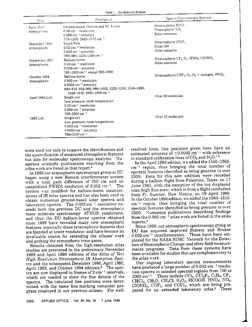
Table t. OUSpectralAtlases

Atlas Descripti;_n Special Spec'_rosc_pic Interest

June 1950

Atmosp_,erlc

December 1953

Atmospheric

September 1957

Atmospheric

October 1994

Atmospheric

April 1984 Lab

1995 Lab

Ground-based. Denver and .Nlt Evans

006-cm :resolution

0.006-cm 1 accuracy

775-1300, 1925-2175 cm l

South Pole

O.02-cm _ resolution

0.002 cm _ accuracy

760-960. 1220-1340 cm

Balloon-borne

0.02-cm 1 resolution

0.002-em- 1 accuracy

760-1950 cm -_ except 960-1060

Balloon-borne

0.002-cm _ resolution

0.0002-cm -1 accuracy

800-810. 934-960, 990-1002, 1220-1230, 1240-1260,

1540-1610, 1680-1690 cm l

Single cell

Low pressure, room temperature

0.02-cm- 1 resolution

0.002-cm- 1 accuracy

760-2000 cm -1

Single cell

Low pressure, room temperature0.002-cm- _ resolution

0.0002-cm- 1 accuracy

760-3100 cm -1

Stratospheric HNO_

Tropospheric NHs

Solar emission

Stratospheric HNO:_

Solar OH

Solar emission

Stratospheric CF4, O2, HNOa, CIONO2

Solar emission

Stratospheric COF2, 0.2, 03 + isotopes, HNO3

Over 30 molecules

Over 15 molecules

were used not only to support the identification andthe quantification of measured atmospheric featuresbut also for molecular spectroscopy analysis. Nu-merous scientific publications resulting from theatlas work are listed in that report. 4

In 1986 our atmospheric spectroscopy group at DU

began using a new Bomem interferometer systemwith a total path difference of 250 cm and an

unapodized FWHM resolution of 0.002 cm-L Thesystem was modified for balloon-borne measure-ments of IR solar spectra and has also been used toobtain numerous ground-based solar spectra andlaboratory spectra. The 0.002-cm -_ resolution ex-ceeds both the previous DU and the atmospherictrace molecule spectroscopy ATMOS)resolutions,and thus the DU balloon-borne spectra obtainedsince 1986 have revealed many new atmospheric

features especially those stratospheric features thatare blended at lower resolution! and have become aninvaluable source for extending the atlases' work

and probing the atmospheric trace gases.Results obtained from the high-resolution atlas

studies are presented in the preliminary November1989 and April 1990 editions of the Atlas of Ve_'High Resolution Stratospheric IR Absorption Spec-tra and the subsequent December 1990, April 1992,April 1993, and October 1994 editions. 6 The spec-tra are now displayed in frames of 2-cm -1 intervals,which are needed to show the fine details of the

spectra. The tabulated line positions were deter-mined with the same line-marking computer pro-

gram employed in our previous atlases. For well-

2822 APPLIED OPTICS Vol. 35, No. 16 1 June 1996

resolved lines, line positions given here have anestimated accuracy of +_0.0002 cm -_ with referenceto standard calibration lines of CO2 and N20. 7s

In the April 1993 edition, we added the 1540-1560-cm -1 region, thus bringing the total number of

spectral features identified as being genuine to over3300. Data for this new addition were recorded

during a balloon flight from Palestine, Texas, on 17June 1991. with the exception of the top displayed

scan _high Sun scan!, which is from a flight conductedfrom Ft. Sumner, New Mexico, on 19 April 1989.In the October 1994 edition, we added the 1560-1610-

cm -_ region, thus bringing the total number of

spectral features identified as being genuine to over3500. Numerous publications describing findingsfrom the 0.002-cm-_ atlas work are listed in the atlas

reportsfiSince 1990, our atmospheric spectroscopy group at

DU has acquired improved Bomem and Bruker0.002-cm -_ interferometers. These have been em-

ployed for the NASA NDSC Network for the Detec-tion of Stratospheric Changei and other field measure-ments programs. Data from these systems havebeen available for studies that are complementary to

the atlas work.Our ongoing laboratory spectra measurements

have produced a large number of 0.002-cm-_ resolu-tion spectra in selected spectral regions from 750 to3000 cm-L These include CC14, CC12F2, C2Hs, CF4,

CHCla, CH20, CHaC1, H202, HCOOH, HNO3, NO2,C1ONO2, COF2, and COC12, which are being pre-

pared for an extended laboratory atlas. ° These

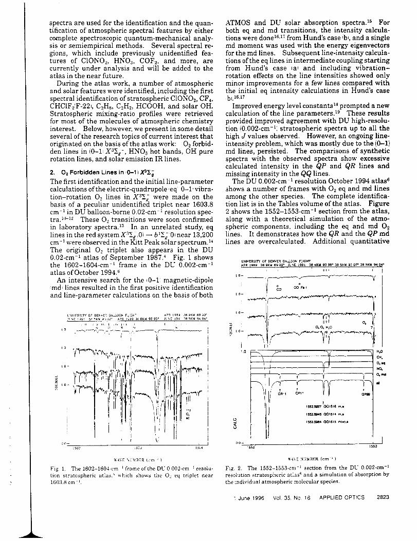
spectraareusedforthe identificationandthequan-tificationof atmosphericspectralfeaturesbyeithercompletespectroscopicquantum-mechanicalanaly-sisorsemiempiricalmethods. Severalspectralre-gions,which include previouslyunidentifiedfea-tures of C1ONQ, HNQ, COF2,and more, arecurrently underanalysisandwill beaddedto theatlasin thenearfuture.

Duringthe atlaswork,a numberof atmosphericandsolarfeatureswereidentified,includingthefirstspectralidentificationofstratosphericC1ONO2,CF4,CHC1F21F-22!,C2H6,C2H2,HCOOH,andsolarOH.Stratosphericmixing-ratioprofileswereretrievedfor mostof themoleculesof atmosphericchemistryinterest. Below,however,wepresentinsomedetailseveraloftheresearchtopicsofcurrentinterestthatoriginatedonthebasisoftheatlaswork: O2forbid-denlinesin (0-11X3_g-, HNO3hotbands,OHpurerotationlines,andsolaremissionIRlines.

2. 02 Forbidden Lines in t0--1) X3t:;

The first identification and the initial line-parametercalculations of the electric-quadrupole, eqi _0-11 vibra-

• " 3_: made on thetion-rotation O_ hnes m X ._ werebasis of a peculiar unidentified triplet near 1603.8

cm-1 in DU balloon-borne 0.02-cm-1 resolution spec-tra. 1°-12 These O2 transitions were soon confirmedin laboratory spectra. _3 In an unrelated study, eq

3"T I lX:lines in the red systemX ,_i0: _ b ,,:1:0: near 13,200• . 4_

1 14cm- were observed m the Kitt Peak solar spectrum.The original 02 triplet also appears in the DU0.02-cm -1 atlas of September 1987. 4 Fig. 1 showsthe 1602-1604-cm -t frame in the DU 0.002-cm -1atlas of October 1994. °

An intensive search for the (0-11 magnetic-dipole_md, lines resulted in the first positive identificationand line-parameter calculations on the basis of both

u_r';zRS:TY OF DENVER _.%._LOC),F:.:C:_7 APEI t90) _6 9Kk( 69 C_O"

J'l",E l_)gl 3d 5K_4 9_,)2._ _R I_, ]_8K)4 9295 ° JL>._ 19_): 28 5Kkm 9404"

LO-

,o-

00-

k_

t_I- ."¢ _i,"l' _ I'

U I!

i, ii

ti

I

T' I, -./"'_'."_

I i

" l:!f

l 5L,1_' :_OJ I_U4

_AVE \L_!3ER (crn )

Fig. 1. The 1602-1604-cm _ frame of the DU 0.002-cm _ resolu-

tion stratospheric atlas. _ which shows the 0,_ eq triplet near

1603.8 cm _1

ATMOS and DU solar absorption spectra, is Forboth eq and md transitions, the intensity calcula-tions were done _s,_ from Hund's case !b), and a singlemd moment was used with the energy eigenvectorsfor the md lines. Subsequent line-intensity calcula-tions of the eq lines in intermediate coupling startingfrom Hund's case ¢a) and including vibration-rotation effects on the line intensities showed only

minor improvements for a few lines compared withthe initial eq intensity calculations in Hund's casebL16.17

Improved energy level constants _s prompted a newcalculation of the line parameters. _9 These resultsprovided improved agreement with DU high-resolu-tion (0.002-cm -_) stratospheric spectra up to all thehigh J values observed. However, an ongoing line-intensity problem, which was mostly due to the (0--1)md lines, persisted. The comparisons of syntheticspectra with the observed spectra show excessivecalculated intensity in the QP and QR lines andmissing intensity in the QQ lines.

The DU 0.002-cm- _ resolution October 1994 atlas _

shows a number of frames with 02 eq and md linesamong the other species. The complete identifica-tion list is in the Tables volume of the atlas. Figure2 shows the 1552-1553-cm -_ section from the atlas,

along with a theoretical simulation of the atmo-spheric components, including the eq and md O_lines• It demonstrates how the QR and the QP mdlines are overcalculated. Additional quantitative

UNIVERSITY OF DEiWVER OALLOOt; F=IGHT

APR 1989 _69K)4 6900" JU_iE l_)9l 38,I, KM 909,8" 385KM 9302* 30 SI(J4 9404"

10_

I0--

<:

.z. _ o_

S0

1.0

k _ i14 i l'

oo CO, FoICO

o.:::o °'

?

m I

J

, , I $5"3b:bSZ

CH,

0,,

Oon_

_,av[ :WU,_ItKR (crn _ )

Fig 2. The 1552-1553-cm -_ section from the DC 0.002-cm -_

resolution stratospheric atlas 6 and a simulation of absorption by

the individual atmospheric molecular species.

1 June 1996 Vol. 35. No. 16 APPLIED OPTICS 2823

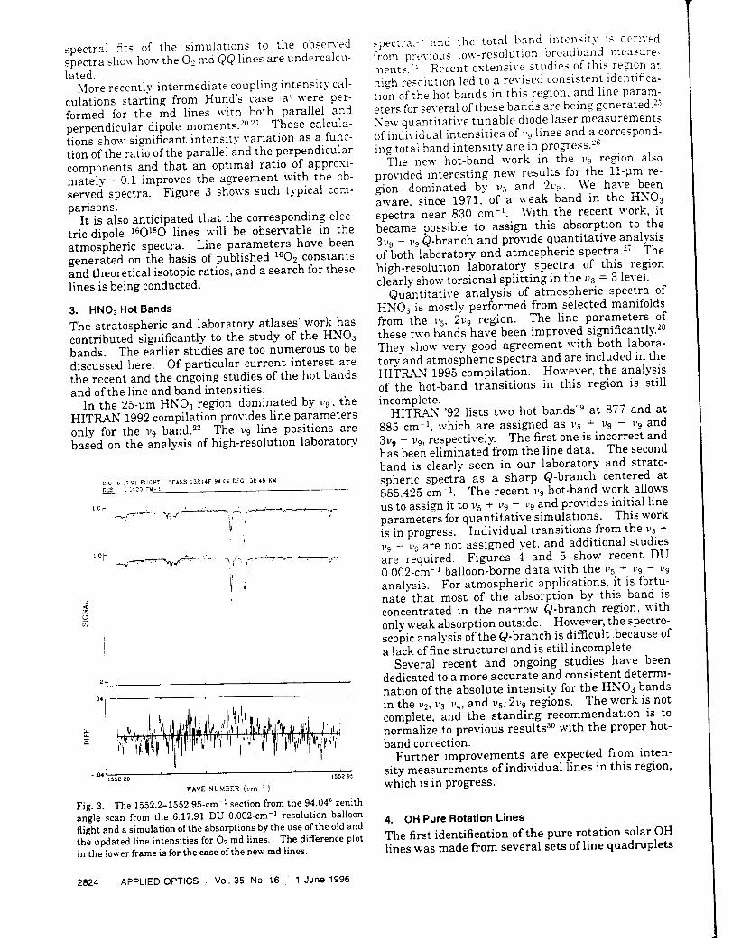
spectral fits of the simulations to the obseraedspectra show how the Oc md QQ lines are undercalcu-lated.

More recently, intermediate coupling intensity cal-culations starting from Hund's case ,a! were per-formed for the md lines with both parallel and

perpendicular dipole moments. 2°21 These calcula-tions show significant intensity variation as a func-tion of the ratio of the parallel and the perpendicular

components and that an optimal ratio of approxi-mately -0.1 improves the agreement with the ob-served spectra. Figure 3 shows such typical com-

parisons.It is also anticipated that the corresponding elec-

tric-dipole 16OlsO lines will be observable in theatmospheric spectra. Line parameters have beengenerated on the basis of published 1602 constantsand theoretical isotopic ratios, and a search for these

lines is being conducted.

3. HNOsHot Bands

The stratospheric and laboratory atlases' work hascontributed significantly to the study of the HNO3bands. The earlier studies are too numerous to be

discussed here. Of particular current interest arethe recent and the ongoing studies of the hot bandsand of the line and band intensities.

In the 25-1_m HNOa region dominated by v9', theHITRA-N 1992 compilation provides line parameters

only for the _'9 band.22 The v9 line positions arebased on the analysis of high-resolution laborato_'

D U b :'; 91 FLEGHT SCANS 13R]4F 94 £4 C[G 58 4B KM

, b

i

" _ ", , • _,;, f-" _ _ , ,_-_i

i! f'

.04 I I 1552951552 20

WAVE NUMIgER (cm : }

Fig. 3. The 1552.2-1552.95-cm -_ section from the 94.04 ° zenith

angle scan from the 6.17.91 DU 0.002-cm -1 resolution balloon

flight and a simulation of the absorptions by the use of the old and

the updated line intensities for 02 md lines. The difference plot

in the lower frame is for the case of the new md lines.

spectra.: and the total band intensity is derivedfrom previous low-resolution broadband measure-ments. :4 Recent extensive studies of this reDon at

high resolution led to a revised consistent identifica-tion of the hot bands in this re,on, and line param-eters for several of these bands are being generated. 2_

New quantitative tunable diode laser measurementsof individual intensities of ,'9 lines and a correspond-

ing total band intensity are in progress, caThe new hot-band work in the 1,9 region also

provided interesting new results for the ll-pm re-gion dominated by _'5 and 2r9!. We have beenaware, since 1971, of a weak band in the HNOa

spectra near 830 cm -1. With the recent work, itbecame possible to assign this absorption to the3v9 - _'9 Q-branch and provide quantitative analysisof both laboratory and atmospheric spectra, e: The

high-resolution laboratoD' spectra of this regionclearly show torsional splitting in the va = 3 level.

Quantitative analysis of atmospheric spectra ofHNOa is mostly performed from selected manifoldsfrom the t'5, 2v9 region. The line parameters ofthese two bands have been improved significantly. 2s

Thev show very good agreement with both labora-toryand atmospheric spectra and are included in theHITRA-N 1995 compilation. However, the analysisof the hot-band transitions in this region is still

incomplete.HITRAN '92 lists two hot bands 29 at 877 and at

885 cm -], which are assigned as _',_ + v9 - l'9 and3v9 - ,9, respectively. The first one is incorrect andhas been eliminated from the line data. The second

band is clearly seen in our laboratory and strato-

spheric spectra as a sharp Q-branch centered at885.425 cm-_. The recent _'9 hot-band work allowsus to assign it to v5 + v9 - _'9 and provides initial line

parameters for quantitative simulations. This workis in progress. Individual transitions from the ,5 -_'9 - 1,9are not assigned yet, and additional studiesare required. Figures 4 and 5 show recent DU0.002-cm -_ balloon-borne data with the "5 - v9 - _'9analysis. For atmospheric applications, it is fortu-nate" that most of the absorption by this band isconcentrated in the narrow Q-branch region, with

only weak absorption outside. However, the spectro-scopic analysis of the Q-branch is difficult :because ofa lack of fine structure! and is still incomplete•

Several recent and ongoing studies have beendedicated to a more accurate and consistent determi-nation of the absolute intensity for the HNOa bands

in the v2, _'a v4, and vs, 2v9 regions. The work is not

complete, and the standing recommendation is tonormalize to previous results a° with the proper hot-band correction.

Further improvements are expected from inten-

sity measurements of individual lines in this region,which is in progress.

4. OH Pure Rotation Lines

The first identification of the pure rotation solar OHlines was made from several sets of line quadruplets

2824 APPLIED OPTICS Vol. 35, No. 16 1 June 1996

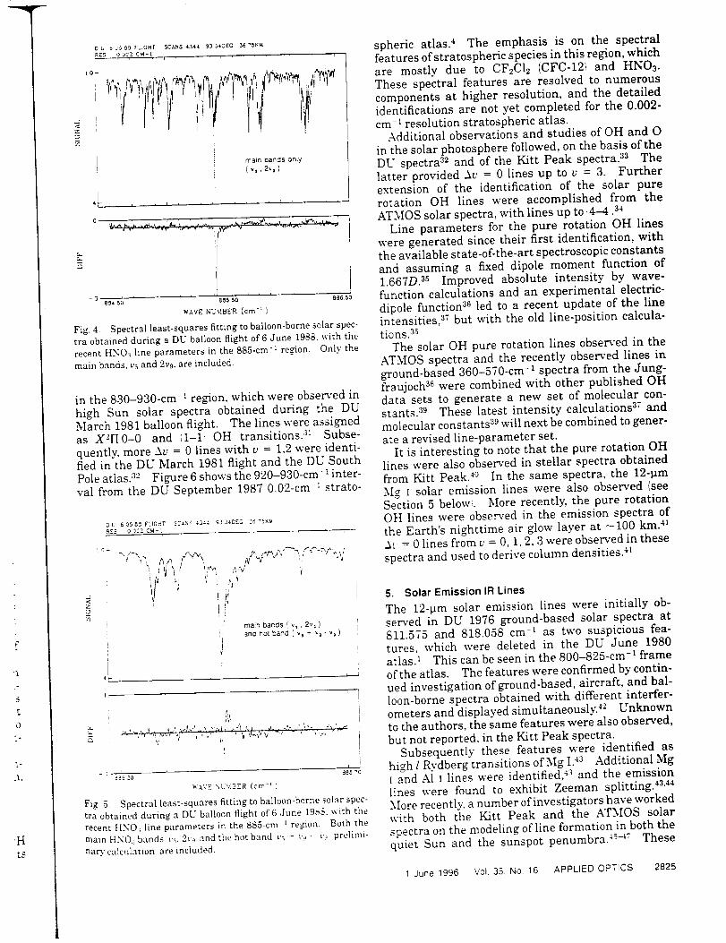
main bands only

( '4,2"_, )

4[- , , i r

i

/!

- 3 8S4 50 i]85 SO

WAVE NU_,tBER (crn -_ )

Fig. 4. Spectral least-squares fitting to balloon-borne solar spec-

tra obtained during a DE balloon flight of 6 June 1988. with the

recent HNO:_ line parameters in the 885-cm-1 re,on. Only the

main bands, t,_ and 2u9, are included.

in the 830-930-cm-1 region, which were observed in

high Sun solar spectra obtained during the DUMarch 1981 balloon flight. The lines were assignedas X2[I0-0 and il-1, OH transitions, at Subse-quently, more Av = 0 lines with v = 1.2 were identi-fied in the DU March 1981 flight and the DU SouthPole atlas, a° Figure 6 shows the 920-930-cm-t inter-val from the DU September 1987 0.02-cm _ strato-

3 L 6 35 8_ FL[CHT 2ZAN3 43_4 93 31DEC n.6 _XM

RE-" 0 3¢2 CM- t

iC-

i

1

4_

'ijivl.i" ":i ,,,,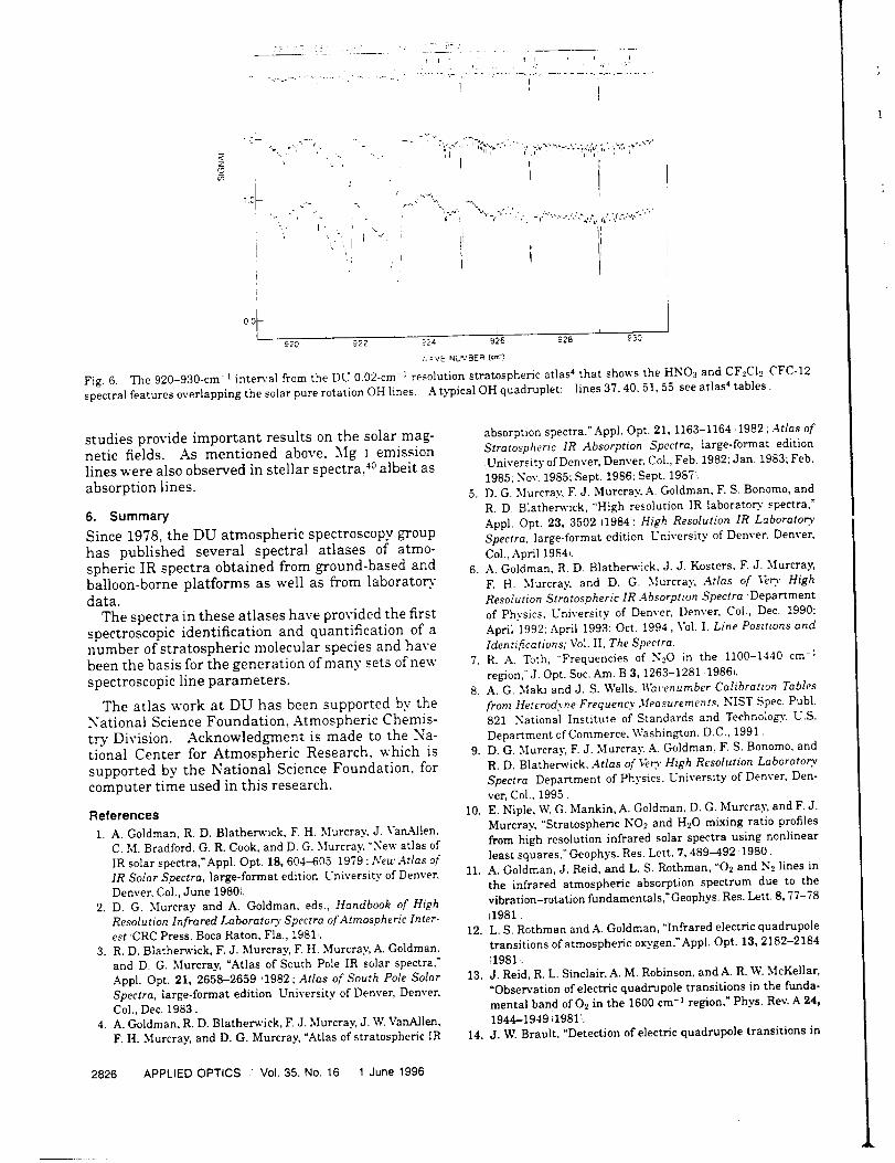![:I

i'!

_V "V ',, ",_

,I;J '_

main bands ( v, , 2%)

an¢ hot _anci :_v s + va " v_ )

' O'

. ,,,. _ %: v.)..,'_..',."...l, ' ,4'_ :_,_ . _ .... '.. ",,'_,,.. -', _,_,_

_ :"c'_'\: "' "i ' ' " i " ''_"_'_" "_ - " ' ""

- : _5 20 ,195 70

WAVE NU_.t3ER (cm -_ )

Fig. 5. Spectral least.squares fitting to balloon-borne solar spec-tra obtained during a DU balloon flight of 6 June 1988. with the

recent HNO:_ line parameters in the 885-cm _ re,on. Both the

main HNO_ bands v_. 2r., and the hot band t,_ - v÷ - __ prelimi-

nan. calculation are included.

spheric atlas. _ The emphasis is on the spectralfeatures of stratospheric species in this region, whichare mostly due to CF_CI., (CFC-121 and HNOa.These spectral features are resolved to numerouscomponents at higher resolution, and the detailedidentifications are not yet completed for the 0.002-cm-1 resolution stratospheric atlas.

Additional observations and studies of OH and Oin the solar photosphere followed, on the basis of theDU spectra ae and of the Kitt Peak spectra, aa Thelatter provided Au = 0 lines up to v = 3. Furtherextension of the identification of the solar purerotation OH lines were accomplished from theATMOS solar spectra, with lines up to t4-4 .a_

Line parameters for the pure rotation OH lineswere generated since their first identification, withthe available state-of-the-art spectroscopic constantsand assuming a fixed dipole moment function of1.667D.a s Improved absolute intensity by wave-function calculations and an experimental electric-dipole function as led to a recent update of the lineintensitiesS but with the old line-position calcula-tions. 35

The solar OH pure rotation lines observed in theATMOS spectra and the recently observed lines inground-based 360-570 -cm-_ spectra from the Jung-fraujoch as were combined with other published OHdata sets to generate a new set of molecular con-stants79 These latest intensity calculations av andmolecular constants 39will next be combined to gener-ate a revised line-parameter set.

It is interesting to note that the pure rotation OHlines were also observed in stellar spectra obtainedfrom Kitt Peak: ° In the same spectra, the 12-1am

Mg [ solar emission lines were also observed (seeSection 5 below;. More recently, the pure rotationOH lines were observed in the emission spectra ofthe Earth's nighttime air glow layer at _ 100 km: t..X:'= 0 lines from v = 0, 1, 2, 3 were observed in these

spectra and used to derive column densities. _

5. Solar Emission IR LinesThe 12-1am solar emission lines were initially ob-served in DU 1976 ground-based solar spectra at811.575 and 818.058 cm -t as two suspicious fea-tures, which were deleted in the DU June 1980atlas. _ This can be seen in the 800-825-cm -t frameof the atlas. The features were confirmed by contin-ued investigation of ground-based, aircraft, and bal-loon-borne spectra obtained with different interfer-ometers and displayed simultaneously :_ Unknownto the authors, the same features were also observed,

but not reported, in the Kitt Peak spectra.Subsequently these features were identified as

high l Rydberg transitions ofMg I. 4a Additional Mgand A1 _ lines were identified: a and the emission

lines were found to exhibit Zeeman splitting. 4a'_4More recently, a number of investigators have workedwith both the Kitt Peak and the ATMOS solar

spectra on the modeling of line formation in both thequiet Sun and the sunspot penumb ra:s-_r These

1 June 1996 Vol. 35. No. 16 APPLIED OPTICS 2825

• ! I

!

If.--

_'=-"_,..- _i _" _-,V ...... . ....... - . .. ",_

i_ ' , i i; p i"

i

i LII

920 922 _24

,'. _VE NUMBER (¢_

Fig. 6. The 920-930-cm -t interval from the DU 0.02-cm-1 resolution stratosphe_dc atlas 4 that shows the HNO3 and CF2C12 CFC-12:

spectra] features overlapping the solar pure rotation OH lines. A typical OH quadruplet: lines 37, 40, 51, 55 _see atlas 4 tables.

studies provide important results on the solar mag-netic fields. As mentioned above, Mg I emissionlines were also observed in stellar spectra, 4° albeit as

absorption lines.

6. Summary

Since 1978, the DU atmospheric spectroscopy grouphas published several spectral atlases of atmo-spheric IR spectra obtained from ground-based andballoon-borne platforms as well as from laboratoo"data.

The spectra in these atlases have provided the firstspectroscopic identification and quantification of anumber of stratospheric molecular species and havebeen the basis for the generation of many sets of new

spectroscopic line parameters.

The atlas work at DU has been supported by theNational Science Foundation, Atmospheric Chemis-

try Division• Acknowledgment is made to the Na-tional Center for Atmospheric Research, which is

supported by the National Science Foundation, forcomputer time used in this research.

References

1. A. Goldman, R. D. Blatherwick, F. H. Murcray, J. \'an._J]en,

C. M. Bradford, G. R. Cook, and D. G. Murcray, "New atlas of

IR solar spectra,"Appl. Opt. 18, 604-605 1979 ; New Atlas of

IR Solar Spectra, large-format edition University of Denver,

Denver, Col., June 19801.

2. D. G. Murcray and A. Goldman, eds., Handbook of High

Resolution Infrared Laboratory Spectra of Atmospheric Inter-

est :CRC Press, Boca Raton, Fla., 1981 ,.

3. R. D. B]atherwick, F. J. Murcray, F. H. Murcray, A. Goldman,

and D. G. Murcray, "Atlas of South Pole IR solar spectra:

Appl. Opt. 21, 2658-2659 ,1982,; Atlas of South Pole Solar

Spectra, large-format edition University of Denver, Denver.

Col., Dec. 19831.

4. A. Goldman. R. D. Blather_'ick, F. J. Murcray, J. W. VanAllen,

F. H. Murcray, and D. G• Murcray, "Atlas of stratospheric IR

absorption spectra:Appl. Opt. 21, 1163-1164 1982 : Atlas of

Stratospheric IR Absorption Spectra, large-format edition

:University of Denver, Denver, Col., Feb. 1982; Jan. 1983; Feb.

1985: Nov. 1985; Sept. 1986: Sept. 1987 _.

5. D. G. Murcray, F. J. Murcra_: A. Goldman, F. S. Bonomo, and

R. D. Blatherwick, "High resolution IR laboratoo" spectra,"

Appl. Opt. 23, 3502 11984: High Resolution IR Laboratory.

Spectra, large-format edition University of Denver, Denver,

Col., April 1984,.

6• A. Goldman, R. D. Blatherwick. J. J. Kosters, F. J. Murcray,

F. H. Murcray, and D. G. Murcra_; Atlas of Veto. High

Resolution Stratospheric IR Absorption Spectra Department

of Physics, University of Denver, Denver, Col., Dec. 1990;

April 1992: April 1993; Oct. 1994, Vol. I, Line Positions and

Identifications: Vol. II, The Spectra.

7. R. A. Toth, "Frequencies of N_O in the 1100-1440 cm -_

region," J. Opt. Soc. Am. B 3, 1263-1281 1986i.

8. A. G. Maki and J. S. Wells, i'_b_.enumber Calibration Tables

from Heterodyne Frequency Measurements, NIST Spec. Publ.

821 National Institute of Standards and Technolo#'. U.S.

Department of Commerce, Washington, D.C., 1991.

9. D. G. Murcray, F. J. Murcray. A. Goldman, F. S. Bonomo, and

R. D. Blather_vick, Atlas of Ve_' High Resolution Laboratory

Spectra Department of Physics, University of Denver. Den-

ver, Col.. 1995,•

10. E• Niple, W. G. Mankin, A. Goldman, D. G. Murcray, and F. J.

Murcray, "Stratospheric NO2 and H20 mixing ratio profiles

from high resolution infrared solar spectra using nonlinear

least squares: Geophys. Res. Lett• 7, 489-492 1980.

11. A. Goldman, J. Reid, and L. S. Rothman, "O2 and No lines in

the infrared atmospheric absorption spectrum due to the

vibration-rotation fundamentals: Geophys. Res. Lett. 8, 77-78

i1981

12. L. S. Rothman and A. Goldman, "Infrared electric quadrupole

transitions of atmospheric oxygen,"Appl. Opt. 13, 2182-2184

!1981.

13. J. Reid, R. L. Sinclair, A. M. Robinson, and A. R. W. McKellar,

"Observation of electric quadrupole transitions in the funda-

mental band of O_ in the 1600 cm -_ region," Phys. Rev. A 24,

1944-1949 i19811.

14. J. W. Brault, "Detection of electric quadrupo]e transitions in

2826 APPLIED OPTICS Vol. 35, No. 16 1 June 1996

;l

.t

),

J

_s

S.

_d

,'y

.[1-

J.

:es

ear

in

;he

-78

_ole

184

:lar,

_da-

,24,

_s in

the oxygen A band at 7600A," J. Mol. Spectrosc. 80, 384-387

1980.

15,. M. Dang-Nhu, R. Zander, A. Goldman, and C. P. Rinsland,

"Identification of magnetic dipole transitions of the fundamen-

tal band of oxygen," J. Mol. Spectrosc. 144, 366-373 19901.

16. T. K. Balasubramanian, R. D'Chuna, and K. Narahari Rao,

"Line strengths in a 3_--3E quadrupole transition with inter-

mediate coupling: application to line intensities in the qua-

drupole fundamental band of the oxygen molecule," J. Mol.

Spectrosc. 144, 374-380 _1990,.

17. T. K. Balasubramanian, V. P. Bellary, and R. D'Chuna,

"Linestrengths for the electric quadrupole fundamental band

of the oxygen molecule with rotation-vibration interaction

corrections,"J. Mol. Spectrosc. 153, 26-31:1992.

18. G. Rouille, G. Millot, R. Saint-Loup, and H. Berger, "High-

resolution stimulated Raman spectroscopy of O_,,_ J. Mol.

Spectrosc. 154, 372-382 1992.19. C. P. Rinsland, A. Goldman, and J.-M. Flaud, "Infrared

spectroscopic parameters of COF2, SFs, C10, N.., and O2," J.

Quant. Spectrosc. Radiat. Transfer 48, 693-699 1992.

20. T. K. Balasubramanian, _,: P. Bellary, and K Narahari Rao,

"Branch intensities in the magnetic dipole rotation-vibration

spectrum of the oxygen molecule," Can. J. Phys. 72, 971-978

1994.

21. A. Goldman, C. P. Rinsland, B. Canova, R. Zander, and hi.

Dang-N'hu, "Improved spectral parameters for the lsO.._ infra-

red forbidden lines in the X3Eg - t0-1 band," J. Quant.

Spectrosc. Radiat. Transfer, 54, 757-765 1995.

22. A. Goldman and C. P. Rinsland, "HNO3 line parameters:

new results and comparisons of simulations with high-

resolution laborato_' and atmospheric spectra, _ J- Quant.

Spectrosc. Radiat. Transfer 48, 653-666 1992.

23. A. Goldman, J. B. Burkholder, C. J. Howard. R. E_cribano,

and A. G. Maki, "Spectroscopic constants for the t'9 infrared

band of HNO3," J. Mol. Spectrosc. 131,195-200 1988.

24. A. Goldman, F. S. Bonomo, W. J. Williams, and D. G. Murcray,

"Statistical band model analysis and integrated intensity for

the 21.8 _m bands of HNO_ vapor," J. Opt. Soc. Am. 65, 10-12

1975.

25. A. Pen-in, J.-M. Flaud. C. Camy-Peyret, B. P. Winnewisser, A.

Goldman, F. J. Murcray, R. D. Blatherwick, F. S. Bonomo,

D G_ Murcray, and C. P. Rinsland, "First analysis of the

3_'_-_'9, 3_9-vs, and 3_,9-2v9 bands of HNO_: torsional split-

ring in the v9 vibrational mode, _ J. Mol. Spectrosc. 166,

2'24-243 1994.

26. J. M. Sirota, A. Perrin, M. Weber, D. Steyert, D. Reuter. and

J.-M Flaud, "Absolute line intensities in the v9 re,on 420 to

460 cm i of HNO:3 by TDL spectroscop>," presented at the

Workshop on Laborato_" and Astronomical High Resolution

Spectra. Brussels 29 Aug.-2 Sept. 1994.

27. A. Perrin, J.-M. Flaud, C. Camy-Peyret, A. Goldman, C. P.

Rinsland, and M. R. Gunson, "Identification of the HNO3

3r9-_'9 band Q branch in stratospheric solar occultation

spectra," J. Quant. Spectrose. Radiat. Transfer 52, 319-322

1994.

28. A. Goldman, C. P. Rinsland, F. J. Murcray, R. D. Blatherwick,

and D. G. Murcray, _High resolution studies of heavy NO_

molecules in atmospheric spectra." J. Quant. Spectrosc. Ra-

dial Transfer 52, 367-377 1994,.

29. L. S. Rothmam R. R. Gamache, R. H. Tipping, C. P. Rinsland,

M. A. H. Smith, D. C. Benner, V. Malathy Devi. J.-M. Flaud, C.

Camv-Peyret, A. Perrin, A. Goldman, S. T. Massie, L. R.

Brown, and R. A. Toth, "The HITRAN molecular database:

editions of 1991 and 1992," J. Quant. Spectrosc. Radiat.

Transfer 48, 469-507 1992.

30. L. P. Giver, F. P. J. Valero, D. Goorvitch, and F. S. Bonomo,

"Nitric-acid band intensities and band model parameters

from 610 to 1760 em-l," J. Opt. Soc. Am. B I, 715-722119841.

3 I. A. Goldman, F. J. Murcray, J. R. Gillis, and D. G. Murcray,

"Identification of new solar OH lines in the 10--12 micron

region,"Astrophys. J. 248, L133-L135 i1981.

32. A. Goldman, D. G. Murcray, D. L. Lambert, and J. F. Dominy,

"The pure rotation spectrum of the hydroxyl radical and the

solar oxygen abundance," Mon. Not. R. Astron. Soc. 203,

767-776 !1983.

33. A. J. Sauva[, N. Grevesse, J. W. Brault, G. M. Stokes, and R.

Zander, "The pure rotation spectrum of OH and the solar

oxygen abundance,_Astrophy s. J- 282,330-338 19841.

34. hi. Geller, "Ahigh-resolution atlas of the infrared spectrum of

the Sun and the Earth atmosphere from space. Vol. III, Key to

Identification of Solar Features," NASA Ref. Publ. 1224

INASA, Washington D.C., 1992i.

35. A. Goldman, J. R. Gillis, and J. A. Coxon. _Spectral line

parameters for the pure rotation bands of solar OH," J.

Quant. Spectrosc. Radiat. Transfer 29, 469--470 19831.

36. D. D. Nelson, Jr., A. Schiffman, D. J. Nesbitt, J. J. Orlando,

and J. B. Burkholder. "H _- O3 Fourier-transform infrared

emission and laser absorption studies of OHX_[I1 radical:

an experimental dipole moment function and state-to-state

Einstein A coefficients." J. Chem. Phys. 93, 7003-7019 !1990).

37. D. Goorvitch, A. Goldman, H. Dothe, R. H. Tipping, and C.

Chackerian Jr., *Hydroxyl XeH pure rotational transitions,"

J. Geophys. Res. 97, D 18, 20,771-20,786 1992.

38. C. B. Farmer, L. Delbouille, G. Roland, and C. Servais, _'he

solar spectrum between 16 and 40 microns." SJI Tech. Rep.

94-2 San Juan Capistrano Research Institute. San Juan

Capistrano, Calif., June 1994:.

39. F. Melen, A. J. Sauval. N. Grevesse, C. B. Farmer, L.

Delbouille, G. Roland. and C. Servais, "A new analysis of the

OH radical spectrum from solar infrared observations," pre-

sented at the Workshop on Laboratory. and Astronomical

High Resolution Spectra. Brussels, 29 Aug.-2 Sept. 1994.

40. D.E. Jennings, D. Deming, G. R. Wiedemann. and J. J. Keady,

"Detection of 12-micron Mg ! and OH lines in stellar spectra,"

Astrophys. J. 310, L39-L43 1986i.

41. J.A. Dodd, W. A. M. Blumberg, S. J. Lipson, J. R. Lowell, P. S.

Armstrong, D. R. Smith. R. M. Nadile, N. B. Wheeler, and

E. R. Huppi, "OH t. N column densities from high-resolution

Earthlimb spectra." Geophys. Res. Lett. 20, 305-308 _19931.

42. F. J. Murcray, A. Goldman, F. H. Murcray, C. M. Bradford,

D. G. Murcray, M. T. Coffey. and W. G. Mankin, "Observation

of new emission lines in the infrared solar spectrum near

12.33, 12.22 and 7.38 microns," Astrophys. J. 247, L97-L99

1981.

4.3. E. S. Chang and R. W. Noyes, "Identification of the solar

emission lines near 12 microns,"Astrophys, d. 275, Lll-L13

1983.

44. J. Brault and R. Noyes, "Solar emission lines near 12 mi-

crons,"Astrophys. J. 269, L61-L66 1983.

45. D. Deming, R. J. Boyle, D. E. Jennings, and G. Wiedemann,

"Solar magnetic field studies using the 12 micron emission

lines. I. Quiet Sun time series and sunspot slices," Astro-

phys. J. 333,978-995 1988.

46. D. Glenar, D. C. Reuter. and D. Deming, %Mg I absorption

features in the solar spectrum near 9 and 12 microns,"

Astrophys. J. 335, L35-L38 1988.

47. E. S. Chang, E. H. Avrett. P. J. Mauas, R. W. Noyes, and R.

Loeser. *Formation of the infrared emission lines of Mg ! in

the solar atmosphere.'.kstrophys. J. 379, L79-L82 19911.

1 June 1996 Vol. 35, No 16 APPLIED OPTICS 2827

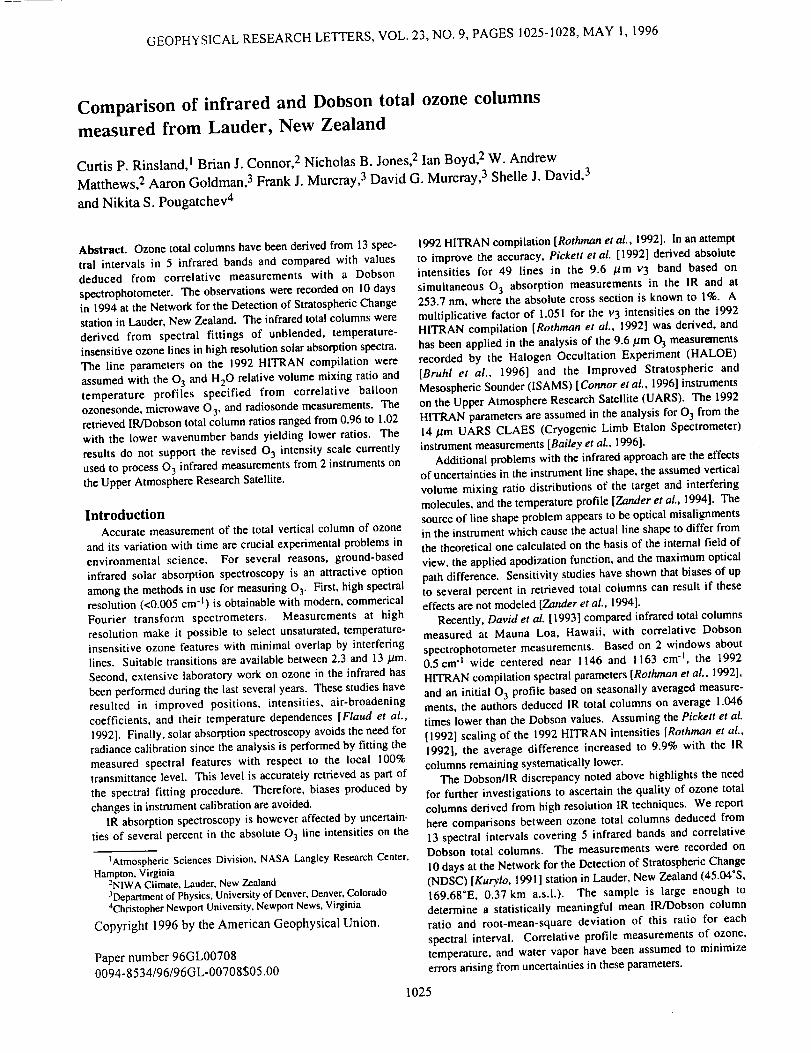
GEOPHYSICAL RESEARCH LETTERS, VOL. 23, NO. 9, PAGES 1025-1028, MAY 1, 1996

Comparison of infrared and Dobson total ozone columns

measured from Lauder, New Zealand

Curtis P. Rinsland, 1 Brian J. Connor, 2 Nicholas B. Jones, 2 Ian Boyd, 2 W. Andrew

Matthews, 2 Aaron Goldman, 3 Frank J. Murcray, 3 David G. Murcray, 3 Shelle J. David, 3

and Nikita S. Pougatchev 4

Abstract. Ozone total columns have been derived from 13 spec-

tral intervals in 5 infrared bands and compared with values

deduced from correlative measurements with a Dobson

spectrophotometer. The observations were recorded on 10 daysin 1994 at the Network for the Detection of Stratospheric Change

station in Lauder, New Zealand. The infrared total columns were

derived from spectral fittings of unblended, temperature-

insensitive ozone lines in high resolution solar absorption spectra.

The line parameters on the 1992 HITRAN compilation were

assumed with the O 3 and H20 relative volume mixing ratio and

temperature profiles specified from correlative balloon

ozonesonde, microwave O 3, and radiosonde measurements. The

retrieved IR/Dobson total column ratios ranged from 0.96 to 1.02with the lower wavenumber bands yielding lower ratios. The

results do not support the revised 03 intensity scale currently

used to process O 3 infrared measurements from 2 instruments on

the Upper Atmosphere Research Satellite.

IntroductionAccurate measurement of the total vertical column of ozone

and its variation with time are crucial experimental problems in

environmental science. For several reasons, ground-based

infrared solar absorption spectroscopy is an attractive option

among the methods in use for measuring O 3. First, high spectralresolution (<0.005 cm "t) is obtainable with modem, commerical

Fourier transform spectrometers. Measurements at high

resolution make it possible to select unsaturated, temperature-

insensitive ozone features with minimal overlap by interfering

lines. Suitable transitions are available between 2.3 and 13/,tm.

Second, extensive laboratory work on ozone in the infrared has

been performed during the last several years. These studies have

resulted in improved positions, intensities, air-broadeningcoefficients, and their temperature dependences [Flaud et al.,

1992]. Finally, solar absorption spectroscopy avoids the need for

radiance calibration since the analysis is performed by fitting the

measured spectral features with respect to the local 100%

transmittance level. This level is accurately retrieved as part of

the spectral fitting procedure. Therefore, biases produced by

changes in instrument calibration are avoided.IR absorption spectroscopy is however affected by uncertain-

ties of several percent in the absolute 03 line intensities on the

tAtmospheric Sciences Division, NASA Langley Research Center,Hampton, Virginia

2NIWA Climate, Lauder, New Zealand3Department of Physics, University of Denver, Denver, Colorado4Christopher Newport University, Newport News, Virginia

Copyright 1996 by the American Geophysical Union.

Paper number 96GL00708

0094-8534/96/96GL-00708505.00

1992 HITRAN compilation [Rothman et al., 1992]. In an attempt

to improve the accuracy, Pickett et al. [1992] derived absoluteintensities for 49 lines in the 9.6 #m v 3 band based on

simultaneous 0 3 absorption measurements in the IR and at253.7 nm, where the absolute cross section is known to 1%. A

multiplicative factor of 1.051 for the v 3 intensities on the 1992

HITRAN compilation [Rothman et al., 1992] was derived, and

has been applied in the analysis of the 9.6/zm 03 measurements

recorded by the Halogen Occultation Experiment (HALOE)

[Bruhl et al., 1996] and the Improved Stratospheric and

Mesospheric Sounder (ISAMS) [Connor et al., 1996] instruments

on the Upper Atmosphere Research Satellite (UARS). The 1992

H1TRAN parameters are assumed in the analysis for 03 from the

14/_m UARS CLAES (Cryogenic Limb Etalon Spectrometer)

instrument measurements [Bailey et aL, 1996].

Additional problems with the infrared approach are the effects

of uncertainties in the instrument line shape, the assumed vertical

volume mixing ratio distributions of the target and interfering

molecules, and the temperature profile [Zander et al., 1994]. The

source of line shape problem appears to be optical misalignments

in the instrument which cause the actual line shape to differ from

the theoretical one calculated on the basis of the internal field of

view, the applied apodization function, and the maximum optical

path difference. Sensitivity studies have shown that biases of up

to several percent in retrieved total columns can result if these

effects are not modeled [Zander et al., 1994].

Recently, David et al. [ 1993] compared infrared total columns

measured at Mauna Loa, Hawaii, with correlative Dobson

spectrophotometer measurements. Based on 2 windows about0.5 cm "1 wide centered near 1146 and 1163 cm l, the 1992

HITRAN compilation spectral parameters [Rothman et al., 1992],

and an initial 0 3 profile based on seasonally averaged measure-ments, the authors deduced IR total columns on average 1.046

times lower than the Dobson values. Assuming the Pickett et al.

[1992] scaling of the 1992 HITRAN intensities [Rothman et al.,

1992], the average difference increased to 9.9% with the IR

columns remaining systematically lower.

The Dobson/IR discrepancy noted above highlights the need

for further investigations to ascertain the quality of ozone total

columns derived from high resolution IR techniques. We report

here comparisons between ozone total columns deduced from

13 spectral intervals covering 5 infrared bands and correlative

Dobson total columns. The measurements were recorded on

10 days at the Network for the Detection of Stratospheric Change

(NDSC) [Kurylo, 1991] station in Lander, New Zealand (45.04"S,

169.68°E, 0.37 km a.s.l.). The sample is large enough to

determine a statistically meaningful mean IR/Dobson column

ratio and root-mean-square deviation of this ratio for each

spectral interval. Correlative profile measurements of ozone,temperature, and water vapor have been assumed to minimize

errors arising from uncertainties in these parameters.

1025

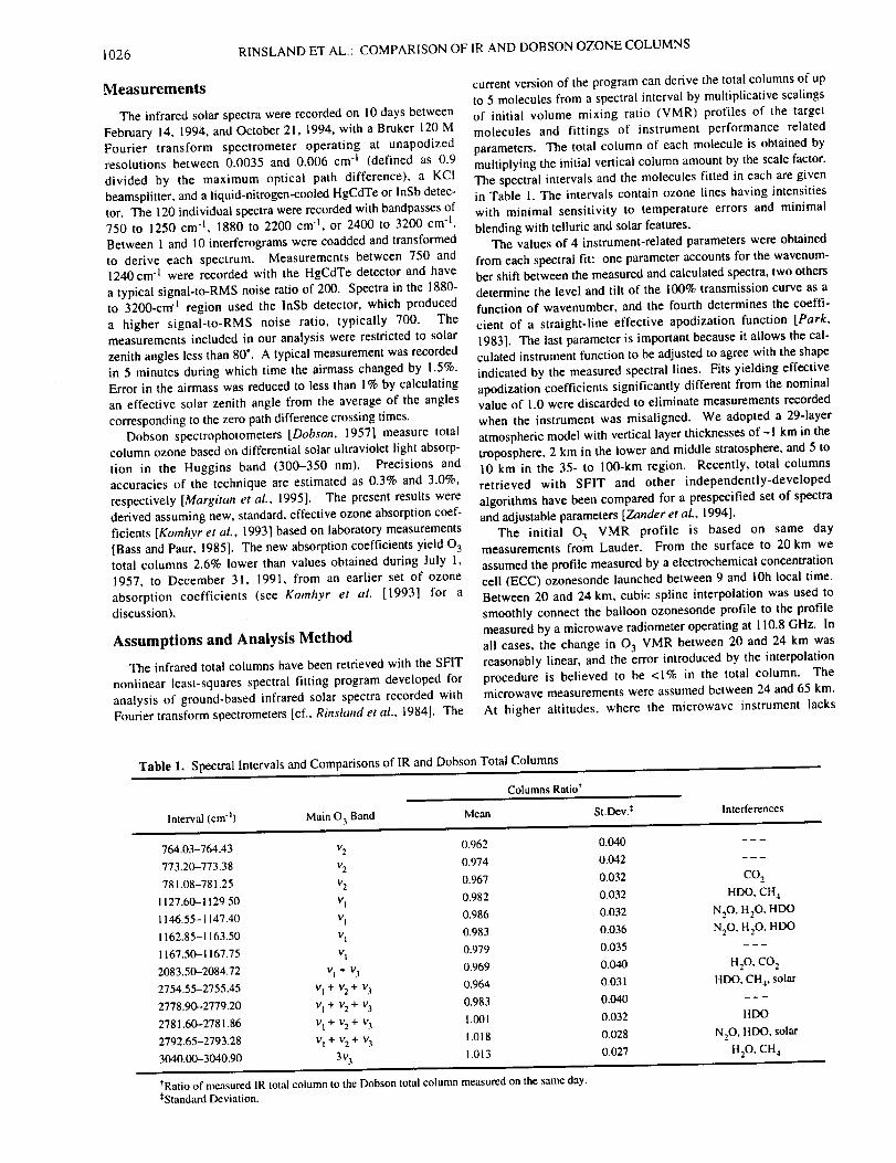
1026 RINSLANDETAL.:COMPARISONOF

Measurements

The infrared solar spectra were recorded on 10 days between

February 14, 1994, and October 21, 1994, with a Bruker 120 M

Fourier transform spectrometer operating at unapodized

resolutions between 0.0035 and 0.006 cm "t (defined as 0.9

divided by the maximum optical path difference), a KCI

beamsplitter, and a liquid-nitrogen-cooled HgCdTe or InSb detec-tor. The 120 individual spectra were recorded with bandpasses of

750 to 1250 cm 1, 1880 to 2200 cm 1, or 2400 to 3200 cm q.

Between 1 and 10 interferograms were coadded and transformed

to derive each spectrum. Measurements between 750 and1240 cm "1 were recorded with the HgCdTe detector and have

a typical signal-to-RMS noise ratio of 200. Spectra in the 1880-

to 3200-crn "1 region used the lnSb detector, which produced

a higher signal-to-RMS noise ratio, typically 700. The

measurements included in our analysis were restricted to solar

zenith angles less than 80*. A typical measurement was recorded

in 5 minutes during which time the airmass changed by 1.5%.

Error in the airmass was reduced to less than I% by calculating

an effective solar zenith angle from the average of the angles

corresponding to the zero path difference crossing times.

Dobson spectrophotometers [Dobson, 1957] measure total

column ozone based on differential solar ultraviolet light absorp-

tion in the Huggins band (300-350 nm). Precisions and

accuracies of the technique are estimated as 0.3% and 3.0%,

respectively [Margitan et al., 1995]. The present results were

derived assuming new, standard, effective ozone absorption coef-

ficients [Komhyr et al., 1993] based on laboratory measurements

[Bass and Paur, 1985]. The new absorption coefficients yield 0 3

total columns 2.6% lower than values obtained during July 1,

1957, to December 31, 1991, from an earlier set of ozone

absorption coefficients (see Komhyr et al. [1993] for a

discussion).

Assumptions and Analysis Method

The infrared total columns have been retrieved with the SFIT

nonlinear least-squares spectral fitting program developed for

analysis of ground-based infrared solar spectra recorded with

Fourier transform spectrometers [cf., Rinsland et al., 1984]. The

IR AND DOBSON OZONE COLUMNS

current version of the program can derive the total columns of up

to 5 molecules from a spectral interval by multiplicative scalings

of initial volume mixing ratio (VMR) profiles of the target

molecules and fittings of instrument performance related

parameters. The total column of each molecule is obtained by

multiplying the initial vertical column amount by the scale factor.

The spectral intervals and the molecules fitted in each are given

in Table l. The intervals contain ozone lines having intensities

with minimal sensitivity to temperature errors and minimal

blending with telluric and solar features.

The values of 4 instrument-related parameters were obtained

from each spectral fit: one parameter accounts for the wavenum-

ber shift between the measured and calculated spectra, two others

determine the level and tilt of the 100% transmission curve as a

function of wavenumber, and the fourth determines the coeffi-

cient of a straight-line effective apodization function [Park,

1983]. The last parameter is important because it allows the cal-

culated instrument function to be adjusted to agree with the shape

indicated by the measured spectral lines. Fits yielding effective

apodization coefficients significantly different from the nominal

value of 1.0 were discarded to eliminate measurements recorded

when the instrument was misaligned. We adopted a 29-layer

atmospheric model with vertical layer thicknesses of ~ ! km in the

troposphere, 2 km in the lower and middle stratosphere, and 5 to

10 km in the 35- to 100-kin region. Recently, total columns

retrieved with SF1T and other independently-developed

algorithms have been compared for a prespecified set of spectra

and adjustable parameters [Zander et al., 1994].

The initial 03 VMR profile is based on same daymeasurements from Lauder. From the surface to 20 km we

assumed the profile measured by a electrochemical concentration

cell (ECC) ozonesonde launched between 9 and 10h local time.

Between 20 and 24 km, cubic spline interpolation was used to

smoothly connect the balloon ozonesonde profile to the profile

measured by a microwave radiometer operating at 110.8 GHz. In

all cases, the change in O 3 VMR between 20 and 24 km was

reasonably linear, and the error introduced by the interpolation

procedure is believed to be <1% in the total column. The

microwave measurements were assumed between 24 and 65 km.

At higher altitudes, where the microwave instrument lacks

Table 1. Spectral Intervals and Comparisons of IR and Dobson Total Columns

Interval (cm l) Main 03 Band Mean

Columns Ratio*

St.Dev. ¢ Interferences

764.03-764.43 v 2 0.962 0.040

773.20-773.38 v 2 0.974 0.042

781.08-781.25 v 2 0.967 0.032

1127.60-1129.50 v I 0.982 0.032

1146.55-1147.40 v t 0.986 0.032

1162.85-1163.50 v t 0.983 0.036

I 167.50-- I 167.75 v t 0.979 0.035

2083.50-2084.72 vl + v3 0.969 0.040

2754.55-2755.45 v t + v2 + va 0.964 0.031

2778.90-2779.20 vl + v2 + v 3 0.983 0.040

2781.60-2781.86 vl + v2 + v3 1.001 0.032

2792.65-2793.28 vt + v2 + v 3 1.018 0.028

3040.00-3040.90 3v 3 1.013 0.027

CO 2

HDO, CH 4

N20 , H20, HDO

N20, H20. HDO

H20. CO 2

HDO, CH 4, solar

HDO

N20 . HDO, solar

H20, CH 4

*Ratio of measured IR total column to the Dobson total column measured on the .same day._:Standard Deviation.

RINSLANDETAL.:COMPARISONOFIRANDDOBSONOZONECOLUMNS 1027

seqsitivity,cubicsplineinterpolationwasusedto smoothlyconnectthemicrowaveprofileto the1976U.S.StandardAtmosphereozoneprofile[Kruegerand Minzner, 1976]. A

description of the EEC ozonesonde sensor and estimates of the

accuracy and precision of the measurements are given by Komhyr

et al. [1995] and Barnes et aL [19851. At present, no papers

describing the Lauder O 3 microwave measurements have been

published. However, this same instrument was used to derive 03

profiles at Table Mountain, California, during the 1989

Stratospheric Ozone lntercomparison Campaign (STOIC). The

precisions, accuracies, and vertical resolutions of the STOIC

microwave measurements are 4%, 7%, and 10 km at 55 mbar

(-20 km); 5%, 8%, and 10 km at 3 mbar (-40 km); and 6%, 10%,

and 17 km at 0.2 mbar (-60 km), respectively [Connor et al.,

1995].

The vertical temperature profiles assumed in the IR analysis

are also based on a combination of same day measurements and

climatology. From the surface to 22 km, we adopted measure-

ments from a meteorological radiosonde flown with the EEC

ozonesonde. A spline interpolation procedure was used to

smoothly connect this profile with National Meteorological

Center temperatures and pressures, which were assumed between

30 and 50 km. Between 50 and 65 km we adopted temperature,

density, and pressure profiles from the MAP (Middle Atmosphere

Program) Handbook 16 zonal average tabulations [Barnett and

Corney, 1985], followed by the 1976 U.S. Standard Atmosphere

values from 65 to 100 kin. The radiosonde temperatures are

estimated to have uncertainties of ~1 K.

The initial H20 VMR profile for each day is also a combina-tion of values from the Lauder daily sounding and climatology.

The radiosonde measurements were combined with the 1976 U.S.

Standard Atmosphere H20 profile by assuming the balloon data

to an altitude of 20 kin, a linear change in the H20 VMR between

altitudes of 20 and 34 kin, and the 1976 U.S. Standard

Atmosphere H20 profile above 34 km. Initial profiles for the

other absorbing molecules are from a variety of sources. Care has

been taken to verify the assumed profiles are realistic for the mid-

latitude, southern hemisphere location of the Lauder station.

The spectroscopic line parameters used in the analysis weretaken from the 1992 HITRAN compilation [Rothman et al.,

1992]. The solar features noted in Table 1 were included by

adding a line at the appropriate wavenumber and fitting the solar

absorption with a one layer model [cf., Rinsland et aL, 1984].

Results and Discussion

Figure 1 shows a sample fit. Absorption by ozone in the

region is dominated by the 3v 3 band. The maximum

discrepancies coincide with the locations of the stronger 0 3 lines.

Sources of error are inaccuracies in the assumed 03 line

parameters, weak lines missing from the spectroscopic database,

and inadequacies in modeling the interfering lines and the

instrument line shape. Similar problems occur in other spectral

regions.The mean and standard deviation of ratios calculated by divid-

ing the ozone total columns retrieved from the IR measurements

by the same day Dobson values are given for each spectral inter-val in Table 1. The standard deviations of the ratios are typically

3%, which highlights the consistency between the two datasets

despite wide differences in instrumentation and data analysis

methods. Although the IR and UV measurements were recorded

on the same day, they were in general not coincident in time.The results in Table 1 indicate IR/Dobson mean column ratios

from -0.96 in the v 2 band to -1.02 in the 3v 3 band. At 10/.tin,

_" 1.0 . . , , . '

0.0•_ -o.5_-1.0

1.0

0,9

_ 0.8bl

_ 0.70

z

0.63040.0

i

I I

,3040.3 304-0.6 ,3040.9

Wavenumber (era -1)

Figure I. Bottom: Measured (solid line) and least-squares, best-

fit calculated (open triangles) Lauder solar spectra in the region of

the 3v 3 band of ozone. The measured spectrum was recorded onApril 27, 1994, at an astronomical zenith angle of 62.24*. Top:Measured minus calculated values on an expanded vertical scale.

Several CH 4 lines and a H20 line at 3040.741 cm I contribute tothe measured absorption.

the average of the 4 IR/Dobson ratios is 0.982. Hence, to obtain

agreement with the Dobson values, the IR intensities in this

region need to be multiplied by 0.982. This factor is higher thanthe Mauna Loa IR/Dobson ratio of 0.956 deduced by David et al.

[1993]. However, David et aL [1993] note that reprocessing of

the Mauna Loa Dobson data with the new, effective O 3 absorp-

tion coefficents [Komhyr et al., 1993] would increase the ratio to

about 0.98, in excellent agreement with the present results.

The errors that normally arise from uncertainties in the target

molecule volume mixing ratio and temperature profiles are neg-

ligible in the present work because correlative measurements

have been adopted for those quantities. However, 3 other

important sources of potential systematic error remain: (1) errors

in the spectroscopic parameters, (2) errors in fitting the

instrument line shape function, and (3) biases introduced by

errors in the retrieval algorithm. Errors in the line intensities are

not considered here since the goal is to determine the offset from

the IR/Dobson column comparisons. The sensitivity to errors in

the air-broadening coefficients and their temperature dependences

have been estimated by repeating retrievals with the 1992

HITRAN air-broadening coefficients of ozone [Rothman et al.,

1992] multiplied by 1.05. The ozone total columns increased by

0.5%. The uncertainty in the instrument line shape function was

estimated by repeating retrievals with the straight-line effective

apodization coefficient [Park, 1983] increased or decreased by

0.1 as compared to the retrieved value. Changes in the ozone

total columns of- 1.5% and +1.5% were obtained, respectively.

Total columns retrieved with SFIT agree with values from

independently-developed algorithms to about 2% when the same

input parameters and fitting options are selected [Zander et al.,

1994]. On the basis of these studies, we estimate the uncertainty

in the mean lR/Dobson ratios in Table 1 as +_3%.

The ozone intensity scale on the 1992 HITRAN compilation

[Rothman et al., 1992] was transferred from the 10/./m to other IR

regions by measuring relative intensities of common lines in

overlapping laboratory spectra. The present work suggests that

this procedure was successful to within a few percent. Very

1028 RINSLAND ET AL.: COMPARISON OF

precise work will be required to determine if the small, systematic

increase in the IR/Dobson column ratio with wavenumber

measured in this work results from errors in the 0 3 intensities, an

artifact in the present analysis, or a combination of both effects.

Recent laboratory measurements are consistent with the pres-

ent results. Birk et aL [1993] compared measured absolute

intensities of 26 transitions in the 0 3 v2 band with values on the

1992 HITRAN database [Rothman et al., 1992]. The average

measured-to-1992 HITRAN ratio was 0.965 + 0.031, close to our

average ratio of 0,967. Barbe et al. [1994] reanalyzed the 2 v I, v 1

+ v 3, and 2v_ bands in the 1850--2300 -cml region based on 03

amounts calculated from the measured sample pressure and the

assumptions that the initial sample contained only 0 3 and the

only 0 3 decay product was 0 2 . These new intensities show no

significant bias relative to the 1992 HITRAN compilation values

[ Barbe et al., 1994, Fig. 31. De Backer and Courtois [1995] used

a tunable diode laser spectrometer to measure the intensities of

about 40 ozone lines in the 9.6/am v 3 band. They derived an

average measured-to-1992 HITRAN ratio of 0.96 + 0.04 (M. R.

De Backer, private communication, 1995). A consistent value for

the amount of ozone in the cell was found three ways: (1) UV

measurements at 253.7 rim, (2) measurements of the sample

pressure and the assumptions that the initial sample contained

only 03 and the only 03 decay product was O 2, and (3) measure-

ment of the 0 3 vapor pressure at the temperature of liquid argon,

where the 0 3 vapor pressure is well known.

Summary and ConclusionsAverage IR-to-Dobson 03 total column ratios of 0.96 to 1.02

have been derived from 13 intervals in 5 infrared bands and

correlative Dobson spectrophotometer measurements. Both sets

of measurements, accurate to about +3%, were recorded on

10 days in 1994 at the NDSC station in Lauder, New Zealand.

Correlative 03 and 1-120 VMR and temperature profiles were

specified in the IR analysis from correlative measurements to

minimize systematic errors. The present results do not support

the 1.051 multiplicative factor recommended by Pickett et al.

[1992] for the 1992 HITRAN line intensities in the O 3 v3 band

[Rothman et al., 1992]. Our results agree with recent laboratory

measurements of absolute 03 intensities and a comparison of

Mauna Loa IR total columns with correlative Dobson

spectrophotometer measurements [David et al., 1993].

Acknowledgments. Research at the NIWA is funded by the New

Zealand Foundation for Research, Science, and Technology (Contract

number CO 1221). Research at the University of Denver, Christopher

Newport University, and NASA Langley Research Center is funded byNASA's Upper Atmosphere Research Program. Special thanks to B. M.

McNamara for recording the infrared spectra, T. Beck and D. Keep for

obtaining the Dobson measurements, and R. Evans of NOAA's Climate

Monitoring and Diagnostic Laboratory for assistance in interpreting the

Dobson measurements.

References

Bailey, P. L., et al.. A comparison of CLAES ozone measurements withcorrelative measurements. J. Geophys. Res., accepted, 1996.

Barbe, A., et al., Experimental and theoretical study of the absoluteintensities of ozone spectral lines in the range 1850-2300 cm "t,

J. Quant. Spectrosc. Radiat. Transfer, 52,341-355, 1994.

IR AND DOBSON OZONE COLUMNS

Barnes, R. A.. A. R. Bandy, and A. L. Tortes, Electrochemical concentra-tion cell ozonesonde accuracy and precision, J. Geophys. Res., 90,

7881-7877. 1985.

Barnett, J., and M. Comey, Middle atmosphere reference model derivedfrom satellite data, Handb. MAP, 16, edited by K. Labitzke. J. J.

Barnett, and B. Edwards, pp. 47-85, Sci. Comm. for Sol. Terr. Phys.

Seer., Univ. of IlL, Urbana. 1985.Bass, A. M., and R. J. Paur, The ultraviolet cross-sections of ozone, 1,

The measurements, in Atmospheric Ozone. edited by C. S. Zerefos and

A. Ghazi, pp. 606-610, D. ReideL Norwell, Mass., 1985.

Birk, M., et al., Line strengths in the v3 - v, hot band of ozone, paperKI8, Thirteenth Colloquium on High "Resolution Spectroscopy,

Riccione, Italy, September 1993.Bruhl. C., et al., HALOE ozone channel validation, J. Geophys. Res.,

accepted, 1996.Connor, B. J., et al.. Error analysis for the ground-based microwave

ozone measurements during STOIC, J. Geophys. Res., 100, 9283-

9292, 1995.Connor, B. J., et al., Ozone in the middle atmosphere as measured by the

improved stratospheric and mesospheric sounder, J. Geophys. Res.,

accepted, 1996.David, S. J., et al.. Determination of total ozone over Mauna Loa using

very high resolution infrared solar spectra, Geophys. Res. Lett., 20,2055-2058, 1993.

De Backer, M. R.. and D. Courtois, Analysis of some ozone lines in the

v_ band with a tunable diode laser spectrometer, paper RA06, 50thIfiternational Symposium on Molecular Spectroscopy, Ohio State

University, Columbus, OH.Dobson. G. M. B., Observer's handbook for the ozone spectrophotometer,

Ann. Int. Geophvs. Year, 5(1). 46-89, 1957.

Flaud, J.-M.. et al..improved spectroscopic line parameters for the ozonemolecule, J. Quant. Spectrosc. Radiat. Transfer, 48, 611-615. 1992.

Komhyr, W. D., C. L. Mateer, and R. D. Hudson, Effective Pass-Paur

1985 ozone absorption coefficients for use with Dobson ozone spec-

trophotometers. J. Geophys. Res., 98, 20,451-20,465, 1993.

Komhyr, W. D., et al., Electrochemical concentration cell ozonesonde

performance evaluation during STOIC 1989, J. Geophys. Res., 100,

9231-9244, 1995.

Krueger, A. J.. and R. A. Minzner, A mid-latitude ozone model for the1976 U.S. Standard Atmosphere, J. Geophys. Res.,81, 4477---4481,

1976.

Kurylo, M. J., Network for the detection of stratospheric change. Proc.Soc. Photo. Opt. Instrum. Eng., 1491, 169-174, 1991.

Margitan. J. J., et al.. Stratospheric ozone intercomparison campaign

(STOIC) 1989: Overview, J. Geophys. Res., 100, 9193-9207, 1995.

Park, J. H., Analysis method for Fourier transform spectroscopy, Appl.

Opt., 22, 835-849. 1983.Pickett, H. M., D. B. Peterson, and J. S. Margolis. Absolute absorption of

ozone in the midinfrared. J. Geophys. Res., 97. 20,787-20,793, 1992.

Rinsland. C. P., et al., Diurnal variations of atmospheric nitric oxide:Ground-based infrared spectroscopic measurements and their

interpretation with time-dependent photochemical model calculations,

J. Geophys. Res., 89, 9613-9622, 1984.Rothman, L. S.. et al.. The HITRAN molecular database: Editions of

1991 and 1992, J. Quant. Spectrosc. Radiat. Transfer, 48, 469-507,

1992.Zander, et al., ESMOS II/NDSC IR spectral fitting algorithms.

Intercomparison exercise, Proceedings of the Atmospheric

Spectroscopy Applications Workshop, Reims, France, pp. 7-12, 1994.

C. P. Rinsland, Mail Stop 401A, NASA Langley Research Center,

Hampton, VA 23681-0001l. Boyd, B. J. Connor, N. B. Jones, and W. Andrew Matthews, NIWA

Climate, Private Bag 50061. Omakau, Lauder 9128, New Zealand

S. J. David, A. Goldman, D. G. Murcray, and F. J. Murcray,

Department of Physics, University of Denver, Denver, CO 80308N. S. Pougatchev. Christopher Newport University, Newport News.

VA 23606-2998

(Received August 17, 1995 ; revised December 20, 1995;

accepted February 15, 1996.)

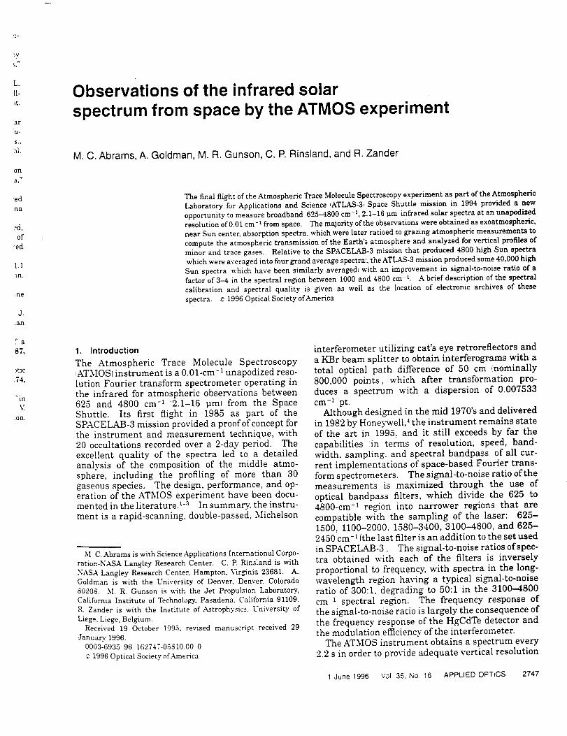
_y

L.

!l-

)t.

ar

'u-

ol.

on

ed

Ra

rd,

of

?ed

1.1

)n.

_ne

J.

lan

_a

87,

_tic

.74,

*'in

:On.

Observations of the infrared solarspectrum from space by the ATMOS experiment

M. C. Abrams, A. Goldman, M. R. Gunson, C. P. Rinsland, and R. Zander

The final flight of the Atmospheric Trace Molecule Spectroscopy experiment as part of the Atmospheric

Laboratory for Applications and Science iATLAS-3, Space Shuttle mission in 1994 provided a new

opportunity to measure broadband 625-4800 cm -1, 2.1-16 :am infrared solar spectra at an unapodized

resolution of 0.01 cm- 1 from space. The majority of the observations were obtained as exoatmospheric,

near Sun center, absorption spectra, which were later ratioed to grazing atmospheric measurements to

compute the atmospheric transmission of the Earth's atmosphere and analyzed for vertical profiles of

minor and trace gases. Relative to the SPACELAB-3 mission that produced 4800 high Sun spectra

which were averaged into four grand average spectral, the ATLAS-3 mission produced some 40,000 high

Sun spectra which have been similarly averagedJ with an improvement in signal-to-noise ratio of a

factor of 3-4 in the spectral region between 1000 and 4800 cm-l. A brief description of the spectral

calibration and spectral quality is given as well as the location of electronic archives of these

spectra. _v 1996 Optical SocietyofAmerica

1. Introduction

The Atmospheric Trace Molecule Spectroscopy,ATMOS1 instrument is a 0.01-cm -1 unapodized reso-

lution Fourier transform spectrometer operating inthe infrared for atmospheric observations between625 and 4800 cm -1 i2.1-16 tim} from the Space

Shuttle. Its first flight in 1985 as part of theSPACELAB-3 mission provided a proof of concept forthe instrument and measurement technique, with20 occultations recorded over a 2-day period. The

excellent quality of the spectra led to a detailedanalysis of the composition of the middle atmo-sphere, including the profiling of more than 30gaseous species. The design, performance, and op-eration of the ATMOS experiment have been docu-mented in the literature} -3 In summary, the instru-

ment is a rapid-scanning, double-passed, Michelson

M. C. Abrams is with Science Applications International Corpo-

raUon-NASA Langley Research Center. C.P. Rinsland is with

NASA Langley Research Center, Hampton, Virginia 23681. A.

Goldman is with the University of Denver. Denver. Colorado

80208. M. R. Gunson is with the Jet Propulsion Laboratory,

California Institute of Technology. Pasadena. California 91109.

R. Zander is with the Institute of Astrophysics, University of

Liege, Liege, Belgium.

Received 19 October 1995: revised manuscript received 29

January. 1996.

0003-6935 96 162747-05510.00 0

1996 Optical Society of America

interferometer utilizing cat's eye retroreflectors and

a KBr beam splitter to obtain interferograms with atotal optical path difference of 50 cm {nominally

800,000 points, which after transformation pro-duces a spectrum with a dispersion of 0.007533

cm -t pt.Although designed in the mid 1970's and delivered

in 1982 by Honeywell, 4 the instrument remains stateof the art in 1995, and it still exceeds by far the

capabilities iin terms of resolution, speed, band-width, sampling, and spectral bandpass of all cur-

rent implementations of space-based Fourier trans-form spectrometers. The signal-to-noise ratio of themeasurements is maximized through the use of

optical bandpass filters, which divide the 625 to4800-cm -_ region into narrower regions that are

compatible with the sampling of the laser: 625-1500, 1100-2000, 1580-3400, 3100-4800, and 625-2450 cm -1 (the last filter is an addition to the set used

in SPACELAB-3. The signal-to-noise ratios of spec-tra obtained with each of the filters is inversely

proportional to frequency, with spectra in the long-wavelength re,on having a typical signal-to-noiseratio of 300:1, degrading to 50:1 in the 3100-4800

cm -_ spectral region. The frequency response ofthe signal-to-noise ratio is largely the consequence ofthe frequency response of the HgCdTe detector andthe modulation efficiency of the interferometer.

The ATMOS instrument obtains a spectrum every

2.2 s in order to provide adequate vertical resolution

1 June 1996 Vol. 35. No 16 APPLIED OPTICS 2747

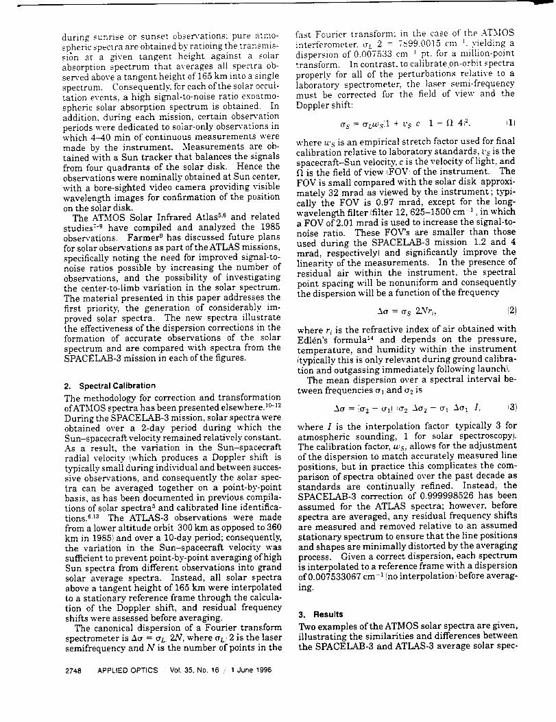
during sunrise or sunset observations: pure atmo-

spheric spectra are obtained by ratioing the transmis-sion at a given tangent height against a solarabsorption spectrum that averages all spectra ob-served above a tangent height of 165 km into a singlespectrum. Consequently. for each of the solar occul-tation events, a high signal-to-noise ratio exoatmo-spheric solar absorption spectrum is obtained. Inaddition, during each mission, certain obser','ation

periods were dedicated to solar-only observations inwhich 4--40 rain of continuous measurements were

made by the instrument. Measurements are ob-tained with a Sun tracker that balances the signals

from four quadrants of the solar disk. Hence theobservations were nominally obtained at Sun center,with a bore-sighted video camera providing visible

wavelength images for confirmation of the positionon the solar disk.

The ATMOS Solar Infrared Atlas 5,6 and related

studies 7-s have compiled and analyzed the 1985observations. Farmer 9 has discussed future plans

for solar observations as part of the ATLAS missions,

specifically noting the need for improved signal-to-noise ratios possible by increasing the number ofobservations, and the possibility of investigatingthe center-to-limb variation in the solar spectrum.The material presented in this paper addresses the

first priority, the generation of considerably im-proved solar spectra. The new spectra illustratethe effectiveness of the dispersion corrections in theformation of accurate observations of the solar

spectrum and are compared with spectra from theSPACELAB-3 mission in each of the figures.

2. Spectral Calibration

The methodology for correction and transformationof ATMOS spectra has been presented elsewhere.I°-12During the SPACELAB-3 mission, solar spectra wereobtained over a 2-day period during which theSun-spacecraft velocity remained relatively constant.As a result, the variation in the Sun-spacecraft

radial velocity (which produces a Doppler shift istypically small during individual and between succes-sive observations, and consequently the solar spec-

tra can be averaged together on a point-by-pointbasis, as has been documented in previous compila-tions of solar spectra 5 and calibrated line identifica-tions. 6,13 The ATLAS-3 observations were made

from a lower altitude orbit 300 km as opposed to 360km in 1985) and over a 10-clay period; consequently,the variation in the Sun-spacecraft velocity wassufficient to prevent point-by-point averaging of high

Sun spectra from different observations into grandsolar average spectra. Instead, all solar spectraabove a tangent height of 165 krn were interpolatedto a stationary reference frame through the calcula-tion of the Doppler shift, and residual frequencyshifts were assessed before averaging.

The canonical dispersion of a Fourier transformspectrometer is 5or = CTL.2N, where ¢L/2 is the lasersemifrequency and N is the number of points in the

fast Fourier transform: in the case of the ATMOS

interferometer. (rL 2 = 7899.0015 tin 1. yielding adispersion of 0.007533 cm _ pt. for a million-pointtransform. In contrast, to calibrate.on-orbit spectra

properly for all of the perturbations relative to alaboratory spectrometer, the laser semi-frequencymust be corrected for the field of view and the

Doppler shift:

crs = C_LWs,:I + Vs Cl ,1 -- tl 412. _11

where U's is an empirical stretch factor used for finalcalibration relative to laboratory standards, Vs is the

spacecraft-Sun velocity, c is the velocity of light, andgl is the field of view iFOV! of the instrument. The

FOV is small compared with the solar disk approxi-mately 32 mrad as viewed by the instrument; typi-cally the FOV is 0.97 mrad, except for the long-wavelength filter ifilter 12,625-1500 cm- 1, in whicha FOV of 2.01 mrad is used to increase the signal-to-noise ratio. These FOV's are smaller than those

used during the SPACELAB-3 mission 1.2 and 4mrad, respectively) and significantly improve thelinearity of the measurements. In the presence ofresidual air within the instrument, the spectral

point spacing will be nonuniform and consequentlythe dispersion will be a function of the frequency

__(r = (rs Z\rri, (2)

where r, is the refractive index of air obtained withEdl6n's formula _4 and depends on the pressure,

temperature, and humidity within the instrument,typically this is only relevant during ground calibra-tion and outgassing immediately following launch!.

The mean dispersion over a spectral interval be-

tween frequencies el and _2 is

5_ = (a2 - ¢rl)I_2 -_a2 - _1 -_1! I, i3)

where I is the interpolation factor _typically 3 for

atmospheric sounding, 1 for solar spectroscopy).The calibration factor, Ws, allows for the adjustmentof the dispersion to match accurately measured line

positions, but in practice this complicates the com-parison of spectra obtained over the past decade asstandards are continually refined. Instead, theSPACELAB-3 correction of 0.999998526 has beenassumed for the ATLAS spectra; however, before

spectra are averaged, any residual frequency shiftsare measured and removed relative to an assumed

stationary spectrum to ensure that the line positionsand shapes are minimally distorted by the averagingprocess. Given a correct dispersion, each spectrumis interpolated to a reference frame with a dispersionof 0.007533067 cm -I (no interpolation)before averag-

ing.

3. Results

Two examples of the ATMOS solar spectra are given,

illustrating the similarities and differences betweenthe SPACELAB-3 and ATLAS-3 average solar spec-

2748 APPLIED OPTICS Vol. 35, No. 16 / 1 June 1996

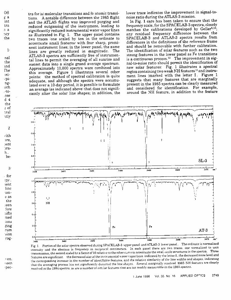
OS

gaint

ira

3 a

ncy

the

,I,

nalthemdFhe_xi-

.-pi-ng-dch-to-

.ose

d4thee of:ral

_tly

2]

vith

'are,_ent_ra-

be-

;

for

_py._entline

_om-

e as

the

)een-foreaiftsreedions

.-ingrumsion

rag-

yen,

veen

_pec-

tra for (a) molecular transitions and (bl atomic transi-tions. A notable difference between the 1985 flightand the ATLAS flights was improved purging andreduced outgassing of the instrument, leading tosignificantly reduced instrumental water vapor linesas illustrated in Fig. 1. The upper panel containstwo traces (one scaled by ten in the ordinate toaccentuate small features)with four sharp, promi-nent instrument lines; in the lower panel, the samelines are greatly reduced in magnitude. TheATLAS-3 spectra are sufficiently free of instrumen-tal lines to permit the averaging of all sunrise andsunset data into a single grand average spectrum.Approximately 10,000 spectra were combined intothis average. Figure 1 illustrates several otherpoints: the method of spectral calibration is quiteadequate, and although the spectra were accumu-lated over a 10-day period, it is possible to formulatean average (as indicated above)that does not signifi-cantly alter the solar line shapes; in addition, the

lower trace indicates the improvement in signal-to-noise ratio during the ATLAS-3 mission.

In Fig. 1 care has been taken to ensure that thefrequency scale, for the SPACELAB-3 spectra, closelymatches the calibrations developed by GellerS, t3;

any residual frequency difference between theSPACELAB-3 and ATLAS-3 spectra results fromdifferences in the definitions of the reference frameand should be removable with further calibration.The identification of solar features such as the twostrong features in the lower panel as Fe transitionsis a continuous process, la The improvement in sig-nal-to-noise ratio should permit the identification ofnew solar features: Fig. 1 illustrates a spectralregion containing two weak NH features Is and instru-ment lines (marked with the letter I. Figure 1suggests that many features that are marginallypresent in the 1985 spectra can be clearly measuredand considered for identification. For example,around the NH feature, in addition to the feature

i .... , .... _ .... , .... J _ " I .... i - -

I0,6

04

02

[ I

O0,,,I i .... r,, ,i

3456 3460 3462

?

i

LO

O8

06

04

_j

I_1

NH

3464

0.2FE

I

SL-3

3466 3468 3470 ¢$a

/ ,,_,"_L,"''--" ,,"_ "_"''_"_''--'_'_ 5/'%"', "_T"V'_':

Fe

3456 34_0 3462 3464

AT-3

I_ , i , . I , ,. I ..... '

3466 3468 3470 ¢m,

Fig. 1. PortionofthesolarspectraobservedduringSPACEL_B-3 upperpanel andATLAS-3 lowerpaneb. The ordinate is normalized

intensity and the abscissa is frequency in reciprocal centimeters. In each panel there are two traces, one normalized to unit

transmission, the second scaled by a factor of 10 relative to the other curve to accentuate the smalI-scale structures in the spectra. Three

features are significant: the decreased size of the instrumental water vapor lines indicated by the letter I, the decreased noise level and

the corresponding increase in the number of identifiable features, and the relative similarity of the line widths and shapes, indicating

that the averaging process has not significantly distorted the line shapes. Several marginally resolved _1985 NH features are clearly

resolved in the 1994 spectra, as are a number of similar features that are not readily measurable in the 1985 spectra.

1 June 1996 Vol. 35, No 16 APPLIED OPTICS 2749

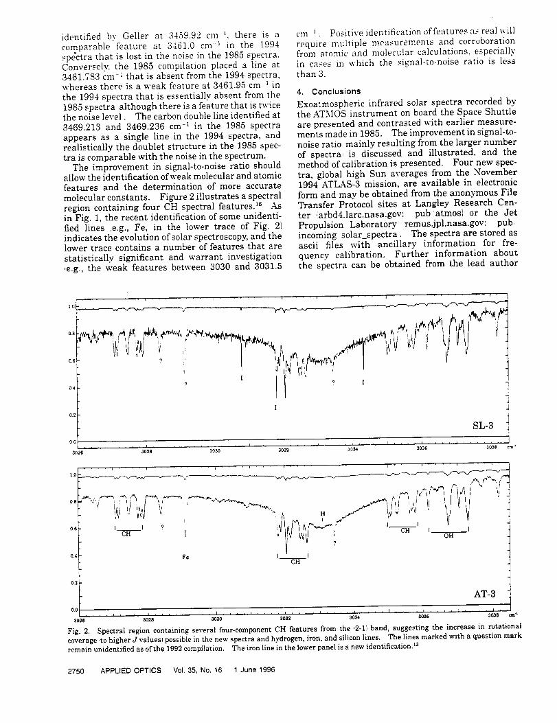
identified by Geller at ;3459.92 cm '. there is acomparable feature at 3461.0 cm _ in the 1994

spectra that is lost in the noise in the 1985 spectra.Conversely, the 1985 compilation placed a line at3461.783 cm-1 that is absent from the 1994 spectra,whereas there is a weak feature at 3461.95 cm-I in

the 1994 spectra that is essentially absent from the1985 spectra although there is a feature that is twicethe noise levell. The carbon double line identified at3469.213 and 3469.236 cm -_ in the 1985 spectra

appears as a single line in the 1994 spectra, andrealistically the doublet structure in the 1985 spec-tra is comparable with the noise in the spectrum.

The improvement in signal-to-noise ratio shouldallow the identification of weak molecular and atomicfeatures and the determination of more accuratemolecular constants. Figure 2 illustrates a spectral

region containing four CH spectral features. 16 Asin Fig. 1, the recent identification of some unidenti-fied lines !e.g., Fe, in the lower trace of Fig. 2)indicates the evolution of solar spectroscopy, and thelower trace contains a number of features that are

statistically significant and warrant investigation_e.g., the weak features between 3030 and 3031.5

cm _ Positive identification of features as real will

require multiple measurements and corroborationfrom atomic and molecular calculations, especially

in cases in which the signal-to-noise ratio is less

than 3.

4. Conclusions

Exoatmospheric infrared solar spectra recorded bythe ATMOS instrument on board the Space Shuttle

are presented and contrasted with earlier measure-ments made in 1985. The improvement in signal-to-

noise ratio mainly resulting from the larger numberof spectra_ is discussed and illustrated, and themethod of calibration is presented. Four new spec-

tra, global high Sun averages from the November1994 ATLAS-3 mission, are available in electronic

form and may be obtained from the anonymous FileTransfer Protocol sites at Langley Research Cen-

ter iarbd4.1arc.nasa.gov: pub atmos) or the Jet

Propulsion Laboratory remus.jpl.nasa.gov: pub,incoming solar_spectral. The spectra are stored asascii files with ancillary information for fre-

quency calibration. Further information aboutthe spectra can be obtained from the lead author

1.0

0.8

0.6

04

02

OC

SL-3 i

3038 era*, , , , , , [ , , , , I , , , , , , , , i3026 ' 3028 ' 3030 3032 3034 3036

• "n

__ ,. , v, -o.6 I_ I ';'

, Ifv ,: o.i

o.,_ Fe I ICH

0.2

AT-3 ,

i i i i L i i i 0128 ] , _ = i I , _ i _ I .... i , , , _ i ...... , .3026 ' 3 3030 3032 3034 3036 3038 ¢_

Fig. 2. Spectral region containing several four-component CH features from the '2-1) band, suggesting the increase in rotational

coverage to higher J values_ possible in the new spectra and hydrogen, iron, and silicon lines. The lines marked with a question mark

remain unidentified as of the 1992 compilation. The iron line in the lower panel is a new identification. _3

2750 APPLIED OPTICS Vol. 35, No. 16 .... 1 June 1996

im.c.abrams@larc.nasa.gov), and collaborative ef-

forts to measure, calibrate, and catalog these spectra

are welcome.

The authors acknowledge contributions from the

entire ATMOS data-processing facility and engineer-

ing teams. Research at the Jet Propulsion Labora-tory, California Institute of Technology, is performedunder contract to the National Aeronautics and

Space Administration. Contributions by R. Zanderwere supported by the Belgian Global Change pro-gram, which is coordinated by the Services Scienti-fiques, Techniques et Culturels, Brussels.

References

1. C. B. Farmer, O. F. Raper, and F. G. O'Callaghan, "Final

report on the first flight of the ATMOS instrument during the

SPACELAB-3 3 mission, April 29 Through May 6, 1985," JPL

Pub. 87 32 iJet Propulsion Laboratory, Pasadena, Calif.,

19871.

2. M. R. Gunson, R. J. Salawitch, M. C. Abrams, L. R. Brown,

T. L. Brown, A. Y. Chang, L. L. Lowes, F. W. Irwin, R. Zandeoz,

E. Mahieu, C. P. Rinsland, M. J. Newchurch, H. A. Michelsen,

A. Goldman, M. M. Abbas, and G. P. Stilles, "The atmospheric

trace molecule spectroscopy ,ATMOS} experiment deployment

on the ATLAS-3 space shuttle mission," to be published in

Geophys. Res. Lett. _1996.3. C. B. Farmer, "High resolution infrared spectroscopy of the

Sun and the earth's atmosphere from space," Mikrochim. Acta

Wien III, 189-214,1987.

4. P. G. Morse, "Progress report on the ATMOS sensor: design

description and development status," presented at the AIAA

Sensor Systems for the 80's Conference, Colorado Springs,

Colo., 2--4 December 1980, paper CP807.

5. C. B. Farmer and R. H. Norton, "Atlas of the infrared

spectrum of the Sun and the earth atmosphere from space," in

The Sun, NASA Ref. Pub. 1224 !NASA, Washington, D.C.,

1989, Vol. I.

6. M. Geller, "Atlas of the infrared spectrum of the Sun and the

earth atmosphere from space," in Key to Identification of Solar

Features, NASA Re['. Pub. 1224 (NASA, Washington, D.C.,

19921, Vol. III.7. N. Grevesse, A. J. Sauval, C. B. Farmer, and R. H. Norton,

"Diatomic molecules in the solar infrared spectrum from

ATMOS-SL 3 high resolution observations," presented at the

Twenty-Seventh Liege International Astrophysical Collo-

quium, Liege, Belgium, 23-26 June 1987.8. N. Grevesse and A. J. Sauval, "The infrared solar spectrum,"

in The Infrared Spectral Region of Stars; Proceedings of the

Montpellier Colloquium 1Cambridge U. Press, Cambridge,

England, 1991, pp. 215-233.

9. C. B. Farmer, "The ATMOS solar atlas," Infrared Sol. Phys.

154, 511-521 i1994.

10. R. H. Norton and C. P. Rinsland, "ATMOS data processing

and science analysis methods," Appl. Opt. 30, 389-400 I1991 _.

11. M. C. Abrams, G. C. Toon, and R. A. Schindler, "A practical

example of the correction of Fourier transform spectra for

detector nonlinearity," Appl. Opt. 33, 6307--6314 _1994!.

12. M. C. Abrams, M. R. Gunson, A. Y. Chang, C. P. Rinsland, and

R. Zander, "Remote sensing of the Earth's atmosphere from

space with high resolution Fourier transform spectroscopy:

development and methodology of data processing for the

Atmospheric Trace Molecule Spectroscopy experiment,"Appl.

Opt. 35, 2774-2786 ;1996.13. M. Geller, "Line identification inATMOS solar spectra, labora-

tory and astronomical high resolution spectra,"ASP Conf. Ser.

81, 88--95 _1995.

14. N. Edl_n, "The dispersion of standard air," J. Opt. Soc. Am. 43,

339-345 !1953.

15. N. Grevesse, D. L. Lambert, A. J. Sauval, E. F. van Dishoeck,

C. B. Farmer, and R. H. Norton, "Identification of solar

vibration-rotation lines of NH and the solar nitrogen abun-

dance," Astron. Astrophys. 232, 225-230 1990.

16. F. Melen, N. Grevesse, A. J. Sauval, C. B. Farmer, R. H.

Norton, H. Bredohl, and I. Dubois, "A new analysis of the

vibration-rotation spectrum of C H from solar spectra," J. Mol.

Spectrosc. 134, 305-313 19891.

cm _

)na[

mrk

1 June 1996 Vol. 35. No. 16 APPL1ED OPTICS 2751

@ Pergamon

J. Quanl. Sp_ctrosc. Radial. Transfer Vo[. 00, No. 0, pp. 00(3-000. 1994Copyright _ 1994 Else_'ier Science Lid

0022-4073(94)00062-X Printed in Great Britain. All rights resc'_'cd0022-4073/94 $7.00 + 0.00

HIGH RESOLUTION STUDIES OF HEAVY NOy

MOLECULES IN ATMOSPHERIC SPECTRA

A. GOLDMAN,t C. P. RINSLAND,_ F. J. MURCRAY,_ R. D. BLATHERWICK,t and D. G.

MURCRAYt

tDepartment of Physics, University of Denver, Denver, CO 80208, and **Atmospheric Sciences Division,

NASA LangleyR_earch Cenler,Hampton, VA 23681-000[,U.S.A.

(Receired ?)

Abstract--New line parameters for two heavy odd nitrogen molecules HNO3 in the v_/2v9

region, and CIONO: in the v_ re,on are incorporated in the analysis of high resolution i.r.atmospheric spectra. The line parameters are tested and renormalized vs laboratory spectra,and then applied to retrievals from balloon-borne and ground-basedsolar absorption spectra.

INTRODUCTION

High resolution (0.002-0.003cm -_) Michelson type interferometer systems are used at theUniversity of Denver to obtain i.r. solar absorption spectra of the stratosphere during balloonflights, as well as ground-based solar spectra. The stratospheric spectra in the region 700-2200 era-'cover spectral signatures of 03 (including isotopic species), NO:, HNO3, 03, N2, COF2, CIONO2,SF6, and others. For a typical study of new spectral features observable in such spectra see thediscussion of the 6 June 1988 flight data by Goldman et al. I Ground-based spectra in the 3-i2/zm

region are obtained regularly from Mauna Loa (Hawaii) and Denver (CO), in support of theNetwork for Detection of Stratospheric Change (NDSC) and the Upper Atmospheric Research

satellite (UARS).In support of the atmospheric observations, numerous laboratory spectra have been obtained

with the same interferometer systems. The laboratory spectra cover mostly the region700-3000cm-' and have also been extended down to 500 or up to 5000cm -I. The moleculescovered include CCI4, CC12F2, CCI3F, CF4, CHCIF2, CH3CI, CHCI3, CH20, C2H6, CIONO:,

COF:, COCI_, COCIF, HCOOH, HNO,, H202, NO2, HNO3, N20_, and others. Analysis ofstratospheric spectral features, combined with analysis of laboratory molecular absorption spectra,improves the spectral line parameters and leads to more complete line identifications and moreaccurate retrieval quantification of atmospheric gases.

In the present paper, updates of line parameters and their application to the University of Denverspectra will be presented for the 11 ]z region of HNO3 and the 780 crn-_ region of CIONO:.

RESULTS AND DISCUSSION

Recent updates of Line parameters for the HNO_ v_/2v9 bands, beyond the HITRAN 92 database,: have allowed improved quantitative analysis of atmospheric spectra in th_ 1 ]./a region. The

first update was initiated by A. G. Maki (unpublished) and included Fermi resonance effects onthe energy levels but unperturbed intensities. This provided improved modeling of the v3 manifoldsin the 860-875 cm -_ region of the atmospheric spectra, as reported by Goldman et al. 1"2This sethas been used successfully for most retrievals to date from high resolution airborne and_,round-based solar spectra. Subsequent update was based on Maki and Wells) who extended theanalysis with Fermi resonance, by adding unperturbed intensities to the published energies and linepositions. This update covered both bands, v,'ith improved agreement in the v5 manifolds and

A. GOLDM_ et a]

Q-branch, but the 2v9 Q-branch was still poorly modeled. The more recent update, based on thework of Perrin et al, 4 extended the treatment with both Fermi and Coriolis interactions, including

perturbed intensities. With this update the modeling of both the v5 and the 2v_ Q.branches is

significantly improved, and the Q-branches are now consistent with most P and R manifolds. Line

intensity plots for the two latest updates were shown in Fig. 1.In order to apply these data to atmospheric spectra in a fashion consistent with previous

retrievals from these bands and from the other major H'NO_ bands, the total band intensities were

normalized to the measured intensities of Giver et al, 5divided by a hot bands factor of 1.30, which

amounts to multiplying the Perrin et al lines _ (shown in Fig. 1) by 1.43. The hot bands are not

analyzed yet, but are not significant in the spectral intervals used for stratospheric retrievals; they

are thus not considered in the line list for this study.

Figure 2 shows a typical fitting in the s'_manifolds with the latest lines to data from the Universityof Denver balloon flight of 6 June 1988. The improvements in the Q-branches modeling is

demonstrated in Fig. 3, also with data from the 6 June 1988 flight. Comparisons with ground-based

spectra to be presented elsewhere, also show significant improvements in the spectral fitting.

Comparisons with retrievals with the previous two line parameters updates show consistency of

better than 4% over the 860-870 cm-I manifolds.The first update of the initial cross-sections for CIONO2 (HITRAN 1986) was provided by the

work of Ballard et al, _ which generated cross-sections in the 700-1800 cm-* at 213-296 K. These

cross-sections were included in the HITRAN 92 data base. 7Recent analysis of the v4CIONO_ region (the most useful for atmospheric retrievals) by Bell et al, s

provided spectroscopic constants for the three main bands in this region, v, _sCIONOj, v4_7CIONO2, and ,', + *'9- *'9_sCIONO:. Based on this analysis, line parameters were generated in

the v_ region, with the relative intensities of the three bands normalized to 0.002 cm -1 resolution

laboratory spectra taken at the University of Denver, and absolute intensities normalized to thevalues of Ballard et al, 6 with the continuum removed (providing consistency of better than 3% with

previous retrievals). The new line parameters were then applied to retrievals in the 780.2 cm -_

region from D.U. balloon-borne and ground-based spectra taken at 0.002-0.006 cm -I resolution.The new line parameters showed improved agreement with observed data, even though the finestructure is not fully modeled yet. Intensity plots of the normalized line parameters are shown in

Fig. 4. Modeling of the 780.2 era-' region from University of Denver laboratory data is shown in

Fig. 5. Fitting to stratospheric spectra obtained by University of Denver during the 6 June 1988

flight is shown in Fig. 6.The new line parameters of HNO3 and C1ONO2 were thus applied in retrievals of altitude mixing

ratio profiles from sunset spectra obtained during two D.U. balloon flights made on 6 June 1988

(from Palestine, Texas, with float altitude of 36.7 kin) and 24 July 1992 (Palestine, Texas, floataltitude of 34kin). Sunset scans were obtained during the 6 June 1988 flight down to 15.60kin

tangent altitude, but only down to 24.30 km tangent altitude during the 24 July 1992 flight; thePinatubo aerosol caused loss of the source signal below this altitude. Both flights covered the same

spectral interval of 700---1350 cm -_ with resolution of ~0.0025 era -I. The resolution and the signalto noise ratio were slightly better during the 6 June 1988 flight. Spectral fitting results were tested

by two non-linear spectral least squares programs, one based on the work of Niple et al, 9 and oneon Rinsland et al, k° combined with the onion-peeling method for the mixing ratio profile. The

agreement between the two methods is better than 2% in any step of the onion-peeling, assuming

the same atmospheric and spectroscopic parameters.The retrieved mixing ralios are shown in Figs. 7, 8, which also include comparisons with prex'ious

results_HNO3 from D.U., 1. ATMOS, Iz LIMS, 13WMO (1986), 14and BLISS,iS'and CIONO: fromATMOS. j6 The results from the two flights are included in the comparisons of'CLAES-UARS

retrievals and other correlative measurements and 2-D global model calculations, as reported by

Mertzenthaler et a[. _7 These comparisons show that both HNO_ and C1ONO2 profiles exhibits

significant variabilities, not fully modeled yet, even for mid latitudes. In particular, shifts in thealtitudes of the peak of the CIONOz profiles such as seen in Fig. 8, also appear in the CLAES

results. .7 The improved line parameters will provide a more accurate and consistent quantification

of these species from i.r. atmospheric spectra.

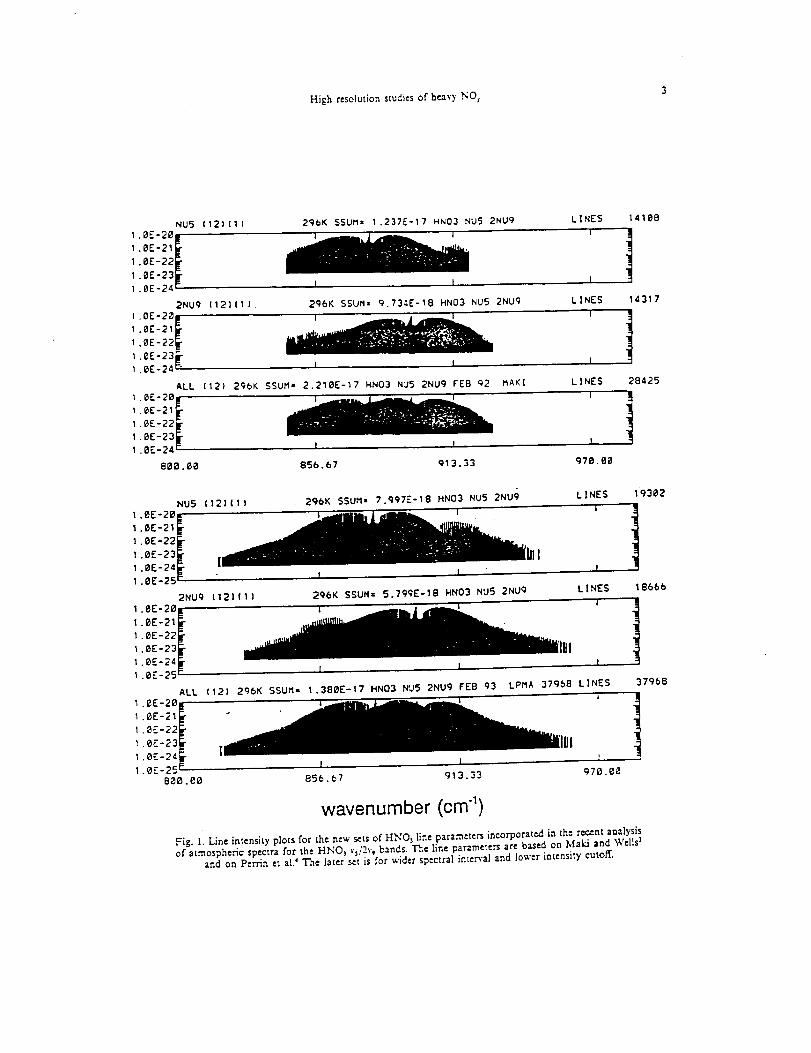
High resolutionstudiesor heavy NO) 3

NU5 112}(II

I .0E-20_

I. 0E-2 I_-

I. 0E-22_-

I. OE-23_rt .0E-24 [

296K SSUM= 1.237E-17 HN03 NU5 2NU9 LINES

i

2NUg (12]11l

1.0E-20_

1.0E-21_

1,0E-22_

1.0E-23_1.0E-24 r"

I I I

2q6K SSUM= g.734E-18 HN03 NU5 2NUq LINES

I I I

141e8

!14317

I I I

ffAK[ LINES

IALL (12) 2C_6K SSUM,, 2.210E-17 HN03 NU5 2NUg FEB 92

t . 0E-20_ j i

1. @E-21_-

1 .QE-22_

1.0E-23_1 .0E-24 r I I

800.00 856.67 g13.33

28425

q70.00

296K 5SUM, 7.997E-18 HN03 NU5 2NU9

f

I I

296K SSUH= 5.799E-18 HN03 NU5 2NUg

LINES 19302

LINES 18666

.OE_20IE -f T

._E-21_"

.eE-22_"

.OE-23_-

.{}E-24_-

.0E_25 r I I

ALL 1121 296K SSUM= 1.380E-17 HNO3 N'J5 2NU9 FEB 93

I. eE-20 !

1 .0E-21

I ._E-22

1 .eE-23

1 .0E-24 I

1.0E-25 I I ¢)70.008_0.e0 856.67 913.33

wavenumber (era "1)

Fig. 1. Line intensity plots for the new sets of HNO) line parameters incorporateA in the re_.nt analysisof atmospheric spectra for the HNO3 vs/2v, bands. T,,e line parameters are based on MaLl and Wells 3

and on P_'rrin et ale The later set is for wider spectral interval and lower intensity cutoff.

LPMA 37968 LINES 37968

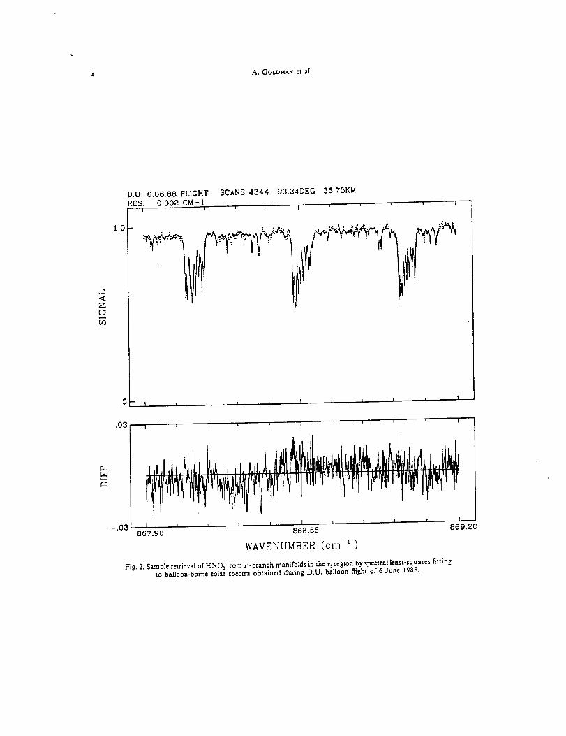
4 A. GOLDMAN el a[

<ZL?

l_O

.5

).U. 6.06.88 FLIGHT

_ES. 0.002 CM- l| i '

SCANS 4344 93.34DEG 36.75KI,(

, |i i | i i i

.:. :,

-- 1 ? I f ! 1 I I I I

i

I ,

i I

.03 i ' ' ' ' l ' ' '

-.03 I i i I I I r i T T '867.90 868.55 869.2U

WAVENUMBER (cm -1 )

FiE. 2. Sample retrieval or H]WO) from P-branch manifolds in th," _'_rc_ion by spectral ]east-squares fittln_to ba]]oon-borne solar spectra obtained during D.U. balloon fl{ght of 6/un¢ 1985.

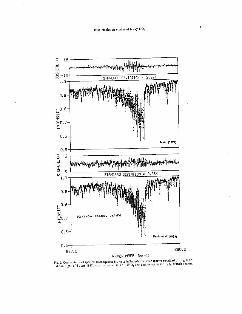
High resolutionstudiesof heavy NOy 5

d

{D STANDARD DEVIATION = 2.72X1.0

0.9-

_0.8-

0.'7-

0.6-

0.5 I

•_ 5w

JQ:(.J

U')¢> -5

1.0

0._-

STANDARD DEVIATION = 0.957.

Penin _ aL (1993)

>-0.8-

u_z

o.7-z

0,6--

0.5 I

SCANS 434.4 93.34DEG 36.'/5KM

877. D 880.0NRVENUHBER (cm-!)

Fig. 3. Comparisons of spectral least-squares fitting to balloon-borne solar spectra obtained during D.U.balloon flight of 6 June 1988, with the recent sets of HNO_ line parameters in the v5 Q-branch region.

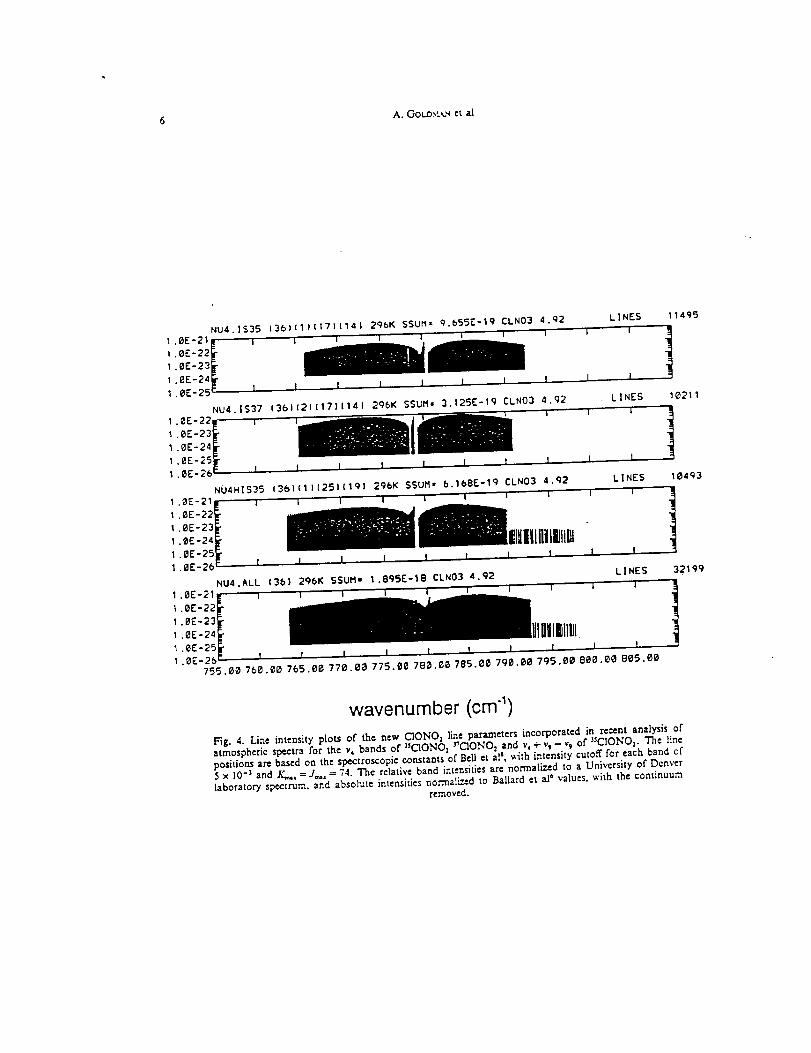
A.GOLD_t,,.'_ et al

NU4.lS35 |36)(1)ll71(14| 296K SSUM= 9.b55E-19 CLN03 4.92 LINES 11495

1 .0E°21 _ _ _

I .@E-22_ _ _11111 _ "i1 .0E-23'

1 .0E-24

I .eE-25

NU4.[$37 (3bl(21(17][141 296K SSUM= 3.125E-19 CLN03 4,q2 . LINES 19211

1.0E-22

1.0E-23

1.0E-24

1.6E-25

1'0E'26_NU4HIS35 13bi(1l{251[10! 29f_K SSUH= b.168E-19 ELN03 4.¢J2 LINES 10493

Nu4.ALL 13b) 296K SSUH= 1.895E-1B CLN03 4.92LINES 32199

755,80 768.00 765.80 770.00 775.00 780.80 785.00 790.00 795.00 880.00 805.00

wavenumber (cm 4)

Eig. 4. Line intensity plots of the new C-'3ONOs line parameters incorporated in recent analysis ofatmos heric s ctra for the v, bands of 3sCIONO: 3_CIONO= and v,+ v,- vt of _CIONO2- The line

p pc . i w't intensitycutoff for each band ofpositionsarc based on the spcctroscop:c constants of Belleta[, _ h5 x 10-3 and K,,,,= 2"=,== 74. The relativeband int.-nsitiesare normalized to a University of Denver

laboratory spectrum, and absolute intensitiesnor:-nali.zgdto Ballard et al6 values,with the continuumremoved.

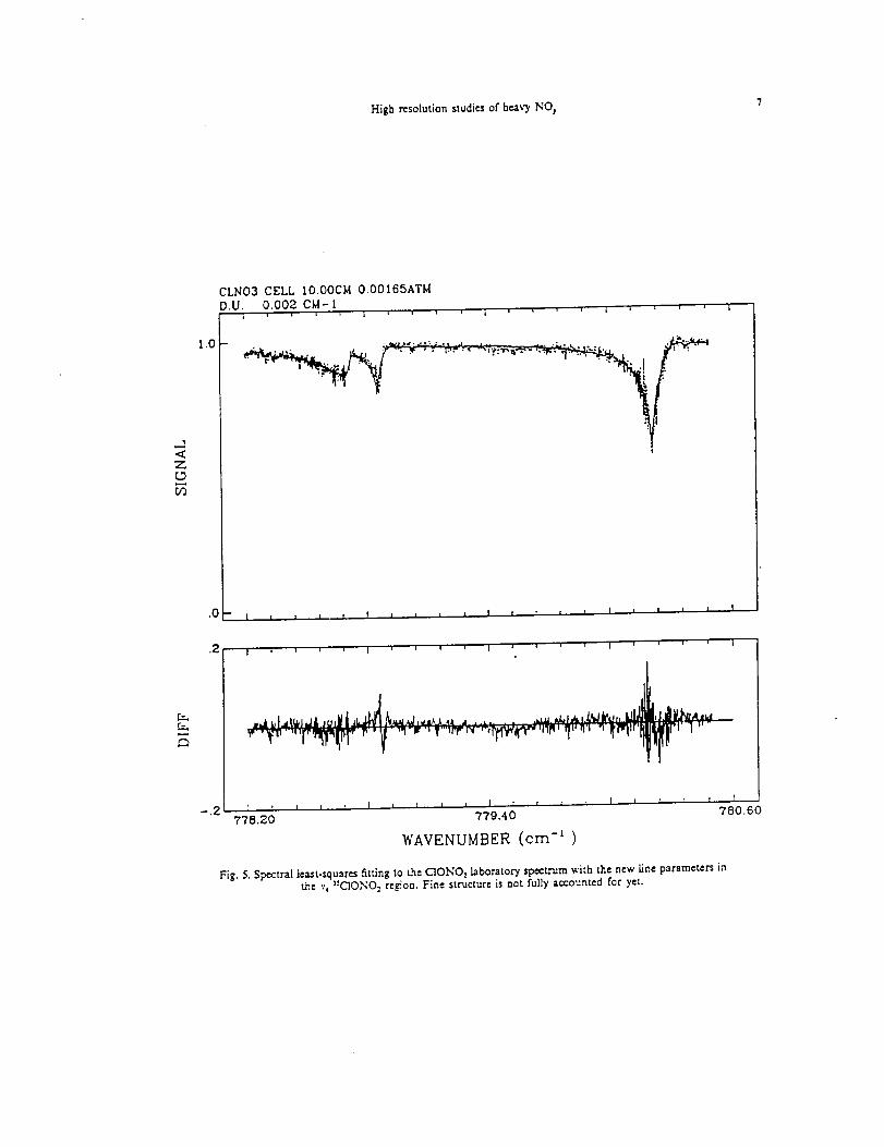
High resolution studies of heavy NOy ?

._iI<Z

1.0

N

r..

B

CLN03 CELL IO.OOCM O.O0165ATM

hU. 0.002 CM- II l L i + i i i

I ' " 'I '

! I I l I _ I I I I ] I : I I I I I ! I

.2

-.2

I * i , l I + i , L I i i i _ 1 + i i i |

'''" '

? T I I _ 1 r T I t [ t I P

779.40778.20

WAVENUMBER (cm -I )

+ I J r _ r

Fig. 5. Spectral least-squares fitting to t+h,"CIONO 2laboratory spectrum with the new llne parameters inMe v+ _CIONO, re,on. Fine structure is not fully accounted for yet.

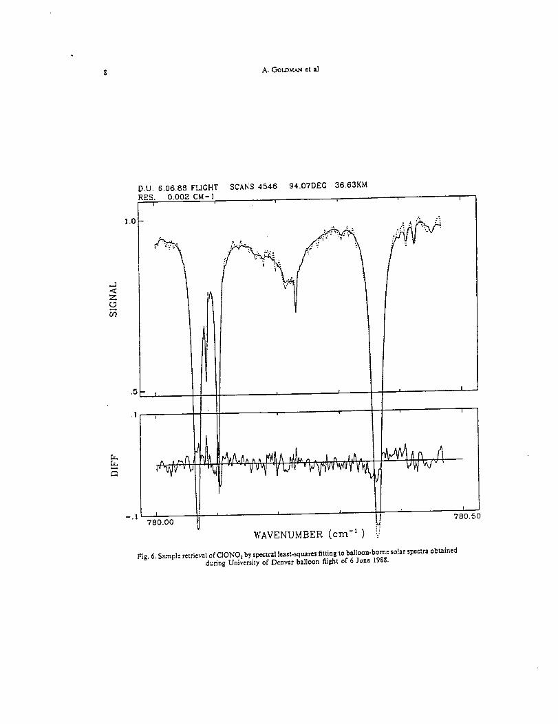
$ A. OoT r'_ et a]

D.U. 6.06.88 FLIGHT

RES. 0.002 CM- l,

1.0 I-

<Z

In

.5- I ! '

-[ I

C_

780.00

SCANS 4546 94.07DEG 36.63KM

i

r

, I

| I

WAVENUMBER (cm -I )

I

780.50

Fig. 6. S_mpL"retrieval o[ C]ONO2 by spectral lcast-sctuams fitting to balloon-borne solar spectra obtainedduring University or Denver balloon flight of 6 June 1988.

High resolution studies of h_vy NO, 9

0j

m°_

.<

40

35

3O

25

2O

\

H:_ \\\

o

O

ATMOS/SpacelabLIMS

WMO [1986]BLISSDU 6-4-90 Fit.DU 6-6-88 Fit.DU 7-24-92 Fit.

\

r I B I 1 T150 2 4 6

HNO 3 Volume Mixing Ratio (ppbv)

Fig. 7. Comparison of the recent retrievals of HNO3 mixing ratio altitude profiles from the Universityof Denver balloon flights of 6 .lune 19SS and 24 luly 1992. The D.U. 4 June 1990 results were obtained

from the v= region." The ATMOS, LIMS, WMO (1986) and BLISS r=sulus are from Ref. 12-15respectively.

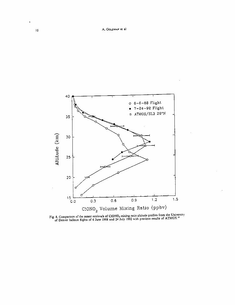
]0 A. GOLDM/_ et al

4O

35

o 6-6-88 Flight

• 7-24-92 Flight

D ATMOS/SL3 29°N

3o

o

25

2O

ira.I , , I , , I , , I , , T , ,0.0 0.3 0.6 0.9 1.2 1.5

CIONO 2 Volume ._iixing Ratio (ppbv)

Fig. 8. Compzr_son of the recent retrievals of C]ONO_ mixing ratio altitude profiles from the Universitvof Denver balloon flights of 6 June 1988 and 24 July 1992 whh previous results of ATMOS) _

Highresolutionstudies of heavy NO r1!

Acknowledgements--T_s research was supported in pan by NSF and in part by NASA. We thank A. G. Maki, J.-M. Flaud,and A. Pen-in for providing theoretical results from their HNO_ studies. Acknowledgement is made to the National Centerfor Atmospheric Research, which is sponsored by the National Science Foundation, for computer time used in tiffs project.

REFERENCES

1. A. Goldman, F. J. Murcray, R. D.,..,l_ather_hck, J. J. Kosters, F. _ Murcray, D. G. Murcray, and C.

P. Rinsland, J. geophys. Res. 94, 5_Q(1989). /t./_qqs-

2. A. Goldman and C. P. Rinsland, JQSRT 48, 653 (1992).

3. A. G. Maki and J. S. Wells, J. molec. Spectrosc. 152, 69 (1992).4. A. Perrin, V. Jaquen, A. Valentin, J.-M. Flaud and C. Camy-Peyret, J. molec. Spectrosc. 157, 112 (1993);

A. Perrin, J.-M. Flaud, C. Camy-Peyret, V. Jaquen, R. Farrenq, F. Guelachvili, Q. Kou, F. Le Roy, M.

Morillon-Chapey, J. Orphal, M. Badaqoui, J.-Y. Mandin, and V. Dana, Y. molec. Spectrosc. 160, 524

(1993).5. L. P. Giver, F. P. J. Valero, D. Goorvitch, and F. S. Bonomo, J. opt. Soc. Am. B. 1, 715 (1984).

6. J. Ballard, W. B. Johnston, M. R. Gunson, and P. T. Wassel, J. geophys. Res. 93, 1659 (1988).

7. S. T. Massie and A. Goldman, JQSRT 48, 713 (1992).

8. W. Bell, G. Duxbury, and D. D. Stuart, J. molec. Spectrosc. 152, 283 (1992).9. E. Niple, W. G. Mankin, A. Goldman, D. G. Murcray, and F. J. Murcray, Geoph)'s. Res. Lett. 7, 489

(1980).10. C.P. Rinsland, A. Go]dman, F. J. Murcray, D. G. Murcray, M. A. H. Smith, R. K. Seals Jr., J. C. Larsen,

and P. L. Rinsland, AppL Opt. 21, 4351 (1982).1I. A. Goldman, F. J. Murcray, R. D. Blather'wick, J. J. Kosters, D. G. Murcray, C. P. Rinsland, J.-M. Flaud,

and C. Camy-Peyrct, J. geopfiys. Res. 97, 2561 (1992).12. J. M. Russel llI, C. B. Farmer, C. P. Rinsland, R. Zander, L. Froidevaux, G. C. Toon, B. Gao, J. Shaw,

and M. Gunson, J. geophys. Res. 93, 1718 (1988).13. J. C. Gille, J. M. Russel Ill, P. L. Bailey, E. E. Remsberg, L. L. Gordley, W. F. J. Evans, H. Fischer,

B. W. Gandrud, A. Girard, J. E. Harries, and S. A. Beck, J. geophys. Res. 89, 5179 (1984); J. C. Gille,

P. L. Bailey, and C. A. Craig, Adv. Space Res. 13, 59 (1993).14. World Meteorological Organization (WMO), "Atmospheric Ozone 1985----Assessment of our understand-

ing of the processes controlling its present distributig.a..,and change, ':W_ Re;,. 16, Geneva (1986).

15. R. D. May and C. R. Webster, J. geophys, l_es. 94, 4(Q_1989). t_ _?_.,_16. R. Zander, M. R. Gunson, J. C. Foster, C. P. Rinsland, and J. Namkung, Y. geophys. Res. 95,¢,._.I,9(1990).

17. J. L. Mergenthaler, J. B. Kumer, A. E. Roche, R. W. Nightingale, D. G. Murcray, F. J. Murcray, J. W.,Villiams, and A. Goldman, AGU 1993 fall meeting, San Francisco, Paper AI2D-2 (1993).

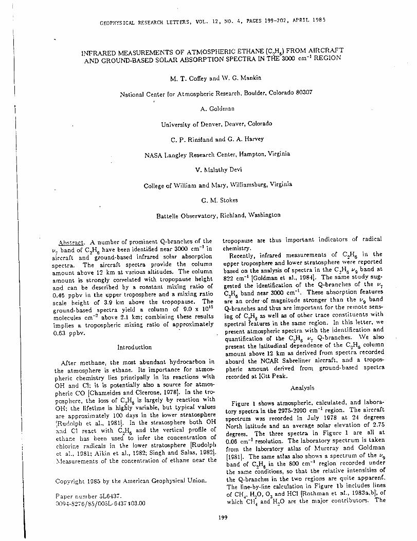
GEOPHYSICAL RESEARCH LETTERS, VOL. 12, NO. 4, PAGES 199-202, APRIL 1985

INFRARED MEASUREMENTS OF ATMOSPIIERIC ETHANE (C?H6) FROM AIRCRAFT

AND GROUND-BASED SOLAR ABSORPTION SPECTRA IN THE 3000 cm -I REGION

M. T. Cofl'ey and IV. G. Mankin

National Center for Atmospheric Research, Boulder, Colorado 80307

A. Goldman

University or Denver, Denver, Colorado

C. P. Rinsland and G. A. Harvey

NASA Langley Research Center, Hampton, Virginia

V. Malathy Devi

College of William and Mary, Williamsburg, Virginia

G. M. Stokes

Battelle Observatory, Richland, \Vashington

_. A number of prominent Q-branches of the

v 7 band of C_H 6 have been identified near 3000 cm -l in

aircraft and ground-based infrared solar absorption

spectra. The aircraft spectra provide the columnamount above 12 km at various altitudes. The column

amount is strongly correlated with tropopause height

and can be described by a constant mixing ratio of

0.46 ppbv in the upper troposphere and a mixing ratio

scale height of 3.9 km above the tropopause. The

ground-based spectra yield a column of 9.0 x 10 Is_o

molecules cm " above 2.1 kin; combining these results

implies a tropospheric mixing ratio of approximately

0.63 ppbv.

Introduction

After methane, the most abundant hydrocarbon in

the atmosphere is ethane. Its importance for atmos-

pheric chemistry lies principally in its reactions with

OH and CI; it is potentially also a source for atmos-

pheric CO [Chameides and Cicerone, 1978]. In the tro-

posphere, the loss of C?H 6 is largely by reaction with

OH; the lifetime is highly variable, but typical values

are approximately 100 days in the lower stratosphere

[Rudolph et al., 19811 . In the stratosphere both OH

and CI react with C_H 6 and the vertical profile ofethane has been used to infer the concentration of

chlorine radicals in the lower stratosphere [Rudolph

et al., 1981; Aikin eta]., 1982; Singh and Salas, 1982].

Measurements of the concentration of ethane near the

Copyright 1985 by the American Geophysical Union.

Paper number 5L6437.

0094-8276/85/005L-6437503.00

tropopause are thus important indicators of radical

chemistry.

Recently, infrared measurements of Co.H 6 in the

upper troposphere and lower stratosphere were reported

based on the analysis of spectra in the C.,H 6 vg band at

822 cm -l [Goldman et al., 1984]. The same study sug-

gested the identification of the Q-branches of the v 7

C_.H 6 band near 3000 cm -t. These absorption featuresare an orderof magnitude stronger than the v 9 band

Q-branches and thus are important for the remote sens-

ing of C_H 6 as well as of other trace constituents with

spectral features in the same region. In this letter, we

present atmospheric spectra with the identification and

quantification of the C.oH 6 v 7 Q-branches. \Ve also

present the latitudinal dependence of the Co H 6 column

amount above 12 km as derived from spectra recorded

aboard the NCAR Sabreliner aircraft, and a tropos-

pheric amount derived from ground-based spectra

recorded at Kitt Peak.

Analysis

Figure I shows atmospheric, calculated, and labora-

tory spectra in the 2975-2990 cm -t region. The aircraft

spectrum wa_ recorded in July 1978 at 2-I degrees

North latitude and an average solar elevation of 2.75

degrees. The three spectra in Figure i are all at

0.06 cm -l resolution. The laboratory spectrum is taken

from the laboratory atlas of Murcray and Goldman

[19811. The same atlas also shows a spectrum of the v 9

band of C_.H 6 in the 800 cm -t region recorded underthe same conditions, so that the relative intensities of

the Q-branches in the two regions are quite apparen{:.

The line-by-line calculation in Figure Ib includes lines

of CH 4, H20, O 3 and HCf [Rothman et al., 1983a,b]_ of

which CH 4 and H.._O are the major contributors. The

199

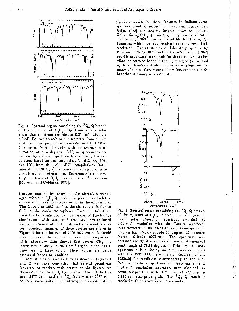
20Z Coffey eL al.: Infrared Measurement of Atmospheric Ethane

_I I r_[_I I r + bIl'+ IT 11 ' II"I I ' 11'I II III '1 I' I' 1' I111 ' I '+'" 111'1 +I'll L'IIII'I I'TIII I............. TIIII I

o

,

0 h I'II III III llll I i_ Ill *I h II II ' Ill I H ll II II ll"lllllllll lllllllill tl _ +"Itll

, I I I I+I I II, ll;t I II I11,,, I +I I, IHI II l+l,l,l,,l,l,,l,l,111 I, II,I+I+, II IIIII+

Lobo+'OlOt y St_¢tlum

z

- (c) - -ii ti Ii nlntnlllhlllSellJ hHnllHl*ntllhlllhltllnl*,htntlln+nhHIl*n+l

29?5 2980 298S 2990

WAVENUMBER (C m'*)

FIg. 1 Spectral region containing the RQ0 Q-branch

of the u 7 band of Coil 6. Spectrum a is a solar

absorption spectrum recorded at 0.06 cm -n with the

NCAR Fourier transform spectrometer from 12 km

ahitude. The spectrum was recorded in July 1978 at

24 degrees North latitude with au average solar

elevation of 2.75 degrees. C_H 6 u; Q-branches are

marked by arrows. Spectrum b is a line-by-line cal-

culation based on line parameters for H20, O.. CH 4and HCI from the 19is2 )YFGL compilations ]Roth-

man et al., 1983a, hi, for conditions correspondhlg to

the observed spectrum in a. Spectrum c is a labora-

tory spectrum of C,.H 6 also at 0.06 cm -I resolution

[Murcray and Goldman, 19811.

features marked by arrows in the aircraft spectrum

agree with the Coil 6 Q-branches in position and relativeintensity and are not accounted for in the calculations.

The feature at 2982 cm -x in the observation is due to

Si I in the sun's atmosphere. These identifications

were further confirmed by comparison of line-by-line

simulations with 0.01 cm -1 resolution ground-hased

spectra obtained at I(itt Peak and additional labora-

tory spectra. Samples of these spectra are shown in

Figure 2 for the interval of 2976-2977 cm-L It should

also be noted that our simulations and comparisons

with laboratory data showed that several CH 4 lineintensities in the 2990-3000 cm -l region in the AFGL

tape are in large error. These values are being

corrected for the next edition.

From studies of spectra such as shown in Figures I

and 2 we have concluded that several prominent

features, as marked with arrows on the figures, "are

dominated by the CoH 6 Q-branches. The PQ3 feature

near 2977 cm -l and'the l_Q0 feature near 2987 cm -l

are the most suitable for atmospheric quantification.

Previous search for these features in balloon-borne

spectra showed no measurable absorptions [I<endall and

Buijs, 1983] for tangent heights down to 19 km.

Unlike the % C_H 6 Q-branches, line parameters [Roth-

man et al., lCJ83b] are not available for the v 7 Q-

branches, which are not resolved even at very high

resolution. Recent s',udies of laboratory spectra by

Pine and Lafferty [19821 and by Dang-Nhu et al. [t984]provide accurate energy levels for the three overlapping

vlbration-rotation bands in the :3 pm region (u s, u7 and

tz8 + t,+t bands) and also approximate intensities for

many of the weaker, resolved lines but exclude the Q-

branches of atmospheric interest.

1.0

0,8

0,6Z

0.4

0.2

0

I0

0.8

z

0.4

0.2

0

1.0

0.8

0.6zo

0.4

o,2 (¢|

02976.0

(o1

i

Ib|

i

• V"

i

297_.5 2977.0

WAVENUMBER (cm "I )

Fig. 2 Spectra] region containing the PQ3 Q-branch

of the v 7 band of C_H 6. Spectrum a is a ground-

based solar absorption spectrum recorded at

0.01 cm -I resolution with the Fourier transform

interferomcter in the McMath solar telescope com-

plex on Kilt Peak {latitude 31 degrees, 57 minutes

North, altitude 2095 m). The spectrum was

obtained shortly after sunrise at a mean astronomical

zenith angle of 78.72 degrees on February 23, 1981.

Spectrum b is a line-by-line simulation calculated

with the 1982 AFGL parameters [Rothman et al.,

1983a,b] for conditions corresponding to the Kilt

Peak atmospheric spectrum a. Spectrum c is a

0.06 cm -I resolution laboratory scan obtained at

room temperature with 0.21 Torr of Coil 6 in a

5.125 cm absorption path. The PQ3 Q-[_ranch is

marked with an arrow in spectra a and c.

Coffeyetal.: InfraredMeasurementof AtmosphericEthane 201

e_

'E

o

o_)..Z

8

z

8(..)

£(.)

i I l I I i i' I

4,

CzH 6 Amo4ml

e 4,

(,

I I I I ! 1 I0 IO ZO _0 40 50 60 ?0

LATITUDE (Notlh)

i 18

16

14 0

c

_o

s

6

2

I O.8O

Fig. 3 Latitudinal dependence of the C_H 6 column

amount above 12 km altitude as derived from the

aircraft data. Column amounts are averaged from

spectra taken over 5 degrees of latitude and

represent typically an average of from 8 to 10 indivi-

dual spectra, some recorded in summer and others in

winter. Also shown is the height of the tropopause.

The solid circles are the average of winter and sum-

mer tropopause heights from the nearest radiosonde

observations to the aircraft location.

The Coil6 quantification is therefore based on theequivalent width method with the PQ3 and RQ 0 intensi-

ties measured from laboratory spectra. The C_.H 6 Q-

branches quantified here are very dense with spectral

lines and not broadened significantly by the instrumen-

tal spectral resolution. Thus, a small absorption by

these Q-branches corresponds to the weak line approxi-

mation, where the integrated absorption is proportional

to the product of gas amount and the integrated inten-

sity. ._ssuming linear absorption in the laboratory

spectrum of Figure 1 gives an integrated intensity ofS _ 3.23 e 0.81 x 10 -10 era-I/molecules cm --_ (at

298 K) for RQ 0. Laboratory measurements at NASA

Langley, Such as in Figure 2c, resulted in an integrated

intensity for PQ of S = 3.91 ± 0.84 x 10 q°

cm-l/molcules cm '-_"at 298 I(. These values have been

used in the present analysis.

Aircraft spectra taken over a number of years and a

wide range of latitudes show C_H 6 absorption above the

flight level of 12 kin. The C_[ 6 column amount is

observed to have a maximum at low latitudes and

decreases toward the pole. The variation with latitude

is strongly correlated with the tropopanse altitude as

shown in Figure 3.

Discussion

The obvious correlation between column amount and

tropopause height leads us to attempt to deduce the

variation of density of C_H 6 in the vicinity of the tro-

popause by fitting the data to the values derived from

a simple parametric model profile. We used a model

with a constant mixing ratio below the tropopause and

an exponential decrease of mixing ratio above the fro-

popause. The two parameters which were fitted are the

tropopause mixing ratio and the mixing ratio scale

height. The parameters were determined by a least

squares fit of the observed columns to the values calcu-

lated from the model profile. The resulting best fit was

for a mixing ratio at the tropopause of 0.46 ppbv and a

scale height of the mixing ratio in the lower strato-

sphere of 3.9 kin. This analysis neglects several impor-

tant variables, particularly the latitude, but the tropo-

pause height is the most significant variable, and the

limited data set does not justify fitting more parame-

ters. The rms difference between the observed and cal-

culated columns is 0.25 x l0 Is molecules cm -°'.

The ground-based measurement in Figure 2 yields a

CoH 6 column of 9.0 x 10 Is molecules cm-" above theol_servation altitude of 2.1 km. The aircraft measure-

meat at that latitude indicated 1.1-x 10 Is molecules

cm -°- above 12 kin. Although the aircraft measure-

ments were made at a different season, if we assume

that they are representative of the time of the ground-

based observation, the column between 2.1 and 12 km

is "7.9 x I0 Is molecules cni -_', corresponding to a mean

mixing ratio of 0.83 ppbv. The ground-bated and air-

craft results are consistent with previous. C_H 6 sampling

measurements [Randolph et al, 1981; Aikin et al.,

1982: Siugh and Salas, 1982 I.

Acknowledgments, \Ve would like to express our

appreciation of the excellent service provided to us by

the NC._R Research Aviation Facility.

The National Center for Atmospheric Research is

sponsored by the National Science Foundation.

References

Aikin, A. C., J. R. Herman, E. J. Maier. and C. J.

McQuillan, Atmospheric chemistry of ethane and

ethylene, .L Geo _ Res., 87, 3105-3118, 1982.

Chameides, W. L., _md R. J. Cicerone, Effects of non-

methane hydrocarbons in the atmosphere, .1.

p_h._. Res. 83, 947-952, 1978.

Dang-Nhu, M., A. S. Pine, and W. J. Lafferty, Les

intensites dans les bande v s, v? et v s + vll de

l'ethane 17C_I-I 6, C.anad, ._1. Phy._., 62, 512-519, 1984.Goldman, A., C. P. Rinsland, F. J. *lurcray, D. C.

Murcray, M. T. Coffey, and \V. G. Mankin,

Balloon-borne and aircraft measurements of ethane

(C_H6) in the upper troposphere and lower strato-

sphere, ,[. Atmos. Chem., 2, 211-221, 1984.Kendall, D. J. W., and H. L. Buijs, Stratospheric NO_

and upper limits of CH3CI and C_H 6 fi-om measure-

ments at 3.4 ym, _, 303,221-222, 1983.

Murcray, D. G., and A. Goldman, Eds., C RG _-

boo.__..kkof _ Resolntion Infrared Laboratory

of Atmosnheric _, CRC Press, Boca Raton,

Florida, 1981.

Pine, A. S., and W. J. Lafferty, Torsional splittings and

assignments of the Doppler-limited spectrum of

ethane in the C-H stretching region, .J. Res. _,

87, 237-258, 1082.

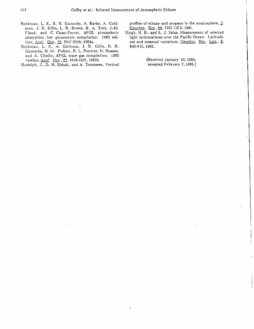
29:_ Coffey et al.: Infrared .Measurement of Atmospheric Ethane

Rothman, L. S., R. R. Gamache, A. Barbe, A. Gold-

man, J. R. Gillis, L. R. Brown, R. A. Toth, J.-M.

Flaud. and C. Camy-Peyret, AFGL atmospheric

absorption line parameters compilation: 1082 edi-

tion, ::_.._. _)_P_L, -°'2-, 2247-2256, 1983a.

Rothman, L. S.. A. Goldman, J. R. Gillis, R. R.

Gamache, H. N[. Pickett, R. L. Poynter, N. Husson,

and A. Chedin, AFGL trace gas compilation: 1982

version, _P_2.!. Ont., 0'2_, 1616-1{327, 1983b.

Rudolph, J., D. H. Ehhalt, and A. Tonnissen, Vertical

profiles of ethane and propane in the stratosphere, J.

_. Res., 86, 72{37-7272. 1981.

Si,lgh, H. B., and L. J. Salas, Measurement of selected

light hydrocarbons over the Pacific Ocean: Latitudi-

nal and seasonal variations, _. Res. Lett., 9.,

842-845, 1082.

(Received January I0, 1085;

accepted February 7, 1985.)

Journal of Atmospheric Chemistry 16: 31-40, 1993.1993 Kluwer Academic Publishers. Printed in the Netherlands.

31

Stratospheric N205, CH4, and N20 Profiles

from IR Solar Occultation Spectra

C. CAMY-PEYRET, J.-M. FLAUD, and A. PERRIN

Laboratoire de Physique Moldculaire et Applications', CNRS Universit_ Pierre and Marie Curie,

Paris, France

C. P. RINSLAND

Atmospheric Sciences Division, NASA Langley Research Center, Hampton, Virginia, U.S.A.

A. GOLDMAN and F. J. MURCRAY

Department of Physics, University of Denver, Denver, Colorado, US.A.

(Received: 23 January 1992; in final form: 3 June 1992)

Abstract. Stratospheric volume mixing ratio profiles of N_O s, CH 4, and N20 have been retrieved

from a set of 0.052 cm -_ resolution (FWHlVl) solar occultation spectra recorded at sunrise during a

balloon flight from Aire sur 19,dour, France (44" N latitude) on 12 October 1990. The N205 results

have been derived from measurements of the integrated absorption by the 1246 cm -t band. Assuming

a total intensity of 4.32 x 10 -17 cm-I/molecule cm -2 independent of temperature, the retrieved N20 s

volume mixing ratios in ppbv (parts per billion by volume, 10"9), interpolated to 2 Ima height spacings,

are 1.64:t:0.49 at 37.5.km, 1.92+0.56 at 35.5 kin, 2.06+0.47 at 33.5 kin, 1.95-1-0.42 at 31.5 kin,1.60 + 0.33 at 29.5 kin, 1.26 + 0.28 at 27.5 kin, and 0.85 + 0.20 at 25.5 kin. Error bars indicate the

estimated 1-a uncertainty including the error in the total band intensity (:t:200 has been assumed).

The retrieved profiles are compared with previous measurements and photochemical model results.

Key words, Atmospheric composition, middle atmosphere, stratosphere, Fourier transform spectros-

copy, balloon measurements, nitrogen oxydes, methane.

1. Introduction

The odd nitrogen family of molecules (primarily NO, NO2, HNO 3, CIONO 2,

HO2NO2, and N205) is one of three key chemically-coupled families important in

the catalytic destruction of ozone in the stratosphere (Crutzen, 1970) (the others

are the odd hydrogen and odd chlorine families). Nitrogen pentoxide (N205) is a

diurnaUy-varying reservoir of the odd nitrogen family, and the present work reports

the accurate measurement of the profile of this molecule at sunrise.

Only a few measurements of N205 have been reported previously. Roscoe

(1982) and Evans (1986) reported tentative observations, based on low-resolution

sunrise measurements, which were followed by 0.015 cm -1 resolution solar occul-

tation measurements of the 743, 1246 cm -_, and 1720 cm -1 bands by the ATMOS

Fourier transform spectrometer (FTS) on Spacelab 3 (Toon et al., 1986; Toon,

" Laboratoire associd atux Universit_s Pierre et Marie Curie et Paris Sud.

32 C. CAMY-PEYRET ET AL.

1987; Rinsland et al., 1989), nighttime emission measurements of the 1246 cm -t

band with a balloon-borne FTS (Kunde et aL, 1988), and morning emission meas-urements of the same band with a balloon-borne FTS (Blatherwick et al., 1989).

The present work reports additional measurements of the 1246 cm -_ N2Osband obtained at sunrise with a high-resolution balloon-borne FTS operating in the

solar occultation mode. The 1246 cm -1 band is overlapped by absorption from a

number of other atmospheric gases, principally CH4 and N20, and to a lesser

extent molecules such as COs, H20, and COF 2. To obtain accurate corrections for

CH4 and N20 interferences, the profiles of both constituents have also been re-

trieved from the spectra, and those results are also reported.

2. Measurements, Data Analysis, and Results

Table I summarizes the most important parameters of the LPMA (Limb Profile

Monitor of the Atmosphere) instrument and the balloon flight data of 12 October

1990, which are analyzed here. Instrumental details have been discussed by Camy-

Peyret et aL (1991); note that a revised set of flight parameters are reported here.Briefly, the LPMA instrument is a rapid-scanning Bomem, Inc. model DA2.01

FTS, which used a HgTdCd detector and a KCI beamsplitter to cover the 800 to

1400 cm_1 region during this balloon flight. The spectral signal-to-rms noise of a

single scan exceeded 100 in the region of the 1246 cm -1 N2Os band. About 40

good spectra were recorded between solar elevation angles of -5.42" and 2.47"from the float altitude of 40.1 kin. This altitude was derived from measurements by

an onboard pressure transducer which were converted to altitude from a correla-

tive pressure-temperature profile (discussed below). The effective instrument reso-lution was about 0.052 cm -l FWHM (full width half maximum absorption). The

field of view (FOV) of the instrument (see Table I) as determined by an iris of 0.6mm at the detector and by the focal length of the output collimator (100 ram) is

6 x 10 -3 rd, i.e. about 2/3 of the angular diameter of the sun. This FOV translates

into a vertical span at the limb of about 2.3 km at a tangent height of 30 kin. The

Table I. Measurement parameters for the 12 October 1990 balloon flight

Parameter Value

Launch site

Float altitude

Instrument

Spectral coverageSpectral resolutionField of view

ApertureScan time

Detector

Beam splitter

Aire sur l'Adour, France (43.7" N, 359.7" E)

40.1 + 0.2 kmBomem DA2.01 Michelson-type interferometer

800-1400 cm -1 (7-12.5 p.m)0.052 cm -sFWHM

6 mrad

40 nun diameter(unobscured)

50s

HgCdTe (cooledto 77 K)KCI

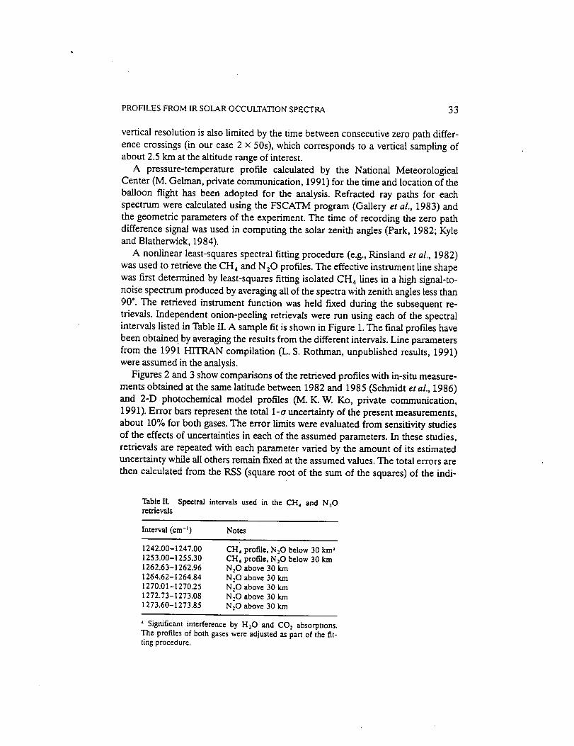
PROFILES FROM IR SOLAR OCCULTATION SPECTRA 33

vertical resolution is also limited by the time between consecutive zero path differ-

ence crossings (in our case 2 x 50s), which corresponds to a vertical sampling ofabout 2.5 km at the altitude range of interest.

A pressure-temperature profile calculated by the National MeteorologicalCenter (M. Gelman, private communication, 1991) for the time and location of the

balloon flight has been adopted for the analysis. Refracted ray paths for each

spectrum were calculated using the FSCATM program (Gallery et aL, 1983) and

the geometric parameters of the experiment. The time of recording the zero pathdifference signal was used in computing the solar zenith angles (Park, 1982; Kyleand Blatherwick, 1984).

A nonlinear least-squares spectral fitting procedure (e.g., Rinsland et al., 1982)

was used to retrieve the CH4 and N20 profiles. The effective instrument line shapewas first determined by least-squares fitting isolated CH4 lines in a high signal-to-

noise spectrum produced by averaging all of the spectra with zenith angles less than

90". The retrieved instrument function was held fixed during the subsequent re-

trievals. Independent onion-peeling retrievals were run using each of the spectral

intervals listed in Table II. A sample fit is shown in Figure 1. The final profiles havebeen obtained, by averaging the results from the different intervals. Line parameters

from the 1991 HITRAN compilation (L. S. Rothman, unpublished results, 1991)

were assumed in the analysis.Figures 2 and 3 show comparisons of the retrieved profiles with in-situ measure-

ments obtained at the same latitude between 1982 and 1985 (Schmidt et al., 1986)

and 2-D photochemical model profiles (M. K. W. Ko, private communication,1991). Error bars represent the total 1-a uncertainty of the present measurements,

about 10% for both gases. The error limits were evaluated from sensitivity studies

of the effects of uncertainties in each of the assumed parameters. In these studies,

retrievals are repeated with each parameter varied by the amount of its estimateduncertainty while all others remain fixed at the assumed values. The total errors are

then calculated from the RSS (square root of the sum of the squares) of the indi-

Table II. Spectral intervals used in the CH( and N.,Oretrievals

Interval (cm -I) Notes

1242.00-1247.001253.00-1255.30

1262.63-1262.96

1264.62-1264.841270.01-1270.25

1272.73-1273.081273.60-1273.85

CH_ profile, NzObelow 30 km _

CH_ profile, N2Obelow 30 kmN2Oabove 30km

N2Oabove 30km

N_O above 30kmN:O above 30km

NzOabove 30km

Significant interference by H,O and CO2 absorptions.The profiles of both gases were adjusted as part of the fit-ting procedure.

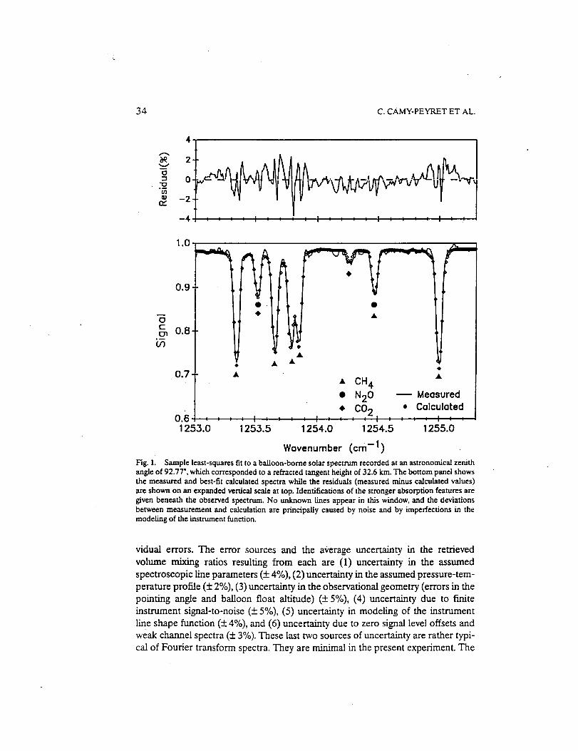
34 c. CAMY-PEYRET ET AL.

2

0-

m 2 -

-4

1.0

0.9

0.8-

b5

: : : : : : : : : ', : : : : 1 l : : : ', : :

0.7"

0.6 :1253.0

: : ' I ' I , , I J12,53.5 1254.0

• CH 4 •

• N20 _ Meosured

• CO 2 • Colculoted, I , I : : : : I : :

1254.5 1255.0

Wavenumber (cm -1)

Fig. 1. Sample least-squares fit to a balloon-borne solar spectrum recorded at an astronomical zenithangle of 92.77 °,which corresponded to a refracted tangent height of 32.6 kin. The bottom panel showsthe measured and best-fit calculated spectra while the residuals (measured minus calculated values)are shown on an expanded vertical scale at top. Identifications of the stronger absorption features aregiven beneath the observed spectrum. No unknown lines appear in this window, and the deviationsbetween measurement and calculation are principally caused by noise and by imperfections in themodeling of the instrument function.

vidual errors. The error sources and the average uncertainty in the retrieved

volume mixing ratios resulting from each are (1) uncertainty in the assumed

spectroscopic line parameters (+ 4%), (2) uncertainty in the assumed pressure-tem-

perature profile (+ 2%), (3) uncertainty in the observational geometry (errors in the

pointing angle and balloon float altitude) (+ 5%), (4) uncertainty due to finite

instrument signal-to-noise (_+5%), (5) uncertainty in modeling of the instrument

line shape function (+_4%), and (6) uncertainty due to zero signal level offsets and

weak channel spectra (_+3%). These last two sources of uncertainty are rather typi-

cal of Fourier transform spectra. They are minimal in the present experiment. The

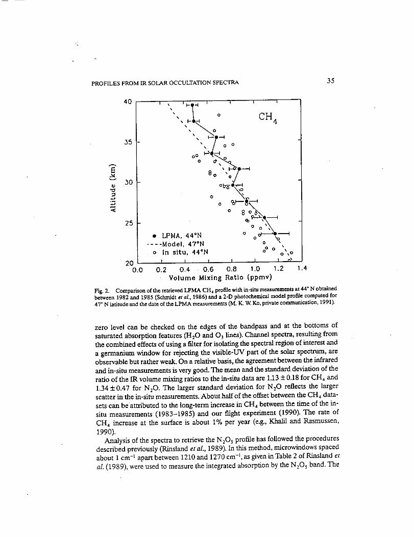
PROFILES FROM IR SOLAR OCCULTATION SPECTRA 35

E

.M

4O

35

3O

25

200.0

I _, I I'- t_ -'_ I 1 I I

" o 4%%%%

• LPMA, 44°N o oo ,o,

.... Model, 47°N oo in situ, 44°N oo o '0'_'_ 0

I I t I I I _

0.2 0.4 0.6 0.8 1.0 1.2Volume Mixing Ratio (ppmv)

.4

Fig. 2. Comparison of the retrieved LPMA CH, profile with in-situ measurements at 44" N obtained

between 1982 and 1985 (Schmidt et al., 1986) and a 2-D photochemical model profile computed for

47" N latitude and the date of the LPMA measurements (M. K. W. Ko, private communication, 1991).

zero level can be checked on the edges of the bandpass and at the bottoms of

saturated absorption features (H20 and O3 lines). Channel spectra, resulting from

the combined effects of using a falter for isolating the spectral region of interest and

a germanium window for rejecting the visible-UV part of the solar spectrum, areobservable but rather weak. On a relative basis, the agreement between the infrared

and in-situ measurements is very good. The mean and the standard deviation of the

ratio of the IR volume mixing ratios to the in-situ data are 1.13:1:0.18 for CH4 and

1.34 + 0.47 for N20. The larger standard deviation for N20 reflects the largerscatter in the in-situ measurements. About half of the offset between the CH4 data-

sets can be attributed to the long-term increase in CH4 between the time of the in-

situ measurements (1983-1985) and our flight experiment (1990). The rate of

CH4 increase at the surface is about 1% per year (e.g., Khalil and Rasmussen,

1990).Analysis of the spectra to retrieve the N205 profile has followed the procedures

described previously (Rinsland et al., 1989). In this method, rnicrowindows spacedabout 1 cm -t apart between 1210 and 1270 cm -t, as given in Table 2 of Rinsland et

al. (1989), were used to measure the integrated absorption by the N20 s band. The

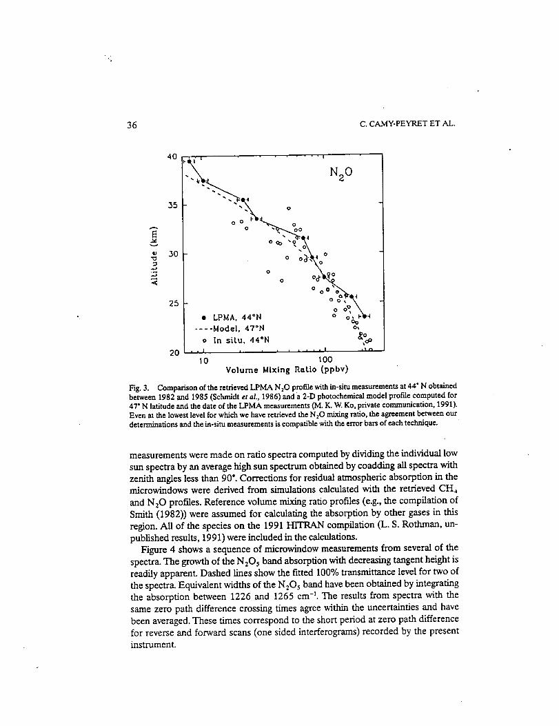
36 C. CAMY-PEYRET ET AL.

40

N20

35 ""_*J

0 _'_ 0

E

30"x3

25

-4• LPMA, 44°N

.... Model, 47°N o,

o In situ, 44°N _oo

20 , , I , , ..... I ,_,',10 100

Volume Mixing RaLio (ppbv)

Fig. 3. Comparison of the retrieved LPMA N 20 profile with in-situ measurements at 44" N obtainedbetween 1982 and 1985 (Schmidt et al., 1986) and a 2-D photochemical model profile computed for47" N latitude and the date of the LPMA measurements (M. K. W. Ko, private communication, 1991).

Even at the lowest level for which we have retrieved the N20 mixing ratio, the agreement between ourdeterminations and the in-situ measurements is compatible with the error bars of each technique.

measurements were made on ratio spectra computed by dividing the individual low

sun spectra by an average high sun spectrum obtained by coadding all spectra with

zenith angles less than 90 °. Corrections for residual atmospheric absorption in themicrowindows were derived from simulations calculated with the retrieved CH4

and N20 profiles. Reference volume mixing ratio profiles (e.g., the compilation ofSmith (1982)) were assumed for calculating the absorption by other gases in this

region. All of the species on the 1991 HTTRAN compilation (L. S. Rothman, un-

published results, 1991) were included in the calculations.Figure 4 shows a sequence of microwindow measurements from several of the

spectra. The growth of the N205 band absorption with decreasing tangent height is

readily apparent. Dashed lines show the fitted 100% transmittance level for two of

the spectra. Equivalent widths of the N:O 5 band have been obtained by integratingthe absorption between 1226 and 1265 cm -t. The results from spectra with the

same zero path difference crossing times agree within the uncertainties and have

been averaged. These times correspond to the short period at zero path differencefor reverse and forward scans (one sided interferograms) recorded by the present

instrument.

PROFILES FROM IR SOLAR OCCULTATION SPECTRA 37

'l'angenLHeight

39.9 krn

35.8 km

34.3 km

30.8 km

24.0 krn

I I ! I !

''k_ ..'_w'"k,r:-:,w.i-._'av ••.......................... -_j_,b-,,,_,_.._"_I llt _.II _I _ • _I

0.8 "_"_t_"*"."

",...0.7

100% Transmission....... 35.8 km.... 34.3 km

0.6 w I I I i1210 1220 1230 1240 1250 1260 1270

Wavenumber (cm -t)

Fig. 4. Examples of microwindow measurements in the region of the 1246 cm -I band of N:O_. Thevalues from each scan, which have been corrected for residual absorption by other gases, are shown onthe same scale, but have been offset vertically for clarity. Refracted tangent heights of the spectra are

given at right. Dashed Lines show 100% transmission levels determined by fitting the microwindowmeasurements from 1210 to 1226 cm -i and 1265 to 1270 cm-L

The profile of N205 has been derived from the measured equivalent widths

using the onion-peeling retrieval method and an assumed temperature-indepen-dent band intensity of 4.32 x 10 -t7 cm-t/molecule cm -2. This value is the same as

adopted previously (Toon et al., 1986; Rinsland et aL, 1989). Recently, Roscoe

(1991) reviewed the published laboratory and atmospheric measurements of N205

and recommended an integrated 1246 cm -l N205 band intensity of 4.01 x 10-_7

cm-_/molecule cm -2. If this lower value is assumed, the published ATMOS meas-

urements and those reported in this study need to be multiplied by a factor of1.077.

Figure 5 presents a comparison of our retrieved N205 profile with previous

published measurements and two photochemical model calculations performed for

conditions corresponding to the ATMOS/Spacelab 3 sunrise measurements at47" S on 1 May 1985. Error bars on the LPMA profile increase with altitude, rang-

ing from 22 to 30%. The uncertainty is dominated by the absolute uncertainty of

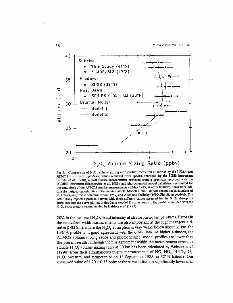
38 C. CAMY-PEYRET ET AL.

4O

35

30

25

Sunrise

• This Study (44°N)

o ^TMOS/SI,3 (47°S)

Predawn

• SIRIS (32°N)Post Daw,i

• SCRIBE 6h55 ''' AM (33°N)

Diurnal Model

......... Model 1

...............Model 2

L.. °.

t

.to !

•---,---_,

.' -I-_ 0_I

I -t----e.._ --I -.- I

.'° . .'

J---_--e--Dl_

.." ... •

•.

o•"

.o°o°

o"

20

O.

I I I I I I I I I :

I

N205 Volume Mixing Ra[io (ppbv)

Fig. 5. Comparison of N2Os volume mixing ratio profiles measured at sunrise by the LPMA and

ATMOS instruments, predawn values retrieved from spectra recorded by the S IRIS instrument

(Kunde et al., 1988), a post-sunrise measurement retrieved from a spectrum recorded with the

SCRIBE instrument (Blatherwick et al., 1989), and photochemical model calculations generaied for

the conditions of the ATMOS sunrise measurements (I May 1985, at 47 ° S latitude). Error bars indi-

cate the 1-sigma uncertainties of the measurements. Models I and 2 denote the model calculations of

M. Natarajan (private communication, 1989) and Allen and Delitsky (1990, Fig. 3), respectively. The

latter study reported profiles derived with three different values assumed for the N:O 5 absorption

cross sections; the curve plotted in this figure (model 2) corresponds to the profile computed with the

N .,Os cross sections recommended by DeMore et al. (I 987).

20% in the assumed N205 band intensity at stratospheric temperatures. Errors in

the equivalent width measurements are also important at the higher tangent alti-tudes (>35 kin), where the N205 absorption is very weak. Below about 31 kin, the

LPMA profile is in good agreement with the other data. At higher altitudes, theATMOS volume mixing ratios and photochemical model profiles are lower than

the present results, although there is agreement within the measurement errors. A

sunrise N205 volume mixing ratio at 30 km has been calculated by Webster et al.

(1990) from their simuitaneous in-situ measurements of NO, NO2, HNO3, 03,

N20, pressure, and temperature on 13 September 1988, at 32" N latitude. Ourmeasured value of 1.70 + 0.35 ppbv at the same altitude is significantly lower than

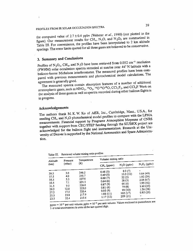
PROFILES FROM IR SOLAR OCCULTATION SPECTRA 39

the computed value of 2.7 + 0.4 ppbv (Webster et al., 1990) (not plotted in the

figure). Our measurement results for CH4, N20, and NzO5 are summarized inTable 1-17.For convenience, the profiles have been interpolated to 2 km altitude

spacings. The error limits quoted for all three gases are believed to be conservative.

3. Summary and Conclusions

Profiles of N205, CH4, and N20 have been retrieved from 0.052 cm -t resolution

(FWHM) solar occultation spectra recorded at sunrise near 44" N latitude with aballoon-borne Michelson intefferometer. The measured profiles have been com-

pared with previous measurements and photochemical model calculations. The

agreement is generally good.The measured spectra contain absorption features of a number of additional

stratospheric gases, such as HNO3, 1603, 160160180' CC12F2' and CC13F. Work onthe analysis of these gases as well as spectra recorded during other balloon flights is

in progress.

Acknowledgements

The authors" thank M. K. W. Ko of AER, Inc., Cambridge, Mass., U.S.A., for

sending CH4 and N20 photochemical model profiles to compare with the LPMAmeasurements. Financial support by Programe Atmosphere Moyenne of CNRS

together with support from CEC/STEP funding through the SIUBEX project areacknowledged for the balloon flight and instrumentation. Research at the Uni-

versity of Denver is suppoffed by the National Aeronautics and Space Administra-

tion.

Table Ill. Retrieved volume mixing ratio profiles

Altitude Pressure Temperature Volume mixing ratio

(kin) (mbar) (K) CH, (ppmv) N_O (ppbv) N:Os (ppbv)

39.5 3.0 246.2 0.48 (5) 8.0 (7) -37.5 4.0 241.7 0.49 (5) 10.3 (10) 1.64 (49)

35.5 5.3 237.0 0.68 (7) 22 (2) 1.92 (56)

33.5 7.1 231.5 0.64 (6) 28 (3) 2.06 (47)

31.5 9.5 226.0 0.87 (9) 66 (6) 1.95 (42)

29.5 12.8 223.0 0.81 (8) 79 (8) 1.60 (33)27.5 17.5 220.4 0.93 (9) 99 (10) 1.26 (28)

25.5 23.8 217.9 1.08 (11) 165 (17) 0.85 (20)

23.5 32.4 215.6 1.17 (12) 209 (21) -

ppmv - 10 4 per unit volume, ppbv - 10 -9 per unit volume. Values enclosed in parentheses are1-a total uncertainties in units of the last quoted digit.

40 C. CAMY-PEYRET ET AL.

References

Allen, M. and Delitsky, M. L., 1990, Stratospheric NO, NO,., and N.,O._: A comparison of model

results with Spacelab 3 atmospheric trace molecule spectroscopy (ATMOS) measurements, J.Geophys. Res. 95, 14077-14082.

Blatherwick, R.D., Murcray, D.G., Murcray, E H., Murcray, E J., Goldman, A., Vanasse, G.A.,

Massie, S. T., and Cicerone, R. J., 1989, Infrared emission measurements of morning stratosphericN205, J. Geophys. Res. 94, 18337-18340.

Camy-Peyret, C., Flaud, J.-M., and Perrin, A., 1991, Balloon-borne solar occultation Fourier transform

spectrometry for measurements of stratospheric trace species, ESA Publ. SP-31Z pp. 179-186.CantreU, C. A., Davidson, J. A., McDaniel, A. H., Shetter, R. E., and Calvert. J. G., 1988, Infrared

absorption cross sections for N20_, Chem. Phys. Lett. 148,358-363.

Crutzen, P. J:, 1970, The influence of nitrogen oxides on atmospheric ozone content, Quart. Z R. Met.Soc. 96,320-325.

DeMore, W. B., Molina, M. J., Sander, S. P., Golden, D. M., Hampson. R. E. Kurzlo, M. J., Howard,C. J., and Ravishankara, A. IL, 1987, Chemical kinetics and photochemical data for use in strato-

spheric modeling, JPL Publ. 87-41.

Evans, W. E J., 1986, Observation of the 8-)xm N,.O, thermal emission feature in the stratosphere,• Appl. Opt. 25, 1866-1868.

Gallery, W. O., Kneizys, E X., and Clough, S. A., 1981, Air mass computer program for atmospherictransmittance/radiance calculation: FSCATM, AFGL-TR-83-0065, Environmental Research

Paper No. 828, Air Force Geophysics Laboratory, Hanscom Air Force Base, Mass.

Khalil, M. A. K. and Rasmussen, R. A., 1990, Atmospheric methane: Recent global trends, Environ.Sci. Technol. 24, 549-553.

Ktmde, V. G., Brasunas, J. C., Maguire, W. C., Herman, J. R., Massie, S.T., Abbas, M. M., Herath,

L. W., and Shaffer, W. A., 1988, Measurement of nighttime stratospheric N,O._ from infrared emis-sion spectra, Geophys. Res. Let*. 15, 1177-1180.

Kyle, T. G. and Blatherwick, 1L, 1984, Smearing of interferograms in Fourier transform spectroscopy,AppL Opt. 23,261-263.

Park, J. H., 1982, Effect of interferogram smearing on atmospheric limb sounding by Fourier trans-form spectroscopy, AppL OpL 21, 1356-1366.

Rimland, C. P., Goldman, A., Murcray, E J., Murcray, D. G., Smith, M. A. I-L, Seals, R. K. Jr., Laden,

J.C., and Rinsland, P.L., 1982, Stratospheric NzO mixing ratio profile from high-resolution

balloon-borne solar absorption spectra and laboratory spectra near 1880 cm -j, AppL Opt. 21,4351--4355.

Rinsland, C. P., Toon, G. C., Farmer, C. B., Norton, R. H., and Namkung, J. S., 1989, Stratospheric

N20 _ profiles at sunrise and sunset from further analysis of the ATMOS/Spacelab 3 solar spectra,J. Geophys. Res. 94, 18341-18349.

Roscoe, H. K., 1982, Tentative observation of stratospheric N,Os, Geophys. Res. Lett. 9,901-902.

Roscoe, H. K., 1991, Review and revision of measurements of stratospheric N.,Os, J. Geophys. Res. 96,10879-10884.

Schmidt, U., Jebsen, C., Johnen, E J., Khedim, A., Klein, E., Knapska, D., Kulessa, G., Rudolph, J..

Schumacher, G., and Schunck, E., 1986, Stratospheric observations of long-lived trace gases atmidlatitudes 1982-1985 (data report), Kernforschungsanlage Jiilich GmbH, Institut fiir Chemic:

Atmosphiifische Chemic, Jiilich, Germany.

Smith, M. A. H., 1982, Compilation of atmospheric gas concentration profiles from 0 to 50 kin,

NASA Tech Memo., TM 83289. (Available as NTIS 82N22822 from the Natl. Tech. Inf. Serv.,Springfield,Va.)

Toon,G.,1987,Reply:Detectionofstratosphericnitrogenspecies,Nature330,42Z

Toon, G. C.,Farmer,C. B.,and Norton, R. H., 1986, Detectionof stratosphericN205 by infraredremotesounding,Nature319,570-571.

Webster,C. R.,May, R.D.,Toumi, R.,and Pyle,J.A., 1990,Activenitrogenpartitioningand thenight-

time formationof NzO 5 in the stratosphere:Simultaneousin-situmeasurements of NO, NO2,HNO 3,05, and N20 usingtheBLISS diodelaserspectrometer,J.Geophys.Res.95,13851-13866.

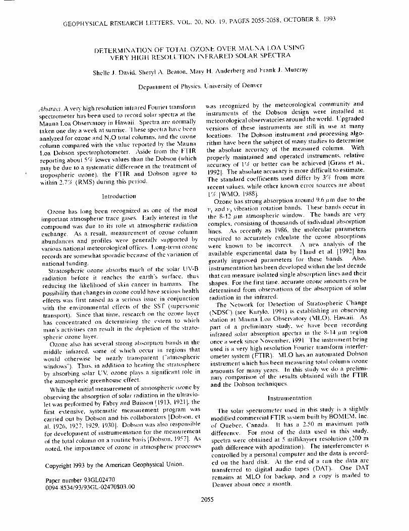
GEOPHYSICAL RESEARCH LETTERS. VOL. 20, NO. 19, PAGES 2055-2058, OCTOBER 8, 1993

DETERMINATION OF TOTAL OZONE OVER MAUNA LOA [;SING

VERY HIGH RESOLUTION INFRARED SOLAR SPECTRA

Shelle J. David. Sheryl A. Beatom Mary H. Anderberg and Frank J. Murcray

Department of Physics, University of Denver

Ahstract. A rely high resolution infrared Fourie, transform

spectrometer has been used to record solar spectra at theMauna Loa Observatory in Hawaii. Spectra are nolmally

taken one day a week at sunrise. These spectra have been

analyzed for ozone and N,O total columns, and the ozone

column compared with the value reported by the Mauna

Loa Dobson spectrophotometer. Aside from the FTIR

reporting about 5f/_ lower values than the Dobson (which

may be due to a systematic difference in the treatment of

tropospheric ozone), the FTIR and Dobson agree to

within 2.7r5_ (RMS) during this period.

Introduction

Ozone has long been recognized as one of the most

important atmospheric trace gases. V.arlv interest in the

compound was due to its role in atmospheric radiation

exchange. As a result, measurement of ozone colunm

abundances and profiles were generally supported by

various national meteorological offices. Long-term ozone

records are solnewhat sporadic because of the variation of

national funding.

Stratospheric ozone absorbs much of the solar UV-B

radiation before it reaches the earth's surface, thus

reducing the likelihood of skin cancer in humans. The

possibili_' that changes in ozone could have serious health

effects was first raised as a serious issue in conjunction

with the environmental effects of the SST (supersonic

transport). Since that time, research on the ozone layer

has concentrated on determining the extent to which

man's actMties can result in the depletion of the strato-

spheric ozone laver.Ozone also has several strong absorption bands in the

middle infrared, some of which occur in regions that

would otherwise be nearly transpa,ent ("atmospheric

windows"). Thus, in addition to heating the stratosphere

by absorbing solar UV, ozone plays a significant role in

the atmospheric greenhouse effect.

While the initial measurement of atmospheric ozone by

observing, the absorption of solar radiation in the ultravio-

let was performed by Fabry and Buisson [1913, 1921 ]. thefirst extensive, systematic measurement program was

carried out by Dobson and his collaborators [Dobson. et

al. 1926. 1927, 1929, 1930]. Dobson was also responsible

for development of instrumentation for the measurementof the total column on a routine basis IDobson. 19571. As

noted, the importance of ozone in atmospheric processes

Copyright 1993 by the American Geophysical Union.

Paper number 93GL024700094-8534/93/93GL-02470503.00

was recognized by the meteorological community and

instruments of the Dobson design were installed at

meteorological observatories around the world. Upgraded

versions of these instruments are still in use at many

locations. The Dobson instrument and processing algo-

rithm have been the subject of man)' studies to determine

the absolute accuracy of the measured column. With

properly maintained and operated instruments, relative

accuracy of l_h or better can be achieved [Grass et al.,

1992]. The absolute accuracy is more difficult to estimate.The standard coefficients used differ by 3_7t from more

recent values, while other known error sources are about

1'/, IWMO. 19881-Ozone has strong absorption around 9.6/Jm due to the

v t and v, vibration rotation bands. These bands occur in

the 8-12/,im atmospheric window. The bands are very

complex, consisting of thousands of individual absorption

lines. As recently as 1986. the molecular parameters

required to accurately calculate the ozone absorptionswere known to be incorrect. A new analysis of the

available experimental data by Flaud et al. 11992] has

greatly improved parameters for these bands. Also,

instrumentation has been developed within the last decade

that can measure isolated single absorption lines and their

shapes. For the first time, accurate ozone amounts can bedetermined from observations of the absorption of solar

radiation in the infrared.

The Network for Detection of Stratospheric Change

(NDSC) (see KuD'lo. 1991) is establishing an obsep,'ingstation at Mauna koa Observatory (MLO), Ha_vaii. As

part of a preliminary stud)', we have been recording

infrared solar absorption spectra in the 8-14/_m region

once a week since November, 1991. The instrument being

used is a very high resolution Fourier transfolm interfer-

ometer system (FTIR). MLO has an atttomated Dobson

instrument which has been measuring total column ozone

amounts for many years. In this study we do a prelimi-

nary comparison of the results obtained with the FTIR

and the Dobson techniques.

Instrumentation

The solar spectrometer used in this stud), is a slightlymodified commercial FTIR system built by BOMEM. inc.

of Quebec. Canada. It has a 2.50 m maximum path

difference. For most of the data used in this study,

spectra were obtained at 5 millikayser resolution (200 m

path difference with apodization). The interferometer is

controlled by a personal computer and the data is record-

ed on the hard disk. At the end of a run the data are

transferred to digital audio tapes (DAT). One DAT

remains at MLO for backup, and a copy is mailed to

Denver about once a month.

2055

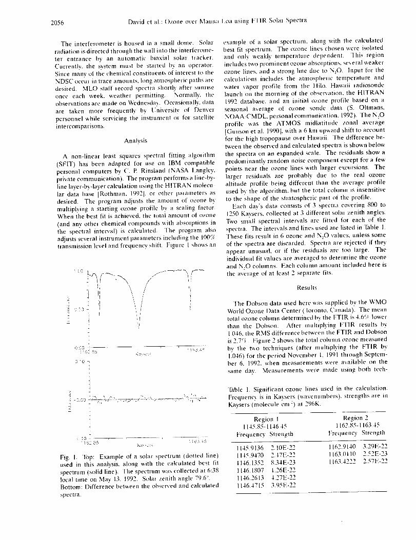
2056 David et al.: Ozone over Maumt l.oa using FFIR Solar Spectra

The interferometer is housed in a small dome. Solar

radiation is directed through the wall into the i,lterferome-

ter entrance by an automatic biaxial solar tracker.Currently. the system must be started by an operator.Since many of the chemical constituents of interest to theNDSC occur in trace amounts, long atmospheric paths aredesired SiLO staff record spectra shortly after st, ariseonce each week. weather permitting. Normally. theobservations are made on Wednesday. Occasionally. data

are taken more frequently by t!niversity of Denver

personnel while servicing the instrument or for satelliteintercomparisons.

Analysis

A non-linear least squares spectral fitting algorithm

(SFIT) has been adapted for use on IBM compatiblepersonal computers by C. R Rinsland (NASA l.angley.private communication). The program performs a line-by-line layer-by-layer calculation using the HITRAN molecu-lar data base [Rothman. 1992], or other parameters asdesired. The program adjusts the amount of ozone bymultiplying a starting ozone profile by a scaling factor.When the best fit is achieved, the totai amount of ozone

(and any other chemical compot, nds with absorptions inthe spectral interval) is calculated. The plogram alsoadjt, sts several instrument parameters including the 100r,_transmission level and frequency shift. Figure 1 shows an

z

E

! CO

f- .... ,,/ !J

i , / i

q

,}.00 ,', ', 62ff5

310

q

65 :-f%

O CO

4

I5

1

t0.10 ,

I 162.85 N_t\ _.1 .*

Fig. 1. Top: Example of a solar spectrum (dotted line)used m this analysis, along with the calculated best fit

spectrum (solid line). The spectrum was collected at 6:38local time on May 13. 1992. Solar zenith angle 79.6:'.Bottom: Difference between the observed and calculated

spectra.

example of a solar spectrum, along with the calculatedbest fit spectrum. The ozone lines chosen we,e isolatedand only weakly tenlperature dependent. This regionincludes two prominent ozone absorptions, several weakerozone lines, and a strong line due to N,O. Input for thecalculations includes the atmospheric temperature and

water xapor profile from the ttilo. Hawaii radiosondelaunch on the morning of the obserxation, the HITRAN1992 database, and an initial ozone profile based on a

seasonal average of ozone sonde data (S. Oltmans.NOAACMDL personal communication. 1992). The N,O

profile was the ATMOS midlatitude zonal average[Gunson et al. 1990 I. with a 6 km upward shift to accountfor the high tropopause over Hawaii. The difference be-tween the observed and calculated spectra is shown below

the spectra on an expanded scale. ]-he residuals show apredominantly random noise component except for a fewpoints near the ozone lines with larger exct, rsions. Thelarger residuals are probably due to the real ozonealtitude profile being different than the average profileused bv the algorithm, but the total column is insensitiveto the shape of the stratospheric part of the p,ofile.

Each day's data consists of 3 spectra covering 800 to

1250 Kaysers. collected at 3 different solar zenith angles.Two small spectral intervals are fitted for each of thespectra. The intervals and lines used are listed m Table I.These fits result in 6 ozone and N.,O values, unless some

of the spectra are discarded. Spectra are rejected if theyappear t, nusual, or if the residuals are too large. Theindividual fit values are averaged to determine the ozoneandN,Ocolulnns. Each column amount included here is

tile average of at least 2 separate fits.

Results

The Dobson data used here was st, pplied by tile WMOWorld Ozone Data Center (lbronto. Canada). The meantotal ozone column determined by the FTIR is 4.6(/, lowerthan the Dobson. After mt|ltiplying FTIR rest, Its by1.046. the RMS difference betwee|l the FTI R and Dobson

is 2.7G. Figure 2 shows the total coh, mn ozone measuredby the lx_o techniques (after multiplying the FTIR by1.046) for the period November 1. 1991 through Septem-ber 6. 1992. when nleasurements were available on thesame day. Measurements were made using both tech-

Table 1. Significant ozone lines used inFrequency is in Kavsers (v,avenumbers).Kaysers,(molecule cm :) at 296K.

the calculation.

strengths are in

Region I1145.85-1146.45

Frequency Strengdl

Region _'1162.85-1163.45

Frequency Strength

1145.9136 2.10E-221145.9470 2.47E-221146.1352 8.34E-231146.1807 1.26E-221146.2613 4.27E-221146.4715 3.95E-22

1162.9140 3 _9E "Y_1163.0110 2.52E-231163 -I._ _ ';TF "Y_

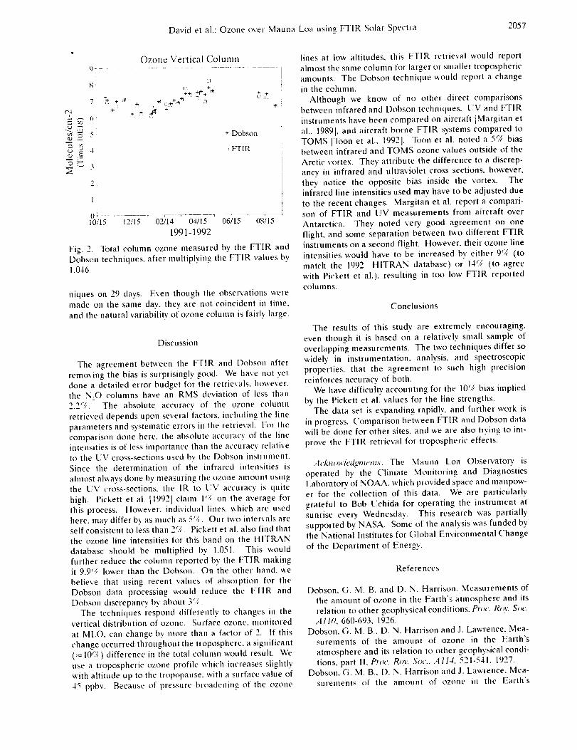
David et al.: Ozone over Mauna Loa using FTIR Sola, Spectra 2057

7

t"-q

e.j ,-.

Ozone Verticnl Column

97 ..............

[]8: ÷

+

2:

+ Dobson

_ VFtR

0 _ ....... --v --- _- .... _ -_ _----_

10/15 t2/15 02/14 04/15 06/15 08/15

1991-1992

Fig. 2. Total column ozone measured by the FTIR and

Dobson techniques, after multiplying the FTIR values by

1.046.

niques on 29 days. Even though the observations were

made on the same day. they are not coincident in time,

and the natural variability of ozone column is fairly large.

Discussion

The agreement between the FTIR and Dobson after

removing the bias is surprisingly good. We have not yet

done a detailed error budget for the retrievals, however,

the N,O columns have an RMS deviation of less than

2.2":_. The absolute accuracy of the ozone column

retrieved depends upon several factors, including the line

parameters and systematic errors in the retrieval. For the

comparison done here, the absolute accuracy of the line

intensities is of less importance than the accuracy relative

to the UV cross-sections used by the Dobson instrument.

Since the determination of the infrared intensities is

almost ahvays done by measuring the ozone amount usingthe UV cross-sections, the IR to [IV accuracy is quite

high. Pickett et al. [1992] claim 1¢4 on the average for

this process. However. individual lines, which are used

here. may differ by as much as 5_;;. Our two intervals are

self consistent to less than 2U_. Pickett et al. also find that

the ozone line intensities for this band on the HITRAN

database should be multiplied by 1.051. This would

further reduce the column reported by the F-HR making

it 9.9(/r lower than the Dobson. On the other band, we

believe that using recent values of absorption for the

Dobson data processing would reduce the FTIR and

Dobson discrepancy by about 3';.

The techniques respond differently to changes in the

vertical distribution of ozone. Surface ozone, monitored

at MLO, can change by more than a factor of 2. If this

change occurred throughout the troposphere, a significant

(= 10r/c) difference in the total column would result. We

use a tropospheric ozone profile which increases slightly

with altitude up to the tropopause, with a surface value of

45 ppbv. Because of pressure broadening of the ozone

lines at low altitudes, this VIIR retrieval would report

almost the same column for larger or smaller tropospheric

amounts. The Dobson technique would report achange

m the column.

Although we know of no other direct comparisons

between infrared and Dobson techniques. L,V and FTIR

instruments have been compared on aircraft [Margitan et

al., 1989], and aircraft borne FTIR systems compared to

TOMS [Toon et al.. 1992]. "loon et al. noted a 59_ bias

between infrared and TOMS ozone values outside of the

Arctic vortex. They attribute the difference to a discrep-

ancy in infrared and ultraviolet cross sections, however,

they notice the opposite bias inside the vortex. The

infrared line intensities used may have to be adjusted due

to the recent changes. Margitan et al. report a compari-

son of FTIR and UV measurements from aircraft over

Antarctica. They noted very good agreement on one

flight, and some separation between two different FrlR

instruments on a second flight. However. their ozone line

intensities would have to be increased by either 9_/c (to

match the 1992 ItlTRAN database) or 14(/r (to agree

with Pickett et al.), resulting in too low FTIR reported

columns,

Conclusions

The results of this study are extremely encouraging,

even though it is based on a relatively small sample of

overlapping measurements. The two techniques differ so

widely in instrumentation, analysis, and spectroscopic

properties, that the agreement to such high precision

reinforces accuracy of both.

We have difficulty accounting for the 10(/r bias implied

by the Pickett et al. values for the line strengths.

The data set is expanding rapidly, and further work is

in progress. Comparison between FTIR and Dobson data

will be done for other sites, and we are also trying to im-

prove the FTIR retrieval for tropospheric effects.

Acknowledgments. The Mauna Loa Obserxatory is

operated by the Climate Monitoring and Diagnostics

Laboratory of NOAA, which provided space and manpow-

er for the collection of this data. We are particularly

grateful to Bob Uchida for operating the instrument at

sunrise every Wednesday. This research was partially

supported by NASA. Some of the analysis was funded bythe National Institutes for Global Environmental Change

of the Department of Energy.

References

Dobson. G. M. B. and D. N. Harrison. Measurements of

the amount of ozone in the Earth's atmosphere and its

relation to other geophysical conditions, Proc. Roy. Soc.

All0, 660-693, 1926.

Dobson. G. M. B., D. N. Harrison and J. Lawrence, Mea-

surements of the amount of ozone in the Earth's

atmosphere and its relation to other geophysical condi-

tions, part II, Proc. Roy. Sot., A114. 521-541. 1927.

Dobson, G. M. B., D. N. Harrison and J. Lawrence, Mea-

surements of the amount of ozone in the Earth's

2058 Davidetal.:OzoneoverMaunal,oausing[:'FIRSolarSpectra

atmosphereanditsrelationtoothergeophysicalcondi-tions,partII!, Proc. Roy. Sot.. ,,t122, 456-486, 1929.

Dobson, G. M. B.. Observations of the anlounI of ozone

in the Earth's atmosphere and its relation to other geo-

physical conditions, part IM Proc. Roy. Sot., A 12_), 411-

433. 1930.

Dobson. G. M. B., Obselwers handbook for the ozone

spectrophotometer. Ann. lnl. Geophvs. Ycap; 5, 90 1957.

Fabrv, C. and M. Buisson. Eabsorption de I'ultraviolet par

I2ozone et al limite du spectre solaire, J. Phys. Rad., 3.

196-206. 1913.

Fabrv, C. and M. Buisson, Etude de I'extremite nltra-

violette du spectre solaire., J. Phys. Rad., 2, 197-226,

1921.

Flaud. J.-M., C. Camy-Peyret. A. Perrin and C. R

Rinsland. hnproved spectroscopic line parameters for

the ozone molecule, J. Ommt. Spectro_c. Radiut. Trans-

JOt; 48, 611, 1992.

Grass, R. D., W. D. Komhyr, G. 1.. Koenig, and R. D.

Evans. Results of international Dobson spectrophotom-

eter calibrations at the LKO, Arosa, Switzerland. 1990,

Proc. Qmldretmial Ozotw Symposium, in press. 1992.Gunson, M. R.. C. B. Farmer. R. H. Norton, R. Zander,

C. P Rinsland. J. H. Shaw and B.-C. Gao, Measu,e-

ments of CH,, N,O, CO, H,O. and O, in the middle

atmosphere by the atmospheric trace molecule spectros-

copy experiment on Spacelab 3, J. Geopto,s. Rcs.. 95,

13,867-13.882, 1990.

Kur',lo. M. J.. Network for the detection of stratospheric

change, Proc. Soc. Photo. Opt. ln._trum. Eng., 1401. 169-

174. 1991.

Margitan. J. J. G. A. Brothers, E. V. Browell. D. Cariolle,M. q_ Coffer, J. C. Farman, C. B. Farmer, G. L.

Gregory, J. W. Harder. D. J. Hoffman, W Hypes, S.Ismail, R. O. Jakoubek, W Komhyr, S. Kooi. A. J.

Drueger, J. C. Larsen, W. Mankin. M. P. McCormick,

G. H. Mount, M. H. Proffitt, A. R. Ravishankara, A. L.

Schmeltekopf, W. L. Starr, G. C. Toon, A. Torres, A. E

Tuck, A. Wahner and I. Watterson, Inlercomparison of

ozone measurements over Antarctica, J. Ge_pto',_. Res..

_)4, 16.557-16.569, 1989.

Pickett, [I. M., D. B. Peterson and J. S. Margolis. Abso-

h.te absorption of ozone in the midinfrared.J. Ge_,phys.

Res., q7, 20787-20793, 1992.

Rothman. L. S., R. R. Gamache, R. H. Tipping, C. P.

Rinsland. M. A. H. Smith, D. C. Benner. V. M. Devi,

J.-M. Flaud, C. Camy-Peyret, A. Perrin, A. Goldman, S.

T. Massie, L. R. Brown and R. A. lbth. l-he HITRAN

molecular database: Editions of 1991 and 1992. J.

Quant. Spectr_,_c. Radiat. Transt_'l; 4& 469-507. 1992.

Toon. G. C.. C. B. Farmer, P. W Schaper, L. l.. Lowes

and R. H. Norton, Composition measurements of the

1989 arctic winter stratosphere by ai,borne infrared

solar absorption spectroscopy. J. Geophy._. Res., 97,

7939-7961. 1992.

WMO, Report of the international ozone trends panel1988. WMO Global Ozone Research and Monitoring

Project. Report no. 18, Volume 1. 439 pp., 1981.

M. H. Anderberg, S. A. Beaton. S. J. David. E J.

Murcray, Department of Physics. University of Denver,

Denver. CO 80208-0202

(Received: July 12. 1993

Accepted: August 9. 1993)

-fne P2 and 2u 2 - l,2 bands of t4N 1602: Electron Spin-Rotation and

Hyperfine Contact Resonances in the (010) Vibrational State

A. PERRIN, "_ J.-M. FLAL'D,* C. CAMY-PEYRET,* A. GOLDMAN,+ F. J. MURCRAY,f

R. D. BLATHERWICK,+ AND C. P. RINSLAND:_

* Laboralo_re de Physique 31o/dctda;re el Applications. t C.VR5, Universitd Pct M. Curie, Bte 76,

4 Place Jus_eu, 75252 Paris Cedex 05. France. tDepartment of Physics, l_'ni_er._itl" olDenver,

Denver, Colorado 80208." and ¢..-l;mospheric Sciences Dirision, ?<-ISA Langle) Research Center,

Hampton, Virginia 23681-0001

High-resolution Fourier transform spectra covering the 720-920 cm -_ spectral region have

been used to perform a reanalysis of the v: band ((010)-(000) vibrational transition) together

with the first analysis of the 2,,: - ,,: hot band of nitrogen dioxide ((020)-¢010) vibrational

transition ). The high-qualit.,, spectra show that. for numerous v: lines, the hyperfine structure is

easily obser_ able in the case of resonances due to the h.vperfme Fermi-type operator. By performing

a full treatment of the spin-rotation and of the h.vperfine operators, a new line list of the v: band

(positions and intensities) has been generated, and it is in excellent agreement with the expedmenlal

spectrum. Also. a thorough anabsis of the 2v2 - v2 hot band has been performed leading to an

extended set of new (020} spin-rotation levels. These levels, together with the [( 100L (020),

(001) } spin-rotation levels deduced previousl3 from the analysis of the _,,, 2v:, and v, cold bands

performed in the 6.3- to 7.5-urn spectral range [A. Pen-in, J.-M. Flaud. C. Camy-Peyret, A.-M.

Vasserot, G. Guelachvili, A. Goldman. F. J. Murcray. and R. D. Blatherwick. d. 3[ol. Spectrosc.

154, 391-406 ( 1992)] were least-squares fitted, allowing one to derive a new set of vibrational

band centers and rotational, spin-rotation, and interaction constants for the I ( 100 )1020 }(001 ) }

interacting states of _4N LrO:. _ 1993 a.cademic Press. Inc.

I. INTRODUCTION

The cold v2 band and the 2v2 - v2 first hot band of nitrogen dioxide, located at 13

_m, correspond, respectively, to the (010 )- (000) and (020)- (010 ) vibrational tran-

sitions of this molecule; consequently, in order to have accurate line positions it is

necessary to have precise parameters for both the upper and the lower vibrationalstates involved in these transitions.

For the (000) and (010) vibrational states, the most recent spectroscopic parameterswere obtained from a simultaneous fit of the available microwave or double resonance

data (Refs. (1-8) and (9, 10) for the (000) and (010) state, respectively) and of the

infrared spin-rotation energy levels obtained from recent analyses of Fourier transform

spectra recorded in the far infrared (11) and in the 13.3-/am (12) spectral regions.

In the analysis of the (000}-(000) band, even at the high resolution of the far-

infrared experimental spectra, the hyperfine structure is usually not detectable, except

in cases of local resonances due to the Fermi contact hyperfine operator. Accordingly,the line list (11, 13, 14) of the pure rotation region of NO2 (_0-200 cm -_) was

generated by explicitly taking into account the spin-rotation and hyperfine structures.

On the other hand. Ibis effect could not be obserxed so accurately in the 13.3-urn

experimental spectrum which was used in Ret: (12) for the analysis of the w. band,

t I.aboratoire associ, a aux Universitrs P, et M. Curie et Paris-Sud.

0022-2852/93 $5.00

Copyright ¢. 1993 b_ Acadermc Press. Inc.

All rights of repro.auction in an,_ form reser'*ed.

456

.x!_ - . !_\\l)>, ,}1 -\ '._. -157

and consequently the line list {]2-14) gcneraled in _lac 13.3-urn spectral range did

;7or include the h.xperfine structure.For the (020) vibrational state, the most recent spectroscopic parameters were ob-

tained from a recent anahsis (]5) of the v_. 2<,. and _,_bands I(100)-I000). (020)-

(000). and (001)-(000) vibrational transitions, respectively) using Fourier transform

spectra (15. I6) covering the 6.3-urn region. Actually the 1001 / state is invohed in astrong Coriolis interaction with tile (020) and ( 100 1 states, and the veo' weak 2_,2

band borrows its intensity from the strong z,__band. In tact. only the K, = 0-2 subbands

for .\: m 46 (because they appear in a clear window bet_veen _,_and <_] and the K, =6 subband for 19 _< N m 62 (because the corresponding (020/ levels are strongly

resonating with levels of (001) state) could be analyzed at 6.7 um(15-]7). Finally.

it must be pointed out that for the energy level calculations of the { (100), (020).

(001) } interacting vibrational states, both the spin-rotation and the vibrational Co-

riolis-type interactions were explicitly taken into account, but that the hyperfine struc-ture was not considered:

(i) For the A-type v3 band. which is by far the strongest band at 6.3 urn. the hyperfine

resonances affect only some v3 nonresolved doublets, the spin splittings of which vanish

in the upper and lower levels of the transition. In this case. the hyperfine structure isblended within the total line _ idth. and the hyperfine components cannot be observed.

(it) Because of the weakness of the _,_and 2v2 bands the hyperfine structures cannot

be precisely measured on the spectra and consequently the hyperfine resonances were

not considered for these bands.

Using new high-resolution Fourier transform spectra recorded in the 13.3-um spectral

region, we report in this paper a reanalysis of the v: band (with a full treatment of the

hyperfine structure), together a ith a first analysis of the hot 2v2 - v2 band of t_N _O2.

II. EXPERIMENTAL DETAILS

The spectra were recorded in the 720-960 cm-_ spectral range at 0.002 cm-J res-olution with the BOMEM Fourier transform spectrometer of the University of Denver.

The optical path length was 1 m. and two spectra were recorded at NO., pressures of1 and 2 Torr. The calibration of the spectra was performed by means of N:O absorption

lines (18. ]9) in the 1150-1250 cm -_ region, and the accuracy of the positions of

unblended lines is estimated to be _0.0002 cm

111._NALYSIS _ND LINE POSITION C_LCULATIONS

The v: Band

The analysis was started by comparing the experimental line positions to the linelist calculated in Ref. (12). O_ erall, the agreement was excellent except for transitions

in which the upper or the lo_er state are invoh'ed in a hyperfine Fermi resonance.

Consequently, a new line list was generated for the v_,band. taking into account not

only the electron spin-rotation interaction, but also. as described in Ref. ( 11 ) for the

(000) state, the magnetic hyperfine hamiltonian (i.e.. the Fermi contact operator to-

gether with the spin-spin dipolar interaction operators ) and the nuclear quadrupoleinteraction. For this calculation we used the vibrational band center, rotational, spin-

rotation, and h.vperfine constants of Ref. (12) and Ref. (11), respectively, for the

upper and lower state of the transition.The agreement this time proved to be excellent for all the lines. Ho_ ever. we obse_'ed

a -0.0004 cm-_ global shift of the observed line positions relative to the calculated

458 l't RRI\ t I ',_

ones. \_hich is duc to a sli_hzl\ diflcrcn_ calibration of the spectra used in the prescnt_ork { 18. /9) compared to that used (201 in 19SS. This leads to a difl'crent vibrational 1

band center ofthe v: band: E,,,_o_= 749.65256l cm _ (instead of74c_.652961 cm

obtained previously in Ref. 112)).To show the quality of_he experimental spectra and of the calculations performed

in the present work. _e show in Figs. 1 and 2 portions around 771.8 and 758.0 cm -_

of the experimental spectra together with line-by-line calculations performed usingeither the line list generated in Ref. (I2) ( no hy perflne structure I or the line list derived

here (full treatment of the hyperfine operators). In both regions, the improvement

brought by the new calculation is very' clear.In the first spectral region, the complex hyperfine structure appears clearly in the

N = even RO_,.;=_ subband. At 771.30 and 771.64 cm -_ i1 is due to a strong hyperfineresonance involving the (010/[22 2 20] and (0t01120 2 18] rotational levels. At 772

crn -_ . since the resonance is weaker, one obser_'es mainly a broadening of the N =

18 doublet structure. The same hyperfine effect can be clearly observed in Fig. 2

around 758 cm -_ for lines belonging to the ROut,=0 subband. It is worth stressing that

in both cases the new calculation, which involves the h.vperfine operators, reproduces

the experimental spectrum with high accuracy.

Tire 2v2 - _'2 Band

Lines from the 2v2 - _', band were already obserxed in the experimental spectrum

(12) which was used in 1988 for the analysis of the 13.3-_m band of nitrogen dioxide.However. because this hot band is weak and because the (020) spectroscopic parameters

available at that time were not precise enough ( only the K, = 0. 1.2 (020) series were

derived from the analysis of the 2v2 band performed at 6.6/am (17) ). only a few lines

involving the K_ = 0, 1.2 (020) rotational series could be analyzed at 13.3 urn.

The (020) parameters were recently significantl.\ improved from a new analysis of

the {v_, 2v,, v3 } interacting bands (15). Indeed. more lines involving the K_ = 0. 1,2 series were assigned: also. lines involving the Ko = 6 rotational series of (020).

which borrow their intensities from _3 through a Coriolis interaction, were ob-

served ( 15. 16).Consequently. from the '1100). (020). (001)I and {010) parameters obtained in

Ref. (15) and l_ef. (12) respectively, it has been possible to better predict the 2_'2 -

z,2line positions, as performed in the present analysis.Because the 2_,2 - _'2band is rather weak. only transitions of this band inxotving .V

_< 30 rotational quantum number could be identified in the spectrum. For transitions

involving the Ko = 0-2 and K, = 6 I020) energy !evels. the agreement betx_een theobserxed and the predicted line positions was excellent, but this x_as not completely

the case for lines involving the Ko = 3-5 (020) rotational levels since small discrepencies

(up to 0.0030 cm -* ) were observed. Using these new data. we then determined thevibrational band centers, rotational, spin-rotation, and coupling constants of the

{(100), (020). (001)} resonating states..as in Ref. (15) the Hamiltonian matrixexplicitly takes into account both the Coriolis and the spin-rotation interactions. Forthis least-squares fit calculation, the 164 (020) new spin-rotation energy levels obtained

in the present work for Ko 4 6 and N _ 30 were combined to the 3230 (100) (001)

and (020) energy levels obtained in Ref. (15).Table I gives the list of vibrational energies and rotational, spin-rotation, and cou-

pling constants deduced from the fit. together with their estimated uncertainty. The

. "..',:;, _. i_\\l)h _1 -\ 'c_, 459

Z5

:2.[)

!J

I.U ---._- _ "._'_.--'

i I i ? ! _ _ ! ' IL:J_I 'Jl !

11!'il 'il 1

LI:

:q=22 ' --, • _,0

-. o

/('%-

I' I;

20

o2_

O.O 771.8 772.07v:.2 7_1.4 771.6era- l

1.0 ," i i _ ; ....... ' 7 tt/ I

" _ f t [! 1 " _ ll /"1- i',I if:! r,,,Jl" f_ iilj !!i 1

0.07,: _ ,5i A ;'_'i_: 7-:8 ,72.0

cm-I

FIG. 1. Experimental spectrum ( bottom trace ) of nitrogen dioxide around 771 cm-_ and calculated spectra

of the absorption due to the _N _O: isotopic species: trace SI and $2 are for the _,: band. respecti,.:ely,

without and _ilh taking into account the h}perfine s:ructure: 'trace $3 is for the 2J,z - _': hot band (no

calculation of _he h.vperfine structure l. All spectra ha',e the same _ enical scale but are displaced for clarity.

On trace SI _e ha_e marked the rotational _ransi/ions belonging :o the gQ_,;._ subband _black dots and

open circles correspond to J = .V _ _, and J = .V - !. respecuxel} _. ]he agreement betx_een obserxation

and calculauon is excellent.

corresponding statistical anal?sis of the results is given in Table II. It is clear that

significant improvements were obtained in the present calculation for the (020) spin-rotation lexels and to a lesser extent for the (001) levels compared with the results

obtained previously (15): the percentages of experimental energy levels which are

reproduced within 0.001 cm -_ are now 84.5 and 79.1_-_ instead of 69.5 and 77% for

(020) and (001), respectively.

IV. SYNTHETIC SPECTRA

This section presents the calculations 2 which have been performed in order to gen-

erate a precise line list of absorption lines of _aN _O2 in the 13.3-urn region.

' Both calculations _ere performed for a reference temperature of 296 K using a Z_ 296 K) = 13 617.9

partition function (this _alue includes the nitrogen nuclear degenerac} ).

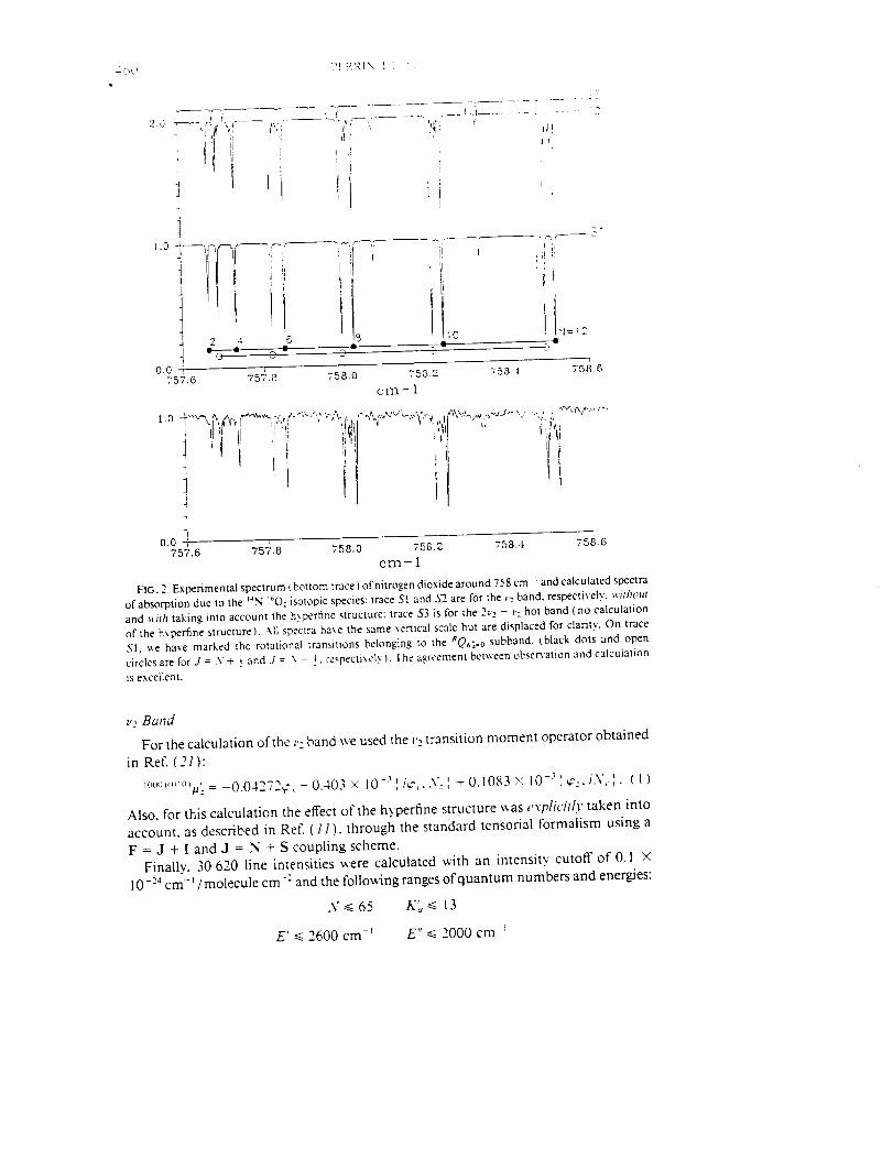
0.0 i _ 758.4, 758.6757.6 757.8 758.0 75_._

¢m-1

FIO. 2. Experimental spectrum ( bottom trace ) of nitrogen dioxide around 758 cm -_ and calculated spectra

of absormion due to the _N _O: isotopic species: trace SI and 5"2_are for the _'2 band. respectively, withola

and uuh taking into account the h.xperfine structure- trace $3 is for the 2_,, - _': hot band (no calculation

of the h xperfine structure). All spectra haxe the same vertical scale but are displaced for clarity. On trace

SI. _e have marked the rotational transitions belonging _o _he _QK;.o subband. _black dots and open

circles are for J = N + ! and J = \ - _,. respectixel.x ). The agreement bctx_een observation and calculation

is excellent.

v, Band

For the calculation of the _,_-band we used the v_,transition moment operator obtained

in Ref. (21):

,oot')_w_u' _.= -0.04272_:, - 0.403 X 10 --_', i_,..V_. ', + 0.1083 )-: 10 -) '__-%.i.V, J. ( 1 )

Also. for this calculation the effect of the hyperfine structure was e.xplicitly taken into

account, as described in Ref. (11 ). through the standard tensorial formalism using a

F = J + I and J = N + S coupling scheme.Finallv. 30 620 line intensities were calculated with an intensity cutoff of 0.1 ×

10-:_ cm-_/molecule cm-: and the following ranges of quantum numbers and energies:

.V_65 K'o_< 13

E'_ < 2600 cm-_ E" _< 2000 cm-

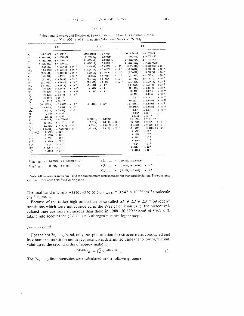
, \Xi) 2,- ,: B\\I)_ _q -\ "t):

TABLE l

Vibrational Energies and Rotational. Spin-Rotation. and Coupling Constants l\_r the

', ( 100 }. ( 020 ). 001 } ', Interacting Vibrational States of _N _O:

461

IC0 020 001

E 1319.76589

A" 8.0932898e

B" 0A3133685 s

C* 0A0928232 z

a_. (0.285392 e

.._, (-0.20710,

_ {0.30118:

6_ [0.518_

6; (0.2987_

H_ (0.33722_

HI. (-0.Z823=

H;K (0.220,

H_ (0.3306

h_ (0.378_

h_i -0.2571

h_ 0.10727

L; {-0.553568

L[_, (0.3250,

L[N {0.3Z5o

P_ 0.867

Q: -0.B439

(_= 0._83418_

(_o (0.230_

_: {-0.3327D

,_s (-0.18430_

_ .._;_ 0.6005_ 0.1678

&_ 0.6322

6_ S 0,3769

6_s 0.244

H_ s 0.29673

L_ s -0.3568

z 0.00012

0.0000082

z 0.00000067

: 0.00000037

± 0.000015} x I0

: 0.00012) x IC

: 0.00071) x 10 e

0.012) x I0 "s

± 0.0040) x 10 I

± 0.00011) x i0 s

: 0.0014) x 10 _

± 0.087) x 10 :°

0.071) x 10 ";z

± 0.029) x 10 _

x I0_°

x i0 -_z

± 0.00027) x 10 e

z 0.0041) x lO '_

± 0.041) x 10 :_

x 10 ll

x 10 18

: 0.000052

: 0013) x I0 -_

± 0.0013] x 10 "2

z 0.00036) x I0 !

x 10 6

x 10s

x 10 "9

x iO _

x I0 )

x I0 6

x I0 g

5498.34688 ± 0.00027 1616.84918 : 0000089

8.776705 e ± 0.000054 7.77425097 : 000000B0

0.43354531 ± 0.000001S 0.430929549 : 0.00000022

0.4086528 s ± 0.0000017 0.406370829 : 0.000000]8

(0.43885_ ± 0.00037) x I0 "_ (0.2524482 : 0.0000181 x 10 "r

[-0.24104 e ± O.O001l) x !0 "4 (-0.t8874_ : 0,000]0) x I0 "4

(0.29g19= ± 0.00043) x 10 .6 (0.302787 : 0.00074) x 10 "s

(0.8617 ± 0.063) x 10 "_ (0.4657 z ± 0.0070) x I0 s

(0131110 ) 0.0024) • iO ") (0.3417 a : 0.0037) x i0 "_

(0.7503, ± 0.0067) x :0 "s (0.279390 z 0.00013) x I0 -s

-0.44346 x 10 "? {-0.25967 ± 0.0013) x 10 ")

-0.8928 x 10 "1° (0.1044 e : 0.0072) x 10 "s

0.1777 x 10"lz (0.3501 : 0.013) x 10 "Iz

(0.562 z : 0.028) x 10 "I

(0.21_ : 0.141 x I0 i°

(0.1277_ : 0.0067) x I0 )z

-0.13633 x 10 "I (-0.486533 ± 0.00031) x 10 "a

(0.3482 o : 0.0064) x lO "I°

(0.871 ± O,t7) x I0 I_

0.867 x l0 ":1

-0.8439 x i0 ":_

0.219473 ± 0.00037 0.1724336 : 0.000044

(0.|76 s : 0.018) x ]C ") (0.2660} : 0.0043} x 10 "3

(-0.3341_ : 0.0015) x IC "_ (-0.31510_ : 0.00041) x I0 "z

{-0.3064 _ 0.012) x 10 "_ (-0.16757_ : 0.00031) x 10 ")

0.6005 x 10 _

0.1678 x iO "s

0.6322 x 10 _

0,3769 x 10 .6

0.244 x 10 _

0.29673 x 10 "_

-0.3688 x lO "s

hi_ol)(o,o) - {-0.29455Z: ± 0.000088) x 10 I hi_o=){l;cl - -0.656Z879 ± 0.000064

hiO6;?_o_:,. (o.736,:o.o311 _IO-' hi_,_:°_- _-o.9193_±0.oo_61_0"

<=0_)(_ " {o.zs6_:o.o33) _ _o

,Yore. All the results are in cm -] and the quoted errors correspond to one standard deviation. The constants

with no errors _ere held fixed dunng the fit.

The total band intensity was found to be S_(uo_-(ooo_= 0.542 X 10 -'8 cm-'/moleculecm--" at 296 K.

Because of the rather high proportion of so-called .XF _ _XJ 4= .LV "forbidden"transitions which were not considered in the 1988 calculation (12), the present cal-

culated lines are more numerous than those in 1988 {30 620 instead of 8065 × 3,

taking into account the (21 + 1 ) = 3 nitrogen nuclear degeneracy).

2u2 -- u2 Band

For the hot 2u_, - v__band, only the spin-rotation fine structure was considered andits vibrational transition moment constant was determined using the following relation,

valid up to the second order of approximation:

(°:°_w_°_u'_-= V'2× _o,,,.oo,,,, (2)

The 2v2 - v2 line intensities were calculated in the following ranges:

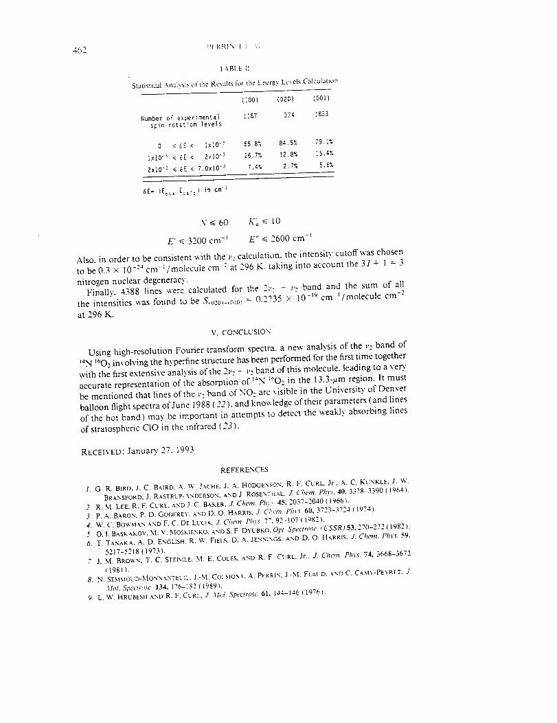
402 I'I RRIN I I ",[

T _,BLE I1

Statistical Ana!i, sis ol_.he Results for the Energy Levels Calculation

Number of experimental

spin-rotation levels

(;oo) (ozo) (OOl)

1187 374 1833

0 _ &E < IxlO _ 65.8% 84.5% 79.1%

IxlO s _ 8E < 2xIO "3 25.7% !2.8% 15.4%

2x10 3 4 8E < 7.0xlO 3 7.4% 2.7% 5.6%

&E- IE=ts-E:a.:[ in cm;

N_<60 K',_< 10

E' 4 3200 cm -_ E" _< 2600 cm -_

Also. in order to be consistent with the l,, calculation, the intensity cutoff was chosen

to be 0.3 X 10 -za cm-_/molecu le cm-: at 296 K. taking into account the 3I + 1 = 3

nitrogen nuclear degeneracy.Finally. 4388 lines were calculated for the 2;,, - i'2 band and the sum of all-2

the intensities was found to be S,0_,0)-,0xo_ = 0 "_'735 × 10-19 cm-I/molecule cm

at 296 K.

V. CONCLUSION

Using high-resolution Fourier transform spectra, a new analysis of the v_, band of

_aN :602 involving the h.vperfine structure has been performed for the first time together

with the first extensive anahsis of the 2v: - v: band of this molecule, leading to a very.'

accurate representation of ihe absorption of laN "_O2 in the 13.3-_m region. It must

be mentioned that lines of the >_ band of NO: are visible in the University of Denver

balloon flight spectra of June 1988 (22). and kno_vledge of their parameters ( and linesof the hot band) may be important in attempts to detect the weakly absorbing lines

of stratospheric CIO in the infrared (23).

RECEIVED" January.' 27. 1993

REFERENCES

1. G. R. BIRD, J. C. BMRD, A. \V. Ja,(HE. J. ¢, HODGENSON, R. F. CURL Jr.. A. C. KUNKLE, J. W'

BRANSFORD, J. RASTRUP-.-\NDERSON, AND J. ROSENTHAL, J. Chem. Phv_s. 40. 3378-3390 (1964).

2. R. M. LEE, R. F. CURL AND J. C. BA.KER, J. Chem. Phy> 45, 2037-2040 ( 19661.

3. P. A. B,_,RON, P. D. GODFRE'_. _,ND D. O. HARRIS. J. C,':em. Phys. 60, 3723-3724 (1974).

4. W. C. BOWMAN _,D F. C. DE LLCI*. J. Chem Phys. 7". 92-107 (1982).

5, O. 1. B_,SK a, KOV. M. V. MOSKIENKO, aND S. F. DYL'BKO. Opt, Speclrosc. (USSR) 53, 270-272 ( 1982 }.

{5. T. TANAKt_, A. D. ENGLISH. R. \V. FIELS, D. A. JENNINGS, AND D. O. H _,RRIS. J. Chem. Phys. 59,

5217-5218(1973).

7. J. M. BROW'N, T. C. STEIMI_E..M.E. COLES, ,_,ND R. F. CURL. Jr., J, Chem. Phys. 74, 3668-3672

( 1981 ).

8. N. SEMMOUD-MONN_.NTELIL. J.-M. COLMONT, A. PERRI'C J.-M. FLAL'D. _-,D C. Cn.MY -PEYRET, J

._Iol. Spectn_sc 134, 176-IS2 (1989).

9. L. \k'. HRUBESH _,ND R. FI CURL, J .11ol. Spectrosc. 61, I44-146 [ 1976}.

,: _,\D 2_: - r: B\\DS OF :N '_O: 463

10 Y. MORINO. M. T:_NIMOTO. S. SMTO. E. HIROT_,. R. A_L,_,T_,. aND T. T_,y_V,_,. J ._Iol. Spectr,)sc 98,

331-3-18 (1983).

11. A. PERRIN, J.-M. FLaUD. C. C_MY-PE'a RET. B. CARLI. _.ND M. CARI_OTTI, Mol. Phys. 63, 791-810

( 19881.

12. A. PERRIN. C. CAMY-PE','RET. J.-M. FLAUD, AND J. K.,_L'PPINEN, .L Mol. Speczrosc. 130, 168-182

(1988).13. A. PERmY, C. CAMY-PEYRET, AND J.-M. FLAUD, J. Quant. Spectrosc. Radiat. Transfer ,IS, 645-651

( 19921.

14. L.S. ROTHMAN, R. R. GAMACHE. R. H. TIPPING, C. P. RINSL-XND, M. A. H. SMITH. D. CHRIS BEN.'NER,

V. MAL*THY-DEVl, J.-M. FL._t_'D. C. CAMY-PEYRET, A. PERRIN, A. GOLDMA.N.S.T. M/_SSIF.

L. R. BROWN, AND R. A. TOTH, J. Quant. Spectrosc. Radiat. Transfer 48, 469-507 (1992).

15. A. PERRIN, J.-M. FLAUD, C. CAMY-PEYRET, A.-M. VASSEROT, G. GUELACHVlLI, A. GOLDMAN, F. J.

ML'RC_*Y. AND R. D. BLATHERWICK, J. Mol. Spectrosc. 154, 391-406 ( 19921.

16. R. A. TOTH, J. Opt. Soc. .4met. B 9, 433-461 (1992).

17. A. PERRIN, J.-M. FLAUD, AND C. CAMY-PEYRET, J. Mol. Spectrosc. 118, 174-179 (1986).

18. R. A. TOTH, J. Opt. Soc. Amer. B 3, 1263-1281 (1986).

19. A. G. MArd AND J. S. WELLS, "'Wavenumber Calibration Tables from Heterodyne Frequency Mea-

surements," NIST Special Publication 821. 1992.

20. G. GUEL*CHVILI AND K. NARAHAm RAO, "Handbook oflnfrared Standards," Academic Press, Orlando,

1986.

21. V. MALATHY DEV1, P. P. DAS, A. BANO, K. NARAHAR1 RAO. J.-M. FLAUD, C. CAMY-PEYRET, AND

J.-P. CHEVILLARD, J.._[ol. Spe¢lrosc. 8g, 251-258 ( 1981 ).

22. A. GOLDMAN. F. J. MURCRAY, R. D. BI.__,THERWICK, J. J. KOSTERS, F. H. MURCILA.Y, F. G. MURCRAY,

AND C. P. RINSLAND, J. Geophys. Res. D94, 14945-14955 (1989).

23. C. P. RINSLAND AND A. GOLDM.A.N, J. Quant. Speclrosc. Radiat. Transfer48, 685-692 (1992).

fne p2 and 2v2 - 1,2 bands of 14N 1602: Electron Spin-Rotation and

Hyperfine Contact Resonances in the (01 0) Vibrational State

A. PERRIN,* J.-M. FLAUD.* C. CAMY-PEYRET.* A. GOLDMAN.+ F. J. MURCRAY,f

R. D. BLATHERWICK,t AND C. P. RINSLAND:_

* Laborato_re de Physique .tlot_cu]aire el .41_plications. _ C.VRS, L'mver_it_ P. ct 31. Curie, Bte 76,

4 Place Jus_leu, 75252 Parts Cedex 05, France, tDcpartment qfPhysic_', L'niverstty of Denver,

Denver. Colorado 8020& and ¢.AmTospheric Sciences Division. A:4SA Langle.I Research Center,

Hampton, Virginia 23681.0001

High-resolution Fourier transform spectra covering the 720-920 cm -_ spectral region have

been used _o perform a reanal.vsis of the v2 band ((010)-(000) vibrational transition) together

with the first analysis of the 2v,, - v2 hot band of nitrogen dioxide ((020)-(010) vibrational

transition). The high-qualib spectra show that. for numerous v: lines, the h.vperfine structure is

easily observable in the case of resonances due to the h._perfine Fermi-type operator. By performing

a full treatment of the spin-rotation and of the hyperfine operators, a new line list of the v2 band

(positions and intensities) has been generated, and it is in excellent agreement with the experimental

spectrum. Also. a thorough anal._sis of the 2v,, - v: hot band has been performed leading to an

extended set of new (020) spin-rotation levels. These levels, together with the [(100), (020),

(001) } spin-rotation levels deduced previousl._ from the anal_sis of the v_, 2v,. and v_ cold bands

performed in the 6.3- to 7.5-urn spectral range [A. Perrin, J.-M. F'laud, C. Camy-Peyret, A.-M.

Vasserot, G. Guelachvili, A. Goldman. F. J. Murcray. and R. D. Blatherwick, J. Mol. Spectrose.

154, 391-406 ( 1992)] were least.squares fitted, allowing one to derive a new set of vibrational

band centers and rotational, spin-rotation, and interaction constants for the ',( 100 )(020)(001 ) }

interacting states of _4N L_O:. _, 1993 _,cademic PresS, Inc.

I. INTRODUCTION

The cold v2 band and the 2v_, - v2 first hot band of nitrogen dioxide, located at 13

#m, correspo rid, respectively, to the ( 010 ) - (000) and (020) - ( 010 ) vibrational tran-

sitions of this molecule; consequently, in order to have accurate line positions it is

necessary to have precise parameters for both the upper and the lower vibrationalstales involved in these transitions.

For the (000) and (010) vibrational states, the most recent spectroscopic parameterswere obtained from a simultaneous fit of the available microwave or double resonance

data (Refs. ( 1-8 ) and ( 9, 10) for the (000) and ( 010 ) slate, respectively) and of the

infrared spin-rotation energy levels obtained from recent analyses of Fourier transform

spectra recorded in the far infrared (11 ) and in the 13.3-urn (12) spectral regions.In the analysis of the (000)-(000) band, even at the high resolution of the far-

infrared experimental spectra, the hyperfine structure is usually not detectable, except

in cases of local resonances due to the Fermi contact hyperfine operator. Accordingly,the line list (1I, 13, 14) of the pure rotation region of NO., (_0-200 cm -_) was

generated by explicitly taking into account the spin-rotation and hyperfine structures.On the other hand, this effect could not be observed so accurately in the 13.3-urn

experimental spectrum which was used in Ref. (12) for the analysis of the v_, band,

' l.aboratoire associ_ aux Universit_s P. et M. Curie et Paris-Sud.

0022-2852/93 $5.00Copyright cg 993 by Academic Press, lnc,

hal nights of reproduclion in an) form resc_.ed.

456

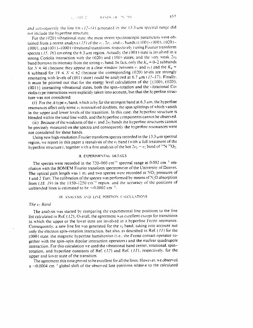
.. ',,,!', 2 !_\,,,i_, ,q _,,, ,'_ 457

and consequently the line list t]2-/41 generated in the 13.3-um spectral range did

not include the hyperfine structure.For the (020) vibrational state, the most recent spectroscopic parameters were ob-

tained from a recent analysis{ ]5) of the v_. 2v:. and z,) bands (( 1001-(0001. (020)-

(000). and (001 )-(000) vibrational transitions, respectively ) using Fourier transform

spectra ( 15, 16) covering the 6.3-_m region. Actualb the (001) state is involved in a

strong Coriolis interaction uith the (020) and (I001 states, and the very weak 2v:

band borro_vs its intensity from the strong ,,__band. In fact. only the K, = 0-2 subbands

for ,V _ 46 (because they appear in a clear window between _,_and _,)) and the K_ =6 subband for 19 _ N _ 62 (because the corresponding (020) levels are strongly

resonating with levels of (001) state) could be analyzed at 6.7/_m (15-17). Finally.

it must be pointed out that for the energy level calculations of the { (100), (020),

(001)} interacting vibrational states, both the spin-rotation and the vibrational Co-

riolis-type interactions were explicitly taken into account, but that the hyperfine struc-ture was not considered:

(i) For the.4-type v_ band. a hich is by far the strongest band at 6.3/_nl. the hyperfine

resonances affect only some v3 nonresolved doublets, the spin splittings of which vanish

in the upper and lower levels of the transition. In this case. the hyperfine structure isblended within the total line width, and the hyperfine components cannot be observed.

(it) Because of the weakness of the z,_and 2v, bands the hyperfine structures cannot

be precisely measured on the spectra and consequently the hyperfine resonances werenot considered for these bands.

Using new high-resolution Fourier transform spectra recorded in the 13.3-pm spectral

region, we report in this paper a reanalysis of the v_,band (with a full treatment of the

hyperfine structure ), together with a first analysis of the hot 2v2 - v: band of _aN 1_O2.

It. EXPERIMENTAL DETAILS

The spectra were recorded in the ?20-960 cm -z spectral range at 0.002 cm -n res-

olution with the BOMEM Fourier transform spectrometer of the University of Denver.

The optical path length was Im. and two spectra were recorded at NO__ pressures of

I and 2 Torr. The calibration of the spectra was performed by means of N:O absorption

lines (18. 19) in the II50-t250 cm -_ region, and the accuracy of the positions ofunblended lines is estimated to be _0.0002 cm -_

III. ANALYSIS _ND LINE POSITION C:d_CUL._TtONS

The v: Band

The anal._sis was started by comparing the experimental line positions to the linelist calculated in Ref. (12). Ox erall, the agreement was excellent except for transitions

in which the upper or the loxver state are involved in a hyperfine Fermi resonance.

Consequently, a new line list was generated for the v: band, taking into account not

only the electron spin-rotation interaction, but also. as described in Ref. (I1) for the

(000) state, the magnetic hyperfine hamiltonian {i.e.. the Fermi contact operator to-

gether with the spin-spin dipolar interaction operators) and the nuclear quadrupoleinteraction. For this calculation we used the vibrational band center, rotational, spin-

rotation, and hyperfine constants of Ref. (12) and Ref. (11), respectively, for the

upper and lower slate of the transition.The agreement this time proved to be excellent for all the lines. However. we obsera'ed

a -0.0004 cm-_ global shift of the observed line positions relative to the calculated

45_, l'l Rt_I'-,I i _i

ones. x_hich is due to a sli_i_.tlx diffcrem calibratio_ of the speclra used ill d_c prcsci_t

_ork ( 18. IV) compared to _b,at used ( 201 in 10SS. This leads to a different vibrational

band centerofthe_'zband: E,,v_ = 749.652561 cm _ (instead of 740.652961 cm

obtained previously in Ref. (12/).To show the quality of the experimental spectra and of the calculations performed

in the present work, _e show in Figs. I and 2 portions around 7"71.8 and 758.0 cm -t

of the experimental spectra together with line-b.v-line calculations performed using

either the line list generated in Ref. ( 12 ) ( no h.xperflne structure I or the line list derived

here (full treatment of the h.vperfine operators). In both regions, the improvement

brought by the new calculation is very clear.In the first spectral region, the complex hyperfine structure appears clearly in the

N = even RQA,;=j subband. At 771.30 and 771.64 cm -_ it is due to a strong hyperfineresonance involving the (010/[22 2 20] and (010)[20 2 18] rotational levels. At 772

cm -_ , since the resonance is weaker, one observes mainly a broadening of the N =

18 doublet structure. The same h.vperfine effect can be clearly observed in Fig. 2

around 758 cm -_ for lines belonging to the RQ_%=(, subband. It is worth stressing that

in both cases the new calculation, which involves the hyperfine operators, reproduces

the experimental spectrum x_ith high accuracy.

The 2_,2 - u2 Band

Lines from the 2,, - ,,- band were already observed in dae experimental spectrum

(12) which was used-in 1988 for the analysis of the 13.3-urn band of nitrogen dioxide.However, because this hot band is weak and because the (020) spectroscopic parametersavailable at that time were not precise enough ( only the/x'o = 0. 1.2 (020) series were

derived from the analysis of the 2v2 band performed at 6.6 um(17)), only a few lines

involving the K, = 0.'1.2 (020) rotational series could be analyzed at 13.3 urn.

The (020) parameters were recently significantly improved from a new analysis of

the { et, 2v_,, v3 } interacting bands (15). Indeed. more lines involving the K_ = 0. 1,2 series were assigned; also. lines involving the K_ = 6 rotational series of (020).

which borrow their intensities from _,_ through a Coriolis interaction, were ob-

ser_,ed ( 15. I6).Consequently. from the ',(100), (020J. (001)i and (010) parameters obtained in

Ref. (151 and l_ef. (12) respectively, it has been possible to better predict the 2_,2 -

,2 line positions, as performed in the present analysis.Because the 2_'z - _'2band is rather weak. only _ransitions of this band involving .V

<_ 30 rotational quantum number could be identified in the spectrum. For transitions

involving the K, = 0-2 and /x', = 6 (020) energ._ ]evels. the agreement between theobserxed and the predicted line positions was excellent, but this was not completely

the case for lines involving the K_, = 3-5 (020) rotational levels since small discrepencies

(up to 0.0030 cm -_ ) v_ere obserxed. Using these new data. we then determined thevibrational band centers, rotational, spin-rotation, and coupling constants of the

{(100), (020). (001)} resonating states. As in Ref. (15) the Hamiltonian matrixexplicitly takes into account both the Coriolis and the spin-rotation interactions. Forthis least-squares fit calculation, the 164 (020) new spin-rotation energy levels obtained

in the present work for K_ _< 6 and N _< 30 were combined to the 3230 (100) (001)

and (020) energy levels obtained in Ref. (15).Table I gives the list of vibrational energies and rotational, spin-rotation, and cou-

pling constants deduced from the fit. together with their estimated uncertainty. The

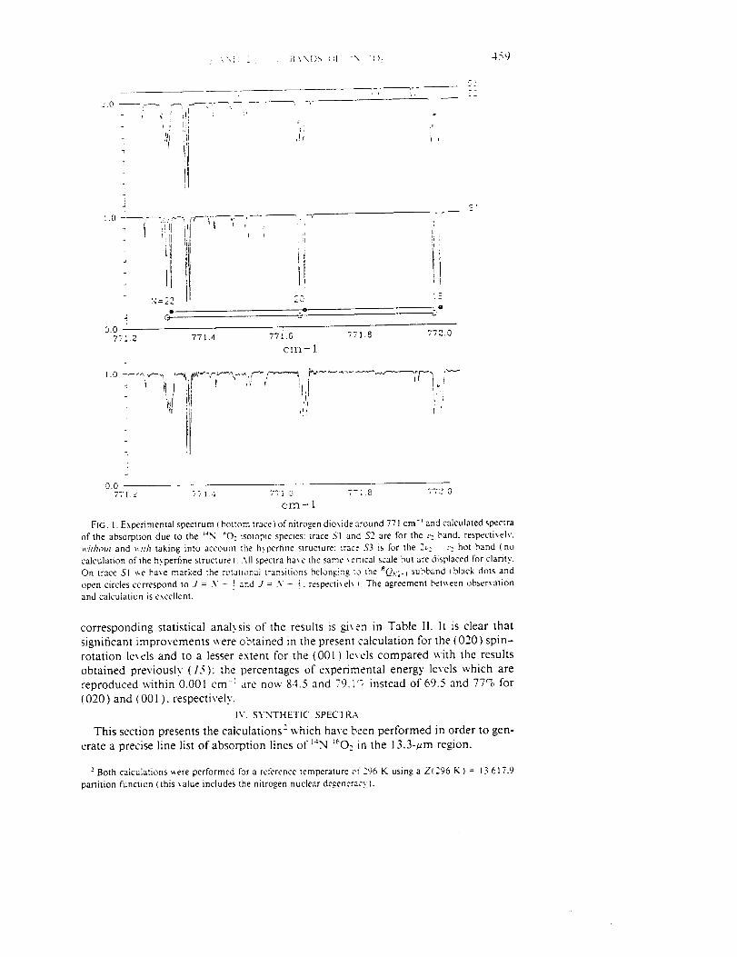
',,'_i_ _ : ]_,\'xl) _, Iq -'x, '_),

2,0

_ i_ :_ ! _[("-- _ _, , ,!

i .i _LI:,

,'1!I ,[Ir

" ' ilFllt I , : ':'

!ilL_ki L:iiI

! !ii20

a @

459

5 -'!2

0.07"71 2 771.4 771.6

cm- 1

77i .8 77z.0

- '_ I, "r 1 ;_ t'_LJ If,

Ii

!,!I ::i_!_i_ l

0.o7:_ z v7{.,_ 7z_ ;, v7:8 :7:Lo

cm-1

FIG. I. Experimental spectrum (bottom trace ) of nitrogen dioxide around 771 cm-_ and calculated spectraof the absorption due to the _'_.N _'O- isotopic species: trace S1 and $2 are for the v: band. respecti,.ely.

without and _ith taking into account the h_perfine structure: trace $3 is for lhe 2_,: - _.2hot band (no

calculation of the h._perfine structure ). All spectra ha_e the same _er-tical scale bul are displaced for clarity.

On trace Sl _e haxe marked the rotational _ransitions belonging _o the _Q_,:._ subband i black dots and

open circles correspond to J = .V - _ and J = V - !. respecti_eb _. ]-he agreement be_een observation

and calculation is excellent.

corresponding statistical analysis of the results is gixen in Table II. It is clear that

significant improvements were obtained in the present calculation for the (020) spin-

rotation lexels and to a lesser extent for the (001) levels compared with the results

obtained previously (15): the percentages of experimental energy levels which are

reproduced within 0.001 cm -] are now 84.5 and 79.1_ instead of 69.5 and 77% for

f020) and (001), respectively.

IV. SYNTHETIC SPECTRA

This section presents the calculations z which have been performed in order to gen-erate a precise line list of absorption lines of _4N _eO2 in the 13.3-_m region.

2 Both calculations v,ere performed for a reference temperature of 296 K using a Z1296 K) = 13 617.9

partition function (this _alue includes the nitrogen nuclear degenerac._ I.

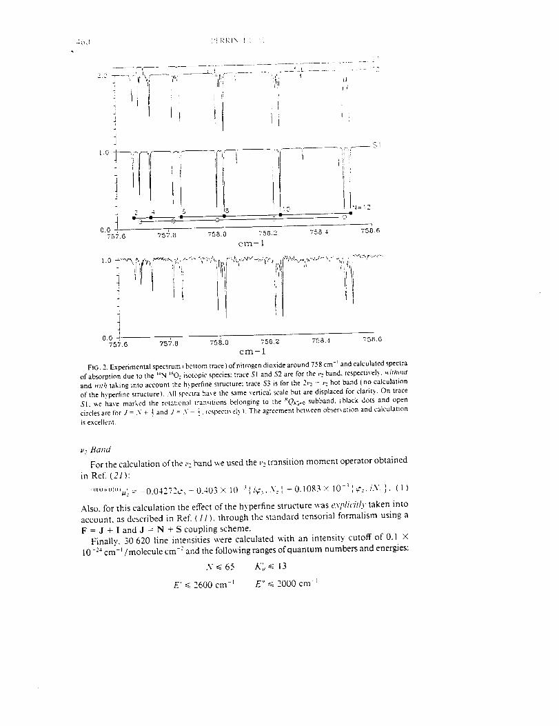
-'(_d 11 F,I-_I", I : '_

20 '_-'_ ' _ "--'

iJ

Z

4 :i !! ;!

i ,/I It I,',i !

i'l i I2 4 6

i =0 @ • DiD

0.0 :

5 ",o

__t t_- ....... --- - 2

H_! I'

ii i

"l=i24

'757.6 v5-).8 v5a.o 758•r, 75+4 7_8•ecrn-1

t .0 .-l-",.,m _ ",,,.,t"""_,',-, .;' ."- "". "?-',','\ _, r""-.?,,...,,4"_..,',,_,., t%\'..-, ,,,.,,,.,-..'-;'_'-". _,' r , :",r."' % ii TV/ l', I ' ' l',lhl _'i 'T "_'.i "vOIr ],tL qh J

! il0.0 ' _

757.6 757.8 75B.0 758.2 758.4 758.6

cm-1

FIG. 2. Experimental spectrum I bottom trace ) of nitrogen dioxide around 758 cm -_ and calculated spectra

of absorption due to the '_N teO: isotopic species: trace SI and 5"2_are for the ,,: band. respectively, wilholll

and uilh taking into accounl the h._perfine structure: trace $3 is for the 2;,_. - ,': hot band (no calculation

of the hyperfine structure)• All spectra have the same xenical scale but are displaced for clarity. On trace

SI. _e have marked the rotational transitions belonging to the RQ_.o subband. _black dots and open

circles are for J = \'4- _ and J = .\ - 1. respectb ely ). The agreement between observation and calculation

is excellent.

v2 Band

For the calculation of the v: band we used the v=transition moment operator obtained

in Ref. (21):

'°_""_°_°>,u'__= -0.04272¢, - 0.403 × 10 -:_', is: , . .',_-', + 0.1083 >: 10 -_', ,;:. i.V, }. ( l )

Also, for this calculation the effect of the hyperfine structure was exl_/icilly taken into

account, as described in Ref. ( 11 ). through the standard tensorial formalism using a

F = J + I and J = N + S coupling scheme.Finallv, 30 620 line intensities were calculated with an intensity cutoff of 0.1 x

10-:_ cm-_/molecule cm-: and the following ranges of quantum numbers and energies:

.V_<65 K;_ < 13

E' _< 2600 cm-_ E" _< 2000 cm-

_- \\D 2,: ,. B\NDS _,'q: -\ _'('l:

T_,BLE l

Vibralional Energies and Rotational, Spin-Rotation. and Coupling Constants for the

_ ( 100"}, (020). CO01 ) i Interacting Vibrational Stales of S4N _Oz

461

I00 020 001

E 1319.75589 ± 0.00012 1498.34588 ± 0.00027 1616.84918 : 0.000089

A" 0.0932898_ ± 0.0000082 8.775705_ ± 0.000054 7.774250g_ : O.O0000BO

B" 0.43133685s ± 0.00000067 0.43354531 ± 0.0000015 0.43092954 s z 0.00000022

C" 0.40928232 z ± 0.00000037 0.4086528 s ± 0.0000017 0.406370B2_ : 0.00000018

,__ (0.285392 s ± 0.000015) X l0 _ (0.438857 ± 0.00037) x 10 "z (0.252448 l = 0.000018) X 10 "z

,._, (-0.20710 i ± 0.00012) x I0"_ (-0.24104 e ± 0.000111 x 10 "4 (-0.188744 : 0.00010) x I0 "a

_ [0.30118: ± 0.000711 x 10.5 (0.299191 ± 0.00043) x _0 "5 (0.302787 : 0.00074) X 10 "6

&_ (0.5186 _ 0.012) x 10s (0.8617 ± 0.053) x 10 .5 (O.4657 z C 0.0070) X 10 "s

&_ (0.29876 ± 0.0040) x 10.7 {0.3111 o ± 0.0024) x i0 "1 (0.3417 e _ 0.0037) x 10-1H,_ (0.33722 z ± 0.00011) I 10s (0.7503_ ± 0.0067) x :0 "s (0.279390 _ 0.00013} x 10 .5

I'_, (-0.2823 o ± 0.00141 x 10 l -0.44346 x 10"t (-0.2596 r ± 0.00131 x 10)

H_ (0.ZZ04 ± 0.087) x 10":0 -0.B928 x 10-l° (0.10445 : 0.0072) x 10"9

H_ (0.330 s _ O.071) x 10":_ 0.1777 x 10"12 [O.360 z ± 0.0131 x 10"12

h_ (0.378_ ± 0.029) x 10 l (0.562_ = 0.028) x 10-?

h_ -0.2571 x 10z° (0.211 = 0.14) x 10 "l©

h_ 0.10727 x t0 -iz (O.1277z : 0.0057) x 10"zzL; (-0.55356 e ± 0.00027) x 10 "e -0.13633 x 10"z (-0.48653] _ 0.00031) x 10"e

L_ N (0.3250_ ± 0.00411 x 10 "i° (0.34820 : 0.0064) x 10 xo

L_N {0.325 o ± O.0411 x l0 ;z (0.871 = 0.27) x 10"1_

p_ 0.867 x 10Lz 0.867 x 10-;l

Q_ -0.8439 x 10-z4 -O.8439 x 10-;4_d 0.163418 e ± 0.000052 0.21947_ ± 0,00037 O.172433_ z 0.000044(_b 10.230 o ± 0.013) x 10.2 (0.1769 = 0.018) x ]0 "_ (0.2660j : 0.0043) x 10_

* _c (-0.3327 o ± 0.00131 x l0 _ (-0.334] 4 _ 0.00151 x 10z (-0.315107 ± 0.00041} x 10-z

_s (-0.184303 _ 0.00036) x 10 _ (-0.306_ _ 0.012) x 10"1 (-0.16757 s z 0.0003]) x ]0 "_

_ _ 0.6005 x 10 ,5 0.5006 x IO -_

,._ 0.1678 x 10"_ O.1678 x 10s

_s 0.6322 x 10_ 0.6322 x 10"_

6_ s 0.3769 x 10-5 0.3769 x 10 .56; s 0.244 x 10"9 0.244 x ]0"_

H_s 0._9573 x 10"s 0.29673 x 10.5

L__ -0.3568 x I0"_ -0.3568 x 10"_

hi_o_}(©zo} . (-0.Z94SSZ_ ± O.OOOO88) x 10= hi_o_}_=_ - -0.565287_ z 0.000064

hi_o;_lozo) - (0.736, ± 0.031) x 10"I hi_,l(,col - (-0.9193_ ± 0.0096) x 10'

Note. All the results are in cm -= and the quoted errors correspond ze one standard deviation. The constants

with no errors_ere held fixed during the fit.

The total band intensity was found to be S_o_0)-(0oo_ = 0.542 × I0 -_8 cm -_/molecule

cm -2 at 296 K.

Because of the rather high proportion of so-called AF 4= ._XJ _a _,\, "forbidden'"transitions which were not considered in the 1988 calculation (12), the present cal-

culated lines are more numerous than those in 1988 (30 620 instead of 8065 × 3,

taking into account the (21 + 1) = 3 nitrogen nuclear degeneracy).

2v2 - v2 Band

For the hot 2v2 - v_,band, only the spin-rotation fine structure was considered andits vibrational transition moment constant was determined using the following relation,

valid up to the second order of approximation:

_"2('"°'°'u';= _"5x ,,.,,,_,o_,,... (2 )

The 2u2 - v2 line intensities were calculated in the following ranges:

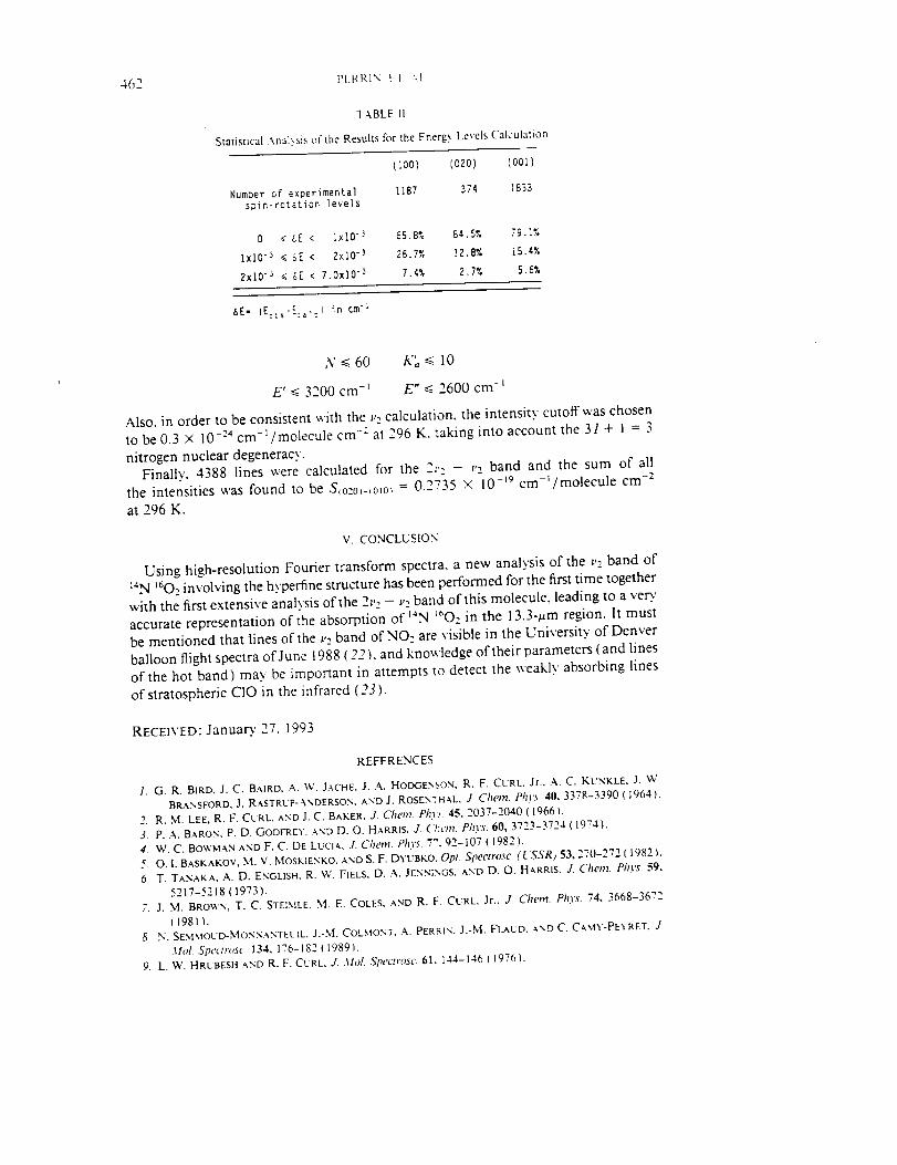
462 PI!RRIX t I \l

T-%BLE II

Statist cal Analysis ol-the Results for the Energ} Levels Calculation

Number of experimentalspin-rotation levels

(ioo) {ozo) (oo:)

1187 374 1833

O _ LE < IxlO _ 65.8% 84.5% 79.1%

IxlO -3 _ _E < 2xlO "3 28.7% !2.8% 15.4%

2xlO "_ _ 6E < 7.0xlO "3 7.4% 2.7% 5.6%

6E- IE:ts-E:_::l in cm"_

N _<60 K;, _< 10

E' _< 3200 cm -_ E" _ 2600 cm -_

Also, in order to be consistent with the p: calculation, the intensity cutoff was chosento be 0.3 X 10 -:4 cm-1/molecu le cm-: at 296 K. taking into account the 3I + 1 = 3

nitrogen nuclear degeneracy.Finally. 4388 lines were calculated for the 2L, - v2 band and the sum of all-2

the intensities was found to be S_o2o)-_o_o_ = 0.2735 × 10 -19 cm-_/molecule cm

at 296 K.

V. CONCLUSION

Using high-resolution Fourier transform spectra, a new analysis of the v2 band of

_N _602 involving the h.vperfine structure has been performed for the first time togetherwith the first extensive analysis of the 2z,2 - _'2band of this molecule, leading to a vers'

accurate representation of ihe absorption of _"N _6Oz in the 13.3-t_m region. It must

be mentioned that lines of the _,_band of NO: are visible in the University of Denver79balloon flight spectra of June 1988 ( -- ). and knowledge oftheir parameters (and lines

of the hot band) may be important in attempts to detect the weakly absorbing lines

of stratospheric CIO in the infrared (23).

RECEIVED: Januars.' 27. 1993

REFERENCES

1. G. R. BIRD, J. C. BAIRD, A. \V. JACHE. J..-%. HODGENSON, R. F. CURL. Jr.. A. C. KL'NKLE, J. W.

BRANSFORD, J. RASTRUP-ANDERSON, AND J. ROSENTH-_L, J. Chem. Phy._ 40, 3378-3390 (1964 }.

R. M. LEE, R. F. CURL AND J. C. BAKER, J. Chem. Phys 45, 2037-2040 (19661.

;i P..-%. BARON, P. D. GODFREY. aND D. O. HARRIS, J. Chem. Phys. 60, 3723-3724 ( 19741.

4. W. C. BOWMAN AND F. C. DE LUCI¢. J. C]lem Phys. 7.9_-107 ( 19821.• (l, SSR) 53, .-,0-- - ( 1982 ).

O. I. BASKAKOV, M. V. MOSK1ENKO. AND S. F. DYUBKO. Opt. Speclrosc. " "_'_ "_7"_

;[ T. TANAKA. A. D. ENGLISH. R. \V. FIELS. D. A. JENNINGS. AND D. O. H¢RRIS. J. Chem. Phys. 59,

5217-5218 (1973).7. J. M. BROWN, T. C. STEIMLE. M. E. COLES. AND R. F. CURL. Jr., J. Chem. Phys. 74, 3668-3672

( 1981/.8. N, SEMMOUD-MONN-'_NTELIL. J.-M. COLMONT, A. PERRIN. J.-M. FLAUD. _,ND C. C_,MY -PEYRET- J

Mol. Sp(,clrosc 134, 176-182 (1989).

9. L. %r. HRUBESH _ND R. F. CURL, J. Mol. Spectrosc. 61. I-$4-146 t 1976}.

,- _,\D 2,: - ,: BANDS OF 'N '_0: 463

10. Y. MORINO, M. TANIMOTO, S. SAITO. E. HIROT_. R. Axw, T-X. a.ND T. TANAI<.A. J _Iol. Spectrose 98,

331-348 (1983).

11. A. PERR1N, J.-M. FLAUD, C. CAMY-PEYRET, B. CARLI. AND M. CARLOTTI, ,_[01. Ph3's. 63, 791-810

(1988).12. A. PERRIN, C. CAMY-PEYRE'I', J.-M. FLAUD, AND J. ICn.UPPINEN, J. 3Iol. Spectrosc. 130, 168-182

(1988).

13. A. PERRIN, C. CAMY-PEYRET, AND J.-M. FLAUD, J. Quant. Spectrosc. Radiat. Transfer 48, 645-651

(1992).14. L.S. ROTHMAN, R. R. GAMACHE, R. H. TIPPING, C. P. RINSL..,,ND, M. A. H. SMITH, D. CHRIS BENNER,

V. MALATHY-DEVI, J.-M. FLAUD, C. CAMY-PEYRET, A. PERRIN, A. GOLDMAN, S. T. MASSI[:'.

L. R. BROWN, AND R. A. TOrH, J. Quant. Spectrosc. Radiat. Transfer 48, 469-507 (1992).

15. A. PERRIN, J.-M. FLAUD, C. CAMY-PEYRET, A.-M. VASSEROT. G. GUELACHVILI, A. GOLDMAN, F. J.

MURCr_.AY, AND R. D. BLATHERWlCK, J. MoL Spectrosc. 154, 391--106 (1992).

16. R. A. Torn, J. Opt. Soc. Amer. B 9, 433-461 (1992).

17. A. PERRIN, J.-M. FLAUD, A_D C. CAMY-PEYRET, J. Mol. Spectrosc. 118, 174-179 (1986).

18. R. A. TOTn, J. Opt. Soc. Amer. B 3, 1263-1281 (1986).

19. A. G. MAIO AND J. S. WELLS, "Wavenumber Calibration Tables from Heterodyne Frequency Mea-

surements," NIST Special Publication 821, 1992.

20. G. GUELAO-IVlU AND K. NARAHAPd RAO, "'Handbook of Infrared Standards," Academic Press, Orlando,

1986.

21. V. MALATHY DEVI, P. P. DAS, A. BANO, K. NARAHARI RAO. J.-M. FLAUD, C. CAMY-PEYRET, AND

J.-P. CHEVILLARD, J. Mol. Spectrosc. 88, 251-258 (1981).

22. A. GOLDMAN, F. J. MURCRAY, R. D. BLATHERWICK, J. J. KOS'I'ERS, F. H. MURCRAY, F. G. MURCRAY,

AND C. P. RaNSLAND, J. Geoph)'s. Res. D 94, 14945-14955 (1989).

23. C. P. RINSLAND AND A. GOLDMAN, J. Quant. Spectrosc. Radiat. Transfer 48, 685-692 (1992).

JOURNAL OF GEOPHYSICAL RESEARCH, VOL. 98, NO. D6, PAGES 10,499-10,507, JUNE 20, 1993

Atmospheric Sulfur Hexafluoride" Sources, Sinks and Greenhouse Warming

_,_ALCOLMK. W. KO, 1 NIEN DAK SZE, l WEI-CHYUNG WANG, 1'2 GEORGE SHIA, 3 AARON GOLDMAN, 4

FRANK J. _[URCRAY, 4 DAVID G. MURCRAY, 4 AND CURTIS P. RINS LANDs

Model calculations using estimated reaction rates of sulfur hexafluoride (SF6) with OH and O(ID)indicate that the atmospheric lifetime due to these processes may be very long (25,000 years). An

upper limit for the UV cross section would suggest a photolysis lifetime much longer than 1000 years.The possibility of other removal mechanisms are discussed. The estimated lifetimes are consistentwith other estimated values based on recent laboratory measurements. There appears to be no known

natural source of SFr. An estimate of the current production rate of SF6 is about 5 kt/yr. Based onhistorical emission rates, we calculated a present-day atmospheric concentrations for SF6 of about 2.5

parts per trillion by volume (pptv) and compared the results with available atmospheric measurements.It is dit_cult to estimate the atmospheric lifetime of SF 6 based on mass balance of the emission rateand observed abundance. There are large uncertainties concerning what portion of the SF6 is releasedto the atmosphere. Even if the emission rate were precisely known, it would be dil_cult to distinguishamong lifetimes longer than 100 years since the current abundance of SF6 is due to emission in the pastthree decades. More information on the measured trends over the past decade and observed verticaland latitudinal distributions of SF6 in the lower stratosphere will help to narrow the uncertainty in thelifetime. Based on laboratory-measured IR absorption cross section for SFr, we showed that SF 6 is .about 3 times more effective as a greenhouse gas compared to CFC 11 on a per molecule basis.

However. its effect on atmospheric warming will be minimal because of its very small concentration.We estimated the future concentration of SF 6 at 2010 to be 8 and 10 pptv based on two projected

emission scenarios. The corresponding equilibrium warming of 0.0035°C and 0.0043°C is to be

compared with the estimated warming due to CO, increase of about 0.8°C in the same period.

I. INTRODUCTION

The Earth's atmosphere contains a trace amount (-few

parts per trillion) of SF6. Earliest measurements [Krey et al.,

1977; Singh et al.. 1977] indicated concentrations of less than

1 part per trillion by volume (pptv) in the 1970s. Although

there is no continuous long-term global monitoring of this

gas, intermittent samplings [Singh et al., 1977, 1979; Leifer

et al., 1982] and sampling of ocean water [Watson and

Liddicoat, 1985] have indicated an increasing trend. Recent

papers by Rinsland et al. [1990a, b] and Zander et al. [1991]

provided additional evidence for the increasing trend. The

possibility that SF 6 may contribute to the global warming

was raised by Ramanathan et al. [1985, 1987], but no

quantitative assessment was made by the authors.Assessment of the greenhouse warming impact of the

species requires knowledge on its radiative property and

information on its lifetime and atmospheric budget so that its

future abundance in the atmosphere can be predicted. Our

understanding of the life cycle (or budget) of atmospheric

SF6 was hampered, in part, by the lack of global emission

data. This paper discusses some of its commercial applica-

tion and usage and provides an estimate of worldwide

production of SF6, from which a global emission rate is

derived and extrapolated for the next 20 years. The second

IAtmospheric and Environmental Research, Incorporated. Cam-

bridge, Massachusetts.'-Now at State University of New York, Albany.3Buffalo Research Laboratory, Allied-Signal Incorporated, Buf-

falo, New York.4Department of Physics. University of Denver. Denver, Colo-

rado.5Atmospheric Science Center, NASA Langley Research Center,

Hampton, Virginia.

Copyright 1993 by the American Geophysical Union.

Paper number 93JD00228.0148-0227/93/93J D-00228505.00

objective of the paper is to estimate the atmospheric lifetime

of SF 6 using several different approaches: estimates based

on a known mechanism (e.g., photolysis and atmospheric

oxidation) and/or mass balance method. The third objective

is to calculate the radiative forcing of SF6 based on our

recent laboratory infrared absorption cross section and to

compute the expected warming over the time period 1950--

2010 according to several emission scenarios.

2. USES OF SULFUR HEXAFLUORIDE AND SOURCES

OF ATMOSPHERIC EMISSIONS

2.1. Applications for Sulfur Hexafluoride and Emission

Sources

Sulfur hexafluoride has a unique combination of chemical,

physical, and electrical properties which make it ideally

suited for some very specialized industrial applications. By

far, its largest use (approximately 80% of production) is for

insulation of electrical equipment. The material's high di-

electric strength and unique arc-quenching ability have en-

abled the development of safe, reliable gas-insulated high-

voltage circuit breakers, substations, transformers, and

transmission lines. Sulfur hexafluoride provides an effective

alternative to insulating oils (which suffer from high mainte-

nance costs, disposal problems, and safety problems due to

the flammable oil). SFr-insulated equipment also has impor-

tant advantages over vacuum- or air-insulated equipment

which require more space and are not well suited for

switching very high voltages.

There are two main sources of emission from SFr-

insulated electrical equipment. SF6 can escape from the

container through seals and gaskets. Older equipment is

prone to leak in this manner as it is typically pressurized to0.015-0.03 N m-Z (100--200 psi) with SF 6. Newer designs for

SFr-filled switchgear allow operation at near-ambient pres-

sure and have greatly improved seals giving rise to leakage

rates of less than l%/yr. Emissions may occur when SFr-

10,499

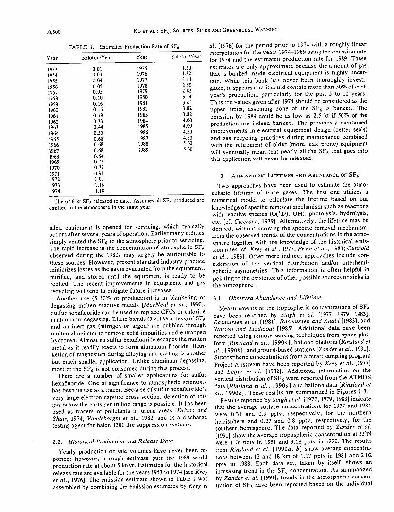
10,500 Ko ET AL.: SF 6, SOURCES, SINKS AND GREENHOUSE WARMING

TABLE 1. Estimated Production Rate of SF 6

Year Kiloton/Year Year Kilotort/Year

1953 0.01 1975 1.501954 0.03 1976 1.821955 0.04 1977 2.141956 0.05 1978 2.501957 0.05 1979 2.821958 0.10 1980 3.141959 0.16 1981 3.451960 0.16 1982 3.821961 0.19 1983 3.821962 0.33 1984 4.001963 0.44 1985 4.001964 0.55 1986 4.501965 0.68 1987 4.501966 0.68 1988 5.001967 0.68 1989 5.001968 0.641969 0.731970 0.771971 0.911972 1.091973 1.18

1974 1.18

The 62.6 kt SF6 released to date. Assumes all SF 6 produced are

emitted to the atmosphere in the same year.

filled equipment is opened for servicing, which typically

occurs after several years of operation. Earlier many utilities

simply vented the SF 6 to the atmosphere prior to servicing.

The rapid increase in the concentration of atmospheric SF 6

observed during the 1980s may largely be attributable to

these sources. However, present standard industry practice

minimizes losses as the gas is evacuated from the equipment,

purified, and stored until the equipment is ready to be

refilled. The recent improvements in equipment and gas

recycling will tend to mitigate future increases.

Another use (5-10% of production) is in blanketing or

degassing molten reactive metals [MacNeal et al., 1990].

Sulfur hexafluoride can be used to replace CFCs or chlorine

in aluminum degassing. Dilute blends (5 vol % or less) of SF 6

and an inert gas (nitrogen or argon) are bubbled through

molten aluminum to remove solid impurities and entrapped

hydrogen. Almost no sulfur hexafluoride escapes the molten

metal as it readily reacts to form aluminum fluoride. Blan-

keting of magnesium during alloying and casting is another

but much smaller application. Unlike aluminum degassing,

most of the SF 6 is not consumed during this process.

There are a number of smaller applications for sulfur

hexafluoride. One of significance to atmospheric scientists

has been its use as a tracer. Because of sulfur hexafluoride's

very large electron capture cross section, detection of this

gas below the parts per trillion range is possible. It has been

used as tracers of pollutants in urban areas [Drivas and

Shair, 1974; Vandeborght et al., 1982] and as a discharge

testing agent for halon 1301 fire suppression systems.

2.2. Historical Production and Release Data

Yearly production or sale volumes have never been re-

ported; however, a rough estimate puts the 1989 world

production rate at about 5 kt/yr. Estimates for the historical

release rate are available for the years 1953 to 1974 [see Krey

et al., 1976]. The emission estimate shown in Table i was

assembled by combining the emission estimates by Krey et

al. [1976] for the period prior to 1974 with a roughly linear

interpolation for the years 1974-1989 using the emission rate

for 1974 and the estimated production rate for 1989. These

estimates are only approximate because the amount of gas

that is banked inside electrical equipment is highly uncer-

tain. While this bank has never been thoroughly investi-

gated, it appears that it could contain more than 50% of each

year's production, particularly for the past 5 to 10 years.

Thus the values given after 1974 should be considered as the

upper limits, assuming none of the SF 6 is banked. The

emission by 1989 could be as low as 2.5 kt if 50% of the

production are indeed banked. The previously mentioned

improvements in electrical equipment design (better seals)

and gas recycling practices during maintenance combined

with the retirement of older (more leak prone) equipment

will eventually mean that nearly all the SF6 that goes into

this application will never be released.

3. ATMOSPHERIC LIFETIMES AND ABUNDANCE OF SF 6

Two approaches have been used to estimate the atmo-

spheric lifetime of trace gases. The first one utilizes a

numerical model to calculate the lifetime based on our

knowledge of specific removal mechanism such as reactions

with reactive species (O(ID), OH), photolysis, hydrolysis,

etc. [cf. Cicerone, 1979]. Alternatively, the lifetime may be

derived, without knowing the specific removal mechanism,

from the observed trends of the concentrations in the atmo-

sphere together with the knowledge of the historical emis-

sion rates [cf. Krey et al., 1977; Prinn et al., 1983; Cunnold

et al., 1983]. Other more indirect approaches include con-

sideration of the vertical distribution and/or interhemi-

spheric asymmetries. This information is often helpful in

pointing to the existence of other possible sources or sinks in

the atmosphere.

3.1. Observed Abundance and Lifetime

Measurements of the tropospheric concentrations of SF 6

have been reported by Singh et al. [1977, 1979, 1983],

Rasmussen et al. [1981], Rasmussen and Khalil [1983], and

Watson and Liddicoat [1985]. Additional data have been

reported using remote sensing techniques from space plat-

form [Rinsland et al., 1990a], balloon platform [Rinsland et

al., 1990b], and ground-based stations [Zander et al., 1991].

Stratospheric concentrations from aircraft sampling program

Project Airstream have been reported by Krey et al. [1977]

and Leifer et al. [1982]. Additional information on the

vertical distribution of SF6 were reported from the ATMOS

data [Rinsland et al., 1990a] and balloon data [Rinsland et

al., 1990b]. These results are summarized in Figures 1-3.

Results reported by Singh et al. [1977, 1979, 1983] indicate

that the average surface concentrations for 1977 and 1981

were 0.31 and 0.9 pptv, respectively, for the northern

hemisphere and 0.27 and 0.8 pptv, respectively, for the

southern hemisphere. The data reported by Zander et al.

[1991] show the average tropospheric concentration at 32"N

were 1.76 pptv in 1981 and 3.18 pptv in 1990. The results

from Rinsland et al. [1990a, b] show average concentra-

tions between 12 and 18 km of 1.17 pptv in 1981 and 2.02

pptv in 1988. Each data set, taken by itself, shows an

increasing trend in the SF 6 concentration. As summarized

by Zander et al. [1991], trends in the atmospheric concen-

tration of SF 6 have been reported based on the individual

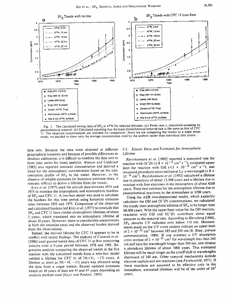
KO ET AL.: SF 6, SOURCES, SINKS AND GREENHOUSE WARMING 10,501

3.5

2,5

g_2

E

_.5

8

1

O.S

0

SF 6 Trends with no loss

47*N, 2 km ]

.... 47°N, 13 km [

___ ,,'.,,,kin I ._

- - 1YI,,oN V.I- l

/57," 2 ,,j. "_"

,,_. , 1 i , I , , , , I

1970 1975 1980 1985 1990

Year

3.5

3

A

2.5

c

1.5

8

1

0.5

0

1970

b SF 6 Trends with CFC 11 Loss Rate

47°N, 2 km Ti

.... 47°N. 13 km /

-- -- - 47°N. 19"kin l /

--. -- 47"N. 22km l _ ._

_.. J

1975 1980 1985 1990

Year

• Krey (NH <10 kin) • Krey (NH <10km)

O Krey (NH 14-18 kin) 0 Krey (NH 14-18 kin)

E3 Leiffer (NH Slral) r7 Leiffer (NH Strat)

• $ir_jh (NH Surface) • Sin<jh (NH Surface)

• Zandet (47°N. Trop) • Zander (47"N, Trop)

• Rasmussen (45°N. surface) • Rasmussen (45°N, surface)

•< Wa! & Lid (470N, surface) < War & Lid (47°N, surface)

Fig. 1. The calculated mixing ratio of SF 6 at 470N for selected altitudes. (a) From case 1, calculated assuming nophotochemical removal. (b) Calculated assuming that the local photochemical removal rate is the same as that of CFC11. The observed concentrations are included for comparison. Since we are comparing the results to a zonal meanmode. we decided to show only the average concentration cited by the authors rather than individual data points.

data sets. Because the data were obtained at different

geographical locations and because of possible differences in

absolute calibration, it is difficult to combine the data sets to

form time series for trend analysis. Watson and Liddicoat

[1985] also reported seawater concentration and derived a

trend for the atmospheric concentration based on the con-

centration profile of SF 6 in the water. However, in the

absence of reliable estimates for historical emission rates, it

remains difficult to derive a lifetime from the trends.

Krey et al. [1977] used the aircraft data between 1974 and

1975 to estimate the tropospheric and stratospheric burdens

of SF 6 and CFC 11. A two-box model was used to calculate

the burdens for this time period using historical emission

rates between 1953 and 1975. Comparison of the observed

and calculated burdens led Krey et al. [1977] to conclude that

SF 6 and CFC 11 have similar stratospheric lifetimes of about

2 years, which translated into an atmospheric lifetime of

about 30 years. However, there is considerable uncertainties

in both the emission rates and the observed burden derived

from the observations.

Indeed, the derived lifetime for CFC 11 appears to be in

conflict with recent findings. The analysis of Cunnold et al.

[1986] used ground-based data of CFC 11 at five monitoring

stations over a 5-year period between 1978 and 1983. Re-

gression analysis comparing the observed trends at the five

stations with the calculated trends from a nine-box model

yielded a lifetime for CFC I1 of 74(+31, -17) years. A

lifetime as short as 59(+ 18, -11) years was obtained using

the data from a single station. Recent updated estimates

based on 10 years of data are 41 and 47 years depending on

analysis method used [Kaye and Penkett, 1993].

3.2. Kinetic Data and Estimates for Atmospheric

Lifetime

Ravishankara et el. [1992] reported a measured rate for

reaction with O(tD) (I.8 × 10 -14 cm 3 s-t), estimated upper

limit for reaction with OH (<5 × 10 -19 cm 3 s-l), and

measured photolysis cross section at Ly a wavelength (1.8 ×

10 -18 cm"). Ravishankara et el. [1992] calculated a lifetime

due to photolysis of about 13,500 years and a lifetime due to

reaction with free electrons in the mesosphere of about 4200

years. Their best estimate for the atmospheric lifetime due to

photochemical reactions in the atmosphere is 3200 years.

Using the AER two-dimensional model, which explicitly

calculates the OH and O(ID) concentrations, we calculated

the steady state atmospheric lifetime of SF 6 to be longer than

60,000 years. With the upper limit value for the OH reaction,

reactions with OH and O(tD) contribute about equal

amounts to the removal rate. According to Hertzberg [1966],

SF 6 absorbs UV radiation only below 110 nm. Measure-ments made on the UV cross section indicate an upper limit

of 2 × 10 -22 cm 2 between 185 and 300 nm (R. Bray, private

communication, 1989). If one assumes a UV absorption

cross section of 2 × 10 -2" cm 2 for wavelength less than 240

nm and zero for wavelength longer than 240 rim, one obtains

a photolysis lifetime of about 1000 years. This estimated

lifetime will be much longer as the cutoff shift to wavelengths

shortward of 240 nm. Other removal mechanisms include

electron capture and ion reactions [see Fershenfeld, 1971]. If

these reactions are assumed to be effective only in the

ionosphere, estimated lifetimes will be of the order of 105

years.

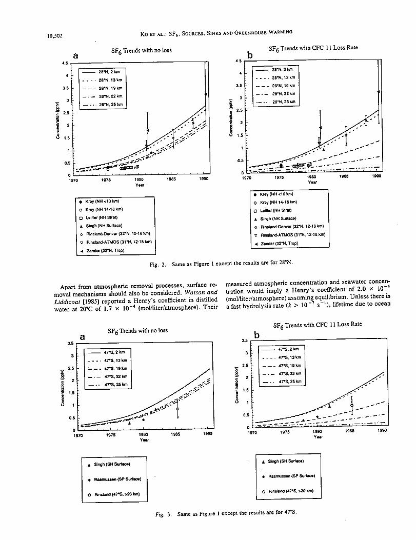
10,502 Ko ET AL.: SF 6, SOURCES, SINKS AND GREENHOUSE WARMING

4.5

aSF 6 Trends with no loss

3.5

3

= 2.5o

"E 2

1.5

O.S

0

1970

28"N, 2 km

.... 28"N, 13 km

----. 28*N, 19 kan

-- • -- 28"N, 22kin

.... 2S'N.2s /'I

L<- "" .A.-S-..-_'"-" L__""

, , , , I _ , _ , I , , _ , I , _ , , I

1975 1980 1985 1990

Year

• Krey (NH <10 kin)

O Krey(NH 14-18km)

Q Leilfer (NH Strat)

• Singh (NH Sudace)

0 Rinsland-Denver (32°N, 12-18 kin)

_7 Rinsland-ATMOS (31"N, 12-18 k.m)

• Z.andet (32*N, Trop)

Fig. 2.

4.5b

SF 6 Trends with CFC 11 Loss Rate

3.5

3

2.5

2

`5 1.5

0.5

1970

28"N, 2 km

.... 28°N, 13 tun

----- 28"N, 19 kJ'n

-- • -- 28"N, 22km

.... 28"N, 25 k,'n

1975 1980 1985 1990

Year

• Krey (NH <10 km)

O Krey(NH 14.18km)

O Leifter (NH Strat)

• Singh (NH Surface)

o Rinsland-Denvet (32*N. 12-18 kin)

V Rinsland-ATMOS (31*N, 12.18 km)

• Zander (32°N, Trop)

Same as Figure I except the results arc for 28°N.

Apart from atmospheric removal processes, surface re-moval mechanisms should also be considered. Watson and

Liddicoat [1985] reported a Henry's coefficient in distilledwater at 20°C of 1.7 x 10 -4 (mol/liter/atmosphere), Their

measured atmospheric concentration and seawater concen-tration would imply a Henry's coefficient of 2.0 x 10 -4

(tool/liter/atmosphere) assuming equilibrium. Unless there isa fast hydrolysis rate (k > 10 -_ s-l), lifetime due to ocean

3.5

aSF 6 Trends with no loss

3

2.5

1.5

,5 1

0.5

0

1970

[ _ 47_S. 2km

.... 47"S. 13 km:..--- 47"S, 19 km

--.-- 47"S. 22 km

/

• , , , , l i l i i I , i l l I i , . , t

1975 1980 1985 1990

Year

3.5

2.5

i2

1.5

`5 1

bSF 6 Trends with CFC 11 Loss Rate

0.5

01970

47°S, 2 k.m

.... 47"S, 13 km

----- 47"S, 19 km

--. -- 47"S,22km.. 47_S, 25kaI .''"

1975 1980 1985 1990Year

• S_ngh (SH Sudace)

. Ra.unuu_ (SP ,Sudan)

O FUndand (47"S, >20 kin)

• Slngh (SH Surface)

,, Rasmussen (SP Sudace)

O PJnstand (47"S, >20 km)

Fig. 3, Same as Figure 1 except the results are for 47"S.

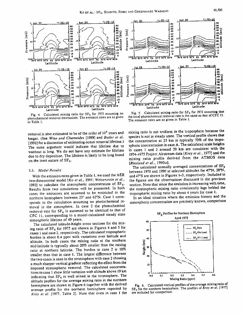
Ko ET AL.: SF 6, SOURCES, SINKS AND GREENHOUSE WARMING10,503

'I........ +'° _ +°

................ eo " [ 4-60 _s_ t os

Latitude Latitude Latitude L_titud_

:ul 29 "1.0E-12.I

P, io

100

EO "11555045 1

4035

30 10

,25

.2°,15 100

• 10

• B

.-,_Zv ...... "LOZT!z-eO05

40,M35

=o.._' _

106

i°%°o-.S eo's 3o's zq 3o'N eo'_ io.ll i°°t°o's °o's 3o's zq 3o.ll eo'N io'l+

Latitude L_tltude

Fig. 4. Calculated mixing ratio for SF6 for 1975 assuming nophotochemical removal mechanism. The emission rates are as givenin Table 1.

._i_.lzo......... "!.oz,t_. ., o_t27....... "i.OZ-:tit_

Latitude Latitude

Fig. 5. Calculated mixing ratio for SF6 for 1975 assuming that

the local photochemical removal rate is the same as that ofCFC 11.

The emission rates are as given in Table 1.

removal is also estimated to be of the order of 104 years and

longer. (See Wine and Chameides [1989] and Butler et a[.

[1991] for a discussion of estimating ocean removal lifetime.)

The same argument would indicate that lifetime due to

washout is long. We do not have any estimate for lifetime

due to dry deposition. The lifetime is likely to be long based

on the inert nature of SFr.

3.3. Model Results

With the emission rates given in Table 1, we used the AER

two-dimensional model [Ko et al., 1991; Weisenstein et al.,

1992] to calculate the atmospheric concentration of SF 6.

Results from two simulations will be presented. In both

cases the emissions are assumed to be restricted to the

northern hemisphere between 23 ° and 62°N. Case 1 corre-

sponds to the calculation assuming no photochemical re-

moval in the atmosphere. In case 2 the photochemical

removal rate for SF 6 is assumed to be identical to that of

CFC 11, corresponding to a model-calculated steady state

atmospheric lifetime of 49 years.The calculated latitude-height cross sections for the mix-

ing ratio of SF6 for 1975 are shown in Figures 4 and 5 for

cases 1 and case 2, respectively. The calculated tropospheric

burden is about 0.4 pptv with variations over latitude and

altitude. In both cases the mixing ratio at the southern

mid-latitude is typically about 20% smaller than the mixing

ratio at northern latitude. The burden in case 2 is 10%

smaller than that in case 1. The largest difference between

the two cases is seen in the stratosphere with case 2 showing

a much sharper vertical gradient reflecting the effect from the

imposed stratospheric removal. The calculated concentra-tions in case 1 show little variation with altitude above 19 km

indicating that SF 6 is well mixed in the stratosphere. The

altitude profiles for the average mixing ratio in the northern

hemisphere are shown in Figure 6 together with the derived

average profile for the northern hemisphere reported by

Krey et al. [1977, Table 2]. Note that even in case I the

mixing ratio is not uniform in the troposphere because the

species is not in steady state. The vertical profile shows that

the concentration at 25 km is typically 70% of the tropo-

spheric concentration in case A. The calculated scale heights

in cases 1 and 2 around 20 km are consistent with the

1974-1975 Project Airstream data [Krey et al., 1977] and the

mixing ratio profile derived from the ATMOS data

[Rinsland et al., 1990a].The calculated annually averaged concentrations of SF6

between 1970 and 1990 at selected altitudes for 47"N, 28"N,

and 47"S are shown in Figures 1-3, respectively. Included in

the figures are the observations discussed in the previous

section. Note that since the emission is increasing with time,

the stratospheric mixing ratio consistently lags behind the

tropospheric mixing ratio by about 4 years for case 1.In an ideal situation where the emission history and the

atmospheric concentration are precisely known, comparison

60

SF 6 Profiles for Northern Hemisphere

April 1975

50

40

,-e

-- SFs Dim

. _ . SF_(NoLoss)

__. SFs(FIILoss)

rl0 | .\ ",

o_ ..................... _ .......

o.o o.I o,2 0.3 0.4 0._ 0.6Mixing Ratio (pptv)

Fig. 6. Calculated vertical profiles of the average mixing ratio ofSF6 for the northern hemisphere. The profiles of Krey et al. [1977]are included for comparison.

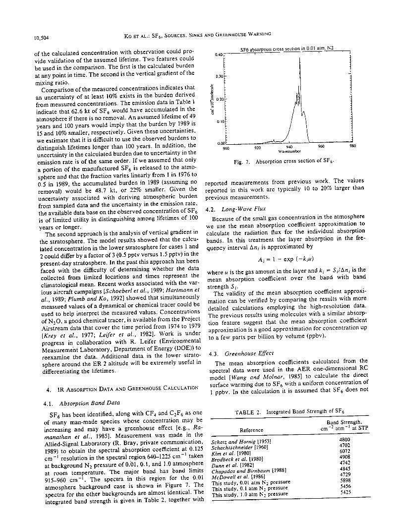
10,504 KO ET AL.: SF6, SOURCES, SINKS

of the calculated concentration with observation could pro-

vide validation of the assumed lifetime. Two features could

be used in the comparison. The first is the calculated burden

at any point in time. The second is the vertical gradient of the

mixing ratio.

Comparison of the measured concentrations indicates that

an uncertainty of at least 10% exists in the burden derived

from measured concentrations. The emission data in Table 1

indicate that 62.6 kt of SF 6 would have accumulated in the

atmosphere if there is no removal. An assumed lifetime of 49

years and 100 years would imply that the burden by 1989 is

15 and 10% smaller, respectively. Given these uncertainties,

we estimate that it is difficult to use the observed burdens to

distinguish lifetimes longer than 100 years. In addition, the

uncertainty in the calculated burden due to uncertainty in the

emission rate is of the same order. If we assumed that only

a portion of the manufactured SF6 is released to the atmo-

sphere and that the fraction varies linearly from 1 in 1976 to

0.5 in 1989, the accumulated burden in 1989 (assuming no

removal) would be 48.7 kt, or 22% smaller. Given the

uncertainty associated with deriving atmospheric burden

from sampled data and the uncertainty in the emission rate,

the available data base on the observed concentration of SF 6

is of limited utility in distinguishing among lifetimes of 100

years or longer.The second approach is the analysis of vertical gradient in

the stratosphere. The model results showed that the calcu-

lated concentration in the lower stratosphere for cases 1 and

2 could differ by a factor of 3 (0.5 pptv versus 1.5 pptv) in the

present-day stratosphere. In the past this approach has beenfaced with the difficulty of determining whether the data

collected from limited locations and times represent the

climatological mean. Recent works associated with the var-

ious aircraft campaigns [Schoeberl et al., 1989; Hartmann et

al., 1989; Plumb and Ko, 1992] showed that simultaneously

measured values of a dynamical or chemical tracer could be

used to help interpret the measured values. Concentrations

of N20, a good chemical tracer, is available from the ProjectAirstream data that cover the time period from 1974 to 1979

[Krey et al., 1977; Leifer et al., 1982]. Work is under

progress in collaboration with R. Leifer (Environmental

Measurement Laboratory, Department of Energy (DOE)) to

reexamine the data. Additional data in the lower strato-

sphere around the ER 2 altitude will be extremely useful in

differentiating the lifetimes.

4. IR ABSORPTION DATA AND GREENHOUSE CALCULATION

4.1. Absorption Band Data

SF 6 has been identified, along with CF4 and C2F 6 as one

of many man-made species whose concentration may be

increasing and may have a greenhouse effect [e.g., Ra-

manathan et al., 1985]. Measurement was made in the

Allied-Signal Laboratory (R. Bray, private communication,

1989) to obtain the spectral absorption coefficient at 0.125

cm-I resolution in the spectral region. 640-1225 cm -I taken

at background N2 pressure of 0.()1, 0.1, and 1.0 atmosphere

at room temperature. The major band has band limits

915-960 cm -l. The spectra in this region for the 0.01

atmosphere background case is shown in Figure 7. The

spectra for the other backgrounds are almost identical. The

integrated band strength is given in Table 2, together with

AND GREENHOUSE WARMING

0'40 I

o 0"30 l

0.20_

°iE

0.10

0.00I

900

SF6 absorption cross section in 0.01 atm. N2i

• r , ,, ,,

920 940 960 980

WavcnLlmb<:r

Fig. 7. Absorption cross section of SF6.

reported measurements from previous work. The values

reported in this work are typically I0 to 20% larger than

previous measurements.

4.2. Long-Wave Flux

Because of the small gas concentration in the atmosphere

we use the mean absorption coefficient approximation to

calculate the radiation flux for the individual absorption

bands. In this treatment the layer absorption in the fre-

quency interval Ani is approximated by

A i = 1 - exp (-kiu)

where u is the gas amount in the layer and k i = Si/Ani is the

mean absorption coefficient over the band with band

strength Si.

The validity of the mean absorption coefficient approxi-

mation can be verified by comparing the results with more

detailed calculations employing the high-resolution data.

The previous results using molecules with a similar absorp-

tion feature suggest that the mean absorption coefficient

approximation is a good approximation for concentration up

to a few parts per billion by volume (ppbv).

4.3. Greenhouse Effect

The mean absorption coefficients calculated from the

spectral data were used in the AER one-dimensional RC

model [Wang and Molnar, 1985] to calculate the direct

surface warming due to SF6 with a uniform concentration of

1 ppbv. In the calculation it is assumed that SF6 does not

TABLE 2. Integrated Band Strength of SF6

Band Strength,

Reference cm - atm at STP

Schatz and Hornig [1953]Schachtschneider [1960]Kim et al. [1980]Brodbeck et al. [1980]Dunn et al. [1982]

Chapados and Birnbaurn [1988]McDowell et al. [1986]This study, 0.01 atm N2 pressureThis study, 0.1 atm N: pressureThis study, 1.0 arm N: pressure

4800470260724908474248454729589854565425

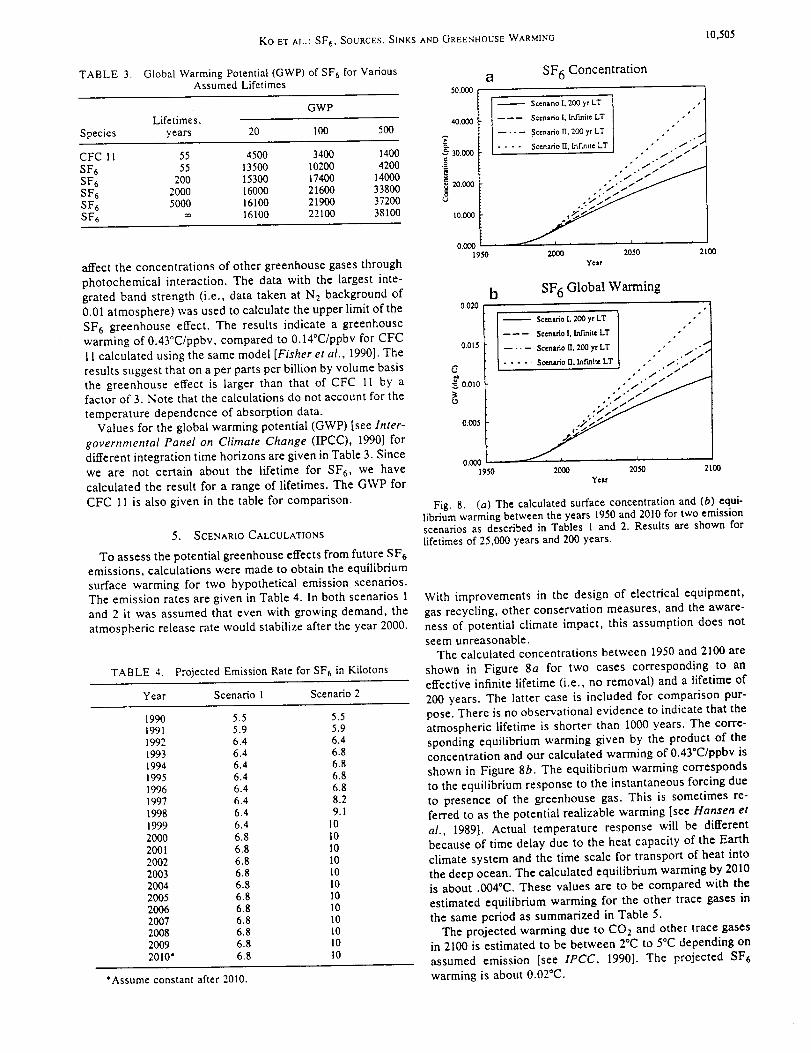
NO ET AL.: SF 6, SOURCES, SINKS AND GREENHOUSE WARMING 10,505

TABLE 3. Global Warming Potential (GWP) of SF s for VariousAssumed Lifetimes

GWP

50.000

Lifetimes, 4o.c_o

Species years 20 I00 500

CFC 11 55 4500 3400 1400 _ 30.000

SFs 55 13500 10200 4200 ._SF 6 200 15300 17400 14000S F 6 2000 16000 21600 33800 _ 20.000

SF 6 5000 16100 21900 37200 taSF6 _ 16100 22100 38100 10.ooo

affect the concentrations of other greenhouse gases through

photochemical interaction. The data with the largest inte-

grated band strength (i.e., data taken at N: background of

0.01 atmosphere) was used to calculate the upper limit of the

SF6 greenhouse effect. The results indicate a greenhouse

warming of 0.43°C/ppbv, compared to 0.14°C/ppbv for CFC

11 calculated using the same model [Fisher et al., 1990]. The

results suggest that on a per parts per billion by volume basis

the greenhouse effect is larger than that of CFC 11 by a

factor of 3. Note that the calculations do not account for the

temperature dependence of absorption data.

Values for the global warming potential (GWP) [see Inter-

governmental Panel on Climate Change (IPCC), 1990] for

different integration time horizons are given in Table 3. Since

we are not certain about the lifetime for SF6, we have

calculated the result for a range of lifetimes. The GWP for

CFC 11 is also given in the table for comparison.

5. SCENARIO CALCULATIONS

To assess the potential greenhouse effects from future SF6

emissions, calculations were made to obtain the equilibrium

surface warming for two hypothetical emission scenarios.

The emission rates are given in Table 4. In both scenarios 1

and 2 it was assumed that even with growing demand, the

atmospheric release rate would stabilize after the year 2000.

TABLE 4. Projected Emission Rate for SF6 in Kilotons

Year Scenario 1 Scenario 2

1990 5.5 5.51991 5.9 5.91992 6.4 6.41993 6.4 6.81994 6,4 6.81995 6.4 6.81996 6.4 6.81997 6.4 8.2

1998 6.4 9.11999 6.4 102000 6.8 102001 6.8 102002 6.8 102003 6.8 102004 6.8 102005 6.8 I02006 6.8 102007 6.8 102008 6.8 102009 6.8 102010" 6.8 10

*Assume constant after 2010.

0.(X)0t950

Et SF 6 Concentration

Scenario I. 200 yr LT • '

------ Scenario l. Infinite LT

.... Scenario rl. 200 yr LT I

.... Scenario H. Infinite LT . / ./so" • /

• /" f

oo'. J_._//

,_ , , t

2000 2050 2100

Year

0.020

0.015

C

0.010

0.005

0.000

1950

SF 6 Global Warming

ScenarioI.200 yr LT • "

-- -- -- Scentrio1,In/miteLT • •"

-- -- Scentno 11 200 yr LT " ."

.... ScenarioII InrmiucLT " /" 1

o" 7_./. /

..:

/

2000 2050 2t00

Year

Fig. 8. (a) The calculated surface concentration and (b) equi-librium warming between the years 1950 and 2010 for two emissionscenarios as described in Tables 1 and 2. Results are shown forlifetimes of 25,000 years and 200 years.

With improvements in the design of electrical equipment,

gas recycling, other conservation measures, and the aware-

ness of potential climate impact, this assumption does not

seem unreasonable.

The calculated concentrations between 1950 and 2100 are

shown in Figure 8a for two cases corresponding to an

effective infinite lifetime (i.e., no removal) and a lifetime of

200 years. The latter case is included for comparison pur-

pose. There is no observational evidence to indicate that the

atmospheric lifetime is shorter than 1000 years. The corre-

sponding equilibrium warming given by the product of theconcentration and our calculated warming of 0.43°C/ppbv is

shown in Figure 8b. The equilibrium warming corresponds

to the equilibrium response to the instantaneous forcing due

to presence of the greenhouse gas. This is sometimes re-

ferred to as the potential realizable warming [see Hansen et

al., 1989]. Actual temperature response will be different

because of time delay due to the heat capacity of the Earth

climate system and the time scale for transport of heat into

the deep ocean. The calculated equilibrium warming by 2010

is about .004"C. These values are to be compared with the

estimated equilibrium warming for the other trace gases in

the same period as summarized in Table 5.

The projected warming due to CO z and other trace gases

in 2100 is estimated to be between 2°C to 5°C depending on

assumed emission [see IPCC, 1990]. The projected SF6

warming is about 0.02°C.

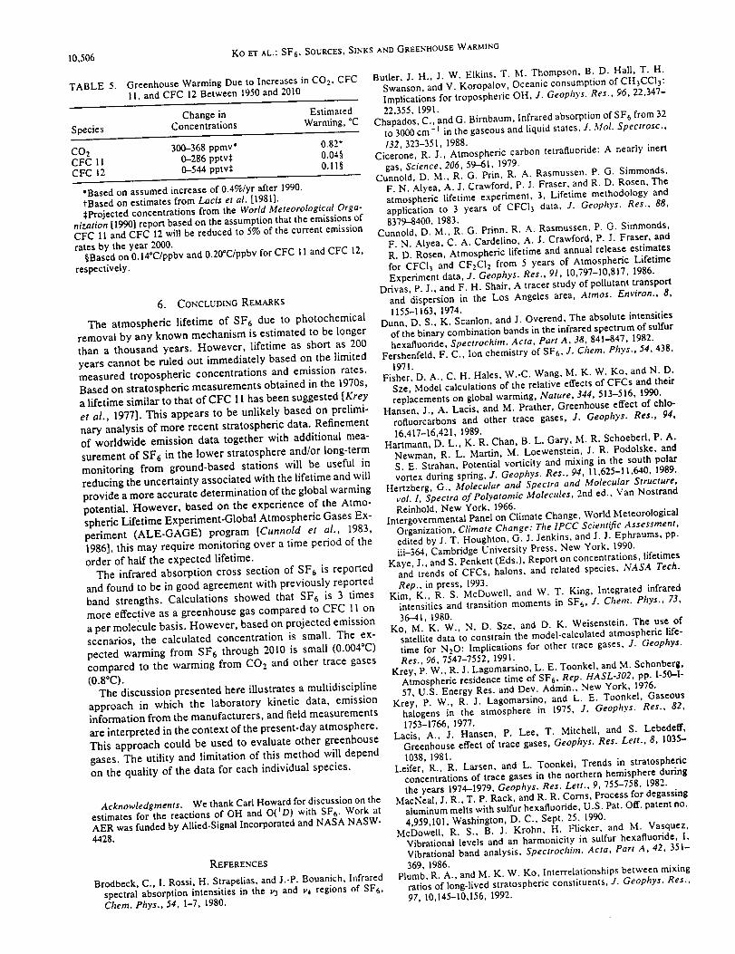
10,506

TABLE5. GreenhouseWarmingDuetoIncreasesinCOz,CFCII,andCFC12Between1950and2010

Changein EstimatedSpecies Concentrations Warming, °C

C02 300-368 ppmv* 0.82_"CFC 11 0--286 pptv$ 0.04§CFC 12 0--544 pptv:_ 0.11 §

Ko ET AL.: SF 6, SOURCES, SINKS AND GREENHOUSE WARMING

*Based on assumed increase of 0.4%/yr after 1990.

l'Based on estimates from Lacis et al. [1981].:_Projected concentrations from the World Meteorological Orga-

nization [1990] report based on the assumption that the emissions ofCFC 11 and CFC 12 will be reduced to 5% of the current emission

rates by the year 2000.§Based on 0.14*C/ppbv and 0.20*C/ppbv for CFC 11 and CFC 12,

respectively.

6. CONCLUDING REMARKS

The atmospheric lifetime of SF6 due to photochemical

removal by any known mechanism is estimated to be longer

than a thousand years. However, lifetime as short as 200

years cannot be ruled out immediately based on the limited

measured tropospheric concentrations and emission rates.

Based on stratospheric measurements obtained in the 1970s,

a lifetime similar to that of CFC 11 has been suggested [Krey

et al., 1977]. This appears to be unlikely based on prelimi-

nary analysis of more recent stratospheric data. Refinement

of worldwide emission data together with additional mea-

surement of SF6 in the lower stratosphere and/or long-term

monitoring from ground-based stations will be useful in

reducing the uncertainty associated with the lifetime and will

provide a more accurate determination of the global warming

potential. However, based on the experience of the Atmo-

spheric Lifetime Experiment-Global Atmospheric Gases Ex-

periment (ALE-GAGE) program [Cunnold et al., 1983,

1986], this may require monitoring over a time period of the

order of haLf the expected lifetime.

The infrared absorption cross section of SF6 is reported

and found to be in good agreement with previously reported

band strengths. Calculations showed that SF6 is 3 times

more effective as a greenhouse gas compared to CFC 11 on

a per molecule basis. However, based on projected emission

scenarios, the calculated concentration is small. The ex-

pected warming from SF6 through 2010 is small (0.004°C)

compared to the warming from CO2 and other trace gases

(0.8°C).The discussion presented here illustrates a multidiscipline

approach in which the laboratory kinetic data, emission

information from the manufacturers, and field measurements

are interpreted in the context of the present-day atmosphere.

This approach could be used to evaluate other greenhouse

gases. The utility and limitation of this method will depend

on the quality of the data for each individual species.

Acknowledgments. We thank Carl Howard for discussion on theestimates for the reactions of OH and O(ID) with SFs. Work atAER was funded by Allied-Signal Incorporated and NASA NASW-

4428.

REFERENCES

Brodbeck, C., I. Rossi, H. Strapelias, and J.-P. Bouanich, Infraredspectral absorption intensities in the v3 and v4 regions of SF6,

Chem. Phys., 54, 1-7, 1980.

Butler, J. H., J. W. Elkins, T. M. Thompson, B. D. Hall, T. H.Swanson, and V. Koropalov, Oceanic consumption of CH3CCI3:

Implications for tropospheric OH, J. Geophys. Res., 96, 22,347-

22,355, 1991.Chapados, C., and G. Birnbaum, Infrared absorption of SF6 from 32

to 3000 cm -t in the gaseous and liquid states, J. Mol. Spectrosc.,

132,323-351, 1988.Cicerone, R. J., Atmospheric carbon tetrafluoride: A nearly inert

gas, Science, 206, 59--61, 1979.Cunnold, D. M., R. G. Prin, R. A. Rasmussen. P. G. Simmonds.

F. N. Alyea, A. J. Crawford, P. J. Fraser, and R. D. Rosen, Theatmospheric lifetime experiment, 3, Lifetime methodology and

application to 3 years of CFCI3 data, J. Geophys. Res., 88,8379-8400, 1983.

Cunnold, D. M., R. G. Prinn, R. A. Rasmussen, P. G. Simmonds,

F. N. Alyea, C. A. Cardelino, A. J. Crawford, P. J. Fraser, andR. D. Rosen, Atmospheric lifetime and annual release estimates

for CFCI3 and CF2C12 from 5 years of Atmospheric LifetimeExperiment data, J. Geophys. Res., 91, 10,797-10,817, 1986.

Drivas, P. J., and F. H. Shair, A tracer study of pollutant transport

and dispersion in the Los Angeles area, Atmos. Environ., 8,

1155-1163, 1974.Dunn, D. S., K. Scanlon, and J. Overend, The absolute intensities

of the binary combination bands in the infrared spectrum of sulfurhexafluoride, Spectrochim. Acta, Part A, 38, 841-847, 1982.

Fershenfeld. F. C., Ion chemistry of SF6, J. Chem. Phys., 54,438,

1971.Fisher, D. A., C. H. Hales, W.-C. Wang, M. K. W. Ko, and N. D.

Sze, Model calculations of the relative effects of CFCs and theirreplacements on global warming, Nature, 344, 513-516, 1990.

Hansen, J., A. Lacis, and M. Prather, Greenhouse effect of chlo-rofluorcarbons and other trace gases, J. Geophys. Res., 94,

16,417-16,421, 1989.Hartmann, D. L., K. R. Chan, B. L. Gary, M. R. Schoeberl, P. A.

Newman, R. L. Martin, M. Loewenstein, J. R. Podolske, andS. E. Strahan, Potential vorticity and mixing in the south polarvortex during spring, J. Geophys. Res., 94, I 1,625-11,640, 1989.

Hertzberg, G., Molecular and Spectra and Molecular Structure,vol. I, Spectra of Polyatomic Molecules, 2nd ed., Van Nostrand

Reinhold, New York, 1966.Intergovernmental Panel on Climate Change, World Meteorological

Organization, Climate Change: The IPCC Scientific Assessment,edited by J. T. Houghton, G. J. Jenkins, and J. J. Ephraums, pp.iii-364, Cambridge University Press, New York, 1990.

Kaye, J., and S. Penkett (Eds.), Report on concentrations, lifetimesand trends of CFCs, halons, and related species, NASA Tech.

Rep., in press, 1993.Kim, K., R. S. McDowell, and W. T. King, Integrated infrared

intensities and transition moments in SF6, J. Chem. Phys., 73,

36--41, 1980.Ko, M. K. W., N. D. Sze, and D. K. Weisenstein, The use of

satellite data to constrain the model-calculated atmospheric life-time for N20: Implications for other trace gases. J. Geophys.Res., 96, 7547-7552, 1991.

Krey, P. W., R. J. Lagomarsino, L. E. Toonkel, and M. Schonberg,Atmospheric residence time of SF6, Rep. HASL-302, pP. 1-50--I-57, U.S. Energy Res. and Dev. Admin., New York, 1976.

Krey, P. W., R. J. Lagomarsino, and L. E. Toonkel, Gaseoushalogens in the atmosphere in 1975, J. Geophys. Res., 82,1753-1766, 1977.

Lacis, A., J. Hansen, P. Lee, T. Mitchell, and S. Lebedeff,Greenhouse effect of trace gases, Geophys. Res. Lett., 8, 1035--

1038, 1981.Leifer, R., R. Larsen, and L. Toonkel, Trends in stratospheric

concentrations of trace gases in the northern hemisphere during

the years 1974--1979, Geophys. Res. Lett., 9,755-758, 1982.MacNeal, J. R., T. P. Rack, and R. R. Corns, Process for degassing

aluminum melts with sulfur hexafluoride, U.S. Pat. Off. patent no.

4,959,101, Washington, D. C., Sept. 25, 1990.McDowell, R. S., B. J. Krohn, H. Flicker, and M. Vasquez,

Vibrational levels and an harmonicity in sutfur hexafluoride, 1,Vibrational band analysis, Spectrochim. Acta, Part A, 42, 351-

369, 1986.Plumb, R. A., and M. K. W. Ko, Interrelationships between mixing

ratios of long-lived stratospheric constituents, J. Geophys. Res.,

97, 10,145-10,156, 1992.

KoETAL.:SFr,SOURCES,SINKSANDGREENHOUSEWARMING

Prinn,R.G.,P.G.Simmonds, R. A. Rasmussen, R. D. Rosen,F. N. Alyea, C. A. Cardelino, A. J. Crawford, D. M. Cunnold,p. J. Fraser, and J. E. Lovelock, The atmospheric lifetime

experiment, I, Introduction, instrumentation, and overview, J.

Oeophys. Res., 88, 8353-8367, 1983.Ramanathan, V., R. J. Cicerone, H. B. Singh, andJ. T. Kiehl, Trace

gas trends and their potential role in climate change, J. Geophys.Res., 90, 5547-5566, 1985.

Ramanathan, V., et al., Climate-chemical interactions and effects of

changing atmospheric trace gases, Rev. Geophys., 25, 1441-1482,

1987.Rasmussen, R. A., and M. A. K. Khalil, Rare trace gases at the

South Pole, Antarct. J. U.S., 18, 250--252, 1983.Rasmussen, R. A., M. A. K. Khalil, and R. W. Dalluge, Atmo-

spheric trace gases in Antarctica, Science, 211,285-287, 1981.Ravishankara, A. R., S. Solomon, A. A. Turnipseed, and R. F.

Warren, Atmospheric lifetimes of long-lived species, Science,

259, 194-199, 1993.Rinsland, C. P., L. R. Brown, and C. B. Farmer, Infrared spectro-

scopic detection of sulfur hexafluoride (SFr) in the lower strato-sphere and upper troposphere, J. Geophys. Res., 95, 5577-5585,1990a.

Rinsland, C. P., A. Goldman, F. J. Murcray, R. D. Blatherwick,J. J. Kosters. D. G. Murcray, N. D. Sze, and S. T. Massie,

Long-term trends in the concentrations of SFr, CHCIF2, andCOF2 in the lower stratosphere from analysis of high-resolutioninfrared solar occultation spectra, J. Geophys. Res., 95, 16,477-

16,490, 1990b.Schachtschneider, J. H., Simultaneous transitions and intermolec-

ular forces, dissertation, Univ. of Minn. at Minneapolis, St. Paul,

1960.Schatz, P. N., and D. F. Hornig, Bond moments and derivatives in

CF4, SiF4, and SF6 from infrared intensities, J. Chem. Phys., 21,

1516-1530, 1953.Schoeberl, M. R., et al., Reconstruction of the constituent distribu-

tion and trends in the Antarctic polar vortex from ER-2 flightobservations, J. Geophys. Res., 94, 16,815-16,845, 1989.

Singh, H. B., L. J. Salas, and L. A. Cavanagh, Distribution, sourcesand sinks of atmospheric halogenated compounds, J. Air Pollut.

Control Assoc., 27, 333-336, 1977.Singh, H. B., L. J. Salas, H. Shigeishi, and E. Scribner, Atmo-

spheric halocarbons, hydrocarbons, and sulfur hexafluoride:Global distributions, sources, and sinks, Science, 203, 899-903,

1979.Singh, H. B., L. J. Salas, and R. E. Stiles, Selected man-made

halogenated chemicals in the air and oceanic environment, J.

Geophys. Res., 88, 3675-3683, 1983.

10,507

Vandeborght, B., J. Kretzschmar, and T. Rymen, On the use of SF6tracer releases for the determination of fugitive emissions, in

Proceedings of Second European Symposium on Physico-Chemical Behaviour of Atmospheric Pollutants, Varese, Italy, 29

September-I October, 1981, edited by B. Versino and H. Ott, pp.517-523, D. Reidcl, Nor-well, Mass., 1982.

Wang, W.-C., and G. Molnai', A model study of the greenhouseeffects due to increasing atmospheric CH4, N20, CFzCI2, and

CFCI3, J. Geophys. Res., 90, 12,971-12,980, 1985.Watson, A. J., and M. I. Liddicoat, Recent history of atmospheric

trace gas concentrations deduced from measurements in the deepsea: Application to sulfur hexafluoride and carbon tetrachloride,Atmos. Environ., 19, 1477-1484, 1985.

Weisenstein, D. K., M. K. W. Ko, and N. D. Sze, The chlorine

budget of the present-day atmosphere: A modeling study, I.Geophys. Res., 97, 2547-2559, 1992.

Wine, P. H., and W. L. Chameides, Possible atmospheric lifetimesand chemical reaction mechanisms for selected HCFCs, HFCs,

CH3CCI3, and their degradation products against dissolutionand/or degradation in seawater and cloudwater, Appendix,

AFEAS report, in Scientific Assessment of Stratosl:heric Ozone,vol. 2, Rep. 20, pp. 273-295, Global Ozone Res. and Monit. Proj.,World Meteorol. Organ., Geneva, 1989.

World Meteorological Organization (WMO), Scientific assessmentof stratospheric ozone: 1989, Rep. 20, Global Ozone Res. andMonit. Project, Geneva, 1990.

Zander, R., C. P. Rinsland, and P. Demoulin, Infrared spectro-

scopic measurements of the vertical column abundance of sulfurhexafluoride, SFr, from the ground, .I. Geophys. Res., 96, 15,447-

15,454, 1991.

A. Goldman, D. G. Murcray, and F. J. Murcray, Department of

Physics, University of Denver, Denver, CO 80208.M. K. W. Ko and N. D. Sze, Atmospheric and Environmental

Research, Incorporated, 840 Memorial Drive, Cambridge, MA

02139.C. P. Rinsland, Atmospheric Science Center, NASA Langley

Research Center, Hampton, VA 23681.G. Shia, Buffalo Research Laboratory, Allied-Signal lncorlx>-

rated, Buffalo, NY 14210.W.-C. Wang, State University at New York, 100 Fuller Road,

Albany, NY 12205.

(Received August 22, 1992;revised January 15, 1993;

accepted January 22, 1993.)

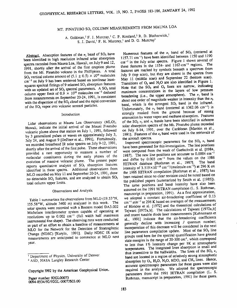
GEOPHYSICAL RESEARCH LETIT_,RS, VOL. 19, NO. 2, PAGES 183-186, JANUARY 24, 1992

MT. PINATUBO SO2 COLUMN MEASUREMENTS FROM MAUNA LOA

A. Goldman, t F. J. Murcray, _ C. P. Rinsland, 2 R. D. Blatherwick, tS. J. David, t F. H. Murcray, t and D. G. Murcray t

Absorption features of the vt band of SOz havebeen identified in high resolution infrared solar absorption

spectra recorded from Mauna Loa, Hawaii, on July 9 and 12,1991, shortly after the arrival of the first eruption plumefrom the Mr. Pinatubo volcano in the Phillipines. A total

SO2 vertical column amount of (5.1 + 0.5) x 10_6moleculescm -z on July 9 has been retrieved based on nonlinear least-

squares spectral fittings of 9 selected SOz absorption featureswith an updated set of SO2 spectral parameters. A SOs totalcolumn upper limit of 0.9 × 1016 molecules cm -2 deducedfrom measurements on September 20-24, 1991, is consistent

with the dispersion of the SO_ cloud and the rapid conversionof the SO2 vapor into volcanic aerosol particles.

Introduction

Lidar observations at Mauna Loa Observatory (MLO),Hawaii, indicate the initial arrival of the Mount Pinatubo

volcanic plume above that station on July 1, 1991, followedby 3 generalized pulses or waves on approximately July 3,July 24, and August 9 [DeFoor et al., 1991]. Fortuitously,we recorded broadband IR solar spectra on July 9-12, 1991,

shortly after the arrival of the first pulse. These observationsprovided a rare opportunity to measure a number ofmolecular constituents during the early phases of theevolution of massive volcanic plume. The present paper

reports quantitative analysis of SOs absorption featuresidentified in these spectra. Additional observations fromMLO recorded on May 11 and September 20-24, 1991, showno detectable SOs features, and are analyzed to obtain SOs

total column upper limits.

Observations and Analysis

Table 1 summarizes the observations from MLO (19.53 °N,

155.58°W, altitude 3400 m) analyzed in this work. Thesolar spectra were recorded with a Bomem model DA3.002Michelson interferometer system capable of operating at

resolutions up to 0.002 cm -t (full width half maximuminstrumental line shape). The observing runs were conducted

as part of an effort to obtain a baseline of measurements atMLO for the Network for the Detection of Stratospheric

Change (NDSC) [Kurylo, 1991]. Daily NDSC IR solarmeasurements are anticipated to commence at MLO next

year.

t Department of Physics, University of Denver2 ASD, NASA Langley Research Center

Copyright 1992 by the American Geophysical Union.

Paper number 92GL000730094-8534/92/92GL-00073503.00

Numerous features of the vt band of SO2 (centered at1157.71 cm -_) have been identified between 1150 and 1190

cm -_ in the July solar spectra. Figure 1 shows several ofthese features in the 1154- and I162-cm -_ regions. Thefeatures are marked by symbols beneath a spectrum from

July 9 (top scan), but they are absent in the spectra fromMay 11 (middle scan) and September 22 (bottom scan).Transitions of O_ and N20 are also identified in Figure 1.Note that the SO2 and O3 lines are narrow, indicatingmaximum concentrations in the layers of low pressurebroadening (i.e., the upper atmosphere). The vl band isabout one order of magnitude weaker in intensity than the v3

band, which is the strongest SO2 band in the infrared.Unfortunately, the v3 band (centered at 1362.06 cm -_) is

strongly masked from the ground because of strongattenuation by water vapor and methane absorption. Featuresof the SO2 v3 and vt bands have been identified in airbornesolar absorption spectra of the Mt. Pinatubo plume recordedon July 8-14, 1991, over the Caribbean [Mankin et al.,1991]. Features of the v3 band were used in the retrievals of

the aircraft spectra.Improved spectroscopic parameters for the SO2 vl band

have been generated for this investigation. The line positionswere computed from the work of Guelachvili et al. [1984,1987]. The new line positions are accurate to 0.0004 cm -1and differ by 0.003 cm -t from the values on the 1986HITRAN database [Rothman et al., 1987]. The band

intensity of 3.519 × 10 -ta cm-t/(m olecule cm-2) at 296 K onthe 1986 HITRAN compilation [Rothman et al., 1987] hasbeen retained since no clear revision could be noted based on

the published papers (summarized by Smith et al. [1985]).The same positions and band intensity have also beenassumed on the 1991 HITRAN compilation (L. S. Rothman,manuscript in preparation, 1991). As a first approximation,we adopted a constant air-broadening coefficient of 0.13cm -t atm -_ at 296 K based on averages of the measurementsof Hinkley et al. [1972] and the theoretical calculations ofTejwani [1972a,b]. The calculations of Tejwani [1972a,b]and recent tunable diode laser measurements [Kuhnemann et

al., 1991] indicate that the air-broadening coefficientsgenerally decline with increasing J quantum number;incorporation of this decrease will be considered in the nextline parameters compilation update. Most of the SO2 linegroups used here for the spectral quantification have groundstate energies in the range of 20-300 cm t, which correspondto less than 1% intensity change per 1K at stratospheric

temperatures. The integrated lines absorption is small andthus insensitive to the halfwidths. The lines of the SOs vtband are located in a region of relatively strong atmospheric

absorption by 03, H20, N20, HDO, and CH4 lines. Hence,accurate spectroscopic parameters for these gases were also

required in the analysis. We adopted the spectroscopicparameters from the 1991 HITRAN compilation (L. S.Rothman, manuscript in preparation, 1991) for these gases.

183

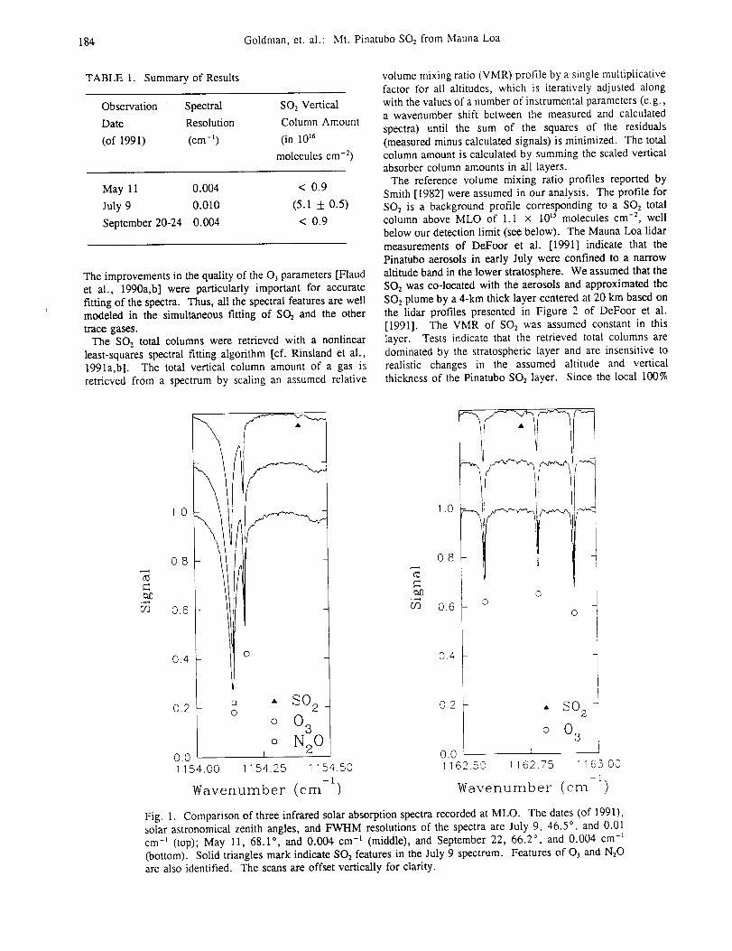
184 Goldman, et. al.: Mt. Pinatubo SO2 from Mauna Loa

TABLE 1. Summary of Results

Observation Spectral SOz Vertical

Date Resolution Column Amount

(of 1991) (cm -_) (in 10 _6

molecules cm -2)

May 11 0.004 < 0.9

July 9 0.010 (5.1 + 0.5)

September 20-24 0.004 < 0.9

The improvements in the quality of the 03 parameters [Flaudet al., 1990a,b] were particularly important for accuratefitting of the spectra. Thus, all the spectral features are wellmodeled in the simultaneous fitting of SO2 and the other

trace gases.The SO2 total columns were retrieved with a nonlinear

least-squares spectral fitting algorithm [cf. Rinsland et al.,1991a,b]. The total vertical column amount of a gas isretrieved from a spectrum by scaling an assumed relative

volume mixing ratio (VMR) profile by a single multiplicativefactor for all altitudes, which is iteratively adjusted alongwith the values of a number of instrumental parameters (e.g.,a wavenumber shift between the measured and calculated

spectra) until the sum of the squares of the residuals(measured minus calculated signals) is minimized. The totalcolumn amount is calculated by summing the scaled verticalabsorber column amounts in all layers.

The reference volume mixing ratio profiles reported bySmith [1982] were assumed in our analysis. The profile forSO2 is a background profile corresponding to a SOz totalcolumn above MLO of 1.1 x 10 t5 molecules cm -2, wellbelow our detection limit (see below). The Mauna Loa lidarmeasurements of DeFoor et al. [1991] indicate that the

Pinatubo aerosols in early July were confined to a narrowaltitude band in the lower stratosphere. We assumed that the

SOz was co-located with the aerosols and approximated theSO2 plume by a 4-kin thick layer centered at 20 km based onthe lidar profiles presented in Figure 2 of DeFoor et al.[1991]. The VMR of SO2 was assumed constant in this

layer. Tests indicate that the retrieved total columns aredominated by the stratospheric layer and are insensitive torealistic changes in the assumed altitude and verticalthickness of the Pinatubo SO_ layer. Since the local 100%

U_

10

0.8

0.6

0.4

\

\

O

0.2 -

. SO 2 ]

0

o 0 3

' _ N20

1.0

0.8

,r.._

0,6

0,4

0.2

0

0

• SO z

o 03

0.0 0.01154.00 1154.25 1 154.,50 1162.50 1162.75 i 165.00

Wavenumber (cm -1) Wavenumber (cm -z)

Fig. 1. Comparison of three infrared solar absorption spectra recorded at MLO. The dates (of 1991),solar astronomical zenith angles, and FWHM resolutions of the spectra are July 9, 46.5 °, and 0.01cm -_ (top); May 11, 68.1 °, and 0.004 cm -t (middle), and September 22, 66.2 °, and 0.004 cm -_(bottom). Solid triangles mark indicate SO 2 features in the July 9 spectrum. Features of 03 and N20are also identified. The scans are offset vertically for clarity.

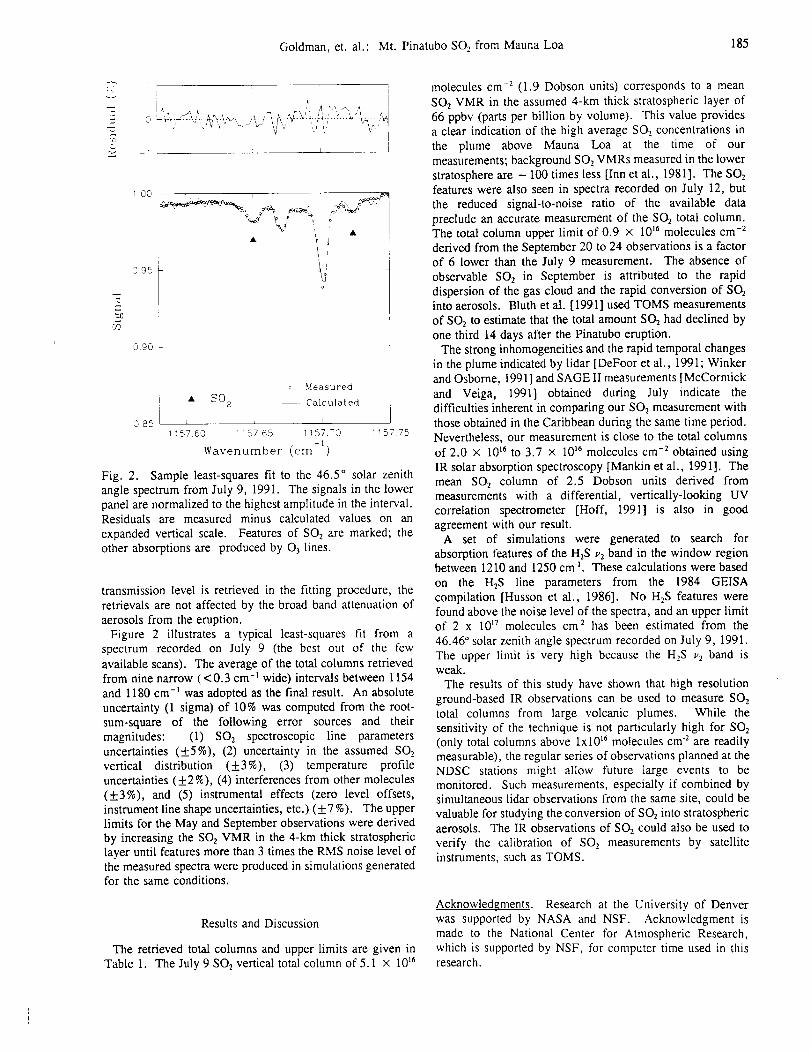
Goldman,et.al.: Mt.PinatuboSO2fromMaunaLoa 185

i!

I

J

,50.

I O0

095

0 9O

i

0 85

Measured

-- Calculated

1157.60 115765 1157.70

-I

Wavenumber (cm )

115775

Fig. 2. Sample least-squares fit to the 46.5 ° solar zenithangle spectrum from July 9, 1991. The signals in the lowerpanel are normalized to the highest amplitude in the interval.Residuals are measured minus calculated values on an

expanded vertical scale. Features of SO2 are marked; theother absorptions are produced by 03 lines.

transmission level is retrieved in the fitting procedure, the

retrievals are not affected by the broad band attenuation ofaerosols from the eruption.

Figure 2 illustrates a typical least-squares fit from aspectrum recorded on July 9 (the best out of the few

available scans). The average of the total columns retrievedfrom nine narrow (<0.3 cm -_ wide) intervals between 1154and 1180 cm -_ was adopted as the final result. An absolute

uncertainty (1 sigma) of 10% was computed from the root-sum-square of the following error sources and their

magnitudes: (1) SO2 spectroscopic line parametersuncertainties (+5%), (2) uncertainty in the assumed SO2vertical distribution (+3 %), (3) temperature profileuncertainties (+2 %), (4) interferences from other molecules(+3%), and (5) instrumental effects (zero level offsets,instrument line shape uncertainties, etc.) (+7%). The upperlimits for the May and September observations were derivedby increasing the SO2 VMR in the 4-km thick stratosphericlayer until features more than 3 times the RMS noise level ofthe measured spectra were produced in simulations generatedfor the same conditions.

Results and Discussion

The retrieved total columns and upper limits are given inTable 1. The July 9 SO2 vertical total column of 5.1 x 1@6

molecules cm -2 (1.9 Dobson units) corresponds to a mean

SO2 VMR in the assumed 4-km thick stratospheric layer of66 ppbv (parts per billion by volume). This value providesa clear indication of the high average SO2 concentrations inthe plume above Mauna Loa at the time of ourmeasurements; background SO2 VMRs measured in the lowerstratosphere are - I00 times less [Inn et al., 1981]. The SO2features were also seen in spectra recorded on July 12, but

the reduced signal-to-noise ratio of the available datapreclude an accurate measurement of the SO_ total column.The total column upper limit of 0.9 x 1016 molecules cm -2derived from the September 20 to 24 observations is a factorof 6 lower than the July 9 measurement. The absence ofobservable SO2 in September is attributed to the rapiddispersion of the gas cloud and the rapid conversion of SO_into aerosols. Bluth et al. [1991] used TOMS measurementsof SO2 to estimate that the total amount SO2 had declined byone third 14 days after the Pinatubo eruption.

The strong inhomogeneities and the rapid temporal changesin the plume indicated by lidar [DeFoor et al., 1991; Winkerand Osborne, 1991] and SAGE II measurements [McCormickand Veiga, 1991] obtained during July indicate thedifficulties inherent in comparing our SO2 measurement withthose obtained in the Caribbean during the same time period.Nevertheless, our measurement is close to the total columnsof 2.0 x 10_6to 3.7 x 1016 molecules cm -2 obtained using

IR solar absorption spectroscopy [Mankin et al., 1991]. Themean SO2 column of 2.5 Dobson units derived frommeasurements with a differential, vertically-looking UVcorrelation spectrometer [Hoff, 1991] is also in goodagreement with our result.

A set of simulations were generated to search for

absorption features of the H2S v2 band in the window regionbetween 1210 and 1250 cm-L These calculations were based

on the H2S line parameters from the 1984 GEISA

compilation [Husson et al., 1986]. No H2S features werefound above the noise level of the spectra, and an upper limitof 2 x 10_7 molecules cm -2 has been estimated from the

46.46 ° solar zenith angle spectrum recorded on July 9, 1991.The upper limit is very high because the H2S v2 band isweak.

The results of this study have shown that high resolutionground-based IR observations can be used to measure SO2total columns from large volcanic plumes. While thesensitivity of the technique is not particularly high for SO2(only total columns above lxl0 t6 molecules cm a are readilymeasurable), the regular series of observations planned at theNDSC stations might allow future large events to bemonitored. Such measurements, especially if combined bysimultaneous lidar observations from the same site, could be

valuable for studying the conversion of SO2 into stratosphericaerosols. The IR observations of SO2 could also be used toverify the calibration of SO2 measurements by satelliteinstruments, such as TOMS.

Acknowledgments. Research at the University of Denverwas supported by NASA and NSF. Acknowledgment ismade to the National Center for Atmospheric Research,which is supported by NSF, for computer time used in thisresearch.

186 Goldman,et.al.: Mt.PinatuboSO2fromMaunaLoa

References

Bluth,G., S.Doiron,C. Schnetzler,L. Walter,andA.Krueger,Globaltrackingof theJune,1991MountPinatuboeruptionclouds,Geophys. Res. Lett., thisissue, 1991.

DeFoor, T. E., E. Robinson, and S. Ryan, Early lidarobservations of the June 1991 Pinatubo eruption plumeat Mauna Loa Observatory, Hawaii, Geophy_, Re$,Lett., this issue, 1991.

Flaud, J.-M., C. Camy-Peyret, C. P. Rinsland, M. A. H.Smith, and V. Malathy Devi, "Atlas of Ozone SpectralParameters from Microwave to Medium Infrared,"Academic Press, Boston, MA, 1990a.

Flaud, J.-M., C. Camy-Peyret, C. P. Rinsland, V. MalathyDevi, M. A. H. Smith, and A. Goldman, Improved lineparameters for ozone bands in the 10-_m region, A_p.p.L.D_P.K,29, 3667-3671, 1990b.

Guelachvili, G., O. N. Ulenikov, and G. A. Ushakova,Analysis of the vl and v3 absorption bands of 32S1_O_,LMol. S_ce.ctros¢,, 108, 1-5, 1984.

Guelachvili, G., O. V. Naumenko, and O. N. Ulenikov,Analysis of the SO2 absorption Fourier spectrum inregions 1055 to 2000 and 2200 to 2550 cm -t, J. Mol.Spectrosc., 125, 128-139, 1987.

Hinkley, E. D., A. R. Calawa, P. L. Kelley, and S. A.Clough, Tunable-laser spectroscopy of the vt band ofSO2, J. Appl. Phys,, 43, 3222-3224, 1972.

Hoff, R. M., Differential SO2 column measurements of theMt. Pinatubo volcanic plume, Geophys. Res. Lett,, thisissue, 1991.

Husson, N., A. Chedin, N. A. Scott, D. Bailly, G. Graner,N. Lacome, A. Levy, C. Rossetti, G. Tarrago, C.Camy-Peyret, J. M. Flaud, A. Bauer, J. M. Colmont,N. Monnanteuil, J. C. Hilico, G. Pierre, M. Loete, J.P. Champion, L. S. Rothman, L. R. Brown, G. Orton,P. Varanasi, C. P. Rinsland, M. A. H. Smith and A.

Goldman, The GEISA spectroscopic line parameters databank in 1984, Ann. Geophy_, 4, A, 185-190, 1986.

Inn, E. C. Y., J. F. Vedder, and D. O. O'Hara,Measurement of stratospheric sulfur constituents,Geophys. Res. Lett., 8, 5-8, 1981.

Kuryto, M. J., Network for the detection of stratosphericchange, SPIE, 1491, 168-174, 1991.

Kuhnemann, F., Y. Heiner, B. Sumpf, and Ka. Herrmann,Line broadening in the v3 band of SOs studied with diodelaser spectroscopy, J. Mol, Spectrosc., in press, 1991.

Mankin, W. G., M. T. Coffey, and A. Goldman, Airborneobservations of SO_, HCe, and O3 in the stratosphericplume of the Pinatubo volcano in July 1991,Res. Lett., this issue, 1991.

McCormick, M. P., and R. E. Veiga, SAGE IImeasurements of early Pinatubo aerosols, Geophys. Res.Lett., this issue, 1991.

Rinsland, C. P., R. Zander, and P. Demoulin, Ground-basedinfrared measurements of HNO3 total columnabundances: Long-term trend and variability, J.Geophys. Res., 96, 9379-9389, 1991a.

Rinsland, C. P., J. S. Levine, A. Goldman, N. D. Sze, M.K. W. Ko, and D. W. Johnson, Infrared measurementsof HF and HCe total column abundances above Kitt

Peak, 1977-1990: Seasonal cycles, long-term increases,and comparisons with model calculations, J. Geophys.Res., 96, 15,523-15,540, 1991b.

Rothman, L. S., R. R. Gamache, A. Goldman, L. R.Brown, R. A. Toth, H. M. Pickett, R. L. Poynter,J.-M. Flaud, C. Camy-Peyret, A. Barbe, N. Husson, C.P. Rinsland, and M. A. H. Smith, The HITRAN

database: 1986 edition, Appl. Opt., 26, 4058-4097,1987.

Smith, M. A. H., Compilation of atmospheric gasconcentration profiles from 0 to 50 km, NASA Tech.Memo., TM 83289, 1982. (Available as NTIS82N22822 from the Natl. Tech. Inf. Serv., Springfield,Va.)

Smith, M. A. H., C. P. Rinsland, B. Fridovich, and K.Narahari Rao, Intensities and collision broadeningparameters from infrared spectra, Chap. 3 in MolecularSpectroscopy: Modern Research, Vol. III, K. NarahariRao, editor, Academic Press, 1985.

Tejwani, G. D. T., Computed linewidths of SO2, researchreport no. UTPA-ERAL-02, November 1972,Department of Physics and Astronomy, University ofTennessee, Knoxville, 1972a.

Tejwani, G. D. T., Calculation of pressure-broadenedlinewidths of SO2 and NO2, J, Chem, Phy$,, 57, 4676-4681, 1972b.

Winker, D. M., and M. T. Osborn, Airborne lidarobservations of the Pinatubo volcanic plume, Geophys.Res. Lett,, this issue, 1991.

A. Goldman, F. J. Murcray, R. D. Blatherwick, S. J.David, F. H. Murcray, and D. G. Murcray, Department ofPhysics, University of Denver, Denver, CO 80208.

C. P. Rinsland, Atmospheric Sciences Division, NASA

Langley Research Center, Hampton, VA 23665

(Received: October 21, 1991;

Accepted: December 2, 1991)

JOURNAL OF MOLECULAR SPECTROSCOPY 148, 274-279 ( 1991 )

The Fundamental Quadrupole Band of 14N2: Line Positions from High-Resolution

Stratospheric Solar Absorption Spectra

The purpose of this note is to report accurate measurements of the positions of O- and S-branch lines of14

the (I-0) vibration-rotation quadrupole band of molecular nitrogen (N2) and improved Dunham coef_cients

derived from a simultaneous least-squares analysis of these measurements and selected infrared and far

infrared data taken from the literature. The new measurements have been derived from stratospheric solar

occultation spectra recorded with Fourier transform spectrometer (FTS) instruments operated at unapodized

spectral resolutions of 0.002 and 0.01 cm -t .The motivation for the present investigation is the need for improved N2 line parameters for use in IR

atmospheric remote sensing investigations. The S branch of the N2 (1-0) quadrupole band is ideal for

calibrating the line-of-sight airmasses of atmospheric spectra since the strongest lines are well placed in an

atmospheric window, their absorption is relatively insensitive to temperature and is moderately strong (typicalline center depths of 10 to 50% in high-resolution ground-based solar spectra and in lower stratospheric

solar occultation spectra), and the volume mixing ratio of nitrogen is constant in the atmosphere and well

known. However, a recent investigation hasshown the need to improve the accuracies of the N2 line positions,

intensities, air-broadened half-widths, and their temperature dependences to fully exploit this calibration

capability ( 1 ). The present investigation addresses the problem of improving the accuracy of the N2 line

positions.Nitrogen is a homonuclear diatomic molecule, and therefore electric dipole pure rotation and vibration-

rotation transitions within the ty._ ground electronic state are forbidden. For this reason, the vibrational

and rotational constants of the ground electronic state have remained poorly determined with most of the

reported values derived from medium-resolution Raman spectra recorded in the far infrared (2-4) andinfrared (3-5) regions. Reuter et al. (6) used a White cell to achieve an absorption path length of 434 mand a FTS to obtain measurements of line positions in the O and S branches oftbe (l-O) vibration-rotation

quadrupole band. The positions derived in Ref. (6) were significantly more precise than achieved previously,and the use of standard IR calibration techniques yielded a wavenumber calibration superior to those of the

Raman investigations. Measurements with line position accuracies of 0.003 to 0.010 cm -_ were reported

from analysis of a spectrum recorded at 0.01-cm -z resolution. The results were limited in accuracy by theweakness of the N2 lines in the measured spectrum (maximum line center absorption of a few tenths of one

percent).The stratospheric measurements reported here were obtained from solar spectra recorded during flights

by two different instruments. The first set of data was acquired from orbit on April 30-May 1, 1985, by the

atmospheric trace molecule spectroscopy (ATMOS) instrument, a high speed FTS operating at an unapodized

spectral resolution of 0.01 cm -_ during its first Shuttle mission onboard Spacelab 3. For an overview of theATMOS instrument and experiment and the Spacelab 3 results, see the review paper by Farmer (7). ATMOS-

related data processing and science analysis methods are described in a paper by Norton and Rinsland (8).

The other set of measurements was obtained with a FTS achieving an unapodized resolution of 0.002 era-t

onboard a balloon platform. The instrument is a modified commercial interferometer operated by the

atmospheric spectroscopy group at the University of Denver. Solar observations were recorded both prior

to and during sunset from a float altitude of 36.6 ± 0.5 km during a flight from the National Scientific

Balloon Facility in Palestine, Texas, on June 4, 1990. A description of the instrumentation and examples

of spectra from several balloon flights ean be found in the paper by Murcray et al. (9).

The positions of unblended N2 lines between S(4) and S(20) (2373 to 2492 cm -t region) have beenmeasured from ATMOS spectra recorded with a filter covering approximately 1580 to 3400 cm -j . The

continuum signal-to-rms noise in the N2 S-branch region is _ 100 in an individual spectrum. The stronger

N2 S-branch lines first appear above the noise level at a tangent altitude of _40 km (10). Because theatmospheric density increases exponentially with decreasing altitude, the nitrogen lines strengthen rapidly

0022-2852/91 $3.00Copyright O 1991 by Academic Prm_ Inc.

All dEi_tl of mpl_duction in any fOrTh rl_icrvcd.

274

NOTES 275

1.0

0.8.

-6 0.6-r"

03 0.4

0.2-A

0.C2410.8

Is(9)

I

2411.0 24111.2 2411.4

Wavenumber (cm -1 )

1.0

0.8 /_

0.6- 006)Cn

b5 0.4.

0.2

o.c i2203.0 2203.1 2203.2

Wavenumber (cm -1)

FIG. 1. Examples of 14N2(1--0) band quadrupole lines in the ATMOS and University of Denver infrared

stratospheric solar occultation spectra. The upper panel (A) shows the region of the S(9) line in a zonal

average ATMOS spectrum with tangent altitude of 19.7 km. The slight decrease in signal to lower wavenumbers

is caused by continuous absorption produced by the N2 pressure-induced (1-0) band and sub-Lorentzian

absorption by the overlapping far wings of the intense CO2 u3 fundamental band (11). The region of theO(16) line is plotted in the lower panel (B). The spectrum was recorded at a tangent altitude of 23.4 km

with the University of Denver FTS. The nitrogen lines are identified and marked with vertical ticks in both

panels.

with decreasing tangent altitude. The most accurate measurements are obtained from spectra recorded neara tangent altitude of 20 km where the stronger S-branch lines are prominent features in the ATMOS spectra(10). t At that altitude, the atmospheric pressure is _40 Torr, so that the effect of pressure-induced line

shifts should be small. At lower tangent altitudes, the signal-to-noise ratio is decreased by continuum absorption

resulting from the collision-induced fundamental vibration-rotation band of N2 and sub-Lorentzian absorption

produced by the superposition of the far wings of the intense COz _3 fundamental band (11). Also, the

absorption by other telluric gases generally increases with decreasing tangent altitude so that interferenceeffects become more of a limitation. For the present work, to improve the signal-to-noise ratio, we derived

the line positions from zonal average ATMOS spectra obtained by coadding nearly equal tangent altitude

spectra recorded during four sunset occultations near 30*N latitude. The line positions were measured with

'To receive this NASA publication, write to authors. A few copies have also been kept on deposit in theEditorial Office of the Journal of Molecular SpectroscopT.

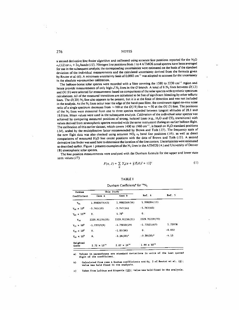
276 NOTES

a second derivative line finder algorithm and calibrated using accurate line positions reported for the N20

_3(12) or v, + 2u2 bands (13). Nitrogen line positions from I to 4 ATMOS zonal spectra have been averaged

for use in the subsequent analysis; the corresponding uncertainties were estimated on the basis of the standarddeviation of the individual measurements and the calculated uncertainty derived from the formula given

by Reuter et al. (6). A minimum uncertainty limit of 0.0002 cm -j was adopted to account for the uncertainty

in the absolute wavenumber calibration.The balloon-borne solar spectra were recorded with a filter covering the 1580 to 2230 cm -j region and

hence provide measurements of only high-J N2 lines in the O branch. A total of 6 N2 lines between O(13)

and O(19) were selected for measurement based on comparisons of the solar spectra with synthetic spectrumcalculations. All of the measured transitions are calculated to be free of significant blending by other telluric

lines. The 0(20) N2 line also appears to be present, but it is at the limit of detection and was not included

in the analysis. As the Nx lines occur near the edge of the band-pass filter, the continuum signal-to-rms noise

ratio of a single spectrum decreases from _ 100 at the O(19) line to _50 at the O(13) line. The positionsof the Nz lines were measured from one to three spectra recorded between tangent altitudes of 28.1 and18.0 km. Mean values were used in the subsequent analysis. Calibration of the individual solar spectra was

achieved by comparing measured positions of strong, isolated lines (e.g., H20 and COx transitions) withvalues derived from stratospheric spectra recorded with the same instrument during an earlier balloon flight.

The calibration of this earlier dataset, which covers 1400 to 1960 cm-', is based on HzO standard positions

(14), scaled by the multiplicative factor recommended by Brown and Toth (15). The frequency scale ofthe new flight data was also checked using accurate NO2 v3 band line positions (16), as well as direct

comparisons of measured H20 line center positions with the data of Brown and Toth (15). A second

derivative line finder was used here to determine the location of the line centers. Uncertainties were estimated

as described earlier. Figure I presents examples of the N_ lines in the ATMOS (A) and University of Denver

(B) stratospheric solar spectra.The line position measurements were analyzed with the Dunham formula for the upper and lower state

term values (17)

F(v, J)= _, Y,j(v+ ½)_[J(J + 1)] s (1)

TABLE i

Dunham Coet_cients s for t4N2

Dunham This Study

Coefficient Case A Case 5 Rof. 6 Ref. 5

Yol 1.9982673(43) 1.9982369(56) 1.998286(13)

Yoz x 10 e -5.761(10) -5.7_7(14) -5.763(_0)

Yo_ x 10 lz O. 4.78 b O.

YIo 2329.91170(20) 2329.91156(21) 2329.91239(70)

Ytl x 102 -1.73717(9) -1.73030(19) -1.73121(67)

Yt2 x i01 O, -i.01(56) O.

Yal x lO s O. -3.28(20) c "3.28(20) a

WeightedError 2.72 x 10 -_ 2.67 x 10-_ 1.99 x 10 -_

1.72975

-0.832

-4.15

a) Values in parentheses are standard deviations in unite of _he last quoted

dlgit of _he coe£flcient.

b) Calculated from case A Dunham coefficients and Eq. 2 of Reuter eC al. (_);

value wae held fixed in the analysis.

c) Taken from Lofthus and Krupente (18); value vas held fixed in the analysis.

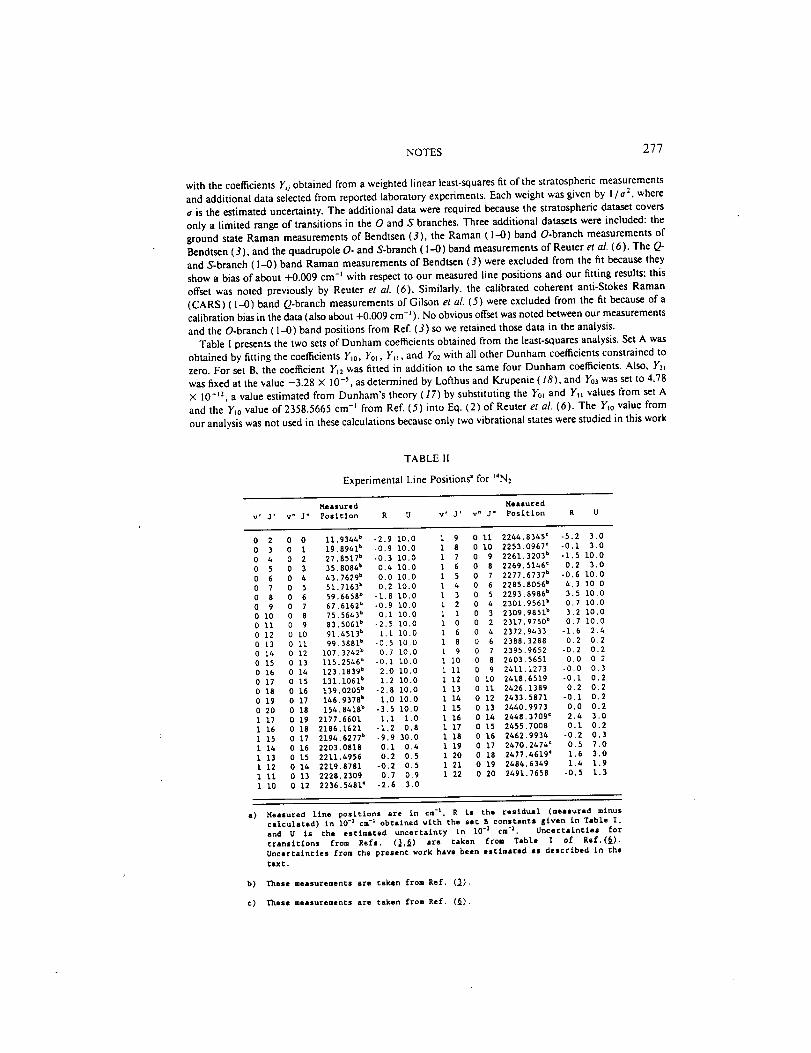
NOTES277

with the coefficients Y,j obtained from a weighted linear least-squares fit of the stratospheric measurements

and additional data selected from reported laboratory experiments. Each weight was given by 1/o 2 , where

o is the estimated uncertainty. The additional data were required because the stratospheric dataset covers

only a limited range of transitions in the O and S branches. Three additional datasets were included: the

ground state Raman measurements of Bendtsen (3), the Raman (1--0) band O-branch measurements of

Bendtsen (3), and the quadrupole O- and S-branch (1-0) band measurements of Reuter eta/. (6). The Q-

and S-branch (I--0) band Raman measurements of Bendtsen (3) were excluded from the fit because they

show a bias of about +0.009 cm -_ with respect to our measured line positions and our fitting results: this

offset was noted previously by Reuter et al. (6). Similarly, the calibrated coherent anti-Stokes Raman

(CARS) (1-0) band Q-branch measurements of G ilson et al. (5) were excluded from the fit because of a

calibration bias in the data (also about +0.009 cm-_). No obvious offset was noted between our measurements

and the O-branch (1--0) band positions from Ref. (3) so we retained those data in the analysis.

Table I presents the two sets of Dunham coeffcients obtained from the least-squares analysis. Set A was

obtained by fitting the coeffacients Y,0, Yo_, Yti, and Y02 with all other Dunham coefficients constrained to

zero. For set B, the coefficient Y_2 was fitted in addition to the same four Dunham coeffcients. Also, Y2_

was fixed at the value -3.28 X 10 -5, as determined by Lofthus and Krupenie (18), and Y03 was set to 4.78

X 10 -_2, a value estimated from Dunham's theory (17) by substituting the Yo_ and YIt values from set A

and the Y_o value of 2358.5665 cm -_ from Ref. (5) into Eq. (2) of Reuter et al. (6). The Yto value from

our analysis was not used in these calculations because only two vibrational states were studied in this work

TABLE II

Experimental Line Positions" for '4N2

Measured Meaeured

v' J' v" J" Posltlon R U v' J' v" J" Posltfon R U

0 2 0 0 ii.9344 b -2.9 i0.0 1 9 0 Ii 2244.8345 © -5.2 3.0

0 3 0 1 19.8941 b -0,9 i0.0 1 8 0 10 2253.0967 = -0.i 3.0

0 4 0 2 27.8517 b -0.3 i0.0 1 7 0 9 2261.3203 b -1.5 i0.0

0 5 0 3 35.8084 b 0.4 i0.0 i 6 0 8 2269.5146 c 0.2 3.0

0 6 0 4 43.7629 b 0.0 10.0 1 5 0 7 2277.6737 b -0.6 lO.O

0 7 0 5 51.7163 _ 0.2 10.0 1 4 0 6 2285.805@ 4.3 10.0

0 8 0 6 59.6658 b -1.8 I0.0 1 3 0 5 2293.898@ 3.5 i0.0

0 9 0 7 67.6162 b -0.9 I0.0 1 2 0 4 2301.9561 b 0.7 i0.0

0 i0 0 8 75.5643 b 0.i I0.0 1 1 0 3 2309.9851 b 3.2 I0.0

0 ii 0 9 83.5061 b -2.5 i0.0 1 0 0 2 2317.9750 b 0.7 I0.0

0 12 0 i0 91.4513 b I.i i0.0 1 6 0 4 2372.9433 -1.6 2.4

0 13 0 II 99.3881 b -0.5 I0.0 I 8 0 6 2388.3288 0.2 0.2

0 14 0 12 107.3242 b 0.7 I0.0 1 9 0 7 2395.9652 -0.2 0.2

0 15 0 13 115.254@ -0.I I0.0 i I0 0 8 2403.5651 0.0 0.2

0 16 0 14 123.1839 b 2.0 i0.0 i 11 0 9 2411.1273 -0.0 0.3

0 17 0 15 131.1061 b 1.2 I0.0 I 12 0 i0 2418.6519 -0.i 0.2

0 18 0 16 139.0205 b -2.8 i0.0 1 13 0 ii 2426.1389 0.2 0.2

0 19 0 17 146.9378 b l.O i0.0 1 14 0 12 2433.5871 -0.i 0.2

0 20 0 18 154.8418 b -3.5 I0.0 1 15 0 13 2440.9973 0.0 0.2

I 17 0 19 2177.6601 l.l 1.0 1 16 0 14 2448.3709 ¢ 2.4 3.0

i 16 0 18 2186.1621 -1.2 0.8 i 17 0 15 2455.7008 0.I 0.2

I 15 0 17 2194.6277 _ -9.9 30.0 1 18 0 16 2462.9934 -0.2 0.3

1 14 0 16 2203.0818 0.i 0.4 i 19 0 17 2470.2474 = 0.5 7.0

i 13 0 15 2211.4956 0.2 0.5 1 20 0 18 2477.4619 = 1.6 3.0

I 12 0 14 22_9.8781 -0.2 0.5 i 21 0 19 2484.6349 1.4 1.9

1 II 0 13 2228.2309 0.7 0.9 i 22 0 20 2491.7658 -0.5 1.3

i l0 0 12 2236.5481 ¢ -2.6 3.0

a) Measured line positions are in cm -t, R Is the residual (measured minus

calculated) in i0 "3 cm "_ obtained wlth the set B constants given in Table I.

and U is the estimated uncertainty in 10 -3 cm "I. Uncertainties for

transitions from Refe. (_,_) are taken from Table I of Ref.(_).

Uncertainties from the present work have been estimated as described in the

text.

b) These measurements are taken from Ref. (_).

C) These measurements are taken from aef. (_).

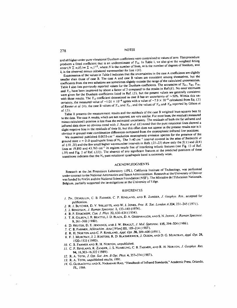
278 NOTES

and all higher-order pure vibrational Dunham coethcients were constrained to values of zero. This procedure

produces a fitted coet_cient that is an underestimate of Y_o. In Table I, we also give the weighted fitting

error (N _ wi6 _ / m Y. wi ) 1/2, where N is the number of lines, m is the n umber of degrees of freedom, and

t_ is the observed minus calculated wavenumber for line i (6).Examination of the values in Table 1 indicates that the uncertainties in the case A coefhcients are slightly

smaller than those of case B. The case A and case B values are consistent among themselves, but the

coet_cients from the two solutions are sometimes slightly outside the range of the calculated uncertainties.

Table I also lists previously reported values for the Dunham coei_cients. The accuracies of Yo_, Yo2, Y_o,

and Y_ have been improved by about a factor of 3 compared to the results in Ref (6). No error estimates

were given for the Dunham coef_cients listed in Ref. (5), but the present values are generally consistent

with those results. The Y_2 coeEacient determined in case B has an uncertainty of _50%. Within this un-

certainty, the measured value of -l.01 × 10 -a agrees with a value of-7.9 × 10 -9 calculated from Eq. (3)

of Reuter et al. (6), the case B values of Y_ and Yo_, and the values of Yt0 and Y2o reported by Gilson et

al. (5).Table II presents the measurement results and the residuals of the case B weighted least-squares best fit

to the data. The case A results, which are not repotted, are very similar. For most lines, the residual (measured

minus calculated) position is less than the estimated uncertainty. The residuals of both the far infrared and

infrared data show no obvious trend with J. Reuter et al. (6) noted that the pure rotational lines showed a

slight negative bias in the residuals of their fit, but this offset does not appear in the present results nor is it

obvious in ground state combination differences computed from the stratospheric infrared line positions.

We examined published 0.0033-cm -_ resolution stratospheric emission spectra for the presence of the

ground state v = 0-0 quadrupole lines of N:. The 7--40 cm -_ interval covered in the atlas of Baldecchi et

aL (19, 20) and the few small higher wavenumber intervals in Refs. (21-23) show only the S( l ) and S(4)

lines at 19.895 and 43.763 cm -t in regions nearly free of interfering telluric features (see Fig. 13 of Ref.

(19) and Fig. 2 of Ref. (23)). The absence of any significant features at the predicted positions of these

transitions indicates that the N2 pure rotational quadrupole band is extremely weak.

ACKNOWLEDGMENTS

Research at the Jet Propulsion Laboratory (JPL), California Institute of Technology, was performed

under contract to the National Aeronautics and Space Administration. Research at the University of Denver

was funded by NASA and the National Science Foundation (NSF). The Minist6re de l'Education Nationale,

Belgium, partially supported the investigations at the University of Liege.

1. PH. DEMOULIN,

REFERENCES

C. B. FARMER, C. P. RINSLAND, AND R. ZANDER, J. Geophys. Res., accepted for

publication.2. R.J. BUTCHER, D. V. WILLETTS, AND W. J. JONES, Proc. R. Soc. London A 324, 231-245 ( 1971 ).

3. J. BEND'I'SEN, J. Raman Spectrosc. 2, 133-145 (1974).

4. B. P. STOICHEFF, Can. J. Phys. 32, 630-634 (1954).

5. T. R. GILSON, I. R. BEATTIE, J. D. BLACK, D. A. GREENHALGH, AND S. N. JENNY, J. Raman Spectrosc.

9, 361-368 (1980).

6. D. REUTER, D. E. JENNINGS, AND J. W. BRAULT, J. MoL Spectrosc. 115, 294-304 (1986).

7. C. B. FARMER, Mikrochim. Acta [ Wien] 111, 189-214 (1987).

8. R. H. NORTON AND C. P. RINSLAND, Appl. Opt. 30, 389-400 ( 1991 ).

9. F. J. MURCRAY, J. J. KOSTERS, R. D. BLATHERWlCK, J. OLSON, AND D. G. MURCRAY, Appl. Opt. 29,

1520-1525 (1990).

10. C. B. FARMER AND R. H. NORTON, unpublished.

11. C. P. RINSLAND, R. ZANDER, J. S. NAMKUNG, C. B. FARMER, AND R. H. NORTON, J. Geophys. Res.

94, 16,303-16,322 (1989).

12. R. A. TOTH, J. Opt. Soc. Am. B Opt. Phys. 4, 357-374 (1987).

13. R. A. TOTH, unpublished results, 1991.14. G. GUELACHVlLI AND K. NARAHARI RAO, "Handbook of Infrared Standards," Academic Press, Orlando,

FL, 1986.

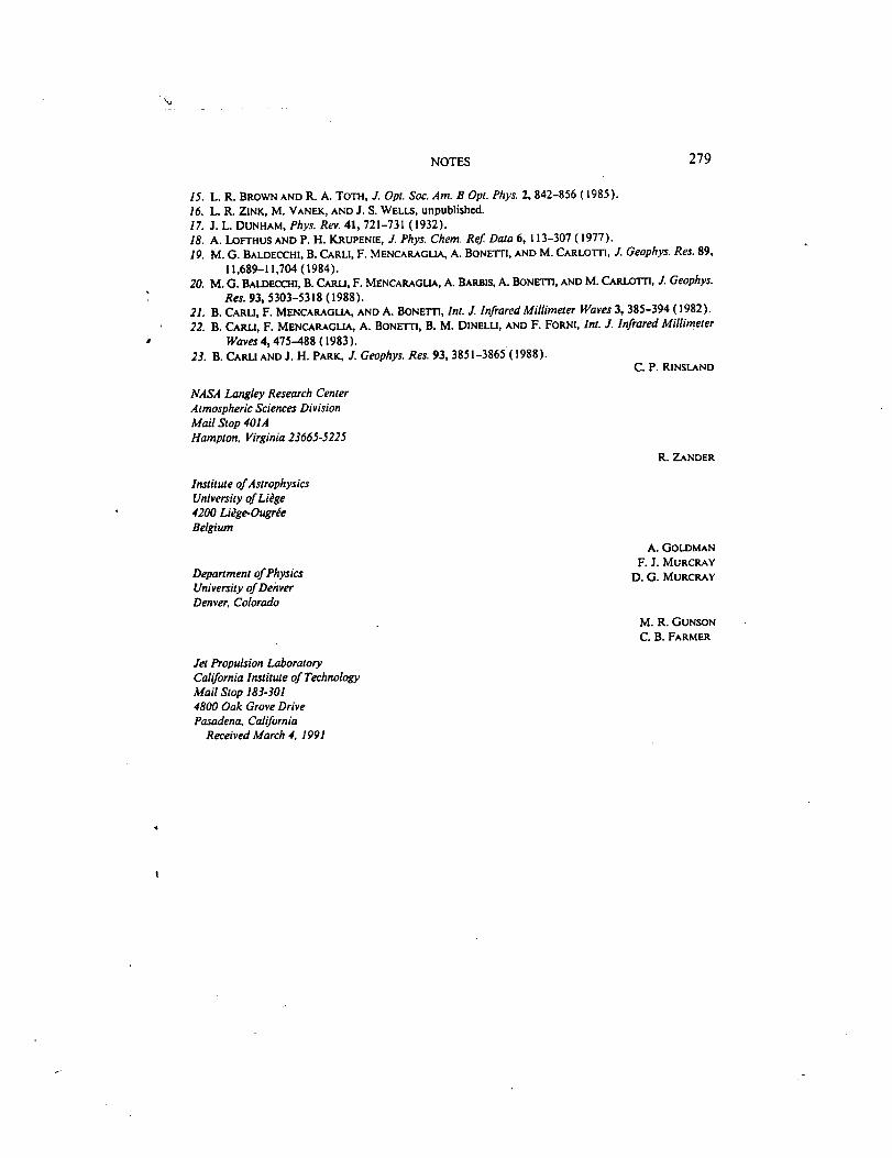
%r

NOTES 279

15. L. R. BROWNAND R. A. TOTH, J. Opt. Soc. Am. B Opt. Phys. 2, 842-856 (1985).

16. L. R. ZINK, M. VANEK, AND J. S. WELLS, unpublished.17. J. L. DUNHAM, Phys. Rev. 41,721-731 (1932).18. A. LoFr'HUS AND P. H. KRUPENtE, J. Phys. Chem. Ref. Data 6, 113-307 (1977).

19. M.G. BALDECCHt, B. CARt.t, F. MENCARAGLIA, A. BONETTI, AND M. CARLOT'i'I, J. Geophys. Res. 89,

11,689-11,704 (1984).20. M.G. BALDEOCHI,B. CARl.I, F. MENCARAGLIA,A. BARBIS, A. BONLrI_, AND M. CARLoI"rl, J. Geophys.

Res. 93, 5303-5318 (1988).

21. B. C^Rta, F. MENCARAGLtA, AND A. BONET'n, Int. J. Infrared Millimeter Waves 3, 385-394 (1982).

22. B. CARt.I, F. MENCARAGLtA, A. BONd"n, B. M. DINELU, AND F. FORNt, Int. J. Infrared Millimeter

Waves 4, 475-488 (1983).23. B. CARU AND J. H. PARK, ./. Geophys. Res. 93, 3851-3865 (1988).

NASA Langley Research Center

Atmospheric Sciences Division

Mail Stop 401A

Hampton, Virginia 23665-5225

Institute of Astrophysics

University of Li#ge

4200 Li#ge-Ougr_e

Belgium

Department of Physics

University of DenverDenver, Colorado

Jet Propulsion Laboratory

California Institute of Technology

Mail Stop 183-301

4800 Oak Grove Drive

Pasadena, CaliforniaReceived March 4, 1991

C. P. RINSLAND

R. ZANDER

A. GOLDMAN

F. J. MURCRAY

D. G. MURCRAY

M. R. GUNSON

C. B. FARMER

°

Analysis of Atmospheric Trace Constituentsfrom High Resolution Infrared Balloon-Borne and

Ground-Based Solar Absorption Spectra

A. Goldman, FJ. Murcray, C.P. Rinsland*, R.D. Blatherwick,

F.H. Murcray, and D.G. Murcray

Department of Physics, University of DenverDenver CO 80208

*Atmospheric Sciences Division, NASA Langley Research CenterHampton VA 23665

Recent results and ongoing studies of high resolution solar absorption spectra will be presented. The analysis of these

spectra is aimed at the identification and quantification of trace constituents important in atmospheric chemistry of the

stratosphere and upper troposphere.

Analysis of balloon-borne and ground-based spectra obtained at 0.0025 cm "1covering the 700-2200 cm q interval will bc

presented. Results from ground-based 0.02 cm "_solar spectra, from several locations such as Denver, South Pole, M. Loa,and New Zealand will also be shown. The 0.0025 cm q spectra show many new spectroscopic features. The analysis of

these spectra, along with corresponding laboratory spectra, improves the spectral line parameters, and thus the accuracyof trace coustituents quantification. The combination of the recent balloon flights, with earlier flights data since 1978 at

0.02 cm': resolution, provides trends analysis of several stratospheric trace species. Results for COF:, F'22,'SFs and other

species will be presented. Analysis of several ground-based solar spectra provides trends for HCI, HI:: and other species.

The retrieval methods used for total column density and altitude distribution for both ground-based and balloon-borne

spectra will be presented. These are extended for the analysis of the ground- based spectra to be obtained by the highresolution interfcrometers of the Network for Detection of Stratospheric Change (NDSC). Progress of the University of

Denver studies for the NDSC will be presented. This will include intercomparlson of solar spectra and trace gasesretrievals obtained from simultaneous scans by the high resolution (0.002.5 cm q) intcrferomctcrs of BRUKER and

BOMEM.

1, INTRODU_ 'TION.

The technique of infrared solar spectra has been used for many years to obtain information about the columnabundance and vertical distribution of atmospheric gases. To maximize retrieval of this information, nonlinear

multiparameters spectral least squares fitting methods have been developed, and since 1980 became an important toolin our research, t'4 Subsequent studies (see below), conducted with higher resolution and signal to noise spectra, allowed

to further enhance these analysis methods.

The spectral least square programs can fit simultaneously several spectral regions of several spectral scans, with three

kinds of parameters: (i) instrumental parameters, such as resolution and background contours with channel and phasecorrections, (il) atmospheric (or laboratory) parameters such as the temperature and gas amounts in isothermal layers,

and (iii) spectral line parameters such as line positions, intensities and half widths. The programs allow the initial

parameters to remain fixed or vary within a constrained range of a priori values. The fitted parameters include the

scaling of the initial mLxing ratio distribution functions which determine the gas amount.

The atmospheric spectroscopy group at the University of Denver has been studying atmospheric infrared absorption

with several types of balloon-borne, aircraft and ground-based spectrometers for many years. The instrumentation used

in recent experiments includes 0.002-0.003 cm "t (unapodized) resolution FTS systems _ and 0.0005 cm "t resolution tunable

diode LHS system 6 for atmospheric solar absorption spectra. Ground-based measurements have been made from various

194 / SPIE Vol. 1491 Remote Sensing of Atmospheric Chemistry (1991) 0-8194-0600-7/91/$4.00

q

locations, e.g. Denver, New Mexico, Hawaii, New Zealand, the South Pole, and McMurdo, during several seasons overthe last few years. Balloon flights were made from several locations in the U.S. and Europe. The field measurements

are supplemented by extensive laboratory spectra, mostly taken with the field spectrometers. The analysis of these spectrahas been very successful in the identification and quantification of atmospheric trace gases, some monitored since 1980,

and upgrading the theoretical capabilities of atmospheric spectroscopy. Analysis of the data includes detailed atlases with

complete identifications of the individual atmospheric and solar lines, molecular spectroscopic constants and line

parameters analysis of selected bands, theoretical line-by-line and cross sections simulations of emission and absorption

spectra, and spectral least-squares fitting using the most current atmospheric absorption parameters. These show good

agreement with the data in many spectral intervals and also many new spectral features in the stratospheric spectrum.In this paper, samples of our recent 0.002-0.003 cm "_data and analysis leading to advances in atmospheric spectroscopywill be discussed. Quantification of several trace gases since 1980 wilt be summarized from 0.02 cm "t and 0.002 cm "t data.

Work in progress with new BRUKER and BOMEM interferometer sys'tems towards the NDSC (Network for Detection

o_ Stratospheric Change) will be presented, including intercomparisons, and further developments in the retrieval

methods.

2.1 Balloon-borne _pectr_

We have studied the new infrared spectroscopic observations of several important stratospheric trace gases obtained

with a 0.002 cm "_resolution interfcromcter system now covering the "]00-2200 cm "t reg ion's4 Most stratosphcrlc speciesare measurable in these spectra. The main molecules studied are 05, HNO3, CQONOa, HO2NO2, NO:, COF_, SF6 and

CHC_F 2. The stratospheric solar spectra, ground-based solar spectra, and laboratory spectra reveal new details of theabsorption by these molecules which are important in dcterminlng the photochemistry and the heat balance of the

atmosphere. It has been possible to assign numerous previously unidentified features to these gases in the stratospheric

spectra and to incorporate several new sets of spectral line parameters and cross sections from their simulation.

Many of these features were not accounted for in the previous line parameters compilations, and will be included infuture data bases, HITILA.N91 and GEISA91. A number of spectral regions have been atlased in detail? Fig. 1 shows

a sample from the atlas. The high resolution 10 Fm spectra have been analyzed with the new ozone line parame tersl* to

determine the isotopic ratios of _6Ot6OISO and t60_80 _60 in the stratosphere.

The excellent agreement between the highly precise laboratory and stratospheric spectra provided significant new

evidence for absorption by the HO2NOa 802.7 cm "t Q branch in the lower stratosphere. The improved resolution of the

flights measurements reveals additional details of the interference in the C_ONO2 780.2 em "t v4 Q branch region,including the identification of overlapping HNO3 _'8 features. New analysis of the COFa v6 band and the u4 band, andrecent analysis of the HNO3 v= and _'s+v9 bands have been applied to both laboratory and stratospheric spectra. Newfeatures of other trace gases (e.g. C_ONOa, HNO3 and CF4 in the 1280 cm "_ region) have been identified in the

stratospheric spectra and are currently under study with new line parameters and cross-sections.

The 5-7 Fm spectra are also being studied for numerous new O3 features. Updated line parameters of HNO3 v:, Os

5_ bands, and H:O ua bands are now used for new retrievals of HNO3. The NO2 spectral lines in the 6 Fm region showthe need for further update. The combination of the high resolution flight data with other solar spectral data allows

improvements in the spectral line parameters of the references gases Oa and N2, but further studies are neede d.tt't2

The long time span covered by medium and high resolution infrared atmospheric absorption measurements generatedconsiderable interest in studying trends of atmospheric trace gases. Thus, an analysis of both recent 0.002 cm "t spectra

and previous 0.02 cm "t spectra provided long term trends for SF6, CHC_F,, and COF2 over the last decade. Exponential

increase rates of (7.4 ± 1.9)%, (9.4 ± 1.3)% and (10.3 ± 1.8)% yea r'_ were found- u

2.2 Gr0und-based spectr_a

We have performed quantitative analysis of the absorption by a number of minor and trace constituents in 0.02 cm "t

SPIE Vol. 1491 Remote Sensing of Atmospheric Chemistry (199t1 1 195

resolution solar absorption spcctra geographical locations, t3"= In addition to various measurements from Denver, theseinclude the total vertical column amounts of H20 (and isotopes), CO:, O_, N20, CH4, CHC_F=, NO, NO=, HCI, and

HNO_ from M. Loa, Hawaii, in February 1987; O3, N20, HNO3, CO:, CH4, and CF=C_, in December 1980 andNovember-December 1986 from the South Pole; HCQ, NO, NO2, and C2H_ in December 1986 from the S. Pole, and

HCQ, HNO_, O_, CQONO2 and NO 2 from McMurdo, Antarctica during the spring 1987 ozone hole. In the M. Loameasurements it was found that the average tropospheric concentrations deduced for COs, N20 and CH, are very

consistent with correlative NOAA GMCC surface data.

Of particular interest is the observed increase in the CF:C_= column amount above the S. Pole over the 6 year period,corresponding to (3.6 - 2.1)% year "t. The column amount of HNO3 for both 1980 and 1986 were not significantlydifferent. Other data sets, such as from the National Solar Observatory (NSO) at Kitt Peak were used for monitoringtrends of HF and HC_ from 0.02-0.005 cm"1spectra obtained during the 1977-1990 period. Linear increase rates of (10.7

-,- 1.1)% year "t and (4.9 -. 0.7)%year q have been obtained for HF and HCQ respectively.

We have also been conducting 0.002-0.003 cm"t resolution solar absorption ground-based measurcmcnts, for periodicobservations and monitoring of the atmosphere from Denver. The initial measurements were made with the balloon-borne BOMEM FTS system: Typical results are shown in Figures 2-5. More recently, dedicated BOMEM andBRUKER FTS have been used, one of which will be moved to Mauna Loa as soon as the NDSC station becomes

operational. Preliminary results are shown in Figures 6-10.

The analysis of the ground-based spectra shows that the trace gases of interest to the NDSC can be well monitoredfrom selected spcctral intervals of multiscans measurements, with temperatures and geometry and instrumentalperformance monitored from reference gases. It is apparent that no more than scale height vertical resolution can usuallybe expected for the altitude distribution of the trace gases, and in some cases only the tropospheric and stratosphericcomponents could be separated. The translation of the statistical errors of the spectral least squares fitting to absoh, tcerrors estimates from a priori constraints and accuracies requires further studies.

3,CONCLUSIONS

High resolution stratospheric spectra show many new spectral features not observed in previous lower resolutionspectra. This requires new analysis of laboratory and atmospheric spectra and improved theoretical calculations for manymolecular bands of atmospheric interest. Atmospheric spectra remain a powerful source for observing and monitoring

our changing atmosphere.

Retrieval methods based on spectral least squares are best suited for spectroscopic quantification, but further

development are desired.

4. A(_KNOWLEDGMENTS

Research was at the University of Denver supported in part by NSF and in part by NASA. Acknowledgement is madeto the National Center for Atmospheric Research, which is sponsored by the National Science Foundation, for computertime used in this work. We thank A. Maki, L.R. Brown, J.-M. Flaud, and C. Camy-Peyret, and others for collaboration

on new spectral line parameters, and to N.D. Sze, M. Ko, R. Cicerone and others for providing photochemical modeling.

1. E. Niple, W.G. Mankin, A. Goldman, D.G. Murcray, and F.J. Murcray, "Stratospheric NO: and HzO Mixing RatioProfiles from High Resolution Infrared Solar Spectra Using Nonlinear Least Squares," Geophys. Res. Lett., 7, 489-492,

1980.2. A. Goldman, D.G. Mureray, F.J. Murcray, and E. Niple, "High Resolution IR Balloon-Borne Solar and Laboratory

Spectra in the HNO 3 1720-cm "t Region: An Analysis," AppL Opt., 19, 3721-3724, 1980.3. C.P. Rinsland, A. Goldman, F.J. Murcray, D.G. Murcray, M.A.H. Smith, R.K. Seals, Jr., J.C. Larscn, and P.L.

Rinsland, "Stratospheric N20 Mixing Ratio Profile from High-Resolutlon Balloon-Borne Solar Absorption Spectra and

195 / SP/E Vo/. 1491 Remote Sensing o/Atmospherlc Chemlstry(1991)

Laboratory Spectra Near 1880 cm'Z," AppL Opt., 2I, 4351-4355, 1982.4. A. Goldman, F.G. Fernald, F.J. Murcray, F.H, Murcray, and D.G. Murcray, "Spectral Least Squares Ouantification

of Several Atmospheric Gases from High Resolution Infrared Solar Spectra Obtained at the South Pole," J. Q_tant.

Spectrosc. Radiat. Transfer, 29, 189-204, 1983.5. F.J. Murcray, J.J. Kosters, R.D. Blatherwick, J. Olson, and D.G. Murcray, "High Resolution Solar Spectrometer

System for Measuring Atmospheric Constituents," AppL Opt., 29, 1520-1525, 1990.6. C.T. McElroy, A. Goldman, P.F. Fogel, and D.G. Murcray, "Heterodyne Spectrophotometry of Ozone in the 9.6-/.tm

Band using a Tunable Diode Laser," J. Geophys. Res., 95, D5, 5567-5575, 1990.7. A. Goldman, F.J. Murcray, D.G. Murcray, J.J. Kosters, C.P. Rinsland, C. Camy-Peyret, J.-M. Flaud, and A. Barbe,

Isotopic Abundances of Stratospheric Ozone from Balloon-Borne High-Resolution Infrared Solar Spectra, J'. Geophys.

Res., 94, 8467-8473, 1989.8. A. Goldman, F.J. Murcray, R.D. Blatherwick, JJ'. Kosters, F.H. Murcray, D.G. Murcray, and C.P. Rinsland, "New

Spectral Features of Stratospheric Trace Gases Identified from High Resolutlon Infrared Balloon-Borne and Laboratory

Spectra,'./. Geophys. Res., 94, 14,945-14,955, 1989.9. A. Goldman, R.D. Blatherwick, J.J. Kosters, F.J. Murcray, F.H. Murcray, and D.G. Murcray, "Atlas of Very High

Resolution Stratospheric IR Absorption Spectra, Volume I, Line Positions and Identifications, Volume II, The Spectra,"

Department of Physics, Univcrsity of Denver, Dee., 1990.10. J.-M. Flaud, C. Camy-Peyret, C.P. Rinsland, V. Malathy Devi, M.A.H. Smith, and A. Goldman, "Improved Line

Parameters for the Ozone Bands in the 10_m Spectral Region," Appl. Opt., 29, 3667-3671, 1990.

11. M. Dang-Nhu, R. Zander, A. Goldman, and C.P. Rinsland, "Identification of Magnetic Dipole Infrared Transitions

of the Fundamental Band of Oxygen," 3".Melee. Spectrosc., I44, 366-373, 1990.12. C.P. Rinsland, R. Zander, Ph. Demoulin, A. Goldman, M.R. Gunson, and C.B. Farmer, "The Fundamental

Quadrupole Band of 14N2: Line Positions from High Resolution Solar Absorption Spectra," To be submitted, 1991.13. C.P. Rinsland, A. Goldman, F.J. Murcray, R.D. Blatherwick, J.J. Kosters, D.G. Murcray, N.D. Sze, and S.T. Massie,

"Long-Term Trends in the Concentration of SF_, CHCQF2, and COFa in the Lower Stratosphere from Analysis of High-Resolution Infrared Solar Occultation Spectra," .L Geophys. Res., 95, DIO, 16,477-16,490, 1990.

14. F.J. Murcray, F.H. Murcray, A. Goldman, D.G. Murcray, and C.P. Rinsland, "Infrared Measurements of Several

Nitrogen Species above the South Pole in December 1980 and November-December 1986," L Geophys. Res., 92, 13,37"3-

13,.376, 1987.15. A. Goldman, C.P. Rinsland, F.J. Murcray, F.H. Murcray, and D.G. Murcray, "Measurements of Atmospheric Gases

above the South Pole in December 1986 from High-Resolution 3 to 4/.tin Solar Spectra," .L Geophys. Res., 93, D6, 7069-

7074, 1988.16. C.P. Rinsland, A. Goldman, F.J. Murcray, F.H. Murcray, R.D. Blatherwiek, and D.G. Murcray, "Infrared

Measurements of Atmospheric Gases Above Mauna Lea, Hawaii, in February 198"/," J. Geophys. Res., 93, DIO, 12,607-

12,626, 1988.17. C.P. Rinsland, A. Goldman, F.J. Murcray, F.H. Murcray, "Increased CF2C_2 (CFC-12) Absorption above the South

Pole," AppL Opt., 27, 627-630, 1988.18. F.J. Mureray, A. Matthews, A. Goldman, P. Johnston, and C.P. Rinsland, "NI-I3 Column Abundances over Lauder,

New Zealand," J. Geophys. Res., 94, 2235-2238, 1988.19. F.J. Murcray, A. Goldman, R.D. Blatherwick, A. Matthews and N. Jones, "HNOj and HC_ Amounts over

McMurdo during the Spring of 1987," J. Geophys. Res., 94, D14, 16,615-16,618, 1989.20. C.P. Rinsland, J.S. Levine, R. Zander, A. Goldman, N.D. Sze, M.K.W. Ko, and D.W. Johnson, "Infrared

Measurements of HF and HCI Total Column Abundance above Kitt Peak, 1977-1990: Seasonal Cycles, Increases in Total

Columns Ratio, and Comparisons with Two-Dimensional Model Calculations," submitted to I. Gcophys. Res, Nov. 1990.

SPIEVol. 1491 RemoteSensing of AtmosphericChemistry(I99I) / 197

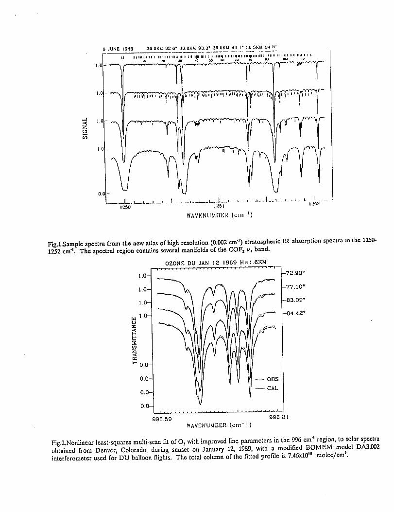
,-1

7_r_

c/}

I.C

1.(

1.0

l.t

0.C

JUNE 19118 36.9KI4 926" :IGOKM 93.3 ° 36,0K1,1 UI I" :ltiSK_,t U,|U"

II Ul |111_ I III I I IIIIIII Illll IIIII I I IIIt¢ IIII I III IIIII I $1| I1| II I III1_ I IIIIII1 IIIIII III II I I I Itl| I I I

tO 20 ;10 40 _0 60 I0 gO _J I(X) I I0

I 0 I I

,.

\

l__.t__.L__J.__J..__l_-a-.--1------,--.l---_ .... ' .... ,...,.. 1--| .... I.-.l. t I ....1250 l;_$l

WAVI!:NtIM[31'II¢. (t:t:_ :)

Fig.l.Sample spectra from the new atlas of high resolution (0.002 cm "1) stratospheric IR absorption spectra in the 1250-1252 cm "t. The spectral region contains several manifolds of the COFa v4 band.

OZONE DU JAN 12 1909 H--l.61(ld

i • , , , • , f I "1"- • , , , • , i , , , , r • ''o m

1.0- -72"90°

1.0- ._..._ _. -77. l 0"

1.0- __ -03.09"

oat.O- --04.42"(J

O3Z.<

E- 0.0-

0.0-.

0.0-

0.0-

996.,_9 996.81

WAVENUMBER tern"' )

I 11 IYI.......oBs

Fig.2.Nonllnear least-squares multl-scan fit of O 5 with improved line parameters in the 996 cm': region, to solar spectraobtained from Denver, Colorado, during sunset on January 12, 1989, with a modified BOMEM model DA3.002

interferometer used for DU balloon (lights. The total column of the fitted profile is 7.46x10 t8 molec/cm z.

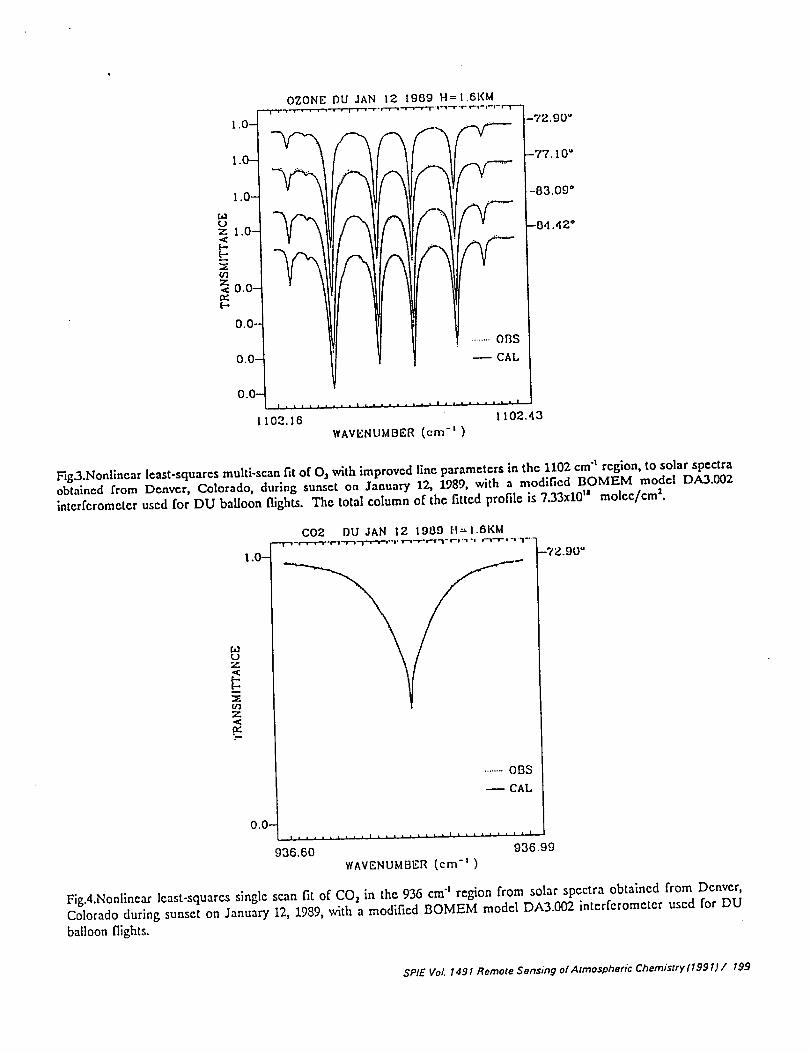
OZONE DU JAN 12 t989 H=I.61(M. . ......

-7:'.90"1.0-

1.0-

l.O-

l.O-

0.0-

0.0-

0.0-

0.0-

102.16

• ... _ --77"I0"

-83.09 °

-Od .42"

1102.43

WAVENUMBER (cm'i)

Fig.3.Nonlincar least-squares multi-scan fit of O 5with improved line parameters in the 1102 cm"tregion, to solar spectraobtained from Denver, Colorado, during sunset on January 12, 1989, with a modified BOMEM model DA3.002

intcrferometer used for DU baUoon flights. The total column of the fitted profile is 7.33x10 ta molec/cm2.

C02 DU JAN 12 1909 H-=I.6KM_ *,,--,w-','T--s'_'-'lr't ¢" I l"-"t'-w" r-l"_ r't 1 i

1.0- --7Z'90=

U

¢/3

z

.......OBS

CAL

0.0-

936.99936.60

WAVENUMBER (crn")

Fig.4.Nonlinear least-squares single scan fit of CO2 in the 936 cm" region from solar spectra obtained from Denver,

Colorado during sunset on January 12, 1989, with a modified BOMEM model DA3.002 interferometer used for DU

balloon flights.

SP/E Vol. ! 491 Remote Sensing o/Atmospheric Chemistry (19911 / 199

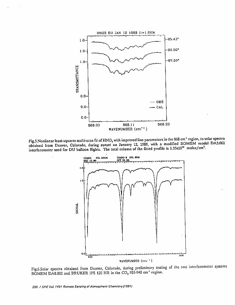
t.)

.<

o3

t-.

1.0-

1.0-

0.0-

0.0-

O.O-t i

868.03

HN03 DU JAN 12 1989 II=I.6KMi i a_--"-'r ]

....... OBS

-- CAL

i a I I I , ' I

868. I I 868.20

WAVENUMBER (crn-')

-_5.43"

-86.80*

--87.50"

Fig.5.Nonlinear least-squares multi-scan fit of HNO_ with improved llne parameters in the 868 cm "t region, to solar spectraobtained from Denver, Colorado, during sunset on January 12, 1989, with a modified BOMEM model DA3.002

interferometer used for DU balloon flights. The total column of the fitted profile is 1.35x10 '6 molcc/cm 2.

COADD SOl. BRUK COADD 8 SOL BOUDEC I0 90 OCT 25 90

I.O

|.C

,,<Z

935 940

WAVENUMBER (cm" t )

Fig.6.Solar spectra obtained from Denver, Colorado, during preliminary testing of the two interferometer systemsBOMEM DA8.002 and BRUKER IFS 120 HR in the CO= 935-940 cm "t region.

200 / SPIE Vol. I49 ! Remote Sensing of Atmospheric Chemistry [I 99 I)

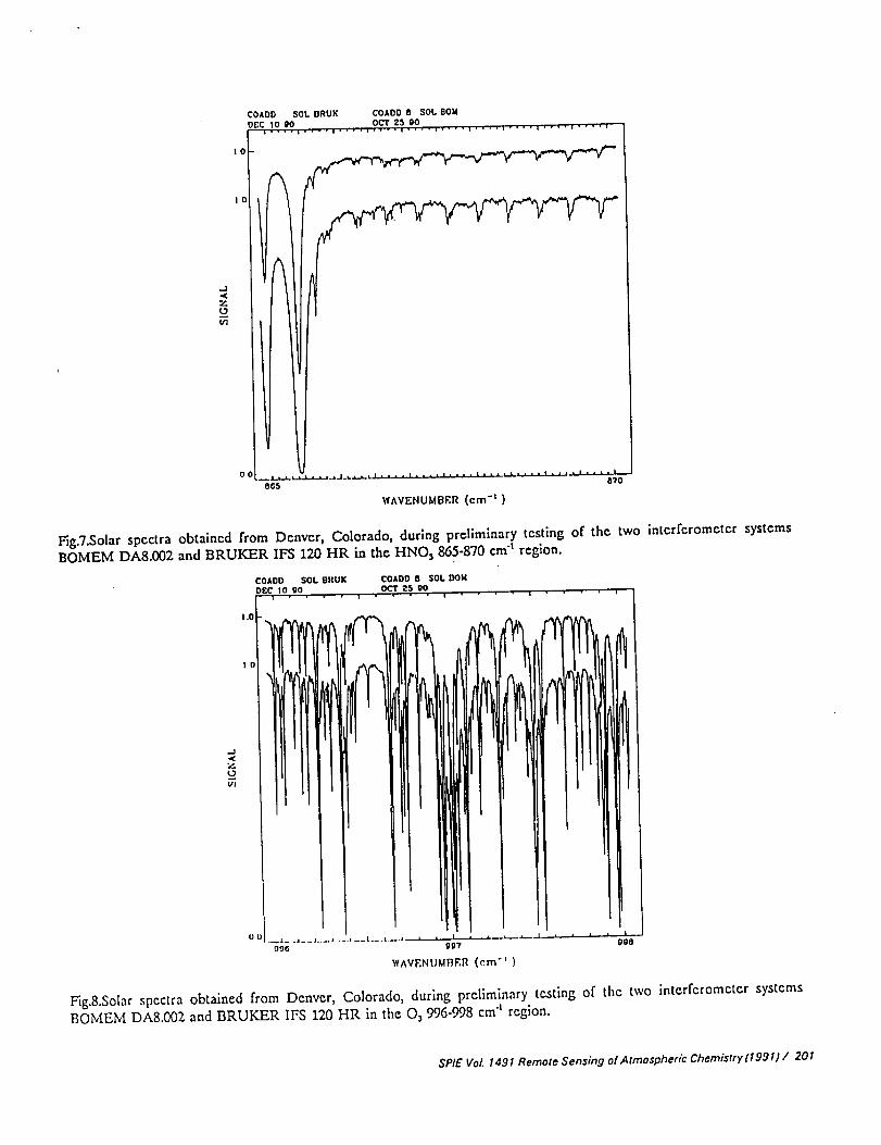
,,..1,<

"wt3N0'1

COADD SOL BRUK COADD B SOt. BO)4

DEC tO 90 OCT 25 90........ m .... i .... i .... i .... ! .... , .... i .... I .... |

1.0

Fig.7.Solar spcctra obtaincd from Dcnvcr, Colorado, during prclimlnary testing of thc two intcrfcrometcr systems

BOMEIVf DAB.002 and BRUKER IFS 120 HR in the HNO 3 865-870 em "L region.

COAOD SOt. 8RUK COADD 8 SOt. 13014

D£C I0 90 OCT 25 90

IO

.J.<

u!

Fig.8.Solar spectra obtained from Denver, Colorado, during preliminary testing of the two interferometer systems

BOMEM DA8.002 and BRUKER IFS 120 HR in the (35 996-998 cm "t region.

SPIE VoL 1491 Remote Sensing of Atmospheric Chemistry(1991) / 20I

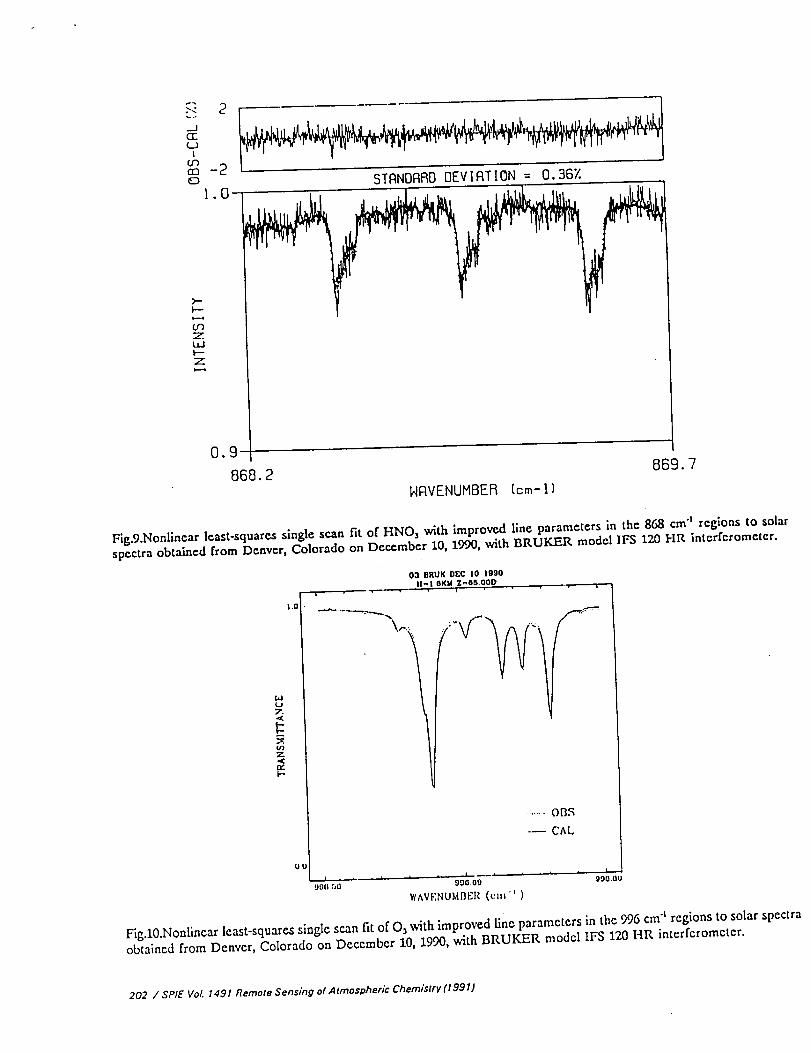
...dc/-(..J

I(.o03C3

(/3

LLII---Z

1.0--

STANDARD DEVIATION = 0.96Z

0.9

868.2 869.7

14RVENUHBER [cm-ll

Fig.9.Nonlinear least-squares single scan fit of HNO3 with improved line parameters in the 868 cm "t regions to solarspectra obtained from Denver, Colorado on December 10, 1990, with BRUKER model IFS :1.20HR interferometer.

03 BRUK DEC I0 IggO

II- | 6KM Z-6500D ---,T---_----T----,-v-- , , ' "

1.I_J7..<

Z

U_

1.0

':.. _; _V _

....... OBS

--- CAL

99U rJO 99609 990.0U

WAVF:NUMi3EI_ (cz.-')

Fig.10.Nonlinear least-squares single scan fit of O_ with improved line parameters in the 996 cm "t regions to solar spectraobtained from Denver, Colorado on December 10, 1990, with BILUKER model IFS 120 1-112.interferometer.

202 / SPIE Vol. 1491 Remote Sensing o/Atmospheric Chemistry(t991)

JOURNAL OF GEOPHYSICAL RESEARCH, VOL. 95, NO. DI0, PAGES 16,477-16,490, SEPTEMBER 20. 1990

Long-Term Trends in the Concentrations of SF 6, CHC1F2, and COF2

in the Lower Stratosphere From Analysis of High-Resolution

Infrared Solar Occultation Spectra

C. P. RINSLAND, I A. GOLDMAN, 2 F. J. MURCRAY, 2 R. D. BLATHERWICK, z J. J- KOSTERS,2

D. G. MURCRAY, 2 N. D. SZE, 3 AND S. T. MASSIE 4

Long-term trends in the concentrations of SF6, CHC1F, (CFC-22), and COF2 in the lowerstratosphere have been derived from analysis of ca. 1980 and-more recent infrared solar occultationspectra recorded near 32°N latitude at -0.02-cm-I resolution. Consistent sets of line parameters andspectral calibration methods have been used in the retrievals to minimize systematic error effects.Quoted error limits are 1 sigma estimated precisions. The SF6 and CHCIF2 results are based onspectra recorded by balloon-borne interferometers in March 1981and June 1988and a comparison ofthese results with the Atmospheric Trace Molecule Spectroscopy (ATMOS) Experiment/Spacelab 3measurements obtained in May 1985 near 30°N latitude. In the 13-18 km altitude range the meanmeasured SF6 mixing ratio in parts per trillion by volume (pptv) increased from I. 17 ± 0.21 in March1981 to 2.02 +--0.20 pptv in June 1988, and the CHCIF2 mixing ratio below 15 km altitude increasedfrom 51 -" 8 pptv in March 1981 to 102 "- 10 pptv in June 1988. The CHCIF2 retrievals used newempirical CHCIF, line parameters derived from 0.03-cm-I resolution laboratory spectra recorded atsix temperatures t_etween 203 and 293 K; the derived mixing ratios are -30% higher than obtained withearlier sets of line parameters, thereby removing a large discrepancy noted previously between IR andin situ measurements of CHCIF.,. Assuming an exponential growth model for fitting the trends, SF6

and CHCIF, mean increase rates of 7.4% - 1.9% and 9.4% - 1.3% year -l , are obtained, respectively,which correspond to cumulative increases by factors of -1.7 and -2.0 in the concentrations of thesegases over the 7.2-year measurement period. Analysis of spectra recorded in October 1979 and April1989 yields COF2 volume mixing ratios that are respectively 0.44 _ 0.17 and 1.21 --- 0.24 times theATMOS/Spacelab 3 values, from which an average COF2 increase rate of 10.3 -" 1.8% year -I overthis time period has been estimated. The present results are compared with previously reportedobservations and trends and with one-dimensional model calculations. The model calculated trends arein reasonably good agreement with the observations.

1. INTRODUCTION

The technique of infrared absorption spectroscopy hasbeen used for many years to measure the concentrations of

gases in the Earth's atmosphere. Because of the long timespan covered by these observations, there has been consid-erable recent interest in analyzing the old spectra and

comparing the results with newer data to determine thelong-term trends of important atmospheric gases. For exam-ple, ground-based spectra recorded more than 35 years agohave been studied to estimate the mean trends in the total

columns of CH4 and CO [Rinsland et al., 1985; Rinsland andLevine, 1985; Zander et al., 1989a, b]. IR spectral measure-ments of the stratosphere do not date back quite as far in

time as the ground-based data sets. Moderate resolution(-0.2 cm -1) stratospheric observations were first obtainedin the late 1960s and early 1970s [e.g., Murcray et al., 1968,1969, 1975; Goldman et al., 1970], followed by high resolu-tion (-0.02 cm -I) data in the late 1970s and early 1980s

[e.g., Goldman et al., 1979; Buijs et al., 1980; Murcray,1984]. We have begun a program of systematic comparison

1Atmospheric Sciences Division, NASA Langley Research Cen-ter. Hampton, Virginia.

-'Department of Physics, University of Denver. Denver. Colo-rado.

3Atmospheric and Environmental Research Incorporated. Cam-bridge, Massachusetts.

4National Center for Atmospheric Research, Boulder, Colorado.

Copyright 1990 by the American Geophysical Union.

Paper number 90JD01293.0148-0227/90i90JD-01293505.00

of the early stratospheric spectra with more recent spectrarecorded with the same or similar instrumentation under

similar observing conditions (for example, same latitude, alldata in the solar occultation mode). An initial analysis of the

data revealed clear evidence for rapidly increasing concen-trations of three important trace gases that have been the

subject of only limited previous stratospheric investigations.In the present paper we report the trends derived for thesethree gases, SF 6, CHC1F2, and COF2.

Sulfur hexafluoride (SF6) and chlorodifluoromethane

(CHCIF_, or CFC-22) are man-made trace atmospheric gaseswith strong absorption bands in the climatically important 8-to 13-_m window region. SF6 is widely used as an electricalinsulating gas in high-voltage electrical and electronic equip-ment such as circuit breakers, capacitors, transformers, andmicrowave components because of its high chemical stabil-

ity and its ability to impede electric breakdown [e.g., Brown,1966]. SF 6 has also been used as a meteorological tracer[e.g., Turk et al., 1968; Reiter, 1971 ; Drivas and Shair, 1974].CFC-22 is primarily used in refrigeration, but about 35% ofthe total is used in fluoropolymer production, which resultsin little release of the gas into the environment [Worm

Meteorological Organization, 1986]. Since both gases are inwide use and their atmospheric lifetimes are believed to be

long (perhaps more than 500 years for SF 6 [Ramanathan etal., 1985] and 10-28 years for CFC-22 [World Meteorological

Organization. 1982, 1989; Wuebbles, 1983; Hammitt et al.,1987; Golombek and Prinn, 1989: Fisher et al., 1990]), thesemolecules can be expected to accumulate in our environ-ment. The principal sink for CFC-22 is the reaction with

tropospheric OH. Monitoring its trend and ascertaining its

16,477

16,478RINSLAND E'I AL.: TRENDS OF SFr, CHCIF:, AND COF_. IN THE LOWER STRATOSPHERE

TABLE I. Parameters for the University of Denver Balloon Flights

Parameter

Value Corresponding to the Flight

October March 23. June 6, April 19,10. 1979 1981 1988 1989

Latitude, °N 32.8 32.8 31.9 34.7

Longitude, °W 106.0 106.0 97,4 103.0Float altitude, km 33.0 * 0.5 33.5 -- 0.5 36.5 - 0.5 36.7 _- 0.5

40 40 20/120 .,0/1 _0Scan time.* s 50 40/250 40/250Maximum path difference,t cm 50Field of view, arcmin 8 8 10 10

Spectral coverage, cm -1 1300-2000 740-1350 720-1300 1400-1960Tropopause geometric height, km 15.0 10.4 14.4 13.8

*Time required to record a single spectrum. The two entries for the June 6, 1988 and April 19, 1989

flights are the times required to recorded the low- and high-resolution interferograms, respectively.Single scans were analyzed from the October 10. 1979 and March 23, 1981 flight observations. In mostcases, two scans with the same zero path difference were coadded, and the average spectrum was used

in the analysis of the June 6. 1988 and April 19. 1989 flight measurements.tThe entries for the June 6, 1988 and April 19, 1989 flights are the maximum path differences of the

low- and high-resolution interferograms, respectively.

emission rates provide a means to derive the atmospheric

lifetime of CFC-22 and the global average OH concentration

[International Global Atmospheric Chemistry Programme,

1989]. This latter result can provide an independent check on

the global average OH concentration deduced recently from

the observed methyl chloroform trends [Prinn et al., 1987].

Carbonyl fluoride (COF,.) is an intermediate product in the

decomposition of chlorofluorocarbons in the stratosphere

[Rowland and Molina, 1975; Sze, 1978]. The Atmospheric

Trace Molecule Spectroscopy (ATMOS) Experiment/

Spaceiab 3 (SL3) measurements indicale that COFz repre-sents one third of the inorganic fluorine column in the

stratosphere, with the remainder contained in HF [Raper et

al., 1987]. COF, is produced mainly from the decomposition

of CCI_F_ [e.g., Rowland and Molina, 1975; Jayanty et al.,

1975] and, to a lesser extent, from other chlorofluorocar-

bons, such as CFC-22 [World Meteorological Organization,

1989]. Carbonyl fluoride is destroyed by photolysis and

reaction with O(JD) in the stratosphere [Sze, 1978]. Its

importance lies in the need to understand the reactions thatfollow the breakup of the chlorofluorocarbons in the strato-

sphere. Recently, it has been suggested that COF,_ may react

with H,O to form HF and CO2 on the surfaces of polar

stratospheric clouds [Wofsy et al., 1990]. Thus observations

of COF, and HF could help elucidate heterogeneous chem-

ical processes which are important for understanding strato-

spheric ozone distributions, particularly over polar regions.

Carbonyl fluoride is also expected to be an important inter-

mediate in the decomposition of currently proposed alterna-

tive fluorocarbons [World Meteorological Organization,

1989].The measurements and trends reported in this paper are

based on the analysis of -0.02-cm -I resolution infrared

solar occultation spectra recorded during four stratospheric

balloon flights from launch sites near 32°N latitude. The

measurements were recorded in October 1979, March 1981,

June 1988, and April 1989. All of the balloon flights were

conducted by the University of Denver atmospheric spec-

troscopy group. In addition, we have compared the retriev-

als with results derived from the infrared solar absorption

spectra obtained by the ATMOS experiment during the SL3

shuttle mission in May 1985 (see Farmer, [1987] for an

overview of the ATMOS experiment and the SL3 results).

Care has been taken to use consistent sets of line parameters

and spectral calibration methods to minimize systematic

error effects so as to derive the most reliable long-term

trends. All of the measurement data (balloon flight plus the

ATMOS results) have been included in deriving the trends.

Model calculations are presented to compare with the ob-

served trends. The calculations are based on the Atmo-

spheric and Environmental Research (AER) one-dimen-

sional model [Sze and 1(o, 1981] with updated rate data

[NASA, i987]. The model domain is from O to 70 kin. It

includes 150 gas-phase reactions and calculates the concen-

trations of the oxygen species (O, O(tD)), the hydrogen

species (H, OH, HO2, H202), the nitrogen species (1'4, NO,

NO2, HNO3, HOzNO,., N205, NO3), the chlorine species

(CI, CIO, OCIO, ClzO2, HCI, HOCI, CIONOa), the bromine

species (Br, BrO, BrNO3, BrCI, HBr), and the tropospheric

source gases (CH4, N2 O, OCS, CSz, C2H6, SFr, CH3C 1,

CC14, CCI3F, CCI2Fz, CHC1F2' CH3CCI3' CF3CCI3' and

other minor CFC species). The surface fluxes for CCI3F and

CClzF 2 are based on emission data reported by Gamlen et

al. [1986]. The emission data for CHCIF2 are uncertain

[World Meteorological Organization, 1986]. The atmo-

spheric release rates (109 gm yr -I) used in the present modelcalculations are 53, 86, and 95 for the years 1975, 1980, and

1985, respectively.

2. BALLOON FLIGHT MEASUREMENTS

Table 1 summarizes important flight and experimental

parameters for the four balloon flights. In all four experi-

ments the spectra were recorded at sunset in the solar

occultation mode. The two early balloon flights were con-

ducted from Holloman Air Force Base near Alamogordo,

New Mexico, on October 10, 1979, and March 23, 1981,

using a modified Bomen model DA2.01 interferometer sys-

tem (optical path difference of 50 cm). High and low sun

spectra from these flights (and an earlier one on October 27,

1978) have been reported in an atlas along with a list of the

measured positions and corresponding atmospheric and so-

lar line identifications [Goldman et al., 1987]. The launches

of the more recent balloon flights occurred from the National

°-

RINSLAND ET AL.: TRENDS OF SF6, CHCIF,. AND COF: IN THE LOWER STRATOSPHERE 16.479

Scientific Balloon Facility (NSBF) near Palestine, Texas, on

June 6, 1988, and from Fort Sumner, New Mexico, on April

19, 1989, using a new interferometer, a modified Bomem

model DA3.002 system capable of recording spectra with a Altitude.

maximum optical path difference of 250 cm. The new system km

has been described recently [Murcray et al.. 1990], and 14.0selected regions of the full resolution spectra from the 1988 t6.0

flight (and some of the high sun data collected during a 18.0

balloon flight on November 18, 1987) have been published in 20.0

an atlas [Goldman et al., 1989a]. A description of the trace 22.024.0

gas features observed in the spectra has also been reported 26.0

[Goldman et al., 1989b]. The full resolution spectra were 28.0

recorded at tangent heights above 17 km (1988 flight) and 30.0

above 29 km (1989 flight). Because spectral lines are pres- 32.0

sure-broadened at low altitudes, very high resolution obser- 34.036.0

rations are less useful in the lower stratosphere and tropo- 38.0

sphere than at higher altitudes, and for this reason the 40.0interferometer was switched to a mode that allowed the

, rapid recording of spectra with a maximum optical pathdifference of 40 cm. Only the lower resolution spectra were

used for the retrievals reported in this work. When appro-

priate, the full resolution scans have been analyzed to verify

the quality of the line parameters assumed in the analysis.

3. DATA ANALYSIS AND RESULTS

AS in a number of earlier investigations, the technique of

nonlinear least squares spectral fitting has been used to

analyze the data. Details and examples of the application of

this method to the analysis of solar occultation spectra are

presented in papers by Niple [1980], Niple et al. [1980],

Goldman et al. [1980], and Rinsland et al. [1982]. Initially,

the vertical profiles of SFr, CHCIF2, and COF,. were re-

trieved from the balloon flight spectra using the onion-

peeling technique [Goldman and Saunders, 1979]. A com-

parison of the retrieved profiles with the reported ATMOS

profiles indicated no differences in the relative vertical

distributions of the three gases outside the errors limits of

the experiments. Therefore to maximize consistency of theresults for the derivation of trends, we assumed the vertical

distributions retrieved from the ATMOS observations and

derived a single multiplicative scaling factor for each gas

relative to the reported ATMOS profile. The scale factors

were determined from the individual spectra, and then the

average and the standard deviation of these values were

computed for each occultation to determine the relative

increase (or decrease) in the stratospheric amount relative to

the ATMOS observations and a statistical estimate of the

TABLE 2. ATMOSSL3 Profiles Assumed in the PresentAnalysis

Volume Mixing Ratio in pptv

SFr" CHCIF,_t COF:_

1.42 70.4 5.051.42 70.1 10.0¢.1.42 68.1 20. I1.12 64.0 31.20.83 51.7 48.40.83_ 44.8 67.40.83§ 39.7 82.80.83§ 35.3 96.90.83§ 33.3§ 1110.83§ 30.1§ 1180.83§ 26.9§ 1160.83._ 21.8§ 1050.83§ 18.6§ 89.40.83§ 15.4§ 73.8§

*Smoothed values from Rinsland et al. [1990].tZander et al. [1987, Table 4] scaled by 1.28. See text.1:Retrieved from v t band manifolds near 1936 cm -t [Rinsland et

al., 1986, Figure 3, heavy full line].

§Extrapolated value.

scatter in the results. For completeness and because we had

to extrapolate the reported volume mixing ratio profiles to

higher and lower altitudes, the assumed ATMOS/SL3 verti-

cal distributions of SF6, CHCIF2, and COF2 are listed in

Table 2.

Except as noted below, line parameters were taken from

the 1986 Air Force Geophysics Laboratory high-resolution

transmission (HITRAN) line list [Rothman et al., 1987].

Correlative pressure-temperature profiles derived from ra-

diosonde and satellite measurements were used in the ray-

tracing calculations (M. Gelman and K. W. Johnson, Na-

tional Meteorological Center (NMC), private commu-

nications, 1982, 1989). The NMC analysis also yields an

estimate of the tropopause height. The value for each

balloon flight is listed in Table 1.

The spectral intervals selected for the analysis are given in

Table 3. In addition to retrieving the concentrations of SF6,

CHCIF,, and COF 2, we included intervals to retrieve the

concentrations of CH4, N2 O, and CO,.. These additional

gases were included in the analysis because of uncertainties

in the instrument pointing angle (about ±0.07 ° which corre-

sponds to about ±0.5 km in the tangent height, I sigma).

Following the procedures used to analyze the ATMOS

observations (see, for example, Zander et al. [1987]), the

TABLE 3. Spectral Regions Analyzed in the Present Study

Spectral TargetRegion, cm -1 Molecules Primary Interfering Molecules Data Sets Investigated

828.82--830.00 CH3_C1F,_ 03. CO,., C2H6945.00-949.00 SF6 CO2, O3, HzO1220.00-1224.50 CH4, NzO 031231.40-1235.00 CH4. N,O COF.,1384.21-1384.70 CO, HDO, 03, H,_O1385.00-1385.__9 CO,. "'"1385.65-1386.10 CO, 0 3, CH4

1936.00-1940.00 COF, CO,_. H20.03. NO. solar CO1952.15-1952.50 CO, solar CO, O3, COF.,1955.40-1955.70 CO, "'"

March 1981, June 1988March 1981, June 1988March 1981, June 1988March 1981, June 1988October 1979, April 1989October 1979, April 1989October 1979, April 1989October 1979, April 1989October 1979, April 1989October 1979, April 1989

16.480 RINSLANO ET AL.: TRENDS Or SF 6, CHCIF2.

tangent altitudes of the individual spectra were adjusted until

the retrieved volume mixing ratios (VMRs) of CH4, N_,O,

and CO,_ were consistent with measurements in the lower

stratosphere.Ideally, we would have preferred to use lines of N2 and 02

to retrieve the tangent heights of the spectra instead of CH4,

N,O, and CO,_ lines because the VMRs of Nz and Oz are

likely to be constant in the stratosphere to our measurement

accuracy, whereas the VMRs of CH4, N,_O, and CO, are

probably increasing with time. These changes with time

complicate the analysis of data sets from different epochs.

The S branch lines of the N2 electric quadrupole (1-0)

vibration-rotation band, which are observable in atmo-

spheric spectra near 2400 cm -I [e.g., Camy-Peyret et al.,

1981; Goldman et al., 1981a], are not included in the spectral

regions covered by any of the four balloon flights. Numerous

lines of the 0 2 electric quadrupole (!-0) vibration-rotation

band have been identified in the 1500-1650 cm -I region of

stratospheric spectra [Goldman et al., 1981a] and are seen in

both the 1979 and 1989 balloon flights, but quantitative

analysis of these features is hampered at present by the large

uncertainty in the absolute values of the electric quadrupole

intensities (about _-35%) [Reid et al., 1981; Rothman and

Goldman, 1981].

The assumed VMRs for CH4 and NzO were chosen on the

basis of accurate measurements from the literature. For CH4

we selected a reference value at ground level of 1.68 parts

per million by volume fppmv) for 1984.5, which corresponds

to the results reported by Steele et al. [1987, Figure 6] for

30°N latitude, and an annual increase of 15.2 pptv obtained

by averaging the value of 17.5 pptv reported by Rasmussen

and Khalil [1986, Table 1] for 1975 to 1985 and the value of

12.8 pptv reported by Steele et al. [19_7] for May 1983 to

April 1985. For Nz O we selected the 1985.0 surface-level

reference value of 307.3 parts per billion by volume (ppbv)

measured in the pacific northwest United States and the

mean annual increase of 1.04 ppbv determined from the

pacific northwest United States measurements and south

pole measurements between 1975 and 1985 [Rasmussen and

Khalil, 1986, Table 1]. In the stratosphere we assumed the

zonal mean northern hemisphere CH4 and NzO profiles (at

-30°N) derived from the ATMOS/SL3 spectra [Gunson et

al., 1990, Table 4a]. To account for the expected increases in

the stratospheric concentrations of these gases with time,

the ATMOS VMRs in each layer were scaled by the ratio of

the calculated tropospheric abundance for the time of the

balloon flight measurement to the calculated tropospheric

abundance for the time of the ATMOS/SL3 flight. Because

the stratospheric profiles of CH4 and N20 near 30°N show

significant seasonal changes [Jones and Pyle, i984] and the

ATMOS/SL3 profiles show evidence for a "fold" in their

vertical distributions between 30 and 40 km which is proba-

bly the result of dynamical motions [Gunson et al., 1990],

CH4 and N20 features were only used to retrieve the tangent

heights of scans within -5 km of the tropopause, where the

lower stratospheric VMRs are very close to those in the

troposphere [e.g., Goldan et al., 1980, Figure 17]. The 1986

HITRAN compilation parameters for CH4 were replaced

with improved values determined from recent analysis of

high-resolution laboratory spectra [Brown et al., 1989;

Champion et al., 1989a, b]All of the retrieved ATMOS profiles from the SL3 spectra

are based on an assumed CO_, VMR of 330 ppmv below 70

AND COP2 IN THE LOWER STRATOSPHERE

km altitude [Gunson et al., 1990]. For consistency with the

ATMOS observations we assumed this profile for the time of

the SL3 observations and scaled it in accordance with the

mean measured rate of increase of 1.42 ppmv yr -l observed

at Mauna Loa Observatory between 1974 and 1985 [Thoning

et al., 1989]. In addition to the updated CH4 line parameters

[Brown et al., 1989; Champion et al., 1989a, b], the line list

used in fitting the CO, microwindow regions included O3

line parameters generated from recent high-resolution labo-

ratory studies [Malathy Devi et al., 1987; Rinsland et al.,

1988a; Flaud et al., 1989; Camy-Peyret et al., 1990]. As

noted in Table 3, O3 lines are observable in a number of the

microwindow regions. For gases such as O3 we assumed

reference profiles appropriate to mid-latitude northern hemi-

sphere conditions [e.g., Smith, 1982].

The precision of the tangent heights, about ±0.2 km (1

sigma), has been estimated from the scatter in the various

determinations for each spectrum. There were no obvious

differences in the tangent heights estimated from the various

gases or different spectral regions. For a well-mixed gas in

the lower stratosphere a 0.2 km change in tangent height is

equivalent to change of about 3% in the VMR [Gunson et al.,

1990]. Systematic errors in the tangent heights are likely to

result mostly from uncertainties in the assumed volume

mixing ratio profiles of CH4, N20, and COz, the assumed

spectroscopic line parameters (primarily caused by errors in

the line intensities), and the assumed pressure-temperature

profiles. Error budget calculations, similar to those per-formed previously [Rinsland et al., 1983], indicate a total

estimated error of -0.5 km (1 sigma) in the individual

tangent heights from the sum of these effects. The tangent

heights of the spectra used in the retrievals are as follows:

17.9_ 19.1, and 21.7 kin, October 10, 1979, flight; 12.4 and

14.3 km, March 23, 1981, flight; 13.8, 14.5, 15.3, and 16.3

kin, June 6, 1988, flight; and 19.0, 19.9, 21.1, 22.1, and 22.6

kin, April 19, 1989, flight.

3.1. SF6

Analysis of SF6 is based on retrievals of the 945.0-949.0

cm -I interval which contains the Q branch of the intense v3

band of SF6 at 947.94 cm -j. This feature, which was

recently identified in the ATMOS/SL3 spectra [Rinsland et

al., 1990], is observable in both the 1981 and 1988 University

of Denver balloon flight spectra of the lower stratosphere

and upper troposphere.In this investigation we assumed the same line parameters

as adopted in the ATMOS analysis [Rinsland et al., 1990].

The primary modifications to the 1986 HITRAN compilation

[Rothman et al., 1987] are the addition of SF6 line parame-

ters with positions and relative intensities for the v3 band

[Bobin et al., 1987], normalized to the band intensity of

Schatz and Hornig [1953], and SF6 air-broadened half

widths calculated by Tejwani and Fox [1987]. The ozone

lines on the 1986 HITRAN compilation [Rothman et al.,

1987] were replaced with a line list derived from analysis of

laboratory spectra recorded with the McMath Fourier trans-

form spectrometer on Kitt Peak [Flaud et al., 1990]. Analy-

sis of the ATMOS observations indicated a constant SF6

VMR of 1.42 _ 0.37 pptv (1 sigma) between 12 and 18 km

and a possible decrease in the SF6 VMR between 18 and 22

km. The evidence for the decline was not conclusive because

of the weakness of the SF6 absorption.

ii _'

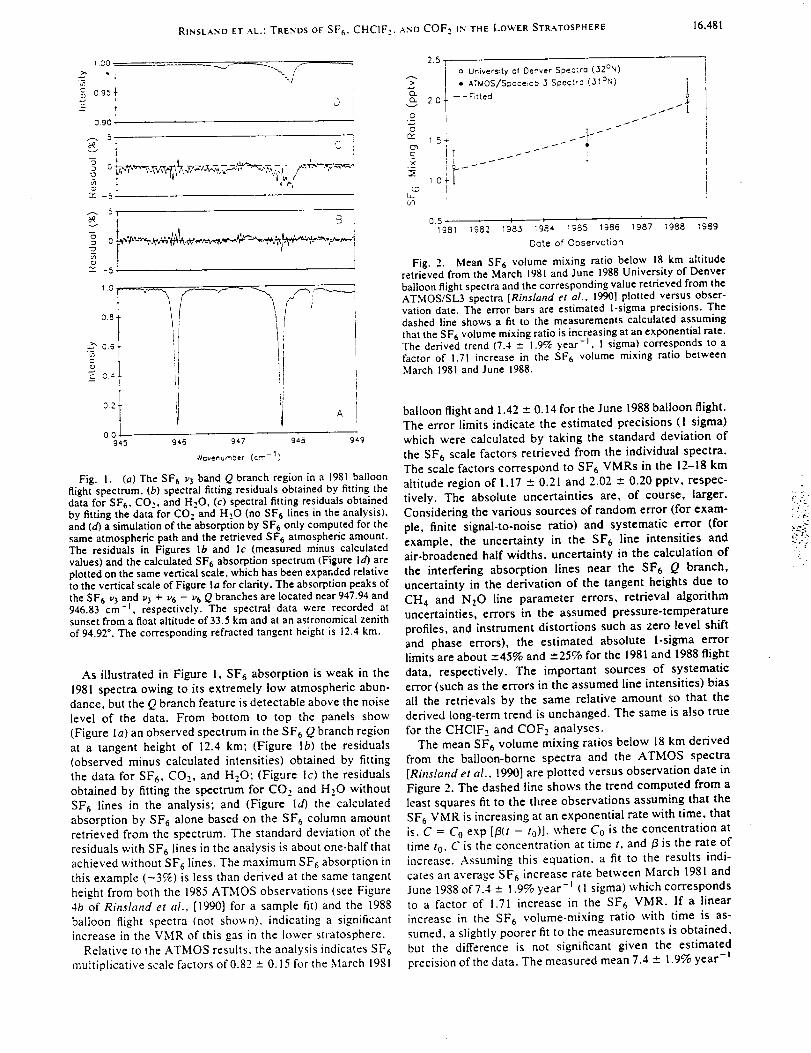
RINSLANO ET AL.: TRENDS OF SF6, CHCIF_.. A,_o COF: IN THE LOWER STRATOSPHERE 16.481

I

T

g o.95_-4

C t

0901

5-,j

N

-5

m

\j

o

; '3

-5

5_

t _ Ir

T

-_ I

- ! _,

02i A001

94-5 94"6 947 945 949

Wavemum_er (cm- 1

Fig. 1. (d) The SF6 v3 band Q branch region in a 1981balloonflight spectrum. (b) spectral fitting residuals obtained by fitting thedata for SF 6, CO,_, and H_,O, (c) spectral fitting residuals obtainedby fitting the data for CO_,and H,.O (no SF6 lines in the analysis),and (d) a simulation of the absorption by SF6 only computed for thesame atmospheric path and the retrieved SF 6 atmospheric amount.The residuals in Figures lb and lc (measured minus calculatedvalues) and the calculated SF6 absorption spectrum (Figure ld) areplotted on the same vertical scale, which has been expanded relativeto the vertical scale of Figure la for clarity. The absorption peaks ofthe SF6 v3 and v3 + v6 - v6 Q branches are located near 947.94 and946.83 cm -I, respectively. The spectral data were recorded atsunset from a float altitude of 33.5 km and at an astronomical zenithof 94.92*. The corresponding refracted tangent height is 12.4 kin.

As illustrated in Figure I, SF6 absorption is weak in the

1981 spectra owing to its extremely low atmospheric abun-dance, but the Q branch feature is detectable above the noiselevel of the data. From bottom to top the panels show

(Figure la) an observed spectrum in the SF 6 Q branch regionat a tangent height of 12.4 km; (Figure Ib) the residuals(observed minus calculated intensities) obtained by fittingthe data for SF 6, CO 2, and H20; (Figure Ic) the residualsobtained by fitting the spectrum for COz and H20 withoutSF 6 lines in the analysis; and (Figure ld) the calculatedabsorption by SF 6 alone based on the SF 6 column amountretrieved from the spectrum. The standard deviation of the

residuals with SF 6 lines in the analysis is about one-half thatachieved without SF 6 lines. The maximum SF 6 absorption inthis example (-3,C'/c) is less than derived at the same tangentheight from both the 1985 ATMOS observations (see Figure4b of Rinsland et al., [1990] for a sample fit) and the 1988

balloon flight spectra (not shown), indicating a significantincrease in the VMR of this gas in the lower stratosphere.

Relative to the ATMOS results, the analysis indicates SF 6

muttiplicative scale factors of 0.82 = 0.15 for the March 1981

2._-

o.

v

o

£3r'_

E

t.DJ_

2.0

T _

L

o University of Denver Spectra (320N)

• ATMOS/Spacelcb .3 Spectr_ (31 ON) !-- - Fitted

0.5 l 19183 i I1981 19'82 _984 _985 1986 1987 1988 1989

O_te of Observatlon

Fig. 2. Mean SF6 volume mixing ratio below 18 km altituderetrieved from the March 1981and June 1988University of Denverballoon flight spectra and the corresponding value retrieved from theATMOS/SL3 spectra [RinMand et ,_/., 1990]plotted versus obser-vation date. The error bars are estimated l-sigma precisions. Thedashed line shows a fit to the measurements calculated assumingthat the SF 6 volume mixing ratio is increasing at an exponential rate.The derived trend (7.4 _ 1.9% year -_ , l sigma) corresponds to afactor of 1.71 increase in the SF6 volume mixing ratio betweenMarch 1981 and June 1988.

balloon flight and 1.42 --- 0.14 for the June 1988 balloon flight.The error limits indicate the estimated precisions (I sigma)

which were calculated by taking the standard deviation of

the SF 6 scale factors retrieved from the individual spectra.The scale factors correspond to SF 6 VMRs in the 12-18 kmaltitude region of 1.17 - 0.21 and 2.02 _ 0.20 pptv, respec-tively. The absolute uncertainties are, of course, larger.Considering the various sources of random error (for exam-ple, finite signal-to-noise ratio) and systematic error (forexample, the uncertainty in the SF6 line intensities andair-broadened half widths, uncertainty in the calculation ofthe interfering absorption lines near the SF6 Q branch,

uncertainty in the derivation of the tangent heights due toCH_ and NzO line parameter errors, retrieval algorithmuncertainties, errors in the assumed pressure-temperature

profiles, and instrument distortions such as zero level shiftand phase errors), the estimated absolute l-sigma errorlimits are about --.45% and "--25% for the 1981 and 1988 flight

data, respectively. The important sources of systematicerror (such as the errors in the assumed line intensities) biasall the retrievals by the same relative amount so that thederived long-term trend is unchanged. The same is also true

for the CHCIF2 and COF., analyses.The mean SF6 volume mixing ratios below 18 km derived

from the balloon-borne spectra and the ATMOS spectra[Rinsland et al., 1990] are plotted versus observation date inFigure 2. The dashed line shows the trend computed from aleast squares fit to the three observations assuming that theSF 6 VMR is increasing at an exponential rate with time, thatis, C = C_ exp [_3(t - to)], where Co is the concentration attime t0. C is the concentration at time t, and/3 is the rate ofincrease. Assuming this equation, a fit to the results indi-cates an average SF 6 increase rate between March 1981 andJune 1988 of 7.4 - 1.9% year -_ (1 sigma) which correspondsto a factor of 1.71 increase in the SF 6 VMR. If a linear

increase in the SF 6 volume-mixing ratio with time is as-sumed, a slightly poorer fit to the measurements is obtained,but the difference is not significant given the estimated

precision of the data. The measured mean 7.4 ± 1.9% year -t

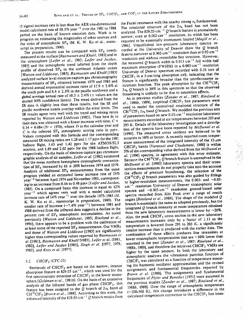
16.482 R1NSLAND ET AL.: TRENDS OF SF_, CHCIF,,

(1 sigma) increase rate is less than the AER one-dimensional

model calculated rate of 10.3% year -I over the 1981 to 1988

period on the basis of known emission data. Work is in

progress on estimating the magnitudes of other sources and

the sinks of atmospheric SF6 (M. K. W. Ko et al., manu-

script in preparation, 1990).

The present results can be compared with SF6 trends

measured at the surface [Rasmussen and Khalil, 1983] and in

the stratosphere [Leifer et al., 1982; Leifer and Juzdan,

1985] and the atmospheric trend inferred from the depth

profile of dissolved SF6 in the northeast Atlantic ocean

[Watson and Liddicoat, 1985]. Rasmussen and Khalil [1983]

analyzed surface level electron-capture gas chromatography

measurements of SF6 obtained between 1979 and 1983 and

derived annual exponential increase rates of 12.9 - 2.6% at

the south pole and 8.6 - 2.3% in the pacific northwest and a

global average annual rate of 10.5 ± 2.4% (-+ values are the

quoted 90% confidence limits). The trend derived from the

IR data is slightly less than these results, but the IR and

pacific northwest trends overlap within the error limits. The

IR results agree very well with the trend and mixing ratios

reported by Watson and Liddicoat [1985]. Their best fit to

their data was obtained with a linear increase with time, C =

0.34 + 0.084 (Yr - 1970), where Yr is the calendar year and

C is the inferred SF6 atmospheric mixing ratio in pptv.

Values computed with this formula and the corresponding

measured IR mixing ratios are 1.28 and 1.17 pptv for the 1981

balloon flight, 1.63 and 1.42 pptv for the ATMOS/SL3

mission, and 1.89 and 2.02 pptv for the 1988 balloon flight,

respectively. On the basis of electron capture gas chromato-

graphic analysis of air samples, Leifer et al. [1982] estimated

that the mean northern hemisphere stratospheric concentra-

tion of SF6 increased by 61 ± 20% beiween 1974 and 1979.

Analysis of additional SF6 measurements from the same

program yielded an estimated linear increase rate of 21%

year -I between April 1974 and November 1983, correspond-

ing to an increase from 0.16 to 0.48 pptv [Leifer andJuzdan,

1985]. On a compound basis this increase is equal to 12%

year -I which agrees very well with a model calculated

increase rate of 14% year -t over the decade 1973-1983 (M.

K. W. Ko et al., manuscript in preparation, 1990). The

smaller rate of increase (-7.4% year -s) between 1981 and

1988 derived from the infrared data suggests a decline in the

percent rate of SF6 atmospheric accumulation. As noted

previously [Watson and Liddicoat, 1985; Rinsland et al.,

1990], there appears to be a problem with the calibration of

at least some of the reported SF6 measurements. Our VMRs

and those of Watson and Liddicoat [1985] are significantly

higher than corresponding values reported by Rasmussen et

al. [1981], Rasmussen and Khalil [1983], Leifer et al. [1981,

1982], Leifer and Juzdan [1985], Singh et al. [1977, 1979,

1983], and Krey et al. [1977].

3.2. CHCIF2 (CFC-22)

Retrievals of CHCIF2 are based on the narrow, intense

absorption feature at 829.05 cm -I, which was used for the

first spectroscopic detection of CHCIF2 in the lower strato-

sphere [Goldman et al., 1981b]. On the basis of an extensive

analysis of the infrared bands of gas phase CHCIF2, thisfeature has been assigned to the Q branch of 2v6 band of

CH35ClF, [Brown et al., 1988]. According to this work, the

enhanced'intensity of the 829.05-cm-i Q branch results from

AND COF: IN THE LOWER STRATOSPHERE

the Fermi resonance with the nearby strong v4 fundamental.

The rotational structure of the 2v6 band has not been

analyzed. The 829.05-cm-I Q branch feature is anomalously

narrow; even at 0.002-cm -_ resolution, its width has been

reported to be essentially instrument limited [Magill et al.,

1986]. Unpublished low-pressure laboratory spectra re-

corded at the University of Denver show the Q branch

feature narrower at 0.002-cm -_ resolution than at 0.02-cm -I

resolution and without recordable fine structure. However,

the measured Q branch width is 0.013 cm -I full width half

maximum absorption (FWHM) in a 0.002-cm -I resolution

University of Denver spectrum recorded with 0.31 ton" of

CHClF2 in a 5-cm-long absorption cell, indicating that the

feature is significantly broader than the interferometer in-

strument function. The peak absorption by the CH35CIF2

2u6 Q branch is 30% in this spectrum so that the observed

broadening is unlikely to be due to saturation effects.

As in previous studies [Zander et al., 1987; Rinsland et

al., 1988b, 1989], empirical CHCIF2 line parameters were

used to model the unresolved rotational structure of the

CH3_CIF2 2v 6 band Q branch. We modified the previous sets

of parameters based on new 0.03-cm-I resolution laboratory

measurements recorded at six temperatures between 203 and

293 K. Details of the laboratory investigation and a descrip-

tion of the spectra have been reported by McDaniel et al.

[1990]. The measured cross sections are believed to be

accurate to 10% or better. A recently reported room temper-

ature measurement of the integrated intensity of the 12-v.m

CHCIF2 bands [Varanasi and Chudamani, 1988] is within

5% of the corresponding value derived from the McDaniel et

al. [1990] spectra, in agreement with this error estimate.

Because the CH35CIF. - Q branch feature is unresolved in the

McDaniel et al. [1990] laboratory spectra and their cross-

section measurements do not properly take into the account

the effects of pressure broadening, the selection of the

CH35CIF2 Q branch parameters was also guided by fittings

to higher-resolution measurements, the 0.003- and -0.02-

cm -I resolution University of Denver stratospheric solar

spectra and -0.005 -cm-I resolution ground-based solar

spectra recorded from Kitt Peak over a range of zenith

angles [Rinsland et al., 1989]. The shape of the modeled Q

branch is essentially the same as adopted previously, but the

integrated Q branch intensity at room temperature obtained

from the new laboratory measurements is lower by -20%.

Also, the peak CHCIF,_ cross section in the new laboratory

measurements increases only by a factor of 1.13 as the

temperature is lowered from 293 to 203 K. a significantly

smaller increase than is predicted with the earlier data. The

combination of these effects produces line intensities at

lower stratospheric temperatures that are --30% lower than

assumed in the past [Zander et al., 1987; Rinsland et al.,

1988b, 1989], and therefore the retrieved CHCIF2 VMRs are

higher by the same amount. In both the laboratory and

atmospheric analyses the vibrational partition function of

CHCIF, was calculated as a function of temperature assum-

ing the'harmonic oscillator approximation and the revised

assignments and fundamental frequencies reported by

Brown et al. [1988]. The assignments and fundamental

frequencies of Plyler and Benedict [1951] were assumed in

the previous studies [Zander et al., 1987; Rinsland et al.,

1988b, 1989]. Over the range of atmospheric temperature

(-200-300 K), this change introduces a difference in the

calculated temperature correction to the CHCIF2 line inten-

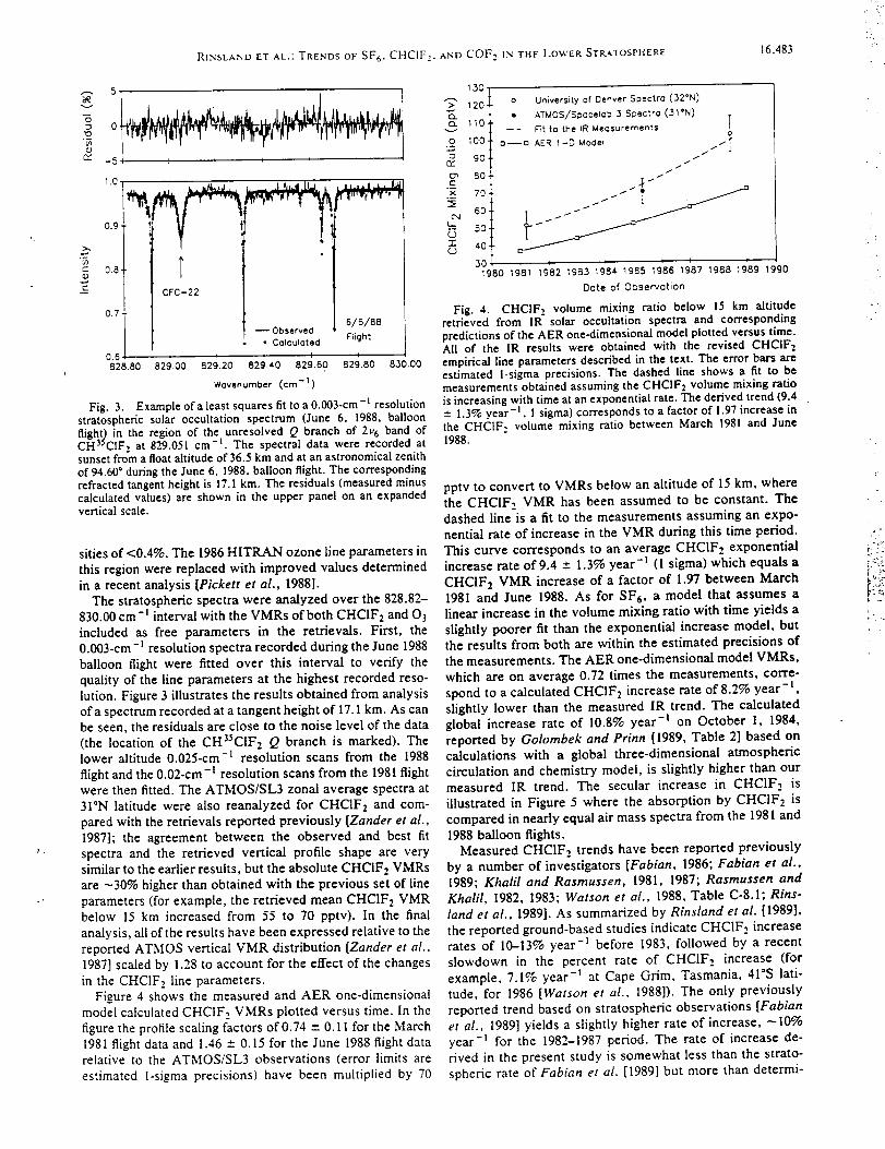
RH_SLAND ET AL.: TRENDS OF SF 6. CHCIF2, AND COF 2 IN THE LOWER STRATOSPHERE 16,483

.-, 5

v

-6

O

C

c"

0

-5

1.0

0.g.

0.8.

0.7.

0.6

828.80

I i t q q

TCFC-22

8/8/88_ Observed

• Calculated Flight

I I I I I

829.00 829.20 829.40 829.60 829,80 830.00

Wavenumber (am -1 )

Fig. 3. Example of a least squares fit to a 0.003-cm-1 resolutionstratospheric solar occultation spectrum (June 6, 1988, balloonflight) in the region of the unresolved Q branch of 2v 6 band ofCH35CIF, at 829.051 cm -L. The spectral data were recorded atsunset from a float altitude of 36.5 km and at an astronomical zenith

of 94.60 ° during the June 6. 1988, balloon flight. The correspondingrefracted tangent height is 17.1 kin. The residuals (measured minuscalculated values) are shown in the upper panel on an expandedvertical scale.

sities of <0.4%. The 1986 HITRAN ozone line parameters in

this region were replaced with improved values determined

in a recent analysis [Pickett et al., 1988].

The stratospheric spectra were analyzed over the 828.82-

830.00 cm-I interval with the VMRs of both CHC1F2 and 03

included as free parameters in the retrievals. First, the

0.003-cm-I resolution spectra recorded during the June 1988

balloon flight were fitted over this interval to verify the

quality of the line parameters at the highest recorded reso-

lution. Figure 3 illustrates the results obtained from analysis

of aspect rum recorded at a tangent height of 17.1 km. As can

be seen, the residuals are close to the noise level of the data

(the location of the CH35CIF2 Q branch is marked). The

lower altitude 0.025-cm -1 resolution scans from the 1988

flight and the 0.02-am-I resolution scans from the 1981 flight

were then fitted. The ATMOS/SL3 zonal average spectra at

31°N latitude were also reanalyzed for CHC1F_ and com-

pared with the retrievals reported previously [Zander et al.,

1987]; the agreement between the observed and best fit

spectra and the retrieved vertical profile shape are very

similar to the earlier results, but the absolute CHCIFz VMRs

are -30% higher than obtained with the previous set of line

parameters (for example, the retrieved mean CHClF_ VMR

below 15 km increased from 55 to 70 pptv). In the final

analysis, all of the results have been expressed relative to the

reported ATMOS vertical VMR distribution [Zander et al.,

1987] scaled by 1.28 to account for the effect of the changes

in the CHCIFz line parameters.

Figure 4 shows the measured and AER one-dimensional

model calculated CHCIF,_ VMRs plotted versus time. In the

figure the profile scaling factors of 0.74 "- 0.11 for the March1981 flight data and 1.46 ± 0.15 for the June 1988 flight data

relative to the ATMOS/SL3 observations (error limits are

estimated l-sigma precisions) have been multiplied by 70

130 I

o University of Denver Spectra (32°N)> 120

_. • ATMOS/Spacelab 3 Spectra (31'N)

Q. 110 Tv --- Fit to the IR Measurements

0 100 o--a AER _-0 Model I._ 1 1

o 90 -"£Y" //

cc_ 80 .T...--/"._ 70J _" "

u_. 50, "I°_O"1" 40,O

301980 19'81 19_82 1933 19t84 1985 I9_86 19_87 1988 lgq8g 1990

Date of Observation

Fig. 4. CHClF, volume mixing ratio below 15 km altituderetrieved from IR" solar occultation spectra and correspondingpredictions of the AER one-dimensional model plotted versus time.All of the IR results were obtained with the revised CHCIFzempirical line parameters described in the text. The error bars areestimated l-sigma precisions. The dashed line shows a fit to bemeasurements obtained assuming the CHCIF2 volume mixing ratiois increasing with time at an exponential rate. The derived trend (9.44" 1.3% year -I , 1 sigma) corresponds to a factor of 1.97 increase in

the CHCIF, volume mixing ratio between March 1981 and June1988.

pptv to convert to VMRs below an altitude of 15 kin, where

the CHCIF, VMR has been assumed to be constant. The

dashed line is a fit to the measurements assuming an expo-

nential rate of increase in the VMR during this time period.

This curve corresponds to an average CHCIFz exponential

increase rate of 9.4 ± 1.3% year -j (l sigma) which equals a

CHCIF 2 VMR increase of a factor of 1.97 between March

1981 and June 1988. As for SF6, a model that assumes a

linear increase in the volume mixing ratio with time yields a

slightly poorer fit than the exponential increase model, butthe results from both are within the estimated precisions of

the measurements. The AER one-dimensional model VMRs,

which are on average 0.72 times the measurements, corre-

spond to a calculated CHCIFz increase rate of 8.2% year- l,

slightly lower than the measured IR trend. The calculated

global increase rate of 10.8% year -t on October I, 1984,

reported by Golombek and Prinn [1989, Table 2] based on

calculations with a global three-dimensional atmospheric

circulation and chemistry model, is slightly higher than our

measured IR trend. The secular increase in CHCIF2 is

illustrated in Figure 5 where the absorption by CHCIF2 is

compared in nearly equal air mass spectra from the 1981 and

1988 balloon flights.

Measured CHC1F_. trends have been reported previously

by a number of investigators [Fabian, 1986; Fabian et al.,

1989; Khalil and Rasmussen, 1981, 1987; Rasmussen and

Khalil, 1982, 1983; Watson et al., 1988, Table C-8.1; Rins-

land et al., 1989]. As summarized by Rinsland et al. [1989],

the reported ground-based studies indicate CHCIF2 increase

rates of 10--13% year -l before 1983, followed by a recent

slowdown in the percent rate of CHCIF., increase (for

example, 7.1% year -I at Cape Grim, Tasmania, 41°S lati-

tude, for 1986 [Watson et al., 1988]). The only previously

reported trend based on stratospheric observations [Fabian

et al., 1989] yields a slightly higher rate of increase, -10%

year -t for the 1982-1987 period. The rate of increase de-

rived in the present study is somewhat less than the strato-

spheric rate of Fabian et al. [1989] but more than determi-

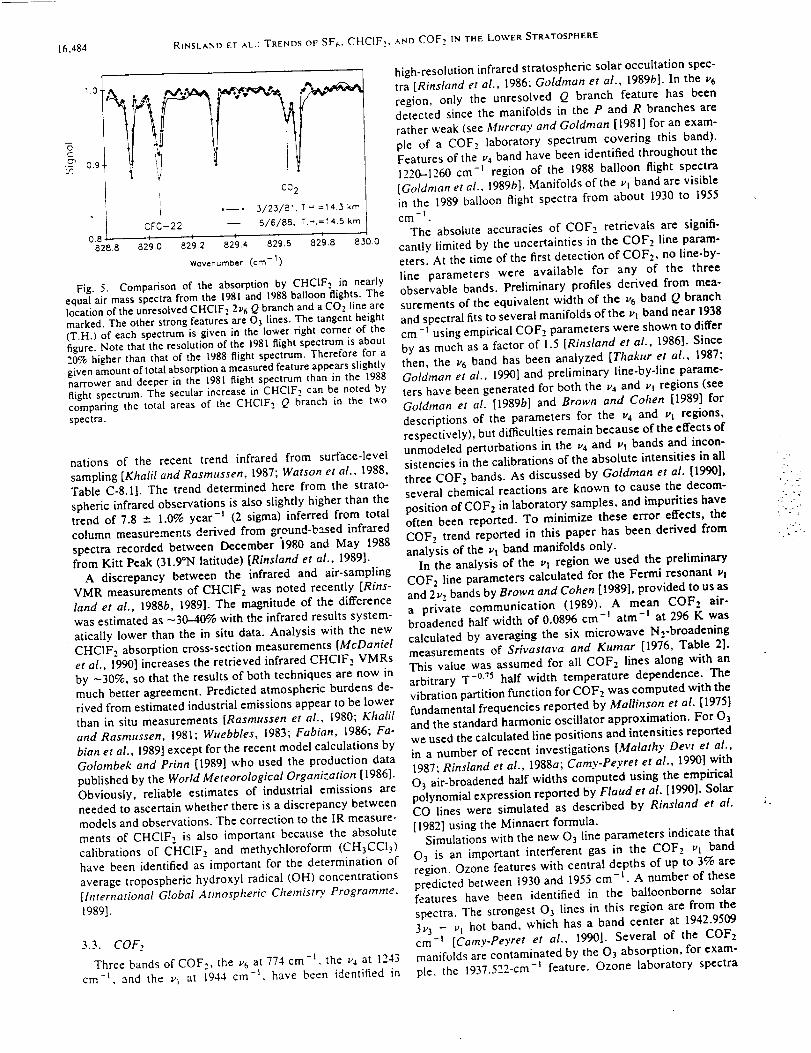
16,484

-6C

0.9+

828.8

RINSLAND ET AL.: TRENDS OF SF_, CHCIF2, AND COF2 IN THE LOWER STRATOSPHERE

CFC-22I ) I i

829.0 829.2 829.4 829.6 829.8 830.0

I tl 'llCO 2

I .--, 3/23/81.T._.=14.3 km6/6/88, T.H,=14.5 km

WGvenumber (cm -1 )

Fig. 5. Comparison of the absorption by CHCIF2 in nearlyequal air mass spectra from the 1981 and 1988 balloon flights. Thelocation of the unresolved CHCIF: 2_'6 Q branch and a CO,. line aremarked. The other strong features are O} lines. The tangent height(T.H.) of each spectrum is given in the lower right corner of the

figure. Note that the resolution of the 1981 flight spectrum is about20% higher than that of the 1988 flight spectrum. Therefore for a

given amount of total absorption a measured feature appears slightlynarrower and deeper in the 1981 flight spectrum than in the 1988

flight spectrum. The secular increase in CHCIF2 can be noted bycomparing the total areas of the CHCIF2 Q branch in the two

spectra.

nations of the recent trend infrared from surface-level

sampling [Khalil and Rasmussen, 1987; Watson et al., 1988,

Table C-8.1]. The trend determined here from the strato-

spheric infrared observations is also slightly higher than the

trend of 7.8 +- 1.0% year -l (2 sigma) inferred from total

column measurements derived from gr.eund-b=sed infrared

spectra recorded between December 1980 and May 1988

from Kitt Peak (31.9°N latitude) [Rinsland et at., 1989].

A discrepancy between the infrared and air-sampling

VMR measurements of CHCIF2 was noted recently [Rins-

land et al., 1988b, 1989]. The magnitude of the difference

was estimated as -30--40% with the infrared results system-

atically lower than the in situ data. Analysis with the new

CHCIF 2 absorption cross-section measurements [McDaniel

et al., 1990] increases the retrieved infrared CHCIF2 VMRs

by -30%, so that the results of both techniques are now in

much better agreement. Predicted atmospheric burdens de-

rived from estimated industrial emissions appear to be lower

than in situ measurements [Rasmussen et al., 1980; Khalil

and Rasmussen, 1981; Wuebbles, 1983; Fabian, 1986; Fa-

bian et at., 1989] except for the recent model calculations by

Golombek and Prinn [1989] who used the production data

published by the World Meteorological Organization [ 1986].

Obviously, reliable estimates of industrial emissions are

needed to ascertain whether there is a discrepancy between

models and observations. The correction to the IR measure-

ments of CHCIF, is also important because the absolute

calibrations of Ci-IC1F, and methychloroform (CH3CCI3)

have been identified as"important for the determination of

average tropospheric hydroxyl radical (OH) concentrations

[International Global Atmospheric Chemistry Programme,

1989].

3.3. COF,.

Three bands of COF,_, the v6 at 774 cm -I, the u4 at 1243

cm -t, and the v I at 1944 cm -I, have been identified in

high-resolution infrared stratospheric solar occultation spec-

tra [Rinsland et al., 1986; Goldman et al., 1989b]. In the v 6

region, only the unresolved Q branch feature has been

detected since the manifolds in the P and R branches are

rather weak (see Murcray and Goldman [1981] for an exam-

ple of a COF, laboratory spectrum covering this band).

Features of the u4 band have been identified throughout the

1220--1260 cm -I region of the 1988 balloon flight spectra

[Goldman etal., 1989b]. Manifolds of the ul band are visible

in the 1989 balloon flight spectra from about 1930 to 1955-I

cm .

The absolute accuracies of COF2 retrievals are signifi-

cantly limited by the uncertainties in the COF2 line param-

eters. At the time of the first detection of COF2, no line-by-

line parameters were available for any of the three

observable bands. Preliminary profiles derived from mea-

surements of the equivalent width of the v6 band Q branch

and spectral fits to several manifolds of the vl band near 1938

cm-i using empirical COFz parameters were shown to differ

by as much as a factor of 1.5 [Rinsland et al., 1986]. Since

then, the _'6 band has been analyzed [Thakur et al., 1987;

Goldman et al.. 1990] and preliminary line-by-line parame-

ters have been generated for both the v4 and _q regions (see

Goldman et al. [1989b] and Brown and Cohen [1989] for

descriptions of the parameters for the v4 and ut regions,

respectively), but difficulties remain because of the effects of

unmodeled perturbations in the v4 and vt bands and incon-

sistencies in the calibrations of the absolute intensities in all

three COFz bands. As discussed by Goldman et al. [1990],

several chemical reactions are known to cause the decom-

position of COF2 in laboratory samples, and impurities have

often been reported. To minimize these error effects, the

COF2 trend reported in this paper has been derived from

analysis of the vt band manifolds only.In the analysis of the vt region we used the preliminary

COF2 line parameters calculated for the Fermi resonant vl

and 2v, bands by Brown and Cohen [1989], provided to us as

a private communication (1989). A mean COFz air-

broadened half width of 0.0896 cm -1 at m-I at 296 K was

calculated by averaging the six microwave Nz-broadening

measurements of Srivastava and Kumar [1976, Table 2].

This value was assumed for all COF2 lines along with an

arbitrary T -°'75 half width temperature dependence. The

vibration partition function for COF, was computed with the

fundamental frequencies reported by Mallinson et al. [1975]

and the standard harmonic oscillator approximation. For O3

we used the calculated line positions and intensities reported

in a number of recent investigations [Malathy Devi et al.,

1987; Rinsland et al., 1988a; Camy-Peyret et al., 1990] with

O3 air-broadened half widths computed using the empirical

polynomial expression reported by Flaud et al. [1990]. Solar

CO lines were simulated as described by Rinsland et al.

[1982] using the Minnaert formula.Simulations with the new O3 line parameters indicate that

03 is an important intefferent gas in the COF2 vl band

region. Ozone features with central depths of up to 3% are

predicted between 1930 and 1955 cm -l. A number of these

features have been identified in the balloonborne solar

spectra. The strongest 03 lines in this region are from the

3v 3 - vt hot band, which has a band center at 1942.9509

cm -I [Camy-Peyret et al., 1990]. Several of the COFz

manifolds are contaminated by the 03 absorption, for exam-

ple, the 1937.522 -cm-_ feature. Ozone laboratory spectra

?.--

. °

_o

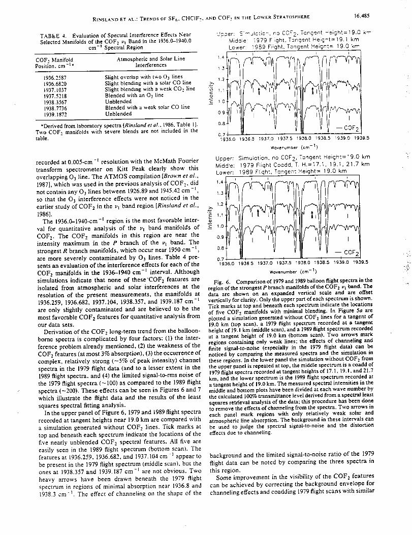
RINSLAND ET AL.: TRENDS OF SF_, CHCIF2. AND COF 2 IN THE LOWER STRATOSPHERE 16,485

TABEE 4. Evaluation of Spectral Interference Effects Near

Selected Manifolds of the COF, vl Band in the 1936.0--1940.0cm- 1 Spectral Region

COF., Manifold Atmospheric and Solar LinePosition, cm -1, Interferences

1936.25871936.68201937.10371937.52181938.35671938.77361939.1872

Slight overlap with two O3 linesSlight blending with a solar CO line >,Slight blending with a _veak CO, line 7,

=Blended with an 03 line oUnblended _

Blended with a weak solar CO lineUnblended

*Derived from laboratory spectra [Rinsland etal.. 1986. Table I].Two COFz manifolds with severe blends are not included in thetable.

recorded at 0.005-cm-t resolution with the McMath Fourier

transform spectrometer on Kitt Peak clearly show this

overlapping 0 3 line. The ATMOS compilation [Brown et al.,

1987], which was used in the previous analysis of COF,_, did

not contain any 03 lines between 1926.89 and 1945.42 cm-I,

so that the 03 interference effects were not noticed in the

earlier study of COFz in the v I band region [Rinsland et al.,

1986].

The 1936.0-1940-cm -t region is the most favorable inter-

val for quantitative analysis of the vl band manifolds of

COFz. The COFz manifolds in this region are near the

intensity maximum in the P branch of the vl band. The

strongest R br.anch manifolds, which occur near 1950 cm -l ,

are more severely contaminated by 03 lines. Table 4 pre-

sents an evaluation of the interference effects for each of the

COFz manifolds in the 1936--1940 cm -I interval. Although

simulations indicate that none of these'COFx features are

isolated from atmospheric and solar interferences at the

resolution of the present measurements, the manifolds at

1936.259, 1936.682, 1937.104, 1938.357, and 1939.187 cm -1

are only slightly contaminated and are believed to be the

most favorable COFz features for quantitative analysis from

our data sets.

Derivation of the COF z long-term trend from the balloon-

borne spectra is complicated by four factors: (1) the inter-

ference problem already mentioned, (2) the weakness of the

COFx features (at most 3% absorption), (3) the occurrence of

complex, relatively strong (-5% of peak intensity) channel

spectra in the 1979 flight data (and to a lesser extent in the

1989 flight spectra, and (4) the limited signal-to-rms noise of

the 1979 flight spectra (-100) as compared to the 1989 flight

spectra (-200). These effects can be seen in Figures 6 and 7

which illustrate the flight data and the results of the least

squares spectral fitting analysis.

In the upper panel of Figure 6, 1979 and 1989 flight spectra

recorded at tangent heights near 19.0 km are compared with

a simulation generated without COF2 lines. Tick marks at

top and beneath each spectrum indicate the locations of the

five nearly unblended COF 2 spectral features. All five are

easily seen in the 1989 flight spectrum (bottom scan). Thefeatures at 1936.259, 1936.682, and 1937.104 cm-I appear to

be present in the 1979 flight spectrum (middle scan), but theones at 1938.357 and 1939.187 cm -t are not obvious. Two

heavy arrows have been drawn beneath the 1979 flight

spectrum in regions of minimal absorption near 1936.8 and1938.3 cm-I. The effect of channeling on the shape of the

brpper: Simulc_.]cn, ro CO-"2. Tcngent He;ght=19.0 kmMiddle: 1979 Flight, Tangent Height=19.1 kmLower: !989 Fiight, Tangent Height= 19.0 km

Upper:Midd!e:Lower:

1936.5 1937.0 1937.5 1938.0 1938.5 1939.0 19,:39.5

Wovenumber (cm- I)

Simufotion, no COF 2, Tongent Height= 19.0 km1979 Flight Coodd, T. H.=17.1, 19.1, 21.7 km

1989 Flight, Tongent Height= 19.0 km

1.3

_>" 1.2

"_ 1.1 I

E 1.o N_ Io.g

0.8

0.7 . , I Z COF'

1936.0 1936.5 1937.0 1937.5 1938.0 1938.5 1939.0 1939.5

Wovenurnber (crn- 1)

Fig. 6. Comparison of 1979 and 1989 balloon flight spectra in theregion of the strongest P branch manifolds of the COF 2 Vl band. Thedata are shown on an expanded vertical scale and are offsetvertically for clarity. Only the upper part of each spectrum is shown.Tick marks at top and beneath each spectrum indicate the locationsof five COF, manifolds with minimal blending. In Figure 5a are

plotted a simulation generated without COF__ lines for a tangent of19.0 km (top scan), a 1979 flight spectrum recorded at a tangent

height of 19.1 km (middle scan), and a 1989 flight spectrum recordedat a tangent height of 19.0 km (bottom scan). Two arrows markregions containing only weak lines; the effects of channeling andfinite signal-to-noise (especially in the 1979 flight data) can benoticed by comparing the measured spectra and the simulation inthese regions. In the lower panel the simulation without COFz fromthe upper panel is repeated at top, the middle spectrum is a coadd of1979 flight spectra recorded at tangent heights of 17.1, 19. i, and 21.7km, and the lower spectrum is the 1989 flight spectrum recorded at

a tangent height of 19.0 kin. The measured spectral intensities in themiddle and bottom plots have been divided at each wave number bythe calculated 100% transmittance level derived from a spectral least

squares retrieval analysis of the data; this procedure has been doneto remove the effects of channeling from the spectra. Two arrows in

each panel mark regions with only relatively weak solar andatmospheric line absorption. The background in these intervals canbe used to judge the spectral signal-to-noise and the distortioneffects due to channeling.

background and the limited signal-to-noise ratio of the 1979

flight data can be noted by comparing the three spectra in

this region.Some improvement in the visibility of the COF2 features

can be achieved by correcting the background envelope for

channeling effects and coadding 1979 flight scans with similar

16.486 RINSLAND ET AL.: TRENDS OF SFr, CHCIF:, A_D COF, IN THE LOWER STRATOSPHERE

o0

EQ)

r"

_,L

09

O.B

07

O6

1936.0 1936.5

• COF 2

1937.0 1937.5 1938.0 1938.5 1939.0 19.39.5

Wavenumber (crn- I)

Fig. 7. Example of a least squares fit in the region of the COFzvl band. The lower panel shows the measured spectrum (solid line)and the least squares best fit calculated spectrum (open diamonds).The measured spectrum has been normalized to the highest mea-sured intensity in the interval; only the upper 40% of the spectra are

plotted. Solid triangles beneath the spectrum mark the location ofthe five nearly unblended COF2 manifolds. The upper panel showsthe residuals (observed minus calculated) on an expanded verticalscale. The measured spectrum was recorded during the 1989 balloon

flight from a float altitude of 32.8 - 0.5 kin. The astronomical zenithangle and the refracted tangent height of the spectrum are 94.08* and21.1 km, respectively. The standard deviation of the fit is 0.74%,close to the noise level in the spectrum.

zenith angles to improve the signal-to'noise. In the lower

panel of Figure 6, reprocessed spectra from the 1979 and

1989 flights are compared with the same spectral simulation

as shown in the upper panel. Each measured spectrum has

been divided by the calculated 100% transmission curve

determined from the spectral least squares retrieval analysis

of the data. Note that the background in the two regions

indicated by heavy arrows is now nearly flat, as in the

simulation• The channeling correction has preserved the fine

spectral structure, as can be seen for example by comparing

the weak lines near 1936.9 cm -t in the 1979 flight spectrum

with the features in the simulation. The 1979 flight spectrum

was produced by coadding spectra recorded at tangent

heights of 17.1, 19.1, and 21.7 km. The signal-to-noise of the

coadded spectrum is improved, although it is still less than

the signal-to-noise of the 1989 flight spectrum at bottom•

Except for the COF2 feature at 1938.357 cm -I , the marked

COF, manifolds appear to be present in the coadded 1979

flight'spectrum, but their absorption depths are consistently

less than measured in the 1989 flight data. Furthermore,

recall that the resolution of the 1979 flight spectra is a factor

of -1.25 higher that the low-resolution spectra from the 1989

flight, so that features of a given absorption strength should

appear narrower and deeper in the 1979 data than in the 1989data. On the basis of these considerations, the balloon flight

measurements indicate a substantial increase in the amount

of COF, in the lower stratosphere between 1979 and 1989.

As for SF6 and CHCIF2, the COF2 retrievals were refer-

enced to an appropriate ATMOS/SL3 profile. First, the

ATMOS analysis was checked by retrieving a COF., profile

from the ATMOS zonal average sunset spectra (30°N lati-

o University of Denver Spectra (-32 °N)

c I.SE ,, ATMOS/SL3 Spectra (3D'N)

"_ 1.4 --- Fit to ttae )R Measurements I

¢'J 1,2 u--u AER 1-D model

0 1.0- i...,._ _ _

.._ 0.8,

o

.__ 0.6 T _

i 10Z 0.2

0.0 i , , I i '1979 1980 19q81 19 )82 1983 1984 1985 1986 1987 1988 19'89 1990

Dote of Observation

Fig. 8. Comparison between measured and AER one-dimen-sional model calculated trends in lower stratospheric COFz. Totalcolumns derived from the October 1979 and April 1989 University ofDenver balloon flight spectra have been normalized to the totalcolumn calculated for the same ray path assuming a profile retrievedfrom the ATMOS/SL3 zonal average filter 2 spectra (30*N latitude,May 1985) [Rinsland et al., 1986]. The error bars are estimatedl-sigma precisions. The dashed line shows a fit to the measurementsobtained with a model that assumes the COF2 volume mixing ratio

is increasing with time at an exponential rate. The derived trend(10.3 - 1.8% year -I, 1 sigma) corresponds to a factor of 2.67increase in the COFz volume mixing ratio between October 1979

and April 1989. The AER one-dimensional model columns havebeen normalized to a value calculated for the date of the SL3

mission.

tude) using the new set of line parameters and comparing the

retrieved profile with the published profile derived from the

same spectral region [Rinsland et al., 1986, Figure 3, heavy

full line). The two profiles agree within 5% below an altitude

of 38 kin. Then, assuming the published ATMOS vertical

VMR distribution (Table 2), each balloon flight spectrum

was analyzed to retrieve a single multiplicative COF2 profile

scaling factor. The gas amounts of COx and NO were also

fitted along with parameters to model the solar CO absorp-

tion lines, the background, channel spectra, and the effective

instrument line shape• The COFz scale factors from the three

analyzed spectra from the 1979 flight (tangent heights of

17.1, 1911, and 21.7 km) were averaged and the standard

deviation was computed to derive a scale factor of 0.44 ±

0.17 (1 sigma). The same procedure was used to analyze the

1989 flight spectra. A COF2 scale factor of 1.21 +-- 0.24 (1

sigma) was derived from fitting five spectra with tangent

heights between 19.0 and 22.6 kin. Figure 7 presents an

example of the least-squares fitting results obtained from the

1989 flight spectra.

Figure 8 shows the measured and AER one-dimensional

model calculated COF, plotted versus time. The dashed line

is a fit to the measurements assuming that the concentrations

of COF, are increasing at an exponential rate. The fitted

curve corresponds to an average COF2 increase rate of 10.3

± l•8%.year -1 (1 sigma) which is equal to a factor of 2.67

increase over the 9.5-year period (October 1979 to April

1989). Referenced to a base altitude of 18.0 kin, the fitted

curve corresponds to an increase in the COF, total vertical

column from 0.43 x 1014 to 1.20 x 1014 molecules cm -2

over the observation period. The measured increase rate

10.3 --- 1.8% year -I (l sigma) is slightly higher than the AER

one-dimensional model calculated rate of 8.3% year -t for

the same time interval. No other measured or model calcu-

lated COF_, trends have been reported.

-. {

..:.

!i£a,":

RINSLAND E'r AL.: TRENDS OF SF6, CHCIF:.._ND COF., tN THE LOWER STRATOSPHERE16,487

1.00 i

t095 I

o,oI 83.20" Zenith J.r_g• H20 ]

0,85 I1936.14 _ 836.22 _g_S30

u_

_5C

1.00, -_

O.g5

090 i _ '

1233.9 12340 12_4.1 123a,.2 12343 1214.4 12_4.5 ' 23(.6

Wovenurnber (cm- i

Fig. 9. Spectral features of the COF 2 vt and v 4 bands in0.0053-cm -t resolution solar spectra recorded with the McMathFourier transform spectrometer and main solar telescope operated

by the National Solar Observatory on Kitt Peak near Tucson,Arizona. The upper panel shows the v t band manifold at 1936.259cm -I in a spectrum recorded at a mean solar astronomical zenithangle of 83.20 ° on the afternoon of November 29, 1988 (bottomcurve), and simulations generated for the same spectral resolutionand atmospheric ray path (upper two curves). The simulation arecalculations of COFz absorption only (top spectrum) and the ab-sorption by all gases except COF_ (middle spectrum). The tick markbeneath the measured spectrum marks the location of the COF,

absorption peak as determined from the spectrum at top. The threespectra are offset vertically for clarity. The lower panel presents asimulation of the absorption by all gases except COF_ (upper curveland a Kitt Peak solar spectrum recorded at a mean solar astronom-ical zenith angle of 75.46" on the morning of December !, 1988(lower curve). The two spectra are offset vertically for clarity. Solidtriangles beneath the measured spectrum indicate the positions ofstrong COFz absorption features determined from line center mea-surements on a 0.003-cm -I resolution laboratory spectrum of

COF2. The strong features at 1234.226 and 1234.315 cm -I areJ3CH4 and 16OI2CIsO lines, respectively. Weak lines of O3 and

N20 have also been identified in this spectral region.

In the future it should be possible to derive the trend in the

COF2 total column from analysis of high-resolution ground-

based solar spectra. As illustrated in Figure 9, the strong

COF2 v) and *'4 band features can be seen from Kitt Peak,

but they appear as very weak absorptions. High air mass,

high signal-to-noise measurements at resolutions greater

than 0.01 cm -l are required. Care must also be taken to

avoid interferences, especially O3 lines, which are visible in

both spectral regions as narrow features, very similar in

appearance to the COF., absorptions. Because atmospheric

transmission in the COF2 vl band region is strongly attenu-

ated by tropospheric water vapor absorption, any long-term,

ground-based COF2 measurement prom-am based on mea-

surements of the vl band manifolds will require observations

from dry, high-altitude sites. Observations such as the one

illustrated in the upper panel of Figure 9 are seldom possible

from Kitt Peak at an altitude of 2.1 km. At present, too few

high-quality atmospheric observations of the COF_, vl band

manifolds have been recorded from Kitt Peak to measure a

reliable long-term COF, trend. Observations in the v4 band

region are potentially more useful since regions less affected

by H,O can be selected, but accurate COF., total column

measurements are not currently possible because of the

absence of COFz line parameters in the 1230-1235 cm -t

region which is the best for ground-based remote sensing.

The COF., vl and v4 band features have also been identified

in high-resolution solar spectra recorded from the Jungfrau-

joch station at an altitude of 3.58 km (R. Zander, private

communication. 1990).

4. SUMMARY AND CONCLUSIONS

Long-term trends in the lower stratospheric concentra-

tions of three trace constituents have been derived from

analysis of high resolution infrared solar occulation spectra

recorded between 1979 and 1989. The derived average rates

of increase are large, 7.4% - 1.9% year -1 for SF 6, 9.4% ±

1.3% year -I for CHCIF,., and 10.3 _ i.8% year -I for COF2

(1 sigma), and in reasonable agreement with model results.

The observed increases illustrate the rapid changes that are

taking place in the composition of our upper atmosphere.

The derived trends of SF6 and CHCIF2 are in generally good

agreement with the limited number of previously reported

stratospheric trend measurements. The COF,. trend mea-

surements and model calculations are the first such results

reported for this molecule. Both SF 6 and CHCIF2 are

expected to be well mixed in the upper troposphere and

lower stratosphere and thus will exhibit little seasonal or

spatial variation. There are, however, significant variations

in our calculated model distributions of COF2. Hence more

frequent measurements are needed to further quantify its

temporal trend.Over the decade of these observations, the IR absorptions

of SF 6 and COFz increased from only slightly above the limit

of detection to features that are readily observable (for

example, Figures 5 and 6). For this reason, these gases were

only recently identified. On the basis of these studies it was

then possible to identify and quantitatively analyze these

features in the earlier data sets. In the future, as other gases

increase in abundance as the result of anthropogenic emis-

sions, similar cases will occur so that these early IR data sets

are likely to provide valuable information on the trends of

molecules not yet readily observable. Comparisons of time

series of spectra in the 8-13 /xm atmospheric window may

also be useful in accessing of changes in the opacity of this

climatically important spectral region.

As demonstrated by this investigation, the systematic

analysis of a time series of infrared solar occultation spectra

can yield significant new information about the trends of

stratospheric gases. The data are precise since no absolute

radiance calibration is required, and temperature uncertain-

ties and the attenuation by broad features (for example,

aerosols and continua) are unimportant if appropriate fea-

tures are selected for analysis. However, it is important to

use consistent retrieval methods and consistent spectro-

scopic linelists to minimize systematic error effects. Because

of the sensitivity and broad spectral coverage capabilities of

high-resolution solar occultation measurements, many spe-

cies encompassing a wide range in concentration are re-

corded simultaneously so that a comprehensive analysis of

chemical families in such data sets can provide a unique

opportunity to study the time history of the chemistry

related to the catalytic destruction of stratospheric ozone.

16,488 RINSLAND ET AL.: TRENDS OF SF 6, CHCIF,, AND COF 2 ty THE LOWER STRATOSPHERE

Acknowledgments. Research at the University of Denver was

supported by NASA and NSF. Acknowledgment is made to theNational Center for Atmospheric Research, which is supported byNSF, for computer time used in this research. Research at NCAR

was supported by the NASA UARS program under contractS-10782-C. We are grateful to Linda R. Brown of the Jet PropulsionLaboratory for sending us the CH4 and COF2 line parameters usedin the analysis. The authors also thank B. Bobin of the Laboratoirede Spectronomie Mol_culaire et Instrumentation Laser, Dijon,France, for sending the calculated line parameters for the SF 6 v3band, and Carolyn Sutton of the STX Corporation for assistance in

processing the spectral data at NASA Langley.

REFERENCES

Bobin, B., C. J. Bord_, J. Bordr, and C. BrYant, Vibration-rotationmolecular constants for the ground and (v3 = I) states of _2SF6from saturated absorption spectroscopy, J. Mol. Spectrosc., 121,

91-127, 1987.Brown, J. A., Sulfur hexafluoride, in Kirk-Othmer Encyclopedia of

Chemical Technology, 2nd ed., pp. 664--671, J. Wiley, New York,

1966.Brown, J. A., D. C. McKean, and J. L. Duncan, Vibrational

anharmonicity and Fermi resonances in CHFzCI, Spectrochim.

Acta, Part A, 44, 553-565, 1988.Brown, L. R., and E. A. Cohen, Assignment of the vl and 2v 2 bands

of COF, at 5.2 ore, paper RE7 presented at 44th Symposium onMolecular Spectroscopy, Ohio State Univ., Columbus, June12-16, 1989.

Brown, L. R., C. B. Farmer, C. P. Rinsland, and R. A. Toth,Molecular line parameters for the atmospheric trace moleculespectroscopy experiment, Appl. Opt., 26, 5154--5182, 1987.

Brown, L. R., M. Loete, and J. C. Hilico, Linestrengths of the v zand v4 bands of t2CH4 and 13CH4, J. Mol. Spectrosc., I33,273-311, 1989.

Buijs, H. L., G. L. Vail, G. Tremblay, and D. J. W. Kendall,Simultaneous measurement of the volume mixing ratios of HCIand HF in the stratosphere, Geophys. Res. Lett., 7, 205-208,1980.

Camy-Peyret, C., J.-M. Flaud, L. Delbouille, G. Roland, J. W.Brault, and L. Testerman, Quadrupole transitions of the 1 _ 0

band of N2 observed in a high resolution atmospheric spectrum,J. Phys., 42, L279---L283, 1981.

Camy-Peyret, C., J.-M. Flaud, C. P. Rinsland, V. Malathy Devi,M. A. H. Smith, and A. Goldman, Line parameters for ozone hot

bands in the 4.8-ta.m spectral region, J. Mol. Spectrosc., 139,353-360, 1990.

Champion, J. P., J. C. Hilico, and L. R. Brown, The vibrationalground state of 12CH4 and 13CH4, J. Mol. Spectrosc., 133,244-255, 1989a.

Champion, J. P., J. C. Hilico C. Wenger, and L. R. Brown,Analysis of the v21v4 dyad of IzCH4 and 3CH4, J. Mol. Spec-trosc., 133,256-272, 1989b.

Drivas, P. J., and F. H. Shair, A tracer study of pollutant transportand dispersion in the Los Angeles area, Atmos. Environ., 8,1155-1163, 1974.

Fabian, P., Halogenated hydrocarbons in the atmosphere, in Hand-

book of Environmental Chemistry, vol. 4, part A, edited by O.Hutzinger, pp. 24-51, Springer-Verlag, New York, 1986.

Fabian, P., R. Borchers, H. Duscha, B. C. KrOger, S. Lal, andB. H. Subbaraya, CHC1F2 (CFC-22): Distribution, budget andenvironmental impact, in Ozone in the Atmosphere, edited by R.D. Bojkov and P. Fabian, pp. 294-297, A. Deepak, Hampton,Va., 1989.

Farmer, C. B., High resolution infrared spectroscopy of the sun andthe Earth's atmosphere from space, Mikrochim. Acta [Wien], 3,

189-214, 1987.Fisher, D. A., C. H. Hales, W.-C. Wang, M. K. W. Ko, and N. D.

Sze, Model calculations of the relative effects of CFCs and their

replacements on global warming, Nature, 344, 513-516, 1990.Flaud, J.-M., C. Camy-Peyret, C. P. Rinsland, M. A. H. Smith. and

V. Malathy Devi, Line parameters for 1603 bands in the 7-_tm

region, J. Mol. Spectros., 134, 106-112, 1989.Flaud, J.-M., C. Camy-Peyret, C. P. Rinsland, V. Malathy Devi,

M. A. H. Smith, and A. Goldman, Improved line parameters forozone bands in the 10-_m spectral region, Appl. Opt., in press,1990.

Gamlen, P. H., B. C. Lane, P. M. Midgley, and J. M. Steed, The

production and release to the atmosphere of CC13F and CCIzFz(chlorofluorocarbons CFC 11 and CFC 12), Atmos. Environ, 20,1077-1085. 1986.

Goldan, P. D., W. C. Kuster, D. L. Albritten, and A. L. Schmelt-

ekopf, Stratospheric CFCI3, CF2CI=, and N20 height profilemeasurements at several latitudes, J. Geophys. Res., 85,413--423,

1980.Goldman, A., and R. S. Saunders, Analysis of atmospheric infrared

spectra for altitude distribution of atmospheric trace constitu-ents-l. Method of analysis, J. Quant. Spectrosc. Radiat. Transfer,

21, 155-161, 1979.Goldman, A., T. G. Kyle, D. G. Murcray, F. H. Murcray, and W.

J. Williams, Long path atmospheric ozone absorption in the

9-10-# region observed from a balloon-borne spectrometer, Appl.Opt., 9, 565-580, 1970.

Goldman, A., D. G. Murcray, F. J. Murcray, G. R. Cook, J. W. Van

Allen, F. S. Bonomo, and R. D. Blatherwick, Identification of the

v3 vibration-rotation band of CF4 in balloon-borne infrared solarspectra, Geophys. Res. Lett., 6,609-612, 1979.

Goldman, A., D. G. Murcray, F. J. Murcray, and E. Niple, Highresolution IR balloon-borne solar spectra and laboratory spectra

in the HNO3 1720-cm -_ region: An analysis, Appl. Opt., 19,3721-3724, 1980.

Goldman, A., J. Reid, and L. S. Rothman, Identification of electric

quadrupole Oz and N2 lines in the infrared atmospheric absorp-tion spectrum due to the vibration-rotation fundamentals, Geo-

phys. Res. Lett., 8, 77-78, 1981a.Goldman, A., F. J. Murcray, R. D. Blatherwick, F. S. Bonomo,

F. H. Murcray, and D. G. Murcray, Spectroscopic identification

of CHCIF 2 (F-22) in the lower stratosphere, Geophys. Res. Lett.,8, 1012-1014, 1981b.

Goldman, A., R. D. Blatherwick, F. J. Murcray, J. W. VanAllen,

F. H. Murcray, and D. G. Murcray, New Atlas of StratosphericIR Absorption Spectra, vol. I, Line Positions and Identifications,Department of Physics, University of Denver, Denver, Colo.,1987.

Goldman, A., R. D. Blatherwick, J. J. Kosters, F. J. Murcray, J. W.VanAllen, F. H. Murcray, and D. G. Murcray, Atlas of Very HighResolution Stratospheric IR Absorption Spectra, preliminaryedition, Department of Physics, University of Denver, Denver,

Colo., 1989a.Goldman, A., F. J. Murcray, R. D. Blatherwick, J. J. Rosters, F. H.

Murcray, D. G. Murcray, and C. P. Rinsland, New spectralfeatures of stratospheric trace gases identified from high resolu-tion infrared balloon-borne and laboratory spectra, J. Geophys.

Res., 94, 14,945-14,955, 1989b.Goldman, A., C. P. Rinsland, R. D. Blather'wick, and F. S.

Bonomo, Spectroscopic line parameters for the v6 band of car-

bonyl fluoride (COFz), Appl. Opt., 29, 1860-1863, 1990.Golombek, A., and R. G. Prinn, Global three-dimensional model

calculations of the budgets and present-day atmosphere lifetimesof CFzCICFCI2 (CFC-113) and CHCIF2 (CFC-22), Geophys. Res.Lett., 16, 1153-1156, 1989.

Gunson, M. R., C. B. Farmer, R. H. Norton, R. Zander, C. P.Rinsland, J. Shaw, and B.-C. Gap, Measurements of CH4, N20,

CO, H20 and O3 in the middle atmosphere by the ATMOSexperiment on Spacelab 3. J. Geophys. Res., in press, 1990.

Hammitt, J. K., F. Carom, P. S. Connell, W. E. Mooz, K. A. Wolf,D. J. Wuebbles, and A. Bamezai, Future emission scenarios forchemicals that may deplete stratospheric ozone, Nature, 330,

711-716, 1987.International Global Atmospheric Chemistry Programme, A Core

Project of the International Geosphere-Biosphere Programme,edited by I. E. Galbally, p. 38, IAMAP Commission on Atmo-spheric Chemistry and Global Pollution, Renwick Pride Pry,

Albury, New Zealand, 1989.Jayanty, R. K. M., R. Simonaitis, and J. Heicklen, The photolysis of

chlorofluoromethanes in the presence of O2 or O3 at 213.9 nm andtheir reactions with O(ID), J. Photochem., 4, 381-398, 1975.

Jones, R. L., and J. A. Pyle, Observations of CH4 and N20 by theNIMBUS 7 SAMS: A comparison with in situ data and two-dimensional numerical model calculations, J. Geophys. Res., 89,

5263-5279, 1984.Khalil, M. A. K., and R. A. Rasmussen, Increase of CHCIF2 in the

Earth's atmosphere, Nature, 292,823-824, 1981.

;

RINSI._.ND ET AL.: TRENDS OF" SF_, CHCIF2.

Khalil,'M. A. K., and R. A, Rasmussen, Chlorocarbons in the

southern hemisphere: Concentrations and temporal trends, in

Baseline Atmospheric Program (Australia) 1985, edited by B. W.

Forgan and P. J. Fraser, pp. 26--29, Department of Science/

Bureau of Meteorology, Australia, 1987.

Krey, P. W., R. J. Lagomarsino, and L. E. Toonkel. Gaseous

halogens in the atmosphere in 1975, J. Geophys. Res., 82,

1753-1766, 1977.

Leifer, R., and R. Juzdan, Measurements of CCI3F, CCI2F.,, CC14,

N,O and SF 6 in the northern hemisphere stratosphere, in Inter-national Council of Scientific Unions Handbook for MAP, vol. 18,

Extended Abstracts, edited by S. Kato, pp. 355-358, Special

Committee for Solar-Terrestrial Physics Secretariat at University

of Illinois, Urbana, 111., 1985. (Available as N86-27795 from the

Natl. Tech. Inf. Serv., Springfield, Va.)

Leifer, R., K. Sommers, and S. F. Guggenheim. Atmospheric trace

gas measurements with a new clean air sampling system, Geo-

phys. Res. Lett., 8, 1079-1081, 1981.Leifer, R., R. Larsen, and L. Toonkel, Trends in stratospheric

concentrations of trace gases in the northern hemisphere during

the years 1974-1979, Geophys. Res. Left., 9, 755-758, 1982.

Magill, J. V., K. M. Gough, and W. F. Murphy, The vibrational

spectrum and normal coordinate analysis of chlorodifluo-romethane, CHCIF2, Spectrochim. Acta, Part A, 42a, 705-715,

1986.

Malathy Devi, V., J.-M. Flaud, C. Camy-Peyret, C. P. Rinsland,and M. A. H. Smith, Line positions and intensities for the vl + _',.

and vz_ + u3 bands of 160 3, J. Mol. Spectrosc., 125, 174-183.

1987.Mallinson, P. D., D. C. McKean, J. H. Holloway, and I. A. Oxton,

Infrared spectra of carbonyl fluorides and general harmonic force

field, Spectrochim. Acta, Part A, 31a, 143-159, 1975.

McDaniel, A. H., C. A. Cantrell, J. A. Davidson, R. E. Shetter, and

J. G. Calvert, The temperature dependent, infrared absorptioncross sections for the chlorofluorocarbons: CFC-II, CFC-12,

CFC-13, CFC-14, CFC-22, CFC-II3, CFC-114, and CFC-115,

Atmos. Chem., in press, 1990.

Murcray, D. G., Atmospheric transmission in the 750-2000 cm -L

region, J. Quant. Spectrosc. Radiat. Transfer, 32,381-396, 1984.

Murcray, D. G., and A. Goldman, CRC HaNdbook of High Reso-

lution Infrared Laboratory Spectra of Atmospheric Interest, CRC

Press, Boca Raton, Fla., 1981.

Murcray, D. G., T. G. Kyle, F. H. Murcray, and W. J. Williams,Nitric acid and nitric oxide in the lower stratosphere, Nature, 218,

78-79, 1968.Murcray, D. G., F. H. Murcray, W. J. Williams, T. G. Kyle, and A.

Goldman, Variation of the infrared solar spectrum between 700and 2240 cm -t with altitude, Appl. Opt., 8, 2519-2536, 1969.

Murcray, D. G., F. S. Bonomo, J. N. Brooks, A. Goldman, F. H.

Murcray, and W. J. Williams, Detection of fluorocarbons in the

stratosphere, Geophys. Res. Lett., 2, 109-112, 1975.

Murcray, F. J., J. J. Kosters, R. D. Blatherwick, J. Olson, and D. G.

Murcray, High resolution solar spectrometer system for measur-

ing atmospheric constituents, Appl. Opt., 29, 1520-1525, 1990.NASA, Chemical kinetics and photochemical data for use in strato-

spheric modeling, Evaluation No. 8, JPL Publ., 87-41, 196 pp.,1987.

Niple, E., Nonlinear least squares analysis of atmospheric absorp-tion spectra, Appl. Opt., 19, 3481-3490, 1980.

Niple, E., W. G. Mankin, A. Goldman, D. G. Murcray, and F. J.

Murcray, Stratospheric NO,_ and H20 mixing ratio profiles from

high resolution infrared solar spectra using nonlinear least

squares, Geophys. Res. Lett., 7, 489--492. 1980.Pickett, H. M., et al.. The vibrational and rotational spectra of

ozone for the (0. 1,0) and (0, 2, 0) states, J. Mol. Spectrosc.. 128,

151-171, 1988.

Plyler, E. K., and W. S. Benedict, Infrared spectra of eighteen

halogen-substituted methanes. J. Res. Natl. Bur. Stand., 47,202-220. 1951.

Prinn, R., D. Cunnold, R. Rasmussen. P. Simmonds, F. Alyea. A.

Crawford, P. Fraser, and R. Rosen, Atmospheric trends in

methylchloroform and the global average for the hydroxyl radical,

Science, 238,945-950, 1987.Ramanathan. V.. R. J. Cicerone. H. B. Singh, and J. T. Kiehl. Trace

gas trends and their potential role in climate change. J. Geophys.

Res., 90. 5547-5566. 1985.

AND COF 2 IN THE LOWER STRATOSPHERE16,489

Raper, O. F., C. B. Farmer, R. Zander, and J. H. Park, Infrared

spectroscopic measurements of halogenated sink and reservoir

gases in the stratosphere with the ATMOS instrument, J. Geo-

phys. Res., 92. 9851-9858, 1987.Rasmussen, R. A., and M. A. K. Khalil, Atmospheric fluorocarbons

and methyl chloroform at the South Pole, Antar. J. U.S., 17,

203-205. 1982.

Rasmussen, R. A., and M. A. K. Khalil, Rare trace gases at the

South Pole, Antar. J. U.S.. 18, 250-252, 1983.

Rasmussen, R. A., and M. A. K. Khalil, Atmospheric trace gases:Trends and distributions over the last decade, Science, 232,

1623-1624, 1986.

Rasmussen, R. A., M. A. K. Khalil, S. A. Penkett, and N. J. D.

Prosser, CHCIFz (F-22) in the Earth's atmosphere, Geophys.

Res. Lett., 7, 809--812, 1980.

Rasmussen, R. A., M. A. K. Khalil, and R. W. Dalluge, Atmo-

spheric trace gases in Antarctica, Science, 211,285-287, 1981.Reid, J., R. L. Sinclair. A. M. Robinson, and A. R. W. McKellar,

Observation of electric quadrupole transitions in the fundamental

band of O,, in the 1600-cm -I region, Phys. Rev. A, 24, 1944-1949,

1981.Reiter, E. R., Atmospheric Transport Processes, part 2, Chemical

Tracers, U.S. Atomic Energy Commission, Washington, D. C.,

1971.

Rinsland, C. P., and J. S. Levine, Free tropospheric carbon mon-oxide concentrations in 1950 and 1951 deduced from infrared total

column amount measurements, Nature, 318, 250-254, 1985.

Rinsland, C. P., A. Goldman, F. J. Murcray, D. G. Murcray, M. A.

H. Smith, R. K. Seals, Jr.. J. C. Larsen, and P. L. Rinsland,

Stratospheric N20 mixing ratio profile from high-resolution bal-

loon-borne solar absorption spectra and laboratory spectra near

1880 cm -I . Appl. Opt., 21, 4351--4355, 1982.

Rinsland, C. P., A. Goldman, F. J. Murcray, D. G. Murcray, M. A.

H. Smith, R. K. Seals, Jr., J. C. Larsen, and P. L. Rinsland,

Stratospheric temperature profile from balloon-borne measure-ments of the 10.4-p.m band of CO_, J. Quant. Spectrosc. Radiat.

Transfer, 30, 327-334, 1983.Rinsland, C. P., J. S. Levine, and T. Miles, Concentration of

methane in the troposphere deduced from 1951 infrared solar

spectra, Nature, 318, 245-249, 1985.Rinsland, C. P., R. Zander, L. R. Brown, C. B. Farmer, J. H. Park,

R. H. Norton, J. M. Russell II1, and O. F. Raper, Detection of

carbonyl fluoride in the stratosphere, Geophys. Res. Lett., 13,

769-772, 1986.Rinsland, C. P., M. A. H. Smith, J.-M. Flaud, C. Camy-Peyret, and

V. Malathy Devi, Line positions and intensities of the 2v 3, vl +

),3. and 2v I bands of 160 3, J. Mol. Spectrosc., 130, 204-212,

1988a.Rinsland, C. P., A. Goldman, F. J. Murcray, F. H. Murcray, R. D.

Blatherwick, and D. G. Murcray, Infrared measurements of

atmospheric gases above Mauna Loa, Hawaii, in February 1987,

J. Geophys. Res., 93, 12,607-12,626, 1988b.Rinsland, C. P., D. W. Johnson, A. Goldman, and J. S. Levine,

Evidence for a decline in the atmospheric accumulation rate of

CHCIF, (CFC-22}, Nature, 337, 535-537. 1989.

Rinsland,'C. P., L. R. Brown, and C. B. Farmer, Infrared spectro-

scopic detection of sulfur hexafluoride (SFr) in the lower strato-

sphere and upper troposphere, J. Geophys. Res., 95. 5577-5585,

1990.Rothman, L. S., and A. Goldman, Infrared electric quadrupole

transitions of atmospheric oxygen, Appl. Opt., 20, 2182-2184,

1981.Rothman, L. S., et al., The HITRAN database: 1986 edition. Appl.

Opt., 26, 4058---4097. 1987.Rowland, F. S., and M. J. Molina. Chlorofluoromethanes in the

environment, Rev. Geophys. Space. Phys., 13, 1-35, 1975.

Schatz, P. N., and D. F. Hornig. Bond moments and derivatives in

CF_, SiFt, and SF 6 from infrared intensities, J. Chem. Phys., 21,

1516--1530, 1953.

Singh. H. B.. L. J. Salas, and L. A. Cavanaugh, Distribution,sources and sinks of atmospheric halogenated compounds, J. Air

Pollut. Control Assoc.. 27, 332-336, 1977.

Singh, H. B.. L. J. Salas. H. Shigeishi, and E. Scribner, Atmo-

spheric halocarbons, hydrocarbons, and sulfur hexafluoride: Glo-bal distributions, sources, and sinks, Science, 203,899-903. 1979.

Singh. H. B.. L. J. Salas, and R. E. Stiles, Selected man-made

16,490 RINSLAND ET AL.: TRENDS OF SE 6, CHC1F2, AND COF 2 tN THE LOWER STRATOSPHERE

halogenated chemicals in the air and oceanic environment, J.

Geophvs. Res., 88, 3675-3683, 1983.Smith. IvI. A. H., Compilation of atmospheric gas concentration

profiles from 0 to 50 km, NASA Tech. Memo. 83289. 1982.

(Available as NTIS 82N22822 from the Natl. Tech. Inf. Serv.,

Springfield, Va.)Srivastava, G. P., and D. Kumar, Microwave pressure broadening

studies of carbonyl fluoride, I. Phys. B.. 9,651-659. 1976.

Steele. L. P., P. J. Fraser, R. A. Rasmussen, IV1. A. K. Khalil, T. J.

Conway, A. J. Crawford, R. H. Gammon, K. A. Masarie, and

K. W. Thoning, The global distribution of methane in the tropo-

sphere, J. Aloros. Chem., 5, 125-171, 1987.

Sze, N. D., Stratospheric fluorine: A comparison between theoryand measurements, Geophys. Res. Lett., 5,781-783, 1978.

Sze, N. D., and M. K. W. Ko, The effects of the rate for OH +

HNO 3 and HO2NO2 photolysis on stratospheric chemistry, At-mos. Environ., 15, 1301-1307, 1981.

Tejwani, G. D. T., and K. Fox, Calculated self- and foreign-gas-broadened linewidths for SF 6, J. Quant. Spectrosc. Radiat.

Transfer, 37, 541-546, 1987.Thakur, K. B., K. Narahari Rao, R. R. Friedl, C. P. Rinsland, and

V. Malathy Devi, Analysis of the v6 band of carbonyl fluoride, J.

Mol. Spectrosc., 123, 255-266, 1987.

Thoning, K. W., P. P. Tans, and W. D. Komhyr, Atmosphericcarbon dioxide at Mauna Loa observatory, 2, Analysis of the

NOAA GbICC data, 1974--1985, J. Geophys. Res., 94, 8549--8565,

1989.Turk. A., S. M. Edmonds, H. L. Mark, and G. F. Collins, Sulfur

hexafluoride as a gas-air tracer, Environ. Sci. Technol., 2, 44--48,

1968.Varanasi, P., and S. Chudamani, Infrared intensities of some

chlorofluorocarbons capable of perturbing the global climate, J.

Geophys. Res., 93, 1666-1668, 1988.Watson, A. J., and M. I. Liddicoat, Recent history of atmospheric

trace gas concentrations deduced from measurements in the deep

sea: Application to sulphur hexafluoride and carbon tetrachloride,

Atmos. Environ., 19, 1477-1484, 1985.Watson, R. T. and Ozone Trends Panel, M. J. Prather and ad hoc

theory panel, and M. J. Kurylo and NASA Panel for DataEvaluation, Present state of knowledge of-the upper atmosphere

1988: An assessment report, NASA Ref. Publ. 1208, 200 pp.,

1988.

Wofsy, S. C., J. H. Yatteau, R. J. Salawitch, M. B. McEIroy, G. C.

Toon, W. G. Mankin. and M. T. Coffey, Heterogeneous conver-

sion of COFz to HF in polar stratospheric clouds, Geophys. Res.

Lett., 17, 461---164, 1990.World Meteorological Organization, The stratosphere 1981 theory

and measurements, Rep. 1 I, Geneva, 1982.World Meteorological Organization, Atmospheric ozone 1985: As-

sessment of our understanding of the processes controlling its

present distribution and change, Rep. 16, Geneva, 1986.World Meteorological Organization, Scientific assessment of strato-

spheric ozone: 1989, Vol. 2, Appendix: AFEAS Report, Rep. 20,

Geneva, 1989.Wuebbles, D. J., Chlorocarbon emission scenarios: Potential impact

on stratospheric ozone, J. Geophys. Res., 88, 1433-1443, 1983.Zander, R., C. P. Rinsland, C. B. Farmer, and R. H. Norton,

Infrared spectroscopic measurements of halogenated source gasesin the stratosphere with the ATMOS instrument, J. Geophys.

Res., 92, 9836-9850, 1987.Zander, R., Ph. Demoulin, D. H. Ehhalt, and U. Schmidt, Secular

increase of the vertical column abundance of methane derived

from IR solar spectra recorded at the Jungfraujoch station, J.

Geophys. Res., 94, 11,029-11,039, 1989a.Zander, R., Ph. Demoulin. D. H. Ehhalt, U. Schmidt, and C. P.

Rinsland, Secular increase of the total vertical column abundance

of carbon monoxide above central Europe since 1950, J. Geophys.

Res., 94, 11,021-11,028, 1989b.

R. D. Blatherwick, A. Goldman, J. J. Kosters, D. G. Murcray,

and F. J. Murcray, Department of Physics, University of Denver,

2112 E. Wesley, Denver, CO 80308.S. T. Massie. National Center for Atmospheric Research, Atmo-

spheric Chemistry Division. P.O. Box 3000, Boulder, CO 80307.C. P. Rinsland, Atmospheric Sciences Division, NASA Langley

Research Center, Mail Code 401A, Hampton, VA 23665.

N. D. Sze, AER Incorporated, 840 Memorial Drive, Cambridge,

MA 02139.

(Received March 16, 1990;

revised June 14, 1990;

accepted June 11, 1990.)

; ? .

{.

[

GEOPHYSICAL RESEARCH LETTERS, VOL. 17, NO. 4, PAGES _37-440, MARCH SUPPLEMENT 1990

BALLOON-BORNE MEASUREMENTS OF TOTAL REACTIVE NITROGEN, NITRIC ACID,AND AEROSOL IN TIlE COLD ARCTIC STRATOSPIIERE

y. Kondo 1, p. Aimedieu 2, W. A. Matthews 3, D. W. Fahey 4, D. G. Murcray 5, D. J. tIofm ann6,

P. V. Johnston a, Y. I wasakal, A. Iwata 1, and W. R. Sheldon 7

Abstract. Total reactive nitrogen (NOy) between 15

and 29 km was measured for the first time on board a

balloon within the Arctic cold vortex. Observations of

HNO3, aerosol, and ozone were made by instruments on

the same balloon gondola which was launched from Es-

range, Sweden (68°N, 20 °E) on January 23, 1989. The

NOy mixing ratio was observed to increase very rapidly

from 6 ppbv at 18 km altitude to a maximum of 21 ppbv

at 21 km, forming a sharp layer with a thickness of about

2 km. A minimum in the NOy mixing ratio of 5 ppbv was

found at 27 kin. The measured HNO3 profile shows broad

similarities to that of NOy. This observation, together

with the observed very low column amount of NO2, shows

that NOz had been almost totally converted to tiNO3,

and that NOy was composed mainly of HNO3. The en-

hanced aerosol concentration between 19 and 22 km sug-

gests that the maximum abundance of HNO3 trapped inthe form of nitric acid trihydrate (NAT) was about 6 ppbv

at 21 km. The sampled air parcels were highly supersat-

urated with respect to NAT. Although extensive denitri-

fication throughout the stratosphere did not prevail, an

indication of denitrification was found at altitudes of 27

and 22 km, and between 18 and 15 km.

Introduction

Total reactive odd nitrogen defined as NOy = NO +

NO2 + NOn + HNO3 + 2(N2Os) + HO2NO2 + CIONO2

+ aerosol nitrate, plays an important role in the chem-

istry of the winter polar stratosphere. HNO3, in combi-nation with H20, forms aerosols composed of nitric acid

trihydrate (NAT) at temperatures higher than that re-

quired for water ice particle formation. These aerosols

can provide sites for heterogeneous reactions, one of which

converts HCI and chlorine nitrate (C1ONO2, a tempo-

rary reservoir of CIO) into reactive chlorine molecules and

HNO._ [e.g. Solomon el al., 1986; McElroy et al., 1986 I. In

1 Research Institute of Atmospherics, Nagoya Uni-

versit..y, Japan_Service d'A4ronomie, CNRS, France

3 Physics and Engineering Laboratory, DSIR, NewZealand

4 Aeronomy Laboratory, NOAA, Colorado5 Department of Physics, University of Denver.

6 Department of Physics and Astronomy, University

of Wyoming7 Department of Physics, University of Houston

Copyright 1990 by the American Geophysical Union.

Paper number 89GL03729.0094-8276/90/89GL-03729503.00

bulk these H20 and NAT aerosols are referred to as polar

stratospheric clouds (PSCs). If aerosols grow to a suffi-

ciently large size, gravitational settling can occur, leading

to denitrification in the stratoslShere. These processes are

considered to be essential for the large ozone depletion in

the Antarctic stratosphere in spring.

Significant reduction of NOy within the polar vortex

has been observed at an altitude of about 20 km in the

Antarctic stratosphere during early spring [Fahey et al.,

1989a]. In addition, significant amounts of aerosols con-taining HNOa have been sampled at temperatures above

the HzO frost point [Fahey el al., 1989b]. By contrast,

much less is understood about heterogeneous processes

occuring in the winter Arctic stratosphere. To investi-

gate heterogeneous processes in that region, instrumented

balloons were flown from the Arctic in late January, 1989

as a part of the TECHNOPS campaign organized by the

Centre National d'Etude Spatiale (CNES). Parameters

which were measured for this purpose included reactive

odd nitrogen, NOy between 15 and 29 km, nitric acid,

and aerosols.

Instrumentation

The balloon-borne NOy instrument is based on the

principle of the conversion of NOy species into NO on

a heated gold surface and the subsequent measurement of

NO by a chemiluminescence detector. A detailed descrip-tion of the instrument is given in Kondo e_ al. [1989].

For the present experiment, _ converter with a diameter

larger than that described in Kondo et al. [19891 was

used to increase the sensitivity. The converter consisted

of 19 gold tubes each of which was 30 cm long, with an

inner diameter of 5.7 mm and a 0.15 mm wall thickness.

They were assembled as a single unit and mounted in

a stainless steel tube 50 cm long, with an inner diame-

ter of 30.5 ram. The temperature of the gold converter

was controlled to be 300 +I°C. Laboratory experiments

have shown an NO2 conversion efficiency as high as 0.98

+0.02, even at 5 mb. Nitric acid in aerosols evaporates

in the converter and is therefore measured as NOy IFahey

et al., 1985, 1989a]. As both the velocity of the sampled

air through the converter and the ascent velocity of the

balloon are a few m/s, no significant enhancement in the

sensitivity of particulate NOy should occur. The accu-

racy of the NOy measurements is estimated to be about

15%.Other instruments which were mounted on the same

gondola were an infrared radiometer from the Univer-

sity of Denver [Murcray et al., 1969], an aerosol counterand an ECC ozonesonde from the University of Wyoming

[ltofmann ct aL, 1989], and a chemiluminescent ozone in-strument from the Service d'Adronomie [Aimedieu ctal.

1987]. The radiometer was designed for measurement of

437

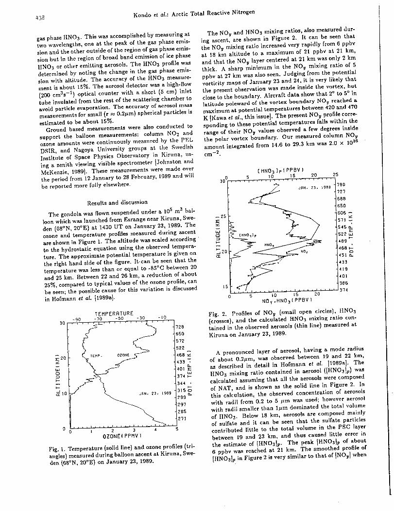
438 Kondo et al.: Arctic Total Reactive Nitrogen

gas phase HNO3. This was accomplished by measuring attwo wavelengths, one at the peak of the gas phase emis-

sion and the other outside of the region of gas phase emis-

sion but in the region of broad band emission of ice phase

tINO3 or other emitting aerosols. The HNO3 profile was

determined by noting the change in the gas phase emis-

sion with altitude. The accuracy of the HNO3 measure-

ment is about 15%. The aerosol detector was a high-flow

(200 cm3s -1) optical counter with a short (5 cm) inlet

tube insulated from the rest of the scattering chamber to

avoid particle evaporation. The accuracy of aerosol mass

measurements for small (r m 0.2#m) spherical particles is

estimated to be about 15%.

Ground based measurements were also conducted to

support the balloon measurements: column NO2 and

ozone amounts were continuously measured by the PEt

DSIR, and Nagoya University groups at the Swedish

Institute of Space Physics Observatory in Kiruna, us-

ing a zenith viewing visible spectrometer [Johnston and

McKenzie, 1989]. These measurements were made over

the period from 12 January to 28 February, 1989 and will

be reported more fully elsewhere.

Results and discussion

The gondola was flown suspended under a 105 m 3 bal-

loon which was launched from Esrange near Kiruna, Swe-

den (68°N, 20 °E) at 1430 UT on January 23, 1989. Theozone and temperature profiles measured during ascent

are shown in Figure 1. The altitude was scaled according

to the hydrostatic equation using the observed tempera-

ture. The approximate potential temperature is given on

the right hand side of the figure• It-can be seen that the

temperature was less than or equal to -85°C between 20

and 25 km. Between 22 and 26 kin, a reduction of about

25%, compared to typical values of the ozone profile, can

be seer*; the possible cause for this variation is discussed

in Hofmann et al. I1989a]-

30

TEMPERQTURE-90 -70 -50 -30 -I0

, , , , _L_' , ' ' ' ' ' ' ; 728

572

522 --

_qr_P • OZONE 468._.._fl---" 433 a..

IJJ374

344 "

299

29'7

285

2"/1

I i I

0 I 2 3 4

0ZONE( PPMV )

r20

rn

i._

31o

Fig. I. Temperature (solid line) and ozone profiles (tri-

angles) measured during balloon ascent at Kiruna, Swe-

den [68°N, 20°E) on January 23, 1989.

The NOy and HNO3 mixing ratios, also measured dur-

ing ascent, are shown in Figure 2. It can be seen that

the NOy mixing ratio increased very rapidly from 6 ppbv

at 18 km altitude to a maximum of 21 ppbv at 21 km,

and that the NOy layer centered at 21 km was only 2 km

thick. A sharp minimum in the NOy mixing ratio of 5

ppbv at 27 km was also seen. Judging from the potential

vorticity maps of January 23 and 24, it is very likely that

the present observation was made inside the vortex, but

close to the boundary. Aircraft data show that 2° to 5° in

latitude poleward of the vortex boundary NOy reached a

maximum at potential temperatures between 420 and 470

K [Kawa ct al., this issue]. The present NOy profile corre-sponding to these potential temperatures falls within the

range of their NOy values observed a few degrees inside

the polar vortex boundary. Our measured column NOy

amount integrated from 14.6 to 29.3 km was 2.0 × 1016

cm -2.

[HN03 ]p I PPBV )0 5 I0 15 20 25

30[ ......... , ......... ' ....

727

688

65O

606 --

_ 545

489468

451 t_.

t ..:_ V 4 3 3._-_S_,/. 419

40!

38615

, ,,, ', 374I l I l I I l I l I I I , , * i , , ,

0 5 10 15 20

N0y .HN03 { PPBV }

Fig. 2. Profiles of NO_/ (small open circles),}INO3

(crosses), and the calculated HNO3 mixing ratio con-tained in the observed aerosols (thin line) measured at

Kiruna on January 23, 1989.

A pronounced layer of aerosol, having a mode radius

of about 0.2ktm, was observed between 19 and 22 kin,

as described in detail in Hofmann et al. ]1989a]. The

HNO3 mixing ratio contained in aerosol (IHNO3]p) was

calculated assuming that all the aerosols were composed

of NAT, and is shown as the solid line in Figure 2. In

this calculation, the observed concentration of aerosols

with radii from 0.2 to 5 Itm was used; however aerosol

with radii smaller than 1/_m dominated the total volume

of HNO3. Below 18 kin, aerosols are composed mainly

of sulfate and it can be seen that the sulfate particles

contributed little to the total volume in the PSC layer

between 19 and 23 kin, and thus caused little error in

the estimate of []{NO3]p. The peak IHNO3]p of about

6 ppbv was reached at 21 kin. The smoothed profile of

[HNO3lp in Figure 2 is very similar to that of INO_] when

Kondo _$ al.: Arctic Total Reactive Nitrogen

a constant 13 +1 ppbv is subtracted from the NOv pro-

file between 20 and 22 km. It should also be noted that

almost all of the small peaks observed in [HNO3]p exactly

match those in NOv.From Figure 2, the comparison of NO v with HNO3 be-

tween 15 and 29 km shows good agreement, considering

the difference in the methods of the measurements and

the likely errors. The derived IINO3 mixing ratios were

based on the average emission over a range of approxi-

mately 60 km detected at an elevation angle of about 15 °during the ascent. As is seen from the sharp peak in the

NO v and IIINO31p profiles between 19 and 21 km, the

HNO3 mixing ratios are averaged over a larger altitude

interval.The vertical NO2 column amount measured by the

ground based visible spectrometer on January 23 wasabout 0.5 x 1015 c m-2, a value similar to, or less than

that typically observed within the Antarctic vortex in

early spring. The uncertainty in the derived vertical col-

umn NO2 amount is =i= 10%. The data sets of NO v ,

[INO3, and column NOt indicate that most of tile reac-tive odd nitrogen species were in the form HNO3 by the

end of january, 1989. By this time nearly all stratospheric

NOz in the locale had been converted into HNO3, consis-

tent with the predictions of a simulation model [Douglas

and Stolarski, 1989] which includes the effects of heteroge-

neous processes in PSCs under Arctic winter conditions.

Using the experimental results of Hanson and Mauers-

berger 11988], the saturation HNO3 vapor mixing ratio

over NAT for the observed temperature profile has been

estimated and is shown in Figure 3 for two assumed H20

mixing ratios. The HNO3 saturation mixing ratio for

1120 -- 4 ppmv is lower than 3 ppbv between 18 and

24 km. Even for H20 = 2 ppmv, the HNO3 saturation

mixing ratio is still lower than 3 ppbv betweem 19 and

21 km. These low HNO3 saturation mixing ratios and

the observed NOv and HNO3 abundances suggest that

3O78O

727

688

65O

606

25 571 _"',r"

545 t,,r-

"-" _ 522 uJ

489t..-

468cD

.._20 451 a,.or..

2pPtlV 433

419

4PPMV 401

386

15 374

0 5 |0 15 20 25 30

HNO3 ( PPBV )

Fig. 3. Calculated equilibrium saturation mixing ratio

for HNO3 over NAT, using the measured temperature

profile on January 23, 1989 and assuming two H20 va-

por mixing ratios, 2 and 4 ppmv.

large enhancements in the aerosol concentration would

be present under equilibrium conditions. The absence of

an enhanced aerosol concentration therefore indicates a

large supersaturation of HNO3 with respect to NAT. The

aircraft data obtained in the Arctic in January, 1989 ID.

W. Fahey, unpublished data, 1989] exhibit similar super-

saturation in air parce[_ below 20 km at the edges of PSC

activity. It is possible that the air sampled on board the

balloon was in the leading edge of a cloud between 18 and

24 kin. The layer in which aerosols were observed showed

the greatest supersaturation with respect to NAT.

The II20 saturation mixing ratio over ice has been cal-

culated using the observed temperature protile; values

ranging from 4.6 to 5 ppmv are indicated between 20 and

21 kin. The average H20 mixing ratio observed during

the Arctic aircraft campaign was near 5 ppmv inside the

polar vortex at altitudes between 18 and 20 km IK. Kelly,

unpublished data, 1989].The NO!t/oz°ne ratio determined using the simultane-

ously measured ozone profile is shown in Figure 4. Both

3O _780

II

_ I 1I 1s l-

- I J- lS'5 Is22i .1'68

,<1'°'

_ " _ i , l , l , J , _ '_3742 3 4 S 6

N0,,,/0ZONE RATIO[ 10 -3 }

Fig. 4. Ratio of NO v to ozone measured at Kiruna on

January 23, 1989.

NO_t and ozone have relatively long lifetimes for only gas

phase chemical processes. This ratio can provide a bet-

ter indication of possible denitrification than NO_t alone

since small scale variations will cancel each other [Fahey,

unpublished data, 1989]. The aircraft data cited above

show a mean value of the NOv/O3 ratio between 3 and

5 x 10 -3 for altitudes between 15 and 20 km for both

60 ° and 70°N latitude. Values much less than 3 x 10 -s

will indicate the loss in NO v • It should also be noted that

ozone profile as shown in Figure 1 does not show signs of

enhanced layers that could also result in the decrease in

the NOv/On ratio. At around 27 km, a large minimum

in the NOv/ozone ratio can be seen. According to the

SAM I[ and lidar haeasurements in previous years by Mc-

Cormick et al. [1982, 1983J, PSCs are sometimes observed

up to this altitude. A possible interpretation of the mini-

mum around 27 km is that PSCs had removed NOv from

,_40I_LJIL_V _ _b.. _L_bVI_ .....

this region. A dip in the NOy/ozone ratio around 22 km

can also be seen, although it is less pronounced. The mea-

sured NOy/O3 ratio was 2.5 :t:l x 10 -3 between 15 and 18

kin, suggesting again considerable NOy depletion. In the

future an important goal should be a background mea-

surement of the winter Arctic stratosphere unperturbed

by heterogeneous processes. The degree of denitrifica-tion in the data presented here may be better understood

when such a background NOy profile is available for com-

parison.

Acknowledgments. We wish to thank CNES for their

excellent balloon operations and logistic support at Es-

range. The balloon fllght was supported by CNES with

partlcipatlon of CNRS. The support of the Ministry of

Education, Science and Culture, the Scandinavia-Japan

Sasakawa Foundation, the Chemical Manufacturers Asso-

ciation, the NSF Division of Atmospheric Chemistry and

Division of Polar Programs, NASA, Esrange, the Swedish

Institute of Space Physics, and the Texas tIigher Edu-

cation Coordinating Board are also gratefully acknowl-

edged.

References

Aimedleu, P., W. A. Matthews, W. Attmannspacher, R.

Hartmannsgruber, J. Cisneros, W. Komhyr, and D.

E. Robbins, Comparison of in situ stratospheric ozone

measurements obtained during the MAP/GLOBUS

1983 campaign, Planet. Space Sei., 35, 563-585,

1987.

Douglass, A. R., and R. S. Stolarski, Impact of heteroge-

neous reactions of stratospheric chemistry of the Arc-

tic, Geophys. Res. Left., _, 131-134, 1989.

Fahey, D. W., C. S. Eubank, G. Hhbler, and F. C. Fehsen-

reid, Evaluation of a catalytic reduction technique for

the measurement of total reactive odd-nltrogen NOy in

the atmosphere, J. Atmos. Chem., :?, 435-468, 1985.

Fahey, D. W., D. M. Murphy, C. S. Eubank, K. Kelly, M.H. Promtt, G. V. Ferry, M. K. W. Ko, M. Loewenstein,

and K. R. Chan, Measurements of nitric oxide and

total reactive nitrogen in the Antarctic stratosphere:

Observations and chemical implications, J. Geophys.

Res., in press, 1989a.

Fahey, D. W., K. K. Kelly, G. V. Ferry, L. R. Poole, J.

C. Wilson, D. M. Murphy, M. Loewenstein, and K. R.

Chan, In situ measurements of total reactive nitrogen,

total water, and aerosol in a polar stratospheric cloud

in the Antarctic, J. Geophys. Res., 94, 11299-11315,

1989b.Hanson, D., and K. Mauersberger, Laboratory studies of

the nitric acid trihydrate: Implications for the south

polar stratosphere, J. Geophys. Res., 15, 855-858,

1988.

Hofmann, D. J., T. L. Deshler, P. Aimedieu. W.A.

Matthews, P. V. Johnston, Y. Kondo, W. R. Sheldon,

G. J. Byrne, and J. R. Benbrook, Stratospheric clouds

and ozone depletion in the Arctic during January 1989,

Nature, 840, 117-121, 1989a.tIofmann, D. J., J. M. Rosen, J. W. IIarder, and J.

V. ttereford, Balloon-borne measurements ol" aerosol,

condensation nuclei, and cloud particles in the strato-

sphere at McMurdo Station, Antarctlca, during the

spring of 1987, J. Geophys. Res., 9_, 11253-11269,

1989b.Johnston, P. V. and R. C. McKenzie, NO2 observation at

45 ° during the decay phase of solar cycle 21, from 1980

to 1987, J. Geophys. Res., 95, 3473-3486, 1989.

Kawa, S. R., D. W. Fahey, L. C. Anderson, M. Loewen-

stein, and K. R. Chan, Measurements of total reactive

nitrogen during the airborne Arctic stratospheric ex-

pedition, Geophys. Res. Left., this issue, 1989.

Kondo, Y., P. Aimedieu, W. A. Matthews, W. R. Sheldon,

and J. R. Benbrook, A mid-latitude balloon-borne ob-

servation of total odd nitrogen, in press, Geophys. Res.

Le_t., 1989.

McElroy, M. B., R. J. Salawitch, and S. C. Wofsy, Antarc-

tic Os: Chemical mechanisms for the spring decrease,

Geophys. Res. Lett., 13, 1296-1299, 1986.

McCormick, M. P., H. M. Steele, P. Hamill, W. P. Chu,

and T. J. Swissler, Polar stratospheric cloud sightings

by SAM II, J. Atmos. Sci., 39, 1387-1397, 1982.McCormick, M. P., C. R. Trepte, and G. S. Kent, Spatial

changes in the stratospheric aerosol associated with the

north polar vortex, Geophys. Res. Left., I0, 941-944,

1983.

Murcray, D. G., T. G. Kyle, F. H. Murcray, and W. J.

Williams, Presence of HNO3 in the upper atmosphere,

J. Opt. Sac. Am., 59, 1131-1134, 1969.

Solomon, S., R. R. Garcia, F. S. Rowland, D. J. Wuebbles,

On the depletion of Antarctic ozone, Nature, $_1, 755-

758, 1986.

y. Kondo, Y. Iwasaka, and A. Iwata, Research In-

stitute of Atmospherics, Nagoya University, Toyokawa,

Aichi, Japan.p. Aimedieu, Service d'A_ronomie, CNRS, Verri_res ie

Buisson, France.W. A. Matthews and P. V. Johnston, Physics and

Engineering Laboratory, Lauder, Central Otago, New

Zealand.

D. W. Fahey, Aeronomy Laboratory, NOAA, Boulder,

Colorado, USA.

D. G. Murcray, Department of Physics, University of

Denver, Denver, Colorado, USA.

D. J. tIofmann, Department of Physics and Astronomy,

University of Wyoming, Laramie, Wyoming, USA.

W. R. Sheldon, Department of Physics, University of

Houston, Houston, Texas, USA.

(Received October 19, 1989;Revised December 6, 1989;

Accepted December 11, 1989)

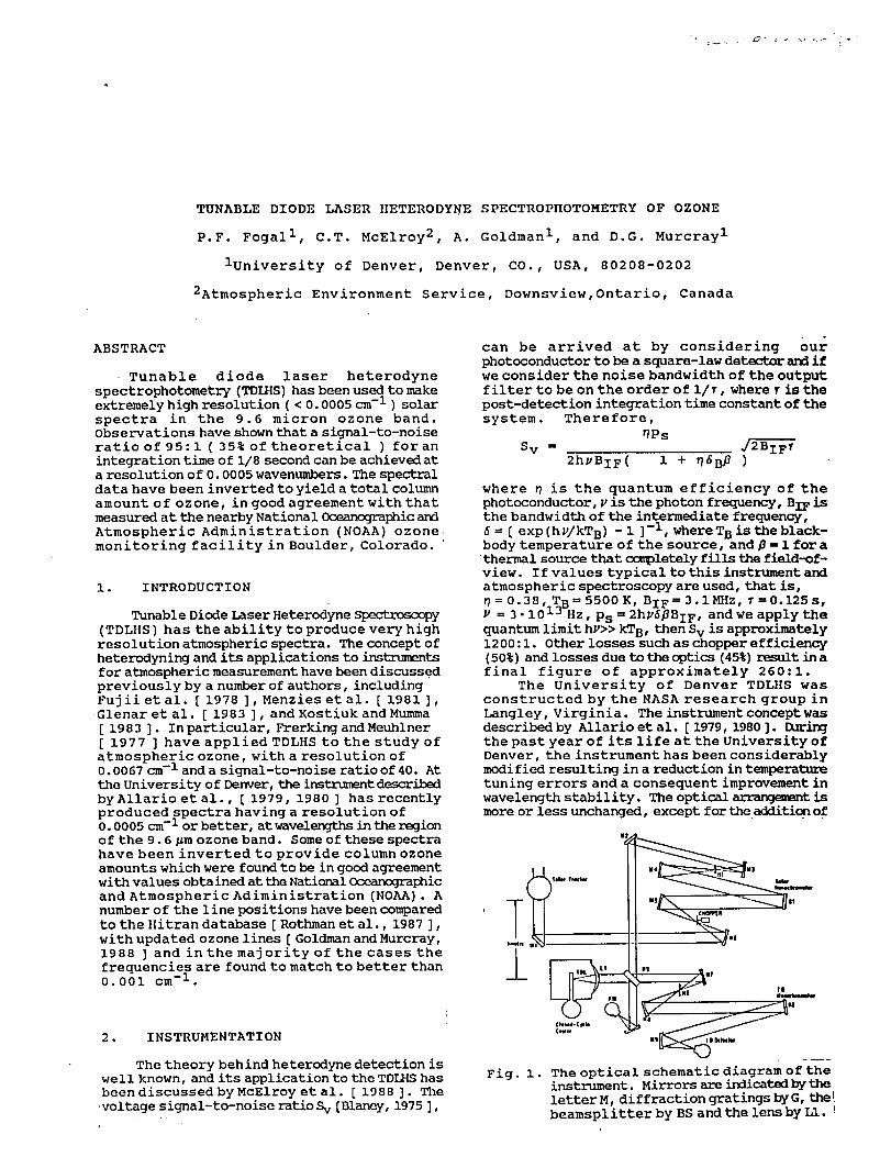
TUNABLE DIODE LASER IIETERODYHE SPECTROPIIOTOMETRY OF OZONE

P.F. Fogal I, C.T. McElroy 2, A. Goldman I, and D.G. Murcray 1

iUniversity of Denver, Denver, CO., USA, 80208-0202

2Atmospheric Environment Service, Downsview,Ontario, Canada

ABSTRACT

Tunable diode laser heterodyne

spectrophotometry (TDLHS) has been used to make

extremely high resolution ( < 0. 0005 cm -I ) solar

spectra in the 9.6 micron ozone band.

Observations have shown that a signal-to-noise

ratioof95:l ( 35% of theoretical ) foran

integration time of 1/8 second can be achieved at

a resolution of 0. 0005 wavenumbers. The spectral

data have been inverted to yield a total column

amount of ozone, in good agreement with that

measured at the nearby National Oceanographic and

Atmospheric Administration (NOAA) ozone

monitoring facility in Boulder, Colorado. '

i. INTRODUCTION

Tunable DiodeLaserHeterod_eSpectroscopy

(TDLHS) has the ability to produce very high

resolution atmospheric spectra. The concept of

heterodyning and its applications to instruments

for atmospheric measurement have been discussed

previously by a number of authors, including

Fujiietal. [ 1978 ], Menziesetal. [ 1981 ],

Glenaret al. [ 1983 ], andKostiukandMumma

[ 1983]. Inparticular, FrerkingandMeuhlner

[ 1977 ] have appliedTDLHS to the study of

atmospheric ozone, with a resolution of

0.0067cm-landasignal-to-noiseratioof40. At

theUniversityofDenver, theins_tdescribed

byAllarioetal., [ 1979, 1980 ] has recently

produced spectra having a resolution of

0.0005cm-lorbetter, atwavelengthsintheregion

of the 9.6 _m ozone band. Some of these spectra

have been inverted to provide column ozone

amounts whichwere found tobeingoodagreement

withvaluesobtainedattheNationalOceanographic

and Atmospheric Adiministration (NOAA). A

number of the line positions have been compared

to the Hitran database[Rothmanetal., 1987],

with updated ozone lines [Goldman and Murcray,

1988 ] and in the majority of the cases the

frequencies are found to match to better than

0.001 cm -I .

2. INSTRUMENTATION

The theory behind heterodyne detection is

well known, and its application tothe TDI/4Shas

been discussed byMcElroyetal. [ 1988 ]. The

voltage signal-to-noiseratioSv[Blaney, 1975],

can be arrived at by considering our

photoconductor to be a square-law detector and if

we consider the noise bandwidth of the output

filter to be on the order of I/r, where T is the

post-detection integration time constant of the

system. Therefore,

_Ps

S v = 4_IF r

2hVBIF ( 1 + U6B@ )

where _ is the quantum efficiency of the

photoconductor, V is the photon frequency, BIF is

the bandwidth of the intermediate frequency,

6 = [ exp (hv/kTB) - 1 ] -i, where T B is the black-

body temperature of the source, and _ = l for a

thermal source that completely fills the field-of-

view. If values typical to this instrument and

atmospheric spectroscopy are used, that is,

7=0.38, TR=5500K, BIF=3.1MHz, f =0.125s,

V 3. 1013-Hz, Ps=2hv6[3BiF, andwe applythe

quantum limit hv>> kTB, then S v is approximately

1200: i. Other losses such as chopper efficiency

(50%) and losses due to the optics (45%) result in a

final figure of approximately 260:1.

The University of Denver TDLHS was

constructed by the NASA research group in

Langley, Virginia. The instrument concept was

describedby Allario et al. [ 1979, 1980 ]. D/ring

the past year of its life at the University of

Denver, the instrument has been considerably

modified resulting in a reduction in temperature

tuning errors and a consequent improvement in

wavelength stability. The optical arl-angement is

more or less unchanged, except for the addition of

±

Fig. i. The optical schematic diagram of the

instrument. Mirrors are indicated by the

letter M, diffraction gratings by G, the I

beamsplitter by BS and the lens by LI. !

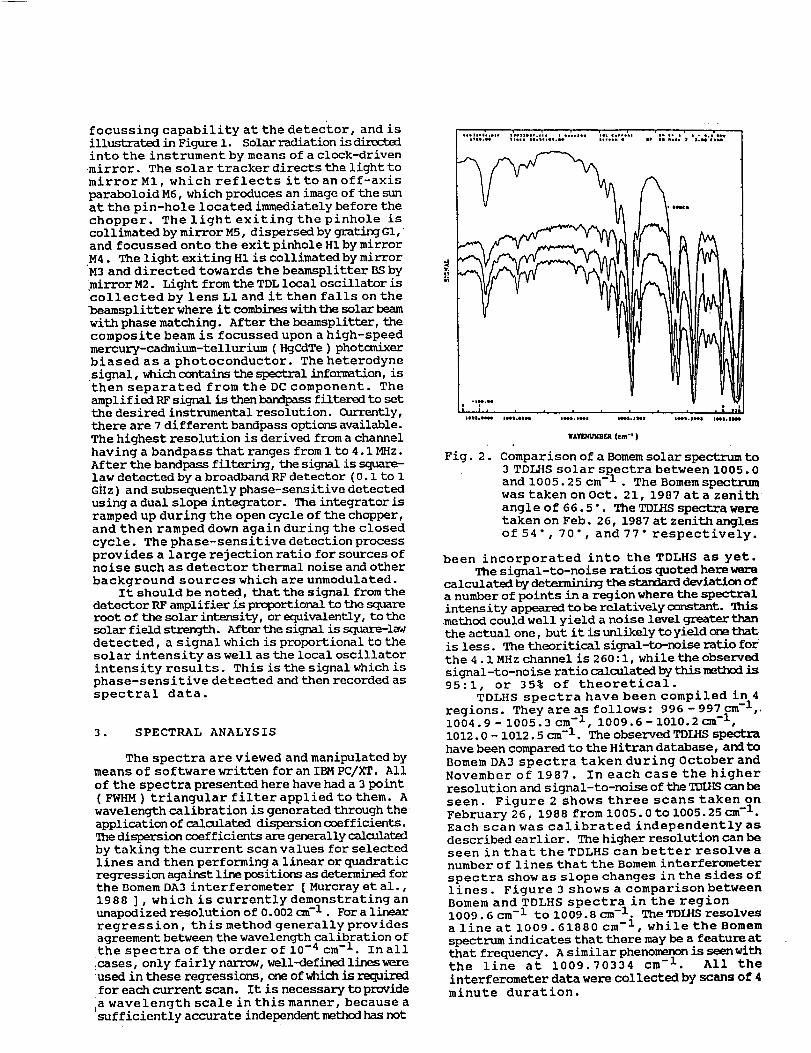
focussing capability at the detector, andisillustz_ted in FigureI. Solarradiationisinto the instrument bymeansof aclock-drivenmirror. Thesolar tracker directs the light tomirror MI, which reflects it to anoff-axisparaboloidM6,whichproducesanimageof thesunat the pin-hole located immediatelybeforethechopper. Thelight exiting the pinhole iscollimatedbymirror M5,dispersedbygratingGI,andfocussedonto the exit pinholeHlbymirrorM4. Thelight exiting HI is collimatedbymirrorM3anddirected towards the beamsplitterBSbymirror M2.Light fromtheTDLlocal oscillator iscollected by lens L1andit then falls onthebeamsplitter where it combines with the solar beam

with phase matching. After the beamsplitter, the

composite beam is focussed upon a high-speed

mercury-cadmium-tellurium ( HgCdTe ) photcmixer

biased asaphotoconductor. Theheterodyne

signal, which contains the spectral information, is

then separated from the DC component. The

amplified RF signal is then bandpass filtered to sot

the desired instrumental resolution. Currently,

there are 7 different bandpass options available.

The highest resolution is derived from a channel

having a bandpass that ranges from i to 4.1 MHz.

After the bandpass filtering, the signal is square-

law detected by a broadband RF detector (0.1 to 1

GHz) and subsequently phase-sensitive detected

using a dual slope integrator. The integrator is

ramped up during the open cycle of the chopper,

and then ramped down again during the closed

cycle. The phase-sensitive detection process

provides a large rejection ratio for sources of

noise such as detector thermal noise and other

background sources which are unmodulated.

It should be noted, that the signal from the

detector RF amplifier is proportional to the square

root of the solar intensity, or equivalently, to the

solar field strength. After the signal is square-law

detected, a signal which is proportional to the

solar intensity as well as the local oscillator

intensity results. This is the signal which is

phase-sensitive detected and then recorded as

spectral data.

3. SPECTRAL ANALYSIS

The spectra are viewed and manipulated by

means of software written for an IBM PC/XT. All

of the spectra presented here have had a 3 point

( FWHM ) triangular filter applied to them. A

wavelength calibration is generated through the

application of calculated dispersion coefficients.

The dispersion coefficients are generally calo/lated

by taking the current scan values for selected

lines and then performing a linear or quadratic

regression against line positions as determined for

the Borne, DA3 interferometer [ Murcray et al.,

1988 ], which is currently demonstrating an

unapodized resolution of 0.002 cm -I . For a lirear

regression, this method generally provides

agreement between the wavelength calibration of

the spectra of the order of 10 -4 cm -I. In all

icases, only fairly narrow, well-defined lines were

used in these regressions, one of which is required

for each current scan. It is necessary to provide

ia wavelength scale in this manner, because a

sufficiently accurate independent method has not

¢.b_l.0:..l, .',.slos,.,'1. t ..',o.. ;IL ¢.,o.'_ 'w_ ¢. I' i - • 0'I..it¢o.N Ii.., l.,s,,es.¢_ s,.... • nP sm l•e. a _,¢¢ q._

• ee_m

_. 0 ,lOel.eO,w JNI.Oi_ it, e i¢¢i II.D_. 0s,e_ l_i.z_ i_i. 1s¢¢

IrAVI:mJXSLq (,:m "I )

Fig. 2. Comparison of a Bomem solar spectrum to

3 TDLHS solar spectra between 1005.0

and 1005.25 cm -I . The Bomem spectrum

was taken on Oct. 21, 1987 at a zenith

angle of 66.5 ". The TDLHS spectra were

taken on Feb. 26, 1987 at zenith angles

of 54", 70", and 77" respectively.

been incorporated into the TDLHS as yet.

The signal-to-noise ratios quoted here were

calculated by determining the standard deviation of

a number of points in a region where the spectral

intensity appeared to be relatively constant. Tnls

method could well yield a noise level greater than

the actual one, but it is unlikely to yield one that

is less. The theoritical signal-to-noise ratio for

the 4.1 MHz channel is 260 :1, while the observed

signal-to-noise ratio calculated by this method is

95:1, or 35% of theoretical.

TDLHS spectra have been compiled in 4

regions. They are as follows: 996 - 997 cm-l,.

1004.9 - 1005.3 cm -I, 1009.6-1010.2 c_ -I,

1012.0 - 1012.5 cm -I . The observed TDI/{S spectra

have been compared to the Hitran database, and to

Bomem DA3 spectra taken during October and

November of 1987. In each case the higher

resolution and signal-to-noise of the TDI/IS can be

seen. Figure 2 shows three scans taken on

February 26, 1988 from 1005.0to1005.25cm -I.

Each scan was calibrated independently as

described earlier. The higher resolution can be

seen in that the TDLHS can better resolve a

number of lines that the Borne, interferometer

spectra show as slope changes in the sides of

lines. Figure 3 shows acomparisonbetween

Bomem and TDLHS spectra in the region

1009.6 cm -I to 1009.8 cm -I. The TDLHS resolves

a line at 1009.61880 cm -I, while theBomem

spectrum indicates that there may be a feature at

that frequency. A similar phenomenon is seen with

the line at 1009.70334 cm -I. All the

interferometer data were collected by scans of 4

minute duration.

,,..... , ....,.,_..,,... .::.:_"_,.-,.. ........°.,, ',..:'_,-'_,"•

I -iN.l,o

Fig. 3. Comparison of TD_S solar spectra to a

_mem solar spect_ between 1009.6 and!

1009.8 cm -I . The Bomem is as described.

in Figure 3, while the TDLHS spectra

were taken on May II, 1988 at zenith

angles of 56.5" and 63.5" respectively

Figure 4 illustrates a spectrum taken January

21, 1987 at the University of Denver ( altitude

I. 6 km, 39.5 "N 105"W ) . This spectrum was taken

while the instrument was in its original

configuration, and it has a signal-to-noise ratio of

45: I, or 17% of theoretical. The curves in Figure

5 compare an expanded portion of the observed

spectrum taken at 0. 0016 cm -I resolution, to a

simulation using line parameters which are the

same as those on the Hitran compilation, with the

exception of the line positions, which were

adjusted to agree with the observed data. The

climatological vertical distribution of ozone at

mid-latitude was taken as a starting point for a

non-linear spectral least squares fitting procedure

which scaled the whole profile until the best

possible agreement between the two curves was

obtained [ Goldman et al., 1983 ]. It can be seen

that the three lines shown are not all fit with the

same precision. This difference is due to the

combined effects of inaccuracies in the compiled

line intensities and hal fwidths, and the fact that

the observed lines result from states of rather

different, relatively high, energies and are

therefore affected differently by changes in the

local temperature.

In order to investigate the possibility that

the observed and simulated spectra might be

brought into better agreement if the temperature

profile of the model atmosphere were changed, the

fitting program was run in such a way that the

temperature profile could be scaled to achieve the

best agreement between the data and the model

results. When this was done a slightly different

total column amount of ozone was obtained, with

no apparent improvement of the fit, with the

difference between the two amounts being about

1.0

1.0

z

0.0

i & I I I i

996.7t

WAVENUMBER (era-i )

Fig. 4. A solar spectrum taken by the TDLHSon

January 21, 1987, at a zenith angle of

60.1". The upper curve shows data from

the Ito 4.1MHz channel, while the

lower oneplotsthesignalfromthel0to

20 MHz bandpass channel.

Fig. 5.

1.0

0.0'

996.68

8%. The column amounts obtained in these

calculations are 344 and 317 m-atm-cm for the

fixed and adjusted temperature profiles,

respectively. The ozone total column amount

determined bytheDobsonozonespectrophotumeter

[ private communication

R. Evans, 1987 ], is

I

996.74

%YAVENUMBER (cm -I )

60.10"

996.80

This figure shows a comparison of the

observed data and the results of a

spectral simulation over a narruwregicn

containing several ozone lines. The

ozone amount was adjusted to give the

best fit, and the spectrum shown was

calculated with 344m-atm-cmof

ozone in the model atmosphere.

996.84

at NOAAat Boulder

fromW. Komhr and

355 m-atm-cm.

TheDobsontotal ozoneamountwasadjustedby3.9%before beingcomparedto the infraredresults, with thereported369Dobsonunit Bouldermeasurementcorrected to 355m-atm-cm.Thisadjustment is neededbecausetheDobsonvaluesare now known to read high compared toultraviolet andchemicalmeasurementsof ozone[ private communication from J.B. Kerr,Atmospheric Environment Service, 1987 ]. •

4. CONCLUSIONS

The TDLHS isjust now beginning torealize

its potential. It ishopedthatabetterselection

of TDL's will become available in the not to

distant future, thereby increasingthe numberof

spectral regions which can be investigated. The

higher resolutionoftheTDLHS providesthe

potential tobetterresolvethespectrallinesof

absorbers whose lines overlap those of other

atmospheric constituents. Higher spectral

resolution will provide better resolution of

constituentverticalprofileswhichwouldbenefit

line shape inversion studies.

ACKNOWLEDGEMENTS

Acknowledgement is made to the National

Center for Atmospheric Research, which is

sponsored by the National Science Foundation, for

computer time used in this research. Funding to

support this work was provided by NASA/Langley.

REFERENCES

Allario, F. , J. M. Hoell, S. J. Katzberg,

J. C. Larsen, 1979 : An Experiment Concept

to Measure Stratospheric Trace Constituents

by Laser Heterodyne Spectroscopy, Proc.

NASA Conf. on High Resolution Infrared

Spectroscopy Techniques for Atmospheric

Measurements, Publ. No. 2134, 57-79.

Allario, F.,J.M. Hoell, andS.J. Katzberg, 1980: An

experimentconcepttomeasurestratospheric

trace constituents by laser heterodyne

spectroscopy, Appl. Phys., 23, 47-56..

Blaney, T. G., Signal-to-NoiseRatioandOther

Characteristics of Heterodyne Radiation

Receivers, 1975: Space ScienceReviews, 17,

691-702.

Frerking, M. A. and D. J. Muehlner, 1977:

Infrared Heterodyne Spectroscopy of

AtmosphericOzone, Appl. ODt.,16,526-528.

Fujii, Y., J. Yamashita, S. Shikata, S. saito, 1978:

Incoherent Optical Heterodyne Detection and

its Application to Air Pollution Detection,

Appl. Opt. , 17, 3444-3449.

Glenar, D.,T. Kostiuk, D.E. Jennings, D. Buhl, and

M. J. Mumma, 1981: Tunable Diode-Laser

Heterodyne Spectrometer for Remote

Observations near8_m,_pDi. ODt., 21,

253-259.

Goldman, A., F. G. Fernauld, F. J. Murcray,

F. H. Murcray, and D. G. Murcray, 1983:

Spectral Least Squares Quantification of

Several Atmospheric Gases From High

ResolutionlnfraredSolarSpect/aObtainedat

theSouthPole, J. Quant, SpeGt_QsG._adiat.

Transfer, 29, 189-204.

Goldman, A. and D. G. Murcray, 1988: High

Resolution Studies of Atmospheric Infrared

Emisssion and Absorption Spectra, Proceedings i

of the spie Conference.

Kostiuk, T., andM. J. Mumma, 1983: Remote

Sensing by IR Heterodyne Spectroscopy,

Appl. Opt., 22, 2644-2654.

McElroy, C. T., A. Goldman, and D. G. Murcray,

1988: Heterodyne Spectrophotometryof

Ozone in the 9.6 Micron Band Using a

Tunable DiodeLaser, submittedtoAmpl. Opt..

Menzies, R. T., C. W. Rutledge, R. A. Zanteson,

and D. L. Spears, 1981: Balloon-Borne Laser

Heterodyne Radiometer for Measurements of

Stratospheric Trace Species, Ar_l. Opt., 20,

536-544 .

Murcray, F. J., J. J. Kosters, and

R. D. Blatherwick, 1988: A Very High

ResolutionFourierTransformSpectrometer

for Balloon-BorneApplications, Suhmittedto

Appl. Opt.

Rothman, L. S. , R. R. Gamache, A. Goldman,

L. R. Brown, R. A. Toth, H. M. Pickett,

R. L. Poynter, J. -M. Flaud, C. Camy-Peyret,

A. Barbe, N. Husson, C. P. Rinsland, and

M. A. H. Smith, 1987: TheHitran Database:

1986 edition, ADD1. OPt., 26, 4058-4097.

JOURNAL OF GEOPHYSICAL RESEARCH, VOL. 93, NO. DI0, PAGES 12,607-12,626, OCTOBER 20, 1988

Infrared Measurements of Atmospheric Gases Above Mauna Loa, Hawaii,

in February 1987

C. P. RINSLAND

Atmospheric Sciences Division, NASA Langley Research Center, Hampton, Virginia

A. GOLDMAN, F. J. MURCRAY, F. H. MURCRAY, R. D. BLATHERWICK, AND D. G. MURCKAY

Physics Department, University of Denver, Denver, Colorado

Infrared solar absorption spectra recorded at 0.02 cm -t resolution from the National Oceanic and

Atmospheric Administration (NOAA) Geophysical Monitoring for Climate Change (GMCO programstation at Mauna Loa, Hawaii (latitude 19.5°N, longitude 155.6"W, elevation 3.40 kin), in February 1987have been analyzed to determine simultaneous total vertical column amounts for 13 atmospheric gases.Average tropospheric concentrations of CO v NzO, CH4, and CHC1Fa and the daytime diurnal vari-ations of the total columns of NO and NO 2 have also been inferred. The retrieved total columns (inmolecules ¢m-') of the nondiurnally varying gases are 1.6 4- 0.2 x l0 ts for HCi, 5.9 4- 1.2 × l0 ts forHNOp 2.0 + 0.2 x 10 ,t for HIt60, 4.4 + 0.7 x 1018 for HltgO, 2.7 4- 0.1 x 1017 for HDO, 2.3 4- 0.2x 10 t9 for CH,, 5.0 + 0.5 x 102t for CO 2, 6.7 4- 0.8 x 10 t8 for 0 3, 4.3 4- 0.4 × I0 t8 for NaO, 1.0 4- 0.2x 10 t6 for C2H 6, and 9.7 + 2.5 x 10 t* for CHCIF2. We compare the total column measurements of HCl

and HNO 3 with previously reported ground-based, aircraft, and satellite measurements. The results forHCl are of particular interest because of the expected temporal increase in the concentration of this gasin the stratosphere. However, systematic differences among stratospheric HCI total column measure-ments from 1978 to 1980 and the absence of observations of free tropospheric HCI above Mauna Loamake it impossible to obtain a reliable estimate of the trend in the total burden of HCl. The measured

HNO_ total column is consistent with aircraft measurements from ~12 km altitude. The 0 3 totalcolumn deduced from the 1R spectra agrees with correlative Mauna Loa Umkehr measurements withinthe estimated error limits. The column-averaged D/H ratio of water vapor is (68 4- 9) x 10 -6, which is0.44 + 0.06 times the reference value of 155.76 x 10"e for standard mean ocean water (SMOW). This

large depletion in the D content of water vapor is similar to published measurements of the uppertroposphere and lower stratosphere. Average tropospheric concentrations deduced for CO2, N20, andCH,, are in good agreement with correlative NOAA GMCC surface data, indicating consistency l:mtweenthe measurement techniques for determining tropospheric volume mixing ratios. Results of the presentstudy indicate that Mauna Loa is a favorable site for infrared monitoring of atmospheric gases. The site

is particularly favorable for monitoring the tropospheric volume mixing ratios of long-lived gases, sincethe high altitude of the tropopause reduces corrections required to account for the decrease in volume

mixing ratio in the stratosphere.

l. INTRODUCTION

This paper presents the results of a quantitative analysis of

absorptions by a number of minor and trace atmospheric

gases in 0.02 cm- t resolution solar absorption spectra record-

ed at a number of solar zenith angles on 4 days in February

1987 by F. J. Murcray and F. H. Murcray at the National

Oceanic and Atmospheric Administration (NOAA) Geophysi-

cal Monitoring for Climate Change (GMCC) program stationat Mauna Loa, Hawaii (latitude 19.5°N, longitude 155.6"W,

elevation 3.40 kin). The spectral data were recorded with a

Michelson-type Fourier transform spectrometer, with a maxi-

mum path difference of 50 cm and a scan time of 62 s. This

instrument has been used previously to obtain many balloon-

borne, ground-based, and laboratory spectra by the University

of Denver spectroscopy group (see Goldman et al. [1988] for a

description of the instrument and data collection system).

There were a numberof reasons for obtaining these obser-

vations. First, Mauna Loa is a dry, high-altitude site, where

there is a very significant reduction in the spectral interference

by the strong H:O absorptions usually present in IR spectra

Copyright 1988 by the American Geophysical Union.

Paper number 88JD03259.0148-0227/88/88JD-03259505-00

recorded from ground-based sites. This reduction allowed us

to Obtain measurements of several key trace atmospheric gases

not usually accessible through ground-based IR observations.

For example, we have been able to obtain simultaneous

measurements o.f the daytime diurnal variations of the total

columns of NO, and NO through observations of NO2 lines

of the strong v_ band at 6.2 tam and the weaker v t + vs band

at 3.4 tam and of the NO lines of the fundamental vibration-

rotation band at 5.3 tam. Second, we were interested in obtain-

ing IR data from a low21atitude station. To our knowledge, no

such ground-based IR Observations have been obtained pre-

viously inthe tropics. The spectra compose a permanent

record of the state of the atmosphere at the time of the obser-

vations and can be compared with spectra from other lo-

cations and times to establish latitudinal distributions and

temporal trends of minor and trace species. We are in the

process ofcollecting data from a number of sites at differentlatitudes for tfiis purpose (e.g., South Pole Station, Antarctica,

New Zealand, Kitt Peak in Arizona, Mount Evans in Col-

orado, NASA Langley in Hampton, Virginia). To our knowl-

edge, with the exceptions of ongoing total ozone measure-

ments with a Dobson instrument and visible region measure-

ments of NO2 obtained in 1978 [Noxon et al., 1983], the

present results prov!de the only measurements of total col-

12,607

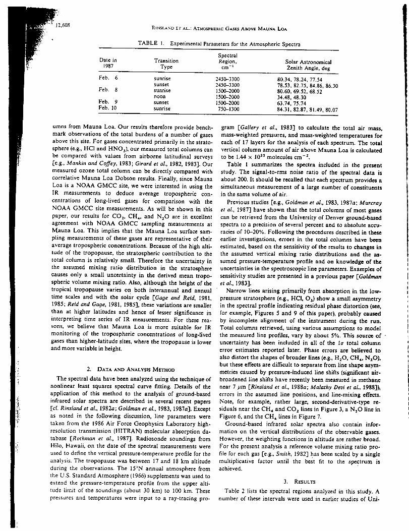
12,608 RINSLANDETAL.: ATMOSPHERIC GASES ABOVE MAUNA LOA

TABLE I. Experimental Parameters for the Atmospheric Spectra

SpectralDate in Transition Region,

1987 Type cm -_

Feb. 6 sunrise 2450--3300sunset 2450-3300

Feb. 8 sunrise 1500--2000

noon 1500-2000Feb. 9 sunset 1500-2000Feb. 10 sunrise 750-1300

Solar Astronomical

Zenith Angle, deg

80.34, 78.24, 77.54

78.53, 82.75, 84.86, 86.3080.60, 69.52, 68.5234.48, 48.3063.74, 75.74

84.31, 82.87, 81.49, 80.07

umns from Mauna Loa. Our results therefore provide bench-

mark observations of the total burdens of a number of gases

above this site. For gases concentrated primarily in the strato-

sphere (e.g., HCI and HNO3), our measured total columns can

be compared with values from airborne latitudinal surveys

[e.g., Mankin and Coffey, 1983; Girard et al., 1982, 1983]. Our

measured ozone total column can be directly compared with

correlative Mauna Loa Dobson results. Finally, since Mauna

Loa is a NOAA GMCC site, we were interested in using the

IR measurements to deduce average tropospheric con-

centrations of long-lived gases for comparison with the

NOAA GMCC site measurements. As will be shown in this

paper, our results for CO 2, CH,, and N,O are in excellent

agreement with NOAA GMCC sampling measurements at

Mauna Loa. This implies that the Mauna Loa surface sam-

piing measurements of these gases are representative of their

average tropospheric concentrations. Because of the high alti-

tude of the tropopause, the stratospheric contribution to the

total column is relatively small. Therefore the uncertainty in

the assumed mixing ratio distribution in the stratosphere

causes only a small uncertainty in the derived mean tropo-

spheric volume mixing ratio. Also, althoughthe height of thetropical tropopause varies on both interannual and annual

time scales and with the solar cycle [Gage and Reid, 1981,

1985; Reid and Gage, 1981, 1985], these variations are smaller

than at higher latitudes and hence of lesser significance in

interpreting time series of IR measurements. For these rea-

sons, we believe that Mauna Loa is more suitable for IR

monitoring of the tropospheric concentrations of long-lived

gases than higher-latitude sites, where the tropopause is lower

and more variable in height.

2. DATA AND ANALYSIS METHOD

The spectral data have been analyzed using the technique of

nonlinear least squares spectral curve fitting. Details of the

application of this method to the analysis of ground-based

infrared solar spectra are described in several recent papers

[cf. Rinsland et al., 1982a; Goldman et al., 1983, 1987a]. Except

as noted in the following discussion, line parameters were

taken from the 1986 Air Force Geophysics Laboratory high-

resolution transmission (HITRAN) molecular absorption da-

tabase [Rothman et al., 1987]. Radiosonde soundings from

Hilo, Hawaii, on the date of the spectral measurements were

used to define the vertical pressure-temperature profile for theanalysis. The tropopause was between 17 and 18 km altitude

during the observations. The 15°N annual atmosphere from

the U.S. Standard Atmosphere (1966) supplements was used to

extend the pressure-temperature profile from the upper alti-

tude limit of the soundings (about 30 kin) to 100 kin. These

pressures and temperatures were input to a ray-tracing pro-

gram [Gallery et al., 1983] to calculate the total air mass,

mass-weighted pressures, and mass-weighted temperatures for

each of 17 layers for the analysis of each spectrum. The total

vertical column amount of air above Mauna Loa is calculated

to be 1.44 x 1025 molecules cm -_.

Table 1 summarizes the spectra included in the present

study. The signal-to-rms noise ratio of the spectral data is

about 200. It should be recalled that each spectrum provides a

simultaneous measurement of a large number of constituents

in the same volume of air.

Previous studies [e.g., Goldman et al., 1983, 1987a; Murcray

et al., 1987] have shown that the total columns of most gases

can be retrieved from the University of Denver ground-based

spectra to a precision of several percent and to absolute accu-

racies of 10-20%. Following the procedures described in these

earlier investigations, errors in the total columns have been

estimated, based on the sensitivity of the results to changes in

the assumed vertical mixing ratio distributions and the as-

sumed pressure-temperature profile and on knowledge of the

uncertainties in the spectroscopic line parameters. Examples of

sensitivity studies are presented in a previous paper [Goldman

et al., 1983].

Narrow lines arising primarily from absorption in the low-

pressure stratosphere (e.g., HCi, 03) show a small asymmetry

in the spectral profile indicating residual phase distortion (see,

for example, Figures 5 and 9 of this paper), probably caused

by incomplete alignment of the instrument during the run.

Total columns retrieved, using various assumptions to model

the measured line profiles, vary by about 5%. This source of -

uncertainty has been included in all of the la total column

error estimates reported later. Phase errors are believed to

also distort the shapes of broader lines (e.g., H20, CH,, NaO),

but these effects are difficult to separate from line shape asym-

metries caused by pressure-induced line shifts (significant air-

broadened line shifts have recently been measured in methane

near 7 gm [Rinsland et al., 1988a; Malathy Deui et al., 1988]),

errors in the assumed line positions, and line-mixing effects.

Note, for example, rather large, second-derivative-type re-

siduals near the CH 4 and CO t lines in Figure 3, a N20 line in

Figure 6, and the CH 4 lines in Figure 7.

Ground-based infrared solar spectra also contain infor-

mation on the vertical distributions of the observable gases.

However, the weighting functions in altitude are rather broad.

For the present analysis a reference volume mixing ratio pro-

file for each gas [e.g., Smith, 1982] has been scaled by a single

multiplicative factor until the best fit to the spectrum isachieved.

3. RESULTS

Table 2 lists the spectral regions analyzed in this study. A

number of these intervals were used in earlier studies of Uni-

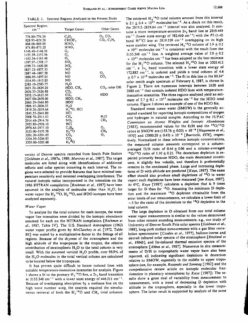
RINSLANDEl"AL.: ATMOSP_RtC GxSES ABOVEMAUNA LOA 12,609

TABLE 2. Spectral Regions Analyzed in the Present Study

Spectral Region,cm-' Target Gases Other Gases

776.00--776.50 CzHz O_. CO,.828.95--829.20 CHCIF, CO:, C,. He,868.(R)-869.00 H N O 3871.80--873.20 HNO 3

1146.40--1146.56 031155.39-I 155.56 031163.34-1163.48 031597.97-1598.17 NO 21599.73-1600.00 NOz1857.23-1857.35 NO1887.48-1887.58 NO 031896.95-1897.05 NO COz1914.95-1915.05 NO

2583.10-2583.75 NzO2621.20-2624.20 HDO, CH4 CO2, solar OH

2626.35-2626.80 COz2632.15-2632.50 CO,. HDO2657.00-2658.00 HDO, CH42660.20-2660.80 HDO2806.15-2806.55 NzO2819.20-2819.64 H2160, HCI2843.55-2843.80 HCI2908.70-2911.02 CH4 H ,O2914.40---2914.70 NO, C_'142925.80-2926.10 HCI

2976.65-2977.10 CzH 6 O33155.00--3155.58 H2160 CH43201.30-3201.65 COz 033204.50-3204.85 CO3205.00-3205.60 Hz_O

versity of Denver spectra recorded from South Pole Station

[Goldman et al., 1987a, 1988; Murcray et al., 1987"]. The target

molecules are listed along with identifications of additional

telluric and solar species occurring in each interval. The re-

gions were selected to provide features that have minimal tem-

perature sensitivity and minimal overlapping interference. The

natural isotopic ratios incorporated in the intensities on the

1986 HITRAN compilation [Rothman et al., 1987] have been

assumed in the analysis of molecules other than HzO; for

water vapor the H z tee, H z tso, and HDO isotopes have been

analyzed separately.

Water Vapor

To analyze for the total column for each isotope, the water

vapor line intensities were divided by the isotopic abundance

assumed for each on the HITRAN compilation [Rothman et

al., 1987, Table IV]. The U.S. Standard Atmosphere (1962)

water vapor profile given by McClatchey et al. [1972, Table

BI"] was scaled by a multiplieative factor in the fittings of all

regions. Because of the dryness of the stratosphere and the

high altitude of the tropopause in the tropics, the relative

contribution of stratospheric HzO to the total column is very

small. With the assumed vertical HzO profile, over 99.9% of

the HzO molecules in the total vertical column are calculated

to be located below the tropopause.

It has proven quite difficult to locate isolated lines with

suitable temperature-insensitive intensities for analysis. Figure

I shows a fit to the primary HztrO line, a 2v 2 band transition

at 3155.348 cm- t with a lower state energy of 446.511 cm- t.

Because of overlapping absorption by a methane line on the

high wave number wing, the analysis required the simulta-

neous retrieval of both the H 2t60 and CH 4 total columns.

The retrieved Hz'60 total column amount from this interval

is 2.1 + 0.4 × I0 't molecules" _m -2. As a cheek on this result,

the 2819.2-2819.64 cm-i interval was also analyzed. It con-

tains a more temperature-sensitive 2v 2 band line at 2819.449

cm-1 (lower state energy of 782.410 cm-t) with the P3 (1-0)

band H3"CI line at 2819.559 cm -l overlapping on its high

wave number wing. The retrieved Hz_60 column of 1.9 + 0.2

× 10 zt molecules cm -2 is consistent with the result from the

3155.348 cm-_ line. A weighted average value of 2.0_ 0.2

× 10 zt molecules cm-2 has been adopted as the best estimate

for the Hzx60 column. The selected H2xsO line at 3205.412

cm -_, a 2v z band transition with a lower state energy of

172.882 cm -_, is isolated and yields a total column of 4.4

+ 0.7 x 10 t8 molecules cm -2. The fit to this line in the 80.34 °

solar zenith angl e spectrum of February 6, 1987, is shown in

Figure 2. There are numerous intervals between 2620 and

2680 cm- _ that contain isolated HDO lines with temperature-

insensitive intensities. The three regions analyzed yield an esti-

mate of 2.7 + 0.1 × 10 _" molecules crn -z for the HDO total

column. Figure 3 shows an example of one of the HDO fits.

Standard mean ocean water (SMOW) is the generally ac-

cepted standard for reporting isotopic compositions of oxygen

and hydrogen in natural samples. According to the IUPAC

Commission on Atomic Weights and Isotopic Abundances

[1983"], recommended values for the D/H and the asO/t60

ratios in SMOW are (155.76 + 0.05) x 10 -_ [Hagemann et al.,

1970] and (2000.20 + 0.45) x 10 -6 [Baertschi, 1976], respec-

tively. Normalized to these reference isotopic concentrations,

the measured column amounts correspond to a column-

averaged D/H ratio of 0.44 + 0.06 and a column-averaged

_sO/t60 ratio of 1.I0 + 0.21. The deuterium depletion is ex-

pected primarily because HDO, the main deuterated constit-

uent, is slightly less volatile, and therefore it preferentially

remains in the condensed phase. Large and increasing deple-

tions of D with altitude are predicted [Kaye, 1987]. The same

effect should also produce small depletions of 1sO in water

vapor; such depletions have been measured [see Kaye, 1987"].

At 0°C, Kaye [1987] calculates a depletion that is 9 times

larger for D than for _sO. Assuming the minimum D deple-

tion and the maximum :sO depletion obtainable from the

error limits of our measurements, we calculate a lower limit of

~5 for the ratio of the deuterium to the _sO depletion in the

total column.

The large depletion in D obtained from our total column

water vapor measurements is similar to the values determined

from other remote sounding measurements, e.g., our study of

University of Denver South Pole solar spectra [Goldman et al.,

1988], long-path surface measurements with a gas filter corre-

lation spectrometer [Cosden et al., 1977], balloon-borne and

aircraft infrared solar spectra of the stratosphere [Rinsland et

aL, 1984b], and far-infrared thermal emission spectra of the

stratosphere [Abbas et al., 1987]. Numerous in situ measure-

ments of D/H in tropospheric water vapor have also been

reported, all indicating significant depletions in deuterium

relative to SMOW, especially in the middle to upper tropo-

sphere (see, for example, Rozanski and Sonnta# [1982] and the

comprehensive review article on isotopic molecular frac-

tionation in planetary atmospheres by Kaye [1987]). The re-

sults show a great deal of variability from measurement to

measurement, with a trend of decreasing D depletion with

altitude in the troposphere, especially in the lower tropo-

sphere. The latter result is supported by analysis of the same

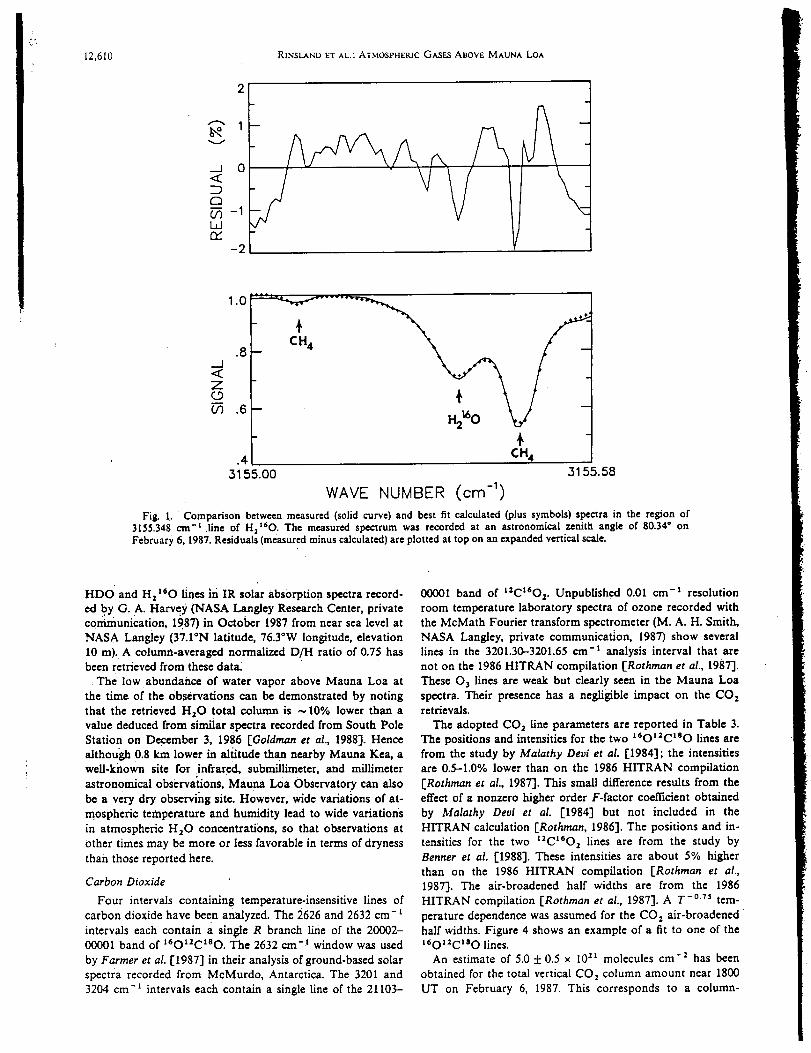
12,610

v

0

C_

_-ILdOC

RINSLAND ET AL.; ATMOSPHERIC GASES ABOVE MAUNA LOA

-2

1.0------.8.... /".=J<7

o_.8

.4 CH4

3155.00 3155.58

WAVE NUMBER (cm -1)

Fig. L Comparison between measured (solid curve) and best fit calculated (plus symbols) spectra in the region of3155.348 cm -L line of H:'SO. The measured spectrum was recorded at an astronomical zenith angle of 80.34 ° onFebruary 6, 1987. Residuals (measured minus calculated) are plotted at top on an expanded vertical scale.

H DO and H z tsO lines in IR solar absorption spectra record-

ed by G. A. Harvey (NASA Langley Research Center, privatecommunication, 19.87) in October 1987 from near sea level at

NASA Langley (37.1°N latitude, 76.3°W longitude, elevation

10 m). A column-averaged normalized D/H ratio of 0.75 has

been retrieved from these data_

, The low abundance of water vapor above Mauna Los at

the time of the observations can be demonstrated by noting

that the retrieved H20 total column is _ 10% lower than a

value deduced from similar spectra recorded from South Pole

Station on December 3, 1986 [Goldman et al., 1988]. Hence

although 0.8 km lower in altitude than nearby Mauna Ken, a

well-known site for .infrared, submiUimeter, and millimeter

astronomical observations, Mauna Los Observatory can also

be a very dry observing site. However, wide variations of at-

mospheric temperature and humidity lead to wide variations

in atmospheric H20 concentratibns, so that observations at

Other times may be more or less favorable in terms of dryness

than those reported here.

Carbon Dioxide

Four intervals containing temperature-insensitive lines of

carbon dioxide have been analyzed. The 2626 and 2632 cm- t

intervals each contain a singl e R branch line of the 20002-00001 band of t6012C180. The 2632 cm -t window was used

by Farmer et al. [1987] in their analysis of ground-based solar

spectra recorded from McMurdo, Antarctica. The 3201 and

3204 cm-t intervals each contain a single line of the 21103-

00031 band of 12C160 v Unpublished 0.01 cm -1 resolution

room temperature laboratory spectra of ozone recorded with

the McMath Fourier transform spectrometer (M. A. H. Smith,

NASA Langley, private communication, 1987) show several

lines in the 3201.30--3201.65 crn -t analysis interval that are

not on the 1986 HITRAN compilation [Rothman et al., 1987].

These O 3 lines are weak but clearly seen in the Mauna Los

spectra. Their presence has a negligible impact on the CO 2retrievals.

The adopted CO 2 line parameters are reported in Table 3.

The positions and intensities for the two 16ol2C180 lines are

from the study by Malathy Devi et al. [1984]; the intensities

are 0.5-1.0% lower than on the 1986 HITRAN compilation

[Rothraan et al., 1987]. This small difference results from the

effect of a nonzero higher order F-factor coetIicient obtained

by Malathy Devi et al. [1984] but not included in the

HITRAN calculation [Rothman, 1986]. The positions and in-

tensities for the two tzCteO2 lines are from the study by

Benner et al. [1988]. These intensities are about 5% higher

than on the 1986 HITRAN compilation [Rothman et al.,

1987]. The air-broadened half widths are from the 1986

HITRAN compilation [Rothman et al., 1987]. A T -°'Ts tem-

perature dependence was assumed for the CO 2 air-broadened

half widths. Figure 4 shows an example of a fit to one of the

t_OlzCtsO lines.

An estimate of" 5.0 + 0.5 x 1021 molecules cm -x has been

obtained for the total vertical CO, column amount near 1800

UT on February 6, 1987. This corresponds to a column-

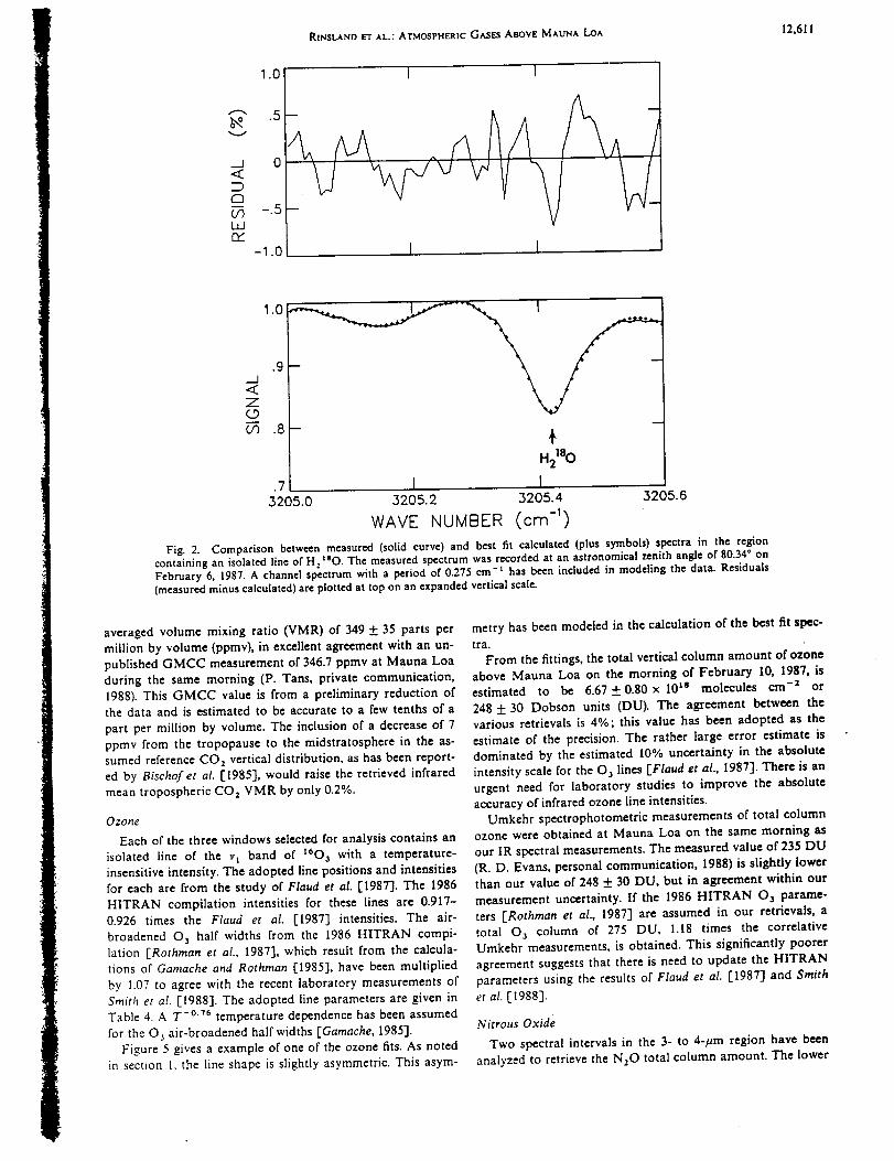
1.01

.5

0<I:

c-_-.5

LOrY

-1.0

RINSLAND El" AL.: ATMOSPHERIC GASES ABOVE MAUNA LOA

[

1 1

12,611

_.J<Z6,_9

V') .8- _,

H2180

.7 I I3205.0 3205.2 3205.4 3205.6

WAVE NUMBER (cm -1)

Fig. 2. Comparison between measured (solid curve) and best fit calculated (plus symbols) spectra in the regioncontaining an isolated line of H 2 tsO. The measured spectrum was recorded at an astronomical zenith angle of 80.34 ° onFebruary 6, 1987. A channel spectrum with a period of 0.275 cm-t has been included in modeling the data. Residuals(measured minus calculated) are plotted at top on an expanded vertical scale.

averaged volume mixing ratio (VMR) of 349 +_ 35 parts per

million by volume (ppmv), in excellent agreement with an un-

published GMCC measurement of 346.7 ppmv at Mauna Loa

during the same morning (P. Tans, private communication,1988). This GMCC value is from a preliminary reduction ofthe data and is estimated to be accurate to a few tenths of a

part per million by volume. The inclusion of a decrease of 7

ppmv from the tropopause to the midstratosphere in the as-sumed reference CO 2 vertical distribution, as has been report-

ed by Bischofet al. [1985], would raise the retrieved infrared

mean tropospheric CO 2 VMR by only 0.2%.

Ozor[e

Each of the three windows selected for analysis contains an

isolated line of the v t band of t60 s with a temperature-insensitive intensity. The adopted line positions and intensities

for each are from the study of Flaud et al. [1987]. The 1986

HITRAN compilation intensities for these lines are 0.917-

0.926 times the Flaud et al. [1987] intensities. The air-

broadened O 3 half widths from the 1986 HITRAN compi-

lation [Rothman et al., 1987], which result from the calcula-

tions of Garnache and Rothman [1985], have been multiplied

by 1.07 to agree with the recent laboratory measurements of

Smith et aI. [1988]. The adopted line parameters are given in

Table 4. A T -°76 temperature dependence has been assumed

for the O 5 air-broadened half widths [Gamache, 1985].

Figure 5 gives a example of one of the ozone fits. As noted

in section 1. the line shape is slightly asymmetric. This asym-

metry has been modeled in the calculation of the best fit spec-

tra.From the fittings, the total vertical column amount of ozone

above Mauna Loa on the morning of February 10, 1987, is

estimated to be 6.67-1-_0.80× 10 ts molecules ¢rn -2 or

248 + 30 Dobson units (DU). The agreement between the

various retrievals is 4%; this value has been adopted as the

estimate of the precision. The rather large error estimate is

dominated by the estimated 10% uncertainty in the absolute

intensity scale for the O 3 lines [Flaud et al., 1987]. There is an

urgent need for laboratory studies to improve the absolute

accuracy of infrared ozone line intensities.

Umkehr spectrophotometric measurements of total columnozone were obtained at Mauna Loa on the same morning as

our IR spectral measurements. The measured value of 235 DU

(R. D. Evans, personal communication, 1988) is slightly lower

than our value of 248 + 30 DU, but in agreement within our

measurement uncertainty. If the 1986 HITRAN 03 parame-

ters [Rothman et al., 1987] are assumed in our retrievals, a

total O 3 column of 275 DU, 1.18 times the correlative

Umkehr measurements, is obtained. This significantly poorer

agreement suggests that there is need to update the HITRAN

parameters using the results of Flaud et al. [1987] and Smith

et al. [1988].

Nitrous Oxide

Two spectral intervals in the 3- to 4-/_m region have been

analyzed to retrieve the N20 total column amount. The lower

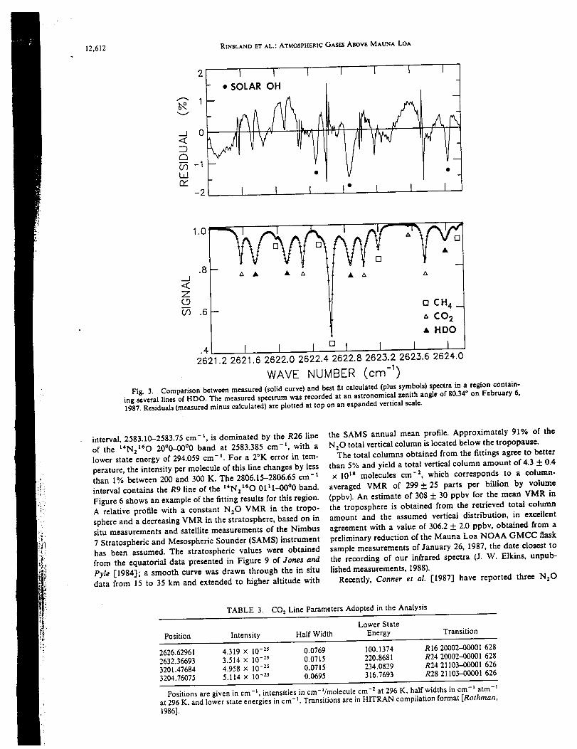
12,612 RINSLAND El" AL.: ATMOSPHERIC GASF._ ABOVE MAUNA LOA

v

J 0.<

3-1LLIrY

-2

I I 1 I

I

lo.8 • ,,,

tt ""Z

C__ Q CH 4 _(/3 .6--

CO 2

• HDO

.4 I I I n I I I t2621.2 2621.6 2622.0 2622.4- 2622.8 262,.3.2 262,.3.6 2624.0

WAVE NUMBER (cm -1)

Fig. 3. Comparison between measured (solid curve) and best fit calculated (plus symbols) spectra in a region contain-ing several lines of HDO. The measured spectrum was recorded at an astronomical zenith angle of 80.34" on February 6,1987. Residuals (measured minus calculated) are plotted at top on an expanded vertical scale.

interval, 2583.10-2583.75 cm-t, is dominated by the R26 line

of the t4N2t60 20 °0--'00°0 band at 2583.385 era -t, with a

lower state energy of 294.059 cm- 1. For a 2°K error in tem-

perature, the intensity per molecule of this line changes by lessthan 1% between 200 and 300 K. The 2806.15-2806.65 cm -1

interval contains the R9 line of the I"N z t60 01 t I_00o0 band.

Figure 6 shows an example of the fitting results for this region.

A relative profile with a constant N20 VMR in the tropo-

sphere and a decreasing VMR in the stratosphere, based on in

situ measurements and satellite measurements of the Nimbus

7 Stratospheric and Mesospheric Sounder (SAMS) instrument

has been assumed. The stratospheric values were obtained

from the equatorial data presented in Figure 9 of Jones and

Pile 1"1984]; a smooth curve was drawn through the in situdata from 15 to 35 km and extended to higher altitude with

the SAMS annual mean profile. Approximately 91% of the

N20 total vertical column is located below the tropopause.The total columns obtained from the fittings agree to better

than 5% and yield a total vertical column amount of 4.3 ___0.4

x l0 Is molecules cm -2, which corresponds to a column-

averaged VMR of 299 + 25 parts per billion by volume

(ppbv). An estimate of 308 + 30 ppbv for the mean VMR in

the troposphere is obtained from the retrieved total column

amount and the assumed vertical distribution, in excellent

agreement with a value of 306.2 + 2.0 ppbv, obtained from a

preliminary reduction of the Mauna Loa NOAA GMCC flask

sample measurements of January 26, 1987, the date closest to

the recording of our infrared spectra (J. W. Elkins, unpub-

lished measurements, 1988).

Recently, Conner et al. 1"1987] have reported three N20

TABLE 3. CO: Line Parameters Adopted in the Analysis

Lower State

Position Intensity Half Width EnergyTransition

2626.62961 4.319 x 10-zs 0.0769 100.1374 RI6 20002-00001 6282632.36693 3.514 x I0 -25 0.0715 220.8681 R24 20002-00001 6283201.47684 4.958 x 10-z_ 0.0715 234.0829 R24 21103-00001 6263204.76075 5.114 x 10 -25 0.0695 316.7693 R28 21103-00001 626

Positions are given in cm -1, intensities in cm-_/molecule cm -z at 296 K, half widths in cm-I atm-at 296 K, and lower state energies in cm-L Transitions are in HITRAN compilation format [Rothman,

1986].

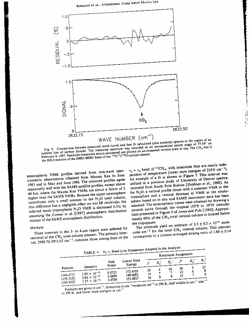
RINSLAND El" AL." ATMOSPHERIC GASES ABOVE NiAUNA LOA

, i

1"0 1

..J4_. .9 -Z(_9

{/3

2632.15

CO 2

2632.50

WAVE NUMBER (cm-_)

Fig. 4. Comparison between measured (solid curve) and best fit calculated (plus symbols) spectra in the region of anisolated line of carbon dioxide. The measured spectrum was recorded at an astronomical zenith angle of 7-/.540 onFebruary 6, 1987. Residuals (measured minus calculated) arc plotted on an expanded vertical scale at top. The CO2 line is

the R24 transition of the 20002-00001 band of the t6ot2CtSO isotopic species.

stratospheric VMR profiles derived from ram-wave spec-

trometric observations obtained from Mauna Kea in June

1983 and in May and June 1986. The retrieved profiles agree

reasonably well with the SAMS satellite profiles, except above

40 kin, where the Mauna Kea VMRs are about a factor of 2

higher than the SAMS VMRs. Because the upper stratosphere

contributes only a small amount to the N20 total column,

this difference has a negligible effect on our IR retrievals; the

inferred mean tropospheric N2 O VMR is decreased 0.3% by

assuming the Conner er ol. [198"/] stratospheric distribution

instead of the SAMS stratospheric distribution.

Methane

Three intervals in the 3- to 4-/_m region were selected for

retrieval of the CH_ total column amount. The primary inter-

val, 2908.70-2911.02 cm-t, contains three strong lines of the

v 2 + v, band of tZCH_, with intensities that are nearly inde-

pendent of temperature (lower state energies of 219.9 era-t) •

An example of a fit is shown in Figure 7. This interval was

utilized in a previous study of University of Denver spei:tra

recorded from South Pole Station [Goldman et al., 1988]. As

for N20, a vertical profile shape with a constant VMR in the

troposphere and a vertical decrease in VMR in the strato-

sphere based on in situ and SAMS instrument data has been

assumed. The stratospheric values were obtained by drawing a

smooth curve through the tropical (10 °S to 10ON latitude)

data presented in Figure 5 of Jones and pyle [1984]. Approxi-

mately 90% of the CH, total vertical column is located below

the tropopause.The retrievals yield an estimate of 2.3 4- 0.2 x 1019 mole-

cules cm -2 for the total CH, vertical column. This amount

corresponds to a column-averaged mixing ratio of 1.60 4- 0.14

TABLE 4. O_ v, Band Line Parameters Adopted in the AnalysisRotational Assignment

Half Lower State .I" Ka" g ¢ 't

Intensity Width Energy J' K°' Kc'Position 3 25

1146.4715 3.95 x 10-:z 0.0723 372.4103 29 4 26 281155.5132 2.84 × 10-:: 0.0699 189.0092 14 7 7 13 6 81163.4222 2.57 × 10-z: 0.0700 253.8827 16 8 8 15 7 9

Positions are given in cm -_ , intensities in cm -_/m°lecule cm-2 at 296 K. half widths in cm -t arm-'

at 296 K, and lower state energies in cm -_

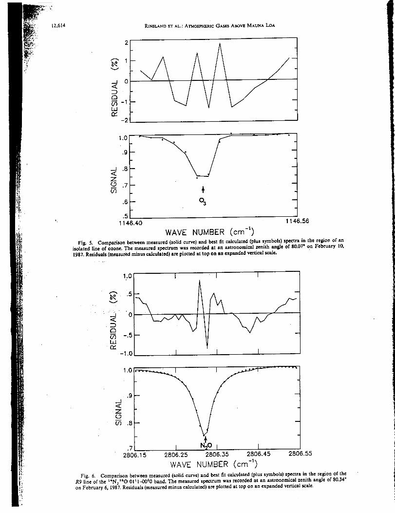
12,614 RINSLAND El" AL.: ATMOSPHERIC GASES ABOVE MAUNA LeA

!!

t i • i T •

1.0.8.9"

.7 _,

.6 03

.511+6.+0 11+6.56

WAVE NUMBER (cm -1)

Fig. 5. Comparison between measured (solid curve) and best fit calculated (plus symbols) spectra in the region of anisolated line of ozone. The measured spectrum was recorded at an astronomical zenith angle of 80.07 ° on February 10,

1987. Residuals (measured minus calculated) are plotted at top on an expanded vertical scale.

1.0

V

-.5ILln/

-1.0

l" T 1

1.0 ¸

_J<

7

(/3 .8

+.7

2806.15 2806.25 2806.35 2806.45 2806.55

WAVE NUMBER (cm-;)

Fig. 6. Comparison between measured (solid curve) and best fit calculated (plus symbols) spectra in the region of the

R9 line of the L+Na _60 01_l-00°0 band. The measured spectrum was recorded at an astronomical zenith angle of 80.34 °

on February 6, 1987. Residuals (measured minus calculated) are plotted at top on an expanded vertical scale.

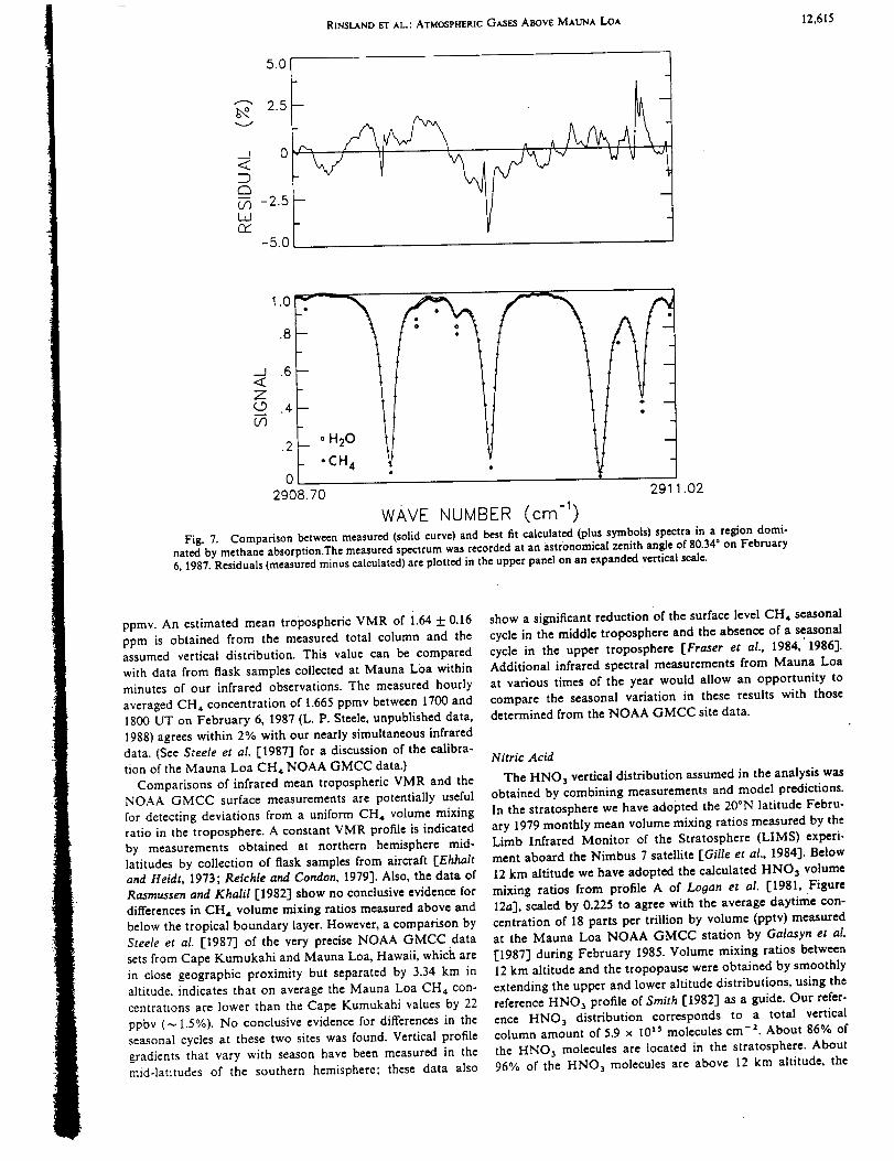
RINSLANDEl"AL.: ATMOSPHERICGnsm A_ovE MAtnqx Lo^ 12.615

t

<

C3

O'3Wc'Y

5.0

2.5

0

-2.5

-5.0

J

ZO

(/3

1.0

.8

.6

T

.4

.2 ° H2

• CH 4 t

0

2908.70 291 .02

wAvE NUMBER (cm -1)

Fig. 7. Comparison between measured (solid curve) and best fit calculated (plus symbols) spectra in a region domi-nated by methane absorption.The measured spectrum was recorded at an astronomical zenith angle of $0.34 ° on February6, 1987. Residuals (measured minus calculated) are plotted in the upper panel on an expanded vertical scale.

ppmv. An estimated mean tropospheric VMR of i.64 _+ 0.16

ppm is obtained from the measured total column and theassumed vertical distribution. This value can be compared

with data from flask samples collected at Mauna Loa withinminutes of our infrared observations. The measured hourly

averaged CH, concentration of 1.665 ppmv between 1700 and

1800 UT on February 6, 1987 (L. P. Steele, unpublished data,

1988) agrees within 2% with our nearly simultaneous infrared

data. (See Steele et al. [1987] for a discussion of the calibra-

tion of the Mauna Loa CH, NOAA GMCC data.)

Comparisons of infrared mean tropospheric VMR and the

NOAA GMCC surface measurements are potentially useful

for detecting deviations from a uniform CH, volume mixing

ratio in the troposphere. A constant VMR profile is indicated

by measurements obtained at northern hemisphere mid-

latitudes by collection of flask samples from aircraft [Ehhalt

and Heidt, 1973; Reichle and Condon, 1979]. Also, the data ofRasmussen and Khalil F1982] show no conclusive evidence for

differences in CH, volume mixing ratios measured above and

below the tropical boundary layer. However, a comparison bySteele et al. [1987] of the very precise NOAA GMCC data

sets from Cape Kumukahi and Mauna Loa, Hawaii, which are

in close geographic proximity but separated by 3.34 km in

altitude, indicates that on average the Mauna Loa CH, con-

centrations are lower than the Cape Kumukahi values by 22

ppbv (~ 1.5%). No conclusive evidence for differences in the

seasonal cycles at these two sites was found. Vertical profile

gradients that vary with season have been measured in themid-latitudes of the southern hemisphere; these data also

show a significant reduction of the surface level CH, seasonal

cycle in the middle troposphere and the absence of a seasonalcycle in the upper troposphere [Fraser et al., 1984,' 1986].Additional infrared spectral measurements from Mauna Loa

at various times of the year would allow an opportunity to

compare the seasonal variation in these results with thosedetermined from the NOAA GMCC site data.

Nitric Acid

The HNO 3 vertical distribution assumed in the analysis wasobtained by combining measurements and model predictions.

In the stratosphere we have adopted the 20°N latitude Febru-

ary 1979 monthly mean volume mixing ratios measured by theLimb Infrared Monitor of the Stratosphere (LIMS) experi-

ment aboard the Nimbus 7 satellite ['GlUe et aL, 1984]. Below

12 km altitude we have adopted the calculated HNO3 volume

mixing ratios from profile A of Logan et aL [1981, Figure

12a], scaled by 0.225 to agree with the average daytime con-

centration of 18 parts per trillion by volume (pptv) measured

at the Mauna Loa NOAA GMCC station by Galasyn et al.

I"1987] during February 1985. Volume mixing ratios between12 km altitude and the tropopause were obtained by smoothly

extending the upper and lower altitude distributions, using the

reference HNO_ profile of Smith [1982] as a guide. Our refer-

ence HNO3 distribution corresponds to a total vertical

column amount of 5.9 x 10 ts molecules cm -z. About 86% of

the HNO3 molecules are located in the stratosphere. About

96% of the HNO3 molecules are above 12 km altitude, the

12,616 RINSLAND El" AL.: ATMOSPHERIC GASES ABOVE MAUNA LOA

v

_O<

C_

OqtadfY

-2

1.0:

/

Z .9(.9

Oq

.8871.8 )73.2

WAVE NUMBER (cm -1)

Fig. 8. Comparison between measured (solid curve) and best fit calculated (plus symbols) spectra in a region contain-ing three P-branch manifolds of the vs band of nitric acid (HNOs). The measured spectrum was recorded at an astro-nomical zenith angle of 84.31 ° on February 10, 1987. Residuals (measured minus calculated) are plotted at top on an

expanded vertical scale.

approximate base altitude of previously reported aircraft total

column amount surveys.

Two spectral intervals containing a number of strong P-

branch manifolds of the v s band of HNO 3 were analyzed,

assuming the 1986 HITRAN compilation line parameters

[Rothman et al., 1987"1. Total column amounts retrieved from

four spectra using these two intervals agree to 5%, a value we

have adopted as the estimate of the precision. The averageretrieved total column amount of 5.9 × l0 ts molecules cm -2

is estimated to have an absolute accuracy of 20%, based on

sensitivity studies similar to those reported by Murcray et al.

l"1987]. Figure 8 shows an example of the fitting results.

Results of a number of -_urveys of the latitudinal variation of

the total vertical column amount of HNO 3 are collected in

Figure 2 of Murcray et al. 1"1987]. At the latitude of Mauna

Loa, these values range from about 4 to 6 × 1015 molecules

cm -z. Hence our Mauna Loa result is located in the upper

part of the range of these measurements.As noted above, measurements and model predictions sug-

gest that the troposphere contributes only a relatively small

amount to our measured total column. However, our infrared

data were recorded in winter, when the HNO 3 surface con-

centrations at Mauna Loa are lowest [Galasyn et al., 1987].

Highest concentrations were measured during the late

summer. Assuming the average daytime surface concentration

of 97 pptv measured in August to scale the same vertical

distribution shape [Logan et al., 1981, Figure 12a, profile A],we calculate a total vertical column of HNO3 below 12 km

altitude of 1.4 × 10 t s molecules can-2, about 24% of our mea-

sured total column. Hence seasonal changes in the tropo-

spheric column amount need to be considered in interpreting

a time series of HNO s total columns measured from the

ground, even from a remote site such as Mauna Loa. Al-

though a diurnal cycle (higher concentrations during the up-

slope wind hours of 0900-2100 LT) in the ground-level con-centrations at Mauna Loa was also observed, Galasyn et al.

1"1987] believe these changes are the result of depletion

through dry deposition on the mountain's elevated surface

and are unlikely to be reflected in the free troposphere. The

daytime measurements of Galasyn et al. [1987] are consistentwith GAMETAG measurements of free tropospheric HNO 3

[Huebert and Lazrus, 1980] obtained during the same time of

the year (see Galasyn et al. [1987] for a discussion).

Hydrogen Chloride

As in two recent ground-based studies [Goldman et al.,

1987a; Farmer et al., 1987], we adopted the P2 transition of

H35CI at 2843.625 cm-t and the R1 transition of H35CI at

2925.897 cm -1 as the principal lines for the atmospheric

quantification of hydrogen chloride. The total columns

derived from the fittings of these two lines agree to better than

5%. An example of a fit to the RI line is shown in Figure 9.

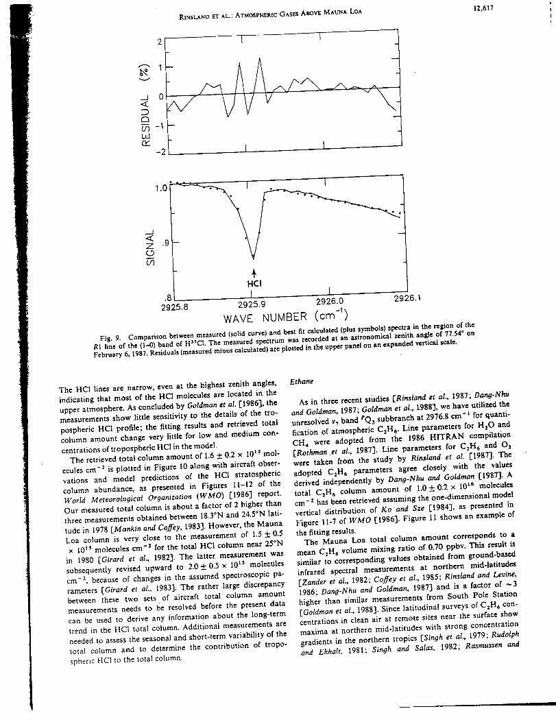
._J 0

:I

_-ILdn"

-2

RINSLAND El" AL.: ATMOSPHERIC GASES ABOVE MAUNA LOA

i -- i i

12,617

1.0

...A

Z 'g

coO'l

HCI.8 j I

2925.8 2925.9 2926.0 2926.1

WAVE NUMBER (c m-l)• ated lus symbols) spectra in the region of the

Corn arison between measured (sohd curve) and best_fit calcul (P tronomical zenith angle of 77.54 ° onFig. 9. the (IP--_)band of H_sc1. The measurea spectrum was recorded at an asRI line of

February 6, 198"/. Residuals (measured minus calculated) are plotted in the upper panel on an expanded vertical scale.

The HCI lines are narrow, even at the highest zenith angles,

indicating that most of the HC1 molecules are located in the

upper atmosphere. As concluded by Goldman et al. [1986], the

measurements show little sensitivity to the details of the tro-

pospheric HCI profile; the fitting results and retrieved totalcolumn amount change very little for low and medium con-

centrations of tropospheric HC1 in the model. 10 t s tool-The retrieved total column amount of 1.6 4- 0.2 x

ecules cm-2 is plotted in Figure 10 along with aircraft obser-

vations and model predictions of the HCI stratospheric

column abundance, as presented in Figures 11-12 of the

World Meteorological Organization (WMO) [1986] report.

Our measured total column is about a factor of 2 higher than

three measurements obtained between 18.3°N and 24.5°N lati-

tude in 1978 [Mankin and Coffey, 1983]. However, the Mauna

Loa column is very close to the measurement of 1.5 + 0.5

x l0 ts molecules cm -2 for the total HCI column near 25°N

in 1980 [Girard et al., 1982]. The latter measurement was

subsequently revised upward to 2.0 4-0.5 x 10 t5 molecules

cm-2 because of changes in the assumed spectroscopic pa-

rameters [Girard et al., 1983]. The rather large discrepancy

between these two sets of aircraft total column amount

measurements needs to be resolved before the present data

can be used to derive any information about the long-term

trend in the HCI total column. Additional measurements are

needed to assess the seasonal and short-term variability of the

total column and to determine the contribution of tropo-

spheric HC1 to the total column.

Ethane

As in three recent studies [Rinsland et al., 1987; Dano "Nhu

and Goldman, 1987; Goldman et al., 1988], we have utifized the

unresolved v_ band PQ3 subbranch at 2976.8 cm- t for quanti-

fication of atmospheric C2H6- Line parameters for H20 and

CH, were adopted from the 1986 HITRAN compilation

[Rothman et al., 1987]. Line parameters for C2H6 and 03

were taken from the study by Rinsland et al. [1987]. The

adopted CzH6 parameters agree closely with the values

derived independently by Dang-Nhu and Goldman [1987]. A

total C=Hs column amount of 1.0 +0.2 x l0 ts molecules

cm-2 has been retrieved assuming the one-dimensional model

vertical distribution of Ko and Sze [1984], as presented in

Figure 11-7 of WMO [1986]. Figure 11 shows an example of

the fitting results.The Mauna Loa total column amount corresponds to a

mean C,H6 volume mixing ratio of 0.70 ppbv. This result is

similar to corresponding values obtained from ground-based

infrared spectral measurements at northern mid-latitudes

[Zander et al., 1982; Coffey et al., 1985; Rinsland and Levine,

1986; Dano -Nhu and Goldman, 1987] and is a factor of ~3

higher than similar measurements from South Pole Station

[Goldman et al., 1988]. Since latitudinal surveys of C:Hs con-

centrations in clean air at remote sites near the surface show

maxima at northern mid-latitudes with strong concentration

gradients in the northern tropics [Sino het al., 1979; Rudolph

and Ehhalt, 1981; Singh and Salas, 1982; Rasmussen and

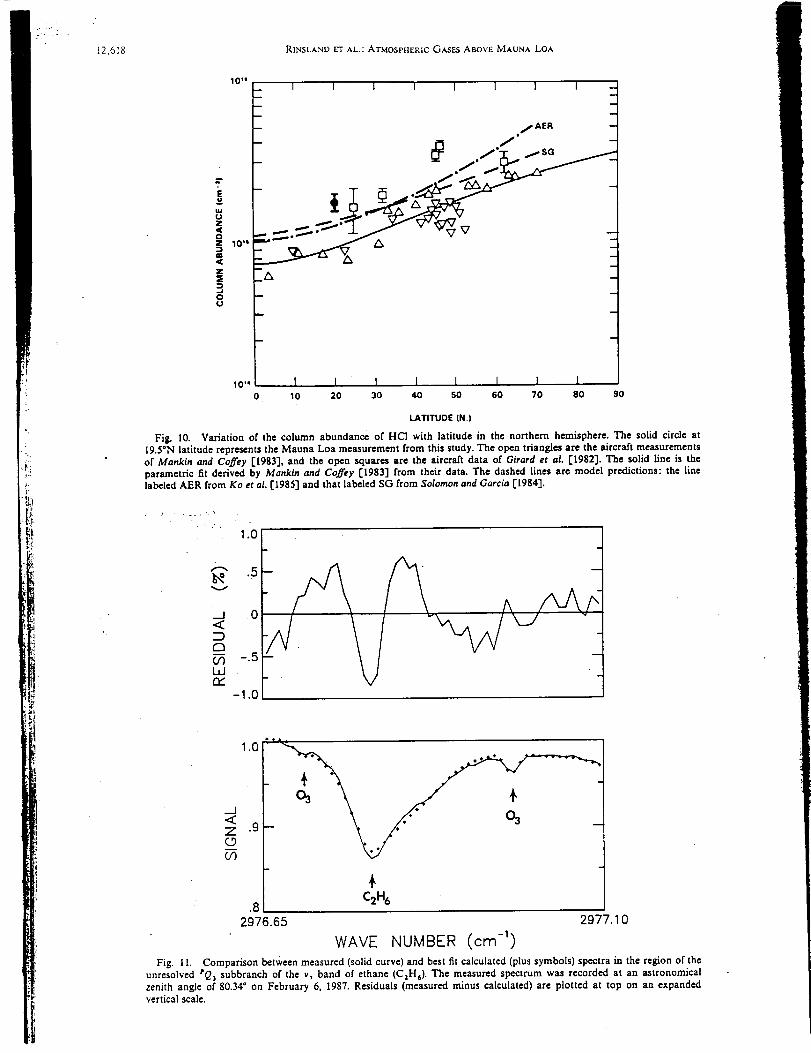
12,618 RINSLAND El" AL.: ATMOSPHERIC GASF..5 ABOVE I_IAUNA LeA

I0 la

10"

Z

30_J

__ I i I I I I I i

-1_ _AER 1

- _" -

_

_o,, I I I I I I I I0 10 20 30 40 S0 60 70 80 90

LATITUDE (N.I

Fig. 10. Variation of the column abundance of HCI with latitude in the northern hemisphere. The solid circle at19.5°N latitude represents the Mauna Lea measurement from this study. The open triangles are the aircraft measurementsof Mankin and Coffey [1983], and the open squares are the aircraft data of Girard et aL [1982]. The solid line is theparametric fit derived by Mankin and Coffey [1983] from their data. The dashed lines are model predictions: the linelabeled AER from Ko et aL [1985] and that labeled SG from Solomon and Garcia [1984].

1.0

"_ .5

v

.-J 0<

=)

-.5I_JrY

-1.0

._J.<Z

Oq

1.0

.9

t •

C2H 6.8

2976.65 2977.10

WAVE NUMBER (cm -1)

Fig. 1 I. Comparison between measured (solid curve) and best fit calculated (plus symbols) spectra in the region of the

unresolved _Q3 subbranch of the vs band of ethane (C2He). The measured sp_trum was recorded at an astronomicalzenith angle of 80.34 ° on February 6, 1987. Residuals (measured minus calculated) are plotted at top on an expandedvertical scale.

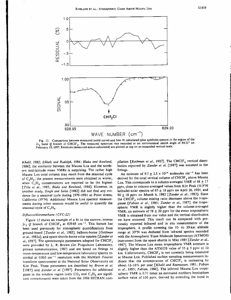
RINSLAND ET AL.: ATMOSPHERIC GASES ABOVE MAUNA LOA 12,619

,5

V

0<

dh

I,ICY

-I .0

1.00

_J<Z .95

(_9

+CH F2Cl

.90

828.95 829.20

WAVE NUMBER (cm -1)

Fig. 12. Comparison between measured (solid curve) and best fit calculated (plus symbols) spectra in the region of the

2v 2 band Q branch of CHCIF:. The measured spectrum was recorded at an astronomical zenith angle of 84.31 ° onFebruary 10. 1987. Residuals (measured minus calculated) are plotted at top on an expanded vertical scale.

Khalil, 1982; Ehhalt and Rudolph, 1984; Blake and Rowland,

1986], the similarity between the Mauna Loa and the north-

ern mid-latitude mean VMRs is surprising. The rather high

Mauna Loa total column may result from the seasonal cycle

of C:H6; the present measurements were obtained in winter,

when C2H 6 concentrations are reported to be the highest

[Tille et al., 1985; Blake and Rowland, 1986]. However, in

another study, Singh and Salas [1982] did not find any evi-

dence for a seasonal cycle during 1979-1981 at Point Arena,

California (39°N). Additional Mauna Loa spectral measure-

ments during other seasons would be useful to quantify the

seasonal cycle of C2H6.

Difluorochloromethane (CFC-22)

Figure 12 shows an example of a fit to the narrow, intense

2v: Q branch of CHCIF: at 829.05 cm-'. This feature has

been used previously for atmospheric quantifications from

ground-based [Zander et al., 1983], balloon-borne [Goldman

et al., 1981a], and space-shuttle-borne solar spectra [Zander et

al., 1987]. The spectroscopic parameters adopted for CHCIF:

were provided by L. R. Brown (Jet Propulsion Laboratory,

private communication, 1987) and are based on fittings to

room-temperature and low-temperature laboratory spectra re-

corded at 0.005 cm-t resolution with the McMath Fourier

transform spectrometer at the National Solar Observatory on

Kitt Peak. These parameters are described by Brown et al.

[1987] and Zander et aL [1987]. Parameters for additional

gases in the window region (only CO: and C_H 6 are signifi-

cant contaminants) were taken from the 1986 HITRAN com-

pilation [Rothman et al., 198_)]. The CHCIF 2 vertical distri-

bution reported by Zander et al. [1987] was assumed in the

fittings.

An estimate of 9.7 4- 2.5 x I0 t" molecules cm -e has been

derived for the total vertical column of CHCIF 2 above Mauna

Loa. This corresponds to a column-averaged VMR of 68 4- 17

pptv, close to column-averaged values from Kitt Peak (31.9°N

latitude) solar spectra of 67 + 16 pptv on April 26, 1981, and

90 4- 18 pptv on March 6, 1982 [Zander et al., 1983]. Since

the CHCIF 2 volume mixing ratio decreases above the tropo-

pause [Fabian et al., 1985; Zander et al., 1987], the tropo-

spheric VMR is slightly higher than the column-averaged

VMR; an estimate of 78 _ 20 pptv for the mean tropospheric

VMR is obtained from our value and the vertical distribution

we have assumed. This result can be compared with pre-

viously reported infrared and in situ measurements of the

troposphere. A profile covering the 10- to 30-km altitude

range at 30°N was deduced from infrared spectra recorded

with the Atmospheric Trace Molecule Spectroscopy (ATMOS)

instrument from the space shuttle in May 1985 [Zander et al.,

1987]. The Mauna Loa mean tropospheric VMR estimate is

slightly higher than the ATMOS value of 55 +_ 5 pptv at 10

kin. Unfortunately, CHC1F2 is not currently being measured

at Mauna Loa. Published surface sampling measurements in-

dicate that the Concentration of CHClF 2 is increasing by

about 12-16% per year [Khalil and Rasmussen, 1981; Fabian

et al., 1985; Fabian, 1986]. The inferred Mauna Loa tropo-

spheric VMR is 0.71 times an estimated northern hemisphere

surface value of ll0 pptv, derived by extending the trend in

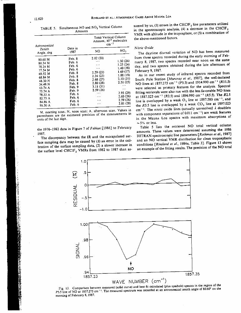
12,620

TABLE 5. Simultaneous NO and NO_ Vertical ColumnAmounts

Total Vertical ColumnAmount, 10 .5 molecules

Astronomical cm-"Zenith Date in

Angle, deg 1987 NO NO:

RINSt.AND _ XL.: ATMOSPHERICGASES ABOVEMAUNX LOA

sumed by us, (3) errors in the CHCIF2 line parameters utilized

in the spectroscopic analysis, (4) a decrease in the CHCIFz

VMR with altitude in the troposphere, or (5) a combination of

the above-mentioned factors.

80.60 M Feb. 8 2.02 (20) '"80.34 M Feb. 6 "'" 1.30 (26)78.24 M Feb. 6 " 1.25 (24)77.54 M Feb. 6 "" 1.40 (28)69.52 M Feb. 8 2.29 (23) !.69 (17)68.84 M Feb. 8 2.34 (23) 1.88 (19)48.30 N Feb. 8 2.68 (27) 2.10 (21)

34.48 N Feb. 8 2.80 (28) 2.51 (25)63.74 A Feb. 9 3.11 (31) ""75.74 A Feb. 9 2.59 (26) ""78.53 A Feb. 6 "" 2.93 (29)82.75 A Feb. 6 "'" 2.60 (26)84.86 A Feb. 6 "" 2.59 (26)86.30 A Feb. 6 "'" 2.81 (28)

M, morning scan; N, noon scan; A, afternoon scan. Values in

parentheses are the estimated precision of the measurements inunits of the last digit.

the 1976-1982 data in Figure 7 of Fabian [1986] to February

1987.

The discrepancy between the IR and the extrapolated sur-

face sampling data may be caused by (1) an error in the cali-

bration of the surface sampling data, (2) a slower increase in

the surface level CHCIF2 VMRs from 1982 to 1987 than as-

Nitric Oxide

The daytime diurnal variation of NO has been measured

from three spectra recorded during the early morning of Feb-

ruary 8, 1987, two spectra recorded near noon on the same

day, and two spectra obtained during the late afternoon of

February 9, 1987.As in our recent study of infrared spectra recorded from

South Pole Station [Murcray et al., 1987], the well-isolated

NO lines at 1857.275 cm -t (P5.5) and 1914.990 cm -t (Rll.5)

were selected as primary features for the analysis. Spectral

fitting retrievals were also run with the less favorable NO lines

at 1887.523 cm- t (R2.5) and 1896.990 cm- t (R5.5). The R2.5

line is overlapped by a weak O 3 line at 1887.580 cm -t, and

the R5.5 line is overlapped by a weak CO 2 line at 1897.023

cm-t. The nitric oxide lines (actually unresolved 2 doublets

with component separations of 0.011 cm-t) are weak features

in the Mauna Loa spectra with maximum absorptions of

~ 5% or less.

Table 5 lists the retrieved NO total vertical column

amounts. These values were determined assuming the 1986

HITRAN spectroscopic line parameters [Rothman et al., 1987]

and art NO vertical VMR distribution for clean tropospheric

conditions [Rinsland et al., 1984a, Table 3"1. Figure 13 shows

an example of the fitting results. The precision of the NO total

1.01

e,"--%

_ .5

_.1<

(f)LdfY

0

-.5

-1.0

J

4

1.00

.98 -._J<ZoO3 .96 --

÷NO

.94 I 1857.551857.25

WAVE NUMBER (crn -1)

Fig. 13. Comparison between measured (solid curve) and best fit calculated (plus symbols) spectra in the region of theP5.5 line of NO at 1857.275 cm- 1. The measured spectrum was recorded at an astronomical zenith angle of 80.60 ° on the

morning of February 8, 1987.

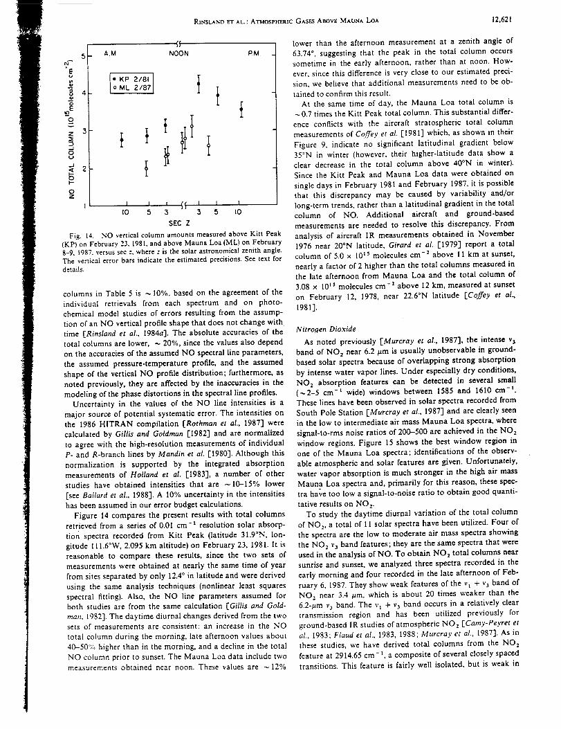
RINSLAND ET AL.: ATMOSPHERIC GASE3 ABOVE MAUNA LOA 12,62l

5-

iE

oE

O

z 3

_dO(.)

..d2

)-

OZ

I

_,.M. NOON

ML 2/87

P.M.

' _ ' It I t IlO 5 3 3 5 I0

SEC Z

Fig. 14. NO vertical column amounts measured above Kitt Peak

(KP) on February 23, 1981. and above Mauna Loa (ML) on February8-9, 1987, versus sec, where z is the solar astronomical zenith angle.The vertical error bars indicate the estimated precisions. See text for

details.

columns in Table 5 is ~ 10%, based on the agreement of the

individual retrievals from each spectrum and on photo-

chemical model studies of errors resulting from the assump-

tion of an NO vertical profile shape that does not change with

time [Rinsland et al., 1984a]. The absolute accuracies of thetotal columns are lower, ~ 20%, since the values also depend

on the accuracies of the assumed NO spectral line parameters,

the assumed pressure-temperature profile, and the assumed

shape of the vertical NO profile distribution; furthermore, as

noted previously, they are affected by the inaccuracies in the

modeling of the phase distortions in the spectral line profiles.

Uncertainty in the values of the NO line intensities is a

major source of potential systematic error. The intensities on

the 1986 HITRAN compilation [Rothman et al., 1987] were

calculated by Gillis and Goldman [1982] and are normalized

to agree with the high-resolution measurements of individual

P- and R-branch lines by Mandin et al. [1980]. Although this

normalization is supported by the integrated absorption

measurements of Holland et al. [1983], a number of other

studies have obtained intensities that are ~10-15% lower

[see Ballard et al., 1988]. A 10% uncertainty in the intensities

has been assumed in our error budget calculations.

Figure 14 compares the present results with total columns

retrieved from a series of 0.01 cm-t resolution solar absorp-

tion spectra recorded from Kitt Peak (latitude 31.9°N, lon-

gitude 111.6°W, 2.095 km altitude) on February 23, 1981. It is

reasonable to compare these results, since the two sets of

measurements were obtained at nearly the same time of year

from sites separated by only 12.4 ° in latitude and were derived

using the same analysis techniques (nonlinear least squares

spectral fitting). Also, the NO line parameters assumed for

both studies are from the same calculation [Gillis and Gold-

man, 1982]. The daytime diurnal changes derived from the two

sets of measurements are consistent: an increase in the NO

total column during the morning, late afternoon values about

40-50% higher than in the morning, and a decline in the total

NO column prior to sunset. The Mauna Loa data include two

measurements obtained near noon. These values are ~ 12%

Lower than the afternoon measurement at a zenith angle of

63.74 ° , suggesting that the peak in the total column occurs

sometime in the early afternoon, rather than at noon. How-

ever, since this difference is very close to our estimated preci-

sion, we believe that additional measurements need to be ob-

tained to confirm this result.

At the same time of day, the Mauna Loa total column is

~ 0.7 times the Kitt Peak total column. This substantial differ-

ence conflicts with the aircraft stratospheric total column

measurements of Coffey et al. [1981] which, as shown in their

Figure 9, indicate no significant latitudinal gradient below

35°N in winter (however, their higher-latitude data show a

clear decrease in the total column above 40°N in winter).

Since the Kitt Peak and Mauna Loa data were obtained on

single days in February 1981 and February 1987, it is possible

that this discrepancy may be caused by variability and/or

long-term trends, rather than a latitudinal gradient in the total

column of NO. Additional aircraft and ground-based

measurements are needed to resolve this discrepancy. From

analysis of aircraft IR measurements obtained in November

1976 near 20°N latitude, Girard et al. [1979] report a total

column of 5.0 x l0 ts molecules cm -2 above 11 km at sunset,

nearly a factor of 2 higher than the total columns measured in

the late afternoon from Mauna Loa and the total column of

3.08 × LOts molecules cm -2 above 12 km, measured at sunset

on February 12, 1978, near 22.6°N latitude [Coffey et al.,

1981].

Nitrogen Dioxide

As noted previously [Murcray et al., 1987], the intense v 3

band of NO 2 near 6.2/am is usually unobservable in ground-

based solar spectra because of overlapping strong absorption

by intense water vapor lines. Under especially dry conditions,

NO 2 absorption features can be detected in several small

(_2-5 cm -I wide) windows between 1585 and 1610 cm -l.These lines have been observed in solar spectra recorded from

South Pole Station EMurcray er al., 1987] and are clearly seen

in the low to intermediate air mass Mauna Loa spectra, where

signal-to-rms noise ratios of 200-500 are achieved in the NO 2

window regions. Figure 15 shows the best window region in

one of the Mauna Loa spectra; identifications of the observ-

able atmospheric and solar features are given. Unfortunately,

water vapor absorption is much stronger in the high air mass

Mauna Loa spectra and, primarily for this reason, these spec-

tra have too low a signal-to-noise ratio to obtain good quanti-

tative results on NO 2.

To study the daytime diurnal variation of the total column

of NO 2, a total of 11 solar spectra have been utilized. Four of

the spectra are the low to moderate air mass spectra showing

the NO 2 v a band features; they are the same spectra that were

used in the analysis of NO. To obtain NO 2 total columns near

sunrise and sunset, we analyzed three spectra recorded in the

early morning and four recorded in the late afternoon of Feb-

ruary 6, 1987. They show weak features of the v 1 + va band of

NO 2 near 3.4 #m, which is about 20 times weaker than the

6.2-#m v 3 band. The vl + v 3 band occurs in a relatively clear

transmission region and has been utilized previously for

ground-based IR studies of atmospheric NOz [Camy-Peyret et

aL, 1983; Flaud et al., 1983, 1988; Murcray et al., 1987]. As in

these studies, we have derived total columns from the NO 2

feature at 2914.65 cm-_, a composite of several closely spaced

transitions. This feature is fairly well isolated, but is weak in

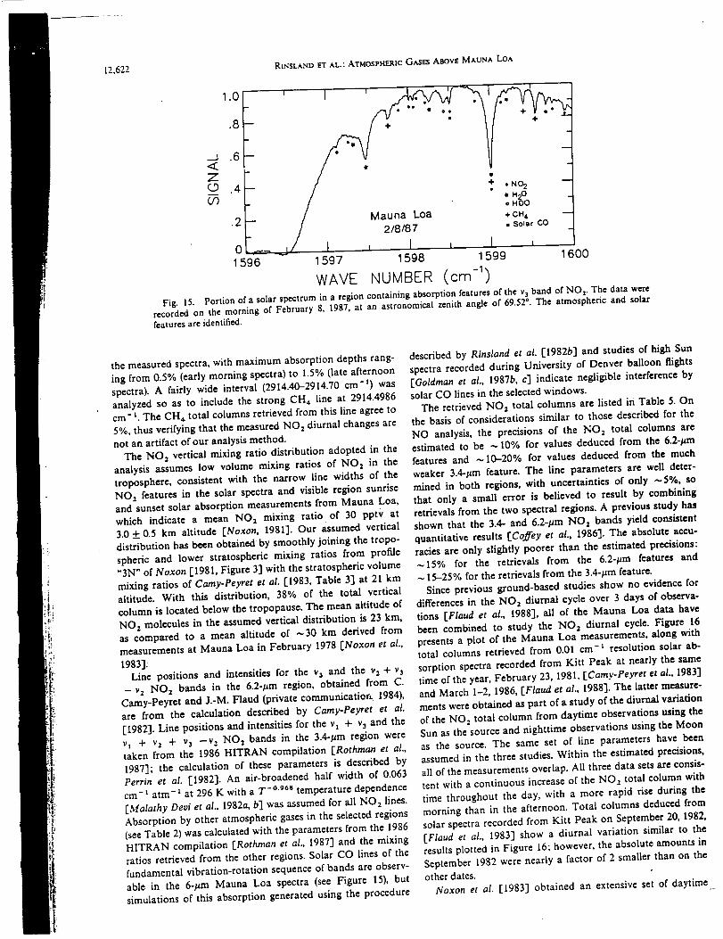
12.622 RINSLAND 121"AL.: ATMOSPFIERIC GASES ABOVE MAUNA LOA

'!I ' ' ' ...•.' '

ZQ_ .4 + "NO2

:I "°# HDO

/ Mauna Loa *CH,• / 2/8/87 . So,at CO

_ ,/ I , I , I ,1 596 1 597 1598 1 599 1 _00

WAVE NUMBER (cm -1)

Fig. 15. Portion of a solar spectrum in a region containing absorption features of the v3 band of NO r The data wererecorded on the morning of February 8, 1987, at an astronomical zenith angle of 69.52 °. The atmospheric and solar

features are identified.

the measured spectra, with maximum absorption depths rang-

ing from 0.5% (early morning spectra) to 1.5% (late afternoon

spectra). A fairly wide interval (2914.40-2914.70 cm -t) was

analyzed so as to include the strong CH, line at 2914.4986

cm = t. The CH4 total columns retrieved from this line agree to

5%, thus verifying that the measured NO2 diurnal changes are

not an artifact of our analysis method•

The NO2 vertical mixing ratio distribution adopted in the

analysis assumes low volume mixing ratios of NO2 in the

troposphere, consistent with the narrow line widths of the

NO2 features in the solar spectra and visible region sunrise

and sunset solar absorption measurements from Manna Loa,

which indicate a mean NO2 mixing ratio of 30 pptv at

3.0 + 0.5 km altitude [Noxon, 1981]. Our assumed vertical

distribution has been obtained' by smoothly joining the tropo-

spheric and lower stratospheric mixing ratios from profile

"3N" of Noxon [1981, Figure 3] with the stratospheric volume

mixing ratios of Camy-Peyret et al. [1983, Table 3] at 21 km

altitude. With this distribution, 38% of the total vertical

column is located below the tropopause. The mean altitude of

NO2 molecules in the assumed vertical distribution is 23 kin,

as compared to a mean altitude of ~ 30 km derived from

measurements at Mauna Loa in February 1978 [Noxon et al.,

1983].Line positions and intensities for the v_ and the v2 + v3

-v 2 NO: bands in the 6.2-#m region, obtained from C.

Camy-Peyret and J.-M. Flaud (private communicatior_. 1984),

are from the calculation described by Camy-Peyret et al.

[1982]. Line positions and intensities for the v: + v_ and the

vt + v2 + v_ -v 2 NO2 bands in the 3.4-gin region were

taken from the 1986 HITRAN compilation [Rothman et al.,

1987]; the calculation of these parameters is described by

Perrin et al. [1982]. An air-broadened half width of 0.063

cm-_ atm-: at 296 K with a T -°'96s temperature dependence

[Malathy Devi et al., 1982a, b] was assumed for all NOz lines.

Absorption by other atmospheric gases in the selected regions

(see Table 2) was calculated with the parameters from the 1986HITRAN compilation [Rothman et al., 1987] and the mixing

ratios retrieved from the other regions• Solar CO lines of the

fundamental vibration-rotation sequence of bands are observ-

able in the 6-#m Mauna Loa spectra (see Figure 15), but

simulations of this absorption generated using the procedure

described by Rinsland et al. [1982b] and studies of high Sun

spectra recorded during University of Denver balloon flights

[Goldman et al., 1987b, c] indicate negligible interference by

solar CO lines in the selected windows.

The retrieved NO: total columns are listed in Table 5. On

the basis of considerations similar to those described for the

NO analysis, the precisions of the NO: total columns are

estimated to be ~ 10% for values deduced from the 6.2-#m

features and ~ 10-20% for values deduced from the much

weaker 3.4-/_m feature. The line parameters are well deter-

mined in both regions, with uncertainties of only ~5%, so

that only a small error is believed to result by combiningretrievals from the two spectral regions. A previous study has

shown that the 3.4- and 6.2-#m NO2 bands yield consistent

quantitative results [Coffey et al., 1986]. The absolute accu-

racies are only slightly poorer than the estimated precisions:

~15% for the retrievals from the 6.2-/_m features and

~ 15-25% for the retrievals from the 3.4-/_m feature.

Since previous ground-based studies show no evidence for

differences in the NO: diurnal cycle over 3 days of observa-

tions [Flaud et al., 1988], all of the Mauna Loa data havebeen combined to study the NO: diurnal cycle. Figure 16

presents a plot of the Mauna Loa measurements, along withtotal columns retrieved from 0.01 crn-t resolution solar ab-

sorption spectra recorded from Kitt Peak at nearly the sametime of the year, February 23, 1981, [Camy-Peyret et al., 1983]

and March 1-2, 1986, [Flaud et al., 1988]. The latter measure-

ments were obtained as part of a study of the diurnal variation

of the NO: total column from daytime observations using the

Sun as the source and nighttime observations using the Moon

as the source. The same set of line parameters have been

assumed in the three studies. Within the estimated preeisioas,

all of the measurements overlap• All three data sets are consis-

tent with a continuous increase of the NO: total column with

time throughout the day, with a more rapid rise during the

morning than in the afternoon. Total columns deduced from

solar spectra recorded from Kitt Peak on September 20, 1982,

[Flaud et al., 1983] show a diurnal variation similar to the

results plotted in Figure 16; however, the absolute amounts in

September 1982 were nearly a factor of 2 smaller than on the

other dates.Noxon et al. [1983] obtained an extensive set of daytime

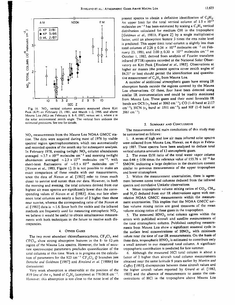
RINSLAND ET AL.: ATMOSPHERIC GASES ASOVE MAUNA LO^ 12,623

O

z

J0

-J

li KP 2/81KP .3/86ML 2/87

NOON P M

2I0 5 3 2 2 3 5 I0

SEC Z

Fig. 16. NO 2 vertical column amounts measured above KiltPeak (KP) on February 23, 1981, and March 1-2. 1986, and aboveMauna Loa (ML) on February 6, 8-9, 1987, versus sec z, where z isthe solar astronomical zenith angle. The vertical bars indicate the

estimated precisions. See text for details.

NO 2 measurements from the Mauna Loa NOAA GMCC sta-

tion. The data were acquired during most of 1978 by visible

spectral region spectrophotometers, which ran automatically

and recorded spectra of the zenith sky for subsequent analysis.

In February 1978, evening twilight NO 2 column abundances

averaged ~3.7 x I0 t5 molecules cm -z and morning twilight

abundances averaged ~2.3 x 10 t5 molecules cm -2, with

short-term fluctuations of ~0.5 x 10 _s molecules cm -z

[Noxon et al., 1983, Figure 1]. It is not possible to make an

exact comparison of these results with our measurements,

since the data of Noxon et al. [1983] refer to times much

closer to sunrise and sunset than our data. However, in both

the morning and evening, the total columns derived from our

highest air mass spectra are significantly lower than the corre-

sponding values of Noxon et al. [1983]. Also, our late after-

noon total columns are nearly a factor of 2 higher than those

near sunrise, whereas the corresponding ratio of the Noxon et

al. [1983] data is ~ 1.6. Since both the visible and the infrared

methods are frequently used for measuring atmospheric NO 2,

we believe it would be useful to obtain simultaneous measure-

ments with both techniques in the future to resolve such dis-

crepancies.

4. OTHER GASES

The two most abundant chlorofluorocarbons, CF2CI 2 and

CFCIj, show strong absorption features in the 8- to 12-#m

region of the Mauna Loa spectra. However, the lack of accu-

rate spectroscopic parameters precludes quantification of the

total columns at this time. Work is in progress on the calcula-

tion of parameters for the 923 cm- l CF2C12 Q branches (see

Deroche and Goldman [1987] and Rinsland et al. [1988b] for

discussions).

Very weak absorption is observable at the position of the

R19 line of the v s band of C2H 2 (acetylene) at 776.0818 cm-1

However. this absorption is too close to the noise level of the

present spectra to obtain a definitive identification of CzH 2.

An upper limit for the total vertical column of 1.5 x 10 ts

moiecules cm-2 has been estimated by scaling a C2H 2 vertical

distribution calculated for medium OH in the troposphere

[Goldman et al., 1981b, Figure 2] by a single multiplicative

factor, until an absorption feature 3 times the rms noise level

is predicted. This upper limit total column is slightly less thantotal columns of 2.28 + 0.34 x 1015 molecules cm -2 on Feb-

ruary 23, 1981, and 2.00___ 0.30 x l0 ts molecules cm -2 on

October 1, 1982, derived from analysis of Fourier transform

infrared (FTIR) spectra recorded at the National Solar Obser-

vatory on Kitt Peak [Rinsland et al., 1985]. Observations at

higher air masses (the present spectra cover zenith angles of

84.31 ° or less) should permit the identification and quantita-

tive measurement ofC2H 2 from Mauna Loa.

A number of additional atmospheric gases have strong IR

absorption bands outside the regions covered by the MaunaLoa observations. Of these, four have been detected using

similar IR instrumentation and could be readily monitored

from Mauna Loa. These gases and their most favorable IR

bands are OCS (v 3 band at 2062 cm- t), CO (1-0 band at 21t7

cm-t), HCN (v3 band at 3311 cm-t), and HF (I-0 band at

3961 cm- l).

5. SUMMARY AND CONCLUSIONS

The measurements and main conclusions of this study may

be summarized as follows:

1. A series of high and low air mass infrared solar spectra

were collected from Mauna Loa, Hawaii, on 4 days in Febru-

ary 1987. These spectra have been analyzed to deduce total

vertical column amounts of 13 atmospheric gases.

2. The mean D/H i'atio of the total watei" vapor column

was 0.44 + 0.06 times the reference value of 155.76 x 10 -6 for

SMOW, indicating a large depletion in the deuterium content

similar to previous measurements of the upper troposphere

and lower stratosphere.

3. Within the measurement uncertainties; there is agree-

ment between ozone total columns deduced from the infrared

spectra and correlative Umkehr observations.

4. Mean tropospheric volume mixing ratios of CO 2, CH,,,

and N:O deduced from our IR observations agree with cor-

relative NOAA GMCC measurements within the measure-

ment uncertainties. This implies that the NOAA GMCC sur-

face volume mixing ratios are good measures of the mean

volume mixing ratios of these gases in the troposphere.

5. The measured HNO 3 total column agrees within the

errors with published aircraft ahd satellite measurements of

the total stratospheric column. Published sampling measure-

ments from Mauna Loa show a" significant seasonal cycle in

the surface level concentrations of HNO 3, with minimum

values near the time of our IR measurements. On the basis of

these data, tropospheric HNO 3 is estimated to contribute onlya small amount to our measured total column. A significant

tropospheric contribution is predicted for late summer.

6. Although the measured HCI total Column is about a

factor of 2 higher than aircraft total column measurements

obtained near the same latitude 9 years earlier by Mankin and

Cofley [1983], discrepancies between these aircraft values and

the higher aircraft values reported by Girard et al. [1982,

1983] and the absence of measurements to assess the con-

centrations of HCI in the troposphere above Mauna Loa

12,624 RINSLAND ET AL.; ATMOSPHERIC GASES ABOVE MAUNA LOA

make it impossible at present to derive information about

long-term trends in the HCI total column from our data.

7. The mean tropospheric volume mixing ratio of CHC1F 2

deduced from the infrared spectra is about 30% lower than a

value obtained from an extrapolation of in situ surface data to

the date of our infrared observations.

8. Simultaneous measurements of the daytime diurnal

variations of the total columns of NO and NO z have been

obtained. To our knowledge, these are the first such observa-

tions that have been reported.

The column amounts reported here were obtained from

spectra recorded with a resolution of 0.02 cm -1. Absolute

accuracies of about 10% have been achieved. The good agree-

ment between the IR and the GMCC data is encouraging. It is

important to recall that several of the sources of error are

systematic (for example, the uncertainties in the assumed line

intensities) and that these effects are eliminated or reduced

significantly when results are normalized to study a time series

of measurements. Hence additional sets of IR measurements

obtained from Mauna Loa and analyzed in the same way

should yield precise information on seasonal and long-term

trends for a number of important atmospheric species.

Observations with a new interferometer operating at a reso-

lution of 0.002 cm-' are planned from Mauna Loa and

should yield improved results. The increased resolution should

permit details of the altitude distributions to be derived from

analysis of the observed pressure-broadening effects as a func-

tion of solar zenith angle. Such effects are apparent in HNO 3

features recorded in initial solar observations from the Univer-

sity of Denver. Improved information on the vertical profile is

necessary, for example, in interpreting secular trends in HCI,

since significant variability of the tropospheric profile may

mask increases observed in the stratospheric total column

[WMO, 1986].

Acknowledoments. Research at the University of Denver was sup-

ported by NASA. Acknowledgment is made to the National Center

for Atmospheric Research, which is supported by the National Sci-ence Foundation, for computer time used in this research. We are

grateful to Linda R. Brown of the Jet Propulsion Laboratory for

allowing use of the ATMOS parameters for CHCIF 2. We also thankCarolyn Sutton of STX Corporation for processing the data at NASA

Langley, Susan Edwards of NASA Langley for assistance in preparingthis manuscript, and an anonymous referee for a number of helpful,

detailed comments.

REFERENCES

Abbas, M. M., J. Guo, B. Carli, F. Mencaraglia, A. Bonetti, M. Car-

[otti, and I. G. Nolt, Stratospheric 05, H20, and HDO distri-butions from balloon-based far-infrared observations, J. Geophys.

Res., 92, 8354-8364, 1987.Baertschi, P., Absolute tsO content of standard mean ocean water,

Earth Planet. Sci. Lett., 31,341-344, 1976.

Ballard, J., W. B. Johnston, B. J. Kerridge, and J. J. Remedios, Experi-

mental spectral line parameters in the 1-0 band of nitric oxide, J.

Mol. Specfrosc., 127, 70-82, 1988.Benner, D. C., V. Malathy Devi, C. P. Rinsland, and P. S. Ferry-

Leeper, Absolute intensities of CO 2 lines in the 3140-3410 cm=

spectral region, Appl. Opt., 27, 1588-1597, 1988.Bischof, W., R. Borchers, P. Fabian, and B. C. Kr/.iger, Increased

concentration and vertical distribution of carbon dioxide in the

stratosphere, Nature, 316, 708-710, 1985.Blake. D. R., and F. S. Rowland, Global atmospheric concentrations

and source strength of ethane, Nature, 321, 231-233, 1986.Brown, L. R., C. B. Farmer, C. P. Rinsland, and R. A. Toth, Molecu-

lar line parameters for the atmospheric trace molecule spectroscopy

experiment, Appl. Opt., 26, 5154-5182, 1987.

Camy-Peyret, C., J.-M. Flaud, A. Perrin. and K. Narahari Rao, Im-

proved line parameters for the v3 and v z + v3 -v: bands of

l'tNt602, d. Mol. Spectrosc., 95, 72-79, 1982.

Camy-Peyret, C., J.-M. Flaud, J. Laurent, and G. M. Stokes, Firstinfrared measurement of atmospheric NOz from the ground, Geo-

phys. Res. Lett., 10, 35-38, 1983.Coffey, M. T., W. G. Mankin, and A. Goldman, Simultaneous spec-

troscopic determination of the latitudinal, seasonal and diurnal

variability of stratospheric N_O, NO, NOz, and HNO_, d. Geo-

phys. Res., 86, 7331-7341, 1981.Coffey, M. T., W. G. Mankin, A. Goldman, C. P. Rinsland, G. A.

Harvey, V. Malathy Devi, and G. M. Stokes, Infrared measure-ments of atmospheric ethane (Call 6) from aircraft and ground-

based solar absorption spectra in the 3000 cm-t region, Geophys.

Res. Lett., 12, 199-202, 1985.

Coffey, M. T., W. G. Mankin, and A. Goldman, Stratospheric NO 2

retrieved from solar absorption spectra in the v3 and v_ + v 3 infra-

red bands, Appl. Opt., 25, 2460--2462, 1986.Conner, B. J., R. L. de Zafra, P. M. Solomon, A. Parrish, J. W.

Barrett, and M. Jaramillo, Nitrous oxide in the tropical middle

atmosphere, observed by ground-based ram-wave spectrometry,

Geophys. Res. Lett., 14, 1254.-1257. 1987.Cosden, T. H., et al., Data compendium for atmospheric laser propa-

gation studies conducted at Cape Canaveral, Florida, February-

May 1977, NRL Memo. Rep. 3611, 123 pp., Nay. Res. Lab., Wash-

ington, D. C., 1977.

Dang-Nhu, M., and A. Goldman,'Line parameters for CzH 6 in the

3000 cm-l region, d. Quant. Spectrosc. Radiat. Transfer, 38, 159-

161, 1987.Deroche, J.-C., and A. Goldman, Line-by-line calculation of CF2Cl 2

(F-12) absorption profile in the 923 crn -_ region, paper presented

at 10th Colloquium on High-Resolution Molecular Spectroscopy,

Dijon, France, Sept. 14-18, 1987.

Ehhalt, D. H., and L. E. Heidt, Vertical profiles of CH4 in the tropo-

sphere and stratosphere, .I. Geophys. Res., 78, 5265--5271, 1973.Ehhalt, D. H., and J. Rudolph, On the importance of light hydro-

carbons in multiphase atmospheric systems, Bet. Kernforschungsan-

laoe diilich, D-5170, 1-43, 1984.Fabian, P., Halogenated hydrocarbons in the atmosphere, in The

Handbook of Environmental Chemistry, voI. 4, part A, edited by O.

Hutzinger, pp. 23-51, Springer-Verlag, New York, 1986.Fabian, P., R. Botchers, B. C. Kriiger, S. Lal, and S. A. Penkett, The

vertical distribution of CHCIF: (CFC-22) in the stratosphere, Geo-

phys. Res. Left., 12, 1-3, 1985.Farmer, C. B_ G. C. Toon, P. W. Schaper, J.-F. Blavier, and L. L.

Lowes, Stratospheric trace gases in the spring 1986 Antarctic atmo-

sphere, Nature, 329, 126-130, 1987.

Flaud, J.-M., C. Camy-Peyret, D. Cariolle, J. Laurent, and G. M.

Stokes, Daytime variation of atmospheric NO 2 from ground-based

infrared measurements, Geophys. Res. Lett., 10, 1104--1107, 1983.

Flaud, J.-M., C. Camy-Peyret, V. Malathy Devi, C. P. Rinsland, and

M. A. H. Smith, The v t and v 3 bands of 1603: Line positions and

intensities, d. Mol. Spectrosc., 124, 209--217, 1987.

Flaud, J.-M., C. Camy-Peyret, J. W. Brault, C. P. Rinsland. and D.

Cariolle, Nighttime and daytime variation of atmospheric NO_

from ground-based infrared measurements, Geophys. Res. Lett., 15,

261-264, 1988.

Fraser, P. J., M. A. K. Khalil, R. A. Rasmussen, and L. P. Steele,

Tropospheric methane in the mid-latitudes of the southern hemi-

sphere, J. Atmas. Chem., 1, 125--135, 1984.Fraser, P. J., P. Hyson, R. A. Rasmussen, A. J. Crawford, and M. A.

K. Khalil, Methane, carbon monoxide, and methylchloroform in

the southern hemisphere, J. Atmos. Chem., 4, 3--42, 1986.

Gage, K. S., and G. C. Reid, Solar variability and the secular vari-

ation in the tropical tropopause, Geophys. Res. Lett., 8, 187-190,

1981.

Gage, K. S., and G. C. Reid, Response of the tropical tropopause toEl Chich6n and the El Nifio of 1982-1983, Geophys. Res. Lett., 12,

195-197, 1985.

Galasyn, J. F., K. L. Tschudy, and B. J. Huebert, Seasonal and diur-

nal variability of nitric acid vapor and ionic aerosol species in the

remote free troposphere at Mauna Loa, Hawaii, .I. Geophys. Res.,

92, 3105--3113, 1987.

Gallery, W. O., F. X. Kneizys, and S. A. Clough, Air mass computer

program for atmospheric transmittance/radiance calculation:

FSCATM, Environ. Res. Pap. 828 (AFGL-TR-83-O065), 145 pp.,

Air Force Geophys. Lab., Bedford, Mass., 1983.

RINSLAND ET AL.: ATMOSPHERIC GASES ABOVE MAUNA LOA 12,625

Gamache, R. R., Temperature dependence of N2-broadened half-

widths of ozone, J. Mol. Spectrosc., 114, 31.--41, 1985.

Gamache, R. R.. and L. S. Rothman, Theoretical N2-broadened half-

widths of _60 3, Appl. Opt., 24, 1651-1656, 1985.Gille, J. C.. et al., Accuracy and precision of the nitric acid con-

centrations determined by the Limb Infrared Monitor of the

Stratosphere Experiment on Nimbus 7, J. Geophys. Res., 89, 5179-

5190, 1984.Gillis, J. R., and A. Goldman, Nitric oxide IR line parameters for the

upper atmosphere, Appl. Opt., 21, 1161-1163, 1982.Girard. A., J. Besson, R. Giraudet, and L. Gramont, Correlated sea-

sonal and climatic variations of trace constitutents in the strato-

sphere, Pure Appl. Geophys., 117, 381-394, 1979.Girard, A., L. Gramont, N. Louisnard, S. Le Boiteux, and G. Fergant,

Latitudinal variation of HNOa, HCI, and HF vertical column den-

sity above 11.5 kin, Geophys. Res. Lett., 9, 135-138, 1982.Girard, A., G. Fergant, L. Gramont, O. Lado-Bordowsky, J. Laurent,

S. Le Boiteux, M. P. Lemaitre, and N. Louisnard, Latitudinal dis-

tribution of ten stratospheric species deduced from simultaneous

spectroscopic measurements, J. Geophys. Res., 88, 5377-5392, 1983.Goldman, A., F. J. Murcray, R. D. Blatherwick, F. S. Bonomo, F. H.

Murcray, and D. G. Murcray, Spectroscopic identification of

CHCIF, (F-22) in the lower stratosphere, Geophys. Res. Lett., 8,

1012-1014, 1981a.Goldman. A., F. J. Murcray, R. D. Blatherwick, J. R. Gillis, F. S.

Bonomo, F. H. Murcray, D. G. Murcray, and R. J. Cicerone,

Identification of acetylene (C2H 2) in infrared atmospheric absorp-

tion spectra, J. Geophys. Res., 86, 12,413-12,146, 1981b.Goldman, A., F. G. Fernald, F. J. Murcray, F. H. Murcray, and D. G.

Murcray, Spectral least squares quantification of several atmo-

spheric gases from high-resolution infrared solar spectra obtained

at the south pole, J. Quant. Spectrosc. Radiat. Transfer, 29, 189-204,

1983.Goldman, A.. F. J. Murcray, R. D. Blatherwick, and D. G. Murcray,

Quantification of HCI from high-resolution, ground-based, infrared

solar spectra in the 3000 cm-t region, J. Quant. Spectrosc. Radiat.

Transfer, 36, 385-387, 1986.Goldman, A., F. J. Murcray, F. H. Murcray, and D. G. Murcray,

Quantification of HCI from high-resolution infrared solar spectraobtained at the south pole in December 1986, Geophys. Res. Lett.,

14, 622--623, 1987a.Goldman, A., R. D. Blatherwick, F. J. Murcray, J. W. VanAllen, F. H.

Murcray, and D. G. Murcray, New atlas of stratospheric IR ab-

sorption spectra, vol. !. Line positions and identifications, Sept.

1987 ed., Dep. of Phys., Univ. of Denver, Denver, Colo., 1987b.

Goldman, A., R. D. Blatherwick, F. J. Mureray, J. W. VanAIlen, F. H.

Murcray, and D. G. Murcray, New atlas of stratospheric IR ab-

sorption spectra, vol. 11, The spectra, Sept. 1987 ed., Dep. of Phys.,Univ. of Denver, Denver, Colo., 1987c.

Goldman, A., F. J. Murcray, F. H. Murcray, D. G. Murcray, and C.

P. Rinsland, Measurements of several atmospheric gases above the

south pole in December 1986 from high-resolution 3- to 4-tam solar

spectra, J. Geophys. Res., 93, 7069-7074, 1988.

Hagemann, R., G. Nief, and E. Roth, Absolute isotopic scale fordeuterium analysis of natural waters. Absolute D/H ratio of

SMOW, Tellus, 22, 712-715, 1970.

Holland, R. F., M. C. Vasquez, W. H. Beattie, and R. S. McDowell,

Absorptivity of nitric oxide in the fundamental vibrational band, J.

Quant. Spectrosc. Radiat. Transfer, 29, 435---438, 1983.Huebert, B. J., and A. L. Lazrus, Tropospheric gas-phase and particu-

late nitrate measurements, J. Geophys. Res., 85, 7322-7328, 1980.

IUPAC Commission on Atomic Weights and Isotopic Abundances,

Isotopic compositions of the elements 1981, Pure Appl. Chem., 55,1119-1136, 1983.

Jones, R. L., and J. A. Pyle, Observations of CH 4 and N_O by the

Nimbus 7 SAMS: A comparison with in situ data and two-

dimensional numerical model calculations, J. Geophys. Res., 89,

5263-5279, 1984.

Kaye, J. A., Mechanisms and observations for isotope fractionation ofmolecular species in planetary atmospheres, Rev. Geophys., 25,

1609-1658, 1987.

Khalil, Ivl. A. K., and R. A. Rasmussen, Increase of CHCIF 2 in the

Earth's atmosphere, Nature, 292, 823-824, 198 I.Ko, M. K. W., and N. D. Sze, Diurnal variation of C10 : Implications

for the stratospheric chemistries of CIONO 2, HOCI, and HCI, J.

Geophys. Res., 89, I 1,619-11,632, 1984.

Ko, M. K. W., K. K. Tung, D. K. Weisenstein, and N. D. Sze, A zonalmean model of stratospheric tracer transport in isentropic coordi-

nates: Numerical simulations for nitrous oxide and nitric acid, J.

Geophys. Res., 90, 2313-2329, 1985.

Logan, J. A.. M. J. Prather, S. C. Wofsy, and M. B. McElroy, Tropo-spheric chemistry: A global perspective, J. Geophys. Res., 86, 7210-

7254, 1981.Malathy Devi, V., B. Fridovich, G. D. Jones, D. G. S. Snyder, and A.

Neuendorffer, Temperature dependence of the widths of

N2-broadened lines of the v_ band of t4Nl6Oz, Appl. Opt., 21,

1537-1538, 1982a.Malathy Devi, V., B. Fridovich, G. D. Jones, D. G. S. Snyder, P. P.

Das, J.-M. Fiaud, C. Camy-Peyret, and K. Narahari Rao, Tunable

diode laser spectroscopy of NO t at 6.2 pm, J. Mol. Spectrosc., 93,

179-195, 1982b.

Malathy Devi, V., C. P. Rinsland, and D. C. Benner, Absolute inten-

sity measurements of CO z bands in the 2395-2680 cm -x region,

Appl. Opt., 23, 4067-.4075, 1984.

Malathy Devi, V., C. P. Rinsland, M. A. H. Smith, and D. C. Benner,Air-broadened Lorentz halfwidths and pressure-induced line shifts

in the v, band of taCHe,, Appl. Opt., 27, 2296--2308, 1988.Mandin, J.-Y., C. Amiot, and G. Guelachvili, Intensity and self-

broadening coefficient measurements from Fourier transform spec-

tra: Application to the nitric oxide fundamental band, Ann. Phys.,

5,91-112, 1980.

Mankin, W. G., and M. T. Coffey, Latitudinal distributions and tem-

poral changes of stratospheric HC1 and HF, J. Geophys. Res., 88,

10,776-10,784, 1983.McClatchey, R. A., R. W. Fenn, J. E. A. Selby, F. E. Volz, and J. S.

Gating, Optical properties of the atmosphere, 3rd ed., Rep.AFCRL-72-0497, ERP 411, Air Force Cambridge Res. Lab., Bed-

ford, Mass., 1972.Murcray, F. J., F. H. Murcray, A. Goldman, D. G. Murcray, and C.

P. Rinsland, Infrared measurements of several nitrogen species

above the south pole in December 1980 and November-December

1986, J. Geophys. Res., 92, 13,373--13,376, 1987.Noxon, J. F., NO, in the mid-Pacific troposphere, Geophys. Res. Lett.,

8, 1223-1226, 1981.Noxon, J. F., W. R. Henderson, and R. B. Norton, Stratospheric

NO 2. 3, The effects of large-scale horizontal transport, J. Geophys.Res., 88, 5240-5248, 1983.

Perrin, A., J.-M. Flaud, and C. Camy-Peyret, Calculated line posi-tions and intensities for the v t + vs and v t + vz + v3 - v, bands

of S'Nt6Oz, Infrared Phys., 22, 343-348, 198ZRasmussen, R. A., and M. A. K. Khalil, Latitudinal distributions _ of

trace gases in and above the boundary layer, Chemosphere, 11,

227-235, 1982.Reichle, H. G., Jr., and E. P. Condon, Vertical profiles of CO and

CH, in the lower and middle troposphere over the eastern United

States January 1978, Geophys. Res. Lett., 6, 949-951, 1979.Reid, G. C., and K. S. Gage, On the annual variation in height of the

tropical tropopause, J. Atmos. Sci., 38, 1928-1938, 1981.

Reid, G. C., and K. S. Gage, Interannual variations in the height of

the tropical tropopause, J. Geophys. Res, 90, 5629-5635, 1985.Rinsland, C. P., and J. S. Levine, Identification and measurement of

atmospheric ethane (C2H6) from a 1951 infrared solar spectrum,

Appt. Opt., 25, 4522--4525, 1986.Rinsland, C. P., M. A. H. Smith, P. L. Rinsland, A. Goldman. J. W.

Brauh, and G. M. Stokes, Ground-based infrared spectroscopic

measurements of atmospheric hydrogen'cyanide. J. Geophys. Res.,

87, 11,119-11,125, 1982a.Rinsland, C. P., A. Goldman, F. J. Murcray, D. G. Murcray, M. A. H.

Smith, R. K. Seals, Jr., J. C. Larsen, and P. L. Rinsland, Strato-

spheric N:O mixing ratio profile from high-resolution, balloon-borne solar absorption spectra and laboratory spectra near 1880

cm - t, Appl. Opt., 21, 4351--.4355, 1982b.Rinsland, C. P., R. E. Boughner, J. C. Larsen, G. M. Stokes, and J. W.

Brault, Diurnal variations of atmospheric nitric oxide: Ground-

based infrared spectroscopic measurements and their interpretation

with time-dependent photochemical model calculations, J. Geophys.

Res., 89, 9613-9622, 1984a.Rinsland, C. P., et al., Simultaneous stratospheric measurements of

H20, HDO, and CH, from balloon-borne and aircraft infrared

solar absorption spectra and tunable diode laser laboratory spectra

of HDO, J. Geophys. Res., 89, 7259-7266, 1984b.Rinsland. C. P., A. Goldman, and G. M. Stokes, identificatibn of

12,626 RINSLAND ET AL.: ATMOSPHERIC GASES ABOVE MAUNA LOA

atmospheric CzH 2 lines in the 3230-3340 cm-t region of high-resolution solar absorption spectra recorded at the National Solar

Observatory, AppL Opt., 24, 2044-2046, 1985.Rinsland, C. P., R. Zander, C. B. Farmer, R. H. Norton, and J. M.

Russell IlI, Concentrations of ethane (C2H 6) in the lower strato-

sphere and upper troposphere and acetylene (CzH,) in the upper

troposphere deduced from Atmospheric Trace Molecule Spec-troscopy/Spacelab 3 spectra, 3. Geophys. Res., 92, 11,951-11,964,

1987.

Rinsland, C. P., V. Ma!athy Devi, M. A. H. Smith, and D. C. Benner,

Measurements of air-broadened and nitrogen-broadened Lorentz

width coefficients and pressure-shift coefficients in the v,, and v 2

bands of t2CH4, Appl. Opt., 27, 631-651, 1988a.Rinsland, C. P., A. Goldman, F. J. Murcray, F. H. Murcray, D. G.

Murcray, and J. S. Levine, Infrared measurements of increased

CFzCI z (CFC-12) absorption above the south pole, Appl. Opt., 27,627-630, 1988b.

Rothman, L. S., Infrared energy levels and intensities of carbon diox-

ide, 3, Appl. Opt., 25, 1795-1816, 1986.Rothman, L. S., et al., The H1TRAN database: 1986 edition, Appl.

Opt., 26, 4058-4097, 1987.Rozanski. K., and C. Sonntag, Vertical distribution of deuterium in

atmospheric water vapour, Tellus, 34, 135-141, 1982.

Rudolph, J., and D. H. Ehha!t, Measurements of C:--C s hydro-carbons over the North Atlantic, d. Geophys. Res., 86, 11,959-

11,964, 1981.

Singh, H. B., and L. J. Sa!as, Measurement of selected light hydro-carbons over the Pacific Ocean: Latitudinal and seasonal vari-

ations, Geophys. Res. Lett., 9, 842-845, 1982.

Singh, H. B., L. J. Salas, H. Shigeishi, and E. Scribner, Atmospheric

• halocarbons, hydrocarbons, and sulfur hexafluoride: Global distri-

butions, sources, and sinks, Science, 203, 899-903, 1979.

Smith, M. A. H., Compilation of atmospheric gas concentration pro-files from 0 to 50 kin, NASA Tech. Memo. 83289, NASA Langley

Res. Cent., Hampton, Va., 1982. (Available as NTIS 82N22822

from the Natl. Tech. Inf. Serv., Springfield, Va.)

Smith, M. A. H., C. P. Rinsland, V. Malathy Devi, D. C. Benner, and

K. B. Thakur, Measurements of air-broadened and nitrogen-

broadened half-widths and shifts of ozone lines near 9 #m, J. Opt.

Soc. Am. B, 5, 585-592, 1988.

Solomon, S., and R. R. Garcia, On the distributions of long-lived

tracers and chlorine species in the middle atmosphere, J. Geophys.

Res., 89, 11,633-11,644, 1984.

Steele, L. P., P. J. Fraser. R. A. Rasmussen, M. A. K. Khalil, T. J.

Conway, A. J. Crawford, R. H. Gammon, K. A. Masarie, and K. W.

Thoning, The global distribution of methane in the troposphere, J.

Atmos. Chem., 5, 125-171, 1987.

Tille, K. J. W., M. Savelsberg, and K. B_ichmann, Airborne measure-

ments of nonmethane hydrocarbons over western Europe: Vertical

distributions, seasonal cycles of mixing ratios and source strengths,

Atmos. Environ., 19, 1751-1760, 1985.

World Meteorological Organization, Atmospheric ozone 1985: As-sessment of our understanding of the processes controlling its pres-

ent distribution and change, Rep. 16, Geneva, Switzerland, 1986.

Zander. R., G. Stokes, and J. Brault, Detection, par voie spce-

troscopique, de racetylene et de r6thane dans ['atmosphere ter-

restre, a partir d'observations solaires infrarouges au sol, C. R.Seances Acad. Sci., Ser. 2, 295, 583-586, 1982.

Zander, R., G. M. Stokes, and J. W. Brault, Simultaneous detection of

FC-II, FC-12. and FC-22, through 8 to 13 micrometers IR solar

observations from the ground, Geophys. Res. Lett., 10, 521-524,

1983.

Zander, R., C. P. Rinsland, C. B. Farmer, and R. H. Norton, Infrared

spectroscopic measurements of halogenated source gases in the

stratosphere with the ATMOS instrument, d. Geophys. Res., 92,

9836-9850, 1987.

R. D. Blatherwick, A. Goldman, D. G. Murcray, F. H. Murcray,

and F. J. Murcray, Physics Department, University of Denver,

Denver, CO 80208.

C. P. Rinsland, Atmospheric Sciences Division, MS 401A, NASA

Langley Research Center, Hampton, VA 23665.

(Received May 3, 1988;

revised July 12, 1988;

accepted July 12, 1988.)

JOURNAL OF GEOPHYSICAL RESEARCH, VOL. 92, NO. DII, PAGES 13,373-13,376, NOVEMBER 20, 1987

Infrared Measurements of Several Nitrogen Species Above the South Pole

in December 1980 and November-December 1986

F. J. MURCRAY, F. H. MURCRAY, A. GOLDMAN, AND D. G. MURCRAY

Physics Department. University of Denver, Denver. Colorado

C. P. RINSLAND

Atmospheric Sciences Division, NASA Langley Research Center. Hampton, Virginia

Ground-based high-resolution infrared solar absorption spectra recorded from the Amundsen-Scott

south pole station have been analyzed to determine total vertical column amounts of HNO3 inDecember 1980 and November 1986, and NO, NO2, in November-December 1986.

INTRODUCTION

In December 1980 and November-December 1986, the

University of Denver atmospheric spectroscopy group re-

corded numerous high-resolution infrared solar absorption

spectra from the Amundsen-Scott south pole station. These

spectra were obtained by Frank J. Murcray and Frank H.

Murcray with a Michelson-type Fourier transform spectrom-

eter and show absorption features of a number of minor and

trace atmospheric gases with a minimum of atmospheric

water vapor absorption. Quantifications of the total column

amounts of 03, CH4, N_O, and H20 from the 1980 observa-

tions [Goldman et al., 1983] and HCI from the 1986 obser-

vations [Goldman et al., 1987] have been reported along with

an atlas of the 750-960 cm-I spectral region [Blatherwick et

al., 1982]. In the present study, we report measurements of

HNO3 total column amounts deduced from both data sets

and NO, and NO2 total column amounts from the 1986 data

set. Nitric acid may be important in the chemistry which

creates the spring Antarctic ozone minimum, since it may

condense in the cold winter polar stratosphere and become

the dominant component of polar stratospheric clouds [Toon

et al., 1986; Crutzen and Arnold, 1986]. The present mea-

surements were obtained shortly after the austral spring

ozone minimum and define for the first time the ambient

levels of these nitrogen species immediately following the

breakup of the polar vortex.

ANALYSIS OF HNO 3 OBSERVATIONS

Spectral intervals near 870 cm -_ for which the best

agreement is obtained between measured and calculated

HNO3 absorption features have been selected for quantita-

tive analysis from spectra obtained on December 5, 1980,

and November 26, 1986. The most prominent absorptions

contained in this region are the regularly spaced P-branch

manifolds of the HNO3 v5 band. The nearly constant solar

zenith angle of the south pole observations allowed the

coadding of several spectral scans on each day, yielding a

signal-to-rms-noise of about 300 near 870 cm -I. The resolu-

tion of the 1980 and 1986 spectra are 0.02 and 0.04 cm -t,

Copyright 1987 by the American Geophysical Union.

Paper number 7D0666.0148-0227/87/007 D-0666502.00

respectively. A multiparameter nonlinear least squares spec-

tral fitting method, the same utilized to quantify gas amounts

in previous ground-based spectra analysis studies [Rinsland

et al., 1982; Goldman et al., 1983, 1986], has been employed

along with the line parameters of the 1986 HITRAN compi-

lation [Rothman et al., 1987]. The HNO3 parameters cover-

ing the 870 cm-t region in the HITRAN compilation were

generated at the University of Denver [Goldman and Gillis,

1984] and have been applied previously to the analysis of

stratospheric solar absorption spectra obtained during a

balloon flight [Goldman et al., 1984]. However, a constant

air-broadened half-width of 0.13 cm -I atm -t at 296 K is

assumed on the 1986 HITRAN compilation [Rothman et al.,

1987], whereas a constant air-broadened halfwidth of 0.10

cm -_ atm -_ at 296 K was assumed in two previous atmo-

spheric studies of HNO3 [Goldman et al., 1980, 1984]. This

difference changes the retrieved HNO3 total column

amounts by less than 5%. The major interference near the

spectral region used is due to water vapor. Under theconditions that exist at the south pole, this interference is

minimal.

Figure i illustrates the agreement between measured and

best fit calculated spectra. All of the observed features in the

fitted region are attributable to HNO3 [Blatherwick et al.,

1982]. A total of six parameters have been adjusted simulta-

neously in this fitting, five of which are instrumental param-

eters to model the level and slope of the 100% transmission

curve, the shift in frequency (cm -t) between the measured

and computed spectrum, and the amplitude and phase of a

weak channel spectrum (period = 1.0 cm -1) observed in the

data. The remaining parameter is a muitiplicative scaling

factor that converts an assumed relative mixing ratio in each

layer to an absolute value. Notice that the calculated 100%transmittance level (dashed curve in Figure i) is several

percent above the measured spectrum. This difference re-sults from the many overlapping weak fundamental and hot

band lines of HNO3 in this region. The presence of an

unresolved HNO3 "continuum" in this region has also been

noted in laboratory studies [Brockman et al., 1978]. The

HNO3 reference mixing ratio profile of Smith [1982] has been

assumed in the analysis. The effective instrument line shape

function has been determined from fittings of 03 lines near

780 cm -1. These lines show an asymmetric shape in the data

13,373

13,374 MURCRAY ET AL.: BRIEF REPORT

1 T T

1.05

1.00

_J<Z .95

.90

.85

I I I I 1

i

I I t I I871.5 872.0 872.5 875.0 875.5 874.0 874.5

WAVENUMBER (cm -1)

Fig. 1. (bottom) Comparison between a ground-based solarabsorption spectrum (solid line) recorded at the south pole onDecember 5, 1980, at an astronomical zenith angle of 67.7 ° and aleast squares best fit to the data (crosses). The intensities of themeasured spectrum have been normalized to the highest intensity inthe fitted region. The dashed curve indicates the modeled 100%transmittance level. (top) Residuals are measured minus calculatedvalues.

indicating residual instrumental distortions. Radiosonde

soundings from the south pole on the date of the measure-

ments have been used to define the atmospheric pressure-

temperature profiles.

Fittings to the 867.0 to 870.0 cm -1 and 871.75 to 874.50

cm -l regions were run and found to yield total column

amounts consistent to 10%. The average results and their

estimated total absolute uncertainties (i sigma) are 1.6 (0.3)

x 1016 molecules cm -2 for the December 1980 spectra and

!.4 (0.4) x 1016 molecules cm -2 for the November 1986 data.

The two measurements agree within the combined total

uncertainties. The sources of error and the estimated uncer-

tainty in the HNO3 total vertical column amount resulting

from each are (1) uncertainty due to instrument effects

(noise, channel spectra, line shape distortions, and zero level

shifts) (-*10% in the 1980 data and -*20% in the 1986 data),

(2) uncertainty in the assumed HNO3 relative mixing ratio

distribution (-*5%), (3) uncertainty in the assumed HNO3

line intensities (-*15%), (4) uncertainty in the assumed

HNO3 air-broadened half-widths and their temperature de-

pendences (-*5%), and (5) uncertainty in the assumed pres-

sure-temperature profile (-*5%).

As a check on the analysis method used in this study, a

solar spectrum recorded on July 10, 1976, at 0.06 cm -_

resolution from Mt. Evans near Denver, Colorado (elevation

4.3 km) by the University of Denver atmospheric sciences

group and a solar spectrum (G. M. Stokes, Battelle Obser-

vatory, private communication, 1984) recorded on October

6, 1982, at 0.005 cm -1 resolution with the McMath Fourier

transform spectrometer on Kitt Peak (31.9°N latitude,

111.6°W longitude, elevation 2095 m) were fitted in the 870

cm -I region to retrieve the HNO3 total vertical column

amounts. The derived values, 0.98 (0.20) x 1016 molecules

cm -2 from the Mt. Evans spectrum and 1.0 (0.2) x 1016

molecules cm -z from the Kitt Peak spectrum, are within the

range of previous measurements obtained near the same

latitudes (see below).

A number of surveys have measured the latitudinal vari-

ation of the total vertical column amount of HNO3, although

only a few of these studies include measurements in the

southern hemisphere. Figure 2 shows the northern and

southern hemisphere survey results included in a recent

assessment document [WMO, 1986] along with the present

measurements at 90°S. Also included are total column

amounts [Gille et al., 1984] inferred from profiles obtained

by the limb infrared monitor of the stratosphere (LIMS)

experiment aboard the Nimbus 7 satellite and the measure-

ments of Williams et al. [1982], the only total column

amounts obtained south of 64°S latitude. The latter results,

which agree very well with the LIMS total columns in the

range of overlapping measurements (48°S to 64°), were

derived from analysis of aircraft emission spectra with a

band model and indicate a rapid latitudinal increase from 1.2

(0.2) x 1016 molecules cm -2 at 53°S to 3.4 (0.7) x 1016

molecules cm -2 at 89°S during the second half of November

in 1978. The south pole spectra were recorded at nearly the

same time of year in 1980 and 1986 but yield total vertical

column amounts nearly a factor of 2 lower than the corre-

sponding value from the Williams et al. [1982] study. Be-

cause of the difference in the measurement techniques

(emission versus absorption), methods of analysis (band

model versus line-by-line and spectral least squares), it is

likely that systematic sources of error may contribute to this

difference.

ANALYSIS OF NO OBSERVATIONS

The well-isolated nitric oxide lines at 1857.275 cm -I and

1914.990 cm -1 were utilized in fittings of a spectrum re-

corded on November 28, 1986. These lines, which have been

used in previous studies of spectra recorded with balloon-borne and aircraft-borne intefferometers [Murcray et al.,

1980; Blatherwick et al., 1980; Coffey et al., 1981], are

relatively weak in the present data set with maximum

absorptions of less than 10%.Assuming the line parameters of the 1986 HITRAN com-

pilation [Rothman et al., 1987] and the reference vertical

distribution of Smith [1982], total vertical column amounts of

5.42 × 1015 and 5.27 × 1015 molecules cm -2 are derived from

the 1857.275 and 1914.990 cm -I lines, respectively. The

mean value, 5.34 × 1015 molecules cm -2, is estimated to be

accurate to about 12%. The NO line widths are narrower

than those of nearby CO2 and H20 lines; tests assuming

different NO vertical distributions indicate that most of the

NO column resides about the tropopause.

Latitude surveys of NO total column amounts are sum-

marized in Figure 10-21 of WMO Report 16 [WMO, 1986].These show a small amount of data in the southern hemi-

sphere and none at high southern latitudes. The northern

hemisphere data shows no indication of a latitudinal gradi-

ent, however the small number of observations coupled with

the scatter in the values make it difficult to draw any definite

conclusions. The values reported by Girard et al. [1979] of 6

× 10 _5 molecules cm -2 at the equator and 4 x 1015 molecules

cm -2 at 50°S were derived for the total column above 11 km

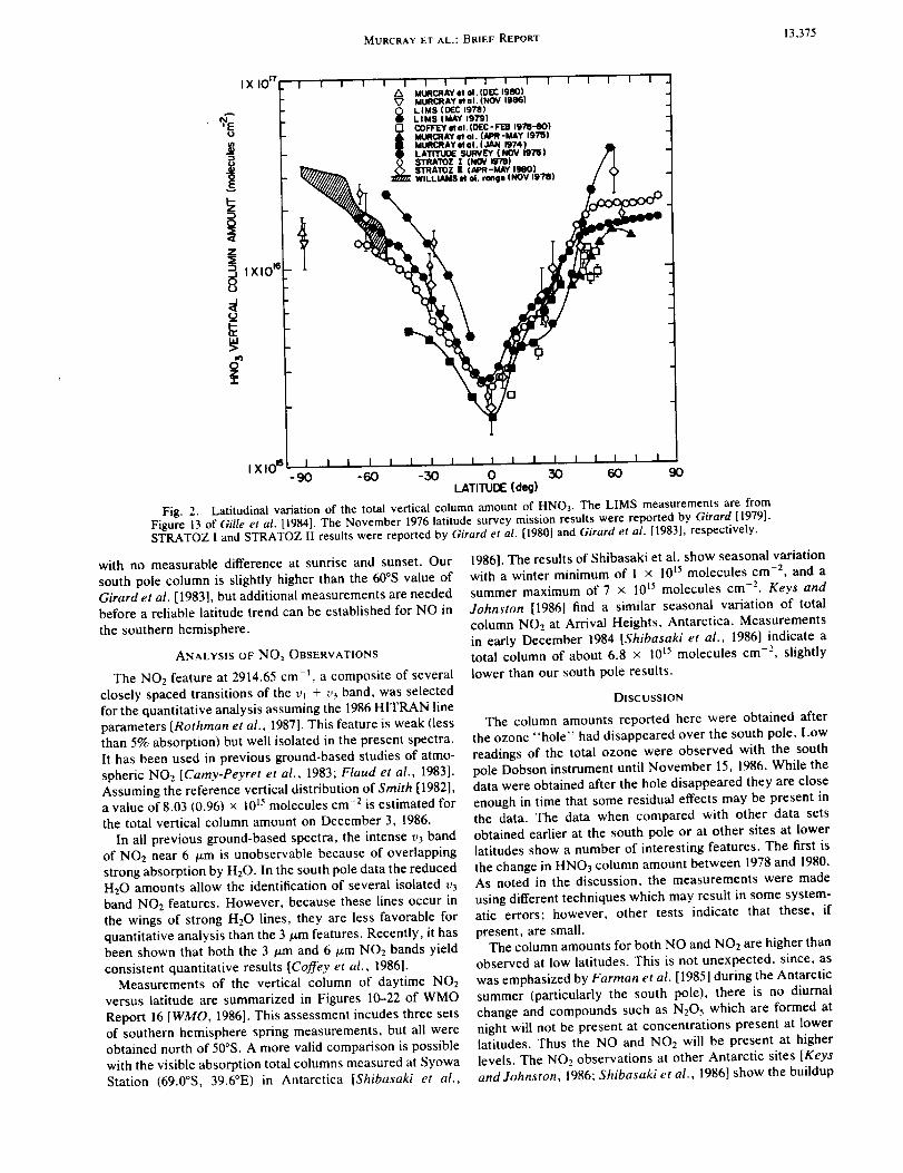
MURCRAY ET AL.: BRIEF REPORT 13,375

./_ MURCRAY 4;t ol. (01_ 19801MURCRAY et ol. (NOV 1986)

LIMS (DEC 1978)L|MS IIdAY 1979)I-1 COFF(YetoI.(DEC-FE:B 1978-80)• MURCRAY et 01. (,4PR-MAY 1975)

I MURCRAY Mal. (JAN 1974)

LATI'TUOE SUI_'EY { NOV 1976)STRATOZ ! (NOV 1978)STRATOZ ][ (_°R-MAY 1980)WILLIAMS et ol. range (NOV 19"t8)

I XI_-90 -coo -50 0 50 60 90

LATITUDE (dt_j)

Fig. 2. Latitudinal variation of the total vertical column amount of HNO3. The LIMS measurements are fromFigure 13 of Gille et al. [1984]. The November 1976 latitude survey mission results were reported by Girard [1979].STRATOZ 1 and STRATOZ I1 results were reported by Girard et al. [1980] and Girard et al. [1983], respectively.

with no measurable difference at sunrise and sunset. Our

south pole column is slightly higher than the 60°S value of

Girard et al. [1983], but additional measurements are needed

before a reliable latitude trend can be established for NO in

the southern hemisphere.

ANALYSIS OF NO2 OBSERVATIONS

The NO2 feature at 2914.65 cm -t, a composite of several

closely spaced transitions of the vt + v3 band, was selected

for the quantitative analysis assuming the 1986 HITRAN line

parameters [Rothman et al., 1987]. This feature is weak (less

than 5% absorption) but well isolated in the present spectra.

It has been used in previous ground-based studies of atmo-

spheric NO2 [Camy-Peyret et al., 1983; Flaud et al., 1983].

Assuming the reference vertical distribution of Smith [1982],

a value of 8.03 (0.96) x 1015 molecules cm -2 is estimated for

the total vertical column amount on December 3, 1986.

In all previous ground-based spectra, the intense v3 band

of NO2 near 6 _.m is unobservable because of overlapping

strong absorption by H20. In the south pole data the reduced

H20 amounts allow the identification of several isolated v3

band NO2 features. However, because these lines occur in

the wings of strong H20 lines, they are less favorable for

quantitative analysis than the 3 _m features. Recently, it has

been shown that both the 3 t_m and 6 txm NO2 bands yield

consistent quantitative results [Coffey et al., 1986].Measurements of the vertical column of daytime NO2

versus latitude are summarized in Figures 10-22 of WMO

Report 16 [WMO, 1986]. This assessment incudes three sets

of southern hemisphere spring measurements, but all wereobtained north of 50°S. A more valid comparison is possible

with the visible absorption total columns measured at Syowa

Station (69.0°S, 39.6°E) in Antarctica [Shibasaki et al.,

1986]. The results of Shibasaki et al. show seasonal variation

with a winter minimum of 1 x l0 ts molecules cm -2, and a

summer maximum of 7 × 1015 molecules cm -2. Keys and

Johnston [1986] find a similar seasonal variation of total

column NO2 at Arrival Heights, Antarctica. Measurements

in early December 1984 [Shibasaki et al., 1986] indicate a

total column of about 6.8 x 10 t5 molecules cm -2, slightly

lower than our south pole results.

DISCUSSION

The column amounts reported here were obtained after

the ozone "hole" had disappeared over the south pole. Low

readings of the total ozone were observed with the south

pole Dobson instrument until November 15, 1986. While thedata were obtained after the hole disappeared they are close

enough in time that some residual effects may be present in

the data. The data when compared with other data sets

obtained earlier at the south pole or at other sites at lower

latitudes show a number of interesting features. The first is

the change in HNO3 column amount between 1978 and 1980.

As noted in the discussion, the measurements were made

using different techniques which may result in some system-

atic errors; however, other tests indicate that these, if

present, are small.The column amounts for both NO and NO2 are higher than

observed at low latitudes. This is not unexpected, since, as

was emphasized by Farman et al. [1985] during the Antarctic

summer (particularly the south pole), there is no diurnal

change and compounds such as N205 which are formed at

night will not be present at concentrations present at lower

latitudes. Thus the NO and NO2 will be present at higher

levels. The NO2 observations at other Antarctic sites [Keys

and Johnston, 1986; Shibasaki et al., 1986] show the buildup

13,376 MURCRAY ET AL.: BRIEF REPORT

in NO2 column as the hours of daylight increases. As noted

in the discussion, the NOz results agree with other observa-

tions; however, the NO results do not agree with the con-

clusion reached by WMO [1986] that the NO column is con-

stant with latitude at a value near 3 × 10 _5 molecules cm 2.

Acknowledgments. The authors thank C. R. Trepte of ST Sys-

tems Corp. (STX) for his help in obtaining the correlative pressure-

temperature profiles. Research at the University of Denver was

supported by NSF under grant DPP-8118005 and by NASA. Ac-

knowledgment is made to the National Center for Atmospheric

Research, which is supported by NSF, for computer time used inthis research.

REFERENCES

Blatherwick, R. D., A. Goldman, D. G. Murcray, G. R. Cook, and

J. W. Van Allen, Simultaneous mixing ratio profiles of strato-

spheric NO and NO, as described from balloon-borne infraredsolar spectra, Geophys. Res. Lett., 7, 471---473, 1980.

Blatherwick, R. D., F. J. Murcray, F. H. Murcray, A. Goldman,

and D. G. Murcray, Atlas of South Pole IR solar spectra, Appl.Opt., 21, 2658-2659, 1982.

Brockman, P., C. H. Bair, and F. Allario, High resolution spectral

measurements of the HNO3 11.3 gm band using tunable diode

lasers, Appl. Opt., 17, 91-100, 1978.

Camy-Peyret, C., J. M. Flaud, J. Laurent, and G. M. Stokes, First

infrared measurement of atmospheric NO, from the ground,

Geophys. Res. Left., 10, 35-38, 1983.

Coffey, M. T., W. G. Mankin, and A. Goldman, Simultaneous

spectroscopic determination of the latitudinal, seasonal, and

diurnal variability of stratospheric N20, NO, NO2, and HNO3, J.Geophys. Res., 86, 7331-7341, 1981.

Coffey, M. T., W. G. Mankin, and A. Goldman, Stratospheric NO,.retrieval from solar absorption spectra in the v3 and v_ + v3 bands,

Appl. Opt., 25, 2460-2462, 1986.Crutzen, P. J., and F. Arnold, Nitric acid cloud formation in the cold

Antarctic stratosphere: A major cause for the springtime 'ozonehole,' Nature, 324,651-655, 1986.

Farman, J. C., R. J. Murgatroyd, A. M. Silnickas, and B. A.

Thrush, Ozone photochemistry in the Antarctic stratosphere in

summer, Q. J. R. Meterol. Soc., 111, 1013, 1985.Flaud, J. M., C. Camy-Peyret, D. Cariolle, J. Laurent, and G. M.

Stokes, Daytime variation of atmospheric NO2 from ground-based infrared measurements, Geophys. Res. Lett., 10,

1104-1107, 1983.

Gille, J. C., J. M. Russell, 1II, P. L. Bailey, E. E. Remsberg, L. L.

Gordley, W. F. Evans, H. Fischer. B. W. Bandrud. A. Girard,

J. E. Harries, and S. A. Beck. Accuracy and precision of the

nitric acid concentrations determined by the limb infrared monitor

of the stratosphere experiment on NIMBUS 7. J. Geophys. Res.,89, 5179-5190, 1984.

Girard, A., J. Besson, R. Giraudet, and L. Gramont, Correlated

seasonal and climatic variations of trace constituents in the

stratosphere, Pure Appl. Geophys., 117, 381-394, 1979.

Girard, A., L. Gramont, D. Imbault, J. Laurent, M. P. Lemaitre, S.

Boiteus, and N. Louisnard, Contribution a l'etude des variations

darts la composition de la stratosphere en fonction de la latitude:

Resultats de al mission STRATOZ, Proc. Quadrenn. Int. Ozone

Symp., 704-711, 1980.

Girard, A., G. Fergant, L. Gramont, O. Lado-Bordowsky, J.

Laurent, S. Le Boiteux, M. P. Lemaitre, and N. Louisnard,

Latitudinal distribution of ten stratospheric species deduced from

simultaneous spectroscopic measurements, J. Geophys. Res., 88,5377-5392, 1983.

Goldman, A., and J. R. Gillis, Line parameters and line-by-line

calculations for molecules of stratospheric interest, progressreport, Physics Department, Univ. of Denver, Denver, Colo.,1984.

Goldman, A., D. G. Murcray, and E. Niple, High resolution IR

balloon-borne solar spectra and laboratory spectra in the HNO3

1720-cm -1 region: An analysis, Appl. Opt., 19, 3721-3724, 1980.

Goldman, A., F. G. Fernald, F. J. Murcray, F. H. Murcray, and

D. G. Murcray, Spectral least squares quantification of several

atmospheric gases from high resolution infrared solar spectra

obtained at the South Pole, J. Quant. Spectrosc. Radiat. Trans-

fer, 29, 189-204, 1983.Goldman, A., J. R. Gillis, C. P. Rinsland, F. J. Murcray, and D. G.

Murcray, Stratospheric HNO3 quantification from line-by-linenonlinear least-squares analysis of high-resolution balloon-borne

solar absorption spectra in the 870-cm-_ region, Appl: Opt., 23,

3252-3255, 1984.

Goldman, A., F. J. Murcray, R. D. Blatherwick, and D.G.

Murcray, Quantification of HCI from high resolution, ground-

based, infrared solar spectra in the 3000 cm-I region, J. Quant.

Spectrosc. Radiat. Transfer, 36, 385-387, 1986.

Goldman, A., F. J. Murcray, F. H. Murcray, and D. G. Murcray,

Quantification of HCI from high resolution infrared solar spectra

obtained at the South Pole in December 1986, Geophys. Res.

Lett., in press, 1987.

Keys, J. G., and P. V. Johnston, Stratospheric NO2 and 03 in

Antarctica: Dynamic and chemically controlled variations,

Geophys. Res. Lett., 13, 1260--1263, 1986.

Murcray, D. G., D. B. Barker, J. N. Brooks, A. Goldman, J. J.

Kosters, F. H. Murcray, and W. J. Williams, Variation of HNO3total column density with latitude and season and a measurement

of stratospheric CF2C12, Proc. Conf. Clim. Impact Assess. Pro-

gram, 4, 432, 1975a.

Murcray, D. G., D. B. Barker, J. N. Brooks, A. Goldman, and W. J.

Williams, Seasonal and latitudinal variation of the stratospheric

concentration of HNO3, Geophys. Res. Lett., 2,223-225, 1975b.

Murcray, F. J., A. Goldman, D. G. Murcray, G. R. Cook, J. W. VanAllen, and R. D. Blatherwick, Identification of isolated NO lines

in balloon-borne infrared solar spectra, Geophys. Res. Lett., 7,673-676, 1980.

Rinsland, C. P., M. A. H. Smith, P. L. Rinsland, A. Goldman, J. W.

Brault, and G. M. Stokes, Ground-based infrared spectroscopic

measurements of atmospheric hydrogen cyanide, J. Geophys.

Res., 87, 11,119-11,125, 1982.

Rothman, L. S., R. P. Gamache, A. Goldman, L. R. Brown, R. A.

Toth, H. Pickett, R. P. Poynter, J. M. Flaud, C. Camy-Peyret, A.

Barbe, N. Husson, C. P. Rinsland, and M. A. H. Smith, The

HITRAN database: 1986 edition, Appl. Opt., in press, 1987.

Shibasaki, K., N. lwagami, and T. Ogawa, Stratospheric nitrogen

dioxide observed by ground-based and balloon-borne techniques

at Syowa Station (69.0°S, 39.6°E), Geophys. Res. Lett., 13,1268-1271, 1986.

Smith, M. A. H., Compilation of atmospheric gas concentrationprofiles from 0 to 50 km, NASA Tech. Memo., TM-83289, 1982.

Toon, O. B., P. Hamill, R. P. Turco, and J. Pinto. Condensation of

HNO3 and HCI in the winter polar stratosphere, Geophys. Res.

Lett., 13, 1284-1287, 1986.

Williams, W. J., J. J. Kosters, and D. G. Murcray, Nitric acid

column densities over Antarctica, J. Geophys. Res., 87,8976-8980, 1982.

WMO, Atmospheric ozone 1985: Assessment of our understanding

of the process controlling its present distribution and change,

Rep. 16, World Meteorol. Organ, Geneva, Switzerland, 1986.

A. Goldman, D. G. Murcray, F. J. Murcray, and F. H. Murcray,

Physics Department, University of Denver, Denver, CO 80208.

C. P. Rinsland, Atmospheric Sciences Division, NASA Langley

Research Center, Hampton, VA 23665.

(Received May 5, 1987;revised August 11, 1987;

accepted August 12, 1987.)

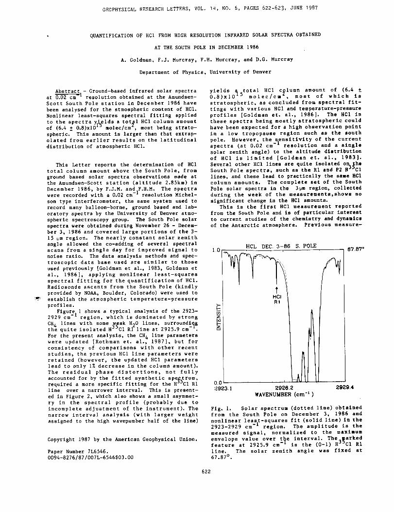
GEOPHYSICAL RESEARCH LETTERS, VOL. 14, NO. 6, PAGES 622-623, JUNE 1987

QUANTIFICATION OF HCI FROM HIGH RESOLUTION INFRARED SOLAR SPECTRA OBTAINED

AT THE SOUTH POLE IN DECEMBER 1986

A. Goldman, F.J. Murcray, F.H. Murcray, and D.G. Murcray

Department of Physics, University of Denver

Abstract - Ground-based infrared solar spectra

at 0.02 cm -I resolution obtained at the Amundsen-

Scott South Pole station in December 1986 have

been analysed for the atmospheric content of HCf.

Nonlinear least-squares spectral fitting applied

to the spectra y._elds a tot_l HCf column amount

of (6.4 ± 0.8)x10"_ molec/cmZ, most being strato-

spheric. This amount is larger than that extrap-

olated from earlier results on the latitudinal

distribution of atmospheric HCI.

This Letter reports the determination of HCI

total column amount above the South Pole, from

ground based solar spectra observations made at

the Amundsen-Scott station (altitude 2.85km) in

December 1986, by F.J.M. and F.H.M. The spectra

were recorded with a 0.02 cm -I resolution Michel-

son type interferometer, the same system used to

record many balloon-borne, ground based and lab-

oratory spectra by the University of Denver atmo-

spheric spectroscopy group. The South Pole solar

spectra were obtained during November 26 - Decem-

ber 3, 1986 and covered large portions of the 3-

15 _m region. The nearly constant solar zenith

angle allowed the co-adding of several spectral

scans from a single day for improved signal to

noise ratio. The data analysis methods and spec-

troscopic data base used are similar to those

used previously [Goldman et al., 1983, Goldman et

al., 1986], applying nonlinear least-squares

spectral fitting for the quantification of HCI.

Radiosonde ascents from the South Pole (kindly

provided by NOAA, Boulder, Colorado) were used to

<_' establish the atmospheric temperature-pressure

profiles.

Figure II shows a typical analysis of the 2923-2929 cm region, which is dominated by strong

CH 4 lines with some _ak H20 lines, surroundingthe quite isolated H_JCI R1 line at 2925.9 cm -_.

For the present analysis, the CH 4 line parameters

were updated [Rothman et. al., 1987], but for

consistency of comparisons with other recent

studies, the previous HCI line parameters were

retained (however, the updated HCf parameters

lead to only i% decrease in the column amount).

The residual phase distortions, not fully

accounted for by the fitted synthetic spectrum,35 lrequired a more specific fitting for the H C1 R

line over a narrower interval. This is present-

ed in Figure 2, which also shows a small asymmet-

ry in the spectral profile (probably due to

incomplete adjustment of the instrument). The

narrow interval analysis (with larger weight

assigned to the high wavepumber half of the line)

Copyright 1987 by the American Geophysical Union.

Paper Number 7L6546.

0094-8276/87/007L-6546503.00

yields _ total HCf c_lumn amount of (6.40.8)x10 5 molec/cm , most of which is

stratospheric, as concluded from spectral fit-

tings with various HCI and temperature-pressure

profiles [Goldman et. al., 1986]. The HCI in

these spectra being mostly stratospheric could

have been expected for a high observation point

in a low tropopause region such as the south

pole. However, the s_nsitivity of the currentspectra (at 0.02 cm- resolution and a single

solar zenith angle) to the altitude distribution

of HCI is limited [Goldman et. al., 1983].

Several other HCf lines are quite isolated one,he

South Pole spectra, such as the R1 and P2 H_CI

lines, and these lead to practically the same HCI

column amounts. The complete set of the South

Pole solar spectra in the 3_m region, collected

during the week of the measurements,shows no

significant change in the HCf amounts.

This is the first HCI measurement reported

from the South Pole and is of particular interest

to current studies of the chemistry and dynamics

of the Antarctic atmosphere. Previous measure-

1.0 67.87°

z

0.0

_J923.1 2929.4

HCL DEC 3-86 S POLE

NOII:tl

,2926.2

WAVENUMBER (cm -_ )

Fig. I. Solar spectrum (dotted llne) obtained

from the South Pole on December 3, 1986 and

nonlinear least-squares fit (solid llne) In the

2923-2929 cm -l region. The amplitude is the

measured signal, normalized to the maximum

envelope value over t_e interval. The markedfeature at 2925.9 cm-" is the (0-I) H35CI R1

llne. The solar zenith angle was fixed st

67.87 ° .

622

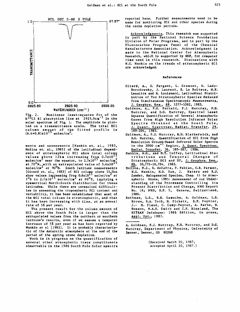
Goldman et al.: HC1 at the South Pole 623

10

z

z

E.-

HCL DEC 3-86 S. POLE

0.0 , i i i I , , , ,

2925.60 2925.90 2926.20

WAVENUMBER (cm-*)

67.87 °

Fig. 2. Nonlinear least-squares fit of theH35C1 R1 absorption line at 2925.9cm -1 in the

solar spectrum of Fig. 1. The amplitude is plot-ted on a transmittance scale. The total HC1

column amount of tge fitted profile is(6.4+0.8)x10 _ molec/cm .

ments and assessments [Mankln et. al., 1983,

Mollna et. al., 1985] of the latltudlnal depend-

ence of stratospheric HCf show total colu_

values above 12km increasing from 0.7xlO "J2 15 2

molec/cm near the equator, to 2.7xi0 molec/cT.O Dat 70 N, with an extrapolated value of 3.4xi0

2 omolec/cm at 90 N. South latitude measurements

[Girard et. al., 1983] of HCf colu_ above ll_Skmshow values ir_c;easlng fro W 0.8xlO *_ molec/cm atO ._9 Z O

1 S to 2.7XI0 molec/cm at 60 S, implylng a

symmetrical North-South distribution for these

latitudes. While there are unresolved difficult-

ies in assessing the tropospheric HCf content and

variability, it has been established that most of

the HCf total column is stratospheric, and that

it has been increasing with time, at an annual

rate of 5Z per year.

The present result for the column amount of

HCf above the South Pole is larger than the

extrapolated values from the northern or southern

latitude's results, even if we assume a temporal

increase of 5Z per year as has been reported by

Mankin et al [1983]. It is probably characteris-

tic of the Antarctic atmosphere at the end of the

period of the spring ozone depletion.

Work is in progress on the quantification of

several other atmospheric trace constituents

observable In the 1986 South Pole Solar spectra

reported here. Further measurements need to be

made for monitoring HCI and other species during

the ozone depletion periods.

AcknowledBments. This research was supported

in part by the National Science Foundation

Division of Polar Programs, and in part by the

Fluorocarbon Program Panel of the Chemical

Manufacturers Association. Acknowledgment is

made to the National Center for Atmospheric

Research, which is supported by NSF, for computer

time used in this research. Discussions with

W.G. Mankln on the trends of stratospheric HCf

are acknowledged.

References

Girard, A., G. Fergant, L. Gramont, O. Lado-

Borodowsky, J. Laurent, S. Le Boiteux, M.P.

Lemaltre and N. Loulsnard, Latitudinal Distri-

bution of Ten Stratospheric Species Deduced

from Simultaneous Spectroscopic Measurements,

J. Geophys. Res., 88, 5377-5392, 1983.

Goldman, A., F.G. Fernald, F.J. Murcray, F.H.

Murcray, and D.G. Hurcray, Spectral Least

Squares Quantification of Several Atmospheric

Gases from High Resolution Infrared Solar

Spectra Obtained at the South Pole,

J. Quant. Spectrosc. Radiat. Transfer, 29,

189-204, 1983.

Goldman, A., F.J. Murcray, R.D. Blatherwlck, and

D.G. Murcray, Quantification of HCl fro,, High

Resolution Ground-Based Infrared Solar Spectra

in the 3000 cm-'L Region, J. Quant. Spectrosc.

Radiat. Transfer, 36, 385-387, 1986.

Mankln, W.G., and M.T. Coffey, Latitudinal Dis-

tributions and Temporal Changes of

Stratospheric HCf and HF, J. Geophys. Res.,

88, I0,776-10,784, 1983.

Mollna, M.J., R. deZafra, P. Fabian, C.B. Farmer,

W.G. Mankin, N.D. Sze, J. Waters and R.J.

Zander, Halogenated Species, Chap. II in Atmo-

spheric Ozone, 1985: Assessment of our Under-

standing of the Processes Controlling its

Present Distribution and Change, WMO Report

No. 16; WMO, B.P. 5, Geneva, Switzerland,

1986.

Rothman, L.S., R.R. Gamache, A. Goldman, L.R.

Brown, R.A. Toth, H. Pickett, R.P. Poynter,

J.- M. Flaud, C. Camy-Peyret, A. Barbe, N.

Husson, M.A.H. Smith and C.P. Rinsland, The

HITRAN Database: 1986 Edition, in press,

Appl. Opt., 1987.

A. Goldman, F.J. Murcray, F.H. Murcray, and D.G.

Murcray, Department of Physics, University of

Denver, Denver, CO 80208

(Received March 20, 1987;

accepted April 20, 1987.)

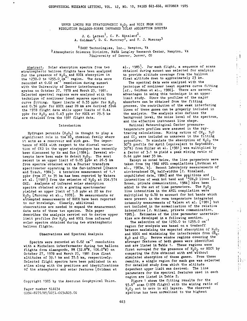
GEOPHYSICALRESEARCH LETTERS, VOL. 12, NO. I0, PAGES 663-666, OCTOBER 1985

UPPER LIMITS FOR STRATOSPHERIC H202 and HOC£ FROM HIGH

RESOLUTION BALLOON-BORNE INFRARED SOLAR ABSORPTION SPECTRA

J. C. Larsen I C P. Kinsland 2,j ,

A. Goldman 3, D. G. Murcray 3, and P. J. Murcray 3

|SASC Technologies, Inc., Hampton, VA

2Atmospheric Sciences Division, NASA Langley Research Center, Hampton, VA

3University of Denver, Denver, CO

Abstract. Solar absorption spectra from two

stratospheric balloon flights have been analyzed

for the presence of H202 and HOC£ absorption in

the 1230.0 to 1255.01c 9 _ region. The data wererecorded at 0.02 cm- resolution during sunset

with the University of Denver interferometer

system on October 27, 1978 and March 23, 1981.

Selected spectral regions were analyzed with the

technique of nonlinear least squares spectral

curve fitting. Upper limits of 0.33 ppbv for H202

and 0.36 ppbv for HOCZ near 28 km are derived from

the 1978 flight data while upper limits of 0.44

ppbv for H202 and 0.43 ppbv for HOC£ at 29.5 km

are obtained from the 1981 flight data.

Introduction

Hydrogen peroxide (H202) is thought to play a

significant role in the HO x chemical family where

it acts as a reservoir and sink gas. The impor-

tance of HOC£ with respect to the diurnal varia-

tion of C£0 in the upper stratosphere has recently

been discussed by Ko and Sze [1984]. Several at-

tempts have been made to detect H202. The most

recent is an upper limit of 0.05 ppbv at 26.5 km

from spectra obtained with a Fourier transform

spectrometer operating in the far-infrared [Chance

and Traub, 1984]. A tentative measurement of 1.1

ppbv from 27 to 35 km has been reported by Waters

et al. [1981] from the emission of H202 at 204.574

GHZ. Analysis of infrared solar absorption

spectra obtained with a grating spectrometer

yielded an upper limit of 1.0 ppbv at 20 km for

H202 [Murcray et al., 1978]. No measurements or

attempted measurements of HOCZ have been reported

to our knowledge. Clearly, additional

observations are needed to expand the measurement

data sets of these two species. This paper

describes the analysis carried out to derive upper

limit profiles for H202 and HOC£ from infrared

solar spectra obtained during two stratospheric

balloon flights.

Observations and Spectral Analysis

Spectra were recorded at 0.02 cm -I resolution

with a Michelson interferometer during two balloon

flights from Alamogordo, NM (32.8°N, I06.0°W) on

October 27, 1978 and March 23, 1981 from float

altitudes of 39.1 km and 33-5 km, respectively.

Selected flight spectra have been published in an

atlas along with the positions and identifications

of the atmospheric and solar features [Goldman et

Copyright 1985 by the American Geophysical Union.

Paper number 5L6634

0094-8276/85/0055-6634503.00

el., 1985]. For each flight, a sequence of scans

obtained during sunset was selected for analysis

to provide altitude coverage from the balloon

float altitude down to approximately 25 km.

The spectral data were analyzed with the

technique of nonlinear least squares curve fitting

[cf., Goldman et el., 1980]. There are several

advantages in using this technique in an upper

limit study. Since the profiles of the major

absorbers can be obtained from the fitting

process, the contribution of the weak interfering

lines of these gases can be properly included in

the analysis. The analysis also defines the

background level, the noise level of the spectrum,

and the effective instrument line shape.

National Meteorological Center pressure-

temperature profiles were assumed in the ray-

tracing calculations. Mixing ratios of CH_, N20

and CO 2 were included as unknowns in the fitting

procedure. To simulate the absorption of H202 the

30°S profile for April (esuivalent to September,

30°N) from Miller et el. [1981J was multiplied by

a factor of 3.1 to yield a peak mixing ratio of

0.64 ppbv near 33 km.

Except as noted below, the line parameters were

taken from the 1982 AFGL compilations [Rothman et

el., 1983a,'b]. Recent laboratory measurements of

air-broadened CH 4 half-widths [C. Rinsland,

unpublished data, 1984] and the p?_itions and

intensities of weak hot band and "kCH_D lines [L.

Brown, private communication, 1984] hive been

added to the set of line parameters. The H202

llne intensities in the AFGL compilation were

multiplied by 0.78 to account for hot bands which

were present in the room temperature integrated

intensity measurements of Valero et al. [1981] but

not included in the normalization of the relative

intensities [J. Hillman, private communication,

1985]. Estimates of the line parameter uncertain-

ties are developed in a following section.

The selection of the 1250.O to 1255.O cm -I

region for analysis was based on a tradeoff

between maximizing the expected absorption of H202

and HOC£ and minimizing the interference from CH 4,

N20 and CO 2. Narrow window regions covering the

stronger features of both gases were identified

and are listed in Table I. These regions were

first surveyed for the presence of M202 or HOC£ by

comparing the fits obtained with and without

simulated absorption of these gases. From these

results, a single region for each gas was selected

for detailed study from which the altitude

dependent upper limit was derived. The line

parameters for the spectral features used in each

region are listed in Table 2.

Figure I shows the fitting results for the

93.6 ° scan (1978 flight) with the mixing ratio of

H202 set to zero in all layers. The observed

spectrum has bees normalized to the highest

i

i ? i;

663

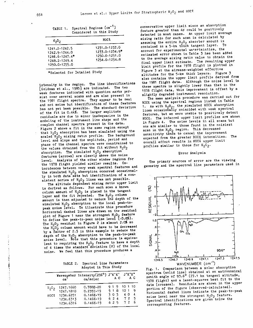
66q Larsenet el.: Upper Limits for Stratospheric H202 and HOC£

TABLE I. Spectral Regions (cm -I)

Considered in this Study

_202 HOC£

1241.2-1242.5

1242.9-1244.O

1246.6-1247.4"

1248.2-1249.4

1250.0-1255.O

1231.O-1232-O

1233.O-1234.9"

1250.O-1251.O

1254.O-1254-8

*Selected for Detailed Study

intensity in the region. The line identifications

[Goldman et al., 1985] are indicated. The two

weak features indicated with question marks per-

sist over several scans and are also present in

the 1981 flight spectra. They appear to be real

and not noise but identification of these features

has not yet been possible. The standard deviation

of the fit is 0.44%. The larger amplitude

residuals are due to minor inadequacies in the

modeling of the instrument line shape and the

complex channel spectra present in the data.

Figure 2 shows a fit in the same region except

that H202 absorption has been simulated using the

scaled H202 mixing ratio profile. The background

level and slope and the amplitude, period and

phase of the channel spectra were constrained to

the values obtained from the fit without H202

absorption. The simulated H202 absorption

features (arrows) are clearly above the noise

level. Analysis of the other window regions for

the 1978 flight yielded similar results. Co-

incidences between very weak spectral features and

the simulated H202 absorption occurred occasional-

ly in both data sets but identification of a con-

sistent series of H202 lines was not possible.

The altitude dependent mixing ratio upper limit

is derived as follows. For each scan a known

column amount of H202 is placed in the tangent

layer and the fit repeated. The H202 column

amount is then adjusted to reduce the depth of the

simulated H202 absorption to the local peak-to-

peak noise level. To illustrate this procedure

horizontal dashed lines are drawn on the residual

plot of Figure I near the strongest H202 feature

to define the peak-to-peak noise level Q~0.8%).

The H202 residual in Figure 2 is almost 2.0% so

the H202 column amount would have to be decreased

by a factor of 2.5 in this example to reduce the

depth of the H202 absorption to the peak-to-peak

noise level. Note that this procedure is equiva-

lent to requiring the H202 feature to have a depth

of 4 times the standard deviation (G) of the local

noise. We feel that this procedure produces a

TABLE 2. Spectral Line Parameters

Adopted in This Study

Wavenumber Intensity(296 °) J'K'K' J'K"K"

cm I cm/molec A C A C

H202

HOC£

1247.1660 O.788E-20 9 I 9 10 I 10

1247.1810 O.235E-19 9 I 8 10 I 9

1234.6251 O.146E-19 3 O 3 4 O 4

1234.63_3 O.146E-19 6 2 4 7 2 5

1234.6316 O.146E-19 6 2 5 7 2 6

conservative upper limit since an absorption

feature greater than 4G could be positively

detected in most cases. An upper limit average

mixing ratio for each scan is calculated by

assuming the entire H202 absorber amount is

contained in a 5-km thick tangent layer. To

account for experimental uncertainties, the

estimated error shown in Table 3 has been added

to the average mixing ratio value to obtain the

final upper limit estimate. The resulting upper

limit profile for the 1978 flight is plotted in

Figure 3 at the airmass-weighted effective

altitudes for _he 5-km thick layers. Figure 3

also contains the upper limit profile derived from

the 1981 flight data. Although the noise level in

these spectra is slightly lower than that in the

1978 flight data, this improvement is offset by a

slightly degraded instrument resolution.

The same analysis procedure was carried out for

HOCZ using the spectral regions listed in Table

I. As with H202, the simulated HOC£ absorptionlines occasionally coincided with weak spectral

features, but we were unable to positively detect

HOC£. The inferred upper limit profiles are shown

in Figure 4. The noise levels in all scans but

one are similar to those found in the noisiest

scan in the H202 region. This decreased

sensitivity tends to cancel the improvement

expected from the greater HOCZ intensities. The

overall effect results in HOCZ upper limit

profiles similar to those for H202.

Error Analysis

The primary sources of error are the viewing

geometry and the spectral line parameters used in

i°tun_

-2

1.0

.9 -

_.1 .8-

Z ".7

.6

.51246.5

' iN/) ' ' , ,

CO,

93.6"

, IC_ , I , I , I1246.7 1246.9 1247.1 1247.3 1247.5

WAVENUMBER (cm-')

Fig. I. Comparison between a solar absorption

spectrum (solid line) obtained at an astronomical

zenith angle of 93.6 ° (27.1 km tangent altitude,

1978 flight) and a least-squares best fit to the

data (crosses). Residuals are shown in the upper

portion of the figure (observed-calculated).

Horizontal dashed lines indicate the peak-to-peak

noise level near the strongest H202 feature.

Spectral identifications are given below the

corresponding features.

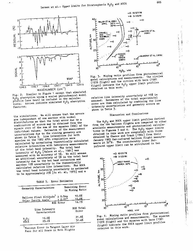
Larsenet al.: Upper Limits for Stratospheric H202 and HOC£

° LCc |_

-2 ; 1 , I , 1 ,

t.O

.9

_a .8<Z0 .7

.6

.s[1246.5

93.6"

1246.7 1246.9 1247.1 1247.3 12 17.5

WAVENUMBER (crn-')

Fig. 2. Similar to Figure I except that simulated

H20p absorption using a scaled photochemical model

profile (see text) is included in the calcula-

tions. Arrows indicate simulated H202 absorption

features.

the simulations- We will assume that the errors

are independent of one another with normal

distributions so that the total error due to a

combination of errors may be obtained from the

square root of the sum of the squares (RSS) of the

individual values- Estimates of the measurement

uncertainties due to the viewing geometry are

shown in Table 3. Line intensities for both

species on the 1982 AFGL compilation werecalculated by normalizin_ theoretically calculated

relative intensities with laboratorY measurements

of the total band intensity. The total band

intensity of H202 [Valero et al., 1981] was

measured with an accuracy of 5%. We will assume

an additional uncertainty of _% in the total band

intensity due to the hot band correction and

another 15% uncertainty in the theoretically

calculated relative llne intensities. For HOC£

the total band intensity uncertainty is estimated

to be approximately 25% [Suet. al, 1979] and a

TABLE 3- Error Estimates

Geometry UncertaintiesResulting Error

in Mixing Ratio

Balloon Float Alti_u del ± O.Skm 10.O%

Solar Zenith Anni e. _ 0.050 I0.0_RSS Error 14.1%

Line Intensity RSS Total

Uncertainties Error

H 0 16.6% 21.8%

H_c_ 292% 32.4%

_Maximum Error in Tangent Layer Air

Mass for all Scans in Both Flights

665

--0 10/27176

_,123/01

4<3 --0MLLF..R _" AL (1981) X _ .

A_iL 30"530*N

3' - "-° -T_• . .... .,,.<) _ |rWATERS ET[- _-'-".... : I/ (,96,1

E L A,NO -'--'_: _ _ : l/ ,

.. _ w_.¢s: _ .-_..--I "-_tL_ 3(L (1984) ." .-(9 ." [

2s: .//' --o

.- / - "mAuo __-6-2C _ *" (|984)

L , , ,, ....i.,o , , ,, ....1.9 1 , ,,"'6 s

15" no- ,oH202, vmf

Fig. 3- Mixing ratio profiles from photochemical

model calculations and measurements. The circles

(1978 flight) and the circles with bare (1981

flight) indicate the H202 upper limit profiles

obtained in this work.

relative line intensity uncertainty of 15% is

assumed. Estimates of the total experimental

error are then calculated by combining the line

intensity uncertainties and geometry errors as

shown in Table 3.

Discussion and Conclusions

The H202 and HOC£ upper limit profiles derived

from the two balloon flights are compared to other

available measurements and photochemical calcula-

tions in Figures 3 and 4. The R202 upper limits

this work are consistent with those

obtained in Chance and Traub [1984] from theirobtained by

January 1983 far-infrared balloon flight measure-

ments at 32°N • The considerably lower far-

infrared upper limit can be attributed to two

.,-O 10127178

5/2318t

4ot- ... - --oF-- - .oc.t .,_,.oE '-

E ! -osBs_ .: _o -s

C- _ .."" "_

°

2°F, , ,l,,,,l I t i ,,,,,I i ,,'"_d1611 I0 eid,o _69

HOCJ, Vine

Fig. 4. Mixing ratio profiles from photochemical

model calculations and measurements. The squares

(1978 flight) and the squares with bars (1981

flight) indicate the HOC£ upper limit profiles

obtained in this work.

i'

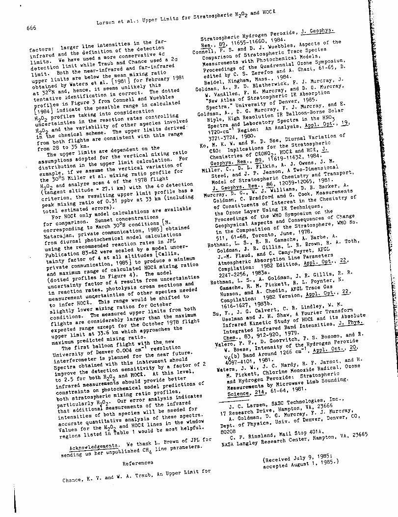
Larsen et al.: Upper Limits for Stratospheric H202 and HOC£

666

factors: larger line intensities in the far-

infrared and the definition of the detection

limits- We have used a more conservative 4c

detection limit while Traub and Chance used a 2o

limit. Both the near-infrared and far-infrared

upper limits are below the mean mixing ratio

obtained by Waters et al. [1981] for February 1981

at 32°N and, hence, it seems unlikely this

tentative identification is correct. The dotted

• es in Figure 3 from Connell and Wuebblesprof£_ .... _e ,ossible range in calculated

_1984] inalca_u _'

H202 profiles taking into considerationuncertainties in the reaction rates controlling

H,02 and the variability of other species involvedi_ the chemical scheme. The upper limits derived'

from both flights are consistent with this range

from 28 to 35 km-The upper limits are dependent on the

assumptions adopted for the vertical mixing ratio

distribution in the upper limit calculation- For

example, if we assume the vertical variation of

the 30°s Miller et al. mixing ratio profile forze scan 4 of the %978 flight

H20 2 and analy _ an I wm_ with the 40 detection

(tangent altitude " _" .....criterion, the resulting upper limit profile has a

peak mixing ratio of 0.31 ppbv at 33 km (including

total estimated errors).

For HOC£ only model calculations are available

for comparison- Sunset concentrations

corresponding to March 30°N conditions [M.

Natarajan, private communication, 1985] obtained

from diurnal photochemical model calculations

using the recommended reaction rates in JPL

Publication 83-62 were scaled by a model uncer-• at all altitudes [Callis,

talnty factor ! f 4_ laR%] to produce a minimum

private commun_ca_lu-, "_'Jand maximum range of calculated HOC£ mixing ratios

(dotted profiles in Figure 4). The model

uncertainty factor of 4 results from uncertainties

in reaction rateS, photolysis cross sections and

. measurement unQertainties of other species needed

to infer HOC£- This range would be shifted to

slightly lower mixing ratios for October

conditions. The measured upper limits from both

flights are considerably larger than the maximum

expected range except for the October 1978 flight

upper limit at 33 ;6 km which approaches the

maximum predicted mixing ratio.

The first balloon flight with the. new

University of Denver 0.004 cm -I resolution

interferometer is planned for the near future.

Spectra obtained with this instrument should

improve the detection sensitivity by a factor of 2

to 2.5 for both H202 and HOC£. At this level,

infrared measurements should provide better

constraints on photochemical model predictions of

both stratospheric mixing ratio profiles,

particularly H 02. Our error analysis indicates

that additiona_ measurements of the infrared

intensities of both species will be needed for

accurate quantitative analysis of these spectra.

Values for the H20 2 and HOC£ lines in the window

regions listed in Table % would be most helpful.

Acknowledgements" We thank L. Brown of JPL for_unnublished CH_ line parameters.

sending us nu_ _ r

References

Chance, K. V. and W. A. Traub, An Upper Limit for

Stratospheric Hydrogen Peroxide,

Res., 89, 11655-11660' %984.

Con_-_ell, _?. S. and D. J. Wuebbles, Aspects of the

Comparison of Stratospheric Trace Species

Measurements with Photochemical Models,

Proceedings of the Quadrennial Ozone Symposium,

edited by C. 5. Zerefos and A. Ghazi, 61-65, D.

Reidel, Hingham, Mass., %984"

Goldman, A., B. D. Blatherwick, F. J- Murcray, j"

W. VanAllen, F. H. Murcray, and D. G. Murcray,

"New Atlas of Stratospheric IR Absorption

Spectra," University of Denver, 1985.

Goldman, A., D. G. Murcray, F. J- Murcray, and E.

Niple, High Resolution IR Balloon-Borne Solarboratory Spectra in the HNO 3

Spectra AnAnalysis, '1720-cm- 5egxon: " "

3721-3724, %980-N. D. Sze, Diurnal Variation of

Ko, M. K. W. an_tions for the StratosphericC£0: ImpliC .... _0 ROCZ and HC£, J_:_-

Ikin.A.JowMiller, _', _" " Two_Dimensional

Steed, and I. P- lesson, A

Model of Stratospheric Chemistry and Transport,

l GeoDhys- Res., 86, 12039-%2065' 1981._. j.--Williams, D. B. Barker, A.

Murcray, u. -, " G. Cook, Measurements

Goldman, C. Bradford and

of Constituents of Interest in the Chemistry of

the Ozone Layer Using IR Techniques,

Proceedings of the WMO Symposium on the

Geophysical Aspects and Consequences of Change

in the Composition of the Stratosphere, _MO }|o.

511, 6%-68, Toronto, June, _978.

Rothman, L. 5., R. R. Gamache, A. Bathe, A.

Goldman, J" R. GilliS, L. R. Brown, R. A. Toth,

J.-M. Flaud, and C. Camy-Peyret, AFGL

Atmospheric Absorption Line parameters

Compilation: %982 Edition, _" 22,

2247-2256, 1983a- I.R. Gillis, R. R.

Rothman, L. S., A. Goldman,Gamache, H. M. Pickett, R. L. Poynter, N.

Husson, and A. Chedin, AFGL Trace Gas

Compilation: _982 Version, _'' 22,

1616-1627, 1983b-

Su, F., J- G. Calvert, C. R. Lindley, W. M.

Uselman and J- H. Shaw, A Fourier Transform

Infrared Kinetic Study of HOC£ and its Absolute

Integrated Infrared Band intensities,

Chem-, 83, 9_2-920, 1979.

Valero---VF. P', D. Goorvitch, F. 5. Bonomo, and R.

W. Boese, Intensity of the Hydrogen Peroxide

v_(b) Band Around 1266 cm-l, _' 20,

4_97-4101, 198_-j. C. Hardy, R. F. Jarnot, and H.

Waters, J" W., Chlorine Monoxide Radical, OzoneM. Pickett, Stratospheric

and Hydrogen Peroxide:

Measurements by Microwave Limb sounding-

6%-64,

l. C. Larsen, SASC Technologies, Inc.,

%7 Research Drive, Hampton, VA, 23666

A. Goldman, D. G. Murcray, F. J- Murcray,

Dept. of physics, Univ. of Denver, Denver, CO,

80208C. P. Rtnsland, Mail Stop 401A,

NASA Langley Research Center, Hampton, VA, 23665

(Received July 9, _985;

accepted August I, 1985-)

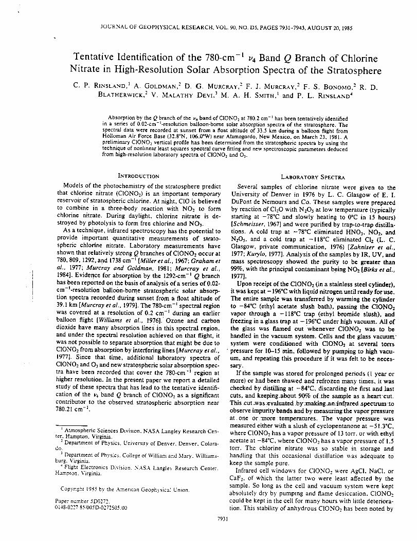
JOURNAL OF GEOPHYSICAL RESEARCH, VOL. 90, NO. D5, PAGES 7931-7943, AUGUST 20, 1985

Tentative Identification of the 780-cm -1 u4 Band Q Branch of Chlorine

Nitrate in High-Resolution Solar Absorption Spectra of the Stratosphere

C. P. RINSLAND, I A. GOLDMAN, 2 D. G. MURCRAY, 2 F. J. MURCRAY, 2 F. S. BONOMO, 2 R. D.

BLATHERWICK, 2 V. MALATHY DEVI, 3 M. A. H. SMITH, I and P. L. RINSLAND 4

Absorption by the Q branch of the v4 band of CIONO,. at 780.2 cm-) has been tentatively identifiedin a series of 0.02-era-t-resolution balloon-borne solar absorption spectra of the stratosphere. Thespectral data were recorded at sunset from a float altitude of 33.5 km during a balloon flight fromHolloman Air Force Base (32.8°N, 106.0°W) near Alamogordo, New Mexico. on March 23. 1981. Apreliminary CIONO: vertical profile has been determined from the stratospheric spectra by using thetechnique of nonlinear least squares spectral curve fitting and new spectroscopic parameters deducedfrom high-resolution laboratory spectra of C[ONO,. and O_.

INTRODUCTION

Models of the photochemistry of the stratosphere predictthat chlorine nitrate (CIONO,.) is an important temporaryreservoir of stratospheric chlorine. At night, C[O is believedto combine in a three-body reaction with NO2 to formchlorine nitrate• During daylight, chlorine nitrate is de-stroyed by photolysis to form free chlorine and NO3.

As a technique, infrared spectroscopy has the potential toprovide important quantitative measurements of strato-spheric chlorine nitrate• Laboratory measurements haveshown that relatively strong Q branches of CIONO2 occur at780, 809, 1292, and 1738 cm -l [Milleretal., 1967; Graham et

al., 1977; Murcray and Goldman, 1981; Murcray et al.,1984]. Evidence for absorption by the 1292-cm -I Q branchhas been reported on the basis of analysis of a series of 0.02-era-l-resolution ballo0n-borne stratospheric solar absorp-tion spectra recorded during sunset from a float altitude of

39.1 km [Murcray et al., 1979]. The 780-cm -I spectral regionwas covered at a resolution of 0.2 cm -j during an earlierballoon flight [Williams et al., 1976].' Ozone and carbon

dioxide have many absorption lines in this spectral region,and under the spectral resolution achieved on that flight, itwas not possible to separate absorption that might be due toC1ONO2 from absorption by interfering lines [Murcray et al.,1977]. Since that time, additional laboratory spectra of

CIONO2 and 03 and new stratospheric solar absorption spec-tra have been recorded that cover the 780-cm -t region athigher resolution• In the present paper we report a detailedstudy of these spectra that has lead to the tentative identifi-

cation of the v4 band Q branch of CIONO2 as a significantcontributor to the observed stratospheric absorption near780.21 cm -i.

t Atmospheric Sciences Division. NASA Langley Research Cen-ter. Hampton, Virginia.

2 Department of Physics. University of Denver. Denver, Colora-do.

Department of Physics. College of William and Mary. Williams-burg. Virginia.

4 Flight Electronics Division. NASA Langley Research Center.Hampton. Virginia.

Copyright 1985 by the American Geophysical Union.

Paper number 5D0272.0148-0227:85,005D-0272505.00

LABORATORY SPECTRA

Several samples of chlorine nitrate were given to theUniversity of Denver in 1976 by L. C. Glasgow of E. I.

DuPont de Nemours and Co. These samples were preparedby reaction of CIzO with NzO5 at low temperature (typicallystarting at -78°C and slowly heating to 0°C in 15 hours)[Schmeisser, 1967] and were purified by trap-to-trap distilla-tions. A cold trap at -78°C eliminated HNO3, NO2, andNzOs, and a cold trap at -118°C eliminated C12 (L. C.Glasgow, private communication, 1976) [Zahniser et al.,1977; Kurylo, 1977]. Analysis of the samples by IR, UV, andmass spectroscopy showed the purity to be greater than99%, with the principal contaminant being NO,, [BVks et ai.,1977].

Upon receipt of the CIONOz (in a stainless steel cylinder),it was kept at - 196"C with liquid nitrogen until ready for use.

The entire sample was transferred by warming the cylinderto -84_C (ethyl acetate slush bath), passing the CIONO2vapor through a -I18"C trap (ethyl bromide slush), andfreezing in a glass trap at -196"C under high vacuum. All ofthe glass was flamed out whenever CIONOz was to behandled in the vacuum system. Cells and the glass vacuum"system were conditioned with CIONO2 at several torrs

• pressure for 10-15 min, followed by pumping to high vacu-um, and repeating this procedure if it was felt to be neces-sary.

If the sample was stored for prolonged periods (1 year ormore) or had been thawed and refrozen many times, it waschecked by distilling at -84°C, discarding the first and lastcuts, and keeping.about 90% of.the sample .as a heart-cut.This cut ,was._evaluated _by.-making.an.Jnfrared .spectrum :toobserve impuritybands and by measuring the vapor pressureat .one or.more _temperatures. The vapor pressure wasmeasured either with a slush of cyclopentanone at -51.3°C,where CIONO2 has a vapor pressure of 13 tort, or with ethylacetate at -84°C, where CIONO_ has a vapor pressure of 1.5tort. The chlorine nitrate was so stable in storage andhandling that this occasional distillation was adequate tokeep the sample pure.

Infrared cell windows for CIONO: were AgCI, NaCI, orCaF2, of which the latter two were least affected by thesample. So long as the cell and vacuum system were keptabsolutely dry by pumping and flame desiccation, CIONO2could be kept in the cell for many hours with little deteriora-

tion. This stability of anhydrous CIONO2 has been noted by

7931

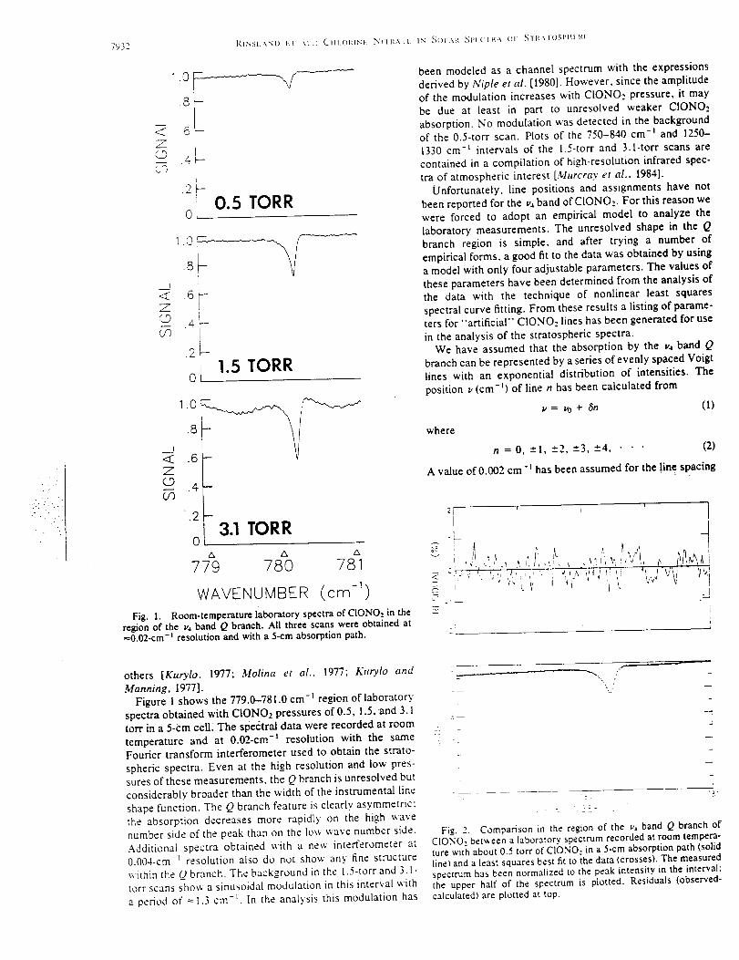
7932 I¢,I,%SI_,XND El .-',1 .: CllLOklNE ._'IlR-\II. IN _t)l ,\/,_ _I)ICIR-\ O1 _11 _,\IOSI'IIIR!

Z/m

bq

1.0

.8

.6I

•2' 0.5 TORR

0

:L<::[ .6Z

(./3

o L 1.5 TORR

3.1 TORR0

& & A

779 780 781

m -1(o )WAVENUMBER

Fig. I. Room-temperature laboratory spectra of CION02 in theregion of the v_ band Q branch. All three scans were obtained at_0.02-cm -) resolution and with a 3-cm absorption path.

been modeled as a channel spectrum with the expressions

derived by Niple et at. [1980]. However, since the amplitude

of the modulation increases with C[ONO: pressure, it may

be due at least in part to unresolved weaker CIONO2

absorption• No modulation was detected in the background

of the 0.5-torr scan. Plots of the 750-840 cm -t and 1250-

1330 cm -t intervals of the 1.5-torr and 3.l-tort scans are

contained in a compilation of high-resolution infrared spec-

tra of atmospheric interest [Murcray et al., 1984].

Unfortunately, line positions and asstgnments have not

been reported for the v_ band of CIONO.,. For this reason we

were forced to adopt an empirical model to analyze the

laboratory measurements. The unresolved shape in the Q

branch region is simple, and after trying a number of

empirical forms, a good fit to the data was obtained by using

a model with only four adjustable parameters. The values of

these parameters have been determined from the analysis of

the data with the technique of nonlinear least squares

spectral curve fitting. From these results a listing of parame-

ters for "artificial" CIONOz lines has been generated for use

in the analysis of the stratospheric spectra.

We have assumed that the absorption by the v4 band Q

branch can be represented by a series of evenly spaced Voigt

lines with an exponential distribution of intensities. The

position v (cm -l) of line n has been calculated from

v = v0 + (_n (1)

where

n = 0, ---1, ---2, ---3, --4, • • • (2)

A value of 0.002 cm-t has been assumed for the !ine spacing

2[ ' I

' ! _ _ _t , _ ,t_,4 _/),_,,;'_ ; I

c..:,_ ,, _....... .,,., . . ,a_._, _tt, 11 t! 1 _ _\r _t4,

_, 'l u

i

£

others [Kurylo, 1977; Molina et al., 1977; Kuryto and

Manning, 1977].

Figure I shows the 779.0--781.0 cm -1 region of laboratory

spectra obtained with CIONOx pressures of 0.5, 1.5, and 3.1tort in a 5-cm cell, The spe&ral data were recorded at room

temperature and at 0.02-cm -t resolution with the same

Fourier transform interferometer used to obtain the strato-

spheric spectra. Even at the high resolution and low pres-

sures of these measurements, the Q branch is unresolved but

considerably broader than the width of the instrumental line

shape function. The Q branch feature is clearly asymmetric:

the absorption decreases more rapidly on the high wave

number side of the peak than on the low wave number side.

Additional spectra obtained with a new intefferometer at

0.004-cm -_ resolution also do not show any fine structure

,,_ithin the Q branch. The background in the 1.5-torr and 3.1-

tort scans shov, a sinusoidal modulation in this interval with

a period of ---1.3 cm -t. In the analysis this modulation has

s 2:2

Fig. 2. Comparison in the region of the v, band Q branch ofCIONO, bet'_een a laboratory spectrum recorded at room tempera-ture witia about 0.5 ton" of C1ONO: in a 5-cm absorption path (solidline) and a least squares best fit to the data (crosses). The measured

spectrum has been normalized to the peak intensity in the interval:the upper half of the spectrum is plotted. Residuals (observed-calculated) are plotted at top.

I{ISSI .\ND I I -\1 .: CtlI(II,_INI[ _lllz\li IN ._IH .\R ._l't{(-IR,\ Ol ,_IRAIObI'ItI'-.R[-. 7933

& The intensity S (in cm-*/molecule cm -2 at 296 K) has been

calculated from

S = Svexp[A(v- vo)] v< vo

S = Sv v = vo 13)

S = S_exp[-B(v- vo) z] v> vo

In (3), v0 corresponds to the position of the absorption peak

of the CIONQ Q branch. The values of v0, Sv, A, and B have

been derived from the least squares fits. Since neither

quantum assignments nor measurements of the temperature

dependence of the absorption are available, an arbitrary

value of 300 cm -* has been adopted for the lower state

energy of all lines. Runs were made with Lorentz half-widths

70 of 0.1 and 0.2 cm -t atm -* at 296 K to study the sensitivity

of the results to the assumed half-width.

The analysis of the laboratory spectra with the technique

of nonlinear least squares spectral curve fitting followed the

procedures described in previous papers [Goldman et al.,

1980; Rinsland et al.. 1983a]. In the present work a subrou-

tine was added to the analysis program to generate a line list

from values for v0. Sv, A, and B. These four parameters and

two parameters for the background level and slope were

adjusted simultaneously in fitting the 182 measured intensi-ties between 779.0 and 781.0 cm -*. For the 1.5 and 3.1 ton-

scans, parameters for the amplitude and phase of the channel

spectrum were added; the period was held fixed at 1.3 cm -_

in the analysis. The Fourier transform technique [cf. Niple et

al., 1980] has been used to convolve the infinite resolution

transmittances with the instrument line shape function.

Figure 2 shows the agreement between the 0.5-ton" labora-

tory Spectrum and the least squares best fit to the data. The

differences in the upper panel are observed minus calculated

intensities expressed as a fraction of the maximum measured

3i ' I ' 1r

C(_ -2--i

2

i

T

?-- ; __

Fig. 3. Comparison in the region of the v_ band Q branch ofC1ONO, between a laboratory spectrum recorded at room tempera-ture with about 3. I torT of CIONO_. in a 5-cm absorption path Isolidline_ and a least squares best fit to the data ¢crosses_. The format isthe same as in Figure 2.

intensity in the fitted region. The rms residual is 0.3% for this

scan. The fits are slightly poorer for the 1.5-ton" and 3. I-ton"

scans. The rms residuals for these spectra are 0.5% and

0.9%, respectively. The fit to the 3. l-tort scan is shown in

Figure 3. As can be seen from this plot. the calculated

spectrum slightly underestimates the absorption in the stron-

gest part of the Q branch. For all three scans the rms residual

of the fit was the same for assumed Lorentz half-widths of

0.1 and 0.2 cm-_ atm-z at 296 K.

Table 1 presents the parameters derived from the fits to

the three laboratory scans, assuming half-widths 3'o of 0.1

and 0.2 cm -*atm -R at 296 K for all lines and that the

measured pressure is due entirely to CIONO:. Also listed is

the sum of individual line intensities Stot. For the three scans

the parameter values derived from the fits are nearly inde-

pendent of the assumed half-width. The agreement between

the values determined from the 0.5-ton" and 1.5-torr scans is

quite good, but slightly lower values for S_ and Stot were

obtained from the analysis of the 3.l-torr scan. This differ-

ence is believed to result from the inadequacies in the simple

model used to analyze the laboratory spectra and possibly

from the decay of CIONO, in the sample. Nitric acid was

observed as a decomposition product in the 3.I-tort scan.

The positions of HNO_ features in the 865-875 cm -_ region

were measured from this scan and compared to calibrated

positions from the University of Denver Atlas of Strato-

spheric Absorption Spectra [Goldman et al., 1983a]. The

average of the differences between the observed and refer-

ence positions was used as a calibration factor for the

determination of I.'0for this scan. Absorption by HNO3 was

not detected in the 0.5-tort scan and is very weak in the 1.5-

ton- scan. The values of v0 listed for these two scans are

uncalibrated.

Because of sample impurities, the values of S,, and St,,, in

Table 1 are lower limits. To obtain an estimate of the partial

pressure of HNO_, the HNO3 features identified in the 3.1-

ton" spectrum were analyzed with the technique of nonlinear

least squares spectral curve fitting. A HNO3 volume mixing

ratio of 0.04 - 0.01 was derived from a fit to the 867.0-870.0

cm -* region with the line parameters generated by Goldman

et al. [1984]. Absorption by HNO3 is much weaker in the 1.5-

ton" scan. A volume mixing ratio of 0.03 ± 0.015 was

estimated for this spectrum from the absorption depth of the

v_ band Q branch at 879 cm-t. An upper limit of 0.10 for the

HNO3 volume mixing ratio in the 0.5-ton- spectrum was

estimated from the same spectral region. No other contami-

nants have been'identified in the 750-1300 cm -I region

covered bythese spectra. However,similar laboratory spec-tra _of CIONO2 covering .the_1200-:2000 :cm-t region-show

absorption bythe :_ band of NO2 near.1600 cm -l. Also, it is

important_to_note that contaminants with only weak or

diffuse bands inthe intervals covered in the laboratory

spectra would not be identified.

We compared the peak absorpiivity (a = in (lo/l)/pD

derived from our laboratory spectra (assuming pure CIONO,

samples) with the values measured by Graham et al. [1977]

after they corrected for the decay of CIONO_,. The values

measured from our 0.5-torr, 1.5-ton", and 3.l-ton" scans are

38.35, and 28 cm -t atm -I at STP, respectively. The lower

value for the 3. l-torr scan probably results from the difficul-

ty in determining the background (100% transmission) level

caused by the stronger absorption of CIONO, in that spec-

trum. The absorptivities derived by Graham et al. are a

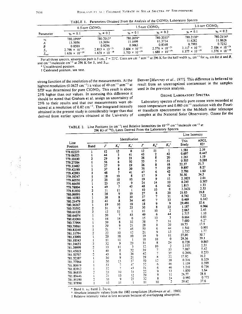
7934 RINSI AND FI A,I .: _tlIORINE NITRATE IN _OI.AR _PFCTRA OF STR-_.TOSPtIERE

TABLE I, Parameters Obtained From the Analysis of the ClONO: Laboratory Spectra

0.5"tort CIONO,. 1.5-torr CIONO,. 3. I-tort CIONO.,

Parameter 3'0 = 0.1 3'0 = 0.2 3'0 = 0.1 Yo = 0.2 3'0 = 0.1 3,o = 0.2

v0 780.1999" 780.2013" 780.2058" 780.2035" 780.2138* 780.2114'A 13.5056 13.3694 11.1699 11.3714 11.6282 11.8626B 0.8503 0.9296 0.9063 0.8348 0.7993 0.7232Sv 2.798 x 10 -21 2.813 × 10-zt 2.604 x 10-:l 2.576 × 10 -:l 2.117 x 10 -:l 2.106 x 10 -zlS_o_ 1.636 × 10 -19 1.629 x 10-19 1.703 × 10-19 1.688 × 10 -19 1.377 x 10 -19 1.376 X 10 -19

For all three spectra, absorption path is 5 cm. T = ... C. Units are cm- arm -* at 296 K for the half-width 3'o,cm-* for vo, cm forA and B,

and cm-t/molecule cm--" at 296 K for Sv and S,o,.

* Uncalibrated position.t Calibrated position, see text.

strong function of the resolution of the measurements. At the

highe st resolution (0.0625 cm-_) a value of 49 cm-t atm-* at

STP was determined for pure CIONO,.. This result is about

25% higher than our values. In assessing this difference it

should be noted that Graham et al. assign an uncertainty of

25% to their results and that our measurements were ob-

tained at a resolution of 0.02 cm -*. The integrated intensity

obtained in the present study is considerably larger than that

derived from earlier spectra obtained at the University of

Denver [Murcray et al., 1977]. This difference is believed to

result from an unrecognized contaminant in the samples

used in the previous analysis.

OZONE LABORATORY SPECTRA

Laboratory spectra of nearly pure ozone were recorded at

room temperature and 0.005 cm -_ resolution with the Fouri-

er transform spectrometer in the McMath solar telescope

complex at the National Solar Observatory. Ozone for the

TABLE 2. Line Positions (in cm -t) and Relative Intensities (in 10-'-3 era-J/molecule cm-Z at296 K) of J603 Lines Derived From the Laboratory Spectra

Line Intensity

Identification This AFGLLine

Position Band J' K,' Kc' J" K," K¢" Study 821

779.02223 1 12 12 0 12 !I 1 1.581 2.39779.06323 1 44 3 41 43 2 42 0.697 0.447779.10190 2 29 9 21 28 8 20 1.261 1.19779.27584 1 56 6 50 55 5 51 0.505 0.288779.33482 1 27 9 19 26 8 18 22.37 21.7779.42190 1 37 8 30 36 7 29 9.897 8.27779.42983 1 48 7 41 47 6 42 2.78¢ 1.60779.59247 1 18 10 8 17 9 9 30.50 34.5779.60550 2 20 I0 I0 19 9 11 2.382_ 2.01779.66458 1 23 15 9 24 14 10 0.245 0.307779.78004 1 49 7 43 48 6 42 1.813 i.33779.81850 2 11 11 1 10 10 0 2.342_ 2.55780.06893 1 28 9 19 27 8 20 21.03 19.8780.10383 1 38 8 30 37 7 31 8.742 7.22780.21479 2 41 8 34 40 7 33 0.469 0.312780.36367 1 19 10 10 18 9 9 29.48_ 32.6780.53592 2 31 9 23 30 8 22 1.187 0.966780.61120 2 12 11 1 11 l0 2 2.062 2.45780.64074 1 50 7 43 49 6 44 1.717 1.10780.65060 l 14 14 0 15 13 3 0.664 0.03

780.77906 1 39 8 32 38 7 31 7.680 6.27780.79861 1 29 9 21 28 8 20 19.75 17.9

780.83348 1 51 7 45 50 6 44 t.541 0.901781.11794 2 22 10 12 21 9 13 1.752 1.77781_!3098 I 20 10 I0 19 9 11 27.90 30.7781.18143 I II 11 1 10 10 0 29.56 39.1

781.24633 2 32 9 23 31 8 24 0.728 0.865781.39999 2 13 11 3 12 i0 2 1.555 2.35781.45019 1 40 8 32 39 7 33 7.067 5.42781.50707 2 43 8 36 42 7 35 0.269, 0.253781.52387 1 30 9 2l 29 8 22 17.92 16.2781.77864 1 50 13 37 50 12 38 0.316 0.329781.80619 1 53 7 47 52 6 46 1.139 0.599781.83912 I 52 7 45 51 6 46 1.210 0.736781.86810 2 23 10 14 22 9 13 1.850 1.64781.89446 1 2l 10 12 20 9 II 26.77 28.8781.95190 2 33 9 25 32 8 24 0.992 0.773781.97890 1 12 11 1 11 10 2 29.62 37.6

* Band I, v.: band 2, 2v.-vz.t Absolute intensity values from the 1982 compilation [Rothman et al., 1983]..+Relative intensity value is less accurate because of overlapping absorption.

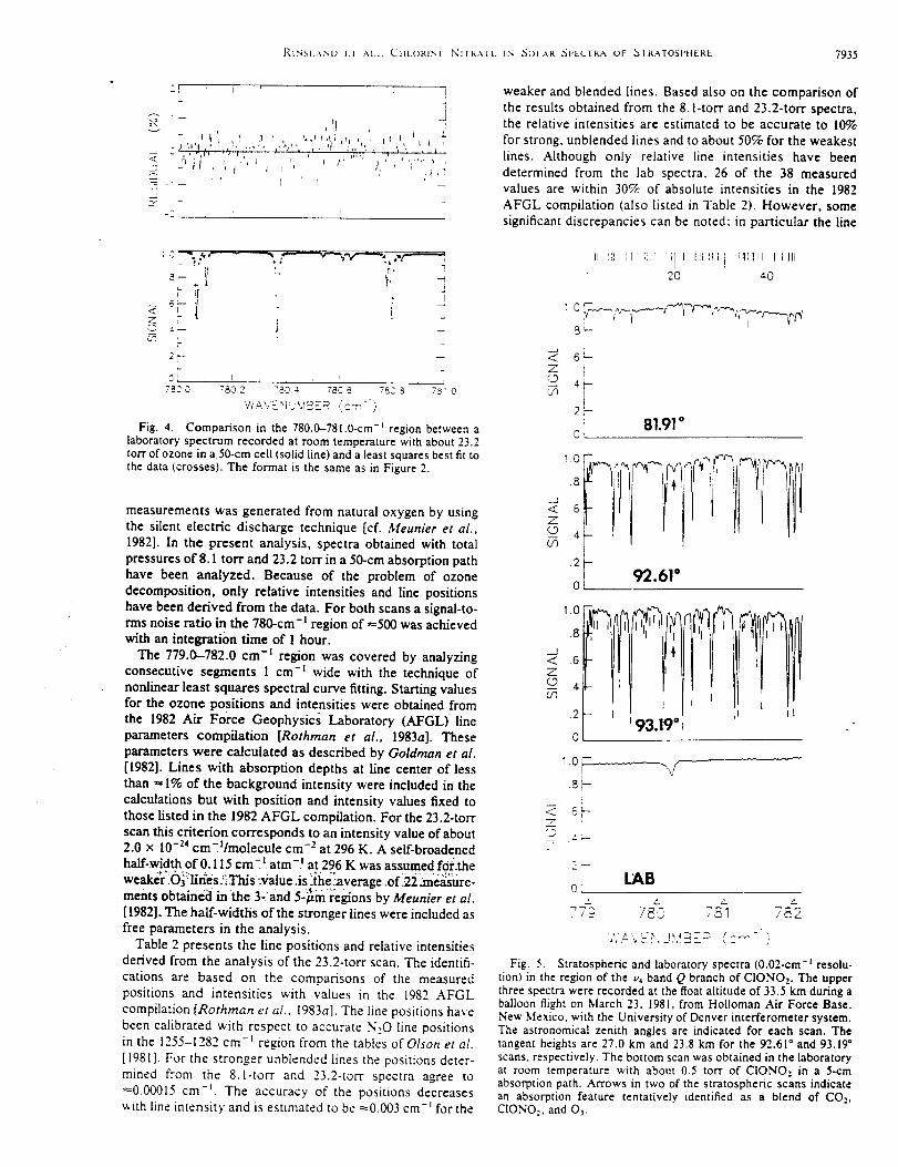
I{INSI.A,",D 1!1 AI_.; Q-'III.ORINE IN_Ii'RAI[. IN _OLAR ,_|qaC-IRA OF ,_'IRATOSI'fIERE 7935

21 i i

v _ ] (

q t i _ i ,, _ j d ,, ,p, S i

-2L

weaker and blended lines. Based also on the comparison of

the results obtained from the 8. l-ton- and 23.2-torr spectra,the relative intensities are estimated to be accurate to 10%

for strong, unblended lines and to about 50% for the weakest

lines. Although only relative line intensities have been

determined from the lab spectra, 26 of the 38 measured

values are within 30% of absolute intensities in the 1982

AFGL compilation (also listed in Table 2). However, some

significant discrepancies can be noted; in particular the line

8- ;!'t!

6'--J

7 -

(_q ..

2--

01 ,7E_ 0

; j

• i i

I_

78,32 78_ ..I. 780 6 78C B

...... ,,a, .......

i

78_ 0

Fig. 4. Comparison in the 780.0-781.0-cm -_ region between alaboratory spectrum recorded at room temperature with about 23.2ton" of ozone in a 50-era cell (solid line) and a least squares best fit tothe data (crosses). The format is the same as in Figure 2.

measurements was generated from natural oxygen by using

the silent electric discharge technique [cf. Meunier et al.,

1982]. In the present analysis, spectra obtained with total

pressures of 8.1 tort and 23.2 torr in a 50-cm absorption path

have been analyzed. Because of the problem of ozone

decomposition, only relative intensities and line positions

have been derived from the data. For both scans a signal-to-

rms noise ratio in the 780-cm -t region of ---500 was achieved

with an integration time of 1 hour.

The 779.0-782.0 cm -t region was covered by analyzing

consecutive segments I cm -I wide with the technique of

nonlinear least squares spectral curve fitting. Starting values

for the ozone Positions and intensities were obtained from

the 1982 Air Force Geophysics Laboratory (AFGL) line

parameters compilation [Rothman et al., 1983a]. These

parameters were calculated as described by Goldman et al.

[1982]. Lines with absorption depths at line center of less

than = 1% of the background intensity were included in the

calculations but with position and intensity values fixed to

those listed in the 1982 AFGL compilation. For the 23.2-torr

scan this criterion corresponds to an intensity value of about2.0 x 10 -24 cm'_tlmolecule cm--" at 296 K. A self-broadened

half-width of0.115 cm -t_ atm-. t at 296 K was assumed for.the

weake]"_O_liffes_ This :4alue ,is _ihe)zverage oL,22-_ae_ure-

merits obtained in the 3-and 5-/.tin regmns by Meunier et al.

[1982], The half-widths of the stronger lines were included as

free parameters in the analysis.

Table 2 presents the line positions and relative intensities

derived from the analysis of the 23.2-tort scan. The identifi-

cations are based on the comparisons of the measured

positions and intensities with values in the 1982 AFGL

compilation [Rothman et al.. 1983a]. The line positions have

been calibrated with respect to accurate N,O line positions

in the 1255-1282 cm -I region from the tables ofOIson et al.

[1981]. For the stronger unblended lines the positions deter-

mined from the 8. l-tort and 23.2-tort spectra agree to

_0.00015 cm -t. The accuracy of the positions decreases

with line intensity and is estimated to be _0.003 cm -_ for the

!lb I',1'_II I_; :IIi I I IIlill:i[ If:l;lltll ililI ! i _ I

20 _0

_.J

<z

C/3

• ,.___i.,_,f_._r U_ ....._"%,-_-c.--_t? l

2'.--81.91 *

O_

__1

< .6z

c/3

.2 --

0

1.o.8

I

< .6ZCO .4Oq

.2

0

z.J ,

.2--

I

o!

_7z

92.61"

93.19"1

LAB

r A r

7EO 78i 782

/

°

Fig. 5. Stratospheric and laboratory spectra (0.02-cm -_ resolu-

tion) in the region of the v_ band Q branch of CIONO,.. The upperthree spectra were recorded at the float altitude of 33.5 km during aballoon flight on March 23, 1981, from Holloman Air Force Base.New Mexico, with the University of Denver interferometer system.The astronomical zenith angles are indicated for each scan. Thetangent heights are 27.0 km and 23.8 km for the 92.61 ° and 93.19"scans, respectively. The bottom scan was obtained in the laboratoryat room temperature with about 0.5 ton- of CIONO, in a 5-cmabsorption path. Arrows in two of the stratospheric scans indicatean absorption feature tentatively identified as a blend of CO,.,CIONO,., and O_.

7936 1(INSI.AND I.T AI ,; CHLORINE NITRATE IN ._OI AR SI'EC1RA OF _TRATOSPHERE

TABLE 3. Parameters for the March 23. 1981, University ofDenver Balloon Flight

Parameter Value

Latitude 32.8°N

Longitude 106.0°WFloat altitude 33.5 - 0.5 kmScan time 40 sMaximum path difference 50 cmField of view 8 arcminPointing accuracy -0.05°Spectral coverage 740 - 1350 cm -_Continuum signal to rms noise at 780 cm -_ 150

Tropopause height 10.4 km

at 780.6505 cm -_ is observed to be much stronger than

indicated by the 1982 AFGL compilation. Perhaps, this

difference is due to an overlapping line from an unassigned

hot band. The line widths measured from the 23.2-tort scan

are only slightly larger than the width of the instrument line

shape function; for this reason the self-broadened widths

derived from this spectrum are believed to be not very

accurate and are not reported.

The weak O3 line at 780.2148 cm -_ occurs close to the

position of the strongest absorption by CIONO2. When the23.2-tort laboratory spectrum is plotted on an expanded

vertical scale, there is an indication that this line is blended

with about a factor of 2 weaker, unassigned 03 line centered

near 780.206 cm -_. This weaker feature is near the noise

level of the present data; higher signal to noise and increased

resolution are needed to determine if this weaker O3 line is

real.

Figure 4 shows the agreement obtained in the 780.0-781.0

cm -1 region between the 23.2-torr laboratory and best-fit

calculated spectra. As in Figure 3 the residuals (observed-

calculated) in the upper panel are expressed as a percentage

of the maximum intensity measured in the region. The rms

residual is 0.35%, very close to the noise level of the data.

Similar results were obtained from the fits to the 779.0-780.0

cm -l and 781.0-782.0 cm -t regions.

STRATOSPHERIC SPECTRA AND ANALYSIS

The stratospheric solar absorption spectra analyzed in thiswork were recorded during sunset with a Michelson-type

Fourier transform interferometer with an apodized FWHM

(full width at half maximum) resolution of 0.02 cm -t. The

balloon flight was performed from Holloman Air Force Base

near Alamogordo, New Mexico, on March 23, 1981. Table 3

summarizes important flight and experimental parameters

and their estimated uncertainties.

Figure 5 shows th6"779.0-:-782.0 cm -_ interval in balloon

flight spectrarecorded Under'high sun and low sun condi-tions and in the-0.5-torr laboratory spectrum of CIONO2.

The solar and atmospheric features identified in the strato-

spheric spectra are marked beneath one of the scans and are

repeated and numbered at top. Table 4 lists the correspond-

ing line positions and identifications. These identifications

are based on comparisons between the observed spectra and

simulated spectra generated with the line parameters and

vertical profiles discussed below and on the agreement

between the measured and reference line positions. An

arrow beneath the low sun stratospheric scans indicates the

feature corresponding in position to the strongest absorption

b v the v._ band Q branch of CIONO__. Based on the consider-

ations discussed in this section, we tentatively identify this

feature as a blend of CIONO2, CO2, and 03. The other

identifications, except for a few minor changes, which result

from comparisons of the balloon spectra with the new O3

laboratory spectra, are from the University of Denver Atlas

of Stratospheric Solar Absorption Spectra [Goldman et al.,

1983a].

Line positions and intensities for 03 were taken from the

analysis of the Kitt Peak laboratory spectra. The transition-

dependent air-broadened half-widths calculated recently for

296 K by Gamache et al. [1984] were assumed in the analysis

(R. R. Gamache, private communication, 1984). For CIONO_.

the line list was calculated with our simple empirical model

assuming the values of A and B derived from fitting the 0.5-

torr lab scan with 3'0 = 0.1 cm -j atm -t at 296 K, 1.25 times

the value of S,, derived from the same analysis (scaled to

agree with the measurements of Graham et al. [1977]) and

the average of the two calibrated values of vo determined

from the fit to the 3. l-tort" lab scan. Line parameters for CO,,,

NO2, and HCN were taken from the 1982 Air Force Geo-

TABLE 4. Identification of Atmospheric and Solar Features inthe 779.0--781.0 cm -) Region

Sequence Position, MolecularNumber cm-t Identification

1 779.021 O32 779.064 O33 779.105 O34 779.263 O35 779.305 HzO6 779.335 O37 779.424 O38 779.508 COz, 03?9 779.592 O3

10 779.667 CO2, O3! 1 779.746 CO2, O312 779.780 O313 779.818 O314 779.870 O315 779.933 O316 780.004 O317 780.070 03, CO:,18 780.103 O319 780.180 '_ "20 780.227 CIONO2?, COz, O321 780.363 O322 780.504 CO2, O323 780.540 O324 780.609 O325 780.648 O_26 780.741 O327 780.794 Os28 780.834 O329 780.871 03, solar.OH

30 780:971 COz31 781.130 O332 781.180 O333 781.245 0334 781.267 C0235 781.311 03, solar OH36 781.381 O337 781.399 O338 781.450 0339 781.523 O340 781.591 O3, CO:41 781.692 CO,., 0342 781.800 0343 781.893 03, solar OH44 781.938 Os45 781.978 03

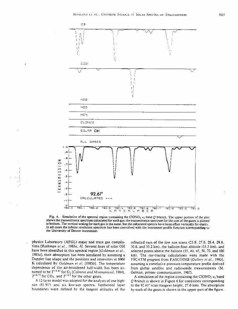
I(INSLAND El AL.: (..'IILORINE NIIbLAIL IN SOLAR SPECTI,,L& OF ,_TR.ATOSPHERE 7937

Ca2

V

N02

!:II

I

I

I

V

1

1

1i;

II ,'

't I:

'_ iIi

t ,

H20

HCN

CLON02

SOLmR OH

V

ALL G_qSE$

8

z

_= .3 --

•2 - 92.61 °CALCULATED _--

.] --

o ) T l ' I r , I !780.O 780. 1 780.2 78.0.3 780 .'_ 7S"_ .5 '780.6 78C .7 7_0 .8 "7_0 ._ 7_i .C

b_ A v E N U M _ E R

Fig. 6. Simulation of the spectral region containing the C1ONO. v_ band Q branch. The upper portion of the plot

shows the transmittance spectrum calculated for each gas; the transmittance spectrum for the sum of the gases is plottedat bottom. The vertical scaling for each gas is the same. but the calculated spectra have been offset vertically for clarity.In all cases the infinite resolution spectrum has been convolved with the instrument profile function corresponding tothe University of Denver instrument.

physics Laboratory fAFGL) major and trace gas compila-

tions [Rothman et al., 1983a, b]. Several lines of solar OH

have been identified in this spectral region [Goldman et al.,

1983a]; their absorption has been simulated by assuming a

Doppler line shape and the positions and intensities at 6000

K calculated by Goldman et al. [1983b]. The temperature

dependence of the air-broadened half-width has been as-

sumed to be T -°s5 for O_ [Colmont and Monnanteuil, 1984],

T -°v5 for COz, and T -°5 for the other gases.

A 12-layer model was adopted for the analysis of one high-

sun (81.9l _) and six low-sun spectra. Isothermal layer

boundaries were defined by the tangent altitudes of the

refracted rays of the low sun scans (23.8, 27.0. 28.4, 29.6,

30.6, and 33.2 kin), the balloon float altitude (33.5 km), and

selected points above the balloon (35, 40, 45, 50.70, and 100

kin). The ray-tracing calculations were made with the

FSCATM program from FASCODIB [Galle©" et al., 1983],

assuming a correlative pressure-temperature profile derived

from global satellite and radiosonde measurements (M.

Gelman, private communication, 1982).

A simulation of the region containing the CIONO2 v, band

Q branch is shown in Figure 6 for conditions corresponding

to the 92.61 ° scan (tangent height. 27.0 kin). The absorption

by each of the gases is shown in the upper part of the figure.

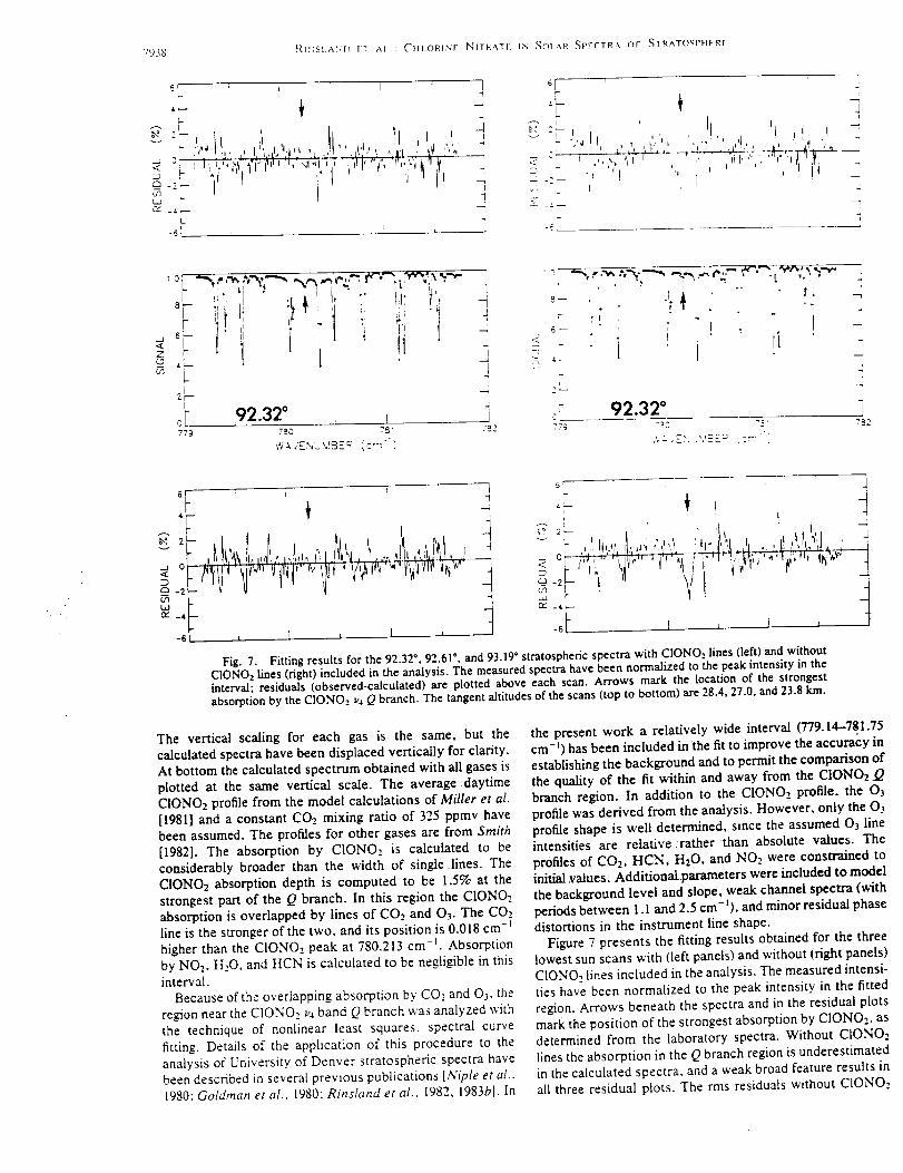
"_)_ ]_.I_'_SIA_[) 11 AI .: C'HI.ORINE NITRAII: IN _OI AR _pFCTR.\ OF ,_IRATOSPHERF

6r i I I

-'$_ !

L -Ii-61 L

. p

v '- ""' " " " "_)--T ''_ ' '" ' "i_L' '" '¸

__..--

8'- LI I ;,ii I/ _ II: iit

Z

k=-

or 92.320773 7BO 78'

I

q

-]7 _ 2

" I_ -_

_' " i • { -6- i ' " li4--

- 92.32 ° -:J2 7B2779 -=* 7_"

t6 i i 1 1

r,,"

-_| , I , I ,

*m + !

or-_,l :,, ,'_ii_,'_ , _'I",__LTW, f;'_ %, ',_ _N'__ __

[£ , , , , ,Fig. 7. Fitting results for the 92.32 °, 92.61 °, and 93.19 ° stratospheric spectra with C1ONO,. lines (left) and without

CIONO_ lines (fight) included in the analysis. The measured spectra have been normalized to the peak intensity in theinterval; residuals (observed-calculated) are plotted above each scan. Arrows mark the location of the strongestabsorption by the CIONO_, v, Q branch. The tangent altitudes of the scans (top to bottom) are 28.4, 27.0, and 23.8 kin.

The vertical scaling for each gas is the same, but the

calculated spectra have been displaced vertically for clarity.

At bottom the calculated spectrum obtained with all gases is

plotted at the same vertical scale. The average daytime

ClONO2 profile from the model calculations of Miller et al.

[1981] and a constant CO2 mixing ratio of 325 ppmv have

been assumed. The profiles for other gases are from Smith

[1982]. The absorption by CIONO_, is calculated to be

considerably broader than the width of single _lines. The

CIONO2 absorption depth is computed to be 1.5% at the

strongest pan of the Q branch. In this region the CIONO2

absorption is overlapped by lines of CO, and 03. The CO,_

line is the stronger of the two, and its position is 0.018 cm-

higher than the C[ONOt peak at 780.213 cm -n. Absorption

by NO,.. H.,O, and HCN is calculated to be negligible in this

interval.

Because of the overlapping absorption by CO., and O_, the

region near the CIONO2 va band Q branch was analyzed with

the technique of nonlinear Least squares, spectral curve

fitting. Details of the application of this procedure to the

analysis of University of Denver stratospheric spectra have

been described in several previous publications [Niple et al..

1980; Goldman et al., 1980; Rinsland et al.. 1982, 1983b]. In

the present work a relatively wide interval (779.14--7gl.75

cm -n) has been included in the fit to improve the accuracy in

establishing the background and to permit the comparison of

the quality of the fit within and away from the CIONO_ O

branch region. In addition to the CIONO2 profile, the O3

profile was derived from the analysis. However, only the O_

profile shape is well determined, since the assumed O_ lineintensities are relative rather than absolute values. The

profiles of CO_; HCN, H:O, and NO2 were constrained to

initial .values. Additional parameters were included to model

the background level and slope, weak channel spectra (with

periods between 1.1 and 2.5 cm-'), and minor residual phase

distortions in the instrument line shape.

Figure 7 presents the fitting results obtained for the three

lowest sun scans with (left panels) and without (fight panels)

CIONO, lines included in the analysis. The measured intensi-

ties have been normalized to the peak intensity in the fitted

region. Arrows beneath the spectra and in the residual plots

mark the position of the strongest absorption by CIONO,_, as

determined from the laboratory spectra. Without CIONO,_

lines the absorption in the Q branch region is underestimated

in the calculated spectra, and a weak broad feature results in

all three residual plots. The rms residuals without CIONO,_

}'_lN'ql AND ET AI.,: CHLOHNL _'IIR.-XI[i IN ,_OLAR _['LC1R,X O[: ,_-IRA1OStq{ERE 7939

_'_ " --' Cq 4.--

o[ 92.611 L -77g 782 77_780 7S _

WAVENUMBER (cm")

ii=: ; i :li , i!!' til

f

92.61 °78C 73:

I1-t4

4

J

)

4J

782

, i

6_ 4 1

oi ,,'LI Ij! t,, :_.! j'!'l _!r'_,l: ,, t)I _..':., i

W.

-s! _ ) J

[-1

-1-1

1I

-it

-i1

'-'- )', t

- _ 7 [i1

__" i _

)q

q

q

4

L.

_0

8

8

93.19 °I I I 1 ,

77g 780 781 782

WAVENUNSER (cm "_)

Fig. 7.

lines in the fit (top to bottotn) are 1.0%, 1. i%, and 1.7%. The

fits with CIONOz lines included in the analysis are consider-

ably better in the CIONO2 Q branch region. The rms

residuals with CIONO: lines in the fit (top to bottom) are

0.9%, 1.0%, and 1.4%.

Figure 8 compares the 0.5-torr laboratory spectrum of

CIONO2 and the residuals obtained for the 92.61 ° and 93.19 °

scans without CIONO,. lines in the analysis. Despite the

difference in the temperature of the laboratory run (_22°C)

and that of the stratosphere and the problem of the contribu-

tion from the overlapping lines of CO,_ and 03, there is fairly

good agreement in both the position and shape of the broad

feature in the residuals and the CIONO._ absorption in the

laboratory spectrum. The large residuals near 780.36 cm -_

result from errors in fitting a strong O3 line: note that these

residuals have a sharper appearance than those of the broadfeature.

Since CO, and O3 lines are calculated to produce discern-

ible absorption near the CIONO, Q branch position, it is

important to try to determine if errors in the parameters

assumed for these lines could cause the large residuals noted

in the fits. The overlapping carbon dioxide line is R29 from

the temperature-sensitive 12201-03301 band of _:C_60_,. To

our know, ledge there have not been any recent measure-

.4.

.9--

0

77g

(continued)

. ¢

,93.19_'780

! _' t,I _)[J

781

WA.VENUMBER (cm-')

782

ments reported for this band. However, the position for this.

line in the 1982 AFGL compilation should be accurate to"0.001 cm -_ or better, since the molecular constants for both

the upper and lower levels have been derived from numerous

experimental measurements [see Rothman et al., 1983a,

Table II). The 1982 AFGL compilation lists three additional

lines of this band in the fitted region: R28 at 779.508 cm -t,R30 at 780.976 cm -_. and R31 at 781.692 cm -). The line

positions measured from the stratospheric spectra agree withthese values to 0.001 cm -I for R28.and R31 and to 0.005

cm -_ for:R30, which is blended with-another COz line of

about the same intensity. Only weak O3 lines are listed near

these line positions in the 1982 AFGL compilation [Rothman

et al.. 1983a]. The new O3 lab spectra also do not show

measurable O3 absorption in the vicinity of these CO, lines.

Minor contamination of the R28 and R31 lines by O3 is likely,

however, since an atlas of 0.04-cm -t resolution laboratory

spectra [Damon et al.. 1981] obtained with 40 times more O3

in the path than used in the Kitt Peak experiment show

absorption near the positions of both lines. Despite these

limitations, the quality of the fits to all three of these CO,

features in the stratospheric spectra suggests that this CO,

band has been simulated fairly well in our analysis. Figure 9

shows an example of a fit near the R31 line on an expanded

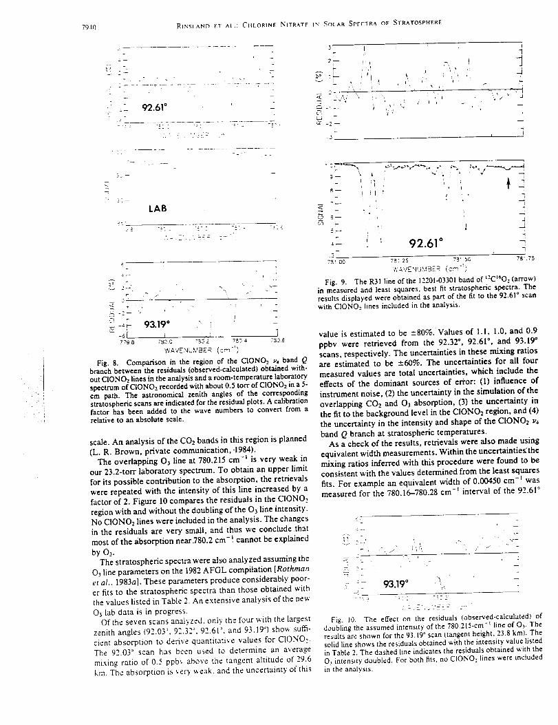
7940 RIN%IAND ET At.: CIII•ORINE NITRATE IN SOLAR SPECTRA OF STRATOSPHERE

c

.

2--

, _ 92.61 °

• _ ...

)2.--

<-

LAB

r- , _ /

,_-_._-93.19 ° " :-6L L _ i _ J77g 8 73_ C 73_ 2 780 4 7S2 6

WAVENUMBER (cm _)

Fig.8. Comparison in the regionof the CIONOz v4 band gbranch between the residuals(observed-calculated)obtainedwith-outCIONOz linesintheanalysisand a room-temperaturelaboratory

spectrumof CIONOz recordedwithabout0.5ton"ofCIONO2 ina 5-cm path•The astronomicalzenithangles of the correspondingstratosphericscansareindicati_dfortheresidualplots.A calibrationfactorhas been added to the wave numbers to convert from a

relativeto an absolutescale.

scale• An analysis of the CO2 bands in this region is planned

(L. R. Brown, private communication, 1984).

The overlapping O3 line at 780.215 cm -I is very weak in

our 23.2-tort laboratory spectrum. To obtain an upper limit

for its possible contribution to the absorption, the retrievals

were repeated with the intensity of this line increased by a

factor of 2. Figure 10 compares the residuals in the CIONO.,

region with and without the doubling of the O3 line intensity.

No CIONOz lines were included in the analysis. The changes

in the residuals are very small, and thus we conclude that

most of the absorption near.780.2 cm-! cannot be explained

by O3.The stratospheric spectra were also analyzed assuming the

03 line parameters on the 1982 AFGL compilation [Rothman

et al., 1983a]. These parameters produce considerably poor-

er fits to the stratospheric spectra than those obtained with

the values listed in Table 2. An extensive analysis of the new

O3 lab data is in progress.Of the seven scans analyzed, only the four with the largest

zenith angles (92.03', 92.32 °. 92.61L and 93.19 °) show suffi-

cient absorption to derive quantitative values for CIONO:.

The 92.03 ° scan has been used to determine an average

mixin o, ratio of 0.5 ppbv above the tangent altitude of 29.6

kin. The absorption is ver> _eak, and the uncertainty of this

"_2,

F2--

;, 'I I

,_ i ¸,

.2¸

,m _.__ _ ,_: _,

u_ , ') 2

,-v -2--

; [i , _ ,

i '_ 'I ,!

; tt I

!

iI

Z

x

92.61 ° -_i

7_1 25 75' 5G 78'75

l

Z - t i

:.,q __ r

d.--

l.t

7_ 0(3

WS,./EF,;ULIBER (.sin-')

Fig. 9. The R31 line of the 12201-03301 band of t"Ct_O.- (arrow)in measured and least squares, best fit stratospheric spectra. The

results displayed were obtained as part of the fit to the 92.61 ° scanwith CIONO., lines included in the analysis.

value is estimated to be ±80%. Values of 1.1, 1.0, and 0.9

ppbv were retrieved from the 92.32 °, 92.61 °, and 93.19 °

scans, respectively. The uncertainties in these mixing ratiosare estimated to be "-60%. The uncertainties for all four

measured values are total uncertainties, which include the

effects of the dominant sources of error: (1) influence of

instrument noise, (2) the uncertainty in the simulation of the

overlapping COz and O3 absorption, (3) the uncertainty in

the fit to the background level in the CIONOz region, and (4)

the uncertainty in the intensity and shape of the CIONO,, _4

band Q branch at stratospheric temperatures.As a check of the results, retrievals were also made using

equivalent width measurements. Within the uncertainties:the

mixing ratios inferred with this procedure were found to be

consistent with the values determined from the least squares

fits. For example an equivalent width of 0.00450 cm -t was

measured for the 780.16-780.28 cm -_ interval of the 92.61 °

-2

:- / t_,",,

93.19 ° ..:

-5 2 - -:'2 2

Fig. 10. The effect on the residuals (observed-calculated) ofdoubling the assumed intensity of the 780.215-cm -t line of Os. Theresults are shown for the 93.19 ° scan (tangent height, 23.8 kin). Thesolid line shows the residuals obtained with the intensity value listedin Table 2. The dashed line indicates the residuals obtained with the

Oa intensity doubled. For both fits, no CIONO: lines were included

in the analysis•

]_INSI..\ND liT A[.,: CtII.ORINE NIIRAI[. IN SOLAR SPLCIRA OI SIKAIOSI'IIERE 7941

scan (tangent height of 27.0 kin). The equivalent widths of

the overlapping CO,_ and O3 lines are calculated to be

0.00066 cm-t and 0.00016 cm-J. respectively. The difference

between the measured equivalent width and the sum of the

calculated CO: and 03 equivalent widths is 0.00371 cm -_.

Using this difference together with an integrated intensity of

1.38 x 10 -19 cm-t/molecule cm -2 for CIONO: in this region

and a total air mass of 2.83 x 10:5 molecules cm-:, an

average mixing ratio of 0.95 ppbv is obtained (assuming the

absorption is on the linear part of the curve of growth).

DISCUSSION

Our analysis has shown that an absorption feature ob-

served near 780.227 cm -* in a sequence of stratospheric

spectra is too strong and too broad to be attributed solely to

known lines of CO., and 03. Although the additional absorp-

tion coincides closely with the CIONO: v4 band Q branch in

position and shape, the identification must be regarded astentative because of the following considerations:

I. It was not possible to identify the 809-cm -I and 1292-

cm -* bands of ClONO2 in the same set of spectra. The

relatively weak _ fundamental at 809 cm -_ falls in a short

gap in the flight data caused by the real-time filter used with

the University of Denver instrument. High-resolution labo-

ratory spectra [Murcray and Goldman, 1981; Murcray et al.,

1984] indicate the _ fundamental Q branch is considerably

broader than the Q branches of the _ and z,., bands. The __

strongest absorption extends over the 1291-1293 cm -_ re-

gion. This region was covered during a balloon flight made

on October 27, 1978. A CIONO2 profile was determined from

those data based on the assumption that a broadband absorp-

tion occurring in this region was due to CIONOz [Murcray et

al., 1979]. It should be emphasized that the 1292-cm -1 band

results were based on simple equivalent width estimates andthe assumption that all the broadband absorption is due to

CIONO2. Thus the CIONOz profile from this earlier flight is

not on as firm a spectroscopic basis as the current analysis.

A complete analysis of the 1292-cm -I region has not been

performed because of the lack of suitable spectroscopic

parameters for HNO3 and CIONO2 in this region. ' Current

plans call for nonlinear least squares analysis of this region

with empirical line parameters for CIONO2 (similar to those

used here for the 780-cm -I Q branch) and HNO3 spectrosco-

pic line parameters for which work is in progress (A. Maki.

private communication, 1984).

2. The line parameters derived from the new laboratory

data for 03 and CIONO2 produce considerable improve-

ments in the least squares fits to the stratospheric spectra.

but the residual plots indicate that problems remain in

modeling the '.experimental data..The poorest fit is ob/_ained

for the 93.19 ° scan,-an(i for this spectrum the rms residual is

about twice the rms-noise of the data. These systematic

problems are believed to be due mostly to minor inaccura-

cies in the assumed line parameters (particularly the posi-

tions and intensities of the weaker O_ lines), and their

presence makes it difficult to analyze a feature as weak as

the CIONO_. Q branch.

3. A weak line appears at 780. 180 cm-_ in the 93.19° scan

and is also observed in the four lower sun scans obtained

during this flight Izenith angles of 94.64 _ to 95.15 °. corre-

sponding to tangent altitudes of 14.2 km to 8.1 km). A line

from the 2_-_. band of O3 is listed at 780.177 cm -_ in the

1982 AFGL compilation [Rothman et a[.. 1983a]. but its

35

3O

as<_

I I I I

EXPERIMENTAL

\\ A • THIS STUDY (33"N)

'_T MO;E MURCRAY (33"N1

I -- Nataroion (30"N)

__------MHIer efOI (30*N)

Pll _ I

�ill

20 I I I I05 I0 15 20

CIONO 2 MIXING RATIO (ppbv)

Fig II Comparison of measured profiles(fromthisstudy andfrom the study of Murcray et al. [19790 and model profiles (M.Natarajan, private communication. 1984. and from the study ofMiller et al. [1981]) of CIONO>

intensity is calculated to be too weak to account for the

observed line. Both the new 03 laboratory spectra and the

atlas of Damon et al. [1981] show no obvious absorption at

this frequency. The presence of this unassigned line has only

a minor influence on the fit to the 93.19 ° scan, but its

occurrence points out the potential pitfalls of relying on a

single, weak feature for a spectroscopic identification.

In Figure l I the two experimental CIONO, mixing ratio

profiles determined from University of Denver stratospheric

spectra are plotted along with a daytime-averaged CIONO,

profile for 30°N (dashed line) calculated by Miller et al.

[1981] and a sunset CIONO2 profile (M. Natarajan, private

communication, 1984) calculated for March at 30*N (solid'-

line) with the model of Callis et al. [ 1983] and recent reaction

rates [NASA Panel for Data Evaluation, 1983]. The experi-

mental mixing ratios are higher on average than the calculat-

ed values, but the experimental error bars are large. The two

experimental profiles agree at all aJtitudes within the uncer-

tainties. There is better agreement between the experimental

and the model profile shapes, but it is difficult to draw firm

conclusions because of the large uncertainties in the experi-

mental values.

SUMMARY AND CONCLUSIONS

We have reported a tentative identification of the 780-cm- =

v4 band Q branch of CIONO: on the basis of an analysis of

0.02-cm -_ resolution balloon-borne stratospheric solar ab-

sorption spectra and new high-resolution laboratory spectra

of CIONO,_ and O3. The preliminary altitude profile deduced

from the data is similar to photochemical model predictions

and to the results obtained previously from the 1292-cm -z

band [Murcray et al., 1979]. but the experimental values

have large uncertainties owing to the difficulties of the

measurements. We caution that only limited significance

should be attached to the differences between the measured

7942 RINSI.AND ET AI.." CIII.ORINE NITRATE IN SOI.AR SPECTRA OF STRATOSPHERE

and model profiles in view of the large experimental uncer-

tainties and the tentative nature of our resutts.

Improved stratospheric and laboratory spectra will be

necessary to obtain a firm identification of CIONO: (which

should be based on more than one feature in the same set of

spectra) and to accurately quantify" its vertical profile. In the

near future we hope to use a narrow-band filter to record

high-resolution stratospheric solar absorption spectra cover-

ing the 780-cm-' and 809-cm -I Q branches of CIONO,.

These measurements should have the higher signal-to-noise

ratio needed to better study the weak, broad absorption

feature detected at the position of the 780-cm- t Q branch. In

the laboratory, additional spectra of C.IONO2 and 03 are

needed. A key issue for CIONO: remains the possibility that

the integrated intensities have been underestimated because

of unrecognized contaminants in the sample. Both the abso-

lute intensities and shapes of the CIONO: Q branches need

to be measured at stratospheric temperatures. Improved line

parameters for the weak O_ lines in the 780-cm -* and 809-

cm- t regions would improve least squares fits to stratospher-

ic spectra.

Acknowledgments. Research at the University of Denver was

supported by NASA, the Chemical Manufacturers Association. andthe National Science Foundation. Research at the College of Wil-

liam and Mary was supported by NASA. The authors thank R. R.

Gamache of the University of Lowell Center for Atmospheric

Research for communicating his calculated 03 air-broadened half-

widths to us prior to publication and Burnie S. Williams of NASA

Langley, Rob Hubbard, Mike Brown, James W. Brault, and GregLadd of the National Solar Observatory for their assistance in

obtaining the 03 laboratory spectra. We also thank Robert K. Seals,

Jr., of blASA Langley and Carolyn H. Sutton of Systems and

Applied Sciences Corporation for helpful comments and SusanEdwards of NASA Langley for typing the manuscript. The National

Solar Observatory is operated by the Association of Universities forResearch in Astronomy under contract with the National Science

Foundation.

REFERENCES

Birks, J. W., B. Shoemaker, T. J. Leck, R. A. Borders, and L. J.

Hart, Studies of reactions of importance in the stratosphere, 2,

Reactions involving chlorine nitrate and chlorine dioxide, J.

Chem. Phys.; 66; 4591-4598, 1977Callis, L. B., M. Natarajan, and R. E. Boughner, On the relation-

ship between the greenhouse effect, atmospheric photochemistry,

and species distribution, J. Geophys. Res., 88, 1401-1426, 1983

Colmont, J. M., and N. Monnanteuil, Measurements of N:-, O,.-,and air-broadened linewidths of ozone in the millimeter region:

Temperature dependence of the linewidths, J. Mol. Spectrosc..

104, 122-128. 1984

Damon, E., R. L. Hawkins, and J. H. Shaw, A spectrum of ozonefrom 760 to-5800.cm-:, interim_technical report:Res. Found.

Proj. 7614201711626, Ohio State Univ., Columbus, .1981.

Gallery, W. O., F. X.:.Kneizys, and.S.A. Clough. Air mass

computer program for atmospheric transmittance/radiance calcu-lation: FSCATM, Environ.-Res. Pap. 828 (AFGL-TR-83-O065).

l.,t5 pp., Air Force Geophys. Lab., Bedford, Mass., 1983.Gamache, R. R., R. W. Davies, and L. S. Rothman, Theoretical

N,-, O2-, and air-broadened halfwidths of 1603 calculated by

quantum Fourier transform theory with realistic collision dynam-

ics. paper presented at 39th Symposium on Molecular Spectrosco-

py. Ohio State Univ.. Columbus. 1984.Goldmo.n.A.. D. G. Murcray. F. J. Murcrax, and E. Niple. High

resolution IR balloon-borne solar spectra and laboratory spectra

in the HNO3 1720-cm-_ region: An analysis. Appl. Opt.. 19. 3721-

372-t. 1980.Goldman. A, J. R. Giltis. D. G. Murcray. A. Barbe. and C.

Secroun, Analysis of the v., and 2v_,-w_ ozone bands from high-

resolution infrared atmospheric spectra, J. Mol. Spectrosc.. 96,

279-287. 1982Goldman. A., R. D. Blather'wick, F. J. Murcray, J. W. Van Allen,

F. H. Murcray, and D. G. Murcray, New Atlas of Stratospheric

IR Absorption Spectra. vol. I, Line Positions and Identifications;

vol. 2, The Spectra, report, Dep. Phys., Univ. Denver, Denver,

Colo., 1983a.Goldman, A.. J. R. Gillis. and J. A. Coxon, Spectral line parameters

for the pure rotation hands of solar OH, J. Quant. Spectrosc.

Radiat. Transfer, 29. 469---470. 1983b.Goldman. A., J. R. Gillis. C. P. Rinsland, F. J. Murcray. and D. G.

Murcray, Stratospheric HNO3 quantification from line-by-line,nonlinear least-squares analysis of high-resolution balloon-borne

solar absorption spectra in the 870-cm-t region. Appl. Opt., 23.

3252-3255, 1984.Graham. R. A., E. C. Tuazon. A. M. Winer, J. N. Pitts, Jr., L. T.

Molina, L. Beaman, and M. J. Molina. High resolution infrared

absorptivities for gaseous chlorine nitrate, Geophys. Res. Lett., 4,

3-5, 1977.

Kurylo, M. J., Flash photolysis resonance fluorescence investiga-tion of the reaction of OQP) atoms with CIONO,., Chem. Phys.

Lett., 49, 467-470, 1977.

Kury[o, M. J., and R. G. blanning. Flash photolysis resonancefluorescence investigation of the reaction of CIQP) atoms with

CIONO,., Chem. Phys. Lett., 48. 279-283, 1977.Meunier, C.. P. Marche, and A. Barbe, Intensities and air broaden-

ing coefficients of Oj in the 5- and 3-v.m regions, J. Mol.

Spectrosc., 95, 271-275, 1982.Miller, R. H., D. L. Bernitt, and I. C. Hisatsune, Infrared spectra of

isotopic halogen nitrates, Spectrochim. Acta, 23A, 223-236, 1967.

Miller, C., D. L. Filkin, A. J. Owens, J. M. Steed, and J. P. Jesson,A two-dimensional model of stratospheric chemistry and trans-

port, J. Geophys. Res., 86, 12,039-12,065, 1981.Molina, L. T., J. E. Spencer, and M. J. Molina, The rate constant

for the reaction of OQP) atoms with CIONOz, Chem. Phys. Lett.,

4J, 158-162, 1977.

Murcray, D. G., and A. Goldman, CRC Handbook of High Resolu-tion Infrared Laboratory Spectra of Atmospheric Interest, CRC

Press, Boca Raton, Fla., 1981.Murcray, D. G., A. Goldman, W. J. Williams, F. H. Murcray, F. S.

Bonomo, C. M. Bradford, G. R. Cook, P. L. Hanst, and M. J.

Molina, Upper limit for stratospheric CIONOz from balloon-borneinfrared measurements, Geophys. Res. Lett., 4, 227-230, 1977.

Murcray, D. G., A. Goldman, F.H. Murcray, F. J. Murcray, andW. J. Williams, Stratospheric distribution of CIONOz, Geophys.

Res. Lett., 6, 857-859, 1979.

Murcray, D. G., F. J. Murcray, F. S. Bonomo, A. Goldman, andR. D. Blatherwick, High resolution IR Laboratory Spectra, Appl.

Opt., 23, 3502, 1984.NASA Panel for Data Evaluation, Chemical kinetics and p.hoto-

chemical data for Use in stratospheric modelling, Evaluation 6,

Publ. 83-62, Jet Propul. Lab.;Pasadena, Calif., .1983.

Niple, E., W. G. Maixkin, A. Goldman, D. G." Mureray, and F. J.

Murcray, Stratospheric NOz and H20 mixing ratio profilesfrom

high resolution infrared solar spectra using-nonlinear least

squares, Geophys. Res. Lett., 7,'489---492,1980.Olson, W. B., A. G. Maki, and W. J. Lafferty, Tables of N,O

absorption linesfor the calibration of tunable infrared lasersfrom

522 cm- _to 657 cm- _and from 1115 cm- _to 1340 cm- _.J. Phys.

Chem. Ref. Data. I0, 1065-q084, 1981.

Rinsland, _(2.L-P.;'-A.:2oGoldman;--F-- J .LMttrcray, D. G. _Murcray,

M.::A.:.H.CSmith,-..Ri'--,KLSeals,"Jr-; J.LC.LLarsen, .and P. L.

Rinsland, _Stratosl_heric NzO mixing_ ratio_profile_from :high-

resolutionballo0n-borne solarabsorption spectra and laboratory

spectra near 1880 cm -t, Appl. Opt., 21, 4351--4355, 1982.

Rinsland. C. P., D. C. Benner, D. J. Richardson, and R. A. Toth.

Absolute intensity measurements of the (11 t0)n "--00°0 band of

CO, at 5.2 gin. Appl. Opt., 22, 3805-3809, 1983a.

Rinsland. C. P., A. Goldman. F. J. Murcray, D. G. Murcray.

M. A. H. Smith, R. K. Seals. Jr., J. C. Larsen, and P. L.

Rinsland. Stratospheric temperature profile from balloon-borne

measurements of the 10.4-_m band of CO-_. J. Quant. Spectrosc.

Radiat. Transfer, 30. 327-334, 1983b.

Rothman. L. S.. R. R. Gamache. A. Barbe, A. Goldman, J. R.Gillis, L. R. Brown. R. A. Toth. J.-M. Flaud, and C. Camy-

Peyret, AFGL atmospheric absorption line parameters compila-

tion: 1982 edition. Appl. Opt.. 22. 2247-2256. 1983a.

Rothman,L.S.,A.Goldman.J.R.Gillis.R.R.Gamache.H.M.Pickett.R.L. Poynter.N.Husson.andA.Chedin.AFGLtracegascompilation:1982version,App[. Opt., 22. 1616-1627, 1983b.

Schmeisser. M.. Chlorine (I) nitrate, lnorg. Syn.. 9. 127-130. 1967.

Smith, M. A. H., Compilation of atmospheric gas concentration

profiles from 0 to 50 kin. Techn. Memor. 83289. NASA Langley

Res. Center, Hampton, Va., 1982.

Williams. W. J., J. J. Kosters, A. Goldman. and D. G. Murcray.

Measurements of stratospheric halocarbon distributions using

infrared techniques. Geophys. Res. Lett.. 3. 379-382. 1976.

Zahniser. M. S.. J. S. Chang. and F. Kaufman, Chlorine nitrate:

Kinetics of formation by CIO + NO_, + M and of reaction with

OH, J. Chem. Phys.. 67, 997-1003, 1977.

R. D. Blatherwick, F. S. Bonomo, A. Goldman, D. G. Murcray,

and F. J. Murcray, Department of Physics. University of Denver,

Denver. CO 80208.

V. Malathy Devi, Department of Physics. College of William and

Mary, Williamsburg. VA 23185.

C. P. Rinsland and M. A. H. Smith. Atmospheric Sciences

Division. NASA Langley Research Center. Hampton. VA 23665.

P. L. Rinsland. Flight Electronics Division. NASA Langley

Research Center, Hampton. VA 23665.

(Received January 3, 1985;revised March 22. 1985:

accepted March 26, 1985.)

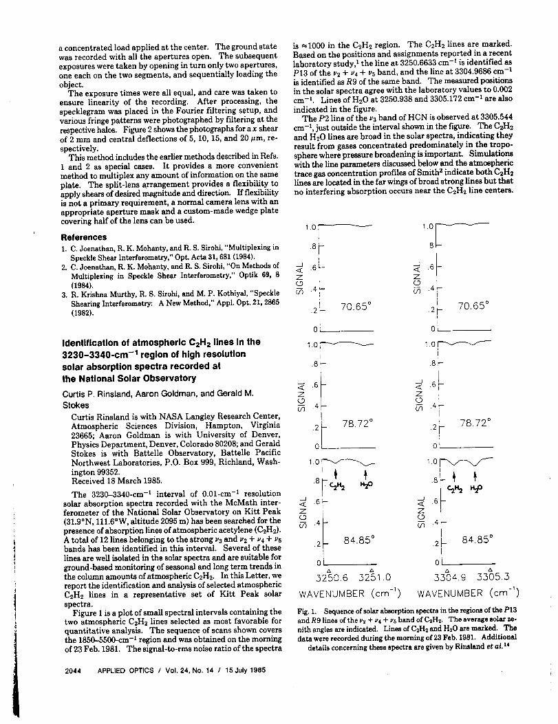
a concentrated load applied at the center. The ground state

was recorded with all the apertures open. The subsequent

exposures were taken by opening in turn only two apertures,one each on the two segments, and sequentially loading the

object.The exposure times were all equal, and care was taken to

ensure linearity of the recording. After processing, the

specklegram was placed in the Fourier filtering setup, and

various fringe patterns were photographed by filtering at the

respective halos. Figure 2 shows the photographs for a x shear

of 2 mm and central deflections of 5, 10, 15, and 20 #m, re-

spectively.This method includes the earlier methods described in Refs.

1 and 2 as special cases. It provides a more convenient

method to multiplex any amount of information on the same

plate. The split-lens arrangement provides a flexibility to

apply shears of desired magnitude and direction. If flexibilityis not a primary requirement, a normal camera lens with an

appropriate aperture mask and a custom-made wedge plate

covering half of the lens can be used.

References

1. C. Joenathan, R. K. Mohanty, and R. S. Sirohi, "Multiplexing in

Speckle Shear [nterferometry," Opt. Acta 31,681 (1984).2. C. Joenathan, R. K. Mohanty, and R. S. Sirohi, "On Methods of

Multiplexing in Speckle Shear Interfarometry," Optik 69, 8(1984).

3. R. Krishna Murthy, R. S. Sirohi, and M. P. Kothiyal, "Speckle

Shearing Interferometry: A New Method," Appl. Opt. 21, 2865

(1982).

Identification of atmospheric C2H2 lines In the3230-3340-cm -1 region of high resolution

solar absorption spectra recorded atthe National Solar Observatory

Curtis P. Rinsland, Aaron Goldman, and Gerald M.

Stokes

Curtis Rinsland is with NASA Langley Research Center,

Atmospheric Sciences Division, Hampton, Virginia

23665; Aaron Goldman is with University of Denver,

Physics Department, Denver, Colorado 80208; and GeraldStokes is with Battelle Observatory, Battelle Pacific

Northwest Laboratories, P.O. Box 999, Richland, Wash-

ington 99352.Received 18 March 1985.

The 3230-3340-cm -1 interval of 0.01-cm -i resolution

solar absorption spectra recorded with the McMath inter-ferometer of the National Solar Observatory on Kitt Peak

{31.9°N, lll.6°W, altitude 2095 m) has been searched for the

presence of absorption lines of atmospheric acetylene (C2H2).A total of 12 lines belonging to the strong vs and v2 + _4 + vsbands has been identified in this interval. Several of these

lines are well isolated in the solar spectra and are suitable for

ground-based monitoring of seasonal and long term trends inthe column amounts of atmospheric C2H2. In this Letter, we

report the identification and analysis of selected atmospheric

C2H2 lines in a representative set of Kitt Peak solar

spectra.Figure 1 is a plot of small spectral intervals containing the

two atmospheric C2H2 lines selected as most favorable for

quantitative analysis. The sequence of scans shown covers

the 1850-5500-cm -i region and was obtained on the morning

of 23 Feb. 1981. The signal-to-rms noise ratio of the spectra

is _1000 in the C2H2 region. The C2H2 lines are marked.

Based on the positions and assignments reported in a recent

laboratory study, t the line at 3250.6633 cm -t is identified asP13 of the v2 + v4 + vs band, and the line at 3304.9686 cm -1

is identified as R9 of the same band. The measured positions

in the solar spectra agree with the laboratory values to 0.002

cm -1. Lines of S20 at 3250.938 and 3305.172 cm-* are also

indicated in the figure.The P2 line of the v3 band of HCN is observed at 3305.544

cm -t, just outside the interval shown in the figure. The C2H2

and H20 lines are broad in the solar spectra, indicating they

result from gases concentrated predominately in the tropo-

sphere where pressure broadening is important. Simulations

with the line parameters discussed below and the atmospheric

trace gas concentration profiles of Smith 2 indicate both C2H2lines are located in the far wings of broad strong lines but that

no interfering absorption occurs near the C2H2 line centers.

z0

03

1.0I

i

.6Li

.4 L-1

.2i 70.65 °r-q

I0 _

I.8_

.._1< .6.7(_9C_ .4

.2

0

1.0

78.72 °

d

.<z(_303

.8 -

.6 -

.4

.2

"2O

84.85 °

0

5250.6 5251.0

.8

._]<f .6Z

o .4_03

I 70.65 °.2 F

I

i

oL

_.o_Iq

.8r-

< .6Z

.2_- 78-72°

0 _

1,0_I

_J< .670

.2 - 84-85°

0& &

5504.9 5305.3

WAVENUMBER (cm -_) WAVENUMBER (cm-')

Fig.i. Sequence ofsolarabsorptionspectraintheregionsofthePI3and R9 linesofthev2+ _4+ _6band ofC2H2. The averagesolarze-

nithanglesareindicated.LinesofC2H2 and H20 aremarked. The

datawererecordedduringthemorning of23 Feb.1981. Additional

detailsconcerningthesespectraare givenby RinslandetaL 14

2044 APPLIED OPTICS / Vol. 24, No. 14 / 15 July 1985

Table I. Total Vertical Column Amounts Uc_t (In 10 Is molecules cm -2)

and Corresponding Average Tropospheric Volume Mixing Ratios _ (in

ppbv) of C:H: above Kltt Peak

Position 23 Feb. 1981 b 1 Oct. 1982 c

Line a (cm -l) uc2H2 _ UC2H2

P13 3250.6633 2.23 0.20 2.14 0.15R9 3304.9686 2.34 0.21 1.86 0.13Average 2.28d 0.20 2.00d 0.14

a In the v2+ _4+ vsband of 12C2H2.bTropopause geopotential altitude ffi10.4 km.c Tropopause geopotential altitude ffi15.6 kin.d Estimated uncertainty ±15%, estimated precision _-10%.

However, long path laboratory spectra of C02 obtained withthe McMath interferometer show that there is minor con-tamination of the 3304.9686-cm -1 line by the P46 line of the22202-01101 band of 12CIeO2.S This interfering C02 line alsoappears in the C02 arias of Smith et al. 4 Long path lengthlaboratory spectra of N20, s CH4, 6and 03 (Ref. 7) indicate thatboth C2H2 lines are free of overlap by weak lines of thesemolecules.

The C2H2 line positions, intensities, and lower state energiesfor the analysis were taken from the 1982 AFGL trace gascompilation, s Since, to our knowledge, no measurements ofair-broadened halfwidths of C2H2 have been reported, weassumed the same dependence with Iml (m = J_ + 1 for R-branch lines and m ffi -J" for the P-branch lines, where J"is the lower state rotational quantum number), as measuredfor N2 broadening in the (v4 + vs) ° band of 12C2H2.9 Thesevalues are 0.0842 cm -1 atm -1 at 296 K for R9 and, by linearinterpolation, 0.0803 cm -1 atm -1 at 296 K for P13. Since thebackground level of the P13 line is affected by strong nearbylines of H20 and the background level of the R9 lines is af-fected by strong nearby lines of H20 and COs, these lines wereincluded in the calculations assuming the parameters listedin the 1982 AFGL major gas compilation. 1° The position ofthe interfering P46 line of the 22202-01101 band of 12C1e02was changed from the 1982 AFGL value 1° of 3305.0394 cm -1to the laboratory value 3 of 3304.9482 cm -1. The 1982 AFGLintensity for this C02 line 1° is in good agreement with a pre-liminary intensity value determined from laboratoryspectra. 3

In situ measurements indicate very low stratosphericconcentrations of C2H2 at 32°N latitude. 11 Therefore, as apreliminary estimate, we have assumed that the C2H2 mixingratio by volume is constant within the troposphere and thatthere are no C2I-I2molecules above the altitude of the tropo-pause. Spectral data obtained in Feb. 1981 and Oct. 1982were analyzed with the technique of nonlinear least-squarescurve fitting. Examples of the application of this procedureto retrieve information about the abundance and verticaldistribution of atmospheric gases from ground-based solarabsorption spectra are given in several recent papers. 12-14Table I presents the total vertical column amounts and cor-responding mean tropospheric mixing ratios deduced fromanalysis of the solar spectra. The retrieved average tropo-spheric mixing ratio values of 0.14 and 0.20 ppbv are slightlylower than ground level mixing ratios of 0.3 ppbv determinedover the Atlantic at 30°N latitude is and 0.4 ppbv determinedover the eastern Pacific at the same latitude. Is Since mea-surements 11 and calculations 11,17 indicate that the C2H2mixing ratio decreases with altitude in the troposphere, thedifferences between the reported ground level measurementsand our results for the average troposphere above 2.1 km arereasonable. Results of the fits to the solar absorption spectraare illustrated in Fig. 2.

R-branch lines near 770 cm -1 of the _5band have been used

previously for spectroscopic measurements of atmosphericC2H2. Goldman et al. 17 determined a preliminary uppertropospheric mixing ratio of 25 pptv near 9 km from solarabsorption spectra obtained during a balloon flight fromHolloman Air Force Base near Alamogordo, N.M. (32°N,106°W). Zander et al. 18analyzed a different set of Kitt Peaksolar spectra than used in the present analysis and determineda mean C2H2 mixing ratio of 27 4- 6 pptv. It is interesting tonote that this latter value is almost an order of magnitudelower than derived in the present study. Although some ofthis difference is probably due to differences in the methodsof analysis (the equivalent width method was used by Zanderet al. is) and uncertainties in the assumed values for thespectroscopic line parameters, the pressure-temperatureprofile, and the shape of the gas concentration profile withaltitude, its magnitude seems too large to result entirely fromthese factors. _ On the other hand, our vertical columnamounts for Feb. 1981 and Oct. 1982 differ by only 14% so thatlarge variability in the total abundance of atmospheric CsH2above Kitt Peak is unlikely. We plan to analyze additionalKitt Peak solar spectra to determine the range of seasonalvariations in the C2H2 vertical column amount.

The C2H2 lines reported here were also confirmed by Coffeyand Mankin 19 from analysis of their stratospheric solar ab-sorption spectra obtained at 0.06-cm -1 resolution from anaircraft at 12-kin altitude. While most of the C2H2 lines inthe 3200-3400-cm -1 region are partially or totally overlappedby other atmospheric lines, the 3250.66- and 3304.97-cm -1lines are quite isolated and show 3-5% absorption in spectraobtained with zenith angles of 91-93 °. The nearby P2 HCNline at 3305.544 cm -1 absorbs ,-_5% in these spectra. Unfor-tunately, the available aircraft spectra do not allow an accu-

1.0 l ' 1 ' I '

- 0 _ I ±. I _ _--

1.00

--J

_Z .95 --'-.D

,90 , I , H2OI ,3304.8 3305.0 3305.2 3305.4

WAVENUMBER (crn -_}

Fig.2. Comparisonbetweenthesolarabsorptionspectrumrecordedatan averageastronomicalzenithangleof84.85° (solidline)andleast-squaresbestfittothedate(crosses)intheregionoftheR9 lineofthev2+ _4+ _5bandofC2H2. The measuredspectrumhasbeennormalized to the highest intensity value in the fitted interval. Lines

Call2 and H20 are identified.

15 July 1985 / Vol. 24, No. 14 1 APPLIED OPTICS 2045

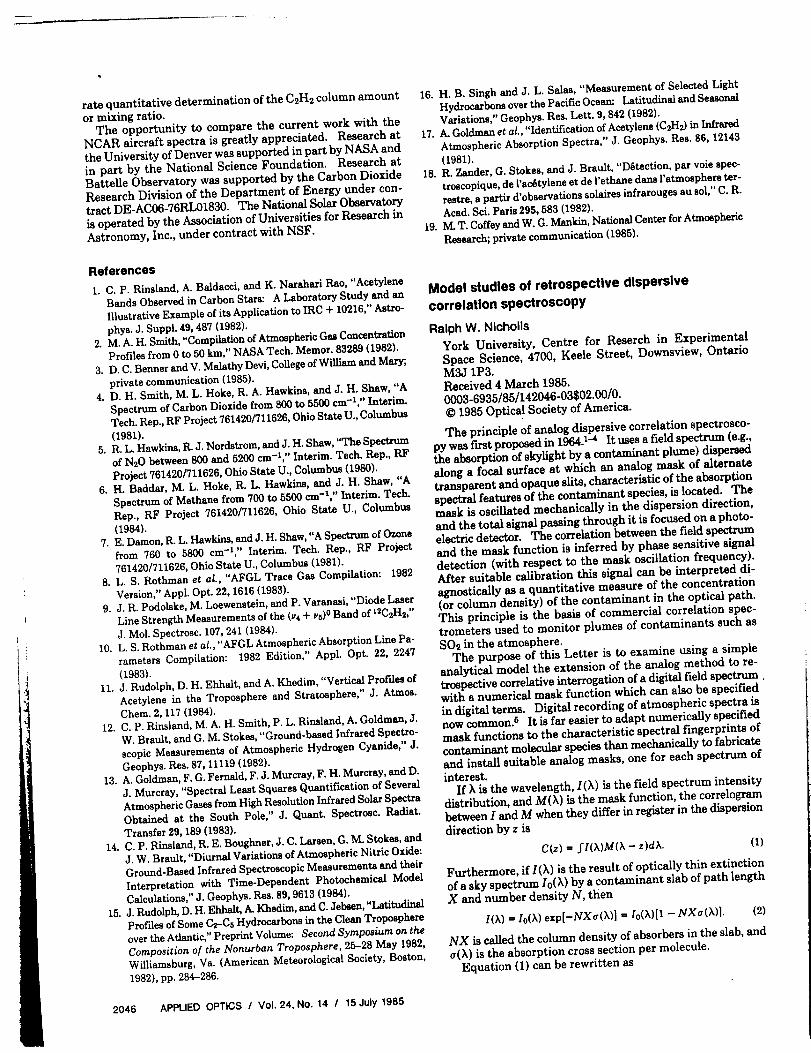
ratequantitative determination of the C2H2 column amount

or mixing ratio.The opportunity to compare the current work with the

NCAR aircraftspectra isgreatly appreciated. Research at

the Universityof Denver was supported in partby NASA and

in part by the National Science Foundation. Research atBattelle Observatory was supported by the Carbon Dioxide

Research Division of the Department of Energy under con-

tractDE-AC06-76RL01830. The National SolarObservatory

isoperated by the Associationof UniversitiesforResearch in

Astronomy, Inc.,under contract with NSF.

References

1. C. P. Rinsland,A. Baldacci,and K. Narahari Rao, "Acetylene

Bands Observed inCarbon Stars: A LaboratoryStudy and an

IllustrativeExample ofitsApplicationtoIRC + 10216,"Astro-

phys.J.Suppl.49,487 (1982).2. M. A. H. Smith,"CompilationofAtmosphericGas Concentration

Profilesfrom 0 to50 kin,"NASA Tech.Memor. 83289 (1982).

3. D. C.Benner and V. Malathy Devi,CollegeofWilliamand Mary;

privatecommunication (1985).4. D. H. Smith, M. L. Hoke, R. A. Hawkins, and J.H. Shaw, "A

Spectrum ofCarbon Dioxidefrom 800 to5500 cm-1,''Interim.Tech.Rep.,RF Project761420/711626,Ohio StateU.,Columbus

(1981).5. R.L. Hawkins, R. J. Nordstrom, and J. H. Shaw, "The Spectrum

of N20 between 800 and 5200 cm-Z," Interim. Tech. Rep., RF

Project 761420/711626, Ohio State U., Columbus (1980).6. H. Baddar, M. L. Hoke, R. L. Hawkins, and J. H. Shaw, "A

Spectrum of Methane from 700 to 5500 cm-1," Interim. Tech.Rep., RF Project 761420/711626, Ohio State U., Columbus

(1984).7. E. Damon, R. L. Hawkins, and J. H. Shaw, "A Spectrum of Ozone

from 760 to 5800 cm-1," Interim. Tech. Rep., RF Project761420/711626, Ohio State U., Columbus (1981).

8. L. S. Rothman et aL, "AFGL Trace Gas Compilation: 1982

Version," Appl. Opt. 22, 1616 (1983).9. J. R. Podoiske, M. Loewenstein, and P. Varanasi, "Diode Laser

LineStrengthMeasurements ofthe(v4+ vs)°Band ofLsCsH2,"

J.Mol.Spectrosc.107,241 (1984).10. L.S.Rothman etal.,"AFGL AtmosphericAbsorptionLine Pa-

rameters Compilation: 1982 Edition,"Appl. Opt. 22, 2247

(1983).ii. J.Rudolph, D. H. Ehhalt,and A. Khedim, "VerticalProf'dasof

Acetylenein the Troposphere and Stratosphere,"J. Atmos.

Chem. 2,117 (1984).12. C. P.Rinsland,M. A. H. Smith,P. L.Rinsland,A. Goldman, J.

W. Brault,and G. M. Stokes,"Ground-based InfraredSpectro-

scopicMeasurements of Atmospheric Hydrogen Cyanide,"J.

Geophys. Res.87,11119 (1982).13. A. Goldman, F.G. Fernald,F.J.Murcray,F.H. Murcray,and D.

J.Murcray, "SpectralLeast SquaresQuantificationofSeveral

AtmosphericGasesfrom High ResolutionInfraredSolarSpectraObtained at the South Pole," J. Quant. Spectrosc.Radiat.

Transfer29,189 (1983).14. C.P. Rinsland,R. E.Boughner,J.C.Larsen,G. M. Stokes,and

J.W. Brault,"DiurnalVariationsofAtmospheric NitricOxide:

Ground-Based InfraredSpectroscopicMeasurements and their

Interpretationwith Time-Dependent Photochemical Model

• ,,jCalculatmns, .Geophys. Res.89,9613 (1984).

15. J.Rudolph,D. H. Ehhalt,A.Khedma, and C.Jel_en,"Latitudinal

ProfilesofSome C2-C5 Hydrocarbonsinthe CleanTroposphere

overtheAtlantic,"PreprintVolume: Second Symposium on the

Compositionof the Nonurban Troposphere,25-28 May 1982,Williamsburg,Va. (American MeteorologicalSociety,Boston,

1982),pp.284--286.

2046 APPLIED OPTICS / Vol. 24, No. 14 I 15July 1985

16. H. B. Singh and J. L. Salas, "Measurement of Selected Light

Hydrocarbons overthe PacificOcean: Latitudinaland SeasonalVariations,"Geophys. Res.Lett.9,842 (1982).

17. A_Goldman etaL,"IdentificationofAcetylene(C2H2)inInfrared

Atmospheric AbsorptionSpectra,"J.Geophys. Res.86,12143

(1981).18. R. Zander,G. Stokes,and J.Brault,"D_taction,par voiespec-

troscopique,de rac_tyleneetde l'ethanedansl'atmosphereter-• " " a

restre,a partird'observationssolalresmfrarougesau sol,C. •

Acad.Sci.Paris295,583 (1982).

19. M.T. Coffeyand W. G. Mankin, NationalCenterforAtmospheric

Research;privatecommunication (1985).

Model studies of retrospective dispersive

correlation spectroscopy

Ralph W. Nicholls

York University, Centre for Reserch in Experimental

Space Science, 4700, Keele Street, Downsview, Ontario

M3J IP3.Received 4 March 1985.0003.6935/85/142046-03502.00/0.© 1985 Optical Society of America.

The principle of analog dispersive correlation spectrosco-..... J :- 1964 z--4It uses a field spectrum (e.g.,

py was XLrS_proposeu ,,, - . ....the absorption of skylight by a contaminant plumej msperseu

along a focal surface at which an analog mask of alternate

transparent and opaque slits, characteristic of the absorption

spectral features of the contaminant species, is located. Themask is oscillated mechanically in the dispersion direction,

and the total signal passing through it is focused on a photo-

electric detector. The correlation between the field spectrumand the mask function is inferred by phase sensitive signaldetection (with respect to the mask oscillation frequency).

After suitable calibration this signal can be interpreted di-

agnostically as a quantitative measure of the concentration

(or column density) of the contaminant in the optical path.

This principle is the basis of commercial correlation spec-trometers used to monitor plumes of contaminants such as

S02 in the atmosphere.The purpose of this Letter is to examine using a simple

analytical model the extension of the analog method to re-

trospective correlative interrogation of a digital field spectrum.with a numerical mask function which can also be specified

in digital terms. Digital recording of atmospheric spectra isnow common. 5 It is far easier to adapt numerically specifiedmask functions to the characteristic spectral fingerprints of

contaminant molecular species than mechanically to fabricate

and install suitable analog masks, one for each spectrum of

interest.If )_ is the wavelength, I(X) is the field spectrum intensity

distribution, and M(),) is the mask function, the correlogram

between I and M when they differ in register in the dispersion

direction by z is

C(z) = fl(k)M(k - z)dk. (1)

Furthermore, if I(X) is the result of optically thin extinctionof a sky spectrum Io(_) by a contaminant slab of path length

X and number density N, then

I()0 ffi Io()_) exp[-NX#(k)] ffi Io(X)[1 - NXa(X)]. (2)

NX is called the column density of absorbers in the slab, and

a(X) is the absorption cross section per molecule.

Equation (1) can be rewritten as

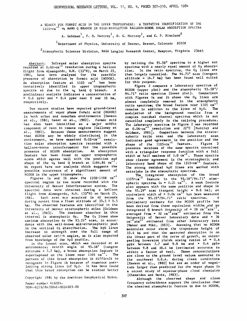
GEOPHYSICAL RESEARCH LETTERS, VOL. 11, NO. 4, PAGES 307-310, APRIL 1984

A SEAECH__OR FORMIC ACID IN THE UPPER TROPOSPHERE: A TENTATIVE IDENTIFICATION OF THEll05-cm v6 BAND Q BRANCH IN HIGH-RESOLUTION BALLOON-BORNE SOLAR ABSORPTION SPECTRA

A. Goldman I, F. H. [lurcray I, D. g. Murcray I, and C. P. Rinsland 2

IDepartment of Physics, University of Denver, Denver, Colorado 80208

2Atmospheric Sciences Division, NASA Langley Research Center, Hampton, Virginia 23665

Abstract. Infrared solar absorption spectrareco--_ed a-t 0.02-cm-" resolution during a balloon

flight from Alamogordo, N.M. (33°N), on March 23,

1981, have been analyzed for the possible

presence of absorption by formic acid (HCOOH).

An absorption feature at II05 cm -l has been

tentatively identified in upper tropospheric

spectra as due to the v6 band Q branch. A

preliminary analysis indicates a concentration of

0.6 ppbv and - 0.4 ppbv near 8 and IO km,

respectively.

Two recent studies have reported ground-level

measurements of vapor phase formic acid (HCOOH)

in both urban and nonurban environments [Dawson

et al., 1980; Hanst et al., 1982]. Formic acid

has also been identified as a major acidic

component of rain in remote regions [Galloway et

al., 1982]. Because these measurements suggest

that HCOOH may be widely dlstrlbute_ in the

environment, we have examSned O.02-cm-" resolu-

tion solar absorption spectra recorded with a

balloon-borne interferometer for the possible

presence of HCOOH absorption. An absorption

feature has been found in upper tropospheric

scans which agrees well with the position a_d

shape of the v6 band Q branch at 1104.86 cm--.

We report here our analysis which suggests the

possible occurrence of a significant amount of

HCOOH in the upper troposphere. -l

Figures la and Ib show the II00-ii08 cm

spectral region in two scans recorded wlth the

University of Denver Interferometer system. The

spectral data were obtained during a balloon

flight from Alamogordo, N.H. (33°N) on _rch 23,

1981. Each scan w_s acquired in 40 seconds

during sunset from a float altitude of 33.5 ± 0.5

km. The observed features are identified in the

University of Denver stratospheric atlas [Goldman

et al., 1983]. The dominant absorber in this

interval is atmospheric 03. The 03 lines show

maximum absorption in the 93.21 ° scan, in accor-

dance with the well-known mld-stratospheric peak

in the vertical 03 distribution. The _20 lines

increase in strength over the full range of

observed solar zenith angles, as is also expected

from knowledge of the H20 profile.

In the lowest scan, which was recorded at an

astronomical zenith angle of 95.58 ° (tangent

altitude = 7.7 km), a broad absorption feature is

superimposed on the lines near 1105 cm-'. The

pattern of this broad absorption is difficult to

recognize in Figure Ib because of numerous over-

lapping strong lines (of 03). It has been found

that this broad absorption can be studied better

Copyright 1984 by the American Geophysical Union.

Paper number 4L6024.

0094-8276/84/004L-0024$03.00

by ratlolng the 95.58 ° spectrum to a higher sun

spectrum with a nearly equal amount of 03 absorp-

tion. In the ratio spectrum, the 03 lines are

then largely cancelled. The 94.71 ° scan (tangent

altitude = 14.7 km) has been found well suited

for this purpose.

Figure 2 compares a laboratory spectrum of

HCOOH (upper plot) and the atmospheric 95.58°/

94.71" ratio spectrum (lower plot). Comparison

with Figures la and Ib shows the O 3 lines are

almost completely removed in the atmospheri_

ratio spectrum; the broad feature near 1105 cm

remains in addition to the lines of H20. The

modulation of the background results from a

complex residual channel spectrum which is not

cancelled completely in the ratioing procedure.

The laboratory spectrum in Figure 2 was recordedat 0.06-cm- resolution and 22°C [tlurcray and

Goldman, 1981]. Comparison between the strato-

spheric ratlo scan and the laboratory scan

indicates good agreement in the position and the

shape of the ll05-cm -I feature. Figure 3

presents versions of the same spectra convolved

with a triangular response function with a fullwidth at half maximum of 1.0 cm- . These spectra

show clearer agreement in the stratospheric andlaboratory band shape of the ll05-cm- feature.

The strong residual _20 lines are marked with

asterisks in the atmospheric spectrum.

The I integrated absorption of the broad

ll05-cm- feature in the 9_.58°/94.71 ° atmo-

spheric spectrum is - 0.21 cm A weak feature

also appears with the same position and shape in

the 95.29 ° scan (tangent hel_ht = 9.8 km); an

equivalent width of - 0.Oh cm- has been measured

from the 95.29°/94.71 ° ratio spectrum. A

preliminary estimate for the HCOOH profile has

been derived from these equivalent widths2and__n

integrated Q branch in_ensi_y of - 28 cm arm ,averaged from - 20 cm- arm- estimated from the

University of Denver laboratory data and - 36cm arm estimated from other laboratory data

[Maker and Nlki, 1983]. Assuming that no HCOOH

molecules occur above the tropopause height of

10.4 km and that the measured absorption is on

the linear part of the curve of growth, an onion-

peeling inversion yields mixing ratios of " 0.6

ppbv between 7.7 and 9.8 km and - 0.4 ppbv

between 9.8 and 10.4 km (estimated accurate to

within a factor of two). These concentrations

are close to the ground level values measured in

the southwest U.S.A. during clean conditions

[Dawson et al., 1980] but are an order of magni-

tude larger than predicted for the vapor phase in

a recent study of aqueous-phase cloud chemistry

[Chameides and Davis, 1983].

Although the observed shape and close

frequency coincidence support the conclusion that

the observed atmospheric feature is due to HCOOH,

307

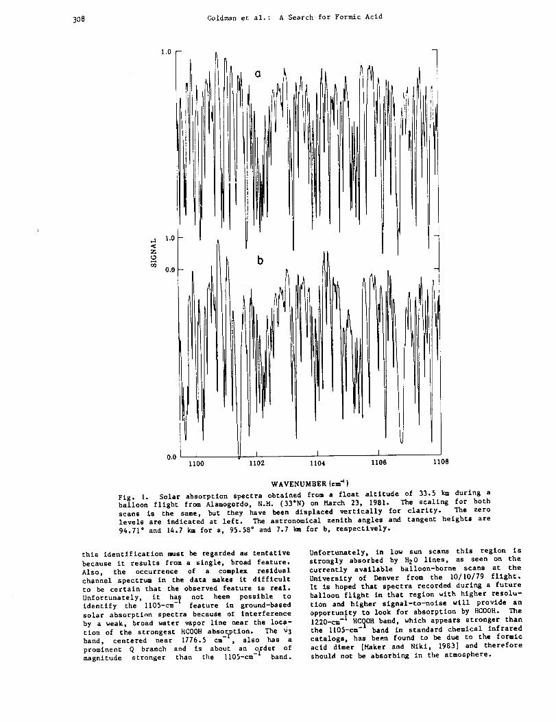
308 Goldmanet al.: A Searchfor FormicAcid

o_

II00 1102 1104 1106 1108

WAVENUMBER (cm d )

Fig. I. Solar absorption spectra obtained from a float altitude of 33.5 km during a

balloon fllght from Alamogordo, N.M. (33°N) on March 23, 1981. The scaling for both

scans is the same, but they have been displaced vertically for clarity. The zero

levels are indicated at left. The astronomical zenith angles and tangent heights are

94.71" and 14.7 km for a, 95.58" and 7.7 km for b, respectively.

this identification must be regarded as tentative

because it results from a single, broad feature.

Also, the occurrence of a complex residual

channel spectrum in the data makes it difficult

to be certain that the observed feature ls real.

Unfortunately, it ha_ not been possible to

identify the ll05-cm-- feature in ground-based

solar absorption spectra because ol interference

by a weak, broad water vapor llne near the loca-

tion of the strongest HCOOH abso__ption. The _3

band, centered near 1776.5 cm , also has a

prominent Q branch and is about an order of

magnitude stronger than the ll05-cm -I band.

Unfortunately, in low sun scans this region is

strongly absorbed by H20 lines, as seen on the

currently available balloon-borne scans at the

University of Denver from the 10/10/79 flight.

It is hoped that spectra recorded during a future

balloon flight in that region with higher resolu-

tion and higher slgnal-to-noise will provide an

opportunlty to look for absorption by HCOOH. The

1220-cm -_ HC_OH band, which appears stronger thanthe ll05-cm- band in standard chemical infrared

catalogs, has been found to be due to the formic

acid dimer [Maker and Niki, 1983] and therefore

should not be absorbing in the atmosphere.

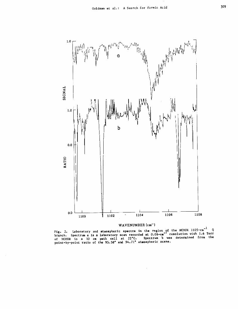
Goldmanet al.: A Searchfor FormicAcid 309

Z

O6_

1.0

0.0

0.0 L

1100 1102 1104 1106 1108

WAVENUMBER (cm-')

Fig. 2. Laboratory and atmospheric spectra in the region__f the HCOOH ll05-cm -I Q

branch. Spectrum a is a laboratory scan recorded at O.06-cm resolution with 1.6 Tort

of HCOOH in a I0 cm path cell at 22°C. Spectrum b was determined from the

point-by-polnt ratio of the 95.58 e and 94.71 ° at_ospherlc scans.

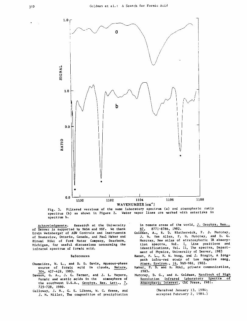
310 Goldmanet al. : A Searchfor FormicAcid

<ZOw_

rn

O

00 [ I I1100 1102 1104 1106 1108

WAVENUMBER (cm-')

Fig. 3. Filtered versions of the same laboratory spectrum (a) and atmospheric ratio

spectrum (b) as shown in Figure 2. Water vapor lines are marked with asterisks in

spectrum b.

Acknowledsments. Research at the University

of Denver is supported by NASA and NSF. We thank

Ervin Weinberger of ASW Controls and Instruments

of Downsvlew, Ontario, Canada, and Paul l_ker and

Hiroml Niki of Ford Motor Company, Dearborn,

Michigan, for useful discussions concerning the

infrared spectrum of formic acid.

References

Chameides, W. L., and D. D. Davis, Aqueous-phase

source of formic acid in clouds, Nature,

304, 427-429, 1983.

Dawson, G. A., J. C. Farmer, and J. L. Moyers,

Formic and acetic acids in the atmosphere of

the southwest U.S.A., Geophys. Res. Latt., _,

725-728, 1980.

Galloway, J. N., G. E. Likens, W. C. Keene, and

J. M. Miller, The composition of precipitation

in remote areas of the world, J. Ceophys. Res.,

87, 8771-8786, 1982.

Goldm--'an, A., R. D. Blatherwick, F. J. Murcray,

j. W. Van Allen, F. H. Murcray, and D. G.

Murcray, New atlas of stratospheric IR absorp-

tion spectra, Vol. I, Line positions and

identifications, Vol. II, The spectra, Depart-

ment of Physics, University of Denver, 1983

Hanst, P. L., N. W. Wong, and J. Bragin, A long-

path infra-red study of Los Angeles smog,

Atmos. Environ., 16, 969-981, 1982.

Maker, P. D. and N. Niki, private communication,

1983.

Murcray, D. G., and A. Goldman, _andbook of Hish

Resolution Infrared Laboratory Spectra of

Atmospheric Interest, CKC Press, 1981.

(Received January 13, 1984;

accepted February 2, 1984.)

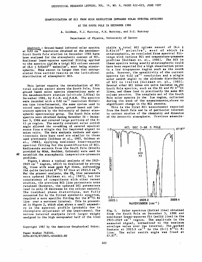
GEOPHYSICALRESEARCHLETTERS,VOL.14,NO.6, PAGES622-623,JUNE1987

QUANTIFICATIONOF HCf FROM HIGH RESOLUTION INFRARED SOLAR SPECTRA OBTAINED

AT THE SOUTH POLE IN DECEMBER 1986

A. Goldman, F.J. Murcray, FoH. Murcray, and D.G. Murcray

Department of Physics, University of Denver

Abstract - Ground-based infrared solar spectra

at 0.02 cm -l resolution obtained at the Amundsen-

Scott South Pole station in December 1986 have

been analysed for the atmospheric content of HCf.

Nonlinear least-squares spectral fitting applied

to the spectra y_elds a tots1 HCf column amount

of (6.4 ± 0.8)xl0 _J molec/cm _, most being strato-

spheric. This amount is larger than that extrap-

olated from earlier results on the latitudinal

distribution of atmospheric HCf.

This Letter reports the determination of HC1

total column amount above the South Pole, from

ground based solar spectra observations made at

the Amundsen-Scott station (altitude 2.85km) in

December 1986, by F.J.M. andiF.H.M. The spectrawere recorded with a 0.02 cm- resolution Michel-

son type interferometer, the same system used to

record many balloon-borne, ground based and lab-

oratory spectra by the University of Denver atmo-

spheric spectroscopy group. The South Pole solar

spectra were obtained during November 26 - Decem-

ber 3, 1986 and covered large portions of the 3-

15 _m region. The nearly constant solar zenith

angle allowed the co-addlng of several spectral

scans from a single day for improved signal to

noise ratio. The data analysis methods and spec-

troscopic data base used are similar to those

used previously [Goldman et al., 1983, Goldman et

al., 1986], applying nonlinear least-squares

spectral fitting for the quantification of HCf.

Radiosonde ascents from the South Pole (kindly

provided by NOAA, Boulder, Colorado) were used to

establish the atmospheric temperature-pressure

profiles.

Figure I shows a typical analysis of the 2923-

2929 cm -l region, which is dominated by strong

CH 4 lines with some _ak H20 lines, surroundingthe quite isolated H_CI El llne at 2925.9 cm -_.

For the present analysis, the CH 4 line parameters

were updated [Rothman et. al., 1987], but for

consistency of comparisons with other recent

studies, the previous HCf line parameters were

retained (however, the updated HCI parameters

lead to only IZ decrease in the column amount).

The residual phase distortions, not fully

accounted for by the fitted synthetic spe_trum,

required a more specific fitting for the H_JC1 R1

line over a narrower interval. This is present-

ed in Figure 2, which also shows a small asymmet-

ry in the spectral profile (probably due to

incomplete adjustment of the instrument). The

narrow interval analysis (with larger weight

assigned to the high wavepumber half of the llne)

Copyright 1987 by the American Geophysical Union.

Paper Number 7L6546.

0094-8276/87/007L-6546503.00

yields a total HCl c_lumn amount of (6.4 ±0.8)x1015 molec/cm , most of which is

stratospheric, as concluded from spectral fit-

tings with various HCI and temperature-pressure

profiles [Goldman et. al., 1986]. The HCf in

these spectra being mostly stratospheric could

have been expected for a high observation point

in a low tropopause region such as the south

pole. However, the sensitivity of the current

spectra (at 0.02 cm -I resolution and a single

solar zenith angle) to the altitude distribution

of HCf is limited [Goldman et. al., 1983].

Several other HCf lines are quite isolated o_he

South Pole spectra, such as the R1 and P2 H_JCI

lines, and these lead to practically the same HCf

column amounts. The complete set of the South

Pole solar spectra in the 3_m region, collected

during the week of the measurements,shows no

significant change in the HCf amounts.

This is the first HCf measurement reported

from the South Pole and is of particular interest

to current studies of the chemistry and dynamics

of the Antarctic atmosphere. Previous measure-

S. POLE1.0 67 .87°

>..

HCL DEC. 3-86

tNCIB1

, ,

_.926.20.0_923.1 2929.4

WAVENUMBER (cm-')

Fig. I. Solar spectrum (dotted llne) obtained

from the South Pole on December 3, 1986 and

nonlinear least-squares fit (solid llne) in the

2923-2929 cm -l region. The amplitude is the

measured signal, normalized to the maximum

envelope value over t_e interval. The markedfeature at 2925.9 cm-" is the (0-I) H35CI RI

llne. The solar zenith angle was fixed at

67.87 ° .

622

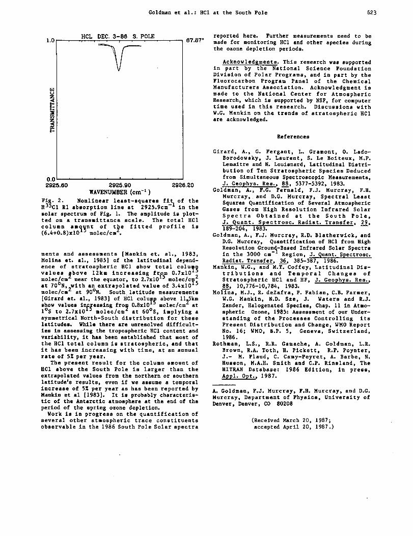
Goldman et al.: HC1 at the South Pole 623

HCL1.0 67.87 °

z

DEC. 3-86 S. POLE

• ....., e •

-V-

0._ I e i e I i e i 1

2925.60 2925.90 2926.20

WAVENUMBER (cm'*)

Fig. 2. Nonlinear least-squares fit of theH35C1 R1 absorption line at 2925.9cm -1 in the

solar spectrum of Fig. 1. The amplitude is plot-ted on a transmittance scale. The total HCI

column amount of t_e fitted profile is(6.4,0.8)x16 _ molec/cm .

merits and assessments [Mankln et. al., 1983,

Molina et. al., 1985] of the latltudlnal depend-

ence of stratospheric HCl show total colu_

values above 12km increasln 8 from 0.7x10 "_molec/cm 2 near the equator, to 2.7xl0_Ymolec/c_

o £_at 70 N, with an extrapolated value of 3.4x10molec/cm 2 at 90°N. South latitude measurements

[Girard et. al., 1983] of HC1 colu_ above ll_km

show values in_;easing frow 0.8xl0 "_ molec/cm" at

l°S to 2.7x10 _ molec/cm z at 60°S, implying a

symmetrical North-South distribution for theselatitudes. While there are unresolved difficult-

ies in assessing the tropospheric HC1 content and

variability, it has been established that most of

the HC1 total column is stratospheric, and that

it has been increasing with time, at an annual

rate of 5% per year.

The present result for the column amount of

HC1 above the South Pole is larger than the

extrapolated values from the northern or southern

latitude's results, even if we assume a temporal

increase of 5% per year as has been reported by

Mankin et al [1983]. It is probably characteris-

tic of the Antarctic atmosphere at the end of the

period of the spring ozone depletion.

Work is in progress on the quantification of

several other atmospheric trace constituents

observable in the 1986 South Pole Solar spectra

reported here. Further measurements need to be

made for monitoring HCl and other species during

the ozone depletion periods.

Acknowledgments. This research was supported

in part by the National Science Foundation

Division of Polar Programs, and in part by the

Fluorocarbon Program Panel of the Chemical

Manufacturers Association. Acknowledgment is

made to the Natlonal Center for Atmospheric

Research, which is supported by NSF, for computer

time used in this research. Discussions with

W.G. Mankin on the trends of stratospheric HCI

are acknowledged.

References

Girard, A., G. Fergant, L. Gramont, O. Lado-

Borodowsky, J. Laurent, S. Le Bolteux, M.P.

Lemaltre and N. Loulsnard, Latitudinal Distri-

bution of Ten Stratospheric Species Deduced

from Simultaneous Spectroscopic Measurements,

J. Geophys. Res., 88, 5377-5392, 1983.

Goldman, A., F.G. Fernald, F.J. Murcray, F.H.

Murcray, and D.G. Murcray, Spectral Least

Squares Quantification of Several Atmospheric

Gases from High Resolution Infrared Solar

Spectra Obtained at the South Pole,

J. Quant. Spectrosc. Radlat. Transfer, 29,

189-204, 1983.

Goldman, A., F.J. Murcray, R.D. Blatherwtck, and

D.G. Murcray, Quantification of HCl from High

Resolution Ground-Based Infrared Solar Spectrain the 3000 cm- Region, J. Quant. Spectrosc.

Radiat. Transfer, 36, 385-387, 1986.

Mankin, W.G., and M.T. Coffey, Latitudinal Dis-

tributions and Temporal Changes of

Stratospheric HCI and HF, J. Geophys. Res.,

88, 10,776-10,784, 1983.

Moltna, M.J., R. deZafra, P. Fabian, C.B. Farmer,

W.G. Mankln, N.D. Sze, J. Waters and R.J.

Zander, Halogenated Species, Chap. 11 in Atmo-

spheric Ozone, 1985: Assessment of our Under-

standing of the Processes Controlling its

Present Distribution and Change, WMO Report

No. 16; WMO, B.P. 5, Geneva, Switzerland,

1986.

Rothman, L.S., R.R. Gamache, A. Goldman, L.R.

Brown, R.A. Toth, H. Pickett, R.P. Poynter,

J.- M. Flaud, C. Camy-Peyret, A. Barbe, N.

Husson, M.A.H. Smith and C.P. Rinsland, The

HITKAN Database: 1986 Edition, in press,

Appl. Opt., 1987.

A. Goldman, F.J. Murcray, F.H. Murcray, and D.G.

Murcray, Department of Physics, University of

Denver, Denver, CO 80208

(Received March 20, 1987;

accepted April 20, 1987.)