Ultraviolet, Infrared & Fluorescence Photography - CiteSeerX
Upload
khangminh22Category
view
1download
0
Spectroscopic infrared ellipsometryon functional polymer films
Spektroskopische Infrarotellipsometrie an funktionalen Polymerfilmen
Promotionsschriftzur Erlangung des akademischen Grades
Doctor rerum naturalium(Dr. rer. nat.)
eingereicht an derFakultät II – Mathematik und Naturwissenschaften
der Technischen Universität Berlin
vorgelegt vonDiplom-Physiker
Andreas Furchner
Genehmigte Dissertation
Promotionsausschuss:Vorsitzender: Prof. Dr. Heinz-Wilhelm Hübers, TU Berlin1. Gutachter: Prof. Dr. Norbert Esser, TU Berlin2. Gutachter: Prof. Dr. Svetlana Santer, Universität Potsdam3. Gutachter: PD Dr. Karsten Hinrichs, TU Dresden
Eingereicht am: 20. Dezember 2013Tag der wissenschaftlichen Aussprache: 7. April 2014
Berlin 2014
D 83

List of publications and book contributions:1. Furchner, A.; Bittrich, E.; Rauch, S.; Uhlmann, P.; Hinrichs, K., “Temperature-Sensitive
Swelling Behavior of Thin Poly(N -isopropylacrylamide) Brushes Studied by In-situ InfraredSpectroscopic Ellipsometry,” Polymeric Materials: Science & Engineering 2012, 107, 372–373, ISBN: 978-0-8412-2777-4.
2. Hinrichs, K.; Bittrich, E.; Aulich, D.; Furchner, A.; Minko, S.; Luzinov, I.; Stamm, M.;Uhlmann, P.; Eichhorn, K.-J., “Ellipsometry for Study of Smart Polymer Brushes,” Poly-meric Materials: Science & Engineering 2012, 107, 655–656, ISBN: 978-0-8412-2777-4.
3. Hinrichs, K.; Furchner, A.; Rappich, J.; Oates, T. W. H., “Polarization-dependent and ellip-sometric infrared microscopy for analysis of anisotropic thin films,” The Journal of PhysicalChemistry C 2013, 117 (26), 13557–13563, DOI: 10.1021/jp401576r.
4. Furchner, A.; Bittrich, E.; Uhlmann, P.; Eichhorn, K.-J.; Hinrichs, K., “In-situ characteriza-tion of the temperature-sensitive swelling behavior of poly(N -isopropylacrylamide) brushesby infrared and visible ellipsometry,” Thin Solid Films 2013, 541, 41–45,DOI: 10.1016/j.tsf.2012.10.135.
5. Bittrich, E.; Uhlmann, P.; Eichhorn, K.-J.; Hinrichs, K.; Aulich, D.; Furchner, A., “Smartpolymer surfaces and films” in Ellipsometry of Functional Organic Surfaces and Films, Eich-horn, K.-J.; Hinrichs, K. (Editors), Springer Berlin 2014, ISBN: 978-3-642-40127-5,DOI: 10.1007/978-3-642-40128-2_5.
6. Furchner, A.; Aulich, D., “Common Polymers and Proteins” in Ellipsometry of FunctionalOrganic Surfaces and Films, Eichhorn, K.-J.; Hinrichs, K. (Editors), Springer Berlin 2014,ISBN: 978-3-642-40127-5, DOI: 10.1007/978-3-642-40128-2_17.
7. Furchner, A.; Aulich, D., “Organic Materials for Optoelectronic Applications” in Ellipsometryof Functional Organic Surfaces and Films, Eichhorn, K.-J.; Hinrichs, K. (Editors), SpringerBerlin 2014, ISBN: 978-3-642-40127-5, DOI: 10.1007/978-3-642-40128-2_18.
8. Hinrichs, K.; Furchner, A.; Sun, G.; Gensch, M; Rappich, J.; Oates, T. W. H., “Infrared el-lipsometry for improved laterally resolved analysis of thin films,” Thin Solid Films, in press2014, DOI: 10.1016/j.tsf.2014.02.006.
Selected contributions at academic conferences and meetings:1. A. Furchner, D. Aulich, E. Bittrich, S. Rauch, K. Hinrichs, “Characterization of optical prop-
erties of PNIPAAm brushes via ex-situ infrared spectroscopic ellipsometry,” Poster presenta-tion at the 6th Workshop Ellipsometry, February 21–24, 2011, Berlin, Germany.
2. A. Furchner, D. Aulich, E. Bittrich, K. Hinrichs, “Characterization of temperature-sensitiveswelling behavior of PNIPAAm brushes via in-situ infrared ellipsometry,” Poster presentationat the DPG spring meeting, March 13–18, 2011, Dresden, Germany.
ii

3. A. Furchner, D. Aulich, S. Pop, G. Sun, N. Esser, K. Hinrichs, “Analysis of thin organic filmsby infrared ellipsometry (IRSE),” Oral presentation and poster presentation at the 26. Tagder Chemie, August 13, 2011, Berlin, Germany.
4. A. Furchner, D. Aulich, E. Bittrich, S. Rauch, P. Uhlmann, K. Hinrichs, “Temperature-sensitive swelling behavior of poly(N -isopropylacrylamide) brushes characterized by in-situinfrared spectroscopic ellipsometry,” Poster presentation at the 7th Workshop Ellipsometry,March 5–7, 2012, Leipzig, Germany.
5. A. Furchner, D. Aulich, E. Bittrich, S. Rauch, P. Uhlmann, K. Hinrichs, “In-situ charac-terization of temperature-sensitive poly(N -isopropylacrylamide) brushes by in-situ infraredspectroscopic ellipsometry,” Oral presentation at the E-MRS spring meeting, Symposium W(Current Trends in Optical and X-Ray Metrology of Advanced Materials for Nanoscale De-vices III), May 13–18, 2012, Strasbourg, France.
6. A. Furchner, D. Aulich, E. Bittrich, S. Rauch, P. Uhlmann, K. Hinrichs, “Temperature-sensitive poly(N -isopropylacrylamide) brushes investigated by in-situ infrared spectroscopicellipsometry,” Oral presentation at the E-MRS spring meeting, Symposium G (FunctionalBiomaterials), May 13–18, 2012, Strasbourg, France.
7. A. Furchner, E. Bittrich, P. Uhlmann, K.-J. Eichhorn, K. Hinrichs, “Combined studies ofin-situ infrared and VIS ellipsometry on temperature-sensitive poly(N -isopropylacrylamide)brushes,” Poster presentation at the Leibniz-Doktoranden-Forum der Sektion D, June 7,2012, Berlin, Germany.
8. A. Furchner, D. Aulich, S. Pop, G. Sun, N. Esser, K. Hinrichs, “Organic-thin-film analysisby infrared ellipsometry (IRSE),” Poster presentation at the 27. Tag der Chemie, June 28,2012, Berlin, Germany.
9. A. Furchner, E. Bittrich, S. Rauch, P. Uhlmann, K. Hinrichs, “Temperature-Sensitive SwellingBehavior of Thin Poly(N -isopropylacrylamide) Brushes Studied by In-situ Infrared Spectro-scopic Ellipsometry,” Poster presentation at the 244th Annual ACS Meeting, PMSE (Poly-meric Matrials: Science and Engineering), August 19–23, 2012, Philadelphia, USA.
10. A. Furchner, A. Kroning, E. Bittrich, S. Rauch, M. König, P. Uhlmann, K.-J. Eichhorn,K. Hinrichs, “Studies on the Swelling Behavior of Thin Polymer Brush Films with In situInfrared Spectroscopic Ellipsometry,” Poster presentation at the 245th Annual ACS Meeting,PMSE (Polymeric Matrials: Science and Engineering), April 7–11, 2013, New Orleans, USA.
11. K. Hinrichs, A. Furchner, J. Rappich, T. W. H. Oates, “Towards ellipsometric infrared mi-croscopy of new materials,” Poster presentation at the 6th International Conference on Spec-troscopic Ellipsometry (ICSE-VI), May 26–31, 2013, Kyoto, Japan.
12. A. Furchner, D. Aulich, E. Bittrich, S. Rauch, P. Uhlmann, K.-J. Eichhorn, K. Hinrichs,“Towards controlled protein adsorption on smart polymer surfaces,” Oral presentation at the6th International Conference on Spectroscopic Ellipsometry (ICSE-VI), May 26–31, 2013,Kyoto, Japan.
iii

Dem inneren Schweinehund . . .

Contents
Page
1. Introduction 11.1. Motivation . . . . . . . . . . . . . . . . . . . . . . . . . . . . . . . . . . . . . 11.2. Polymer brushes . . . . . . . . . . . . . . . . . . . . . . . . . . . . . . . . . . 4
2. Experimental section 72.1. Ellipsometry . . . . . . . . . . . . . . . . . . . . . . . . . . . . . . . . . . . . 7
2.1.1. Fundamentals . . . . . . . . . . . . . . . . . . . . . . . . . . . . . . . 82.1.2. (In-situ) VIS ellipsometry . . . . . . . . . . . . . . . . . . . . . . . . . 102.1.3. FT-IR ellipsometry . . . . . . . . . . . . . . . . . . . . . . . . . . . . 11
a) The Fourier-transform spectrometer . . . . . . . . . . . . . . . . . 11b) The infrared ellipsometer . . . . . . . . . . . . . . . . . . . . . . . 12c) In-situ set-up for temperature- and pH-dependent measurements . 14d) ATR FT-IR ellipsometry . . . . . . . . . . . . . . . . . . . . . . . 16
2.1.4. tan Ψ and ∆ measurements . . . . . . . . . . . . . . . . . . . . . . . . 16a) Quasi-ideal optical components . . . . . . . . . . . . . . . . . . . 16b) Imperfect optical components . . . . . . . . . . . . . . . . . . . . 20c) Correction procedure for in-situ spectra . . . . . . . . . . . . . . . 29
2.2. Complementary methods . . . . . . . . . . . . . . . . . . . . . . . . . . . . . 302.2.1. Infrared microscopy . . . . . . . . . . . . . . . . . . . . . . . . . . . . 302.2.2. Infrared transmission spectroscopy . . . . . . . . . . . . . . . . . . . . 332.2.3. Atomic force microscopy . . . . . . . . . . . . . . . . . . . . . . . . . 35
2.3. Data analysis . . . . . . . . . . . . . . . . . . . . . . . . . . . . . . . . . . . . 372.3.1. Dispersion models of dielectric functions . . . . . . . . . . . . . . . . . 372.3.2. Optical layer models and matrix formalisms . . . . . . . . . . . . . . . 42
a) General considerations . . . . . . . . . . . . . . . . . . . . . . . . 42b) Box models for quantitative spectra evaluation . . . . . . . . . . . 44
2.3.3. Fitting procedure and error estimation . . . . . . . . . . . . . . . . . . 462.4. Materials and sample preparation . . . . . . . . . . . . . . . . . . . . . . . . 47
2.4.1. Overview of polymers, model proteins, and buffer solutions . . . . . . 472.4.2. Preparation of polymer brushes and spin-coated polymer films . . . . 50
a) Polymer brushes . . . . . . . . . . . . . . . . . . . . . . . . . . . . 50b) Pre-characterization of PAA brushes . . . . . . . . . . . . . . . . 51c) Spin-coated polymer films . . . . . . . . . . . . . . . . . . . . . . 52
v

3. Results and discussion 533.1. Optical properties of 55–135 nm thick spin-coated polymer films . . . . . . . 53
3.1.1. Reference measurements . . . . . . . . . . . . . . . . . . . . . . . . . . 53a) PGMA . . . . . . . . . . . . . . . . . . . . . . . . . . . . . . . . . 53b) PNIPAAm . . . . . . . . . . . . . . . . . . . . . . . . . . . . . . . 55
3.1.2. Overview and pre-characterization . . . . . . . . . . . . . . . . . . . . 583.1.3. Homogeneity tests . . . . . . . . . . . . . . . . . . . . . . . . . . . . . 593.1.4. Optical constants in the infrared from spectroscopic ellipsometry . . . 613.1.5. Humidity effects on PNIPAAm films . . . . . . . . . . . . . . . . . . . 63
a) Qualitative band analysis . . . . . . . . . . . . . . . . . . . . . . . 64–Measurements in H2O atmosphere . . . . . . . . . . . . . . . 64–Measurements in D2O atmosphere . . . . . . . . . . . . . . . 68–Evaporating water films . . . . . . . . . . . . . . . . . . . . . 71
b) Quantitative band analysis . . . . . . . . . . . . . . . . . . . . . . 74–Swelling in H2O atmosphere . . . . . . . . . . . . . . . . . . . 74–Optical simulations . . . . . . . . . . . . . . . . . . . . . . . 75–Summary . . . . . . . . . . . . . . . . . . . . . . . . . . . . . 80
3.1.6. Temperature-induced structural changes . . . . . . . . . . . . . . . . . 813.2. Optical properties of 4–15 nm thin PNIPAAm brushes in dry and humid state 83
3.2.1. Overview, pre-characterization, and homogeneity tests . . . . . . . . . 83a) Brush conformation . . . . . . . . . . . . . . . . . . . . . . . . . . 83b) Homogeneity tests with atomic force microscopy . . . . . . . . . . 84c) Pushing the sensitivity limits of infrared microscopy . . . . . . . . 85
3.2.2. Properties of the PGMA/PNIPAAm interface . . . . . . . . . . . . . . 863.2.3. Polymer–polymer interactions in PNIPAAm brushes . . . . . . . . . . 88
a) Time-dependent N -deuteration (H↔D exchange) . . . . . . . . . 88b) Quantitative band analysis . . . . . . . . . . . . . . . . . . . . . . 91
3.2.4. Humidity effects on PNIPAAm brushes . . . . . . . . . . . . . . . . . 943.3. Temperature-sensitive swelling of PNIPAAm brushes in H2O and D2O . . . . 96
3.3.1. Analysis of vibrational bands . . . . . . . . . . . . . . . . . . . . . . . 983.3.2. Testing for hysteresis effects . . . . . . . . . . . . . . . . . . . . . . . . 1003.3.3. Dependence on grafting density and molecular weight . . . . . . . . . 102
3.4. Temperature-dependent optical constants of H2O and D2O . . . . . . . . . . 1053.5. Systematic investigations of PNIPAAm brushes in aqueous solutions . . . . . 110
3.5.1. Motivation . . . . . . . . . . . . . . . . . . . . . . . . . . . . . . . . . 1103.5.2. Strategy for the quantitative modeling of in-situ spectra . . . . . . . . 110
a) In-situ brush model . . . . . . . . . . . . . . . . . . . . . . . . . . 110b) Incidence angle and baseline-correction . . . . . . . . . . . . . . . 111
vi

c) Swollen-brush thickness and water content . . . . . . . . . . . . . 112d) Modeling the amide I and II bands . . . . . . . . . . . . . . . . . 113
3.5.3. Hydration of PGMA films . . . . . . . . . . . . . . . . . . . . . . . . . 1133.5.4. Structural properties of the brush–water interface . . . . . . . . . . . . 116
a) Simulating in-situ swollen-brush spectra below the LCST . . . . . 116b) Changing interactions within the collapsed brush above the LCST 119c) Further band changes due to hydration . . . . . . . . . . . . . . . 121d) Comparison with in-situ VIS ellipsometry . . . . . . . . . . . . . . 122e) Conclusions and outlook . . . . . . . . . . . . . . . . . . . . . . . 123
3.6. Protein adsorption . . . . . . . . . . . . . . . . . . . . . . . . . . . . . . . . . 1243.6.1. Motivation . . . . . . . . . . . . . . . . . . . . . . . . . . . . . . . . . 1243.6.2. pH-dependent properties of human serum albumin . . . . . . . . . . . 126
a) HSA monolayers . . . . . . . . . . . . . . . . . . . . . . . . . . . . 126b) HSA solutions . . . . . . . . . . . . . . . . . . . . . . . . . . . . . 129
3.6.3. Temperature-dependent protein resistance of PNIPPAm brushes . . . 1303.6.4. pH-dependent protein adsorption on PAA brushes . . . . . . . . . . . 132
a) Protein adsorption process . . . . . . . . . . . . . . . . . . . . . . 133b) Controlled protein desorption . . . . . . . . . . . . . . . . . . . . 135c) Swelling behavior and protein content . . . . . . . . . . . . . . . . 138d) Analyzing the spectrally overlapping effects . . . . . . . . . . . . . 139e) Future studies using optical simulations . . . . . . . . . . . . . . . 142
4. Summary and outlook 143
Appendices 145A. Details on Fourier-transform spectrometers . . . . . . . . . . . . . . . . . . . 145B. Details on imperfect optical components . . . . . . . . . . . . . . . . . . . . . 147C. Abelès transfer-matrix method . . . . . . . . . . . . . . . . . . . . . . . . . . 153D. VIS-ellipsometric pre-characterization of spin-coated polymer films . . . . . . 155E. Additional homogeneity tests with infrared microscopy and AFM . . . . . . . 156F. Evaporating films of normal water . . . . . . . . . . . . . . . . . . . . . . . . 158G. Hydration of amide groups at higher humidity . . . . . . . . . . . . . . . . . 159
Bibliography 161
List of figures 188
List of tables 192
Nomenclature 193
Acknowledgements 197
Statement of authorship 198
vii

„Das Rauschen im Walde und kleine Wubbel im Signal.“

1. Introduction
1.1. Motivation
Spectroscopic infrared ellipsometry [1–4] is a powerful optical technique that combines themany advantages of ellipsometry with those of infrared spectroscopy. Ellipsometry [5–10]measures the change of polarization state upon reflection or transmission of light at a sample.It is a non-destructive method that allows one to determine absolute sample propertieswithout the need for a reference standard. Probing the infrared range with ellipsometrygives quantitative access to the molecular vibrations of organic material systems, whichin turn contain valuable information about, for instance, chemical composition, structuralproperties, and interactions [11–15]. Infrared ellipsometry shows its high potential for in-situ investigations of film properties at the solid–liquid interface in aqueous environments.Among others, applications range from biosensing [16], the monitoring of growth or etchingprocesses [17–19], to the study of functional polymer films or brushes [20–25], the latter ofwhich is the main interest of this thesis.
Functional polymer films—and stimuli-responsive polymer brushes in particular—are ofhigh technological interest. External stimuli like temperature [26], pH [27], salinity [28],or electric fields [29] can induce changes in structure and chemistry of these films, whichoften results in switching between states of distinctly different surface characteristics. Byadjusting the sample parameters of film or brush, such as composition, grafting density,end-functionalization, or molecular weight, the switching behavior can be tuned towardsthe needs of the desired application. Polymer brushes are either prepared as mono brushesmade from a single polymer species, or as mixed brushes made from two or more polymerspecies with different properties and switching behaviors upon external stimuli. Both typesof brushes can lead to attractive surface functionalizations and promising applications likeminiaturized sensors [30–32], tunable surface wetting [29, 33], controlled cell adhesion [34–37]and adsorption of biomolecules [24, 38–40], as well as drug delivery systems [41, 42].
One of the most extensively studied and important representatives for temperature-sensi-tive polymers is poly(N -isopropylacrylamide) [PNIPAAm]. In aqueous environment, it under-goes a coil-to-globule phase transition around its lower critical solution temperature (LCST)at about 32 ℃ [43–45]. For polymer brushes made of end-grafted PNIPAAm chains, the tran-sition temperature can be shifted, for instance, by changes in grafting density [26], renderingthese brushes especially useful for bioapplications like controlled protein adsorption or cellgrowth [46–49]. Swelling behavior and hydration states of PNIPAAm in solution [45, 50–54]as well as of PNIPAAm hydrogels [55–60] and microgels [61–63] are very well investigated.Few studies, however, exist on the LCST behavior of PNIPAAm mono brushes [26, 47, 64] and
Erp
ErsΨ
Er
∆ = 261◦
1 of 198
Erp
ErsΨ
Er
∆ = 0◦

Introduction 1.1. Motivation
possible conformational changes [26, 47, 65] during the phase transition. A deep knowledge ofboth is necessary, though, in order to successfully tune more complex mixed-brush systemsthat are based on PNIPAAm as the temperature-sensitive component. Such mixed PNIPAAmbrushes that contain, for example, poly(2-vinylpyridine) [P2VP] [46, 66] or poly(acrylic acid)[PAA] [67] are particularly promising candidates for controlling protein adsorption and celladhesion. The same is true for mixed P2VP/PAA brushes [20, 21, 27, 38].
In this work, in-situ infrared ellipsometry is used as an appropriate tool for studyingswelling and deswelling effects of PNIPAAm brushes as well as changing interactions at thesolid–liquid interface. A custom-made in-situ flow cell [20], together with the convenientgeometry of the set-up, enables the quantitative evaluation of measured spectra on thebasis of physical models according to the sample properties. This yields valuable informationabout temperature-dependent polymer–water and polymer–polymer interactions within thebrushes. To achieve this aim and to obtain physically meaningful results from the modelingprocess, systematic investigations of PNIPAAm films and brushes in dry, humid, and wetstate are needed. The results of these quantitative studies are the foundation for inter-preting in-situ spectra of protein-adsorption on polymer brushes. With regard to proteinadsorption on mixed PNIPAAm/PAA brushes, the long-term goal is to better understandbrush–protein interactions, changes in brushes structure and chemistry upon protein adsorp-tion and desorption, as well as conformational changes of the protein.
The outline of this thesis is as follows: After an introduction to polymer brushes in Sec-tion 1.2., the experimental methods used in this work are described in Sections 2.1. and 2.2.These methods are infrared and visible ellipsometry, infrared microscopy and transmissionspectroscopy, as well as atomic force microscopy. Extended correction formulae are derivedthat allow for accurate ellipsometric measurements needed for quantitative spectra evalua-tion. General aspects of data analysis, optical layer models, and the fitting procedure arediscussed in Section 2.3. In Section 2.4., an overview is given on the material systems ofinterest as well as on sample preparation and pre-characterization.
Results are discussed in six parts. In the first part, Section 3.1., spin-coated PNIPAAmfilms are thoroughly investigated for their optical properties. After pre-characterization andseveral homogeneity tests, the optical constants of these films are determined in dry state withinfrared ellipsometry. In a subsequent systematic study, humidity effects on PNIPAAm filmsare analyzed qualitatively as well as quantitatively. Lastly, temperature effects in dry stateare studied. In the second part, Section 3.2., similar investigations are performed on variousPNIPAAm brushes. Furthermore, polymer–polymer interactions in dry state are studiedwith time-dependent deuteration experiments. Qualitative and semi-quantitative studies onthe temperature-dependent swelling behavior of PNIPAAm brushes in aqueous solutions arepresented in Section 3.3. The influence of changing interactions around the LCST is discussed,and hysteresis effects are addressed.
Eip
Eis45◦
Ei
∆ = 0◦
2 of 198

1.1. Motivation Introduction
The next two parts aim at the quantitative modeling of in-situ PNIPAAm-brush spectrabelow and above the LCST. In the first step, Section 3.4., the optical constants of waterand heavy water are determined in dependence of temperature using special transmissioncells with micrometer-short path lengths. In the second step, Section 3.5., swelling and wa-ter content of PNIPAAm brushes are modeled. Most importantly, different interactions atthe brush–water interface are identified and quantified. In the last part, Section 3.6., themodel protein human serum albumin (HSA) is analyzed pH-dependently in solution and inadsorbed state on several substrates. PNIPAAm mono brushes are studied for their HSA-repelling properties. Lastly, controlled pH-dependent HSA adsorption and desorption at PAAmono brushes are investigated in a time-resolved way with in-situ infrared ellipsometry. Com-plementary measurements with visible ellipsometry allow the determination of buffer contentand amount of adsorbed protein within the swollen brush. In a semi-quantitative analysis,the switching behavior of a pure PAA brush [23] is compared to the switching behavior inthe presence of bound protein. The findings of this thesis are summarized in Section 4.
Erp
ErsΨ
Er
∆ = 261◦
3 of 198
Erp
ErsΨ
Er
∆ = 10◦

Introduction 1.2. Polymer brushes
1.2. Polymer brushesThis section gives a brief overview on the terminology of polymer brushes as well as importantbrush parameters used for pre-characterization. Various structural definitions of polymerbrushes exist in the literature [68–71]. In this thesis, the term polymer brush describes layersof densely grafted polymer chains, the behavior of which is dominated by strong interactionsbetween the chains [68]. In aqueous environment, these interactions can cause swelling effects,as illustrated in Fig. 1.1, which often occur in dependence on external stimuli like temperatureor pH. Examples of swellable brushes are PNIPAAm and PAA brushes, which respectivelyreact upon changes in temperature and pH.
PNIPAAm brushes are neutral water-soluble brushes [69] that undergo a phase transitionbetween a swollen and a collapsed state around their lower critical solution temperature ofabout 32 ℃ [43–45, 69, 72]. Swelling behavior and transition temperature are depending ongrafting density and molecular weight, but are also strongly influenced by the solvent qual-ity [26, 68–70]. Polymer–polymer and polymer–water interactions seem to play an importantrole during the phase transition [26, 50, 60, 65]. Figure 1.2 shows how interactions betweenPNIPAAm’s amide groups and surrounding water molecules are expected to change towardsintra- and interchain amide–amide interactions above the LCST.
PAA brushes, on the other hand, are weak polyelectrolyte brushes [69, 73] with ionizablecarboxylic groups at each monomer unit. The swelling of PAA brushes strongly dependson the salt concentration. In this respect, the terms osmotic-brush regime and salted-brushregime are often used in order to distinguish whether the swelling behavior is dominated byosmotic pressure or excluded-volume interactions [69, 70, 73], respectively.
Polymer brushes investigated in this thesis were exclusively prepared with the grafting-tomethod [74] in a two-step process shown in Fig. 1.3. In the first step, the linker polymerpoly(glycidylmethacrylate) [PGMA], which is equipped with epoxy groups, is attached to a
Collapsed state Swollen state
←− Stimulus −→Figure 1.1: Swelling and collapsing of a stimuli-responsive polymer brush upon external stimuli.
Eip
Eis45◦
Ei
∆ = 0◦
4 of 198

1.2. Polymer brushes Introduction
H
O
H
C
O N
H
[ ]
n
O
H
H
C
O
N
H
C
O N
H
[ ]
n
[] n
T < LCST T > LCSTFigure 1.2: Changing interactions of temperature-responsive (grafted) PNIPAAm chains in aqueous environ-
ment. The swelling behavior depicted in Fig. 1.1 is related to polymer–water interactions, whichdominate below the LCST. Above the LCST, polymer–polymer interactions become relevant.The brush is getting more hydrophobic and deswells.
silicon substrate via epoxy-ring-opening reactions that results in ether bonds between PGMAand substrate. PGMA serves as an anchoring layer for the subsequently grafted brush layer.In the second step, PAA or COOH-functionalized PNIPAAm is reacted with the linker layervia ester-bond formation between PGMA’s epoxy groups and the carboxylic groups of thepolymer. The actual grafting process takes place in a vacuum oven, which allows one toadjust the grafting density of the polymer-brush top-layer by choosing appropriate values forannealing time and temperature [75].
1.) H
O
Si
+O
RPGMA RPGMA
OH
O
Si
2.) RPoly
O
OH+
O
RPGMA
RPoly
O
O
RPGMA
OH orRPoly
O
O
RPGMA
OH
Figure 1.3: Two-step grafting process. 1.) Attachment of the PGMA anchoring layer to the silicon substratevia epoxy-ring-opening reactions, resulting in ether bonds. 2.) Grafting of the polymer-brushtop-layer via reactions between the carboxylic groups of the COOH-functionalized polymer andPGMA’s epoxy groups, resulting in ester bonds [76].
Erp
ErsΨEr
∆ = 261◦
5 of 198
Erp
ErsΨ
Er
∆ = 20◦

Introduction 1.2. Polymer brushes
Characteristic parameters of polymer brushes are [26, 68, 70] the surface concentration
Γ = ϱ · d , (1.1)
the distance dg between grafting sites,
dg =
Mn
Γ ·NA, (1.2)
and the grafting densityσ = Γ ·NA
Mn
= d−2g , (1.3)
where ϱ is the density of the grafted polymer, d denotes the thickness of the brush layer indry state, NA is the Avogadro constant, and Mn is the number-average molecular weightof the polymer. These parameters are very useful in order to determine the conformationalstate of the prepared polymer systems. At low grafting densities, the polymer chains usuallyexist in the so-called mushroom regime and behave more or less like individual chains. Ifthe distance between grafting sites, however, approaches the size of the grafted polymerchains, then interactions between different chains become relevant, and the polymer systemundergoes a transition towards the brush regime with stretched chains [68]. A more detaileddiscussion on brush preparation, pre-characterization, and brush conformation is presentedin Sections 2.4. and 3.2.1.a).
Eip
Eis45◦
Ei
∆ = 0◦
6 of 198

2. Experimental section
2.1. Ellipsometry
Ellipsometry [5–10] is a non-invasive optical measurement technique. It is known for its abilityto determine thicknesses and dielectric functions of thin layers with very high accuracy,thereby providing access to fundamental physical parameters of the sample. Ellipsometryoffers many insights, ranging from characterization of substrate properties, surface roughness,and multi-layer systems to detailed analysis of structural properties, such as anisotropy,molecular orientation, chemical composition, and interactions.
An advancing field of ellipsometry is in-situ infrared [19–25, 77] and visible ellipsome-try [24–26, 46, 67, 77–82] on organic samples in contact with aqueous solutions. While chang-ing the environmental conditions like temperature, pH, or solvent, in-situ ellipsometry al-lows one to monitor and quantify, for example, conformational changes, water content, de-gree of swelling, interactions at the solid–liquid interface, as well as adsorption processes ofbiomolecules, such as cells or proteins. In the last years—besides its traditional applicationsin silicon technology and optoelectronics—ellipsometry has thereby gained more and moreimportance in biochemistry and biomedicine [12, 16, 83–89].
Spectroscopic ellipsometry is widely used in the infrared, the visible, and the ultravioletspectral range, but also for vibrational spectroscopy in the Terahertz and microwave regions.Visible ellipsometry has its strength, among others, in using high-intensity light sources thatallow for very short measurement times in the range of minutes or even seconds. On theother hand, it is very sensitive to smallest changes in refractive indices and layer thicknesses,including, for instance, changes in water content of solid–liquid interfaces [26]. This sensi-tivity is imperative for studying potential bioapplications like the controlled adsorption anddesorption of proteins on organic surfaces [66, 82].
Owing to its high spectral contrast, infrared-spectroscopic ellipsometry (IR-SE) is partic-ularly suited for studying organic material systems, such as polymer brushes [20, 21, 23, 25]and protein adsorption thereon [90]. This is because the infrared spectral range reveals thevibrational bands associated with the chemical structure of the various organic componentsunder investigation. IR-SE is highly sensitive to structural and chemical changes of the sam-ple [21, 23]. It is therefore the primary experimental method used in this work to investigatepolymer-film and polymer-brush systems, stimuli-induced changes, protein adsorption pro-cesses, as well as interactions between organic constituents and solvent.
In the following, a brief introduction to the principle of ellipsometry is given. Afterwards,visible ellipsometry and the in-situ set-up at the IPF Dresden are presented. The main fo-cus, though, lies on infrared ellipsometry. Details on the various in-situ set-ups as well as
Erp
ErsΨEr
∆ = 261◦
7 of 198
Erp
ErsΨ
Er
∆ = 30◦

Experimental section 2.1. Ellipsometry: Fundamentals
the measuring principle are shown. Imperfect optical components are discussed, and cor-rection formulae for the measured ellipsometric parameters are derived. Lastly, methods ofdata analysis are outlined with details on optical modeling, the fitting procedure, and errorestimation.
2.1.1. FundamentalsEllipsometry [5, 6, 8, 91, 92] measures how light changes its state of polarization when it isreflected off or transmitted through a sample. The name ellipsometry is derived from the factthat the final state is usually elliptical polarization [93]. Figure 2.1 depicts the basic set-upof an ellipsometer in reflection mode. It consists of a light source that emits radiation overa certain desired spectral range, two (linear) polarizers called polarizer and analyzer thatare respectively placed before and after the sample, an optional phase-shifting compensator,as well as a photo-sensitive detector. The sample is irradiated under a (variable) incidenceangle ϕ0, while the detector is positioned at the appropriate reflection or transmission angleaccording to the sample geometry.
ϕ0
Sample
Light source Detector
Polarizer Analyzer
Compensator
Figure 2.1: Schematic set-up of a variable-angle ellipsometer with two polarizers and an optional phase-shifting compensator. The compensator can also be placed behind the sample, or two compen-sators may be used to measure the whole Müller matrix of the sample [94].
Figure 2.2 illustrates the measuring principle of ellipsometry. The azimuth angle of thefirst polarizer defines the incoming state of polarization with respect to the plane of inci-dence, which is the plane spanned by the propagation direction of the light and the surfacenormal. Depending on the polarizer azimuth, the light exhibits a component Eip paralleland a component Eis perpendicular to the plane of incidence. Sample properties like thick-ness and dielectric function cause the light to be reflected in a defined elliptically polarizedstate with components Erp and Ers that usually differ in amplitude and show phase shiftsδp and δs, respectively. Ratios of intensities measured at various analyzer positions allow
Eip
Eis45◦
Ei
∆ = 0◦
8 of 198

2.1. Ellipsometry: Fundamentals Experimental section
Sample
x
y
Ei
Eip
Eis
Planeof incidence
z
Erp
Ers
45◦
Er
Ψ
∆
ϕ0
tan Ψ · ei∆ =Erp/Eip
Ers/Eis
=rprs
Figure 2.2: Visualization of the characteristic changes in the polarization state of light upon reflection offthe sample. The changes from linear polarization with electric-field strengths Eip and Eis toelliptical polarization with Erp and Ers are captured by the amplitude ratio tan Ψ and the phasedifference ∆ between parallel and perpendicular component with respect to the plane of incidence.
one to characterize the ellipse, that is, to determine the changes in amplitude (tan Ψ) andphase difference (∆) between parallel and perpendicular component. This is expressed in thefundamental equation
ρ = tan Ψ · ei∆ = Erp/EipErs/Eis
= rprs
(2.1)
withtan Ψ = |rp|
|rs|and ∆ = δp − δs . (2.2)
Erp
ErsΨEr
∆ = 261◦
9 of 198
Erp
ErsΨ
Er
∆ = 40◦

Experimental section 2.1. Ellipsometry: (In-situ) VIS ellipsometry
Here, rp and rs are the p- and s-polarized complex reflection coefficients. Although theabsolute phases δp and δs are not accessible in a standard ellipsometry set-up, their difference∆ can be obtained from the complex ellipsometric ratio ρ. If |cos ∆| ≈ 1 or if ∆ must bedetermined unambiguously between 0◦ ≤ ∆ < 360◦, then a compensator (retarder) is requiredthat causes an additional phase shift between p and s component. The compensator can beplaced either before or after the sample, depending on the experimental situation, as will bediscussed later.
The above equations are sufficient to describe the samples investigated in this thesis,which are all isotropic. In principle, generalized ellipsometry [8, 95] allows one to measureanisotropic samples. Müller-matrix ellipsometry [94, 96] is usually applied for depolarizingand/or optically active samples. Equation (2.1) already hints at the many advantages ofellipsometry [97] compared to other techniques like standard reflection intensity measure-ments. Ellipsometry directly accesses at least two independent sample-specific parametersper wavelength. In this respect, it is an absolute technique, because no reference sample isneeded. Since ellipsometers used in this work measure intensity ratios, the results are also lessprone to changes in atmospheric conditions. This is especially useful in the infrared whereabsorption due to water vapor poses an intrinsic measurement problem [4, 20]. Via appropri-ate optical modeling [5, 6, 8], presented in Section 2.3., ellipsometry is capable of determiningthe real as well as the imaginary part of the sample’s dielectric function.
2.1.2. (In-situ) VIS ellipsometrySample pre-characterization after preparation was performed with an SE 402 visible ellip-someter (Sentech Instruments GmbH, Berlin, Germany) and a Woollam alpha-SE (J. A.Woollam Co., Inc., Lincoln NE, USA) by Eva Bittrich [75] and Sebastian Rauch [98] at theIPF Dresden. The final pre-characterization was done at ISAS Berlin using a Sentech SE 801,a rotating-analyzer ellipsometer that measures Ψ and ∆ according to Fig. 2.1 in the spec-tral range between 240–930 nm. Additionally, a Sentech SE 850 ellipsometer was used forthickness-homogeneity maps of polymer samples. This ellipsometer is equipped with micro-focus apertures that allow measuring spots of 250 × 250 µm2.
In-situ measurements were performed by Eva Bittrich at the IPF Dresden. The experi-mental set-up is shown in Fig. 2.3. An M-2000 diode-array rotating-compensator ellipsome-ter (J. A. Woollam Co., Inc., Lincoln NE, USA) is combined with a custom-made in-situcell [26, 99] (IPF Dresden) that resolves a spectral range of 371–800 nm. The polymer-brushsample, usually prepared on a polished single-crystal silicon wafer of {100} orientation, is at-tached inside a batch cuvette (TSL Spectrosil, Hellma, Müllheim, Germany) that is mountedon a heating plate for temperature-dependent measurements. The cuvette is irradiated nor-mal to its sides with an incidence angle of 68◦. The large angle makes for a very high phase
Eip
Eis45◦
Ei
∆ = 0◦
10 of 198

2.1. Ellipsometry: FT-IR ellipsometry Experimental section
Light source Detector
Polarizer AnalyzerCompensator
Heating stagePolymer brush
Cuvette
Figure 2.3: Schematic of the heatable in-situ cuvette used for temperature-dependent VIS-ellipsometric mea-surements at the IPF Dresden.
sensitivity and consequently a high thickness sensitivity [26]. This enables in-situ VIS ellip-sometry to quantify, for instance, the pH- or temperature-dependent swelling degree of suchbrush systems in short measurement times and with very high precision [26, 67].
2.1.3. FT-IR ellipsometry
a) The Fourier-transform spectrometer
Ellipsometry in the infrared is strongly limited by the low intensity of available light sources.To overcome this problem, the ellipsometer is coupled to a Fourier-transform spectrome-ter [1, 2], as shown in Fig. 2.5. Basically, the spectrometer is a Michelson interferometer [100]consisting of a globar as radiation source, a beamsplitter, as well as a movable and a station-ary mirror. Depending on the displacement z of the movable mirror, the recombined lightbeam at the exit of the spectrometer exhibits wavelength-dependent constructive or destruc-tive interference, which results in an intensity interferogram I(z) measured at the detector.The corresponding intensity spectrum I(ν̃) in energy space, then, is given by the Fouriertransform of I(z), displayed schematically in Fig. 2.4. This already indicates one of manyadvantages of utilizing a Fourier-transform spectrometer, for example, the high through-put and an increased signal-to-noise ratio due to the absence of dispersive optical elements.Details on Fourier-transform spectrometers and spectra acquisition are given in Appendix A.
I (ν )I (z )
z [cm]
FFT
ν [cm–1]
˜
˜
Figure 2.4: Interferogram and corresponding single-channel intensity spectrum in energy space after apodiza-tion (see Appendix A.) and Fast-Fourier transform (FFT) [101].
Erp
ErsΨ
Er
∆ = 261◦
11 of 198
Erp
ErsΨ
Er
∆ = 50◦

Experimental section 2.1. Ellipsometry: FT-IR ellipsometry
ϕ0
Sample
Mirror optics←→
Interferometer
BS
Globar
Aperture DetectorPolarizer Analyzer
Retarder
Figure 2.5: Schematic set-up of a Fourier-transform infrared ellipsometer. The interferometer on the leftcomprises a globar as the lightsoure, an adjustable Jacquinot aperture, a beamsplitter (BS), anda movable as well as a stationary mirror. A mirror optics couples the light to the ellipsometeron the right. An optional retarder prism can be inserted into the optical train for sensitive phasemeasurements.
b) The infrared ellipsometer
An infrared ellipsometer that is coupled to a Fourier-transform spectrometer (see Fig. 2.5)is usually set up like a standard ellipsometer, with the main difference being the materialsused for the compensator. There exist various kinds of infrared compensators or retardersin the literature [1, 15, 102, 103]. In the present work, total-reflection retarder prisms cutfrom KBr or KRS-5 crystals are used, because they are easily calibrated, as will be shown inSection 2.1.4., and they exhibit an almost constant retardation over the extended mid-infraredspectral range of 7000–400 cm−1 [1, 3]. For accurate phase measurements of the sample, theretarder is inserted into the optical train and the corresponding ellipsometer arm is pivotedaccording to the base angle of the retarder.
Although the use of a Fourier-transform spectrometer speeds up the measurement processsignificantly, full ellipsometric measurements of tan Ψ and ∆ can still take several minutes oreven hours, depending on the choice of resolution and detector, sample thickness, intensity ofthe molecular vibrations, and desired signal-to-noise ratio. In order to keep the measurementtime as short as possible, the spectral resolution and the kind of detector have to be selectedcarefully. Furthermore, the atmospheric conditions have to be held constant to ensure thatthe final spectra contain vibrational information of the sample only.
For most polymer and protein samples, it is sufficient to measure with a standard spectralresolution of 4 cm−1. If very narrow vibrational bands need to be resolved, though, then theresolution must be increased accordingly [104]. The left panel of Fig. 2.6 shows the CHx-bending modes of a PNIPAAm polymer film measured with infrared microscopy at 2 cm−1
Eip
Eis45◦
Ei
∆ = 0◦
12 of 198

2.1. Ellipsometry: FT-IR ellipsometry Experimental section
2 cm–1 resolution
1500 1475 1450 1425 1400 1375 1350
Ref
lect
ivit
y [a.
u.]
Wavenumber [cm–1]
δs (CH3)δs (CH2)
δas (CH3) δas (CH2)
4 cm–1 resolution
7000 6000 5000 4000 3000 2000 1000
Inte
nsi
ty [a.
u.]
Wavenumber [cm–1]
UnpurgedPurged
Figure 2.6: Left: Reflectivity spectra of a PNIPAAm polymer film in the CHx-bending region measured withinfrared microscopy at 2 cm−1 and 4 cm−1 resolution. Right: Empty-channel FT-IR spectra at4.0 cm−1 resolution with and without purging of the ellipsometer chamber with dry air. The spec-trum in purged state resembles that of a black-body radiator, except for the cut-off at 700 cm−1
caused by the barium fluoride window of the MCT detector.
and 4 cm−1 resolution. The bending vibrations exhibit band widths of about 10 cm−1. Clearly,the correct band amplitudes and shapes can only be resolved accurately at higher resolutions.
The right panel of Fig. 2.6 demonstrates the effects of CO2 and water vapor on an infraredintensity spectrum if the ellipsometer is exposed to normal air conditions with a relativehumidity of ≈ 20%. Water in particular is a strong infrared absorber over a large spectralrange, which is very unfavorable for measuring organic samples. The amide vibrational bandsof proteins, for instance, become completely inaccessible if masked by water-vapor absorption.For this reason, the ellipsometer is placed inside a plexiglas chamber with small definedopenings, and the whole set-up, that is, ellipsometer as well as spectrometer, is constantlypurged with dry air. This not only leads to stable atmospheric conditions with reduced watercontent, but it also increases the signal-to-noise ratio because more photons are reaching thedetector. Besides purging, a special measurement protocol [4], introduced in Section 2.1.4.,decreases the effects of slight time-dependent environmental variations.
The final point addresses the choice of detectors [3, 105–107]. Various types of detectorswith different characteristics are commercially available. In the present work, DTGS andMCT detectors were used. Pyroelectric detectors based on DTGS (deuterated triglycinesulfate) are thermal detectors that exhibit a high linearity of the detected signals. Thisis crucial for measurements involving a Fourier-transform spectrometer, because intensityvariations in the interferogram require a very high dynamic range. Since TGS crystals arehygroscopic, the detector must be sealed with an appropriate window, which in turn narrowsthe accessible spectral range. KBr is a typical window material with a lower transmission
Erp
ErsΨ
Er
∆ = 261◦
13 of 198
Erp
ErsΨ
Er
∆ = 60◦

Experimental section 2.1. Ellipsometry: FT-IR ellipsometry
limit of about 350 cm−1. DTGS detectors were utilized in this work for quantitative ex-situreference measurements of spin-coated polymer films and thin polymer brushes as well as forinfrared-transmission measurements (see Section 2.2.1.) of water, heavy water, and proteinsolutions. Photovoltaic MCT detectors (mercury cadmium telluride, HgCaTe) cooled withliquid nitrogen are the preferred choice if higher sensitivity paired with high linearity isrequired, for example, in in-situ experiments. MCT detectors used in this work exhibit aspectral cut-off at 700 cm−1, which also coincides with the transmission limit of the BaF2windows installed in the detectors. All reference measurements were performed in a home-built ellipsometer (ISAS Berlin) externally attached to a Bruker IFS 55 Fourier-transformspectrometer. In-situ measurements, on the other hand, were executed in a second custom-built ellipsometer attached to a Bruker Vertex 70 Fourier-transform spectrometer.
Prior to the actual sample measurement, the signal-to-noise is usually assessed by twoshort consecutive sample measurements, the ratio of which gives a 100% line [105] withcorresponding noise fluctuations. Measurement time (number of repetitive cycles × scans),Jacquinot aperture of the spectrometer, and other parameters are set accordingly.
The next two sections introduce the in-situ flow cells for non-ATR and ATR measurementsthat respectively involve wedge-shaped and prism-shaped silicon substrates.
c) In-situ set-up for temperature- and pH-dependent measurements
In-situ measurements in the infrared are challenging for at least two major reasons. First,the sample cannot be probed through the aqueous solution, since infrared radiation has apenetration depth of only a few micrometers in water [108]. Second, measurement times areusually quite long due to the small intensity of infrared light sources. Typical times rangefrom 5 min to 60 min or even up to several hours if high resolution and/or high signal-to-noise ratio is required. This sets very high standards for the stability of the experimentalconditions.
Figure 2.7 shows how in-situ infrared ellipsometry is facilitated using a custom-made flowcell (ISAS Berlin) [20]. Samples are prepared on highly polished infrared-transparent wedge-shaped silicon (111) substrates (26 × 20 mm2, Vario GmbH, Wildau, Germany). In contrastto plane-parallel substrates, the wedge suppresses interferences that would otherwise arisefrom multiple internal reflections. Moreover, inner and outer reflex are well separated, sincetheir angular difference is larger than twice the opening angle of ±4◦ in the optical set-up.
The small wedge angle of 1.5◦ offers many advantages compared to standard attenuated-total-reflection (ATR) geometries. Sample preparation is the same as for normal flat sub-strates. Absorption effects inside the substrate are almost negligible due to the short opticalpath length of about 2.35 mm through the wedge. This makes it possible to extend the acces-sible spectral region well below 1000 cm−1. Also phase coherence is nearly unaffected, whichallows for straightforward phase measurements ∆.
Eip
Eis45◦
Ei
∆ = 0◦
14 of 198

2.1. Ellipsometry: FT-IR ellipsometry Experimental section
Reflection from
substrate backside
Incident light Reflection from solid–liquid interface
Tubing
Silicon wedge
Quartz window
Pt1000
Figure 2.7: Schematic of the temperature-controlled in-situ flow cell used for infrared-ellipsometric measure-ments. The wedge-shaped sample substrates allows the separation of inner and outer reflex.
A metal frame secures the sample to the actual flow cell, which consists of polyether etherketone (PEEK), an organic polymer with excellent chemical resistance properties needed formeasurements in low- or high-pH solutions. A quartz window at the back of the cell (alsosecured by a metal frame) allows visual inspection of the cell content and, in principle, thepossibility to implement additional simultaneous optical techniques like reflection anisotropyspectroscopy (RAS) [109].
In-situ measurements require that temperature, pH, and other possibly influential param-eters are controlled precisely. Temperature regulation of the cell is accomplished by Peltierheating/cooling at the rear metal frame. A PID controller (PS01, OsTech GmbH i. G., Berlin,Germany) triggered by a Pt1000 sensor at the inner side of the sample wedge adjusts thetemperature in the range of 20 ℃ to 50 ℃ without overshoots and with a stability of ±0.05 ℃.This precision is imperative since the optical properties of solvents like water change dra-matically with temperature [110] and thereby cover the spectral information of the actualsample [25]. Properties like pH or salt concentration of the solution can be changed via inletand outlet tubes made from polytetrafluorethylen (PTFE) that are connected to a peristalticpump. The whole set-up is purged with dry air to ensure constant atmospheric conditionsand to reduce absorption of infrared radiation due to atmospheric water vapor.
Sample alignment takes place in two steps. At first, the wedge is autocollimated andaligned with respect to the outer reflex. Under an incidence angle of about 50◦, rotation ofthe sample holder is then adjusted for the inner reflex until maximum intensity is reachedat the detector. At the substrate/film interface, internal incidence angles between 5◦ and 16◦
are feasible, depending on the refractive index of the substrate as well as the external angleof incidence.
Photovoltaic MCT detectors offer a high enough sensitivity for in-situ measurements ata standard resolution of 4 cm−1. If necessary, measured spectra are low-pass filtered andsmoothed using cubic interpolating splines [111] or Savitzky–Golay filters [112, 113].
Erp
ErsΨ
Er
∆ = 261◦
15 of 198
Erp
ErsΨ
Er
∆ = 70◦

Experimental section 2.1. Ellipsometry: tan Ψ and ∆ measurements
d) ATR FT-IR ellipsometry
For in-situ attenuated-total-reflection (ATR) measurements, the wedge-shaped silicon sub-strate is replaced by a silicon ATR prism (Vario GmbH, Wildau, Germany), as shown inFig. 2.8. The prisms used in this work are infrared-transparent down to at least 1200 cm−1,allowing to spectrally resolve the vibrational bands of organic samples, such as proteins.After securing the prism by evenly tensioning the metal frame to avoid stress and twisting,horizontal rotation of the sample holder and vertical tilt of the prism with respect to its sidefaces are adjusted. With ϕ0 = 45◦, the incidence angle of the infrared beam is set slightlyofforthogonal to the side faces, which have a base angle of 49◦, thus preventing backreflec-tions towards the spectrometer. Temperature stability of the cell slightly reduces to ±0.10 ℃,which is due to the larger mass of the ATR crystal compared to the thin silicon wedges.
Incident light Reflection from solid–liquid interface
Tubing
ATR prism
Quartz window
Pt1000
Figure 2.8: Schematic of the attenuated-total-reflection (ATR) in-situ flow cell used for infrared-ellipsometricATR measurements. Adsorbates like proteins are detectable down to sub-monolayer thickness.
2.1.4. tan Ψ and ∆ measurementsThis section covers three topics concerning ellipsometric measurements. In part a), the basicconcept behind tan Ψ and ∆ acquisition is presented. Part b) deals with imperfect opticalcomponents of the set-up and derives correction formulae for tan Ψ and ∆. Part c) addressesthe correction procedure for in-situ spectra measured through wedge-shaped substrates.
a) Quasi-ideal optical components
The basic concept behind ellipsometric measurements of tan Ψ and ∆ is best demonstratedwithin the Jones formalism [114] in a simple arrangement of a light source that emits naturalunpolarized light with field strength E0, an ideal polarizer with fixed azimuth α1, a reflectingisotropic sample with complex reflection coefficients rp and rs, and a rotating analyzer withvariable azimuth α2, followed by an ideal detector [1].
Eip
Eis45◦
Ei
∆ = 0◦
16 of 198

2.1. Ellipsometry: tan Ψ and ∆ measurements Experimental section
From the incoming unpolarized light, the first polarizer generates linearly polarized lightwith components
Eip = E0 cosα1 and Eis = E0 sinα1 (2.3)
parallel (p) and perpendicular (s) to the plane of incidence, respectively. After reflection offthe sample, the corresponding electric-field strengths read
Erp = rpEip = |rp|eiδpEip and Ers = rsEis = |rs|eiδsEis . (2.4)
The analyzer, then, polarizes according to
E = Erp cosα2 + Ers sinα2 = (rp cosα1 cosα2 + rs sinα1 sinα2)E0 . (2.5)
Finally, the detector measures the intensity
I(α1, α2) = |E|2 = EE∗
= |Erp|2 cos2 α2 + |Ers|2 sin2 α2 + 2 Re(ErpE∗rs) cosα2 sinα2
= |E0|2|rp|2 cos2 α1 cos2 α2 + |rs|2 sin2 α1 sin2 α2 + 1
2Re(rpr∗s) sin 2α1 sin 2α2
= 1
2(s0 + s1 cos 2α2 + s2 sin 2α2) , (2.6)
which is the second harmonic of the analyzer azimuth α2. The Fourier coefficients sj (j = 0,1, 2, 3) are the Stokes parameters [115] that define total intensity, linear polarization in p/sdirection, linear polarization in ±45◦ direction, as well as circular polarization:
s0 = |Erp|2 + |Ers|2 =|rp|2 cos2 α1 + |rs|2 sin2 α1
|E0|2 (2.7)
s1 = |Erp|2 − |Ers|2 =|rp|2 cos2 α1 − |rs|2 sin2 α1
|E0|2 (2.8)
s2 = 2 Re(ErpE∗rs) = sin 2α1Re(rpr∗
s) |E0|2 (2.9)s3 = −2i Im(ErpE∗
rs) = −i sin 2α1Im(rpr∗s) |E0|2 (2.10)
Essentially, ellipsometry measures the Stokes parameters by analyzing the detector intensitiesI(α1, α2) at different azimuths α1 and α2. The third parameter s3 can be accessed by placinga phase-shifting retarder before or after the sample.
The third line of Eq. (2.6) shows that the measured intensities are, in principle, symmetricin α1 and α2, and it should therefore be possible to rotate either the polarizer or the analyzer.In a real experimental situation, however, non-idealities like polarization sensitivity of thedetector or source polarization restrict this freedom and dictate to fix the correspondingpolarizer. Details on this subject are covered in Section 2.1.4.b).
Erp
ErsΨ
Er
∆ = 261◦
17 of 198
Erp
ErsΨ
Er
∆ = 80◦

Experimental section 2.1. Ellipsometry: tan Ψ and ∆ measurements
For historical reasons, the more intuitive parameterization of amplitude ratio tan Ψ andphase difference ∆ between parallel and perpendicular component is widely used. This pa-rameterization is very convenient for the qualitative interpretation of ellipsometric measure-ments, especially in the infrared, as will become apparent. With the trigonometric relations
tan Ψ′ ≡ tan Ψtanα1
, cos 2Ψ = 1 − tan2 Ψ1 + tan2 Ψ , and sin 2Ψ = 2 tan Ψ
1 + tan2 Ψ , (2.11)
Eq. (2.6) yields [1]
I(α1, α2) = 12s0 ·
1 − cos 2Ψ′ cos 2α2 + sin 2Ψ′ cos ∆ sin 2α2
, (2.12)
with the ellipsometric parameters
tan Ψ · ei∆ = Erp/EipErs/Eis
= rprs, tan Ψ = |rp|
|rs|, and ∆ = δp − δs . (2.13)
In terms of Stokes parameters, this reads
−s1 = s0 cos 2Ψ′ , (2.14)s2 = s0 sin 2Ψ′ cos ∆ , (2.15)s3 = s0 sin 2Ψ′ sin ∆ . (2.16)
s3 is obtained from measurements I(α1, α2) with an additional retarder in the optical trainthat introduces a phase shift δRet. The second Stokes parameter s̃2, then, is proportional tocos(∆ + δRet): I(α1, α2) = 1
2(s̃0 + s̃1 cos 2α2 + s̃2 sin 2α2) (2.17)
Since non-ideal retarders influence the transmission of light [1, 116], it is necessary to accountfor changes in the total intensity s0 → s̃0 as well as in s1 → s̃1. It is useful to remember theaddition theorem
s̃2
s̃0= sin 2Ψ′ cos(∆ + δRet) = sin 2Ψ′(cos ∆ cos δRet − sin ∆ sin δRet) . (2.18)
Together with Eqs. (2.15) and (2.16), this relates s̃2 to s2 and s3,
s̃2
s̃0= s2
s0cos δRet − s3
s0sin δRet , (2.19)
and thereby leads to
sin 2Ψ′ sin ∆ =
s2
s0cos δRet − s̃2
s̃0sin δRet
. (2.20)
Eip
Eis45◦
Ei
∆ = 0◦
18 of 198

2.1. Ellipsometry: tan Ψ and ∆ measurements Experimental section
The determination of tan Ψ and ∆ after Eq. (2.12) takes place from measurements I(α2)with fixed polarizer, typically α1 = 45◦, at analyzer azimuths α2 = 0◦, 90◦, 45◦, and 135◦:
cos 2Ψ′ = I(90◦) − I(0◦)I(90◦) + I(0◦) , sin 2Ψ′ cos ∆ = I(45◦) − I(135◦)
I(45◦) + I(135◦) (2.21)
To reduce influences from instrumental drift and changing atmospheric conditions on the el-lipsometric parameters in the infrared, intensities at 0◦ and 90◦ are alternatingly measured fora given number of cycles and then averaged before the equivalent sequence of measurementsat 45◦ and 135◦ is performed [4].
If |cos ∆| ≈ 1 or if ∆ needs to be determined unambiguously over the whole range between0◦ ≤ ∆ < 360◦, retarder measurements I(α2) are performed at the same azimuths, whichyields sin ∆ after Eq. (2.20). In practice, additional empty-channel measurements E(α2) with-out a sample, carried out at the same azimuths, have to be performed in order to compensatefor possible imperfections of polarizers, retarder, and interferometer. In Eqs. (2.21), then, theintensities I(α2) have to be replaced by I(α2)/E(α2), in first-order approximation. How im-perfections of optical elements are treated in a rigorous way is presented in the next section.
With the four Stokes parameters at hand, the degree of polarization P can be definedaccording to [1, 3, 4]
P =
s2
1 + s22 + s2
3
s0=
cos2 2Ψ′ + sin2 2Ψ′ (cos2 ∆ + sin2 ∆) 5 1 . (2.22)
Ideally, P should reach unity. In real experiments, however, depolarization effects can oc-cur either at the sample or at other optical elements in the set-up. Depending on the sizeof these effects, they must be considered within a proper theoretical framework, e. g., theMüller matrix formalism, which is also introduced in Section 2.1.4.b). Note that measured(cos2 ∆ + sin2 ∆) usually differs from unity, too. This is due to lateral variations in ∆, overwhich the actual measurement is averaging. The so-called degree of phase polarization
Pph =
⟨cos ∆⟩2 + ⟨sin ∆⟩2 =s2
2 + s23
s20 − s2
1
1/2
exp5 1 (2.23)
is an important quantity for assessing the quality of the measurement [1, 116]. Among others,Pph is strongly affected by scattering at the sample surface, inside the sample (for example, inATR crystals), or inside the retarder [3], by variations in thickness or refractive index acrossthe illuminated area, or by interference patterns of optically thick transparent samples. Acorrection according to
sin 2Ψ′ cos ∆ = s2
s0Pphand sin 2Ψ′ sin ∆ = s3
s0Pph(2.24)
can prove fruitful for the correct determination of ∆ in the presence of these effects.
Erp
ErsΨ
Er
∆ = 261◦
19 of 198
Erp
ErsΨ
Er
∆ = 90◦

Experimental section 2.1. Ellipsometry: tan Ψ and ∆ measurements
b) Imperfect optical components – The Müller matrix formalism
Typical infrared ellipsometers suffer from polarizing effects of the interferometer and fromnon-ideal polarizers with degree of polarization much smaller than unity [1]. Wire-grid polar-izers used in the infrared also show a generic phase shift between transmitted and attenuatedcomponent [117, 118]. In order to minimize these effects on the measured ellipsometric param-eters, a calibration protocol [1, 119] has to be followed that allows one to quantify the non-idealities and reincorporate them in correction formulae yielding ellipsometer-independenttan Ψ and ∆ spectra. The derivation of these formulae is based on the Müller matrix formal-ism [120, 121], which—in contrast to the Jones formalism [114]—enables the characterizationof optical systems with partial polarization.
The general procedure is presented, extending the original calculations of A. Röseler [1]towards arbitrary source and interferometer polarization as well as independent polarizerand analyzer imperfections, including phase retardation. Exemplarily, interferometer andpolarizer parameters are determined for a laboratory ellipsometer. In the end, correctionformulae are obtained for different relevant experimental scenarios, including ellipsometrywith strongly direction-dependent source polarization found, for instance, at a synchrotron.
The polarization state of electromagnetic radiation can be characterized by the four Stokesparameters s0, s1, s2, and s3 [115], which, for convenience, are usually combined into a Stokesvector S [120]:
S =
s0s1s2s3
=
Ix + IyIx − Iy
I+π/4 − I−π/4Ir − Il
(2.25)
The virtual intensities I describe the polarization components in the respective directions.x and y are horizontal and vertical direction, ±π/4 are the azimuths ±45◦, and r and l
represent right- and left-circular polarization. The total intensity is given by the zerothcomponent of the Stokes vector, I0 = s0 = Ix + Iy.
How Stokes vectors behave when interacting with optical elements is described by theMüller matrix formalism [6, 89, 120, 121]. Each element is characterized by a 4×4 matrix Mn
under which a Stokes vector S transforms into a new vector S ′ = Mn ·S. The Müller matrixM of the whole system, then, is the ordered product of its N single-component matrices,
M = MN · MN−1 · . . . · M2 · M1 . (2.26)
Altogether, the Stokes vector Sin of the incident radiation transforms as
SD = M · Sin . (2.27)
In that way, the system Müller matrix M relates the intensity sD0 measured at a detector
Eip
Eis45◦
Ei
∆ = 0◦
20 of 198

2.1. Ellipsometry: tan Ψ and ∆ measurements Experimental section
with the properties of the optical system. Within the Müller calculus, a typical infraredellipsometer comprising the following optical components can now be described:
Globar Sin = [s0, 0, 0, 0]TInterferometer / window / mirror optics MInterferometer
Polarizer MPolSample MSample
Retarder MRetAnalyzer MPol
Focusing mirror MMirrorDetector window MDet
Detector SD = [sD0 , s
D1 , s
D2 , s
D3 ]T
Before the light passes through the first polarizer, it can be parameterized by a Stokes vector
S̄ = [̄s0, s̄1, s̄2, s̄3]T = MInterferometer · Sin (2.28)
that represents the optical response of the globar radiation with the interferometer and themirror optics. After the analyzer, an ellipsoidal gold or aluminium mirror focuses the lightonto the detector. Normally, the mirror is aligned at a small angle . 45◦ with respect tothe light beam. Its Müller matrix can therefore be approximated by the identity matrixMMirror = diag(1, 1, 1, 1). The same holds true for ideal detectors with carefully installedwindows, which minimizes stress-induced birefringence. These simplifications lead to thedetector intensity
SD(α1, α2) = MPol(α2) · MRet · MSample · MPol(α1) · S̄ . (2.29)
The required Müller matrices for polarizers, retarder, and isotropic sample are summarizedin Appendix B. They contain the ellipsometric parameters tan Ψ and ∆ of the sample, theretarder parameters tanψRet and δRet, as well as the polarization degrees ci = cosϑi and thephase retardations δi of polarizer (i = 1) and analyzer (i = 2). Infrared ellipsometers used inthis work are set up with polarizers as the only rotating elements. The corresponding Müllermatrices need to be derived in dependence of the azimuth angles α1 and α2. In contrast,the retarder is fixed in its orientation with respect to the plane of incidence. Other typesof ellipsometers also make use of rotating retarders, for instance, at the IRIS beamline atBESSY II [15, 22, 122, 123].
Full ellipsometric measurements of tan Ψ and ∆ require knowledge about the retarderphase δRet, the imperfection parameters ψRet, ci, and δi, as well as the radiation-characterizingStokes parameters s̄0, s̄1, s̄2, and s̄3. These parameters are determined from empty-channelcalibration measurements with and without retarder. After calibration, the sample is usuallymeasured without retarder to obtain tan Ψ, and additionally with retarder to accurately
Erp
ErsΨ
Er
∆ = 261◦
21 of 198
Erp
ErsΨ
Er
∆ = 100◦

Experimental section 2.1. Ellipsometry: tan Ψ and ∆ measurements
determine the phase ∆. The small intensity of infrared light sources, compared to the visiblerange, limits the possible realistic number of measurements at different polarizer/analyzersettings. A minimum number of four azimuth combinations (α1, α2) with at least one non-parallel setting is required, though, to determine both Ψ and ∆ accurately. For practicalreasons, the azimuths αi = 0◦, 45◦, 90◦, and 135◦ are chosen, which simplifies the polarizerMüller matrices significantly. tan Ψ and ∆ are usually deduced from measurements at 0◦/0◦,90◦/90◦ and 45◦/45◦, 135◦/45◦ polarizer/analyzer positions, respectively.
The measured detector intensities for full ellipsometry are given below:
E(α1, α2) ≡ MPol(ϑ2, δ2, α2) · MPol(ϑ1, δ1, α1) · S̄ ,R(α1, α2) ≡ MPol(ϑ2, δ2, α2) · MRet(ψRet, δRet) · MPol(ϑ1, δ1, α1) · S̄ ,I(α1, α2) ≡ MPol(ϑ2, δ2, α2) · MSample(Ψ,∆) · MPol(ϑ1, δ1, α1) · S̄ ,I(α1, α2) ≡ MPol(ϑ2, δ2, α2) · MRet(ψRet, δRet) · MSample(Ψ,∆) · MPol(ϑ1, δ1, α1) · S̄
(2.30)
Equations (2.30) are now written in explicit form for the azimuths αi = 0◦, 90◦, 45◦, and 135◦
using the symbolic notation 8
8
≡
0◦
90◦
and
88
≡
45◦
135◦
. For brevity, sample detector in-
tensities are only shown for azimuth combinations of 0◦ and 90◦ as well as 45◦ and 135◦. Othercombinations for rotating-polarizer/-analyzer measurements can be found in Appendix B.
Empty-channel detector intensities without retarder
E 8
8
, 8
8
= K1K2
s̄01 + [±c1][±c2]
+ s̄1 [±c1 ± c2]
(2.31)
E 8
8, 8
8
= K1K2s̄01 + [±c1][±c2]
+ s̄2 [±c1 ± c2]
(2.32)
E 8
8
, 8
8
= K1K2s̄0 + s̄1 [±c1] + s̄2 [s1][±c2] cos δ1 + s̄3 [±s1][±c2] sin δ1
(2.33)
E 8
8, 8
8
= K1K2
s̄0 + s̄2 [±c1] + s̄1 [s1][±c2] cos δ1 − s̄3 [±s1][±c2] sin δ1
(2.34)
[±c1] and [±s1] refer to the two different polarizer positions given in the first argumentof E , while [±c2] refers to the two analyzer positions given in the second argument.As will be discussed later in more detail, Eqs. (2.31)–(2.34) allow one to determine thepolarization degrees c1 and c2, s1, the phase shift δ1, as well as the normalized Stokesparameters s̄1/s̄0, s̄2/s̄0, and s̄3/s̄0 in front of the first polarizer. The constants Ki, ci, si,and δi are given by
Ki = τ iM + τ im2 , ci = cos 2ϑi = τ iM − τ im
τ iM + τ im, si = sin 2ϑi =
2τ iMτ
im
τ iM + τ im, δi = δiM − δim ,
(2.35)where τ iM and τ im are maximum and minimum transmittances of polarizer and analyzer.
Eip
Eis45◦
Ei
∆ = 0◦
22 of 198

2.1. Ellipsometry: tan Ψ and ∆ measurements Experimental section
Detector intensities of sample without retarder
I 8
8
, 8
8
= K1K2KSs̄01 + [±c1][±c2]
+ s̄1 [±c1 ± c2] (2.36)
− cos 2Ψs̄0 [±c1 ± c2] + s̄1
1 + [±c1][±c2]
I 8
8, 8
8
= K1K2KSs̄0 + s̄2 [±c1] − cos 2Ψ
s̄1 [s1] cos δ1 − s̄3 [±s1] sin δ1
(2.37)
+ sin 2Ψ cos ∆s̄0 [±c1][±c2] + s̄2 [±c2]
+ sin 2Ψ sin ∆
s̄1 [±s1][±c2] sin δ1 + s̄3 [s1][±c2] cos δ1
Here, KS = (|rp|2 + |rs|2)/2. With polarizer imperfections and Stokes parameters knownfrom calibration, tan Ψ and cos ∆ are determined from Eqs. (2.36) and (2.37).
Empty-channel detector intensities with retarder
Retarder calibration measurements of ψRet and δRet correspond to a sample measurementin which the retarder acts as the sample. Detector intensities R(α1, α2) can thereforebe obtained from Eqs. (2.36) and (2.37) using the substitution
R(α1, α2) = I(α1, α2)Ψ→ψRet,∆→δRet,KS→KR
. (2.38)
KR is given in Appendix B., Eq. (B.7).
Detector intensities of sample with retarder
I 88
, 8
8
= K1K2KSKR
1 + cos 2Ψ cos 2ψRet
s̄01 + [±c1][±c2]
+ s̄1 [±c1 ± c2]
(2.39)
−cos 2Ψ + cos 2ψRet
s̄0 [±c1 ± c2] + s̄1
1 + [±c1][±c2]
I 8
8, 8
8
= K1K2KSKR
1 + cos 2Ψ cos 2ψRet
s̄0 + s̄2 [±c1]
(2.40)
−cos 2Ψ + cos 2ψRet
s̄1 [s1] cos δ1 − s̄3 [±s1] sin δ1
+ sin 2Ψ sin 2ψRet cos(∆+δRet)
s̄0 [±c1][±c2] + s̄2 [±c2]
+ sin 2Ψ sin 2ψRet sin(∆+δRet)
s̄1 [±s1][±c2] sin δ1 + s̄3 [s1][±c2] cos δ1
With cos 2ψRet and δRet determined from calibration, tan Ψ can also be calculated fromEq. (2.39), similar to measurements without retarder. Equation (2.40) allows the com-putation of cos(∆ + δRet), which yields sin ∆ and thereby 0◦ ≤ ∆ < 360◦, as will beshown in the following Subsection 4.
Erp
ErsΨ
Er
∆ = 261◦
23 of 198
Erp
ErsΨ
Er
∆ = 110◦

Experimental section 2.1. Ellipsometry: tan Ψ and ∆ measurements
With equations for the various detector intensities at hand, it is now possible to quantifythe polarizer imperfections and the incident Stokes parameters by combining the intensitiesE(α1, α2) into convenient differences, sums, and ratios. After that, correction formulae fortan Ψ and ∆ for different experimental situations will be given.
1. Polarizer imperfections and incident Stokes parameters:
Combinations of empty-channel intensities
2s̄0 [1 − c1c2] K1K2 = E( 8 , 8 ) + E( 8 , 8 )= E( 8 , 8 ) + E( 8 , 8 )
(2.41)
2s̄0 [1 + c1c2] K1K2 = E( 8 , 8 ) + E( 8 , 8 )= E( 8 , 8 ) + E( 8 , 8 )
(2.42)
2s̄1 [c1 + c2] K1K2 = E( 8 , 8 ) − E( 8 , 8 ) (2.43)2s̄2 [c1 + c2] K1K2 = E( 8 , 8 ) − E( 8 , 8 ) (2.44)2s̄1 [c1 − c2] K1K2 = E( 8 , 8 ) − E( 8 , 8 ) (2.45)2s̄2 [c1 − c2] K1K2 = E( 8 , 8 ) − E( 8 , 8 ) (2.46)
4s̄0 K1K2 = E( 8 , 8 ) + E( 8 , 8 ) + E( 8 , 8 ) + E( 8 , 8 )= E( 8 , 8 ) + E( 8 , 8 ) + E( 8 , 8 ) + E( 8 , 8 )
(2.47)
E( 8 , 8 ) − E( 8 , 8 )E( 8 , 8 ) + E( 8 , 8 ) =
c1c2 − s̄2
s̄0c1
1 − s̄2
s̄0c2
,E( 8 , 8 ) − E( 8 , 8 )E( 8 , 8 ) + E( 8 , 8 ) =
s̄1
s̄0c1 − s̄3
s̄0s1c2 sin δ1
1 − s̄2
s̄0s1c2 cos δ1
(2.48)
E( 8 , 8) − E( 8 , 8)E( 8 , 8) + E( 8 , 8) =
c1c2 + s̄2
s̄0c1
1 + s̄2
s̄0c2
,E( 8 , 8) − E( 8 , 8)E( 8 , 8) + E( 8 , 8) =
s̄1
s̄0c1 + s̄3
s̄0s1c2 sin δ1
1 + s̄2
s̄0s1c2 cos δ1
E( 8 , 8) − E( 8 , 8 )E( 8 , 8) + E( 8 , 8 ) =
c1c2 + s̄2
s̄0c2
1 + s̄2
s̄0c1
,E( 8 , 8 ) − E( 8 , 8 )E( 8 , 8 ) + E( 8 , 8 ) =
s̄1
s̄0cos δ1 − s̄3
s̄0sin δ1
s1c2
1 + s̄2
s̄0c1
E( 8 , 8 ) − E( 8 , 8)E( 8 , 8 ) + E( 8 , 8) =
c1c2 − s̄2
s̄0c2
1 − s̄2
s̄0c1
,E( 8 , 8 ) − E( 8 , 8 )E( 8 , 8 ) + E( 8 , 8 ) =
s̄1
s̄0cos δ1 + s̄3
s̄0sin δ1
s1c2
1 − s̄2
s̄0c1
Eip
Eis45◦Ei
∆ = 0◦
24 of 198

2.1. Ellipsometry: tan Ψ and ∆ measurements Experimental section
7000 6000 5000 4000 3000 2000 1000
0.90
0.92
0.94
0.96
0.98
1.00|sin δ|
Pol
ariz
er p
aram
eter
s
Wavenumber [cm–1]
cos 2ϑ
7000 6000 5000 4000 3000 2000 1000
0.00
0.02
0.04
0.06
0.08
0.10
|s3/s0|
s2/s0
s1/s0
Sto
kes
par
amet
ers
Wavenumber [cm–1]
Figure 2.9: Degree of polarization cos 2ϑ and absolute sine of the phase shift δ between transmitted andattenuated component of a KRS-5 polarizer (left) as well as normalized Stokes parameters s̄1/s̄0,s̄2/s̄0, and |̄s3/s̄0| of the incident radiation in front of the first polarizer (right), measured in acustom-built infrared ellipsometer attached to a Bruker IFS55 FT-IR spectrometer.
Equations (2.41)–(2.48) are easily solved for c1, s1, c2, |sin δ1|, s̄1/s̄0, s̄2/s̄0, and |̄s3/s̄0|. Thesign of s̄3/s̄0 and sin δ1 has to be determined from additional retarder measurements (seeAppendix B.) or from theoretical considerations about the phase shift in wire-grid polar-izers [117]. The above equations have a rather obvious meaning: With crossed polarizers inEq. (2.41), a deviation from zero is a direct measure of the polarizers’ degree of polarization c1and c2, or, in other words, a measure of the leaking unpolarized part that passes the polarizersdue to c1c2 < 1. Equations (2.42)–(2.44) reflect the definition (2.25) of a Stokes vector. Theintensity sums and differences E( 8 , 8 ) + E( 8 , 8 ), E( 8 , 8 ) − E( 8 , 8 ), and E( 8 , 8 ) − E( 8 , 8 )respectively measure the total intensity s̄0 of the incident radiation, linear polarization s̄1in x/y direction, and linear polarization s̄2 in ±45◦ direction. Measurements that involveonly the polarizer positions 45◦ and 135◦—the left column of Eqs. (2.48)—are sensitive to s̄2.Combining 0◦ and 90◦ with 45◦ or 135◦ positions—the right column of Eqs. (2.48)—one issensitive to circular polarization (s̄3) and the phase shift δ1 of the first polarizer. For idealdetectors, the phase shift δ2 of the analyzer has no influence on the measured intensities.
KRS-5 polarizer imperfections cos 2ϑ and |sin δ| as well as the normalized Stokes param-eters s̄1/s̄0, s̄2/s̄0, and |̄s3/s̄0| measured in a custom-built infrared ellipsometer are shownin Fig. 2.9. The ellipsometer was attached to a Bruker IFS55 FT-IR spectrometer. Between400 cm−1 and 2000 cm−1, the degree of polarization cos 2ϑ is larger than 99%. The relativephase shift δ between transmitted and attenuated component is approximately 90◦, in agree-ment with measurements by den Boer et al. [118]. The Stokes parameters were normalizedto the total intensity s̄0. Their magnitude therefore shows their relative importance in fu-ture correction formulae. s̄3/s̄0 is de facto zero, which is not unexpected since there are noelliptically polarizing elements inside the interferometer. s̄2/s̄0 is almost negligible, whereas
Erp
ErsΨ
Er
∆ = 261◦
25 of 198
Erp
ErsΨ
Er
∆ = 120◦

Experimental section 2.1. Ellipsometry: tan Ψ and ∆ measurements
s̄1/s̄0 is definitely non-negligible. Depending on the sample, s̄2/s̄0 plays an important role forthe correct measurement of ∆.
When comparing the polarizer parameters with the Stokes parameters, one finds a slightspectral interdependence; the phase shift δ, for example, exhibits a steep drop at about900 cm−1 where s̄1/s̄0 has a zero-crossing. This is, to some extent, unphysical, since in-terferometer and polarizers are separate optical elements. However, it hints at small—butnegligible—oversimplifications of the used Müller matrix model. Typical possible reasonsare non-uniform illumination of the polarizers, stress-induced birefringence of the detectorwindow, the wedge-shaped geometry of the wire-grid polarizers, multiple reflections withinthe polarizers, or polarizer-stress due to the mounting mechanism [3]. In principle, theseeffects are readily implementable into the calculations by including the appropriate Müllermatrices [6, 89, 124]. Calibration becomes more complicated, though, because the number ofimperfection parameters exceeds the number of empty-channel intensity equations at 4 × 4azimuth combinations. While it is, of course, possible to measure at additional different com-binations, one must bear in mind that the signal-to-noise ratio in the final tan Ψ and ∆spectra will suffer with an increasing number of free imperfection parameters that are tobe determined by calibration. Hence, accuracy has to be balanced against precision, given acertain S/N ratio. One might circumvent this problem by using a sample with known opticalproperties as a calibration standard.
A method to reduce the propagation of polarizer imperfections into the ellipsometric pa-rameters is using tandem wire-grid polarizers [125], at the expense of intensity though. Withtwo polarizers in sequence and aligned axes of maximum transmission, the degree of polariza-tion cos 2ϑ improves according to the better attenuation, tanϑsingle ≈ 0.01 → (tanϑtandem)2 ≈0.0001. Since ci = cos 2ϑi → 1 and si = sin 2ϑi → 0, Eqs. (2.31)–(2.48) for the measured de-tector intensities simplify significantly. As a consequence, correction formulae for tan Ψ and ∆become much more convenient, as is shown in Appendix B.
2. tan Ψ from parallel-polarizer measurements without retarder:From the ratios of sample to empty-channel intensities at 0◦/0◦ and 90◦/90◦ polarizer/analyzerpositions, it follows that
(tan Ψuncorr.)2 ≡ I( 8 , 8 ) / E( 8 , 8 )I( 8 , 8 ) / E( 8 , 8 ) = 1 − cos 2Ψ · E+
1 + cos 2Ψ · E−, E± = ±
s̄1
s̄0(1 + c1c2) ± (c1 + c2)
(1 + c1c2) ± s̄1
s̄0(c1 + c2)
.
(2.49)
For ideal polarizers, ϑ1 = ϑ2 = 0, i. e., c1 = c2 = 1 and E± = 1. Thus, one directly measures|rp| and |rs|, even in the presence of source or interferometer polarization. Equation (2.49)
Eip
Eis45◦Ei
∆ = 0◦
26 of 198

2.1. Ellipsometry: tan Ψ and ∆ measurements Experimental section
simplifies to
tan Ψideal = |rp||rs|
=
I( 8 , 8 ) / E( 8 , 8 )I( 8 , 8 ) / E( 8 , 8 )
ϑ1=ϑ2=0
. (2.50)
In the case of imperfect polarizers, i. e., c1, c2 < 1, a correction formula for tan Ψ is obtainedfrom Eq. (2.49) by solving for cos 2Ψ:
tan Ψcorr. =
1 − cos 2Ψ1 + cos 2Ψ , cos 2Ψ = 1 − (tan Ψuncorr.)2
E+ + E− (tan Ψuncorr.)2 (2.51)
At small wavenumbers, typically < 2000 cm−1, mid-infrared polarizers exhibit cos 2ϑi ≈ 1,for which E± → 1 in Eq. (2.49). At higher wavenumbers, on the other hand, the degree ofpolarization usually drops down—for example, to approximately 0.9 for KRS-5 polarizers(see Fig. 2.9)—and thus, a correction of tan Ψ after Eq. (2.51) becomes necessary.
3. tan Ψ from parallel-polarizer measurements with retarder:For various reasons like stability of the set-up or quickness of spectra acquisition in in-situmeasurements, it is often desirable to skip the measurements without retarder and measuresolely with retarder in the optical train. Similar to the previous case without retarder, thecorresponding intensity ratios read
I ≡I( 8 , 8 ) / E( 8 , 8 )I( 8 , 8 ) / E( 8 , 8 )
= (1 + cos 2Ψ cos 2ψRet) − (cos 2Ψ + cos 2ψRet) · E+
(1 + cos 2Ψ cos 2ψRet) + (cos 2Ψ + cos 2ψRet) · E−. (2.52)
Again for ideal polarizers, one obtains
I( 8 , 8 ) / E( 8 , 8 )I( 8 , 8 ) / E( 8 , 8 )
ϑ1=ϑ2=0
= (1 − cos 2Ψ) (1 − cos 2ψRet)(1 + cos 2Ψ) (1 + cos 2ψRet)
= (tan Ψ)2 · (tanψRet)2 . (2.53)
Solving Eq. (2.52) for tan Ψ yields an appropriate correction formula for imperfect polarizers:
tan Ψcorr. =
1 − cos 2Ψ1 + cos 2Ψ , cos 2Ψ = 1 − I − cos 2ψRet(E+ + E−)
E+ + IE− + cos 2ψRet1 − I
(2.54)
Before applying this formula, cos 2ψRet has to be determined from calibration measurementsR(α1, α2) with retarder, that is, by Eqs. (2.49) and (2.51) with I(α1, α2) → R(α1, α2) andΨ → ψRet.
Erp
ErsΨ
Er
∆ = 261◦
27 of 198
Erp
ErsΨ
Er
∆ = 130◦

Experimental section 2.1. Ellipsometry: tan Ψ and ∆ measurements
4. cos ∆ and sin ∆ from 45◦ and 135◦ measurements:Measuring at polarizer combinations of 45◦ and 135◦ allows one to determine cos ∆, or equiv-alently, 0◦ ≤ ∆ ≤ 180◦:
I( 8 , 8 ) − I( 8 , 8 )I( 8 , 8 ) + I( 8 , 8 ) =
c1
s̄2
s̄0− sin 2Ψ cos ∆ c2
+ s1 sin δ1
s̄3
s̄0cos 2Ψ − s̄1
s̄0sin 2Ψ
√1 − cos2 ∆ c2
−1 + s̄2
s̄0sin 2Ψ cos ∆ c2 + s1 cos δ1
s̄1
s̄0cos 2Ψ + s̄3
s̄0sin 2Ψ
√1 − cos2 ∆ c2
(2.55)
With the known imperfection and Stokes parameters from calibration as well as tan Ψ from0◦/0◦ and 90◦/90◦ measurements, Eq. (2.55) can be solved for cos ∆. Correction parameters ofvery small absolute values can be neglected in correction formulae. For infrared ellipsometersused in this work, this concerns terms proportional to s̄3/s̄0 and s1 cos δ1. Equation (2.55)then simplifies to
I( 8 , 8 ) − I( 8 , 8 )I( 8 , 8 ) + I( 8 , 8 ) ≈
c1
s̄2
s̄0− sin 2Ψ cos ∆ c2
− s̄1
s̄0sin 2Ψ
√1 − cos2 ∆ s1c2 sin δ1
−1 + s̄2
s̄0sin 2Ψ cos ∆ c2
, (2.56)
which yields a quadratic equation in cos ∆. To unambiguously quantify ∆ in the full rangebetween 0◦ ≤ ∆ < 360◦, cos ∆ and sin ∆ must be known. This requires additional mea-surements with retarder. With
I( 8 , 8 ) − I( 8 , 8 )I( 8 , 8 ) + I( 8 , 8 ) according to Eq. (2.40), one measures the phasecos(∆ + δRet). Using the retarder phase shift δRet as determined from calibration, sin ∆ isthen calculated with the help of the addition theorem
sin ∆ = cos ∆ cos δRet − cos(∆ + δRet)sin δRet
. (2.57)
Measurements with retarder are also necessary if |cos ∆| ≈ ±1, because small errors in cos ∆then propagate into large errors in ∆.
As discussed in Section 2.1.3.a), the complete set of ellipsometer-independent ellipsometricparameters tan Ψ, cos ∆, and sin ∆—calculated from Eqs. (2.51)/(2.54), (2.56), and (2.57)—finally enables one to determine the sample’s degree of polarization
P =
⟨cos 2Ψ⟩2 + ⟨sin 2Ψ⟩2⟨cos ∆⟩2 + ⟨sin ∆⟩2
(2.58)
as well as degree of phase polarization
Pph =
⟨cos ∆⟩2 + ⟨sin ∆⟩2 , (2.59)
which, for unknown samples, are crucial quantities for assessing the quality of the measure-ment [1, 116].
Eip
Eis45◦
Ei
∆ = 0◦
28 of 198

2.1. Ellipsometry: tan Ψ and ∆ measurements Experimental section
5. Rotating polarizer and rotating analyzer:In contrast to tan Ψ, the ellipsometric phase ∆ must be determined from measurements withat least one non-parallel polarizer combination. If the detector, however, exhibits polarization-dependent properties, it is advantageous to measure both tan Ψ and ∆ with a fixed analyzer,commonly set to 45◦ or 135◦, and a rotating polarizer at different positions. For strong orvarying source polarization, on the other hand, the polarizer is held fixed at 45◦, while theanalyzer is being rotated. This measuring mode is important, for example, for measurementsat a synchrotron (BESSY II), where the beam properties vary with time and usually showdirection-dependent pre-polarization [126–128].
Equations for rotating polarizer and rotating analyzer set-ups are given in Appendix B.
c) Correction procedure for in-situ spectra
Probing the sample through the backside of a silicon wedge is a very elegant method from amethodological point of view. Quantitative interpretation of measured in-situ spectra requiresspecial care, though. Two kinds of measurements have to be distinguished. The first are in-situexperiments performed on a single sample. Recorded tan Ψ spectra are then analyzed withrespect to the initial sample conditions, tan Ψ/ tan Ψinitial. This method of self-referencingautomatically takes care of systematic errors like sample misalignment or beam divergence.Protein adsorption on PAA brushes in dependence of pH, for instance, is studied in thisway (see Section 3.6.4.). The second kind are measurements that have to be repeated ontwo different samples. This concerns, for example, temperature-dependent experiments onPNIPAAm brushes (see Section 3.5.), where a separate reference substrate without brushis measured (tan Ψref) to compensate for the T -dependent bulk-water contributions thatwould otherwise mask the much smaller spectral signatures of the brush [25]. A quantitativeevaluation of in-situ spectra obtained with this method is not straightforward, since smalldifferences in the optical paths as well as different tensions of the substrates due to themetal-frame mounting mechanism cause baseline distortions in tan Ψ/ tan Ψref .
In order to remove these distortions, both brush and reference sample are also measuredin dry state within the in-situ cell before performing the actual in-situ measurements. Theratio tan Ψdry/ tan Ψref, dry is then used for baseline compensation. Since the dry-state samplespectrum also contains contributions from the film-side of the substrate, tan Ψdry is firstinterpolated between the non-absorbing regions of the film. This approach works very wellfor films with dry-state thicknesses below ≈ 20 nm. For thicker films, effects from thin-filminterference [129] become non-negligible. These effects are accounted for by simulating thecorresponding ratio tan Ψsimul
dry / tan Ψsimulref, dry in an appropriate optical model (see Section 2.3.)
and multiplying the result with the dry-state-corrected spectra. The correction formula, then,reads tan Ψ/ tan Ψref → (tan Ψ/ tan Ψref)/(tan Ψdry/ tan Ψref, dry) · (tan Ψsimul
dry / tan Ψsimulref, dry).
Phase differences ∆ − ∆ref are corrected similarly by substituting “/ → −” and “· → +”.
Erp
ErsΨ
Er
∆ = 261◦
29 of 198
Erp
ErsΨ
Er
∆ = 140◦

Experimental section 2.2. Complementary methods: Infrared microscopy
2.2. Complementary methodsThis section presents three experimental methods, namely infrared microscopy, infraredtransmission spectroscopy, and atomic force microscopy, that were used for complementaryqualitative and quantitative measurements.
2.2.1. Infrared microscopyCompared to standard laboratory ellipsometers, infrared microscopes usually offer higher lat-eral resolution down to a few 10 µm, which is very useful for characterizing sample homogene-ity and thickness. Another appealing aspect is the capability to quickly switch between differ-ent types of objectives with different beneficial properties, for example, a Cassegrain objec-tive [105, 130, 131] employed in standard reflection or transmission mode, a grazing-incidenceobjective [130, 131] for higher sensitivity with respect to thin films on metal substrates, oran ATR objective [131, 132] that is helpful for samples with low reflectivity or transmittanceand for achieving higher lateral resolution. Also the wide variety of commercially availableeasy-to-use sample stages render infrared microscopy a very attractive experimental method.
Cassegrainobjective
Sample
Light source DetectorAperture
ϕ1
ϕ2
N2 outlet
Purgetubes
CaF2 window
Pressurevalve
Heating/cooling stageInsulated tubing
Dewar
Pump
Figure 2.10: Schematic of the infrared-microscopy set-up for temperature-dependent reflection measurements.
Figure 2.10 displays the optical train in a Bruker Hyperion 3000 FT-IR microscope withCassegrain objective (15x, numerical aperture = 0.4) that was used in this work. The micro-scope is externally attached to a Bruker Vertex 70 FT-IR spectrometer and uses a photo-voltaic MCT detector. The small active detector area and two knife-edge apertures in front
Eip
Eis45◦
Ei
∆ = 0◦
30 of 198

2.2. Complementary methods: Infrared microscopy Experimental section
of objective and detector restrict the lateral resolution to values below 160 × 160 µm2. TheCassegrain objective comprises two parabolic mirrors that define a range of incidence anglesbetween ϕ1 = 9.8◦ and ϕ2 = 23.6◦. Influences of water vapor and CO2 on the measurementsare reduced by dry-air purging of spectrometer and microscope, the latter of which is enclosedwithin a sealed plexiglas chamber to maintain constant atmospheric conditions.
Optionally, the sample can be mounted on a heating/cooling stage for temperature-sensi-tive measurements (THMS600 + LNP95, Linkam Scientific Instruments, Surrey, England).The Pt1000-controlled silver heating stage reaches temperatures of up to 600 ℃ with atemperature stability of ±0.1 ℃ without overshoots. Additional connections to a reservoirof liquid nitrogen also enable low-temperature measurements down to −196 ℃. The exhaustdry nitrogen is recycled through a pumping system in order to purge the sample chamber, toavoid condensation at the CaF2 window, and to keep the tubing flexible. Purging is crucialbecause water vapor shows a highly temperature-sensitive infrared absorption signature thatis difficult to remove from the final spectra.
Some measurements were intentionally performed under changing atmospheric conditions(see Section 3.1.5.). If necessary, reflectivity spectra were corrected for water-vapor andCO2 absorption using the correction algorithm provided by the OPUS spectroscopy software(Bruker, Leipzig, Germany). Possible correction artifacts need to be evaluated carefully.
Thin-layer samples are usually measured in reflection, but standard transmission mea-surements are also possible through a small tapered hole in the heating stage. In general,relative reflectivity spectra with respect to a reference surface are obtained with the refer-ence sample placed on the same mapping stage. Measurements on wedge-shaped samples areperformed on a modified mapping table that compensates for the wedge angle. Importantlyfor infrared-transparent substrates, the table has a small recess below the sample in order toprevent backside reflections from an otherwise present wedge/table interface, which wouldarise due to the small incidence angles of the Cassegrain objective.
A grazing-incidence objective (Bruker, Leipzig, Germany), shown in Fig. 2.11, is beneficialfor measurements of polymer films on gold substrates owing to the higher film sensitivity atlarger incidence angles [130, 131]. The optical train of the objective [133] is similar to thestandard Cassegrain objective in Fig. 2.10, except for three additional mirrors that cause thelight beam to be reflected twice off the sample surface under much higher incidence angles.This double reflection increases the sensitivity by a factor of about 2.
Infrared microscopy can also be upgraded to full polarization-dependent ellipsometric in-frared microscopy [134, 135]. For this purpose, a polarizer is placed before the objective, andan analyzer is placed before the detector. The otherwise ill-defined optical plane is estab-lished by inserting an optical-plane-aperture (a circular disc with a centered slit) into thestandard thread of the Cassegrain objective. Also, a retarder may be placed in front of theanalyzer for higher phase sensitivity.
Erp
ErsΨ
Er
∆ = 261◦
31 of 198
Erp
ErsΨ
Er
∆ = 150◦

Experimental section 2.2. Complementary methods: Infrared microscopy
Grazing-incidenceobjective
Sample
Figure 2.11: Schematic of the grazing-incidence objective for high-sensitivity infrared-microscopy measure-ments of thin films on gold substrate. The geometry of microscope and objective is such thatincident and reflected light beams illuminate the front and back hemisphere, respectively.
Among others, applications of quantitative ellipsometric infrared microscopy cover thick-ness maps of thin films, the determination of in-plane and out-of-plane properties of nano-meter-thin silicon-oxide films, laterally resolved mobility studies of thin conducting filmsthat exhibit plasmon resonances in the mid-infrared, as well as measurements of tilt-anglevariations in ordered organic films.
Optical simulations:In order to quantitatively evaluate reflectivity spectra obtained from infrared microscopy,some parts of the optical-modeling process had to be adjusted. A spin-coated PNIPAAmfilm (on gold substrate) with known optical properties (see Section 3.1.4.) served as a refer-ence sample. It was measured with both the Cassegrain objective and the grazing-incidenceobjective. For the Cassegrain objective, measured spectra were successfully reproduced byaveraging forward-simulated spectra under several incidence angles between ϕ1 and ϕ2. Al-ternatively, simulations at the mean incidence angle of about 16◦ resulted in almost identicalspectra.
Modeling grazing-incidence spectra is more involved due to the double reflection and theasymmetrical range of incidence angles. Nanometer-thin polymer films on gold have a reflec-tivity close to 1. The double reflection of the objective can therefore be approximated by afactor of 2 in reflectivity band amplitudes. For polymers used in this work, this approximationholds for thicknesses up to about 200 nm. Observed band amplitudes are strongly dependenton the incidence angle as well as the wavenumber positions of the vibrational bands. Thisallows one to estimate the objective’s range of incidence angles. Unlike for the Cassegrainobjective, the angle distribution is asymmetrical, and presumably not every angle is weighedthe same. It is, thus, not sufficient to use a mean incidence angle. It turns out that simulationsof averaged spectra between ϕ0 = 54◦ and 72◦ agree very well with measured spectra.
Eip
Eis45◦
Ei
∆ = 0◦
32 of 198

2.2. Complementary methods: Infrared transmission spectroscopy Experimental section
2.2.2. Infrared transmission spectroscopyInfrared ellipsometry is very sensitive to the refractive index n and to large extinction co-efficients k of the measured material. Owing to the limited precision of ∆ measurements,however, it is rather insensitive to small k values, typically to k . 0.01, depending on samplethickness and measuring conditions. In this case, transmission measurements are a preferablecomplementary method.
In principle, ellipsometry can also be performed in transmission mode, and the sampleproperties can be evaluated with standard optical models. Indeed, this approach is used inthis work to determine the extinction coefficient of infrared-transparent silicon substrates andwedges. When it comes to measuring k of water or other liquids, unpolarized transmission isusually favourable due to the low penetration depth of infrared radiation and the consequentlylow signal-to-noise ratio. In the stretching and bending regions of water, infrared radiation istotally absorbed in water after a path length of approximately 6–20 µm. Nevertheless, specialtransmission cells with window spacings in the micrometer range still enable an accuratedetermination of k.
I0
I
Liquid cell
dCaF2
dCell
dCaF2
I0
I
Gas cell
d
Figure 2.12: Schematic of transmission cells for gases and liquids.
The extinction coefficient k is measured according to Lambert–Beer’s law [136, 137], asvisualized in Fig. 2.12. If light of an initial intensity I0 travels through a medium over acertain distance d, then the absorption coefficient α of this medium is related to the finalintensity I by the negative-exponential dependence
T = I
I0= e−α·d. (2.60)
The wavenumber-dependent k(ν̃), then, is given by α = 4π ν̃ k. Instead of the transmit-tance T , the absorbance A = − lnT is often a more convenient representation for liquidswith large k values. Note that absorbance is sometimes defined with a logarithmic base of 10instead of e, which leads to differently scaled absorption coefficients by a factor of ln 10.
Erp
ErsΨ
Er
∆ = 261◦
33 of 198
Erp
ErsΨ
Er
∆ = 160◦

Experimental section 2.2. Complementary methods: Infrared transmission spectroscopy
[ { ]
Figure 2.13: Measured transmittances of two empty transmission cells with different path lengths dCell.
When dealing with gases, the respective transmission cells, as shown in Fig. 2.12, usuallyhave a large path length d of some millimeters. Optical effects due to the window spacing playonly a minor role in the determination of k. For liquids, and especially for water, however, thewindows have to be separated by only a few micrometers, resulting in multiple reflections thatcause interference fringes in the mid-infrared. Figure 2.13 shows measured transmittances oftwo empty cells with different path lengths dCell. The path lengths can be estimated by thefringe method [138], that is, by counting the number of complete interference fringes betweentwo wavenumbers ν̃1 and ν̃2 in the transmittance spectra:
dCell = #Fringes2n(ν̃2 − ν̃1)
(2.61)
Here, n denotes the refractive index of the cell content, which is equal to 1 for air. Interferencefringes are damped if the cell is filled with a liquid, but they are still non-negligible in regionsof small absorption.
Several procedures exist in the literature to deal with these fringes in order to extract thetrue values of k(ν̃) of the liquid. These methods range from naïve averaging of the data todeconvolution techniques that damp the fringes by removing the corresponding frequency inFourier space [139]. More elaborate methods include the actual cell and window geometry—also considering non-parallel windows—and then calculate a generalized relation between T
and k based on the optical path in this extended optical model [140].A simpler method is to use a window material with a refractive index similar to the
one of the liquid under investigation. The transmission coefficients at the window/cell in-terfaces, then, are close to 1, and multiple reflections are largely suppressed. In the mid-infrared region, the refractive index of water varies around n ≈ 1.33. A suitable windowmaterial for investigations of aqueous solutions, therefore, is calcium flouride (CaF2) [141]with nCaF2 ≈ 1.30 . . . 1.42 between 1000–4000 cm−1 [142]. CaF2 reduces interference fringessignificantly, but does not eliminate them completely in regions of small absorption. For
Eip
Eis45◦
Ei
∆ = 0◦
34 of 198

2.2. Complementary methods: Atomic force microscopy Experimental section
this reason, transmission spectra were simulated in an optical layer model consisting ofAir/Window/Liquid/Window/Air using the Abelès method (see Appendix C.). This auto-matically accounts for multiple reflections within the transmission cell and allows one toaccess k (and n) of the liquid. Details on the modeling process are given in Section 3.4.
Insulated tubing
Heatingstage
Inlet
Outlet
Light source Detector
CaF2 window
Epoxy spacerHeatedcirculatingbath
Figure 2.14: Schematic of the transmission set-up for temperature-dependent measurements of liquids.
Figure 2.14 shows the transmission set-up used in this work to measure the temperature-dependent extinction coefficients of water and heavy water as well as the pH-dependentproperties of human serum albumin solved in water. The AquaSpec transmission cells [143](micro-biolytics GmbH, Esslingen am Neckar, Germany) consist of two 4 mm thick CaF2 win-dows separated by an epoxy spacer (dCell = 6.6 µm or 3.2 µm). A syringe connected to aninjection port allows for a quick exchange of the cell content. The inner cell itself is enclosedby a stainless-steel cylinder in contact with a heating stage that is temperature-controlledby a heated circulating bath. For reference measurements of I0, the cylinder is replaced by asteel cylinder of the same geometry, but without the actual transmission cell [144]. The wholecell is placed inside the internal compartment of a Bruker Vertex 70 FT-IR spectrometer.Intensity spectra were measured with a DTGS detector at 4 cm−1 resolution.
2.2.3. Atomic force microscopyAn essential pre-characterization method for sample quality and film homogeneity is atomicforce microscopy. Its basic measuring concept is depicted in Fig. 2.15, which shows a sche-matic of an XE-100 atomic force microscope (Park Systems Corp., Suwon, Korea) used inthis work.
The sample is mounted on a two-dimensional mapping table that is controlled by piezomotors in x and y direction. In a totally decoupled piezo-driven z stage, a cantilever with asharp tip is then used to measure the surface topography of the sample upon scanning alongx and y based on the changing interaction forces between cantilever and sample surface.
Erp
ErsΨ
Er
∆ = 261◦
35 of 198
Erp
ErsΨ
Er
∆ = 170◦

Experimental section 2.2. Complementary methods: Atomic force microscopy
Feedback control
Laser
z scannerCantilever
Mirror
Position-sensitivephoto diode
Sample
x-y scanner
yx
Non-contact modeContact mode
Figure 2.15: Schematic of the atomic force microscope used for surface-topography measurements.
Two measuring modes have to be distinguished. In so-called contact mode, a bendablecantilever is positioned closely to the sample surface. Its tip position is monitored with aposition-sensitive photo diode that detects a reflected laser beam. If the interaction forceschange due to changes in the sample’s height profile, the cantilever will bend either towardsthe surface or away from it. This deflection is measured at the photo diode, and, consequently,a feedback control is adjusting the vertical position of the z scanner, aiming for a constantforce between tip and surface. The surface topography is then derived from the current x,y, and z positions. A drawback of contact mode is tip wearout that occurs on samples withlarge height differences over small lateral distances.
Non-contact mode makes use of a piezoelectric bimorph that vibrates a stiff cantilevernear its intrinsic resonance frequency with an amplitude of a few nanometers. Changes invan der Waals forces between tip and sample surface are measured via shifts in amplitude orfrequency of the resonance. By adjusting the tip-to-sample distance at the z stage, a feedbackloop compensates for these changes to maintain a constant amplitude. Again, the current x,y, and z positions yield the surface topography of the sample.
Although contact mode offers high scanning speed and atomic resolution, non-contactmode is the preferred method for soft and biological samples [145], because even for thinadsorbed fluid layers, the distance between tip and sample surface remains constant, whichreduces tip wearout and sample damage. Non-contact mode is also less prone to imagedistortions. For these reasons, all measurements were performed in non-contact mode.
Eip
Eis45◦
Ei
∆ = 0◦
36 of 198

2.3. Data analysis: Dispersion models of dielectric functions Experimental section
2.3. Data analysisEllipsometry is an indirect method. Except for a few simple cases, the ellipsometric parame-ters tan Ψ and ∆ cannot be related to physical sample properties in a closed analytical form.These properties have to be extracted with the help of optical-model simulations [6, 8]. Thestandard procedure is to calculate tan Ψ and ∆ based on the model using sample parameterslike layer thicknesses and dielectric functions as input parameters. In an iterative best-fitroutine, these parameters are then varied—and thereby determined—until measured andsimulated spectra match within the uncertainties of the experiment.
Since optical models are based on the dielectric function ε(ν̃) of the sample, this sectionat first overviews the origins of ε(ν̃), its relation to the refractive index, as well as theinterdependence of its real and imaginary part via Kramers–Kronig relations. Then, differentmodels of dielectric functions are presented, and optical layer models used in this work areintroduced. Finally, details on the fitting process as well as on error estimation are given.
2.3.1. Dispersion models of dielectric functionsBefore going into details about models of dielectric functions ε(ν̃), it is helpful to establishthe physical context in which ε appears. The dielectric function or dielectric constant arisesfrom the Maxwell equations of electrodynamics in the presence of a macroscopic continu-ous medium. ε connects the dielectric displacement D⃗ with the macroscopic electric-fieldstrength E⃗ [146, 147]:
D⃗(ν̃) = ε0E⃗(ν̃) + P⃗ (ν̃)= ε0 [1 + χe(ν̃)] E⃗(ν̃)= ε0 ε(ν̃) E⃗(ν̃)
(2.62)
Here, ε0 is the vacuum permittivity, and χe(ν̃) denotes the electric susceptibility of thematerial. P⃗ is the macroscopic polarization density or electric-dipole density of the dielectricmaterial,
P⃗ (ν̃) = Np ⟨ p⃗(ν̃)⟩ , (2.63)
with Np being the average number of dipole moments p⃗ per unit volume. In the linear-opticsapproximation [146, 147], higher-order multipole moments in P⃗ are usually negligible.
Solving Maxwell’s wave equations results in transversal plane waves. For isotropic materialsat space-time coordinates (r, t), one finds
E(r, t) = E0 · eiω(t− ncr+δ)e−ω k
cr = E0 · eiω(t− N
cr+δ) , (2.64)
Erp
ErsΨ
Er
∆ = 261◦
37 of 198
Erp
ErsΨ
Er
∆ = 180◦

Experimental section 2.3. Data analysis: Dispersion models of dielectric functions
with the vacuum speed of light c, the angular frequency ω (related to the optical frequency fby f = ω/2π), the phase δ, and the complex refractive index N = n − ik, which com-prises the real refractive index n as well as the extinction coefficient k. In the literature, thewavenumber-dependent n(ν̃) and k(ν̃) are often also referred to as the optical constants ofthe material.
The dielectric function ε(ν̃) is related to the complex refractive index by
ε = ε1 − iε2 = N2 = (n− ik)2 = n2 − k2 − 2ink . (2.65)
From this equation, the following useful conversion formulae are found:
ε1 = n2 − k2, ε2 = 2nk (2.66)
n =12
ε2
1 + ε22 + ε1
1/2, k =
12
ε2
1 + ε22 − ε1
1/2(2.67)
Note that ε(ν̃) and χe(ν̃) are scalars for isotropic and second-rank tensors for anisotropicmaterials.
Real and imaginary part of the dielectric function are not independent. They are, in fact,related by Kramers–Kronig (K–K) integral relations [148, 149] based on the principle ofcausality,
ε1(ν̃) = ε∞ + 2π
P∞
0
ξ ε2(ξ)ξ2 − ν̃2 dξ , ε2(ν̃) = −2ν̃
πP
∞0
ε1(ξ) − ε∞
ξ2 − ν̃2 dξ , (2.68)
where P denotes the Cauchy principal value of the integral. The high-frequency dielectricconstant ε∞ contains all contributions to the dielectric function above a given cut-off fre-quency ν̃∞. Similar equations hold for p- and s-polarized reflectivity [150] and also for n andk using the replacements ε1 → n and ε2 → k. If k is known over the whole spectral rangefrom 0 cm−1 to infinity, then n can be calculated directly using the above K–K relation, andvice versa. In practice, however, measurement resolution is finite, and the optical proper-ties of spectrometer and other elements restrict the feasible spectral limits. Therefore, theintegral has to be replaced by a finite sum, whereby K–K conversion becomes potentiallyproblematic. If, though, the energy limits of the sum are far away from regions of strongabsorption, then K–K conversion still yields valid results [150, 151]. Since physical models ofdielectric functions have to obey the Kramers–Kronig relations, it is, in general, best practiceto perform a K–K consistency check in order to test the validity of the applied model.
Figure 2.16 displays the real part ε1 of a typical polymer dielectric function over a largeenergy range. Electronic transitions are usually observed in the VIS/UV region, whereasmolecular vibrations appear in the infrared spectral range. Effects of orientational polar-ization as, e. g., libration vibrations of water are found in the THz/microwave range of the
Eip
Eis45◦
Ei
∆ = 0◦
38 of 198

2.3. Data analysis: Dispersion models of dielectric functions Experimental section
Figure 2.16: Real part ε1 of a typical polymer dielectric function with electronic transitions in the VIS/UV,molecular vibrations in the infrared, and libration vibrations in the THz/microwave spectralrange. The high-frequency dielectric constant ε∞, arbitrarily set in this example between theinfrared and visible range, sums up all contributions to the dielectric function above the saidcutoff.
spectrum. At infinitely high frequency, ε1 approaches unity because the corresponding vibra-tions or transitions can no longer follow the oscillations of incoming light [8]. In the figure, ε∞
denotes the high-energy contributions to the dielectric function above the accessible energyrange from the viewpoint of infrared-spectroscopic measurements. In simulations of molecu-lar vibrations, ε∞ is an important quantity for setting the correct baseline in the real partof the dielectric function.
Models of dielectric functions are necessary if the dielectric functions themselves are un-known or if tables of optical constants are likely not to reflect the actual sample properties.Bulk dielectric constants, for instance, are tabulated for many materials but usually differfrom the corresponding thin-film dielectric constants [108, 152, 153]. In these cases, or in gen-eral for unknown samples, the dielectric functions have to be determined either empiricallyor by appropriate optical modeling. Empirical models tend to be restricted to a small spec-tral range and have to be used with caution, since they can produce potentially unphysicaldispersion. Physical optical models, on the other hand, characterize the optical propertiesaccording to the underlying physics that describe the interaction of electromagnetic radiationwith the material.
Constant n and k:For infrared-transparent silicon substrates, it is often sufficient to approximate the opticalproperties in the mid-infrared by constant values n = 3.42 and k = 0.00 [154], especially whenmodeling in-situ spectra that have to be referenced to some initial spectrum at the beginningof the in-situ experiment or to a reference sample with equivalent substrate. From experi-ence, minor differences in accuracy that would arise from using the true optical constantsobtained from separate substrate measurements are in the sub-percent range compared toother spectral features stemming, for example, from an in-situ switching process of a polymer.
Erp
ErsΨEr
∆ = 261◦
39 of 198
Erp
ErsΨ
Er
∆ = 190◦

Experimental section 2.3. Data analysis: Dispersion models of dielectric functions
Cauchy dispersion:Many polymers exhibit regions of negligibly small absorption. Typically, there is a transparentwindow in the visible spectral range between about 800–400 nm (12500–25000 cm−1) and alsoin the mid-infrared between 2000–2700 cm−1, depending on the molecular composition of thepolymer. In these regions, the refractive index can be modeled according to Cauchy [155]after
n(λ) = a0 + a2
λ2 + a4
λ4 − a−2 · λ2 , λ = wavelength [nm] , (2.69)
where the first three terms are due to absorption in the ultraviolet and X-ray regions, whilethe last term is due to infrared absorption [150]. A similar equation with a different set ofcoefficients is used to model small absorptions k(λ). Note that the Cauchy model does notobey Kramers–Kronig consistency. Cauchy dispersions are used in this work to determine thethicknesses and high-frequency dielectric constants ε∞ of polymer films and brushes, whichis necessary for the quantitative evaluation of infrared-ellipsometric spectra.
Lorentz and Gaussian oscillators:Electromagnetic radiation E⃗ can be absorbed by molecules if the radiation excites a vibrationthat correlates with a change in the molecule’s electric dipole moment p⃗, that is, if thevibration is connected with a non-vanishing transition dipole moment Mij between initialstate i and final state j [147, 156],
k ∝ Mij = |⟨j| E⃗ · p⃗ |i⟩|2 ≈ |E|2 |⟨j| ∂p/∂q |i⟩|2 cos2 θ. (2.70)
Here, q⃗ is the molecular distortion and θ is the angle between E⃗ and p⃗. Obviously, absorptionof infrared radiation is anisotropic. The distribution of electric dipoles in the material, though,determines the kind of anisotropy (biaxially, uniaxially). In isotropic materials, the electricdipoles are distributed randomly.
The interaction between radiation and molecules is usually derived in analogy to Lorentz’considerations [157, 158] of electrons, bound to fixed nuclei, that constitute an ensemble ofharmonic oscillators [146, 147]. Newton’s equation of motion of an oscillator exposed to an ex-ternal time-varying electromagnetic field E⃗(ω, t) = E⃗0 ·eiωt with angular frequency ω = 2π c ν̃is given by
m∗
d2r⃗
dt2 + γd⃗rdt + ω2
0 r⃗
= −e∗E⃗(ω, t) , (2.71)
where the three terms on the left-hand side denote kinetic, damping, and restoring force. r⃗ isthe displacement of the oscillator with respect to its equilibrium position, γ is the dampingconstant, and e∗ and m∗ are the effective charge and reduced mass of the dipole, respectively.In the linear-optics approximation, the external field E⃗ induces an electric dipole momentp⃗ = −e∗ r⃗, and at the same time, the oscillator becomes polarized, that is, p⃗ = α̂ ε0 E⃗, which
Eip
Eis45◦
Ei
∆ = 0◦
40 of 198

2.3. Data analysis: Dispersion models of dielectric functions Experimental section
is characterized by the electric polarizability α̂. Via Eq. (2.63), this microscopic polarization p⃗contributes to the overall electric-dipole density P⃗ on a macroscopic scale: P⃗ = Np α̂ ε0 E⃗.From Eq. (2.62), one finds the relation ε = 1 + Np α̂, which links the macroscopic dielectricfunction ε to the microscopic polarizability α̂. Integrating Eq. (2.71) and combining the resultfor the displacement r⃗ with these equations then yields
ε(ω) = 1 + S ω20
ω20 − ω2 + iωγ
with S = Np e∗2
ε0m∗ω20. (2.72)
Written in wavenumbers, the above equation reads
ε(ν̃) = 1 + F
ν̃20 − ν̃2 + iΓ̃ν̃
, (2.73)
with the reparameterization
F = S ω20
(2π c)2 = S ν̃20 and Γ̃ = γ
2π c . (2.74)
The dielectric function of a single Lorentz vibration can thereby be characterized by threeparameters: the oscillator strength F , the center frequency ν̃0, and the dampening constant Γ̃.
Lorentz oscillators are used in this work for modeling the majority of molecular vibrations.Some vibrations, however, are strongly influenced by hydrogen bonding. This concerns mainlyvibrations of C=O and N−H groups, which can form hydrogen bonds with one another andwith water. As a result of microscopically varying Gaussian-distributed strengths of hydrogenbonding, the band shapes become Gaussian as well [150, 159, 160]. The imaginary part of thecorresponding dielectric function is given by
ε2(ν̃) = F̃k=±1
k · exp−
ν̃ − k · ν̃0
σ̃
2 , (2.75)
and the real part ε1(ν̃) is obtained by Kramers–Kronig transform. Similar to the Lorentzoscillator, the Gaussian oscillator is parameterized by the oscillator strengths F̃ , the centerfrequency ν̃0, as well as the dampening σ̃.
Multiple molecular vibrations εvib(ν̃) within a material are modeled by assuming that thedielectric function can be written as a sum of the various oscillator contributions [147]:
ε(ν̃) = ε∞ +j
ε(j)vib(ν̃) (2.76)
If Gaussian oscillators are used together with Lorentz oscillators, then the sum is calculatedin ε2(ν̃), and the real part is computed by Kramers–Kronig transform.
Erp
ErsΨ
Er
∆ = 261◦
41 of 198
Erp
ErsΨ
Er
∆ = 200◦

Experimental section 2.3. Data analysis: Optical layer models and matrix formalisms
Modified effective-medium approximation (mEMA):Dielectric functions of mixtures of different materials can be described by effective-mediumtheories. In this thesis, the effective-medium approximation after Bruggeman [97, 161, 162] isused, which allows one to calculate an effective dielectric function εeff(ν̃) according to
0 =Mi=1
fiεi − εeff
εi + 2εeffwith
Mi=1
fi = 1 . (2.77)
The Bruggeman EMA assumes a random mixture of the M constituents with variable volumefractions fi. Inversion of Eq. (2.77) in order to solve for εeff yields an algebraic equation ofdegree M . Care must be taken in the computational implementation in order to find thecorrect complex roots, especially for three or more components.
Protein adsorption on PAA polymer brushes measured with VIS ellipsometry is modeledwith a three-component EMA of brush, buffer solution, and protein. Humidity-dependentswelling of polymer films as well as swelling of polymer brushes in aqueous environmentare evaluated quantitatively using polymer–water mEMA layers. In these modified EMAlayers, changing polymer–polymer and polymer–water interactions are taken into account byadjusting the corresponding oscillator parameters of the polymer constituent.
2.3.2. Optical layer models and matrix formalisms
a) General considerations
Substrate εs
Ambient εaϕa
ϕs
Eip, Eis Erp, Ers
Substrate ds, εs
Layer 1 d1, ε1
Layer 2 d2, ε2
Ambient εa
Eip, Eis Erp, Ers
Figure 2.17: Reflection and transmission in a semi-infinite ambient/substrate system (left) and a stratifiedlayer system (right) with multiple reflections between the various interfaces.
With suitable models of dielectric functions at hand, optical layer models of the sample arenow briefly introduced. They allow one to simulate the ellipsometric parameters tan Ψ and ∆,based on the sample’s dielectric functions, and compare them with experimental data. Thesimplest experimental situation is an isotropic bulk substrate with perfect surface in contactwith an isotropic ambient, as represented in the left panel of Fig. 2.17. In this case, the
Eip
Eis45◦
Ei
∆ = 0◦
42 of 198

2.3. Data analysis: Optical layer models and matrix formalisms Experimental section
well-known Fresnel equations are used to calculate the complex p- and s-polarized reflectioncoefficients rp and rs as well as transmission coefficients tp and ts at the a/s interface betweentop medium a and bottom medium s:
rasp = Ns cosϕa −Na cosϕsNs cosϕa +Na cosϕs
, rass = Na cosϕa −Ns cosϕsNa cosϕa +Ns cosϕs
(2.78)
tasp = 2Na cosϕaNs cosϕa +Na cosϕs
, tass = 2Na cosϕaNa cosϕa +Ns cosϕs
(2.79)
ϕa = ϕ0 and ϕs are the reflection and transmission angles, which are related by Snell’s law:
Na sinϕa = Ns sinϕs (2.80)
The ellipsometric ratio ρ = tan Ψ · ei∆ = rp/rs is easily computed by inserting the correspon-ding complex refractive indices Na and Ns of ambient and substrate into the above equations.With a little bit of algebra, one can also invert ρ(ν̃), which results in an expression for thesubstrate dielectric function [6, 8]:
εs(ν̃) = sin2 ϕ0
1 + tan2 ϕ0
1 − ρ(ν̃)1 + ρ(ν̃)
2 (2.81)
For measured tan Ψ and ∆ and with the incidence angle ϕ0, this allows one to calculateεs(ν̃) directly without the use of any dielectric-function model. Equation (2.81) is used inthis work to determine the dielectric functions of gold and etched silicon substrates, whichare necessary for the subsequent evaluations of polymer dielectric functions.
In the case of more complicated sample geometries, it is common to consider a stack oflayers with ideal interfaces on top of the substrate, as represented in the right panel ofFig. 2.17. If the sample consists of only one or two layers, it is fairly simple to calculate thereflection coefficients at each interface—again using the Fresnel equations—and sum up thecontributions from multiple reflections within the layers. The results are the so-called Airyequations [6, 8] for the p- and s-polarized component. This approach, however, becomes verytedious for multi-layer samples and even more complicated if anisotropy has to be considered.A more general procedure are matrix formalisms that calculate so-called transfer matrices Tjfor each layer. Similar to the Müller matrix formalism, the whole optical system, i. e., thewhole sample, is represented by a characteristic matrix
T = TAmb · [Tz · Tz−1 · . . . · T2 · T1] · TSub (2.82)
from which reflection and transmission coefficients are extracted. Isotropic samples can betreated with the Abelès method [163], a 2 × 2 matrix formalism based on the 2 × 2 Jones
Erp
ErsΨ
Er
∆ = 261◦
43 of 198
Erp
ErsΨ
Er
∆ = 210◦

Experimental section 2.3. Data analysis: Optical layer models and matrix formalisms
formalism [114]. Generalized cases of anisotropic stratified layers are described by Azzam andBashara [5] in a 4 × 4 formalism after Berreman [164]. A rigorous treatment of arbitrarilyanisotropic systems is provided by Schubert [7, 165]. For a computational implementation ofhis formalism, the corresponding equations from Ref. [7] should be used, because the originalpaper [165] contains some typing errors in Eqs. (20) and (22).
In the present work, most optical-layer-model simulations were performed using Abelès’method, which is presented in detail in Appendix C. Nevertheless, Schubert’s equations werealso used to check for possibly existing anisotropy in polymer samples. Both methods werecoded in Matlab® (R2011a). However, Abelès’ equations are preferred in the case of isotropicsamples for reasons of computational speed.
b) Box models for quantitative spectra evaluation
In the following, the most important optical layer models used in this work are presented.These models are applied for simulating and fitting ellipsometric parameters tan Ψ and ∆ aswell as reflectivities R measured with infrared microscopy and transmittances T measuredwith infrared spectroscopy. In all models, ambient and substrate are depicted at the top andbottom, respectively. n = 1 and k = 0 are used for air. Silicon substrates are modeled withn = 3.42 and k = 0 [154], with literature data of n and k for the oxide layer [18]. The materialsystems investigated with these models are introduced in Section 2.4.
Each model is based on some parameters obtained from preceding modeling processes.Starting point are the optical constants of spin-coated polymer films determined in drystate, which are then used to model thin polymer brushes. Humidity effects on polymer filmsand brushes are investigated using literature data for n and k of water at room tempera-ture [166]. Finally, temperature-dependent swelling effects of polymer brushes are analyzed.For these, dispersions n(T ) and k(T ) of water and heavy water are determined from separatetransmission measurements with a model according to Fig. 2.12.
Spin-coated polymer films in dry state:
Au Direct inversionAir
⇒ nAu, kAu
Au nAu, kAu
PGMA,spin-coated
Cauchy layer;oscillator layer
Air
⇒ n∞ and d of PGMA;nPGMA, kPGMA
Au nAu, kAu
PGMA nPGMA, kPGMA
PNIPAAm,spin-coated
Cauchy layer;oscillator layer
Air
⇒ n∞ and d of PNIPAAm;nPNIPAAm, kPNIPAAm
Figure 2.18: Optical layer models for determining the optical constants n and k of gold substrates by inversionof tan Ψ and ∆ after Eq. (2.81), and of spin-coated PGMA and PNIPAAm films by using Cauchydispersions in the visible range to obtain n∞ and d as well as oscillator fits in the infrared tomodel the vibrational bands. Applied in Sections 3.1.2. and 3.1.4.
Eip
Eis45◦
Ei
∆ = 0◦
44 of 198

2.3. Data analysis: Optical layer models and matrix formalisms Experimental section
Polymer brushes in dry state:
Si n = 3.42, k = 0
SiO2 Literature n, k
Air
⇒ d of SiO2
Reference sample
Si n = 3.42, k = 0
SiO2 Literature n, k
PGMA nPGMA, kPGMA
Air
⇒ d of PGMAReference sample
Si n = 3.42, k = 0
SiO2 Literature n, k
PGMA nPGMA, kPGMA
PNIPAAmbrush Oscillator layer
Air
⇒ d of PNIPAAm, changesin oscillator composition
Figure 2.19: Optical layer models for PNIPAAm brushes to determine the thicknesses of silicon oxide, PGMAlinker, and brush top-layer. Deuteration effects on PNIPAAm are studied by analyzing changesin the oscillator composition of the brush layer. Applied in Sections 3.2.1. and 3.2.3.b).
Polymer films and brushes in humid state:
SubstrateAir
Reference sample
Substrate
PGMA nPGMA, kPGMA
PNIPAAm,spin-coatedor brush
mEMA layer ofPNIPAAm
+H2O
Air
⇒ d and water content ofswollen PNIPAAm, changesin oscillator composition
Figure 2.20: Box model for studying humidity effects on PNIPAAm films and brushes using a mEMA for thepolymer–water layer. The substrate is Au or Si + SiO2. Applied in Sections 3.1.5.b) and 3.2.4.
Polymer films and brushes in wet state:
SiO2 Literature n, k
Si n = 3.42, k = 0
Reference sample
Water n(T ) and k(T ) fromtransmission
measurements
Water
PGMA mEMA layer ofPGMA+Water
SiO2 Literature n, k
Si n = 3.42, k = 0
⇒ d and water contentof PGMA
Water
PNIPAAmbrush
mEMA layer ofPNIPAAm
+Water
PGMA mEMA layer ofPGMA+Water
SiO2 Literature n, k
Si n = 3.42, k = 0
⇒ d and water content ofswollen brush, changesin oscillator composition
Figure 2.21: Box models for studying temperature-dependent swelling effects of spin-coated PGMA filmsand of PNIPAAm brushes in water measured through silicon wedges. mEMA layers are used todetermine swollen-film thicknesses, water contents, as well as changing interactions, which causealterations in the oscillator composition of the polymer components. Applied in Section 3.5.
Erp
ErsΨ Er
∆ = 261◦
45 of 198
Erp
ErsΨ
Er
∆ = 220◦

Experimental section 2.3. Data analysis: Fitting procedure and error estimation
2.3.3. Fitting procedure and error estimationOptical modeling consists of two steps: selecting an appropriate layer model and fitting theactual measured data. In the first step, the number of layers is fixed and dielectric functionsare assigned to each layer. The dielectric functions are either taken from tabulated data sets,or they are described by model functions with a certain number of free parameters. In orderto minimize the absolute difference between measured and simulated spectra, the free param-eters are then fitted in the second step using the reduced χ2 or biased estimator [167, 168].For ellipsometric measurements, the estimator is given by
χ2 = 12M −K − 1
Mi=1
tan Ψexp(ν̃i) − tan Ψcalc(ν̃i)σ̄tan Ψ(ν̃i)
2
+
∆exp(ν̃i) − ∆calc(ν̃i)σ̄∆(ν̃i)
2 , (2.83)
where M denotes the number of spectral data points, K is the number of real-valued fit pa-rameters, (tan Ψexp,∆exp) and (tan Ψcalc,∆calc) are experimental and calculated tan Ψ and ∆data, and (σ̄tan Ψ, σ̄∆) are the corresponding experimental errors. Equivalent expressions for χ2
are used for reflectivity or transmittance measurements by substituting measured and calcu-lated data for Rexp(ν̃i) and Rcalc(ν̃i) as well as T exp(ν̃i) and T calc(ν̃i), respectively.
Including the errors, or weight factors, into the fit is essential for obtaining physicallymeaningful fit results. These errors contain statistical as well as systematic contributions.While the statistical errors in the infrared are correlated with the energy-dependent intensitydistribution of the globar radiation, the systematic ones are not that easy to estimate [169].The degree of polarization of polarizer and analyzer was chosen as a first weight factor.Additionally, ∆ values in the vicinity of 0◦ and 180◦ were weighed less. Furthermore, ∆ spectrawere rescaled by a factor between 150 and 180 in order to match the absolute values of tan Ψ.
Minimization of χ2 itself is then performed using the Levenberg–Marquardt algorithmfor non-linear curve fitting [169, 170], which is provided by a predefined Matlab® routine.This returns the fitted parameters, residual between measured and fitted spectra, as wellas the Jacobian matrix, from which fit errors and correlations between fit parameters arecomputed [169, 170]. The goodness of the fit is then evaluated by the absolute value of χ2
as well as the cross correlations between fit parameters, which should be small. Additional,and potentially larger, upper and lower bounds for fit errors are estimated by varying thecorresponding fit parameters and judging the impact on the deviation between measurementand simulation.
Eip
Eis45◦
Ei
∆ = 0◦
46 of 198

2.4. Materials and sample preparation: Overview Experimental section
2.4. Materials and sample preparationThis section summarizes the polymers that were used in this thesis for the preparation ofpolymer brushes and spin-coated polymer films. Furthermore, model proteins and buffersolutions are discussed, and details on sample preparation are described.
2.4.1. Overview of polymers, model proteins, and buffer solutionsIn the present work, three types of polymers were investigated by means of infrared andvisible ellipsometry, namely carboxy-terminated poly(N -isopropylacrylamide) [PNIPAAm],poly(acrylic acid) [PAA], and poly(glycidylmethacrylate) [PGMA]. Their molecular struc-tures are shown in Fig. 2.22. PNIPAAm and PAA are stimuli-responsive polymers that aremainly used in temperature- and pH-dependent switching experiments, respectively. PGMAprovides an anchoring layer that serves as a linker between substrate and stimuli-responsivepolymer top-layer. All polymers were purchased from Polymer Source Inc. (Dorval, Canada).
PNIPAAmPoly(N -isopropylacrylamide)
T -sensitive
C
O N
H
S
COOH
[ ]
n
PAAPoly(acrylic acid)
pH-sensitive
C
OH O
[ ]
n
PGMAPoly(glycidylmethacrylate)
Linker polymer
⌊ ⌋
n
⌈ ⌉
C O
O
O
Figure 2.22: Chemical structure of the polymers used in this work.
Characteristic polymer properties of PNIPAAm, PAA, and PGMA are listed in Tab. 2.1.These properties [171] are the number-average molecular weight Mn, the heterogeneity indexor polydispersity index Mw/Mn (PDI), which is the ratio between weight-average molecu-lar weight Mw and Mn, the number of monomers Nmono per chain, the length dchain ofa fully stretched chain, as well as the glass-transition temperature Tg. The monomer num-ber Nmono is calculated from the ratio between Mn and the molecular weight of one monomer(113.16 g/mol for PNIPAAm, 72.06 g/mol for PAA, and 142.15 g/mol for PGMA). The
Erp
ErsΨ Er
∆ = 261◦
47 of 198
Erp
ErsΨ
Er
∆ = 230◦

Experimental section 2.4. Materials and sample preparation: Overview
length dchain is computed by
dchain = Nmono ·ncc · a2cc(1 − cos γcc) , (2.84)
with acc = 0.154 nm being the C−C bond length [172], γcc = 109.45◦ the angle of a C−Cbond, and ncc the number of C−C bonds per monomer. The glass-transition temperatureswere determined with differential scanning calorimetry by Eva Bittrich at the IPF Dres-den [75]. Note that the unit Dalton is often used for molecular masses (1 Da ≡ 1 g/mol).
Polymer Acronym Mn [g/mol] Mw/Mn Nmono dchain [nm] Tg [℃]
Poly(glycidylmethacrylate) PGMA 17 500 1.70 123 31 59Poly(acrylic acid) PAA 26 500 1.12 368 93 105
Poly(N -isopropylacrylamide) PNIPAAmPN56k 56 000 1.22 (1.40) 495 124PN94k 94 000 1.27 831 209PN132k 132 000 1.28 1166 293 140
Table 2.1: Overview of the utilized polymers with characteristic parameters (number-average molecularweight Mn, polydispersity index Mw/Mn, monomer number Nmono, stretched-chain length dchain,glass-transition temperature Tg). PN56k (PDI = 1.40) was used for spin-coated PNIPAAm films.
Proteins:Human serum albumin (HSA) [173] was utilized in this thesis as a model protein to studyprotein ad- and desorption on PNIPAAm and PAA brushes. It is a globular protein thatconstitutes about 55–60% of the total protein content in human blood plasma [174–177]with a typical concentration of about 50 mg/ml. HSA is important for maintaining the colloidosmotic pressure, for buffering the pH, and for transporting less water-soluble substances likefatty acids, trace elements, and certain hormons [178]. Furthermore, it is especially significantfor biomedical applications due to its extraordinary ligand-binding properties [178, 179].
HSA is a single-stranded polypeptide with known amino acid sequence [173, 180]. In crystalstate, it has a heart-shaped form with dimensions 3 × 8 × 8 nm3 as determined from X-raydiffraction experiments [179], whereas HSA in solved state exhibits an ellipsoidal shape withdimensions 4 × 4 × 14 nm3 [173]. It is characterized by a repeating pattern of three α-helicalhomologous domains, numbered I, II, and III, with each domain being divided into two sub-domains A and B [177, 178] (see Fig. 2.23). Different information about the helical secondarystructure of HSA is found in the literature [173, 174, 179, 181–184]. Dockal et al. [174] report66% α-helix, 2% β-sheets, 2% β-turns, and 26% random coil for defatted human serumalbumin with slight variations within the three domains [173, 174, 179, 182].
The protein exists in different isomeric forms depending on the pH value of the solu-tion [178, 181, 184]. HSA has a molecular weight of 66 430 g/mol and an isoelectric point(IEP) of 4.7 in the lipid-bound [185] and 5.7 in the defatted case [186].
Eip
Eis45◦
Ei
∆ = 0◦
48 of 198

2.4. Materials and sample preparation: Overview Experimental section
Figure 2.23: Three-domain structure (I, II, III) of HSA with sub-domains A and B, connected by randomcoil. N-terminus and C-terminus (start and end of the amino acid chain terminated by a freeNH2 and COOH group, respectively) are marked in the figure. The protein secondary structureis shown in different colors. For further details, see Refs. [177, 178]. Reprinted from Il Farmaco 60(6–7), Roberto Artali, Gabriella Bombieri, Luisella Calabi, and Antonio Del Pra, “A moleculardynamics study of human serum albumin binding sites”, pages 485–495, © 2005, with kindpermission from Elsevier.
Substrates:Samples were prepared on various substrates for different purposes. While flat Si (100) sub-strates are used for temperature-dependent infrared-microscopy measurements as well as (in-situ) VIS-ellipsometric investigations on polymer brushes and films, wedge-shaped Si (111)substrates (1.5◦) are mainly employed for in-situ infrared-ellipsometry experiments. Refer-ence measurements of spin-coated polymer films with very high optical contrast are possibleusing Au substrates. Owing to the metal-surface selection rule [187–190] for thin layers,though, only transition dipole components perpendicular to the substrate surface can beobserved in the spectra. Si (100) substrates, Si (111) wedges, and gold-coated microscopeslides (200 nm) were purchased from Silicon Materials (Kaufering, Germany), Vario GmbH(Wildau, Germany), and Ssens BV (Enschede, The Netherlands), respectively.
Buffer solutions:Infrared-ellipsometric swelling experiments on PNIPAAm brushes were performed using puri-fied water (H2O) from a Millipore Direct-Q 3 UV system (Merck Millipore, Billerica, USA) assolvent. All VIS-ellipsometry measurements and experiments involving PAA brushes and/orproteins, on the other hand, were carried out in pH-stabilizing buffer solutions. Monosodiumdihydrogen phosphate (NaH2PO4) and disodium hydrogen phosphate (Na2HPO4) were usedto prepare buffers with different pH values and a constant salt concentration of 10 mM.
Erp
ErsΨEr
∆ = 261◦
49 of 198
Erp
ErsΨ
Er
∆ = 240◦

Experimental section 2.4. Materials and sample preparation: Preparation
During in-situ experiments, the pH of the solutions was constantly monitored with a mem-brane pH meter (HI 8314, HANNA instruments, Kehl am Rhein, Germany) within an error of±0.05. Purified water from a Milli-Q Direct 8 system (EMD Millipore Corporation, Billerica,USA) was used for VIS-ellipsometry experiments at the IPF Dresden.
2.4.2. Preparation of polymer brushes and spin-coated polymerfilms
a) Polymer brushes
Polymer mono brushes are usually prepared in three steps: cleaning of the substrate, graftingof the anchoring layer, and grafting of the stimuli-responsive polymer top-layer. All polymer-brush samples investigated in this work were prepared either on silicon (100) substrates oron silicon (111) wedges at the IPF Dresden by Eva Bittrich [75] and Sebastian Rauch [98],who also performed pre-characterization measurements using visible ellipsometry.
1. Cleaning: Several cleaning protocols exist that ensure the formation of high amountsof free OH groups on top of the silicon substrate, leading to a very hydrophilic interfacethat is necessary for the following grafting process. In the first method, which was usedhere prior to the grafting of PAA, the substrate is cleaned with hot piranha solution (3 : 1,H2SO4 : 30% H2O2) for 1 h, rinsed with H2O, and dried under nitrogen flux. In the secondmethod, used prior to the grafting of PNIPAAm, the silicon substrate is treated with absoluteethanol (EtOH) in an ultrasonic bath for 15 min and dried under nitrogen flux. Afterwards,they are exposed to a cleaning solution of NH4OH /H2O2 /H2O (1:1 :5) at 70 ℃ for 20 min,rinsed twice with H2O, and dried again.
2. Anchoring layer: In the next step of brush preparation, a thin layer of PGMA is depositedby spin-coating (Spin 150, SPS Coating, Putten, The Netherlands) a solution of 0.02 wt%PGMA in CHCl3 with subsequent annealing at 100 ℃ in a vacuum oven for 20 min in order toreact the silanol groups of the substrate with a fraction of PGMA’s epoxy groups. The formedanchoring layer is thus equipped with remaining epoxy groups for the following grafting-toprocess [74].
3.1 Preparation of PNIPAAm mono brushes: A PNIPAAm solution in THF (1 wt%) is spin-coated onto the anchoring layer and annealed at 150 ℃ in a vacuum oven. The annealingtemperature is chosen slightly above the glass-transition temperature of PNIPAAm, therebyincreasing the mobility of the polymer chains in order for the COOH groups of PNIPAAmto form ester bondings with PGMA. The grafting density is controlled by choosing an ap-propriate annealing time, typically between 5 min and 20 h [75]. To remove noncovalentlybonded polymer, the resulting films are first immersed in THF, then extracted in THF for6 h, rinsed with EtOH, and finally dried under nitrogen flux.
Eip
Eis45◦
Ei
∆ = 0◦
50 of 198

2.4. Materials and sample preparation: Preparation Experimental section
3.2 Preparation of PAA Guiselin brushes: Onto the formed PGMA anchoring layer, a PAAsolution in EtOH (1 wt%) is spin-coated and annealed at 80 ℃ in a vacuum oven for 30 min toreact the COOH groups of PAA with the remaining epoxy groups of PGMA. The annealingtemperature is chosen well below the glass-transition temperature of PAA, which restrictschain mobility and consequently the maximum number of bonds between PAA and PGMA,thereby increasing the possible swelling degree of the brush [75]. After the annealing process,the PAA chains have an average of 1–2 anchoring points [75, 82], thus forming so-calledGuiselin brushes [191, 192]. Ungrafted PAA is removed by extraction in 96% EtOH.
VIS ellipsometry (SE 402, Sentech Instruments GmbH, Berlin, Germany; and Woollamalpha-SE, J. A. Woollam Co., Inc., Lincoln NE, USA) was employed after each preparationstep at the IPF Dresden to pre-characterize the individual layers of the samples. The finalpre-characterization of PNIPAAm brushes was performed at ISAS Berlin via atomic forcemicroscopy and visible ellipsometry (Sentech SE 801), as will be discussed in Section 3.2.1.
b) Pre-characterization of PAA brushes
PAA Guiselin brushes are used in this work for pH-dependent swelling and protein-adsorptionexperiments monitored with in-situ visible and infrared ellipsometry. For this purpose, fourbrushes were prepared on silicon wafers and wedges. Layer thicknesses as determined by VISellipsometry are given in Tab. 2.2.
S1: VIS S2: IR S3: IR S4: IRdSiO2 [nm] 1.4 ± 0.1 2.5 ± 0.1 1.9 ± 0.1 2.9 ± 0.1
dPGMA [nm] 2.3 ± 0.2 2.5 ± 0.2 2.8 ± 0.2 2.7 ± 0.2dPAA [nm] 4.7 ± 0.3 6.9 ± 0.3 7.4 ± 0.3 5.1 ± 0.3σ [nm−2] 0.15 ± 0.01 0.22 ± 0.01 0.23 ± 0.01 0.16 ± 0.01
Table 2.2: VIS-ellipsometry results for dry-layer thicknesses d and grafting densities σ of the four PAAbrushes used for in-situ VIS and IR measurements. Data from Ref. [99] were used for the dispersionrelations of substrate and SiO2. In order to determine the single-layer thicknesses, the refractiveindex of PGMA was set to nPGMA = 1.525, while a two-parameter Cauchy dispersion relationnPAA(λ) = a0 + a2/λ
2 was used for the PAA layer. The bulk density ϱPAA = 1.4 g/cm3 [193] wasused to calculate the grafting densities after Eq. (1.3). Sample pre-characterization by Eva Bittrich.
Owing to the different crystal orientations, the silicon wedges and wafers exhibit differ-ent surface roughnesses after the chemical cleaning. This results in slightly different self-crosslinking and thicknesses of the PGMA layer and thereby of the top PAA-brush layer.
It is known that the swelling and dissociation behavior of PAA Guiselin brushes is quali-tatively the same as that of end-grafted brushes [23, 192]. Also pH-sensitive HSA adsorptionis showing similar trends [194]. Results from protein experiments are therefore expected tobe comparable with existing literature on end-grafted PAA brushes [39, 195–198].
Erp
ErsΨEr
∆ = 261◦
51 of 198
Erp
ErsΨ
Er
∆ = 250◦

Experimental section 2.4. Materials and sample preparation: Preparation
c) Spin-coated polymer films
For reference measurements and for the determination of thin-film polymer optical constants,polymer films of PNIPAAm and PGMA with thicknesses between 55–140 nm were spin-coated onto silicon substrates (flat and wedge-shaped) as well as gold substrates. PNIPAAmwith Mn = 56 000 g/mol and PDI = 1.40 as well as PGMA with Mn = 17 500 g/mol andPDI = 1.70 were used. Sample preparation is basically the same as for regular polymer-brush samples but without annealing. PGMA and PNIPAAm films were also prepared withannealing to have reference films that reproduce the conditions in polymer brushes as closelyas possible. After annealed spin-coated films have been measured ex-situ or in-situ, they can,in principle, be converted to thin polymer brushes by extracting the non-covalently bondedpolymer film in an appropriate solvent. All spin-coated films were also pre-characterized withVIS ellipsometry (Sentech SE 801). Details are given in Section 3.1.2.
Eip
Eis45◦
Ei
∆ = 0◦
52 of 198

3. Results and discussion
3.1. Optical properties of 55–135 nm thick spin-coatedpolymer films
The aim of this section is to determine the optical constants n and k of spin-coated PGMAand PNIPAAm films using infrared ellipsometry. This is the foundation for further quantita-tive studies of polymer films and brushes in dependence of external stimuli like temperature.Priorly, a general discussion on the vibrational bands observed in polymer reference spectrais given. In order to evaluate film quality and homogeneity, the films are afterwards pre-characterized with visible ellipsometry, atomic force microscopy, and infrared microscopy. Itturns out that PNIPAAm films show swelling effects in humid air that affect the spectralcomposition of the characteristic polymer vibrational bands. In a systematic study underH2O- and D2O-atmospheric conditions, these effects are investigated thouroughly by meansof infrared microscopy and corresponding optical simulations. In the end, the influence oftemperature on the structural properties of a spin-coated PNIPAAm film is studied.
3.1.1. Reference measurementsSpin-coated and annealed PNIPAAm and PGMA films on gold substrates were measuredwith infrared microscopy, as shown in Fig. 3.1, to obtain reference spectra that are necessaryfor future discussions of vibrational bands. Most important bands are labeled, and bandpositions are marked in the case of PNIPAAm. Small-intensity bands were identified bysecond-derivative analysis [199]. For PGMA, the focus lies on the prominent epoxy and estervibrations, which are relevant for studying effects of grafting density and annealing time onpolymer brushes. Such is the case, for instance, for the amide A, I, and II bands of PNIPAAmand the ν(C=O) band of PGMA.
a) PGMA
In polymer brushes investigated in this thesis, PGMA provides the anchoring layer betweensubstrate and functional polymer top-layer. Since PGMA layers are comparably thin, it issufficient to analyze only the most prominent vibrational bands that might contribute topolymer-brush spectra as well as bands that are possibly involved in the grafting processof the brush layer. This concerns the vibrational bands associated with PGMA’s epoxy andester groups. Corresponding band assignments according to references [200–203] are listed inTab. 3.1.
Erp
ErsΨEr
∆ = 261◦
53 of 198
Erp
ErsΨ
Er
∆ = 260◦

Results and discussion 3.1. Thick spin-coated polymer films: Reference measurements
Amide A
Amide II
Amide I
RP
olym
er/R
Au [a.
u.]
3600 3400 3200 3000 2800 1800 1600 1400 1200 1000 800
PGMA PNIPAAm
3314
ν (C=O)
δ (CHx)
ν (CHx)
Wavenumber [cm–1]14
6414
59
1387
1367
975
926
880
839
2971
2914
2875
2850
3437
3066
3190
2903
1265
1215
1174
1154
1130
1095
1346
1324
1661
1550
723
1735
1267
1233
1174
3061
3001
1152
909 85
0
1131
1040
1282
2934
⌊ ⌋
n
⌈ ⌉
C O
O
O
C
O N
H
S
COOH
[ ]
n
Figure 3.1: Infrared-microscopic reference measurements of a spin-coated and annealed 105 nm thickPGMA film (orange) and a 116 nm thick PNIPAAm film (blue) on Au using a grazing-incidenceobjective.
Epoxy rings of glycidyl groups
O
show characteristic ring-breathing as well as asymmetric and symmetric deformation modes,which in the case of PGMA are observed at 1267 cm−1, 909 cm−1, and 850 cm−1, respec-tively. Furthermore, CHx-stretching vibrations of the ring’s methylene and methyne groupsare found at respectively 3061 cm−1 and 3001 cm−1. Below 3000 cm−1, other CHx-stretchingvibrations of the polymer are, of course, also visible.
The ester groups
C O
O
Eip
Eis45◦
Ei
∆ = 0◦
54 of 198

3.1. Thick spin-coated polymer films: Reference measurements Results and discussion
of PGMA make for the prominent sharp carbonyl-stretching vibration at 1735 cm−1 and thecharacteristic C−O−C-stretching vibration at 1233 cm−1, which appears as a shoulder of theepoxy ring-breathing mode at 1267 cm−1.
Details on how epoxy- and ester-specific vibrational bands change when grafting a polymertop-layer will be discussed in Section 3.2.2.
ν̃ [cm−1] Band assignment – PGMA Reference
3061 ν(CH2) of epoxy-methylene group (−CH2·O−) [200]3001 ν(CH) of epoxy-methyne group (>CH·O−) [200]1735 ν(C=O) of ester group [203]1267 Breathing mode of epoxy ring [201, 202]1233 ν(C−O−C) of ester group1131 ω(CH2), wagging of epoxy-methylene group [201]909 γas(C−O−C), asymmetric deformation of epoxy ring [201, 202]850 γs(C−O−C), symmetric deformation of epoxy ring [201, 202]
Table 3.1: Band assignments of annealed spin-coated PGMA films (Mn = 17 500 g/mol, PDI = 1.70)according to references [200–203].
b) PNIPAAm
Table 3.2 presents a detailed overview of PNIPAAm’s vibrational bands with band assign-ments according to references [50, 51, 203–215]. The vibrations were categorized into sixgroups: skeletal vibrations (800–1200 cm−1), the amide III region (1200–1320 cm−1), CHx-bending vibrations (1320–1480 cm−1), the amide II and I regions (1480–1750 cm−1), CHx-stretching vibrations (2800–3020 cm−1), and combination bands (3020–3600 cm−1).
The main functional groups of PNIPAAm are—as the name poly(N -isopropylacrylamide)already implies—amide groups
C
O N
H
that are connected to the main chain of the polymer. The nitrogen atoms of each amidegroup are in turn connected to isopropyl groups. Amide groups involve several combinationsof transition dipole moments that make for characteristic spectral features in the vibrationalspectrum. In order of decreasing frequency, the corresponding vibrational bands are namedamide A, B, I, II, III, IV, V, VI, and VII [206].
Erp
ErsΨEr
∆ = 261◦
55 of 198
Erp
ErsΨ
Er
∆ = 270◦

Results and discussion 3.1. Thick spin-coated polymer films: Reference measurements
In the resolved spectral range of 3600–700 cm−1, the lowest observed band is the amide Vvibration at 723 cm−1, which consists mainly of out-of-plane N−H-bending. The amide III re-gion consists of complicated combination bands comprising the in-phase vibration of in-planeN−H-bending and C−N-stretching with small contributions from C−C-stretching and in-plane C=O-bending. Amide II contains primarily the out-of-phase vibration of in-plane N−H-bending (60%) and C−N-stretching (≈ 40%) with smaller contributions from in-plane C=O-bending as well as C−C- and N−C-stretching. Amide I arises mainly from C=O-stretching(80%) with minor contributions from out-of-phase C−N-stretching, C−C−N-deformation,and in-plane N−H-bending. C=O-stretching of PNIPAAm occurs at lower frequencies com-pared to ν(C=O) of PGMA. This is due to the strong mesomeric electron-releasing tendenciesof the amide group’s nitrogen atom, which causes an increase in electron density on the C=Obonds and, thus, a weakening of the ν(C=O) force constant [215, 216].
Amide A and B constitute a Fermi resonance doublet between N−H-stretching and thefirst overtone of amide II (mainly N−H-bending). N−H-stretching is observed at 3437 cm−1
and 3314 cm−1, which respectively correspond to free and bonded N−H, where bonded refersto hydrogen bonding of the H atoms to oxygen atoms of neighboring C=O groups. The N−H-stretching band is particularly broad and exhibits a Gaussian shape [150, 159, 160] owing tomicroscopically varying strengths of hydrogen bonding within the polymer film. In general,hydrogen bonding plays an important role in the vibrational composition of PNIPAAm’samide bands, both in dry state as well as in aqueous environment or humid state. Diffe-rent hydration states of PNIPAAm also affect the CHx-bending and -stretching regions [50].Details on hydrogen bonding and hydration states will be discussed in Section 3.1.5.
The relatively broad band at about 1720 cm−1 arises mainly from different overlappingstretching vibrations associated with free and hydrogen-bonded C=O groups. These C=Ovibrations originate primarily from ester groups of the PGMA anchoring layer between sub-strate and PNIPAAm film. Additional contributions are due to ester groups formed be-tween PGMA and the telechelic COOH groups of the carboxy-terminated PNIPAAm chainends [26] as well as due to carboxylic groups of non-covalently bonded PNIPAAm. The lattertwo contributions, however, are small comparing the overall chain length of approximately500 monomer units (Tab. 2.1) to one COOH unit. A detailed analysis of the vibrational bandat 1720 cm−1 is given in Section 3.2.2.
Another broad band is visible at about 3500 cm−1. Although samples are normally mea-sured in dried air, it is likely that this band is associated with small amounts of water boundwithin the polymer layer. This hypothesis is supported by the findings in Section 3.1.5.,which show the water-binding capabilities of PNIPAAm films under humid conditions.
Importantly for the analysis of thin polymer brushes, the amide I/II and amide A regionsare not overlapped by any characteristic spectral features of the PGMA sublayer. This is ofspecial relevance when studying the effects of deuteration on the amide I and II bands.
Eip
Eis45◦
Ei
∆ = 0◦
56 of 198

3.1. Thick spin-coated polymer films: Reference measurements Results and discussion
ν̃ [cm−1] Band assignment – PNIPAAm Reference
3437 ν(N−H)f [208]3314 Amide A: ν(N−H)b [207, 208]3190 Amide I + Amide II [208]3066 Amide B: Fermi resonance (see text) [207, 208, 215]2971 νas(CH3) [50]2934 νas(CH2) [50]2914 ν(CH) [50]2903 ν(CH) [50]2875 νs(CH3) [50]2850 νs(CH2) [50]1661 Amide I: mainly ν(C=O) [204]1550 Amide II: mainly δip(N−H) + ν(C−N) [204]1467 δas(CH3) [50]1459 δas(CH2) [50]1387 δs(CH3) [50]1367 δs(CH2) [50]1346 δ(CH)? [203]1324 δ(CH)?, Amide III region [203], [50, 204, 213, 215]1282 Amide III region [50, 204, 213, 215]1265 Amide III region [50, 204, 213, 215]1215 Amide III region [50, 204, 213, 215]1174 Unclear [50, 210]1154 Skeletal ν(C−CH3) or ρ(N−C)? [50, 214], [204]1130 ρ(CH3) [50, 210]1095 Skeletal ν(N−C) or C−C vibration [204], [214]1040 Likely a skeletal C−C vibration [203, 204]975 Likely a skeletal C−C vibration [203, 204]926 Likely a skeletal C−C vibration [203, 204]880 Skeletal ν(C−C) + δ(O=C−N) [204]839 Likely a skeletal C−C vibration [203, 204]723 Amide V: δop(N−H) [204, 205]
Table 3.2: Band assignments of annealed spin-coated PNIPAAm films (Mn = 56 000 g/mol, PDI = 1.40)according to references [50, 51, 203–215].
The CHx-stretching region comprises three distinct bands at 2971 cm−1, 2934 cm−1, and2875 cm−1 that are associated with νas(CH3), νas(CH2), and νs(CH3), respectively, withsmaller shoulders related to νa(CH2) and ν(CH) vibrational modes. νas(CH3) and νas(CH2)might be involved in Fermi resonances, partly with overtones of CHx-bending modes, therebygiving rise to another small contribution at about 2950 cm−1 [211, 217].
Erp
ErsΨ
Er
∆ = 261◦
57 of 198
Erp
ErsΨ
Er
∆ = 280◦

Results and discussion 3.1. Thick spin-coated polymer films: Overview/pre-characterization
3.1.2. Overview and pre-characterization with VIS ellipsometrySpin-coated PGMA and PNIPAAm films with different thicknesses were prepared on sili-con (111) and (100) as well as on gold substrates. Table 3.3 gives an overview of the sampleswith corresponding layer thicknesses as determined by VIS ellipsometry.
Substrate dSiO2 [nm] Polymer dPGMA [nm] dFilm [nm] dFilm, off [nm]
Si (100) 1.3 ± 0.1 PGMA 2.2 ± 0.31.1 ± 0.1 PNIPAAm 2.5 ± 0.3 132.0 ± 0.5
Si (111) 1.4 ± 0.11.2 ± 0.1 PGMA 119.2 ± 0.51.2 ± 0.1 PGMA 69.0 ± 1.21.4 ± 0.1 PNIPAAm 2.4 ± 0.3 119.0 ± 0.5 117.2 ± 0.51.4 ± 0.1 PNIPAAm 2.5 ± 0.3 62.5 ± 0.5 —
Au — PGMA 105.6 ± 0.5— PGMA 55.8 ± 0.5— PNIPAAm 2.5 ± 0.3 117.8 ± 0.5 116.0 ± 0.5— PNIPAAm 2.5 ± 0.3 60.7 ± 1.5 53.5 ± 0.5
Table 3.3: Overview of spin-coated polymer films with layer thicknesses determined by VIS ellipsometry.PNIPAAm films were measured near the center of the samples (dFilm) and also off-center (dFilm, off).Samples on Si (100) are used for temperature-dependent measurement with infrared microscopy(see Section 3.1.6.). Samples on Si (111) and Au are used for determining the optical constantsof PGMA and PNIPAAm (Section 3.1.4.) as well as for humidity-dependent swelling experiments(Section 3.1.5.).
For the modeling process of VIS-ellipsometric spectra, literature data for silicon [218] wereused, and a Cauchy model with nSiO2(λ) = 1.452+3600/λ2 was assumed for silicon oxide. Theoptical constants of gold were determined by inversion of corresponding ellipsometric spectrausing Eq. (2.81). All polymer films were modeled with Cauchy layers. Films on Si (111) andAu were prepared from the same batches of polymers. Therefore, a joint fit on Cauchy param-eters and film thicknesses was performed on the ellipsometric spectra of the correspondingfour PGMA and the four PNIPAAm samples (see Fig. D.1 in Appendix D.). With regard toinfrared ellipsometry, the resulting high-frequency refractive indices are found to be
PGMA: n∞ = 1.502 ± 0.005,PNIPAAm: n∞ = 1.478 ± 0.005.
(3.1)
Layer thicknesses of PNIPAAm films show small variations when measured either directlyafter preparation or after a few days. This is due to swelling effects in humid air, which willbe discussed in Section 3.1.5. For the same reason, the value of n∞ of PNIPAAm in Eq. (3.1)is slightly smaller than the true dry-state value derived in Section 3.1.4.
Eip
Eis45◦
Ei
∆ = 0◦
58 of 198

3.1. Thick spin-coated polymer films: Homogeneity tests Results and discussion
3.1.3. Homogeneity tests with mapping VIS ellipsometry, AFM,IR microscopy, and IR ellipsometry
Inspection of spin-coated polymer samples with visible microscopy hints at certain film in-homogeneities, as illustrated in Fig. 3.2 by a 23 000 µm × 670 µm map of the 116 nm thickPNIPAAm film on gold.
Figure 3.2: Visible-microscopy map (11 · 500 µm × 670 µm, 1000 µm separation) of the 116 nm thickPNIPAAm film on Au.
The center of the sample seems to be covered in a clustered way, whereas the polymerappears to be distributed more evenly towards the sample edges. This varying density orthickness distribution can be explained by the spin-coating process itself. Non-Newtonianshear thinning can occur if the film is spun from a highly concentrated polymer solution,leading to a decreasing film thickness with increasing radial distance from the center [219].
AFM measurements, shown in Fig. 3.3, support this hypothesis. Film thickness varies upto 30 nm in the very center of the sample, but the film becomes much more homogeneousaway from the center area of about 3 × 3 mm2.
0 10 20 30 400
10
20
30
40
[nm]
m] [m] [0 10 20 30 40
0
5
10
15
20
25
[nm]
Figure 3.3: AFM maps of thickness variations z of the 116 nm thick PNIPAAm film on Au. The left and rightmap respectively correspond to spots within the 6th and 8th visually mapped fields in Fig. 3.2.
Erp
ErsΨ
Er
∆ = 261◦
59 of 198
Erp
ErsΨ
Er
∆ = 290◦

Results and discussion 3.1. Thick spin-coated polymer films: Homogeneity tests
Mapping VIS ellipsometry (see Fig. 3.4) as well as linescans with infrared microscopy(Fig. E.1 in Appendix E.) also confirm these thickness trends. All subsequent measurementswere therefore performed off-center where the film is most homogenous. This is essential fora quantitative evaluation of infrared-ellipsometric spectra, which relies on ideal interfaces.
Figure 3.4: VIS-ellipsometric thickness map of the dmean = 116 nm thick PNIPAAm film on Au over an areaof 20 × 10 mm2 around the center of the sample. Micro-focus apertures allowed for spot sizes of250 × 250 µm2. The purple rectangle marks the approximate sample area that was probed withinfrared ellipsometry in Section 3.1.4.
Thickness maps of spin-coated PNIPAAm films on silicon (111) wedges (see Appendix E.)show similar thickness trends. Film homogeneity, however, is not as good towards the edges,which poses potential problems for measurements of the ellipsometric phase ∆. Figure 3.5compares the ellipsometrically determined degrees of phase polarization Pph of two PNIPAAmfilms on silicon and gold substrates. Deviations from unity in the silicon spectra confirmthe stronger film inhomogeneities. These spectra were therefore not used for quantitativeevaluation. Spin-coated PGMA films on silicon and gold were also investigated with infraredmicroscopy and ellipsometry. These films show slight thickness variations in the nanometer
1800 1600 1400 1200 1000 800
0.94
0.96
0.98
1.00
62.5 nm PNIPAAm on Si
60.7 nm PNIPAAm on Au
Pph
Wavenumber [cm–1]
Figure 3.5: Degree of phase polarization Pph of the 62.5 nm thick PNIPAAm film on Au and the 60.7 nmthick PNIPAAm film on Si, measured at ϕ0 = 65◦.
Eip
Eis45◦
Ei
∆ = 0◦
60 of 198

3.1. Thick spin-coated polymer films: Optical constants Results and discussion
range as well. In contrast to PNIPAAm films, these variations seem to occur non-uniformlyover the whole sample area rather than in a monotonic decrease towards the edges.
To conclude, outside the center area of the samples, the thickness variations of spin-coatedPNIPAAm and PGMA films on gold—though demonstrable—are very small compared tothe overall film thicknesses. They are therefore negligible with regard to upcoming infraredellipsometry measurements, which probe the sample with a much larger spot size.
3.1.4. Optical constants in the infrared from spectroscopicellipsometry
In order to determine the optical constants n and k of PGMA and PNIPAAm in themid-infrared, spin-coated polymer films on gold substrates were measured ellipsometricallyunder three angles of incidence. The optical model for fitting these spectra consisted of goldsubstrate—with optical constants determined by inversion of gold reference measurementsaccording to Eq. (2.81)—and isotropic oscillator layers for the polymer films with initial valuesfor high-frequency refractive indices n∞ as determined by VIS ellipsometry in Section 3.1.2.Each vibrational band was described by a Lorentzian oscillator with three free parameters:center frequency ν̃0, oscillator strength F , and dampening constant Γ̃. Bands like ν(NH)or subcomponents of amide bands that are strongly influenced by hydrogen bonding were
tan
Ψ0.94
0.96
0.98
PNIPAAm
tan
Ψ
FittedMeasured
0.96
0.97
0.98
PGMA
FittedMeasured
3000 2000 1000
140
150
160
170
∆ [
° ]
Wavenumber [cm–1]
3000 2000 1000
150
160
170
∆ [
° ]
Wavenumber [cm–1]
Figure 3.6: Measured and fitted tan Ψ at ϕ0 = 55◦ and ∆ at ϕ0 = 55◦, 60◦, and 65◦, 2 cm−1 resolution, ofthe spin-coated 116 nm thick PNIPAAm film and the 55 nm thick PGMA film on Au substrate.
Erp
ErsΨ
Er
∆ = 261◦
61 of 198
Erp
ErsΨ
Er
∆ = 300◦

Results and discussion 3.1. Thick spin-coated polymer films: Optical constants
modeled using Gaussian oscillators [150, 159, 160] with analogous parameters ν̃0, σ̃, and F̃ .A joint fit on layer thicknesses, high-frequency refractive index, and oscillator parameterswas performed on the two PGMA samples and then on the two PNIPAAm samples usingthe PGMA fit results for the PGMA anchoring sublayer. Results for n∞ are
PGMA: n∞ = 1.5007 ± 0.0070,PNIPAAm: n∞ = 1.4832 ± 0.0060.
(3.2)
Figure 3.6 exemplarily shows measured and fitted tan Ψ and ∆ spectra of the 116 nm thickPNIPAAm film and the 55 nm thick PGMA film on gold substrate. Measurements and fit arein very good agreement. No uniaxial anisotropy was found. In-plane anisotropy was ruled outby transmission measurements of spin-coated PNIPAAm films on flat silicon (100) wafers.Importantly for the isotropic fit, the amide I and II bands could be described by respectivelythree and two subcomponents. These correspond to free and hydrogen-bonded C=O andN−H groups, details of which will be discussed in Section 3.1.5.
The optical constants of PNIPAAm and PGMA derived from the oscillator parametersof the fit are displayed in Fig. 3.7. They serve as the starting input parameters for opticalsimulations concerning PNIPAAm brushes, temperature-dependent in-situ studies, and alsohumidity effects on PNIPAAm films, which are investigated in the next section.
n
1.3
1.4
1.5
1.6
1.7
PNIPAAm
n
1.3
1.4
1.5
1.6
1.7
PGMA
3000 2000 10000.0
0.1
0.2
0.3
k
Wavenumber [cm–1]
3000 2000 10000.0
0.1
0.2
0.3
k
Wavenumber [cm–1]
Figure 3.7: Optical constants n and k of spin-coated and annealed PNIPAAm and PGMA films in the mid-infrared as determined by infrared-spectroscopic ellipsometry at 2 cm−1 resolution.
Eip
Eis45◦
Ei
∆ = 0◦
62 of 198

3.1. Thick spin-coated polymer films: Humidity effects Results and discussion
3.1.5. Humidity effects on PNIPAAm filmsThe hydration state of PNIPAAm in aqueous solutions is depending on temperature andother parameters [45, 50, 54, 60, 220]. Deswelling of solvated PNIPAAm chains, for example,can be induced by temperature changes around the LCST, leading to a coil-to-globule transi-tion. Furthermore, PNIPAAm hydrogels and microgels are known to be swelling when beingexposed to water or saturated water vapor [56–59, 61, 63]. It seems therefore natural to askwhether swelling is also possible for spin-coated PNIPAAm films in humid air. If so, char-acteristic changes in the polymer vibrational bands should enable one to draw conclusionsabout different polymer–water and polymer–polymer interactions. As will be shown in thissection, swelling can occur in the supposedly dry state if the humidity is sufficiently high.This drastic effect was investigated with infrared microscopy for PNIPAAm films on goldand silicon substrates, and also for PNIPAAm brushes, as will be shown in Section 3.2.4.
Two typical reflectivity spectra of a PNIPAAm film in humid and dry state are shownin Fig. 3.8. Humidity affects positions and/or shapes of literally every vibrational band ofPNIPAAm between 4000–1000 cm−1. The potential causes for this are manyfold and include,for instance, changing polymer–water interactions, changes of water content within the film,as well as alterations of structural properties like swelling or deswelling. In order to un-derstand the origin of these effects, a systematic study concerning interactions within thefilm is necessary. PNIPAAm films were therefore investigated in H2O atmosphere as well asD2O atmosphere at different humidities. This allows one to identify the various vibrationalcomponents associated with different polymer–polymer and polymer–water interactions. Fur-thermore, evaporating H2O and D2O drops were used to achieve higher water contents ofthe films and to confirm the results of the qualitative band analysis. After this, measuredspectra are evaluated quantitatively to gain information about water content and—mostimportantly—humidity-dependent polymer–water interactions.
Amide IIIAmide IIAmide I
Humid state
Dry state
3500 3000 1600 1400 1200
0.84
0.88
0.92
0.96
1.00
Amide A
δs (CHx)
δas (CHx)
RP
NIP
AA
m/R
Au
Wavenumber [cm–1]
ν (CHx)
Figure 3.8: Effects of high (35%) and low humidity (< 2%) on the 116 nm thick PNIPAAm film on Au.
Erp
ErsΨ
Er
∆ = 261◦
63 of 198
Erp
ErsΨ
Er
∆ = 310◦

Results and discussion 3.1. Thick spin-coated polymer films: Humidity effects
a) Qualitative band analysis
Measurements in H2O atmosphere:Figure 3.9 displays reflectivity spectra of the 116 nm thick PNIPAAm film on gold substratein dependence of humidity (35% . . . < 2%). The stretching region ν(H2O) of liquid water isvisible as a broad asymmetric band at about 3450 cm−1 in humid state. With decreasinghumidity, this band diminishes, thus proving the release of water from the film. ν(H2O) isoverlapping and thereby changing the apparent band positions and amplitudes in the ν(NH)region of PNIPAAm. Similarly, the bending vibration δ(H2O) of water is masking the amide Ivibration, partly shifting it to lower wavenumbers and also distorting its amplitude.
Interactions between water and polymer within the polymer film manifest themselves inchanges in frequency and shape of the amide bands as well as the CHx vibrational bands,similar to PNIPAAm in aqueous solutions [45, 50, 60]. The vibrational components of amide I,II, and III are strongly affected by interactions. The amide I band arises primarily fromC=O-stretching, while the amide II band contains mainly a coupling between in-plane N−H-bending and C−N-stretching [50, 204, 205, 213]. C=O and N−H groups can form hydrogenbonds with one another and with neighboring water molecules [221, 222]. Alterations in thespectral composition of the amide bands are therefore a direct measure of the hydrationstate, correlating with hydrogen-bond strength and electron density on the bonds [50, 215].In dry state, intra- and interchain hydrogen bonding >C=O · · · H−N< can occur. If wateris present, additional >N−H · · · OH2 and >C=O · · · H2O bonding is possible [223, 224] andmay even be favored energetically, at least at temperatures below the LCST.
AIIAI AIII
Wet
Dry Amide IIAmide I
Wet Dry
3500 3000 1600 1400 1200
0.84
0.88
0.92
0.96
1.00δ (CHx)
RP
NIP
AA
m/R
Au
Wavenumber [cm–1]
ν ( H2O) δ ( H2O)
ν (NH) ν (CHx)
1700 1650 1600 1550 1500 1450 1400
0.84
0.88
0.92
0.96
1.00δas (CHx)
δ ( H2O)
RP
NIP
AA
m/R
Au
Wavenumber [cm–1]
Figure 3.9: Effects of changing humidity on the 116 nm thick PNIPAAm film on Au measured with infraredmicroscopy. Regions of prominent liquid-water absorption are marked in light blue. The rightplot shows a zoom of the amide I (AI) and amide II (AII) bands. Humidity was constantlyreduced (starting at 35%) by increasing the rate of dry-air purging of the microscope chamber.All reflectivity spectra were baseline-corrected and also corrected for water-vapor absorption.
Eip
Eis45◦Ei
∆ = 0◦
64 of 198

3.1. Thick spin-coated polymer films: Humidity effects Results and discussion
In general, hydrogen bonding lowers the frequency of stretching vibrations [ν(C=O),ν(NH)], since it lowers the corresponding restoring force, but it increases the frequencyof bending vibrations [δ(NH)], because it introduces an additional restoring force [215]. InFig. 3.9, the amide II band is shifting from 1549 cm−1 at 35% humidity to 1539 cm−1 in dry air(humidity < 2%). Specifically, Fig. 3.10 illustrates three amide II subcomponents as revealedby second-derivative analysis, shown in Fig. 3.11, all three of which are present in humidstate, but only two of which are observed in dry state. The first component at 1544 cm−1
is found in both states and can therefore be assigned to N−H groups that are hydrogen-bonded to C=O groups. The second component at 1554 cm−1 is only present in humid state.It is, thus, reasonable to assign it to N−H groups hydrogen-bonded to water. At higher hu-midity, this component slightly shifts to higher wavenumbers, in agreement with ν(NH) at3314 cm−1, which shifts to lower wavenumbers. The third component at 1509 cm−1 is alsovisible in both states, with less intensity at increasing humidity though. Different possibleassignments are proposed in the literature [50, 60, 210, 225], but it is plausible to attribute itto free N−H groups [225], since it is not present in dilute PNIPAAm solutions [50, 225]. Theaforementioned frequency shifts of amide II subcomponents induced by hydrogen bondingare visualized in Fig. 3.10.
Mono-H2O1554 cm−1
N H O
H
H
Single1544 cm−1
N H O
C
Free1509 cm−1
N H
Figure 3.10: Frequency shifts of amide II subcomponents (N−H-bending) due to hydrogen bonding of N−Hgroups to O=C groups and water molecules.
Assignments of vibrational bands and band shifts in the amide I region are more compli-cated owing to effects of the overlapping water-bending vibration δ(H2O) at about 1650 cm−1.Next to this free-water contribution, which is too broad to be accessible with second-derivative analysis, one would expect at least eight other components in humid state that addto the amide I envelope. The first two components stem from stretching vibrations of C=Ogroups that form hydrogen bonds with either water, >C=O · · · H2O<, or neighboring amidegroups, >C=O · · · H−N<. Since oxygen atoms in C=O groups can form up to two hydrogenbonds, two additional respective components should occur. A fifth component arises fromC=O groups that form mixed hydrogen bonds, that is, one with water and one with H−N.The sixth component is due to stretching vibrations of free C=O groups that are not involvedin any hydrogen bonding. Finally, the last two components arise from water-bending vibra-tions for which changes in the force constant are caused by OH2 · · · O=C or H2O · · · H−Nhydrogen bonding.
Erp
ErsΨ
Er
∆ = 261◦
65 of 198
Erp
ErsΨ
Er
∆ = 320◦

Results and discussion 3.1. Thick spin-coated polymer films: Humidity effects
1660
15091544
15541625
164516641680
Dry
Wet
1700 1650 1600 1550 1500
Wavenumber [cm–1]
2nd d
eriv
ativ
e [a
. u.]
Figure 3.11: Second-derivative spectra corresponding to the 116 nm thick PNIPAAm film on Au in Fig. 3.9showing band-component changes in the amide I and II region during changing humidity.
Five components are observable in the second-derivative spectra at wavenumber positions1680 cm−1, 1664 cm−1, 1660 cm−1, 1645 cm−1, and 1625 cm−1. Three further minor contribu-tions at 1698 cm−1, 1684 cm−1, and 1654 cm−1 are visible in humid state. They are, however,not reliable for interpretation, considering the signal-to-noise ratio of the original spectra andpossible 2nd-derivative artifacts due to residual water-vapor absorption. Also, the compo-nents at 1664 cm−1 and 1660 cm−1 are overlapping closely, that is, the latter might actuallyoccur at slightly lower wavenumbers.
Katsumoto et al. [225] performed quantum chemical calculations for NIPAAm dimers indry and solved state. They found various vibrational components corresponding to free andhydrogen-bonded C=O groups as well as two vibrations that are likely to be due to O−Hbending of water molecules bonded to amide groups. These findings coincide with the single-bonded components found in the 2nd-derivative spectra of Fig. 3.11, meaning that at a certainhumidity level, polymer–water interactions start to resemble these of PNIPAAm in solution.It is, however, not clear how their results translate to polymer chains in which C=O groupscan form more than one hydrogen bond to neighboring N−H groups.
Similar to Hashimoto et al. [60], it is temptative to assign the bands at respectively1680 cm−1, 1664 cm−1, and 1645 cm−1 to free (non-bonded), single-bonded, and double-bonded C=O groups in dry state, whereas the bands at 1660 cm−1 and 1625 cm−1 mightbe assigned to C=O groups that are involved in mono- or dihydrogen bonding with wa-ter, respectively (this nomenclature must not be confused with dihydrogen bonds of thetype X1−H · · · H−X2 [226, 227]). With increasing humidity, the free-water contribution atabout 1650 cm−1 begins to influence the observed band positions at 1660 cm−1 and 1625 cm−1,shifting the former to lower and the latter to higher wavenumbers. Given the relative ampli-tude of δ(H2O) compared to ν(H2O) [228] and its contribution to the amide I envelope, the
Eip
Eis45◦Ei
∆ = 0◦
66 of 198

3.1. Thick spin-coated polymer films: Humidity effects Results and discussion
signatures of the two additional water-bending vibrations might be too small to be observableat the current signal-to-noise ratio and the used resolution of 4 cm−1. It is also unclear atthis moment whether the band at 1660 cm−1 originates solely from C=O groups with mixedhydrogen bonds (“C=O · · · H−N hydrogen bond weakened by hydration” in Hashimoto’snomenclature [60]) or if it also contains contributions from monohydrogen-bonded C=Ogroups (>C=O · · · H2O) with a free lone pair of electrons. The small component at 1654 cm−1,which is visible at low humidity, might be ascribable to the latter contributions.
Free1680 cm−1
C O
Single1664 cm−1
C O
H
N
Mixed1660 cm−1
C O
H
N
H
OH
Double1645 cm−1
C O
H
N
H
N
Di-H2O1625 cm−1
C O
H
OH
H
OH
Figure 3.12: Frequency shifts of amide I subcomponents (C=O-stretching) due to hydrogen bonding of C=Ogroups to H−N groups and water molecules.
The above assignments, visualized in Fig. 3.12, are supported by comparing the relativepeak intensities of the several second-derivative amide I and II components. It is knownfor NIPAAm monomers in aqueous solutions that isolated free N−H groups still exist upto certain water concentrations [60]. One would therefore expect only small changes in thecorresponding band at 1509 cm−1 upon increasing humidity. Furthermore, C=O groups ofPNIPAAm can form two hydrogen bonds, whereas N−H groups can form only one. The sameholds for oxygen and hydrogen atoms of water molecules. Therefore, the amount of free C=Ogroups (1680 cm−1) should decrease significantly, preceding the decrease of free N−H groupsand the nearly isosbestic conversion between amide–amide-bonded (1544 cm−1) and amide–water-bonded (1554 cm−1) N−H groups with increasing humidity. Starting at low humidity,hydration of C=O groups should result at first in the formation of monohydrogen or mixedhydrogen bonds (1660 cm−1), since there are not enough water molecules available to forma water-hydrogen bond network that allows for dihydrogen bonding (1625 cm−1). All of theaforementioned effects are observed in the spectra.
For unambiguous band assignments, complementary theoretical considerations and mea-surements at higher humidity seem necessary, though. Because the latter are not feasible atthe current experimental conditions, the PNIPAAm film was also investigated under D2Oatmosphere subsequent to deuteration, which sheds more light onto the nature of hydrogenbonding within the film in the presence of water.
Erp
ErsΨ
Er
∆ = 261◦
67 of 198
Erp
ErsΨ
Er
∆ = 330◦

Results and discussion 3.1. Thick spin-coated polymer films: Humidity effects
Lastly, it has to be mentioned that the binding of water from the atmosphere is a reversibleprocess. Repeated measurements also show that changes in water content can occur withinseveral minutes, provided a quick change in humidity. Complete drying, however, is observedonly after at least 24 h. Even then, small amounts of water still seem to be bound withinthe film. It is not possible, though, to distinguish whether this residual water is due to thestrength of the hydrogen bonds or due to residual water vapor within the microscope chamber.
Measurements in D2O atmosphere:N -deuteration [229, 230] (>N−H → >N−D) of the PNIPAAm film was achieved by pipet-ting a small drop of heavy water with a diameter of about 10 mm onto the polymer layer.Since the water-soluble PNIPAAm was not grafted completely to the PGMA bottom-layer,it accumulated in the center of the water drop upon evaporation, thus forming a film with acertain thickness gradient. After ca. 90 min, full N -deuteration of the dried film was verifiedby the absence of N−H-specific vibrations, such as the amide A and II bands. For compara-bility of spectra to measurements in H2O atmosphere (Figs. 3.9 and 3.11), a sample positionwas chosen that lead to similar band amplitudes in the CHx-stretching and amide I regions.Paper towels placed inside the purged microscope chamber (H2O humidity < 2%) were thensoaked with D2O, which upon evaporation created D2O-atmospheric conditions. Humiditywas estimated to be approximately 20% by comparing the amplitudes of water-vapor-specificD2O and H2O bands in the respective gold-reference single-channel spectra.
Reflectivity spectra and corresponding second-derivative spectra obtained between humidand dry state are shown in Figs. 3.13 and 3.14. Deuteration of amide groups causes obviousalterations in the amide bands of PNIPAAm. The amide II band, which is stated to bethe out-of-phase resonance between in-plane N−H-bending and C−N-stretching [204, 205],is completely absent. Also amide A and B as well as other combination bands that involveN−H-bending or -stretching vibrations are no longer present.
Four distinct regions of new vibrational bands are observed in the measured spectra afterdeuteration. One band at 1163 cm−1 replaces the band at 1174 cm−1, which is of unknownorigin. A second broad contribution at 1367 cm−1 is located at exactly the same position asthe symmetric CH2-bending vibration, thereby altering the apparent amplitude ratio betweenδs(CH3) at 1387 cm−1 and δs(CH2). Both new bands at 1163 cm−1 and 1367 cm−1 are almostunaffected by humidity. The intense amide II’ band at about 1450 cm−1 is overlapping withthe asymmetric CHx-bending vibrations at 1467 cm−1 and 1459 cm−1. Four additional com-ponents are observed within the amide II’ envelope at wavenumbers 1470 cm−1, 1449 cm−1,1427 cm−1, and 1406 cm−1. These components partly show a strong dependence on humidity,as will be discussed in a moment. Bands in the amide A region of the undeuterated film arereplaced by their deuterated counterparts that appear between 2120 cm−1 and 2720 cm−1.This ν(ND) or amide A’ region [207] is strongly overlapped by the stretching region ν(D2O)of heavy water, which occurs within the same spectral window. The D2O-stretching region
Eip
Eis45◦
Ei
∆ = 0◦
68 of 198

3.1. Thick spin-coated polymer films: Humidity effects Results and discussion
AII’AI
Wet
Dry
Amide A’
Amide II’Amide I
Wet Dry
3000 2500 1600 1400 1200
RP
NIP
AA
m/R
Au [a.
u.]
Wavenumber [cm–1]
ν ( D2O) δ ( D2O)
ν (CHx)
1700 1650 1600 1550 1500 1450 1400
+ δas (CHx)
RP
NIP
AA
m/R
Au [a.
u.]
Wavenumber [cm–1]
Figure 3.13: Effects of changing D2O humidity on a deuterated PNIPAAm film on Au measured with infraredmicroscopy. Regions of prominent liquid-water absorption are marked in light blue. The rightplot shows a zoom of the amide I (AI) and amide II’ (AII’) bands. All reflectivity spectra werebaseline-corrected and corrected for atmospheric CO2 absorption between 2300–2385 cm−1.
itself exhibits several major vibrational components [228] that make it difficult to analyze thepolymer vibrational bands. The amide A’ region comprises at least five components observedin dry state at 2611 cm−1, 2547 cm−1, 2491 cm−1, 2424 cm−1, and 2366 cm−1, where the firstcomponent at 2611 cm−1 appears to consist of two closely located subcomponents. The bandat 2366 cm−1 might be overlapped by slight residues from asymmetric CO2-stretching be-tween 2300–2385 cm−1. The origin of the amide A’ components is not yet fully understood.
Band assignments for the deuterated film are, in general, rather intricate. However, somesimilarities to the undeuterated film are expected and also observed. Since the amide I bandarises mainly from C=O-stretching, it should exhibit an almost identical spectral composi-tion in both the deuterated and the undeuterated case. Indeed, the amide I band still consistsof three (slightly shifted) major components at 1673 cm−1, 1658 cm−1, and 1632 cm−1 in drystate and two major components at 1655 cm−1 and 1617 cm−1 in humid state. Their inten-sities also scale similarly with humidity. It is therefore reasonable to assign the first threebands to free, single-bonded, and double-bonded C=O groups, that is, to intra- or interchain>C=O · · · D−N-bonded carbonyl groups. The last two bands are assigned to monohydrogen-and dihydrogen-bonded C=O groups with D2O, i. e., >C=O · · · D2O. Upon deuteration,N−D-bending is shifting to lower wavenumbers compared to N−H-bending. Small contri-butions of in-plane N−H-bending to the amide I band [215], then, explain the sensitivity ofthis band towards N -deuteration and why the observed band components show downshiftsof about 6–13 cm−1. At 1638 cm−1, a minor contribution is visible at low humidity thatmight correspond to the small component at 1654 cm−1 in H2O-atmospheric measurements,possibly indicating monohydrogen-bonded C=O groups with one free lone pair of electrons.
Erp
ErsΨ
Er
∆ = 261◦
69 of 198
Erp
ErsΨ
Er
∆ = 340◦

Results and discussion 3.1. Thick spin-coated polymer films: Humidity effects
1468 1427
1655
Dry
Wet
14061449
14701617
163216581673
1700 1650 1600 1450 1400
Wavenumber [cm–1]
2nd d
eriv
ativ
e [a
. u.]
Figure 3.14: Second-derivative spectra corresponding to the deuterated PNIPAAm film on Au in Fig. 3.13showing band-component changes in the amide I and II’ region during changing D2O humidity.
Contradictory assignments, if any, are discussed in the literature concerning vibrationalbands that arise from major contributions of N−D modes. Based on theoretical calculationson NMA (N -methylacetamide), some authors state that N−D-bending—due to its shiftedfrequency—no longer couples to C−N-stretching (or couples less) [208, 215, 231], whereby theamide II band is instead replaced by the unperturbed ν(CN) vibration at about 1470 cm−1
(amide II’) and the δ(ND) vibration at about 970 cm−1 (amide III’) [204, 208], the latter ofwhich mixes with other bands in the 1070–900 cm−1 region [215]. Completely opposite rea-soning assigns the amide II’ band to the coupling of N−D-bending and C−N-stretching [232].Other authors assign the band solely to N−D-bending [225], to C−N−D-bending [233], orto N−D-bending coupled via Fermi resonance with other unspecified vibrations [234].
Amide II’ shows certain similarities compared to the undeuterated amide II band. Whilethe component at 1449 cm−1 is only slightly affected by humidity, a strong correlation isobserved between the dry-state component at 1427 cm−1 and the humid-state componentat 1470 cm−1. The effects of humidity on amide II’ resemble the previously discussed be-havior of the amide II band. This suggests that amide II’ contains non-negligible contribu-tions from N−D-bending. The 1427 cm−1 component might be assigned to free N−D groups,whereas the components at 1449 cm−1 and 1470 cm−1 might be assigned to amide–amide-and amide–D2O-bonded N−D groups, respectively. In order to better distinguish the lattertwo components, additional measurements with higher water content within the film wereperformed, as will be discussed later. Unambiguous assignments in the amide II’ region arealso complicated owing to the spectral overlap with δas(CHx). This requires optical simula-tions, which are not straightforward, though, due to film inhomogeneities. It is noteworthythat the non-overlapped CHx-bending region of the undeuterated film also contains threeminor components at about 1442 cm−1, 1425 cm−1, and 1407 cm−1. Their origin, however, is
Eip
Eis45◦
Ei
∆ = 0◦
70 of 198

3.1. Thick spin-coated polymer films: Humidity effects Results and discussion
yet unclear. Theoretical considerations like density-functional-theory calculations might aidreliable band assignments in this region.
Discussions of band components in the amide A’ region are usually avoided in the litera-ture, which is partly due to the overlapping water-stretching vibrations. Deuteration studieson nylon-66 [229] and other polyamide films [208, 235] show that the two major componentsof this region arise from Fermi resonance between N−D-stretching and a combination modeof amide II’ + amide III’ (1470 cm−1 + 970 cm−1). For the measured deuterated PNIPAAmfilms, however, no unequivocal band is visible in a wide range around 970 cm−1, and bandassignments in the amide II’ and III’ regions are generally not certain at the moment. Itis therefore difficult to identify the true origin of the coupling or resonance concerning thecorresponding components at 2491 cm−1 and 2424 cm−1. In order to verify if these two bandsare really connected via Fermi resonance, one needs to perform temperature-dependent mea-surements in dry state over a large temperature range, which will be the aim of futurestudies. The wavenumber position of N−D-stretching is expected to increase with tempera-ture due to weakening of the hydrogen bonds [208, 214, 229]. Therefore, the resonance withthe combination band should be disrupted and the doublet be replaced by a single band.
Despite the aforementioned uncertainties, one nevertheless expects at least two contribu-tions within amide A’ that correspond to the stretching vibrations of free and hydrogen-bonded N−D. The observed bands at 2547 cm−1 and 2424 cm−1 might be assigned to thesevibrations with the following reasoning: Observed absorption frequencies of single bonds are,to first-order approximation, proportional to the square root of force constant divided byreduced mass µ [156, 203], with µ = m1m2/(m1 + m2). Provided that the force constantsof N−H- and N−D-stretching are approximately equal, one therefore expects ν(ND)f andν(ND)b to be located at about 2510 cm−1 and 2420 cm−1, respectively.
In summary, the measurements under D2O atmosphere substantiate the band assignmentsfor the amide I and II regions of the undeuterated film. Assuming similar interactions be-tween the two water species and the polymer, the observations on the spectral composition ofamide I and II/II’ allow one to assign distinct bands that correspond to amide–amide- as wellas amide–water-interacted C=O and N−H/N−D groups. How these bands change in ampli-tude depending on humidity has been sufficiently demonstrated. Nevertheless, measurementsat yet higher water content of the polymer film should further clarify polymer–water inter-actions. For this reason, the evaporation of water (heavy water) films from an undeuterated(deuterated) PNIPAAm layer is examined next.
Evaporating water films:Measurements of aqueous PNIPAAm solutions [50] show that the amide I and II bands eachconsist essentially of one vibration located at about 1620 cm−1 and 1555 cm−1, respectively.Compared to the results discussed above, these vibrations correspond to dihydrogen-bondedC=O groups and monohydrogen-bonded N−H groups with water. This is expected from
Erp
ErsΨ
Er
∆ = 261◦
71 of 198
Erp
ErsΨ
Er
∆ = 350◦

Results and discussion 3.1. Thick spin-coated polymer films: Humidity effects
Amide II’Amide I
Wet
Dry
Amide A’
2800 2400 1700 1600 1500 1400
+ δas (CHx)R
PN
IPA
Am/R
Au [a.
u.]
Wavenumber [cm–1]
ν ( D2O)
ν (CHx)
Figure 3.15: Evaporating D2O drop from a deuterated, ≈ 200 nm thick, PNIPAAm film on Au substratemeasured over a period of 80 min. A quick release of water is indicated by the sudden jumpin ν(D2O) amplitude and amide I/II’ positions and shapes. Artifacts from D2O vapor causedby evaporation are visible between 2700–2900 cm−1. All spectra were corrected for atmosphericCO2 absorption between 2300–2385 cm−1.
investigations on NMA solutions, which establish that the carbonyl oxygen atoms are nor-mally solvated by two water molecules [236], although the interaction potential of a singleH2O molecule favors a linear hydrogen bond [221].
Evaporating water films from PNIPAAm layers were investigated in order to verify whetherdihydrogen-bonded C=O groups are also favored for PNIPAAm films at higher water con-tents. In-situ spectra of an evaporating D2O drop are displayed in Fig. 3.15 and reveal drasticchanges in the amide regions of PNIPAAm. Initially, the prominent stretching region ν(D2O)clearly indicates the presence of large amounts of water, either within the film, on top of it, orboth. Larger band shifts of amide I and II compared to measurements in humid air, though,show that significantly more water molecules are interacting with the polymer. Moreover, theamide I component at 1620 cm−1 (dihydrogen-bonded C=O) is gaining intensity at higherwater content, while the component at about 1650 cm−1 (mixed hydrogen-bonded C=O)stays almost constant. Second-derivative analysis even shows that the 1650 cm−1 componentstarts to decrease in amplitude, which suggests a conversion from mixed- to dihydrogen-bonded C=O groups. This substantiates that the amide carbonyl groups of PNIPAAm arepreferably solvated by two water molecules if the water content is sufficiently high. Concomi-tantly, the components at 2547 cm−1 in the amide A’ band and 1427 cm−1 in the amide II’band further decrease in amplitude. Their previous assignments to free N−D-stretching anda free-N−D-bending contribution to amide II’ therefore seem justified.
At a certain point during water evaporation, a sharp transition between hydrated andalmost-dry state occurs within less than 2 min, as is evident from Fig. 3.15. This can beexplained by the following proposed model for the several stages of the evaporation process,
Eip
Eis45◦
Ei
∆ = 0◦
72 of 198

3.1. Thick spin-coated polymer films: Humidity effects Results and discussion
represented schematically in Fig 3.16. After pipetting a drop of water onto the polymer layer,the polymer film becomes strongly hydrated by water molecules and is covered with a bulk-water film. Diffusion of PNIPAAm chains into that film is expected to be slow. The topmostwater layer is therefore considered to be almost free of polymer. Importantly, diffusion ofwater is in equilibrium between polymer–water layer and bulk water. In contrast, there is ahigh concentration gradient of water between water top-layer and dry air of the microscopechamber, leading to evaporation of the water drop. As the drop size decreases, the locationof the highest concentration gradient moves towards the polymer–water interface, resultingin diffusion of water molecules out of the polymer film into the water top-layer. This is inagreement with a decreasing amount of dihydrogen-bonded C=O groups (1620 cm−1), whichindicates a slow dehydration of the film. A sudden jump in amplitude and frequency of amidebands and ν(D2O) then correlates with a quick release of water from the polymer layer dueto the steep increase in concentration gradient of water, once the bulk-water film is gone.Only small amounts of water molecules remain bound within the polymer film. Completedrying is observed after additional purging for 40 min. This relatively long time period isrelated to the fact that the atmosphere inside the microscope was not completely dry duringwater evaporation (estimated 3–5% D2O humidity from single-channel spectra).
The measurements show that the PNIPAAm film reacts very quickly upon changes inhumidity or aqueous environment, which is of interest for possible applications.
Strongly hydrated
⇀ ↽ ⇀ ↽
Less hydrated
⇀ ↽ ⇀ ↽
Almost dry Dry state∗
Figure 3.16: Proposed model of an evaporating water drop from a PNIPAAm layer, showing a sharp transi-tion (∗) between hydrated (swollen, amide–water interacted) and dry (collapsed, amide–amideinteracted) state. The thick blue arrows indicate diffusion of water molecules into the dry air,whereas the black double arrows represent the equilibrium of water diffusion between polymer–water film and bulk water.
A final analysis concerns the CHx-stretching and -bending vibrations during D2O evapo-ration. Their frequencies are highly indicative for the current solvation state of PNIPAAm.Maeda et al. [50, 237] observed band shifts to lower wavenumbers occurring above the LCSTof PNIPAAm in aqueous solution. They correlated these shifts to a dehydration of the iso-propyl groups, which is supported by ab-initio calculations [238]. Upon evaporation of theD2O film, similar downshifts are detected. Corresponding in-situ second-derivative spec-tra are displayed in Fig. 3.17. Most prominent red shifts occur for νas(CH3) [4 cm−1] andνas(CH2) [3 cm−1] as well as for δs(CH3) and δs(CH2) [2 cm−1]. These shifts further demon-strate the water-binding capabilities of PNIPAAm films.
Erp
ErsΨ
Er
∆ = 261◦
73 of 198
Erp
ErsΨ
Er
∆ = 0◦

Results and discussion 3.1. Thick spin-coated polymer films: Humidity effects
DryWet
3000 2950 2900 2850 1400 1375 1350
ν (CH)ν (CH)
νs (CH3)
δs (CH3)
δs (CH2)
νs (CH2)
Wavenumber [cm–1]
2nd d
eriv
ativ
e [a
. u.]
νas (CH2)
νas (CH3)
Figure 3.17: 2nd-derivative spectra of the CHx-stretching and -bending regions during evaporation of a D2Ofilm from a deuterated, ≈ 500 nm thick, PNIPAAm film on Au. Small artifacts of D2O vaporoverlap from 2800-2900 cm−1.
Spectra of evaporating H2O films from undeuterated PNIPAAm layers (see Appendix F.)show essentially the same characteristics as discussed for the D2O case. Notably, the almostcomplete conversion from free N−H groups (1509 cm−1) in dry state to hydrogen-bondedN−H (1554 cm−1) in wet state supports the band assignments in the amide A and II regions.
b) Quantitative band analysis
Swelling in H2O atmosphere:Compared to gold substrates, film-interference effects [129] for polymer films below ≈ 200 nmthickness are more obvious when using silicon instead. Changes in the onset of the interfer-ence pattern allow one to sensitively monitor swelling and deswelling. To verify humidity-dependent swelling, the 117 nm thick PNIPAAm film on silicon was measured between 35%and < 2% humidity, as shown in Fig. 3.18. In humid state, the presence of water within thefilm is again evident from the broad ν(H2O) band around 3500 cm−1. Thickness interferenceis clearly visible as a slope in the baselines. Between 35% humidity (light blue line) and drystate (black line), this slope is decreasing distinctly, proving the deswelling of the film.
From reflectivity spectra referenced to the initial humid state (lower part of Fig. 3.18),the changes in baseline slope are even more evident. Downward- and upward-pointing bandsrespectively amount to decreasing and increasing contributions of a spectral component withrespect to the humid starting conditions, whereas sigmoidal shapes indicate band shifts oroverlapping amplitude changes. Band shifts are observed in the amide as well as the CHx-stretching and -bending regions of PNIPAAm. To be specific, the largest CHx vibrationalshifts occur for bands associated with the isopropyl groups. νas(CH3), for instance, shifts
Eip
Eis45◦
Ei
∆ = 0◦
74 of 198

3.1. Thick spin-coated polymer films: Humidity effects Results and discussion
Dry
Wet
Amide I and IIR
PN
IPA
Am/R
Si
Rat
io
Dry
Wet
0.86
0.88
0.90
0.92
0.94
0.96
ν (NH)
δ (CHx)
ν (CHx)
δ ( H2O)ν ( H2O)
4000 3800 3600 3400 3200 3000 2800 2600 2000 1800 1600 14000.99
1.00
1.01
Wavenumber [cm–1]
Figure 3.18: Effects of changing humidity on the 117 nm thick PNIPAAm film on Si. The top part showsfour reflectivity spectra ranging from 35% humidity (light blue line) to dry-air conditions (blackline, baseline-corrected). Referenced spectra with respect to the humid starting conditions areplotted in the lower part and clearly demonstrate the release of bound water (changing ν(H2O)intensity) and deswelling of the film (changing baseline slope) accompanied by shifts in theamide, ν(CHx), and δ(CHx) vibrational bands of PNIPAAm.
from 2973 cm−1 down to 2971 cm−1, showing once more its sensitivity towards various hy-dration states, in accordance to measurements of PNIPAAm solutions below and above theLCST [50, 53, 237]. The amide I/II region exhibits an expected W shape that originates, onthe one hand, from an overlap with the decreasing δ(H2O) contribution and, on the otherhand, from an upward shift of amide I (mostly due to free C=O groups) as well as a down-ward shift of amide II (more free N−H groups) upon the release of water from the film. Theamide III band at 1260 cm−1 (not shown) is also affected in humid state, since it containscontributions from N−H-bending vibrations that shift to higher wavenumbers.
Optical simulations:A quantitative analysis of the swelling behavior requires optical simulations that are based onan appropriate optical model. Usually in the literature, band fits are performed directly ontothe reflectivity spectra using Gaussian band shapes. While this is to some extent justified asa first-order approximation for isotropic films of thicknesses below ≈ 100 nm, this methodalso has several drawbacks. First, optical effects like thickness-induced band shifts play animportant role for thicker or inhomogeneous films and may lead to misinterpretations of
Erp
ErsΨ
Er
∆ = 261◦
75 of 198
Erp
ErsΨ
Er
∆ = 10◦

Results and discussion 3.1. Thick spin-coated polymer films: Humidity effects
actual band positions and shapes. Second, out-of-plane anisotropy is normally neglected, butit becomes apparent that p-polarized reflectivity has potentially strong effects at non-normalincidence [134]. And finally, film thickness and quantitative material composition are notaccessible directly. For these reasons, reflectivity spectra were simulated or fitted within anoptical layer model that is based on the optical properties of the sample under investigation.
The modeling process of humidity-dependent reflectivity spectra consists of five parts.First, choosing a realistic optical model. Second, verifying that the dry-state spectrum can besimulated within that model using the optical constants n and k of PNIPAAm as previouslydetermined by infrared ellipsometry (Section 3.1.4.). Third, estimating water content andthickness of the polymer film. Fourth, finding oscillator parameters for the additional amidecomponents in humid state. And fifth, fitting the oscillator strengths of the amide I and IIsubcomponents to extract their relative contributions to the respective band envelopes.
The polymer–water film was modeled with a Bruggeman effective-medium approximation,which assumes a random mixture of polymer and water with variable volume fractions.Literature data were used for n and k of water at room temperature [166]. The observedstrong band shifts of amide I and II indicate that hydration of the film affects not only thetopmost layer, but indeed the whole film. Therefore, the film was modeled as a single layerwithout any gradient in volume fractions. The optical constants of the gold substrate weredetermined ellipsometrically. In the case of silicon substrate with native oxide layer, n = 3.42and k = 0 were assumed for silicon [154], while literature data were used for the oxide [18].
Comparison of dry-state simulated spectra and measured spectra in Figs. 3.9 and 3.18reveals a small downward shift of amide I and a small upward shift of amide II. At the sametime, a slight deviation is observed around 3500 cm−1, which coincides with the ν(H2O)region. This indicates that the purging of the microscope chamber was not sufficient toachieve a true dry state. A small amount of water still remained within the polymer filmeven after 24 h of purging. Hence, the final spectrum cannot be described solely by thedry-state optical constants. Additional humid-state oscillators are necessary.
Water content fH2O and swollen-film thickness d̃ in the simulated spectra were estimated byusing the observed ν(H2O) amplitude as a marker. Simultaneously, the baseline slopes in thereferenced spectra were analyzed. It turns out that the PNIPAAm film on gold contains ap-proximately fH2O = (1.0 ± 0.5) vol% water in dry state and fH2O = (9.5 ± 1.0) vol% in humidstate with corresponding film thicknesses of d̃ = (119.0 ± 0.5) nm and d̃ = (127.0 ± 1.0) nm,respectively. Water contents and film thicknesses of the PNIPAAm film on silicon substrateare fH2O = (0.5 ± 0.5) vol% and fH2O = (7.5 ± 1.2) vol% as well as d̃ = (117.0 ± 0.5) nm andd̃ = (125.0 ± 1.5) nm. The smaller uptake of water and the smaller swelling degree might beexplained by the film inhomogeneities shown in Appendix E.
In order to extract the oscillator parameters of the several amide components in humidstate, the first measured spectrum of PNIPAAm on gold at approximately 35% humidity
Eip
Eis45◦
Ei
∆ = 0◦
76 of 198

3.1. Thick spin-coated polymer films: Humidity effects Results and discussion
was evaluated. Two additional oscillators were used for the amide I band corresponding tostretching vibrations of C=O groups that form two hydrogen bonds with water and thosethat form mixed hydrogen bonds (amide–amide and amide–water). One additional oscillatorwas placed within the amide II band corresponding to N−H groups hydrogen-bonded towater. Positions, oscillator strengths, and band widths of the additional oscillators as well asoscillator strengths of the dry-state components were set as free fit parameters.
Table 3.4 gives an overview of the fitted oscillator parameters of dry-state and humid-statecomponents obtained from infrared ellipsometry and microscopy, respectively. As expected,components that involve one or more hydrogen bond with water molecules exhibit broaderband widths compared to free components. Fit errors in the amide II region are much smallerthan in the amide I region, since amide I comprises three closely situated components in thecenter of its band envelope.
Band Component ν̃0 [cm−1] σ̃ [cm−1]
Amide I ν(C=O), free (no hydrogen bonds) 1678.2 ± 0.8 19.7 ± 0.9ν(C=O), single (bonded with H−N group) 1663.2 ± 0.5 18.6 ± 1.3ν(C=O), mixed (bonded with one H−N and one H2O) 1657.0 ± 2.5 29.9 ± 1.9ν(C=O), double (bonded with two H−N groups) 1643.8 ± 0.4 30.6 ± 0.9ν(C=O), di-H2O (bonded with two H2O molecules) 1628.0 ± 0.6 35.6 ± 1.0
Amide II δ(N−H), free (no hydrogen bonds) 1507.7 ± 0.2 25.5 ± 0.5δ(N−H), single (bonded with O=C group) 1532.9 ± 0.2 42.5 ± 0.4δ(N−H), mono (bonded with OH2) 1542.9 ± 2.0 46.1 ± 1.3
Table 3.4: Oscillator parameters ν̃0 (center frequency) and σ̃ (band width) of amide I and II subcomponentsobtained from fits on ellipsometric measurements in dry state (Section 3.1.4.) and microscopymeasurements in humid state.
In the next step, reflectivity spectra of PNIPAAm on gold—including the final spectrum inthe almost-dry state—were fitted using the amplitudes F̃ of the eight oscillators in Tab. 3.4as free fit parameters, whereas oscillator positions and widths were being fixed. Furthermore,the amide A/B as well as the ν(CHx) and δ(CHx) regions were modeled by adjusting thecorresponding oscillator positions and strengths.
Results of fitted and simulated spectra are displayed in Fig. 3.19. The left panel shows ref-erenced spectra between the final dry state and the initial humid state for both the PNIPAAmfilm on gold and on silicon substrate. The change in baseline slope corresponding to changesin swollen-film thickness was successfully modeled, and generally good agreement betweenmeasured and simulated band shapes is found. Four results obtained from the simulationswill now be discussed in detail.
First, the measured band shape of ν(H2O) deviates slightly from the simulated one, whichis based on the optical properties of bulk water [228]. This deviation can be explained by the
Erp
ErsΨEr
∆ = 261◦
77 of 198
Erp
ErsΨ
Er
∆ = 20◦

Results and discussion 3.1. Thick spin-coated polymer films: Humidity effects
Wet Dry
4000 3500 3000 2500 1800 1600 1400
0.98
1.00
1.02
1.04
SimulatedMeasured
Au
Si
+0.03
δ (CHx)
Amide I/II
Amide B
Amide A
Rdry/R
wet
Wavenumber [cm–1]
Amide IIν (CHx)
ν ( H2O)
1700 1650 1600 1550 1500
0.92
0.94
0.96
0.98
1.00
FittedMeasured
Amide I
RP
NIP
AA
m/R
Au
Wavenumber [cm–1]
Figure 3.19: Measured and simulated/fitted reflectivity spectra of spin-coated PNIPAAm films in dependenceof humidity. Left: Referenced spectra between final dry states and initial humid states corre-sponding to the 117 nm and 116 nm thick PNIPAAm films on Si (upper spectra, Cassegrainobjective) and on Au (lower spectra, grazing-incidence objective), respectively. Right: Fittedamide I and II bands of the 116 nm thick PNIPAAm film on Au between 35% and < 2% humid-ity. Measured grazing-incidence spectra were scaled by a factor of 0.5 to account for the doublereflection caused by the optical path within the objective (see Section 2.2.1.).
fact that the properties of bound water within the polymer film are dominated by polymer–water interactions. These interactions strongly influence the water-stretching vibrations, butalso the bending and combination bands at respectively 1650 cm−1 and 2115 cm−1 [228]. Com-pared to the simulations, the measured combination band (not shown) exhibits a narrowerband width, whereas ν(H2O) seems to be shifted to higher wavenumbers with a simultaneousincrease in amplitude. Similar effects were observed by Max and Chapados [239] who com-pared the spectral compositions of pure water and KCl-solvated water using factor analysisof ATR absorbance spectra. As an outlook, a combined set-up of infrared microscopy andvisible ellipsometry would allow the determination of water content and swollen-film thick-ness with more accuracy. It would then be feasible to fit on the sub-vibrational bands ofν(H2O) to characterize the effects of polymer–water interactions on water.
The second point concerns the CHx-stretching and -bending regions. The sigmoidal bandshapes in the referenced spectra correspond to band shifts of up to 2 cm−1 between humidand dry state. Table 3.5 lists the CHx-oscillator positions before and after hydration of thefilm at 35% humidity. As discussed before, these shifts are a direct measure of the hydrationstate of PNIPAAm.
Third, due to the upward-shifting amide II band and the downward-shifting amide Aband (N−H-stretching) with increasing humidity, the Fermi resonance between amide A andamide B—the first overtone of amide II—is enhanced. This causes an increase in oscillatorstrength by a factor of ≈ 1.6 for amide B and a decrease by a factor of ≈ 0.8 for amide A.
Eip
Eis45◦
Ei
∆ = 0◦
78 of 198

3.1. Thick spin-coated polymer films: Humidity effects Results and discussion
Band Dry-state, ν̃0 [cm−1] Humid-state, ν̃0 [cm−1] Band shift [cm−1]
νas(CH3) 2970.1 2972.1 +2.0νas(CH2) 2934.6 2936.1 +1.5νs(CH3) 2872.7 2873.2 +0.5δas(CH3) 1468.3 1467.8 −0.5δas(CH2) 1457.9 1458.9 +1.0δs(CH3) 1386.0 1387.0 +1.0δs(CH2) 1366.1 1366.9 +0.8
Table 3.5: Oscillator center frequencies ν̃0 of PNIPAAm’s CHx-stretching and -bending vibrations in dry andhumid state obtained from optical simulations. The overall errors are estimated to be ±0.6 cm−1.
Amide B is shifting from 3066 cm−1 in dry state to 3074 cm−1 in humid state, while amide Ais shifting from 3313 cm−1 to 3296 cm−1, showing its strong dependence on film hydration.
The final and essential point addresses the band composition of amide I and II. The rightpanel of Fig. 3.19 clearly shows that the measured band shapes can be described quantita-tively using the eight oscillators of free, amide–amide, and amide–water interacted C=O andN−H groups. Figure 3.20 shows the progression of fitted oscillator strengths with increas-ing humidity, i. e., with increasing water content and swollen-film thickness. Comparing therelative changes in oscillator strengths, hydration of the film equally affects free and single-bonded C=O groups, whereas double-bonded C=O groups become hydrated much slower.Hydration of the latter seems to be faster, though, at higher water contents. Hydration ofN−H groups mainly affects previously single-bonded groups. Even at 9.5 vol% water content,a significant amount of free N−H groups persists, which is in agreement with the small in-fluence of hydration on ν(NH)f at 3437 cm−1 in Fig. 3.9. Compared to free carbonyl groups,50% of free N−H groups in dry state remain free at 35% humidity, whereas only 20% offree C=O stay non-hydrated. This might be explained by the fact that water offers twice asmany hydrogen atoms for possible hydrogen bonding with C=O than oxygen atoms for N−H.Similarly, 15% of single-bonded N−H, 11% of single-bonded C=O, and 55% of the originallydouble-bonded C=O groups remain non-hydrated. Because single-bonded C=O groups havea free lone pair of electrons, hydrogen bonding between water and these groups is favoredenergetically over breaking the double-hydrogen bond between C=O and two H−N groups.Lastly, the amount of water-bonded N−H groups increases almost linearly with increasinghumidity, as expected. The same is true for mixed-bonded C=O groups at low humidity.At a water content of about 6 vol%, however, this increase is slowing down. Simultaneously,the amount of dihydrogen-bonded C=O groups continuously increases at a faster rate. Ex-trapolating these findings, dihydrogen bonding seems to be favored at higher water contentssuch that the majority of C=O groups will be hydrated by two water molecules. Preliminarysimulations of evaporating water films from PNIPAAm films support this hypothesis.
Erp
ErsΨEr
∆ = 261◦
79 of 198
Erp
ErsΨ
Er
∆ = 30◦

Results and discussion 3.1. Thick spin-coated polymer films: Humidity effects
��� ��� ��� ��� ��� ��� ��� ��� ��
�������������������� ��� ��� ��� ��� ��� ��� ��
�����������������
� � � � � � ����
���
���
���
��
������������� ���� ��
���
��
������������
������� ��� ��� �
������� �������� ��� � � � � � �
���
���
���
���
�������������� ������������
������
������� ��� ��� �
������� �������� ��
Figure 3.20: Fitted oscillator strengths of the amide I and II subcomponents in dependence of water contentand thickness of the swollen ddry = 116 nm thick PNIPAAm film on Au. Largest and smallestwater content correlate with humidities of respectively 35% and < 2%. Stretching vibrations ofcarbonyl components in amide I refer to C=O groups that are either free, single- or double-hydrogen-bonded to H−N groups, dihydrogen-bonded to H2O, or mixed-bonded to both N−Hand H2O. Similarly, components of N−H-bending in amide II refer to N−H groups that are free,single-bonded to O=C groups, or monohydrogen-bonded to H2O. Fit errors are marked as errorbands. Estimated errors of water content and film thickness did not exceed ±1 vol% and ±1 nm.Data points are connected to guide the eye.
Summary:In the first part, PNIPAAm films were measured with infrared microscopy in H2O atmosphereand also in D2O atmosphere after N -deuteration of the films. By means of second-derivativeanalysis, this allowed the identification of several subcomponents that make up the amide Iand amide II/II’ band envelopes in dry as well as in humid or wet state. These subcompo-nents correspond to amide–amide and amide–water interacted C=O and N−H groups, therelative amplitudes of which reflect the current hydration state of the PNIPAAm films. Mea-surements of evaporating D2O and H2O drops from PNIPAAm films substantiated the bandassignments and gave insights into the diffusion equilibrium between polymer–water layer andwater top-layer. In the second part, reflectivity spectra of PNIPAAm films were successfullymodeled in dependence of humidity. Quantitative interpretation concerning water content,swollen-film thickness, and the complex composition of PNIPAAm’s amide I and II bandswas possible within the Bruggeman effective-medium approximation. Measured band shiftsof CHx-stretching and -bending vibrations that correlate with the hydration state could bereproduced. Finally, the various amide-oscillator contributions were analyzed, which yieldedquantitative insights into changing polymer–polymer and polymer–water interactions.
Eip
Eis45◦
Ei
∆ = 0◦
80 of 198

3.1. Thick spin-coated polymer films: Temperature effects Results and discussion
3.1.6. Temperature-induced structural changesTemperature is known to have strong effects on the structural properties of PNIPAAm inaqueous solution [26, 50, 60]. A coil-to-globule transition is observed above the LCST, whichmanifests itself in changing polymer–water and polymer–polymer interactions. Hysteresiseffects depending on temperature are also well established [50, 240]. Whether or not temper-ature induces similar effects in a PNIPAAm film of very low water content is investigated inthis section.
Infrared microscopy combined with a temperature-controlled in-situ stage was used torecord reflectivity spectra of the 132 nm thick spin-coated PNIPAAm film on flat silicon (100)substrate. Before the measurements, the film was exposed to humid air and therefore swollento a certain extent. The cell was then purged with nitrogen gas for several minutes to removeresidual water vapor. Using the optical layer model introduced in the previous section, thewater content of the film was estimated to be approximately 1.5% in the initial state at 20 ℃.Measurements were performed while heating the sample from 20 ℃ to 50 ℃, then cooling itdown to 5 ℃, and finally heating it up to 20 ℃ again. Referenced reflectivities with respectto the initial state are depicted in Fig. 3.21.
4000 3500 3000 1800 1600 1400
*
*
*
*
*
*Sequence
10 ◦C
35 ◦C
40 ◦C
40 ◦C
35 ◦C
30 ◦C
25 ◦C
ν (CHx)
0.00120
◦C
20 ◦C
5 ◦C
δ ( H2O) and Amide I/IIν (NH)ν ( H2O)
50 ◦C
133 nm PNIPAAm on Si-substrate
R(T
)/R
(20
◦ C)
Wavenumber [cm–1]
20 ◦C 20
◦C
50 ◦C
20 ◦C
5 ◦C
20 ◦C
30 ◦C
25 ◦C
Figure 3.21: Temperature-dependent reflectivity of the 132 nm thick PNIPAAm film on Si (100) substrate.Spectra were referenced to the 2.2 nm thin PGMA film measured at the same temperatures andthen also referenced to the initial state at 20 ℃, thereby revealing changes with respect to thatstate. Spectra discussed in the text are marked (∗) and displayed as thicker lines.
Erp
ErsΨEr
∆ = 261◦
81 of 198
Erp
ErsΨ
Er
∆ = 40◦

Results and discussion 3.1. Thick spin-coated polymer films: Temperature effects
In the heating cycle to 50 ℃, the overall spectral features resemble those observed inhumidity-dependent measurements, as was shown in Fig. 3.18. Downward- and upward-pointing bands respectively refer to decreasing and increasing contributions of the corre-sponding spectral component, while sigmoidal shapes suggest band shifts. The release ofwater from the film is indicated by a decrease in ν(H2O) amplitude, an upward-shift ofν(NH), downward-shifts of ν(CHx), as well as a W shape of the amide I/II region caused byoverlapping band shifts. Furthermore, the increasing baseline slope at higher wavenumberscorrelates with a slight deswelling of the film. However, when cooling the film down to 20 ℃again, the observed band changes and baseline slope are not reversed entirely.
At 5 ℃, the water-stretching band ν(H2O) reaches its initial amplitude, whereas theW shape of amide I/II is flipped. The strongly upward-pointing bands around 1636 cm−1
and 1547 cm−1, which respectively correspond to hydrogen-bonded C=O and N−H groups,as well as the downward-pointing bands at 1678 cm−1 and 1509 cm−1 of free C=O and N−Hshow that more amide groups are hydrogen-bonded, both to other amide groups and to water.This is especially evident from the ν(NH) band of bonded N−H groups that is downward-shifted by ≈ 3 cm−1 compared to the initial state with the same water content. Closerinspection reveals that the contributions of amide–amide and amide–water interacted N−Hgroups are approximately equally strong. The main spectral contributions in the amide Iband stem from double-bonded or dihydrogen-bonded C=O groups, while the same amountof single- or mixed-bonded groups is present as in the initial state. Two hydrogen bonds withH−N groups or water molecules therefore seem favored.
Finally, heating of the film to 20 ℃ results again in a small release of water, coinciding withmore free C=O and N−H groups. Nevertheless, structural changes of the film are apparentcomparing the amide regions to the fifth measured spectrum at 35 ℃ with similar water con-tent. Such non-reversible changes were not observed in humidity-dependent measurementsat constant temperature, discussed in the previous section. Amide I and II obviously exhibithysteresis effects induced by temperature. If these effects are in some way connected witha coil-to-globule transition is still an open question. Wang et al. [240] suggest that intra-chain hydrogen bonding may play an important role after the coil-to-globule transition forPNIPAAm in aqueous solutions, but also that these intrachain bonds are dissolved againbelow 25 ℃ due to the good-solvent qualities of water. This, however, is not observed in thepresent case, probably due to the low water content of the film. Future investigations couldaim at measurements during repeated heating and cooling cycles as well as different initialwater contents to gain a deeper understanding of the polymer–water and polymer–polymerinteractions.
Eip
Eis45◦
Ei
∆ = 0◦
82 of 198

3.2. Optical properties of PNIPAAm brushes: Pre-characterization Results and discussion
3.2. Optical properties of 4–15 nm thin PNIPAAmbrushes in dry and humid state
This section aims at first at the pre-characterization of polymer brushes by VIS ellipsometry.Brush criteria are applied in order to determine whether the prepared films exhibit brushor mushroom conformation. Layer homogeneity is then tested with atomic force microscopyand infrared microscopy. Interactions at the PGMA/PNIPAAm interface are analyzed byconsidering the various grafting-density effects. The brush profile as well as the strengths ofhydrogen bonds between amide groups are investigated with time-resolved N -deuteration ex-periments. Polymer–polymer interactions within the brushes are then quantified by describingthe measured spectra using the optical constants of spin-coated PGMA and PNIPAAm films.Finally, the swelling behavior of brushes and spin-coated films in humid air is compared.
3.2.1. Overview, pre-characterization, and homogeneity tests
a) Brush conformation
PNIPAAm brushes with different molecular weights and grafting densities were preparedon silicon (111) wedges. Criteria are presented in the literature [68, 70] that allow one toestimate whether the polymer films really exist in the brush regime or rather in a mushroomor an intermediate regime. In the brush regime,
dg / (2Rg) ≪ 1 , (3.3)
where dg is the distance between grafting sites, and Rg is the radius of gyration. For goodand bad solvents, Rg can respectively be approximated by the Flory Radius RF and theradius RC of a collapsed chain [26, 70]:
Good solvent: Rg → RF = lmono ·N3/5mono
Bad solvent: Rg → RC = lmono ·N1/3mono
(3.4)
Here, the monomer length is given by lmono = dchain/Nmono after Eq. (2.84). Assuming thatwater is a good solvent for PNIPAAm below the LCST [50], then the first criterion shouldapply. The second criterion, however, is a much tighter one for the film being in the brushregime [26]. The above criteria were, for instance, applied in Refs. [26, 47]. Further consider-ations concerning the correct estimation of Rg can also be found in Ref. [26].
Table 3.6 gives an overview on characteristic sample parameters, including layer thick-nesses and the brush-criteria ratios dg/(2RF) and dg/(2RC). PGMA and PNIPAAm layerthicknesses were determined with VIS ellipsometry employing optical modeling in analogy to
Erp
ErsΨ
Er
∆ = 261◦
83 of 198
Erp
ErsΨ
Er
∆ = 50◦

Results and discussion 3.2. Optical properties of PNIPAAm brushes: Pre-characterization
Section 3.1.2. Thicknesses were fitted using Cauchy layers for which the corresponding Cauchyparameters were fixed to the values determined from the spin-coated PGMA and PNIPAAmfilms. The densities ϱPNIPAAm = 1.07 g/cm3 [241, 242] and ϱPGMA = 1.08 g/cm3 [243] wereused to calculate the grafting densities σ after Eq. (1.3).
No. Top-layer d Γ σ dg RF dg/(2RF) RC dg/(2RC) t[nm] [mg/m2] [nm−2] [nm] [nm] [nm] [hh:min]
1 SiO2 1.52 PGMA 2.4 2.6 0.089 0:203 PN56k 10.8 11.6 0.124 2.84 10.4 0.14 1.99 0.71 3:404 PN56k 11.5 12.3 0.132 2.75 10.4 0.13 1.99 0.69 15:245 PN132k 4.0 4.3 0.020 7.16 17.4 0.21 2.65 1.35 0:296 PN132k 8.0 8.6 0.039 5.06 17.4 0.15 2.65 0.96 1:157 PN132k 12.5 13.4 0.061 4.05 17.4 0.12 2.65 0.76 15:248 PN132k 14.5 15.5 0.071 3.76 17.4 0.11 2.65 0.71 19:07
9 PN94k 12.6 13.5 0.086 3.40 14.2 0.10 2.36 0.72 16:00
Table 3.6: Overview of PNIPAAm-brush thicknesses d (as determined by VIS ellipsometry) as well as surfaceconcentrations Γ, grafting densities σ, distances dg between grafting sites, Flory radiiRF, collapsed-chain radii RC, brush-criteria ratios dg/(2RF) for good solvents and dg/(2RC) for bad solvents, aswell as annealing times t. Parameters were calculated after Eqs. (1.1)–(1.3) and (3.4). Thicknesseswere fitted using Cauchy layers for PGMA and PNIPAAm with fixed parameters as determinedfrom spin-coated films according to Section 3.1.2. Errors of thicknesses and grafting densitiesdid not exceed 0.3 nm and 0.005 nm−2. Brushes 3–8 had the same oxide thickness of 1.5 nm andPGMA thickness of 2.4 nm, whereas brush 9 exhibited 0.9 nm SiO2 and 2.7 nm PGMA thickness.Samples 1 and 2 serve as reference samples for relative tan Ψ and reflectivity measurements.
With respect to the brush criteria in Eq. (3.4), all PNIPAAm films fulfill dg/(2RF) ≪ 1and therefore exist in the brush regime below the LCST at good-solvent conditions. At bad-solvent conditions—above the LCST, for example—the brushes are probably in a transitionor mushroom regime, which has potential influence on the deswelling behavior [26].
b) Homogeneity tests with atomic force microscopy
Average layer thicknesses and grafting densities of the prepared brushes range between4.0–14.5 nm and 0.02–0.13 nm−2, respectively. How annealing time (⇔ grafting density) isaffecting surface homogeneity was tested with atomic force microscopy. Figure 3.22 exemplar-ily shows the surface topographies of the PGMA anchoring layer as well as of three differentPNIPAAm brushes with thicknesses of 4.0 nm, 8.0 nm, and 10.8 nm. For grafting densities≥ 0.04 nm−2, the brush layers form closed films and are generally very smooth with root-mean-square roughness values smaller than 0.8 nm. The PGMA layer as well as the smoothestPNIPAAm brushes typically show values around Rrms = 0.35 nm. Only AFM measurementsof brush 5 (top-right map in Fig. 3.22), which has the smallest grafting density of 0.02 nm−2,
Eip
Eis45◦
Ei
∆ = 0◦
84 of 198

3.2. Optical properties of PNIPAAm brushes: Pre-characterization Results and discussion
Figure 3.22: AFM surface topography measurements (1000 × 500 nm2) of a PGMA anchoring layer (top-left, Rrms = 0.37 nm), a 56 kDa PNIPAAm brush (bottom-left, Rrms = 0.36 nm), as well astwo 132 kDa PNIPAAm brushes (top-right, Rrms = 0.67 nm; bottom-right, Rrms = 0.46 nm).Root-mean-squared roughness values Rrms were calculated according to Rrms = [ 1
n
ni=1 z
2i ]0.5,
with the sum running over the measured height positions zi of all n pixels of the image. Fromseparate left- and right-scans, the errors of Rrms were estimated to be 0.05 nm.
indicate that the film is not closed completely. Small holes with diameters between 10 nmand 50 nm suggest that the annealing time was not long enough for the PNIPAAm chainsto covalently bond with the PGMA sublayer in an even distribution.
c) Pushing the sensitivity limits of infrared microscopy
Next to atomic force microscopy, infrared microscopy was employed to test the brushes forsample homogeneity on a larger scale. Reflectivity measurements of three different PN132kbrushes with thicknesses of 4.0 nm, 8.0 nm, and 14.5 nm are displayed in Fig. 3.23. Linescanswere performed with a standard Cassegrain objective on three consecutive spots separatedby 200 µm, with the microscope’s knife-edge apertures set to 160×160 µm2. The 2.4 nm thinPGMA anchoring-layer sample served as the reference surface. Owing to the low signal-to-noise ratio caused by the small spot size and the small thickness of the polymer films, eachspot was measured for 128 min in order to spectrally resolve even low-intensity vibrationalbands. This could only be achieved by precisely controlling the atmospheric conditions insidethe microscope chamber using dry-air purging with adjustable purge rate.
Measured reflectivities RBrush/RPGMA of the three spots prove the lateral homogeneityof the brushes within the given spot size at the current signal-to-noise ratio. Band shapes,amplitudes, and positions do not change from spot to spot. Notably, infrared microscopy iscapable of resolving even the small amide and ν(CHx) bands of the 4.0 nm ultra-thin brush.
Erp
ErsΨ
Er
∆ = 261◦
85 of 198
Erp
ErsΨ
Er
∆ = 60◦

Results and discussion 3.2. Optical properties of PNIPAAm brushes: Grafting effects
4.0 nm
8.0 nm
14.5 nm
4.0 nm
8.0 nm
14.5 nm
3100 3050 3000 2950 2900 2850
0.0005
Amide B
νs (CH3)
νas (CH2)
νas (CH3)R
Bru
sh/R
PG
MA [a.
u.]
Wavenumber [cm–1]
1700 1600 1500 1400
0.001
δas (CHx)
Amide II
Amide I
RB
rush/R
PG
MA [a.
u.]
Wavenumber [cm–1]
Figure 3.23: Homogeneity tests with infrared microscopy on PNIPAAm brushes 5, 6, and 8 with thicknessesof 4.0 nm, 8.0 nm, and 14.5 nm. With a standard Cassegrain objective, three spots separatedby 200 µm were measured on each brush (black, green, and red lines). The ν(CHx) and amide I/IIregions of PNIPAAm are respectively shown in the left and right panel.
3.2.2. Properties of the PGMA/PNIPAAm interfaceThe characteristic carbonyl and epoxy bands of PGMA as well as the ester bands that orig-inate from the PGMA/PNIPAAm bond can, in principle, be used to study grafting-densityeffects of the functional PNIPAAm top-layer as well as interactions at the PGMA/PNIPAAminterface. Figure 3.24 depicts the mechanism by which PNIPAAm covalently bonds to thePGMA anchoring layer. The carboxy-terminated chain ends react with epoxy groups ofPGMA, resulting mainly in ester bondings that give rise to characteristic C=O- and C−O−C-stretching vibrations in the infrared. With increasing grafting density (annealing time), onetherefore expects an increase in amplitudes of these ester-specific bands with a simultaneousdecrease of epoxy-specific bands.
RPNI
O
OH+
O
RPGMA
RPNI
O
O
RPGMA
OH orRPNI
O
O
RPGMA
OH
Figure 3.24: Principal grafting reactions between PNIPAAm’s carboxylic groups and PGMA’s epoxy groupsresulting in ester bonds [76].
Figure 3.25 shows measured tan Ψ spectra in the ν(C=O) and amide I/II regions forthe PGMA anchoring layer and the brushes 3–8 with layer thicknesses between 4.0 nm and14.5 nm. The band composition of amide I and II is identical to the one of spin-coatedPNIPAAm films discussed in Section 3.1.5.a). Amide I consists of three components sit-uated at 1680 cm−1, 1664 cm−1, and 1645 cm−1, corresponding to stretching vibrations of
Eip
Eis45◦
Ei
∆ = 0◦
86 of 198

3.2. Optical properties of PNIPAAm brushes: Grafting effects Results and discussion
tan
Ψ /
tan
ΨSiO
2
Increasing brushthickness
1750 1700 1650 1600 1550 1500
0.001
Amide IIν (C=O) Amide I
Wavenumber [cm–1]
Figure 3.25: Referenced tan Ψ spectra of the PGMA anchoring layer (upmost line) and PNIPAAm brushes3–8 in order of increasing layer thickness (black to gray lines, 4.0 nm to 14.5 nm). Spectra werebaseline-shifted to coincide at 1770 cm−1 for better comparability.
C=O groups that are free, single-bonded, and double-bonded with H−N groups, respec-tively. Amide II, on the other hand, consists of two components at 1544 cm−1 and 1509 cm−1,corresponding to bending-vibration contributions of single-bonded and free N−H groups.
With increasing grafting densities, amide I and II scale accordingly. No relative amplitudechanges are observed between the different components. In contrast, a slight decrease of freePGMA C=O-stretching is found at 1735 cm−1 accompanied by band broadening as well asan increase at 1730 cm−1 and a broad feature at 1710 cm−1. The latter is pure film effect orig-inating from an increase in film thickness. The former three observations might be explainedby hydrogen bonding of PGMA’s C=O groups with H−N groups of PNIPAAm, which causesthe downward-shift and band broadening of ν(C=O). Hydrogen bonding is possible due tothe anticipated interpenetration of PNIPAAm chains into the PGMA layer [243, 244]. Withregard to in-situ experiments in aqueous environment, band broadening is also expected dueto hydrogen-bond interactions between C=O groups and water.
Since the PGMA layers of the prepared brushes are only 2.4 nm thin, it is difficult tomonitor changes in the other vibrational bands of PGMA, which are all less prominent thanν(C=O). Small band changes are observed between 1100–1300 cm−1 (not shown), possiblycorrelating with C−O−C-stretching of ester groups and other PGMA-specific vibrations.However, these vibrational bands are strongly overlapped by the broad amide III bandof PNIPAAm, which prohibits unambiguous interpretations. CH-stretching of the epoxy-methyne group at 3001 cm−1 is observable as a small shoulder in the νas(CH3) band ofPNIPAAm, but no changes with grafting density can be discussed at the current signal-to-noise ratio.
Similarly, no significant changes are found for the deformation vibrations of the epoxyrings at 909 cm−1 and 850 cm−1. This is not totally unexpected since the maximum grafting
Erp
ErsΨ
Er
∆ = 261◦
87 of 198
Erp
ErsΨ
Er
∆ = 70◦

Results and discussion 3.2. Optical properties of PNIPAAm brushes: N -deuteration
density of σPNIPAAm = 0.136 nm−2 (see Tab. 3.6), which also coincides with the number ofCOOH end groups/nm2, is still very small compared to the surface concentration of epoxygroups [243], given by σPGMA ·Nmono ≈ 11.0 epoxy groups/nm2 (see Tabs. 2.1 and 3.6). Thisalso holds when considering that the number of available epoxy groups for grafting reactionsreduces by about 70% [244] to 3.3 groups/nm2 due to self-crosslinking and interactions ofparts of the PGMA chains with the substrate (the so-called train fraction).
Systematic studies of PNIPAAm brushes with constant layer thickness but varying chainlengths might shed more light on the vibrational properties of the PGMA/PNIPAAm inter-face.
3.2.3. Polymer–polymer interactions in PNIPAAm brushesTime-dependent N -deuteration experiments are a useful tool in order to learn more aboutpolymer–polymer interactions within a PNIPAAm film, including the strength of hydro-gen bonds between amide groups. Unlike the spin-coated PNIPAAm films discussed earlier,PNIPAAm brushes allow one to study the effects of N -deuteration on the whole film moreeasily, since all polymer chains are covalently bonded to the PGMA anchoring sublayer.Treatment of the brushes with liquid D2O followed by drying therefore has less impact onfilm thickness and homogeneity. This makes it possible to investigate deuterated brushesquantitatively in dry state, which is the foundation for a detailed analysis of polymer–waterinteractions during temperature-dependent swelling experiments in D2O.
For measurements of undeuterated and deuterated PNIPAAm brushes, the polymer-brushsamples were mounted onto a movable sample holder, installed, and aligned within the purgedellipsometer chamber. After tan Ψ measurements in undeuterated state, the brushes weresubmerged into D2O and then dried under water-vapor-free conditions inside the ellipsometer.The drying process, as monitored via repeated tan Ψ measurements of the ν(D2O) bandamplitude, was completed after only a few minutes.
a) Time-dependent N -deuteration (H↔D exchange)
The upper panel of Fig. 3.26 shows referenced tan Ψ spectra of the ddry = 14.5 nm thinPN132k brush at several intermediate stages of the N−H → N−D exchange process betweenundeuterated and fully deuterated state. Band-amplitude changes of amide A, I, and II upondeuteration are observed as expected from the previous deuteration studies of spin-coatedPNIPAAm films in Section 3.1.5.a). Due to the changing N−H/N−D composition, amide Aand II decrease in amplitude, while amide A’ and II’ bands of increasing amplitudes arise atcorrespondingly lower frequencies. The amide I band is slightly shifting to lower wavenumbersand increasing in amplitude. This is related to small contributions of N−H-bending to amide Iin the undeuterated case that occur at higher wavenumbers compared to N−D-bending.
Eip
Eis45◦
Ei
∆ = 0◦
88 of 198
3.2. Optical properties of PNIPAAm brushes: N -deuteration Results and discussion
Amide AAmide A’
Amide I
Amide II Amide II’
exchangeta
n Ψ
Bru
sh /
tan
ΨP
GM
A
ν (CHx)
0.0005
t
t
tan
ΨB
rush
/ tan
ΨP
GM
A
δas (CHx) δs (CHx)
0.001
→N–H N–D
t t
Amide A Amide A’
Amide I
Amide II Amide II’
exchange
3500 3250 3000 2750 2500
→N–D N–H
tan
ΨB
rush
/ tan
ΨP
GM
A
Wavenumber [cm–1]
ν (CHx)
0.0005
tt
1700 1600 1500 1400
tan
ΨB
rush
/ tan
ΨP
GM
A
Wavenumber [cm–1]
δas (CHx) δs (CHx)
0.001
t t
Figure 3.26: Effects of N -deuteration (N−H → N−D, upper spectra) and de-deuteration (lower spectra) onthe ddry = 14.5 nm thin 132 kDa PNIPAAm brush measured ellipsometrically at ϕ0 = 65◦.Measurements were performed at intermediate stages between undeuterated (black lines) anddeuterated (brown lines) state after repeatedly immersing the sample in liquid D2O (H2O) withsubsequent drying. Immersion times were t = [10, 20, 25, 30, 60, 190, 620, 1500, 58000] s in theN−H → N−D cycle and t = [10, 20, 30, 60, 110, 200, 400, 800, 1400, 2400, 4800, 120000] s inthe N−D → N−H cycle. Cumulative immersion times up to the second last spectra were 2455 sand 10230 s, respectively. Spectra were PGMA-referenced and baseline-corrected. Artifacts fromatmospheric CO2 absorption are overlapping the amide A’ band around 2350 cm−1. The firstspectrum in the upper panel (black line) contains minute residues of N−D vibrations originatingfrom previous deuteration experiments on that sample.
Besides the amplitude changes of amide II upon deuteration, its band envelope is undergo-ing alterations as well. In dry state, the band consists of two contributions stemming from freeN−H-bending at about 1509 cm−1 and C=O-interacted N−H-bending at about 1544 cm−1,as was shown in Section 3.1.5.a). At first, contributions from interacted N−H groups de-crease in amplitude, whereas the free contributions are almost unaffected. With progressingdeuteration, the amplitude ratio between interacted and free contribution decreases further.Similar effects are observed in the amide II’ band envelope between 1470–1420 cm−1.
Erp
ErsΨ
Er
∆ = 261◦
89 of 198
Erp
ErsΨ
Er
∆ = 80◦

Results and discussion 3.2. Optical properties of PNIPAAm brushes: N -deuteration
10 100 1000 10000 100000
100% N–H
max
min
Rel
ativ
e am
ide
II a
mpl. [a.
u.]
tcumulative [s]
DeuterationDe-deuteration
100% N–D 100% N–H
100% N–D
Figure 3.27: Time-dependent amide II band amplitude during N−H → N−D and N−D → N−H exchangewithin the ddry = 14.5 nm thin PNIPAAm brush, corresponding to the measured spectra inFig. 3.26. The time coordinate reflects cumulative immersion times of the brush in liquid D2O(black squares) and liquid H2O (brown circles). The brush was dried for 20 min prior to eachmeasurement. For better comparison, the relative amplitudes tan Ψ(tcumulative)/ tan Ψmax areplotted for the H→D cycle, whereas 1−tan Ψ(tcumulative)/ tan Ψmax is shown for the D→H cycle.tan Ψmax is the maximum band amplitude in the fully undeuterated state at tcumulative = 0 s.
The lower panel of Fig. 3.26 shows the reverse N−D → N−H exchange process. Althoughthe spectra are qualitatively similar, it is noteworthy that free and interacted N−H groupsform to an approximately equal amount at the beginning. Only at longer immersion times,more interacted groups are affected by D→H exchange. This might be explained by thebrush’s depth profile, that is, the relative amounts of polymer and water at a given distancefrom the substrate. Neutron reflectometry on PNIPAAm brushes below the LCST [245, 246]reveals a gradient-like profile, meaning that the topmost parts of the brush are substantiallymore hydrated than the deeper parts closer to the substrate. The exchange process thereforeprimarily affects the topmost parts of the polymer chains at first. Since these—after drying ofthe brush—are less likely to be involved in interchain amide–amide interactions, one observesa larger amplitude ratio between free and interacted N−H groups compared to the finalundeuterated state.
The main difference between the N−H → N−D process and the N−D → N−H process liesin the exchange rate, which differs considerably by a factor of about 4–8. This is illustratedin Fig. 3.27, which shows the time-dependent amide II band amplitude for both processes.In detail, the kinetics of the exchange processes are governed by the accessibility of watermolecules at the amide groups’ nitrogen atoms as well as the strength of N−H and N−Dhydrogen bonding and the strength of amide-hydrogen bonding to neighboring carbonylgroups within the polymer chains.
Eip
Eis45◦
Ei
∆ = 0◦
90 of 198

3.2. Optical properties of PNIPAAm brushes: N -deuteration Results and discussion
Figure 3.27 substantiates the hypothesis that the brush profile is playing an important roleduring the exchange process. Approximately half of the amide groups are deuterated veryquickly after only about tcumulative = 100 s, which might be due to the high water content inthe topmost portion of the brush. The exchange then slows down significantly and approachesan exponential rate. After about tcumulative = 1000 s, the rate slows down even more. Thismight be related to the lower water content of the brush near the substrate, but also tothe inaccessibility of free N−H groups to D2O molecules. Eventually, these groups becomedeuterated after longer immersion times in D2O. This could be explained by the good-solventqualities of water below the LCST and the high mobility of the polymer chains.
De-deuteration occurs much slower than deuteration, with the onset of the exponentialexchange rate at tcumulative ≈ 500 s and the less-than-exponential rate at tcumulative ≈ 6000 s.This verifies that N−D · · · O=C hydrogen bonds are much stronger than N−H · · · O=C bondswithin the brush. The strength of amide–amide hydrogen bonding not only determines theexchange rate, but it also has significant influence on the temperature-dependent switchingbehavior of PNIPAAm brushes in H2O and D2O, as will be shown in Section 3.3. In thisrespect, the temperature dependence of the brush profile might be of importance, too. To gainmore insights, the measurements should therefore also be repeated at elevated temperaturesof the D2O and H2O solutions above the LCST of PNIPAAm, which is the aim of futurework. Since the profile is then expected to exhibit a very sharp transition between low andhigh water content [245, 246], one would anticipate a more exponential exchange rate rightfrom the beginning of the exchange experiment.
H↔D exchange was proven to be a reversible process by repeating the measurementsseveral times.
b) Quantitative band analysis
Figure 3.28 compares the effects of full N -deuteration on the ddry = 10.8 nm thin 56 kDaPNIPAAm brush and the ddry = 14.5 nm thin 132 kDa brush. No significant differences arefound in the composition of the amide bands, which might be explained by the very similarvalues of dg/(2RF) = 0.14 and 0.11, respectively (see Tab. 3.6). These values state thatthe two brushes exhibit a similar brush conformation and therefore almost identical amide–amide interactions, despite their different grafting densities of respectively 0.124 nm−2 and0.071 nm−2.
Some differences are found when comparing the dry-state measurements of brushes afterbrush preparation (Fig. 3.25) and after in-situ experiments in H2O and D2O (Fig. 3.28). Asmall decrease in film thickness of about 10–20% is found, accompanied by an amplitudedecrease of vibrational bands corresponding to free C=O and N−H groups at 1680 cm−1
and 1509 cm−1, respectively. This indicates that a small fraction of non-covalently bondedPNIPAAm chains remained present after brush preparation—either within the brush or
Erp
ErsΨ
Er
∆ = 261◦
91 of 198
Erp
ErsΨ
Er
∆ = 90◦

Results and discussion 3.2. Optical properties of PNIPAAm brushes: N -deuteration
Amide II’
Amide A’Amide A132 kDa, 14.5 nm
56 kDa, 10.8 nm
Amide I
Amide II
3500 3000 2500 1700 1600 1500 1400 1300
0.002
δs (CHx)
+ δas (CHx)
Wavenumber [cm–1]
tan
ΨB
rush
/ tan
ΨP
GM
A
ν (CHx)
Figure 3.28: Referenced dry-state tan Ψ spectra of undeuterated (black lines) and deuterated (brown lines)PNIPAAm brushes. The upper and lower spectra respectively correspond to the 10.8 nm thin56 kDa brush and the 14.5 nm thin 132 kDa brush. Spectra were baseline-shifted for better com-parability. Small baseline changes occur owing to slight sample misalignments upon immersionof the brushes in liquid D2O.
probably on top of it—and is being washed out during the experiments in liquid water.Directly after preparation, the top part of the polymer film is therefore unlikely to existin brush conformation. Thus, amide–amide interactions reduce, leading to higher relativeamounts of free amide groups.
The amide I and II/II’ bands of the PN132k brush in Fig. 3.28 are now analyzed quan-titatively by simulating the corresponding tan Ψ spectra using an optical layer model ofSi/SiO2/PGMA/PNIPAAm. n = 3.42 and k = 0 were assumed for the silicon substrate [154],while literature data were used for the oxide layer [18]. The optical properties of brush andanchoring layer were described by the dry-state optical constants of spin-coated PNIPAAmand PGMA films, as determined in Section 3.1.4.
The left panel of Fig. 3.29 shows measured and simulated spectra in the ν(C=O) region ofPGMA as well as the amide I/II and δ(CHx) regions of PNIPAAm. Overall, good agreementis found for amide I and II. Small deviations, however, are observed in the CHx-bendingvibrational bands. Also the PGMA-related C=O-stretching band around 1735 cm−1 differsmarkedly, which is related to PNIPAAm–PGMA interactions and self-crosslinking of PGMAchains during the grafting process of the PNIPAAm top-layer, as discussed in Section 3.2.2.These differences can be accounted for by adjusting the corresponding oscillator parametersin the simulation. With regard to in-situ measurements in liquid water, further changesare expected in the C=O-stretching region due to additional PGMA–water interactions.
Eip
Eis45◦
Ei
∆ = 0◦
92 of 198

3.2. Optical properties of PNIPAAm brushes: N -deuteration Results and discussion
Deuterated PNIPAAm brushUndeuterated PNIPAAm brush
Amide I Amide II Amide II’Amide I
1800 1700 1600 1500 14000.990
0.992
0.994
0.996
0.998
1.000
1.002PGMA
tan
ΨB
rush
/ tan
ΨP
GM
A
Wavenumber [cm–1]
δas (CHx)
δs (CHx)
SimulatedMeasured
1800 1700 1600 1500 14000.990
0.992
0.994
0.996
0.998
1.000
1.002PGMA
δs (CHx)
+ δas (CHx)
tan
ΨB
rush
/ tan
ΨP
GM
A
Wavenumber [cm–1]
SimulatedMeasured
Figure 3.29: Measured and simulated PGMA-referenced tan Ψ spectra at ϕ0 = 65◦ of the fully undeuterated(left) and fully deuterated (right) PN132k brush from Fig. 3.28 in the amide I/II and δ(CHx)regions of PNIPAAm and the ν(C=O) region of PGMA. Simulations were carried out withdBrush = 10.5 nm using the optical constants of PNIPAAm and PGMA as determined fromspin-coated polymer films in Section 3.1.4. Oscillator frequencies and amplitudes of amide Iand II subcomponents were adjusted in the deuterated case, while maintaining constant bandwidths.
Corresponding changes in oscillator frequency, amplitude, and band width of νPGMA(C=O)could then be used to analyze the PGMA/water and PGMA/PNIPAAm interaction strengthsas well as the amount of water- and PNIPAAm-interacted carbonyl groups.
In the following discussions, the focus lies on PNIPAAm-specific vibrational bands. Lessfree C=O and N−H groups of PNIPAAm are found in the simulated brush spectra comparedto the measured ones, which can be seen in the band composition of amide I and II. Thecorresponding free subcomponents at respectively 1680 cm−1 and 1509 cm−1 show lower am-plitudes at the expense of larger amounts of double-bonded C=O groups (1645 cm−1) andsingle-bonded N−H groups (1544 cm−1). This is explained by the fact that a smaller portionof PNIPAAm chains is exposed to the surface in the much thicker spin-coated films. Thus,the optical constants of these films, which were used for the simulations, are more dominatedby amide–amide-interacted C=O and N−H groups.
The right panel of Fig. 3.29 shows measured and simulated spectra of the same brush,but in fully deuterated state. In order to simulate tan Ψ, the corresponding C=O and N−Hoscillators within amide I and II were shifted according to positions obtained from second-derivative analysis, while keeping the band widths of the oscillators constant. Since transitiondipole moments of N−H-related vibrational modes as well as the strength of C=O · · · H−Nhydrogen bonds are changing upon deuteration, the oscillator strengths of single- and double-bonded ν(C=O) had to be increased, whereas the amplitude of the single-bonded δ(N−D)contributions to amide II’ had to be reduced.
Erp
ErsΨ
Er
∆ = 261◦
93 of 198
Erp
ErsΨ
Er
∆ = 100◦

Results and discussion 3.2. Optical properties of PNIPAAm brushes: Humidity effects
As before, similarly good agreement is found for the amide I band, with the same smalldifference in the free ν(C=O) contribution, observed at 1673 cm−1 in the deuterated state.In contrast, the simulated amide II’ band clearly deviates in form of a distinct band at1459 cm−1, which is associated with asymmetric bending vibrations of CH2 groups in thePNIPAAm main chain. Differences are also observed in the δs(CH3) and δs(CH2) bands atrespectively 1387 cm−1 and 1367 cm−1. Again, the measured band shapes can be reproducedby adjusting the corresponding oscillator strengths and positions. Theoretical input fromDFT calculations or other methods is needed, however, to discuss the nature of these bandchanges. Whether deuteration is also affecting the CHx groups of PNIPAAm is not clear atthis moment. If so, the strongest effect seems to occur for the CH2-associated bands, whichstands in stark contrast to the fact that CH3 groups of PNIPAAm are more hydrated inaqueous solutions than CH2 groups (see Fig. 3.17 and Ref. [50]).
It is clear from the above simulations that PNIPAAm brushes, including polymer–polymerinteractions, can be described quantitatively using optical layer models. Despite the devia-tions in the CHx-specific bands, the simulated (un)deuterated PNIPAAm parameters can beused as a starting point for modeling in-situ spectra of brushes in liquid H2O and D2O.
3.2.4. Humidity effects on PNIPAAm brushesPNIPAAm brushes show similar swelling effects in humid air as the spin-coated PNIPAAmfilms discussed in Section 3.1.5. Reflectivity spectra of the thickest brush, plotted in the leftpanel of Fig. 3.30, were measured with infrared microscopy in four humidity steps between35% and < 2%. The broad ν(H2O) band of water and the changing baseline slope are clearlyvisible in the first two spectra, indicating the presence of water and the swelling/deswellingof the brush. Band shifts in the amide regions are observed as expected. Subcomponents ofamide I and II corresponding to free, amide–amide-, and amide–water-interacted C=O andN−H groups increase and decrease according to humidity. Amide A is shifting by approxi-mately 10 cm−1 between dry and humid state due to changing polymer–water interactions,which also enhances the Fermi resonance between amide A and B at higher water contents ofthe brush. In contrast to spin-coated films, PNIPAAm brushes seem to bind more water inhumid state, which is indicated by the larger ν(H2O) band amplitude. Moreover, the releaseof bound water occurs much more quickly upon decreasing humidity.
A quantitative analysis of the measured spectra is difficult due to the baseline drift atlow wavenumbers, which is probably caused by backside reflections of the transparent siliconwedges. For this reason, the brush was also measured ellipsometrically, as shown in the rightpanel of Fig. 3.30. The larger angle of incidence of ϕ0 = 65◦ compared to ϕ̄0 ≈ 16◦ of theCassegrain objective makes for a higher sensitivity towards changes in band amplitudes andpositions.
Eip
Eis45◦
Ei
∆ = 0◦
94 of 198

3.2. Optical properties of PNIPAAm brushes: Humidity effects Results and discussion
AB
AA
AIIAI AAAA AI AIIAB
4000 3500 3000 1700 1600 1500
0.0005
Dry
Wet
ν (CHx)
Wavenumber [cm–1]
ν ( H2O) δ ( H2O)
RB
rush/R
PG
MA
3500 3000 1700 1600 1500
Dry
Wet
ν ( H2O) δ ( H2O)
tan
ΨB
rush
/ tan
ΨP
GM
A
Wavenumber [cm–1]
0.002
Figure 3.30: Effects of changing humidity on the ddry = 14.5 nm thin PNIPAAm brush. Reflectivity wasmeasured with infrared microscopy (left, Cassegrain objective) at humidities between 35% (lightblue line) and< 2% (black line). tan Ψ measurements with infrared ellipsometry (right, ϕ0 = 65◦)were performed at (20 ± 8)% and < 0.5% humidity. Amide A, B, I, and II bands are marked asAA, AB, AI, and AII, respectively. Reflectivity spectra were baseline-corrected and also correctedfor water-vapor absorption.
Spectra were simulated using the same optical model with oscillator parameters of amide Iand II as introduced in Section 3.1.5. At the highest achievable humidity of (20 ± 8)%,the brush exhibits a water content of fH2O = (7.5 ± 1.5) vol%, which is much higher com-pared to the 5.5 vol% observed at 20% humidity for spin-coated films. Oscillator strengthsof the amide I and II subcomponents, however, are almost the same as for the film atfH2O = 7.5 vol%. This suggests that polymer–water interactions are comparable despite theslightly different water-binding qualities. Further investigations are necessary in order tounderstand these differences. Also, the atmospheric conditions have to be controlled moreprecisely to exclude systematic errors in humidity.
Additional measurements were also performed at humidities higher than 35%. For this, apolymer-brush sample was mounted inside the in-situ flow cell. The cell was filled with water,and subsequently emptied and slowly dried. This allowed the monitoring of the transitionfrom mainly dihydrogen-bonded C=O groups in wet state, over mainly monohydrogen- ormixed-bonded C=O groups in humid state, to amide-interacted and free groups in dry state.The corresponding analysis can be found in Appendix G.
Erp
ErsΨ
Er
∆ = 261◦
95 of 198
Erp
ErsΨ
Er
∆ = 110◦
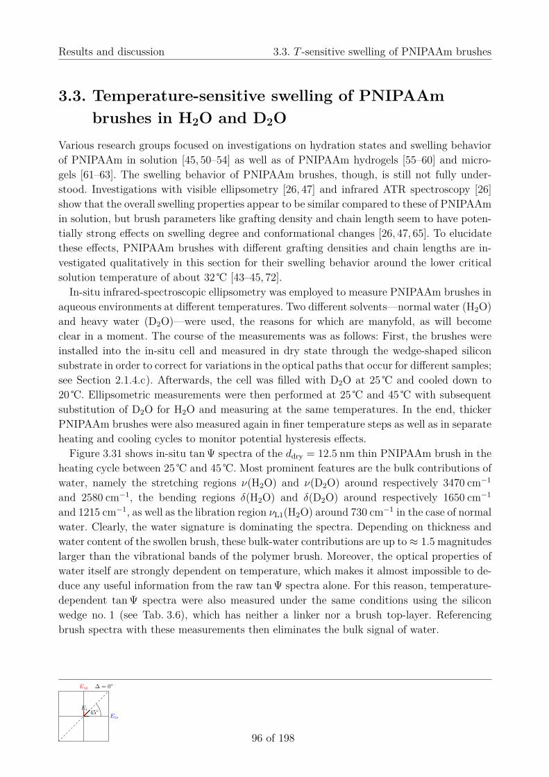
Results and discussion 3.3. T -sensitive swelling of PNIPAAm brushes
3.3. Temperature-sensitive swelling of PNIPAAmbrushes in H2O and D2O
Various research groups focused on investigations on hydration states and swelling behaviorof PNIPAAm in solution [45, 50–54] as well as of PNIPAAm hydrogels [55–60] and micro-gels [61–63]. The swelling behavior of PNIPAAm brushes, though, is still not fully under-stood. Investigations with visible ellipsometry [26, 47] and infrared ATR spectroscopy [26]show that the overall swelling properties appear to be similar compared to these of PNIPAAmin solution, but brush parameters like grafting density and chain length seem to have poten-tially strong effects on swelling degree and conformational changes [26, 47, 65]. To elucidatethese effects, PNIPAAm brushes with different grafting densities and chain lengths are in-vestigated qualitatively in this section for their swelling behavior around the lower criticalsolution temperature of about 32 ℃ [43–45, 72].
In-situ infrared-spectroscopic ellipsometry was employed to measure PNIPAAm brushes inaqueous environments at different temperatures. Two different solvents—normal water (H2O)and heavy water (D2O)—were used, the reasons for which are manyfold, as will becomeclear in a moment. The course of the measurements was as follows: First, the brushes wereinstalled into the in-situ cell and measured in dry state through the wedge-shaped siliconsubstrate in order to correct for variations in the optical paths that occur for different samples;see Section 2.1.4.c). Afterwards, the cell was filled with D2O at 25 ℃ and cooled down to20 ℃. Ellipsometric measurements were then performed at 25 ℃ and 45 ℃ with subsequentsubstitution of D2O for H2O and measuring at the same temperatures. In the end, thickerPNIPAAm brushes were also measured again in finer temperature steps as well as in separateheating and cooling cycles to monitor potential hysteresis effects.
Figure 3.31 shows in-situ tan Ψ spectra of the ddry = 12.5 nm thin PNIPAAm brush in theheating cycle between 25 ℃ and 45 ℃. Most prominent features are the bulk contributions ofwater, namely the stretching regions ν(H2O) and ν(D2O) around respectively 3470 cm−1
and 2580 cm−1, the bending regions δ(H2O) and δ(D2O) around respectively 1650 cm−1
and 1215 cm−1, as well as the libration region νL1(H2O) around 730 cm−1 in the case of normalwater. Clearly, the water signature is dominating the spectra. Depending on thickness andwater content of the swollen brush, these bulk-water contributions are up to ≈ 1.5 magnitudeslarger than the vibrational bands of the polymer brush. Moreover, the optical properties ofwater itself are strongly dependent on temperature, which makes it almost impossible to de-duce any useful information from the raw tan Ψ spectra alone. For this reason, temperature-dependent tan Ψ spectra were also measured under the same conditions using the siliconwedge no. 1 (see Tab. 3.6), which has neither a linker nor a brush top-layer. Referencingbrush spectra with these measurements then eliminates the bulk signal of water.
Eip
Eis45◦Ei
∆ = 0◦
96 of 198

3.3. T -sensitive swelling of PNIPAAm brushes Results and discussion
δ ( D2O)
4000 3000 2000 10000.98
1.00
1.02
1.04
1.06
1.08
1.10
1.12
25 ◦C → 45
◦CHeating cycle
ν L1 ( H2O)ta
n Ψ
Bru
sh(T
)
Wavenumber [cm–1]
ν ( H2O)
δ ( H2O)
ν ( D2O)
H2O
D2O
Figure 3.31: Temperature-dependent in-situ tan Ψ spectra of the ddry = 12.5 nm thin PNIPAAm brush mea-sured in H2O and D2O between 25 ℃ and 45 ℃.
Referenced tan Ψ spectra are shown in Fig. 3.32, and an enlarged view of the amide regionof PNIPAAm is presented in Fig. 3.33. The vibrational bands of the brush—predominantlythe amide bands and the ν(CHx) vibrations—are now clearly visible, as are influences ofthe two different solvents. The optical contrast between reference and brush measurementsmanifests itself in downward-pointing polymer bands and upward-pointing water bands atthe corresponding positions of ν(H2O), ν(D2O), δ(H2O), δ(D2O), and νL1(H2O). A quan-titative analysis of these bands and their temperature-dependent variations gives valuableinformation about thickness and water content of the brush around the phase transition [25].Details will be presented in Section 3.5.4.
There are various reasons why D2O was used as a second solvent. For one thing, thebending vibration of normal water at 1650 cm−1 is substantially masking the amide I bandof PNIPAAm at about 1630 cm−1, making a quantitative analysis of the brush structurerather difficult. Figure 3.33 illustrates this effect. In H2O, the amide I band appears smallerin amplitude compared to measurements in heavy water. When using D2O, the bendingvibration of water is shifting to about 1215 cm−1, thereby exposing the true nature of theamide I band. For another thing, PNIPAAm brushes below the LCST are strongly hydratedin aqueous solutions [26], which leads to large contributions of the free-water signature thatin turn overlaps with the amide I band. Furthermore, interactions between PNIPAAm andwater are expected to be different, because D2O can form stronger hydrogen bonds thanH2O, despite its similar bond length [45, 50, 247, 248]. The phase transition is also likelyto be affected [50], which in turn yields deeper insights into polymer–water and polymer–polymer interactions. Also, information about the brush’s depth profile can, in principle, beextracted from the exchange rate between heavy and normal water when substituting onesolvent for another.
Erp
ErsΨ
Er
∆ = 261◦
97 of 198
Erp
ErsΨ
Er
∆ = 120◦

Results and discussion 3.3. T -sensitive swelling of PNIPAAm brushes: Band analysis
4000 3500 3000 2500 2000 1500 1000
0.988
0.990
0.992
0.994
0.996
0.998
1.000
Cooling cycle: 40 ◦C → 25
◦C
[tan
ΨW
ater
/ tan
ΨB
rush
](T
)
Wavenumber [cm–1]
ν (CHx)
ν ( H2O) δ ( H2O)
Amide region
ν ( D2O) δ ( D2O)
H2O
D2O
Heating cycle: 20 ◦C → 45
◦C
3500 3000 2500 2000 1500 1000
0.988
0.990
0.992
0.994
0.996
0.998
1.000
Amide A
[tan
ΨW
ater
/ tan
ΨB
rush
](T
)
ν (CHx)
Wavenumber [cm–1]
ν ( H2O) δ ( H2O)
Amide region
ν ( D2O) δ ( D2O)
H2O
D2O
Amide B
Figure 3.32: Referenced tan Ψ spectra of the ddry = 12.5 nm thin PN132k brush during temperature-dependent switching in H2O and D2O between 20 ℃ and 45 ℃. Note that the strong doubleband around 3700 cm−1 is an artifact corresponding to combination vibrations of atmosphericCO2 [249].
1750 1700 1650 1600 1550 1500 1450 1400
0.988
0.989
0.990
0.991
δ ( H2O)
+ δas (CHx)
Amide II’ Amide II
[tan
ΨW
ater
/ tan
ΨB
rush
](T
)
Wavenumber [cm–1]
Amide IH2O
D2O
1700 1650 1600 1550 1500 1450 1400
0.988
0.989
0.990
0.991
δ ( H2O)
[tan
ΨW
ater
/ tan
ΨB
rush
](T
)
+ δas (CHx)
Amide II’ Amide II
Wavenumber [cm–1]
Amide I
H2O
D2O
Heating cycle: 20 ◦C → 45
◦C Cooling cycle: 40 ◦C → 25
◦C
Figure 3.33: Amide region of the ddry = 12.5 nm thin PN132k brush during temperature-dependent switchingin H2O and D2O between T = 20 ℃ and T = 45 ℃.
3.3.1. Analysis of vibrational bandsFrom Figs. 3.32 and 3.33, it is already obvious that the amide bands are strongly affectedin shape and position when the PNIPAAm brush is heated above its lower critical solutiontemperature. Furthermore, changes in optical contrast in the ν(H2O) and ν(D2O) regionsindicate temperature-dependent changes of the amount of bound water inside the brush.Owing to the referencing, thickness and absolute water content of the brush cannot beestimated directly, but can only be accessed by quantitative optical simulations. Nonetheless,
Eip
Eis45◦Ei
∆ = 0◦
98 of 198

3.3. T -sensitive swelling of PNIPAAm brushes: Band analysis Results and discussion
qualitative spectra evaluation with respect to changes in composition and position of thevibrational bands is still possible and already yields useful information about the brushstructure below and above the LCST.
The initial measurements were performed in D2O, which causes N -deuteration of the amidegroups, as was thoroughly discussed in Sections 3.1.5.a) and 3.2.3. Instead of an amide IIband around 1550 cm−1, which involves several δ(NH) contributions, an amide II’ band isobserved at about 1470 cm−1, which consists of δ(ND) contributions and is partly overlappedby the asymmetric CHx-bending vibrations. During the first measurements in H2O, the brushstill contained deuterated amide groups. Full de-deuteration took place during the heatingcycle, which can be seen from the increasing amide II and the decreasing amide II’ amplitude.Furthermore, amide A and B bands at about 3300 cm−1 and 3070 cm−1, respectively, becomevisible, which are associated with ν(NH) and the first overtone of amide II. Note that thevery small amide II band in the D2O spectra also hints at minute residues of N−H groupswithin the brush in deuterated state.
The signal-to-noise ratio is not sufficient for making any definite statements about possiblecompositional changes of amide II and II’. Both bands seem to shift towards lower wave-numbers at increasing temperatures. Following the band assignments in Section 3.1.5., theseshifts might be associated with increasing amounts of amide-interacted N−H and N−Dgroups at the expense of water-interacted groups, which indicates a dehydration of the brushabove the LCST. Optical simulations, however, are needed to verify this hypothesis.
Band changes of amide I around 1630 cm−1 are much more pronounced and can there-fore be discussed with more certainty. In heavy water, the band is shifting from 1626 cm−1
at 20 ℃ to 1641 cm−1 at 45 ℃, with a sharp transition in amplitude and frequency occurringbetween 33 ℃ and 34 ℃. Similar shifts are observed in normal water where the transitionoccurs between 32 ℃ and 33 ℃. In the latter case, however, amide I is overlapped by theupward-pointing δ(H2O) band, and it is also influenced by the simultaneous D→H exchange.
As discussed in Section 3.1.5., the amide I band composition characteristically dependson changes in the different kinds of polymer–water and polymer–polymer hydrogen bonding.In both D2O and H2O, amide I seems to comprise two or more subcomponents. Second-derivative analysis shown in Fig. 3.34 is helpful in order to identify them. In D2O, twomajor amide I subcomponents are found at about 1626 cm−1 and 1647 cm−1. In H2O, twoequivalent components are observed at 1635 cm−1 and 1650 cm−1. The exact oscillator po-sitions can only be derived from optical simulations owing to film effects and possible bandshifts due to the measurement geometry. In comparison with the band assignments in Sec-tion 3.1.5. (see Figs. 3.11 and 3.14), the subcomponents correlate mainly with dihydrogen-bonded water-interacted C=O groups below the LCST (lower-wavenumber subcomponents;C=O · · · D2O and C=O · · · H2O) as well as double-bonded amide-interacted C=O groupsabove the LCST (higher-wavenumber subcomponents; C=O · · · D−N and C=O · · · H−N).
Erp
ErsΨ
Er
∆ = 261◦
99 of 198
Erp
ErsΨ
Er
∆ = 130◦
Results and discussion 3.3. T -sensitive swelling of PNIPAAm brushes: Hysteresis effects
1750 1700 1650 1600 1550 1500 1450 1400
50 ◦C → 25
◦C
50 ◦C → 25
◦C
25 ◦C → 50
◦C
25 ◦C → 50
◦C
Wavenumber [cm–1]
2nd d
eriv
ativ
e [a
. u.]
Sequence
H2O
D2O
D2O
H2O
Figure 3.34: Second-derivative spectra corresponding to the ddry = 12.5 nm thin PNIPAAm brush inFig. 3.32, showing band-component changes in the amide I and II/II’ region during deswellingand reswelling of the brush in H2O and D2O between 25 ℃ and 50 ℃.
These assignments are in agreement with transmission measurements of PNIPAAm solu-tions [45, 50] and ATR FT-IR measurements on PNIPAAm brushes [26].
It can be concluded that polymer–water interactions dominate within the brush belowthe LCST. This is probably related to the good-solvent qualities of water and the expectedstrong hydration of the brush, as discussed in Section 3.2.1.a). Bittrich et al. [26] reporttypical water contents of 80–90 vol%. Above the LCST, at presumably bad-solvent qualitiesand much lower water content [26], the brush deswells while polymer–polymer interactionsbecome more relevant.
A detailed quantitative band analysis of amide I will be given in Section 3.5.4. It thenturns out that amide I contains mainly dihydrogen-bonded C=O groups below the LCST,but also a small contribution from mixed hydrogen-bonded groups that form one hydrogenbond with water and one with H−N groups. Above the LCST, the amount of mixed- anddihydrogen-bonded groups decreases, while double-bonded C=O groups become favored.
3.3.2. Testing for hysteresis effectsVIS ellipsometry [26] and QCM measurements [64] on PNIPAAm brushes reveal that theLCST behavior is governed by certain hysteresis effects—similar to PNIPAAm in solu-tion [45, 50]—that predominantly affect the thickness of the swollen brush. Furthermore,the phase transition with temperature seems to be rather pronounced at higher graftingdensities, whereas a more gradual transition is observed at lower grafting densities [26, 75].
Eip
Eis45◦
Ei
∆ = 0◦
100 of 198

3.3. T -sensitive swelling of PNIPAAm brushes: Hysteresis effects Results and discussion
�� �� �� �� �� �� ��
�� �� ������� ��� �����
������
�� �� ������� ��� �����
�����
�����
��� ���
���� ��
�������������
�����
�� �� �� �� �� �� ��
�����
�����
��� ���
���� ��
�������������
�����
������
Figure 3.35: ν(H2O) and ν(D2O) amplitude progressions of the ddry = 12.5 nm thin PN132k brush of Fig. 3.32during temperature-dependent swelling in H2O and D2O. Amplitudes of ν(H2O) and ν(D2O)were measured around 3450 cm−1 and 2510 cm−1, respectively. Experimental errors are markedas error bands to guide the eye.
Information about the switching behavior of PNIPAAm brushes can also be obtained frominfrared-ellipsometric spectra, even without optical simulations. This is owing to the nature ofthe ν(H2O) and ν(D2O) stretching bands of water. The optical contrast associated with thesebands changes if either thickness or water content of the swollen brush varies. Figure 3.35shows the temperature dependence of the ν(H2O) and ν(D2O) amplitudes during heating andcooling of the ddry = 12.5 nm thin PN132k brush in H2O and D2O between 20 ℃ and 50 ℃.Starting at maximum amplitudes at low temperatures, the water-band amplitudes undergo atransition of sigmoidal shape towards smaller amplitudes at higher temperatures. These am-plitude changes can be connected with a decrease in brush thickness, that is, with deswellingor collapsing of the polymer chains towards the substrate, but they are also associated witha changing water content and with the temperature-dependence of the bulk-water opticalproperties themselves (see Section 3.4.). For H2O, a distinct transition occurs with an inflec-tion point at about (32.2 ± 0.3) ℃, close to the LCST of PNIPAAm in solution [43–45]. ForD2O, the transition is less pronounced, and its inflection point lies at about (33.0 ± 1.0) ℃.Similar to PNIPAAm solutions, this delayed transition might be associated with strongerhydrogen bonds between amide groups and water within the deuterated swollen brush [50].
For both H2O and D2O, no obvious hysteresis effects are observed during deswelling andreswelling. Band amplitudes upon heating and cooling overlap within the experimental er-rors. These findings agree with the results by Bittrich et al. [26] who investigated brusheswith Mn = 47 000 g/mol and found distinct hysteresis effects only at grafting densities larger
Erp
ErsΨ
Er
∆ = 261◦
101 of 198
Erp
ErsΨ
Er
∆ = 140◦

Results and discussion 3.3. T -sensitive swelling of PNIPAAm brushes: Grafting density
than σ = 0.07 nm−2. The brush analyzed with infrared ellipsometry exhibits σ = 0.06 nm−2,which is probably why a hysteresis is not present or not that pronounced. Further mea-surements of brushes with different grafting densities and molecular weights are necessary,though, to validate whether or not grafting density is the only influential parameter. Note,however, that considering only the water-band amplitudes is just a rough estimation of pos-sible swelling and hysteresis effects. A more complete picture can only be obtained fromoptical simulations (discussed in Section 3.5.4.) that factor in changes in baseline slope dueto thin-film interference effects. Together with the water-band amplitudes and shapes, thisslope is directly related to the thickness and water content of the swollen brush.
The peak positions of amide I as well as of the CHx-stretching and -bending vibrationsalso show similar temperature-dependent progressions as the ν(H2O) and ν(D2O) amplitudes.Since the shifts in amide I are related to amplitude changes of different subcomponents, thespectra must be evaluated quantitatively within a proper optical model to gain conclusiveresults about hysteresis effects, which is the aim of future work.
3.3.3. Dependence on grafting density and molecular weightAs previously discussed, the actual switching behavior of PNIPAAm brushes is more com-plex than just a temperature-dependent deswelling and reswelling. Changing polymer–waterand polymer–polymer interactions are intrinsically important during the LCST transition.For better understanding the dependencies of this transition, five brushes with differentgrafting densities between σ = 0.020 nm−2 and 0.124 nm−2 as well as molecular weights ofMn = 132 000 g/mol and 56 000 g/mol were measured in-situ in D2O and H2O at 25 ℃ and45 ℃. Corresponding spectra are compared in Fig. 3.36, ordered by increasing dry-state brushthickness from bottom to top.
Except for the ddry = 14.5 nm thick brush, neither brush was measured in fully deuteratedor de-deuterated state, which is why different amplitude ratios are found between amide IIand II’. The same is true for amide A/B and amide A’. Nevertheless, an analysis of the amide Icomposition in both D2O and H2O—following the band analysis in Section 3.3.1.—shows thatall brushes undergo a similar transition from mainly polymer–water-interacted amide groupsbelow the LCST to polymer–polymer-interacted amide groups above the LCST. Simultane-ously, a deswelling and/or reduction of water content inside the brushes is correlated, again,with the decreasing ν(H2O) and ν(D2O) band amplitudes.
Notably, all brush spectra obtained in D2O show a lower baseline compared to H2O. At thesame time, the ν(D2O) band amplitudes are much smaller than the corresponding ν(H2O)amplitudes. The PN132k brush with ddry = 4.0 nm even shows negative ν(D2O) bands.This is also found for the 2.4 nm thin PGMA anchoring layer, which was measured in D2Oand H2O, too. Brush spectra in D2O also exhibit small contributions from upward-pointing
Eip
Eis45◦
Ei
∆ = 0◦
102 of 198

3.3. T -sensitive swelling of PNIPAAm brushes: Grafting density Results and discussion
4000 3500 3000 2500 1700 1600 1500 1400 1300
45 ◦C25
◦C →
25 ◦C → 45
◦C
–
–
–
–
–
ddry = 4.0 nm, σ = 0.020 nm–2
ddry = 8.0 nm, σ = 0.039 nm–2
ddry = 10.8 nm, σ = 0.124 nm–2
ddry = 12.5 nm, σ = 0.061 nm–2
ddry = 14.5 nm, σ = 0.071 nm–2
PGMAν (C=O)
CO2
Brush 5, Mn = 132 kDa
Brush 6, Mn = 132 kDa
Brush 7, Mn = 132 kDa
Brush 3, Mn = 56 kDa
Brush 8, Mn = 132 kDa
0.001ν (CHx)
ν ( D2O)ν ( H2O)
[tan
ΨW
ater
/ tan
ΨB
rush
](T
)
Wavenumber [cm–1]
AI AII AII’
δ (CHx)
δ ( H2O)D2O:
H2O:
AAAB
AA’
Figure 3.36: Referenced tan Ψ spectra of PNIPAAm brushes no. 3, 5, 6, 7, and 8—see Tab. 3.6 inSection 3.2.1.a)—during temperature-dependent switching in D2O (black and gray lines) andH2O (blue and red lines) from 25 ℃ to 45 ℃. Spectra were baseline-corrected according to Sec-tion 2.1.4.c) and Savitzky–Golay-smoothed (31 points, polynomial order 5). Spectra of differentbrushes are baseline-shifted for better comparability, whereas the baseline relations in each setof four brush spectra (blue, red, black, gray) are kept true. Amide A, B, A’, I, II, and II’ bandsare marked as AA, AB, AA’, AI, AII, and AII’, respectively.
ν(H2O) bands. This hints at minute residues of H2O in the D2O reference measurements.No ν(H2O) peaks are observed in the raw D2O tan Ψ spectra, though. The causes of theaforementioned effects are not fully understood yet and thus still under investigation.
For the four PN132k brushes, the relative ν(H2O) bands at 25 ℃ and 45 ℃ as well as therelative baseline slopes scale according to changes in grafting density and dry-state brushthickness. Larger amplitude changes are observed for higher grafting densities. This suggeststhat all brushes exhibit the same brush and mushroom (or intermediate) conformations below
Erp
ErsΨ
Er
∆ = 261◦
103 of 198
Erp
ErsΨ
Er
∆ = 150◦

Results and discussion 3.3. T -sensitive swelling of PNIPAAm brushes: Grafting density
and above the LCST, respectively, as proposed in Section 3.2.1.a). The ν(H2O) bands andbaseline slopes of the PN56k brush scale a little bit differently with dry-state brush thicknesscompared to the PN132k brushes. Absolute values of swollen-brush thickness and watercontent are therefore expected to show a different dependence on grafting density, which isin accordance with VIS-ellipsometry measurements [26].
The main goal in the next sections is to understand the swelling behavior of PNIPAAmbrushes quantitatively on the basis of optical layer models. Swollen-brush thickness and wa-ter content in dependence of temperature have to be determined and should match withcorresponding values from in-situ visible ellipsometry. Quantifying the amide-band composi-tion, then, will reveal absolute amounts of water- and amide-interacted amide groups belowand above the LCST.
In-situ brush spectra can only be modeled successfully if high-quality optical constantsn(T ) and k(T ) are used for H2O and D2O. These must therefore be determined first. Inprinciple, the same in-situ infrared-ellipsometry set-up as used for measuring the brushesis suitable for this task. If the substrate geometry is properly accounted for [20] and thesubstrate’s optical constants are known, then measured tan Ψ and ∆ spectra can be in-verted directly to obtain n and k. Indeed, this strategy proved successful for modeling thetemperature-dependent swelling behavior of the ddry = 12.6 nm thick PN94k brush [25]. How-ever, the results are affected by several systematic errors. These originate, for example, fromlateral variations in substrate properties, time-dependent changes of the native oxide layer,non-linearity of the MCT detector, as well as variations in the optical path due to the openingangle of the beam and the wedged-shaped substrate. For these reasons, additional transmis-sion measurements were performed that allow one to calculate the extinction coefficient k(T )and, consequently, the refractive index n(T ) by Kramers–Kronig integral relations.
Details about transmission measurements of water are given in Section 3.4. PNIPAAmbrushes are then modeled quantitatively in Section 3.5.
Eip
Eis45◦
Ei
∆ = 0◦
104 of 198

3.4. Temperature-dependent optical constants of H2O and D2O Results and discussion
3.4. Temperature-dependent optical constants of H2Oand D2O
The optical properties of water vary strongly in dependence of temperature [110, 250–253].In order to successfully model ellipsometric in-situ spectra of brushes in aqueous solutions,it is therefore imperative to determine n(T ) and k(T ) of H2O and D2O as the first step.The optical constants of liquids are usually obtained from measurements in ATR configura-tion [151, 166]. In the current work, however, special transmission cells were used to performtransmission measurements on normal and heavy water between 8000–700 cm−1 in a tem-perature range from 20–45 ℃. By means of optical modeling, these measurements allow oneto calculate the extinction coefficients k(T ) and, consequently, the refractive indices n(T ) byKramers–Kronig integral relations.
Two transmission cells with path lengths of dCell = 6.60 µm and 3.26 µm were available.H2O and D2O were measured in both cells between 20 ℃ and 45 ℃, as shown in Fig. 3.37.Since absorbance is scaling proportionally with wavenumber, transmittance in the D2O-stretching region around 2500 cm−1 is considerably larger compared to the H2O-stretchingregion at 3400 cm−1, despite the similar absolute k values. The H2O-stretching bands mea-sured with the 6.60 µm cell are too strong to be detectable without band distortions. Theminimum transmittance in this case is about 0.03%, which is too small even for the verylinearly responding DTGS detector [136]. The minimum transmittances in the other spectraare larger than 0.20%. Since the photometric accuracy of the utilized Vertex 70 spectrom-eter is better than 0.10% transmission, these spectra should be suitable for a quantitativeevaluation. This was confirmed for the D2O measurements by rescaling the correspondingabsorbance spectra of the short and long cells to match in band amplitudes (remember thatabsorbance is proportional to path length). Except for differences in the interference fringesabove 4000 cm−1, the measured band shapes coincide, suggesting that the stretching bandscan be considered distortion-free.
Some artifact bands are observed at 2512 cm−1 and 1456 cm−1 in the H2O spectra and at3418 cm−1 and 1461 cm−1 in the D2O spectra. These bands can be assigned to HOD vibra-tions due to minute residues of D2O or H2O that are bound by the epoxy spacer separatingthe windows. These residues are difficult to remove when changing the liquid, even if the cellis purged multiple times. Slowly over time during the measurements, H2O ↔ D2O exchangeoccurs within the epoxy, giving rise to the aforementioned vibrational bands. Their positionscoincide with two different HOD species, as demonstrated by Max and Chapados who inves-tigated H2O/D2O mixtures using factor analysis [228]. These species—denoted as OH3D andOD3H—respectively correspond to small amounts of D−O−H molecules hydrogen-bonded toH−O−H without the presence of D2O molecules, on the one hand, as well as small amounts
Erp
ErsΨ
Er
∆ = 261◦
105 of 198
Erp
ErsΨ
Er
∆ = 160◦

Results and discussion 3.4. Temperature-dependent optical constants of H2O and D2O
[ { ]
Figure 3.37: Transmittance spectra (4 cm−1 resolution) of liquid H2O and D2O measured between 20 ℃and 45 ℃ using transmission cells with path lengths of 6.60 µm (top) and 3.26 µm (bottom).Minimum transmittances in the stretching regions of H2O and D2O are denoted at the left. Thephotometric accuracy of the spectrometer was 0.10% transmission.
of D−O−H hydrogen-bonded to D−O−D without the presence of H2O on the other hand.Either specie absorbs in both the stretching and the bending regions of H2O and D2O. Tominimize their effect on the true n and k values of pure H2O and D2O, only the 6.60 µmspectra were used for D2O, since these are almost free of HOD bands. The situation for H2Ospectra is more difficult and will be discussed in a moment.
The transmission cells used in this work consist of CaF2 windows that are transparentdown to ≈ 900 cm−1. Since water absorbs significantly between 900–0 cm−1, it is necessaryto extrapolate the accessible wavenumber region in order for the Kramers–Kronig transformto yield reliable results. Starting point for the investigations, therefore, was the meticulousstudy by Max and Chapados [166] who provide reference data for n and k of H2O and D2O atroom temperature from 6000 cm−1 to 0 cm−1. To avoid artificial concatenation of measureddata above and reference data below 900 cm−1, the optical constants were first fitted overthe whole range of 6000–0 cm−1 after Eq. (2.75) using Gaussian oscillators that correspondto the various vibrational modes of (heavy) water. Initial values for oscillator positions,amplitudes, and band widths were taken from Refs. [166, 228]. The resulting set of oscillatorsserved as input parameters for the following fitting process of measured transmission spectra.During the fits, parameters of oscillators situated below ≈ 1200 cm−1 were held constant.Nevertheless, since these are also expected to be affected by temperature [110, 250, 254], theirpotential effect on the refractive index n via Kramers–Kronig transform must be evaluated
Eip
Eis45◦
Ei
∆ = 0◦
106 of 198

3.4. Temperature-dependent optical constants of H2O and D2O Results and discussion
in the end. H2O spectra were fitted with two additional oscillators placed at 2512 cm−1 and1456 cm−1 that correspond vibrations of small HOD residues. After the fit, n and k wererecalculated at each temperature without these two oscillators.
The modeling process is now described in more detail. A five-layer optical model con-sisting of Air/CaF2/Water/CaF2/Air was assumed after Fig. 2.12 with literature data forthe CaF2 windows [142, 255]. This model produces fast oscillations within the 4 mm thickwindows. Since these oscillations are well below the spectral resolution of the measurement(4 cm−1), they were damped by emulating the apodization process during spectra acquisitionof the Fourier spectrometer. For this, the computed transmittances were transformed intoFourier space by Fast-Fourier transform (FFT) [101], multiplied with the Blackman–Harrisfour-term apodization function [256], and then transformed back into wavenumber space byinverse FFT.
The path lengths of the cells were, at first, estimated from empty-cell measurements indry state using the fringe method [138]. Max and Chapados also derived analytical equationsfor calculating the transmittance of a cell with non-parallel windows that has a varying pathlength of dCell ± δCell [140]. By applying these equations, the path lengths were determinedaccurately, and plane-parallelism of the windows was verified up to δCell = ±10 nm.
Thermal expansion of the cells was then measured in dry and wet state. Between 20 ℃and 45 ℃, an increase in path length of 50 nm was found for the empty 6.60 µm cell, whereasthe 3.26 µm cell expanded by 35 nm. In wet state, obvious interference fringes are only vis-ible between approximately 4000–8000 cm−1. This region was used to determine dCell(T ),which resulted in the same increases in path lengths as obtained in dry state. Temperature-dependent changes in refractive index of the CaF2 windows are expected to be smaller than0.0004 in the probed temperature range [257] and are therefore negligible.
Transmittance (absorbance) spectra were now fitted by varying the parameters of oscilla-tors situated between 4200–1150 cm−1 for D2O and between 5200–1200 cm−1 for H2O. Aftereach iteration during the fits, current n and k values were recalculated from 6000–0 cm−1
with the high-frequency dielectric constant being fixed to ε∞ = (1.333)2 [166]. The resultingtemperature-dependent optical constants n(T ) and k(T ) are plotted in Fig. 3.38.
With minor restrictions, n(T ) and k(T ) can be considered accurate enough for simulatingpolymer-brush spectra between 4000–1100 cm−1 for D2O and between 4000–1300 cm−1 forH2O. Below 1100 cm−1, the absorption properties of the CaF2 windows dominate the trans-mittance spectra and hinder a reliable fit on parameters of oscillators situated in this region.This also affects the very broad ν2 − νL2 combination band of H2O around 1190 cm−1 [228].The associated oscillator had to be fixed, which causes slight deviations in k between 1400–1100 cm−1 compared to ATR absorbance measurements in the literature [110]. Furthermore,in the case of H2O, some artifacts from HOD vibrations remain around 2500 cm−1 and1450 cm−1, even after recalculation of n and k without the corresponding oscillators. The
Erp
ErsΨ
Er
∆ = 261◦
107 of 198
Erp
ErsΨ
Er
∆ = 170◦

Results and discussion 3.4. Temperature-dependent optical constants of H2O and D2O
n(T
)
1.2
1.3
1.4
1.5
H2O
n(T
)
1.2
1.3
1.4
1.5
D2O
4000 3500 3000 2500 2000 15000.0
0.1
0.2
0.3
k(T
)
Wavenumber [cm–1]
4000 3500 3000 2500 2000 15000.0
0.1
0.2
0.3
k(T
)
Wavenumber [cm–1]
Figure 3.38: Temperature-dependent optical constants of H2O and D2O as determined from infrared trans-mission measurements. Temperatures were T = [20, 25, 28, 30, 31, 32, 33, 34, 35, 36, 38, 40, 45] ℃.
absolute k values in these two regions, however, are small compared to the stretching andbending vibrations and also to polymer bands that occur there. Importantly, HOD bands alsooverlap with both the stretching and the bending vibrations of H2O and D2O. This causesan overestimation of the respective band amplitudes by about 1–3% in the k spectra.
The temperature-dependent influence of ε∞ on n and k has yet to be determined. ε∞ wasvaried by ±5%, but its effect on transmittance spectra could not be distinguished fromchanges in path lengths of the cells. Lastly, the libration regions below 1000 cm−1 also un-dergo changes with increasing temperature [110, 250, 254] and therefore yield T -dependentcontributions to n and k via the Kramers–Kronig transform. To estimate this effect, theamplitudes of oscillators situated in these regions were varied up to ±10% with increas-ing temperature, as shown in Fig. 3.39 for the refractive index at 45 ℃. At 1100 cm−1, theabsolute values of n(45 ℃) change by ±0.014 for H2O and by ±0.004 for D2O. Deviationsfrom the fitted results quickly diminish at higher wavenumbers in the case of D2O. ForH2O, the influence of bands involving libration modes is stronger since these are located athigher wavenumbers. Complementary transmission measurements using, for example, cellswith ZnSe or Si windows, which exhibit transmission cut-offs at lower wavenumbers comparedto CaF2, might aid in determining physically correct libration oscillator parameters.
Eip
Eis45◦
Ei
∆ = 0◦
108 of 198

3.4. Temperature-dependent optical constants of H2O and D2O Results and discussion
n(4
5 ◦ C
)
4000 3500 3000 2500 2000 15001.1
1.2
1.3
1.4
1.5
Wavenumber [cm–1]
H2O
n(4
5 ◦ C
)
4000 3500 3000 2500 2000 1500 10001.1
1.2
1.3
1.4
1.5
Wavenumber [cm–1]
D2O
Figure 3.39: Effect of the Kramers–Kronig transform on n(45 ℃) of H2O and D2O (red lines) when varyingthe amplitudes of oscillators associated with librations below 1000 cm−1 by ±10% (light bands).
Erp
ErsΨ
Er
∆ = 261◦
109 of 198
Erp
ErsΨ
Er
∆ = 180◦

Results and discussion 3.5. PNIPAAm brushes revisited: Motivation and modeling strategy
3.5. Systematic investigations of PNIPAAm brushes inaqueous solutions
3.5.1. MotivationQuantitative interpretation of infrared spectra of functional polymer films or proteins inaqueous environment is always complicated by the overlapping vibrational bands of water.Experiments are therefore often performed in heavy water to separate water and polymercontributions, as was discussed in Section 3.3. In particular, the amide I and II bands arestrongly altered in amplitude, position, and shape by the bending vibration of normal water,which is of the same order of magnitude. This can pose severe problems that are, however,easily overlooked when just regarding the amide region of the spectrum. As a result, quan-titative conclusions about amide-band composition, for example, are drawn from basicallyuninterpretable spectra. Often it is attempted to subtract the water contributions in orderto reveal a “more true” band composition [258–260]. While this might work in some casesfor transmission spectra, it does not necessarily work for reflection spectra, mainly becauseof film effects. Even for transmission measurements, the subtraction approach is rather ques-tionable, since the strong oscillators associated with the molecular vibrations of water cancause strong band shifts of the measured water bands, depending on the water content of thefilm. In reflection, these shifts can be of the order of some 10 cm−1, rendering impossible aquantitative evaluation that is based on band analysis at the level of the measured spectra.
This is the main reason why simulating the spectra within a physical model is not onlybeneficial, but essential for gaining physically meaningful results. Because the model is basedon the actual sample properties, it is possible to separate the different spectral contributionsthat originate from water, polymer brush, or anchoring layer. Also film effects, which oftencause inconceivable effects on the spectra, are taken care of within the model. Most impor-tantly, overlapping water bands do not pose an intrinsic problem any longer. On the contrary,they are automatically accounted for, since the water content is a physical parameter of themodel.
3.5.2. Strategy for the quantitative modeling of in-situ spectra
a) In-situ brush model
The aim of the modeling process in the long run is to extract quantitative information aboutbrush structure and interactions between polymer and water in dependence of temperature aswell as brush parameters like grafting density. For this purpose, a box model is assumed withconstant water content inside the brush and an instantaneous transition to 100 vol% water at
Eip
Eis45◦
Ei
∆ = 0◦
110 of 198

3.5. PNIPAAm brushes revisited: Modeling strategy Results and discussion
the brush–water/water interface (see Fig. 2.21). This brush profile should be accurate enoughto correctly describe the polymer brush above its LCST [245, 246]. Below the LCST, wherethe profile is expected to show a gradual decrease from low to high water content towardsthe brush surface [245, 246], this model can be thought of as a description to obtain averagevalues for brush thicknesses and water contents. Regardless of the profile, polymer–polymerand polymer–water interactions are always accessible, because the infrared light is probingthe complete brush depth.
The optical layer model of the brushes consists of Water/Brush/PGMA/SiO2/Si, withwater being the substrate material of the model and silicon being the ambient, accord-ing to Figs. 2.7 and 2.21. Water is modeled using the temperature-dependent optical con-stants of H2O and D2O determined in Section 3.4., whereas literature data are used forthe oxide layer [18], and n = 3.42 and k = 0 are assumed for the silicon substrate [154].The brush and PGMA layers are modeled with a modified Bruggeman effective-mediumapproximation between water and polymer constituents. In principle, the brush profile canbe implemented into the model, too. With measurements at only one incidence angle, though,there are not enough independent experimental quantities to extract an unambiguously cor-rect profile. As for the previously discussed modeling of polymer films and brushes—seeSections 3.1.5.b) and 3.2.3.b)—changing polymer–polymer and polymer–water interactionsare quantified within the mEMA layer by adjusting the corresponding oscillator parametersof the polymer. Reference spectra of a silicon wedge in contact with water are simulatedwithin the same model, but without PGMA and brush top-layers.
In the first step of the modeling process, the thickness d̃ and the water content fWater ofthe swollen or collapsed brush have to be determined. In the second step, spectral changesof PNIPAAm’s amide and CHx vibrational bands with respect to the dry state are analyzed,which yields insights into the various interactions that occur at the solid–liquid interface.Since water-specific and polymer-specific bands are overlapping one another, the first andsecond step of the modeling process have to be repeated in an iterative manner.
b) Incidence angle and baseline-correction
During the measurements, the external angle of incidence was set to ϕ0 = 45◦ with respect tothe outer reflex at the silicon wedge. With a wedge angle of 1.5◦ and a rotation of the sampleholder of 7.4◦ to detect the inner reflex, the internal angle of incidence is given by ϕ̃0 = 11.8◦
according to Snell’s law. In order to account for the opening angle of the set-up, spectra aresimulated at ϕ̃0 = [10.8◦, 11.8◦, 12.8◦] and then averaged. This is imperative because strongvibrational bands like ν(H2O) are very sensitive to smallest changes in ϕ̃0.
It is clear from the wedge geometry in Fig. 2.7 that measured spectra contain contributionsfrom the incident air/wedge interface as well as the wedge/air interface at the reflection side.The corresponding transmission coefficients after the Fresnel equations, however, cancel to
Erp
ErsΨEr
∆ = 261◦
111 of 198
Erp
ErsΨ
Er
∆ = 190◦
Results and discussion 3.5. PNIPAAm brushes revisited: Modeling strategy
first-order approximation in referenced tan Ψ spectra if brush and reference measurementsare performed under the same angle of incidence [20].
Measured spectra are baseline-corrected as described in Section 2.1.4.c). The additionaldry-state correction factor tan Ψsimul
dry / tan Ψsimulref, dry and the correction difference ∆simul
dry −∆simulref, dry
that are used to compensate for thin-film-interference effects are simulated within the abovemodel by replacing water with air and the polymer oscillator layers by constant valuesn = n∞ = 1.5007 and k = 0 for PGMA as well as n = n∞ = 1.4832 and k = 0 for PNIPAAm,as determined in Section 3.1.4.
c) Swollen-brush thickness and water content
Within the brush model, the parameters d̃ and fWater for thickness and water content of theswollen brush are strongly correlated. Changing either one of them produces very similareffects in the band amplitudes of both polymer and water. In order to decorrelate the twoparameters, additional phase measurements ∆ at (multiple) large angles of incidence seemnecessary. With the flow cell for in-situ infrared ellipsometry, however, the internal incidenceangle at the substrate/brush interface is smaller than 16◦. At this angle, tan Ψ and ∆ are twoalmost redundant parameters. Furthermore, ∆ measurements are not feasible for ultra-thinbrushes at a sufficiently high signal-to-noise ratio. Due to the strong absorbing qualities ofwater in the mid-infrared, there is also no absorption-free region that would allow for theseparation of thickness and refractive index by using, for example, Cauchy dispersions. Adifferent strategy must therefore be pursued.
The overall thickness of the polymer–water layer is of the order of several 10 nm and, thus,induces thin-film interference, which causes a distinct baseline drift at higher wavenumbers.This spectral characteristic is used to fix the thickness of the swollen-brush layer. Simul-taneously, the large vibrational bands of water—especially the ν(H2O) band—are analyzedto fix the water content of the brush. With increasing swollen-brush thickness, the ν(H2O)amplitude becomes more sensitive to fWater. Most importantly, the frequency of ν(H2O) isshifting to higher wavenumbers with increasing water content, because ν(H2O) comprises fivevery strong oscillators [228]. Also the band shape is changing markedly. Both effects allowone to decorrelate d̃ and fWater sufficiently.
As a boundary condition, measured amplitudes of polymer-specific bands that are not ex-pected to change with varying water content have to be reproduced correctly. This concerns,for example, the asymmetric CHx-bending vibrations of PNIPAAm, the frequencies of whichare sensitive to hydration, but the amplitudes of which remain almost constant. This can beseen, for example, in humidity-dependent measurements of PNIPAAm films (see Fig. 3.8 inSection 3.1.5.). The amplitudes of symmetric CHx-bending as well as CHx-stretching vibra-tions show small correlations with hydration. The former increase slightly, whereas the latterdecrease at higher humidities.
Eip
Eis45◦
Ei
∆ = 0◦
112 of 198

3.5. PNIPAAm brushes revisited: Hydration of PGMA Results and discussion
d) Modeling the amide I and II bands
Amide I and II respectively consist of five and three subcomponents that are associatedwith free, amide-interacted, and water-interacted C=O and N−H groups, as discussed inSection 3.1.5.a). The number of free fit parameters of the corresponding oscillators is largeenough to reproduce virtually any observed band shape and amplitude. It is therefore imper-ative to enforce a physical constraint onto the simulated spectra. This constraint is given bythe total number of C=O and N−H groups and the associated average number Np of dipolemoments probed by the infrared light.
For a layer with a single Lorentzian oscillator after Eqs. (2.72) and (2.74), the oscillatorstrength F is proportional to Np,
F ∼ Np , (3.5)
with ν̃0 being the center frequency of the oscillator. From Eq. (2.75) and the imaginary partof Eq. (2.73), one obtains an analogous expression for a single Gaussian oscillator,
Np ∼ F̃ σ̃ ν̃0, (3.6)
where F̃ and σ̃ are its strength and band width. For the five Gaussian amide I oscillatorsand the three Gaussian amide II oscillators, this yields the constraints
j
F̃ (j) σ̃(j) ν̃(j)0
!= const. (3.7)
Equation (3.7) is expected to be successfully applicable for amide I, which consists mainly ofC=O-stretching contributions. Since amide II is a coupled mode of N−H-bending and C−N-stretching, hydrogen bonding might affect the corresponding transition dipole moments inunexpected ways and thereby alter the above constraint.
The different contributions of amide I and II subcomponents to the overall band envelopesare modeled by varying the oscillator strengths F̃ only. Except for the di-H2O- and H2O-interacted ν(C=O) and δ(N−H) components at respectively 1625 cm−1 and 1554 cm−1, allband widths σ̃ are held constant. It is assumed that band shifts due to weakening of hydrogenbonds at elevated temperatures are negligibly small compared to amplitude changes.
3.5.3. Hydration of PGMA filmsBefore investigating the actual swelling behavior of PNIPAAm brushes, hydration effectsof the PGMA anchoring layer must be understood, since these have a potentially stronginfluence on the quantitative modeling of the brushes. Fukuda et al. [261] showed with opticalmicrography that PGMA gels swell in many solvents, but do not swell at all in water, despitethe presence of hydroxy groups on the polymer chains. In order to verify this non-swelling
Erp
ErsΨ
Er
∆ = 261◦
113 of 198
Erp
ErsΨ
Er
∆ = 200◦

Results and discussion 3.5. PNIPAAm brushes revisited: Hydration of PGMA
0.98
1.00
1.02
ν (CHx)
fingerprintPGMA
υC1 ( H2O)
υC2 ( H2O)
ν L1 ( H2O)
δ ( H2O)
[tan
ΨW
ater
/ tan
ΨP
GM
A](
25 ◦ C
)
ν ( H2O)
ν (C=O)
SimulatedMeasured
6000 5000 4000 3000 2000 1000
−3
−2
−1
−0
[∆W
ater
– ∆
PG
MA](
25 ◦ C
)
δ ( H2O)
Wavenumber [cm–1]
ν ( H2O)
ν (C=O)
fingerprintPGMA
[ ◦ ]
Figure 3.40: Measured and simulated referenced and baseline-corrected ellipsometric in-situ spectra of the119 nm thick PGMA film in H2O at 25 ℃. The baseline slope in tan Ψ as well as band shapesand amplitudes of the water vibrational bands and PGMA-specific bands are modeled correctly.Deviations in ∆ and in tan Ψ below 2000 cm−1 are likely to be related to film inhomogeneities.
in the infrared, the 119 nm thick spin-coated PGMA film was measured in-situ in H2O andD2O at 25 ℃ and 45 ℃. These measurements were also performed for two other reasons.First, the film is thick enough to yield prominent film-interference effects. This allows one toconfirm whether the baseline-correction procedure for ellipsometric in-situ spectra proposedin Section 2.1.4.c) works properly. Second, PGMA does not exhibit any vibrational bandsin the ν(D2O) region between 2800–2000 cm−1. Therefore, general aspects of using aqueousD2O solutions can be addressed quantitatively, and the validity of the model in which H2Ois replaced by D2O can be tested.
Figure 3.40 compares measured and simulated referenced and baseline-corrected tan Ψ and∆ spectra of the 119 nm thick PGMA film in H2O at 25 ℃. The optical contrast betweenfilm and reference sample is reproduced correctly, which can be seen from the matchingamplitudes and shapes of the water-specific vibrational bands. These are the large ν(H2O)band around 3480 cm−1, the δ(H2O) and νL1(H2O) bands around respectively 1650 cm−1
and 730 cm−1, and even the two small but broad combination bands around 5150 cm−1 and
Eip
Eis45◦
Ei
∆ = 0◦
114 of 198

3.5. PNIPAAm brushes revisited: Hydration of PGMA Results and discussion
4000 3500 3000 1750 1700 1650
0.97
0.98
0.99
1.00
1.01
1.02
1.03
45 ◦C
25 ◦C
[tan
ΨH
2O
/ tan
ΨP
GM
A](T
)
Wavenumber [cm–1]
ν ( H2O)
ν (CHx)
ν (C=O)
δ ( H2O)
Simulated, 45
◦C
Simulated, 25
◦CMeasured in H2O
3000 2500 2000 1750 1700 1650 1600
0.97
0.98
0.99
1.00
1.01
1.02
1.03
[tan
ΨD
2O
/ tan
ΨP
GM
A](T
)
Wavenumber [cm–1]
ν ( D2O)
ν (CHx)
ν (C=O)
Simulated, 45
◦C
Simulated, 25
◦CMeasured in D2O
45 ◦C
25 ◦C
Figure 3.41: Measured and simulated in-situ tan Ψ spectra of the 119 nm thick PGMA film in H2O (left) andD2O (right) at 25 ℃ and 45 ℃ in the water-stretching and PGMA-carbonyl-stretching regions.ν(D2O) is overlapped by atmospheric CO2 absorption around 2350 cm−1.
2100 cm−1 [228]. The simulated baseline slope in tan Ψ at higher wavenumbers agrees withthe measurement. Small baseline deviations observed between 2000–1300 cm−1 are probablyrelated to film inhomogeneities, as discussed in Section 3.1.3. and in Appendix E.
Simulation parameters for thickness d̃ and water content fH2O of the PGMA layer wered̃(25 ℃) = (122 ± 2) nm and fH2O(25 ℃) = (4 ± 2) vol%. These values substantiate Fukuda’sresults that PGMA does not swell in water. The strong self-crosslinking between the PGMAchains might explain why the polymer is unsolvable in water. The latter was confirmed by re-peating the in-situ measurements several times and afterwards measuring a non-changing dry-state thickness with VIS ellipsometry. The very small hydration of the PGMA layer, if any,also manifests itself in the fact that the vibrational bands of PGMA can be described by thepure dry-state optical constants, that is, the PGMA bands do not undergo amplitude changesor frequency shifts. This is true for all ν(CHx) and fingerprint bands. The only exception is thecarbonyl-stretching band ν(C=O) at 1735 cm−1, details of which will be given in a moment.
Figure 3.41 shows measured and simulated tan Ψ spectra of the PGMA layer in H2O andD2O at 25 ℃ and 45 ℃. Thickness and water content are found to be d̃(45 ℃) = (122 ± 2) nmand fH2O(45 ℃) = (1 ± 1) vol% in H2O. For simulations in heavy water, the same parametersfor d̃ and fD2O were used as for normal water. The simulated ν(C=O) peak position occursat 1735.5 cm−1 in H2O and at 1735.0 cm−1 in D2O. This difference is due to the overlappingupward-pointing δ(H2O) band in the case of normal water. The measured ν(C=O) band isshifted to 1734.0 cm−1 and 1733.5 cm−1, respectively, and it also exhibits a smaller amplitude.Both effects indicate hydrogen bonding C=O · · · H2O of carbonyl groups to surrounding watermolecules. Whether hydrogen bonding takes place only in the topmost part of the PGMAlayer or whether the very small hydration does affect the whole layer, cannot be deduced
Erp
ErsΨ
Er
∆ = 261◦
115 of 198
Erp
ErsΨ
Er
∆ = 210◦
Results and discussion 3.5. PNIPAAm brushes revisited: Brush–water interface
from the simulations. With regard to measurements of PNIPAAm brushes, it can be expected,though, that the ν(C=O) band will show similar or even stronger changes, because additionalhydrogen bonding is possible with PNIPAAm’s N−H groups.
The final point concerns the water-specific bands, in particular the ν(D2O) band around2500 cm−1. Although PGMA bands as well as the baseline slope at higher wavenumbersdo not differ significantly in D2O compared with PGMA in H2O, relatively strong ampli-tude deviations are observed between measured and simulated water bands, as shown inthe right panel of Fig. 3.41. The measured ν(D2O) bands are much smaller in amplitude.At first glance, this decrease in optical contrast seems to suggest a fundamentally strongerhydration of the PGMA film. However, with d̃ and fD2O as the only free parameters of themodel, the measured band amplitudes cannot be reproduced while maintaining correct bandshapes of ν(D2O). A control measurement of the 2.4 nm thin PGMA anchoring layer evenshows downward-pointing D2O bands, which means that the effective refractive index of thePGMA–D2O layer should be smaller than the refractive index of pure D2O. The nature ofthese effects is still under investigation. In the following, the focus will therefore lie on thequantitative evaluation of PNIPAAm swelling experiments in H2O only.
Nevertheless, the above findings for PGMA in contact with H2O confirm that quantitativemodeling of in-situ infrared-ellipsometric spectra is possible and that layer thicknesses andwater contents can be extracted correctly.
3.5.4. Structural properties of the brush–water interfaceIn-situ measurements were performed on the ddry = 14.5 nm thin PN132k brush in H2O andD2O at 25 ℃ and 45 ℃. The sequence of measurements was H2O→D2O→H2O at 25 ℃ fol-lowed by H2O→D2O→H2O at 45 ℃ after heating the in-situ cell at a rate of about 1 ℃/min.As expected from the N -deuteration experiments in Section 3.2.3., H→D exchange occursmuch faster than D→H exchange. Further details about deuteration and de-deuteration ef-fects are still being analyzed. The main interest now lies in swelling effects of the brush inH2O as well as variations in polymer–water interactions induced by temperature changes. Inthe following, the initial H2O brush spectra at each of the two temperatures are thereforeevaluated quantitatively.
a) Simulating in-situ swollen-brush spectra below the LCST
Figure 3.42 compares measured and simulated brush spectra in H2O at 25 ℃—below the lowercritical solution temperature of PNIPAAm. The band amplitude and shape of ν(H2O) around3460 cm−1 as well as the baseline slope above 3700 cm−1 allowed for the determination ofboth thickness, d̃(25 ℃) = (57 ± 3) nm, and water content, fH2O(25 ℃) = (79.5 ± 2.0) vol%,of the swollen brush. These values amount to a swelling degree of about d̃/ddry = 4 and are
Eip
Eis45◦
Ei
∆ = 0◦
116 of 198

3.5. PNIPAAm brushes revisited: Brush–water interface Results and discussion
6000 5000 4000 3000 2000 15000.998
1.000
1.002
1.004
1.006
Simulated
PGMA
δ (CHx)
AIIAI ν (CHx)
υC2 ( H2O)
[tan
ΨH
2O
/ tan
ΨB
rush
](25
◦ C)
Wavenumber [cm–1]
ν ( H2O)
ν (C=O)
υC1 ( H2O)
δ ( H2O)
AA
AB
Measured
Figure 3.42: Measured and simulated referenced and baseline-corrected ellipsometric tan Ψ spectra of theddry = 14.5 nm thin PN132k brush in H2O at 25 ℃. The baseline slope in tan Ψ as well asband shapes and amplitudes of the water vibrational bands and PNIPAAm-specific bands weremodeled successfully.
in accordance with VIS-ellipsometric measurements by Burkert et al. [46] on a PN132k brushwith very similar dry-state thickness and grafting density [46].
The left panel of Fig. 3.43 shows the same spectra in comparison with a simulation inwhich all brush oscillators are set to zero amplitudes. With the water-stretching band beingreproduced in the simulated tan Ψ spectrum, the δ(H2O) band at 1650 cm−1 is intrinsicallyfixed in amplitude, position, and shape. This, then, enables one to determine the compositionof the overlapping amide I and II bands. Moreover, band shapes and positions of most of theremaining PNIPAAm-specific bands as well as the ν(C=O) band of the PGMA anchoringlayer could be modeled successfully. The obtained band changes with respect to the dry-state—shown in the right panel of Fig. 3.43—yield valuable information about hydrationproperties of the brush as well as polymer–polymer and polymer–water interactions.
Several spectral features reflect the strong hydration of the brush. First, the oscillatorfrequencies of the CHx-bending vibrations between 1480–1320 cm−1 are shifted by up to+6 cm−1 compared to the dry state. Similar shifts are observed in the CHx-stretching regionbetween 3020–2800 cm−1. The measured νas(CH3) band in particular also shows a smalleramplitude compared to the simulation. This suggests that the band is indeed involved in aFermi resonance, possibly with CHx-bending vibrations [217], which changes upon hydrationof the brush. Second, amide I and II are shifted to lower and higher wavenumbers, respec-tively. These shifts are induced by changes in band composition that reflect the differenttypes of interactions within the brush. Details will be discussed in a moment. Third, as aconsequence of the amide I and II shifts, the three bands in the amide A/B region are shiftedand also undergo amplitude changes. The amide I/II-overtone band at 3194.7 cm−1 in dry
Erp
ErsΨ Er
∆ = 261◦
117 of 198
Erp
ErsΨ
Er
∆ = 220◦
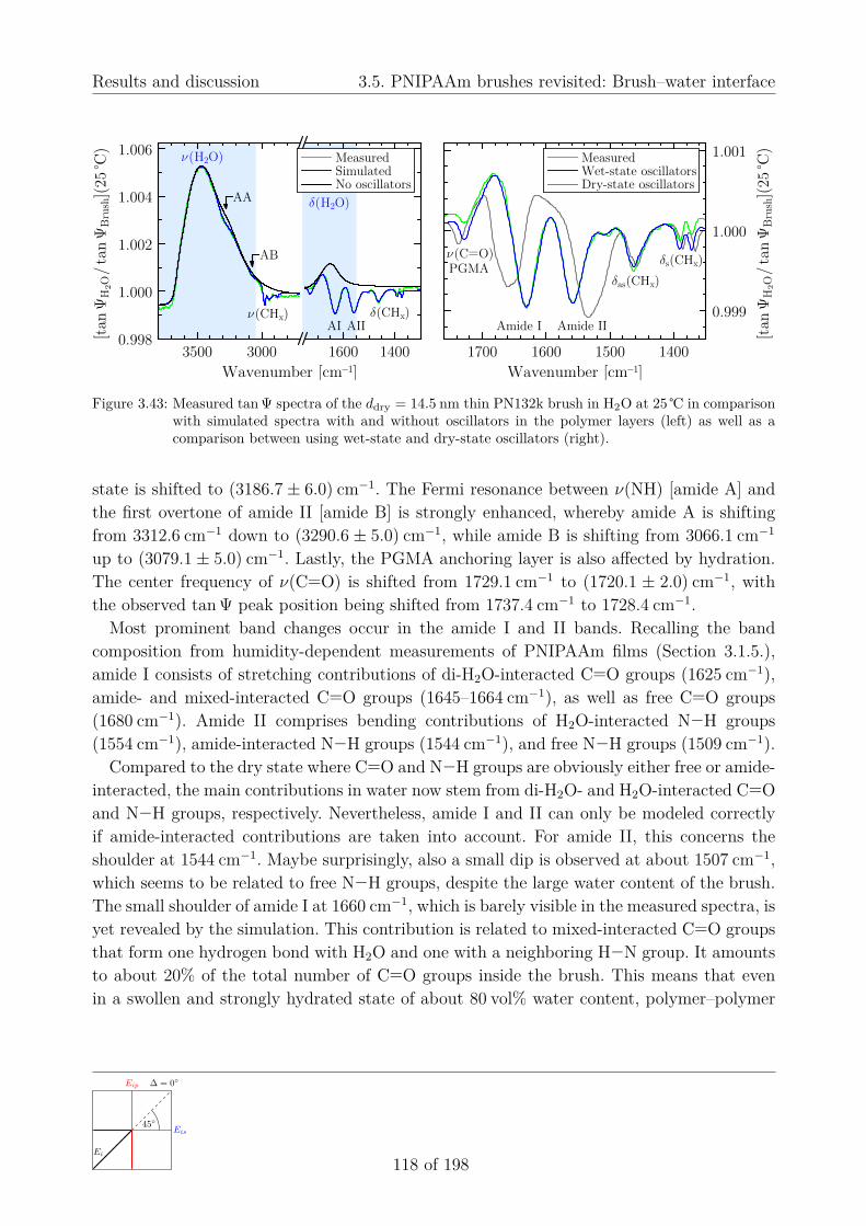
Results and discussion 3.5. PNIPAAm brushes revisited: Brush–water interface
3500 3000 1600 14000.998
1.000
1.002
1.004
1.006
No oscillators
SimulatedMeasured
[tan
ΨH
2O
/ tan
ΨB
rush
](25
◦ C)
Wavenumber [cm–1]
PGMA ν (C=O)
Amide I Amide II
ν ( H2O)
δ ( H2O)
ν (CHx)AI AII
δ (CHx)
AA
AB
1700 1600 1500 1400
0.999
1.000
1.001
δs (CHx)
δas (CHx)
[tan
ΨH
2O
/ tan
ΨB
rush
](25
◦ C)
Wavenumber [cm–1]
Dry-state oscillators
Wet-state oscillatorsMeasured
Figure 3.43: Measured tan Ψ spectra of the ddry = 14.5 nm thin PN132k brush in H2O at 25 ℃ in comparisonwith simulated spectra with and without oscillators in the polymer layers (left) as well as acomparison between using wet-state and dry-state oscillators (right).
state is shifted to (3186.7 ± 6.0) cm−1. The Fermi resonance between ν(NH) [amide A] andthe first overtone of amide II [amide B] is strongly enhanced, whereby amide A is shiftingfrom 3312.6 cm−1 down to (3290.6 ± 5.0) cm−1, while amide B is shifting from 3066.1 cm−1
up to (3079.1 ± 5.0) cm−1. Lastly, the PGMA anchoring layer is also affected by hydration.The center frequency of ν(C=O) is shifted from 1729.1 cm−1 to (1720.1 ± 2.0) cm−1, withthe observed tan Ψ peak position being shifted from 1737.4 cm−1 to 1728.4 cm−1.
Most prominent band changes occur in the amide I and II bands. Recalling the bandcomposition from humidity-dependent measurements of PNIPAAm films (Section 3.1.5.),amide I consists of stretching contributions of di-H2O-interacted C=O groups (1625 cm−1),amide- and mixed-interacted C=O groups (1645–1664 cm−1), as well as free C=O groups(1680 cm−1). Amide II comprises bending contributions of H2O-interacted N−H groups(1554 cm−1), amide-interacted N−H groups (1544 cm−1), and free N−H groups (1509 cm−1).
Compared to the dry state where C=O and N−H groups are obviously either free or amide-interacted, the main contributions in water now stem from di-H2O- and H2O-interacted C=Oand N−H groups, respectively. Nevertheless, amide I and II can only be modeled correctlyif amide-interacted contributions are taken into account. For amide II, this concerns theshoulder at 1544 cm−1. Maybe surprisingly, also a small dip is observed at about 1507 cm−1,which seems to be related to free N−H groups, despite the large water content of the brush.The small shoulder of amide I at 1660 cm−1, which is barely visible in the measured spectra, isyet revealed by the simulation. This contribution is related to mixed-interacted C=O groupsthat form one hydrogen bond with H2O and one with a neighboring H−N group. It amountsto about 20% of the total number of C=O groups inside the brush. This means that evenin a swollen and strongly hydrated state of about 80 vol% water content, polymer–polymer
Eip
Eis45◦
Ei
∆ = 0◦
118 of 198

3.5. PNIPAAm brushes revisited: Brush–water interface Results and discussion
6000 5000 4000 30000.998
1.000
1.002
1.004
1.006
81.5%
77.5%Water content:79.5%
[tan
ΨH
2O
/ tan
ΨB
rush
](25
◦ C)
Wavenumber [cm–1]
ν ( H2O)
Simulated Measured
±2% water content
Figure 3.44: Sensitivity of the ν(H2O) band and the baseline in tan Ψ towards changes of ±2 vol% in watercontent of the ddry = 14.5 nm thin PN132k brush in H2O at 25 ℃. The thickness of the swollenbrush is d̃(25 ℃) = (57 ± 3) nm.
interactions (C=O · · · H−N) play an important role in the swelling behavior of the brush.During the simulation, the constraint of Eq. (3.7) for the conserved number of dipole
moments could be maintained for amide I. For amide II, on the other hand, it did nothold. The measured amide II band is much smaller than expected. This can be seen inthe right panel of Fig. 3.43 by comparing simulated spectra based on dry- and wet-stateoscillators. Possible reasons for this deviation are still being investigated to exclude, forexample, systematic errors from the baseline-correction procedure.
Before moving on to measurements of the brush at 45 ℃, it has to be mentioned that theabove simulations rest solely upon the high optical contrast in the infrared. Decorrelatingswollen-brush thickness d̃ and water content fH2O, for instance, is only possible becauseν(H2O) scales highly non-linear with fH2O and is extremely sensitive to absolute changes inwater content if the polymer brush is strongly hydrated. This is illustrated in Fig. 3.44, whichshows the impact of a varying water content of ±2 vol% on the simulated spectra. Withincreasing fH2O, the optical contrast between brush and water-reference spectra reduces,leading to a strongly decreasing ν(H2O) band amplitude. Simultaneously, the baseline slopeat higher wavenumbers decreases as well. With these dependencies in mind, the possibleprecision of determining d̃ and fH2O can, in principle, be vastly improved by recording tan Ψspectra at several angles of incidence.
b) Changing interactions within the collapsed brush above the LCST
From several studies on comparable PNIPAAm brushes [26, 46], it is expected that the mea-sured PN132k brush deswells above its LCST, similar to a coil-to-globule transition. Inter-actions within the brush are expected to change from mainly polymer–water-dominated to
Erp
ErsΨ Er
∆ = 261◦
119 of 198
Erp
ErsΨ
Er
∆ = 230◦

Results and discussion 3.5. PNIPAAm brushes revisited: Brush–water interface
3500 3000 1700 1600 15000.998
1.000
1.002
1.004
1.006
Simulated, 45
◦C
Simulated, 25
◦CMeasured
Simulated, 45
◦C
Simulated, 25
◦CMeasured
δas (CHx)
[tan
ΨH
2O
/ tan
ΨB
rush
](T
)
Wavenumber [cm–1]
ν (C=O)PGMA
AI AII ν (CHx)
ν ( H2O)
δ ( H2O)45 ◦C
25 ◦C
1750 1700 1650 1600 1550 1500
0.999
1.000
1.001
[tan
ΨH
2O
/ tan
ΨB
rush
](T
)
Wavenumber [cm–1]
Amide I Amide II
45 ◦C
25 ◦C
Figure 3.45: Measured and simulated tan Ψ spectra of the ddry = 14.5 nm thin PN132k brush in H2O at25 ℃ and 45 ℃, with a zoom of the amide I/II region shown in the right panel. Swollen-brushthicknesses and water contents are d̃(25 ℃) = (57 ± 3) nm and fH2O(25 ℃) = (79.5 ± 2.0) vol%as well as d̃(45 ℃) = (17 ± 5) nm and fH2O(45 ℃) = (28.0 ± 12.0) vol%.
polymer–polymer-dominated [26, 262]. Figure 3.45 compares measured and simulated spectraat both 25 ℃ and 45 ℃. The spectrum above the LCST was modeled successfully with a brushthickness of d̃(45 ℃) = (17 ± 5) nm and a water content of fH2O(45 ℃) = (28.0 ± 12.0) vol%.These values are smaller than the ones obtained by Burkert et al. [46] from VIS ellipsometryon a similar ddry = 12.5 nm thick brush. The two brushes differ only slightly in grafting den-sity, with σ = 0.07 nm−2 and σBurkert = 0.06 nm−2. Whether or not this small difference in σcan cause such changes in the swelling behavior has yet to be investigated with systematicgrafting-density-dependent measurements.
Nevertheless, the simulations reveal drastic changes in polymer–polymer and polymer–water interactions. The amide bands—especially the amide I band—undergo substantialalterations. This is illustrated in Fig. 3.46, which shows the number of dipoles associated withthe five ν(C=O) amide I subcomponents in wet state at 25 ℃ and 45 ℃ as well as in humidstate (35% humidity) and in dry state. No free or single-bonded C=O groups are present if thebrush is in contact with liquid water. This agrees with humidity-dependent measurements onspin-coated PNIPAAm films discussed in Section 3.1.5.b). There, Fig. 3.20 shows the ν(C=O)oscillator strengths for water contents between 1–9 vol%. Extrapolating the results indicatesthat all previously free or single-bonded C=O groups become mixed- or dihydrogen-bondedif the water content of the film reaches approximately 14 vol%. As discussed before, the brushcontains about 20% mixed-bonded and 80% di-H2O-bonded C=O groups at 25 ℃ withoutthe presence of double-bonded groups, meaning that there are no pure polymer–polymerinteractions below the LCST. Water therefore dictates the interactions within the brush.At 45 ℃, less di-H2O-bonded C=O groups are found. Simultaneously, mixed-bonded groups
Eip
Eis45◦
Ei
∆ = 0◦
120 of 198

3.5. PNIPAAm brushes revisited: Brush–water interface Results and discussion
Free Single Mixed Double Di-H2O1628.0 cm–11643.8 cm–11657.0 cm–11663.2 cm–11678.2 cm–1
# o
f ν (C
=O
) dip
oles
[a.
u.]
Dry
35%
45 ◦ C
25 ◦ C
Dry
35%
45 ◦ C
25 ◦ C
Dry
35%
45 ◦ C
25 ◦ C
Dry
35%
45 ◦ C
25 ◦ C
Dry
35%
45 ◦ C
25 ◦ C
Figure 3.46: Hydration-dependent number of ν(C=O) dipoles of the five amide I subcomponents shown forthe PNIPAAm brush in H2O at 25 ℃ and 45 ℃, determined with in-situ infrared ellipsometry, incomparison with the ones of spin-coated PNIPAAm films in humid state (35% humidity) and drystate, determined infrared-microscopically and -ellipsometrically, respectively; see Sections 3.1.4.and 3.1.5.b).
increase in number, but most importantly, double-bonded C=O groups are highly favored.Remember that these are C=O groups that form hydrogen bonds with two neighboring H−Ngroups. Polymer–polymer interactions therefore heavily influence the swelling behavior of thebrush.
c) Further band changes due to hydration
The final point concerns temperature-dependent band shifts of PNIPAAm’s amide A and B aswell as CHx-stretching and -bending bands. Table 3.7 compares obtained values for oscillatorfrequencies ν̃0 in water at 25 ℃ and 45 ℃ as well as in dry state. All observed band shiftsare in accordance with the strength of hydration at the corresponding state. Strongest shiftsof −22 cm−1 and +13 cm−1 are respectively found for amide A and B at 25 ℃. The δ(CHx)bands are shifted by up to +6 cm−1 with respect to the dry state. With decreasing watercontent of the brush, the bands tend to shift towards their dry-state values. Interestingly,the ν(CHx) bands are shifted by up to +9 cm−1 at 25 ℃, but also remain shifted by about+6 cm−1 at 45 ℃. This confirms, on the one hand, that these bands are highly indicative forthe current hydration state of the brush, as was suggested by Maeda et al. [50] for aqueousPNIPAAm solutions. On the other hand, it might indicate that the hydration of isopropylgroups and the main chain of the polymer differs from the hydration of amide groups. Thissuggests that the CH3 groups are intrinsically involved in the actual deswelling behavior.The experimental errors in the ν(CHx) region, however, are too large to obtain conclusiveevidence for this hypothesis. Similarly strong ν(CHx) band shifts were also reported byBittrich et al. [26] who performed ATR-infrared measurements on a PN132k brush.
Erp
ErsΨEr
∆ = 261◦
121 of 198
Erp
ErsΨ
Er
∆ = 240◦

Results and discussion 3.5. PNIPAAm brushes revisited: Brush–water interface
Band Swollen state at 25 ℃ Collapsed state at 45 ℃ Dry state
[cm−1] → ν̃0 Shift ν̃0 Shift ν̃0
Amide A 3290.6 −22.0 3308.6 −4.0 3312.6Amide B 3079.1 +13.0 3072.1 +6.0 3066.1νas(CH3) 2978.1 +8.0 2976.1 +6.0 2970.1νas(CH2) 2943.6 +9.0 2940.6 +6.0 2934.6νs(CH3) 2879.7 +7.0 2877.7 +5.0 2872.7δas(CH3) 1470.3 +2.0 1469.3 +1.0 1468.3δas(CH2) 1461.9 +4.0 1459.9 +2.0 1457.9δs(CH3) 1391.0 +5.0 1389.0 +3.0 1386.0δs(CH2) 1372.1 +6.0 1369.1 +3.0 1366.1
Table 3.7: Oscillator center frequencies ν̃0 of PNIPAAm’s amide A/B, CHx-stretching, and CHx-bendingvibrations in wet state at 25 ℃ and 45 ℃ as well as in dry state, obtained from optical simulations.The overall errors are estimated to be ±5.0 cm−1 for amide A/B, ±1.5 cm−1 for ν(CHx), and±0.5 cm−1 for δ(CHx). Band shifts are given with respect to the dry-state values.
d) Comparison with in-situ VIS ellipsometry
In order to assess the reliability of the infrared-ellipsometric simulations, the results forthe ddry = 14.5 nm thick PN132k brush discussed above and for the ddry = 12.6 nm thickPN94k brush (see Tab. 3.6) published in Ref. [25] are compared with VIS-ellipsometric re-sults from the literature [25, 46]. Table 3.8 shows the corresponding values for swollen-brushthicknesses d̃ and water contents fH2O.
Overall good agreement is found for the thicknesses of the swollen or collapsed brushes,keeping in mind the slight temperature differences between VIS and infrared measurements.The water content matches below the LCST for the PN132k brush. Above the LCST, theinfrared results indicate a stronger deswelling with correspondingly much less water boundwithin the brush. Note, however, that the VIS measurements were performed in phosphatebuffer solutions at pH 7.4, whereas unbuffered purified water was used for all infrared mea-surements. The use of a buffer might significantly influence the LCST behavior of PNIPAAmbrushes [263].
Despite these differences, the trends in both thickness and water content as well as thecorrelation between these two parameters are reasonably similar for infrared and visibleellipsometry. This substantiates the trustworthiness of the in-situ infrared approach and thesubsequent quantitative analysis of the amide band composition.
Accuracy and precision for the infrared PN132k results are much better compared to thePN94k results due to several improvements of the optical set-up and the procedure of spectraevaluation, including the baseline-correction and the use of higher-quality optical constantsof water (see Section 3.4.) in the simulation.
Eip
Eis45◦
Ei
∆ = 0◦
122 of 198

3.5. PNIPAAm brushes revisited: Brush–water interface Results and discussion
PN132k PN94k
Method T [℃] d̃ [nm] fH2O [vol%] T [℃] d̃ [nm] fH2O [vol%]
IR 25.00 ± 0.05 57 ± 3 79.5 ± 2.0 24.7 ± 0.2 43 ± 8 86 ± 1345.00 ± 0.05 17 ± 5 28.0 ± 12.0 38.6 ± 0.2 20 ± 9 68 ± 15
VIS 23.0 ± 0.1 46.3 ± 0.3 74.8 ± 0.3 24.6 ± 0.1 45.6 ± 0.5 —40.0 ± 0.1 26.7 ± 0.6 58.2 ± 0.3 38.6 ± 0.1 19.5 ± 0.5 —
Table 3.8: Comparison between IR- and VIS-ellipsometric results for T -dependent swollen-brush thicknesses d̃and water contents fH2O of PNIPAAm brushes with different molecular weights. IR results for theddry = 14.5 nm thick PN132k brush are compared with VIS results from Ref. [46] for a 12.5 nmthick brush. The ddry = 12.6 nm thick PN94k brush (IR) is compared with an 11.0 nm thick brush(VIS), details of which were already published in Ref. [25]. Note that VIS measurements wereperformed in 10 mM PBS buffer at pH 7.4, whereas purified water from a Millipore system wasused for IR measurements. VIS data for water contents fH2O were not available in the case of thePN94k brush.
e) Conclusions and outlook
In-situ measurements of PGMA films and PNIPAAm brushes with corresponding opticalsimulations show the high potential of in-situ infrared ellipsometry for gaining quantitativeinsights into the structural properties of thin organic films in contact with aqueous solutions.With careful optical modeling, it was possible to obtain thicknesses and water contents ofthe ddry = 14.5 nm thin PN132k brush in swollen and collapsed state. Using the dry- andwet-state oscillators as determined by ex-situ infrared ellipsometry and humidity-dependentinfrared microscopy on spin-coated PNIPAAm films, the band compostion of amide I wassuccessfully analyzed. Changing polymer–polymer and polymer–water interactions were iden-tified below and above the LCST. Also band shifts of CHx-bending and -stretching vibrationscould be connected with the current hydration state.
The obtained results already reveal many details about the brush properties. Furtherimprovements of both the optical set-up and the spectra-evaluation process are yet feasibleto gain even deeper insights and increase the accuracy. As mentioned before, measurements atmultiple angles of incidence would allow one to decorrelate film thickness and water contentmore easily. Also anisotropy could be probed this way. Moreover, rigorously derived equationsfor tan Ψ and ∆ that included the geometry and tension of the wedge-shaped substrate wouldeliminate some of the possible issues due to the baseline-correction procedure. With theseimprovements, the brush profile should be determinable, because every band in tan Ψ—andespecially the water-stretching band—is highly sensitive to incidence angle, thickness, watercontent, and distribution of water throughout the depth profile.
Erp
ErsΨEr
∆ = 261◦
123 of 198
Erp
ErsΨ
Er
∆ = 250◦

Results and discussion 3.6. Protein adsorption: Motivation
3.6. Protein adsorption
3.6.1. MotivationControlling adsorption and desorption of proteins or cells at biocompatible surfaces is of highpotential for biomedical and biotechnological applications. In this respect, various polymerand polymer-brush systems have been investigated in the literature using visible ellipsometry,infrared spectroscopy, quartz crystal microbalance, zeta-potential analysis, X-ray microscopy,fluorescence microscopy, and other techniques. These polymer systems include, for instance,fluorohydrocarbon polymers [99], PAA mono brushes [39, 82], PNIPAAm brushes [46–49] andPNIPAAm-modified surfaces [264, 265], PEG [46] and PEG-based brushes [40, 266], PHEMAbrushes [267–269], PS- and PMMA-based surfaces [270–273], hyperbranched polyesters [274],binary P2VP/PAA brushes [38], as well as binary P2VP/PNIPAAm brushes [46, 66] andPNIPAAm/PAA brushes [67].
The basic idea behind controlling the protein-binding properties of polymer surfaces is touse external stimuli like pH or temperature to switch the surface between an adsorbing anda repelling state. Regarding polymer brushes, this can be achieved with either mono brushesor mixed brushes. PAA brushes, for example, can be switched between the two states bychanging the pH value of the aqueous environment [39, 82]. Mixed brushes, on the otherhand, may contain a passive component and at least one active component that is sensitiveto stimuli and might react, e. g., by swelling, thereby determining the surface propertiesof the brush. Examples are P2VP/PAA [20, 21, 27, 38] and PAA-b-PS/PEG brushes [22]where P2VP and PAA are pH-sensitive, or PNIPAAm/P2VP [46, 66] and PNIPAAm/PAAbrushes [67] in which PNIPAAm is the active component reacting upon temperature changes.
Mixed brush
T < TcT > Tc
AdsorptionDesorption
Figure 3.47: Sketch of proteins adsorbing and desorbing at a mixed binary brush upon changes in tempera-ture. The passive light green polymer is protein-adsorbing, whereas the active (swellable) darkgreen polymer is protein-repelling. Around a critical temperature Tc, the brush switches betweena protein-adsorbing and a protein-repelling state.
Eip
Eis45◦
Ei
∆ = 0◦
124 of 198
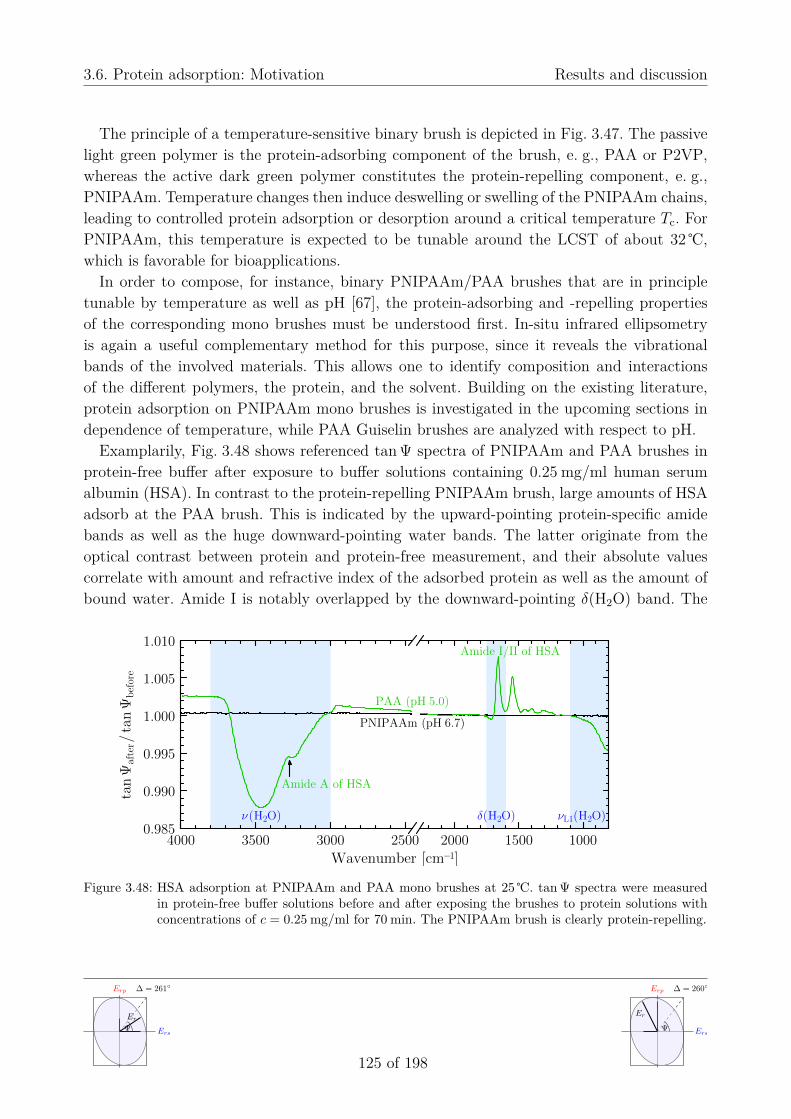
3.6. Protein adsorption: Motivation Results and discussion
The principle of a temperature-sensitive binary brush is depicted in Fig. 3.47. The passivelight green polymer is the protein-adsorbing component of the brush, e. g., PAA or P2VP,whereas the active dark green polymer constitutes the protein-repelling component, e. g.,PNIPAAm. Temperature changes then induce deswelling or swelling of the PNIPAAm chains,leading to controlled protein adsorption or desorption around a critical temperature Tc. ForPNIPAAm, this temperature is expected to be tunable around the LCST of about 32 ℃,which is favorable for bioapplications.
In order to compose, for instance, binary PNIPAAm/PAA brushes that are in principletunable by temperature as well as pH [67], the protein-adsorbing and -repelling propertiesof the corresponding mono brushes must be understood first. In-situ infrared ellipsometryis again a useful complementary method for this purpose, since it reveals the vibrationalbands of the involved materials. This allows one to identify composition and interactionsof the different polymers, the protein, and the solvent. Building on the existing literature,protein adsorption on PNIPAAm mono brushes is investigated in the upcoming sections independence of temperature, while PAA Guiselin brushes are analyzed with respect to pH.
Examplarily, Fig. 3.48 shows referenced tan Ψ spectra of PNIPAAm and PAA brushes inprotein-free buffer after exposure to buffer solutions containing 0.25 mg/ml human serumalbumin (HSA). In contrast to the protein-repelling PNIPAAm brush, large amounts of HSAadsorb at the PAA brush. This is indicated by the upward-pointing protein-specific amidebands as well as the huge downward-pointing water bands. The latter originate from theoptical contrast between protein and protein-free measurement, and their absolute valuescorrelate with amount and refractive index of the adsorbed protein as well as the amount ofbound water. Amide I is notably overlapped by the downward-pointing δ(H2O) band. The
4000 3500 3000 2500 2000 1500 10000.985
0.990
0.995
1.000
1.005
1.010
νL1 ( H2O)δ ( H2O)
PAA (pH 5.0)
PNIPAAm (pH 6.7)
Amide I/II of HSA
Wavenumber [cm–1]
ν ( H2O)
Amide A of HSA
tan
Ψaf
ter /
tan
Ψbef
ore
Figure 3.48: HSA adsorption at PNIPAAm and PAA mono brushes at 25 ℃. tan Ψ spectra were measuredin protein-free buffer solutions before and after exposing the brushes to protein solutions withconcentrations of c = 0.25 mg/ml for 70 min. The PNIPAAm brush is clearly protein-repelling.
Erp
ErsΨEr
∆ = 261◦
125 of 198
Erp
ErsΨ
Er
∆ = 260◦

Results and discussion 3.6. Protein adsorption: pH-dependent properties of HSA
band amplitudes of amide I and II also reflect the amount of adsorbed protein. The bandshapes, on the other hand, give valuable information on the protein conformation [215, 275].
Protein structure, brush chemistry, water content, and interactions are accessible in theinfrared, but yield overlapping spectral information. Before investigating HSA adsorption atPNIPAAm and PAA brushes in more detail, it is thus necessary to identify the characteristicvibrational bands of HSA and test if they are affected, for example, by changes in pH.
3.6.2. pH-dependent properties of human serum albuminIn order to determine the effects of pH on the structural properties of adsorbed and solvatedhuman serum albumin, in-situ measurements were performed on differently concentratedHSA solutions using ATR infrared ellipsometry and infrared transmission spectroscopy. Thesetechniques are sensitive enough to resolve the amide bands of the protein, the band compo-sition of which allows one to assess the protein secondary structure [215, 275]. In the firststep, HSA (mono)layers on silicon and CaF2 substrates are investigated at pH 5 and 7. Theresults are then used in the second step to interpret spectra of different protein solutions.
a) HSA monolayers
The kinetics of protein adsorption are governed by various parameters, such as flow conditionsof proteins towards the adsorbing surface, pH and temperature of the solution, difference inprotein concentration between solution and surface, as well as protein–water, water–surface,
c = 0.25 mg/ml
AA AIIAI
c = 5.00 mg/ml
Fingerprint
AA AI AII
Protein adsorption
3500 3000 1600 1400
0.999
1.000
1.001
δ ( H2O)
ν (CHx)
ν ( H2O)
tan
Ψ /
tan
ΨpH
5, buffer
Wavenumber [cm–1]
3500 3000 1600 1400
0.999
1.000
1.001
δ ( H2O)ν ( H2O)
ν (CHx)
tan
Ψ /
tan
ΨpH
5, buffer
Wavenumber [cm–1]
Figure 3.49: HSA-(mono)layer formation on a silicon ATR crystal from two differently concentrated HSAsolutions at pH 5 measured with ATR ellipsometry at 25 ℃. Left: c = 0.25 mg/ml, 4 cm−1
resolution, monitored over 100 min. Right: c = 5.00 mg/ml, 16 cm−1 resolution, recorded over70 min. Spectra were referenced to protein-free buffer solutions at pH 5 measured before theadsorption process. Amide A, I, and II bands are labeled with AA, AI, and AII, respectively.For better amplitude comparability, all spectra were baseline-corrected to coincide at 1710 cm−1.
Eip
Eis45◦
Ei
∆ = 0◦
126 of 198

3.6. Protein adsorption: pH-dependent properties of HSA Results and discussion
and protein–surface interactions [276–278]. The protein concentration in solution, for in-stance, correlates with the initial adsorption rate, the amount of adsorbed proteins, but alsowith conformational changes of the proteins during the adsorption process [276–279]. Thelatter can involve structural rearrangements of the proteins due to spreading at the sur-face [276–278] as well as changing protein–water interactions and changes in the hydrationstate [215, 278, 280, 281]. Water in particular plays an important role during the adsorptionprocess [278, 280].
Both the protein- and the water-specific vibrational bands are readily accessible by meansof infrared spectroscopy. Figure 3.49 shows the time-dependent formation of HSA layerson silicon ATR crystals from two different HSA solutions at pH 5 with concentrations ofc = 0.25 mg/ml and c = 5.00 mg/ml. The adsorption processes were measured with ATRellipsometry over periods of 100 min and 70 min, respectively. Most prominent features inthe spectra are the downward-pointing protein-specific amide A, I, and II bands as well asthe upward-pointing ν(H2O) band due to the optical contrast between protein spectra andprotein-free reference spectra. Further small HSA bands are also observable in the CHx-stretching and fingerprint regions.
Most of the protein is already adsorbed after the first few minutes, as is evident fromthe time-dependent amide II amplitude progression, shown in Fig. 3.50. In detail, the HSAadsorption kinetics depend on the protein concentration within the buffer solution. At thesmaller concentration of c = 0.25 mg/ml, the amide band amplitudes increase by about 20%with respect to the initial spectrum, while the ν(H2O) band amplitude remains almost con-stant. In contrast, at the higher concentration of c = 5.00 mg/ml, the ν(H2O) amplitude in-creases continuously. This suggests either a dehydration of adsorbed proteins due to spreadingand conformational changes, or the accumulation of more than just a protein monolayer on
c = 5.00 mg/ml
c = 0.25 mg/ml
0 10 20 30 40
Am
ide
II a
mplitu
de
[a. u
.]
t [min]
Figure 3.50: Amide II tan Ψ band amplitude during HSA adsorption, corresponding to the spectra inFig. 3.49. To guide the eye, points were connected by fitting a function “Ampl. ∝ ta/(ta + ba)”with free parameters a and b.
Erp
ErsΨEr
∆ = 261◦
127 of 198
Erp
ErsΨ
Er
∆ = 270◦

Results and discussion 3.6. Protein adsorption: pH-dependent properties of HSA
the silicon substrate. Furthermore, the amide II amplitude increases by about 9%, whereasamide I increases by 20%. This change in amplitude ratio of amide I/II is also indicativeof structural changes of the proteins during adsorption. The effect is even stronger whenconsidering that amide I is also overlapped by the upward-pointing water-bending vibrationδ(H2O), which is likely to evolve similarly with ν(H2O).
Since the measured spectra also contain contributions from the protein/buffer interface aswell as the protein solution itself, it is difficult to study the effects of pH on the adsorbedlayer alone. The ATR flow cell was therefore purged with protein-free buffer to remove thesespectral contributions. Note that this rinsing process might also partly remove non-stronglybound proteins, which causes potential problems for a quantitative analysis concerning theamount of adsorbed protein [278]. Subsequent purging of the cell with buffer at pH 5, 7,and again 5 resulted in the spectra displayed in Fig. 3.51. A certain amount of proteins isdesorbing from the substrate or the protein layer when changing the pH from 5 to 7. Loweringthe buffer’s pH back to 5 also causes some desorption or rearranging at the substrate, whichis probably due to the flow conditions within the cell. Nevertheless, differences in compositionof the protein-specific vibrational bands can be discussed.
Analysis of the amide I and II band compositions can yield valuable information about thesecondary structure of the protein [215, 275], that is, the contributions of α-helix, β-sheets,β-turns, and random-coil conformations to the overall protein structure. In agreement with
pH 5
pH 7pH 5
c = 0.25 mg/ml
Amide A Amide IIAmide I
3800 3600 3400 3200 3000 2800 1700 1650 1600 1550 1500
0.9992
0.9996
1.0000
1.0004
1.0008 δ ( H2O)
ν (CHx)
ν ( H2O)
tan
Ψ /
tan
ΨpH
5, buffer
Wavenumber [cm–1]
Figure 3.51: HSA layer—adsorbed from a protein solution with c = 0.25 mg/ml—in subsequent contact withbuffer solutions at pH 5 (red line), 7 (green line), and 5 (black line). The baseline-corrected tan Ψspectra were referenced to protein-free buffer before the adsorption process. Small residues ofwater-vapor absorption are overlapping the amide I/II region.
Eip
Eis45◦
Ei
∆ = 0◦
128 of 198

3.6. Protein adsorption: pH-dependent properties of HSA Results and discussion
ATR FT-IR measurements on HSA solutions at pH 7.4 by Barbucci and Magnani [183], themain contribution to amide I is situated at about 1656 cm−1 and is assignable to α-helix aswell as random-coil conformation [275]. Smaller band components are observed at 1675 cm−1
and 1631 cm−1, corresponding to β-sheet conformation [275]. Importantly for the upcomingHSA adsorption experiments on PAA brushes, the relative α-helix and β-sheets contributionsto the amide band envelopes do not change between pH 5 and 7.
HSA (mono)layers were also measured with infrared transmission microscopy. Protein wasadsorbed to the CaF2 windows of the transmission cell from HSA solutions at pH 5 withc = 0.25 mg/ml and c = 1.00 mg/ml. Afterwards, transmission spectra were collected whilepurging the cell with protein-free buffer at pH 5 and 7. Within the given signal-to-noise ratio,no significant pH-dependent changes were found in the amide I and II band compositions.
b) HSA solutions
After the adsorption of HSA layers from low-concentrated HSA solutions as described above,higher-concentrated protein solutions were investigated in transmission as well as with ATRellipsometry. For this, the monolayer measurements in protein-free buffer served as a refer-ence to subtract the spectral contributions stemming from the adsorbed layers. Figure 3.52shows referenced absorbance spectra of HSA solutions at pH 5 and 7 with concentrationsof c = (10.0 ± 0.2) mg/ml. Similar to the protein layers discussed in the previous section,solvated HSA does not undergo conformational changes between pH 5–7 (within the errorof c), in agreement with Ref. [282]. ATR measurements confirm this result.
pH 5
pH 7
c = 10 mg/ml
Amide A
Amide II
Amide I
Fingerprint region
3800 3600 3400 3200 3000 2800 1700 1600 1500 1400 1300 1200 1100 0.015
0.010
0.005
0.000
0.005
0.010
–
–
–δ ( H2O)
ν (CHx)
ν ( H2O)
ASol
ution
– A
Mon
olay
er
Wavenumber [cm–1]
pH 7
pH 5
Figure 3.52: Absorbances of HSA solutions with concentrations of c = (10.0 ± 0.2) mg/ml at pH 5 (red line)and 7 (green line) measured with a dCell = 3.26 µm transmission cell at 25 ℃. Spectra werereferenced to absorbances of HSA (mono)layers in contact with protein-free buffer.
Erp
ErsΨ
Er
∆ = 261◦
129 of 198
Erp
ErsΨ
Er
∆ = 280◦

Results and discussion 3.6. Protein adsorption: PNIPPAm brushes
3.6.3. Temperature-dependent protein resistance of PNIPPAmbrushes
PNIPAAm brushes were investigated in the literature for temperature- and pH-dependentHSA adsorption using visible ellipsometry [46, 47]. Burkert et al. [46] showed that HSA ad-sorbs on PN132k brushes below pH < 4 and attributed this to the denaturation of the pro-tein and its molten globule-like state [184]. Above pH 4, however, no adsorption was found.Within the sensitivity of their ellipsometry set-up, Xue et al. [47] verified the HSA repellencyof PNIPAAm brushes at pH 7 for various grafting densities between σ = 0.08–0.21 nm−2 andmolecular weights ranging from Mn = 44 000 g/mol to 202 000 g/mol. They also analyzedBSA (bovine serum albumin) adsorption on PNIPAAm brushes. No adsorption was foundwith visible ellipsometry, but small amounts of adsorbed BSA could be verified using ra-dioisotope assays.
In-situ infrared ellipsometry might shed more light on the subject. The ddry = 14.5 nmthin PN132k brush was measured for HSA adsorption at 25 ℃ and 40 ℃ using a proteinconcentration of c = 0.25 mg/ml at pH 6.7. At each temperature, a measurement sequenceof protein-free buffer, HSA in buffer, and protein-free buffer was conducted. At the end, thebrush was measured again at 25 ℃ in protein-free buffer. Corresponding referenced tan Ψspectra at the three temperatures are displayed in Fig. 3.53.
Deviations from unity in the form of upward- or downward-pointing bands are an indi-cator of structural or chemical changes of the brush. The first spectrum at 25 ℃ exhibits a
4000 3500 3000 2500 2000 1500 10000.9995
1.0000
1.0005
–0.0003
+0.0002
25 ◦C
40 ◦C
25 ◦C
δ ( H2O)
tan
Ψaf
ter /
tan
Ψbef
ore
Wavenumber [cm–1]
ν ( H2O)
Figure 3.53: Temperature-dependent HSA resistance of a PNIPAAm and PAA mono brush. Referenced tan Ψspectra with respect to protein-free buffer were measured at 25 ℃, 40 ℃, and again 25 ℃ afterexposing the brush to protein solution with concentration of c = 0.25 mg/ml for several minutes.
Eip
Eis45◦
Ei
∆ = 0◦
130 of 198
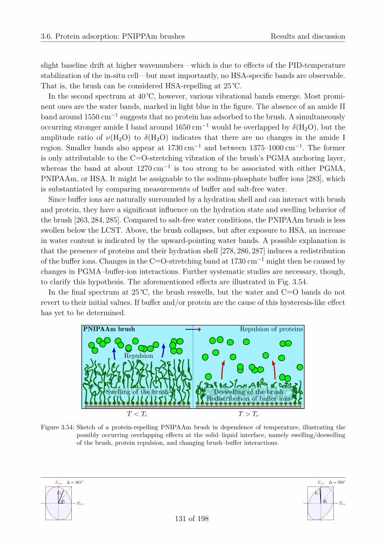
3.6. Protein adsorption: PNIPPAm brushes Results and discussion
slight baseline drift at higher wavenumbers—which is due to effects of the PID-temperaturestabilization of the in-situ cell—but most importantly, no HSA-specific bands are observable.That is, the brush can be considered HSA-repelling at 25 ℃.
In the second spectrum at 40 ℃, however, various vibrational bands emerge. Most promi-nent ones are the water bands, marked in light blue in the figure. The absence of an amide IIband around 1550 cm−1 suggests that no protein has adsorbed to the brush. A simultaneouslyoccurring stronger amide I band around 1650 cm−1 would be overlapped by δ(H2O), but theamplitude ratio of ν(H2O) to δ(H2O) indicates that there are no changes in the amide Iregion. Smaller bands also appear at 1730 cm−1 and between 1375–1000 cm−1. The formeris only attributable to the C=O-stretching vibration of the brush’s PGMA anchoring layer,whereas the band at about 1270 cm−1 is too strong to be associated with either PGMA,PNIPAAm, or HSA. It might be assignable to the sodium-phosphate buffer ions [283], whichis substantiated by comparing measurements of buffer and salt-free water.
Since buffer ions are naturally surrounded by a hydration shell and can interact with brushand protein, they have a significant influence on the hydration state and swelling behavior ofthe brush [263, 284, 285]. Compared to salt-free water conditions, the PNIPAAm brush is lessswollen below the LCST. Above, the brush collapses, but after exposure to HSA, an increasein water content is indicated by the upward-pointing water bands. A possible explanation isthat the presence of proteins and their hydration shell [278, 286, 287] induces a redistributionof the buffer ions. Changes in the C=O-stretching band at 1730 cm−1 might then be caused bychanges in PGMA–buffer-ion interactions. Further systematic studies are necessary, though,to clarify this hypothesis. The aforementioned effects are illustrated in Fig. 3.54.
In the final spectrum at 25 ℃, the brush reswells, but the water and C=O bands do notrevert to their initial values. If buffer and/or protein are the cause of this hysteresis-like effecthas yet to be determined.
PNIPAAm brush Repulsion of proteins
T > Tc
Deswelling of the brushRedistribution of buffer ions
T < Tc
Swelling of the brush
Repulsion
Figure 3.54: Sketch of a protein-repelling PNIPAAm brush in dependence of temperature, illustrating thepossibly occurring overlapping effects at the solid–liquid interface, namely swelling/deswellingof the brush, protein repulsion, and changing brush–buffer interactions.
Erp
ErsΨ
Er
∆ = 261◦
131 of 198
Erp
ErsΨ
Er
∆ = 290◦
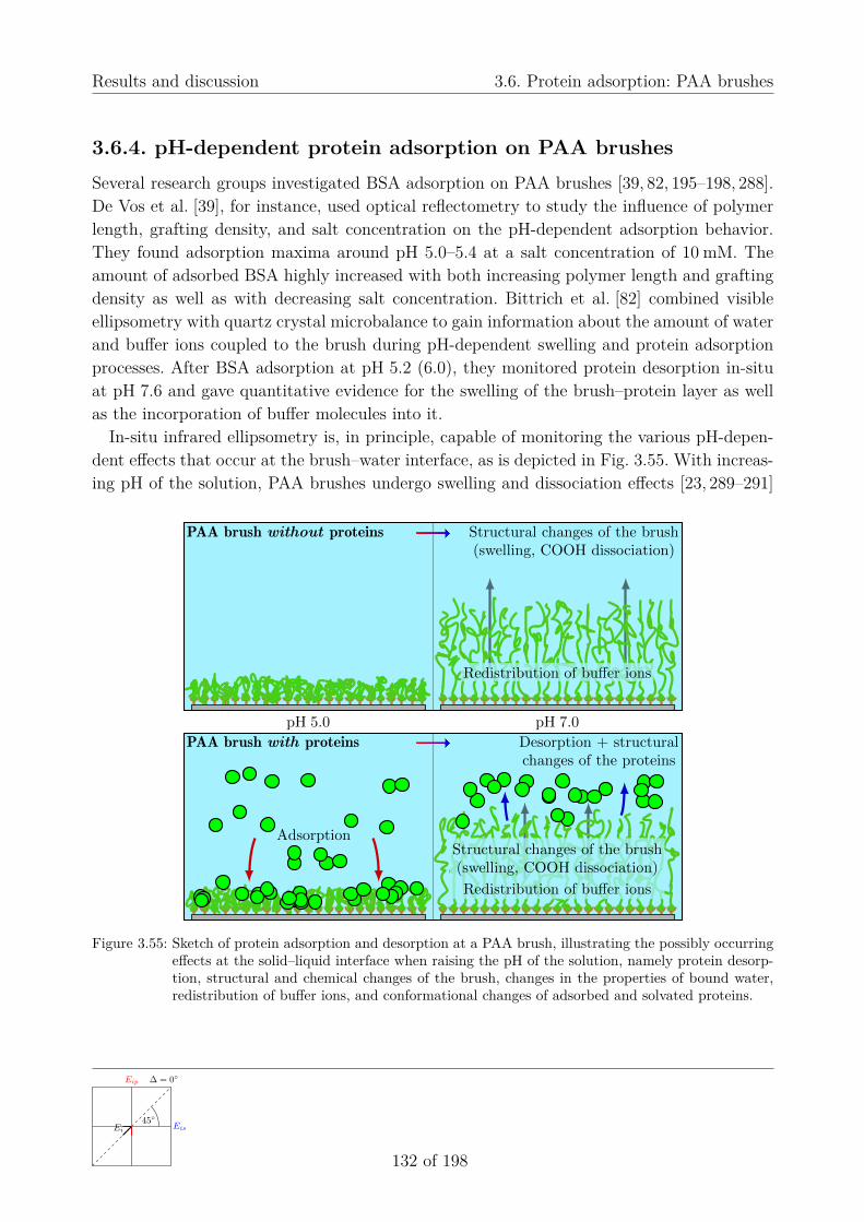
Results and discussion 3.6. Protein adsorption: PAA brushes
3.6.4. pH-dependent protein adsorption on PAA brushesSeveral research groups investigated BSA adsorption on PAA brushes [39, 82, 195–198, 288].De Vos et al. [39], for instance, used optical reflectometry to study the influence of polymerlength, grafting density, and salt concentration on the pH-dependent adsorption behavior.They found adsorption maxima around pH 5.0–5.4 at a salt concentration of 10 mM. Theamount of adsorbed BSA highly increased with both increasing polymer length and graftingdensity as well as with decreasing salt concentration. Bittrich et al. [82] combined visibleellipsometry with quartz crystal microbalance to gain information about the amount of waterand buffer ions coupled to the brush during pH-dependent swelling and protein adsorptionprocesses. After BSA adsorption at pH 5.2 (6.0), they monitored protein desorption in-situat pH 7.6 and gave quantitative evidence for the swelling of the brush–protein layer as wellas the incorporation of buffer molecules into it.
In-situ infrared ellipsometry is, in principle, capable of monitoring the various pH-depen-dent effects that occur at the brush–water interface, as is depicted in Fig. 3.55. With increas-ing pH of the solution, PAA brushes undergo swelling and dissociation effects [23, 289–291]
PAA brush without proteins Structural changes of the brush(swelling, COOH dissociation)
Redistribution of buffer ions
PAA brush with proteins
pH 5.0 pH 7.0
Desorption + structuralchanges of the proteins
Structural changes of the brush(swelling, COOH dissociation)
Redistribution of buffer ions
Adsorption
Figure 3.55: Sketch of protein adsorption and desorption at a PAA brush, illustrating the possibly occurringeffects at the solid–liquid interface when raising the pH of the solution, namely protein desorp-tion, structural and chemical changes of the brush, changes in the properties of bound water,redistribution of buffer ions, and conformational changes of adsorbed and solvated proteins.
Eip
Eis45◦
Ei
∆ = 0◦
132 of 198

3.6. Protein adsorption: PAA brushes Results and discussion
with a simultaneous ion redistribution inside the brush [23, 28, 290, 292, 293]. If proteins ad-sorb, then structural changes of both brush and protein as well as desorption of proteins cantake place upon changing the pH. The challenge is to unequivocally assign the correspondingspectral signatures in the infrared, since these all overlap to some degree.
The present work focuses on the investigation of HSA adsorption on PAA Guiselin brushesat pH 5 with subsequent partial protein desorption between pH 6–7. Infrared ellipsometry isemployed to gain insights into brush/protein structure and chemistry during protein adsorp-tion and desorption. Data from additional swelling/dissociation experiments [23] are usedto interpret the measured infrared spectra. In-situ visible ellipsometry is utilized to obtainquantitative information about brush thickness and amount of adsorbed protein.
For the VIS protein, IR protein, and IR PAA swelling/dissociation experiments, the PAA-brush samples S1, S2/S3, and S4 were used, respectively—see Section 2.4.2.b). Samples S2and S3 showed similar trends, and therefore only spectra of sample S2 are presented here.Infrared measurements were done by Dennis Aulich, while VIS-ellipsometric measurementsincluding quantitative evaluation were performed by Eva Bittrich at the IPF Dresden.
a) Protein adsorption process
The in-situ cell was filled with a 10 mM buffer solution at pH 5.0. The brush was kept in con-tact with the solution for 30 min in order to stabilize the temperature of the in-situ system aswell as to reach an equilibrium state between solution and brush. A tan Ψ spectrum recordedat that sample state served as the reference spectrum for all subsequent measurements.
Fingerprint
AA
AII
AIc = 0.25 mg/ml
Amide II
Amide I
3500 3000 1600 14000.985
0.990
0.995
1.000
1.005
1.010
δ ( H2O)
ν (CHx)
ν ( H2O)tan
Ψ /
tan
ΨpH
5.0
, buffer
Wavenumber [cm–1]
0 20 40 60 80 100
Proteinadsorption
Ban
d a
mplitu
de
[a. u
.]
t [min]
ν ( H2O)
Figure 3.56: HSA adsorption at 25 ℃ on the ddry = 7.4 nm thin PAA brush from a c = 0.25 mg/ml pro-tein solution at pH 5.0. Left: Measured tan Ψ spectra referenced to initial protein-free buffer.Amide A, I, II, and the fingerprint region of HSA are marked as AA, AI, AII, and FP, respec-tively. Raw data measured by Dennis Aulich. Right: Time-dependent (85 s resolution) tan Ψband amplitudes (|“Peak height” − 1.000|) of ν(H2O), amide I, and amide II. To guide the eye,points were connected by fitting functions “Ampl. ∝ ta/(ta + ba)” with free parameters a and b.
Erp
ErsΨ
Er
∆ = 261◦
133 of 198
Erp
ErsΨ
Er
∆ = 300◦

Results and discussion 3.6. Protein adsorption: PAA brushes
Human serum albumin was added to the buffer solution such that a concentration ofc = 0.25 mg/ml was obtained. The adsorption process was then monitored over a period ofabout 120 min by repeated tan Ψ measurements, as displayed in the left panel of Fig. 3.56.The right panel shows the corresponding time-dependent amplitude progressions of the char-acteristic protein-amide bands between 1700–1500 cm−1 as well as the broad water-stretchingband around 3500 cm−1. After about 110 min, these bands showed no further variations,which indicates maximum adsorption. Besides the major contributions due to adsorbed pro-tein, the amide and water bands also contain minor contributions from the interface betweenbrush and protein buffer solution. This influence on the overall tan Ψ amplitudes can be esti-mated from tan Ψ measurements of the previously discussed experiments on protein-repellingPNIPAAm brushes. There, one finds tan Ψ amplitudes of about 0.00025 for ν(H2O) and ofless than 0.00005 for amide I/II. If proteins adsorb to the PAA brush, the optical contrast inthe amide I/II region decreases even further. The influence of the protein solution is thereforenegligibly small compared to the measured band amplitudes in Fig. 3.56, which are largerthan 0.008 and 0.004, respectively. In other words, the observed water and amide bands areonly associated with the structural and chemical properties of the brush–protein layer.
The large amplitudes of the amide and water bands indicate ternary protein adsorp-tion [294], that is, adsorption within the brush. The amount of adsorbed HSA correlatesdirectly with the amide II band amplitude, which scales almost linearly. ν(H2O) reflectsboth the amount of adsorbed protein and the amount of additional water bound to thebrush, but also the thickness of the swollen brush. The water bands scale highly non-linearas was shown in Section 3.5.4.a). Amide I at about 1659 cm−1 correlates with the amount ofadsorbed protein, too, but it is overlapped by the downward-pointing δ(H2O) band around1650 cm−1. The exact position of δ(H2O) also depends on the water and protein content ofthe brush. Figure 3.57 shows a zoom of the amide I and II bands during protein adsorption.
�( )
[ { ]
Figure 3.57: Amide I/II region during the HSA adsorption process on the PAA brush shown in Fig. 3.56. Thedownward-pointing δ(H2O) band is overlapping the amide I (and II) band at about 1650 cm−1.
Eip
Eis45◦
Ei
∆ = 0◦
134 of 198

3.6. Protein adsorption: PAA brushes Results and discussion
As more and more protein is penetrating the brush, both amide I and δ(H2O) are increasingin amplitude, leading to a shift of amide I from 1659.5 cm−1 to 1660.8 cm−1 between initialand final adsorption spectrum. Also the apparent band shape is changing slightly. Note thatboth effects are pure optical effects and do not indicate any conformational changes of theprotein upon adsorption. This is also evident from the amide II band shape, which is notchanging at all. Furthermore, both amide bands resemble the band shapes obtained fromtransmission measurements of HSA solutions (Fig. 3.52). This means that the protein sec-ondary structure remains almost undisturbed after protein adsorption onto the brush, whichis important for possible applications.
A more detailed analysis of the protein conformation should build on optical simulationsthat factor in film effects as well as the influence of water on the amide bands. Otherwise,wrong conclusions might be drawn from the measured band shapes and amplitudes alone.
b) Controlled protein desorption
After maximum adsorption of HSA, the in-situ cell was consecutively purged with protein-free buffer solutions of increasing pH in order for the protein to desorb. The whole desorptionprocess was monitored by repetitive tan Ψ measurements over a period of 240 min, as shownin Fig. 3.58. Corresponding time-resolved amplitudes of the characteristic ν(H2O), amide I,and amide II bands are plotted in Fig. 3.59.
[ { ]
�( )�( )
Figure 3.58: HSA desorption from the ddry = 7.4 nm thin PAA brush in protein-free buffer solutions betweenpH 5.4–7.0. Measured tan Ψ spectra were referenced to the initial protein-free buffer spectrumat pH 5.0 before exposing the brush to proteins. Raw data measured by Dennis Aulich. Notethat the amide I band is strongly overlapped by the downward-pointing δ(H2O) band.
Erp
ErsΨ
Er
∆ = 261◦
135 of 198
Erp
ErsΨ
Er
∆ = 310◦

Results and discussion 3.6. Protein adsorption: PAA brushes
pH 7.0pH 6.2pH 6.0pH 5.7pH 5.4pH 5.0, with HSA
Amide II
Amide I
0 20 40 60 80 100 120 140 160 180 200 220 240 260 280 300 320 340
ν ( H2O)
Ban
d a
mplitu
de
[a. u
.]
t [min]
Figure 3.59: Time-dependent (85 s resolution) tan Ψ band amplitudes (|“Peak height” − 1.000|) of ν(H2O),amide I, and amide II during HSA adsorption at pH 5.0 and controlled HSA desorption withincreasing pH, corresponding to the PAA-brush spectra in Figs. 3.56 and 3.58. To guide the eye,points during desorption were connected by fitting exponential-decay functions.
At pH 5.4, the relative amplitude changes of ν(H2O) and amide I are smaller than 2%compared to the last adsorption spectrum at pH 5.0. This suggests that adsorbed proteinsstayed attached to the brush and that only loosely bound proteins or proteins in solutionwere removed from the cell. Amide II, in fact, is almost unaltered, which rather indicates aslight deswelling of the brush. At pH 5.7—at the isoelectric point (IEP) of defatted HSA—the infrared signature still presents no notable changes. This is explained by the intrinsicpH value inside the brush, which generally differs from the one in solution [23, 290, 291].
The desorption process of HSA is initiated at pH 6.0. tan Ψ spectra recorded over a periodof 68 min (red lines) show exponentially decreasing H2O and HSA band amplitudes towardsa stable point at which desorption and re-adsorption are in equilibrium. The ν(H2O) andamide I peaks diminish to about 60% of their initial values, while amide II reduces to 76%.HSA seems to desorb due to its negative net charge above the IEP, resulting in electrostaticrepulsion from the likewise negatively charged brush. Over the next 92 min, the pH value ofthe buffer was increased stepwise to 6.2 (purple lines) and 7.0 (green to black lines). This leadto further desorption indicated by a continuing decrease of the ν(H2O), amide I, and amide IIamplitudes, the absolute values of which dropped down to 8%, 12%, and 37%, respectively.
During the desorption process, the amplitude ratio between amide I and II decreases con-tinuously until amide II even exceeds amide I at pH 7.0. This would suggest substantialstructural changes of the adsorbed protein. However, the pH-dependent HSA measurementsin Section 3.6.2. showed that HSA does not undergo significant conformational changes be-tween pH 5.0 and 7.0. The observed changes in the amide I/II ratio could therefore beoriginating from either the buffer solution, from the brush structure and chemistry itself,and/or from changing brush–protein interactions. This will now be discussed in more detail.
Eip
Eis45◦Ei
∆ = 0◦
136 of 198
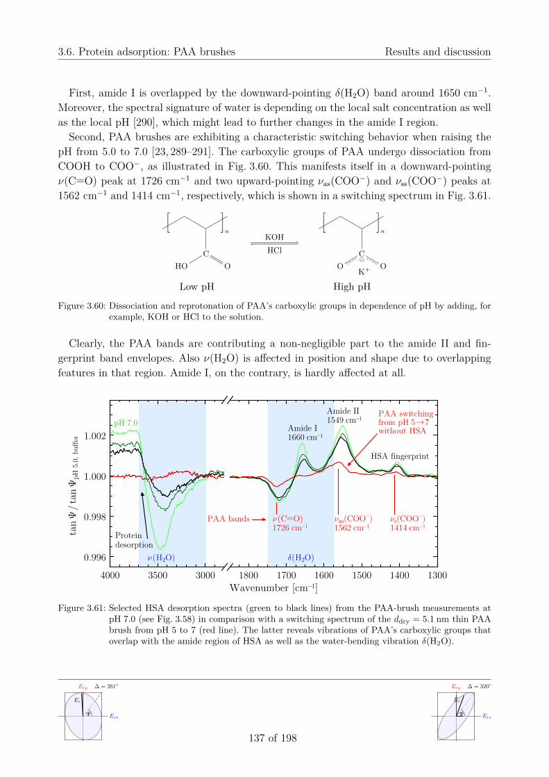
3.6. Protein adsorption: PAA brushes Results and discussion
First, amide I is overlapped by the downward-pointing δ(H2O) band around 1650 cm−1.Moreover, the spectral signature of water is depending on the local salt concentration as wellas the local pH [290], which might lead to further changes in the amide I region.
Second, PAA brushes are exhibiting a characteristic switching behavior when raising thepH from 5.0 to 7.0 [23, 289–291]. The carboxylic groups of PAA undergo dissociation fromCOOH to COO−, as illustrated in Fig. 3.60. This manifests itself in a downward-pointingν(C=O) peak at 1726 cm−1 and two upward-pointing νas(COO−) and νss(COO−) peaks at1562 cm−1 and 1414 cm−1, respectively, which is shown in a switching spectrum in Fig. 3.61.
C
OH O
[ ]
nKOH
HCl C
O O
[ ]
n
K+
Low pH High pH
Figure 3.60: Dissociation and reprotonation of PAA’s carboxylic groups in dependence of pH by adding, forexample, KOH or HCl to the solution.
Clearly, the PAA bands are contributing a non-negligible part to the amide II and fin-gerprint band envelopes. Also ν(H2O) is affected in position and shape due to overlappingfeatures in that region. Amide I, on the contrary, is hardly affected at all.
Proteindesorption
4000 3500 3000 1800 1700 1600 1500 1400 1300
0.996
0.998
1.000
1.002
HSA fingerprint
tan
Ψ /
tan
ΨpH
5.0
, buffer
Wavenumber [cm–1]
pH 7.0
δ ( H2O)ν ( H2O)
PAA bands1726 cm–1 1562 cm–1 1414 cm–1ν (C=O) νas(COO–
) νs(COO– )
1660 cm–1
1549 cm–1
Amide I
Amide II
from pH 5 7→without HSA
PAA switching
Figure 3.61: Selected HSA desorption spectra (green to black lines) from the PAA-brush measurements atpH 7.0 (see Fig. 3.58) in comparison with a switching spectrum of the ddry = 5.1 nm thin PAAbrush from pH 5 to 7 (red line). The latter reveals vibrations of PAA’s carboxylic groups thatoverlap with the amide region of HSA as well as the water-bending vibration δ(H2O).
Erp
ErsΨ
Er
∆ = 261◦
137 of 198
Erp
ErsΨ
Er
∆ = 320◦

Results and discussion 3.6. Protein adsorption: PAA brushes
PAA brushes also swell in the order of some 10% between pH 5.0–7.0 owing to electrostaticrepulsion between the negatively charged COO− groups [289, 291]. It is rather unlikely thatthe swelling behavior and the simultaneous incorporation of buffer ions into the brush [82] arenot influenced by the presence of bound proteins. Changes in swelling would result in differentamounts and distributions of water and buffer ions inside the brush, thereby modifyingamplitude and shape of the water vibrational bands around 3460 cm−1 and 1650 cm−1.
Third, the considerable amount of free charges in the brush–protein system might inducean enhanced switching amplitude of the PAA brush, resulting in much more pronounced car-boxylic bands, which would in turn affect the apparent amide II band shape and amplitude.
All of the aforementioned effects give rise to potentially ambiguous changes or distortionsof the vibrational bands in the desorption spectra and cannot be verified or falsified by pureanalysis of these spectra alone. Additional measurements as well as optical-model calculationsbecome necessary.
c) Swelling behavior and protein content
In order to quantitatively assess the thickness dcombined of the swollen brush–protein layer aswell as its PAA, water, and HSA contents (% PAA, % H2O, and % HSA), the experiment wasrepeated at the IPF Dresden using in-situ VIS ellipsometry. Measured tan Ψ and ∆ spectra
5 5 5 6 7
40
45
50
55
60
65
pH
dco
mbin
ed [nm
]
dcombined
0
20
40
60
80
100
% PAA
Buffer only +HSA Buffer only
% P
AA
, %
H2O
, %
HSA
ΓHSA [m
g/m
2 ] % HSA ΓHSA
% H2O
Figure 3.62: pH-dependent thickness dcombined of the combined brush–protein layer, volume percentage ofPAA (% PAA), water (% H2O) and protein (% HSA) within the brush, as well as the absoluteamount of adsorbed protein ΓHSA as determined by in-situ VIS ellipsometry on the ddry = 4.7 nmthin PAA brush. Starting condition was the PAA brush swollen in a 10 mM buffer solution atpH 5. After several minutes, the solution was exchanged for pH 5 buffer containing 0.25 mg/mlHSA. After 85 min, the solution was consecutively replaced for protein-free buffer solutions atpH 5, 6, and 7, and these were kept inside the cell for 60, 100, and 60 min, respectively. tan Ψ and∆ spectra were recorded at the end of each equilibration period. Measurements and quantitativeevaluation were performed by Eva Bittrich.
Eip
Eis45◦Ei
∆ = 0◦
138 of 198

3.6. Protein adsorption: PAA brushes Results and discussion
were evaluated with a three-component EMA layer of brush/buffer/protein. The absoluteamount of adsorbed protein ΓHSA was derived using a modified de Feijter approach [82, 295].
Figure 3.62 shows pH-dependent results for dcombined, % PAA, % H2O, % HSA, and ΓHSA.At pH 5 without protein, the brush is swollen by a factor of 8.5 compared to the dry state.With 89 vol%, its water content is accordingly high. After exchanging the solution for a HSAsolution with c = 0.25 mg/ml, the swollen-brush thickness increased from 39.7 nm to 43.8 nmand decreased again to 42.1 nm after replacing the solution for protein-free buffer. Withinthe experimental errors, however, ΓHSA decreased only marginally. This deswelling of thebrush confirms the previous observations of an almost constant amide II band and slightlydiminishing amide I and ν(H2O) bands when exchanging the HSA solution for protein-freebuffer.
At pH 6, partial protein desorption takes place. Simultaneously, the brush begins to swellwhile binding additional buffer solution. At pH 7, the majority of proteins desorbs, with14% remaining adsorbed to the brush compared to the pH 5 state. This is a surprisinglysimilar value compared to the amide I amplitude ratio of 12% between final desorption stateat pH 7.0 and initial state at pH 5.4 in the in-situ infrared-ellipsometry measurements. Thisalso suggests that the main contribution in the final amide II band envelope must havenon-protein origins.
Lastly, the brush is swollen to almost 60 nm at pH 7 with a correspondingly high buffercontent. This swelling behavior of PAA brushes—and polyelectrolyte brushes in general—isnot yet fully understood by means of infrared spectroscopy. The VIS-ellipsometric results,however, allow one to estimate the effects of COOH dissociation on the HSA–PAA spectra,as will be discussed in the next section.
d) Analyzing the spectrally overlapping effects
In order to understand the final desorption spectrum in Figs. 3.58 and 3.61, a detailedlook at the PAA-specific bands is necessary. The top panel of Fig. 3.63 shows measuredinfrared-ellipsometric tan Ψ spectra [23] of a PAA brush switched between pH 2 and 10.COOH → COO− dissociation at increasing pH is revealed by corresponding changes in theν(C=O) and ν(COO−) bands, as discussed before. Another band at 1250 cm−1 is attributedto ν(CO) of the non-ionized COOH groups. The broad band around 2050 cm−1 can be as-signed to a combination of far-infrared PAA bands with δ(H2O) [296]. A second broad fea-ture observed at about 2580 cm−1 is associated with vibrations of COOH−H2O-interactedcarboxylic groups [296]. Upward- and downward-pointing bands respectively correlate withincreasing and decreasing amounts of corresponding vibrations with respect to the referencespectrum at pH 2.
Similar to the swelling behavior of PNIPAAm brushes discussed in Section 3.5., one wouldexpect distinct ν(H2O) and δ(H2O) bands of large amplitude, knowing that the brush is
Erp
ErsΨ
Er
∆ = 261◦
139 of 198
Erp
ErsΨ
Er
∆ = 330◦

Results and discussion 3.6. Protein adsorption: PAA brushes
{
� ( )�( )
{
� ( {){
{� ( {)
{
{
�( ) � ( ){
!!!!
[ { ]
� ( )
� ( )� ( {)
� ( {)
�( ) �( )
Figure 3.63: Top: In-situ tan Ψ measurements from Ref. [23] showing the switching of the ddry = 5.1 nmthin PAA brush from pH 2 to 10 in steps of pH 1 by adding KOH to the solution. Spectraare referenced to the initial state at pH 2. Upward- and downward-pointing bands thereforerespectively correlate with increasing and decreasing amounts of the corresponding molecularvibrations with respect to that state. Bottom: PAA switching spectra from pH 5 to 7 (red line),8 (green line), and 9 (blue line) in comparison with the final HSA desorption spectrum (blackline) from the PAA-brush measurements at pH 7.0 (see Fig. 3.58).
swelling by several 10 nm with increasing pH. On the contrary, no unambiguous water bandis visible in the δ(H2O) region between 1700–1600 cm−1, whereas a sigmoidal band shapeis found between 3700–3000 cm−1 in the ν(H2O) region. This shape is probably related tothe fact that the local pH inside the brush is influenced by the local salt concentrationdepending on the distance from the substrate. Theoretical investigations by Gong et al. [290]show that for a PAA brush with a grafting density of σ = 0.30 nm−2, the local pH variesbetween 4.2 and 5.8 if the buffer solution has a pH of 5.8. With this difference, the vibrationalbands of water, which overlap with the PAA bands, change accordingly [239, 297], and so doPAA–buffer interactions.
The lower panel of Fig. 3.63 shows a comparison between the final HSA–PAA desorp-tion spectrum and three PAA switching spectra from pH 5 → 7, pH 5 → 8, and pH 5 → 9without protein. Striking similarities are found in the 1800–1100 cm−1 region, whereas the
Eip
Eis45◦
Ei
∆ = 0◦
140 of 198

3.6. Protein adsorption: PAA brushes Results and discussion
{{{ !
!!
[ { ]
�( ) �( )
Figure 3.64: Ratios between final referenced HSA–PAA desorption tan Ψ spectrum at pH 7.0 (see Fig. 3.58)and referenced PAA switching spectra from pH 5 to 7 (red line), 8 (green line), and 9 (blueline). Taking the ratio should remove PAA-specific bands and leave only bands that are due toremaining adsorbed HSA.
water-stretching region between 3700–3000 cm−1 differs notably. This is, in part, explainedby the small absolute amount of still-adsorbed protein, but the similar relative amounts of% PAA = 7.7% and % HSA = 5.5%, which both are very small compared to % H2O = 83.2%.Bulk-like water contributions therefore still dominate the ν(H2O) region of the HSA–PAAspectrum. The PAA and HSA bands, however, are of the same order of magnitude. Further-more, amide I is almost unaffected by overlapping PAA bands, while amide II is enhancedby νas(COO−). The amplitude ratios between the amide bands and the other characteristicHSA bands can therefore be used to compare the relative band amplitudes with the onesobtained from HSA transmission measurements in order to determine the contributions ofthe PAA bands to the spectral composition. With these considerations in mind, the influenceof the COOH and COO− bands on the HSA–PAA spectrum is now estimated based on theassumption that the different samples from the HSA and PAA swelling experiments yieldcomparable switching amplitudes.
Figure 3.64 displays the ratio between the final HSA–PAA spectrum and the three PAAswitching spectra from pH 5 to 7, 8, and 9. The bands at 2580 cm−1 and 2050 cm−1 are nolonger present due to the referencing, hence indicating the applicability of the method. Theupward-pointing amide I band is still overlapped by the downward-pointing δ(H2O) band.From optical simulations, the ratio between δ(H2O) and ν(H2O) band amplitude is known tobe approximately 0.5. With this knowledge, the δ(H2O) band can then be subtracted fromamide I. This finally allows one to compare the amide I/II and amide/fingerprint ratios forthe different PAA switching spectra. Best agreement is found if the brush is switching frompH 5.0 to 8.5.
Erp
ErsΨ
Er
∆ = 261◦
141 of 198
Erp
ErsΨ
Er
∆ = 340◦

Results and discussion 3.6. Protein adsorption: PAA brushes
The above result does not imply a pH of 8.5 within the PAA brush, because the spectra onlyreflect relative pH-induced changes. It rather suggests a larger local pH difference inside thebrush due to differently distributed ions and counterions if protein is adsorbed and then partlydesorbed again. The large amount of free charges within the brush–protein system thereforeseems to cause an enhanced switching amplitude of the PAA brush, which is equivalentlyinduced if the buffer solution shows a pH difference of (8.5 − 5.0) = 3.5. These findings arein agreement with several investigations that demonstrate a counterion redistribution in thepresence of proteins [82, 298] as well as charge-regulation processes of brush and proteinsupon protein adsorption and desorption [39, 82, 288, 299].
e) Future studies using optical simulations
In-situ infrared ellipsometry turned out to be a very useful method for investigating proteinadsorption on polymer brushes. By analyzing the protein-specific amide bands, it was shownthat HSA adsorption and desorption at PAA brushes can be monitored in-situ with a timeresolution of at least 85 s. Next to protein desorption, chemical changes of the brush couldbe observed upon increasing pH. Interpreting in-situ IR-SE spectra quantitatively, however,is a difficult task, because the various different effects at the solid–liquid interface yieldoverlapping spectral information. Nevertheless, a semi-quantitative evaluation was possiblewith the help of additional input from in-situ VIS ellipsometry measurements. It could thenbe demonstrated that the presence of proteins leads to changes in the pH-dependent switchingbehavior of the brush.
In the end, full optical simulations are imperative for a deeper quantitative understandingof structure and chemistry of brush and protein. Systematic studies are needed that allowone to distinguish the several overlapping effects that make for the effective refractive in-dex of the brush–protein system. In the first step, the swelling and dissociation behavior ofPAA brushes has to be described in dependence of salt concentration and distribution byan appropriate effective-medium model. This model must include the buffer solution as wellas the polymer in the form of separate low-pH and high-pH carboxyl oscillators in order toquantify brush–buffer interactions correctly. The brush profile might be considered, too. Inthe second step, the optical constants of the protein, as determined, e. g., from ATR ellip-sometry or transmission measurements, are used to model protein adsorption and desorptionat the brush in a three-component brush/buffer/protein mEMA model, similar to the spec-tra evaluation of VIS-ellipsometry data. This should reveal the interactions among the threecomponents at a quantitative level. Preliminary results as well as the successful quantitativemodeling of PNIPAAm brushes in Section 3.5. already indicate that this modeling processis indeed feasible.
Eip
Eis45◦
Ei
∆ = 0◦
142 of 198

4. Summary and outlook
Functional polymer films have great potential for possible biochemical and biomedical appli-cations. In particular, surfaces that are tunable in dependence of external stimuli like tem-perature are of special interest. Infrared ellipsometry and microscopy are two techniques thatallow one to probe the structural and chemical properties of such organic surfaces. Moreover,these techniques are applicable for in-situ purposes. Up until now, the biggest obstacle wasto quantitatively separate the different effects that occur at the solid–liquid interface when asample is in contact with aqueous environment. This problem was successfully tackled in thisthesis. New experimental as well as optical-modeling strategies were developed that enableone to access various sample properties, such as layer thicknesses, water content, and—mostimportantly—changing interactions among and between the sample constituents and solvent.
Infrared ellipsometry was used to determine the optical constants of spin-coated 55–135 nmthick PNIPAAm and PGMA films in dry state, which served as the foundation for subsequentquantitative spectra evaluation of stimuli-dependent experiments. The optical constants werebuilt from sums of oscillator contributions corresponding to the molecular vibrations of thepolymers. The amide I and II bands of PNIPAAm were found to consist of respectivelythree and two subcomponents that are related to different polymer–polymer hydrogen-bondinteractions between C=O and N−H groups of the polymer.
A variety of humidity-dependent infrared-microscopic measurements on PNIPAAm filmsin H2O and D2O vapor were conducted in order to identify different polymer–water hydrogen-bond interactions. The set of dry-state PNIPAAm oscillators was consequently extended forseveral new wet-state oscillators. With this extended set at hand, it was possible to modelPNIPAAm films at different humidities. A modified EMA approach allowed one to quantifythickness and water content of the swollen polymer layers, as well as to track changingpolymer–polymer and polymer–water interactions throughout the drying process of the films.This yielded deeper insights into the different hydration states of PNIPAAm.
Next, 4.0–14.5 nm thin PNIPAAm brushes were characterized in dry state in dependenceof grafting density and molecular weight. Ellipsometric spectra could be described with theoptical constants of the spin-coated films. Small changes in the band composition of amide Iand II compared to the thicker films were assigned to larger relative amounts of surface-exposed non-interacted amide groups. Time-dependent N -deuteration experiments revealedthe relative strengths of hydrogen bonding inside the brushes. Deuterated-brush spectra weremodeled by redshifting the corresponding amide oscillators. PNIPAAm brushes in humid airshowed similar swelling effects and polymer–water interactions as the thicker films.
The temperature-dependent swelling behavior of PNIPAAm brushes in aqueous envi-ronment was successfully monitored with in-situ infrared ellipsometry. To achieve this, anexisting in-situ cell was mounted to a redesigned sample holder with a PID-controlled Peltier
Erp
ErsΨ
Er
∆ = 261◦
143 of 198
Erp
ErsΨ
Er
∆ = 350◦

Summary and outlook
heating-and-cooling system that features a stability of ±0.05 ℃. This made it possible toseparate the spectral information of brush and overlapping bulk-water signature. Measure-ments in H2O and D2O, then, gave insights into changing interactions during (de)swelling.
The main goal was to describe ellipsometric in-situ spectra at a quantitative level. Sincethe optical properties of water vary strongly in the probed temperature range of 20–50 ℃, theoptical constants of H2O and D2O had to be determined first. Transmission measurementswere performed using special cells with micrometer-short path lengths in order to resolve thestrong vibrational bands of water. A careful optical-modeling strategy was pursued to fit onthe optical constants with a high enough accuracy for the following brush evaluation.
After introducing a baseline-correction procedure for in-situ infrared-ellipsometric spectra,a spin-coated thick PGMA film served as the first test sample. As expected, the film showedalmost no swelling. The layer thickness, as previously determined from ex-situ measure-ments, could be reproduced correctly. Afterwards, a PNIPAAm brush of 14.5 nm dry-statethickness was measured below and above its lower critical solution temperature (LCST),the temperature around which the brush undergoes a phase transition from an extended toa collapsed state. Again, spectra were modeled successfully. Swollen-brush thicknesses andwater contents showed similar tendencies as determined by VIS ellipsometry on comparablebrushes. The swelling and deswelling behavior was confirmed, and most importantly, chang-ing polymer–polymer and polymer–water interactions were identified based on the set ofdry- and wet-state oscillators. Below the LCST, the brush is strongly hydrated, such thatpolymer–water interactions dominate. Nevertheless, about a fifth of PNIPAAm’s C=O groupsform mixed hydrogen bonds with water and neighboring H−N groups. Above the LCST, thebrush collapses and releases a significant amount of water. Polymer–water interactions arestill present, but C=O groups tend to form hydrogen bonds with two H−N groups.
A semi-quantitative analysis was performed concerning protein monolayers and solutions ofhuman serum albumin (HSA), as well as HSA-repelling and -adsorbing PNIPAAm and PAAbrushes, respectively. Time-resolved infrared ellipsometry allowed the monitoring of protein-adsorption processes on PAA brushes at pH 5 with subsequent controlled protein-desorptionat increasing pH. Simultaneously, an enhanced switching amplitude of the PAA brushes wasfound. Complementary in-situ VIS-ellipsometric measurements gave quantitative informationabout PAA, water, and HSA contents as well as the amount of still-adsorbed protein.
All in all, in-situ infrared ellipsometry and microscopy on organic films in contact withwater or water vapor as well as protein solutions have proven to be valuable tools for gaining adeeper understanding of film properties and interactions. For the first time, spectra were eval-uated quantitatively on the basis of physical models. The successful modeling of PNIPAAmbrushes, which proved it possible to separate film effects and interactions, is the cornerstonefor future investigations on more complicated material systems like mixed brushes, and forstudying, for example, structural changes of proteins during adsorption to thin films.
Eip
Eis45◦
Ei
∆ = 0◦
144 of 198

Appendices
A. Details on Fourier-transform spectrometersFourier-transform spectrometers offer several advantages compared to dispersive spectrome-ters. All spectral components emitted by the globar are measured simultaneously, limited onlyby the absorption properties of the used optical elements in the set-up like beamsplitter andtransmission windows. A consequence of this so-called multiplex or Fellgett advantage [300]is an increased signal-to-noise ratio because no monochromator is needed to scan the wholespectrum. The Jacquinot advantage [301] refers to the fact that monochromators also re-quire entrance and exit slits, which in turn decrease the throughput. In Fourier-transformspectrometers, however, the throughput is determined only by a single circular Jacquinotaperture that limits the diameter of the collimated globar beam.
Globars are silicon carbide rods heated to elevated temperatures between about 1000 ℃ and1600 ℃. Their spectral behavior is comparable to that of a black-body radiator, which allowsone to measure a wide spectral range at once. Close to the path of the actual globar radiation,light from a HeNe laser is being sent through the interferometer. Its purpose is twofold. Viaan appropriate internal detector, on the one hand, it enables the measuring of the mirrorposition by evaluating the corresponding sinusoidal laser interferogram [105]. Zero-crossingsin this interferogram then trigger the sampling of the globar interferogram at equidistantpositions, which is necessary for standard Fourier-transform algorithms [101]. The accuracyand stability of the laser wavelength at 632.8 nm (1/15802 cm−1) directly correlate withan accurate determination of the mirror position—usually better than 0.005 µm [105]—andconsequently, they make for a very high wavenumber accuracy < 0.01 cm−1. This automaticinternal wavenumber calibration [105] is known in the literature as Connes’ advantage [302].On the other hand, the HeNe laser ensures a coherent superposition of interferograms fromconsecutive scans [303], which is of special importance for in-situ measurements that can lastseveral minutes or even hours.
Two important points concern the actual Fourier transform of the interferogram: apodiza-tion and zero-filling. Defining the optical path length L as twice the mirror displacement,L = 2z, the interferogram in an ideal spectrometer measured with an ideal detector is givenby [1]
I(L) =+∞
−∞
I(ν̃) cos(2π ν̃L) dν̃ ⇔ I(ν̃) =+∞
−∞
I(L) cos(2π ν̃L) dL , (A.1)
where integration over L from −∞ to +∞ results in a spectrum I(ν̃) over the wholewavenumber range. In practice, however, the mirror displacement is limited, meaning that
Erp
ErsΨ
Er
∆ = 261◦
145 of 198
Erp
ErsΨ
Er
∆ = 0◦

Appendices A. Details on Fourier-transform spectrometers
the maximum optical path length is a finite value Lmax. In a computational implementationof the Fourier transform, e. g., the Fast-Fourier transform (FFT) algorithm [101], the inte-gral therefore has to be replaced by a finite sum with limits ±Lmax. This causes artifacts inthe transformed spectra [304] which have to be accounted for appropriately: A naïve boxcartruncation introduces sidelobes to the true instrument line shape. In order to remove these,an apodization function D(L) that smoothly decays to zero at ±Lmax is inserted as a convo-lution function into the Fourier transform in Eq. (A.1) [1, 104, 105]. While different functions(triangular, bell-shaped, etc.) with different effects on sidelobes and maximum resolutionare discussed in the literature [104, 303, 305], the Blackman–Harris three-term apodizationfunction [256] is solely used in the present work.
The Fast-Fourier transform requires that the number of data points in the interferogramis a power of 2. To fulfill this requirement, the appropriate number of zeros is added tothe ends of the interferogram. This so-called zero-filling is also applied for other reasons:First, if desired, to maintain the number of data points for spectra recorded at differentresolutions [305]. And second, it is used to reduce the picket-fence effect [306, 307] that ariseswhen the spectrum contains sharp features that do not coincide with the sampling points ofthe FFT [308]. A zero-filling factor of 2 (recommended standard) or even 4 or 8, then, provessufficient in order to interpolate the spectrum and increase its quality [105, 308]. Zero-fillingis important, for example, for measurements on polymers with very sharp vibrational bands.
For further details on Fourier-transform spectrometers, the interested reader is referred toRefs. [1, 105, 199, 306, 307].
Eip
Eis45◦
Ei
∆ = 0◦
146 of 198

B. Details on imperfect optical components Appendices
B. Details on measurements with imperfect opticalcomponents
This appendix provides additional information about the Müller matrix formalism intro-duced in Section 2.1.4.b). Müller matrices Mn are usually derived in the eigensystems of theoptical elements. When calculating the matrix of the whole system, they therefore have to betransformed into the system of the incident Stokes vector. This is accomplished by rotatormatrices R(α):
R(α) ≡ MRot(α) =
1 0 0 00 cos 2α sin 2α 00 − sin 2α cos 2α 00 0 0 1
(B.1)
In the cartesian coordinate system defined with the z axis parallel to the propagation direc-tion of the light, rotation about an angle α transforms a Stokes vector according to
S ′(α) = R(α)S . (B.2)
In order to transfrom Müller matrices from their eigensystem into the original coordinatesystem, incident and resulting Stokes vectors are subject to inverse rotations,
Mnew(α) = R(−α) · Mold · R(α) . (B.3)
Overview of Müller matrices:Ideal polarizer with transmission axis in x direction with respect to the cartesian coordinatesystem (defined by the plane of incidence):
MPol = 12
1 1 0 01 1 0 00 0 0 00 0 0 0
(B.4)
Non-ideal polarizer with degree of polarization smaller than 1, parameterized by themaximum and minimum transmittances τM and τm:
MPol(ϑ) = K ×
1 cos 2ϑ 0 0
cos 2ϑ 1 0 00 0 sin 2ϑ 00 0 0 sin 2ϑ
(B.5)
Erp
ErsΨ
Er
∆ = 261◦
147 of 198
Erp
ErsΨ
Er
∆ = 10◦

Appendices B. Details on imperfect optical components
Here, K = τM + τm
2 , cos 2ϑ = τM − τm
τM + τm≡ degree of polarization, sin 2ϑ = 2√
τMτm
τM + τm, and
tanϑ =τm/τM ≡ attenuation. For ideal polarizers, τm = sin 2ϑ = tanϑ = 0 and cos 2ϑ = 1.
Ideal retarder with phase shift δRet = δf − δs between fast (f) and slow (s) axis:
MRet(δRet) =
1 0 0 00 1 0 00 0 cos δRet sin δRet0 0 − sin δRet cos δRet
(B.6)
Products of the matrices (B.5) and (B.6) now allow one to describe polarization effects ofreal retarders, isotropic samples, and non-ideal polarizers [89, 94, 309]:
Real retarder with phase shift δRet = δf − δs and tanψRet =τf/τs ̸= 0:
MRet(ψRet, δRet) = KR ×
1 − cos 2ψRet 0 0
− cos 2ψRet 1 0 00 0 sin 2ψRet cos δRet sin 2ψRet sin δRet0 0 − sin 2ψRet sin δRet sin 2ψRet cos δRet
KR = τs + τf
2 (B.7)
Note that the sign of ψRet is mere definition.
Isotropic reflecting surface with ellipsometric parameters tan Ψ and ∆ as well as reflectioncoefficients rp and rs:
MSample(Ψ,∆) = KS ×
1 − cos 2Ψ 0 0
− cos 2Ψ 1 0 00 0 sin 2Ψ cos ∆ sin 2Ψ sin ∆0 0 − sin 2Ψ sin ∆ sin 2Ψ cos ∆
KS = |rp|2 + |rs|2
2 (B.8)
Anisotropic, depolarizing, or optically active samples exhibit non-zero block-off-diagonal ma-trix elements. Measuring their whole Müller matrix usually requires two retarders in theoptical train, one before and one after the sample.
Eip
Eis45◦
Ei
∆ = 0◦
148 of 198

B. Details on imperfect optical components Appendices
Wire-grid polarizer with additional phase shift δ = δM−δm between τM and τm component:
MPol(ϑ, δ) ≡ MPol(ϑ) · MRet(δ) = K ×
1 cos 2ϑ 0 0
cos 2ϑ 1 0 00 0 sin 2ϑ cos δ sin 2ϑ sin δ0 0 − sin 2ϑ sin δ sin 2ϑ cos δ
(B.9)
Wire-grid polarizer with arbitrary orientation α of the τM axis:
MPol(ϑ, δ, α) ≡ R(−α) · MPol(ϑ, δ) · R(α) , (B.10)
= K ×
1 c · cos 2α c · sin 2α 0
c · cos 2α cos2 2α + s · sin2 2α cos δ sin 2α cos 2α(1 − s · cos δ) −s · sin 2α sin δc · sin 2α sin 2α cos 2α(1 − s · cos δ) sin2 2α + s · cos2 2α cos δ s · cos 2α sin δ
0 s · sin 2α sin δ −s · cos 2α sin δ s · cos δ
As before,
K = τM + τm
2 , c = cos 2ϑ = τM − τm
τM + τm, s = sin 2ϑ = 2√
τMτm
τM + τm, δ = δM − δm . (B.11)
The small intensity of infrared light sources limits the feasible number of measurements atdifferent polarizer settings. Four azimuth combinations (α1, α2) with at least one non-parallelsetting are sufficient to accurately determine both Ψ and ∆. With αi = 0◦, 45◦, 90◦, and 135◦,the trigonometric functions appearing in the polarizer Müller matrices simplify to 0 or ±1:
MPol(ϑi, δi,t
0◦90◦
45◦135◦
|
) = Ki ×
1
q±ci0y q 0
±ci
y0
q±ci0y q 1
si cos δi
y0
q 0∓si sin δi
y
q 0±ci
y0
qsi cos δi
1y q
±si sin δi0
y
0q 0
±si sin δi
y q∓si sin δi
0y
si cos δi
(B.12)
Here, si = sin 2ϑi and ci = cos 2ϑi, with i = 1, 2 for the first and second polarizer.
With Müller matrices for the several optical elements at hand, it is now possible to calculatethe detector intensities for calibration and sample measurements:
E(α1, α2) ≡ MPol(ϑ2, δ2, α2) · MPol(ϑ1, δ1, α1) · S̄ ,R(α1, α2) ≡ MPol(ϑ2, δ2, α2) · MRet(ψRet, δRet) · MPol(ϑ1, δ1, α1) · S̄ ,I(α1, α2) ≡ MPol(ϑ2, δ2, α2) · MSample(Ψ,∆) · MPol(ϑ1, δ1, α1) · S̄ ,I(α1, α2) ≡ MPol(ϑ2, δ2, α2) · MRet(ψRet, δRet) · MSample(Ψ,∆) · MPol(ϑ1, δ1, α1) · S̄
(B.13)
Erp
ErsΨEr
∆ = 261◦
149 of 198
Erp
ErsΨ
Er
∆ = 20◦

Appendices B. Details on imperfect optical components
Equations (B.13) are now given explicitly for the azimuths αi = 0◦, 90◦, 45◦, and 135◦ usingsymbolic notation
8
8
≡
0◦
90◦
and
88
≡
45◦
135◦
.
Empty-channel detector intensities without retarder
E 8
8
, 8
8
= K1K2
s̄01 + [±c1][±c2]
+ s̄1 [±c1 ± c2]
(B.14)
E 8
8, 8
8
= K1K2
s̄01 + [±c1][±c2]
+ s̄2 [±c1 ± c2]
(B.15)
E 8
8
, 8
8
= K1K2
s̄0 + s̄1 [±c1] + s̄2 [s1][±c2] cos δ1 + s̄3 [±s1][±c2] sin δ1
(B.16)
E 8
8, 8
8
= K1K2
s̄0 + s̄2 [±c1] + s̄1 [s1][±c2] cos δ1 − s̄3 [±s1][±c2] sin δ1
(B.17)
Detector intensities of sample without retarder
I 8
8
, 8
8
= K
s̄01 + [±c1][±c2]
+ s̄1 [±c1 ± c2]
− cos 2Ψs̄0 [±c1 ± c2] + s̄1
1 + [±c1][±c2]
(B.18)
I 8
8, 8
8
= K
s̄0 + s̄2 [±c1] − cos 2Ψs̄1 [s1] cos δ1 − s̄3 [±s1] sin δ1
+ sin 2Ψ cos ∆
s̄0 [±c1][±c2] + s̄2 [±c2]
+ sin 2Ψ sin ∆
s̄1 [±s1][±c2] sin δ1 + s̄3 [s1][±c2] cos δ1
(B.19)
I 8
8, 8
8
= K
s̄0 + s̄1 [±c1] − cos 2Ψs̄0 [±c1] + s̄1
+ sin 2Ψ cos ∆
s̄2 [s1][±c2] cos δ1 + s̄3 [±s1][±c2] sin δ1
+ sin 2Ψ sin ∆
s̄3 [s1][±c2] cos δ1 − s̄2 [±s1][±c2] sin δ1
(B.20)
I 8
8, 8
8
= K
s̄0 + s̄1 [s1][±c2] cos δ1 + s̄2 [±c1] − s̄3 [±s1][±c2] sin δ1
− cos 2Ψs̄0 [±c2] + s̄1 [s1] cos δ1 + s̄2 [±c1][±c2] − s̄3 [±s1] sin δ1
(B.21)
K ≡ K1K2KS
Eip
Eis45◦
Ei
∆ = 0◦
150 of 198

B. Details on imperfect optical components Appendices
Empty-channel detector intensities with retarder
Retarder calibration measurements of ψRet and δRet correspond to a sample measurementin which the retarder acts as sample. Detector intensities R(α1, α2) can therefore beobtained from Eqs. (B.18)–(B.21) using the substitution
R(α1, α2) = I(α1, α2)Ψ→ψRet,∆→δRet,KS→KR
. (B.22)
Detector intensities of sample with retarder
With the help of the addition theorems
cos ∆ cos δ − sin ∆ sin δ = cos(∆ + δ) ,sin ∆ cos δ + cos ∆ sin δ = sin(∆ + δ) ,
(B.23)
one finds that the phase shifts of sample and retarder add up.
I 8
8
, 8
8
= K1 + cos 2Ψ cos 2ψRet
s̄01 + [±c1][±c2]
+ s̄1 [±c1 ± c2]
−cos 2Ψ + cos 2ψRet
s̄0 [±c1 ± c2] + s̄1
1 + [±c1][±c2]
(B.24)
I 88, 8
8
= K1 + cos 2Ψ cos 2ψRet
s̄0 + s̄2 [±c1]
−cos 2Ψ + cos 2ψRet
s̄1 [s1] cos δ1 − s̄3 [±s1] sin δ1
+ sin 2Ψ sin 2ψRet cos(∆+δRet)
s̄0 [±c1][±c2] + s̄2 [±c2]
+ sin 2Ψ sin 2ψRet sin(∆+δRet)
s̄1 [±s1][±c2] sin δ1 + s̄3 [s1][±c2] cos δ1
(B.25)
I 88
, 8
8
= K1 + cos 2Ψ cos 2ψRet
s̄0 + s̄1 [±c1]
−cos 2Ψ + cos 2ψRet
s̄0 [±c1] + s̄1
+ sin 2Ψ sin 2ψRet cos(∆+δRet)
s̄2 [s1][±c2] cos δ1 + s̄3 [±s1][±c2] sin δ1
+ sin 2Ψ sin 2ψRet sin(∆+δRet)
s̄3 [s1][±c2] cos δ1 − s̄2 [±s1][±c2] sin δ1
(B.26)
I 88, 8
8
= K1 + cos 2Ψ cos 2ψRet
s̄0 + s̄1 [s1][±c2] cos δ1 + s̄2 [±c1] − s̄3 [±s1][±c2] sin δ1
−cos 2Ψ + cos 2ψRet
s̄0 [±c2] + s̄1 [s1] cos δ1 + s̄2 [±c1][±c2] − s̄3 [±s1] sin δ1
(B.27)
K ≡ K1K2KSKR
Erp
ErsΨEr
∆ = 261◦
151 of 198
Erp
ErsΨ
Er
∆ = 30◦

Appendices B. Details on imperfect optical components
tan Ψ and ∆ from rotating-polarizer or rotating-analyzer measurements:In addition to tan Ψ measurements with parallel polarizers, equations for measurements withfixed analyzer or polarizer are now presented. If the detector exhibits polarization-dependentproperties, it is preferable to measure tan Ψ with a fixed analyzer at different polarizerpositions. The analyzer, then, is commonly set to 45◦ or 135◦. For strong or varying sourcepolarization and “benign detectors” on the other hand, the polarizer is held fixed at 45◦,while the analyzer is being rotated. This measuring mode is important, for example, formeasurements at a synchrotron (BESSY II) where the beam properties usually show strongtime dependence.
The following equations show intensity combinations for the cases of rotating-polarizer androtating-analyzer with 0◦/90◦ and 45◦/135◦ azimuths of the non-fixed polarizer.
Rotating polarizer:
I( 8 , 8 ) − I( 8 , 8 )I( 8 , 8 ) + I( 8 , 8 ) =
c1
s̄1
s̄0− cos 2Ψ
+ s1c2 sin δ1
− s̄3
s̄0sin 2Ψ cos ∆ + s̄2
s̄0sin 2Ψ sin ∆
1 − s̄1
s̄0cos 2Ψ + s1c2 cos δ1
− s̄2
s̄0sin 2Ψ cos ∆ − s̄3
s̄0sin 2Ψ sin ∆
(B.28)
I( 8 , 8 ) − I( 8 , 8 )I( 8 , 8 ) + I( 8 , 8 ) =
c1
s̄2
s̄0− sin 2Ψ cos ∆ c2
+ s1 sin δ1
s̄3
s̄0cos 2Ψ − s̄1
s̄0sin 2Ψ sin ∆ c2
−1 + s̄2
s̄0sin 2Ψ cos ∆ c2 + s1 cos δ1
s̄1
s̄0cos 2Ψ + s̄3
s̄0sin 2Ψ sin ∆ c2
(B.29)
Rotating analyzer:
I( 8 , 8 ) − I( 8 , 8 )I( 8 , 8 ) + I( 8 , 8 ) = −
c2
cos 2Ψ
1 + s̄2
s̄0c1
+ s1
− s̄1
s̄0cos δ1 + s̄3
s̄0sin δ1
1 + s̄2
s̄0c1 − cos 2Ψ s1
s̄1
s̄0cos δ1 − s̄3
s̄0sin δ1
(B.30)
I( 8 , 8) − I( 8 , 8 )I( 8 , 8) + I( 8 , 8 ) =
c2
sin 2Ψ cos ∆
s̄2
s̄0+ c1
+ sin 2Ψ sin ∆ s1
s̄3
s̄0cos δ1 + s̄1
s̄0sin δ1
1 + s̄2
s̄0c1 − cos 2Ψ
s̄1
s̄0s1 cos δ1 − s̄3
s̄0s1 sin δ1
(B.31)
Equations (B.28)–(B.31) can be solved for tan Ψ and cos ∆ with prior knowledge of theimperfection parameters ci, si, and δi as well as the Stokes parameters s̄0, s̄1, s̄2, and s̄3;see Subsection 1. in Section 2.1.4.b). Similar equations are obtained for measurements withretarder, which are necessary for determinating ∆ between 0◦ and 360◦.
Eip
Eis45◦
Ei
∆ = 0◦
152 of 198

C. Abelès transfer-matrix method Appendices
C. Abelès transfer-matrix methodThe Abelès method allows one to calculate p- and s-polarized reflection and transmissioncoefficients of an isotropic multi-layer stack with isotropic ambient and substrate. Free pa-rameters of the model are the layer thicknesses dj and complex refractive indices Nj =
√εj,
together with the ambient and substrate parameters Na =√εa and Ns =
√εs. The 2 × 2
transfer matrices of ambient, substrate, and layers read [1, 6, 310]
T p, sAmb =
qp,s(ϕa, Na) 1qp,s(ϕa, Na) −1
, (C.1)
T p, sSub =
1 0
qp,s(ϕs, Ns) 0
, (C.2)
T p, sj =
cos βj i sin βj / qp,s(ϕj, Nj)
i sin βj · qp,s(ϕj, Nj) cos βj
, (C.3)
with the abbreviations
qp(ϕ,N) ≡ cosϕ/N, qs(ϕ,N) ≡ cosϕ ·N, (C.4)
and the angular phase thickness βj of the j-th layer,
βj = 2π ν̃ cosϕj Nj dj . (C.5)
The product Nj dj is often referred to as the optical thickness of the layer. The transmissionangles ϕj inside the j-th layer are calculated by Snell’s law, Nj sinϕj = Nj+1 sinϕj+1. Finally,reflection and transmission coefficients as well as reflectivity and transmittance in p ands direction are calculated from Eqs. (C.1)–(C.3) by [1, 6, 310]
rp = T p21
T p11, Rp = |rp|2 , tp = 2qp(ϕa, Na)
T p11
, Tp =Reqp(ϕs , Ns)
Reqp(ϕa, Na)
|tp|2 , (C.6)
rs = T s21
T s11, Rs = |rs|2 , ts = 2qs(ϕa, Na)
T s11
, Ts =Reqs(ϕs , Ns)
Reqs(ϕa, Na)
|ts|2 . (C.7)
The ellipsometric ratios ρ = tan Ψ · ei∆ = rp/rs and ρ̃ = tan Ψ̃ · ei∆̃ = tp/ts are readilycomputed using the above equations. Unpolarized reflectivity and transmittance are given
Erp
ErsΨEr
∆ = 261◦
153 of 198
Erp
ErsΨ
Er
∆ = 40◦

Appendices C. Abelès transfer-matrix method
byR = Rp +Rs
2 and T = Tp + Ts2 . (C.8)
If the substrate cannot be regarded as semi-infinite and reflections from its backside have tobe considered, then—according to the sample geometry shown in Fig. 2.17—the substratehas to be treated as a regular layer with defined thickness ds, and the ambient (usually air)is being promoted to the new substrate.
Taylor expansion of T p, sj reveals that transfer matrices of very thin layers commute to
first order. Although ellipsometry is very sensitive to thin-film layer thicknesses, this showsthat it is very difficult to determine the order of layers in unknown thin-film layer stacks.Systematic sample characterization after each preparation step is therefore preferred whendealing with complex-structured samples, if possible.
Eip
Eis45◦
Ei
∆ = 0◦
154 of 198

D. VIS-ellipsometric pre-characterization of spin-coated polymer films Appendices
D. VIS-ellipsometric pre-characterization ofspin-coated polymer films
Figure D.1 displays measured and joint-fitted Ψ and ∆ spectra of the spin-coated PGMAand PNIPAAm films that were introduced in Section 3.1.2. Films were prepared on Si (111)and Au substrates and measured at three different angles of incidence.
Ψ, ∆
[ °
]
Ψ
∆
Ψ
∆
300 400 500 600 700 8000
50
100
150
200
250
300 Measured Fitted
PGMA
Wavelength [nm]
400 500 600 700 8000
50
100
150
200
250
300PNIPAAm
Measured Fitted
Ψ, ∆
[ °
]
Wavelength [nm]
Figure D.1: Measured (black lines) and fitted (green lines) Ψ and ∆ spectra of spin-coated PGMA (left) andPNIPAAm (right) films at 65◦, 60◦, and 55◦ angle of incidence. For both polymers, a joint fiton polymer thicknesses and Cauchy parameters was performed using measured spectra from twofilms on silicon (111) and two films on gold substrates (see Tab. 3.3).
Erp
ErsΨ
Er
∆ = 261◦
155 of 198
Erp
ErsΨ
Er
∆ = 50◦

Appendices E. Additional homogeneity tests with infrared microscopy and AFM
E. Additional homogeneity tests with infraredmicroscopy and AFM
Figure E.1 shows a reflectivity linescan of the 116 nm thick PNIPAAm film on gold substratecorresponding to the six left-most visually mapped fields in Fig. 3.2 (see Section 3.1.3.). Smallband-amplitude changes confirm the slight decrease in film thickness towards the edges ofthe sample.
Amide regionEdge
Center
Amide II
Amide I
Edge
Center
3500 3250 3000 1750 1500 1250
δ (CHx)
ν (CHx)
ν (NH)
RP
NIP
AA
m/R
Au [a.
u.]
Wavenumber [cm–1]
1700 1600 1500 1400
δs (CHx)
RP
NIP
AA
m/R
Au [a.
u.]
Wavenumber [cm–1]
δas (CHx)
Figure E.1: Infrared-microscopy linescan of the 116 nm thick PNIPAAm film on Au corresponding to thecenters of the first six fields in Fig. 3.2. Baselines were corrected to coincide between 1900–2250 cm−1. Small amplitude changes in the vibrational bands of PNIPAAm amount to a decreasein mean film thickness of approximately 4 nm towards the edges of the sample.
Complementary to homogeneity tests on spin-coated PNIPAAm films on gold, linescanswere also performed on PNIPAAm films on silicon (111) wedges using visible and infraredmicroscopy. Figure E.2 shows a visible-microscopy map of the 117 nm thick PNIPAAm filmover an area of 6030 µm × 500 µm.
Figure E.2: Visible-microscopy map (9 · 670 µm × 500 µm) of the 117 nm thick PNIPAAm film on Si.
Similar artifacts from the spin-coating process are found as described for PNIPAAm filmson gold. A homogeneity linescan with IR microscopy, as shown in Fig. E.3, confirms a smalldecrease in film thickness towards the edges of the sample. The characteristic baseline slopecaused by thin-film interference [129] reduces. Concomitantly, slight decreases in amplitudeof the δ(CHx) and ν(CHx) vibrational bands are monitored when comparing the peak heights
Eip
Eis45◦
Ei
∆ = 0◦
156 of 198

E. Additional homogeneity tests with infrared microscopy and AFM Appendices
Amide region
Edge
Center Edge
Center
4000 3500 3000 2500 2000 1500 1000
ν (CHx)
ν (NH)
RP
NIP
AA
m/R
Si [a
. u.]
Wavenumber [cm–1]
1480 1460 1440 1420 1400 1380 1360
RP
NIP
AA
m/R
Si [a
. u.]
Wavenumber [cm–1]
δs (CH3)δs (CH2)
δas (CHx)
Figure E.3: Infrared-microscopy linescan of the 117 nm thick PNIPAAm film on Si corresponding to thecenters of the first five fields in Fig. E.2. Baselines were corrected to coincide between 1900–2250 cm−1. Small amplitude changes in the δ(CHx) region as well as changes in baseline slopecorrelate with a decreasing film thickness of a few nanometers towards the edge of the sample.
using Lorentzian curve fits. Note that for this sample, the larger amide and ν(NH) bandsproved to be unsuitable for analysis due to minute residues of water-vapor absorption.
AFM measurements (Fig. E.4) in the center of the sample as well as near the edges indicatethat the film is less homogenous on a microscopic scale compared to PNIPAAm films on goldsubstrate. The center area of the sample exhibits thickness variations of about 35 nm, butthe film still shows inhomogeneities of approximately ±5 nm with increasing radial distancefrom the center, which is problematic for accurate ellipsometric phase measurements ∆.
0 10 20 30 400
10
20
30
40
[nm]
m] [m] [0 10 20 30 40
0
5
10
15
20
25
[nm]
Figure E.4: AFM maps of thickness variations z of the 117 nm thick PNIPAAm film on Si(111). The left/rightmap correspond to spots within the 5th/9th visually mapped fields in Fig. E.2.
Erp
ErsΨ
Er
∆ = 261◦
157 of 198
Erp
ErsΨ
Er
∆ = 60◦

Appendices F. Evaporating films of normal water
F. Evaporating films of normal waterSimilar to in-situ infrared-microscopy measurements of evaporating D2O films from spin-coated deuterated PNIPAAm layers in Section 3.1.5.a), evaporation of H2O drops fromundeuterated films was also monitored, as shown in Fig. F.1. Upon evaporation, a quickconversion from amide–water-interacted to amide–amide-interacted and free C=O and N−Hgroups is observed. This is indicated, on the one hand, by a decrease of the amide–water-hydrogen-bonded N−H-bending contribution at 1554 cm−1 with a simultaneous increase ofthe amide–amide-bonded and free contributions at 1544 cm−1 and 1509 cm−1, respectively.In wet state, almost no free N−H groups are present, as can be seen from the small am-plitudes of free N−H-bending and -stretching at respectively 1509 cm−1 and 3437 cm−1. Onthe other hand, stretching vibrations of dihydrogen-bonded C=O at 1625 cm−1, which areclearly visible in the presence of the water film, vanish in dry state, while contributions fromfree C=O groups at 1680 cm−1 increase in amplitude. Since amide I is strongly overlapped bythe water-bending vibration δ(H2O) at about 1650 cm−1, it is difficult—without an appro-priate optical model—to evaluate the relative contributions of single-bonded, mixed-bonded,and double-bonded C=O groups to the amide I band envelope (see Section 3.1.5.a), thecorresponding stretching vibrations of which occur at 1664 cm−1, 1660 cm−1, and 1645 cm−1.
Next to the changing band composition of amide I and II, the strong hydration of the filmalso manifests in shifts of ν(CHx) and δ(CHx) to higher wavenumbers compared to the drystate. Furthermore, the amide B resonance at about 3066 cm−1 between ν(NH) and the firstovertone of amide II is strongly enhanced due to the downward-shifting ν(NH) band and theupward-shifting amide II band.
Amide IIAmide I
Wet
Dry
Amide A B
3400 3000 1700 1600 1500 1400
δ ( H2O)
δas (CHx)
RP
NIP
AA
m/R
Au [a.
u.]
Wavenumber [cm–1]
ν ( H2O)
ν (CHx)
Figure F.1: Evaporating H2O drop from an undeuterated, ≈ 160 nm thick, PNIPAAm film on Au substratemeasured over a period of 75 min. A jump in ν(H2O) and amide I/II amplitudes indicates a quickrelease of water. A second smaller jump coincides with a point where the dry-air purge rate ofthe microscope chamber was increased. All spectra were corrected for water-vapor absorption.
Eip
Eis45◦
Ei
∆ = 0◦
158 of 198

G. Hydration of amide groups at higher humidity Appendices
G. Hydration of amide groups at higher humidity
The band shapes of amide I and II that are measured for aqueous PNIPAAm solutions [50]suggest that the majority of PNIPAAm’s carbonyl oxygen atoms is indeed solvated by twowater molecules. In order to establish the transition from monohydrogen- or mixed-bondedC=O groups to dihydrogen-bonded groups, brush measurements at high water content arenecessary. For this purpose, the drying process of the ddry = 12.5 nm thick brush was moni-tored within the in-situ cell, which allowed for higher humidities than 35% and, thus, for asmooth transition between wet, humid, and dry state.
Ellipsometric measurements were performed at 25 ℃, starting with an initial dry-statemeasurement for reference purposes, followed by a wet-state measurement for which the cellfilled with liquid H2O. The dry state was then achieved by emptying the cell and slowlypurging it with dry air over a period of 732 min. Time-dependent tan Ψ spectra referencedto the initial dry-state spectrum are plotted in Fig. G.1.
At first, the vibrational spectrum is dominated by the stretching, bending, and librationvibrations of liquid water, marked in light blue in the left panel. Importantly for a quantitativeas well as a qualitative band analysis, the water bands are of sigmoidal shape at high waterconcentrations and cannot be interpreted as simple absorption-like bands. This affirms theimportance of optical simulations for a correct understanding of infrared spectra.
In the right panel, the water-content is sufficiently low, such that upward- and downward-pointing peaks respectively indicate increasing and decreasing band components with respect
Wet
Dryt = 732 min
t = 60 min
AIIAI
Wet
Dryt = 732 min
t = 273 min
5000 4000 3000 2000 1500 1000
1.00
1.02
1.04
1.06
1.08νL1( H2O)
Wavenumber [cm–1]
ν ( H2O)
δ ( H2O)
tan
Ψ(t
) /
tan
Ψdry
4000 3000 1700 1600 1500
0.9995
1.0000
1.0005
1.0010ν ( H2O) δ ( H2O)
tan
Ψ(t
) /
tan
Ψdry
Wavenumber [cm–1]
Figure G.1: Drying of the ddry = 12.5 nm thin PNIPAAm brush within the in-situ cell. tan Ψ spectra arereferenced to an initial dry-state spectrum obtained before filling the in-situ cell with water.Single-cycle spectra (left) were recorded over a period of 1 min each. Spectra at the end of thedrying process (right) were averaged over 40 min. Strong sigmoidal shapes of the amide I (AI)and amide II (AII) bands indicate substantial changes in polymer–water and polymer–polymerinteractions.
Erp
ErsΨ
Er
∆ = 261◦
159 of 198
Erp
ErsΨ
Er
∆ = 70◦

Appendices G. Hydration of amide groups at higher humidity
to the dry state. Downward-pointing peaks are observed at about 1670 cm−1 correspondingto free and single-bonded C=O groups as well as around 1542 cm−1 and 1509 cm−1 corre-sponding to single-bonded and free N−H groups, respectively. Water-bonded N−H groupscorrelate with the upward-pointing peak at about 1565 cm−1. The strongly upward-pointingpeak around 1635 cm−1 contains major contributions from dihydrogen-bonded C=O groups(1628 cm−1), but still some small contributions from mixed-bonded groups (1657 cm−1) andpossibly double-bonded groups (1644 cm−1). The peak also contains a non-negligible con-tribution from the water-bending vibration at about 1650 cm−1. This amide I compositionshows the tendency of the C=O groups to form hydrogen bonds with two water molecules,instead of one, at higher water contents.
The sigmoidal shape of amide II confirms the strong hydration of the brush. Accordingly,the two dips in the ν(H2O) bands at approximately 3290 cm−1 and 3080 cm−1 show thestrongly enhanced Fermi-resonance between N−H-stretching (amide A) and the first overtoneof amide II (amide B).
Eip
Eis45◦
Ei
∆ = 0◦
160 of 198

Bibliography
[1] Röseler, A., Infrared Spectroscopic Ellipsometry. Akademie-Verlag Berlin, 1990, ISBN: 3-05-500623-2, http://d-nb.info/910758638. (Cited on pages 1, 11, 12, 16, 18, 19, 20, 28, 145, 146,and 153).
[2] Röseler, A., “Spectroscopic ellipsometry in the infrared,” Infrared Physics 1981, 21 (6), 349–355, DOI: 10.1016/0020-0891(81)90042-7. (Cited on pages 1 and 11).
[3] Röseler, A., Spectroscopic Infrared Ellipsometry, in Handbook of Ellipsometry, Tomp-kins, H. G.; Irene, E. A. (Editors). William Andrew, Inc., Norwich, 2005. ISBN: 978-0-8155-1499-2, http://www.sciencedirect.com/science/book/9780815514992. (Cited on pages 1, 12,13, 19, and 26).
[4] Röseler, A.; Korte, E.-H., Infrared Spectroscopic Ellipsometry, in Handbook of VibrationalSpectroscopy, Chalmers, J. M.; Griffiths, P. R. (Editors). John Wiley & Sons, Ltd, Chichester,2006. ISBN: 978-0-471-98847-2, DOI: 10.1002/0470027320.s2208. (Cited on pages 1, 10, 13,and 19).
[5] Azzam, R. M. A.; Bashara, N. M., Ellipsometry and Polarized Light. North-Holland Publ. Co.,Amsterdam, 1977, ISBN: 0-7204-0694-3. (Cited on pages 1, 7, 8, 10, and 44).
[6] Tompkins, H. G.; Irene, E. A., Handbook of Ellipsometry. William Andrew, Inc., Norwich,2005, ISBN: 978-0-8155-1499-2, http://www.sciencedirect.com/science/book/9780815514992.(Cited on pages 1, 7, 8, 10, 20, 26, 37, 43, and 153).
[7] Schubert, M., Infrared Ellipsometry on Semiconductor Layer Structures. Springer Berlin Hei-delberg, 2005, ISBN: 978-3-540-23249-0, DOI: 10.1007/b11964. (Cited on pages 1, 7, and 44).
[8] Fujiwara, H., Spectroscopic Ellipsometry: Principles and Applications. John Wiley & Sons,Ltd, Chichester, 2007, ISBN: 978-0-470-01608-4, DOI: 10.1002/9780470060193. (Cited onpages 1, 7, 8, 10, 37, 39, and 43).
[9] Losurdo, M.; Hingerl, K., Ellipsometry at the Nanoscale. Springer Berlin Heidelberg, 2013,ISBN: 978-3-642-33955-4, DOI: 10.1007/978-3-642-33956-1. (Cited on pages 1 and 7).
[10] Hinrichs, K.; Eichhorn, K.-J., Ellipsometry of Functional Organic Surfaces and Films.Springer Berlin, 2014, ISBN: 978-3-642-40127-5, DOI: 10.1007/978-3-642-40128-2. (Cited onpages 1 and 7).
[11] Hinrichs, K.; Tsankov, D.; Korte, E.-H.; Röseler, A.; Sahre, K.; Eichhorn, K.-J., “Compara-tive Study of an Anisotropic Polymer Layer by Infrared Spectroscopic Techniques,” AppliedSpectroscopy 2002, 56 (6), 737–743, DOI: 10.1366/000370202760077694. (Cited on page 1).
[12] Garcia-Caurel, E.; Drévillon, B.; De Martino, A.; Schwartz, L., “Application of Fourier Trans-form Infrared Ellipsometry to Assess the Concentration of Biological Molecules,” AppliedOptics 2002, 41 (34), 7339–7345, DOI: 10.1364/AO.41.007339. (Cited on pages 1 and 7).
[13] Hinrichs, K.; Röseler, A.; Gensch, M.; Korte, E.-H., “Structure analysis of organicfilms by mid-infrared ellipsometry,” Thin Solid Films 2004, 455–456, 266–271,DOI: 10.1016/j.tsf.2004.01.011. (Cited on page 1).
Erp
ErsΨ
Er
∆ = 261◦
161 of 198
Erp
ErsΨ
Er
∆ = 80◦
Bibliography
[14] Hinrichs, K.; Gensch, M.; Nikonenko, N.; Pionteck, J.; Eichhorn, K.-J., “Spectroscopic Ellip-sometry for Characterization of Thin Films of Polymer Blends,” Macromolecular Symposia2005, 230 (1), 26–32, DOI: 10.1002/masy.200551138. (Cited on page 1).
[15] Roodenko, K.; Mikhaylova, Y.; Ionov, L.; Gensch, M.; Stamm, M.; Minko, S.; Schade, U.;Eichhorn, K.-J.; Esser, N.; Hinrichs, K., “Ultrathin responsive polyelectrolyte brushes stud-ied by infrared synchrotron mapping ellipsometry,” Applied Physics Letters 2008, 92 (10),103102, DOI: 10.1063/1.2892132. (Cited on pages 1, 12, and 21).
[16] Zhang, X.; Tretjakov, A.; Hovestädt, M.; Sun, G.; Syritski, V.; Reut, J.; Volkmer, R.; Hin-richs, K.; Rappich, J., “Electrochemical functionalization of gold and silicon surfaces by amaleimide group as a biosensor for immunological application,” Acta Biomaterialia 2013, 9(3), 5838–5844, DOI: 10.1016/j.actbio.2012.10.022. (Cited on pages 1 and 7).
[17] Hinrichs, K.; Gensch, M.; Röseler, A.; Esser, N., “Infrared ellipsometric study on the initialstages of oxide growth on Si(001),” Journal of Physics: Condensed Matter 2004, 16 (39),S4335–S4343, DOI: 10.1088/0953-8984/16/39/008. (Cited on page 1).
[18] Hinrichs, K.; Roodenko, K.; Rappich, J., “In situ monitoring of the etching of thin siliconoxide films in diluted NH4F by IR ellipsometry,” Electrochemistry Communications 2008, 10(2), 315–318, DOI: 10.1016/j.elecom.2007.12.014. (Cited on pages 1, 44, 76, 92, and 111).
[19] Intelmann, C. M.; Hinrichs, K.; Syritski, V.; Yang, F.; Rappich, J., “Recombination Be-haviour at the Ultrathin Polypyrrole Film/Silicon Interface Investigated by In-situPulsed Photoluminescence,” Japanese Journal of Applied Physics 2008, 47 (1), 554–557,DOI: 10.1143/JJAP.47.554. (Cited on pages 1 and 7).
[20] Mikhaylova, Y.; Ionov, L.; Rappich, J.; Gensch, M.; Esser, N.; Minko, S.; Eichhorn, K.-J.;Stamm, M.; Hinrichs, K., “In Situ Infrared Ellipsometric Study of Stimuli-ResponsiveMixed Polyelectrolyte Brushes,” Analytical Chemistry 2007, 79 (20), 7676–7682,DOI: 10.1021/ac070853a. (Cited on pages 1, 2, 7, 10, 14, 104, 112, and 124).
[21] Hinrichs, K.; Aulich, D.; Ionov, L.; Esser, N.; Eichhorn, K.-J.; Motornov, M.; Stamm, M.;Minko, S., “Chemical and Structural Changes in a pH-Responsive Mixed Polyelec-trolyte Brush Studied by Infrared Ellipsometry,” Langmuir 2009, 25 (18), 10987–10991,DOI: 10.1021/la901219f. (Cited on pages 1, 2, 7, and 124).
[22] Aulich, D.; Hoy, O.; Luzinov, I.; Eichhorn, K.-J.; Stamm, M.; Gensch, M.; Schade, U.;Esser, N.; Hinrichs, K., “In-situ IR synchrotron mapping ellipsometry on stimuli-responsivePAA-b-PS/PEG mixed polymer brushes,” physica status solidi (c) 2010, 7 (2), 197–199,DOI: 10.1002/pssc.200982492. (Cited on pages 1, 7, 21, and 124).
[23] Aulich, D.; Hoy, O.; Luzinov, I.; Brücher, M.; Hergenröder, R.; Bittrich, E.; Eichhorn, K.-J.;Uhlmann, P.; Stamm, M.; Esser, N.; Hinrichs, K., “In Situ Studies on the Switching Behaviorof Ultrathin Poly(acrylic acid) Polyelectrolyte Brushes in Different Aqueous Environments,”Langmuir 2010, 26 (15), 12926–12932, DOI: 10.1021/la101762f. (Cited on pages 1, 3, 7, 51,132, 133, 136, 137, 139, and 140).
Eip
Eis45◦
Ei
∆ = 0◦
162 of 198

Bibliography
[24] Hoy, O.; Zdyrko, B.; Lupitskyy, R.; Sheparovych, R.; Aulich, D.; Wang, J.; Bittrich, E.;Eichhorn, K.-J.; Uhlmann, P.; Hinrichs, K.; Müller, M.; Stamm, M.; Minko, S.; Luzi-nov, I., “Synthetic Hydrophilic Materials with Tunable Strength and a Range of Hy-drophobic Interactions,” Advanced Functional Materials 2010, 20 (14), 2240–2247,DOI: 10.1002/adfm.201000170. (Cited on pages 1 and 7).
[25] Furchner, A.; Bittrich, E.; Uhlmann, P.; Eichhorn, K.-J.; Hinrichs, K., “In-situ character-ization of the temperature-sensitive swelling behavior of poly(N -isopropylacrylamide)brushes by infrared and visible ellipsometry,” Thin Solid Films 2013, 541, 41–45,DOI: 10.1016/j.tsf.2012.10.135. (Cited on pages 1, 7, 15, 29, 97, 104, 122, and 123).
[26] Bittrich, E.; Burkert, S.; Müller, M.; Eichhorn, K.-J.; Stamm, M.; Uhlmann, P., “Tempera-ture-Sensitive Swelling of Poly(N -isopropylacrylamide) Brushes with Low Molecular Weightand Grafting Density,” Langmuir 2012, 28 (7), 3439–3448, DOI: 10.1021/la204230a. (Citedon pages 1, 2, 4, 6, 7, 10, 11, 56, 81, 83, 84, 96, 97, 100, 101, 104, 119, 120, and 121).
[27] Ionov, L.; Houbenov, N.; Sidorenko, A.; Stamm, M.; Luzinov, I.; Minko, S., “Inverse and Re-versible Switching Gradient Surfaces from Mixed Polyelectrolyte Brushes,” Langmuir 2004,20 (23), 9916–9919, DOI: 10.1021/la048158a. (Cited on pages 1, 2, and 124).
[28] Currie, E. P. K.; Sieval, A. B.; Fleer, G. J.; Cohen Stuart, M. A., “Polyacrylic Acid Brushes:Surface Pressure and Salt-Induced Swelling,” Langmuir 2000, 16 (22), 8324–8333,DOI: 10.1021/la991528o. (Cited on pages 1 and 133).
[29] Lahann, J.; Mitragotri, S.; Tran, T.-N.; Kaido, H.; Sundaram, J.; Choi, I. S.; Hoffer, S.; So-morjai, G. A.; Langer, R., “A Reversibly Switching Surface,” Science 2003, 299 (5605), 371–374, DOI: 10.1126/science.1078933. (Cited on page 1).
[30] Gupta, S.; Agrawal, M.; Uhlmann, P.; Simon, F.; Oertel, U.; Stamm, M., “Gold NanoparticlesImmobilized on Stimuli Responsive Polymer Brushes as Nanosensors,” Macromolecules 2008,41 (21), 8152–8158, DOI: 10.1021/ma801557u. (Cited on page 1).
[31] Tokarev, I.; Tokareva, I.; Minko, S., “Optical Nanosensor Platform Operating in Near-Physiological pH Range via Polymer-Brush-Mediated Plasmon Coupling,” ACS Applied Ma-terials & Interfaces 2011, 3 (2), 143–146, DOI: 10.1021/am101250x. (Cited on page 1).
[32] Akkahat, P.; Mekboonsonglarp, W.; Kiatkamjornwong, S.; Hoven, V. P., “Surface-GraftedPoly(acrylic acid) Brushes as a Precursor Layer for Biosensing Applications: Effect of GraftDensity and Swellability on the Detection Efficiency,” Langmuir 2012, 28 (11), 5302–5311,DOI: 10.1021/la204542e. (Cited on page 1).
[33] Motornov, M.; Sheparovych, R.; Tokarev, I.; Roiter, Y.; Minko, S., “Nonwettable Thin Filmsfrom Hybrid Polymer Brushes Can Be Hydrophilic,” Langmuir 2007, 23 (1), 13–19,DOI: 10.1021/la061737q. (Cited on page 1).
[34] Roosjen, A.; Kaper, H. J.; van der Mei, H. C.; Norde, W.; Busscher, H. J., “Inhibition of ad-hesion of yeasts and bacteria by poly(ethylene oxide)-brushes on glass in a parallel plate flowchamber,” Microbiology 2003, 149 (11), 3239–3246, DOI: 10.1099/mic.0.26519-0. (Cited onpage 1).
Erp
ErsΨ
Er
∆ = 261◦
163 of 198
Erp
ErsΨ
Er
∆ = 90◦
Bibliography
[35] Cringus-Fundeanu, I.; Luijten, J.; van der Mei, H. C.; Busscher, H. J.; Schouten, A. J., “Syn-thesis and Characterization of Surface-Grafted Polyacrylamide Brushes and Their Inhibitionof Microbial Adhesion,” Langmuir 2007, 23 (9), 5120–5126, DOI: 10.1021/la063531v. (Citedon page 1).
[36] Nejadnik, M. R.; van der Mei, H. C.; Norde, W.; Busscher, H. J., “Bacterial adhesionand growth on a polymer brush-coating,” Biomaterials 2008, 29 (30), 4117–4121,DOI: 10.1016/j.biomaterials.2008.07.014. (Cited on page 1).
[37] Zdyrko, B.; Klep, V.; Li, X.; Kang, Q.; Minko, S.; Wen, X.; Luzinov, I., “Polymer brushes asactive nanolayers for tunable bacteria adhesion,” Materials Science and Engineering: C 2009,29 (3), 680–684, DOI: 10.1016/j.msec.2008.12.017. (Cited on page 1).
[38] Uhlmann, P.; Houbenov, N.; Brenner, N.; Grundke, K.; Burkert, S.; Stamm, M., “In-Situ In-vestigation of the Adsorption of Globular Model Proteins on Stimuli-Responsive Binary Poly-electrolyte Brushes,” Langmuir 2007, 23 (1), 57–64, DOI: 10.1021/la061557g. (Cited onpages 1, 2, and 124).
[39] de Vos, W. M.; Biesheuvel, P. M.; de Keizer, A.; Kleijn, J. M.; Cohen Stuart, M. A., “Ad-sorption of the Protein Bovine Serum Albumin in a Planar Poly(acrylic acid) BrushLayer As Measured by Optical Reflectometry,” Langmuir 2008, 24 (13), 6575–6584,DOI: 10.1021/la8006469. (Cited on pages 1, 51, 124, 132, and 142).
[40] Kizhakkedathu, J. N.; Janzen, J.; Le, Y.; Kainthan, R. K.; Brooks, D. E., “Poly(oligo(ethyleneglycol)acrylamide) Brushes by Surface Initiated Polymerization: Effect of MacromonomerChain Length on Brush Growth and Protein Adsorption from Blood Plasma,” Langmuir2009, 25 (6), 3794–3801, DOI: 10.1021/la803690q. (Cited on pages 1 and 124).
[41] Motornov, M.; Tam, T. K.; Pita, M.; Tokarev, I.; Katz, E.; Minko, S., “Switchable selectivityfor gating ion transport with mixed polyelectrolyte brushes: approaching ’smart’ drug deliverysystems,” Nanotechnology 2009, 20 (43), 434006, DOI: 10.1088/0957-4484/20/43/434006.(Cited on page 1).
[42] Luo, Y.-L.; Zhang, L.-L.; Xu, F., “Synthesis, thermo-responsive micellization and caffeine drugrelease of novel PBMA-b-PNIPAAm block polymer brushes,” Polymer Science Series A 2012,54 (4), 270–281, DOI: 10.1134/S0965545X12040049. (Cited on page 1).
[43] Heskins, M.; Guillet, J. E., “Solution Properties of Poly(N-isopropylacrylamide),” Jour-nal of Macromolecular Science: Part A – Chemistry 1968, A2 (8), 1441–1455,DOI: 10.1080/10601326808051910. (Cited on pages 1, 4, 96, and 101).
[44] Kubota, K.; Fujishige, S.; Ando, I., “Solution Properties of Poly(N -isopropylacrylamide) inWater,” Polymer Journal 1990, 22 (1), 15–20, DOI: 10.1295/polymj.22.15. (Cited on pages 1,4, 96, and 101).
[45] Cheng, H.; Shen, L.; Wu, C., “LLS and FTIR Studies on the Hysteresis in Association andDissociation of Poly(N -isopropylacrylamide) Chains in Water,” Macromolecules 2006, 39 (6),2325–2329, DOI: 10.1021/ma052561m. (Cited on pages 1, 4, 63, 64, 96, 97, 100, and 101).
Eip
Eis45◦
Ei
∆ = 0◦
164 of 198

Bibliography
[46] Burkert, S.; Bittrich, E.; Kuntzsch, M.; Müller, M.; Eichhorn, K.-J.; Bellmann, C.;Uhlmann, P.; Stamm, M., “Protein Resistance of PNIPAAm Brushes: Application to Switch-able Protein Adsorption,” Langmuir 2010, 26 (3), 1786–1795, DOI: 10.1021/la902505q.(Cited on pages 1, 2, 7, 117, 119, 120, 122, 123, 124, and 130).
[47] Xue, C.; Yonet-Tanyeri, N.; Brouette, N.; Sferrazza, M.; Braun, P. V.; Leckband, D. E., “Pro-tein Adsorption on Poly(N -isopropylacrylamide) Brushes: Dependence on Grafting Densityand Chain Collapse,” Langmuir 2011, 27 (14), 8810–8818, DOI: 10.1021/la2001909. (Citedon pages 1, 2, 83, 96, 124, and 130).
[48] Xue, C.; Choi, B.-C.; Choi, S.; Braun, P. V.; Leckband, D. E., “Protein Adsorption Modes De-termine Reversible Cell Attachment on Poly(N -isopropyl acrylamide) Brushes,” AdvancedFunctional Materials 2012, 22 (11), 2394–2401, DOI: 10.1002/adfm.201103056. (Cited onpages 1 and 124).
[49] Halperin, A.; Kröger, M., “Thermoresponsive Cell Culture Substrates Based on PNIPAMBrushes Functionalized with Adhesion Peptides: Theoretical Considerations of Mechanismand Design,” Langmuir 2012, 28 (48), 16623–16637, DOI: 10.1021/la303443t. (Cited onpages 1 and 124).
[50] Maeda, Y.; Higuchi, T.; Ikeda, I., “Change in Hydration State during the Coil–Globule Tran-sition of Aqueous Solutions of Poly(N -isopropylacrylamide) as Evidenced by FTIR Spec-troscopy,” Langmuir 2000, 16 (19), 7503–7509, DOI: 10.1021/la0001575. (Cited on pages 1,4, 55, 56, 57, 63, 64, 65, 71, 73, 75, 81, 83, 94, 96, 97, 100, 101, 121, and 159).
[51] Meersman, F.; Wang, J.; Wu, Y.; Heremans, K., “Pressure Effect on the Hydration Proper-ties of Poly(N -isopropylacrylamide) in Aqueous Solution Studied by FTIR Spectroscopy,”Macromolecules 2005, 38 (21), 8923–8928, DOI: 10.1021/ma051582d. (Cited on pages 1, 55,57, and 96).
[52] Sun, B.; Lin, Y.; Wu, P.; Siesler, H. W., “A FTIR and 2D-IR Spectroscopic Study on theMicrodynamics Phase Separation Mechanism of the Poly(N -isopropylacrylamide) AqueousSolution,” Macromolecules 2008, 41 (4), 1512–1520, DOI: 10.1021/ma702062h. (Cited onpages 1 and 96).
[53] Lai, H.; Wu, P., “A infrared spectroscopic study on the mechanism of temperature-induced phase transition of concentrated aqueous solutions of poly(N-isopropyl-acrylamide) and N-isopropylpropionamide,” Polymer 2010, 51 (6), 1404–1412,DOI: 10.1016/j.polymer.2010.01.036. (Cited on pages 1, 75, and 96).
[54] Zhang, L. P.; Noda, I.; Wu, Y., “An application of concatenated 2D correlation spectroscopy:Exploration of the reversibility of the temperature-induced hydration variation of poly(N -isopropylmethacrylamide) in aqueous solution,” Journal of Molecular Structure 2010, 974(1–3), 80–87, DOI: 10.1016/j.molstruc.2009.11.045. (Cited on pages 1, 63, and 96).
[55] Ito, K.; Ujihira, Y.; Yamashita, T.; Horie, K., “Change in free volume during volume phasetransition of poly(N -isopropylacrylamide) gel as studied by positron annihilation life-times: temperature dependence,” Polymer 1999, 40 (15), 4315–4323, DOI: 10.1016/S0032-3861(98)00657-0. (Cited on pages 1 and 96).
Erp
ErsΨ
Er
∆ = 261◦
165 of 198
Erp
ErsΨ
Er
∆ = 100◦

Bibliography
[56] Okajima, T.; Harada, I.; Nishio, K.; Hirotsu, S., “Kinetics of volume phase transition inpoly(N-isopropylacrylamide) gels,” The Journal of Chemical Physics 2002, 116 (20), 9068–9077, DOI: 10.1063/1.1473655. (Cited on pages 1, 63, and 96).
[57] Wang, W.; Troll, K.; Kaune, G.; Metwalli, E.; Ruderer, M.; Skrabania, K.; Laschewsky, A.;Roth, S. V.; Papadakis, C. M.; Müller-Buschbaum, P., “Thin Films of Poly(N -isopropylacrylamide) End-Capped with n-Butyltrithiocarbonate,” Macromolecules 2008, 41(9), 3209–3218, DOI: 10.1021/ma7027775. (Cited on pages 1, 63, and 96).
[58] Harms, S.; Rätzke, K.; Faupel, F.; Egger, W.; Ravello, L.; Laschewsky, A.; Wang, W.; Müller-Buschbaum, P., “Free Volume and Swelling in Thin Films of Poly(N -isopropylacrylamide)End-Capped with n-Butyltrithiocarbonate,” Macromolecular Rapid Communications 2010,31 (15), 1364–1367, DOI: 10.1002/marc.201000067. (Cited on pages 1, 63, and 96).
[59] Sun, S.; Hu, J.; Tang, H.; Wu, P., “Chain Collapse and Revival Thermodynamics of Poly(N -isopropylacrylamide) Hydrogel,” The Journal of Physical Chemistry B 2010, 114 (30), 9761–9770, DOI: 10.1021/jp103818c. (Cited on pages 1, 63, and 96).
[60] Hashimoto, C.; Nagamoto, A.; Maruyama, T.; Kariyama, N.; Irisa, Y.; Ikehata, A.; Ozaki, Y.,“Hydration States of Poly(N -isopropylacrylamide) and Poly(N ,N -diethylacrylamide) andTheir Monomer Units in Aqueous Solutions with Lower Critical Solution Temper-atures Studied by Infrared Spectroscopy,” Macromolecules 2013, 46 (3), 1041–1053,DOI: 10.1021/ma302317m. (Cited on pages 1, 4, 63, 64, 65, 66, 67, 81, and 96).
[61] Daly, E.; Saunders, B. R., “A Study of the Effect of Electrolyte on the Swelling and Stabilityof Poly(N -isopropylacrylamide) Microgel Dispersions,” Langmuir 2000, 16 (13), 5546–5552,DOI: 10.1021/la991292o. (Cited on pages 1, 63, and 96).
[62] Al-Manasir, N.; Zhu, K.; Kjøniksen, A.-L.; Knudsen, K. D.; Karlsson, G.; Nyström, B., “Ef-fects of Temperature and pH on the Contraction and Aggregation of Microgels in Aque-ous Suspensions,” The Journal of Physical Chemistry B 2009, 113 (32), 11115–11123,DOI: 10.1021/jp901121g. (Cited on pages 1 and 96).
[63] Clarke, K. C.; Lyon, L. A., “Modulation of the Deswelling Temperature of ThermoresponsiveMicrogel Films,” Langmuir 2013, 29 (41), 12852–12857, DOI: 10.1021/la403280s. (Cited onpages 1, 63, and 96).
[64] Liu, G.; Zhang, G., “Collapse and Swelling of Thermally Sensitive Poly(N -isopropylacryl-amide) Brushes Monitored with a Quartz Crystal Microbalance,” The Journal of PhysicalChemistry B 2005, 109 (2), 743–747, DOI: 10.1021/jp046903m. (Cited on pages 1 and 100).
[65] Yim, H.; Kent, M. S.; Mendez, S.; Lopez, G. P.; Satija, S.; Seo, Y., “Effects of Grafting Den-sity and Molecular Weight on the Temperature-Dependent Conformational Change of Poly(N -isopropylacrylamide) Grafted Chains in Water,” Macromolecules 2006, 39 (9), 3420–3426,DOI: 10.1021/ma0520949. (Cited on pages 2, 4, and 96).
[66] Bittrich, E.; Burkert, S.; Eichhorn, K.-J.; Stamm, M.; Uhlmann, P., Control of Protein Ad-sorption and Cell Adhesion by Mixed Polymer Brushes Made by the “Grafting-To” Ap-proach, in Proteins at Interfaces III State of the Art, Horbett, T.; Brash, J. L.; Norde, W.(Editors). American Chemical Society, Washington, DC, 2012. ISBN: 978-0-841-22796-5,DOI: 10.1021/bk-2012-1120.ch008. (Cited on pages 2, 7, and 124).
Eip
Eis45◦
Ei
∆ = 0◦
166 of 198

Bibliography
[67] Bittrich, E.; Kuntzsch, M.; Eichhorn, K.-J.; Uhlmann, P., “Complex pH- and temperature-sensitive swelling behavior of mixed polymer brushes,” Journal of Polymer Science Part B:Polymer Physics 2010, 48 (14), 1606–1615, DOI: 10.1002/polb.22021. (Cited on pages 2, 7,11, 124, and 125).
[68] Brittain, W. J.; Minko, S., “A structural definition of polymer brushes,” Journal of PolymerScience Part A: Polymer Chemistry 2007, 45 (16), 3505–3512, DOI: 10.1002/pola.22180.(Cited on pages 4, 6, and 83).
[69] Toomey, R.; Tirrell, M., “Functional Polymer Brushes in Aqueous Media from Self-Assembledand Surface-Initiated Polymers,” Annual Review of Physical Chemistry 2008, 59 (1), 493–517,DOI: 10.1146/annurev.physchem.59.032607.093623. (Cited on page 4).
[70] Israelachvili, J. N., Intermolecular and Surface Forces, Third Edition. Academic Press Inc,San Diego, 2011, ISBN: 978-0-12-391927-4. (Cited on pages 4, 6, and 83).
[71] Azzaroni, O., “Polymer brushes here, there, and everywhere: Recent advances in their practi-cal applications and emerging opportunities in multiple research fields,” Journal of PolymerScience Part A: Polymer Chemistry 2012, 50 (16), 3225–3258, DOI: 10.1002/pola.26119.(Cited on page 4).
[72] Taylor, L. D.; Cerankowski, L. D., “Preparation of films exhibiting a balanced tempera-ture dependence to permeation by aqueous solutions—a study of lower consolute behav-ior,” Journal of Polymer Science: Polymer Chemistry Edition 1975, 13 (11), 2551–2570,DOI: 10.1002/pol.1975.170131113. (Cited on pages 4 and 96).
[73] Zhulina, E. B.; Borisov, O. V., “Structure and interaction of weakly charged polyelectrolytebrushes: Self-consistent field theory,” The Journal of Chemical Physics 1997, 107 (15), 5952–5967, DOI: 10.1063/1.474320. (Cited on page 4).
[74] Zdyrko, B.; Iyer, K. S.; Luzinov, I., “Macromolecular anchoring layers for polymer grafting:comparative study,” Polymer 2006, 47 (1), 272–279, DOI: 10.1016/j.polymer.2005.11.029.(Cited on pages 4 and 50).
[75] Bittrich, E., Design of new responsive materials based on functional polymer brushes. PhDthesis, Technische Universität Dresden, Dresden, Germany, 2010. http://nbn-resolving.de/urn:nbn:de:bsz:14-qucosa-62669. (Cited on pages 5, 10, 48, 50, 51, and 100).
[76] Blank, W. J.; He, Z. A.; Picci, M., “Catalysis of the epoxy-carboxyl reaction,” Journal of Coat-ings Technology 2002, 74 (926), 33–41, DOI: 10.1007/BF02720158. (Cited on pages 5 and 86).
[77] Bittrich, E.; Uhlmann, P.; Eichhorn, K.-J.; Aulich, D.; Furchner, A., Smart polymer surfacesand films, in Ellipsometry of Functional Organic Surfaces and Films, Eichhorn, K.-J.; Hin-richs, K. (Editors). Springer Berlin, 2014. ISBN: 978-3-642-40127-5, DOI: 10.1007/978-3-642-40128-2_5. (Cited on page 7).
[78] Habicht, J.; Schmidt, M.; Rühe, J.; Johannsmann, D., “Swelling of Thick Polymer BrushesInvestigated with Ellipsometry,” Langmuir 1999, 15 (7), 2460–2465, DOI: 10.1021/la980573d.(Cited on page 7).
Erp
ErsΨ
Er
∆ = 261◦
167 of 198
Erp
ErsΨ
Er
∆ = 110◦

Bibliography
[79] Biesalski, M.; Johannsmann, D.; Rühe, J., “Synthesis and swelling behavior of a weak polyacidbrush,” The Journal of Chemical Physics 2002, 117 (10), 4988–4994, DOI: 10.1063/1.1490924.(Cited on page 7).
[80] Biesalski, M.; Johannsmann, D.; Rühe, J., “Electrolyte-induced collapse of a polyelectrolytebrush,” The Journal of Chemical Physics 2004, 120 (18), 8807–8814, DOI: 10.1063/1.1690242.(Cited on page 7).
[81] Schmaljohann, D.; Beyerlein, D.; Nitschke, M.; Werner, C., “Thermo-Reversible Swelling ofThin Hydrogel Films Immobilized by Low-Pressure Plasma,” Langmuir 2004, 20 (23), 10107–10114, DOI: 10.1021/la034653f. (Cited on page 7).
[82] Bittrich, E.; Rodenhausen, K. B.; Eichhorn, K.-J.; Hofmann, T.; Schubert, M.; Stamm, M.;Uhlmann, P., “Protein adsorption on and swelling of polyelectrolyte brushes: A simultane-ous ellipsometry-quartz crystal microbalance study,” Biointerphases 2010, 5 (4), 159–167,DOI: 10.1116/1.3530841. (Cited on pages 7, 51, 124, 132, 138, 139, and 142).
[83] Hahn Berg, I. C.; Muller, D.; Arnebrant, T.; Malmsten, M., “Ellipsometry and TIRF Studiesof Enzymatic Degradation of Interfacial Proteinaceous Layers,” Langmuir 2001, 17 (5), 1641–1652, DOI: 10.1021/la0008683. (Cited on page 7).
[84] Garcia-Caurel, E.; Nguyen, J.; Schwartz, L.; Drevillon, B., “Application of FTIR ellipsometryto detect and classify micro-organisms,” in Society of Photo-Optical Instrumentation Engi-neers (SPIE) Conference Series, Proceedings SPIE 5141, Diagnostic Optical Spectroscopy inBiomedicine II, Vol. 5141, pp. 249–259. 2003. DOI: 10.1117/12.500939. (Cited on page 7).
[85] Wang, Z. H.; Jin, G., “A Label-Free Multisensing Immunosensor Based on Imaging Ellipsom-etry,” Analytical Chemistry 2003, 75 (22), 6119–6123, DOI: 10.1021/ac0347258. (Cited onpage 7).
[86] Fang, S.; Qing, H., “Application of ellipsometry in researches of biomedicine,” Journal of Clin-ical Rehabilitative Tissue Engineering Research 2004, 8 (14), 2796–2798. (Cited on page 7).
[87] Nikonenko, N. A.; Bushnak, I. A.; Keddie, J. L., “Spectroscopic Ellipsometry of Mucin Layerson an Amphiphilic Diblock Copolymer Surface,” Applied Spectroscopy 2009, 63 (8), 889–898,DOI: 10.1366/000370209788964449. (Cited on page 7).
[88] Almodóvar, J.; Place, L. W.; Gogolski, J.; Erickson, K.; Kipper, M. J., “Layer-by-Layer As-sembly of Polysaccharide-Based Polyelectrolyte Multilayers: A Spectroscopic Study of Hy-drophilicity, Composition, and Ion Pairing,” Biomacromolecules 2011, 12 (7), 2755–2765.(Cited on page 7).
[89] Garcia-Caurel, E.; Ossikovski, R.; Foldyna, M.; Pierangelo, A.; Drévillon, B.; De Martino, A.,Advanced Mueller Ellipsometry Instrumentation and Data Analysis, in Ellipsometry at theNanoscale, Losurdo, M.; Hingerl, K. (Editors). Springer Berlin Heidelberg, 2013. ISBN: 978-3-642-33955-4, DOI: 10.1007/978-3-642-33956-1_2. (Cited on pages 7, 20, 26, and 148).
[90] Aulich, D. M., Spektroskopische In-situ-Infrarotellipsometrie an stimuli-reaktiven Polymer-bürsten. PhD thesis, Technische Universität Berlin, Berlin, Germany, 2010. Mensch undBuch Verlag, ISBN: 978-3-86664-818-0, http://d-nb.info/1006152482. (Cited on page 7).
Eip
Eis45◦Ei
∆ = 0◦
168 of 198

Bibliography
[91] Rothen, A., “The Ellipsometer, an Apparatus to Measure Thicknesses of Thin Surface Films,”Review of Scientific Instruments 1945, 16 (26), 26–30, DOI: 10.1063/1.1770315. (Cited onpage 8).
[92] Rothen, A., “Measurements of the thickness of thin films by optical means, from Rayleighand Drude to Langmuir, and the development of the present ellipsometer,” in SymposiumProceedings on Ellipsometry in the measurement of surfaces and thin films, Passaglia, E.;Stromberg, R. R.; Kruger, J. (Editors), Vol. National Bureau of Standards Miscellaneous Pub-lication 256, pp. 7–21. 1964. (Cited on page 8).
[93] Drude, P., “Ueber die Gesetze der Reflexion und Brechung des Lichtes an derGrenze absorbirender Krystalle,” Annalen der Physik 1887, 268 (12), 584–625,DOI: 10.1002/andp.18872681205. (Cited on page 8).
[94] Collins, R. W.; An, I.; Chen, C., Rotating Polarizer and Analyzer Ellipsometry, in Handbookof Ellipsometry, Tompkins, H. G.; Irene, E. A. (Editors). William Andrew, Inc., Norwich,2005. ISBN: 978-0-8155-1499-2, http://www.sciencedirect.com/science/book/9780815514992.(Cited on pages 8, 10, and 148).
[95] Schubert, M., Theory and Application of Generalized Ellipsometry, in Handbook of El-lipsometry, Tompkins, H. G.; Irene, E. A. (Editors). William Andrew, Inc., Norwich,2005. ISBN: 978-0-8155-1499-2, http://www.sciencedirect.com/science/book/9780815514992.(Cited on page 10).
[96] Azzam, R. M. A., “Photopolarimetric measurement of the Mueller matrix by Fourier analysisof a single detected signal,” Optics Letters 1978, 2 (6), 148–150, DOI: 10.1364/OL.2.000148.(Cited on page 10).
[97] Aspnes, D. E., The Accurate Determination of Optical Properties by Ellipsometry, in Hand-book of Optical Constants of Solids, Palik, E. D. (Editor). Academic Press, San Diego, 1985.ISBN: 0-12-544420-6. (Cited on pages 10 and 42).
[98] Rauch, S.; Eichhorn, K.-J.; Kuckling, D.; Stamm, M.; Uhlmann, P., “Chain Extension ofStimuli-Responsive Polymer Brushes: A General Strategy to Overcome the Drawbacks ofthe “Grafting-To” Approach,” Advanced Functional Materials 2013, 23 (45), 5675–5681,DOI: 10.1002/adfm.201300849. (Cited on pages 10 and 50).
[99] Werner, C.; Eichhorn, K.-J.; Grundke, K.; Simon, F.; Grählert, W.; Jacobasch, H.-J., “In-sights on structural variations of protein adsorption layers on hydrophobic fluorohydrocarbonpolymers gained by spectroscopic ellipsometry (part I),” Colloids and Surfaces A: Physico-chemical and Engineering Aspects 1999, 156 (1–3), 3–17, DOI: 10.1016/S0927-7757(99)00007-2. (Cited on pages 10, 51, and 124).
[100] Michelson, A. A.; Morley, E., “On the Relative Motion of the Earth and the LuminiferousÆther,” Philosophical Magazine 1887, 24 (151), 449–463. (Cited on page 11).
[101] Cooley, J. W.; Tukey, J. W., “An algorithm for the machine calculation of complex Fourierseries,” Mathematics of Computation 1965, 19, 297–301, DOI: 10.2307/2003354. (Cited onpages 11, 107, 145, and 146).
Erp
ErsΨ
Er
∆ = 261◦
169 of 198
Erp
ErsΨ
Er
∆ = 120◦

Bibliography
[102] Röseler, A.; Molgedey, W., “Improvement in accuracy of spectroscopic IR ellipsometry by theuse of IR retarders,” Infrared Physics 1984, 24 (1), 1–5, DOI: 10.1016/0020-0891(84)90039-3.(Cited on page 12).
[103] den Boer, J. H. W. G.; Kroesen, G. M. W.; de Hoog, F. J., “Spectroscopic rotating compen-sator ellipsometry in the infrared: retarder design and measurement,” Measurement Scienceand Technology 1997, 8 (5), 484–492, DOI: 10.1088/0957-0233/8/5/004. (Cited on page 12).
[104] Griffiths, P. R., Resolution and Instrument Line Shape Function, in Handbook of VibrationalSpectroscopy, Chalmers, J. M.; Griffiths, P. R. (Editors). John Wiley & Sons, Ltd, Chichester,2006. ISBN: 978-0-471-98847-2, DOI: 10.1002/0470027320.s0111. (Cited on pages 12 and 146).
[105] Günzler, H.; Gremlich, H.-U., IR-Spektroskopie. Wiley-VCH, Weinheim, 2003, ISBN: 978-3-527-30801-9. (Cited on pages 13, 14, 30, 145, and 146).
[106] Theocharous, E.; Birch, J. R., Detectors for Mid- and Far-Infrared Spectrometry: Selec-tion and Use, in Handbook of Vibrational Spectroscopy, Chalmers, J. M.; Griffiths, P. R.(Editors). John Wiley & Sons, Ltd, Chichester, 2006. ISBN: 978-0-471-98847-2,DOI: 10.1002/0470027320.s0213. (Cited on page 13).
[107] “Characteristics and use of infrared detectors: Technical information SD-12,” Solid StateDivision, Hamamatsu Photonics K. K., Hamamatsu City, Japan, 2004. (Cited on page 13).
[108] Palik, E. D., Handbook of Optical Constants of Solids I and II. Academic Press, San Diego,1985 and 1991, ISBN: 0-12-544420-6 and 0-12-544422-2. (Cited on pages 14 and 39).
[109] Sun, G.; Zhang, X.; Kaspari, C.; Haberland, K.; Rappich, J.; Hinrichs, K., “In-Situ Moni-toring the Growth of Polypyrrole Films at Liquid/Solid Interface Using a Combination ofPolarized Infrared Spectroscopy and Reflectance Anisotropy Spectroscopy,” Journal of TheElectrochemical Society 2012, 159 (10), H811–H815, DOI: 10.1149/2.044210jes. (Cited onpage 15).
[110] Larouche, P.; Max, J.-J.; Chapados, C., “Isotope effects in liquid water by infrared spec-troscopy. II. Factor analysis of the temperature effect on H2O and D2O,” The Journal ofChemical Physics 2008, 129 (6), 064503, DOI: 10.1063/1.2960583. (Cited on pages 15, 105,106, 107, and 108).
[111] Knott, G. D., Interpolating Cubic Splines. Birkhäuser Boston, New York, 1999, ISBN: 978-0-8176-4100-9. (Cited on page 15).
[112] Savitzky, A.; Golay, M. J. E., “Smoothing and Differentiation of Data by Simpli-fied Least Squares Procedures,” Analytical Chemistry 1964, 36 (8), 1627–1639,DOI: 10.1021/ac60214a047. (Cited on page 15).
[113] DeNoyer, L. K.; Dodd, J. G., Smoothing and Derivatives in Spectroscopy, in Handbook of Vi-brational Spectroscopy, Chalmers, J. M.; Griffiths, P. R. (Editors). John Wiley & Sons, Ltd,Chichester, 2006. ISBN: 978-0-471-98847-2, DOI: 10.1002/0470027320.s4501. (Cited onpage 15).
[114] Jones, R. C., “A new calculus for the treatment of optical systems,” Journal of the OpticalSociety of America 1941, 31, 488–493. (Cited on pages 16, 20, and 44).
Eip
Eis45◦Ei
∆ = 0◦
170 of 198

Bibliography
[115] Stokes, G. G., “On the composition and resolution of streams of polarized light from differentsources,” Cambridge Philosophical Society Transactions 1856, 9, 399–416. (Cited on pages 17and 20).
[116] Röseler, A., “Problem of polarization degree in spectroscopic photometric ellipsometry(polarimetry),” Journal of the Optical Society of America A 1992, 9 (7), 1124–1131,DOI: 10.1364/JOSAA.9.001124. (Cited on pages 18, 19, and 28).
[117] Stobie, R. W.; Dignam, M. J., “Transmission Properties of Grid Polarizers,” Applied Optics1973, 12 (7), 1390–1391, DOI: 10.1364/AO.12.001390. (Cited on pages 20 and 25).
[118] den Boer, J. H. W. G.; Kroesen, G. M. W.; Haverlag, M.; de Hoog, F. J., “Spectroscopic IRellipsometry with imperfect components,” Thin Solid Films 1993, 234 (1–2), 323–326,DOI: 10.1016/0040-6090(93)90278-W. (Cited on pages 20 and 25).
[119] Röseler, A., “IR spectroscopic ellipsometry: instrumentation and results,” Thin Solid Films1993, 234 (1–2), 307–313, DOI: 10.1016/0040-6090(93)90275-T. (Cited on page 20).
[120] Müller, H., “The foundation of optics,” Journal of the Optical Society of America 1948,38 (7), 661, http://www.opticsinfobase.org/josa/abstract.cfm?uri=josa-38-7-657. Abstract inProceedings of the Winter Meeting of the Optical Society of America. (Cited on page 20).
[121] Parke III, N. G., Matrix Optics. PhD thesis, Massachusetts Institute of Technology (MIT),Cambridge, USA, 1948. (Cited on page 20).
[122] Hinrichs, K.; Gensch, M.; Dittmar, G.; Silaghi, S. D.; Schade, U.; Zahn, D. R. T.; Kröning, S.;Volkmer, R.; Esser, N., IR-Synchrotron Mapping Ellipsometry for Characterization ofBiomolecular Films, in BESSY – Annual Report 2006, Godehusen, K. (Editor), pp. 285–287.Berliner Elektronenspeicherring-Gesellschaft für Synchrotronstrahlung m. b. H. (BESSY),Berlin, 2007. (Cited on page 21).
[123] Sun, G.; Rosu, D. M.; Zhang, X.; Hovestädt, M.; Pop, S.; Schade, U.; Aulich, D.; Gensch, M.;Ay, B.; Holzhütter, H.-G.; Zahn, D. R. T.; Esser, N.; Volkmer, R.; Rappich, J.; Hinrichs, K.,“Synchrotron infrared spectroscopic ellipsometry for characterization of biofunctional sur-faces,” physica status solidi (b) 2010, 247 (8), 1925–1931, DOI: 10.1002/pssb.200983945.(Cited on page 21).
[124] Wold, E.; Bremer, J., “Mueller matrix analysis of infrared ellipsometry,” Applied Optics 1994,33 (25), 5982–5993, DOI: 10.1364/AO.33.005982. (Cited on page 26).
[125] den Boer, J. H. W. G.; Kroesen, G. M. W.; de Zeeuw, W.; de Hoog, F. J., “Improved polarizerin the infrared: two wire-grid polarizers in tandem,” Optics Letters 1995, 20 (7), 800–802,DOI: 10.1364/OL.20.000800. (Cited on page 26).
[126] Gensch, M.; Hinrichs, K.; Röseler, A.; Korte, E.-H.; Schade, U., “Instrumentation for FT-IRreflection spectroscopy with synchrotron radiation,” Analytical and Bioanalytical Chemistry2003, 376 (5), 626–630, DOI: 10.1007/s00216-003-1985-z. (Cited on page 29).
[127] Hinrichs, K.; Gensch, M.; Röseler, A.; Korte, E.-H.; Sahre, K.; Eichhorn, K.-J.; Esser, N.;Schade, U., “Fourier Transform Infrared Synchrotron Ellipsometry for Studying theAnisotropy of Small Organic Samples,” Applied Spectroscopy 2003, 57 (10), 1250–1253,DOI: 10.1366/000370203769699117. (Cited on page 29).
Erp
ErsΨ
Er
∆ = 261◦
171 of 198
Erp
ErsΨ
Er
∆ = 130◦

Bibliography
[128] Gensch, M.; Korte, E.-H.; Esser, N.; Schade, U.; Hinrichs, K., “Microfocus-infrared syn-chrotron ellipsometer for mapping of ultra thin films,” Infrared Physics & Technology 2006,49 (1–2), 74–77, DOI: 10.1016/j.infrared.2006.01.007. (Cited on page 29).
[129] Tolstoy, V. P.; Chernyshova, I. V.; Skryshevsky, V. A., Handbook of Infrared Spectroscopy ofUltrathin Films. John Wiley & Sons, Inc., Chichester, 2003, ISBN: 978-0-471-23432-6,DOI: 10.1002/047123432X.ch1. (Cited on pages 29, 74, and 156).
[130] Claybourn, M., External Reflection Spectroscopy, in Handbook of Vibrational Spectroscopy,Chalmers, J. M.; Griffiths, P. R. (Editors). John Wiley & Sons, Ltd, Chichester, 2006.ISBN: 978-0-471-98847-2, DOI: 10.1002/0470027320.s2201. (Cited on pages 30 and 31).
[131] Fredericks, P. M., Depth Profiling by Microspectroscopy, in Handbook of Vibrational Spec-troscopy, Chalmers, J. M.; Griffiths, P. R. (Editors). John Wiley & Sons, Ltd, Chichester,2006. ISBN: 978-0-471-98847-2, DOI: 10.1002/0470027320.s2801. (Cited on pages 30 and 31).
[132] Fitzpatrick, J.; Reffner, J. A., Macro and Micro Internal Reflection Accessories, in Handbookof Vibrational Spectroscopy, Chalmers, J. M.; Griffiths, P. R. (Editors). John Wiley & Sons,Ltd, Chichester, 2006. ISBN: 978-0-471-98847-2, DOI: 10.1002/0470027320.s2302. (Cited onpage 30).
[133] “Product Note M28-10/09: A697-G Grazing Angle Objective,” Bruker Optics, Bruker, Leipzig,2009. (Cited on page 31).
[134] Hinrichs, K.; Furchner, A.; Rappich, J.; Oates, T. W. H., “Polarization-Dependent and Ellip-sometric Infrared Microscopy for Analysis of Anisotropic Thin Films,” The Journal of Phys-ical Chemistry C 2013, 117 (26), 13557–13563, DOI: 10.1021/jp401576r. (Cited on pages 31and 76).
[135] Hinrichs, K.; Furchner, A.; Sun, G.; Gensch, M.; Rappich, J.; Oates, T. W. H., “Infrared el-lipsometry for improved laterally resolved analysis of thin films,” Thin Solid Films, in press2014, DOI: 10.1016/j.tsf.2014.02.006. (Cited on page 31).
[136] Griffiths, P. R., Beer’s Law, in Handbook of Vibrational Spectroscopy, Chalmers, J. M.; Grif-fiths, P. R. (Editors). John Wiley & Sons, Ltd, Chichester, 2006. ISBN: 978-0-471-98847-2,DOI: 10.1002/0470027320.s4601. (Cited on pages 33 and 105).
[137] Coates, J., Classical Methods of Quantitative Analysis, in Handbook of Vibrational Spec-troscopy, Chalmers, J. M.; Griffiths, P. R. (Editors). John Wiley & Sons, Ltd, Chichester,2006. ISBN: 978-0-471-98847-2, DOI: 10.1002/0470027320.s4602. (Cited on page 33).
[138] Chalmers, J. M., Mid-infrared Spectroscopy of the Condensed Phase, in Handbook of Vibra-tional Spectroscopy, Chalmers, J. M.; Griffiths, P. R. (Editors). John Wiley & Sons, Ltd,Chichester, 2006. ISBN: 978-0-471-98847-2, DOI: 10.1002/0470027320.s0104. (Cited onpages 34 and 107).
[139] Pistorius, A. M. A.; DeGrip, W. J., “Deconvolution as a tool to remove fringes from an FT-IRspectrum,” Vibrational Spectroscopy 2004, 36 (1), 89–95, DOI: 10.1016/j.vibspec.2004.04.001.(Cited on page 34).
Eip
Eis45◦
Ei
∆ = 0◦
172 of 198

Bibliography
[140] Max, J.-J.; Chapados, C., “Infrared transmission equations in a five media system: gas andliquid,” Journal of Mathematical Chemistry 2010, 47 (2), 590–625, DOI: 10.1007/s10910-009-9587-4. (Cited on pages 34 and 107).
[141] Griffiths, P. R., Introduction to Vibrational Spectroscopy, in Handbook of Vibrational Spec-troscopy, Chalmers, J. M.; Griffiths, P. R. (Editors). John Wiley & Sons, Ltd, Chichester,2006. ISBN: 978-0-471-98847-2, DOI: 10.1002/9780470027325.s8901. (Cited on page 34).
[142] Palik, E. D., Handbook of Optical Constants of Solids II. Academic Press, San Diego, 1991,ISBN: 0-12-544422-2. (Cited on pages 34 and 107).
[143] Masuch, R.; Moss, D. A., “Stopped Flow Apparatus for Time-Resolved Fourier TransformInfrared Difference Spectroscopy of Biological Macromolecules in 1H2O,” Applied Spectroscopy2003, 57 (11), 1407–1418, DOI: 10.1366/000370203322554581. (Cited on page 35).
[144] Chalmers, J. M., Mid-infrared Spectroscopy: Anomalies, Artifacts and Common Errors, inHandbook of Vibrational Spectroscopy, Chalmers, J. M.; Griffiths, P. R. (Editors). John Wiley& Sons, Ltd, Chichester, 2006. ISBN: 978-0-471-98847-2, DOI: 10.1002/0470027320.s3101.(Cited on page 35).
[145] Khanna, V. K., Nanosensors: Physical, Chemical, and Biological. CRC Press, Taylor & FrancisGroup, Boca Raton, 2012, ISBN: 978-1-4398-2712-3, DOI: 10.1063/PT.3.1480. (Cited onpage 36).
[146] Jackson, J. D., Classical Electrodynamics. John Wiley & Sons, Inc., New York, 3 ed., 1999,ISBN: 978-0-471-30932-1. (Cited on pages 37 and 40).
[147] Tolstoy, V. P.; Chernyshova, I. V.; Skryshevsky, V. A., Absorption and Reflection of In-frared Radiation by Ultrathin Films, in Handbook of Infrared Spectroscopy of Ultra-thin Films. John Wiley & Sons, Inc., Chichester, 2003. ISBN: 978-0-471-23432-6,DOI: 10.1002/047123432X.ch1. (Cited on pages 37, 40, and 41).
[148] Kronig, R. de L., “On the theory of dispersion of X-rays,” Journal of the Optical Society ofAmerica 1926, 12 (6), 547–556, DOI: 10.1364/JOSA.12.000547. (Cited on page 38).
[149] Kramers, H. A., “La diffusion de la lumière par les atomes,” in Atti del Congresso Inter-nazionale dei Fisici, Como-Pavia-Roma, Vol. 2, pp. 545–557. 1927. (Cited on page 38).
[150] Bertie, J. E., Optical Constants, in Handbook of Vibrational Spectroscopy, Chalmers, J. M.;Griffiths, P. R. (Editors). John Wiley & Sons, Ltd, Chichester, 2006. ISBN: 978-0-471-98847-2, DOI: 10.1002/0470027320.s0112. (Cited on pages 38, 40, 41, 56, and 62).
[151] Bertie, J. E.; Eysel, H. H., “Infrared Intensities of Liquids I: Determination of Infrared Opticaland Dielectric Constants by FT-IR Using the CIRCLE ATR Cell,” Applied Spectroscopy 1985,39 (3), 392–401, DOI: 10.1366/0003702854248575. (Cited on pages 38 and 105).
[152] Furchner, A.; Aulich, D., Common Polymers and Proteins, in Ellipsometry of Functional Or-ganic Surfaces and Films, Eichhorn, K.-J.; Hinrichs, K. (Editors). Springer Berlin, 2014.ISBN: 978-3-642-40127-5, DOI: 10.1007/978-3-642-40128-2_17. (Cited on page 39).
Erp
ErsΨ
Er
∆ = 261◦
173 of 198
Erp
ErsΨ
Er
∆ = 140◦

Bibliography
[153] Furchner, A.; Aulich, D., Organic Materials for Optoelectronic Applications, in Ellipsometryof Functional Organic Surfaces and Films, Eichhorn, K.-J.; Hinrichs, K. (Editors). SpringerBerlin, 2014. ISBN: 978-3-642-40127-5, DOI: 10.1007/978-3-642-40128-2_18. (Cited onpage 39).
[154] Palik, E. D., Handbook of Optical Constants of Solids. Academic Press, San Diego, 1985,ISBN: 0-12-544420-6. (Cited on pages 39, 44, 76, 92, and 111).
[155] Cauchy, A.-L., “Sur la réfraction et la réflexion de la lumière,” Bulletin des Sciences Mathé-matiques 1830, 14, 6–10. (Cited on page 40).
[156] Steele, D., Infrared Spectroscopy: Theory, in Handbook of Vibrational Spectroscopy,Chalmers, J. M.; Griffiths, P. R. (Editors). John Wiley & Sons, Ltd, Chichester, 2006.ISBN: 978-0-471-98847-2, DOI: 10.1002/0470027320.s0103. (Cited on pages 40 and 71).
[157] Lorentz, H. A., The theory of electrons and its applications to the phenomena of light and radi-ant heat. B. G. Teubner, Leipzig, 1916, ISBN: 978-0-486-49558-3, http://archive.org/details/electronstheory00lorerich. (Cited on page 40).
[158] Seshadri, K. S.; Jones, R. N., “The shapes and intensities of infrared absorption bands—Areview,” Spectrochimica Acta 1963, 19 (6), 1013–1085, DOI: 10.1016/0371-1951(63)80187-3.(Cited on page 40).
[159] Bertie, J. E.; Zhang, S. L., “Infrared intensities of liquids XXI: integrated absorption intensi-ties of CH3OH, CH3OD, CD3OH and CD3OD and dipole moment derivatives of methanol,”Journal of Molecular Structure 1997, 413–414, 333–363, DOI: 10.1016/S0022-2860(97)00152-X. (Cited on pages 41, 56, and 62).
[160] De Sousa Meneses, D.; Malki, M.; Echegut, P., “Structure and lattice dynamics of binary leadsilicate glasses investigated by infrared spectroscopy,” Journal of Non-Crystalline Solids 2006,352 (8), 769–776, DOI: 10.1016/j.jnoncrysol.2006.02.004. (Cited on pages 41, 56, and 62).
[161] Bruggeman, D. A. G., “Berechnung verschiedener physikalischer Konstanten von heterogenenSubstanzen. I. Dielektrizitätskonstanten und Leitfähigkeiten der Mischkörper aus isotropenSubstanzen,” Annalen der Physik 1935, 416 (7), 636–664, DOI: 10.1002/andp.19354160705.(Cited on page 42).
[162] Aspnes, D. E., “Optical properties of thin films,” Thin Solid Films 1982, 89 (3), 249–262,DOI: 10.1016/0040-6090(82)90590-9. (Cited on page 42).
[163] Abelès, F., “Recherches sur la propagation des ondes électromagnétiques sinusoidales dans lesmilieux stratifiés. Application aux couches minces,” Annales de Physique 1950, 5, 596–640and 706–782. (Cited on page 43).
[164] Berreman, D. W., “Optics in Stratified and Anisotropic Media: 4 x 4-Matrix For-mulation,” Journal of the Optical Society of America 1972, 62 (4), 502–510,DOI: 10.1364/JOSA.62.000502. (Cited on page 44).
[165] Schubert, M., “Polarization-dependent optical parameters of arbitrarily anisotropic homoge-neous layered systems,” Physical Review B 1996, 53 (8), 4265–4274, DOI: 10.1103/Phys-RevB.53.4265. (Cited on page 44).
Eip
Eis45◦
Ei
∆ = 0◦
174 of 198

Bibliography
[166] Max, J.-J.; Chapados, C., “Isotope effects in liquid water by infrared spectroscopy. III. H2Oand D2O spectra from 6000 to 0 cm−1,” The Journal of Chemical Physics 2009, 131 (18),184505, DOI: 10.1063/1.3258646. (Cited on pages 44, 76, 105, 106, and 107).
[167] Jellison, G. E., Jr., “Use of the biased estimator in the interpretation of spectroscopic ellip-sometry data,” Applied Optics 1991, 30 (23), 3354–3360, DOI: 10.1364/AO.30.003354. (Citedon page 46).
[168] Jellison, G. E., Jr., “Data analysis for spectroscopic ellipsometry,” Thin Solid Films 1993,234 (1–2), 416–422, DOI: 10.1016/0040-6090(93)90298-4. (Cited on page 46).
[169] Jellison, G. E., Jr., Data Analysis for Spectroscopic Ellipsometry, in Handbook of El-lipsometry, Tompkins, H. G.; Irene, E. A. (Editors). William Andrew, Inc., Norwich,2005. ISBN: 978-0-8155-1499-2, http://www.sciencedirect.com/science/book/9780815514992.(Cited on page 46).
[170] Press, W. H.; Teukolsky, S. A.; Vetterling, W. T.; Flannery, B. P., Numerial Recipes – The Artof Scientific Computing. Cambridge University Press, New York, 2007, ISBN: 978-0-521-88068-8. (Cited on page 46).
[171] Atkins, P.; de Paula, J., Physical Chemistry. W. H. Freeman and Company, New York, 2006,ISBN: 0-7167-8759-8. (Cited on page 47).
[172] Lide, D. R., CRC Handbook of Chemistry and Physics, 90th Edition. CRC Press/Taylor andFrancis, Boca Raton, 2009, ISBN: 978-1-4200-9084-0. (Cited on page 48).
[173] Peters, T., Jr., All about Albumin: Biochemistry, Genetics, and Medical Applications. Aca-demic Press, Inc., San-Diego, 1995, ISBN: 978-0-12-552110-9, http://www.sciencedirect.com/science/book/9780125521109. (Cited on page 48).
[174] Dockal, M.; Carter, D. C.; Rüker, F., “The Three Recombinant Domains of Human SerumAlbumin: Structural Characterization and Ligand Binding Properties,” The Journal of Bi-ological Chemistry 1999, 274 (41), 29303–29310, DOI: 10.1074/jbc.274.41.29303. (Cited onpage 48).
[175] Fernández-San Millán, A.; Mingo-Castel, A.; Miller, M.; Daniell, H., “A chloroplast trans-genic approach to hyper-express and purify Human Serum Albumin, a protein highlysusceptible to proteolytic degradation,” Plant Biotechnology Journal 2003, 1 (2), 71–79,DOI: 10.1046/j.1467-7652.2003.00008.x. (Cited on page 48).
[176] Bordbar, A.-K.; Sohrabi, N.; Gharibi, H., “Binding Set Analysis for Interaction of HumanSerum Albumin with Cethyl Trimethylammonium Bromide,” Bulletin of the Korean ChemicalSociety 2004, 25 (6), 791–795, DOI: 10.5012/bkcs.2004.25.6.791. (Cited on page 48).
[177] Artali, R.; Bombieri, G.; Calabi, L.; Del Pra, A., “A molecular dynamics studyof human serum albumin binding sites,” Il Farmaco 2005, 60 (6–7), 485–495,DOI: 10.1016/j.farmac.2005.04.010. (Cited on pages 48 and 49).
[178] Fasano, M.; Curry, S.; Terreno, E.; Galliano, M.; Fanali, G.; Narciso, P.; Notari, S.; As-cenzi, P., “The extraordinary ligand binding properties of human serum albumin,” IUBMBLife 2005, 57 (12), 787–796, DOI: 10.1080/15216540500404093. (Cited on pages 48 and 49).
Erp
ErsΨ
Er
∆ = 261◦
175 of 198
Erp
ErsΨ
Er
∆ = 150◦

Bibliography
[179] He, X. M.; Carter, D. C., “Atomic structure and chemistry of human serum albumin,” Nature1992, 358 (6383), 209–215, DOI: 10.1038/358209a0. (Cited on page 48).
[180] Dayhoff, M. O., Atlas of Protein Sequence and Structure. National Biomedical Research Foun-dation, Washington, D.C. (Cited on page 48).
[181] Wallevik, K., “Reversible Denaturation of Human Serum Albumin by pH, Temperature, andGuanidine Hydrochloride Followed by Optical Rotation,” The Journal of Biological Chemistry1973, 248 (8), 2650–2655, http://www.jbc.org/content/248/8/2650. (Cited on page 48).
[182] Wetzel, R.; Becker, M.; Behlke, J.; Billwitz, H.; Böhm, S.; Ebert, B.; Hamann, H.;Krumbiegel, J.; Lassmann, G., “Temperature Behaviour of Human Serum Albumin,”European Journal of Biochemistry 1980, 104 (2), 469–478, DOI: 10.1111/j.1432-1033.1980.tb04449.x. (Cited on page 48).
[183] Barbucci, R.; Magnani, A., “Conformation of human plasma proteins at polymer sur-faces: the effectiveness of surface heparinization,” Biomaterials 1994, 15 (12), 955–962,DOI: 10.1016/0142-9612(94)90075-2. (Cited on pages 48 and 129).
[184] Muzammil, S.; Kumar, Y.; Tayyab, S., “Molten globule-like state of human serum albuminat low pH,” European Journal of Biochemistry 1999, 266 (1), 26–32, DOI: 10.1046/j.1432-1327.1999.00810.x. (Cited on pages 48 and 130).
[185] Longsworth, L. G.; Jacobsen, C. F., “An Electrophoretic Study of the Binding of Salt Ions byβ-Lactoglobulin and Bovine Serum Albumin,” The Journal of Physical and Colloid Chemistry1949, 53 (1), 126–134, DOI: 10.1021/j150466a010. (Cited on page 48).
[186] Gianazza, E.; Frigerio, A.; Astrua-Testori, S.; Righetti, P. G., “The behavior of serum albuminupon isoelectric focusing on immobilized pH gradients,” Electrophoresis 1984, 5 (5), 310–312,DOI: 10.1002/elps.1150050512. (Cited on page 48).
[187] Francis, S. A.; Ellison, A. H., “Infrared Spectra of Monolayers on Metal Mirrors,” Journal ofthe Optical Society of America 1959, 49 (2), 131–137, DOI: 10.1364/JOSA.49.000131. (Citedon page 49).
[188] Sheppard, N., The Historical Development of Experimental Techniques in VibrationalSpectroscopy, in Handbook of Vibrational Spectroscopy, Chalmers, J. M.; Griffiths, P. R.(Editors). John Wiley & Sons, Ltd, Chichester, 2006. ISBN: 978-0-471-98847-2,DOI: 10.1002/0470027320.s0101. (Cited on page 49).
[189] Kattner, J.; Hoffmann, H., External Reflection Spectroscopy of Thin Films on Dielec-tric Substrates, in Handbook of Vibrational Spectroscopy, Chalmers, J. M.; Griffiths, P. R.(Editors). John Wiley & Sons, Ltd, Chichester, 2006. ISBN: 978-0-471-98847-2,DOI: 10.1002/0470027320.s2204. (Cited on page 49).
[190] Chalmers, J. M.; Everall, N. J., Qualitative and Quantitative Analysis of Plastics, Poly-mers and Rubbers by Vibrational Spectroscopy, in Handbook of Vibrational Spectroscopy,Chalmers, J. M.; Griffiths, P. R. (Editors). John Wiley & Sons, Ltd, Chichester, 2006.ISBN: 978-0-471-98847-2, DOI: 10.1002/9780470027325.s6101.pub2. (Cited on page 49).
Eip
Eis45◦
Ei
∆ = 0◦
176 of 198

Bibliography
[191] Guiselin, O., “Irreversible Adsorption of a Concentrated Polymer Solution,” Europhysics Let-ters 1992, 17 (3), 225–230, DOI: 10.1209/0295-5075/17/3/007. (Cited on page 51).
[192] Aubouy, M.; Guiselin, O.; Raphaël, E., “Scaling Description of Polymer Interfaces: Flat Lay-ers,” Macromolecules 1996, 29 (22), 7261–7268, DOI: 10.1021/ma9604348. (Cited on page 51).
[193] Ichinose, I.; Kawakami, T.; Kunitake, T., “Alternate Molecular Layers of Metal Oxides andHydroxyl Polymers Prepared by the Surface Sol-Gel Process,” Advanced Materials 1998, 10(7), 535–539, DOI: 10.1002/(SICI)1521-4095(199805)10:7<535::AID-ADMA535>3.0.CO;2-Q.(Cited on page 51).
[194] Bittrich, E.; Aulich, D.; Eichhorn, K.-J.; Hinrichs, K.; Uhlmann, P.; Luzinov, I.; Stamm, M.,“Control of Protein Adsorption and Release by Stimuli-Responsive Polymer Brushes,” inPolymeric Materials: Science & Engineering, no. 101, pp. 930–931. 2009. (Cited on page 51).
[195] Rosenfeldt, S.; Wittemann, A.; Ballauff, M.; Breininger, E.; Bolze, J.; Dingenouts, N., “In-teraction of proteins with spherical polyelectrolyte brushes in solution as studied by small-angle x-ray scattering,” Physical Review E 2004, 70 (6), 061403, DOI: 10.1103/Phys-RevE.70.061403. (Cited on pages 51 and 132).
[196] Biesheuvel, P. M.; Leermakers, F. A. M.; Cohen Stuart, M. A., “Self-consistent field theory ofprotein adsorption in a non-Gaussian polyelectrolyte brush,” Physical Review E 2006, 73 (1),011802, DOI: 10.1103/PhysRevE.73.011802. (Cited on pages 51 and 132).
[197] Hollmann, O.; Czeslik, C., “Characterization of a Planar Poly(acrylic acid) Brush as a Ma-terials Coating for Controlled Protein Immobilization,” Langmuir 2006, 22 (7), 3300–3305,DOI: 10.1021/la053110y. (Cited on pages 51 and 132).
[198] Hollmann, O.; Gutberlet, T.; Czeslik, C., “Structure and Protein Binding Capacity of a Pla-nar PAA Brush,” Langmuir 2007, 23 (3), 1347–1353, DOI: 10.1021/la061881b. (Cited onpages 51 and 132).
[199] Chalmers, J. M.; Griffiths, P. R., Handbook of Vibrational Spectroscopy. John Wiley & Sons,Ltd, Chichester, 2006, ISBN: 978-0-471-98847-2, DOI: 10.1002/0470027320. (Cited onpages 53 and 146).
[200] Henbest, H. B.; Meakins, G. D.; Nicholls, B.; Taylor, K. J., “Detection of the epoxide groupby infrared spectroscopy,” Journal of the Chemical Society 1957, (0), 1459–1462,DOI: 10.1039/JR9570001459. (Cited on pages 53 and 55).
[201] Nyquist, R. A., Interpreting Infrared, Raman and Nuclear Magnetic Resonance Spectra. Aca-demic Press Inc, San Diego, 2001, ISBN: 978-0-12-523475-7, http://www.sciencedirect.com/science/book/9780125234757. (Cited on pages 53 and 55).
[202] Nyquist, R. A.; Fiedler, S., “Infrared study of styrene oxide and phenylacetylene in varioussolutions,” Vibrational Spectroscopy 1994, 7 (2), 149–162, DOI: 10.1016/0924-2031(94)85025-9. (Cited on pages 53 and 55).
[203] Coates, J., Interpretation of Infrared Spectra, A Practical Approach, in Encyclopedia of An-alytical Chemistry. John Wiley & Sons, Ltd, Chichester, 2000. ISBN: 978-0-470-02731-8,DOI: 10.1002/9780470027318.a5606. (Cited on pages 53, 55, 57, and 71).
Erp
ErsΨ
Er
∆ = 261◦
177 of 198
Erp
ErsΨ
Er
∆ = 160◦

Bibliography
[204] Miyazawa, T.; Shimanouchi, T.; Mizushima, S.-i., “Normal Vibrations of N -Methylacetamide,” Journal of Chemical Physics 1958, 29 (3), 611–616,DOI: 10.1063/1.1744547. (Cited on pages 55, 57, 64, 68, and 70).
[205] Cheam, T. C.; Krimm, S., “Infrared intensities of amide modes in N -methylacetamideand poly(glycine I) from ab initio calculations of dipole moment derivatives ofN -methylacetamide,” The Journal of Chemical Physics 1985, 82 (4), 1631–1641,DOI: 10.1063/1.448395. (Cited on pages 55, 57, 64, and 68).
[206] Bandekar, J., “Amide modes and protein conformation,” Biochimica et BiophysicaActa (BBA) – Protein Structure and Molecular Enzymology 1992, 1120 (2), 123–143,DOI: 10.1016/0167-4838(92)90261-B. (Cited on pages 55 and 57).
[207] Lee, S.-H.; Mirkin, N. G.; Krimm, S., “A quantitative anharmonic analysis of theamide A band in α-helical poly(L-alanine),” Biopolymers 1999, 49 (3), 195–207, DOI: 10.1002/(SICI)1097-0282(199903)49:3<195::AID-BIP1>3.0.CO;2-G. (Cited onpages 55, 57, and 68).
[208] Wu, P.; Siesler, H. W., “The assignment of overtone and combination bands in the near in-frared spectrum of polyamide 11,” Journal of Near Infrared Spectroscopy 1999, 7 (2), 65–76,DOI: 10.1255/jnirs.236. (Cited on pages 55, 57, 70, and 71).
[209] Maeda, Y.; Nakamura, T.; Ikeda, I., “Change in Solvation of Poly(N ,N -diethylacrylamide)during Phase Transition in Aqueous Solutions As Observed by IR Spectroscopy,” Macro-molecules 2002, 35 (27), 10172–10177, DOI: 10.1021/ma020945w. (Cited on pages 55 and 57).
[210] Katsumoto, Y.; Tanaka, T.; Sato, H.; Ozaki, Y., “Conformational Change of Poly(N -iso-propylacrylamide) during the Coil–Globule Transition Investigated by Attenuated Total Re-flection/Infrared Spectroscopy and Density Functional Theory Calculation,” The Journalof Physical Chemistry A 2002, 106 (14), 3429–3435, DOI: 10.1021/jp0124903. (Cited onpages 55, 57, and 65).
[211] Cheng, X.; Canavan, H. E.; Stein, M. J.; Hull, J. R.; Kweskin, S. J.; Wagner, M. S.; Somor-jai, G. A.; Castner, D. G.; Ratner, B. D., “Surface Chemical and Mechanical Propertiesof Plasma-Polymerized N -Isopropylacrylamide,” Langmuir 2005, 21 (17), 7833–7841,DOI: 10.1021/la050417o. (Cited on pages 55 and 57).
[212] Chen, X.; Yang, T.; Kataoka, S.; Cremer, P. S., “Specific Ion Effects on Interfacial WaterStructure near Macromolecules,” Journal of the American Chemical Society 2007, 129 (40),12272–12279, DOI: 10.1021/ja073869r. (Cited on pages 55 and 57).
[213] Uversky, V. N.; Permyakov, E. A., Methods in Protein Structure and Stability Analysis: Vibra-tional Spectroscopy. Molecular Anatomy and Physiology of Proteins. Nova Science Publishers,Inc., New York, 2007, ISBN: 978-1-60021-703-6. (Cited on pages 55, 57, and 64).
[214] Sun, B.; Lin, Y.; Wu, P., “Structure Analysis of Poly(N-isopropylacrylamide) Using Near-Infrared Spectroscopy and Generalized Two-Dimensional Correlation Infrared Spectroscopy,”Applied Spectroscopy 2007, 61 (7), 765–771, DOI: 10.1366/000370207781393271. (Cited onpages 55, 57, and 71).
Eip
Eis45◦
Ei
∆ = 0◦
178 of 198

Bibliography
[215] Barth, A., “Infrared spectroscopy of proteins,” Biochimica et Biophysica Acta (BBA) – Bioen-ergetics 2007, 1767 (9), 1073–1101, DOI: 10.1016/j.bbabio.2007.06.004. (Cited on pages 55,56, 57, 64, 65, 69, 70, 126, 127, and 128).
[216] Sathyanarayana, D. N., Vibrational Spectroscopy: Theory and Applications. New Age Interna-tional (P) Ltd., Publishers, New Delhi, 2004, ISBN: 978-81-224-1517-9. (Cited on page 56).
[217] Miyamae, T.; Akiyama, H.; Yoshida, M.; Tamaoki, N., “Characterization of Poly(N -isopropylacrylamide)-Grafted Interfaces with Sum-Frequency Generation Spectroscopy,”Macromolecules 2007, 40 (13), 4601–4606, DOI: 10.1021/ma070399c. (Cited on pages 57and 117).
[218] Jellison, G. E., Jr., “Optical functions of silicon determined by two-channel polarization modu-lation ellipsometry,” Optical Materials 1992, 1 (1), 41–47, DOI: 10.1016/0925-3467(92)90015-F. (Cited on page 58).
[219] Hall, D. B.; Underhill, P.; Torkelson, J. M., “Spin coating of thin and ultrathin polymer films,”Polymer Engineering & Science 1998, 38 (12), 2039–2045, DOI: 10.1002/pen.10373. (Citedon page 59).
[220] Wu, Y.; Meersman, F.; Ozaki, Y., “A Novel Application of Hybrid Two-DimensionalCorrelation Infrared Spectroscopy: Exploration of the Reversibility of the Pressure-and Temperature-Induced Phase Separation of Poly(N -isopropylacrylamide) and Poly(N -isopropylmethacrylamide) in Aqueous Solution,” Macromolecules 2006, 39 (3), 1182–1188,DOI: 10.1021/ma0521755. (Cited on page 63).
[221] Buck, M.; Karplus, M., “Hydrogen Bond Energetics: A Simulation and Statistical Analysisof N -Methyl Acetamide (NMA), Water, and Human Lysozyme,” The Journal of PhysicalChemistry B 2001, 105 (44), 11000–11015, DOI: 10.1021/jp011042s. (Cited on pages 64and 72).
[222] DeCamp, M. F.; DeFlores, L.; McCracken, J. M.; Tokmakoff, A.; Kwac, K.; Cho, M., “Amide IVibrational Dynamics of N -Methylacetamide in Polar Solvents: The Role of Electro-static Interactions,” The Journal of Physical Chemistry B 2005, 109 (21), 11016–11026,DOI: 10.1021/jp050257p. (Cited on page 64).
[223] Mitchell, J. B. O.; Price, S. L., “On the relative strengths of amide. . .amide and amide. . .waterhydrogen bonds,” Chemical Physics Letters 1991, 180 (6), 517–523, DOI: 10.1016/0009-2614(91)85003-F. (Cited on page 64).
[224] Dixon, D. A.; Dobbs, K. D.; Valentini, J. J., “Amide-Water and Amide-Amide HydrogenBond Strengths,” The Journal of Physical Chemistry 1994, 98 (51), 13435–13439,DOI: 10.1021/j100102a001. (Cited on page 64).
[225] Katsumoto, Y.; Tanaka, T.; Ihara, K.; Koyama, M.; Ozaki, Y., “Contribution of Intramolec-ular C=O · · · H−N Hydrogen Bonding to the Solvent-Induced Reentrant Phase Separation ofPoly(N -isopropylacrylamide),” The Journal of Physical Chemistry B 2007, 111 (44), 12730–12737, DOI: 10.1021/jp0750452. (Cited on pages 65, 66, and 70).
Erp
ErsΨ
Er
∆ = 261◦
179 of 198
Erp
ErsΨ
Er
∆ = 170◦

Bibliography
[226] Richardson, T.; de Gala, S.; Crabtree, R. H.; Siegbahn, P. E. M., “Unconventional HydrogenBonds: Intermolecular B−H · · · H−N Interactions,” Journal of the American Chemical Society1995, 117 (51), 12875–12876, DOI: 10.1021/ja00156a032. (Cited on page 66).
[227] Popelier, P. L. A., “Characterization of a Dihydrogen Bond on the Basis of the Elec-tron Density,” The Journal of Physical Chemistry A 1998, 102 (10), 1873–1878,DOI: 10.1021/jp9805048. (Cited on page 66).
[228] Max, J.-J.; Chapados, C., “Isotope effects in liquid water by infrared spectroscopy,” The Jour-nal of Chemical Physics 2002, 116 (11), 4626–4642, DOI: 10.1063/1.1448286. (Cited onpages 66, 69, 77, 78, 105, 106, 107, 112, and 115).
[229] Garton, A.; Phibbs, M. K., “Some Advances in the Technique of N-deuteration of Polyamidesto Measure Amorphous Orientation,” Die Makromolekulare Chemie, Rapid Communications1982, 3 (8), 569–574, DOI: 10.1002/marc.1982.030030808. (Cited on pages 68 and 71).
[230] Scarpa, J. S.; Mueller, D. D.; Klotz, I. M., “Slow Hydrogen–Deuterium Exchange in a Non-α-helical Polyamide,” Journal of the American Chemical Society 1967, 89 (24), 6024–6030,DOI: 10.1021/ja01000a006. (Cited on page 68).
[231] Herrebout, W. A.; Clou, K.; Desseyn, H. O., “Vibrational Spectroscopy of N -Methylacetamide Revisited,” The Journal of Physical Chemistry A 2001, 105 (20),4865–4881, DOI: 10.1021/jp004396c. (Cited on page 70).
[232] Maeda, Y.; Yamamoto, H.; Ikeda, I., “Effects of ionization on the phase behavior of poly(N -isopropylacrylamide-co-acrylic acid) and poly(N ,N -diethylacrylamide-co-acrylic acid) in wa-ter,” Colloid and Polymer Science 2004, 282 (11), 1268–1273, DOI: 10.1007/s00396-004-1069-4. (Cited on page 70).
[233] Yamauchi, H.; Maeda, Y., “LCST and UCST Behavior of Poly(N -isopropylacrylamide) inDMSO/Water Mixed Solvents Studied by IR and Micro-Raman Spectroscopy,” The Journalof Physical Chemistry B 2007, 111 (45), 12964–12968, DOI: 10.1021/jp072438s. (Cited onpage 70).
[234] Brzezinski, B.; Zundel, G., “Anilides of 6-Methyl-Picolinic Acid N-Oxide InfraredInvestigations,” Zeitschrift für Physikalische Chemie 1977, 105 (3–4), 125–133,DOI: 10.1524/zpch.1977.105.3_4.125. (Cited on page 70).
[235] Cannon, C. G., “The infra-red spectra and molecular configurations of polyamides,” Spec-trochimica Acta 1960, 16 (3), 302–319, DOI: 10.1016/0371-1951(60)80092-6. (Cited onpage 71).
[236] Kwac, K.; Cho, M., “Molecular dynamics simulation study of N -methylacetamide in water.I. Amide I mode frequency fluctuation,” The Journal of Chemical Physics 2003, 119 (4),2247–2255, DOI: 10.1063/1.1580807. (Cited on page 72).
[237] Maeda, Y.; Nakamura, T.; Ikeda, I., “Changes in the Hydration States of Poly(N -alkylacrylamide)s during Their Phase Transitions in Water Observed by FTIR Spectroscopy,”Macromolecules 2001, 34 (5), 1391–1399, DOI: 10.1021/ma001306t. (Cited on pages 73and 75).
Eip
Eis45◦
Ei
∆ = 0◦
180 of 198

Bibliography
[238] Gu, Y.; Kar, T.; Scheiner, S., “Fundamental Properties of the CH · · · O Interaction: Is It aTrue Hydrogen Bond?,” Journal of the American Chemical Society 1999, 121 (40), 9411–9422, DOI: 10.1021/ja991795g. (Cited on page 73).
[239] Max, J.-J.; Chapados, C., “Interpolation and Extrapolation of Infrared Spectra ofBinary Ionic Aqueous Solutions,” Applied Spectroscopy 1999, 53 (12), 1601–1609,DOI: 10.1366/0003702991946064. (Cited on pages 78 and 140).
[240] Wang, X.; Qiu, X.; Wu, C., “Comparison of the Coil-to-Globule and the Globule-to-CoilTransitions of a Single Poly(N -isopropylacrylamide) Homopolymer Chain in Water,” Macro-molecules 1998, 31 (9), 2972–2976, DOI: 10.1021/ma971873p. (Cited on pages 81 and 82).
[241] Saunders, B. R., “On the Structure of Poly(N -isopropylacrylamide) Microgel Particles,” Lang-muir 2004, 20 (10), 3925–3932, DOI: 10.1021/la036390v. (Cited on page 84).
[242] van Krevelen, D. W.; te Nijenhuis, K., Properties of Polymers – Their Correlation with Chem-ical Structure; their Numerical Estimation and Prediction from Additive Group Contributions.Elsevier, Amsterdam, The Netherlands, 2009, ISBN: 978-0-08-054819-7. (Cited on page 84).
[243] Iyer, K. S.; Luzinov, I., “Effect of Macromolecular Anchoring Layer Thickness andMolecular Weight on Polymer Grafting,” Macromolecules 2004, 37 (25), 9538–9545,DOI: 10.1021/ma0493168. (Cited on pages 84, 87, and 88).
[244] Iyer, K. S.; Zdyrko, B.; Malz, H.; Pionteck, J.; Luzinov, I., “Polystyrene Layers Graftedto Macromolecular Anchoring Layer,” Macromolecules 2003, 36 (17), 6519–6526,DOI: 10.1021/ma034460z. (Cited on pages 87 and 88).
[245] Yim, H.; Kent, M. S.; Satija, S.; Mendez, S.; Balamurugan, S. S.; Balamurugan, S.;Lopez, G. P., “Evidence for vertical phase separation in densely grafted, high-molecular-weight poly(N -isopropylacrylamide) brushes in water,” Physical Review E 2005, 72 (5),051801, DOI: 10.1103/PhysRevE.72.051801. (Cited on pages 90, 91, and 111).
[246] Elliott, L. C. C.; Jing, B.; Akgun, B.; Zhu, Y.; Bohn, P. W.; Fullerton-Shirey, S. K., “Load-ing and Distribution of a Model Small Molecule Drug in Poly(N -isopropylacrylamide)Brushes: a Neutron Reflectometry and AFM Study,” Langmuir 2013, 29 (10), 3259–3268,DOI: 10.1021/la305088k. (Cited on pages 90, 91, and 111).
[247] Laukkanen, A.; Valtola, L.; Winnik, F. M.; Tenhu, H., “Formation of Colloidally Stable PhaseSeparated Poly(N -vinylcaprolactam) in Water: A Study by Dynamic Light Scattering, Mi-crocalorimetry, and Pressure Perturbation Calorimetry,” Macromolecules 2004, 37 (6), 2268–2274, DOI: 10.1021/ma035124l. (Cited on page 97).
[248] Liu, M.; Bian, F.; Sheng, F., “FTIR study on molecular structure of poly(N -isopropylacryl-amide) in mixed solvent of methanol and water,” European Polymer Journal 2005, 41 (2),283–291, DOI: 10.1016/j.eurpolymj.2004.09.008. (Cited on page 97).
[249] Martin, P. E.; Barker, E. F., “The Infrared Absorption Spectrum of Carbon Dioxide,” PhysicalReview 1932, 41 (3), 291–303, DOI: 10.1103/PhysRev.41.291. (Cited on page 98).
[250] Maréchal, Y., “Infrared spectra of water. I. Effect of temperature and of H/D isotopic di-lution,” The Journal of Chemical Physics 1991, 95 (8), 5565–5573, DOI: 10.1063/1.461630.(Cited on pages 105, 106, and 108).
Erp
ErsΨ
Er
∆ = 261◦
181 of 198
Erp
ErsΨ
Er
∆ = 180◦

Bibliography
[251] Libnau, F. O.; Toft, J.; Christy, A. A.; Kvalheim, O. M., “Structure of Liquid Water Deter-mined from Infrared Temperature Profiling and Evolutionary Curve Resolution,” Journal ofthe American Chemical Society 1994, 116 (18), 8311–8316, DOI: 10.1021/ja00097a043. (Citedon page 105).
[252] Iwata, T.; Koshoubu, J.; Jin, C.; Okubo, Y., “Temperature Dependence of the Mid-InfraredOH Spectral Band in Liquid Water,” Applied Spectroscopy 1997, 51 (9), 1269–1275,DOI: 10.1366/0003702971942196. (Cited on page 105).
[253] Wagner, R.; Benz, S.; Möhler, O.; Saathoff, H.; Schnaiter, M.; Schurath, U., “Mid-infraredExtinction Spectra and Optical Constants of Supercooled Water Droplets,” The Journalof Physical Chemistry A 2005, 109 (32), 7099–7112, DOI: 10.1021/jp051942z. (Cited onpage 105).
[254] Zelsmann, H. R., “Temperature dependence of the optical constants for liquid H2O and D2O inthe far IR region,” Journal of Molecular Structure 1995, 350 (2), 95–114, DOI: 10.1016/0022-2860(94)08471-S. (Cited on pages 106 and 108).
[255] Deutsch, T. F., “Absorption coefficient of infrared laser window materials,” Journal of Physicsand Chemistry of Solids 1973, 34 (12), 2091–2104, DOI: 10.1016/S0022-3697(73)80057-5.(Cited on page 107).
[256] Harris, F. J., “On the use of windows for harmonic analysis with the discrete Fourier trans-form,” Proceedings of the IEEE 1978, 66 (1), 51–83, DOI: 10.1109/PROC.1978.10837. (Citedon pages 107 and 146).
[257] Leviton, D. B.; Frey, B. J.; Madison, T. J., “Temperature-dependent refractive index of CaF2and Infrasil 301,” in Society of Photo-Optical Instrumentation Engineers (SPIE) ConferenceSeries, Proceedings SPIE 6692, Cryogenic Optical Systems and Instruments XII, Vol. 6692,p. 669204. 2007. DOI: doi:10.1117/12.735594. (Cited on page 107).
[258] Dousseau, F.; Therrien, M.; Pézolet, M., “On the Spectral Subtraction of Water from the FT-IR Spectra of Aqueous Solutions of Proteins,” Applied Spectroscopy 1989, 43 (3), 538–542,DOI: 10.1366/0003702894202814. (Cited on page 110).
[259] Rahmelow, K.; Hübner, W., “Infrared Spectroscopy in Aqueous Solution: Difficultiesand Accuracy of Water Subtraction,” Applied Spectroscopy 1997, 51 (2), 160–170,DOI: 10.1366/0003702971940080. (Cited on page 110).
[260] Bouhekka, A.; Bürgi, T., “In situ ATR-IR spectroscopy study of adsorbed protein: Visiblelight denaturation of bovine serum albumin on TiO2,” Applied Surface Science 2012, 261,369–374, DOI: 10.1016/j.apsusc.2012.08.017. (Cited on page 110).
[261] Fukuda, T.; Kohara, N.; Onogi, Y.; Inagaki, H., “Swelling of Poly(glycidyl Methacrylate) GelParticles by Organic Solvents,” Journal of Applied Polymer Science 1991, 43 (12), 2201–2205,DOI: 10.1002/app.1991.070431207. (Cited on page 113).
[262] Deshmukh, S. A.; Sankaranarayanan, S. K. R. S.; Suthar, K.; Mancini, D. C., “Role of Solva-tion Dynamics and Local Ordering of Water in Inducing Conformational Transitions inPoly(N -isopropylacrylamide) Oligomers through the LCST,” The Journal of Physical Chem-istry B 2012, 116 (9), 2651–2663, DOI: 10.1021/jp210788u. (Cited on page 120).
Eip
Eis45◦
Ei
∆ = 0◦
182 of 198

Bibliography
[263] Hobabi, M.-R.; Hassanzadeh, D.; Azarmi, S.; Entezami, A. A., “Effect of synthesis methodand buffer composition on the LCST of a smart copolymer of N -isopropylacrylamideand acrylic acid,” Polymers for Advanced Technologies 2007, 18 (12), 986–992,DOI: 10.1002/pat.951. (Cited on pages 122 and 131).
[264] Yu, Q.; Zhang, Y.; Chen, H.; Wu, Z.; Huang, H.; Cheng, C., “Protein adsorption onpoly(N -isopropylacrylamide)-modified silicon surfaces: Effects of grafted layer thicknessand protein size,” Colloids and Surfaces B: Biointerfaces 2010, 76 (2), 468–474,DOI: 10.1016/j.colsurfb.2009.12.006. (Cited on page 124).
[265] Matsuzaka, N.; Nakayama, M.; Takahashi, H.; Yamato, M.; Kikuchi, A.; Okano, T.,“Terminal-Functionality Effect of Poly(N -isopropylacrylamide) Brush Surfaces onTemperature-Controlled Cell Adhesion/Detachment,” Biomacromolecules 2013, 14 (9),3164–3171, DOI: 10.1021/bm400788p. (Cited on page 124).
[266] Heyes, C. D.; Groll, J.; Möller, M.; Nienhaus, G. U., “Synthesis, patterning and applicationsof star-shaped poly(ethylene glycol) biofunctionalized surfaces,” Molecular BioSystems 2007,3 (6), 419–430, DOI: 10.1039/B700055N. (Cited on page 124).
[267] Yoshikawa, C.; Goto, A.; Tsujii, Y.; Fukuda, T.; Kimura, T.; Yamamoto, K.; Kishida, A.,“Protein Repellency of Well-Defined, Concentrated Poly(2-hydroxyethyl methacrylate)Brushes by the Size-Exclusion Effect,” Macromolecules 2006, 39 (6), 2284–2290,DOI: 10.1021/ma0520242. (Cited on page 124).
[268] Yoshikawa, C.; Goto, A.; Ishizuka, N.; Nakanishi, K.; Kishida, A.; Tsujii, Y.; Fukuda, T.,“Size-Exclusion Effect and Protein Repellency of Concentrated Polymer Brushes Preparedby Surface-Initiated Living Radical Polymerization,” Macromolecular Symposia 2007, 248(1), 189–198, DOI: 10.1002/masy.200750220. (Cited on page 124).
[269] Inoue, Y.; Nakanishi, T.; Ishihara, K., “Elastic Repulsion from Polymer Brush Lay-ers Exhibiting High Protein Repellency,” Langmuir 2013, 29 (34), 10752–10758,DOI: 10.1021/la4021492. (Cited on page 124).
[270] Li, L.; Hitchcock, A. P.; Robar, N.; Cornelius, R.; Brash, J. L.; Scholl, A.; Doran, A., “X-rayMicroscopy Studies of Protein Adsorption on a Phase-Segregated Polystyrene/PolymethylMethacrylate Surface. 1. Concentration and Exposure-Time Dependence for AlbuminAdsorption,” The Journal of Physical Chemistry B 2006, 110 (33), 16763–16773,DOI: 10.1021/jp062442o. (Cited on page 124).
[271] Li, L.; Hitchcock, A. P.; Cornelius, R.; Brash, J. L.; Scholl, A.; Doran, A., “X-ray MicroscopyStudies of Protein Adsorption on a Phase Segregated Polystyrene/PolymethylmethacrylateSurface. 2. Effect of pH on Site Preference,” The Journal of Physical Chemistry B 2008, 112(7), 2150–2158, DOI: 10.1021/jp076583h. (Cited on page 124).
[272] Kumar, N.; Parajuli, O.; Gupta, A.; Hahm, J.-i., “Elucidation of Protein Adsorption Behavioron Polymeric Surfaces: Toward High-Density, High-Payload Protein Templates,” Langmuir2008, 24 (6), 2688–2694, DOI: 10.1021/la7022456. (Cited on page 124).
Erp
ErsΨEr
∆ = 261◦
183 of 198
Erp
ErsΨ
Er
∆ = 190◦

Bibliography
[273] Wörz, A.; Berchtold, B.; Moosmann, K.; Prucker, O.; Rühe, J., “Protein-resistantpolymer surfaces,” Journal of Materials Chemistry 2012, 22 (37), 19547–19561,DOI: 10.1039/C2JM30820G. (Cited on page 124).
[274] Reichelt, S.; Eichhorn, K.-J.; Aulich, D.; Hinrichs, K.; Jain, N.; Appelhans, D.; Voit, B.,“Functionalization of solid surfaces with hyperbranched polyesters to control pro-tein adsorption,” Colloids and Surfaces B: Biointerfaces 2009, 69 (2), 169–177,DOI: 10.1016/j.colsurfb.2008.11.025. (Cited on page 124).
[275] Barth, A.; Zscherp, C., “What vibrations tell about proteins,” Quarterly Reviews of Bio-physics 2002, 35 (04), 369–430, DOI: 10.1017/S0033583502003815. (Cited on pages 126, 128,and 129).
[276] Baszkin, A.; Norde, W., Physical Chemistry of Biological Interfaces. Marcel Dekker, Inc.,New York, 1999, ISBN: 978-0-8247-7581-0. (Cited on page 127).
[277] Dickinson, E., Food Colloids: Interactions, Microstructure and Processing. The Royal Societyof Chemistry, Cambridge, 2004, ISBN: 0-85404-638-0. (Cited on page 127).
[278] Vogler, E. A., “Protein adsorption in three dimensions,” Biomaterials 2012, 33 (5), 1201–1237, DOI: 10.1016/j.biomaterials.2011.10.059. (Cited on pages 127, 128, and 131).
[279] Mora, M. F.; Wehmeyer, J. L.; Synowicki, R.; Garcia, C. D., “Investigating Protein Adsorp-tion via Spectroscopic Ellipsometry,” in Biological Interactions on Materials Surfaces,Puleo, D. A.; Bizios, R. (Editors), pp. 19–41. Springer US, 2009. ISBN: 978-0-387-98160-4, DOI: 10.1007/978-0-387-98161-1_2. (Cited on page 127).
[280] Chou, D. H.; Morr, C. V., “Protein-water interactions and functional properties,” Journal ofthe American Oil Chemists’ Society 1979, 56 (1), A53–A62, DOI: 10.1007/BF02671785.(Cited on page 127).
[281] Krishnan, A.; Liu, Y.-H.; Cha, P.; Allara, D.; Vogler, E. A., “Interfacial energetics of globular-blood protein adsorption to a hydrophobic interface from aqueous-buffer solution,” Journalof The Royal Society Interface 2006, 3 (7), 283–301, DOI: 10.1098/rsif.2005.0087. (Cited onpage 127).
[282] Foster, J. F., Binding properties of albumin, in Albumin Structure, Function and Uses,Rosenoer, V. M.; Oratz, M.; Rothschild, M. A. (Editors). Pergamon Press, Oxford, 1977.ISBN: 0080196039. (Cited on page 129).
[283] Steger, E.; Herzog, K., “Zum Schwingungsspektrum der Phosphorsäure. I. Infrarot- undRAMAN-Spektren von Phosphatlösungen,” Zeitschrift für anorganische und allgemeineChemie 1964, 331 (3–4), 169–182, DOI: 10.1002/zaac.19643310308. (Cited on page 131).
[284] Ataman, M., “Properties of aqueous salt solutions of poly(ethylene oxide). Cloudpoints, θ temperatures,” Colloid and Polymer Science 1987, 265 (1), 19–25,DOI: 10.1007/BF01422658. (Cited on page 131).
[285] Ishida, N.; Biggs, S., “Salt-Induced Structural Behavior for Poly(N -isopropylacryamide)Grafted onto Solid Surface Observed Directly by AFM and QCM-D,” Macromolecules 2007,40 (25), 9045–9052, DOI: 10.1021/ma071878e. (Cited on page 131).
Eip
Eis45◦
Ei
∆ = 0◦
184 of 198

Bibliography
[286] Zhang, L.; Wang, L.; Kao, Y.-T.; Qiu, W.; Yang, Y.; Okobiah, O.; Zhong, D., “Mapping hy-dration dynamics around a protein surface,” Proceedings of the National Academy of Sciences2007, 104 (47), 18461–18466, DOI: 10.1073/pnas.0707647104. (Cited on page 131).
[287] Ebbinghaus, S.; Kim, S. J.; Heyden, M.; Yu, X.; Heugen, U.; Gruebele, M.; Leitner, D. M.;Havenith, M., “An extended dynamical hydration shell around proteins,” Proceedings of theNational Academy of Sciences 2007, 104 (52), 20749–20752, DOI: 10.1073/pnas.0709207104.(Cited on page 131).
[288] Biesheuvel, P. M.; Wittemann, A., “A Modified Box Model Including Charge Regulation forProtein Adsorption in a Spherical Polyelectrolyte Brush,” The Journal of Physical Chem-istry B 2005, 109 (9), 4209–4214, DOI: 10.1021/jp0452812. (Cited on pages 132 and 142).
[289] Wu, T.; Gong, P.; Szleifer, I.; Vlcek, P.; Subr, V.; Genzer, J., “Behavior of Surface-AnchoredPoly(acrylic acid) Brushes with Grafting Density Gradients on Solid Substrates: 1. Exper-iment,” Macromolecules 2007, 40 (24), 8756–8764, DOI: 10.1021/ma0710176. (Cited onpages 132, 137, and 138).
[290] Gong, P.; Wu, T.; Genzer, J.; Szleifer, I., “Behavior of Surface-Anchored Poly(acrylic acid)Brushes with Grafting Density Gradients on Solid Substrates: 2. Theory,” Macromolecules2007, 40 (24), 8765–8773, DOI: 10.1021/ma071018y. (Cited on pages 132, 133, 136, 137,and 140).
[291] Dong, R.; Lindau, M.; Ober, C. K., “Dissociation Behavior of Weak Polyelectrolyte Brusheson a Planar Surface,” Langmuir 2009, 25 (8), 4774–4779, DOI: 10.1021/la8039384. (Citedon pages 132, 136, 137, and 138).
[292] Lyatskaya, Y. V.; Leermakers, F. A. M.; Fleer, G. J.; Zhulina, E. B.; Birshtein, T. M., “Analyt-ical Self-Consistent-Field Model of Weak Polyacid Brushes,” Macromolecules 1995, 28 (10),3562–3569, DOI: 10.1021/ma00114a009. (Cited on page 133).
[293] Dukhin, S. S.; Zimmermann, R.; Werner, C., “Surface Conductivity Reveals Counterion Con-densation within Grafted Polyelectrolyte Layers,” The Journal of Physical Chemistry B 2007,111 (5), 979–981, DOI: 10.1021/jp065585j. (Cited on page 133).
[294] Currie, E. P. K.; Norde, W.; Cohen Stuart, M. A., “Tethered polymer chains: surface chem-istry and their impact on colloidal and surface properties,” Advances in Colloid and InterfaceScience 2003, 100–102, 205–265, DOI: 10.1016/S0001-8686(02)00061-1. (Cited on page 134).
[295] de Feijter, J. A.; Benjamins, J.; Veer, F. A., “Ellipsometry as a tool to study the adsorptionbehavior of synthetic and biopolymers at the air–water interface,” Biopolymers 1978, 17 (7),1759–1772, DOI: 10.1002/bip.1978.360170711. (Cited on page 139).
[296] Max, J.-J.; Chapados, C., “Infrared Spectroscopy of Aqueous Carboxylic Acids: Comparisonbetween Different Acids and Their Salts,” The Journal of Physical Chemistry A 2004, 108(16), 3324–3337, DOI: 10.1021/jp036401t. (Cited on page 139).
[297] Zundel, G., “Hydration Structure and Intermolecular Interaction in Polyelec-trolytes,” Angewandte Chemie International Edition in English 1969, 8 (7), 499–509,DOI: 10.1002/anie.196904991. (Cited on page 140).
Erp
ErsΨ
Er
∆ = 261◦
185 of 198
Erp
ErsΨ
Er
∆ = 200◦

Bibliography
[298] Henzler, K.; Haupt, B.; Lauterbach, K.; Wittemann, A.; Borisov, O.; Ballauff, M., “Adsorp-tion of β-Lactoglobulin on Spherical Polyelectrolyte Brushes: Direct Proof of Counterion Re-lease by Isothermal Titration Calorimetry,” Journal of the American Chemical Society 2010,132 (9), 3159–3163, DOI: 10.1021/ja909938c. (Cited on page 142).
[299] de Vos, W. M.; Leermakers, F. A. M.; de Keizer, A.; Cohen Stuart, M. A.; Kleijn, J. M.,“Field Theoretical Analysis of Driving Forces for the Uptake of Proteins by Like-ChargedPolyelectrolyte Brushes: Effects of Charge Regulation and Patchiness,” Langmuir 2010, 26(1), 249–259, DOI: 10.1021/la902079u. (Cited on page 142).
[300] Fellgett, P. B., Theory of Infra-Red Sensitivities and its Application to Investigations of StellarRadiation in the Near Infra-Red. PhD thesis, University of Cambridge, Cambridge, UnitedKingdom, 1951. (Cited on page 145).
[301] Jacquinot, P., “The Luminosity of Spectrometers with Prisms, Gratings, or Fabry-Perot Etalons,” Journal of the Optical Society of America 1954, 44 (10), 761–765,DOI: 10.1364/JOSA.44.000761. (Cited on page 145).
[302] Connes, J.; Connes, P., “Near-Infrared Planetary Spectra by Fourier Spectroscopy. I. In-struments and Results,” Journal of the Optical Society of America 1966, 56 (7), 896–910,DOI: 10.1364/JOSA.56.000896. (Cited on page 145).
[303] Jackson, R. S., Continuous Scanning Interferometers for Mid-infrared Spectrometry, in Hand-book of Vibrational Spectroscopy, Chalmers, J. M.; Griffiths, P. R. (Editors). John Wiley& Sons, Ltd, Chichester, 2006. ISBN: 978-0-471-98847-2, DOI: 10.1002/0470027320.s0204.(Cited on pages 145 and 146).
[304] Bretzlaff, R. S.; Bahder, T. B., “Apodization effects in Fourier transform infrared dif-ference spectra,” Revue de Physique Appliquée (Paris) 1986, 21 (12), 833–844,DOI: 10.1051/rphysap:019860021012083300. (Cited on page 146).
[305] Hanssen, L. M.; Zhu, C., Wavenumber Standards for Mid-infrared Spectrometry, in Handbookof Vibrational Spectroscopy, Chalmers, J. M.; Griffiths, P. R. (Editors). John Wiley & Sons,Ltd, Chichester, 2006. ISBN: 978-0-471-98847-2, DOI: 10.1002/0470027320.s0701. (Cited onpage 146).
[306] Herres, W.; Gronholz, J., “Understanding FT-IR data processing. Part 1: Data acquisitionand Fourier transformation,” Computer applications in the laboratory (CAL) 1984, 2 (4),216–220, http://d-nb.info/01210910X. (Cited on page 146).
[307] Gronholz, J.; Herres, W., “Understanding FT-IR data processing. Part 2: Details of the spec-trum calculation,” Instruments & Computers 1985, 6 (10), 6–12. (Cited on page 146).
[308] McNaughton, D., Instrumentation and Methods for High-resolution Gas-phase Spectroscopy,in Handbook of Vibrational Spectroscopy, Chalmers, J. M.; Griffiths, P. R. (Editors). John Wi-ley & Sons, Ltd, Chichester, 2006. ISBN: 978-0-471-98847-2, DOI: 10.1002/0470027320.s0215.(Cited on page 146).
[309] den Boer, J. H. W. G., Spectroscopic IR ellipsometry with imperfect components. PhD thesis,Technische Universiteit Eindhoven, Eindhoven, The Netherlands, 1993. ISBN: 90-386-0017-8.(Cited on page 148).
Eip
Eis45◦
Ei
∆ = 0◦
186 of 198

Bibliography
[310] Furman, Sh. A.; Tikhonravov, A. V., Basics of optics of multilayer systems. Editions Fron-tières, Gif-sur-Yvette, France, 1992, ISBN: 2-86332-110-2. (Cited on page 153).
Erp
ErsΨ
Er
∆ = 261◦
187 of 198
Erp
ErsΨ
Er
∆ = 210◦

List of figures
1. Introduction Page1.1 Swelling and collapsing of a stimuli-responsive polymer brush . . . . . . . . . 41.2 T -dependent interactions in PNIPAAm chains in aqueous environment . . . 51.3 Two-step grafting process of anchoring layer and brush top-layer . . . . . . . 5
2. Experimental section2.1. Ellipsometry
2.1 General ellipsometer set-up . . . . . . . . . . . . . . . . . . . . . . . . . . . . 82.2 Three-dimensional visualization of the (Ψ,∆) parameterization . . . . . . . . 92.3 In-situ cuvette for visible-ellipsometric measurements . . . . . . . . . . . . . 112.4 Interferogram and corresponding single-channel intensity spectrum . . . . . . 112.5 Fourier-transform infrared ellipsometer . . . . . . . . . . . . . . . . . . . . . 122.6 FT-IR spectra with and without purging and at different resolutions . . . . . 132.7 In-situ flow cell for infrared-ellipsometric measurements . . . . . . . . . . . . 152.8 In-situ flow cell for infrared-ellipsometric ATR measurements . . . . . . . . . 162.9 Measured polarizer imperfections and incident Stokes parameters . . . . . . 25
2.2. Complementary methods2.10 Infrared microscope with Cassegrain objective and heating/cooling stage . . 302.11 Grazing-incidence objective . . . . . . . . . . . . . . . . . . . . . . . . . . . 322.12 Transmission cells for gases and liquids . . . . . . . . . . . . . . . . . . . . . 332.13 Transmittances of two empty transmission cells with different path lengths . 342.14 Temperature-controlled transmission set-up for liquid samples . . . . . . . . 352.15 Atomic force microscope . . . . . . . . . . . . . . . . . . . . . . . . . . . . . 36
2.3. Data analysis2.16 Dielectric function in the THz, IR, VIS, and UV spectral range . . . . . . . . 392.17 Ambient/substrate and multi-layer optical systems . . . . . . . . . . . . . . 422.18 Optical layer model for spin-coated polymer films in dry state . . . . . . . . 442.19 Optical layer model for polymer brushes in dry state . . . . . . . . . . . . . 452.20 Optical layer model for polymer films and brushes in humid state . . . . . . 452.21 Optical layer model for polymer brushes in wet state . . . . . . . . . . . . . 45
2.4. Materials and sample preparation2.22 Chemical structure of PNIPAAm, PAA, and PGMA . . . . . . . . . . . . . . 472.23 Three-domain structure of human serum albumin . . . . . . . . . . . . . . . 49
Eip
Eis45◦
Ei
∆ = 0◦
188 of 198
List of figures
3. Results and discussion3.1. Thick spin-coated polymer films
3.1 Reference measurements of spin-coated PGMA and PNIPAAm films . . . . . 543.2 Visible-microscopy map of the 116 nm thick PNIPAAm film on Au . . . . . . 593.3 AFM measurements of the 116 nm thick PNIPAAm film on Au . . . . . . . . 593.4 VIS-ellipsometric thickness map of the 116 nm thick PNIPAAm film on Au . 603.5 Degree of phase polarization Pph of PNIPAAm films on Au and Si . . . . . . 603.6 tan Ψ and ∆ spectra of spin-coated PGMA and PNIPAAm films on Au . . . 613.7 Optical constants n and k of PNIPAAm and PGMA . . . . . . . . . . . . . 623.8 Effects of high and low humidity on the 116 nm thick PNIPAAm film on Au 633.9 Effects of changing humidity on the 116 nm thick PNIPAAm film on Au . . . 643.10 Frequency shifts of amide II subcomponents (N−H-bending) due to hydrogen
bonding of N−H groups to O=C groups and water molecules . . . . . . . . . 653.11 2nd-derivative spectra of the 116 nm thick PNIPAAm film on Au . . . . . . 663.12 Frequency shifts of amide I subcomponents (C=O-stretching) due to hydrogen
bonding of C=O groups to H−N groups and water molecules . . . . . . . . . 673.13 Effects of changing D2O humidity on a deuterated PNIPAAm film on Au . . 693.14 2nd-derivative spectra of a PNIPAAm film during changing D2O humidity . 703.15 Evaporating D2O drop from a deuterated PNIPAAm film on Au . . . . . . . 723.16 Proposed model of an evaporating water drop from a PNIPAAm layer . . . . 733.17 2nd-derivative spectra of CHx-PNIPAAm bands during D2O evaporation . . 743.18 Effects of changing humidity on the 117 nm thick PNIPAAm film on Si . . . 753.19 Fitted spectra of spin-coated PNIPAAm films in dependence of humidity . . 783.20 Fitted oscillator strengths of PNIPAAm films in dependence of humidity . . 803.21 T -dependent reflectivity of the 132 nm thick PNIPAAm film on Si (100) . . . 81
3.2. Optical properties of thin brushes3.22 AFM measurements of a PGMA anchoring layer and PNIPAAm brushes . . 853.23 Homogeneity tests of PNIPAAm brushes with infrared microscopy . . . . . . 863.24 Grafting reactions between PNIPAAm and PGMA . . . . . . . . . . . . . . 863.25 tan Ψ spectra of a PGMA layer and PNIPAAm brushes with varying thicknesses 873.26 Effects of N -deuteration on the ddry = 14.5 nm thin 132 kDa PNIPAAm brush 893.27 t-dependent amide II amplitude of a PNIPAAm brush during H↔D exchange 903.28 Dry-state tan Ψ spectra of (un)deuterated PNIPAAm brushes . . . . . . . . 923.29 Measured and simulated tan Ψ spectra of an (un)deuterated PN132k brush . 933.30 Effects of changing humidity on the ddry = 14.5 nm thin PNIPAAm brush . . 95
Erp
ErsΨ Er
∆ = 261◦
189 of 198
Erp
ErsΨ
Er
∆ = 220◦

List of figures
3.3. Temperature-sensitive swelling of PNIPAAm brushes in H2O and D2O3.31 T -dependent in-situ tan Ψ spectra of the ddry = 12.5 nm thin PNIPAAm brush 973.32 Referenced tan Ψ(T ) spectra of the ddry = 12.5 nm thin PNIPAAm brush . . 983.33 Amide region of the ddry = 12.5 nm thin PNIPAAm brush during switching . 983.34 2nd-derivative spectra of the ddry = 12.5 nm thin PNIPAAm brush . . . . . . 1003.35 ν(H2O)/ν(D2O) amplitudes during T -dependent switching of a PN132k brush 1013.36 Referenced tan Ψ(T ) spectra of different PNIPAAm brushes in H2O and D2O 103
3.4. Temperature-dependent optical constants of H2O and D2O3.37 Transmittance spectra of H2O and D2O measured between 20 ℃ and 45 ℃ . 1063.38 Temperature-dependent optical constants of n and k of H2O and D2O . . . . 1083.39 Effect of the Kramers–Kronig transform on n(45 ℃) of H2O and D2O . . . . 109
3.5. Systematic investigations of PNIPAAm brushes in aqueous solutions3.40 Measured and simulated in-situ tan Ψ and ∆ spectra of 119 nm PGMA on Si 1143.41 In-situ tan Ψ spectra of 119 nm PGMA in H2O and D2O at 25 ℃ and 45 ℃ . 1153.42 Measured/simulated tan Ψ of the 14.5 nm thin PN132k brush in H2O at 25 ℃ 1173.43 Influence of different oscillator states on simulated tan Ψ brush spectra . . . 1183.44 Sensitivity of the ν(H2O) band towards changes in water content . . . . . . . 1193.45 Measured/simulated tan Ψ of the PN132k brush in H2O at 25 ℃ and 45 ℃ . 1203.46 Hydration-dependent number of ν(C=O) amide I dipoles . . . . . . . . . . . 121
3.6. Protein adsorption3.47 Sketch of temperature-dependent protein adsorption on a mixed binary brush 1243.48 HSA adsorption at PNIPAAm and PAA mono brushes . . . . . . . . . . . . 1253.49 HSA-(mono)layer formation on a silicon ATR crystal . . . . . . . . . . . . . 1263.50 Amide II tan Ψ band amplitude during HSA adsorption . . . . . . . . . . . . 1273.51 HSA layer in contact with pH 5 and 7 buffer solutions . . . . . . . . . . . . . 1283.52 Absorbances of HSA solutions with c = 10 mg/ml at pH 5 and 7 . . . . . . . 1293.53 Temperature-dependent HSA resistance of a PNIPAAm mono brush . . . . . 1303.54 Sketch of a protein-repelling PNIPAAm brush in dependence of temperature 1313.55 Sketch of pH-dependent protein adsorption and desorption at a PAA brush . 1323.56 HSA adsorption on the ddry = 7.4 nm thin PAA Guiselin brush . . . . . . . . 1333.57 Zoom of the amide I/II region during HSA adsorption on a PAA brush . . . 1343.58 HSA desorption from the ddry = 7.4 nm thin PAA brush . . . . . . . . . . . . 1353.59 t-dependent tan Ψ amplitudes during HSA ad-/desorption at a PAA brush . 1363.60 pH-dependent dissociation and reprotonation of PAA’s carboxylic groups . . 1373.61 HSA desorption from and pH-dependent switching of a PAA brush . . . . . 1373.62 pH-dependent thickness and PAA/H2O/HSA contents of a PAA brush . . . 1383.63 pH-dependent switching of a PAA brush compared with HSA desorption . . 1403.64 HSA–PAA tan Ψ desorption spectrum at pH 7.0 without PAA contributions 141
Eip
Eis45◦
Ei
∆ = 0◦
190 of 198

List of figures
AppendicesD. VIS-ellipsometric pre-characterization of spin-coated polymer films
D.1 Fitted VIS-ellipsometric spectra of spin-coated PGMA and PNIPAAm films 155E. Additional homogeneity tests with infrared microscopy and AFM
E.1 Infrared-microscopy linescan of the 116 nm thick PNIPAAm film on Au . . . 156E.2 Visible-microscopy map of the 117 nm thick PNIPAAm film on Si . . . . . . 156E.3 Infrared-microscopy linescan of the 117 nm thick PNIPAAm film on Si . . . . 157E.4 AFM measurements of the 117 nm thick PNIPAAm film on Si (111) . . . . . 157
F. Evaporating films of normal waterF.1 Evaporating H2O drop from an undeuterated PNIPAAm film on Au . . . . . 158
G. Hydration of amide groups at higher humidityG.1 Drying of the ddry = 12.5 nm thin PNIPAAm brush within the in-situ cell . . 159
Erp
ErsΨ Er
∆ = 261◦
191 of 198
Erp
ErsΨ
Er
∆ = 230◦

List of tables
2. Experimental section Page2.1 Characteristic polymer parameters . . . . . . . . . . . . . . . . . . . . . . . 482.2 Dry-layer thicknesses and grafting densities of PAA Guiselin brushes . . . . . 51
3. Results and discussion3.1 Band assignments of PGMA . . . . . . . . . . . . . . . . . . . . . . . . . . . 553.2 Band assignments of PNIPAAm . . . . . . . . . . . . . . . . . . . . . . . . . 573.3 Layer thicknesses of spin-coated polymer films on silicon and gold . . . . . . 583.4 Oscillator parameters of amide I and II subcomponents of PNIPAAm . . . . 773.5 Dry- and humid-state oscillator frequencies of PNIPAAm’s CHx bands . . . 793.6 Layer thicknesses and characteristic parameters of PNIPAAm brushes . . . . 843.7 Wet- and dry-state oscillator frequencies of characteristic PNIPAAm bands . 1223.8 IR- and VIS-ellipsometric results for brush thicknesses and water contents . 123
Eip
Eis45◦
Ei
∆ = 0◦
192 of 198

Nomenclature
List of abbreviations:AA, AB, AI, AII, . . . Amide A, B, I, II, . . . bands of undeuterated PNIPAAmAA’, AII’, . . . Amide bands of deuterated PNIPAAmAFM Atomic force microscopyATR Attenuated total reflectionBaF2 Barium fluorideBSA Bovine serum albuminCaF2 Calcium fluorideDFT Density Functional TheoryDTGS Deuterated triglycine sulfateEMA Effective-medium approximationFFT Fast-Fourier transformIEP Isoelectric pointIPF Dresden Leibniz Institute of Polymer Research DresdenIR-SE Infrared-spectroscopic ellipsometryK–K Kramers–KronigKBr Potassium bromideKRS-5 Thallium bromoiodideLCST Lower critical solution temperatureMCT Mercury cadmium telluridemEMA Modified effective-medium approximationNIPAAm N -isopropylacrylamideNMA N -methylacetamideP2VP Poly(2-vinylpyridine)PDI Polydispersity indexPEG Poly(ethylene glycol)PHEMA Poly(2-hydroxyethyl methacrylate)PID Proportional-integral-derivativePMMA Poly(methylmethacrylate)PN56k PNIPAAm with Mn = 56 000 g/molPN94k PNIPAAm with Mn = 94 000 g/molPN132k PNIPAAm with Mn = 132 000 g/molPS PolystyreneQCM Quartz crystal microbalanceS/N Signal-to-noiseVIS VisibleZnSe Zinc selenide
Erp
ErsΨEr
∆ = 261◦
193 of 198
Erp
ErsΨ
Er
∆ = 240◦

Nomenclature
List of polymers, proteins, and chemicals: Purchased fromPAA Poly(acrylic acid) Polymer Source, Inc.PGMA Poly(glycidylmethacrylate) Polymer Source, Inc.PNIPAAm Poly(N -isopropylacrylamide) Polymer Source, Inc.
HSA Human serum albumin, defatted Sigma-Aldrich
CHCl3 Chloroform (99%+) Acros OrganicsD2O Heavy water (99.99 atom% D) Sigma-AldrichEtOH Absolute ethanol (99%) Sigma-AldrichH2O Purified waterH2O2 Hydrogen peroxide (33%) Sigma-AldrichH2SO4 Concentrated sulfuric acid Sigma-AldrichNa2HPO4 Disodium hydrogen phosphate Sigma-AldrichNaH2PO4 Monosodium dihydrogen phosphate Sigma-AldrichNH4OH Ammonium hydroxide (25%) Acros OrganicsPBS Phosphate buffered saline Sigma-AldrichTHF Tetrahydrofuran (99.98%) Acros Organics
List of mathematical symbols:A Absorbancea0, a2, a4, a−2 Coefficients of the Cauchy dispersion relationc Concentrationci = cos 2ϑi Degree of polarization of the i-th polarizerd Layer thicknessd̃ Swollen-film thickness, swollen-brush thicknessdCell Path length of a transmission celldchain Length of a fully stretched polymer chainddry Dry-state layer thicknessdg Distance between grafting sitesdwet Wet-state layer thicknessE⃗ Electric field vectorEip, Eis, Erp, Ers Incident/reflected electric-field-vector components in p/s directionF , F̃ Oscillator strengths of Lorentzian and Gaussian oscillatorsfH2O, fWater, fD2O H2O (D2O) content of a swollen/collapsed polymer brush or filmk Extinction coefficientlmono Monomer lengthMn Number-average molecular weightMw Weight-average molecular weightN Complex refractive indexNmono Monomer numberNp Number of dipole moments per unit volume
Eip
Eis45◦
Ei
∆ = 0◦
194 of 198

Nomenclature
n Real refractive indexn∞ High-frequency refractive indexP Degree of polarizationPph Degree of phase polarizationP⃗ Macroscopic polarization densityp⃗ Microscopic polarization, electric dipole momentR ReflectivityRC Radius of a collapsed polymer chainRF Flory radiusRg Radius of gyrationrp, rs Reflection coefficients in p and s directionS Stokes vectorSD Detector intensitys0, s1, s2, s3 Stokes parameterss̃0, s̃1, s̃2, s̃3 Stokes parameters with retarder in the optical trains̄0, s̄1, s̄2, s̄3 Stokes parameters of radiation in front of the first polarizersi = sin 2ϑi Sine corresponding to ci = cos 2ϑiT TemperatureT Transmittancet Timetp, ts Transmission coefficients in p and s directionz Surface topography measured with AFM
E(α1, α2) Empty-channel detector intensity without retarderI(α1, α2) Detector intensity of sample without retarderI(α1, α2) Detector intensity of sample with retarderMj Müller matrix of the j-th optical elementP Cauchy principal valueR Rotator matrixR(α1, α2) Empty-channel detector intensity with retarderTj Transfer matrix of the sample’s j-th layer
α̂ Microscopic polarizabilityα1, α2 Azimuths of polarizer and analyzerΓ Surface concentrationΓ̃ Reparameterized dampening constant of a Lorentzian oscillatorγ Dampening constant of a Lorentzian oscillatorγas Asymmetric deformation vibrationγs Symmetric deformation vibration∆ Phase difference between p- and s-polarized reflection coefficientsδ Bending vibrationδas Asymmetric bending vibration
Erp
ErsΨEr
∆ = 261◦
195 of 198
Erp
ErsΨ
Er
∆ = 250◦

Nomenclature
δi Phase shift in the i-th polarizerδip In-plane bending vibrationδop Out-of-plane bending vibrationδp Phase shift of p-polarized light upon reflection/transmissionδRet Phase shift of retarderδs Phase shift of s-polarized light upon reflection/transmissionδs Symmetric bending vibrationε Dielectric functionε0 Vacuum permittivityε1 Real part of the dielectric functionε2 Imaginary part of the dielectric functionεeff Effective dielectric functionε∞ High-frequency dielectric constantλ Wavelengthν Stretching vibrationνas Asymmetric stretching vibrationνL Libration vibrationνs Symmetric stretching vibrationν̃ Wavenumberν̃0 Oscillator center frequencyρ Rocking vibrationρ Ellipsometric ratio between p- and s-polarized reflection coefficientsϱ Densityσ Grafting densityσ̃ Dampening constant of a Gaussian oscillatorσ̄ Experimental errorτ Transmittance of polarizer or retarderϕ0 Angle of incidenceϕ̄0 Average angle of incidenceϕ̃0 Internal angle of incidence at the silicon-wedge/sample interfaceχ Biased estimator (reduced chi-squared)χe Electric susceptibilitytan Ψ Amplitude ratio between p- and s-polarized reflection coefficientstanψRet Amplitude ratio between transmission coefficients of the retarderω Wagging vibration
Eip
Eis45◦
Ei
∆ = 0◦
196 of 198

Acknowledgements
First and foremost, I would like to express my deepest gratitude to my advisor and mentorPD Dr. Karsten Hinrichs. Not only did he provide constant support and encouragementthroughout the whole 3.5-year experience, but his positive attitude and tireless efforts todiscuss and share insights were truly inspiring and motivating, and made this thesis possible.I am truly grateful that he gave me the opportunity to work on this very interesting topic,and also to present the results at several national as well as international conferences.
I deeply thank Prof. Dr. Norbert Esser for giving me the chance to pursue my research andconsequently prepare this thesis at ISAS Berlin. I am indebted to Prof. Dr. Norbert Esserand Prof. Dr. Svetlana Santer who agreed to review this work.
Many thanks go to our colleagues Dr. Eva Bittrich, Dr. Sebastian Rauch, Dr. Klaus-JochenEichhorn, and Dr. Petra Uhlmann at the IPF Dresden. Especially to Eva and Sebastianwho prepared and pre-characterized all polymer samples investigated in this work, and whoalso kindly shared their knowledge concerning the physical and chemical properties of thesematerial systems. I am indebted to Eva who performed additional in-situ visible ellipsometryon polymer brushes and provided me with the results of the quantitative evaluation.
Special thanks go to my roommates Dr. Dennis Aulich, Annika Kroning, and Dr. SimonaPop. To Dennis for the numerous interesting discussions and for introducing me to ourellipsometer set-ups during my first months at the institute; to Annika whose expertise inchemistry was essential for many parts of this work; and to Simona whose calm natureensured a tranquil and relaxing working atmosphere. Funny thanks go to Özgür Savas, ourmost reliable coffee drinker. He also kindly performed many of the AFM measurements andoffered important assistance at the infrared microscope. I would also like to thank Dr. TomOates for many inspiring conversations. Many thanks also to Dr. Guoguang Sun who providedsignificant knowledge about several chemical cleaning processes and chemistry in general.
I am deeply thankful for Sebastian Geisler’s input concerncing the construction of a newtemperature-controlled sample stage for our infrared in-situ cell. This made it possible toperform very accurate and reproducible temperature-dependent in-situ measurements. Inthis respect, I would also like to thank Carsten Roland, Ilona Fischer, Rainer Sorge, and UweDahlke who helped with experimental set-ups and construction issues. I am also grateful toour in-house workshop, in particular to Ralf Herzlieb, Gerhard Hinte, and Annika Michalikwho built a new adjustable sample holder for the in-situ cell.
All colleagues at ISAS Berlin and ISAS Dortmund are specially acknowledged for providinga very pleasant and enjoyable working environment. I also want to thank the merciless teamof proofreaders for valuable comments on the manuscript. Lastly, but very importantly, Ideeply thank my family and friends for their constant support and encouragement.
Erp
ErsΨEr
∆ = 261◦
197 of 198
Erp
ErsΨ
Er
∆ = 260◦

Statement of authorship
This doctoral thesis has been submitted for the degree of Doctor rerum naturalium. I herebycertify that it has been composed by myself, and describes my own work, unless otherwiseacknowledged in the text. All references have been quoted, and all sources of information havebeen specifically acknowledged. The thesis does not contain work extracted from a thesis,dissertation, or research paper previously presented for another degree at this or any otheruniversity. I have prepared this thesis specifically for the degree of Dr. rer. nat., while undersupervision at the Leibniz-Institut für Analytische Wissenschaften – ISAS – e. V. betweenJuly 2010 and December 2013.
Berlin, December 20, 2013Andreas Furchner
Eip
Eis45◦
Ei
∆ = 0◦
198 of 198
Copyright © 2022 FDOKUMEN


![Temperature-dependent infrared spectroscopic and crystallographic study of α,α[sup ʹ]-dimethyl oligothiophenes in neutral form](https://static.fdokumen.com/doc/165x107/633cbc71b29f243d4600ec33/temperature-dependent-infrared-spectroscopic-and-crystallographic-study-of-sup.jpg)