This article was downloaded by:[Treisman, Michel]On: 16 July 2008Access Details: [subscription number 794998493]Publisher: Psychology PressInforma Ltd Registered in England and Wales Registered Number: 1072954Registered office: Mortimer House, 37-41 Mortimer Street, London W1T 3JH, UK

The Quarterly Journal ofExperimental Psychology Section AHuman Experimental PsychologyPublication details, including instructions for authors and subscription information:http://www.informaworld.com/smpp/title~content=t713683590

The internal clock: Electroencephalographic evidencefor oscillatory processes underlying time perceptionMichel Treisman a; Norman Cook a; Peter L. N. Naish a; Janice K. MacCrone aa University of Oxford, Oxford, U. K.

Online Publication Date: 01 May 1994

To cite this Article: Treisman, Michel, Cook, Norman, Naish, Peter L. N. andMacCrone, Janice K. (1994) 'The internal clock: Electroencephalographic evidencefor oscillatory processes underlying time perception', The Quarterly Journal of

Experimental Psychology Section A, 47:2, 241 — 289

To link to this article: DOI: 10.1080/14640749408401112URL: http://dx.doi.org/10.1080/14640749408401112

PLEASE SCROLL DOWN FOR ARTICLE

Full terms and conditions of use: http://www.informaworld.com/terms-and-conditions-of-access.pdf

This article maybe used for research, teaching and private study purposes. Any substantial or systematic reproduction,re-distribution, re-selling, loan or sub-licensing, systematic supply or distribution in any form to anyone is expresslyforbidden.

The publisher does not give any warranty express or implied or make any representation that the contents will becomplete or accurate or up to date. The accuracy of any instructions, formulae and drug doses should beindependently verified with primary sources. The publisher shall not be liable for any loss, actions, claims, proceedings,demand or costs or damages whatsoever or howsoever caused arising directly or indirectly in connection with orarising out of the use of this material.

Dow

nloa

ded

By:

[Tre

ism

an, M

iche

l] A

t: 20

:20

16 J

uly

2008

THE QUARTERLY JOURNAL OF EXPERIMENTAL PSYCHOLOGY, 1994, 47A (2) 241-289

The Internal Clock: Electroencephalographic Evidence

for Oscillatory Processes Underlying Time Perception

Michel Treisman, Norman Cook, Peter L.N. Naish, and Janice K. MacCrone

University of Oxford, Oxford, U. K .

It has been proposed that temporal perception and performance depend on a biological source of temporal information. A model for a temporal oscil- lator put forward by Treisman, Faulkner, Naish, and Brogan (1990) predicted that if intense sensory pulses (such as auditory clicks) were presented to subjects a t suitable rates they would perturb the frequency at which the temporal oscillator runs and so cause over- or underestimation of time. The resulting pattern of interference between sensory pulse rates and time judg- ments would depend on the frequency of the temporal oscillator and so might allow that frequency to be estimated. Such interference patterns were found using auditory clicks and visual flicker (Treisman & Brogan, 1992; Treisman et al., 1990). The present study examines time estimation together with the simultaneously recorded electroencephalogram to examine whether evidence of such an interference pattern can be found in the EEG.

Alternative models for the organization of a temporal system consisting of an oscillator or multiple oscillators are considered and predictions derived from them relating to the EEG. An experiment was run in which time inter- vals were presented for estimation, auditory clicks being given during those intervals, and the E E G was recorded concurrently. Analyses of the E E G revealed interactions between auditory click rates and certain EEG com- ponents which parallel the interference patterns previously found. The overall pattern of EEG results is interpreted as favouring a model for the organization of the temporal system in which sets of click-sensitive oscillators spaced at intervals of about 12.8 Hz contribute to the EEG spectrum. These are taken to represent a series of harmonically spaced distributions of oscil- lators involved in time-keeping.

Requests for reprints should be sent to Michel Treisman, Department of Experimental Psychology, Oxford University, South Parks Road, Oxford OX1 3UD, U.K.

This work was performed while M. Treisman was in receipt of support from the Medical Research Council of Great Britain. N. Cook is now at the Department of Neuropsychology, Neurology Clinic, University Hospital, Zurich CH-8091, Switzerland. P.L.N. Naish is now at the Army Personnel Research Establishment, Farnborough, Hants GU14 6TD. J .K. MacCrone is now at P.O. Box 334, APO San Francisco, CA 96555.

0 1994 The Experiments1 Psychology Society

Dow

nloa

ded

By:

[Tre

ism

an, M

iche

l] A

t: 20

:20

16 J

uly

2008

242 TREISMAN ET AL.

We can judge time and the durations of time intervals just as we can judge distance and spatial extent. Both are equally necessary for skilled motor function in a three-dimensional world. It is generally accepted that distance is computed from the basic sensory inputs in vision and hearing. But how do we judge time? Attempts to explain our experience of time as computed in a similar way from visual and other sensory cues have not led to a coherent account of time perception, especially at small intervals. Earlier studies (Treisman, 1963, 1984, 1991; Treisman & Brogan, 1992; Treisman et al., 1990; Treisman, Faulkner, & Naish, 1992) have reviewed a wide range of previous work on time and give references. These reviews will not be repeated here. Our earlier studies trace an attempt to provide an alternative to the “cue” or cognitive model of time experience, by giving substance to a model that assumes that time perception arises from a specific temporal sensory system, based on a biological internal clock (Hoagland, 1933). Our earlier work will be described only as necessary to bring us to the starting point of the present study: an attempt to find direct evidence for a temporal sensory system by examining the electroencephalo- gram (EEG).

Treisman (1963, 1984) put forward an information-processing model of temporal processing that employed an internal source of temporal informa- tion to measure time. This source was a temporal pacemaker emitting regular pulses. These pulses were counted, and these counts were employed by further components of the internal clock, such as a store, a counter, and a comparator. The counter could be switched on and off by external stimuli so as to provide measures of the durations elapsing between such stimuli.

Judgments of time can vary quite markedly under different conditions. For example, if subjects’ body temperatures are raised they may give shortened time productions, indicating an increase in the speed of the pacemaker. But subjects kept at 4.4”C for an hour while lightly dressed also give shortened time productions (Lockhart, 1967). To account for such effects Treisman (1963) proposed that the pacemaker may vary in the degree of arousal or activation specific to it, that raised activation increases its speed, and that both stressful low or high temperatures may increase its activation.

This model was successful in explaining a number of features of temporal performance, such as the occurrence of Weber’s law in temporal discrim- ination. Thus it seemed of interest to use it as a basis for examining a popular hypothesis: that the electroencephalographic alpha rhythm may be the source of temporal information (e.g. Surwillo, 1966; Werboff, 1962). To test this, Treisman (1984) recorded the alpha rhythm while subjects produced a standard duration repeatedly throughout a session. There was much less variation in the alpha frequency during the session than in the concurrent time productions, and the changes in alpha frequency could be

Dow

nloa

ded

By:

[Tre

ism

an, M

iche

l] A

t: 20

:20

16 J

uly

2008

THE INTERNAL CLOCK 243

either positively or negatively correlated with the concurrent changes in time productions. This seemed to exclude the possibility that the alpha rhythm represented the output of an internal clock that directly determined time productions.

But issues arise that cannot be explained adequately by a model based o n a unitary pacemaker whose arousal may vary.

First, it is a common observation that the stability of temporal per- ception or performance may depend on the task. The apparent duration of a concert may depend on listeners’ interest in or boredom with the music, but their ability to assess the tempo of the music may be unchanged. Also, if a subject repeatedly reproduces a standard time interval, these reproductions may lengthen considerably during the course of a session while simple reaction times show little change (Treisman, 1963). The original model did not allow for these different types of performance.

Second, we need to consider whether there is a single internal clock, or multiple clocks. The two types of organization would have different im- plications. Treisman et al. (1990) and Treisman et al. (1992) have argued for a model in which time-keeping employs multiple pacemakers, and similar timing devices underlie both perception and the control of perform- ance. Multiple pacemakers embedded at the different levels of a motor control hierarchy would make it possible for a central motor program to specify the sequence and relative durations of movements only, and to devolve their detailed production and coordinated time-keeping to peri- pheral local pacemakers.

But such a system would impose conflicting demands on the pacemaker. To maintain coordination between different limbs that are engaged in performing complex actions, the pacemakers controlling those limbs should run at the same rate. Central instructions should be interpreted in relation to the same stable frequency. However, such a system, based on pace- makers that all share the same unvarying rate, would be inflexible. Activities that involve continuous modifications of pace, as in varying one’s running speed, or that require different rates of movement in different limbs, as may occur in dancing, would lay an inordinate burden of real-time parameter recalculation on a single central program working with fixed rates. A simpler way to accommodate continuous adjustments in speed would be to allow the parameters in the central motor program to continue unchanged, but alter the rates of the appropriate peripheral clocks. Thus a runner could move through a range of speeds without losing coordination: the central parameters would determine relative timings, and coordinated variation in pacemaker frequencies would determine the final overall speed. But for this to be possible, all clock rates must be flexibly adjustable.

Thus we need a model for the temporal pacemaker that can satisfy two opposed requirements: there must be a stable reference frequency, but the output frequency must be easily adjustable.

Dow

nloa

ded

By:

[Tre

ism

an, M

iche

l] A

t: 20

:20

16 J

uly

2008

244 TREISMAN ET AL.

The Calibrated Temporal Pacemaker Model

The calibrated temporal pacemaker model illustrated in Figure 1 was put forward to meet these requirements (Treisman et al., 1990). It consists of two components. The first is a Temporal Oscillator (TO) that emits pulses at a regular oscillator frequency, 4). This frequency is normally maintained at a stable value, the characteristic or reference frequency of the temporal oscillator FC,".

The second component is a gain control or Calibration Unit (CU). The two components function in sequence to determine the final output rate of the pacemaker pulses, Fp. The CU operates as a frequency divider or multiplier, multiplying Fo, the output from the TO, by a calibration factor C, to give the final frequency of the pulses that are transmitted by the pacemaker to the time-processing mechanisms of the internal clock:

This model has both of the properties required of a temporal pacemaker. First, the CU allows it to exhibit flexibility and variation. The model assumes that there are mechanisms that can cause arousal or activation to vary and that act specifically on the CU (but not the TO), and that as CU

F p = CfF,,.

TEMPORAL PACEMAKER

I I I I

S FIG. 1. Calibrated temporal pacemaker model. The pacemaker consists of (1) a temporal oscillator (TO) and (2) a calibration unit (CU). The TO is made up of elementary units linked by connections whose effects may be inhibitory or excitatory, reducing or increasing the specific arousal of the units they act on. This system is self-exciting. It emits regular pulses at an oscillator frequency, F,,, whose characteristic value is F,.,,. These pulses go to the calibration unit or gain control, which emits the final pacemaker output, at a frequency Fp, to provide the timing information employed by the further temporal processing mechanisms.

Dow

nloa

ded

By:

[Tre

ism

an, M

iche

l] A

t: 20

:20

16 J

uly

2008

THE INTERNAL CLOCK 245

activation increases C, increases, thus raising Fp. Thus a gradual increase in the tempo of performance, such as the rate of walking or dancing, can be determined by a constant output from the TO which is modulated by a gradual increase in C,. This model would allow the sensory input from a sudden intense or threatening stimulus, such as a thunderclap, to act directly on all CUs to increase their activation immediately, so that C, increases in a similar way for each. This allows the emergency to speed up all movements similarly and quickly, without causing incoordination. The model also accounts for the apparent slowing of time sometimes experi- enced in situations of danger: as Fp increases, external events will seem to take place more slowly.

The model meets the second requirement, too. The TO exhibits stability: it is resistant to the effects of incoming stimuli and its rate does not change as overall arousal changes. Thus it provides a stable reference frequency. Also, the CU may be bypassed and Fo, the output from the TO, employed directly in tasks requiring unvarying speed of action.

The TO is assumed to be a non-linear biological oscillator. What char- acteristics might we expect such a mechanism to possess?

Non-linear Oscillation. Recent work on the biological oscillators responsible for circadian and other physiological rhythms (Moore-Ede, Sulzman, & Fuller, 1982; Winfree, 1987) and on non-linear dynamics (e.g. Devaney, 1989; Glass & Mackey, 1988; Stoker, 1950/1992) provides useful indications of the characteristics that a temporal oscillator might have.

Many animals and plants show persisting circadian rhythms when isol- ated from environmental time cues (Moore-Ede et al., 1982). Activity may alternate with rest with a period similar to but not usually identical to 24 hr, indicating that the frequency is endogenously controlled. Circadian frequencies may be very stable and are temperature-compensated. Circa- dian clocks may be reset or entrained by appropriate environmental time cues, usually on a daily basis. There are restrictions on the frequencies to which a circadian clock can be entrained, and the phases in its cycle at which this can happen. If an environmental time cue such as light onset recurs at a frequency not too different from the natural frequency of the circadian oscillator, it may entrain the latter. But if the period of recurrence is too short or too long, it will fall outside the range in which entrainment is possible. The sensitivity of a circadian oscillator to an entrainment cue also changes with its phase, giving a phase-response curve. Thus in early subjective night a light flash may produce phase delay, in late subjective night phase advance, but presented during subjective day this stimulus has little effect (Moore-Ede et al., 1982).

The behaviour of an oscillator may be represented by a suitable equation of motion F = ma, where F is force, m is mass, and a is acceleration. If a

Dow

nloa

ded

By:

[Tre

ism

an, M

iche

l] A

t: 20

:20

16 J

uly

2008

246 TREISMAN ET AL.

particle of mass m oscillates with simple harmonic motion, the equation of motion becomes mu = -kx, where k is the elastic constant, x is the displacement of the particle, and -kx is then a force acting in the direction opposite to the displacement. The natural angular frequency of this oscil- lation is given by w = (k/m)".'. If a viscous (linear) damping force -cv, where c is a constant and v is the velocity of the particle, is added to the elastic force, the equation of motion becomes ma + cv + kx = 0. These terms may be described respectively as the inertia force, damping force, and restoring or elastic force.

Damping causes the oscillation to disappear. However, an external oscil- latory force applied to the oscillator may maintain forced vibrations in it. If the external force is given by F,, cos oft, where FO is its amplitude, of is its angular frequency, and t is time, then the equation of motion for the forced oscillation is

ma + cv + kx = Fo cos oft (1) If wf = w, energy resonance occurs; that is, energy transfer to the oscillator is maximal (Alonso & Finn, 1970).

One type of non-linear oscillation occurs when the damping force is non-linear. A differential equation proposed by van der Pol (1927) to model the non-linear limit-cycle oscillations arising in this case may be written as

u + E(X2 - l)v + x = 0

(Wever, 1984; Glass & Mackey, 1988). When the amplitude (and thus x') is small, damping is negative and the oscillation increases; at large amplitudes damping decreases the oscillation. Thus the state of rest is not a stable state, and self-sustained free oscillations may build up from rest even in the absence of an applied force (Stoker, 195011992).

Interactions between physiological rhythms or between such rhythms and external frequencies may be modelled as periodically forced limit cycles. A favoured model is the sinusoidally forced van der Pol equation. Phase-locked oscillations may be excited in such non-linear systems by an external periodic force when the applied frequency lies in a limited range of entrainment about the natural frequency of the oscillator, w. Limit-cycle oscillations may also show phase-locking or entrainment to a forcing stimulus when n cycles of the applied frequency correspond to m cycles of the spontaneous oscillation, where n and m are relatively prime integers. We shall refer to external frequencies related to the natural frequency of the system by mw, = nw, where n and m are relatively prime integers, as simply related frequencies or simple frequencies.

The parameters (intensity and period) of a periodic forcing function at which a spontaneously oscillating system may show stable phase-locking to it may be represented on a graph that plots the intensity of the forcing

Dow

nloa

ded

By:

[Tre

ism

an, M

iche

l] A

t: 20

:20

16 J

uly

2008

THE INTERNAL CLOCK 247

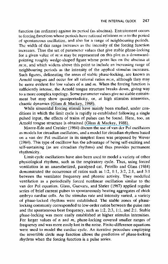
function (as ordinate) against its period (as abscissa). Entrainment occurs to forcing functions whose periods have rational relations m:n to the period of spontaneous oscillation, and also for a range of neighbouring periods. The width of this range increases as the intensity of the forcing function increases. Thus the set of parameter values that give stable phase-locking for a given value of m:n may be represented on this plot as a downward- pointing roughly wedge-shaped figure whose point lies on the abscissa at m:n, and which widens above this point to include an increasing range of neighbouring periods as the intensity of the applied stimulus increases. Such figures, delineating the areas of stable phase-locking, are known as Arnold tongues and occur for all rational ratios m:n, although they may be more evident for low values of n and m. When the forcing function is sufficiently intense, the Arnold tongue structure breaks down, giving way to a more complex topology. Some parameter values give no stable entrain- ment but may show quasiperiodicity, or, at high stimulus intensities, chaotic dynamics (Glass & Mackey, 1988).

While sinusoidal forcing stimuli have mainly been studied, under con- ditions in which the limit cycle is rapidly re-established following a single pulsed input, the effects of trains of pulses can be found. Here, too, an Arnold tongue structure is obtained (Glass & Mackey, 1988).

Moore-Ede and Czeisler (1984) discuss the use of van der Pol oscillators as models for circadian oscillators, and a model for circadian rhythms based on a van der Pol oscillator in its simplest form was proposed by Wever (1984). This type of oscillator has the advantage of being self-exciting and self-sustaining (as are circadian rhythms) and thus provides permanent rhythmicity.

Limit-cycle oscillations have also been used to model a variety of other physiological rhythms, such as the respiratory cycle. Thus, using forced ventilation in an anaesthetized, paralysed cat, Petrillo and Glass (1984) demonstrated the occurrence of ratios such as 1:2, 1 : 1 , 3:2, 2:1, and 3:l between the ventilator frequency and phrenic activity. They modelled ventilation as a periodically forced nonlinear oscillation similar to the van der Pol equation. Glass, Guevara, and Shrier (1987) applied regular series of brief current pulses to spontaneously beating aggregates of chick embryo cardiac cells. As the stimulus rate and intensity varied, a variety of phase-locked rhythms were established. The stable zones of phase- locking commonly corresponded to low-order ratios between the pulse rate and the spontaneous beat frequency, such as 1:2, 2:3, 1:1, and 2:l. Stable phase-locking was more easily established at higher stimulus intensities. For larger values of n and m, phase-locking covered smaller ranges of frequency and was more easily lost in the noise. Finite-difference equations were used to model the cardiac cycle. An iterative procedure employing the invertible circle map function allows the prediction of phase-locking rhythms when the forcing function is a pulse series.

Dow

nloa

ded

By:

[Tre

ism

an, M

iche

l] A

t: 20

:20

16 J

uly

2008

248 TREISMAN ET AL.

The Temporal Pacemaker as a Non-linear Oscillator

We shall assume that the temporal oscillator may be modelled as a limit- cycle of the van der Pol type. It might then seem that the TO could be investigated by examining the effects of applied oscillations on its fre- quency F‘). There are two difficulties in designing an experiment to do this. First, the calibrated pacemaker model assumes that the TO evolved to emit a stable frequency, uninfluenced by environmental phenomena. Thus it should be protected from external influences, such as imposed oscilla- tions, that might perturb it. These should be barred from reaching the TO, or if they do get through to it, they should be rapidly suppressed. If SO,

sudden brief pulses might be more effective than a sinusoidal oscillation, which suggests that attempts to affect F,, should preferably employ regular trains of intense sensory pulses. The second difficulty is that we have no direct measure of Fo, and must infer changes in this frequency from observed changes in sensory performance. For example, if the TO is run- ning slowly a subject should estimate a given clock interval as being shorter than if the TO is running rapidly.

The mathematical analysis of periodically forced nonlinear oscillators is a difficult problem and they are not fully understood. However, Figure 2 illustrates the results of a computer simulation of the effects of trains of pulses on a simulated TO of the form represented schematically in Figure 1. The TO consists of three interconnected “units”. The activation of each unit is a positive quantity that varies as a function of an assumed constant input and of the excitatory and inhibitory transmissions it receives from the other units. The output from each unit is a linear function of its activa- tion, within limits, and may be excitatory or inhibitory. The activation threshold at which a unit commences to transmit output on an inhibitory path is higher than for excitation. The effect is to produce non-linear damping, and regular self-sustaining oscillations result. Modelling the TO as a network connecting “units” rather than as a single pacemaker cell, and the details of the network employed in the simulation, are not essential to the model. They represent only one possible instantiation of a non-linear TO.

When the simulation was run with suitable parameters, it settled down to give a regular oscillation in activation in the units. When the activation of one unit (Unit 3 in Figure 1) exceeded a threshold, a pulse was trans- mitted to the CU. The characteristic frequency of these TO output pulses, FC.,), was normalized to unity. Forced runs were also simulated in which regular “arousal pulses” added an additional increment in activation to each unit at a rate FA. When the system stabilized, the emission rate from

Dow

nloa

ded

By:

[Tre

ism

an, M

iche

l] A

t: 20

:20

16 J

uly

2008

1.1-

up 1.0

0.9-

SIMULATION OF THE TEMPORAL PACEMAKER

1/5 OSCILLATOR OUTPUT

’

V6 113 112 213 1 LR 3R 2 3

8.0 -

75 -

7.0 - P

65-

0.8 *’

PACEMAKER OUTPUT

2l3

114 215 35

- I . . . . I . . . . I . . . . , . . . . . , . . . . I .

FIG. 2. Simulations of the calibrated pacemaker model. Upper panel: The TO output, F,,, for different rates FA of an arousal pulse input train. Lower panel: The corresponding CU output, Fp, plotted against FA. This is given by Fp = CfF,, = (5 + FA)F,,. Values of FA simply related to F,,,, are indicated by labelled vertical lines.

249

Dow

nloa

ded

By:

[Tre

ism

an, M

iche

l] A

t: 20

:20

16 J

uly

2008

250 TREISMAN ET AL.

Unit 3 (F,,) was recorded. F,, is plotted against the “arousal pulse rates” FA in the upper panel of Figure 2. Thus for FA = 1 (the normalized TO characteristic frequency, represented by the dotted line), the T O output does not depart from unity (though its phase may be altered). For values of FA in a small range of arousal pulse rates around FA = 1, F,, is also entrained to FA. Thus when FA is just less than 1, F,, is reduced, and when FA is just greater than 1, F,, is increased, giving a local dip followed by a peak. Thus for n : m = 1:1 we see a d ippeak perturbation. We have defined as “simply related arousal pulse rates” (Fs,A) rates that stand in low-valued integral ratios to F,,(,, that is, such that FsTA = (n/rn)F,,, where n and rn are low-valued positive integers without common factors. Some simple arousal rates are indicated by vertical lines labelled with the corres- ponding values of n:m. Dippeak perturbations are most clearly seen at Fs.A values for which 1 d n d 3, 1 d rn S 5 . Where the n:m integers are high the effects seen are small. Because the spacing of the more marked perturbations in the specific interference pattern is not regular, giving a pattern of unequal intervals, recognition of a similar pattern in experi- mental data would provide a possible basis for identifying the value of F,, determining the latter.

Similar relations have been observed before in biological systems: von Holst (193711973) reported relations such as 2:3 in different fins of a fish, and Sokolov (1963) noted that with photic driving at 27 Hz, cortical frequencies of 9, 13.5, 18, and 27 Hz (nlm = 311, 211, 312, and 111) were evoked.

The model also assumes that arousal pulse rate has a monotonic effect on the activation of the calibration unit and so on its output, the final pacemaker frequency, Fp. This was represented in the simulation by Fp = C,F,, = (5 + FA)F(). With the CU included in the simulation, we get the monotonic increase in Fp illustrated in the lower panel of Figure 2. Estimations of a constant presented duration would be directly propor- tional to Fp.

The simulation illustrates a type of interference pattern that might be seen if intense sensory pulses were presented during time intervals whose durations a subject estimated. If the estimates showed such a pattern of d ippeak perturbations as sensory pulse rate varied, this would be evidence for non-linear oscillators underlying time perception.

Our model allows external stimulation to affect time judgments in two ways. First, as the intensity or frequency of sensory stimulation increases it will increase the arousal of the CU and so increase the calibration factor. Thus the louder the tone used to reproduce a time interval, the shorter the reproduction would be. Second, undesirably but perhaps unavoidably, sufficiently intense stimulus pulses may disturb the rhythm of the TO in a non-linear fashion, perturbing time judgments similarly.

Dow

nloa

ded

By:

[Tre

ism

an, M

iche

l] A

t: 20

:20

16 J

uly

2008

THE INTERNAL CLOCK 251

An Experimental Search for Interference Patterns

We face interesting questions. Can an interference pattern be demon- strated in temporal estimation‘? If a pattern is found, can the TO charac- teristic frequency be estimated from it? Can physiological correlates of the oscillator frequency be shown?

Treisman et al. (1990) searched for such interference patterns using a para- digm with the following features. A time interval T, was presented for es- timation. Simultaneously with T, (within the accuracy allowed by the VDU scan rate) the subject heard a series of loud clicks at a regular rate. The sub- ject typed in an estimate E of the presented duration. The effects of different click rates on subjects’ estimates were examined. If click rates near simple frequencies interact with a non-linear temporal oscillator as in the model, an interference pattern, such as is illustrated in Figure 2, might be seen.

Their first experiment had five conditions (C5 to C25), presented in separ- ate sessions. In each condition 11 click rates, covering a 5-Hz range at 0.5-Hz intervals, such as 2.5 to 7.5 Hz (C5), . . . ,22.5 to 27.5 Hz (C25), were employed, in a random sequence over trials. On each trial an asterisk appeared on the VDU for an interval T, , accompanied by clicks presented at the rate selected for that trial. The subject was told the clicks were dis- tractors and was asked to estimate the duration of the asterisk in seconds. In case subjects attempted to estimate the click burst duration, the first click accompanied the onset of the asterisk and the last its offset. As a single constant interval cannot always begin and end on a click if bursts of clicks are given at different rates, some variation in the intervals presented was unavoidable. Thus a reference duration was defined, such as 500 msec, and on each trial the actual duration presented (T,) was the nearest duration larger than the reference duration that could begin and end concurrently with a click train at the rate selected for that trial, for example, 571 msec for 7 clicks at 10.5 Hz. In each session two reference durations were employed, one being selected randomly on each trial: the ‘‘long’’ (L) refer- ence duration was 250-msec greater than the “short” (S) duration. The mean S and L values of T, for condition C5 (click rates 2.5 to 7.5 Hz) were 827 and 1067 msec, and for the higher click-rate conditions they were 536 and 784 msec. Thus the value of T, (and NA, the number of auditory clicks accompanying the presented interval) varied at different click rates.

We expect E to increase with T,, and it may also increase as NA increases if each click contributes specific arousal to the CU. Evidence for a mono- tonic effect of click rate on E was found. To separate out any non-linear effects of click rate on the temporal oscillator, the regression of E onto T, and NA was found, and the residuals, the departures of E from this regres- sion, were examined. The bilinear regression is represented by

E = c,T, + c,NA + c (2)

Dow

nloa

ded

By:

[Tre

ism

an, M

iche

l] A

t: 20

:20

16 J

uly

2008

252 TREISMAN ET AL.

where ct, c,, and c are constants. (For more details regarding procedure and the exclusion of artefacts see Treisman et al., 1990.) Equation 2 was fitted to the data for each condition. Deviations from the line of best fit caused by error alone should scatter randomly around this line, and the deviations should decrease with the size of the sample. But deviations caused by mode interactions between the click rate and a non-linear oscil- lator may be similar on repeated testing, and with larger samples they should summate, unless variation in F,,(, between subjects or sessions causes their positions to vary.

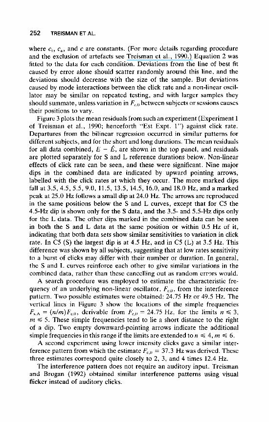
Figure 3 plots the mean residuals from such an experiment (Experiment 1 of Treisman et al., 1990; henceforth “Est Expt. 1”) against click rate. Departures from the bilinear regression occurred in similar patterns for different subjects, and for the short and long durations. The mean residuals for all data combined, E - E , are shown in the top panel, and residuals are plotted separately for S and L reference durations below. Non-linear effects of click rate can be seen, and these were significant. Nine major dips in the combined data are indicated by upward pointing arrows, labelled with the click rates at which they occur. The more marked dips fall at 3.5, 4.5, 5.5, 9.0, 11.5, 13.5, 14.5, 16.0, and 18.0 Hz, and a marked peak at 25.0 Hz follows a small dip at 24.0 Hz. The arrows are reproduced in the same positions below the S and L curves, except that for C5 the 4.5-Hz dip is shown only for the S data, and the 3.5- and 5.5-Hz dips only for the L data. The other dips marked in the combined data can be seen in both the S and L data at the same position or within 0.5 Hz of it, indicating that both data sets show similar sensitivities to variation in click rate. In C5 (S) the largest dip is at 4.5 Hz, and in C5 (L) at 3.5 Hz. This difference was shown by all subjects, suggesting that at low rates sensitivity to a burst of clicks may differ with their number or duration. In general, the S and L curves reinforce each other to give similar variations in the combined data, rather than these cancelling out as random errqrs would.

A search procedure was employed to estimate the characteristic fre- quency of an underlying non-linear oscillator, F,,, , from the interference pattern. Two possible estimates were obtained: 24.75 Hz or 49.5 Hz. The vertical lines in Figure 3 show the locations of the simple frequencies F,.A = (n/m)Fc, l , , derivable from F,,[, = 24.75 Hz, for the limits n 6 3, m S 5. These simple frequencies tend to lie a short distance to the right of a dip. Two empty downward-pointing arrows indicate the additional simple frequencies in this range if the limits are extended to n d 4, m d 6.

A second experiment using lower intensity clicks gave a similar inter- ference pattern from which the estimate F,,(, = 37.3 Hz was derived. These three estimates correspond quite closely to 2, 3, and 4 times 12.4 Hz.

The interference pattern does not require an auditory input. Treisman and Brogan (1992) obtained similar interference patterns using visual flicker instead of auditory clicks.

Dow

nloa

ded

By:

[Tre

ism

an, M

iche

l] A

t: 20

:20

16 J

uly

2008

6 0

2 0

- 2 0

- 6 0

100 0 2 4 6 6 1 0 1 2 1 4 1 6 1 8 2 0 2 2 2 4 2 6 2 S 3 0

6 0 -

2 0 -

- 2 0 -

- 6 0 -

6 0 -

2 0 -

- 2 0 -

- 6 0 -

I SHORT

b

I

4

. . . . l O O ' ' ' ' ' ' ' ' ' ' ' ' ' ' l ' ' ' l l ' ' ' l l ' ' ' l l ~

0 2 4 6 6 1 0 1 2 1 4 1 6 1 8 2 0 2 2 2 4 2 6 2 8 3 0

AUDITORY CLICK RATE FIG. 3. Experiment 1 of Treisman et al. (1990). Upper panel: Equation 2 was fitted to each condition for each subject, and the mean values of thc residuals E - about the regressions of E onto T, and N A are plotted against auditory click ratc. Lower panel: mean residuals for short durations and long durations. Nine dips in the combined data are indicated by upward- pointing arrows. These are reproduced in the same positions below the S and L curves. The vertical lines indicate the locations of the simple frequencies F,.A = (n/m)F<.,,, for F,,, = 24.75 Hz, n < 3, m < 5 . The two open arrows in the upper panel indicate the additional simple frequencies obtained for the limits (n,,,, rn,,,) = (4, 6) .

253

Dow

nloa

ded

By:

[Tre

ism

an, M

iche

l] A

t: 20

:20

16 J

uly

2008

254 TREISMAN ET AL.

If similar internal clocks are employed in perception and in the control of movement, it should be possible to demonstrate similar interference effects in motor timing. In a choice reaction-time experiment, Treisman et al. (1992) presented auditory clicks that commenced at the onset of the stimulus and continued until the response had been completed. In time estimation, if the clock runs slow an estimate of a constant interval is reduced, giving a dip. If a clock pacing motor response runs slow, the time to produce the movement should be lengthened, giving a peak. Thus time- estimation dips should correspond to response-time peaks.

An interference pattern affecting response-time durations was found, in which major peaks tended to correspond to the major dips found with time estimation. F,,” was estimated at 49.8 Hz, which may be compared with the estimate of 49.5 Hz given by Est Expt. 1.

Ti me Estimation and the Elect roencep ha log ram

Different experimental paradigms have produced evidence for a non-linear oscillator underlying temporal performance. If we could identify the output of the hypothesized TO as a component in the electroencephalogram (EEG), this would be important evidence for the model, and it would also provide direct physiological support for what may be regarded as a new sense organ, an organ for the perception of time. But past observations of the EEG have failed to produce clear positive results.

Many investigators have sought evidence of an internal clock in the EEG; the alpha rhythm has usually been the favoured candidate (e.g. Surwillo, 1966; Werboff, 1962). But such attempts have been unconvinc- ing. Treisman (1984) required subjects to produce a 4-sec duration repeatedly during a session, and recorded their EEG at the same time. If the clock slows down over a period, the subjects’ time productions should get longer; and if the alpha rhythm represents the clock, its frequency should slow down in the same proportion, and vice versa. But Treisman’s (1984) results showed that the time productions and the concurrent alpha rhythm could equally well vary in the same or opposite directions, and in different proportions, the productions being far more variable than the alpha rhythm. This seemed incompatible with the hypothesis that the alpha rhythm represents the ticking of the internal clock.

This is an argument for rejecting the alpha rhythm hypothesis. But it is an argument based on a model in which there is a unitary temporal pacemaker whose rate may vary as a function of its arousal, producing correlated changes in time productions and in the corresponding physio- logical output (Treisman, 1963). But the work reviewed above shows that these assumptions may be too simple. The calibrated pacemaker model posits that two separate devices provide a stable reference frequency F,..,,,

Dow

nloa

ded

By:

[Tre

ism

an, M

iche

l] A

t: 20

:20

16 J

uly

2008

THE INTERNAL CLOCK 255

and introduce additional rate variation into the final output rhythm Fp, and this distinction between the two rhythms F,,(, and F p suggests that the question might usefully be re-examined. On the calibrated pacemaker model, the alpha rhythm could represent F,.,], yet because observed time productions reflect the final CU output with its additional variability, these productions might not show any clear relation to the alpha rhythm. Thus comparing alpha and time productions may have been ill-adapted to reveal a relation between the alpha frequency and F,,,,. (We give alpha this role only to illustrate the argument; the model is not committed to the assump- tion that the alpha rhythm rather than some other EEG oscillation repres- ents the temporal information source.)

The arousal pulse paradigm (Treisman et al., 1990) provides a way to bypass the difficulty with Treisman’s (1984) argument. In the calibrated pacemaker model, clicks produce an interference pattern by interacting with the TO. If the T O output is present as a component oscillation (not necessarily the alpha rhythm) in the EEG, the frequency of this oscillation should decrease if clicks are administered at rates that reduce time estim- ates, and the reverse. If we could observe such an effect of arousal pulses on a component of the EEG, this would provide direct evidence for the physiological nature of the internal clock, and the frequencies so affected would provide evidence relating to our estimates of F,, .

If it proves possible to demonstrate an action of arousal pulses on the EEG, what pattern of EEG changes might we see? Three interesting alternatives, based on different models for the organization of a TO system, suggest themselves.

1. A Single Temporal Oscillator. It has been possible to interpret the results above in terms of a single internal clock. In this model, the EEG would contain an oscillation representing the output of the single TO, perhaps at a frequency such as 24.75 Hz. If this single oscillatory process could be isolated for observation, we would see its frequency modulated by dips and peaks when clicks are presented at rates close to those rates that are simply related to its characteristic frequency. The remainder of the EEG spectrum would not be affected.

2 . A Single Temporal Oscillator Coupled to Multiple Non-temporal Oscillators. In the first model, sensory pulses interact with the single TO without involving other mechanisms. But there are many biological oscil- lators, and we know that they may interact with each other. Sinus arrhyth- mia provides a familiar example. Thus even if temporal performance were determined by a single TO, this oscillator might interact with biological oscillators that are not themselves concerned with measuring time, and if these non-temporal oscillators (NTOs) are sensitive to the effects of arousal

Dow

nloa

ded

By:

[Tre

ism

an, M

iche

l] A

t: 20

:20

16 J

uly

2008

256 TREISMAN ET AL.

pulses, their interactions with the TO could contribute to the interference pattern,

Consider a non-temporal oscillator model based on the following assumptions: (a) Click-sensitive NTOs (and one TO) exist, with different characteristic frequencies. (b) Arousal pulses perturb an oscillator (tem- poral or non-temporal) significantly only when the pulse rates presented are close to the characteristic frequency of the oscillator (that is, the effects produced by simply related pulse rates can be neglected). (c) Phase-locking may occur between any two biological oscillators whose frequencies bear simple (n :m) relations to one another; that is, n cycles of one frequency correspond to m cycles of the other. Thus if an oscillator at frequency n is perturbed by click rates near this frequency, this perturbation may be transmitted to an oscillator at frequency m to which it is phase-locked. Thus a set of NTOs whose characteristic frequencies (such as 8.25 or 12.4 Hz) are simply related to that of the TO (say 24.75 Hz) may be coupled to it. If clicks are given at rates in a range about 24.75 Hz, they may induce a dip-peak perturbation directly. Click rates near the frequency of an NTO would perturb it, and this would produce a secondary per- turbation of the TO output. In this way, the interference patterns found with time estimation and motor performance would be produced. The advantage of such a system of interacting oscillators might be that their interactions normally tended to stabilize their frequencies.

What EEG pattern would such a model predict? This depends on the number of NTOs and the extent of interaction between them. If the tem- poral oscillation can be observed, it will show an interference pattern. Each click rate will perturb any click-sensitive NTOs with similar characteristic frequencies; thus clicks at 10 Hz will perturb oscillators at about 10 Hz, and so on. If NTOs are limited to those that are simply related to the TO, perturbable oscillations would be present in the EEG spectrum at a spacing similar to that seen in the interference pattern, for example, at 1/4, 2/5, 1/2, 213 of F&,, etc, and would show perturbations at about their charac- teristic frequencies.

If the number of click-sensitive NTOs is high and significant phase- locking occurs between suitable pairs of NTOs, 10-Hz clicks might also perturb oscillators at about 15 Hz, 20 Hz, and so on. The greater the number of such NTOs, the more chaotic the overall picture would become.

3 . Single Temporal Oscillators at Harmonically Related Frequencies. We are able to estimate time intervals of very different orders of magnitude- fractions of a second, minutes, or hours. To explain this ability it may be necessary to postulate parallel internal clocks running at different rates (Treisman, 1965). Eisler (1981) has presented evidence for a model for

Dow

nloa

ded

By:

[Tre

ism

an, M

iche

l] A

t: 20

:20

16 J

uly

2008

THE INTERNAL CLOCK 257

duration discrimination which includes two parallel clocks. Kristofferson (1984) has presented evidence for multiple temporal quanta related by a doubling rule.

If the temporal system employs parallel TOs running at different fre- quencies to estimate different orders of duration, it may sometimes need to relate time measures recorded at one frequency to measures recorded at another order of frequency. In the production of a rhythmic sequence, for example, an oscillator at one frequency might be responsible for long intervals (bars) , and an oscillator at another frequency for short intervals (notes), and the desired relation between these two intervals would need to be carefully maintained. To ensure facility and accuracy of translation and coordination between durations recorded by TOs of different fre- quencies, these frequencies should be harmonically rather than randomly related. This would, for example, allow phase-locking between the TOs.

Thus the harmonically related TO model assumes that temporal performance is subserved by a sequence of TOs with harmonically related characteristic frequencies, such as 24.75 Hz, 49.5 Hz, 74.25 Hz. The model predicts that if such oscillatory outputs can be isolated in the EEG, they will show interference patterns, spaced at equal intervals in the spectrum. As the different values of F,..,, are harmonically related, their sensitivities to arousal pulses will be similar, giving similar patterns. The EEG spectrum intervening between the harmonically related temporal oscillations should show no effects of clicks, unless click-sensitive NTOs also occur.

Is the temporal oscillator at a given frequency single, or are such TOs duplicated? The models above assume that there is either a single TO or a set of harmonically spaced single TOs. But skilled movement may require that we time more than one action of the same order of duration con- currently, for example, when we time the movements of the arms and legs in dancing. If we must employ similar overlapping time intervals, then to read them all from a single time source without confusion would require complex ancillary mechanisms. Alternatively, the temporal system might have a number of TOs available at a given frequency, so that individual TOs selected from this set could be dedicated to timing individual over- lapping durations, when this is required. To allow for this, we could replace the assumption of a single TO in each of the three models above by the assumption that there is a set of TOs, sharing a common or approximately similar F,.o. (In the harmonically related TO model there would be several such sets, their mean frequencies being harmonically related.) As bio- logical exactness is rare, it is likely that the TOs in a set would have similar but not identical F,..()S, and we can consider these frequencies as distributed (perhaps normally) about a mean value. Adding the present assumption to the three models above gives us “TO distribution” versions of them. If

Dow

nloa

ded

By:

[Tre

ism

an, M

iche

l] A

t: 20

:20

16 J

uly

2008

258 TREISMAN ET AL.

there is more than one distribution, the mean value of distribution i may be represented as E,(Fc,,,).

We have three sets of predictions, but could they be observed? Inspec- tion of the EEG as normally recorded would be unlikely to show such effects. Most probably, EEG frequencies come from many sources. Even if the TO output contributes an oscillation to the EEG, it is likely to be lost from sight among many other EEG variations at similar or different frequencies that emanate from neural activities unrelated to the time- keeping process and which may be of much greater power. Our need to detect slight changes in the frequency of a TO output lost in the EEG is analogous to the problem of detecting that one of the violinists in the string section of the orchestra has ceased playing one note in the current chord and instead is playing another. We need a method of data analysis that might render our predicted effects detectable.

A Model of the Effects of TO Frequency Shift on the

One or more oscillatory processes involved in timing and sensitive to clicks may be hidden in the EEG, obscured by activity arising from many other sources. How can the timing needle be found in the electroencephalo- graphic haystack?

If we knew in what small band of EEG frequencies F,, lay, we could examine this band closely. A statistic that will be affected if any oscillation in this band changes its frequency is the centroid, the mean frequency of the band when each constituent is weighted by the power at that value. Thus, assuming Fc,o is 24.75 Hz, suppose we examine the band from 21 to 25 Hz at 1-Hz intervals. There will be power at each frequency, including power at 24 Hz contributed by Fc+O, which together determine the weighted mean frequency. If we now present clicks at a rate that reduces the TO output to Fo = 22 Hz, the power previously contributed by Fc,o to 24 Hz will now be present at 22 Hz instead, and the weighted mean frequency of the band will fall. The extent of the fall will depend on the proportion of the power in this band contributed by the TO. Thus if we can identify the right band of frequencies, and we examine its centroid as a function of click rate, an interference pattern may become visible. As we do not know which band to select, we can examine a wide range of bands and hope to find such an effect in one of them.

This argument applies if there is a single temporal oscillator in the band. If there is a TO distribution, what effects will TO frequency shifts produce on the EEG? To examine this, a simple model of the EEG with arbitrary parameters, EEGSi,, was simulated for the case of a single TO distribution.

EEG: EEG,,,

Dow

nloa

ded

By:

[Tre

ism

an, M

iche

l] A

t: 20

:20

16 J

uly

2008

THE INTERNAL CLOCK 259

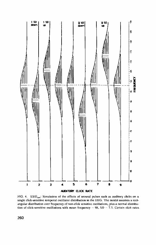
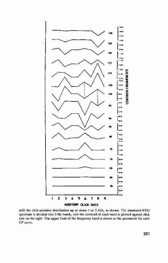
The simulated EEG was assumed to have a rectangular distribution of non-click-sensitive power over frequency (power density O S ) , with a single normal distribution of click-sensitive frequencies superimposed (maximum power density 0.4) representing a set of similar temporal oscillators. This is illustrated in the left panel of Figure 4, which shows the simulated EEG frequency spectrum on the ordinate (for EEGSi, frequencies from 50 to 130 Hz), and power density (not labelled) on the abscissa. We see the rectangular spectrum with the normal click-sensitive distribution super- imposed. This figure (the power spectrum of the simulated EEG) is repeated nine times, for nine different auditory click rates, represented at successive points on the abscissa. At click rates 1, 4, 5, 7, and 9, which are assumed to have no effect on the TO distribution, the mean of the distribution falls at its normal value of 98 Hz (the dotted line). In each case it has a standard deviation of 7.5 Hz. Click-rate 2 moves the TO distribution downwards 1 SD, click-rate 3 moves it up 1 SD, click-rate 6 moves it down 2 SD and click-rate 8 moves it up 2 SD.

The right panel illustrates an analysis in which the EEGSi, spectrum was divided into 5-Hz bands, Band(51-55), Band(56-60), . . . , Band(126- 130), and the centroid was found for each band at each click rate. For each band these points are joined to give a centroid frequency (CF) curve that shows how click rate affects the centroid of that band. [Each CF curve is labelled with the upper limit of the band, e.g. CF(51-55) is labelled “55” . ]

These plots reveal interesting overall patterns. The click-sensitive dis- tribution is shifted down 2 SD at click-rate 6, and this produces a charac- teristic pattern. The centroid frequency curve for Band(101-105), CF( 101- 105) (labelled “ l O S ’ ) , shows a peak at click-rate 6, as do neighbouring higher bands. CF(96-100) and the CF curves immediately below it show dips at this click rate. The effect is to produce a “diamond pattern” between CF(101-105) and CF(96-100) (indicated by the vertical dashed line plotted against click-rate 6). Because of its shape, the downward shift of the click-sensitive frequency distribution removes relatively more power at the lower frequencies in Band( 101-105) than at the higher frequencies in the band, raising its centroid, and the shift has similar effects on neigh- bouring higher CF bands. In Band(96-100) and the three bands below it, the downward shift of the distribution causes a relative increase of click- sensitive power in the lower part of each band, so that the centroids fall. This produces the “diamond” shape.

In still lower bands (61-65, . . . ,76-80), the downward intrusion of the tail of the TO distribution adds power mainly to the upper end of each band, raising the centroid frequencies to give peaks again. For click-rate 6, this change-over from dips to peaks occurs between Band(76-80) and Band(81-85), producing a “cross pattern” [whose location corresponds roughly to the new position of the T O distribution mean, at 83 Hz, in

Dow

nloa

ded

By:

[Tre

ism

an, M

iche

l] A

t: 20

:20

16 J

uly

2008

._.I 1

1 2 3 4 5 6 7 8 9

mTOFIY CLtCK RATE

FIG. 4. EEG,,,: Simulation of the effects of arousal pulses such as auditory clicks on a single click-sensitive temporal oscillator distribution in the EEG. The model assumes a rect- angular distribution over frequency of non-click sensitive oscillations, plus a normal distribu- tion of click-sensitive oscillations with mean frequency = 98, SD = 7.5. Certain click rates

260

Dow

nloa

ded

By:

[Tre

ism

an, M

iche

l] A

t: 20

:20

16 J

uly

2008

I I In-

I - tz

1 2 3 4 5 6 7 8 9

AUO~TORY aim RATE

shift the click-sensitive distribution up or down 1 or 2 SDs, as shown. The simulated EEG spectrum is divided into 5-Hz bands, and the centroid of each band is plotted against click rate on the right. The upper limit of the frequency band is shown as the parameter for each CF curve.

26 1

Dow

nloa

ded

By:

[Tre

ism

an, M

iche

l] A

t: 20

:20

16 J

uly

2008

262 TREISMAN ET AL.

Band(81-85)]. Thus in any system resembling EEG,,,, the appearance of a “diamond-cross pattern”, a diamond vertically above a cross, indicates that a downward shift of a distribution of click-sensitive frequencies has occurred.

At click-rate 8, the click-sensitive distribution has moved upwards 2 SD, which gives a similar but reversed picture. There is now a diamond between CF(91-95) and CF(96-100), and a cross between CF(111-115) and CF(116- 120) (the mean of the distribution has moved up to 113 Hz). Thus a “cross- diamond pattern”, a cross vertically above a diamond, indicates an upward shift of a click-sensitive distribution. Successive “diamond-cross” and “cross-diamond’’ patterns indicate a transition from phase-locking giving retardation to phase-locking giving acceleration of click-sensitive oscil- lators.

At click-rates 2 and 3, the downward and upward TO shifts are only half as great, and the centroid shifts although similar are less clearly marked.

We can now make predictions for the three models of TO organization, in their single TO and distribution forms, for an analysis in which the EEG spectrum is divided into bands and centroid frequencies are found.

If there is a single temporal oscillator only, an interference pattern should be seen in the band containing F,,(,, provided that entrainment to different click rates does not cause the TO frequency to shift outside the band. If F,, does cross a boundary, the resulting pattern depends on the division into bands and may differ from the time-estimation interference pattern. For example, suppose that Fc,u = 22 Hz, and that we define a band from 21 to 25 Hz. If clicks at 21 Hz cause the TO output to fall to F,, = 21 Hz, the centroid of the band will fall as in time-estimation inter- ference patterns. But if clicks at 20 Hz reduce F,, to 20 Hz, then CF(21-25) will rise, as power is lost from the lower part of the band; and CF(16-20) will also rise, power being added to the upper part of this band. Thus the pattern is distorted in a way that depends on FC,(, , the band boundaries chosen, and the effectiveness of the clicks.

The main features of the pattern predicted if a single temporal oscillator distribution replaces the single TO are more robust. They are illustrated in Figure 4 and have been discussed above.

The NTO model with a single temporuf oscillator predicts an interference pattern in the band containing F,.,,, (with the possible distortions noted above for the single TO model). With a distribution of TO frequencies, the pattern illustrated by EEG,,, will be substituted at this location. For either version interactions may also be seen between each click rate and any NTOs that exist at about that rate; for example, clicks at 10 Hz might perturb oscillations from, say, 9 to 11 Hz. This would add perturbations

Dow

nloa

ded

By:

[Tre

ism

an, M

iche

l] A

t: 20

:20

16 J

uly

2008

THE INTERNAL CLOCK 263

along a “positive diagonal” as a function of click rate. The greater the extent of click-NTO interactions at simple frequencies, the more chaotic the overall picture would become.

The harmonically related single temporal oscillators should show similar sensitivities to arousal pulses. Thus patterns resembling that produced by a unique TO but repeated at harmonic intervals will be seen. If T O dis- tributions are substituted for the single TO at each level, so that a sequence of click-sensitive distributions is hidden in the EEG with harmonically related mean characteristic frequencies Ei(FC,()), then patterns like those shown by EEG,,, should be repeated at constant intervals in the EEG spectrum. As well as the interference patterns in bands containing Ei(FC.(,), the diamond-cross and cross-diamond configurations should repeat.

EXPERIMENT 1

An experiment was designed to examine these predictions. It asked the following questions.

First, can any evidence be found that at certain rates auditory clicks may alter the frequencies of one or more oscillatory processes in the EEG spectrum? This would show that neural effects of clicks can entrain bio- logical oscillators.

Second, if certain click rates do affect EEG oscillations, will they do so in a pattern related to the time-estimation and response-time interference patterns previously obtained? If so, this would provide evidence that the EEG oscillations that arousal pulses affect are components of a biological timing system.

Third, if subjects estimate time intervals while exposed to clicks, and the EEG is recorded, will the effects on the EEG and any time-estimation interference pattern be related? For consistency, we would hope to see some relation.

Fourth, if clicks produce an interference pattern affecting EEG oscilla- tions, which if any of the three TO organizational models will be sup- ported? A clear answer would throw light on the overall organization of time-keeping.

In the following experiment the EEG was recorded while subjects estimated temporal durations presented together with concurrent auditory clicks. The conditions were chosen to favour obtaining evidence of an effect on the EEG, rather than to best demonstrate a time-estimation inter- ference pattern.

Dow

nloa

ded

By:

[Tre

ism

an, M

iche

l] A

t: 20

:20

16 J

uly

2008

264 TREISMAN ET AL.

Method

Three male adults served as subjects. Two (MT and PN) were experimenters and had served as subjects in earlier experiments, but PN was naive regarding the purpose of the experiment at the time it was performed.

Subjects.

Apparatus and Procedure. The subject sat in an unilluminated shielded cubicle facing a VDU. This was controlled by an Apple I1 computer, placed in an adjoining room to avoid interference. The loudspeaker of a tape recorder in the cubicle presented a burst of computer-generated clicks at about 65-70 dBA concurrently with the duration to be estimated on each trial. The initial click in each train was given at the onset of an asterisk that appeared in the centre of the VDU screen, and the final click at its termination. A trial commenced with a short high-pitched tone generated by the computer. After an interval that varied randomly between 0.6 and 0.9 sec the temporal duration to be estimated (T,, the duration of the asterisk on the screen) was presented. The subject then gave his estimate orally. This was entered into the computer by an experimenter in the adjoining room. This initiated the next trial.

In each session 31 click rates were used, ranging from 2.5 Hz to 17.9 Hz at intervals as close to 0.5 Hz as could be achieved using a software timer that counted 2-msec intervals. (These were 2.5, 3.0, 3.5, 4.0, 4.5, 5.0, 5.5, 6.0, 6.5,7.0, 7.5,7.9, 8.5, 8.9, 9.4, 10.0, 10.4, 11.1, 11.6, 11.9, 12.5, 13.2, 13.5, 13.9, 14.7, 15.2, 15.6, 16.1, 16.7, 17.2, and 17.9 Hz.) The durations presented varied with the click rate, so as to allow the train of clicks to coincide with the duration of the asterisk, subject to the random temporal quantization introduced by the VDU scan. There were two reference dura- tions, T , and T2 , their values depending on the click rate: for the lowest 10 auditory click rates (7 Hz or less), Ti (the shorter reference duration) was 700 msec, and for the upper 21 click rates (7.5 Hz or more), Ti was 500 msec; T2 was always 1000 msec. On each trial an auditory click rate and a reference duration were chosen at random. The duration closest to the selected reference duration that also corresponded to an integral number of inter-click intervals at the selected click rate was presented as T,; values based on Ti or T2 are referred to as Short (S) or Long (L), respectively. PN and CM received 768 trials, 12 trials at each combination of click rate and reference duration (except that, by error, 24 trials were given for 17.2 Hz). MT received 576 trials, 9 trials for each click-rate/ reference-duration combination (18 for 17.2 Hz). Each subject did one session. These lasted 55 to 65 min and there were no breaks.

One Ag-AgCI earth electrode was attached to the subject’s earlobe, and an electroencephalogram was recorded between two central electrodes,

Dow

nloa

ded

By:

[Tre

ism

an, M

iche

l] A

t: 20

:20

16 J

uly

2008

THE INTERNAL CLOCK 265

one on the forehead and one on the occipital area. The EEG was monitored on a Grass Model 7D Polygraph and simultaneously recorded on an SE Eight Four digital tape recorder, together with signals indicating the onset and offset of each time presentation.

Results Time Estimation. The time estimates for each session were fitted to

the bilinear function (Equation 2) and the overall mean residuals are plotted, for S and L durations, in the lower panels of Figure 5 . The S and L data from Est Expt. 1 of Treisman et al. (1990) are shown in the upper panels for the same click rate range. For each curve, some of the main dips are labelled.

The prime objective was to obtain an adequate quantity of EEG data, sampled over a wide range of click rates, but excluding any variation that might occur from one session to another. To maximize EEG observations, subjects worked without a break for about an hour; and to allow a wide range of click rates to be examined, the number of estimates made at each rate was low. This design is not the best for demonstrating time-estimation effects: previous work suggests that short sessions separated by adequate rest periods are desirable. Although the present data were obtained under less satisfactory conditions, and the amplitudes of dips and peaks vary more than in the earlier fime-estimation data, the locations of the main dips show substantial agreement across the experiments. Six of the present S dips (4.5, 5.5 , 7.0, 8.9, 13.2, and 16.1 Hz) are close to or coincide with dips seen in Est Expt. 1 (S). Five of the present L dips (4.0, 6.5, 8.5, 11.1, and 13.5 Hz) are within 0.5 Hz of dips obtained in Est Expt. I (L). Thus there is agreement, within the limits set by the previously noted tendency for dips to vary in location within about 0.5 Hz, among subjects, con- ditions, and with the passage of time (Treisman et al., 1990).

EEG Results. The analysis was similar to that described for EEG,,,. The EEG spectrum was divided into 5-Hz bands, the centroid of each band was found at each click rate, and the relation between the centroid fre- quency curve and click rate was examined.

Each session was analysed as follows. For each trial, a 500-msec epoch of the EEG record, measured from the onset of the asterisk marking the presented time interval T,, was sampled at l-msec intervals. If the variance of the epoch exceeded a criterion, the record was excluded as possibly containing artefacts. The data were analysed for two levels of the rejection criterion for each subject: a strict or high criterion (in the signal detection theory sense) which accepted only records showing low levels of variance, and a lax or low criterion which accepted a larger set of epochs (including

Dow

nloa

ded

By:

[Tre

ism

an, M

iche

l] A

t: 20

:20

16 J

uly

2008

15

0

10

0

50

AU

DIT

OR

Y C

LIC

K R

ATE

- 1

50

-

10

0

- E

x 1:

S

- E

x 1:

L

- 5

0

-

FIG

. 5.

L d

urat

ions

. The

cor

resp

ondi

ng re

sults

for

Est

Exp

t. 1

are

plot

ted

abov

e. S

ome

dips

are

labe

lled

in e

ach

case

. M

ean

resid

uals

over

sub

ject

s for

tim

e es

timat

es fi

tted

to E

quat

ion

2, p

lott

ed in

the

left

low

er p

anel

for

S du

ratio

ns a

nd o

n th

e ri

ght f

or

0-

-50

t 5.5

S.0

11

.5

13.5

$

6.0

-1

00

4.5

7.0

-15

0

0-

-50

-

y -1

00

a 3

-15

0 " '

I'

' '

' " " ' "

''

I ''

ft

tt

t -

'6.5

6

.5

11.5

13

.6

16

.5

- 3.

5 5.

5

"

"I

'

I'

" "

"I

"

' "

EE

G E

x:S

K

50

-

50

0-

0

-

-50

-

-50

-10

0

13.2

16

.1

-10

0

- 4.

5 7.

0 8.

9

" " '

"

''

" " "

''

I "

EE

G E

x:L

- - -

4.Q

7.

5 9

.4

13

.5

' '

' '

' '

' '

' '

' ' '

' ' ' '

' '

-15

0

Dow

nloa

ded

By:

[Tre

ism

an, M

iche

l] A

t: 20

:20

16 J

uly

2008

THE INTERNAL CLOCK 267

the low variance set) with, o n average, a greater level of variance. These will be referred to as the high-criterion and low-criterion data. No other artefact rejection procedure was used. Each record accepted was subject to a power spectrum analysis. This was performed over a range of 1 to 200 Hz and carried out off-line using fast Fourier transform routines from the NAG library.

The average spectrum was then found for each click rate, pooling spectra for short and long presented intervals, as these were indistinguishable to the subject over the first 500 msec. The average spectrum at each click rate was then divided into 5-Hz bands, Band(1-5), Band(&lO), . . . , Band(196-200), and the centroid was found for each band at that click rate. The centroid for Band([k - 41 - k ) is defined as:

f k f k

where fi refers to EEG frequency and p i is the mean power at that fre- quency given by the power spectrum analyses. The results for each subject are given below.

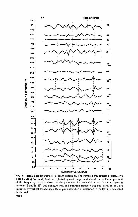
Subject PN. Figure 6 shows 5-Hz-frequency-band centroid frequency curves plotted against auditory click rate for each band up to Band(85-90), for the high criterion data. An average of 11.3 records was accepted by the high criterion at each click rate. (The number of trials at each click rate for S and L durations taken together was 24.) Figure 7 shows the results for further high-criterion bands up to Band(196-200). Figure 8 gives low-criterion data up to Band(96100) (19.5 records per click rate).

These data provide an answer to our first experimental question. Figure 6 shows that auditory clicks do affect components of the EEG, and the effects are patterned: the clicks do not simply cause a general increase in noise. Similar patterns can be seen in different CF curves. Certain click rates affect the centroids of some bands but not others. Thus Band(56-60) (labelled 60 in the figure) and Band(76.80) show little variation with click rate. Other bands, such as Band(21-25) and Band(46-50) show similar patterns. The occurrence of resemblances between bands indicates that, for PN, click rates that are effective tend to act on subsets of EEG fre- quencies. Does this hold for the other subjects?

Subject CM. Figures 9 and 10 show CM’s high-criterion curves up to Band(196200) (15.9 records per click rate); Figure 11 shows his low- criterion curves (23.9 records per click rate) up to Band(116-120).

Again, auditory clicks have selective effects on the EEG. Some bands, such as Band(21-25) and Band(46.50) show similar patterns, as was the

Dow

nloa

ded

By:

[Tre

ism

an, M

iche

l] A

t: 20

:20

16 J

uly

2008

PN Hlgh Crltcrlon

90

87 0

82.2 & = 77.51 L : - , - 6 0

75

67.9

62 3

57.5 I 9 6 0

324)

27 5

222

17.3

I22

73

5

2.4 0 2 4 6 8 10 I2 14 16 18 20

AUDITORY CLICK RATE FIG. 6. EEG data for subject PN (high criterion). The centroid frequencies of successive 5-Hz bands up to Band(8690) are plotted against the presented click rates. The upper limit of the frequency band IS shown as the parameter for each CF curve Diamond patterns between Band(21-25) and Band(26-30), and between Band(46-50) and Band(51-55), are indicated by vertical dashed lines. Band pairs identified as described in the text are bracketed on the right. 268

Dow

nloa

ded

By:

[Tre

ism

an, M

iche

l] A

t: 20

:20

16 J

uly

2008

PN High trtterlon

06.9L--- , , 0 2 4 6 8 10 I2 14 16 I8 20

AUOITOORY CLICK RATE

FIG. 7. as in Figure 6.

PN (high-criterion data). Centroids are plotted for Band(8690) to Band(196200),

269

Dow

nloa

ded

By:

[Tre

ism

an, M

iche

l] A

t: 20

:20

16 J

uly

2008

97.4

92.7

87. I

82.2

77.51

72.7

57.5

4.6

37.4

32.5 1 27.61

22.2

I 7.4

12.2

7.31 7.2

2.5 1 2.4

Low Crlterlon PN

fi loo

m

25

20 ' I

15

, I 5 -+-+--- I

4 6 8 10 12 14 I6 18 20

AUDITORY aim RATE FIG. 8. PN (low-criterion data). Plotted as in Figure 6 for Band(1-5) to Band(9&10). Diamond patterns contained in Ef2(21-30) and Bf2(46-55) are indicated by dashed lines. An additional diamond is shown at 3.5 Hz.

270

Dow

nloa

ded

By:

[Tre

ism

an, M

iche

l] A

t: 20

:20

16 J

uly

2008

cn 1-119 criterion

92.6 {

3 82.21

to 0

3

w 87.01

77.4

2 72.8 c = 62.61 0

62.4

57.5 I 5251

47.51 47.4

I 42.5

37.4

32.4 1 27.4 I

22.2

17.2 1 12.31

7.4 1

2& 1

AUDITORY CLICK RATE FIG. 9. CM (high-criterion data). Centroid frequencies plotted against click rate up to Band(91-95). Diamond patterns are indicated by vertical dashed lines for Band pairs BP(21-30) and B P ( 4 6 5 5 ) . Band pairs identified as described in the text are indicated by brackets.

27 1

Dow

nloa

ded

By:

[Tre

ism

an, M

iche

l] A

t: 20

:20

16 J

uly

2008

CM High Criterion

rn r

1975

1774

1726l

16751

1623

15751

1525

0 15241

ln51 1474

13731 + Z 1324 0 Y 1

12751 j-1

1123

10751

IW51

97 9741 3

97 5 , --7 ---. - - ~ - - T - . _ l ,

2 4 6 8 10 12 14 I6 18 20

AUDITORY CLICK RATE FIG. 10. Band( 9 1-95) to Band( 1 96-200).

272

CM (high-criterion data). Centroid frequencies plotted against click rate from

Dow

nloa

ded

By:

[Tre

ism

an, M

iche

l] A

t: 20

:20

16 J

uly

2008

Low Crttalm Ctl

I !

I!! 4 6 I 10 12 14 16 18 20

AUDITOW aim RATE FIG. 1 I . Band( 116-120).

CM (low-criterion data). Centroid frequencies plotted against click rate up to

273

Dow

nloa

ded

By:

[Tre

ism

an, M

iche

l] A

t: 20

:20

16 J

uly

2008

274 TREISMAN ET AL.

case for PN. Others, such as Rand(S6-60) and Band(76-80), are little affected. as for PN.

Subject M T . Figures 12 and 13 plot MT’s high-criterion data up to Band(19&200) (8.9 records per click rate), and Figure 14 plots low- criterion data (13.0 records) up to Band(116-120).

The same general pattern is seen as before. However, the magnitudes of the effects are notably greater. Whereas for PN and CM the unit on the ordinate was 0.1 Hz, for MT it is 0.2 Hz. For PN the mean standard deviation of the centroid frequency measure for BP(21-30) (high criterion) was 0.034 and for CM it was 0.032, but for MT it was 0.049. Thus M T s click-induced variance is more than twice that of the other subjects. Possible interpretations are that his TOs are more sensitive to interference, or that click-sensitive oscillations constitute a greater proportion of his EEG. It may be relevant that MT’s time estimates were also the most sensitive to clicks: when Equation 2 was fitted, PN’s value of c, indicated an increase in his time estimates of 2 msec per click; for CM, c, was 18 msec; and for MT, 29 msec. (Note that we interpret this component of the linear regression as an effect on the CU.)

The overall results concur in giving a positive answer to our first question: it appears that the neural effects of auditory clicks interact with biological oscillators of some sort. What do the data say in answer to our second question: are these patterns of interaction related to the interference patterns obtained in the earlier experiments on temporal and motor performance?

One estimate of the F,,, given by Est Expt. 1 was 24.75 Hz. If this figure is approximately correct, we would expect the centroid frequency of Band(21-25) to show evidence of click-sensitivity. If the different click rates affect the CF in ways that are related to their effects on temporal performance, we should see a pattern of dips in CF(21-25) bearing some similarity to the interference patterns obtained with time estimation (cf. Figure 3) or motor timing (Treisman et al., 1992), despite the differences in experimental procedure and the measures compared, and the small variations that may occur in the locations of features as a function of condition.

Figure 15 compares the high criterion CF(21-25) curves for each subject with the response-time interference pattern obtained from an experiment in which choice response times were recorded while subjects were exposed to different auditory click rates (Treisman et al., 1992). On our model, a retardation of the clock will cause a dip in time estimates and will slow motor action, producing a peak in response time. The vertical lines in the figure mark the locations of all peaks, large or small, in the combined response-time data from Treisman et al.’s (1992) Experiment 1; a peak

Dow

nloa

ded

By:

[Tre

ism

an, M

iche

l] A

t: 20

:20

16 J

uly

2008

87.83

87.6 -

87.4.

MT Hlgh Crlterlon

---- 1 7 0 1 65

4 6 0

2.2 -- ! c : - 0 2 4 6 8 10 12 14 16 I8 20

AUDITORY CLICK RATE FIG. 12. Band( 8 6 % J) .

M T (high-criterion data). Centroid frequencies plotted against click rate up to

275

Dow

nloa

ded

By:

[Tre

ism

an, M

iche

l] A

t: 20

:20

16 J

uly

2008

07 0 L-.- . - 0 2 4 6 11 10 I2 I 4 16 18 20

AUDITORY aim RATE

FIG. 13. Band ( 1 9 6 2 M ) .

MT (high-criterion data). Centroid frequencies plotted against click rate up to

276

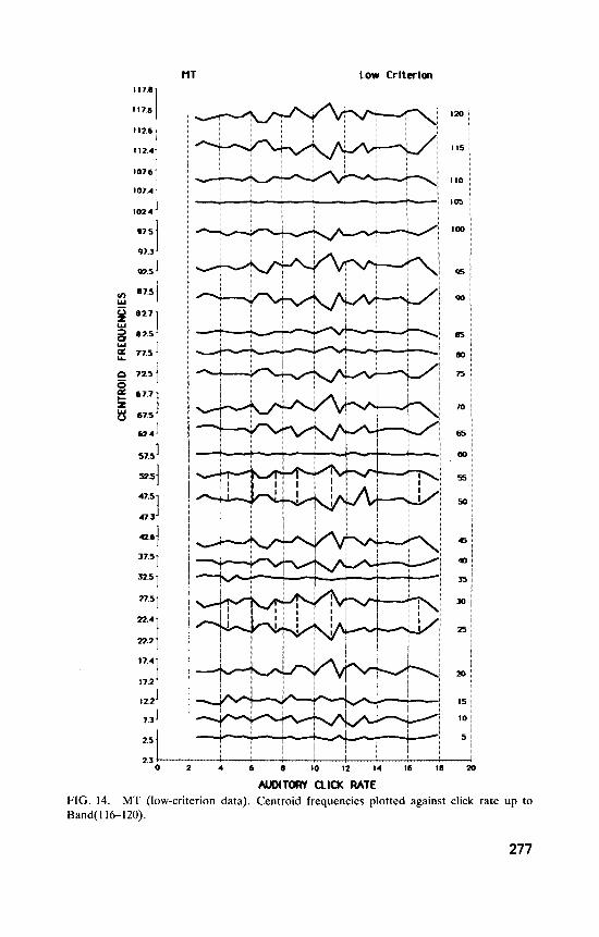
Dow

nloa

ded

By:

[Tre

ism

an, M

iche

l] A

t: 20

:20

16 J

uly

2008

2.3 ,"-

MT Low Criterlon

1 2 0

I15

c -. 105

4 6 0 10 12 14 I6 I 8

AUDITORY aim RATE 3

FIG. 14. Band(l16-120).

MT (low-criterion data). Centroid frequencies plotted against click rate up to

277

Dow

nloa

ded

By:

[Tre

ism

an, M

iche

l] A

t: 20

:20

16 J

uly

2008

278

> 0 Z W

W U LL

i3

a II

0 U + Z w 0

FIG. 15

TREISMAN ET AL.

Reaction Time Peaks EEG: Band(Z1 - 25) 22.8 1

22.7 -

22.6 -

22.5 -

22.4 -

22.3 -

22.2 -

22.1 0 1 2 3 4 S 6 7 8 9 1 0 1 1 12 13 1 4 1 5 1 6 1 7 1 8 1 9 2 0

AUDITORY CLICK RATE The high-criterion curve CF(21-25) plotted against click rate for each subject. The

curves for CM and PN are displaced 0.2 Hz and 0.4 H z upward, respectively. Vertical lines are drawn at the positions of all peaks in the combined response-time data of Treisman et al. (1992) in the present click-rate range.

was defined as any point greater than its immediate neighbour on either side, whatever the magnitude of the difference. Is there any agreement between CF dips and response-time peaks?

The CF(21-25) curve for PN shows parallels to the response-time data. Of the eight dips in CF, six correspond within 0.1 Hz to response-time peaks (3.0, 5.5, 9.4, 11.6, 12.5, and 13.5 Hz); the other two lie 0.5 or 0.6 Hz from a response-time peak. CM’s high-criterion CF(21-25) curve has two dips that correspond within 0.1 Hz to response-time peaks, and five that lie 0.4 to 0.6 Hz to the right of a response-time peak. MT has five dips within 0.1 Hz of a response-time peak, and two within 0.4 Hz. Thus these data support a relation between the EEG and the response-time interference patterns.

Advancing to the fourth question: do the EEG data enable us to select among our models of TO organization?

We can reject the single TO model. This predicted that the CF in one band or at most two neighbouring bands would be click-sensitive. This is

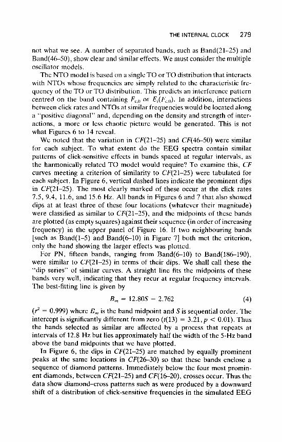
Dow

nloa

ded

By:

[Tre

ism

an, M

iche

l] A

t: 20

:20

16 J

uly

2008

THE INTERNAL CLOCK 279

not what we see. A number of separated bands, such as Band(21-25) and Band(4&S0), show clear and similar effects. We must consider the multiple oscillator models.

The NTO model is based on a single T O or TO distribution that interacts with NTOs whose frequencies are simply related to the characteristic fre- quency of the TO or TO distribution. This predicts an interference pattern centred on the band containing F,,, or E,(FL,,J. In addition, interactions between click rates and NTOs at similar frequencies would be located along a “positive diagonal” and, depending on the density and strength of inter- actions, a more or less chaotic picture would be generated. This is not what Figures 6 to 14 reveal.

We noted that the variation in CF(21-25) and CF(46-50) were similar for each subject. To what extent do the EEG spectra contain similar patterns of click-sensitive effects in bands spaced at regular intervals, as the harmonically related TO model would require? To examine this, CF curves meeting a criterion of similarity to CF(21-25) were tabulated for each subject. In Figure 6, vertical dashed lines indicate the prominent dips in CF(21-25). The most clearly marked of these occur at the click rates 7.5, 9.4, 11.6, and 15.6 Hz. All bands in Figures 6 and 7 that also showed dips at at least three of these four locations (whatever their magnitude) were classified as similar to CF(21-25), and the midpoints of these bands are plotted (as empty squares) against their sequence (in order of increasing frequency) in the upper panel of Figure 16. If two neighbouring bands [such as Band(1-5) and Band(6-10) in Figure 71 both met the criterion, only the band showing the larger effects was plotted.

For PN, fifteen bands, ranging from Band(6-10) to Band(186-190), were similar to CF(21-25) in terms of their dips. We shall call these the “dip series” of similar curves. A straight line fits the midpoints of these bands very well, indicating that they recur at regular frequency intervals. The best-fitting line is given by

B, = 12.80s - 2.762

(? = 0.999) where Em is the band midpoint and S is sequential order. The intercept is significantly different from zero (t(13) = 3.21, p < 0.01). Thus the bands selected as similar are affected by a process that repeats at intervals of 12.8 Hz but lies approximately half the width of the 5-Hz band above the band midpoints that we have plotted.

In Figure 6 , the dips in CF(21-25) are matched by equally prominent peaks at the same locations in CF(26-30) so that these bands enclose a sequence of diamond patterns. Immediately below the four most promin- ent diamonds, between CF(21-25) and CF( 16-20), crosses occur. Thus the data show diamond-cross patterns such as were produced by a downward shift of a distribution of click-sensitive frequencies in the simulated EEG

(4)

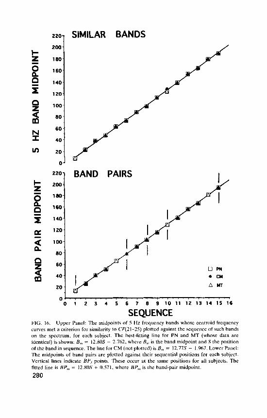
Dow

nloa

ded

By:

[Tre

ism

an, M

iche

l] A

t: 20

:20

16 J

uly

2008

220-

200-

180-

160-

140-

120-

100-

80 -

6 0 -

40 -

20 -

0‘

‘OI 20

SIMILAR BANDS

BAND PAIRS BAND PAIRS

o w .CM A M T

o w .CM A M T

0 1 2 3 4 5 6 7 8 9 1 0 1 1 1 2 1 3 1 4 1 5 1 6

SEQUENCE FIG. 16. Upper Panel: The midpoints o f 5-Hz frequency bands whose centroid frequency curves met a criterion for similarity to CF(21-25) plotted against the sequence of such bands on the spectrum, for each subject. The best-fitting line for PN and MT (whose data are identical) is shown: B., = 12.80s - 2.762, where B,,, is the band midpoint and S the position of the band in sequence. The line for C M (not plotted) is B,,, = 12.773 - 1.967. Lower Panel: The midpoints of band pairs are plotted against their sequential positions for each subject. Vertical lines indicate B P , points. These occur at the same positions for all subjects. The fitted line is BP,, = 12.80S + 0.571, where BP,,, is the band-pair midpoint.

280

Dow

nloa

ded

By:

[Tre

ism

an, M

iche

l] A

t: 20

:20

16 J

uly

2008

THE INTERNAL CLOCK 281

model (cf. Figure 4). This pattern is predicted if there is an underlying TO distribution, but not a single TO. The main difference from the diamond- cross pattern at “click-rate 6” in the simulation is that here the transition from diamond to cross occurs more rapidly. If the present data reflect the downward shift of an underlying distribution of click-sensitive frequencies, the extent of the shift and perhaps the standard deviation of the underlying distribution may be less than the parameters assumed in EEG,,, .

In Figure 4 the diamond above a cross produced by the simulated down- ward shift at click-rate 6 was paired with a cross above a diamond at click-rate 8, caused by the distribution moving upwards. This second diamond was one band lower than the first. Similar patterns can be seen in Figure 6: for example, the diamond-cross pattern at 11.6 Hz is followed by a cross-diamond pattern at 11.9 Hz, the cross lying between Band(21- 25) and Band(26-30) and the diamond lying between Band(l6-20) and Band(21-25), that is, displaced down one band as compared with the diamond at 11.6 Hz. A similar combination of patterns is seen at 15.6 and 16.1 Hz.

We shall refer to successive curves that enclose a series of diamond patterns between them, such as CF(21-25) and CF(26-30), as a band pair ( B P ) ; in this case BP2(21-30) (the subscript “2” indicates that the two bands are immediately successive). If a curve with peaks and a curve with dips are separated by an intermediate curve that is not clearly character- ized, the band pair ranges over three bands ( B P , ) . For example, CF(6-10) and CF(16-20) in Figure 6 have respectively a dip and a peak at 7.5 Hz, 9.4 Hz, 11.6 Hz, and 15.6 Hz, but the intermediate curve CF(11-15) is variable. Several band pairs can be recognized in Figures 6 ,7 , and 8. How regularly are such structures spaced in the EEG spectrum?

We identified above those curves that have a similar pattern of dips to CF(21-25). Applying the same criterion to peaks, a “peak series” of curves similar to CF(26-30) can be identified. It was found that for PN the “peak series” curves could all be matched to “dip series” curves to give band pairs that ranged over two or three bands. In Figures 6 and 7, these band pairs are identified by brackets. The band-pair midpoints are plotted as empty squares in the lower panel of Figure 16, in order of their sequence S in the record [but assuming that for S = 6 a point is missing, as the curve that would have complemented the dip series curve CF(71-75) failed to meet the peak series criterion]. Vertical lines indicate the positions in the sequence at which the band pairs ranged over three rather than two bands. The points cluster closely around the best-fitting line

BP,,, = 12.80s + 0.571 ( 5 ) (9 = 0.999) where BP,,, is the band-pair midpoint. The intercept is not significantly different from zero (t(12) = 1.109). This shows that the band- pair midpoints are spaced as the elements of a harmonic series with a

Dow

nloa

ded

By:

[Tre

ism

an, M

iche

l] A

t: 20

:20

16 J

uly

2008

282 TREISMAN ET AL.

fundamental frequency of about 12.8 Hz. (We are reminded that in the output from EEG,,, the diamonds corresponded approximately to the position of Fc.,).)

PN’s low-criterion data in Figure 8 are similar to the high-criterion data in Figure 6 except that they are somewhat more noisy, and the band pairs now all show diamonds at 3.5 Hz. It seems that including higher variance records provides evidence of processes that are especially sensitive at this low rate.

The regular spacing of similar bands and band pairs in PN’s data, showing patterns resembling the simulated TO distribution predictions, strongly favours a model in which sets of TOs recur at harmonically related intervals. What do the other subjects show?

For CM, the CF plots in Figures 9, 10, and 11 show the same tendency for patterns to repeat in regularly spaced frequency bands as was seen for PN. Vertical dashed lines in Figure 9 indicate some prominent dips in CF(21-25). For the high-criterion data, CF curves meeting a criterion of similarity to CF(21-25) were tabulated. The criterion required dips at at least three of 7.9, 10.0, 11.9, 13.9, 15.6, and 16.7 Hz. This gave the “dip series” of fourteen bands that are plotted (as filled circles) in the upper panel of Figure 16 (assuming that there is a missing point at S = 1). Thir- teen of the 14 points are identical with those found for PN, and the best- fitting curve is very similar, B, = 12.77s - 1.967 (? = 0.999), and is not shown separately. For the intercept, 412) = 2.11, p = 0.057.

The dips in CF(21-25) for CM are broader and more rounded than was found for PN, as too are the peaks in CF(26-30). One consequence is that in three cases a peak in the upper curve is displaced by one step from a dip in the lower curve. If we allow for this by matching up dips and peaks that occur at neighbouring click rates, diamond patterns can be recognized at 10.0, 11.6-11.9, 13.5-13.9, 15.6, and 16.7-17.2 Hz, as shown by the vertical dashed lines. A “peak series” of curves similar to CF(26-30) was identified, the criterion being at least three peaks at 10.0, 11.6, 13.5, 15.6, or 17.2 Hz. This is a strict criterion as it takes no account of the rounding of the dips and peaks in CM’s data. Eleven band pairs were identified. These are plotted in Figure 16 with gaps for missing points. Inspection of Figures 9 and 10 suggests that the rejected points represent near misses.

Figure 11 includes the higher variance records. This produces some blurring of the diamond at 11.6 to 11.9 Hz, but defines new diamonds at 3.5 and 5.0 Hz. Overall, CM’s data strongly support the conclusions drawn from PN’s data.

MT’s data also show patterns repeating at regular intervals. In Figure 12 diamonds enclosed by Band(21-25) and Band(26-30) are indicated by vertical dashed lines, at 4.0, 5.5, 11.1, 12.5, and 16.1 Hz. The midpoints of bands meeting a criterion of similarity to CF(21-25) (dips at at least

Dow

nloa

ded

By:

[Tre

ism

an, M

iche

l] A

t: 20

:20

16 J

uly

2008

THE INTERNAL CLOCK 283

four of 4.0, 7.9, 11.1, 12.5, and 16.1 Hz) are plotted in the upper panel of Figure 16. These fifteen points are identical with those for PN. A peak series of curves similar to CF(26-30) was also found. The two series of curves define 15 band pairs [BP2(21-30) has a diamond at 5.5 Hz; in the other band pairs this is replaced by one at 6.0 Hz]. These have the same values as for the other subjects and are plotted in Figure 16.

The inclusion of higher variance EEG records (cf. Figure 14) produces some changes. The diamonds previously at 4.0, 5.5, and 16.1 Hz shift to 4.5, 6.0, and 16.7 Hz; the diamond at 12.5 Hz is blurred; and new diamonds appear at 7.5 and 8.9 Hz.

Figure 17 compares the CF interference patterns for each subject [BP2(21-30) is replotted]; it also shows the S and L time-estimation inter- ference patterns from Est Expt. 1 and the mean time-estimation residuals for the present experiment.

Dashed vertical lines indicate the locations of diamonds in the three BP, plots; where complementary peaks and dips differ by about 0.5 Hz, dotted lines are drawn. A number of dips are labelled. Despite differences in the placement of diamonds, there is considerable agreement among the band-pair curves. Each shows eight reasonably prominent diamonds over this range. Two have diamonds at 3.5 Hz and at 5.0 to 5.5 Hz, the third has diamonds at 4.5 and 6.0 Hz. Two have diamonds at 7.5 Hz. MT has a diamond at 11.1 Hz; PN a diamond at 11.6 Hz; and CM a diamond at 11.1 to 11.6 Hz. Two subjects have diamonds at 13.5 Hz, two at 15.6 Hz, two at 16.7 Hz. Diamond placement is not identical for any two subjects, but there are family resemblances.

There are also parallels between the placement of diamonds in the EEG and the locations of dips in the time-estimation interference patterns. Two diamonds (PN and CM) and one dip occur at 3.5 Hz (Ex 1:L); one diamond and two dips at 4.5 Hz (MT, Ex l:S, EEG Ex); two diamonds at 5.0 or 5.5 Hz and two dips at 5.5 Hz; two diamonds at 7.5 Hz and two dips at 7.0 Hz; two diamonds at 8.5 and 8.9 Hz and three dips at 8.5, 8.9, and 9.0 Hz; three diamonds at 11 .1 , 11.6, and 11.1-11.6 Hz, one dip at 11.1, and two dips at 11.5 Hz; two diamonds at 13.5 and one at 13.9 Hz, three dips at 13.5 Hz; two diamonds at 15.6 Hz and two dips at 16.0 and 16.1 Hz; two diamonds at 16.7 Hz and a dip at 16.5 Hz. There is variation in the location of these features, but there are overall resemblances.

We may conclude that there are sufficient parallels among the EEG patterns, and between the former and the time-estimation and response- time interference patterns to show that common processes are at work. In general, the evidence supports a model in which sets of temporal oscil- lators of similar frequency are themselves distributed at equal steps in the EEG spectrum: the harmonically spaced temporal oscillator distribution model.

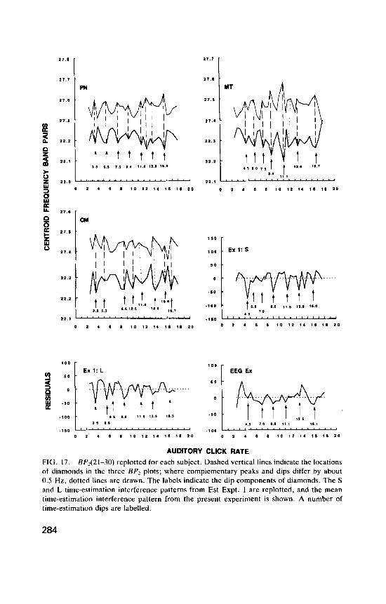
Dow

nloa

ded

By:

[Tre

ism

an, M

iche

l] A

t: 20

:20

16 J

uly

2008

2 1 , s

2 1 . 1

2 1 . 6

PN

0 2 4 8 8 1 0 1 2 1 4 i b 1 8 2 0 W 3

27 .8 r

0 2 4 8 8 1 0 1 2 1 4 1 8 1 8 2 0

2 1 . 7

2 1 . 8

27.5

21.4

22 .1

2 2 . 2

2 2 . 1 1 1 . 1

0 2 4 8 8 1 0 1 2 I 4 1 8 1 0 2 0

5 0

*.o ,,$ ts.5 t s o

0 2 4 8 8 1 0 1 2 1 4 1 8 1 8 2 0

Ex 1: L Y 5 0

- 3 o -

.50

1 - 5 0 -

.100 1.5 5.5

-110 ' " ' " " ' " a " " '

0 2 4 8 8 1 0 1 2 1 4 1 8 1 8 2 0

l o o 1 EEG Ex

.. 1 5 7 0 i n * I t I1 1

0 2 4 8 8 1 0 1 2 1 4 1 6 1 8 2 0 . l o o " " " ' " ' " ' " "

AUDITORY CLICK RATE FIG. 17. BP2(21-30) replotted for each subject. Dashed vertical lines indicate the locations of diamonds in the three BP, plots; where complementary peaks and dips differ by about 0.5 Hz, dotted lines are drawn. The labels indicate the dip components of diamonds. The S and L time-estimation interference patterns from Est Expt. 1 are replotted, and the mean time-estimation interference pattern from the present experiment is shown. A number of time-estimation dips are labelled.

284

Dow

nloa

ded

By:

[Tre

ism

an, M

iche

l] A

t: 20

:20

16 J

uly

2008

THE INTERNAL CLOCK 285

DISCUSSION AND CONCLUSION

Could the recurrence of similar band pairs at regular intervals be an artefact of the power spectrum analysis? For example, we might assume that the EEG contains a single distribution of click-sensitive TOs that emit non- sinusoidal signals. If so, Fourier analysis of a TO output would display it as a fundamental and a series of harmonics that would all show the same variations when the subject is exposed to clicks. However, this would predict that the magnitude of the CF dips and peaks, and the spread of the band pairs, would increase with harmonic number. For example, if there were a single distribution of non-sinusoidal oscillators ranging in frequency from 21 to 30 Hz, their second harmonics would span 42 to 60 Hz. Thus, successive band pairs should be increasingly widely spaced on a linear scale of frequency. But we have seen that band pairs stay within a range of 10 or 15 Hz whatever their position in the spectrum.

Interference patterns can be compared “horizontally” in terms of the effects of click rate, or “vertically” in terms of location in the EEG spec- trum. Consistency across subjects seems very different in the two cases. The locations of “dip” and “peak series” bands in the EEG spectrum are almost the same in different subjects. Furthermore, band pairs at sequence positions 1, 6, 8, 10, or 15 (but at no other positions) always range over three bands. These regularities suggest that subjects share a similar stable underlying organization of temporal mechanisms.

In contrast, the locations of EEG diamonds and d ippeak perturbations show family resemblances but not identity among subjects. A simple explanation for this difference might be that it expresses a difference in resolution. The EEG is quantized at 5-Hz intervals, whereas the locations of perturbations have been determined at 0.5- or 0.1-Hz intervals (Treisman et al., 1990). This is a problem that deserves further study.

Why do two-band band pairs and three-band band pairs occur at the same sequence positions for each subject? This may reflect an interaction between the locations of the click-sensitive distributions and the way our analysis divided the spectrum into bands. A 2-SD shift of the click-sensitive frequency distribution in the EEG,,, model may produce different effects depending on where the mean of the distribution is initially located in relation to the 5-Hz bands. If it is initially centred in a band, that band shows a dip and the band above shows a peak in response to a downward shift, giving a two-band band pair. But if the mean lies at the lower or upper margin of a band initially, the dip occurs in the band below and the peak in the band above, giving a three-band band pair.

Despite Treisman’s (1984) rejection of the alpha rhythm as the temporal timing frequency (on the basis of predictions from a unitary pacemaker model) more recent time-estimation data (Treisman et al., 1990) suggest

Dow

nloa

ded

By:

[Tre

ism

an, M

iche

l] A

t: 20

:20

16 J

uly

2008

286 TREISMAN ET AL.

that a frequency of 12.4 Hz may underlie estimates of F,,,); and the spacing of EEG band pairs suggests an underlying repetition frequency of 12.8 Hz. Although such values lie in the alpha frequency band, this does not neces- sarily imply that “the alpha frequency” is the temporal information source. Even if a frequency or frequencies in the alpha range are emitted by oscillators used in timing, these could well constitute only a small com- ponent of the EEG frequencies between 8 and 13 Hz.

The best interpretation of the overall data that we can offer at this stage is that timing depends on temporal pacemakers, each consisting of an oscillator linked to a gain control unit, as in Figure 1. The brain contains several sets of similar TOs, each set giving rise to a distinct distribution of click-sensitive frequencies. The distributions have similar variances, and their means recur at regular intervals, of approximately 12.8 Hz, on the EEG spectrum. This system of distributions is similar in different subjects.

Treisman (1965) noted that we judge intervals of time in seconds, hours, or weeks, and asked: “To the extent that we rely on the internal clock, does the same clock give us measures of all these periods? . . . perhaps a series of parallel Pacemakers firing at different rates . . . may serve different orders of time.” A number of later studies have provided evidence that could be interpreted in terms of multiple pacemakers (Eisler, 1975, 1981, 1990; Kristofferson, 1980, 1984; Pastore, 1987; Povel, 1981; Vorberg & Hambuch, 1978, 1984; Wing, 1980; Wing & Kristofferson, 1973a, 1973b).

The present results provide the basis for a model based on an extensive system of parallel pacemakers. In this model, time-keeping depends on a sequence of parallel harmonically related frequencies or distributions of frequencies. These may be employed for temporal tasks involving time scales of different orders. This system of reduplicated clocks allows both the possibility of continuous adjustment (by varying the effect of the Calib- ration Unit attached to each TO) and of step adjustments, the transition from one click-sensitive band to another. While this account is tentative, it may serve as a basis for future research.

REFERENCES Alonso, M . , & Finn, E.J. (1970). Physics. Reading, MA: Addison-Wesley. Devaney, R.L. (1989). A n introduction to chaotic dynamical systems (2nd ed . ) . Reading,

MA: Addison-Wesley. Eisler, H. (1975). Subjective duration and psychophysics. Psychological Review. K2.

429450. Eisler, H . (1981). Applicability of the parallel-clock model to duration discrimination.

Perception and Psychophysics, 29, 225-233. Eisler, H . (1990). Breaks in the psychophysical function f o r duration. In H . G . Geissler.

M.H. Miiller, & W. Prinz (Eds.), Psychophysical explorations of mental structures (pp. 242-252). Stuttgart: Hofgrefe & Huber.

Dow

nloa

ded

By:

[Tre

ism

an, M

iche

l] A

t: 20

:20

16 J

uly

2008

THE INTERNAL CLOCK 287

Glass, I>.. Gucvara, M.R., & Shricr, A . (1987). Universal bifurcations and the cl of cardiac arrhythmias. Annals of fhe New York Academy o/Sciences, 504, 168-178.

Glass, I.., & Mackcy, M.C. (1988). From clocks tu chaos: The rhythms of’ life. Princeton, NJ : Princeton University Press.

Hoagland, H. (1933). The physiological control of judgments of duration: Evidence for a chemical clock. Journal of General Psychology, 9. 267-287.

Kristoffcraon, A.B. (1980). A quanta1 step function in duration discrimination. Perception and Psychophysics, 27, 300-306.

Kristotferson, A.B. (1984). Quanta1 and deterministic timing in human duration discrimina- tion. In: J . Gibbon and L. Allan (Eds.), Timing and Time Perception. Annals ofthe New York Academy of Sciences, 423, 3-15.

Lockhart, J.M. (1967). Ambient temperature and time estimation. Journal of Experimental Psychology, 73, 286291,

Moore-Ede, M.C., & Czeisler, C.A. (Eds.) (1984). Mathematical models of the sleep-wake cycle. New York: Raven Press.

Moore-Ede, M.C., Sulzman, F.M., & Fuller, C.A. (1982). The clocks that time us. Cambridge, MA: Harvard University Press.

Pastore, R.E. (1987). Categorical perception: Some psychophysical models. In S. Harnad (Ed.), Cafegorical perception: The groundwork of cognition (pp. 29-52). Cambridge: Cambridge University Press.

Petrillo, G.A., & Glass, L. (1984). A theory for phase locking of respiration in cats to a mechanical ventilator. American Journal of Physiology, 246, R31 I-R320.

Povel, D.-J. (1981). Internal representation of simple temporal patterns. Journal of Experi- mental Psychology: Human Perception and Performance, 7 , 3-18.

Sokolov, Y.N. (1963). Perception and the conditioned reflex. Oxford: Pergamon Press. Stoker, J . J . (195011992). Nonlinear vibrations in mechanical and electrical systems. New

Surwillo, W.W. (1966). Time perception and the “internal clock”: Some observations on

Treisman, M. (1963). Temporal discrimination and the indifference interval: Implications

Treisman, M. (1965). The psychology of time. Discovery, 26 (lo), 40-45. Treisman, M. (1984). Temporal rhythms and cerebral rhythms. In: J . Gibbon & L. Allan

(Eds.), Timing and Time Perception. Annals of the New York Academy of Sciences, 423,

Treisman, M. (1991). Time perception and the timing of action: A model of the temporal pacemaker. Communicazioni Scienrifiche di Psicologia Generale, 5 n.s., 71-101.

Treisman, M., & Brogan, D. (1992). Time perception and the internal clock: Effects of visual flicker on the temporal oscillator. European Journal of Cognitive Psychology, 4 , 41-70.

Treisman, M., Faulkner, A, , Naish, P.L.N., & Brogan, D. (1990). The internal clock: Evidence for a temporal oscillator underlying time perception with some estimates of its characteristic frequency. Percephon, 19, 705-743.

Trekman, M., Faulkner, A, , & Naish, P.L.N. (1992). On the relation between time percep- tion and the timing of motor action: Evidence for a temporal oscillator controlling the timing of movement. Quarterly Journal of Experimental Psychofogy, 45A, 235-263.

van der Pol, B. (1927). Forced oscillations in a circuit with non-linear resistance. (Reception with reactive triode). Philosophical Magazine, 3, 65-80.

von Holst, E. (1937/1973). Vom Wesen der Ordnung im Zentralnervensystem. Naiur- wissenschaften, 25, 625-631, 641447. Republished in E. von Holst, The behavioural physiology of animals and man, Vol. I (pp. 3-32). London: Methuen, 1973 (transl. R. Martin).

York: Wiley.

the role of the electroencephalogram. Brain Research, 2, 39&392.

for a model of the “internal clock”. Psychological Monographs, 77, Whole No. 576, 1-31.

542-565.

Dow

nloa

ded

By:

[Tre

ism

an, M

iche

l] A

t: 20

:20

16 J

uly

2008

288 TREISMAN ET AL.

Vorberg, D., & Hambuch. R. (1978). On the temporal control of rhythmic performance. In J . Requin (Ed.), Attention and Performance 1/11 (pp. 535-555). Hillsdale, NJ: Lawrence Erlbaum Associates Inc.

Vorberg, D., & Hambuch, R. (1984). Timing of two-handed rhythmic performance. In J . Gibbon & L. Allan (Eds.), Timing and Time Perception. Annals of the New York Academy of Sciences, 423, 390-406.

Werboff, J . (1962). Time judgment as a function of electroencephalographic activity. Experi- mental Neurology, 6 , 152-160.

Wever, R.A. (1984). Toward a mathematical model of circadian rhythmicity. In M.C. Moore-Ede & C.A. Czeisler (Eds.), Mathematical models of the sleep-wake cycle (pp. 17-79). New York: Raven Press.

Winfree, A.T. (1987). The timing of biological clocks. New York: Freeman. Wing, A.M. (1980). The long and short of timing in response sequences. In G.E. Stelmach

Wing, A.M., & Kristofferson, A.B. (1973a). The timing of interresponse intervals. Per-

Wing, A.M., & Kristofferson, A.B. (1973b). Response delays and the timing of discrete

& J . Requin (Eds.), Tutorials in motor behavior. Amsterdam: North-Holland.

ception and Psychophysics, 13, 455-460.

motor responses. Perception and Psychophysics, 14, 5-12

Final manuscript received 23 March 1994

APPENDIX

91

141

Glossary of Symbols A band pair ranging over two bands: a pair of successive 5-Hz bands whose CF curves enclose a sequence of diamond patterns between them. A band pair ranging over three successive bands. Constant in regression of E onto T, and N A . Coefficient of NA in regression of E onto T, and NA. Coefficient of T, in regression of E onto T, and NA. The calibration factor. The CU multiplies the TO output by C, to give the final pacemaker output, Fp. The centroid of a band of EEG frequencics ranging from

The Calibration Unit, the second component of the tem- poral pacemaker. An estimate of a presented time interval. An EEG frequency. An arousal frequency, the frequency of a regular series of sensory pulses that can modify the specific arousal of the calibration unit or interfere with the T O . The frequency of the temporal oscillator. The characteristic frequency of the TO. The final pacemaker output, the frequency of the timing pulses emitted by the CU.

f k - 4 tofk.

Dow

nloa

ded

By:

[Tre

ism

an, M

iche

l] A

t: 20

:20

16 J

uly

2008

THE INTERNAL CLOCK 289

F\.A

L NA NTO

PI R S S T/

TO

An arousal frequency that has a simple rational relation to FC.,), such that F,,A = (n/rn)Fc,,, where n and rn are low- valued relatively prime positive integers. Long durations. The number of clicks presented concurrently with T,. A non-temporal oscillator that may interact with the tem- poral oscillator but does not itself produce timing pulses. The power at frequencyf, given by power spectrum analysis. An estimate ratio: EIT,. Short durations. Sequence position of band pairs on EEG spectrum. Short reference duration. Long reference duration. A temporal duration presented to a subject for estimation. The Temporal Oscillator, the first component of the tem- poral pacemaker.