The Great Lakes Runoff Intercomparison Project Phase 4
36
Hydrol. Earth Syst. Sci., 26, 3537–3572, 2022 https://doi.org/10.5194/hess-26-3537-2022 © Author(s) 2022. This work is distributed under the Creative Commons Attribution 4.0 License. The Great Lakes Runoff Intercomparison Project Phase 4: the Great Lakes (GRIP-GL) Juliane Mai 1 , Hongren Shen 1 , Bryan A. Tolson 1 , Étienne Gaborit 2 , Richard Arsenault 3 , James R. Craig 1 , Vincent Fortin 2 , Lauren M. Fry 4 , Martin Gauch 5 , Daniel Klotz 5 , Frederik Kratzert 5,6 , Nicole O’Brien 7 , Daniel G. Princz 8 , Sinan Rasiya Koya 9 , Tirthankar Roy 9 , Frank Seglenieks 7 , Narayan K. Shrestha 7 , André G. T. Temgoua 7 , Vincent Vionnet 2 , and Jonathan W. Waddell 10 1 Department of Civil and Environmental Engineering, University of Waterloo, Waterloo, ON, Canada 2 Meteorological Research Division, Environment and Climate Change Canada, Dorval, QC, Canada 3 Department of Construction Engineering, École de technologie supérieure, Montreal, QC, Canada 4 Great Lakes Environmental Research Laboratory, National Oceanic and Atmospheric Administration, Ann Arbor, MI, USA 5 Institute for Machine Learning, Johannes Kepler University, Linz, Austria 6 Google Research, Vienna, Austria 7 National Hydrological Service, Environment and Climate Change Canada, Burlington, ON, Canada 8 National Hydrological Service, Environment and Climate Change Canada, Saskatoon, SK, Canada 9 Department of Civil and Environmental Engineering, University of Nebraska–Lincoln, Lincoln, NE, USA 10 Great Lakes Hydraulics and Hydrology Office, U.S. Army Corps of Engineers, Detroit, MI, USA Correspondence: Juliane Mai ([email protected]) Received: 22 March 2022 – Discussion started: 29 March 2022 Revised: 5 June 2022 – Accepted: 10 June 2022 – Published: 8 July 2022 Abstract. Model intercomparison studies are carried out to test and compare the simulated outputs of various model se- tups over the same study domain. The Great Lakes region is such a domain of high public interest as it not only resembles a challenging region to model with its transboundary loca- tion, strong lake effects, and regions of strong human impact but is also one of the most densely populated areas in the USA and Canada. This study brought together a wide range of researchers setting up their models of choice in a highly standardized experimental setup using the same geophysi- cal datasets, forcings, common routing product, and loca- tions of performance evaluation across the 1×10 6 km 2 study domain. The study comprises 13 models covering a wide range of model types from machine-learning-based, basin- wise, subbasin-based, and gridded models that are either lo- cally or globally calibrated or calibrated for one of each of the six predefined regions of the watershed. Unlike most hy- drologically focused model intercomparisons, this study not only compares models regarding their capability to simulate streamflow (Q) but also evaluates the quality of simulated ac- tual evapotranspiration (AET), surface soil moisture (SSM), and snow water equivalent (SWE). The latter three outputs are compared against gridded reference datasets. The com- parisons are performed in two ways – either by aggregating model outputs and the reference to basin level or by regrid- ding all model outputs to the reference grid and comparing the model simulations at each grid-cell. The main results of this study are as follows: 1. The comparison of models regarding streamflow re- veals the superior quality of the machine-learning-based model in the performance of all experiments; even for the most challenging spatiotemporal validation, the ma- chine learning (ML) model outperforms any other phys- ically based model. 2. While the locally calibrated models lead to good perfor- mance in calibration and temporal validation (even out- performing several regionally calibrated models), they lose performance when they are transferred to locations that the model has not been calibrated on. This is likely to be improved with more advanced strategies to trans- fer these models in space. Published by Copernicus Publications on behalf of the European Geosciences Union.
-
Upload
khangminh22 -
Category
Documents
-
view
1 -
download
0
Transcript of The Great Lakes Runoff Intercomparison Project Phase 4

Hydrol. Earth Syst. Sci., 26, 3537–3572, 2022https://doi.org/10.5194/hess-26-3537-2022© Author(s) 2022. This work is distributed underthe Creative Commons Attribution 4.0 License.
The Great Lakes Runoff Intercomparison ProjectPhase 4: the Great Lakes (GRIP-GL)Juliane Mai1, Hongren Shen1, Bryan A. Tolson1, Étienne Gaborit2, Richard Arsenault3, James R. Craig1,Vincent Fortin2, Lauren M. Fry4, Martin Gauch5, Daniel Klotz5, Frederik Kratzert5,6, Nicole O’Brien7,Daniel G. Princz8, Sinan Rasiya Koya9, Tirthankar Roy9, Frank Seglenieks7, Narayan K. Shrestha7,André G. T. Temgoua7, Vincent Vionnet2, and Jonathan W. Waddell10
1Department of Civil and Environmental Engineering, University of Waterloo, Waterloo, ON, Canada2Meteorological Research Division, Environment and Climate Change Canada, Dorval, QC, Canada3Department of Construction Engineering, École de technologie supérieure, Montreal, QC, Canada4Great Lakes Environmental Research Laboratory, National Oceanic and Atmospheric Administration, Ann Arbor, MI, USA5Institute for Machine Learning, Johannes Kepler University, Linz, Austria6Google Research, Vienna, Austria7National Hydrological Service, Environment and Climate Change Canada, Burlington, ON, Canada8National Hydrological Service, Environment and Climate Change Canada, Saskatoon, SK, Canada9Department of Civil and Environmental Engineering, University of Nebraska–Lincoln, Lincoln, NE, USA10Great Lakes Hydraulics and Hydrology Office, U.S. Army Corps of Engineers, Detroit, MI, USA
Correspondence: Juliane Mai ([email protected])
Received: 22 March 2022 – Discussion started: 29 March 2022Revised: 5 June 2022 – Accepted: 10 June 2022 – Published: 8 July 2022
Abstract. Model intercomparison studies are carried out totest and compare the simulated outputs of various model se-tups over the same study domain. The Great Lakes region issuch a domain of high public interest as it not only resemblesa challenging region to model with its transboundary loca-tion, strong lake effects, and regions of strong human impactbut is also one of the most densely populated areas in theUSA and Canada. This study brought together a wide rangeof researchers setting up their models of choice in a highlystandardized experimental setup using the same geophysi-cal datasets, forcings, common routing product, and loca-tions of performance evaluation across the 1×10⁶ km2 studydomain. The study comprises 13 models covering a widerange of model types from machine-learning-based, basin-wise, subbasin-based, and gridded models that are either lo-cally or globally calibrated or calibrated for one of each ofthe six predefined regions of the watershed. Unlike most hy-drologically focused model intercomparisons, this study notonly compares models regarding their capability to simulatestreamflow (Q) but also evaluates the quality of simulated ac-tual evapotranspiration (AET), surface soil moisture (SSM),
and snow water equivalent (SWE). The latter three outputsare compared against gridded reference datasets. The com-parisons are performed in two ways – either by aggregatingmodel outputs and the reference to basin level or by regrid-ding all model outputs to the reference grid and comparingthe model simulations at each grid-cell.
The main results of this study are as follows:
1. The comparison of models regarding streamflow re-veals the superior quality of the machine-learning-basedmodel in the performance of all experiments; even forthe most challenging spatiotemporal validation, the ma-chine learning (ML) model outperforms any other phys-ically based model.
2. While the locally calibrated models lead to good perfor-mance in calibration and temporal validation (even out-performing several regionally calibrated models), theylose performance when they are transferred to locationsthat the model has not been calibrated on. This is likelyto be improved with more advanced strategies to trans-fer these models in space.
Published by Copernicus Publications on behalf of the European Geosciences Union.

3538 J. Mai et al.: Great Lakes model intercomparison GRIP-GL
3. The regionally calibrated models – while losing lessperformance in spatial and spatiotemporal validationthan locally calibrated models – exhibit low perfor-mances in highly regulated and urban areas and agri-cultural regions in the USA.
4. Comparisons of additional model outputs (AET, SSM,and SWE) against gridded reference datasets show thataggregating model outputs and the reference dataset tothe basin scale can lead to different conclusions than acomparison at the native grid scale. The latter is deemedpreferable, especially for variables with large spatialvariability such as SWE.
5. A multi-objective-based analysis of the model per-formances across all variables (Q, AET, SSM, andSWE) reveals overall well-performing locally calibratedmodels (i.e., HYMOD2-lumped) and regionally cal-ibrated models (i.e., MESH-SVS-Raven and GEM-Hydro-Watroute) due to varying reasons. The machine-learning-based model was not included here as it is notset up to simulate AET, SSM, and SWE.
6. All basin-aggregated model outputs and observationsfor the model variables evaluated in this study are avail-able on an interactive website that enables users to visu-alize results and download the data and model outputs.
1 Introduction
Model intercomparison projects are usually massive un-dertakings, especially when multiple (independent) groupscome together to compare a wide range of models over largeregions and a large number of locations (Duan et al., 2006;Smith et al., 2012; Best et al., 2015; Kratzert et al., 2019c;Menard et al., 2020; Mai et al., 2021; Tijerina et al., 2021).The aim of such projects is diverse. It might be to identifymodels that are most appropriate for certain objectives (e.g.,simulating high flows or representing soil moisture) or tostudy the differences in model setups and implementationsin detail.
Intercomparison projects are also well suited for intro-ducing new models through the inherent benchmarking withother models (Best et al., 2015; Kratzert et al., 2019c;Rakovec et al., 2019). In particular, the recent successful ap-plication of data-driven models in hydrologic applicationsnecessitate standardized experiments – such as model inter-comparison studies – to make sure that the models are usingthe same information and strategies to enable fair compar-isons.
Several model intercomparison have been carried out oversubdomains (here called regions) of the Great Lakes in thepast (Fry et al., 2014; Gaborit et al., 2017a; Mai et al., 2021)
under the umbrella of the Great Lakes Runoff Intercompar-ison Projects (GRIP). The GRIP projects were envisionedsince the Great Lakes region with its transboundary locationleads to (a) challenges such as finding datasets that are con-sistent across borders or models that are only set up on eitherside of the border, (b) challenges in the modeling itself dueto, for example, climatic conditions driven by large lake ef-fects and substantial areas of heavy agricultural land use andurban areas, and (c) a high public interest since the GreatLakes watershed is one of the most densely populated areasin Canada (32 % of the population) and the USA (8 % of thepopulation; Michigan Sea Grant, 2022). Another reason forthe high public interest is that changes in runoff to the GreatLakes have implications for water levels, which have under-gone dramatic changes (from record lows in 2012–2013 torecord highs in 2017–2020) in recent decades. The afore-mentioned GRIP projects were set up over regions of theentire Great Lakes watershed, i.e., Lake Michigan (GRIP-M; Fry et al., 2014), Lake Ontario (GRIP-O; Gaborit et al.,2017a), and Lake Erie (GRIP-E; Mai et al., 2021), and pri-marily investigated the model performances regarding sim-ulated streamflow even though studies show that additionalvariables beyond streamflow might be helpful to improve re-alism of models (Demirel et al., 2018; Tong et al., 2021).
Previous GRIP studies have pointed out limitations regard-ing the conclusions that can be drawn. In particular, the laststudy (GRIP-E by Mai et al., 2021) listed the following chal-lenges in the concluding remarks:
I. There was only a short period of forcings (5 years) tocalibrate and evaluate the models.
II. There was only a comparison of streamflow but no ad-ditional variables like soil moisture.
III. Even though all models use the same forcings, all otherdatasets (soil texture, vegetation, basin delineation, etc.)were not standardized.
Hence, model differences might be due to different qualityinput data but not due to differences in models themselves.The study presented here will address these previous GRIPstudy limitations. Furthermore, this study demonstrates someunique intercomparison aspects that are not necessarily com-mon practice in large-scale hydrologic model intercompari-son studies. Key noteworthy aspects of this intercomparisonstudy are as follows:
1. Datasets used. Hydrologic and land surface modelsneed data to be set up (e.g., soil and land cover) andto be forced (e.g., with precipitation). The forcing datahave, at best, a high temporal and spatial resolution,a complete coverage of the domain of interest, a longavailable time period, and no missing data. In this study,models will be using common datasets for these forc-ings, and all geophysical datasets are required to set up
Hydrol. Earth Syst. Sci., 26, 3537–3572, 2022 https://doi.org/10.5194/hess-26-3537-2022

J. Mai et al.: Great Lakes model intercomparison GRIP-GL 3539
the various kinds of models. A recently developed 18-year-long forcing dataset will be employed (Gasset etal., 2021). This addresses limitations (I) and (III) above.
2. Variables compared. Models are traditionally only eval-uated for one primary variable (e.g., streamflow). In thisstudy, models will be evaluated regarding variables be-yond streamflow such as evapotranspiration, soil mois-ture, and snow water equivalent. This addresses limita-tion (II) above.
3. Method of comparison. A model intercomparison mightinclude various model types, e.g., lumped models vs.semi-distributed or conceptual vs. physically based vs.data driven. To compare these models – especially whennot only comparing time series like streamflow – modelagnostic methods are needed (meaning methods that donot favor one type of model over others). We will per-form comparisons on different scales and use metrics toaccount for these issues. This addresses an issue associ-ated with limitation (II).
4. Types of models considered. Model intercomparisonstudies traditionally use conceptual or physically basedhydrologic models. The rising popularity and success ofdata-driven models in hydrologic science (e.g., Herathet al., 2021; Nearing et al., 2021; Feng et al., 2021),however, warrant the inclusion of such models in suchstudies, given that the data-driven, machine-learning-based models face the same information and input dataas traditional models to guarantee a fair comparison.A machine-learning-based model was included in thisstudy to demonstrate the advantages and limitationsof state-of-the-art machine-learning-based models com-pared to conceptual and physically based models.
5. Communication of results. Large studies with manymodels and locations at which they are compared lead tovast amounts of model results. During such a study, it ischallenging for collaborators to process and compare allresults. After the study is completed, it is equally chal-lenging to present all results in detail in a paper suchthat the data and results are accessible to others. In thisstudy, we shared data through an interactive website,which was first internally accessible during the studyand then publicly shared to enhance data sharing, ex-ploring, and communication with a broader audience.
The remainder of the paper is structured as follows. Sec-tion 2 presents the materials used and methods appliedincluding a description of datasets, models, metrics, andtypes of comparative analyses. Section 3 describes and dis-cusses the results of the analyses performed, while Sect. 4summarizes the conclusions that can be drawn from theexperiments performed here. Note that this work is ac-companied by an extensive Supplement, primarily provid-ing more details for model setups, and an interactive web-
site (http://www.hydrohub.org/mips_introduction.html, lastaccess: 6 July 2022) (Mai, 2022), for sharing and exploringcomparative results.
2 Materials and methods
This section first describes the study domain (Sect. 2.1),datasets used to set up and force models (Sect. 2.2), and thecommon routing product produced for this study and usedby most of the models (Sect. 2.3). A brief description ofthe 13 participating models can be found in Sect. 2.4. Thedatasets used to calibrate and validate the models regardingstreamflow and the datasets to evaluate the models beyondstreamflow are introduced in Sects. 2.5 and 2.6, respectively,followed by Sect. 2.7, which defines the metrics to determinethe models’ ability to simulate the variables provided in thesedatasets using two different approaches, depending on whichspatial aggregation is applied (Sect. 2.8). A multi-objectiveanalysis described in Sect. 2.9 is performed to augment theprevious single objective analyses that evaluated the perfor-mance across the four variables independently. The data used(e.g., model inputs) and produced (e.g., model outputs) inthis study are made available through an interactive website,for which features are explained in Sect. 2.10.
2.1 Study domain
The domain studied in this work is the St. Lawrence Riverwatershed, including the Great Lakes basin and the OttawaRiver basin. The five Great Lakes located within the studydomain contain 21 % of the world’s surface fresh water andapproximately 34 million people in the USA and Canada livein the Great Lakes basin. This is about 8 % of the USA’s pop-ulation and about 32 % of Canada’s population (MichiganSea Grant, 2022). The study domain chosen consists of sixmajor regions, i.e., the five local lake regions (i.e., regionsthat are partial watersheds and do not include upstream areasdraining into upstream lakes) draining into Lake Superior,Lake Huron, Lake Michigan, Lake Erie, and Lake Ontario,and one region that is defined by the Ottawa River watershed.The latter was included as it was important to some collabo-rators to evaluate how well models performed on this highlymanaged/human-impacted watershed. Furthermore, the Ot-tawa River flow has implications for Lake Ontario outflowmanagement.
The study domain (including the Ottawa River watershed)is 915 798 km2 in size, of which 630 844 km2 (68.9 %) areland, while 284 954 km2 (31.1 %) are water bodies. These es-timates are derived using the common routing product usedin this study; more information about this product can befound in Sect. 2.3. The outline of the study domain is dis-played in Fig. 1.
The land cover of land areas (water bodies excluded) isdominated by forest (71 %) and cropland (6.2 %), estimated
https://doi.org/10.5194/hess-26-3537-2022 Hydrol. Earth Syst. Sci., 26, 3537–3572, 2022

3540 J. Mai et al.: Great Lakes model intercomparison GRIP-GL
based on the North American Land Change Monitoring Sys-tem (NALCMS; NACLMS, 2017). The soil types of landareas (water bodies excluded) are dominated by sandy loam(47.3 %), loam (19.1 %), loamy sand (11.5 %), and silt loam(10.5 %). These estimates are derived using the verticallyaveraged soil data based on the entire soil column up to2.3 m from the Global Soil Dataset for Earth System Mod-els (GSDE; Shangguan et al., 2014) dataset, and soil classesare based on the United States Department of Agriculture’s(USDA) classification. The elevation of the Great lakes wa-tershed (including the Ottawa River watershed) ranges from17 to 1095 m. The mean elevation is 270 m, and the median is247 m. These estimates are derived using the HydroSHEDS90 m (3 arcsec) digital elevation model (DEM) data (Lehneret al., 2008). These datasets – NALCMS, GSDE, and Hy-droSHEDS – summarize the common datasets used by allpartners in this study to setup models. More details about thedatasets are provided in Sect. 2.2.
2.2 Meteorologic forcings and geophysical datasets
All models contributing to this study used the same set of me-teorologic forcings and geophysical datasets to set up and runtheir models. Additional datasets required to set up specificmodels had to be reported to the team and made availableto all collaborators in order to make sure everyone wouldhave the chance to use that additional information as well.The common datasets used here were determined after thepreceding Great Lakes Runoff Intercomparison project forLake Erie (GRIP-E; Mai et al., 2021) in which contributorswere allowed to use datasets of their preference. The teamfor the Great Lakes project (Great Lakes Runoff Intercom-parison Project Phase 4: the Great Lakes – GRIP-GL) eval-uated all datasets used by all models in GRIP-E and decidedtogether which single dataset to commonly use in GRIP-GL.This led to the situation in which most models had to be setup again as, for all models, at least one dataset differed fromwhat was used in GRIP-E and what was decided to be usedin GRIP-GL. The common datasets are briefly described inthe following.
The Regional Deterministic Reanalysis System v2(RDRS-v2) was employed as meteorologic forcing (Gassetet al., 2021). RDRS-v2 is an hourly and 10 km by 10 km me-teorologic forcing dataset covering North America (Fig. 2a).Forcing variables such as precipitation, temperature, humid-ity, and wind speed, among others, are available from Jan-uary 2000 until December 2017 through the Canadian Sur-face Prediction Archive (CaSPAr; Mai et al., 2020b). Thedataset has been provided to all the participating groups intwo stages. First, only data for the calibration period (January2000 to December 2010) were shared. Second, after finaliz-ing the calibration of all models, the data were shared for thevalidation period (January 2011 until December 2017). Thisallowed for a true blind (temporal) validation of the models.This was possible since the RDRS-v2 dataset was not pub-
licly available when the GRIP-GL project started, and theparticipating groups (except the project leads) did not haveaccess to the data. The forcings were aggregated according tothe needs of each model. For example, lumped models usedaggregated basin-wise daily precipitation and minimum andmaximum daily temperature instead of the native gridded,hourly inputs.
The HydroSHEDS dataset (Lehner et al., 2008) was usedas the common digital elevation model (DEM) for theproject. It has a 3 arcsec resolution which corresponds toabout 90 m at the Equator. Since the upscaled HydroSHEDSDEMs with 15 arcsec (500 m) and 30 arcsec (1 km) are con-sistent with the best-resolution dataset, the collaboratorswere allowed to pick the resolution most appropriate fortheir setup. The DEM was then postprocessed to the spe-cific needs of each model. For example, some lumped mod-els required the average elevation of each watershed as an in-put. The data were downloaded from the HydroSHEDS web-site (https://www.hydrosheds.org, last access: 6 July 2022),cropped to the study domain, and provided to the collabora-tors.
The Global Soil Dataset for Earth System Models (GSDE;Shangguan et al., 2014) was used as the common soil datasetfor all models in this study. This dataset, with a 30 arcsecspatial resolution (approximately 1 km at the Equator), con-tains eight layers of soil up to a depth of 2.3 m. The datawere downloaded directly from the website mentioned inthe Shangguan et al. (2014) publication and preprocessed forthe needs of the collaborators and models. For example, thedata were regridded to the grid of the meteorologic RDRS-v2forcings, as this was the grid for which most distributed mod-els were set up. Some other models required the aggregationof soil properties to specific (fixed) layers different to thosedistributed. The project leads also converted the soil texturesprovided to soil classes as this was required by a few mod-els. All these data products were converted to a standardizedNetCDF format and shared with the collaborators.
As a common land cover dataset for all models, theNorth American Land Change Monitoring System (NAL-CMS) product including 19 land cover classes for NorthAmerica was used. The dataset has a 30 m by 30 m resolu-tion and is based on Landsat imagery from 2010 for Mex-ico and Canada and from 2011 for the USA. The data canbe downloaded from a website (NACLMS, 2017). The datawere downloaded, cropped to the study domain, and savedin a common TIFF file format. Furthermore, model-specificpostprocessing of the data included regridding to model gridsand aggregation of the land cover classes to the eight classescommon in MODIS. Those datasets were saved in standardNetCDF file formats and provided to the collaborators.
2.3 Routing product
The GRIP-GL routing product is derived from the Hy-droSHEDS DEM (Lehner et al., 2008), drainage directions,
Hydrol. Earth Syst. Sci., 26, 3537–3572, 2022 https://doi.org/10.5194/hess-26-3537-2022

J. Mai et al.: Great Lakes model intercomparison GRIP-GL 3541
Figure 1. Study domain and streamflow gauging locations. In total, 212 streamflow gauging stations (dots) located in the Great Lakeswatershed, including the Ottawa River watershed (gray area in panels a and b), have been used in this study. Note that all selected gaugingstations eventually drain to one of the Great Lakes or the Ottawa River, and none are downstream of any of the Great Lakes. Hence, mostmodels do not simulate the areas of the Great Lakes themselves. Panel (a) shows the location of stations used for calibration regardingstreamflow, where 66 of them are downstream of a low human impact watershed (objective 1; large black dots), and 104 stations are mostdownstream, draining into one of the five lakes or the Ottawa River (objective 2; smaller dots with a white center). In total, there are141 stations used for calibration, as 29 stations are both low human impact and most downstream (large black dots with white center;141= 66+ 104− 29). Panel (b) shows the 71 validation stations, of which 33 are low human impact, 52 are most downstream, and 14 areboth low human impact and most downstream (71= 33+52−14). The number of stations is added in parenthesis to the labels in the legend.Panel (c) shows the six main regions of the study domain, i.e., the Lake Superior region (SUP), the Lake Michigan region (MIC), the LakeHuron region (HUR), the Lake Erie region (ERI), the Ottawa River region (OTT), and the Lake Ontario watershed (ONT).
and flow accumulation. All of them are in 3 arcsec (90 m) res-olution. The GRIP-GL routing product is generated by Bas-inMaker (Version 1.0; Han, 2021), which is a set of Python-based geographic information system (GIS) tools for sup-porting vector-based watershed delineation, discretization,and simplification and incorporating lakes and reservoirs intothe network. This toolbox has been successfully applied forproducing the Pan-Canadian (Han et al., 2020) and NorthAmerican routing product (Han et al., 2021b). More detailedinformation, a user manual, and tutorial examples can befound on the BasinMaker website (Han et al., 2021a).
In this study, we used the HydroSHEDS DEM, flow di-rection, and flow accumulation at the 3 arcsec resolution forBasinMaker to delineate the watersheds and discretize theminto subbasins. The HydroLAKES database, which providesa digital map of lakes globally (Messager et al., 2016), isused in the watershed delineation as well. The Terra andAqua combined Moderate Resolution Imaging Spectrora-diometer (MODIS) Land Cover Type (MCD12Q1) Version6 data (USGS, 2019) is used in BasinMaker to estimate theManning’s n coefficient for the floodplains. The global riverchannel bankfull width database developed by Andreadis etal. (2013) is used to calculate geometry characteristics ofriver cross sections.
This routing product is compatible with other hydrologi-cal models (i.e., runoff-generating models at any resolution,either gridded or vector based) when the Raven hydrologicmodeling framework (Craig et al., 2020) is used as the rout-ing module. The routing product contains adequate informa-tion for hydrologic routing simulation, including the rout-
ing network topology, attributes of watersheds, lakes, andrivers, and initial estimates for routing parameters (e.g., Man-ning’s coefficient). The key to routing arbitrary-resolutionspatiotemporal runoff fluxes through Raven is the derivationof grid weights to remap the fluxes of runoff onto the rout-ing network discretization. A workshop on how to couplethe models participating in this study with the Raven frame-work in routing-only mode was held in October 2020. Af-ter that workshop, all models except one decided to use thecommon routing product and route their model-generatedrunoff through the Raven modeling framework. The GEM-Hydro-Watroute model (see the list of models in Sect. 2.4and Table 1) was the only model to use its native rout-ing scheme. Preliminary calibrated versions of, for exam-ple, the subbasin-based Soil and Water Assessment Tool(SWAT) were tested with and without Raven-based routingacross 13 individually calibrated basins. These tests con-firmed that SWAT showed notably improved streamflow pre-dictions when their water fluxes for routing were handledwith Raven-based routing in comparison to their native lakeand channel routing approaches (Shrestha et al., 2021).
The common routing product includes the explicit repre-sentation of 573 lakes (214 located in calibration basins and359 in validation basins). Small lakes with a lake area lessthan 5 km2 were not included to achieve a balance betweenlake representation and computational burden. BasinMakerrequires a threshold of flow accumulation to identify streamsand watersheds. We used a flow accumulation value of 5000for this parameter. Generally, the smaller this value, the moresubwatersheds and tributaries will be identified.
https://doi.org/10.5194/hess-26-3537-2022 Hydrol. Earth Syst. Sci., 26, 3537–3572, 2022

3542 J. Mai et al.: Great Lakes model intercomparison GRIP-GL
Figure 2. Meteorologic forcing data and auxiliary datasets. (a) The meteorologic forcings are provided by the Regional DeterministicReanalysis System v2 (RDRS-v2; 10 km; hourly; Gasset et al., 2021). The figure shows the mean annual precipitation derived for the18 years during which the dataset is available and used in this study (2000–2017). The forcing inputs are preprocessed as needed by themodels, e.g., aggregated to basin averages or aggregated to daily values. (b) Actual evapotranspiration estimates and (c) surface soil moisturefrom the Global Land Evaporation Amsterdam Model (GLEAM v3.5b; 25 km; daily; Martens et al., 2017) and (d) snow water equivalentestimates from the ERA5-Land dataset (Muñoz Sabater, 2019; 10 km; daily) have been used to evaluate the calibrated model setups. Alldatasets have been cropped to the study domain (black line). The actual evapotranspiration and surface soil moisture (panels b and d) arenot available over the lake area (missing grid cells). Panels (b–d) show the mean annual estimates for the auxiliary variables. The averagesoil moisture (panel c) is based on summer time steps only (June to October), while for the snow water equivalent annual mean only valueslarger than 1 mm of daily snow water equivalent were considered. In both cases, this is what was considered to evaluate model performanceregarding these variables.
The routing product was prepared at three equivalent spa-tial scales. First, the routing networks for each of the 212gauged basins (141 calibration basins and 71 validationbasins) were individually delineated. The gauged basins werediscretized into 4357 subbasins (2187 for calibration basinsand 2170 for validation basins) with an average size of about220 km2 (221 km2 for calibration basins and 215 km2 forvalidation basins). The 573 lake subbasins are further dis-cretized into one land and one lake hydrological responseunit (HRU) per lake subbasin. Second, for models that wereregionally calibrated, for ease of simulating entire regions at
once, the above gauge-based routing networks were aggre-gated into six regional routing networks. Importantly, at all212 gauge locations, the regional routing networks has up-stream routing networks that are equivalent to the individualrouting networks for each gauge. Third, the global setup forthe entire Great Lakes region was prepared but not used byany of the collaborators. More details about the streamflowgauge stations are given in Sect. 2.5.
Hydrol. Earth Syst. Sci., 26, 3537–3572, 2022 https://doi.org/10.5194/hess-26-3537-2022

J. Mai et al.: Great Lakes model intercomparison GRIP-GL 3543
2.4 Participating models
The 13 models participating in this study are listed in Ta-ble 1, including the (a) co-authors leading the model setups,calibration, validation, and evaluation, (b) calibration strat-egy, (c) routing scheme used, and (d) temporal and (e) spa-tial resolution of the models. The models are grouped ac-cording to their major calibration strategy. The first groupis the machine-learning-based model, which also happens tobe the only model with a global setup (Sect. 2.4.1); the sec-ond group is comprised of the seven models that are locallycalibrated (Sect. 2.4.2), and the third group is the five modelsthat followed a regional calibration strategy (Sect. 2.4.3). Thecalibration strategy (local, regional, and global) and calibra-tion setup (algorithm, objective, and budget) was subject tothe expert judgment of each modeling team. The main goalof this project was to deliver the best possible model setupunder a given set of inputs; the standardization and enforce-ment of calibration procedures would have limited this sig-nificantly due to the wide range of model complexity andruntimes. The models are briefly described below, includinga short definition of these three calibration strategies. Moredetails about the models can be found in the Supplement, in-cluding the lists of parameters that have been calibrated foreach model.
Please note that the model names follow a pattern. The lastpart of the name indicates whether the model does not requirerouting (e.g., XX-lumped), used the common Raven routing(e.g., XX-Raven), or used another routing scheme (i.e., XX-Watroute).
2.4.1 Machine-learning-based model
– LSTM-lumped. One model based on machine learn-ing, a Long Short-Term Memory network (LSTM), wascontributed to this study. The model is called LSTM-lumped throughout this study. LSTM networks werefirst introduced by Hochreiter and Schmidhuber (1997)and used for rainfall–runoff modeling by Kratzert et al.(2018). The model was set up using the NeuralHydrol-ogy Python library (Kratzert et al., 2022). An LSTM isa deep-learning model that learns to model relevant hy-drologic processes purely from data. The LSTM setupused in this study is similar to that from Kratzert et al.(2019c) and has been successfully applied for stream-flow prediction in a variety of studies (e.g., Klotz etal., 2021; Gauch et al., 2021; Lees et al., 2021). Themodel inputs are nine basin-averaged daily meteoro-logic forcing data (precipitation, minimum and maxi-mum temperature, u/v components of wind, etc.), ninestatic scalar attributes derived for each basin from theseforcings for the calibration period (mean daily precipi-tation, fraction of dry days, etc.), 10 attributes derivedfrom the common land cover dataset (fraction of wet-lands, cropland, etc.), six attributes derived from the
common soil database (sand, silt, and clay content, etc.),and five attributes derived from the common digital el-evation map (mean elevation, mean slope, etc.). Theaforementioned data and attributes are based solely onthe common dataset (Sect. 2.2). Streamflow is not partof the input variables. A full list of attributes used can befound in Sect. S3.1 in the Supplement. The LSTM setupfollows a global calibration strategy, which means thatthe model was trained for all 141 calibration stations atthe same time, resulting in a single trained model for theentire study domain that can be run for any (calibrationor validation) basin as soon as the required input vari-ables are available. The LSTM training involved fittingaround 300 000 model parameters. This number should,however, not be directly compared to the number of pa-rameters in traditional hydrological models because theparameters of a neural network do not explicitly corre-spond to individual physical properties. The training ofone model takes around 2.75 h on a single graphics pro-cessing unit (GPU). The Supplement contains the fulllist of inputs, and a more detailed overview of the train-ing procedure (Sect. S3.1). Unlike process-based hydro-logic models, the internal states of an LSTM do not havea direct semantic interpretation but are learned by themodel from scratch. In this study, the LSTM was onlytrained to predict streamflow, which is why it did notparticipate in the comparison of additional variables inthis study. Note, however, that even though the modeldoes not explicitly model additional physical states, itis nevertheless possible – to some degree – to extractsuch information from the internal states with the helpof a small amount of additional data (Lees et al., 2022;Kratzert et al., 2019a).
2.4.2 Locally calibrated models
The following models follow a local calibration strategy, i.e.,the models are trained for each of the 141 calibration sta-tions individually. This leads to one calibrated model setupper basin. In order to simulate streamflow for basins that arenot initially calibrated (spatial or spatiotemporal validation),the model needs a calibrated parameter set to be transferredto the uncalibrated basin. This parameter set is provided by a(calibrated) donor basin. All locally calibrated models in thisstudy used the same donor basins for the validation basins, asdescribed in Sect. 2.5. The individual models will be brieflydescribed in the following (one model per paragraph). Moredetails for each model can be found in the Supplement.
– LBRM-CC-lumped. The Large Basin Runoff Model(LBRM) – described by Crowley (1983), with recentmodifications to incorporate the Clausius–Clapeyron re-lationship, LBRM-CC, described by Gronewold et al.(2017) – is a lumped conceptual rainfall–runoff modeldeveloped by NOAA Great Lakes Environmental Re-search Laboratory (GLERL) for use in the simulation of
https://doi.org/10.5194/hess-26-3537-2022 Hydrol. Earth Syst. Sci., 26, 3537–3572, 2022

3544 J. Mai et al.: Great Lakes model intercomparison GRIP-GL
Table 1. List of participating models. The table lists the participating models and the lead modelers responsible for model setups, calibration,and validation runs. The models are separated into three groups (see headings in the table), namely machine learning (ML) models whichare all globally calibrated, hydrologic models that are calibrated at each gauge (local calibration), and models that are trained for eachregion, such as the Lake Erie or Lake Ontario watershed (regional calibration). Note that the temporal and spatial resolution of the fluxesof the land surface scheme (LSS) can be different from the resolutions used in the routing (Rout.) component. All LSS grids are set to theRDRS-v2 meteorological data forcing grid of around 10 km by 10 km. The two numbers given in the column specifying the spatial resolution(XXX+YYY) correspond to the spatial resolution of the models regarding calibration basins (XXX) and validation basins (YYY).
Model Lead Calibr. Routing Temporal Spatialname modeler(s) strategy scheme resolution resolution
Machine learning model(s) (global calibration):
LSTM-lumped Gauch, Klotz, and Kratzert Global None Daily Basins (141+ 71)
Hydrologic and land surface model(s) with the calibration of each gauge individually (local calibration):
LBRM-CC-lumped Waddell and Fry Local None Daily Basins (141+ 71)HYMOD2-lumped Rasiya Koya and Roy Local None Daily Basins (141+ 71)GR4J-lumped Mai and Craig Local None Daily Basins (141+ 71)HMETS-lumped Mai and Craig Local None Daily Basins (141+ 71)Blended-lumped Mai, Craig, and Tolson Local None Daily Basins (141+ 71)Blended-Raven Mai, Craig, and Tolson Local Raven Daily LSS – subbasins (2187+ 2170)
Rout. – subbasins (2187+ 2170)VIC-Raven Shen and Tolson Local Raven LSS – 6 h LSS – grid (10 km)
Rout. – daily Rout. – subbasins (2187+ 2170)
Hydrologic and land surface model(s) with the calibration of entire regions (regional calibration):
SWAT-Raven Shrestha and Seglenieks Regional Raven Daily LSS – subbasins (3230+ 2268)Rout. – subbasins (2187+ 2170)
WATFLOOD-Raven Shrestha and Seglenieks Regional Raven Hourly LSS – grid (10 km)Rout. – subbasins (2187+ 2170)
MESH-CLASS-Raven Temgoua and Princz Regional Raven LSS – 30 min LSS – grid (10 km)Rout. – daily Rout. – subbasins (2187+ 2170)
MESH-SVS-Raven Gaborit and Princz Regional Raven LSS – 10 min LSS – grid (10 km)Rout. – 6 h Rout. – subbasins (2187+ 2170)
GEM-Hydro-Watroute Gaborit Regional Watroute LSS – 10 min LSS – grid (10 km)Rout. – hourly Rout. – grid (1 km)
total runoff into the Great Lakes (e.g., used by the U.S.Army Corps of Engineers in long-term water balancemonitoring and seasonal water level forecasting). Themodel will be referred to as LBRM-CC-lumped here-after. Inputs to LBRM-CC-lumped include daily are-ally averaged (lumped) precipitation, maximum temper-ature, and minimum temperature, as well as the con-tributing watershed area. All these inputs are based onthe common dataset described in Sect. 2.2. For eachbasin, LBRM-CC-lumped’s nine parameters were cali-brated against the Kling–Gupta efficiency (KGE; Guptaet al., 2009) using a dynamically dimensioned search(DDS) algorithm (Tolson and Shoemaker, 2007) run for300 iterations within the OSTRICH optimization pack-age (Matott, 2017). A list of the calibrated nine param-eters is given in Table S3 in the Supplement. LBRM-CC-lumped was modified for this project to output ac-tual evapotranspiration (AET) in addition to the conven-tional outputs, which included snow water equivalent.
LBRM does not provide a soil moisture as a volume pervolume. Accordingly, we used the LBRM-CC-lumpedupper soil zone moisture (mm) as a proxy for surfacesoil moisture. It should be noted that, subsequent to theposting of model results, an error was found in the cali-bration setup that resulted in ignoring an important con-straint on the proportionality constant controlling poten-tial evapotranspiration (PET; see Lofgren and Rouhana,2016 for an explanation of this constraint). In addition,the LBRM-CC-lumped modeling team found that animproved representation of the long-term average tem-peratures applied in the PET formulation improves theAET simulations in some tested watersheds (PET is afunction of the difference between daily temperatureand long-term average temperature for the day of year).The impact of these bug fixes on the performance re-garding streamflow or other variables like evapotranspi-ration across the entire study domain is not yet clearand will need to be confirmed through the recalibration
Hydrol. Earth Syst. Sci., 26, 3537–3572, 2022 https://doi.org/10.5194/hess-26-3537-2022

J. Mai et al.: Great Lakes model intercomparison GRIP-GL 3545
of the model. Accordingly, accounting for these PETmodifications may improve the LBRM-CC-lumped per-formance in simulating AET in future studies. BecauseLBRM/LBRM-CC is conventionally used for simulat-ing seasonal and long-term changes in runoff contri-butions to the lakes’ water balance, the evaluation haspreviously focused on simulated runoff; simulated AET,surface soil moisture (SSM), and snow water equivalent(SWE) are not typically evaluated. However, LBRMstudies, such as those by Lofgren and Rouhana (2016)and Lofgren et al. (2011), did evaluate simulated AET,leading to the development of the LBRM-CC-lumped.More model details are given in Sect. S3.2 in the Sup-plement.
– HYMOD2-lumped. HYMOD2 (Roy et al., 2017) isa simple conceptual hydrologic model simulatingrainfall–runoff processes on a basin scale. Due to itslumped nature, it will be referred to as HYMOD2-lumped hereafter. It produces daily streamflow at basinlevel (lumped) by using daily precipitation and PET.The latter is calculated in this study using the Harg-reaves method (Hargreaves and Samani, 1985) usingthe minimum and maximum daily temperatures. Addi-tionally, the version of HYMOD2-lumped used in thisstudy includes snowmelt and rain–snow partitioning, forwhich temperature and relative humidity data are re-quired. The basin drainage area and latitude were theother two bits of information relevant for the version ofthe model implemented in this study. All forcing dataand geophysical basin characteristics used are providedin the common dataset (Sect. 2.2). In total, 11 model pa-rameters are calibrated against the KGE using the shuf-fled complex evolution (SCE) algorithm (Duan et al.,1992). The SCE was set up with two complexes and amaximum of 25 (internal) loops, and the algorithm con-verged on average after 1800 model evaluations. Onecalibration trial was performed for each basin. The listof the 11 calibrated parameters is provided in Table S4in the Supplement. The model variables for AET andSWE are vertically lumped and saved as model outputsto evaluate them against reference datasets. The proxyvariable used for SSM is the storage content in the non-linear storage tank (C) from which the runoff is de-rived (see the schematic diagram of HYMOD2 shownin Fig. 4 of Roy et al., 2017). This storage content iswritten as a function of the height of water in the tankas follows: C(t)= Cmax×(1−(1−(H(t)/Hmax))
1+b).H and Hmax represent the height and maximum heightof water, respectively, while b is a unitless shape param-eter, and Cmax is the maximum storage capacity. Addi-tional model details can be found in Sect. S3.3 in theSupplement.
– GR4J-lumped, HMETS-lumped, and Blended-lumped.The models GR4J (Perrin et al., 2003), HMETS (Martel
et al., 2017), and the Blended model (Mai et al., 2020a)are set up within the Raven hydrologic modelingframework (Craig et al., 2020). The models are setup in the lumped mode and will therefore be calledGR4J-lumped, HMETS-lumped, and Blended-lumped,respectively, hereafter. The three models run on a dailytime set up. The forcings required are daily precipita-tion and minimum and maximum daily temperature.The models require the following static basin attributeswhich are all derived based on the common set ofgeophysical data (Sect. 2.2): basin center latitudeand longitude in degrees (◦), basin area in kilometerssquared (km2), basin average elevation in meters (m),basin average slope in degrees (◦), and fraction offorest cover in the basin (only HMETS-lumped andBlended-lumped). The models are calibrated againstKGE using the DDS algorithm. The models GR4J-lumped and HMETS-lumped were given a budget of500 model evaluations per calibration trial, while theBlended-lumped model, which has more parametersthan the other two models, was given a budget of 2000model evaluations per trial. In total, 50 independentcalibration trials per model and basin were performed;the best trial (largest KGE) was designated as thecalibrated model. The tables of calibrated parameterscan be found in Tables S5–S7 in the Supplement. Formodel evaluation, the model outputs for actual evapo-transpiration (AET) are saved using the Raven customoutput AET_Daily_Average_BySubbasin.The surface soil moisture SSM is de-rived using the saved custom outputSOIL[0]_Daily_Average_BySubbasin,which is water content2 in millimeters (mm) of the topsoil layer and is converted using the unitless porosityφ and soil layer thickness τ0 in millimeters (mm) intothe unitless soil moisture SSM=2/(φ · τ0)). Thesnow water equivalent estimate is the custom Ravenoutput SNOW_Daily_Average_BySubbasin.Additional details for these three models can be foundin Sects. S3.4–S3.6 in the Supplement.
– Blended-Raven. The semi-distributed version of theabove Blended model is also set up within the Ravenhydrologic modeling framework. The set up is simi-lar to the Blended-lumped model, with the differencethat, instead of modeling each basin in a lumped mode,here, each basin is broken into subbasins (2187 in to-tal across all calibration basins and 2170 overall in val-idation basins), and these subbasins were further dis-cretized into two different hydrologic response units(lake and non-lake). The simulated streamflows arerouted between subbasins using the common routingproduct (Sect. 2.3) within Raven and is hence calledBlended-Raven hereafter. The model produces simula-tion results at the subbasin level but outputs are only
https://doi.org/10.5194/hess-26-3537-2022 Hydrol. Earth Syst. Sci., 26, 3537–3572, 2022

3546 J. Mai et al.: Great Lakes model intercomparison GRIP-GL
saved for the most downstream subbasins (141 calibra-tion; 71 validation). The model uses the same forcingvariables (gridded and not lumped) and basin attributesas the Blended-lumped model. Calibration, validation,and evaluation are exactly the same as described for theBlended-lumped model above. The model parameterscalibrated can be found in Sect. S3.7 and Table S8 inthe Supplement.
– VIC-Raven. The Variable Infiltration Capacity (VIC)model (Liang et al., 1994; Hamman et al., 2018) is asemi-distributed macroscale hydrologic model that hasbeen widely applied in water and energy balance stud-ies (Newman et al., 2017; Xia et al., 2018; Yang etal., 2019). In this study, VIC was forced with the grid-ded RDRS-v2 meteorological data, including precipi-tation, air temperature, atmospheric pressure, incomingshortwave radiation, incoming longwave radiation, va-por pressure, and wind speed at the 6 h time step and10 km by 10 km spatial resolution. Other data, suchas topography, soil, and land cover, are derived fromthose datasets, as described in Sect. 2.2. VIC was usedfor runoff generation simulation at grid cell level, andthe resultant daily gridded runoff and recharge fluxeswere aggregated to subbasin level for the Raven rout-ing, which then produced daily streamflow at the outletof each catchment. The VIC model using Raven rout-ing will be referred to as VIC-Raven hereafter. In to-tal, 14 parameters of the VIC-Raven model were cali-brated at each of the 141 calibration catchments usingthe DDS algorithm to maximize the objective metric ofthe KGE. The optimization is repeated for 20 trials, eachwith 1000 calibration iterations, and the best result outof 20 was designated as the calibrated model. The VICmodel outputs including the soil moisture, evaporation,and snow water equivalent in snowpack are dumped formodel evaluation. A list of the 14 calibrated model pa-rameters and more details about the VIC-Raven setupcan be found in Table S9 and Sect. S3.8 in the Supple-ment, respectively.
2.4.3 Regionally calibrated models
Models following the regional calibration strategy focusedon simultaneously calibrating model parameters to all cali-bration stations within a region (rather than estimating pa-rameters for each gauged basin individually). All regionallycalibrated models utilized the same six subdomains (herecalled regions) which are the Ottawa River watershed andthe local watersheds of Lake Erie, Lake Ontario, etc. (seeFig. 1c). This results in six model setups for the whole studydomain for each of the regionally calibrated models. Thesemodels can be run for validation stations using those regionalsetups as soon as it is known in which region the validationbasin is located.
– SWAT-Raven. The Soil and Water Assessment Tool(SWAT) was originally developed by the U.S. Depart-ment of Agriculture and is a semi-distributed, physi-cally based hydrologic and water quality model (Arnoldet al., 1998). For each of the six regions, the geo-physical datasets (DEM, soil, and land use), as pre-sented in Sect. 2.2, were used to create subbasins whichwere further discretized into hydrologic response units.Subbasin-averaged daily forcing data (maximum andminimum temperature and precipitation), as presentedin Sect. 2.2, were then used simulate land–surface pro-cesses. The vertical flux (total runoff) produced at thesubbasin spatial scale was then fed to a lake and riverrouting product (Han et al., 2020), integrated into Ravenmodeling framework (Craig et al., 2020), for subse-quent routing. Note that the SWAT subbasins and rout-ing product subbasins are not equivalent, and hence,aggregation to routing product subbasins was neces-sary, similar to the aggregation for gridded models. Theintegrated SWAT-Raven model was calibrated againstdaily streamflow using the OSTRICH platform (Ma-tott, 2017) by optimizing the median KGE values ofall the calibration gauges in each region using 17SWAT-related and two Raven related parameters. SeeSect. S3.9 and Table S10 in the Supplement for fur-ther details of the parameters and model. The calibra-tion budget consisted of three trials, each with 500 iter-ations, and the best result out of the three trials was des-ignated as the calibrated model. SWAT-simulated dailyactual evapotranspiration, volumetric soil moisture (ag-gregated for the top 10 cm), and snow water equivalentat the subbasin spatial scale were used to further evalu-ate the model.
– WATFLOOD-Raven. WATFLOOD is a semi-distributed, gridded, physically based hydrologicmodel (Kouwen, 1988). A separate WATFLOODmodel for each of the six regions (Fig. 1c) wasdeveloped using the common geophysical datasetsand hourly precipitation and temperature data at aregular rotated grid of about 0.09 decimal degrees(≈ 10 km). Model grids were further discretized intogrouped response units. Hourly gridded runoff andrecharge to lower zone storage (LZS) were aggregatedto the subbasin level for the Raven routing, whichthen produced hourly streamflow at the outlet of eachcatchment. Streamflow calibration and validation ofthe integrated WATFLOOD-Raven was carried outusing the same methodology (different parameters) asdescribed in the previous section for SWAT-Raven. Werefer to Sect. S3.10 and Table S11 in the Supplementfor further details of the 11 WATFLOOD and 6 Ravenparameters used during model calibration. Actualevapotranspiration and snow water equivalent are directoutputs of the WATFLOOD model and were used to
Hydrol. Earth Syst. Sci., 26, 3537–3572, 2022 https://doi.org/10.5194/hess-26-3537-2022

J. Mai et al.: Great Lakes model intercomparison GRIP-GL 3547
evaluate the model. Volumetric soil moisture, however,is not a state variable of the model. Hence, the rescaledupper zone storage (UZS) was used as a proxy toqualitatively evaluate the volumetric soil moisture.
– MESH-CLASS-Raven. MESH (Modélisation Environ-nementale communautaire-Surface and Hydrology) is acommunity hydrologic modeling platform maintainedby Environment and Climate Change Canada (ECCC;Pietroniro et al., 2007). MESH uses a grid-based mod-eling system and accounts for subgrid heterogeneity us-ing the grouped response units (GRUs) concept fromWATFLOOD (Kouwen et al., 1993). GRUs aggregatesubgrid areas by common attributes (e.g., soil and vege-tation characteristics) and facilitate parameter transfer-ability in space (e.g., Haghnegahdar et al., 2015). TheMESH model setup here is using the Canadian LandSurface Scheme (CLASS) to produce grid-based modeloutputs, which are passed to the Raven routing to gen-erate the streamflow at the locations used in this study.The model will hence be referred to as MESH-CLASS-Raven hereafter. The following meteorologic forcingvariables from the RDRS-v2 dataset (Sect. 2.2) are usedto drive CLASS: incoming shortwave radiation, incom-ing longwave radiation, precipitation rate, air tempera-ture, wind speed, barometric pressure, and specific hu-midity (all provided at or near surface level). The modelsimulates vertical energy and water fluxes for vegeta-tion, soil, and snow. The MESH-CLASS-Raven grid isthe same as the forcing data (≈ 10 km by 10 km) andproduces outputs at an hourly time step. The MESH-CLASS streamflow outputs were aggregated to a dailytime step and then aggregated to subbasin level for theRaven routing, which then produced daily streamflowat the outlet of each subbasin. Streamflow calibrationand validation of the integrated MESH-CLASS-Ravenmodel was carried out using the same methodology (dif-ferent parameters) as described in the previous sectionsfor SWAT-Raven and WATFLOOD-Raven. The calibra-tion algorithm chosen is the DDS algorithm, with a sin-gle trial and a maximum of 240 iterations (per region).A list of the 20 model parameters calibrated is avail-able in Sect. S3.11 and Table S12 in the Supplement.The calibration was computationally time-consuming(at least 2 weeks for each region). For model evalua-tion, the MESH output control flag was used to acti-vate the output of the daily average auxiliary variables(AET, SSM, SWE). The actual evapotranspiration (AETin mm) was directly computed by the model while thesurface soil moisture (SSM in m3 m−3) was obtained byadding the volumetric liquid water content of the soil (inm3 m−3) to the volumetric frozen water content of thesoil (in m3 m−3). The snow water equivalent (SWE inmm) was obtained by adding the snow water equivalentof the snowpack at the surface (in mm), with liquid wa-
ter storage held in the snow (e.g., meltwater temporarilyheld in the snowpack during melt; in mm).
– MESH-SVS-Raven. The MESH (Modélisation Envi-ronnementale communautaire-Surface and Hydrology)model not only includes the CLASS land surfacescheme (LSS) but also the soil, vegetation, and snow(SVS; Alavi et al., 2016) LSS and the Watroute rout-ing scheme (Kouwen, 2018). MESH allows, for exam-ple, us to emulate the GEM-Hydro-Watroute model out-side of ECCC informatics infrastructure. In this study,however, the hourly MESH-SVS gridded outputs of to-tal runoff and drainage were provided to the Ravenrouting scheme, which is computationally less expen-sive than the Watroute routing scheme (more info inSect. S3.13 in the Supplement). The model will be re-ferred to as MESH-SVS-Raven hereafter. The follow-ing meteorological forcing variables from the RDRS-v2 dataset (Sect. 2.2) are used to drive the SVS LSS(same as that used for MESH-CLASS-Raven): incom-ing shortwave radiation, incoming longwave radiation,precipitation rate, air temperature, wind speed, baro-metric pressure, and specific humidity. SVS also needsgeophysical fields such as soil texture, vegetation cover,slope, and drainage density. All of these variables werederived from the common geophysical datasets usedfor this project (Sect. 2.2), except for drainage den-sity, which is derived from the National Hydro Net-work (NHN) dataset over Canada (Natural ResourcesCanada, 2020) and from the National HydrographyDataset (NHD) dataset over the United States of Amer-ica (USGS, 2021). In this study, the MESH-SVS-Ravengrid is the same as the forcing data (around 10 km by10 km), and SVS was run using a 10 min time step. TheRaven routing was used with a 6 h time step. Routingresults were aggregated to a daily time step for modelperformance evaluation. MESH-SVS-Raven was cali-brated using a global calibration approach (Gaborit etal., 2015) but applied for each of the six regions of thecomplete area of interest, therefore resulting in what iscalled in this study a regional calibration method. Theobjective function consists of the median of the KGEvalues obtained for the calibration basins located in aregion. The calibration algorithm consists of the DDSalgorithm, with a single calibration trial and a maximumof 240 iterations, which took about 10 d to complete foreach region. The list of the 23 parameters calibrated isprovided in Sect. S3.12 and Table S13 in the Supple-ment. Regarding the MESH-SVS-Raven auxiliary vari-ables required for additional model evaluation, daily av-erages valid from 00:00 to 00:00 UTC were computedbased on the hourly model outputs. For surface soilmoisture (SSM), the average of the first two SVS soillayers was computed in order to obtain simulated soilmoisture values valid over the first 10 cm of the soil col-
https://doi.org/10.5194/hess-26-3537-2022 Hydrol. Earth Syst. Sci., 26, 3537–3572, 2022

3548 J. Mai et al.: Great Lakes model intercomparison GRIP-GL
umn, which is the depth to which the GLEAM SSM val-ues correspond. AET is a native output of the model,and the average SWE over a grid cell was computedbased on a weighted average of the two SVS snow-packs, where SVS simulates snow over bare ground andlow vegetation in parallel to snow under high vegetation(Alavi et al., 2016; Leonardini et al., 2021).
– GEM-Hydro-Watroute. GEM-Hydro (Gaborit et al.,2017b) is a physically based, distributed hydrologicmodel developed at Environment and Climate ChangeCanada (ECCC). It relies on GEM-Surf (Bernier et al.,2011) to represent five different surface tiles (glaciers,water, ice over water, urban, and land). The land tileis represented with the SVS LSS (Alavi et al., 2016;Husain et al., 2016; Leonardini et al., 2021). GEM-Hydro also relies on Watroute (Kouwen, 2018), a 1Dhydraulic model, to perform 2D channel and reservoirrouting. The model will be referred to as GEM-Hydro-Watroute in this study. It was preferred to use its nativegridded routing scheme of Watroute during this study,instead of the common Raven routing scheme used byother hydrologic models, in order to investigate the po-tential benefit of calibration for the experimental ECCChydrologic forecasting system named the National Sur-face and River Prediction System (NSRPS; Durnfordet al., 2021), which relies on GEM-Hydro-Watroute.GEM-Surf forcings are the same as those used forMESH-SVS-Raven, except that GEM-Surf needs bothwind speed and wind direction (available in RDRS-v2), and surface water temperature and ice cover frac-tion (taken from the analyses of the ECCC RegionalDeterministic Prediction System). Regarding the geo-physical fields needed by GEM-Surf, they consist ofthe same as those used for MESH-SVS-Raven, exceptthat some additional fields are required, like surfaceroughness and elevation (taken or derived from the com-mon geophysical datasets used in this project). More-over, the Watroute model used here mainly relies on Hy-droSHEDS 30 arcsec (≈ 1 km) flow direction data (Hy-droSHEDS, 2021), Global Multi-resolution Terrain Ele-vation Data 2010 (GMTED2010; USGS, 2010), and onClimate Change Initiative Land Cover (CCI-LC) 2015vegetation cover (ESA, 2015). The surface componentof GEM-Hydro-Watroute was employed here with thesame resolution as the forcings (≈ 10 km) and with a10 min time step, with outputs aggregated to hourly af-terwards. The Watroute model used here has a 30 arcsec(≈ 1 km) spatial resolution and a dynamic time stepcomprised between 30 and 3600 s. Daily flow aver-ages were used when computing model performances.GEM-Hydro-Watroute is computationally intensive; itwas not optimized to perform long-term simulationsbut is rather oriented towards large-scale forecasting.Moreover, the Watroute routing scheme is computa-
tionally expensive, and its coupling with the surfacecomponent is not optimized either. See Sect. S3.13in the Supplement for more information about GEM-Hydro-Watroute computational time. It is therefore verychallenging to calibrate GEM-Hydro-Watroute directly.Several approaches have been tried to circumvent thisissue in the past, and each approach has its own draw-backs (see Gaborit et al., 2017b; Mai et al., 2021). Inthis study, a new approach is explored, consisting of cal-ibrating some SVS and routing parameters with MESH-SVS-Raven, transferring them back in GEM-Hydro-Watroute (more information in Sect. S3.13 and Ta-ble S14 in the Supplement), and further manually tuningWatroute Manning coefficients afterwards. However,because this approach leads to different performancesfor MESH-SVS-Raven and GEM-Hydro-Watroute forseveral reasons explained in Sect. S3.13 in the Supple-ment, they are presented here as two different models.Exactly the same approach as for MESH-SVS-Ravenwas used for GEM-Hydro-Watroute streamflow valida-tion and for the additional model evaluation variables.
2.5 Model calibration and validation setup anddatasets
The models participating in this study were calibrated andvalidated based on streamflow observations made availableby either Water Survey Canada (WSC) or the U.S. Geo-logical Survey (USGS). The streamflow gauging stationsselected for this project had to have at least a (reported)drainage area of 200 km2 (to avoid too flashy watershed re-sponses in the hydrographs) and less than 5 % of missing(daily) data between 2000 and 2017, which is the study pe-riod, i.e., warmup period (January to December 2000), cali-bration period (January 2001 to December 2010), and valida-tion period (January 2011 to December 2017). The low por-tion of missing data was to avoid not having enough data toproperly estimate the calibration and validation performanceof the models. It is known that the calibration period (2001–2010) is a dry period, while the validation period (2011–2017) is known to be very wet (US Army Corps of Engi-neers: Detroit District, 2020a). This might have an impact onmodel performances – especially in temporal validation ex-periments. In this study, no specific method has been appliedto account for these trends in the meteorologic forcings.
Besides a minimum size and data availability, the stream-flow gauges need to be either downstream of a low humanimpact watershed (objective 1) or most downstream of areasdraining into one of the five Great Lakes or into the OttawaRiver (objective 2). If a watershed is most downstream andhuman impacts are low, the station would hence be classi-fied as both objective 1 and 2. Objective 1 was defined togive all models – especially the ones without the possibil-ity to account for watershed management rules – the abilityto perform well. Objective 2 was chosen since the ultimate
Hydrol. Earth Syst. Sci., 26, 3537–3572, 2022 https://doi.org/10.5194/hess-26-3537-2022

J. Mai et al.: Great Lakes model intercomparison GRIP-GL 3549
goal of many operational models in this region is to estimatethe flow into the lakes (or the Ottawa River). This classifi-cation of gauges was part of the study design that ended upnot being evaluated in this paper. This is because each of themodeling teams decided to build their models using all ob-jective 1 and objective 2 stations treated the same way. Assuch, our results do not distinguish performance differencesfor these two station and/or watershed types. The informa-tion is included here so that followup studies, by our teamand others, can evaluate this aspect of the results.
The stations were selected such that they are distributedequally across the six regions (five lakes and the OttawaRiver) and would be used for either calibration (cal) or val-idation (val). The assignment of a basin to be either usedfor calibration or validation was done such that two-thirdsof the basins (141) are for training, and the remaining basins(71) are for validation. There are 33 stations located withinthe Lake Superior watershed (21 cal; 12 val), 45 within theLake Huron watershed (29 cal; 16 val), 35 stations within theLake Michigan watershed (27 cal; 8 val), 48 locations withinthe Lake Erie watershed (36 cal; 12 val), 31 stations withinthe Lake Ontario watershed (21 cal; 10 val), and 20 stationslocated within the Ottawa River watershed (7 cal; 13 val).The location of these 212 streamflow gauging stations is dis-played in Fig. 1. A list of the 212 gauging stations, includingtheir area, region they are located in, objectives they wereselected for, and whether they were used for calibration orvalidation is given in Table S15 in the Supplement.
To summarize the steps of calibration and validation of allmodels regarding streamflow, we provide the following list:
A. Calibration was performed for 141 calibration locationsfor the period January 2001 to December 2010 (2000was discarded as warmup).
B. Temporal validation was performed for 141 locationswhere models were initially calibrated but are now eval-uating the simulated streamflow from January 2011 un-til December 2017.
C. Spatial validation was performed for 71 validation lo-cations from January 2001 until December 2010.
D. Spatiotemporal validation was performed for 71 valida-tion locations from January 2011 until December 2017.
The temporal validation (B; basin known but time period nottrained) can be regarded as being the easiest of the three val-idation tasks (assuming climate change impacts are not toostrong, no major land cover changes happened, etc.). Thespatial validation (C; time period trained but location un-trained) can be regarded as being more difficult, especiallyfor locally calibrated models, given that one either needsa global/regional model setup or a good parameter transferstrategy for ungauged/uncalibrated locations. The spatiotem-poral validation (D) can be regarded as being the most diffi-cult validation experiment as both the location and time pe-
riod were not included in model training. The two latter val-idation experiments, including the spatial transfer of knowl-edge, provide an assessment of the combined quality of amodel which, in this context, includes the model structure/e-quations, calibration approach, and regionalization strategy.
All locally calibrated models used the same (simple) donorbasin mapping for assigning model parameter values fromthe calibrated basins to other basins used for spatial and spa-tiotemporal validation. The donor basins were assigned usingthe following strategy: (a) if there exists a nested basin (ei-ther upstream or downstream) that was trained, then use thatbasin as donor, (b) if there are multiple of those nested candi-dates, then use the one that is the most similar with respect todrainage area, and (c) if there is no nested basin trained, thenuse the calibration basin which spatial centroid is the closestto the spatial centroid of the validation basin. There are cer-tainly more appropriate/advanced ways to do regionalization,but the main objective was to ensure that the models used thesame approach. We wanted to avoid favoring a few modelsby testing more advanced approaches with them and then ap-plying that method to other models which might have favoredother strategies. The donor basin mapping is provided in Ta-ble S16 in the Supplement.
The WSC and USGS streamflow data were downloaded bythe project leads, the units were converted to be consistent incubic meters per second (m3 s−1), and then shared with theteam in both CSV and NetCDF file formats to make sure allteam members used the same version of the data for calibra-tion. Note that at first only the data from the 141 calibrationlocations was shared. The validation locations and respectiveobservations were only made available after the calibrationof all models was finished to allow for a true blind (spatialand spatiotemporal) validation.
2.6 Model evaluation setup and datasets
In order to assess the model performance beyond stream-flow, a so-called model evaluation was performed. Modelevaluation means that a model was not (explicitly) trainedagainst any of the data used for evaluation. We distinguishmodel evaluation from the model validation of streamflowbecause, when building the models, although the modelingteams knew their model would be assessed based on stream-flow validation, they did not know in advance that additionalvariables beyond streamflow would be assessed against otherobservations (this was only decided later in the study). It isnot known if the models have been trained in previous stud-ies against any of the observations we use for validation ormodel evaluation. Any model previously using such data toinform model structure or process formulations might havean advantage relative to another model whose structural de-velopment did not involve testing in this region. Such kindsof model developments are, however, the nature of model-ing in general and are assumed to determine the quality of amodel that is to be assessed here exactly.
https://doi.org/10.5194/hess-26-3537-2022 Hydrol. Earth Syst. Sci., 26, 3537–3572, 2022

3550 J. Mai et al.: Great Lakes model intercomparison GRIP-GL
The evaluation datasets were chosen based on the follow-ing criteria: (a) they had to be gridded to allow for a consis-tent evaluation approach across all additional variables, (b)the time step of the variables preferably had to be daily tomatch the time step of the primary streamflow variable, (c)they had to be available over the Great Lakes for a long timeperiod between 2001 and 2017 (study period) to allow fora reliably long record in time and space, (d) they had to beopen source to allow for the reproducibility of the analysis,(e) they had to be variables typically simulated in a widerange of hydrologic and land surface models, and (f) theyhad to have been at least partially derived on distributed ob-servational datasets for the region (e.g., ground or satelliteobservations).
There were two evaluation variables taken from theGLEAM (Global Land Evaporation Amsterdam Model)v3.5b dataset (Martens et al., 2017). GLEAM is a set of al-gorithms using satellite observations of climatic and envi-ronmental variables in order to estimate the different com-ponents of land evaporation and surface and root zone soilmoisture, potential evaporation, and evaporative stress con-ditions. The first variable used in this project is actual evap-otranspiration (AET; variable E in the dataset; see Fig. 2b)given in millimeters per day (mmd−1), and the second vari-able is surface soil moisture (SSM; variable SMsurf in thedataset; see Fig. 2c) given in cubic meters per cubic meter(m3 m−3) and valid for the first 10 cm of the soil profile.Both variables are available over the entire study domain ona 0.25◦ regular grid and for the time period from 2003 until2017 with a daily resolution.
The third evaluation variable is snow water equivalent(SWE) which is available in the ERA5-Land dataset (MuñozSabater, 2019, variable sd therein; see Fig. 2d). ERA5-Land combines a large number of historical observations intoglobal estimates of surface variables using advanced model-ing and data assimilation systems. ERA5-Land is availablefor the entire study period and domain on a daily temporalscale and a 0.1◦ regular grid. The data are given in metersof water equivalent and have been converted to convertedto kilograms per square meter (i.e., millimeter) to allow forcomparison with model outputs.
The ERA5-Land dataset was chosen over the availableground truth SWE observations like the CanSWE dataset(Canadian historical Snow Water Equivalent dataset; Vion-net et al., 2021) because (a) the ERA5-Land dataset isavailable over the entire modeling domain, while CanSWEis only available for the Canadian portion, (b) the ERA5-Land dataset is gridded, allowing for similar comparison ap-proaches as used for AET and SSM, and (c) the ERA5-Landdataset is available on a daily scale, while the frequency ofdata in CanSWE varies from biweekly to monthly, whichwould have limited the number of data available for modelevaluation. We, however, provide a comparison of the ERA5-Land and CanSWE observations by comparing the grid cellscontaining at least one snow observation station available in
CanSWE and derive the KGE of those two time series overthe days on which both datasets provide estimates. The re-sults show that 83 % of the locations show an at least mediumagreement between the ERA5-Land SWE estimates and theSWE observations provided through the CanSWE dataset(KGE larger than or equal 0.48). A detailed description anddisplay of this comparative analysis can be found in Sect. S1in the Supplement.
These three auxiliary evaluation datasets were downloadedby the project leads and merged into single files from annualfiles, such that the team only had to deal with one file pervariable. The data were subsequently cropped to the mod-eling domain and then distributed to the project teams instandard NetCDF files with a common structure, e.g., spa-tial variables are labeled in the same way, to enable an eas-ier handling in processing. Besides these preprocessing steps,the gridded datasets were additionally aggregated to the basinscale, resulting in 212 files – one for each basin – to allow fornot only a grid-cell-wise comparison but also a basin-levelcomparison. The reader should refer to Sects. 2.7 and 2.8for more details on performance metrics and basin-wise/grid-cell-wise comparison details, respectively.
2.7 Performance metrics
In this study, the Kling–Gupta efficiency (KGE; Gupta et al.,2009) and its three components α, β, and r (Gupta et al.,2009) are used for streamflow calibration and validation andmodel evaluation regarding AET, SSM, and SWE. The com-ponent α measures the relative variability in a simulated ver-sus an observed time series (e.g., Q(t) or AET(x′,y′, t) orSWE(x′,y′, t) of one grid cell (x′,y′)). The component βmeasures the bias of a simulated versus an observed time se-ries while the component r measures the Pearson correlationof a simulated versus an observed time series. The overallKGE is then based on the Euclidean distance from its idealpoint in the untransformed criteria space and converting themetric to the range of the Nash–Sutcliffe efficiency (NSE),i.e., optimal performance results in a KGE and NSE of 1 andsuboptimal behavior is lower than 1. The KGE is defined asfollows:
KGE= 1−√(1−α)2+ (1−β)2+ (1− r)2 ∈ (−∞,1]. (1)
To make comparisons easier, we transformed the range ofthe KGE components to match the range of the KGE. Weintroduce the following component metrics:
KGEα = 1−√(1−α)2
= 1−√(1− σysim/σyobs)
2 ∈ (−∞,1] (2)
Hydrol. Earth Syst. Sci., 26, 3537–3572, 2022 https://doi.org/10.5194/hess-26-3537-2022

J. Mai et al.: Great Lakes model intercomparison GRIP-GL 3551
KGEβ = 1−√(1−β)2
= 1−√(1− ysim/yobs)2 ∈ (−∞,1] (3)
KGEr = 1−√(1− r)2 ∈ (−∞,1], (4)
with y being a time series (either simulated, sim, or observed,obs) and r being the Pearson correlation coefficient.
We use the overall KGE to estimate the model perfor-mances regarding streamflow (components are shown in theSupplement only), AET, and SWE. For surface soil mois-ture, we used the correlation component of KGE (KGEr )since most models do not explicitly simulate soil moisturebut only saturation or soil water storage in a conceptual soillayer where depth is not explicitly modeled. We thereforeagreed to report only the standardized soil moisture simu-lations, which are defined as follows:
SSM′ =SSM−µSSM
σSSM, (5)
where µSSM is the mean, and σSSM denotes the standarddeviation of a surface soil moisture time series. The meanand variance of those standardized time series SSM′ hencecollapse to 0 and 1, respectively, and the KGE componentsβ and α are noninformative. The Pearson correlation r ,however, is informative. Note that the Pearson correlationfor standardized and non-standardized datasets is the same(r(SSM′)= r(SSM)).
Several levels of model performance are introduced in thisstudy to allow for a categorization of results and models. Thethresholds defined in the following for the individual compo-nents have been chosen based on expert opinions and reflectthe subjective level of quality expected from the models. Thelevels can be adapted depending on the stronger or looser ex-pectations. The thresholds of the components are then com-bined to the (derived) thresholds for KGE.
We defined a medium performance to not over- or under-estimate bias and variability by more than 30 %. A correla-tion is expected to be at least 0.7. All performances belowthis are regarded as poor quality. A good performance is de-fined as bias and variability being over- or underestimated atmost by 20 % and a correlation being at least 0.8. An excel-lent performance is defined as not more than 10 % over- orunderestimation in the variability or bias and a correlation ofat least 0.9. The resulting ranges for the KGE and its threecomponent performances are derived using Eqs. (1)–(4) andsummarized in Table 2. These performance levels are con-sistently used throughout this study to categorize the modelperformances regarding streamflow and additional variables.
2.8 Basin-wise and grid-wise model comparisons forindividual simulated variables
We decided to use two approaches to compare the model out-puts with streamflow observations and the reference datasets
for AET, SSM, and SWE in order to account for the widerange of spatial discretization approaches used by the partic-ipating models. In total, six models were set up in a lumpedmode (basin-wise output), two models operated on a sub-basin discretization, and five models are set up in a griddedmode where the model grids do not necessarily match thegrid of the AET, SSM, or SWE reference datasets. Pleaserefer to Table 1 for the spatial resolution of the individualmodels.
In the calibration and validation phases of the project(Sect. 2.5), the simulated time series of streamflow are com-pared in the traditional way with the observed time seriesof streamflow at gauging stations. We used the Kling–Guptaefficiency metric (Eq. 1) to compare the simulated dailystreamflow estimates with the corresponding observations.
In the evaluation phase (Sect. 2.6) the additional vari-ables were compared to their simulated counterparts. Theadditional variables chosen for evaluation are gridded andon a daily timescale. Model evaluation for additional vari-ables is compared with the following two strategies. Thefirst comparison is performed basin-wise, meaning that ref-erence datasets and simulations are both aggregated to basinlevel, e.g., gridded evapotranspiration AET(x,y, t) is aggre-gated to area-weighted mean evapotranspiration AET(t) ofall grid cells that contribute to a basin domain. This resultsin 212 observed time series per variable and 212 simulatedtime series per model and variable. The corresponding basin-wise observed and simulated time series are then comparedusing KGE (Eq. 1) for evapotranspiration and snow waterequivalent and the Pearson correlation coefficient (Eq. 4) forsurface soil moisture. The second comparison strategy is tocompare all models in a grid-cell-wise manner, thereby ap-propriately enabling the evaluation of how well distributedmodels can simulate spatial patterns within basins. In this ap-proach, all model outputs are regridded to the grid of the ref-erence datasets (i.e., 0.25◦ regular grid for GLEAM’s evapo-transpiration and surface soil moisture and 0.1◦ regular gridfor ERA5-Land’s snow water equivalent). Regridding is heremeant as the areally weighted model outputs contributing toeach grid cell available in the reference datasets; no higher-order interpolation was applied. The reference (gridded) andsimulated (regridded) time series are then compared for eachgrid cell, leading to a map of model performance per variable(i.e., KGE(x,y)). Again, the KGE is used for evapotranspi-ration and snow water equivalent and the Pearson correlationcoefficient for surface soil moisture.
Note that also lumped models and models that are basedon a subbasin discretization are regridded to the referencegrids. In those cases, each grid cell is overlaid with the(sub)basin geometries, and the area-weighted contribution ofthe (sub)basin-wise outputs to the grid cell are determined.
Basin-wise comparisons match a lumped modeling per-spective, while grid-cell-wise comparisons are a better ap-proach for distributed models. The authors are not awareof past studies including grid-cell-wise comparisons across
https://doi.org/10.5194/hess-26-3537-2022 Hydrol. Earth Syst. Sci., 26, 3537–3572, 2022
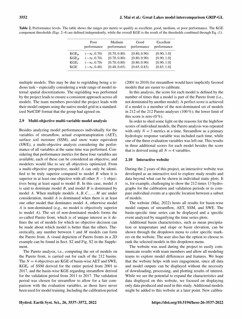
3552 J. Mai et al.: Great Lakes model intercomparison GRIP-GL
Table 2. Performance levels. The table shows the ranges per metric to qualify as excellent, good, medium, or poor performance. The KGEcomponent thresholds (Eqs. 2–4) are defined independently, while the overall KGE is the result of the thresholds combined through Eq. (1).
Poor Medium Good Excellentperformance performance performance performance
KGEα (−∞,0.70) [0.70,0.80) [0.80,0.90) [0.90,1.0]KGEβ (−∞,0.70) [0.70,0.80) [0.80,0.90) [0.90,1.0]KGEr (−∞,0.70) [0.70,0.80) [0.80,0.90) [0.90,1.0]KGE (−∞,0.48) [0.48,0.65) [0.65,0.83) [0.83,1.0]
multiple models. This may be due to regridding being a te-dious task – especially considering a wide range of model in-ternal spatial discretizations. The regridding was performedby the project leads to ensure a consistent approach across allmodels. The team members provided the project leads withtheir model outputs using the native model grid in a standard-ized NetCDF format that the group had agreed on.
2.9 Multi-objective multi-variable model analysis
Besides analyzing model performances individually for thevariables of streamflow, actual evapotranspiration (AET),surface soil moisture (SSM), and snow water equivalent(SWE), a multi-objective analysis considering the perfor-mance of all variables at the same time was performed. Con-sidering that performance metrics for these four variables areavailable, each of these can be considered an objective, andmodelers would like to see all objectives optimized. Froma multi-objective perspective, model A can only be identi-fied to be truly superior compared to model B when it issuperior in at least one objective with all other N − 1 objec-tives being at least equal to model B. In this case, model Ais said to dominate model B, and model B is dominated bymodel A. When multiple models A,B,C, . . .,M are underconsideration, model A is dominated when there is at leastone other model that dominates model A, otherwise modelA is non-dominated (e.g., no model is objectively superiorto model A). The set of non-dominated models forms theso-called Pareto front, which is of unique interest as it de-fines the set of models for which no objective decision canbe made about which model is better than the others. The-oretically, any number between 1 and M models can formthe Pareto front. A visual depiction of Pareto fronts in a 2Dexample can be found in Sect. S2 and Fig. S2 in the Supple-ment.
The Pareto analysis, i.e., computing the set of models onthe Pareto front, is carried out for each of the 212 basins.TheN = 4 objectives are KGE of basin-wise AET and SWE,KGEr of SSM derived for the entire period from 2001 to2017, and the basin-wise KGE regarding streamflow derivedfor the validation period from 2011 to 2017. The validationperiod was chosen for streamflow to allow for a fair com-parison with the evaluation variables, as those have neverbeen used for model training. Including the calibration period
(2001 to 2010) for streamflow would have implicitly favoredmodels that are easier to calibrate.
In this analysis, the score for each model is defined by thenumber of times that a model is part of the Pareto front (i.e.,not dominated by another model). A perfect score is achievedif a model is a member of the non-dominated set of modelsin 212 of the 212 Pareto analyses (100 %); the lower limit ofthis score is zero (0 %).
In order to shed some light on the reasons for the high/lowscores of individual models, the Pareto analysis was repeatedwith only N = 3 metrics at a time. Streamflow as a primaryhydrologic response variable was included each time, whileone of the three evaluation variables was left out. This resultsin three additional scores for each model besides the scorethat is derived using all N = 4 variables.
2.10 Interactive website
During the 2 years of this project, an interactive website wasdeveloped as an interactive tool to explore study results anddata beyond what can be shown in individual static plots. Itis, for example, challenging to show the 212 times 13 hydro-graphs for the calibration and validation periods or to com-pare individual events at a specific location between a subsetof models.
The website (Mai, 2022) hosts all results for basin-wisemodel outputs of streamflow, AET, SSM, and SWE. Thebasin-specific time series can be displayed and a specificevent analyzed by magnifying the time series plots.
Additional basin characteristics, such as mean precipita-tion or temperature and slope or basin elevation, can beshown through the dropdown menu to color specific mark-ers on the website. The user also has the option to choose torank the selected models in this dropdown menu.
The website was used during the project to easily com-municate results with team members and allow all modelingteams to explore model differences and features. We hopethat the website helps with user engagement, since all dataand model outputs can be displayed without the necessityof downloading, processing, and plotting results of interest.While we see the potential to expand the characteristics anddata displayed on this website, we focused on displayingonly data produced and used in this study. Additional modelsmight be added to this website at a later point. New calibra-
Hydrol. Earth Syst. Sci., 26, 3537–3572, 2022 https://doi.org/10.5194/hess-26-3537-2022

J. Mai et al.: Great Lakes model intercomparison GRIP-GL 3553
tion and validation results produced with revisions to theseGRIP-GL models will be posted on HydroHub if the respec-tive modeling teams decide to recalibrate their models. Arequirement is that the models are set up and run with thecommon dataset (Sect. 2.2), and the models are calibrated,validated and evaluated at the required locations and for allfour variables. The website will incorporate updates to thedatasets (for example, resulting from improved calibration orbug fixes) as they become available.
3 Results and discussion
The results of the four different comparative analyses per-formed in this study are presented in this section. The dis-cussion of each analysis will be presented right after the re-sults to improve readability. Section 3.1 will present the re-sults and insights gained through the analysis of model per-formances regarding streamflow. The performances are com-pared for all 13 participating models and the four experi-ments listed in Sect. 2.5, i.e., calibration, temporal valida-tion, spatial validation, and spatiotemporal validation. Sec-tion 3.2 will focus on the outcomes of the analysis of themodels’ performance regarding the three additional variables(actual evapotranspiration, surface soil moisture, and snowwater equivalent) when the outputs of each model are lumpedto the basin scale, while Sect. 3.3 will analyze the perfor-mance at the grid cell scale. Section 3.4 will present the re-sults of the multi-objective multi-variable model analysis inorder to integrate the model performance across the four vari-ables into one overall metric per model to allow for a high-level model intercomparison. Then, Sects. 3.2–3.4 includeanalyses of model performances regarding the auxiliary vari-ables. Those will hence be based on only 12 models since themachine-learning-based LSTM-lumped model is not trainedto output such intermediate variables and would need fittingwith additional data to predict them.
3.1 Model performance regarding streamflow
The results of the streamflow performances across all mod-els and location are presented in Fig. 3. The figure containsone panel for each of the experiments performed to com-pare the models. Each panel will be described and discussedin one of the following sections, e.g., Sect. 3.1.1 describesthe calibration results, Sect. 3.1.2 describes the results of thetemporal validation, Sect. 3.1.3 the spatial validation, andSect. 3.1.4 the spatiotemporal validation. Results are sum-marized in Sect. 3.1.5.
3.1.1 Experiment A: calibration
First, all modeling groups were asked to calibrate their mod-els regarding streamflow at 141 streamflow gauging stationsduring the time period starting from January 2001 until De-cember 2010. The forcings for the year 2000 were pro-
vided but assigned as the warmup period and not included.It was known a priori that the models would be assessedby KGE and the median KGE across all stations. The re-sults are shown in Fig. 3a. Therein, the models (y axis) aregrouped according to the three types of calibration schemes(globally, locally, or regionally calibrated) while the gauges(x axis) are grouped according to the lakes/river that theyultimately drain into. The only globally calibrated model,i.e., LSTM-lumped, has almost perfect scores for all gauges.This is not surprising, as these are training results thatcould theoretically be trained to achieve a KGE of 1.0 ev-erywhere with ML models. Due to this, these results areusually not even shown in the ML community. They areadded here for completeness. The locally calibrated group ofmodels, i.e, LBRM-CC-lumped, HYMOD2-lumped, GR4J-lumped, HMETS-lumped, Blended-lumped, Blended-Raven,and VIC-Raven, shows median KGE performances between0.80 (VIC-Raven) and 0.88 (Blended-lumped). Interestingly,there is no indication that semi-distributed locally calibratedmodels perform better (or worse) than the lumped modelsas, for example, the semi-distributed VIC-Raven model isthe one with the lowest performance (median KGE of 0.80),while the semi-distributed Blended-Raven is one of the best(median KGE of 0.86). Nevertheless, all locally calibratedmodels exhibit good or excellent performance levels (see Ta-ble 2), and we do not want to read too much into minor dif-ferences in the KGE performance. There are no major dif-ferences between the six drainage regions for these models,and no location can be identified that appears to have badKGE values across all locally calibrated models, which usu-ally indicates data issues for this streamflow gauge ratherthan a model issue. The regionally calibrated models, i.e.,SWAT-Raven, WATFLOOD-Raven, MESH-CLASS-Raven,MESH-SVS-Raven, and GEM-Hydro-Watroute show an ex-pected lower performance than the locally calibrated groupof models. The KGE performances spread between 0.50 and0.63 and can hence be classified as medium quality (see Ta-ble 2). The main reason why GEM-Hydro-Watroute hasa significantly lower performance than MESH-SVS-Raven,despite the former mainly relying on parameters calibratedwith the latter, is believed to be due to a bug that was presentin the MESH-SVS-Raven model and related to the reading ofvegetation cover from the geophysical files provided to themodel. Note that this bug was not present in previous stud-ies (Gaborit et al., 2017b; Mai et al., 2021), as it was due tothe specific NetCDF format used with MESH-SVS-Raven in-put/output files during this work. This led to the SVS LSS notusing the right information for vegetation cover during cali-bration and therefore led to calibrated parameters that werenot optimal for SVS inside GEM-Hydro-Watroute, where thereading of vegetation cover was done properly. It is expectedthat, when the bug is fixed and MESH-SVS-Raven is recal-ibrated, both MESH-SVS-Raven and GEM-Hydro-Watroutewill exhibit better scores regarding the auxiliary evapotran-spiration variable and that GEM-Hydro-Watroute streamflow
https://doi.org/10.5194/hess-26-3537-2022 Hydrol. Earth Syst. Sci., 26, 3537–3572, 2022

3554 J. Mai et al.: Great Lakes model intercomparison GRIP-GL
Figure 3. Model performance regarding streamflow. The performance is shown for (a) the 141 calibration stations and (b) the 71 validationlocations for the calibration period. The results for the validation period of the calibration and validation sites are shown in panels (c)and (d), respectively. In summary, panel (b) shows the spatial validation, panel (c) shows the temporal validation, and panel (d) shows thespatiotemporal validation across the locations (x axis) and the 13 models (y axis). The locations are grouped according to their location withinthe six watersheds (vertical black lines) of Lake Erie (ERI), Lake Huron (HUR), Lake Michigan (MIC), Lake Ontario (ONT), Ottawa River(OTT), and Lake Superior (SUP). The horizontal black lines separate the machine-learning-based global LSTM model from the models thatare calibrated locally and the models that are calibrated per region. The performance is quantified using the Kling–Gupta efficiency (KGE).The median KGE performance of each model for each of the four evaluation scenarios is added as labels to each panel. The thresholdsfor medium, good, and excellent performance classifications are added as labels to the color bar. Figures showing the results of the threecomponents of KGE (bias, variability, and correlation) can be found in Figs. S3–S5 in the Supplement. For the spatial distribution of theseresults and the simulated and observed hydrographs, please refer to the website (http://www.hydrohub.org/grip-gl/maps_streamflow.html,last access: 6 July 2022).
performances will be closer to the performances of MESH-SVS-Raven. A revised version of both models will be postedon HydroHub when this is done. Because this bug was dis-covered after this study was completed, there was no time leftto restart the work for MESH-SVS-Raven and GEM-Hydro-Watroute. However, new results for both models could beadded to the website in the near future. Some basins seem tobe difficult to model across all the regionally calibrated mod-els. These basins are watersheds (a) with strong flow regula-tion (e.g., 02BD002 and 02DD010), (b) that are located in ur-ban areas (e.g., 02HA006, 02HA007, 02HC049, 04166500,and 04174500), and (c) in agricultural regions in the USA(e.g., 04085200 and 04072150). Such basins appear in all re-
gions except the Ottawa region (OTT), which is an indicatorthat the basins selected for calibration in the Ottawa Riverwatershed may not be strongly regulated or may not includesignificant urban areas. Hence, the set of basins might not bevery representative when models are validated in this region.
3.1.2 Experiment B: temporal validation
After calibration, we performed three validation experi-ments. The first and easiest validation test was temporal val-idation using the same basins as in calibration but evaluat-ing the performance for the time period from January 2011to December 2017 (Fig. 3c). As expected, the KGE per-formance is decreasing for all models. The median KGE
Hydrol. Earth Syst. Sci., 26, 3537–3572, 2022 https://doi.org/10.5194/hess-26-3537-2022

J. Mai et al.: Great Lakes model intercomparison GRIP-GL 3555
of the machine learning model decreases by 0.15, but themodel still maintains a median KGE of 0.82 which is thebest overall median KGE of all models in the temporal val-idation experiment. The performances of the locally cali-brated models are all very similar among each other, withmedian KGE values between 0.74 and 0.79. The two Blendedmodel setups (Blended-lumped and Blended-Raven) lose themost skill compared to calibration but are still the two best-performing models in this group together with HYMOD2-lumped (median KGE of 0.79, 0.76, and 0.76, respectively).The differences in the performance across the regionally cal-ibrated models are larger. The best is WATFLOOD-Raven(median KGE of 0.62; decreased by 0.01 compared tocalibration), while MESH-CLASS-Raven and GEM-Hydro-Watroute show the lowest median KGE values overall (me-dian KGE of 0.45 and 0.46, respectively). Overall, the patternof basins with a low performance and a good performance aresimilar to the patterns seen in the calibration (see the collo-cation of red and blue cells in Fig. 3a and c), indicating thatthe performance decrease in the temporal validation is sim-ilar for all stations, and no station deteriorates significantlywhen the time period is changing.
3.1.3 Experiment C: spatial validation
The second, more challenging, validation experiment was torun models in the calibrated time period but at locations thatwere not used (or even known) during calibration (Fig. 3b).The ML-based model loses more of its overall performancethan in temporal validation (decrease by 0.21 vs. 0.15) butis still significantly better than all other models (medianKGE of 0.76 vs. the second-best (Blended-lumped) modelwith a median KGE of 0.61). The locally calibrated mod-els show similar (medium) performances among themselves,with some gauges performing consistently poorly (the en-tire column is red), which can be attributed to the fact thatall models used the same – probably not the most suitable –donor basin to transfer the parameters to the basin in ques-tion in order to derive a streamflow estimate. It is expectedthat the overall performance of the locally calibrated modelscould be improved by a more sophisticated approach deter-mining the donor basins. It is unlikely that the poor perfor-mance of some locations is a model-specific problem as thelocally calibrated models are diverse in setup and complex-ity (e.g., compare the conceptual GR4J-lumped and semi-distributed, physically based VIC-Raven). It should be men-tioned that the two regions with large sets of calibrated basinsand fewer basins in validation (e.g., Lake Michigan (MIC)and Lake Erie (ERI) watersheds) show much better resultsand fewer stations with poor performance across all models.This is very likely due to the fact that the pool the donorbasin can be chosen from is very large, and the likelihoodof assigning a similar basin is higher. In contrast, the regionof the Ottawa River basin had only a limited set of basinsfor calibration, which was previously discussed to be poten-
tially not very representative as the calibration set did notcontain highly managed basins or basins in urban or agri-cultural areas. Besides that, the set of validation basins isall widespread in space, and in many cases, the only avail-able donor basin is far away and thus unlikely to be a goodproxy for the validation location. The regionally calibratedmodels do not show as strong a loss of performance whenvalidated spatially. The median KGE decreases on averageby 0.16 (0.10 if outlier KGE of MESH-CLASS-Raven is ig-nored), while the median KGE of locally calibrated modelsis decreasing by 0.27 (spatial validation performance com-pared to the respective median performance during calibra-tion). The overall performance of the regionally calibratedmodels (median KGE between 0.47 and 0.52, while ignoringthe outlier median KGE of 0.17 for MESH-CLASS-Raven)is much closer to the performance of the locally calibratedmodels (median KGE between 0.52 and 0.61) in the spatialvalidation compared to the larger performance gap in the cal-ibration.
3.1.4 Experiment D: spatiotemporal validation
The third validation experiment is the spatiotemporal valida-tion (Fig. 3d) in which the models are assessed for (a) basinsthat are not calibrated and (b) a time period that was not usedfor calibration. The spatiotemporal validation is a combina-tion of the two previous (temporal and spatial) validation ex-periments and is hence regarded as the most challenging vali-dation experiment that the models undergo in this study. Thespatiotemporal validation shows consistent results with thetwo previous experiments. Almost all models degrade in per-formance compared to the spatial validation but not as muchas the skill was reduced when comparing temporal validationwith spatial validation. Some models even slightly increasetheir median performance (by at most 0.03) compared to thespatial validation (i.e., GR4J-lumped, WATFLOOD-Raven,MESH-CLASS-Raven, and MESH-SVS-Raven), but we donot want to read too much into this, as the skill of those mod-els was already poor to begin with. Again, the performance ofthe regionally calibrated models is much closer to the averageperformance of the locally calibrated models as compared tothe large performance gaps in calibration and temporal vali-dation. As expected, the results generally show temporal val-idation to be easier task than spatial (or spatiotemporal) vali-dation. The overall performance of locally calibrated modelsis expected to improve when a more sophisticated method todetermine donor basins is applied.
3.1.5 Summary of streamflow performanceexperiments
In summary, the machine-learning-based LSTM-lumpedmodel is by far the best model, not only in calibration butalso in every validation scenario. The model skill is excellentin calibration and spatial and temporal validation and can
https://doi.org/10.5194/hess-26-3537-2022 Hydrol. Earth Syst. Sci., 26, 3537–3572, 2022

3556 J. Mai et al.: Great Lakes model intercomparison GRIP-GL
still be classified as good in spatiotemporal validation. Thehighest-ranking spatial and spatiotemporal validation perfor-mance levels of the LSTM model is noteworthy, given thattheir model training involved fitting roughly 300 000 modelparameters. LSTM training procedures were therefore in-credibly and, to many co-authors, surprisingly successful atavoiding overfitting.
The LSTM-lumped model shows significant improve-ments (especially in validation) compared to the precedingLSTM model in the GRIP-E project (Mai et al., 2021, calledML-LSTM therein). This is due to several reasons, whichinclude the following: (a) more training data (streamflow lo-cations and forcings) were available in the GRIP-GL project,which is a known ingredient to guarantee good performanceof data-driven models, (b) the team setting up the modelgained expertise, and (c) additional basin characteristics wereused to train the models (Table S2 in the Supplement). Be-sides the excellent skill of the model throughout, another ad-vantage is its global setup, which means that it is easy toobtain streamflow at stations beyond the ones used here forvalidation. This strong performance of the LSTM-lumpedmodel is in line with results from prior studies (Kratzert etal., 2019b).
The locally calibrated models – mostly conceptual and fast– might be a good starting point for streamflow estimates,especially with a more advanced donor basin mapping. Un-less sophisticated parameter transfer methods are tested andemployed, locally calibrated models are not well suited forsimulations in ungauged areas due to their lack of spatial ro-bustness. The impact of more sophisticated donor basin map-ping methods will be evaluated in a followup study. The per-formance level of the locally calibrated models can be clas-sified as excellent to good in calibration, good in temporalvalidation, and medium in spatial and spatiotemporal valida-tion. Even though the models are (strictly speaking) not thesame as in the previous GRIP-E project, similar trends werefound there as well. In GRIP-E, the calibration performancesin calibration were good (median KGE of 0.63 to 0.78 formost models, excluding SWAT), and a significant decreasein the temporal validation was the only validation performedin GRIP-E (median KGE values between 0.44 to 0.68 ex-cluding SWAT).
The regionally calibrated models are more stable – mean-ing that they lose less performance relatively – compared tolocally calibrated models and have the advantage that theyprovide setups over entire regions. This makes it straightfor-ward to derive streamflow estimates for ungauged/untrainedlocations (spatial and spatiotemporal validation). The region-ally calibrated models show medium performance levels incalibration, medium performances in temporal validation,and medium (on the verge of poor) performances in spatialand spatiotemporal validation, with the exception of MESH-CLASS-Raven which is poor in both. MESH-SVS-Ravenand WATFLOOD-Raven perform very well compared to theother regionally calibrated models. The latter model is no-
table, as this was the model that showed the weakest valida-tion performance during GRIP-E. The regionally calibratedmodels generally have their lowest performances in man-aged, urban, and agricultural basins. This might be an indi-cation that all these models could be improved (a) if associ-ated processes like reservoir operation rules, tile drainage, orhandling of processes over impervious/sealed areas are bet-ter represented in those models and (b) if models would bespecifically trained for such basins since the representationof only two to three basins with those specific characteristicswithin the entire set of calibration basins of a region mightnot be sufficient to constrain/calibrate all parameters requiredfor those processes. In other words, the models that were re-gionally calibrated during this work following a geographicalsubdivision of the whole domain into six regions may insteadbenefit from being calibrated over all agricultural, urban, andnatural basins of the whole domain, following a morpholog-ical instead of a geographical subdivision.
Regarding possibility (a), a strong improvement of GEM-Hydro-Watroute was, for example, noticed when using theDynamically Zoned Target Release (DZTR) reservoir model(Yassin et al., 2019) to represent regulated reservoirs inWatroute, for gauges 02KF005 (Ottawa River, with nineupstream managed reservoirs), 02DD010 (Lake Nipissing),and 02AD012 (Lake Nipigon). In this study, GEM-Hydro-Watroute was the only model to include a reservoir regula-tion model in its routing scheme, for basins whose gaugesare 02KF005, 02DD010, and 02LB005, and probably bene-fited from it for these gauges. However, given that this uniquestrategy was only applied in 3 of the 212 studied basins, ithad little impact on overall GEM-Hydro-Watroute compara-tive performance.
Regarding improvement possibility (b), a significant lossof performance can be noticed for the Ottawa region, evenwith regionally calibrated models, regarding spatial valida-tion. In this region, only a few calibration basins were se-lected, and these generally include agricultural areas andwere therefore not representative of the general morphologyof the region, which is generally forested (natural) and re-flected in the validation basins.
Please note that all hydrographs and performance esti-mates of the four experiments regarding streamflow per-formance can be found on the interactive website associ-ated with this work (http://www.hydrohub.org/grip-gl/maps_streamflow.html, last access: 6 July 2022). The users cancompare hydrographs at all locations for models of interestand zoom in on specific time periods/events. Followup stud-ies could look at the performance of subsets of models forspecific events or under specific, e.g., low or high flow, con-ditions.
Hydrol. Earth Syst. Sci., 26, 3537–3572, 2022 https://doi.org/10.5194/hess-26-3537-2022

J. Mai et al.: Great Lakes model intercomparison GRIP-GL 3557
3.2 Basin-wise model performance regarding auxiliaryvariables
In this section, the performance of models regarding addi-tional variables at the basin scale (comparable to stream-flow) will be analyzed for 12 models. The 13th model, i.e.,machine-learning-based LSTM-lumped, is not (yet) able toprovide estimates for those variables and will not be consid-ered for the remaining analyses. The basin-wise comparisonof additional variables implies that the reference datasets andthe subbasin-based and gridded model outputs were aggre-gated to basin level. Once the outputs and reference datasetsare aggregated in space, the resulting daily time series arecompared. The 212 calibration and validation locations arecompared without distinguishing them (as done for stream-flow) since the additional variables were never calibrated,and their performances are therefore of validation quality.The results for the three additional variables are presentedin Fig. 4. Each panel of Fig. 4 represents the results for oneof the three variables and will be discussed one by one in thefollowing three sections (Sects. 3.2.1–3.2.3). The last section(Sect. 3.2.4) will summarize these results and discussions.
3.2.1 Basin-wise comparison of actualevapotranspiration
Regarding actual evapotranspiration (AET), the locally cali-brated models exhibit, on average, a lower performance thanthe regionally calibrated, physically based models (Fig. 4a).
The only exception is the HYMOD2-lumped model. Dur-ing its development, the focus was on improving the real-ism of simulated AET, which was achieved by introducinga model structure in HYMOD2-lumped that produced simu-lated AET results closely approximating GLEAM AET (Royet al., 2017). In other words, the HYMOD2-lumped modelwas implicitly preinformed by this dataset, which wouldexplain the superior performance seen here. Note that allevaporation-related (and other) parameters were recalibratedusing only streamflow observations in this study and werenot reused from the development stage presented by Roy etal. (2017).
Besides the HYMOD2-lumped with a median KGE of0.72, only regionally calibrated models show good perfor-mance levels (above KGE of 0.65), i.e., SWAT-Raven witha median KGE of 0.74, MESH-SVS-Raven with a medianKGE of 0.68, and GEM-Hydro-Watroute with a medianKGE of 0.70. This is notable as these aforementioned re-gionally calibrated models showed consistently lower perfor-mances regarding streamflow compared to the locally cal-ibrated models. Regarding MESH-SVS-Raven and GEM-Hydro-Watroute, it is possible that their performance regard-ing AET could be even slightly better once the bug presentin MESH-SVS-Raven and affecting vegetation cover duringthis work is fixed (see Sect. 3.1.1). Note that this bug proba-
bly affected these two models to a lower degree for the otherauxiliary variables.
The other models exhibit medium performance levelsabove KGE values of 0.48. The two exceptions with poorperformance levels are GR4J-lumped with a median KGE of0.44 and LBRM-CC-lumped with a median KGE of 0.15.
The significantly low performance of LBRM-CC-lumpedwas surprising. Subsequent to the posting of model results,an error was found in the calibration setup that resulted inan important constraint on the proportionality constant con-trolling PET being ignored (see Lofgren and Rouhana, 2016,for an explanation of this constraint). In addition, the LBRM-CC-lumped team has found that an improved representationof the long-term average temperatures applied in the PET for-mulation would improve results in some watersheds (PET isa function of the difference between daily temperature andlong-term average temperature for the day of year). Accord-ingly, this may improve the LBRM-CC-lumped performancein simulating AET in future studies.
Note that there are no clusters of stations/basins in whichseveral models perform exceptionally well or badly, whichin turn means that the differences between models are indeedmodel specific and not caused by any general problem withdata at certain stations. Furthermore, there are no differencebetween regions, i.e., models in one region performing sig-nificantly better or worse than in other regions, which meansthat models perform similarly in all geographic regions nomatter the amount of human impact or land use or if sta-tions where originally calibrated or only validated regardingstreamflow.
3.2.2 Basin-wise comparison of surface soil moisture
The model performances regarding surface soil moistureare consistent both across models and locations (Fig. 4b).The performance levels can be classified as poor (KGErof lower than 0.7) for LBRM-CC-lumped (0.59), HMETS-lumped (0.63), Blended-lumped (0.67), Blended-Raven(0.68), SWAT-Raven (0.66), and WATFLOOD-Raven (0.50).Even though they are classified as poor, correlation coeffi-cients of above 0.6 for some largely conceptual models aresurprising – especially given that most do not even explicitlysimulate soil moisture internally but convert simulated watercontents into proxy soil moisture estimates.
The other models show medium performance levels(KGEr of at least 0.7), i.e., HYMOD2-lumped (0.70),GR4J-lumped (0.70), VIC-Raven (0.72), MESH-CLASS-Raven (0.76), MESH-SVS-Raven (0.76), and GEM-Hydro-Watroute (0.76). It is notable that the four models that per-form best are all physically based models that explicitly sim-ulate soil moisture as a state variable.
WATFLOOD-Raven seems to be an outlier with its poormedian KGEr performance of 0.50. Especially stations lo-cated in the Lake Erie watershed show low correlation valuescompared to the reference dataset, which can be explained by
https://doi.org/10.5194/hess-26-3537-2022 Hydrol. Earth Syst. Sci., 26, 3537–3572, 2022

3558 J. Mai et al.: Great Lakes model intercomparison GRIP-GL
Figure 4. Basin-wise model performance regarding auxiliary variables. The performance of 12 models (y axis) is shown for (a) actualevapotranspiration, (b) surface soil moisture, and (c) snow water equivalent. The model outputs are aggregated to the 212 basins (x axis)used in this study (141 calibration locations and 71 validation locations). The performance is evaluated for observations available between2001 and 2017 (the overall period used for streamflow calibration and validation). The Kling–Gupta efficiency (KGE) is used to evaluatethe simulations of actual evapotranspiration and snow water equivalent, while the Pearson correlation is used for the (standardized) surfacesoil moisture. The color bar in each panel is organized such that blue (red) colors indicate good (poor) performance. The machine-learning-based LSTM model is not simulating these additional variables and is hence not included. The basins (x axis) are grouped into six regionsof the Lake Erie (ERI), Lake Huron (HUR), Lake Michigan (MIC), Lake Ontario (ONT), Ottawa River (OTT), and Lake Superior (SUP)watersheds. The basin order is the same across the three panels. The horizontal black line separates models that are calibrated locally frommodels that are calibrated per region. For the spatial distribution of these results and the simulated and reference time series, please refer tothe website (e.g., the website for actual evapotranspiration; http://www.hydrohub.org/grip-gl/maps_aet.html, last access: 6 July 2022).
Hydrol. Earth Syst. Sci., 26, 3537–3572, 2022 https://doi.org/10.5194/hess-26-3537-2022
J. Mai et al.: Great Lakes model intercomparison GRIP-GL 3559
the fact that WATFLOOD does not explicitly simulate SSM,and therefore, the rescaled Upper Zone Storage (UZS) wasused as a proxy for SSM. Specific parameter settings werechosen to mimic the behavior in urban areas (i.e., low valueof infiltration coefficient and low value of upper zone reten-tion limiting UZS) and restricting fluctuations in the UZS asthis would be expected for SSM, but these parameter settingsare likely not enough to fully capture SSM dynamics in urbanareas.
There are – similar to AET – no significant performancedifferences between regions. No basin can be identified asan outlier with significantly lower or higher performance,which indicates that all models are in good agreement withthe GLEAM-v3.5 soil moisture reference dataset, and no in-consistency can be diagnosed.
3.2.3 Basin-wise comparison of snow water equivalent
The most diverse model performance across models and lo-cations can be observed for snow water equivalent (Fig. 4c).One model performs poorly (median KGE below 0.48),seven models show an overall medium performance (KGE atleast 0.48), while the other four models perform well (KGEat least 0.65).
The overall best-performing models are GEM-Hydro-Watroute (median KGE of 0.71), Blended-Raven (medianKGE of 0.70), MESH-SVS-Raven (median KGE of 0.65),and Blended-lumped (median KGE of 0.65). This repre-sents an interesting mix of models, as they are (a) physicallybased and distributed (GEM-Hydro-Watroute and MESH-SVS-Raven), (b) conceptual and lumped (Blended-lumped),and (c) conceptual and distributed (Blended-Raven). It henceshows that even simplified, lumped, and conceptual modelshave the potential to simulate basin-scale SWE with a similarquality as more complex, distributed models.
The models with the weakest performance are VIC-Raven(median KGE of 0.47), GR4J-lumped (median KGE of 0.49),HMETS-lumped (median KGE of 0.49), and LBRM-CC-lumped (median KGE of 0.50). Again, these are simulta-neously conceptual/lumped and physically based/distributedmodels. The weakly performing models are exclusively lo-cally calibrated and might have suffered from poor donorbasin mapping. However, other locally calibrated models likethe two Blended models used the same (potentially inappro-priate) donor basins and show superior performance.
SWE is the only variable that reveals clear differences inperformance between regions. The Lake Superior (SUP) wa-tershed is the region where all models show good perfor-mance at all location, whereas in other regions, e.g., in theLake Huron (HUR) watershed, several locations show poorperformance across most models. The locations with poorperformance (red color across most models) are located inthe same geographical area, i.e., the land area south of LakeHuron, north of Lake Erie, and west of Lake Ontario which is– besides being the most densely populated area of the Great
Lakes watershed – heavily impacted by lake effects in precip-itation and complex precipitation phase (Mekis et al., 2020),which affects snow accumulation and melt. Another reasonfor the poor performances of the models in this region mightbe the quality of the forcing datasets which are known to haveproblems in lake areas. It is not surprising that most mod-els exhibit lower performances in these regions compared toelsewhere.
It is, however, notable that some models, e.g., the lo-cally calibrated Blended-Raven model and the regionallycalibrated WATFLOOD-Raven model perform exceptionallywell at locations where other models deteriorate in perfor-mance, even though it does not use special snow processesbut the basic formulation of the temperature index model(Anderson, 1973). The Blended-Raven model is not usingany special algorithm to simulate snow processes. It indeeduses the same algorithmic representation as the Blended-lumped model, which is slightly worse at these locations.But the subbasin discretization of the Blended-Raven model(only difference to the Blended-lumped model) seems to im-prove performances at several locations.
3.2.4 Summary of basin-wise comparisons of auxiliaryvariables
In summary, the common assumption that distributed, physi-cally based models are intrinsically of superior quality whenevaluating model states beyond streamflow cannot be con-firmed in all cases.
For actual evapotranspiration, a locally calibrated, con-ceptual model (HYMOD2-lumped) shows exceptional per-formance on par with more complex models (i.e., SWAT-Raven, MESH-SVS-Raven, and GEM-Hydro-Watroute).Even though, for surface soil moisture, physically basedmodels are generally best (i.e., MESH-CLASS-Raven,MESH-SVS-Raven, and GEM-Hydro-Watroute), the lesscomplex and locally calibrated models (i.e., HYMOD2-lumped, GR4J-lumped, and VIC-Raven) can lead to compa-rable performances when SSM is standardized, as describedin Sect. 2.7 and evaluated based on its correlation with ob-servations. Indeed, when looking at the true KGE for ac-tual SSM values, only MESH-SVS-Raven and GEM-Hydro-Watroute showed reasonable performances (not shown here),partly because SVS represents the actual SSM values overthin superficial soil layers. However, a physically basedmodel (WATFLOOD-Raven) shows an outlier with a poorperformance across all locations for SSM. For snow waterequivalent, there are as many locally calibrated/conceptualmodels performing well as there are physically based mod-els, i.e., Blended-lumped and Blended-Raven vs. MESH-SVS-Raven and GEM-Hydro-Watroute.
The analysis of basin-aggregated estimates might, how-ever, favor models that are set up and run on this (basin)scale. The distributed/gridded models might be indeed su-perior when the subgrid variability is analyzed. Hence, the
https://doi.org/10.5194/hess-26-3537-2022 Hydrol. Earth Syst. Sci., 26, 3537–3572, 2022

3560 J. Mai et al.: Great Lakes model intercomparison GRIP-GL
next section will focus on analyzing the models on the na-tive, gridded resolution of the reference dataset rather thanaggregating models and reference dataset to basin scale.
Note that all time series and metrics are availableon the websites associated with this study. The web-sites are especially insightful, as they provide a spatialrepresentation of the stations, which is not available inFig. 4. On the websites, the users will be able to iden-tify the region where, for example, the weaker-performingsnow water equivalent basins are located. There is onewebsite for each additional variable analyzed here, i.e.,actual evapotranspiration (http://www.hydrohub.org/grip-gl/maps_aet.html, last access: 6 July 2022), surface soilmoisture (http://www.hydrohub.org/grip-gl/maps_ssm.html,last access: 6 July 2022), and snow water equivalent(http://www.hydrohub.org/grip-gl/maps_swe.html, last ac-cess: 6 July 2022).
3.3 Grid-cell-wise model performance regardingauxiliary variables
In this section, the results of the model comparisons for thethree additional variables are presented. In contrast to theprevious section, the variables are compared at the grid cellscale rather than per basin. This means that all model outputswere regridded to the grid of the corresponding referencedataset. The performance metrics are then compared at eachgrid cell, leading to maps of performances presented in Fig. 5for actual evapotranspiration, Fig. 6 for surface soil mois-ture, and Fig. 7 for snow water equivalent. The results willbe presented for only 12 models as the machine-learning-based LSTM-lumped model did not simulate these additionalvariables. The results will be presented and discussed in thefollowing three sections (Sects. 3.3.1–3.3.3), while the lastsection summarizes the findings (Sect. 3.3.4).
3.3.1 Grid-cell-wise comparison of actualevapotranspiration
The results of the grid-cell-wise comparisons regarding ac-tual evapotranspiration (Fig. 5) are consistent with the basin-wise comparisons discussed before (see Sect. 3.2.1 andFig. 4a). The best models (visually and by numbers) arethe locally calibrated HYMOD2-lumped and the regionallycalibrated SWAT-Raven. Other models with a good perfor-mance are MESH-SVS-Raven and GEM-Hydro-Watroute,while the weakest models are the two locally calibratedLBRM-CC-lumped and GR4J-lumped models. Note that themedian performance per model is not exactly the same as theperformance value for the basin-wise comparison (Sect. 3.2;Fig. 4). This is due to the fact that the basin-wise perfor-mances are derived as being the median over 212 basins,while in the grid-cell-wise comparisons they are derived overthe 1213 grid-cells that appear in the reference dataset andare available in all 12 model outputs.
The grid-cell-wise analysis provides more insights intowhere results are good or weak spatially. In general, the lo-cally calibrated models (LBRM-CC-lumped to VIC-Raven)exhibit discontinuous (patchwork) patterns of performance,as expected, while the regionally calibrated models (SWAT-Raven to GEM-Hydro-Watroute) are more seamless – at leastwithin each of the six main regions. The discontinuous natureof model outputs (and hence their performance when com-pared to continuous fields of observations) has been reportedin the literature before (e.g., Mizukami et al., 2017; Yang etal., 2019).
The locally calibrated LBRM-CC-lumped model showspoor performance (median KGE of 0.14) in large regions(likely to improve once the error in the calibration setupis resolved and a better representation of long-term aver-age temperatures is in place; see details in Sect. 2.4.2).The HYMOD2-lumped model performs (very) well (me-dian KGE of 0.76) everywhere (almost no red cells in entiredomain). The GR4J-lumped model exhibits a poor perfor-mance (median KGE of 0.39), with deficiencies especially innorthern latitudes but also south of Lake Ontario and LakeErie. The HMETS-lumped model with its medium perfor-mance level (median KGE of 0.53) has a patchwork perfor-mance due to its local calibration and the transfer of param-eter sets to validation basins. The latter are the reason forthe patchy red regions, especially in the Ottawa River basin,as that region might not have had enough basins for train-ing (as discussed earlier). The Blended-lumped and Blended-Raven models both exhibit medium performance levels (me-dian KGE of 0.58 and 0.56, respectively), with their spa-tial patterns of performance being similar. This is expected,given the very similar nature of these two models. The pat-terns are patchy but overall good, except in validation basins,which might be caused by a (potentially) inappropriate donorbasin being assigned. The VIC-Raven model’s medium per-formance (median KGE of 0.57) is the lowest in validationbasins and west and north of Lake Erie. The latter might bedue to the model’s weakness in simulating AET over urbanareas.
The regionally calibrated SWAT-Raven exhibits a me-dian KGE of 0.73 and hence performs comparably wellas the locally calibrated HYMOD2-lumped with almost noweak-performing (red) grid cells. The WATFLOOD-Ravenshows a medium performance level (median KGE of 0.56),with the weakest performance around Lake Erie (highly ur-ban and agricultural) and within the Ottawa River water-shed (potentially caused by not enough basins for train-ing). The medium-performing MESH-CLASS-Raven model(median KGE of 0.60) shows similar behavior in the LakeErie watershed to the WATFLOOD-Raven and the MESH-SVS-Raven model. It has some further deficiencies aroundLake Superior. The MESH-SVS-Raven model is performingwell (median KGE of 0.66), with the lowest performancein regions of heavy agricultural activity southwest of LakeErie. The GEM-Hydro-Watroute with its good overall per-
Hydrol. Earth Syst. Sci., 26, 3537–3572, 2022 https://doi.org/10.5194/hess-26-3537-2022

J. Mai et al.: Great Lakes model intercomparison GRIP-GL 3561
formance (median KGE of 0.66) shows the weakest per-formances over (a) the Ottawa River watershed due to lim-ited training data/basins in this region, which were not suffi-cient to calibrate the model in this region appropriately, and(b) the agricultural regions southwest of Lake Erie. Again,MESH-SVS-Raven and GEM-Hydro-Watroute could proba-bly have a slightly better AET performance if the bug presentin MESH-SVS-Raven and affecting vegetation cover duringthis work were fixed (see Sect. 3.1.1).
3.3.2 Grid-cell-wise comparison of surface soilmoisture
The results of the comparison of grid-cell-wise model out-puts with the gridded reference dataset of surface soil mois-ture (Fig. 6) are consistent with the results previously dis-cussed for the basin-wise comparisons (see Sect. 3.2.2 andFig. 4b) but allow for a more detailed analysis of the regionsof poor performance, which might help to point to potentialmodel improvements.
Note that the median performances per model are not ex-actly the same values as the ones reported for the basin-wisecomparison, since those are derived as the median over 212basins, while here they are derived over the 1213 grid cellsthat appear in the reference dataset and are available in all12 model outputs. Also note that the following discussion ofresults will list the individual models in reverse order com-pared to their appearance in the panels of Fig. 6 due to themore natural flow of the discussion.
The regionally calibrated MESH-CLASS-Raven, MESH-SVS-Raven, and GEM-Hydro-Watroute models are visually(and by numbers) the best performing. Their performancelevels (median KGEr of 0.73, 0.71, and 0.72, respectively)can be classified as medium. The three spatial performancepatterns look very similar, which can be explained by the factthat CLASS and SVS share similarities regarding soil mois-ture processes. The soil moisture estimates are especiallypoor around Lake Erie and within the parts of the OttawaRiver watershed that were not calibrated (northeastern partof the Great Lakes basin) because of the persistence of thevariability in soil properties in this region. The other region-ally calibrated model SWAT-Raven is performing well in thesouthern parts of the Great Lakes watershed and has a lowerperformance in northern parts of the Ottawa River watershedand the Lake Superior region.
Most locally calibrated models show similar performances(median KGEr of 0.62 to 0.65) with some patchwork patternsof weak performances, especially in regions that are poten-tially located in validation basins. The HMETS-lumped hasa consistently lower performance overall (median KGEr of0.59), compared to the Blended-lumped and Blended-Ravenmodels, which is interesting as the Blended model struc-ture of the those two models was built upon the HMETS-lumped model. The improvement shows the added valueof the Blended structure upon the original fixed HMETS-
lumped model structure. The LBRM-CC-lumped model hasthe overall weakest performance, mostly due to its lowerperformance across the Ottawa River basin, which is con-sistent with the weak performance of this model regardingthe actual evapotranspiration discussed earlier. Several av-enues have been identified after posting the model results forLBRM-CC-lumped that may, after recalibration, improve theLBRM-CC-lumped performance in future studies.
3.3.3 Grid-cell-wise comparison of snow waterequivalent
The performance of the grid-cell-wise model outputs com-pared to a gridded reference dataset of snow water equivalent(Fig. 7) are consistent overall with the results previously dis-cussed for the basin-wise comparisons (see Sect. 3.2.3 andFig. 4c). The results, however, highlight the large variabilityin performances in space and across models.
Note that the median performances per model are not ex-actly the same values as the ones for the basin-wise compar-isons. The latter are derived as being the median over 212basins, while here they are derived over the 6174 grid cellsthat appear in the reference dataset and are available in all 12model outputs.
In contrast to the two previous variables analyzed, the dif-ference between the basin-wise and the grid-cell-wise com-parisons are significant for some models. We label differ-ences equal to or larger than 0.05 in median KGE as be-ing significant. All significant differences are improvementscompared to the basin-wise performances, i.e., LBRM-CC-lumped increases performance from a median KGE of 0.50 to0.59, GR4J-lumped from 0.49 to 0.65, VIC-Raven from 0.47to 0.58, SWAT-Raven from 0.54 to 0.61, MESH-CLASS-Raven from 0.57 to 0.71, and MESH-SVS-Raven from 0.65to 0.74. This behavior can be explained as follows. In total,193 of the 212 basins used in this study have similar drainageareas between 300 and around 5000 km2, 11 basins have adrainage area between 5000 and 10 000 km2, 6 basins arebetween 10 000 and 20 000 km2 in size, and the two largestbasins have a drainage area of 25 000 and 90 000 km2. Thesecond-largest basin covers the entire northernmost part ofthe Lake Superior watershed and is draining towards stream-flow gauge 02AD012, while the largest basin is draining to-wards streamflow gauge 02KF005 within the Ottawa Riverbasin. It covers large parts of the domain east of the Geor-gian Bay and north of Lake Ontario (see the website for thedrainage domain of all streamflow locations). The largest(90 000 km2) basin covers around 15 % of the entire do-main analyzed in the grid-cell-wise comparisons; the second-largest basin (25 000 km2) covers around 4 % of the domain.Hence, if a model is performing well in theses areas, it willcontribute to 19 % of the entire KGE score, while in a basin-wise comparison, it is only two of 212 basins, which equalsto around 1 % of the overall score. It can be seen in Fig. 7 thatmodels that have good (blue and dark blue) performances in,
https://doi.org/10.5194/hess-26-3537-2022 Hydrol. Earth Syst. Sci., 26, 3537–3572, 2022

3562 J. Mai et al.: Great Lakes model intercomparison GRIP-GL
Figure 5. Grid-cell-based model performance regarding actual evapotranspiration. The performance of 12 models (panels) regarding actualevapotranspiration (AET) is shown. The model outputs are regridded to the grid of the reference dataset (here GLEAM v3.5b; variable E).Only grid cells that are available in the reference dataset and all 12 models are displayed (1213 grid cells in total) and used to derive theKling–Gupta efficiency (KGE) metrics based on all available observations between January 2001 and December 2017. The median KGEacross space is added as a label at the top of each panel. The color bar has labels added to categorize the performance into medium, good,and excellent. The machine-learning-based LSTM model is not displayed, as this is the only model not simulating actual evapotranspirationexplicitly.
for example, the Ottawa River watershed (northeastern partof the Great Lakes watershed), exhibit a significant gain re-garding the median KGE performance when derived per gridcell.
This result emphasizes the importance of decisions madeto evaluate model performances. Basin-wise comparisonsseem to be easier to communicate and derive – especially fora wide range of models with different underlying model dis-cretizations. But comparisons that use the native resolutionof reference datasets (here gridded) might be more appropri-ate. We showcase here that even models that are not set up ingridded mode, i.e., lumped and subbasin-based models canbe converted to a grid scale to match the resolution of thereference datasets. The results also show that lumped mod-els not necessarily deteriorate when compared on a grid cellscale. The results indeed suggest quite the contrary since, forexample, models like LBRM-CC-lumped and GR4J-lumpedincrease their median KGE score because they predicated thesnow water equivalent accurately in these large basins.
The detailed analysis of the models (again in reverse order)shows that the regionally calibrated GEM-Hydro-Watroute,MESH-SVS-Raven, and MESH-CLASS-Raven models per-form equally and exhibit a good performance level (medianKGE of 0.72, 0.74, and 0.71, respectively). Main areas ofweak performance are the most densely populated area ofthe study domain, i.e., the region north and west of Lake Erieand south of Lake Huron/Georgian Bay. The WATFLOOD-Raven shows a medium, patchy performance overall (medianKGE of 0.58). No specific areas of weak or excellent per-formance can be identified. SWAT-Raven’s medium overallperformance (median KGE of 0.61) pattern looks similar tothe two MESH and the GEM-Hydro-Watroute models, withoverall larger and more pronounced weaker areas.
The locally calibrated VIC-Raven with its overall mediumperformance (median KGE of 0.58) shows a different pat-tern of weak regions. The low-performing regions are nowmostly located in the Ottawa River basin and east of LakeSuperior. The weaker-performing regions seem to be mostly
Hydrol. Earth Syst. Sci., 26, 3537–3572, 2022 https://doi.org/10.5194/hess-26-3537-2022

J. Mai et al.: Great Lakes model intercomparison GRIP-GL 3563
Figure 6. Grid-cell-based model performance regarding surface soil moisture. The performance of 12 models (panels) regarding surface soilmoisture (SSM) is shown. The model outputs are regridded to the grid of the reference dataset (here GLEAM v3.5b; variable SMsurf).Only grid cells that are available in the reference dataset and all 12 models are displayed (1213 grid cells in total) and used to derive thePearson correlation coefficients (KGEr ) based on all available summer month observations (June to October) between 2001 and 2017. Themedian KGEr across space is added as a label at the top of each panel. The color bar has labels added to categorize the performance intomedium, good, and excellent. The machine-learning-based LSTM model is not displayed, as this is the only model not simulating surfacesoil moisture explicitly. Note that only VIC-Raven, SWAT-Raven, MESH-CLASS-Raven, MESH-SVS-Raven, and GEM-Hydro simulate(surface) soil moisture explicitly, while the remaining models used proxy variables for soil moisture. All SSM estimates were standardizedto account for the proxy nature of the variables (Eq. 5) and, hence, only the correlation coefficients (KGEr ) are reported here.
forested, which might indicate that the calibration based ononly streamflow is not properly constraining parameters gov-erning the evolution of snow in forested environments inVIC. The Blended-lumped and Blended-Raven models showa similar, good performance compared to each other (me-dian KGE of 0.66 and 0.68, respectively), while the dis-tributed Blended-Raven is slightly superior in most regions(especially west of Lake Michigan and west and north ofLake Erie). This highlights again the added value of a dis-tributed model setup compared to its lumped counterpart (atleast for the Blended model). The HMETS-lumped modelwith its medium overall performance (median KGE of 0.53)shows similar weak regions but is more pronounced (weaker)than the two Blended models which, again, demonstrates theadded value of the Blended model structure as the Blendedmodels are based upon the HMETS model with added struc-tural flexibility. The LBRM-CC-lumped, HYMOD2-lumped,
and GR4J-lumped models show comparable medium perfor-mances (median KGE of 0.59, 0.62, and 0.65, respectively)with weakest performances in the southern part of the GreatLakes watershed and consistently better performances abovearound 46◦ N.
Most notable is that, even though the most complex phys-ically based models (MESH-CLASS-Raven, MESH-SVS-Raven, and GEM-Hydro-Watroute) show the best perfor-mance overall, some locally calibrated and more conceptualmodels are not significantly weaker (e.g., Blended-Raven).Especially in regions where the physically based models areweak (e.g., corridor between Lake Huron and Lake Erie),those conceptual, local models perform much better. Thereis the potential that, when more sophisticated approaches areapplied to assign donor basin mappings, these locally cal-ibrated models might significantly improve relative to themore complex models.
https://doi.org/10.5194/hess-26-3537-2022 Hydrol. Earth Syst. Sci., 26, 3537–3572, 2022

3564 J. Mai et al.: Great Lakes model intercomparison GRIP-GL
Figure 7. Grid-cell-based model performance regarding snow water equivalent. The performance of 12 models (panels) regarding snow waterequivalent (SWE) is shown. The model outputs are regridded to the grid of the reference dataset (here ERA5-Land; variable sd). Only gridcells that are available in the reference dataset and all 12 models are displayed (6174 grid cells in total) and used to derive the Kling–Guptaefficiency (KGE) values based on all available observations larger than 1 mm of daily SWE between January 2001 and December 2017. Themedian KGE across space is added as a label at the top of each panel. The color bar has labels added to categorize the performance intomedium, good, and excellent. The machine-learning-based LSTM model is not displayed, as this is the only model not simulating snow waterequivalent explicitly.
3.3.4 Summary grid-cell-wise comparisons of auxiliaryvariables
The grid-cell-wise comparisons lead, in general, to simi-lar conclusions to the basin-wise evaluation with more de-tailed insights regarding spatial performance distributions.The main conclusion – as seen for the snow water equivalentvariable – is that one needs to be aware of the underlying as-sumptions when results are compared on a basin scale, i.e.,when outputs are spatially aggregated before the comparison.This leads to situations where (a) large basins will have thesame weight when compared to smaller basins and (b) largevariability in the performances within a basin can cancel eachother out when aggregated in space before the performanceis evaluated. The impact of this depends on the resolutionand spatial variability of the reference dataset; it seems thatactual evapotranspiration and surface soil moisture are morerobust, i.e., similar on basin and grid scale, while snow water
equivalent led to large differences between the two methodsof comparison.
In contrast to basin-wise comparisons, the grid-cell-wisecomparisons enhance analysis of spatial inconsistencies(patchwork patterns), which are most apparent in locally cal-ibrated models but to some extent also visible for regionallycalibrated models. The spatial analysis improves the identifi-cation of the reasons of weak model performances due to themore intuitive comparison with, for example, land use typesor urban areas. This identification of regions with poor per-formance might lead to more targeted model improvements– especially when other models are able to simulate vari-ables in those regions. The regions of weaker performancefor the auxiliary variables and models used here can be ex-plained with poor donor basin selection, urban and agricul-tural land use, and regions for which not enough calibrationbasins were used during training (Ottawa River region).
It cannot be confirmed that physically based models arealways better performing than more conceptual models. It
Hydrol. Earth Syst. Sci., 26, 3537–3572, 2022 https://doi.org/10.5194/hess-26-3537-2022

J. Mai et al.: Great Lakes model intercomparison GRIP-GL 3565
might be beneficial to use locally calibrated, simplified mod-els to augment physically based models.
The variability in model performance (meaning the degreeof patchwork patterns) looks reasonable even for lumpedmodels; no large discontinuities can be observed. This ismost likely be caused by the large set and good spatial distri-bution of locations (basins) used for training. A smaller setor a more clustered selection of training basins would haveled to larger regions of weak performance, as can be seen ofthe Ottawa River basin where this indeed impacted the over-all performance. We encourage followup studies to look intomore local comparisons of the model outputs derived hereand provided as open datasets.
3.4 Multi-objective multi-variable analysis of modelperformances
The multi-objective analysis of model performances is toconsolidate the results of the models that provided simu-lated streamflow and the three additional variables (Fig. 8).Hence, the machine-learning-based LSTM-lumped model isnot included here as it only estimated streamflow. The per-formances at the basin scale are evaluated to make sure thatall four variables are handled equally (no grid-cell-wise per-formance metrics). In the same vein, only streamflow sim-ulations of the validation period are used, ensuring that thePareto analysis is based only on validation/evaluation data.
The results are shown for all four variables (Fig. 8a) andfor groups of three variables each, where one of the addi-tional variables of AET, SSM, or SWE is discarded (Fig. 8b–d, respectively). The latter three are included to discusswhether a good (or weak) model performance is exclusivelydue to a superior performance of one of those additional vari-ables.
The results show that the locally calibrated models per-form better (without any exception) for the calibration basins(orange bars) compared to the validation basins (red bars).Exactly the opposite is happening for the regionally cali-brated models (light blue bars for calibration basins vs. darkblue bars for validation basins), which highlights the strongerspatial robustness of regionally or globally calibrated frame-works, even though the parameter transfer strategy employedhere with locally calibrated models could be improved. Onlywhen surface soil moisture is not included does the perfor-mance of two regionally calibrated models (MESH-SVS-Raven and GEM-Hydro-Watroute) drop for the set of vali-dation basins.
The results, including all four variables (Fig. 8a), indicatethat HYMOD2-lumped is the locally calibrated model (redcolored bars) with the highest overall performance, followedby the Blended-Raven and the VIC-Raven model. The bestoverall regionally calibrated model is GEM-Hydro-Watroute,followed by MESH-SVS-Raven. MESH-CLASS-Raven isthird best in calibration but is outperformed by SWAT-Ravenfor the validation basins due to SWAT-Raven’s significant
improvement for validation basins. Models with a poor per-formance overall are the two locally calibrated LBRM-CC-lumped and HMETS-lumped and the regionally calibratedWATFLOOD-Raven.
In this study, HYMOD2-lumped and SWAT-Ravenachieve their maximum performance when their exception-ally good performance for actual evapotranspiration (AET)is taken into account, as can be seen by their significant per-formance loss (both −39 %) when this variable is not in-cluded in the multi-objective analysis (Fig. 8b). This meansthat these two models are usually part of the Pareto front ofnon-dominated models because no other model is as goodat simulating AET. Similarly, the performance of the fol-lowing model would have been significantly lower if sur-face soil moisture (SSM) were not included in the analy-sis (Fig. 8c): GR4J-lumped (−25 %), MESH-CLASS-Raven(−36 %), MESH-SVS-Raven (−29 %), and GEM-Hydro-Watroute (−26 %). This, in turn, means that these modelsperform comparably better than other models regarding sur-face soil moisture. A significant drop in performance can bedetected for the Blended-Raven model (−25 %) when thesnow water equivalent is not considered (Fig. 8d), show-ing that this model outperforms several others for snow esti-mates.
The models for which the overall performance is mainlydue to a single specific variable’s performance (HYMOD2-lumped and SWAT-Raven for AET, MESH-CLASS-Raven orMESH-SVS-Raven or GEM-Hydro-Watroute for SSM, andBlended-Raven for SWE) are considered good starting pointsto study in order to improve models with a lower perfor-mance for these variables. This is due to the fact that the re-moval of a variable and a simultaneous drop in performanceof a model can only be caused by this model often dominat-ing other models with respect to this variable. Note that themodels with good performance for specific variables listedabove are not necessarily the models that are the best for thisvariable (Sect. 3.2), e.g., GEM-Hydro-Watroute is slightlybetter than Blended-Raven for SWE (see Fig. 4c; medianKGE values of 0.71 and 0.70, respectively). However, thereis a significant number of basins for which Blended-Ravenis better than the GEM-Hydro-Watroute model (and mostother models), especially in the Lake Huron (HUR) and LakeErie (ERI) watershed. This leads to the fact that the Blended-Raven is on the Pareto front for all of those basins since it isoutperforming so many other models in those basins, eventhough GEM-Hydro-Watroute is better (by median). Eventhough GEM-Hydro-Watroute can definitely be consideredstate of the art for SWE simulations, one might want to studywhy Blended-Raven is so much better in those basins. ThePareto analysis was performed to reveal results like this.
The four Pareto analyses collectively show that threemodels appear notably less frequently in the group ofnon-dominated models, i.e., LBRM-CC-lumped, HMETS-lumped, and WATFLOOD-Raven. They show deficiencies inmore than one variable (e.g., multiple instances where the
https://doi.org/10.5194/hess-26-3537-2022 Hydrol. Earth Syst. Sci., 26, 3537–3572, 2022

3566 J. Mai et al.: Great Lakes model intercomparison GRIP-GL
frequency in which they are non-dominated falls between10 % and 35 % of the 212 basins). Using these models as isfor additional applications in the Great Lakes region withoutrevisions/recalibration would warrant careful justification.
Locally calibrated models – especially HYMOD2-lumped, Blended-Raven, and VIC-Raven – show equivalent(if not better) results for calibration basins compared to thebest regionally calibrated models, but generally significantlylower performances for validation basins. The performanceof locally calibrated models is likely to improve for valida-tion basins with a revised donor basin mapping.
4 Conclusions
We present a carefully designed framework to compare mod-els of different types (lumped, gridded, and subbasin-based,conceptual and physically based, locally, regionally, andglobally calibrated) consistently. The framework includes us-ing the same data to set up and force the models, using(mostly) the same routing, and the same methods of modelperformance estimation regarding streamflow and additionalvariables such as actual evapotranspiration (AET), surfacesoil moisture (SSM), and snow water equivalent (SWE). Thestrong focus on standardizing datasets and methods leads toobserved performance differences that are, to a large extent,specific to the model or specific to subjective model buildingdecisions (e.g., calibration details) rather than performancedifferences between models caused by input data of differentquality or inconsistencies in the postprocessing simulationoutputs.
The majority of modeling teams learned about a poor as-sumption they made, which was a data processing error or abug in their model code, as a direct result of them interactingwith other study co-authors not on their modeling team. Firstof all, this is evidence of the value of model intercomparisonstudies for collectively improving hydrologic model quality.Second of all, this suggests that, whenever possible, modelintercomparisons should be iterative so as to enable teams tomake changes to their model/approach. This is of course achallenge given that most study co-authors received no fund-ing explicitly supporting their participation in the model in-tercomparison.
Overall, this study generates a valuable model intercom-parison dataset (fully documented input and model outputdatasets). This allows new models to be added to the inter-comparison by future researchers. Just as important is thatthis rich dataset is available for followup studies focusedon learning why we saw the differences we did (e.g., givendominant LSTM-lumped performance for streamflow, whichLSTM model build decisions were most important?). Ouranalysis and conclusions below are necessarily focused onreporting observed performance similarities and differencesamong the models.
The metrics for evaluating the model performance for eachof the variables are presented together with a multi-objective-based Pareto method to integrate all performance metricsproposing an objective approach to evaluate model acrossall four variables, leading to insights for specific models andgroups of models. Furthermore, not only the calibration per-formance of the models regarding streamflow but also theperformances in three different validation experiments (tem-poral, spatial, and spatiotemporal validation) are produced.The additional variables (AET, SSM, and SWE) are evalu-ated for all stations, and the entire time period at once as themodels were not trained using those data.
The results show that the globally calibrated machine-learning-based LSTM-lumped model is superior, regardingstreamflow, in all experiments. The model does, however,not simulate any of the additional variables (AET, SSM, andSWE) as it is purely data driven and not calibrated using dataother than streamflow. It is hence not possible to evaluate theoverall model performance (based on all four variables). It islikely that a small amount of additional data would alreadysuffice to fit the model to these additional variables (Lees etal., 2022).
The locally calibrated (and mostly conceptual) models –with their advantage of being easy to set up and computa-tionally efficient to allow for high-budget calibration experi-ments – show good performances in calibration and temporalvalidation and medium performances as soon as streamflowis evaluated at stations that have not been calibrated. Interest-ingly, it can be shown that the worst-performing locally cal-ibrated model is performing on average better than the bestregionally calibrated (more complex and physically based)models regarding streamflow. Furthermore, the locally cal-ibrated models are not necessarily performing worse thanphysically based models when evaluated for the three addi-tional variables (AET, SSM, and SWE), which, for SSM, is,however, due to the standardization of the variable and thefact that it was evaluated based on correlation in this study,since most conceptual models do not explicitly representactual SSM values for superficial soil. The top-performingmodels, when considering all four variables analyzed here,are GEM-Hydro-Watroute, HYMOD2-lumped, and MESH-SVS-Raven. It is also clear that regionally calibrated mod-els show a stronger spatial robustness than locally calibratedmodels when looking at the multi-objective evaluation of thefour variables and comparing the drop in performance be-tween calibration and validation basins. It is, however, ex-pected that, for locally calibrated models, the spatial valida-tion performance and the performance regarding additionalvariables can be improved with a more sophisticated donorbasin mapping strategy, which is the objective of an ongoingfollowup study. Unless such improved transfer methods arein place, it seems advisable to not use locally calibrated mod-els for ungauged basins, as their spatial transfer can lead topoor performances at single gauges (in contrast to the medianperformance across many stations as analyzed here).
Hydrol. Earth Syst. Sci., 26, 3537–3572, 2022 https://doi.org/10.5194/hess-26-3537-2022

J. Mai et al.: Great Lakes model intercomparison GRIP-GL 3567
Figure 8. Multi-objective analysis of model performances. The 12 models (x axis) that provided streamflow (Q) simulations and resultsfor the three additional variables – actual evapotranspiration (AET), surface soil moisture (SSM), and snow water equivalent (SWE) – areanalyzed using a multi-objective analysis to determine the number of times a model is superior in at least one of the considered performancemetrics. This measure of non-dominance (y axis) is derived using (a) all four variables (Q, AET, SSM, and SWE), (b) considering allvariables but not AET, (c) all variables but not standardized SSM, and (d) all variables except SWE. The metrics are derived for timeperiods not used during calibration, i.e., 2011 to 2017 for streamflow and 2001 to 2017 for all other variables. The estimates are derivedusing the basin-wise performances presented in Figs. 3 and 4. The derived percentages of non-dominance are added as labels above eachbar in black. The percentages are derived for calibration basins (lighter colored bars) and validation locations (darker shaded bars). Panels(b–d) additionally show a gray labeled percentage value on top of the gray horizontal line, which indicated perfect model skill. Those gray-colored percentage values indicate how the model skill changed compared to the skill when all four variables are used (panel a). The modelsare grouped into models that locally calibrated each basin independently (red bars) and models that calibrated all locations of each regionsimultaneously (blue bars).
https://doi.org/10.5194/hess-26-3537-2022 Hydrol. Earth Syst. Sci., 26, 3537–3572, 2022

3568 J. Mai et al.: Great Lakes model intercomparison GRIP-GL
The regionally calibrated (and physically based) modelsare advantageous as they are set up over an entire region,and simulated parameter fields (including the additional vari-ables) are more realistic (i.e., continuous) since they do notexhibit the patchwork pattern caused by local setups. Thesesetups also allow for a seamless prediction of streamflow atungauged/untrained locations and hence overcome the prob-lem of the donor basin mapping intrinsically. These modelsare, however, more time-consuming to set up and calibrate.The results show that regionally calibrated models are amongthe top-performing models (e.g, GEM-Hydro-Watroute andMESH-SVS-Raven), when all four variables are considered,while they are consistently outperformed by the locally cali-brated models regarding streamflow, even if streamflow per-formances between the best regionally calibrated and locallycalibrated models become much closer when looking at val-idation basins over the validation period (corresponding tothe most difficult spatiotemporal validation evaluation per-formed here). Most regionally calibrated models show defi-ciencies in basins that contain highly managed waterbodies,urban areas, and in regions with predominantly agriculturalland use, especially on the USA side of the Great Lakes. Lim-ited training data provide another reason for weaker modelperformance, as shown for the Ottawa River basin. It is ex-pected that physically based distributed models could there-fore strongly benefit from additional process representation(e.g., tile drains in agricultural areas, artificial drainage net-works in urban areas, etc.) and from a better subdivision ofa large domain to perform regional calibration, for example,by calibrating basins with a similar dominant land cover typesimultaneously (e.g., agricultural, urban, and natural) ratherthan by calibrating very different basins in the same regionat the same time. More work is needed to assess the feasi-bility and efficiency of such a methodology, however. Re-garding water management, the representation of reservoirregulation, which is generally done in the routing schemedirectly, but could probably be integrated inside machine-learning-based models as well, could improve performancesfor heavily regulated watersheds.
Top-performing models, when all variables are consid-ered together, are the locally calibrated HYMOD2-lumped(closely followed by Blended-Raven and VIC-Raven) andthe regionally calibrated GEM-Hydro-Watroute and MESH-SVS-Raven (closely followed by SWAT-Raven and MESH-CLASS-Raven), while the worst-performing models areLBRM-CC-lumped, HMETS-lumped, and WATFLOOD-Raven. From the multi-objective analysis, including theadditional variables (AET, SSM, and SWE; Sect. 3.4),we learned that some models perform exceptionallywell for additional variables compared to other compo-nents of that model (HYMOD2-lumped and SWAT-Ravenfor AET, MESH-CLASS-Raven, MESH-SVS-Raven, andGEM-Hydro-Watroute for SSM, and Blended-Raven forSWE). When looking at the specific performances foreach individual additional variable (Sects. 3.2 and 3.3),
the best models are HYMOD2-lumped, SWAT-Raven,MESH-SVS-Raven, and GEM-Hydro-Watroute for AET,HYMOD2-lumped (based on basin-wise only), GR4J-lumped (based on basin-wise only), VIC-Raven (basedon basin-wise only), MESH-CLASS-Raven, MESH-SVS-Raven, and GEM-Hydro-Watroute for SSM, and Blended-lumped (based on basin-wise only), Blended-Raven, MESH-CLASS-Raven (based on grid-cell-wise only), MESH-SVS-Raven, and GEM-Hydro-Watroute for SWE.
The comparison of the two approaches to determine themodel performance regarding gridded additional variables,i.e., grid-cell-wise and basin-wise comparison, shows thatone needs to be aware of underlying assumptions when ag-gregating gridded/distributed model outputs spatially. Thisespecially holds when basins are of a very different size orvariables exhibit large variability in space (such as SWE).
Across all models, it can be shown that most models showlower model performances (across all variables) in urban andagricultural regions and in regions where snow is difficultto simulate due to urban areas and strong lake effects (e.g.,eastern shoreline regions of Lake Huron, Lake Erie, and LakeOntario).
The results and data produced in this study are made avail-able through an interactive website to encourage followupstudies and facilitate the communication of the results witha broad audience (beyond the hydrologic modeling commu-nity) and to encourage the use of those data for more detailedanalyses and followup studies.
Future work will focus on (among others) testing more ad-vanced donor basin mappings for the locally calibrated mod-els, comparing the model outputs for additional variables atregions where performance is low in order to identify reasonsbehind the poor performance, fixing identified bugs in severalmodels and/or improving calibration methods leading to im-proved models, adding additional models to the website oncethey become available, and furthering calibration efforts, in-cluding the additional variables besides streamflow, to furtherimprove model realism.
Code and data availability. The code and data used for this anal-ysis are made available on the Federated Research Data Reposi-tory (FRDR; https://doi.org/10.20383/103.0598; Mai et al., 2022).The basin-scale results of this study are available at http://www.hydrohub.org/mips_introduction.html#grip-gl (Mai, 2022). Basin-Maker, used for producing the routing product, is available athttp://hydrology.uwaterloo.ca/basinmaker/ (Han et al., 2021a). TheRaven hydrologic modeling framework used for routing in mostmodels and for the simulation of GR4J-lumped, HMETS-lumped,Blended-lumped, and Blended-Raven is available at http://raven.uwaterloo.ca (Craig, 2022).
Supplement. The supplement related to this article is available on-line at: https://doi.org/10.5194/hess-26-3537-2022-supplement.
Hydrol. Earth Syst. Sci., 26, 3537–3572, 2022 https://doi.org/10.5194/hess-26-3537-2022

J. Mai et al.: Great Lakes model intercomparison GRIP-GL 3569
Author contributions. The first four authors are lead contributorsof this project, while the other authors are ordered alphabeti-cally by last name. All co-authors provided feedback on the pa-per and participated on a regular basis in the monthly project meet-ings where we discussed experimental setups and results. Beyondthat, the co-authors contributed the following: JM managed theproject, designed experiments, selected streamflow gauging sta-tions, prepared input data, processed model outputs, prepared fig-ures and wrote main parts of the paper, created the website dis-playing all results, and did the setup and calibration of the GR4J-lumped, HMETS-lumped, Blended-lumped, and Blended-Ravenmodels. HS designed the experiments, selected streamflow gaug-ing stations, generated the routing product for the Great Lakesand derived all basin characteristics, selected streamflow gaug-ing stations, prepared input data, and did the setup and calibra-tion of the VIC-Raven model. BAT co-managed the project, de-signed the experiments, selected streamflow gauging stations, andcontributed to the outlining of the paper. ÉG prepared the geo-physical fields and forcing files used by the regionally calibratedmodels and gave support in preparing the output files containingtheir auxiliary variables, helped review the Raven delineation setup,and did the setup and calibration of the GEM-Hydro-Watrouteand MESH-SVS-Raven models. RA provided the ERA5-Land datafor snow water equivalent. JRC supported the setup and cali-bration of the GR4J-lumped, HMETS-lumped, Blended-lumped,and Blended-Raven models. VF supported the setup and calibra-tion of the GEM-Hydro-Watroute and MESH-SVS-Raven models.LMF supported the setup and calibration of the LBRM-CC-lumpedmodel. MG did the setup and calibration of the LSTM-lumpedmodel and gave feedback on the website design. DK and FK sup-ported the setup and calibration of the LSTM-lumped model andgave feedback on the website design. NO’B supported the setupand calibration of the WATFLOOD-Raven model. DGP supportedthe setup and calibration of MESH-SVS-Raven, MESH-CLASS-Raven, and WATFLOOD-Raven. SRK did the setup and calibrationof the HYMOD2-lumped model. TR supported the setup and cali-bration of the HYMOD2-lumped model. FS supported the setup andcalibration of the SWAT-Raven, WATFLOOD-Raven, and MESH-CLASS-Raven models. NKS did the setup and calibration of theSWAT-Raven and WATFLOOD-Raven models. AGTT did the setupand calibration of the MESH-CLASS-Raven model. VV comparedthe ERA5-Land SWE reference dataset with SWE observationsfrom the CanSWE dataset and provided the according codes. JWWdid the setup and calibration of the LBRM-CC-lumped model.
Competing interests. The contact author has declared that none ofthe authors has any competing interests.
Disclaimer. Publisher’s note: Copernicus Publications remainsneutral with regard to jurisdictional claims in published maps andinstitutional affiliations.
Acknowledgements. This study contains modified Copernicus Cli-mate Change Service Information for ERA5-Land for the period2000 to 2017 (last access: 5 October 2021). The work was madepossible by the facilities of the Shared Hierarchical Academic Re-
search Computing Network (SHARCNET; https://www.sharcnet.ca, last access: 6 July 2022) and Compute/Calcul Canada. FrederikKratzert has been partially supported by a Google Faculty ResearchAward. The Federal State of Upper Austria supports the ELLIS UnitLinz, the LIT AI Lab, and the Institute for Machine Learning whereMartin Gauch, Daniel Klotz, and Frederik Kratzert are/were em-ployed during this project. Martin Gauch has been supported by theLIT DeepFlood project. This is NOAA Great Lakes Environmentalpublication no. 2005. The authors thank Matteo Giuliani and oneanonymous referee, for reviewing our work.
Financial support. This research has been supported primarily bythe Canada First Research Excellence Fund provided to the GlobalWater Futures (GWF) Project and the Integrated Modeling Programfor Canada (IMPC).
Review statement. This paper was edited by Alberto Guadagniniand reviewed by Matteo Giuliani and one anonymous referee.
References
Alavi, N., Bélair, S., Fortin, V., Zhang, S., Husain, S. Z., Carrera,M. L., and Abrahamowicz, M.: Warm Season Evaluation of SoilMoisture Prediction in the Soil, Vegetation, and Snow (SVS)Scheme, J. Hydrometeorol., 17, 2315–2332, 2016.
Anderson, E. A.: National Weather Service River Forecast Sys-tem – Snow accumulation and ablation model, Tech. rep.,https://repository.library.noaa.gov/view/noaa/13507 (last access:6 July 2022), 1973.
Andreadis, K. M., Schumann, G. J. P., and Pavelsky, T.: A simpleglobal river bankfull width and depth database, Water Resour.Res., 49, 7164–7168, 2013.
Arnold, J. G., Srinivasan, R., Muttiah, R. S., and Williams, J.R.: Large Area Hydrologic Modeling and Assessment Part I:Model Development, J. Am. Water Resour. As., 34, 73–89,https://doi.org/10.1111/j.1752-1688.1998.tb05961.x, 1998.
Bernier, N. B., Bélair, S., Bilodeau, B., and Tong, L.: Near-Surfaceand Land Surface Forecast System of the Vancouver 2010 WinterOlympic and Paralympic Games, J. Hydrometeorol., 12, 508–530, 2011.
Best, M. J., Abramowitz, G., Johnson, H. R., Pitman, A. J., Bal-samo, G., Boone, A., Cuntz, M., Decharme, B., Dirmeyer, P. A.,Dong, J., Ek, M., Guo, Z., Haverd, V., van den Hurk, B. J. J.,Nearing, G. S., Pak, B., Peters-Lidard, C., Santanello Jr., J. A.,Stevens, L., and Vuichard, N.: The Plumbing of Land SurfaceModels: Benchmarking Model Performance, J. Hydrometeorol.,16, 1425–1442, 2015.
Craig, J. R.: Raven hydrologic modeling framework website, http://raven.uwaterloo.ca/, last access: 6 July 2022.
Craig, J. R., Brown, G., Chlumsky, R., Jenkinson, R. W., Jost, G.,Lee, K., Mai, J., Serrer, M., Sgro, N., Shafii, M., Snowdon, A. P.,and Tolson, B. A.: Flexible watershed simulation with the Ravenhydrological modelling framework, Environ. Modell. Softw.,129, 104728, https://doi.org/10.1016/j.envsoft.2020.104728,2020.
https://doi.org/10.5194/hess-26-3537-2022 Hydrol. Earth Syst. Sci., 26, 3537–3572, 2022

3570 J. Mai et al.: Great Lakes model intercomparison GRIP-GL
Crowley II, T. E.: Great Lakes basins (USA-Canada) runoff model-ing, J. Hydrol., 64, 135–158, 1983.
Demirel, M. C., Mai, J., Mendiguren, G., Koch, J., Samaniego, L.,and Stisen, S.: Combining satellite data and appropriate objec-tive functions for improved spatial pattern performance of a dis-tributed hydrologic model, Hydrol. Earth Syst. Sci., 22, 1299–1315, https://doi.org/10.5194/hess-22-1299-2018, 2018.
Duan, Q., Sorooshian, S., and Gupta, V.: Effective and efficientglobal optimization for conceptual rainfall-runoff models, WaterResour. Res., 28, 1015–1031, 1992.
Duan, Q., Schaake, J., Andréassian, V., Franks, S., Goteti, G.,Gupta, H. V., Gusev, Y. M., Habets, F., Hall, A., Hay, L., Hogue,T., Huang, M., Leavesley, G., Liang, X., Nasonova, O. N., Noil-han, J., Oudin, L., Sorooshian, S., Wagener, T., and Wood,E. F.: Model Parameter Estimation Experiment (MOPEX): Anoverview of science strategy and major results from the secondand third workshops, J. Hydrol., 320, 3–17, 2006.
Durnford, D., Carrera, M., Dupont, F., Deacu, D., Gaborit, É.,Garnaud, C., Fortin, V., Bélair, S., Lespinas, F., Bilodeau, B.,Khedhaouriria, D., Gauthier, N., Roy, G., Matte, P., Vionnet, V.,Badawy, B., Liu, X., Bekcic, B., Shin, L., Champoux, O., Aba-hamowicz, M., Keita, S., Morales-Marin, L., Morin, J., Hata, Y.,and Martinez, Y.: Hydrological Prediction Systems at Environ-ment and Climate Change Canada, in: American MeteorologicalSociety 101st Annual Meeting, 10–15 January 2021, virtual con-ference, 586–597, 2021.
ESA: Land Cover CCI vegetation cover, http://maps.elie.ucl.ac.be/CCI/viewer/download.php (last access: 6 December 2021), 2015.
Feng, D., Lawson, K., and Shen, C.: Mitigating Predic-tion Error of Deep Learning Streamflow Models inLarge Data-Sparse Regions With Ensemble Modelingand Soft Data, Geophys. Res. Lett., 48, e2021GL092999,https://doi.org/10.1029/2021GL092999, 2021.
Fry, L. M., Gronewold, A. D., Fortin, V., Buan, S., Clites, A. H.,Luukkonen, C., Holtschlag, D., Diamond, L., Hunter, T., Segle-nieks, F., Durnford, D., Dimitrijevic, M., Subich, C., Klyszejko,E., Kea, K., and Restrepo, P.: The Great Lakes Runoff Intercom-parison Project Phase 1: Lake Michigan (GRIP-M), J. Hydrol.,519, 3448–3465, 2014.
Gaborit, É., Ricard, S., Lachance-Cloutier, S., Anctil, F., and Tur-cotte, R.: Comparing global and local calibration schemes froma differential split-sample test perspective, Can. J. Earth Sci., 52,990–999, 2015.
Gaborit, É., Fortin, V., Tolson, B., Fry, L., Hunter, T., andGronewold, A. D.: Great Lakes Runoff Inter-comparison Project,phase 2: Lake Ontario (GRIP-O), J. Great Lakes Res., 43, 217–227, 2017a.
Gaborit, É., Fortin, V., Xu, X., Seglenieks, F., Tolson, B., Fry, L.M., Hunter, T., Anctil, F., and Gronewold, A. D.: A hydrologicalprediction system based on the SVS land-surface scheme: effi-cient calibration of GEM-Hydro for streamflow simulation overthe Lake Ontario basin, Hydrol. Earth Syst. Sci., 21, 4825–4839,https://doi.org/10.5194/hess-21-4825-2017, 2017b.
Gasset, N., Fortin, V., Dimitrijevic, M., Carrera, M., Bilodeau, B.,Muncaster, R., Gaborit, É., Roy, G., Pentcheva, N., Bulat, M.,Wang, X., Pavlovic, R., Lespinas, F., Khedhaouiria, D., and Mai,J.: A 10 km North American precipitation and land-surface re-analysis based on the GEM atmospheric model, Hydrol. Earth
Syst. Sci., 25, 4917–4945, https://doi.org/10.5194/hess-25-4917-2021, 2021.
Gauch, M., Kratzert, F., Klotz, D., Nearing, G., Lin, J., and Hochre-iter, S.: Rainfall–runoff prediction at multiple timescales with asingle Long Short-Term Memory network, Hydrol. Earth Syst.Sci., 25, 2045–2062, https://doi.org/10.5194/hess-25-2045-2021,2021.
Gronewold, A. D., Hunter, T., Allison, J., Fry, L. M., Kompoltow-icz, K. A., Bolinger, R. A., and Pei, L.: Project Documenta-tion Report for Great Lakes seasonal and inter-annual water sup-ply forecasting improvements project Phase I: Research and De-velopment, Tech. rep., NOAA-GLERL, Ann Arbor, MI, https://www.glerl.noaa.gov/pubs/fulltext/2018/20180020.pdf (last ac-cess: 16 December 2021), 2017.
Gupta, H. V., Kling, H., Yilmaz, K. K., and Martinez, G. F.: Decom-position of the mean squared error and NSE performance criteria:Implications for improving hydrological modelling, J. Hydrol.,377, 80–91, 2009.
Haghnegahdar, A., Tolson, B. A., Craig, J. R., and Paya, K. T.:Assessing the performance of a semi-distributed hydrologicalmodel under various watershed discretization schemes, Hydrol.Process., 29, 4018–4031, 2015.
Hamman, J. J., Nijssen, B., Bohn, T. J., Gergel, D. R., andMao, Y.: The Variable Infiltration Capacity model version5 (VIC-5): infrastructure improvements for new applicationsand reproducibility, Geosci. Model Dev., 11, 3481–3496,https://doi.org/10.5194/gmd-11-3481-2018, 2018.
Han, M.: BasinMaker GIS Toolbox v1.0, GitHub [code], https://github.com/dustming/basinmaker/releases/tag/v1.0 (last access:19 January 2022), 2021.
Han, M., Mai, J., Tolson, B. A., Craig, J. R., Gaborit, É., Liu,H., and Lee, K.: Subwatershed-based lake and river rout-ing products for hydrologic and land surface models ap-plied over Canada, Can. Water Resour. J., 45, 237–251,https://doi.org/10.1080/07011784.2020.1772116, 2020.
Han, M., Mai, J., Tolson, B. A., Craig, J. R., and Shen, H.: Bas-inMaker GIS Toolbox website, http://hydrology.uwaterloo.ca/basinmaker/ (last access: 19 January 2022), 2021a.
Han, M., Shen, H., Tolson, B. A., Craig, J. R., Mai, J., Lin, S., Basu,N., and Awol, F.: North American Lake-River Routing Prod-uct v 2.1, derived by BasinMaker GIS Toolbox, Zenodo [dataset], https://doi.org/10.5281/zenodo.4728185, 2021b.
Hargreaves, G. H. and Samani, Z. A.: Reference crop evapotranspi-ration from temperature, Appl. Eng. Agric., 1, 96–99, 1985.
Herath, H. M. V. V., Chadalawada, J., and Babovic, V.: Hydrologi-cally informed machine learning for rainfall–runoff modelling:towards distributed modelling, Hydrol. Earth Syst. Sci., 25,4373–4401, https://doi.org/10.5194/hess-25-4373-2021, 2021.
Hochreiter, S. and Schmidhuber, J.: Long Short-Term Memory, Neural Comput., 9, 1735–1780,https://doi.org/10.1162/neco.1997.9.8.1735, 1997.
Husain, S. Z., Alavi, N., Bélair, S., Carrera, M., Zhang, S., Fortin,V., Abrahamowicz, M., and Gauthier, N.: The Multibudget Soil,Vegetation, and Snow (SVS) Scheme for Land Surface Parame-terization: Offline Warm Season Evaluation, J. Hydrometeorol.,17, 2293–2313, 2016.
HydroSHEDS: HydroSHEDS website, https://www.hydrosheds.org/, last access: 3 March 2021.
Hydrol. Earth Syst. Sci., 26, 3537–3572, 2022 https://doi.org/10.5194/hess-26-3537-2022

J. Mai et al.: Great Lakes model intercomparison GRIP-GL 3571
Klotz, D., Kratzert, F., Gauch, M., Keefe Sampson, A., Brand-stetter, J., Klambauer, G., Hochreiter, S., and Nearing,G.: Uncertainty estimation with deep learning for rainfall–runoff modeling, Hydrol. Earth Syst. Sci., 26, 1673–1693,https://doi.org/10.5194/hess-26-1673-2022, 2022.
Kouwen, N.: WATFLOOD: a Micro-Computer Based Flood Fore-casting System Based on Real-Time Weather Radar, Can. Wa-ter Resour. J., 13, 62–77, https://doi.org/10.4296/cwrj1301062,1988.
Kouwen, N.: WATFLOOD/CHARM Canadian Hydrologicaland routing model, http://www.civil.uwaterloo.ca/watflood/downloads/manual.pdf (last access: 20 January 2022), 2018.
Kouwen, N., Soulis, E. D., Pietroniro, A., Donald, J., and Harring-ton, R. A.: Grouped response units for distributed hydrologicmodeling, J. Water Res. Pl.-ASCE, 119, 289–305, 1993.
Kratzert, F., Klotz, D., Brenner, C., Schulz, K., and Herrnegger,M.: Rainfall–runoff modelling using Long Short-Term Mem-ory (LSTM) networks, Hydrol. Earth Syst. Sci., 22, 6005–6022,https://doi.org/10.5194/hess-22-6005-2018, 2018.
Kratzert, F., Herrnegger, M., Klotz, D., Hochreiter, S., and Klam-bauer, G.: NeuralHydrology – Interpreting LSTMs in Hy-drology, Springer International Publishing, Cham, 347–362,https://doi.org/10.1007/978-3-030-28954-6_19, 2019a.
Kratzert, F., Klotz, D., Herrnegger, M., Sampson, A. K., Hochre-iter, S., and Nearing, G. S.: Toward Improved Predictions in Un-gauged Basins: Exploiting the Power of Machine Learning, Wa-ter Resour. Res., 55, 11344–11354, 2019b.
Kratzert, F., Klotz, D., Shalev, G., Klambauer, G., Hochreiter,S., and Nearing, G.: Towards learning universal, regional, andlocal hydrological behaviors via machine learning applied tolarge-sample datasets, Hydrol. Earth Syst. Sci., 23, 5089–5110,https://doi.org/10.5194/hess-23-5089-2019, 2019c.
Kratzert, F., Gauch, M., Nearing, G. S., and Klotz, D.: NeuralHy-drology – A Python library for Deep Learning research in hy-drology, Journal of Open Source Software, 7, 4050, 2022.
Lees, T., Buechel, M., Anderson, B., Slater, L., Reece, S., Coxon,G., and Dadson, S. J.: Benchmarking data-driven rainfall–runoff models in Great Britain: a comparison of long short-term memory (LSTM)-based models with four lumped con-ceptual models, Hydrol. Earth Syst. Sci., 25, 5517–5534,https://doi.org/10.5194/hess-25-5517-2021, 2021.
Lees, T., Reece, S., Kratzert, F., Klotz, D., Gauch, M., De Bruijn,J., Kumar Sahu, R., Greve, P., Slater, L., and Dadson, S. J.:Hydrological concept formation inside long short-term mem-ory (LSTM) networks, Hydrol. Earth Syst. Sci., 26, 3079–3101,https://doi.org/10.5194/hess-26-3079-2022, 2022.
Lehner, B., Verdin, K., and Jarvis, A.: New Global HydrographyDerived From Spaceborne Elevation Data, Eos T. Am. Geophys.Un., 89, 93–94, 2008.
Leonardini, G., Anctil, F., Vionnet, V., Abrahamowicz, M., Nadeau,D. F., and Fortin, V.: Evaluation of the Snow Cover in theSoil, Vegetation, and Snow (SVS) Land Surface Model, J. Hy-drometeorol., 22, 1663–1680, https://doi.org/10.1175/JHM-D-20-0249.1, 2021.
Liang, X., Lettenmaier, D. P., Wood, E. F., and Burges, S. J.: A sim-ple hydrologically based model of land surface water and energyfluxes for general circulation models, J. Geophys. Res.-Atmos.,99, 14415–14428, https://doi.org/10.1029/94JD00483, 1994.
Lofgren, B. M. and Rouhana, J.: Physically Plausible Methods forProjecting Changes in Great Lakes Water Levels under ClimateChange Scenarios, J. Hydrometeorol., 17, 2209–2223, 2016.
Lofgren, B. M., Hunter, T. S., and Wilbarger, J.: Effects of using airtemperature as a proxy for potential evapotranspiration in climatechange scenarios of Great Lakes basin hydrology, J. Great LakesRes., 37, 744–752, 2011.
Mai, J.: GRIP-GL interactive website, http://www.hydrohub.org/mips_introduction.html#grip-gl, last access: 19 January 2022.
Mai, J., Craig, J. R., and Tolson, B. A.: Simultaneouslydetermining global sensitivities of model parameters andmodel structure, Hydrol. Earth Syst. Sci., 24, 5835–5858,https://doi.org/10.5194/hess-24-5835-2020, 2020a.
Mai, J., Kornelsen, K. C., Tolson, B. A., Fortin, V., Gasset,N., Bouhemhem, D., Schäfer, D., Leahy, M., Anctil, F., andCoulibaly, P.: The Canadian Surface Prediction Archive (CaS-PAr): A Platform to Enhance Environmental Modeling in Canadaand Globally, B. Am. Meteorol. Soc., 101, E341–E356, 2020b.
Mai, J., Tolson, B. A., Shen, H., Gaborit, É., Fortin, V., Gas-set, N., Awoye, H., Stadnyk, T. A., Fry, L. M., Bradley, E.A., Seglenieks, F., Temgoua, A. G. T., Princz, D. G., Gharari,S., Haghnegahdar, A., Elshamy, M. E., Razavi, S., Gauch,M., Lin, J., Ni, X., Yuan, Y., McLeod, M., Basu, N. B., Ku-mar, R., Rakovec, O., Samaniego, L., Attinger, S., Shrestha,N. K., Daggupati, P., Roy, T., Wi, S., Hunter, T., Craig, J. R.,and Pietroniro, A.: Great Lakes Runoff Intercomparison ProjectPhase 3: Lake Erie (GRIP-E), J. Hydrol. Eng., 26, 05021020,https://doi.org/10.1061/(ASCE)HE.1943-5584.0002097, 2021.
Mai, J., Shen, H., Tolson, B. A., Gaborit, E., Arsenault, R., Craig,J. R., Fortin, V., Fry, L. M., Gauch, M., Klotz, D., Kratzert, F.,O’Brien, N., Princz, D. G., Koya, S. R., Roy, T., Seglenieks,F., Shrestha, N. K., Temgoua, A. G. T., Vionnet, V., and Wad-dell, J. W.: The Great Lakes Runoff Intercomparison ProjectPhase 4: Lake Erie (GRIP-GL), FRDR [data set and code],https://doi.org/10.20383/103.0598, last access: 22 June 2022.
Martel, J.-L., Demeester, K., Brissette, F., Poulin, A., and Arse-nault, R.: HMETS – A Simple and Efficient Hydrology Modelfor Teaching Hydrological Modelling, Flow Forecasting and Cli-mate Change Impacts, Int. J. Eng. Educ., 33, 1307–1316, 2017.
Martens, B., Miralles, D. G., Lievens, H., van der Schalie, R., deJeu, R. A. M., Fernández-Prieto, D., Beck, H. E., Dorigo, W. A.,and Verhoest, N. E. C.: GLEAM v3: satellite-based land evapora-tion and root-zone soil moisture, Geosci. Model Dev., 10, 1903–1925, https://doi.org/10.5194/gmd-10-1903-2017, 2017.
Matott, L. S.: OSTRICH – An Optimization Software Toolkitfor Research Involving Computational Heuristics Documenta-tion and User’s Guide, State University of New York at BuffaloCenter for Computational Research, 17.12.19 edn., http://www.civil.uwaterloo.ca/envmodelling/Ostrich_v17.12.19.zip (last ac-cess: 6 July 2022), 2017.
Mekis, E., Stewart, R. E., Theriault, J. M., Kochtubajda, B., Bonsal,B. R., and Liu, Z.: Near-0 ◦C surface temperature and precipi-tation type patterns across Canada, Hydrol. Earth Syst. Sci., 24,1741–1761, https://doi.org/10.5194/hess-24-1741-2020, 2020.
Menard, C. B., Essery, R., Krinner, G., Arduini, G., Bartlett, P.,Boone, A., Brutel-Vuilmet, C., Burke, E., Cuntz, M., Dai, Y.,Decharme, B., Dutra, E., Fang, X., Fierz, C., Gusev, Y., Hage-mann, S., Haverd, V., Kim, H., Lafaysse, M., Marke, T., Na-sonova, O., Nitta, T., Niwano, M., Pomeroy, J., Schädler, G., Se-
https://doi.org/10.5194/hess-26-3537-2022 Hydrol. Earth Syst. Sci., 26, 3537–3572, 2022
3572 J. Mai et al.: Great Lakes model intercomparison GRIP-GL
menov, V., Smirnova, T., Strasser, U., Swenson, S., Turkov, D.,Wever, N., and Yuan, H.: Scientific and human errors in a snowmodel intercomparison, B. Am. Meteorol. Soc., 102, 1–46, 2020.
Messager, M. L., Lehner, B., Grill, G., Nedeva, I., and Schmitt, O.:Estimating the volume and age of water stored in global lakesusing a geo-statistical approach, Nat. Commun., 7, 1–11, 2016.
Michigan Sea Grant: Great Lakes Fast Facts, https://www.michiganseagrant.org/topics/great-lakes-fast-facts/, last access:19 January 2022.
Mizukami, N., Clark, M. P., Newman, A. J., Wood, A. W., Gut-mann, E. D., Nijssen, B., Rakovec, O., and Samaniego, L.: To-wards seamless large-domain parameter estimation for hydro-logic models, Water Resour. Res., 53, 8020–8040, 2017.
Muñoz Sabater, J.: ERA5-Land hourly data from 1981 to present,Copernicus Climate Change Service (C3S) Climate Data Store(CDS) [data set], https://doi.org/10.24381/cds.e2161bac, 2019.
NACLMS: NACLMS website, http://www.cec.org/north-american-environmental-atlas/land-cover-2010-landsat-30m/ (last access:15 February 2022), 2017.
Natural Resources Canada: National hydro network – NHN– Geobase series, https://open.canada.ca/data/en/dataset/a4b190fe-e090-4e6d-881e-b87956c07977 (last access: 3 March2021), 2020.
Nearing, G. S., Kratzert, F., Sampson, A. K., Pelissier, C. S.,Klotz, D., Frame, J. M., Prieto, C., and Gupta, H. V.: WhatRole Does Hydrological Science Play in the Age of Ma-chine Learning?, Water Resour. Res., 57, e2020WR028091,https://doi.org/10.1029/2020WR028091, 2021.
Newman, A. J., Mizukami, N., Clark, M. P., Wood, A. W., Nijssen,B., and Nearing, G.: Benchmarking of a Physically Based Hy-drologic Model, J. Hydrometeorol., 18, 2215–2225, 2017.
Perrin, C., Michel, C., and Andréassian, V.: Improvement of a parsi-monious model for streamflow simulation, J. Hydrol., 279, 275–289, 2003.
Pietroniro, A., Fortin, V., Kouwen, N., Neal, C., Turcotte, R., Davi-son, B., Verseghy, D., Soulis, E. D., Caldwell, R., Evora, N., andPellerin, P.: Development of the MESH modelling system for hy-drological ensemble forecasting of the Laurentian Great Lakesat the regional scale, Hydrol. Earth Syst. Sci., 11, 1279–1294,https://doi.org/10.5194/hess-11-1279-2007, 2007.
Rakovec, O., Mizukami, N., Kumar, R., Newman, A. J., Thober, S.,Wood, A. W., Clark, M. P., and Samaniego, L.: Diagnostic Evalu-ation of Large-Domain Hydrologic Models Calibrated Across theContiguous United States, J. Geophys. Res.-Atmos., 124, 13991–14007, 2019.
Roy, T., Gupta, H. V., Serrat-Capdevila, A., and Valdes, J. B.: Us-ing satellite-based evapotranspiration estimates to improve thestructure of a simple conceptual rainfall–runoff model, Hydrol.Earth Syst. Sci., 21, 879–896, https://doi.org/10.5194/hess-21-879-2017, 2017.
Shangguan, W., Dai, Y., Duan, Q., Liu, B., and Yuan, H.: A globalsoil data set for earth system modeling, J. Adv. Model. Earth Sy.,6, 249–263, 2014.
Shrestha, N. K., Seglenieks, F., Shen, H., and Mai, J.: SWAT-RAVEN coupled model for enhanced streamflow simulation overthe Great Lakes region, in: IAGLR 2021 – 64th Annual Confer-ence on Great Lakes Research, 17–21 May 2021, virtual confer-ence, 1–15, 2021.
Smith, M., Koren, V., Reed, S., Zhang, Z., Zhang, Y., Moreda, F.,Cui, Z., Mizukami, N., Anderson, E. A., and Cosgrove, B. A.:The distributed model intercomparison project – Phase 2: Moti-vation and design of the Oklahoma experiments, J. Hydrol., 418–419, 3–16, 2012.
Tijerina, D., Condon, L., FitzGerald, K., Dugger, A., ONeill,M. M., Sampson, K., Gochis, D., and Maxwell, R.: Conti-nental Hydrologic Intercomparison Project, Phase 1: A Large-Scale Hydrologic Model Comparison Over the Continen-tal United States, Water Resour. Res., 57, e2020WR028931,https://doi.org/10.1029/2020WR028931, 2021.
Tolson, B. A. and Shoemaker, C. A.: Dynamically dimen-sioned search algorithm for computationally efficient water-shed model calibration, Water Resour. Res., 43, W01413,https://doi.org/10.1029/2005WR004723, 2007.
Tong, R., Parajka, J., Salentinig, A., Pfeil, I., Komma, J.,Széles, B., Kubán, M., Valent, P., Vreugdenhil, M., Wag-ner, W., and Blöschl, G.: The value of ASCAT soil mois-ture and MODIS snow cover data for calibrating a concep-tual hydrologic model, Hydrol. Earth Syst. Sci., 25, 1389–1410,https://doi.org/10.5194/hess-25-1389-2021, 2021.
US Army Corps of Engineers: Detroit District: Great Lakes Update– Vol. 206: From Record-Lows to Record-Highs in 6 years, https://www.lre.usace.army.mil/Portals/69/docs/GreatLakesInfo/docs/UpdateArticles/update206.pdf?ver=2020-07-01-115844-313(last access: 1 June 2022), 2020.
US Army Corps of Engineers: Detroit District: Great Lakes Update– Vol. 206: From Record-Lows to Record-Highs in 6 years, https://www.lre.usace.army.mil/Portals/69/docs/GreatLakesInfo/docs/UpdateArticles/update206.pdf?ver=2020-07-01-115844-313(last access: 1 June 2022), 2020b.
USGS: USGS EROS Archive – Digital Elevation – GlobalMulti-resolution Terrain Elevation Data 2010 (GMTED2010),https://doi.org/10.5066/F7J38R2N, 2010.
USGS: MCD12Q1 v006 MODIS/Terra+Aqua Land Cover TypeYearly L3 Global 500 m SIN Grid, https://lpdaac.usgs.gov/products/mcd12q1v006/ (last access: 3 March 2021), 2019.
USGS: National Hydrography Dataset, https://www.usgs.gov/core-science-systems/ngp/national-hydrography/national-hydrography-dataset, last access: 3 March 2021.
Vionnet, V., Mortimer, C., Brady, M., Arnal, L., and Brown,R.: Canadian historical Snow Water Equivalent dataset (Can-SWE, 1928–2020), Earth Syst. Sci. Data, 13, 4603–4619,https://doi.org/10.5194/essd-13-4603-2021, 2021.
Xia, Y., Mocko, D. M., Wang, S., Pan, M., Kumar, S. V., Peters-Lidard, C. D., Wei, H., Wang, D., and Ek, M. B.: ComprehensiveEvaluation of the Variable Infiltration Capacity (VIC) Model inthe North American Land Data Assimilation System, J. Hydrom-eteorol., 19, 1853–1879, 2018.
Yang, Y., Pan, M., Beck, H. E., Fisher, C. K., Beighley, R. E., Kao,S.-C., Hing, Y., and Wood, E. F.: In Quest of Calibration Densityand Consistency in Hydrologic Modeling: Distributed ParameterCalibration against Stream, Water Resour. Res., 55, 7784–7803,2019.
Yassin, F., Razavi, S., Elshamy, M., Davison, B., Sapriza-Azuri,G., and Wheater, H.: Representation and improved param-eterization of reservoir operation in hydrological and land-surface models, Hydrol. Earth Syst. Sci., 23, 3735–3764,https://doi.org/10.5194/hess-23-3735-2019, 2019.
Hydrol. Earth Syst. Sci., 26, 3537–3572, 2022 https://doi.org/10.5194/hess-26-3537-2022