INTERNATIONAL JOURNAL FOR NUMERICAL METHODS IN ENGINEERINGInt. J. Numer. Meth. Engng 2007; 69:948–977Published online 31 July 2006 in Wiley InterScience (www.interscience.wiley.com). DOI: 10.1002/nme.1795

The global modal parameterization for non-linear model-orderreduction in flexible multibody dynamics

Olivier Bruls1,∗,†, Pierre Duysinx2,‡ and Jean-Claude Golinval1,§

1LTAS-Vibrations et Identification des Structures, University of Liege, Chemin des Chevreuils, 1, B52/3,B-4000 Liege, Belgium

2LTAS-Ingenierie des vehicules terrestres, University of Liege, Chemin des Chevreuils, 1, B52/3,B-4000 Liege, Belgium

SUMMARY

In flexible multibody dynamics, advanced modelling methods lead to high-order non-linear differential-algebraic equations (DAEs). The development of model reduction techniques is motivated by controldesign problems, for which compact ordinary differential equations (ODEs) in closed-form are desirable.In a linear framework, reduction techniques classically rely on a projection of the dynamics onto a linearsubspace. In flexible multibody dynamics, we propose to project the dynamics onto a submanifold ofthe configuration space, which allows to eliminate the non-linear holonomic constraints and to preservethe Lagrangian structure. The construction of this submanifold follows from the definition of a globalmodal parameterization (GMP): the motion of the assembled mechanism is described in terms of rigidand flexible modes, which are configuration-dependent. The numerical reduction procedure is presented,and an approximation strategy is also implemented in order to build a closed-form expression of thereduced model in the configuration space. Numerical and experimental results illustrate the relevance ofthis approach. Copyright q 2006 John Wiley & Sons, Ltd.

Received 12 January 2006; Revised 6 May 2006; Accepted 7 May 2006

KEY WORDS: model reduction; component-mode technique; non-linear projection; flexible multibodydynamics; parallel mechanisms

∗Correspondence to: Olivier Bruls, LTAS-Vibrations et Identification des Structures, University of Liege, Chemindes Chevreuils, 1, B52/3, B-4000 Liege, Belgium.

†E-mail: o.bruls@ulg.ac.be‡E-mail: p.duysinx@ulg.ac.be§E-mail: jc.golinval@ulg.ac.be

Contract/grant sponsor: Belgian National Fund for Scientific Research

Copyright q 2006 John Wiley & Sons, Ltd.

THE GLOBAL MODAL PARAMETERIZATION IN FLEXIBLE MULTIBODY DYNAMICS 949

1. INTRODUCTION

Facing the demand for faster, lighter and more accurate machines, the interest for complex flexiblemechanisms with parallel topology has grown for several years in the fields of high-speed robotsand machine-tools, large manipulators, space robots and foldable structures. Indeed, for a flexiblemechanism, the bandwidth of motion is no more limited by the first natural frequency of vibrationso that a lighter design and/or faster motions can be achieved. Parallel kinematic machines alsohave a higher stiffness and a reduced moving mass, since the actuators can be fixed to the base.Subsequent challenges arise for the control system, which has to deal with the flexible dynamicsand the complex non-linear kinematics in order to guarantee tracking performances, stability anddisturbance rejection. The control design problem has to be solved using a dynamic model, whichshould ideally satisfy the following requirements:

1. Accuracy is needed in the bandwidth and in the workspace of interest.2. A low-order model is usually necessary for the construction of a low-order controller.3. Considering the large number of control techniques developed for various classes of non-

linear ODEs (e.g. Lagrangian, linear parameter varying, affine, passive, differentially flat ortwo-time-scale systems), we look for closed-form and structured expressions which are freefrom algebraic constraints.

4. Computational efficiency is also critical for real-time implementation or for numericaloptimization of a control law.

5. The formulation should be systematic for convenience and reliability.6. Finally, the model should be easily exported to specialized control software.

Modern formalisms in flexible multibody dynamics allow a detailed and reliable representationof complex mechanical systems. However, high levels of accuracy and generality can only bereached at the price of sophisticated models, which require important computational efforts. Forexample, the non-linear finite element approach [1, 2] is certainly one of the most general andsystematic method, but the finite element parameterization involves a large number of redundantnodal co-ordinates, leading to a high-order numerical DAE model. Alternatively, the floatingframe of reference approach [1, 3–6] relies on a more compact parameterization, with a distinctionbetween rigid and flexible co-ordinates, but in case of complex parallel mechanisms, the model isstill represented by a rather large number of non-linear DAEs.

A possible breakthrough may come from the combination of the non-linear finite elementmethod with a reduction technique, in order to build a simplified model with a minimized lossof accuracy. The control system is expected to be robust with respect to the omitted dynamics.Among reduction techniques, a distinction can be made between learning-based approaches, suchas the method of Bottasso et al. [7] which involves the training of an artificial neural network,and projection methods, which are specifically addressed here. In the following review, we shallsee that the projection can be defined either in the phase space (i.e. the state space) or in theconfiguration space.

1.1. Linear subspaces for linear systems

In linear system theory, a reduction procedure usually involves the construction of a subspace ofthe state space that contains the essential dynamics. Balanced truncation methods [8–10] rely ona singular value decomposition, and they lead to a reduced-order model with an a priori bound

Copyright q 2006 John Wiley & Sons, Ltd. Int. J. Numer. Meth. Engng 2007; 69:948–977DOI: 10.1002/nme

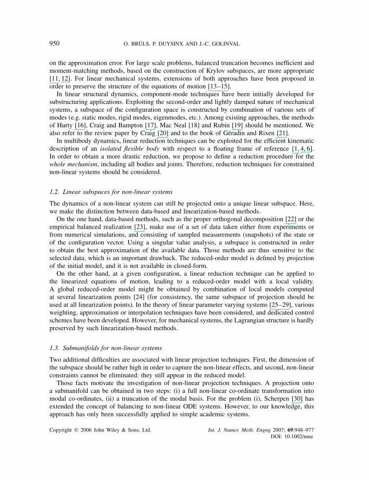
950 O. BRULS, P. DUYSINX AND J.-C. GOLINVAL

on the approximation error. For large scale problems, balanced truncation becomes inefficient andmoment-matching methods, based on the construction of Krylov subspaces, are more appropriate[11, 12]. For linear mechanical systems, extensions of both approaches have been proposed inorder to preserve the structure of the equations of motion [13–15].

In linear structural dynamics, component-mode techniques have been initially developed forsubstructuring applications. Exploiting the second-order and lightly damped nature of mechanicalsystems, a subspace of the configuration space is constructed by combination of various sets ofmodes (e.g. static modes, rigid modes, eigenmodes, etc.). Among existing approaches, the methodsof Hurty [16], Craig and Bampton [17], Mac Neal [18] and Rubin [19] should be mentioned. Wealso refer to the review paper by Craig [20] and to the book of Geradin and Rixen [21].

In multibody dynamics, linear reduction techniques can be exploited for the efficient kinematicdescription of an isolated flexible body with respect to a floating frame of reference [1, 4, 6].In order to obtain a more drastic reduction, we propose to define a reduction procedure for thewhole mechanism, including all bodies and joints. Therefore, reduction techniques for constrainednon-linear systems should be considered.

1.2. Linear subspaces for non-linear systems

The dynamics of a non-linear system can still be projected onto a unique linear subspace. Here,we make the distinction between data-based and linearization-based methods.

On the one hand, data-based methods, such as the proper orthogonal decomposition [22] or theempirical balanced realization [23], make use of a set of data taken either from experiments orfrom numerical simulations, and consisting of sampled measurements (snapshots) of the state orof the configuration vector. Using a singular value analysis, a subspace is constructed in orderto obtain the best approximation of the available data. Those methods are thus sensitive to theselected data, which is an important drawback. The reduced-order model is defined by projectionof the initial model, and it is not available in closed-form.

On the other hand, at a given configuration, a linear reduction technique can be applied tothe linearized equations of motion, leading to a reduced-order model with a local validity.A global reduced-order model might be obtained by combination of local models computedat several linearization points [24] (for consistency, the same subspace of projection should beused at all linearization points). In the theory of linear parameter varying systems [25–29], variousweighting, approximation or interpolation techniques have been considered, and dedicated controlschemes have been developed. However, for mechanical systems, the Lagrangian structure is hardlypreserved by such linearization-based methods.

1.3. Submanifolds for non-linear systems

Two additional difficulties are associated with linear projection techniques. First, the dimension ofthe subspace should be rather high in order to capture the non-linear effects, and second, non-linearconstraints cannot be eliminated: they still appear in the reduced model.

Those facts motivate the investigation of non-linear projection techniques. A projection ontoa submanifold can be obtained in two steps: (i) a full non-linear co-ordinate transformation intomodal co-ordinates, (ii) a truncation of the modal basis. For the problem (i), Scherpen [30] hasextended the concept of balancing to non-linear ODE systems. However, to our knowledge, thisapproach has only been successfully applied to simple academic systems.

Copyright q 2006 John Wiley & Sons, Ltd. Int. J. Numer. Meth. Engng 2007; 69:948–977DOI: 10.1002/nme

THE GLOBAL MODAL PARAMETERIZATION IN FLEXIBLE MULTIBODY DYNAMICS 951

In order to develop a method applicable to realistic multibody systems with non-linear holonomicconstraints, the physical properties of the system can be exploited for the construction of an adequatenon-linear co-ordinate transformation. We call the resulting reduced parameterization the globalmodal parameterization (GMP).

1.4. Outline

For a general holonomic Lagrangian system, Section 2 defines the general framework for a modelreduction procedure, which accounts for the gyroscopic and centrifugal forces, and which preservesthe Lagrangian structure. At this level, we assume the existence of a modal parameterization withindependent co-ordinates.

Section 3 is dedicated to the construction of the GMP, based on a decomposition of the motioninto a large amplitude rigid motion and a small amplitude elastic displacement. The order reductionfollows from a parametric component-mode synthesis in the configuration space. The consistencyand the validity of the GMP are analysed in detail. In particular, we show that a mode trackingstrategy needs to be implemented in the configuration space.

Section 4 describes the reduced-order model and the numerical reduction algorithm. We considerthat the initial model is formulated according to the non-linear finite element method, but since ourtheory assumes linear elasticity, other initial formulations could have been selected. Even thoughthe global consistency of the reduced-order model is guaranteed, the reduction algorithm onlygives the numerical value of its parameters locally at a given configuration.

In order to build a closed-form expression in the configuration space, an approximation strategyis developed in Section 5. As in rigid robotics, a simple look-up table technique could be considered[31], but we prefer a more advanced approach. For instance, artificial neural networks, kriging,polynomial or rational approximations can be used to solve this standard approximation problem.We present an adaptive piecewise polynomial approximation, which appears very effective for ourapplications.

Two examples are considered in Section 6: a flexible four-bar mechanism and a large manipulator.For this last application, the reduced-order model has been used for control design and experimentalresults are reported. Finally, some conclusions are drawn in Section 7.

2. LAGRANGIAN MECHANICS AND MODEL REDUCTION

2.1. Equations of motion for a constrained mechanical system

Let us consider a holonomic dynamic system, with a n × 1 vector of generalized co-ordinates q.For a flexible mechanism, those co-ordinates may be absolute nodal co-ordinates, Cartesianco-ordinates and/or relative co-ordinates. The system is characterized by

• its potential energy: V(q),• its kinetic energy: K(q, q) = 1

2 qTMqq(q)q (Mqq is the symmetric mass matrix),

• a set of m independent holonomic kinematic constraints: U(q) = 0,• the virtual work of applied generalized forces gq: �W= �qTgq.

The real trajectory between the time instants t1 and t2 satisfies the Hamilton principle. Followingthe Lagrange multiplier method, this principle is equivalent to∫ t2

t1[�(L − kTU) + �W] dt = 0

Copyright q 2006 John Wiley & Sons, Ltd. Int. J. Numer. Meth. Engng 2007; 69:948–977DOI: 10.1002/nme

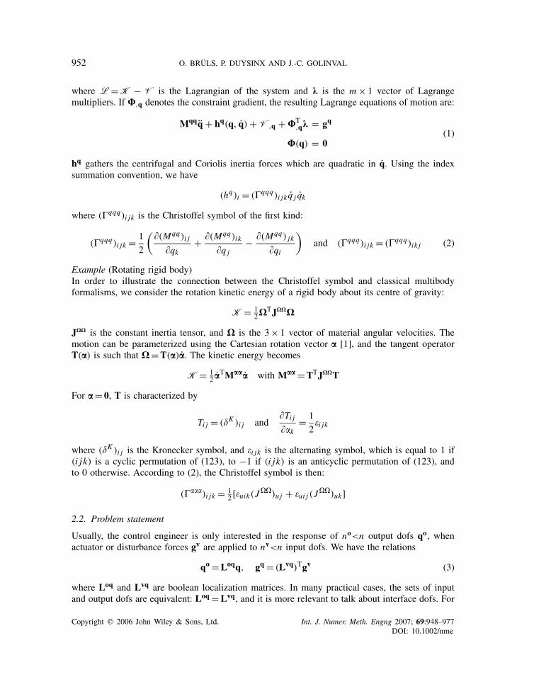
952 O. BRULS, P. DUYSINX AND J.-C. GOLINVAL

where L=K − V is the Lagrangian of the system and k is the m × 1 vector of Lagrangemultipliers. If U,q denotes the constraint gradient, the resulting Lagrange equations of motion are:

Mqqq + hq(q, q) + V,q +UT,qk = gq

U(q) = 0(1)

hq gathers the centrifugal and Coriolis inertia forces which are quadratic in q. Using the indexsummation convention, we have

(hq)i = (�qqq)i jk q j qk

where (�qqq)i jk is the Christoffel symbol of the first kind:

(�qqq)i jk = 1

2

(�(Mqq)i j

�qk+ �(Mqq)ik

�q j− �(Mqq) jk

�qi

)and (�qqq)i jk = (�qqq)ik j (2)

Example (Rotating rigid body)In order to illustrate the connection between the Christoffel symbol and classical multibodyformalisms, we consider the rotation kinetic energy of a rigid body about its centre of gravity:

K= 12X

TJXXX

JXX is the constant inertia tensor, and X is the 3× 1 vector of material angular velocities. Themotion can be parameterized using the Cartesian rotation vector a [1], and the tangent operatorT(a) is such that X=T(a)a. The kinetic energy becomes

K= 12 a

TMaaa with Maa=TTJXXT

For a= 0, T is characterized by

Ti j = (�K )i j and�Ti j��k

= 1

2�i jk

where (�K )i j is the Kronecker symbol, and �i jk is the alternating symbol, which is equal to 1 if(i jk) is a cyclic permutation of (123), to −1 if (i jk) is an anticyclic permutation of (123), andto 0 otherwise. According to (2), the Christoffel symbol is then:

(����)i jk = 12 [�uik(J��)u j + �ui j (J

��)uk]

2.2. Problem statement

Usually, the control engineer is only interested in the response of no<n output dofs qo, whenactuator or disturbance forces gv are applied to nv<n input dofs. We have the relations

qo =Loqq, gq = (Lvq)Tgv (3)

where Loq and Lvq are boolean localization matrices. In many practical cases, the sets of inputand output dofs are equivalent: Loq =Lvq, and it is more relevant to talk about interface dofs. For

Copyright q 2006 John Wiley & Sons, Ltd. Int. J. Numer. Meth. Engng 2007; 69:948–977DOI: 10.1002/nme

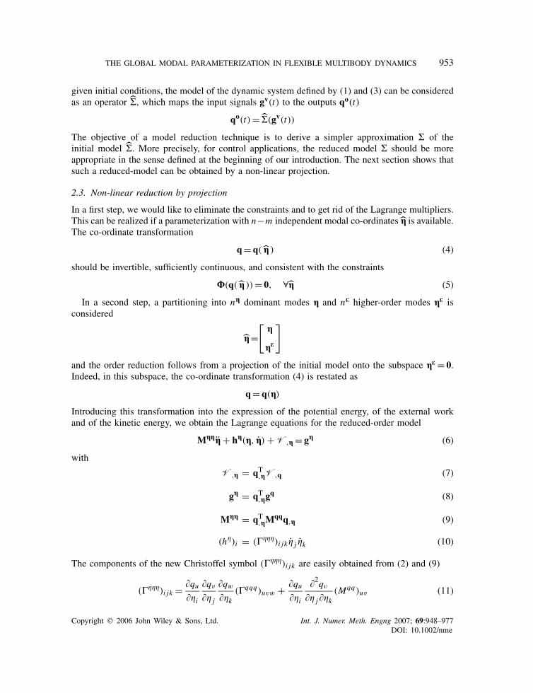
THE GLOBAL MODAL PARAMETERIZATION IN FLEXIBLE MULTIBODY DYNAMICS 953

given initial conditions, the model of the dynamic system defined by (1) and (3) can be consideredas an operator �, which maps the input signals gv(t) to the outputs qo(t)

qo(t) = �(gv(t))

The objective of a model reduction technique is to derive a simpler approximation � of theinitial model �. More precisely, for control applications, the reduced model � should be moreappropriate in the sense defined at the beginning of our introduction. The next section shows thatsuch a reduced-model can be obtained by a non-linear projection.

2.3. Non-linear reduction by projection

In a first step, we would like to eliminate the constraints and to get rid of the Lagrange multipliers.This can be realized if a parameterization with n−m independent modal co-ordinates g is available.The co-ordinate transformation

q= q( g ) (4)

should be invertible, sufficiently continuous, and consistent with the constraints

U(q( g ))= 0, ∀g (5)

In a second step, a partitioning into ng dominant modes g and ne higher-order modes ge isconsidered

g=[g

ge

]and the order reduction follows from a projection of the initial model onto the subspace ge= 0.Indeed, in this subspace, the co-ordinate transformation (4) is restated as

q=q(g)

Introducing this transformation into the expression of the potential energy, of the external workand of the kinetic energy, we obtain the Lagrange equations for the reduced-order model

Mggg+ hg(g, g) + V,g= gg (6)

with

V,g = qT,gV,q (7)

gg = qT,ggq (8)

Mgg = qT,gMqqq,g (9)

(h�)i = (����)i jk � j �k (10)

The components of the new Christoffel symbol (����)i jk are easily obtained from (2) and (9)

(����)i jk = �qu��i

�qv

�� j

�qw

��k(�qqq)uvw + �qu

��i

�2qv

�� j��k(Mqq)uv (11)

Copyright q 2006 John Wiley & Sons, Ltd. Int. J. Numer. Meth. Engng 2007; 69:948–977DOI: 10.1002/nme

954 O. BRULS, P. DUYSINX AND J.-C. GOLINVAL

In Equations (10) and (11), indices i, j, k are in the range 1, . . . , ng, while indices u, v, w are inthe range 1, . . . , n. It is noticeable that the transformation (11) involves not only the Jacobian of theco-ordinate transformation but also the second-order derivatives or curvatures, which reflects thenon-tensorial nature of the Christoffel symbol [32]. Clearly, the contribution of the curvatureswould vanish for a linear co-ordinate transformation.

The quality of the approximation � depends on the ability of the dominant modes g to capturethe essential dynamics of the initial model. In multibody dynamics, the distinction between rigidand flexible modes is essential for the definition of an effective GMP.

3. THE GLOBAL MODAL PARAMETERIZATION

Before defining the GMP, the concepts of rigid and flexible configuration spaces should be clarified.For a flexible mechanism with s rigid kinematic modes, we have the inequality

s � n − m

and the particular case s = n − m corresponds to a rigid mechanism. The flexible manifold �ftq ,

with intrinsic dimension n − m, is defined as the set of kinematically admissible configurationswhich satisfy the m kinematic constraints

�ftq ={q∈Rn|U(q) = 0}

In contrast, the rigid configuration space �rtq ⊂ �

ftq , with intrinsic dimension s, is defined as the

set of undeformed configurations. The motivation for the notations �ftq and �rt

q will become clearerin the following (the superscript t stands for ‘total’).

3.1. Definition of the GMP

A few physical considerations and assumptions lead to the definition of the GMP.

1. The overall motion is decomposed into a large amplitude rigid motion qr ∈ �rtq and a small

amplitude elastic displacement qf

q=qr + qf

2. As will be discussed in Section 3.2, a restricted part of the rigid configuration space �rq ⊂ �rt

qcan be parameterized using s independent parameters h. Hence, there exists a regular andinvertible kinematic mapping q

q : �h → �rq, h �→ qr = q(h)

where �h ⊂ Rs represents the set of allowed variations of h.3. The elastic displacement is a deviation from the rigid motion, which is parameterized using

(n − m) − s independent modal co-ordinates d:

qf = qf(h, d) with qf(h, 0) = 0 ∀h∈ �h (12)

Copyright q 2006 John Wiley & Sons, Ltd. Int. J. Numer. Meth. Engng 2007; 69:948–977DOI: 10.1002/nme

THE GLOBAL MODAL PARAMETERIZATION IN FLEXIBLE MULTIBODY DYNAMICS 955

Under the small deformation assumption, we make a first-order MacLaurin expansion withrespect to d

qf(h, d) � �qf

�d(h, 0)d=Wqd(h)d

�qf/�d is interpreted as a flexible mode shape matrix Wqd, which depends on the con-

figuration h. In Section 3.3, we shall see that Wqd(h) can be constructed according to aparametric component-mode synthesis in �h.

4. Considering a partitioning of the flexible modes into nd dominant modes d and ne higher-order modes de:

d=[d

de

], qf =Wqd(h)d+Wqe(h)de

the order reduction is obtained by a projection onto the subspace de= 0. In this subspace,we have

qf =Wqd(h)d

In summary, the GMP is a mapping

GMP : �h× �d → �fq, (h, d) �→ q= q(h) +Wqd(h)d (13)

whose regularity and invertibility will be demonstrated in Section 3.4. �d ⊂ Rnd represents the

set of allowed variations of d (it is a neighbourhood of the origin), and �fq ⊂ �

ftq is a submanifold

of the flexible manifold. To make a connection with Section 2.3, we have

g=[h

d

]and g=

[h

d

]The reduction formulae (7)–(11) require the first- and second-order derivatives of the co-ordinate

transformation. The differentiation of the GMP and the interpretation of the Jacobian q,h(h) as amatrix of rigid-body modes Wqh(h) lead to

q,g(h, d) =[Wqh(h) + �

�h(Wqd(h)d) Wqd(h)

](14)

so that for an undeformed configuration (d= 0)

q,g(h, 0)=[Wqh(h) Wqd(h)] =Wqg(h) (15)

At an undeformed configuration, the second-order derivatives are associated with the sensitivitiesof the rigid and flexible modes

�2qi�� j��k

(h, 0) = �(�q�)ik

�� j,

�2qi�� j��k

(h, 0) = �(�q�)ik

�� j,

�2qi�� j��k

(h, 0) = 0 (16)

Copyright q 2006 John Wiley & Sons, Ltd. Int. J. Numer. Meth. Engng 2007; 69:948–977DOI: 10.1002/nme

956 O. BRULS, P. DUYSINX AND J.-C. GOLINVAL

In order to exploit the Lagrange multiplier technique, the GMP should be formulated in termsof the augmented co-ordinates u

u=[q

k

]

The Lagrange multipliers represent internal forces and, in the absence of external loads, their valueis zero at an undeformed configuration. Assuming linear elasticity, k is proportional to d, and theGMP is reformulated

GMPu : �h× �d → �fu, (h, d) �→

[q

k

]=[q(h)

0

]+⎡⎣Wqd(h)

Wkd(h)

⎤⎦ dwith �f

u ⊂ �fq ×Rm . We shall use the equivalent notations

GMPu : �h× �d → �fu, (h, d) �→ u= qu(h) +Wud(h)d

Moreover, the augmented rigid configuration spaces are trivially defined by

�rtu =�rt

q × {0}m, �ru = �r

q × {0}m

The next two sections give more details about the parameterization of the rigid motion andof the flexible motion, respectively. Afterwards, Section 3.4 will demonstrate the consistency ofthe GMP.

3.2. Parameterization of the rigid kinematics

We seek for a set of s independent co-ordinates h able to parameterize the rigid configuration space�rtu . For parallel kinematic machines, �rt

u is a manifold which cannot be globally parameterizedusing a unique set of independent co-ordinates. In other words, any set of minimal co-ordinatesleads to singular configurations, which represent bounds for the validity of the parameterization.We refer to References [33–36] for detailed analysis of singularities in mechanism analysis. Ourobjective is to define a minimal parameterization with a relevant validity region �r

u ⊂ �rtu .

We propose to select the minimal co-ordinates h as the actuated co-ordinates, i.e. the co-ordinatesassociated with the generalized forces exerted by the actuators. For instance, for a motorized hinge,the actuated co-ordinate is the angle between the connected links, whereas for a linear actuator, itis the relative distance between the connected bodies. As a consequence of this choice, the actuatorco-ordinates will appear explicitly in the reduced model, which is extremely valuable for the designof the control system. An implicit assumption is that the number of actuators is equal to s. Thisdoes not imply that the reduction method is only applicable to fully actuated mechanisms, it simplymeans that in any other situation, the definition of the independent parameters is left to the user.

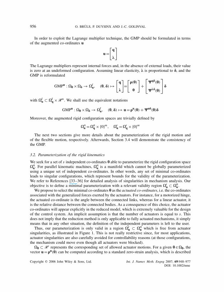
Thus, our parameterization is only valid in a region �ru ⊂ �rt

u which is free from actuatorsingularities, as illustrated in Figure 1. This is not really restrictive since, for most applications,actuator singularities are also carefully avoided for controllability reasons (at those configurations,the mechanism could move even though all actuators were blocked).

�h ⊂ Rs represents the corresponding set of allowed actuator motions. For a given h∈ �h, thevector u= qu(h) can be computed according to a standard zero-strain analysis, which is described

Copyright q 2006 John Wiley & Sons, Ltd. Int. J. Numer. Meth. Engng 2007; 69:948–977DOI: 10.1002/nme

THE GLOBAL MODAL PARAMETERIZATION IN FLEXIBLE MULTIBODY DYNAMICS 957

Figure 1. Rigid four bar mechanism, with an actuator at the lower left hinge. The configuration space isa 1-dimensional manifold, whose projection in the plane of the co-ordinates ze and � is also represented.Configuration (b) is an actuator singularity; it separates two regions for which the actuator parameterizationis regular. The parameterization is not regular in the total configuration space �rt

u , since configurations(a) and (c) are possible for the same value of �.

in Reference [36], and summarized hereafter. First of all, we consider that the actuator co-ordinatesare included among the set of n co-ordinates q, so that

u=

⎡⎢⎢⎣h

q∗

k

⎤⎥⎥⎦=[h

u∗

]

where q∗ are the n − s non-actuated co-ordinates. Any static equilibrium configuration achievesa minimum of the augmented elastic potential energy V + kTU, which leads to the stationarityconditions

V,q∗ +UT,q∗k = 0

U(q) = 0(17)

Starting from a known reference configuration uref = qu(href), and given a target value h∈ �h,this non-linear equation can be solved for u∗ according to a Newton procedure. If the referenceand the target configurations are sufficiently close to each other, the algorithm converges to theunique solution u∈ �r

u. Otherwise, intermediate configurations have to be considered, so that thealgorithm can progress sequentially to the target configuration with several smaller increments.

For pre-stressed mechanisms, the concept of rigid configuration space should be replaced bythe concept of ‘equilibrium configuration space’. Equation (17) would still be relevant, but theinternal forces k and the actuator forces V,h might be different from zero at a static equilibrium.In this paper, we do not want to enter into more details, and we leave the problem of pre-stressedmechanisms aside.

Copyright q 2006 John Wiley & Sons, Ltd. Int. J. Numer. Meth. Engng 2007; 69:948–977DOI: 10.1002/nme

958 O. BRULS, P. DUYSINX AND J.-C. GOLINVAL

3.3. Parameterization of the flexible motion

The GMP involves a configuration-dependent mode-shape matrix Wud(h), which is defined bya parametric component-mode synthesis. Indeed, given a configuration h∈ �h, the mode-shapematrix Wud is constructed as an optimal basis to describe the linearized motion around the stateq= q(h), q= 0: [

Mqq 0

0 0

][�q

�k

]+[Kqq

t UT,q

U,q 0

][�q

�k

]=[0

0

](18)

Kqqt is the exact tangent stiffness operator, whose expression is detailed in Reference [36].We consider a partitioning of the n + m initial dofs

u=

⎡⎢⎢⎣h

qg

ui

⎤⎥⎥⎦h are s actuator (or rigid) dofs, qg are ng constraint dofs where additional external loads are applied,and ui are the remaining internal dofs, including the Lagrange multipliers, which are not loadedand can be condensed by the reduction procedure. Accordingly, the mass and stiffness matricesappearing in (18) are rewritten⎡⎢⎢⎢⎣

Mrr Mrg Mri

Mgr Mgg Mgi

Mir Mig Mii

⎤⎥⎥⎥⎦ ,

⎡⎢⎢⎢⎣Krr Krg Kri

Kgr Kgg Kgi

Kir Kig Kii

⎤⎥⎥⎥⎦and a complete basis of modes is defined:

• The s rigid modes Wuh, which also form the Jacobian of qu(h), satisfy⎡⎢⎢⎢⎣Krr Krg Kri

Kgr Kgg Kgi

Kir Kig Kii

⎤⎥⎥⎥⎦⎡⎢⎢⎢⎣

I

Wgh

Wih

⎤⎥⎥⎥⎦=

⎡⎢⎢⎣0

0

0

⎤⎥⎥⎦ , Wuh=

⎡⎢⎢⎢⎣I

Wgh

Wih

⎤⎥⎥⎥⎦• The ng constraint modes Wuc are the static deformations obtained when the rigid dofs h arefixed and unit displacements are imposed to the constrained dofs qg

⎡⎣Kgg Kgi

Kig Kii

⎤⎦[ I

Wic

]=[gg

0

], Wuc=

⎡⎢⎢⎣0

I

Wic

⎤⎥⎥⎦ (19)

Copyright q 2006 John Wiley & Sons, Ltd. Int. J. Numer. Meth. Engng 2007; 69:948–977DOI: 10.1002/nme

THE GLOBAL MODAL PARAMETERIZATION IN FLEXIBLE MULTIBODY DYNAMICS 959

• The internal modes Wui are the normalized eigenmodes when rigid and constraint dofs arefixed. Each eigenmode Wuk is one solution to the eigenvalue problem

(Kii − �2kM

ii)Wik = 0, (Wik)TMiiWik = 1, Wuk =

⎡⎢⎢⎣0

0

Wik

⎤⎥⎥⎦ (20)

If the modes are sorted by eigenvalue, Wui can be partitioned into ni dominant modes Wui

and ne higher-order modes Wue

Wui= [Wui Wue]

The total matrix of flexible modes is

Wud=[Wuc Wui Wue]The reduction method of Hurty [16] relies on a truncation of the higher-order modes

Wud=[Wuc Wui], nd= ng + ni

This leads to an exact representation of the static response of the structure at the interface dofs(h and qg). The method of Craig and Bampton [17], which does not isolate the rigid modes fromthe flexible modes, is clearly irrelevant in this context.

3.4. Consistency of the global modal parameterization

The GMP (13) is a regular co-ordinate transformation if the following criteria are satisfied:

• It defines a bijection between �h× �d and �fu. This will be analysed in Section 3.4.2.

• It is continuously differentiable in �h× �d. By construction, the rigid mapping qu(h) isa smooth function in �h. In contrast, the flexible modes Wud(h) have only been definedlocally by component-mode synthesis, and their continuity will be analysed in Sections 3.4.3and 3.4.4.

• The Jacobian (14) has maximal rank in �h× �d. This condition is easily checked: at anundeformed configuration, the Jacobian is composed of rigid and flexible modes, whoselinear independence is guaranteed by construction. For small deformations, this property ispreserved by continuity.

Moreover, we have to demonstrate that the constraints are automatically satisfied by the GMP (seecondition (5)).

3.4.1. Satisfaction of the constraints. Let us introduce the GMP into the constraint equation andmake a Taylor series expansion around an undeformed configuration

U(q(h) +Wqdd) =U(q(h)) +U,qWqdd+ O(‖d‖2)

The first term vanishes by definition of the rigid parameterization and the second by constructionof the flexible modes (consider Equations (19) and (20), and the structure of the stiffness matrixin (18)). As a conclusion, the constraints are automatically satisfied provided that second-ordercontributions of the deformations are negligible.

Copyright q 2006 John Wiley & Sons, Ltd. Int. J. Numer. Meth. Engng 2007; 69:948–977DOI: 10.1002/nme

960 O. BRULS, P. DUYSINX AND J.-C. GOLINVAL

3.4.2. One-to-one property. To each vector (h, d) ∈ �h× �d, the GMP assigns a unique vectoru∈ �f

u. This section demonstrates the converse: for a given u∈ �fu, there is only one (h, d) ∈

�h× �d such that u= qu(h) +Wud(h)d.Suppose that another solution (h′, d′) also satisfies u= qu(h′) + Wud(h′)d′. Since h appears

explicitly among the co-ordinates u, we have h′ = h, and the flexible co-ordinates satisfy

qu(h) +Wud(h)d= qu(h) +Wud(h)d′ ⇒ Wud(d− d′) = 0

From the linear independence of the flexible modes, we deduce that d− d′ = 0.

3.4.3. Continuity of the constraint modes. The constraint modes Wuc are defined from a linearstatic analysis when the rigid dofs are fixed. From Equation (19), we have

Wic(h) =−(Kii(h))−1Kig(h)

Since Kii is invertible (otherwise additional rigid modes should be defined), and since everystiffness coefficient is continuous and differentiable, so are the constraint modes.

3.4.4. Continuity of the internal modes. The internal modes Wii are obtained after two steps:(i) the eigenvalue problem (20) is solved, (ii) the eigenmodes are sorted according to their eigen-value, and the first ni modes are selected.

For a simple eigenvalue �k and the associated internal mode wk , it is instructive to differentiatethe eigenvalue problem in (20). An infinitesimal variation ��l of the co-ordinate �l leads tovariations ��2

k and �wk such that(�Kii

��l− �2

k�Mii

��l

)wk��l − Miiwk��2

k + (Kii − �2kM

ii)�wk = 0 (21)

A pre-multiplication by wTk together with the normalization condition in (20) yields

��2k

��l=wTk

(�Kii

��l− �2

k�Mii

��l

)wk

Since the right-hand side is well-defined, we conclude that the variations of �2k with respect to �l

are continuous, and that the derivative ��2k/��l exists (the continuity of the derivative depends on

the continuity of wk). Thus, (21) can be rewritten

(Kii − �2kM

ii)�wk��l

=−(

�Kii

��l− �2

k�Mii

��l− ��2

k

��lMii

)wk

Even though the right-hand side is well-defined,�wk could be affected by arbitrarily large variationsin the kernel of Kii −�2

kMii. However, for a simple eigenvalue, this kernel is one-dimensional and

such variations are forbidden by the normalization condition. In this case, the internal modes arenecessarily continuous and differentiable.

Copyright q 2006 John Wiley & Sons, Ltd. Int. J. Numer. Meth. Engng 2007; 69:948–977DOI: 10.1002/nme

THE GLOBAL MODAL PARAMETERIZATION IN FLEXIBLE MULTIBODY DYNAMICS 961

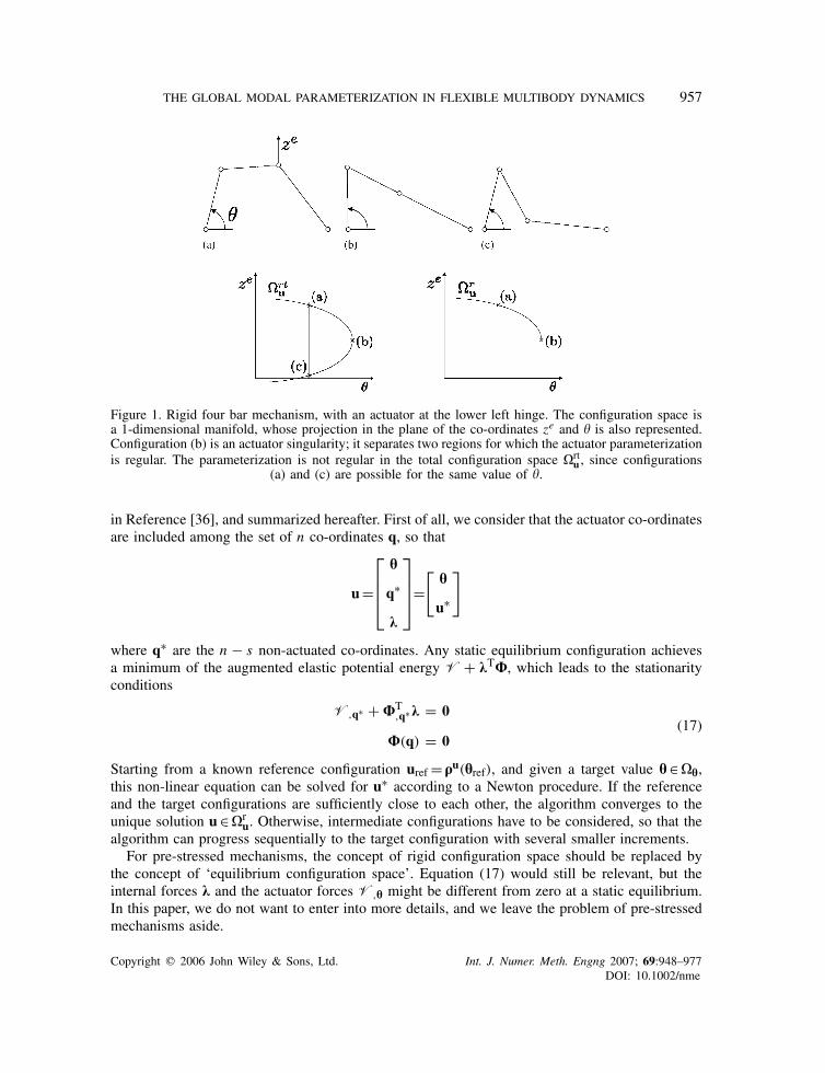
Figure 2. Crossing of the eigenfrequencies in a one-dimensional configuration space.

A multiple eigenvalue can occur if two different eigenvalues cross each other. The differ-entiability of multiple eigenvalues and of their eigenmodes has been extensively discussed inthe structural optimization community, see for instance Reference [37]. Let us consider asystem with a one-dimensional configuration space and two eigenvalues, as illustrated inFigure 2. Away from �b, the eigenvalues �1 and �2 and their respective eigenvectors w1 andw2 are well-separated and continuous. At �b, we have a double eigenvalue, whose eigenvectoris undefined in the subspace spanned by w1 and w2. Thus, the major pitfall is a permutationphenomenon, which will actually occur if the eigenvectors are sorted and selected according to theireigenvalues

Wii(�1) = [w1 w2] ∀�1<�b

Wii(�1) = [w2 w1] ∀�1>�b

This discussion can be extended for a s-dimensional configuration space, and we conclude that arefinement in the computation of the internal modes is necessary to avoid permutations.

Our algorithm is initialized at a germ configuration where the eigenmodes are sorted and selectedaccording to their eigenvalues. From this germ, it gradually progresses in the whole configura-tion space �h, but the eigenmodes are then sorted and selected according to a mode trackingstrategy, as suggested by Kim and Kim [38]. These authors have exploited the Modal AssuranceCriterion (MAC value) which is a measure from 0 to 1 of the correlation between two modes,a unitary value meaning perfect correlation. The correlation is realized between the eigenmodesat the current configuration and at a reference configuration. More precisely, the MAC matrix,which is filled with the MAC numbers of all pairs of modes, is rendered as close as possible to theidentity.

The internal modes can only be validated if the deviation of the MAC-matrix from the identitysatisfies a tolerance condition. For example, if the reference configuration is far from the currentconfiguration, the correlation may be poor and the consistency cannot be guaranteed. In this case,the procedure should be restarted with a closer reference configuration, as will be explained inSection 5.2.

3.4.5. Conclusion. From this consistency analysis, we conclude that the Global Modal Parame-terization (13) is well-defined, provided that a mode-tracking strategy is implemented. Hence, theGMP defines a reduction procedure in the sense of Section 2.3. The reduced equations of motionand the reduction algorithm are developed in the Section 4.

Copyright q 2006 John Wiley & Sons, Ltd. Int. J. Numer. Meth. Engng 2007; 69:948–977DOI: 10.1002/nme

962 O. BRULS, P. DUYSINX AND J.-C. GOLINVAL

4. REDUCED-ORDER MODEL

From the definition of the GMP, the reduced equations of motion (6) can be derived, but the generaltransformation relations (7)–(11) hide very complex expressions. However, in flexible multibodydynamics, the small deformation assumption allows to omit higher-order contributions of d, whichconsiderably simplifies the formulation of the elastic and inertia forces.

4.1. Elastic forces

The elastic potential energy is a strongly non-linear function V(q), and we seek for an approxima-tion in terms of the reduced co-ordinates h and d. For small deformations, we have the followingresult, demonstrated in Reference [36]:

V,g=[V,h

V,d

]�[

0

Kdd(h)d

](22)

where Kdd(h) is defined at the undeformed configuration q(h)

Kdd= (Wqd)TKqqt W

qd=[Kcc 0

0 X2

]Kcc is the ng × ng symmetric stiffness matrix associated with the constraint modes, andX2 = diag{�2

i } is the diagonal matrix of the ni squared internal eigenvalues.

4.2. Inertia forces

Theoretically, the reduced mass matrix and Christoffel symbol depend on the whole set of modalparameters g. However, the dependence with respect to the flexible co-ordinates d can be neglected,so that the inertia forces become

d

dt

(�K�g

)− �K

�g�Mgg(h)g+ hg(h, g) (23)

with

(h�)i = (����(h))i jk � j �k

Again, the computation of Mgg and (����)i jk is only needed at an undeformed configuration.Equations (9), (11) and (15) lead to

Mgg = (Wqg)TMqqWqg

(����)i jk = (�q�)ui (�q�)v j (�

q�)wk(�qqq)uvw︸ ︷︷ ︸

≡(����)i jk

+ (�q�)ui�2qv

�� j��k(Mqq)uv︸ ︷︷ ︸

≡(����)i jk

Using (16), ���� can be computed from a sensitivity analysis of the mode shapes with respectto h, according to a finite difference approach. In our finite element formulation, the Christoffel

Copyright q 2006 John Wiley & Sons, Ltd. Int. J. Numer. Meth. Engng 2007; 69:948–977DOI: 10.1002/nme

THE GLOBAL MODAL PARAMETERIZATION IN FLEXIBLE MULTIBODY DYNAMICS 963

symbol (�qqq)uvw is not directly available, and its expression cannot be used explicitly for thecomputation of (����)i jk . For this reason, we propose an algorithm for (����)i jk which onlyinvolves the computation of the forces hq. Let us define hg

(h�)i = (����)i jk � j �k

At an undeformed configuration, it is easily verified that: hg= (Wqg)Thq. For a given g, hg canthus be computed in the following way:

1. Compute q=Wqgg.2. Compute hq (initial model).3. Deduce hg= (Wqg)Thq.

From this observation, all coefficients (����)i jk can be identified from two series of tests whenzero or unit velocities are imposed to appropriate modal co-ordinates:

• Identification of the ‘diagonal’ terms (����)iaa (a = 1, . . . , ng). Impose �a = 1, and use:

(h�)i = (����)iaa (no sum for a)

• Identification of the ‘off-diagonal’ terms (����)iab (a = 1, . . . , ng and b= a + 1, . . . , ng).Impose �a = �b = 1, and use:

(h�)i = (����)iaa + (����)ibb + 2(����)iab (no sum for a nor for b)

4.3. Reduced equations of motion

Considering that the external loads are transformed according to (8) and (15)

gg=WqgTgq

the reduced equations of motion follow:

Mgg(h)g+ hg(h, g) + Kgg(h)g= gg (24)

with the structure

Mgg=

⎡⎢⎢⎢⎣Mhh Mhc Mhi

Mch Mcc Mci

Mih Mic I

⎤⎥⎥⎥⎦ , Kgg=

⎡⎢⎢⎣0 0 0

0 Kcc 0

0 0 X2

⎤⎥⎥⎦ , gg=

⎡⎢⎢⎣ga + (Wgh)Tgg

gg

0

⎤⎥⎥⎦ga denotes the actuator forces and gg the forces applied to the constraint dofs. This model is fullydescribed by Mgg, Kgg, (����)i jk and Wgh, which smoothly depend on h. Model (24) has theLagrangian structure provided that the approximations (22) and (23) are acceptable, i.e. that thedeformations are sufficiently small.

Copyright q 2006 John Wiley & Sons, Ltd. Int. J. Numer. Meth. Engng 2007; 69:948–977DOI: 10.1002/nme

964 O. BRULS, P. DUYSINX AND J.-C. GOLINVAL

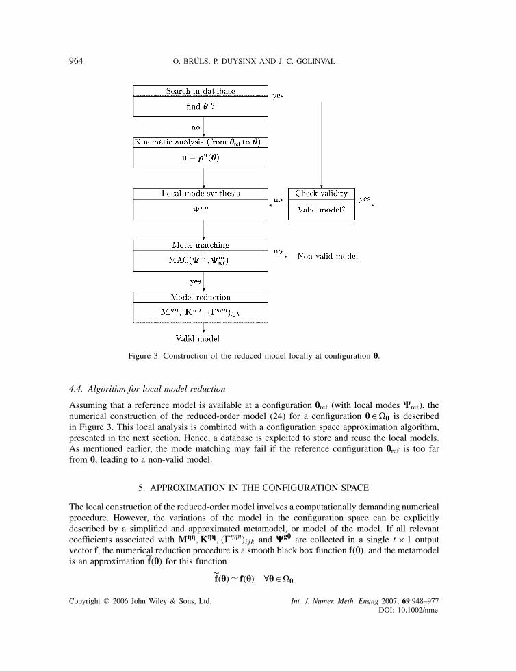
Figure 3. Construction of the reduced model locally at configuration h.

4.4. Algorithm for local model reduction

Assuming that a reference model is available at a configuration href (with local modes Wref), thenumerical construction of the reduced-order model (24) for a configuration h∈ �h is describedin Figure 3. This local analysis is combined with a configuration space approximation algorithm,presented in the next section. Hence, a database is exploited to store and reuse the local models.As mentioned earlier, the mode matching may fail if the reference configuration href is too farfrom h, leading to a non-valid model.

5. APPROXIMATION IN THE CONFIGURATION SPACE

The local construction of the reduced-order model involves a computationally demanding numericalprocedure. However, the variations of the model in the configuration space can be explicitlydescribed by a simplified and approximated metamodel, or model of the model. If all relevantcoefficients associated with Mgg,Kgg, (����)i jk and Wgh are collected in a single t × 1 outputvector f, the numerical reduction procedure is a smooth black box function f(h), and the metamodelis an approximation f(h) for this function

f(h) � f(h) ∀h∈ �h

Copyright q 2006 John Wiley & Sons, Ltd. Int. J. Numer. Meth. Engng 2007; 69:948–977DOI: 10.1002/nme

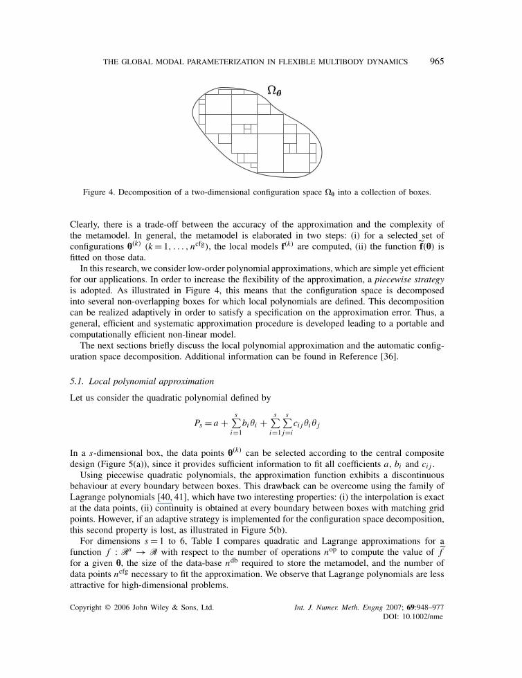
THE GLOBAL MODAL PARAMETERIZATION IN FLEXIBLE MULTIBODY DYNAMICS 965

Figure 4. Decomposition of a two-dimensional configuration space �h into a collection of boxes.

Clearly, there is a trade-off between the accuracy of the approximation and the complexity ofthe metamodel. In general, the metamodel is elaborated in two steps: (i) for a selected set ofconfigurations h(k) (k = 1, . . . , ncfg), the local models f(k) are computed, (ii) the function f(h) isfitted on those data.

In this research, we consider low-order polynomial approximations, which are simple yet efficientfor our applications. In order to increase the flexibility of the approximation, a piecewise strategyis adopted. As illustrated in Figure 4, this means that the configuration space is decomposedinto several non-overlapping boxes for which local polynomials are defined. This decompositioncan be realized adaptively in order to satisfy a specification on the approximation error. Thus, ageneral, efficient and systematic approximation procedure is developed leading to a portable andcomputationally efficient non-linear model.

The next sections briefly discuss the local polynomial approximation and the automatic config-uration space decomposition. Additional information can be found in Reference [36].

5.1. Local polynomial approximation

Let us consider the quadratic polynomial defined by

Ps = a +s∑

i=1bi�i +

s∑i=1

s∑j=i

ci j�i� j

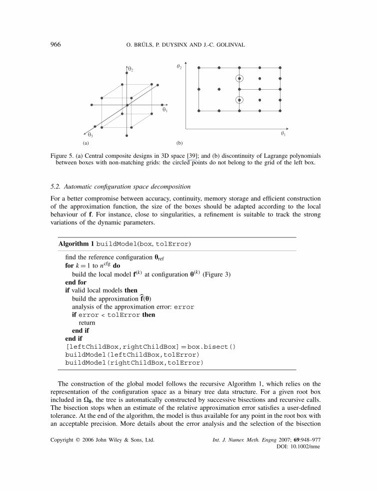
In a s-dimensional box, the data points h(k) can be selected according to the central compositedesign (Figure 5(a)), since it provides sufficient information to fit all coefficients a, bi and ci j .

Using piecewise quadratic polynomials, the approximation function exhibits a discontinuousbehaviour at every boundary between boxes. This drawback can be overcome using the family ofLagrange polynomials [40, 41], which have two interesting properties: (i) the interpolation is exactat the data points, (ii) continuity is obtained at every boundary between boxes with matching gridpoints. However, if an adaptive strategy is implemented for the configuration space decomposition,this second property is lost, as illustrated in Figure 5(b).

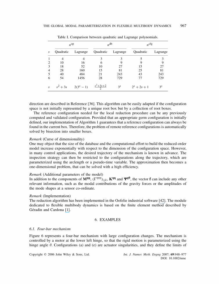
For dimensions s = 1 to 6, Table I compares quadratic and Lagrange approximations for afunction f : Rs → R with respect to the number of operations nop to compute the value of ffor a given h, the size of the data-base ndb required to store the metamodel, and the number ofdata points ncfg necessary to fit the approximation. We observe that Lagrange polynomials are lessattractive for high-dimensional problems.

Copyright q 2006 John Wiley & Sons, Ltd. Int. J. Numer. Meth. Engng 2007; 69:948–977DOI: 10.1002/nme

966 O. BRULS, P. DUYSINX AND J.-C. GOLINVAL

(a) (b)

Figure 5. (a) Central composite designs in 3D space [39]; and (b) discontinuity of Lagrange polynomialsbetween boxes with non-matching grids: the circled points do not belong to the grid of the left box.

5.2. Automatic configuration space decomposition

For a better compromise between accuracy, continuity, memory storage and efficient constructionof the approximation function, the size of the boxes should be adapted according to the localbehaviour of f. For instance, close to singularities, a refinement is suitable to track the strongvariations of the dynamic parameters.

Algorithm 1 buildModel(box, tolError)

find the reference configuration hreffor k = 1 to ncfg dobuild the local model f(k) at configuration h(k) (Figure 3)

end forif valid local models thenbuild the approximation f(h)analysis of the approximation error: errorif error < tolError then

returnend if

end if[leftChildBox,rightChildBox]=box.bisect()buildModel(leftChildBox,tolError)buildModel(rightChildBox,tolError)

The construction of the global model follows the recursive Algorithm 1, which relies on therepresentation of the configuration space as a binary tree data structure. For a given root boxincluded in �h, the tree is automatically constructed by successive bisections and recursive calls.The bisection stops when an estimate of the relative approximation error satisfies a user-definedtolerance. At the end of the algorithm, the model is thus available for any point in the root box withan acceptable precision. More details about the error analysis and the selection of the bisection

Copyright q 2006 John Wiley & Sons, Ltd. Int. J. Numer. Meth. Engng 2007; 69:948–977DOI: 10.1002/nme

THE GLOBAL MODAL PARAMETERIZATION IN FLEXIBLE MULTIBODY DYNAMICS 967

Table I. Comparison between quadratic and Lagrange polynomials.

nop ndb ncfg

s Quadratic Lagrange Quadratic Lagrange Quadratic Lagrange

1 4 4 3 3 5 32 10 16 6 9 9 93 18 52 10 27 15 274 28 160 15 81 25 815 40 484 21 243 43 2436 54 1456 28 729 77 729

s s2 + 3s 2(3s − 1) s2+3s+22 3s 2s + 2s + 1 3s

direction are described in Reference [36]. This algorithm can be easily adapted if the configurationspace is not initially represented by a unique root box but by a collection of root boxes.

The reference configuration needed for the local reduction procedure can be any previouslycomputed and validated configuration. Provided that an appropriate germ configuration is initiallydefined, our implementation of Algorithm 1 guarantees that a reference configuration can always befound in the current box. Therefore, the problem of remote reference configurations is automaticallysolved by bisection into smaller boxes.

Remark (Curse of dimensionality)One may object that the size of the database and the computational effort to build the reduced-ordermodel increase exponentially with respect to the dimension of the configuration space. However,in many control applications, the desired trajectory of the mechanism is known in advance. Theinspection strategy can then be restricted to the configurations along the trajectory, which areparameterized using the arclength or a pseudo-time variable. The approximation then becomes aone-dimensional problem, that can be solved with a high efficiency.

Remark (Additional parameters of the model)In addition to the components of Mgg, (����)i jk , Kgg and Wgh, the vector f can include any otherrelevant information, such as the modal contributions of the gravity forces or the amplitudes ofthe mode shapes at a sensor co-ordinate.

Remark (Implementation)The reduction algorithm has been implemented in the Oofelie industrial software [42]. The modulededicated to flexible multibody dynamics is based on the finite element method described byGeradin and Cardona [1].

6. EXAMPLES

6.1. Four-bar mechanism

Figure 6 represents a four-bar mechanism with large configuration changes. The mechanism iscontrolled by a motor at the lower left hinge, so that the rigid motion is parameterized using thehinge angle �. Configurations (a) and (e) are actuator singularities, and they define the limits of

Copyright q 2006 John Wiley & Sons, Ltd. Int. J. Numer. Meth. Engng 2007; 69:948–977DOI: 10.1002/nme

968 O. BRULS, P. DUYSINX AND J.-C. GOLINVAL

(e)(d)(c)(b)(a)

Figure 6. Large configuration changes of the four-bar mechanism.

our study in the configuration space (actually, the configuration space of interest is restricted to� ∈ [−1.75, 1.75] rad). At the singular configurations, the actuator is not able to control the motionof the mechanism, and the aligned links may bend upward or downward, depending on otherexternal forces.

We consider that the operations of a tool cause vertical loads on the upper right hinge, andone constraint mode is therefore associated with the vertical displacement ze of that point. Threeinternal modes are also selected to represent the deformations of the mechanism. The initialfinite element model contains 84 generalized co-ordinates and 7 Lagrange multipliers, whereas thereduced model involves 5 modal co-ordinates (1 rigid mode, 1 constraint mode, 3 internal modes),which are represented for configuration (d) in Figure 7. Two internal modes have an out-of-planedeformation. For this one-dimensional configuration space, the Lagrange interpolation techniqueis selected and different versions of the reduction algorithm are tested.

First, the configuration space is decomposed into 32 regular boxes, and the mode tracking algo-rithm is disabled. The natural frequencies of the selected internal modes are plotted in Figure 8, onthe left. The algorithm selects the three modes with the lowest frequencies, so that non-smooth vari-ations are observed whenever an eigenvalue crossing occurs. The perturbations around � = 0.7 radare attributed to the fourth internal mode, whose natural frequency drops at configuration (c). Thissituation is of course not acceptable, since it leads to a non-consistent parameterization of themotion. The mode tracking strategy is able to remedy this situation, as attested by the results onthe right plot in Figure 8.

For the components associated with the rigid mode, Figure 9 illustrates the variations of themass matrix and Christoffel symbol in the configuration space. A vertical asymptote is expectedclose to the extreme singular configurations. Mathematically, the components of the rigid modesgrow to infinity at those points, which explains the phenomenon. From the actuator point of view,the mechanical blocking at the singularity is equivalent to an infinite inertia. It is also observedthat the Christoffel symbol is connected with the gradient of the mass matrix, in agreement withEquation (2).

Then, the adaptive decomposition is considered, leading to a set of 37 irregular boxes (only 5more than for the regular grid). Figure 10 compares the relative approximation errors

erri (�) = ‖ fi (�) − fi (�)‖‖ fi (�)‖

At the singularity, low-order polynomials defined on a regular grid are not able to representefficiently the strongly non-linear behaviour of the system. Due to a refinement of the grid close

Copyright q 2006 John Wiley & Sons, Ltd. Int. J. Numer. Meth. Engng 2007; 69:948–977DOI: 10.1002/nme

THE GLOBAL MODAL PARAMETERIZATION IN FLEXIBLE MULTIBODY DYNAMICS 969

z

y

z

x

z

x y

Figure 7. Mode shapes for configuration (d). From top to bottom: rigid mode, constraint mode (� is fixed),and 3 internal modes (� and ze are fixed).

to the singularity, the adaptive method is able to overcome this difficulty. In other parts of theconfiguration space, small errors are tolerated allowing a coarser discretization.

The equivalent stiffness associated with the constraint mode is analysed in Figure 11. Close to thesingularities, this stiffness decreases to zero, but it takes very large values around configuration (c).

Copyright q 2006 John Wiley & Sons, Ltd. Int. J. Numer. Meth. Engng 2007; 69:948–977DOI: 10.1002/nme

970 O. BRULS, P. DUYSINX AND J.-C. GOLINVAL

0 1 20

1

2

3

4

5

6

7

8

θ (rad)

Freq

uenc

ies

(Hz)

ω1

ω2

ω3

0 1 20

1

2

3

4

5

6

7

8

θ (rad)

Freq

uenc

ies

(Hz)

ω1

ω2

ω3

Without tracking With tracking

Figure 8. Natural frequencies in the configuration space: importance of the tracking strategy.

0 1 2100

200

300

400

500

600

700

θ (rad)

Iner

tia (

kg.m

2 )

0 1 2

0

500

1000

1500

2000

2500

θ (rad)

Chr

isto

ffel (

kg.m

2 )

Figure 9. Variations of the equivalent inertia associated with the rigid mode (M��)11, and ofthe component of the Christoffel symbol (����)111.

At this configuration, the two left links are aligned, and any vertical motion ze induces tractionor compression efforts, involving tremendous strain energy. As a result, the vertical deflection ofthe effector is almost blocked. The regular grid leads to a rough approximation in a large domainaround the peak, which may strongly affect the quality of the model. The adaptive grid is far moreefficient.

From this example, we conclude that the variations of the stiffness and inertia parameters inthe configuration space receive a consistent physical interpretation, but that the mode-trackingstrategy is essential for the reliability of the results. A polynomial approximation can accuratelycapture the non-linear changes in the parameters of the model, and the adaptive configuration spacedecomposition is valuable to reduce the approximation error and to optimize the computationalresources.

Copyright q 2006 John Wiley & Sons, Ltd. Int. J. Numer. Meth. Engng 2007; 69:948–977DOI: 10.1002/nme

THE GLOBAL MODAL PARAMETERIZATION IN FLEXIBLE MULTIBODY DYNAMICS 971

0 1 20

0.005

0.01

0.015

θ (rad)

regularadaptive

0 1 20

0.05

0.1

θ (rad)

regularadaptive

Figure 10. Comparison of the relative errors for regular and adaptive grids.

0 1 20

1000

2000

3000

4000

5000

6000

7000

8000

9000

θ (rad)

Stiffn

ess (

N/m

)

regularadaptiveexact

0.65 0.7 0.75 0.8 0.85 0.90

2

4

6

8

10

12

x 106

θ (rad)

Stiffn

ess (

N/m

)regularadaptiveexact

Figure 11. Equivalent stiffness associated with the constraint mode for two different axis ranges.

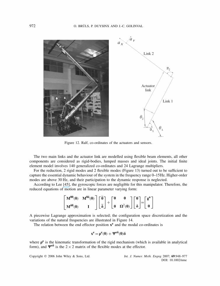
6.2. Long-reach manipulator

The long-reach manipulator Ralf, shown in Figure 12, has been developed at the IMDL researchcentre of the Georgia Institute of Technology [43, 44]. It operates in a vertical plane and the twokinematic dofs are controlled by hydraulic actuators. The structure consists of two main links(3.05m long) and a parallel actuation mechanism. Ralf has a high payload to weight ratio, and it isstiff enough to achieve real-world applications. However, flexible phenomena affect the positioningaccuracy.

The first actuator moves the first link relative to the base, the second moves the second linkrelative to the first through the parallel mechanism. Two linear position sensing transducers, fixed tothe hydraulic cylinder, measure the cylinder extension. Moreover, in order to detect the vibrationsof the mechanism, two accelerometers have been placed at the tip, in two orthogonal directions.As seen in Figure 12, the rigid configuration of Ralf can be described either using the relativeangles �1 and �2 of the main links, or the actuator extensions �1 and �2.

Copyright q 2006 John Wiley & Sons, Ltd. Int. J. Numer. Meth. Engng 2007; 69:948–977DOI: 10.1002/nme

972 O. BRULS, P. DUYSINX AND J.-C. GOLINVAL

Link 1

Link 2

Actuatorlink

a X

a Y

Figure 12. Ralf, co-ordinates of the actuators and sensors.

The two main links and the actuator link are modelled using flexible beam elements, all othercomponents are considered as rigid-bodies, lumped masses and ideal joints. The initial finiteelement model involves 140 generalized co-ordinates and 24 Lagrange multipliers.

For the reduction, 2 rigid modes and 2 flexible modes (Figure 13) turned out to be sufficient tocapture the essential dynamic behaviour of the system in the frequency range 0–15Hz. Higher-ordermodes are above 30 Hz, and their participation to the dynamic response is neglected.

According to Lee [45], the gyroscopic forces are negligible for this manipulator. Therefore, thereduced equations of motion are in linear parameter varying form:⎡⎣Mhh(h) Mhd(h)

Mdh(h) I

⎤⎦[ hd

]+[0 0

0 X2(h)

][h

d

]=[ga

0

]

A piecewise Lagrange approximation is selected; the configuration space discretization and thevariations of the natural frequencies are illustrated in Figure 14.

The relation between the end effector position xe and the modal co-ordinates is

xe = qe(h) +Wed(h)d

where qe is the kinematic transformation of the rigid mechanism (which is available in analyticalform), and Wed is the 2× 2 matrix of the flexible modes at the effector.

Copyright q 2006 John Wiley & Sons, Ltd. Int. J. Numer. Meth. Engng 2007; 69:948–977DOI: 10.1002/nme

THE GLOBAL MODAL PARAMETERIZATION IN FLEXIBLE MULTIBODY DYNAMICS 973

Flexible modesRigid modes

Figure 13. Mode shapes, home configuration.

0.8 0.9 1 1.1 1.2 1.3

0.8

0.9

1

1.1

1.2

1.3

θ1 (m)

θ 2 (m

)

0.7 0.8 0.9 1 1.1 1.2 1.3 1.42.5

3

3.5

4

4.5

5

5.5

6

6.5

7

θ1 (m)

ω (

Hz)

ω1

ω2

(a) (b)

Figure 14. (a) Configuration space discretization; and (b) variations of the natural frequencies alonga diagonal line in the configuration space from the lower left corner to the upper right corner.

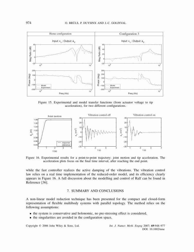
Around a fixed configuration, a frequency-domain analysis is possible for the linearized system.For experimental validation, a model of the hydraulic actuators has also been developed and someparameters have been identified. The structural damping has been adjusted to a value around 1%(actually, the dominant damping effect in the overall system comes from the actuators and thecontrol system). A comparison between the resulting model and experimental results is given inFigure 15. Some discrepancies can be observed, which are attributed to the weaknesses of theidentification procedure. Nevertheless, we conclude that a reduced-order model is able to capturethe configuration-dependent dynamics of a real manipulator.

This model has been exploited for the development of a position and vibration controllerbased on a two-time-scale strategy: the slow controller is a classical joint-tracking controller,

Copyright q 2006 John Wiley & Sons, Ltd. Int. J. Numer. Meth. Engng 2007; 69:948–977DOI: 10.1002/nme

974 O. BRULS, P. DUYSINX AND J.-C. GOLINVAL

100

101

0

20

40

Mag

Rat

io (

dB)

Input: v1 ; Output: a

Y

100

101

0

100

200

Pha

se (

deg)

Freq (Hz)

ModelExperiment

100

101

0

20

40

60

Mag

Rat

io (

dB)

Input: v1 ; Output: a

Y

100

101

0

100

200

300

Pha

se (

deg)

Freq (Hz)

ModelExperiment

Home configuration Configuration 3

Figure 15. Experimental and model transfer functions (from actuator voltage to tipacceleration), for two different configurations.

0 1 2 3 4

0.94

0.96

0.98

1

1.02

1.04

1.06

1.08

t (s)

θ 2 (m

)

responsereference

1 2 3 4

0

10

20

30

t (s) t (s)

a Y (

m/s

2 )

1 2 3 4

0

10

20

30a Y

(m

/s2 )

Joint motion Vibration control off Vibration control on

Figure 16. Experimental results for a point-to-point trajectory: joint motion and tip acceleration. Theacceleration plots focus on the final time interval, after reaching the end point.

while the fast controller realizes the active damping of the vibrations. The vibration controllaw relies on a real time implementation of the reduced-order model, and its efficiency clearlyappears in Figure 16. A full discussion about the modelling and control of Ralf can be found inReference [36].

7. SUMMARY AND CONCLUSIONS

A non-linear model reduction technique has been presented for the compact and closed-formrepresentation of flexible multibody systems with parallel topology. The method relies on thefollowing assumptions:

• the system is conservative and holonomic, no pre-stressing effect is considered,• the singularities are avoided in the configuration space,

Copyright q 2006 John Wiley & Sons, Ltd. Int. J. Numer. Meth. Engng 2007; 69:948–977DOI: 10.1002/nme

THE GLOBAL MODAL PARAMETERIZATION IN FLEXIBLE MULTIBODY DYNAMICS 975

• the deformations are small, the elastic behaviour is linear, and centrifugal stiffening effectsare not taken into account.

The reduction is achieved at the mechanism level by projection of the dynamics onto a submani-fold of the configuration space. This procedure is formally defined in two steps: (i) a full co-ordinatetransformation into independent modal co-ordinates, (ii) a truncation of the higher-order flexiblemodes. In the resulting GMP, the new co-ordinates have a clear physical interpretation in termsof rigid and flexible modes, and the actuator co-ordinates appear explicitly. The reduced-ordermodel still has the Lagrangian structure; the mass matrix, the stiffness matrix, and the Christoffelsymbol are configuration-dependent. Their coefficients are represented approximately using piece-wise polynomial functions, with the advantages of computational efficiency and portability. In thereduction procedure, the accuracy loss is localized at two levels:

• the truncation of the flexible modal basis (the rigid motion is exactly represented),• the approximation in the configuration space.

The procedure is systematic and the user only needs to provide high-level information: an initialmodel of the mechanism (e.g. a finite element model), the partitioning into rigid, constraint, andinternal dofs, the number of internal modes, a region of the configuration space, and the toleranceon the approximation error. The mode shapes are selected automatically according to a parametriccomponent-mode synthesis. The technique of Hurty [16] has been selected but this choice isnot restrictive: other component-modes proposed in the literature could be later considered. As aspecial case, the method is applicable to rigid mechanisms; it is then equivalent to the constraintelimination technique described in Reference [46].

Two examples have been successfully analysed: a flexible four-bar mechanism and a flexiblemanipulator. For the manipulator, an experimental validation has been realized, and the model hasbeen exploited for the design and implementation of a position and vibration controller.

The method could also be used for the offline numerical optimization of a control law (trajectorygeneration, inverse dynamics, training of a feedback action) or to fit a more structured model (e.g.polytopic linear model [28], model based on linear fractional transformation [29]). In future work,the reduction method will be exploited in order to facilitate a system-level simulation. It wouldalso be interesting to examine the convergence of simulation results with respect to the number ofmodes in the reduced-model.

ACKNOWLEDGEMENTS

This work has been supported by the Belgian National Fund for Scientific Research (FNRS) which isgratefully acknowledged. It also presents research results of the Belgian Program on Inter-UniversityAttraction Poles initiated by the Belgian Federal Science Policy Office (AMS IAP V/06). The scientificresponsibility rests with its authors. The experimental work on Ralf has been realized in collaboration withProf. W. J. Book and R. Krauss from the Georgia Institute of Technology in Atlanta; they are gratefullyacknowledged.

REFERENCES

1. Geradin M, Cardona A. Flexible Multibody Dynamics: A Finite Element Approach. Wiley: New York, 2001.2. Shabana AA. Dynamics of Multibody Systems (2nd edn). Cambridge University Press: Cambridge, MA, 1998.3. De Veubeke BF. The dynamics of flexible bodies. International Journal of Engineering Science 1976; 14:895–913.4. Shabana AA, Wehage RA. A coordinate reduction technique for dynamic analysis of spatial substructures with

large angular rotations. Journal of Structural Mechanics 1983; 11:401–431.

Copyright q 2006 John Wiley & Sons, Ltd. Int. J. Numer. Meth. Engng 2007; 69:948–977DOI: 10.1002/nme

976 O. BRULS, P. DUYSINX AND J.-C. GOLINVAL

5. Book WJ. Recursive Lagrangian dynamics of flexible manipulator arms. International Journal of RoboticsResearch 1984; 3(3):87–101.

6. Cardona A, Geradin M. A superelement formulation for mechanism analysis. International Journal for NumericalMethods in Engineering 1991; 32(8):1565–1594.

7. Bottasso CL, Croce A, Leonello D. Neural-augmented planning and tracking pilots for maneuvering multibodydynamics. Proceedings of the ECCOMAS Conference on Advances in Computational Multibody Dynamics,Madrid, Spain, June 2005.

8. Moore BC. Principal component analysis in linear systems: controllability, observability and model reduction.IEEE Transactions on Automatic Control 1981; 26:17–32.

9. Glover KD. All optimal Hankel-norm approximation of linear multivariable systems and their L∞-error bounds.International Journal of Control 1984; 39(6):1115–1193.

10. Sorensen DC, Antoulas AC. The sylvester equation and approximate balanced reduction. Linear Algebra and itsApplications 2002; 351–352:671–700.

11. Grimme EJ. Krylov projection methods for model reduction. Ph.D. Thesis, ECE Department, University ofIllinois, Urbana, Champaign, 1997.

12. Gallivan K, Vandendorpe A, Van Dooren P. Model reduction of MIMO systems via tangential interpolation.SIAM Journal on Matrix Analysis and Applications 2004; 26(2):328–349.

13. Su TJ, Craig RJ. Model reduction and control of flexible structures using Krylov vectors. AIAA Journal ofGuidance, Control, and Dynamics 1991; 14(2):260–267.

14. Meyer DG, Srinivasan S. Balancing and model reduction for second-order form linear systems. IEEE Transactionson Automatic Control 1996; 41(11):1632–1644.

15. Bai Z, Su Y. Dimension reduction of large-scale second-order dynamical systems via a second-order Arnoldimethod. SIAM Journal on Scientific Computing 2005; 26(5):1692–1709.

16. Hurty WC. Dynamic analysis of structural systems using component modes. AIAA Journal 1965; 3(4):678–685.17. Craig R, Bampton M. Coupling of substructures for dynamic analysis. AIAA Journal 1968; 6(7):1313–1319.18. Mac Neal R. A hybrid method of component mode synthesis. Computers and Structures 1975; 1:581–601.19. Rubin S. Improved component mode representation for structural dynamics analysis. AIAA Journal 1975;

13(8):995–1006.20. Craig R. A review of time-domain and frequency domain component-mode synthesis methods. International

Journal of Analytical and Experimental Modal Analysis 1987; 11(6):562–570.21. Geradin M, Rixen D. Mechanical Vibrations: Theory and Application to Structural Dynamics (2nd edn). Wiley:

New York, 1997.22. Pearson K. On lines and planes of closest fit to points in space. Philosophical Magazine 1901; 2:609–629.23. Lall S, Marsden JE, Glavaski S. A subspace approach to balanced truncation for model reduction of nonlinear

control systems. International Journal of Robust Nonlinear Control 2002; 12:519–535.24. Rewienski MJ. A trajectory piecewise-linear approach to model order reduction of nonlinear dynamical systems.

Ph.D. Thesis, Massachusetts Institute of Technology, 2003.25. Takagi T, Sugeno M. Fuzzy identification of systems and its applications to modeling and control. IEEE

Transactions on Systems, Man, and Cybernetics 1985; 15:116–132.26. Nelles O. Nonlinear system identification with local linear neuro-fuzzy models. Ph.D. Thesis, Darmstadt, TU,

1999.27. Murray-Smith R. A local model network approach to nonlinear modelling. Ph.D. Thesis, Department of Computer

Science, University of Strathclyde, Glasgow, Scotland, November 1994.28. Angelis GZ. System analysis, modelling and control with polytopic linear models. Ph.D. Thesis, Technische

Universiteit Eindhoven, 2001.29. Scherer CW. LPV control and full block multipliers. Automatica 2001; 37:361–375.30. Scherpen J. Balancing for nonlinear systems. System and Control Letters 1993; 21:143–153.31. Raibert MH. Analytical equations vs. table look-up for manipulation: a unifying concept. Proceedings of the

IEEE Conference on Decision and Control, New Orleans, 1977.32. Papastavridis JG. Tensor Calculus and Analytical Dynamics. CRC Press: Boca Raton, FL, 1998.33. Park FC, Kim JW. Singularity analysis of closed kinematic chains. Journal of Mechanical Design (ASME) 1999;

121(1):32–38.34. Zlatanov D, Bonev I, Gosselin C. Constraint singularities as configuration space singularities, 2001.

http://www.parallemic.org/Reviews/Review008.html [5 May 2006].35. Liu G, Lou Y, Li Z. Singularities of parallel manipulators: a geometric treatment. IEEE Transactions on Robotics

and Automation 2003; 19(4):579–594.

Copyright q 2006 John Wiley & Sons, Ltd. Int. J. Numer. Meth. Engng 2007; 69:948–977DOI: 10.1002/nme

THE GLOBAL MODAL PARAMETERIZATION IN FLEXIBLE MULTIBODY DYNAMICS 977

36. Bruls O. Integrated simulation and reduced-order modeling of controlled flexible multibody systems.Ph.D. Thesis, University of Liege, Belgium, 2005.

37. Haftka RT, Gurdal Z, Kamat MP. Elements of Structural Optimization (2nd edn). Kluwer Academic Publishers:Dordrecht, The Netherlands, 1990.

38. Kim TS, Kim YY. MAC-based mode-tracking in structural topology optimization. Computers and Structures2000; 74:375–383.

39. Montgomery DC. Design and Analysis of Experiments (4th edn). Wiley: New York, 1997.40. Zienkiewicz OC, Taylor RL. The Finite Element Method. Vol. I. Basic Formulations and Linear Problems

(4th edn). McGraw-Hill: London, 1989.41. Press WH, Teukolsky SA, Vetterling WT, Flannery BP. Numerical Recipes in C—The Art of Scientific Computing

(2nd edn). Cambridge University Press: Cambridge, MA, 1992.42. Cardona A, Klapka I, Geradin M. Design of a new finite element programming environment. Engineering

Computations 1994; 11:365–381.43. Wilson TR. The design and construction of flexible manipulators. Master’s Thesis, Georgia Institute of Technology,

1986.44. Huggins JD. Experimental verification of a model of a two-link flexible, lightweight manipulator. Master’s Thesis,

Georgia Institute of Technology, 1988.45. Lee JW. Dynamic analysis and control of lightweight manipulators with flexible parallel link mechanism. Ph.D.

Thesis, Georgia Institute of Technology, 1990.46. Bruls O, Duysinx P, Golinval J-C. A model reduction method for the control of rigid mechanisms. MUBO 2006;

15(3):215–231.

Copyright q 2006 John Wiley & Sons, Ltd. Int. J. Numer. Meth. Engng 2007; 69:948–977DOI: 10.1002/nme