Optimization of Multibody Systems and theirStructural Components

Olivier Bruls, Etienne Lemaire, Pierre Duysinx, and Peter Eberhard

Abstract This work addresses the optimization of flexible multibody systems basedon the dynamic response of the full system with large amplitude motions and elasticdeflections. The simulation model involves a nonlinear finite element formulation, atime integration scheme and a sensitivity analysis and it can be efficiently exploitedin an optimization loop.In particular, the paper focuses on the topology optimization of structural compo-nents embedded in multibody systems. Generally, topology optimization techniquesconsider that the structural component is isolated from the rest of the mechanism anduse simplified quasi-static load cases to mimic the complex loadings in service. Incontrast, we show that an optimization directly based on the dynamic response ofthe flexible multibody system leads to a more integrated approach.The method is applied to truss structural components. Each truss is represented bya separate structural universe of beams with a topology design variable attached toeach one. A SIMP model (or a variant of the power law) is used to penalize inter-mediate densities. The optimization formulation is stated as the minimization of themean compliance over a time period or as the minimization of the mean tip deflec-tion during a given trajectory, subject to a volume constraint. In order to illustratethe benefits of the integrated design approach, the case of a two degrees-of-freedomrobot arm is developed.

Olivier Bruls · Etienne Lemaire · Pierre DuysinxDepartment of Aerospace and Mechanical Engineering (LTAS), University of Liege, Belgium, e-mail: o.bruls@ulg.ac.be, e-mail: e.lemaire@ulg.ac.be, e-mail: p.duysinx@ulg.ac.be

Peter EberhardInstitute of Engineering and Computational Mechanics, University of Stuttgart, Germany, e-mail:eberhard@itm.uni-stuttgart.de

1

2 Olivier Bruls, Etienne Lemaire, Pierre Duysinx, and Peter Eberhard

1 Introduction

This work addresses the optimization of flexible multibody systems with large am-plitude motions and elastic deflections. For example, in deployable space structures,piston engines, automotive suspensions, robots and high-speed machine-tools, thearticulated components undergo large displacements and elastic deformations, andare subject to transient loads and nonlinear dynamic effects. The performance ofsuch systems often depends on the mechanical design in a non-intuitive way.

Several researchers have addressed the optimization of the geometric parametersof rigid mechanisms, see among others [9, 18, 24], and also of the connectivity ofmechanisms made of rigid members as in [27, 36]. Synthesis methods based onexhaustive search among possible combinations of links and joints were studiedin [35]. Optimization techniques have also been exploited to solve optimal controlproblems in multibody dynamics, see for instance [11].

Initially developed in structural optimization, topology optimization techniqueshave often been used to optimize the layout of isolated linear elastic structural com-ponents under fixed loadings. Layout optimization of structures without any priorknowledge on the structural topology can be worked out by formulating the prob-lem as an optimal material distribution on a given design domain, see [7] for details.As the optimal material distribution problem is generally solved numerically usinga finite element discretization approach, the design domain is divided into finite el-ements and an existence variable is attached to each element. The optimal materialdistribution problem could be solved as a discrete valued problem, but this approachwould require extensive computational resources because of its highly combinato-rial nature. The solution of the discrete problem can be avoided by considering analternative formulation in which the discrete existence variables are replaced bycontinuous density parameters running from void to solid via all intermediate den-sities. The density field may be interpreted as the spatial distribution of a fictitiousporous material. This continuous formulation presents the advantage to allow usingsensitivity analysis and mathematical programming algorithms to solve the problemin an efficient way.

In most cases, the modelling of the intermediate density properties is based onthe power-law model, also called SIMP model [6]. The effective Young’s modulusE and the effective density ρ are given in term of the continuous existence variablex by

E = xp E0, ρ = x ρ0 (1)

where the index 0 denotes the solid material properties. The factor p is introducedto penalize the intermediate densities in order to end up with contrasted “black andwhite” designs. A typical topology optimization result is presented in Fig. 1. In thefinal density map, black elements represent solid parts which belong to the optimalstructure while white elements represent voids without any mechanical resistance.

Some extensions of topology optimization have been proposed for componentswith nonlinear geometric conditions [15, 34], nonlinear material behaviour [29] orfast dynamic effects [33]. In our particular case, interesting extensions of topology

Optimization of Multibody Systems and their Structural Components 3

0

0.1

0.2

0.3

0.4

0.5

0.6

0.7

0.8

0.9

1Void : x=0

Solid: x=1

Fig. 1 Formulation of topology optimization as an optimal material distribution

optimization are also concerned with the design of compliant mechanisms [32, 37].In this case, the mechanism is considered as a whole, and the design results inmassive beam-like components with compliant hinges. The compliant mechanismstreated in these works are usually not subject to high inertia effects coming from fastmotions of the motorized joints as in multibody systems dynamics and the compli-ant hinges generally do not undergo large rotations as in kinematic joints (hinges,sliders, etc.) under the action of attached motors or actuators.

This paper addresses the optimization of mechanisms composed of structuralcomponents and discrete kinematic joints. Due to their large motions, such mecha-nisms cannot be modelled as compliant mechanisms, but must be treated as multi-body systems. When applying classical topology optimization techniques, one mayconsider that each structural component is isolated from the rest of the mechanismand use simplified quasi-static load cases to mimic the complex loadings in service.However, two main drawbacks are associated with this approach. Firstly, definingthe equivalent load cases is a rather difficult task, which is often based on trialsand errors and which requires some expertise. In [26], a systematic definition of thequasi-static loads from the transient response of the system is proposed. However,this method leads to a large number of load cases (typically, one load case per timestep) and both the transient analysis and the static optimization procedure have to berepeated several times if the loads strongly depend on the mechanical design. Sec-ondly, topology optimization is often sensitive to loading conditions, especially formultiple load cases and stress constraints (see [7] for illustrative examples), so thatthe optimal character of the resulting design can become questionable if the loadingis approximative. For these reasons, in order to obtain better optimal layouts, thispaper proposes an optimization procedure directly based on the dynamic responseof the full flexible multibody system.

Literature reports some attempts to combine topology optimization with multi-body dynamics for the design of structural components. In [2, 3, 31], a design pro-cedure is proposed where each iteration of the optimization process involves two se-quential steps. First, the dynamic response is computed using a model of the flexiblemultibody system, which is based on a floating frame of reference approach and on a

4 Olivier Bruls, Etienne Lemaire, Pierre Duysinx, and Peter Eberhard

modal representation of the structural flexibility. Second, the topology optimizationis performed and the finite element model of the structural component is updated ac-cordingly. At each iteration, the modal representation of the structural componentsshould thus be recomputed from the updated finite element model. Considering thecomplexity of the resulting software architecture, it seems that the computation ofthe sensitivities is a challenging problem, so that gradient-based optimization tech-niques may not be utilized without significant approximations.

In order to overcome those limitations, a more integrated topology optimiza-tion technique is proposed here, based on the nonlinear finite element approach forflexible multibody systems described in [23]. The method is similar to the usual ap-proach used in topology optimization in which the continuum domain is discretizedinto finite elements, see [7]. The nonlinear finite element formalism accounts forboth large rigid-body motions and elastic deflections of the structural components.The design variables are classically density-like parameters associated to a SIMPlaw interpolation of effective material properties, see Eq. (1).

The nonlinear equations of motion are solved using a generalized-α time inte-gration scheme, see for instance [4], and the sensitivity analysis of mechanical re-sponses is based on a direct differentiation method as described in [12]. The efficientsolution of the optimization problem relies on the sequential convex programmingconcept at the core of the CONLIN software [22].

In the present study, the method is applied to truss components, which are mod-elled using the flexible beam finite element available in our multibody simulationcode. Each truss is represented by a structural universe of beams with a topology(i.e. existence) design variable attached to each one. The optimization formulationcan be stated as the minimization of the mean compliance over a time period oras the minimization of the mean tip deflection during a given trajectory, subject toa volume constraint. In order to illustrate the benefits of the integrated design ap-proach, the case of a two degrees-of-freedom robot arm is developed.

2 Optimization of flexible multibody systems

2.1 Equations of motion

A flexible multibody system can be modelled using the nonlinear finite elementmethod proposed in [23]. After finite element discretization, the motion of eachflexible body is represented by absolute nodal coordinates, which are gathered inthe vector q. The kinematic joints which connect the different bodies impose a setof nonlinear kinematic constraints between nodal coordinates, which are noted asΦ(q, t) = 0. The model of a multibody system has the general form

M(q,x)q = g(q, q,x, t)−ΦT,qλ , (2)

Φ(q,x, t) = 0 (3)

Optimization of Multibody Systems and their Structural Components 5

with the initial conditions at time t = 0 s

q(0) = q0(x), (4)q(0) = q0(x). (5)

Equation (2) represents the dynamic equilibrium and Eq. (3) the kinematic con-straints. The mass matrix is denoted by M, which is not constant in case of largerotations, g = gext − gint − gdam− ggyr gathers the external, internal, damping andcomplementary inertia forces, Φ ,q is the constraint gradient and λ is the vector ofLagrange multipliers.

The equations of motion (2-3) depend on a set of n design variables x whichcan be related with the geometry of the system, its topology, its physical data or itsapplied loads. For given values of the design parameters x, the dynamic responseq(x, t), λ (x, t) is defined as the solution to the system of differential-algebraic equa-tions (2-5).

2.2 Formulation of the optimization problem

We consider the general form of optimization problems in multibody dynamics withinequality constraints and bounds for the design variables

minx f0 (x)

s.t.{

f j (x)≤ f j, j = 1, ...,mxi ≤ xi ≤ xi, i = 1, ...,n

(6)

where the objective function f0(x) and the design constraints f j(x) ( j ≥ 1) dependon the dynamic response q(x, t), λ (x, t). Introducing the compact notation

zT (x, t) = [qT (x, t) qT (x, t) qT (x, t) λT (x, t)], (7)

the objective function and the design constraints take the general form

f(x) =∫ t f

0G(z(x, t),x, t)dt +F0(z(x,0),x)+F f (z(x, t f ),x, t f ). (8)

In this expression, the integrand G accounts for the dynamic behaviour during thecomplete time interval [0, t f ], while the functions F0 and F f specifically accountfor the initial and final states. The following developments could be extended tosituations where the final time t f also depends on the design variables.

6 Olivier Bruls, Etienne Lemaire, Pierre Duysinx, and Peter Eberhard

2.3 Time integration method

Equations (2) and (3) form a set of nonlinear differential and algebraic equations. Assuggested in [23], it can be solved using the generalized-α method [17]. Despite thepresence of algebraic constraints and despite the non-constant character of the massmatrix, this scheme leads to accurate and reliable results, provided the introductionof a small amount of numerical damping [4]. Let us briefly describe the formulationof this algorithm.

At time step n+ 1, the numerical variables qn+1, qn+1, qn+1 and λ n+1 have tosatisfy the coupled system (2) and (3). According to the generalized-α method, avector a of acceleration-like variables is defined by the recurrence relation

(1−αm)an+1 +αman = (1−α f )qn+1 +α f qn, a0 = q0, (9)

and the integration scheme is obtained using a in the Newmark integration formulae

qn+1 = qn +hqn +h2(12−β )an +h2

βan+1, (10)

qn+1 = qn +h(1− γ)an +hγan+1 (11)

where h denotes the step size. Second-order accuracy and unconditional stabilityis guaranteed if the algorithmic parameters α f , αm, β and γ are properly selectedaccording to [17].

For one time step, the numerical solution is computed using Algorithm 1, whichactually solves Eqs. (9-11) together with the dynamic equilibrium at time tn+1. TheNewton iterations try to bring the residuals r = Mq−g+Φ

T,qλ and Φ to zero using

the linearized form of Eqs. (2) and (3)

M∆ q+Ct∆ q+Kt∆q+ΦT,q∆λ = ∆r, (12)

Φ ,q∆q = ∆Φ (13)

where Ct = ∂r/∂ q and Kt = ∂r/∂q denote the tangent damping and stiffness ma-trices. It can be demonstrated, see [4], that the iteration matrix of the algorithm isgiven by

St =

[(β ′M+ γ ′Ct +Kt) Φ

T,q

Φ ,q 0

]with β ′ = (1−αm)/(h2β (1−α f )) and γ ′ = γ/(hβ ).

2.4 Evaluation of the objective function and of the designconstraints

In order to evaluate the objective function and the design contraints f(x), it is conve-nient to introduce an intermediate variable y(x, t) defined by the differential equa-

Optimization of Multibody Systems and their Structural Components 7

Algorithm 1 [qn+1, qn+1, qn+1,λ n+1,an+1] = Al phaStep(qn, qn, qn,an)

qn+1 := 0an+1 := 1/(1−αm)(α f qn−αman)qn+1 := qn +hqn +h2(0.5−β )an +h2βan+1qn+1 := qn +h(1− γ)an +hγan+1λ n+1 := 0for i = 1 to imax do

Compute the residuals r and Φ

if√‖r‖2 +‖Φ‖2 < tol then

breakend if[

∆q∆λ

]:=−S−1

t

[rΦ

]qn+1 := qn+1 +∆qqn+1 := qn+1 + γ ′∆qqn+1 := qn+1 +β ′∆qλ n+1 := λ n+1 +∆λ

end foran+1 := an+1 +(1−α f )/(1−αm)qn+1

tiony(x, t) = G(z(x, t),x, t) (14)

with the initial conditiony(x,0) = F0(z(x,0),x). (15)

As a consequence, f(x) is computed from y according to

f(x) = y(x, t f )+F f (z(x, t f ),x, t f ). (16)

Equation (14) is easily solved by time integration, for instance, using an adapta-tion of Algorithm 1 for first-order differential equations [13]. Accordingly, an inter-mediate variable w is introduced such that

(1−αm)wn+1 +αmwn = (1−α f )yn+1 +α f yn, w0 = y0, (17)

and the integration scheme is obtained using w in the integration formulae

yn+1 = yn +h(1− γ)wn +hγwn+1. (18)

2.5 Sensitivity analysis

Gradient-based optimization codes usually require the sensitivities of the simula-tion results with respect to the design parameters. For problems involving a ratherlarge number of design parameters, e.g. in topology optimization, the efficient andreliable computation of those sensitivities is an important issue. Indeed, the finite

8 Olivier Bruls, Etienne Lemaire, Pierre Duysinx, and Peter Eberhard

difference technique, which is based on repeated simulations with perturbed valuesof each design parameter, quickly becomes inefficient in this case. Therefore, moreefficient algorithms should be implemented for the sensitivities, such as automaticdifferentiation [20] or semi-analytical approaches [10, 12].

In this paper, the semi-analytical direct differentiation method is presented forthe computation of the sensitivities, i.e. the sensitivities are computed by differenti-ation of the time integration algorithm. For a given design parameter x, we use thenotation (•)′ = ∂ (•)/∂x. The sensitivity of the objective function and of the designconstraints with respect to this design parameter is computed using the chain rule ofdifferentiation

f′ = y′(x, t f )+F f,z(z(x, t f ),x, t f )z′(x, t f )+F f

,x(z(x, t f ),x, t f ) (19)

where F f,z (resp. F f

,x) represents the partial derivative of F f with respect to the pa-rameter z (resp. x). In this expression, the sensitivities z′ and y′ can be computed asdescribed below.

According to the direct differentiation method, the sensitivities z′= (q′, q′, q′,λ ′)are obtained by solving the differentiated form of Eqs. (2) and (3)

Mq′+Ct q′+Ktq′+ΦT,qλ′+ r,x = 0, (20)

Φ ,qq′+Φ ,x = 0 (21)

with the initial conditions

q′(0) = q′0, (22)q′(0) = q′0. (23)

The partial derivatives r,x and Φ ,x which appear in those equations are sometimesreferred to as pseudo-loads. Even though the dynamic equilibrium is nonlinear withrespect to q, q, q and λ , one observes that the sensitivity equations (20-21) are linearwith respect to q′, q′, q′ and λ

′.At time step n+ 1, the sensitivities can be computed using the same integration

algorithm as for the dynamic response, i.e.

[q′n+1, q′n+1, q

′n+1,λ

′n+1,a

′n+1] = Al phaStep′

(q′n, q

′n, q′n,a′n). (24)

More precisely, Al phaStep′ is the same algorithm as Al phaStep, excepted that theresiduals r and Φ are replaced by the residuals of Eqs. (20) and (21). Since Eqs. (20)and (21) are linear, a single Newton iteration is sufficient to get the exact values ofthe sensitivities at the current time step. In particular, the iteration matrix St is thesame as for the original problem. Hence, even for a large number of design param-eters, this matrix should be computed and factorized only once for the sensitivityanalysis at time step n+1. However, while an approximate iteration matrix is oftensufficient to achieve convergence for the original problem, an exact expression isnecessary to solve the sensitivity problem in a single iteration.

Optimization of Multibody Systems and their Structural Components 9

In a similar way, the sensitivity y′ satisfies the differentiated form of Eq. (14)

y′ = G,zz′+G,x (25)

with the initial condition

y′(0) = F0,qq′0 +F0

,qq′0 +F0,x. (26)

Algorithm 2 [f, f′] = Ob jectiveFunctionAndSensitivities(x)initialize q0, q0, q0, a0, y0, y0, w0initialize q′0, q′0, q′0, a′0, y′0, y′0, w′0for n = 0 to n f −1 do

[qn+1, qn+1, qn+1,λ n+1,an+1] = Al phaStep(qn, qn, qn,an)yn+1 = G(zn+1,x, tn+1)wn+1 = ((1−α f )yn+1 +α f yn−αmwn)/(1−αm)yn+1 = yn +h(1− γ)wn +hγwn+1[q′n+1, q

′n+1, q

′n+1,λ

′n+1,a′n+1] = Al phaStep′ (q′n, q′n, q′n,a′n)

y′n+1 = G,zz′+G,xw′n+1 = ((1−α f )y′n+1 +α f y′n−αmw′n)/(1−αm)y′n+1 = y′n +h(1− γ)w′n +hγw′n+1

end forf = yn f +F f (zn f ,x, t f )

f′ = y′n f+F f

,z(zn f ,x, t f )z′n f+F f

,x(zn f ,x, t f )

In summary, the dynamic response, the objective function, the design constraintsand their sensitivities can be computed efficiently in a single but extended simu-lation. The complete procedure is described in Algorithm 2. The implementationeffort to develop this algorithm in an existing simulation software is limited sincethe core routine Al phaStep does not need to be modified and since the sensitivityroutine Al phaStep′ closely resembles it.

2.6 Optimization algorithms

Several optimization methods have been applied to solve problems in structural andapplied mechanics. Depending on the problem characteristics and the available in-formation, one or several of these methods can be selected. On the one hand, heuris-tic methods such as Genetic Algorithms [5] or Particle Swarm methods [36] are al-gorithms inspired by natural phenomena. These algorithms only require the compu-tation of the design function values and their global convergence can be guaranteedeven for non-convex problems with local minima. They can tackle problems withdiscrete valued variables and non-smooth functions. However, the main drawbackof these methods is their slow convergence rate and the large number of functionevaluations usually needed to reach the optimum, which results in a high computa-

10 Olivier Bruls, Etienne Lemaire, Pierre Duysinx, and Peter Eberhard

tional load for large scale systems. Thus, they are generally restricted to problemswith a small number of design variables (about 10). On the other hand, one cantake advantage of mathematical programming (MP) methods, which usually requirethe design function derivatives. Their convergence speed is generally higher thanfor heuristic methods. MP methods have been successfully applied to solve largescale structural and multidisciplinary optimization problems. Furthermore, due totheir high convergence speed, the optimal solution can be obtained within a limitednumber of iterations and function evaluations. Amongst the well-known applica-tions of mathematical programming, we can mention CONLIN [22], MMA and itsextensions [14, 38, 39], FAIPA [25] or IPOPT [40].

Original Constraintf(x) = 0

Convexapproximationf(x) = 0

x1

x2

x

x

x

0

opt sub-problem

opt

~

Fig. 2 Iterative solution of structural optimization problems using a sequential convex program-ming approach

CONLIN, MMA and its extensions are based on the so-called sequential convexprogramming approach, which relies on two concepts sketched in Fig. 2.

1. The original optimization problem in Eq. (6) that is highly non-linear and implicitin the design variables is replaced by a sequence of explicit and convex sub-problems, that are built based on local approximation of design functions

minx f0 (x)

s.t.{

f j (x)≤ f j, j = 1, ...,m,xi ≤ xi ≤ xi, i = 1, ...,n.

(27)

The local approximations are established using the sensitivities as well as a vari-ant of the Taylor series expansion of the design functions.

2. Each local convex subproblem is solved efficiently using fast and effectivemathematical programming algorithms such as Lagrangian maximization (dualmethod) or interior point methods.

Optimization of Multibody Systems and their Structural Components 11

Dual methods allow to reach the optimum of the local convex subproblem withina limited number of iterations independent of the number of design variables. Theconcept has proved to be very general and efficient in topology optimization prob-lems, see e.g. [15, 33, 37].

In the present work, CONLIN [22] has been selected for its fast convergenceproperties for large scale topology optimization problems. The sensitivities shall beefficiently evaluated as shown in Sect. 2. CONLIN, which is an acronym for CON-vex LINearization, relies on a particular first order Taylor expansion based on acombination of both direct variables and reciprocal variables 1/xi. The direct vari-able expansion is used when the first order derivative is positive while the reciprocalexpansion is exploited when their first order derivative is negative

f j(x) = f j(x0)+∑+

∂ f j

∂xi(xi− x0

i )−∑−(x0

i )2 ∂ f j

∂xi(

1xi− 1

x0i) (28)

where x0 is the expansion point in state space, ∑+ is the sum over all the termsfor which the derivative is positive and ∑− is the sum over all the terms for whichthe derivative is negative. As illustrated in Fig. 3, f (x) is approximated by a linearfunction fl(x) or by a reciprocal function fr(x) depending on the sign of its firstderivative at the point of approximation. It can be demonstrated that the CONLINscheme (28) is unconditionally convex and that it is the most conservative approx-imation that can be generated with linear and reciprocal variables. This means thatthe approximation (28) tends to lie in the feasible domain of the constraint. It fol-lows that the CONLIN method mostly tends to generate feasible new solutions. Theconvex and separable character of the approximated functions allows the use of dualoptimizers and second order maximization algorithms for the sub-problems.

45 90 180

100

105

110

115

120

125

130

135

140

145

f(x)

f (x)l

f (x)r

~

~

Fig. 3 CONLIN approximation [14]

For the applications treated in this paper, a coupled software interface is usedwhere the dynamic response and the sensitivity analysis are computed using the

12 Olivier Bruls, Etienne Lemaire, Pierre Duysinx, and Peter Eberhard

OOFELIE finite element software [16] and the optimization of the design variablesis achieved by the CONLIN software [22].

3 Topology optimization techniques

Topology optimization techniques rely on a finite element discretization of the con-tinuous elastic domain. The design variables are the pseudo-densities (existencevariables) of the elements of the mesh. The modelling of material properties withintermediate densities is based on the SIMP model in Eq. (1). This power law de-creases the stiffness (i.e. the efficiency) of intermediate densities while the cost interms of material volume stays linear. The available amount of material being lim-ited, the use of intermediate densities is penalized and the optimal design usuallyends up with mostly void and solid regions. The exponent p in Eq. (1) is classicallychosen equal to 3.

In the equations of motion, the density variables only appear in the expression ofthe inertia and internal elastic forces. Those forces are computed by a finite elementassembly procedure

ginert(q, q, q,x) =ne

∑e=1

LTe ginert

e (qe, qe, qe,xe), (29)

gint(q,x) =ne

∑e=1

LTe gint

e (qe,xe) (30)

where ne is the number of elements of the mesh, ginert is the vector of inertia forces

ginert(q, q, q,x) = M(q,x)q+ggyr(q, q,x) (31)

and Le is the Boolean localization matrix of the element dofs

qe = Leq. (32)

Since the elementary inertia forces depend linearly on ρ and the elementary elasticforces depend linearly on E, the SIMP law yields

ginerte (qe, qe, qe,xe) = xe ginert

e (qe, qe, qe,1), (33)gint

e (qe,xe) = xpe gint

e (qe,1). (34)

In those equations, the right-hand-side depends on the inertia force and the internalforce of the full-density element, which is readily available in a standard finite el-ement simulation software. As a consequence, the relation between the residual rand the set of design parameters x is known analytically and the pseudo-load can becomputed on the element level

Optimization of Multibody Systems and their Structural Components 13

(r,x)e = ginerte (qe, qe, qe,1)+ pxp−1

e ginte (qe,1). (35)

The global pseudo-load is then obtained by numerical assembly according to

r,x =ne

∑e=1

LTe (r,x)e. (36)

3.1 Application to the design of static trusses

In order to illustrate the principle of topology optimization techniques, the designof static trusses is first considered. Truss topology optimization has been initiallyinvestigated by Michell [30] at the beginning of the 20th century. The application ofnumerical methods to the truss optimization problem is more recent and has beenproposed in [19] and [21] leading to the so-called ground structure approach, see[28] for a review. While the problem was classically formulated in terms of stresses,several developments have been performed to establish a displacement formulationof the problem, see e.g. [1, 8].

Starting from an initial truss, i.e. the ground structure, the objective of the methodis to remove the less efficient structural members. In practice, the ground structure isoften created by connecting a set of chosen nodes with rods or beams in all possibleways. Then, as for topology optimization of continuum structures, a density variablex is attached to each structural member. Inspired by topology optimization methods,the modelling of material properties with intermediate densities can be based on theSIMP model in Eq. (1).

For example, the design problem can often be stated as the minimization of thecompliance

c =12

∫V

εT Hε dV (37)

where ε denotes the strain vector, H is the Hooke tensor, and V is the volume of thestructure. A design constraint is imposed on the maximal volume of material

V =ne

∑e=1

xeVf ull,e ≤ ηVf ull (38)

where ne is the number of bars, Vf ull,e is the volume of the full bar e, Vf ull is the vol-ume of the full truss and η is a coefficient between 0 and 1. Moreover, each densityis bounded by xmin ≤ x ≤ 1. In the numerical applications presented hereafter, wehave selected the values η = 0.4 and xmin = 0.01.

In order to illustrate the topology optimization of static trusses, let us consider alinkage composed of cylindrical beams and subject to a static tip load, as shown inFig. 4. The beams are made of aluminum (density = 2700 kg/m3, Young’s modulus= 70E9 Pa, Poisson ratio = 0.32), and their diameter is 0.02 m. The minimization ofthe compliance (37) under the volume constraint (38) leads to the optimal truss rep-

14 Olivier Bruls, Etienne Lemaire, Pierre Duysinx, and Peter Eberhard

resented in Fig. 4. After a few iterations, the density variables are either close to 0 orsignificantly larger than zero. It is noticeable that the optimal design, which resultsfrom a fully automatic optimization procedure, is acceptable for the engineeringcommon sense.

1.00

0.802

0.604

0.406

0.208

0.0100

Density1.00

0.802

0.604

0.406

0.208

0.0100

Density

Fig. 4 Initial and optimal truss for a static tip load.

3.2 Topology optimization of multibody systems

A more challenging problem is the optimization of truss linkages included in multi-body systems. In a classical approach, one would reformulate the dynamic problemas a set of static problems. In a first step, a rigid multibody software is used in orderto precompute the loads applied to each component, and in a second step, the topol-ogy of each linkage is optimized independently using the static approach describedin the previous section. For this purpose, a set of static load cases should be definedin order to mimic the precomputed dynamic loads.

Alternatively, an integrated optimization approach is proposed here, which isbased on a dynamic multibody analysis. The advantages are that (i) the dynamiccoupling between large overall rigid-body motions and deformations is properlytaken into account, (ii) a single dynamic analysis is required by the optimizer in-stead of a patchwork of static analyses, (iii) topology-dependent loads can be con-sidered, and (iv) the objective function and the design constraints may be definedwith respect to the actual dynamic problem.

As seen in the previous section, static topology optimization problems are oftenformulated as the minimization of the compliance of the deformed structure. In

Optimization of Multibody Systems and their Structural Components 15

order to extend this approach to dynamic problems, the objective function may bedefined as the mean compliance over the trajectory

c =1t f

∫ t f

0

nc

∑i=1

c(i) dt (39)

where nc represents the number of structural components and c(i) is the instanta-neous compliance of component i defined by Eq. (37).

For a robot arm, a task-oriented objective function could be preferred. For exam-ple, the mean squared tip-deflection over the trajectory is defined by

d =1t f

∫ t f

0‖r− rrigid‖2 dt (40)

where the vector r represents the actual tip position and rrigid is the tip position of theundeformed mechanism. Clearly, a reduction of d corresponds to an improvementin the trajectory tracking performances.

4 Example

4.1 Problem description

Figures 5 and 6 represent a robot arm composed of two truss linkages interconnectedby revolute joints and moving in a horizontal plane, so that gravity can be ignored.The parameters of each truss structure were given in Sect. 3.1. Moreover, a non-design mass of 5 kg is fixed at the tip of the manipulator.

Each revolute joint is driven by an ideal motor which imposes a smooth jointtrajectory θ1(t) and θ2(t). As illustrated in Figs. 5 and 6, a point-to-point trajectoryhas been selected, which is composed of an acceleration phase, a constant speedphase, and a deceleration phase. The numerical data are θ1i = θ2i = π/3 rad, θ1 f =θ2 f = π/2 rad, acceleration (deceleration) = 2 rad/s2, velocity = 0.5 rad/s.

For each linkage separately, an upper bound is imposed to the volume of material

V(i) ≤ 0.4Vf ull,(i), i = 1,2 (41)

where V(i) is the volume of linkage i, see Eq. (38), and Vf ull,(i) is the volume of thelinkage with full densities.

The simulation and the sensitivity analysis are realized using the numerical algo-rithm described in Sect. 2 with a time step h = 0.02 s. The algorithmic coefficientsβ , γ , α f and αm are defined according to the method of Chung and Hulbert [17] andthe value 0.8 is selected for the spectral radius at infinite frequencies.

16 Olivier Bruls, Etienne Lemaire, Pierre Duysinx, and Peter Eberhard

0 0.5 11

1.1

1.2

1.3

1.4

1.5

1.6

time (s)

θ (r

ad)

Fig. 5 Kinematic model. Imposed joint trajectory for θ1 and θ2.

Fig. 6 Initial and final configurations.

4.2 Optimization

The minimization of the mean compliance defined by Eq. (39) leads to the designrepresented in Fig. 7. We observe that the mass densities are reduced as one pro-gresses from the ground to the tip, i.e. that densities are lower in areas with largeamplitude motions. A possible explanation is that the addition of materials in thoseareas increases the total amount of kinetic energy in the system, which leads tohigher inertia forces and vibration excitations. We intend to continue our investiga-tions in order to verify this interpretation and to check if this phenomenon is causedby the existence of a local minimum. After 7 iterations, the dynamic problem be-comes badly conditioned and the time integrator is no more able to compute theresponse of the system.

Since the minimization of the mean compliance does not lead to an acceptabledesign, we have considered the minimization of the mean squared tip-deflection

Optimization of Multibody Systems and their Structural Components 17

0.627

0.512

0.396

0.281

0.165

0.0500

Density0.627

0.512

0.396

0.281

0.165

0.0500

Density

1 2 3 4 5 6 71.4

1.5

1.6

1.7

1.8

1.9

2

2.1

iteration

Mea

n co

mpl

ianc

e

Fig. 7 Minimization of the mean compliance.

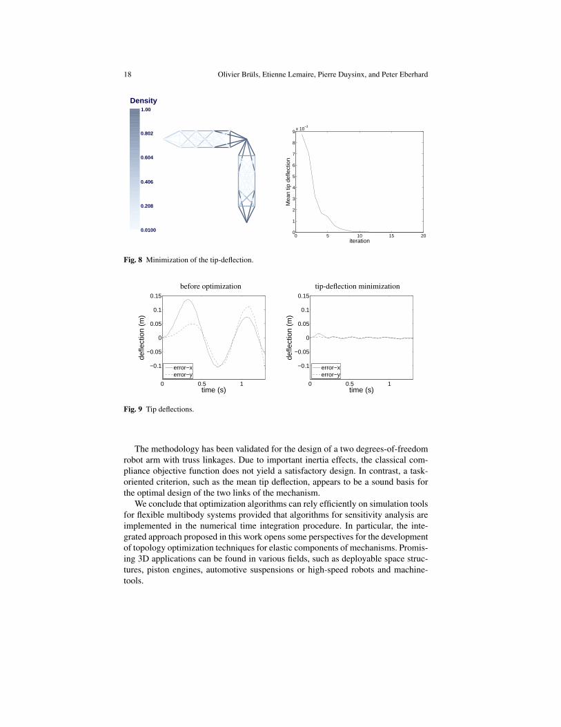
defined by Eq. (40). Actually, this formulation in terms of trajectory tracking per-formances is closer to the user expectations, which represents a clear advantage. Therigid trajectory rrigid is computed from the joint trajectory using the rigid kinematicrelations of the manipulator. The resulting optimal design, which is represented inFig. 8, is very attractive from an engineering point of view. Its superiority is furtherdemonstrated in Fig. 9, which compares the tip deflections for the various designs.One also observes that the final design is not the same for the two structural com-ponents, which makes sense since they are subject to different load conditions. Thisagain motivates the interest in the integrated optimization approach proposed inthis paper, which properly accounts for the dynamic loads during the motion of themultibody system.

5 Conclusions

This paper is about the optimization of flexible multibody systems based on theirdynamic response. The proposed approach involves a nonlinear finite element for-mulation, a generalized-α time integrator, a direct differentiation sensitivity analysisand an optimization algorithm.

In particular, the topology optimization of linkages included in multibody sys-tems is addressed. The material properties are described by a SIMP model and asequential convex programming optimizer is used. The developments have beenimplemented in the OOFELIE simulation package, which is coupled with the CON-LIN optimizer.

18 Olivier Bruls, Etienne Lemaire, Pierre Duysinx, and Peter Eberhard

1.00

0.802

0.604

0.406

0.208

0.0100

Density1.00

0.802

0.604

0.406

0.208

0.0100

Density

0 5 10 15 200

1

2

3

4

5

6

7

8

9x 10

−3

iteration

Mea

n tip

def

lect

ion

Fig. 8 Minimization of the tip-deflection.

before optimization tip-deflection minimization

0 0.5 1

−0.1

−0.05

0

0.05

0.1

0.15

time (s)

defle

ctio

n (m

)

error−xerror−y

0 0.5 1

−0.1

−0.05

0

0.05

0.1

0.15

time (s)

defle

ctio

n (m

)

error−xerror−y

Fig. 9 Tip deflections.

The methodology has been validated for the design of a two degrees-of-freedomrobot arm with truss linkages. Due to important inertia effects, the classical com-pliance objective function does not yield a satisfactory design. In contrast, a task-oriented criterion, such as the mean tip deflection, appears to be a sound basis forthe optimal design of the two links of the mechanism.

We conclude that optimization algorithms can rely efficiently on simulation toolsfor flexible multibody systems provided that algorithms for sensitivity analysis areimplemented in the numerical time integration procedure. In particular, the inte-grated approach proposed in this work opens some perspectives for the developmentof topology optimization techniques for elastic components of mechanisms. Promis-ing 3D applications can be found in various fields, such as deployable space struc-tures, piston engines, automotive suspensions or high-speed robots and machine-tools.

Optimization of Multibody Systems and their Structural Components 19

References

1. Achtziger W, Bendsøe M, Ben-Tal A, Zowe J (1992) Equivalent displacement based formu-lations for maximum strength truss topology design. Impact of Computing in Science andEngineering 4(4):315–345

2. Albers A, Haussler P (2005) Topology optimization of dynamic loaded parts using multibodysimulation and durability analysis. In: NAFEMS seminar ’Optimization in Structural Mechan-ics’, Wiesbaden, Germany

3. Albers A, Ottnad J, Haussler P, Minx J (2007) Structural optimization of components in con-trolled mechanical systems. In: Proceedings of the ASME 2007 IDETC/CIE Conference

4. Arnold M, Bruls O (2007) Convergence of the generalized-α scheme for constrained mechan-ical systems. Multibody System Dynamics 18(2):185–202

5. Arora J (2004) Introduction to Optimum Design, 2nd edn. Academic Press, San Diego6. Bendsøe M (1989) Optimal shape design as a material distribution problem. Structural Opti-

mization 1:193–2027. Bendsøe M, Sigmund O (2003) Topology Optimization: Theory, Methods, and Applications.

Springer Verlag, Berlin8. Bendsøe M, Ben-Tal A, Zowe J (1994) Optimization methods for truss geometry and topology

design. Structural Optimization 7(3):141–1589. Bestle D, Eberhard P (1992) Analyzing and optimizing multibody systems. Mechanics of

Structures and Machines 20:67–9210. Bestle D, Seybold J (1992) Sensitivity analysis of constrained multibody systems. Archive of

Applied Mechanics 62:181–19011. Bottasso C, Croce A, Ghezzi L, Faure P (2004) On the solution of inverse dynamics and

trajectory optimization problems for multibody systems. Multibody System Dynamics 11:1–22

12. Bruls O, Eberhard P (2008) Sensitivity analysis for dynamic mechanical systems with finiterotations. International Journal for Numerical Methods in Engineering 74(13):1897–1927

13. Bruls O, Golinval JC (2006) The generalized-α method in mechatronic applications. Journalof Applied Mathematics and Mechanics (ZAMM) 86(10):748–758

14. Bruyneel M, Duysinx P, Fleury C (2004) A family of MMA approximations for structuraloptimization. Structural and Multidisciplinary Optimization 24(4):263–276

15. Buhl T, Pedersen C, Sigmund O (2000) Stiffness design of geometrically non-linear structuresusing topology optimization. Structural and Multidisciplinary Optimization 19(2):93–104

16. Cardona A, Klapka I, Geradin M (1994) Design of a new finite element programming envi-ronment. Engineering Computations 11:365–381

17. Chung J, Hulbert G (1993) A time integration algorithm for structural dynamics with im-proved numerical dissipation: The generalized-α method. ASME Journal of Applied Mechan-ics 60:371–375

18. Collard JF, Fisette P, Duysinx P (2005) Contribution to the optimization of closed-loop multi-body systems: Application to parallel manipulators. Multibody System Dynamics 13:69–84

19. Dorn W, Gomory R, Greenberg H (1964) Automatic design of optimal structures. Journal deMecanique 3:25–52

20. Eberhard P, Bischof C (1999) Automatic differentiation of numerical integration algorithms.Mathematics of Computation 68:717–731

21. Fleron P (1964) The minimum weight of trusses. Bygningsstatiske Meddelelser 35:81–9622. Fleury C (1989) CONLIN: an efficient dual optimizer based on convex approximation con-

cepts. Structural Optimization 1(2):81–8923. Geradin M, Cardona A (2001) Flexible Multibody Dynamics: A Finite Element Approach.

John Wiley & Sons, New York24. Hansen J (2002) Synthesis of mechanisms using time-varying dimensions. Multibody System

Dynamics 7:127–14425. Herskovits J, Mappa P, Goulart E, Soares C (2005) Mathematical programming models and

algorithms for engineering design optimization. Computer Methods in Applied Mechanicsand Engineering 194(30-33):3244–3268

20 Olivier Bruls, Etienne Lemaire, Pierre Duysinx, and Peter Eberhard

26. Kang B, Park G, Arora J (2005) Optimization of flexible multibody dynamic systems usingthe equivalent static load method. AIAA Journal 43(4):846–852

27. Kawamoto A, Bendsøe M, Sigmund O (2004) Articulated mechanism design with a degree offreedom constraint. International Journal for Numerical Methods in Engineering 61(9):1520–1545

28. Kirsch U (1989) Optimal topologies of truss structures. Computer Methods in Applied Me-chanics and Engineering 72:15–28

29. Maute K, Schwarz S, Ramm E (1998) Adaptive topology optimization of elastoplastic struc-tures. Structural Optimization 15(2):81–91

30. Michell A (1904) The limit of economy of material in frame structures. Philosophical Maga-zine 8(6):589–597

31. Muller O, Haussler P, Lux R, Ilzhofer B, Albers A (1999) Automated coupling ofMDI/ADAMS and MSC.CONSTRUCT for the topology and shape optimization of flexiblemechanical systems. In: ADAMS Users Conference, Berlin, Germany

32. Nishiwaki S, Frecker M, Min S, Kikuchi N (1998) Topology optimization of compliant mech-anisms using the homogenization method. International Journal for Numerical Methods inEngineering 42(3):535–559

33. Pedersen C (2003) Topology optimization for crashworthiness of frame structures. Interna-tional Journal of Crashworthiness 8(1):29–39

34. Pedersen C, Buhl T, Sigmund O (2001) Topology synthesis of large-displacement compliantmechanisms. International Journal for Numerical Methods in Engineering 50:2683–2705

35. Pucheta M, Cardona A (2007) An automated method for type synthesis of planar link-ages based on a constrained subgraph isomorphism detection. Multibody System Dynamics18(2):233–258

36. Sedlaczek K, Eberhard P (2007) Augmented Lagrangian particle swarm optimization in mech-anism design. Journal of System Design and Dynamics 1(3):410–421

37. Sigmund O (1997) On the design of compliant mechanisms using topology optimization. Me-chanics of Structures and Machines 25:493–524

38. Svanberg K (1987) The method of moving asymptotes - a new method for structural optimiza-tion. International Journal for Numerical Methods in Engineering 24:359–373

39. Svanberg K (2002) A class of globally convergent optimization methods based on conservativeconvex separable approximations. SIAM Journal on Optimization 12(2):555–573

40. Waechter A, Biegler LT (2006) On the implementation of a primal-dual interior point fil-ter line search algorithm for large-scale nonlinear programming. Mathematical Programming106(1):25–57