An Application of the Udwadia-Kalaba Dynamic Formulation to Flexible Multibody Dynamics
22
Journal of the Franklin Institute 347 (2010) 173–194 An application of the Udwadia–Kalaba dynamic formulation to flexible multibody systems Ettore Pennestr`ı a, , Pier Paolo Valentini a , Domenico de Falco b a Universit a di Roma Tor Vergata - Roma, Italy b II Universit a di Napoli, Italy Received 15 July 2009; received in revised form 22 September 2009; accepted 2 October 2009 Abstract For the transient response analysis of a flexible slider-crank mechanism, the coordinate partitioning scheme and the Udwadia–Kalaba formulation are herein compared. The flexibility of the coupler has been modelled by means of a single Timoshenko beam element. The present analytical treatment can be viewed as an extension of the model discussed by Shabana in his textbook. & 2009 The Franklin Institute. Published by Elsevier Ltd. All rights reserved. Keywords: Multibody dynamics; Flexible multibody dynamics; Coordinate partitioning; Timoshenko beam 1. Introduction The modelling of mechanical systems taking into account the effects of distributed flexibility is required when the influence of deformation on the dynamics is important. Scientific literature offers several formalisms and analyses for systems with distributed elasticity of the links (e.g. [1–11]). The modelling of flexible linkages with sliding joints is considered in [12,13]. Linearized input–output representation of flexible multibody systems is proposed in [14]. This form of representation is particularly useful for control purposes, as demonstrated by the examples discussed in the cited reference. ARTICLE IN PRESS www.elsevier.com/locate/jfranklin 0016-0032/$32.00 & 2009 The Franklin Institute. Published by Elsevier Ltd. All rights reserved. doi:10.1016/j.jfranklin.2009.10.014 Corresponding author. E-mail address: [email protected] (E. Pennestr`ı).
Transcript of An Application of the Udwadia-Kalaba Dynamic Formulation to Flexible Multibody Dynamics
ARTICLE IN PRESS
Journal of the Franklin Institute 347 (2010) 173–194
0016-0032/$3
doi:10.1016/j
�CorrespoE-mail ad
www.elsevier.com/locate/jfranklin
An application of the Udwadia–Kalaba dynamicformulation to flexible multibody systems
Ettore Pennestrıa,�, Pier Paolo Valentinia, Domenico de Falcob
aUniversit �a di Roma Tor Vergata - Roma, ItalybII Universit �a di Napoli, Italy
Received 15 July 2009; received in revised form 22 September 2009; accepted 2 October 2009
Abstract
For the transient response analysis of a flexible slider-crank mechanism, the coordinate
partitioning scheme and the Udwadia–Kalaba formulation are herein compared. The flexibility of
the coupler has been modelled by means of a single Timoshenko beam element. The present
analytical treatment can be viewed as an extension of the model discussed by Shabana in his
textbook.
& 2009 The Franklin Institute. Published by Elsevier Ltd. All rights reserved.
Keywords: Multibody dynamics; Flexible multibody dynamics; Coordinate partitioning; Timoshenko beam
1. Introduction
The modelling of mechanical systems taking into account the effects of distributedflexibility is required when the influence of deformation on the dynamics is important.
Scientific literature offers several formalisms and analyses for systems with distributedelasticity of the links (e.g. [1–11]).
The modelling of flexible linkages with sliding joints is considered in [12,13]. Linearizedinput–output representation of flexible multibody systems is proposed in [14]. This form ofrepresentation is particularly useful for control purposes, as demonstrated by the examplesdiscussed in the cited reference.
2.00 & 2009 The Franklin Institute. Published by Elsevier Ltd. All rights reserved.
.jfranklin.2009.10.014
nding author.
dress: [email protected] (E. Pennestrı).
ARTICLE IN PRESS
Nomenclature
[_]/[€] dots denote differentiation with respect to timefuig position of point P in the deformed state of body i
fui0g position of point P in the undeformed state of body i
fuif g displacement vector of point P due to elastic deformation of body i
flig Lagrange multipliers appearing in the dynamic equation of body i
fQielg elastic forces on body i
fQieg external forces on body i
fQivg quadratic velocity forces on body i
mi mass of body i
aEI
kG‘ element lengthk shear coefficientl Lagrange multipliers[Ai] transform matrix of body i
[Cqi ] Jacobian matrix with respect to coordinates qi
[Aiy]
@
@yi
½Ai�
[Ki] body i stiffness matrix[mi] mass matrix of body i
[Si] matrix of element shape functions[Cq] Jacobian matrixfdri
cg vector of virtual displacements of forces application pointsfCg vector of constraintsfF i
eg vector of external forces on body i
fQg vector of generalized external forces acting on the mechanismfqig generalized coordinates of body i
fQieg vector of external generalized forces acting on body i
fqg vector of generalized coordinatesT
ikinetic energy of the finite element
Ui
strain energy of the finite elementri density of body i
yi angle of rotation of body i with respect to inertial coordinate systema area of the element sectionab area of the coupler sectionE Young modulusEI flexural rigidityG shear modulusg acceleration gravityIc moment of inertia of the crank with respect to center of massJi0 moment of inertia of the i body with respect to origin oi
k stiffness matrix of the Timoshenko beam elementL crank lengthLb length of the undeformed coupler
E. Pennestrı et al. / Journal of the Franklin Institute 347 (2010) 173–194174
ARTICLE IN PRESS
M mass matrix of the entire systemm mass matrix of the Timoshenko beam elementmb mass of the couplermc mass of the crankoiGx and oiGy Cartesian components of the vector joining oi, origin of local axes,
with G, center of mass of body i.Vi volume of body i
x abscissa measured along the beam axis (see Fig. 1)
E. Pennestrı et al. / Journal of the Franklin Institute 347 (2010) 173–194 175
A widely adopted flexible multibody dynamics formulation, based on the use of floatingframe of reference, has been proposed by Shabana (e.g. [15,16]).
Such formulation defines a differential-algebraic equations (DAE) system where theunknowns are the sets of rigid (qr) and flexible (qf ) coordinates and the Lagrangemultipliers l. Shabana suggests to solve the DAE system through the coordinatepartitioning scheme [17,18]. In this paper a different strategy will be adopted. In particularthe Udawdia–Kalaba formulation [19] will be tested for the dynamic analysis of a flexiblelinkage. This last formulation, deduced from the Gauss’ Principle of Least Action, doesnot require the use of Lagrange multipliers and gives explicitly the vector of accelerationsthrough a sequence of standard linear algebra operations. No previous applications of thisformulation to flexible multibody systems are known to the authors. Thus one of thepurposes of this paper is the comparison of the numerical efficiency between theUdwadia–Kalaba formulation and the coordinate partitioning scheme usually adopted inthese studies.
Our analysis will be focused on the transient response of a flexible slider-crankmechanism. As another element of novelty, the coupler is modelled with a single elementTimoshenko beam whereas the crank is rigid [20]. The first application of the Timoshenkobeam element in flexible multibody dynamics is due to Shabana and Bakr [21]. Assuming aTimoshenko beam model, all the elements of mass, Jacobian matrices and generalizedforces vectors have been deduced in analytical form. A higher number of beam elementscould have been used. Our choice to use only one beam element allows a direct comparisonbetween the symbolic analytical expressions reported by Shabana [16] and those deducedin this paper.
2. Description of the Timoshenko beam element
It is well known that as the ratio depth of the beam to the wavelength of vibrationincreases, the Euler–Bernoulli beam model tends to overestimate natural frequency. In thiscase the Timoshenko beam model, where the effects of shear deformation and rotaryinertia of the beam are included, is more appropriate.
In literature there are different Timoshenko finite element beam models. In this paper wewill adopt the one proposed by Davis et al. [22]. This section outlines the main steps for thededuction of stiffness and mass matrices.
ARTICLE IN PRESS
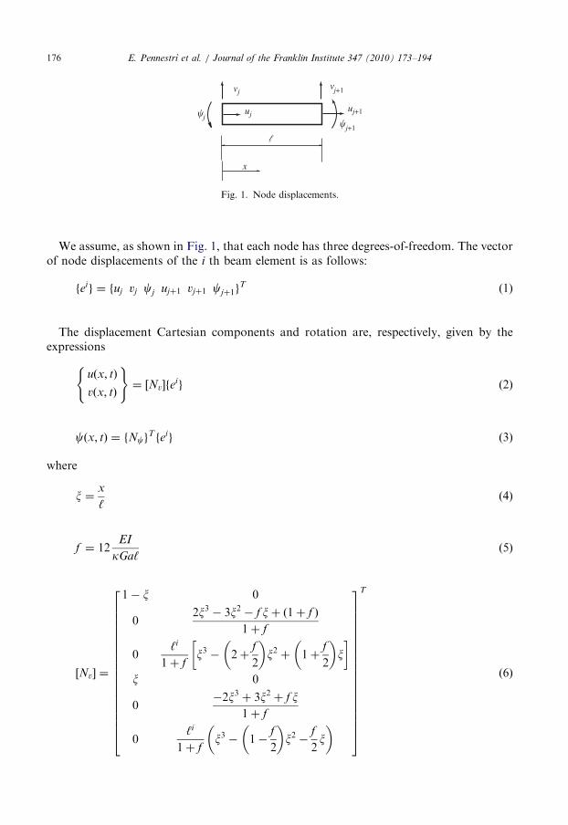
Fig. 1. Node displacements.
E. Pennestrı et al. / Journal of the Franklin Institute 347 (2010) 173–194176
We assume, as shown in Fig. 1, that each node has three degrees-of-freedom. The vectorof node displacements of the i th beam element is as follows:
feig ¼ fuj vj cj ujþ1 vjþ1 cjþ1gT ð1Þ
The displacement Cartesian components and rotation are, respectively, given by theexpressions
uðx; tÞ
vðx; tÞ
( )¼ ½Nv�fe
ig ð2Þ
cðx; tÞ ¼ fNcgT feig ð3Þ
where
x ¼x
‘ð4Þ
f ¼ 12EI
kGa‘ð5Þ
½Nv� ¼
1� x 0
02x3 � 3x2 � f xþ ð1þ f Þ
1þ f
0‘i
1þ fx3 � 2þ
f
2
� �x2 þ 1þ
f
2
� �x
� �x 0
0�2x3 þ 3x2 þ f x
1þ f
0‘i
1þ fx3 � 1�
f
2
� �x2 �
f
2x
� �
2666666666666666664
3777777777777777775
T
ð6Þ
ARTICLE IN PRESSE. Pennestrı et al. / Journal of the Franklin Institute 347 (2010) 173–194 177
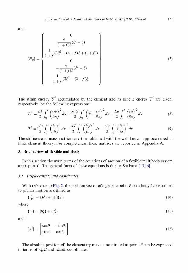
and
½Nc� ¼
06
ð1þ f Þ‘ðx2 � xÞ
1
1þ fð3x2 � ð4þ f Þxþ ð1þ f ÞÞ
0
�6
ð1þ f Þ‘ðx2 � xÞ
1
1þ fð3x2 � ð2� f ÞxÞ
8>>>>>>>>>>>>>>>><>>>>>>>>>>>>>>>>:
9>>>>>>>>>>>>>>>>=>>>>>>>>>>>>>>>>;
ð7Þ
The strain energy Uiaccumulated by the element and its kinetic energy T
iare given,
respectively, by the following expressions:
Ui¼
EI
2
Z ‘
0
@c@x
� �2
dxþkaG
2
Z ‘
0
c�@v
@x
� �2
dxþEa
2
Z ‘
0
@u
@x
� �2
dx ð8Þ
Ti¼
ria
2
Z ‘
0
@v
@t
� �2
dxþriI
2
Z ‘
0
@c@t
� �2
dxþria
2
Z ‘
0
@u
@t
� �2
dx ð9Þ
The stiffness and mass matrices are then obtained with the well known approach used infinite element theory. For completeness, these matrices are reported in Appendix A.
3. Brief review of flexible multibody
In this section the main terms of the equations of motion of a flexible multibody systemare reported. The general form of these equations is due to Shabana [15,16].
3.1. Displacements and coordinates
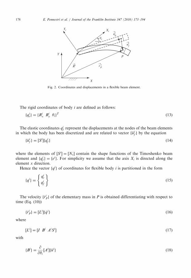
With reference to Fig. 2, the position vector of a generic point P on a body i constrainedto planar motion is defined as
friPg ¼ fR
ig þ ½Ai�fuig ð10Þ
where
fuig ¼ fui0g þ fu
if g ð11Þ
and
½Ai� ¼cosyi �sinyi
sinyi cosyi
" #ð12Þ
The absolute position of the elementary mass concentrated at point P can be expressedin terms of rigid and elastic coordinates.
ARTICLE IN PRESS
X
Y
XiYi
�i
Ri→r i→
P
ui→f
ui→0
P
Fig. 2. Coordinates and displacements in a flexible beam element.
E. Pennestrı et al. / Journal of the Franklin Institute 347 (2010) 173–194178
The rigid coordinates of body i are defined as follows:
fqirg ¼ fR
ix Ri
y yigT ð13Þ
The elastic coordinates qif represent the displacements at the nodes of the beam elements
in which the body has been discretized and are related to vector fuif g by the equation
fuif g ¼ ½S
i�fqif g ð14Þ
where the elements of ½Si� ¼ ½Nv� contain the shape functions of the Timoshenko beamelement and fqi
f g ¼ feig. For simplicity we assume that the axis Xi is directed along the
element x direction.Hence the vector fqig of coordinates for flexible body i is partitioned in the form
fqig ¼qi
r
qif
( )ð15Þ
The velocity f_riPg of the elementary mass in P is obtained differentiating with respect to
time (Eq. (10))
f_riPg ¼ ½L
i�f _qig ð16Þ
where
½Li� ¼ ½I Bi AiSi� ð17Þ
with
fBig ¼@
@yi
½Ai�fuig ð18Þ
ARTICLE IN PRESSE. Pennestrı et al. / Journal of the Franklin Institute 347 (2010) 173–194 179
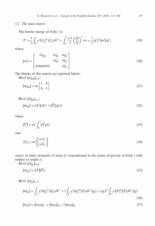
3.2. The mass matrix
The kinetic energy of body i is
Ti ¼1
2
ZVi
rif_riPg
T f_ripg dV i
þ
Z ‘
0
riI
2
@c@t
� �2
dx ¼1
2f _qigT ½mi�f _qig ð19Þ
where
½mi� ¼
miRR mi
Ry miRf
miyy mi
yf
symmetric miff
2664
3775 ð20Þ
The blocks of this matrix are reported below:Block ½mi
RR�2�2:
½miRR� ¼ mi
1 0
0 1
� �ð21Þ
Block ½miRy�2�1:
½miRy� ¼ ½A
i0 �ðfI i1g þ ½S
i�fqi
f gÞ ð22Þ
where
½Si� ¼ mi
Z 1
0
½Si� dx ð23Þ
and
fI i1g ¼ mi
oiGx
oiGy
( )ð24Þ
vector of static moments of mass mi concentrated in the center of gravity of body i withrespect to origin oi.
Block ½miRf �2�6:
½miRf � ¼ ½A
i�½Si� ð25Þ
Block ½miyy�1�1:
½miyy� ¼
ZVi
rifui0g
T fui0g dV i
þ 2
ZVi
rifui0g
T ½Si� dV ifqi
f g þ fqif g
T
ZVi
ri½Si�T ½Si� dVifqi
f g
ð26Þ
½myy� ¼ ð½myy�Þrr þ ð½myy�Þrf þ ð½myy�Þff ð27Þ
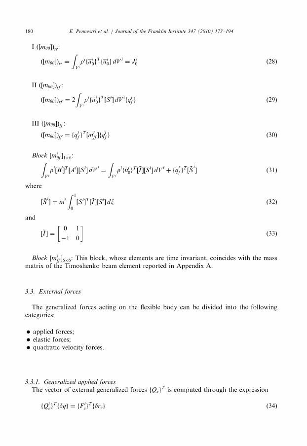
ARTICLE IN PRESSE. Pennestrı et al. / Journal of the Franklin Institute 347 (2010) 173–194180
I ð½myy�Þrr:
ð½myy�Þrr ¼
ZVi
rifui0g
T fui0g dV i
¼ Ji0 ð28Þ
II ð½myy�Þrf :
ð½myy�Þrf ¼ 2
ZV i
rifui0g
T ½Si� dV ifqi
f g ð29Þ
III ð½myy�Þff :
ð½myy�Þff ¼ fqif g
T ½miff �fq
if g ð30Þ
Block ½miyf �1�6:Z
Vi
ri½Bi�T ½Ai�½Si� dVi¼
ZV i
rifui0g
T ½~I �½Si� dViþ fqi
f gT ½ ~S
i� ð31Þ
where
½ ~Si� ¼ mi
Z 1
0
½Si�T ½ ~I �½Si� dx ð32Þ
and
½ ~I � ¼0 1
�1 0
� �ð33Þ
Block ½miff �6�6: This block, whose elements are time invariant, coincides with the mass
matrix of the Timoshenko beam element reported in Appendix A.
3.3. External forces
The generalized forces acting on the flexible body can be divided into the followingcategories:
�
applied forces; � elastic forces; � quadratic velocity forces.3.3.1. Generalized applied forces
The vector of external generalized forces fQegT is computed through the expression
fQieg
T fdqg ¼ fFieg
T fdrcg ð34Þ
ARTICLE IN PRESSE. Pennestrı et al. / Journal of the Franklin Institute 347 (2010) 173–194 181
Since
fdriPg ¼ ½I Bi AiS
i�
dRi
dyi
dqif
8><>:
9>=>; ð35Þ
if we let
fQieg ¼
QieR
Qiey
Qief
8><>:
9>=>; ð36Þ
then
fQieRg ¼ fF
ieg ð37aÞ
fQieyg
T ¼ fF ieg
T fBig ð37bÞ
fQief g
T ¼ fF ieg
T ½Ai�½Si� ð37cÞ
3.3.2. Generalized elastic forces
This type of forces follows from the strain energy accumulated within the body.In our case these forces are denoted by
fQielg ¼ �½K
i�fqg ð38Þ
where
½Ki� ¼0 0
0 k
� �ð39Þ
is the body i stiffness matrix. The block k, reported in Appendix A, coincides with thestiffness matrix of the Timoshenko beam element.
3.3.3. Generalized quadratic velocity forces
The presence of these forces is due to the time variance of the mass matrix. In particularthe vector fQi
vg contains both centrifugal and Coriolis forces acting on body element i. Itsgeneral expression is
fQivg ¼ �½ _m
i�f _qig þ1
2
@
@fqigðf _qigT ½mi�f _qigÞ
� �ð40Þ
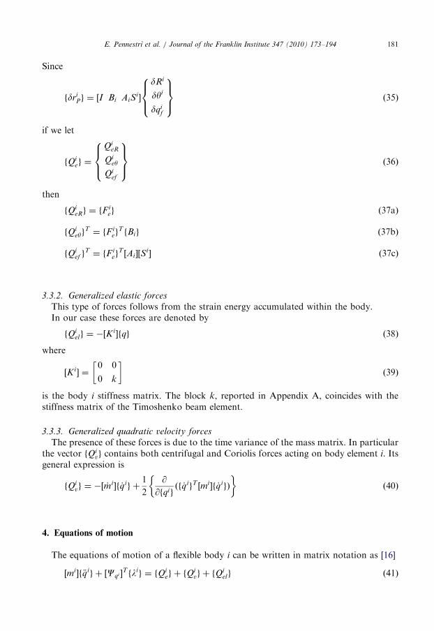
4. Equations of motion
The equations of motion of a flexible body i can be written in matrix notation as [16]
½mi�f €qig þ ½Cqi �T flig ¼ fQi
eg þ fQivg þ fQ
ielg ð41Þ
ARTICLE IN PRESSE. Pennestrı et al. / Journal of the Franklin Institute 347 (2010) 173–194182
In the remaining part of the section, the general expressions of the terms of (41) will bereported for completeness. These terms will be then particularized for the case of a slider-crank coupler.
5. The flexible slider-crank
In our model the slider crank is composed of three bodies: the crank, the coupler and theframe (see Fig. 3). The crank will be considered rigid whereas the coupler is modelled as asingle Timoshenko beam element. This in full analogy with the analysis based on theEuler–Bernoulli beam element discussed by Shabana [16].The coupler and the frame are connected by means of a pin-in-the-slot kinematic pair.The rigid coordinates are chosen according to the method of constraint equations
presented in several references (e.g. [16,18,23]).In this section will be deduced explicitly the terms involved in the DAE system
M CTq
Cq 0
" #€q
l
� �¼
Q
g
( )ð42Þ
where
fgg ¼ �ð½Cq�f _qgÞqf _qg � 2½Cqt�f _qg � fCttg ð43Þ
5.1. Kinematic constraint equations
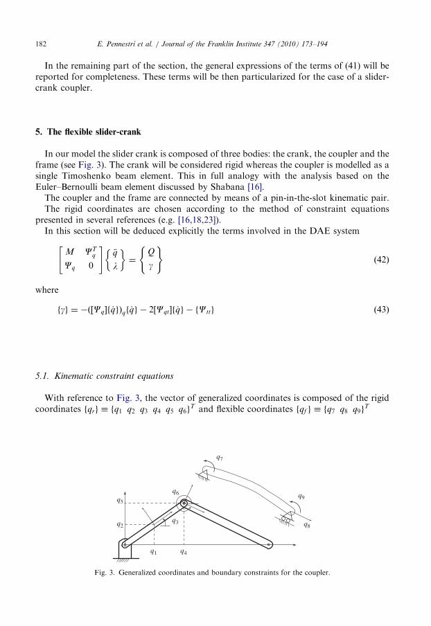
With reference to Fig. 3, the vector of generalized coordinates is composed of the rigidcoordinates fqrg � fq1 q2 q3 q4 q5 q6g
T and flexible coordinates fqf g � fq7 q8 q9gT
q1
q2q3
q4
q5
q6
q7
q8
q9
Fig. 3. Generalized coordinates and boundary constraints for the coupler.
ARTICLE IN PRESSE. Pennestrı et al. / Journal of the Franklin Institute 347 (2010) 173–194 183
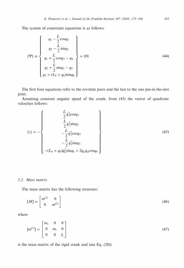
The system of constraint equations is as follows:
fCg �
q1 �L
2cosq3
q2 �L
2sinq3
q1 þL
2cosq3 � q4
q2 þL
2sinq3 � q5
q5 þ ðLb þ q8Þsinq6
8>>>>>>>>>>>><>>>>>>>>>>>>:
9>>>>>>>>>>>>=>>>>>>>>>>>>;
¼ f0g ð44Þ
The first four equations refer to the revolute pairs and the last to the one pin-in-the-slotjoint.
Assuming constant angular speed of the crank, from (43) the vector of quadraticvelocities follows:
fgg ¼ �
L
2_q23cosq3
L
2_q23sinq3
�L
2_q23cosq3
�L
2_q23sinq3
�ðLb þ q8Þ _q26sinq6 þ 2 _q6 _q8cosq6
8>>>>>>>>>>>>><>>>>>>>>>>>>>:
9>>>>>>>>>>>>>=>>>>>>>>>>>>>;
ð45Þ
5.2. Mass matrix
The mass matrix has the following structure:
½M� ¼mð1Þ 0
0 mð2Þ
" #ð46Þ
where
½mð1Þ� ¼
mc 0 0
0 mc 0
0 0 Ic
264
375 ð47Þ
is the mass matrix of the rigid crank and (see Eq. (20))
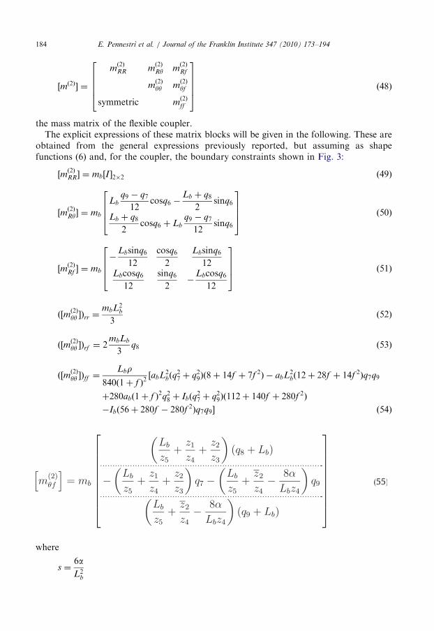
ARTICLE IN PRESSE. Pennestrı et al. / Journal of the Franklin Institute 347 (2010) 173–194184
½mð2Þ� ¼
mð2ÞRR m
ð2ÞRy m
ð2ÞRf
mð2Þyy m
ð2Þyf
symmetric mð2Þff
26664
37775 ð48Þ
the mass matrix of the flexible coupler.The explicit expressions of these matrix blocks will be given in the following. These are
obtained from the general expressions previously reported, but assuming as shapefunctions (6) and, for the coupler, the boundary constraints shown in Fig. 3:
½mð2ÞRR� ¼ mb½I �2�2 ð49Þ
½mð2ÞRy� ¼ mb
Lb
q9 � q7
12cosq6 �
Lb þ q8
2sinq6
Lb þ q8
2cosq6 þ Lb
q9 � q7
12sinq6
2664
3775 ð50Þ
½mð2ÞRf � ¼ mb
�Lbsinq6
12
cosq6
2
Lbsinq6
12Lbcosq6
12
sinq6
2�
Lbcosq6
12
2664
3775 ð51Þ
ð½mð2Þyy �Þrr ¼
mbL2b
3ð52Þ
ð½mð2Þyy �Þrf ¼ 2
mbLb
3q8 ð53Þ
ð½mð2Þyy �Þff ¼
Lbr
840ð1þ f Þ2½abL2
bðq27 þ q2
9Þð8þ 14f þ 7f 2Þ � abL2bð12þ 28f þ 14f 2Þq7q9
þ280abð1þ f Þ2q28 þ Ibðq
27 þ q2
9Þð112þ 140f þ 280f 2Þ
�Ibð56þ 280f � 280f 2Þq7q9� ð54Þ
where
s ¼6aL2
b
ARTICLE IN PRESSE. Pennestrı et al. / Journal of the Franklin Institute 347 (2010) 173–194 185
z1 ¼ �Lbð2þ sÞ
z2 ¼ Lbð1þ sÞ
z2 ¼ Lbðs� 1Þ
z3 ¼ 3ð1þ 2sÞ
z4 ¼ 4ð1þ 2sÞ
z5 ¼ 5ð1þ 2sÞ
From the expression of Timoshenko beam mass matrix reported in Appendix A oneobtains
½mð2Þff � ¼
mð3;3Þ symmetric
0 mð4;4Þ
mð3;6Þ 0 m6;6
264
375 ð56Þ
5.3. Elastic forces
Since the crank is rigid there is not any elastic force acting on it, therefore
fQð1Þel g ¼ f0g ð57Þ
The elastic forces acting on the coupler are computed by means of the followingexpression:
fQð2Þel g ¼ �
0 0
0 Kb
" #q4
q5
q6
q7
q8
q9
8>>>>>>>>><>>>>>>>>>:
9>>>>>>>>>=>>>>>>>>>;
ð58Þ
where
½Kb� ¼E
1þ f
ð4þ f ÞI
Lb
symmetric
0abð1þ f Þ
Lb
ð2� f ÞI
Lb
0ð4þ f ÞI
Lb
266666664
377777775
ð59Þ
is the stiffness matrix of the coupler.
ARTICLE IN PRESSE. Pennestrı et al. / Journal of the Franklin Institute 347 (2010) 173–194186
5.4. Quadratic velocity forces
The quadratic velocity vector can be splitted as follows:
fQvg ¼ fQð1ÞTv Q
ð2ÞTvR Q
ð2ÞTvy Q
ð2ÞTvf g
T ð60Þ
From (40) one obtains
fQð1Þv g ¼ f0g ð61Þ
fQð2ÞvRg ¼ mb _q
26
q8 þ Lb
2cosq6 � a11q7sinq6 þ a12q9
q8 þ Lb
2sinq6 þ a11q7cosq6 þ a12q9
8>><>>:
9>>=>>;
�mb _q6
2 _q7a11cosq6 þ _q8sinq6 þ 2 _q9a12cosq6
2 _q7a11sinq6 � _q8cosq6 þ 2 _q9a12sinq6
( )ð62Þ
where
a11 ¼Lb
1þ12aL2
b
1
4�
2þ6aL2
b
3þ
1þ6aL2
b
2
0BB@
1CCA
a12 ¼Lb
1þ12aL2
b
1
4�
1�6aL2
b
3�
3aL2
b
0BB@
1CCA
fQð2Þvy g ¼ �2 _q6 ðb11q7 þ b12q9Þ _q7 þ ðb12q7 þ b11q9Þ _q9 þ
mb
3ðq8 þ LbÞ _q8
n oð63Þ
where
b11 ¼ mbL2b
ð7f 2 þ 14f þ 8Þ
840ð1þ f 2Þþ ILbr
ð10f 2 þ 5f þ 4Þ
30ð1þ f 2Þ
b12 ¼ �mbL2b
ð7f 2 þ 14f þ 6Þ
840ð1þ f 2Þþ ILbr
ð5f 2 � 5f þ 1Þ
30ð1þ f 2Þ
fQð2Þvf g ¼ 2mb _q
26
c11 þ c12
c21 þ c22
c31 þ c32
8><>:
9>=>; ð64Þ
where
c11 ¼mb _q
26L
2b
840ð1þ f 2Þ½ð8þ 14f þ 7f 2Þq7 � ð6þ 14f þ 7f 2Þq9�
ARTICLE IN PRESSE. Pennestrı et al. / Journal of the Franklin Institute 347 (2010) 173–194 187
c21 ¼mb _q
26
3ðq8 þ LbÞ
c32 ¼mb _q
26L
2b
840ð1þ f 2Þ½ð8þ 14f þ 7f 2Þq9 � ð6þ 14f þ 7f 2Þq7�
c12 ¼2mb _q6
1þ12aL2
b
� � Lb
21þ
3aL2
b
� ��
Lb
5�
Lb
31þ
6aL2
b
� �� �_q8
c32 ¼2mb _q6
1þ12aL2
b
� � Lb
41�
6aL2
b
� ��
Lb
5þ
2aLb
� �_q8
c22 ¼ �c12 _q7 þ c32 _q9
_q8
5.5. External forces
The vector of external generalized forces is
fQg ¼
Qð1Þe
Qð2ÞeR þQ
ð2ÞvR
Qð2Þey þQ
ð2Þvy
Qð2Þef þQ
ð2Þvf
8>>>>><>>>>>:
9>>>>>=>>>>>;þ
Qð1Þel
Qð2Þel
8<:
9=; ð65Þ
where
fQð1Þe g ¼ f0 �mcg 0gT ð66Þ
fQð2ÞeRg ¼ f0 �mbggT ð67Þ
fQð2Þey g ¼ �
1
2mbgðLb þ q8Þcosq6 þ
mbgLb
1
8þ
3
2
aL2
b
� �
1þ12aL2
b
sinq6ðq7 � q9Þ ð68Þ
ARTICLE IN PRESSE. Pennestrı et al. / Journal of the Franklin Institute 347 (2010) 173–194188
fQð2Þef g ¼
�
mbgLb
1
8þ
3
2
aL2
b
� �
1þ12aL2
b
cosq6
�1
2mbgsinq6
mbgLb
1
8þ
3
2
aL2
b
� �
1þ12aL2
b
cosq6
8>>>>>>>>>>>>>>>>><>>>>>>>>>>>>>>>>>:
9>>>>>>>>>>>>>>>>>=>>>>>>>>>>>>>>>>>;
ð69Þ
6. The Udwadia–Kalaba formulation
This formulation, proposed Udwadia and Kalaba, is presented in detail in the bookauthored [19] and in a series of papers (e.g. [24–37]).Expressed the equations of dynamics according to the multibody formalism (42), the
accelerations vector at a given time can be computed by means of the following matrixexpression:
f €qg ¼ f €qf g þ ½M��1=2½D�þðfgg � ½Cq�f €qf gÞ ð70Þ
where
f €qf g ¼ ½M��1fQg ð71Þ
are the accelerations when the system is unconstrained and
½M��1 ¼ ½M��1=2½M��1=2 ð72Þ
½D� ¼ ½Cq�½M��1=2 ð73Þ
In (70) the prescribed accelerations due to rheonomic constraints cannot be expressed interms of accelerations of elastic coordinates.The Lagrange multipliers are expressed by the following formula [37]:
flg ¼ ð½Cq�½M��1½Cq�
T Þ�1ðfgg � ½Cq�f €qf gÞ ð74Þ
7. Numerical results
In this section are presented the results of the dynamic analysis of the flexible slider-crank whose coupler has been modelled with a single Timoshenko beam element.In particular a direct numerical comparison will be made with the Euler–Bernoulli’s
model discussed in the textbook of Shabana [16]. The main numerical data of this exampleare the same proposed by Meijaard [20].
�
crank length: L ¼ 0:1524m; � coupler length: Lb ¼ 0:3048m;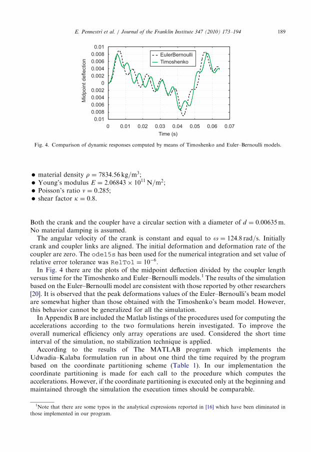
ARTICLE IN PRESS
0 0.01 0.02 0.03 0.04 0.05 0.06 0.070.01
0.0080.0060.0040.002
00.0020.0040.0060.0080.01
Time (s)
Mid
poin
t def
lect
ion
EulerBernoulliTimoshenko
Fig. 4. Comparison of dynamic responses computed by means of Timoshenko and Euler–Bernoulli models.
E. Pennestrı et al. / Journal of the Franklin Institute 347 (2010) 173–194 189
�
1
tho
material density r ¼ 7834:56 kg=m3;
� Young’s modulus E ¼ 2:06843� 1011 N=m2; � Poisson’s ratio n ¼ 0:285; � shear factor k ¼ 0:8.Both the crank and the coupler have a circular section with a diameter of d ¼ 0:00635m.No material damping is assumed.
The angular velocity of the crank is constant and equal to o ¼ 124:8 rad=s. Initiallycrank and coupler links are aligned. The initial deformation and deformation rate of thecoupler are zero. The ode15s has been used for the numerical integration and set value ofrelative error tolerance was RelTol ¼ 10�6.
In Fig. 4 there are the plots of the midpoint deflection divided by the coupler lengthversus time for the Timoshenko and Euler–Bernoulli models.1 The results of the simulationbased on the Euler–Bernoulli model are consistent with those reported by other researchers[20]. It is observed that the peak deformations values of the Euler–Bernoulli’s beam modelare somewhat higher than those obtained with the Timoshenko’s beam model. However,this behavior cannot be generalized for all the simulation.
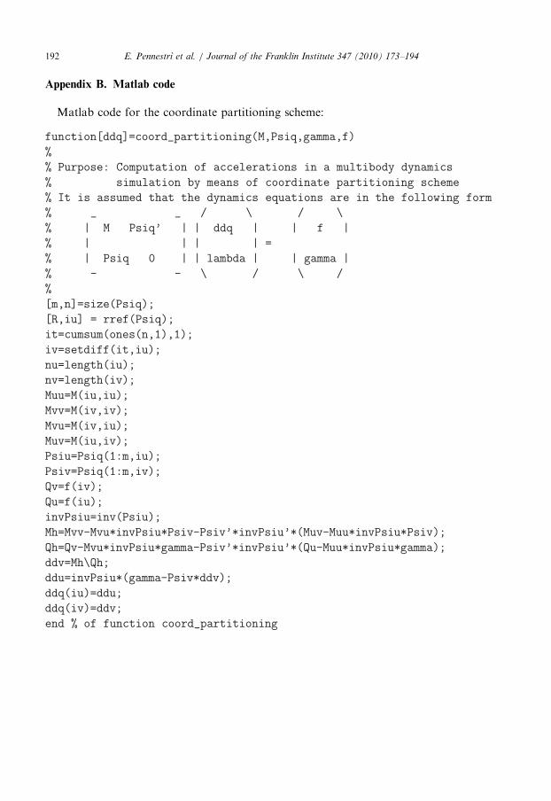
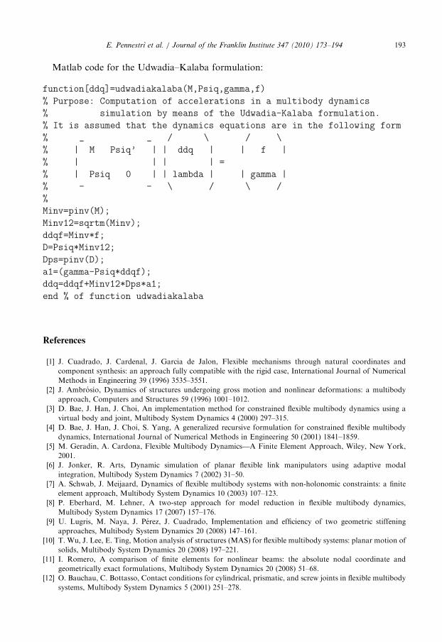
In Appendix B are included the Matlab listings of the procedures used for computing theaccelerations according to the two formulations herein investigated. To improve theoverall numerical efficiency only array operations are used. Considered the short timeinterval of the simulation, no stabilization technique is applied.
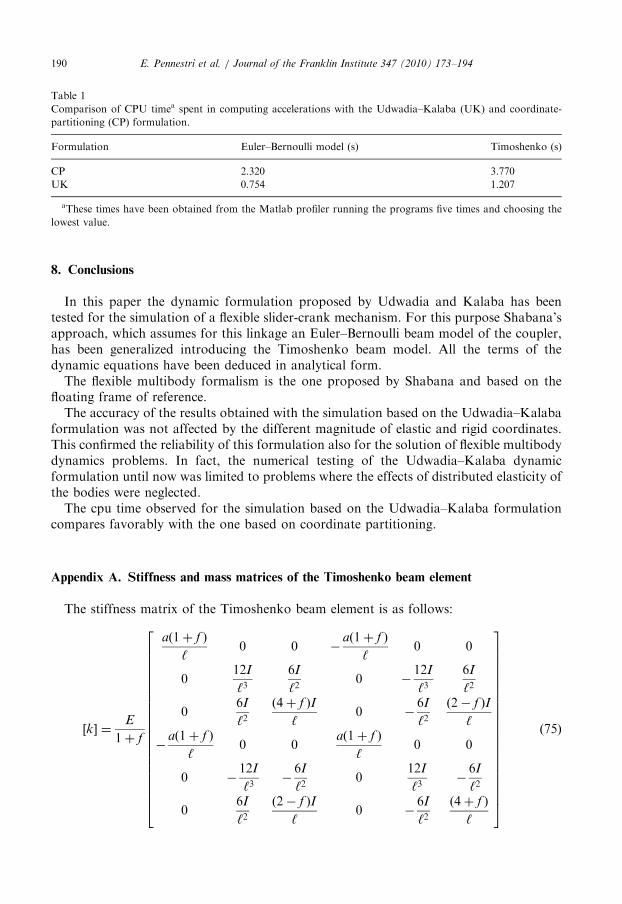
According to the results of The MATLAB program which implements theUdwadia–Kalaba formulation run in about one third the time required by the programbased on the coordinate partitioning scheme (Table 1). In our implementation thecoordinate partitioning is made for each call to the procedure which computes theaccelerations. However, if the coordinate partitioning is executed only at the beginning andmaintained through the simulation the execution times should be comparable.
Note that there are some typos in the analytical expressions reported in [16] which have been eliminated in
se implemented in our program.
ARTICLE IN PRESS
Table 1
Comparison of CPU timea spent in computing accelerations with the Udwadia–Kalaba (UK) and coordinate-
partitioning (CP) formulation.
Formulation Euler–Bernoulli model (s) Timoshenko (s)
CP 2.320 3.770
UK 0.754 1.207
aThese times have been obtained from the Matlab profiler running the programs five times and choosing the
lowest value.
E. Pennestrı et al. / Journal of the Franklin Institute 347 (2010) 173–194190
8. Conclusions
In this paper the dynamic formulation proposed by Udwadia and Kalaba has beentested for the simulation of a flexible slider-crank mechanism. For this purpose Shabana’sapproach, which assumes for this linkage an Euler–Bernoulli beam model of the coupler,has been generalized introducing the Timoshenko beam model. All the terms of thedynamic equations have been deduced in analytical form.The flexible multibody formalism is the one proposed by Shabana and based on the
floating frame of reference.The accuracy of the results obtained with the simulation based on the Udwadia–Kalaba
formulation was not affected by the different magnitude of elastic and rigid coordinates.This confirmed the reliability of this formulation also for the solution of flexible multibodydynamics problems. In fact, the numerical testing of the Udwadia–Kalaba dynamicformulation until now was limited to problems where the effects of distributed elasticity ofthe bodies were neglected.The cpu time observed for the simulation based on the Udwadia–Kalaba formulation
compares favorably with the one based on coordinate partitioning.
Appendix A. Stiffness and mass matrices of the Timoshenko beam element
The stiffness matrix of the Timoshenko beam element is as follows:
½k� ¼E
1þ f
að1þ f Þ
‘0 0 �
að1þ f Þ
‘0 0
012I
‘36I
‘20 �
12I
‘36I
‘2
06I
‘2ð4þ f ÞI
‘0 �
6I
‘2ð2� f ÞI
‘
�að1þ f Þ
‘0 0
að1þ f Þ
‘0 0
0 �12I
‘3�6I
‘20
12I
‘3�6I
‘2
06I
‘2ð2� f ÞI
‘0 �
6I
‘2ð4þ f Þ
‘
266666666666666666664
377777777777777777775
ð75Þ
ARTICLE IN PRESSE. Pennestrı et al. / Journal of the Franklin Institute 347 (2010) 173–194 191
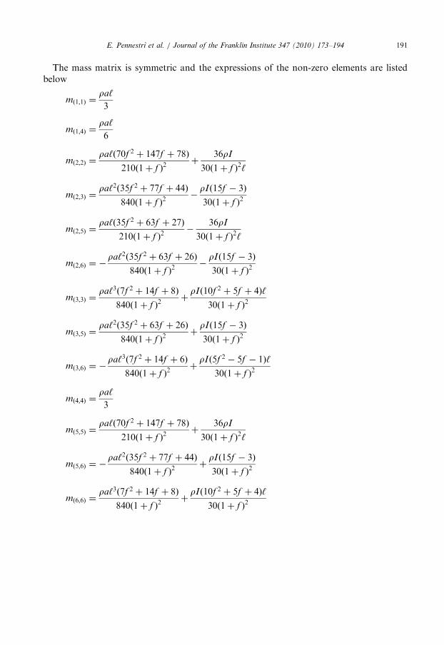
The mass matrix is symmetric and the expressions of the non-zero elements are listedbelow
mð1;1Þ ¼ra‘
3
mð1;4Þ ¼ra‘
6
mð2;2Þ ¼ra‘ð70f 2 þ 147f þ 78Þ
210ð1þ f Þ2þ
36rI
30ð1þ f Þ2‘
mð2;3Þ ¼ra‘2ð35f 2 þ 77f þ 44Þ
840ð1þ f Þ2�
rIð15f � 3Þ
30ð1þ f Þ2
mð2;5Þ ¼ra‘ð35f 2 þ 63f þ 27Þ
210ð1þ f Þ2�
36rI
30ð1þ f Þ2‘
mð2;6Þ ¼ �ra‘2ð35f 2 þ 63f þ 26Þ
840ð1þ f Þ2�
rIð15f � 3Þ
30ð1þ f Þ2
mð3;3Þ ¼ra‘3ð7f 2 þ 14f þ 8Þ
840ð1þ f Þ2þ
rIð10f 2 þ 5f þ 4Þ‘
30ð1þ f Þ2
mð3;5Þ ¼ra‘2ð35f 2 þ 63f þ 26Þ
840ð1þ f Þ2þ
rIð15f � 3Þ
30ð1þ f Þ2
mð3;6Þ ¼ �ra‘3ð7f 2 þ 14f þ 6Þ
840ð1þ f Þ2þ
rIð5f 2 � 5f � 1Þ‘
30ð1þ f Þ2
mð4;4Þ ¼ra‘
3
mð5;5Þ ¼ra‘ð70f 2 þ 147f þ 78Þ
210ð1þ f Þ2þ
36rI
30ð1þ f Þ2‘
mð5;6Þ ¼ �ra‘2ð35f 2 þ 77f þ 44Þ
840ð1þ f Þ2þ
rIð15f � 3Þ
30ð1þ f Þ2
mð6;6Þ ¼ra‘3ð7f 2 þ 14f þ 8Þ
840ð1þ f Þ2þ
rIð10f 2 þ 5f þ 4Þ‘
30ð1þ f Þ2
ARTICLE IN PRESSE. Pennestrı et al. / Journal of the Franklin Institute 347 (2010) 173–194192
Appendix B. Matlab code
Matlab code for the coordinate partitioning scheme:
ARTICLE IN PRESSE. Pennestrı et al. / Journal of the Franklin Institute 347 (2010) 173–194 193
Matlab code for the Udwadia–Kalaba formulation:
References
[1] J. Cuadrado, J. Cardenal, J. Garcia de Jalon, Flexible mechanisms through natural coordinates and
component synthesis: an approach fully compatible with the rigid case, International Journal of Numerical
Methods in Engineering 39 (1996) 3535–3551.
[2] J. Ambrosio, Dynamics of structures undergoing gross motion and nonlinear deformations: a multibody
approach, Computers and Structures 59 (1996) 1001–1012.
[3] D. Bae, J. Han, J. Choi, An implementation method for constrained flexible multibody dynamics using a
virtual body and joint, Multibody System Dynamics 4 (2000) 297–315.
[4] D. Bae, J. Han, J. Choi, S. Yang, A generalized recursive formulation for constrained flexible multibody
dynamics, International Journal of Numerical Methods in Engineering 50 (2001) 1841–1859.
[5] M. Geradin, A. Cardona, Flexible Multibody Dynamics—A Finite Element Approach, Wiley, New York,
2001.
[6] J. Jonker, R. Arts, Dynamic simulation of planar flexible link manipulators using adaptive modal
integration, Multibody System Dynamics 7 (2002) 31–50.
[7] A. Schwab, J. Meijaard, Dynamics of flexible multibody systems with non-holonomic constraints: a finite
element approach, Multibody System Dynamics 10 (2003) 107–123.
[8] P. Eberhard, M. Lehner, A two-step approach for model reduction in flexible multibody dynamics,
Multibody System Dynamics 17 (2007) 157–176.
[9] U. Lugris, M. Naya, J. P�erez, J. Cuadrado, Implementation and efficiency of two geometric stiffening
approaches, Multibody System Dynamics 20 (2008) 147–161.
[10] T. Wu, J. Lee, E. Ting, Motion analysis of structures (MAS) for flexible multibody systems: planar motion of
solids, Multibody System Dynamics 20 (2008) 197–221.
[11] I. Romero, A comparison of finite elements for nonlinear beams: the absolute nodal coordinate and
geometrically exact formulations, Multibody System Dynamics 20 (2008) 51–68.
[12] O. Bauchau, C. Bottasso, Contact conditions for cylindrical, prismatic, and screw joints in flexible multibody
systems, Multibody System Dynamics 5 (2001) 251–278.
ARTICLE IN PRESSE. Pennestrı et al. / Journal of the Franklin Institute 347 (2010) 173–194194
[13] S. Lee, T. Park, J.H. Seo, J. Yoon, K. Jun, The development of a sliding joint for very flexible multibody
dynamics using absolute nodal coordinate formulation, Multibody System Dynamics 20 (2008) 223–237.
[14] J. Jonker, R. Aarts, J. van Dijk, A linearized input–output representation of flexible multibody systems for
control synthesis, Multibody System Dynamics 21 (2009) 99–122.
[15] A. Shabana, Dynamic analysis of large scale inertia-variant flexible systems, Ph.D. Thesis, The University of
Iowa, 1982.
[16] A. Shabana, Dynamics of Multibody Systems, Cambridge University Press, Cambridge, 2005.
[17] R. Wehage, E. Haug, Generalized coordinate partitioning for dimension reduction in analysis of constrained
dynamic systems, ASME Journal of Mechanical Design 104 (1982) 247–266.
[18] E. Haug, Computer-Aided Kinematics and Dynamics of Mechanical Systems, Allyn and Bacon, 1989.
[19] F. Udwadia, R. Kalaba, Analytical Dynamics: A New Approach, Cambridge University Press, Cambridge,
1996.
[20] J. Meijaard, Validation of flexible beam elements in dynamics programs, in: M. Pereira, J. Ambrosio (Eds.),
Computer Aided Analysis of Flexible and Mechanical Systems, vol. II, NATO-Advanced Study Institute,
1993, pp. 229–245.
[21] E. Bakr, A. Shabana, Timoshenko beams and flexible multibody system dynamics, Journal of Sound and
Vibration 116 (1987) 89–107.
[22] R. Davis, R. Heshell, G. Warburton, A Timoshenko beam element, Journal of Sound and Vibration 22
(1972) 475–487.
[23] P. Nikravesh, Computer-Aided Analysis of Mechanical Systems, Prentice-Hall, Englewood Cliffs, NJ, 1988.
[24] F. Udwadia, R. Kalaba, A new perspective on constrained motion, Proceedings of the Royal Society London
(A) 439 (1992) 407–410.
[25] F. Udwadia, R. Kalaba, An alternate proof for the equation of motion for constrained mechanical systems,
Applied Mathematics and Computation 70 (1995) 339–342.
[26] F. Udwadia, R. Kalaba, Equations of motion for mechanical systems, Journal of Aerospace Engineering 9
(1996) 64–69.
[27] F. Udwadia, Equations of motion for mechanical systems: a unified approach, Journal of Non-Linear
Mechanics 31 (1996) 951–958.
[28] F. Udwadia, R. Kalaba, The explicit Gibbs–Appell equation and generalized inverse forms, Quarterly of
Applied Mathematics LVI (1998) 277–288.
[29] A. Arabyan, W. Fu, An improved formulation for constrained mechanical systems, Multibody System
Dynamics 2 (1998) 49–69.
[30] F. Udwadia, Fundamental principles of Lagrangian dynamics: mechanical systems with non-ideal,
holonomic and non-holonomic constraints, Journal of Mathematical Analysis and Applications 251
(2000) 341–355.
[31] F. Udwadia, R. Kalaba, Explicit equations of motion for mechanical systems with non ideal constraints,
ASME Journal of Applied Mechanics 68 (2001) 462–467.
[32] F. Udwadia, R. Kalaba, Analytical dynamics with constraint forces that do work in virtual displacements,
Applied Mathematics and Computation 121 (2001) 211–217.
[33] F. Udwadia, R. Kalaba, On the foundations of analytical dynamics, International Journal Non-Linear
Mechanics 37 (2002) 1079–1090.
[34] F. Udwadia, R. Kalaba, What is the general form of the explicit equations of motion for constrained
mechanical systems, ASME Journal of Applied Mechanics 69 (2002) 335–339.
[35] F. Udwadia, On constrained motion, Applied Mathematics and Computation 164 (2005) 313–320.
[36] F. Udwadia, Equations of motion for constrained mechanical systems and their control, Journal of
Optimization Theory and Applications 127 (2005) 627–638.
[37] D. de Falco, E. Pennestrı, L. Vita, Investigation of the influence of pseudoinverse matrix calculations on
multibody dynamics simulations by means of the Udwadia–Kalaba formulation, Journal of Aerospace
Engineering 22 (2009) 365–372.