A general formulation of Bead Models applied to flexible fibers and

active filaments at low Reynolds number

Blaise Delmottea,b, Eric Climenta,b, Franck Plourabouea,b,∗

aUniversity of Toulouse INPT-UPS: Institut de Mecanique des Fluides, Toulouse, France.bIMFT - CNRS, UMR 5502 1, Allee du Professeur Camille Soula, 31 400 Toulouse, France.

Abstract

This contribution provides a general framework to use Lagrange multipliers for the simula-tion of low Reynolds number fiber dynamics based on Bead Models (BM). This formalismprovides an efficient method to account for kinematic constraints. We illustrate, with severalexamples, to which extent the proposed formulation offers a flexible and versatile frameworkfor the quantitative modeling of flexible fibers deformation and rotation in shear flow, thedynamics of actuated filaments and the propulsion of active swimmers. Furthermore, a newcontact model called Gears Model is proposed and successfully tested. It avoids the use ofnumerical artifices such as repulsive forces between adjacent beads, a source of numericaldifficulties in the temporal integration of previous Bead Models.

Keywords: Bead Models, fibers dynamics, active filaments, kinematic constraints, Stokesflows

1. Introduction

The dynamics of solid-liquid suspensions is a longstanding topic of research while itcombines difficulties arising from the coupling of multi-body interactions in a viscous fluidwith possible deformations of flexible objects such as fibers. A vast literature exists on theresponse of suspensions of solid spherical or non-spherical particles due to its ubiquitousinterest in natural and industrial processes. When the objects have the ability to deformmany complications arise. The coupling between suspended particles will depend on thepositions (possibly orientations) but also on the shape of individuals, introducing intricateeffects of the history of the suspension.

When the aspect ratio of deformable objects is large, those are generally designated asfibers. Many previous investigations of fiber dynamics, have focused on the dynamics of rigidfibers or rods [1, 2]. Compared to the very large number of references related to particle

∗Corresponding author: Franck Plouraboue. Tel.: +33 5 34 32 28 80Email addresses: blaise.delmotte@imft.fr (Blaise Delmotte), eric.climent@imft.fr (Eric

Climent), franck.plouraboue@imft.fr (Franck Plouraboue )

Preprint submitted to Journal Computational Physics January 14, 2015

arX

iv:1

501.

0293

5v1

[ph

ysic

s.fl

u-dy

n] 1

3 Ja

n 20

15

suspensions, lower attention has been paid to the more complicated system of flexible fibersin a fluid.

Suspension of flexible fibers are encountered in the study of polymer dynamics [3, 4]whose rheology depends on the formation of networks and the occurrence of entanglement.The motion of fibers in a viscous fluid has a strong effect on its bulk viscosity, microstruc-ture, drainage rate, filtration ability, and flocculation properties. The dynamic responseof such complex solutions is still an open issue while time-dependent structural changes ofthe dispersed fibers can dramatically modify the overall process (such as operation units inwood pulp and paper industry, flow molding techniques of composites, water purification).Biological fibers such as DNA or actin filaments have also attracted many researches tounderstand the relation between flexibility and physiological properties [5].

Flexible fibers do not only passively respond to carrying flow gradients but can also bedynamically activated. Many of single cell micro-organisms that propel themselves in a fluidutilize a long flagellum tail connected to the cell body. Spermatozoa (and more generally one-armed swimmers) swim by propagating bending waves along their flagellum tail to generatea net translation using cyclic non-reciprocal strategy at low Reynolds number [6]. Thesenatural swimmers have been modeled by artificial swimmers (joint microbeads) actuated byan oscillating ambient electric or magnetic field which opens breakthrough technologies fordrug on-demand delivery in the human body [7].

Many numerical methods have been proposed to tackle elasto-hydrodynamic couplingbetween a fluid flow and deformable objects, i.e. the balance between viscous drag andelastic stresses. Among those, “mesh-oriented” approaches have the ambition of solving acomplete continuum mechanics description of the fluid/solid interaction, even though someapproximations are mandatory to describe those at the fluid/solid interface. Without beingall-comprehensive, one can cite immerse boundary methods (e.g. [8, 9, 10, 11]), extendedfinite elements (e.g. [12]), penalty methods [13, 14], particle-mesh Ewald methods [15],regularized Stokeslets [16, 17], Force Coupling Method [18].

In the specific context of low Reynolds number elastohydrodynamics [19], difficulties arisewhen numerically solving the dynamics of rigid objects since the time scale associated withelastic waves propagation within the solid can be similar to the viscous dissipation time-scale. In the context of self propelled objects the ratio of these time scales is called “Spermnumber”. When the Sperm number is smaller or equal to one, the object temporal responseis stiff, and requires small time steps to capture fast deformation modes. In this regime,fluid/structure interaction effects are difficult to capture. One possible way to circumventsuch difficulties is to use the knowledge of hydrodynamic interactions of simple objects inStokes flow.

This strategy is the one pursued by the Bead Model (BM) whose aim is to describea complex deformable object by the flexible assembly of simple rigid ones. Such flexibleassemblies are generally composed of beads (spheres or ellipsoids) interacting by some elasticand repulsive forces, as well as with the surrounding fluid. For long elongated structures,alternative approaches to BM are indeed possible such as slender body approximation [20,21, 22] or Resistive Force Theory [23, 24, 25].

One important advantage of BM which might explain their use among various commu-

2

nities (polymer Physics [26, 29, 31, 34], micro-swimmer modeling in bio-fluid mechanics[38, 39, 40, 43], flexible fiber in chemical engineering [46, 48, 50, 52]), relies on their para-metric versatility, their ubiquitous character and their relative easy implementation. Weprovide a deeper, comparative and critical discussion about BM in Section 2. However, wewould like to stress that the presented model is more clearly oriented toward micro-swimmermodeling than polymer dynamics.

One should also add that BM can be coupled to mesh-oriented approaches in order to pro-vide accurate description of hydrodynamic interactions among large collection of deformableobjects at moderate numerical cost [43]. Many authors only consider free drain, i.e no Hy-drodynamic Interactions (no HI), [27, 49, 48, 53] or far field interactions associated with theRotne-Prager-Yamakawa tensor [40, 36, 35, 54]. This is supported by the fact that far-fieldhydrodynamic interactions already provide accurate predictions for the dynamics of a singleflexible fiber when compared to experimental observations or numerical results. In order toillustrate the method we use, for convenience, the Rotne-Prager-Yamakawa tensor to modelhydrodynamic interactions. We wish to stress here that this is not a limitation of the pre-sented method, since the presented formulation holds for any mobility problem formulation.However, it turns out that for each configuration we tested, our model gave very good com-parisons with other predictions, including those providing more accurate description of thehydrodynamic interactions.

The paper is organized as follows. First, we give a detailed presentation of the BeadModel for the simulation of flexible fibers. In this section, we propose a general formulation ofkinematic constraints using the framework of Lagrange multipliers. This general formulationis used to present a new Bead Model, namely the Gears Model which surpasses existingmodels on numerical aspects. The second part of the paper is devoted to comparisons andvalidations of Bead Models for different configurations of flexible fibers (experiencing a flowor actuated filaments).

Finally, we conclude the paper by summarizing the achievements we obtain with ourmodel and open new perspectives to this work.

2. The Bead Model

2.1. Detailed Review of previous Bead Models

The Bead Model (BM) aims at discretizing any flexible object with interacting beads.Interactions between beads break down into three categories: hydrodynamic interactions,elastic and kinematic constraint forces. Hydrodynamics of the whole object result frommultibody hydrodynamic interactions between beads. In the context of low Reynolds num-ber, the relationship between stresses and velocities is linear. Thus, the velocity of theassembly depends linearly on the forces and torques applied on each of its elements. Elasticforces and torques are prescribed according to classical elasticity theory [55] of flexible mat-ter. Constraint forces ensure that the beads obey any imposed kinematic constraint, e.g.fixed distance between adjacent particles. All of these interactions can be treated separatelyas long as they are addressed in a consistent order. The latter is the cornerstone whichdifferentiates previous works in the literature from ours. Numerous strategies have been

3

employed to handle kinematic constraints.

[32, 40, 35, 34] and [50] used a linear spring to model the resistance to stretching andcompression without any constraint on the bead rotational motion (Fig. 1). The resultingstretching force reads:

Fs = −ks(ri,i+1 − r0i,i+1) (1)

where

• ks is the spring stiffness,

• ri,i+1 = ri+1 − ri is the distance vector between two adjacent beads (for simplicity,equations and figures will be presented for beads 1 and 2 and can easily be generalizedto beads i and i+ 1),

• r01,2 is the vector corresponding to equilibrium.

However, regarding the connectivity constraint, the spring model is somehow approxi-mate. A linear spring is prone to uncontrolled oscillations and the problem may becomeunstable. Many other authors, among which [28, 29, 30], thus use non-linear spring modelsfor a better description of polymer physics. Nevertheless, the repulsive force stiffness has animportant numerical cost in time-stepping as will be discussed in section 2.6.3. Furthermore,unconstrained bead rotational motion leads to spurious hydrodynamic interactions and thuslimits the range of applications for these BM.

Alternatively, [49, 48, 53, 47] and [46] constrained the motion of the beads such thatthe contact point for each pair ci remains the same. While more representative of a flexibleobject, this approach exhibits two main drawbacks:

1. a gap between beads is necessary to allow the object to bend (see Fig. 2),

2. it requires an additional center to center repulsive force, and thus more tuning numer-ical parameters to prevent overlapping between adjacent beads.

Consider two adjacent beads, with radius a, linked by a hinge c1 (typically called balland socket joint). The gap εg defines the distance between the sphere surfaces and the joint(see Fig. 3). Denote pi the vector attached to bead i pointing towards the next joint, i.e.the contact point ci.

The connectivity between two contiguous bodies writes:

[r1 + (a+ εg)p1]− [r2 − (a+ εg)p2] = 0 (2)

and its time derivative

[r1 − (a+ εg)p1 × ω1]− [r2 + (a+ εg)p2 × ω2] = 0. (3)

ri and ωi are the translational and rotational velocities of bead i. The constraint forces andtorques associated to (3) are obtained either by solving a linear system of equations involv-ing beads velocities [53], or by inserting (3) into the equations of motion when neglecting

4

Figure 1: Spring model: linear spring to keep constant the inter-particle distance.

Figure 2: Joint Model: overlapping due to bending if no gap between beads.

Figure 3: Joint Model: c1 is separated by a gap εg from the beads.

Figure 4: Gears Model: contact velocity must be the same for each bead (no-slip condition).

5

hydrodynamic interactions [49, 48].The gap width 2εg controls the maximum curvature κJmax allowed without overlapping. Fromthe sine rule, one can derived the simple equation relating εg and κJmax

κJmax =

√1−

(a

a+εg

)2

a(4)

Once aware of these limitations, the gap εg, range and strength of the repulsive force shouldbe prescribed depending on the problem to be addressed.[56] and [43] proposed a more sophisticated Joint Model than those hitherto cited, using afull description of the links dynamics along the curvilinear abscissa. They derived a subtleconstraint formulation which ensures that the tangent vector to the centerline is continuousand that the length of links remains constant. These two works are worth mentioning sincethey avoid an empirical tuning of repulsive forces. Yet, [56] computed the constraint forcesand torques with an iterative penalty scheme instead of using an explicit formulation.

Finally, it is worth mentioning that the bead model proposed in [31] circumvents theinextensibility difficulty by imposing constraints on the relative velocities of each successivesegments, so that their relative distance is kept constant. Using bending potential, [31]permit overlap between beads with restoring torque (cf. Fig. 2). A Lagrangian multiplierformulation of tensile forces is also used in [57], which is equivalent to a prescribed equaldistance between successive beads. Again, inextensibility condition does not prevent beadoverlapping due to bending in this formulation. The computation of contact forces whichis proposed in the following section 2.2 generalizes the Lagrangian multiplier formulationof [31] to generalized forces. Using more complex constraints involving both translationaland angular velocities, we show that it is possible to accommodate both non-overlappingand inextensibility conditions without additional repulsive forces (using the rolling no-slipcontact with the gears model detailed in 2.3). This proposed general formulation is also wellsuited for any type of kinematic boundary conditions as illustrated in Section 3.4.

2.2. Generalized forces, virtual work principle and Lagrange multipliers

The model and formalism proposed in this article rely on earlier work in Analytical Me-chanics and Robotics [58, 59]. The concept of generalized coordinates and constraints whichhas proven to be very useful in these contexts is described here. Generalized coordinatesrefer to a set of parameters which uniquely describes the configuration of the system relativeto some reference parameters (positions, angles,...). For describing objects of complex shape,let us consider the position ri of each bead i ∈ 1, Nb with associated orientation vector piwhich is defined by three Euler angles p ≡ (θ, φ, ψ). In the following, any collection of vectorpopulation (r1, ..ri, ..rNb

) ≡ R will be capitalized, so that R is a vector in R3Nb . Hence thecollection of orientation vectors pi will be denoted P, which is a vector of length 3Nb, thecollection of velocities dri

dt= ri = vi, will be denoted V, the collection of angular velocity

pi ≡ ωi will be Ω, the collection of forces fi, F, the collection of torques γi, Γ. All V, Ω, Fand Γ are vectors in R3Nb .

6

Let us then define some generalized coordinate qi for each bead, which is defined by qi ≡(ri,pi) ≡ r1,i, r2,i, r3,i, θi, φi, ψi so that the collection of generalized positions (q1, ..qi, ..qNb

) ≡Q is a vector in R6Nb . Generalized velocities are then defined by vectors qi ≡ (vi,ωi) withassociated generalized collection of velocities Q.

Articulated systems are generically submitted to constraints which are either holonomic,non-holonomic or both [33]. Holonomic constraints do not depend on any kinematic param-eter (i.e any translational or angular velocity) whereas non-holonomic constraints do.

In the following we consider non-holonomic linear kinematic constraints associated withgeneralized velocities of the form [60]

J Q + B = 0, (5)

such that J is a 6Nb×Nc matrix and B is a vector of Nc components. Nc is the number ofconstraints acting on the Nb beads. B and J might depend (even non-linearly) on time t

and generalized positions Q, but do not depend on any velocity of vector Q, so that relation(5) is linear in Q. In subsequent sections, we provide specific examples for which this classof constraints are useful. Here we describe, following [60, 58] how such constraints can behandled thanks to some generalized force that can be defined from Lagrange multipliers. Theidea formulated to include constraints in the dynamics of articulated systems is to searchadditional forces which could permit to satisfy these constraints. First, one must rely ongeneralized forces fi ≡ (fi,γi) which include forces and torques acting on each bead, whosecollection (f1, fi, ..fNb

) is denoted F. Generalized forces are defined such that the total workvariation δW is the scalar product between them and the generalized coordinates variationsδQ

δW = F · δQ = F · δR + Γ · δP, (6)

so that, on the right hand side of (6) one also gets the translational and the rotationalcomponents of the work. Then, the idea of virtual work principle is to search some virtualdisplacement δQ that will generate no work, so that

F · δQ = 0. (7)

At the same time, by rewriting (5) in differential form

J dQ + Bdt = 0, (8)

admissible virtual displacements, i.e those satisfying constraints (8), should satisfy

J δQ = 0. (9)

Combining the Nc constraints (9) with (7) is possible using any linear combination of theseconstraints. Such linear combination involves Nc parameters, the so-called Lagrange multi-pliers which are the components of a vector λ in RNc . Then from the difference between (7)and the Nc linear combination of (9) one gets

(F − λ ·J ) · δQ = 0. (10)

7

Prescribing an adequate constraint force

Fc = λ ·J , (11)

permits to satisfy the required equality for any virtual displacement. Hence, the con-straints can be handled by forcing the dynamics with additional forces, the amplitude ofwhich are given by Lagrange multipliers, yet to be found. Note also, that this first result im-plies that both translational forces and rotational torques associated with the Nc constraintsare both associated with the same Lagrange multipliers.

This formalism is particularly suitable for low Reynolds number flows for which trans-lational and angular velocities are linearly related to forces and torques acting on beads bythe mobility matrix M (

VΩ

)= M

(FΓ

)+

(V∞

Ω∞

)+ C : E∞. (12)

V∞ =(v∞1 , ...,v

∞Nb

)and Ω∞ =

(ω∞1 , ...,ω

∞Nb

)correspond to the ambient flow evaluated at

the centers of mass ri. E∞ is the rate of strain 3 × 3 tensor of the ambient flow. C is athird rank tensor called the shear disturbance tensor, it relates the particles velocities androtations to E∞ [54]. Matrix M (and tensor C) can also be re-organized into a generalizedmobility matrix M (generalized tensor C resp.) in order to define the linear relation betweenthe previously defined generalized velocity and generalized force

Q = MF + V ∞ + C : E∞, (13)

where V ∞ =(v∞1 ,ω

∞1 , ...,v

∞Nb,ω∞Nb

). The explicit correspondence between the classical ma-

trix M and the hereby proposed generalized coordinate formulation M is given in AppendixA. Hence, as opposed to the Euler-Lagrange formalism of classical mechanics, the dynam-ics of low Reynolds number flows does not involve any inertial contribution, and provide asimple linear relationship between forces and motion. In this framework, it is then easy tohandle constraints with generalized forces, because the total force will be the sum of theknown hydrodynamic forces Fh, elastic forces Fe, inner forces associated to active fibers Faand the hereby discussed and yet unknown contact forces Fc to verify kinematic constraints

F = F′ + Fc, with (14)

F′ = Fh + Fe + Fa. (15)

Hence, if one is able to compute the Lagrange multipliers λ, the contact forces will providethe total force by linear superposition (14), which gives the generalized velocities with (13).Now, let us show how to compute the Lagrange multiplier vector. Since the generalizedforce is decomposed into known forces F′ and unknown contact forces Fc = λ ·J , relations(14) and (13) can be pooled together yielding

MFc = MλJ = Q−MF′ − V ∞ − C : E∞. (16)

8

So that, using (5),

J MJ Tλ = −B−J (MF′ + V ∞ + C : E∞) , (17)

one gets a simple linear system to solve for finding λ, where J T stands for the transpositionof matrix J .

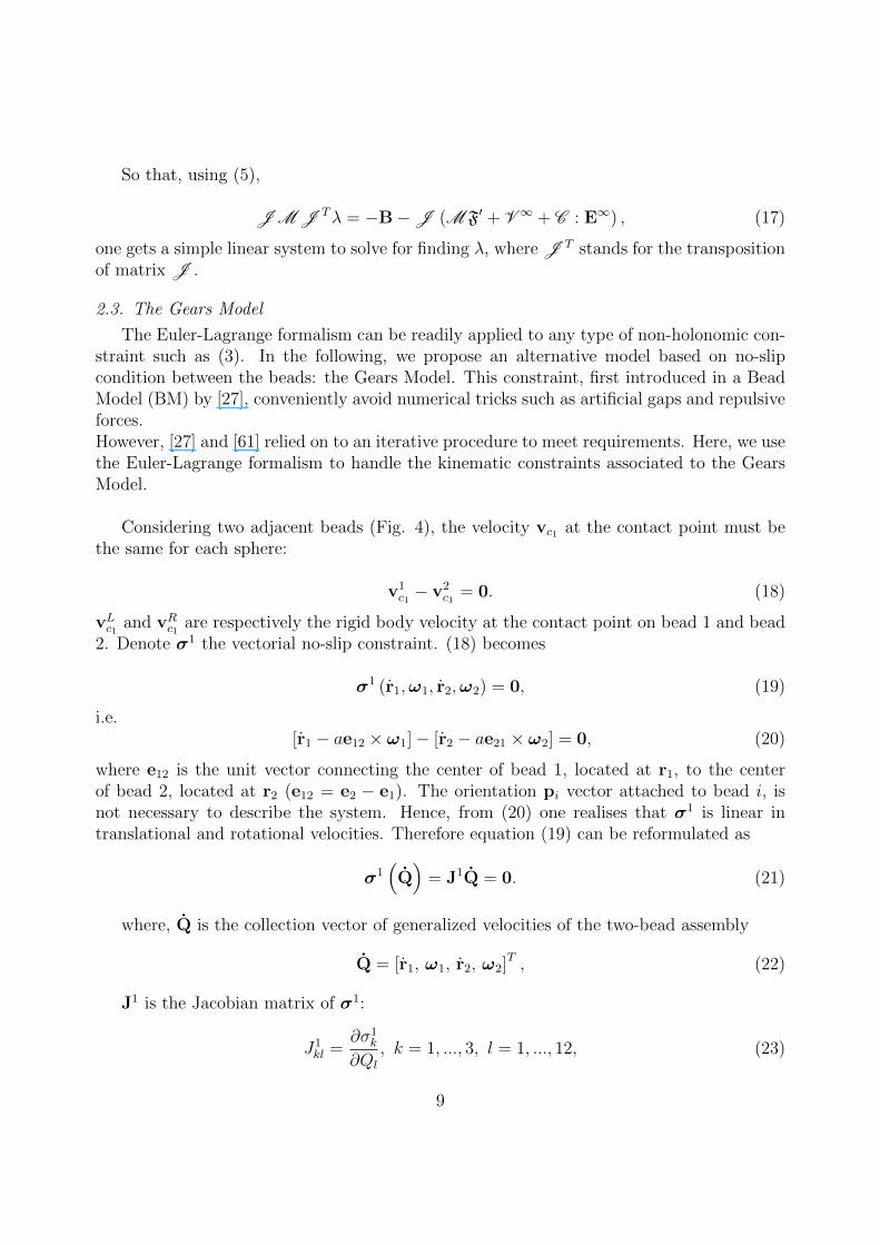
2.3. The Gears Model

The Euler-Lagrange formalism can be readily applied to any type of non-holonomic con-straint such as (3). In the following, we propose an alternative model based on no-slipcondition between the beads: the Gears Model. This constraint, first introduced in a BeadModel (BM) by [27], conveniently avoid numerical tricks such as artificial gaps and repulsiveforces.However, [27] and [61] relied on to an iterative procedure to meet requirements. Here, we usethe Euler-Lagrange formalism to handle the kinematic constraints associated to the GearsModel.

Considering two adjacent beads (Fig. 4), the velocity vc1 at the contact point must bethe same for each sphere:

v1c1− v2

c1= 0. (18)

vLc1 and vRc1 are respectively the rigid body velocity at the contact point on bead 1 and bead2. Denote σ1 the vectorial no-slip constraint. (18) becomes

σ1 (r1,ω1, r2,ω2) = 0, (19)

i.e.[r1 − ae12 × ω1]− [r2 − ae21 × ω2] = 0, (20)

where e12 is the unit vector connecting the center of bead 1, located at r1, to the centerof bead 2, located at r2 (e12 = e2 − e1). The orientation pi vector attached to bead i, isnot necessary to describe the system. Hence, from (20) one realises that σ1 is linear intranslational and rotational velocities. Therefore equation (19) can be reformulated as

σ1(Q)

= J1Q = 0. (21)

where, Q is the collection vector of generalized velocities of the two-bead assembly

Q = [r1, ω1, r2, ω2]T , (22)

J1 is the Jacobian matrix of σ1:

J1kl =

∂σ1k

∂Ql

, k = 1, ..., 3, l = 1, ..., 12, (23)

9

J1 =[

J11 J1

2

]=

[I3 −ae×12 −I3 ae×21

],

(24)

and

e× =

0 −e3 e2

e3 0 −e1

−e2 e1 0

. (25)

For an assembly of Nb beads, Nb − 1 no-slip vectorial constraints must be satisfied. TheGears Model (GM) total Jacobian matrix J GM is block bi-diagonal and reads

J GM =

J1

1 J12

J22 J2

3. . . . . .

JNb−1Nb−1 JNb−1

Nb

(26)

where Jαβ is the 3× 6 Jacobian matrix of the vectorial constraint α for the bead β.The kinematic constraints for the whole assembly then read

J GMQ = 0. (27)

The associated generalized forces Fc are obtained following Section 2.2.

2.4. Elastic forces and torques

We are considering elastohydrodynamics of homogeneous flexible and inextensible fibers.These objects experience bending torques and elastic forces to recover their equilibriumshape. Bending moments derivation and discretization are provided. Then, the role ofbending moments and constraint forces is addressed in the force and torque balance for theassembly.

2.4.1. Bending moments

The bending moment of an elastic beam is provided by the constitutive law [55, 62]

m(s) = Kbt× dt

ds, (28)

where Kb(s) is the bending rigidity, t is the tangent vector along the beam centerlineand s is the curvilinear abscissa. Using the Frenet-Serret formula

dt

ds= κn, (29)

the bending moment writesm(s) = Kbκb, (30)

10

Figure 5: Beam discretization and bending torques computation of beads 1, 3 and 5. Re-maining torques are accordingly obtained: γb2 = m (s3) and γb4 = −m (s3).

where κ(s) defines the local curvature, n(s) and b(s) are the normal and binormal vectors ofthe Frenet-Serret frame. When the link considered is not straight at rest, with an equilibriumcurvature κeq(s), (30) is modified into

m(s) = Kb (κ− κeq) b. (31)

Here, the beam is discretized into Nb − 1 rigid rods of length l = 2a (Cf Fig. 5).Inextensible rods are made up of two bond beads and linked together by a flexible jointwith bending rigidity Kb. Bending moments are evaluated at joint locations si = (i − 1)lfor i = 2, ..., Nb − 1, where si correspond to the curvilinear abscissa of the mass center ofthe ith bead.

The bending torque on bead i is then given by

γbi = m (si+1)−m (si−1) , (32)

with m (si) = Kbκ (si) b (si). See Fig. 5 for the torque computation on a beam discretizedwith four rods.

The local curvature κ (si) is approximated using the sine rule [42]

κ(si) =1

a

√1 + ei−1,i.ei,i+1

2(33)

where ei−1,i is the unit vector connecting the center of mass of bead i−1 to the center of massof bead i. This elementary geometric law provides the radius of curvature R(si) = 1/κ(si)of the circle circumscribing neighbouring bead centers ri−1, ri and ri+1.

A more general version of the discrete curvature proposed in [63] can also be used in thecase of three dimensional motion. In that case, the curvature of the fiber is discretized as

11

in [63]

κ (si) =ei−1,i × ei,i+1

2a, (34)

where, again, ei−1,i is the unit vector connecting the center of mass of bead i − 1 to thecenter of mass of bead i. The bending moment reads

m (si) = Kbκ (si) . (35)

To include the effect of torsional twisting about the axis of the fiber, one would have tocompute the relative orientation between the frames of reference attached to the beadsusing Euler angles [56] (see Section 2.2) or unit quaternions as in [53]. This would providethe rate of change of the twist angle along the fiber centerline and thus the twisting torqueacting on each bead. In the following, only bending effects are considered.

2.4.2. Force and moment acting on each bead

The Gears Model proposed in this paper does not need to consider gaps to allow bending.Fc also ensures the connectivity condition and circumvent the use of repulsive forces asdistances between adjacent bead surfaces remain constant. More specifically, the tangentialcomponents of the force Fc, which is only one part of the generalized force Fc, acts as tensileforce.

For each bead i, contact forces applied from bead i to bead i + 1 at contact point cibetween bead i and i+ 1 (Figure 4 for two beads) is denoted fci . From Newton third law atcontact point ci, the contact force applied to bead i from bead i+ 1 is obviously −fci . Totalforce acting on bead i from contact, and hydrodynamic forces fhi reads

fi = fci−1− fci + fhi (36)

Similarly, the contact force fci at point ci produces a moment mci = ati× fci associated withlocal tangent vector ti = ei,i+1 and distance a to the neutral fiber at point ci. Total momentacting on bead i from contact points moments, elastic and hydrodynamic torques are then

γi = mci−1−mci + γbi + γhi . (37)

The contribution of contact force and contact moment acting on bead i exactly equalsthe contribution of the generalized contact force. Indeed, using the kinematic constraintsJacobian (26) in (11), and computing the force and torque contributions, one exactly recoversthe first and the second contributions of the right-hand-side of (36) and (37). In AppendixB, we also show that this model is consistent with classical formulation for slender bodyforce and moment balance when the bead radius tends to zero.

2.5. Hydrodynamic coupling

Moving objects (rigid or flexible fibers) in a viscous fluid experience hydrodynamic forc-ing. The interactions are mediated by the fluid flow perturbations which can alter the motion

12

and the deformation of the fibers in a moderately concentrated suspension. The existenceof hydrodynamic interactions has also an effect on a single fiber dynamics while differentparts of the fiber can respond to the ambient flow but also to local flow perturbations re-lated to the fiber deformation. Resistive Force Theory (RFT) can be used to estimate thefiber response to a given flow assuming that the fiber is modeled by a large series of slenderobjects [64, 23]. Slender body theory has also been used [20, 65] to relate local balanceof drag forces with the filament forces upon the fluid resulting in a dynamical system tomodel the deformation of the fiber centerline. This model provided interesting results onthe stretch-coil transition of fibers in vortical flows.

In our beads model, the fiber is composed of spherical particles to account for the finitewidth of its cross-section. The hydrodynamic interactions are provided through the solutionof the mobility problem which relates forces, torques to the translational and rotational ve-locities of the beads. This many-body problem is non-linear in the instantaneous positionsof all particles of the system. Approximate solutions of this complex mathematical problemcan be achieved by limiting the mobility matrices to their leading order. The simplest modelis called free drain as the mobility matrix is assumed to be diagonal neglecting the HI withneighbouring spheres. Pairwise interactions are required to account for anisotropic drageffects within the beads composing the fiber. The Rotne-Prager-Yamakawa (RPY) approxi-mation is one of the most commonly used methods of including hydrodynamic interactions.This widely used approach has been recently updated by Wajnryb et al. [54] for the RPYtranslational and rotational degrees of freedom, as well as for the shear disturbance tensorC which gives the response of the particles to an external shear flow (12).

2.6. Numerical implementation

2.6.1. Integration scheme and algorithm

The kinematics of the constrained system results from the superposition of individualbead motions. Positions are obtained from the temporal integration of the equation ofmotion with a third order Adams-Bashforth scheme

dridt

= vi, (38)

where ri, vi are the position and translational velocity of bead i.The time step ∆t used to integrate (38) is fixed by the characteristic bending time [46]

∆t <µ(2a)4

Kb. (39)

where µ is the suspending fluid viscosity.The evaluation of bead interactions must follow a specific order. Elastic and active forces

can be computed in any order. Constraint forces and torques must be estimated afterwardsas they depend on F′. Then velocities and rotations are obtained from the mobility relation.And finally, bead positions are updated.

13

• Initialization: positions ri(0),

• Time Loop

1. Evaluate mobility matrix M (Q) and C : E∞ (see Section 2.5),

2. Calculate local curvatures (33) and bending torques γbi (32) to get Fe,

3. Add active forcing Fa and ambient velocity V ∞ if any,

4. Compute the Jacobian matrix associated with non-holonomic constraints J (Q),

5. Solve (17) to get the constraint forces Fc = λJ ,

6. Sum all the forcing terms F = Fe + Fa + Fc,

7. Apply mobility relation (13) to obtain the bead velocities Q,

8. Integrate (38) to get the new bead positions.

2.6.2. Implementation of the Joint Model

To provide a comprehensive comparison with previous works, we exploit the flexibilityof the Euler-Lagrange formalism to implement the Joint Model as described in [49] supple-mented with hydrodynamic interactions. The joint constraint for two neighbouring beadsreads

[ri − (a+ εg)pi × ωi]− [ri+1 + (a+ εg)pi+1 × ωi+1] = 0. (40)

Using the Euler-Lagrange formalism, (40) is reformulated with the Joint Model (JM)Jacobian matrix

J JMQ = 0, (41)

where J JM has the same structure as in (26) and

Ji =[

Ji1 Ji2]

=[

I3 −(a+ εg)p×i −I3 −(a+ εg)p

×i+1

].

(42)

Accordingly, the corresponding set of forces and torques Fc are obtained from Section2.2. As mentioned in Section 2.1, such formulation does not prevent beads from overlappingwhen bending occurs. A repulsive force Fr is added according to [46] (the force profileproposed by [49] is very stiff, thus very constraining for the time step):

Frij =

−F0 exp

(−dij + δD

d0

)eij, dij ≤ −δD,

−F0

(1

2− dij

2δD

)eij, −δD < dij ≤ δD,

0, rij > δD.

(43)

δD is an artificial surface roughness, dij is the surface to surface distance. dij < 0indicates overlapping between beads i and j. d0 is a numerical damping distance which hasto be tuned to prevent overlapping. F0 is the repulsive force scale chosen in order to avoid

14

numerical instabilities. To deal with this issue, [46] proposed to evaluate F0 from bendingand viscous stresses. A slight modification of their formula for inertialess particles yields

F0 = C16πµL (v∞ − v) + C2

√KbEb

L3, (44)

the bar denotes the average over the constitutive beads or joints where C1 and C2 areadjustable constants. Eb is the bending energy

Eb =

Nb−1∑i=1

Kb (κ(si)− κeq(si))2 , (45)

Bending moments are evaluated at the joint locations sJi = (a+εg)+(i−1)×2(a+εg), i =1, ..., Nb − 1. Joint curvature is given by

κ(sJi ) =2

a+ εg

√1 + pi.pi+1

2, (46)

Similarly to (32), bending torque on bead i is

γbi = m(sJi)−m

(sJi−1

). (47)

Bead orientation pi is integrated with a third order Adams-Bashforth scheme

dpidt

= ωi × pi. (48)

The procedure is similar to the Gears Model. pi are initialized together with the posi-tions. The repulsive force Fr is added to F′ and can be computed between step 1 and 5 ofthe aforementioned algorithm. Time integration of (48) is performed at step 8.

2.6.3. Constraints and numerical stability

At each time step, the error on kinematic constraints ε is evaluated, after application ofthe mobility relation (13), between step 7 and step 8:

εGM(t) =∥∥∥J GMQ

∥∥∥2

=

(Nb−1∑i=1

(vLci − vRci

)2

)1/2

(49)

for the Gears Model, and

εJM(t) =∥∥∥J JMQ

∥∥∥2

(50)

for the Joint Model.

To verify the robustness of both models and Lagrange formulation, a numerical study iscarried out on a stiff configuration.

15

A fiber of aspect ratio rp = 10 with bending ratio BR = 0.01 is initially aligned with a shearflow of magnitude γ = 5s−1. For this aspect ratio, Nb = 10 beads are used to model thefiber with the Gears Model.

Joint Model involves additional items to be fixed. Nb = 9 spheres are separated by a gapwidth 2εg = 0.25a. The repulsive force is activated when the surface to surface distance dijreaches the artificial surface roughness δD = 2(a+ εg)/10. The remaining coefficients are setto reduce numerical instabilities without affecting the Physics of the system: d0 = (a+εg)/4,C1 = 5 and C2 = 0.5.

Fig. 6 shows the evolution of the maximal mean deviation from the no-slip/joint con-straint εM = max

tε(t)/(Nb − 1) normalized with the maximal shear velocity γL depending

on the dimensionless time step γ∆t. First, one can observe that for both Joint and Gearsmodels, εM/γL weakly depends on γ∆t and the resulting motion of the beads complies veryprecisely with the set of constraints, within a tolerance close to unit roundoff (< 2.10−16).Secondly, Joint Model is unstable for time steps 100 times smaller than Gears Model. Theonset for numerical instability indicates that the repulsive force stiffness dominates overbending, thus dictating and restricting the time step.As a comparison, [46] matched connectivity constraints within 1% error for each fiber seg-ment. To do so, they had to use an iterative scheme reducing the time step by 1/3 eachiteration to meet requirements and limit overlapping between adjacent segments. For similarresults, a stiff configuration, such as the sheared fiber, is therefore more efficiently simulatedwith the Gears Model.Thirdly, inset of Fig. 6 shows that, for a given time step, the Gears Model constraints εM/γLare satisfied whatever the shear magnitude. Hence, (39) ensures unconditionally numericalstability as bending is the only limiting effect for the Gears Model.

Hence, the robustness of the Euler-Lagrange formalism and the numerical integration wechose provide a strong support to the Gears Model over the Joint Model.

As a final remark to this section, it is important to mention that the numerical costof the proposed method strongly depends on the choice for the mobility matrix computa-tion, as usual for bead models. If the mobility matrix is computed taking into accountfull hydrodynamic interactions with Stokesian Dynamics, most of the numerical cost willcome from its evaluation in this case. This limitation could be overcame using more sophis-ticated methods such as Accelerated Stokesian Dynamics [66] or Force Coupling Method[18]. Moreover, when considering Rotne-Prager-Yamakawa mobility matrix, its cost onlyrequires the evaluation of O ((6Nb)

2) terms. Furthermore, the main algorithmic complexityof bead models does not come from the time integration of the bead positions which onlyrequires a matrix-vector multiplication (13) at a O ((6Nb)

2) cost. Fast-multipole formulationof a Rotne-Prager-Yamakawa matrix can even provide a O (6Nb) cost for such matrix-vectormultiplication [67].

The main numerical cost indeed comes from the inversion of the contact forces problem

16

100

101

102

103

1.52

2.53

× 10-17

10-4

10-3

10-2

10-1

100

0.5

1

1.5

2× 10

-16

Figure 6: Dependence of the constraints εM/γL on the time step γ∆t, + : Gears Model, : Joint Model. Inset: εM/γL with the Gears Model for a fixed time step given by (39)

for different values of γ.

(17). It is worth noting that this linear problem isNc×Nc which is slightly different fromNb×Nb, but of the same order. Furthermore, problem (17) gives a direct, single step procedureto compute the contact forces, as opposed to previous other attemps [27, 46, 56] whichrequired iterative procedures to meet forces requirements, involving the mobility matrixinversion at each iteration. The cost for the inversion of (17) lies in-between O(N2

c ) andO(N3

c ) depending on the inversion method.

3. Validations

3.1. Jeffery Orbits of rigid fibers

Much of our current understanding of the behavior of fibers experiencing a shear flow hascome from the work of Jeffery [68] who derived the equation for the motion of an ellipsoidalparticle in Stokes flow. The same equation can be used for the motion of an axisymmetricparticle by using an equivalent ellipsoidal aspect ratio. Rigid fibers can be approximated byelongated prolate ellipsoids. An isolated fiber in simple shear flow rotates in a periodic orbitwhile the center of mass simply translates in the flow (no migration across streamlines). Theperiod T (51) is a function of the aspect ratio of the fiber and the flow shear rate while theorbit depends on the initial orientation of the object relative to the shear plane

T =2π(re + 1/re)

γ. (51)

17

5 10 15 20

20

30

40

50

60

70

80

90

100

Figure 7: Tumbling period T depending on fiber aspect ratio rp. : theoretical law (51)with re given by (53), : theoretical law (51) with re given by (52), 4 : Gears Model,5 : Joint Model.

γ is the shear rate of the carrying flow. re is the equivalent ellipsoidal aspect ratio whichis related to the fiber aspect ratio rp (length of the fiber over diameter of the cross-sectionwhich turns out to rp = Nb with Nb beads). The fiber is initially placed in the plane ofshear and is composed on Nb beads. No gaps between beads is required in the Joint Modelbecause the fiber is rigid and flexibility deformations are negligible. We have compared theresults with two relations for re: Cox [1]

re =1.24rp√

ln(rp), (52)

and Larson [69]

re = 0.7rp. (53)

This classic and simple test case has been successfully validated in [27, 49, 34]. Both theJoint and Gears models give a correct prediction of the period of Jeffery orbits (Fig. 7). Thescaled period γT of simulations remains within the two evolutions based on equations (52)and (53). We have tried to compare with the linear spring model proposed by Gauger andStark [40] (and used by Slowicka et al. [50] with a more detailed formulation of hydrodynamicinteractions). In this latter model, there is no constraint on the rotation of beads and thesimulations failed to reproduce Jeffery orbits (the fiber does not flip over the axis parallelto the flow).

18

3.2. Flexible fiber in a shear flow

The motion of flexible fibers in a shear flow is essential in paper making or compositeprocessing. Prediction and control of fiber orientations and positions are of particular in-terest in the study of flocks disintegration. Many models have been designed to predictfiber dynamics and much experimental work has been conducted. The wide variety of fiberbehaviors depends on the ratio of bending stresses over shear stress, which is quantified bya dimensionless number, the bending ratio BR [70, 53]

BR =E(ln 2re − 1.5)

µγ2r4p

(54)

E is the material Young’s Modulus and µ is the suspending fluid viscosity.In the following, we investigate the response of the Gears Model with known results onflexible fiber dynamics.

3.2.1. Effect of permanent deformation

[70, 71] analysed the motion of flexible threadlike particles in a shear flow depending onBR. They observed important drifts from the Jeffery orbits and classified them into cate-gories. Yet, the goal of this section is not to carry out an in-depth study on these phenomena.Instead, the objective is to show that our model can reproduce basic features characteristicof sheared flexible filaments. We analyze first the influence of intrinsic deformation on themotion.If a fiber is straight at rest, it will symmetrically deform in a shear flow. When aligned withthe compressive axes of the ambient rate of strain E∞, the fiber adopts the “S-shape” ob-served in Fig. 8a. When aligned with the extensional axes, tensile forces turn the rod backto its equilibrium shape. This symmetry is broken when the filament is initially slightlydeformed or has a permanent deformation at rest, i.e. a nonzero equilibrium curvatureκeq > 0 . An initial small perturbation of the shape of a straight filament aligned with flowcan induce large deformations during the orbit. This phenomenon is known as the bucklinginstability whose onset and growth are quantified with BR [72, 73]. Fig. 8b illustrates theevolution of a flexible sheared filament with BR = 0.04 and a very small intrinsic deforma-tion κeq = 1/(100L). The equilibrium dimensionless radius of curvature is 2Req/L = 200.During the tumbling motion it decreases to a minimal value of 2Rmin/L = 0.26. Bucklingthus increases by 770 times the maximal fiber curvature.

3.2.2. Maximal fiber curvature

[74] measured the radius of curvature R of sheared fiber for aspect ratios rp ranging from283 to 680. They reported on the evolution of the minimal value Rmin, i.e. the maximalcurvature κmax, with BR. [53] used the Joint Model with prolate spheroids but no hydro-dynamic interactions and compared their results with [74]. Both experimental results from[74] and simulations from [53] are accurately reproduced by the Gears Model.

Hydrodynamic interactions between fiber elements play an important role in the bendingof flexible filaments [74, 46, 50]. As mentioned in Section 2.5 the use of spheres to build

19

-0.5 0 0.5-0.6

-0.4

-0.2

0

0.2

0.4

0.6

(a)

-0.5 0 0.5 1-0.4

-0.2

0

0.2

0.4

(b)

Figure 8: Orbit of a flexible filament in a shear flow with BR = 0.04. Temporal evolutionis shown in the plane of shear flow. a) Symmetric “S-shape” of a straight filament, κeq = 0.b) Buckling of a permanently deformed rod with an intrinsic curvature κeq = 1/(100L).

any arbitrary object is well suited to compute these hydrodynamic interactions. However,modeling rigid slender bodies in a strong shear flow becomes costly when increasing the fiberaspect ratio. First, the aspect ratio of a fiber made up of Nb spheres is rp = Nb. Each timeiteration requires the computation of M and C : E∞ and the inversion of a linear system(17) corresponding to Nc relations of constraints with Nc ≥ 3 (Nb − 1). Secondly, for a givenshear rate γ and bending ratio BR, the Young’s modulus increases as r4

p. According to (39),the time step becomes very small for large E. [53] partially avoided this issue by neglectingpairwise hydrodynamic interactions (M is diagonal), and by assembling prolate spheroidsof aspect ratios re ∼ 10.

Yet, it is shown in Fig. 9a that for a fixed BR, 2Rmin/L converges asymptotically to aconstant value with rp. An asymptotic regime (relative variation less than 2%) is reachedfor rp ≥ 25. Choosing rp = 35 thus enables a valid comparison with previous results.

Our simulation results compare well with the literature data (Fig. 9b) and better matchwith to experiments than [53]. When BR ≥ 0.04, the Gears Model clearly underestimatesmeasurements for κeq = 1/(10L) and overestimates them for κeq = 0 . However, Salinasand Pittman [74] indicated that the error quantification on parameters and measurements isdifficult to estimate as the fibers were hand-drawn. Notably, drawing accuracy decreases forlarge radii of curvature, which leads to the conclusion that the hereby observed discrepancymight not be critical. They did not report the value of permanent deformation κeq for thefibers they designed, whereas, as evidenced by [71], it has a strong impact on Rmin. Anumerical study of this dependence should be conducted to compare with [71], Fig. 7.[46] used the same approach as [53] with hydrodynamic interactions to repeat numerically

20

5 10 15 20 25 30 350.1

0.2

0.3

0.4

0.5

0.6

0.7

0.8

(a)

0 0.02 0.04 0.06 0.080

0.1

0.2

0.3

0.4

0.5

(b)

Figure 9: a) Minimal radius of curvature depending on fiber length for several bendingratios. : BR = 0.01, : BR = 0.03, 5 : BR = 0.04 , 4 : BR = 0.07. b)Minimal radius of curvature along BR. : current simulations with aspect ratio rp = 35and intrinsic curvature κeq = 0 ; • : current simulations with aspect ratio rp = 35 andintrinsic curvature κeq = 1/(10L) ; simulation results from [53] with κeq = 1/(10L): ( ♦ :rp = 50, 4 : rp = 100, 5 : rp = 150, : rp = 280) ; + : experimental measurementsfrom [74], rp = 283.

21

the experiments from [74] ; but their results, though reliable, were displayed such that directcomparison with previous work is not possible.To conclude, it should be noted that, in [53], the aspect ratio does not affect 2Rmin/L for afixed BR, confirming the asymptotic behavior observed in Fig. 9a.

3.3. Settling Fiber

Consider a fiber settling under constant gravity force F⊥ = F⊥e⊥ acting perpendicularlyto its major axis. The dynamics of the system depends on three competing effects: theelastic stresses which tend to return the object to its equilibrium shape, the gravitationalacceleration which uniformly translates the object and the hydrodynamic interactions whichcreates local drag along the filament. After a transient regime, the filament reaches steadystate and settles at a constant velocity with a fixed shape (see Figs. 10a and 10b). Thissteady state depends on the elasto-gravitational number

B = F⊥L/Kb. (55)

[75, 41] and [65] examined the contribution of each competing effect by measuring the nor-mal deflection A, i.e. the distance between the uppermost and the lowermost point of thefilament along the direction of the applied force (Fig. 10b) ; and the normal friction co-efficient γ⊥/γ

0⊥ as a function of B. γ0

⊥ is the normal friction coefficient of a rigid rod. Tocompute hydrodynamic interactions [75] used Stokeslet ; [41], the Force Coupling Method(FCM) [18] ; [65], Slender Body Theory.

Similar simulations were carried out with both the Joint Model described in Section 2.6.2and the Gears Model. Fiber of length L = 68a is made out of Nb = 31 beads with gap width2εg = 0.2a for the Joint Model and Nb = 34 for the Gears Model. To avoid both overlappingand numerical instabilities with the Joint Model, the following repulsive force coefficientswere selected: d0 = (a + εg)/4, δD = (a + εg)/5, C1 = 0.01 and C2 = 0.01. No adjustableparameters are required for Gears Model.

Fig. 11 shows that our simulations agree remarkably well with previous results exceptslight differences with [65] in the linear regime B < 100. Using Slender Body Theory, [65]made the assumption of a spheroidal filament instead of a cylindrical one, with aspect ratiorp = 100, i.e. three times larger than other simulations, whence such discrepancies. Thenormal friction coefficient (Fig. 11b ), resulting from hydrodynamic interactions, perfectlymatches the value obtained by [41] with the Force Coupling Method. The FCM is known tobetter describe multibody hydrodynamic interactions. Such a result thus supports the useof the simple Rotne-Prager-Yamakawa tensor for this hydrodynamic system.

Differences between Gears and Joint Models implemented here are quantified by mea-suring the relative discrepancies on the vertical deflection A

εA =AG − AJAG

, (56)

22

-0.3 -0.2 -0.1 0 0.1 0.2 0.3-0.3

-0.2

-0.1

0

0.1

0.2

0.3

(a)

-0.3 -0.2 -0.1 0 0.1 0.2 0.3-0.3

-0.2

-0.1

0

0.1

0.2

0.3

(b)

Figure 10: Shape of settling fiber for B = 10000 in the frame moving with the center of mass(xc, zc). a) Metastable “W” shape, t = 12L/Vs. b) Steady “horseshoe” shape at t = 53L/Vs.Vs is the terminal settling velocity once steady state is reached.

and on the normal friction coefficient γ⊥/γ0⊥

εγ⊥ =

(γ⊥/γ⊥0

)G−(γ⊥/γ⊥0

)J(

γ⊥/γ⊥0)G

. (57)

Discrepancies between Joint and Gears models remain below 5% except at the thresholdof the non-linear regime (B ≈ 100) where εA reaches 15% and εγ⊥ ≈ 7.5%.

In accordance with [75], a metastable “W” shape is reached for B > 3000 (Fig. 10a)until it converges to the stable “horseshoe” state (Fig. 10b).

3.4. Actuated Filament

The goal of the following sections is to show that the model we proposed is not only validfor passive objects but also for active ones. Elastohydrodynamics also concern swimming atlow Reynolds number [6]. Many type of micro-swimmers have been studied both from theexperimental and theoretical point of view. Among them two categories are distinguished:ciliates and flagellates. Ciliates propel themselves by beating arrays of short hairs (cilia)on their surface in a synchronized way (Opalina, Volvox, Paramecia). Flagellates undulateand/or rotate their external appendage to push (pull) the fluid from their aft (fore) part(spermatozoa, Chlamydomonas Rheinardtii, Bacillus Subtilis, Eschericia Coli). Recent ad-vances in nanotechnologies allows researchers to design artificial swimming micro-devicesinspired by low Reynolds number fauna [7, 76, 77].In that scope, the study of bending wave propagation along passive elastic filament has been

23

100

101

102

103

10410

-4

10-3

10-2

10-1

100

(a)

100

101

102

103

104

0.6

0.8

1

(b)

Figure 11: a) Scaled vertical deflection A/L depending on B. • : Gears Model, ♦ :Joint Model, : FCM results from [41], 4 : Stokeslets results from [75], 5 : Slenderbody theory results from [65]. b) Normal friction coefficient vs. B. • : Gears Model,♦ : Joint Model, : FCM results from [41], 4 : Stokeslets results from [75].

24

investigated by [78], [79] and [80, 24].

The experiment of [79] consists in a flexible filament tethered and actuated at its base.The base angle was oscillated sinusoidally in plane with an amplitude α0 = 0.435rad andfrequency ζ.Deformations along the tail result from the competing effects of bending and drag forcesacting on it. A dimensionless quantity called the Sperm number compares the contributionof viscous stresses to elastic response [19]

Sp = L

(ζ(γ⊥/L

)Kb

)1/4

=L

lζ. (58)

γ⊥ is the normal friction coefficient. When using Resistive Force Theory,(γ⊥/L

)is changed

into a drag per unit length coefficient ξ⊥. lζ can be seen as the length scale at which bendingoccurs. Sp. 1 corresponds to a regime at which bending dominates over viscous friction: thewhole filament oscillates rigidly in a reversible and symmetrical way. Sp 1 corresponds toa regime at which bending waves are immediately damped and the free end is motionless [19].

The experiment of [80] is similar to [79] except that the actuation at the base is rota-tional. Here, the filament was rotated at a frequency ζ forming a base angle α0 = 0.262radwith the rotation axis.

In both contributions, the resulting fiber deformations were measured and compared toResistive Force Theory for several values of Sp. Simulations of such experiments [79, 80]were performed with the Gears Model.

3.4.1. Numerical setup and boundary conditions at the tethered base element

Corresponding kinematic boundary conditions for BM are prescribed with the constraintformulation of the Euler-Lagrange formalism.

Planar actuation. In the case of planar actuation [79], we consider that the tethered, i.e.the first, bead is placed at the origin and has no degree of freedom

rc1 = 0,

ωc1 = 0.(59)

Denote α0 the angle formed between ex and e1,2.The trajectory of bead 2 must follow

rc2(t) =

2a cos (α0 sin (ζt))0

2a sin (α0 sin (ζt))

. (60)

25

The translational velocity of the second bead r2(t) is thus constrained by taking the deriva-tive of (60)

rc2(t) =

−2aα0ζ cos (ζt) sin (α0 sin (ζt))0

2aα0ζ cos (ζt) cos (α0 sin (ζt))

. (61)

Helical actuation. In the case of helical beating [80, 24], the anchor point of the filament isslightly off-centered with respect to the rotation axis ex [24]: r(0) = δ0 (cf. Fig. 13, Leftinset). [24] measured a value δ0 = 2mm with a filament length varying from L = 2cm to10cm. Here we take δ0 = δ0 sinα0 with δ0 = 2.7a and vary the filament length by changingthe number of beads Nb to match the experimental range δ0/L = 0.1→ 0.02. The positionof bead 1 must then follow

rc1(t) =

δ0 cos (α0 sin (ζt)) cos (α0 cos (ζt))

δ0 cos (α0 sin (ζt)) sin (α0 cos (ζt))

δ0 sin (α0 sin (ζt))

. (62)

The translational velocity of the first bead r1(t) is thus constrained by taking the derivativeof (62)

rc1(t) =

δ0α0ζ [− cos (ζt) sin (α0 sin (ζt)) cos (α0 cos (ζt))

+ sin (ζt) sin (α0 cos (ζt)) cos (α0 sin (ζt))]

δ0α0ζ [− cos (ζt) sin (α0 sin (ζt)) sin (α0 cos(ζt))− sin (ζt) cos (α0 cos (ζt)) cos (α0 sin (ζt))]

δ0α0ζ cos (ζt) cos (α0 sin (ζt))

. (63)

And the rotational velocity is set to zero ω1 = 0.The velocity of the second bead rc2(t) is prescribed in synchrony with bead 1:

rc2(t) =

(δ0 + 2a)α0ζ [− cos (ζt) sin (α0 sin (ζt)) cos (α0 cos (ζt))

+ sin (ζt) sin (α0 cos (ζt)) cos (α0 sin (ζt))]

(δ0 + 2a)α0ζ [− cos (ζt) sin (α0 sin (ζt)) sin (α0 cos (ζt))− sin (ζt) cos (α0 cos (ζt)) cos (α0 sin (ζt))]

(δ0 + 2a)α0ζ cos (ζt) cos (α0 sin (ζt))

. (64)

The rotational velocity ω2 is consistently constrained by the no-slip condition. The three-dimensional curvature κ is discretized with (34).

In both cases, imposing actuation at the base of the filament therefore requires theaddition of three vectorial kinematic constraints, (59) and (61), to the no-slip conditions:Nc = 3(Nb − 1) + 3× 3. The additional Jacobian matrix Jact writes

Jact =

I3 03 03 03 · · · 03 03

03 I3 03 03 · · · 03 03

03 03 I3 03 · · · 03 03

. (65)

26

The corresponding right-hand side Bact contains the imposed velocities

Bact =

00−rc2

(66)

for planar beating, and

Bact =

−rc10−rc2

(67)

for helical beating.Jact and Bact are simply appended to J and B respectively; corresponding forces and

torques Fc are computed as explained before in Section 2.2.

3.4.2. Comparison with experiments and theory

The dynamics of the system can be described by balancing elastic stresses (flexion andtension) with viscous drag. Subsequent coupled non-linear equations can be linearized withthe approximation of small deflections or solved with an adaptive integration scheme [81,23, 25].

Planar actuation. [79] considered both linear and non-linear theories and included the effectof a sidewall by using the corrected RFT coefficients of [82].Simulations are in good agreement with experiments, linear and non-linear theories for Sp= 1.73, 2.2, and 3.11 (Fig. 12). Even though sidewall effects were neglected here, the GearsModel provides a good description of non-linear dynamics of an actuated filament in Stokesflow.

Helical actuation. Once steady state was reached, [80] measured the distance of the tip of therotated filament to the rotation axis d = r(L) (cf. Fig. 13, Left inset). Figure 13 comparestheir measures with our numerical results. Insets show the evolution of the filament shapewith Sp. The agreement is quite good. Numerical simulations slightly overestimate d for30 < Sp4 < 90. This may be due to the lack of information to reproduce experimentalconditions and/or to measurement errors. As stated in [24], taking the anchoring distanceδ0 into account is important to match the low Sperm number configurations where δ0/L isnon-negligible and the filament is stiff. If the anchoring point was aligned with the rotationaxis (δ0 = 0), the distance to the axis of the rod free end would be d/L = sinα0 = 0.259 forsmall Sp, as shown on Fig. 13.

3.5. Planar swimming Nematode

Locomotion of the nematode Caenorhabditis Elegans is addressed here as its dynamicsand modeling are well documented [43, 39]. C. Elegans swims by propagating a contractionwave along its body length, from the fore to the aft (Fig. 14a). modeling such an activefilament in the framework of BM just requires the addition of an oscillating driving torqueγD(s, t) to mimic the internal muscular contractions. To do so, [43] used the preferred

27

-0.25

-0.125

0

0.125

0.25

0 0.5 1-0.1

0

0.1

-0.25

-0.125

0

0.125

0.25

a)

b)

c)

Figure 12: Comparison with experiments and numerical results from [79]. Gears Modelresults are superimposed on the original Fig. 3 of [79]. Snapshots are shown for four equallyspaced intervals during the cycle for one tail with α0 = 0.435rad. • : experiment, :linear theory, : non-linear theory, : Gears Model, a) ζ = 0.5 rad.s−1, Sp= 1.73.b) ζ = 1.31 rad.s−1, Sp= 2.2. c) ζ = 5.24 rad.s−1, Sp= 3.11.

28

00.5

11.5

−0.2

0

0.2−0.2

−0.1

0

0.1

0.2

00.5

11.5

−0.1

0

0.1−0.1

−0.05

0

0.05

0.1

00.5

11.5

−0.5

0

0.5−0.5

0

0.5

10410

010

110

210

310

40

0.05

0.1

0.15

0.2

0.25

0.3

Figure 13: Comparison with experiments from [80]. (Insets) Evolution of the filament shapewith Sp4. Snapshots are shown for twenty equally spaced intervals during one period atsteady state. Gray level fades as time progresses. Left inset: δ0/L is the distance of thetethered bead to the rotation axis, d/L is the distance of the free end to the rotation axis.(Main figure) Distance of the rod free end to the rotation axis normalized by the filamentlength d/L. ♦ : experiment, • : Gears Model with no anchoring distance δ0/L = 0, :Gears Model with δ0/L = 0.1→ 0.02 as in [24].

29

curvature model. In this model, the driving torque results from a deviation in the centerlinecurvature from

κD(s, t) = −κD0 (s) sin (ks− 2πft) , (68)

where κD0 (s) is prescribed to reproduce higher curvature near the head:

κD0 (s) =

K0, s ≤ 0.5L

2K0 (L− s) /L, s > 0.5L.(69)

The amplitude K0, wave number k and the associated Sperm number

Sp = L(fµ/Kb

)1/4(70)

were tuned to reproduce the measured curvature wave of the free-swimming nematode. Theyobtained the following set of numerical values: K0 = 8.25/L, k = 1.5π/L and Sp∗ = 22.61/4

. The quantity of interest to compare with experiments is the distance the nematode travelsper stroke V/(fL). Kb is assumed to be constant along s and is deduced from the otherparameters. As for (32), the torque applied on bead i results from the difference in activebending moments across neighbouring links

γDi (t) = mD (si+1, t)−mD (si−1, t) , (71)

with mD (si, t) = KbκD(si, t)b(si). γD is added to Fa at step 3 of the algorithm in Section

2.6.1.To match the aspect ratio of C. Elegans, rp = 16, [43] put Nb = 15 beads together

separated by gaps of width 2εg = 0.2a. Here we assemble Nb = 16 beads, avoiding the useof gaps, and employ the same target-curvature wave and numerical coefficient values.

The net translational velocity V ∗ = V/(fL) = 0.0662 obtained with our model matchesremarkably well with the numerical results V/(fL) = 0.0664 [43] and experimental measure-ments V/(fL) ≈ 0.07 [39].

3.6. Cooperative swimming

One of the configurations explored in [83] has been chosen as a test case for the interac-tions between in-phase or out-of phase swimmers. Two identical, coplanar C. Elegans swimin the same direction with a phase difference ∆φ which is introduced in the target curvature,and thus in the driving torque, of the second swimmer

κD,2(s, t) = −κD0 (s) sin (ks− 2πft+ ∆φ) . (72)

The initial shape of the swimmers is taken from their steady state. We define d as thedistance between their center of mass at initial time (see inset of Fig. 14b). Similarly to[83] Fig. 3, our results (Fig. 14b) show that antiphase beating enhance the propulsion,whereas in-phase swimming slows the system as swimmers get closer. Even though themodel swimmer here is different, the quantitative agreement with [83] is strikingly good.

30

(a)

0.2 0.4 0.6 0.8 1 1.2 1.4 1.6 1.8

−0.2

0

0.2

0.4

0.6

0.8

1

(b)

Figure 14: a) Simulated wave motion of a swimming model C. Elegans. The nematodeswims leftward and gray level fades as time progresses. Motion is shown in a frame movingwith the microswimmer center of mass. b) (Inset) Two C. Elegans beating in the sameplane at a distance d in opposite phase (∆φ = π). Nematodes swim leftward and gray levelfades as time progresses. (Main figure) Swimming speed of the center of mass of the systemV normalized by the isolated swimming speed of C. Elegans V ∗. : in-phase motion(∆φ = 0) ; : antiphase motion (∆φ = π).

31

Numerical work by [84] also revealed that the average swimming speed of infinite sheets infinite Reynolds number flow is maximized when they beat in opposite phase. The conclusionthat closer swimmers do not necessarely swim faster than individual ones has also beenreported in [85]. They measured a decrease in the swimming speed of 25% for groups ofhouse mouse sperm, as obtained on Fig. 14b for d/L = 0.2.

3.7. Spiral swimming

Many of the flagellate microorganisms such as spermatozoa, bacteria or artificial micro-devices use spiral swimming to propel through viscous fluid. Propulsion with rotating rigidor flexible filaments has been thoroughly investigated in the past years ([86, 36, 87, 56, 24,88, 77]). In this section we illustrate the versatility of the proposed model by investigatingthe effect of the Sperm number and the eccentricity of the swimming gait on the swimmingspeed of C. Elegans.

3.7.1. Numerical configuration

The target curvature of C. Elegans κD remains unchanged except that it is now directedalong two components which are orthogonal to the helix axis. A phase difference ∆φ = π/2is introduced between these two components. The resulting driving moment writes:

mD (si, t) = αKbκD(si, t)e⊥ + βKbκD(si, t,∆φ = π/2)eb. (73)

e‖, e⊥, eb are body fixed orthonomal vectors. e‖ is directed along the axis of the helix,e⊥ is a perpendicular vector and eb is the binormal vector completing the basis (Fig. 15inset). The magnitude of the curvature wave along e⊥ (resp. eb) is weighted by a coefficientα (resp. β). The trajectory of a body element in the plane e⊥, eb describes an ellipsewhose eccentricity depends on the value of the ratio β/α. When β/α = 0 the drivingtorque is two-dimensional and identical to the one used in Section 3.5. When β/α = 1 themagnitude of the driving torque is equal in both direction, the swimming gait describes acircle in the plane e⊥, eb (see Fig. 15 inset). For the sake of simplicity, here we takee‖, e⊥, eb = ex, ey, ez. As in 3.4, the curvature is evaluated with (34). In the following,α = 1 and only β is varied in the range [0; 1].

3.7.2. Results

Figure 15 compares the planar swimming speed of C. Elegans V ∗, with its “helical”version V , depending on the Sperm number defined in Section 3.5 (68) and on the ratioβ/α. The Sperm number Sp lies in the range [171/4; 10001/4] = [2.03; 5.62]. The lowerbound is dictated by the stability of the helical swimming. When Sp < 2.03, the imposedcurvature reaches a value such that the swimmer experiences a change in shape which is nothelical. This sudden change in shape breaks any periodical motion and makes irrevelant themeasurement of a net translational motion. Such limitation is only linked to the choice ofthe numerical coefficients of the target curvature model.

For the characteristic value Sp∗ = 22.61/4 chosen by [43], the purely helical motionprovides a swimming speed four times faster than planar beating. Even though the modelswimmer is different here, this result qualitatively agrees with the observation of [56] for

32

2 3 4 5 60

1

2

3

4

5

6

7

Figure 15: Helical swimming of C. Elegans. (Inset) Snapshot for Sp∗ = 22.61/4 and β/α = 1.• : trajectory of the center of mass. (Main figure) Swimming speed of the center of mass

V normalized by the planar swimming speed of C. Elegans V ∗. : β/α = 1, :β/α = 0.5, : β/α = 0 (planar motion),

which spiral swimming was faster than planar beating. Beyond a critical value Sp ≈ 2.6,planar beating is faster. For β/α = 0.5 the swimming speed is always smaller than for planarbeating except when Sp < 2.15. This last observation is not intuitive. A more extensivestudy on the effect of the eccentricity of the swimming gait on the swimming speed wouldbe of interest.

4. Conclusions

We have provided a simple general theoretical framework for kinematic constraints tobe used in three-dimensional BM. This framework permits to handle versatile and complexkinematic constraints between flexible assembly of spheres, and/or more complex non de-formable objects at low Reynolds numbers. Using Stokes linearity, this formulation requires,at each time step, the inversion of a O(Nc × Nc) linear system for an assembly having Nc

constraints. Constraints are exactly matched (up to machine precision) and their evaluationis insensitive to time-step. Furthermore, since the formulation explicitly handles mobilitymatrices, it can be used with any approximation for hydrodynamics interactions, from freedrain (no HI) to full Stokesian Dynamics. The proposed framework also implicitly incorpo-rates the generic influence of external flows on kinematic constraints, as opposed to previousBM formulation which necessitates some adjustments to the ambient flow in most cases.

We also propose a simple Gears Model to describe flexible objects, and we show that such

33

model successfully predicts the fiber dynamics in an external flow, its response to an externalmechanical forcing and the motion of internally driven swimmers. Quantitative agreementwith previous works is obtained for both slender objects (fibers, actuated filaments) andnon-slender swimmers (C. Elegans), allowing its use in a wide variety of contexts. TheGears Model is easy to implement and fulfills several important improvements over previousBM :

• There is no limitation on the fiber curvature, since Gears Model does not need anyrepulsive force nor gap width to be defined.

• Gears Model is more generic than previous ones, since there is no need for numericalparameter to be tuned.

• When compared with Lagrange multiplier formulation of Joint Model, Gears Model isalso much more stable by two orders of magnitude in time-step, a drastic improvementwhich offers nice prospects for the modeling of complex flexible assemblies.

Finally it should be noted that even if we only consider simple collections of spheres, anycomplex assembly can be easily treated within a similar framework, which provide interestingprospects in the future modeling of complex microorganims, membranes or cytoskeletonmicro-mechanics.

Acknowledgements

The authors would like to acknowledge support from the ANR project MOTIMO: Sem-inal Motility Imaging and Modeling. We are also thankful to Pr Pierre Degond, Yuan-nanYoung and Eric E. Keaveny for fruitful discussions.

Appendix A. Correspondence between M and M

Matrix M defined in (13) results from the rearrangement of the well-known mobilitymatrix M. This operation is necessary in order to combine constraint equation (5) andmobility relation (12) to obtain the constraint forces Fc.

Matrix M relates the collection of velocities V = (v1, ...,vNb) and rotations Ω =

(ω1, ...,ωNb) to the collection of forces F = (f1, ..., fNb

) and torques Γ =(γ1, ...,γNb

)(

VΩ

)=

(MV F MV T

MΩF MΩT

)(FΓ

), (A.1)

where MV F is the 3Nb× 3Nb matrix relating all the bead velocities to the forces appliedto their center of mass

MV F =

MV F11 . . . MV F

1Nb...

. . ....

MV FNb1 . . . MV F

NbNb

. (A.2)

34

(A.1) is not consistent with the structure of the generalized velocity Q = (v1,ω1, ...,vNb,ωNb

)and force F =

(f1,γ1, ..., fNb

,γNb

)vectors. Thus we rearrange M into M such that

Mii =

MV Fii MV T

ii

MΩFii MΩT

ii

, (A.3)

to obtain a mobility equation suited for the Euler-Lagrange formalism q1...

qNb

=

M11 . . . M1Nb

.... . .

...MNb1 . . . MNbNb

f1

...fNb

. (A.4)

(A.4) is strictly equivalent to (13).

Appendix B. Asymptotic limit of force and moment balance on the GearsModel

In this appendix we show that slender body formulation for elastic fibers, when appliedto Gears Model is consistent with the discrete formulation of force and moments balance(36) and (37) in the asymptotic limit of small beads.

The force balance equation for a beam is [55]

∂nis

∂s+ f = 0, (B.1)

nis(s) is the resultant internal stress on a cross-section S(s) at arclength position s alongthe centerline

nis(s) =

∫S(s)

σ · t dS, (B.2)

for which the tangent vector to neutral fiber centerline is also the unit normal vector to cross-section S(s). f is the force per unit length which contains any supplementary contributionto the internal elastic response of the material (e.g. hydrodynamic force per unit length).The moment balance reads [55]

∂mis

∂s+ t× nis + τ = 0, (B.3)

where mis(s) is the moment of the flexion and torsion stresses on the cross-section which arerelated to the local deformation of Frenet-Serret coordinates and τ is the torque per unitlength resulting from supplementary contributions to the internal elastic response.

Let us consider the curvilinear integral of (B.1) over each bead i, following the centerlineof the skeleton joining the contact point ci−1 between bead i− 1 and i and the bead centerri, as well as the bead center and the contact point ci between bead i and i+ 1 (see Figure4). The curvilinear arclength s thus varies from 2ai to 2a(i+ 1) within bead i.

35

Following the centerline, the integral of the internal stress contribution to (B.1) reads∫ 2a(i+1)

2ai

∂nis

∂sds = nis(2a(i+ 1))− nis(2ai). (B.4)

In the limit of pointwise contacts, the normal stress produced by contact forces at contactpoint ci−1 located at point xci−1

reads

σ · t = fci−1δS(x− xci−1

), (B.5)

where δS stands for the surface Dirac distribution at the bead surface. Consequently themoment distribution associated with a Dirac contact forces applied at xci−1

is

mci−1δS(x− xci−1

) = ati−1 × fci−1δS(x− xci−1

). (B.6)

Since the area of the cross-section S(s) normal to the centerline tends to the bead surfaceitself as s→ 2ai or s→ 2a(i+ 1), one can find that nis(2ai)→ fci−1

and nis(2a(i+ 1))→ fcias a → 0 using (B.4), (B.5) and (B.2). Hence, the finite size integral of (B.1), fulfills thefollowing limit as the bead radius tends to zero

fci−1− fci + f = 0, (B.7)

which is consistent with the force used in (36).The second term of the moment balance equation (B.3) from contact point ci−1 to bead

center ri is∫ 2a(i+1/2)

2ai

t× nis ds = ti−1 ×∫ 2a(i+1/2)

2ai

nis ds = ti−1 ×(∫

Vi−

σ dV

)· ti−1, (B.8)

where volume Vi− is the half-bead joining contact point ci−1 with bead center ri, whosepointing outward normal at ri is ti−1 = ei−1,i. The surface Si− enclosing half-bead Vi− iscomposed of half-sphere Si− and disk Di−, Si− = Si− ∪ Di−. Similarly, considering themoment balance equation (B.3) from bead center ri to contact point ci leads to∫ 2a(i+1)

2a(i+1/2)

t× nis ds = ti ×∫ 2a(i+1)

2a(i+1/2)

nis ds = ti ×(∫

Vi+

σ dV

)· ti, (B.9)

where volume Vi+ is the half-bead joining bead center ri to contact point ci, whose pointingoutward normal at ri is −ti = ei+1,i. The surface Si+ enclosing half-bead Vi+ is composedof half-sphere Si+ and disk Di+, Si+ = Si+ ∪ Di+. Hence the integrated contribution ofthe second term of the moment balance equation (B.3) is the sum of the right-hand-side of(B.8) and (B.9) which ought to be evaluated from the volume integral of the total stress overVi− ∪ Vi+ inside bead i. Since the stress tensor inside the beads is not known, it is possibleto relate it to the applied normal force at bead surface. Using divergence theorem on anyvolume V , enclosed by surface S, one finds∫

V

σαβdV =

∫S

(σαγ · nγ)xβdS =

∫S

σ · n⊗ xdS ≡ DS, (B.10)

36

where n is the normal pointing outward surface S, whilst introducing the tensor DS as-sociated with the first moment contribution of the stress at surface S. If the surface S isthe surface enclosing the considered bead, DS is the usual stress tensor, associated withthe hydrodynamic interactions between the fluid and the bead. When considering hydrody-namic interactions, DS is usually decomposed into a symmetric tensor called stresslet andan anti-symmetric one called couplet. Using relation (B.10) in (B.8) as well as (B.9), onefinds the following four contributions∫ 2a(i+1)

2a(i)

t× nis ds = ti−1 ×(DSi− + DDi−

)· ti−1 + ti ×

(DSi+ + DDi+

)· ti, (B.11)

to the integration of the second term of (B.3). In the limit of bead radius tending to zero,then ti−1 → ti, so that the outward normal vector to Di−, ti−1, tends to the opposite of theoutward normal vector to Di+. Since Di− → Di+, this implies in turn, that DDi− → −DDi+ .Furthermore, since in the asymptotic limit of zero bead radius, Si− ∪Si+ → S, one findsthat

∫ 2a(i+1)

2a(i)

t× nis ds→(ti−1 × (DSi− · ti−1) + ti × (DSi+ · ti)

)→ ti × (DS · ti), (B.12)

where S is the bead surface here. For now, we concentrate on the contact forces contributionto (B.12). Using the contact surface force (B.5) it is then easy to compute the contact forcescontribution to (B.12),∫ 2a(i+1)

2a(i)

t× nisc ds→(ati−1 × fci−1

− ati × fci)

=(mci−1

−mci

)(B.13)

Hence, result (B.13) is consistent with moment balance used in (37).

References

[1] R. Cox, The motion of long slender bodies in a viscous fluid. Part 2. Shear flow, Journal of FluidMechanics 45 (1971) 625.

[2] A. Meunier, Friction coefficient of rod-like chains of spheres at very low Reynolds numbers. II. Numericalsimulations, Journal de Physique II 4 (1994) 561–566.

[3] H. Yamakawa, Transport properties of polymer chains in dilute solution: hydrodynamic interaction,The Journal of Chemical Physics 53 (1970) 436.

[4] M. Yamanoi, J. M. Maia, T. Kwak, Analysis of rheological properties of fibre suspensions in a Newtonianfluid by direct fibre simulation. Part 2: Flexible fibre suspensions, Journal of Non-Newtonian FluidMechanics 165 (2010) 1064–1071.

[5] H. Jian, A. V. Vologodskii, T. Schlick, A combined Wormlike-Chain and Bead Model for dynamicsimulations of long linear DNA, Journal of Computational Physics 136 (1997) 168–179.

[6] E. Purcell, Life at low Reynolds number, Am. J. Phys 45 (1977) 3–11.[7] R. Dreyfus, J. Baudry, M. L. Roper, M. Fermigier, H. A. Stone, J. Bibette, Microscopic artificial

swimmers, Nature 437 (2005) 862–865.

37

[8] A. L. Fogelson, C. S. Peskin, A fast numerical method for solving the three-dimensional stokes’ equationsin the presence of suspended particles, Journal of Computational Physics 79 (1988) 50–69.

[9] J. Stockie, S. Green, Simulating the motion of flexible pulp fibres using the immersed boundary method,Journal of Computational Physics 147 (1998) 147–165.

[10] L. Zhu, C. S. Peskin, Simulation of a Flapping Flexible Filament in a Flowing Soap Film by theImmersed Boundary Method, Journal of Computational Physics 179 (2002) 452–468.

[11] L. Zhu, C. S. Peskin, Drag of a flexible fiber in a 2D moving viscous fluid, Computers & Fluids 36(2007) 398–406.

[12] G. J. Wagner, N. Mos, W. K. Liu, T. Belytschko, The extended finite element method for rigid particlesin stokes flow, Int. J. Numer. Meth. Engng 51 (2001) 293–313.

[13] R. Glowinski, T. Pan, J. Periaux, Distributed lagrange multiplier methods for incompressible viscousflow around moving rigid bodies, Computer Methods in Applied Mechanics and Engineering 151 (1998)181 – 194.

[14] A. Decoene, S. Martin, B. Maury, Microscopic modelling of active bacterial suspensions, Math. Model.Nat. Phenom 6 (2011) 98–129.

[15] D. Saintillan, E. Darve, E. S. G. Shaqfeh, A smooth particle-mesh ewald algorithm for stokes suspensionsimulations: The sedimentation of fibers, Physics of Fluids 17 (2005) 033301.

[16] S. D. Olson, S. Lim, R. Cortez, Modeling the dynamics of an elastic rod with intrinsic curvature andtwist using a regularized Stokes formulation, Journal of Computational Physics 238 (2013) 169–187.

[17] J. Simons, S. Olson, R. Cortez, L. Fauci, The dynamics of sperm detachment from epithelium in acoupled fluid-biochemical model of hyperactivated motility., Journal of theoretical biology 354 (2014)81–94.

[18] K. Yeo, M. R. Maxey, Simulation of concentrated suspensions using the force-coupling method, Journalof Computational Physics 229 (2010) 2401–2421.

[19] C. Wiggins, R. Goldstein, Flexive and propulsive dynamics of elastica at low Reynolds number, PhysicalReview Letters 80 (1998) 3879–3882.

[20] A.-K. Tornberg, M. J. Shelley, Simulating the dynamics and interactions of flexible fibers in Stokesflows, Journal of Computational Physics 196 (2004) 8–40.

[21] E. A. Gaffney, H. Gadelha, D. J. Smith, J. R. Blake, J. C. Kirkman-Brown, Mammalian sperm motility:observation and theory, in: Davis, SH and Moin, P (Ed.), Annual Review of Fluid Mechanics, Vol 43,volume 43 of Annual Review of Fluid Mechanics, 2011, pp. 501–528.

[22] C. Pozrikidis, Shear flow past slender elastic rods attached to a plane, International Journal of Solidsand Structures 48 (2011) 137–143.

[23] E. Lauga, Floppy swimming: Viscous locomotion of actuated elastica, Physical Review E 75 (2007)041916.

[24] N. Coq, O. D. Roure, M. Fermigier, D. Bartolo, Helical beating of an actuated elastic filament., Journalof physics. Condensed matter : an Institute of Physics journal 21 (2009) 204109.

[25] H. Gadelha, E. A. Gaffney, D. J. Smith, J. C. Kirkman-Brown, Nonlinear instability in flagellardynamics: a novel modulation mechanism in sperm migration?, Journal of the Royal Society, Interface/ the Royal Society 7 (2010) 1689–97.

[26] Y. Gao, M. a. Hulsen, T. G. Kang, J. M. J. den Toonder, Numerical and experimental study of arotating magnetic particle chain in a viscous fluid, Physical Review E 86 (2012) 041503.

[27] S. Yamamoto, T. Matsuoka, A method for dynamic simulation of rigid and flexible fibers in a flowfield, The Journal of Chemical Physics 98 (1993) 644.

[28] R. M. Jendrejack, M. D. Graham, J. J. de Pablo, Hydrodynamic interactions in long chain polymers:Application of the Chebyshev polynomial approximation in stochastic simulations, The Journal ofChemical Physics 113 (2000) 2894.

[29] R. M. Jendrejack, J. J. de Pablo, M. D. Graham, Stochastic simulations of DNA in flow: Dynamicsand the effects of hydrodynamic interactions, The Journal of Chemical Physics 116 (2002) 7752.

[30] C. M. Schroeder, E. S. G. Shaqfeh, S. Chu, Effect of Hydrodynamic Interactions on DNA Dynamics inExtensional Flow: Simulation and Single Molecule Experiment, Macromolecules 37 (2004) 9242–9256.

38

[31] A. Montesi, D. C. Morse, M. Pasquali, Brownian dynamics algorithm for bead-rod semiflexible chainwith anisotropic friction., The Journal of chemical physics 122 (2005) 84903.

[32] X. Schlagberger, R. R. Netz, Orientation of elastic rods in homogeneous Stokes flow, EurophysicsLetters (EPL) 70 (2005) 129–135.

[33] A. Bailey, C. Lowe, A. Sutton, Efficient constraint dynamics using MILC SHAKE, Journal of Compu-tational Physics 227 (2008) 8949–8959.

[34] M. Yamanoi, J. M. Maia, Stokesian dynamics simulation of the role of hydrodynamic interactions onthe behavior of a single particle suspending in a Newtonian fluid. Part 1. 1D flexible and rigid fibers,Journal of Non-Newtonian Fluid Mechanics 166 (2011) 457–468.

[35] H. Wada, R. R. Netz, Non-equilibrium hydrodynamics of a rotating filament, Europhysics Letters(EPL) 75 (2006) 645–651.

[36] M. Manghi, X. Schlagberger, R. R. Netz, Propulsion with a rotating elastic nanorod, Physical ReviewLetters 068101 (2006) 1–4.

[37] E. Lauga, T. R. Powers, The hydrodynamics of swimming microorganisms, Reports on Progress inPhysics 72 (2009) 096601.

[38] J. W. Swan, J. F. Brady, R. S. Moore, Modeling hydrodynamic self-propulsion with Stokesian Dynamics.Or teaching Stokesian Dynamics to swim, Physics of Fluids 23 (2011) 071901.

[39] A. Bilbao, V. Padmanabhan, K. Rumbaugh, S. Vanapalli, J. Blawzdziewicz, Navigation and chemotaxisof nematodes in bulk and confined fluids, Bulletin of the American Physical Society 58 (2013).

[40] E. Gauger, H. Stark, Numerical study of a microscopic artificial swimmer, Physical Review E 74 (2006)021907.

[41] E. E. Keaveny, Dynamics of structures in active suspensions of paramagnetic particles and applicationsto artificial micro-swimmers, Ph.D. thesis, 2008.

[42] C. P. Lowe, Dynamics of filaments: modelling the dynamics of driven microfilaments., Philosophicaltransactions of the Royal Society of London. Series B, Biological sciences 358 (2003) 1543–50.

[43] T. Majmudar, E. E. Keaveny, J. Zhang, M. J. Shelley, Experiments and theory of undulatory locomotionin a simple structured medium., Journal of the Royal Society, Interface / the Royal Society 9 (2012)1809–23.

[44] R. S. Berman, O. Kenneth, J. Sznitman, A. M. Leshansky, Undulatory locomotion of finite filaments:lessons from Caenorhabditis elegans, New Journal of Physics 15 (2013) 075022.

[45] C. Joung, N. Phan-Thien, X. Fan, Direct simulation of flexible fibers, Journal of Non-Newtonian FluidMechanics 99 (2001) 1–36.

[46] S. Lindstrom, T. Uesaka, Simulation of the motion of flexible fibers in viscous fluid flow, Physics ofFluids 19 (2007) 113307.

[47] D. Qi, Direct simulations of flexible cylindrical fiber suspensions in finite Reynolds number flows., TheJournal of Chemical Physics 125 (2006) 114901.

[48] R. F. Ross, D. J. Klingenberg, Dynamic simulation of flexible fibers composed of linked rigid bodies,The Journal of Chemical Physics 106 (1997) 2949.

[49] P. Skjetne, R. F. Ross, D. J. Klingenberg, Simulation of single fiber dynamics, The Journal of ChemicalPhysics 107 (1997) 2108.

[50] A. M. Slowicka, M. L. Ekiel-Jezewska, K. Sadlej, E. Wajnryb, Dynamics of fibers in a wide microchan-nel., The Journal of Chemical Physics 136 (2012) 044904.

[51] B. D. Hoffman, E. S. G. Shaqfeh, The dynamics of the coil-stretch transition for long, flexible polymersin planar mixed flows, Journal of Rheology 51 (2007) 947.

[52] J. Wang, E. J. Tozzi, M. D. Graham, D. J. Klingenberg, Flipping, scooping, and spinning: Drift ofrigid curved nonchiral fibers in simple shear flow, Physics of Fluids 24 (2012) 123304.

[53] C. Schmid, L. Switzer, D. Klingenberg, Simulations of fiber flocculation: Effects of fiber properties andinterfiber friction, Journal of Rheology 44 (2000) 781.

[54] E. Wajnryb, K. A. Mizerski, P. J. Zuk, P. Szymczak, Generalization of the RotnePragerYamakawamobility and shear disturbance tensors, Journal of Fluid Mechanics 731 (2013) R3.

[55] L. Landau, E. Lifshitz, Theory of elasticity, 3rd Edition, Pergamon Press, 1975.

39

[56] E. E. Keaveny, M. R. Maxey, Spiral swimming of an artificial micro-swimmer, Journal of FluidMechanics 598 (2008) 293–319.

[57] P. S. Doyle, E. S. G. Shaqfeh, A. P. Gast, Dynamic simulation of freely draining flexible polymers insteady linear flows, Journal of Fluid Mechanics 334 (1997) 251–291.

[58] P. Nikravesh, An overview of several formulations for multibody dynamics, in: Product Engineering,2005, pp. 183–226.

[59] V. A. Joshi, R. N. Banavar, R. Hippalgaonkar, Design and analysis of a spherical mobile robot,Mechanism and Machine Theory 45 (2010) 130–136.

[60] D. Greenwood, Classical Dynamics, Dover Publications, 1997.[61] S. Yamamoto, T. Matsuoka, Dynamic simulation of fiber suspensions in shear flow, The Journal of

Chemical Physics 102 (1995) 2254–2260.[62] T. Bishop, R. Cortez, O. Zhmudsky, Investigation of bend and shear waves in a geometrically exact

elastic rod model, Journal of Computational Physics 193 (2004) 642–665.[63] L. Fauci, C. Peskin, A computational model of aquatic animal locomotion, Journal of Computational

Physics 108 (1988) 85–108.[64] N. Coq, S. Ngo, O. du Roure, M. Fermigier, D. Bartolo, Three-dimensional beating of magnetic

microrods, Physical Review E 82 (2010) 041503.[65] L. Li, H. Manikantan, D. Saintillan, S. E. Spagnolie, The sedimentation of flexible filaments, Journal

of Fluid Mechanics 735 (2013) 705–736.[66] A. Sierou, J. F. Brady, Accelerated Stokesian Dynamics simulations, Journal of Fluid Mechaniss 448

(2001) 115–146.[67] Z. Liang, Z. Gimbutas, L. Greengard, J. Huang, S. Jiang, A fast multipole method for the rotne-prager-

yamakawa tensor and its applications, J. Comput. Phys. 234 (2013) 133–139.[68] G. Jeffery, The motion of ellipsoidal particles immersed in a viscous fluid, Proceedings of the Royal

Society of London. Series A, 102 (1922) 161–179.[69] R. Larson, The structure and rheology of complex fluids, Oxford University Press, New York, 1999.[70] O. Forgacs, S. Mason, Particle motions in sheared suspensions: IX. Spin and deformation of threadlike

particles, Journal of Colloid Science 14 (1959) 457–472.[71] O. Forgacs, S. Mason, Particle motions in sheared suspensions: X. Orbits of flexible threadlike particles,

Journal of Colloid Science 14 (1959) 473–491.[72] L. Becker, M. Shelley, Instability of elastic filaments in shear flow yields first-normal-stress differences,

Physical Review Letters 87 (2001) 198301.[73] L. Guglielmini, A. Kushwaha, E. S. G. Shaqfeh, H. a. Stone, Buckling transitions of an elastic filament

in a viscous stagnation point flow, Physics of Fluids 24 (2012) 123601.[74] A. Salinas, J. Pittman, Bending and breaking fibers in sheared suspensions, Polymer Engineering &

Science (1981) 23–31.[75] M. Cosentino Lagomarsino, I. Pagonabarraga, C. Lowe, Hydrodynamic induced deformation and ori-

entation of a microscopic elastic filament, Physical Review Letters 94 (2005) 148104.[76] L. Zhang, J. J. Abbott, L. Dong, K. E. Peyer, B. E. Kratochvil, H. Zhang, C. Bergeles, B. J. Nelson,

Characterizing the swimming properties of artificial bacterial flagella, NanoLetters 9 (2009) 3663–3667.[77] E. E. Keaveny, S. W. Walker, M. J. Shelley, Optimization of chiral structures for microscale propulsion,

NanoLetters 13 (2013) 531–537.[78] C. H. Wiggins, D. Riveline, a. Ott, R. E. Goldstein, Trapping and wiggling: elastohydrodynamics of

driven microfilaments., Biophysical Journal 74 (1998) 1043–60.[79] T. S. Yu, E. Lauga, a. E. Hosoi, Experimental investigations of elastic tail propulsion at low Reynolds

number, Physics of Fluids 18 (2006) 091701.[80] N. Coq, O. Du Roure, J. Marthelot, D. Bartolo, M. Fermigier, Rotational dynamics of a soft filament:

Wrapping transition and propulsive forces, Physics of Fluids (1994-present) 20 (2008) 051703.[81] S. Camalet, F. Julicher, Generic aspects of axonemal beating, New Journal of Physics 24 (2000).[82] N. D. Mestre, W. Russel, Low-Reynolds-number translation of a slender cylinder near a plane wall,

Journal of Engineering Mathematics 9 (1975) 81–91.

40

[83] I. Llopis, I. Pagonabarraga, M. Cosentino Lagomarsino, C. Lowe, Cooperative motion of intrinsic andactuated semiflexible swimmers, Physical Review E 87 (2013) 032720.

[84] L. J. Fauci, Interaction of oscillating filaments: a computational study, Journal of ComputationalPhysics 86 (1990) 294–313.

[85] S. Immler, H. D. M. Moore, W. G. Breed, T. R. Birkhead, By hook or by crook? Morphometry,competition and cooperation in rodent sperm., PloS one 2 (2007) e170.

[86] R. Cortez, L. Fauci, A. Medovikov, The method of regularized stokeslets in three dimensions: analysis,validation, and application to helical swimming, Physics of Fluids (1994-present) 17 (2005) 031504.

[87] B. Qian, T. Powers, K. Breuer, Shape transition and propulsive force of an elastic rod rotating in aviscous fluid, Physical review letters 100 (2008) 078101.

[88] C.-Y. Hsu, R. Dillon, A 3d motile rod-shaped monotrichous bacterial model, Bulletin of mathematicalbiology 71 (2009) 1228–1263.

41