The Effect of Steel Beam Elastic Restraint on the Critical ...

��

Citation: Piotrowski, R.; Szychowski,

A. The Effect of Steel Beam Elastic

Restraint on the Critical Moment of

Lateral Torsional Buckling. Materials

2022, 15, 1275. https://doi.org/

10.3390/ma15041275

Academic Editors: Marco Andreini,

Mario D’Aniello and

Roberto Tartaglia

Received: 23 December 2021

Accepted: 4 February 2022

Published: 9 February 2022

Publisher’s Note: MDPI stays neutral

with regard to jurisdictional claims in

published maps and institutional affil-

iations.

Copyright: © 2022 by the authors.

Licensee MDPI, Basel, Switzerland.

This article is an open access article

distributed under the terms and

conditions of the Creative Commons

Attribution (CC BY) license (https://

creativecommons.org/licenses/by/

4.0/).

materials

Article

The Effect of Steel Beam Elastic Restraint on the CriticalMoment of Lateral Torsional BucklingRafał Piotrowski * and Andrzej Szychowski

Faculty of Civil Engineering and Architecture, Kielce University of Technology, 25-314 Kielce, Poland;[email protected]* Correspondence: [email protected]

Abstract: This paper reports the results of the next stage of the authors’ investigations into the effect ofthe elastic action of support nodes on the lateral torsional buckling of steel beams with a bisymmetricI-section. The analysis took into account beam elastic restraint against warping and against rotation inthe bending plane. Such beams are found in building frames or frame structures. Taking into accountthe support conditions mentioned above allows for more effective design of such elements, comparedwith the boundary conditions of fork support, commonly adopted by designers. The entire range ofvariation in node rigidity was considered in the study, namely from complete freedom of warping tocomplete restraint, and from complete freedom of rotation relative to the stronger axis of the crosssection (free support) to complete blockage (full fixity). The beams were conservatively assumedto be freely supported against lateral rotation, i.e., rotation in the lateral torsional buckling plane.Calculations were performed for various values of the indexes of fixity against warping and againstrotation in the beam bending plane. In the study, formulas for the critical moment of bilaterally fixedbeams were developed. Also, approximate formulas were devised for elastic restraint in the supportnodes. The formulas concerned the most frequent loading variants applied to single-span beams.The critical moments determined in the study were compared, with values obtained using LTBeamNsoftware (FEM). Good compliance of results was observed. The derived formulas are useful for theengineering design of this type of structures. The designs are based on a more accurate calculationmodel, which, at the same time offers simplicity of calculation.

Keywords: critical moment of lateral torsional buckling; elastic supports; elastic restraint againstwarping; elastic restraint against rotation in the beam bending plane

1. Introduction

Lateral torsional buckling (LTB) of steel beams commonly used in general or industrialconstruction is an issue that has been examined by researchers for many years. A vastmajority of publications focus on fork-supported beams, whereas real building structuresgenerally have more complex boundary conditions. The reason is that the model of forksupport allows for the use of simple functions, usually trigonometric ones, which spec-ify beam displacements caused by the LTB phenomenon. Such an approach facilitatesan analysis of other parameters that affect the LTB critical moment. Idealised boundaryconditions of that type were taken into account to investigate the effect of the following:(a) the distribution of the bending moment over the beam length, e.g., [1–6], (b) the coor-dinates of the points of transverse load application over the height of the cross section,e.g., [1,7–10], (c) discrete (point-based) restraint against displacement and/or the crosssections’ torsion over of the beam length, e.g., [11–18], (d) LTB of monosymmetric crosssections [2,4,8,19], (e) the use of complete and incomplete (inserted) end plates [20–22],(f) coped beams [20,21,23–27], effect on the LTB critical moment, (g) modification of the en-ergy equation leading to a nonlinear analysis of eigenvalue problem [28], and (h) interactionbetween buckling and LTB of beam columns [29–32].

Materials 2022, 15, 1275. https://doi.org/10.3390/ma15041275 https://www.mdpi.com/journal/materials

https://doi.org/10.3390/ma15041275

https://doi.org/10.3390/ma15041275

https://creativecommons.org/

https://creativecommons.org/licenses/by/4.0/

https://creativecommons.org/licenses/by/4.0/

https://www.mdpi.com/journal/materials

https://www.mdpi.com

https://orcid.org/0000-0003-0249-8685

https://orcid.org/0000-0003-1653-0324

https://doi.org/10.3390/ma15041275

https://www.mdpi.com/journal/materials

https://www.mdpi.com/article/10.3390/ma15041275?type=check_update&version=3

Materials 2022, 15, 1275 2 of 26

For actual frames, framework, or grate structures, the fork support adopted in thecomputational model is considered a conservative approach, although in some cases ofcoped beams, a nodal element is weakened relative to the fork support [20–25,27]. Theissue cannot be overlooked because oversimplification of the mounting node connectionmay lead to a considerable reduction in structural resistance, resulting from the conditionof spatial loss of stability.

Contemporary design methods aim to provide the most accurate representation ofthe structural element behaviour in the computational model. Consequently, it is possibleto take account of the reserves of LTB resistance of those beams, for which the boundaryconditions are stronger compared with the theoretical fork support. In this way, thestructural reliability is better accounted for because it is not based on unknown resistancereserves, but on objective measures.

This approach harmonises with the sustainable development principles. The structuralsystem behaviour, which is decisive for structural reliability, is described in the computa-tional models. Consequently, they need to be as accurate as possible. The created resistancereserve is measurable. It is not hidden in unknown resistance reserves resulting fromthe simplification of the boundary conditions of the member under examination. Thisapproach allows for a more optimal design of steel structures. Taking into account thepotential reserves of structure resistance puts a demand on the diligence of the designer,who needs to employ adequate computational models. Consequently, it is important tohave an option of verifying computations with the use of simplified analytical methods.The dual approach to the reliability of computational procedures improves the safety ofbuildings already at the design stage.

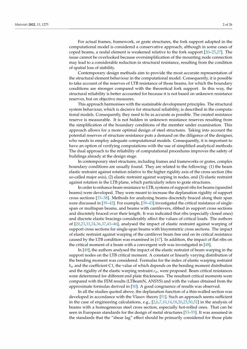
In contemporary steel structures, including frames and frameworks or grates, complexboundary conditions are usually found. They are related to the following: (1) the beamelastic restraint against rotation relative to the higher rigidity axis of the cross section (theso-called major axis), (2) elastic restraint against warping in nodes, and (3) elastic restraintagainst rotation in the LTB plane, which particularly refers to grate structures.

In order to enhance beam resistance to LTB, systems of support ribs for beams (spandrelbeams) were developed. They were meant to increase the deplanation rigidity of supportcross sections [33–38]. Methods for analysing beams discretely braced along their spanwere discussed in [39–42]. For example, [39–43] investigated the critical resistance of single-span or multispan beams, and beams with cantilevers, ribbed in support cross sectionsand discretely braced over their length. It was indicated that ribs (especially closed ones)and discrete elastic bracings considerably affect the values of critical loads. The authorsof [20,23,33,34,36,37,43–46], analysed the impact of elastic restraint against warping ofsupport cross sections for single-span beams with bisymmetric cross sections. The impactof elastic restraint against warping of the cantilever beam free end on its critical resistancecaused by the LTB condition was examined in [47]. In addition, the impact of flat ribs onthe critical moment of a beam with a convergent web was investigated in [48].

In [49], the authors analysed the impact of the elastic restraint of beam warping in thesupport nodes on the LTB critical moment. A constant or linearly varying distribution ofthe bending moment was considered. Formulas for the index of elastic warping restraintkw and the coefficient C1, the value of which depends on the bending moment distributionand the rigidity of the elastic warping restraint cw, were proposed. Beam critical resistanceswere determined for different end plate thicknesses. The resultant critical moments werecompared with the FEM results (LTBeamN, ANSYS) and with the values obtained from theapproximate formulas derived in [50]. A good congruence of results was observed.

In all the studies quoted above, the deplanation function of a thin-walled section wasdeveloped in accordance with the Vlasov theory [51]. Such an approach seems sufficientin the case of engineering calculations, e.g., [2,6,7,10,14,18,20,23,50,52] in the analysis ofbeams with a homogeneous steel cross section, especially hot-rolled ones. That can beseen in European standards for the design of metal structures [53–55]. It was assumed inthe standards that the “shear lag” effect should be primarily considered for those plate

Materials 2022, 15, 1275 3 of 26

girder sections or cold-formed elements, in which a substantial width of the cantilever orspanning chords (e.g., decks in steel bridges) were found. Detailed guidelines are given inSection 3 of the standard [55].

A more general formulation of the warping function for cross sections of structuralmembers is given in [56]. The formulation is particularly applicable to composite structures.The paper proposed a new theory termed Generalized Warping Beam Theory (GWBT),which takes into account the effect of nonuniform warping of the cross section. That wasdone using a single, independent parameter for each warping type. Shear warping ineach direction, and also primary as well as secondary torsional warping, were considered.This approach accounted for shear lag in both the element bending and in torsion. Manyexamples of computations were included to confirm the effectiveness of the method.

The effect of the elastic action of nodes with respect to the LTB critical moment inbeams, analysed in accordance with the thin-walled bar theory [51], was investigated byGizejowski [23] as well as Gizejowski and Bródka [57]. The solution [23], a modification ofthe Lindner proposal [20] and the extension of the formula specified in ENV 1993-1-1 [58],used the concept of buckling length coefficients. Like for axially compressed elements, thecoefficients were applied to flexural buckling (relative to the cross section minor axis) andtorsional buckling (relative to the bar longitudinal axis). The coefficients were determinedin the same way as for the buckling of braced frame columns. It was concluded that takinginto account the additional rigidity of complete end plates combined with other elementsof a framework structure contributed to an increase in the LTB critical moment.

According to the authors’ knowledge, apart from [23,57], the literature on the subjectdoes not offer unambiguous analytical formulas for the LTB critical moment, which wouldsimultaneously take account of the effect of elastic restraint against warping and elasticrestraint against rotation relative to the major axis in support cross sections.

Obviously, such calculations can be performed using the finite element method,e.g., LTBeam or LTBeamN software employing finite bar elements, or by utilising moreadvanced 3D modelling, e.g., Abaqus software with shell or solid elements. However, itshould be emphasised that, in order to improve the safety of structures already at the designstage, FEM calculations should be verified by at least a simplified analytical estimation.Such approximate formulas could also facilitate more advanced preliminary design. Asregards basic static schemes, the formulas can be applied at the principal design stage. Anexpert analysis revealed cases in which designers less experienced in FEM modelling mademistakes when constructing a numerical model (e.g., modelling the boundary conditions inthe beam support nodes). Then, relatively simple approximate formulas make it possibleto correct calculations.

A good example of such an approach is offered in [59]. The authors developedapproximate analytical formulas to determine local buckling stress for a large group of hot-rolled sections under complex load conditions. The calculations can also be performed usingFEM software, e.g., Abaqus or FSM, e.g., CUFSM. However, the possibility of verifying theresults of numerical calculations with relatively simple approximate formulas encouragedthe authors to carry out extensive research in this field.

As already mentioned, many studies show that, in an analysis of LTB of beams withfork support, in order to approximate the function of beam displacements (angle of twist,lateral deflection), the researchers usually use trigonometric functions, which providea good approximation of the critical resistance. However, in the analysis of elasticallyrestrained beams, this approach causes difficulties when describing the degree of elasticfixity of beam support cross sections. Therefore, in their previous studies [50,52,60], theauthors utilised an alternative method for the description of beam displacements upona loss of stability, namely employing power polynomials with a simple physical (static)interpretation. As indicated before, this approach facilitates the description of the torsionangle function and beam lateral deflection when the conditions of its elastic restraintagainst warping and lateral rotation in the support nodes are taken into account. A detaileddiscussion of the approach is given in [50,52]. Power polynomials proved successful in a

Materials 2022, 15, 1275 4 of 26

stability analysis of thin-walled members [61], and also in studies into local buckling of thethin-walled elements with open cross sections subjected to warping torsion [62].

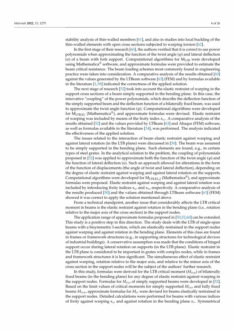
In the first stage of their research [60], the authors verified that it is correct to use powerpolynomials when approximating the function of the twist angle (ϕ) and lateral deflection(u) of a beam with fork support. Computational algorithms for MLTB were developedusing Mathematica® software, and approximate formulas were provided to estimate thebeam critical resistance. The beam loading schemes most commonly found in engineeringpractice were taken into consideration. A comparative analysis of the results obtained [60]against the values generated by the LTBeam software [63] (FEM) and by formulas availablein the literature [1,58] indicated the correctness of the applied solution.

The next stage of research [52] took into account the elastic restraint of warping in thesupport cross sections of a beam simply supported in the bending plane. In this case, theinnovative “coupling” of the power polynomials, which describe the deflection function ofthe simply supported beam and the deflection function of a bilaterally fixed beam, was usedto approximate the twist angle function (ϕ). Computational algorithms were developedfor MLTB,EL (Mathematica®), and approximate formulas were devised. Elastic restraintof warping was included by means of the fixity index κω. A comparative analysis of theresults obtained [52] and the values provided by LTBeam [63] and Abaqus (FEM) software,as well as formulas available in the literature [34], was performed. The analysis indicatedthe effectiveness of the applied solution.

The issues related to the interaction of beam elastic restraint against warping andagainst lateral rotation (in the LTB plane) were discussed in [50]. The beam was assumedto be simply supported in the bending plane. Such elements are found, e.g., in certaintypes of steel grates. In the analytical solution to the problem, the coupling of polynomialsproposed in [52] was applied to approximate both the function of the twist angle (ϕ) andthe function of lateral deflection (u). Such an approach allowed for alterations in the formof the function of displacements (the angle of twist and lateral deflection), depending onthe degree of elastic restraint against warping and against lateral rotation on the supports.Computational algorithms were developed for MLTB,EL,2 (Mathematica®), and approximateformulas were proposed. Elastic restraint against warping and against lateral rotation wasincluded by introducing fixity indices κω and κu, respectively. A comparative analysis ofthe results produced [50] and the values obtained through LTBeam software [63] (FEM)showed it was correct to apply the solution mentioned above.

From a technical standpoint, another issue that considerably affects the LTB criticalmoment in beams is the elastic restraint against rotation in the bending plane (i.e., rotationrelative to the major axis of the cross section) in the support nodes.

The application range of approximate formulas proposed in [50,52,60] can be extended.This study is a positive step in this direction. The study deals with the LTB of single-spanbeams with a bisymmetric I-section, which are elastically restrained in the support nodesagainst warping and against rotation in the bending plane. Elements of this class are foundin frames or framework structures (e.g., in supporting structures for technological devicesof industrial buildings). A conservative assumption was made that the conditions of hingedsupport occur during lateral rotation on supports (in the LTB plane). Elastic restraint inthe LTB plane is considered to be important in grates with complex nodes, while in framesand framework structures it is less significant. The simultaneous effect of elastic restraintagainst warping, rotation relative to the major axis, and relative to the minor axis of thecross section in the support nodes will be the subject of the authors’ further research.

In this study, formulas were derived for the LTB critical moment (Mcr,u) of bilaterallyfixed beams (in the bending plane) for any degree of elastic restraint against warping inthe support nodes. Formulas for Mcr,o of simply supported beams were developed in [52].Based on the limit values of critical moments for simply supported Mcr,o and fully fixedbeams Mcr,u, approximate formulas for Mcr were devised for beams elastically restrained inthe support nodes. Detailed calculations were performed for beams with various indicesof fixity against warping κω and against rotation in the bending plane κν. Symmetrical

Materials 2022, 15, 1275 5 of 26

boundary conditions relative to the midspan of a beam were adopted. The results obtainedwere compared with those from FEM (LTBeamN).

In this study, the following assumptions were made: (1) over its length, the single-span beam has a constant, bisymmetrical hot-rolled I-section, or its welded equivalent,(2) boundary conditions, symmetrical with respect to the beam midspan, are found,(3) three load distributions, most common in engineering practice, are considered,(4) the conditions of the beam elastic support concern the following: (a) restraint of rotationwith respect to the major axis of the cross section, (b) limitation of the cross section warping(warping function in accordance with [51]).

Compared with the solutions discussed in the literature, this study offers a novelapproach, which involves the following:

(i) Approximate formulas were derived for the LTB critical moment (Mcr,u) of steel beamswith bisymmetrical cross section that are bilaterally fixed against bending (My) andelastically restrained against warping. The LTB critical moment represents the upperlimit of the critical resistance in the elastic range.

(ii) Approximate formulas were derived for Mcr, for any degree of elastic restraint againstrotation about the section major axis, and against warping at the support nodes. Thatwas done based on the indexes of fixity that are independent of one another.

(iii) A solution was obtained that allows for a more accurate representation of the actualLTB behaviour of a steel beam using a relatively simple analytical model(cf. calculation example in Section 5.4).

2. Beam Elastic Restraint against Warping and against Rotation in Its Bending Plane

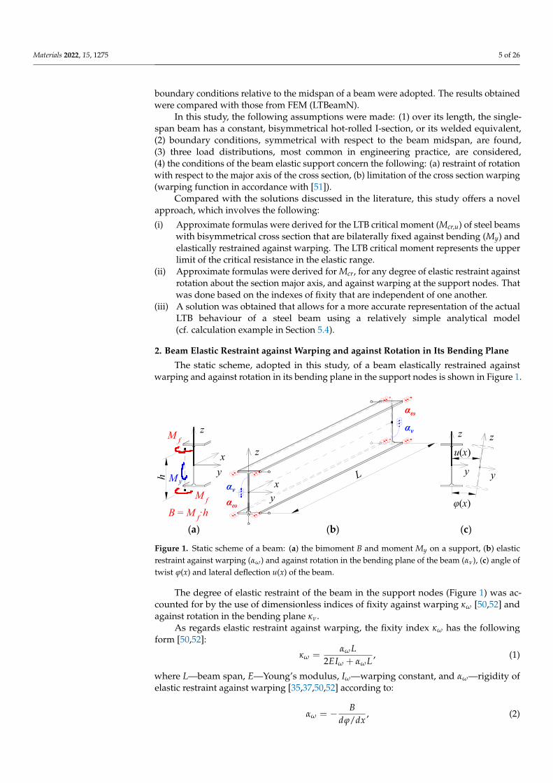
The static scheme, adopted in this study, of a beam elastically restrained againstwarping and against rotation in its bending plane in the support nodes is shown in Figure 1.

Materials 2022, 15, x FOR PEER REVIEW 5 of 27

the support nodes. Formulas for Mcr,o of simply supported beams were developed in [52]. Based on the limit values of critical moments for simply supported Mcr,o and fully fixed beams Mcr,u, approximate formulas for Mcr were devised for beams elastically restrained in the support nodes. Detailed calculations were performed for beams with various indi-ces of fixity against warping κω and against rotation in the bending plane κν. Symmetrical boundary conditions relative to the midspan of a beam were adopted. The results ob-tained were compared with those from FEM (LTBeamN).

In this study, the following assumptions were made: (1) over its length, the single-span beam has a constant, bisymmetrical hot-rolled I-section, or its welded equivalent, (2) boundary conditions, symmetrical with respect to the beam midspan, are found, (3) three load distributions, most common in engineering practice, are considered, (4) the condi-tions of the beam elastic support concern the following: (a) restraint of rotation with re-spect to the major axis of the cross section, (b) limitation of the cross section warping (warping function in accordance with [51]).

Compared with the solutions discussed in the literature, this study offers a novel ap-proach, which involves the following: (i) Approximate formulas were derived for the LTB critical moment (Mcr,u) of steel

beams with bisymmetrical cross section that are bilaterally fixed against bending (My) and elastically restrained against warping. The LTB critical moment represents the upper limit of the critical resistance in the elastic range.

(ii) Approximate formulas were derived for Mcr, for any degree of elastic restraint against rotation about the section major axis, and against warping at the support nodes. That was done based on the indexes of fixity that are independent of one another.

(iii) A solution was obtained that allows for a more accurate representation of the actual LTB behaviour of a steel beam using a relatively simple analytical model (cf. calcula-tion example in Section 5.4).

2. Beam Elastic Restraint against Warping and against Rotation in Its Bending Plane The static scheme, adopted in this study, of a beam elastically restrained against

warping and against rotation in its bending plane in the support nodes is shown in Figure 1.

Figure 1. Static scheme of a beam: (a) the bimoment B and moment My on a support, (b) elastic restraint against warping (αω) and against rotation in the bending plane of the beam (αν), (c) angle of twist φ(x) and lateral deflection u(x) of the beam.

The degree of elastic restraint of the beam in the support nodes (Figure 1) was ac-counted for by the use of dimensionless indices of fixity against warping κω [50,52] and against rotation in the bending plane κν.

As regards elastic restraint against warping, the fixity index κω has the following form [50,52]:

zz

z

y

y

yx

xy

z

M yL

M f

M f

B = M f·h

h

φ(x)

αν

u(x)

αω

αναω

(a) (b) (c)

Figure 1. Static scheme of a beam: (a) the bimoment B and moment My on a support, (b) elasticrestraint against warping (αω) and against rotation in the bending plane of the beam (αν), (c) angle oftwist ϕ(x) and lateral deflection u(x) of the beam.

The degree of elastic restraint of the beam in the support nodes (Figure 1) was ac-counted for by the use of dimensionless indices of fixity against warping κω [50,52] andagainst rotation in the bending plane κν.

As regards elastic restraint against warping, the fixity index κω has the followingform [50,52]:

κω =αω L

2EIω + αω L, (1)

where L—beam span, E—Young’s modulus, Iω—warping constant, and αω—rigidity ofelastic restraint against warping [35,37,50,52] according to:

αω = − Bdϕ/dx

, (2)

Materials 2022, 15, 1275 6 of 26

where B—bimoment at the support point of the beam, ϕ—angle of twist, and dϕ/dx—warpingof the section.

The index of elastic fixity against warping changes is from κω = 0 for complete warpingfreedom to κω = 1 for full prevention of warping.

The κν index of elastic fixity of the beam support section against rotation in the bendingplane (i.e., against rotation relative to the major axis of the cross section) is expressed bythe equation:

κν =ανL

4EIy + ανL, (3)

where Iy—second moment of inertia in bending about the y-axis; αν—rigidity of elasticrestraint against rotation in the beam bending plane according to the equation:

αν =My

dν/dx, (4)

where My—bending moment relative to the major axis of the support cross section, ν—verticaldeflection, and dν/dx—rotation relative to the y axis in the support cross section.

The index of fixity against rotation in the bending plane of the beam ranges fromκν = 0 for complete freedom of rotation (hinge support) to κν = 1 for complete preventionof rotation (fixity).

The rigidities of elastic restraint against warping αω (Equation (2)) and against rotationαν (Equation (4)) can be expressed as a function of the fixity indices (κω, κν) according tothe equations:

αω =2κωEIω

(1− κω)L; αν =

4κνEIy

(1− κν)L. (5)

3. LTB Critical Moment of a Fixed Beam3.1. Function of the Twist Angle

A program for numerical calculations (MLTB,EL) was proposed in [52]. With theprogram, it is possible to determine the LTB critical moment of a beam, which in its supportnodes is simply supported in the bending plane, and elastically restrained against warping.In MLTB,EL software, the function of the beam twist angle (ϕ) was approximated using theinnovative “coupling” of power polynomials. This was done according to the equation [52]:

ϕ(x) = ∑3i=1 ai((1− κω) ·WPi + κω ·WUi), (6)

where ai—free parameters of the twist angle function, κω—elastic restraint index accordingto Equation (1); WPi—polynomials describing the deflection function of a simply supportedbeam; and WUi—polynomials describing the deflection function of a fixed beam.

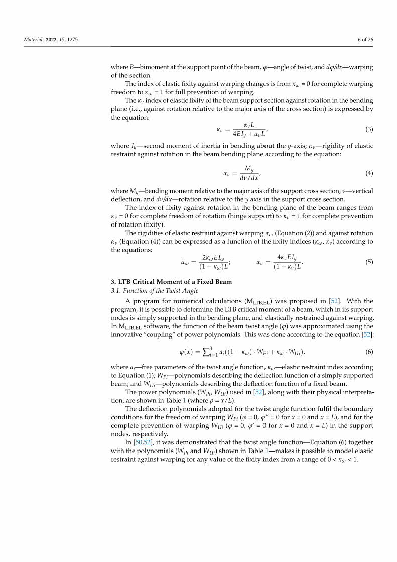
The power polynomials (WPi, WUi) used in [52], along with their physical interpreta-tion, are shown in Table 1 (where ρ = x/L).

The deflection polynomials adopted for the twist angle function fulfil the boundaryconditions for the freedom of warping WPi (ϕ = 0, ϕ” = 0 for x = 0 and x = L), and for thecomplete prevention of warping WUi (ϕ = 0, ϕ’ = 0 for x = 0 and x = L) in the supportnodes, respectively.

In [50,52], it was demonstrated that the twist angle function—Equation (6) togetherwith the polynomials (WPi and WUi) shown in Table 1—makes it possible to model elasticrestraint against warping for any value of the fixity index from a range of 0 < κω < 1.

Materials 2022, 15, 1275 7 of 26

Table 1. Application of polynomials.

Item Polynomials Physical Interpretation

I II III

1 WP1 = ρ− 2ρ3 + ρ4


𝜅 = , (1)

where L—beam span, E—Young’s modulus, Iω—warping constant, and αω—rigidity of elastic restraint against warping [35,37,50,52] according to: 𝛼 = − ⁄ , (2)

where B—bimoment at the support point of the beam, φ—angle of twist, and dφ/dx—warping of the section.

The index of elastic fixity against warping changes is from κω = 0 for complete warp-ing freedom to κω = 1 for full prevention of warping.

The κν index of elastic fixity of the beam support section against rotation in the bend-ing plane (i.e., against rotation relative to the major axis of the cross section) is expressed by the equation: 𝜅 = , (3)

where Iy—second moment of inertia in bending about the y-axis; αν—rigidity of elastic restraint against rotation in the beam bending plane according to the equation: 𝛼 = / , (4)

where My—bending moment relative to the major axis of the support cross section, ν—vertical deflection, and dν/dx—rotation relative to the y axis in the support cross section.

The index of fixity against rotation in the bending plane of the beam ranges from κν = 0 for complete freedom of rotation (hinge support) to κν = 1 for complete prevention of rotation (fixity).

The rigidities of elastic restraint against warping αω (Equation (2)) and against rota-tion αν (Equation (4)) can be expressed as a function of the fixity indices (κω, κν) according to the equations: 𝛼 = ( ) ; 𝛼 = ( ) . (5)

3. LTB Critical Moment of a Fixed Beam 3.1. Function of the Twist Angle

A program for numerical calculations (MLTB,EL) was proposed in [52]. With the pro-gram, it is possible to determine the LTB critical moment of a beam, which in its support nodes is simply supported in the bending plane, and elastically restrained against warp-ing. In MLTB,EL software, the function of the beam twist angle (φ) was approximated using the innovative “coupling” of power polynomials. This was done according to the equation [52]: 𝜑(𝑥) = ∑ 𝑎 (1 − 𝜅 ) ⋅ 𝑊 + 𝜅 ⋅ 𝑊 , (6)

where ai—free parameters of the twist angle function, κω—elastic restraint index according to Equation (1); WPi—polynomials describing the deflection function of a simply sup-ported beam; and WUi—polynomials describing the deflection function of a fixed beam.

The power polynomials (WPi, WUi) used in [52], along with their physical interpreta-tion, are shown in Table 1 (where ρ = x/L).

Table 1. Application of polynomials.

Item Polynomials Physical Interpretation I II III

1 𝑊 = 𝜌 − 2𝜌 + 𝜌 x

z

2 WP2 = ρ− 10ρ3 + 15ρ4 − 6ρ5


2 𝑊 = 𝜌 − 10𝜌 + 15𝜌 − 6𝜌

3 𝑊 = 𝜌 − 26𝜌 + 73𝜌 − 72𝜌 + 24𝜌

4 𝑊 = 𝜌 − 2𝜌 + 𝜌

5 𝑊 = 𝜌 − 4𝜌 + 5𝜌 − 2𝜌

6 𝑊 = 2𝜌 − 13𝜌 + 29𝜌 − 27𝜌 + 9𝜌

The deflection polynomials adopted for the twist angle function fulfil the boundary conditions for the freedom of warping WPi (φ = 0, φ” = 0 for x = 0 and x = L), and for the complete prevention of warping WUi (φ = 0, φ’ = 0 for x = 0 and x = L) in the support nodes, respectively.

In [50,52], it was demonstrated that the twist angle function—Equation (6) together with the polynomials (WPi and WUi) shown in Table 1—makes it possible to model elastic restraint against warping for any value of the fixity index from a range of 0 < κω < 1.

3.2. Determination of Mcr,u with the Energy Method The elastic LTB critical moment of a bilaterally fixed (Mcr,u), bisymmetric I-beam was

determined using the energy method [9]. The elastic restraint against warping in the sup-port nodes was taken into account.

The degree of elastic restraint of nodes in the beam bending plane is not a typical boundary condition for lateral–torsional buckling. However, it strongly affects the longi-tudinal distribution of the bending moment My. As a result, in order to determine Mcr,u for beams fixed in the bending plane and elastically restrained against warping on the sup-ports, the work done by external forces for this type of support and load should be taken into account in the functional of the total potential energy. In such an approach, complete prevention of rotation of the beam cross section in the precritical bending plane is repre-sented by the support moments of restraint. It should be noted that in the precritical state (My < Mcr), the bending of a beam proceeds relative to the y–y axis, while in the post-critical state (My > Mcr), due to lateral deflection and the angle of twisting after LTB, the bending of the beam is biaxial.

Boundary conditions corresponding to LTB should be separated from boundary con-ditions that affect the distribution of support moments My (fixity in the bending plane). This is important in the case of elastic restraints of nodes. Such restraints occur in modern node structures, especially in framework systems, where simplified connection details are used. The separation of the boundary conditions of LTB from the static scheme of the sup-port is also found in the LTBeamN software.

As a result, the load critical value was calculated from the equation: ∆𝛱 = ∆𝑈 , + ∆𝑈 , − ∆𝑇, (7)

where ΔUs,1—elastic energy of beam bending and torsion, ΔUs,2—energy of beam elastic restraint against warping in the support nodes, and ΔT—work done by external forces.

The elastic energy of beam bending and torsion was determined based this equation from [9]: ∆𝑈 , = 𝐸𝐼 𝑑𝑥 + 𝐺𝐼 𝑑𝑥 + 𝐸𝐼 𝑑𝑥 , (8)

where Iz—second moment of inertia in bending about z-axis, It—Saint Venant’s torsion constant, G—shear modulus, and u—the lateral deflection function.

x

z

x

z

x

z

x

z

x

z

3 WP3 = ρ− 26ρ3 + 73ρ4 − 72ρ5 + 24ρ6


2 𝑊 = 𝜌 − 10𝜌 + 15𝜌 − 6𝜌

3 𝑊 = 𝜌 − 26𝜌 + 73𝜌 − 72𝜌 + 24𝜌

4 𝑊 = 𝜌 − 2𝜌 + 𝜌

5 𝑊 = 𝜌 − 4𝜌 + 5𝜌 − 2𝜌

6 𝑊 = 2𝜌 − 13𝜌 + 29𝜌 − 27𝜌 + 9𝜌











x

z

x

z

x

z

x

z

x

z

4 WU1 = ρ2 − 2ρ3 + ρ4


2 𝑊 = 𝜌 − 10𝜌 + 15𝜌 − 6𝜌

3 𝑊 = 𝜌 − 26𝜌 + 73𝜌 − 72𝜌 + 24𝜌

4 𝑊 = 𝜌 − 2𝜌 + 𝜌

5 𝑊 = 𝜌 − 4𝜌 + 5𝜌 − 2𝜌

6 𝑊 = 2𝜌 − 13𝜌 + 29𝜌 − 27𝜌 + 9𝜌











x

z

x

z

x

z

x

z

x

z

5 WU2 = ρ2 − 4ρ3 + 5ρ4 − 2ρ5


2 𝑊 = 𝜌 − 10𝜌 + 15𝜌 − 6𝜌

3 𝑊 = 𝜌 − 26𝜌 + 73𝜌 − 72𝜌 + 24𝜌

4 𝑊 = 𝜌 − 2𝜌 + 𝜌

5 𝑊 = 𝜌 − 4𝜌 + 5𝜌 − 2𝜌

6 𝑊 = 2𝜌 − 13𝜌 + 29𝜌 − 27𝜌 + 9𝜌











x

z

x

z

x

z

x

z

x

z6 WU3 = 2ρ2 − 13ρ3 + 29ρ4 − 27ρ5 + 9ρ6


2 𝑊 = 𝜌 − 10𝜌 + 15𝜌 − 6𝜌

3 𝑊 = 𝜌 − 26𝜌 + 73𝜌 − 72𝜌 + 24𝜌

4 𝑊 = 𝜌 − 2𝜌 + 𝜌

5 𝑊 = 𝜌 − 4𝜌 + 5𝜌 − 2𝜌

6 𝑊 = 2𝜌 − 13𝜌 + 29𝜌 − 27𝜌 + 9𝜌











x

z

x

z

x

z

x

z

x

z

3.2. Determination of Mcr,u with the Energy Method

The elastic LTB critical moment of a bilaterally fixed (Mcr,u), bisymmetric I-beam wasdetermined using the energy method [9]. The elastic restraint against warping in thesupport nodes was taken into account.

The degree of elastic restraint of nodes in the beam bending plane is not a typicalboundary condition for lateral–torsional buckling. However, it strongly affects the longi-tudinal distribution of the bending moment My. As a result, in order to determine Mcr,ufor beams fixed in the bending plane and elastically restrained against warping on thesupports, the work done by external forces for this type of support and load should betaken into account in the functional of the total potential energy. In such an approach,complete prevention of rotation of the beam cross section in the precritical bending plane isrepresented by the support moments of restraint. It should be noted that in the precriticalstate (My < Mcr), the bending of a beam proceeds relative to the y–y axis, while in thepost-critical state (My > Mcr), due to lateral deflection and the angle of twisting after LTB,the bending of the beam is biaxial.

Boundary conditions corresponding to LTB should be separated from boundary condi-tions that affect the distribution of support moments My (fixity in the bending plane). Thisis important in the case of elastic restraints of nodes. Such restraints occur in modern nodestructures, especially in framework systems, where simplified connection details are used.The separation of the boundary conditions of LTB from the static scheme of the support isalso found in the LTBeamN software.

As a result, the load critical value was calculated from the equation:

∆Π = ∆Us,1 + ∆Us,2 − ∆T, (7)

where ∆Us,1—elastic energy of beam bending and torsion, ∆Us,2—energy of beam elasticrestraint against warping in the support nodes, and ∆T—work done by external forces.

The elastic energy of beam bending and torsion was determined based this equationfrom [9]:

∆Us,1 =12

(EIz

∫ L

0

(d2udx2

)2

dx + GIt

∫ L

0

(dϕ

dx

)2dx + EIω

∫ L

0

(d2 ϕ

dx2

)2

dx

), (8)

where Iz—second moment of inertia in bending about z-axis, It—Saint Venant’s torsionconstant, G—shear modulus, and u—the lateral deflection function.

Materials 2022, 15, 1275 8 of 26

The energy of elastic restraint against warping in the support nodes was determinedfrom the following equation [52]:

∆Us,2 =αω

2

((dϕ

dx

)2

x=0+

(dϕ

dx

)2

x=L

). (9)

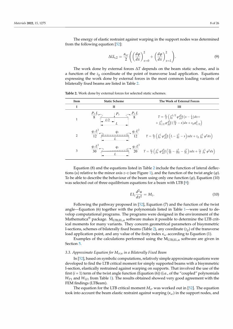
The work done by external forces ∆T depends on the beam static scheme, and isa function of the zg coordinate of the point of transverse load application. Equationsexpressing the work done by external forces in the most common loading variants ofbilaterally fixed beams are listed in Table 2.

Table 2. Work done by external forces for selected static schemes.

Item Static Scheme The Work of External Forces

I II III

1


The energy of elastic restraint against warping in the support nodes was determined from the following equation [52]: ∆𝑈 , = + . (9)

The work done by external forces ΔT depends on the beam static scheme, and is a function of the zg coordinate of the point of transverse load application. Equations express-ing the work done by external forces in the most common loading variants of bilaterally fixed beams are listed in Table 2.


Item Static Scheme The Work of External Forces I II III

1

𝑇 = 𝑃2 𝜑 𝑑 𝑢𝑑𝑥 𝑥 − 𝐿4 𝑑𝑥/ + + 𝜑 𝑑 𝑢𝑑𝑥 3𝐿4 − 𝑥 𝑑𝑥/ + 𝑧 𝜑 /

2

𝑇 = 𝑞2 𝜑 𝑑 𝑢𝑑𝑥 𝐿 − 𝐿6𝑥 − 𝑥 𝑥𝑑𝑥 + 𝑧 𝜑 𝑑𝑥

3

𝑇 = 𝑞2 𝜑 𝑑 𝑢𝑑𝑥 3𝐿10 − 𝐿15𝑥 − 𝑥3𝐿 𝑥𝑑𝑥+ 𝑧2 𝜑 𝑑𝑥

Equation (8) and the equations listed in Table 2 include the function of lateral deflec-tions (u) relative to the minor axis z–z (see Figure 1), and the function of the twist angle (φ). To be able to describe the behaviour of the beam using only one function (φ), Equation (10) was selected out of three equilibrium equations for a beam with LTB [9]: 𝐸𝐼 = 𝑀 . (10)

Following the pathway proposed in [52], Equation (7) and the function of the twist angle—Equation (6) together with the polynomials listed in Table 1—were used to de-velop computational programs. The programs were designed in the environment of the Mathematica® package. MLTB,EL,u software makes it possible to determine the LTB critical moments for many variants. They concern geometrical parameters of bisymmetric I-sec-tions, schemes of bilaterally fixed beams (Table 2), any coordinate (zg) of the transverse load application point, and any value of the fixity index κω according to Equation (1).

Examples of the calculations performed using the MLTB,EL,u software are given in Sec-tion 5.

3.3. Approximate Equation for Mcr,u in a Bilaterally Fixed Beam In [52], based on symbolic computations, relatively simple approximate equations

were developed to find the LTB critical moment for simply supported beams with a bi-symmetric I-section, elastically restrained against warping on supports. That involved the use of the first (i = 1) term of the twist angle function (Equation (6)) (i.e., of the “coupled” polynomials WP1 and WU1 from Table 1). The results obtained showed very good agree-ment with the FEM findings (LTBeam).

The equation for the LTB critical moment Mcr was worked out in [52]. The equation took into account the beam elastic restraint against warping (κω) in the support nodes, and also any ordinate (zg) of the point of transverse load application, relative to the shear centre of the cross section. The equation is as follows [52]:

Pz8

Pz L8

Pz L

LL/2

L

qz

12qz L2

12qz L2

L

qz

20qz L2

30qz L2

T = Pz2

(∫ L/20 ϕ d2u

dx2

(x− L

4

)dx+

+∫ L

L/2 ϕ d2udx2

( 3L4 − x

)dx + zg ϕ2

L/2

)

2






1


2


3








Pz8

Pz L8

Pz L

LL/2

L

qz

12qz L2

12qz L2

L

qz

20qz L2

30qz L2

T = qz2

(∫ L0 ϕ d2u

dx2

(L− L2

6x − x)

xdx + zg∫ L

0 ϕ2dx)

3






1


2


3








Pz8

Pz L8

Pz L

LL/2

L

qz

12qz L2

12qz L2

L

qz

20qz L2

30qz L2

T = qz2

(∫ L0 ϕ d2u

dx2

(3L10 −

L2

15x −x2

3L

)xdx +

zg2

∫ L0 ϕ2dx

)

Equation (8) and the equations listed in Table 2 include the function of lateral deflec-tions (u) relative to the minor axis z–z (see Figure 1), and the function of the twist angle (ϕ).To be able to describe the behaviour of the beam using only one function (ϕ), Equation (10)was selected out of three equilibrium equations for a beam with LTB [9]:

EIzd2udx2 = Mz. (10)

Following the pathway proposed in [52], Equation (7) and the function of the twistangle—Equation (6) together with the polynomials listed in Table 1—were used to de-velop computational programs. The programs were designed in the environment of theMathematica® package. MLTB,EL,u software makes it possible to determine the LTB crit-ical moments for many variants. They concern geometrical parameters of bisymmetricI-sections, schemes of bilaterally fixed beams (Table 2), any coordinate (zg) of the transverseload application point, and any value of the fixity index κω according to Equation (1).

Examples of the calculations performed using the MLTB,EL,u software are given inSection 5.

3.3. Approximate Equation for Mcr,u in a Bilaterally Fixed Beam

In [52], based on symbolic computations, relatively simple approximate equations weredeveloped to find the LTB critical moment for simply supported beams with a bisymmetricI-section, elastically restrained against warping on supports. That involved the use of thefirst (i = 1) term of the twist angle function (Equation (6)) (i.e., of the “coupled” polynomialsWP1 and WU1 from Table 1). The results obtained showed very good agreement with theFEM findings (LTBeam).

The equation for the LTB critical moment Mcr was worked out in [52]. The equationtook into account the beam elastic restraint against warping (κω) in the support nodes, and

Materials 2022, 15, 1275 9 of 26

also any ordinate (zg) of the point of transverse load application, relative to the shear centreof the cross section. The equation is as follows [52]:

Mcr =−B1EIzzg +

√EIz

(B3GItL2 + B4EIω + B2

1EIzz2g

)B2L2 , (11)

where zg—ordinate of the point of transverse load application with respect to shear centre(see Figure 2) and B1, B2, B3, B4—coefficients according to Table 3.


𝑀 = , (11)

where zg—ordinate of the point of transverse load application with respect to shear centre (see Figure 2) and B1, B2, B3, B4—coefficients according to Table 3.

Figure 2. The static scheme of a beam elastically restrained in the support nodes (κω, κν) under the load of a force concentrated (Pz) at the midspan.

Table 3 lists the B1, B2, B3, and B4 coefficients for beams simply supported against bending My, and the most common loading schemes [52].

Table 3. Coefficients B1, B2, B3, B4 for simply supported beams (Mcr,o) and selected loading schemes.

Item Static scheme Coefficients I II III

1

𝐵 = 7.242 ⋅ (1.563 − 2.5𝜅 + 𝜅 ) 𝐵 = 1.522 − 2.467𝜅 + 𝜅 𝐵 = 19.248 ⋅ 𝐵 ⋅ (1.457 − 2.4𝜅 + 𝜅 ) 𝐵 = 231.816 ⋅ 𝐵 ⋅ (1.2 − 𝜅 )

2

𝐵 = 5.250 ⋅ (1.476 − 2.429𝜅 + 𝜅 ) 𝐵 = 1.507 − 2.455𝜅 + 𝜅 𝐵 = 13.092 ⋅ 𝐵 ⋅ (1.457 − 2.4𝜅 + 𝜅 ) 𝐵 = 157.633 ⋅ 𝐵 ⋅ (1.2 − 𝜅 )

3

𝐵 = 5.322 ⋅ (1.476 − 2.429𝜅 + 𝜅 ) 𝐵 = 1.507 − 2.455𝜅 + 𝜅 𝐵 = 13.624 ⋅ 𝐵 ⋅ (1.457 − 2.4𝜅 + 𝜅 ) 𝐵 = 163.486 ⋅ 𝐵 ⋅ (1.2 − 𝜅 )

The procedure adopted in this study is the same as that employed in [52]. The McrLT_fix_sym.cal.nb program was developed in the Mathematica® package to carry out symbolic transformations. Like in [50,52], the function of the twist angle was approxi-mated only by the first (i = 1) term of the series (Equation (6)) using the polynomials WP1 and WU1 (Table 1). As a result, it was possible to devise a relatively simple approximate equation concerning the LTB critical moment for an I-beam, bilaterally fixed (for bending My) and elastically restrained against warping. The equation was transformed into the form of Equation (11). Coefficients B1, B2, B3, and B4 for the most common variants of load application in bilaterally fixed beams are shown in Table 4.

Table 4. Coefficients B1, B2, B3, and B4 for selected static schemes of fixed beams (Mcr,u).


1

𝐵 = 23.333 ⋅ (1.563 − 2.5𝜅 + 𝜅 ) 𝐵 = 1.522 − 2.467𝜅 + 𝜅 𝐵 = 31.032 ⋅ 𝐵 ⋅ (1.457 − 2.4𝜅 + 𝜅 ) 𝐵 = 372.934 ⋅ 𝐵 ⋅ (1.2 − 𝜅 )

L/2

L+ z

g

x

z A

A

zz

y y

Pz

c=s

A-APz

φ(x)

κνu(x)

κωκν

κω

L

Pz

L/2

L

qz

L

qz

Pz8

Pz L8

Pz L

LL/2

Figure 2. The static scheme of a beam elastically restrained in the support nodes (κω , κν) under theload of a force concentrated (Pz) at the midspan.

Table 3 lists the B1, B2, B3, and B4 coefficients for beams simply supported againstbending My, and the most common loading schemes [52].


Item Static Scheme Coefficients

I II III

1


𝑀 = , (11)






1

𝐵 = 7.242 ⋅ (1.563 − 2.5𝜅 + 𝜅 ) 𝐵 = 1.522 − 2.467𝜅 + 𝜅 𝐵 = 19.248 ⋅ 𝐵 ⋅ (1.457 − 2.4𝜅 + 𝜅 ) 𝐵 = 231.816 ⋅ 𝐵 ⋅ (1.2 − 𝜅 )

2

𝐵 = 5.250 ⋅ (1.476 − 2.429𝜅 + 𝜅 ) 𝐵 = 1.507 − 2.455𝜅 + 𝜅 𝐵 = 13.092 ⋅ 𝐵 ⋅ (1.457 − 2.4𝜅 + 𝜅 ) 𝐵 = 157.633 ⋅ 𝐵 ⋅ (1.2 − 𝜅 )

3

𝐵 = 5.322 ⋅ (1.476 − 2.429𝜅 + 𝜅 ) 𝐵 = 1.507 − 2.455𝜅 + 𝜅 𝐵 = 13.624 ⋅ 𝐵 ⋅ (1.457 − 2.4𝜅 + 𝜅 ) 𝐵 = 163.486 ⋅ 𝐵 ⋅ (1.2 − 𝜅 )




1

𝐵 = 23.333 ⋅ (1.563 − 2.5𝜅 + 𝜅 ) 𝐵 = 1.522 − 2.467𝜅 + 𝜅 𝐵 = 31.032 ⋅ 𝐵 ⋅ (1.457 − 2.4𝜅 + 𝜅 ) 𝐵 = 372.934 ⋅ 𝐵 ⋅ (1.2 − 𝜅 )

L/2

L+ z

g

x

z A

A

zz

y y

Pz

c=s

A-APz

φ(x)

κνu(x)

κωκν

κω

L

Pz

L/2

L

qz

L

qz

Pz8

Pz L8

Pz L

LL/2

B1 = 7.242 ·(1.563− 2.5κω + κ2

ω

)B2 = 1.522− 2.467κω + κ2

ωB3 = 19.248 · B2 ·

(1.457− 2.4κω + κ2

ω

)B4 = 231.816 · B2 · (1.2− κω)

2


𝑀 = , (11)






1

𝐵 = 7.242 ⋅ (1.563 − 2.5𝜅 + 𝜅 ) 𝐵 = 1.522 − 2.467𝜅 + 𝜅 𝐵 = 19.248 ⋅ 𝐵 ⋅ (1.457 − 2.4𝜅 + 𝜅 ) 𝐵 = 231.816 ⋅ 𝐵 ⋅ (1.2 − 𝜅 )

2

𝐵 = 5.250 ⋅ (1.476 − 2.429𝜅 + 𝜅 ) 𝐵 = 1.507 − 2.455𝜅 + 𝜅 𝐵 = 13.092 ⋅ 𝐵 ⋅ (1.457 − 2.4𝜅 + 𝜅 ) 𝐵 = 157.633 ⋅ 𝐵 ⋅ (1.2 − 𝜅 )

3

𝐵 = 5.322 ⋅ (1.476 − 2.429𝜅 + 𝜅 ) 𝐵 = 1.507 − 2.455𝜅 + 𝜅 𝐵 = 13.624 ⋅ 𝐵 ⋅ (1.457 − 2.4𝜅 + 𝜅 ) 𝐵 = 163.486 ⋅ 𝐵 ⋅ (1.2 − 𝜅 )




1

𝐵 = 23.333 ⋅ (1.563 − 2.5𝜅 + 𝜅 ) 𝐵 = 1.522 − 2.467𝜅 + 𝜅 𝐵 = 31.032 ⋅ 𝐵 ⋅ (1.457 − 2.4𝜅 + 𝜅 ) 𝐵 = 372.934 ⋅ 𝐵 ⋅ (1.2 − 𝜅 )

L/2

L+ z

g

x

z A

A

zz

y y

Pz

c=s

A-APz

φ(x)

κνu(x)

κωκν

κω

L

Pz

L/2

L

qz

L

qz

Pz8

Pz L8

Pz L

LL/2

B1 = 5.250 ·(1.476− 2.429κω + κ2

ω

)B2 = 1.507− 2.455κω + κ2

ωB3 = 13.092 · B2 ·

(1.457− 2.4κω + κ2

ω

)B4 = 157.633 · B2 · (1.2− κω)

3


𝑀 = , (11)






1

𝐵 = 7.242 ⋅ (1.563 − 2.5𝜅 + 𝜅 ) 𝐵 = 1.522 − 2.467𝜅 + 𝜅 𝐵 = 19.248 ⋅ 𝐵 ⋅ (1.457 − 2.4𝜅 + 𝜅 ) 𝐵 = 231.816 ⋅ 𝐵 ⋅ (1.2 − 𝜅 )

2

𝐵 = 5.250 ⋅ (1.476 − 2.429𝜅 + 𝜅 ) 𝐵 = 1.507 − 2.455𝜅 + 𝜅 𝐵 = 13.092 ⋅ 𝐵 ⋅ (1.457 − 2.4𝜅 + 𝜅 ) 𝐵 = 157.633 ⋅ 𝐵 ⋅ (1.2 − 𝜅 )

3

𝐵 = 5.322 ⋅ (1.476 − 2.429𝜅 + 𝜅 ) 𝐵 = 1.507 − 2.455𝜅 + 𝜅 𝐵 = 13.624 ⋅ 𝐵 ⋅ (1.457 − 2.4𝜅 + 𝜅 ) 𝐵 = 163.486 ⋅ 𝐵 ⋅ (1.2 − 𝜅 )




1

𝐵 = 23.333 ⋅ (1.563 − 2.5𝜅 + 𝜅 ) 𝐵 = 1.522 − 2.467𝜅 + 𝜅 𝐵 = 31.032 ⋅ 𝐵 ⋅ (1.457 − 2.4𝜅 + 𝜅 ) 𝐵 = 372.934 ⋅ 𝐵 ⋅ (1.2 − 𝜅 )

L/2

L+ z

g

x

z A

A

zz

y y

Pz

c=s

A-APz

φ(x)

κνu(x)

κωκν

κω

L

Pz

L/2

L

qz

L

qz

Pz8

Pz L8

Pz L

LL/2

B1 = 5.322 ·(1.476− 2.429κω + κ2

ω

)B2 = 1.507− 2.455κω + κ2

ωB3 = 13.624 · B2 ·

(1.457− 2.4κω + κ2

ω

)B4 = 163.486 · B2 · (1.2− κω)

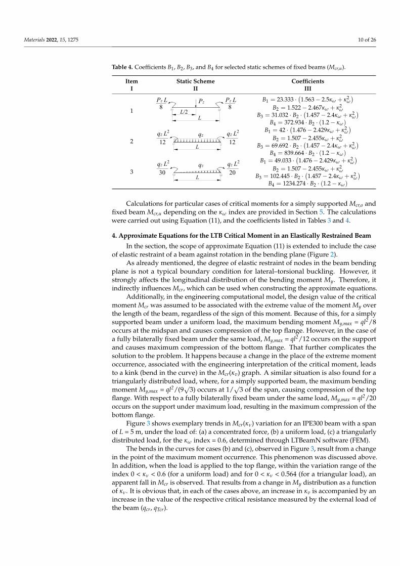
The procedure adopted in this study is the same as that employed in [52]. TheMcrLT_fix_sym.cal.nb program was developed in the Mathematica® package to carry outsymbolic transformations. Like in [50,52], the function of the twist angle was approximatedonly by the first (i = 1) term of the series (Equation (6)) using the polynomials WP1 andWU1 (Table 1). As a result, it was possible to devise a relatively simple approximateequation concerning the LTB critical moment for an I-beam, bilaterally fixed (for bendingMy) and elastically restrained against warping. The equation was transformed into theform of Equation (11). Coefficients B1, B2, B3, and B4 for the most common variants of loadapplication in bilaterally fixed beams are shown in Table 4.

Materials 2022, 15, 1275 10 of 26


Item Static Scheme CoefficientsI II III

1


𝑀 = , (11)






1

𝐵 = 7.242 ⋅ (1.563 − 2.5𝜅 + 𝜅 ) 𝐵 = 1.522 − 2.467𝜅 + 𝜅 𝐵 = 19.248 ⋅ 𝐵 ⋅ (1.457 − 2.4𝜅 + 𝜅 ) 𝐵 = 231.816 ⋅ 𝐵 ⋅ (1.2 − 𝜅 )

2

𝐵 = 5.250 ⋅ (1.476 − 2.429𝜅 + 𝜅 ) 𝐵 = 1.507 − 2.455𝜅 + 𝜅 𝐵 = 13.092 ⋅ 𝐵 ⋅ (1.457 − 2.4𝜅 + 𝜅 ) 𝐵 = 157.633 ⋅ 𝐵 ⋅ (1.2 − 𝜅 )

3

𝐵 = 5.322 ⋅ (1.476 − 2.429𝜅 + 𝜅 ) 𝐵 = 1.507 − 2.455𝜅 + 𝜅 𝐵 = 13.624 ⋅ 𝐵 ⋅ (1.457 − 2.4𝜅 + 𝜅 ) 𝐵 = 163.486 ⋅ 𝐵 ⋅ (1.2 − 𝜅 )




1

𝐵 = 23.333 ⋅ (1.563 − 2.5𝜅 + 𝜅 ) 𝐵 = 1.522 − 2.467𝜅 + 𝜅 𝐵 = 31.032 ⋅ 𝐵 ⋅ (1.457 − 2.4𝜅 + 𝜅 ) 𝐵 = 372.934 ⋅ 𝐵 ⋅ (1.2 − 𝜅 )

L/2

L

+ zg

x

z A

A

zz

y y

Pz

c=s

A-APz

φ(x)

κνu(x)

κωκν

κω

L

Pz

L/2

L

qz

L

qz

Pz8

Pz L8

Pz L

LL/2

B1 = 23.333 ·(1.563− 2.5κω + κ2

ω

)B2 = 1.522− 2.467κω + κ2

ωB3 = 31.032 · B2 ·

(1.457− 2.4κω + κ2

ω

)B4 = 372.934 · B2 · (1.2− κω)

2


2

𝐵 = 42 ⋅ (1.476 − 2.429𝜅 + 𝜅 ) 𝐵 = 1.507 − 2.455𝜅 + 𝜅 𝐵 = 69.692 ⋅ 𝐵 ⋅ (1.457 − 2.4𝜅 + 𝜅 ) 𝐵 = 839.664 ⋅ 𝐵 ⋅ (1.2 − 𝜅 )

3

𝐵 = 49.033 ⋅ (1.476 − 2.429𝜅 + 𝜅 ) 𝐵 = 1.507 − 2.455𝜅 + 𝜅 𝐵 = 102.445 ⋅ 𝐵 ⋅ (1.457 − 2.4𝜅 + 𝜅 ) 𝐵 = 1234.274 ⋅ 𝐵 ⋅ (1.2 − 𝜅 )

Calculations for particular cases of critical moments for a simply supported Mcr,o and fixed beam Mcr,u depending on the κω index are provided in Section 5. The calculations were carried out using Equation (11), and the coefficients listed in Tables 3 and 4.

4. Approximate Equations for the LTB Critical Moment in an Elastically Restrained Beam

In the section, the scope of approximate Equation (11) is extended to include the case of elastic restraint of a beam against rotation in the bending plane (Figure 2).

As already mentioned, the degree of elastic restraint of nodes in the beam bending plane is not a typical boundary condition for lateral–torsional buckling. However, it strongly affects the longitudinal distribution of the bending moment My. Therefore, it in-directly influences Mcr, which can be used when constructing the approximate equations.

Additionally, in the engineering computational model, the design value of the critical moment Mcr was assumed to be associated with the extreme value of the moment My over the length of the beam, regardless of the sign of this moment. Because of this, for a simply supported beam under a uniform load, the maximum bending moment My,max = ql2/8 oc-curs at the midspan and causes compression of the top flange. However, in the case of a fully bilaterally fixed beam under the same load, My,max = ql2/12 occurs on the support and causes maximum compression of the bottom flange. That further complicates the solution to the problem. It happens because a change in the place of the extreme moment occur-rence, associated with the engineering interpretation of the critical moment, leads to a kink (bend in the curve) in the Mcr(κv) graph. A similar situation is also found for a trian-gularly distributed load, where, for a simply supported beam, the maximum bending mo-ment My,max = ql2/(9√3) occurs at 1/√3 of the span, causing compression of the top flange. With respect to a fully bilaterally fixed beam under the same load, My,max = ql2/20 occurs on the support under maximum load, resulting in the maximum compression of the bottom flange.

Figure 3 shows exemplary trends in Mcr(κν) variation for an IPE300 beam with a span of L = 5 m, under the load of: (a) a concentrated force, (b) a uniform load, (c) a triangularly distributed load, for the κω index = 0.6, determined through LTBeamN software (FEM).

L

qz

12qz L2

12qz L2

L

qz

20qz L2

30qz L2

B1 = 42 ·(1.476− 2.429κω + κ2

ω

)B2 = 1.507− 2.455κω + κ2

ωB3 = 69.692 · B2 ·

(1.457− 2.4κω + κ2

ω

)B4 = 839.664 · B2 · (1.2− κω)

3


2

𝐵 = 42 ⋅ (1.476 − 2.429𝜅 + 𝜅 ) 𝐵 = 1.507 − 2.455𝜅 + 𝜅 𝐵 = 69.692 ⋅ 𝐵 ⋅ (1.457 − 2.4𝜅 + 𝜅 ) 𝐵 = 839.664 ⋅ 𝐵 ⋅ (1.2 − 𝜅 )

3

𝐵 = 49.033 ⋅ (1.476 − 2.429𝜅 + 𝜅 ) 𝐵 = 1.507 − 2.455𝜅 + 𝜅 𝐵 = 102.445 ⋅ 𝐵 ⋅ (1.457 − 2.4𝜅 + 𝜅 ) 𝐵 = 1234.274 ⋅ 𝐵 ⋅ (1.2 − 𝜅 )

Calculations for particular cases of critical moments for a simply supported Mcr,o and fixed beam Mcr,u depending on the κω index are provided in Section 5. The calculations were carried out using Equation (11), and the coefficients listed in Tables 3 and 4.


In the section, the scope of approximate Equation (11) is extended to include the case of elastic restraint of a beam against rotation in the bending plane (Figure 2).

As already mentioned, the degree of elastic restraint of nodes in the beam bending plane is not a typical boundary condition for lateral–torsional buckling. However, it strongly affects the longitudinal distribution of the bending moment My. Therefore, it in-directly influences Mcr, which can be used when constructing the approximate equations.

Additionally, in the engineering computational model, the design value of the critical moment Mcr was assumed to be associated with the extreme value of the moment My over the length of the beam, regardless of the sign of this moment. Because of this, for a simply supported beam under a uniform load, the maximum bending moment My,max = ql2/8 oc-curs at the midspan and causes compression of the top flange. However, in the case of a fully bilaterally fixed beam under the same load, My,max = ql2/12 occurs on the support and causes maximum compression of the bottom flange. That further complicates the solution to the problem. It happens because a change in the place of the extreme moment occur-rence, associated with the engineering interpretation of the critical moment, leads to a kink (bend in the curve) in the Mcr(κv) graph. A similar situation is also found for a trian-gularly distributed load, where, for a simply supported beam, the maximum bending mo-ment My,max = ql2/(9√3) occurs at 1/√3 of the span, causing compression of the top flange. With respect to a fully bilaterally fixed beam under the same load, My,max = ql2/20 occurs on the support under maximum load, resulting in the maximum compression of the bottom flange.

Figure 3 shows exemplary trends in Mcr(κν) variation for an IPE300 beam with a span of L = 5 m, under the load of: (a) a concentrated force, (b) a uniform load, (c) a triangularly distributed load, for the κω index = 0.6, determined through LTBeamN software (FEM).

L

qz

12qz L2

12qz L2

L

qz

20qz L2

30qz L2 B1 = 49.033 ·

(1.476− 2.429κω + κ2

ω

)B2 = 1.507− 2.455κω + κ2

ωB3 = 102.445 · B2 ·

(1.457− 2.4κω + κ2

ω

)B4 = 1234.274 · B2 · (1.2− κω)

Calculations for particular cases of critical moments for a simply supported Mcr,o andfixed beam Mcr,u depending on the κω index are provided in Section 5. The calculationswere carried out using Equation (11), and the coefficients listed in Tables 3 and 4.


In the section, the scope of approximate Equation (11) is extended to include the caseof elastic restraint of a beam against rotation in the bending plane (Figure 2).

As already mentioned, the degree of elastic restraint of nodes in the beam bendingplane is not a typical boundary condition for lateral–torsional buckling. However, itstrongly affects the longitudinal distribution of the bending moment My. Therefore, itindirectly influences Mcr, which can be used when constructing the approximate equations.

Additionally, in the engineering computational model, the design value of the criticalmoment Mcr was assumed to be associated with the extreme value of the moment My overthe length of the beam, regardless of the sign of this moment. Because of this, for a simplysupported beam under a uniform load, the maximum bending moment My,max = ql2/8occurs at the midspan and causes compression of the top flange. However, in the case ofa fully bilaterally fixed beam under the same load, My,max = ql2/12 occurs on the supportand causes maximum compression of the bottom flange. That further complicates thesolution to the problem. It happens because a change in the place of the extreme momentoccurrence, associated with the engineering interpretation of the critical moment, leadsto a kink (bend in the curve) in the Mcr(κv) graph. A similar situation is also found for atriangularly distributed load, where, for a simply supported beam, the maximum bendingmoment My,max = ql2/(9

√3) occurs at 1/

√3 of the span, causing compression of the top

flange. With respect to a fully bilaterally fixed beam under the same load, My,max = ql2/20occurs on the support under maximum load, resulting in the maximum compression of thebottom flange.

Figure 3 shows exemplary trends in Mcr(κν) variation for an IPE300 beam with a spanof L = 5 m, under the load of: (a) a concentrated force, (b) a uniform load, (c) a triangularlydistributed load, for the κω index = 0.6, determined through LTBeamN software (FEM).

The bends in the curves for cases (b) and (c), observed in Figure 3, result from a changein the point of the maximum moment occurrence. This phenomenon was discussed above.In addition, when the load is applied to the top flange, within the variation range of theindex 0 < κν < 0.6 (for a uniform load) and for 0 < κν < 0.564 (for a triangular load), anapparent fall in Mcr is observed. That results from a change in My distribution as a functionof κν. It is obvious that, in each of the cases above, an increase in κv is accompanied by anincrease in the value of the respective critical resistance measured by the external load ofthe beam (qcr, qTcr).

Materials 2022, 15, 1275 11 of 26Materials 2022, 15, x FOR PEER REVIEW 11 of 27

Figure 3. Trends in Mcr variation according to LTBeamN software as a function of the fixity index κν: (a) beam under the concentrated force load at the midspan, (b) beam under a uniform load, (c) beam under a triangularly distributed load.

The bends in the curves for cases (b) and (c), observed in Figure 3, result from a change in the point of the maximum moment occurrence. This phenomenon was dis-cussed above. In addition, when the load is applied to the top flange, within the variation range of the index 0 < κν < 0.6 (for a uniform load) and for 0 < κν < 0.564 (for a triangular load), an apparent fall in Mcr is observed. That results from a change in My distribution as a function of κν. It is obvious that, in each of the cases above, an increase in 𝜅𝑣 is accompa-nied by an increase in the value of the respective critical resistance measured by the exter-nal load of the beam (qcr, qTcr).

Figure 3. Trends in Mcr variation according to LTBeamN software as a function of the fixity index κν:(a) beam under the concentrated force load at the midspan, (b) beam under a uniform load, (c) beamunder a triangularly distributed load.

This effect can be seen in Figure 4. The example concerned an IPE300 beam with aspan of L = 5 m, under a uniform load at the height of the top flange, for κω = 0. The solidline (Figure 4a) represents a graph of the critical moment variation as a function of the κν

index determined according to LTBeam (FEM). The broken line indicates a graph of theso-called equivalent moment Me defined in Figure 4b. The symbols M1 and M2 representthe critical moments for a simply supported (κν = 0) and completely fixed (κν = 1) beam,respectively. A kink in the graph of the Mcr(κν) curve illustrates a change in the place of

Materials 2022, 15, 1275 12 of 26

occurrence of the My maximum absolute value. A similar effect is also observed for othervalues of the κω index from a range of (0–1).


This effect can be seen in Figure 4. The example concerned an IPE300 beam with a span of L = 5 m, under a uniform load at the height of the top flange, for κω = 0. The solid line (Figure 4a) represents a graph of the critical moment variation as a function of the κν index determined according to LTBeam (FEM). The broken line indicates a graph of the so-called equivalent moment Me defined in Figure 4b. The symbols M1 and M2 represent the critical moments for a simply supported (κν = 0) and completely fixed (κν = 1) beam, respectively. A kink in the graph of the Mcr(κν) curve illustrates a change in the place of occurrence of the My maximum absolute value. A similar effect is also observed for other values of the κω index from a range of (0–1).

Figure 4. (a) Exemplary graph of Mcr(κν) for IPE300 (L = 5 m) according to LTBeam, (b) definition of the equivalent moment Me.

The decrease in the value of Mcr despite an increase in the κν index also occurs in the case of a load with a concentrated force. This applies to the entire variation range of κν. The reason is that, with κν < 1, the My maximum value always occurs in the span (for κν = 1, the absolute values of the span and the support moment are equal), and the point of Mymax occurrence does not change.

Based on the analyses of the issues mentioned above, the authors decided to search for approximate equations containing the values of Mcr,o and Mcr,u, which should be deter-mined depending on the index of elastic restraint against warping (κω).

The approximate equation for the LTB critical moment of a beam elastically re-strained in the support nodes has the following form: 𝑀 (𝜅 , 𝜅 ) = 𝑀 , (𝜅 , 𝜅 = 0) + 𝑀 , (𝜅 , 𝜅 = 1) − 𝑀 , (𝜅 , 𝜅 = 0) ∙ 𝜂(𝜅 ), (12)

where 𝑀 , (𝜅 , 𝜅 = 0)—the LTB critical moment for a simply supported beam and a given value of the 𝜅𝜔 index, 𝑀 , (𝜅 , 𝜅 = 1)—the LTB critical moment for a fully fixed beam and a given value of the 𝜅𝜔 index, 𝜂(𝜅 )—the coefficient of interaction.

Equation (12) can be converted to a simplified form: 𝑀 = 𝑀 + (𝑀 − 𝑀 ) ∙ 𝜂, (13)

where the following were substituted: 𝑀 = 𝑀 , (𝜅 , 𝜅 = 0), 𝑀 = 𝑀 , (𝜅 , 𝜅 = 1), 𝜂 =𝜂(𝜅 ). Adopting the above makes it easier to solve the problem, and offers a relatively sim-

ple estimation of Mcr at a technically sufficient level of accuracy (±5%). A similar concept of the so-called coefficient of interaction was employed earlier

while devising approximate equations that involved the local buckling of hot-rolled sec-tions, as discussed in [59].

Figure 4. (a) Exemplary graph of Mcr(κν) for IPE300 (L = 5 m) according to LTBeam, (b) definition ofthe equivalent moment Me.

The decrease in the value of Mcr despite an increase in the κν index also occurs in thecase of a load with a concentrated force. This applies to the entire variation range of κν. Thereason is that, with κν < 1, the My maximum value always occurs in the span (for κν = 1,the absolute values of the span and the support moment are equal), and the point of Mymaxoccurrence does not change.

Based on the analyses of the issues mentioned above, the authors decided to searchfor approximate equations containing the values of Mcr,o and Mcr,u, which should bedetermined depending on the index of elastic restraint against warping (κω).

The approximate equation for the LTB critical moment of a beam elastically restrainedin the support nodes has the following form:

Mcr(κω, κv) = Mcr,o(κω, κv = 0) + [Mcr,u(κω, κv = 1)−Mcr,o(κω, κv = 0)]·η(κv), (12)

where Mcr,o(κω, κv = 0)the LTB critical moment for a simply supported beam and a givenvalue of the κω index, Mcr,u(κω, κv = 1)the LTB critical moment for a fully fixed beam anda given value of the κω index, η(κv)—the coefficient of interaction.

Equation (12) can be converted to a simplified form:

Mcr = Mo + (Mu −Mo)·η, (13)

where the following were substituted: Mo = Mcr,o(κω, κv = 0), Mu = Mcr,u(κω, κv = 1),η = η(κv).

Adopting the above makes it easier to solve the problem, and offers a relatively simpleestimation of Mcr at a technically sufficient level of accuracy (±5%).

A similar concept of the so-called coefficient of interaction was employed earlier whiledevising approximate equations that involved the local buckling of hot-rolled sections, asdiscussed in [59].

Equations for the coefficient of interaction η(κν) were developed for three loadingschemes of a single-span beam, which are most commonly found in practice: (a) a forceconcentrated at the midspan P, (b) a uniformly distributed load q, and (c) a triangu-larly distributed load qT. For each of the load types mentioned above, the η coefficientswere determined for three typical coordinates of the point of transverse load application,i.e., (a) a load applied to the top flange—TF (zg = +h/2), (b) to the centre of gravity of thecross section—CG (zg = 0), and (c) a load applied to the bottom flange—BF (zg = −h/2).

Materials 2022, 15, 1275 13 of 26

The development of approximate equations for the coefficient of interaction η waspreceded by numerical simulations for large sets of cases, performed using LTBeamNsoftware. The most common hot-rolled sections, namely IPE, HEA, and HEB, were takeninto consideration. On this basis, it was concluded that:

• in the case of the load of (a) a force concentrated at the midspan, (b) uniformly dis-tributed, or (c) distributed triangularly and applied to the top flange TF, the critical load(Pcr, qcr, qTcr) can be determined as a linear combination of a critical load for a simplysupported (Po, qo, qTo) and fully fixed beam (Pu, qu, qTu) according to the equations:

Pcr = (1− κv)Po + κvPu

qcr = (1− κv)qo + κvqu

qTcr = (1− κv)qTo + κvqTu.

(14)

As for a uniformly or triangularly distributed load, a change in the location of theextreme value of the moment My (identified with the critical moment Mcr and expressed asa function of the κν index) also occurs; the coefficient of interaction depends on the limitvalues of Mo, Mu, i.e., η = η(κv, Mo, Mu).

• in the case of a concentrated force load at the midspan, applied in the axis of gravityof the cross section CG, or applied to the bottom flange BF of the beam, the η(κv)coefficient depends on the κν index in a linear manner (see Figure 3a) for variouscoefficients of proportionality η = aiκv (where: ai—a coefficient depending on thepoint of the load application, CG or BF);

• in the case of a load distributed uniformly or triangularly, and applied in the axis ofgravity of the cross section CG, or applied to the bottom flange BF of the beam, thebest results for the η(κv) coefficient were obtained when assuming its linear variationas a function of the κv index in the form of η = aiκv + bi (where: ai, bi—coefficientsdepending on the point of load application).

The proposed approximate equations produce accuracy of the critical moment Mcrestimation with an average level of ±5%. In rare cases, the error in estimation could behigher, but does not exceed ±8%. It should be indicated that Mcr is used to determine therelative slenderness of a beam in lateral–torsional buckling, based on which, the reductionfactor of LTB (χLT) is determined. The accuracy of estimation of Mcr with a level of even±8% translates into the accuracy of estimation of the χLT factor with a maximum level of±1.5%, which is sufficient from a technical standpoint. Better accuracy of Mcr estimationcould be achieved, but at the cost of a considerable extension of the approximate equations.

The equations for the η(κv) coefficient put forward in this study take the following form:

1. Load of a force concentrated at the midspan:

TF:η(κv) =

2κv

1 + κv. (15)

CG:η(κv) = κv. (16)

BF:η(κv) = 0.95κv. (17)

2. Uniformly distributed load:

Materials 2022, 15, 1275 14 of 26

TF:for a range of : 0 < κv ≤ 0.6

η(κv) =κv [(2.333−0.333κv)M0+(0.5κv−1.5)Mu ]

(1+κv)(M0−Mu);

for a range of : 0.6 < κv < 1

η(κv) =[1+κv(1.333κv−0.333)]M0−2κv

2 Mu(1+κv)(M0−Mu)

.

(18)

CG:for a range of : 0 < κv ≤ 0.6

η(κv) = 0.12κv;


η(κv) = 2.28κv − 1.32.

(19)

BF:for a range of : 0 < κv ≤ 0.6

η(κv) = 0.22κv;


η(κv) = 2.02κv − 1.12.

(20)

3. Triangularly distributed load:

TF:for a range of : 0 < κv ≤ 0.564

η(κv) =κv [(2.386−0.386κv)M0+(0.495κv−1.283)Mu ]

(1+κv)(M0−Mu);


η(κv) =[1+κv(1.386κv−0.386)]M0−1.778κv

2 Mu(1+κv)(M0−Mu)

.

(21)

CG:for a range of : 0 < κv ≤ 0.564

η(κv) = 0.1κv;


η(κv) = 2.04κv − 1.13.

(22)

BF:for a range of : 0 < κv ≤ 0.564

η(κv) = 0.19κv;


η(κv) = 1.9κv − 1.03.

(23)

With the form of the approximate equations for the loading diagrams shown above,it is possible to create simple spreadsheets or carry out manual calculations. An exampleof such calculations is given in Section 5.3. It must be remembered that the values ofthe moments Mo and Mu are to be substituted into Equations (12), (13), (18) and (21) asabsolute values.

5. Verification of Approximate Equations by FEM5.1. Assumptions

Analytical calculations performed according to the approximate Equation (11) forbilaterally fixed beams, and Equation (13) for elastically restrained beams, were verifiedusing LTBeam and LTBeamN (FEM) software.

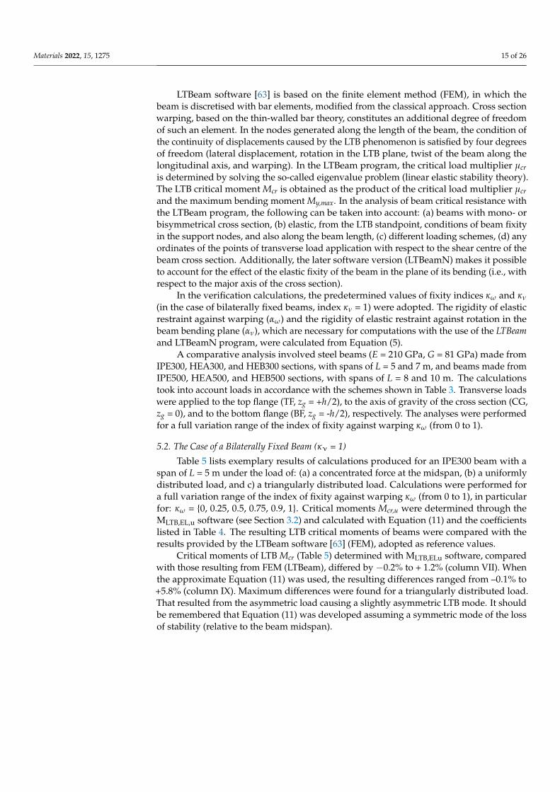
Materials 2022, 15, 1275 15 of 26

LTBeam software [63] is based on the finite element method (FEM), in which thebeam is discretised with bar elements, modified from the classical approach. Cross sectionwarping, based on the thin-walled bar theory, constitutes an additional degree of freedomof such an element. In the nodes generated along the length of the beam, the condition ofthe continuity of displacements caused by the LTB phenomenon is satisfied by four degreesof freedom (lateral displacement, rotation in the LTB plane, twist of the beam along thelongitudinal axis, and warping). In the LTBeam program, the critical load multiplier µcris determined by solving the so-called eigenvalue problem (linear elastic stability theory).The LTB critical moment Mcr is obtained as the product of the critical load multiplier µcrand the maximum bending moment My,max. In the analysis of beam critical resistance withthe LTBeam program, the following can be taken into account: (a) beams with mono- orbisymmetrical cross section, (b) elastic, from the LTB standpoint, conditions of beam fixityin the support nodes, and also along the beam length, (c) different loading schemes, (d) anyordinates of the points of transverse load application with respect to the shear centre of thebeam cross section. Additionally, the later software version (LTBeamN) makes it possibleto account for the effect of the elastic fixity of the beam in the plane of its bending (i.e., withrespect to the major axis of the cross section).

In the verification calculations, the predetermined values of fixity indices κω and κν

(in the case of bilaterally fixed beams, index κν = 1) were adopted. The rigidity of elasticrestraint against warping (αω) and the rigidity of elastic restraint against rotation in thebeam bending plane (αν), which are necessary for computations with the use of the LTBeamand LTBeamN program, were calculated from Equation (5).

A comparative analysis involved steel beams (E = 210 GPa, G = 81 GPa) made fromIPE300, HEA300, and HEB300 sections, with spans of L = 5 and 7 m, and beams made fromIPE500, HEA500, and HEB500 sections, with spans of L = 8 and 10 m. The calculationstook into account loads in accordance with the schemes shown in Table 3. Transverse loadswere applied to the top flange (TF, zg = +h/2), to the axis of gravity of the cross section (CG,zg = 0), and to the bottom flange (BF, zg = -h/2), respectively. The analyses were performedfor a full variation range of the index of fixity against warping κω (from 0 to 1).

5.2. The Case of a Bilaterally Fixed Beam (κν = 1)

Table 5 lists exemplary results of calculations produced for an IPE300 beam with aspan of L = 5 m under the load of: (a) a concentrated force at the midspan, (b) a uniformlydistributed load, and c) a triangularly distributed load. Calculations were performed fora full variation range of the index of fixity against warping κω (from 0 to 1), in particularfor: κω = {0, 0.25, 0.5, 0.75, 0.9, 1}. Critical moments Mcr,u were determined through theMLTB,EL,u software (see Section 3.2) and calculated with Equation (11) and the coefficientslisted in Table 4. The resulting LTB critical moments of beams were compared with theresults provided by the LTBeam software [63] (FEM), adopted as reference values.

Critical moments of LTB Mcr (Table 5) determined with MLTB,ELu software, comparedwith those resulting from FEM (LTBeam), differed by −0.2% to + 1.2% (column VII). Whenthe approximate Equation (11) was used, the resulting differences ranged from –0.1% to+5.8% (column IX). Maximum differences were found for a triangularly distributed load.That resulted from the asymmetric load causing a slightly asymmetric LTB mode. It shouldbe remembered that Equation (11) was developed assuming a symmetric mode of the lossof stability (relative to the beam midspan).

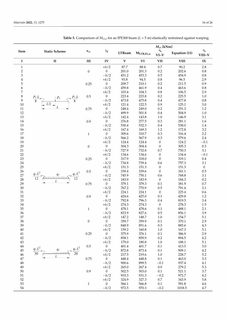
Materials 2022, 15, 1275 16 of 26

Table 5. Comparison of Mcr,u for an IPE300 beam (L = 5 m) elastically restrained against warping.

Item Static Scheme κω zg

Mcr [kNm]

LTBeam MLTB,EL,u%

VI–V Equation (11) %VIII–V

I II III IV V VI VII VIII IX

1



Item Static Scheme κω zg Mcr [kNm]

LTBeam MLTB,EL,u %

VI−V Equation

(11) %

VIII−V I II III IV V VI VII VIII IX 1

0 +h/2 87.7 88.4 0.7 90.2 2.8

2 0 201.0 201.3 0.2 202.6 0.8 3 −h/2 451.2 453.3 0.5 454.9 0.8 4

0.25 +h/2 93.8 94.5 0.8 96.5 2.9

5 0 209.7 210.1 0.2 211.5 0.9 6 −h/2 459.8 461.9 0.4 463.6 0.8 7

0.5 +h/2 103.4 104.3 0.8 106.5 2.9

8 0 223.4 223.8 0.2 225.5 1.0 9 −h/2 473.8 475.8 0.4 477.8 0.8

10 0.75

+h/2 121.4 122.5 0.9 125.1 3.0 11 0 248.4 249.0 0.2 251.3 1.2 12 −h/2 499.9 501.8 0.4 504.9 1.0 13

0.9 +h/2 142.4 143.8 1.0 146.9 3.1

14 0 276.8 277.5 0.3 281.1 1.6 15 −h/2 530.4 532.3 0.4 538.0 1.4 16

1 +h/2 167.4 169.3 1.2 172.8 3.2

17 0 309.6 310.7 0.3 316.4 2.2 18 −h/2 566.2 567.9 0.3 579.6 2.4 19

0 +h/2 124.4 124.4 0 124.2 −0.1

20 0 304.3 304.4 0 305.3 0.3 21 −h/2 727.9 732.8 0.7 750.3 3.1 22

0.25 +h/2 134.6 134.6 0 134.4 −0.1

23 0 317.9 318.0 0 319.1 0.4 24 −h/2 734.8 739.4 0.6 757.3 3.1 25

0.5 +h/2 151.3 151.3 0 151.3 0

26 0 339.4 339.6 0 341.1 0.5 27 −h/2 745.9 750.1 0.6 768.8 3.1 28

0.75 +h/2 183.9 183.9 0 184.3 0.2

29 0 379.1 379.3 0.1 381.9 0.7 30 −h/2 767.2 770.9 0.5 791.4 3.1 31

0.9 +h/2 224.1 224.1 0 225.4 0.6

32 0 424.6 425.0 0.1 429.8 1.2 33 −h/2 792.8 796.3 0.4 819.5 3.4 34

1 +h/2 274.3 274.3 0 278.3 1.5

35 0 478.1 478.6 0.1 488.1 2.1 36 −h/2 823.9 827.6 0.5 856.1 3.9 37

+h/2 147.2 148.7 1.0 154.7 5.1 38 0 0 359.7 359.9 0.1 370.1 2.9 39 −h/2 848.9 851.6 0.3 885.6 4.3 40 +h/2 159.2 160.8 1.0 167.3 5.1 41 0.25 0 375.9 376.1 0.1 386.9 2.9 42 −h/2 858.1 859.9 0.2 894.5 4.2 43 +h/2 179.0 180.8 1.0 188.1 5.1 44 0.5 0 401.4 401.7 0.1 413.5 3.0 45 −h/2 872.8 873.4 0.1 909.1 4.2 46 +h/2 217.5 219.6 1.0 228.7 5.2 47 0.75 0 448.4 448.8 0.1 463.0 3.3 48 −h/2 900.6 899.5 −0.1 937.4 4.1 49 +h/2 265.0 267.4 0.9 279.2 5.3 50 0.9 0 502.5 503.0 0.1 521.1 3.7 51 −h/2 933.3 931.3 −0.2 972.7 4.2

Pz8

Pz L8

Pz L

LL/2

L

qz

12qz L2

12qz L2

L

qz

20qz L2

30qz L2

0+h/2 87.7 88.4 0.7 90.2 2.8

2 0 201.0 201.3 0.2 202.6 0.83 −h/2 451.2 453.3 0.5 454.9 0.84

0.25+h/2 93.8 94.5 0.8 96.5 2.9

5 0 209.7 210.1 0.2 211.5 0.96 −h/2 459.8 461.9 0.4 463.6 0.87

0.5+h/2 103.4 104.3 0.8 106.5 2.9

8 0 223.4 223.8 0.2 225.5 1.09 −h/2 473.8 475.8 0.4 477.8 0.8

100.75

+h/2 121.4 122.5 0.9 125.1 3.011 0 248.4 249.0 0.2 251.3 1.212 −h/2 499.9 501.8 0.4 504.9 1.013

0.9+h/2 142.4 143.8 1.0 146.9 3.1

14 0 276.8 277.5 0.3 281.1 1.615 −h/2 530.4 532.3 0.4 538.0 1.416

1+h/2 167.4 169.3 1.2 172.8 3.2

17 0 309.6 310.7 0.3 316.4 2.218 −h/2 566.2 567.9 0.3 579.6 2.419




LTBeam MLTB,EL,u %

VI−V Equation

(11) %


0 +h/2 87.7 88.4 0.7 90.2 2.8

2 0 201.0 201.3 0.2 202.6 0.8 3 −h/2 451.2 453.3 0.5 454.9 0.8 4

0.25 +h/2 93.8 94.5 0.8 96.5 2.9

5 0 209.7 210.1 0.2 211.5 0.9 6 −h/2 459.8 461.9 0.4 463.6 0.8 7

0.5 +h/2 103.4 104.3 0.8 106.5 2.9

8 0 223.4 223.8 0.2 225.5 1.0 9 −h/2 473.8 475.8 0.4 477.8 0.8

10 0.75

+h/2 121.4 122.5 0.9 125.1 3.0 11 0 248.4 249.0 0.2 251.3 1.2 12 −h/2 499.9 501.8 0.4 504.9 1.0 13

0.9 +h/2 142.4 143.8 1.0 146.9 3.1

14 0 276.8 277.5 0.3 281.1 1.6 15 −h/2 530.4 532.3 0.4 538.0 1.4 16

1 +h/2 167.4 169.3 1.2 172.8 3.2

17 0 309.6 310.7 0.3 316.4 2.2 18 −h/2 566.2 567.9 0.3 579.6 2.4 19

0 +h/2 124.4 124.4 0 124.2 −0.1

20 0 304.3 304.4 0 305.3 0.3 21 −h/2 727.9 732.8 0.7 750.3 3.1 22

0.25 +h/2 134.6 134.6 0 134.4 −0.1

23 0 317.9 318.0 0 319.1 0.4 24 −h/2 734.8 739.4 0.6 757.3 3.1 25

0.5 +h/2 151.3 151.3 0 151.3 0

26 0 339.4 339.6 0 341.1 0.5 27 −h/2 745.9 750.1 0.6 768.8 3.1 28

0.75 +h/2 183.9 183.9 0 184.3 0.2

29 0 379.1 379.3 0.1 381.9 0.7 30 −h/2 767.2 770.9 0.5 791.4 3.1 31

0.9 +h/2 224.1 224.1 0 225.4 0.6

32 0 424.6 425.0 0.1 429.8 1.2 33 −h/2 792.8 796.3 0.4 819.5 3.4 34

1 +h/2 274.3 274.3 0 278.3 1.5

35 0 478.1 478.6 0.1 488.1 2.1 36 −h/2 823.9 827.6 0.5 856.1 3.9 37

+h/2 147.2 148.7 1.0 154.7 5.1 38 0 0 359.7 359.9 0.1 370.1 2.9 39 −h/2 848.9 851.6 0.3 885.6 4.3 40 +h/2 159.2 160.8 1.0 167.3 5.1 41 0.25 0 375.9 376.1 0.1 386.9 2.9 42 −h/2 858.1 859.9 0.2 894.5 4.2 43 +h/2 179.0 180.8 1.0 188.1 5.1 44 0.5 0 401.4 401.7 0.1 413.5 3.0 45 −h/2 872.8 873.4 0.1 909.1 4.2 46 +h/2 217.5 219.6 1.0 228.7 5.2 47 0.75 0 448.4 448.8 0.1 463.0 3.3 48 −h/2 900.6 899.5 −0.1 937.4 4.1 49 +h/2 265.0 267.4 0.9 279.2 5.3 50 0.9 0 502.5 503.0 0.1 521.1 3.7 51 −h/2 933.3 931.3 −0.2 972.7 4.2

Pz8

Pz L8

Pz L

LL/2

L

qz

12qz L2

12qz L2

L

qz

20qz L2

30qz L2

0+h/2 124.4 124.4 0 124.2 −0.1

20 0 304.3 304.4 0 305.3 0.321 −h/2 727.9 732.8 0.7 750.3 3.122

0.25+h/2 134.6 134.6 0 134.4 −0.1

23 0 317.9 318.0 0 319.1 0.424 −h/2 734.8 739.4 0.6 757.3 3.125

0.5+h/2 151.3 151.3 0 151.3 0

26 0 339.4 339.6 0 341.1 0.527 −h/2 745.9 750.1 0.6 768.8 3.128

0.75+h/2 183.9 183.9 0 184.3 0.2

29 0 379.1 379.3 0.1 381.9 0.730 −h/2 767.2 770.9 0.5 791.4 3.131

0.9+h/2 224.1 224.1 0 225.4 0.6

32 0 424.6 425.0 0.1 429.8 1.233 −h/2 792.8 796.3 0.4 819.5 3.434

1+h/2 274.3 274.3 0 278.3 1.5

35 0 478.1 478.6 0.1 488.1 2.136 −h/2 823.9 827.6 0.5 856.1 3.937




LTBeam MLTB,EL,u %

VI−V Equation

(11) %


0 +h/2 87.7 88.4 0.7 90.2 2.8

2 0 201.0 201.3 0.2 202.6 0.8 3 −h/2 451.2 453.3 0.5 454.9 0.8 4

0.25 +h/2 93.8 94.5 0.8 96.5 2.9

5 0 209.7 210.1 0.2 211.5 0.9 6 −h/2 459.8 461.9 0.4 463.6 0.8 7

0.5 +h/2 103.4 104.3 0.8 106.5 2.9

8 0 223.4 223.8 0.2 225.5 1.0 9 −h/2 473.8 475.8 0.4 477.8 0.8

10 0.75

+h/2 121.4 122.5 0.9 125.1 3.0 11 0 248.4 249.0 0.2 251.3 1.2 12 −h/2 499.9 501.8 0.4 504.9 1.0 13

0.9 +h/2 142.4 143.8 1.0 146.9 3.1

14 0 276.8 277.5 0.3 281.1 1.6 15 −h/2 530.4 532.3 0.4 538.0 1.4 16

1 +h/2 167.4 169.3 1.2 172.8 3.2

17 0 309.6 310.7 0.3 316.4 2.2 18 −h/2 566.2 567.9 0.3 579.6 2.4 19

0 +h/2 124.4 124.4 0 124.2 −0.1

20 0 304.3 304.4 0 305.3 0.3 21 −h/2 727.9 732.8 0.7 750.3 3.1 22

0.25 +h/2 134.6 134.6 0 134.4 −0.1

23 0 317.9 318.0 0 319.1 0.4 24 −h/2 734.8 739.4 0.6 757.3 3.1 25

0.5 +h/2 151.3 151.3 0 151.3 0

26 0 339.4 339.6 0 341.1 0.5 27 −h/2 745.9 750.1 0.6 768.8 3.1 28

0.75 +h/2 183.9 183.9 0 184.3 0.2

29 0 379.1 379.3 0.1 381.9 0.7 30 −h/2 767.2 770.9 0.5 791.4 3.1 31

0.9 +h/2 224.1 224.1 0 225.4 0.6

32 0 424.6 425.0 0.1 429.8 1.2 33 −h/2 792.8 796.3 0.4 819.5 3.4 34

1 +h/2 274.3 274.3 0 278.3 1.5

35 0 478.1 478.6 0.1 488.1 2.1 36 −h/2 823.9 827.6 0.5 856.1 3.9 37

+h/2 147.2 148.7 1.0 154.7 5.1 38 0 0 359.7 359.9 0.1 370.1 2.9 39 −h/2 848.9 851.6 0.3 885.6 4.3 40 +h/2 159.2 160.8 1.0 167.3 5.1 41 0.25 0 375.9 376.1 0.1 386.9 2.9 42 −h/2 858.1 859.9 0.2 894.5 4.2 43 +h/2 179.0 180.8 1.0 188.1 5.1 44 0.5 0 401.4 401.7 0.1 413.5 3.0 45 −h/2 872.8 873.4 0.1 909.1 4.2 46 +h/2 217.5 219.6 1.0 228.7 5.2 47 0.75 0 448.4 448.8 0.1 463.0 3.3 48 −h/2 900.6 899.5 −0.1 937.4 4.1 49 +h/2 265.0 267.4 0.9 279.2 5.3 50 0.9 0 502.5 503.0 0.1 521.1 3.7 51 −h/2 933.3 931.3 −0.2 972.7 4.2

Pz8

Pz L8

Pz L

LL/2

L

qz

12qz L2

12qz L2

L

qz

20qz L2

30qz L2

+h/2 147.2 148.7 1.0 154.7 5.138 0 0 359.7 359.9 0.1 370.1 2.939 −h/2 848.9 851.6 0.3 885.6 4.340 +h/2 159.2 160.8 1.0 167.3 5.141 0.25 0 375.9 376.1 0.1 386.9 2.942 −h/2 858.1 859.9 0.2 894.5 4.243 +h/2 179.0 180.8 1.0 188.1 5.144 0.5 0 401.4 401.7 0.1 413.5 3.045 −h/2 872.8 873.4 0.1 909.1 4.246 +h/2 217.5 219.6 1.0 228.7 5.247 0.75 0 448.4 448.8 0.1 463.0 3.348 −h/2 900.6 899.5 −0.1 937.4 4.149 +h/2 265.0 267.4 0.9 279.2 5.350 0.9 0 502.5 503.0 0.1 521.1 3.751 −h/2 933.3 931.3 −0.2 972.7 4.252 +h/2 324.9 327.3 0.7 343.9 5.853 1 0 566.1 566.8 0.1 591.8 4.654 −h/2 972.5 970.3 −0.2 1018.5 4.7

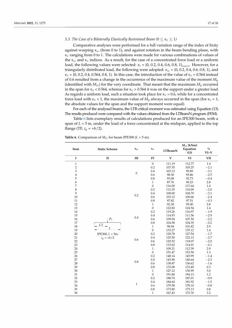
Materials 2022, 15, 1275 17 of 26

5.3. The Case of a Bilaterally Elastically Restrained Beam (0 ≤ κv ≤ 1)

Comparative analyses were performed for a full variation range of the index of fixityagainst warping κω (from 0 to 1), and against rotation in the beam bending plane, withκν ranging from 0 to 1. The calculations were made for various combinations of values ofthe κω and κν indices. As a result, for the case of a concentrated force load or a uniformload, the following values were selected: κi = {0, 0.2, 0.4, 0.6, 0.8, 1}i=ω,v. However, for atriangularly distributed load, the following were adopted: κω = {0, 0.2, 0.4, 0.6, 0.8, 1}, andκv = {0, 0.2, 0.4, 0.564, 0.8, 1}. In this case, the introduction of the value of κv = 0.564 insteadof 0.6 resulted from a change in the occurrence of the maximum value of the moment My(identified with Mcr) for the very coordinate. That meant that the maximum My occurredin the span for κv < 0.564, whereas for κv > 0.564 it was on the support under a greater load.As regards a uniform load, such a situation took place for κv = 0.6, while for a concentratedforce load with κv < 1, the maximum value of My always occurred in the span (for κv = 1,the absolute values for the span and the support moment were equal).

For each of the analysed beams, the LTB critical moment was estimated using Equation (13).The results produced were compared with the values obtained from the LTBeamN program (FEM).

Table 6 lists exemplary results of calculations produced for an IPE300 beam, with aspan of L = 5 m, under the load of a force concentrated at the midspan, applied to the topflange (TF, zg = +h/2).

Table 6. Comparison of Mcr for beam IPE300 (L = 5 m).

Item Static Scheme κω κν

Mcr [kNm]

LTBeamN Equation(13)

%VI–V

I II III IV V VI VII

1


52 +h/2 324.9 327.3 0.7 343.9 5.8 53 1 0 566.1 566.8 0.1 591.8 4.6 54 −h/2 972.5 970.3 −0.2 1018.5 4.7

Critical moments of LTB Mcr (Table 5) determined with MLTB,ELu software, compared with those resulting from FEM (LTBeam), differed by −0.2% to + 1.2% (column VII). When the approximate Equation (11) was used, the resulting differences ranged from –0.1% to + 5.8% (column IX). Maximum differences were found for a triangularly distributed load. That resulted from the asymmetric load causing a slightly asymmetric LTB mode. It should be remembered that Equation (11) was developed assuming a symmetric mode of the loss of stability (relative to the beam midspan).

5.3. The Case of a Bilaterally Elastically Restrained Beam (0 ≤ 𝜅 ≤ 1) Comparative analyses were performed for a full variation range of the index of fixity

against warping κω (from 0 to 1), and against rotation in the beam bending plane, with κν ranging from 0 to 1. The calculations were made for various combinations of values of the κω and κν indices. As a result, for the case of a concentrated force load or a uniform load, the following values were selected: κi = {0, 0.2, 0.4, 0.6, 0.8, 1}i=ω,v. However, for a triangu-larly distributed load, the following were adopted: κω = {0, 0.2, 0.4, 0.6, 0.8, 1}, and κv = {0, 0.2, 0.4, 0.564, 0.8, 1}. In this case, the introduction of the value of κv = 0.564 instead of 0.6 resulted from a change in the occurrence of the maximum value of the moment My (iden-tified with Mcr) for the very coordinate. That meant that the maximum My occurred in the span for κv < 0.564, whereas for κv > 0.564 it was on the support under a greater load. As regards a uniform load, such a situation took place for κv = 0.6, while for a concentrated force load with κv < 1, the maximum value of My always occurred in the span (for κv = 1, the absolute values for the span and the support moment were equal).

For each of the analysed beams, the LTB critical moment was estimated using Equa-tion (13). The results produced were compared with the values obtained from the LTBeamN program (FEM).

Table 6 lists exemplary results of calculations produced for an IPE300 beam, with a span of L = 5 m, under the load of a force concentrated at the midspan, applied to the top flange (TF, zg = +h/2).


Item Static Scheme κω κν Mcr [kNm]

LTBeamN Equation (13) % VI−V

I II III IV V VI VII 1

IPE300, L = 5m zg = +h/2

0

0 111.19 112.77 1.4 2 0.2 107.55 105.25 −2.1 3 0.4 103.13 99.89 −3.1 4 0.6 98.30 95.86 −2.5 5 0.8 93.08 92.73 −0.4 6 1 87.76 90.23 2.8 7

0.2

0 116.00 117.64 1.4 8 0.2 112.35 110.09 −2.0 9 0.4 108.00 104.70 −3.1

10 0.6 103.12 100.66 −2.4 11 0.8 97.82 97.51 −0.3 12 1 92.38 95.00 2.8 13

0.4

0 122.82 124.54 1.4 14 0.2 119.26 116.97 −1.9 15 0.4 114.93 111.56 −2.9 16 0.6 109.94 107.50 −2.2

L

Pz

L/2

IPE300, L = 5mzg = +h/2

0

0 111.19 112.77 1.42 0.2 107.55 105.25 −2.13 0.4 103.13 99.89 −3.14 0.6 98.30 95.86 −2.55 0.8 93.08 92.73 −0.46 1 87.76 90.23 2.87

0.2

0 116.00 117.64 1.48 0.2 112.35 110.09 −2.09 0.4 108.00 104.70 −3.1

10 0.6 103.12 100.66 −2.411 0.8 97.82 97.51 −0.312 1 92.38 95.00 2.813

0.4

0 122.82 124.54 1.414 0.2 119.26 116.97 −1.915 0.4 114.93 111.56 −2.916 0.6 109.94 107.50 −2.217 0.8 104.58 104.35 −0.218 1 98.94 101.82 2.919

0.6

0 133.27 135.12 1.420 0.2 129.78 127.54 −1.721 0.4 125.50 122.13 −2.722 0.6 120.52 118.07 −2.023 0.8 115.02 114.91 −0.124 1 109.21 112.39 2.925

0.8

0 151.47 153.50 1.326 0.2 148.14 145.99 −1.427 0.4 143.90 140.64 −2.328 0.6 138.87 136.62 −1.629 0.8 133.08 133.49 0.330 1 127.12 130.99 3.031

1

0 191.80 194.13 1.232 0.2 188.74 187.01 −0.933 0.4 184.64 181.92 −1.534 0.6 179.58 178.10 −0.835 0.8 173.80 175.13 0.836 1 167.43 172.76 3.2

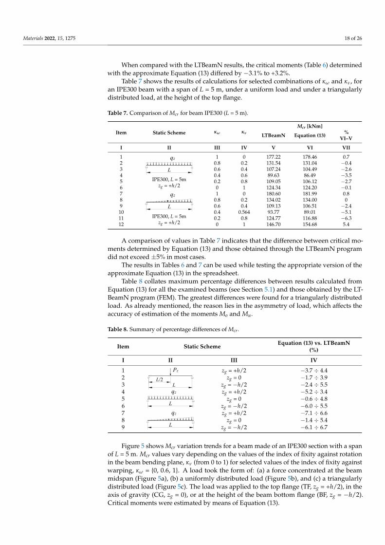
Materials 2022, 15, 1275 18 of 26

When compared with the LTBeamN results, the critical moments (Table 6) determinedwith the approximate Equation (13) differed by −3.1% to +3.2%.

Table 7 shows the results of calculations for selected combinations of κω and κν, foran IPE300 beam with a span of L = 5 m, under a uniform load and under a triangularlydistributed load, at the height of the top flange.


Item Static Scheme κω κν

Mcr [kNm]

LTBeamN Equation (13) %VI–V

I II III IV V VI VII

1


17 0.8 104.58 104.35 −0.2 18 1 98.94 101.82 2.9 19

0.6

0 133.27 135.12 1.4 20 0.2 129.78 127.54 −1.7 21 0.4 125.50 122.13 −2.7 22 0.6 120.52 118.07 −2.0 23 0.8 115.02 114.91 −0.1 24 1 109.21 112.39 2.9 25

0.8

0 151.47 153.50 1.3 26 0.2 148.14 145.99 −1.4 27 0.4 143.90 140.64 −2.3 28 0.6 138.87 136.62 −1.6 29 0.8 133.08 133.49 0.3 30 1 127.12 130.99 3.0 31

1

0 191.80 194.13 1.2 32 0.2 188.74 187.01 −0.9 33 0.4 184.64 181.92 −1.5 34 0.6 179.58 178.10 −0.8 35 0.8 173.80 175.13 0.8 36 1 167.43 172.76 3.2

When compared with the LTBeamN results, the critical moments (Table 6) deter-mined with the approximate Equation (13) differed by –3.1% to +3.2%.

Table 7 shows the results of calculations for selected combinations of κω and κν, for an IPE300 beam with a span of L = 5 m, under a uniform load and under a triangularly distributed load, at the height of the top flange.


Item Static scheme κω κν Mcr [kNm]



IPE300, L = 5m zg = +h/2

1 0 177.22 178.46 0.7 2 0.8 0.2 131.54 131.04 −0.4 3 0.6 0.4 107.24 104.49 −2.6 4 0.4 0.6 89.63 86.49 −3.5 5 0.2 0.8 109.05 106.12 −2.7 6 0 1 124.34 124.20 −0.1 7

IPE300, L = 5m zg = +h/2

1 0 180.60 181.99 0.8 8 0.8 0.2 134.02 134.00 0 9 0.6 0.4 109.13 106.51 −2.4

10 0.4 0.564 93.77 89.01 −5.1 11 0.2 0.8 124.77 116.88 −6.3 12 0 1 146.70 154.68 5.4

A comparison of values in Table 7 indicates that the difference between critical mo-ments determined by Equation (13) and those obtained through the LTBeamN program did not exceed ±5% in most cases.

The results in Tables 6 and 7 can be used while testing the appropriate version of the approximate Equation (13) in the spreadsheet.

Table 8 collates maximum percentage differences between results calculated from Equation (13) for all the examined beams (see Section 5.1) and those obtained by the LTBeamN program (FEM). The greatest differences were found for a triangularly distrib-uted load. As already mentioned, the reason lies in the asymmetry of load, which affects the accuracy of estimation of the moments Mo and Mu.

L

qz

L

qz

IPE300, L = 5mzg = +h/2

1 0 177.22 178.46 0.72 0.8 0.2 131.54 131.04 −0.43 0.6 0.4 107.24 104.49 −2.64 0.4 0.6 89.63 86.49 −3.55 0.2 0.8 109.05 106.12 −2.76 0 1 124.34 124.20 −0.17


17 0.8 104.58 104.35 −0.2 18 1 98.94 101.82 2.9 19

0.6

0 133.27 135.12 1.4 20 0.2 129.78 127.54 −1.7 21 0.4 125.50 122.13 −2.7 22 0.6 120.52 118.07 −2.0 23 0.8 115.02 114.91 −0.1 24 1 109.21 112.39 2.9 25

0.8

0 151.47 153.50 1.3 26 0.2 148.14 145.99 −1.4 27 0.4 143.90 140.64 −2.3 28 0.6 138.87 136.62 −1.6 29 0.8 133.08 133.49 0.3 30 1 127.12 130.99 3.0 31

1

0 191.80 194.13 1.2 32 0.2 188.74 187.01 −0.9 33 0.4 184.64 181.92 −1.5 34 0.6 179.58 178.10 −0.8 35 0.8 173.80 175.13 0.8 36 1 167.43 172.76 3.2

When compared with the LTBeamN results, the critical moments (Table 6) deter-mined with the approximate Equation (13) differed by –3.1% to +3.2%.

Table 7 shows the results of calculations for selected combinations of κω and κν, for an IPE300 beam with a span of L = 5 m, under a uniform load and under a triangularly distributed load, at the height of the top flange.


Item Static scheme κω κν Mcr [kNm]



IPE300, L = 5m zg = +h/2

1 0 177.22 178.46 0.7 2 0.8 0.2 131.54 131.04 −0.4 3 0.6 0.4 107.24 104.49 −2.6 4 0.4 0.6 89.63 86.49 −3.5 5 0.2 0.8 109.05 106.12 −2.7 6 0 1 124.34 124.20 −0.1 7

IPE300, L = 5m zg = +h/2

1 0 180.60 181.99 0.8 8 0.8 0.2 134.02 134.00 0 9 0.6 0.4 109.13 106.51 −2.4

10 0.4 0.564 93.77 89.01 −5.1 11 0.2 0.8 124.77 116.88 −6.3 12 0 1 146.70 154.68 5.4

A comparison of values in Table 7 indicates that the difference between critical mo-ments determined by Equation (13) and those obtained through the LTBeamN program did not exceed ±5% in most cases.

The results in Tables 6 and 7 can be used while testing the appropriate version of the approximate Equation (13) in the spreadsheet.

Table 8 collates maximum percentage differences between results calculated from Equation (13) for all the examined beams (see Section 5.1) and those obtained by the LTBeamN program (FEM). The greatest differences were found for a triangularly distrib-uted load. As already mentioned, the reason lies in the asymmetry of load, which affects the accuracy of estimation of the moments Mo and Mu.

L

qz

L

qz

IPE300, L = 5mzg = +h/2

1 0 180.60 181.99 0.88 0.8 0.2 134.02 134.00 09 0.6 0.4 109.13 106.51 −2.410 0.4 0.564 93.77 89.01 −5.111 0.2 0.8 124.77 116.88 −6.312 0 1 146.70 154.68 5.4

A comparison of values in Table 7 indicates that the difference between critical mo-ments determined by Equation (13) and those obtained through the LTBeamN programdid not exceed ±5% in most cases.

The results in Tables 6 and 7 can be used while testing the appropriate version of theapproximate Equation (13) in the spreadsheet.

Table 8 collates maximum percentage differences between results calculated fromEquation (13) for all the examined beams (see Section 5.1) and those obtained by the LT-BeamN program (FEM). The greatest differences were found for a triangularly distributedload. As already mentioned, the reason lies in the asymmetry of load, which affects theaccuracy of estimation of the moments Mo and Mu.

Table 8. Summary of percentage differences of Mcr.

Item Static Scheme Equation (13) vs. LTBeamN(%)

I II III IV

1



Item Static Scheme Equation (13) vs.

LTBeamN (%)

I II III IV 1

zg = +h/2 −3.7 ÷ 4.4 2 zg = 0 −1.7 ÷ 3.9 3 zg = –h/2 −2.4 ÷ 5.5 4

zg = +h/2 −5.2 ÷ 3.4 5 zg = 0 −0.6 ÷ 4.8 6 zg = –h/2 −6.0 ÷ 5.5 7

zg = +h/2 −7.1 ÷ 6.6 8 zg = 0 −1.4 ÷ 5.4 9 zg = –h/2 −6.1 ÷ 6.7

Figure 5 shows Mcr variation trends for a beam made of an IPE300 section with a span of L = 5 m. Mcr values vary depending on the values of the index of fixity against rotation in the beam bending plane, κν (from 0 to 1) for selected values of the index of fixity against warping, κω = {0, 0.6, 1}. A load took the form of: (a) a force concentrated at the beam midspan (Figure 5a), (b) a uniformly distributed load (Figure 5b), and (c) a triangularly distributed load (Figure 5c). The load was applied to the top flange (TF, zg = +h/2), in the axis of gravity (CG, zg = 0), or at the height of the beam bottom flange (BF, zg = −h/2). Critical moments were estimated by means of Equation (13).

L

Pz

L/2

L

qz

L

qz

zg = +h/2 −3.7 ÷ 4.42 zg = 0 −1.7 ÷ 3.93 zg = −h/2 −2.4 ÷ 5.54




LTBeamN (%)

I II III IV 1

zg = +h/2 −3.7 ÷ 4.4 2 zg = 0 −1.7 ÷ 3.9 3 zg = –h/2 −2.4 ÷ 5.5 4

zg = +h/2 −5.2 ÷ 3.4 5 zg = 0 −0.6 ÷ 4.8 6 zg = –h/2 −6.0 ÷ 5.5 7

zg = +h/2 −7.1 ÷ 6.6 8 zg = 0 −1.4 ÷ 5.4 9 zg = –h/2 −6.1 ÷ 6.7


L

Pz

L/2

L

qz

L

qz

zg = +h/2 −5.2 ÷ 3.45 zg = 0 −0.6 ÷ 4.86 zg = −h/2 −6.0 ÷ 5.57




LTBeamN (%)

I II III IV 1

zg = +h/2 −3.7 ÷ 4.4 2 zg = 0 −1.7 ÷ 3.9 3 zg = –h/2 −2.4 ÷ 5.5 4

zg = +h/2 −5.2 ÷ 3.4 5 zg = 0 −0.6 ÷ 4.8 6 zg = –h/2 −6.0 ÷ 5.5 7

zg = +h/2 −7.1 ÷ 6.6 8 zg = 0 −1.4 ÷ 5.4 9 zg = –h/2 −6.1 ÷ 6.7


L

Pz

L/2

L

qz

L

qz zg = +h/2 −7.1 ÷ 6.68 zg = 0 −1.4 ÷ 5.49 zg = −h/2 −6.1 ÷ 6.7

Figure 5 shows Mcr variation trends for a beam made of an IPE300 section with a spanof L = 5 m. Mcr values vary depending on the values of the index of fixity against rotationin the beam bending plane, κν (from 0 to 1) for selected values of the index of fixity againstwarping, κω = {0, 0.6, 1}. A load took the form of: (a) a force concentrated at the beammidspan (Figure 5a), (b) a uniformly distributed load (Figure 5b), and (c) a triangularlydistributed load (Figure 5c). The load was applied to the top flange (TF, zg = +h/2), in theaxis of gravity (CG, zg = 0), or at the height of the beam bottom flange (BF, zg = −h/2).Critical moments were estimated by means of Equation (13).

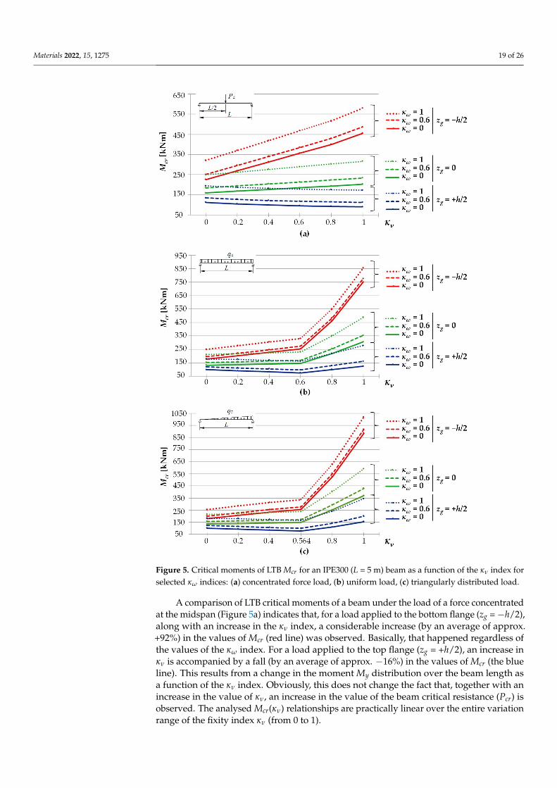
Materials 2022, 15, 1275 19 of 26Materials 2022, 15, x FOR PEER REVIEW 20 of 27

Figure 5. Critical moments of LTB Mcr for an IPE300 (L = 5 m) beam as a function of the κν index for selected κω indices: (a) concentrated force load, (b) uniform load, (c) triangularly distributed load.

A comparison of LTB critical moments of a beam under the load of a force concen-trated at the midspan (Figure 5a) indicates that, for a load applied to the bottom flange (zg = −h/2), along with an increase in the κν index, a considerable increase (by an average of approx. +92%) in the values of Mcr (red line) was observed. Basically, that happened re-gardless of the values of the κω index. For a load applied to the top flange (zg = +h/2), an increase in κν is accompanied by a fall (by an average of approx. −16%) in the values of Mcr (the blue line). This results from a change in the moment My distribution over the beam length as a function of the κν index. Obviously, this does not change the fact that, together with an increase in the value of κν, an increase in the value of the beam critical resistance (Pcr) is observed. The analysed Mcr(κν) relationships are practically linear over the entire variation range of the fixity index κν (from 0 to 1).

Figure 5. Critical moments of LTB Mcr for an IPE300 (L = 5 m) beam as a function of the κν index forselected κω indices: (a) concentrated force load, (b) uniform load, (c) triangularly distributed load.

A comparison of LTB critical moments of a beam under the load of a force concentratedat the midspan (Figure 5a) indicates that, for a load applied to the bottom flange (zg =−h/2),along with an increase in the κν index, a considerable increase (by an average of approx.+92%) in the values of Mcr (red line) was observed. Basically, that happened regardless ofthe values of the κω index. For a load applied to the top flange (zg = +h/2), an increase inκν is accompanied by a fall (by an average of approx. −16%) in the values of Mcr (the blueline). This results from a change in the moment My distribution over the beam length asa function of the κν index. Obviously, this does not change the fact that, together with anincrease in the value of κν, an increase in the value of the beam critical resistance (Pcr) isobserved. The analysed Mcr(κν) relationships are practically linear over the entire variationrange of the fixity index κν (from 0 to 1).

Materials 2022, 15, 1275 20 of 26

With respect to a beam under a uniform load (Figure 5b), generally bilinear Mcr(κν)relationships were noted, with a kink in the curve for κν = 0.6 (the graph is slightly nonlinearonly in the case of zg =−h/2 in a range of 0.6 < κν < 1). As already mentioned, for κν = 0.6, achange in the site of the maximum moment My occurrence is observed. Within the variationrange of the fixity index κν from 0 to 0.6, for a load applied to the bottom flange (zg =−h/2),an increase (by an average of approx. +38%) in the values of the critical moment (thered line) was found. However, for a load applied to the top flange (zg = +h/2), a fall(by an average of approx. −18%) in the moment Mcr (the blue line) is seen. Like for theconcentrated force load, the effect is caused by a change in the moment My distributionover the beam length as a function of the κν index. Also in this case, the value of the beamcritical resistance (qcr) grows with an increase in the values of κν (see Figure 4). However,in a range of 0.6 < κν < 1, an increase in the κν index is accompanied by an increase in Mcrexpressed as a function of the index of elastic restraint against warping κω (the largest onefor zg = −h/2). When the rotation in the beam bending plane (κν = 1) was fully prevented,the resulting increase in Mcr ranged from approx. +26% (κω = 0, zg = +h/2) to approx.+324% (κω = 0, zg = −h/2) compared with complete freedom of rotation (κν = 0).

With respect to a beam under a triangularly distributed load (Figure 5c), as was thecase with a beam under a uniform load (see Figure 5b), the resulting Mcr(κν) relationshipswere basically bilinear, with a kink in the curves at κν = 0.564. However, in this case, amore rapid increase in Mcr was observed above this point. Within a range of variation ofthe fixity index κν from 0 to 0.564 (Figure 5c), for a load applied to the top flange (the blueline), a fall in the Mcr values was noted. It was comparable to fall in the Mcr values underthe uniform load (cf. Figure 5b). When a load was applied to the bottom flange (the redline), an increase in Mcr could be seen (Figure 5b). Full prevention of rotation in the beambending plane (κν = 1), in contrast to its complete freedom (κν = 0), resulted in an increasein Mcr from approx. +53% (κω = 0, zg = +h/2) to approx. +391% (κω = 0, zg = −h/2).

Figure 6 shows the trends in variation in LTB critical moments Mcr of the beam withgeometrical parameters as per Figure 5. LTB critical moments varied depending on thevalues of the index of fixity against warping κω (from 0 to 1). In Figure 6a,b, the variationwas shown for selected values of the index of fixity against rotation in the beam bendingplane, κν = {0, 0.6, 1}, and in Figure 6c κν = {0, 0.564, 1}. Critical moments of the beam wereestimated by Equation (13). The Mcr(κω) relationships were slightly nonlinear over theentire variation range of the fixity index κω (from 0 to 1). It should be noted that, to increasethe clarity of the Mcr(κω) graphs, in Figure 6b,c it was decided not to show cases for κν = 1at zg = −h/2, since their values greatly exceeded Mcr for the remaining curves. In this case,for a uniform load, the Mcr graph ranged from approx. 750 to approx. 860 kNm, and for atriangularly distributed load the range was from approx. 880 to approx. 1020 kNm.


Figure 6. Critical moments of LTB for an IPE300 (L = 5 m) beam as a function of the κω index for selected values of the κν index: (a) concentrated force load, (b) uniform load, (c) triangular load.

Figure 7 shows a comparison of the variation trends in LTB critical moments Mcr of the beam, determined by the LTBeamN program (the solid line) and calculated with Equa-tion (13) (the broken line), depending on the index of fixity against rotation in the beam bending plane κν (from 0 to 1), for the index of fixity against warping κω = 0.6 and the ordinate of the applied load zg = +h/2.

Figure 6. Cont.

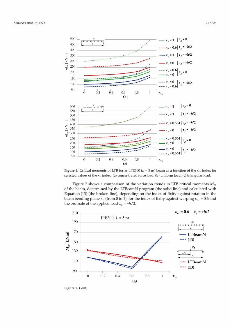
Materials 2022, 15, 1275 21 of 26


Figure 6. Critical moments of LTB for an IPE300 (L = 5 m) beam as a function of the κω index for selected values of the κν index: (a) concentrated force load, (b) uniform load, (c) triangular load.

Figure 7 shows a comparison of the variation trends in LTB critical moments Mcr of the beam, determined by the LTBeamN program (the solid line) and calculated with Equa-tion (13) (the broken line), depending on the index of fixity against rotation in the beam bending plane κν (from 0 to 1), for the index of fixity against warping κω = 0.6 and the ordinate of the applied load zg = +h/2.

Figure 6. Critical moments of LTB for an IPE300 (L = 5 m) beam as a function of the κω index forselected values of the κν index: (a) concentrated force load, (b) uniform load, (c) triangular load.

Figure 7 shows a comparison of the variation trends in LTB critical moments Mcrof the beam, determined by the LTBeamN program (the solid line) and calculated withEquation (13) (the broken line), depending on the index of fixity against rotation in thebeam bending plane κν (from 0 to 1), for the index of fixity against warping κω = 0.6 andthe ordinate of the applied load zg = +h/2.


Figure 7. Comparison of graphs showing the variation in LTB critical moments Mcr, determined by LTBeamN program and calculated with Equation (13): (a) a concentrated force load and a uniform load; (b) a triangularly distributed load.

The exemplary graphs of Mcr variation (LTBeamN vs. Equation (13)) shown in Figure 7 have very similar shapes. The most noticeable discrepancy was found for a beam under a triangularly distributed load (see Figure 7b) for the fixity index κν ranging from 0.4 to 0.8 and for κν = 1. In that case, the maximum percentage differences in the results did not exceed ±6%.

5.4. Example of Calculations The application of the approximate equations developed in the study is shown in the

example. The procedure for solving the problem is illustrated by the consecutive steps of calculations.

Problem. A steel beam with an IPE 300 cross section (Iy = 8360 cm4, Iz = 604 cm4, It = 20.7 cm4, Iω = 125,900 cm6) and a span of L = 6 m, is loaded by uniform forces applied to the top flange (h/2 = 15 cm). The rigidities of the beam elastic restraint in the support nodes are: (a) rigidity against warping: αω = 27.9 kNm3/rad, (b) rigidity against rotation in the bending plane: αν = 53,320 kNm/rad. Determine the LTB critical moment for the beam, Mcr.

Solution. 1. Calculation of elastic restraint indices of the beam: (a) against warping according to

Equation (1): κω = 0.76; (b) against rotation in the bending plane according to Equation (3): κν = 0.82;

2. The critical moment Mo of a beam simply supported against bending relative to the axis of higher rigidity (κν = 0), and elastically restrained against warping (κω = 0.76), was calculated from Equation (11) and Table 3 (row 2): Mo = 101.51 kNm;

Figure 7. Cont.

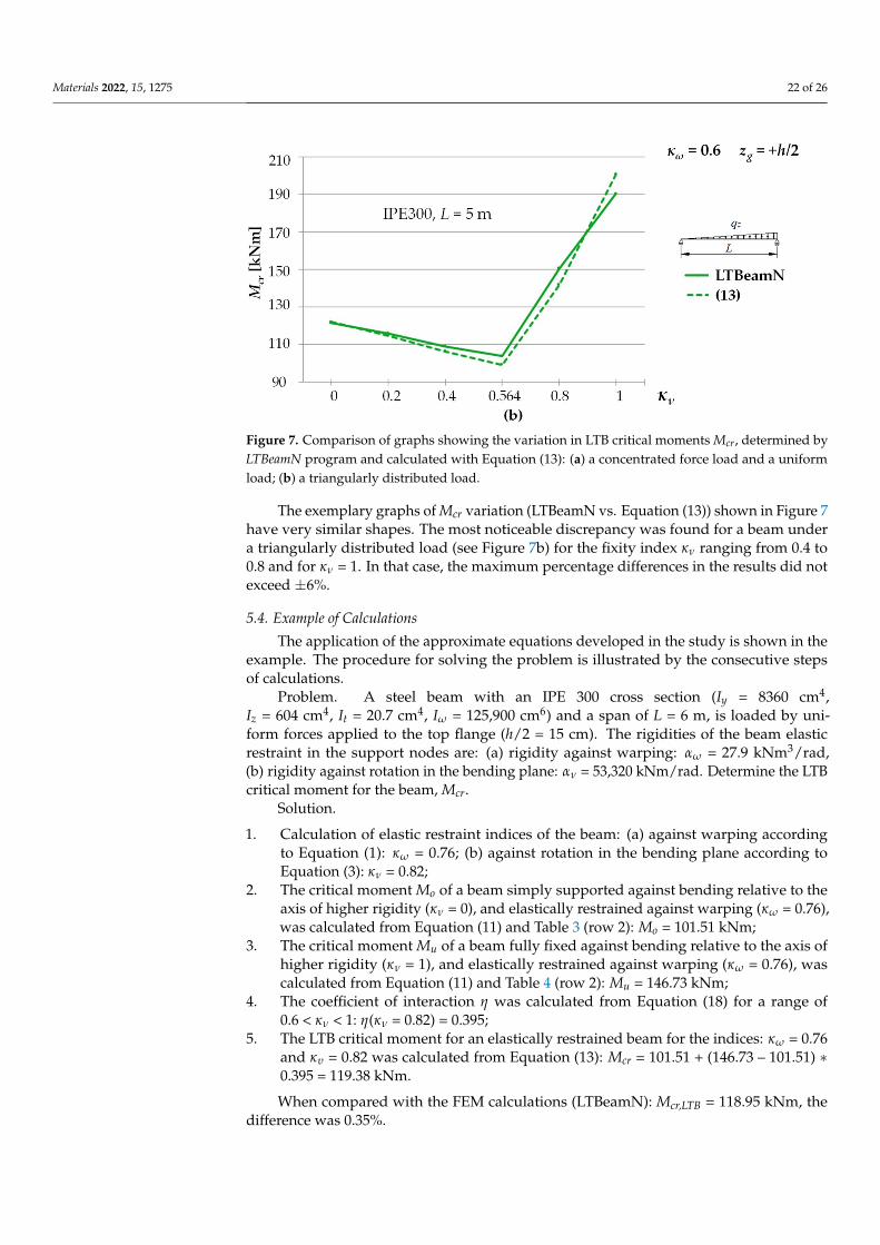
Materials 2022, 15, 1275 22 of 26


Figure 7. Comparison of graphs showing the variation in LTB critical moments Mcr, determined by LTBeamN program and calculated with Equation (13): (a) a concentrated force load and a uniform load; (b) a triangularly distributed load.

The exemplary graphs of Mcr variation (LTBeamN vs. Equation (13)) shown in Figure 7 have very similar shapes. The most noticeable discrepancy was found for a beam under a triangularly distributed load (see Figure 7b) for the fixity index κν ranging from 0.4 to 0.8 and for κν = 1. In that case, the maximum percentage differences in the results did not exceed ±6%.

5.4. Example of Calculations The application of the approximate equations developed in the study is shown in the

example. The procedure for solving the problem is illustrated by the consecutive steps of calculations.

Problem. A steel beam with an IPE 300 cross section (Iy = 8360 cm4, Iz = 604 cm4, It = 20.7 cm4, Iω = 125,900 cm6) and a span of L = 6 m, is loaded by uniform forces applied to the top flange (h/2 = 15 cm). The rigidities of the beam elastic restraint in the support nodes are: (a) rigidity against warping: αω = 27.9 kNm3/rad, (b) rigidity against rotation in the bending plane: αν = 53,320 kNm/rad. Determine the LTB critical moment for the beam, Mcr.

Solution. 1. Calculation of elastic restraint indices of the beam: (a) against warping according to

Equation (1): κω = 0.76; (b) against rotation in the bending plane according to Equation (3): κν = 0.82;

2. The critical moment Mo of a beam simply supported against bending relative to the axis of higher rigidity (κν = 0), and elastically restrained against warping (κω = 0.76), was calculated from Equation (11) and Table 3 (row 2): Mo = 101.51 kNm;

Figure 7. Comparison of graphs showing the variation in LTB critical moments Mcr, determined byLTBeamN program and calculated with Equation (13): (a) a concentrated force load and a uniformload; (b) a triangularly distributed load.

The exemplary graphs of Mcr variation (LTBeamN vs. Equation (13)) shown in Figure 7have very similar shapes. The most noticeable discrepancy was found for a beam undera triangularly distributed load (see Figure 7b) for the fixity index κν ranging from 0.4 to0.8 and for κν = 1. In that case, the maximum percentage differences in the results did notexceed ±6%.

5.4. Example of Calculations

The application of the approximate equations developed in the study is shown in theexample. The procedure for solving the problem is illustrated by the consecutive stepsof calculations.

Problem. A steel beam with an IPE 300 cross section (Iy = 8360 cm4,Iz = 604 cm4, It = 20.7 cm4, Iω = 125,900 cm6) and a span of L = 6 m, is loaded by uni-form forces applied to the top flange (h/2 = 15 cm). The rigidities of the beam elasticrestraint in the support nodes are: (a) rigidity against warping: αω = 27.9 kNm3/rad,(b) rigidity against rotation in the bending plane: αν = 53,320 kNm/rad. Determine the LTBcritical moment for the beam, Mcr.

Solution.

1. Calculation of elastic restraint indices of the beam: (a) against warping accordingto Equation (1): κω = 0.76; (b) against rotation in the bending plane according toEquation (3): κν = 0.82;

2. The critical moment Mo of a beam simply supported against bending relative to theaxis of higher rigidity (κν = 0), and elastically restrained against warping (κω = 0.76),was calculated from Equation (11) and Table 3 (row 2): Mo = 101.51 kNm;

3. The critical moment Mu of a beam fully fixed against bending relative to the axis ofhigher rigidity (κν = 1), and elastically restrained against warping (κω = 0.76), wascalculated from Equation (11) and Table 4 (row 2): Mu = 146.73 kNm;

4. The coefficient of interaction η was calculated from Equation (18) for a range of0.6 < κν < 1: η(κν = 0.82) = 0.395;

5. The LTB critical moment for an elastically restrained beam for the indices: κω = 0.76and κυ = 0.82 was calculated from Equation (13): Mcr = 101.51 + (146.73 – 101.51) ∗0.395 = 119.38 kNm.

When compared with the FEM calculations (LTBeamN): Mcr,LTB = 118.95 kNm, thedifference was 0.35%.

Materials 2022, 15, 1275 23 of 26

6. Conclusions

When taking into account the actual beam boundary conditions in the support nodes,which include elastic restraint against warping and elastic restraint against rotation in thebeam bending plane, it is possible to calculate the critical moment precisely. Consequently,the LTB reduction factor and the beam design resistance can be determined more accurately.That points to the optimal design of this class of steel members.

Based on the results, it can be concluded that, from a technical standpoint, the LTBcritical moments expressed as a function of the κω index, calculated with Equation (11) [52]and the coefficients in Table 3 (for a simply supported beam—Mo), and the coefficientsin Table 4, proposed in this study (for a bilaterally fixed beam—Mu), provide sufficientapproximation compared with FEM. Therefore, Mcr for elastically restrained beams in thesupport nodes (κω, κν) can be estimated on the basis of Equation (13).

A comparison of critical moments (Tables 6–8), estimated by Equation (13) and ob-tained from the LTBeamN program (FEM), showed very good congruence with the resultsfrom an engineering standpoint. Critical loads were determined for: (1) different fixityindices (κω, κν) ranging from 0 to 1, (2) various (characteristic) points of transverse loadapplication (top flange, axis of gravity of the cross section, bottom flange).

For a given value of the index of fixity against rotation in the beam bending plane(κν), an increase in the index of fixity against warping (κω) leads to an increase in the LTBcritical moment. For example, for the beam shown in Figure 6a, for κω = 1, the increasein the critical moment ranged from approx. +27% (for zg = −h/2) to approx. +91% (forzg = h/2) compared with complete freedom of warping (κω = 0).

However, for a given value of the index of fixity against warping (κω), an increase inthe index of fixity against rotation in the bending plane (κν) caused an increase in the beamcritical resistance, measured by the respective critical load (Pcr, qcr, qTcr).

The effect of an apparent fall in the critical moment value, which occurs for beamsunder a load applied at the height of the top flange, resulted from changes in the distributionof My expressed as a function of κν (see Figure 4). This effect was not observed when a loadwas applied at the cross section centre of gravity, or when the beams were under a loadapplied at the height of the bottom flange.

For example, when the beam was under the load of a force concentrated at the midspan(Figure 5a), an increase in the values of κν at zg = −h/2 was accompanied by an increase inMcr (by an average of approx. 92%). That translated into an increase in the critical resistancePcr by an average of approx. 284%. Conversely, for zg = +h/2, in spite of a fall in the criticalmoment values (by an average of approx. 16% for κν =1), an increase in Pcr by an averageof approx. 68% was noted, compared with complete freedom of rotation (κν = 0).

As regards a beam under a uniform load, for κν from 0.6 to 1 (Figure 5b), and a beamunder a triangularly distributed load, for κν from 0.564 to 1 (Figure 5c), and any value ofκω from a range of (0–1), the result showed a considerable increase in the values of Mcrand critical load of the beam. However, within a variation range of the fixity index κν from0 to 0.6 (Figure 5b) and from 0 to 0.564 (Figure 5c), an increase (by an average of approx.+38%, zg = −h/2) or a fall (by an average of approx. −18%, zg = +h/2) in the values of thecritical moment was observed, compared with complete freedom of rotation (κν = 0). Also,for these beam loading schemes at zg = +h/2 (similar to the case of a concentrated forceload), with the increase in κν, the beam critical resistance grew, in spite of the formal dropin the values of Mcr. The effect can be seen in Figure 4. Complete prevention of rotationin the beam bending plane (κν = 1), compared with complete freedom of rotation (κν = 0),resulted in an increase in Mcr from approx. +26% (κω = 0, zg = +h/2) to approx. +324%(κω = 0, zg = −h/2) (see Figure 5b), and from approx. +53% (κω = 0, zg = +h/2) to approx.+391% (κω = 0, zg = −h/2).

Taking into account a more precise description of the boundary conditions of beams withrespect to fork support is a logical development in the modern design of steel structures.

Equations (11) and (13) can be applied to preliminary selection of the section andalso, in many technically important cases, to principal design. The equations can also

Materials 2022, 15, 1275 24 of 26

be used to verify Mcr calculations with FEM software. Such verification will be helpfulfor less experienced designers. It can be employed to make necessary corrections, e.g., oferrors in the specification of beam boundary conditions in the FEM programs. The majoradvantage of the adopted approach is that a steel structure reliability is already enhancedat the planning stage.

Author Contributions: Conceptualization, A.S. and R.P.; methodology, A.S. and R.P.; software, R.P.;validation, R.P. and A.S.; formal analysis, R.P. and A.S.; investigation, R.P. and A.S.; writing—originaldraft preparation, R.P. and A.S.; writing—review and editing, A.S.; visualization, R.P. All authorshave read and agreed to the published version of the manuscript.

Funding: The work is supported by the program of the Minister of Science and Higher Educationunder the name: Regional Initiative of Excellence in 2019–2022 project number 025/RID/2018/19financing amount PLN 12.000.000.

Institutional Review Board Statement: Not applicable.

Informed Consent Statement: Not applicable.

Conflicts of Interest: The authors declare no conflict of interest.

References1. Bijak, R. Critical Moment for Lateral Torsional Buckling of Unbraced Bisymmetric I-Beams with Fork Support. In Proceedings of the

XII International Scientific and Technical Conference Metal Structures, Wrocław, Poland, 15–17 June 2011; pp. 144–151. (In Polish)2. Lim, N.H.; Park, N.H.; Kang, Y.J.; Sung, I.H. Elastic buckling of I-beams under linear moment gradient. Int. J. Solids Struct. 2003,

40, 5635–5647. [CrossRef]3. López, A.; Yong, D.J.; Serna, M.A. Lateral-torsional buckling of steel beams: A general expression for the moment gradient factor. In

Proceedings of the International Colloquium on Stability and Ductility of Steel Structures, Lisbon, Portugal, 6–8 September 2006.4. Mohri, F.; Damil, N.; Potier-Ferry, M. Linear and non-linear stability analyses of thin-walled beams with monosymmetric I

sections. Thin-Walled Struct. 2010, 48, 299–315. [CrossRef]5. Serna, M.A.; López, A.; Puente, I.; Yong, D.J. Equivalent uniform moment factors for lateral-torsional buckling of steel members.

J. Constr. Steel Res. 2006, 62, 566–580. [CrossRef]6. Trahair, N.S.; Bradford, M.A.; Nethercot, D.A.; Gardner, L. The Behavior and Design of Steel Structures to EC3, 4th ed.;

Taylor & Francis: London, UK, 2008.7. Bijak, R. The lateral buckling of simply supported unrestrained bisymmetric I-shape beams. Arch. Civ. Eng. 2015, 61, 127–140.

[CrossRef]8. Mohri, F.; Brouki, A.; Roth, J.C. Theoretical and numerical stability analyses of unrestrained, mono symmetric thin-walled beams.

J. Constr. Steel Res. 2003, 59, 63–90. [CrossRef]9. Timoshenko, S.P.; Gere, J.M. Theory of Elastic Stability, 2nd ed.; McGraw-Hill: New York, NY, USA, 1961.10. Weiss, S.; Gizejowski, M. Stability of Metal Structures. Rod Systems, 1st ed.; Arkady: Warszawa, Poland, 1991. (In Polish)11. Valentino, J.; Trahair, N.S. Torsional Restraint against Elastic Lateral Buckling. J. Struct. Eng. 1998, 124, 1217–1225. [CrossRef]12. Yura, J. Fundamentals of beam bracing. Eng. J. 2001, 38, 11–26.13. Gosowski, B. Non-uniform torsion of stiffened open thin-walled members of steel structures. J. Constr. Steel Res. 2007, 63, 849–865.

[CrossRef]14. Gosowski, B.; Redecki, M. Lateral-torsional buckling moments for I-beams with local lateral restraints. Inz. Bud. 2012, 68, 140–144.

(In Polish)15. Lee, H.E.; Nguyen, C.T.; Moon, J.H.; Joo, H.S. Lateral-torsional buckling of discretely-braced i-girder. Procedia Eng. 2011, 14,

264–271. [CrossRef]16. Stroetmann, R. Lateral torsional and distortional buckling of cross-connected beams. In Proceedings of the 8th International

Conference on Advances in Steel Structures, Lisbon, Portugal, 21–24 July 2015.17. Piotrowski, R.; Siedlecka, M. Point Protection of Primary Beams of Steel Grillages Against Lateral Torsional Buckling. Adv. Sci.

Technol. Res. J. 2020, 14, 1–8. [CrossRef]18. Nguyen, C.T.; Moon, J.; Le, V.N.; Lee, H.E. Lateral–torsional buckling of I-girders with discrete torsional bracings. J. Constr. Steel

Res. 2010, 66, 170–177. [CrossRef]19. Beyer, A.; Bureau, A. Simplified method for lateral-torsional buckling of beams with lateral restraints. Steel Constr. 2019, 12,

318–326. [CrossRef]20. Lindner, J. Influence of constructional details on the load carrying capacity of beams. Eng. Struct. 1996, 18, 752–758. [CrossRef]21. Bijak, R.; Brzezinska, K. Reduction in the Critical Moment for Lateral Torsional Buckling of Coped Beams. Appl. Mech. Mater.

2015, 797, 3–10. [CrossRef]

http://doi.org/10.1016/S0020-7683(03)00330-5

http://doi.org/10.1016/j.tws.2009.12.002

http://doi.org/10.1016/j.jcsr.2005.09.001

http://doi.org/10.1515/ace-2015-0040

http://doi.org/10.1016/S0143-974X(02)00007-X

http://doi.org/10.1061/(ASCE)0733-9445(1998)124:10(1217)


http://doi.org/10.1016/j.proeng.2011.07.032

http://doi.org/10.12913/22998624/121532


http://doi.org/10.1002/stco.201900039

http://doi.org/10.1016/0141-0296(95)00111-5

http://doi.org/10.4028/www.scientific.net/AMM.797.3

Materials 2022, 15, 1275 25 of 26

22. Maljaars, J.; Stark, J.W.B.; Steenbergen, H.M.G.M. Buckling of coped steel beams and steel beams with partial endplates. HERON2004, 49, 233–271.

23. Gizejowski, M. Lateral buckling of steel beams with limited rotation ability at supports. Inz. Bud. 2001, 10, 589–594. (In Polish)24. Johnston, G.; Driver, R.G.; Callele, L. Behaviour and Stability of Double-coped Beam-to-girder Connections under Combined

Loading. In Proceedings of the Annual Stability Conference, Structural Stability Research Council, Toronto, ON, Canada, 25–28March 2014.

25. Maljaars, J.; Stark, J.W.B.; Steenbergen, H.M.G.M.; Abspoel, R. Lateral–torsional buckling resistance of coped beams. J. Constr.Steel Res. 2005, 61, 1559–1575. [CrossRef]

26. Maljaars, J.; Stark, J.W.B.; Steenbergen, H.M.G.M.; Abspoel, R. Development and validation of a numerical model for buckling ofcoped beams. J. Constr. Steel Res. 2005, 61, 1576–1593. [CrossRef]

27. Lam, C.C.; Yam, M.C.H.; Iu, V.P.; Cheng, J.J.R. Design for lateral torsional buckling of coped I-beams. J. Constr. Steel Res. 2000, 54,423–443. [CrossRef]

28. Barszcz, A.M.; Gizejowski, M.A.; Stachura, Z. On Elastic Lateral-Torsional Buckling Analysis of Simply Supported I-ShapeBeams Using Timoshenko’s Energy Method. In Modern Trends in Research on Steel, Aluminium and Composite Structures, 1st ed.;Gizejowski, M.A., Kozłowski, A., Chybinski, M., Rzeszut, K., Studzinski, R., Szumigała, M., Eds.; Taylor & Francis: London, UK,2021; pp. 92–98. [CrossRef]

29. Mohri, F.; Bouzerira, C.; Potier-Ferry, M. Lateral buckling of thin-walled beam-column elements under combined axial andbending loads. Thin-Walled Struct. 2008, 46, 290–302. [CrossRef]

30. Mohri, F.; Damil, N.; Potier-Ferry, M. Buckling and lateral buckling interaction in thin-walled beam-column elements withmono-symmetric cross sections. Appl. Math. Model. 2013, 37, 3526–3540. [CrossRef]

31. Gizejowski, M.; Barszcz, A.M.; Stachura, Z. Elastic Flexural-Torsional Buckling of Steel I-Section Members Unrestrained betweenEnd Supports. Arch. Civ. Eng. 2021, 67, 635–656. [CrossRef]

32. Gizejowski, M.; Kozłowski, A.; Stachura, Z. Experimental investigations of the flexural-torsional buckling resistance: Steel rolledI-section beam-columns under moment gradient. Ce/Pap. Online Collect. Conf. Pap. Civ. Eng. 2021, 4, 2115–2123. [CrossRef]

33. Piotrowski, R.; Szychowski, A. Impact of support closed section ribs on the critical moment for lateral torsional buckling of steelbeams. Struct. Environ. 2018, 10, 5–18. [CrossRef]

34. Lindner, L.; Gietzelt, R. Stabilisierung von Biegeträgern mit I-Profil durch angeschweiβte Kopfplatten. Stahlbau 1984, 3, 69–74.35. Gotluru, B.P.; Schafer, B.W.; Pekoz, T. Torsion in thin-walled cold-formed steel beams. Thin-Walled Struct. 2000, 37, 127–145.

[CrossRef]36. Kurzawa, Z.; Rzeszut, K.; Szumigała, M.; Chybinski, M. The influence of frontal plates on the load-carrying capacity of beams in

bending. Inz. Bud. 2006, 62, 163–166. (In Polish)37. Pi, Y.-L.; Trahair, N.S. Distortion and warping at beam supports. J. Struct. Eng. 2000, 126, 1279–1287. [CrossRef]38. Wierzbicki, K. Influence of Bimoment Restraints on the Load-Bearing Capacity of a Steel I-Beam. Civ. Environ. Eng. Rep. 2020, 30,

33–47. [CrossRef]39. Bijak, R.; Kowal, Z.; Malec, M. Critical Load Capacity of Continuous Beams Stiffened with Closed Section Ribs. Current Research and

Development Problems in Construction; Metal and Wooden Constructions: Krynica, Poland, 1988; pp. 17–22. (In Polish)40. Brezina, V. The Stability of Bars in Steel Structures; Arkady: Warszawa, Poland, 1966. (In Polish)41. Gergovich, K. The Analysis of Stability of Steel Complex Rods. Current Research and Development Problems in Construction; Metal and

Wooden Constructions: Krynica, Poland, 1988; pp. 41–46. (In Polish)42. Gosowski, B. Research for Lateral Torsional Buckling of I-Section Steel Beams with Closed Section Ribs. Current Research and Development

Problems in Construction; Metal and Wooden Constructions: Krynica, Poland, 1988; pp. 47–52. (In Polish)43. Kowal, Z.; Malec, M. Critical resistance of beams with support ribs with closed section. Inz. Bud. 1989, 2, 71–74. (In Polish)44. Pałkowski, S. Lateral torsional buckling of I-beams with end plates. Inz. Bud. 1997, 8, 394–395. (In Polish)45. Masarira, A. The effect of joints on the stability behaviour of steel frame beams. J. Constr. Steel Res. 2002, 58, 1375–1390. [CrossRef]46. Živner, T.J. The Influence of Constructional Detail to Lateral-Torsional Buckling of Beams. Procedia Eng. 2012, 40, 504–509.

[CrossRef]47. Trinh, D.K.; Nguyen, M.T.; Bui, H.C. Effects of End-Plate on the Critical Moment of I-Section Cantilever Beam with Free End

Restrained Laterally. J. Sci. Technol. Civ. Eng. 2021, 15, 102–109. [CrossRef]48. Kus, J.; Maleska, T. Lateral Torsional Buckling of Tapered Steel I-Beams with Stiffener Ribs. In Modern Trends in Research on

Steel, Aluminium and Composite Structures, 1st ed.; Gizejowski, M.A., Kozłowski, A., Chybinski, M., Rzeszut, K., Studzinski, R.,Szumigała, M., Eds.; Taylor & Francis: London, UK, 2021; pp. 428–434. [CrossRef]

49. Lebastard, M.; Couchaux, M.; Bureau, A.; Hjiaj, M. Lateral-Torsional Buckling of beams with warping restraints at Supports.Ce/Pap. Online Collect. Conf. Pap. Civ. Eng. 2021, 4, 2262–2270. [CrossRef]

50. Piotrowski, R.; Szychowski, A. Lateral Torsional Buckling of Steel Beams Elastically Restrained at the Support Nodes. Appl. Sci.2019, 9, 1944. [CrossRef]

51. Vlasov, V.Z. Thin-Walled Elastic Beams, 2nd ed.; Israel Program for Scientific Translations: Jerusalem, Israel, 1961.52. Piotrowski, R.; Szychowski, A. Lateral-torsional buckling of beams elastically restrained against warping at supports. Arch. Civ.

Eng. 2015, 61, 155–174. [CrossRef]



http://doi.org/10.1016/S0143-974X(99)00058-9

http://doi.org/10.1201/9781003132134-8

http://doi.org/10.1016/j.tws.2007.07.017

http://doi.org/10.1016/j.apm.2012.07.053

http://doi.org/10.24425/ace.2021.136494

http://doi.org/10.1002/cepa.1529

http://doi.org/10.30540/sae-2018-001

http://doi.org/10.1016/S0263-8231(00)00011-2

http://doi.org/10.1061/(ASCE)0733-9445(2000)126:11(1279)

http://doi.org/10.2478/ceer-2020-0048

http://doi.org/10.1016/S0143-974X(02)00017-2

http://doi.org/10.1016/j.proeng.2012.07.134

http://doi.org/10.31814/stce.nuce2021-15(1)-09

http://doi.org/10.1201/9781003132134-55

http://doi.org/10.1002/cepa.1548

http://doi.org/10.3390/app9091944

http://doi.org/10.1515/ace-2015-0042

Materials 2022, 15, 1275 26 of 26

53. EN 1993-1-1 Eurocode 3: Design of Steel Structures—Part 1-1: General Rules and Rules for Buildings. In The European Union:Edict of Government; CEN: Brussels, Belgium, 2005.

54. EN 1993-1-3 Eurocode 3: Design of Steel Structures—Part 1-3: General Rules—Supplementary Rules for Cold-Formed Membersand Sheeting. In The European Union: Edict of Government; CEN: Brussels, Belgium, 2006.

55. EN 1993-1-5 Eurocode 3: Design of Steel Structures—Part 1-5: General Rules—Plated Structural Elements. In The European Union:Edict of Government; CEN: Brussels, Belgium, 2006.

56. Argyridi, A.; Sapountzakis, E. Generalized Warping in Flexural-Torsional Buckling Analysis of Composite Beams. J. Appl. Comput.Mech. 2016, 2, 152–173. [CrossRef]

57. Gizejowski, M.; Bródka, J. Frame structures with semi-rigid joints-stability problems. In Proceedings of the Research of theUltimate Load Capacity of Metal Strutures, Szklarska Poreba, Poland, 23–25 October 1998; Biegus, A., Ed.; OWPWr: Wrocław,Poland, 1998; pp. 159–168. (In Polish)

58. European Prestandard ENV 1993-1-1:1992 Eurocode 3: Design of Steel Structures. Part 1.1: General Rules and Rules for Buildings;European Committee for Standardization: Brussels, Belgium, 1992.

59. Gardner, L.; Fieber, A.; Macorini, L. Formulae for calculating elastic local buckling stresses of full structural cross-sections.Structures 2019, 17, 2–20. [CrossRef]

60. Piotrowski, R.; Szychowski, A. Applying the Energy Method and Polynomials to the Determination of the Critical BucklingMoments in Beams. In Concrete and Metal Structures, 1st ed.; Flizikowski, J., Piotrowska, E., Podhorecki, A., Eds.; WUUT-P:Bydgoszcz, Poland, 2015; pp. 249–257. (In Polish)

61. Jakubowski, S. Buckling of thin-walled girders under compound load. Thin-Walled Struct. 1988, 6, 129–150. [CrossRef]62. Szychowski, A. A theoretical analysis of the local buckling in thin-walled bars with open cross-section subjected to warping

torsion. Thin-Walled Struct. 2014, 76, 42–55. [CrossRef]63. Galéa, Y. Moment critique de déversement élastique de poutres fléchies. Présentation du logiciel LTBEAM. Rev. Constr. Mét.

CTICM 2003, 40, 47–76.

http://doi.org/10.22055/JACM.2016.12525

http://doi.org/10.1016/j.istruc.2019.01.012

http://doi.org/10.1016/0263-8231(88)90004-3

http://doi.org/10.1016/j.tws.2013.11.002

The Effect of Steel Beam Elastic Restraint on the Critical ...

Documents

Transcript of The Effect of Steel Beam Elastic Restraint on the Critical ...