Deep-Sea Research II, Vol. 42, No. 2-3, pp. 465-477, 1995

0%7-0645(95)ooo3&5 Copyright fQ 1’995 Elsevia science Ltd

Printed in Great Britain. AU rights reserved 0967-0645/95 s9.50+ 0.00

The die1 cycle in the integrated particle load in the equatorial Pacific: A comparison with primary production

IAN D. WALSH,* SUNG PYO CHUNG,* MARY JO RICHARDSON* and WILFORD D. GARDNER*

(Received 5 July 1994; in revised form 13 February 1995; accepted 2 March 1995)

Abstract-As part of the U.S. JGOFS EqPac process study beam c profiles were obtained during two time-series occupations of the equator at 14o”W (‘IT008 and lTO12). CTD/transmissometer profiles were routinely performed three times a day, roughly at dawn, noon, and just prior to sunset. Additionally, ‘die1 experiment’ days of intensive profiling (every 3 h) were conducted twice during lTUO8 and three times during TTO12. The beam attenuation profiles clearly show a die1 cycle, with morning lows and evening highs. Transforming the beam c data into suspended particle concentration, and then integrating the particle load to the 1% and 0.1% light depths for each day yields the die1 change in the particle load. Apart from changes in scattering and effective cross section, the die1 change in the integrated particle load (IPL) represents the cycling of mass into and out of the small particle pool.

The daytime increase in the integrated particle load (AIPL, defined as the IPL from the evening profile minus the IPL from the morning profile) was converted to carbon units by assuming a 0.4 particulate organic carbon (POC) to particulate matter concentration (PMC) ratio. Our estimate of the net daily POC increase to the 1% light level averaged over the TlBO8 cruise was 26 mmol C m -’ day-’ (n = 7, SD = 7) and 41 mmol m -’ day-’ (n = 15, SD = 13) for TTo12. The integration of the 0.1% light level was 29 mmol mm2 day-i during ‘lTOO8, and 41 mmol mm2 day-’ for lTO12. As the optical method in situ includes the effects of growth, respiration, mixing, settling, grazing and aggregation, our data are not directly comparable to 14C uptake-based primary production measurements. Rather, the difference between the optical estimates of the change in the particle pool and primary production estimates can be ascribed to removal processes in sifu, primarily grazing and aggregation.

INTRODUCTION

Optical variability in the upper ocean derives from changes in the concentration and optical properties of suspended particles. Phytoplankton are a key, if not dominant, component of the small particle concentration (e.g. Kiefer and Austin, 1974; Kirk, 1983; Siegel et al., 1989; Olson et al., 1990; Dickey, 1991; Stramska and Dickey, 1992). Transmissometers have been an effective tool in measuring optical variability, from which we can infer spatial and temporal variability of particle concentrations (e.g. Gardner et al., 1990, 1993; Dickey ef al., 1993). Die1 variations of the beam attenuation coefficient (c) at 660 nm have been used to estimate primary production (Siegel et al., 1989; Cullen et al., 1992; Walsh et al., 1992). However, laboratory studies have found that physiological changes can contribute to changes in the beam attenuation coefficient (Ackleson et al.,

“Department of Oceanography, Texas A & M University, College Station, TX 77843, U.S.A.

465

466 I. D. Walsh er ul

1990, 1993; Stramski and Reynolds, 1993) such that die1 variability in beam attenuation cannot be directly related to cell abundance.

In determining net production of particulate matter in the euphotic zone we are primarily concerned with changes in the mass concentration of particles and not the abundance (number per liter) of particles. Most of the die1 increases in cp (beam attenuation coefficient due to particles) can be explained by cell division and cell growth (Olson et al., 1990; DuRand et al., 1994: Vaulot et al., 1994). Indeed, Stramski and Reynolds (1993) found that die1 variations in organic C-specific attenuation were quite small, suggesting that die1 changes in cp may be used to estimate production in terms of particulate organic carbon.

The data reported here were obtained during the U.S. JGOFS (Joint Global Ocean Flux Study) process study in the central equatorial Pacific-the EqPac program. The major scientific goals of EqPac are to determine how large a role the equatorial Pacific plays in global biogeochemical cycles and how efficient the carbon pump is in the equatorial Pacific (Murray et al., 1992). Two time-series cruises to the equatorial pacific in March/April and October of 1992 provided an opportunity to compare short-term and seasonal variability in particle production and loss.

During the EqPac cruises primary production was determined in situ and on-deck bottle incubations using carbon and oxygen isotopes (Bender et al., 1994; Sanderson etal., 1995). These methods, while not without sampling problems, represent the best available methodologies for directly determining both gross and net primary production. We present here a complementary optical measurement based method for estimating particle production. Determining in situ the change in the small particle mass concentration avoids the problems attendant to bottle incubations. Changes in the small particle concentration cannot be expected to yield identical results to bottle incubations because the optical determination in situ includes the effects of mixing, settling, grazing, aggregation, and respiration.

METHODS

As part of the JGOFS EqPac program in 1992, the R.V. Thompson carried out two time-series cruises on the equator at 14o”W. Time-series I (‘ITOO8) was made from 23 March to 9 April, and Time-series II (TTO12) from 2-21 October. Beam c profiles were obtained by interfacing a Sea Tech transmissometer (25 cm path-length, 660 nm wave- length) with a Sea Bird CTD. CTD/transmissometer profiles were routinely obtained three times a day, roughly at dawn (-05:OO h), noon (12:00-13:OO h), and just prior to sunset (-17:OO h). Additional ‘die1 experiment’ days of intensive profiling (7-9 times per day) were conducted twice during IT008 and three times during TTO12. Because of other long operations, the regular profile schedule was not met on all days. During both cruises between 3 and 19 liters of water from various depths were filtered directly from the spigot through pre-weighed 0.4 pm Poretics filters for gravimetric determination of particulate matter concentration (PMC) in water bottle samples for the calibration of beam attenua- tion data (Gardner et al., 1995). Dregs (i.e. below spigot) samples were not taken routinely and are not included in this analysis.

As part of the data reduction procedure, beam transmission values were extracted from the raw (24 Hz) CTD files at ldb intervals with single cycle voltage fluctuations removed. The data were corrected for factory and field air calibrations and adjusted for changing

The die1 cycle in the equatorial Pacific 467

temperature, salinity, index of refraction, and pressure. The data were not averaged, binned or smoothed. Per cent transmission was converted to the total beam attenuation coefficient (c) using the equation:

VI5 = T = eCcz, (1)

where V, is the corrected instrument voltage output, 5 is the maximum voltage of the transmissometer output, T is per cent transmission, c is the beam attenuation coefficient with units of m-l, and z is the optical pathlength in meters (in this case, 0.25 m).

The beam attenuation coefficient in natural seawater is a summation of the beam attenuation coefficients for seawater (c,), “yellow matter” (c,), and particles (c,) (Pak et al., 1988):

c = c, + CY + cp. (2)

The contribution of c, is constant and assumed equal to 0.364 m-l in particle-free water for this instrument (Sea Tech instrument manual). At 660 nm, the value of c,, is assumed constant and negligible in oligotrophic waters (Bricaud et al., 1981; Gordon et al., 1984; Pak et al., 1988; Gardner et al., 1993). Therefore, since variations in beam attenuation result primarily from changes in particle concentrations, our beam attenuation data here are reported as cp. To obtain cp, c was calculated from the corrected transmission values. The minimum value in the upper 400 m, c,in, for each profile and each cruise was determined. All profiles were shifted to the cruise minimum such that the minimum beam attenuation value was equal through the whole cruise though the depth of that minimum varied slightly (200 to 250 m for lT008,150 to 250 m for TTOl2). This adjustment allowed for differences in the ‘cleanliness’ of the transmissometer’s optical windows between casts. Thus we assumed no systematic change in the particle load at some depth below the euphotic zone during each cruise. This assumption has little impact on the analysis of the euphotic zone data since there is a large gradient between the near surface concentrations (40 to 130 ,ug 1-l) and the cruise minima as determined by filtration (4 to 10 ,ug 1-r). Furthermore, as we are mostly concerned here with the die1 variability in the surface layer (e.g. 13 to 30,ug 1-t day-‘), even a long term trend within each cruises’ deeper data set is well within the errors inherent in the method, though no such trend was detected from the filtration or transmissometer data. The cruise minimum was subtracted from all c values to yield adjusted cr. A linear fit was performed between the adjusted cp values and the particle mass concentrations obtained from water filtered from the rosette water bottles. Finally, the x-intercept value was subtracted from the adjusted cp for all profiles to obtain a final calibrated cp that was zero for a particle mass concentration of zero. The beam cp time series for selected depths during both cruises is presented in Fig. 1.

Due to the small volume of water in the beam (0.044 liter), transmissometers are not quantitatively sensitive to large particles (e.g. marine snow size aggregates). Most of the cr, signal comes from particles less than 20 pm (Pak et al., 1988; Richardson et al., 1993). Beam cp is a function of particle size and index of refraction, but for a homogeneous population of particles, cp is strongly correlated with filtered PMC. The above regression yielded the following relationships between cp and PMC @g 1-l):

PMC = 451 x cp for TTOO8 (r2 = 0.87) (3)

PMC = 642 x cp for TTO12 (r2 = 0.90). (4)

468 1. D. Walsh et al.

-lOIT -4---40m _BOm AZOOm

0.20

g 015 . v

u” 0.10

E # 0.05 &

0.00 82 84 86 88 90 92 94 96 98 100 102

0.20

g 015 . v

0” 0.10

E ; 0.05

a 0.00

275 277 279 281 283 285 287 289 291 293 295

Local Year Day Fig. 1. Beam c,, time series during TToO8 and TTOl7 at 10,40,X0, and 200 m depths. The pattern of die1 cycles during TTO12 appears more regular than during TTOO8, but the lack of consistent profiling intervals biases the data. Stippled days during TTOO8 lack pairs of morning/evening casts. For both time series the value of beam cP generally decreases with depth. Similarly, the die1 cycle

decreases with depth. At 2W m there is no apparent die1 cycle.

While these slopes are lower than reported from other areas (e.g. the North Atlantic Bloom Experiment (PMC = 1024 x cp) (Gardner et nl., 1993)), they are similar to that found in the Gulf of Mexico (PMC = 660 x cp) (Walsh, 1990). We assume the smaller slope for TTOO8 results from a smaller size population of particles as compared to TTO12.

The integrated particle load (IPL) was derived by converting the cp profiles into mass concentration using equations (3) and (4) and integrating with 1 m resolution from the surface to the depths of the 1% and 0.1% light levels from daily optics profiles (C. Davis, personal communication; Fig. 2). The IPL for each profile on a given day was calculated by applying the same 1% or 0.1% light level defined for that day (Fig. 3). The die1 change in IPL (AIPL) was calculated by difference between the maximum IPL (evening profile) and the minimum IPL (morning profile) on each day. On some days during ‘IT008 one of these profiles was not made due to other operations, so the AIPL’s were calculated only for days with at least a morning and evening profile (Table 1).

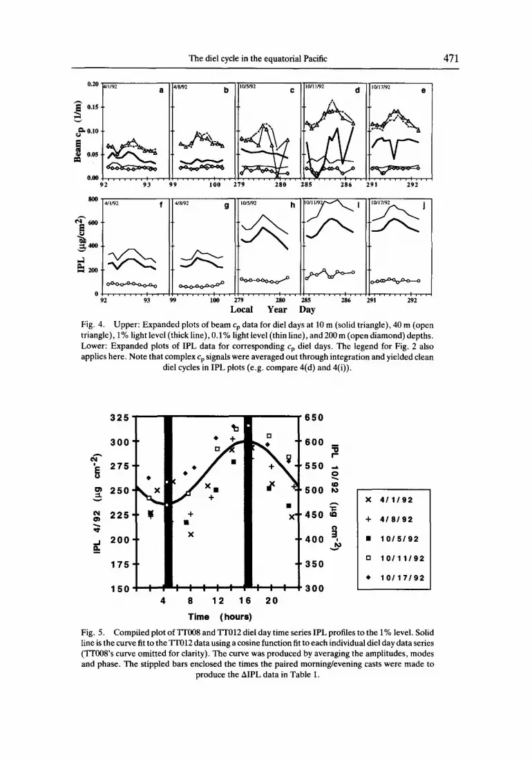
Some caution with respect to these data is needed given that the number of profiles per day constitutes a sparse data set, especially when compared to mooring data (Hamilton et al., 1990; Foley et&. ,1994). Sparse sampling with respect to the phase of a signal can result in biased data (Wiggert et al., 1993), and while the morning/evening paired data certainly is generally in phase with the signal, the profiles were not likely to have been taken at exactly the extremes, and therefore the estimated change in the particle load from pairs of profiles represents at best a minimum. To estimate the error associated with the sparse sampling the die1 day data (7 to 9 profiles per day) were compiled from TTOO8 and TTO12 (Figs 4 and 5). A curve was fit to the data using a cosine function fit to each individual die1 day data series. A single curve was produced by averaging the amplitudes, modes and phase. The resultant curve presented in Fig. 5 represents the amplitude and mode of the average of the

The die1 cycle in the equatorial Pacific 469

Local Year Day Local Year Day

82 86 90 94 98 102 275 279 283 287 291 295 0

20

40

3 60

g 80

d 100

120

140

160

Fig. 2. Depths of the light levels used for the integration depth in calculating the IPL. Data courtesy of Curtis Davis (NRL). The 0.1% light level for day 288 (126 m) was estimated by using

the CTD PAR data.

-PL to 1% level - IPL to 0.1% level + IR diff(0.1.1%)

82 84 86 88 90 92 94 96 98 100 102 800

R <600 jyo - 200

d 0 275 277 279 281 283 28.5 2.87 289 291 293 295

Local Year Day

Fig. 3. IPL (Integrated Particle Load) time series during IT008 (upper panel) and IT012 (lower panel) for times when light levels were available. The IPL to the 0.1% light level (thin line) follows the trend of the IPL to the 1% light level (thick line). While the IPL difference (open circle) between the 0.1% and 1% light level remained nearly flat during ITOO8, it showed some low- frequency variation during ‘ITU12. Stippled days during ‘IT008 lack pairs of morning/evening casts.

470 I. D. Walsh et al.

Table 1. AIPL and estimated organic C‘ production (C prod) at the I % and 0. I % light levels for EqPac cruises TTOOX and T7lI12. Organic carbon production was estimated by assuming that 40% of AIPL was carbon and converting to moles. Note that integration to the 0.1% light level during T7Q12 sometimes results in a lower estimate

of production, a consequence of the hydrodynamic variability apparent in Figs 1 and 4

Day Date (mmiddlyy) yzf+r yi!;”

I?o light level 0.1% light level

AIPL (‘ prod AIPL C prod (mgm ’ (mm01 C Depth (mg mm’ (mm01 C day-‘) m z day ’ ) (db) day -‘) mm2 day-‘)

TTOOS 3125192 3/27/92 3/29/92 3131192 4/l/92 412192 418192

85 95 347 X7 97 1168 89 93 688 91 x7 66X 92 88 XX4 93 Y2 x37 99 X5 767

Average SD

7x0 737 ___

TT012 1012192 I O/4/92 10/5/92 1 O/6/92 1017192 1 O/8/92 10/10/92 IO/l 1192 IO/l 2192 10/14/Y2 10/16/92 1 o/ 17192 1 O/l X/Y2 10/19/92 10/2O/Y2

276 27X 27Y 2X0 2x1 2X2 284 2x5 286 28X 290 2Yl 292 ‘Y3 704

XI

xs X7 73 X7 77 70 70 69 77 77 76 70 6X Xl

IIJ.: 130s I256 I220 7065 17si 1302 1621 1061 XhS

1143 1057 11x0 700 568

Avcragc I’25 SD 388

I46 450 145 1347 139 694 136 781 137 957 I46 943 13s 819

XSh 376

IX I186 128 135x I?4 1272 I25 990 12’) 7054 I?.? 1794 I17 13Y4 I10 I x2x IO0 78’) 126 850 II0 1107 I I5 I297 I23 I337 102 x94 121 365

123-1 33X

15 45 23 26 32 31 27

‘9 Q

TTO12 die1 day data sets. The stippled bars span the times of the paired morning/evening profiles used to produce the ATPL data in Table I. While the paired data fall close to the peaks of the resultant average curve, there was a range of approximately 3 h in the phases of the individual die1 day tits. For the resultant average curve, the underestimation error associated with missing the peak by 1 h in the AIPL is 3%, for 2 h, 6%) and for 3 h. 15%. Therefore, the largest error, if all profiles missed all peaks by 3 h is 30%. Figure 5 suggests much smaller errors.

RESULTS

The time series of cp at 10,40, 80, and 200 m depths during EqPac TTOOS and TTO12 cruises are presented in Fig. 1. Beam c,values during ‘IT012 (up to -0.17 rn-‘) were much

The die1 cycle in the equatorial Pacific 471

92 93 99 100 219 280 285 286

92 93 99 100 279 280 285 286

Local Year Day

:91 292

!91 292

Fig. 4. Upper: Expanded plots of beam cr, data for die1 days at 10 m (solid triangle), 40 m (open triangle), 1% light level (thick line), 0.1% light level (thin line), and 200 m (open diamond) depths. Lower: Expanded plots of IPL data for corresponding cr, die1 days. The legend for Fig. 2 also applies here. Note that complex cp signals were averaged out through integration and yielded clean

die1 cycles in IPL plots (e.g. compare 4(d) and 4(i)).

325

300

T 275

z 250

z 225

;; g 200

175

?? ? ?

??

??

/

??

Xa +

+ a

X

650

I I I 300 4 8 12 18 20

X 411192

+ 418192

W 10/5/92

0 10111192

?? 10117192

Time (hours)

Fig. 5. Compiled plot of IT008 and TTO12 die1 day time series IPL profiles to the 1% level. Solid line is the curve fit to the TTO12 data using a cosine function fit to each individual die1 day data series (TTOO8’s curve omitted for clarity). The curve was produced by averaging the amplitudes, modes and phase. The stippled bars enclosed the times the paired morning/evening casts were made to

produce the AIPL data in Table 1.

472 I. D. Walsh et al.

greater than the values during ‘IT008 (up to -0.10 m- ‘). A distinct feature of these plots is the die1 cycles with morning lows and evening highs. The pattern of die1 cycles in October (TTO12) is much more apparent than during March/April (TTOO8). The difference in the die1 response between the cruises is more apparent than real due to the lack of regular morning/evening pairs of profiles (stippled days) during TTOO8. The 80 m cp time series is occasionally out of phase with the 10 and 40 m data, and displays a high degree of point to point variability. Similar variability is seen in the temperature and salinity data at 80 m and is most likely the result of internal waves and/or fluctuations within the equatorial undercurrent (Gardner et al., 1995).

Note that not only were the cp values greater during TTO12 as compared to TTOO8, but the slope of the PMCIc, correlation was also greater. The filtration data show that PMCs during ‘IT008 were in the range of 8-4Opg 1-l and lO-126pg 1-l during TTO12 in the upper water column (~200 m). The difference in particle mass between the two cruises is clearly shown in the IPL data (Fig. 3). While the IPL to the 1% light level during IT008 ranges from 205 to 390 pg cme2, it ranges from 367 to 632,ug cme2 during TTO12. The IPLs at the 1% and 0.1% light levels also exhibit die1 cycles with morning lows and evening highs as seen in the cp data (Fig. 1).

DISCUSSION

Assuming no changes in scattering and effective cross section, changes in the IPL represent the cycling of mass into and out of the suspended small particle pool. The major contributors to changes in the particle load in the euphotic zone can be summarized in the equation

AIPL=PP-S-G-(A+D) (5)

where PP is the integrated primary production (including respiration), S is the loss of small particles due to settling and mixing from the layer, G is the grazing loss, and A and D represent the losses and gains to the small particle pool due to aggregation and disaggre- gation, respectively (all in units of mg m -2 t-i integrated over the same depth range). Die1 AIPL was calculated from the TTOO8 and IT012 IPL data using only those days with morning/evening pairs of CTD data (Table l), For the EqPac data set then, the time constant for AIPL is 12 h (Fig. 5).

To convert the AIPL data to carbon we conservatively estimated that 40% of the change in the PMC was due to organic carbon. While POC was measured on the cruises, the POC data reported (Ducklow, personal communication) results in a mean POC/PMC ratio of 2 (range of 0.9 to 2.5) for IT008 (i.e. more organic carbon than total particulate matter) and 0.8 (range 0.7 to 2) for TTO12. The filtrations for POC and PMC were made from the same depths but used different methodologies and filter types (GF/F vs Poretics 0.4 pm pore size). The reason for the discrepancy has not been resolved. The POC/PMC ratio of 0.4 observed for the NABE data set (Gardner et al., 1993) is a conservative estimate for converting the particle mass production to carbon fixation for the EqPac data set.

With these caveats, estimated net carbon production to the 1% light level based on the daytime increase in the IPL averaged over the TTOOS cruise period was 26 mmol C rnp2 day-’ (n=7, SD=7), and 41 mmol m-2 day-’ (n=15, SD=13) for lTO12 (Table 1). The observed increase in production for TT012 over IT008 is statistically significant, as the p- value was 0.002 for the hypothesis that there was no difference in production between

The die1 cycle in the equatorial Pacific 473

275 277 279 281 283 285 287 289 291 293 295

84 86 88 90 92 94 96 98 100 102 104

Local Year Day Fig. 6. Time series of the optically determined biomass specific production rate bbea,,, J at the 1% light level derived by normalizing AIPL by the morning IPL value. There is no significant difference between the mean vahre of pbcamC from 13008 (open square) and TT012 (solid

diamond). Upper x-axis for ‘IT012 data.

‘IT008 and lTO12, and 0.06 for the hypothesis that there was a 30% increase of production during IT012 compared to TTOO8. However, if the IPL for the morning is assumed to be the available biomass and AIPL the production, an optically determined biomass normal- ized production rate can be derived, i.e. &,eam =. Comparing ,&,_, c for both TWO8 and IT012 shows that while particle load was greater during TM12 as compared to ‘ITOO8, production normalized to the particle load was essentially the same during the two periods (Fig. 6).

The in situ and incubation data using 14C showed that the integrated area1 primary production to the 0.1% light level for IT008 was 90 mmol C mm2 day-i and 129 mmol C me2 day-’ for ‘IT012 (Barber, personal communication). Bender et al. (1994) determined net organic C production using an oxygen isotope method. Their results integrated to the 5% light level were 70 mmol C mW2 day-’ for TTOO8, and 100 mmol C me2 day-’ for lTO12. Our carbon specific production estimates are the lowest of the three methods. However, our estimate is based on the problematic estimated POC/PMC. Indeed, our estimate of the die1 change in particle mass is as great as the estimated carbon production (Table 1). If we used the cruise data for POC instead of PMC, then our organic carbon specific production estimates would be two to four times higher, approaching equality with the other methodologies.

It is interesting that while production values from each method (i4C, oxygen and AIPL) were quite different, each method showed the same percentage (about 40%) of production increase during IT012 compared to lTOO8. Furthermore, plotting the time series of the production data from IT012 for days that both the 14C production data and AIPL are available shows a rough correlation of the trends in the data over time (Fig. 7). An even better correlation is apparent from the time series plot of the chlorophyll specific production and ,L.+,_, c (Fig. 7(D)). Because the number of data pairs is small (N = 10 for TTO12), the significance of the correlations is limited. The correlation in the ratioed data, which does not rely on the POUPMC conversion factor, suggests that the IPL and production data are being driven by similar if not the same forcing functions.

474 I. D. Walsh et al.

??AIPL + 14c

1% 2000

mgC m-2 d-*

AIPL 1000 mg m-2 d-1

0

B v = 0.99 x - 436 k= 0.51

T Sg. F= 0.13

2ooo1 V AIPL

1000 mg m-2 d- 1

275 285 295 0

Year Day

C D

T

2 80 0.5

? 0.4 T

1000 2000

‘4C mgC m-2 d-1

‘,I W&7 x - 0.144

Sig. F= 0.02

275 285 295 3 20 40 60 80

Year Day Chl. Specific Production

mgC mgChl-1 m-2 d-1

Fig. 7. (A) Time series plot of “C productton and AIPL integrated in the 0.1% level from TTO12 for days in which both measurements arc available. Note that “C production is carbon production while AIPL is total mass. (B) Linear regression of AIPL on “‘C production. The regression is significant at the >85% level. (C) Time series plot of chlorophyll specific t4C production and the optically determined biomass specific production rate integrated to the 0.1% level from ‘IT012 for days in which both measurements are available. (D) Linear regression of AlPL on 14C production.

The regression is significant at the >97% level. ‘?C data courtesy of R. Barber (Duke).

The large difference between our carbon specific production data and the other production measurements may be explained by the difference between in situ and bottle- determined productivity. The water samples procured for the incubations were commonly taken shortly after midnight, while the observed minimum beam cp concentrations occurred just before dawn. If the loss of particulate mass occurs solely through respiration and the community respiration rates are equal for the sample and in situ, then the bottle concentrations would track the in situ data during preparation and no systematic affect would bias the data. However, if the major change in the particle concentration occurs via a forcing function not represented in the sample, e.g. grazing and aggregation, then the incubation methods overestimate the actual net production by overestimating the initial phytoplankton population. Considering that the biomass specific production rate was similar between T’TOO8 and TTO12 (Fig. 6), however, the correction to the incubation data could be made simply by dividing the incubation productivity by the ratio between the integrated particle load at the time the samples were taken (IPL at sample time) and the

The die1 cycle in the equatorial Pacific 475

minimum integrated particle load (IPL before dawn). The ratio was about 1.15 for both cruises. This correction is therefore small at best.

More importantly, the in situ optical method implicitly includes the effects of mixing/ settling, grazing and aggregation losses on the small particle pool. The change in the integrated particle load does not therefore reflect growth per se, but the net impact on the particle concentration from the relevant forcing functions summarized in equation (5). Simplifying, settling losses can be assumed small as settling velocities of individual particles are negligible. Mixing losses can also be assumed small as the 1% and 0.1% light levels are below the depth of die1 mixing (Gardner et al., 1995). From equation (5) then, the summation of the grazing and net aggregation terms equals the difference between the 14C incubation data and AIPL data. Cullen et al. (1992) suggested that transmissometers may not be sensitive to zooplankton biomass, and that based upon the biological system model of Smith et al. (1984) production from beam c should be multiplied by 1.5 to 2 for comparison with 14C data, i.e.:

G = a x AIPL, 0.5 c= as 1. (6)

For the EqPac time series grazing by macroheterotrophs on a 24 h basis was estimated to be approximately 80% of primary production during IT008 and 70% during TTO12 (Landry etal., 1994). Assuming that half the grazing occurs during the day, then grazing by microheterotrophs would be greater than the carbon specific AIPL increase seen during the day, and therefore higher than estimated by Cullen et al. (1992).

For both TTOOS and ‘IT012 the estimated carbon production from the observed AIPL is approximately one third of the measured 14C primary production. Grazing would account for 40% and 35% of PP, leaving approximately 25% of the carbon production to be accounted for by dark respiration and net aggregation. As the grazing loss is of the same order as the daytime AIPL and no net increase in the IPL was seen on a day to day basis, it follows that grazing alone is sufficient to account for the observed dark period decrease in the IPL (Figs 3 and 5). Die1 changes in aggregate abundance in the euphotic zone were observed during EqPac (Walsh et al., in preparation), evidence that some of the small particle mass does go to the aggregate pool.

In conclusion, the changes in IPL (AIPL) over time reflect biogeochemical cycling in the surface ocean. AIPL represents the change in small particle mass which is the sum of biological production, grazing, aggregation, input or export due to vertical settling, mixing, and advective transport. Although the conversion from beam c to PMC to POC remains problematic, similar patterns in the day to day variability of AIPL and 14C primary production along with coherence in the production/biomass ratios between the two methods suggests that AIPL can be used to estimate in situ production and track changes in the biological system in surface waters. As a first-order approximation, the die1 cycle in the IPL can be accounted for by the net autotrophic production balanced by losses to grazing and aggregation. Considering the measured and estimated flux through the grazers, this analysis supports the hypothesis that grazing is the major control of primary production in the equatorial Pacific. This study also found that although production increased between March/April and October, biomass specific production &,_,J was not significantly different between these time periods.

Acknowledgements-The authors wish to acknowledge the support of the Captains and crew of the R.V. Thompson in the collection of this data set. The enormous job of handling the post-processing of the raw

476 I. D. Walsh et (I/.

hydrographic data was performed by J. Murray and J. Postel. This work has been stimulated and improved by many interactions with our co-workers in the EqPac program. In particular, T. Dickey, J. Murray and an anonymous reviewer supplied many helpful comments. This work was funded by NSF Grant OCE-9022348.

REFERENCES

Ackleson S. G.. J. J. Cullen, J. Brown and M. Lesser (1993) Irradiancc-induced variability in light scatter from marine phytoplankton in culture. Journal of Plankton Research, 15,737-759.

Ackleson S. G., J. J. Cullen, J. Brown and M. P. Lesser (1990) Some changes in optical properties of marine phytoplankton in response to high light intensity. In: Ocean Optics (X), Proceedings of SPIE-The International Society for Optical Engineering, Vol. 1302, pp. 238-249.

Bender M.. J. Orchardo. M. L. Dickson and M. E. Carr (1994) Net and gross Oz production on the equator, 14o”W. during Eqpac. Eos, Transactions of the American Geophysical Union. 15.29.

Bricaud A.. A. Morel and L. Prieur (1981) Absorption by dissolved matter of the sea (yellow substance) in the UV and visible domains. Limnology und Oceanography. 26,43-S.

Cullen J. J.. M. R. Lewis. C. 0. Davis and R. T. Barber (1992) Photosynthetic characteristics and estimated growth rates indicate grazing is the proximate control of primary production in the Equatorial Pacific. Journal of Geophysical Research, 97.630-654.

Dickey T. D. (1991) The emergence of concurrent high-resolution physical and bio-optical measurements in the upper ocean and their applications. Review of Geophysics, 29,383-413.

Dickey T., T. Granata, J. Marra, G. Langdon, J. Wiggert, Z. Chai-Jochner, M. Hamilton. J. Vazquez, M. Stramska, R. Bidigare and D. Siegel (1993) Seasonal variability of bio-optical and physical properties in the Sargasso Sea. Journal of Geophysical Research, 98,865-898.

DuRand M. D.. R. J. Olson and E. R. Zettler (1994) Flow cytometric analysis of phytoplankton growth during diel studies in the Equatorial Pacific. Eos, Transactions of the American Geophysical Llnion. 75,28-29.

Foley D. G.. T. D. Dickey, R. R. Bidigarc and M. J. McPhaden (19Y4) The influence of tropical instability waves OS primary production in the equatorial Pacific. Eos. Trunsuction.s of the Americun Geophysical Union, 75, 29.

Gardner W. D.. 1. D. Walsh and M. J. Richardson (lYY3) Biophysical forcing of particle production and distribution during a spring bloom in the North Atlantic. Deep-Sea Reseurch, 40. 171-195.

Gardner W. D., M. J. Richardson, I. D. Walsh and B. L. Berglund (1990) In-situ optical sensing of particles for determination of oceanic processes: What satellites can’t XC, but transmissometers can. Oceanography. 3(2). 1 I-17.

Gardner W. D.. S. P. Chung. M. J. Richardson and I. D. Walsh (lY9S) The oceanic mixed-layer pump in the equatorial Pacific. Deep-Seu Research II, 42.757-775.

Gordon H. R., R. C. Smith and J. R. V. Zaneveld (1984) Introduction to ocean optics. In: Ocean Optics VII, Proceedings of SPIE-The International Society for Optical Engineering SPIE, Vol. 489, pp. 2-41.

Hamilton M., T. C. Granata, T. D. Dickey, J. D. Wiggert, D. A. Siegel, J. Marra and C. Langdon (1990) Diel variations of bio-optical properties in the Sargasso Sea. In: Ocean Optics X, Proceedings of SPIE-The International Society for Optical Engineering. SPIE. Vol. 1302. pp. 214-224.

Kiefer D. A. and R. W. Austin (1974) The effect of varying phytoplankton concentration on submarine light transmission in the Gulf of California. Limnology and Oceanography, 19, 55-64.

Kirk J. T. 0. (1983) In: Lightandphotosynthesis in aquaticecosystems. Cambridge University Press, New York. Landry M. R., J. D. Kirshtein and J. Constantinou (1994) Microzooplankton grazing in the Equatorial Pacific.

Eos, Transactions of the American Geophysicul Union. 75,SO. McPhaden M. J. (1993) TOGA-TAO and the 1991-93 El Nido-Southern Oscillation Event. Oceanography, 6,

36-44. Murray J. W., M. W. Leinen. R. A. Feely, J. R. Toggweiler and R. Wanninkhof (1992) EqPac: a process study in

the central equatorial Pacific. Oceanography, S(3), 134-142. Olson R. J., S. W. Chisholm, E. R. Zettler and E. G. Armbrust (lY90) Pigments, size, and size distribution of

synechococcus in the North Atlantic and Pacific Oceans. Limnology and Oceanography, 35,45-58. Pak H.. D. A. Kiefer and J. C. Kitchen (1988) Meridional variations in the concentration of chlorophyll and

microparticles in the North Pacific Ocean. Deep-Sea Research. 35, 1151-1171. Richardson, M. J., W. D. Gardner, S. P. Chung and I. D. Walsh (1993) Source of beam attenuation signal as a

function of particle size. The Oceanography Society Meeting Abstracts, Seattle, Washington, p. 71.

The die1 cycle in the equatorial Pacific 477

Sanderson M., C. Hunter, S. Fitzwater, R. M. Gordon and R. Barber (1995) Primary productivity and trace- metal contamination measurements from a clean rosette system versus ultra clean Go-Flo bottles. Deep-Sea Research II, 42,431-440.

Siegel D. A., T. D. Dickey, L. Washburn, M. K. Hamilton and B. K. Mitchel(l989) Optical determination of particulate abundance and production variations in the ohgotrophic ocean. Deep-Sea Research, 36, 211- 222.

Smith R. E. H., R. J. Geider and T. Platt (1984) Microplankton productivity in the oligotrophic ocean. Nature, 311,252-254.

Stramska M. and T. D. Dickey (1992) Variability of bio-optical properties of the upper ocean associated with die1 cycles in phytoplankton population. Journal of Geophysical Research, 91, 17,873-17,887.

Stramski D. and R. A. Reynolds (1993) Die1 variations in the optical properties of a marine diatom. Limnology and Oceanography, 38,1347-1364.

Vaulot D., D. Marie, F. Partensky, R. J. Olson and S. W. Chisholm (1994) Prochlorococcus divides once a day at the Equator. Eos, Transactions of the American Geophysical Union, 75,28.

Walsh I. D. (1990) Project CATSTIX: Camera, Transmissometer, and Sediment Trap Integration Experiment. PhD Dissertation, Texas A & M University, 96 pp.

Walsh I. D., W. D. Gardner and M. J. Richardson (1992) Transmissometer profiles in the equatorial Pacific during the JGOFS EQPAC program: Estimates of primary production. Eos, 73,295.

Wiggert, J. T., T. D. Dickey and T. Granata (1994). The effect of temporal undersampling on primary production estimates. Journal of Geophysical Research, 99,3361-3371.