ARTICLE IN PRESS

0165-1684/$ - se

doi:10.1016/j.si

�Correspondfax: +813 5734

E-mail addr

(R.L.G. Cavalc

Signal Processing 88 (2008) 326–338

www.elsevier.com/locate/sigpro

Steady-state analysis of constrained normalized adaptive filtersfor MAI reduction by energy conservation arguments

R.L.G. Cavalcante�, I. Yamada�

Department of Communications and Integrated Systems, Tokyo Institute of Technology, 2-12-1-S3-60 Ookayama,

Meguro-ku, Tokyo 152-8550, Japan

Received 9 April 2007; received in revised form 18 July 2007; accepted 20 July 2007

Available online 29 August 2007

Abstract

We derive the steady-state performance of a common class of adaptive filters for multiple access interference (MAI)

reduction in code division multiple access (CDMA) systems. The adaptive filters under study utilize estimates of the desired

user’s amplitude and are divided into three groups of least-mean-square (LMS) algorithms differing by the choice of the

normalization factor. The steady-state performance is deduced from energy-conservation relations that include a possibly

erroneous estimate of the desired user’s amplitude. The analyses show that blind algorithms using information about the

desired user’s amplitude achieve similar performance to that of nonblind algorithms. In addition, geometric considerations

reveal the conditions under which the choice of the normalization factor is expected to have great impact on the

convergence properties of the algorithms. Numerical simulations show good agreement with theory.

r 2007 Elsevier B.V. All rights reserved.

Keywords: Multiuser interference; Energy conservation relations; Steady-state analysis

1. Introduction

In direct sequence/code division multiple accesssystems (DS/CDMA), multiple users share the samechannel at the same time. Hence, at the receiver thedetection of the transmitted symbols of a desireduser is strongly affected by the interference origi-nated from the other users in the system. Thisinterference is known as multiple access interference(MAI). Without proper mitigation, this MAI causessevere performance degradation in the detection ofthe transmitted information.

e front matter r 2007 Elsevier B.V. All rights reserved

gpro.2007.07.023

ing authors. Tel.: +813 5734 2503;

2905.

esses: renato@comm.ss.titech.ac.jp

ante), isao@comm.ss.titech.ac.jp (I. Yamada).

In multiuser systems, a receiver that achieves theminimum bit error rate (BER) generally demandshigh computational complexity [1]. Therefore, linearadaptive filters with low computational complexityhave been introduced to mitigate MAI [2]. Linearadaptive filters try to approximate a filter thatminimizes (or maximizes) a mathematically tract-able cost function closely related to the BER.Usually, these adaptive filters track the filtermaximizing the signal-to-interference-noise ratio(SINR) [2–13], and the main difference betweenthem lies in the choice of the adaptive algorithm.

In particular, a great deal of effort has beendevoted to the study of blind linear receivers basedon the recursive least-squares (RLS) and least-mean-square (LMS) algorithms. RLS-based recei-vers show good convergence speed [10], but they

.

ARTICLE IN PRESSR.L.G. Cavalcante, I. Yamada / Signal Processing 88 (2008) 326–338 327

demand higher computational complexity thanLMS-based receivers and often suffer from numer-ical instabilities [8] caused by the inherent matrixinversion and possible model mismatch. Moreover,for this particular application, conventional fastversions with linear complexity of the RLS algo-rithm are hard to be applied because there isno time-index-shifting property of the input data[10]. Furthermore, in relatively fast time-varyingscenarios, LMS-based receivers can outperformRLS-based receivers [13] because the trackingbehavior of the LMS algorithm is usually superiorto that of the RLS algorithm in nonstationaryenvironments [14]. In this study, the focus is onLMS-based receivers.

When a training sequence is necessary for thefilter adaptation in a LMS-based receiver, the LMSalgorithm is said to be nonblind; otherwise, it is saidto be blind. Blind LMS algorithms are preferablebecause the overhead imposed by training sequencesis not present, so the throughput of the system ispotentially higher. They are usually obtained byrestricting the adaptive filter to satisfy a constraintdetermined by the desired user’s signature. Acelebrated blind LMS algorithm for MAI mitiga-tion has been proposed in [2]. Unfortunately, thesteady-state performance achieved with this ap-proach is much worse than the performanceachieved with nonblind algorithms, especially whenthe level of background noise is small. Thisperformance difference between blind and nonblindalgorithms can be reduced if estimates of the desireduser’s amplitude and transmitted symbol are utilizedeffectively in the blind algorithms [4,9,12,15].

Table 1

Characterization of the adaptive filters under study

Group Algorithm a

I GP [4] A1

I SAGP [4] ~A1

I OPM-GP [4] 0

II Modified GP A1

II Modified SAGP [12] ~A1

II Modified OPM-GP [5] 0

III BLMS (normalized)[9] 0

III CLMS-AE (normalized)[9] ~A1

III DD-CLMS-AE (normalized)[9] ~A1

We can further divide LMS algorithms into non-normalized algorithms [2,9] and normalized algo-rithms [4,5,9,11–13]. Normalized LMS algorithmsare frequently used because they are potentiallyfaster than non-normalized LMS algorithms forboth uncorrelated and correlated input data [16].The work in [9] introduces a normalization factorthat reduces the sensitivity of LMS algorithms tochanges in the number of users and/or the signal-to-noise ratio (SNR). In [4] the normalization factorhas been derived from projections onto closednonconvex sets. By considering geometric propertiesof projections onto closed convex sets, [5,12,15]have proposed a normalization factor aiming at fastconvergence speed.

In this study, we deduce closed-form expressionsfor the steady-state performance of constrainednormalized LMS algorithms. The closed-formexpressions are derived by including the possibleinformation about the desired user’s amplitude intoenergy-conservation relations [17–19]. More pre-cisely, we focus on the steady-state performance ofthe algorithms introduced in [4,5,9,12]. Thesealgorithms are examples of a more general class ofreceivers presented in [13], which in turn is based onthe adaptive projected subgradient method [20]. Forsimplicity, we divide the algorithms into threedifferent groups according to their normalizationfactors (cf. Table 1):

�

Group I [4]: the OPM-based gradient projection(OPM-GP) algorithm, the generalized projection(GP) algorithm, and the space alternating gen-eralized projection (SAGP) algorithm;

~b1½i� gðr½i�Þ

sgnðhTi�1r½i�Þ kr½i�k2

sgnðhTi�1r½i�Þ kr½i�k2

- kr½i�k2

sgnðhTi�1r½i�Þ r½i�TPr½i�

sgnðhTi�1r½i�Þ r½i�TPr½i�

– r½i�TPr½i�

– b½i� ¼ ð1� kÞb½i � 1� þ kkr½i�k2,b½0� ¼ kr½0�k2; 0oko1

b1½i� b½i� ¼ ð1� kÞb½i � 1� þ kkr½i�k2,b½0� ¼ kr½0�k2; 0oko1

sgnðhTi�1r½i�Þ b½i� ¼ ð1� kÞb½i � 1� þ kkr½i�k2,b½0� ¼ kr½0�k2; 0oko1

ARTICLE IN PRESSR.L.G. Cavalcante, I. Yamada / Signal Processing 88 (2008) 326–338328

�

1

alg

wo

the

arg

Group II [5,12]: the modified OPM-GP algo-rithm, the modified GP algorithm, and themodified SAGP algorithm;

� Group III [9]1: the constrained (normalized)

LMS with amplitude estimation (CLMS-AE)algorithm, the decision directed CLMS-AE(DD-CLMS-AE) algorithm, and the blind LMS(BLMS) algorithm.

The steady-state performance analysis reveals that(i) the algorithms of Group II have better conver-gence rate than those of Group I; (ii) the differencein steady-state performance between Groups I andII (when the same step size is used) increases as theangle between the desired user’s signature and theinput signal decreases; (iii) the algorithms of GroupsI and III have similar performance when the sameamount of information is used; and (iv) properuse of the estimate of the desired user’s amplitudeis highly expected to improve the steady-stateperformance. (NOTE: These results can be imme-diately extended to adaptive array antenna systemsif the sources transmit symbols with constantmodulus.)

A short conference version of this study waspresented in [21]. Here, we present a fully detailedderivation of the steady-state performance andshow extensive numerical simulations to confirmthe expressions.

2. Preliminaries

2.1. System model

For simplicity, we consider a synchronous BPSKDS-CDMA system with K active users and M chipsper symbol over a flat fading channel model. Notethat an extension of the analysis to asynchronoussystems with constant modulus symbols over afrequency-selective channel model (see, for example,[3, Section II], [22]) is straightforward. If thereceiver is synchronized with the desired user, thereceived vector r½i� 2 RM is given by

r½i� ¼ A1b1½i�s1 þXK

k¼2

Akbk½i�sk þ n½i�. (1)

A sound performance analysis for the non-normalized

orithms of this group is also provided in [9]. However, the

rk in [9] neither discusses the algorithms in [4,5,12] nor derives

steady-state performance by using energy conservation

uments.

where Ak 2 ½0;1Þ, bk½i� 2 f�1;þ1g, sk 2 RM (s1; . . . ;sK linearly independent), and n½i� are the kth user’samplitude, kth user’s transmitted bit, kth user’sreceived signature [2], and noise. Hereinafter weassume that the channel is a slowly fadingchannel, i.e., the channel is approximately constantfor a sufficiently large block of transmitted symbols.Without loss of generality, the first user is thedesired user and kskk

2 ¼ sTk sk ¼ 1 (k ¼ 1; . . . ;K).We also use the following common assumptions[9,22].

Assumption 1. The noise vector n½i� is a zero-meanGaussian random vector with Efn½i�n½i�T�g ¼ s2nIM ,where IM is the M-dimensional identity matrix.

Assumption 2. Efbk½i�g ¼ 0, k ¼ 1; . . . ;K and

Efbq½i�br½i�g ¼1; q ¼ r;

0; otherwise:

(

Assumption 3. bk½i�, k ¼ 1; . . . ;K , and n½i� aremutually independent.

The detector estimates the transmitted bits with aproperly designed filter h 2 RM by

~b1½i� ¼ sgnðhTr½i�Þ, (2)

where

sgnðxÞ ¼þ1 for xX0;

�1 otherwise:

�

2.2. Optimal constrained filters

The linear minimum mean squared error (MMSE)filter is defined by

hMMSEopt 2 arg min

h2RMEfjhTr½i� � b1½i�j

2g. (3)

Under Assumptions 1–3, we readily verify thathMMSEopt ¼ A1R�1s1, where R ¼ E½r½i�r½i�T� ¼

PKk¼1

A2ksksTk þ s2nIM . In addition, from (2), we conclude

that the BER is the same for hMMSEopt and any filter of

the form h ¼ nR�1s1, provided that n40. In blindreceivers, a commonly used filter is hopt:¼ðR�1s1Þ=ðsT1 R�1s1Þ, which is uniquely given as thesolution to the optimization problem

hopt 2 argminh2Cs

EfjhTr½i� � ab1½i�j2g; 8a 2 ½0;1Þ,

(4)

where Cs:¼fh 2 RM jhTs1 ¼ 1g.Note that, by imposing the constraint Cs, the

solution does not change irrespective of the choice

ARTICLE IN PRESSR.L.G. Cavalcante, I. Yamada / Signal Processing 88 (2008) 326–338 329

of a [9,12]. By setting a ¼ 0, hopt can be realizedwithout knowledge of b1½i�. However, as shown inSection 3, practical blind adaptive algorithms can berealized even with aa0 by replacing b1½i� by itsestimate ~b1½i�, and proper choice of a40 gives betterperformance than a ¼ 0.

3. Steady-state analysis of adaptive filters for MAI

suppression

3.1. Classification of the adaptive filters under study

The adaptive filters of interest track the solutionhopt in (4) and are expressed by2

hi ¼ P hi�1 � mðhTi�1r½i� �

~b1½i�aÞr½i�

gðr½i�Þ

� �þ s1, (5)

where h0 ¼ s1 and m is the step size. The parametersa, ~b1½i�, and the normalization factor gðr½i�Þ aresummarized in Table 1. In this table, the parameter~A1 is an estimate of A1 and k is a forgetting factorused to track E½kr½i�k2�, the estimation of which isgiven by b½i�. For the algorithms of Groups I and II,the step size m belongs to the range 0omo2; for thealgorithms of Group III, m is a sufficiently smallpositive constant. The algorithms of Group I andtheir modified versions (algorithms of Group II)differ in the choice of the normalization factorgðr½i�Þ. The matrix P:¼ðIM � s1s

T1 Þ is the orthogonal

projection onto ðspanfs1gÞ?, hence P satisfies:

(a) P2 ¼ P, (b) Ps1 ¼ 0, and (c) kPxkpkxk,x 2 RM . We introduce for the first time the modifiedGP algorithm so that the GP algorithm also has itsmodified counterpart. Note that Pxþ s1 is themetric projection of x onto Cs, hence hi 2 Cs, i.e.,hT

i s1 ¼ hTopts1 ¼ 1, i ¼ 0; 1; 2; . . . .

For mathematical tractability, we assume in ouranalyses that ~b1½i� ¼ b1½i� for the algorithms usingaa0. In Section 4, we show that the proposedanalysis is in very good agreement with numericalsimulations not imposing this assumption. For thealgorithms requiring an amplitude estimate, westudy the performance by fixing a to a possiblyerroneous estimate of A1. With this approach we seehow well the amplitude estimation algorithm shouldperform in order to achieve a desired SINR level (anefficient amplitude estimation algorithm has beenindependently proposed in [4] and [9]).

2See [12] for the details of the derivation of this equation for the

algorithms of Groups I and II; for the details of the algorithms of

Group III, see [9].

For notational simplicity, we define the following:

~hi:¼hi � hopt 2 ðspanfs1gÞ?, ð6Þ

ep½i�:¼r½i�TP ~hi ¼ r½i�T ~hi, ð7Þ

ea½i�:¼r½i�TP ~hi�1 ¼ r½i�T ~hi�1, ð8Þ

vðaÞ½i�:¼hToptr½i� � b1½i�a, ð9Þ

uðaÞ½i� ¼ hTi�1r½i� � b1½i�a. ð10Þ

The above variables can be interpreted as follows:

�

~hi : weight error distribution � ep½i� : a posteriori estimation error � ea½i� : a priori estimation error � vðaÞ½i� :

vðaÞ½i� ¼ ðA1 � aÞb1½i�|fflfflfflfflfflfflfflfflffl{zfflfflfflfflfflfflfflfflffl}desired user’ s residual symbol

þXK

k¼2

Akbk½i�hToptsk|fflfflfflfflfflfflfflfflfflfflfflfflffl{zfflfflfflfflfflfflfflfflfflfflfflfflffl}

residual interference

þ hToptn½i�|fflfflffl{zfflfflffl}

filtered noise

[vðaÞ½i� is the output of the filter hopt minus thescaled version of the transmitted symbol (ab1½i�).]

� uðaÞ½i� : output of the filter hi�1 minus the scaled

version of the transmitted symbol ðab1½i�Þ.

Note that, unlike the discussion in [17] and [18,Chapter 6], the above definitions include theavailable information about the desired user’samplitude. We also adopt the following assump-tions to simplify the analysis in Section 3.2.Although these assumptions do not hold in general,they are good approximations due to the reasonsgiven below.

Assumption 4. At steady-state, ea½i� and the con-sidered normalization factors gðr½i�Þ are indepen-dent.

The justification of this assumption is given inAppendix A.

Assumption 5. v2ðaÞ½i� is independent of r½i�.

This assumption holds when the noise varianceapproaches zero because in such a case hT

optr½i� ¼A1b1½i� (see [6]). Hence v2ðaÞ½i� is a constant andtherefore independent of r½i�. Even in more generalsituations, Assumption 5 simplifies the steady-state

ARTICLE IN PRESSR.L.G. Cavalcante, I. Yamada / Signal Processing 88 (2008) 326–338330

analysis and shows good agreement with numericalsimulations.

3.2. Steady-state performance

We introduce one more assumption beforeproceeding with the steady-state analysis.

Assumption 6.

Er½i�r½i�T

gðr½i�Þ

� �¼

Efr½i�r½i�Tg

Efgðr½i�Þgand E

b1½i�r½i�

gðr½i�Þ

� �

¼Efb1½i�r½i�g

Efgðr½i�Þg¼

A1s1Efgðr½i�Þg

.

The above relations are reasonable approxima-tions because gðr½i�Þ � constant for the normal-ization factors used in this paper. The justificationis similar to the justification of Assumption 4 inAppendix A.

Now we are ready to analyze the steady-stateperformance of the adaptive filters in (5).

Proposition 1. Under Assumptions 1–6, the adaptive

filters in (5) with ~b1½i� ¼ b1½i� satisfy

(1)

(unbiasedness) limi!1

Efhig ¼ hopt for 0omo2and

2

(2)

3For a fair comparison, the step sizes should be selected in such

limi!1

SINRðhiÞ ¼A1

s2vðaÞm2b=a� m

þ hToptRhopt � A2

1

,

(11)

where

a ¼ Er½i�TPr½i�

g2ðr½i�Þ

� �,

b ¼ E1

gðr½i�Þ

� �,

s2vðaÞ ¼ Efv2ðaÞ½i�g ¼ a2 � 2aA1 þ hToptRhopt,

and

SINRðhi�1Þ ¼A2

1

EfjhTi�1r½i� � A1b1½i�j

2g. (12)

a way that all algorithms present the same convergence rate and

then we compare the steady-state performance. A second

approach is to set the step sizes in such a way that all algorithms

present the same steady-state performance and then we compare

the convergence rate [9]. We derived the steady-state performance

of all algorithms, so the later approach is used in this study.

Proof. The proof is given in Appendix B.

Next, we study the influence of the ratio a=b andthe parameter a on the steady-state performance ofeach group of adaptive filters.

3.2.1. Algorithms based on gðr½i�Þ ¼ r½i�TPr½i�This case is the simplest one because a ¼ b.

Hence, from Proposition 1, the steady-state SINRfor the algorithms of Group II is given by

SINRGroup II ¼A2

1

s2vðaÞm2� m

þ hToptRhopt � A2

1

. (13)

For fixed step size m, the global maximum of (13) isclearly reached at a ¼ A1. Thus we conclude that agood estimate of the amplitude A1 is expected toimprove the steady-state performance.

3.2.2. Algorithms based on gðr½i�Þ ¼ kr½i�k2

For these algorithms, by the Cauchy–Schwartz’sinequality, we have

a ¼ Er½i�TPr½i�

g2ðr½i�Þ

� �pE

kr½i�k kPr½i�k

g2ðr½i�Þ

� �

pEkr½i�k2

g2ðr½i�Þ

� �¼ E

1

kr½i�k2

� �¼ b.

Hence, the steady-state performance is given by

SINRGroup I ¼A2

1

s2vðaÞm2b=a� m

þ hToptRhopt � A2

1

XA2

1

s2vðaÞm2� m

þ hToptRhopt � A2

1

¼ SINRGroup II. ð14Þ

As in the case of the algorithms based ongðr½i�Þ ¼ r½i�TPr½i�, algorithms of Group I using anestimate of A1 have better performance than thoserelying on a ¼ 0 (if the step size is the same). Inaddition, the algorithms of Group I achieve higherSINR than their modified versions (algorithms ofGroup II) when the same step size is used. There-fore, for a fair comparison,3 different step sizesshould be employed.

The steady-state performance of the algorithms ofGroup I depends on the ratio b=a, of which theexact value may not be easily obtained. However, ifthe bound in (14) is tight, the performance of the

ARTICLE IN PRESS

1 2 3 4 5 6 7 8 90.82

0.84

0.86

0.88

0.9

0.92

0.94

0.96

0.98

1

Ak/A1, k=2,…,K

a/b

Gold sequences, K=5

Random sequences, K=5

Gold sequences, K=20

Random sequences, K=20

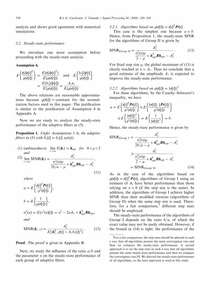
Fig. 1. Influence of the number of users (K), the choice of the

signatures, and power relations on a=b. The results were obtained

by simulations. Length-31 codes and SNR 15 dB. Note that, for

well-designed signatures, such as those based on Gold sequences,

and/or for highly interfered channels, the steady-state perfor-

mance of the algorithms of Group I and their counterparts of

Group II is expected to be very close.

R.L.G. Cavalcante, I. Yamada / Signal Processing 88 (2008) 326–338 331

algorithms of Group II is also a good approxima-tion of the performance of the algorithms of GroupI. By Pr½i� ¼ r½i� � ðr½i�Ts1Þs1, we deduce

a

b¼

Er½i�TPr½i�

kr½i�k4

� �E

1

kr½i�k2

� �

¼ 1�

Ekr½i�k2ks1k

2 cos2 y½i�kr½i�k4

� �E 1kr½i�k2

n o

¼ 1�

Ecos2 y½i�kr½i�k2

� �E

1

kr½i�k2

� � , ð15Þ

where cos y½i� ¼r½i�Ts1kr½i�k

and y½i� is the angle between

r½i� and s1 (recall that ks1k ¼ 1). From (15), ifcos y½i� is small on average, the ratio a=b is expectedto be close to one and thus the bound in (14) is tight.A small cos y½i� has the equivalent geometricinterpretation of r½i� being nearly orthogonal to s1.From the model in (1), when good spreading codesare used (jsTk sjj5kskk

2; kaj) and the power of theinterfering users is high, the ratio a=b is expected tobe close to one, and we conclude that the bound istight in such a situation. The ratio a=b for differentscenarios is illustrated in Fig. 1.

Remark 1. The algorithms of Group II have beenspecially devised to outperform those of Group Iwhen the angle y½i� is small. Unfortunately, in such asituation the bound (14) is not tight. Hence, for a faircomparison, the relation between the step size of thealgorithms of Group I (denoted by m1) and the stepsize of the algorithms of Group II (denoted by m2)has to be set in such a way that SINRGroup I ¼

SINRGroup II. If the same parameter a is the same,SINRGroup I ¼ SINRGroup II is satisfied when

m2m1¼

a

b. (16)

3.2.3. Algorithms based on gðr½i�Þ ¼ b½i�Making use of the fact that kr½i�k � constant for

well designed signatures, we have that b½i� � kr½i�k2

(see Appendix A). Therefore, we expect that thealgorithms with gðr½i�Þ ¼ b½i� and those with gðr½i�Þ ¼kr½i�k2 perform similarly if the parameter a is thesame.

Corollary 1. The steady-state SINR achieved by the

modified OPM-GP algorithm is bounded by

SINRmodified OPM�GPp2� mm

. (17)

Proof. The presence of noise cannot increase theSINR, so the best performance is achieved whensn ! 0. In this situation, we have

s2vðaÞja¼0 ¼ ðhToptr½i�Þ

2¼ A2

1 (18)

and

hToptRhopt ¼ A2

1 (19)

(see the discussion after Assumption 5). Substitu-tion of (18) and (19) into (13) yields

SINRmodified OPM�GP ¼ ð2� mÞ=m,

which concludes the proof. &

Remark 2 (On Corollary 1). All studied algorithmswith a ¼ 0 are expected to achieve similar steady-state performance when good spreading codes areused [see discution after (14)]. In such a situation,the bound in (17) is also a good approximation ofthe best performance achieved by these algorithms,and we conclude that the choice of the step sizeimplicitly defines the maximum achievable SINR. Incontrast, algorithms using the desired user’s ampli-tude (a ¼ A1) satisfy limsn!0;i!1SINRðhiÞ ¼ 1,

ARTICLE IN PRESSR.L.G. Cavalcante, I. Yamada / Signal Processing 88 (2008) 326–338332

8m 2 ð0; 2Þ, which can be easily verified by substitut-ing s2vðaÞja¼A1

¼ 0 and hToptRhopt ¼ A2

1 into (11).

4. Simulation results

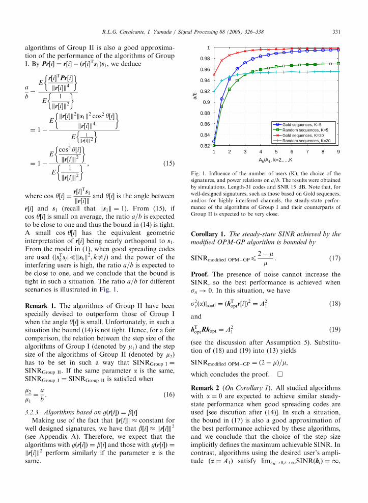
Fig. 2(a) shows theoretical and simulated curvesfor the OPM-GP algorithm, the GP algorithm, andtheir modified counterparts, which belong to GroupII. The algorithms of Group III perform similarly tothe algorithms of Group I, so the performancecurves of the former group are omitted for visualclarity. The system has 20 users, the signatures arechosen from length-31 Gold spreading codes, thedesired user’s amplitude is A1 ¼ 1, and eachinterferer has 9.54 dB power advantage over thedesired user’s power. All algorithms have the samestep size m ¼ 0:3, so comparing their relativeperformance is not possible because such a compar-ison would not be fair (see discussion after Eq. (14)).However, by fixing all step sizes to the same value,we can verify the following: (i) the tightness of thebound in (14) according to the angle y½i�, (ii) thebound given by Corollary 1 for the algorithms thatemploy a ¼ 0, and (iii) the validity of Assumptions 4and 5. The simulated values are obtained byaveraging the last 1000 out of 3000 iterations ofthe ensemble-average curve, which in turn isobtained by averaging the SINR curve over 1000realizations. The ratio b=a, which is necessary tocalculate the SINR of the algorithms of Group I,is obtained through simulations. The maximum

0 5 10 15 20 25 30

0

5

-5

10

15

20

25

30

SIN

R [

dB

]

SNR [dB]

GP (theory)

GP (simulation)

Modified GP (theory)

Modified GP (simulation)

Modified OPM−GP (limit)

Modified OPM−GP (theory)

Modified OPM−GP (simulation)

OPM−GP (theory)

OPM−GP (simulation)

−OPM−GP (theory and simulation)

−Modified OPM−GP (theory and simulation)

Fig. 2. Simulated and theoretical SINR curves as a function of SNR

sequences.

SINR achieved by the modified OPM-GP algorithmis calculated according to Corollary 1. Hereafter, wedefine SNR ¼ A2

1=s2n. From Fig. 2(a), we see that,

when MAI is high and Gold sequences areemployed, the algorithms of Group I and theircounterparts of Group II show very close perfor-mance, as predicted (see also Fig. 1 and (14)).

In Fig. 2(b) we decrease the number of users tofive. In addition, the signatures are changed torandom sequences—i.e., each element of sk belongsto the set f�1=

ffiffiffiffiffiffiMp

;þ1=ffiffiffiffiffiffiMpg and the possible

values have the same probability—, and all usershave the same power. These changes decrease theangle between the desired user’s signature and thereceived signal, so the bound in (14) is not expectedto be tight because the signatures lose theirgood cross-correlation properties. Note that As-sumption 4 is less reliable under such a scenario.Other parameters are the same as in Fig. 2(a). Fromthe numerical simulations, we see that the gap interms of steady-state performance between thealgorithms of Group I and their modified counter-parts of Group II (with the same step size) is morepronounced for the OPM-GP algorithm. This fact isalso predicted by (14) because s2vðaÞ is larger for theOPM-GP algorithm.

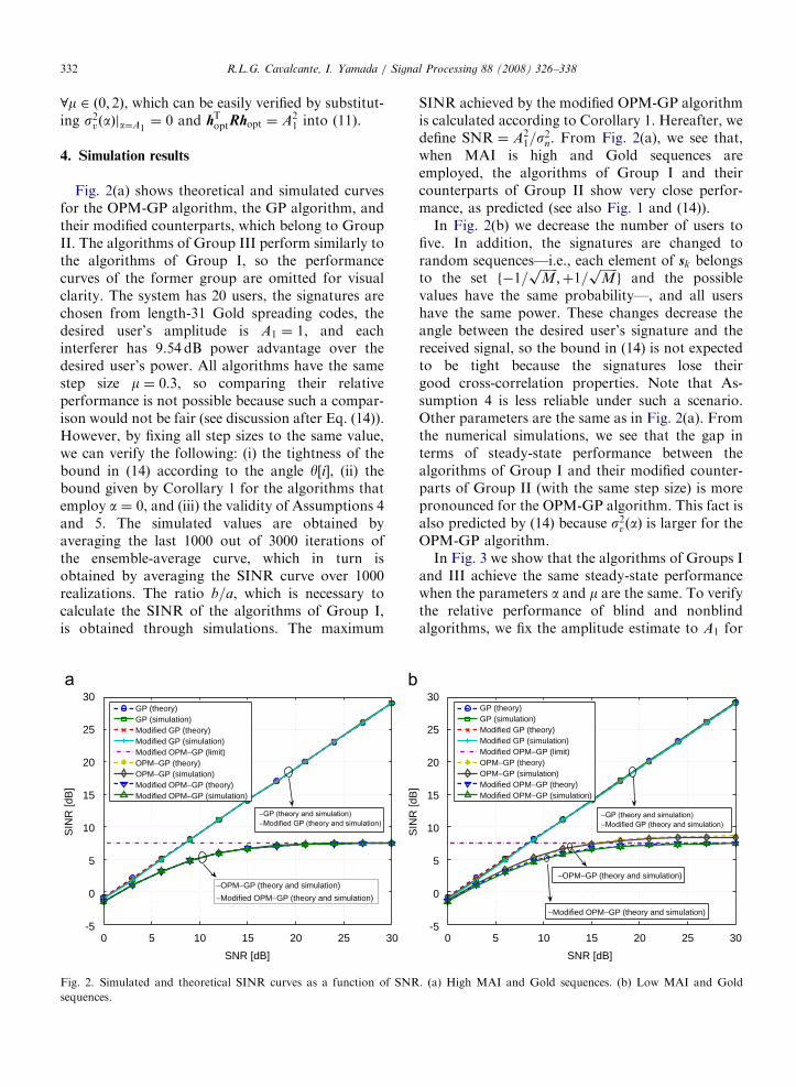
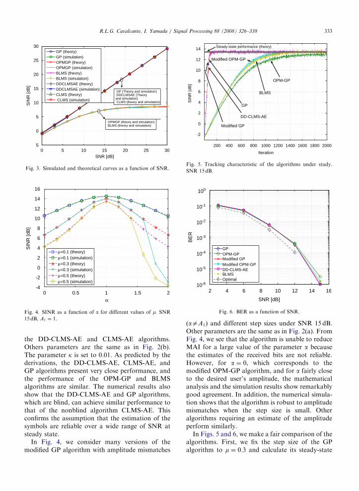
In Fig. 3 we show that the algorithms of Groups Iand III achieve the same steady-state performancewhen the parameters a and m are the same. To verifythe relative performance of blind and nonblindalgorithms, we fix the amplitude estimate to A1 for

SNR [dB]

0

5

-5

10

15

20

25

30

SIN

R [

dB

]

0 5 10 15 20 25 30

GP (theory)

GP (simulation)

Modified GP (theory)

Modified GP (simulation)

Modified OPM−GP (limit)

Modified OPM−GP (theory)

Modified OPM−GP (simulation)

OPM−GP (theory)

OPM−GP (simulation)

−OPM−GP (theory and simulation)

−Modified OPM−GP (theory and simulation)

. (a) High MAI and Gold sequences. (b) Low MAI and Gold

ARTICLE IN PRESS

0 5 10 15 20 25 305

0

5

10

15

20

25

30

SNR [dB]

SIN

R [

dB

]

GP (theory)

GP (simulation)

OPMGP (theory)

OPMGP (simulation)

BLMS (theory)

BLMS (simulation)

DDCLMSAE (theory)

DDCLMSAE (simulation)

CLMS (theory)

CLMS (simulation)

GP (Theory and simulation) DDCLMSAE (Theoryand simulation) CLMS (theory and simulation)

OPMGP (theory and simulation) BLMS (theory and simulation)

Fig. 3. Simulated and theoretical curves as a function of SNR.

0 0.5 1 1.5 2

0

2

-2

α

-4

4

6

8

10

12

14

16

SIN

R [dB

]

μ=0.1 (theory)

μ=0.1 (simulation)

μ=0.3 (theory)

μ=0.3 (simulation)

μ=0.5 (theory)

μ=0.5 (simulation)

Fig. 4. SINR as a function of a for different values of m. SNR

15 dB, A1 ¼ 1.

200 400 600 800 1000 1200 1400 1600 1800 2000

0

2

-2

4

6

8

10

12

14

Iteration

SIN

R [dB

]

GP

BLMS

OPM-GP

Modified GP

Modified OPM-GP

Steady-state performance (theory)

DD-CLMS-AE

Fig. 5. Tracking characteristic of the algorithms under study.

SNR 15dB.

2 4 6 8 10 12 14 16

100

10-1

10-2

10-3

10-4

10-5

10-6

SNR [dB]

BE

R

GP

Modified GP

Modified OPM-GP

DD-CLMS-AEBLMS

Optimal

OPM-GP

Fig. 6. BER as a function of SNR.

R.L.G. Cavalcante, I. Yamada / Signal Processing 88 (2008) 326–338 333

the DD-CLMS-AE and CLMS-AE algorithms.Others parameters are the same as in Fig. 2(b).The parameter k is set to 0.01. As predicted by thederivations, the DD-CLMS-AE, CLMS-AE, andGP algorithms present very close performance, andthe performance of the OPM-GP and BLMSalgorithms are similar. The numerical results alsoshow that the DD-CLMS-AE and GP algorithms,which are blind, can achieve similar performance tothat of the nonblind algorithm CLMS-AE. Thisconfirms the assumption that the estimation of thesymbols are reliable over a wide range of SNR atsteady state.

In Fig. 4, we consider many versions of themodified GP algorithm with amplitude mismatches

ðaaA1Þ and different step sizes under SNR 15 dB.Other parameters are the same as in Fig. 2(a). FromFig. 4, we see that the algorithm is unable to reduceMAI for a large value of the parameter a becausethe estimates of the received bits are not reliable.However, for a ¼ 0, which corresponds to themodified OPM-GP algorithm, and for a fairly closeto the desired user’s amplitude, the mathematicalanalysis and the simulation results show remarkablygood agreement. In addition, the numerical simula-tion shows that the algorithm is robust to amplitudemismatches when the step size is small. Otheralgorithms requiring an estimate of the amplitudeperform similarly.

In Figs. 5 and 6, we make a fair comparison of thealgorithms. First, we fix the step size of the GPalgorithm to m ¼ 0:3 and calculate its steady-state

ARTICLE IN PRESSR.L.G. Cavalcante, I. Yamada / Signal Processing 88 (2008) 326–338334

SINR. Then, the step sizes of all other algorithmsare calculated in such a way that all algorithmsachieve the same steady-state performance asthe GP algorithm. Unless explicitly mentioned,Ak ¼ 3A1, ka1, and other parameters of thesimulations are the same as in Fig. 2(b). The ratioa=b for the algorithms of Group I is obtained bysubstitution of the expectations in (15) by temporalmeans in each realization. We assume that the ratioa=b is the same for the algorithms of Groups I andIII because these algorithms have similar steady-state performance when the parameters a and m arethe same. The BER curves are obtained byconsidering the last 1000 out of 3000 transmittedsymbols. In Fig. 6 we also plot the BER of theoptimal filter hopt ¼ R�1s1=ðsT1 Rs1Þ for comparisonpurposes. From Fig. 5, we verify that the algorithmsthat use estimates of the desired user’s transmittedbits and amplitude are faster than those that rely ona ¼ 0. Comparing algorithms with the same para-meter a, we have a slight advantage in terms ofconvergence speed to the algorithms of Group II.This advantage is not surprising because the algo-rithms of Group II have been proposed to improvethe tracking characteristics of those of Group I [5,15],especially when y½i� is small on average. RegardingFig. 6, we adjusted the step sizes so that all algorithmshave the same SINR, therefore the BER performanceis almost the same for all compared algorithms. Thisresult is also expected because linear filters achievingthe same SINR should have close BER performance(see [9] and references therein).

5. Conclusion

We have studied the steady-state performance of acommon class of adaptive filters for MAI reduction.A closed-form steady-state expression for algorithmswith different normalization factors has been derivedin a unified way by including the possible informa-tion about the desired user’s amplitude into theenergy conservation relation. This closed-form ex-pression has been useful to compare differentnormalized algorithms in a fair way in many differentscenarios without a time-consuming trial-and-errorapproach to adjust the step sizes. Even though thealgorithms of Group II should use smaller step sizesthan those of Groups II and III for a faircomparison, the algorithms of Group II have super-ior convergence speed. We have also shown that thealgorithms (of any Group) that use informationabout the desired user’s amplitude achieve good

stead-state performance with good convergencespeed. Finally, we have demonstrated that themaximum SINR achieved by the algorithms thatdo not use any information about the desired user’samplitude is severely limited by the choice of the stepsize, and even a rough estimate of this amplitude cangreatly improve the steady-state SINR.

Acknowledgment

The authors would like to thank Prof. KohichiSakaniwa of Tokyo Institute of Technology for helpfulsuggestions and comments. This work was partiallysupported by JSPS Grants-in-Aid (C-19500186).

Appendix A. Justification of Assumption 4

We start by justifying Assumption 4 for gðr½i�Þ ¼r½i�TPr½i�.

If we rewrite (1) as

r½i� ¼ SAb½i� þ n½i�,

where S ¼ ½s1; . . . ; sK �, A ¼ diagðA1; . . . ;AK Þ, b½i� ¼½b1½i�; . . . ; bK ½i��

T, then

gðr½i�Þ ¼ r½i�TPr½i�

¼ kr½i�k2 � ðr½i�Ts1Þ2

¼ b½i�TASTSAb½i� þ n½i�Tn½i�

þ 2n½i�TASb½i� � ðr½i�Ts1Þ2. ðA:1Þ

Noticing that in CDMA systems the signatures aredesigned to satisfy sTk sj � 0, jak, and the symbolshave constant modulus, we get

b½i�TASTSAb½i� �XK

k¼1

A2k (A.2)

and

ðr½i�Ts1Þ2� A2

1. (A.3)

Using the law of large numbers [23, pp. 191–194]and the fact that in CDMA systems the spreadingfactor M is large, we can replace sample means byexpectations (a similar approximation is found in[24]), i.e.,

n½i�Tn½i� ¼Mn½i�Tn½i�

M

¼M

PMk¼1nk½i�

2

M

�MEfn1½i�2g

¼Ms2n ðA:4Þ

ARTICLE IN PRESSR.L.G. Cavalcante, I. Yamada / Signal Processing 88 (2008) 326–338 335

and

n½i�TASb½i� ¼Mn½i�TASb½i�

M� 0, (A.5)

where we define n½i�¼:½n1½i� . . . nM ½i��T. In the above

derivation, we used the fact that the randomvariables nj½i�, j ¼ 1; . . . ;M, are i.i.d. and indepen-dent of bk½i�, k ¼ 1; . . . ;K . Substitution of(A.2)–(A.5) into (A.1) yields

gðr½i�Þ �XK

k¼2

A2k þMs2n,

which is a constant. Hence the independence of ea½i�

and gðr½i�Þ is a good approximation. Similarly, wecan repeat the above derivation for gðr½i�Þ ¼ kr½i�k2

to show that

gðr½i�Þ �XK

k¼1

A2k þMs2n.

For the algorithms of Group III, by substitutingkr½i�k2 � constant (as shown above) into the defini-tion of b½i� in Table 1, we also have thatb½i� � constant.

4The existence of such a decomposition has been mentioned

in [9].5Even if r½i� and the filter ~hi�1 are not independent, which can

happen in frequency selective fading channels, this assumption is

frequently used in the analysis of adaptive filters [16,22].

Appendix B. Proof of Proposition 1

B.1. Proof of Part 1

An extension of the proof of Part 1 to OSTBC-MIMO systems with imperfect channel state in-formation has been given in [25,26]. Here, we showa slightly simplified version of the proof shown in[26] for completeness. We start with the followingclaim.

Claim 1. If R has full rank, the matrix PR can be

decomposed into PR ¼ QSQ�1, where Q 2 RM�M ,S ¼ diagðl1; . . . ; lM Þ 2 RM�M (lk, k ¼ 1; . . . ;M,are the eigenvalues of PR), l1X � � �XlM�140, and

lM ¼ 0. In addition, by further decomposing Q�T

into Q�T¼:½q1 . . . qM �, we have that qTMP ¼ 01�M ,

where 01�M is the M-dimensional row vector of zeros

and qM is a scaled version of s1.

Proof. As R1=2PR1=2 2 RM�M is symmetric, therealways exist two matrices U 2 RM�M and S 2RM�M such that R1=2PR1=2 ¼ USUT, where S ¼diagðl1; . . . ; lMÞ, and U is an orthogonal matrix

(UT ¼ U�1). Hence

PR ¼ R�1=2R1=2PR1=2R1=2

¼ R�1=2USUT R1=2

¼ R�1=2USU�1R1=2.

The matrix R has full rank and the positivesemidefinite matrix P has rank M � 1, so we havethat USUT (or, equivalently, USU�1) is a positivesemidefinite matrix with rank M � 1. Thus wecan arrange S and U in such a way thatS ¼ diagðl1; � � � ; lMÞ with l1X . . .XlM�140 andlM ¼ 0. Upon defining Q ¼ R�1=2U 2 RM�M , weconclude that PR ¼ QSQ�1.4

To prove that qTMP ¼ 01�M , we only need to

observe that the left eigenvectors of PR are thecolumns of Q�T [27, p. 316], and qM is theeigenvector associated with the eigenvalue 0. Thuswe verify that qT

MPR ¼ 01�M ¼ qTMPRR�1 ¼ qT

MP.The vector qM is a scaled version of s1 becauserankðPRÞ ¼M � 1 and sT1 PR ¼ 01�M .

Considering that the filter provides ~b1 ¼ b1, wecan rewrite (5) as

hi ¼ P hi�1 � mðhTi�1r½i� � b1½i�aÞ

r½i�

gðr½i�Þ

� �þ s1

¼ Phi�1 þ s1 � mPhTi�1r½i�

r½i�

gðr½i�Þþ maPb1½i�

r½i�

gðr½i�Þ

¼ hi�1 � mPr½i�

gðr½i�Þr½i�Thi�1 þ maPb1½i�

r½i�

gðr½i�Þ

¼ IM � mPr½i�r½i�T

gðr½i�Þ

� hi�1 þ maP

r½i�b1½i�

gðr½i�Þ,

where we used the fact that hi�1 ¼ Phi�1 þ s1. Using(6) in the above equation and taking expectation onboth sides, we arrive at

Ef~hig ¼ IM � mPEr½i�r½i�T

gðr½i�Þ

� �� Ef~hi�1g

þ maPEr½i�b1½i�

gðr½i�Þ

� �� mPE

r½i�r½i�T

gðr½i�Þ

� �hopt.

ðB:1Þ

To obtain the last identity, we also used the factthat r½i� and ~hi�1 are independent [see the modelin (1)].5

ARTICLE IN PRESSR.L.G. Cavalcante, I. Yamada / Signal Processing 88 (2008) 326–338336

The last two terms of (B.1) are equal to zero because(i) Ps1 ¼ 0 and (ii) PRhopt ¼ Ps1=ðsT1 R�1s1Þ ¼ 0(see also Assumption 6). Hence,

Ef~hig ¼ IM � mPR

Efgðr½i�Þg

� Ef~hi�1g. (B.2)

Decomposing PR into PR ¼ QSQ�1 according toClaim 1, we can rewrite (B.2) as

Q�1Ef~hig ¼ IM �m

Efgðr½i�ÞgS

� Q�1Ef~hi�1g

¼ IM �m

Efgðr½i�ÞgS

� IM �

mEfgðr½i � 1�Þg

S

� Q�1Ef~hi�2g

¼ IM �m

Efgðr½i�ÞgS

� . . . IM �

mEfgðr½2�Þg

S

� Q�1Ef~h1g

¼ IM �m

Efgðr½i�ÞgS

� i�1

Q�1Ef~h1g

¼

1� ml1

Efgðr½i�Þg

� i�1

� � � 0 0

..

. . .. ..

. ...

0 � � � 1� mlM�1

Efgðr½i�Þg

� i�1

0

0 � � � 0 1

266666666664

377777777775

Q�1Ef~h1g, ðB:3Þ

where Efgðr½i�Þg¼trðEfr½i�TPr½i�gÞ¼trðEfPr½i�r½i�TgÞ ¼trðPRÞ for the algorithms of Group II or Efgðr½i�Þg ¼trðEfr½i�r½i�TgÞ ¼ trðRÞ for the algorithms of Groups Iand III. We also used the fact that the channel is slowlyfading, which implies that Efgðr½i�Þg ¼ Efgðr½j�Þg, iaj

(at least for a block that is large enough to guaranteethe convergence of the algorithms). As trðPRÞ ¼PM

k¼1lk, lkX0 (k ¼ 1; . . . ;M) and R is positivedefinite, we have that

0plkotrðPRÞ ¼ trðR� s1sT1 RÞ

¼ trðRÞ � trðsT1 Rs1ÞotrðRÞ,

k ¼ 1; . . . ;M,

where trð:Þ stands for trace. Then we conclude that0olk=trðPRÞo1, for k ¼ 1; . . . ;M � 1. Thus, fork ¼ 1; . . . ;M � 1, any step size m 2 ð0; 2Þ is enoughto guarantee that limi!1ð1� mlk=Efgðr½i�ÞgÞi�1 ¼ 0because j1� mlk=Efgðr½i�Þgjo1.

Eq. (5) shows that Efh1g ¼ Pxþ s1, where x ¼E h0 � mðhT

0 r½i� � ~b1½i�aÞr½i�=gðr½i�Þ �

and h0 is aninitial deterministic filter. Hence, as hopt ¼ Phopt þ

s1 and qTMP ¼ 0 (from Claim 1), for i!1, (B.3)

reduces to

limi!1

Q�1Ef~hig ¼ ½0 . . . 0 qTMðPxþ s1 � Phopt � s1Þ�

T

¼ 0M�1,

which completes the proof. &

B.2. Proof of Part 2

From Assumptions 2 and 3, we have

EfjhTi�1r½i� � A1b1½i�j

2g

¼ EfðhTi�1r½i�Þ

2g � 2EfhT

i�1r½i�A1b1½i�g þ A21

¼ EfðhTi�1r½i�Þ

2g � A2

1. ðB:4Þ

By noting that (i) hi�1 is independent of r½i� and that(ii) Efxg ¼ EyfExfxjygg [17] [18, p. 296] for any tworandom variables x and y, we deduce an approx-imation of EfðhT

i�1r½i�Þ2g for sufficiently large i asfollows. First, we can check that

Efe2a½i�g þ hToptRhopt

¼ EfðhTi�1r½i�Þ2g � 2EfhTi�1r½i�r½i�Thoptg

þ EfhToptr½i�r½i�Thoptg þ hT

optRhopt

¼ EfðhTi�1r½i�Þ2g � 2EfEfhTi�1r½i�r½i�Thoptjhi�1gg þ 2hT

optRhopt

¼ EfðhTi�1r½i�Þ2g � 2ðEfhi�1g � hoptÞTRhopt

¼ EfðhTi�1r½i�Þ2g ði!1Þ,

where, in the last line, we used Part 1 of theproposition (limi!1 Efhig ¼ hopt).

ARTICLE IN PRESSR.L.G. Cavalcante, I. Yamada / Signal Processing 88 (2008) 326–338 337

At steady state, (B.4) is equivalently rewritten as

EfjhTi�1r½i� � A1b1½i�j

2g ¼ Efe2a½i�g þ hToptRhopt � A2

1,

i!1. ðB:5Þ

Hence, to obtain the steady-state SINR, we onlyneed to evaluate Efe2a½i�g, i!1.

For the adaptive filters in (5), by Ps1 ¼ 0, we have

Phi ¼ P hi�1 � muðaÞ½i�r½i�

gðr½i�Þ

� �.

With this relation, we follow [17] [18, Chapter 6] tofind an approximation for Efe2a½i�g, i!1. Sub-tracting both sides from Phopt:

P ~hi ¼ P ~hi�1 � muðaÞ½i�r½i�

gðr½i�Þ

� �. (B.6)

Thus, left multiplying both sides by r½i�T, we have

ep½i� ¼ ea½i� � muðaÞ½i�r½i�TPr

gðr½i�Þ. (B.7)

Hence

ea½i� � ep½i�

r½i�TPr½i�¼ m

uðaÞ½i�gðr½i�Þ

. (B.8)

Substituting (B.8) into (B.6), we deduce

P ~hi þPr½i�ea½i�

r½i�TPr½i�¼ P ~hi�1 þ

Pr½i�ep½i�

r½i�TPr½i�.

Taking the square norm of both sides with P2 ¼ P,we arrive at the energy-conservation relation (thecross terms cancel out due to (7) and (8)):

~hT

i P ~hi þe2a½i�

r½i�TPr½i�¼ ~h

T

i�1P~hi�1 þ

e2p½i�

r½i�TPr½i�. (B.9)

Taking expectation on both sides and imposing the

steady-state condition, Ef~hT

i P ~hig ¼ Ef~hT

i�1P~hi�1g,

we get

Ee2a½i�

r½i�TPr½i�

� �¼ E

e2p½i�

r½i�TPr½i�

( ). (B.10)

Substitution of (B.7) into (B.10) yields the variancerelation for steady-state performance,

E mu2ðaÞ½i�r½i�TPr½i�

g2ðr½i�Þ

� �¼ 2E

ea½i�uðaÞ½i�gðr½i�Þ

� �. (B.11)

Using the relation uðaÞ½i� ¼ ea½i� þ vðaÞ½i� in the lastequation together with Assumptions 4 and 5, we can

show that

2Efe2a½i�gE1

gðr½i�Þ

� �¼ mEfe2a½i�gE

r½i�TPr½i�

g2ðr½i�Þ

� �

þ mEfv2ðaÞ½i�gEr½i�TPr½i�

g2ðr½i�Þ

� �.

Isolating Efe2a½i�g, we finally get

Efe2a½i�g ¼s2vðaÞm

2b=a� m. (B.12)

Therefore, combining (12), (B.5) and (B.12), wearrive at the desired result (11).

References

[1] S. Verdu, Multiuser Detection, Cambridge University Press,

Cambridge, UK, 1998.

[2] M. Honig, U. Madhow, S. Verdu, Blind adaptive multiuser

detection, IEEE Trans. Inform. Theory 41 (4) (1995)

944–960.

[3] U. Madhow, M.L. Honig, MMSE interference suppression

for direct-sequence spread-spectrum CDMA, IEEE Trans.

Commun. 42 (12) (1994) 3178–3188.

[4] S.C. Park, J.F. Doherty, Generalized projection algorithm

for blind interference suppression in DS/CDMA commu-

nications, IEEE Trans. Circuits Syst. II 44 (6) (1997)

453–460.

[5] J. A. Apolinario, S. Werner, P. S. R. Diniz, T. Laakso,

Constrained normalized adaptive filters for CDMA mobile

communications, in: Proceedings EUSIPCO, Vol. IV, 1998,

pp. 2053–2056.

[6] X. Wang, H.V. Poor, Blind multiuser detection: a subspace

approach, IEEE Trans. Inform. Theory 44 (2) (1998)

677–690.

[7] M. Honig, M.K. Tsatsanis, Adaptive techniques for

multiuser CDMA receivers, IEEE Signal Process. Mag. 17

(3) (2000) 49–61.

[8] M. L. Honig, S. L. Miller, M. J. Shensa, L. B. Milstein,

Performance of adaptive linear interference suppression

in the presence of dynamic fading, IEEE Trans. Commun.

49 (4).

[9] G.V. Moustakides, Constrained adaptive linear multiuser

detection schemes, special issue on multiuser detection,

J. VLSI Signal Process. 39 (1–3) (2002) 293–309.

[10] X. Wang, H.V. Poor, Wireless Communication Systems,

Prentice-Hall, Upper Saddle River, NJ, 2004.

[11] R.L.G. Cavalcante, I. Yamada, K. Sakaniwa, A fast blind

MAI reduction based on adaptive projected subgradient

method, IEICE Trans. Fundamentals E87-A (8) (2004)

1973–1980.

[12] M. Yukawa, R.L.G. Cavalcante, I. Yamada, Efficient blind

MAI suppression in DS/CDMA systems by embedded

constraint parallel projection techniques, IEICE Trans.

Fundamentals E88-A (8) (2005) 2062–2071.

[13] R. L. G. Cavalcante, M. Yukawa, I. Yamada, Set-theoretic

DS/CDMA receivers for fading channels by adaptive

ARTICLE IN PRESSR.L.G. Cavalcante, I. Yamada / Signal Processing 88 (2008) 326–338338

projected subgradient method, in: Proceedings IEEE GLO-

BECOM, 2005.

[14] S. Haykin, A.H. Sayed, J.R. Zeidler, P. Yee, P.C. Wei,

Adaptive tracking of linear time-variant systems by extended

RLS algorithms, IEEE Trans. Signal Process. 45 (5) (1997)

1118–1128.

[15] M. Yukawa, I. Yamada, Adaptive beamforming by con-

strained parallel projection in the presence of spatially-

correlated interferences, in: ICASSP, 2006.

[16] S. Haykin, Adaptive Filter Theory, fourth ed., Prentice-Hall,

Upper Saddle River, NJ, 2002.

[17] N.R. Yousef, A.H. Sayed, A unified approach to the steady-

state and tracking analyses of adaptive filters, IEEE Trans.

Signal Process. 49 (2) (2001) 314–324.

[18] A.H. Sayed, Fundamentals of Adaptive Filtering, Wiley,

Hoboken, NJ, 2003.

[19] H. Shin, A.H. Sayed, Mean-square performance of a family

of affine projection algorithms, IEEE Trans. Signal Process.

52 (1) (2004) 90–102.

[20] I. Yamada, N. Ogura, Adaptive subgradient method for

asymptotic minimization of sequence of nonnegative convex

functions, Numer. Funct. Anal. Optim. 25 (7/8) (2004) 593–617.

[21] R. L. G. Cavalcante, I. Yamada, Steady-state analysis of

constrained normalized adaptive filters for CDMA systems,

in: ICASSP, 2006.

[22] R. Schober, W.H. Gerstacker, L.H.-J. Lampe, Data-aided

and blind stochastic gradient algorithms for widely linear

MMSE MAI suppression for DS-CDMA, IEEE Trans.

Signal Process. 52 (3) (2004) 746–756.

[23] A. Papoulis, Probability, Random Variables, and Stochastic

Processes, second ed., McGraw-Hill, Singapore, 1987.

[24] J. Benesty, H. Rey, L.R. Vega, S. Tressens, A nonparametric

VSS NLMS algorithm, IEEE Signal Process. Lett. 13 (10)

(2006) 581–584.

[25] R. L. G. Cavalcante, I. Yamada, Multiaccess interference

reduction in OSTBC-MIMO systems by adaptive projected

subgradient method, in: ICASSP, 2007.

[26] R. L. G. Cavalcante, I. Yamada, Multiaccess interference

suppression in orthogonal space-time block coded MIMO

systems by adaptive projected subgradient method, IEEE

Trans. Signal Process., accepted for publication.

[27] G.H. Golub, C.F.V. Loan, Matrix Computations, third ed.,

The Johns Hopkins University Press, Baltimore, MD,

1996.