New Gaussianity measures based on order statistics: application to ICA

Neurocomputing 51 (2003) 303–320www.elsevier.com/locate/neucom

New Gaussianity measures based on orderstatistics: application to ICA�

Y. Blanco∗, S. ZazoETS Ingenieros Telecomunicaci�on, Universidad Polit�ecnica de Madrid, Ciudad Universitaria s=n,

Madrid 28040, Spain

Received 5 March 2001; accepted 23 November 2001

Abstract

In this paper we propose and analyze a set of alternative statistical distances between distribu-tions based on the cumulative density function instead of traditional probability density function.In particular, these new Gaussian distances provide new cost functions whose maximization per-forms the extraction of one independent component at each successive stage of a de1ation ICAprocedure. The new Gaussianity measures improve the ICA performance and also increase therobustness against outliers in comparison with traditional ones. c© 2002 Elsevier Science B.V.All rights reserved.

Keywords: Independent component analysis; Blind source separation; Cumulative density function; Orderstatistics; Gaussianity measure

1. Introduction

The goal of BSS (blind source separation) is to extract N unknown independentsources (s = [s1 : : : sN ]H ) from a set of their linear mixtures (y = [y1 : : : yM ]H ); thesystem mixture is expressed according to y(n) =Hs(n), where HM×N is the unknownmixture matrix (with M¿N ). Most of the methods perform a spatial decorrelationpreprocessing [15] over y to obtain the decorrelated observable z = [z1 : : : zM ]H ; inthis way, the global mixture is expressed by z(n) = Vs(n), where V is an unknownorthogonal matrix. Later, independent component analysis (ICA) is applied in orderto ;nd a linear unitary transformation w(n) = Bz(n) so that the components wi are as

� Work partly supported by national projects TIC98-0748 abd 07T=0032=2000.∗ Corresponding author.E-mail address: [email protected] (Y. Blanco).

0925-2312/03/$ - see front matter c© 2002 Elsevier Science B.V. All rights reserved.PII: S0925 -2312(01)00707 -X

304 Y. Blanco, S. Zazo /Neurocomputing 51 (2003) 303–320

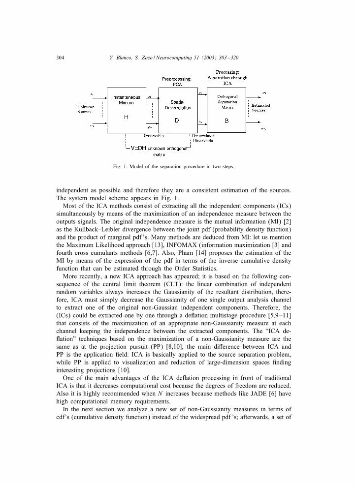
Fig. 1. Model of the separation procedure in two steps.

independent as possible and therefore they are a consistent estimation of the sources.The system model scheme appears in Fig. 1.

Most of the ICA methods consist of extracting all the independent components (ICs)simultaneously by means of the maximization of an independence measure between theoutputs signals. The original independence measure is the mutual information (MI) [2]as the Kullback–Leibler divergence between the joint pdf (probability density function)and the product of marginal pdf ’s. Many methods are deduced from MI: let us mentionthe Maximum Likelihood approach [13], INFOMAX (information maximization [3] andfourth cross cumulants methods [6,7]. Also, Pham [14] proposes the estimation of theMI by means of the expression of the pdf in terms of the inverse cumulative densityfunction that can be estimated through the Order Statistics.

More recently, a new ICA approach has appeared; it is based on the following con-sequence of the central limit theorem (CLT): the linear combination of independentrandom variables always increases the Gaussianity of the resultant distribution, there-fore, ICA must simply decrease the Gaussianity of one single output analysis channelto extract one of the original non-Gaussian independent components. Therefore, the(ICs) could be extracted one by one through a de1ation multistage procedure [5,9–11]that consists of the maximization of an appropriate non-Gaussianity measure at eachchannel keeping the independence between the extracted components. The “ICA de-1ation” techniques based on the maximization of a non-Gaussianity measure are thesame as at the projection pursuit (PP) [8,10]; the main diMerence between ICA andPP is the application ;eld: ICA is basically applied to the source separation problem,while PP is applied to visualization and reduction of large-dimension spaces ;ndinginteresting projections [10].

One of the main advantages of the ICA de1ation processing in front of traditionalICA is that it decreases computational cost because the degrees of freedom are reduced.Also it is highly recommended when N increases because methods like JADE [6] havehigh computational memory requirements.

In the next section we analyze a new set of non-Gaussianity measures in terms ofcdf’s (cumulative density function) instead of the widespread pdf ’s; afterwards, a set of

Y. Blanco, S. Zazo /Neurocomputing 51 (2003) 303–320 305

equivalent distances built over inverse cdf’s is proposed, whose main advantage is thedirect implementation by means of the Order Statistics. The new measures are directlyapplied to ICA due to the “ICA estimation principle” [10], this issue is analyzed inSection 4.1. Section 4.2 will deal with the adaptive processing of the new cost functionsand the de1ation ICA procedure for the multidimensional case. Some comparativeresults conclude the paper.

2. Theoretical fundamentals: Gaussianity measures based on the cdf

A Gaussianity measure is an appropriate distance between the analyzed signal wi

and the equivalent Gaussian distribution g with the same power. Negentropy is theoriginal Gaussianity measure; it was de;ned as the Kullback–Leibler distance betweenboth pdf ’s: fwi ; fg. Kurtosis [11] arises like an estimation of Negentropy achievedby means of expansions of the pdf ’s in terms of some cumulants; recently, a familyof Gaussianity measures (built with non-linearities) has been proposed in [9] like anextension of the Kurtosis measure.

2.1. De2nition

In addition, we recall that the distance between two distributions can be equallyevaluated using cdf’s instead of pdf ’s. Speci;cally, let us de;ne a family of distributiondistances through the norm concept applied to the diMerence between both cdf’s; letus call F and FR the cdf to be analyzed and the reference one, respectively:

d∞(F; FR) = maxx

|F(x) − FR(x)|; L∞ Norm; (1)

dp(F; FR) =(∫ ∞

−∞|F(x) − FR(x)|p dx

)1=p

; Lp Norm: (2)

Furthermore, it can be appreciated that the in;nite norm in Eq. (1) is exactly thewell known KormogoroM–Smirnov test [8] (KS test) to evaluate whether or not twodistributions are coincident. For ICA proposal, it is needed to evaluate the distancesbetween the analyzed signal wi and its equivalent Gaussian, therefore, it results inapplying previous distances:

d∞(Fwi ; Fg) = maxx

|Fwi(x) − Fg(x)|; (3)

dp(Fwi ; Fg) =(∫ ∞

−∞|Fwi(x) − Fg(x)|p dx

)1=p

: (4)

2.2. Proof

Next, we show that previous de;nitions hold the following distance property in orderto corroborate their feasibility as an ICA procedure:

d(Fwi ; Fg) = 0 ⇔ c = 2; andd(Fwi ; Fg)¿ 0 ∀c �= 2; (5)


where c is the “Gaussianity parameter” in the “generalized Gaussian family” (Eq. (6));c = 2 implies that wi is Gaussian, c¡ 2 corresponds to a superGaussian signal andc¿ 2 to a subGaussian one; wi is assumed with a unit variance and null mean in orderto simplify

fwi(x) =

√�(3=c)�(1=c)3

c2

exp

− |x|c√(�(1=c)�(3=c) )

c

; (6)

where � is the complete Gamma function (see [1]) de;ned as follows:

�(y) =∫ ∞

0exp(−t)ty−1 dt: (7)

After a mathematical development from Fwi(x) =∫ x−∞ fwi(u) du, we have obtained the

following cdf expression in terms of the incomplete Gamma function � (see [1]):

Fwi(x) =

0:5 + A 1

c

(1a

)1=c

�(

1c; axc

)if x¿ 0

0:5 − A 1c

(1a

)1=c

�(

1c; axc

)if x¡ 0

; (8)

where A and a depend on c as follows:

A =

√�(3=c)�(1=c)3

c2;

a =

√(�(1=c)�(3=c)

)−1=c

; (9)

and function � is de;ned as (see [9])

�(�; y) =∫ y

−∞exp(−t)t�−1 dt: (10)

Now, Fwi for several values of c (in Eq. (8)) and Fg (in Eq. (8) with c = 2) aresubstituted in Eqs. (3) and (4) in order to compute the new Gaussianity measures. Theimplementation is carried out through the following summation on a set of discretevalues on the cdf domain x, with suQcient precision (Rx):(∫ ∞

−∞|Fwi(x) − Fg(x)|p dx

)1=p

�(

Rx∑x

|Fwi(x) − Fg(x)|p)1=p

: (11)

In Fig. 2, the most representative new Gaussianity measures (in;nite Norm, p = 1; 2)are calculated as we have just explained and they are represented in front of c.

From the direct observation of Fig. 2, it is concluded that the property in Eq. (5)holds.


0 2 4 6 8 10 12 14 16 18 200

0.05

0.1

0.15

c parameter

Gau

ssia

nity

dis

tanc

esd

1d

2d

inf

Fig. 2. Gaussianity measures based on cdf’s expressions of the generalized family Gaussian.

The ;nal conclusion in this section is that the distance measures proposed are shownto be measures of Gaussianity (therefore of non-Gaussianity) since they oMer a globalminimum when the analyzed distribution is Gaussian and the function grown mono-tonically according to the distribution shifts far away from the Gaussian (Fig. 2 isconclusive at this point).

3. Practical implementation: Gaussianity measures based on order statistics

3.1. De2nition

The estimation of F̂wi is necessary in the evaluation of previous distances (3), (4) butit would require a high computational cost if it is to be performed through accumulatedhistograms; fortunately, an equivalent distance easy to estimate can be established interms of inverse cdf’s: Qwi =F−1

wi; Qg =F−1

g ; more indeed, the diMerence between d∞and dp is that distances are considered over the horizontal axis instead of the verticalone:

D∞(Qwi ; Qg) = maxx

|Qwi(x) − Qg(x)|; L∞ Norm; (12)

Dp(Qwi ; Qg) =

(∫ 1

0|Qwi(x) − Qg(x)|p dx

)1=p

; Lp Norm: (13)


The close relationship between F and Q implies that proof property 5 in the previoussection is generalized:

D(Qwi ; Qg) = 0 ⇔ c = 2; and D(Qwi ; Qg)¿ 0∀c �= 2: (14)

Since Q is the inverse of F , both functions present the same character (increasing ordecreasing character); consequently, the distances d and its correspondent D present thesame behavior, in other words, the curves in Fig. 2 for Q hold the same properties thancurves for F . Therefore Eqs. (12) and (13) are appropriate non-Gaussianity measures.

The estimation of Qwi can be performed very robustly in a simple practical way byordering a suQciently large set of n temporal discrete samples from {wi[1]; : : : ; wi[n]}and obtaining the set of order statistics (OS) wi(1) ¡wi(2) ¡ · · ·¡wi(n); The OS are aconsistent estimation of the quantiles of the distribution:

Q̂wi

(kn

)= wi(k) ⇔ F̂(wi(k)) =

kn: (15)

Consequently, the estimation of Eqs. (12) and (13) can be expressed using OS notation:

D̂∞(Qwi ; Qg) = maxk

∣∣∣∣wi(k) − Qg

(kn

)∣∣∣∣ ; L∞ Norm; (16)

D̂p(Qwi ; Qg) =

(1n

n∑k=1

∣∣∣∣wi(k) − Qg

(kn

)∣∣∣∣p)1=p

; Lp Norm; (17)

where Qg(k=n) is the k=n quantile of the equivalent Gaussian distribution.Actually, previous equations imply the estimation of a ;nite set of discrete values of

the inverse cdf Q in the non-Gaussianity measures in Eqs. (12) and (13), if n is largeenough (around 1000 samples), then the estimation is really robust. At this point, it isnecessary to clarify that the Kolmogorov–Smirnov estimator in Eq. (16) uses only oneordered sample, therefore it can be applied if one requires to reduce the complexityof the algorithm; where as using any measure with the whole set of order statisticscontains more information since the cdf is estimated through a large set of its discretevalues. Next section is focused on simplifying the non-Gaussianity measure as muchas possible in order to reduce the computational cost.

3.2. Kolmogoro4–Smirnov test through OS

Let us remark that in;nite norm in Eq. (16) is a modi;ed KS estimator performinga hypothesis test that is equivalent to the one well known in the literature [12] (statedin Section 2), but using the inverse cdf Qwi instead of the ordinary Fwi .

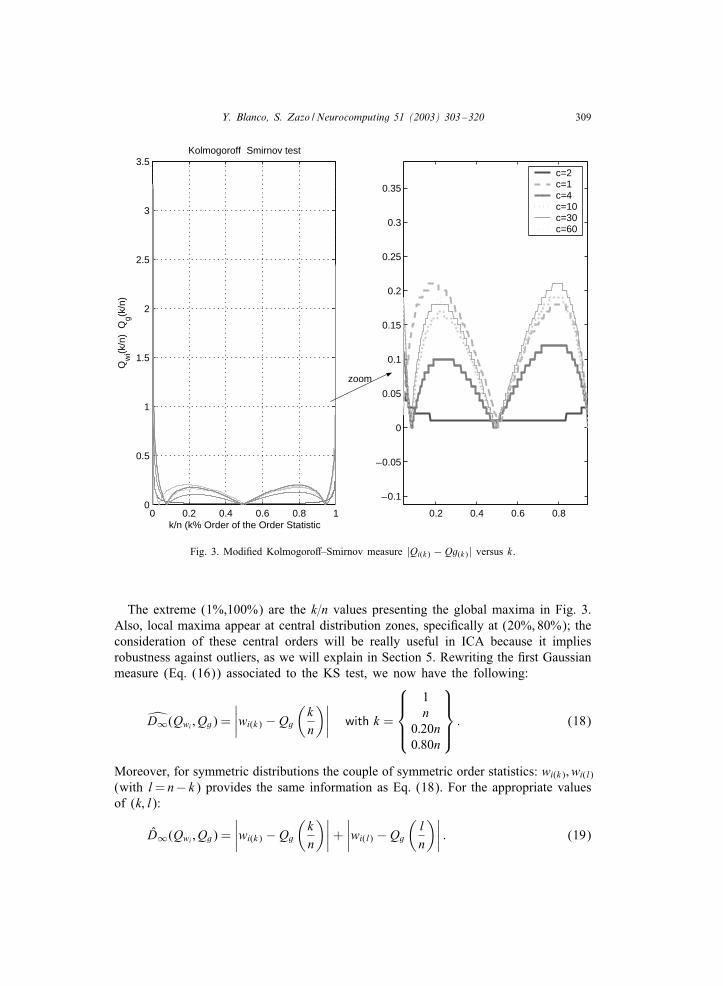
At this moment, our goal is the establishment of a pre;xed value k=n in order toreduce the computational cost because only one ordered sample would be required inthe estimation of the Gaussianity measure L∞Norm; let us search the k=n values thatmaximize the absolute value in Eq. (16); for this proposal, several distribution typeshave been chosen for several values of the Gaussianity family parameter “c” (seeEq. (6)). In Fig. 3, the function |Qi(k) − Qg(k)| is represented in front of the k index(expressed as %).


0 0.2 0.4 0.6 0.8 10

0.5

1

1.5

2

2.5

3

3.5

k/n (k% Order of the Order Statistic

Qw

i(k/n

) Q

g(k/n

)

Kolmogoroff Smirnov test

0.2 0.4 0.6 0.8

_0.1

_0.05

0

0.05

0.1

0.15

0.2

0.25

0.3

0.35

c=2 c=1 c=4 c=10c=30c=60

zoom

Fig. 3. Modi;ed KolmogoroM–Smirnov measure |Qi(k) − Qg(k)| versus k.

The extreme (1%,100%) are the k=n values presenting the global maxima in Fig. 3.Also, local maxima appear at central distribution zones, speci;cally at (20%, 80%); theconsideration of these central orders will be really useful in ICA because it impliesrobustness against outliers, as we will explain in Section 5. Rewriting the ;rst Gaussianmeasure (Eq. (16)) associated to the KS test, we now have the following:

D̂∞(Qwi ; Qg) =∣∣∣∣wi(k) − Qg

(kn

)∣∣∣∣ with k =

1n

0:20n0:80n

: (18)

Moreover, for symmetric distributions the couple of symmetric order statistics: wi(k); wi(l)

(with l= n− k) provides the same information as Eq. (18). For the appropriate valuesof (k; l):

D̂∞(Qwi ; Qg) =∣∣∣∣wi(k) − Qg

(kn

)∣∣∣∣+∣∣∣∣wi(l) − Qg

(ln

)∣∣∣∣ : (19)


Fig. 4. Distribution representation examples through OS estimation.

Taking into account that Qg(k=n) = −Qg(l=n), the absolute values in Eq. (19) areanalyzed in Fig. 4 showing two possible situations:{

wi(k) ¿Qg

(kn

)and wi(l) ¡Qg

(ln

)}either

{wi(k) ¡Qg

(kn

)and wi(l) ¿Qg

(ln

)}:

(20)

Consequently, Eq. (19) ;nally results: 1

D̂∞(Qwi ; Qg) =∣∣∣∣wi(k) − wi(l) + 2Qg

(ln

)∣∣∣∣ withk; l = 80%n; 20%n

ork; l = n; 1:

(21)

1 Let us give the numerically deduced constant values Qg(1%) ∼= −3:8245; Qg(20%) � −0:8412 tobe used in Eq. (21), which correspond to the equivalent (same power as wi) Gaussian distribution with(0; "2 = 1); let us remark that the output channel power "2

wiis always 1 because E[zzT] = I and B is

constrained to be unitary.


Table 1Estimator variance for several Gaussianity measures. D∞1 is D∞ with (k=n; l=n) = (100%; 1%) and D∞2 isD∞ with (k=n; l=n) = (80%; 20%)

Kurtosis log(cosh) D1 D2 D∞1 D∞2

n = 500 Unif. 2; 8 × 10−3 10−3 8 × 10−3 8 × 10−3 10−4 6; 1 × 10−3

n = 2500 Unif. 5 × 10−4 0 10−3 10−3 3 × 10−6 1; 2 × 10−3

n = 500 Lap. 1.65 6 × 10−3 9 × 10−3 1; 8 × 10−3 1.52 3; 9 × 10−3

n = 2500 Lap. 0.45 10−3 10−3 2 × 10−3 1.46 8 × 10−4

3.3. Statistical analysis

Let us call D∞; D1 and D2 as the new “Gaussianity estimators” based on OS inEqs. (21) and (17).

Let us analyze how much eQcient are the new Gaussianity estimators compared toother traditional ones. For this proposal, two representative Gaussianity measures havebeen chosen: the Kurtosis [11] and the non-linearity log(cosh(:)) proposed in [9]. EveryGaussianity measure has been calculated for 1000 independent realizations in order tocalculate the corresponding variance. Table 1 shows the variance of the estimation forn = 500 and 2500 processed samples.

Data in Table 1 oMer the following interesting contributions from a statistical pointof view:

• Kurtosis, as well as D∞(1%;100%), are highly eQcient for subGaussian signals, whilethey are ineQcient for superGaussian ones.

• D∞(1%;100%)is the most eQcient estimator for subGaussian signals, whileD∞(20%;80%) is the most eQcient for superGaussian ones.

• If we have to choose one estimator consistent enough in both distributions it would belog(cosh()), although D1; D2 and D∞(20%;80%) present comparable results; therefore,they are extremely eQcient for both distributions character.

• To summarize, the Kolmogorov–Smirnov estimator can be applied to reduce thecomplexity, although in this case the statistics of the source (sub, super Gaussian) hasto be taken into account to choose the extreme or the central OS, respectively. Usingany measure with the whole set of order statistics does not require any knowledgeabout the kind of distribution and is more consistent since the cdf is estimatedthrough a large set of its discrete values.

4. ICA application of the new non-Gaussianities

4.1. ICA capability

The well known CLT states that the linear combination of non-Gaussian independentvariables wi = $jpijsj always increases the Gaussianity of the resultant distribution;consequently, decreasing the Gaussianity of any output wi will provide the extraction


of some independent component. This CLT consequence is formally exposed in thefollowing ICA estimation principle enunciated and proved by HyvWarien in [10]:

ICA estimation principle 2: Maximum non-Gaussianity. Find the local maxima ofnon-Gaussianity of a linear combination wi =$jpijsj under the constraint that thevariance of wi is constant. Each local maximum gives one independent component.

On the one hand, the distance measures based on the cumulative density functionhave been proved to be “non-Gaussianities” in the previous section, and thereforecould be applied to any of the output channels wi to extract one of the independentcomponents sj.

On the other hand, every output channel is wi = bHi z, where bHi is the i-row of theseparation matrix B; therefore if the ICA algorithm guarantees that every separationvector bi is unitary the output wi will have the same variance or power for every valueof bi.

From these two points the conclusion is clear: the proposed non-Gaussianities willpresent a local maximum at any output channel for each independent component if biis forced to be unitary. Therefore, a multistage procedure must be applied to obtain adiMerent independent component at each output channel: the non-Gaussianity is max-imized at each output channel successively under the constriction that the vector bihas to be orthonormal to the previously obtained vectors. The orthogonality among theseparation vectors implies that the extracted components are decorrelated, and whenone independent component has already been extracted decorrelation and independenceare equivalent (see [9,10] for more details).

To illustrate the quoted ICA estimation principle, the non-Gaussianity ICA cost func-tions corresponding to a simple mixture of two sources (one Laplacian source as rep-resentative of superGaussian and the other subGaussian source as a representative ofsubGaussian) are represented in order to visualize in a graph the shape of the costfunction. In the TITO scenario, the original sources are mixed through an orthonor-mal matrix V parameterized by the rotation angle &, therefore, the separation matrixwould be

B=

[cos (') sin (')

−sin (') cos (')

]: (22)

Consequently, the output analysis channel depends on the error angle (='−& accordingto

w1 = cos (()s1 + sin (()s2; (23)

obviously, when ( = 0 or )=2, the ICA-BSS problem is solved with the consequentextraction of both sources at w.

Figs. 5 and 6 show that the non-Gaussianity measures based on OS applied to thechannel w1 present a local maxima at the solution ( = 0 that gives the extraction ofs1 in w1 and another local maxima at ( = )=2 that gives the extraction of the otherindependent component s2.


-1.5 -1 -0.5 0 0.5 1 1.5 2 2.50.02

0.04

0.06

0.08

0.1

0.12

0.14

0.16

error angle

D1(w

1)

non-gaussianity ICA cost functions in a TITO BSS problem

-1.5 -1 -0.5 0 0.5 1 1.5 2 2.50.5

1

1.5

2

2.5

3

3.5x 10

-3

error angle

D2(w

1)

Fig. 5. Cost functions D1(w1) and D2(w2) in front of the error angle ( = ' − &.

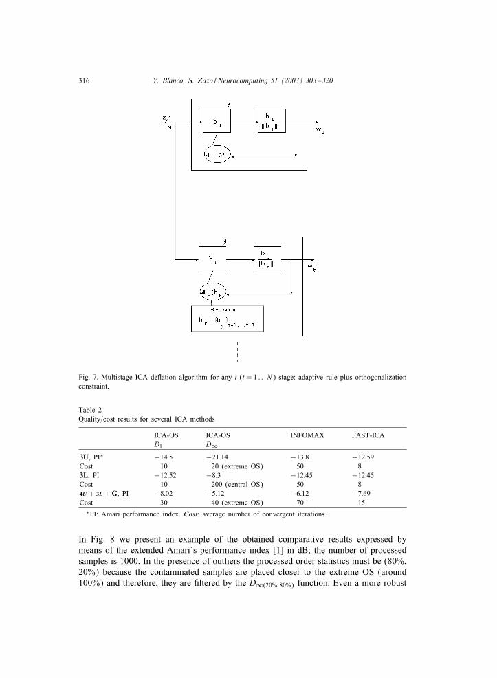
4.2. ICA de;ation algorithm

Taking into account that wi = bTi z, where bT

i is the i-row of the separation matrix B,the goal is to update bi properly at each i stage by means of the optimization of anICA cost function J (wi(bi)). Let us take J (wi(bi)) =D∞; J (wi(bi)) will be optimizedby means of a stochastic gradient rule plus a constraint:

bi[t + 1] = bi[t] + +∇J |bi[t];bi is orthonormal to {b1; : : : ; bi−1}:

(24)

Let us remark that the gradient expression of a similar cost function was deduced in[10] for the simplest scenario where N=2. Let us now generalize the gradient algorithmin [4] to the multidimensional problem. The gradient of J (wi(bi)) in Eq. (21) is

∇J |bi[t] = Sd(wi(k) − wi(l))

dbi

∣∣∣∣bi[t]

; (25)


-1.5 -1 -0.5 0 0.5 1 1.5 2 2.50

1

2

3

4

5

6

error angle

Din

f1(w

1)

non-gaussianity ICA cost functions in a TITO BSS problem

-1.5 -1 -0.5 0 0.5 1 1.5 2 2.50

0.1

0.2

0.3

0.4

0.5

error angle

Din

f2(w

1)

Fig. 6. Cost functions D∞(1%;100%) (up) and D∞(20%;80%) (down) in front of the error angle ( = ' − &.

where

S = sign(wi(k) − wi(l) + 2Qg

(ln

))bi[t]

:

Applying the chain rule we have

d(wi(k) − wi(l))dbi

∣∣∣∣bi[t]

= z

(dwi(k)

dwi

∣∣∣∣bi[t]

− dwi(l)

dwi

∣∣∣∣bi[t]

): (26)

The derivative of any r-order statistics with respect to wi was obtained by means ofthe derivative of a vector in [4] and it ;nally gives

dwi(r)

dwi

∣∣∣∣bi[t]

= er = [0; 0; ::0; 1; 0::0]T;

where

er[j] =

{1 if wi[j] = wi(r)

0 rest

}j=1:::n

: (27)


The generalization of the previous adaptive algorithm to D1 and D2 can be performedstraightforward, for example, for J = D1:

∇Jt |bi[t] =1nz

n∑k=1

S(k)ek

∣∣∣∣∣bi[t]

; (28)

where

S(k) = sign(wt(k) − Qg

(kn

)|bi[t])

:

Additionally, as it was explained in Section 4.1 this optimization must be accomplishedby the proper constraint explained in [10]: after each t iteration, bi is normalized andprojected over the subspace orthonormal Ci−1 to the vectors obtained at every previousstage in order to guarantee the independence among all the extracted sources. Let usquote that the Ci−1 expression is

Ci−1 = I − (Bi−1BHi−1)−1BH

i−1; (29)

where

Bi−1 = {b1; : : : ; bi−1}:The whole ICA multistage de1ation algorithm is presented in the scheme in Fig. 7.

5. Results

In order to compare the ICA performance of the new cost functions and its corre-sponding algorithm convergence with other representative ICA methods (INFOMAX[3] as a representative of “ICA simultaneous extraction” and Fast ICA as a represen-tative of “ICA de1ation” [9]) we have considered three representative examples ofmixtures. For each case, one hundred arbitrary mixtures have been generated and sepa-rated averaging Amari’s performance index in dB (extended quality separation measure[2]); 1000 samples per output channel have been processed; +=0:5 and 0.01 have beenchosen as the adaptation step for Dp and D∞, respectively, that oMer the best trade oMbetween quality and convergence level. Besides this, the computational cost has beenevaluated by averaging the number of required iterations for the algorithm to converge.The results are shown in Table 2.

Next, in order to compare the robustness against outliers of the new ‘Gaussianitymeasure based on OS’ with other representative measures (Kurtosis and the non-linearityproposed in [9]) several kinds of sources have been mixed through a ;xed orthogo-nal mixture matrix V(2 × 2). After that, the corresponding ICA algorithm is appliedover the decorrelated observable z= Vs. In this scenario, every original source so hasbeen contaminated with uniform outliers of power "2

u =4"2so according to the following

pdf ’s relation:

fs(x) = (1 − /)fso(x) + /fu(x): (30)


Fig. 7. Multistage ICA de1ation algorithm for any t (t = 1 : : : N ) stage: adaptive rule plus orthogonalizationconstraint.

Table 2Quality=cost results for several ICA methods

ICA-OS ICA-OS INFOMAX FAST-ICAD1 D∞

3U, PI∗ −14:5 −21:14 −13:8 −12:59Cost 10 20 (extreme OS) 50 83L, PI −12:52 −8:3 −12:45 −12:45Cost 10 200 (central OS) 50 84U + 3L + G, PI −8:02 −5:12 −6:12 −7:69Cost 30 40 (extreme OS) 70 15

∗PI: Amari performance index. Cost: average number of convergent iterations.

In Fig. 8 we present an example of the obtained comparative results expressed bymeans of the extended Amari’s performance index [1] in dB; the number of processedsamples is 1000. In the presence of outliers the processed order statistics must be (80%,20%) because the contaminated samples are placed closer to the extreme OS (around100%) and therefore, they are ;ltered by the D∞(20%;80%) function. Even a more robust


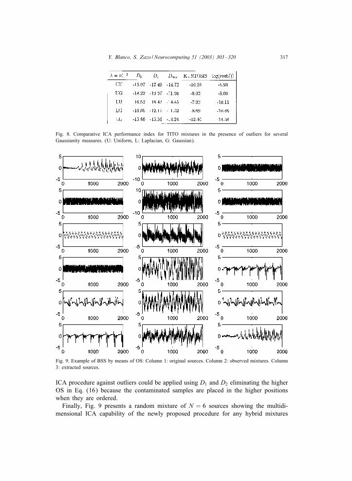
Fig. 8. Comparative ICA performance index for TITO mixtures in the presence of outliers for severalGaussianity measures. (U: Uniform, L: Laplacian, G: Gaussian).

Fig. 9. Example of BSS by means of OS: Column 1: original sources. Column 2: observed mixtures. Column3: extracted sources.

ICA procedure against outliers could be applied using D1 and D2 eliminating the higherOS in Eq. (16) because the contaminated samples are placed in the higher positionswhen they are ordered.

Finally, Fig. 9 presents a random mixture of N = 6 sources showing the multidi-mensional ICA capability of the newly proposed procedure for any hybrid mixtures


0 10 20 30 40 50 60 70 80 90 100

_ 0.2

_ 0.4

0

0.2

0.4

0.6

0.8

1

iteration number

Fig. 10. Example of convergence of the gradient algorithm: coeQcients of b3 at 3-stage.

since the given sources are fragments of voice, 4PAM communication signal, a sinu-soidal signal, an arti;cial uniform source and two images. In this example, the chosenOS have been (1%,100%). The quality of the separation (−18 dB) corroborates thecapability for any kind of mixture. Also, Fig. 10 shows the right convergence of thecoeQcients of vector b3 to one of the solutions, indicating its fast behavior, becausethe ;nal state is reached in 30–40 iterations.

6. Brief summary

We propose a set of non-Gaussianity measures D based on OS applied to solve theICA problem under the “non-Gaussianity ICA estimation principle”. From the analysisalong the paper (corroborated by the “statistical analysis” and the results shown inFig. 8 and Table 2) the conclusions are:

• Non-Gaussianity measures D1; D2 and D∞(20%;80%) are more robust against outliersthan the others.


• ICA with OS using D1; D2 improves quality and its convergence level is comparableto Fast ICA for any kind of distribution.

• ICA with OS using D∞(1%;100%) (with the extreme order statistics) improves qualityand its convergence level is comparable to Fast ICA when most of the distributionsare subGaussian, but it needs to guarantee the absence of no outliers.

• ICA with OS using D∞(20%;80%) (with the central order statistics) improves qualitywhen most of the distributions are superGaussian even in the presence of outliers,but the convergence is slow because of the irregular shape of the cost function (seeFig. 6)

• Therefore, the best option in a generic scenario is to use D1; D2; the advantage ofusing D∞ is the reduced complexity of the algorithms since only two samples areused but it has to take into account both the statistical character of the source andthe presence or absence of outliers in order to choose the optimum couple of orderstatistics.

• Another advantage is the easy and eQcient implementation of a gradient rule for Dsince the optimization is based only on simple reordering of samples. The imple-mentation for multidimensional mixtures is performed very eQciently by constrainingthe search of any separation vector to the subspace orthonormal to the previouslyextracted vectors.

Acknowledgements

We sincerely thank the anonymous reviewer’s fundamental comments for the ;nalconclusion of this work.

References

[1] M. Abramowitz, I.A. Stegun, Handbook on Mathematical Functions, Dover Publications Inc., New York,1972.

[2] S. Amari, A. Cichocki, H.H. Yang, A new learning algorithm for blind signal separation, Proceedingsof the Neural Information Processing Systems, Vol. 8, NIPS 96, 1996, pp. 757–763.

[3] A.J. Bell, T.J. Sejnowski, An information maximization approach to blind separation and blinddeconvolution, Neural Comput. 7 (6) (1995) 1129–1159.

[4] Y. Blanco, S. Zazo, J.M. PZaez-Borrallo, Adaptive processing of blind source separation through ’ICAwith OS’, Proceedings of the International Conference on Acoustics and Signal Processing ICASSP’00,Vol I, 2000, pp. 233–236 S.

[5] Y. Blanco, S. Zazo, J.C. Principe, Alternative statistical caussianity measure using the cumulative densityfunction, Proceedings of the Second Workshop on Independent Component Analysis and Blind SignalSeparation: ICA’00, 2000, pp. 537–542.

[6] J.F. Cardoso, A. Soulimiac, Blind beamforming for non Gaussian signals, IEE Proceedings-F 140 (6)(1993) 362–370.

[7] P. Common, Independent component analysis, a new concept, Signal Process. 36 (1992) 287–314.[8] J. Friedman, Exploratory projection pursuit, J. Am. Stat. Assoc. 82 (1992) 249–266.[9] A. HyvWarien, E. Oja, A fast ;xed point algorithm for independent component analysis, Neural Comput.

9 (7) (1997) 1483–1492.[10] A. HyvWarien, J. Karhunen, E. Oja, Independent Component Analysis, Wiley, New York, 2001.


[11] S.Y. Kung, C. Mejuto, Extraction of independent components from hybrid mixture: knicnet learningalgorithm and applications, in: proceedings of the International Conference on Acoustics and SignalProcessing ICASSP’98, Vol. II, 1998, pp. 1209, 1211.

[12] A. Papoulis, Probability and Statistics, Prentice-Hall International, Inc., Englewood CliMs, NJ, 1999.[13] D.T. Pham, P. Gharat, C. Jutten, Separation of a mixture of independent sources through a maximum

likelihood approach, Proceedings of the EUSIPCO, 1992, pp. 771–774.[14] D.T. Pham, Blind source separation of instantaneous mixtures of sources based on order statistics, IEEE

Trans. Signal Process. 40 (2) (2000).[15] S. Zazo, Y. Blanco, J.M. PZaez-Borrallo, Order statistics: a new approach to the problem of blind source

separation, Proceedings of the ;rst Workshop on Independent Component Analysis and Blind SignalSeparation: ICA’99, 1999, pp. 413–418.

Yolanda Blanco Archilla obtained her degree in Physics Sciences (Electronics)from the University of Salamanca (1994). From 1994 to 1997 she was with the“Universidad Ponti;cia de Salamanca” as an Associate Professor. In 1997 sheobtained a Fellowship from the “Researcher Training Program” of the SpanishGovernment to follow the Ph.D. program in the Applied Signal Processing Group(GAPS) from the Polytechnical University of Madrid; Her Ph.D. degree of BlindSource Separation and Independent Component Analysis, is expected to be re-ceived by September 2001. At this moment, she is working as a senior engineerin “Massana Technologies”.

Santiago Zazo Bello received his Telecom Engineering degree and Doctorate inEngineering from the Universidad Politecnica de Madrid (UPM) in 1990 and1995, respectively. From 1991 to 1994 he was with the University of Valladolidand from 1995 to 1997, with the University Alfonso X El Sabio at Madrid. In1998, he joined Polytechnical University of Madrid as an Associate Professor inSignal Theory and Communications. His main research activities are in the ;eldof Signal Processing with applications to Audio, Communications and Radar.Since1990, he has participated in 12 projects with the Spanish industry and oneEuropean project (ESPRIT). He is also the coauthor of six international papersand more than 40 conference papers.

New Gaussianity measures based on order statistics: application to ICA

Documents

Transcript of New Gaussianity measures based on order statistics: application to ICA