
Optimal Bayesian classification in nonstationary streaming environments
Upload
independentCategory
view
1download
0
Finite Sample and Optimal Inference in Possibly
Nonstationary ARCH Models with Gaussian and
Heavy-Tailed Errors∗
J��� ����� �����† and E��� M. I������
‡
Université de Montréal University of Alicante
First version: April 27th, 2004
Abstract
Most of the literature on testing ARCH models focuses on the null hy-pothesis of no-ARCH effects. In this paper, we consider the general problemof testing any possible set of coefficient values in ARCH models, which maybe non-stationary, with Gaussian and non-Gaussian errors, as well as with anynumber exogenous regressors in the mean equation. Both Engle-type and point-optimal tests are studied. Special problems considered include the hypothesisof no-ARCH effects and IARCH structure. We propose exact inference basedon pivotal Monte Carlo tests [as in Dufour and Kiviet (1996, 1998) and Du-four, Khalaf, Bernard and Genest (2004)] and maximised Monte Carlo tests[Dufour (2004))], depending on whether nuisance parameters are present. Thiswill allow the introduction of dynamics in the mean equation as well. We showthat the method suggested provides provably valid tests in both finite and largesamples, in cases where standard asymptotic and bootstrap methods may failin the presence of heavy-tailed errors [as shown by Hall and Yao (2003)]. Theperformance of the proposed procedures with both Gaussian and non-Gaussian
∗The second author thanks the hospitality of the Department of Economics at the Uni-versity of Montreal while visiting them, and the financial support from an ESRC grant(Award number: T026 27 1238).
†Canada Research Chair Holder (Econometrics). CIRANO, CIREQ, and Dé-partement de sciences économiques, Université de Montréal. Mailing address: Dé-partement de sciences économiques, Université de Montréal, C. P. 6128 succur-sale Centre-ville, Montréal, Québec, Canada H3C 3J7. TEL: 1 514 343 2400;FAX: 1 514 343 5831; e-mail: [email protected]. Web page:http://www.fas.umontreal.ca/SCECO/Dufour.
‡Dpt. Fundamentos del Análisis Económico. University of Alicante. Campus de SanVicente, 03080, Alicante, Spain. E-mail address: [email protected].
1
errors is analyzed in a simulation experiment. Our results show that the pro-posed procedures work well from the viewpoints of size and power. The powersgains provided by the point optimal procedures are in many cases spectacular.The tests also exhibit good behaviour outside the stationarity region [followingthe work of Jensen and Rahbek (2004)]. Finally, the technique is applied tothe US inflation.
1 Introduction
In this paper we focus on developing finite sample inference procedures as well asoptimal tests for ARCH(p) models. Specially, we concentrate on testing any value ofthe conditional heteroscedastic coefficients. This also allows us to test for the presenceof ARCH effects and the unit root case (with the IARCH process), and we compareour results with other available procedures. There are already available several testsfor accounting for ARCH and GARCH effects: see for example Engle (1982), Lee(1991) and Lee and King (1993). More recently, Dufour, Khalaf, Bernard and Genest(2004) have proposed to improve the properties of the inference by exploiting theuse of Monte Carlo (MC) techniques. In this paper we propose also the use of MCtechniques, although we go further, and we present new procedures for testing anyvalue of the conditional heteroscedastic coefficients. Among others, we propose apoint optimal test. We also use the Maximised Monte Carlo (MMC) technique todeal with nuisance parameters (see Dufour (2004) for more details).
In the case of testing the null of IGARCH(1,1), Lumsdaine (1995) gets resultsthat Wald tests seem to have the best size, although the standard Lagrange multiplierstatistic is badly oversized. At the same time, versions of the LM that are robustto possible nonnormality of the data perform only marginally better. In any case,Lumsdaine reports that in general, from her simulations, the Lagrange multiplier,likelihood ratio and Wald do not behave very well in small samples. Our frameworkalso allows us to test for this hypothesis and with the MC technique we will be ableto control for the size.
We also show through simulation that the tests developed in this paper can beapplied both in the framework of gaussian and non-gaussian errors; including errorsfollowing a t-distribution with very low degrees of freedom (where asymptotic theorybreaks down). Hall and Yao (2003) report problems with the conservatism of theirsubsampling technique when the tails of the errors are very light and problems withthe anticonservatism for heavy-tails. Due to the fact that our procedure controls thesize and the exactness of the test, this makes our proposal more attractive than thesubsampling technique of Hall and Yao (2003). Our simulations also show that ouroptimal procedure has very good power. That implies that the procedures developedin this paper can be used by practicioners in any type of scenarios: including gaus-sian and non-gaussian errors without being worried about the existence of moments.Besides, Hall and Yao (2003) only show results for sample sizes 1000 and 500 and
2
even already in those cases their procedure has size problems. We will show the goodperfomance of our procedure even for sample sizes of 50.
Jensen and Rahbek (2004) have shown recently that the QMLE is always asymp-totically normal provided that the fourth moment of the innovation process is finitein an ARCH(1) model. However, although this shows what happens asymptotically,it is still unknown in the literature which is the effect of being in a non-stationarityregion in finite samples. In this paper we also consider a case where we are in a non-stationary region, and we will provide the behaviour of tests in this framework. Againin this case, the existence of moments is crucial for the result of Jensen and Rahbek(2004), while our tests (through the MC) can work both in the non-stationary regionand in those cases where moments do not exist (with very fat tails).
Finally, making use of the Monte Carlo technique, we can afford the introductionof any number of exogenous variables in a very straightforward way. With asymptoticapproximations, this would change the framework of the test, while the Monte Carlotechnique takes that into account directly. We also make operational our proceduresfor testing the null of a sub-group of the ARCH coefficients equal to a value by makinguse of the Maximised Monte Carlo (MMC) technique. We go even further, and withthe MMC we can allow for the existence of dynamics in the mean equation.
The inmediate applications of the results in this paper are several. Among them,first, from our inference procedures we can construct confidence intervals for condi-tional volatility. Second, we can retrieve from there predictions of volatility throughthe confidence intervals and point predictions. Third, from our method we can getpredictions of the underlying variables.
The plan of the paper is as follows. We first present three different tests for anyvalue of the ARCH coefficients, among which we consider a point optimal test. Laterwe carried out a simulation study to find out about the size and power propertiesof the proposed test procedures. In Section 3 we show the usefulness of our testin practice, when we re-visit the analysis of the US implicit price deflator for GNP.Finally, in Section 4 we conclude.
2 Alternative test statistics for any value of the
ARCH coefficients
We proceed now to propose alternative tests for any value of the ARCH coefficients.We consider the next model:
yt = xtβ +
q∑
i=1
φiyt−i + εt (1)
εt =√
htηt, t = 1, ...T, ht = E(ε2t/It−1
)= θ0 + θ1ε
2
t−1 + θ2ε2
t−2 + ...+ θpε2
t−p (2)
3
where xt = (xt1, xt2, ..., xtk ) , X ≡ [x1, ..., xT ] is a full-column rank T × k matrix,β = (β
1, ..., βk ) is a k × 1 vector of unknown coefficients,
√h1, ...,
√hT are (possibly
random) scale parameters, and ηt = (η1, ..., ηT ) is a random vector. The case of a
conditional gaussian distribution is a special case, although we can allow for possiblyany other distribution.
Let’s consider first the case where we only deal with exogenous in the mean equa-tion. We are interested in the problem of testing any possible set of values for theARCH coefficients:
H0 : ht = ht = θ0 + θ1ε2
t−1 + ...+ θpε2
t−p (3)
We stress the fact that our procedures allow as well to test the null hypothesisof no-ARCH and the integrated ARCH cases. Our scenario using the MC techniqueallows us as well the introduction of exogenous variables in the mean equation, and wealso show later in the simulation study that we can allow for the presence of normal ornon normal errors (including those cases where asymptotic theory even breaks down(see Hall and Yao (2003)). Due to the fact that we are using residual-based tests (seee.g. Dufour, Khalaf, Bernard and Genest (2004) for more details), we can justify thatthe tests are invariant to the choice of the intercept in the conditional variance andin the mean equation, and to the parameters of any number of exogenous variablesthat are included in the mean equation. We justify this in the following propositionand corollary:
Proposition 1 (Pivotality of a statistic).Under (1) and (2), let S (y,X) = (S1 (y,X) , S2 (y,X) , ..., Sm (y,X)) be any vec-
tor of real-valued statistics such that
S (cy +Xd,X) = S (y,X) ,∀c, d ∈ Rk.
Then, for any positive constant√h0 > 0, we can write
S (y,X) = S(ε/√h0,X
)
and the conditional distribution of S (y,X), given X, is completely determined bythe matrix X and the conditional distribution of ε/
√h0 = ∆η/
√h0 given X, where
∆ = diag (√ht, t = 1, ..., T ). In particular, under H0 in (3), we have:
S (y,X) = S (η,X)
where η = ε/√ht, and the conditional distribution of S (y,X) , given X, is com-
pletely determined by the matrix X and the conditional distribution of η given X.
4
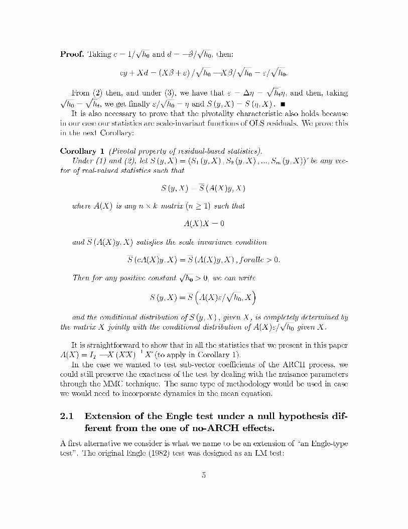
Proof. Taking c = 1/√h0 and d = −β/√h0, then:
cy +Xd = (Xβ + ε) /√h0 −Xβ/
√h0 = ε/
√h0.
From (2) then, and under (3), we have that ε = ∆η =√htη, and then, taking√
h0 =√ht, we get finally ε/
√h0 = η and S (y,X) = S (η,X) .
It is also necessary to prove that the pivotality characteristic also holds becausein our case our statistics are scale-invariant functions of OLS residuals. We prove thisin the next Corollary:
Corollary 1 (Pivotal property of residual-based statistics).Under (1) and (2), let S (y,X) = (S1 (y,X) , S2 (y,X) , ..., Sm (y,X)) be any vec-
tor of real-valued statistics such that
S (y,X) = S (A(X)y,X)
where A(X) is any n × k matrix (n ≥ 1) such that
A(X)X = 0
and S (A(X)y,X) satisfies the scale invariance condition
S (cA(X)y,X) = S (A(X)y,X) , forallc > 0.
Then for any positive constant√h0 > 0, we can write
S (y,X) = S(A(X)ε/
√h0,X
)
and the conditional distribution of S (y,X) , given X, is completely determined bythe matrix X jointly with the conditional distribution of A(X)ε/
√h0 given X.
It is straightforward to show that in all the statistics that we present in this paperA(X) = IT −X (XX)−1 X (to apply in Corollary 1).
In the case we wanted to test sub-vector coefficients of the ARCH process, wecould still preserve the exactness of the test by dealing with the nuisance parametersthrough the MMC technique. The same type of methodology would be used in casewe would need to incorporate dynamics in the mean equation.
2.1 Extension of the Engle test under a null hypothesis dif-
ferent from the one of no-ARCH effects.
A first alternative we consider is what we name to be an extension of “an Engle-typetest”. The original Engle (1982) test was designed as an LM test:
5
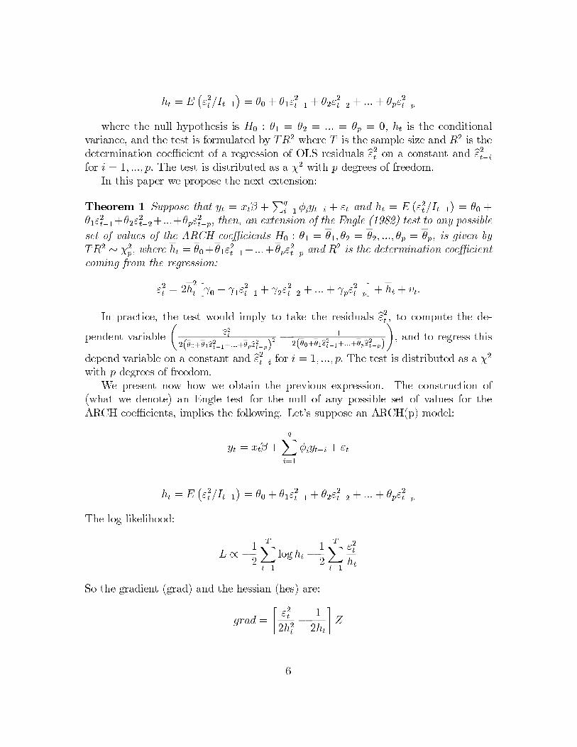
ht = E(ε2t/It−1
)= θ0 + θ1ε
2
t−1 + θ2ε2
t−2 + ...+ θpε2
t−p
where the null hypothesis is H0 : θ1 = θ2 = ... = θp = 0, ht is the conditionalvariance, and the test is formulated by TR2 where T is the sample size and R2 is thedetermination coefficient of a regression of OLS residuals ε2t on a constant and ε2t−i
for i = 1, ..., p. The test is distributed as a χ2 with p degrees of freedom.In this paper we propose the next extension:
Theorem 1 Suppose that yt = xtβ +∑q
i=1 φiyt−i + εt and ht = E (ε2t/It−1) = θ0 +θ1ε
2t−1+θ2ε
2t−2+...+θpε
2t−p, then, an extension of the Engle (1982) test to any possible
set of values of the ARCH coefficients H0 : θ1 = θ1, θ2 = θ2, ..., θp = θp, is given byTR2
∼ χ2p, where ht = θ0+θ1ε2t−1+ ...+θpε2t−p and R2 is the determination coefficientcoming from the regression:
ε2t = 2h2
t
[γ0 + γ1ε
2
t−1 + γ2ε2
t−2 + ...+ γpε2
t−p
]+ ht + vt.
In practice, the test would imply to take the residuals ε2t , to compute the de-
pendent variable
(ε2t
2(θ0+θ1 ε2
t−1+...+θpε2
t−p)2 −
1
2(θ0+θ1 ε2
t−1+...+θpε2
t−p)
), and to regress this
depend variable on a constant and ε2t−i for i = 1, ..., p. The test is distributed as a χ2
with p degrees of freedom.We present now how we obtain the previous expression. The construction of
(what we denote) an Engle test for the null of any possible set of values for theARCH coefficients, implies the following. Let’s suppose an ARCH(p) model:
yt = xtβ +
q∑i=1
φiyt−i + εt
ht = E(ε2t/It−1
)= θ0 + θ1ε
2
t−1 + θ2ε2
t−2 + ...+ θpε2
t−p
The log-likelihood:
L ∝ −1
2
T∑t=1
log ht −1
2
T∑t=1
ε2tht
So the gradient (grad) and the hessian (hes) are:
grad =
[ε2t2h2t
−
1
2ht
]Z
6
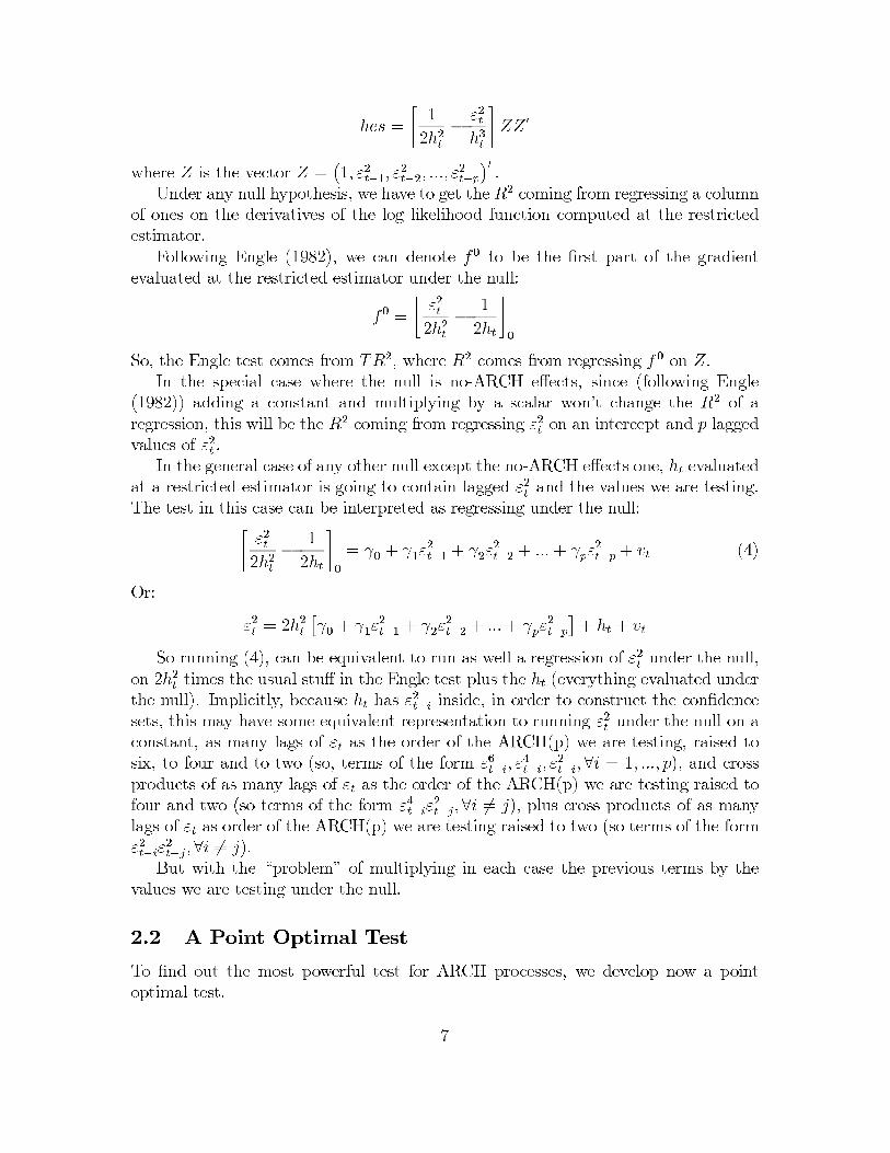
hes =
[1
2h2t−
ε2th3t
]ZZ ′
where Z is the vector Z =(1, ε2t−1
, ε2t−2, ..., ε2
t−p
)′
.
Under any null hypothesis, we have to get the R2 coming from regressing a columnof ones on the derivatives of the log likelihood function computed at the restrictedestimator.
Following Engle (1982), we can denote f0 to be the first part of the gradientevaluated at the restricted estimator under the null:
f0 =
[ε2t2h2t
−1
2ht
]0
So, the Engle test comes from TR2, where R2 comes from regressing f 0 on Z.In the special case where the null is no-ARCH effects, since (following Engle
(1982)) adding a constant and multiplying by a scalar won’t change the R2 of aregression, this will be the R2 coming from regressing ε2t on an intercept and p laggedvalues of ε2t .
In the general case of any other null except the no-ARCH effects one, ht evaluatedat a restricted estimator is going to contain lagged ε2t and the values we are testing.The test in this case can be interpreted as regressing under the null:[
ε2t2h2t
−1
2ht
]0
= γ0+ γ
1ε2t−1
+ γ2ε2t−2 + ...+ γpε
2
t−p + vt (4)
Or:
ε2t = 2h2t[γ0+ γ
1ε2t−1 + γ
2ε2t−2 + ...+ γpε
2
t−p
]+ ht + vt
So running (4), can be equivalent to run as well a regression of ε2t under the null,on 2h2t times the usual stuff in the Engle test plus the ht (everything evaluated underthe null). Implicitly, because ht has ε2t−i inside, in order to construct the confidencesets, this may have some equivalent representation to running ε2t under the null on aconstant, as many lags of εt as the order of the ARCH(p) we are testing, raised tosix, to four and to two (so, terms of the form ε6t−i, ε
4
t−i, ε2
t−i,∀i = 1, ..., p), and crossproducts of as many lags of εt as the order of the ARCH(p) we are testing raised tofour and two (so terms of the form ε4t−iε
2
t−j,∀i �= j), plus cross products of as manylags of εt as order of the ARCH(p) we are testing raised to two (so terms of the formε2t−iε
2
t−j,∀i �= j).But with the “problem” of multiplying in each case the previous terms by the
values we are testing under the null.
2.2 A Point Optimal Test
To find out the most powerful test for ARCH processes, we develop now a pointoptimal test.
7
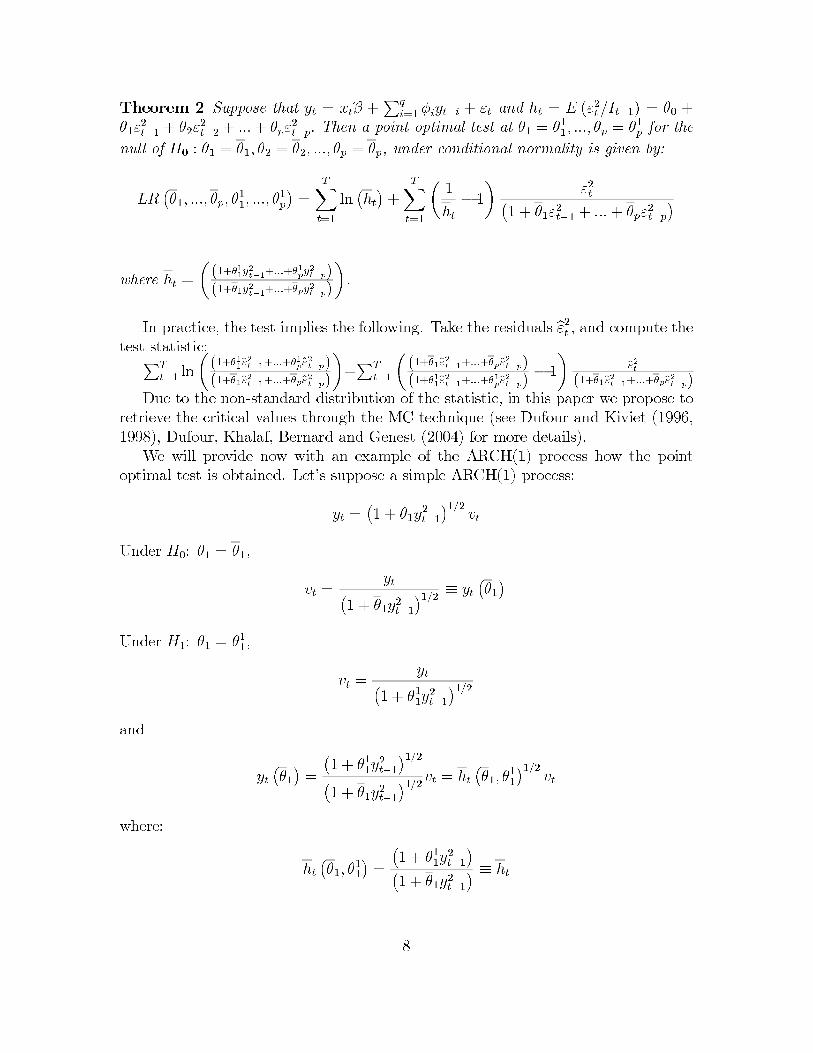
Theorem 2 Suppose that yt = xtβ +∑q
i=1 φiyt−i + εt and ht = E (ε2t/It−1) = θ0 +θ1ε
2t−1 + θ2ε
2t−2 + ...+ θpε
2t−p. Then a point optimal test at θ1 = θ11, ..., θp = θ1p for the
null of H0 : θ1 = θ1, θ2 = θ2, ..., θp = θp, under conditional normality is given by:
LR(θ1, ..., θp, θ
1
1, ..., θ1p
)=
T∑t=1
ln(ht
)+
T∑t=1
(1
ht
− 1
)ε2t(
1 + θ1ε2t−1 + ...+ θpε2t−p
)
where ht =
((1+θ1
1y2t−1
+...+θ1py2t−p)
(1+θ1y2t−1+...+θpy2t−p)
).
In practice, the test implies the following. Take the residuals ε2t , and compute thetest statistic:∑T
t=1 ln
((1+θ1
1ε2t−1+...+θ1pε
2
t−p)(1+θ1ε
2
t−1+...+θpε2
t−p)
)+∑T
t=1
((1+θ1ε
2
t−1+...+θpε2
t−p)(1+θ1
1ε2t−1+...+θ1pε
2
t−p)− 1
)ε2t
(1+θ1 ε2
t−1+...+θpε2
t−p)Due to the non-standard distribution of the statistic, in this paper we propose to
retrieve the critical values through the MC technique (see Dufour and Kiviet (1996,1998), Dufour, Khalaf, Bernard and Genest (2004) for more details).
We will provide now with an example of the ARCH(1) process how the pointoptimal test is obtained. Let’s suppose a simple ARCH(1) process:
yt =(1 + θ1y
2
t−1
)1/2vt
Under H0: θ1 = θ1,
vt =yt(
1 + θ1y2t−1)1/2 ≡ yt
(θ1)
Under H1: θ1 = θ11,
vt =yt(
1 + θ11y2t−1
)1/2and
yt(θ1)=
(1 + θ11y
2t−1
)1/2(1 + θ1y2t−1
)1/2vt = ht
(θ1, θ
1
1
)1/2vt
where:
ht
(θ1, θ
1
1
)=
(1 + θ11y
2t−1
)(1 + θ1y2t−1
) ≡ ht
8
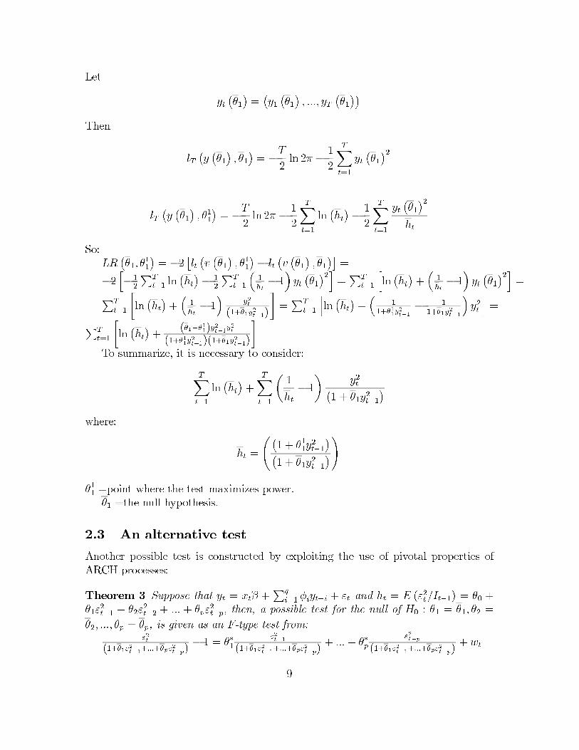
Let
yt(θ1)=(y1(θ1), ..., yT
(θ1))
Then
lT(y(θ1), θ1
)= −
T
2ln 2π −
1
2
T∑t=1
yt(θ1)2
lT(y(θ1), θ1
1
)= −
T
2ln 2π −
1
2
T∑t=1
ln(ht
)−
1
2
T∑t=1
yt(θ1)2
ht
So:
LR(θ1, θ
1
1
)= −2
[lt(v(θ1), θ11)− lt
(v(θ1), θ1
)]=
−2[−
1
2
∑T
t=1 ln(ht
)−
1
2
∑T
t=1
(1
ht− 1
)yt(θ1)2]
=∑T
t=1
[ln(ht
)+(1
ht− 1
)yt(θ1)2]
=∑T
t=1
[ln(ht
)+(1
ht− 1
)y2t
(1+θ1y2
t−1)
]=∑T
t=1
[ln(ht
)+(
1
1+θ11y2t−1
−
1
1+θ1y2
t−1
)y2t
]=
∑T
t=1
[ln(ht
)+
(θ1−θ11)y2t−1y2t
(1+θ11y2t−1)(1+θ1y
2
t−1)
]To summarize, it is necessary to consider:
T∑t=1
ln(ht
)+
T∑t=1
(1
ht
− 1
)y2t(
1 + θ1y2t−1)
where:
ht =
((1 + θ11y
2t−1
)(1 + θ1y2t−1
))
θ11 =point where the test maximizes power.
θ1 =the null hypothesis.
2.3 An alternative test
Another possible test is constructed by exploiting the use of pivotal properties of
ARCH processes:
Theorem 3 Suppose that yt = xtβ +∑q
i=1 φiyt−i + εt and ht = E (ε2t/It−1) = θ0 +θ1ε2t−1 + θ2ε2t−2 + ... + θpε2t−p, then, a possible test for the null of H0 : θ1 = θ1, θ2 =
θ2, ..., θp = θp, is given as an F-type test from:ε2t
(1+θ1ε2
t−1+...+θpε
2
t−p)− 1 = θ∗1
ε2t−1
(1+θ1ε2
t−1+...+θpε
2
t−p)+ ...+ θ∗p
ε2t−p
(1+θ1ε2
t−1+...+θpε
2
t−p)+ wt
9
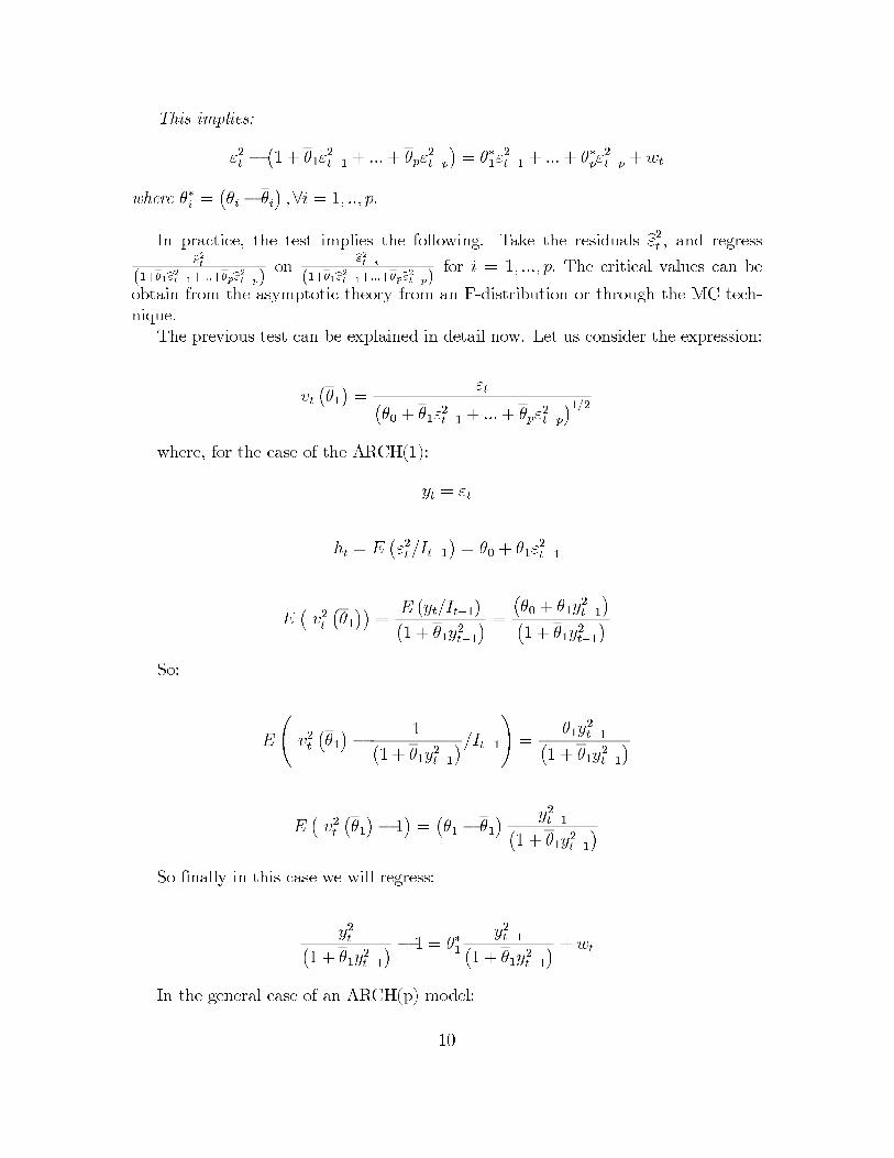
This implies:
ε2t −(1 + θ1ε
2
t−1 + ...+ θpε2
t−p
)= θ∗1ε
2
t−1 + ...+ θ∗pε2
t−p + wt
where θ∗i =(θi − θi
),∀i = 1, .., p.
In practice, the test implies the following. Take the residuals ε2t , and regressε2t
(1+θ1ε2
t−1+...+θpε2
t−p)on
ε2t−i
(1+θ1 ε2
t−1+...+θpε2
t−p)for i = 1, ..., p. The critical values can be
obtain from the asymptotic theory from an F-distribution or through the MC tech-nique.
The previous test can be explained in detail now. Let us consider the expression:
vt(θ1)=
εt(θ0 + θ1ε2t−1 + ...+ θpε2t−p
)1/2where, for the case of the ARCH(1):
yt = εt
ht = E(ε2t/It−1
)= θ0 + θ1ε
2
t−1
E(v2t(θ1))
=E (yt/It−1)(1 + θ1y2t−1
) = (θ0 + θ1y
2t−1
)(1 + θ1y2t−1
)So:
E
(v2t(θ1)−
1(1 + θ1y2t−1
)/It−1)=
θ1y2t−1(
1 + θ1y2t−1)
E(v2t(θ1)− 1
)=(θ1 − θ1
) y2t−1(1 + θ1y2t−1
)So finally in this case we will regress:
y2t(1 + θ1y2t−1
) − 1 = θ∗1y2t−1(
1 + θ1y2t−1) + wt
In the general case of an ARCH(p) model:
10
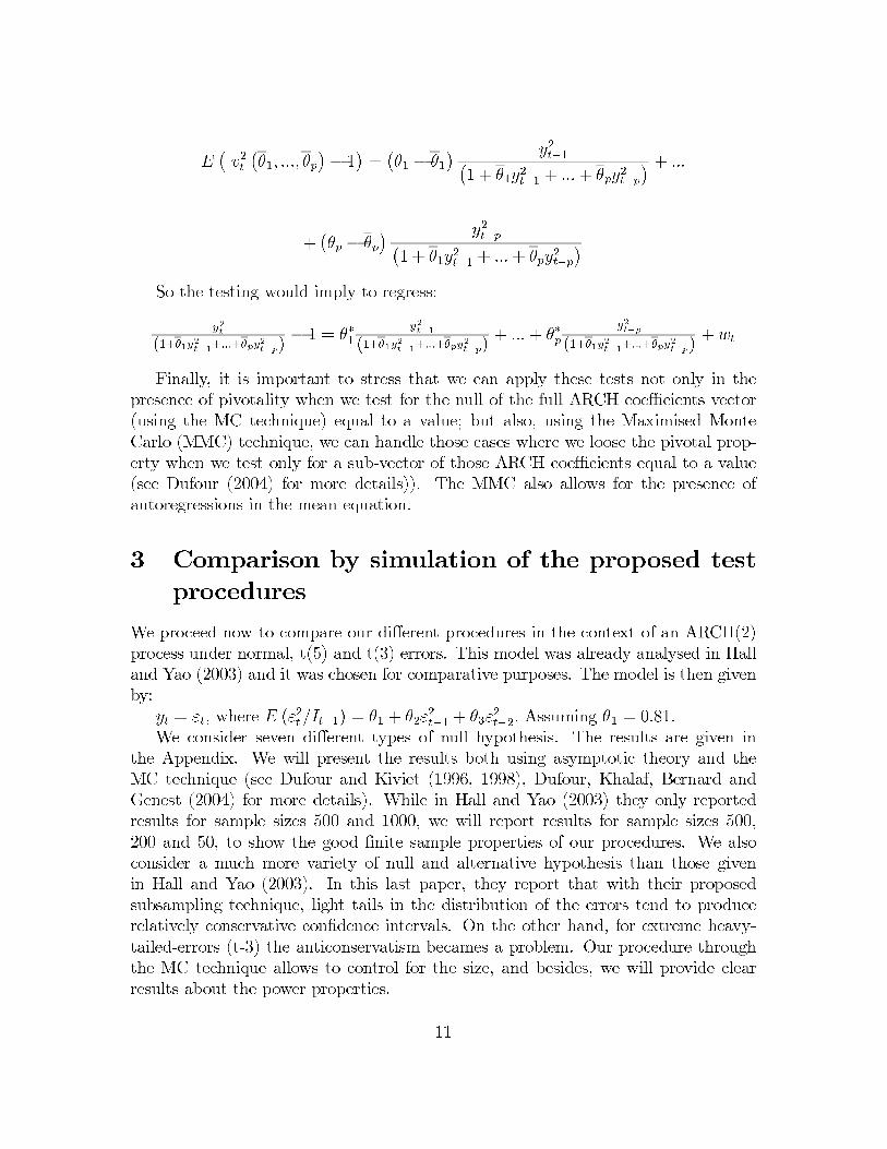
E(v2t
(θ1, ..., θp
)− 1
)=
(θ1 − θ1
) y2t−1(1 + θ1y2t−1 + ...+ θpy2t−p
) + ...
+(θp − θp
) y2t−p(1 + θ1y2t−1 + ...+ θpy2t−p
)
So the testing would imply to regress:
y2t
(1+θ1y2
t−1+...+θpy
2
t−p)− 1 = θ∗1
y2t−1
(1+θ1y2
t−1+...+θpy
2
t−p)+ ...+ θ∗p
y2t−p
(1+θ1y2
t−1+...+θpy
2
t−p)+ wt
Finally, it is important to stress that we can apply these tests not only in thepresence of pivotality when we test for the null of the full ARCH coefficients vector(using the MC technique) equal to a value; but also, using the Maximised MonteCarlo (MMC) technique, we can handle those cases where we loose the pivotal prop-erty when we test only for a sub-vector of those ARCH coefficients equal to a value(see Dufour (2004) for more details)). The MMC also allows for the presence ofautoregressions in the mean equation.
3 Comparison by simulation of the proposed test
procedures
We proceed now to compare our different procedures in the context of an ARCH(2)process under normal, t(5) and t(3) errors. This model was already analysed in Halland Yao (2003) and it was chosen for comparative purposes. The model is then givenby:
yt = εt, where E (ε2t/It−1) = θ1 + θ2ε2t−1 + θ3ε
2t−2. Assuming θ1 = 0.81.
We consider seven different types of null hypothesis. The results are given inthe Appendix. We will present the results both using asymptotic theory and theMC technique (see Dufour and Kiviet (1996, 1998), Dufour, Khalaf, Bernard andGenest (2004) for more details). While in Hall and Yao (2003) they only reportedresults for sample sizes 500 and 1000, we will report results for sample sizes 500,200 and 50, to show the good finite sample properties of our procedures. We alsoconsider a much more variety of null and alternative hypothesis than those givenin Hall and Yao (2003). In this last paper, they report that with their proposedsubsampling technique, light tails in the distribution of the errors tend to producerelatively conservative confidence intervals. On the other hand, for extreme heavy-tailed-errors (t-3) the anticonservatism becames a problem. Our procedure throughthe MC technique allows to control for the size, and besides, we will provide clearresults about the power properties.
11
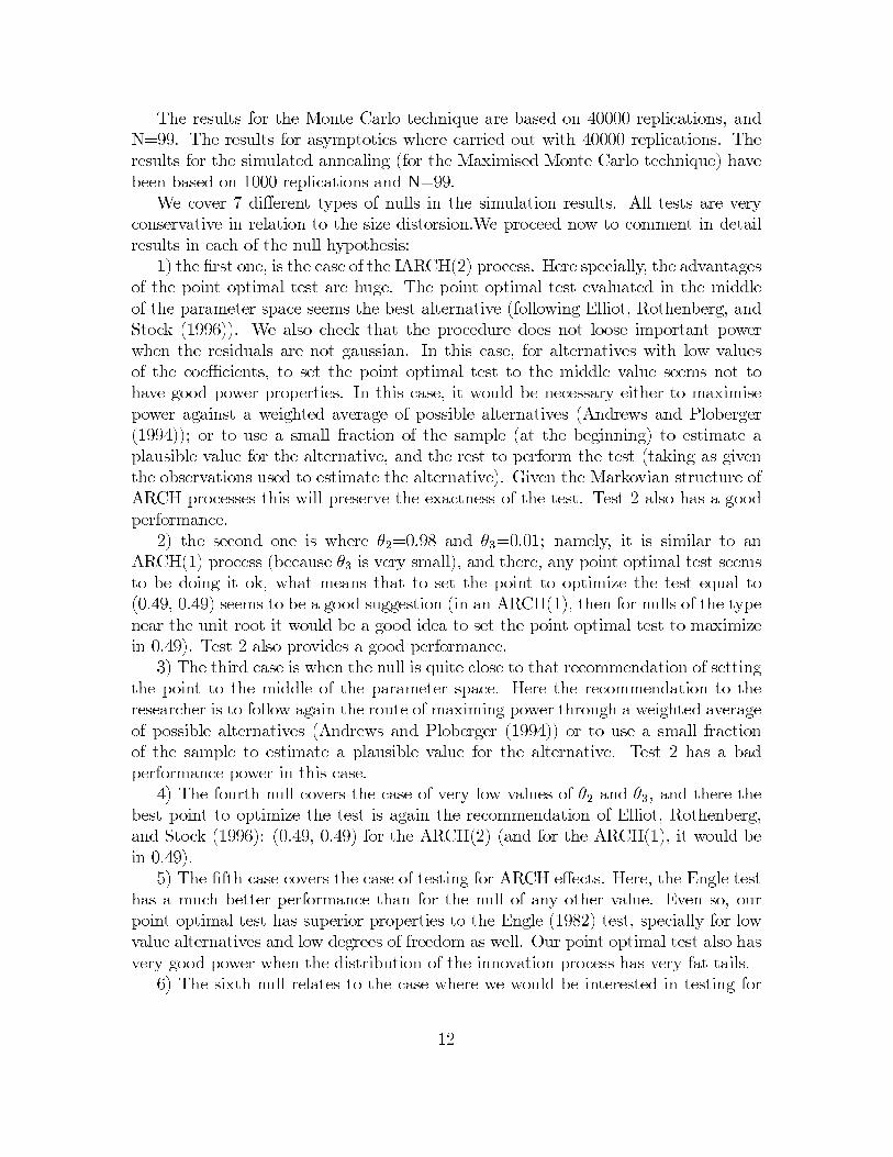
The results for the Monte Carlo technique are based on 40000 replications, andN=99. The results for asymptotics where carried out with 40000 replications. Theresults for the simulated annealing (for the Maximised Monte Carlo technique) havebeen based on 1000 replications and N=99.
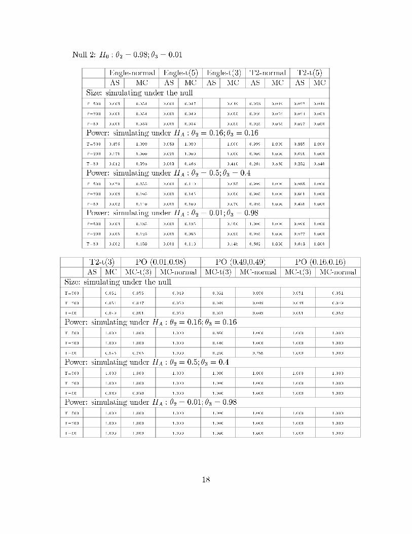
We cover 7 different types of nulls in the simulation results. All tests are veryconservative in relation to the size distorsion.We proceed now to comment in detailresults in each of the null hypothesis:
1) the first one, is the case of the IARCH(2) process. Here specially, the advantagesof the point optimal test are huge. The point optimal test evaluated in the middleof the parameter space seems the best alternative (following Elliot, Rothenberg, andStock (1996)). We also check that the procedure does not loose important powerwhen the residuals are not gaussian. In this case, for alternatives with low valuesof the coefficients, to set the point optimal test to the middle value seems not tohave good power properties. In this case, it would be necessary either to maximisepower against a weighted average of possible alternatives (Andrews and Ploberger(1994)); or to use a small fraction of the sample (at the beginning) to estimate aplausible value for the alternative, and the rest to perform the test (taking as giventhe observations used to estimate the alternative). Given the Markovian structure ofARCH processes this will preserve the exactness of the test. Test 2 also has a goodperformance.
2) the second one is where θ2=0.98 and θ3=0.01; namely, it is similar to anARCH(1) process (because θ3 is very small), and there, any point optimal test seemsto be doing it ok, what means that to set the point to optimize the test equal to(0.49, 0.49) seems to be a good suggestion (in an ARCH(1), then for nulls of the typenear the unit root it would be a good idea to set the point optimal test to maximizein 0.49). Test 2 also provides a good performance.
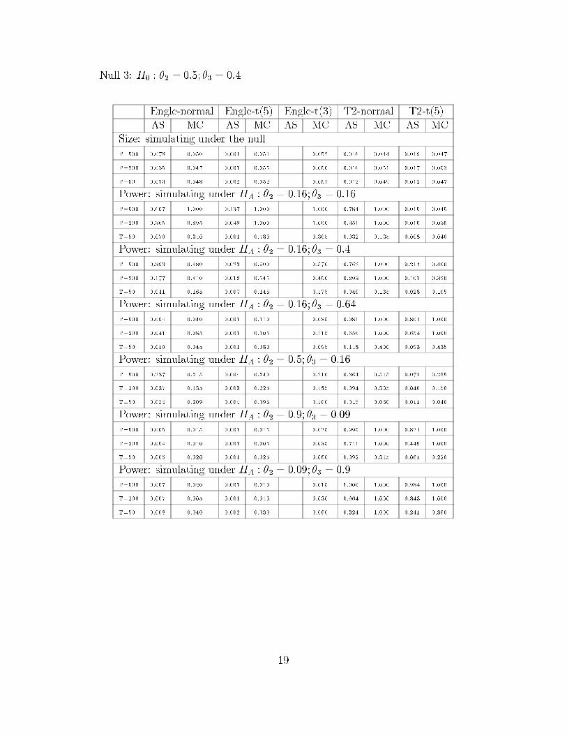
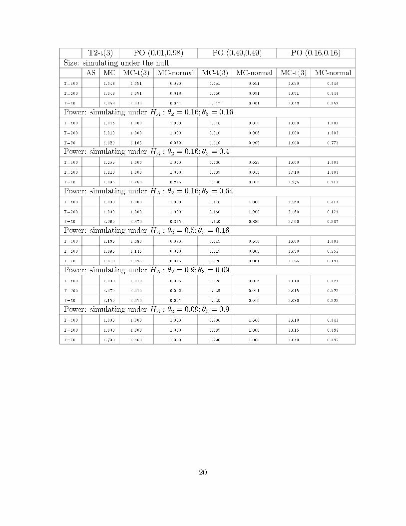
3) The third case is when the null is quite close to that recommendation of settingthe point to the middle of the parameter space. Here the recommendation to theresearcher is to follow again the route of maximing power through a weighted averageof possible alternatives (Andrews and Ploberger (1994)) or to use a small fractionof the sample to estimate a plausible value for the alternative. Test 2 has a badperformance power in this case.
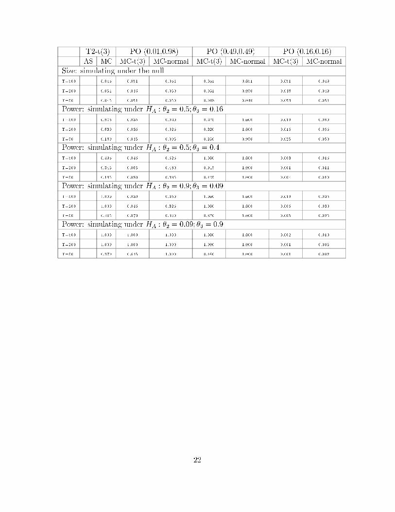
4) The fourth null covers the case of very low values of θ2 and θ3, and there thebest point to optimize the test is again the recommendation of Elliot, Rothenberg,and Stock (1996): (0.49, 0.49) for the ARCH(2) (and for the ARCH(1), it would bein 0.49).
5) The fifth case covers the case of testing for ARCH effects. Here, the Engle testhas a much better performance than for the null of any other value. Even so, ourpoint optimal test has superior properties to the Engle (1982) test, specially for lowvalue alternatives and low degrees of freedom as well. Our point optimal test also hasvery good power when the distribution of the innovation process has very fat tails.
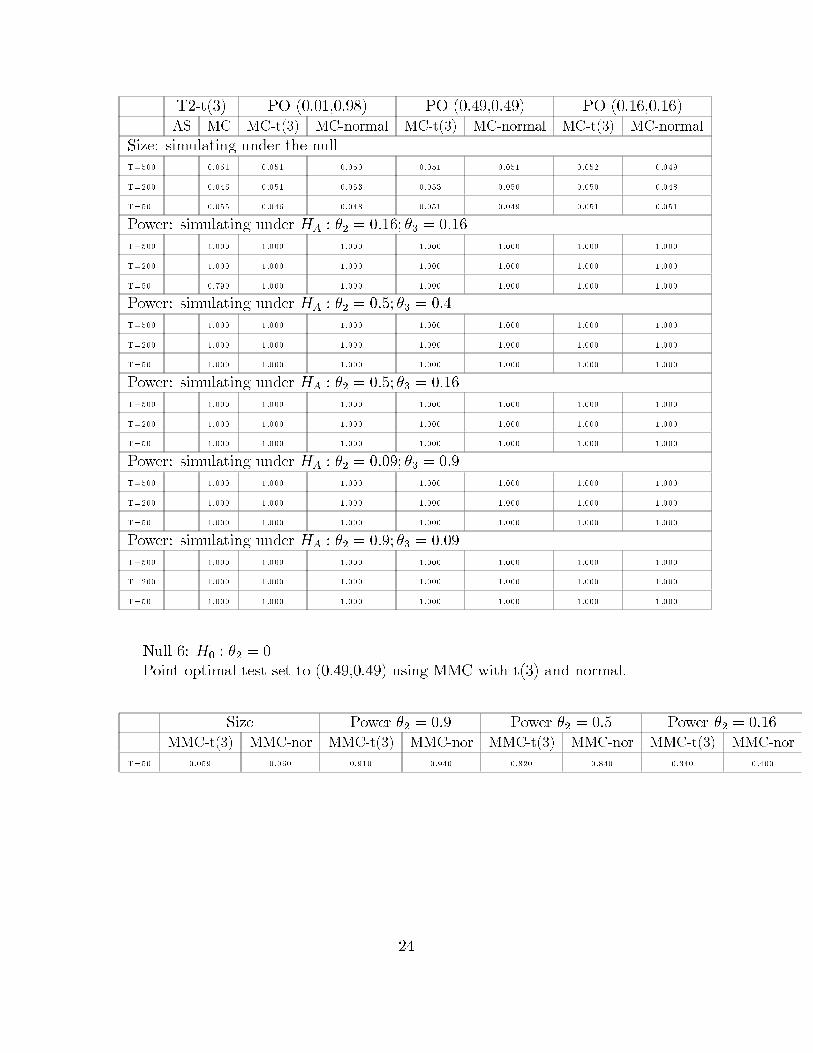
6) The sixth null relates to the case where we would be interested in testing for
12
subsets of the whole set of ARCH coefficients. we see how the MMC technique alsomakes our tests operational in case we want to test for a null hypothesis different fromthe one of the whole coefficient ARCH vector equal to a value. The MMC techniquewas carried out using the simulated annealing algorithm. The results show that evenfor sample sizes of 50, the point optimal test although it decreases the power foralternative hypothesis quite close to the null, still has good power, after optimisingthe p-value out of all possible values for the nuisance parameters.
7) In the seventh case, we consider a non-stationary case where we show thebehaviour of our point optimal case against the asymptotic alternatives (in the contextof Jensen and Rahbek (2004)). They have proved that in the setting of a non-stationary region, the QMLE is still asymptotically normal. However, there are stillno results in the literature that show what happens in small samples. We provideresults in this context both when the fourth moment of the innovation process existsand when it does not exist. We show that the behaviour of our point optimal testin this setting has very good power regardless if the errors have very fat tails or not(at the same time of controlling for the size). The extension of the Engle test andteh other test we propose have very low power in some of the alternatives. Thispossibility of very good behaviour of point optimal tests outside the stationarityregion was already showed in Dufour and King (1991).
So, from the simulation results, we advice the practitioners always to use as arule of thumb the value equal to the middle of the parameter space (e.g. 0.49 foran ARCH(1) process); and when it is possible, it is always better to maximise poweragainst a weighted alternative as in Andrews and Ploberger (1994), or to split thesample size, and to use a small fraction of the sample (at the beginning) to estimatea plausible value for the alternative. We also show the behaviour of the point optimaltest under non-normal-t(3) errors, and the findings indicate good power in these cases(allowing also for control of the size and then, improving on Hall and Yao (2003)).
4 Application of an ARCH model for US Inflation
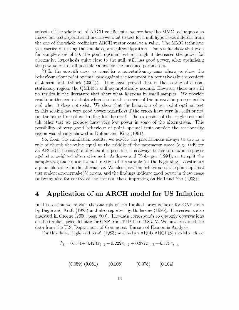
In this section we re-visit the analysis of the Implicit price deflator for GNP doneby Engle and Kraft (1983) and also reported by Bollerslev (1986). The series is alsoanalysed in Greene (2000, page 809). The data corresponds to quaterly observationson the implicit price deflator for GNP from 1948.II to 1983.IV. We have obtained thedata from the U.S. Department of Commerce: Bureau of Economic Analysis.
For this data, Engle and Kraft (1983) selected an AR(4)-ARCH(8) model such as:
πt = 0.138 + 0.423πt−1 + 0.222πt−2 + 0.377πt−3 − 0.175πt−4
(0.059) (0.081) (0.108) (0.078) (0.104)
13
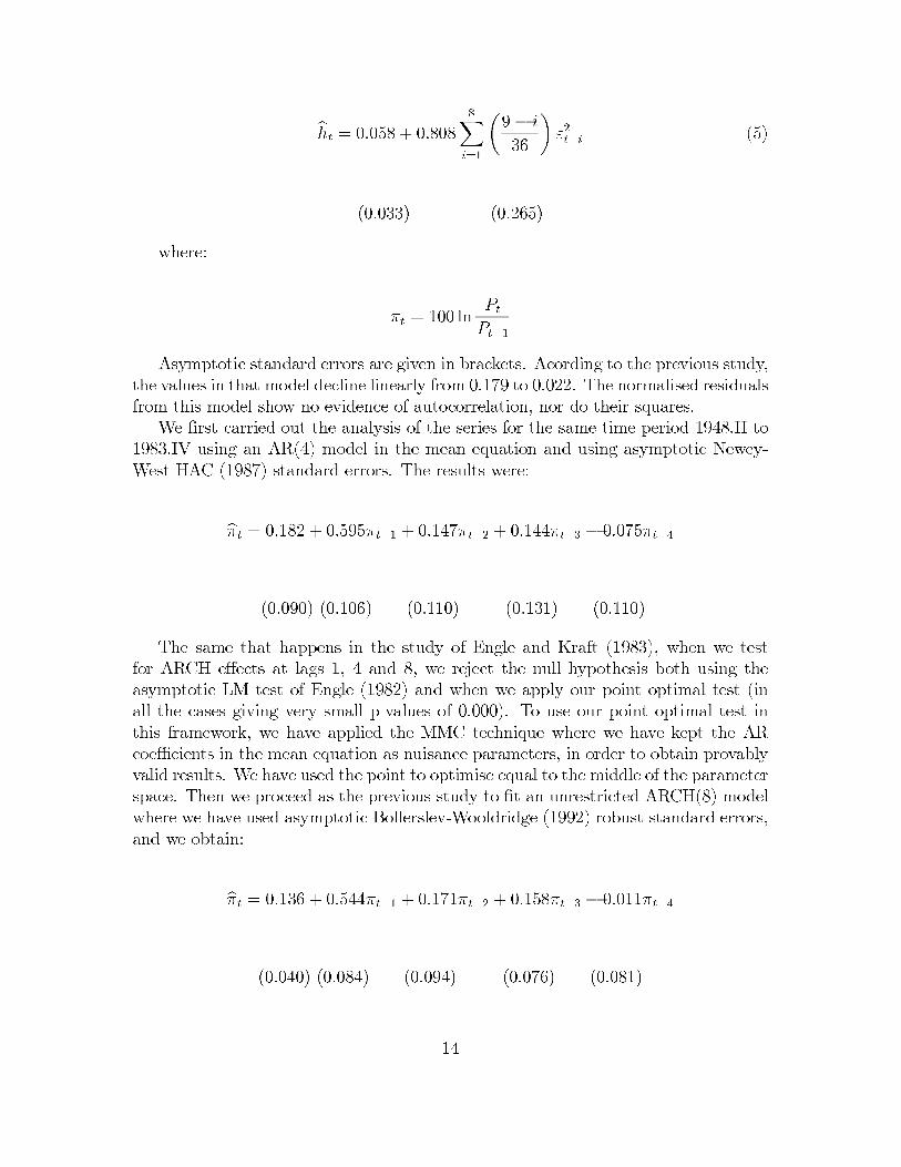
ht = 0.058 + 0.8088∑
i=1
(9 − i
36
)ε2
t−i(5)
(0.033) (0.265)
where:
πt = 100 lnPt
Pt−1
Asymptotic standard errors are given in brackets. Acording to the previous study,the values in that model decline linearly from 0.179 to 0.022. The normalised residualsfrom this model show no evidence of autocorrelation, nor do their squares.
We first carried out the analysis of the series for the same time period 1948.II to1983.IV using an AR(4) model in the mean equation and using asymptotic Newey-West HAC (1987) standard errors. The results were:
πt = 0.182 + 0.595πt−1 + 0.147πt−2 + 0.144πt−3 − 0.075πt−4
(0.090) (0.106) (0.110) (0.131) (0.110)
The same that happens in the study of Engle and Kraft (1983), when we testfor ARCH effects at lags 1, 4 and 8, we reject the null hypothesis both using theasymptotic LM test of Engle (1982) and when we apply our point optimal test (inall the cases giving very small p-values of 0.000). To use our point optimal test inthis framework, we have applied the MMC technique where we have kept the ARcoefficients in the mean equation as nuisance parameters, in order to obtain provablyvalid results. We have used the point to optimise equal to the middle of the parameterspace. Then we proceed as the previous study to fit an unrestricted ARCH(8) modelwhere we have used asymptotic Bollerslev-Wooldridge (1992) robust standard errors,and we obtain:
πt = 0.136 + 0.544πt−1 + 0.171πt−2 + 0.158πt−3 − 0.011πt−4
(0.040) (0.084) (0.094) (0.076) (0.081)
14
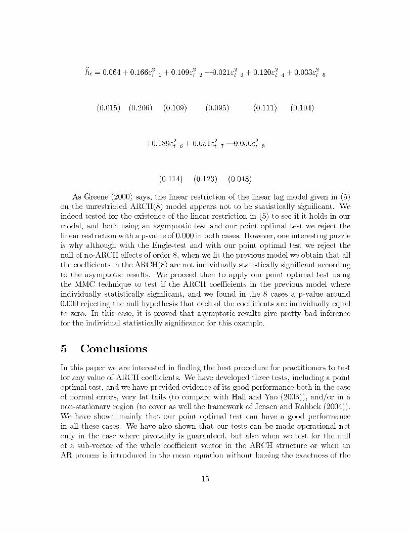
ht = 0.064 + 0.166ε2t−1
+ 0.109ε2t−2− 0.021ε2
t−3+ 0.120ε2
t−4+ 0.033ε2
t−5
(0.015) (0.206) (0.109) (0.095) (0.111) (0.104)
+0.189ε2t−6
+ 0.051ε2t−7− 0.050ε2
t−8
(0.114) (0.123) (0.048)
As Greene (2000) says, the linear restriction of the linear lag model given in (5)on the unrestricted ARCH(8) model appears not to be statistically significant. Weindeed tested for the existence of the linear restriction in (5) to see if it holds in ourmodel, and both using an asymptotic test and our point optimal test we reject thelinear restriction with a p-value of 0.000 in both cases. However, one interesting puzzleis why although with the Engle-test and with our point optimal test we reject thenull of no-ARCH effects of order 8, when we fit the previous model we obtain that allthe coefficients in the ARCH(8) are not individually statistically significant accordingto the asymptotic results. We proceed then to apply our point optimal test usingthe MMC technique to test if the ARCH coefficients in the previous model whereindividually statistically significant, and we found in the 8 cases a p-value around0.000 rejecting the null hypothesis that each of the coefficients are individually equalto zero. In this case, it is proved that asymptotic results give pretty bad inferencefor the individual statistically significance for this example.
5 Conclusions
In this paper we are interested in finding the best procedure for practitioners to testfor any value of ARCH coefficients. We have developed three tests, including a pointoptimal test, and we have provided evidence of its good performance both in the caseof normal errors, very fat tails (to compare with Hall and Yao (2003)), and/or in anon-stationary region (to cover as well the framework of Jensen and Rahbek (2004)).We have shown mainly that our point optimal test can have a good performancein all these cases. We have also shown that our tests can be made operational notonly in the case where pivotality is guaranteed, but also when we test for the nullof a sub-vector of the whole coefficient vector in the ARCH structure or when anAR process is introduced in the mean equation without loosing the exactness of the
15

test. We have also reported the usefulness of our test in the case of an ARCH modelapplied to the US inflation.
In summary, a general rule to advice to practitioners (supported by the simula-tion results) is to use our point optimal test setting the point to optimise equal tothe middle value of the parameter space (following the recommendation of Elliot,Rothenberg, and Stock, (1996)). This would be a good rule of thumb, although thebest recommendation, if possible, is to maximise power against a weighted averageof alternatives (Andrews and Ploberger (1994)) or to split the sample using a smallfraction at the beginning to estimate a plausible value for the alternative. Our simula-tions show that our point optimal test has good properties in finite samples regardlessif the errors are gaussian or not (including if the errors have very fat-tails) and/or ifthe process is in the stationarity region or not.
16
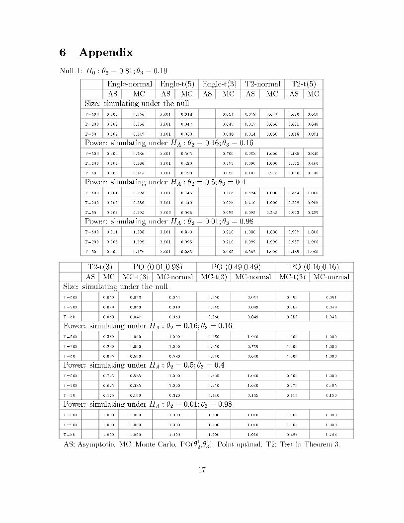
6 Appendix
Null 1: H0 : θ2 = 0.81; θ3 = 0.19
Engle-normal Engle-t(5) Engle-t(3) T2-normal T2-t(5)AS MC AS MC AS MC AS MC AS MC
Size: simulating under the nullT=500 0.002 0.050 0.001 0.048 0.051 0.018 0 .047 0.020 0.050
T=200 0.002 0.050 0.001 0.047 0.047 0.017 0 .050 0.021 0.049
T=50 0.002 0.047 0.001 0.050 0.048 0.014 0 .050 0.018 0.051
Power: simulating under HA : θ2 = 0.16; θ3 = 0.16
T=500 0.004 0.780 0.001 0.565 0.700 0.963 1 .000 0.438 0.845
T=200 0.003 0.560 0.001 0.420 0.555 0.690 1 .000 0.192 0.460
T=50 0.006 0.145 0.001 0.130 0.095 0.101 0 .315 0.050 0.145
Power: simulating under HA : θ2 = 0.5; θ3 = 0.4
T=500 0.001 0.395 0.001 0.145 0.115 0.824 1 .000 0.554 1.000
T=200 0.003 0.280 0.001 0.140 0.075 0.410 1 .000 0.298 0.955
T=50 0.003 0.095 0.002 0.065 0.055 0.095 0 .245 0.093 0.255
Power: simulating under HA : θ2 = 0.01; θ3 = 0.98
T=500 0.011 1.000 0.001 0.370 0.220 1.000 1 .000 0.997 1.000
T=200 0.003 1.000 0.001 0.095 0.210 0.999 1 .000 0.967 1.000
T=50 0.009 0.170 0.001 0.085 0.095 0.582 1 .000 0.485 1.000
T2-t(3) PO (0.01,0.98) PO (0.49,0.49) PO (0.16,0.16)AS MC MC-t(3) MC-normal MC-t(3) MC-normal MC-t(3) MC-normal
Size: simulating under the nullT= 500 0.050 0 .048 0.051 0.050 0.051 0.050 0 .051
T= 200 0.049 0 .050 0.049 0.049 0.049 0.054 0 .049
T= 50 0.050 0 .047 0.050 0.050 0.049 0.050 0 .048
Power: simulating under HA : θ2 = 0.16; θ3 = 0.16
T= 500 0.330 1 .000 1.000 0.060 1.000 1.000 1 .000
T= 200 0.230 1 .000 1.000 0.050 0.755 1.000 1 .000
T= 50 0.095 0 .500 0.580 0.040 0.090 1.000 1 .000
Power: simulating under HA : θ2 = 0.5; θ3 = 0.4
T= 500 0.795 0 .535 1.000 0.325 1.000 0.600 1 .000
T= 200 0.625 0 .335 1.000 0.210 1.000 0.270 0 .495
T= 50 0.175 0 .190 0.320 0.140 0.485 0.110 0 .150
Power: simulating under HA : θ2 = 0.01; θ3 = 0.98
T= 500 1.000 1 .000 1.000 1.000 1.000 1.000 1 .000
T= 200 1.000 1 .000 1.000 1.000 1.000 1.000 1 .000
T= 50 1.000 1 .000 1.000 1.000 1.000 0.485 0 .705
AS: Asymptotic. MC: Monte Carlo. PO(θ12,θ1
3): Point optimal. T2: Test in Theorem 3.
17
Null 2: H0 : θ2 = 0.98; θ3 = 0.01
Engle-normal Engle-t(5) Engle-t(3) T2-normal T2-t(5)AS MC AS MC AS MC AS MC AS MC
Size: simulating under the nullT=500 0.003 0.054 0.001 0.047 0.049 0.023 0 .049 0.022 0.049
T=200 0.001 0.054 0.001 0.049 0.055 0.026 0 .052 0.024 0.053
T=50 0.001 0.053 0.001 0.054 0.055 0.025 0 .055 0.027 0.050
Power: simulating under HA : θ2 = 0.16; θ3 = 0.16
T=500 0.456 1.000 0.089 1.000 1.000 0.999 1 .000 0.885 1.000
T=200 0.171 1.000 0.021 1.000 1.000 0.909 1 .000 0.625 1.000
T=50 0.012 0.395 0.003 0.465 0.410 0.261 0 .560 0.232 0.540
Power: simulating under HA : θ2 = 0.5; θ3 = 0.4
T=500 0.029 0.255 0.001 0.110 0.085 0.999 1 .000 0.988 1.000
T=200 0.008 0.195 0.001 0.145 0.050 0.905 1 .000 0.861 1.000
T=50 0.002 0.110 0.001 0.100 0.070 0.395 1 .000 0.431 1.000
Power: simulating under HA : θ2 = 0.01; θ3 = 0.98
T=500 0.003 0.135 0.001 0.135 0.150 1.000 1 .000 0.999 1.000
T=200 0.005 0.125 0.001 0.085 0.095 0.995 1 .000 0.977 1.000
T=50 0.002 0.130 0.001 0.110 0.145 0.662 1 .000 0.613 1.000
T2-t(3) PO (0.01,0.98) PO (0.49,0.49) PO (0.16,0.16)AS MC MC-t(3) MC-normal MC-t(3) MC-normal MC-t(3) MC-normal
Size: simulating under the nullT= 500 0.051 0 .055 0.049 0.051 0.050 0.051 0 .051
T= 200 0.051 0 .047 0.050 0.049 0.049 0.048 0 .049
T= 50 0.049 0 .051 0.050 0.051 0.048 0.051 0 .052
Power: simulating under HA : θ2 = 0.16; θ3 = 0.16
T= 500 1.000 1 .000 1.000 0.860 1.000 1.000 1 .000
T= 200 1.000 1 .000 1.000 0.440 1.000 1.000 1 .000
T= 50 0.545 0 .765 1.000 0.250 0.785 1.000 1 .000
Power: simulating under HA : θ2 = 0.5; θ3 = 0.4
T= 500 1.000 1 .000 1.000 1.000 1.000 1.000 1 .000
T= 200 1.000 1 .000 1.000 1.000 1.000 1.000 1 .000
T= 50 0.980 0 .930 1.000 1.000 1.000 1.000 1 .000
Power: simulating under HA : θ2 = 0.01; θ3 = 0.98
T= 500 1.000 1 .000 1.000 1.000 1.000 1.000 1 .000
T= 200 1.000 1 .000 1.000 1.000 1.000 1.000 1 .000
T= 50 1.000 1 .000 1.000 1.000 1.000 1.000 1 .000
18
Null 3: H0 : θ2 = 0.5; θ3 = 0.4
Engle-normal Engle-t(5) Engle-t(3) T2-normal T2-t(5)AS MC AS MC AS MC AS MC AS MC
Size: simulating under the nullT=500 0.078 0.050 0.001 0.051 0.052 0.016 0 .044 0.019 0.047
T=200 0.035 0.047 0.001 0.055 0.050 0.016 0 .051 0.017 0.053
T=50 0.013 0.048 0.002 0.052 0.051 0.012 0 .049 0.012 0.047
Power: simulating under HA : θ2 = 0.16; θ3 = 0.16
T=500 0.607 1.000 0.137 1.000 1.000 0.784 1 .000 0.015 0.045
T=200 0.365 0.895 0.049 1.000 1.000 0.351 1 .000 0.010 0.035
T=50 0.070 0.310 0.001 0.780 0.305 0.032 0 .135 0.008 0.040
Power: simulating under HA : θ2 = 0.16; θ3 = 0.4
T=500 0.393 0.480 0.023 0.600 0.570 0.762 1 .000 0.214 0.400
T=200 0.177 0.410 0.012 0.545 0.450 0.293 1 .000 0.101 0.320
T=50 0.041 0.165 0.007 0.145 0.175 0.040 0 .135 0.028 0.105
Power: simulating under HA : θ2 = 0.16; θ3 = 0.64
T=500 0.094 0.040 0.001 0.110 0.085 0.981 1 .000 0.804 1.000
T=200 0.041 0.085 0.001 0.105 0.115 0.656 1 .000 0.654 1.000
T=50 0.019 0.045 0.001 0.080 0.095 0.118 0 .400 0.093 0.435
Power: simulating under HA : θ2 = 0.5; θ3 = 0.16
T=500 0.237 0.215 0.004 0.240 0.210 0.364 0 .515 0.071 0.255
T=200 0.037 0.135 0.003 0.225 0.185 0.094 0 .305 0.040 0.150
T=50 0.024 0.209 0.004 0.095 0.100 0.015 0 .060 0.011 0.040
Power: simulating under HA : θ2 = 0.9; θ3 = 0.09
T=500 0.005 0.015 0.001 0.015 0.025 0.995 1 .000 0.824 1.000
T=200 0.004 0.010 0.001 0.005 0.035 0.711 1 .000 0.449 1.000
T=50 0.005 0.020 0.001 0.025 0.060 0.092 0 .315 0.061 0.220
Power: simulating under HA : θ2 = 0.09; θ3 = 0.9
T=500 0.007 0.020 0.001 0.010 0.015 1.000 1 .000 0.984 1.000
T=200 0.007 0.005 0.001 0.010 0.030 0.964 1 .000 0.843 1.000
T=50 0.008 0.040 0.002 0.030 0.060 0.324 1 .000 0.241 0.860
19
T2-t(3) PO (0.01,0.98) PO (0.49,0.49) PO (0.16,0.16)Size: simulating under the null
AS MC MC-t(3) MC-normal MC-t(3) MC-normal MC-t(3) MC-normal
T= 500 0.048 0 .051 0.050 0.051 0.051 0.050 0 .049
T= 200 0.048 0 .051 0.048 0.050 0.051 0.051 0 .048
T= 50 0.053 0 .046 0.051 0.047 0.051 0.048 0 .052
Power: simulating under HA : θ2 = 0.16; θ3 = 0.16
T= 500 0.015 1 .000 1.000 0.015 0.010 1.000 1 .000
T= 200 0.010 1 .000 1.000 0.010 0.006 1.000 1 .000
T= 50 0.020 0 .165 0.070 0.010 0.005 1.000 0 .770
Power: simulating under HA : θ2 = 0.16; θ3 = 0.4
T= 500 0.255 1 .000 1.000 0.030 0.025 1.000 1 .000
T= 200 0.210 1 .000 1.000 0.035 0.015 0.710 1 .000
T= 50 0.095 0 .250 0.275 0.030 0.015 0.375 0 .310
Power: simulating under HA : θ2 = 0.16; θ3 = 0.64
T= 500 1.000 1 .000 1.000 0.175 1.000 0.250 0 .315
T= 200 1.000 1 .000 1.000 0.150 1.000 0.160 0 .175
T= 50 0.260 0 .370 0.815 0.120 0.380 0.100 0 .085
Power: simulating under HA : θ2 = 0.5; θ3 = 0.16
T= 500 0.160 0 .380 0.070 0.015 0.010 1.000 1 .000
T= 200 0.095 0 .145 0.030 0.015 0.005 0.690 0 .555
T= 50 0.040 0 .035 0.015 0.020 0.001 0.185 0 .130
Power: simulating under HA : θ2 = 0.9; θ3 = 0.09
T= 500 1.000 0 .010 0.005 0.025 0.015 0.010 0 .025
T= 200 0.970 0 .010 0.002 0.025 0.011 0.015 0 .022
T= 50 0.150 0 .010 0.001 0.025 0.010 0.030 0 .020
Power: simulating under HA : θ2 = 0.09; θ3 = 0.9
T= 500 1.000 1 .000 1.000 0.960 1.000 0.010 0 .040
T= 200 1.000 1 .000 1.000 0.585 1.000 0.015 0 .036
T= 50 0.790 0 .860 1.000 0.290 1.000 0.040 0 .035
20

Null 4: H0 : θ2 = 0.16; θ3 = 0.25
Engle-normal Engle-t(5) Engle-t(3) T2-normal T2-t(5)AS MC AS MC AS MC AS MC AS MC
Size: simulating under the nullT=500 0.077 0.049 0.016 0.051 0.045 0.017 0 .049 0.022 0.047
T=200 0.002 0.048 0.001 0.049 0.056 0.018 0 .047 0.028 0.051
T=50 0.003 0.046 0.001 0.053 0.045 0.014 0 .041 0.019 0.052
Power: simulating under HA : θ2 = 0.5; θ3 = 0.16
T=500 0.019 0.020 0.001 0.005 0.005 0.919 1 .000 0.685 1.000
T=200 0.001 0.005 0.001 0.005 0.020 0.526 1 .000 0.399 1.000
T=50 0.001 0.020 0.001 0.025 0.015 0.109 0 .380 0.102 0.355
Power: simulating under HA : θ2 = 0.5; θ3 = 0.4
T=500 0.003 0.020 0.001 0.001 0.001 0.863 1 .000 0.602 1.000
T=200 0.001 0.015 0.001 0.001 0.001 0.466 1 .000 0.313 0.910
T=50 0.001 0.030 0.001 0.001 0.001 0.090 0 .220 0.076 0.195
Power: simulating under HA : θ2 = 0.9; θ3 = 0.09
T=500 0.001 0.001 0.001 0.001 0.001 1.000 1 .000 0.985 1.000
T=200 0.001 0.001 0.001 0.001 0.001 0.970 1 .000 0.846 1.000
T=50 0.001 0.005 0.001 0.020 0.010 0.361 1 .000 0.261 0.690
Power: simulating under HA : θ2 = 0.09; θ3 = 0.9
T=500 0.005 0.015 0.001 0.001 0.001 0.999 1 .000 0.965 1.000
T=200 0.001 0.001 0.001 0.005 0.001 0.912 1 .000 0.729 1.000
T=50 0.001 0.005 0.001 0.020 0.010 0.254 0 .995 0.172 0.400
21
T2-t(3) PO (0.01,0.98) PO (0.49,0.49) PO (0.16,0.16)AS MC MC-t(3) MC-normal MC-t(3) MC-normal MC-t(3) MC-normal
Size: simulating under the nullT= 500 0.045 0 .051 0.051 0.051 0.051 0.051 0 .049
T= 200 0.051 0 .046 0.050 0.051 0.050 0.048 0 .049
T= 50 0.045 0 .051 0.050 0.048 0.049 0.053 0 .051
Power: simulating under HA : θ2 = 0.5; θ3 = 0.16
T= 500 0.975 0 .035 0.030 0.375 1.000 0.010 0 .060
T= 200 0.630 0 .035 0.025 0.320 1.000 0.015 0 .055
T= 50 0.180 0 .045 0.005 0.250 0.950 0.025 0 .050
Power: simulating under HA : θ2 = 0.5; θ3 = 0.4
T= 500 0.495 0 .045 0.525 1.000 1.000 0.003 0 .015
T= 200 0.345 0 .065 0.480 0.915 1.000 0.001 0 .011
T= 50 0.185 0 .080 0.335 0.425 1.000 0.004 0 .010
Power: simulating under HA : θ2 = 0.9; θ3 = 0.09
T= 500 1.000 0 .030 0.350 1.000 1.000 0.010 0 .035
T= 200 1.000 0 .045 0.325 1.000 1.000 0.005 0 .030
T= 50 0.465 0 .070 0.320 0.870 1.000 0.005 0 .025
Power: simulating under HA : θ2 = 0.09; θ3 = 0.9
T= 500 1.000 1 .000 1.000 1.000 1.000 0.002 0 .010
T= 200 1.000 1 .000 1.000 1.000 1.000 0.001 0 .005
T= 50 0.370 0 .645 1.000 0.460 1.000 0.001 0 .002
22
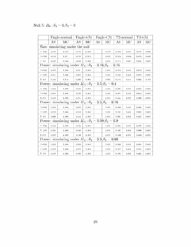
Null 5: H0 : θ2 = 0; θ3 = 0
Engle-normal Engle-t(5) Engle-t(3) T2-normal T2-t(5)AS MC AS MC AS MC AS MC AS MC
Size: simulating under the nullT=500 0.045 0.052 0.045 0.048 0.047 0.023 0 .049 0.016 0.046
T=200 0.043 0.051 0.041 0.053 0.050 0.023 0 .048 0.028 0.048
T=50 0.039 0.050 0.033 0.048 0.050 0.019 0 .047 0.025 0.050
Power: simulating under HA : θ2 = 0.16; θ3 = 0.16
T=500 0.957 1.000 0.984 1.000 1.000 0.923 1 .000 0.873 1.000
T=200 0.654 1.000 0.815 1.000 1.000 0.620 1 .000 0.650 1.000
T=50 0.191 0.375 0.288 0.665 0.960 0.170 0 .575 0.241 0.700
Power: simulating under HA : θ2 = 0.5; θ3 = 0.4
T=500 1.000 1.000 0.995 1.000 1.000 0.999 1 .000 0.900 1.000
T=200 0.991 1.000 0.976 1.000 1.000 0.961 1 .000 0.834 1.000
T=50 0.528 1.000 0.594 1.000 1.000 0.541 1 .000 0.488 1.000
Power: simulating under HA : θ2 = 0.5; θ3 = 0.16
T=500 1.000 1.000 0.995 1.000 1.000 0.998 1 .000 0.980 1.000
T=200 0.698 1.000 0.962 1.000 1.000 0.926 1 .000 0.886 1.000
T=50 0.433 1.000 0.512 1.000 1.000 0.387 1 .000 0.420 1.000
Power: simulating under HA : θ2 = 0.09; θ3 = 0.9
T=500 0.999 1.000 0.976 1.000 1.000 0.999 1 .000 0.976 1.000
T=200 0.984 1.000 0.949 1.000 1.000 0.509 1 .000 0.888 1.000
T=50 0.568 1.000 0.543 1.000 1.000 0.468 1 .000 0.443 1.000
Power: simulating under HA : θ2 = 0.9; θ3 = 0.09
T=500 1.000 1.000 0.990 1.000 1.000 0.998 1 .000 0.981 1.000
T=200 0.990 1.000 0.961 1.000 1.000 0.957 1 .000 0.906 1.000
T=50 0.558 1.000 0.580 1.000 1.000 0.490 1 .000 0.481 1.000
23
T2-t(3) PO (0.01,0.98) PO (0.49,0.49) PO (0.16,0.16)AS MC MC-t(3) MC-normal MC-t(3) MC-normal MC-t(3) MC-normal
Size: simulating under the nullT= 500 0.051 0 .051 0.050 0.051 0.051 0.052 0 .049
T= 200 0.046 0 .051 0.053 0.053 0.050 0.050 0 .048
T= 50 0.055 0 .046 0.048 0.051 0.049 0.051 0 .051
Power: simulating under HA : θ2 = 0.16; θ3 = 0.16
T= 500 1.000 1 .000 1.000 1.000 1.000 1.000 1 .000
T= 200 1.000 1 .000 1.000 1.000 1.000 1.000 1 .000
T= 50 0.790 1 .000 1.000 1.000 1.000 1.000 1 .000
Power: simulating under HA : θ2 = 0.5; θ3 = 0.4
T= 500 1.000 1 .000 1.000 1.000 1.000 1.000 1 .000
T= 200 1.000 1 .000 1.000 1.000 1.000 1.000 1 .000
T= 50 1.000 1 .000 1.000 1.000 1.000 1.000 1 .000
Power: simulating under HA : θ2 = 0.5; θ3 = 0.16
T= 500 1.000 1 .000 1.000 1.000 1.000 1.000 1 .000
T= 200 1.000 1 .000 1.000 1.000 1.000 1.000 1 .000
T= 50 1.000 1 .000 1.000 1.000 1.000 1.000 1 .000
Power: simulating under HA : θ2 = 0.09; θ3 = 0.9
T= 500 1.000 1 .000 1.000 1.000 1.000 1.000 1 .000
T= 200 1.000 1 .000 1.000 1.000 1.000 1.000 1 .000
T= 50 1.000 1 .000 1.000 1.000 1.000 1.000 1 .000
Power: simulating under HA : θ2 = 0.9; θ3 = 0.09
T= 500 1.000 1 .000 1.000 1.000 1.000 1.000 1 .000
T= 200 1.000 1 .000 1.000 1.000 1.000 1.000 1 .000
T= 50 1.000 1 .000 1.000 1.000 1.000 1.000 1 .000
Null 6: H0 : θ2 = 0
Point optimal test set to (0.49,0.49) using MMC with t(3) and normal.
Size Power θ2 = 0.9 Power θ2 = 0.5 Power θ2 = 0.16
MMC-t(3) MMC-nor MMC-t(3) MMC-nor MMC-t(3) MMC-nor MMC-t(3) MMC-nor
T= 50 0.059 0 .060 0.910 0.940 0.820 0.840 0.340 0 .400
24
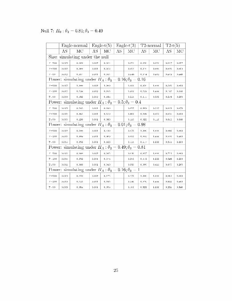
Null 7: H0 : θ2 = 0.81; θ3 = 0.49
Engle-normal Engle-t(5) Engle-t(3) T2-normal T2-t(5)AS MC AS MC AS MC AS MC AS MC
Size: simulating under the nullT=500 0.003 0.049 0.002 0.051 0.051 0.020 0 .050 0.017 0.052
T=200 0.002 0.049 0.001 0.052 0.052 0.016 0 .049 0.015 0.053
T=50 0.002 0.051 0.001 0.051 0.048 0.014 0 .052 0.013 0.049
Power: simulating under HA : θ2 = 0.16; θ3 = 0.16
T=500 0.007 1.000 0.002 1.000 1.000 0.956 1 .000 0.505 0.950
T=200 0.007 0.720 0.002 0.695 1.000 0.723 1 .000 0.137 0.535
T=50 0.009 0.180 0.002 0.185 0.225 0.111 0 .390 0.018 0.065
Power: simulating under HA : θ2 = 0.5; θ3 = 0.4
T=500 0.003 0.505 0.001 0.180 0.655 0.363 0 .565 0.018 0.070
T=200 0.001 0.385 0.001 0.150 0.400 0.108 0 .355 0.016 0.050
T=50 0.005 0.120 0.001 0.080 0.115 0.022 0 .110 0.012 0.040
Power: simulating under HA : θ2 = 0.01; θ3 = 0.98
T=500 0.002 0.600 0.001 0.430 0.975 1.000 1 .000 0.989 1.000
T=200 0.001 0.360 0.001 0.360 0.695 0.992 1 .000 0.910 1.000
T=50 0.004 0.090 0.001 0.100 0.125 0.417 1 .000 0.311 1.000
Power: simulating under HA : θ2 = 0.49; θ3 = 0.81
T=500 0.001 0.080 0.002 0.045 0.040 0.927 1 .000 0.724 1.000
T=200 0.001 0.090 0.001 0.075 0.050 0.513 1 .000 0.348 1.000
T=50 0.001 0.060 0.001 0.040 0.085 0.099 0 .455 0.077 0.265
Power: simulating under HA : θ2 = 0.16; θ3 = 1
T=500 0.003 0.160 0.002 0.175 0.275 1.000 1 .000 0.984 1.000
T=200 0.003 0.125 0.001 0.185 0.240 0.970 1 .000 0.832 1.000
T=50 0.003 0.085 0.001 0.095 0.100 0.323 1 .000 0.231 0.840
25
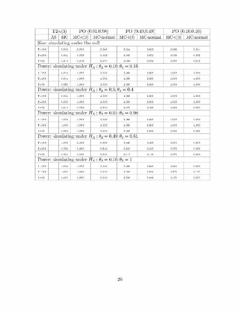
T2-t(3) PO (0.01,0.98) PO (0.49,0.49) PO (0.16,0.16)AS MC MC-t(3) MC-normal MC-t(3) MC-normal MC-t(3) MC-normal
Size: simulating under the nullT= 500 0.050 0 .052 0.049 0.051 0.053 0.049 0 .047
T= 200 0.051 0 .053 0.052 0.049 0.052 0.049 0 .052
T= 50 0.049 0 .048 0.051 0.048 0.050 0.052 0 .049
Power: simulating under HA : θ2 = 0.16; θ3 = 0.16
T= 500 0.050 1 .000 1.000 1.000 1.000 1.000 1 .000
T= 200 0.075 1 .000 1.000 1.000 1.000 1.000 1 .000
T= 50 0.035 1 .000 1.000 1.000 1.000 1.000 1 .000
Power: simulating under HA : θ2 = 0.5; θ3 = 0.4
T= 500 0.055 1 .000 1.000 1.000 1.000 1.000 1 .000
T= 200 0.075 1 .000 1.000 1.000 1.000 1.000 1 .000
T= 50 0.040 0 .280 0.220 0.370 0.285 0.390 0 .355
Power: simulating under HA : θ2 = 0.01; θ3 = 0.98
T= 500 1.000 1 .000 1.000 1.000 1.000 1.000 1 .000
T= 200 1.000 1 .000 1.000 1.000 1.000 1.000 1 .000
T= 50 0.920 1 .000 1.000 1.000 1.000 0.556 0 .390
Power: simulating under HA : θ2 = 0.49; θ3 = 0.81
T= 500 1.000 0 .290 0.860 0.540 0.500 0.055 0 .050
T= 200 0.725 0 .165 0.315 0.255 0.515 0.055 0 .065
T= 50 0.300 0 .135 0.220 0.115 0.190 0.055 0 .060
Power: simulating under HA : θ2 = 0.16; θ3 = 1
T= 500 1.000 1 .000 1.000 1.000 1.000 0.825 0 .800
T= 200 1.000 1 .000 1.000 1.000 1.000 0.425 0 .415
T= 50 0.625 0 .905 1.000 0.705 1.000 0.175 0 .155
26
References
Andrews, D.W.K. and W. Ploberger (1994), Optimal Tests when a Nuisance Pa-rameter is Present only under the Alternative, Econometrica 62, 6, 1383-1414.
Bollerslev, T (1986), Generalized Autoregressive Conditional Heteroscedasticity,Journal of Econometrics 31, 307-327.
Bollerslev, T. and J. M. Wooldridge (1992), Quasi Maximum Likelihood Estima-tion and Inference in Dynamic Models with Time Varying Covariances. Econometric
Reviews 11, 143-172.Dufour, J. M. (2004), Monte Carlo Tests with Nuisance Parameters: A General
Approach to Finite-Sample Inference and Nonstandard Asymptotics in Econometrics,Mimeo.
Dufour, J. M., L. Khalaf, J.-T.- Bernard and I. Genest (2004), Simulation-BasedFinite-Sample Tests for Heteroscedasticity and ARCH Effects, Journal of Economet-
rics, forthcoming.Dufour, J. M. andM. King (1991), Optimal Invariant Tests for the Autocorrelation
Coefficient in Linear Regressions with Stationary or Nonstationary AR(1) Errors,Journal of Econometrics 47, 115-143.
Dufour, J. M. and J.-F. Kiviet (1996), Exact Tests for Structural Change in FirstOrder Dynamic Models, Journal of Econometrics 70, 39-68.
Dufour, J. M. and J.-F. Kiviet (1998), Exact Inference Methods for First-OrderAutoregressive Distributed Lag Models, Econometrica 66, 79-104.
Elliot, G., T.J. Rothenberg, and J.H. Stock, (1996), Efficient Tests for an Autore-gressive Unit Root, Econometrica, 64, 813-836.
Engle, R. F. (1982), Autoregressive Conditional Heteroscedasticity with Estimatesof the Variance of United Kingdom Inflation, Econometrica 50, 987-1007.
Engle, R. F. and D. Kraft (1983), Multiperiod Forecast Error Variances of InflationEstimated from ARCH Models. In A. Zellner, ed., Applied Time Series Analysis of
Economic Data. Washington D.C.: Bureau of the Census.Greene, W. H. (2000), Econometric Analysis, fourth edition, Prentice-Hall.Hall, P. and Q. Yao (2003), Inference in ARCH and GARCHModels with Heavy-
Tailed Errors, Econometrica 71, 285-317.Jensen, S. T. and A. Rahbek (2004), Asymptotic Normality of hte QMLE of
ARCH in the Nonstationary Case, Econometrica 72, 2, 641-646.Lee, J. H. H. (1991), A Lagrange Multiplier Test for GARCH Models, Economics
Letters 37, 265-271.Lee, J. H. and M. L. King (1993), A Locally Most Mean Powerful Based Score Test
for ARCH and GARCH Regression Disturbances, Journal of Business and Economic
Statistics 11, 17-27. Correction 12 (1994), 139.Lumsdaine, R. (1995), Finite-Sample Properties of the Maximum Likelihood Es-
timator in GARCH(1,1) and IGARCH(1,1) Models. A Monte Carlo Investigation,Journal of Business and Economic Statistics 13, 1-10.
27

Newey, W. K. and K. D. West (1987), A Simple, Positive Semi-Definite Het-eroskedasticity and Autocorrelation Consistent Covariance Matrix, Econometrica 55,703-708.
28
Copyright © 2022 FDOKUMEN