Journal of Systems Architecture 57 (2011) 790–798

Contents lists available at ScienceDirect

Journal of Systems Architecture

journal homepage: www.elsevier .com/locate /sysarc

Temporal partitioning of data flow graph for dynamicallyreconfigurable architecture

Bouraoui Ouni ⇑, Ramzi Ayadi, Abdellatif MtibaaLaboratory of Electronic and Microelectronic, Faculty of Science at Monastir, 5000 Monastir, Tunisia

a r t i c l e i n f o a b s t r a c t

Article history:Received 14 December 2010Received in revised form 17 May 2011Accepted 19 May 2011Available online 31 May 2011

Keywords:Temporal partitioningReconfigurable architectureFPGA-engineeringVLSI applicationsAlgorithmData flow graph

1383-7621/$ - see front matter � 2011 Elsevier B.V. Adoi:10.1016/j.sysarc.2011.05.002

⇑ Corresponding author.E-mail address: bouraoui_ouni@yahoo.fr (B. Ouni)

In this paper, we present a novel temporal partitioning algorithm that temporally partitions a data flowgraph on reconfigurable system. Our algorithm can be used to resolve the temporal partitioning problemat the behaviour level. Our algorithm optimizes the whole latency of the design; this aim can be reachedby minimizing the latency of the graph and the number of partitions at the same time. Consequently, ouralgorithm starts by the lowest possible number of partitions; and next it uses the eigenvectors of thegraph to find the best schedule of nodes that minimizes the latency of the graph. The proposed method-ology was tested on several examples on reconfigurable architecture based on Xilinx Vertex-II XC2V1000FPGA device. The results show significant reduction in the design latency compared to famous relatedalgorithms used in this field.

� 2011 Elsevier B.V. All rights reserved.

1. Introduction

Dynamically reconfigurable architectures (DRA) have the po-tential for achieving high performance at a relatively low cost fora wide range of applications. DRA combine programmable process-ing units with reconfigurable hardware units. The later is usuallybased on dynamically reconfigurable Field Programmable GateArray (FPGA). Designers have used the temporal partitioningapproach [1–4] to divide the application into temporal partitions,which are configured one after the one on target FPGA. The firstpartition receives input data, performs computations and storesthe intermediate data into an on-board memory. The device is thenreconfigured for the next partition, which computes results basedon intermediate data from the previous partition. A controllerinteracts with both the reconfigurable hardware and the memoryand is used to load new configuration. The temporal partitioninghas become an essential issue for several important VLSI applica-tions. Application with several tasks has entailed problem com-plexities that are unmanageable for existing programmabledevice. Thus, the temporal partitioning is used to divide the appli-cation into smaller, more manageable components, with the tradi-tional goals such as latency optimization or communication costoptimization, etc. In this paper we present a new temporal parti-tioning algorithm that minimizes the whole latency of the graph.The proposed approach shows that to reduce the whole latency

ll rights reserved.

.

of the graph, we need to maximize the cut size between designpartitions. Next, the algorithm uses the graph’s eigenvectors tomaximize the cut size.

2. Related works

In the literature, many methods have been used to solve thetemporal partitioning problem. In this section we detail the famoustemporal partitioning algorithms.

The ‘‘ILP’’ integer linear programming [2,5,6] is one of the fa-mous approaches that widely used to solve the temporal partition-ing problem. The authors started by getting a lower bound on thenumber of partitions for the particular problem. To calculate thelower number of partitions, the authors summed the area of allnodes, this value divided by the available reconfigurable resourcewill be the minimum number of partition required to obtain solu-tion. Next, the authors introduced two 0–1 variables called XTP andWPT1T2. XTP = 1 if the node T is placed in partition P, otherwiseXTP = 0. WPT1T2 = 1 (if node Ti is placed in any partition 1, . . .,p � 1and node Tj is placed in any partition p, . . .,N and Tj depends onTi) OR (if node Ti is placed in partition p and node Tj is placed inany partition p + 1, . . .,N and Tj depends on Ti) otherwiseWPT1T2 = 0. The main problem of the ILP approaches for partitioninga graph is its high execution time. In fact, the size of the computa-tion model grows very fast; therefore the algorithm can only be ap-plied to small examples. To overcome this problem, some authorsreduced the size of the model by reducing the set of constraints in

B. Ouni et al. / Journal of Systems Architecture 57 (2011) 790–798 791

the problem formulation, but the numbers of variables and prece-dence constraints to be considered still remain high.

The network flow methodology has been used [7–9] and im-proved in [10]. This method is a recursive bipartition approach thatsuccessively partitions a set of remaining nodes in two sets, one ofwhich is a final partition, whereas a further partition step must beapplied on the second one. The goal to be reached during partition-ing is the minimization of the communication overhead among thepartitions, which also means the minimization of the communica-tion cost. The goal is formulated as the minimization of the overallcut-size among the partitions. A little cut size among the partitionsmeans fewer edges connecting the partitions, less communicationand therefore a good partitioning quality. However, the model isconstructed by inserting a great amount of nodes and edges inthe original graph. The resulting graph may grow too big. In theworst case, the number of nodes in the new graph can be twicethe number of the nodes in the original graph. The number of addi-tional edges also grows dramatically and become difficult tohandle.

The list scheduling algorithm has been used in [11–15]. Themain idea of this method consists in placing all nodes of the graphon a list. The first partition is built by removing nodes from the listto the partition until the size of the target area is reached. Then, anew partition is built and the process is repeated until all nodes areplaced in partition. This technique is often oriented by the ASAP(As Soon As Possible) and/or the ALAP (As Late As Possible) sched-uling. The mobility of a given node, i.e. the difference between itsALAP – value and its ASAP – value, can be used as its priority. Atany time step t, the so-called ready set, that is the set of operationsready to be scheduled, is constructed. The ready set contains oper-ations whose predecessors have already been scheduled early en-ough to complete their execution at time t. The algorithm checkswhether there are enough resources of a given type k to implementall the operations of type k. If so, the operations are assigned theresources, otherwise, higher priority nodes are assigned the avail-able resources and the rest of the operations will be scheduled la-ter, when some resources will be available. If the mobility of a nodeis used as priority criteria, it is possible that all operators in theready list are on critical paths, which means that their mobilityis zero. As a consequence, the complete depth of each operator isincreased by one, thus increasing the latency of the graph’s execu-tion. The main advantage of the list scheduling technique is its veryfast run time.

3. Data flow graph

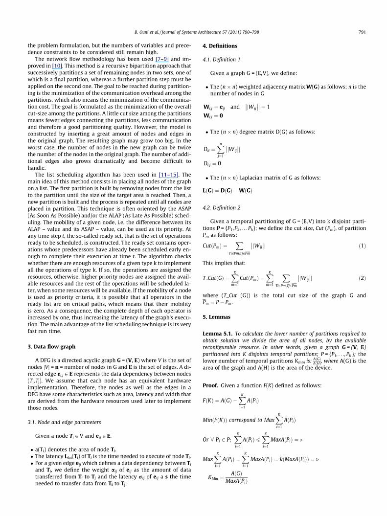
A DFG is a directed acyclic graph G = (V, E) where V is the set ofnodes jVj = n = number of nodes in G and E is the set of edges. A di-rected edge ei,j 2 E represents the data dependency between nodes(Ti,Tj). We assume that each node has an equivalent hardwareimplementation. Therefore, the nodes as well as the edges in aDFG have some characteristics such as area, latency and width thatare derived from the hardware resources used later to implementthose nodes.

3.1. Node and edge parameters

Given a node Ti 2 V and eij 2 E.

� a(Ti) denotes the area of node Ti.� The latency Llat(Ti) of Ti is the time needed to execute of node Ti.� For a given edge eij which defines a data dependency between Ti

and Tj, we define the weight aij of eij as the amount of datatransferred from Ti to Tj and the latency rij of eij a s the timeneeded to transfer data from Ti to Tj.

4. Definitions

4.1. Definition 1

Given a graph G = (E,V), we define:

� The (n � n) weighted adjacency matrix W(G) as follows; n is thenumber of nodes in G

Wi;j ¼ eij and jWij

�� ��j ¼ 1

Wi;i ¼ 0

� The (n � n) degree matrix D(G) as follows:

Dii ¼Xn

j¼1

jWij

�� ��jDi;j ¼ 0

� The (n � n) Laplacian matrix of G as follows:

LðGÞ ¼ DðGÞ �WðGÞ

4.2. Definition 2

Given a temporal partitioning of G = (E,V) into k disjoint parti-tions P = {P1,P2, . . .Pk}; we define the cut size, Cut (Pm), of partitionPm as follows:

CutðPmÞ ¼X

Ti2Pm;Tj2Pm

jWij

�� ��j ð1Þ

This implies that:

T CutðGÞ ¼XK

m¼1

CutðPmÞ ¼XK

m¼1

XTi2Pm;Tj2Pm

jWij

�� ��j ð2Þ

where (T_Cut (G)) is the total cut size of the graph G andPm ¼ P � Pm.

5. Lemmas

Lemma 5.1. To calculate the lower number of partitions required toobtain solution we divide the area of all nodes, by the availablereconfigurable resource. In other words, given a graph G = (V, E)partitioned into K disjoints temporal partitions; P = {P1, . . ., Pk }; thelower number of temporal partitions Kmin is: AðGÞ

AðHÞ, where A(G) is thearea of the graph and A(H) is the area of the device.

Proof. Given a function F(K) defined as follows:

FðKÞ ¼ AðGÞ �XK

i¼1

AðPiÞ

MinðFðKÞÞ correspond to MaxXK

i¼1

AðPiÞ

Or 8 Pi 2 P;XK

i¼1

AðPiÞ 6XK

i¼1

MaxAðPiÞ ¼ .

MaxXK

i¼1

AðPiÞ ¼XK

i¼1

MaxAðPiÞ ¼ kðMaxAðPiÞÞ ¼ .

KMin ¼AðGÞ

MaxAðPiÞ

792 B. Ouni et al. / Journal of Systems Architecture 57 (2011) 790–798

Or 8 Pi 2 P; AðPiÞ 6 AðHÞ ¼ .Max AðPiÞ ¼ AðHÞ ¼ .

KMin ¼AðGÞAðHÞ

MaxðFðKÞÞ correspond to MinXK

i¼1

AðPiÞ

Or 8 Pi 2 P;XK

i¼1

AðPiÞPXK

i¼1

Min AðPiÞ ¼ .

MinXK

i¼1

AðPiÞ ¼XK

i¼1

MinAðPiÞ ¼ kðMinAðPiÞÞ ¼ .

KMax ¼AðGÞ

MinAðPiÞor MinAðPiÞ ¼ Min aðTmÞ; Tm 2 V ¼ .

KMax ¼AðGÞ

Min aðTmÞ

Lemma 5.2. Given a temporal partitioning of G(V,E) into k disjointpartitions P = {P1,P2, . . ., Pk} and Given K indicator vector Xm(i) = [Xm

(1),Xm(2), . . .,Xm(n)], where m = 1,2, . . . , k and i = 1,2, . . .,n. XmðiÞ ¼jV j � jPmj if Ti 2 Pm; �jPmj otherwise; jPmj is the number of nodesin partition Pm

CutðPmÞ ¼ Vj j2ðXtmLðGÞXmÞ ð3Þ

Proof

XtmLðGÞXm¼Xt

mDðGÞXm�XtmWðGÞXm

¼XVj j

i¼1

DiðxmðiÞÞ2�XVj j

i¼1

XVj j

j¼1

Wi;jxmðiÞxmðjÞ

¼12

XVj j

i¼1

ðDiþDiÞðxmðiÞÞ2�XVj j

i¼1

XVj j

j¼1

Wi;jxmðiÞxmðjÞ

¼12

XVj j

i¼1

DiðxmðiÞÞ2�2XVj j

i¼1

XVj j

j¼1

WijxmðiÞxmðjÞþXVj j

j¼1

DjðxmðjÞÞ2 !

¼12

XVj j

i¼1

XVj j

j¼1

Wi;jðxmðiÞ�xmðjÞÞ2¼12

XVj j

i¼1

XVj j

j¼1

Wijð Vj jÞ2

¼ Vj j2

2

XVj j

i¼1

XVj j

j¼1

Wij¼2 Vj j2

2

XTi2Pm ;Tj2Pm

Wij¼ V2��� ��� X

Ti2Pm ;Tj2Pm

Wijj j

¼CutðPmÞ

Lemma 5.3. Given a temporal partitioning of G(V,E) into k disjointpartitions P = {P1,P2, . . ., P}

CutðPmÞ 6 Vj j kMax

4

kMax is the highest eigenvalues of matrix L(G)

Proof. In [16] authors showed that

kMax ¼ maxxm – 0Xt

mLðGÞXm

XtmXm

ð4Þ

Based on Eqs. (3) and (4)

XtmXm ¼ Pmj jð Vj j � Pmj jÞ2 þ ð Vj j � Pmj jÞ Pmj j2

¼ Pmj jð Vj j � Pmj jÞ Vj j ð5Þ

Based on Eqs. (4) and (5)

CutðPmÞ 6Pmj jð Vj j � PmÞj jkMax

Vj j or Pmj jð Vj j � PmÞj j 6 Vj j2

4

¼ .CutðPmÞ 6 Vj j kMax

4ð6Þ

Lemma 5.4. Given a (n � n) matrix M defined as follows: Mij ¼ 1Pmj j if

Ti and Tj 2 Pm; 0 otherwise

XðGÞXtðGÞ ¼ M

where X(G) is the matrix that contains the k indicator vectors, as de-fined in 5.2, as columns.

Proof. The ijth of XXt isPK

m¼1XmðiÞXmðjÞ. The term Xm(i) Xm(j) willbe non-zero if and only if both Ti and Tj, are in Pm, hence the sum is1/lPml when Ti and Tj are in the same partition; 0 otherwise.

6. Temporal partitioning of data flow graph

A temporal partitioning P of a data flow graph G = (V,E), is itsdivision into some disjoints partitions such as: P = {P1, . . .,Pk}.

A temporal partitioning is feasible in accordance to a reconfigu-rable device H with area A(H) and pins T(H) if:

� 8Pi 2 P; AðPiÞ ¼P

Ti2PiaðTiÞ 6 AðHÞ

� T CutðGÞ ¼PK

m¼1CutðPmÞ ¼PK

m¼1

PTi2Pm ;Tj2Pm

Wij

�� �� 6 TðHÞ: thevariable kWijk = 1 signifies that Tj depends on Ti. When node Ti

is being placed in partition Pm and Tj is being placed outsidePm, therefore the data being communicated between them willhave to be stored in the memory. Consequently, the sum of allthe data being communicated across all partition should be lessthan the pins constraint.

7. Problem formulation

In this paper we aim to solve the following problem:Given a data flow graph G(V,E): Find the way of graph partitioning

that minimizes the whole latency of the graph while respecting allconstraints.

Given a temporal partitioning P of the graph G = (V,E)into K dis-joints temporal partitions P = P1, . . .,Pk. The whole latency ofP(LatP) is calculated as follows:

LatP ¼ KCT þ DðGÞ ð7Þ

CT is the time needed to reconfigure the device

DðGÞ ¼Xk

i¼1

Pij j ð8Þ

Let C ¼ fCPi1 ; . . . ;CPi

n g be the set of paths in the partition Pi. Hence

Pij j ¼max16j6nð CPi

j

��� ���Þ ð9Þ

We apply Eq. (10) on all couples (Ti,Tj); Tj depends on Ti

LlatðTiÞ ¼ LlatðTiÞ þ rij ð10Þ

Using Eq. (10)

CPij

��� ��� ¼ XTm2C

Pij

LlatðTmÞ ð11Þ

Using Eqs. (7) and (11) the whole latency can be expressed asfollows:

B. Ouni et al. / Journal of Systems Architecture 57 (2011) 790–798 793

LatP ¼ KCT þXk

i¼1

max16j6n

XTm2C

Pij

LlatðTmÞ ð12Þ

Based on Eq. (12) to minimize the whole latency, we need to min-imize the term [max16j6n

PTm2CPi

jLlatðTmÞ].One solution is to mini-

mize the number of nodes in every path CPij ;C

Pij 2 C. On the other

hand, given two nodes T1,T2 2 V: if T1; T2 2 CPij then there is an edge

e12 between T1 and T2. For that reason, to minimize the number ofnodes in every path CPi

j , one solution is to minimize the number ofedges in every path CPi

j . This aim can be reached by minimizing thenumber of edges in partition Pi. This can be also reached by maxi-mizing the number of edges between the different partitions. As aresult, the whole latency minimization problem can be expressedas follows: given a graph G(V,E): Find the way of graph partitioningsuch as number of edges between design partition has highest valuewhile respecting all constraints.

On the other hand using definition 2, the above problem can beshown as: how to maximize the total cut size (T_Cut) between thedesign partitions. Hence, the latency minimization problem can beexpressed as follows:

Minimize ðLatPÞ )Maximize ðT CutðGÞÞ ð13Þ

8. Proposed algorithm

Our algorithm aims to solve the following problem: Given a DFGG = (V,E) and a set of constraints: Find the way of graph partitioningin optimal number of temporal partitions that minimize the whole la-tency of the graph while respecting all constraints.

Our algorithm is composed by two main steps. The first stepaims to find an initial partitioning Pin that minimizes whole latencyof the graph. Next, if the area constraint is satisfied after the firststep then we adopts the initial partitioning, else we go to the sec-ond step. Hence, the second step aims to find the final partitioningP of the graph while satisfying the area constrain. If the second stepcannot find a feasible scheduling then we relax the number of par-tition by one and the algorithm goes to the first step. And, we re-start to find a feasible solution in the new number partitions.

T2

T3

T5

T6

T4 T1

T7

Fig. 1. Graph G.

Table 1Parameters of graph G.

Nodes T1 T2 T3 T4 T5 T6 T7

Area (CLB) 225 210 220 200 276 196 130Latency (ns) 20 40 30 60 10 20 10Edges E12 E13 E27 E43 E46 E56 E57

Latency (ns) 30 40 10 10 20 30 10

8.1. First step: initial partitioning

As shown in Eq. (13) the whole latency minimization problemcan be solved by maximizing the total cut size between design par-titions. In this section, we present a good solution for this problem.

We introduce the graph complement G0 ðV ; EÞ of G(V,E) as fol-lows: the complement of a graph G is a graph G0 on the same nodessuch that two nodes of G0 are connected if and only if they are notconnected in G.

Given a temporal partitioning of G(V,E) into k disjoint partitionsP = {P1,P2, . . .,Pk}, we have:

CutðPmðGÞÞ þ CutðPmðG0ÞÞ ¼ Pmj jð Vj j � Pmj jÞ ¼ . ð14ÞCutðPmðGÞÞ ¼ Pmj jð Vj j � Pmj jÞ � CutðPmðG0ÞÞ ð15Þ

Based on Eq. (15), "Pm 2 P; if Pm has the highest cut in the graphG then it has the lowest cut in the graph G0. Hence, if (T_Cut (G)) hasthe highest value then (T_Cut(G0)) has the lowest value. Therefore,the whole latency minimization problem can be shown as: how tominimize the total cut (T_Cut(G0)) of the graph G0 instead of howmaximize (T_Cut(G)) of the graph G. As a result, to minimize thewhole latency of the graph (G), we need to minimize the totalcut size of the graph G0

Based on Eq. (3) of 5.2,

T CutðG0Þ ¼XK

m¼1

CutðPmðG0ÞÞ ¼ K Vj j2 þXk

m¼1

XtmLðG0ÞXm

¼ K Vj j2 þ trace XtðG0ÞLðG0ÞXðG0Þ� �

ð16Þ

Therefore, to minimize T(Cut(G0)) we need to minimize :

trace XtðG0ÞLðG0ÞXðG0Þ� �

:

In [17] the authors showed that the lowest value of trace½XtðG0ÞLðG0ÞXðG0Þ� can be obtained if the matrix X(G0) contains the first k eigen-vectors corresponding to the k lowest eigenvalues of matrix L(G0) ascolumns. As conclusion, the whole latency minimization problemcan be solved by choosing an assignment matrix X(G0) that containsthe first k eigenvectors of the k lowest eigenvalues of matrix L(G0) ascolumns.

The initial partitioning step of our algorithm is summarized bythe following steps:

(1) Compute the minimum number of partitions:Kmin = dArea(G)/Area(H)e

(2) Compute the laplacian matrix L(G0) of G0

(4) Compute k lowest eigenvalues of L(G0)(5) Construct the (n � k) assignment matrix X(G0) that has the K

eignvectors of the k lowest eigenvalues of L(G0) as columns(6) Compute Z = X(G0)Xt(G0)(7) Construct the (n � n) matrix M = Mi,j from Z. Mi,j = 1 if

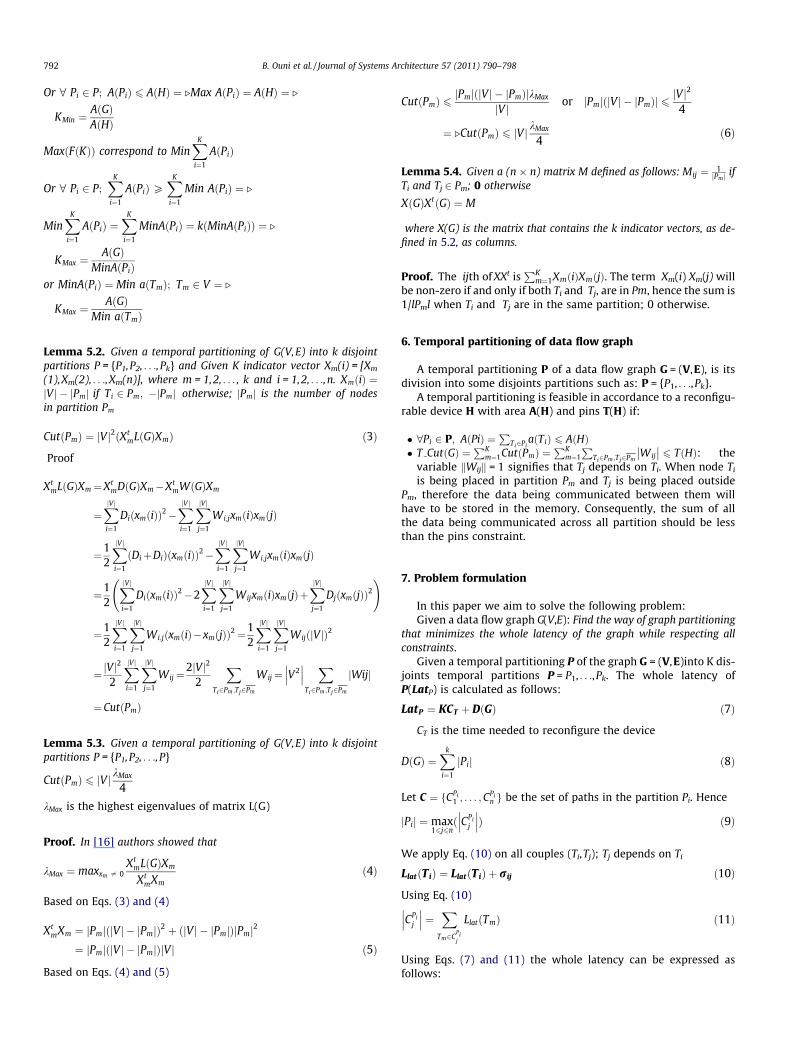
Zi,j P 1/jVj, 0 otherwise(8) Use lemma 4 to generate the initial partitioning from matrix

M9) If the area constraint is satisfied then final partitioning = ini-

tial partitioning; else go to step 2 (we mean by go to step 2:go to final partitioning step)

8.1.1. ExampleApplying the above steps on the graph G of Fig. 1, let 600 CLB be

the area of the device. The parameters of the nodes and arcs areshown in Table 1.

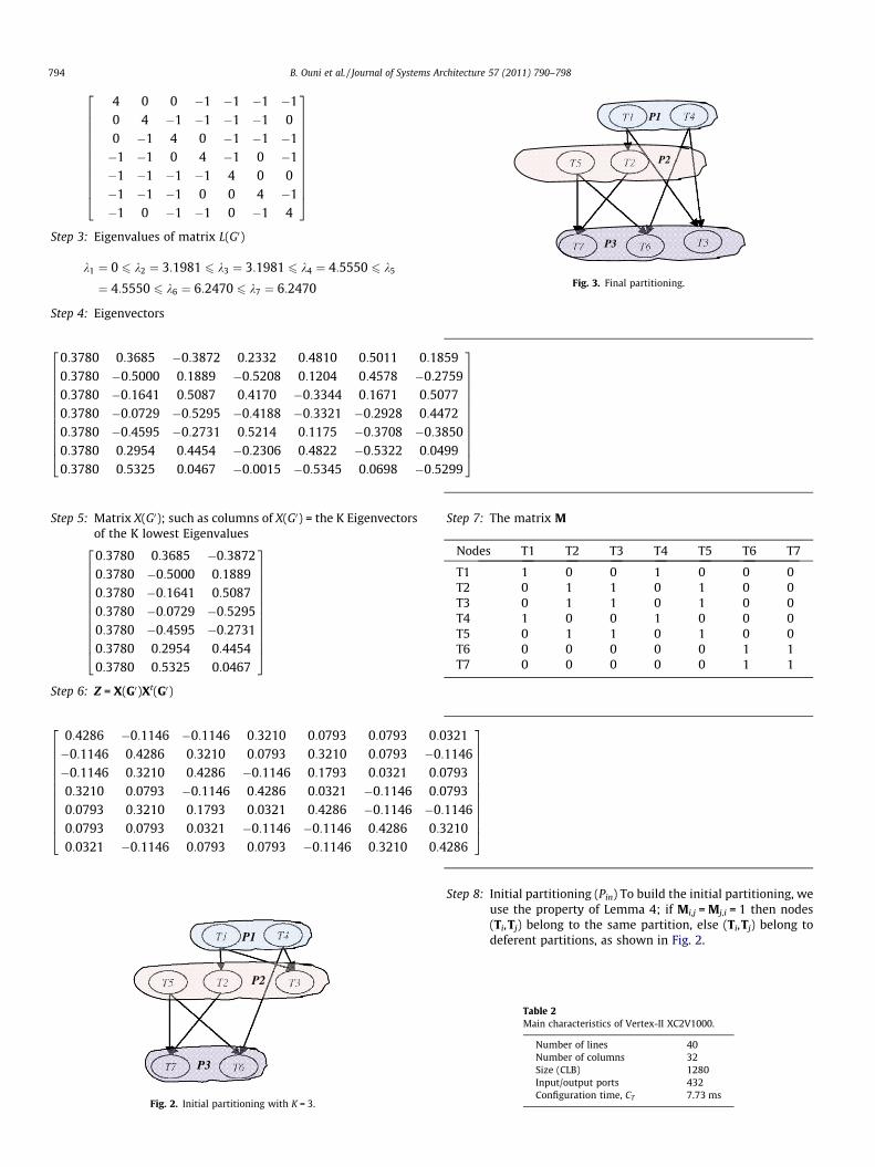
Step 1: K = area(G)/area (H) = 1457/600 = 2, 42 = 3Step 2: Laplacian matrix L(G0) of G0

0:370:370:370:370:370:370:37

2666666666664

0:4�0:�0:0:30:00:00:0

2666666666664

P1

P2

794 B. Ouni et al. / Journal of Systems Architecture 57 (2011) 790–798

4 0 0 �1 �1 �1 �10 4 �1 �1 �1 �1 00 �1 4 0 �1 �1 �1�1 �1 0 4 �1 0 �1�1 �1 �1 �1 4 0 0�1 �1 �1 0 0 4 �1�1 0 �1 �1 0 �1 4

2666666666664

3777777777775

P3

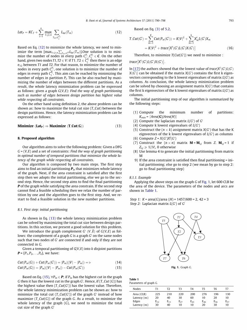
Step 3: Eigenvalues of matrix L(G0)

Fig. 3. Final partitioning.

k1 ¼ 0 6 k2 ¼ 3:1981 6 k3 ¼ 3:1981 6 k4 ¼ 4:5550 6 k5

¼ 4:5550 6 k6 ¼ 6:2470 6 k7 ¼ 6:2470

Step 4: Eigenvectors

80 0:3685 �0:3872 0:2332 0:4810 0:5011 0:185980 �0:5000 0:1889 �0:5208 0:1204 0:4578 �0:275980 �0:1641 0:5087 0:4170 �0:3344 0:1671 0:507780 �0:0729 �0:5295 �0:4188 �0:3321 �0:2928 0:447280 �0:4595 �0:2731 0:5214 0:1175 �0:3708 �0:385080 0:2954 0:4454 �0:2306 0:4822 �0:5322 0:049980 0:5325 0:0467 �0:0015 �0:5345 0:0698 �0:5299

3777777777775

Step 5: Matrix X(G0); such as columns of X(G0) = the K Eigenvectorsof the K lowest Eigenvalues

0:3780 0:3685 �0:38720:3780 �0:5000 0:18890:3780 �0:1641 0:50870:3780 �0:0729 �0:52950:3780 �0:4595 �0:27310:3780 0:2954 0:44540:3780 0:5325 0:0467

2666666666664

3777777777775

Step 6: Z = X(G0)Xt(G0)

P1

P2

P3

Fig. 2. Initial partitioning with K = 3.

286 �0:1146 �0:1146 0:3210 0:0793 0:0793 0:01146 0:4286 0:3210 0:0793 0:3210 0:0793 �01146 0:3210 0:4286 �0:1146 0:1793 0:0321 0:0210 0:0793 �0:1146 0:4286 0:0321 �0:1146 0:0793 0:3210 0:1793 0:0321 0:4286 �0:1146 �0793 0:0793 0:0321 �0:1146 �0:1146 0:4286 0:3321 �0:1146 0:0793 0:0793 �0:1146 0:3210 0:4

Step 7: The matrix M

3:1177:1122

Nodes

2146

939346

1086

3777777777775

T1

Table 2Main cha

NumbNumbSize (CInput/Config

T2

racteristic

er of lineser of columLB)

output pouration tim

T3

s of Vertex

ns

rtse, CT

T4

-II XC2V1

403212437.

T5

000.

802

73 ms

T6

T7

T1

1 0 0 1 0 0 0 T2 0 1 1 0 1 0 0 T3 0 1 1 0 1 0 0 T4 1 0 0 1 0 0 0 T5 0 1 1 0 1 0 0 T6 0 0 0 0 0 1 1 T7 0 0 0 0 0 1 1

Step 8: Initial partitioning (Pin) To build the initial partitioning, weuse the property of Lemma 4; if Mi,j = Mj,i = 1 then nodes(Ti,Tj) belong to the same partition, else (Ti,Tj) belong todeferent partitions, as shown in Fig. 2.

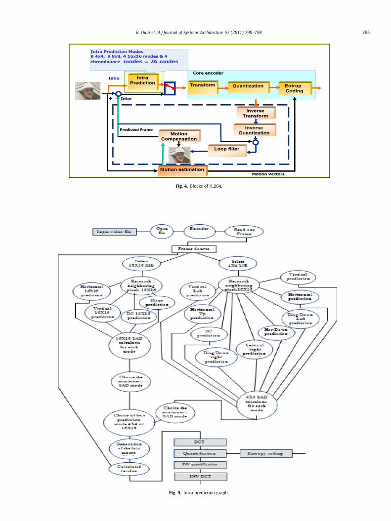
Fig. 4. Blocks of H.264.

Fig. 5. Intra prediction graph.

B. Ouni et al. / Journal of Systems Architecture 57 (2011) 790–798 795

796 B. Ouni et al. / Journal of Systems Architecture 57 (2011) 790–798

8.2. Second step: final partitioning

In this step, we start from the initial partitioning Pin given by thefirst step and the set of partitions Pi 2 Pin, where A(Pi) > A(H). Ourtechnique balances nodes from partition Pi to Pj or inversely untilthe satisfaction of the area constraint. The balance of nodes is basedon the force F(Ti, Pi ? Pj) associated with partition Pi on a node Ti tobe scheduled into partition Pj and on the force F(Ti,Pj ? Pi) associ-ated with partition Pj on a node Ti to be scheduled into partition Pi.For instance let us assume that Pi < Pj; Pi, Pj 2 Pin.

These forces are calculated as follows:

FðTi;Pi ! PjÞ ¼ d1ðTiÞ � OFðTiÞ ð17Þ

d1(Ti) = 0, if there is a node Tj 2 Pi and Tj is an output of Ti, otherwised1(Ti) = 1.

OF(Ti) = (Nu(Ti) + 1). Given a nodes Ti;2 Pi; Tj 2 Pj; NuðTiÞ ¼PTj2piaijTj; aij = 1 if Tj is an input of Ti, 0 otherwise

FðTi;Pj ! PiÞ ¼ d2ðT iÞ � InFðTiÞ ð18Þ

d2(Ti) = 0, if there is a node Tj 2 Pi and Tj is an input of Ti, otherwised2(Ti) = 1.

InF(Ti) = (Nq(Ti) + 1), Given a nodes Ti 2 Pj, Tj 2 Pi ; NqðTiÞ ¼PTj2pj

/ijTj; /ij = 1 if Tj is an output of Ti, 0 otherwise

In general, due to the scheduling of one node, other node sched-ules will also be affected. At each iteration, the force of every nodebeing scheduled in every possible partition is computed. Then, thedistribution graph is updated and the process repeats until nomore nodes remain to be scheduled.

8.2.1. ExampleConsidering the partitioning solution shown above in Fig. 2

TaDe

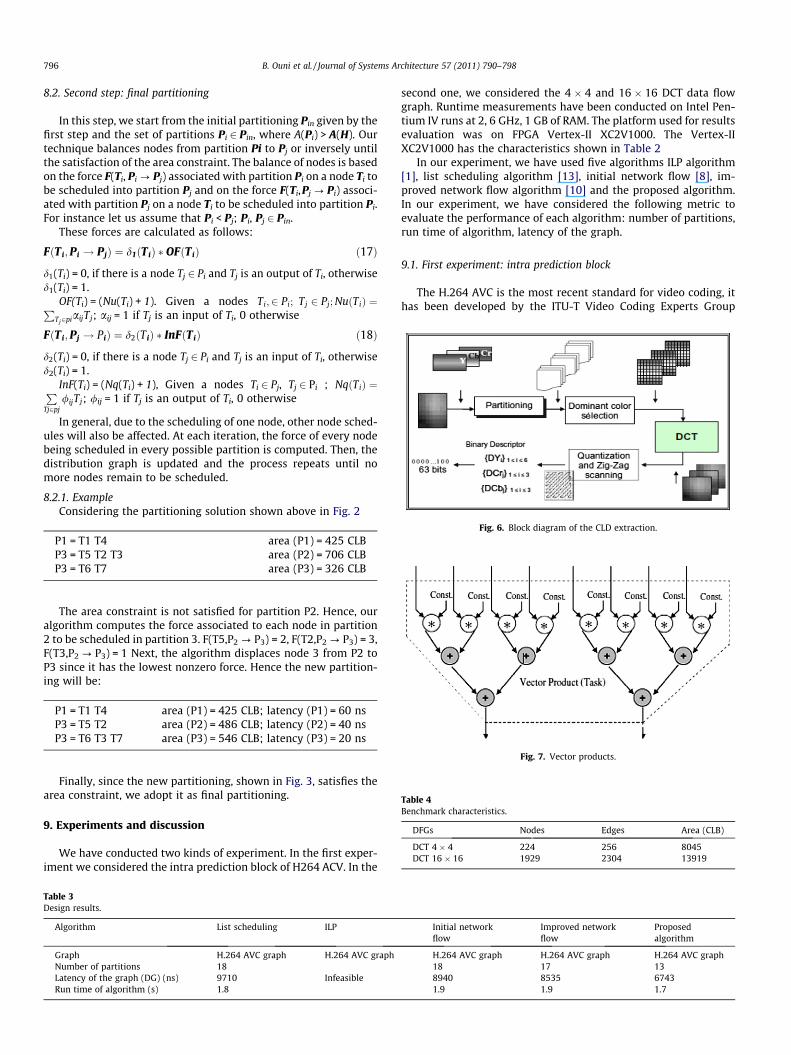
Fig. 6. Block diagram of the CLD extraction.

P1 = T1 T4

ble 3sign results.

Algorithm List schedul

Graph H.264 AVC gNumber of partitions 18Latency of the graph (DG) (ns) 9710Run time of algorithm (s) 1.8

area (P1) = 425 CLB

P3 = T5 T2 T3 area (P2) = 706 CLB P3 = T6 T7 area (P3) = 326 CLB

The area constraint is not satisfied for partition P2. Hence, ouralgorithm computes the force associated to each node in partition2 to be scheduled in partition 3. F(T5,P2 ? P3) = 2, F(T2,P2 ? P3) = 3,F(T3,P2 ? P3) = 1 Next, the algorithm displaces node 3 from P2 toP3 since it has the lowest nonzero force. Hence the new partition-ing will be:

P1 = T1 T4

area (P1) = 425 CLB; latency (P1) = 60 ns P3 = T5 T2 area (P2) = 486 CLB; latency (P2) = 40 ns P3 = T6 T3 T7 area (P3) = 546 CLB; latency (P3) = 20 ns

Fig. 7. Vector products.

Table 4Benchmark characteristics.

DFGs Nodes Edges Area (CLB)

DCT 4 � 4 224 256 8045DCT 16 � 16 1929 2304 13919

Finally, since the new partitioning, shown in Fig. 3, satisfies thearea constraint, we adopt it as final partitioning.

9. Experiments and discussion

We have conducted two kinds of experiment. In the first exper-iment we considered the intra prediction block of H264 ACV. In the

ing ILP

raph H.264 AVC graph

Infeasible

second one, we considered the 4 � 4 and 16 � 16 DCT data flowgraph. Runtime measurements have been conducted on Intel Pen-tium IV runs at 2, 6 GHz, 1 GB of RAM. The platform used for resultsevaluation was on FPGA Vertex-II XC2V1000. The Vertex-IIXC2V1000 has the characteristics shown in Table 2

In our experiment, we have used five algorithms ILP algorithm[1], list scheduling algorithm [13], initial network flow [8], im-proved network flow algorithm [10] and the proposed algorithm.In our experiment, we have considered the following metric toevaluate the performance of each algorithm: number of partitions,run time of algorithm, latency of the graph.

9.1. First experiment: intra prediction block

The H.264 AVC is the most recent standard for video coding, ithas been developed by the ITU-T Video Coding Experts Group

Initial networkflow

Improved networkflow

Proposedalgorithm

H.264 AVC graph H.264 AVC graph H.264 AVC graph18 17 138940 8535 67431.9 1.9 1.7

Table 5Design results.

Algorithm List scheduling ILP Initial Network flow Improved Network flow Proposed algorithm

Graph 4 � 4 DCT graph 4 � 4 DCT graph 4 � 4 DCT graph 4 � 4 DCT graph 4 � 4 DCT graphNumber of partitions 9 infeasible 9 9 7Latency of the graph D(G) (ns) 4770 4395 4570 3492Run time of algorithm 0,2 sec 0,12 sec 0,12 sec 0,3 secGraph 16 � 16 DCT graph 16 � 16 DCT graph 16 � 16 DCT graph 16 � 16 DCT graph 16 � 16 DCT graphNumber of partitions 15 infeasible 15 15 12latency of the graph D(G) (ns) 6610 6420 7730 5196Run time of algorithm (s) 1.5 1.5 1.5 1.5

B. Ouni et al. / Journal of Systems Architecture 57 (2011) 790–798 797

(VCEG) together with the ISO/IEC Moving Picture Experts Group(MPEG). It includes most of the techniques that have been usedin previous standards such as H.261, MPEG-1, MPEG-2, MPEG-4,H.261, and H.263. Fig. 4 shows the main blocks of H.264

The prediction algorithms represent the main elements of theH264 algorithms. Indeed, the prediction ‘‘Inter’’ exploits the tem-poral correlation between successive images and the prediction‘‘Intra’’ exploits the spatial correlation in the same image. Thesetwo modes of prediction allow a considerable gain in terms ofquality and compression ratio. According intra mode, shown inFig. 5, the predicted block is based on previous encoded blocks.This predicted block is subtracted from the current block prior toencoding. For the luminance (luma) samples, the predicted blockmay be formed by 4 � 4 sub block or by 16 � 16 macro block.There is one of nine optional prediction modes for 4 � 4 lumablock; 4 optional modes for 16 � 16 luma block.

Table 3 gives the different solutions provided by the ILP algo-rithm, the list scheduling, the initial network flow technique, theenhance network flow and the proposed algorithm. Result showsthat our algorithm has always the lowest number of partitions. Re-sults show a D(G) improvement of 30.55% compared to list sched-uling, 24.57% compared to network flow algorithm, 20.99%compared to enhanced network flow algorithm.

9.2. Second experiment: DCT data flow graph

Fig. 6 shows the Color Layout Descriptor ‘‘CLD’’ is a low-level vi-sual descriptor that can be extracted from images or video frames.The process of the CLD extraction consists of four stages: Imagepartitioning, selection of a single representative color for eachblock, DCT transformation and non linear quantization andZig-Zag scanning.

Since DCT is the most computationally intensive part of the CLDalgorithm, it has been chosen to be implemented in hardware, andthe rest of subtasks (partitioning, color selection, quantization, zig-zag scanning and Huffman encoding) were chosen for softwareimplementation. The model proposed in [15] is based on 16 vectorproducts. Thus, the entire DCT is a collection of 16 nodes, whereeach node is a vector product as presented in Fig. 7.

There are two kinds of nodes in the graph ‘‘T1’’ and ‘‘T2’’. Thestructure of ‘‘T1’’ and ‘‘T2’’is similar to vector product, but with dif-ferent bits widths. Table 4 gives the characteristics of 4 � 4 DCT,16 � 16 DCT, 16-FFT and 64- FFT graphs. Table 5 summarizes thedesign results given by each algorithm. Results show an improve-ment of 19.75% compared to the best algorithm (initial networkflow algorithm).

As conclusion our algorithm has a good trade-off between la-tency of the graph and number of partitions. Hence, our algorithmcan be qualified to be a good temporal partitioning candidate. Infact, an optimal partitioning algorithm needs to balance computa-tion required for each partition and reduce the number of partitionso that mapped applications can be executed faster on dynamicallyreconfigurable hardware.

10. Conclusion

In this paper a new temporal partitioning techniques has beenpresented and compared. The proposed algorithm aims to reducethe whole latency of a data flow graph. Our algorithms can be usedto resolve the temporal partitioning problem at the behaviour le-vel. The results show an improvement in term of whole latencycompared to related algorithms. Furthermore, results show thatour algorithm has a good execution time, indeed the complexityis k ⁄ n; where k is the number of partitions and n is the numberof nodes in the graph. Hence, our algorithm can be applied effi-ciently to rapid prototyping of data flow graph, with better resultsin term of whole latency, on dynamically reconfigurablearchitecture.

References

[1] K. Kaul, R. Vermuri, S. Govindarajan, I. Ouaiss, An automated temporalpartitioning tool for a class of DSP application workshop and reconfigurablecomputing, in: International Conference on Parallel Architecture andCompilation Technique PACT, 1998, pp. 22–27.

[2] Byungil Jeong, Hardware Software Partitioning for ReconfigurableArchitectures, MS theses School of Elec. Eng, Seoul National University. 1999.

[3] J.M.P. Cardoso, H.C. Neto, An enhance static-list scheduling algorithm fortemporal partitioning onto rpus, IFIP TC10 WG10.5 in: 10 Int. Conf. on VeryLarge Scale Integration (VLSI’99), Portugal, 1999, pp. 485–496.

[4] B. Ouni, A. Mtibaa, M. Abid, Synthesis and time partitioning for reconfigurablesystems, Design Automation for Embedded Systems Journal 9 (2005) 177–191.

[5] K. Kaul, R. Vermuri, Integrate Block processing and design space exploration intemporal partitioning for RTR architecture, in: International ReconfigurableArchitecture Workshop, RAW’99, Springer Publication, pp. 606–615.

[6] G.M. Wu, J.M. Lin, Y.W. Chang, Generic ILP-based approaches for time-multiplexed FPGA partitioning, IEEE Transactions on Computer-Aided Design20 (10) (2001) 1266–1274.

[7] H . Liu, D.F. Wong, Network flow based circuit partitioning for time-multiplexed FPGAs, in: Proc. IEEE/ACM Int. Conf. Comput.-Aided Des., 1998,pp. 497–504.

[8] H. Liu, D.F. Wong, Network flow based multi-way partitioning with area andpin constraints, IEEE Transactions on Computer Aided Design of IntegratedCircuits and Systems 17 (1) (1998).

[9] Wai-Kei Mak, E.F.Y. Young, Temporal logic replication for dynamicallyreconfigurable FPGA partitioning, IEEE Transactions on Computer-AidedDesign 22 (7) (2003) 952–959.

[10] Yung-Chuan Jiang, Jhing-Fa Wang, Temporal partitioning data flow graphs fordynamically reconfigurable computing, IEEE Transactions on Very Large ScaleIntegration Systems 15 (12) (2007).

[11] Bouraoui Ouni, Ramzi Ayadi, Mohamed Abid, Novel temporal partitioningalgorithm for run time reconfigured systems, Journal of Engineering andApplied Sciences (3) (2008).

[12] Bouraoui Ouni, Abdellatif Mtibaa, El-Bay Bourennane scheduling approach forrun time reconfigured systems, International Journal of Computer Sciencesand Engineering Systems (4) (2009).

[13] S. Trimberger, Scheduling designs into a time-multiplexed FPGA, in: Proc. ACMInt. Symp. Field Program. Gate Arrays, 1998, pp. 53–160.

[14] J. Cardoso, M. P, On combining temporal partitioning and sharing of functionalunits in compilation for reconfigurable architectures, IEEE Transaction onComputer 52 (10) (2003) 1362–1375.

[15] Mtibaa Abdellatif, Ouni Bouraoui, Abid Mohamed, An efficient list schedulingalgorithm for time placement problem, Computers and Electrical Engineering33 (4) (2007) 285–298.

[16] Bojan Mohar, Svatopluk Poljak, Eigenvalues and the max-Cut problem,Czechoslovak Mathematical Journal 40 (1990) 2 343–352.

[17] D. Gleich, Hierarchical directed spectral graph partitioning, StanfordUniversity Technical Report, <http://www.stanford.edu/�dgleich/publications/directed-spectral.pdf>, 2005.

s Architecture 57 (2011) 790–798

Bouraoui Ouni received his licence and his masterrespectively in 1999 and 2001 and his thesis in 2008from the faculty of science of Monastir. Since 2002 hehas been an Assistant Professor in Digital Electronic atthe High Institute of Informatics and Telecommunica-tion of Hamman Sousse and the National School ofEngineering of Sousse. His research interest includeshigh level synthesis, methodologies development forreconfigurables architectures.

798 B. Ouni et al. / Journal of System

Ramzi Ayadi received his Licence, and Master inMicroelectronics, respectively in 2004, 2007 from theFaculty of Science of Monastir, Tunisia. Currently, heprepares, in the Engineering School of Monastir, histhesis interest include methodologies development forreconfigurable architectures.

Abdellatif Mtibaa is currently Professor in Micro-Elec-tronics and Hardware Design with Electrical Depart-ment at the National School of Engineering of Monastirand Head of Circuits Systems Reconfigurable-ENIM-Group at Electronic and microelectronic Laboratory. Heholds a Diploma in Electrical Engineering in 1985 andreceived his PhD degree in Electrical Engineering in2000. His current research interests include System onProgrammable Chip, high level synthesis, rapid proto-typing and reconfigurable architecture for real-timemultimedia applications. Dr. Abdellatif Mtibaa hasauthored/co-authored over 100 papers in internationaljournals and conferences. He served on the technical

program committees for several international conferences. He also served as a co-organizer of several international conferences.