TECHNICAL Qnn7 REPORT - International Nuclear ...

.,<,MJ£W - . "' ," i ',.rtis, » ^ , t ^ V

^ s " . - ^

TECHNICAL Qnn7REPORT ö l r Z /

Hydraulic testing in crystallinerock. A comparative study ofsingle-hole test methods

Karl-Erik Almén*, Jan-Erik Andersson, Leif Carlsson,Kent Hansson, Nils-Åke LarssonSwedish Geological Company

•Since Feb. 1986 with SKB

Uppsala, December 1986

SVENSK KÄRNBRÄNSLEHANTERING ABSWEDISH NUCLEAR FUEL AND WASTE MANAGEMENT CO

BOX 5864 S-102 48 STOCKHOLMTEL 08-652800 TELEX 13108-SKB

HYDRAULIC TESTING IN CRYSTALLINE ROCK

A COMPARATIVE STUDY OF SINGLE-HOLE TEST METHODS

Karl-Erik Almén*, Jan-Erik Andersson, Leif Carlsson,Kent Hansson, Nils-Ake Larsson

Swedish Geological Co, Uppsala

*Since Feb. 1986 with SKB

December 1986

This report concerns a study which was conductedfor SKB. The conclusions and viewpoints presentedin the report are those of the' author(s) and do notnecessarily coincide with those of the client.

A list of other reports published in this seriesduring 1986 is attached at the end of this report.Information on KBS technical reports from1977-1978 (TR 121), 1979 (TR 79-28), 1980 (TR 80-26),1981 (TR 81-17), 1982 (TR 82-28), 1983 (TR 83-77),1984 (TR 85-01) and 1985 (TR 85-20) is availablethrough SKB.

SWEDISH GEOLOGICAL COMPANY (SGAB) REPORTDivision of Engineering Geology Date: 1986-12-11Client: SKB ID-no: IRAP 86329

HYDRAULIC TESTING IN CRYSTALLINE ROCK

A COMPARATIVE STUDY OFSINGLE-HOLE TEST METHODS

Karl-Erik Almén *Jan-Erik AnderssonLeif CarlssonKent HanssonNil s-Åke Larsson

Sveriges Geologiska AB

December 1986

* Since Feb. 1986 with SKB

ABSTRACT

Swedish Geological Company (SGAB) conducted a l i t e r a t u r e survey

on hydraul ic tes t ing in c r y s t a l l i n e rock and car r ied out s ing le -

hole hydraul ic tes t ing in borehole Fi 6 in the Finnsjön area of

centra l Sweden. The tests were performed during the spring of

1981. The purpose was to make a comprehensive evaluat ion of

d i f f e r e n t methods appl icable in c r y s t a l l i n e rocks and to

recommend methods fo r use in current and scheduled inves t iga t ions

in a range of low hydraul ic conduct iv i ty rocks. A t o ta l of e ight

d i f f e r e n t methods of tes t ing were compared using the same

equipment. This equipment was thoroughly tested as regards the

e l a s t i c i t y of the packers and change in volume of the t es t

sec t ion . The use of a hyd rau l i ca l l y operated down-hole valve

enabled a l l the tests to be conducted.

Twelve d i f f e ren t 3-m long sections were tested in bo-ehole Fi 6.

The hydraul ic conduct iv i ty calculated ranged from about-14 -6

5 x 10 m/s to 1 x 10 m/s. The methods used were

water i n jec t i on under constant head and then at a constant

r a t e - o f - f l o w , each of which was fol lowed by a pressure f a l l - o f f

per iod . Water loss , pressure pulse, slug and d r i l l stem tes ts

were also performed. In te rp re ta t ion was car r ied out using s tan-

dard t rans ien t evaluation methods for f low in porous media. The

methods used showed themselves to be best sui ted to spec i f i c con-

d u c t i v i t y ranges. Among the less time-consuming methods, water

loss , slug and d r i l l stem tests usual ly gave somewhat higher hyd-

rau l i c conduct iv i ty values but s t i l l comparable to those obtained

using the more time-consuming t e s t s . These l a t t e r t e s t s , however,

provided supplementary information on hydraul ic and physical pro-

per t ies and flow cond i t ions , together wi th hydraul ic conduct iv i ty

values representing a larger volume of rock.

The methods that in 1981 was recommended fo r use in the standard

hydraul ic tes t ing programme was two-hour water i n j ec t i on tes ts

under a constant head, fol lowed by a f a l l - o f f period of two

hours. The select ion was based on the c r i t e r i a of easy handling

and evaluat ion of a large amount of data , a p p l i c a b i l i t y in a wide

range of hydraulic conduc t i v i t i es , large inf luence volume and

neg l ig ib le changes in the volume of the section tes ted .

TT

CONTENTS Page

ABSTRACT

INTRODUCTION 1

1. SINGLE-HOLE TESTS, TYPES AND METHODS 4

2. CHARACTERIZATION OF FRACTURED CRYSTALLINE ROCK 82.1 General 82.2 Conceptual model 8

2.3 Hydraulic properties 102 3.1 Hydraulic conductivity 102 . " , 2 Porosity 112.3.3 Specific storage coef f ic ient 132.3.4 Hydraulic head 152.4 Theoretical models of crysta l l ine rocks 162.5 Interpretation of single-hole tests 18

3. INFLUENCE OF SKIN AND BOREHOLE STORAGE EFFECTS ON

SINGLE-HOLE TESTS 22

3.1 General 223.2 Skin effect 223.3 Borehole storage effect 25

4. INJECTION/DRAWDOWN TESTS IN HOMOGENEOUS FORMATIONS 284.1 General 284.2 Radial flow 284.2.1 Constant-rate-of-flow tests 284.2.2 Constant-pressure tests 374.3 Spherical flow 404.3.1 Constant-rate-of-flow tests 404.3.2 Constant-pressure tests 434.4 Steady-state injection tests 444.4.1 General 444.4.2 Theory and analysis 444.4.3 Applications 46

III

5. RECOVERY TESTS IN HOMOGENEOUS FORMATIONS 475.1 General 475.2 Radial f low 47

5.2.1 Tests a f te r a constant - ra te-o f - f low period 47

5.2.2 Tests a f te r a constant-pressure period 53

5.3 Spherical f low 55

5.3.1 Tests a f te r a cons tant - ra te-o f - f low period 55

5.3.2 Tests a f te r a constant-pressure period 57

6. DUAL-POROSITY FORMATIONS 58

6.1 General 58

6.2 Theoretical models of dual-porosi ty formations 59

6.3 Theory and tes t i n te rp re ta t i on 61

6.3.1 Constant- rate-of- f low tests 61

6.3.2 Constant-pressure tests 64

7. BOREHOLES INTERSECTED BY DISCRETE FRACTURES 66

7.1 General 66

7.2 Conceptual models 66

7.3 Theory and in te rp re ta t i on 69

7.3.1 Drawdown and i n j ec t i on tests 69

7.3.2 Build-up ( f a l l - r f f ) tests 76

8. PULSE RESPONSE TESTS 78

8.1 General 78

8.2 Slug tests 78

8.3 Pressure pulse tests 82

8.4 D r i l l stem tests (DST) 85

9. TESTS PERFORMED 88

9 .1 General 88

9.2 Description of the test site 899.2.1 Finnsjön field research area 899.2.2 3orehole Fi 6 90

IV

Test equipment 91

Measuring probe 92Flow meters and in jec t ion system 93

Performance tests on equipment 94Elast ic propert ies of the tes t equipment 95Correction for the e l a s t i c i t y of the equipment 96

Test methods 99Constant-rate-of-flow injection tests 99Presssure f a l l - o f f tests a f ter i n jec t ion at aconstant-rate-of- f low 100Constant-pressure in ject ion tests 101Pressure f a l l - o f f tests af ter in ject ion at constantpressure 101Water loss measurements 101

Slug tests 102Pressure pulse tests 102

D r i l l stem tests 103

10. RESULTS AND COMMENTS 105

Constant-rate-of-f low in ject ion tests 105

Evaluation 105

Results 107

Pressure f a l l - o f f tests after in ject ion at a

constant-rate-of- f low 115Evaluation 115

Results 116Constant-pressure in ject ion tests 117

Evaluation 117

Results 119

Pressure f a l l - o f f tests af ter in ject ion atconstant pressure 124

Evaluation 124Results 125

10.5 Water loss measurements 12610.5.1 Evaluation 12610.5.2 Results 126

9.39.39.3

9.39.39.39.4

9.49.4

9.4

9.4

9.4

9.49.4

9.4

10.

10.

10.

10.10.

10.10.10.

10.10.

10.

10.10.

.1

.2

.3

.4

.5

.1

.2

.3

.4

.5

.6

.7

.8

RE

1

1.11.22

2.1

2.23

3.13.24

4.14.2

10.6 Slug tests 126

10.6.1 Evaluation 12610.6.2 Results 12810.7 Pressure pulse tests 12910.7.1 Evaluation 12910.7.2 Results 13110.8 Drill stem tests 13410.8.1 Evaluation 13410.8.2 Results 134

11. COMPARISONS OF DIFFERENT METHODS 13711.1 Summary of results 13711.2 Section-by-section comparisons 13811.3 Method comparisons 14511.4 Conclusions 15111.4.1 Applicability of the various methods 15211.4.2 Selection of a method 153

12. HYDRAULIC TESTING FOR SITE CHARACTERIZATION 15712.1 Hydraulic tests - methods and equipment 15712.1.1 Test sequence 15712.1.2 Test equipment 15812.1.3 Description of graphs plotted 16112.2 Hydrogeological data base 162

REFERENCES 165

DESIGNATIONS 174

APPENDIX - CORE LOGS 176

INTRODUCTION

At the request of the Swedish Nuclear Fuel and Waste Management

Co. (SKB), the Swedish Geological Company (SGAB) conducted a

comprehensive study of the methods used to carry out various

types of single-hole hydraulic test . Tne work comprised studies

of the theoretical conditions for the tests and their evaluation.

On the basis of this work, a f ie ld measurement programme was then

implemented to test the appl icabi l i ty of the methods.

The method tests were performed in borehole Fi 6 in the Finnsjöntest area of northern Uppland in central Sweden during thespring of 1981. The following methods of hydraulic testing wereemployed:

o Transient constant-rate-of-flow inject ion test

o Pressure f a l l - o f f test (after the above test)o Transient constant-pressure inject ion test

o Pressure f a l l - o f f test (after the above test)o Water injection test with constant pressure under assumed

steady-state conditions (water loss test)o Slug test

o Pressure pulse testo Dr i l l stem test

The same equipment, with minor modifications, was used for a l lmethod tests. The method tests were preceded by comprehensivetests of the e last ic i ty of the packers and volume changes in thetest sections.

The aim of this method study was to gain experience andinformation on which to base decisions for the selection ofmethods of hydraulic testing suitable for investigation of lowhydraulic conductivity, crystal l ine bedrock. A basicconsideration was, i f possible, to select a main method for usein the SKB standard programme for si te characterization.Important c r i te r ia in the selection of a method included ease ofhandling, large measuring range (range of hydraulicconductivi t ies), representativeness (large influence volume),volume-stable test section, minimization of instrument and

measurement procedure errors.

Chapter 1 specifies the principles for hydraulic tests, describesvarious types of test, together with the circumstances underwhich each is used and what information it provides.

Chapter 2 contains views on the properties of a crystalline

bedrock as a groundwater transport medium. Significant hydraulic

parameters, such as hydraulic conductivity, porosity and specific

storage, are defined and quantified. Finally, different

theoretical models for interpretation of single-hole hydraulic

tests are discussed.

Skin and borehole storage effects are two factors that may affect

the response of a test and which it is important to take into

account in the evaluation of a test. These factors and how to

keep them to a minimum by the design of tests and instruments are

described in Chapter 3.

Chapters 4 and 5 deal with hydrailie tests (injection and draw-

down) and recovery tests (build-up and fall-off), evaluated in

accordance with assumed homogeneous conditions. Chapters 6 and 7

contain a presentation of alternative methods of evaluating these

tests, in which the crystalline rock is assumed to act as a

dual-porosity medium and as a single fracture in a porous medium

respectively.

Chapter 8 deals with pulse response tests and their evaluation.

Chapters 9 and 10 contain descriptions of the eight methods of

testing and the equipment used in the field tests, together with

the results and comments on each method. The results from field

tests are compared in Chapter 11, both section-by-section for all

methods and in pairs of methods. Conclusions are drawn and recom-

mendations given.

Chapter 12 contains a presentation of the selected method of

single-hole testing and equipment for site characterization and

the motives for the selection. The scope of data from single-holehydraulic tests collected hitherto (for the period 1981-1985) isalso presented.

1. SINGLE-HOLE TESTS, TYPES AND METHODS

A geological hydraulic test is generally understood to mean thetesting of hydraulic conditions in a groundwater reservoir bymeans of applying some type of controlled disturbance to thereservoir. This disturbance usually involves pumping water intoor out of the reservoir. The borehole or well in which the dis-turbance is introduced is called the active borehole (wel l ) . Theeffect of the disturbance is recorded in the form of water-pressure and/or flow changes, in both time and space. I f theeffects are only recorded in the active borehole, the test isreferred to as a single-hole test . Whenever recording is carriedout in surrounding observation boreholes or wells, the terminterference test is used.

Hydraulic testing is normally used to determine the hydraulicparameters of a groundwater reservoir, i t s hydraulic boundariesand i t s relationship with the surrounding geological andhydraulic features. A disturbance introduced into a reservoirover a long period and under constant conditions may generate newgroundwater conditions, in which the effects of the disturbancedo not change with time. Such a state is called steady state,whereas the state in which the effects of the disturbance changewith time are called transient.

The response, R, to a disturbance, St, in a groundwater reser-

voir , G, may generally be stated as a function of a large number

of factors:

R = f (St , G, t , x . f B , B , P., L.) (1-1)1 3 0 1 1

where St = magnitude and function of the disturbanceG = hydraulic boundaries of the groundwater reservoirt = ti mex. = space coordinatesB = disturbing effects associated with the active

boreholeB = disturbing effects associated with the observation

borehole

P. = hydraulic parameters of the groundwdter reservoir

L. = leakage into or out of the groundwater reservoir.

To obtain the greatest possible amount of information and thebest evaluation conditions, hydraulic tests are carried out underas controlled conditions as possible. This implies that the timepart of the disturbance should be completely constant, therecording of the disturbance in time and space good and othergeometrical conditions known.

Several types of hydraulic test are used. Basically, they involveinjecting water into or removing water from the reservoir for acertain time. In practice, the following three types of hydraulicdisturbance may be discerned:

o Injection of water into (or removal from) a borehole at a

constant rate, and recording the effect as a change in the

water pressure.

o Injection of water into (or removal from) a borehole at aconstant water pressure, and recording the effect as achange in the rate of flow.

o Instantaneous inject ion of a l imited volume of water into(or removal of water from) a borehole, or subjecting aborehole section to (positive or negative) water pressure(pulse) and recording the transient decay of the pulse(pulse response tests) .

The f i r s t type of disturbance is normally used in drawdown (testpumping) and water inject ion tests. During these tests water ispumped out of or into the borehole (section) at a constant rateand the resulting change in pressure or, a l ternat ively, change inwater level in the borehole is recorded continually as a functionof time. An inject ion test normally involves an inject ion phase,and a pressure-decline ( f a l l - o f f ) phase after completion of in -jection (cf. recovery tests in Chapter 5). Whenever the pressurechange in the la t ter phase is recorded continually, the test iscalled a pressure f a l l - o f f test.

In other types of hydraulic disturbance, the water pressure iskept constant in the borehole (section) and the amount of injec-t ion or removal of water required to maintain the pressure isthen recorded continuously as a function of time. Whenever wateris removed from the borehole, the test is called a constant draw-down test and when water is injected, i t is called an injectiontest at constant pressure. A variant of th is la t te r type of testis water loss test , in which the flow of water injected atvarious pressures is recorded under assumed steady-state condi-t ions.

Pulse response tests are tests at which the response of any kindof instantaneous change in the hydrostatic pressure in a borehole(section) is used to determine the hydraulic conductivity. Thetests may be divided into slug, pressure pulse and d r i l l stemtests. During a slug test the response is monitored underchanging water-level conditions. Usually the hydrostatic pressurein the section tested is observed by measuring the change in thewater level in the steel tubing as a function of time. In forma-tions of very low permeability pressure pulse tests may be analternative as these require shorter test periods since the testsare performed under fu l l y confined conditions. A pressure pulsetest is basically a pressurized slug test . The d r i l l stem test ,commonly used in the o i l - industry , is usually a combination oftwo slug test periods, with the intervening and subsequent reco-very periods under confined conditions.

Common to a l l transient methods of testing is the recording ofthe response to an applied controlled disturbance in an existingflow domain. Depending on, among other things, the type ofdisturbance applied, the response may be influenced by dif ferentdisturbing factors. The most important is borehole storage, whichreflects a change in water volume in the borehole tested due tochanges in pressure. In an unconfined test system where thechange in head corresponds to a direct change of the water level ,the borehole storage coeff icient may be 1 000 - 100 000 timesgreater than in a confined test system. This means that the timerequired for a hydraulic test in an unconfined system may beabout three to f ive orders of magnitude longer than for the sametest in a confined system. Furthermore, the effects of borehole

storage occur only in tests in which the water pressure (and/orwater temperature) changes with time. Thus, in general, noeffects of borehole storage occur when using injection tests at aconstant pressure. Another factor which may affect hydraulictests is the skin effect, which reflects the hydraulic communica-tion between the borehole and the surrounding rock. The transientresponse (flow rate and/or pressure) may be affected by the skineffect.

Selection of a method of testing is dependent on, among otherthings, the magnitude of the hydraulic conductivity. In general,there should be an ambition to reduce the influence of boreholestorage or to perform the test in such a manner that the effectsof borehole storage can be evaluated. Tests containing transitionfrom unconfined to confined test systems (or vice versa) duringthe test should be avoided.

The (equivalent) hydraulic conductivity in crystalline bedrockmay be determined by analytical methods, developed and used forinvestigations in porous aquifers with various hydraulicconductivities. In crystalline rocks the hydraulic conductivityis dependent on the fracture frequency and fracture interconnec-tion. The hydraulic conductivity in large parts of the rock maybe very low, while in parts with high fracture frequencies,especially fracture zones, the hydraulic conductivity may berather high. These conditions mean that different methods must beused, depending on the magnitude of the hydraulic conductivityand that the tests have to be carried out with a knowledge of theimportance of the disturbing factors that may exert an influence.

a2. CHARACTERIZATION OF FRACTURED CRYSTALLINE ROCK

2.1 General

A fractured rock is generally complex, heterogeneous andanisotropic. In order to quantify the groundwater flowbehaviour and to treat such systems matematically, certainidealizations are needed. Basically, two di f ferent approachesmay be used to model groundwater flow in fractured rocks with alow-permeability matrix, the discrete and the continuumapproach. In the discrete approach the groundwater flow isstudied in individual fractures, usually by representing eachfracture as a conduit formed by two parallel plates. To applythe discrete approach, the geometry of the fracture system mustbe known. The groundwater flow in the network of discretefractures is determined by modelling flow through the ind iv i -dual fractures.

In the continuum approach the fractured rock is representedeither by an equivalent single-porosity porous medium or by twointeracting porous media (fracture continuum and matrixcontinuum). The la t ter approach is generally called a dual-porosity model.

2.2 Conceptual model

A fractured crystalline rock is generally divided into severalblocks of irregular shape and size by structural features suchas fractures and fracture zones. Fracture zones are generallydefined as zones of closely-spaced interconnected discretefractures. Fracture zones may range in width from less than ametre to hundreds of metres. In the concept used in the Swedishsite characterization programme the rock has been subdividedinto three groups, the regional and local fracture zones andthe rock mass. The regional fracture zones are usuallytopographically marked and extend several kilometres. Thesezones are separated by approximately 1 to 5 km and part therock into bloc!..,. The blocks are intersected by the localfracture zones, which vary in width from less than a metre to

tens of metres. The rock mass constitutes the sparselyfractured rock between the local fracture zones (see Fig2.2.1).

y

t- o \

«* / o0 .K: I

\ . - - • ' ' ^

o

-V'

IJ

IIII

^ iiI I

tto- f II• 1 M

ff«ciw* fow«a FRACTURE ZOHE WIDTH

M « r m » SO m < rvgton

Figure 2.2.1 Rock mass, regional and local fracture zonesconstituting the different hydraulic units of thedifferent hydraulic units in the Fjällveden testsite. After Ahlbom et al (1983a).

With respect to groundwater flow, the rock mass (between thefracture zones) may generally be represented by a large numberof intact matrix blocks of irregular shape and size separatedby arbitrarily distributed fracture planes of varying size anddegree of interconnection. The main groundwater transport flowis assumed to occur in the largest fractures with largestapertures and extents. These fractures, which are marked witharrows in Fig 2.2.2, control the hydraulic conductivity andtransmissivity of the rock mass.

The minor fractures do not contribute significantly to thetotal conductivity but may contribute to the total porosity of

10

the rock mass by diffusion processes. However, a certain hyd-

raulic conductivity may be present in the minor fractures which

are connected to the larger fractures. Thus, all fractures are

not interconnected or may have such a small aperture that no

flow takes place in these fractures under natural conditions.

The blocks of intact, undeformable rock, which are shaded with

spots in Fig 2.2.2, may be considered as virtually impermeable.

The rock mass may thus be divided into three different regions:

the large fractures, the network of minor fractures and the

intact matrix blocks (Norton and Knapp, 1977).

Figure 2.2.2 Schematic representation of different fracturesand their geometric relationship in the rock mass.The arrows denote fractures constituting thekinematic porosity (hydraulic fractures). Smallerfractures connected to the hydraulic fracturesconstitute the diffusion ocrosity, the remainderthe residual porosity. After Norton and Knapp(1977).

2.3 Hydraulic properties

2.3.1 Hydraulic conductivity

The average (bulk) hydraulic conductivity, K, of a rock as

described above is dominated by the conductivity of the network

11

of mfn^ronnected larger fractures or flow channels (K = K ).The ( i - t r i ns i c ) hydraulic conductivity of the flow channels canbr -..--•i-jlated from tracer tests (Andersson and Klockars, 1985).Her?, i t is assumed that the transport of water occurs withinconcentrated flow paths (channels) in a fracture plane ratherthan usi-ig the paräl le; l -p late model of Snow (1968). The resul-ting hydraulic fracture conductivity, K , may either be cal-

eculated from the residence time or from the flow rate to thesection being tested in an observation borehole.

The rat io between the average hydraulic conductivity of the

rock and the hydraulic fracture conductivity, called the

kinematic (or flow) porosity, 0 may be expressed (An-

dersson and Klockars, 1985) as

Ke

In general, the hydraulic fracture conductivity is anisotropic

and depends on the direction from the active borehole.

2.3.2 Porosity

The total porosity of a crystalline rock may according to

Norton and Knapp (1977), be expressed as (Fig 2.2.2)

2-2!

where 0 = total porosity

0 = effective porosity

0 = diffusion porosity

0 = residual porosity

It should be pointed out that in the paper by Norton and Knapp

no distinction was made between kinematic porosity and effec-

tive porosity. The effective porosity is here defined as the

volume of interconnected pores through which flow can occur

under natural conditions divided by the total bulk volume of

the rock. The diffusion porosity is represented by the minor

fractures connected to the larger ones and which also intercon-

nects these to each other. Only diffusion transport is possible

in the minor fractures, due to the limited aperture and/or lack

of interconnection. The pore volume, which is related to neit-

her the flow porosity nor the diffusion porosity, represents

the residual porosity.

According to Norton and Knapp (1977), who have compiled data

from different investigations, the total porosity is 1 to 2 %

for crystalline (granitic) rocks. The effective porosity is

about 1 %, the diffusion porosity about 5 % and the residual

porosity about 94 % of the total porosity. Thus the effective—4

porosity of intact granitic rocks is in the order of 10and may be assumed to vary between 10" and 10" (see

Table 2.1).

From investigations in a low-permeability crystalline rock mass

in the Stripa Mine in Sweden, Andersson and Klockars (1985)

determined the effective and kinematic porosity from

small-scale tracer tests at a depth of about 360 m below ground

level. The corresponding average hydraulic conductivity of the

rock is in the order of 10" m/s. At the Finnsjön test

area in Sweden, Gustafsson and Klockars (1981) calculated the

flow (or kinematic) porosity in a fracture zone (100 m depth)

with a hydraulic conductivity in the order of 10 m/s from

shallow tracer tests. The resets are presented in Table 2.1.

Öqvist and Jämtlid (1984) measured the porosity on core samples

from crystalline rocks from three different investigation areas

in Sweden using geophysical methods. The porosity values deter-

mined, which are supposed to represent the sum of the effective

and diffusion porosity, vary between 10" and 10* ,

with a mean value of 5x10 .

13

Table 2.1 Different porosities in crystalline rock determined

by various investigators.

Reference Rock u n i t

Norton & 10"2

Knapp (1977)

Heimli (1974) 10" 3 -10 ' 2

Andersson 4Klockars (1985)

Gustafsson &Klockars (1981)

10-4

5-10"4 9 - i (T 2

•10'5 3 , 9 - K f 4

8,5-10 -4

" t i g h t " rock

rock mass

f rac tu re zone(100 m depth)

2.3.3 Specific storage coefficient

The specific storage coefficient of a rock, which is related tothe (effective) pcrosity of the rock, represents the volume ofwater that can be released from (or stored in) a unit volume ofthe (bulk) rock when the hydraulic head is changed by one unit.The volume released depends on both the effective porosity ofthe rock and the total compressibility of the system (rock pluswater). The confined two-dimensional specific storagecoefficient of an elastic aquifer may, according to Me Whortherand Sunada (1977), be expressed:

Ss =(2-3!

In this equation, c , represents the bulk vertical

compressibility and c the water compressibility. For

hydraulic testing in crystalline rock, 0 should represent

the effective porosity or the sum of effective and diffusion

porosity, depending on the duration of the test. The storage

coefficient, S, of a confined section of a borehole with length

L is for cylindrical flow defined as S = S L. The specific

storage coefficient of crystalline rock is usually determined

from hydraulic field tests and rather few values exist so far

(Table 2.2).

Black and Barker (1981) investigated the specific storagecapacity in three 300-m deep boreholes in crystal l ine rocks atAltnabreac in Scotland, using slug and pressure pulse tests.Based on physical properties, such as rock compressibility andporosity, they calculated a minimum value of the equivalentspecific storage coeff ic ient for the rock mass to 2 x 10m . However, for most of the hydraulic tests, values ofthe specific storage coeff icient below the minimum possible,based on standard porous medium analysis, were determined (seeFig 2.3.1). This Figure indicates that flow may sometimes occurin single fractures or flow channels rather than in anequivalent porous medium.

lo*10

suufciciwiir

•

* .

— T

•

10

11

1»

'I'

•( FLOW

I

1

1

1

f>1>N«K j

//t

/ -i

• •

•rilSUKES /

' r i * *ui ic« WITH

'pomxii MriLLinat

T T 7 T 'I

•

/

7. r*

f .*'fONOUS *

HCOU

•T " f •?«lfl< l lHIf l • ' '

Figure 2.3.1 Results from slug tests in three boreholes atAltnabreac. After Black and Barker (1981).

Specific storage values have been determined from single-holeand interference tests at the Stripa Mine in Sweden by Carlssonand Olsson (1985 a and b). The test si te is located about 360 mbelow ground leve l . Single-hole tests in a fracture zone about50 m thick showed a typical dual-porosity pressure response.From these tests the specific storage of the fracture zone was

15

rmined to 1-2 x 10 nf and for tie rock mass 5-8

x 10"7 m"1.

Th° specific storage has also been determined from cross-holetests by different authors, e.g. Black et al (1982) atCarwynnen Quarry in Cornwall, Hsieh et al (1985) in the Orachlegranite in Arizona and finally in the Swedish site characteri-zation programme (Andersson och Hanson, 1986). The calculatedvalues of specific storage range from 8 x 10 m to 5x 10"6 nf1.

Table 2.2 Specific storage values in crystalline rock, deter-

mined fro* hydrualic tests.

Reference

Single-hole tests

Black i Barker (1981)

Carlsson I Olsson (1985)

Cross-hole test:

Black S Holmes (1982)

Carlsson I Olsson (1985)

Neuman et al (1985)

Test-sites

in

Sweden

Gideä

Svartboberget

Fjäl Iveden

V -

^.2-10

1-2-10

5-8-10

I 0 ' 1 0 -

8-10'3

2 . . 0 - 7

5.10'6

3-10"*

4 -10 ' 6

1-5-10

-7

-7

-7

-2-10"6

- 2 -10 ' 6

-10'4

-10"5

-7

Rock voluae (depth

bulk rock

fracture

bulk rock

bu! It roc k

bulk rock

fracture

bulk rock

fracturefracture

bulk rock

(0-300

zone C60

(3bd

(ioO

m)

m)

m)

m)

(100-200 m)

zone (260

(100

zone (100

zone (100

(100

m)

IB)

IB)

IB)

IB)

Test wthod

slug i pulse tests

injection tests- - .

build-up tests

const, rate injec-tion test

interference tests(const, rate!

const.head injection

pumping tests- - -

2.3.4 Hydraulic head

Apart from hydraulic conductivity and specific storage

coefficient, the hydraulic head distribution in the rock is

also required to describe the groundwater flow within an area

quantitatively. In the uppermost part of the bedrock the hyd-

raulic head and groundwater level in Sweden are generally cont-

rolled by the topography. The effect of the topographically

16

induced hydraulic gradients decreases rap illy witn increasing

depth in a homogeneous medium. At greater depth, fractures and

fracture zones with high hydraulic conductivity have an impor-

tant effect on the distribution of the hydraulic head. Hydrau-

lic head distributions from several boreholes, determined from

hydraulic (injection) tests, have been used in numerical

groundwater model studies froir, three test sites in Sweden by

Carlsson et el (1983a). An example of the distribution of the

hydraulic head along a borehole is shown [n Fig 2.3.2.

Km 3

Figure 2.3.2 Hydraulic head in 25-m long sections in boreholesKm 1-3. From Ahlbom et al ( 1 9 8 3 D ) .

2.4 Theoretical models of crystalline rocks

In discrete fracture models the rock matrix blocks are

generally assumed to be effectively impermeable and the network

of interconnected fractures and fracture zones are considered

to form the only void space available for groundwater flow

(Louis 1969, Maim', 1971, Gale 1975). Using this approach the

flow in single fractures is described by an idealized

parallel-piate model.

Depending on the scale of investigation in relation to the

scale of fracturing the fractures may either be characterized

17

individually or by using average flow properties within thearea investigated. Large scale discontinuities, such asfracture zones, require individual characterization (discreteapproach). Smaller scale fractures in the rock mass require anaveraged or statistical approach. Statistical models based onfracture orientations and apertures measured in boreholes maybe used to generate an equivalent anisotropic porous medium.

In the continuum approach the network of fractures is

represented by an equivalent porous medium (fracture

continuum). If the matrix blocks are permeable they are

represented by another continuum which interacts with the

fracture continuum (dual porosity models). If the matrix blocks

are impermeable, the fractured rock mass may be represented

solely by the fracture continuum. This may either be isotropic

or anisotropic.

The theoretical approach that is the most appropriate one

depends mainly on the scale of the test with respect to

fracture density and size of the flow domain. When fracture

density is low, a discrete approach may be required to study

small-scale tests. On the other hand, when the fracture density

is high and the area investigated rather large the continuum

approach may be valid and probably most appropriate. The

problem of scale and the connectivity of fracture systems in

crystalline rocks has been studied by de Marsily (1985). On a

regional scale a stochastic model may be the most relevant app-

roach as discussed by Carnahan et al (1983).

To describe groundwater flow mathematically, both the discrete

and continuum approach requires input of detailed information

on the three-dimensional distribution of hydraulic properties

and hydraulic boundary conditions in the rock, hydraulic tests,

including single-hole and interference tests, can provide hyd-

raulic conductivity and specific storage values for discrete

fractures or the rock, and identification of hydraulic bounda-

ries.

l ö

2.5 Interpretation of single-hole tests

Most theoretical models used for interpreting hydraulic testsin fractured crystalline rock are based on the assumption thatthe fractured rock can be represented by an equivalent conti-nuous porous medium, either a single-porosity or a dual porositymedium. This concept is shown schematically in Fig 2.5.1. Thefractured rock is represented by a single fracture and as anequivalent porous medium. The corresponding hydraulic conducti-vities for the single fracture and the porous medium to yieldthe same flux through the fracture and porous medium respecti-vely are calculated for the given boundary conditions.

FRACTURE FLOW AND

EQUIVALENT POROUS MEDIA

SINGLE FRACTURE

— 2 y , |

EQUIVALENT CONTINUUM

Hb-0

REAL SYSTEM0-0

Figure 2.5.1 Il lustration of the equivalent continuum concept.After Gale (1982).

In a real system i t is the degree of fracture interconnectionthat to a great extent determines the total (effective)hydraulic conductivity of the rock. Depending on the estimateof the porosity, the assumption of an equivalent continuum maypresent a different view of the velocity f ie ld than theassumption of continuous single fractures. The true hydraulic

conductivity and flow velocity through a real system ofinterconnected fractures is likely to l ie somewhere betweenthese two extreme assumptions (Gale, 1982).

The size of the investigated volume during a hydraulic test(radius of influence) depends mainly on the hydraulicproperties of the rock and the test duration. I f possible, thetest duration should be selected with respect to the actualmagnitude of the hydraulic properties and the fracturedistribution to obtain representative parameter values from aparticular test, i .e. longer test times in low-permeable rocksections. Ideally, the volume investigated should be largeenough to be treated, together with i ts inhomogeneities, as anequivalent homogeneous and porous medium with representativeaverage values of the hydraulic parameters (Long et al 1982). Arepresentative volume element (REV) of the rock mass is definedas the minimum volume of rock that must be investigated toachieve stable, representative values of the hydraulicparameters. If this volume is increased further, the calculatedparameter values wil l not change significantly. The limitationsof standard hydraulic tests are discussed by Carnahan et al(1983).

The assumption of representing the crystalline rock as a dual-porosity medium has been investigated by Black et al (1982) bymeans of single-hole tests and sinusoidal interference tests.By comparing the actual f ield test responses with various theo-retical models they concluded that the model describing cylind-rical flow with interacting slabs of permeable matrix material(dual-porosity model) probably best adhered to the f ield data.Carlsson and Olsson (1985a) presented results from single-holetests from the Stripa Mine indicating a dual-porosity response.Such a behaviour is l ikely to occur during long term testingwhen two hydraulic units with significantly different proper-ties are present within the volume of rock being tested, e.g. afracture zone and the surrounding rock.

In Chapters 4 to 8, different theoretical models used for theinterpretation of various single-hole transient tests (constantrate, constant pressure, slug tests, pressure pulse tests and

drill stem tests) are presented. All models are based on theassumption that the fractured rock can be represented by anequivalent isotropic porous medium. In order to distinguishbetween different flow regimes, the test data are generallyplotted on various graphs, e.g. linear flow, cylindrical flowand spherical flow plots. The tests may then be analysed accor-ding to the theoretical model that best conforms to the actualtest data. This technique has been discussed by Gringarten(1982) on evaluation of test data from fractured reservoirs. Adetailed discussion of problems in identifying different flowregimes from various graphs is presented by Ershaghi and Wood-bury (1985). Typical pressure behaviours for linear, radial andspherical flow regimes in various graphs are shown in Figures2.5.2 a-c.

3 Linear Flow

Log AP

Log At

AP

I/TÄT

AP

Log At

AP

AP

b Radial Flow

Log AP

Log At

AP

I/TÄT

AP

Log At

AP

TÄT

AP

/ Ä t

C SPHERICAL FLOW

Figure 2.5.2 Pressure behaviour as a function of time duringdifferent flow regimes. From Ershaghi and Woodbu-ry (1985)a) linear flowb) radial flowc) spherical flow

3. INFLUENCE OF SKIN AND BOREHOLE STORAGE EFFECTS ON

SINGLE-HOLE TESTS

3.1 General

Borehole storage and skin effects may influence the transientpressure response at the active borehole during hydraulic tes-ting. Both effects characterize the hydraulic conditions at ornear the active borehole. The skin effect reflects al l factorswhich may affect the hydraulic interaction between the boreholeand surrounding rock. These factors include, in general, alte-red hydraulic c iductivity adjacent to the borehole due todr i l l ing, partial penetration and completion, the deviation ofthe borehole and turbulent flow effects. Skin effects are nor-mally present in all kinds of hydraulic test, both during draw-down (injection) and build-up ( fa l l -o f f ) .

Borehole storage effects are caused by the volume of f luidwhich is stored in the borehole i tsel f or in an isolatedsection of the borehole. Borehole storage effects normally onlyoccur in constant-rate-of-flow tests, when the pressure ischanging during the test, particularly in low-permeabilityformations. In constant-pressure tests the down-the-holepressure is kept constant. However, during the buildup (orfa l l -of f ) period after constant drawdown (injection) testsborehole storage effects may influence the pressure response.

3.2 Skin effect

The skin effect, which is characterized by the skin factor,represents the effective area connected to the borehole. Inrelation to the nominal radius of the borehole the area mayeither be increased, due to natural or induced fractures inter-secting the borehole (negative skin), or reduced, due to damage(clogging) or other factors mentioned above (positive skin).

In theory, the skin effect may be treated in one of two ways.

In the first approach, the skin is assumed to be concentrated

to an inf in i tesimal ly thin zone around the borehole wall inwhich no storage of f lu id can take place (van Everdingen 1953,Hurst 1953). This approach makes the case with negative skinmerely a theoretical one. The idealized pressure distr ibut ionaround an active borehole according to this concept with apositive skin factor is shown in Fig 3 .2 .1 .

Figure 3.2.1 Pressure distr ibut ion around a boreho^e with a

positive skin factor. ( Inf in i tes imal ly thin skin

zone).

The other approach considers the skin effect as being locatedwithin a skin zone with a f i n i t e radius around the borehole. Inthis zone, the hydraulic conductivity may either be increased(negative skin factor) or reduced (posit ive skin factor) (seeFig 3.2.2). This approach is most common for fractured (orstimulated) boreholes, resulting in a skin-zone w-'th increasedhydraulic properties (negative skin). In this case, the skinfactor may be calculated in analogy with Earlougher (1977):

5s (K/K -1) In r / rs s w ( 3 - 1 )

K and K represent the hydraulic conductivity of the(unaffected) formation and of the skin-zone, respectively,

while r and r denote the radius of the skin-zone ands w

(nominal) borehole radius, respectively. I f the skin factor isknown, Eqn. (3-1) may be used to estimate K or r . I t isalso possible to define an effective borehole radius, r

wf'

which takes into account the skin effect (Earlougher 1977):

r , = r ewf w (3-2)

Eqn. (3-2) implies that the effective radius is greater thanthe nominal borehole radius if the skin factor is negative, andvice versa. For boreholes intersected by single fractures, theeffective radius is generally a function of the fracturelength. According to Earlougher (1977) the skin factor may varyfrom about -5 for a fractured well to oo for a completely clog-ged well.

POS SKIN NEG SKIN

K

PRESSURE PROFIL!

Figure 3.2.2 Pressure distribution around a borehole with askin zone of f in i te thickness for a positive andnegative skin factor respectively.

For other borehole conditions, such as partially penetratingwells or deviating boreholes, additional so-called pseudo-skinfactors can be defined. Theoretical calculations have shown

that turbulent flow effects in pressure testing of groundwateris normally negligible for hydraulic conductivities less thanabout 10" m/s with normally occuring flow rates and pres-sure differences (Andersson and Carlsson, 1980).

3.3 Borehole storage effect

Since water is slightly compressible, the volume of watercontained in a borehole (section) will change with timewhenever the water pressure in the borehole (section) ischanged due to drawdown or injection. In a constant flow-ratedrawdown test (in an open borehole) the total flow rate, Q,pumped from the borehole during the beginning of the test isderived partly from the formation and partly from the waterstored in the borehole. The contribution of water from the for-mation, Q increases successively during the test to consti-tute the total flow rate pumped from the borehole after a cer-tain time. The time at which this happens, depends mainly onthe magnitude of the borehole storage capacity, characterizedby the borehole storage coefficient, C (Fig 3.3.1). The greaterthe value of C, the longer the period before the total flowcomes from the formation, i.e. Q = Q.

Figure 3.3.1 Relationship between the formation flow rate andthe total flow rate for different values of theborehole storage coefficient. After Earlougher(1977).

The borehole storage coefficient, C, is generally defined as(Earlougher 1977):

^ (3-3)Ap

-W and Ap are the change in water volume and water pressure inthe active borehole (section) respectively. In the metricsystem, C is expressed in the units m /Pa. The volume ofwater may also be changed due to volume changes in the equip-ment used for testing (packers, tubes, etc.) as a result 01*changes in water pressure.

The magnitude of the borehole storage coefficient depends onthe actual configuration of the test system. If a free waterlevel in an open borehole without packers changes continuouslyduring the test as a result of drawdown or injection, theborehole storage coefficient, C, is defined (Earlougher 1977)as:

VC = - (3-4)

pg

V is the effect ive volume per unit length (metre) of theborehole space in which the water level can rise or f a l lf reely.

For confined systems, i .e . sections of the borehole isolated bypackers, the borehole storage coeff ic ient is calculated fromthe following expression (Earlougher 1977):

C = V c = V L e (3-5)w w u w

V and L is the total volume and length of the confinedwsection, respectively and c is the compressibility of water.

The dimensionless borehole storage coefficient, C isdefined, in analogy with Earlougher (1977) as:

, C ° 9 (3-6)

The borehole storage coefficient for an open test system with achanging water level is normally 10 -10 times greater thanthat of a confined system (Table 3.1). In low-permeabilityrock, large disturbances of the test data by borehole storageeffects are avoided i f confined sections of the borehole aretested-, particulary for constant-rate-of-flow testing. When thepressure in the borehole is kept constant during the test,borehole storage effects wi l l generally not occur. The effectsof borehole storage may also be modified by changing the lengthof the (confined) test section.

Boreholediameter

2 r (mm)

Sectionlength

L (m)

Borehole storage c o e f f i c i e n tC (m3/Pa)

Test system

Open Closed

200 2 4 3 E(-11)10 < 3 E(-6) 2 E(-10)50 ( 8 E(-10)

110 2 ( 9 EC-12)10 ; 1 E(-6) 5 E(-11)50 i 2 EC-10)

76 2 ( 5 EC-12)10 )S EC-7) 2 EC-11)50 | 1 EC -10 )

56 2 / 3 EC - 1 2 )10 7 3 E C - 7 ) 1 E C - 1 1 )50 J 6 EC-11 )

46 2 ( 2 E C - 1 2 )10 < 2 EC-7 ) 8 EC-12 )50 | 4 EC-11 )

Table 3.1 Approximate values of the borehole storage

coefficient for different borehole diameters in an

open and closed test system respectively.

4. INJECTION/DRAWDOWN TESTS IN HOMOGENEOUS FORMATIONS

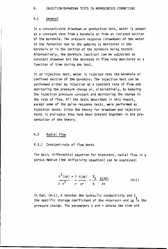
4.1 General

In a constant-rate drawdown or production test, water is pumpedat a constant rate from a borehole or from an isolated section'of the borehole. The pressure response (drawdown) of the waterin the formation due to the pumping is monitored in theborehole or in the section of the borehole being tested.Alternatively, the borehole (section) can be subjected toconstant drawdown and the decrease in flow rate monitored as afunction of time during the test.

In an injection test, water is injected into the borehole orconfined section of the borehole. The injection test can beperformed either by injection at a constant rate of flow andmonitoring the pressure change or, alternatively, by keepingthe injection pressure constant and monitoring the change inthe rate of flow. All the tests described in this report,except some of the pulse response tests, were performed asinjection tests. Since the theory for drawdown and injectiontests is analogous they have been treated together in the pre-sentation of the theory.

4.2 Radial flow

4.2.1 Constant-rate of flow tests

The basic differential equation for transient, radial flow in aporous medium (the diffusivity equation) can be expressed:

(4-Dar K 3t

In Eqn. (4-1), K denotes the hydraulic conductivity and Sthe specific storage coefficient of the reservoir and Ap is thepressure change. The parameters t and r denote the time and

radial distance, respectively. The (line-source) solution tothis equation was presented by Theis (1935). Eqn. (4-1) assumesthat there are no effects of skin and borehole storage duringthe test . When such effects influence the tes t , the equationmust be modified accordingly.

Skin effects

The change in head, H, or pressure change at the active bore-hole, including the skin ef fect , for a constant rate-of-f lowdrawdown test can be expressed in analogy with Earlougher(1977) as:

•-[2nKL L

u u J

In Eqn. (4-2), H represents the difference between the initial,static piezometric pressure, p., and the actual pressureduring the drawdown period, p , in the active borehole

W T

(section). The other symbols are defined in the l i s t ofsymbols. The dimensionless change in pressure or head, p isgenerally a function of the dimensionless test time, t andthe dimensionless radial distance from the borehole, r Thedimensionless pressure or head change for drawdown tests isdefined according to Earlougher (1977) as:

0 - Isll* - - ^L ( ) /pq (4-3)D " 0 ' Q

where H is the head change and p -p the pressurei Kwf y

change. For injection tests the pressure change is defined as

p -;-p.. The dimensionless time is defined as:wf Ki

(4-4!

The dimensionless distance from the active borehole is definedas

rD . I (4-5)

where r is the radial distance from the active borehole andr the borehole radius- At the active borehole r = r sow w

Basically, two different (exact) solutions of the p ( t - l -function exist. The exponent-integral solution (also called theline-source or Theis solution) assumes that the radius of theactive borehole is infinitesimally small (r - - > „ ) , (see Fig4.2.1). This solution is normally used to analyse interferencetests whenever r is large. The other solution, called thefinite-radius borehole solution or the PDCI solution, assumesthat the active borehole has a f in i te radius. At the activeborehole (section) this solution was presented by van Everding-en and Hurst (1949) (see Fig 4.2.1). I f t > 100 the exponen-t ia l integral solution for the active borehole (in the absenceof skin) may be approximated by the following logarithmicexpression (Earlougher 1977):

PD = 1.151 (log tQ + 0.351) (4-6)

However, when t >5 the difference between the exponentialintegral solution and the logarithmic approximation is only 2%. In high-permeability formations the condition of t_>100 atthe active borehole is normally reached only after a few minu-tes of testing. However, in low-permeability formations, tmay be less than 100 for a substantial part of the t rs t . Thefinite-radius borehole solution (PDCI), the exponential integ-ral solution and the logarithmic approximation of the lattersolution are presented in Fig. 4.2.1. As may be seen from this

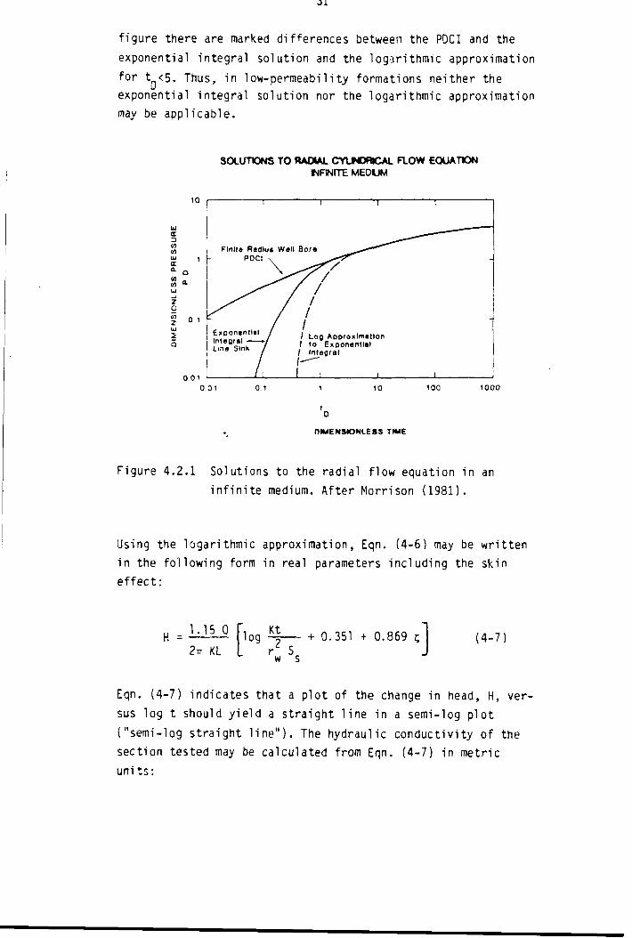
figure there are marked differences between the POCI and theexponential integral solution and the logarithmic approximationfor t <5. Thus, in low-permeability formations neither theexponential integral solution nor the logarithmic approximationmay be applicable.

10

Ui<rDmmiuEa.

zg»i

zUJ

5a

o 1 -

0 01

SOLUTIONS TO RADIAL CYUNDRICAL R O W EQUATIONINFINITE MEDUM

Finns Radius Well BorePOCI

/ Log ApproximationI to Exponential/ Integral

0 Ot 0.1 10 100 tooo

OlMENStOWLEBS TIME

Figure 4.2.1 Solutions to the radial flow equation in an

in f in i te medium. After Morrison (1981).

Using the logarithmic approximation, Eqn. (4-6) may be writtenin the following form in real parameters including the skinef fect :

2TT KL

log Kt + 0.351 + 0.869 (4-71

Eqn. (4-7) indicates that a plot of the change in head, H, ver-sus log t should yield a straight l ine in a semi-log plot("semi-log straight l i ne " ) . The hydraulic conductivity of thesection tested may be calculated from Eqn. (4-7) in metricunits:

AH(4.8)

In Eqn. (4-8), H represents the change in head during a loga-

rithmic time cycle. The skin factor is determined from Eqn.

(4-7):

2.13

w

(4-9)

H. . represents the change in head at t = 1 minute. Theeffective radius of the borehole (section), r can thenbe calculated from Eqn. (3-2). The additional head change,H , due to the skin effect may be expressed from Eqn. (4-2 )as follows:

(4-10)

The radius of influence, r., at specific times during thetest can for practical situations be estimated from the logarithmic approximation of p in Eqn. (4-6) according to Ear-lougher (1977), in metric units:

r s ^ — ( 4 . u ;Ss

Using the f ini te borehole radius solution of p Eqn. (4-2)may be used for type-curve matching. A type-curve may be const-ructed with p as a function of t_e by using the effec-tive borehole radius instead of the nominal rc'diu*. The draw-down or injection f ield data are plotted with log H as a func-tion of log t . The hydraulic conductivity can be obtained fromthe pressure (or head) match from Eqn. (4-12) in metric units:

Hm LU-12)

H is the change in head at the matchpoint on the data curvecorresponding to the value of (p_) on the type curve. The

u ineffective borehole radius, r , can be obtained from the

w f irtime match by the definition of the product t e * fromEqns. (4-4) and (3-2). The effective radius is given in metricunits by the following expression:

(4-13!

2CIn Eqn. (4-13), t and (L,e ) denote the time values

m Dmon the data curve and type curve respectively. The skin factormay be calculated from the estimate of r using Eqn. •(3-2). W

Borehole storage and skin effects

The theoretical pressure behaviour at the active borehole whenboth skin and borehole storage effects occur was presented byAgarwal et al (1970) in the form of type curves. The solutioncan be represented by Eqn. (4-3) but p is now a function ofboth t and C , i .e . p ( t ,C ). The dimensionlessborehole storage coeff ic ient, C is defined by Eqn. (3-7).

The type-curve solution is based on a constant rate of flowdrawdown (injection) test in a borehole of f i n i t e radias. Aninf initesimally thin skin-zone surrounds the borehole which islocated in a formation of i n f i n i te extent. The type curves areplotted with p ( t . ,C ) as a function of t for d i f fe -rent values of C with the skin factor as a parameter (seeFig. 4.2.2). The curves marked with C =0 represent the f i n i t eborehole radius solution of p for dif ferent skin factors butno borehole storage effect.

10* 10'

OMCNSMNLC» TIMC I .

Figure 4.2.2 Type-curves for borehole storage and skin

effects.

After Agarwal et al (1970).

As can be seen in Fig 4.2.2, the type curves are i n i t i a l l ystraight lines of unit slope in a log-log graph. During th isperiod, which is dominated by borehole storage ef fects, v i r -tual ly no water is derived from the formation, i t comes fromthe borehole (section) i t se l f . This period may be representedby an i n f i n i t e l y large skin factor. The pressure change duringthe borehole storage dominated period may be approximated by(Agarwal et al 1970):

P - ^D " C D

(4-14)

Eqn. (4-14) shows that the pressure change is directly propor-tional to the test duration. During this period, no informationabout the hydraulic properties of the formation can be obtai-ned. However, the borehole storage coefficient can be calcula-ted from the straight line of unit slope as follows (Earlougher1977):

Q tC = (4-15)

H1

In Eqn. (4-15) t and H are the time and head change at anarb i t ra r i l y chosen point on the log-log straight l ine of unitslope. The value of C, calculated from Eqn. (4-15) should beapproximately the same as the one determined from boreholecompletion data according -to Eqn. (3-4) or (3-5).

After a t ransi t ion period the borehole storage type curves mer-ge with the curves marked C = 0. At this time the borehc^estorage effects have ceased. The intersection between the cur-ves represents approximately the time for the star t of radialflow in the system and the beginning of the semi-log straightl i ne . To obtain a unique match with these type curves, theC -value should be known because of the similar shape of thetype curves. I f C is known, or can be estimated, the hydrau-l i c conductivity may be calculated from the pressure (or head)

match using Eqn. (4-12). The skin factor may be estimated as aparameter value. I f C is not known, a unique match is impos-sible. In this case the type curves may only be used as a diag-nostic tool and to estimate the start of the semi-log straightl ine (Ramey 1982).

Gringarten et al (1979) presented a modified form of the typecurves for borehole storage and skin ef fects. The type curvesare based on the same a:sumptions as the Agarwal et al (1970)

solution. The type curves are presented as p (t_,C_) ver-2s D u D

sus t /c with the product C-e as a curve parameter(see Fig. 4.2.3). The l imi ts of the di f ferent flow regimes andapproximate ranges of various borehole conditions (damaged,fractured) are indicated on the type curves. These curvesshould better represent fractured boreholes with borehole sto-rage effects (low values of C e ' ) . Fractured boreholes arerepresented by the inf in i te-conduct iv i ty solution (see Chapter7).

«P*O0XIH*T( ENDOf UNIT SLOWLOG-LOG K)STRAIGHT UHt

Figure 4.2.3 Modified type-curve for borehole storage and skineffects. After Gringarten et al (1979).

The type curves may be used to calculate the hydraulic conduc-t i v i t y from the pressure (or head) match from Eqn. (4-12). Fromthe time match, the borehole storage coeff ic ient may becalculated using the following expression in metric uni ts:

C =2* KL (4-16)

I f C is known, the skin factor may be determined from thedef in i t ion of tQ/C and the parameter value (CDe ' ) m

as follows in metric units:

; = 1.15 logv rc S i

SL5rZv rc S

SL-5L C p g

(4-17)

When the effects of borehole storage have ceased to influence

the pressure behaviour and radial flow has started in the

formation, analysis can be made on a semi-log p lot , provided

that the logarithmic approximation of p in Eqn. (4-6) is

va l id . The head change, H, is plotted as a function of the testtime, t , on the data curve. For drawdown and inject ion tests,the beginning of the semi-log straight l ine is given by thefollowing condition (Earlougher 1977):

t > (60+3.5;)C (4-18]

After this time the hydraulic conductivity and skin factor mav

be calculated from Eqns. (4-8) and (4-9) respectively.

4.2.2 Constant-pressure tests

When a borehole (section) is tested at constant pressure, noborehole storage effects occur since the down-the-hole pressuredoes not change during the test . However, during the subsequentbuild-up ( f a l l - o f f ) test borehole storage effects may be impor-tant. The solution of the d i f fus iv i t y equation, regarding thedecline in flow rate with time, for the constant-pressure caseof radial flow was presented by van Everdingen and Hurst (1949)and Jacob and Lohman (1952). Uraiet and Raghavan (1980 a) i n -cluded the skin effect in this solut ion. They considered theskin region to be an annular region concentric with the boreho-le and with a hydraulic conductivity di f ferent (higher orlower) from the formation conductivity.

The reciprocal transient flew rate at the borehole (section)

during a constant-pressure test , with the skin effect taken

into account, may be expressed as follows in metric units:

Q ( t ) 2 * K L H Q L Q D ( t D )+ C (4-19)

H is the constant drawdown or injection head at the boreholeo(section). The dimensionless flow rate function Q (t.)represents the theoretical solution of Q as a function ofdimensionless time, t defined by Eqn. (4-4). The effective

38

borehole radius concept for constant rate of flow tests also

applies to the constant-pressure case (Uraiet and Raghavan

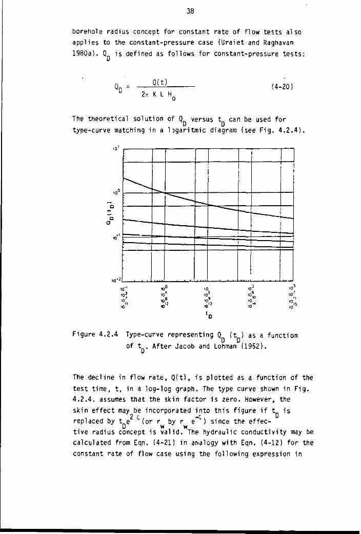
1980a). Q is defined as follows for constant-pressure tests:

Q(t)2w K L H,

(4-20)

The theoretical solution of Q versus t can be used for

type-curve matching in a l^garitmic diagram (see Fig. 4.2.4)

10 '

Figure 4.2.4 Type-curve representing Q ( t ) as a function

of t After Jacob and Lohman (1952).

The decline in flow rate, Q( t ) , is plotted as a function of the

test time, t , in a log-log graph. The type curve shown in Fig.

4.2.4. assumes that the skin factor is zero. However, the

skin effect may be incorporated into this figure i f t . isOr _r D

replaced by t e (or r by r e ) since the effec-D w w

tive radius concept is valid. The hydraulic conductivity may becalculated from Eqn. (4-21) in analogy with Eqn. (4-12) for theconstant rate of flow case using the following expression in

39

metric un i ts :

0.159 Q(t)K = m (4-21)

H L Q r,(tn)o u LJ m

Q(t) and Q ( t ) are the flow rates at the matchpointon the data curve and type curve respectively. The effectiveborehole radius, r and skin factor can be determined

wffrom Eqn. (4-13) and Eqn. (3-2) respectively. As may be seen inFig 4.2.4, the rate of flow declines rapidly at early times( t < 1000). Then the type cu>*ve becomes very f l a t . Thus,since type-curve matching requires the type curve to be of cha-racter is t ic shape to obtain a unique match, this method is onlysuitable at early times ( t <_ 1000).

The dimensionless flow rate Q ( t ) may be approximated by1/p when t_ > 1000. I f the logarithms, approximation ofp in Eqn. (4-6) is used, the reciprocal flow rate can, inanalogy with Eqn. (4-7), be expressed in metric units (Uraietand Raghavan 1980a) as:

1/Q(t) = L2JL- [log -£— + 0.351 + 0.869K L H r S

O L w S

(4-22)

Eqn. (4-22) implies that a semi-log graph of 1/Q(t) versus log

t should y ie ld a straight l i ne . The hydraulic conductivity maybe calculated from the slope of the straight l ine in metricunits:

0.183K = (4-23)

A(l/Q(t)) is the change in flow rate during a logarithmic time

cycle. Eqn. (4-23) only provides a rel iable value of the

hydraulic conductivity i f t > 1000. In low-permeability

formations t may be less than 1000. In such cases, the value

of K calculated from Eqn. (4-23) must be corrected according to

40

a procedure described by Uraiet and Raghavan (1980a). Providedthat the logarithmic approximation is va l id , the skin factormay be derived from Eqns. (4-22) and (4-23) and is giv?n inmetric units by:

KI / Q ( t ) , •t a 1.15 | Ulm - log - 7 — - z. 13 | (4-24)

(VQ(t))

1/Q(t) . is obtained by extrapolating the straight l ineto 1 minute. Eqn. (4-24) is similar to Eqn. (4-9) for the cons-tant-rate case. The skin factor for the constant-pressure caseis a measure of the increase or reduction in flow rate due tothe skin-zone. This may be expressed as follows (Uraiet andRaghavan 1980a):

(4-25)

4.3 Spherical flow

4.3.1 Constant-rate tests

Particularly i f the formation (or part of i t ) is very thick inrelation to the length of the section of borehole tested, aspherical flow regime may occur during the test . The basic par-t i a l d i f ferent ia l equation for transient, spherical flow in aporous medium may, with spherical coordinates, be expressed as:

(4-26)

This equation is very similar to the d i f fus iv i t y equation for

transient, radial flow, given by Eqn. (4-1). The head (or pres-

sure) change for spherical flow geometry may, for the

constant-rate case, be expressed using Eqn. (4-26) in metric

units:

41

p - "H = wf

pg 4n K r(4-27)

ws

H represents the difference between the i n i t i a l stat ic pressu-

re, P., and the pressure, p , , at a certain time, t , ini w T

the borehole (section) and r is the pseudo-sphericalborehole radius (Brigham et at 1980). The parameters p tand r denote dimensionless pressure change, time and distan-ce from the active borehole respectively. The parameter p isdefined as follows for spherical flow:

Pn =K r w s H

(4-28)

The definitions of t and r are the same as for radialflow, given by Eqns. (4-4) and (4-5) respectively, except thutthey are based on the radius for spherical flow, r , in

wsthis case (instead of r ).

w

The solution of the function p (t , r ) for sphericalflow is presented in a paper by Onyekonwu and Home (1983). Atthe active borehole (r = 1) this solution may be expressed:

1 - (4-29)

In Eqn. (4-29) erfc is the complementary error function. Forlong durations this equation may be approximated as

PD = 1 - e (4-30)

and for short durations, it may be approximated as

42

P s 2 W — H (4-31)" i t

Eqn. (4-31) assumes that no borehole storage and skin effectsoccur. ThuSj the practical use of the short-term solution isl imited (Onyekonwu and Home, 1983). I f borehole storage andskin effects occur, the test data should be analysed using amethod presented by Brigham et al (1980). The long-term datamay be analysed by plott ing the head change, H, versus thereciprocal square root of time, l / v T , as indicated by Eqn.(4-30). The data points should fa l l on a straight l ine in alinear graph. The hydraulic conductivity may be calculated fromthe slope of this l ine by inserting Eqn. (4-30) into Eqn.(4-27) in accordance with the following equation:

2/3

2 )

V 4 * 3 / 2 • m /K = | 2 ] (4-32)

4 * 3 / 2 • m

where m is the slope of the straight l i ne .

The pseudo-spherical (effective) borehole radius is dependenton many factors, such as borehole conditions, type of wellcompletions, etc. (Brigham et al 1980). According to Culham(1974), the effective borehole radius, r , for sphericalflow can be expressed:

r = (4.33;ws 2 ln(L/rw )

L is the length of the section open to flow and r is thew

actual borehole radius. Eqn. (4-33) is derived for steady-stateconditions but may also be used under conditions that only app-roach the steady state (Culham 1974).

43


The dimen sionless flow rate Q for spherical flow conditionsis defined for constant-pressure tests by Chatas (1966) similarto Eqn. (4-28) for constant flow-rate tests:

0 Q U) (4-34)C 4 * K r H

WS 0

Neglecting the skin ef fect , the change in flow-rate with time,

Q(t) , at the borehole (section) during a constant-pressure test

under spherical flow conditions may be expressed using Eqn.

(4-34) in metric units:

Q(t) = 4n K r H Qn(tn) (4-351

H is the constant drawdown or inject ion head at the ac-t ive borehole (section) and r is the effective boreholeradius for spherical flow conditions. The dimensionless time,t is defined by Eqn. (4-4), based on the effective radius,r , for spherical flow. The theoretical solution of thefunction Q (t_) for a constant-pressure test with spheri-cal flow conditions was presented by Chatas (1966):

(4-36)

Eqn. (4-36) indicates that a plot of the flow rate Q ( t ) versus

1/vT should y ie ld a straight l ine in a l inear graph. The

(average) spherical hydraulic conductivity may be calculated

from the slope of this l ine by combining Eqn. (4-36) and (4-34)

as follows:

44

K -_ E (4-37)V A 1/2 u c 1/2 /

ws o s

where m is the slope of the straight l ine.

4.4 Steady-state injection tests

4.4.1 General

The constant-head injection test has been widely used to esti-mate the hydraulic conductivity in geotechnical and groundwaterproblems. In real i ty, the flow domain in all groundwater tes-ting is of f in i te extent. A steady state implies that thegroundwater flow is constant in magnitude and direction at al lpoints in the reservoir and does not change with time. A truesteady-state situation very seldom occurs in practice. At best,a quasi-steady-state situation may be achieved during a limitedperiod of time. However, methods of analysis based on assumedsteady-state conditions are often used. This is due to theirmathematical simplicity and also to the fact that they givefair ly good agreement with corresponding methods of transientanalysis.

4.4.2 Theory and analysis

Under steady-state conditions the right hand side of Eqn (4-1)wil l be zero as no change in head occurs. The steady-statesolution for an injection (or drawndown) test in a confinedsection of an active borehole may be expressed by:

H - h = —9 l f , ( r / r ) (4-38)0 2it K L W

45

where H = the applied head change in the active borehole

section

h = the head change at distance r

r = radial distance from the active borehole section

In Eqn. (4-38) the flow from (or to) the active borehole isassumed to be two-dimensional ( rad ia l ) . At greater distancesfrom the active borehole, part icularly when the length of thetest section is short, i t may be assumed that the flow changesto three-dimensional (spherical) flow. This implies that thehead change, h, at a distance r from the active borehole (wherespherical flow is assumed) may be calculated, according to Moye(1967), using the expression:

h -- 9 (4-39)4TT K r

If r is the distance within which the flow is assumed to be

radial and beyond which the flow is spherical, Eqn. (4-38) and

(4-39) may be combined:

H = 2 In (r/r) + 2 (4.40;0 2T. K L W 4TT K r

According to Moye (1967) it may be assumed that r = L/2 which

implies that

L K L L 2,

From this expression the average hydraulic conductivity of the

test section may be calculated using:

r 1 • In (L/2 r ) ]L_ 1 (4-42)L L 2it J

Ho

46

The expression within brackets is generally called Moye's cons-tant. Eqn. (4-42) is normally used to calculate the hydraulicconductivity from steady-state, constant-head injection testsin crystalline rock in Sweden.

4.4.3 Applications

Doe and Remer (1982) presented a theoretical comparison ofhydraulic conductivity calculated from steady-state andtransient tests in non-porous fractured rock. They found thatthe hydraulic conductivity is generally overestimated bysteady-state methods. They concluded that the error incalculating the hydraulic conductivity by steady-state methodsis generally less than one order of magnitude and normallywithin a factor of about two or three of transient methods.

Andersson and Persson (1985) made a comparison of steady-stateand transient analyses using field data from a large number ofsingle-hole tests in crystalline rock in Sweden. They foundthat the mean value of hydraulic conductivity (423 tests) fromsteady-state analysis (t=15 minutes) was about 2.7 times grea-ter than the corresponding mean value from transient test ana-lysis (t = 2 hours). Steady-state analysis occasionally resultsin 10-20 times higher values than transient analysis. Theseconclusions are in good agreement with the results obtained byDoe and Remer (1982).

47

5. BUILD-UP/FALL-OFF TESTS IN HOMOGENEOUS FORMATIONS

5.1 General

When a production or injection test is stopped the pressurechange caused by the preceding production or injection phaserecovers and trie actual pressure approaches the stat ic pressurein the borehole (section). Theoretically, the recovery periodis treated as i f the production (or injection) goes oncontinuously and, at the during period, an image boreholeinjects into (or produces from the active borehole at the samerate, i .e . the net flow rate is zero. This implies that thedrawdown/injection period and the bu i ld -up/ fa l l -o f f periods areinterrelated and that the pressure response during the recoveryperiod is dependent on the duration of the precedingdrawdown/injection period (see Fig. 5.1.1). This is true forboth constant-flow and constant-pressure tests.

In general, the drawdown (injection) type curves cannot be useddirectly to analyse recovery data unless the drawdown orinjection period is much longer than the longest recovery timeto be analysed. In addit ion, the correct radial-f low semi-logstraight l ine wi l l not develop during the recovery test i f thedrawdown or injection period is too short, no matter how longthe recovery period is (Raghavan 1980). The theories forbuild-up and f a l l - o f f tests are analogous.

5.2 Radial flow

5.2.1 Tests after a constant-rate-of-flow period

The build-up (or f a l l - o f f ) data obtained during the recovery

period may be represented in two ways, either as the residual

drawdown (p -p ) or as the actual build-up,p -p , as defined in Fig. 5.1.1. The residual drawdownws Kp *

is generally used for semi-log analysis (the Horner method andthe MDH method) whereas the actual pressure change duringbuild-up is more suited for type-curve analysis in a log-log

48

graph.

PRESSURE

TIME

Fig. 5.1.1. Schematic representation of pressure build-up

behaviour following a constant rate of drawdown

period, t . After Agarwal (1980).

Horner method

The basic dimensionless build-up eouation, p t in terms ofthe residual drawdown can be expressed according to theprinciple of superposition (Earlougher 1977):

JDs0 pg

( 5 " n

The f i r s t term in Eqn. (5-1) represents the dimensionlesspressure change during the entire drawdown period and i t sextent during the recovery period (see Fig. 5.1.1). During therecovery period the current time is denoted dt . The drawdowncurve is defined by Eqn. (4-3). The second term in Eqn. (5-1)represents the pressure build-up curve during the recoveryperiod, superposed on the drawdown curve. I f the semi-log

49

approximation of P in Eqn. (4-6) is applied, then Eqn. (5-1for the residual drawdown during a build-up test may beexpressed as

0.183 Q • t + dt

This is the well-known Horner equation in metric units. Eqn.(5-2) indicates that i f the residual drawdown is plotted versusthe expression ( t + dt)/dt, or i ts reciprocal value, in a

psemilog graph, the data points should fal l on a straight l ine.The equation takes into account the production time since t

pis included. However, the theoretical slope of the straightline for radial flow wil l only exist i f the production time issufficiently long (Raghavan 1980). For a homogeneous formationwithout borehole storage and skin effects, the drawdown orinjection period and also the recovery period must be suff i -ciently long for the logarithmic approximation of the two termson the right-hand side of Eqn. (5-1) to be valid. Thiscondition may not always be ful l f i l led in low-permeabilityformations (see Section 4.2.1).

If the build-up response is influenced by borehole storage andskin effects, the production time required for the correctsemilog straight line to develop is given by the following con-dition (Raghavan 1980):

pD 2n KL t= E_ > 200 (5-3!

D C pg

In Eqn. (5-3) t and C represent the dimensioniess

production or injection time and borehole storage coefficient

respectively. The condition in Eqn. (5-3), which is valid for

C. ^>100, may be reduced to t n/Cn >50 if anD ~ DL) U —

error of 10 % is accepted in the K value. In addition, the

recovery period must also be sufficiently long. The time, dt,

for the straight line to develop during recovery is given by

(Raghavan 1980):

50

d t n 2n KL dt_J> = - 60 + 3.5 S (5-4)CD C Pg

The hydraulic conductivity may be calculated from the slope ofthe straight line in the Horner graph from Eqns. (4-8) and(5-2), provided the conditions in Eqns. (5-3) and (5-4) areful l f i l led. The skin factor is determined from the followingexpression for a build-up test (Earlougher 1977):

u J " " - - ^ - log (4-) - 2.»1 (5_5)

In Eqn. (5-5), p is the pressure at the stop of the draw-down/injection period and p is the pressure after

1 mm1 minute of recovery. This pressure must be taken from theextrapolated straight l ine. For a pressure fa l l -o f f test, thepressure difference in the f i rs t term of Eqn. (5-5) should bereplaced by P -p

p 1 minThe Horner method also permits determination of the in i t ia lstatic pressure, p., in the section tested, provided thepreceding drawdown or injection period is sufficiently long.This is performed by extrapolating the straight line to aninf ini te recovery time, i.e. when ( t + dt)/dt = 1 on thetime scale (Earlougher 1977). The extrapolated pressure valueis generally denoted p . I f the formation being tested isinf initely large, the extrapolated pressure wil l be identicalto the static pressure. However, i f the drawdown or injectiontime is short, the build-up or fa l l -of f curve wil l level offtowards the static pressure by the end of the test. If effectsof depletion occur, e.g. in f ini te formations, during thedrawdown test the average pressure in the formation wil lgenerally be lower than the extrapolated pressure.

As already mentioned, the Horner method may not be applicablein very low-permeability formations. The theory of this method

is based on the assumption that the radius of the borehole is

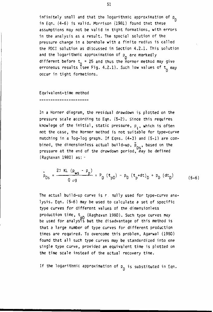
51

i n f i n i t e l y small and that the logarithmic approximation of pin Eqn. (4-6) is val id. Morrison (1981) found that theseassumptions may not be val id in t ight formations, with errorsin the analysis as a resul t . The special solution of thepressure change in a borehole with a f i n i t e radius is calledthe PDCI solution as discussed in Section 4 .2 .1 . This solutionand the logarithmic approximation of p are markedlydif ferent before t = 25 and thus the Horner method may giveerroneous results (see Fig. 4.2.1). Such low values of t mayoccur in t igh t formations.

Equivalent-time method

In a Horner diagram, the residual drawdown is plotted on thepressure scale according to Eqn. (5-2). Since this requiresknowlege of the i n i t i a l , stat ic pressure, p., which is oftennot the case, the Horner method is not suitable for type-curvematching in a log-log graph. I f Eqns. (4-3) and (5-1) are com-bined, the dimensioniess actual build-up, p , based on thepressure at the end of the drawdown period, may be defined(Raghavan 1980) as: -

2n KL (p - p )

TT = PD ( V " P° ( V d t ) D + PD < d V (5-6!v pg

The actual build-up curve is r -nally used for type-curve analys is . Eqn. (5-6) may be used to calculate a set of specifictype curves for dif ferent values of the dimensionlessproduction time, t (Raghavan 1980). Such type curves maybe used for analysis but the disadvantage of this method isthat a large number of type curves for d i f ferent productiontimes are required. To overcome this problem, Agarwal (1980)found that a l l such type curves may be standardized into onesingle type curve, provided an equivalent time is plotted onthe time scale instead of the actual recovery time.

I f the logarithmic approximation of p is substituted in Eqn.

52

(5-6) the following expression is obtained (Agarwal 1980)

r t n x dtn 1log (-E2 ö) + 0.351

L d t n + t n _ Jn n

= 1.15 log (-E2 ö) + 0.351 (5-7)L J

Eqn. (5-7) is analogous to the drawdown Eqn. (4-6). Agarwal(1980) demonstrated that replotting a set of type curves fordifferent production times with the time expression in Eqn.(5-7) on the time scale instead of the actual recovery time,dt, resulted in a single curve identical to the drawdown typecurve for al l values of the production time. Thus, the build-updata may be plotted as a function of the expression (t x

pdt ) / ( t + dt) in a log-log graph and matched with thecorresponding drawdown type curve for all production times. Theequivalent time, dt , is defined as

t x dtdt = -E (5-8)

e dt + t

The equivalent-time method may also be applied to other testconditions and other type curve solutions, such as boreholestorage and skin effects, fractured formations, multiple-ratetesting as well as to conventional semi-log analysis. I f skindamage affects the build-up data a skin factor must be added tothe right-hand side of Eqn. (5-7). I f both borehole storage andskin effects occur, the corresponding drawdown type curve mays t i l l be used and also semi-log analysis i f the (dimensionless)production time is sufficiently long and the conditions statedby Eqns. (5-3) and (5-4) are satisfied.

With a skin factor included in Eqn. (5-7), this may in analogywith Eqn. (4-7), be written in the following form:

0.183 Q T t x dtH = (p - P w"n = I l o a (~P ] + 1oq ( *] + ° ' 8 6 9[ t x dt

dt + tws r p ' K,

Eqn. (5-9) indicates that if the absolute build-up pressure,p , or the actual build-up pressure difference is plottedversus dt in a semi-log graph, a straight line should

53

develop i f the conditions in Eqns. (5-3) and (5-4) aresat is f ied. This graph is similar to a Horner graph but has theadvantage that the build-up data may be plotted on a real timescale both versus dt and d t , which permits direct comparisonof the curves so that the effect of the production time isv is ib le . The hydraulic conductivity is calculated from theslope of the straight l ine using Eqn. (4-8). The skin factormay be determined from Eqn. (4-9).

As in the Horner graph, the stat ic pressure, p., in thetested interval can be determined in the semi-log graph byextrapolating the straight l ine to i n f i n i t e recovery time. Thistime corresponds in this case to a recovery time in which dt

e= t as may be seen from Eqn. (5-8).

5.2.2 Tests after a constant-pressure period

The pressure build-up (or f a l l - o f f ) behaviour after a period ofconstant-pressure production (or injection) is similar to theconstant-rate case. The dimensionless residual drawdown duringrecovery for the constant-pressure case is defined by Uraietand Raghavan (1980 b):

2n KL (p. - Pws) 2JI KL H

5-10)

This equation is identical to Eqn. (4-3) for the constant-ratecase except that the flow rate, Q, is replaced by Q , whichis the instantaneous flow rate at the end of the drawdown/inject ion period.

54

Homer method

I f the residual pressure change during the recovery periodaf ter production or i n jec t i on at constant pressure i s p lo t tedin a Horner graph, as described in the previous sect ion, thedata points w i l l again f a l l on a s t ra igh t l i ne provided theproduction (or injection) period is sufficiently long. I f thereare no borehole storage or skin effects, the straight line withcorrect slope wil l develop for dimensionless recovery timesdt >40 i f the dimensionless production (or injection) timet D>1000. When t n is less than 1000, no extensivestraight-line portion can be identified in the Horner graph.For long recovery times the slope of the straight linedecreases and wil l eventually reach zero (horizontal line) whenthe recovery pressure reaches the static pressure in thesection tested (Uraiet and Raghavan 1980 b).

I f the two conditions mentioned above are satisfied, the hyd-raulic conductivity may be calculated in analogy with Eqn.(4-8) as follows:

0.183 0nK = E (5-11)

L AH

In Eqn. (5-11), 0 is the rate of flow at the end of thep

drawdown/injection period and H is the change in residualhead per logarithmic time cycle. I f the dimensionless flow timeis less than 1000, the maximum slope of the build-up (orfal lof f) curve should be used to estimate the hydraulicconductivity. I f borehole storage and skin effects are present,the recovery time and production time required for the straightline to develop are given by the conditions in Eqns. (5-4) and(5-3) respectively. The hydraulic conductivity is calculatedfrom Eqn. (5-11) and the skin factor for a build-up test fromEqn. (4-9) as for the constant-rate-of-flow case (Uraiet andRaghavan 1980 b). The static pressure in the section tested isestimated by extrapolating the straight line in the Horner

55

graph, as described in the previous section, unless the stat ic

pressure is alredy reached during the test .

Equivalent-time method

I f the build-up (or f a l l - o f f ) data are plotted on an equivalenttime scale, as described in the previous section, type curvematching with drawdown type curves may be performed in a logloggraph. This means that the type curves including boreholestorage and skin effect as presented by Agarwal et al (1970)and Gringarten et al (1979) may be used to analyse build-up andfa l l - o f f tests after a period of constant-pressure productionor injection (see Section 4.2.1). In this case the rate of flowat the end of the drawdown/injection period should be used tocalculate the hydraulic conductivity from Eqn. (4-12). Theanalysis may also be performed on a semi-log graph as describedin the previous section. The hydraulic conductivity and skinfactor may be determined from Eqns. (5-11) and (4-9)respectively. The method also permits a determination of thestatic pressure, p., of the section tested.

5.3 Spherical flow

5.3.1 Tests after a constant rate of flow period

The basic borehole pressure build-up (and f a l l - o f f ) equationafter a constant flow rate test may be expressed as (Culham1974):

H ' =oVTs

4n3/23 / Z

(5-12)

Eqn. (5-12) indicates that a plot of the residual change in

head, H', in the borehole versus the time expression

( l / \ d t - l / \ t +dt) in a linear graph should result in a

56

straight l ine with slope, m. From this slope the hydraulic con-

ductivity may be calculated as:

2/3

K = S- (5-13)

V 4 , 3 / 2 - m I

Eqn. (5-13) is identical to Eqn. (4-32) for constante-ratedrawdown/injection tests. In Eqn. (5-13) the slope, m, isexpressed in metres of water per reciprocal square-root of thetime in seconds. By comparing Eqn. (5-12) with Eqn. (4-7) forradial flow i t can be seen that no geometrical factor ispresent in the build-up equation for spherical flow. For radialflow, the geometrical factor is the formation thickness or thelength of the section being tested. Thus, for spherical flow,the borehole conditions (perforation, open hole completion,etc.) do not influence the pressure build-up curve. Thepressure build-up is instead controlled by the formation somedistance from the borehole (Moran and Finklea 1962).

The hydraulic conductivity calculated from Eqn. (5-13) shouldbe regarded as an average value of the spherical volumeinfluenced by the test, including anisotropic properties. Asseen from Eqn. (5-13), the hydraulic conductivity is , forspherical flow conditions, independent of both the effectiveborehole radius and the length of the section tested. The skinfactor for spherical flow may be determined in analogy withCulham (1974):

x. - n K L m- 1.0 (5-14)

In Eqn. (5-14), p f is the pressure immediately before theend of the drawdown/injection period and p is the pressureat the recovery time dt . The pressure value, p., isobtained from the (extrapolated) straight line portion of the

buildup curve. The effective borehole radius, r forws

spherical flow should be used in Eqn. (5-14).

57

The i n i t i a l , stat ic pressure, p., or head in the sectiontested may also be determined from the build-up curve forspherical flow by extrapolating the straight l ine to i n f i n i t erecovery time as for radial flow. In this case, the i n f i n i t erecovery time corresponds to a zero value of the expression onthe time scale.

5.3.2 Tests after a constant-pressure period

According to Moran and Finklea (1962) the build-up Eqn. (5-12)after a period of constant flow may also be used for analysisof build-up (or f a l l - o f f ) tests after a constant-pressureperiod for long durations, when the applied pressure or headchange, H , has returned to within 10-20 % of. i t s (constant)value. This means that the hydraulic conductivity may becalculated from Eqn. (5-13) i f Q is replaced by Q and theskin factor determined from Eqn. (5-14^.

6. DUAL-POROSITY FORMATIONS

6.1 General

A dual-porosity formation is considered to be composed of twointeracting porous media regions with both primary andsecondary porosity. The primary porosity region is associatedwith the rock matrix whose hydraulic properties are generallycontrolled by depositional and l i th i f icat ion processes. Thesecondary porosity region consists of the fracture system whosehydraulic properties are generally the result of thermalstresses and tectonic processes. In general, the permeabilityof the matrix blocks is low and the fracture system exhibitshigh permeability and transmissivity. The storage capacity ofthe two regions depends on the (effective) porosity of eachregion.

Fig. 6.1.1 Schematic representation of a fractured medium, apurely fractured medium, a dual-porosity medium anda heterogeneous medium. After Mavor and Cinco-Ley(1979).

Dual-porosity formations may be classified into four differentcategories (Streltsova 1976) (see Fig. 6.1.1). The f i rs tcategory, a fractured medium, consists of a formation whoseprimary porosity region contains the majority of the storagecapacity while the secondary porosity region constitutes thewater transmitting capacity of the medium.

The second model, a purely fractured medium, represents amedium whose matrix permeability and matrix porosity are

59

negligible. Thus, both the storage and transmitting capacity ofthe medium are due entirely to the fracture network. Thiscategory is one limiting form of the behavior of f i r s tcategory.

The third group is a dual porosity medium, in which the storagecapacity of the primary and secondary regions of the medium areof the same order of magnitude, while the transmitting capacityis due to the fracture system.

The final category is a heterogeneous medium in which thefractures are f i l led with a material with a permeability thatis lower than that of the matrix.

6.2 Theoretical models of dual-porosity formations

The f i rs t category reservoir model in Fig. 6.1.1. is mostfrequently used in the petroleum industry to describe thepressure behaviour of porous naturally fractured reservoirs. Insuch theoretical models the storage capacity of the rock isassociated with the intergranular, primary or matrix porosity,while the transmitting capacity is attributed almost entirelyto the fracture system. The matrix (effective) porosity isgenerally assumed to be much higher than the fracture(effective) porosity. The category models in cases two andthree, described above, may thus be regarded as special casesof this theoretical model. Thus, in the following text thef i rs t three cases are grouped together.

In general, the dual-porosity formation is treated as acontinuum with the fractures extending throughout thereservoir. Serving as flow channels with high transmissivity,the fractures control the f luid pressure distribution in therock mass. When the pressure in the fractures is changed,pressure differentials across the matrix blocks are created,resulting in a time-dependent cross-flow between the fracturesand matrix blocks. This cross-flow is considered asone-dimensional. The high hydraulic diffusivity of thefractures result in a rapid pressure response along the

60

fractures, while the rock matrix exhibits a delayed response topressure changes occuring in surrounding fractures. Ultimately,the pressure in the fractures and matrix w i l l equi l ibrate,after which the formation acts as a uniform medium withcomposite.properties of both matrix and fracture system.

Several di f ferent model geometries have been described inl i terature to represent dual-porosity formations. The rockmatrix may either be divided into parallelepipedes by anorthogonal fracture network (the block model) or,al ternat ively, into layers by a set of horizontal fractures(the layer model). Other matrix geometries, such as spheres andcylinders, have also been considered. The result ing pressureresponse i s , however, similar for most of these matrixgeometries but the actual parameter values calculated for thesystem may vary according to the di f ferent assumed geometries(Najurieta 1980, Moench 1984).

Two di f ferent assumptions regarding the nature of the flow inthe matrix due to pressure changes at the fracture/matrixinterface have been applied in the theoretical models. F i r s t l y ,the matrix flow is assumed to be independent of spatialposition within the matrix element which implies apseudo-steadystate cross-flow in the matrix. This assumptionneglects the storage capacity of the rock matrix by allowing aninstantaneous pressure change throughout the matrix as soon aspressure changes occur in the fractures (Streltsova 1983).According to this assumption, the pressure response of such amedium has a characteristic S-shaped, f l a t transit ional curvewith an inf lect ion point in a logarithmic graph.

Secondly, other models assume that the cross-flow between therock matrix and fractures is transient and can be representedby a one-dimensional d i f fus iv i ty- type flow equation. Thisspatially-dependent flow takes into account not only the matrixpermeability but also the storage capacity of the matrix. Thisassumption leads to a di f ferent transit ional pressure response,both regarding the time of onset and shape of the curve. Thismodel has been adopted by Najurieta (1980), Serra et al (1983),Streltsova (1983) and others. Streltsova also made a c r i t i ca l

61

examination of the consequences of the two di f ferent assump-tions regarding the matrix cross-flow.Gringarten (1984) presented a review on theory and practice forreservoirs with "double-porosity" behaviour. He also presentedf ie ld data from naturally fractured reservoirs whose pressureresponse is similar to the response resulting from theassumption of pseudo-steady-state cross-flow in the matrix.Moench (1984) explained this behaviour as a result of fractureskin, a thin skin of low-permeability material, deposited onthe surfaces of the matrix blocks. The effect of this fractureskin in naturally fractured reservoirs would be to delay thecross-flow between the matrix blocks and the fractures. Thepressure response with fracture skin is similar to the onepredicted under the assumption of pseudo-steady-statecross-flow (without fracture skin). According to Moench (1984)fracture skin may occur as a result of mineral alterat ion ordeposition created by the flow of groundwater in the fractures.

The hydraulic conductivity, K ., of the fracture system in adual-porosity formation is assumed to be approximately equal tothe (bulk) hydraulic conductivity, K, of the rock mass sinceal l flow to (or from) the borehole (section) is considered totako place via the fracture system.

6.3 Theory and test interpretation

6.3.1 Constant-rate-of-flow tests

The theoretical pressure behaviour of the model presented bySerra et al (1983) and Streltsova (1983) is adopted in thisreport. In this model the formation is represented as anisotropic, dual-porosity reservoir of uniform thickness and ofin f in i te extent, bounded by impermeable layers above and below.The matrix is subdivided by a set of parallel horizontalfractures. I t is assumed that a l l production from (or inject ioninto) the borehole is via the fracture system and also thatvertical one-di mensiona1, transient cross-flow occurs in thematrix. The properties of both the matrix and fracture systemare assumed to be constant. An inf in i tesimal ly thin skin around

the borehole walls is considered but borehole storage and

fracture skin effects are neglected. The flow in the fractures

is assumed to occur only in the radial direction.

The general dif ferential equation for the groundwater flow in

the fracture system may be written in analogy with Streltsova

(1983) and Moench (1984):

1 3(AP ) S

• —3(AP ) _ S

s f a (Ap) , qra

Sr2 r 3r K 3t KL

In Eqn. (6-1) the parameters S and K are based on bulk

properties of the rock mass. The flow term, q , in Eqn. (6-1)

represents the transient cross-flow from the matrix blocks to

the fractures. At the matrix/fracture interface (z=0) the

cross-flow per unit area and unit time may be expressed

according to Streltsova (1983):

The corresponding differential equation for the pressure change

in the matrix, Ap , is expressed by Streltsova (1283):m

32 K 3 tm

lo-j)

General analytical solutions for the fracture pressure

distribution (Eqn. 6-1) and the matrix pressure distribution

(Eqn. 6-3) are presented in Laplace space by Streltsova (1983).

Serra et al (1983) also derived a similar analytical solution

for the same type of dual-porosity model, together with

approximate solutions for intermediate and long times. Both

typer, of solution assume transient flow in the matrix rock.

63

The general solution for the pressure drawdown (or inject ion)behaviour in the active borehole in dual-porosity formationsinvolves three dif ferent flow regimes. Flow regimes 1 and 3represent the early and late time responses respectively andare characterized by two parallel straight lines in a semi-loggraph. I f transient cross-flow is assumed the intermediate timeflow regime 2 is also characterized by a semi-log straightl ine , but the slope is approximately half that of flow regimes1 and 3. The ident i f icat ion of the di f ferent flow regimes isimportant when analysing f i e l d data from dual-porosity for-mations.

During flow regime 1 the pressure response is dominated by thecompressible fracture system. During this flow regime thematrix flow has not begun to influence the pressure response.Flow regime 1 constitutes one of the l imi t ing forms of tft?solution for dual-porosity formations. During flow regime 2 theflow in the matrix, whose response is delayed because of thelow matrix permeability, starts to influence the pressureresponse of the system. This wi l l result in a slower pressurechange than during flow regime 1. Flow regime 2 is alsocharacterized by an increase in the t o t a l , effective storage ofthe system due to the matrix storage becoming active.

As time progresses, the matrix blocks near the active boreholebecome depleted and the pressures in the matrix blocks andfractures equalize. The matrix flow support must then beprovided by matrix blocks ever further from the activeborehole. At a certain time this results in a delay between theflow transport in the fractures to the borehole and the releaseof f lu id by thr. distant matrix blocks. After this time thefractured formation behaves as an equivalent uniform mediumwith a transmissivity corresponding to the fracture system anda composite storage capacity that is the sum of the matrix andfracture storage capacities. This period corresponds to flowregime 3, which forms the second l imi t ing form cf the solutionfor the pressure response in dual-porosity formations.

The hydraulic conductivity of the fracture system (which is

assumed to equal the conductivity of the rock mass) and skin

64

factor can be determined from any of the three flow regimes, i fpresent, in a semi-log graph. From flow periods 1 and 3 thehydraulic conductivity, K, is calculated from the slope of thestraight l ine from Eqn. (4-8), whereas during flow period 2 theconductivity may be calculated from the same equation i f thefactor 0.183 is replaced by 0.183/2 since the slope of thestraight l ine is halved.

I f the specific storage, S of the fracture system isknown, the skin factor can be estimated from flow regime 1 (thef i r s t straight l ine) by Eqn. (4-9) i f S is replaced byS . . Accordingly, i f the total specific storage capacity ofthe formation, which is the sum of the specific storagecoefficients in the matrix and fracture system, the skin factormay be estimated from flow regime 3 (the second straight l ine)by the following expression for a drawdown test :

- log ( 6 " 4 )

I f borehole storage occurs, the pressure data during flowperiod 1 may be distorted and i f the test is short only theintermediate flow regime, 2, may be present (Mavor and Cinco-Ley 1979). To determine the significance of borehole storageeffects in dual-porosity formations, the borehole storage t>pecurves presented in Section 4.2.1 may be used for early times.


Raghavan and Ohaeri (1981) considered theory for constant-pressure tests in dual-porosity formations assuming both thepseudosteady-state and transient flow transfer between thematrix system and the fracture system. The model by Raghavanand Ohaeri (1981) is the same as the one described by Serra etal (1983) for constant-rate-of-flow tests (see Section 6.3.1).In this model i t is assumed that the fracture system can bereplaced by an equivalent set of horizontal fractures. As inthe constant-rate-of-flow case early, intermediate and late

65

flow periods may be ident i f ied for constant-pressure tests. I ftransient flow transfer is assumed between the fracture systemand the matrix, an i n i t i a l decline in the flow rate w i l l occur.During late times the system behaves as an equivalenthomogeneous formation in analogy with constant-rate-of-flowtests.

The analysis of constant-pressure tests in dual-porosityformations is analogous to constant flow rate tests. This meansthat the test may be analysed in a semi-log graph by plott ingthe reciprocal flow rate, 1/Q(t), versus the test time, t , asdescribed for homogeneous reservoirs in Section 4.2.2. Thehydraulic conductivity may be determined from either the early- or the late semi-log straight l ine using Eqn. (4-23). As forconstant-rate-of-flow tests the skin factor may be estimatedfrom the early straight l ine using Eqn. (4-24) i f S isreplaced by S . Al ternat ively, the skin factor may also bedetermined from the late straight l ine from the same equation

i f the sum S +S _ is known or can be estimated,sm sf

66

7. BOREHOLES INTERSECTED BY DISCRETE FRACTURES

7.1 General

When the region near the borehole is dominated by a discretefracture plane which intersects along the whole or part of theborehole, the early transient flow behaviour is modified compa-red to a homogeneous medium. This si tuat ion is part icular lyaccentuated when a borehole in a low-permeability formation isstimulated by hydraulic fractur ing. In crystal l ine rock, alinear flow type behaviour is sometimes also observed duringearly times of hydraulic tests, indicating flow to the sectiontested in naturally discrete fractures near the borehole.

A linear flow type response may also be caused by channeling

effects in irregular flow paths in the rock. Such flow paths

may have a very large hydraulic conductivity and play an

important role from a contaminant migration point of view

(Rasmuson and Neretnieks 1986).

7.2 Conceptual models

An analytical model for flow in fracture-dominated reservoirshas recently been presented by Karasaki et al (1985). Thismodel is based on a composite system with two concentricregions. The inner region contains a vert ical (or paral lel)fracture of f i n i t e length which intersects the borehole (sec-tion) tested. Water enters this fracture primarily from inter-sections with other fractures. The water then flows l inear lyinto (or out of) the borehole (see Fig. 7.2.1). The outerregion is considered as a porous medium in which only radialflow takes place. Thus, the conseptual model of this systemconsists of an inner zone with linear flow and certain hydrau-l i c properties and an outer zone with radial flow and separatehydraulic properties (see Fig. 7.2.2). No borehole storage orskin effects are considered in this model. Under favourableconditions the hydraulic parameters for each region may beestimated from type-curve matching using this model.

67

Flow Direction

Figure 7.2.1 Flow to a borehole intersected by a discretefracture. After Karasaki et al (1985).

K2, SS2

Radial flow region

Figure 7.2.2 Composite model of l inear-radial flow. After

Karasaki et al (1985).

68

A model for the pressure behaviour of boreholes intersected bya single (vert ical) fracture plane of l imited horizontal extentwas developed by Cinco-Ley et al (1978) and Cinco-Ley and Sama-niego (1981) (see Fig. 7.2.3). I t is assumed that water fromthe surrounding formation flows horizontally and perpendiculartowards the fracture plane which then acts as a flow channel tothe borehole. Both the fracture and the formation are treatedas porous media regions. The model suggested by Karasaki et al(1985) is a modification of this la t ter model. Only high-con-ductivi ty fractures are considered.

BOREHOLE

Figure 7.2.3 Borehole intersected by a vertical fracture withf i n i te conductivity. The groundwater reservoirhas impermeable upper and lower boundaries andthe horizontal extent is i n f i n i t e . AfterCinco-Ley et al (1978).

69

7.3 Theory and interpretation

7.3.1 Drawdown and injection tests

Constant-rate-of-flow tests

Cinco-Ley et al 11978) defined a number of dimensionlessparameters. The dimensionless pressure is defined according toEqn. (4-3), in Section 4.2.1. The dimensionless time, t ,generally defined by Eqn. (4-4), is in this case based on thefracture half-length, x •

(7-1)

The dimensionless fracture conductivity, F is defined:

K eFc D

= (7"2)CU K xf

In Eqn. (7-2), K and K denote the hydraulic conductivity ofthe fracture and formation respectively and e is the fracturewidth (aperture).

Figs. 7.3.1 and 7.3.2 show the pressure change during a cons-tant-rate-of-flow test in an active borehole intersected by asingle vertical fracture in semi-log and log-log representationrespectively. As the parameter F increases, the curvesapproaches the infinite-conductivity solution by Gringarten etal (1974). This solution is also included in the graphs. As canbe seen from Fig. 7.3.2 the curves form straight lines with aslope of 0.25 for short times in the log-log graph. For largevalues of F the curves approach a straight line with aslope of 0.5 (infinite-conductivity fractures). For long timesthe curves form straight lines in the semi-log graph.

7C

10" 10 '

Df

Figure 7.3,1 Type-curves with dimensionless pressure as afunction of dimensionless time in a semi-log plotfor an active borehole intersected by a verticalfracture. After Cinco-Ley et al (1978).

4.1 jiPRÖXIIfATÉ ISTAirn Of SEMILOS

10

Figure 7.3.2 The same type-curves as in Fig. 7.3.1 in log-log

representation. After Cinco-Ley et al (1978).

71

Generally, the transient pressure response for boreholesintersected by a single vertical fracture plane can be dividedinto four different flow periods (see Fig. 7.3.3). During veryearly times, there is a pressure response within the fracture,resulting in a flow which is essentially linear (see Fig. .7.3.3a). This linear fracture flow period is characterized by astraight line with a slope of 0.5 in a log-log graph. However,this flow period occurs too early to be of practical use in thetest analysis.

r -/Bo^( \ h o i e ; —

Fra

FKAC TU SE L i N E A R

1

ii

F i l l A T

1

i

i

\ c

I O N

' i '

L I N E A R

- \- 1 >

eturt

Fracture

F L i "

i ' 1 11 1 [ 1 i

! ! ! jli M I!

B I L

\

F

P S E U B O

! " !

• i ! : i

N E A ? e •„ ") W

\ ' /

ractur*

(d)» A O I A L F L O »

Figure 7.3.3 Flow regimes for an active borehole intersecteda, b, c, d by a vertical fracture with f in i te conductivity.

After Cinco-Ley and Samaniego (1981).

After a transition flow period, the bilinear flow period maydevelop (Fig. 7.3.3b). During this period, two flows occursimultaneously. One flow is linear, incompressible flow withinthe fracture and the other is a linear compressible flow in theformation. This flow period is characterized by a straight linewith a slope of 0.25 in a log-log graph (see Fig. 7.3.2). Theduration of the bilinear flow period depends primarily on thevalue of F The bilinear flow period is not operativewhen the fracture has a high storage capacity (high ratio offracture porosity to matrix porosity) and i ts conductivity ishigh.

72

For a low-conductivity .fracture, the bi l inear flow period isfollowed by a transi t ion period towards the pseudo-radial flowperiod. High-conductivity fractures (F > 300) alsoexhibit a linear-formation-flow period after a transi t ionperiod (see Fig. 7.3.3c). The formation linear flow period isdominated by linear flow in the matrix towards the fracture.This flow period is characterized by a straight l ine of slope0.5 in a log-log graph (see Fig. 7.3.2). After a transi t ionperiod the pseudo-radial flow period star ts . This period ischaracterized by a straight l ine of slope 1.15 in a semi-loggraph (see Fig. 7.3.1). This is the theoretical slope forradial flow in a homogeneous formation (see Section 4.2.1).

The pressure response during the bi l inear flow period may be

expressed (Cinco-Ley and Samaniego 1981) as:

2.45 1/4W (7-3)

This equation indicates that a linear graph of p versus4r— i—D

\ t produces a straight l ine of slope 2.45/^F n

intercepting the or ig in .

During the formation linear flow period, which only appears forhigh-conductivity fractures, the dimensionless pressure changeat the borehole may be approximated (Raghavan 1976) as:

PD =

This equation indicates that a linear graph of P versus

\t~~ produces a straight l ine of s1ope\fl intercepting the

or ig in . Eqn. (7-4) is a special case of the short time solution

in the model by Karasaki et al (1985) (see Section 7.2).

During the pseudo-radial flow period the dimension!ess pressure

change using the logarithmic approximation may be expressed

(Barker and Ramey 1978) as:

73

PD = 1.151 (log t D f + 0.351) + 2.30 log ^ + ; f (7-5)w

Eqn. (7-5) indicates that P versus log t should y ie ld astraight l ine in a semi-log graph. In this equationdenotes the fracture pseudo-skin factor, which represents thereduction in the pressure change at the borehole due to thefracture. This pseudo-skin factor should be negative. Duringthe pseudo-radial flow period, a fractured borehole behavesl ike an unfractured borehole with an increased effective radius(Cinco-Ley and Samaniego 1981).

The test interpretation may be made by combined analysis in the

log-log, semi-log and linear graphs. In the log-log graph the

head change H is plotted versus time, t . The analysis is

performed by matching to the type curves shown in Fig. 7.3.2.

The hydraulic conductivity of the formation is calculated from

Eqn. (4-12) and the fracture half-length from Eqn. (7-1). The

fracture conductivity, K e, is then calculated from Eqn.

(7-2).

During the pseudo-radial flow period a conventional analysismay be made on a semi-log graph with H versus log t , asdescribed in Section 4 .2 .1 . The hydraulic conductivity of theformation is determined using Eqn. (4-8) and the ( to ta l ) skinfactor using Eqn. (4-9).

During the bi l inear flow period the change in head, H, is1/4

plotted versus t in a l inear graph. The slope, m, ofthe straight l ine intercepting the or igin is then determined.Effects of skin damage (e.g. clogging) and borehole storage maycause the straight l ine to deviate from the origin (Cinco-Leyand Samaniego 1981). The fracture conductivity, K e, iscalculated from Eqn. (7-3):

( K f 6 ) 0 . 5

2ir m L (KSS)1/4

74

The value of K e obtained can then be used as a control inthe type-curve matching procedure in the log-log graph.

Constant-oressure tests

The theoretical flow rate behaviour was investigated for thecase of a constant pressure being maintained in a boreholeintersected by a vert ical fracture by Agarwal et al (1979) andGuppy et al (1981). The same basic model and assumptions wereused as in the constant flow rate case investigated by Cinco—Ley et al (1978). The dimensionless reciprocal flow rate at theborehole, defined by Eqn. (4-20), may be expressed as a func-tion of dimensionless time and dimensionless fracture conducti-v i t y . These parameters are defined as earl ier by Eqns. (7-1)and (7-2) respectively.

The logarithmic type curves for short times for the constant-pressure case exhibit an early straight l ine with a slope of0.25, indicating bi l inear flow, as in the constant-rate-of-flowcase. These type curves are similar in shape to the constant-rate-of-flow type curves shown in Fig. 7.3.2. The same flowperiods as described for the constant-rate-of-flow case, i .e .the fracture l inear, b i l inear , formation linear and pseudo-radial flow periods, may also be ident i f ied for the constant-pressure case.

The approximate short-time solution for the constant-pressure

case may be expressed (Guppy et al 1981) as:

Df ( 7"7 )

Eqn. (7-7) represents the bi l inear flow period for a low ormedium-conductivity fracture. This equation indicates that

1/4

a linear graph of 1/Q versus t should yield astraight line passing through the origin if no skin damage hasoccurred. The fracture conductivity, K e, may be determined

75

from the slope of the straight l ine, which is proportional to2.72/\F~. The approximate solution for high-conductivityfractures (F >300), representing the formation-linear flowperiod, may be expressed (Guppy et al 1981) as:

" ' (7 8)

1/2

Eqn. (7-8) indicates that a linear plot of 1/Q versus twil l yield a straight line through the origin. As can be seenfrom Eqns. (7-7) and (7-8), a log-log plot of 1/Q versus t wi l lhave an early slope of 0.25 during the bilinear flow period and0.5 during the formation-linear flow period as in the constant-rate-of-flow case.

The interpretation of constant-pressure tests is analogous tothat of constant-rate-of-flow tests, i .?. a combined ofanalysis in log-log, semi-log and linear graphs. The reciprocalflow-rate 1/Q, plotted versus time, t , can be matched to thetype curves for the constant-pressure case. The hydraulicconductivity of the formation is calculated from Eqn. (4-21).

During the pseudo-radial flow period the hydraulic conductivityof the formation is calculated from semi-log analysis usingEqn. (4-23) and the (total) skin factor from Eqn. (4-24).During the bilinear flow-period the reciprocal flow rate is

1/4

plotted versus t in a linear graph. The fractureconductivity, K e, is calculated from Eqn. (7-7):

( K f e ) 0 ' 5 2 - ^ l ( 7 -9 )2, m L HQ (KSs)1 / 4

As in the constant-rate-of-flow case effects of skin damage may

distor t the bil inear flow analysis.

76

7.3.2 Build-up (Fa l l -o f f ) tests

The build-up or f a l l - o f f behaviour is strongly influenced bythe preceding production or in jec t ion time. To account fort h i s , the equivalent time method proposed by Agarwal. (1980) maybe used (see Section 5.2). The app l i cab i l i t y of th is method toboreholes intersected by a single ver t ica l f racture wasinvestigated by P.osato et al (1982). The equivalent time isdefined by Eqn. (5-8) . The dimensionless form of th is equationcan for ( ve r t i ca l l y ) fractured boreholes be expressed in analo-gy with Eqn. (4-4) as

In th is equation, t denotes the production (or in jec t ion)time and dt is the recovery t ime.

Tests a f ter a constant-rate-of- f low period

Rosato et al (1982) found that the build-up (or f a l l - o f f ) curvew i l l fo l low the constant - ra t f -o f - f low drawdown solut ion both atearly and late times when -^ta are plotted on the equivalent-time scale. This observation applies equally well to thel i near , b i l inear and pseudo-radial flow periods. This meansthat the same analysis as described for constant-rate-of- f lowtests may be applied for bui ld-up and f a l l - o f f tests providedthe changes in head are p lot ted versus the equivalent t ime. Atintermediate recovery times, the agreement between the bui 'd-upcurve and f a l l - o f f curve is not per fect , par t i cu la r l y forhigh-conduct iv i ty f ractures. This is due to the fact that theequivalent-t ime method assumes that the semi-log approximation

of P in Eqn. (4-6) for radial flow is va l i d . The response ofa low-conductivi ty f racture should be better approximated byradial flow solutions than a high-conductivi ty fracture (Rosatoet al 1982).

77

Tests after a constant-pressure period

The build-up or fa l l -of f curves after production (or injection)at constant pressure may also be analysed using the constant-rate-of-flow drawdown solution when the equivalent-time methodis used. To do this, a pseudo-production time, t , must be

PPused to calculate dt instead of the actual production time.According to Rosato et al (1982) the pseudo-production time maybe determined as follows:

t - Itot (7_U)PP " %

In this equation, V i s the cumulative f luid volumetot

produced or injected and Q is the flow rate at the end ofthe test. I t follows that the pseudo-production time is alwaysgreater than the actual production time, t , since the flow

prate declines during a constant-pressure test. To conclude, theconstant-rate -of-flow drawdown curves may be used to analysebuildup-data from the linear, bilinear and pseudo-radial flowperiods, both for constant-rate-of-flow and constant-pressuretests, with the equivalent-time method. The test interpretationis performed using the equations presented in Section 7.3.1.

78

8. PULSE RESPONSE TESTS

8.1 General

In pulse response tests, the decay of an instantaneous(pressure) pulse applied to a borehole (section) is monitoredas a function of time. Depending on the test conditions, thesetests may be divided into slug tests, pressure pulse tests anddrill stem tests. The pressure variations during differentpulse response tests are shown in Fig. 8.1.1. The aim of suchtests is mainly to determine the hydraulic properties ofrelatively lowconductive to virtually impermeable formations.In general, the main advantage of pulse response tests is therelatively short test time required. But a consequence, theradius of investigation during the tests is limited.

Pulse response tests may thus be an alternative to waterinjection tests and pumping tests in tight formations (Forsterand Gale 1982). With the pressure pulse test it is alsopossible to get information about the extent of minor fissuresintersecting the borehole section (Wang et al, 1977). Drillstem tests permit determination of the hydraulic conductivityand skin factor as well as the natural static pressure in dif-ferent test sections of the borehole provided the permeabilityis not too low.

8.2 Slug tests

A slug test is performed under open borehole conditions, i.e.the section being tested is exposed to atmospheric pressure andthe change in water level in a standpipe is monitored over aperiod. The response curves are interpreted according to thetheory of transient, radial flow in a porous medium.

test arrangement

static pressureT

79

»slug test^ >pulse test v r drillst'em test — t' I fflow period ; build-up period

ducer/

test section

packer

t ( m e

pressure in test sect.

in the steelmandrel

P « n .!< M |1 l |

II I) U U 0 Ut< 0 t-o t t«o t--o* t l«o t-o t - t ; f

P P, WJI P P-^P PIJI P, PO PL'; " I 1 -o) p i "

p P P.» P P-^P P-JP P. P. Pi" P'.1-1 " i . " 0 1. . . .

Figure 8.1.1 Pressure conditions and test conditions invarious response tests.

To derive the theory for interpretation of slug tests, thed i f fus iv i ty equation, Eqn. (4-1) is normally used withappropriate boundary conditions. An interpretation techniquefor slug tests was presented by Cooper et al (1967) which waslater extended by Papadopulos et al (1973). In this theory, theskin effect in the borehole section was not taken into account.

The flow boundary condition for slug tests may be expressed

(Cooper et al 1967) as follows:

2 n r KL3h(r t ) 3 H(t)

3 t

(8-1)

Eqn. (8-1) states that the flow to or from the formation equalsthe change of volume of water per unit time in the boreholesection (according to Darcy's Law). In Eqn. (8-1), r andr denote the (nominal) radius of the borehole and the insideradius of the standpipe respectively.

80

Ramey et al (1975) presented a method for interpret ing slugtests which also took the skin effect into account. The skinwas regarded as being concentrated to an inf in i tes imal ly thinskin-zone at the borehole walls (see Section 3.2). The theore-t ical head decline, H, during a slug test , expressed as a frac-tion of the total head change, H , (Ramey et al 1975) takesthe following form:

H/H0 -F(C, l /CD . t I J ) (8-2)

In Eqn. (8-2), F is a function of the skin factor, dimension-

less borehole storage coeff icient C and dimensionless time

t Ramey et al (1975) showed that the solution may berepresented graphically in a single graph with H/H versus

2 c °t /C , with the expression C_e as a parameter. Thesolution may thus be plotted as a set of type curves in a log-log or semi-log graph. Fig. 8.2.1 shows slug test type curvesin a semi-log graph.

Figure 8.2.1 Type-curves in a semi-log graph for analysing

slug test data. After Earlougher (1977).

81

The normalized head change H/H js plotted versus the testtime, t , in a semi-and/or log-log graph. Also (1-H/H ) may beplotted as a function of time in a log-log graph. These datacurves are then matched to respective type curves in the usualmanner- The hydraulic conductivity may in a l l cases becalculated using the following expression in metric units inanalogy with Ramey et al (1975):

(IB, (8_3)CD

In Eqn. (8-3), C is the borehole storage coeff icient for an

open borehole system and t and (t_/Cn) are the timem D D m

value on the data curve and type curve respectively. Since foran open borehole system C =nr / p g (according to Eqn.(3-5)), Eqn. (8-3) may be expressed as:

K = — (-2) (8-4)2 Ltm CD m

The skin factor is determined from the parameter value2'

(C e * ) m according to Eqn. (4-17).

The effect on slug tests of a skin-zone with a f in i te radiusaround the borehole and a hydraulic conductivity that isdifferent from that of the formation has been investigated byFaust and Mercer (1984). They found that when the hydraulicconductivity of the skin-zone is lower than that of theformation (positive skin effect), the estimates of hydraulicconductivity from slug tests may be more representative of theskin-zone i tsel f than of the formation, particularly i f thetransmissivity of the skin-zone is much lower than that of theformation.

On the other hand, when the hydraulic conductivity is higher inthe skin-zone (negative skin effect), the effect of theskinzone should not significantly affect evaluation of thehydraulic conductivity of the formation. Moench and Hsieh

82

(1985) found that the method of Ramey et al (1975) may be used

for interpretating (open-borehole) slug tests in most cases.

8.3 Pressure pulse tests

Pressure pulse tests are normally used in very low-permeabilityformations. In this kind of test the secton being tested has nocontact with atmospheric pressure during the test . Instead, thepressure pulse decay is monitored as a function of time in aconfined test section. Thus, in this case the confined boreholestorage coeff icient dominates the pulse decay. Since thiscoeff icient is several orders of magnitude less than theborehole storage coeff icient under open borehole conditions,the test times required for pressure pulse tests are usuallymuch shorter than for slug tests.

The boundary flow condition in Eqn. (8-1) for slug tests

corresponds (Bredehoeft and Papadopulos 1980) to the following

condition for pressure pulse tests :

2 n r KL 3 h ( V *) , y c p o J ^ 1 (8-5)a t ¥ w ' 3 1

Eqn. (8-5) states that (for a test on a secton subject to over-pressure) the flow rate from the borehole into the formationequals the expansion of the volume of water contained in thetest section per unit time during the pulse decay. I t isassumed that no changes in the volume of the test equipmenttake place.

The principal difference between slug tests and pressure pulsetests may be seen by comparing Eqns. (8-1) and (8-5). Theright-hand sides of these two equations describe the changein the volume of water per unit time. This change in volume maybe expressed using the general def in i t ion of the boreholestorage coeff icient in Eqn. (3-4):

AV = CAP = Cpg H <8"6)

83

In Eqn. (8-6), AV is the change in the volume of water in thesection being tested, ap and AH is the change in pressure andhead respectively. From Eqn. (8-6) the change in volume perunit time may be expressed in d i f ferent ia l form as:

3V = C p g o^j_ ( 8 _ 7 ;

3t

By inserting the expressions for open and confined boreholeconditions into Eqn. (8-7), the right-hand sides of Eqrts. (2-1)and (8-5) respectively are obtained. Al l other boundaryconditions are identical for slug tests and pressure pulsetests. This implies that the theory and interpretation areequivalent for slug tests and pressure pulse tests.

Bredehoeft and Papadopulos (1980) derived a method forinterpreting pressure pulse tests analogous to the theory forslug tests by Cooper et al (1967). Skin effects were notconsidered. Neuzil (1982) pointed out the importance of anapproximate equilibrium pressure in the section being testedbefore the test to eliminate natural pressure trends during thepressure pulse test . He also recommended the use of aneffective compressibility in the calculations, rather than thewater compressibility, to account for compliance effects of thetest equipment during pressure pulse tests (see Section 2.3.5).

The solution by Ramey et al (1975) in Eqn. (8-2) may thus alsobe used for interpreting pressure pulse tests provided theconfined borehole storage coeff icient is used in thecalculations. This solution considers an inf in i tesimal ly thinskin-zone. The same interpretation techniques are used forpressure pulse tests as for slug tests, as described in theprevious section. The hydraulic conductivity is calculatedusing Eqn. (8-3). Using an effect ive compressibility, c ,r

ef finstead of c , and C, calculated from Eqn. (8-3), may beapproximated by the following expression:

K . " V f °1 i l \ (8-8)

84

However, Moench and Hsieh (1985) pointed out that the pressurepulse test may only y ie ld information on the hydraulicproperties of the skin-zone since only a small quantity ofwater needs to leave (or enter) the test section for thehydraulic head to change in the section. This amount of watermay be dissipated in the skin-zone i t s e l f and thus the testdata wi l l represent only the skin-zone.

As pointed out by Bredehoeft and Papadopulos (1980) the time

required for a complete pulse decay to the original pressure in

the test interval is generally very long both for pressure

pulse tests and slug tests. Usually the f i r s t 50 % of the pulse

decay (H/H = 0.5) or maximum 80 % (H/H = 0.2) iso o

suff ic ient to analyse both types of tes t . The real test timerequired for an actual test depends on the hydraulic propertiesof the section being tested.

A special theory for pressure pulse tests in a confined sectionof a t ight formation with minor, horizontal fractures has beendeveloped by Wang et al (1977). With th is theory, the fractureaperture and hydraulic conductivity of a single, horizontalfracture can be determined. I f long-term data are available,the fracture geometry can also be investigated using thismethod. I t is assumed that the aperture and hydraulicconductivity of the fracture are constant and independent ofpressure. No skin effects are considered.

The theory is based on the d i f fus iv i t y equation, Eqn. (4-1),for transient, radial flow in a discrete fractue. The hydraulicproperties of the fracture are based on in t r ins ic fractureproperties. The hydraulic conductivity, K , in a discretefracture is represented by the parallel-plate-model for laminarflow in a smooth fracture according to Eqn. (2-3).

The solution of Eqn. (4-1) for a fracture of i n f i n i t e extent isidentical to the one obtained for slug tests and for pressurepulse tests. Wang et al (1977) presented solutions for afracture with both i n f i n i t e and f i n i t e extents. For theinterpreting of pressure pulse tests a linear relationship canbe constructed between the aperture and the time for a certain

85

pulse decay. Using this relationship the fracture aperture canbe estimated from the actual pulse decay time. The hydraulicconductivity of the fracture is then calculated from Eqn.(2-3). This value can then be transformed into an equivalentrock mass hydraulic conductivity for the section being tested(see Section 10.7.1).

8.4 Drill stem tests (Dci >

A drill stem test is .-'orally performed with two flow periodswith two intervenv .'.covery periods (see Fig. 8.4.1). Duringthe flow periods •'_• change in the water level in a standpipeis monitored ar in a slug test. During the recovery periods thepressure change is monitored under confined borehole condi-tions.

DRILL STEM TESTING

f [^ i***r <y rrsr\tf-> r W - m too*. Q0%*9

tmjtm TOOL

•

no* tunom

1AJ I-7M-1X-114

HTDIOtOClC itUDffS(N(H« 1- OC2A2/lF/i5/S»04

Figure 8.4.1 Pressure behaviour during drill stem testing.After Updegraff et al (1980).

86

The interpretation of the flow periods during a DST isidentical to the interpretation of the slug tests described inSection 8.2. The hydraulic conductivity is estimated from Eqn.(8-4) and the skin factor from Eqn. (4-17). If the water levelrises above the top of the standpipe during the flow period ofa DST, the test data from these periods cannot be evaluatedusing the slug test theory presented.

During the recovery periods of a DST, the residual pressurechange may be expressed by the Horner Eqn. (5-2). The flow rateduring a DST is normally defined as the average flow rateduring the previous flow period by dividing the cumulativevolume of water produced in the standpipe by the duration ofthe flow period. The duration of the previous flow period isgenerally used as t in Eqn. (5-2). Although it is possibleto calculate the actual flow rate at a certain time during theflow periods from the pressure change, the flow rate is gene-rally considered as being constant during the flow periods inanalysis of the build-up periods in a DST.

The data from the recovery periods are generally plotted in aHorner graph (see Section 5.2.1). The first recovery period isusually short so the most reliable interpretation is obtainedfrom the second recovery period. The hydraulic conductivity iscalcualted from the slope of the straight line in the Hornergraph from Eqn. (4-8). If borehole storage affects the recoverydata, the time criterion in Eqn. (5-4) must be satisfied. Theskin factor for the recovery period is determined in analogywith Eqn. (4-9) according to Earlougher (1977):

151 IIHJEID ^M + 1og ( -L ) - log (-»—) - 2.13 (8-9)L A H 60 S J

In Eqn. (8-9), t is expressed in minutes and p, . isp 1 mi n

the extrapolated pressure at dt = 1 minute. The second term maybe neglected if t is much longer than 60 minutes. Theprecovery period(s; during ?. DST may also be analysed using theequivalent-time method (see Section 5.2.1) as a multiple ratetest.

87

The Horner graph may also be used to estimate the naturalstatic pressure or head in the section being tested byextrapolating the straight line (see Section 5.2.1). The statichead determined should be approximately the same for both thefirst and second recovery periods. The radius of influenceduring a DST can for practical purposes be estimated from Eqn.(4-11).

88

9. TESTS PERFORMED

9.1 General

The project test programme involved performance of thefollowing methods of hydraulic testing: transient injectiontests at constant pressurs or constant rate of flow, pressurefall-off tests after transient injection tests, water lossmeasurements, slug tests, pressure pulse tests arid drill stemtests. The work was carried out during the spring of 1981. Alltests were performed in two different intervals of boreholeFi 6 of the Finnsjön field research area (see Table 9.1). Theaim of the tests was to study the applicability of the variousmethods in crystalline bedrock. The results of measurementsmade using the various methods were compared, and equipment andmeasurement procedures tested and adjusted. The experiencegained from the tests was the basis for selection of a standardhydraulic testing method being used in study site investiga-tions since 1981.

Table 9.1 Tests performed and sections used in borehole Fi 6at Finnsjön test site.

Boreholesection

(mi

61-6464-6767-7070-7373-7676-7979-8282-8580-8888-9191-94

163-166166-169169-172172-175175-178178-181181-184184-187187-190190-193193-196196-199

T R A N S ! 1 E N T Tconst, flow-rjt»injection

XX

XX

X

X

1

X

X

fall-off

XX

X

E S T Sconst, pressureinjection fall-off

X

XX X

X

X X

XX X

X X

»tter-losstests

XXXXXXXXXXX

XXX

XXX

xXXXX

slug-tests

XX

X

XX

XX

pressurepulsetests

XX

XX

X

XX

X.(

drill-stemtests

XX

X

xx

x%

89

9.2 Description of the test site

9.2.1 Finnsjön field research area

The Finnsjön field research area is situated to the east ofFinnsjön lake in northern Uppland (140 km north of Stockholm)and consists of a runoff area covering approximately 25 km2(see Fig. 9.2.1). The average annual precipitation is about 670mm and the evaporation has been estimated at approximately 475mm. The topography is relatively flat, with levels rangingbetween 20 and 44 metres above sea level. The soil cover, ofwhich glacial deposits (till) constitute the main part, aremostly shallow. About 20% of the area consists of exposed rock.The bedrock consists of granite and granodiorite in the centralpart of the area. Leptite is found in the northern and southernparts of the area, and greenstones were also found in thenorthern part.

The geology, hydrology and groundwater conditions of the fieldresearch area have been described by several authors, includingAlmén et al (1979) end Olkiewicz et al (1979). Since 1984extensive investigations of a fracture zone is going on in theFinnsjön area (Ahlbom et al 1986).

Figure 9.2.1 Map showing the location of borehole Fi 6 at theFinnsjön test site.

90

9.2.2 Borehole Fi 6

Borehole Fi 6 is 691 m deep and was dr i l l ed ver t ica l ly from anelevated plateau in the western part of the Finnsjön area. Theplateau consists of a relat ively well exposed area of bedrockwhich is composed mainly of grandiori te. The main type of rockfound in the borehole changes between a grew and a red,medium-grained to f ine medium-grained schistosed granodiorite(Olkiewicz et a l , 1979).

Horizons with a red medium-grained, unstrat i f ied granite occurbelow a depth of 330 m. Pegmatite dykes between 2 and 10 cmwide are widespread. A few metabasite horizons were alsoencountered. Fractures and fracture zones are relat ively evenlydistr ibuted in the borehole. An average of 2.48 fractures/metrehas been estimated from core logs.

Hydraulic tests have earl ier been carried out in the borehole

between depths 61 m and 679 m. These were performed as waterloss me., urements with a section length of 3 m and a number of

single \ cker measurements. The test results indicate that thehydrf ' c conductivity is re lat ively evenly distr ibuted between

2 x .; m/s and 1 x 10" m/s down to a depth of 400m, v.\ , ;he exception of f ive sections in which values of

aroi.n '. x 10" m/s were measured. Sections below a depthof •?-'.: m were dominated by hydraulic conductivit ies of between1 ' O" m/s and 1 x 10" m/s. On the basis of thesere i- ts presented by Carlsson et al (1980), borehole sections64-vj and 166-196 were selected for investigation of the

met::ds presented in this report. The core logs for theupp;-most 200 metres are appended to this report as Appendix 1.

The elevated plateau should constitute a local in-flow area,

with only a l imited hydraulic gradient near the borehole. The

groundwater level in the hole throughout the duration of the

test period was about 3.5 metres below ground level .

91

9.3 Test equipment

All tests of methods carried out were performed with a basicset of equipment that was modified to meet the specialrequirements of the various methods. Fig. 9.3.1 shows theequipment used in the transient injection tests. The main partsof the equipment are the measuring probe, injection equipmentwith flow meter, recording instrument, control equipment andhoisting rig.

It should be mentioned in this context that after the methodtests had been completed (1981) with the equipment describedbelow, the instrumentation has been improved and is subject tocontinual enhancement (Almén et al, 1983 and Almén et al ,1986).

FLOWMETER ALT 1

Figure 9.3.1 Configuration of equipment used to investigatedifferent methods of testing.

92

9.3.1 Measuring probe

The measuring probe consists of a test valve, pressuretransducer and two packers separated by an infiltration pipe.The packers, whose construction is shown in Fig. 9.3.2, weredeveloped within the project in a special effort to minimizethe elastic properties of the equipment. The 1-m long sealingelements of chloroprene rubber are expanded against the wallthe borehole using water pressure and delimit a 3-m long testsection from the remainder of the borehole. A hydraulicallyoperated test valve was constructed (see Fig, 9.3.3) to permitaccurate pressure measurement in a completely confined testsection at the transient start and termination of some tests,e.g. pressure pulse tests.

A: PACKER BOOY Cannular tube

* • 20 mm0, 10 Tin

B: PACKER (inflated!

Pressingsleeve Area with cordage

Figure 9.3.2 Drawing showing the principle of the Ux:53packer.

The pressure transducer is located immediately above thepackers and in hydraulic connection with the test section,which implies that the pressure there is measured, irrespectiveof whether the test valve is open or closed. The pressure inthe section and the sealing pressure in the packers is read offdigitally and recorded continually using an analogue chartrecorder.

The measuring probe is connected to a string consisting of 2-mlong steel pipes of 10 mm i.d. and 20 mm o.d., with '0' ringsto seal joints. The packers and test valve are operatedhydraulically through steel-reinforced hydraulic hoses.

93

1. Connection for pressuresupply hose

2. Slide

3. Return spring

4. F i l ter

5. Connection to the test sec-tion

6- Connection to pipe string

Figure 9.3.3 Hydraulically operated test valve.

9.3.2 Flow meters and injection system

The rate of water flow to the test section was recorded eitherby using rotameter type flow meters or by measuring the waterhead in a series of standpipes of known diameter. The rotameterflow meters were used in transient constant-rate-of-flowinjection tests and water-loss measurements. The injection ratewas adjusted manually using control and needlo valves on a flowmeter board. Rotameters with ranges that overlapped one anotherto provide a total range of 8.5 x 10" 1/min to 65 1/minwere used.

The second flow measurement system was used in the constant-pressure injection tests. The flow meter consisted in this caseof five connected, closed graduated cylinders with insidediameters 4, 9, 18, 37.5 and IOC mm respectively, control

94

valves, gas regulators and a differential pressure transducer.With the gas pressure (injection pressure) suitably set, thewater was pressed out of one of the graduated cylinders anddown through the pipe string into the test section. The flowrate could be calculated from a recording of the differentialpressure (head of water) between the upper and lower parts ofthe graduated cylinder. To permit performance of longerinjection tests without stoppages, two parallel sets ofcylinders were provided and used alternately. The range thatcould be measured using this configuration was from about5 x 10" 1/min to 1.5 1/min.

For the remaining tests, the equipment was modified as follows:Slug, pressure pulse and d r i l l stem tests were performedwithout flow meters or pumping equipment. During certainpressure pulse tests, overpressure was generated in the pipestring using a pressure vessel connected to the system.

9.3.3 Performance tests on equipment

Transient hydraulic tests involve recording changes in pressureor flow rate as a function of time. These changes are dependenton the elastic properties of the water, formation and measuringequipment, as well as the water conducting properties of theformation and borehole conditions. In this case, the packerswere regarded as being the component with the greatestelasticity. During tests in which the water pressure is keptconstant, the equipment wil l only act elastically (change inthe volume of the test section) during the in i t ia l stage. Butduring pulse response and constant-rate-of-flow injectiontests and recovery tests, in which the pressure in the sectionvaries, the entire test sequence may be affected by theelasticity of the packers. This wil l affect evaluation of thetests, particularly in test sections with low hydraulicconductivity.

Against this background, the elastic properties of a number ofpackers were tested (see Table 9.2). The selection of packer

95

equipment for the hydraulic tests was decided on the basis ofthe results. A method for correcting the influence of theelasticity on pulse response tests was also developed.

Table 9.2 Change in volume and effective compressibility on0.1 MPa change in pressure in a 0.7-m test sectionin a brass pipe, and in a 3-m measurement section ina borehole. The various components of the change involume have been separated. The values shown are forthe selected type of packer.

0.7-mtestwith

sectionpackers

0.6-mtestwithends

sectionwelded

3-mmeasurementsection

Total volume

Compress ib i 1 i tyof water

Change in volumeof brass pipe

Change in volumeof packers

Total change involume

Effectivecompressibility

(m3)

(m3)

(m3)

(m3) •

(m3)

(Pa'')

1.3-10'3

6.0-10"8

7.4- TO"8

7.3-10"7

8.6-10'7

6.6-10'9

1.5-10"3

6.9-10"8

7.4-10"8

-

1.4-10'7

9.3-10''°

6.4-10"3

2.9-10'7

-

7.3-10"7

1.0-1C"6

1.6-1C"9

9.3.4 Elastic properties of the test equipment

Testing of the elastic properties of the various items ofmeasuring equipment (packers) was performed in a test pipelowered into water, to simulate conditions in a borehole aswell as possible. Changes in volume and pressure in a 0.6 -0.8 m long test section were recorded in the following tests(Fig. 9.3.4).

96

In Test 1, the sealing phase of the packer was tested byrecording continually the quantity of water displaced. Thetotal time required for sealing was also determined. In Test 2,a 0.4 MPa pressure pulse was applied to the test section. Thelonger the applied pressure was retained, the better theimplied result.

The aim of Test 3 was to determine the elasticity of the packerrubber by pressurizing the test section in stages. The volumeof water pumped in and the stabilization of the pressure in thesection between each pressure stage were recorded. Test 4 wassimilar to Test I, but in this case a thin cannular tube, which

-9 2corresponded to a transmissivity of about 3 x 10 m /s,was connected to the section. The duration of the pressure pul-se tests or its deviation from the pressure-curve of the cannu-lar tube provided an indication of the elasticity of the system(principally the packers).

As mentioned earlier, the packer selected was the one thatexhibited the least elasticity and shortest time to achieve aseal.

9.3.5 Correction for the elasticity of the equipment

During a pressure pulse test, the water pressure is changedmomentarily in a test section, after which the decline inpressure is recorded as a function of time. In theory it isassumed that the test section is incompressible and that allpressure changes are due to the compressibility of the waterand the hydraulic conductivity and compressibility of theformation.

The tests on packers, above all Test 4 described in the pre-vious section, however, indicated elastic changes in volume. Asa complementary study, therefore, the change in volume of thetest pipe was determined in a separate test using fixed endpieces. The relationship between the volume of water pressed inand the pressure in the test section was then analysed with

97

Flowmcter

IIChart -recorder

Tesfpipe Pressuretrancducer

Packer , L , Oiff pressure 'ransducer

CZZ'

Level tubing

;l B

Connuia

Test 1

A: Manually operated valve, open

B: Manually operated valve, open

C: Hydraulically operated test valve, closed

1: Length of the test section

Test 2

A: Open

B: Closed

C: Opened for 3 seconds

Test 3

A: Open

B: Alternately open and closed

C: Closed

Test 4

A: Open

B: Closed

C: Opened for 3 seconds

Figure 9.3.4 Equipment configuration b> the packer tests.

98

respect to the compressibility of the water and the change involume of the packers and the test pipe, in accordance with therelationship:

AV = Ap-V-C + AV + AV (9 -1 )W f ' "

where V = volume of the test sectionAV = total change in volumeAV = change in volume of the test pipeAV = change in volume of the packersAp = pressure increase that caused the changes

c = compressibility of water

I t was thereby possible to calculate the change in volume of

the packers, while the effective compressibility, c , , was

determined (see also Table 9.2) in accordance with:

* -1 (9-2)Ap V

For the 3-m test section length used in the f ie ld tests

described in this report, the effective compressibility used-9 -1

was 1.6 x 10 Pa . The re l i ab i l i t y of this value waschecked in the f ie ld by calculating c f f from pressurepulse tests through the cannular tube. The tests was conductedin the t ight casing of borehole Fi 6 with the cannuUr tubeconnected to the pipe between the down-hole valve and the testsection. Data from Test 4 was also used. The known transmissi-

-9 2vity of the cannular tube, 3 x 10 m /s , was used when

calculating c from the type-curve method (Eqn 8-8) andthe Wang method described in section 10.7.1. The results showgood agreement with the c ...value determined from the

effelast ic i ty tests (Table 9.3). The use of c , instead ofc is thus jus t i f ied for a 3-m long test section. With longersection lengths, the influence of the packers on the c -value diminishes in significance, i .e . c , approachesc .

99

Table 9.3 Effective compressibility of test sections

determined from pressure pulse tests through a

cannular tube.

Test

Laboratory,without packer0.6-m section

Laboratory,with packer,0.7-m section

Compressibility

Type-curvemethod

(Pa"1)

0.6-1.5-10"9

1.6-5.8-10'10

• cw

Wangmethod

(Pa"1)

-

Compressibility

Type-curvemethod

(Pa"1)

1.3-3.0-10"9

2.3-7.9-10"9

• c e f f

Wangmethod

(Pa"1)

-

Field= +40 kPa 7.8-10-10 5.5-10"10 2.7-10"9

FieldAP = -69 kPa 4.2-10

-10 -10 1.5-10-9

FieldAp = 270 kPa 1.0-10

-9

3.3-10

T .0 -tO"9 3.6-10"9

1.9-10"

1.1-10 -9

2.5-10-9

9.4 Test methods

9.4.1 Constant-rate-of-flow inject ion tests

In conjunction with the expansion of the packers and sealingoff a given test section, the enclosed water was pressed up inthe pipe string to a maximum height of 1.4 m and overpressurewas generated in the test section. In high-conductivitysections, this head of water quickly drained into thesurrounding formation, but i t took a long time inlow-conductivity zones. To speed up th is process, this columnof water was removed manually from the pipe str ing immediatelyafter sealing the packers.

After completion of packer sealing, (for about 30 minutes,determined from tests on the equipment) the down hole testvalve was closed, the pipe str ing was f i l l e d with water and

100

connected to the injection equipment above ground level. Usinga special shunt valve, all the injection equipment could becompletely bled of air and a preselected water flow adjusted.Injection into the section was then started instantaneouslywith the correct rate of flow, by closing the shunt line andopening the test valve. Injection at a constant rate of flowwas normally carried out for 180 minutes, during which thetransient build-up in the section was recorded continually on achart recorder.

The rate of water flow was selected on the basis of earlierwater loss measurements (se? Section 9.4.5). I f earliermeasurements had not been made i t would have been d i f f icu l t toselect the correct rate of flow, as too low rate of flowresults in insufficient or nonexistent pressure build-up.Excessive rate of flow, on the other hand, causes the pressureto increase too quickly, which may result in the test having tobe broken off too early.

A momentary deviation from complete transient build-up fromreference pressure occured at the start of al l injection test.As the test valve was opened, the pressure increased by about0.05 MPa, corresponding to the height of the water column fromthe pressure head of the section to the injection equipment atground level. This means that evaluation of the in i t ia l part ofthe pressure curve may be affected.

9.4.2 Pressure fal l -of f tests after injection at a constant-rate-of-flow

These tests formed the continuation of the transient constant-flow injection tests. The pressure achieved at the end of atransient constant-flow test was confined into the testsection, using the down hole test valve. The decline inpressure in the section was then recorded continuously by thechart recorder.

101

9.4.3 Constant-pressure inject ion tests

After the expansion of the packers was completely finished andthe resulting squeeze pressure in the section had been reduced,the test valve was closed, the pipe str ing f i l l e d with waterand connected to the inject ion equipment at ground level . Whenthe system had been completely bled of a i r , the requiredinjection pressure was applied in the pipe str ing down to thetest valve in the borehole. This was permitted to stand for awhile, to check that the rate of flow was zero, i .e . no leakagein the test valve, pipe jo in ts or other parts of the injectionsystem. Injection of water into the measurement section wasthen started instantaneously by opening the test valve. Theflow meter was checked to ensure that a suitable graduatedmeasuring cylinder was connected. The inject ion pressure(usually 0.2 MPa) and the declining rate of flow was recordedby the chart recorder for about 180 minutes.

9.4.4 Pressure f a l l - o f f tests after injection at constant

pressure

These tests formed the continuation of the transient constant-pressure inject ion tests. Basically, they were performed in thesame manner as those described in Section 9.4.2. The testsection was confined and the pressure f a l l - o f f was recorded.

9.4.5 Water loss measurements

Packer sealing was allowed to continue unt i l the packers wereregarded as being completely expanded. As the tests werecarried out before the performance tests on the packersdescribed ear l ie r , the time to achieve a complete seal was notknown. Afterwards, i t may be said, for these tests, that thetime allowed to achieve a seal was too short, which may haveaffected measurements in zones of low-conductivity close to thelower l im i t of measurement. After sealing of the packers, thepipe str ing was f i l l e d with water and connected to the alreadybled inject ion equipment above ground level .

102

Water injection was started by increasing the pressure in thesection to 0.2 MPa as quickly as possible. This pressure wasthen kept constant by regulating the rate of flow. Initially,the flow rate dropped relatively quickly, but the curvegradually became flatter. The rate of flow was read off when ithad become "stable" for about 3 minutes. The pressure was thenincreased momentarily to 0.4 MPa, and a new rate of flow valuewas determined in a corresponding manner. The total injectiontime was normally 10 - 15 minutes.

9.4.6 Slug tests

The water column pressed up into the pipe string in conjunctionwith the expansion of the packers was removed as quickly aspossible. After the recommended packer sealing period, the downhole test valve was closed, A hose was lowered about 10 m intothe pipe string through which pressurized gas was led to forcean approximately B-m high column of water out of the pipestring. The test section was then subjected to a momentarychange in pressure (pressure drop) by opening the test valve.The pressure recovery was then recorded continuously by thechart recorder.

9.4.7 Pressure pulse tests

The squeeze pressure obtained in the test section inconjunction with sealing of the packers was released, the testvalve closed, and various types of pulse (pressure above orbelow the original water pressure in the test section) weretested as follows:

a) The pipe string was filled with water (from the groundwatertable up to the top of the pipe string, about 3.5 m). Thedown hole test valve was then opened for 1 - 2 seconds.

103

M The pipe string was filled with water to the top. To thiswas applied a pressure corresponding to water column ofabout 10 m, using pressurized gas, and the test valve wasopened for 1 - 2 seconds.

c) A hose was lowered about 10 m into the pipe string in orderto force approximately 5 m of water column out of the pipestring by gas pressure. The test valve was then opened for1 - 2 seconds.

The short ( 1 - 2 second) pulses caused a momentary pressurechange in the test section. The subsequent pressure recoverywas recorded continuously by the analogue chart recorder.

9.4.8 Drill stem tests

The principle for a drill stem test is that the response of amomentary change in pressure is recorded under alternating openand closed test conditions. The various parts of the test arecalled flow and recovery periods respectively.

After completion of packer sealing, including removal of thewater column pressed up, the test valve was closed. As in slugtests and pressure pulse tests, a water column of approximately5 m was forced out of the pipe string by the gas pressure. Thefirst flow period of the drill stem test was startedinstantaneously by opening the test valve (see Fig. 8.4.1).The various phases of the drill stem tests were performed inaccordance with the schedule in Table 9.3 by opening andclosing the test valve alternately (the pressure recovery isrelated to the initial, momentary pressure change).

104

Table 9.4 Schedule used for the drill stem tests performed.

Test phase Pressure recovery

1st flow period 10 - 15%1st recovery period approx. 80%2nd flow period 20 - 30»2nd recovery period 90 - 100*

105

10. RESULTS AND COMMENTS

10.1 Constant-rate-of- f low in jec t ion tests

10.1.1 Evaluation

The transient test theories shown in Chapter 4 were originallyderived for drawdown tests. But they may also be used forinjection tests as the theory behind both types of test isidentical, with the exception of the direction of water flow.

In evaluating constant-flow injection tests, the transientpressure change dp (or H was plotted as a function of the timet in both semi-log and log-log graphs (see Section 4.2.1). As acomplement to this, dp was also plotted as a function of ^ T inlinear graphs. This latter type of graph was used primarily tofaci l i tate identification of various flow regimes, speciallylinear flow, and thereby provide more reliable evaluation.

The (equivalent) hydraulic conductivity and skin factor of therock was normally determined from the semi-log graph inaccordance with Eqns. (4-8) and (4-9), whereas the hydraulicand physical properties of any fractures were evaluated fromthe log-log graph in combination with the linear one. Theapparent fracture length and conductivity were calculated fromthe log-log graph in accordance with Eqns. (7-2) and (7-3) andthe fracture conductivity from the linear one in accordancewith Eqn. (7-4).

The effective borehole radius and specific storage coefficientcannot be determined simultaneously from transient single-holetests as they are related to one another (see Eqn. 4-13). Inthis investigation, i t was decided to calculate the effectiveborehole radius using the skin factor (Eqn. 3-2). Determinationof the skin factor is conditional on the specific storagecoefficient being known or possible to estimate (in accordancewith Eqn. 4-9).

106

VI

100 -

10 -

I

J7

/ / 1

/ /

7/

7 ?,jr -

: -

' i ' ni| 1 1

.--12 n-10 10 10 •

HYDRAULIC CONDUCTIVITY K (m/s)

Fig. 10.1.1 Theoretical relationship between the radius ofinfluence and the hydraulic conductivity of asection under homogeneous conditions and a 3-htest duration.

In this study of methods, the specific storage coefficient hasbeen estimated on the basis of experience from otherinvestigations in crystalline rock. Thus, the specific storagecoefficient for the rock was taken as S = io" m"for sections with a hydraulic conductivity above 10 m/s,and S = 10* m" for sections in which K is below10"7 m/s.

The radius of influence, i.e. the radius of the rock influencedby the test, was calculated approximately in accordance withEqn. (4-11). This equation, which applies to homogeneous andisotropic conditions, should provide an apparent minimum valuefor the radius of influence in fractured formations. If one ormore fractures are present in a section, the actual radius ofinfluence should be larger than that obtained from Eqn. (4-11).

107

The radius of influence calculated in accordance with Eqn.(4-11) as a function of the hydraulic conductivity of the rockfor various values of specific storage coefficient is showngraphically in Fig. 10.1.1. The graph is based on a testduration of 3 hours.

It should be pointed out that certain sections were found to bealmost impermeable, i.e. a very small flow into the sectioncauses such a ""arge rise in pressure that, in certain cases,the test had to be discontinued. In such sections the result isvery sensitive to any deformation of the equipment. 1 hevalidity of the theory used may also be questioned in suchcases. This results in that the calculated values of thehydraulic paramaters for these sections should be regarded asbeing approximate.

10.1.2 Results

The results of the transient constant-flow injection tests areshown in Table 10.1 and are commented on section by sectionbelow. In the f i r s t instance, the equivalent hydraulicconductivity of the rock (section conductivity), K, wascalculated for each section. Where possible, the fractureconductivity, K e, and apparent fracture length, 2 x , weredetermined. I t should be noted that the fracture conductivityis the hydraulic conductivity, K of a vertical fracturemultiplied by the fracture aperture, e. The fractureconductivity may therefore be compared to the transmissivityconcept. The ratio K e/L, in which L is the length of thesection, was also determined. The resulting skin factor andeffective borehole radius, r determined from i t , and, inappropriate cases pseudo-skin-factor, < for the fracture,were determined. An apparent value for the radius of influence,r , is also stated, and the test duration, t , for eachsection. Test responses and interpretation are presented formost sections.

108

Table iO.l Results of transient injection tests with constantflow-rate.

Section

M

67-701 '

70-73

76-79

79-822 '

85-88

166-169

178-18!

181-184

190-1933)

(min)

180

180

180

180

180

180

180

180

180

K

(m/s)

1.9-10"7

(9.0-10"1 3 )

(7.5-10"1 3 )

1.5-10"9

(4 .4-10" 1 3 }

(6 .6 -10 ' 1 3 )

t . 2 - 1 0 " 6

4.1-10" 1 0

2.2M0" 9

-3.4

-

-

-3.2

-

-

4.8

-2.7

-3.9

rwf

fm)

0.84

-

-

0.65

-

2.3 - TO"4

0.40

1.33

re

(m)

21

(0.15)

(0.14)

6.0

(0.10)

(0.13)

53

3.2

7.3

Note: Values wiihin brackets denote approximative evaluationof parameter.

1)

2)

3)

Kfe -

Kfe/L

Kfe =

K fe/l

8.4-

=2.8

1<T7 m2/s

,-IQ" m/s

inf ini te

2.5-

- 8.

, 0" 8 m2/s

2"10"9 «/s

2xf .

' f -

2xf =

2xf .

5.6 m

-3.3

7.3 m

14.2 m

Section 67 - 70 m

The pressure build-up during transient constant-flow injectiontests is shown in semi-log, log-log and \ t graphs in Fig.10.1.2a-c. The pressure change curves obtained indicate thatevaluation should be performed in accordance with the model fora vertical fracture with f ini te fracture conductivity. In thelog-log graph, a straight line with a slope of 1:4, indicatingbilinear flow, can be identified up to a time of 6 minutes.This flow regime is represented by a straight line in thelinear graph. As this line passes through the origin, i tindicates that l i t t l e or no clogging appears to occur in thefracture. The deviation from a straight line in the beginningis probably due to a failure to build up a constant flow forabout the f i r s t 0.3 minutes. The fracture conductivity wascalculated from the linear graph (see Fig. 10.1.2c). The theoryis described in Chapter 7.

o<

o . c -

109

100

10

o<UJX

001 0.1

TIME (mml

10

T I M E (min)

too

b.

• • • J^-—*"' -. r o » i " < • • . . ' a ' ^ / ,

J r ' i 1

, 11000

10 20 3.0

Figure 10.1.2 Transient injection test with constant flowrate. Section 67-70 m a) semi-log graph

110

After the bilinear flow regime, follows a transition period ofup to about 40 minutes, after which radial flow takes place inthe rock. This stage corresponds to a straight line in thesemi-log graph, from which the hydraulic conductivity and skinfactor of the rock were determined.

The interpretation may be summarized as one (equivalent) 5.6-mlorg vertical fracture with f ini te conductivity that intersectsthe test section. L i t t le or no clogging was present in thefracture.

Sections 70 - 73, 76 - 79, 85 - 88 and 166 - 169 m

The transient pressure build-up in the semi-log graph forsection 70 - 73 is shown together with the interpretation linein Fig. 10.1.3. This section has been interpreted as beingalmost impermeable. The delay in pressure build-up thatoccurred is assumed to be associated with deformation of thetest equipment. The response in the log-log graph is dominatedby borehole storage effects, so that i t not possible to make aquantitative evaluation of the hydraulic conductivity or skinfactor in this case. The radius of influence probably onlyextends in the order of a few centimetres outside the borehole.

The calculated value of K must be regarded as at) apparentmeasurement value. In addition to deformation of the equipment,variations in temperature may also have affected theevaluation. A correction was applied for packer deformationduring the pressure build-up stage. The test responses insections 76 - 79, 85 - 88 and 166 - 169 are similar.

Section 79 - 82 m

The pressure build-up in the log-log graph (Fig. 10.1.4)follows a straight line with a slope of 1:2 at an early stage.The straight line stops after about 20 minutes. The pressureresponse may be interpreted as linear flow in one (vertical)

I l l

fracture that intersects the section. This interpretation issupported by the pressure build-up plotted in linear graphs.

Data points after about 20 minutes represent a transitionperiod to pseudo-radial flow. I f the data pointr are matched toa type curve for a vertical fracture, pseudo-radial flow wouldhowever not appear to have been achieved during the test (180minutes). So evaluation formulas applicable to radial flowcannot be used in this case. But an approximate evaluation maybe made in the log-log graph by matching a type curve for avertical fracture. This evaluation provides approximate valuesfor the hydraulic conductivity of the rock and an apparentfracture length, using Eqns. (4-12) and (7-1) respectively.

Section 178 - 181 m

The pressure build-up curve is relatively f la t , apart from thef i rs t half minute, when the most of the total increase inpressure took place (Fig. 10.1.5). The relatively high rate offlow used in the injection test (Q = 2.75 x 10" m /s)implies that the section is intersected by one or more fractu-res. The fast fa l l -of f in pressure at the beginning of thetests indicates clogging effects in the fracture or fracturesystem. Radial flow occurs after about 40 minutes. The f latpart of the curve before this time may mask a linear flow regi-me. This prevents unambigious evaluation of any fracture para-meters. The hydraulic conductivity of the rock and thesection's skin factor were calculated from the semi-log graph.I t should be pointed out that the skin factor calculated is arelatively high and positive, which implies partial clogging offractures.

112

TIME Imin)

Fig. 10.1.3 Transient injection test with constant flow rate.Section 70 - 73 m.

100

Xo

3<

0.1

7 9 - 3 2

0.01

K = 1 5 10'm A

0.1 1 10

TIME (mm)100 1000

Fig. 10.1.4 Transient injection tast with constant flow rate.Section 79 - 82 m.

113

Section 181 - 184 m

The pressure build-up in this section is shown together withthe plotted interpretation lines in a semi-log graph in Fig.10.1.6. The shape of pressure build-up curve obtained indicatesthat the evaluation should be made in accordance with the modelfor dual-porosity formations (see Chapter 6).

The section has been interpreted as being a medium withdual-porosity, consisting of a system of minor fractures in anotherwise relatively impervious rock mass. The hydraulicconductivity of the fracture system was calculated from theslope of the two parallel lines. The skin factor was calculatedfrom the later straight l ine.

Section 19C - 193 m

Two tests, separated by an interval of about 14 hours, wereperformed in this section. However, the tests show a somewhatdifferent pressure build-up behaviour.

The pressure response in the f i r s t test is relatively f la t upto a time of about 15 minutes. The curve then rises steeplybefore levelling off by the end of the test. The response maybe interpreted as injection into a partly clogged fracture. Inthe second test (Fig. 10.1.7), the pressure rise is relativelylarge during the f i rs t minute, after which the curve levels offand only starts to rise again after about 30 minutes toapproach a straight line with a slope of 1:4 in the log-loggraph. The earlier response may have been caused by boreholestorage effects in combination with clogging. The pressureresponse may be interpreted as linear flow in a verticalfracture with f ini te conductivity. Pseudo-radial flow was notachieved during the test (180 minutes). This implies that thehydraulic conductivity and apparent fracture length must beestimated from the log-log graph.

114

1 10

TIME (mini

Figure 10.1.5 Transient injection test with constant flowrate. Section 178 - 181 m.

TIME (mm)

Figure 10.1.6 Transient injection test with constant flowrate. Section 181 - 184 m.

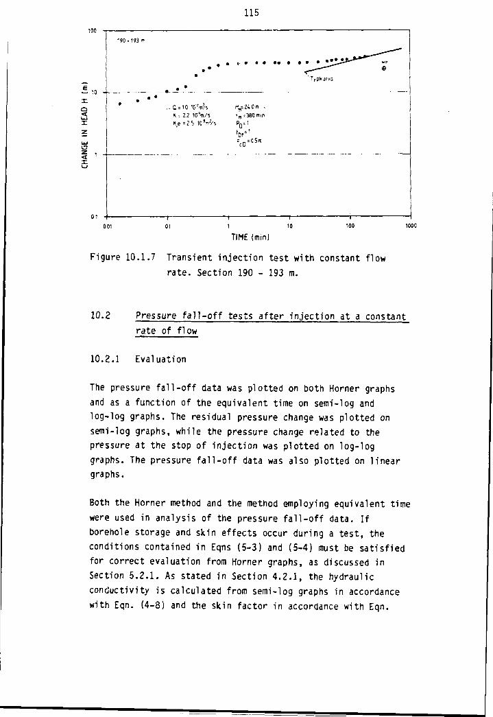
115

100

i

01

190-193 m

T/pkurva

K -- 2.2 ICfWs

Ke =2 5, 10 'V/s

^ = 24.0 m •

t - = 380 min

001 100 1000

TIME (mm)

Figure 10.1.7 Transient inject ion test with constant flow

rate. Section 190 - 193 m.

10.2 Pressure f a l l - o f f tests after inject ion at a constant

rate of flow

10.2.1 Evaluation

The pressure f a l l - o f f data was plotted on both Horner graphsand as a function of the equivalent time on semi-log andlog-log graphs. The residual pressure change was plotted onsemi-log graphs, while the pressure change related to thepressure at the stop of injection was plotted on log-loggraphs. The pressure f a l l - o f f data was also plotted on lineargraphs.

Both the Horner method and the method employing equivalent timewere used in analysis of the pressure f a l l - o f f data. I fborehole storage and skin effects occur during a test , theconditions contained in Eqns (5-3) and (5-4) must be sat isf iedfor correct evaluation from Horner graphs, as discussed inSection 5 .2 .1 . As stated in Section 4 .2 .1 , the hydraulicconductivity is calculated from semi-log graphs in accordancewith Eqn. (4-8) and the skin factor in accordance with Eqn.

116

(4-9). In log-log graphs, the hydraulic conductivity is

calculated in accordance with Eqn. (4-12) and the effective

borehole radius in accordance with Eqn. (4-13). In evaluation,

the same specific storage coefficient as stated in Section

10.1.1 was assumed.

10.2.2 Results

The results from pressure fa l l -o f f tests after constant-flowinjection are shown in Table 10.2 and are commented on, sectionby section, below. The designations used are the same as thosein the injection tests described in the previous section.

In section 70 - 73, pressure fa l l -of f takes place considerablymore slowly than the pressure build-up in the injection stage.At the end of the test (130 minutes), only about 302 of themaximum pressure rise at the cessation of injection haddissipated, which confirms the assumption that the section wasvirtually impervious. As pointed out in Section 10.1.2 (section70 - 73), tests in almost impervious sections are moresensitive to deformation of and leakage in equipment andchanges in the packer pressure as a result of small changes intemperature. The results should therefore be regarded asapparent and approximate.

Table 10.2 Results of transient pressure fa l l -o f f tests afterinjection with constant flow rate.

Section dt K ; r(m) (min) (m/s) (m)

67

7079

- 70

- 73 *

- 82 *

55

130

42

1

<9

7

.8xlO"7

.2x10•9xlO-10

-4

<-l-3

.1

.5

.2

1>0

0

.63

.13

.69

* Approximative evaluation

117

Section 67 - 70 m

The pressure fa l l -o f f is presented in a semi-log graph as afunction of the equivalent time, together with the interpreta-tion l ine, in Fig. 10.2.1. The pressure fa l l -of f behaviour issimilar to the pressure build-up during the injection phase,but is somewhat slower. The pressure fa l l -of f time is alsoshorter. The calculated hydraulic conductivity and skin factorvalues are in good agreement with the results from theinjection test. The static pressure in the section was found tobe -0.2 m, i.e. 0.2 m below the actual pressure before theinjection test.

Section 79 - 82 m

The pressure fa l l -o f f test was discontinued after 42 minutes,at which point about 60 % of the pressure build-up during theinjection test had dissipated. The pressure fa l l -o f f data wereplotted on both a Horner graph and as a function of equivalenttime. As true radial flow does not occur during the injectiontest, the radial flow theory is not applicable during thepressure fa l l -of f test. Test data are shown in a linear graphin Fig. 10.2.2. The points approximate closely to a straightline in this graph, which indicates linear flow, even duringthe pressure fa l l -o f f test. The hydraulic conductivityevaluation is approximate due to the absence of the radial flowperiod.

10.3 Constant-pressure injection tests

10.3.1 Evaluation

In evaluating transient constant-pressure injection tests, theflow rate Q(t) was plotted as a function of the time, t , on alog-log graph and 1/Q(t) as a function of t on semi-log andlog-log graphs. In certain cases, 1/Q(t) was also plotted as afunction of yj t on a linear graph in a manner analogous toconstant-flow rate tests. From this graph the fractureconductivity was determined in accordance with Eqn. (7-8).

R E S I D U A L HEAD CHANGE H 1 ( m ) R E S I D U A L HEAD CHANGE H 1 ( m )

o

tan

t

o

c*

i/>o

o"3

1

CD

ororo

insure

-tio>

1O- * >- h

<-»•

ID(/irf-

O>fter

c .ort

o'

U3

tt>

OO3V)r*O)3

- h

OC

"5O»

(T)*t/5<DO<-!•

~C-itt

1/)C-iCO

-t,OJ

1o- t i—ti

l / lr+

O

3

roo

o3

:QU

119

The hydraulic conductivity of the test sections was preferablyevaluated from the semi-log graphs in accordance with Eqn.(4-24) and the skin factor in accordance with Eqn. (4-25). Inevaluatior, the same specific storage coefficient as that sta-ted in Section 10.1.1 was assumed. In evaluation in accordancewith the dual-porosity model, the hydraulic conductivity wascalculated in accordance with Eqn. (4-24) and the skin factorfrom the later straight line in accordance with Eqn. (4-25).

The data curves for the constant-pressure injection tests onsemi-log graphs are very similar to those obtained fo.-

corresponding constant-flow rate tests. This implies thatpractically the same information is obtained from the two typesof test.

The effective borehole radius was calculated in accordance withEqn. (3-2). As the radius of influence is assumed to beindependent of the injection pressure, i t was calculatedapproximately in accordance with Eqn. (4-11), in a manneranalagous to that used in the constant-flow rate injectiontests.

10.3.2 Results

The results from the transient constant-pressure injection testare shown in Table 10.3 and are commented on, section bysection in the text below. The designations used are the sameas those used in the injection tests described in earlierpresentations of results.

Sections 76 - 79 and 166 - 169 are low-conductivity sections,so that equipment defo'mations and variations in temperaturemay strongly influence the pressure changes. The interpretationcurves are also based on only a few measurer1 values. Theevaluation is therefore approximate.

120

In testing sections 172 - 175 and 178 - 181, maintenance of aconstant injection pressure proved to be a problem. In theformer section, the flow rate curve rises sharply and becomes astraight line (radial flow - semi-log graph) after a very flatstart. The latter test developed into a constant-flow rate test(cf. Section 10.1.2). Radial flow occurred after about 10minutes and the pressure response implies a partially cloggedfracture or fracture system.

Table 10.3 Results of transient injection tests with constantpressure.

Section

(m)

67-70

76-79

79-82

166-169

172-175

178-181

181-184

190-193

(min)

180

70

180

180

180

90

180

180

K(m/s)

1.7*10"7

(6.0-10"14)

t.3'10"9

(2.8-10"14)

(1.8-10"9)

2.3-10"6*

4.1-10'10

2.6-10'9

-3.4

-

-2.3

-

-2.3

-

-1.0

-3.2

V(m)

0.84

-

0.28

-

0.25

-

0.08

0.69

re(m)

20

(0.08)

5.6

(0.03)

6.6

53

3.2

7.9

* evaluated as constant flow-rate test

() values within brackets are approximative

121

Section 67 - 70 m

The transient change in flow rate coincides after about 10minutes with a straight line in a semi-log graph (see Fig.10.3.1). After 60 minutes, this line is moved laterally,parallel to the original one, probably caused by a flow meterchange. Calculated values of the hydraulic conductivity, skinfactor and fracture conductivity are in good agreement with thevalues of corresponding parameters from the constant-flow ratetest.

Section 79 - 82 m

The transient test response on this section, together with theinterpretation line on a semi-log graph, are shown in Fig.10.3.2.

The flow rate values are relatively scattered, but the positionselected for the interpretation line is quite clear. Radialflow occurs after about 15 minutes. After about 100 minutes ofinjection time, a positive hydraulic boundary is implied. Thehydraulic conductivity and skin factor were calculated from thesemi-log graph.

Section 181 - 184 m

The transient test response on th is section, together with theinterpretation l ine on a semi-log graph, are shown in Fig.10.3.3.

The test response was evaluated in accordance with thedual-porosity model in a manner analogous to correspondingtheory for constant-flow rate inject ion tests (see Chapter 6) .The hydraulic conductivity and skin factor were calculated inaccordance with Eqns. (4-24) and (4-25) respectively. Thesection was interpreted as a medium with dual-porosity,consisting of a system of minor fractures in an otherwiserelat ively impervious rock mass (cf . corresponding constant-flow rate injection tes t ) .

122

a to

oa:a.

a o

67 - 7 0 m

1000

TIME (min)

Figure 10.3.1 Transient injection test with constant pressure.Section 67 - 70 m.

TIME (mm)


123

TIHE (min)


2

O

2ex.

TIME (mini

Figure 10.3.4 Transient injection test with constant» pressure.Section 190 - 193 m.

124

Section 190 - 193 m

After about 15 minutes of in ject ion time, the transient flow

rate curve coincides well with a straight l ine on the semi-log

graph (Fig. 10.3.4). The hydraulic conductivity and skin factor

were evaluated on the basis of this straight l ine and the

values exhibi t good agreement with corresponding values from

the constant-flow rate tes t .

10.4 Pressure f a l l - o f f tests after in ject ion atconstant-pressure

10.4.1 Evaluation

In evaluating the transient pressure f a l l - o f f tests af ter

constant-pressure in jec t ion , the residual pressure change, H,

was plotted on Horner graphs and as a function of the

equivalent time on semi-log graphs. The pressure change in

relat ion to the pressure at the stop of in ject ion was plotted

as a function of the equivalent time on log-log graphs. The

pressure change was also plotted on l inear graphs.

The hydraulic conductivity was calculated in accordance withEqn. (5-11) and the skin factor in accordance with Eqn. (5-5) .The flow rate value used was the momentary flow rate at thestop of in jec t ion , ^ery fast pressure f a l l - o f f was obtained insome tes ts . This may possibly be due to the shortness of the(dimensionless) in ject ion time. In th is case, the actualpressure approaches the s tat ic pressure in the sectionasymptotically (see Section 5.2.1). Equipment faul ts cannoteither be ruled out for these tests . The specif ic storagecoef f ic ient value stated ear l ier was assumed (see Section10.1.1).

125

10.4.2 Results

The results from the pressure f a l l - o f f tests af ter constant-

pressure inject ion are shown in Table 10.4 and are commented

on, section by section in the text below. The designations used

are the same as those in ear l ier presentations of resul ts .

In section 79 - 82, the pressure f a l l - o f f test was discontinuedafter 40 minutes, at which time 60" of the applied in ject ionpressure had dissipated. The graphs show that radial flow wasnot achieved during the test . The l inear graph implies insteadthat l inear flow existed (cf . corresponding test in Section10.2.2). The evaluation of the hydraulic conductivity isapproximate because of the short duration of the test . I t wasnot possible to determine rel iably the stat ic pressure in th issection.

Sections 172 - 175, 181 - 184 and 190 - 193 exhibi t similarbehaviour. In a l l cases the pressure f a l l - o f f was largelycomplete after a very short time (about 1 minute). Because ofthe short duration of the test , the results must be regarded asbeing uncertain. In sections 172 - 175 and 190 - 193, thepressure change curve levels off towards zero, i . e . the actualpressure acting in the section before the in ject ion tes t . Insection 181 - 184, the pressure change curve levels of f towardsa value of +0.25 m, i . e . 0.25 m above the pressure prevail ingbefore the inject ion tes t .

Table 10.4 Results of pressure f a l l - o f f tests after

inject ion with constant pressure.

Section dt K c r(m) (min) (m/s) (m)

0.620.040.040.04

79172181190

- 82- 175- 184- 193

400.0.1.

8577

7.5X10"10

9.4X10-10

1.6X10"10

1.3xlO"9

-3.1-0.4-0.3-0.3

126

10.5 Water loss measurements

10.5.1 Evaluation

The water loss measurements were evaluated using equationsvalid for steady-state conditions. Thus, Eqn. (4-41) was used,and as data values, the flow measured under the la t te r part ofeach test and the actual inject ion pressure were used. In notest were real steady-state conditions measured under which theformulas used become s t r i c t l y va l id . But in a l l cases, thechange in flow rate with time was considered to be so smallduring the la t te r part of the test that steady-state conditionswere assumed in the evaluation.

10.5.2 Results

The (equivalent) hydraulic conductivity values calculated for

the rock at a constant injection pressure of 0.2 MPa are

presented in Table 10.5.

10.6 Slug tests

10.6.1 Evaluation

In evaluating the slug tests, the normalized pressure change,

H/H was plotted on semi-log and log-log graphs as afunction of the time (see Section 8.2). The equivalenthydraulic conductivity of the section was preferably calculatedfrom the semi-log graph by matching the data curve to the typecurve in accordance with Ramey et al (1975) and entering thematch point coordinates into Eqn. (8-4). As a complement,corresponding evaluation was carried out from log-log graphs incertain cases.

127

Table 10.5 Results from water loss tests performed with aninjection pressure of 0.2 MPa.

Section

(m)

Hydraulicconductivity

(m/s)

Section

(m)

Hydraulicconductivity

(m/s)

61 - 64

64 - 67

67 - 70

70 - 73

73 - 76

76 - 79

79 - 82

82 - 85

85 - 88

88 - 91

91 - 94

3.9 x 10

7.5 x 10

5.3 x 10

2.2 x 10

-9

-10

-7

-11

<1.8 x 1 0 ' 1 1 *

2.4 x 10

7.5 x 10

-11

-9

5.8 x Kf11*<1.8 x 10"1 1*

<1.8 x 10"1 1*

<1.8 x 10"1 1*

163 - 166 <1.8 x 1 0 ' 1 1 *

166 - 169 <1.8 x lO"1 1 *

169 - 172 <1.8 x 1 0 " U *

172 - 175 5.4 x 10"9

175 - 178 1.6 x 10"8

178 - 181 5.7 x 10~7

181 - 184 2.1 x 10"9

184 - 187 1.5 x 10"7

187 - 190 3.6 x 10"9

190 - 193 2.1 x 10"8

193 - 196 1.2 x 10"7

196 - 199 6.0 x 10"9

* The value 1.8 x 10" m/s constitutes the lower measure-ment l im i t for a l l sections.

Table 10.6 Results from the slug tests.

Section

(m)

Number

of tes ts '

0 U

Test

duration

(min)

H/Ho

at end

of test

K,K mean

(m/s)

Coinments

64-6767-7079-82

178-181181-184

190-193

1

1 2

2

1

1

1

9307.5-4É

955-1000

5.5

188

70

40%1 - 2 *

0»

OX

39*

0*

3.9-10

7.6-10

3.5-10

1.2-10"

5.5-10"

1.7-10*

-10

- 7 "

-9

193-196 20 1.3-10 -6

Good match to the type curve.

Good match apart from the f i r s t part of the curve.

Identical curves but d i f f i c u l t to in te ioret . Hatchcarried out on f ina l part .

Very good match.

Good match.

The data curve may be divided into two parts, eachof vihich may be matched to its type curve and givethe same value of K.

Relatively good curve match.

• 0 • with overpressure applied

U • with underpressure applied

" K r a n g e : 6 . 0 - 1 0 * 7 t o 9 . 3 - 1 0 " 7 m/s

128

10.6.2 Results

The results from the slug tests are presented in Table 10.6.

The following designations are used:

K The equivalent hydraulic conductivity of the rock(conductivity in the section)

K-range the range in the value of K from several tests in thesame section

K-mean the logarithmic average value of K in a section

the pressure change in relat ion to the momentarypressure change

Examples of response curves for slug tests are given forsections 181 - 184 and 190 - 193 in Figs. 10.6.1 and 10.6.2.

10 -

01 -

I t •

oX

X

n -

m •

0 •

» • . i — j 1—•-. — — . 1

^ : \^-::;::L\

!

i i

—

TIKE 1st k I

Fig. 10.6.1 Slug test. Section 181 - 184 m.

129

Fig. 10.6.2 Slug test . Section 190 - 193 m.

10.7 Pressure pulse tests

10.7.1 Evaluation

As in the case of the slug tests, the normalized pressurechange during pressure pulse tests was plotted on semi-log andlog-log graphs. Evaluation was then carried out using twomethods: by matching the f i e ld curves to type curves, inaccordance with Ramey et al (1975) - the type-curve method, andby evaluation in accordance with Wang et al (1977) - herereferred to as the Wang method.

The type-curve method is employed in the same manner as in

evaluating slug tests (see Sections 8.2 and 8.3). In pressure

130

pulse tests, evaluation is preferably carried out from asemi-log graph plot . But Eqn. (8-8) is used instead of Eqn.(8-4). As the compressibility of water is of decisiveimportance for the decay of the pressure pulse, i t s value wascorrected for deformation of the equipment. The compressibilityof water was replaced by an effective compressibility of1.6 x 10"9 Pa"1 (see Section 9.3.5).

TIME (sec)

Figure 10.7.1 Theoretical relationship between fractureaperture and test time at pulse decays of 50,85, 90 and 95 %. After Wang et al (1977).

The Wang method is based on consideration of the section as animpervious mass of rock penetrated by minor fractures (seeSection 8.3). From the semi-log plot of H/H as a function oftime, the time at which 90, 85 or 50% of the applied pressurepulse remains, i.e. H/H = 0.9, 0.85 or 0.5 respectively. Theaperture, e, of the assumed fracture may then be obtained,using a special graph in which the fracture aperture is plottedas a function of this time (see Fig. 10,7.1). (In using thismethod of evaluation, it was assumed that there is only oneplane, parallel fracture per section.) The hydraulic

131

conductivity in the fracture, K , may then be calculated,using Eqn. (2-2). I f this conductivity is spread out over thewhole length of the section in accordance with Eqn. (2-4), aconductivity value is obtained that is comparable with theequivalent hydraulic conductivity of the rock obtained fromother types of test . In the preparation of the graph mentionedabove, as in the type-curve method, the compressibility ofwater was replaced by the effective compressibility. Thedynamic viscosity was set at 1.4 x 10" Pa . s.

10.7.2 Results

The results from the pressure pulse tests are presented inTable 10.7. In most cases, the applied pressure had dissipatedcompletely by the end of the test. In addition to thedesignations used in presentation of the results of slug tests,the following were used:

e fracture apertureK hydraulic conductivity in the fracture

Examples of results from the pressure pulse tests performed insections 166 - 169 and 181 - 184 are shown in Fig. 10.7.2 andFig. 10.7.3 respectively. The type curves used for interpreta-tion are also shown in the figures.

132

Table 10.7 Results from pressure pulse tests evaluated using

the type-curve method and the Wang method.

Section

(ml

64-67

67-70

76-79

79-82

166-169

178-181

181-181

190-193

193-196

c ont. r< a

Section,(mi

Numberof tests*

0 U

4 4

6 1

1

5 1

• |

2 1

2 1

4 3

7 1

n g m e

Kf(ro/s)

Testduration

(min)

5-35

2-5

50

10-45

120

0.8-1.5

0.8-2

0.2-0.4

0.2-0.3

t h o d

H/Ho

at endof test

0-3*

0-1%

92%

0-7%

721

0%

0-1%

OS

0*

K range(m/s)

T y p e -

K range(m/s)

2.9-10"10

3.0-10"9

3.7M0" 8

1.5-10~S

1.3-10"8

1.3M0"7

1.1-10"7

c u r v e

- 6.0-10"9

- 3.2-10'8

- 6.0-10"8

- 2.3-10"8

- 2.3-10"8

- 1.7-10'7

- 1.5'10"7

K, K mean(m/s)

m e t h o d

K, K mean(m..s)

2.5-10"9

8.0-10"9

5.4-10-14

4.7-10"8

1.8-10-13

1.8M0"8

1.7-10"8

1.5MO'7

1.2-10"7

Comments

W a

H/HO

50,

50,

n g

85,

501

95%

50%

851

50%

85,

50%

50%

m e t h o d

e •

(•-m)

90% 13.5-21

29-58

2.7

44-59

2.3

24

901 25-28

46-64

55-62

64-67

67-70

76-79

79-82

166-169

178-181

181-184

190-193

193-196

1 . 1 - 1 0 " 4 - 2 . 6 - 1 0-4 4 . 8 M 0 " 1 0 - 1 . 8 M 0 "

4 . 9 - 1 0 ' 4 - 1 , 9 - 1 0 -34 . 8 - 1 0 -9

4 . 3 - 1 0 -6

1 . 2 - 1 0 J - 2 . 0 - 1 0 -3 1 . 7 - 1 0 -8

3 . 7 - 1 0 *

4 . 0 - 1 ( 1 "

8 . 8 - 1 0

1 . 8 - 1 0 '

-10

3 . 8 - 1 0 -12

3.1-10

3.2-10

3.7-10

1.2-10

- 4 . 4 - 1 0-4 3 . 0 - 1 0 " 9 - 4 . T 1 0 -9

-32 .4 -10

1.8-10 - 2 .2 -10

1.8-10"

3 . 2 - 1 0 '

- 5.0-

- 4 .6 -

2 .2 -10"

2 .4 -10

2.5-10

3.5-10

3.8-10

3.8-10

-12

-9

-9

-8

Good type-curve match throughout the curve The r e -Suits using the Wang method for various H/Ho leve lsare s i m i l a r . Good agreement Between the two methods.

Unre l iab le values from the type-curve method becauseof poor matching despi te the s i m i l a r i t y of the datacurves.

Curve match u n r e l i a b l e ( requ i red ex t rapo la t ion of theupper part of the data curve) . The resu l ts must be re-garded as apparent values.

S imi lar data curves , but very d i f f i c u l t to match datacurves.

Comments as f o r section 76-79.

Data curves very d i f f i c u l t to i n t e r p r e t . Only one testevaluated using the Wang method.

Good type curve match. Mean value from three t e s t s .method resu l ts from three tes ts are well c o l l e c t e d .

Poor curve matching.

S imi la r data curves , but very poor match to the typecurves.

0 = overpressure pulse appl ied

u = underpressure pulse appl ied

133

• T ' - i .

C,.». 5

TIME (s*kl

Fig. 10.7.2 Pressure pulse test; section 166 - 169 m.

et -

ot •

<u •

02 -

0 -

• • 1 1 1 ' •

' . • o k ' i ' :

\ • !

i

\ '1 \: \ ;: V .

10' to1

TIME (sek)

Fig. 10.7.3 Pressure pulse test; section 181 - 184

134

10.8 D r i l l stem tests

10.8.1 Evaluation

In evaluating the drill stem tests, the flow and recoveryperiods were dealt with separately. The flow periods wereevaluated in the same manner as the slug tests (see Section10.6.1). The recovery (pressure fall-off) periods wereevaluated in accordance with the Horner method (see Sections8.4 and 5.2). As the data points follow a straight line, thehydraulic conductivity of the rock may be calculated inaccordance with Eqn. (4-8) and the skin factor in accordancewith Eqn. (8-9). The piezometric pressure in the section wasalso determined by extrapolating this line.

10.8.2 Results

The results from the tests are presented in Table 10.8. Thegreatest emphasis has been placed on the results from thesecond recovery period as this usually provides a more reliableevaluation than other periods.

The designations uscJ are the same as in the presentation ofthe slug and pressure pulse tests, with the addition of:

H* deviation from the piezometric head existing in thesection before sealing by the packers.

Data plots from the first flow period and second recoveryperiod of the drill stem test in section 67 - 70 are presented,together with the type curve used and interpretation line, inFigs. 10.8.1a and b, respectively.

135

Table 10.8 Results from drill stem tests.

Section Flow period

(m) (m/ s)

Recovery period

K Skin factor H*

(m/s) ; (m)

Comnents

64-67

67-70

79-82

'78-131

181-184

190-193

193-196

6 . 0 - 1 0• I D ' 1 0

2.0. . A - 6 "

3.2-10 -9

2.8-10

6.0-10

6.5-10

7.9110"

"9

3.7-10

4.9-10"

•10

>3.6-10

5.1-10

>2.O-1O

3.7-10"

-10

-0.6

-3 .0

-1 .9

-1.2

0.24

0.14

- 0

<0.3

•8.0

3.9

0.47

** Range of values of K: 1.3 • 10"6 to 3.2 • to'6 m/s

Two tests performed. Results from the flow periods are inaverage. The recovery periods during one test were too shortto permit interpretat ion.

H- ± 0 . 1 , because of the f l a t intercept between the straigr.tl ine and the time axis.

Unreliable result because of too short periods. The straightl ine was extrapolated to H* • 0 for the recovery period.

I t was only possible to interpret one of the flow periods. Therecovery period was excessively affected by borehole storageand skin e f fec ts .

The recovery period was affected oy borehole storage e f f e c t s .

ii

!

i

i

—

• • —HP

\»si 3 10'6 • / !

V ;i

i 1

i

j

j

TIME (stttl

Fig. 10.8.1a Dri l l stem test, flow period; section 67 - 70 m.

136

< 1X

<X

Qm =1 37.10"5 mVs

AH:1 69 m

K i 4 9-10"7 m/s

\

H*=O.U m—-"*

10,-z

Fig. 10.8.1b Drill stem test, recovery period.

Section 67 - 70 m.

The applicability of the method of testing used is dependent on

the magnitude of the hydraulic conductivity. As the test may be

divided into two flow and recovery periods, the pressure range

and test duration within each period may be too short in

relation to the hydraulic conductivity of the test section.

With only one flow period (to about 25% pressure dissipation)

and a subsequent recovery period (to, if possible, 100%

pressure dissipation) it should be possible to achieve more

reliable evaluation, especially from the recovery period. It

should be noted that data, particularly from the flow periods,

are usually affected by borehole storage effects.

11.

137

COMPARISONS OF DIFFERENT METHODS

This chapter deals with and compares the results obtained fromall the injection, pressure fall-off and pulse response tests.The tests are first summarized and compared section by section,after which the methods are compared in relation to differentranges of conductivity. Finally, the applicability of themethods is reported and the selection of a method discussed.

11.1 Summary of results

The calculated hydraulic conductivity values are presented inTable 11.1. A varying number of methods for determiningconductivity were used in the different sections. The timeavailable and the limited applicability of individual methodsto certain ranges of conductivity restricted the number oftests. If the method permitted it, the skin factor was alsodetermined and is shown in Table 11.2.

Table 11.1 Summary of hydraulic conductivity values calcula-ted from hydraulic tests in borehole Fi 6 atFinnsjön test site.

Section

64-67

67-70

70-73

76-79

79-82

BS-88

1*6-169

172-175

178-181

181-184

190-193

193-196

" f *

ConstantInjectn.

-7*1.9-10 '

9 .0 -10" 1 3

7 . 5 - t D - ' 3

1.5-10" '

4 . 4 - 1 0 ' 1 3

6 . 6 - 1 0 ' 1 3

fiovrttefill-Ofl

1

<9

7

1 . 2 - 1 0 ' 6 "

4 .1 -10 - ' °

2.2-10 '

• 8.4 i 10''

tnffntte

.8-10"'

.2-10"12

.no'10

1 • • • I ft

Coxsttitt tinjectn.

1.

6.

1.

Z,

1.

Z.

4.

Z.

MO"7

o-,o"u

3-10-'

.S-HT1 4

8-10" '

3 - I0 ' 6

1-10"10

6-10" '

2.5 • 10

refsureft 11-off

7.

1.

1.

1.

-a

.5-

.4-

.6

J.

,2

10

10

10

to

/ J

-9

-10

-10

-9

Utter '

•etsun

7.5-10"

5.3-10'

2.2-10

Z.4-10'

7.5'10'

-1.6-10'

•ci.8-10

5.4-10'

5.7-1».'

2.1-10'

2.1 10

1.2-10

loii

•ents

•10

• 7

•11

•11

• 9

•11

• 1 1

•9

• 7

•9

•8

• 7

Slu,

tens

3.9-tO

7.6-10

3.5-10

1.2-10

5.5-10

1.7-1(1

1.3-10

-10

-7

-9

-6

-9

-7

-6

Pressu

Type-cMthod

2.5-

8.0-

5.4-

4.7-

1.8-

1.7-

1.5-

1.2-

10

10

10

10

10

10

10

10

10

re Put

ur»e

• 9

-9

-14

-8

-13

•8

•8

-7

-7

le testsVtno•ethod

8.8-10'1 0

1.8-10'8

3.8-10'12

z.rio'9

2.4-10'12

2.5-10"'

3.5-10"'

J.8-10"8

3.8-10'8

on i i s

f lo .period

6.0-10'

2.0-10"

t "

10

*

3.2-10"'

Z.8-10"

S.0-10"

6.5-10"

7 9-10"

1

9

8

7

testsrecoveryperiod

3.7-10'

4.9-10'

>3.6-1O'

5.1-10'

> 2 . 0 l 0 '

3.7-10

10

• 7

• 1 0

• 7

•8

• 7

138

Table 11.2 Summary of values on the skin factor calculatedfrom hydraulic tests in borehole Fi 6 at Finnsjöntest site.

Section

T r a n s

Constant

injectn.

i e n t t e

Flow-rate

fall-Off

s t s

Constant

injectn.

Pressure

fall-off

Dri11-stem

t e s t s recovery

64-67

67-70

70-73

76-79

79-82

85-88

166-169

172-175

178-181

181-184

190-193

193-196

-3.4

. . .

. . .

-3 .2. . .

. . .

4.8

- 2 . 7

- 3 . 9

- 4 . 1

- 3 . 2

-3 .4

-2 .3

- 2 . 3

- 1 . 0

- 3 . 2

-3 .1

-0 .4

-0 .3

-0 .3

- 0 . 6

-3 .0

- 1 . 9

- 1 . 2

<0.3

8.0

not possible to determine the skin factor

Section 64 - 67 m

11.2 Section-by-section comparison

The calculated hydraulic conductivity values are dealt withsection by section below and in Figs. 11.2.1 to 11.2.12. Thevalue of K obtained using each method of testing is presentedin the f igures, where relevant, as ranges of the value of Kcalculated from the logarithmic average value.

The following tests were performed: water loss measurement,

pressure pulse tests, slug tests and d r i l l stem tests. The

results from the tests are uniformly spread between 3.7 x

10" m/s ( d r i l l stem and pressure f a l l - o f f ) and 2.5 x

10 m/s (pressure pulse tes t ) .

139

WATER LOSS TEST

SLUG TEST

PULSE TEST

DRILL STEM TEST

y ; . - : . - m :

&nv7jr77^

10"9 10"'

Hydraulic conductivity im/s i

Fig 11.2.1 Summary of Results from Section 64 - 67 m

Section 67 - 70 m

All methods were performed in this section, except pressuref a l l - o f f after constant-pressure in ject ion. The values for thehydraulic conductivity of the rock calculated from thetransient injection tests and pressure f a l l - o f f afterconstant-flow inject ion were well collected between 1.7 x10 and 1.9 x 10 m/s_. The values for water lossmeasurements, slug tests and d r i l l stem tests are in the range4.9 x 10" to 2.0 x 10" m/s. The results from pressurepulse tests deviate. They range from 8.0 x 10"9 to 1.8 x10 m/s, which is probably due to the conductivity in thissection being above the proper measuring range of the method.

Section 70 - 73 m

The results obtained from water loss measurement (2.2 x10 m/s), transient constant-flow inject ion tests (9.0 x10 m/s) and subsequent pressure f a l l - o f f tests (<9.2 x10 ) must be regarded as unreliable. Changes intemperature during the course of measurement, for example, mayhave affected the transient tests and the steady-state testsare close to the lower measurement l i m i t .

CONSTANT FLOW

140

~~T [—r T T T TT

CONSTANT PRESSUREs • ' " ; s

WATER LOSS TES*

SLUG TEST

PULSE TES'

DRILL STEM TEST

-9 -7

EX3

I

10 10 10

H y d r a u l i c c o n d u c t i v i t y ( m / s l

,-6 10,-5

Fig 11.2.2 Summary of results from section 67 - 70 m.

CONSTANT FLOW

WATER LOSS 'EST

— I

10"' 10'

Hydraulic conductivity Im/s)

Fig 11.2.3 Summary of results from section 70-73 m.

Section 76 - 79 m

The results from the tests are between 5.4 x 10" and 2.4x 10 m/s. The methods used were the two types oftransient injection test , pressure pulse tests and steady-statetests. The comments to section 70 - 73 apply in other respects.

141

CONSTANT FLOW

CONSTANT PRESSURE

WATER LOSS TEST

PULSE TEST

. A N C 5 " f ' - ' C I

10'1 - 1 < • 10',-13 n-12

Hydraulic conductivity (m/sl

Fig 11.2.4 Summary of results from section 76-79 m.

Section 79 - 82 m

This is the only section in which a l l methods were performed.The transient injection tests and pressure f a l l - o f f testsprovide results that were close, 7.5 x 10" to 1.5 x10 m/s. The pressure f a l l - o f f period of the d r i l l stemtest provided the result K > 3.6 x 1O~ m/s, while theresults from the remaining tests ranged from 3.2 x iO to4.7 x 10'8 m/s.

CONSTANT FLOW

' A . , ' J "

CONSTANT PRESSUREN - f ' ': •*

WATER LOSS TEST

SLUG TEST

PULSE TEST' '01 , S ,• f MF'rt.7,

ORILL STEM TEST

-!10 V 10

Hydraulic conductivity (m/s)

M i l

10",-10

Fig. 11.2.5 Summary of results from section 79 - 82 m.

142

Section 85 - 88 m

Only water loss measurement and ? transient constant-flowinjection test were performed in this section. The water lossmeasurement gave a value of K < 1.8 x 10- m/s (lowermeasurement l i m i t ) , while the transient test , which gave avalue of K of 4.4 x 10" m/s, is very sensitive to smallchanges in temperature of the measuring system.

Section 166 - 169 m

The results from the methods used, water loss measurement, thetransient injection tests and pulse response tests, range from2.8 x 10~14 to 1.8 x lO"11 m/s, of which the lattervalue represents the lower measurement limit for water lossmeasurement. The results for this section may also be more orless affected by variations in temperature.

Section 172 - 175 m

In this section, a transient constant-pressure injection test,with subsequent pressure fall-off, and water loss measurementwere oerformed. The values obtained range between 9.4 x

-in' -Q10 and 5.4 x 10 m/s.

CONSTANT FLOW

WATER LOSS TEST

11

10.•13 .-12 .-1110 10

Hydraulic conductivity !m/sl

10,-10


143

CONSTANT FLOWNJECTION

CONSTANT PRESSURE

WATER LOSS TEST

PULSE TEST

TYftCUBVS METHOD

W««GS METHOO

1

1

1

11

1

1 1 1 1 , 1 1

Fig. 11.2.7

,.-11 10,-to

Hydraulic conductivity (m/sl

Summary of results from section 166 - Ib9 m.

CONSTANT PRESSURE

WATER LOSS TEST

11

1

n-100"'10 " 10



CONSTANT FLOW

CONSTANT PRESSUREi N j f C T ON

WATER LOSS TEST

SLUG TEST

PULSE TEST

ORILL STEM TEST

m

1

11

1

1

1

10'7 10«


Fig. 11.2.9 Sumnary of results from section 178 - 181 m.

144

Section 178 - 181 m

All methods were performed in this section, with the exception

of the pressure f a l l - o f f tests (the transient constant-pressure

inject ion test was evaluated as a constant-flow test (see . .

Section 10.3.2)). The results from the tests, except for the

pressure pulse tes t , are re la t ive ly close, within the range

from 2.8 x 10~7 to 2.3 x 10" m/s. The values of K—8

obtained from the pressure pulse test were 1.8 x 10 m/s(type-curve method) and 2.5 x 10 m/s (Wang method).

Section 181 - 184 m

Only the pressure f a l l - o f f af ter in ject ion with constant flowis missing from this section. The values of K for the twotransient in ject ion tests were the same, 4.1 x 10 m/s.The pressure f a l l - o f f test af ter in ject ion at constant pressurewas evaluated at 1.6 x 10 m/s, whereas the results fromthe remaining tests ranged from 2 . 1 x 1 0 to 1.7 x10"8 m/s.

Section 190 - 193 m

All the tests were also performed in th is section, with theexception of the pressure f a l l - o f f test after in ject ion atconstant pressure. The values obtained from pressure f a l l - o f f

and transient inject ion tests range between 1.3 x 10 and-9

2.6 x 10 m/s. The results from the other tests range from2.0 x 10"8 to 1.7 x 10"7 m/s.

Section 193 - 196 m

Only pulse response tests and water loss measurement wereperformed in this section. The results range between 3.8 x10 m/s (Wang method) and 1.3 x 10 m/s (slug test).

145

11.3 Method comparisons

The results obtained from this work permit no statisticalanalyses, but certain conclusions may be drawn in conjunctionwith comparisons of the methods. The comparison applies to thespecial methods of testing, instruments and external conditionsapplicable during this work (see sections dealing with eachmethod, Section 9.4).

CONSTANT FLOWIH1K7I0H

CONSTANT PRESSURE

INJECTION

fin Off

WATER LOSS TEST

SLUG TEST

PULSE TEST

TYPfCuRVE METHOD

• «NG S HETHOO

DRILL STEM TESTfLOW PEBlOO

10,-10 10~9 10"



146

CONSTANT FLOWINJECTION

CONSTANT PRESSUREINJECT ON

WATER LOSS TEST

SLUG TEST

PULSE TEST•YPECuflvE "iE'MOO

DRILL STEM TEST

fLOW PEPIOD

8 u ^ D UP PERIOD

10 " 10

Hydraulic conductivity Im/s)

10

Fig. 11.2.11 Sunmary of results from section 190 - 193 m.

WATER LOSS TEST

SLUG TEST

PULSE TEST

rvPECURvE MfTHOD

W4N0S MfTHDD

DRILL STEM TEST

H O W PEBIOD

Bui LO -IP PEOiOD

Hydraulic conducfivity (m/s)

Fig. 11.2.12 Sunmary of results from section 193 - 196 m.

147

Transient constant-flow and constant-pressure injection tests

In this comparison the test åt constant-pressure in section 178- 181 is excluded since, as a result of the problem ofmaintaining the pressure constant, the test was evaluated as aconstant-flow test.

-12If the conductivity values above 1 x 10 m/s are compa-red, which may be regarded as the lower measurement limit ofthe methods, the agreement is yery good between the two met-hods. The greatest difference between the methods correspondsto a factor of 1.7, whereas the same result was obtained forone test section. The skin factor also shows good agreement.

Pressure fall-off - transient injection tests

Seven pressure fall-off tests were performed. Comparisonbetween two of them and comparison with the transient injectiontests as regards hydraulic conductivity shows that theagreement is good (if section 70 - 73 is excluded, as theresult from this section may be regarded as unreliable becausethe pressure fall-off was too short, below 30%). The greatestdifference corresponds to a factor of 2.6 (section 181 - 184).

Determination of the skin factor from the pressure fall-offtests resulted, as for the transient injection tests, insimilar values.

Water loss measurements - transient injection tests

Both water loss measurements and transient injection tests wereperformed in ten sections. The results of steady-state testsfrom four of them are near to the lower measurement limit,leaving six sections for comparative studies.

148

In al"! cases but one (section 178 - 181) the hydraulicconductivity calculated from the water loss measurements isgreater than that from the transient injection tests. Thedifference varies between factors 3 and 11. Correspondingequivalent hydraulic conductivities for the rock may bedetermined in sections in which the fracture conductivity wascalculated. This value is always between the value calculatedfrom the transient injection test and that from the water lossmeasurement. As the values of K from water loss measurementsare based on an injection duration of 5 - 10 minutes (not fullsteady-state conditions), they should naturally provide a valuethat is too high (Andersson & Persson, 1985). On the otherhand, the values of K from the water loss measurements areaffected by any clogging effects adjacent to the section beingtested. Instead, the effect of this is that the value of K fromwater Toss measurements is too small in relation to that fromthe transient injection tests (cf. section 178 - 181). The skinfactor cannot be determined from water loss measurements.

Slug tests - transient injection tests

Material for comparison of the hydraulic conductivity obtainedusing slug tests and transient injection tests is availablefrom the five measurement sections. In all cases the value fromthe slug test is above the value of K from the transientinjection test. Deviation is greatest in the case of lowconductivity values. In one case the factor is 77 for a value

_9of K of about 10 m/s (section 190 - 193), whereas

agreement is good at values of K around 10 m/s.

Slug test - water loss measurement

Agreement is good in comparisons between slug tests and waterloss measurement in seven measurement sections (factor: 1.9 -

-82.6) for conductivity values below 10" m/s (3 sections).The variation is greater for conductivity values above 10m/s with a factor of 1.4 - 11.

149

Pressure pulse tests: Type-curve method - Wang method

Pressure pulse tests were performed in nine measurementsections and evaluated using the type-curve method and the Wangmethod (Section 10.7.1). Because of the basic differencebetween the methods, evaluations of the same data curve mayprovide different results. In 6 out of 7 measurement sectionsthe type-curve method provided the highest value of K in theconductivity range above 1 x 10 m/s. The differenceranges between factors 2.3 and 7.2. In the range of K below 1 x10 m/s (2 sections), the Wang method provided resultsthat were higher by the factors 13 and 70 respectively.

Pressure pulse tests - transient injection tests

Comparisons between pressure pulse tests and transientinjection tests may be made in seven measurement sections. Intwo sections in which the results from the transient injectiontests and also the other methods of testing, are collectedaround 5 x 10 m/s, the results from pressure pulse testsare lower by one or two orders of magnitude. This deviation isassumed to be due to the inapplicability of pressure pulse testin such high-conductivity sections.

-10 -8For values of K between 10 and 10 m/s, on theother hand, the values from pressure pulse tests are 8 - 4 7times higher than those from corresponding injection tests (thesmallest deviation was obtained using the Wang method). Incomparison with the other methods the results from thesesections are well collected within a factor of ten. In twosections in which the K value is below 10" m/s, theresults obtained using the Type-curve method agree best withthose from the injection tests, but the scatter is very large.

150

Drill stem tests - transient injection tests

Results for comparison of drill stem tests and transientinjection tests are available from five sections. Agreement isgood in two of these sections, with the greatest differencecorresponding to a factor of 3.5. The remaining sectionsprovided results that were between 3 and 30 times higher thanthose from the injection tests. In only one case has it beenpossible to use the flow period for evaluation. The drill stemtests gave slightly higher skin factor values than theinjection tests. Compared with the other pulse response tests(pressure pulse tests, slug tests), the values obtained usingthe drill stem test, above all from the recovery period, appearto be closer to those from the transient injection tests. Theresults would probably be improved by modifying the method ofmeasurement as described earlier (see Section 10.8.2).

In the above comparison of pairs of tests, preference has beengiven to comparison of the transient injection tests with theother tests. This does not imply that the injection tests areabsolutely correct, but they do represent a greater radius ofinfluence because of their longer duration and they are alsoperformed with continuous data collection and the possibilityof separating the various flow regimes. This reduces the riskof incorrect interpretation and minimizes skin and boreholestorage effects on the interpretation.

As noted above, it is not possible to compare only thecalculated values of K obtained using the various methods. Theduration of the test must be taken into account because it isprincipally the duration that determines the radius ofinfluence of the test or the flow regime that is applicable. Afast method of testing always has inherent limitations in thatit only permits investigation of the immediate surroundings ofthe borehole.

The pulse response tests and water loss measurements normallyprovide higher hydraulic conductivity values than transientinjection tests. This may be explained in part by the

151

relatively short duration of the former tests. This normallyimplies that only a limited volume in the immediate vicinity ofthe borehole is investigated. This volume of material may beaffected by skin effects (positive skin effect due to cloggingor negative skin effect as a result of narrow fractures aroundthe borehole caused in conjunction with drilling). Thedeviation in results between short tests and longer tests mayalso be regarded as a problem of the scale of investigation,c.f. representative elementary volume as discussed in section2.5.

The deviation from the results of the transient injection testsis, however, relatively small for water loss measurements, anddrill stem and slug tests. The pressure pulse test, which isthe fastest method, appears to be less reliable. But it may be

suitable method for testing formations with very lowpermeability, with values of K below 10" m/s, in which,despite everything, the radius of influence of transientinjection tests is small and it is impractical to perform thetest.

11.4 Conclusions

The results and experience gained from the tests performedprovide valuable information on the applicability andmeasurement accuracy of the methods. As pointed out at thebeginning, the selection of a method for determining hydraulicconductivity must be made on the basis of the range ofconductivity within which determination is to be carried out.In investigations of crystalline bedrock for storage ofradioactive waste, interest is centred round the possibility ofdetermining low hydraulic conductivities with great accuracyover a relatively wide range. This range may generally be saidto comprise conductivity values below 10" m/s.

152

11.4.1 Applicability of the various methods

The results from this investigation were used as a basis forpreparing the general sunmary contained in Fig. 11.4.1. Thisfigure indicates the ranges of hydraulic conductivity withinwhich the various methods are applicable. The presentation isbased on the following conditions:

o diameter of the borehole, r = 56 urnw

o length of the measurement section, L = 3 mo inside diameter of the pressure pipe, r = 10 mmo maximum available test duration, t = 180 min

CONSTANT FLOWNJECTION TEST

CONSTANT PRESSURENJECTION TEST

FALL OFF TEST

WATER LOSS TEST

SLUG TEST

PULSE TESTtypecurve method '

PULSE TESTWang's method •

DRILL STEM TEST

• i«,.iu

• 140

. 1M

, . 0 It

• HO

. . 0 1 »

_ „" ?////////////////////£ r#>~,= 0*2

V 0.37

i •- 1

',: 0.37

•+- 4-»•" 1 0 " X T " 10'* 1 0 ' W 7

HYDRAULIC CONDUCTIVITY I m / s )

•m ISM i

10 '

. 1: It

Figure 11.4.1 Ranges of hydraulic conductivity suitable forvarious methods of testing.

The measurement limits of the various methods are dependent onthe special equipment used. For certain tests, such as thepulse response tests, the range limits are directly dependenton the duration of the test. The upper measurement limit iscontrolled by ttie minimum acceptable test duration to achieveadequate measurement accuracy, whereas the lower measurement

153

limit is determined by the maximum available test duration. Theranges presented may b: regarded as guiding values and may bealtered by, for example, the use of different equipment,different available test durations or other requirements onmeasurement accuracy.

Fig. 11.4.1 has been supplemented by the addition of the

estimated radius of influence for the range limits of each

method. This radius is dependent on the hydraulic conductivity

and duration of the test. The radius of influence calculated in

accordance with Eqn. (4-11) is for homogeneous conditions. The

actual radius of influence for sections containing extensive

fractures would probably be much larger (see Section 10.1.1).

Different methods provide different quantities of information

on the properties of the bedrock and the groundwater flow

conditions adjacent to the borehole. Table 11.3 gives an

overall picture of the type of information provided by the

various methods. An X indicates that the method is capable of

providing corresponding information. (X) indicates that the

information may be derived secondarily or that it is uncertain

whether the information can be obtained.

11.4.2 Selection of a method

Various criteria for selecting a method are tabulated in Table

11.4, which also contains an indication of how well the various

methods satisfy the stipulated conditions. Tables 11.3 and 11.4

show that transient constant-pressure injection tests and

subsequent pressure fall-off tests are regarded as being the

methods of hydraulic testing that best satisfy the stipulated

demand criteria.

154

Table 11.3 Type of information obtained from the various hyd-raulic tests.

Type of test H* Hydr. Flowbound, regime

A Transient injection test

A1 constant flow-rate

A2 constant pressure

B Pressure fall-off test

C Water loss measurement

D Slug test

E Pressure pulse test

E1 Type-curve method

E2 Wang method

F Drill stem test

X

X

X

X

X

X

(X)

X

X

X

(X)

(X)

X

X

X

X

X

X

X

X

X

X X

X

X

(X)

Table 11.4 Criteria for selecting a method, based on theresults obtained. The method designations are asin Table 11.3.

Criteron

0

0

0

0

0

0

Applicable over a largemeasuring range

Does not affect the mea-surement section by de-formation etc.

Easy to evaluate

Large radius of influence

Provides several parametersin addition to value of K

Short test duration

A1

X

X

X

X

A2

X

X

X

X

X

B

X

X

X

X

C D

X

X

X

(X)

X X

El

X

E2

X

F

X

X

155

The advantages of transient constant-pressure injection testsinclude:

o Possibility of measuring over a large range of hydraulicconductivities

o The equipment used is more suitable for injection tests atconstant pressure that those with constant flow. This isbecause the range of measurement with transient flow islarger than for a corresponding transient pressure.

o The pressure is constant in the measurement section and inthe entire system. This implies negligible borehole storageeffects and small deformation of the equipment whilemeasurements are being made.

o Evaluation is based on a large number of measured datapoints.

o Large radius of influence which should providerepresentative values on the hydraulic parameters.

o Possibility of determining the skin factor ?.nd effectiveborehole radius and the possibility of determiningapproximately the apparent fracture parameters, such asfracture length (aperture) and the product, K e, in theevent of any vertical fractures.

o Certain qualitative information may be obtained, such asidentification of hydraulic boundaries and different flowregimes.

For transient injection tests to provide the maximum amount of•information, a minimum injection time of 2 hours isrecommended. This implies that a greater volume of rock isaffected by the test and not only the immediate vicinity of theborehole as is the case with shorter tests. The amount of rockaffected is dictated not only by the duration of the test butprincipally by the hydraulic parameters of the rock. Therepresentativeness of the calculated conductivity values should

156

be seen in relation to the volume of rock investigated. Thegreater the volume of rock, the greater the probabil i ty thatthe conductivity values are representative mean values for therock tested and i t s inhomogeneity and that the formation may beregarded as an equivalent, homogeneous and porous medium, wnichis normally assumed in evaluation. I f the volume of rockinvestigated is suf f ic ient ly large, the magnitude of i t shydraulic parameters w i l l not change signi f icant ly i f thevolume is further increased (see Section 2.5).

I f a test duration of 2 hours is selected, i t should in mostcases (for sections with a hydraulic conductivity above about10 m/s) be possible to evaluate the results from thesemi-log graphs considering the temporal constraints applicableto this type of evaluation. This evaluation method is regardedas giving the most rel iable determination of the hydraulic con-ductivity and skin factor. Evaluation from the log-log graphsand linear graphs may be used as a complement, to identi fy d i f -ferent flow regimes and determine the properties of any f ractu-res. But correct evaluation of the subsequent pressure f a l l - o f ftest also requires that the injection period be suf f ic ient lylong.

The pressure f a l l - o f f tests imply a possibi l i ty of comparingand checking corresponding values obtained from the inject iontests and to determine the piezometric pressure in the section.The duration of pressure f a l l - o f f should be of the same orderof magnitude as the injection time.

157

12. HYDRAULIC TESTING FOR SITE CHARACTERIZATION

On the basis of the literature studies and field tests descri-bed in this report a hydraulic test programme was in 1981 pre-pared for use in the SKE study site investigations carried outlater. The aim of these site investigations was to clarify thesuitability of various rock formations as final repositoriesfor Swedish highly radioactive waste. These investigations wereperformed using the same methods in all areas. A certain amountof programme updating is though being carried out continuously.This 'standard programme' comprises geological and geophysicalmethods as well as hydrogeological ones and is reported in theSKB series of Technical Reports: Ahlbom et al (1983c) (methods)and Almén et al (1983) (equipment). A brief presentation ofthe hydraulic test configuration and equipment selected forsite characterization investigations is given below, togetherwith a few words about the scope of measurements and the quan-tity of data that is available today.

12.1 Hydraulic tests - methods and equipment

12.1.1 Test sequence

In the hydrogeological part of the standard programme, thehydraulic tests constitute the most extensive operation. Asnoted in the comparisons of methods (Chapter 11), the transientinjection test at constant pressure and subsequent pressurefall-off test is regarded as being the most suitable one forthis type of investigation.

For the transient single-hole injection tests, a double packersystem was used. The standard pucker spacing was 25 m. Theentire length of the borehole was first tested with thisspacing. Detailed tests of sections with higher hydraulicconductivities were then conducted using a packer spacing of 5or 10 m. At some of the sites, short-duration (steady-state)tests were also performed with a packer spacing of 2 or 3 m.

158

The transient test sequence may be divided in three di f ferentphases with the following durations:

* Packer sealing 0.5 hours* Water injection test 2 hours* Pressure f a l l - o f f test 2 hours

After the packer sealing has been completed a constantpressure, in general 200 kPa (20 m), is applied to the testsection. In highly-conductive sections such a high inject ionpressure may not be achieved and a lower pressure level must beselected.

12.1.2 Test-equipment

Two different sets of test equipment were used for the

single-hole injection tests, a steel pipe string system (Fig.

12.1.1) which is än improved version of the one used in Finn-

sjön and an umbilical hose system (Fig. 12.1.2). In the latter

system the test sequence is automatically controlled while the

steel pipe system is manually controlled. The two equipment

systems described here was used in the site investigations bet-

ween 1981-1985. During 1986 both systems have been further

inproved (Almén et al 1986).

Pipe string system

During the injection phase a constant head is maintained in the

test section by manual regulation of the flow rate. The manual-

ly recorded flow meter covers the range in flow rate of 1.5 x-9 3 -4 3

10 m /s - 2.5 x 10 m /s.

Data collection and processing are schematically presented, inthe block diagram in Fig. 12.1.3. The central unit of the dataaquisition system is a data logger; data are stored on cassettetapes. Pressure and temperature values are assembled in the

159

DATA

UOGC.

»MPUREP BOX

1CNAST0£C. CISP

Figure 12.1.1 Schematic arrangement of steel tubing system.

910

Umbilical hose reelInjection water tankControl pane'

Umbilical bote hydraulic driven excitef S6Instrument panel

Measuring wheel for umbidcai hoseTransformerInfection water c*9§fy*ng s\stamElectrical power and Signal transmission

Hydraulic jachup legHydraulic winchThermal curtains

Figure 12.1.2 Instrument trailer - Umbilical hose system.

160

data logger with scanning at time intervals that increase insteps.

The absolute pressure in the section before injection isentered manually as digital data (multimeter value) as well asall section identi f icat ion data and indications of thedifferent phases of the test sequence. In parallell with thedata logger the test data are also registered on a chartrecorder, primarily for the test operator to keep control ofthe progress of the test.

Cassette tapes with test data are sent to the main computercentre for layback. Together with punched flow rate data, thetest data are processed for plotting of the data graphs and arethen stored. In addition to the injection pressure and flowrate data which are used for evaluation, the packer inflationpressure and water temperature a e also plotted. Variatons inthese parameters may sometimes influence the tests (mainly inlow-conductivity sections).

Flow(Manuell)

Temperaturem, water

TemperatureA,f

IdentitySequence(Digital)

Transducermeasurementsection

Transducerpacker

Datalogger

— •

i

Amplifier

<

Chartrecorder

Comouter

Printer Plotter Storing

Figure 12.1.3 Data flow and handling scheme.

161

Umbilical hose system

This equipment consists of two units, an instrument trailer anda recording trailer. On the recording trailer the recordingequipment is built around a field computer, which is connectedvia an expansion box to a data logger and a tape recorder. Thecomputer also works directly on-line with a plotter. Thissystem enables control of the test method to be used andrecording and storage of information while the test is inprogress. After the test has been completed, the data tape mayagain be read into the computer for plotting. In order to makefast evaluations in the field there is another computer whichenables plotting of the test data at the same time as aquisi-tion of new test data is carried out by the other system.

The umbilical hose system is because of its automatic testcontrol and data aquisition a sophisticated version of thesteel mandrel system. However, because of somewhat differentranges (on pressure transducers and) on the flow meters themeasuring range is somewhat narrower with this equipment. Thereare three flow meters in the system. They represent threestrictly delimited measuring ranges, together covering a rangeof 0.5 x 10'9 to 1.2 x 10"4 m3/s.

12.1.3 Description of graphs plotted

The different phases of the transient injecton tests (packersealing, injection and fall-off) are documented on severalgraphs (A, B and C graphs respectively). The A graphs (Al - A5)show in linear time backgorund information and overview of flowand section pressure during the entire test sequence. The Bgraphs (Bl - B4) reflect the test data from the injection phaseand the C graphs (Cl - C2) from the fall-off phase.

Al: This plot shows the pressure change after lowering of thepacker system to a certain level an dal so during the packerinflation phase. The plot also shows the flow meter calibration(cannula test).

162

A2 - A3: These graphs describe the changes in flow rate andpressure in the test section respectively, during the entiretest sequence.

A4 - A5: These plots show the (free) groundwater level in theborehole, barometric and packer in f la t ion pressure togetherwith the temperature of the outdoor a i r , inject ion water at thesurface and groundwater in the test section.

Bl : This graph i l lus t ra tes the pressure in the test sectionduring the injection phase versus test time on a semi-loggraph.

B2 - B3: These plots describe the reciprocal of the flow rate

versus the fourth root of time and versus time on a log-log

scale respectively.

B4: This graph shows changes in the flow rate (and reciprocal

of the flow rate) versus time in a log-log graph.

Cl: This plot shows the pressure f a l l - o f f in the test sectionafter cessation of inject ion in a log-log graph.

C2: This plot describes the pressure f a l l - o f f in a Hornergraph (semi-log).

12.2 Hydrogeoiogical data base

Five sites in various parts of the country (Fig. 12.2.1) wereinvestigated in accordance with the standard programme forwhich this report contained the basic information. On average10 - 15 core boreholes were subjected to hydraulic testing oneach s i te . The boreholes were 56 mm in diameter and reached avert ical depth of 300 - 900 metres. Most boreholes were d r i l l edwith an incl inat ion of 60 - 70 degrees to the horizontal, whichimplies a total borehole length of some 700 - 800 metres. Thus,a total of about 30,000 borehole-metres were tested, correspon-ding to 1,200 hydraulic tests in 25-m sections. To which shouldbe added detailed measurements in 5 and/or 10-m sections, ofwhich there were some 400.

163

Figure 12.2.1 Location of study sites investigated 1981-1985.

Data from these investigations, together with all otherhydrogeoiogicai information, is stored in a data base that isbeing built up (Gentzschein, 1986). The aim is that this database will be used to store all geoscientific information fromresearch being carried out to ensure that the highly radioacti-ve waste can be stored in a reassuring manner in a final repo-sitory located in crystalline rock.

The hydrogeoiogicai data base contains data from the followinginvestigation operations:

Hydraulic testsGroundwater level mappingPiezometryInterference testsTracer testsHydraulic data classified into groups (rock mass, fracturezones, etc.)

164

The following information from transient single-hole injectiontests is available in the data base:

o Raw data from each section tested, as text files in a VAX750 computer.

o Borehole information, such as identifying code, X, Y and Zcoordinates, borehole length, casing length and diameter,superficial deposits, inclination and declination of bore-holes, core diameter, borehole deviation logs, and eventsthat occured in the borehole prior to testing (boreholehistory).

o Records of the type of equipment used in each test (pipestring/umbilical hose system) and the instrumentation (ty-pes of pressure gauge, flow meter, packer, data logger,etc.).

o Data calculated from each test, including:

hydraulic conductivity (steady state) (KSS)hydraulic conductivity from injection phase (KI)hydraulic conductivity from fall-off phase (KT)representative hydraulic conductivity (K)transmissivity (T = K x L) (T)skin factor calculated from injection phase (ZI)skin factor calculated from fall-off phase (ZT)environmental pressure in the section tested (PS)

o Outer hydraulic boundary conditions (positive or negativeboundary), identification of dominant flow regime(s) duringthe test and assessment of the quality of the test.

165

REFERENCES

Agarwal, R. G., Al-Hussainy, R and Ramey, H. J . , J r . , 1970: An

Invest igat ion of Well bore Storage and Skin Ef fect in Un-

steady L iquid Flow: I . Ana ly t ica l Treatment, Soc. Pet. Eng.

J . , Sept. 1970, pp 279-290. Trans. , AlfoE, 249.

Agarwal, R.G., Carter , R.D. and Pol lock, C.B., 1979: Evalua-

t ion and Predict ion of Performance of Low-Permeability Gas

Wells Stimulated by Massive Hydraulic F rac tu r ing . J . Pet.

Tech., March 1979, pp 362-372. Trans. , AIME, 267.

Agarwal, R.G. 1980: A new Method to Account fo r Producing Time

Effects When Drawdown Type Curves are Used to Analyze Pres-

sure Buildup and Other Test Data. Soc. Pet. Eng. Paper

9289.

Ahlbom, K., Carlsson, L. , Car ls ten, L-E., Duran, 0 . , Larsson,

N-Å., Olsson, 0 . , 1983 a: Evaluation of the Geological ,

Geophysical and Hydrogeological Conditions at F jä l l veden. -

KBS Technical Report TR 83-52.

Ahlbom, K., A lb ino , B. , Carlsson, L . , Danielson, J . , N i lsson,

G., Olsson, 0 . , Sehlstedt , S . , S te j ska l , V. , Stenberg, L.

1983 b: Evaluation of the Geological , Geophysical and Hyd-

rogeological Conditions at Kamlunge, - KBS Technical Report

TR 83-54.

Ahlbom, K., Carlsson, L. and Olsson, O. 1983c: Final disposal

of spent nuclear f u e l - g e o l o g i c a l , hydrogeological and geo-

physical methods fo r s i t e charac te r i za t ion . SKBF/KBS Tech-

nical Report TR 83-43.

Ahlbom, K., Andersson, P., Ekman, L. , Gustafsson, E., Smel l ie ,

J . and Tu l lbo rg , E-L. 1986: Prel iminary invest iga t ions of

f rac ture zones in the Brandan area, Finnsjön study s i t e .

SKB Technical Report TR 86-05.

166

Almén, K-E., Ekman, L. och Olkiewicz, A., 1979: Försöksom-

rådet vid Finnsjön. Beskrivning t i l l berggrunds- och jord-

artskartor. SKBF-KBS Teknisk rapport TR 79-Q2. (In

Swedish).

Almén, K-E. et a l , 1983: Final disposal of spent nuclear

fuel - equipment for si te characterization. SKBF/KBS Tech-

nical Report TR 83-44.

Almén, K-E. et a l , 1986: Equipment for geological, geophy-

s i ca l , hydrogeological and hydrochemical characterization.

SKB Technical Report TR 86-16.

Andersson, P. and Klockars, C-E., 1985: Hydrogeological inves-

tigations and tracer tests in a well-defined rock mass in

the Stripa mine. SKB "echnical Report TR 85-12.

Andersson, J-E. och Carlsson, L., 1980: Hydrauliska tester i

berg. Del 1: Influens av brunnsmagasin och skin vid olika

transienta tester. SKBF-KBS Arbetsrapport AR 80-28. (In

Swedish).

Andersson, J-E. and Persson, 0., 1985: Evaluation of single-

hole hydraulic tests in fractured crystal l ine rock by

steady-state and transient methods. SKB Technical Report TR

85-19.

Andersson, J-E. och Hansson, K., 1986: Hydrauliska tester i

berg. Del 6: Interferenstester. SKB Arbetsrapport AR 86-22.

(In pre^s).

Barker, B.J. and Ramey, H.J., 1978: Transient Flow to F in i te-

Conductivity Vertical Fractures. Soc. Pet. Eng. Paper 7489.

Black, J .H. , Holmes, D.C. and Noy, D.J., 1982: Hydraulic tes-

t ing in granite using the sinusoidal wave method. Rep.

Inst . Geol. Sci. ENPU 82-4.

167

Bredehoeft, J.D. and Papadopulos, I .S., 1980: A Method for

Determining the Hydraulic Properties of Tight Formations.

Water Resourc. Res. v 16, no 1 1980, pp 233-238.

Brigham, W.E. et a l . , 1980: The Analysis of Spherical Flow

with Well bore Storage. Soc. Pet. Eng. Paper 9294.

Carlsson, L., Gentzschein, B., Gidlund, G., Hansson, K.,

Svenson, T. och Thoregren, U., 1980: Kompletterande permea-

b i I i tesmätningar i Finnsjöområdet. KBS Teknisk Rapport TR

80-10. (In Swedish).

Carlsson, L., Winberg, A. and Grundfelt, B., 1983: Model ca l -

culations of the groundwater flow at Finnsjön, Fjällveden,

Gideå and Kami unge. KBS Technical Report TR 83-45.

Carlsson, L. and Olsson, T., 1985 a: Hydrogeological and

Hydrogeochemical Investigations in Boreholes-/Shut-in

tests. Stripa Project. Internal Report 85-08.

Carlsson, L. and Olsson, T., 1985 b: Hydrogeological and Hyd-

rogeochemical Investigations in Boreholes-Injection-recove-

ry tests and interference tests. Stripa Project. Internal

Report 85-09.

Carnahan, C L . , Delany, J.M., Long, J.C.S., Si lva, R.J., Wat-

kins, D.J., White, A.F. and Wilson, C.R. 1983: Selected

hydrologic and geochemical issues in si te characterization

for nuclear waste disposal. NUREG/CR - 2983.

Chatas, A.T., 1966: Unsteady Spherical Flow in Petroleum

Reservoirs. Soc. Pet. Eng. J . , June 1966, pp 102-114.

Cinco-L., H., Samaniego, F. and Dominquez, N., 1978: Pressure

Behavior for a Well with a Finite-Conductivity Vertical

Fracture. Soc. Pet. Eng. J . , Aug 1978, pp 253-264.

Cinco-L., and Samaniego, F., 1981: Transient Pressure Analysis

for Fractured Wells. J . Pet. Tech., Sept 1981, pp

1749-1766.

168

Cooper, H.H., Bredehoeft, J.D. and Papadopulos, I .S., 1967:

Response of a Finite-Diameter Well to an Instaneous Charge

of Water. Water Resour. Res. v 3, no 1 (1967) pp 263-269.

Culham, W.E. 1974: Pressure Buildup Equations for Spherical

Flow Regime Problems. Soc. Pet. Eng. J . , Dec. 1974, pp

545-555.

Doe, T. and Remer, J , , 1982: Analysis of Constant-head WellTests in Nonporous Fractured Rock. Proceedings of the 3rdInternational Well-testing Symposium, Berkeley, Cal i fornia.

Earlougher, R.C., J r . , 1977: Advances in Well Test Analysis. -

Soc. Pet. Engr. Monograph Series, Vol 5. SPE, Dallas 1977.

Ershagi, I . and Woodbury, J . J . , 1985: Examples of P i t faTs in

Well Test Analysis. J . Pet. Tech., Feb. 1985, pp 335-341.

van Everdingen, A.F. and Hurst, W., 1949: The Application of

the Laplace Transformation to Flow Problems in Reservoirs.

Trans., AIME (1949) 186, pp 305-324.

van Everdingen, A.F., 1953: The skin effect and i t s influence

on the productive capacity of a we l l . Trans., AIME 198, pp

17i-176.

Faust, C.R. and Mercer, J.W., 1984: Evaluation of slug tests

in wells containing a f ini te-thickness skin. Water Resour.

Res., 20(4), pp 504-506.

Forster, C.B. and Gale, J.E., 1980: Injection versus pressure

pulse borehole tests in fractured crystal l ine rocks- obser-

vations and recent experience. Proc. 3rd Invitat ional

Well-Testing Symposium, March 26-28, 1980, LBL-12076, Ber-

keley, Cal i fornia.

Gale, J . , 1975: A numerical f i e ld and laboratory study of flow

in rocks with deformable fractures.- Ph. D. thesis, Univer-

sity of Cal i fornia, Berkeley.

169

Gale, J .E. , 1982: Assessing the Permeability Characeristics of

Fractured Rock. Geological Society of America, Special

Paper 189.

Gentzschein, B., 1986: Description of hydrogeological data in

SKB's database. SKB Technical Report TR 86-22. (In press).

Gringarten, A.C., Ramey, H.J., and Raghavan, R., 1974: Unstea-

dy-State Pressure distr ibut ion created by a Well with a

single Inf ini te-conductivi ty Vertical Fracture. Soc. Pet.

Eng. J . , Aug. 1974, pp 347-360. Trans AIME 257.

Gringarten, A.C., Bourdet, D., Landei , P.A., and Kniazeff, V.,

1979: A comparison between d i f fern t skin and wellbore sto-

rage type curves for early-time transient analysis. Soc.

Pet. Eng. Paper 8205.

Gringarten, A.C., 1982: Flow Test evaluation of Fractured

Reservoirs. Geological Society of America, Special Paper

189.

Gringarten, A.C., 1984: Interpretation of Tests in Fissured

and Multilayered Reservoirs with Double-Porosity Behavior:

Theory and Practice. J . Pet. Tech., Apri l 1984, pp 549-564.

Guppy, K.H., Cinco-L., H. and Ramey, H.J., 1981: Transient

Flow Behavior of a Vert ical ly Fractured Well Producing at

Constant Pressure. Soc. Pet. Eng. Paper 9963.

Gustafsson, E. and Klockars, C-E., 1981: Studies on groundwa-

ter transport in fractured crystal l ine rock under control-

led conditions using nonradioactive tracers. KBS Technical

Report TR 81-07.

Heimli, P., 1974: Bergarters porosite, permeabili l e t , fuktut-

vidgelse, kap i l l a r i t e t . Norges Tekniske Högskole, Rapport

12, Trondheim.

Hsieh, P.A., Neuman, S.P., St i les, G.K. and Simpson, E.S.,

1985: Field determination of the Three-Dimensional Hydrau-

170

Tic Conductivity Tensor of Anisotropic Media, Part 2: Met-

hodology and Application to Fractured Rocks. Water Resour.

Res. Vol 21, No 11, Nov. 1985.

Hurst, W., 1953: Establishment at the Skin Effect and itsimpediment to fluid flow into a well bore. Pet. EngB-6-B-16. October, 1953.

Jacob, C.E. and Lohman, S., 1952: Nonsteady flow to a well ofconstant drawdown in an extensive aquifer. Trans. Am. Geop-hys. Union, Aug. 1952 pp 559-569.

Karasaki, K., Witherspoon, P.A. and Long, J.C.S., 1985: A NewAnalytical Model for Fracture-Dominated Reservoirs. Soc.Pet. Eng. Paper 14171.

Long, J.C.S., J.S. Remer, C.R. Wilson and Witherspoon, P.A.,

1982: Porous media equivalents for networks of discontinous

fractures, Water Resour. Res. 18(3), pp 1253-1265, 1982.

Louis, D., 1969: A study of groundwater flow in jointed rock

and its influence on stability of rock masses. Rock Mech.

Res. Rept. No 10, Imp. Coll., London, 90pp.

Maini, T., 1971: In situ Hydraulic parameters in Jointed Rock

- Their Measurement and Interpretation. - Ph. D. Thesis,

Imp. Coll. of Sci. and Technol., London 1971.

de Marsily, G., 1985: Flow and transport in fractured rocks -Connectivity and scale effect. Proceedings of the 17thInternational Congress of I.A.H., Tuscon, Arizona, January7-11, 1985.

Mavor, M.J. and Cinco-L., H., 1979: Transient Pressure Beha-

vior of Naturally Fractured Reservoirs. Soc. Pet. r.ng.

Paper 7977.

Me Whorter, D.3. and Sunada, D.K., 1977: Grcund-water hydrolo-gy and hydraulics. Water Resources Publications, Fort Col-lins, Colorado.

171

Moench, A.F., 1984: Double-Porosity Models for a Fissured

Groundwater Reservoir With Fracture Skin. Water Resour.

Res., Vol. 20, No. 7, July 1984, pp 831-846.

Moench, A.F. and Hsieh, P.A., 1985: Analysis of Slug Test Datain a well with Finite Thickness Skin. Proceedings of the17th International Congress of I. A. H., Tuscon, Arizona,January 7-11, 1985.

Morän, J.H., and Finklea, E.E., 1962: Theoretical Analysis ofPressure Phenomena Associated with the Wireline FormationTester. J. Pet. Tech., Aug. 1962, pp 899-908. Trans., AIME,Vol. 225.

Morrison, D. C , 1981: The validity of the Homer plot for

tight reservoirs. Paper presented at the 32nd annual tech-

nical meeting of the Petroleum Society of CIM in Calgary,

May 3-6, 1981.

Moye, D.G., 1967: Diamond Drilling for Foundation Exploration.

Civil Eng. Trans., Inst. Eng. Australia, Apr. 1967, pp

95-100.

Najurieta, H.L., 1980: A Theory for Pressure Transient Analy-sis in Naturally Fractured Reservoirs. J. Pet. Tech., July1980, pp 1241-1250.

Neuzil, D.E., 1982: On Conducting the Modified 'Slug' Test inTight Formations. Water Resour. Res. v. 18, No 2, pp.439-441.

Norton, D., Knapp, R. 1977: Transport Phenomena in hydrother-

mal Systems: The Nature of Porosity. - American Journal of

Science, Vol 1277, Oct 1977, pp 913-936.

Olkiewicz, A., Scherman, S. och Kornfält, K-A., 1979: Komplet-terande berggrundsundersökningar inom Finnsjö- och Karls-hamnsonrådena. KBS Teknisk Rapport TR 79-05. (In Swedish).

172

Onyekonwu, M.O. and Home, R.N. 1983: Pressure Response of a

Reservoir w i th Spher ica l ly Discontinuous Proper t ies . J .

Pet. Tech., Nov. 1983, pp 2127-2134.

Papadopulos, I .S . , Bredehoeft, J.D. and Cooper, H.H., 1973: On

the Analysis of 'Slug Tes t ' Data. Water Resour. Res. v 9,

no 4, 1973 pp 1087-1089.

Raghavan, R., 1976: Some Pract ical Considerations in the Ana-

l ys i s of Pressure Data. J . Pet. Tech, Oct 1976, pp

1256-1268. Trans AIME 269.

Raghavan, R., 1980: The Ef fec t of Producing Time on Type Curve

Analys is . J . Pet. Tech., June 1980, pp 1053-1064.

Raghavan, R. and Ohaeri, C. 1981: Unsteady Flow to a Well Pro-

duced at a Constant Pressure in a Fractured Reservoir . Soc.

Pet. Eng. Paper 9902.

Ramey, H.J . , Agarwal, R.G. and Mar t in , I . , 1975: Analysis of

'Slug Tes t ' or DST Flow Period Data. J . Cdn. Pet. Tech.,

Ju ly-Sept . 1975, pp 37-42.

Ramey, H.J . , 1982: Pressure Transient Test ing. J . Pet. Tech.

July 1982, pp 1407-1413.

Rasmuson, A. and Neretnieks, I . , 1986: Radionuclide t ranspor t

in fas t channels in c r y s t a l l i n e rock. SKB Technical Report

TR 86-13.

Rosato, N.D., Bennet, C O . , Reynolds, A.C. and Raghavan, R.,

1982: Analysis of Short-Time Buildup Data for F in i te-Con-

duc t i v i t y Fractures. J .Pet . Tech., Oct. 1982, pp 2413-2422.

Serra, K., Reynolds, A.C. and Raghavan, R. 1983: New pressurp

t rans ient analysis methods of naturaly f rac tured reser-

vo i r s . J . Pet. Tech., Dec. 1983, pp 2271-2283.

173

Snow, D.T., 1968: Rock fracture spacing, openings and porosi-

t i es . J . Soil Mech. and Foundation Eng. ASCE 94 (1968), pp

73-91.

Streltsova, T.D., 1976: Hydrodynamics of ground-water flow in

a fractured formation. Water Resour. Res., vol 12, No 3, pp

405-414.

Streltsova, T.D., 1983: Well pressure behavior of a naturally

fractured aquifer. Soc. Pet. Eng. J . , Oct 1983, pp 769-780.

Theis, V., 1935: The relation between the lowering of the pie-

zometric surface and the rate and duration of discharge of

a well using ground-water storage. Trans. Am. Geophys.

Union, Vol 16, pp 519-524.

Updegraff, CD. , Kennedy, K.G., Bakr. A.A., Culver, C.N. and

Kam, J.T. , 1980: Testing Low to Moderately Transmissive

Zones in Basalt Rocks. Third Invitational Well Testing Sym-

posium, March 1980, Cal i fornia. (Abstract).

Uraiet, A.A. and Raghavan, R., 1980 a: Unsteady Flow to a Well

Producing at constant Pressure. J . Pet. Tech. Oct. 1980, pp

1803-1812.

Uraiet, A.A. and Raghavan, R., 1980 b: Pressure Buildup Analy-

sis for a Well Produced at constant Bottomhole pressure. J .

Pet. Tech., Oct. 1980, pp 1813-1824.

Wang, J.S.Y., Narasimhan, J.N. , Tsang, C.F. and Witherspoon,

P.A., 1977: Transient Flow in Tight Fractures. Proceedings

of Invitat ional Well-Testing Symposium (Oct. 1977), Berke-

ley, Cal i fornia.

Öqvist, U. and Jämtl id, A., 1984: Geofysiska perametermatning-

ar på borrkärnsprov från Finnsjön, Sternö och Stripa. KBS

Arbetsrapport AR 84-16. (In Swedish).

DESIGNATIONS

2b

C

c

cbceffcweFcDgH

Ho

H'

HsH*

AH

h

K

Kfe

L

m

P

PiP0

PP

pwfPwsAp

ApsQ

Q,

(m)

(m3/Pa)

(Pa"1).

(Pa"1)

(Pa"1)A

(Pa"1)

(m)

(m/s^)

(m)

(m)

(m)

(m)(m)

(m)

(m)

(m/s)

(m2/s)

(m)

(Pa)

(Pa)

(Pa)

(Pa)

(Pa)

(Pa)

(Pa)

(Pa)

(m3/s)

(m3/s)

174

aperture for horizontal fracture >

borehole storage coefficient

compressibility

bulk vertical compressibility of the rock

effective compressibility

compressibility of water

fracture aperture

dimensionless fracture capacity

acceleration of gravity

change in head (or alternatively head) in the sectiontested

injection head applied for injection tests or alt.momentary head change for pulse response tests

residual head change (alt. head) in the sectiontested

head change due to skin effect

extrapolated head difference

change in head per logaritmic cycle

head change (or alt. head) some distance from thesection tested

hydraulic conductivity

fracture conductivity

length of test section

slope of straight line in linear graph

pressure

static pressure

pressure immediately before start of injection/drawdown test

pressure immediately before stop of injection/drawdown test

pressure during injection/drawdown test

pressure during fall-off/build-up test

change in pressure per logaritmic cycle

pressure change due to skin effect

total flow rate

formation flow rate

175

e imdrawdown test

Q (m /s) flow rate immediately before stop of injection/

Q(t) (m ,. s) transient flow rate

A(1/Q) (s/m3) change in reciprocal flow rate per logaritmic cycle

q (m/s) specific flow rate per unit area

r (m) radial distance from section tested

r (m) radius of casing or tubing

r, (m) radius of inner zone with linear flow (section 7.2)

r. (m) radius of influence

r (m) radius of boreliOle or well

r r (m) effective borehole radius (radial flow)

r (m) effective borehole radius (spherical flow)W J

S (-) storage coefficient

S (m~ ) specific storage coefficient

T (m /s) transmissivity

t (s, min) time after start of injection/drawdown test

t (s, min) duration of injection/drawdown test

t (s, min) pseudo-duration of injectijn/drawdown test

dt (s, min) time after stop of injection/drawdown test

V (m ) volume

V. . (m ) cumulative volume of water injected or produced

V (ni") volume per unit length of borehole or tubingV (m ) volume of test sectionw

x, (m) half- length of ver t ica l fracture

z (m) vert ical coordinate

$ (-) porosity

$k (-) kinematic porosity

$ (-) ef fect ive porosity

o (kg/m3) dersity

p (kg/m3) density of water

u (Ns/m2) dynamic viscosity

; (-) skin factor

Subscript: D refers to corresponding di>ensionless parameter

e refers to s'ngle fracture or fracture plane

f refers to fracture system

m refers to rock matrix

m. refers to matchpoint-coordinate

s refers to skin zone

t refers to total

w refers to borehole or well

APPENDIX,

Core logs

176

CORE LOGS

for the upper 216 m of borehole Fi 6 (from Olkiewicz

et al 1979).

List of symbols

Fractures

30

•

Zones of

' if

Fracture

Bi

C

CaCl

E

Fe

Py

QT1

Mylonit

Coattu fractures, the figures denote the angle againstthe borehole direction.

Fractures with fresh irregular surfaces.

weakness

Crushed zone

Fracture zone with mainly coated fractures with a separa-tion of fracture core intersections less than 10 cm.

Fracture zone with fresh irregular fractures with a separa-tion of fracture core intersections less than 10 cm.

Shear zone

Slickenside

fillings, abbreviations

Biotite

Clay

Calcile

Chlorite

Epidote

Iron precipitation, rust

Pyrite

Quartz

Talc

Mylonite

177 8orrkame*ar?erer. cDjupe* . me^er

* NN S .'ON

0 - 2L-

7-m

20

30

909090

25

80

90n 9090

7 -

9 -

O -

'L-

' 6 -

17-\

IS"

5050

60

70

70

75

& 1 0

a io-1 5-i 45

70

8075

10

80

70

703060

55!

T9- 7050

-_l is

2020

Ca P« . Cl

Co

Fe

F*

C l . E

Ca Cl Fe

Cl Ca

Cl

Co.F»

Cl Co

Ca Cl

CaCa

Ci

Ca Cl

r

9C9 C

3D"O

80

25

T~l 90

•y50

jr-i

9090

SO

55

40

J 7 -

4 0 - I

t l -

4 5 - ;

4 6 -

60

IS3090

50

3D

20

Co Ci

CoCl.C

Ca. Cl

Ca

Q ClQCa.Pe

Cl

Cl

Ca

Ca

Ci

CaCa Cl

-,

- —

-h

30

3D

25

4560

> 30

Fe

Co

Co

Co. C

Ca

Co

Ca Fe.Cl

ClCl CaCl

Cl Ca Ft

O Ca

C.0 Mylon.tCa M y i o n i r

' Cl £ Ca

i Cn

C! ZaC1 Co F»

• ^ £<•

Co C:

C i Co

so- :1

51-

52-

53-

54-

55-

56-

57-

53-

5 9 -

*

•

•

70

7060

6 0 -

6 ' -

62-

63-

64-

65-

96-

6 7 -

: i

•

60I 20

90

Ca

60 C! Ca

30

704545

CaCo ClCo C

40 Ca.Cl

50 0 Py

CoCaCa

80 Co Py

4 5 B. Py

80 Cl

80 B.

v-

178

96-!•20-

73-

r>-\

79-

7 9 -

2D B i . Py

10 Bi Py Cl

80-\U—-i so

81-

82-\

86-

87-

L_ - 55

89-\

9 0 -

91-\

I !9S-I ' ;

99-;

100-

101-

102-

» j -

75 0. P>

eo

O6-

107-

.-H

40

5

X

•o

CoCl

Co

Co

Cl

Co

, Cl

a

109-

110-

111-

112-

113-

11/ —

'15-

116-

•

•

•

•

i

30

2020

X

Co Cl

X Co Cl

Cl Co f-t

Cl Co Bi

' 5 3'

122-\

125-

45

308035

BBI

Co

'26-

127-

rX-\

129-

10 Co

65 Co

15 Ca.Q Py50 Ca80 Co0-5 Co Ci E

90 Co

133-\

!3l-\

I3S-'

136- ;

40 Co Cl

3-15 Ca Cl

139 - I jj i 35 Co C i

9J-I

9*-!

"7-\ ' i

'18-1 1 60 8. U2-\ ,} 5-10 Fe Co

n9-\

96-1 120-\

1 7Q

,u-\ , ! | 3-5

Co

75 . • Ca

• \\ 5-10

10

118-1 65 Bi

1L9-\

»so-! .

151-\ '

153-

155-1

'56-8

»57-1

(59-1

ISO "I

l61-\

- 580

Co

0-10 Ca Cl

'• \

. 1!

•

r 5-10

0-5

S

30

1 10

Si

Co

c

C

Co

Cl

'»»-•

'SS--v—I 10

<v-\

172-1

IT?-1

175- *

176-\

177-1

178-

W - l

»W-

» * . - ; • 5 C a

X5

35

ClCl

ci-prov på okant

tt mm

i

I

!96- ;

F

5=>' 45

; 70

ii 10

iJ X- 1 10

Cl CaCoiCa'

Co Cl

CaCa

70 Ca 0 Cl

80 Co Cl

• M 45 Co.CI

»86-I

»87-| 1 8 0

797-

198-

199-

200-,

201-\

Co. a

Ca

Ca.Cl

P 55206-1

207-a,

208-\

209H

210-

I 5-15 Ca.Ci

ias-1

166-:190-\

»91-L

>6e-\

List of SKB reports

Annual Reports1977-78TR121KBS Technical Reports 1-120.Summaries. Stockholm, May 1979.

1979TR 79-28The KBS Annual Report 1979.KBS Technical Reports 79-01 -79-27.Summaries. Stockholm, March 1980.

1980TR 80-26The KBS Annual Report 1980.KBS Technical Reports 80-01-80-25.Summaries. Stockholm, March 1981

1981TR81-17The KBS Annual Report 1981.KBS Technical Reports 81-01 -81-16.Summaries. Stockholm, April 1982

1982TR 82-28The KBS Annual Report 1982.KBS Technical Reports 82-01 -82-27Summaries. Stockholm, July 1983.

1983TR 83-77The KBS Annual Report 1983.KBS Technical Reports 83-01 -83-76.Summaries. Stockholm, June 1984.

1984TR 85-01Annual Research and Development Report1984Including Summaries of Technical Reports Issuedduring 1984. (Technical Reports 84-01 -84-19)Stockholm June 1985.

1985TR 85-20Annual Research and Development Report1985Including Summar'as of Technical Reports Issuedduring 1985. (Ter inical Reports 85-01 -85-19)Stockholm May 1986

Technical Reports1986

. TR 86-01I: An analogue validation study of natural

radionuclif1; migration in crystallinerock usir > jranium-series disequili-brium '•• > iies

II: A cr; orison of neutron activation anda'p'\n spectroscopy analyses of thoriumr crystalline rocks

1 i Smellie, Swedish Geological Co, A B MacKenzie•«nd R D Scott, Scottich Universities Research ReactorCentreFebruary 1986

TR 86-02Formation and transport of americiumpseudocolloids in aqueous systemsU OlofssonChalmers University of Technology, Gothenburg,SwedenB AllardUniversity of Linköping, SwedenMarch 26, 1986

TR 86-03Redox chemistry of deep groundwaters inSwedenD Kirk NordstromUS Geological Survey, Menlo Park, USAIgnasi PuigdomenechRoyal Institute of Technology, Stockholm, SwedenApril 1,1986

TR 86-04Hydrogen production in alpha-irradiatedbentoniteTrygve EriksenRoyal Institute of Technology, Stockholm, SwedenHilbert ChristensenStudsvik Energiteknik AB, Nyköping, SwedenErling BjergbakkeRisö National Laboratory, Roskilde, DenmarkMarch "986

TR 86-05Preliminary investigations of fracturezones in the Brändan area, Finnsjön studysiteKaj Ahtoom, Peter Andersson, Lennart Ekman,Erik Gustafsson, John Smellie,Swedish Geological Co, UppsalaEva-Lena Tullborg, Swedish Geological Co, GöteborgFebruary 1986

TR 86-06Geological and tectonic description of theKlipperås study siteAndrzej OlkiewiczVladislav Stejska!Swedish Geological CompanyUppsala, October. 1986

TR 86-07Geophysical investigations at theKlipperås study siteStefan SehlstedtLeif StenbergSwedish Geological CompanyLuleå. July 1986

TR 86-08Hydrogeological investigations at theKlipperås study siteBengt GentzscheinSwedish Geological CompanyUppsala, June 1986

TR 86-09Geophysical laboratory investigations oncore samples from the Klipperås study siteLeif StenbergSwedish Geological CompanyLuleå. July 1986

TR 86-10Fissure fillings from the Klipperås studysiteEva-Lena TullborgSwedish Geological CompanyGöteborg, June 1986

TR 86-11Hydraulic fracturing rock stress measure-ments in borehole Gi-1, Gideå Study Site,SwedenBjarni Bjamason and Ove StephanssonDivision of Rock Mechanics,Luleå University of Technology. SwedenApril 1986

TR 86-12PLAN 86 - Costs for management of theradioactive waste from nuclear powerproductionSwedish Nuclear Fuel and Waste Management CoJune 1986

TR 86-13Radionuclide transport in fast channels incrystaline rockAnders Rasmuson. Ivars NeretnieksDepartment of Chemical EngineeringRoyal Institute of Technology, StockholmMarch 1985

TR 86-14Migration of fission products and actinidesin compacted bentoniteBörje TorstenfeltDepartment of Nuclear Chemistry, Chalmers Universityof Technology, GöteborgBert AllardDepartment of water in environment and society,Linköping university, LinköpingApril 24, 1986

TR 86-15Biosphere data base revisionUlla Bergström, Karin Andersson, Björn Sundblad.Studsvik Energiteknik AB, NyköpingDecember 1985

TR 86-16Site investigationEquipment of geological, geophysical,hydrogeological and hydrochemicalcharacterizationKarl-Erik Almén, SKB StockholmOlle Andersson. IPA-Konsult AB, OskarshamnBengt Fridh, Bengt-Erik Johansson,Mikael Sehlstedt. Swedish Geological Co. MalaErik Gustafsson, Kenth Hansson. Olle Olsson.Swedish Geological Co, UppsalaGöran Nilsson, Swedish Geological Co. LuleaKarm Axeisen, Peter Wikberg, Royal Instituteof Technology StockholmNovember 1986

TR 86-17Analysis of groundwater from deepboreholes in KlipperåsSif LaurentIVL, Swedish EnvironmentalResearch InstituteStockholm, 1986-09-22

TR 86-18Technology and costs for decommission-ing the Swedish nuclear power plants.Swedish Nuclear Fuel and Waste Management CoMay 1986

TR 86-19Correlation between tectoniclineaments and permeability values ofcrystalline bedrock in the Gideå areaLars O Ericsson, Bo RongeVIAK AB, VällingbyNovember 1986

TR 86-20A Preliminary Structural Analysis of thePattern of Post-Glacial Faults in NorthernSwedenChristopher Talbot, Uppsala UniversityOctober 1986

TR 86-21Steady-state flow in a rock mass intersect-ed by permeable fracture zones. Calcula-tions on case 2 with the GWHRT-codewithin level 1 of the HYDROCOIN projectBjörn Lindbom, KEMAKTA Consultants Co, StockholmDecember 1986

TR 86-22Description of hydrogeological data inSKBr database GeotabBengt Gentzschein, Swedish Geological Co. UppsalaDecember 1986

TR 86-23Settlement of canisters with smectite clayenvelopes in deposition holesRoland Pusch, Swedish Geological Co. LundDecember 1986

TR 86-24Migration of Thorium, Radium and Cs-137in till soils and their uptake in organic mat-ter and peatOve Landström, Björn Sundblad, Studsvik EnergiteknikAB, NyköpingOctober 1936

TR 86-25Aspects of the physical state of smectite-adsorbed waterRoland Pusch, Ola Kärnland, Swedish Geological Co,LundDecember 1986

TR 86-26Model shear tests of canisters with smec-tite clay envelopes in deposition holesLennart Börgesson, Swedish Geological Co, LundDecember 1986

TECHNICAL Qnn7 REPORT - International Nuclear ...

Documents

Transcript of TECHNICAL Qnn7 REPORT - International Nuclear ...