Research Collection - International Nuclear Information ...
210
Research Collection Doctoral Thesis Sensitivity study for proton decay via p → vK using a 10 kiloton dual phase liquid argon time projection chamber at the Deep Underground Neutrino Experiment Author(s): Alt, Christoph Publication Date: 2020 Permanent Link: https://doi.org/10.3929/ethz-b-000462924 Rights / License: In Copyright - Non-Commercial Use Permitted This page was generated automatically upon download from the ETH Zurich Research Collection . For more information please consult the Terms of use . ETH Library
-
Upload
khangminh22 -
Category
Documents
-
view
4 -
download
0
Transcript of Research Collection - International Nuclear Information ...

Research Collection
Doctoral Thesis
Sensitivity study for proton decay via p → vK using a 10 kilotondual phase liquid argon time projection chamber at the DeepUnderground Neutrino Experiment
Author(s): Alt, Christoph
Publication Date: 2020
Permanent Link: https://doi.org/10.3929/ethz-b-000462924
Rights / License: In Copyright - Non-Commercial Use Permitted
This page was generated automatically upon download from the ETH Zurich Research Collection. For moreinformation please consult the Terms of use.
ETH Library
DISS. ETH NO. 27164
Sensitivity study for proton decay via
p→ νK+ using a 10 kiloton dual phase
liquid argon time projection chamber at the
Deep Underground Neutrino Experiment
A thesis submitted to attain the degree of
DOCTOR OF SCIENCES of ETH ZURICH
(Dr. sc. ETH Zurich)
presented by
CHRISTOPH ALT
M. Sc. RWTH, RWTH Aachen University
born on January 3rd, 1990
citizen of Belgium
accepted on the recommendation of
Prof. Dr. André Rubbia, examinerProf. Dr. Federico Sánchez Nieto, co-examiner
2020

ii

Acknowledgments
First and foremost, I would like to express my appreciation to Prof. André Rubbiafor welcoming me into his group after only a handful of exchanged emails and a Skypeinterview, and for giving me the opportunity to pursue my PhD in such an excellentenvironment. I am very grateful for your well-conceived and expedient advice. On thesame note, I would like to thank Prof. Federico Sánchez Nieto for co-examining myPhD thesis.I am very thankful to Laura Molina Bueno and Sebastien Murphy for their knowl-edgeable support on the 3x1x1m3 data analysis and detector simulation, and to BalintRadics for closely following my work on proton decay and for giving invaluable insightsinto analysis methodologies and statistical interpretations. I would also like to thankDavide Sgalaberna and Stephen Dolan for always taking the time to understand thedetails of my work and for providing practical suggestions, and Christian Regenfus,Shuoxing Wu and Thierry Viant for sharing their knowledge on technical aspects ofdual phase liquid argon time projection chambers with me.I had the great pleasure of working on the Deep Underground Neutrino Experimentwith Dorota Stefan, Robert Sulej, Thomas Junk, Tingjun Yang and Vito Di Benedetto,and I am grateful for their help in understanding the software and computing aspectsof physics experiments. I very much appreciate my peers Ana, Andrea, Caspar, Chiara,Jose and Kevin for discussions about all dierent kinds of topics and for not lettingme do my PhD alone.On a personal note, I am deeply thankful to my parents for giving me the support andfreedom to do whatever I want, and to Lourdes for always being there for me.
iii

iv

Abstract
Proton decay is the most promising candidate for a baryon number violating processthat could explain the matter-antimatter asymmetry in today's universe within thetheoretical framework of baryogenesis. Despite big experimental eorts since the 1980s,no evidence for proton decay has been found, but the search remains of great interestsince the measured lower proton lifetime limits for various decay modes are below thepredictions of favored Grand Unied Theories and supersymmetric theories of 1034 −1035 years. The third generation of proton decay experiments with Hyper-Kamiokande,JUNO and the Deep Underground Neutrino Experiment (DUNE) is currently beingbuilt in order to test proton lifetimes up to 1035 years. The DUNE far detector willenable the search for proton decay with four 10 kiloton liquid argon time projectionchambers (LAr TPCs), a detector technology that combines large ducial masses withhigh resolution imaging capabilities of ionizing particles. Two projects within DUNEhave been carried out in the scope of this thesis: the implementation, tuning andvalidation of a full dual phase LAr TPC detector simulation and a sensitivity study forthe proton decay mode p→ νK+ in a 10 kiloton dual phase LAr TPC based on MonteCarlo simulations with atmospheric neutrino interactions as background.Chapter 1 begins with an introduction to the theoretical considerations for proton decayand summarizes past, current and future proton decay searches. The general workingprinciple of a dual phase LAr TPC and the implementation, tuning and validationof the detector simulation based on data of the 3x1x1m3 prototype are described inchapters 2 through 4. An overview of DUNE and a description of the 10 kiloton dualphase LAr TPC are given in chapter 5. The proton decay signal and atmosphericneutrino background event generation with the simulation toolkit GENIE is explainedin chapter 6 and the proton decay sensitivity study with a full detector simulation andautomated reconstruction and cut ow analysis is presented in chapter 7, representingthe rst such study for a dual phase LAr TPC.The sensitivity study yields a signal selection eciency of 46 % at 0 background andthe current best limit of τ/Br (p→ νK+) > 5.9×1033 years by Super-Kamiokande canbe conrmed with an exposure of 120 kiloton · years if no proton decay is observed. Inbackground-free conditions, the sensitivity scales linearly with the exposure and a lowerproton lifetime limit of τ/Br (p→ νK+) > 5.1×1034 years can be measured with DUNEat an exposure of 1 megaton · year, assuming the same signal eciency and backgroundreduction for the entire DUNE far detector complex. All background events are clearlydistinguishable from p → νK+ by eye in the event display and further improvementsin the reconstruction and analysis could substantially increase the sensitivity.
v

vi

Kurzfassung
Protonenzerfall ist der vielversprechendste Kandidat für einen baryonenzahlverletzen-den Prozess der die Materie-Antimaterie-Asymmetrie im heutigen Univserum im Rah-men der Baryogenese erklären könnte. Trotz grossem experimentellem Aufwand seitden 1980er Jahren ist bisher kein Nachweis für Protonenzerfall gelungen. Da dieunteren Grenzen der gemessenen Protonenlebenszeiten für verschiedene Zerfallsmodiunter den Voraussagen von bevorzugten grossen vereinheitlichten Theorien und super-symmetrischen Theorien von 1034 − 1035 Jahren liegen bleibt die Suche nach Proto-nenzerfall jedoch von grossem Interesse. Die dritte Generation von Protonenzerfallsex-perimenten, bestehend aus Hyper-Kamiokande, JUNO und dem Deep UndergroundNeutrino Experiment (DUNE), wird zurzeit gebaut um Protonenlebenszeiten von biszu 1035 Jahren zu testen. Der DUNE Ferndetektor wird die Suche nach Protonenzerfallmit vier Zeitprojektionskammern, die jeweils 10 Kilotonnen üssiges Argon enthalten,ermöglichen. Diese Detektortechnologie, im Englischen liquid argon time projectionchamber (LAr TPC) genannt, verbindet grosse Massen mit hochauösender Abbildung-stechnik für ionisierende Teilchen. Zwei Projekte zu DUNE wurden im Rahmen dieserArbeit ausgeführt: die Implementierung, Justierung und Validierung einer vollständi-gen Detektorsimulation für eine zweiphasige LAr TPC und eine Sensitivitätsstudie fürden Protonenzerfallsmodus p→ νK+ in einer zweiphasigen LAr TPC mit einer Massevon 10 Kilotonnen basierend auf Monte-Carlo-Simulationen mit atmosphärischen Neu-trinointeraktionen als Hintergrund.Kapitel 1 beginnt mit einer Einführung der theoretischen Überlegungen zum Protonen-zerfall and fasst die zurückliegenden, aktuellen und zukünftigen Protonenzerfallsexper-imente zusammen. Das allgemeine Funktionsprinzip einer zweiphasigen LAr TPC unddie Implementierung, Justierung und Validierung der Detektorsimulation basierend aufDaten des 3x1x1m3 Prototyps sind in den Kapiteln 2 bis 4 erläutert. Eine Übersichtzu DUNE und eine Charakterisierung der zweiphasigen 10-Kilotonnen-LAr TPC sindin Kapitel 5 gegeben und die Ereignissimulation des Protonenzerfallsignals und des at-mosphärischen Neutrinohintergrunds mit dem Simulationspaket GENIE ist in Kapitel6 erklärt. Die Protonenzerfallsensitivitätsstudie mit einer vollständigen Detektorsim-ulation und automatisierten Rekonstruktion und Cut-Flow-Analyse ist in Kapitel 7ausgeführt und stellt die erste Studie dieser Art für zweiphasige LAr TPC dar.Die Sensitivitätsstudie erzielt eine Signalselektierungsezienz von 46 % ohne verbleiben-de Hintergrundereignisse und der aktuell beste Grenzwert des Super-Kamiokande-Experiments von τ/Br (p→ νK+) > 5.1× 1034 Jahren kann mit einer Exposition von120 Kilotonnen · Jahren bestätigt werden falls kein Protonenzerfall beobachtet wird.
vii

Die Sensitivität skaliert linear mit der Exposition unter hintergrundfreien Bedingun-gen und eine untere Grenze für die Protonenlebenszeit von τ/Br (p→ νK+) > 5.1 ×1034 Jahren kann bei einer Exposition von 1 Megatonne · Jahr mit DUNE gemessenwerden wenn die gleiche Signalselektierungsezienz und Hintergrundreduzierung fürden gesamten Ferndetektorkomplex angenommen wird. Alle Hintergrundereignissesind mit dem Auge eindeutig unterscheidbar vom Protonenzerfall via p → νK+ imEreignis-Display und weitere Verbesserungen in der Rekonstruktion und Analyse bi-eten Spielraum für eine wesentliche Verbesserung der Sensitivität.

Contents
List of Figures xiii
List of Tables xxv
1 Introduction 1
1.1 A brief history of proton decay . . . . . . . . . . . . . . . . . . . . . . 11.2 The Standard Model of Particle Physics . . . . . . . . . . . . . . . . . 21.3 Grand Unication . . . . . . . . . . . . . . . . . . . . . . . . . . . . . . 3
1.3.1 Georgi-Glashow model . . . . . . . . . . . . . . . . . . . . . . . 41.3.2 Supersymmetric extension . . . . . . . . . . . . . . . . . . . . . 5
1.4 Big Bang theory and Baryogenesis . . . . . . . . . . . . . . . . . . . . . 61.5 Future proton decay searches . . . . . . . . . . . . . . . . . . . . . . . 7
2 The 3x1x1m3 dual phase LAr TPC prototype 9
2.1 History of the liquid argon time projection chamber . . . . . . . . . . . 102.2 General working principle of a DP LAr TPC . . . . . . . . . . . . . . . 112.3 Argon as detector medium . . . . . . . . . . . . . . . . . . . . . . . . . 11
2.3.1 Energy loss of charged particles in matter . . . . . . . . . . . . 122.3.2 Ionization and primary scintillation . . . . . . . . . . . . . . . . 142.3.3 Electron transport in liquid argon . . . . . . . . . . . . . . . . . 162.3.4 Electron extraction into argon gas . . . . . . . . . . . . . . . . . 212.3.5 Electron transport in argon gas . . . . . . . . . . . . . . . . . . 242.3.6 Light propagation . . . . . . . . . . . . . . . . . . . . . . . . . . 28
2.4 Experimental apparatus and detector design . . . . . . . . . . . . . . . 282.4.1 Cryostat and cryogenic system . . . . . . . . . . . . . . . . . . . 282.4.2 TPC . . . . . . . . . . . . . . . . . . . . . . . . . . . . . . . . . 302.4.3 Light detection system . . . . . . . . . . . . . . . . . . . . . . . 342.4.4 Readout electronics . . . . . . . . . . . . . . . . . . . . . . . . . 352.4.5 Charge readout calibration system . . . . . . . . . . . . . . . . 382.4.6 Trigger system . . . . . . . . . . . . . . . . . . . . . . . . . . . 38
3 3x1x1m3 charge readout characterization and detector simulation 41
3.1 Charge readout characterization . . . . . . . . . . . . . . . . . . . . . . 413.1.1 Charge readout calibration . . . . . . . . . . . . . . . . . . . . . 413.1.2 Charge readout shaping . . . . . . . . . . . . . . . . . . . . . . 44
ix

x Contents
3.1.3 Noise characterization . . . . . . . . . . . . . . . . . . . . . . . 453.2 Detector simulation . . . . . . . . . . . . . . . . . . . . . . . . . . . . . 46
3.2.1 Event generator . . . . . . . . . . . . . . . . . . . . . . . . . . . 473.2.2 Detector geometry implementation . . . . . . . . . . . . . . . . 483.2.3 Energy loss, ionization and scintillation . . . . . . . . . . . . . . 483.2.4 Electron transport . . . . . . . . . . . . . . . . . . . . . . . . . 483.2.5 Preamplier and ADC . . . . . . . . . . . . . . . . . . . . . . . 493.2.6 Light propagation . . . . . . . . . . . . . . . . . . . . . . . . . . 49
4 Analysis of 3x1x1m3 data and validation of detector simulation 51
4.1 Data reconstruction . . . . . . . . . . . . . . . . . . . . . . . . . . . . . 514.1.1 Pedestal subtraction . . . . . . . . . . . . . . . . . . . . . . . . 514.1.2 Noise lter . . . . . . . . . . . . . . . . . . . . . . . . . . . . . . 524.1.3 Hit nder . . . . . . . . . . . . . . . . . . . . . . . . . . . . . . 544.1.4 2D pattern recognition . . . . . . . . . . . . . . . . . . . . . . . 564.1.5 3D track reconstruction . . . . . . . . . . . . . . . . . . . . . . 56
4.2 Data analysis . . . . . . . . . . . . . . . . . . . . . . . . . . . . . . . . 574.2.1 Cosmic muon selection . . . . . . . . . . . . . . . . . . . . . . . 574.2.2 Monte Carlo waveform shaping . . . . . . . . . . . . . . . . . . 604.2.3 Charge readout uniformity . . . . . . . . . . . . . . . . . . . . . 614.2.4 Charge resolution . . . . . . . . . . . . . . . . . . . . . . . . . . 63
5 The Deep Underground Neutrino Experiment 67
5.1 Experimental setup . . . . . . . . . . . . . . . . . . . . . . . . . . . . . 685.1.1 Neutrino beam . . . . . . . . . . . . . . . . . . . . . . . . . . . 685.1.2 Near detector . . . . . . . . . . . . . . . . . . . . . . . . . . . . 695.1.3 Far detector . . . . . . . . . . . . . . . . . . . . . . . . . . . . . 71
5.2 Physics program . . . . . . . . . . . . . . . . . . . . . . . . . . . . . . 735.2.1 Long baseline neutrino oscillation . . . . . . . . . . . . . . . . . 735.2.2 Core-collapse supernova neutrino detection . . . . . . . . . . . . 78
6 Proton decay signal and background event simulation 83
6.1 Nuclear model . . . . . . . . . . . . . . . . . . . . . . . . . . . . . . . . 846.1.1 Nucleon density distribution . . . . . . . . . . . . . . . . . . . . 856.1.2 Spectral functions . . . . . . . . . . . . . . . . . . . . . . . . . . 85
6.2 Intranuclear propagation . . . . . . . . . . . . . . . . . . . . . . . . . . 886.3 Signal event simulation . . . . . . . . . . . . . . . . . . . . . . . . . . . 936.4 Atmospheric neutrino background event simulation . . . . . . . . . . . 94
6.4.1 Unoscillated atmospheric neutrino ux . . . . . . . . . . . . . . 946.4.2 Oscillation of the atmospheric neutrino ux . . . . . . . . . . . 966.4.3 Neutrino-argon interactions and cross sections . . . . . . . . . . 97

Contents xi
7 Proton decay sensitivity study 109
7.1 Signal event samples . . . . . . . . . . . . . . . . . . . . . . . . . . . . 1097.2 Background event samples . . . . . . . . . . . . . . . . . . . . . . . . . 111
7.2.1 Expected interaction rates . . . . . . . . . . . . . . . . . . . . . 1127.2.2 Final state particles . . . . . . . . . . . . . . . . . . . . . . . . . 116
7.3 Detector simulation parameters . . . . . . . . . . . . . . . . . . . . . . 1167.4 Reconstruction . . . . . . . . . . . . . . . . . . . . . . . . . . . . . . . 119
7.4.1 Hit nder . . . . . . . . . . . . . . . . . . . . . . . . . . . . . . 1197.4.2 2D Monte Carlo truth matching . . . . . . . . . . . . . . . . . . 1207.4.3 3D track reconstruction . . . . . . . . . . . . . . . . . . . . . . 121
7.5 Analysis . . . . . . . . . . . . . . . . . . . . . . . . . . . . . . . . . . . 1237.5.1 Event preselection . . . . . . . . . . . . . . . . . . . . . . . . . 1257.5.2 3D track identication . . . . . . . . . . . . . . . . . . . . . . . 1267.5.3 Final event selection . . . . . . . . . . . . . . . . . . . . . . . . 1367.5.4 Results for G18_10b_00_000 samples . . . . . . . . . . . . . . 146
7.6 Proton decay sensitivity result . . . . . . . . . . . . . . . . . . . . . . . 146
8 Conclusions 151
A Intranuclear propagation cross sections and interaction
shares in GENIE 155
B Neutrino-argon cross sections in GENIE 161
C 1D particle and track distributions for proton decay
sensitivity study 167
Bibliography 173

xii Contents

List of Figures
1.1 Elementary particles in the Standard Model of Particle Physics. Figureis taken from reference [10]. . . . . . . . . . . . . . . . . . . . . . . . . 3
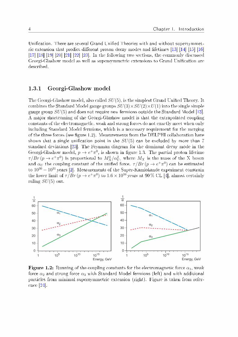
1.2 Running of the coupling constants for the electromagnetic force α1,weak force α2 and strong force α3 with Standard Model fermions (left)and with additional particles from minimal supersymmetric extension(right). Figure is taken from reference [24]. . . . . . . . . . . . . . . . . 4
1.3 Feynman diagrams for proton decay via p→ e+π0 in Grand Unication(left) and via p→ νK+ with supersymmetric extension (right). . . . . . 5
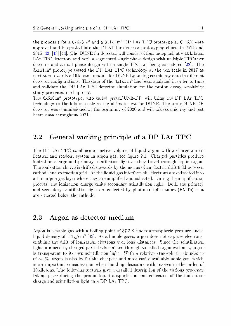
2.1 Sketch of a dual phase liquid argon time projection chamber. Figure istaken from reference [28]. . . . . . . . . . . . . . . . . . . . . . . . . . . 12
2.2 Linear stopping power −dE/ds of muons, pions, kaons and protons inliquid argon as function of their kinetic energy according to the Betheequation 2.1. The liquid argon density used for this plot is 1.4 g/cm3. . 14
2.3 Left: drift velocity of electrons in liquid argon for drift elds 0.1 kV/cm <εD < 100 kV/cm from dierent measurements [37] [58] [59] [60] [61][62].All data are corrected to a common temperature of 87K according toequation 2.6. The zoom-in shows the drift eld region of interest for LArTPCs. The solid line is a t of all data points between 0 and 2 kV/cm ac-cording to the function in equation 2.7. The gure is taken from reference[42]. Right: ratio qeDq,T/µq for drift elds 1 kV/cm < εD < 10 kV/cmfrom dierent measurements, where qe is the charge of the electron,µq = vD/εD the electrical mobility and Dq,T the transverse diusionconstant. The solid line shows a t of all data points according to thefunction in equation 2.16. All data sets are described in reference [67].The gure is taken from reference [42]. . . . . . . . . . . . . . . . . . . 17
2.4 Left: longitudinal and transverse electron diusion for a drift eld ofε = 0.5 kV/cm as a function of drift time and drift distance. Right:attenuation of the drifting electrons for a drift eld of ε = 0.5 kV/cm asa function of O2-equivalent impurities, drift time and drift distance. . . 20
2.5 Left: energy potential of the electron in liquid Φl and gas Φg as functionof the distance to the liquid-gas interface at z = 0. Right: potentialbarrier V for electrons crossing the liquid-gas interface as a function ofthe extraction eld in liquid εl. . . . . . . . . . . . . . . . . . . . . . . 23
xiii
xiv List of Figures
2.6 Left: shares of the fast and slow electron extraction component as afunction of the extraction eld in liquid εl. Data is taken from reference[78]. Right: characteristic extraction time of the slow component as afunction of the extraction eld in liquid εl. Data is taken from reference[75]. . . . . . . . . . . . . . . . . . . . . . . . . . . . . . . . . . . . . . 24
2.7 Left: electron drift velocity in argon gas as a function of the reducedelectric eld measured by [79]. The electric eld in the top axis corre-sponds to SATP. Figure is taken from reference [42]. Right: longitudinaland transverse diusion coecients in argon gas as a function of the re-duced electric eld. The electric eld in the top axis corresponds toSATP. Figure is taken from reference [42]. . . . . . . . . . . . . . . . . 25
2.8 Left: electron-argon atom cross section for elastic scattering, total exci-tation and ionization as a function of electron kinetic energy. Figure istaken from reference [42]. Right: energy distributions of free electronsin argon gas for four dierent electric elds obtained from Magboltzsimulations. Figure is taken from reference [42]. . . . . . . . . . . . . . 26
2.9 Technical drawing of the 3x1x1m3 dual phase liquid argon time projec-tion chamber experimental apparatus. . . . . . . . . . . . . . . . . . . . 29
2.10 Technical drawing of the 3x1x1m3 dual phase liquid argon time projec-tion chamber inside the cryostat. . . . . . . . . . . . . . . . . . . . . . 30
2.11 Exploded view drawing of the 3x1m2 charge readout plane sandwich forthe 3x1x1m3 prototype. . . . . . . . . . . . . . . . . . . . . . . . . . . 31
2.12 Left: photograph of the anode with a highlighted readout strip in eachview. Right: photograph of the LEM with indicated hole dimensions.The 60 µm copper coating is visible around the drilled holes. . . . . . . 32
2.13 Electric eld inside the CRP simulated with the GARFIELD softwarepackage. The ionization electrons follow the white lines that representthe continuation of the electric drift eld lines to the anode. The greenlines depict the electric eld lines that emerge from the extraction gridwires. The background color represents the strength of the electric eldaccording to the color scale. . . . . . . . . . . . . . . . . . . . . . . . . 34
2.14 Grouping of the charge readout strips at the level of the FEBs andSGFTs and mapping conventions for anode and LEM modules as wellas charge readout channels. One FEB collects two groups of 32 channelsfrom neighboring anode modules, as depicted by the color code. Thenumbers 1 to 12 inside the boxes show the numbering convention for thetwelve anode and LEM modules. The three meters long readout stripsin view 0 are dened as charge readout channels 0 to 319 and the onemeter long readout strips in view 1 are dened as channels 320 to 1279. 36

List of Figures xv
2.15 Left: CSA gain with a linear regime for input charges of up to 400 fC anda logarithmic regime for charge injections between 400 fC and 1 250 fC.Right: CSA response to an instantaneous charge injection of 1 fC. Theamplitude is dened by the CSA gain in the linear regime of g =2.5 mV/fC and the shape by the CSA shaping function. The integral is10.1 mV · µs. . . . . . . . . . . . . . . . . . . . . . . . . . . . . . . . . . 37
3.1 Averaged waveform of channel 320 in view 1 after pedestal subtractionfrom pulsing with 150mV and 100 ns ramp-up time. . . . . . . . . . . . 42
3.2 Integrated pulsing signals for charge injections of 150mV in all readoutchannels. Values outside the green shaded area are excluded from thecalibration. . . . . . . . . . . . . . . . . . . . . . . . . . . . . . . . . . 43
3.3 Calibration factors obtained with dierent charge injections normalizedto calibration factor obtained with a charge injection of 150 fC. . . . . . 44
3.4 Normalized CSA shaping function and normalized averaged pulsing wave-forms in view 0 and view 1. The dashed line in the zoom shows the tof the pulsing waveforms. . . . . . . . . . . . . . . . . . . . . . . . . . . 45
3.5 Top: event display of noise run 729. The FCN manifests as horizontallines, typically in groups of 32 channels. Bottom: waveform of channel540. The SBO shapes the baseline to a sine wave. . . . . . . . . . . . . 46
3.6 Normalized cross-correlation RNCC according to equation 3.6 for all read-out channel pairs in noise run 729. Strong correlations between groups ofneighboring channels with multiplicities of 16, 32, 48 and 64 are observed. 47
4.1 Top: event display of a crossing muon after pedestal subtraction. FCNand SBO patterns are clearly visible. Since time and channel numbercan be converted into spatial coordinates, the event display shows theprojections of the crossing muon along the two readout views. Bottom:Waveform of channel 850 containing ionization charge from the crossingmuon at t ≈ 600 µs. . . . . . . . . . . . . . . . . . . . . . . . . . . . . . 53
4.2 Top: event display of a crossing muon after noise lter. Bottom: Wave-form of channel 850 containing ionization charge from the crossing muonat t ≈ 600 µs. . . . . . . . . . . . . . . . . . . . . . . . . . . . . . . . . 54
4.3 Noise-ltered waveform with tted single and adjacent hits. . . . . . . . 56
4.4 Dashed empty histograms: simulated particle ux entering the TPC.Solid lled histograms: simulated particle ux that fullls the PMTtrigger condition. . . . . . . . . . . . . . . . . . . . . . . . . . . . . . . 59
4.5 Direction of selected tracks in data run 840. The denitions of θ and φare given in table 4.1. The main peak at low θ and φ reects triggeringmuons that cross the detector along the 3meter view. The second peakaround θ = 155 is at in φ and originates from so called o-time muonsthat entered the detector within one readout window before or after atrigger and therefore follows the primary cosmic muon ux. . . . . . . . 59

xvi List of Figures
4.6 Position of all hits in the selected tracks in the projection of view 1 indata run 840. The triggering muons are clearly visible as at tracksentering from the sides. The o-time muons are randomly distributedinside the detector, c.f. gure 4.5. The dark vertical lines with fewerhits depict the LEM borders (every 50 cm) and malfunctioning readoutchannels. . . . . . . . . . . . . . . . . . . . . . . . . . . . . . . . . . . . 60
4.7 Mean hit full width at half maximum (FWHM), amplitude and chargein view 0 for the selected tracks as function of the track direction in data(left) and Monte Carlo (right). The rst bin in φ and the last bin in θare left empty since they contain tracks with only a handful of long hitsin view 0 that are often not well reconstructed. . . . . . . . . . . . . . . 62
4.8 Position of all hits in the selected tracks in the charge readout plane. Asin gure 4.8, the triggering muons are visible as tracks entering from theleft or right and the o-time muons are randomly distributed across thereadout plane. The dark vertical lines with fewer hits depict the LEMborders (every 50 cm) and malfunctioning readout channels, c.f. gure4.6. . . . . . . . . . . . . . . . . . . . . . . . . . . . . . . . . . . . . . 63
4.9 Average dQ/ds across the charge readout plane and mean dQ/ds for eachLEM. The four corner LEMs were operated at lower voltage dierences. 63
4.10 Hit dQ/ds distribution in both readout views t with a convolution ofa Landau and a Gaussian distribution. The t range from 4 fC/cm to30 fC/cm excludes the tail on the left that originates from noise hits. . 65
5.1 Sketch of the Deep Underground Neutrino Experiment. The acceleratorcomplex and near detector are hosted at Fermilab and the far detectoris hosted at the Sanford Underground Research Facility. Figure is takenfrom reference [28]. . . . . . . . . . . . . . . . . . . . . . . . . . . . . . 67
5.2 Simulated DUNE neutrino (left) and antineutrino (right) beam ux atthe far detector, normalized to 1.1 × 10²¹ protons on target (POT).Contaminations arise from semileptonic and hadronic decays of kaonsand in-ight decaying muons. Some parameters of the LBNF beamline,such as target and magnetic horn design, have not been optimized yetand the shown ux is simulated with the reference beam design. Figureis taken from reference [99]. . . . . . . . . . . . . . . . . . . . . . . . . 69
5.3 DUNE near detector complex with ArgonCube (right) and MPF (mid-dle) in extreme o-axis position. The 3DST+KLOE detector (left) willbe permanently on-axis. The neutrino beam enters from the right asindicated by the red line that penetrates the 3DST+KLOE detector. . 70
5.4 Technical drawing of the 12 kiloton dual phase LAr TPC far detectormodule for DUNE. Figure is taken from reference [28]. . . . . . . . . . 72
5.5 Neutrino oscillation parameters obtained by NuFit v4.1 [103] [104]. ∆m3l =∆m31 > 0 for normal mass ordering and ∆m3l = ∆m32 < 0 for invertedmass ordering. Inverted mass ordering is disfavored by ∆χ2 = 9.3. Fig-ure is taken from reference [104]. . . . . . . . . . . . . . . . . . . . . . 76

List of Figures xvii
5.6 Electron neutrino (left) and antineutrino (right) appearance probabilityin the DUNE muon neutrino and antineutrino beams at the far detec-tor (L = 1 300 km) for normal neutrino mass ordering and dierent truevalues of δCP as function of neutrino energy. The black line shows the ap-pearance probability if θ13 was equal to zero, in which case no dierencebetween neutrinos and antineutrinos could be observed (c.f. equation5.13). Figure is taken from reference [99]. . . . . . . . . . . . . . . . . . 76
5.7 Left: signicance√
∆χ2 between normal (NO) and inverted (IO) neu-trino mass ordering as function of the true value of δCP for seven (blue)and ten (orange) years of data taking, assuming true normal neutrinomass ordering and the detector employment and beam operation sched-ule outlined in this section. Multiple ts with random throws for vari-ations in statistics, systematic uncertainties and oscillation parametershave been performed. The solid lines represent the median sensitivityof all ts and the transparent bands cover 68% (1σ) of all ts. Figureis taken from reference [99]. Right: signicance
√∆χ2 between NO
and IO as function of experiment run time, assuming the same detec-tor employment and beam operation schedule. The red band shows thediscrimination power for δCP = −π/2 and the green band for all truevalues of δCP. The solid black lines at the top of both bands representthe sensitivity when sin2 (θ23) is constrained to 0.088 ± 0.003 and thedashed lines at the bottom of both bands when θ23 is left unconstrained.Figure is taken from reference [99]. . . . . . . . . . . . . . . . . . . . . 77
5.8 Left: signicance σ with which the non-existence of CP violation inthe neutrino sector can be excluded as function of the true value ofδCP for seven (blue) and ten (orange) years of data taking, assumingtrue normal neutrino mass ordering and the detector employment andbeam operation schedule outlined in this section. Multiple ts withrandom throws for variations in statistics, systematic uncertainties andoscillation parameters have been performed. The solid lines representthe median sensitivity of all ts and the transparent bands cover 68%(1σ) of all ts. Figure is taken from reference [99]. Right: signicance σwith which the non-existence of CP violation in the neutrino sector canbe excluded as function of experiment run time for 75% (dark green) and50% (turquoise) of δCP values in δCP ∈ [−π,+π) and for the maximumCP violating phase of δCP = −π/2 (red). The solid black lines at thetop of each band represent the sensitivity when sin2 (θ23) is contrainedto 0.088± 0.003 and the dashed lines at the bottom of both bands whenθ23 is left unconstrained. Figure is taken from reference [99]. . . . . . . 78
5.9 Neutrino luminosities from a core-collapse supernova. The red curverepresents the identical luminosities of νµ, νµ, ντ and ντ . The meanneutrino energy is ∼10 MeV. Figure is taken from reference [107]. . . . 80

xviii List of Figures
6.1 Black curve: renormalized nucleon density distribution for argon as afunction of radial position according to the Woods-Saxon model in equa-tion 6.2 with parameters R = 3.53 fm and a = 0.54 fm [124]. Red curve:renormalized nucleon density distribution multiplied by square of radialposition, showing the radial probability distribution of nucleons insidethe argon nucleus. . . . . . . . . . . . . . . . . . . . . . . . . . . . . . . 86
6.2 Neutron (left) and proton (right) momentum distribution in argon forglobal relativistic Fermi gas with Bodek-Ritchie extension (GRFG BR)and local Fermi Gas (LFG). . . . . . . . . . . . . . . . . . . . . . . . . 87
6.3 Proton momentum vs. radial position for a local Fermi gas in argon.According to the Woods-Saxon model, the nucleon density is highest atthe center of the nucleus and drops towards its edge, resulting in thesame trend for the Fermi momentum (c.f. section 6.1.1 and equation 6.4). 88
6.4 Points: total K+-nucleon cross section data obtained from a partialwave analysis provided through the INS DAC services [126] [127]. Line:interpolation of data points with 3rd order polynomials. . . . . . . . . . 89
6.5 Total averaged cross sections per nucleon for proton, neutron and pioninteractions in 40
18Ar obtained from a partial wave analysis providedthrough the INS DAC services [126] [127]. . . . . . . . . . . . . . . . . 90
6.6 Points: nal state interaction shares of K+ inside 4018Ar as a function
of kinetic energy for single nucleon and multi-nucleon elastic scatterprocesses in the GENIE hA2018 model as measured by Friedman [129].Line: interpolation of data points with 2nd order polynomials. . . . . . 91
6.7 Points: nal state interaction shares of K+ inside 4018Ar as function of
kinetic energy for single nucleon elastic scatters and charge exchange inthe GENIE hN2018 model obtained from a partial wave analysis pro-vided through the INS DAC services [126] [127]. Line: interpolation ofdata points with 3rd order polynomials. . . . . . . . . . . . . . . . . . . 93
6.8 Top: HKKM2014 unoscillated dierential atmospheric muon neutrinoux at maximum solar activity for the Sanford Underground ResearchFacility at Eν = 100 MeV as function of cos(θ) and φ. cos(θ) = −1points upwards (antiparallel to gravity) and cos(θ) = 1 points down-wards in the direction of gravity. φ = 0 points south and φ = 90
points east. Bottom left: same ux as in the top plot, averaged overzenith and azimuth angles and shown over the full energy range. Thedierence between neutrino and antineutrino uxes (see picture on theright) is too small to be resolved in logarithmic scale. Bottom right:zoom of the left plot in linear scale with separate uxes for neutrinos anantineutrinos. . . . . . . . . . . . . . . . . . . . . . . . . . . . . . . . . 95
6.9 Bottom: HKKM2014 oscillated dierential atmospheric neutrino ux atmaximum solar activity averaged over zenith and azimuth angles for theSanford Underground Research Facility up to 1000 MeV. The oscillationpattern as function of neutrino energy is clearly visible for muon and tauneutrinos and antineutrinos, c.f. equation 5.10 in section 5.2.1. . . . . . 96
List of Figures xix
6.10 Total (top), charged current (bottom left) and neutral current (bottomright) cross sections on argon of all six neutrino avors as function ofneutrino energy for GENIE tune G18_02a_02_11a. The neutral cur-rent cross-sections are identical for all neutrino avors νe, νµ and ντ aswell as for all antineutrino avors νe, νµ and ντ . . . . . . . . . . . . . . 98
6.11 Charged current (top) and neutral current (bottom) muon neutrino crosssections on argon for all processes as function of neutrino energy in GE-NIE tune G18_02a_02_11a, c.f. table 6.2. The charged current elasticscattering o single electrons is only implemented for electron neutrinosand antineutrinos in GENIE as the corresponding energy threshold formuon and tau neutrinos and antineutrinos is very high, see section 6.4.3.1. 99
6.12 Ratio of the charged current quasi-elastic scatter cross sections fromthe Nieves model over the Llewellyn-Smith model as implemented inGENIE for tune G18_10b_00_000 and G18_02a_02_11a, respectively(c.f. table 6.1). . . . . . . . . . . . . . . . . . . . . . . . . . . . . . . . 105
6.13 Ratio of the charged meson exchange current cross sections from theValencia model over the empirical model as implemented in GENIE fortune G18_10b_00_000 and G18_02a_02_11a, respectively (c.f. table7.1). . . . . . . . . . . . . . . . . . . . . . . . . . . . . . . . . . . . . . 106
7.1 Signal K+ kinetic energy distributions before and after nal state inter-actions (FSI) for GENIE tunes G18_02a_02_11a and G18_10b_00_000.The total number of signal K+ after FSI in tune G18_10b_00_000 isreduced by 15 % as the hN2018 intranuclear propagation model includescharge exchange of K+ into K0, c.f. table 7.1. In both tunes, the scat-tered K+ distributions peak at low kinetic energies. . . . . . . . . . . . 110
7.2 Kinetic energy distributions of struck protons and neutrons after leav-ing the argon nucleus in the proton decay signal samples for GENIEtunes G18_02a_02_11a and G18_10b_00_000. The sharp drop atEkin = 25 MeV in tune G18_10b_00_000 reects the fact that protonsand neutrons below 25 MeV do not interact in the hN2018 intranuclearpropagation model (see section 6.2.0.2). . . . . . . . . . . . . . . . . . . 110
7.3 Dierential atmospheric neutrino-argon interaction spectrum normal-ized to 1 megaton · year (top) and ratio of charged current over neutralcurrent interactions (bottom) for all neutrino avors in the G18_02a_02_11asample. . . . . . . . . . . . . . . . . . . . . . . . . . . . . . . . . . . . . 113
7.4 Dierential muon neutrino-argon interaction spectrum for all chargedcurrent (top) and neutral current (bottom) processes normalized to1 megaton · year in the G18_02a_02_11a sample. . . . . . . . . . . . . 114
7.5 Kinetic energy distributions of all nal state particles except neutrinosfrom all neutrino avors and interaction processes at an exposure of1 megaton · year in the G18_02a_02_11a background sample. The lastbin on the x-axis represents D mesons as well as Λ and Σ baryons and thebin size along the y-axis is 10 MeV. The corresponding 1D distributionscan be found in gure C.1 in appendix C. . . . . . . . . . . . . . . . . . 117

xx List of Figures
7.6 Event display of a typical proton decay event (top) and a muon neutrinocharged current quasi-elastic scatter (bottom). The top waveform showsthe channel around 435 cm in view 1 and the bottom waveform at around445 cm in view 1. Since the event time is always set to 0, the driftdistance is obtained by multiplying the measured drift time with thedrift velocity. . . . . . . . . . . . . . . . . . . . . . . . . . . . . . . . . 118
7.7 Event distributions for the total number of hits in both views (top left),total charge of all hits in both views (top right) and number of recon-structed tracks with QTrack, LAr > 40 fC in the best view (bottom) in theG18_02a_02_11a signal and 10 megaton · years background samples. . 126
7.8 Track charge distributions in liquid argon measured in the best view inthe G18_02a_02_11a signal (top) and 10 megaton · years background(bottom) samples before event preselection. The signal sample is renor-malized to 100 000 events before event preselection for the middle plot.The bin size along the y-axis in both plots is 10 fC. The corresponding1D distributions can be found in gure C.2 in appendix C. . . . . . . . 127
7.9 Track charge distributions in liquid argon measured in the best view inthe G18_02a_02_11a signal (top) and 10 megaton · years background(bottom) samples after event preselection. The signal sample is renor-malized to 100 000 events before event preselection for this plot. Thebin size along the y-axis in both plots is 10 fC. The corresponding 1Ddistributions can be found in gure C.3 in appendix C. . . . . . . . . . 129
7.10 Maximum share of readout channels without a hit assigned to the 3Dtrack between track starting and stopping point in both viewsNTrack, Missing hits
in the G18_02a_02_11a signal (top) and 10 megaton · years background(bottom) samples after event preselection. The signal sample is renor-malized to 100 000 events before event preselection for this plot. Thebin size along the y-axis in both plots is 0.01. The corresponding 1Ddistributions can be found in gure C.4 in appendix C. . . . . . . . . . 130
7.11 3D track stopping power proles with the mean stopping power 〈−dE/ds〉and residual kinetic energy Ekin, residual at each hit for signal K+ and forprotons, π± and µ± in background events in the G18_02a_02_11a sig-nal and 10 megaton · years background samples after event and particlepreselection. The signal sample is renormalized to 100 000 events beforeevent preselection for this plot. . . . . . . . . . . . . . . . . . . . . . . 133
7.12 3D track fraction vs. signal K+-likeness of signal K+ and of protons,π± and µ± tracks in the background sample obtained from the neu-ral network using the G18_02a_02_11a signal and 10 megaton · yearsbackground samples after event and particle preselection. . . . . . . . . 134

List of Figures xxi
7.13 Number of 3D tracks misidentied as signal K+ in signal (top) andbackground (bottom) sample as function of signal K+ track selectioneciency using the signal K+-likeness obtained from the neural networkin the G18_02a_02_11a signal and 10 megaton · years background sam-ples after event and particle preselection. The signal sample is renor-malized to 100 000 events before event preselection for this plot. . . . . 135
7.14 Track length distributions in the G18_02a_02_11a signal (top) and10 megaton · years background (bottom) samples after event preselec-tion. The signal sample is renormalized to 100 000 events before eventpreselection for this plot. The bin size along the y-axis in both plots is1 cm. The corresponding 1D distributions can be found in gure C.5 inappendix C. . . . . . . . . . . . . . . . . . . . . . . . . . . . . . . . . . 137
7.15 νµ NC RES background event that motivates cut 4.2.5 to require a min-imum angle between the K+ and µ+ of α > 10 in the best view. Theproton is misidentied as signal K+ and shadows the rst part of the π+
track, which in turn is misidentied as µ+ from the K+ decay, producingan event topology that is very similar to the proton decay signal. . . . . 138
7.16 Number of hits per track in best view in the G18_02a_02_11a signal(top) and 10 megaton · years background (bottom) samples after eventpreselection. The signal sample is renormalized to 100 000 events beforeevent preselection for this plot. The bin size along the y-axis in bothplots is 1. The corresponding 1D distributions can be found in gureC.6 in appendix C. . . . . . . . . . . . . . . . . . . . . . . . . . . . . . 139
7.17 Top: signal K+ selection eciency as function of true kinetic energythroughout the analysis. Since every signal event contains exactly oneK+, the y-axis can also be interpreted as signal event selection eciency.Bottom: signal K+ selection eciency as function of true K+ startdirection after the neural network classication. The ranges of θ and φhave been downsized by exploiting dierent symmetries in the detector:φ = 0 is parallel to the readout strips in one of the readout viewsand φ = 45 is in the middle of both readout view orientations. θ =90 is parallel to the charge readout plane and θ = 0 is parallel andantiparallel to the drift direction. . . . . . . . . . . . . . . . . . . . . . 141
7.18 Event displays of events 3 (top) and 4 (bottom) in table 7.9. In Event3, the proton is misidentied as signal K+ and the π+ as µ+ from K+
decay. Since there are two showering particles e− and e+, the event doesnot pass cut 4.3. The rst part of the proton track (p) in event 4 ismisidentied as signal K+, and the π+ as µ+ from K+ decay. The kinkand two ionization peaks in the proton track are clearly visible, and theseparately reconstructed track p′ fails cut 4.4. . . . . . . . . . . . . . . 144

xxii List of Figures
7.19 Event displays of events 7 (top) and 10 (bottom) in table 7.9. In Event7, the µ− is misidentied as signal K+ and the π+ as µ+ from K+ decay.The additional proton track fails cut 4.4. In Event 10, the proton ismisidentied as signal K+ and the π− as µ+ from K+ decay. Since theµ− is captured by an argon atom, there is no showering particles andthe event fails cut 4.3. . . . . . . . . . . . . . . . . . . . . . . . . . . . 145
7.20 Signal eciency distributions of 200 kiloton · years and 1 megaton · yearsubsamples with one and ve background events, respectively. The blueline indicates the reference eciency εr = 54.2 % for the full 10 megaton · yearsG18_02a_02_11a sample with 50 background events. . . . . . . . . . . 148
7.21 Lower proton lifetime limit over proton decay branching ratio τ/Br (p→ K+ν)at 90 % condence level for exposures up to 1 megaton · year in a DUNEdual phase LAr TPC far detector module, assuming the obtained signalselection eciency of ε = 46 % ± ∆ε. The total uncertainty ∆ε is theroot mean square of the constant systematic uncertainty ∆syst
ε = 0.8 %and the exposure-dependent statistical uncertainty, c.f. equations 7.10through 7.12. The latest published limit from Super-Kamiokande isτ/Br (p→ K+ν) > 5.9× 1033 years at an exposure of 260 kiloton · years[5]. . . . . . . . . . . . . . . . . . . . . . . . . . . . . . . . . . . . . . . 149
A.1 Total averaged cross sections per nucleon for photons in 4018Ar obtained
from a partial wave analysis provided through the INS DAC services[126] [127]. . . . . . . . . . . . . . . . . . . . . . . . . . . . . . . . . . . 155
A.2 DierentialK+-nucleon cross-section probability density function (p.d.f.)for elastic scatters on protons and neutrons and for charge exchange withneutrons in 40
18Ar obtained from a partial wave analysis provided throughthe INS DAC services [126] [127]. . . . . . . . . . . . . . . . . . . . . . 156
A.3 Final state interaction shares of neutrons and protons inside 4018Ar as
function of their kinetic energy in the GENIE hA2018 model. . . . . . . 157A.4 Final state interaction shares of charged and neutral pions inside 40
18Aras function of the pion kinetic energy in the GENIE hA2018 model. . . 157
A.5 Final state interaction shares of neutrons inside 4018Ar as function of the
neutron kinetic energy in the GENIE hN2018 model. The abbreviationCMP stands for compound nucleus formation. The data is obtainedfrom a partial wave analysis provided through the INS DAC services[126] [127]. . . . . . . . . . . . . . . . . . . . . . . . . . . . . . . . . . . 158
A.6 Final state interaction shares of protons inside 4018Ar as function of the
proton kinetic energy in the GENIE hN2018 model. The data is obtainedfrom a partial wave analysis provided through the INS DAC services[126] [127]. . . . . . . . . . . . . . . . . . . . . . . . . . . . . . . . . . . 158
A.7 Final state interaction shares of neutral pions inside 4018Ar as function of
the pion kinetic energy in the GENIE hN2018 model. The abbreviationCMP stands for compound nucleus formation. The data is obtainedfrom a partial wave analysis provided through the INS DAC services[126] [127]. . . . . . . . . . . . . . . . . . . . . . . . . . . . . . . . . . . 159

List of Figures xxiii
A.8 Final state interaction shares of positively charged pions inside 4018Ar as
function of the pion kinetic energy in the GENIE hN2018 model. Thedata is obtained from a partial wave analysis provided through the INSDAC services [126] [127]. . . . . . . . . . . . . . . . . . . . . . . . . . . 159
A.9 Final state interaction shares of negatively charged pions inside 4018Ar as
function of the pion kinetic energy in the GENIE hN2018 model. Thedata is obtained from a partial wave analysis provided through the INSDAC services [126] [127]. . . . . . . . . . . . . . . . . . . . . . . . . . . 160
B.1 Charged current (top) and neutral current (bottom) electron neutrinocross sections on argon for all processes as function of neutrino energyin GENIE tune G18_02a_02_11a, c.f. table 6.2 in section 6.4.3. . . . . 162
B.2 Charged current (top) and neutral current (bottom) electron antineu-trino cross sections on argon for all processes as function of neutrinoenergy in GENIE tune G18_02a_02_11a, c.f. table 6.2 in section 6.4.3. 163
B.3 Charged current (top) and neutral current (bottom) muon antineutrinocross sections on argon for all processes as function of neutrino energyin GENIE tune G18_02a_02_11a, c.f. table 6.2 in section 6.4.3. Thecharged current elastic scattering o single electrons is only implementedfor electron neutrinos and antineutrinos in GENIE as the correspondingenergy threshold for muon and tau neutrinos and antineutrinos is veryhigh, see section 6.4.3.1. . . . . . . . . . . . . . . . . . . . . . . . . . . 164
B.4 Charged current (top) and neutral current (bottom) tau neutrino crosssections on argon for all processes as function of neutrino energy inGENIE tune G18_02a_02_11a, c.f. table 6.2 in section 6.4.3. Thecharged current elastic scattering o single electrons is only implementedfor electron neutrinos and antineutrinos in GENIE as the correspondingenergy threshold for muon and tau neutrinos and antineutrinos is veryhigh, see section 6.4.3.1. . . . . . . . . . . . . . . . . . . . . . . . . . . 165
B.5 Charged current (top) and neutral current (bottom) tau antineutrinocross sections on argon for all processes as function of neutrino energyin GENIE tune G18_02a_02_11a, c.f. table 6.2 in section 6.4.3. Thecharged current elastic scattering o single electrons is only implementedfor electron neutrinos and antineutrinos in GENIE as the correspondingenergy threshold for muon and tau neutrinos and antineutrinos is veryhigh, see section 6.4.3.1 . . . . . . . . . . . . . . . . . . . . . . . . . . . 166
C.1 Kinetic energy distributions of all nal state particles except neutrinosfrom all neutrino avors and interaction processes at an exposure of1 megaton · year in the G18_02a_02_11a background sample. . . . . . 167
C.2 Track charge distributions in liquid argon measured in the best view inthe G18_02a_02_11a signal (top) and 10 megaton · years background(bottom) samples before event preselection. The signal sample is renor-malized to 100 000 events before event preselection. . . . . . . . . . . . 168

xxiv List of Figures
C.3 Track charge distributions in liquid argon measured in the best view inthe G18_02a_02_11a signal (top) and 10 megaton · years background(bottom) samples after event preselection. The signal sample is renor-malized to 100 000 events before event preselection for this plot. Thebin size along the y-axis in both plots is 10 fC. . . . . . . . . . . . . . . 169
C.4 Maximum share of readout channels without a hit assigned to the 3Dtrack between track starting and stopping point in both viewsNTrack, Missing hits
in the G18_02a_02_11a signal (top) and 10 megaton · years background(bottom) samples after event preselection. The signal sample is renor-malized to 100 000 events before event preselection for this plot. Thebin size along the y-axis in both plots is 0.01. . . . . . . . . . . . . . . 170
C.5 Track length distributions in the G18_02a_02_11a signal (top) and10 megaton · years background (bottom) samples after event preselec-tion. The signal sample is renormalized to 100 000 events before eventpreselection for this plot. The bin size along the y-axis in both plots is1 cm. . . . . . . . . . . . . . . . . . . . . . . . . . . . . . . . . . . . . . 171
C.6 Number of hits per track in best view in the G18_02a_02_11a signal(top) and 10 megaton · years background (bottom) samples after eventpreselection. The signal sample is renormalized to 100 000 events beforeevent preselection for this plot. The bin size along the y-axis in bothplots is 1. . . . . . . . . . . . . . . . . . . . . . . . . . . . . . . . . . . 172

List of Tables
2.1 Symbols, denitions and values or units of universal constants, particlevariables and liquid argon properties that are used in section 2.3.1. . . 13
2.2 Longitudinal diusion coecient measured by three dierent experi-ments. The results are corrected for eventual initial spreads of thedrifting electron clouds at their origin. They are, however, not cor-rected for the contribution of Coulomb repulsion among the driftingelectrons, which depends on the electron density and was estimated tobe 0.2mm2/ms in the case of ICARUS 3T. . . . . . . . . . . . . . . . . 19
2.3 Top: nominal TPC high voltage settings and elds. Bottom: nominalPMT high voltage settings and gains. . . . . . . . . . . . . . . . . . . . 35
3.1 Fit parameters describing normalized averaged pulsing waveforms inview 0 and view 1 according to equation 3.5. . . . . . . . . . . . . . . . 45
3.2 Normalization factor K and cuto energy EC for dierential primarycosmic ray nucleon ux of the considered particles according to equation3.7. . . . . . . . . . . . . . . . . . . . . . . . . . . . . . . . . . . . . . . 47
4.1 Denitions of θ and φ in the detector coordinate system. . . . . . . . . 57
4.2 Number of collected events, trigger conguration and electric eld set-tings of run 840. . . . . . . . . . . . . . . . . . . . . . . . . . . . . . . . 57
6.1 List of event generation models for the two GENIE tunes used in theproton decay sensitivity study in chapter 7. The abbreviation GRFGBR stands for global relativistic Fermi gas with Bodek-Ritchie extension.∗the atmospheric neutrino ux simulation is not part of GENIE butmentioned in this table to provide a clear overview of all models involvedin the event generation. . . . . . . . . . . . . . . . . . . . . . . . . . . . 84
6.2 Possible neutrino interaction processes on heavy atoms classied by scat-tering partner. All processes can occur via neutral and charged current.The scattering o two correlated nucleons is also called meson exchangecurrent (MEC). . . . . . . . . . . . . . . . . . . . . . . . . . . . . . . . 97
6.3 List of neutrino-argon interaction models for the two GENIE tunes usedin the proton decay sensitivity study as already shown in table 6.1. . . 100
xxv
xxvi List of Tables
7.1 Summary of signalK+ nal state interactions for GENIE tunes G18_02a_02_11aand G18_10b_00_000 as well as for NEUT. . . . . . . . . . . . . . . . 111
7.2 Number of atmospheric neutrino interactions on argon for neutrino ener-gies fromEν = 100 MeV to Eν = 100 GeV at an exposure of 1 megaton · yearin the G18_02a_02_11a sample. The elastic electron scatters (EEL)are listed separately since the neutral and charged current processes aremixed in GENIE for electron neutrinos and antineutrinos, and only neu-tral current elastic scatters are simulated for muon and tau neutrinosand antineutrinos. . . . . . . . . . . . . . . . . . . . . . . . . . . . . . . 115
7.3 Parameters used in the 10 kiloton DP LAr TPC detector simulation forthe proton decay sensitivity study. . . . . . . . . . . . . . . . . . . . . . 119
7.4 Upper limit on the number of observed signal events S at 90 % condencelevel for up 10 expected background events B and N0 = B measuredevents according to the Feldman-Cousins approach. Values are takenfrom tables V and IV in reference [138]. . . . . . . . . . . . . . . . . . . 123
7.5 Main leptonic and semileptonic (left) and hadronic (right) K+ decaymodes and branching ratios obtained from reference [46]. . . . . . . . . 124
7.6 Signal and background selection eciencies and total numbers of back-ground events for event preselection cuts in the G18_02a_02_11a signaland 10 megaton · years background samples. The cut labeled as 1 com-bines cuts 1.1, 1.2 and 1.3. . . . . . . . . . . . . . . . . . . . . . . . . . 125
7.7 Number of 3D tracks before and after event preselection, after individualand combined track preselection cuts and after the neural network clas-sication in the G18_02a_02_11a signal and 10 megaton · years back-ground samples. The signal sample is renormalized to 100 000 eventsbefore event preselection for this table. The cut labeled as 2 combinescuts 2.1, 2.2 and 2.3. . . . . . . . . . . . . . . . . . . . . . . . . . . . . 131
7.8 Signal and background selection eciencies and number of backgroundevents for event preselection and consecutive nal event selection cuts inthe G18_02a_02_11a signal and 10 megaton · years background samples.140
7.9 Background events in the 10 megaton · years G18_02a_02_11a samplethat survive nal event selection cut 4.2. The nal state particles (FSP)emerging from the neutrino interaction and the signal particles they aremisidentied as (ID) are shown in the right column. Only two eventssurvive cut 4.3 and the nal state particle with IDX refers to the particlethat fails cut 4.4. . . . . . . . . . . . . . . . . . . . . . . . . . . . . . . 142
7.10 Signal and background selection eciencies and number of backgroundevents for individual and combined event preselection cuts and for con-secutive nal event selection cuts in the G18_10b_00_000 signal and2 megaton · years background samples. . . . . . . . . . . . . . . . . . . 146
7.11 Signal selection eciencies ε and numbers of expected background eventsB for the G18_02a_02_11a and G18_10b_00_000 samples. . . . . . 146
Chapter 1
Introduction
Proton decay has rst been theorized by Andrei Sakharov as a possible explanationfor the matter-antimatter asymmetry in today's universe, and independent theoreticalconsiderations in particle physics have delivered dierent potential processes throughwhich the proton can decay. The pioneering theoretical groundwork has triggered bigexperimental eorts across the world, but no evidence for proton decay has been founduntil this very day, excluding many of the aforementioned theories. Future protondecay experiments will yield an increase in sensitivity by a factor of ∼10, allowing totest some of the most promising remaining theories.This chapter begins with a brief history of theoretical considerations and experimentalsearches for proton decay in section 1.1. Subsequently, dierent theoretical frameworksand their role in proton decay are explained in more detail in sections 1.2 through 1.4.Eventually, future proton decay experiments are discussed in section 1.5.
1.1 A brief history of proton decay
Forbidden in the Standard Model of Particle Physics, proton decay has rst been con-sidered by Andrei Sakharov in 1967 as one of the three so-called Sakharov conditionsto explain the asymmetry of matter and antimatter that is observed in the universe[1]. In the 1970s, theories for Grand Unication and Supersymmetry were developed toaddress unanswered questions in particle physics that are not directly related to protondecay. One prediction of Grand Unication and Supersymmetry, however, is protondecay. The dominant proton decay modes of the various Grand Unied Theories withand without supersymmetric extension are p→ νK+ and p→ e+π0, respectively. Thepredicted proton lifetime depends on the details of the dierent theories and variesbetween 1028 years and 1039 years [2].Experimental searches for proton decay began in the early 1980s with the Fréjus,Soudan, IMB and Kamiokande underground experiments. Fréjus and Soudan used irontracking calorimeters, a technology in which the bulk of the detector mass, and thus themajority of the observed protons, is stored in thin iron plates or iron oxide-loaded con-crete plates. The decay products of the proton can be measured with gas proportionaltubes located in between the iron or concrete plates. The IMB and Kamiokande ex-
1

2 Chapter 1. Introduction
periments both deployed fully active water Cherenkov detectors. The ultrapure waterin these detectors is surrounded by photomultiplier tubes that measure the Cherenkovradiation emitted by the decay products of the protons. Cherenkov radiation is emittedwhen charged particles travel faster than the speed of light in a medium. The mainbackground in all four experiments originates from atmospheric neutrinos interactinginside the detector. Analyses with hard selection cuts have been carried out in order tosearch for proton decay at the few-events level in low-background conditions. Despiterunning for several years, none of the experiments found evidence for proton decay,and lower lifetime limits for dierent decay modes were determined. For the two mostcommonly discussed decay modes, the lower lifetime limits per branching ratio wereτ/Br (p→ e+π0) > 5.5 × 1032 years and τ/Br (p→ νK+) > 1.6 × 1032 years at 90%condence level (CL) [3]. In order to probe higher proton lifetimes, larger detectorswith more protons were needed. The Soudan 2 and Super-Kamiokande detectors, bothbigger versions of their predecessors, started taking data in 1989 and 1996, respectively.Soudan 2 completed operation in 2001 and Super-Kamiokande, after being upgradedseveral times, still continues taking data without having found evidence for protondecay. Super-Kamiokande improved the lifetime limits in almost all decay modes, andthe current best limits, among others, are τ/Br (p→ e+π0) > 1.6 × 1034 years andτ/Br (p→ νK+) > 5.9 × 1033 years at 90% CL [4] [5]. In addition to the search forproton decay, the aforementioned experiments are also able to measure neutrinos of var-ious origins. Important discoveries include the detection of Supernova burst neutrinoswith Kamiokande and IMB in 1987 [6] [7] and the observation of neutrino oscillations inthe atmospheric neutrino ux by Super-Kamiokande in 1998 [8]. Since 2009, the Super-Kamiokande detector is used as far detector in the long baseline neutrino oscillationexperiment T2K [9].
1.2 The Standard Model of Particle Physics
The Standard Model of Particle Physics describes all known elementary particles andtheir interactions through the electromagnetic, weak and strong forces, see gure 1.1.The gravitational force is not described in the Standard Model.The elementary particles can be divided into fermions and bosons, with every fermionhaving a corresponding antifermion with the same properties except for opposite elec-tric charge. Fermions have spin 1/2 and can be further subdivided into quarks andleptons, which are the constituents of all known matter in the universe. Quarks interactthrough all four fundamental forces. Charged leptons interact through the electromag-netic, weak and gravitational forces while neutral leptons, also called neutrinos, onlyinteract through the weak and gravitational forces. The carriers of the electromagnetic,weak and strong forces are called gauge bosons and have spin 1. The discovery of thescalar Higgs boson with spin 0 in 2012 completes the Standard Model.Quarks are only found in bound states within hadrons. There are three types ofhadrons: baryons consisting of three quarks, antibaryons consisting of three antiquarksand mesons consisting of one quark and one antiquark. The baryon number B isconserved in the Standard Model:

1.3 Grand Unication 3
B =1
3(nq − nq) (1.1)
where nq is the number of quarks and nq the number of antiquarks. The proton isthe lightest baryon and consists of two up-quarks and one down-quark. Since protondecay would violate the baryon number conservation, it is forbidden in the StandardModel. However, in some theories that lie beyond the Standard Model, baryon numberviolation is explicitly allowed. The two theories that are most vigorously pursued areGrand Unication and Supersymmetry.
Figure 1.1: Elementary particles in the Standard Model of Particle Physics. Figureis taken from reference [10].
1.3 Grand Unication
In Grand Unied Theories, the electromagnetic, weak and strong forces are merged intoone single force at the so-called unication energy of around 1014 GeV. New massivebosons X, Y with masses close to the unication energy are predicted to be the carriersof the unied force. The unication energy is about 10 orders of magnitude above thehighest ever achieved energy in a laboratory of 13 TeV at the LHC in Geneva, Switzer-land, and a direct test of Grand Unication in the foreseeable future can therefore beexcluded [12]. Proton decay searches constitute a more realistic option to test Grand
4 Chapter 1. Introduction
Unication. There are several Grand Unied Theories with and without supersymmet-ric extension that predict dierent proton decay modes and lifetimes [13] [14] [15] [16][17] [18] [19] [20] [21] [22] [23]. In the following two sections, the commonly discussedGeorgi-Glashow model as well as supersymmetric extensions to Grand Unication aredescribed.
1.3.1 Georgi-Glashow model
The Georgi-Glashow model, also called SU(5), is the simplest Grand Unied Theory. Itcombines the Standard Model gauge groups SU(3)×SU(2)×U(1) into the single simplegauge group SU(5) and does not require new fermions outside the Standard Model [13].A major shortcoming of the Georgi-Glashow model is that the extrapolated couplingconstants of the electromagnetic, weak and strong forces do not exactly meet when onlyincluding Standard Model fermions, which is a necessary requirement for the mergingof the three forces (see gure 1.2). Measurements from the DELPHI collaboration haveshown that a single unication point in the SU(5) can be excluded by more than 7standard deviations [25]. The Feynman diagram for the dominant decay mode in theGeorgi-Glashow model, p → e+π0, is shown in gure 1.3. The partial proton lifetimeτ/Br (p→ e+π0) is proportional to M4
X/α2U , where MX is the mass of the X boson
and αU the coupling constant of the unied force. τ/Br (p→ e+π0) can be estimatedto 1030− 1031 years [2]. Measurements of the Super-Kamiokande experiment constrainthe lower limit of τ/Br (p→ e+π0) to 1.6× 1034 years at 90% CL [4], almost certainlyruling SU(5) out.
Figure 1.2: Running of the coupling constants for the electromagnetic force α1, weakforce α2 and strong force α3 with Standard Model fermions (left) and with additionalparticles from minimal supersymmetric extension (right). Figure is taken from refer-ence [24].

1.3 Grand Unication 5
Figure 1.3: Feynman diagrams for proton decay via p → e+π0 in Grand Unication(left) and via p→ νK+ with supersymmetric extension (right).
1.3.2 Supersymmetric extension
Motivated by the hierarchy problem in particle physics that addresses the fact that theweak force is much stronger than gravity, supersymmetric models assume the existenceof so-called superpartners for every Standard Model particle. In the minimal supersym-metric model, every Standard Model particle has one superpartner. The superpartnerdiers by spin 1/2 from its Standard Model counterpart, resulting in a bosonic su-perpartner for each Standard Model fermion and vice versa [26]. The supersymmetricparticles change the running of the coupling constants so that, for masses of the su-perpartners near the TeV scale, the coupling constants now seem to perfectly meet atthe so-called GUT scale ΛGUT = 1016 GeV [25], see gure 1.2. With a higher X bosonmass near the new unication energy ΛGUT , τ/Br (p→ e+π0) is now predicted to be1035− 1037 years [2], which is compatible with the latest Super-Kamiokande result, c.f.section 1.3.1.Supersymmetric extension of Grand Unied Theories (SUSY GUTs) also enables addi-tional proton decay channels through the exchange of supersymmetric particles. Thesimple coupling of quarks to a single supersymmetric particle predicts proton lifetimesin the order of seconds, which obviously can not be true. Therefore, a new symmetrycalled R-parity PR is introduced:
PR = (−1)3B+L+2s (1.2)
where B is baryon number, L lepton number and s spin. All Standard Model particleshave R-parity of +1 and all supersymmetric particles have R-parity of −1. Since the R-Parity product of all involved particles
∏i PR,i needs to be conserved at all interaction
vertices, proton decay in SUSY GUTs can only occur through loops of supersymmetricparticles. Furthermore, the up and down quarks in the initial state of the proton haveto transition to quarks of a dierent generation in the nal state. Since charm, bottomand top quarks are heavier than a proton, only strange quarks are energetically allowedto appear in the nal state. Proton decay via p→ νK+ is therefore the most commonprediction by SUSY GUTs, with lifetimes of up to 1034 − 1035 years [18] [19] [20] [21]

6 Chapter 1. Introduction
[22] [23], see gure 1.3. The current best limit of τ/Br (p→ νK+) > 5.9 × 1033 yearsat 90 % CL by Super-Kamiokande [5] is below the prediction of many SUSY GUTs andthe search for p→ νK+ remains of great interest.
1.4 Big Bang theory and Baryogenesis
The Big Bang theory describes the evolution of the universe from the earliest peri-ods and makes several testable predictions about today's universe that were conrmedby astronomical observations, such as Hubble's law and the cosmic microwave back-ground. One key assumption of the Big Bang theory is that matter and antimatterwere created in equal amounts and, at high energies in the early universe, the creationand annihilation processes of matter-antimatter-pairs were in equilibrium. Examplesfor these processes are electron-positron- and proton-antiproton-pair production andannihilation:
e− + e+ ↔ γγ (1.3)
p+ p↔ γγ (1.4)
With decreasing energies of the expanding universe, annihilation of matter-antimatter-pairs became dominant over their creation, eventually leading to the annihilation of allmatter and antimatter into photons. The existence of matter and the absence of anti-matter in today's universe, however, implies a small excess of matter over antimatterin the order of 10−10 already in the early universe, both in the baryonic and leptonicsectors. A hypothetical baryonic process that could have created this excess is calledBaryogenesis, and it requires the three so-called Sakharov conditions [1]:
1. Baryon number violation
2. C-symmetry and CP-symmetry violation
3. Interactions out of thermal equilibrium
The rst condition is required since, per denition, the production of an excess ofbaryons over antibaryons violates the baryon number conservation. To ensure thatthere is no process that produces an excess of antibaryons over baryons that counter-balances the former, C- and CP-symmetry violation is required. Lastly, the interactionthat produced the excess of baryons over antibaryons can not have happened in a ther-mal equilibrium, as the gained excess would have been destroyed again by its reversedreaction.C- and CP-symmetry violation was discovered in the weak decay of neutral kaons in1964 [11] and the hypothetical baryon number violating process happened out of thethermal equilibrium when the interaction rate was smaller than the rate of expansionof the universe, which can be easily achieved in the early universe. The only Sakharovcondition that has not been veried yet is the baryon number (B) violating process

1.5 Future proton decay searches 7
itself, for which proton decay is the most promising candidate. Since the predictedproton decay modes conserve B−L by violating both baryon and lepton (L) numbers,proton decay could explain the matter-antimatter asymmetry in the baryon and leptonsector (c.f. sections 1.3.1 and 1.3.2).
1.5 Future proton decay searches
As discussed in section 1.3.1 and 1.3.2, the measured lower lifetime limits for p→ e+π0
and p → νK+, as well as for other decay modes, are below the predicted lifetimes ofmany Grand Unied Theories. Three future experiments that will be able to test pro-ton lifetimes of up to 1035 years are currently being built: Hyper-Kamiokande, JUNOand the Deep Underground Neutrino Experiment (DUNE). Hyper-Kamiokande willdeploy a 258 kilotons water Cherenkov detector that uses the same technology as itspredecessor Super-Kamiokande [27], and the JUNO detector will consist of a sphericaltank with an inner diameter of 35 m that is lled with 20 kilotons of liquid scintillator,a well established technology from neutrino experiments. The DUNE far detector willcomprise four liquid argon time projection chambers (LAr TPCs) with a ducial massof ∼10 kilotons each [28]. While the ducial mass and thus the total number of protonsin DUNE will be a factor of ∼ 10 lower than in Hyper-Kamiokande, DUNE will stillbe competitive in the p → νK+ channel since the K+ from proton decay is too slowto produce Cherenkov light in water. Super- and Hyper-Kamiokande therefore rely onmeasuring the O (MeV) photon emitted by the excited parent nucleus of the decayingproton and the decay products of the K+. The JUNO detector is capable of taggingthe K+ from proton decay but its spatial resolution is limited as only the scintillationlight is recorded by the surrounding PMTs. LAr TPCs on the other hand have a highresolution imaging capability that allows for precise tracking and identication of allcharged particles based on their ionization charge. Since the main background in pro-ton decay searches originates from atmospheric neutrinos, and K+ production is veryrare in neutrino-nucleus interactions, identifying K+ with a high eciency is the keyto a strong background reduction at high signal selection eciencies, and therefore toa good proton decay sensitivity. The LAr TPC technology is explained in detail inchapter 2 on the basis of the 3x1x1m3 dual phase LAr TPC prototype.

8 Chapter 1. Introduction

Chapter 2
The 3x1x1m3 dual phase liquid argon
time projection chamber prototype
Chapter 1 concluded with an outlook on the DUNE experiment that will, among othergoals, search for proton decay with four independent ∼10 kiloton LAr TPC detectormodules. The LAr TPC is a large scale liquid noble gas detector in which the ionizationcharge of charged particles is drifted and collected by narrowly-spaced readout wires toprovide high resolution images of interactions inside the detector. This technology isespecially suitable for the search of rare and faint events, e.g. in long-baseline neutrinooscillation experiments or proton decay and dark matter searches. Argon liquees at87K under atmospheric pressure, making it imperative to operate the whole detectorin well-controlled cryogenic conditions, which adds to the complexity of the system.The rst ton-scale LAr TPC with a signal readout immersed in liquid argon has beensuccessfully operated in the early 1990s as part of the ICARUS experiment. The dualphase LAr TPC is an advancement of the initial single phase LAr TPC technology witha charge amplication and readout system in gaseous argon. The charge amplicationconstitutes a big advantage for faint events and for detector masses at the kilotonscale as it enables longer drift distances of the ionization charge without losing signalstrength due to charge attenuation caused by impurities. The 3x1x1m3 detector is therst ton-scale DP LAr TPC that has been operated in the context of the DUNE fardetector prototyping eorts.In this chapter, a summary of the single and dual phase LAr TPC development in ahistorical context is given in section 2.1, followed by a short explanation of the generalDP LAr TPC working principle in section 2.2. Section 2.3 discusses and quanties therelevant processes of signal production and propagation in a DP LAr TPC. Eventually,a detailed description of the 3x1x1m3 DP LAr TPC prototype is given in section 2.4.
9

10 Chapter 2. The 3x1x1m3 dual phase LAr TPC prototype
2.1 History of the liquid argon time projection cham-
ber
The liquid argon time projection chamber (LAr TPC) is a neutrino, proton decay anddark matter detector technology that was rst considered in 1977 [29]. It aims at com-bining a large ducial mass with a high resolution 3D imaging readout by drifting andcollecting the ionization charge produced in particle interactions in liquid argon overseveral meters. Following a period of R&D studies with small detector volumes thatfocused on the liquid argon purication and readout electronics, the ICARUS collabo-ration continuously operated a 3 ton LAr TPC for several years in the early 1990s anddeployed a 50L LAr TPC in a neutrino beam at CERN in 1997, collecting both highquality cosmic ray and neutrino events [30] [31]. In 2001, the rst surface test of theICARUS 600 ton LAr TPC (T600) was carried out. The recorded cosmic ray eventsserved as basis for the development of reconstruction algorithms and analysis tech-niques. The liquid argon purication has been a major challenge in the development ofICARUS T600 since impurities such as oxygen and water cause ionization charge lossesduring the drift. With a typical drift velocity of 1-2m/ms and a measured electronlifetime of 2ms, the ICARUS T600 detector established the feasibility of electron driftover several meters in a 600 ton LAr TPC [32]. The rst LAr TPC physics experimenteventually started in 2011 when ICARUS T600 was installed at the Gran Sasso Un-derground Laboratory to measure neutrinos originating from CERN over a baseline of730 km [33].Based on the success of the ICARUS T600 surface test in 2001, LAr TPCs were consid-ered as far detectors in long baseline neutrino oscillation experiments with the ultimategoals of measuring the CP violating phase in the lepton sector δCP and the neutrinomass hierarchy. The required mass for the far detector is in the range of 10-100 kilotonsand due to the limited electron lifetime and the resulting drift length threshold, theinitial single phase LAr TPC technology would require a large number of independentTPCs, increasing both cost and complexity. To address this issue, a dual phase LArTPC (DP LAr TPC) design was developed in 2004 [34]. In the DP LAr TPC, theionization charge is extracted into argon gas, where it is amplied and collected. Theamplication process allows for longer drift distances as it recovers losses of the ioniza-tion charge during the drift, enabling a single monolithic DP LAr TPC with a maximumdrift length in the order of 10m and a ducial mass in the order of 10-100 kilotons.While the charge attenuation in liquid argon can be compensated by the amplicationin gas and can likely be further reduced by developing better purication technologies,the diusion of the drifting electrons limits the maximum drift to a distance in theorder of 10m as it becomes comparable to the spatial resolution of the charge readoutof ∼3 mm, see sections 2.3.3.2 and 2.4.2.2. The R&D eorts towards a multi-kilotonDP LAr TPC resulted in a rst 3 L prototype in 2008, successfully demonstrating theDP LAr TPC working principle [35] [36]. In 2011, the second 200L prototype with acharge readout area of 40x76 cm2 and a drift length of 60 cm was operated with a stablecharge amplication factor of 14 [37] [38]. Following more R&D on the charge readoutsystem [39] [40] and the approval of the DUNE long baseline neutrino experiment [41],
2.2 General working principle of a DP LAr TPC 11
the proposals for a 6x6x6m3 and a 3x1x1m3 DP LAr TPC prototype at CERN wereapproved and integrated into the DUNE far detector prototyping eorts in 2014 and2015 [42] [43] [44]. The DUNE far detector will consist of four independent ∼10 kilotonLAr TPC detectors and both a segmented single phase design with multiple TPCs perdetector and a dual phase design with a single TPC are being considered [28]. The3x1x1m3 prototype tested the DP LAr TPC technology at the ton scale in 2017 asnext step towards a 10 kiloton module for DUNE by taking cosmic ray data in dierentdetector congurations. The data of the 3x1x1m3 has been analyzed in order to tuneand validate the DP LAr TPC detector simulation for the proton decay sensitivitystudy presented in chapter 7.The 6x6x6m3 prototype, also called protoDUNE-DP, will bring the DP LAr TPCtechnology to the kiloton scale as the ultimate test for DUNE. The protoDUNE-DPdetector was commissioned at the beginning of 2020 and will take cosmic ray and testbeam data throughout 2021.
2.2 General working principle of a DP LAr TPC
The DP LAr TPC combines an active volume of liquid argon with a charge ampli-cation and readout system in argon gas, see gure 2.1. Charged particles produceionization charge and primary scintillation light as they travel through liquid argon.The ionization charge is drifted upwards by the means of an electric drift eld betweencathode and extraction grid. At the liquid-gas interface, the electrons are extracted intoa thin argon gas layer where they are amplied and collected. During the amplicationprocess, the ionization charge emits secondary scintillation light. Both the primaryand secondary scintillation light are collected by photomultiplier tubes (PMTs) thatare situated below the cathode.
2.3 Argon as detector medium
Argon is a noble gas with a boiling point of 87.3K under atmospheric pressure and aliquid density of 1.4 g/cm3 [45]. As all noble gases, argon does not capture electrons,enabling the drift of ionization electrons over long distances. Since the scintillationlight produced by charged particles is emitted through so-called argon excimers, argonis transparent to its own scintillation light. With a relative atmospheric abundanceof ∼1%, argon is also by far the cheapest and most easily available noble gas, whichis an important consideration when building detectors with masses in the order of10 kilotons. The following sections give a detailed description of the various processestaking place during the production, transportation and collection of the ionizationcharge and scintillation light in a DP LAr TPC.

12 Chapter 2. The 3x1x1m3 dual phase LAr TPC prototype
Figure 2.1: Sketch of a dual phase liquid argon time projection chamber. Figure istaken from reference [28].
2.3.1 Energy loss of charged particles in matter
All symbols used in this section are summarized in table 2.1 and their values are takenfrom reference [46] if not otherwise stated.
There are several mechanisms through which charged particles lose energy when trav-eling in matter. Energy loss through ionization of the target atoms is the dominantmechanism for particle momenta that correspond to βγ = p
m0c. 1000.
When also neglecting the very low momentum region (0.1 . βγ . 1000), the massstopping power through ionization of charged particles heavier than electrons and fortarget materials with intermediate Z-values can be described by the Bethe formula withan accuracy of a few percent:⟨
−dEds
⟩= Kz2Z
A
1
β2
[1
2ln
(2mec
2β2γ2Wmax
I2
)− β2 − δ (βγ)
2
](2.1)
The mass stopping power 〈−dE/ds〉 is the kinetic energy loss per unit length and pertarget material density. Wmax is the maximum energy transfer in a single collision andδ (βγ) the Sternheimer parametrization for the density eect correction that accountsfor the changing behavior of the particle's electric eld at high energies:

2.3 Argon as detector medium 13
Wmax =2mec
2β2γ2
1 + 2γme/M + (me/M)2 (2.2)
δ (βγ) =
δ0102(x−x0), if x < x0
2 ln (10)x− C + a (x1 − x)k , if x0 6 x < x1
2 ln (10)x− C, if x > x1
(2.3)
with x = −log10 (βγ). δ0, x0, x1, C, a and k (sometimes called m) are materialconstants. A general recipe to calculate these constants is described in reference [48]and the corresponding values can be found in reference [45].
Symbol Denition Value or unit
Universal constants
c speed of light in vacuum 3× 10⁸ m/sK 4πNAr
2emec
2 0.307MeV cm2/molNA Avogadro constant 6.02× 10²³ mol−1
re e2/4πε0mec2 (classical electron radius) 2.82 fm
me electron rest mass 0.511MeV/c2
Penetrating particle
v particle velocity m/sM particle rest mass MeV/c2
p particle momentum MeV/cβ v/c
γ 1/√
1− β2 (Lorentz factor)z absolute particle charge
Liquid argon [45]ρ density 1.396 g/cm3
Z atomic number 18A atomic mass 39.948 g/molI mean excitation energy 188 eVδ0 parameter for density correction 0x0 parameter for density correction 0.2x1 parameter for density correction 3.0C parameter for density correction 5.2146a parameter for density correction 0.19559k parameter for density correction 3.0
Table 2.1: Symbols, denitions and values or units of universal constants, particlevariables and liquid argon properties that are used in section 2.3.1.
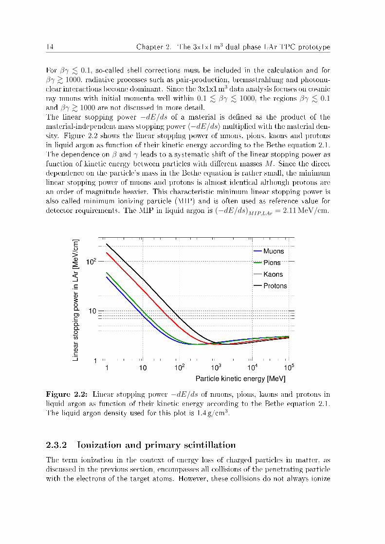
14 Chapter 2. The 3x1x1m3 dual phase LAr TPC prototype
For βγ . 0.1, so-called shell corrections must be included in the calculation and forβγ & 1000, radiative processes such as pair-production, bremsstrahlung and photonu-clear interactions become dominant. Since the 3x1x1m3 data analysis focuses on cosmicray muons with initial momenta well within 0.1 . βγ . 1000, the regions βγ . 0.1and βγ & 1000 are not discussed in more detail.The linear stopping power −dE/ds of a material is dened as the product of thematerial-independent mass stopping power 〈−dE/ds〉multiplied with the material den-sity. Figure 2.2 shows the linear stopping power of muons, pions, kaons and protonsin liquid argon as function of their kinetic energy according to the Bethe equation 2.1.The dependence on β and γ leads to a systematic shift of the linear stopping power asfunction of kinetic energy between particles with dierent masses M . Since the directdependence on the particle's mass in the Bethe equation is rather small, the minimumlinear stopping power of muons and protons is almost identical although protons arean order of magnitude heavier. This characteristic minimum linear stopping power isalso called minimum ionizing particle (MIP) and is often used as reference value fordetector requirements. The MIP in liquid argon is (−dE/ds)MIP,LAr = 2.11 MeV/cm.
Figure 2.2: Linear stopping power −dE/ds of muons, pions, kaons and protons inliquid argon as function of their kinetic energy according to the Bethe equation 2.1.The liquid argon density used for this plot is 1.4 g/cm3.
2.3.2 Ionization and primary scintillation
The term ionization in the context of energy loss of charged particles in matter, asdiscussed in the previous section, encompasses all collisions of the penetrating particlewith the electrons of the target atoms. However, these collisions do not always ionize

2.3 Argon as detector medium 15
the target atom to create an electron-ion pair. If the transferred energy is too small toliberate an electron from its parent atom, the atom transitions into an excited state.The excited state Ar∗ typically lives long enough to form an excited argon dimer Ar∗2with another argon atom in the ground state, also called argon excimer [49]:
Ar∗ + Ar→ Ar∗2
The argon excimer decays by emitting photons in the so-called vacuum ultravioletregion (VUV) with a peak at 128 nm, or 9.7 eV [50]:
Ar∗2 → 2Ar + γ
Argon does not have an atomic electron transition close to 9.7 eV and is thus transparentto the emitted VUV light. This light is usually referred to as primary scintillation light,in order to prevent confusion with the VUV light produced by drifting electrons in argongas, see section 2.3.5.3. Argon excimers can be formed in singlet or triplet states withlifetimes of τ1 ≈ 6 ns and τ2 ≈ 1600 ns, respectively [51] [52]. The exact lifetime valuesof the singlet and triplet states depend on the purity of the argon.If the transferred energy from the penetrating particle is large enough to ionize anargon atom, the liberated electron can escape the region of ionization in some cases.The probability R for an electron to escape the Coulomb attraction of its parent andneighboring ions can be described by a modied version of Birk's law, which initiallydescribes the light yield of ionizing particles:
R =A
1 + 1ρkε
(−dE
ds
) (2.4)
where ρ is the liquid argon density, ε the external electric eld and − (dE/ds) thelocal linear stopping power. The parameters A = 0.8 and k = 0.0486 kV ·MeV−1·g · cm−3 have been measured in a 3 ton LAr TPC by the ICARUS collaboration [53].The external electric drift, which is the drift eld in a LAr TPC, helps the electron toovercome the Coulomb attraction, while a higher − (dE/ds) leads to a higher local iondensity and thus to a stronger Coulomb attraction. Other models that describe therecombination process are the Onsager model [54] and the Box model [55].If the electron can not escape, it will rst lose its kinetic energy in collisions with argonatoms and eventually get captured. In case the electron gets captured by a single argonion, it will produce a photon that will quickly get re-captured by another argon atom.The electron can also get captured by an ionized molecular state of argon Ar+2 thatwas formed by one ionized and one neutral argon atom in the region of ionization.This capture produces a highly excited argon atom Ar∗∗ that will eventually producean argon excimer and scintillation light:

16 Chapter 2. The 3x1x1m3 dual phase LAr TPC prototype
Ar+ + Ar→ Ar+2
Ar+2 + e− → Ar∗∗ + Ar
Ar∗∗ → Ar∗ + heat
Ar∗ + Ar→ Ar∗2Ar∗2 → 2Ar + γ
The dierent ionization and scintillation processes can be summarized by the workfunctions We− = 23.6 eV and Wγ = 19.5 eV, which are experimentally determinedvalues of the average deposited energy that is necessary to create one electron-ion pairand one scintillation photon [56] [49].For a MIP in liquid argon at the 3x1x1m3 nominaldrift eld of ε = 0.5 kV/cm, the average number of free electrons per unit length thatescape the region of ionization can be calculated as follows, c.f. section 2.3.1:
dNe9
ds=
(−dE/ds)MIP, LAr
We9·R =
6.24× 10⁴
cm∧= 10
fC
cm≡ dQ
ds(2.5)
The minimum charge deposition in the 3x1x1m3 is thus dQ/ds = 10 fC/cm.
2.3.3 Electron transport in liquid argon
The dierent aspects of electron transport in liquid argon in a LAr TPC are driftvelocity, diusion, attenuation and space charge eects, and a detailed description foreach aspect follows in sections 2.3.3.1 through 2.3.3.4.
2.3.3.1 Drift velocity
Free electrons created in the ionization process are drifted towards the top of the detec-tor with an average drift velocity that reects the equilibrium between the accelerationby the drift eld and collisions with argon atoms. Other than in argon gas, the atoms inliquid argon are polarized by drifting electrons and form electric dipoles, which changesthe scattering cross-section between electrons and argon atoms [57].The average drift velocity depends on the liquid argon temperature and the drift eld.The dependence on the temperature can be expressed by an average temperature gra-dient [58]:
∆vDvD
= (−1.72± 0.02) % · ∆T
K(2.6)
where vD is the average drift velocity and ∆T the temperature dierence. Figure 2.3shows several measurements of vD as a function of the drift eld, corrected to a commontemperature of 87K according to equation 2.6 [42]. All data points are tted with theempirical function proposed in reference [58]:
vD (T, εD) = (P1 (T − T0) + 1)(P3εD ln (1 + P4/εD) + P5ε
P6D
)+ P2 (T − T0) (2.7)

2.3 Argon as detector medium 17
where T is the liquid argon temperature and εD the drift eld. The data in gure 2.3agrees well with a more recent measurement in reference [63]. The drift velocity at thenominal 3x1x1m3 operating conditions equals to:
vD (T = 87 K, εD = 0.5 kV/cm) = 1.6m
ms(2.8)
Figure 2.3: Left: drift velocity of electrons in liquid argon for drift elds 0.1 kV/cm <εD < 100 kV/cm from dierent measurements [37] [58] [59] [60] [61][62]. All data arecorrected to a common temperature of 87K according to equation 2.6. The zoom-inshows the drift eld region of interest for LAr TPCs. The solid line is a t of alldata points between 0 and 2 kV/cm according to the function in equation 2.7. Thegure is taken from reference [42]. Right: ratio qeDq,T/µq for drift elds 1 kV/cm <εD < 10 kV/cm from dierent measurements, where qe is the charge of the electron,µq = vD/εD the electrical mobility and Dq,T the transverse diusion constant. Thesolid line shows a t of all data points according to the function in equation 2.16. Alldata sets are described in reference [67]. The gure is taken from reference [42].
2.3.3.2 Diusion
Diusion describes the scattering of drifting electrons due to collisions with argonatoms. A point-like cluster of electrons that starts in the region of ionization willexpand around its center during the drift, both along the drift direction (longitudinaldiusion) and in the plane perpendicular to the drift direction (transverse diusion).In the framework of the theory of molecular kinetic motion of particles suspended ina uid, the probability density distribution of a diusing particle that starts at x = 0can be written for the 1-dimensional case along x as [64]:

18 Chapter 2. The 3x1x1m3 dual phase LAr TPC prototype
f (x, t) =1√
4πD
e−x2
4Dt√t
(2.9)
where the diusion constant D is given by Einstein's relation:
D = µkBTFl (2.10)
with mobility µ = vD/F and F the force applied to the particles, kB the Boltzmannconstant and TFl the temperature of the uid. The probability to nd the particlebetween x1 and x2 at the time t is thus:
P (x1, x2, t) =
∫ x2
x1
f (x, t) dx =
∫ x2
x1
1√4πD
e−x2
4Dt√tdx (2.11)
The mean displacement λL,T of a particle is dened as the square root of the arithmeticmean of all displacements:
λL,T =√
2 ·D · t (2.12)
In case of thermal electrons in liquid argon and a drift eld below ∼ 0.2 kV/cm, forwhich the electron temperature is equal to the liquid argon temperature and the elec-trical mobility is constant (c.f. gure 2.3), the diusion constant is typically givenas:
Dq =µqkBTLAr
qe(2.13)
where µq = µqe = vD/εD is the electrical mobility, TLAr the liquid argon temperatureand qe the charge of the electron.For higher drift elds, the electrons are no longer in thermal equilibrium with the liq-uid argon since they acquire enough energy from the drift eld to exceed the liquidargon temperature. The electron mobility and temperature, and thus diusion, there-fore depend on the drift eld, and the resulting diusion coecients are given by thegeneralized Einstein relations, which can be obtained by using the energy dependenceof the electron-atom collision cross-section [65] [66]:
Dq,T =kBTeqe
µq (2.14)
Dq,L =kBTeqe
(µq + εD
∂µq∂εD
)(2.15)
where Te is the electron temperature. The equations 2.9 to 2.12 remain valid forhigh drift elds. Since Te is not accessible experimentally, direct measurements ofthe electron diusion through the mean displacement λL,T as a function of drift timet according to equation 2.12 are necessary to quantify Dq,T and Dq,L. In case of

2.3 Argon as detector medium 19
transverse diusion, the ratio qeDq,T/µq has been measured as function of the drifteld from 2 kV/cm to 10 kV/cm by [57], see gure 2.3. The presented data is ttedwith a power law for extrapolation to lower drift elds [42]:
qeDq,T/µq = 0.064 · ε0.77D (2.16)
The extrapolation disagrees with the data measured between 1 kV/cm < εD < 2 kV/cmand can be interpreted as an upper limit. Evaluating equation 2.16 at nominal 3x1x1m3
operating conditions and multiplying the result with the corresponding electrical mo-bility, one obtains:
Dq,T (εD = 0.5 kV/cm) ≈ 1.44mm2
ms(2.17)
The longitudinal diusion coecient has been measured directly by [63] [68] [69] andthe results are summarized in table 2.2. The resulting mean displacements λL,T as afunction of drift time and drift length are shown in gure 2.4.
Experiment Drift eld εD [kV/cm] Dq,L [mm2/ms]
ICARUS 3T [68] 0.1 - 0.35 0.48BNL [63] 0.5 0.72
DarkSide 50 [69] 0.2 0.412±0.009
Table 2.2: Longitudinal diusion coecient measured by three dierent experiments.The results are corrected for eventual initial spreads of the drifting electron cloudsat their origin. They are, however, not corrected for the contribution of Coulombrepulsion among the drifting electrons, which depends on the electron density and wasestimated to be 0.2mm2/ms in the case of ICARUS 3T.
2.3.3.3 Electron attenuation
Contaminants in liquid argon such as oxygen and water can capture drifting electronsand attenuate the charge signal. The loss of electrons can be quantied by an expo-nential law:
Ne9(t) = Ne9,0 · e−t/τe9 (2.18)
where Ne9(t) is the number of surviving electrons at drift time t, Ne9,0 the numberof initially produced electrons and τe9 the free electron lifetime. τe9 depends on theconcentration of oxygen and water as well as on the drift eld. The free electron lifetimefor oxygen impurities and drift elds up to ∼1 kV/cm was experimentally determinedto [60]:
τe9 ≈307 µs
ρO2 [ppb](2.19)

20 Chapter 2. The 3x1x1m3 dual phase LAr TPC prototype
Figure 2.4: Left: longitudinal and transverse electron diusion for a drift eld ofε = 0.5 kV/cm as a function of drift time and drift distance. Right: attenuation ofthe drifting electrons for a drift eld of ε = 0.5 kV/cm as a function of O2-equivalentimpurities, drift time and drift distance.
where ρO2 = NO2/NAr is the relative number of O2 molecules with respect to argonmolecules in parts-per-billion (ppb). A measurement of the free electron lifetime forwater impurities can be found in reference [70]:
τe9 ≈17 µs
ρH2O [ppb](2.20)
The result is given without information about the drift eld. Following the conventionthat impurities are given in O2-equivalents, 1 ppb of H2O corresponds to ∼18 ppb ofO2. Using modern ltration techniques that can substantially reduce the oxygen andwater impurities in liquid argon, a free electron lifetime of 15ms has been observed[71], which corresponds to a 20 parts-per-trillion (ppt) oxygen contamination. Theattenuation of the drifting charge as function of drift time and oxygen contaminationis shown in gure 2.4.
2.3.3.4 Space charge
The space charge eect describes the distortion of the drift eld due to the high ion den-sity inside liquid argon. Although electrons and ions are produced in same quantities,the ion density is higher since ions move slower than electrons.The ion drift velocity depends on the drift eld and is typically given as:
vD,Ar+ = εD · µAr+ (2.21)
where εD is the drift eld and µAr+ = 2× 1094 cm2 · V91 · s91 the constant ion mobility[72]. The average ion density inside liquid argon can be estimated as follows:

2.3 Argon as detector medium 21
ρAr+ =Φµ ·
⟨−dE
ds
⟩µ−LAr ·R · L
We9 · vD,Ar+(2.22)
with Φµ the cosmic ray muon ux as dominant contribution to ionization,〈−dE/ds〉µ the average linear stopping power of cosmic ray muons in liquid argon, R theprobability for an electron to escape the region of ionization according to the modiedBirk's law in equation 2.4, L the average path of cosmic ray muons inside liquid argonand We9 the electron work function for argon. For typical values of ε = 0.5 kV/cm,〈−dE/ds〉µ = 2.11 MeV/cm, Φµ = 200 m−2 s−1, R = 0.7 and L = 1 m, the averageion density results to ρAr+ = 1.25 × 107 cm−3. The drift of the already produced ionstowards the cathode together with the continuing production of new ions results in anincreasing ion density, and thus in a decreasing drift eld, towards the cathode.Convection of the liquid argon due to temperature gradients, movements of the pumps(c.f. section 2.4.1.2) as well as border eects of the drift cage (c.f. section 2.4.2.1) leadto additional inhomogeneities in ion density and drift eld. Electronegative impuritiesin liquid argon such as O2 can trap drifting electrons to form negative ions O9
2 thatdrift towards the anode and partially cancel the eects from the positive argon ions.Since the average density of impurities is much greater than the average density of thedrifting electrons, the production rate for negative ions can be estimated to:
dρO92
dt=ρe9
τe9(2.23)
where ρe9 is the free electron density and τe9 the free electron life time, see section2.3.3.3. In addition, argon ions that are produced during the charge amplication inargon gas can ow back into the liquid and signicantly contribute to the space chargeeect, see section 2.3.5.2.Another consequence of the high argon ion density is the recombination of driftingelectrons with ions. The recombination rate depends on the local ion and electrondensity:
− dρe9
dt= −dρAr+
dt= kr · ρAr+ · ρe9 (2.24)
where kr is the electron-ion recombination rate that depends on the drift eld. Avalue of kr ≈ 6.5 × 1094 cm3/s can be obtained for a drift eld of εD = 0.5 kV/cm byextrapolating measurements from reference [73]. Corresponding to section 2.3.3.3, theelectron lifetime due to recombination with argon ions can be written as:
τe9 =1
kr · ρAr+(2.25)
2.3.4 Electron extraction into argon gas
The drifting electrons need to be transferred into argon gas phase when they reachthe liquid-gas interface. As liquid and gas argon are dielectric materials, a charge isinduced at the interface by the approaching electrons. Following the method of image
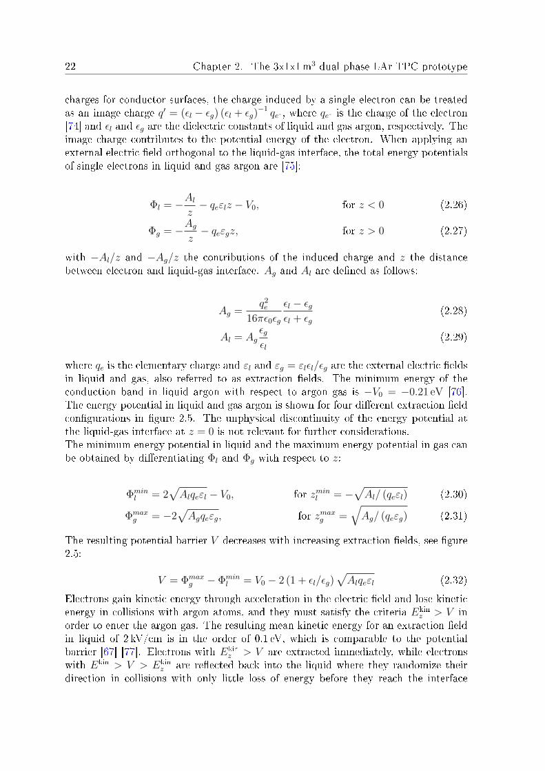
22 Chapter 2. The 3x1x1m3 dual phase LAr TPC prototype
charges for conductor surfaces, the charge induced by a single electron can be treatedas an image charge q′ = (εl − εg) (εl + εg)
−1 qe9 , where qe9 is the charge of the electron[74] and εl and εg are the dielectric constants of liquid and gas argon, respectively. Theimage charge contributes to the potential energy of the electron. When applying anexternal electric eld orthogonal to the liquid-gas interface, the total energy potentialsof single electrons in liquid and gas argon are [75]:
Φl = −Alz− qeεlz − V0, for z < 0 (2.26)
Φg = −Agz− qeεgz, for z > 0 (2.27)
with −Al/z and −Ag/z the contributions of the induced charge and z the distancebetween electron and liquid-gas interface. Ag and Al are dened as follows:
Ag =q2e
16πε0εg
εl − εgεl + εg
(2.28)
Al = Agεgεl
(2.29)
where qe is the elementary charge and εl and εg = εlεl/εg are the external electric eldsin liquid and gas, also referred to as extraction elds. The minimum energy of theconduction band in liquid argon with respect to argon gas is −V0 = −0.21 eV [76].The energy potential in liquid and gas argon is shown for four dierent extraction eldcongurations in gure 2.5. The unphysical discontinuity of the energy potential atthe liquid-gas interface at z = 0 is not relevant for further considerations.The minimum energy potential in liquid and the maximum energy potential in gas canbe obtained by dierentiating Φl and Φg with respect to z:
Φminl = 2
√Alqeεl − V0, for zminl = −
√Al/ (qeεl) (2.30)
Φmaxg = −2
√Agqeεg, for zmaxg =
√Ag/ (qeεg) (2.31)
The resulting potential barrier V decreases with increasing extraction elds, see gure2.5:
V = Φmaxg − Φmin
l = V0 − 2 (1 + εl/εg)√Alqeεl (2.32)
Electrons gain kinetic energy through acceleration in the electric eld and lose kineticenergy in collisions with argon atoms, and they must satisfy the criteria Ekin
z > V inorder to enter the argon gas. The resulting mean kinetic energy for an extraction eldin liquid of 2 kV/cm is in the order of 0.1 eV, which is comparable to the potentialbarrier [67] [77]. Electrons with Ekin
z > V are extracted immediately, while electronswith Ekin > V > Ekin
z are reected back into the liquid where they randomize theirdirection in collisions with only little loss of energy before they reach the interface
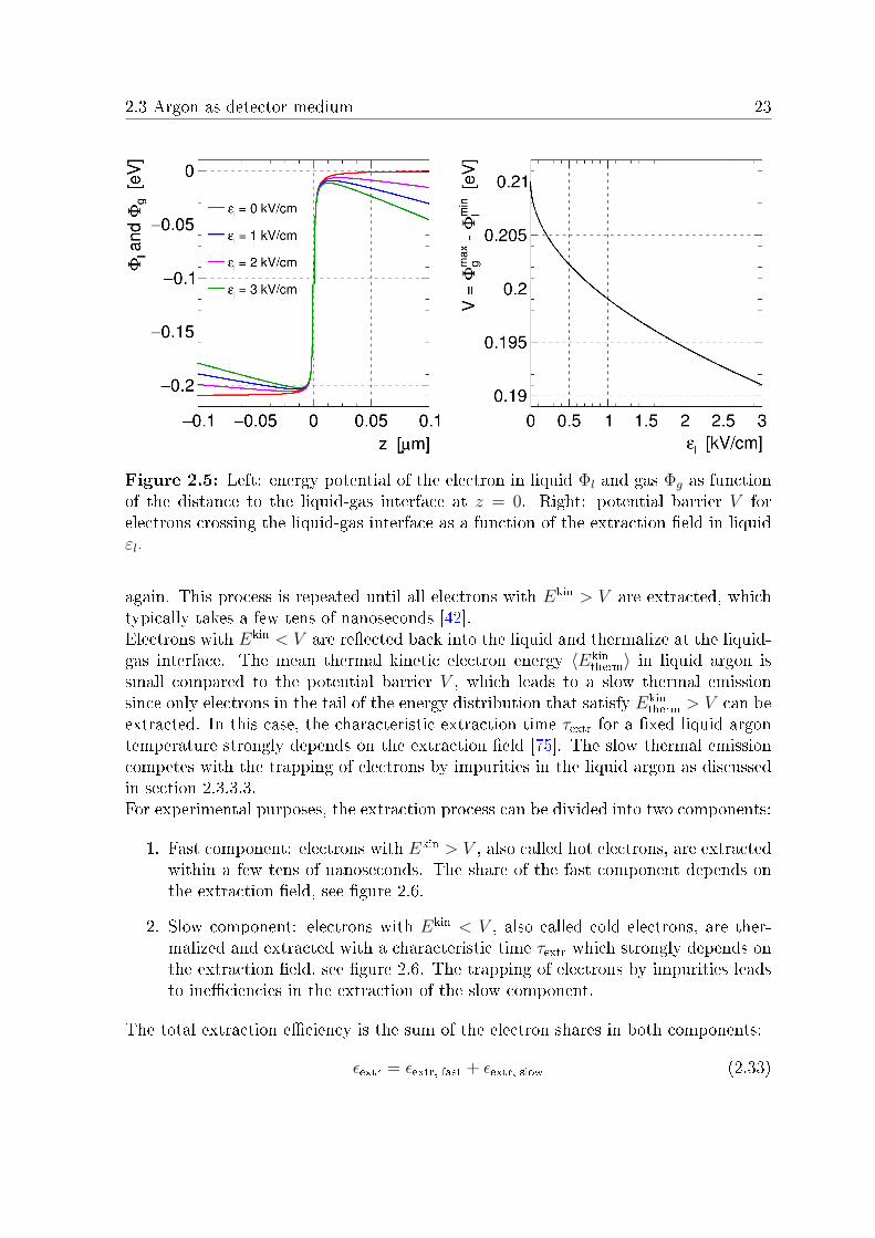
2.3 Argon as detector medium 23
Figure 2.5: Left: energy potential of the electron in liquid Φl and gas Φg as functionof the distance to the liquid-gas interface at z = 0. Right: potential barrier V forelectrons crossing the liquid-gas interface as a function of the extraction eld in liquidεl.
again. This process is repeated until all electrons with Ekin > V are extracted, whichtypically takes a few tens of nanoseconds [42].Electrons with Ekin < V are reected back into the liquid and thermalize at the liquid-gas interface. The mean thermal kinetic electron energy 〈Ekin
therm〉 in liquid argon issmall compared to the potential barrier V , which leads to a slow thermal emissionsince only electrons in the tail of the energy distribution that satisfy Ekin
therm > V can beextracted. In this case, the characteristic extraction time τextr for a xed liquid argontemperature strongly depends on the extraction eld [75]. The slow thermal emissioncompetes with the trapping of electrons by impurities in the liquid argon as discussedin section 2.3.3.3.For experimental purposes, the extraction process can be divided into two components:
1. Fast component: electrons with Ekin > V , also called hot electrons, are extractedwithin a few tens of nanoseconds. The share of the fast component depends onthe extraction eld, see gure 2.6.
2. Slow component: electrons with Ekin < V , also called cold electrons, are ther-malized and extracted with a characteristic time τextr which strongly depends onthe extraction eld, see gure 2.6. The trapping of electrons by impurities leadsto ineciencies in the extraction of the slow component.
The total extraction eciency is the sum of the electron shares in both components:
εextr = εextr, fast + εextr, slow (2.33)

24 Chapter 2. The 3x1x1m3 dual phase LAr TPC prototype
Figure 2.6: Left: shares of the fast and slow electron extraction component as afunction of the extraction eld in liquid εl. Data is taken from reference [78]. Right:characteristic extraction time of the slow component as a function of the extractioneld in liquid εl. Data is taken from reference [75].
2.3.5 Electron transport in argon gas
The electron transport in argon gas in a DP LAr TPC in terms of drift velocity,diusion, charge amplication and secondary scintillation is described in sections 2.3.5.1through 2.3.5.3.
2.3.5.1 Drift velocity and diusion
In gases, the quantities of drifting electrons are typically given as a function of thereduced electric eld ε/N , since the mean electron energy depends on ε/N over broadranges of ε and N , where ε is the electric eld and N the number density of the gas.The unit of the reduced electric eld is Townsend: 1 Td = 10−17 V · cm2.The electron drift velocity in argon gas has been measured over the range of ε/N from0.25 to 50 Td [79] and the longitudinal and transverse diusion coecients have beendeduced from drift velocity measurements by [80], see gure 2.7. The electric eldin the top axes in gure 2.7 are determined from the reduced electric eld with thenumber density of an ideal gas at standard ambient temperature and pressure (SATP)with T = 20 C and p = 1 bar.
The total drift time of electrons in argon gas in a DP LAr TPC is in the order ofmicroseconds, while the drift time in liquid argon is in the order of milliseconds. Thecontribution to the total drift time of electrons and eects related to diusion in argongas can therefore be neglected.

2.3 Argon as detector medium 25
Figure 2.7: Left: electron drift velocity in argon gas as a function of the reducedelectric eld measured by [79]. The electric eld in the top axis corresponds to SATP.Figure is taken from reference [42]. Right: longitudinal and transverse diusion coe-cients in argon gas as a function of the reduced electric eld. The electric eld in thetop axis corresponds to SATP. Figure is taken from reference [42].
2.3.5.2 Charge amplication
Charge amplication describes the multiplication of free electrons in gases throughionization of gas atoms. Since the rst ionization potential of atoms is typically higherthan the energy of free thermal electrons in gases at SATP, an electric eld is neces-sary for the electrons to acquire more energy. In the case of argon, the rst ionizationpotential is at 15.7 eV [81].Free electrons in argon gas gain energy through acceleration in the electric eld andlose energy in collisions with argon atoms. The resulting electron energy distributioncan be simulated with the software package Magboltz, which solves the Boltzmannequations for electrons in gas mixtures in the presence of electric and magnetic elds[82]. Besides temperature, pressure and electric eld, Magboltz requires cross sectiontables for electron-argon collisions as input for the simulation. Figure 2.8 shows theelectron-argon cross section for elastic scattering, excitation and ionization as functionof electron kinetic energy. Electrons change direction but do not not lose energy in elas-tic scatters. For excitation and ionization, several transitions at dierent energies exist,with 11.5 eV and 15.7 eV being the lowest for excitation and ionization, respectively.The resulting electron energy distributions are shown in gure 2.8 for four dierentelectric elds.The high energy tail that extends beyond the rst ionization potential of 15.7 eV be-comes more populated with increasing electric elds. The electrons in this tail canionize argon atoms to produce additional free electrons, which in turn can contributeto the ionization process themselves, resulting in an exponentially growing process alsoknown as Townsend avalanche. The Magboltz simulation returns the rst Townsendcoecient α, which is the number of electron-ion pairs produced by a single electronper unit drift length. In an empirical approximation, the rst Townsend coecientdepends on the electric eld ε as well as the gas density ρ and composition:

26 Chapter 2. The 3x1x1m3 dual phase LAr TPC prototype
Figure 2.8: Left: electron-argon atom cross section for elastic scattering, total ex-citation and ionization as a function of electron kinetic energy. Figure is taken fromreference [42]. Right: energy distributions of free electrons in argon gas for four dier-ent electric elds obtained from Magboltz simulations. Figure is taken from reference[42].
α = Aρe−Bρε (2.34)
where A and B are constants that depend on the gas composition. Given a constantgas density and varying electric eld, as it is the case for most electron multiplicationdevices, the ratio of free electrons n that are created along the drift path to initial freeelectrons n0 is called gain G and can be calculated as follows:
G =n
n0
= exp
[∫S
α (ε (s)) ds
](2.35)
where S is the drift path. For a constant electric eld, the expression for the gain canbe simplied to:
G = eαs (2.36)
where s is the drift distance. Since electron multiplication is a stochastic process,equation 2.35 and 2.36 only describe the average gain of a multitude of avalanches.Townsend avalanches with total electron populations ne9 < 105 are governed by the socalled Furry probability [83] [84]. For a single electron entering a multiplication regionwith a uniform electric eld, the probability for n additional electrons to emerge fromionization is:
P (n) =1
G
(1− 1
G
)n−1
(2.37)

2.3 Argon as detector medium 27
The most probable number of emerging electrons is zero and the average number ofemerging electrons is G. The variance of the Furry distribution is G2 (1− 1/G). Thestandard deviation can be approximated with G for large gains. Applying the centrallimit theorem, the Furry distribution becomes Gaussian for large numbers of initialelectrons n0
e9 at the beginning of the multiplication process. In this case, the averagenumber of emerging electrons is Gn0
e9 and the standard deviation is G√n0e9 . A side
eect of the multiplication process is the backow of argon ions into liquid argon,enhancing the space charge eect discussed in section 2.3.3.4.The Townsend avalanche is the basic principle of all electron multiplication devicesin gas, which typically consist of two electrodes at short distance in order to achieveelectric elds of several 10 kV/cm. In the case of the 3x1x1m3 prototype, two electrodesat a distance of 1mm, that are separated by an insulator, form a parallel plate capacitorcalled large electron multiplier (LEM), see section 2.4.2.2. Holes piercing the LEM formthe electron multiplication regions.In addition to the ionization process described above, the excitation of argon atomscan indirectly contribute to the total number of electrons. When an argon atom isin an excited state after the collision with an electron, it can form an argon excimerand subsequently produce scintillation light at 9.7 eV through the process describedin section 2.3.2. The scintillation light is not energetic enough to ionize argon atoms,but it can extract electrons from the conduction band of the electrodes through thephotoelectric eect. A similar, but slower, eect can be observed by back drifting argonions that eject electrons when impinging on the electrodes. In Townsend avalancheswith high numbers of electrons, both of these eects can turn into a continuous currentwhich may trigger the formation of an electron-ion plasma in the multiplication region,also known as streamers. When stretched across the entire multiplication region andconnecting both electrodes of the multiplication device, the electron-ion plasma actsas a conductor which leads to a complete discharge of the electrodes within a shorttime. The heat produced by the heavy current can damage the electrodes. In mostgas multiplication devices, the likelihood to produce streamers is reduced by adding aso-called quenching gas that can absorb the scintillation light emitted by the Townsendavalanche. The high purity requirement for LAr TPCs, however, prevents the use ofquenching gases, c.f. section 2.3.3.3. The multiplication devices for DP LAr TPCsare therefore designed to provide mechanical quenching against discharges, see section2.4.2.2.
2.3.5.3 Secondary scintillation light
As described in the previous section, free electrons in an electric eld inside argon gascan gain enough energy to excite argon atoms and, through the formation of argonexcimers, produce scintillation light. In accordance with the primary scintillation lightthat is produced by the penetrating particle in liquid argon, the scintillation lightproduced in argon gas is referred to as secondary scintillation light. The lifetime of theexcimer in the triplet state in gas of τ2 ≈ 3670 ns has been reported to be higher thanin liquid argon [52].The electroluminescence yield Y is dened as the produced number of photons per
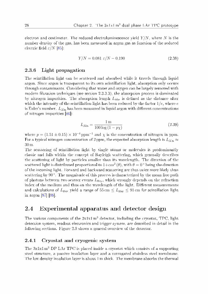
28 Chapter 2. The 3x1x1m3 dual phase LAr TPC prototype
electron and centimeter. The reduced electroluminescence yield Y/N , where N is thenumber density of the gas, has been measured in argon gas as function of the reducedelectric eld ε/N [85]:
Y/N = 0.081 ε/N − 0.190 (2.38)
2.3.6 Light propagation
The scintillation light can be scattered and absorbed while it travels through liquidargon. Since argon is transparent to its own scintillation light, absorption only occursthrough contaminants. Considering that water and oxygen can be largely removed withmodern ltration techniques (see section 2.3.3.3), the absorption process is dominatedby nitrogen impurities. The absorption length LAbs is dened as the distance afterwhich the intensity of the scintillation light has been reduced by the factor 1/e, where eis Euler's number. LAbs has been measured in liquid argon with dierent concentrationsof nitrogen impurities [86]:
LAbs =1 m
100 log (1− pχ)(2.39)
where p = (1.51± 0.15)× 10−4 ppm−1 and χ is the concentration of nitrogen in ppm.For a typical nitrogen concentration of 2 ppm, the expected absorption length is LAbs ≈30 m.The scattering of scintillation light by single atoms or molecules is predominantlyelastic and falls within the concept of Rayleigh scattering, which generally describesthe scattering of light by particles smaller than its wavelength. The direction of thescattered light is distributed proportional to 1+cos2 (θ), with θ = 0 being the directionof the incoming light. Forward and backward scattering are thus twice more likely thanscattering by 90 . The magnitude of this process is characterized by the mean free pathof photons between two scatter events LRay, which strongly depends on the refractionindex of the medium and thus on the wavelength of the light. Dierent measurementsand calculations of LRay yield a range of 55 cm ≤ LRay ≤ 91 cm for scintillation lightin argon [87] [88].
2.4 Experimental apparatus and detector design
The various components of the 3x1x1m3 detector, including the cryostat, TPC, lightdetection system, readout electronics and trigger system, are described in detail in thefollowing sections. Figure 2.9 shows a general overview of the detector.
2.4.1 Cryostat and cryogenic system
The 3x1x1m3 DP LAr TPC is placed inside a cryostat which consists of a supportingsteel structure, a passive insulation layer and a corrugated stainless steel membrane.The low density insulation layer is about 1m thick. The membrane absorbs the thermal

2.4 Experimental apparatus and detector design 29
Figure 2.9: Technical drawing of the 3x1x1m3 dual phase liquid argon time projectionchamber experimental apparatus.
stress and separates the liquid argon from the insulation. The ∼23m3 volume insidethe membrane is partially lled with liquid argon. The isolating lid of the cryostat, alsocalled top-cap, is 1.2m thick and hosts feedthroughs for the cryogenic, high voltage,signal readout and charge readout plane alignment systems.The cryostat is at room temperature and atmospheric pressure before the liquid ar-gon is introduced. An elaborate cryogenic system is needed to purge, cool down andll the cryostat as well as to maintain a stable operating state over long periods of time.
2.4.1.1 Purging, cooling down and lling
At the beginning of the lling procedure, liquid argon is introduced through severalventing pipes at the oor of the membrane. The evaporating argon cools down thecryostat and pushes the remaining air upwards. In the open loop purge, the excess gasmixture of air and argon gas is released to the exterior through a chimney vent in thetop-cap. After removing all remaining air and reaching impurities for oxygen, nitrogenand water at the parts-per-million (ppm) level, the cryogenic system is switched tothe closed loop mode: the excess gas is circulated though a gas purier that lters

30 Chapter 2. The 3x1x1m3 dual phase LAr TPC prototype
oxygen and water before it is reinserted into the cryostat. When the impurities cannot be further reduced in the closed loop, a mixture of argon gas at room temperatureand liquid argon is introduced through atomizing nozzles to increase the cooling speed.After reaching a temperature of around 170K, the cryostat is lled with liquid argonat a ow rate of ∼12L/min.
2.4.1.2 Operational mode
During the operation of the detector, the liquid argon is continuously circulated througha purication cartridge that removes oxygen and water impurities. The circulationpump is located inside a 3.5m high vessel, also called pump tower (see gure 2.9).The pump tower decouples the liquid argon inside the TPC from turbulence producedby the pump. A liquid nitrogen heat exchanger inside the pump tower compensatesthe heat load from the circulation pump, the cryostat insulation and feedthroughs byliquefying the boiled-o argon. The argon gas pressure inside the cryostat is kept at∼ 1000mbar, slightly above the surrounding atmospheric pressure of 950-980mbar toprevent air and humidity from leaking inside the cryostat.
2.4.2 TPC
The 3x1x1m3 TPC encompasses the drift cage and the charge readout plane, see gure2.10. A detailed description of the dierent components can be found in sections 2.4.2.1through 2.4.2.3.
Figure 2.10: Technical drawing of the 3x1x1m3 dual phase liquid argon time projec-tion chamber inside the cryostat.
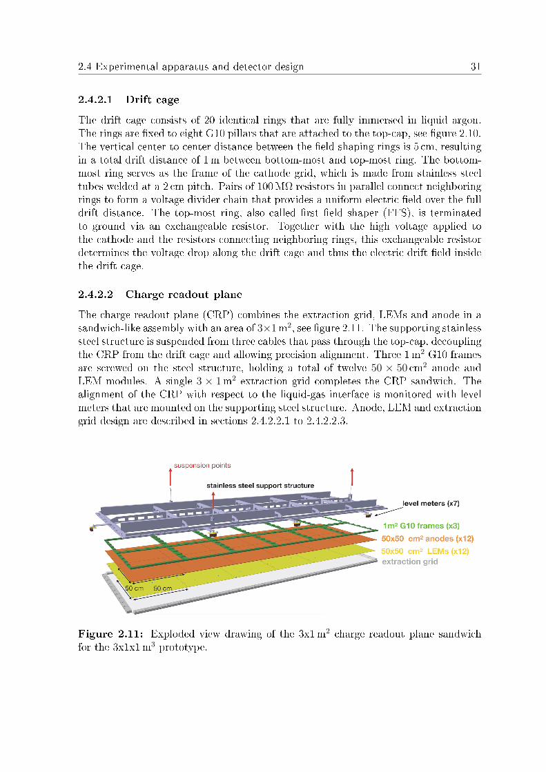
2.4 Experimental apparatus and detector design 31
2.4.2.1 Drift cage
The drift cage consists of 20 identical rings that are fully immersed in liquid argon.The rings are xed to eight G10 pillars that are attached to the top-cap, see gure 2.10.The vertical center-to-center distance between the eld-shaping rings is 5 cm, resultingin a total drift distance of 1m between bottom-most and top-most ring. The bottom-most ring serves as the frame of the cathode grid, which is made from stainless steeltubes welded at a 2 cm pitch. Pairs of 100MΩ resistors in parallel connect neighboringrings to form a voltage divider chain that provides a uniform electric eld over the fulldrift distance. The top-most ring, also called rst eld shaper (FFS), is terminatedto ground via an exchangeable resistor. Together with the high voltage applied tothe cathode and the resistors connecting neighboring rings, this exchangeable resistordetermines the voltage drop along the drift cage and thus the electric drift eld insidethe drift cage.
2.4.2.2 Charge readout plane
The charge readout plane (CRP) combines the extraction grid, LEMs and anode in asandwich-like assembly with an area of 3×1m2, see gure 2.11. The supporting stainlesssteel structure is suspended from three cables that pass through the top-cap, decouplingthe CRP from the drift cage and allowing precision alignment. Three 1m2 G10 framesare screwed on the steel structure, holding a total of twelve 50 × 50 cm2 anode andLEM modules. A single 3 × 1m2 extraction grid completes the CRP sandwich. Thealignment of the CRP with respect to the liquid-gas interface is monitored with levelmeters that are mounted on the supporting steel structure. Anode, LEM and extractiongrid design are described in sections 2.4.2.2.1 to 2.4.2.2.3.
Figure 2.11: Exploded view drawing of the 3x1m2 charge readout plane sandwichfor the 3x1x1m3 prototype.

32 Chapter 2. The 3x1x1m3 dual phase LAr TPC prototype
2.4.2.2.1 Anode
The anode is a four-layer printed circuit board (PCB) with two orthogonal sets ofcharge readout strips with a pitch of 3.125mm, see gure 2.12. The readout stripsof neighboring anode modules are connected, resulting in a 3m and a 1m long set ofreadout strips that are called view 0 and view 1, respectively (see gure 2.14). View 0has 320 readout strips while view 1 has 960 readout strips.
2.4.2.2.2 LEM
A LEM is a standard PCB epoxy plate pierced with holes of 500µm diameter in ahoneycomb pattern. The pitch between holes is 800µm, yielding about 180 holes percm2, see gure 2.12. Each LEM module has an area of 50 × 50 cm2 and a thicknessof ∼1.12mm, including 60µm of copper coating on both sides. In order to preventdischarges, the LEM borders have a 2mm clearance followed by a 2mm copper guardring, and the pins for the high voltage supply are soldered in imprinted pads with a10mm circular clearance and a 2mm copper guard ring. LEM and anode modulesare screwed together before they are xed to the G10 frames. The screw holes have a2mm copper guard ring and the screws have spacers that keep the distance betweenthe upper LEM face and anode to 2mm.
Figure 2.12: Left: photograph of the anode with a highlighted readout strip in eachview. Right: photograph of the LEM with indicated hole dimensions. The 60 µmcopper coating is visible around the drilled holes.
2.4.2.2.3 Extraction grid
The extraction grid is constructed from stainless steel wires that are oriented along thetwo charge readout views. The wire diameter is 100 µm and the wire pitch of 3.125mmmatches that of the charge readout strips to provide a uniform extraction eld and toavoid charge shadowing of the readout strips. Groups of 32 wires are soldered on bothends on independent wire holders that are xed to the CRP supporting steel structureat a distance of 1 cm to the lower LEM face. The 3m long wires along charge readoutview 0 are tensed with a force of 3N while the 1m long wires along charge readout view1 are tensed with 1N. The wires along the two charge readout views are interlaced in

2.4 Experimental apparatus and detector design 33
order to prevent broken wires to sag into the liquid argon or to stick to the lower LEMface. Since all wire holders are electrically connected, the complete extraction grid canbe brought to the same potential with one high voltage contact.
2.4.2.3 High voltage systems and electric eld conguration
In this section, the high voltage system and electric elds in the drift cage and theCRP are discussed.
2.4.2.3.1 Drift cage
The cathode is connected to a Heinzinger 300 kV power supply through a dedicatedhigh voltage feedthrough with a safety clearance to the steel membrane and drift cage inorder to avoid discharges, see gure 2.10. The cathode is brought to a nominal negativepotential of -56.5 kV. The eective resistance between the eld-shaping rings of 50MΩadds up to a total resistance of 950MΩ between cathode and FFS. The resistancebetween FFS and ground of 130MΩ results in a nominal FFS potential VFFS of:
VFFS = −56.5 kV ×(
1− 950 MΩ
950 MΩ + 130 MΩ
)= −6.8 kV (2.40)
With the total drift distance of ∼1m, the nominal drift eld strength results to εD =0.5 kV/cm.
2.4.2.3.2 CRP
The lower and upper faces of the 12 LEM modules, also called LEM down and LEMup, all have individual high voltage supply channels. The extraction grid has twoseparate high voltage supply channels and connectors. The LEM and extraction gridvoltages are provided by a CAEN high voltage supply module. The extraction grid isplaced ∼3mm above the upper edge of the FFS and its nominal potential of Vextr =−6.5 kV matches VFFS, guaranteeing a smooth continuation of the electric eld linesfrom the drift cage into the CRP. The nominal potentials of LEM down and LEMup are VLEM,down = −4.3 kV and VLEM,up = −1 kV, respectively. The extraction eldbetween extraction grid and LEM down in liquid and gas is calculated as follows:
εextr,l =| VFFS − VLEM,down |dL
(1− εL
εG
)+D εL
εG
(2.41)
εextr,g =| VFFS − VLEM,down | −εextr,l dL
dG(2.42)
where dL is the distance between extraction grid and liquid-gas interface, dG the dis-tance between liquid-gas interface and LEM down, and D = dL + dG = 1 cm the xeddistance between extraction grid and LEM down. The values of dL and dG depend

34 Chapter 2. The 3x1x1m3 dual phase LAr TPC prototype
on the alignment of the CRP with respect to the liquid-gas interface. The dielec-tric constant of liquid argon is εL = 1.5 and the corresponding value for argon gas isεG = 1.0. With dL = dG = 0.5 cm, the nominal extraction elds in liquid and gas areεextr,l = 2 kV/cm and εextr,g = 3 kV/cm. The extraction eld in liquid is strong enoughto transfer most of the free electrons into the gas argon layer, c.f. section 2.3.4. Insidethe gas layer, electrons follow the eld lines into the LEM holes. The nominal voltagedrop between LEM down and LEM up over the eective distance between the two cop-per surfaces of 1mm creates a strong electric eld of εamp = 33 kV/cm inside the LEMholes, also referred to as amplication eld. The electrons are accelerated and reachvelocities high enough to kick out shell electrons from the argon atoms, producing aso-called Townsend avalanche (see section 2.3.5.2). After leaving the LEM holes, theelectrons enter the induction gap between LEM up and anode. The nominal inductioneld εind = 5 kV/cm focuses the electrons onto the charge readout strips. A simulationof the electric eld lines inside the CRP is shown in gure 2.13 and the nominal valuesfor the voltages and electric eld strengths are summarized in table 2.3.
Figure 2.13: Electric eld inside the CRP simulated with the GARFIELD softwarepackage. The ionization electrons follow the white lines that represent the continuationof the electric drift eld lines to the anode. The green lines depict the electric eldlines that emerge from the extraction grid wires. The background color represents thestrength of the electric eld according to the color scale.
2.4.3 Light detection system
The scintillation light produced in liquid and gas is detected by ve PMTs that arelocated below the cathode, see gures 2.9 and 2.10. The photosensitive window of the

2.4 Experimental apparatus and detector design 35
PMTs, also called photocathode, is made of borosilicate and has a diameter of eightinches. Tetraphenyl butadiene (TPB) is used to shift the scintillation light wavelengthof 128 nm into the high quantum eciency region of borosilicate around 420 nm. Thephotocathodes of three PMTs are directly coated with a thin layer of TPB, while theremaining two PMTs have a transparent acrylic plate coated with TPB mounted infront of the photocathode.Two dierent high voltage supply systems are tested. The negative base system biasesthe photocathode of the PMT with a negative voltage while the anode is grounded. Thissetup requires an additional cable to read out the signal from the anode. The positivebase system applies a positive voltage to the anode, enabling high voltage supply andsignal readout through the same cable. The gains of the PMTs have been calibratedwith single photoelectron counts during detector operation. The main properties ofthe ve PMTs are summarized in table 2.3.
Electrode Voltage [kV]
Anode 0LEMs up -1
LEMs down -4.3Extraction grid -6.8First eld shaper -6.8
Cathode -56.5
Region Field [kV/cm]
Induction 5Amplication 33
Extraction in gas 3Extraction in liquid 2
Drift 0.5
PMT Base TPB coating Voltage [kV] Gain [106]
1 - Photocathode 1.2 0.92± 0.132 - Plate 1.2 1.01± 0.123 + Photocathode 1.1 0.95± 0.114 + Plate 1.1 1.26± 0.155 - Photocathode 1.2 1.33± 0.15
Table 2.3: Top: nominal TPC high voltage settings and elds. Bottom: nominalPMT high voltage settings and gains.
2.4.4 Readout electronics
The charge and light signal are read out out with two separate systems. While thelight readout system consists of commercially available components, the charge readoutsystem has been developed specically for the 3x1x1m3 prototype. Both systems areexplained sections 2.4.4.1 and 2.4.4.2.

36 Chapter 2. The 3x1x1m3 dual phase LAr TPC prototype
2.4.4.1 Charge readout
Groups of 32 charge readout strips are connected to the bottom ange of a so-calledsignal feedthrough (SGFT). Inside the SGFT, the charge signal of two 32-strips groupsis fed into a front-end board (FEB), which hosts four application-specic integrated cir-cuits (ASICs) as well as a series of passive electronic components for each readout stripin order to reduce electronic noise and protect the ASICs against discharges, includinga decoupling capacitor of 2.2 nF. Each ASIC features 16 input channels that consist ofa charge sensitive amplier (CSA), a dierential output buer stage acting as a lowpass lter and a 1 pF test capacitor for calibration purposes. The FEB is mountedonto the bottom side of a 1.5m long G10 blade which is inserted into the SGFT withguiding rails. Only when fully inserted, the FEB is electrically connected to the bottomange and thus to the charge readout strips. This setup allows to remove the FEBsduring detector operation, while the proximity of the FEBs to the anode and the lowtemperature at the bottom of the SGFT minimize the electronic noise. Each of thefour SGFTs contains ve FEBs and thus serves 320 charge readout strips. Figure 2.14shows the grouping of the charge readout strips on the level of the FEBs and SGFTs.
Figure 2.14: Grouping of the charge readout strips at the level of the FEBs andSGFTs and mapping conventions for anode and LEM modules as well as charge readoutchannels. One FEB collects two groups of 32 channels from neighboring anode modules,as depicted by the color code. The numbers 1 to 12 inside the boxes show the numberingconvention for the twelve anode and LEM modules. The three meters long readoutstrips in view 0 are dened as charge readout channels 0 to 319 and the one meter longreadout strips in view 1 are dened as channels 320 to 1279.
The dierential analogue output signals of the FEBs are guided upwards and connectedto the top anges of the SGFTs. From the top anges, the signal is fed into AdvancedMezzanine Cards (AMC) located outside of the detector. When triggered, the analog-to-digital converter (ADC) chips on the AMCs digitize and store the input signal over adynamic range of 1 800mV with a resolution of 12 bit. The ADCs record 1667 samplesper event with a sampling rate of 2.5 MHz, resulting in a event time window of 666.8 µs,which is slightly bigger than the electron drift time of 625µs over the full 1m drift atthe nominal drift eld of 0.5 kV/cm (c.f. section 2.3.3.1). The digitized data is sent to

2.4 Experimental apparatus and detector design 37
a customized data acquisition (DAQ) system where it is written to disk.In order to achieve a high signal-to-noise ratio, a low noise CSA is used on the FEBsthat amplies the charge signal of the readout strips, converts it into a voltage andshapes the voltage output with a RC-CR circuit. These processes can be quantiedwith the gain g, which is the ratio of output voltage amplitude over total input chargefor an instantaneous charge injection. The CSA gain at 110K is 2.5mV/fC for inputcharges up to 400 fC and decreases for higher input charges, providing both a highsignal-to-noise ratio for small charge signals and a large dynamic range. The outputvoltage saturates at an input charge of around 1250 fC, see gure 2.15. The RC andCR elements of the shaping circuit have time constants of τ1 = 2.83 µs and τ2 = 0.47 µs,respectively. The shaping function is given by:
V (t) =1
τ1 − τ2
·(e−t/τ1 − e−t/τ2
)(2.43)
The shaped output voltage for a instantaneous charge injection of 1 fC is shown ingure 2.15.
Figure 2.15: Left: CSA gain with a linear regime for input charges of up to 400 fCand a logarithmic regime for charge injections between 400 fC and 1 250 fC. Right: CSAresponse to an instantaneous charge injection of 1 fC. The amplitude is dened by theCSA gain in the linear regime of g = 2.5 mV/fC and the shape by the CSA shapingfunction. The integral is 10.1 mV · µs.
2.4.4.2 Light readout
The analog signals of the ve PMTs are directly fed into a commercial CAEN v1720board that hosts 12-bit ADCs with a dynamic range of 2V and a sampling rate of250MHz. Two dierent readout windows can be used during data taking. With theshorter readout window of 4µs, only the signal of the primary scintillation light isrecorded. The secondary scintillation light is produced when the ionization electronsreach the argon gas, which can take up to 625µs at nominal drift eld for particlesthat crossed the bottom of the TPC, and the longer readout window of 1 ms allows the
38 Chapter 2. The 3x1x1m3 dual phase LAr TPC prototype
recording of both primary and secondary scintillation light. The digitized data is sentto a computer equipped with a CAEN A2818 PCI card that writes the data to diskusing the MIDAS DAQ system [89].
2.4.5 Charge readout calibration system
The ends of the charge readout strips that are not fed into the SGFTs are connected toa dedicated 1 pF capacitor, c.f. gure 2.14. Groups of 32 capacitors share a connectorto the so-called slow-control feedthrough. A voltage generator can be used to chargegroups of 32 capacitors, inducing a current on the readout strips that simulates thecollection of ionization electrons of the charge Q = 1 pF · U , where U is the voltageset by the generator. The voltage can be ramped up within 100 ns to simulate a fastcharge injection on the readout strips, while longer ramp up times are used to simulatea continuous charge injection. The generator sends a trigger to the charge readoutelectronics 300 µs before the voltage is ramped up, so that the signal is well within thereadout window of 666.8 µs. The system is used to calibrate the charge readout stripsduring detector operation.
2.4.6 Trigger system
Two independent trigger systems have been implemented for the 3x1x1m3: an externalcosmic ray tagger and an internal PMT trigger. Both systems are described below.
2.4.6.1 Cosmic ray tagger
The cosmic ray tagger (CRT) consists of two 1.8×1.8 m2 panels mounted on the outsideof the supporting steel structure of the cryostat on either side of the 3m readout view,see gure 2.9. Each panel comprises two modules with 16 scintillator strips to readboth the vertical and horizontal coordinates of crossing particles. The signals of thescintillator strips are fed into silicon photomultipliers (SiPMs) through wavelength-shifting bers. A dedicated front-end board amplies and digitizes the SiPM signalsand sends the data to the CRT data acquisition computer. In the case of a coincidenceof at least one scintillator strip in all four modules, a trigger signal is sent to the chargeand light readout systems. The CRT selects almost exclusively cosmic muons that crossthe TPC along the 3m readout view. The two CRT panels can be shifted vertically toallow dierent azimuthal angular acceptances. In the standard conguration with bothpanels at the same height, the azimuthal angular acceptance is ±13.5 with respect tothe horizontal plane.
2.4.6.2 PMT trigger
The PMT trigger logic is a coincidence of all ve PMTs surpassing an amplitude of250ADC counts within a time window of 80 ns. The threshold of 250ADC countsyields an average trigger rate of 3Hz, which is the maximum achievable rate of thecharge readout DAQ system. In order to reduce the loss of data packets in the DAQ

2.4 Experimental apparatus and detector design 39
system, a trigger veto window of 200ms is opened after each trigger, which results inan eective trigger rate close to 2Hz.

40 Chapter 2. The 3x1x1m3 dual phase LAr TPC prototype

Chapter 3
3x1x1m3 charge readout
characterization and detector
simulation
As explained in chapter 2, the 3x1x1m3 DP LAr TPC is part of the prototyping eortstowards the DUNE far detector and can be used to tune the DP LAr TPC detectorsimulation, which plays a crucial role in the proton decay sensitivity study presentedin chapter 7.This chapter therefore begins with the examination of the 3x1x1m3 calibration datato characterize the charge readout of the detector in section 3.1. The general simu-lation workow for the 3x1x1m3 detector and the implementation of the results fromthe charge readout characterization into the simulation are discussed subsequently insection 3.2. The results from the charge readout characterization are also used in thereconstruction and analysis of the 3x1x1m3 cosmic ray data presented in chapter 4that further contributes to the validation of the detector simulation.
3.1 Charge readout characterization
The charge readout characterization encompasses three topics that are explained in thefollowing sections: the charge readout calibration, the charge readout shaping and thenoise characterization.
3.1.1 Charge readout calibration
All 40 groups of 32 charge readout strips are pulsed individually with the calibrationsystem described in section 2.4.5. The rise time is set to 100 ns and the voltage to150mV, resulting in a total injected charge of Q = 1 pF ·150 mV = 150 fC. Around 100pulses are recorded and averaged oine for each of the 40 groups to mitigate uctua-tions due to electronic noise. The pedestal is calculated for each channel separately byaveraging over the ADC counts between t = 245 µs and t = 295 µs. Figure 3.1 showsthe averaged waveform of charge readout channel 320 after pedestal subtraction.
41

42 Chapter 3. 3x1x1m3 charge readout characterization and detector simulation
Figure 3.1: Averaged waveform of channel 320 in view 1 after pedestal subtractionfrom pulsing with 150mV and 100 ns ramp-up time.
A small bump is observed at around t = 315 µs that follows the main peak. The bumpis only observed when the FEBs are close to cryogenic temperatures and most likelyoriginates from a changed behavior of the shaping RC-CR circuit at cold temperatures,c.f. section 2.4.4.1.The signals of all channels are integrated individually from t = 296 µs to t = 360 µs. Theintegrals of channels 160 to 191 are ∼50% larger than the average of all other channels,see gure 3.2. These channels share the same connector to the voltage generator andthe higher integrals are most likely due to an accidentally installed input capacitanceof 1.5 pF instead of 1 pF, c.f. section 2.4.5. The 18 channels with integrals lower than3 000 ADC · µs are excluded from further analysis. The mapping convention of chargereadout channels to charge readout strips in the two readout views can be found ingure 2.14.Common calibration factors for channels in view 0 and view 1 are calculated by av-eraging the integrals of the good channels in the green shaded area in gure 3.2 anddividing by the input charge of 150 fC:
γView 0 = (23.9± 1.2)ADC · µs
fC, γView 1 = (26.7± 1.0)
ADC · µs
fC(3.1)
where the errors are the standard deviation. The dierence between view 0 and view 1originates from dierent capacitances to ground of the readout strips in the two views.The capacitance per unit length of a single readout strip to the entirety of all otherelectric components of the anode has been measured to C ′Strip = 156 pF/m [96], withthe main contribution coming from the crossing readout strips of the readout viewperpendicular to the considered strip. Since the anode is terminated to ground during

3.1 Charge readout characterization 43
Figure 3.2: Integrated pulsing signals for charge injections of 150mV in all readoutchannels. Values outside the green shaded area are excluded from the calibration.
detector operation, the injected charge is split between the strip-anode capacitance andthe parallel-connected decoupling capacitor on the FEB side CDec = 2.2 nF, c.f. section2.4.4.1. By assuming that C ′Strip = 156 pF/m is the capacitance between a single stripand the anode, the ratio of charge arriving at the FEB to injected charge in the tworeadout views can be approximated to:
QFEB, View 0
QInj
=CDec
CDec + 3 m · C ′Strip= 0.82 (3.2)
QFEB, View 1
QInj
=CDec
CDec + 1 m · C ′Strip= 0.93 (3.3)
The expected ratio of measured charge between view 1 and view 0 is thus:
QFEB, View 1
QFEB, View 0
=0.93
0.82= 1.13 (3.4)
which agrees well with the measured ratio of γView 1/γView 0 = 1.12 ± 0.03. The errorof γView 1/γView 0 is propagated from the respective standard errors of the mean.In order to validate the calibration constants for smaller charge injections, a groupof 32 readout strips in each view has been pulsed with voltages between 14mV and150mV. Calibration factors and errors are calculated in the same way as for equation3.1. Figure 3.3 shows the calibration factors for dierent input charges normalized tothe previously calculated calibration factors obtained with a charge injection of 150 fCand the propagated standard errors of the mean. As no major deviations are found,the calibration factors in equation 3.1 are used in the following.

44 Chapter 3. 3x1x1m3 charge readout characterization and detector simulation
Figure 3.3: Calibration factors obtained with dierent charge injections normalizedto calibration factor obtained with a charge injection of 150 fC.
3.1.2 Charge readout shaping
The capacitance of the readout strips to ground does not only aect the total chargethat arrives at the FEB, but also the signal shaping in the CSA (c.f. sections 2.4.4.1 and3.1.1). Since the duration of charge injection from the pulsing device is only 100 ns andthe CSA shaping with time constants τ1 = 2.83 µs and τ1 = 0.47 µs takes much longer,the pulsing measurements can be used to characterize the shaping function at operatingconditions. Figure 3.4 shows the normalized expected CSA shaping function accordingto equation 2.43 and the normalized averaged pulsing waveforms in view 0 and view1 with the start time of charge injection set to t = 0. While the pulsing waveform inview 1 almost perfectly follows the expected CSA shaping function, the waveform inview 0 is considerably broader due to the bigger capacitance to ground of the read-out strips. In order to quantify the observed shaping functions, both waveforms are twith a double exponential ignoring the second and third bump (see zoom in gure 3.4):
f (t) =A · e−
t−t0τA
1 + e− t−t0
τB
(3.5)
The obtained t parameters are summarized in table 3.1.

3.1 Charge readout characterization 45
Figure 3.4: Normalized CSA shaping function and normalized averaged pulsing wave-forms in view 0 and view 1. The dashed line in the zoom shows the t of the pulsingwaveforms.
A t0 [µs] τA [µs] τB [µs]
View 0 1.42 0.80 0.146 0.132View 1 1.47 0.75 0.140 0.124
Table 3.1: Fit parameters describing normalized averaged pulsing waveforms in view0 and view 1 according to equation 3.5.
3.1.3 Noise characterization
In order to study the electronic noise, data with random triggers are taken. The ex-traction grid and LEM voltage supplies are switched o to prevent ionization electronsto reach the anode. The remaining high voltage supplies are switched on successivelyto test their eect on the noise. Two electronic noise patterns have been observed:
1. Slow baseline oscillations (SBO): low frequency noise around 1 kHz.
2. Fast coherent noise (FCN): high frequency noise between 100 kHz and 1 MHz thatappears simultaneously in various groups of readout channels.
Figure 3.5 shows an event display and a waveform from noise run 729 during which thedetector was at operating conditions with all electronic components except extractiongrid and LEMs at nominal values.Groups of readout channels with similar FCN patterns can be dened using the nor-malized cross-correlation factor RNCC between pairs of readout channels:

46 Chapter 3. 3x1x1m3 charge readout characterization and detector simulation
Figure 3.5: Top: event display of noise run 729. The FCN manifests as horizontallines, typically in groups of 32 channels. Bottom: waveform of channel 540. The SBOshapes the baseline to a sine wave.
RNCC =1
N · σ2x · σ2
y
N∑n=1
(xn − µx) · (yn − µy) (3.6)
where N = 1667 is the number of ADC samples, µx,y the mean and σ2x,y the variance
of all ADC samples in the readout channels x and y, and xn and yn the ADC count ofthe n-th sample in the two readout channels. Fig 3.6 shows the the normalized cross-correlation factor for all pairs of readout channels in noise run 729. The strongestcorrelations occur among groups of neighboring channels with multiplicities of 16, 32,48 and 64, corresponding to the grouping scheme of the charge readout system (seesection 2.4.4.1).
3.2 Detector simulation
The 3x1x1m3 detector simulation is implemented in LArSoft, a common softwareframework for LAr TPC simulation and event reconstruction [90]. The dierent simu-lation steps are explained in the following sections.

3.2 Detector simulation 47
Figure 3.6: Normalized cross-correlation RNCC according to equation 3.6 for all read-out channel pairs in noise run 729. Strong correlations between groups of neighboringchannels with multiplicities of 16, 32, 48 and 64 are observed.
3.2.1 Event generator
The 3x1x1m3 detector is exposed to cosmic ray induced air showers. The simulateddierential primary cosmic ray nucleon ux is given by the experimentally observedpower law:
φ (E) = K ·(
E
1 GeV
)−γ(3.7)
where the slope changes from γ = 2.71 to γ = 3 at the cuto energy EC . The con-sidered primary cosmic particles and their normalization factors K and cuto energiesEC are summarized in table 3.2.
Primary particle K [nucleons/(m2 · s · sr ·GeV)] EC [GeV]
p 1.72× 10⁴ 2.0× 10⁶
He 9.20× 10³ 4.0× 10⁶
C & N & O 6.20× 10³ 1.4× 10⁶
Mg 9.20× 10³ 2.6× 10⁶
Fe 6.20× 10³ 5.2× 10⁶
Table 3.2: Normalization factor K and cuto energy EC for dierential primarycosmic ray nucleon ux of the considered particles according to equation 3.7.

48 Chapter 3. 3x1x1m3 charge readout characterization and detector simulation
A database with presimulated air showers for the dierent primary cosmic particleshas been generated with CORSIKA for the location of the detector at CERN [91]. Thesecondary particle ux is sampled from the database and the center of the air shower isplaced randomly in the area above the detector. The CORSIKA Monte Carlo sampleis only used to validate the track selection, see section 4.2.1. For all other analyses,Monte Carlo samples with a so-called particle gun, that places single particles with awell dened start position and momentum inside the detector, are generated.
3.2.2 Detector geometry implementation
A simplied description of the detector geometry that serves the purpose of a realisticsimulation of cosmic ray air showers hitting the detector is used. The main consider-ation for the implementation of the cryostat geometry is the energy loss of particlesbefore they enter the TPC. For reasons of simplicity, the supporting steel structure,which is in fact a web of steel bars, is modeled as a homogeneous box made of 50%air and 50% steel (c.f. gure 2.9) . The passive insulation layer as well as the liquidand gas argon volumes are implemented according to their design parameters. Thecorrugated stainless steel membrane that separates the insulation from the argon isagain modeled as a simple homogeneous box. As for the TPC, only the PMTs andcharge readout strips are implemented in the LArSoft geometry, and the two chargereadout views are modeled with straight wires with a pitch of 3.125mm.
3.2.3 Energy loss, ionization and scintillation
The event generator produces a set of particle four-vectors that can be correlated inspace and time. The particles are propagated through the geometry using a GEANT4interface [92]. During the propagation, GEANT4 calculates the energy loss and simu-lates secondary interactions in step sizes of ∼0.1mm. The local number of free electronsper unit length for each step is calculated from the step energy loss dE and step lengthds with a modied version of Birk's law:
dNe
ds= −dE
ds· RWe
(3.8)
where We = 23.6 eV is the average energy to produce one electron-ion pair and R thefraction of electron-ion pairs that do not recombine and therefore contribute to thesignal, see table 2.1 and equation 2.4.As for the scintillation light, an experimentally determined yield of 24 000 photons perMeV of deposited energy is used. The ratio of argon excimer singlets over triplets, andtherefore of fast over slow scintillation photons, is assumed to be constant at 0.3 (c.f.section 2.3.2).
3.2.4 Electron transport
The ionization electrons are drifted upwards from the center of each GEANT4 step.The drift time to the CRP is calculated with the drift velocity vD = 1.6 m/ms that

3.2 Detector simulation 49
corresponds to the nominal drift eld of εD = 0.5 kV/cm, see gure 2.3. In orderto account for losses due to contaminants in liquid argon, the number of electronsthat arrive at the CRP is reduced according to equation 2.18 and the correspondingfree electron lifetime. Longitudinal and transverse diusion during the drift is imple-mented by smearing the electron distribution that arrives at the liquid-gas interfacealong the drift direction and in the plane perpendicular to the CRP with a mean dis-placement λL,T =
√2 ·DL,T · tDrift, using the diusion constants DL = 0.62 mm2/ms
and DT = 1.63 mm2/ms (c.f. section 2.3.3.2). Subsequently, the electrons are splitinto a fast and slow component. The electrons in the fast component are extractedinstantaneously, while the time distribution of extracted electrons in the slow compo-nent follows an exponential decay. The shares of electrons in both components and thecharacteristic extraction time for the slow component depend on the extraction eldin liquid and are shown in gure 2.6. The drift time and diusion in gas are negligibleand the extracted electrons are projected onto the CRP without additional delay orsmearing. The electrons at the CRP are multiplied with the LEM transparency factortLEM ≤ 1 that considers the loss of electrons through absorption by the lower and upperLEM electrodes and with the LEM gain factor GLEM ≥ 1 that describes the ampli-cation of the electrons inside the LEM holes. The eective gain GE = tLEM · GLEM
describes the ratio of electrons collected at the anode over extracted electrons. TheLEM transparency tLEM depends on the extraction eld in gas, the amplication eldand the induction eld. The corresponding values are taken from ANSYS and Gareldsimulations, see gure 4.32 in reference [93]. The LEM gain GLEM only depends onthe amplication eld and is calculated from eective gain measurements of the 3 LDP LAr TPC prototype, see gure 15 in reference [36]. The resulting electrons at theanode are shared equally between the two readout views and each electron is assignedto the closest readout channel in its respective view. The assumption of equal chargesharing between the readout views is validated as part of the charge resolution analysisin section 4.2.4 as well as in reference [52].
3.2.5 Preamplier and ADC
All readout channels with at least one collected electron now hold a waveform withthe collected charge as function of time. The charge waveform is shaped throughconvolution with the normalized t shaping function of the corresponding readoutview that were obtained in section 3.1.2. The shaped charge waveform is transformedinto a voltage through multiplication with the gain obtained in section 3.1.1. Onlythe linear regime of the CSA is simulated since the collected charge is typically below400 fC, see section 2.4.4.1 and gure 2.15. Finally, the voltage waveform is digitized intime samples of 400 ns according to the 12 bit ADC over a dynamic range of 1800mV.
3.2.6 Light propagation
The scintillation light is propagated to the PMTs by using a so-called photon librarywhich holds the probability for a photon to reach a certain PMT as well as the cor-

50 Chapter 3. 3x1x1m3 charge readout characterization and detector simulation
responding arrival time distribution. The parameters of the photon library depend onthe production point of the photon and are obtained beforehand by simulating the fullpropagation of one million photons emerging from 96 dierent points, with each pointbeing at the center of a 25x25x25 cm3 box in the active volume. A 3D interpolationof the photon library parameters allows to propagate photons from every point insidethe TPC. For the generation of the photon library, a more detailed geometry is usedthat includes the cathode grid, drift cage and LEMs. While drift cage and LEMs areassumed to be fully reective, the stainless steel cathode grid absorbs all scintillationphotons. Furthermore, the Rayleigh scattering length is set to 55 cm and the refractiveindex of liquid argon to 1.38, see chapter 7 in reference [94].

Chapter 4
Analysis of 3x1x1m3 data and
validation of detector simulation
An accurate detector simulation is crucial for the proton decay sensitivity study pre-sented in chapter 7, and a charge readout characterization has been carried out to tunethe corresponding simulation in chapter 3. In order to validate the detector simulationbeyond the charge readout and to asses important parameters like the charge sharingbetween the readout views and the charge resolution, cosmic ray data have been re-constructed and analyzed.This chapter covers the full reconstruction chain of the 3x1x1m3 cosmic ray data insection 4.1. Based on the reconstructed parameters, several analyses on detector per-formance and validation of detector simulation that are relevant for the proton decaysensitivity study are carried out in section 4.2.
4.1 Data reconstruction
The rst two steps in the data reconstruction are pedestal subtraction and noise lteringof the raw waveforms. The modied waveforms are subsequently searched for energydepositions, also called hits, and a pattern recognition algorithm denes groups of hitsthat are thought to originate from the same particle independently in both readoutviews. Eventually, pairs of similar hit groups are matched between the two views toreconstruct a 3D track. The dierent reconstruction steps are explained in more detailin the following sections.
4.1.1 Pedestal subtraction
The pedestal is dened as the ADC count that is measured when no ionization chargereaches the anode. Although the ionization charge exclusively induces positive signals,the pedestal is set slightly above 0 in order to correctly measure electronic noise uc-tuations and potential negative signals. Since the pedestal can vary in time and doesvary by channel, it is calculated for every event and channel separately. In order to ndand exclude time samples that contain ionization charge from the pedestal calculation,
51

52 Chapter 4. Analysis of 3x1x1m3 data and validation of detector simulation
a so-called early signal nder (ESF) is applied. The amplitude of ionization chargesignals can be small compared to the amplitude of the slow baseline oscillations SBOin certain electric eld congurations, c.f. section 3.1.3. In these cases, the ioniza-tion charge signal can not always be found by looking for ADC counts above a globalthreshold. The ESF therefore calculates a local baseline by averaging over 100 ADCsamples as it moves along the waveform towards increasing times, with each samplerepresenting a time span of 400 ns (see section 2.4.4.1). The subsequent ADC samplesare tested for three dierent thresholds that are tuned to accept signals from ionizationcharge while ignoring noise uctuations:
9 consecutive samples ≥1ADC count above local baseline, of which
4 consecutive samples are ≥2ADC counts above local baseline, of which
1 sample is ≥5ADC counts above local baseline
The ESF is applied a second time, moving from the end of the waveform to decreasingtimes in order to detect signals within the rst 100 samples of the waveform. TheFCN can distort the signal of small amounts of ionization charge in a way that it is notdetectable by the ESF. In these cases, pedestal is overestimated as it includes ionizationcharge. A solution for this problem is discussed in section 4.1.2.For the ionization charge that is detected, a so-called region of interest (ROI) is denedfrom the rst sample≥1ADC count above the local baseline until the rst sample belowthe local baseline. To account for ionization charge signals that are only partiallyidentied due to noise uctuations, the ROI is extended by 10 and 30 samples towardsearlier and later times, respectively. The asymmetry of this extension is motivatedby the asymmetry of the CSA shaping function, see section 2.4.4.1 and gure 2.15.Eventually, the pedestal is dened as the average of all ADC samples that are notinside a ROI and is subtracted from all ADC samples. Figure 4.1 shows an eventdisplay of a crossing muon after pedestal subtraction.
4.1.2 Noise lter
As already discussed in the previous section, the two noise patterns identied in section3.1.3 can distort and hide the ionization charge signal. The noise lter therefore aimsat removing the noise without modifying the ionization charge signal. The SBO areremoved by tting a cubic function to the waveform of each channel, excluding the ROIsfound by the ESF during pedestal subtraction from the t. The resulting cubic functionis subtracted from the waveform. The FCN is rst ltered in correlated channel groupswith multiplicity 16 and then in all 40 groups with multiplicity 32, see section 3.1.3 andgure 3.6. For each sample, the lter calculates the average ADC count of all channelsin the group by excluding ROIs, and the average ADC count is subtracted from eachchannel.The performance of both SBO and FCN removal relies on the correct detection ofall ionization charge signals by the ESF, which is not always possible when the noisepatterns are still present. The hiding of signals due to the SBO is eectively solved in
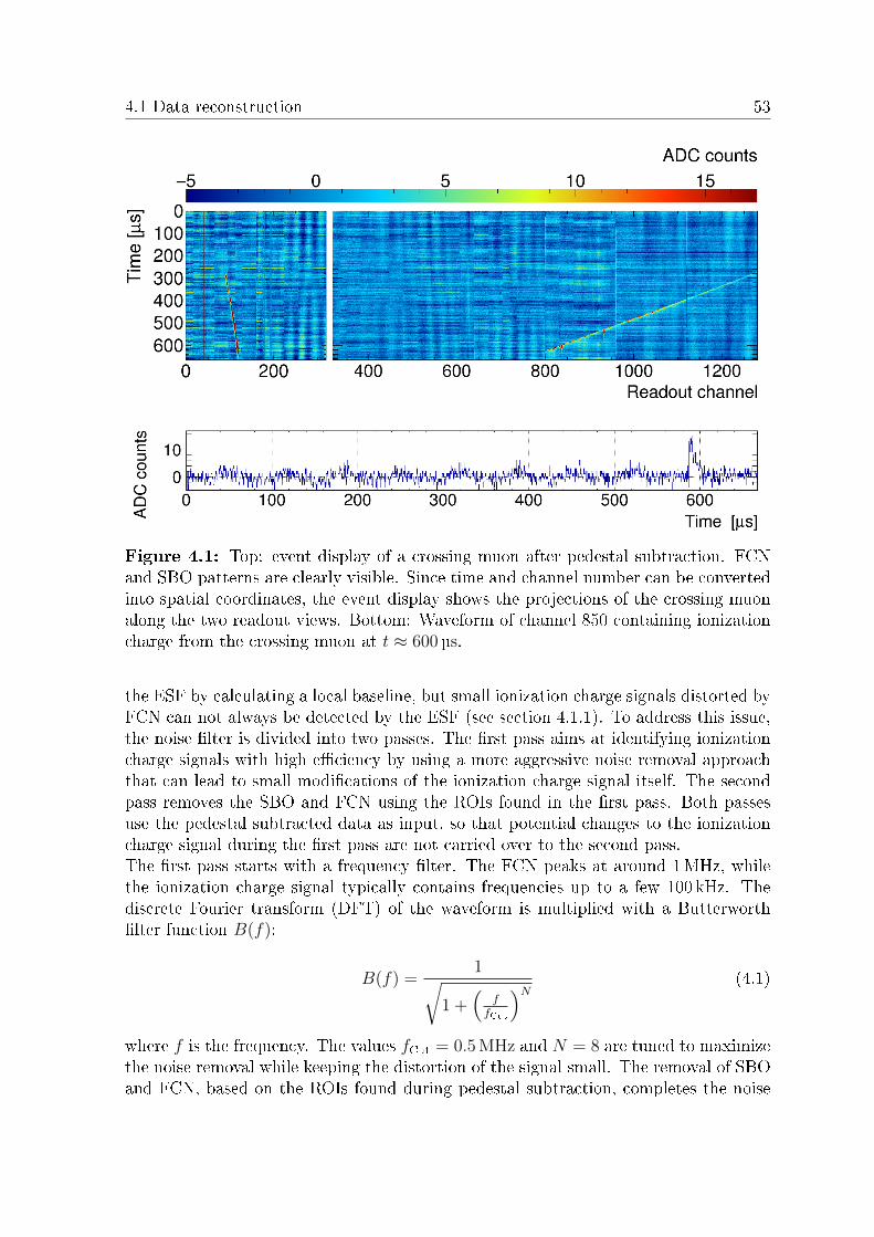
4.1 Data reconstruction 53
Figure 4.1: Top: event display of a crossing muon after pedestal subtraction. FCNand SBO patterns are clearly visible. Since time and channel number can be convertedinto spatial coordinates, the event display shows the projections of the crossing muonalong the two readout views. Bottom: Waveform of channel 850 containing ionizationcharge from the crossing muon at t ≈ 600 µs.
the ESF by calculating a local baseline, but small ionization charge signals distorted byFCN can not always be detected by the ESF (see section 4.1.1). To address this issue,the noise lter is divided into two passes. The rst pass aims at identifying ionizationcharge signals with high eciency by using a more aggressive noise removal approachthat can lead to small modications of the ionization charge signal itself. The secondpass removes the SBO and FCN using the ROIs found in the rst pass. Both passesuse the pedestal subtracted data as input, so that potential changes to the ionizationcharge signal during the rst pass are not carried over to the second pass.The rst pass starts with a frequency lter. The FCN peaks at around 1MHz, whilethe ionization charge signal typically contains frequencies up to a few 100 kHz. Thediscrete Fourier transform (DFT) of the waveform is multiplied with a Butterworthlter function B(f):
B(f) =1√
1 +(
ffCut
)N (4.1)
where f is the frequency. The values fCut = 0.5 MHz and N = 8 are tuned to maximizethe noise removal while keeping the distortion of the signal small. The removal of SBOand FCN, based on the ROIs found during pedestal subtraction, completes the noise

54 Chapter 4. Analysis of 3x1x1m3 data and validation of detector simulation
ltering of the rst pass. The ESF is applied again to the ltered waveform to searchfor previously undetected signals and to remove potential noise ROIs found duringpedestal subtraction.The second pass only applies the SBO and FCN removal on the pedestal subtractedwaveforms, based on the ROIs found in the rst pass. After the second pass, theESF is applied a last time to determine the nal ROIs used as input for the followingreconstruction. Figure 4.2 shows a crossing muon event display after noise removal.
Figure 4.2: Top: event display of a crossing muon after noise lter. Bottom: Wave-form of channel 850 containing ionization charge from the crossing muon at t ≈ 600 µs.
4.1.3 Hit nder
The hit nder searches for hits within each ROI separately and calculates hit quanti-ties such as the hit start time, amplitude and integral. A hit is dened as the unity ofneighboring ADC samples containing ionization charge produced by a single particle.While the ESF only identies groups of ADC samples that contain ionization charge,the hit nder assigns each of the ADC samples to a hit and thus to a potential particle.The 3x1x1m3 mainly recorded cosmic muons. Since there usually are no other parti-cles in the vicinity of a cosmic muon, most ROIs contain only one hit from the muon.Muons do, however, produce so-called delta electrons that have enough kinetic energyto ionize argon atoms themselves and leave the initial region of ionization. In orderto deal with overlapping hits from muons and delta electrons, the hit nder is dividedinto a peak nder and a hit tter which are explained in the following two sections.

4.1 Data reconstruction 55
4.1.3.1 Peak nder
The amplitude threshold of the peak nder is Amin = 5 ADC. By denition, each ROIcontains at least one sample above this threshold, c.f. section 4.1.1. To nd peaks andto split up overlapping ionization charge from two or more particles, the peak nderstarts from the sample with the maximum ADC count within the ROI and walks tothe left until it nds the start point of the hit, which is either a sample with ADCcount ≤ 0 or an inection point signaling a second hit. An inection point is denedas a sample that is followed by at least four consecutive samples with equal or higherADC counts. The same procedure is repeated walking from the sample with maximumADC count to the right until the end point of the hit. The hit start and end times aredened as the sample time of the start and end point. If the maximum ADC count ofthe remaining samples outside the rst hit is greater than or equal to Amin, a secondhit is dened in the same way. This procedure is repeated until no ADC count greaterthan or equal to Amin is left outside the already found hits in the ROI. When no morehits are found, a hit lter is applied to identify and remove potential noise hits. A hitis classied as noise hit if it satises at least one of the following criteria:
1. Hit ADC sum ≤ 10 ADC · ticks
2. Hit width: tEnd − tStart ≤ 4 µs
3. Hit ADC sum over hit width ≤ 2 ADC · ticks / µs
4.1.3.2 Hit tter
In order to smooth out noise uctuations, single hits are tted with the same doubleexponential function used in the characterization of the charge readout shaping, c.f.section 3.1.2:
f (t) =A · e−
t−t0τA
1 + e− t−t0
τB
(4.2)
where A, t0, τA and τB are free parameters. The slopes of the rising and falling edges ofthe hit are modeled with τA and τB. Adjacent, and thus potentially overlapping hits,are tted simultaneously with a sum of double exponential functions:
F (t) =N∑i=1
fi (t) =N∑i=1
Ai · e−t−t0,iτA,i
1 + e−t−t0,iτB,i
(4.3)
Figure 4.3 shows a noise-ltered waveform with tted single and adjacent hits. Thepeak time, full width at half maximum (FWHM) and integral of the hit are calculatedfrom the t function. The hit start and end time, the hit amplitude and the hit ADCcount sum between start and end time are determined directly from the ADC waveformand complete the set of hit parameters that are relevant for 2D pattern recognition,3D track reconstruction and analysis.

56 Chapter 4. Analysis of 3x1x1m3 data and validation of detector simulation
Figure 4.3: Noise-ltered waveform with tted single and adjacent hits.
4.1.4 2D pattern recognition
The hit nder produces a collection of hits in both readout views that are sorted bychannel and time. For each hit, two spatial coordinates can be determined from theposition of the readout channel and the hit peak time. The next step in the recon-struction is the identication of groups of hits that originate from the same particleindependently in each view. Reconstruction algorithms typically accomplish this taskby looking for two types of patterns: continuous lines of hits originating from tack-likeparticles such as muons and cone-like groups of hits from showering particles such aselectrons. Since only muons will be considered in the following analyses, the Lineclusteralgorithm that was tuned for the reconstruction of track-like patterns is used. Lineclus-ter starts from the reconstructed hit with the lowest channel number and adds similarhits to the leading edge of hit collection, taking into account the hit position, hit inte-gral and FWHM. When no more similar hits are found, the hit collection is declaredcomplete and the algorithm starts over with the remaining hits until no additionalline-like patterns are found.
4.1.5 3D track reconstruction
In order to reconstruct parameters from track-like particles, such as track length orlocal energy deposits along the track, that are needed for the following analyses, a 3Dreconstruction of the particle is necessary. The projection matching algorithm is usedto reconstruct 3D tracks by combining hit collections with similar start and end timesand charge contents from the two readout views [95]. From the rst and last hits inboth views, the two 3D end points of the track are determined. A 3D spline betweenthe 3D end points is t to the track by minimizing the distance between the 2D splineprojection and the hits in both readout views. The length of the track segment ds fromwhich a single hit has collected charge is calculated for each hit in both views usingthe readout channel pitch and the local direction of the spline expressed as θ and φ:
dsView 0 =3.125 mm
sin (θ) · sin (φ)(4.4)
dsView 1 =3.125 mm
sin (θ) · cos (φ)(4.5)
The denitions θ and φ are given in table 4.1. The charge content QHit of a hit can beobtained from the hit ADC count sum SHit and the calibration factor γ of the respective

4.2 Data analysis 57
view, c.f. equation 3.1 and section 4.1.3:
QHit = SHit/γ (4.6)
Eventually, the recorded charge per unit length dQHit/ds is determined for all hits inboth views and used in the data analysis, where it is called dQ/ds.
Angle Denition
θ = 0 up-goingθ = 90 parallel to CRPθ = 180 down-going
φ = 0 parallel to strips in view 0φ = 90 parallel to strips in view 1
Table 4.1: Denitions of θ and φ in the detector coordinate system.
4.2 Data analysis
In this section, several analyses on the performance of the detector and the validationof the detector simulation that are relevant for the proton decay sensitivity studyare carried out. All analyses are based on reconstructed tracks of cosmic muons inrun 840. The electric eld settings of this run are summarized in table 4.2. Due toa malfunctioning connector, the extraction grid voltage was limited to -5 kV. As aconsequence, the nominal extraction, amplication and induction elds could not bereached simultaneously (c.f. table 2.3) and the conguration of run 840 is the bestcompromise for the following analyses. The extraction and amplication elds in table4.2 are only valid for the eight central LEMs. The corner LEMs 1, 3, 10 and 12 wereoperated at a lower voltage dierences due to a higher discharge risk, c.f. gure 2.14.
Run Events Trigger εD εextr,l εamp εind
840 35 845 PMT 0.5 kV/cm 1.73 kV/cm 28 kV/cm 1.5 kV/cm
Table 4.2: Number of collected events, trigger conguration and electric eld settingsof run 840.
4.2.1 Cosmic muon selection
With a frequency of around 1 kHz, muons are the most common particles to enterthe TPC. The total trigger rate at nominal drift eld of εD = 0.5 kV/cm, however, isonly ∼2Hz and an eye scan of 350 events yields a muon trigger share of 47 %. The low

58 Chapter 4. Analysis of 3x1x1m3 data and validation of detector simulation
trigger rate and the relatively small share of muon triggers is caused by the coincidencePMT trigger that only selects muons crossing the detector along the 3meter side, seesection 2.4.6.2. The remaining triggers are electromagnetic and hadronic showers witha trigger share 38 % and 15 %, respectively.Since the applied reconstruction algorithm can not distinguish between track-like andshower-like events and showering events are typically reconstructed as several tracksalong the center of the shower, the so-called Highway algorithm was developed todistinguish tracks in showering events from real particle tracks. The Highway algorithmplaces a narrow box with a width of 3.5 cm and a wide box with a width of 7 cm aroundthe 2D projection of the reconstructed track in both views. In order to account fortilted tracks due to multiple scattering or space charge (c.f. section 2.3.3.4), a newpair of boxes that follows the local track direction is used for every 50 cm section alongthe track. Since the narrow box is fully contained inside the wide box, the collectedcharge in the wide box Qwide is always equal or bigger than the charge in the narrowbox Qnarrow. The charge box ratio QR is dened as follows for each pair of boxes inboth views:
QR =Qwide −Qnarrow
Qwide
(4.7)
Muons and other track-like particles have a small CBR close to 0 since they onlygenerate ionization charge in close vicinity of their path. Showers, on the other hand,typically leave a cone-like trace of ionization charge in the detector which reects inhigher CBR values.To tune the cut value of QR for distinguishing between track- and shower-like particles,a Monte Carlo sample with cosmic air showers was generated with the simulation toolsdescribed in section 3.2. Figure 4.4 shows the momentum distribution of particlesentering the detector as well as triggering particles. Since the light signal processingis not implemented in the detector simulation, a simplied trigger condition based onthe number and timing of detected photons in each PMT has been applied. Whilethe real PMT trigger is based on ADC amplitude thresholds (see section 2.4.6.2), thetrigger condition in the Monte Carlo sample is fullled if there is a 80 ns time windowin which all ve PMTs recorded Nγ ≥ 1 750 photons. The absolute trigger rate of2.36Hz in the simulation is in good agreement with the one in data of 2Hz. Theshares of muon, electromagnetic shower and hadronic shower triggers are 33 %, 58 %and 9 %, respectively. The Monte Carlo sample is reconstructed with the same toolsused for data, and the Highway algorithm is applied to all reconstructed 3D tracks.Requiring QR < 0.2 and a reconstructed track length of Lreco > 50 cm, the muontrack selection eciency is 61% and the overall contamination of tracks coming fromelectromagnetic and hadronic showers is 6% and 5.5%, respectively. While hadronicshowers predominantly produce hadronic particles that are hard to distinguish frommuons with the reconstructed parameters, the contamination of tracks emerging fromelectromagnetic showers could be further reduced by choosing tighter selection cutsfor QR and Lreco, or by including additional reconstructed parameters in the trackselection. This would, however, reduce the muon track selection eciency and the

4.2 Data analysis 59
found compromise between eciency and contamination works best for the followinganalyses. The track direction and hit position distributions after track selection cutsfor data run 840 are shown in gures 4.5 and 4.6, and features of the cosmic ray muonux and trigger selection are clearly visible.
−1 0 1 2 3lg(P(GeV))
10−3
10−2
10−1
100
101
102
103
104
105
Rat
e,H
z
Primary and triggered flux
µ±
e±, γ
p, n, π±
Figure 4.4: Dashed empty histograms: simulated particle ux entering the TPC.Solid lled histograms: simulated particle ux that fullls the PMT trigger condition.
Figure 4.5: Direction of selected tracks in data run 840. The denitions of θ and φ aregiven in table 4.1. The main peak at low θ and φ reects triggering muons that crossthe detector along the 3meter view. The second peak around θ = 155 is at in φ andoriginates from so called o-time muons that entered the detector within one readoutwindow before or after a trigger and therefore follows the primary cosmic muon ux.
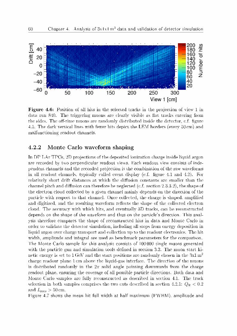
60 Chapter 4. Analysis of 3x1x1m3 data and validation of detector simulation
Figure 4.6: Position of all hits in the selected tracks in the projection of view 1 indata run 840. The triggering muons are clearly visible as at tracks entering fromthe sides. The o-time muons are randomly distributed inside the detector, c.f. gure4.5. The dark vertical lines with fewer hits depict the LEM borders (every 50 cm) andmalfunctioning readout channels.
4.2.2 Monte Carlo waveform shaping
In DP LAr TPCs, 2D projections of the deposited ionization charge inside liquid argonare recorded by two perpendicular readout views. Each readout view consists of inde-pendent channels and the recorded projection is the combination of the raw waveformsin all readout channels, typically called event display (c.f. gure 4.1 and 4.2). Forrelatively short drift distances at which the diusion constants are smaller than thechannel pitch and diusion can therefore be neglected (c.f. section 2.3.3.2), the shape ofthe electron cloud collected by a given channel mainly depends on the direction of theparticle with respect to that channel. Once collected, the charge is shaped, ampliedand digitized, and the resulting waveform reects the shape of the collected electroncloud. The accuracy with which hits, and eventually 3D tracks, can be reconstructeddepends on the shape of the waveform and thus on the particle's direction. This anal-ysis therefore compares the shape of reconstructed hits in data and Monte Carlo inorder to validate the detector simulation, including all steps from energy deposition inliquid argon over charge transport and collection up to the readout electronics. The hitwidth, amplitude and integral are used as benchmark parameters for the comparison.The Monte Carlo sample for this analysis consists of 100 000 single muons generatedwith the particle gun and simulation tools dened in section 3.2. The muon start ki-netic energy is set to 1GeV and the start positions are randomly chosen in the 3x1m2
charge readout plane 1 cm above the liquid-gas interface. The direction of the muonsis distributed randomly in the 2π solid angle pointing downwards from the chargereadout plane, ensuring the coverage of all possible particle directions. Both data andMonte Carlo samples are fully reconstructed as described in section 4.1. The trackselection in both samples comprises the two cuts described in section 4.2.1: QR < 0.2and Lreco > 50 cm.Figure 4.7 shows the mean hit full width at half maximum (FWHM), amplitude and

4.2 Data analysis 61
charge in view 0 for the selected tracks as a function of the track direction. Only hitswithin the eight central LEMs are selected since the corner LEMs were operated atlower voltage dierences, see section 4.2. View 0 is chosen as reference in this analysissince the DP LAr TPC design for the DUNE far detector only includes 3meters longreadout strips, see section 5.1.3.1. Some areas in the data plots are empty since thereare not reconstructed tracks in the corresponding directions, c.f. gure 4.5.As expected, the mean hit FWHM, amplitude and charge increase towards low valuesof φ and high values of θ because the track segment from which charge is collected bya single readout channel increases. Data and Monte Carlo match well both in generaltrend and absolute numbers, validating the detector simulation in terms of charge de-position and transportation as well as waveform shaping.
4.2.3 Charge readout uniformity
The uniformity of the charge readout plane is an important aspect of the DP LAr TPC.Deformations of the supporting structure, dierences in the tension of the extractiongrid wires and variations in the LEM thickness can alter the local extraction, amplica-tion and induction elds and thus the amount of collected charge, which has a negativeimpact on the charge resolution. As no non-uniformity is introduced in the detectorsimulation, this analyses is only carried out for data. The same data sample and trackselection as for the previous analysis are used: QR < 0.2 and Lreco > 50 cm. Figure 4.8shows the distribution of hits in selected tracks in the charge readout plane. A goodcoverage is achieved across the full plane. For all hits, the collected charge per unitlength dQ/ds is calculated according to the method described in section 4.1.5. Figure4.9 shows the average dQ/ds across the charge readout plane and the mean dQ/ds foreach LEM. The regions mentioned in the list below are excluded from the calculationof the LEM mean dQ/ds. The measured charge in the corner LEMs is lower since theywere operated at a lower voltage dierences, see section 4.2. The central LEMs showa uniform distribution except for two patterns:
1. Vertical lines between 80 cm and 90 cm in view 1
2. Isolated tracks above 30 cm and below -30 cm in view 0 and between 100 cm and200 cm in view 1
The rst pattern originates from a group of 32 extraction grid wires along view 1 thatwas not properly tightened, c.f. section 2.4.2.2. The second pattern is in a regionwith low statistics of reconstructed hits, c.f. gure 4.6. Since the applied cuts allowfor some hadronic and electromagnetic showers to be selected, isolated tracks with ahigher dQ/ds are expected. Apart from these patterns, the data shows a good overalluniformity of the charge readout plane with only small deviations.

62 Chapter 4. Analysis of 3x1x1m3 data and validation of detector simulation
Data Monte Carlo
Figure 4.7: Mean hit full width at half maximum (FWHM), amplitude and charge inview 0 for the selected tracks as function of the track direction in data (left) and MonteCarlo (right). The rst bin in φ and the last bin in θ are left empty since they containtracks with only a handful of long hits in view 0 that are often not well reconstructed.

4.2 Data analysis 63
Figure 4.8: Position of all hits in the selected tracks in the charge readout plane. Asin gure 4.8, the triggering muons are visible as tracks entering from the left or rightand the o-time muons are randomly distributed across the readout plane. The darkvertical lines with fewer hits depict the LEM borders (every 50 cm) and malfunctioningreadout channels, c.f. gure 4.6.
Figure 4.9: Average dQ/ds across the charge readout plane and mean dQ/ds for eachLEM. The four corner LEMs were operated at lower voltage dierences.
4.2.4 Charge resolution
The charge resolution describes the smearing in the measurement of the depositedionization charge, with contributions from the electron transport, readout electronicsand reconstruction. In order to determine the charge resolution in both views underidentical conditions, tracks with angles between 35 < φ < 55 that look similar inboth views are selected for this analysis. Furthermore, the track selection cuts discussedin section 4.2.1 are applied: QR < 0.2 and Lreco > 50 cm. Only hits within the eightcorner LEMs are selected, excluding the region between 80 cm and 90 cm in view 1 thatwas identied to have loose extraction grid wires (c.f. section 4.2.3). For all selectedhits in both readout views, the collected charge per unit length dQ/ds is calculated,

64 Chapter 4. Analysis of 3x1x1m3 data and validation of detector simulation
see section 4.1.5. In case all selected tracks originated from monoenergetic muons, thedeposited charge in liquid argon would follow the Landau distribution. The electrontransport, readout electronics, reconstruction and contamination from electromagneticand hadronic showers, however, introduce a smearing of the charge information thatcan be approximated with a Gaussian distribution. The measured dQ/ds distributioncan therefore be modeled with the convolution of a Landau and a Gaussian distribution.Figure 4.10 shows the dQ/ds distribution and the Landau-Gauss t for both readoutviews. The charge resolution R is dened as the ratio of the standard deviation of theGaussian over the most probable value of the dQ/ds distribution:
R =σ
〈dQ/ds〉 (4.8)
The charge resolutions are RView 0 = 14.0 % and RView 1 = 13.5 %. These values arelarger than the resolution measured with the 3 L DP LAr TPC prototype of around8 %, see gure 51 in reference [42]. Reasons for this discrepancy are manifold:
1. Electrons are lost in the stochastic extraction process at the liquid-gas interfacedue to the low extraction eld, see section 2.3.4
2. Not all selected tracks are MIPs
3. The space charge eect can locally alter the drift eld and therefore aects theamount of produced ionization charge, see section 2.3.2
4. Measured tracks are tilted due to the space charge eect which introduces asmearing in the reconstructed track direction and dQ/ds distribution
5. Small non-uniformities in the charge readout plane, see section 4.2.3
6. Electronic noise
The low extraction eld is the consequence of a malfunctioning high voltage connector,see section 4.2. The other eects can be mitigated with more advanced reconstructionand calibration tools. The measured charge resolution is nevertheless good enough toenable ecient particle identication in a DP LAr TPC DUNE far detector module,which is a crucial element of the proton decay sensitivity study. In addition to deter-mining the charge resolution, this analysis also demonstrates that the charge is sharedequally between the two readout views for the selected track topologies as the dQ/dsdistribution peaks at the same value in both views, validating the assumption madefor the detector simulation in section 3.2.4.

4.2 Data analysis 65
Figure 4.10: Hit dQ/ds distribution in both readout views t with a convolution of aLandau and a Gaussian distribution. The t range from 4 fC/cm to 30 fC/cm excludesthe tail on the left that originates from noise hits.

66 Chapter 4. Analysis of 3x1x1m3 data and validation of detector simulation

Chapter 5
The Deep Underground Neutrino
Experiment
The Deep Underground Neutrino Experiment (DUNE) is a future long baseline neu-trino oscillation experiment hosted by the Fermi National Accelerator Laboratory (Fer-milab) that will comprise a neutrino beam and two particle detectors, see gure 5.1.Besides neutrino oscillation, DUNE's main physics searches include proton decay andcore-collapse supernova neutrino detection.
Figure 5.1: Sketch of the Deep Underground Neutrino Experiment. The acceleratorcomplex and near detector are hosted at Fermilab and the far detector is hosted at theSanford Underground Research Facility. Figure is taken from reference [28].
The DUNE near detector will measure the unoscillated neutrino ux and neutrino crosssections 574m downstream from the beam production point. The far detector will belocated 1 500m underground at the Sanford Underground Research Facility (SURF) tomeasure the oscillated neutrino ux at a baseline of 1 300 km. The far detector complexwill consist of four independent 10 kiloton LAr TPC modules, providing enough massfor competitive proton decay and other rare event physics searches that are carriedout in parallel to the neutrino oscillation measurement. Both single phase and dualphase LAr TPC technologies are currently considered for the far detector modules and
67

68 Chapter 5. The Deep Underground Neutrino Experiment
the prototyping eorts for DP LAr TPCs have been explained in detail based on the3x1x1m3 detector in chapters 2 through 4.In this chapter, the experimental setup of DUNE is described in section 5.1, includingthe design for a DP LAr TPC far detector module. The physics program for longbaseline neutrino oscillation and core-collapse supernova neutrino detection is discussedin section 5.2. The search for proton decay in a DP LAr TPC far detector module isthe main topic of this thesis and the corresponding sensitivity study is presented inchapter 7.
5.1 Experimental setup
The experimental setup of DUNE consists of a neutrino beam and a near and fardetector complex. The general design of the various components has been nalizedthroughout the past few years and is described in the following, but individual designparameters may be updated in the future.
5.1.1 Neutrino beam
The existing proton accelerator complex at Fermilab is currently being upgraded underthe Proton Improvement Plan II (PIP-II) in order to deliver the high intensity neutrinobeam that is necessary to achieve the neutrino oscillation physics goals of DUNE [41][98]. The upgraded accelerator chain will start with a new, superconducting radio-frequency cavity linear accelerator that provides a 800MeV proton beam to the booster.The booster accelerates the beam to 8GeV and feeds into the main injector, whichcan be operated at nal proton energies between 60GeV and 120GeV. Subsequently,the proton beam is extracted into the new Long Baseline Neutrino Facility (LBNF)beamline where it is directed towards the near and far detectors and smashed into agraphite target. The resulting hadronic showers contain a variety of hadrons such aspions, kaons, neutrons and protons, with pions being the most common. The chargedparticles inside the hadron shower are focused into a 200m long decay pipe by a seriesof magnetic horns. Pions decay into muons and muon neutrinos with a branching ratioof 99.99% [46]:
π+ → µ+νµ (5.1)
π− → µ−νµ (5.2)
The neutrinos emerging from this decay form the neutrino beam. While most muonsstop inside the shielding at the end of the decay pipe to decay at rest, some decayin-ight and contribute to the neutrino beam:
µ+ → e+νµνe (5.3)
µ− → e−νµνe (5.4)

5.1 Experimental setup 69
The LBNF beamline can be operated in neutrino and antineutrino mode by reversingthe horn currents to focus either negatively or positively charged particles. Figure 5.3shows the simulated DUNE neutrino and antineutrino beam ux at the far detector,normalized to 1.1× 10²¹ protons on target (POT). The LBNF beam power depends onthe nal proton energy and ranges from 0.9MW to 1.2MW. The beam is scheduledto start operation in 2026 and a maximum beam power increase to 2.4MW is foreseenalongside further upgrades of the proton accelerator complex in 2032.
Figure 5.2: Simulated DUNE neutrino (left) and antineutrino (right) beam ux atthe far detector, normalized to 1.1 × 10²¹ protons on target (POT). Contaminationsarise from semileptonic and hadronic decays of kaons and in-ight decaying muons.Some parameters of the LBNF beamline, such as target and magnetic horn design,have not been optimized yet and the shown ux is simulated with the reference beamdesign. Figure is taken from reference [99].
5.1.2 Near detector
The DUNE near detector complex will be located 574m downstream of the LBNFbeamline target under a rock overburden of about 60m that reduces the cosmic raymuon ux to a tolerable rate. The main task of the near detector is the measurementof the unoscillated neutrino ux and neutrino cross sections on argon to constrainsystematic uncertainties in the long baseline neutrino oscillation analysis. The neardetector concept is currently under development and foresees three particle detectors:ArgonCube, MPD and 3DST+KLOE, see gure 5.3.ArgonCube is a novel LAr TPC detector technology with a pixelated charge readoutand a large area photon detection system. With a ducial mass of 50 tons, ArgonCubewill measure ∼8×10⁷ muon neutrino charged current interactions per year and enablesa detailed study of neutrino interactions on argon as they are seen at the far detector.MPD stands for Multi-Purpose Detector and combines a high pressure gas argon TPCin a magnetic eld of 0.5T with a surrounding electromagnetic calorimeter and muon

70 Chapter 5. The Deep Underground Neutrino Experiment
Figure 5.3: DUNE near detector complex with ArgonCube (right) and MPF (middle)in extreme o-axis position. The 3DST+KLOE detector (left) will be permanentlyon-axis. The neutrino beam enters from the right as indicated by the red line thatpenetrates the 3DST+KLOE detector.
tagger. The MPD will be capable of measuring neutrino and antineutrino interactionson argon with sign selection and low energy thresholds to complement the reconstruc-tion of muons that leave the ArgonCube detector. Both ArgonCube and MPD will beinstalled on a rail system that allows the detectors to be moved transversely to thebeam axis in order to measure the neutrino ux at a variety of o-axis angles, a sys-tem called DUNE-PRISM. The peak neutrino ux energy decreases notably already atsmall o-axis angles and DUNE-PRISM can therefore provide a precise and extensivemapping of reconstructed to true neutrino energies that will inform the long baselineoscillation analysis, c.f. section 5.2.1. Furthermore, the observed neutrino energy spec-trum at the far detector can be mimicked by combining neutrino ux measurements atdierent o-axis angles, and mapped to the true neutrino ux energy spectrum. Thistechnique will reduce systematic uncertainties in the oscillation analysis since the con-version from reconstructed to true neutrino energy would otherwise rely on neutrinointeraction models that are not complete and therefore introduce biases.The 3DST+KLOE detector will consist of an eight tonne 3D scintillator tracker (3DST)active target, a low density tracker and the repurposed electromagnetic calorimeter andmagnet of the KLOE experiment. All 3DST+KLOE detector components will be in-stalled inside the magnet system. The 3DST+KLOE detector will be permanently

5.1 Experimental setup 71
positioned on-axis to deliver a continuous characterization of the neutrino beam.
5.1.3 Far detector
The far detector will measure the oscillated neutrino ux on-axis at a baseline of1 300 km and will be composed of four ∼10 kiloton LAr TPC modules, for which bothsingle phase and dual phase technologies are considered [28]. The staged installationschedule foresees the start of operation of the rst module in 2026.The location at the Sanford Underground Research Facility provides a rock overburdenof 1 500m that decreases the cosmic ray muon ux to about 4 per square meter perday. The low muon ux is essential for LAr TPCs in the kiloton scale in order to limitthe trigger rate and space charge eect, c.f. section 2.3.3.4.The design of both single phase and dual phase LAr TPC modules for the DUNEfar detector is the result of decades-long R&D (see section 2.1) and the proton decaysensitivity study in chapter 7 is carried out for a 10 kiloton dual phase LAr TPC modulethat is described in the following section.
5.1.3.1 DP LAr TPC module design
The design of the DP LAr TPC module for the DUNE far detector is largely basedon the 3x1x1m3 prototype, see chapter 2. This section therefore highlights the designchanges that have been made with respect to the prototype as well as challenges thatarise with upscaling the design for a multi-kiloton detector.The dimensions of the charge readout area for the far detector module are 12× 60m2
and the maximum drift distance is 12m, yielding ∼12 kilotons of liquid argon insidethe TPC. Since the ducial mass will be somewhat smaller, the detector mass is usuallyquoted as 10 kiloton. The cryostat and drift cage are easily scalable to multi-kilotonsize.The charge readout area consists of 80 independent 3 × 3m2 charge readout planes(CRPs) that are equipped with one 3 × 3m2 extraction grid and 36 anode and LEMmodules with an area of 50× 50 cm2 each, c.f. section 2.4.2.2. A gap of 1 cm betweenneighboring CRPs simplies the installation procedure and allows for independentalignment. Some changes in the CRP design with respect to the 3x1x1m3 prototypehave been made:
1. The supporting structure will be made of Invar, a nickel-iron alloy with a verylow thermal expansion coecient. The G10 frame that holds the anode-LEMsandwiches has a larger thermal expansion coecient and is therefore thermallydecoupled from the supporting structure.
2. The LEM border clearance has been increased to 10mm and the copper guardrings around the screw holes, high voltage pins and LEM border have been in-creased to 5mm to prevent discharges.
3. Groups of 64 extraction grid wires are soldered onto wire-tensioning pads andeach wire is tensioned and positioned independently in a dedicated groove on the

72 Chapter 5. The Deep Underground Neutrino Experiment
pad.
The 3 × 3m2 CPRs with the changes listed above and a 6x6x6m3 drift cage are cur-rently tested with protoDUNE-DP, c.f. section 2.1.A component that is more dicult to scale is the cathode high voltage supply. In orderto achieve a drift eld of 0.5 kV/cm over a distance of 12m, the cathode grid has tobe brought to a potential of -600 kV. There are currently no commercially availablepower supplies that can provide such a high voltage and a joint R&D program betweenDUNE and an industry partner aims at scaling up the 300 kV high voltage supply thatis currently deployed in protoDUNE-DP. The high voltage supply will be connected tothe high voltage feedthrough at the top of the cryostat and guided to the cathode viaan extender in close distance to the eld-shaping rings of the drift cage, c.f. section2.4.2.1. Metallic rings are installed around the insulation of the high voltage extenderand connected to the eld-shaping rings to bring the electric eld between extenderand drift cage down to 0.The photon detection system (PDS) will cover the area below the drift cage with 720evenly distributed PMTs. The main purpose of the PDS is to provide triggers fornon-beam events and accurate event timing. Furthermore, the PDS can complementthe event reconstruction and analysis from the collected ionization charge with calori-metric measurements and timing information. The PMT density of 1/m2 guaranteesa trigger eciency close to 100% for events in the GeV region such as beam neutrinointeractions and proton decay. Figure 5.4 shows a sketch of the 12 kiloton dual phasefar detector module with the dierent components.
Figure 5.4: Technical drawing of the 12 kiloton dual phase LAr TPC far detectormodule for DUNE. Figure is taken from reference [28].

5.2 Physics program 73
5.2 Physics program
The primary physics goals of DUNE are a precision neutrino oscillation measurementto determine the CP violating phase δCP in the lepton sector and the neutrino masshierarchy as well as the search for proton decay and the detection of core-collapse su-pernova neutrinos.The existence of CP violation in the lepton sector is a requirement for leptogenesis, ahypothetical process to explain the matter-antimatter asymmetry in the universe. Asopposed to baryogenesis, in which baryonic processes are responsible for the matter-antimatter asymmetry (see section 1.4), leptogenesis assumes that the asymmetry wascreated through leptonic processes in the early universe.The primary physics goals are complemented by a variety of measurements such asatmospheric neutrino oscillation, geoneutrinos, solar neutrinos and neutrino cross sec-tions.The long baseline neutrino oscillation and core-collapse super nova programs are dis-cussed in more detail in sections 5.2.1 and 5.2.2.The theoretical context for protondecay has been described in chapter 1 and a sensitivity study for the proton decaymode p→ νK+ is presented in chapter 7.
5.2.1 Long baseline neutrino oscillation
Neutrino oscillation was rst discovered in measurements of the atmospheric neutrinoux in 1998 by the Super-Kamiokande experiment [8]. This observation constitutes therst evidence for physics beyond the Standard Model of Particle Physics since neutrinosare massless in the Standard Model and neutrino oscillation requires that at least twoof the three neutrino avors νe, νµ and ντ possess a mass. In the quantum mechanicalpicture, a neutrino with a distinct avor eigenstate νe, νµ and ντ that emerges from aweak interaction is a linear combination of the three mass eigenstates ν1, ν2 and ν3:
|να〉 =3∑j=1
U∗αj |vj〉 , α = e, µ, τ (5.5)
where U∗αj are the elements of the conjugate transpose of the Pontecorvo-Maki-Nakagawa-Sakata matrixMPMNS. For Dirac neutrinos,MPMNS can be parametrized as follows:
MPMNS =
Ue1 Ue2 Ue3Uµ1 Uµ2 Uµ3
Uτ1 Uτ2 Uτ3
(5.6)
=
1 0 00 c23 s23
0 9s23 c23
· c13 0 s13e
9iδCP
0 1 09s13e
9iδCP 0 c13
· c21 s12 09s12 c12 0
0 0 1

74 Chapter 5. The Deep Underground Neutrino Experiment
with ckl = cos (θkl) and skl = sin (θkl), where θkl is the mixing angle and k = 1, 2 andl = 2, 3.The mass eigenstates |νj〉 are orthogonal eigenstates of the Hamiltonian and propagatewith dierent phase factors. In vacuum, the Hamiltonian is Hvac = Ej and the phasefactors simply are e9iEjt/~. Using ~ = 1, the propagation of |να〉 as a plane wave canbe written as:
|να(t)〉 =3∑j=1
U∗αje9iEjt |vj〉 , α = e, µ, τ (5.7)
Due to their low masses, neutrinos are ultra-relativistic even at low energies and Ejcan be approximated through a Taylor expansion and by using pj ' p ' E to:
Ejc=1=√p2j +m2
j (5.8)
' E +m2j
2E(5.9)
Dierent masses mj therefore lead to varying shares of the mass-eigenstates as theneutrino propagates through space, which results in changing probabilities to measurethe avor eigenstates νe, νµ and ντ through a weak interaction. This phenomenon iscalled neutrino oscillation. Using the orthogonality of |vj〉, the probability to measure
a neutrino avor eigenstate νβ at a distance Lc=1= t from the production point of the
avor eigenstate να is therefore:
P (να → νβ) = | 〈νβ|να(L)〉 |2 =
∣∣∣∣∣3∑j=1
UβjU∗αj e
−im2jL
2E
∣∣∣∣∣2
, α, β = e, µ, τ (5.10)
Equation 5.7 and 5.10 are only valid for neutrinos traveling in vacuum. In DUNE,neutrinos will travel 1 300 km through the earth and their propagation can be alteredby coherent forward scattering o electrons, neutrons and protons. An eective Hamil-tonian He = Hvac +Hmat can be dened to describe the propagation of neutrino avoreigenstates in matter according to equation 5.7. The contribution from all neutral cur-rent scatters and from charged current scatters o nucleons is avor-independent andtherefore has no impact on the oscillation probabilities. Charged current scatters oelectrons only occurs for electron neutrinos and the corresponding eective Hamiltonianpotential is:
He = VCCνeγ0νe (5.11)
with the Dirac-matrix γ0 and the charge current potential VCC =√
2GFne9 , where GF
is the Fermi constant and ne9 the electron density. VCC can be expressed by the matterdensity ρ and the electron fraction per nucleus Ye9 :

5.2 Physics program 75
VCC = Ye9 ·ρ
[g/cm3]· 7.56× 10−14 eV (5.12)
In neutrino beam mode, DUNE will measure the energy spectrum of the unoscillatedmuon neutrino beam with the near detector as well as the energy spectrum of theoscillated neutrino ux at the far detector, c.f. section 5.1.1. The probability forelectron neutrino appearance in a muon neutrino beam in leading order, includingmatter eects, is [102]:
P (νµ → νe) = sin2 (θ23) sin2 (θ13)sin2 (∆31 − aL)
(∆31 − aL)2 ∆231 (5.13)
+ sin (2θ23) sin (2θ13) sin (2θ12)sin (∆31 − aL)
∆31 − aL∆31
· sin (aL)
aL∆21cos (∆31 + δCP)
+ cos2 (θ23) sin2 (2θ12)sin2 (aL)
(aL)2 ∆221
with ∆kl = ∆m2klL/4E in natural units and a = VCC/2 = GFne9/
√2. The three
mixing angles θ12, θ23 and θ13 as well as the squared mass dierence ∆m221 = m2
2 −m2
1 and the absolute value of ∆m231 = m2
3 − m21 have been determined by dierent
neutrino oscillation experiments over the past decades. The sign of ∆m231 has not been
determined yet and depends on the neutrino mass hierarchy for which there are tworemaining possibilities: normal ordering with m1 < m2 < m3 and inverted orderingwith m3 < m1 < m2. The CP violating phase δCP ∈ [−π,+π) has only been measuredwith low precision and no values can be excluded with the benchmark signicanceof 5 standard deviations. The current best values from a selected global analysis t,assuming both normal and inverted mass ordering, are summarized in gure 5.5.In antineutrino beammode, the electron antineutrino appearance probability P (νe → νµ)is given by equation 5.13 with changed signs for a and δCP and the oscillation prob-ability for neutrino energies of several GeV at the DUNE baseline of L = 1 300 kmdiers strongly between neutrinos and antineutrinos, see gure 5.6. By measuring theasymmetry A in the appearance probability of electron neutrinos and antineutrinos ina muon neutrino and antineutrino beam as function of neutrino energy, DUNE will beable to unambiguously determine the neutrino mass hierarchy and δCP:
A =P (νµ → νe)− P (νµ → νe)
P (νµ → νe) + P (νµ → νe)(5.14)
This can be achieved because the asymmetry associated to the mass hierarchy is largerthan the asymmetries from δCP and matter eects at the peak of the neutrino ux

76 Chapter 5. The Deep Underground Neutrino Experiment
Figure 5.5: Neutrino oscillation parameters obtained by NuFit v4.1 [103] [104].∆m3l = ∆m31 > 0 for normal mass ordering and ∆m3l = ∆m32 < 0 for invertedmass ordering. Inverted mass ordering is disfavored by ∆χ2 = 9.3. Figure is takenfrom reference [104].
Figure 5.6: Electron neutrino (left) and antineutrino (right) appearance probability inthe DUNEmuon neutrino and antineutrino beams at the far detector (L = 1 300 km) fornormal neutrino mass ordering and dierent true values of δCP as function of neutrinoenergy. The black line shows the appearance probability if θ13 was equal to zero, inwhich case no dierence between neutrinos and antineutrinos could be observed (c.f.equation 5.13). Figure is taken from reference [99].

5.2 Physics program 77
at ∼3 GeV, and the asymmetry associated to δCP is dominant in the energy regionbelow the peak, c.f. gure 5.6. Figure 5.7 shows the sensitivity of DUNE to the masshierarchy as a function of δCP and experiment run time, assuming the following stageddetector deployment and beam operation schedule [99]:
1. t = 0− 1 years: two far detector modules with a total ducial mass of 20 kilotonsand beam operation at 1.2MW, resulting in 1.1× 10²¹ protons on target (POT).
2. t = 1−3 years: three far detector modules with a total ducial mass of 30 kilotons.No changes in beam operation.
3. t = 3−6 years: four far detector modules with a total ducial mass of 40 kilotons.No changes in beam operation.
4. t > 6 years: beam operation at 2.4MW.
Figure 5.7: Left: signicance√
∆χ2 between normal (NO) and inverted (IO) neutrinomass ordering as function of the true value of δCP for seven (blue) and ten (orange)years of data taking, assuming true normal neutrino mass ordering and the detectoremployment and beam operation schedule outlined in this section. Multiple ts withrandom throws for variations in statistics, systematic uncertainties and oscillation pa-rameters have been performed. The solid lines represent the median sensitivity of allts and the transparent bands cover 68% (1σ) of all ts. Figure is taken from refer-ence [99]. Right: signicance
√∆χ2 between NO and IO as function of experiment run
time, assuming the same detector employment and beam operation schedule. The redband shows the discrimination power for δCP = −π/2 and the green band for all truevalues of δCP. The solid black lines at the top of both bands represent the sensitivitywhen sin2 (θ23) is constrained to 0.088 ± 0.003 and the dashed lines at the bottom ofboth bands when θ23 is left unconstrained. Figure is taken from reference [99].
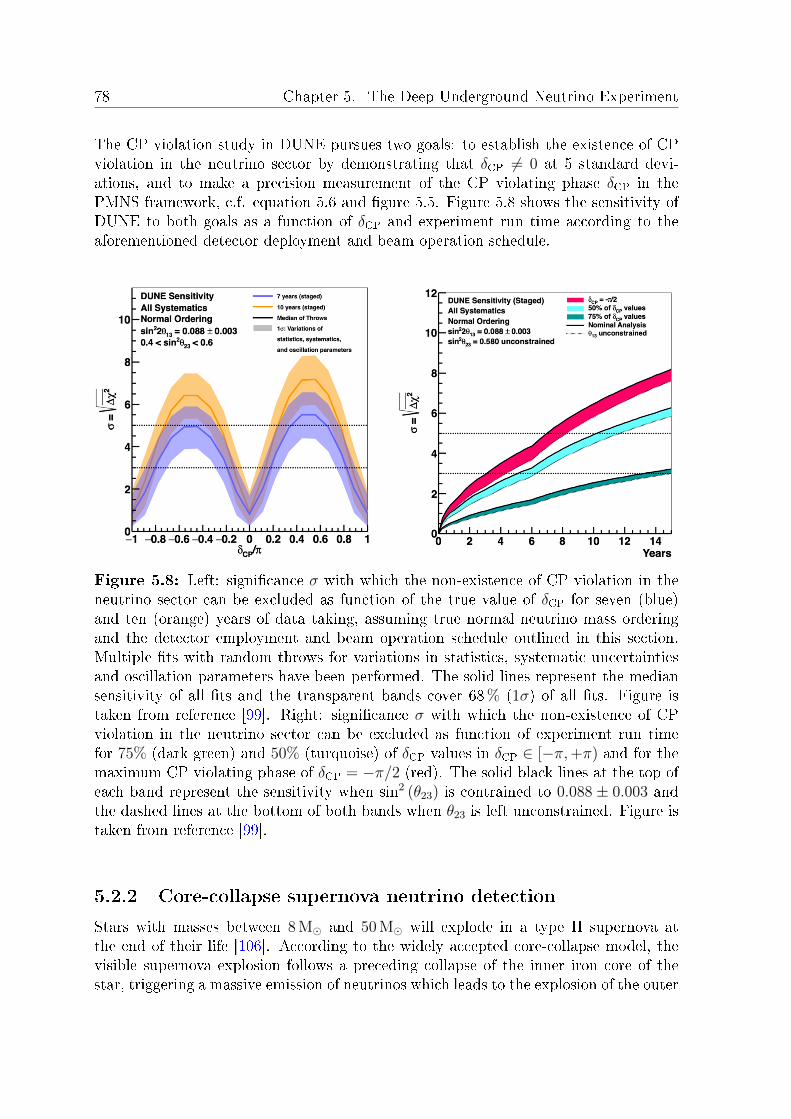
78 Chapter 5. The Deep Underground Neutrino Experiment
The CP violation study in DUNE pursues two goals: to establish the existence of CPviolation in the neutrino sector by demonstrating that δCP 6= 0 at 5 standard devi-ations, and to make a precision measurement of the CP violating phase δCP in thePMNS framework, c.f. equation 5.6 and gure 5.5. Figure 5.8 shows the sensitivity ofDUNE to both goals as a function of δCP and experiment run time according to theaforementioned detector deployment and beam operation schedule.
Figure 5.8: Left: signicance σ with which the non-existence of CP violation in theneutrino sector can be excluded as function of the true value of δCP for seven (blue)and ten (orange) years of data taking, assuming true normal neutrino mass orderingand the detector employment and beam operation schedule outlined in this section.Multiple ts with random throws for variations in statistics, systematic uncertaintiesand oscillation parameters have been performed. The solid lines represent the mediansensitivity of all ts and the transparent bands cover 68% (1σ) of all ts. Figure istaken from reference [99]. Right: signicance σ with which the non-existence of CPviolation in the neutrino sector can be excluded as function of experiment run timefor 75% (dark green) and 50% (turquoise) of δCP values in δCP ∈ [−π,+π) and for themaximum CP violating phase of δCP = −π/2 (red). The solid black lines at the top ofeach band represent the sensitivity when sin2 (θ23) is contrained to 0.088 ± 0.003 andthe dashed lines at the bottom of both bands when θ23 is left unconstrained. Figure istaken from reference [99].
5.2.2 Core-collapse supernova neutrino detection
Stars with masses between 8 M and 50 M will explode in a type II supernova atthe end of their life [106]. According to the widely accepted core-collapse model, thevisible supernova explosion follows a preceding collapse of the inner iron core of thestar, triggering a massive emission of neutrinos which leads to the explosion of the outer

5.2 Physics program 79
shells. A qualitative discussion of the core-collapse model and accompanying neutrinoemission according to Janka follows [107].Towards the end of their life, massive stars accumulate an iron core that is surroundedby shells of lighter elements. The core continues to grow due to the fusion of lighterelements into iron inside the surrounding shells. Iron itself does not undergo nuclearfusion since it has the highest nuclear binding energy per nucleon of all elements, andthe increasing gravitational pressure can therefore only be supported by an increasingdegeneracy pressure of electrons inside the core. When the mass of the iron corereaches the Chandrasekhar limit of about 1.4 M [108], the temperature inside the coreof ∼1010 K is high enough for thermal photons to disintegrate iron atoms, convertingthermal energy to rest mass and triggering the core collapse. Due to the increasingdensity in the collapsing core, the Fermi energy of the degenerate electrons exceedsthe threshold for electron capture on protons and a rst wave of electron neutrinos isproduced that can escape the core:
e9 + p→ n+ νe (5.15)
With decreasing electron density and degeneracy pressure, the collapse accelerates,and the outer parts of the core reach velocities up to 30% of the speed of light. Theneutrino production from electron capture continues during the collapse. When thecore density exceeds 1011−1012 g/cm3, the interaction length of neutrinos becomes tooshort to escape the core.Repulsive neutron interactions and increasing neutron degeneracy pressure abruptlystop the inner core collapse only a few milliseconds after the core reached the Chan-drasekhar limit. The still-collapsing outer core matter bounces o the inner core,resulting in a shock wave traveling outwards. The production of more electron neu-trinos is triggered by electron captures in the wake of the shock wave, trapping theminside the dense core. Once the shock front reaches lower densities, electron neutri-nos produced in its wake can escape in the so called breakout burst. Within a fewtens of milliseconds, the energy of the shock wave is completely absorbed inside thecore through disintegration of heavy elements into free nucleons at a radius of about∼150 km, also bringing the neutrino breakout burst to a halt.The inner core, heated up by the absorption of the gravitational energy released in thecollapse, forms a proto-neutron star. The star cools down over the course of severalseconds by emitting neutrinos and antineutrinos of all avors, mainly produced by theannihilation of electron-positron pairs, nucleon bremsstrahlung and positron captureon neutrons. In the rst phase of the the cool-down, the core continues to accumu-late matter from the shells, leading to a hot accretion zone on its surface that sparksthe production of additional electron neutrinos and antineutrinos through electron andpositron capture. The neutrinos produced inside the proto-neutron star and in theaccretion zone continuously escape the inner region and interact inside the outer shellsof the star, heating them up and pushing them outwards. This process is called neu-trino heating and is mainly driven by electron neutrino and antineutrino capture onprotons and neutrons. The fast expansion of the hot outer shells causes a visible explo-sion typically referred to as supernova. The proto-neutron star continues to cool down

80 Chapter 5. The Deep Underground Neutrino Experiment
until about 10 s after reaching the Chandrasekhar limit and most neutrinos leave thestar within that time scale, carrying away most of the energy released in the collapse.The dierent neutrino emission processes in the core-collapse model predict a distinctneutrino ux with a mean neutrino energy of around 10MeV, see gure 5.9.
Figure 5.9: Neutrino luminosities from a core-collapse supernova. The red curverepresents the identical luminosities of νµ, νµ, ντ and ντ . The mean neutrino energy is∼10 MeV. Figure is taken from reference [107].
The Kamiokande, IMB and Beksan experiments detected 11, 8 and 5 electron antineu-trinos with energies between 8MeV and 40MeV over a period of several seconds fromthe supernova SN 1987A. The measurements are in good agreement with the predictedneutrino ux originating from the processes in the core collapse and subsequent cool-ing of the proto-neutron star, conrming the basic picture of the core-collapse modeldescribed above [6] [7] [110].About three core-collapse supernovae per century occur in the Milky Way galaxy. Ifthe neutrinos from a core-collapse supernova would reach the earth during the lifetimeof DUNE, the far detector would mainly observe electron neutrino charged currentinteractions with argon nuclei, while electron antineutrino charged current interactionswith argon nuclei and neutral current electron scatters of all avors will occur aboutten times less frequent:
νe + 4018Ar→ e9 + 40
19K∗
(5.16)
νe + 4018Ar→ e+ + 40
17Cl∗
(5.17)(−)
νl + e9 → (−)
νl + e9 (5.18)
The electrons and positrons from supernova neutrino charged current interactions aswell as the particles emitted in the de-excitation of the scattered atoms are detectable.The neutrino energy detection threshold in DUNE for the described interactions is

5.2 Physics program 81
Eν & 5 MeV [99]. The number of neutrino interactions for a core-collapse supernovaat a distance of 10 kpc from the Earth is around 1 000 for one 10 kiloton DUNE fardetector module. The number of interactions increases linearly with the detector massand decreases with the square of the supernova distance. The good energy resolutionof DUNE combined with its large mass enables a high statistics precision measurementof core-collapse supernova neutrinos to further test the core-collapse model and toconstrain dierent model parameters.

82 Chapter 5. The Deep Underground Neutrino Experiment

Chapter 6
Proton decay signal and background
event simulation
For the proton decay sensitivity study presented in chapter 7, both signal and back-ground Monte Carlo samples are required. The signal sample consists of proton decayevents inside an argon nucleus via the decay mode p → νK+, and the backgroundsample consists of atmospheric neutrino interactions on argon as they constitute thedominant source of background in proton decay searches, c.f. sections 1.1 and 1.5.The physics processes inside the argon nucleus are very dierent from those alreadydescribed in the detector simulation of the 3x1x1m3 DP LAr TPC prototype in chap-ter 3, and the simulation of both signal and background samples is therefore dividedinto event generation and detector simulation. The detector simulation is identical forsignal and background samples and follows after the event generation, encompassingall processes that take place after particles emerging inside the argon nucleus have leftthe nuclear environment. The DP LAr TPC detector simulation has been explainedand validated with the 3x1x1m3 prototype data in chapters 3 and 4 and the detectorsimulation is scaled according to the design of the 10 kiloton DP LAr TPC module forthe DUNE far detector as described in section 5.1.3.1. All detector simulation param-eters used in the proton decay sensitivity study are summarized in chapter 7.The simulation toolkit GENIE v3_00_06 is used for the signal and background eventgeneration [112]. For the signal sample, the simulation includes the modeling of theinitial state of the argon nucleus, the decay kinematics of the proton and the intranu-clear propagation of the charged kaon. The initial state of the argon nucleus is denedby the nuclear model, which is divided into nucleon density distribution and spectralfunction in GENIE. The spectral function describes the nucleon momentum distribu-tion and nucleon binding energies. The atmospheric neutrino background simulationcomprises the atmospheric neutrino ux, nuclear model, neutrino-argon interactionsand intranuclear transport of particles emerging inside the nucleus.There exists a variety of models for all processes involved in the event generation andGENIE provides ocial tunes that represent consistent combinations of the interde-pendent processes in the nuclear model, intranuclear propagation and neutrino-argoninteractions. The atmospheric neutrino ux is modeled independently and passed to
83

84 Chapter 6. Proton decay signal and background event simulation
GENIE as input for the background sample simulation, see sections 6.4.1 and 6.4.2.The proton decay sensitivity study in chapter 7 is carried out with two ocial GE-NIE tunes labeled G18_02a_02_11a and G18_10b_00_000. The spectral function,intranuclear propagation and some of the neutrino interaction models used in tuneG18_02a_02_11a are empirical while the G18_10b_00_000 tune mainly uses theo-retically motivated models, making these two tunes a good combination to assess thesystematic uncertainty of the proton decay sensitivity study in terms of event genera-tion modeling, which generally constitutes the dominant contribution to the systematicuncertainty in this study. Table 6.1 shows the model combinations for the used tuneswith the nuclear model split into nucleon density distribution and spectral function.The nuclear model and the model for intranuclear propagation of particles emerginginside the nucleus are used in both signal and background simulation, and they aredescribed in sections 6.1 and 6.2. Subsequently, the remaining aspects of the signaland atmospheric neutrino background simulation are explained in sections 6.3 and 6.4.
GENIE tune G18_02a_02_11a G18_10b_00_000
Signal & background
Nucleon density distribution Woods-Saxon [113] Woods-SaxonSpectral function GRFG BR [114] [115] local Fermi gas
Intranuclear propagation hA2018 hN2018
Background
Atmospheric neutrino ux∗ HKKM2014 oscillated HKKM2014 oscillated
Elastic electron scattering Marciano and Parsa [116] Marciano and ParsaCoherent scattering Berger and Sehgal [117] Berger and Sehgal
Quasi-elastic scattering (NC) Ahrens [118] AhrensQuasi-elastic scattering (CC) Llewellyn-Smith [119] Nieves [120]
Resonance production Berger and Sehgal [121] Berger and SehgalMeson exchange current (NC) empirical empiricalMeson exchange current (CC) empirical Valencia [122]
Deep inelastic scattering Paschos [123] Paschos
Table 6.1: List of event generation models for the two GENIE tunes used in theproton decay sensitivity study in chapter 7. The abbreviation GRFG BR stands forglobal relativistic Fermi gas with Bodek-Ritchie extension.∗the atmospheric neutrino ux simulation is not part of GENIE but mentioned in thistable to provide a clear overview of all models involved in the event generation.
6.1 Nuclear model
The nuclear model describes the initial state of the argon nucleus in terms of densitydistribution, momentum distribution and binding energies of its nucleons. Heavy nuclei

6.1 Nuclear model 85
like argon are dicult to model and there exists a variety of approaches with dier-ent predictions. Although the three aforementioned quantities are interdependent, thedensity distribution is typically parameterized independently while the momentum dis-tribution and binding energies are commonly modeled together with so-called spectralfunctions.The density distribution in GENIE follows the Woods-Saxon model and is explainedin section 6.1.1. The spectral functions used within the GENIE tune scheme for theproton decay sensitivity study in chapter 7 are the global relativistic Fermi gas withBodek-Ritchie extension and the local Fermi gas, c.f. table 6.1. Both spectral functionsare described in sections 6.1.2.1 and 6.1.2.2.
6.1.1 Nucleon density distribution
Thanks to the spherical symmetry of the nucleus, the spatial distribution of nucleonsonly depends on the radial position and can thus be expressed by a radial nucleondensity distribution. In GENIE, the nucleon density is derived from the Woods-Saxonpotential V (r) that is motivated by dierential cross section measurements from elasticnucleon scatter experiments on medium and heavy nuclei [113]:
V (r) =−V0
1 + er−Ra
(6.1)
where V0 is the potential well depth, r the radial position of the nucleon, R the radiusof the nucleus and a the so-called surface thickness that describes the nucleon densitydiuseness at the nuclear surface. The Woods-Saxon potential describes the force feltby the nucleons, and the Woods-Saxon nucleon density ρ (r) is directly proportional to−V (r):
ρ (r) =ρ0
1 + er−Ra
(6.2)
This function is sometimes referred to as two-parameter Fermi model and the valuesfor argon of R = 3.53 fm and a = 0.54 fm have been obtained from elastic electronscattering data [124]. The normalization constant ρ0 is dened as:
ρ0 = A · 3
4πR3· 1
1 +(π · a
R
)2 = 0.176 nucleons/fm3 (6.3)
with A = 40 the mass number of argon. Figure 6.1 shows the renormalized nucleondensity and radial probability distribution for argon.
6.1.2 Spectral functions
The global relativistic Fermi gas with Bodek-Ritchie extension and the local Fermi gas,which are used within the GENIE tune scheme for the proton decay sensitivity studyin chapter 7, are explained in the two following sections.

86 Chapter 6. Proton decay signal and background event simulation
Figure 6.1: Black curve: renormalized nucleon density distribution for argon as afunction of radial position according to the Woods-Saxon model in equation 6.2 withparameters R = 3.53 fm and a = 0.54 fm [124]. Red curve: renormalized nucleon den-sity distribution multiplied by square of radial position, showing the radial probabilitydistribution of nucleons inside the argon nucleus.
6.1.2.1 Global relativistic Fermi gas with Bodek-Ritchie extension
In the global relativistic Fermi gas (GRFG) model, nucleons are treated as non-interacting fermions in a global potential well. All energy states are lled accordingto the Pauli exclusion principle for protons and neutrons separately. The dierence inenergy between the highest and lowest occupied state is called Fermi energy EF. Sincethe kinetic energy of the lowest occupied state is 0 in a Fermi gas, the Fermi energy isequal to the kinetic energy of the highest occupied state:
EF =~2
2m0
(3π2N
V
) 23
(6.4)
where ~ is the reduced Planck constant, m0 the rest mass of the nucleons, N thetotal number of nucleons and V the volume of the nucleus. Rather than the Fermienergy, nuclear models typically use the Fermi momentum pF, which is the dierencein momentum between the highest and lowest occupied state. Both quantities can beconverted into each other with the nucleon's rest mass:
pF =
√(EF +m0)2 −m2
0 (6.5)
The most common argon isotope 4018Ar has 18 protons and 22 neutrons, which leads to
a slightly higher Fermi momentum for neutrons compared to protons. Since the GRFGassumes a constant potential well, the binding energy Eb is identical for all nucleons.

6.1 Nuclear model 87
The Fermi momentum and binding energy has been measured in quasielastic electronscatters on nine dierent target nuclei from lithium to lead [125]. The results are inter-polated in GENIE to obtain the Fermi momentum of neutrons and protons and theirbinding energy in argon of pF,n = 259 MeV/c, pF,p = 242 MeV/c and Eb = 29.5 MeV[112]. The corresponding Fermi energies are EF,n = 35 MeV and EF,p = 30.7 MeV.Motivated by deep-inelastic lepton scattering experiments that measured the structurefunctions of dierent nuclear targets, Bodek and Ritchie have extended the GRFG byincorporating nucleon-nucleon correlations that break the assumption of non-interactingnucleons and lead to a high momentum tail above the Fermi momentum [114] [115].Figure 6.2 shows the GRFG with Bodek-Ritchie extension for neutrons and protons inargon.
Figure 6.2: Neutron (left) and proton (right) momentum distribution in argon forglobal relativistic Fermi gas with Bodek-Ritchie extension (GRFG BR) and local FermiGas (LFG).
6.1.2.2 Local Fermi gas
The local Fermi gas treats nucleons as non-interacting fermions in a local potential. InGENIE, the Woods-Saxon model is used to calculate a local Fermi energy for sphericalshells inside the nucleus according to equation 6.4, c.f. section 6.1.1. The nucleon mo-mentum distribution for a given radial position is constructed by lling all energy statesup to the local Fermi energy. Although the potential now depends on the radial posi-tion, the same binding energy as for the global relativistic Fermi gas of Eb = 29.5 MeVis assumed for all nucleons. Figure 6.2 shows the local Fermi gas momentum distribu-tion for neutrons and protons in argon averaged over all radial positions. Figure 6.3shows the proton momentum vs. radial position for a local Fermi gas in argon.

88 Chapter 6. Proton decay signal and background event simulation
Figure 6.3: Proton momentum vs. radial position for a local Fermi gas in argon.According to the Woods-Saxon model, the nucleon density is highest at the centerof the nucleus and drops towards its edge, resulting in the same trend for the Fermimomentum (c.f. section 6.1.1 and equation 6.4).
6.2 Intranuclear propagation
The K+ from proton decay and hadrons and photons from neutrino interactions caninteract with nucleons inside the nucleus. These so-called nal state interactions (FSI)can signicantly alter the observable event. In GENIE, the FSI are simulated bystepping the particles through the nucleus in the direction of their momentum in stepsizes of LStep = 0.05 fm, and calculating the interaction probability for each step withthe nucleon density and interaction cross section. The nucleon density ρ (r) is evaluatedfor each step according to the Woods-Saxon distribution in equation 6.2, now using aslightly dierent value for the radius R as the nucleus has changed with proton decayor neutrino interaction. The new radius is parametrized as follows:
R = A0.35 fm = 3.60 fm (6.6)
where A = 39 has been used as the new mass number of the nucleus after proton decay,which is also the case for most neutrino interactions (c.f. section 6.4.3).The total cross section σtot (Ekin) for K+-nucleon interactions is determined for thekinetic energy of the K+ from a partial wave analysis (PWA) that combines results ofdierent xed target kaon scattering experiments [126] [127], see gure 6.4.The K+-nucleon cross sections from the PWA are increased by 10% in GENIE to geta good agreement with K+-nucleon scattering data from Bugg et. al, which is only

6.2 Intranuclear propagation 89
Figure 6.4: Points: total K+-nucleon cross section data obtained from a partial waveanalysis provided through the INS DAC services [126] [127]. Line: interpolation ofdata points with 3rd order polynomials.
available for K+ momenta between 600MeV/c and 1 500MeV/c [128]. The cross sec-tions for neutrons, protons, pions and photons are available separately for interactionson protons and neutrons [126] [127]. The total averaged cross sections per nucleon foran argon nucleus with 22 neutrons and 18 protons are shown in gure 6.5 for neutrons,protons and pions. Photon interactions inside the nucleus play a minor role in theproton decay sensitivity study and the corresponding cross sections are shown in gureA.1 in Appendix A. All cross sections are provided for kinetic energies up to 1 800MeV.For higher energies, the value at 1 800MeV is taken. Neutral and negatively chargedkaon nal state interactions are not considered in GENIE.The mean free path λMFP is calculated from the nucleon density and particle-nucleoncross section for each step:
λMFP =1
ρ (r) · σtot (Ekin)(6.7)
and a path length d is determined by multiplying the mean free with the naturallogarithm of a random number X between 0 and 1:
d = −λMFP · ln (X) (6.8)
If the path length is larger than the step size LStep, no interaction occurs and anotherstep is taken in the direction of the particle's momentum. This procedure is repeateduntil an interaction occurs (d ≤ Lstep) or the particle leaves the nucleus by reaching a

90 Chapter 6. Proton decay signal and background event simulation
Figure 6.5: Total averaged cross sections per nucleon for proton, neutron and pioninteractions in 40
18Ar obtained from a partial wave analysis provided through the INSDAC services [126] [127].
radial position greater than the tracking radius RT:
RT = 3 · 1.4 fm · A1/3 = 14.2 fm (6.9)
where 1.4 fm ·A1/3 = 4.75 fm for A = 39 is an often used parametrization of the nuclearradius, and the factor 3 enlarges the tracking radius since the Woods-Saxon nucleondensity extends beyond the nuclear radius, c.f. gure 6.1.The details of the particle-nucleon scatters depend on the interaction model, of whichthere are two implemented in GENIE: hA2018 and hN2018. hA2018 is an empiricalmodel that simulates eective particle-nucleus scatters. Once a particle has scatteredinside the nucleus, both the particle and the struck nucleon leave the nucleus withoutchance of re-interaction. hN2018 is a full intranuclear cascade model in which particlescan undergo multiple scatters on nucleons inside the nucleus. Both models are usedwithin the GENIE tune scheme for the proton decay sensitivity study in chapter 7, c.f.table 6.1. A detailed explanation of the models follows in sections 6.2.0.1 and 6.2.0.2with focus on the K+ FSI as they represent the dominant systematic uncertainty inthe proton decay sensitivity study.
6.2.0.1 hA2018 model
hA2018 is an empirical intranuclear particle transport model that simulates eectiveparticle-nucleus scatters instead of a full intranuclear cascade. Two types of interactions

6.2 Intranuclear propagation 91
are implemented for K+ in hA2018: elastic scatters o a single nucleon and elasticscatters o multiple nucleons. The shares of the two processes have been measured byFriedman for K+ kinetic energies up to 2 000MeV [129], see gure 6.6.
Figure 6.6: Points: nal state interaction shares of K+ inside 4018Ar as a function
of kinetic energy for single nucleon and multi-nucleon elastic scatter processes in theGENIE hA2018 model as measured by Friedman [129]. Line: interpolation of datapoints with 2nd order polynomials.
For the single nucleon elastic scatter, a random nucleon is picked and the momentum ofthe nucleon is determined from the spectral function at the position of the interaction.The scattering angle of the K+ is randomly sampled from dierential cross sectionresults and depends on the kinetic energy of the K+ [126] [127], see gure A.2 in Ap-pendix A. The two-body scatter kinematics are calculated for the obtained scatteringangle and the outgoing K+ momentum is rotated randomly in the transverse plane ofthe incoming K+ momentum. The outgoing nucleon momentum is rotated accordinglyin order to conserve the total momentum. The scattered K+ and nucleon leave thenucleus without further interactions. As a result of empirical tuning inside GENIE,the binding energy E ′b = 25 MeV is subtracted from all scattered particles and addedto the energy of the remnant nucleus if the initial kinetic energy of the K+ is greaterthan 100MeV, otherwise no binding energy is removed.In the multi-nucleon elastic scatter process, the multi-nucleon system is randomly cho-sen to be either one proton and one neutron or two protons and one neutron. TheK+-nucleon system is then treated as a single particle cluster with the momentumand kinetic energy of the K+, meaning that no Fermi motion is taken into accountfor the involved nucleons. The particle cluster is decayed into the K+ and involved

92 Chapter 6. Proton decay signal and background event simulation
nucleons with the TGenPhaseSpace routine in ROOT that takes into account the four-momentum vector of the K+-nucleon cluster and the particle's masses [130]. Thedirections of the outgoing K+ and nucleons are randomly chosen in the center-of-massframe. The kinetic energies of all involved particles are reduced by the binding energyEb = 29.5 MeV and the particles leave the nucleus without further interaction, c.f.section 6.1.2.1 and 6.1.2.2.Possible interactions for neutrons, protons and pions are elastic scatters on single nu-cleons, charge exchange, absorption and pion production. The charge exchange processfollows the same procedure as the single K+-nucleon elastic scatter, with the incidentparticle exchanging the charge ±e with the struck nucleon. Absorption of pions, pro-tons and neutrons lead to multi-nucleon knockout similar to the multi-nucleon elasticscatter process described for K+. Pion production produces an additional pion andknocks out the struck nucleon. Photons do not interact in the hA2018 model. Theinteraction shares of neutrons, protons and pions for the aforementioned processes areshown in gures A.3 and A.4 in Appendix A as function of their kinetic energy. Theinteraction shares are provided for kinetic energies up to 1 800MeV in case of K+ andup to 1 000MeV in case of neutrons, protons and pions. For higher energies, the valueat the maximum kinetic energy is taken.
6.2.0.2 hN2018 model
The hN2018 model is a full intranuclear cascade model and possible K+-nucleon in-teractions are elastic scatters o single nucleons and charge exchange with neutrons.The corresponding interaction shares are obtained from a partial wave analysis [126][127], see gure 6.7. Both interactions follow the same procedure as the elastic scatterso single nucleons in the hA2018 model, c.f. section 6.2.0.1: a nucleon is randomlypicked and the momentum of the nucleon is determined from the spectral function atthe position of the interaction. The scattering angle of the K+ is randomly sampledfrom dierential cross section measurements and the two-body scatter kinematics arecalculated for the selected scattering angle, see gure A.2 in Appendix A. The outgoingK+ or K0 momentum is rotated randomly in the transverse plane of the incoming K+
momentum, and the outgoing nucleon momentum is rotated accordingly to conservethe total momentum. If the kinetic energy of the K+ before the interaction is greaterthan 100MeV, the empirically tuned binding energy E ′b = 25 MeV is subtracted fromall particles involved in the interaction and added to the energy of the remnant nu-cleus, otherwise no binding binding energy is removed. Unlike the hA2018 model, thehN2018 model continues to step the scattered kaon and nucleon through the nucleusuntil they leave the nucleus, allowing multiple interactions per particle.The possible interactions for neutrons and protons are elastic scatters, pion productionand compound nucleus formation. Neutrons and protons with Ekin < 25 MeV do notinteract in the hN2018 model in order to avoid large numbers of nal state particles dueto the high cross sections at low nucleon energies, c.f. gure 6.5. Pions can undergoelastic scatters, charge exchange, absorption and pion production. Photons can onlydo pion production. The interaction shares of neutrons, protons and pions are shownin gures A.5 through A.9 in Appendix A as function of their kinetic energy.

6.3 Signal event simulation 93
Figure 6.7: Points: nal state interaction shares of K+ inside 4018Ar as function of
kinetic energy for single nucleon elastic scatters and charge exchange in the GENIEhN2018 model obtained from a partial wave analysis provided through the INS DACservices [126] [127]. Line: interpolation of data points with 3rd order polynomials.
The interaction shares of all particles are provided for kinetic energies up to 1 800MeV.For higher energies, the value at 1 800MeV is taken.
6.3 Signal event simulation
In the proton decay signal event simulation in GENIE, the position of the decayingproton is randomly sampled from the Woods-Saxon nucleon density distribution, seesection 6.1.1. The momentum of the proton in the laboratory frame is determined fromthe specied spectral function and the direction of the proton is chosen randomly, c.f.section 6.1.2. The two-body decay p → νK+ is calculated in the proton's rest frameassuming massless neutrinos, and the decay particles are boosted back into the labframe. The intranuclear propagation of the K+ is simulated according to the chosenpropagation model while the ν escapes the nucleus and the detector without interact-ing, see section 6.2. The simulation is run for both GENIE tunes G18_02a_02_11aand G18_10b_00_000 with their respective spectral functions and intranuclear prop-agation models, see table 6.1. The kinetic energy distributions of K+ and knocked-outprotons and neutrons is shown in section 7.1 of chapter 7.

94 Chapter 6. Proton decay signal and background event simulation
6.4 Atmospheric neutrino background event simula-
tion
Atmospheric neutrino interactions constitute the dominant background for proton de-cay searches. Besides the nuclear model and intranuclear propagation, which are ex-plained in detail in sections 6.1 and 6.2, the atmospheric neutrino background eventsimulation encompasses the simulation of the initially unoscillated atmospheric neu-trino ux, the oscillation of atmospheric neutrino ux and neutrino interactions withargon. The simulation and oscillation of the initial atmospheric neutrino ux are de-scribed in sections 6.4.1 and 6.4.2. Neutrino interactions on argon are explained insection 6.4.3 with particular emphasis on kaon production as possible background forproton decay searches via p→ νK+.
6.4.1 Unoscillated atmospheric neutrino ux
Atmospheric neutrinos emerge from leptonic and semileptonic decays in cosmic rayinduced air showers. Since good knowledge of the initially unoscillated atmosphericneutrino ux has been of fundamental importance for experiments studying atmo-spheric neutrino oscillation such as Super-Kamiokande (c.f. section 1.1), sophisticatedmodels have been developed to predict the initial atmospheric neutrino ux at dierentexperimental sites. The dominant contribution to the ux comes from leptonic decaychains of charged pions and kaons, with the most important ones being:
π+ → µ+νµ , µ+ → e+νµνe
π− → µ−νµ , µ− → e−νµνe
(6.10)
K+ → µ+νµ , µ+ → e+νµνe
K− → µ−νµ , µ− → e−νµνe
The HKKM2014 model that is used in this thesis simulates the unoscillated dierentialatmospheric neutrino ux for νe, νe, νµ and νµ as function of energy, zenith angle θand azimuth angle φ [111]. The ux is calculated at 101 energy values that are equallyspaced in logarithmic scale between Eν = 100 MeV and Eν = 10 TeV. At every energyvalue, the ux is calculated for 20 zenith angle bins with bin size ∆cos(θ) = 0.1 fromcos(θ) = −1 to cos(θ) = +1 and for 12 azimuth angle bins with bin size ∆φ = 30 fromφ = 0 to φ = 360 . The calculation takes into account the primary cosmic ray ux,solar cycle, air density proles and geomagnetic model. Figure 6.8 shows the dierentialmuon neutrino ux at maximum solar activity for the Sanford Underground ResearchFacility that is hosting the DUNE far detector at the rst energy value E = 100 MeVfor all bins in cos(θ) and φ, as well as the corresponding ux over the full energy rangeaveraged over zenith and azimuth angles.The muon neutrino ux is roughly double the electron neutrino ux as pions and kaonspredominantly decay into a muon and a muon neutrino, and the muons decay into an

6.4 Atmospheric neutrino background event simulation 95
Figure 6.8: Top: HKKM2014 unoscillated dierential atmospheric muon neutrinoux at maximum solar activity for the Sanford Underground Research Facility at Eν =100 MeV as function of cos(θ) and φ. cos(θ) = −1 points upwards (antiparallel togravity) and cos(θ) = 1 points downwards in the direction of gravity. φ = 0 pointssouth and φ = 90 points east. Bottom left: same ux as in the top plot, averagedover zenith and azimuth angles and shown over the full energy range. The dierencebetween neutrino and antineutrino uxes (see picture on the right) is too small to beresolved in logarithmic scale. Bottom right: zoom of the left plot in linear scale withseparate uxes for neutrinos an antineutrinos.
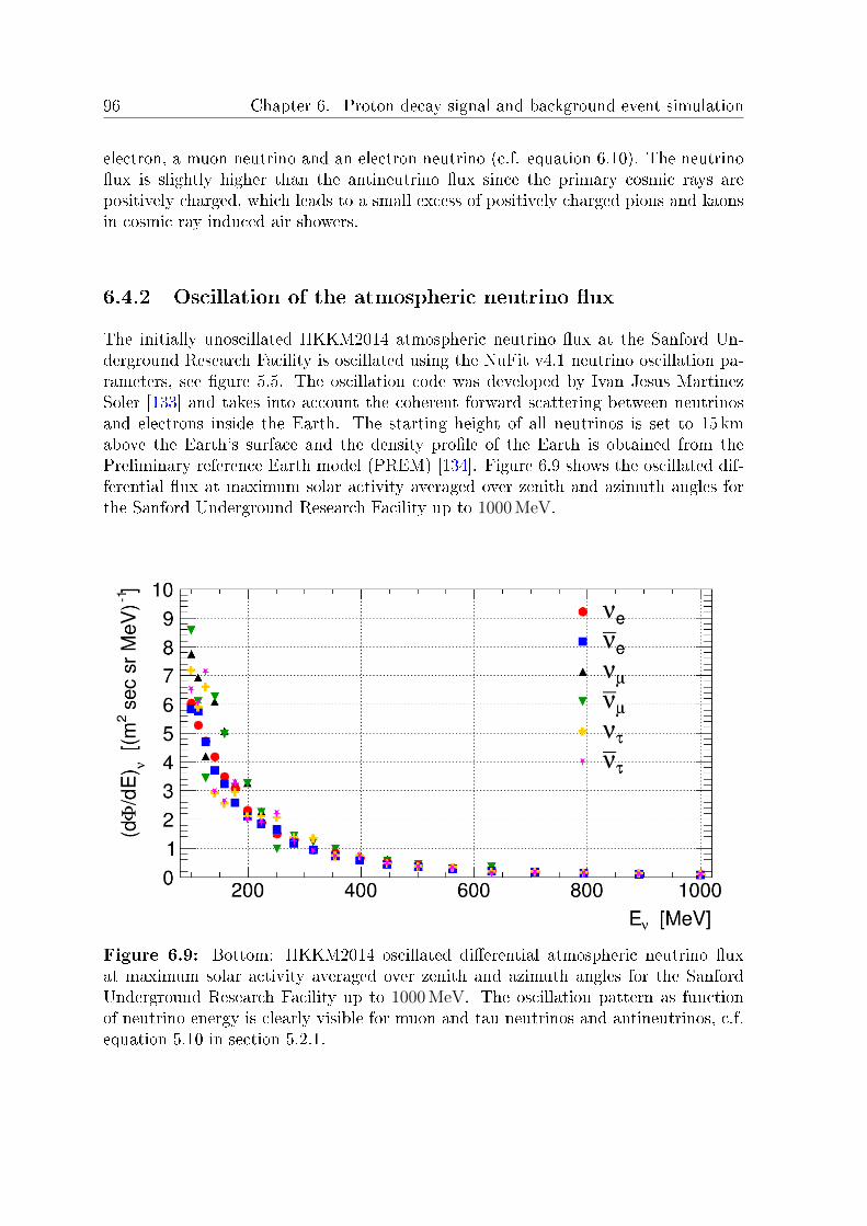
96 Chapter 6. Proton decay signal and background event simulation
electron, a muon neutrino and an electron neutrino (c.f. equation 6.10). The neutrinoux is slightly higher than the antineutrino ux since the primary cosmic rays arepositively charged, which leads to a small excess of positively charged pions and kaonsin cosmic ray induced air showers.
6.4.2 Oscillation of the atmospheric neutrino ux
The initially unoscillated HKKM2014 atmospheric neutrino ux at the Sanford Un-derground Research Facility is oscillated using the NuFit v4.1 neutrino oscillation pa-rameters, see gure 5.5. The oscillation code was developed by Ivan Jesus MartinezSoler [133] and takes into account the coherent forward scattering between neutrinosand electrons inside the Earth. The starting height of all neutrinos is set to 15 kmabove the Earth's surface and the density prole of the Earth is obtained from thePreliminary reference Earth model (PREM) [134]. Figure 6.9 shows the oscillated dif-ferential ux at maximum solar activity averaged over zenith and azimuth angles forthe Sanford Underground Research Facility up to 1000 MeV.
Figure 6.9: Bottom: HKKM2014 oscillated dierential atmospheric neutrino uxat maximum solar activity averaged over zenith and azimuth angles for the SanfordUnderground Research Facility up to 1000 MeV. The oscillation pattern as functionof neutrino energy is clearly visible for muon and tau neutrinos and antineutrinos, c.f.equation 5.10 in section 5.2.1.

6.4 Atmospheric neutrino background event simulation 97
6.4.3 Neutrino-argon interactions and cross sections
Atmospheric neutrinos entering the DUNE far detector have a small chance of inter-acting with an argon atom via the weak force, c.f. section 1.2. There are severaltypes of neutrino interactions and the rst distinction can be made with respect to theexchanged gauge boson:
1. Neutral current (NC) interactions exchange a Z boson
2. Charged current interactions exchange a W+ or W− boson
The neutrino continues to exist after a NC interaction. In CC interactions, the neutrinois transformed into its corresponding charged lepton, c.f. gure 1.1, and the charge +eor −e is transferred to the scattering partner. Figure 6.10 shows the total, NC andCC cross sections of all six neutrino avors on argon as function of neutrino energyfrom Eν = 100 MeV to Eν = 100 GeV for GENIE tune G18_02a_02_11a. The lowerlimit of Eν = 100 MeV is chosen to match the corresponding limit of the atmosphericneutrino ux (see section 6.4.1) while Eν = 100 GeV represents a conservative upperlimit for neutrino-argon interactions that are a potential background in proton decaysearches. The NC cross sections are identical for all neutrino avors νe, νµ and ντ aswell as for all antineutrino avors νe, νµ and ντ and therefore only shown once forneutrinos and once for antineutrinos.Both NC and CC interactions on heavy atoms such as argon can be further dividedinto 6 processes that are dened by the scattering partner, see table 6.2.
Abbreviation Process
EEL Elastic scattering o a single electronCOH Coherent scattering o a whole nucleusQE Quasi-elastic scattering o a single nucleonRES Resonance production o a single nucleonMEC Scattering o two correlated nucleonsDIS Deep inelastic scattering o a single quark
Table 6.2: Possible neutrino interaction processes on heavy atoms classied by scat-tering partner. All processes can occur via neutral and charged current. The scatteringo two correlated nucleons is also called meson exchange current (MEC).
Figure 6.11 shows the muon neutrino NC and CC cross sections on argon for all pro-cesses in GENIE tune G18_02a_02_11a. Muon neutrinos are chosen as reference sincethey constitute the most dangerous background for the proton decay sensitivity studyin chapter 7. The corresponding cross sections for νe, ντ , νe, νµ and ντ can be foundin appendix B.The sum of the six process cross sections corresponds to the total CC and NC inter-action cross sections. The cross sections for elastic scatters o single electrons canbe calculated analytically in electroweak theory as this process only involves two free

98 Chapter 6. Proton decay signal and background event simulation
Figure 6.10: Total (top), charged current (bottom left) and neutral current (bottomright) cross sections on argon of all six neutrino avors as function of neutrino energyfor GENIE tune G18_02a_02_11a. The neutral current cross-sections are identicalfor all neutrino avors νe, νµ and ντ as well as for all antineutrino avors νe, νµ and ντ .

6.4 Atmospheric neutrino background event simulation 99
Figure 6.11: Charged current (top) and neutral current (bottom) muon neutrinocross sections on argon for all processes as function of neutrino energy in GENIE tuneG18_02a_02_11a, c.f. table 6.2. The charged current elastic scattering o singleelectrons is only implemented for electron neutrinos and antineutrinos in GENIE asthe corresponding energy threshold for muon and tau neutrinos and antineutrinos isvery high, see section 6.4.3.1.

100 Chapter 6. Proton decay signal and background event simulation
elementary particles. Since nucleons and nuclei are extended objects, the analyticalcalculation of cross sections for processes other than elastic electron scattering is di-cult and parametrizations are used instead. In addition to the initial neutrino energy,the neutrino-nucleus cross sections depend on the squared four-momentum transfer Q2,and the cross sections in gures 6.10 and 6.11 are averaged over Q2. For low Q2, therelative rate of coherent scatters is higher since the probing wavelength is typicallytoo large to resolve single nucleons and quarks. With increasing Q2, meson exchangecurrents, quasi-elastic scatters and resonance production become more important asthe probing wavelength becomes short enough to resolve pairs of nucleons and singlenucleons. For high Q2, deep inelastic scatters become dominant as the probing wave-length can resolve single quarks. Since the average Q2 increases with the energy of theincoming neutrino, this trend can be observed for the process cross sections in gure6.11.There exists a variety of models for the six neutrino-nucleus interaction processes intable 6.2, and those used in this thesis within the GENIE tune scheme are summa-rized in table 7.1 and explained in more detail in the following sections. In general,the cross sections for both GENIE tunes G18_02a_02_11a and G18_10b_00_000are very similar since the same models are used for all processes except for CC QEand CC MEC interactions, and the G18_10b_00_000 cross sections are therefore notshown. The dierences between the models for these two processes are highlighted inthe respective sections.
GENIE tune G18_02a_02_11a G18_10b_00_000
Elastic electron scattering Marciano and Parsa [116] Marciano and ParsaCoherent scattering Berger and Sehgal [117] Berger and Sehgal
Quasi-elastic scattering (NC) Ahrens [118] AhrensQuasi-elastic scattering (CC) Llewellyn-Smith [119] Nieves [120]
Resonance production Berger and Sehgal [121] Berger and SehgalMeson exchange current (NC) empirical empiricalMeson exchange current (CC) empirical Valencia [122]
Deep inelastic scattering Paschos [123] Paschos
Table 6.3: List of neutrino-argon interaction models for the two GENIE tunes usedin the proton decay sensitivity study as already shown in table 6.1.
6.4.3.1 Elastic electron scattering
The implementation of the elastic electron scattering in both GENIE tunes followsthe calculations from Marciano and Parsa [116]. The neutral current process in thet-channel is possible for all neutrino and antineutrino avors:
(−)
νl + e9 → (−)
νl + e9 (l = e, µ, τ) (6.11)
The charged current process in the t-channel is possible for all neutrino avors, butnot for antineutrinos:

6.4 Atmospheric neutrino background event simulation 101
νl + e9 → l− + νe (l = e, µ, τ) (6.12)
and the charged current process in the s-channel is only possible for electron antineu-trinos:
νe + e9 → l− + νl (l = e, µ, τ) (6.13)
All elastic electron scatters have a neutrino and charged lepton in the nal state thatemerge outside of the nucleus and therefore do not undergo nal state interactions.The lower neutrino energy threshold for charged current interactions is given by:
Eνl ≥m2l −m2
e
2me
(6.14)
where l indicates the avor e, µ or τ of the charged lepton emerging from the interactionand ml the lepton mass. The corresponding thresholds for muon neutrinos Eνµ &10.8 GeV and tau neutrinos Eντ & 3 TeV are high compared to typical neutrino energiesand the corresponding processes are therefore neglected in GENIE, c.f. gure 6.9.
6.4.3.2 Coherent scattering
In a coherent scatter, the neutrino exchanges a Z or W± with the argon nucleus asa whole. This process requires a small four-momentum transfer Q with a wavelengthlarge enough to include the entire nucleus, resulting in a low cross section comparedto other neutrino-argon interactions (see gure 6.11). The recoiled nucleus stays intactand a single neutral pion emerges in the neutral current interaction while a charged pionemerges alongside a charged lepton in the charged current interaction, see equations6.15 through 6.17. Both pions and leptons are produced outside of the nucleus.
(−)
νl + Ar→ (−)
νl + Ar + π0 (6.15)
νl + Ar→ l− + Ar + π+ (6.16)
νl + Ar→ l+ + Ar + π− (6.17)
In both GENIE tunes, coherent scatters are described with the model of Berger andSehgal that is developed in the framework of the partially conserved axial vector currenttheory and tested against pion carbon scattering data [117].
6.4.3.3 Quasi-elastic scattering
The neutral current quasi-elastic interaction for neutrinos and antineutrinos is possiblewith both neutrons and protons as scattering partners. The charged current interactionfor neutrinos, however, is only possible with a neutron as scattering partner whileantineutrinos can only scatter o a proton:

102 Chapter 6. Proton decay signal and background event simulation
(−)
νl +N → (−)
νl +N (N = n, p) (6.18)
νl + n→ l− + p (6.19)
νl + p→ l+ + n (6.20)
In GENIE, a nucleon position is randomly chosen from the Woods-Saxon density distri-bution and the nucleon momentum is sampled from the spectral function, see sections6.1.1 and 6.1.2. Following the interaction, the scattered nucleon leaves the nucleus,potentially interacting with other nucleons as described in section 6.2. The neutralcurrent process in GENIE follows the Ahrens model for both tunes [118]. For thecharged current process, both the Llewellyn-Smith model [119] and the Nieves model[120] are available and applied in tune G18_02a_02_11a and G18_10b_00_000, re-spectively (c.f. table 7.1).Although the nucleon is a bound state of three quarks that can be described by quantumchromodynamics (QCD), the strong interactions inside the nucleon are at energies toolow for perturbative QCD and the nucleon is instead modeled with eective theories. Inthe Ahrens, Llewellyn-Smith and Nieves models, nucleon form factors have been usedto parameterize the internal charge distribution of nucleons to calculate quasi-elasticscattering cross sections. Since the atmospheric neutrino ux decreases exponentiallywith the neutrino energy and the quasi-elastic scattering cross section is dominant forneutrino energies up to ∼1 GeV, quasi-elastic scatters are the most common interactionof atmospheric neutrinos on argon (c.f. gure 6.9 and 6.11). Therefore, the Ahrens andLlewellyn-Smith model are described in more detail in sections 6.4.3.3.1 and 6.4.3.3.2.A comparison between the Llewellyn-Smith and Nieves model to assess the dierencebetween the two GENIE tunes follows in section 6.4.3.3.3.
6.4.3.3.1 Ahrens model
The quasi-elastic neutral current dierential cross section in the Ahrens model is givenas function of the four-momentum transfer squared Q2:
dσ
dQ2=G2FM
2N
8πE2ν
(A(Q2)±B
(Q2) (s− u)
M2N
+ C(Q2) (s− u)2
M4N
)(6.21)
where the ± distinguishes between neutrinos (+) and antineutrinos (−), GF = 1.166×10⁻⁵ GeV−2 is the Fermi coupling constant,MN the mass of the nucleon scattering part-ner, Eν the initial neutrino energy and s = (pi,ν + pi,N)2 and u = (pi,ν − pf,N)2 are theMandelstam variables with pi,ν being the initial four-momentum vector of the neutrino,pi,N the initial four-momentum vector of the nucleon and pf,N the nal four-momentumvector of the nucleon. For massless neutrinos, one obtains: s− u = 4MNEν −Q2. Thefunctions A, B and C depend on Q2 and are built from the vector (F1,2) and axialvector (FA) nucleon form factors:
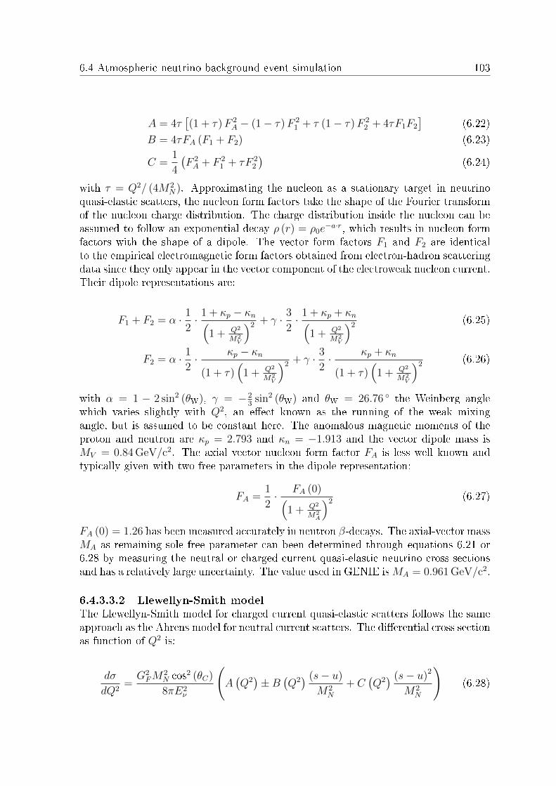
6.4 Atmospheric neutrino background event simulation 103
A = 4τ[(1 + τ)F 2
A − (1− τ)F 21 + τ (1− τ)F 2
2 + 4τF1F2
](6.22)
B = 4τFA (F1 + F2) (6.23)
C =1
4
(F 2A + F 2
1 + τF 22
)(6.24)
with τ = Q2/ (4M2N). Approximating the nucleon as a stationary target in neutrino
quasi-elastic scatters, the nucleon form factors take the shape of the Fourier transformof the nucleon charge distribution. The charge distribution inside the nucleon can beassumed to follow an exponential decay ρ (r) = ρ0e
−a·r, which results in nucleon formfactors with the shape of a dipole. The vector form factors F1 and F2 are identicalto the empirical electromagnetic form factors obtained from electron-hadron scatteringdata since they only appear in the vector component of the electroweak nucleon current.Their dipole representations are:
F1 + F2 = α · 1
2· 1 + κp − κn(
1 + Q2
M2V
)2 + γ · 3
2· 1 + κp + κn(
1 + Q2
M2V
)2 (6.25)
F2 = α · 1
2· κp − κn
(1 + τ)(
1 + Q2
M2V
)2 + γ · 3
2· κp + κn
(1 + τ)(
1 + Q2
M2V
)2 (6.26)
with α = 1 − 2 sin2 (θW), γ = −23
sin2 (θW) and θW = 26.76 the Weinberg anglewhich varies slightly with Q2, an eect known as the running of the weak mixingangle, but is assumed to be constant here. The anomalous magnetic moments of theproton and neutron are κp = 2.793 and κn = −1.913 and the vector dipole mass isMV = 0.84 GeV/c2. The axial vector nucleon form factor FA is less well known andtypically given with two free parameters in the dipole representation:
FA =1
2· FA (0)(
1 + Q2
M2A
)2 (6.27)
FA (0) = 1.26 has been measured accurately in neutron β-decays. The axial-vector massMA as remaining sole free parameter can been determined through equations 6.21 or6.28 by measuring the neutral or charged current quasi-elastic neutrino cross sectionsand has a relatively large uncertainty. The value used in GENIE isMA = 0.961 GeV/c2.
6.4.3.3.2 Llewellyn-Smith model
The Llewellyn-Smith model for charged current quasi-elastic scatters follows the sameapproach as the Ahrens model for neutral current scatters. The dierential cross sectionas function of Q2 is:
dσ
dQ2=G2FM
2N cos2 (θC)
8πE2ν
(A(Q2)±B
(Q2) (s− u)
M2N
+ C(Q2) (s− u)2
M2N
)(6.28)

104 Chapter 6. Proton decay signal and background event simulation
where θC = 13.05 is the Cabibbo angle. The Mandelstam variables and the functionA dier from the ones calculated in the Ahrens model due to the outgoing lepton massml:
s− u = 4MNEν +Q2 −m2l (6.29)
A =m2l +Q2
M2N
[(1 + τ)F 2
A − (1− τ)F 21 + τ (1− τ)F 2
2 + 4τF1F2 (6.30)
− m2l
4M2n
((F 2
1 + F 22
)2+ (FA + 2FP )2 − 4 (1 + τ)F 2
P
)]with FP the pseudoscalar nucleon form factor that can be expressed as function of theaxial vector nucleon form factor FA:
FP =2M2
N
m2π +Q2
FA (6.31)
where mπ = 139.57 MeV is the charged pion mass. All other parameters in equation6.28 are identical to those in the Ahrens model in equation 6.21.
6.4.3.3.3 Comparison between Llewellyn-Smith and Nieves model
Like the Llewellyn-Smith model, the Nieves model uses form factors to parametrizethe internal charge distribution of nucleons in the calculation of charged current quasi-elastic scatter cross sections. The parametrization and resulting cross sections dierbetween the two models and instead of going through the details of the Nieves model,the cross section ratio of the Nieves model over the Llewellyn-Smith model is shownas function of neutrino energy for all neutrino avors in gure 6.12. The cross sectionratio can be converted directly into a quasi-elastic interaction ratio since the neutrinoux is identical for both GENIE tunes.
6.4.3.4 Resonance production
Resonance production is similar to quasi-elastic scatters, with the dierence that thestruck nucleon transitions into an excited resonance state. There are dierent statesof proton and neutron quantum excitations, with the lowest exited state being a Delta(∆) baryon with mass m∆ = 1 232 MeV and spin and isospin of 3/2. There are sev-eral ∆ excitation states with dierent masses and each state comprises four dierentcombinations of up and down quarks with total charges ranging from −1e to +2e. Res-onance production becomes energetically possible when the center of mass energy ofthe neutrino-nucleon system exceeds the dierence between the lowest-mass ∆ baryonand the nucleon mass, which is the case for neutrino energies above Eν & 200 MeVwhen taking into account Fermi motion, c.f. gure 6.11.The Berger and Sehgal model for resonance production is applied in both GENIE tunes[121], considering 17 dierent resonance states consisting of up and down quarks withmasses up to 1 950 MeV. Lighter resonances typically decay into nucleon-pion pairs:

6.4 Atmospheric neutrino background event simulation 105
Figure 6.12: Ratio of the charged current quasi-elastic scatter cross sections fromthe Nieves model over the Llewellyn-Smith model as implemented in GENIE for tuneG18_10b_00_000 and G18_02a_02_11a, respectively (c.f. table 6.1).
∆++ → p+ π+ (6.32)
∆+ → p+ π0 or n+ π+ (6.33)
∆0 → p+ π− or n+ π0 (6.34)
∆− → n+ π− (6.35)
As the resonance states have very short lifetimes, they are decayed immediately and theintranuclear propagation is simulated for the decay products. Heavier resonances canalso produce pairs of kaons and strange baryons, such as the Sigma (Σ) and Lambda (Λ)baryon. This process is called associated kaon production and represents a potentialsource of background for proton decay searches via p → νK+ due to the presence ofa kaon. It will be shown in chapter 7 that the strange baryon and its decay productscan be used to distinguish associated kaon production events from proton decay.W− bosons in charged current interactions can turn an up quark into a strange quarkto produce strange baryon resonances. The lightest of these resonances has a mass of1405 MeV and typically decays into a pion and a Σ baryon, and heavier resonances candecay into a nucleon and K− or K0. The latter is referred to as single kaon productionas there are no accompanying strange particles in addition to the kaon. Single K+ cannot be produced as they contain an antistrange quark. The leptons from the chargedcurrent interaction make these events distinguishable from proton decay via p→ νK+.Strange baryon resonance production, however, is not implemented in GENIE.

106 Chapter 6. Proton decay signal and background event simulation
6.4.3.5 Meson exchange current
Meson exchange current events are quasi-elastic scatters o a correlated nucleon pair.This process is implemented as an empirical model for both neutral and charged currentinteractions in tune G18_02a_02_11a and for neutral current interactions in tuneG18_10b_00_000. The charged current interactions in tune G18_10b_00_000 aresimulated according to the Valencia model [122], see table 7.1. The empirical GENIEmodel is tuned with data from the MiniBoone and NOMAD experiments and thecross sections for both neutral and charged current interactions are set to 30 % of thecorresponding quasi-elastic cross sections, c.f. gure 6.11. The charged current MECcross section of the Valencia model is calculated independently of the quasi-elasticcross section. In both models, both hit nucleons leave the nucleus after simulatingthe intranuclear propagation. Figure 6.13 shows the cross section ratio of the Valenciamodel over the empirical model as function of neutrino energy for all neutrino avors.
Figure 6.13: Ratio of the charged meson exchange current cross sections fromthe Valencia model over the empirical model as implemented in GENIE for tuneG18_10b_00_000 and G18_02a_02_11a, respectively (c.f. table 7.1).
6.4.3.6 Deep inelastic scattering
In deep inelastic scatters, the squared four-momentum transfer Q2 is high enough toresolve quarks and the neutrino scatters o a single valence or sea quark. This processis dominant for neutrino energies above Eν & 3 GeV, see gure 6.11. Neutrino and an-tineutrino neutral current interactions are possible with both up and down quarks asscattering partner. Charged current scatters o down quarks are only possible for neu-trinos while charged current scatters o up quarks are only possible for antineutrinos.The struck quark always gains enough kinetic energy to leave its parent nucleon. The

6.4 Atmospheric neutrino background event simulation 107
remnant nucleon and the free quark hadronize inside the nucleus, typically producinga jet of nucleons and pions. Associated kaon production in deep inelastic scatters ispossible when the struck quark radiates o a gluon that in turn produces a strange-antistrange quark pair. The strange quark forms a Σ or Λ baryon with the two quarksof the remnant parent nucleon and the antistrange quark forms a K+ or K0 by combin-ing with an up or down quark. As already discussed in section 6.4.3.4, associated kaonproduction is a potential background for proton decay searches via p→ νK+, but theaccompanying Σ or Λ can be used to distinguish it from proton decay. In contrast toresonance production, single kaon production in charged current DIS is implemented inGENIE. This process is Cabibbo suppressed and the accompanying charged lepton andparticles produced in the hadronization process make it distinguishable from protondecay via p→ νK+.The DIS cross sections in GENIE are calculated according to the Paschos model [123]and the hadronization is simulated with an empirical model based on bubble chamberdata in the low-energy region and with PYTHIA6 for higher energies [135].

108 Chapter 6. Proton decay signal and background event simulation

Chapter 7
Proton decay sensitivity study
In this chapter, a proton decay sensitivity study via p → νK+ is presented for a10 kiloton DP LAr TPC far detector module in DUNE with atmospheric neutrino in-teractions on argon as background. The sensitivity study is carried out for two setsof signal and background Monte Carlo event samples that were generated with the of-cial tunes G18_02a_02_11a and G18_10b_00_000 of the GENIE event generator.These tunes are consistent combinations of the interdependent models that describe theinitial state of the argon nucleus, neutrino-argon interactions and intranuclear propa-gation, see chapter 6. The signal and background Monte Carlo event samples are runthrough the DP LAr TPC detector simulation that is explained and validated basedon the 3x1x1m3 DP LAr TPC prototype in chapters 3 and 4 and scaled to the de-sign of the 10 kiloton DP LAr TPC module for the DUNE far detector as described insection 5.1.3.1. After detector simulation, the Monte Carlo samples are reconstructedand analyzed in order to extract the sensitivity of DUNE to the proton decay modep → νK+, which is the lower lifetime limit that can be measured if no proton decayevent is observed.An overview of the proton decay signal and atmospheric neutrino background eventsamples before detector simulation is given in sections 7.1 and 7.2, followed by a sum-mary of parameters used in the detector simulation in section 7.3. The reconstructionand analysis are described in chapter 7.4 and 7.5 and the sensitivity results are pre-sented in section 7.6.
7.1 Signal event samples
For both GENIE tunes, ∼100 000 proton decay events have been generated accordingto the signal event simulation workow described in chapter 6. The kinetic energydistribution of K+ from proton decay, hereafter referred to as signal K+, is shownbefore and after nal state interactions (FSI) in gure 7.1. Most signal K+ lose energyin FSI since their initial kinetic energy is almost always higher than the kinetic energyof the struck nucleon. The kinetic energy distribution of struck nucleons after theyleave the nucleus is shown in gure 7.2.
109

110 Chapter 7. Proton decay sensitivity study
Figure 7.1: Signal K+ kinetic energy distributions before and after nal state inter-actions (FSI) for GENIE tunes G18_02a_02_11a and G18_10b_00_000. The totalnumber of signal K+ after FSI in tune G18_10b_00_000 is reduced by 15 % as thehN2018 intranuclear propagation model includes charge exchange of K+ into K0, c.f.table 7.1. In both tunes, the scattered K+ distributions peak at low kinetic energies.
Figure 7.2: Kinetic energy distributions of struck protons and neutrons afterleaving the argon nucleus in the proton decay signal samples for GENIE tunesG18_02a_02_11a and G18_10b_00_000. The sharp drop at Ekin = 25 MeV in tuneG18_10b_00_000 reects the fact that protons and neutrons below 25 MeV do notinteract in the hN2018 intranuclear propagation model (see section 6.2.0.2).

7.2 Background event samples 111
Table 7.1 summarizes the signal K+ nal state interactions for both GENIE tunes andcompares them to those simulated with a separate event generation toolkit for neutrinointeractions called NEUT that was developed in the context of the T2K experiment[131]. NEUT uses the Woods-Saxon model for nucleon density, a custom full intranu-clear cascade model to simulate nal state interactions and kaon-nucleon cross sectionsfrom a partial wave analysis by Hyslop et al. [132]. As NEUT does not include a pro-ton decay event generator, the K+ from proton decay are fed into NEUT and placedinside the nucleus according to the Woods-Saxon density distribution with a randomdirection. The underlying proton momentum distribution was obtained from the localFermi gas spectral function, c.f. section 6.1.2.2. The models used in NEUT are iden-tical or very similar to those in GENIE tune G18_10b_00_000, and their resultingnal state interaction rates are in good agreement.
GENIE tune G18_02a_02_11a G18_10b_00_000 NEUT
Total nal state interactions 32% 32% 35%
Single nucleon elastic scatter 11% 17% 22%Multi-nucleon elastic scatter 21% / /
Charge exchange / 15% 13%
Table 7.1: Summary of signal K+ nal state interactions for GENIE tunesG18_02a_02_11a and G18_10b_00_000 as well as for NEUT.
In both GENIE tunes, 32 % of signal K+ undergo nal state interactions, result-ing in 68 % of events that only have a single K+ in the nal state outside the nu-cleus. The 11 % of signal K+ that undergo single nucleon elastic scatters in tuneG18_02a_02_11a are accompanied by one nucleon in the nal state while the 21 %that undergo multi-nucleon elastic scatters have two or three nucleons in the nal state,c.f. section 6.2.0.1. For tune G18_10b_00_000, the nucleon multiplicity in events withnal state interactions is more complex as multiple interactions are possible, and 15 %of events have a K0 instead of a K+ in the nal state due to K+-neutron charge ex-change, c.f. section 6.2.0.2. Events without K+ in the nal state are excluded fromthe proton decay sensitivity study and the signal selection eciencies are weightedaccordingly, see section 7.5.4.It is worthwhile to mention that, as opposed to some other event generators, the parentnucleus does not emit a O (MeV) photon after proton decay in GENIE.
7.2 Background event samples
The dierential neutrino-argon interaction spectra, total interaction numbers for agiven exposure and sample sizes for GENIE tunes G18_02a_02_11a and G18_10b_00_000are discussed in section 7.2.1. An overview of the resulting nal state particles thatare visible inside the detector is given in section 7.2.2.

112 Chapter 7. Proton decay sensitivity study
7.2.1 Expected interaction rates
The background event simulation is performed separately for all six neutrino avorswith GENIE. For any given avor, the directionally averaged oscillated dierentialatmospheric neutrino ux is convoluted with the total neutrino-argon cross section,resulting in an unnormalized energy distribution of interacting neutrinos (c.f. sections6.4.2 and 6.4.3). In a second step, GENIE randomly picks a neutrino energy fromthe obtained distribution and randomly determines the type of the neutrino-argon in-teraction by weighting the possible processes with their cross sections at the chosenneutrino energy, yielding a neutrino interaction energy distribution for all neutral andcharged current processes. Due to the format of the neutrino uxes and cross sections,the interaction distributions are given per neutrino energy, per angular acceptance andper exposure. Since the neutrino ux is averaged over all directions and the angularacceptance is A = 4π steradian, the distributions can simply be multiplied by A. Theexposure is the product of detector mass and experiment run time. The referenceexposure of 1 megaton · year, which corresponds to 4.76 × 1041 argon atoms · secondsfor 40
18Ar, is used for most gures and tables in this chapter and eectively represents25 years of uninterrupted data taking with four 10 kiloton DUNE far detector modules,which is a conservative upper limit on the expected exposure for DUNE. Figure 7.3shows the dierential neutrino-argon interaction spectrum as function of neutrino en-ergy from Eν = 100 MeV to Eν = 100 GeV for an exposure of 1 megaton · year as wellas the ratio of charged current over neutral current interactions for all neutrino avorsin tune G18_02a_02_11a. The upper and lower neutrino energy limits correspond tothe energy range of the neutrino-argon cross sections that is justied in section 6.4.3and includes all neutrino energies that are relevant for proton decay background stud-ies. The dierential interaction spectrum of all charged and neutral current processesfor muon neutrinos are shown in gure 7.4 for the G18_02a_02_11a sample. The totalnumber of expected interactions for all neutrino avors and interaction processes canbe calculated by integrating the corresponding dierential neutrino-argon interactionspectra over the energy, and the results for an exposure of 1 megaton · year are shown intable 7.2. The corresponding spectra and numbers for the G18_10b_00_000 sampledier only for quasi-elastic and deep inelastic scatters and since the same neutrino uxis used in both samples, the deviations are proportional to the cross-section ratios be-tween the models that are shown in section 6.4.3.3 and 6.4.3.6. The G18_10b_00_000spectra and numbers are therefore not shown separately.For rare event searches in low-background environments, it is especially importantto simulate a multiple of the expected background events in order to minimize thestatistical uncertainty. The upper limit of the sample size is set by the available com-putational power and 10 megaton · years and 2 megaton · years have been generated forGENE tune G18_02a_02_11a and G18_10b_00_000, respectively. While both sam-ples represent a multiple of the exposure expected from a single 10 kiloton DP LAr TPCmodule as well as from the entire DUNE far detector complex, the G18_02a_02_11asample is used as high-statistics reference sample to tune the analysis and determinethe statistical uncertainty on the sensitivity for proton decay via p→ µK+.

7.2 Background event samples 113
Figure 7.3: Dierential atmospheric neutrino-argon interaction spectrum normalizedto 1 megaton · year (top) and ratio of charged current over neutral current interactions(bottom) for all neutrino avors in the G18_02a_02_11a sample.

114 Chapter 7. Proton decay sensitivity study
Figure 7.4: Dierential muon neutrino-argon interaction spectrum for all chargedcurrent (top) and neutral current (bottom) processes normalized to 1 megaton · year inthe G18_02a_02_11a sample.
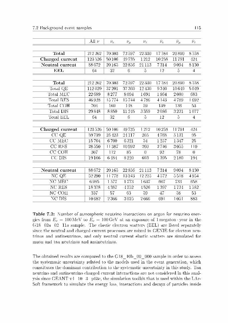
7.2 Background event samples 115
All ν νe νµ ντ νe νµ ντ
Total 212 262 70 303 72 597 22 330 17 584 20 890 8 558Charged current 123 526 50 106 49 735 1 212 10 258 11 791 424Neutral current 88 672 20 165 22 856 21 113 7 314 9 094 8 130
EEL 64 32 6 5 12 5 4
Total 212 262 70 303 72 597 22 330 17 584 20 890 8 558Total QE 112 029 37 201 37 360 12 430 9 340 10 649 5 049Total MEC 22 689 8 277 8 094 1 691 1 864 2 080 683Total RES 46 928 15 774 15 744 4 786 4 143 4 789 1 692Total COH 704 169 148 59 139 136 53Total DIS 29 848 8 850 11 245 3 359 2 086 3 231 1 077Total EEL 64 32 6 5 12 5 4
Charged current 123 526 50 106 49 735 1 212 10 258 11 791 424CC QE 59 739 25 423 24 117 205 4 768 5 131 95CC MEC 15 704 6 700 6 321 54 1 257 1 347 25CC RES 28 550 11 387 10 992 260 2 746 3 055 110CC COH 367 112 85 0 92 78 0CC DIS 19 166 6 484 8 220 693 1 395 2 180 194
Neutral current 88 672 20 165 22 856 21 113 7 314 9 094 8 130NC QE 52 290 11 778 13 243 12 225 4 572 5 518 4 954NC MEC 6985 1 577 1 773 1 637 607 733 658NC RES 18 378 4 387 4 752 4 526 1 397 1 734 1 582NC COH 337 57 63 59 47 58 53NC DIS 10 682 2 366 3 025 2 666 691 1 051 883
Table 7.2: Number of atmospheric neutrino interactions on argon for neutrino ener-gies from Eν = 100 MeV to Eν = 100 GeV at an exposure of 1 megaton · year in theG18_02a_02_11a sample. The elastic electron scatters (EEL) are listed separatelysince the neutral and charged current processes are mixed in GENIE for electron neu-trinos and antineutrinos, and only neutral current elastic scatters are simulated formuon and tau neutrinos and antineutrinos.
The obtained results are compared to the G18_10b_00_000 sample in order to assessthe systematic uncertainty related to the models used in the event generation, whichconstitutes the dominant contribution to the systematic uncertainty in this study. Tauneutrino and antineutrino charged current interactions are not considered in this anal-ysis since GEANT v4_10_3_p03e, the simulation toolkit that is used within the LAr-Soft framework to simulate the energy loss, interactions and decays of particles inside

116 Chapter 7. Proton decay sensitivity study
the detector, contains a bug in the decay of tau leptons. Since the tau lepton massof 1.78 GeV/c2 is large compared to the visible energy in a proton decay event and itsdecay modes produce event topologies that are very dierent from those in the protondecay signal samples, tau neutrino and antineutrino charged current interactions donot represent a dangerous background for the p → νK+ sensitivity study and theirexclusion does not impair the validity of the presented results.
7.2.2 Final state particles
After simulating the neutrino-argon interaction and the intranuclear propagation ofparticles emerging inside the nucleus, GENIE provides a set of nal state particles thatare visible inside the detector for each interaction. Since the directionally averagedatmospheric neutrino ux was passed to GENIE along the arbitrary direction +z, thenal state particles are rotated by the angle between the positive z-axis and a directionrandomly sampled from the direction-dependent ux distribution, see section 6.4.1 andgure 6.8.For a given neutrino interaction, the particles in the nal state and their energies aregoverned by the neutrino avor, neutrino-argon interaction process, neutrino energyand scattering partner. The exact composition of the nal state, however, also dependson the squared four-momentum transfer and random processes in the intranuclear prop-agation. For deep inelastic scatters, the hadronization of the struck quark and remnantnucleon introduces additional variations in the nal state. Neutrons and protons areby far the most abundant particles in the nal state, followed by pions, muons andelectrons. Figure 7.5 shows the kinetic energy distributions of all nal state particles,except neutrinos, up to Ekin = 1000 MeV for all neutrino avors and interaction pro-cesses at an exposure of 1 megaton · year in the G18_02a_02_11a background sample.The upper limit of Ekin = 1000 MeV is well above the energy of any particle in the pro-ton decay signal sample and neutrino interactions that produce particles with higherenergies can be easily distinguished from proton decay, c.f. section 7.1. Positivelyand negatively charged muons, pions and kaons are listed separately since stopping µ+
decay into a O (10 MeV) Michel positron and two neutrinos inside the detector, whilestopping µ− are captured by an argon atom in 75 % of the cases in GEANT4 and onlyproduce O (MeV) photons while cascading down. The µ− eventually exchanges a W−
boson with the nucleus which can lead to nucleon knock-outs. The presence of thepositron from the K+ decay chain in the signal sample is later used in the nal eventselection in section 7.5.3.
7.3 Detector simulation parameters
The nal state particles in the signal and background samples are imported into LAr-Soft to simulate their energy loss, interactions and decays inside the detector as well asthe detector response to eventually obtain ADC waveforms, c.f. sections 3.2.2 through3.2.5. The general detector geometry in the simulation is adapted to the 10 kiloton DPLAr TPC module as described in section 5.1.3.1, but a smaller version of the detector

7.3 Detector simulation parameters 117
Figure 7.5: Kinetic energy distributions of all nal state particles except neutrinosfrom all neutrino avors and interaction processes at an exposure of 1 megaton · yearin the G18_02a_02_11a background sample. The last bin on the x-axis represents Dmesons as well as Λ and Σ baryons and the bin size along the y-axis is 10 MeV. Thecorresponding 1D distributions can be found in gure C.1 in appendix C.
with nine 3 × 3m2 charge readout planes, that are arranged as a square, and the fulldrift distance of 12m is used in order to save computation time. All event verticesare placed below the center of the 9 × 9 m2 charge readout area at a drift distanceof LDrift = 6 m, ensuring that all signal events and almost all background events arefully contained. The energy loss, interactions and decays of particles are simulatedwith GEANT4. The local ionization charge is determined from the energy loss with amodied version Birk's law, see section 3.2.3. The attenuation of the drifting charge isnot taken into account and the diusion is simulated as explained in section 3.2.4. Theextraction eciency into the argon gas layer is 100 % and all electrons are extractedwithout delay. The eective LEM gain is set to GE = 20 and the charge is sharedequally between the two readout views. The preamplier shaping function and gain aswell as the ADC parameters from the 3x1x1m3 prototype are used and no electronicnoise or ADC pedestal is simulated, c.f. section 2.4.4.1. The scintillation light, andthus the internal light trigger, has not been simulated for this study as the correspond-ing tools in LArSoft were not ready when the samples were produced, and the eventtime of proton decays and neutrino interactions is always 0.Figure 7.6 shows the event display of a typical proton decay event and of a muonneutrino charged current quasi-elastic scatter, the most common process in the atmo-spheric neutrino background sample. The parameters for the 10 kiloton DP LAr TPCdetector simulation are summarized in table 7.3.
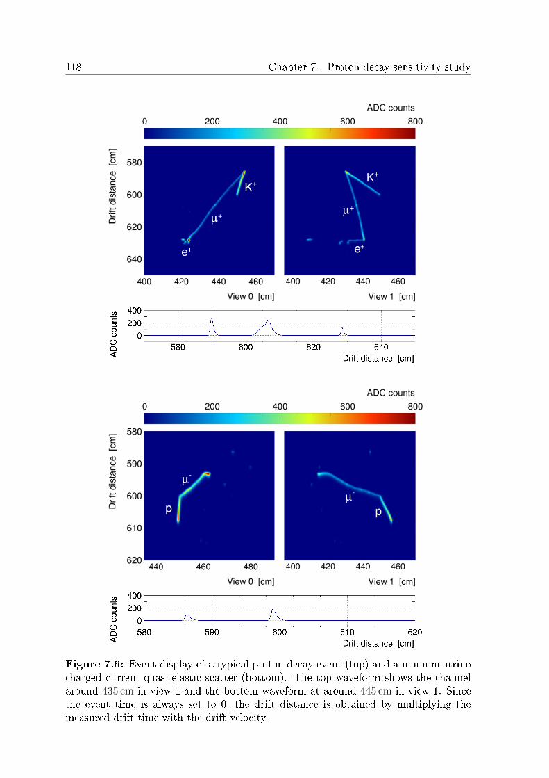
118 Chapter 7. Proton decay sensitivity study
Figure 7.6: Event display of a typical proton decay event (top) and a muon neutrinocharged current quasi-elastic scatter (bottom). The top waveform shows the channelaround 435 cm in view 1 and the bottom waveform at around 445 cm in view 1. Sincethe event time is always set to 0, the drift distance is obtained by multiplying themeasured drift time with the drift velocity.

7.4 Reconstruction 119
Parameter Value
TPC length × width × height 9 m× 9 m× 12 mLiquid argon density 1.396 g/cm3
Event vertex position 4.5 m× 4.5 m× 6 mWork function for e9 in liquid argon We9 = 23.6 eV
Birk's parameter A 0.8Birk's parameter k 0.0486 kV ·MeV−1 · g · cm−3
Drift eld εD 0.5 kV/cmDrift velocity vD 1.6 m/ms
Longitudinal diusion constant DL 0.62 mm2/msTransverse diusion constant DT 1.63 mm2/ms
Electron lifetime τe9 ∞Electron extraction eciency εextr, fast 1
Eective LEM gain GE 20Preamplier gain g 2.5 mV/fCADC dynamic range 1 800mVADC resolution 12 bit
ADC sampling rate 2.5MHzReadout window size 20 000 samples = 8 msReadout channel pitch 3.125 mm
Table 7.3: Parameters used in the 10 kiloton DP LAr TPC detector simulation forthe proton decay sensitivity study.
7.4 Reconstruction
The reconstruction of the signal and background samples follows the same approachas the reconstruction of the 3x1x1m3 prototype data and consists of the hit nder,the 2D Monte Carlo truth matching and the 3D track reconstruction, c.f. section4.1. The biggest dierence with respect to the 3x1x1m3 data reconstruction is the2D Monte Carlo truth matching: instead of using a reconstruction algorithm to denegroups of hits that are thought to originate from the same particle, Monte Carlo truthinformation is used to group hits from the same particle independently in both readoutviews.The hit nder and 2D Monte Carlo truth matching are implemented in LArSoft, whilethe 3D track reconstruction is performed outside of LArSoft for this study. The detailsof the dierent algorithms are explained in detail in sections 7.4.1 through 7.4.3.
7.4.1 Hit nder
Since no electronic noise and ADC pedestals are simulated, the raw waveforms areperfectly smooth and the pedestal subtraction, noise lter and hit tter can be skipped

120 Chapter 7. Proton decay sensitivity study
and only the peak nder is applied, see section 4.1 on the 3x1x1m3 data reconstruction.The peak nder amplitude threshold is set to Amin = 1ADC count and the inectionpoint threshold is set to four consecutive ticks with equal or higher ADC counts, c.f.section 4.1.3.1. No noise hit lter is applied. The ADC count sum SHit is convertedinto the hit charge QHit with the calibration factor that results from the preampliersimulation:
QHit =SHit
25.9 ADC·µsfC
(7.1)
The corresponding deposited charge in liquid argon that is contained inside the hitQHit, LAr is obtained by correcting for the eective gain:
QHit, LAr =QHit
GE
(7.2)
The hit start, peak and end time, the hit amplitude and the hit charge in liquid argonserve as input for further reconstruction and analysis.
7.4.2 2D Monte Carlo truth matching
2D pattern recognition algorithms group hits that are thought to originate from thesame particle independently in both readout views by looking for two types of patterns:continuous lines of hits originating from tack-like particles such as muons, pions, kaonsand protons, and cone-like groups of hits from showering particles such as electronsand photons. Several 2D pattern recognition algorithms are currently in developmentand available within LArSoft. The performance of those algorithms is sucient to re-construct single through-going muons in the 3x1x1m3 prototype, but proton decay andatmospheric neutrino events typically contain multiple connected tracks and showersand the available algorithms often fail to group hits correctly in events for which thegrouping can be easily done by eye. In order to not limit the signicance of this studyby premature reconstruction algorithms, hits originating from the same particle aregrouped with Monte Carlo truth information by tracing back the origin of the chargeinside a hit. If a hit contains charge from more than one particle, it is assigned to thehit group of the particle with the highest charge contribution to that hit. Hits fromDelta electrons are assigned to the hit group of the initial particle. No information onthe nature of the particle is used in the 2D Monte Carlo truth matching or downstream3D track reconstruction and analysis.After the truth matching, all hits within a group are sorted along the channel coor-dinates in their respective view to dene 2D end points. The increase of the linearstopping power, and thus charge deposition, of charged particles towards their stop-ping points (also called Bragg peak, c.f. sections 2.3.1 and 2.3.2) is used to determinethe 2D starting and stopping points: the hit group is temporarily split in two halvesand the 2D end point in the half with the highest average hit charge is dened as 2Dstopping point while the remaining 2D end point is dened as the 2D starting point.
7.4 Reconstruction 121
The transverse diusion after 6 m drift at a drift eld of εD = 0.5 kV/cm is λT ≈3.3 mm, which is similar to the readout channel pitch (c.f. section 2.3.3.2). The chargedeposited in liquid argon along a particle's trajectory is therefore not only drifted tothe overlying readout channel, but also diuses into neighboring channels. This eectis most important at the end points of a particle where the diusing charge createsadditional hits in the charge readout plane that extend beyond the actual 2D projec-tion of the particle's trajectory, making the particle appear longer and tilted. Since theaccurate determination of the particle length and direction is essential to the protondecay sensitivity study, the outermost hits in the 2D hit groups with a charge contentless than half of the average hit charge of the group are excluded from the 2D end,starting and stopping point determination.
7.4.3 3D track reconstruction
The information from the hit nder and 2D Monte Carlo truth matching in LArSoftis written to standard ROOT les, and the 3D track reconstruction and analysis isperformed outside of LArSoft. Most parameters obtained in the 3D reconstructionare only sensible for track-like particles, but they are determined for all reconstructedparticles with at least one hit in both readout views. A distinction between track-and shower-like particles will be made later on based on the number of missing hitsbetween track starting and stopping point. Some of the track parameters discussedin the following, like the 3D track length and orientation, can only be calculated fortracks with at least two hits in one of the readout views. For tracks with only onehit in each view, e.g. from low-energy photons, the track length is set to 0 and theorientation of the track as well as the stopping power prole are not dened.The total deposited charge of the track in liquid argon is calculated for both viewsindependently by adding up the charge in liquid of all hits in the respective view:
QTrack, LAr = 2 ·∑i
QHit, LAr, i (7.3)
The factor 2 accounts for the charge sharing between the two readout views, c.f. section7.3. In the analysis, only the QTrack, LAr value measured in the view with the most hits,also called best view, is used.The 2D end points of hit groups from the same particle are matched between thetwo readout views based on their drift coordinate to obtain two 3D end points. Sincematched endpoints usually have a slightly dierent drift coordinate in the two views,the values from the best view are taken as the drift coordinates for the 3D end points.If a 2D stopping point in one view is matched with a 2D starting point in the otherview, the 3D starting and stopping points are determined from the 2D starting andstopping points in the best view.A 3D track, in the following sometimes just called track, is obtained by connecting the3D starting and stopping points with a straight line. The length of the track segmentds from which single readout channels have collected charge can be determined from

122 Chapter 7. Proton decay sensitivity study
the orientation of the 3D track with respect to the charge readout plane (see table 4.1for denitions of θ and φ):
dsView 0 =3.125 mm
sin (θ) · sin (φ)(7.4)
dsView 1 =3.125 mm
sin (θ) · cos (φ)(7.5)
The local charge deposition per unit length of the particle in liquid argon, dQ/ds, canbe determined at all hits in both views independently:
dQ
ds= 2 · QHit, LAr
ds(7.6)
As in the calculation of the total particle charge in liquid argon in equation 7.3, thefactor 2 accounts for the charge sharing between the two readout views. Eventually,the linear stopping power of the particle −dE/ds is calculated at all hits by usingequations 2.4 and 2.5 in section 2.3.2:
−dEds
=We9
R· dQds
=We9
A
1+ 1ρkεD
(− dEds )
· dQds
(7.7)
⇔ −dEds
=1
AdQds·We9− 1
ρkεD
(7.8)
where A = 0.8 and k = 0.0486 kV ·MeV−1· g · cm−3 are the Birk's parameters, We9 =23.6 eV the work function for e9 in liquid argon and εD = 0.5 kV/cm the electric drifteld, see table 7.3. The deposited energy of the particle at each hit ∆EHit is calculatedby multiplying −dE/ds with ds. With this information, a stopping power prole alongthe particle's trajectory from starting to stopping point can be obtained for both viewsindependently. In addition to excluding hits from diusion, all hits between the hitwith the highest energy, also called biggest hit, and the stopping point are excludedfrom the stopping power prole. These hits originate either from diusion and were notidentied as such or the particle did not completely cross the corresponding readoutchannel before it stopped since the last complete hit of a particle should be the biggestone (c.f. gure 2.2 in section 2.3.1). The mean stopping power 〈−dE/ds〉 and residualkinetic energy Ekin, residual of the particle at all hits are plotted against each other toobtain the stopping power prole, starting with the biggest hit and walking along thetrajectory towards the starting point of the particle (see gure 7.11 in section 7.5.2.2).The mean stopping power at any given hit is the average −dE/ds of all hits betweenthat hit and the biggest hit, and the residual kinetic energy is the sum of ∆EHit of thosehits. The mean stopping power 〈−dE/ds〉 at each hit is used instead of the stoppingpower −dE/ds in order to minimize the eect of local uctuations along the particle's

7.5 Analysis 123
trajectory. If the particle comes to a full stop in the detector before interacting ordecaying, the residual kinetic energy is equal to the kinetic energy of the particle atany given hit. It was shown in section 2.3.1 that the stopping power as function ofkinetic energy is dierent for each particle, and the proles can therefore be used forparticle identication in the analysis. For particles that do not come to a full stop,the stopping power prole will be shifted and the particle identication eciency willdecrease.
7.5 Analysis
The cut ow analysis of signal and background samples is solely based on the recon-structed parameters explained in sections 7.4.1 through 7.4.3. The cuts are tuned forthe G18_02a_02_11a signal and background samples, and the same cuts are laterapplied to the G18_10b_00_000 samples. The goal of the analysis is to assess thesensitivity of a 10 kiloton dual phase LAr TPC far detector module in DUNE to protondecay via p → νK+. In this study, the sensitivity is dened as lower proton lifetimelimit over the proton decay branching ratio τ/Br for p → νK+ at 90 % condencelevel (CL) for a given exposure if no proton decay event is observed, meaning that thetotal number of observed events N0 is less than or equal to the number of expectedbackground events B. Besides the exposure, the lower proton lifetime limit dependson the signal selection eciency, the number of observed events and the number ofexpected background events. It increases linearly with the signal selection eciency εand exposure T while the dependence on the number of observed events and expectedbackground events is more complicated and expressed through the factor S:
τ/Br(p→ K+ν
)> T ·Np · ε ·
1
S(7.9)
where T is the exposure in kiloton·years, Np = 2.7× 1032 is the number of protons inone kiloton of argon and S the upper limit on the number of observed signal eventsat 90 % CL. S depends on the number of expected background events B and the totalnumber of observed events N0 and is obtained from the Feldman-Cousins approach tothe classical statistical analysis of small signals [138]. The values of S for up to 15expected background events and 20 measured events can be found in tables V and IVin reference [138]. The corresponding values for up to 10 expected background eventsin the most likely case of N0 = B measured events are shown in table 7.4.
B = N0 0 1 2 3 4 5 6 7 8 9 10S 2.44 3.36 3.91 4.42 4.60 4.99 5.47 5.53 5.99 6.30 6.50
Table 7.4: Upper limit on the number of observed signal events S at 90 % condencelevel for up 10 expected background events B and N0 = B measured events accordingto the Feldman-Cousins approach. Values are taken from tables V and IV in reference[138].

124 Chapter 7. Proton decay sensitivity study
The highest lower proton lifetime limit can be measured at the maximum value of ε/S,see equation 7.9. Since most signal events contain only a K+ within a well-denedenergy range as well as its decay products, and atmospheric neutrino interactions cannot produce single kaons, it is possible to reduce the expected background to 0. Foronly one expected background event, the value of S increases already by a factor of3.36/2.44 = 1.38, requiring the signal eciency to increase by 38 % in order to reachthe same lower proton lifetime limit as for B = 0 in the case of measuring N0 = Bevents.The main advantage of LAr TPCs over the competing water Cherenkov technologyis the ne-grained imaging capability which enables the identication of all ionizingparticles with a good eciency. For the proton decay search via p → νK+, Super-and Hyper-Kamiokande rely on measuring the O (MeV) photon emitted by the ex-cited parent nucleus of the decaying proton and the decay products of the K+ sincethe K+ itself is too slow to produce Cherenkov light in water, c.f. section 1.5. Sincemuons and electrons with similar energies to those expected from the kaon decay chainare common in atmospheric neutrino interactions on argon (c.f. gure 7.5), Super-and Hyper-Kamiokande need to apply tighter cuts for background reduction which de-creases their sensitivity to p→ νK+.The analysis presented in this section is therefore based on signal K+ identication.The K+ has a mean lifetime of τK+ = 12.38 ns [46] and ∼92 % of K+ in the signalsample decay at rest. The main decay channels and their branching ratios are summa-rized in table 7.5.
Decay mode Branching ratio
µ+νµ 63.5 %π0e+νe 5.1 %π0µ+νµ 3.4 %
Decay mode Branching ratio
π+π0 20.7 %π+π+π− 5.6 %π+π0π0 1.8 %
Table 7.5: Main leptonic and semileptonic (left) and hadronic (right)K+ decay modesand branching ratios obtained from reference [46].
Only the most common kaon decay channel K+ → µ+νµ is considered in this studyand the overall analysis and results are assumed to be transferable to all kaon decaychannels. The µ+ has a mean lifetime of τµ+ = 2.2 µs and decays in more than 99.9 %of the cases into a O (10 MeV) Michel positron and two neutrinos µ+ → e+νeνµ [46].The analysis is subdivided into three stages that are described in sections 7.5.1 through7.5.3: the event preselection, the 3D track identication and the nal event selection.All selection cuts are tuned for the G18_02a_02_11a signal and 10 megaton · yearsbackground samples. While the analysis yields an event selection eciency for thesignal sample and absolute event numbers for the background sample, the particle dis-tributions in both signal and background samples are more natural to read in absolutenumbers. Therefore, the signal sample is renormalized to 100 000 events wheneversignal particle distributions and numbers are shown, so that the corresponding ecien-cies can be easily extracted. The signal selection eciencies and the total number of

7.5 Analysis 125
background events in the G18_10b_00_000 signal and 2 megaton · years backgroundsample for the same selection cuts are summarized in section 7.5.4.
7.5.1 Event preselection
The event preselection is the rst step in this analysis and uses reconstructed globalevent parameters to reject background events while maintaining a high signal selectioneciency. The used parameters and cuts are:
1.1 The total number of hits in both views: 100 < NEvent, Hits < 800
1.2 The total charge of all hits in both views: 400 fC < QEvent, LAr < 2 000 fC
1.3 The number of reconstructed tracks with QTrack, LAr > 40 fC in best view: 3 ≤NEvent, Tracks ≤ 4
The distributions for NEvent, Hits, QEvent, LAr and NEvent, Tracks are shown in gure 7.7.The cut values for cuts 1.1 and 1.2 are chosen to include ∼99.9 % of signal events whilerejecting a large number of background events. The track multiplicity cut 1.3 with threeor four allowed tracks aims the K+ and daughter µ+ and e+ and a potential protonin the signal sample, c.f. section 7.1. Since the reconstructed track multiplicity inboth signal and background samples is dominated by low-energy photons emitted afterneutron captures and it is not realistic to identify tracks of single low-energy particleswith a high eciency in a full reconstruction without Monte Carlo truth information,only tracks with a reconstructed charge of more than 40 fC in liquid argon measuredin the best view are considered for the multiplicity. The track charge distributions upto 1 000 fC are shown in gure 7.8 and the cut value of 40 fC is chosen to reject most ofthe low-energy photon tracks in the signal and background samples. At the same time,40 fC corresponds to a 4 cm long track of a minimum ionizing particle in liquid argon,which is well above the detection and reconstruction threshold (c.f. section 2.3.2). Thesignal selection eciencies and total numbers of background events are shown in table7.6 for the individual and combined event preselection cuts.
Cut Signal eciency Background eciency Background events
/ 100 % 100 % 2 122 620
1.1 99.9 % 39.5 % 838 8061.2 99.9 % 31.8 % 674 9631.3 94.2 % 23.1 % 489 663
1 94.1 % 8.7 % 184 365
Table 7.6: Signal and background selection eciencies and total numbers ofbackground events for event preselection cuts in the G18_02a_02_11a signal and10 megaton · years background samples. The cut labeled as 1 combines cuts 1.1, 1.2and 1.3.

126 Chapter 7. Proton decay sensitivity study
Figure 7.7: Event distributions for the total number of hits in both views (top left),total charge of all hits in both views (top right) and number of reconstructed trackswith QTrack, LAr > 40 fC in the best view (bottom) in the G18_02a_02_11a signal and10 megaton · years background samples.
7.5.2 3D track identication
No Monte Carlo truth information on the type of the particles that are present in thedetector was used in the reconstruction, and the goal of the 3D track identication isto determine the type of the particle that created a given 3D track. Due to the na-ture of the signal and the consequent global analysis strategy of identifying the signalK+, a simplied identication is used that only uses two classes of particles: signalK+ vs. all other particles. In a rst step, three preselection cuts are applied in orderto select signal K+-like tracks and reject tracks of all other particles. Subsequently,a neural network is used to determine how signal K+-like the preselected 3D tracks are.

7.5 Analysis 127
Figure 7.8: Track charge distributions in liquid argon measured in the best view in theG18_02a_02_11a signal (top) and 10 megaton · years background (bottom) samplesbefore event preselection. The signal sample is renormalized to 100 000 events beforeevent preselection for the middle plot. The bin size along the y-axis in both plots is10 fC. The corresponding 1D distributions can be found in gure C.2 in appendix C.
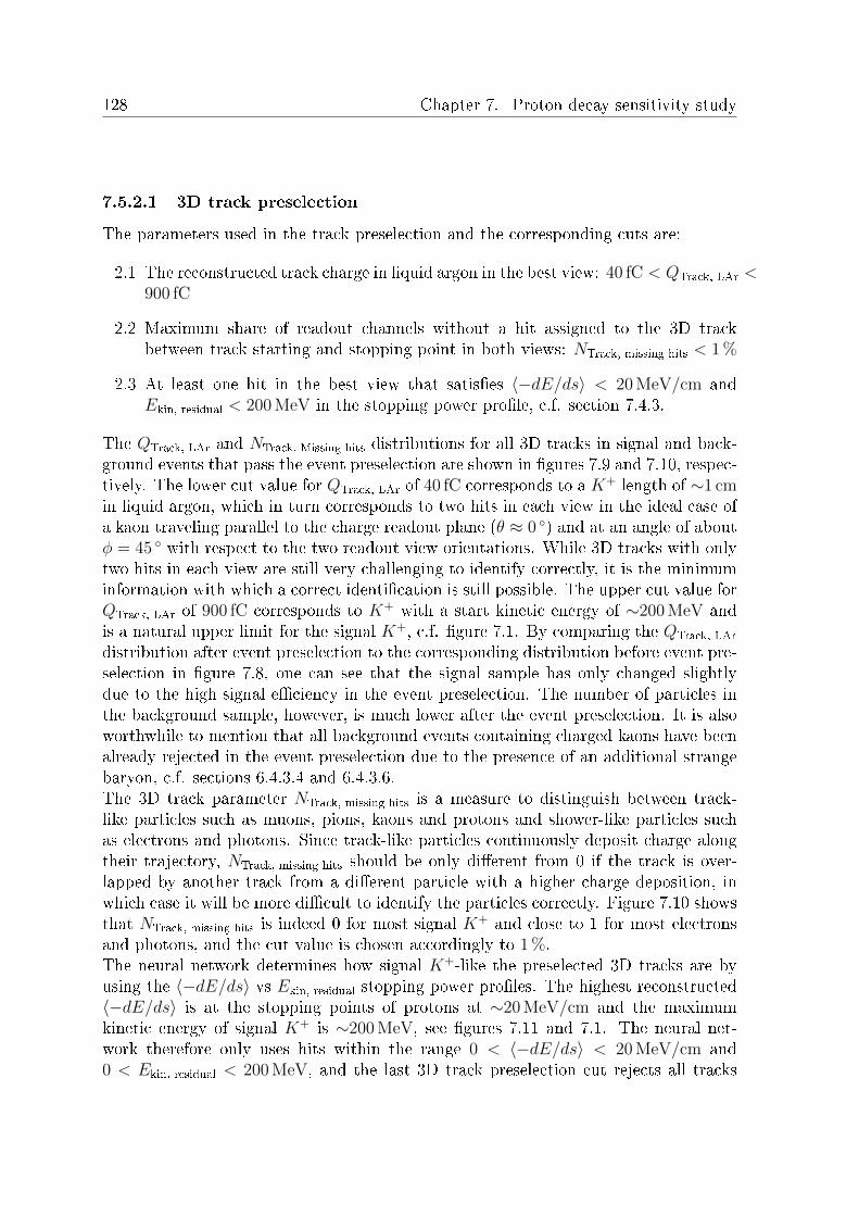
128 Chapter 7. Proton decay sensitivity study
7.5.2.1 3D track preselection
The parameters used in the track preselection and the corresponding cuts are:
2.1 The reconstructed track charge in liquid argon in the best view: 40 fC < QTrack, LAr <900 fC
2.2 Maximum share of readout channels without a hit assigned to the 3D trackbetween track starting and stopping point in both views: NTrack, missing hits < 1 %
2.3 At least one hit in the best view that satises 〈−dE/ds〉 < 20 MeV/cm andEkin, residual < 200 MeV in the stopping power prole, c.f. section 7.4.3.
The QTrack, LAr and NTrack, Missing hits distributions for all 3D tracks in signal and back-ground events that pass the event preselection are shown in gures 7.9 and 7.10, respec-tively. The lower cut value for QTrack, LAr of 40 fC corresponds to a K+ length of ∼1 cmin liquid argon, which in turn corresponds to two hits in each view in the ideal case ofa kaon traveling parallel to the charge readout plane (θ ≈ 0 ) and at an angle of aboutφ = 45 with respect to the two readout view orientations. While 3D tracks with onlytwo hits in each view are still very challenging to identify correctly, it is the minimuminformation with which a correct identication is still possible. The upper cut value forQTrack, LAr of 900 fC corresponds to K+ with a start kinetic energy of ∼200 MeV andis a natural upper limit for the signal K+, c.f. gure 7.1. By comparing the QTrack, LAr
distribution after event preselection to the corresponding distribution before event pre-selection in gure 7.8, one can see that the signal sample has only changed slightlydue to the high signal eciency in the event preselection. The number of particles inthe background sample, however, is much lower after the event preselection. It is alsoworthwhile to mention that all background events containing charged kaons have beenalready rejected in the event preselection due to the presence of an additional strangebaryon, c.f. sections 6.4.3.4 and 6.4.3.6.The 3D track parameter NTrack, missing hits is a measure to distinguish between track-like particles such as muons, pions, kaons and protons and shower-like particles suchas electrons and photons. Since track-like particles continuously deposit charge alongtheir trajectory, NTrack, missing hits should be only dierent from 0 if the track is over-lapped by another track from a dierent particle with a higher charge deposition, inwhich case it will be more dicult to identify the particles correctly. Figure 7.10 showsthat NTrack, missing hits is indeed 0 for most signal K+ and close to 1 for most electronsand photons, and the cut value is chosen accordingly to 1 %.The neural network determines how signal K+-like the preselected 3D tracks are byusing the 〈−dE/ds〉 vs Ekin, residual stopping power proles. The highest reconstructed〈−dE/ds〉 is at the stopping points of protons at ∼20 MeV/cm and the maximumkinetic energy of signal K+ is ∼200 MeV, see gures 7.11 and 7.1. The neural net-work therefore only uses hits within the range 0 < 〈−dE/ds〉 < 20 MeV/cm and0 < Ekin, residual < 200 MeV, and the last 3D track preselection cut rejects all tracks

7.5 Analysis 129
that do not have hits within that range. Table 7.7 shows the number of 3D tracks insignal and background samples before and after the event preselection as well as forthe three individual and combined track preselection cuts.
Figure 7.9: Track charge distributions in liquid argon measured in the best view in theG18_02a_02_11a signal (top) and 10 megaton · years background (bottom) samplesafter event preselection. The signal sample is renormalized to 100 000 events beforeevent preselection for this plot. The bin size along the y-axis in both plots is 10 fC.The corresponding 1D distributions can be found in gure C.3 in appendix C.
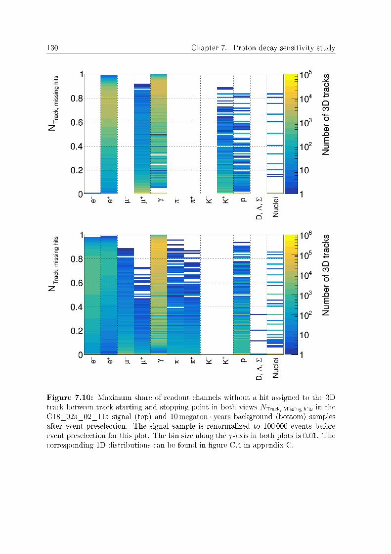
130 Chapter 7. Proton decay sensitivity study
Figure 7.10: Maximum share of readout channels without a hit assigned to the 3Dtrack between track starting and stopping point in both views NTrack, Missing hits in theG18_02a_02_11a signal (top) and 10 megaton · years background (bottom) samplesafter event preselection. The signal sample is renormalized to 100 000 events beforeevent preselection for this plot. The bin size along the y-axis in both plots is 0.01. Thecorresponding 1D distributions can be found in gure C.4 in appendix C.

7.5 Analysis 131
Signal
Cut All e− e+ µ+ γ K+ p Nuclei
/ 534 282 14 99 964 99 995 199 243 95 418 35 438 4 210
1 487 175 12 94 063 94 068 175 256 90 100 29 988 3 688
2.1 293 928 0 93 699 92 227 58 87 896 20 001 472.2 245 307 11 429 78 451 53 686 83 675 26 556 2 4992.3 466 020 12 93 837 93 241 171 635 82 880 21 472 2 943
2 165 513 0 418 76 477 2 76 373 12 203 40
3 58 131 0 5 36 0 57 925 165 0
Background
Cut All e− e+ µ− µ+ γ
/ 85 234 763 1 631 558 519 967 509 791 159 134 71 746 219
1 3 293 611 68 526 23 872 67 903 9 855 2 593 623
2.1 567 373 56 892 22 988 52 294 6 763 36 2202.2 1 320 455 2 174 104 55 448 7 735 802 3852.3 3 099 079 65 709 23 678 66 992 9 416 2 538 119
2 309 748 1 848 90 43 161 5 534 320
3 10 338 36 1 407 89 4
Cut π− π+ K− K+ p D, Λ, Σ Nuclei
/ 603 886 674 595 7 520 29 258 7 473 896 5 860 1 873 079
1 12 624 14 265 0 0 447 554 125 55 264
2.1 11 854 13 544 0 0 361 818 80 4 9202.2 8 640 11 430 0 0 396 013 108 36 4182.3 11 945 13 584 0 0 328 249 102 41 285
2 7 805 10 404 0 0 237 397 54 3 135
3 302 704 0 0 8 683 0 112
Table 7.7: Number of 3D tracks before and after event preselection, after individualand combined track preselection cuts and after the neural network classication inthe G18_02a_02_11a signal and 10 megaton · years background samples. The signalsample is renormalized to 100 000 events before event preselection for this table. Thecut labeled as 2 combines cuts 2.1, 2.2 and 2.3.

132 Chapter 7. Proton decay sensitivity study
7.5.2.2 Neural network
After the 3D track preselection, a neural network is used to determine the signal K+-likeness of all remaining tracks. The input to the neural network are the stoppingpower proles with the mean stopping power 〈−dE/ds〉 and residual kinetic energyEkin, residual at each hit, see section 7.4.3. Figure 7.11 shows the stopping power prolesfor signal K+ and for protons, π± and µ± in the background sample after particlepreselection. The average signal K+ stopping power prole is easily distinguishablefrom the proton, π± and µ± proles, promising a good discrimination between signalK+ and other particles. The µ+ and proton stopping power proles in the signalsample are similar to the corresponding distributions in the background sample andare therefore not shown separately.The neural network is built using the TensorFlow library with an implementation ofthe Keras application programming interface [136] [137]. It is trained with separatesignal and background samples that are generated identically to the analysis signaland background samples. The signal event training sample contains ∼65 000 eventsand the background event sample size corresponds to an exposure of 2 megaton · years.The same event and particle preselection cuts are applied to the training samples andthe neural network is trained on a 3D track basis to distinguish between two classesof tracks: signal K+ tracks vs. tracks from all other particles in both signal andbackground samples, meaning that also e.g. µ+ tracks in the signal sample are used inthe training (c.f. table 7.7).The input layer to the network consists of the stopping power prole of an individualtrack. In order to limit the layer size, the stopping power prole is divided in 20equally sized bins for 〈−dE/ds〉 between 0 and 20MeV/cm and 20 equally sized bins forEkin, residual between 0 and 200 MeV, yielding 400 neurons for the input layer. The inputlayer is connected to the rst inner layer with 64 neurons through the Rectied LinearUnit (ReLU) activation function. The rst inner layer is in turn connected through theReLU activation function to the second inner layer, which also consists of 64 neurons.The second inner layer is connected to the output layer through the softmax activationfunction. The output layer consists of two neurons: one for the signal K+-likeness ofthe track and one for the signal K+-unlikeness. The softmax activation function forcesthe sum of both output values to 1 so that the information in both values is redundant,and the signal K+-likeness output value is used for further analysis. The network istrained during multiple epochs and, for each epoch, 90 % of the reshued trainingsamples are used to train the network while the remaining 10 % are used for validation.If the performance on the validation subsample does not increase over 10 epochs, thetraining is complete and the network is applied to the G18_02a_02_11a signal and10 megaton · years background analysis samples, returning a signal K+-likeness valuebetween 0 and 1 for all tracks remaining after event and 3D track preselection that willbe used in the nal event selection in section 7.5.3. A return value of 1 means thatthe track is signal K+-like while 0 means signal K+-unlike. The signal K+-likenessof signal K+ tracks and of protons, π± and µ± tracks in the background sample isshown in gure 7.12. It is worthwhile repeating that all tracks in the signal sample areclassied by the neural network and that e.g. a proton or a muon in the signal sample

7.5 Analysis 133
Figure 7.11: 3D track stopping power proles with the mean stopping power〈−dE/ds〉 and residual kinetic energy Ekin, residual at each hit for signal K+ andfor protons, π± and µ± in background events in the G18_02a_02_11a signal and10 megaton · years background samples after event and particle preselection. The sig-nal sample is renormalized to 100 000 events before event preselection for this plot.

134 Chapter 7. Proton decay sensitivity study
Figure 7.12: 3D track fraction vs. signal K+-likeness of signal K+ and of protons,π± and µ± tracks in the background sample obtained from the neural network usingthe G18_02a_02_11a signal and 10 megaton · years background samples after eventand particle preselection.
can have a high signal K+ likeness, c.f. table 7.7. The µ+ and proton track signal K+
likeness distributions in the signal sample are similar to the corresponding distribu-tions in the background sample and are therefore not shown separately. Tracks frome±, γ, D mesons, Λ and Σ baryons and nuclei are very dierent from signal K+ tracksand the corresponding distributions are not shown. For any given cut value for thesignal K+-likeness, the total number of selected non-signal K+ 3D tracks in the signaland background samples can be calculated as function of the signal K+ track selectioneciency by integrating the distributions in gure 7.12 from 1 to 0. The correspondingcurves are shown in gure 7.13.For the nal event selection, all tracks with a signal K+-likeness of 0.83 or higher areconsidered to be signalK+ tracks, which corresponds to a signal K+ selection eciencyof 76 % for K+ that pass the event and particle preselection and to about 10 000 tracksmisidentied as signal K+ in the background sample, c.f. gure 7.13. The signal K+-likeness cut value of 0.83 marks an inection point for proton, pion and muon tracksin the background sample, and lower cut values would lead to an exponential increasein misidentied tracks with only a small gain in signal K+ track selection eciency,c.f. gures 7.12 and 7.13. The neural network classication is labeled as cut 3 and theexact numbers of selected tracks can be found in table 7.7.

7.5 Analysis 135
Figure 7.13: Number of 3D tracks misidentied as signal K+ in signal (top) andbackground (bottom) sample as function of signal K+ track selection eciency usingthe signal K+-likeness obtained from the neural network in the G18_02a_02_11asignal and 10 megaton · years background samples after event and particle preselection.The signal sample is renormalized to 100 000 events before event preselection for thisplot.

136 Chapter 7. Proton decay sensitivity study
7.5.3 Final event selection
In the nal event selection, three cuts are applied that aim at 3D tracks from the signalK+ and its daughter µ+ and e+. The fourth and nal cut allows only for short tracksfrom track-like particles in addition to the K+, µ+ and e+, which are potential protonsfrom nal state interactions (see section 7.1). The cuts are applied to all events thatsurvive the event preselection. As opposed to cut 4.1, cuts 4.2 to 4.4 are composed ofseveral criteria and the targeted tracks do not have to survive the track preselection.The used parameters and cut values are:
4.1 Exactly one 3D track with a signal K+-likeness of 0.83 or higher from the neu-ral network classication, hereafter referred to as signal K+ track (c.f. section7.5.2.2)
4.2 Exactly one track that satises the following criteria, aiming at the µ+ from K+
decay:
4.2.1 520 fC < QTrack, LAr < 760 fC
4.2.2 Length of track: 40 cm < LTrack < 56 cm
4.2.3 NTrack, missing hits < 10 %
4.2.4 Distance between track starting point and signal K+ track stopping point:DK+ < 5 cm
4.2.5 Angle to signal K+ track in best view: α > 10
4.3 Exactly one track that satises the following criteria, aiming at the e+ from µ+
decay:
4.3.1 NTrack, missing hits > 10 %
4.3.2 Number of hits in best view: NTrack, Hits > 10
4.3.3 QTrack, LAr > 40 fC
4.4 No additional track with:
4.4.1 NTrack, missing hits < 10 %
4.4.2 QTrack, LAr > 40 fC
4.4.3 LTrack > 5 cm
Since all events in the G18_02a_02_11a signal sample contain oneK+, cut 4.1 requiresexactly one signal K+-like track. About 92 % of signal K+ decay at rest, producingmono-energetic µ+ with Ekin = 152.5 MeV in the two body decay K+ → µ+νµ. Thecorresponding 3D track has a well-dened charge deposition and length and cuts 4.2.1and 4.2.2 are chosen accordingly, see gures 7.9 and 7.14. Furthermore, the µ+ trackis typically track-like with less than 10 % missing hits (cut 4.2.3, see gure 7.10), andit should be close to the end point of the signal K+. The maximum distance between

7.5 Analysis 137
the µ+ track starting point and signal K+ track stopping point of 5 cm in cut 4.2.4is chosen to be rather large since the rst hits of the µ+ are typically shadowed bythe highly-ionizing stopping K+, an eect that worsens if the µ+ travels back in thedirection of the stopping K+ track.
Figure 7.14: Track length distributions in the G18_02a_02_11a signal (top) and10 megaton · years background (bottom) samples after event preselection. The signalsample is renormalized to 100 000 events before event preselection for this plot. Thebin size along the y-axis in both plots is 1 cm. The corresponding 1D distributions canbe found in gure C.5 in appendix C.

138 Chapter 7. Proton decay sensitivity study
The last cut 4.2.5 for the µ+ track is introduced since some events in the backgroundsample contain a proton that is misidentied as signal K+ and a muon or pion withsimilar length and charge deposition as the µ+ from K+ decay that travels in the samedirection as the proton. Since the proton track shadows the rst part of the muon orpion track, it seems like the muon or pion emerge from the proton, just like the µ+
emerges from the K+ decay. The minimum angle α under which two close tracks canbe separated depends on the charge diusion and the length of the track. The shortestsignal K+ tracks after the neural network classication have a length of ∼20 mm andthe transverse diusion at 6 m drift is λT ≈ 3.3 mm (c.f. section 2.3.3.2), resulting inα = arcsin (3.3 mm/20 mm) ≈ 10 . Figure 7.15 shows such a background event witha proton misidentied as signal K+ and π+ misidentied as µ+ from K+ decay in thenal state.
Figure 7.15: νµ NC RES background event that motivates cut 4.2.5 to require aminimum angle between the K+ and µ+ of α > 10 in the best view. The proton ismisidentied as signal K+ and shadows the rst part of the π+ track, which in turnis misidentied as µ+ from the K+ decay, producing an event topology that is verysimilar to the proton decay signal.
The positron from the muon decay µ+ → e+νeνµ, also called Michel positron, typicallyproduces a shower-like 3D track with more than 10 % missing hits, and cut 4.3.1 ischosen accordingly (see gure 7.10). The cut 4.3.2 on the charge and cut 4.3.3 on thenumber of hits in the best view avoid low-energy photons in both signal and back-ground samples, see gures 7.9 and 7.16.

7.5 Analysis 139
Figure 7.16: Number of hits per track in best view in the G18_02a_02_11a signal(top) and 10 megaton · years background (bottom) samples after event preselection.The signal sample is renormalized to 100 000 events before event preselection for thisplot. The bin size along the y-axis in both plots is 1. The corresponding 1D distribu-tions can be found in gure C.6 in appendix C.
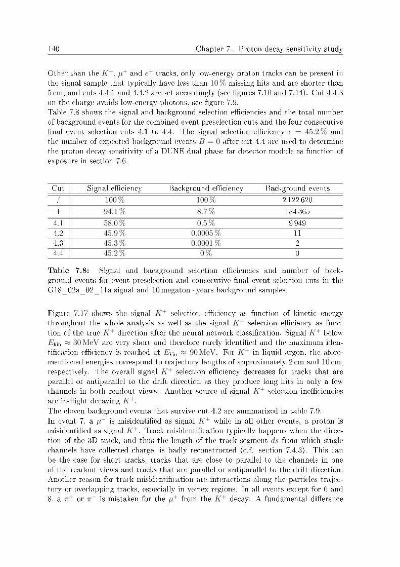
140 Chapter 7. Proton decay sensitivity study
Other than the K+, µ+ and e+ tracks, only low-energy proton tracks can be present inthe signal sample that typically have less than 10 % missing hits and are shorter than5 cm, and cuts 4.4.1 and 4.4.2 are set accordingly (see gures 7.10 and 7.14). Cut 4.4.3on the charge avoids low-energy photons, see gure 7.9.Table 7.8 shows the signal and background selection eciencies and the total numberof background events for the combined event preselection cuts and the four consecutivenal event selection cuts 4.1 to 4.4. The signal selection eciency ε = 45.2 % andthe number of expected background events B = 0 after cut 4.4 are used to determinethe proton decay sensitivity of a DUNE dual phase far detector module as function ofexposure in section 7.6.
Cut Signal eciency Background eciency Background events
/ 100 % 100 % 2 122 620
1 94.1 % 8.7 % 184 365
4.1 58.0 % 0.5 % 9 9494.2 45.9 % 0.0005 % 114.3 45.3 % 0.0001 % 24.4 45.2 % 0 % 0
Table 7.8: Signal and background selection eciencies and number of back-ground events for event preselection and consecutive nal event selection cuts in theG18_02a_02_11a signal and 10 megaton · years background samples.
Figure 7.17 shows the signal K+ selection eciency as function of kinetic energythroughout the whole analysis as well as the signal K+ selection eciency as func-tion of the true K+ direction after the neural network classication. Signal K+ belowEkin ≈ 30 MeV are very short and therefore rarely identied and the maximum iden-tication eciency is reached at Ekin ≈ 90 MeV. For K+ in liquid argon, the afore-mentioned energies correspond to trajectory lengths of approximately 2 cm and 10 cm,respectively. The overall signal K+ selection eciency decreases for tracks that areparallel or antiparallel to the drift direction as they produce long hits in only a fewchannels in both readout views. Another source of signal K+ selection inecienciesare in-ight decaying K+.The eleven background events that survive cut 4.2 are summarized in table 7.9.In event 7, a µ− is misidentied as signal K+ while in all other events, a proton ismisidentied as signal K+. Track misidentication typically happens when the direc-tion of the 3D track, and thus the length of the track segment ds from which singlechannels have collected charge, is badly reconstructed (c.f. section 7.4.3). This canbe the case for short tracks, tracks that are close to parallel to the channels in oneof the readout views and tracks that are parallel or antiparallel to the drift direction.Another reason for track misidentication are interactions along the particles trajec-tory or overlapping tracks, especially in vertex regions. In all events except for 6 and8, a π+ or π− is mistaken for the µ+ from the K+ decay. A fundamental dierence

7.5 Analysis 141
Figure 7.17: Top: signal K+ selection eciency as function of true kinetic energythroughout the analysis. Since every signal event contains exactly one K+, the y-axiscan also be interpreted as signal event selection eciency. Bottom: signal K+ selectioneciency as function of true K+ start direction after the neural network classication.The ranges of θ and φ have been downsized by exploiting dierent symmetries in thedetector: φ = 0 is parallel to the readout strips in one of the readout views andφ = 45 is in the middle of both readout view orientations. θ = 90 is parallel to thecharge readout plane and θ = 0 is parallel and antiparallel to the drift direction.

142 Chapter 7. Proton decay sensitivity study
Event 4.3 ν Eν [MeV] Interaction Target FSP Ekin [MeV] ID
1 7 νe 446 CC RES p e− 116 e+
p 24 K+
π+ 153 µ+ → e+
2 7 νe 584 CC RES p e− 138 e+
p 69 K+
n 74π+ 155 µ+ → e+
3 7 νe 489 CC RES p e− 107 e+
p 94 K+
π+ 135 µ+ → e+
4 3 νe 866 NC RES p p 136 K+ +Xn 17n 9π+ 154 µ+ → e+
5 7 νe 1 244 NC QE n p 130 K+
n 54π− 159 µ+
6 7 νe 954 NC RES n p 341 µ+
p 39 K+
p 97 n 21-56
7 3 νµ 641 CC RES p µ− 24 K+
p 211 Xp 5π+ 147 µ+ → e+
8 7 νµ 604 CC MEC p & n µ− 170p 312 µ+
p 34 K+
9 7 νµ 5 184 NC RES p p 221 K+
p 56π− 151 µ+
10 7 νµ 583 NC RES p p 134 K+
p 7π− 136 µ+
11 7 νµ 43 051 NC RES p p 250 K+
p 15π− 160 µ+
Table 7.9: Background events in the 10 megaton · years G18_02a_02_11a samplethat survive nal event selection cut 4.2. The nal state particles (FSP) emergingfrom the neutrino interaction and the signal particles they are misidentied as (ID) areshown in the right column. Only two events survive cut 4.3 and the nal state particlewith ID X refers to the particle that fails cut 4.4.
7.5 Analysis 143
between the eleven background events that pass cut 4.2 and signal events is that themisidentied signal K+ and µ+ share the same vertex in the background sample whilethe µ+ emerges from the decaying K+ in the signal sample. The background eventspass cut 4.2 anyway because the misidentied signal K+ track is shorter than the re-quired distance between K+ stopping point and µ+ starting point of DK+ < 5 cm incut 4.2.4 or because its starting and stopping points were confused, which is more likelyto happen in busy vertex regions with overlapping tracks. Those tracks typically havetwo reconstructed ionization peaks: one at their starting point in the vertex region dueto overlapping tracks and one at their stopping point due to the Bragg peak. A moresophisticated reconstruction algorithm could identify tracks with two ionization peaksand exclude them from the signal K+ identication, although this would also reducethe signal selection eciency since, in some events, additional protons are present atthe starting point of the K+ track in the signal sample.In the nine events that do not survive cut 4.3, events 1, 2 and 3 have two shower-liketracks instead of 1: the e− from the νe charged current interaction and the e+ fromthe decay chain π+ → µ+νµ → e+νeνµ. Event 6 has no shower-like tracks since onlyneutrons and protons are present. Event 5, 8, 9, 10 and 11 do contain π− or µ−, buthave no shower-like tracks since the µ− usually does not produce a Michel electron inliquid argon as it gets captured by an argon atom and cascades down to the groundstate of the muonic atom by emitting O (MeV) photons, eventually exchanging a W−
boson with the nucleus that subsequently emits O (MeV) nucleons. It is worthwhilementioning that the µ± from π± decays are typically not reconstructed as their kineticenergy is too low.Event 4 and 7 survive cut 4.3 since the only showering particle is the e+ from the π+
decay chain. In event 4, the proton that is misidentied as signal K+ interacts with anargon atom before it stopped, mimicking the Bragg peak of a signal K+. The protontrack has a clear kink after the interaction, producing a separate reconstructed trackthat fails cut 4.4. In event 7, the µ− is misidentied as signal K+, and the proton inthe nal state with Ekin = 211 MeV fails cut 4.4. Figures 7.18 and 7.19 show eventdisplays with the aforementioned features of events 3, 4, 7 and 10.

144 Chapter 7. Proton decay sensitivity study
Figure 7.18: Event displays of events 3 (top) and 4 (bottom) in table 7.9. In Event3, the proton is misidentied as signal K+ and the π+ as µ+ from K+ decay. Sincethere are two showering particles e− and e+, the event does not pass cut 4.3. The rstpart of the proton track (p) in event 4 is misidentied as signal K+, and the π+ asµ+ from K+ decay. The kink and two ionization peaks in the proton track are clearlyvisible, and the separately reconstructed track p′ fails cut 4.4.

7.5 Analysis 145
Figure 7.19: Event displays of events 7 (top) and 10 (bottom) in table 7.9. In Event7, the µ− is misidentied as signalK+ and the π+ as µ+ fromK+ decay. The additionalproton track fails cut 4.4. In Event 10, the proton is misidentied as signal K+ andthe π− as µ+ from K+ decay. Since the µ− is captured by an argon atom, there is noshowering particles and the event fails cut 4.3.

146 Chapter 7. Proton decay sensitivity study
7.5.4 Results for G18_10b_00_000 samples
The analysis described in sections 7.5.1 through 7.5.3 is applied to theG18_10b_00_000 signal and 2 megaton · years background sample with the same cuts,including the neural network that was trained with the G18_02a_02_11a trainingsamples. The signal and background selection eciencies and number of backgroundevents before and after the event preselection and after the nal event selection areshown in table 7.10. The 15 % of events in which the K+ charge-exchanged into a K0
inside the nucleus are excluded from the analysis and the signal eciency thereforestarts at 85 %, c.f. section 7.1. The event and track distributions look very similar tothose in the G18_02a_02_11a sample and are therefore not shown. The backgroundis reduced to 0 after cut 4.2 already, but the signal selection eciency after cut 4.4 ofε = 46.8 % is used for comparison with the G18_02a_02_11a sample.
Cut Signal eciency Background eciency Background events
/ 85 % 100 % 424 524
1.1 84.8 % 34.7 % 147 1661.2 84.9 % 28.3 % 120 1191.3 81.5 % 22.9 % 97 012
1 81.4 % 7.9 % 33 340
4.1 59.8 % 0.4 % 1 6884.2 47.3 % 0 % 04.3 46.8 % 0 % 04.4 46.8 % 0 % 0
Table 7.10: Signal and background selection eciencies and number of backgroundevents for individual and combined event preselection cuts and for consecutive nalevent selection cuts in the G18_10b_00_000 signal and 2 megaton · years backgroundsamples.
7.6 Proton decay sensitivity result
The signal selection eciencies ε and numbers of expected background events B forthe G18_02a_02_11a and G18_10b_00_000 samples are summarized in table 7.11.
Sample ε B Background sample size
G18_02a_02_11a 45.2 % 0 10 megaton · yearsG18_10b_00_000 46.8 % 0 2 megaton · years
Table 7.11: Signal selection eciencies ε and numbers of expected background eventsB for the G18_02a_02_11a and G18_10b_00_000 samples.

7.6 Proton decay sensitivity result 147
The mean signal eciency of both samples ε = 46 % is used to calculate the sensitivityto p → νK+, which is dened as the lower proton lifetime limit over proton decaybranching ratio τ/Br at 90 % condence level for a given exposure if no proton decayevent is observed, c.f. section 7.5 and equation 7.9. The full spread between the meaneciency ε = 46 % and the eciencies in the two samples of ∆syst
ε = 0.8 % is denedas systematic uncertainty on the signal selection eciency.In order to assess the statistical uncertainty on the signal selection eciency, the neuralnetwork signal K+-likeness cut has been loosened to 0.245 to obtain 50 backgroundevents in the 10 megaton · years G18_02a_02_11a sample after the nal event selec-tion cut 4.4, c.f. sections 7.5.2.2 and 7.5.3. From the full G18_02a_02_11a sample,50 subsamples of 200 kiloton · years and 10 subsamples of 1 megaton · year are denedrandomly. These subsample sizes are conservative estimates for the minimum and max-imum expected exposure of the entire DUNE far detector complex with four 10 kilotonLAr TPC modules. The signal K+-likeness cut is adapted for each subsample in orderto obtain one background event in the 200 kiloton · years subsamples and 5 backgroundevents in the 1 megaton · year subsamples, starting at a signal K+-likeness cut of 0 andincreasing it in steps of 0.01 in order to obtain the minimum cut value necessary toreach the target number of background events in each subsample, which corresponds tothe maximum signal selection eciency. The same approach was chosen for obtaining50 background events in the full sample with the signalK+-likeness cut of 0.245. In twoof the 200 kiloton · years subsamples, no background event can be found by adaptingthe signal K+-likeness cut and these two samples are excluded from the following cal-culations. Figure 7.20 shows the signal selection eciency distributions of the dierentsubsamples and the reference signal selection eciency εr for the full sample with 50background events. Since the distributions are asymmetric, the standard deviationsσ′ε = 2.0 % and σ′′ε = 1.5 % are not a good measure for the statistical uncertaintyon ε. Instead, the statistical uncertainties at the exposures of 200 kiloton · years and1 megaton · year are dened as the dierence between the reference eciency εr andthe most extreme values in the respective distributions:
∆stat′
ε = +2.7−5.2 % at 200 kiloton · years (7.10)
∆stat′′
ε = +2.7−2.3 % at 1 megaton · year (7.11)
A linear interpolation and extrapolation towards lower exposures of the obtained valuesfor ∆stat′
ε and ∆stat′′ε yields the statistical uncertainties on the mean signal selection
eciency ∆statε at all exposure up to 1 megaton · year. As the systematic and statistical
uncertainties are independent, they can be added up in quadrature to obtain the totaluncertainty on the mean signal selection eciency:
∆ε =
√(∆systε
)2+ (∆stat
ε )2 (7.12)
The systematic and statistical uncertainties are added up to obtain the total uncer-tainty on the signal selection eciency:With the expected number of background events B = 0, it is only sensible to calculatethe lower proton lifetime limit when no events are observed (N0 = 0), and the resulting

148 Chapter 7. Proton decay sensitivity study
Figure 7.20: Signal eciency distributions of 200 kiloton · years and 1 megaton · yearsubsamples with one and ve background events, respectively. The blue line indicatesthe reference eciency εr = 54.2 % for the full 10 megaton · years G18_02a_02_11asample with 50 background events.
upper limit on the number of observed signal events at 90 % CL is S = 2.44, see table7.4. Figure 7.21 shows the lower proton lifetime limit over proton decay branchingratio τ/Br (p→ K+ν) at 90 % condence level for exposures up to 1 megaton · yearaccording to equation 7.9 if no event is observed, using ε = 46 %±∆ε and S = 2.44.The latest published limit by Super-Kamiokande of τ/Br (p→ K+ν) > 5.9×1033 yearsat an exposure of 260 kiloton · years represents the world's best limit [5] and can be con-rmed with a DUNE dual phase LAr TPC module after an exposure of ∼120 kiloton·years. A limit of τ/Br (p→ K+ν) > 5.1 × 1034 years can be reached with DUNE atan exposure of 1 megaton · year, assuming the same signal eciency and backgroundrejection for the entire DUNE far detector complex, while Hyper-Kamiokande predictsτ/Br (p→ K+ν) > 3.2 × 1034 years at an exposure of 1.9 megaton · years with the so-called 1TankHD design [27].The Super-Kamiokande analysis yields B = 0.38 expected background events whileno events are observed, and the Hyper-Kamiokande sensitivity quotes B ≈ 1 permegaton·year. In the case of Super-Kamiokande, the upper limit on the number ofobserved signal events at 90 % CL according to Feldman-Cousins is S = 2.1, whicheectively leads to a better lower lifetime limit compared to an analysis with B = 0and, consequently, S = 2.44 (c.f. equation 7.9). A similar scenario is often assumedin sensitivity studies and could also be considered for DUNE by tuning the presented

7.6 Proton decay sensitivity result 149
analysis to e.g. B = 0.5 at a given exposure. In case no events will be observed inDUNE within that exposure, S would be equal to 1.94 and the resulting lower lifetimelimit would be better by a factor of 2.44/1.94 = 1.26 compared to the results in gure7.21 that are based on B = 0, even without accounting for the concomitant increase insignal selection eciency. However, the likelihood that no background event will occuris only 60 % for B = 0.5, and one or multiple observed events could originate frombackground uctuations or proton decay. In background-free conditions on the otherhand, every observed event can be interpreted as proton decay.
Figure 7.21: Lower proton lifetime limit over proton decay branching ratioτ/Br (p→ K+ν) at 90 % condence level for exposures up to 1 megaton · year in aDUNE dual phase LAr TPC far detector module, assuming the obtained signal selec-tion eciency of ε = 46 %±∆ε. The total uncertainty ∆ε is the root mean square of theconstant systematic uncertainty ∆syst
ε = 0.8 % and the exposure-dependent statisticaluncertainty, c.f. equations 7.10 through 7.12. The latest published limit from Super-Kamiokande is τ/Br (p→ K+ν) > 5.9×1033 years at an exposure of 260 kiloton · years[5].

150 Chapter 7. Proton decay sensitivity study
Chapter 8
Conclusions
The current world's best limit on the proton decay lifetime per branching ratio for thedecay mode p → K+ν by Super-Kamiokande is τ/Br (p→ K+ν) > 5.9 × 1033 years[5], which is below the predictions of favored Grand Unied Theories with supersym-metric extension (SUSY GUTs) of 1034 − 1035 years. In this thesis, the sensitivity of a10 kiloton dual phase LAr TPC module in DUNE to the proton decay mode p→ K+νwas assessed based on Monte Carlo simulations by considering atmospheric neutrinointeractions as background. Only the kaon decay mode K+ → µ+νµ was studied andthe results are assumed to be transferable to other kaon decay modes. Cosmogenicbackground, in which neutral kaons originating from cosmic muon interactions insidethe surrounding rocks enter the TPC undetected and undergo charge exchange, has notbeen considered. Single charged kaons with kinetic energies below 200 MeV producedin these events are indistinguishable from proton decay via p→ K+ν and could there-fore represent irreducible background. The cosmogenic background rate is expected tobe very low due to the rock overburden of the DUNE far detector and the resultingcosmic muon ux of only ∼4/ (m2 · day), and a detailed study is necessary to quantifythe impact on the proton decay sensitivity.The simulation of both signal and background samples is divided into event generationand detector simulation. The dual phase LAr TPC detector simulation was validatedand tuned with cosmic ray data collected by the 3x1x1m3 dual phase LAr TPC pro-totype and adapted to the dimensions of the 10 kiloton dual phase LAr TPC module.The simulation toolkit GENIE v3_00_06 was used for event generation, which includesthe modeling of the initial state of the argon nucleus, decay kinematics of the protonand intranuclear propagation of the charged kaon for the signal sample. In the back-ground sample, GENIE simulates the initial state of the argon nucleus, neutrino-argoninteractions and intranuclear transport of particles emerging inside the nucleus. Theatmospheric neutrino ux was obtained from the HONDAmodel. The dominant contri-bution to systematic uncertainties on the proton decay sensitivity is expected from theevent generation models, and the sensitivity study was therefore carried out with twoocial GENIE tunes labeled G18_02a_02_11a and G18_10b_00_000 that representconsistent combinations of the interdependent processes in the event generation. Themodels in tune G18_02a_02_11a are mostly empirical while the G18_10b_00_000
151

152 Chapter 8. Conclusions
tune mainly uses theoretically motivated models.The analysis focuses on the signal K+ identication and yields 0 background events fora maximum exposure of 10 megaton · years at an average signal selection eciency ofε = 46 %. The largest contribution to the signal selection ineciency comes from low-energy signal K+ that scattered o nucleons inside the argon nucleus. These scattersoccur for 32 % of K+ in both signal samples since the same K+-nucleon cross sectionsare used in the intranuclear propagation in both GENIE tunes. The nature of thescatters diers between the tunes, but the signal K+ usually lose a large amount oftheir kinetic energy to the low-energy nucleons in all scatters, independent of the scat-tering process, which leads to a low overall identication eciency for scattered signalK+. The dominant contribution to the systematic uncertainty within the event gen-eration therefore originates from the K+-nucleon cross sections and the resulting totalsystematic uncertainty on the selection eciency related to event generation modelsof ∆ε = 0.8 % is thus relatively small. Since there is only one data set of K+-nucleoncross sections available within GENIE, an independent cross-check of the signal K+
nal state interactions was carried out with the simulation toolkit NEUT, yielding aninteraction rate of 35 % and conrming the results from GENIE. The statistical uncer-tainty on the signal selection eciency depends on the exposure and was estimated toabout 2 − 5 % for exposures up to 1 megaton · year by dividing the 10 megaton · yearsbackground sample into smaller subsamples.In the detector simulation, a mostly ideal detector was assumed with e.g. no chargeattenuation and no electronic noise. On the other hand, all events were placed in thecenter of the detector at a drift distance of 6m. The diusion of the drifting charge at6m is higher than the average diusion in events placed randomly inside the detectoras it grows with the square root of the drift time, and the overall charge smearing fromdiusion is therefore slightly overestimated compared to a real experiment.The trigger for potential proton decay events in DUNE will be provided by the scin-tillation light signal recorded with PMTs that are located below the TPC. For thesensitivity study in this thesis, the scintillation light was not simulated. While thetrigger eciency for high energy events like proton decay is close to 100 % and a fulltrigger simulation would therefore not introduce substantial ineciencies [139], thelight system could considerably improve the particle identication and thus the pre-sented sensitivity. With a time resolution in the order of nanoseconds, separate lightashes from the signal K+ and daughter µ+ and e+, as well as the distinct periodswithout light emission that correspond to the K+ and µ+ lifetimes of 12 ns and 2.2 µs,can be reconstructed and matched to the ionization charge signal recorded by the TPC.It is important to keep in mind that the 2D pattern recognition was based on MonteCarlo truth information since the corresponding reconstruction algorithms are currentlybeing developed. A full reconstruction will yield a somewhat lower signal selection e-ciency, but the most problematic event topologies were already removed in the analysis(see gure 7.17) and the impact of a full reconstruction is therefore not expected tocrucially change the presented results. At the same time, improvements in the recon-struction, by e.g. including multiple scatters in 3D tracks, can further improve thesignal selection eciency and background rejection.

153
With the obtained signal eciency of ε = 46 % at 0 background, the DUNE dual phaseLAr TPC will be able to conrm the latest published limit by Super-Kamiokandeof τ/Br (p→ K+ν) > 5.9 × 1033 years [5] after an exposure of ∼120 kiloton · years.The sensitivity increases linearly with the exposure in background-free conditions andfor an exposure of 1 megaton · year, DUNE can set a limit of τ/Br (p→ K+ν) >5.1 × 1034 years when assuming that the obtained signal eciency and backgroundrejection are valid for the whole DUNE far detector complex, reaching the predictedrange of the most promising SUSY GUTs of 1034 − 1035 years.Since kaons produced in atmospheric neutrino interactions on argon are always ac-companied by at least one detectable particle, there is no irreducible background forproton decay searches via p → K+ν. Additionally, it has been shown that even themost persistent background events in this study are clearly distinguishable from thesignal in the event display (see gures 7.6, 7.15, 7.18 and 7.19), but the automatedreconstruction and cut ow analysis lead to relatively high losses in the signal selec-tion eciency. This thesis represents the rst proton decay sensitivity study for adual phase LAr TPC with a full simulation, reconstruction and analysis chain, andthe reconstruction and analysis can be further improved. A realistic lower limit on thesignal selection eciency at 0 background can be estimated to 64 % by assuming thatall signal events can be correctly identied except for the 32 % of events in which theK+ scatters inside the nucleus and for the 4 % of remaining events in which the K+ isdicult to reconstruct and identify since it travels within 20 parallel or antiparallelto the drift direction, c.f. gures 7.1 and 7.17. Even higher signal selection ecienciesare possible since many of the scattered K+ have enough kinetic energy to produce avisible and distinctive track inside the detector.

154 Chapter 8. Conclusions

Appendix A
Intranuclear propagation cross
sections and interaction shares in
GENIE
Figure A.1: Total averaged cross sections per nucleon for photons in 4018Ar obtained
from a partial wave analysis provided through the INS DAC services [126] [127].
155

156Appendix A. Intranuclear propagation cross sections and interaction
shares in GENIE
Figure A.2: DierentialK+-nucleon cross-section probability density function (p.d.f.)for elastic scatters on protons and neutrons and for charge exchange with neutrons in4018Ar obtained from a partial wave analysis provided through the INS DAC services[126] [127].
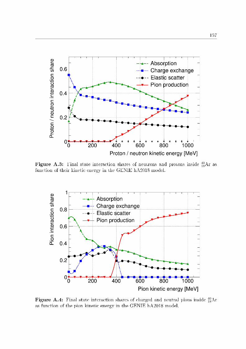
157
Figure A.3: Final state interaction shares of neutrons and protons inside 4018Ar as
function of their kinetic energy in the GENIE hA2018 model.
Figure A.4: Final state interaction shares of charged and neutral pions inside 4018Ar
as function of the pion kinetic energy in the GENIE hA2018 model.

158Appendix A. Intranuclear propagation cross sections and interaction
shares in GENIE
Figure A.5: Final state interaction shares of neutrons inside 4018Ar as function of the
neutron kinetic energy in the GENIE hN2018 model. The abbreviation CMP standsfor compound nucleus formation. The data is obtained from a partial wave analysisprovided through the INS DAC services [126] [127].
Figure A.6: Final state interaction shares of protons inside 4018Ar as function of the
proton kinetic energy in the GENIE hN2018 model. The data is obtained from a partialwave analysis provided through the INS DAC services [126] [127].

159
Figure A.7: Final state interaction shares of neutral pions inside 4018Ar as function of
the pion kinetic energy in the GENIE hN2018 model. The abbreviation CMP standsfor compound nucleus formation. The data is obtained from a partial wave analysisprovided through the INS DAC services [126] [127].
Figure A.8: Final state interaction shares of positively charged pions inside 4018Ar as
function of the pion kinetic energy in the GENIE hN2018 model. The data is obtainedfrom a partial wave analysis provided through the INS DAC services [126] [127].

160Appendix A. Intranuclear propagation cross sections and interaction
shares in GENIE
Figure A.9: Final state interaction shares of negatively charged pions inside 4018Ar as
function of the pion kinetic energy in the GENIE hN2018 model. The data is obtainedfrom a partial wave analysis provided through the INS DAC services [126] [127].
Appendix B
Neutrino-argon cross sections in
GENIE
161

162 Appendix B. Neutrino-argon cross sections in GENIE
Figure B.1: Charged current (top) and neutral current (bottom) electron neutrinocross sections on argon for all processes as function of neutrino energy in GENIE tuneG18_02a_02_11a, c.f. table 6.2 in section 6.4.3.

163
Figure B.2: Charged current (top) and neutral current (bottom) electron antineutrinocross sections on argon for all processes as function of neutrino energy in GENIE tuneG18_02a_02_11a, c.f. table 6.2 in section 6.4.3.

164 Appendix B. Neutrino-argon cross sections in GENIE
Figure B.3: Charged current (top) and neutral current (bottom) muon antineutrinocross sections on argon for all processes as function of neutrino energy in GENIE tuneG18_02a_02_11a, c.f. table 6.2 in section 6.4.3. The charged current elastic scat-tering o single electrons is only implemented for electron neutrinos and antineutrinosin GENIE as the corresponding energy threshold for muon and tau neutrinos andantineutrinos is very high, see section 6.4.3.1.

165
Figure B.4: Charged current (top) and neutral current (bottom) tau neutrino crosssections on argon for all processes as function of neutrino energy in GENIE tuneG18_02a_02_11a, c.f. table 6.2 in section 6.4.3. The charged current elastic scat-tering o single electrons is only implemented for electron neutrinos and antineutrinosin GENIE as the corresponding energy threshold for muon and tau neutrinos andantineutrinos is very high, see section 6.4.3.1.

166 Appendix B. Neutrino-argon cross sections in GENIE
Figure B.5: Charged current (top) and neutral current (bottom) tau antineutrinocross sections on argon for all processes as function of neutrino energy in GENIE tuneG18_02a_02_11a, c.f. table 6.2 in section 6.4.3. The charged current elastic scat-tering o single electrons is only implemented for electron neutrinos and antineutrinosin GENIE as the corresponding energy threshold for muon and tau neutrinos andantineutrinos is very high, see section 6.4.3.1

Appendix C
1D particle and track distributions for
proton decay sensitivity study
Figure C.1: Kinetic energy distributions of all nal state particles except neutrinosfrom all neutrino avors and interaction processes at an exposure of 1 megaton · yearin the G18_02a_02_11a background sample.

168Appendix C. 1D particle and track distributions for proton decay
sensitivity study
Figure C.2: Track charge distributions in liquid argon measured in the best viewin the G18_02a_02_11a signal (top) and 10 megaton · years background (bottom)samples before event preselection. The signal sample is renormalized to 100 000 eventsbefore event preselection.

169
Figure C.3: Track charge distributions in liquid argon measured in the best viewin the G18_02a_02_11a signal (top) and 10 megaton · years background (bottom)samples after event preselection. The signal sample is renormalized to 100 000 eventsbefore event preselection for this plot. The bin size along the y-axis in both plots is10 fC.

170Appendix C. 1D particle and track distributions for proton decay
sensitivity study
Figure C.4: Maximum share of readout channels without a hit assigned to the 3Dtrack between track starting and stopping point in both views NTrack, Missing hits in theG18_02a_02_11a signal (top) and 10 megaton · years background (bottom) samplesafter event preselection. The signal sample is renormalized to 100 000 events beforeevent preselection for this plot. The bin size along the y-axis in both plots is 0.01.

171
Figure C.5: Track length distributions in the G18_02a_02_11a signal (top) and10 megaton · years background (bottom) samples after event preselection. The signalsample is renormalized to 100 000 events before event preselection for this plot. Thebin size along the y-axis in both plots is 1 cm.

172Appendix C. 1D particle and track distributions for proton decay
sensitivity study
Figure C.6: Number of hits per track in best view in the G18_02a_02_11a signal(top) and 10 megaton · years background (bottom) samples after event preselection.The signal sample is renormalized to 100 000 events before event preselection for thisplot. The bin size along the y-axis in both plots is 1.

Bibliography
[1] A. D. Sakharov, Violation of CP Invariance, C Asymmetry, and Baryon Asymme-try of the Universe, JETP Lett. 5 24 (1967)
[2] A. Bueno et al., Nucleon Decay Searches with large Liquid Argon TPC Detectorsat Shallow Depths: atmospheric neutrinos and cosmogenic backgrounds, JHEP 04
41 (2007)
[3] J. L. Hewett et al., Fundamental Physics at the Intensity Frontier,arXiv:1205.2671v1 [hep-ex]
[4] M. Miura et al. [Super-Kamiokande Collaboration], Search for Proton Decay viap→ e+π0 and p→ µ+π0 in 0.31 megaton·years exposure of the Super-KamiokandeWater Cherenkov Detector, Phys. Rev. D 95 012004 (2017)
[5] K. Abe et al. [Super-Kamiokande Collaboration], Search for Proton Decay viap → νK+ using 260 kiloton·year data of Super-Kamiokande, Phys. Rev. D 90
072005 (2014)
[6] K. Hirata et al., Observation of a neutrino burst from the supernova SN1987A,Phys. Rev. Lett. 58 1490 (1987)
[7] R. M. Bionta et al., Observation of a neutrino burst in coincidence with supernova1987A in the Large Magellanic Cloud, Phys. Rev. Lett. 58 1494 (1987)
[8] Y. Fukuda et al. [Super-Kamiokande Collaboration], Evidence for oscillation ofatmospheric neutrinos, Phys. Rev. Lett. 81 1562 (1998)
[9] K. Abe et al. [T2K Collaboration], The T2K Experiment, Nucl. Inst. and Meth.A 659 106 (2011)
[10] https://en.wikipedia.org/wiki/Particle_physics, accessed on June 5th,2019
[11] J. H. Christenson et al., Evidence for the 2π Decay of the K02 Meson, Phys. Rev.
Lett. 13 138 (1964)
[12] Oliver S. Brüning et al., LHC Design Report Vol.1: The LHC Main Ring, CERN-2004-003-V1 (2004)
173

174 Bibliography
[13] H. Georgi and S. L. Glashow, Unity of All Elementary-Particle Forces, Phys.Rev. Lett. 32 438 (1974)
[14] J. R. Ellis, D. V. Nanopoulos and J. Walker, Flipping SU(5) out of trouble, Phys.Lett. B 550 99 (2002)
[15] A. Hebecker and J. March-Russell, Proton decay signatures of orbifold GUTs,Phys. Lett. B 539 119 (2002)
[16] I. R. Klebanov and E. Witten, Proton Decay in Intersecting D-brane Models,Nucl. Phys. B 664 3 (2003)
[17] N. Arkani-Hamed, S. Dimopoulos, G. F. Giudice and A. Romanino, Aspects ofSplit Supersymmetry, Nucl. Phys. B 709 3 (2005)
[18] P. Nath, A. H. Chamseddine and R. Arnowitt, Nucleon decay in supergravityunied theories, Phys. Rev. D 32 2348 (1985)
[19] Q. Sha and Z. Tavartkiladze, Flavor problem, proton decay and neutrino oscil-lations in SUSY models with anomalous U(1), Phys. Lett. B 473 272 (2000)
[20] V. Lucas and S. Raby, Nucleon decay in a realistic SO(10) SUSY GUT, Phys.Rev. D 55 6986 (1997)
[21] J. C. Pati, Probing Grand Unication Through Neutrino Oscillations, Leptogen-esis, and Proton Decay, Int. J. Mod. Phys. A 18 4135 (2003)
[22] K. S. Baby, J. C. Pati and F. Wilczek, Suggested new modes in supersymmetricproton decay, Phys. Lett. B 423 337 (1998)
[23] M. L. Alciati, F. Feruglio, Y. Lin and A. Varagnolo, Proton Lifetime from SU(5)Unication in Extra Dimensions, Springer Nature 503 54 (2005)
[24] https://www.nobelprize.org/prizes/physics/2004/popular-information/, accessed on June 6th, 2019
[25] U. Amaldi, W. de Boer and H. Furstenau, Comparison of grand unied theorieswith electroweak and strong coupling constants measured at LEP, Phys. Lett. B260 447 (1981)
[26] S. Dimopoulos, S. Raby and Frank Wilczek, Supersymmetry and the scale ofunication, Phys. Rev. D 24 1681 (1981)
[27] K. Abe et al. [Hyper-Kamiokande Collaboration], Hyper-Kamiokande Design Re-port, arXiv:1805.04163v2 [physics.ins-det]
[28] B. Abi et al. [DUNE Collaboration], The DUNE Far Detector Technical DesignReport, Volume I: Introduction to DUNE, arXiv:2002.02967 [physics.ins-det]

Bibliography 175
[29] C. Rubbia, The Liquid Argon Time Projection Chamber: A New Concept forNeutrino Detectors, CERN-EP-77-08 (1977)
[30] P. Benetti et al., A three-ton liquid argon time projection chamber, Nucl. Inst.and Meth. A 332 395 (1993)
[31] F. Arneodo et al. [ICARUS Collaboration], The ICARUS 50 l LAr TPC in theCERN Nu Beam, arXiv:hep-ex/9812006
[32] S. Amoruso et al. [ICARUS Collaboration], Analysis of the liquid argon purity inthe ICARUS T600 TPC, Nucl. Inst. and Meth. A 516 68 (2004)
[33] C. Rubbia et al. [ICARUS Collaboration], Underground operation of the ICARUST600 LAr-TPC: rst results, JINST 6 (2011)
[34] A. Rubbia, Experiments for CP violation: A Giant liquid argon scintillation,Cerenkov and charge imaging experiment?, arXiv:hep-ph/0402110
[35] A. Badertscher et al., Operation of a double phase pure argon Large ElectronMultiplier Time Projection Chamber: comparison of single and double phase oper-ation, Nucl. Inst. and Meth. A 617 188 (2010)
[36] A. Badertscher et al., First operation of a double phase LAr Large ElectronMultiplier Time Projection Chamber with a two-dimensional projective readoutanode, Nucl. Inst. and Meth. A 641 48 (2011)
[37] A. Badertscher et al., First operation and drift eld performance of a large areadouble phase LAr Electron Multiplier Time Projection Chamber with an immersedGreinacher high-voltage multiplier, JINST 7 P08026 (2012)
[38] A. Badertscher et al., First operation and performance of a 200 lt double phaseLAr LEM-TPC with a 40x76 cm2 readout, JINST 8 P04012 (2013)
[39] C. Cantini et al., Long-term operation of a double phase LAr LEM Time Projec-tion Chamber with a simplied anode and extraction-grid design, JINST 9 P03017(2014)
[40] C. Cantini et al., Performance study of the eective gain of the double phaseliquid Argon LEM Time Projection Chamber, JINST 10 P03017 (2015)
[41] R. Acciarri et al. [DUNE collaboration], Long-Baseline Neutrino Facility (LBNF)and Deep Underground Neutrino Experiment (DUNE) Conceptual Design ReportVolume 1: The LBNF and DUNE Projects, arXiv:1601.05471 [physics.ins-det]
[42] L. Agostino et al. [LBNO-DEMO (WA105) collaboration], LBNO-DEMO: Large-scale neutrino detector demonstrators for phased performance assessment in viewof a long-baseline oscillation experiment, CERN-SPSC-2014-013, SPSC-TDR-004(2014)

176 Bibliography
[43] L. Agostino et al. [LBNO-DEMO (WA105) collaboration], Progress Report onLBNO-DEMO/WA105, CERN-SPSC-2015-013, SPSC-SR-158 (2015)
[44] L. Agostino et al. [LBNO-DEMO (WA105) collaboration], Short Status Updateon LBNO-DEMO/WA105, CERN-SPSC-2015-027, SPSC-SR-166 (2015)
[45] http://pdg.lbl.gov/2018/AtomicNuclearProperties/, accessed on June 16th,2019
[46] M. Tanabashi et al. (Particle Data Group), Phys. Rev. D 98 030001 (2018)
[47] R. M. Sternheimer, S. M. Seltzer and M. J. Berger, The Density Eect for theIonization Loss of Charged Particles in Various Substances, Atomic Data andNuclear Data Tables 30 261 (1984)
[48] R. M. Sternheimer and R. F. Peierls, General Expression for the Density Eectfor the Ionization Loss of Charged Particles, Phys. Rev. B 3 3681 (1971).
[49] T. Doke et al., Absolute Scintillation Yields in Liquid Argon and Xenon forVarious Particles, Jpn. J. Appl. Phys. 41 1538 (2002)
[50] T. Strickler and E. T. Arakawa, Optical emission from argon excited by alphaparticles: Quenching studies, J. Chem. Phys. 41 1783 (1964)
[51] S. Kubota, M. Hishida and J. Raun, Evidence for a triplet state of the self-trappedexciton states in liquid argon, krypton and xenon, J. Phys. C 11 2645 (1978)
[52] B. Aimard et al., A 4 tonne demonstrator for large-scale dual-phase liquid argontime projection chambers, JINST 13 P11003 (2018)
[53] S. Amoruso et al. [ICARUS collaboration], Study of electron recombination inliquid argon with the ICARUS TPC, Nucl. Inst. and Meth. A 523 275 (2004)
[54] L. Onsager, Initial recombination of ions, Phys. Rev. 54 554 (1938)
[55] J. Thomas and D. A. Imel, Recombination of electron-ion pairs in liquid argonand liquid xenon, Phys. Rev. A 36 614 (1987)
[56] M. Miyajima et al., Average energy expended per ion pair in liquid argon, Phys.Rev. A 9 1438 (1974)
[57] J. Lekner, Motion of Electrons in Liquid Argon, Phys. Rev. 158 130 (1967)
[58] W. Walkowiak, Drift velocity of free electrons in liquid argon, Nucl. Inst. andMeth. A 449 288 (2000)
[59] S. Amoruso et al., Analysis of the liquid argon purity in the ICARUS T600 TPC,Nucl. Inst. and Meth. A 516 68 (2004)

Bibliography 177
[60] E. Buckley et al., A study of ionization electrons drifting over large distances inliquid argon, Nucl. Inst. and Meth. A 275 364 (1989)
[61] L. S. Miller, S. Howe and W. E. Spear, Charge Transport in Solid and Liquid Ar,Kr, and Xe, Phys. Rev. 166 871 (1967)
[62] D. W. Swan, Drift velocity of electrons in liquid argon, and the inuence ofmolecular impurities, Proc. Phys. Soc. 83 659 (1964)
[63] Yichen Li et al., Measurement of Longitudinal Electron Diusion in Liquid Ar-gon, Nucl. Inst. and Meth. A 816 160 (2016)
[64] A. Einstein, Über die von der molekularkinetischen Theorie der Wärme geforderteBewegung von in ruhenden Flüssigkeiten suspendierten Teilchen, Ann. Phys. 322549 (1905)
[65] G. H. Wannier, Motion of gaseous ions in strong electric elds, Bell SystemTechnical Journal 32 170 (1953)
[66] R. E. Robson, A thermodynamic treatment of anisotropic diusion in an electriceld, Australian Journal of Physics 25 685 (1972)
[67] E. Shibamura et al., Ratio of diusion coecient to mobility for electrons in liquidargon, Phys. Rev. A 20 2547 (1979)
[68] P. Cennini et al., Performance of a three-ton liquid argon time projection cham-ber, Nucl. Inst. and Meth. A 345 230 (1994)
[69] P. Agnes et al. [DarkSide collaboration], Electroluminescence pulse shape andelectron diusion in liquid argon measured in a dual-phase TPC, Nucl. Inst. andMeth. A 904 23 (2018)
[70] R. Andrews et al., A system to test the eects of materials on the electron driftlifetime in liquid argon and observations on the eect of water, Nucl. Inst. andMeth. A 608 251 (2009)
[71] M. Antonello et al., Experimental observation of an extremely high electron life-time with the ICARUS-T600 LAr-TPC, JINST 9 P12006 (2014)
[72] T. H. Dey and T. J. Lewis, Ion mobility and liquid motion in liqueed argon,Journal of Physics D: Applied Physics 1 1019 (1968)
[73] K. Shinsaka et al., Electronion recombination rate constants in gaseous, liquid,and solid argon, J. Chem. Phys. 88 7529 (1988)
[74] T. Sometani and K. Hasebe, Method for solving electrostatic problems having asimple dielectric boundary, Am. J. Phys. 45 918 (1977)
[75] A. Borghesani et al., Electron transmission through the Ar liquid-vapor interface,Phys. Lett. A 149 481 (1990)

178 Bibliography
[76] A. I. Bolozdynya, Two-phase emission detectors and their applications, Nucl.Inst. and Meth. A 422 314 (1999)
[77] E. M. Gushchin et al., Electron dynamics in condensed argon and xenon, Sov.Phys. JETP 55 650 (1982).
[78] E. M. Gushchin et al., Emission of hot electrons from liquid and solid argon andxenon, Sov. Phys. JETP 55 860 (1982)
[79] Y. Nakamura and M. Kurachi, Electron transport parameters in argon and itsmomentum transfer cross section, J. Phys. D 21 718 (1988)
[80] M. Suzuki, T. Taniguchi and H. Tagashira, Momentum transfer cross section ofargon deduced from electron drift velocity data, J. Phys. D 23 842 (1990)
[81] I. Velchev, W. Hogervorst and W. Ubachs, Precision VUV spectroscopy of Ar Iat 105 nm, J. Phys. B: At. Mol. Phys. 32 L511 (1999)
[82] https://magboltz.web.cern.ch/magboltz/, accessed on July 16th, 2019
[83] T. Ficker, Statistics of Electron Avalanches and Streamers, Acta Polytechnica47 31 (2007)
[84] W. H. Furry, On Fluctuation Phenomena in the Passage of High Energy Electronsthrough Lead, Phys. Rev. 52 569 (1937)
[85] C. M. B. Monteiroa et al., Secondary scintillation yield in pure argon, Phys. Lett.B 668 167 (2008)
[86] B. J. P. Jones et al., A measurement of the absorption of liquid argon scintillationlight by dissolved nitrogen at the part-per-million level, JINST 8 P07011 (2013)
[87] E. Grace et al., Index of refraction, Rayleigh scattering length, and Sellmeiercoecients in solid and liquid argon and xenon, Nucl. Inst. and Meth. A 867 204(2017)
[88] M. Babicz et al., Experimental study of the propagation of scintillation light inLiquid Argon, Nucl. Inst. and Meth. A 936 178 (2019)
[89] https://midas.psi.ch/, accessed on July 29th, 2019
[90] E. L. Snider and G. Petrillo, LArSoft: toolkit for simulation, reconstruction andanalysis of liquid argon TPC neutrino detectors, J. Phys.: Conf. Ser. 898 042057(2017)
[91] D. Heck, J. Knapp, J. N. Capdevielle, G. Schatz and T. Thouw, CORSIKA: AMonte Carlo code to simulate extensive air showers, FZKA-6019 (1998)
[92] S. Agostinelli et al., GEANT4: A Simulation toolkit, Nucl. Inst. and Meth. A506 250 (2003)

Bibliography 179
[93] Philippe Cotte, Le projet WA105: un prototype de chambre à projection tem-porelle à argon liquide diphasique utilisant des détecteurs LEMs, Physique desHautes Energies - Expérience [hep-ex], Université Paris-Saclay, 2019
[94] Anne Chappuis, Étude et simulation de la lumière de scintillation produite et sepropageant dans une chambre à dérive double-phase à argon liquide, dans le con-texte du projet DUNE, Physique Nucléaire Théorique [nucl-th], Université Greno-ble Alpes, 2018
[95] M. Antonello et al., Precise 3D track reconstruction algorithm for the ICARUST600 liquid argon time projection chamber detector, Adv. High Energy Phys. 2013260820 (2013)
[96] C. Schlösser, Commissioning and Charge Readout Calibration of a 5 Ton DualPhase Liquid Argon TPC, Master Thesis, ETH Zurich
[97] J. Strain et al. [DUNE collaboration], Long-Baseline Neutrino Facility (LBNF)and Deep Underground Neutrino Experiment (DUNE) Conceptual Design Re-port Volume 3: Long-Baseline Neutrino Facility for DUNE, arXiv:1601.05823[physics.ins-det]
[98] M. Ball et al., The PIP-II Conceptual Design Report, FERMILAB-DESIGN-2017-01, FERMILAB-TM-2649-AD-APC (2017)
[99] B. Abi et al. [DUNE Collaboration], The DUNE Far Detector Technical DesignReport, Volume II: DUNE Physics, arXiv:2002.03005 [hep-ex]
[100] B. Abi et al. [DUNE Collaboration], The DUNE Far Detector Technical DesignReport, Volume III: DUNE Far Detector Technical Coordination, arXiv:2002.03008[physics.ins-det]
[101] B. Abi et al. [DUNE Collaboration], The DUNE Far Detector Technical De-sign Report, Volume IV: Far Detector Single-phase Technology, arXiv:2002.03010[physics.ins-det]
[102] H. Nunokawa, S. J. Parke and J. W. Valle, CP Violation and Neutrino Oscilla-tions, Prog. Part. Nucl. Phys. 60 338 (2008)
[103] I. Esteban et al., NuFit v4.1 (2019), http://www.nu-t.org/, accessed on January25th, 2020
[104] I. Esteban et al., Global analysis of three-avour neutrino oscillations: synergiesand tensions in the determination of θ23, δCP , and the mass ordering, JHEP 01
106 (2019)
[105] I. Esteban et al., Updated t to three neutrino mixing: exploring the accelerator-reactor complementarity, JHEP 01 87 (2017)

180 Bibliography
[106] Gerry Gilmore, The Short Spectacular Life of a Superstar, Science 304 1915(2004)
[107] Hans-Thomas Janka, Neutrino Emission from Supernovae, Handbook of Super-novae, Springer International Publishing (2017)
[108] Elliott H. Lieb and Yau Horng-Tzer, A Rigorous Examination of the Chan-drasekhar Theory of Stellar Collapse, The Astrophysical Journal 323 140 (1987)
[109] C. L. Fryer and K. C. B. New, Gravitational Waves from Gravitational Collapse,Living Rev. Relativ. 14 1 (2011)
[110] E. N. Alekseev et al., Properties of the Supernova 1987A Neutrino SignalRecorded by the Baksan Underground Scintillation Telescope, Soviet AstronomyLetters 14 41 (1988)
[111] M. Honda et al., Atmospheric neutrino ux calculation using the NRLMSISE-00atmospheric model, Phys. Rev. D 92 023004 (2015)
[112] C. Andreopoulos et al., The GENIE Neutrino Monte Carlo Generator, Nucl.Inst. and Meth. A 614 87 (2010)
[113] Roger D. Woods and David S. Saxon, Diuse Surface Optical Model for Nucleon-Nuclei Scattering, Phys. Rev. 95 577 (1954)
[114] A. Bodek and J. L. Ritchie, Fermi-motion eects in deep-inelastic lepton scat-tering from nuclear targets, Phys. Rev. D 23 1070 (1981)
[115] A. Bodek and J. L. Ritchie, Further studies of Fermi-motion eects in leptonscattering from nuclear targets, Phys. Rev. D 24 1400 (1981)
[116] W. J. Marciano and Z. Parsa, Neutrino-electron scattering theory, J. Phys. G29 2629 (2003)
[117] Ch. Berger and L. M. Sehgal, Partially conserved axial vector current and co-herent pion production by low energy neutrinos, Phys. Rev. D 79 053003 (2009)
[118] L. A. Ahrens et al., Measurement of neutrino-proton and antineutrino-protonelastic scattering, Phys. Rev. D 35 785 (1987)
[119] C.H. Llewellyn Smith, Neutrino Reactions at Accelerator Energies, Physics Re-ports 3 261 (1972)
[120] J. Nieves, J. E. Amaro and M. Valverde, Inclusive quasielastic charged-currentneutrino-nucleus reactions, Phys. Rev. C 70 055503 (2004)
[121] Ch. Berger and L. M. Sehgal, Lepton mass eects in single pion production byneutrinos, Phys. Rev. D 76 113004 (2007)

Bibliography 181
[122] J. Nieves, I. Ruiz Simo and M. J. Vicente Vacas, Inclusive charged-currentneutrino-nucleus reactions, Phys. Rev. C 83 045501 (2011)
[123] E. A. Paschos and J. Y. Yu, Neutrino Interactions In Oscillation Experiments,Phys. Rev. D 65 033002 (2002)
[124] H. De Vries, C. W. De Jager and C. De Vries, Nuclear charge and magnetizationdensity distribution parameters from elastic electron scattering, Atom. Data Nucl.Data Tabl. 36 495 (1987)
[125] E. J. Moniz et al., Nuclear fermi momenta from quasielastic electron scattering,Phys. Rev. Lett. 26 445 (1971)
[126] R. A. Arndt et al., The SAID PWA program, Int. J. Mod. Phys. A 18 449(2003)
[127] SAID Program, Data Analysis Center, Institute for Nuclear Studies, GeorgeWashington University, http://gwdac.phys.gwu.edu/, accessed on July 9th, 2014
[128] D. V. Bugg et. al, Kaon-Nucleon Total Cross Sections from 0.6 to 2.65 GeV/c,Phys. Rev. 168 1466 (1968)
[129] J. H. Friedman, A study of the reactions K−p→ pK0π−, K−p→ pK
0π0π−, and
K−p→ nK0π+π− from 2.1 to 2.7 GeV/c, PhD thesis, Calif. U. Berkeley (1969)
[130] Rene Brun and Fons Rademakers, ROOT - An Object Oriented Data AnalysisFramework, Nucl. Inst. and Meth. A 389 81 (1997)
[131] Yoshinari Hayato, A neutrino interaction simulation program library NEUT,Acta Phys. Polon. B 40 2477 (2009)
[132] John S. Hyslop et al., Partial-wave analysis of K+-nucleon scattering, Phys.Rev. D 46 961 (1992)
[133] Ivan Jesus Martinez Soler, https://orcid.org/0000-0002-0308-3003, ac-cessed on April 3rd, 2020
[134] Adam M. Dziewonski and Don L. Anderson, Preliminary reference Earth model,Physics of the Earth and Planetary Interiors 25 Issue 4 297 (1981)
[135] Torbjorn Sjostrand, Stephen Mrenna and Peter Skands, PYTHIA 6.4 Physicsand Manual, JHEP 05 26 (2006)
[136] Martín Abadi et al., TensorFlow: Large-Scale Machine Learning on Heteroge-neous Systems, https://www.usenix.org/system/files/conference/osdi16/
osdi16-abadi.pdf, accessed on June 24th, 2020
[137] François Chollet et al., Keras, https://keras.io, accessed on June 24th, 2020

182 Bibliography
[138] Gary J. Feldman and Robert D. Cousins, A Unied Approach to the ClassicalStatistical Analysis of Small Signals, Phys. Rev. D 57 3873 (1998)
[139] Jose Alfonso Soto Oton, Light detection in DUNE Dual Phase, Proceedings ofScience 367 179 (2019)

Curriculum Vitae
Personal data
First name: ChristophLast name: AltDate of birth: January 3rd, 1990Place of birth: Eupen, BelgiumNationality: Belgian
Education
11.2016 - 10.2020 Doctoral studies in Physics
ETH Zurich, Switzerland
Thesis: "Sensitivity study for proton decay via p →νK+ using a 10 kiloton dual phase liquid argon timeprojection chamber at the Deep Underground NeutrinoExperiment"
Supervisor: Prof. Dr. André Rubbia
10.2013 - 09.2015 Master of Science in Physics
RWTH Aachen University, Germany
Thesis: "Energy scale validation and development ofa vertex reconstruction method for the Double Choozexperiment"
Supervisor: Prof. Dr. Christopher Wiebusch
10.2008 - 09.2013 Bachelor of Science in Physics
RWTH Aachen University, Germany
Thesis: "Evaluation of spirometer measurements to de-termine the gas composition in the transition radiationdetector of the AMS-02 experiment"
Supervisor: Prof. Dr. Stefan Schael
183