KEK—90-21

JP9109010 KEK Report 90-21 February 1991 A

FOURTH ADVANCED ICFA BEAM DYNAMICS WORKSHOP on Collective Effects in Short Bunches

KEK, Japan 24 - 29 September 1990

PROCEEDINGS Editors: K. Hirata and T. Suzuki

ICFA

International Committee for Future Accelerators Sponsored by the Particles and Fields Commissions of IUPAP

NATIONAL LABORATORY FOR HIGH ENERGY PHYSICS

© National Laboratory for High Energy Physics, 1991

KEK Reports are available from:

Technical Information & Library National Laboratory for High Energy Physics l-10ho,Tsukuba-shi Ibaralri-ken, 305 JAPAN

Phone: 0298-64-1171 Telex: 3652-534 (Domestic)

(0)3652-534 (International) Fax: 0293-64-4604 Cable: KEKOHO

Preface

The Workshop on "Collective Effects in Short Bunches" was held at KEK, Tsukuba from 24 to 29 September 1990. It was the fourth workshop in a series which is being organized by the Beam Dynamics Panel of the International Committee for Future Accelerators (ICFA).

i) The first workshop was held in March 1987 in Brookhaven National Laboratory on "Production of Low-Emittance Electron and Positron Beams";

ii) The Second in April 1988 at the Hotel de la Paix in Lugano on "Aperture-Related Limitations of the Performance and Beam Lifetime in Storage Rings";

iii) The third in May to June 1989 at the Institute of Nuclear Physics in Novosibirsk on "Beam-Beam Effects in Circular Colliders".

The Workshop started with a few review talks. The work was organized in four working groups on the following topics:

1. Longitudinal Effects, coordinated by B.Zotter 2. Transverse Effects, coordinated by A. W. Chao 3. Proton Instability, coordinated by A. G. Ruggiero 4. Impedance Calculation Including Coherent Synchrotron Radiation Effect,

coordinated by R. L. Gluckstern and R. L. Warnock. The working group coordinators gave summary talks at the end.

These proceedings contain the review talks, the summary talks, and contributions of the participants.

We should like to thank KEK for support and all the participants, in particular the working group coordinators, for their hard work and for submitting their contributions mostly within the deadline.

This Workshop was supported by grants-in-aid of the Foundation for High Energy Accelerator Science and the Tsukuba EXPO'85 Memorial Foundation.

K. Hirata and T. Suzuki Editors

ORGANIZING COMMITTEE

E. Keil (Chainnan) A. A. Kolomensky V. I. Balbekov G. Leemann A. Chao C. Pellegrini S. Y. Chen A. Piwinslri N. Dikansky T. Suzuki B. P. Dmitrievsky R. Talman C.-S. Hsue S. Tazzari

LOCAL ORGANIZING COMMITTEE

T. Suzuki (Chairman) S.Mori H. Hirabayashi K.Oide K. Hiiata (Scientific Secretary) K.Takata S. Kamada K.Yokoya S. Kurokawa M. Yoshioka

n

CONTENTS

Preface Organizing Committee

Summary of the Working Group on Longitudinal Effects 1 "Short is Beautiful"

B. Zotter

Summary Report: Transverse Instability Working Group 11 A. Chao

Summary of die Working Group on Proton Bunches 17 A. G. Ruggiero

Summary of die Working Group on Impedance 25 R. L. Gluckstern

Report for Working Group on Coherent Synchrotron Radiation 30 R. L. Warnock

Weak Turbulence and the Heating of the Beam near the 36 Threshold of Instability

D. Pestrikov

A Review of Self-consistent Integral Equations for the 49 Stationary Distribution in Electron Bunches

B. Zotter

Effects of the Potential-Well Distortion on the Longitudinal 64 Single-Bunch Instability

K. Oide

A New Type of Bunch Lengthening 73 K. Hirata

Longitudinal Transient Problems 83 J.-M. Wang

The Device for Bunch Selffocusing 90 A. V. Burov and A. V. Novokhatski

The Cure of Transverse Mode Coupling Instability in Super-ACO 101 M.-P. Level

Suppression of Single Bunch Beam Breakup by BNS Damping 109 R. L. Gluckstem, F. Neri and J.BJ. van Zeijts

Single Bunch Beam Breakup 116 R. L. Gluckstem, F. Neri and LB J. van Zeijts

On the Beam Break-up Instability in Storage Rings 118 D. V. Pestrikov

Beam Dynamic Issues at Fermilab. 126 K.-Y. Ng

High Frequency Behavior of the Coupling Impedance for a Large 135 Number of Obstacles

R. L. Gluckstem and Rui Li

Measurement of the Asymptotic Behavior of the High 138 Frequency Impedance

A. Hofmann, T. Risselada and B. Zotter

Short-Range Impedance 142 K. Yokoya

Shielded Coherent Synchrotron Radiation and Its Effect on 151 Very Short Bunches

R. L. Warnock

Impedance Scaling and Synchrotron Radiation Intercept 161 W. Chou

Coherent Synchrotron Radiation 171 T. Nakazato

Coherent Synchrotron Radiation in LEP 181 L. Rivkin, A. Hofmann and B. Zotter

Coherent Radiation in an Undulator 185 Y.H.Chin

List of Paticipants 195

IV

Summary of the Working Group on Longitudinal Effects "Short is Beautiful" *

Bruno Zotter

Abstract

The working group on longitudinal effects concentrated on the task of keep­ing the bunches short. Bunch shortening has been observed at low intensities in the "potential well region", in particular for capacitive walls. At higher in­tensities, the onset of "turbulence" lengthens the bunches for all impedances. Understanding this behaviour in terms of mode coupling or other theories is re­quired to correctly predict the threshold and to find ways to shift it to higher currents.

- 1 -

1 Introduction The title of this workshop contained specifically the mention "short bunches" - mid fur­thermore, in his opening address, the Director of KEK stressed the relevance of short bunches for the future "B-factories" planned both in Japan and the rest of the world. Other planned machines have similar objectives. In order to reach the high luminosities desired, one needs to apply strong focussing down to very low beta values at the inter­action point. However, due to the increase of transverse beam size at the bunch edges ("hour-glass effect"), the luminosity increases only as long as the bunch length is smaller the beta function. Thus we chose the subtitle "Short is Beautiful" to emphasize the main goal of our discussions.

Workshops are usually too short to do actual work - less than 3 days were available between the plenary talks and the final summaries. Nevertheless, our working group organized, listened to, and discussed about a dozen individual presentations related to the subject. The major points will be described below. Also a number of talks in the plenary sessions were of relevance for longitudinal effects and will be included.

2 Bunch Shortening It is well known that bunch "lengthening" may become "shortening" under some circum­stances, e.g. for electrons seeing capacitive wall impedances in the "potcutiiil well region", i.e. for low currents. The induced voltage in such an impedance has a phase such as to increase the slope of the applied RF voltage, leading to an increase of the synchrotron frequency and a decrease of the bunch length.

However, this is only correct above transition - which is always the case for electrons in high-energy storage rings, but not necessarily for protons. For low-energy protons (or ions), the dominant space-charge or "negative-mass" effect leads to bunch lengthening, since it has the negative sign of a capacitance (assuming a time dependence oc expju/t). At higher energies the space-charge impedance becomes much smaller (a y~2), and the - usually inductive - wall impedance becomes dominant. This again leads to bunch lengthening if the energy is now above transition. However, for very short bundles (compared to the dimensions of the obstacles, e.g. electrons in RF cavities), the "effective" wall impedance may become capacitive, and bunch shortening is expected to occur.

(Marginal) bunch shortening had been observed in SPEARjl] at low currents, probably mainly due to the strong capadtive impedance of a number of RF cavities installed to reach high energies. However, after several years of operation below top energy, some RF cavities were removed and the free space used for the installation of other equipment. The bunches became longer, which was no problem until an attempt was made to increase the luminosity with a "mini-beta" insertion: now a shorter bunch length would have been needed again, in order to avoid the hourglass effect, but the space for the old cavities was no longer available (nor were the cavities themselves).

Kari Bane[2] (SLAC) described the so-called "SPEAR capadtor", a section of disk loaded waveguide with deep slots and varying iris apertures following the beam size, de­signed to increase the capadty in the available space of 2 m length as much as possible.

- 2 -

After installation of the device, shorter bunches were indeed observed at low currents. How­ever, in order to get a high luminosity, also the current had to be high as possible. When it was increased above the "turbulent threshold", the "potential-well bunch-shortening" was no longer effective and the bunches became almost as long as before.

Nikolai Oikanskii described a similar idea which has recently been spear-headed by Burov[3). Dielectric walls were proposed for storage rings,, whose essentially capacitive impedance should shorten the bunches. While this would probably work at low current levels, the onset of "turbulence" at the higher currents required for high-luminosities will again lead to bunch lengthening.

Recently, bunch shortening at low currents was also measured in LEP[4], but the reso­lution of the sampling scope connected to a pick-up button was not good enough to rule out a bunch length independent of current below the turbulent threshold. Measurements with the streak camera - which is still showing inconsistent results - will be required to obtain better resolution.

A remarkable result is also the absence of any bunch lengthening - or shortening -in CESR, up to the highest currents of over 70 mA per bunch, was presented by Mike Billing (Cornell Univ.). It is claimed that this should be close to the threshold expected from simulation - after earlier predictions of thresholds at lower current levels which had to be revised by new impedance estimates.

One of the major problems in getting short and strong bunches is a clear understanding of the onset of turbulence, which will be required in order to find ways to increase the threshold.

3 Turbulence and Longitudinal Mode Coupling

Another subject of discussion was the microwave instability, introduced by Jiunn-Ming Wang (BNL). It is often identified with "turbulence" - i.e. coupling of a large number of modes and subsequent instability. For bunches which are long compared to the wavelength of the oscillation (e.g.protons), the coasting-beam theory can be applied locally. For short bunches (e.g. electrons) these wavelengths usually correspond to frequencies well beyond the cut-off of the vacuum chamber. There impedances are much smaller since energy cannot be stored in cavities, but propagates (with the wrong phase velocity) in the beam pipes.

The threshold of the microwave instability is given by the "Boussard criterion"[5],which has been obtained empirically. Sometimes this is also called "localized Keil-Schnell crite­rion", as it can be seen as a modification of the original, simplified criterion for coasting beams[6], where the average energy spread and current are replaced by (the highest) local values for bunched beams. Above the turbulent threshold, the equations for the particle distribution have been solved only for the waterbag-model[7]. This solution could be com­bined with the (simplified) potential well theory, but this required the introduction of a somewhat arbitrary "critical frequency" to evaluate the "critical impedance" which had to be added to the "effective impedance" above the turbulent threshold[8|.

The interpretation of the microwave instability as the mechanism behind "turbulent

- 3 -

bunch lengthening'1, and its explanation by coupling of two adjacent (higher) modes was first proposed by F.Sacherer[9). However, the required strong impedances at frequencies well beyond the vacuum chamber cutoff made the model less plausible, just as an earlier model by Month and Messerschmid [10).

Extensions of the theory to coupling of the dipole mode with its mirror image ( m = l and m=- l ) were published a few years later [11],[12]. This did away with the requirement for large impedances at very high-frequencies, but comparison of predictions for the turbulent threshold with measurements at SPEAR[1] were unsatisfactory.

A more recent eigenvalue analysis[13], which takes full account of the potential well deformation below the turbulent threshold, yields much higher thresholds both for very short and for long bunches when applied to a resonator impedance (see Fig.5 of ref.[14j). It is interesting to note that the smallest eigenvalues with non-zero imaginary part - ex­cept for a few spurious ones - appear just where the lowest radial dipole mode reaches zero (but belong to a different radial mode). Similarly, Rick Baartman (TRIUMF) has obtained thresholds for hollow beams when the lowest radial dipole modes reached zero fre­quency (see Fig.6 of ref.[14|). In experiment, such strong shifts of the (dipole) synchrotron frequency have never been observed.

Quite recently, it has been claimed[15] - as reported by Laurent Favarque - that mode coupling of the (coherent) dipole modes m = l and m=- l should be impossible since their frequency remains strictly constant with increasing current. This is quite independent of the particle distribution, if the incoherent frequency shift is taken into account properly (assuming that the bunch is short enough so that the applied RF voltage may be approxi­mated by a linear function). It was further claimed that the quadrupole frequency remains always higher than the dipole frequency, so that also coupling between the modes m = l and m=2 is not possible.

This absence of longitudinal mode-coupling can easily be understood in terms of "rigid dipole oscillations": with varying beam current, a bunch slides as a whole - together with its potential well deformation - up and down on the (linearized) RF voltage with a constant slope. Therefore the coherent synchrotron frequency, which is proportional to the square root of this slope, also remains unchanged, quite independent of the bunch distribution. Since the bunch length is inversely proportional to the synchrotron frequency for electrons with constant energy spread (i.e. below turbulence), and to its square root for protons with constant phase space area, it mus* also remain constant. However, for the bunch-shape modes used in standard mode analysis, the bunch is deformed in addition to sliding up and down the applied RF voltage. Then even for the m = l (dipole) modes a shift of the synchrotron frequencies will occur. It may thus be necessary to complete the usual mode picture to include the rigid dipole oscillation.

A better model to understand the transition to turbulence is probably the thermo­dynamic description used by Bob Meller[lCJ. There it is claimed that a dynamic (time-dependent) solution becomes energetically favored over the static one when the potential energy of the bunch due to the shift of its center becomes large enough (which happens approximately for &<t>, « la). Similarly, two Russian delegates, Dikansidi and Pestrikov (Novosibirsk) - who have recently published a book on beam dynamics using kinetic theory (as yet only available in Russian) - emphasize the possibility of energy transfer between

- 4 -

modes by thermal fluctuations even if their frequencies do not overlap. Experimental results on the behavior of longitudinal sidebands in the TRISTAN Ac­

cumulation Ring were presented by Kahtoro Satoh. They show clearly that the satellites do not overlap when the "turbulent threshold" is reached, i.e. where the energy spread starts to increase. However, a widening or splitting of the m = l satellite is visible near the threshold as can be seen in Fig.l.

4 Time-domain Analysis and Simulation

The "Two-particle model" has given excellent results for transverse single bunch effects. Application of the same model to the longitudinal phase plane was described by K.Oide (KEK) in a talk in the plenary session [17|. However, the results are not completely satisfactory. Extension to three or more particles may be required to get better results.

An attempt to take into account the localized (time-dependent) nature of real impedances was described by Hirata. He has developed an analytic mapping technique taking into ac­count both radiation damping and quantum excitation, but solutions so far have only been obtained for very simplified impedances[18]. In this very nonlinear model, the turbulent threshold is identified with the appearance of bifurcations and chaotic motion, such as has been proposed some time ago by Perry WiIson[19).

Nearly all laboratories have developed computer codes permitting the simulation of collective effects, in particular longitudinal effects such as bunch lengthening, shift of the stable phase angle, beam-loading and energy spread increase ("widening"). Most of these codes rely on the knowledge of the impedance (or wake potential) of the total machine, but computer codes for wake potentials are usually limited to a single or few obstacles due to restrictions in the number of mesh points by excessive computation times and memory requirements. However, it is not always correct to simply add up these contributions. In particular, for very short bunches (compared to the size of the obstacle) the impedance of a large number of cavities tends to be reduced and to grow only proportional to the square root of the number of cavities[20]. On the other hand, for a large number of very small obstacles, their effect may add up coherently and thus increase quadratically with their number.

Simulation results of Gilbert Bcsnier(Univ. of Rennes)for the ESRF in Grenoble were shown by Favarque. As can be seen in the attached Fig.2, a "broad-band resonator impedance" tends to split very short bunches into two distinct peaks, mid even the energy distribution becomes non-Gaussian at high currents. For very-low Q resonators (Fig.3) the line-density develops long tails, while it becomes very irregular for long bunches at or above the threshold current (Fig.4). Similar results obtained with a completely indepen­dent program were described by Oide (KEK).

5 Conclusions

As described in the companion "Review of Self-Consistent Integral Equations for the Stationary Distribution in Electron Bunches"(l4], solutions for the bunch shape in the

- 5 -

potential-well region, i.e. for beam currents below the turbulent threshold, are now known for resistive, inductive, and - at least approximately - for capacitive wall impedances. The last case is of particular importance for shortening bunches. However, the onset of anomalous bunch lengthening (and energy "widening") at currents above the "turbulent threshold" will usually bring the bunchlength almost back to the values without potential-well shortening. Most machines now under design need to store as high currents as possible, hence this effect clearly needs to be better understood in order to find ways to avoid it.

Multi-particle simulation is now generally used, and its results usually agree reasonably well with observations, but often only after the parameters have been re-adjusted to get the desired values. The predictive power of these simulations is often restricted by the limited knowledge of the impedance (or the wake potential) for the total machine. These need not be the simple sum of the impedance of all components as has been generally assumed.: Hence it is also important to improve the computational means to estimate impedances and wakes of large pieces of structures.

top

References

|1] P. Wilson et al, Trans.IEEE NS-24(1977) p.1211

[2] K. Bane, SLAC Pub (1988) [3] A. Burov, Part.Accel 28 (1990) p.525 [4] D. Brandt et al, CERN/LEP Report MD-35 (July 1990) [5] D. Boussard, CERN Div.Report MPS/DL-75/5 (1975) [6J E. Keil, W. Schnell, CERN/ISR Div. Report 69-48 (1969) (7J A. Chao, J. Gareyte, SLAC SPEAR-Note 197 (1975) (8) A. Hofmann, J. Maidment, CERN-LEP Note 168 (1979) [9| F. Sacherer, Trans.IEEE-NS 22(1977) p. 1393

(10) E. Messerschmid, M. Month, Nuclear Instr. Methods (1976) [11] B. Zotter, Trans.IEEE-NS 28(1981) p.2435 [12J T. Suzuki, Y. Chin, K. Satoh, KEK Preprint 82-26(1982) [13] K. Oide, K. Yokoya, KEK Preprint 1990 [14] B. Zotter, these Proceedings [15] G. Besnier, Proceedings of the ESRF workshop Oct. 1988 [16] R. Meller, Proceed. PAC (1987) p.2405 [17] K. Oide, this workshop [18] S. Petracca, F. Ruggiero, K. Hirata CERN/SL [19] P. Wilson, Cornell Workshop on Instabilities (1981) [20] R. Giuckstern, these Proceedings

- 6 -

l.«4MW 3. UM I.MI1V « . « M CTBl 4.44.10Hz WHN. IOkH=/ HCFi- T W O I M * / c m . « . U I M m m . lOkHc/ W i - 3 M I * 1<M«/

, •

/ 1 / \ / \ J\ •K*, \ iiali

Ml«t U H t t VtHi 3kH:< SWPt tOa*/« ATTl I 04M m i l IkHz* v w . t.tWIV 3.3XA I.MMV 10. I IM CTRi 4.4418HI I N N i 10km/ » i - S M t a 1041/ CTKi 4.441«H<

3kHt« »•»< t o * * / * A T T l l M M

lOkrtx/ acPt- SMS* I M I /

i 1 ^>x I-

i

, _A / \ A 1 A

/ V / \ 1 » \ « » * • . / 1 A \ 1 J JA x»

Rtw, |kHt* Vtw. 3kHt« SUP! MMf /« M T l l M H * W , IkHt* VWi SkHt« M > l « « • • / « A T T l I M M 1.34VW 4>.W« , 0 # 1 I W

CT«t 4.4*10Hi SMNi tOkHt/ M f i - 3S«(a 10*1 / c m , ( , 4 t l g w I M N i IQfeHt/ W F t - SSalfa I M > /

L t t I £ -, i A- 5 t ^ i j tt ^ ^ - - J ^ _ J ^ .

I ^^•>My MtUi i kH i l VtM, 3kHzt SWPl 40a* / t A T T l t M M M H , U H t t VWl 3kH>« SM*« 40s l /« ATTl I 0 « M l . t * HV 7.»rl» IJMnV I2 .WM CTR< 4.4410H: SMMi 10km/ NCF>- 33Ma I M * / e T £ t 4.44>iaH* m W i lOkHl/ K T l - M h I M I /

i

ii \ 1 JL - \ il — - ) - 4-1-- \ il — - ) - il \ v. 1 n J\ n

"->*

a ̂ E E w KtMl lkH>« v m , SkHK W i 40«S/« M T l l M H M H , ( k H a a VWi 3kHz« SMPf 4 0 - t / t ATT«tO«M

Fig.l: Measured spectrum of longitudinal modes in TRISTAN-AR for current levels 3.1 - 12.6 mA. (turb. threshold 7 mA) (K. Satoh)

- 7 -

phase space distribution and inducedpotential line density energy spread

a ( R M Q Relative bunch length squared ji M * jM iHV If * 1

toncwur jM\

energy spread

""""T threshold 10 I(mA)' 20

Fig <9L Simulation of short bunch (a = 74mm) in resonator impedance (Rs=5 kfl , Q=l, fr=4.24 GHz) (G. Besnier)

- 8 -

ineitfe

I(mA)-»

Fig J : Simulation of short bunch ( o * 7,5mm) in very low Q resonator (R s=2.16 left , Q=0.055, fr=4.68GHz) (G. Besnier)

- 9 -

( • ) rhMAftwxcraiMMfa**

1-0

TJ2 2 2.4

FrT^Mo

• I N . .•TN -•TN. -^rfc^ *rh%. ^1-s.

"^..• /vfN •^t^w.

•TN. • I N

•IN, /-IN ^TN •-IN • iN

(b ) •Uonnnmn«tJUprrioa«ototjit,rt«oMU>urQ*i,fr »43«.OHi

9 <i»MQ

2 (a^/o,.) -1 .8 ^0^^

A.-2.4(*t«B)

T 1 1 1 5 1 i i ' 4 *

Fig J | : Simulation of long bunch evolution (o • 4.5cm) in resonator impedance (R*=5 W* . Q*l. fr»=4>24 GHz)

- 1 0 -

Summary Report Transverse Instability Working Group

M. Billing, A. Chao, E. Keil, D. Pestrikov, R. Ruth, K. Satoh, T. Shidara, T. Suzuki, M. Takanaka, T. Toyomasu

(reported by A. Chao)

The theme of this working group contains two aspects:

- review the status of some selected topics - identify future studies concerning the above topics.

It is clear at the start that we would not be able to address all the transverse instability issues known to us, so we have concentrated on four selected topics only:

- beam break-up in linacs - transverse mode coupling instability in storage rings

coherent synchro-betatron effects - the anomalous anti-damping effect observed at CESR.

Our conclusions are summarized below.

Single Bunch Beam Break-up and BNS Damping

The BNS damping1 is the most effective means known to minimize the beam break-up for linac colliders. The damping is achieved by the "autophasing" condition

Aoap = I W(z'-z) p(z') dz' J z (1)

where Ae>p is the betatron frequency modulation along the bunch as a function of the longitudinal position z, W is the wake function and p is the longitudinal bunch density.

- 1 1 -

The physics of the BNS damping is straightforward and is basically understood, but the present analyses are not complete. Below are some possible improvements.

(1) Autophasing applies in an averaged sense. Wake function W is a quantity averaged over the length of each impedance object. Focussing of the betatron motion is assumed to be smooth in many analyses. Acceleration of beam energy is sometimes ignored. Most of these approximations are probably reasonable, or can be improved relatively easily.

(2) Validity of the autophasing condition is often not satisfied locally but satisfied only if integrated over the entire length of the linac. This means the BNS damping is effective only against injection errors. Errors due to a misaligned quadrupole in the middle of the linac is not damped as effectively. Note that even this averaged BNS damping is an important success at the SLC. However, the TeV linear colliders may be more demanding.

(3) Real machines necessarily involve interplays among several effects such as

- transverse and longitudinal wake effects misalignment of quadrupoles misalignment of accelerator structures

- injection errors - error dispersion coupled with energy error due to longitudinal

wake field, BNS scheme, if phasing, etc. - strong focussing

The consensus is that good progress has been made on analysis. This should be continued, but the interplay study in realistic designs is best done by simulations. As an example, an important practical question is: Assume the linac has been autophased to control injection errors, is there a (presumably sophisticated) orbit correction scheme that simultaneously controls

x- and y-orbits x- and y-dispersions wake field effects accelerator structure misalignment effects

Some of these studies are presently being pursued.2

- 1 2 -

Transverse Mode Coupling

Transverse mode coupling instability is one of the most cleanly observed effects in short bunch cases. One observes a clean signal of two merging modes, one corresponding to m=0, the other m=-l. The situation is not so definitive in the case of longitudinal mode coupling.

Like the case of beam break-up, the basic physics of transverse mode coupling instability is clear, but some of the details are incomplete:

- The m=0 mode frequency necessarily shifts down with beam intensity for short bunches. Usually the m=-l mode frequency shifts up - not necessarily so, but usually so. In the LEP case, it was observed that the m=-l mode frequency shifts down. Some detailed understanding of this observation is needed. Most likely the question inevitably will focus on the assumed model of the impedance. For LEP, the mode coupling instability threshold (when the two modes presumably merge) has yet to be established.

- The m=+l mode frequency shift with beam intensity is larger than expected in SuperACO and EPA. Chromaticity dependence observed at SuperACO agrees with expectation qualitatively but not quantitatively.3 These need study.

- Effect of a spread of betatron frequency on mode coupling instability needs to be addressed theoretically. This involves Landau damping.

- A theory that deals with mode coupling among internal bunch modes (m) and multi-bunch mode (M) needs work.

- More work is needed to study the interplay between longitudinal potential-well-distortion and transverse mode coupling effects.

In addition to the above, there is a theory problem of a more fundamental nature, i.e. what happens when the mode frequency shift is comparable or larger than the synchrotron frequency ? 4 We expect something qualitatively different from a simple mode coupling picture, but we need a clearer focus of the question. It would be necessary to sort out what breaks down under what

- 1 3 -

conditions. To answer this question probably will involve the understanding of

- breaking down of perturbation theory - breaking down of two-particle models - transition between bunched and coasting beams - transition between short and long bunches - choice of base modes, polar versus Cartesian

convergence of eigenmode analysis for various impedances

It is possible that the basic ingredients in understanding the transverse mode coupling instability are all there. Given impedance (important assumption), one can in fact write a simulation program that predicts all observations even though the complexity may make an analytical prediction difficult. In this regard, the simulation effort is again emphasized.

Intensity-Dependent Synchro-betatron Effects

This is an important practical problem, impacting the operation of several machines, e.g. SPEAR, PETRA, TRISTAN, and LEP. The working group emphasized the need to pay attention to this problem.

There are two types of intensity dependent effects: incoherent and coherent. The incoherent effects come from two sources:

(longitudinal wake) x (closed orbit) x S(s) (transverse wake) x (dispersion at impedance) x S(s) (2)

The coherent effects come from

(longitudinal wake) x 5(s) (3)

where 5(s) represents the fact that the impedance is localized.

For the incoherent effects, the exact distribution of rf cavities in the machine does not matter much because the effect comes from errors. The same is not true for coherent synchro-betatron effects.

Analysis of synchro-betatron effects is in a reasonably good shape. There seems to be good agreement between 1-st order perturbation theory and simulation.5 It remains to confront them with experimental measurements, which is encouraged.

- 1 4 -

One thing to do next is to apply the theory to specific machines, either future ones or existing ones. For example, one could try to address the following questions:

- optimal rf distribution - correction schemes

tolerance of closed orbit and/or dispersion errors

Anomalous Anti-Damping

This is a dominating effect observed at CESR,6 but so far nowhere else, and is not yet understood. The situation did not improve with the working group. The group noted the interesting features of this unique instability effect:

- mainly a horizontal, multi-bunch effect - insensitive to beam energy and bunch length, but sensitive to

beam intensity - impedance source is not rf cavities, ceramic sections, or kicker

magnets - behavior is different between e+ and e-- damping/anti-damping rate » head-tail damping rate »

radiation damping rate - effect goes away when vacuum pumps are switched off - and yet, the effect is not correlated with the vacuum but with

the vacuum pump voltage! - Experiment is way ahead of vacuum theory. The leading

theory at the present time is a "beam-rf-pump ion-plasma" instability.7

Clearly more thinking is needed on this effect, which remains anomalous towards the end of the workshop.

References

1. V. Balakin, A. Novokhatsky, and V. Smirnov, Proc. 12th Int. Conf. on High Energy Accel., p. 119, 1983.

2. R. Ruth and T. Raubenheimer, private communication, this workshop.

- 1 5 -

3. M. Level, these proceedings. 4. This issue was raised in the spirit of a workshop. Actually some

important pieces already exist. See R. Ruth, PhD thesis, BNL-51425 (1981), R.D. Ruth and J. M. Wang, IEEE Trans. Nucl. Sci., NS-28, 3, 2405 (1981).

5. T. Suzuki, private communication, this workshop. 6. M. Billing, et al, Proc. 1989 IEEE Part. Accel. Conf., Chicago, p. 1163. 7. M. Billing, private communication, this workshop.

- 1 6 -

Collective Effects in Short Bunches

S u m m a r y of the Working Group on Proton Bunches

A.G. Ruggiero*

Accelerator Development Department

Brookhaven National Laboratory Upton, NY 11973

October 10, 1990

Several people have attended meetings of this working group; some of them on a

regular basis and others occasionally; some of them made presentations on specific

technical issues and others took part in the discussion. Only very few have been

silent; all have given their contribution which I like to acknowledge here and which

I tried to take into account in the preparation of this report. The list of all the

participants to the study group is given at the end of the report.

Formula t ion of t h e p rob lem

Our interpretation of the assignment given to the Working Group on Proton

Bunches is to determine:

Under which conditions a short bunch of protons is stable?

That is:

• Assign accelerator/storage ring/collider: Circumference, lattice, betatron

tunes, ft, chromaticity and the like...

• Assign beam dimensions and energy: j , horizontal and vertical dimen­

sions, betatron emittances, longitudinal bunch area, bunching factor,

bunch length, momentum spread and the like...

• Assign rf to keep beam bunched: voltage, frequency, phase and the like...

• Assign electromagnetic environment: vacuum chamber, instrumentation,

control and diagnostic devices and the like...

Then what is the maximum number N of protons that one can store in the bunch

without altering the assigned parameters?

This formulation of the problem does not specify over what period of time stability is required and what does "short" as in "short bunch" mean.

Work performed under the auspices of the U.S. Department of Energy.

- 1 7 -

Space Charge. A Collective but Incoherent Effect.

A typical proton accelerator complex is made of a source, a pre-injector, an

injector accelerator followed by a final accelerator or a storage ring or a collider. The

function of the injector accelerator is to prepare the beam bunch with the required

dimensions and intensity to the design energy.

By far the most important limitation is the space charge limit at injection. The

maximum number N of protons that one can store in the bunch for given longitudinal

and transverse emittances is set by the space charge limit at injection. Of course,

once the beam has been accelerated to a sufficiently large energy, its density could

be increased by resorting to one of several cooling techniques. But by even doing

so, the limit will occur again, at the new energy level, and set by the incoherent

space-charge effects.

There are conventional ways to calculate the space charge limit, for instance the

space charge tune-shift in free space (no vacuum chamber). The worst case is usually

taken, which corresponds to a beam with a gaussian distribution in every direction.

And a number AQ is quoted as the maximum tolerated. Yet there is no agreement

on the magnitude of this value (0.1 to 1), and there is also no clear understanding

on the physical significance of this limit, except that it implies also a betatron tvme

spread across the beam distribution and that the spread should be confined in the

tune diagram to a region that does not cross strong low-order resonances. Moreover,

the effects of the presence of the vacuum chamber should also be calculated because

they are important at large energies and for very tight beam bunches. But technically

they are more difficult to evaluate.

At first sight it seems that different accelerators have different limits as it is

obtained by quoting space-charge tune-shifts. Only recently there has been a more

systematic effort to reconcile different observations. Since this effect primarily sets

the main limitation of intensity in a proton bunch, it deserves a careful and consistent

analysis; more than it has been done so far. It certainly requires more work in the

future, since it is the consensus that the theoretical understanding is incomplete.

As an example, recently it has been determined with the assistance of computer

simulations, that a gaussian distribution is not consistent with space-charge effects.

If the beam intensity is significantly large, the beam distribution will evolve toward

a flatter one which will make the tune spread small enough to indeed avoid crossing

- 1 8 -

major resonances like that half-integral ones. The beam dimensions will have to increase at the same time.

A Very Short Proton Bunch According to the assignment of the workshop, let us start with the case of the

shortest conceivable bunch. This is a zero-length, pointlike bunch, with no dimen­sions and therefore no internal structure. If this bunch is at the center of oscillations in all directions, then it will remain indefinitely there, stable. The only way one can add a perturbation is to displace the bunch from the center of oscillation so that it will start coherent oscillations. For instance, let us displace the bunch in the longitu­dinal phase space; it will then start a synchrotron oscillation satisfying the following equation:

+00 f + w, 2 r = —iAr YJ nZ (nu>o + «*)

—00

which is correct for a small displacement r and where A is a combined beam-accelerator parameter which has a sign depending on the case the beam energy is above or below the transition energy through the parameter ij = \{j} —I/72, that is

2irNe*

A derivation of this equation can be obtained very easily for example following the analysis done by Pellegrini and Sands (PEP-258, Oct. 1977). The quantity to the right hand side represents the interaction between the beam bunch and the surrounding coupling impedance over many turns.

We can search for a solution of the form r ~ exp (tut) where u = u>s + A is the coherent frequency and A is the measure of the complex shift. For stability the imaginary part A,- of the shift A must be positive. This depends only on the resistive component R of the impedance Z = R + iX. Since R{—ia) = R(w) then

A °° A, = — £ ^ [R(nuo + <•"*) - R(nuo - w,)]

J « = i

In the case of a narrow-band resonator impedance only one mode n is important and At- is then simply given by the difference of the resistive part of the impedance calculated at the upper and lower synchrotron bands. Depending on the location of the resonance frequency with respect to nwo one can have an instability that was

- 1 9 -

pointed out first by K.W. Robinson. Thus a very short bunch can be unstable by

interacting with a resonator. This nevertheless has to be of very high figure of quality

Q in order to interact with the bunch from turn to turn, which makes the instability

unlike. It is more a problem for many bunches interacting with each other. At the

fundamental frequency, to compensate for beam loading, one detunes the if system

anyway and chooses the direction of detuning so to avoid the Robinson instability.

Thus, in conclusion this form of instability does not seem to be of any consequence

to the stability of a single proton bunch.

The same analysis can be done also for the transverse motion with similar results.

Long Proton Bunches

A very short proton bunch, if one disregards space-charge and Robinson type of

instability, is therefore stable since it lacks any internal structure. In the limit the

bunch length vanishes, the wavelength of the perturbation also reduces to zero and

the corresponding frequency increase infinitely and the coupling impedance Z —* 0.

The issue is then the following: when the proton bunch is longer than a given (small)

length, it may become unstable. The topic of the Workshop also may be it should

have been:

Coherent Effects in Long (Proton) Bunches

The SSC is believed to be the case with the shortest proton bunch requirement

with a = 7.5 cm and a design goal of N = 7 x 10 9 which one would like to increase

subsequently by a factor 3 - 40. Even in this case we are dealing with relatively long

bunches. Because of their length, individual bunch instabilities are easily observed.

The frequency range of interest is about the same for all proton accelerators. The

longest wavelength equals about the bunch length and the shortest is about the

transverse dimension of the vacuum chamber. The range is about a hundred MHz to

one or two GHz.

By tar the most dominant instabilities observed are: head-tail effect and longi­

tudinal microwave instability. The first has for a characteristic signature the depen­

dence on the machine chromaticity. If this is made exactly zero then the beam is

stable. In practice control of the chromaticity may be difficult and the prescription

to cure the beam is to provide a corrected chromaticity, slightly positive or negative,

depending on the case one is above or below transition energy, so that only the mode

m=0 which involves the motion of the bunch center of gravity, is unstable and all

- 2 0 -

the other modes m>0 are stable. The mode m=0 is then detected and damped with

the action of an external damper or with an octupole magnet to provide for Landau

damping. The theory of head-tail is well understood and explains the experimental

observations in essentially all the proton accelerators. The longitudinal microwave

instability shows up experimentally very clearly as a coherent signal at one frequency,

usually around a GHz, propagating around the contour of the bunch. All the cases

observed are consistent \rith a single-mode model and can be easily explained by

applying "ad hoc" the coasting beam theory with local beam parameters. For in­

stance the following stability criterion on the longitudinal coupling impedance seems

to apply

Transverse microwave instabilities have been more rarely observed, but also here

the application "ad hoc" of the coasting beam criteria since more than sufficient, that

is the use for instance of the stability criterion on the transverse coupling impedance

mfiE X l eRI,[(n-u)V + Qf

In conclusion coasting beam criteria applied "ad hoc" and the single-mode ap­

proximation seem to explain results of existing proton accelerators rather well. But

often it is stated that really one is dealing with a fast instability where the following

condition applies

Synchrotron Period > Growth Time

We shall come back to this point later.

Transition Energy Crossing

This requires a very special care. When crossing the transition energy indeed

the proton bunches are the shortest. No longitudinal internal motion is involved,

since all the particles move with the same revolution frequency. Because n —» 0 then

the synchrotron frequency and the current threshold also vanish, but fortunately the

growth time of the instability also becomes infinitely large. Clearly one is dealing

with a point of singularity in the acceleration cycle which can be solved by properly

integrating through the a period around the transition crossing where the beam is

unstable. Observations in several accelerators have indeed shown the formation of

negative-mass instability soon after crossing the transition. Also in this case the

application of coasting beam criteria "ad hoc" seems to be adequate.

- 2 1 -

Intrabeam Scattering

Particles scatter with each other by Coulomb interaction. In the process, trans­

verse and longitudinal momenta are exchanged with each other. The amount of

exchange depends very strongly on the properties of the lattice functions and on the

beam energy. It results a slow increase of the beam bunch dimensions. Intrabeam

scattering, like the transition energy crossing, is indeed a purely individual bunch

phenomenon. It is a diffusion process which takes place over a long period of time.

The rate is proportional to the density in the six-dimensional phase-space. In the

long range it sets a lower limit on the bunch length that it can be achieved for a given

number of particles. Since the diffusion rate is proportional to (Q2/A) with Q the

charge state, it is clearly a dominant phenomena in a heavy-ion collider like RHIC.

V a c u u m re la ted Effects

There also a lot of vacuum related phenomena which depend on the intensity of

the proton bunches. For instance, ions and electrons can be produced by ionization of

the residual gas. In the case of protons which are positively charged, electrons may be

trapped by the periodic attractive action of the proton bunches. This effect has been

observed sporadically and of course can be controlled to some degree by improving

the vacuum. The observed signatures are: the electron oscillation frequency in their

trapped status, the partial space charge neutralization which may lead to an increase

of the space charge tune-depression, and a coherent instability of the electrons and

protons oscillating against each other. Usually many proton bunches are required for

trapping. A single, short proton bunch is not usually sufficient for trapping of the

electrons and the resulting motion (of the protons) is always stable. It is typically a

multi-bunch phenomena.

The Issue of Mode-Coupl ing for Proton Bunches

As we have said before, the application of the coasting beam criteria seem to be

more than adequate for the explanation of instability in proton bunches. Moreover,

this approach assumes that only one mode is responsible for the bunch instability;

and again this assumption is consistent with the experimental data where indeed only

single modes have been observed.

There is a paper by F . Sacherer published in 1973 which claims to prove that

an individual bunch cannot possibly be unstable also when the coupling impedance

is the one due to a narrow-band resonator. This seems to be in contrast with the

- 2 2 -

proof of existence of the Robinson instability. Hereward (1975), trying to justify

Sacherer's result, invokes again the coasting beam model as the possible mechanism

that could make the bunch unstable. Nevertheless, he argues, two conditions are

to be satisfied, namely: the wavelength of the perturbation is much smaller than

the bunch length, and the synchrotron period is longer than the growth time of the

instability calculated according to the coasting beam model, that is one is dealing

with a "fast instability". If the calculated growth time is too long, than there is an

average process around the bunch which would make the bunch always stable.

In 1977 Sacherer published a second paper where he proves that an individual

bunch can be unstable if two modes of the perturbation couple with each other.

This requires that the two modes cause a frequency shift large enough to cover at

least the range of two synchrotron bands. It is also argued in the paper that the

instability resulting from mode-coupling would yield a lower current threshold than

the one predicted by the more conventional coasting beam theory. It is also argued

that mode-coupling is required to make a bunch unstable also for the case of "slow

instability". Unfortunately (or fortunately) this type of instability has never been

observed in any proton accelerator. This is also true for the corresponding behavior

in the transverse plane. Transverse mode-coupling has been observed now in few

electron storage rings, but never in proton accelerators. It has been conjectured that

it is either the presence of synchrotron radiation or the length of the bunch that

causes the difference.

Also during 1977 another paper was published by Ruggiero trying to solve the

same problem. Only a very special case was considered, where the coupling impedance

is a constant resistance Z. For this case a dispersion relation can be derived still based

on the single-mode analysis,

l = -"ZIl>hjsi±W, where $ , is the unperturbed distribution in the amplitude H of the synchrotron

oscillations, ft, is the angular synchrotron frequency, in general a function of H, and

ft is the complex collective frequency. It is seen that in absence of Landau damping

the bunch can be unstable with a growth rate that can take any value with respect

to the synchrotron frequency. Thus, according to this paper it does not seem to be

necessary to invoke mode-coupling to explain & 'slow instability' for proton bunches.

- 2 3 -

List of Participants A. Ando Osaka, Univ. R. Baartman, TRIUMF K.Y. Ng, Fermilab S. Machida, KEK R. Cappi, CERN D. Pestrikov, INP, Novosibiisk A. Chao, SSC T.S. Wang, LANL A. Noda, Univ. of Tokyo H. Okamoto, Kyoto Univ. J. Holt, KEK C. Ohomori, Univ. of Tokyo I. Yamane, KEK Y. Mori, KEK E. Shaposfanikova, INR, Moscow S. Kamada, KEK A.G. Ruggiero, BNL

Summary of the Working Group on Impedance R.L. Gluckstern

University of Maryland College Park, MD 20742

I. Introduction The members of the combined working groups on impedance and coherent

radiation were J. Bisognano T. Nakazato F. Caspers K.Y. Ng W. Chou S. Okuda R. Gluckstern R. Warnock S. Heifets K. Yokoya A. Mikhailichenko

Visiting presentations were made by A. Ruggiero, R. Ruth and B. Zotter. The summary for the working group on coherent radiation will be separately provided by R. Warnock.

Several subjects were discussed. Brief summaries and references are presented below.

II. Computation of Z(a) in the Complex u Plane (K. Yokoya) K. Yokoya presented a paper on the computation of impedance in the

complex plane at a plenary session. It was briefly discussed in the working group. Basically his idea is that Z(u) is analytic in the upper half complex plane and therefore

1 ,«» dw Z(u)

J-» R I Z ( u + i »„.) - r-r : (1)

" T 2xi J _. u - u' - i u

because of Cauchy's Theorem. The rapid oscillations of Z ((•>) for high

- 2 5 -

frequency on the real axis are damped as one goes to w > 0 and the re­

sult is a smoother variation of Z(u„ + i u ) with <•>_ which is much easier R I R

to calculate. Host applications do not depend on knowing the details of

the oscillations of Z (t>). The method can be used as long as u is no

greater than the highest frequency of interest.

Some concern was expressed that computational errors must be con­

sidered carefully, since these errors will propagate exponentially. In

addition, information at high frequency may be needed for obstacles like

bellows, even for long bunches. But the basic idea should greatly

simplify the calculation of the effects of impedance at high frequency.

III. Tapering (K. Yokoya and W. Chou)

Future linear colliders will require beams of very small dimensions.

Some form of collimation will be needed. The problem is how to design a

collimator which does not generate troublesome wakefields.

K. Yokoya has analyzed the impedance of slowly tapered structures .

He uses a conformal transformation to new variables:

z + ir -» Z * iP (2)

with p " 1 being the boundary corresponding to r - a(z). He then expands

in powers of a' * da/dz and obtains a result which is valid for small

kaa' and either large ka and arbitrary Aa/a or arbitrary ka and small

K. Yokoya, "Impedance of Slowly Tapered Structures", CERN Report SL/90-88 <AP) July 1590.

-26-

2 Aa/a. He then compares with the results of Cooper, Krinsky and Morton 3 and of Chou and finds agreement in the overlapping regions.

W. Chou presented some results in the planary session for the im­

pedance of the beam pipe transitions in the SSC between the 5 cm pipe

diameter and the 4 cm quad diameter. He used TBCI and compared the re­

sults with those of the boundary perturbation method to obtain simple

formulas for small taper angle. More work is needed for long straight

sections where high-Q resonant peaks may cause coupled bunch

instabilities.

Several suggestions came up in the discussion. These include the

recommendation to deviate from periodic geometry wherever possible and

the importance of rounding corners in beam pipe transition regions.

IV. Large Number of Obstacles; High Frequency (R. Gluckstern)

R. Gluckstern presented the results of an analysis of Z«J) for high 4 N and u in the plenary session . The results agree with earlier results

for a periodic structure when N -> to, and with Palmer's prediction of Vlt/u

for (•> -* «o with large N .

The following items were brought up in the working group discussion

2 R.K. Cooper, S. Krinsky and P.L. Morton, Particles Accelerators 12, 1 (1982) .

3 w. Chou, "Study of Transverse Loss Factor for the Tapered Sections in the APS Storage Ring", ANL Light Source Note (1986). 4 R.L. Gluckstern, "High Frequency Dependence of the Longitudinal Coupling Impedance for a Large Number of Obstacles", Proceedings of the Particle Accelerator Conference, Chicago, IL, March 1989, p. 1157. R.B. Palmer, "A Qualitative Study of Wakefields for Very Short Bunches", SLAC Report SLAC-PUB-4433, October 1987.

-27-

1) In superconducting r.f. cavities for linear colliders the Vn/u depen­

dence suggests the use of many cavities and cells to reduce the im­

pedance. This could make higher order mode coupling more difficult.

2) It would be useful to derive a general result for M clusters of

cavities, each having N cells, where M and N are large.

3) It would be useful to derive the result for a single obstacle in a

storage ring where the attenuation length is greater than the circum­

ference.

4) It would be useful to derive a general result for N obstacles, where

the bunches are long compared to the length of a single obstacle.

v. High Frequency Impedance {S. Heifets)

S. Keifets presented an analysis of high frequency impedances in the

plenary sessions. In this work he obtained the finite frequency sum rule

and derived semi-empirical formulae for loss factors. The work also in­

cluded two approaches to a perturbation calculation of impedance and a

discussion of the transition in the form of the impedance in going from a

cavity to a step.

These methods should be useful in the analysis of the longitudinal

and transverse coupling impedance for several geometries of interest.

VI. Kinks in Beam Pipes/RHIC (ft. Ruggiero)

A. Ruggiero described the efforts to calculate the impedance for

RHIC with kinks in the beam pipe. There was no consensus on the serious­

ness of such discontinuities. One suggestion was to explore the micro­

wave literature for analogous results with kinks in wave guides.

- 2 8 -

VII. Convex Structures (R. Gluckstern)

Some work has recently been started on the calculation of the

coupling impedance for an iris in a beam pipe. Preliminary results

suggest that the real and imaginary parts of the admittance may have a

simpler variation with frequency than the impedance.

VIII. Loss Factor for Short Pulses (B. Zotter)

B. Zotter presented some work of Hofmann, Risselada and Zotter re­

analyzing the data reported earlier on the frequency dependence of the

loss factor. In this work, the synchrotron radiation effect was sub­

tracted and the frequency dependence of the loss factor was obtained by

considering the variation of the spread in the image charge with energy. -1/2 The results for three energies clearly fit a u dependence. This re­

sult, up to 62 GHz, may be the highest frequency measurement at present -1/2 of the a behavior.

A. Hofmann, T. Risselada, IEEE Trans, in Nucl. Sci., Vol. NS-30, Nov. 4, p. 2400 (1983) .

- 2 9 -

Report for Working Group on Coherent Synchrotron Radiation Fourth Advanced ICFA Beam Dynamics Workshop

on Collective Effects in Short Bunches Tsukuba, Japan, September 24-29,1990

Robert L. Warnock Stanford Linear Accelerator Center, Stanford University, Stanford, California 94309

The working group on Coherent Synchrotron Radiation met jointly with the work­ing group on Impedances and Wake Fields. Since coherent radiation is strongly affected by the shielding due to the vacuum chamber, the two subjects have much in com­mon. In fact the theory of coherent radiation might be described as the theory of impedances and wake fields with curved particle trajectories. Parts of the theory have been pursued now and then over many years, whereas experiments are a relatively new development. For experiments see Ref. 2 , and references therein. I will review separately our discussions on experiments and theory.

Exper iments

(1) The experiment of Nakazato et al. at Tohoku University,2 the first to claim definitive evidence for coherent synchrotron radiation, was discussed. J. Bisognano raised the question of how to be certain that the observed radiation was really a curva­ture effect. In this experiment there is a sharp transition in the transverse dimension of the vacuum chamber at the entrance to the bending magnet. The incoming beam tube is about 10 cm across. It connects to a large tank in the region of the magnet, about 30 cm wide and 1 m long. Could it be that the sharp transition results in excitation of modes in the tank, irrespective of any curvature effect, with the particles in the bunch radiating coherently into those modes? As in the case of true coherent synchrotron radiation, the intensity of this "induced r.f." would vary as N2, where N is the number of particles in the bunch. This issue was already addressed in Ref. 2 , which mentioned a theoretical estimate of the induced r.f. and also an attempt to intercept r.f. by a thin aluminum window at a point upstream from the point of emission of observed light. In the working group, T. Nakazato affirmed his belief that the effect is not important, pointing out that a displacement of the beam was found to have a strong effect on the intensity at the fixed detector; i.e., the radiation had pronounced directionality. Also, strong polarization of the radiation was observed, as would be expected of synchrotron radiation but not of induced cavity radiation.

R e m a r k : The frequency distribution of coherent synchrotron radiation depends very sensitively on both the charge distribution in the bunch and the characteristics of the shielding. This is especially noticeable near the frequency threshold for appreciable coupling impedance. Thus, a theoretical curve such as the dotted curve in Fig.2a of Ref. 2 should be regarded as quite model-dependent.

(2) S. Okuda reported on a new experiment in progress at Osaka University. The experiment makes use of a very high intensity 38 meV beam from the ISIR linac, with N = 2 — 3 • 1 0 n and a clean bunch profile of Gaussian appearance, with length <r « 9 mm. The experimenters find an enhancement in intensity of about 10 1 1 in

* Work supported by the Department of Energy, contract DE-AC03-76SF00515.

- 3 0 -

comparison with computed incoherent synchrotron radiation at the same wavelength (around 2 — 3 mm). They plan to measure the frequency spectrum, and to vary the bunch length by means of a bunch compressor.

(3) We learned of a proposed experiment at the Cornell University injector linac, by Eric Blum et ai. Unlike the Tohoku experiment, there would be no abrupt change in vacuum chamber dimensions at the entrance to the bending region. Another proposed experiment,3 by A. Hofmann, L. Rivkin, and B. Zotter at LEP, was described by Rivkin in the plenary session. It appears to me that the parameters quoted for this experiment make the observation of coherent radiation a doubtful matter. My estimates, based on either of two models of the shielding!" indicate that coherent radiation in the LEP experiment should be totally suppressed by the shielding, unless the bunch spectrum has a much higher proportion of high frequency components than a Gaussian would have. The authors of Ref.3 base their proposal on a formula derived from an early paper of SchifF . They and Hofmann make the puzzling statement that Schiff's model consists of two infinite, parallel, conducting plates, with the beam circulating in a plane midway between the plates. SchifF states that his model has only one plate, and that the model gives an upper bound on the coherent power, not necessarily a close estimate for the actual power. I am not sure of the pedigree of Schiff's formula, since he gives no derivation, but it clearly has no resemblance to the well-known formula for two parallel plates.' In particular, it does not display the sharply defined frequency threshold for appreciable coupling impedance that has been confirmed by several investigators in several models that are more realistic than the single plate model (parallel plates, concentric cylinders, pillbox, torus). In the LEP experiment, the threshold is so high in frequency that it lies far outside the bunch spectrum (assumed to be roughly Gaussian). See the numerical considerations in item (5) below.

(4) F. Caspers raised the possibility of studying curvature effects by means of bench measurements. One could set up a curved strip line in the proximity of a corresponding curved metal surface. According to Caspers, it is well known that radiation from such a configuration can be observed. One could excite the line with a fixed frequency, or with a pulse, and look at the angular distribution of intensity. Another possibility would be to put a wire inside a toroidal chamber, so as to simulate a beam in a storage ring. The questions to be answered by such measurements are not yet clear. The interpretation of experiments in which a conductor replaces a beam could be materially different from what we are accustomed to in the usual configurations without curvature (straight pipe with cavities, etc.). The dispersion relation for resonances of a smooth toroidal chamber is completely different from that of cavity resonances, and that may have an impact in the interpretation of wire measurements, just as it has an impact in the study of coherent instabilities of a beam in such a chamber. It may be possible to study the problem along the lines followed by Gluckstern and Li for a wire in a straight tube.*

- 3 1 -

Theory

(5) The simplest useful model of shielding consists of two infinite, parallel, perfectly conducting plates. The beam follows a circular orbit in a plane midway between the plates. According to Faltens and Laslett, the maximum value of Re Z(n, nu0)/n is

rRe £(n,nw 0), g , . . max I s «300-^ ohms , (1) * n n

where g = h/2 and R is the radius of the orbit. Also, Re Z(n, nu„)/n is negligibly small for n less than a threshold given roughly by

n = x{R/k)3'2 . (2)

The results (1) and (2) were obtained by numerical evaluation of a somewhat compli­cated formula for the impedance that is stated in terms of high-order Bessel functions. During the workshop, I noticed that the formula could be simplified so as to make these results obvious. Using appropriate asymptotic forms of the Bessel functions, one finds that the following formula holds to a good approximation:

ReZ(n,TW„) ,*R}2 r 2 xR 3, R " 2 Z * t J e X p t~3n2 { T ) J * ( 3 )

Here only the dominant term (axial mode number p = 1) has been included, and the vertical size of the beam is much less than k. The maximum value of the expression (3) is

in agreement with (1) . The maximum occurs at n = x21'^{Rlk)3/'i, and (2) is a good representation of the threshold. The formula (3) makes it much easier to calculate the radiated power and the wake field, following the formulas given in Ref. 1. To find the radiated power by Eq.(2.11) of Ref. 1, we must evaluate |A„|2Re(n,nu>0) near its maximum, where An is the Fourier coefficient of the longitudinal charge distribution. For a Gaussian bunch of length a this quantity is proportional to

-exp[ - ( ¥>'-3?(f>3i • < 5 > Since the factor 1/n has little effect on locating the maximum, we look for the maximum of the exponential factor, and find that it lies at the point n such that the exponent of the bunch spectral density |A„|2 is

- ( f ) 2 = - ( | ) 1 / 2 | ( f ) 3 / 2 . (6) In the most favorable case for the LEP experiment (90° lattice, observation in mini-wiggler) we have h = 6cm, <r = 1.8mm, R = 250m, and (6) has the value —8.8, so

- 3 2 -

that the bunch spectral density is down by a factor 1.5 • 1 0 - 4 from its maximum value. Since the spectral density has to be fairly close to its maximum to get appreciable radiation, this does not look favorable for the LF-P experiment. By contrast, in the Tohoku experiment (with a = 2.2mm, A = 30cm, and R = 2.44m) the spectral density is at 9/10 of its maximum. The toroidal model will predict even less coherent radiation at LEP, since the threshold is at a somewhat higher frequency.

(6) S. Heifets pointed out that the usual concept of impedance does not always apply when the trajectory bends through an angle a < 2x. This is true if one defines impedance by imposing the synchronism constraint w = nu0 on the general impedance Z(n,u), which is the Fourier transform of the Green function G(0 — ff,t — $*). By keeping n and u> as independent variables, one can treat an arc of a circle. Responding to Heifets' remark, I found the following formula for the energy change during traversal of an arc of angle a:

oo °° AU = -(q°f± £ ) M2 I du,S2(%(%- - n))ReZ(n,u,) , (7)

—oo

where q is the total charge, A a is the Fourier coefficient of the longitudinal charge distribution as defined in Ref. 1, and

_. . sinx ,„.

Here it is assumed that the charge is created at the beginning of the arc and destroyed at the end. A more elaborate calculation has been set up, in which charge conservation is accounted for by allowing the charge to come in and go out on straight trajectories extending to infinity. Although the integrals for the straight paths have not yet been evaluated, it appears at first sight that they have a minor effect.

(7) It is often assumed that the energy radiated from an arc of angle a is approx­imately a/2ir times that radiated from a full circle. The accuracy of this assumption can be checked through Eq. (7). For this purpose, one can get an approximation for ReZ analogous to Eq. (3), but allowing n and w to be independent. Approximating S2(x) by a triangle for |x| < x and by 0 elsewhere, one then finds

A t f « - 9

2 o w o X ) | A » | 2 R e Z ( n , i i w 0 ) , (9)

provided that

a>(tyi*) 1 / 2 . (10)

This is indeed a/2x times the result for a full circle given in Ref. 1. Heifets noted that {h/R)ll2 is roughly n - 1 / 3 at the mode n where the impedance is maximum, and that in any mode n the angular spread in the radiation about the plane of the orbit is also around n - 1 ' 3 (in the usual theory for radiation from a point charge, without

- 3 3 -

shielding). Thus, the condition (10), which was invoked to justify certain expansions in the derivation of (9), can be stated as the requirement that the angle a be much larger than the angular spread of (unshielded) radiation about the orbital plane (at the preferred frequency corresponding to maximum impedance with shielding).

(8) There was some discussion aimed at finding a simple explanation of the thresh­old condition Eq. (2). Notice that the value of (2) is typically much higher than the familiar waveguide cutoff, which lies near n = R/h. The lowest synchronous resonance in a smooth toroidal chamber (rectangular cross section, width w, height h) lies at a value of n somewhat greater than n0 = xR^/kw1^2. Thus the effective threshold in the toroidal model is at n = n< > n„, since the impedance is negligible below the lowest resonance. In an impromptu remark, R. Gluckstern offered a way to understand this threshold by imagining what might happen when a straight rectangular wave guide is bent into a circle of average radius R. In a straight guide of width w and height ft, the phase velocity v^ = w/fc is determined by

( ^ ) 2 + (^) 2 + * 2 - £ ) 2 = o , (ii) w ft c

where the integers m and p are not both zero (for TE modes) or both not zero (for TM modes). If n is considerably larger than the pipe cutoff value, we can expand v+ to lowest order in powers of n - 2 , where n — uR/c, to obtain

Now suppose that the guide is bent to form a torus with outer (inner) radius R ± u>/2. The velocity of a point on a wave front will vary linearly with r. Suppose that the wave is in phase with the particle of velocity c at r = R; then its phase velocity at the outer wall is c(l + w/2R). It is reasonable to identify this velocity with the phase velocity (12) for the straight pipe; that is, to assume that bending decreases the phase velocity, except at the outer wall. For m = 0 and p = 1 this gives exactly the value n0 stated above. A closer look shows that this is not a complete story, since the wave guide modes and torus modes are not in proper correspondence. As the discussion of Ref. 8 shows, each torus mode is a superposition of TE and TM wave guide modes; therefore the m = 0, p = 1 case, a pure waveguide TE mode, cannot correspond completely to the lowest torus resonance.

S. Heifets and A. Mikhailichenko also expressed some ideas about the intuitive basis of the threshold and the maximum value of ReZ/n. The reader may consult their written account, prepared after the workshop.

In my view, a clear and reliable physical picture is likely to come only from further thought about the exact theory, which is gradually becoming simpler and clearer. It is possible to derive the exact results for the parallel-plate model in just a few lines, and the approximation (3) in a few more, as I will show in a later paper.

- 3 4 -

(9) F. Caspers pointed out that there is much theoretical work on curved waveg­uides in the microwave literature. Although there is no account of beam current in such work, the methods used to solve the homogeneous Maxwell equations still could be of use in our subject. Caspers called attention to the book of Lewin et a/."01 that describes techniques for handling waveguides of general cross-sectional form, treating curvature by a perturbative method. After the workshop, I learned that H. Hahn and S. Tepikian have applied a perturbative method to treat the toroidal chamber at low frequencies.

(10) Unfortunately, we did not have time to discuss the possible role of curvature effects in coherent instabilities in storage rings. As Bisognano emphasized, it is easy to believe in coherent synchrotron radiation, but relatively difficult to see whether it plays a role in bunch stability. It is not enough simply to have values of the coupling impedances, since the usual threshold criteria for instability may not hold in this novel dynamical situation. Particles following trajectories with different radii of curvature synchronize with different resonant modes of the structure. Furthermore, the toroidal chamber has a peculiar dispersion curve w = w(n) that is almost parallel to the syn­chronism line UJ = u0n. Therefore the tiny change in bending radius between one side of the bunch and the other can bring in a fairly wide band of resonances. This effect should be carefully accounted for in a stability study based on the Vlasov equation. One hopes that there will be results on this problem at the next conference on collective effects in short bunches.

References

1. R. L. Warnock, "Shielded Coherent Synchrotron Radiation and its Effect on Very Short Bunches", these Proceedings and SLAC-PUB-5375.

2. T. Nakazato in these Proceedings, and T. Nakazato, M. Oyamada, N. Niimura, S. Urasawa, 0 . Konno, A. Kagaya, R. Kato, T. Kamiyama, Y. Torizuka, T. Nanba, Y. Kondo, Y. Shibata, K. Ishi, T. Ohsaka, and M. Bcezawa, Phys. Rev. Lett. 63,1245 (1989).

3. L. Rivkin, A. Hofmann, and B. Zotter, these Proceedings.

4. L. Schiff, Rev. Set. Instr. 17, 6 (1946).

5. A. Hofmann, CERN LEP-TH Note 4,1982.

6. R. L. Gluckstern and R. Li, Proc. 14th International Conf. on High Energy Accc.trators, Tsukuba, Japan, August, 1989.

7. A. Fattens and L. J. Laslett, Part. Accel. 4,152 (1973).

8. R. L. Warnock and P. Morton, Part. AcceL 25,113 (1990)

9. S. Heifets and A. Mikhailichenko, SLAC/AP-83. 10. L. L. Lewin, D. C. Chang, and E. F. Kuester, Electromagnetic Waves and Curved

Structures, (Peregrinus, London).

11. H. Hahn and S. Tepikian, Brookhaven National Laboratory, private communica­tion.

- 3 5 -

WEAK TURBULENCE AND THE HEATING OF THE BEAM NEAR THE THRESHOLD OF INSTABILITY.

D.Pestrikov Institute of Nuclear Physics. Novosibirsk 630090, USSR

1. It is well known that in the storage rings the bunch length and momentum spread can increase with its intensity. In many cases such effects are associated with .the unstable longitudinal coherent oscillations of the bunch and related turbulent phenomena [1]. The theoretical and experimental study of this subject shows that depending on the specific conditions the instability stops, when the bunch momentum spread either reaches the value corresponding to threshold of the instability or overshoots it [23, C33. The nonlinear saturation of coherent oscillations and associated blow-up of the beam momentum spread have been analyzed in [4], [5] assuming that the variations of the momentum distribution function of the beam occur adiabatically slower then amplitudes of coherent oscillations. For beams in the storage ring it seems that this assumption can work well near the thresholds of coherent instabilities. As the main result the overshoot of the threshold momentum spread has been predicted.

Nevertheless in the same region of parameters the interaction of particles and long living coherent fluctuations i.e. coherent oscillations, which are generated by the thermal motion of particles, can give significant contribution into the relaxation of the beam momentum distribution. Below but not very close to the threshold of the instability the corresponding collision integrals can be calculated assuming that collective motion in the beam is presented only by fluctuations and using quasi nonlinear approximation [63. The kinetic in this case is described by the couple of kinetic equations - one for particles and another for beam fluctuations. This channel of the beam relaxation stops also slightly below the threshold and thus predicts the overshoot effect.

Above the threshold due to the blow-up of oscillations besides the fluctuating background the systematic coherent oscillations can survive in the beam. If, as usually, such

-36-

oscillations ars described by Vlasov's equation, their wake fields perturb the motion of particles in the beam in the same way like the external field. It conserves the total phase space volume of the beam, but changes the symmetry of its stationary state and due to mismatching of particles phase trajectories with new ring acceptancB can increase the effective phase space volume as well as momentum spread in the beam. As the increments of coherent instabilities are functionals of the beam stationary state, both they and coherent tune shifts become dependent on the amplitude of coherent oscillations, which is specific for turbulent oscillations. The calculation of such dependencies presents very difficult mathematical problem and generally needs some perturbation approach. In this paper we shall discuss the simplest case, when the beam and its coherent oscillations evolve near the threshold of the negative mass instability. Besides the mathematical simplification, the results of such calculations can be used as heuristic ones to predict the behaviour of very short bunches, when one may expect that instability rates will significantly exceed the frequency of synchrotron oscillations.

2. Without the beam cooling the negative mass instability is described by the Vlasov's equation

where p = S - o t , S i s the particle azimuth,

Ap = p - p is the deviation of the particle momentum from its S 2 2

synchronous value, E = ymc is the energy of the particle, y. nc is the transition energy of the ring, E(f>,t) is electric field induced by the particle in surrounding electrodes. Since for particles E can be considered as the external field, eq.(l) describes the evolution of the beam distribution with the constant phase space volume. Thus, if trajectories of particles in this field are known and, for instance, are written via initial conditions ( ^ 0,Ap Q)

-37-

? 0 = *> ( 0 ,<*>,Ap,t>, Ap 0= p ( 0 )(»>,Ap,t) 12)

the solution of eq(l) can be written via initial distribution of the beam

f(*>,Ap,t> = f ( 0 )<*> ( C"(*>,Ap,t),p ( 0 ,(«>,Ap,t)).

Though, in interesting cases the calculation of trajectories (2) in the self consistent field E is very difficult and, hence, some approximations or numerical methods must be used for particular calculations.

Using the periodicity of E and f in ^ we can write

E(f>,t) = J E n(t)exp(in*>)

f(*>,Ap,t) = f Q(Ap,t) + J fn<Ap,t)exp(in,j>) n*0

and replace eq.(l) by the system

•^z— + inw* Ap f = - eE -̂ r > eE St O n n £Ap L n-n <JAp

n's«0 <t) -zO— , (3)

3T-= - I e E-n' ( t> SAT" n'*0

(4)

This system becomes self consistent provided harmonics E and f n n

are coupled. If we shall adopt the phenomenological description for the interaction of the beam and surroundings via the coupling impedance Z (to), the necessary equation reads n

Neu> Z (&>) E = — p , p f dApf (Ap) , (5)

E = f d t e x p ( i o i t ) E ( t ) , Im w > 0 , n ,o> J n

0 where N is the number of particles in the beam, n is the orbit perimeter. In this paper we shall assume that the impedance Z (o>)

n is the slow function of the frequency and can be replaced by Z Inu ) = Z , besides we shall use |Z I » |Z I, (Z = Z + iZ ) and n s n • n • • n ' n n n

-38-

const , |n |« n. r ' • ' " o

CZn/n, = | *• <x 1/n , jn|» n ,

(6)

where n is the harmonic number corresponding to the cut-off frequency.

Provided amplitudes of harmonics E are small, one can find solutions of eq.(3),eq.(4) as a power series of the parameter

eE « 1, (7)

,1/2 |no£|<y

where a is the momentum spread of the beam. As |2L|'""~ estimates the ratio of the separatrix size, corresponding to the harmonic E , to the momentum spread in the beam, this parameter will be small, if only a small amount of particles from N is captured into the separatrix. Once to describe the motion of a particle inside the separatrix the whole series must be known, one may expect that such an approach will be successful only for the description of those effects, which mainly are sensitive to perturbations of uncaptured particles. But in the beam with unstable coherent oscillations it may happen that particles, which were initially uncaptured, will be captured into the separatrix in some time (see Fig.l).

20

-20

^1\A/VV & * t 'i I

100

Fig.l The example of the phase trajectory of a particle, which is captured during the rise time of the instability;

p is Ap, divided by the separatrix size.

-39-

Therefore the solutions, which will be discussed below, will give an adequate description of the beam only for limited time intervals.

3. Let us briefly discuss the basic properties of the solutions in the first approximation, when the system (3,4) can be linearized. Then f. describes the stationary state of the beam and so «?fn/dt= 0, while the eigen frequencies of oscillations f Ct)=f exp(-i«)t) are the roots of the dispersion equation n n, u>

oo Q n f 9f ZO£,p

£in,a)) = 1 * I dip = 0 , Im w >0, (8) noi' J o> - nu. (Ap)

-oo

0*. n* " f o , -̂ - ,. n ' n m-For the necative mass instability ( IZ I » IZ I, CI < 0 ) and

1 n * * n • n provided the stationary distribution is even f(Ap) = f(-Ap), eq.(3) has unstable solutions ( Im u> > 0) only in the region

2 2 |I2 | 2 (nAto)*", where Au> = jtu' jer is the frequency spread in the beam. The roots of this equation, corresooncinq to unstable solutions, are imaginary u> = to and can be found from the following aquation

r Ap «?f /*ip dAo =; =; = l/Cf . (10) J (nd>'Ap)~+ 6" O n ->»

It has simple solutions far above or very close to the threshold of the instability

2 1/2 ~n l*Vil

1 , A/ t h« N

(11) 1 - Nth/N , \N -N\ « N

where e« _ 2np v

s ., i i / , .2 s s At.h = M<<r/P > 7 ,. • (12) 'th 2* "th I'/n-'-s' 2 ,_ . . e ii ( Z /n ) s n

-40-

is the threshold current of the beam. Numerical calculation of <5 n

(Fig.2) shows that it does not deviate too much in wider region from simple eq.(ll).

Provided n increases the increments of the long-wavelength modes |r>|« n increase, whereas for the short—wavelength modes |n| > n. they generally decrease and change the sign after the harmonic number

/l?i n d - (13)

Au Above the threshold (A/ > N.. ) harmonics E (t) exponentially

tn n grow dE dt

= <5 E n n <5 > 0 n (14)

H..

0 2 2 1 (nAw) / |C5 I 1 n ' Fig.2 The dependence of the ratio X = 6 /Id I on the beam

n n ' n • frequency spread.

and are coupled with harmonics f (Ap,t) via the following equation

fn(Ap,t) = f^0)exp(-in<^Apt) + eE^ 0 )exp(-in<^Apt) 3fQ

inco'Ap + 6 0 n dAp

eE (t) n 9f, (15)

inco'Ap +• <5 9Ap

- 4 1 -

For particles with momenta jnas'Apj » S the first and the second items in this equation are vast oscillating functions of time. The third item describes the systematical grow of f (t). Below, we

n shall adopt that namely this item determines the behaviour of f (Ap,t) on the large time and therefore shall write eq.(lS) as

eE (t) *f fp(Ap,t) = - — . (16)

incj'Ap + 6 dAp 0 n 4. Let us discuss now the influence of the nonlinear terms in

eq.(3),eq.(4) on the instability. We shall start with eq.(4), which describes the modification of f. by induced fields. To calculate its r.h.s. in the lowest approximation in x o n e has to substitute there f from eq.(16>, which is equivalent to the n averaging of this equation over the time interval

1/A6> « At « 1/6 , Aw = |"Q<7|.

The resulting equation reads

D = I e E j 2 ^ ^- (17) (n^Ap) Z

+ % and describes the evolution of f_ in the quasi nonlinear approximation. Such equation was used, for instance, in [4] for the description of the beam behaviour above the threshold of the instability. Though eq.(17) has the form of the diffusion equation, just like initial eq.(3) and eq.(4) it describes time-inversive processes - the variation of the effective phase space volume of the beam in own inducted fields. This becomes especially clear, if nonlinear corrections to the distribution function are connected with distortions of a particle phase trajectories by the self consistent fields [6]. The same result yields the direct calculation of the beam entropy rate

>H S= - £ - I dApf(Ap.t)ln(f)

2 In the first approximation in \x | using eqs.(16),(17) one can get

-42-

S = SQ+ 6S = 0

S0= - &S = j dAp D(Ap)f f ~-ln(f )1 ,

where S. corresponds to the distribution function f . In analogy with S the value S. yields the rise time of the effective phase space volume of the beam. For Gaussian distributions it reads

<5

n • n I 2

The integration of eq.(17) with Ap yields

£f-= -2j6 | e E l 2 f dAp ^ g «- , (18) d t L n "' J * A p (n^'Ap) 2

+ <52

n O n -oo <r = J" dAp Ap f Q(Ap,t).

As & is the root of the dispersion equation (10), the integral in eq.(lS) can be calculated exactly. Then, using eq.(10) and eq.(14), we can rewrite eq.(lS) in the farm of the energy conservation law

_2,_ ,2 d ar P".̂ } = O. (19)

(0) Hence, if tr. is the initial momentum spread in the beam and E in n is initial value of E , eq.(19) yields

n 2 a 2 ( t ) = ^in* y % (|E_r~ l E I ' T ) - (20)

n ' n ' Using E = - Atew.Z p /n, eq.(20) can also be rewritten in the form n u n n

* 2 < t ) = *in + Y. ^ < n ) ( ' p n | 2 - l"n 0 )| 2>. n

where a (n) is the momentum spread corresponding to the threshold of the instability (12).

5. Nonlinear corrections to the increments of coherent oscillations can be calculated from eq.(3). We shall find its solution as the iteration series

-43-

f (Ap ,t) = f ( 1 > + f < 2 )+ f ( 3 )

+ . . . , where the item of the first order in x is determined by eq.(15) (or eq.(16)), while the others can be calculated using

. . . of , — - + in<o'Ap f ( m '= -e Y E , — - , m = 1,2... (21)

a*. On U n-n a t n'x 0 ** P

The nonlinear correction to the increment <5 is determined by n

those terms in eq.(3), which are proportional to the harmonic E . n

If for the sake of simplicity we shall trace the evolution of the particular harmonic n = q, then the items of interest are caused by the decay of the harmonic q into harmonics q-n and n and their subsequent merging into harmonic q. For more simplification, we shall adopt that initially only one harmonic q is presented in the beam f (Ap,t= 0) = 6 f (Ap,t=0). n n,q q Then during the evolution the spectrum of f(Ap,t) will contain only harmonic numbers, which are proportional to q. Moreover, since the nonlinearity in the eq.(3) is quadratic, the increase of the harmonic number in the beam is connected with the contribution from processes with increasing number of the interacting modes, which were induced by the harmonic q. Therefore for the higher harmonic numbers the amplitudes will be proportional to higher powers of x • In the lowest approximation in x the nonlinear correction into f is determined by the harmonic f_ q 2q

df at oi OT- + *<*<>«> fq = - S E q — " ̂ - q - a j 3 " ' ( 2 2 )

which in the same approximation satisfies the equation

af af «»f ( 1 )

^ • 2iqa>'Ap f 2 q = - * E 2 q - ^ " s ^ W " (23)

Since f is the fastest harmonic and we consider the oscillations near the threshold, the linear part of the eq.(23) yields the

-44-

function of time either decaying or growing slower than the nonlinear correction. Thus, the fastest part of this solution takes the form

2 2 e E , a , , &f f- « - - J

2 q « ^ 2 fe m (AP~ *A| ] • l q% A pl » 6q ( 2 4 )

After the substitution of the eq.(24) in the eq.(22) one can get the equation describing the evolution of f in cubic approximation in Xn

di f 31n e 2|E , 2

ST + l q " 0 A p f q = - e E q 1 SAP" " -7—T~ SSp

l Ap *Ap J J J (25) 0Ap When solving eq.(25) one has to remember that the distribution function f. in in the nonlinear item coincides with unperturbed distribution. Let it be, for instance, the Gauss distribution function

1 ._2 f n= exp f - -*£=• 1. (26)

YZJT o-Then the repetition of calculations, which led to eq.(16), gives

eE &f f ( Ap,t) = - . q (1 - UJ 2) - ^ , (27) ^ lqw'Ap + 6 H

0 q while the integration of this equation over Ap yields the dispersion equation

^ f 1 ~ l * n ! 2 l f d A p IBS 5 A £ ^ 5 — - 1- <28) q l q J J ^ P ( q ^ A p , 2

+ < 5 2 < | * q | 2 )

I t can a l s o be w r i t t e n i n the form

£ (i<5 ) = £ < 0 ) + &£ = 0 , q q q q '

where s is the dielectric constant of the beam calculated in q

the linear approximation (see eq.(8)), and

-45-

S s

q * l*qT a r 2 _ f.

(qw')2 J 3f, dAp

Ap dAp Eqs.(27) and (28) show that the distortion of phase trajectories by induced fields of the beam generally suppress the interaction and thus stabilizes the oscillations. The coincidence of eq.(28) and eq.(10) allows one to use eq.(ll) to calculate the instantaneous increments of nonlinear coherent oscillations in the close vicinity of the threshold. Taking into account the main powers of \x \ o n l B c a n 9 e '

V U q l 2 ' - ( l Q nl> 1 / 2 {^-^n- (29)

6. The evolution of both the coherent oscillations and effective momentum spread of the beam is described by the combined solution of eq.(17) (or eq.(19)) and modified eq.(14)

a H e q l 2 - - * y K , l 2 ) | e q l 2 . The typical result of such calculations is shown in Fig.3

(30)

1 >S. i v

M. ,' l1 ) /

1 ,-

o !-

^3_

l«nl f c 20

Fig.3 The dependencies on the time of 1. (a- ../& ) ; 2. \p I and 3. 6 (t). i q i q

It indicates that the beam reaches the stationary state above the threshold of the instability and therefore no overshoot phenomena

-46-

is predicted in the considered approximation. It is obvious also from eg.(30) and eq.(lV) that within this approach the beam can only reach the threshold, if nonlinear corrections to increments of the instability are neglected.

If the beam is cooled (say, by the synchrotron radiation for electrons and positrons, or by the electron cooling for heavy particles), eq.(19) must be modified and will take the form

where cr is the beam r.m.s. momentum spread without collective effects. If a .> a , eqs.(30),(31) have no stationary solutions, st c On the contrary, above the threshold ( a .< a ) the stationary

st c solution of sqs.(30), (31) exists and has the form

^=*st • *q(lEq!st ] = °- ( 3 2 )

Provided the stationary state is occurred in the close vicinity to the threshold, one can find from eq.(30)

e l E q l = " " V ^ 1 ~ T | | / T C ' T» " Tc ' ( 3 3 )

Both such stationary state and the found dependence of increments on the amplitude are specific for coherent oscillations in the regime of the weak turbulence C7].

Since eq.(30) has no stationary solution below the threshold of the instability, eq.(33) determines the value, which exists only in the region T B<T and vanishes at T B=T . These properties are specific for so-called parameter of the order describing the phase transitions of the 2-d kind [8] in the beam — below transition temperature ( T ) the beam is partially bunched.

As it was mentioned before, for the complete description of the beam relaxation near the threshold of the instability the kinetic of the beam coherent fluctuations must be taken into account. Initial calculations related to this subject, which have been performed in [6>1 showed that such a relaxation stops, when

-47-

the beam becomes slightly below the threshold of the instability and therefore the beam omentum spread overshoots the threshold value. These calculations also indicate the fundamental role of the dissipation in the beam surroundings for that overshoot phenomenon.

B.Breyzman and N.Dikansky are acknowledged for useful discussions.

REFERENCES

1. Channell P.J., Sessler A.M. NIM. 1976, v.136, p.473. 2. Month M., Messerschmidt E. IEEE Trans. on Nucl. Sci., 1977,

NS-24, p.1208. 3. Ruggiero A. Proc of the 10-th Intern. Conf. on High Energy

Accelerators, Protvino July 1977, v.2, p.260. 4. Chin Y., Yokoya K. Phys. Rev. D, 1983, v.28, p.2141. 5. Bogacz S.A., Ng K.-Y. FERMILAB-Pub-87/55, 1987. 6. Dikansky N.S., Pestrikov D.V. Physics of Intense Beams in

Storage Rings. Nauka, Novosibirsk 1989. 7. Landau L.D. DAN USSR, 1944, v.44, p.339. 8. Landau L.D., Lifshitz E.M. Statistical Physics. M:Nauka, 1964.

-48-

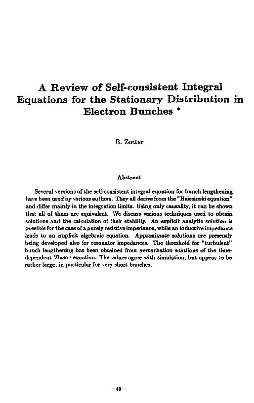
A Review of Self-consistent Integral Equations for the Stationary Distribution in

Electron Bunches *

B. Zotter

Abstract

Several versions of the self-consistent integral equation for bunch lengthening have been used by various authors. They all derive from the "Haissinski equation" and differ mainly in the integration limits. Using only causality, it can be shown that all of them are equivalent. We discuss various techniques used to obtain solutions and the calculation of their stability. An explicit analytic solution is possible for the case of a purely resistive impedance, while an inductive impedance leads to an implicit algebraic equation. Approximate solutions are presently being developed also for resonator impedances. The threshold for "turbulent" bunch lengthening has been obtained from perturbation solutions of the time-dependent Vlasov equation. The values agree with simulation, but appear to be rather large, in particular for very short bunches.

- 4 9 -

1 Introduction Lengthening of electron bunches in storage rings and circular accelerators was first ob­served experimentally [lj,[2|,[3|,[4],[5j. The first analytic studies [6],(7j,(8] identified the mechanism as a deformation of the "potential well", formed by the external RF voltage, due to the "induced voltage" in the wall impedances. The problem was treated in linear approximation and scaling laws were obtained [9] which were in good agreement with ob­servations at low current levels. However, the theory failed to predict the appearance of the "turbulent threshold" which was observed experimentally as the onset of stronger bunch lengthening, accompanied by an increase of the energy spread ("bunch widening"). First attempts to determine the stability of the solution in the deformed potential well were published already in the late 70's and early 80's [10|,[llj,(12j, and again more recently [13J,[14|.

In a more empirical - and not self-consistent - description of bunch lengthening [15], assuming that the bunches remain Gaussian, the stability threshold can be found by equat­ing the solutions in the "potential well region" and in the "turbulent region" based on the waterbag solution [16]. With some minor modifications [17], this approach has been used since many years in the computer program BBI [18] which showed very good agreement with measurements in machines with long bunches (DCI in Orsay, EPA at CERN), but seems to become less dependable for shorter ones.

The stationary potential well equation has been derived for distributed impedances all around the ring. For localized impedances, such as are usually assumed for computer simulation, one needs in general the time-dependent equation of motion. First attempts to treat this case analytically have been made using mapping techniques [19],[20]. In actual machines, both localized and distributed impedances may occur simultaneously, but no theory exists at present which covers both cases.

2 The Haissinski Equation

The first self-consistent theory was derived from the Fokker-Planck equation [21], and led to a nonlinear integral equation for the line-density A(r) which has become known as the "Haissinski equation".

A(r) = K exp [-[/.(r) - $ £ dt VUO] (1)

The constant K has to be determined from the normalization condition /f^ A(r)tfr = 1, U„(T) is the potential well due to the external RF voltage (for a linear RF it becomes

a parabolic wellr2/2), divided by <r| £ « / / V i s a parameter proportional to the bunch current divided by the gradient of

the RF voltage, and Vi„4 is the "induced voltage" (per unit charge), which can be expressed in terms of

the wake function (delta-function wake potential or "Green function" G(t) ) by

VUt)=l~dt'G(t')\(t-t') (2)

- 5 0 -

i.e. it contains the unknown line-density in the integrand. Still in the year of its publication, the Haissinski equation was applied [22],(23] to a

simplified resonator, consisting essentially of two parallel plates without beam holes, for which the wake function could be derived analytically. The integral equation was solved numerically by iteration. With increasing current, it showed a growing deformation of the bunch shape from the Gaussian valid for increasing current. The line-density became wider and more and more asymmetric, with a steeper slope in front and a longer tail behind (the bunch looks as if it was leaning forwards, see Fig.l). After some numerical problems were overcome, solutions could be obtained for arbitrarily high currents. A new derivation of the integral equations for potential-well deformation, using essentially thermodynamic conservation laws, has recently been published [24] and agrees - at least for electrons - with the Haissinski equation.

3 Step Function Response

Shortly after the first publication of the Haissinski equation, it was realized that the double integral

fdt Tdt'G(t')\(t-t') (3) Jo Jo

could be reduced to a single one by inverting the order of integration [25]. The "Green function" or "wake function" (delta function wake potential) is replaced by the "step function response" (wake potential of a unit step)

S{t)= fTdt'G(t') (4) Jo

and one obtains the integral equation

A(r) = A'exp [-U0(r) -f£°dt 5(r)A(r + r)J (5)

In this form, the integral contains the unknown function only at earlier times r+t, t > 0, i.e. one can evaluate it directly by starting integration well ahead of the bunch where A(r) = 0. However, the normalization integral has to be fulfilled by changing the parameter K. Since the line density depends non-linearly on K, several iteration steps are still needed to obtain the correct solution. This can be avoided be rewriting the equation for p(r) = £A(r) and solving for selected values of (A'. Then the normalization condition yields J^ dtp(t) = f, i.e. the corresponding current (divided by the voltage gradient). This technique has been applied to the parallel plate resonator [26], to a capacitive impedance [27], as well as to more realistic wake potentials of complete vacuum chambers [28].

4 Resistive Impedance

The integral equation in the almost identical form

A(T-) = A" exp \-U0(T) - i f_^ dt S(T - r)A(r)] (6)

- 5 1 -

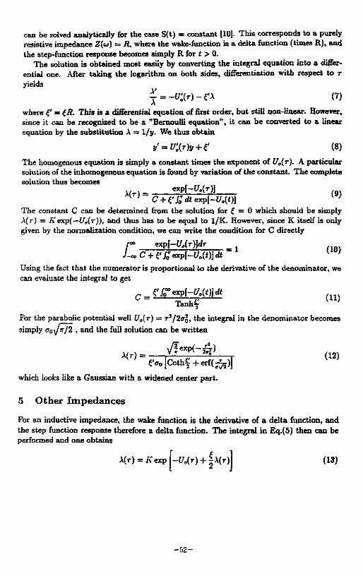
can be solved analytically for the case S(t) = constant (10). This corresponds to a purely resistive impedance Z(u) = R, where the wake-function is a delta function (times R), and the step-function response becomes simply R for t > 0.

The solution is obtained most easily by converting the integral equation into a differ­ential one. After taking the logarithm on both sides, differentiation with respect to r yields

J = -U'0(T)-?\ (7)

where £' = iR. This is a differential equation of first order, but still non-linear. However, since it can be recognized to be a "Bernoulli equation", it can be converted to a linear equation by the substitution A = 1/y. We thus obtain

y' = V'a{T)y + l' (8)

The homogenous equation is simply a constant times the exponent of U0(T). A particular solution of the inhomogenous equation is found by variation of the constant. The complete solution thus becomes

The constant C can be determined from the solution for £ = 0 which should be simply A(r) = A'exp(—U„(T)), and thus has to be equal to 1/K. However, since K itself is only given by the normalization condition, we can write the condition for C directly

cxp[-tt,(r)]dr r J—C

- ~ C + f/ 0

Texp[-tf o(0]<fc 1 ( 1 0 )

Using the fact that the numerator is proportional to the derivative of the denominator, we can evaluate the integral to get

C ~ Tlnh? ( 1 1 )

For the parabolic potential well U0(T) = r2/2<7Jj, the integral in the denominator becomes simply <j0\Jx/2 , and the full solution can be written

A ( r ) = y?«y-fr (12) ?<70[Coth?f+erf(;3-)]

which looks like a Gaussian with a widened center part.

5 O t h e r I m p e d a n c e s

For an inductive impedance, the wake function is the derivative of a delta function, and the step function response therefore a delta function. The integral in Eq.(5) then can be performed and one obtains

A(r)=A'exp -U,{r) + |A(r)j (13)

- 5 2 -

where the factor 1/2 comes form the fact thnt the delta function in the integrand occurs at the integration limit. Thus wc get an algebraic equation for A(r), which cannot be solved explicitly, however. Numerical solutions give asymmetrically distorted Gaussians (leaning forward), and solution becomes difficult for large values of the parameter (. However, by solving for the independent variable r it is easy to convince oneself that solutions exist for all values of the parameter.

The case of a purely capacitive impedance leads to an integro-difFerential equation [29). Its numerical solution shows that the bunches remain essentially Gaussian, but with a reduced length. An approximate solution has recently been published in ref.[30] without derivation. It is supposed to hold when the induced potential is very large.

For a resonator impedance, which encompasses all three special cases discussed above, the step-function response can be written as the imaginary part of a complex exponential: the kernel, which is in general a function of the difference of the time displacement and the integration variable r — t (see Eq.(6)), then becomes a product of functions of its two variables: „ _

271 5 ( r - ' ) = -firlm ( e x p ( J w i r ) e x p ( - J w » t ) ] (14)

where ux = (u>r/2Q)(W + j) and W = \/4Q* — 1. R is the shunt impedance, Q the quality factor, and ur the resonant frequency of the impedance.

An integral equation with such a "degenerate kernel" can be solved directly if it is of the "Fredholm type", i.e. if the limits of integration are fixed. However, since the above expression for the kernel is valid only for r < t, and vanishes otherwise due to causality, the Haissinski equation is really of the "Volterra type" with a variable upper limit. It can still be written as a "Fredholm" integral equation if one multiplies the kernel with a step-function. Expanding the step-function into a Fourier series then again yields an integral equation of the Fredholm type, but containing an infinite number of terms. Truncation to only a few terms yields surprisingly good numerical results in a much shorter time than direct solution of the integral equation. Furthermore it appears possible to sum the series for the shift of the synchronous angle explicitly. Solutions for short and medium bunch lengths (u>,<70 = 0.5andl.O) are shown in Fig.2 and 3 as function of the parameters oc / .

6 Stability

Empirically, the solution of the potential well equation is not valid above the "turbulent threshold". One can then assume that a time-dependent solution ("microwave instability") of the Fokker-Planck equation becomes energetically favored. Thus the Haissinski equation is then no longer valid.

One standard method to investigate stability is to add a small, exponentially time-dependent perturbation and to find the appearance of an imaginary part of the frequency. This method was first applied to the linearized Vlasov equation, in ref.[10j to a bunch deformed in a potential-well. It was claimed that the resulting dispersion relation (for electrons) differed from the usual one obtained for stability against coupled-bunch motion, but no numerical examples were given.

- 5 3 -

A similar method was used in ref.[12j, where stability determined from the sign of the real parts of the eigenvalues of the coefficient matrix of an expansion in orthogonal polynomials. However, in this paper the potential-well deformation of the Gaussian was not taken into account explicitly. An increase in the length of the Gaussian could be included by interpreting w, as the modified, current-dependent synchrotron frequency.

Recently, this technique has been applied directly to the numerical solutions of the self-consistent potential well (Haissinski) equation [14j. For short bunches, a large discrepancy has been found both with the thresholds obtained using an undeformed Gaussian, and with the so-called "localized Keil-SchnelT(31] or "Boussard" [32] criterion. This gives much lower values for the threshold, but is admittedly only a lower bound as it was derived by approximating the exact stability limit [33],[34],[35] with an inscribed circle. The discrepancy can be reduced considerably by

• a) using a Gaussian with modified a (as was usually done in the past) • b) replacing the low-frequency limit Z/n by the "effective impedance"

fZ\ _^ T.[Z{p»o)lp)hm(puo)

where hm(u>) is the spectral power density of the m-th mode of oscillation of a bunch which is given by (u»<r)2n* exp(—(W<T)2] for a Gaussian distribution. In the potential well region, one should take m=l (dipole mode) [17]. For a resonator impedance, the total effective impedance is then approximately equal to If! for long bunches, but only

(£ ) = ( u v O * | - | (16)

for short ones {wraT0 « 1). This fact will considerably increase the threshold current for short bunches, as has been measured recently in LEP [36].

• c) replacing the inscribed circle of the "Keil-Schnell criterion by the correct stability limit (depending on the'argument of the complex impedance) increases the stability limit for long bunches, where the impedance is more inductive and the inscribed circle is a bad approximation (see Fig.4).

7 Moment Expansions

Since the deformation of the Gaussian is not very large - depending on the type of impedance the bunches are shifted (first moment), lengthened or shortened (second mo­ment), become slightly asymmetric (third moment) or the center is widened more or less than the tails (fourth moment). An analysis of bunch lengthening in resonator impedances including up to the third moment ("skewness") was described in the ESRF Impedance workshop [37]: in particular for bunch lengths where the impedance is essentially resistive, the effect of the asymmetry was found to be rather important. In addition, the stability of the solution (using the Boussard criterion) was compared with the vanishing of the slope of the total potential inside the bunch. It has been a assumed that this might be a criterion

- 5 4 -

(15)

for stability [5| since the synchrotron frequency becomes imaginary for a negative slope of the potential. Agreement between the two criteria is only approximate, however.

As a by-product of this analysis, it appeared.that longitudinal mode- coupling of the dipole mode (m=l ) with its mirror-image (m=-l ) or with the quadrupole mode (m=2) should not occur for a linear RF voltage: the "coherent" frequency shift of the dipole mode is exactly cancelled by the "incoherent" shift for any particle distribution, and hence the coherent dipole tune does not change with current (a longitudinally moving bunch takes its potential well with it). The quadrupole tune changes, but by less than the synchrotron tune so that it stays always above the dipole tune. It has not been shown that the same is true for higher modes (m 1=2), but it is rather unlikely to have large impedances at frequencies above the beam-pipe cut-off. Hence the "mode-coupling" theory (38], does not appear to be a plausible candidate to explain turbulent bunch lengthening.

In Pig.5 we show the distribution of eigenvalues as function of the beam intensity ob­tained by Oide-Yokoya [14] for a resonator impedance. I have added the dashed lines which are the limits of the solutions for each (azimuthal) mode-number m = l to m=4. This shows clearly that the eigenvalues remain real (apart from two spurious values) even when the higher radial modes of neighboring m-values are overlapping. The appearance of the instability seems to be consistent with the vanishing of the lowest m = l (dipole) mode. A similar result has also been obtained recently [13) for a hollow beam with a space-charge impedance (see Fig.G).

The coupling of the m = l and m=-l modes has been proposed as mechanism of the turbulent threshold some time ago (11),(12| - but was contested because the thresholds obtained in this manner were much higher than those observed experimentally. In addition, the frequency of the dipole mode measured does not change much, and certainly does not vanish at the threshold. A possible explanation of these discrepancies is the fact that the "rigid" dipole mode is actually not included in the standard mode analysis, where the bunch edges are kept fixed. Therefore the frequency of the dipole mode may vary with current - but does not agree with the rigid dipole mode usually observed experimentally. Another difficulty is the fact that the Vlasov equation is probably not sufficient to describe behavior above the turbulent threshold, since additional "excitation" terms must be active in order to increase the energy spread. These terms have to be added to the quantum excitation in the Fokker- Planck equation, which should be used instead. One paper has been published using a "quasi-stationary", time-dependent solution (39] to explain the behaviour above the threshold. The results showed overshoot also for electrons, with periodic damping to values below the equilibrium value. This is not in agreement with the usual behavior observed in most machines, but slow oscillations of the bunch length have been seen occasionally. Nonlinear saturation and the resulting overshoot due to a single "sharp" impedance have been estimated using a non-perturbative treatment of the Vlasov equation [40]. A thermodynamic approach to the behaviour of the bunchlength above the "turbulent threshold" has been the subject of a thesis[41], of which an abridged version has been published[42]. The threshold was calculated by equating the free energies of the stationary and of the time dependent solutions. A numerical comparison of the theory both with simulation and experiments at SPEAR was made and showed good agreement for not too short bunches.

- 5 5 -

More recently, time dependent solutions have been obtained by studying the behavior of bunches in discrete (localized) impedances using (analytic) mapping techniques (19|,(20). Only the very simplified case of a constant wake (capacitive impedance) could be treated: the thresholds predicted are thus not comparable with experiment. Work on more realistic impedances is being continued.

Many computer simulations of bunch lengthening have been published, usually using several hundred or thousand super-particles [43], [27], [44), [45], [46], [47], [48], [49]. In general they show both (anomalous) bunch lengthening and bunch widening but the cur­rent threshold is not always clearly visible. Simulation of existing machines with realistic parameters is rather scarce - recently a comparison of bunch lengthening in the SLAC damping rings [29] gave reasonable agreement. More work in this direction is strongly encouraged.

8 Conclusions There exists a vast literature on bunch lengthening in circular accelerators and storage rings - of which only a part has been cited in 'his review. In spite of this, there is no satisfactory explanation for the existence of a "turbulent" threshold and the region above it, where anomalous bunch lengthening and bunch widening (increase of energy spread) occur simultaneously. Several semi-einpirical models yield results in good agreement with observation over a limited range of parameters, usually for longer bunch lengths where the impedance is mainly inductive. Computer simulation can yield satisfactory results also for shorter bunches, but has rarely been applied to existing machines. Unfortunately, it also does not give clear insight into the physical processes involved.

References

[1] R. Belbeoch et al., Proc. Natl. Conf. Moscow (1968) p.129 [2] P. Amman, Trans.IEEE-NS 16 (1969) p.1073 [3] I. Grigorievet aL.Proc. Intl. Conf. Yerevan (1969) p.121

[4] B. Richter et al., Proc. Part. Accel. Conf. San Francisco (1973) p.753 [5] P. Wilson et al, Trans.IEEE-NS 24 (1977) p. 1211 (6] C. Pellegrini, A. Sessler, Nuovo Cimento 53B (1968) p.198 [7] K. Robinson, CEA Intl. Report CEAL-183 (1969) [8] A. Lebedev, Proc. School Enrico Fermi XLVI (1969) p. 185 [9] C. Pellegrini, A. Sessler, Nuovo Cimento 3A (1971) p.U6

[10] A. Ruggiero, Trans.IEEE-NS 24 (I9J7) p.1205 [11] B. Zotter, Trans.IEEE-NS 28 (1981) p.2537 [12] T. Suzuki, Y. Chin, K. Satoh, Part.Accel. (1983) [13] R. Baartman, Part.Accel. 28 (1990) p.95-99

- 5 6 -

[14] K. Oide, K. Yokoya, KEK Preprint 90-10 (1990) (15] A. Hofmann, J. Maidineut, CERN-LEP Note 108 (1979) [16] A. Chao, J. Gareyte, SLAC SPEAR-Note 197 (1975) [17] B. Zotter, CERN Div. Report LEP/TH 81-14 (1981) [18] A. Hofmann, K. Hubner, B. Zotter, Trans.IEEE-NS 26 (1979) p.3514 [19] K. Hirata, Part.Accel. 22 (1987) p.57 [20] S. Petracca, F. Ruggiero, K. Hirata CERN/SL Div. Report in prep.(1990) [21] J. Haissinski, Nuovo Cimento 18 B (1973) p.72 [22] M. Chatard-Moulin, B. Jecko, A. Papiernik, Univ. Limoges Reports A-1/2 (1973) [23] A. Papiernik, M. Chatard, B. Jecko, Proc.Intl.Conf. San Francisco (1974) p.375 [24] S. Ivanov, CERN SL Report 90-19 (1990) [25] P. Germain, H. Hereward, CERN Div. Report MPS/DL-75/5 (1975) [26] E. Keil, SLAC Report PEP-126 (1975) [27] A. Renieri, Frascati Report (1976) [28] K. Bane, P.Wilson, Trans.IEEE-NS 24 (1977) 1485 [29| K. Bane, R. Ruth, SLAC Preprint (1989) [30] A. Burov, Part.Accel.28 (1990)p.47) [31] E. Keil, W. Schnell, CERN-ISR Report 69-48 (1969) [32] D. Boussard, CERN-SPS Report Lab.II/RF/75-2 (19'5) [33] K. Neil,A. Sessler, Rev.Sci.Instr. 36 (1965) p.429 [34] A. Ruggiero, V. Vaccaro, CERN Div. Report ISR/68-33 (1968) [35] B. Zotter, CERN Div.Report ISR/GS 76-11 (1976) [36] D. Brandt et al, CERN/LEP Comm. Report 21 (1989) [37] G. Besnier, Proc.ESRF Impedance Workshop, Grenoble (1988) [38] F. Sacherer, Trans.IEEE-NS 24 (1977) p. 1393 [39] Y. Chin, K. Yokoya, KEK-Picpriiit 82-31 (1983) [40J S. Bogasz.K. Y. Ng, Proceedings PAC 1987, p.1201 [41] R. Meller, Thesis Cornell University 1986 [42] R. Meller, Proc. PAC 1987, p. 1145 [43] R. Dory, MURA Report 654 (1962), PhD Thesis Madison [44] K. Bane, P. Wilson, Trans.IEEE NS-24 (1977) p. 1485 [45] T. Weiland, DESY Report 81-088 (1981) [46] D. Brandt, CERN-LEP Note 512 (1984) [47] R. Siemann, Nucl.Instr.Methods 203 (1982) p.57 [48] V. Nys, CERN LEP Report TH/86-34 (1986) [49] T. Wang, CERN SL Report 90-08 (1990)

- 5 7 -

T= 0,34 ns A 1(A)

V (o) =0,509 10"v/s J. 200 0 = 1,05 10V l/lo =1,262

2 0 Figure 1: Variation of bunch shape in a parallel plate resonator for a bunch length of ar = 0.34ns (M.Chatard-Moulin et al)

- 5 8 -

Bunch Shape for Resonator Impedarj - — i — ] 1 — J — i — i — ; — i — i — : — ; — i — i — i — i — j — i — i — i — i — ; — ; —

e = 0.50 - 10.00 !

Figure 2: Variation of bunch shape in a resonator impedance for a short buncii uror„ = 0. for increasing current (J.Hagel)

- 5 9 -

Bunch Shape for Resonator Impedance

Figure 3: Variation of bunch shape in a resonator impedance for a bunch of medium length vr<7TC = 1.0 for increasing current (J.Hogel)

- 6 0 -

-i 1—ri 1 1 1 — i — i 1 — i — i — i 1 r- <U

m

o

U n 55

JUX.

Pi

I • . . L -i i • <-

in d o

d Figure 4: Stabilty diagram for Gaussian distribution and inscribed circle approximation ("Keil-Schnell criterion")

- 6 1 -

— : — : — i i—TT~:—I—I— r

•Ml \ 11 ~i 1 — i — i 1 1 1 r

r±L\ mf=3 •

-L ! I

0

— -®^c' I.

1 1 i 1 1 • i \ • :

I I I I '• ! !

i i !

i i i i

" r ' i Li

! ! '. • i i

I ; : t

i :

S7"**.

r ' i r I l l l l - I r l i l ) i i i l

0 2.5 7.5 10

Figure 5: Distribution of Eigen-frequencies for Resonator Impedance (Q=l) as function of current (K.Oide-K.Yolcojra)

- 6 2 -

-IWsiioM Current

Figure 6: Frequency spectrum of longitudinal modes in a hollow bunch for space-charge impedance (R.Baartman)

- 6 3 -

Effects of the Potential-Well Distortion on the Longitudinal Single-Bunch Instability

KATSUNOBU OIDE

KEK, National Laboratory for High Energy Physics

Oho, Tsukuba, Ibaraki 303, Japan

ABSTRACT

Effects of the potential-well distortion on the longitudinal single-bunch insta­

bility in an electron storage ring are examined. A method which calculates the

intensity threshold including the potential well is proposed. As the result, the

spectra of the eigenvalues and the threshold of the instability become greatly dif­

ferent from those calculated without the potential-well distortion.

INTRODUCTION

The longitudinal single-bunch collective motion of an electron beam in a storage

ring is described by the Vlasov equation

for the distribution function «/> = 4>(p, q, 0) in the longitudinal phase space. The

independent variable p = (j£0 — E)/Eo&t is the relative energy deviation, q = zjat

the longitudinal position, and 6 = u>,t the phase of the synchrotron motion. We

have introduced Eo as the nominal beam energy, at the natural energy spread, at

the natural bunch length, and u, the nominal synchrotron angular frequency. We

chose the sign of p for convention.

- 6 4 -

The charge of the bunch induces the longitudinal field V(q) with the longitu­

dinal wake function W(q) as

+00

V(q,0) = l j /(?',0)W(q> - qW , (2)

where f(q, 0) is the longitudinal density of electrons

+00

/ M ) = J *(p,qJ)dP , (3) —00

and normalized as f f{q,8)dq = 1. The parameter I represents the beam intensity

as

I=2^\E~o) ' ( 4 )

where N is the number of the particles in the bunch and v, the nominal synchrotron

tune. We only consider an ultra-relativistic case, thus assume W(q) = 0 for q < 0.

STATIONARY SOLUTION

The stationary solution of (1) is written as

UP, q) = (2*) - , / 2 exp(- P72)/o(?) , (5)

where the stationary density /o satisfies the equation

( CO CO \

~\~I J J fo{q")W{q"-q')dq"dA . (6) The form (5) comes from the fact that the energy spread of the bunch is determined

- 6 5 -

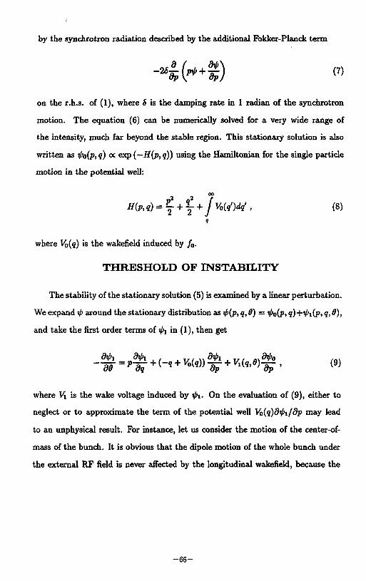
by the synchrotron radiation described by the additional Fokker-Planck term

on the r.h.s. of (1), where 6 is the damping rate in 1 radian of the synchrotron

motion. The equation (6) can be numerically solved for a very wide range of

the intensity, much far beyond the stable region. This stationary solution is also

written as 4>o(p, g) oc exp (—H(p, g)) using the Hamiltonian for the single particle

motion in the potential well:

CO

#(?,«) = y + y + / W W , (8) i

where V0(q) is the wakefield induced by f0.

THRESHOLD OF INSTABILITY

The stability of the stationary solution (5) is examined by a linear perturbation.

We expand if) around the stationary distribution as if>(p, q, ff) = >̂o(p, ?)+^i(p, 9,0),

and take the first order terms of ipi in (1), then get

-$-,$ + ( - , + *W)$ + Kb.O$, 0)

where Vi is the wake voltage induced by if>\. On the evaluation of (9), either to

neglect or to approximate the term of the potential well V0(q)dipi/dp may lead

to an unphysical result. For instance, let us consider the motion of the center-of-

mass of the bunch. It is obvious that the dipole motion of the whole bunch under

the external RF field is never affected by the longitudinal wakefield, because the

- 6 6 -

wakefield is an internal force. Therefore there always exists one trivial solution

for (1) which corresponds to the motion of the center-of-mass of the bunch. The

solution is

rj> = exp{-i9)il>0{p - ia, q + a) , (10)

where a is the amplitude of the motion of the center-of-mass with an arbitrary

magnitude. Thus the first order deviation of (10) from i/>0 for a small a

satisfies the perturbed equation (9). If one modifies the potential-well term in (9),

the center-of-mass motion (11) becomes no longer the solution of (S). Therefore one

may get an unphysical mode of the motion of the bunch instead of the trivial but

physical solution. Couplings of unphysical modes also give incorrect information

on the stability.

To solve this problem as exactly as possible, we introduce a method which is

a simple extension of the usual mode-coupling method. Firstly we define action-

angle variables (J,<j>), which rewrite the Hamiltonian (8) as H = H(J). These

variables rewrites Eq. (9) to

where w(J) = d<j>/d9 = dH/dJ is the angular frequency of the single-particle

motion in the potential well. The origin of <j> is placed on the g-axis. Equation (12)

suggests us that Tpi can be expanded in terms of the orthogonal modes as

^i = Y^(Cnmcosm^> + S™sinm(t>)A„{J)exp(-i>0) , (13) nm

where the function A n (7 ) takes the value 1/AJ„ in the strip around the n-th mesh

- 6 7 -

point J = J„ with the thickness AJ n , and zero outside. Since Eq. (12) contains

no derivative by J, we do not worry about the discontinuity of A„(J), as far as

only the first order calculation of the eigenvalue is concerned. After substituting

(13) to (12), we multiply An(J)AJ„cosm^> or A„(J)AJ nsinm^ on the both side,

and integrate them over J and ft then obtain

*tiCnm =mu„Snm

iftSnm = ~ mUnCnm - - Y, Cn'm- I<^»(J)AJ„^0(J) ( dJ'kn.{J') * n'm' % {

2* 2*

I d<j> J dftp(J, ftW {q(J\ ft) - q(J, 4)) sin m<t> cos m'ft

(14) 2* 2 *

X

0 0

On deriving (14), the relation dt/>0/dp = —p*l>o has been used. In the integral to

get Vi, we have changed the variables from (p1,^) to (J', ft) with dp'dq' = dJ'dft.

We have also assumed u(J) is smooth enough in the strip A„(J) and evaluated the

integral at the center with the value uin = w(J n). Note that Snm terms never make

the wakefield because of the anti-symmetry of sin m<f> in p-direction, and terms

with p cos m<j> also vanishes in the same way. Making use of the equation of motion

p = u(J)dq/ dft we rewrite the integrand of (14) as

P(J, 4>W W, ft) - «M 4)) = ~§^F (q(J\ ft) - q(J, ft)) , (15)

where F is a primitive function of W, i.e., F'(q) = W(q). U we substitute (15)

into (14) and integrate it by part by ft the second equation of (14) becomes

i(tSnm — — munCnm

111 2 *

munih>(Jn)AJn Y] Cn'm' I d$ I dftF{q(Jn; ft)-q(JB, ft)) cosm<j> cos m'ft

(16)

We have again assumed the smoothness of w, q, and F in the strip A„(J), and

- 6 8 -

evaluated their integral of J and J' by the values at Jn and •/„«. Note that the

smoothness of the wake function W is not necessary to derive (16). Combining

(16) and the first equation of (14), we get a linear equation for Cnm:

- f C n m = - ^ Akmn'm'Cn'm' , (17) n'm'

with

Mnmn>mi = m unSnniSmmi

rm 2a;^o(J n)AJ n f f , , . . , , . , , „ « » ( 1 8 ) + I —1— / / cosm<f>cosm<j> F(q{Jn'><?) ~9Wn,9))d<f>d<p

o o

where Snni is the Kronecker's delta. The system becomes unstable when the matrix

M has a negative or a complex eigenvalue. For several kinds of the wake function

W(q), there are regions of the intensity where the Hamiltonian H(p,q) has two

or more stable fixed points in the phase space. In such cases, the one-to-one

correspondence between H and J is broken, and each strip in J-space which has

the same value of H should be treated separately in the above equations, i.e., the

angle variable <f> should be varied from 0 to 2ir in each strip.

RESULTS FOR A RESONATOR

The eigenvalue of (18) is obtained numerically. As an example of this method,

we show a result for a Wakefield of a resonator which has a resonant frequency u0,

a shunt impedance R, and a Q-value Q:

W(q) = ^ exp(-W0</2<?) (cos W l * - ( 4 ^ i ^ ) , (* > 0) (19)

where ut = (1 — l/4<32) I / r2w0 and t = qat/c. This wakefield has the longitudinal

- 6 9 -

5

4

. i ' . ; i ; ! • ; j ; !

: ! • • , i : I : !

: : : i : ! ; ! -

j - 'Un i i l i J ! ; : : ! : ; : ; ! ; ! ! ! ! ! ! !^ : : = : : ' I ! • : = : • ! ! 1 : ! i " • : ! ' :" ! -

3

: • • : : • : ! i ! . ' i : ' ' : : : : ' : : ; i ! J -

- • ' ' ' ' L l i i i i N i i i i i i l i j I l i j i i i K S : • i • : i 1 1 i ! ! : 'ST at

2 • ' i i i i i i i i i i ! I N I j i i MI i i i u • I i s i 1 i ! i i I ! ! ! i : ! i i j

i ! ! i '• | !

: ! ! i i "

1M i -1 ̂ . . M l l l l l l l j l i l ! ! 1

i j l | lU

: Ml! ! | I j i n ; n ' • i • i . 1 i i i i 1 1 1 1 1 1—

10 IS

Fig. 1. Spectra with the potential-well distortion.

impedance

R 1 + iQ(u0/u - w/w 0) '

(20)

Figure 1 plots the spectra of the eigenvalues ft (the square roots of the eigen­

values of M) as a function of the intensity / obtained by this method. Each dot

represents the real part of ft, in unit of the natural synchrotron frequency w,. The

unstable eigenvalues are depicted by crosses and the size of a cross represents the

magnitude of the imaginary part of ft. Here a resonator with the parameters of

Q = 1, uioR = 1> and woc^/c = 0.4 is used. The number of meshes in ./-direction

is 30, and the azimuthal modes m < 4 are taken into account. At zero intensity,

- 7 0 -

5 j — l 1 1 1 1 1 1 1 1 1 1 1 ' 1 1 1—

4 • , # , , l ! I ! ! ! ! ! ! ! ! I t I ! I ! ! ! ! ! ! ! ! '—

3 — • • • ' ! • ! • ! ; ! ' ' • I ! ! ! ! ! ! ! ! ! ! ! ! ! ' •— "2. \ ^̂ V U

r»r I i i i i i i i i i vJxxiXyOCXi/' i i 0 5 10 15

I

Fig. 2. Spectra without the potential-well distortion.

all eigenvalues are degenerated into integers. As the intensity increases the degen­

eration is solved and there appears a wide tune spread due to the potential-well

distortion. In this case the instability appears around / >t 13.5 with 3tft ~ 0.72.

Its growth rate is about Oft ~ 0.04 at / = 15.

For a comparison we show in Fig. 2 the result without the potential-well

distortion. Here we neglect the V0 term in (9), and make the stationary distribution

V>o always Gaussian both in p- and q- directions. All other parameters are same

as before. This result remarkably changes from that of Fig. 1. The amount of

the tune spread is drastically decreased and only a few modes have significant

tune shifts as the intensity increases. There appears an instability at / ~ 10 with

- 7 1 -

%t/i = 0. This instability with zero frequency comes from the tune shift of the dipole

motion, but includes an unphysical effect caused by the neglect of the potential

well. Another instability is seen at / ~ 12 with 2tfi ~ 1, as a coupling between

m = 1 and m = 2 modes. The growth rate, S/i ~ 0.5 at / = 15, calculated without

the potential well is much bigger than the real one, and also rapidly grows as the

intensity increases beyond the threshold. If the growth rate behaves like the result

without the potential well, the threshold intensity does not strongly depend on the

damping rate of a ring. The result with the potential-well distortion, however, tells

that the growth rate of the instability slowly increases, and the actual threshold

may strongly depend on the damping rate. This, example shows that it is essential

to include the effects of the potential-well distortion on the longitudinal instability.

More examples and comparisons with simulation are shown in Ref. 1.

REFERENCES

1. K. Oide and K. Yokoya, KEK-Preprint-90-10, 1990.

- 7 2 -

A New Type of Bunch Lengthening

K. Hirata 1, KEK, National Laboratory for High Energy Physics, Tsukuba, Ibaraki 305, Japan S. Petracca 2 and F. Ruggiero CERN CH-1211 Geneva 23 Switzerland

Abstract

Using a constant wake localized at one point in a ring as an example, it is shown how the feature of the bunch lengthening for the highly localized wake is different from that predicted by the conventional theory where the wake force is averaged over one turn. For this example, the space of parameters (strength of the wake force, synchrotron tune and the damping time) is classified into three regions: 1) only a period-one fixed point exists, 2) only a period-two fixed point exists and 3) both types of fixed points can exist (bi-stable regime). This feature is predicted by a Gaussian model and confirmed by multi-particle tracking.

1 Introduction The particle distribution in a bunch is affected by the wake force: a bunch interacts with itself through the interaction between particles and the environment[l]Many kinds of wake sourses are distributed in the ring but each wake force source should be regarded as a localized object. Usually, however, the wake force is treated by a smoothing: one averages the wake force over one turn and assumes that this averaged wake is distributed uniformly. The validity of this simplification is not clear: in the case of the external nonlinear field, the time averaging of the force makes the dynamics completely different.

In the uniformely distributed case, we have a scenario of the instability and a standard technique exists for electron rings: the stability analysis around the solution of the potential well distortion (PWD) equation[2,3,4]. This enables us to predict the threshold for turbulent bunch lengthening, if we use accurate PWD solution[5]. As for the localized case, however, this method tells us very little. The aim of this paper 3 is to investigate the localized case by considering a simplified model.

Recently, one of the authors proposed a model to study the localized effect analytically[7]. Here, we extend it. We will show that the model predicts a new type of bunch lengthening. The bunch length, or more exactly, the longitudinal envelope matrix in the steady state, has a structure of the cusp catastrophe[8]: depending on the parameters (strength of the wake force, synchrotron tune and damping time), the steady state envelope is either in period-one or in period-two motions: in some particular cases, the bunch can choose one of them according to the intitial condition.

'A part of the work was done when K.H. stayed in CERN. 2 0 n leave of absence from Dipartimento di Matematica e Applicazioni, Universita' di Napoli, Via

Mezzocannone 8, 80123 Napoli, Italy. 3 A partial acount of the work was published elsewhere [6].

- 7 3 -

2 The Model It is convenient to start by summarizing some main features of the preceding paper[7].

We consider the case where there is only one localized wake source in the ring. It is straightforward to extend this case to more general cases, even to uniformly distributed cases. The opposite is not true.

Introducing the normalized synchrotron variables

_ longitudinal displacement _ energy deviation . nominal bunch length ' <TE

the motion of a particle in one turn is written as

\£)~*U\A*7 + *>/F^R-#*i))' ( 2 )

Here ag l s the nominal energy spread, U is the rotation matrix for the synchrotron oscillation

(3) U=( C 0 S " S i n " V „ = 2™, ^ —sia/i cos/z J

OR JO

v being the synchrotron tune, A = exp(—2/T), T is the synchrotron damping time measured in units of the revolution period and f a Gaussian random variable with < r > = 0 and < r 2 > = 1. The wake force 4>(xi) is given by

eQ

where e denotes the electron charge, Q the total charge in the bunch and p(x) is the charge density normalized to unity. Here W(u) is the longitudinal wake function (measured in Volt/Coulomb).

The above stochastic mapping is equivalent to an infinite hierarchy of deterministic mappings for the statistical quantities

x{ = < x{ > , ff.y = < (xt - Xi){xj - Xj) >, (5)

and so on, which are the moments of the phase-space distribution •tl>(x1,x2). The original mapping can be conveniently split into three parts, representing the

effect of radiation, wake force and synchrotron oscillation, respectively.

Radiation:

x'~ = Mi «ii = «ii (6) a\i — Atria o'n = A V 2 2 + (1 - A 2)

- 7 4 -

Wake force:

Xi

x2- < 4>(xt) > (7)

a'u = <r\i- < (xi - 5 1 )^(x 1 ) > <722 = ff22 - 2 < (*2 - * 2 ) # * l ) > + < ^(Xl ) 2 > - < fl>(X!) > 2

'11

Synchrotron oscillation:

x'i = ^UijXj

a'a = £ UafnJJ* (8)

Up to this point, everything is fairly general. In principle, this system should include an infinite number of equations for all higher order moments. We now introduce the Gaussian model proposed in [7]: the distribution function in phase space is always approximated as a Gaussian, i.e.

1 1 2 _ V>(*i,x2) = 9 T v / d e ( , o

e x P [ _ 2 % °iil(Xi ~ *Mxi ~ * ' ) ! ' ( 9 )

even in presence of the wake force. This simplification corresponds to a truncation of the series in Eq. (7). In what follows we consider only first and second-order moments according to Eqs. (6), (7) and (8). This set of mappings is called moment mapping.

For the sake of simplicity, as in [7], we limit ourselves to the case of a constant wake function

Then, introducing the dimensionless parameter Fo

Fo = ^ ( 1 1 )

representing the strength of the wake force, Eq. (7) becomes

x\ = Si,

*• - f F° x3 = x2 -

*'n 2 '

<Tll, ( 1 2 )

i Fay/o\i

°22 ~ ' M " ^ f + 1 2 '

- 7 5 -

Since, for a constant wake, the i ; is completely decoupled from <r,y in the moment mapping, Eqs. (6), (12) and (8) and since the mapping for the £,- is trivial, we will discuss the second-order moments <T;J only in the subsequent investigation. Their evolution depends on three parameters: F0, u and T.

3 Features of the Model 3.1 Period-One Fixed Point The period-one fixed point of the moment mapping, Eqs. (6), (8) and (12), is[7]

« ) 1 / 2 = -*Fo + [1 + (« 2 + W * , (13)

^ ~ 2 V 5 F ( 1 + A)' ( 1 4 )

where

ff% = 1 + Fo 12*(1-A*)* ' < 1 5 >

x ( l - A ) + A ( 2 > - 6 ) 12i(l + A)(l - A 2) " l '

Here, the fixed point a^ is evaluated on Poincare surface surface built just before the wake source.

In order to investigate the stability of this fixed point, it is convenient to denote by a the vector of the second-order moments

^ i i \ (18)

Then the moment mapping can be written as a vector valued function of a, i.e.

7 = 3(3). (19)

Expanding a around ?<„, we obtain the linearized mapping

65' = A4 (<r~; F0, v, T)6a. (20)

Here the 3 x 3 stability matrix M(a,Fo,v,T) is defined by dS/da. The period-one fixed point is stable if and only if all the (complex) eigenvalues of

the matrix M(a00, FQ, V, T) have norm smaller than one. Since the eigenvalue equation is of third order, the eigenvalues can be written down explicitly. The region where the period-one fixed point is unstable is called the second region and is shown in Fig.l for some parameters.

- 7 f i -

100

Fo

0 100 200

Figure 1: The second region where the period-one fixed point is unstable.

3.2 Period-Two State What happens in the second region where the period-one fixed point is unstable? A numerical tracking of the moment mapping shows that period-two solutions develop, which are the fixed points of

S=§[3(S))t S±S(5). (21)

Period-two solutions obviously occur in alternating pairs, S^,5f, related by

*5=sra- (22) When the current, or Fo, is small enough, the a™ repeats itself every turn in the

steady state. 'Vhen F0 is increased and the parameters belong to the second region, it begins to change every two turns.

In the second region, the period-two solution is stable, as long as studied by the numerical tracking. Moreover, it is also stable in some region outside it. That is, in some region, both the period-one and the period-two motions are stable. Thus the parameter space is divided into three parts:

The first region Only the period-one solution is stable, The second region Only the period-two solution is stable, The third region Both period-one and period-two solutions arc stable.

The situation (obtained by the numerical tracking) is illustrated in Fig.2. In the figure,

- 7 7 -

Continuous

Discontinuous

* f T

Figure 2: The parameter space and three regions.

three regions are shown with the number. In the third region, the state is not a single valued function of the parameters. The actual state depends on the initial conditions.

Let us go up along the line (f-g-h-i, in the figure). At f, the system is period-one. At g, the period-one state becomes unstable and the period-two state developes. The period-two state remains stable for larger Fa (g-h-i). If the change is adiabatic, the state is still period-two. At h, however, the period-one state becomes stable again. If the change of parameters is too rapid, the system can change into period-one there. At i, the both kinds of states are possible. When we go down from the period-one state at i, the state jumps to period-two at h.

The change of <TU as a function of Fo (i.e. along the line f-g-h-i in Fig. 2) is shown in Fig. 3. The period-one solution always exists but it is unstable for certain range of parameters, shown by a dashed line in the figure. The points g and h in Fig. 2 corresponds to Fa ~ 2 and Fo ~ 6 in Fig.3, respectively.

When the parameters are changed slowly along a line (a-o-c-d-e, in Fig. 2), the system shows hysteresis. Let us start at a, where the state is period-one. If we move from a to e, the af- remains to be period-one until d, where it jumps to period-two. If we start from e, the state is period-two until b. The transitions are discontinuous and show hysteresis.

The state structure is that of the cusp catastrophe[8].

4 Multiparticle tracking The dynamical structure of the equilibrium synchrotron envelope found in the previous section is, to the best of our knowledge, quite new. The discussion was based on the Gaussian approximation. It is thus quite interesting to see whether this new feature comes merely from a big simplification of the model or it also occurs in a more accurate treatment.

To this end, a multiparticle tracking code is made, which tracks many particles according to the map Eq. (2). The calculation of the wake force <j> is done by a sorting

- 7 8 -

J F 0

0 8 10 12

Figure 3: The bunch length <Tn as a function of FQ. Parameters are v = 0.2 and T = 25. The dashed line is the unstable period-one solution. The results of the multiparticle tracking are also superposed (See section 4).

routine. Thanks to the nature of the constant wake function, all one should do is count the number of particles preceding each particle.

The results of the multiparticle tracking are shown in Fig. 3. The comparison with the results of the Gaussian model shows a quite satisfactory qualitative/quantitative agreement, including the bistability of period-one and period-two states.

The synchrotron phase space distributions corresponding to the period-one and period-two fixed points are shown in Fig. 4 a) and b+c), respectively, for the same set of parameters.

In the tracking, it is a little difficult to confirm that the system has reached the equilibrium. In particular, for the period-one state such as shown in Fig. 4-(a), the number of super particles in the four islands seem to tend to be eqaualized. However, one needs infinitely many turns to confirm this. It is also difficult to decide the exact threshold for the discontinuous change. Near threshold, the period-one state becomes easily unstable as a consequence of a tiny fluctuation, which depends on the number of superparticles. Within these limitations, it can be said that the qualitative and quantitative features of the model were confirmed by multiparticle tracking.

5 Discussion

5.1 Reality of the Model Obviously, the present model is too simple and cannot be used to predict the per­formance of a particular ring. We have used the constant wake only because of its

- 7 9 -

a 10

o -

-10

Tl I I I I I I I I I I I I I I I I I I I I IT I I I I I I I I I I I I

•M,

11 i i i i i i 1 1 i i i i l i i 1 1 l i i i i

b 10

0

-10

T I I I I I I I I I I I I I I I I I I I I I I I

•j& A

J* M * •

* • "

-10 0 \.r LI • I I | I l I 11 I I I I | I I 11 | I I I I

10

10

0

P- mk

• 1111 n 111111111111 l i 1111 — i o

11111111111

•aa*: m • • • I ' ' ' ' ' • ' I ' " I • ' '

-10 0 10 -10 0 10

Figure 4: The phase space distribution for (a) the period-one and (b+c) the period-two cases at a Poincare surface section built before the wake source. In the period-two case, the steady-state phase space alternates (b) and (c) every turn. Parameters are v = 0.2, T = 25 and F0 = 9.

- 8 0 -

simplicity. The Gaussian model itself seems to have worked well. Despite the extreme simplifi­

cation, the model showed quite a good agreement with multiparticle tracking results. It is, however, doubtful that this model applies similarly well to more general wake func­tions. If the wake function oscillates several times within the bunch, there is no hope to use the Gaussian approximation. In order to improve our model, we plan to consider a more general wake function (e.g., a superposition of Gauss-Hermite functions[9]) and a Stratonovich expansion of the phase-space distribution as in [10]. The latter allows the introduction of higher-order moments of the particle distribution, although the manipulation of analytic expressions may become very cumbersome (for example, the dimension of the stability matrix may become quite large).

5.2 Localized and Uniformly Distributed Wakes We have studied a localized wake. As discussed in [7], one can also study the case of uniformly distributed wake by introducing a periodicity N, and letting it go to infinity. From the eigenvalue analysis, we can show that the period-one fixed point is always stable in this limit. The limit

lim <ru (23)

corresponds to the solution of the PWD equation[2,3,4]. In the case of a constant wake function, it is known that the solution of the PWD equation is always stable[7,5]. It has been shown that the localized case is completely different: the dependence of the steady-state on the parameters is much more complicated. It is more dynamical and allows period-doubling bifurcation and bistable staes. For more general wake forces, we may expect more complicated dynamical features: sucessive period doubling bifurcation and chaos, for example.

The localization effects become more important when v, is larger, T is smaller and the wake force is stronger: these are the direction of the future high luminosity storage rings.

Two of the authors, K.H. and S.P., would like to thank all the members of the LEP Theory group for their hospitality and help. In particular, B. Zotter and E. Keil are acknowledged for useful comments and discussions.

References [1] A.W. Chao, SLAC-PUB 2946 (1982) and references quoted in [7J. [2] E.G. Hereward, PEP Note 53 (1973). [3] J. Haissinski, Nuovo Cimento 18B, 72 (1973). [4] A. Renieri, LNF-75/11R (1975). [5] K. Oide and K. Yokoya, KEK Preprint 90-10 A (1990). [6] K. Hirata, S. Petracca and F. Ruggiero, Bifurcation of the Equilibrium Distribution

in Synchrotron Phase Space for Electron Storage Rings with Localized Constant Wake Force, CERN SL/90-96(AP).

[7] K. Hirata, Particle Accelerators 22, 57 (1987).

- 8 1 -

[8] For example, E. C. Zeeman, Catastrophe Theory, Addison-Wesley, Reading,Mass (1977).

[9] T. Wang and B. Zotter, An Expansion Method for Calculating Wake Potentials, CERN/LEP-TH/89-75(1989).

[10] K. Hirata, Beyond Gaussian Approximation for Beam-Beam Interaction, CERN Report,CERN/LEP-TH/88-56 (1988).

- 8 2 -

LONGITUDINAL TRANSIENT PROBLEMS

Jiunn-Ming Wang Brookhaven National Laboratory, Upton, NY 11973, USA

1. INTRODUCTION We propose in this paper a simplified method of treating the longitudinal transient

problems in a linac or in a storage ring. The simplification comes about because we solve the Vlasov equation accurately only up to the first order in die frequency slip factor TI=1/72—1/7,2, (die transition energy y, = °° for a linac.) To this order of approxi­mation. Landau damping is ignored.

2. EQUATION OF MOTION We characterize the longitudinal position of a beam particle by the variable s. In

a linac, s is the distance from the entrance of the linac to where the particle is, and in a storage ring, it is the longitudinal Serret-Frenet coordinate. This variable will be treated as the independent variable of the equation of motion.

The reference particle can be defined by the following energy equation,

ib(*) = # + r j (i) where y is die energy in units of mc1, the subscript 0 refers to the reference particle, and the superscript (0) refers to the initial value, (die value at s =0.) The acceleration rate T is taken to be a constant throughout this paper.

The time it takes for the reference particle to travel from s=0 to s=s is

h i s ) = J R^T = ( PoTo-P^Yf ). (2) o Po(* )c

with po = Vl-l/Yo-Suppose mat a general beam particle reaches the position s at time t, men we can

define a pair of canonical variables (x,y) for this particle by % = -t+h(s), (3)

and

Y = Y~Yo. W In terms of these variables, the equations of motion can be written as

Work supported by the Department of Energy, contract DE-AC02-76CH 00016

- 8 3 -

4 i = ̂ )Y. (5) as

% = eEM-r, (6)

where

PoYoc with

TKj) = l/y^-l/7i 2 .

For a linac, the transition energy % = «°. The quantity EM in (6) is the total longitu­dinal electric field ( nonnalized to mc2 ) present in the accelerator. It can be written as

Elot =Eg +Eind +Eext • (7)

where Eg is the electric field produced by the rf generator, E^ is the beam induced field, and £„ , is the external field which can be noise or/and intended excitation field such as that due to a stripline kicker. Let us introduce a short hand notation

eF = eEtot-T, = e(.Eg+EM+Eext)-r. (8)

The effects of the radiation energy loss can be absorbed into I\

3. VLASOV EQUATION The Vlasov equation corresponding to the above equations of motion is

^ + X(s)y^ + eF(x,s)^ = Q, (9)

where , F = *F(T,Y,J) is the density function in the (x,7) phase space, and we have used the short hand notation (8).

It is often very convenient to convert the Vlasov equation into an integral form. Let ,P<W(T,7) be the initial value of *P, and let

/ (s, s'') = !&)-$(* ' ) , with

s Us) = jets'Us'),

0

then it can be verified by direct substitutions that the Vlasov equation is equivalent to the following equation:

- 8 4 -

¥(T,Y, s) = ^ ( T . Y ) + ,Pa>(T,Y,5) (10a)

= ¥<°>[T-/(S,0)Y,Y] - e ) <tf F[x -fisyfi.s]

JL+ / (* , / ) A y[ t - /(*, .$') Y, 7. ^ ] dOb)

Note that the arguments of the ¥ < 0 ) , s in (10a) and in (106) are not quite the same; however, the two equations are consistent In (10a), the filamentation contribution is included in l P ( 1 \ while in (106), part of it is included in the first term on die right hand side.

The beam current / is related to ¥ by I(Tj) = ldy*¥(x,y,s). (11a)

We write, corresponding to (10a), / (t, s) = / ( 0 >(t) + Ia\x, s) (lib)

with /<°>(x) = jdy ¥ ( 0 ) (x , Y). (lie)

and /(1>( T, s) = J dy ¥<»( x, y, s). (1 Id)

Note that ^ and /fa,s') are of order 0(i\). In the next section we shall extract from (10) a set of simpler equations which is valid to this order of T|.

4. SIMPLIFIED EQUATIONS For the purpose of investigating the change of the energy spread in a linac or a

storage ring, it is useful to define the following energy moments:

/n(l(x,s) = J d Y Y t l ^ ( W ) - (12) From (11a) and (12),

m0(T,s) = I(x,s).

It is straight forward to derive from (10) the following recursion relations which is valid to O (r|):

J3_ ds

1 Us) ds m. l (T,*»*(M>J^mJ=eu|- YFm\L-i (13)

For |i = 0, the right hand side of this equation should be taken as zero, and the equa­tion can be written as

d_ ds Ms) ds

/(V)+C-^-[F/]=0. (13b)

- 8 5 -

It suffices to investigate just (13b) if we are interested only in the T distribution and not in the y distribution of the beam.

5. BEAM INDUCED FIELD It was mentioned at the end of Section 2 that Ewt includes the longitudinal elec­

tric field Eind induced by the beam current For a storage ring, we write

*«<«)=• ^XJdtWi-^+if+pTdKir.s-pL), (14) tnc L p

where L =2nR is the circumference of the ring and T0=2rc/<Bo is the revolution period. The summation over p above accounts for the multi-turn effects. For a linac with constant impedance, we write correspondingly

* * ( « ) = ^ - Jd fW(-x+f ) / ( f ) , (15) mcLL

with L the linac length. The impedance function Z(co) is related to the wake field W(t) above by

W(t)=Y-jde>Z(a>)e-iat. (16)

The results of this section will be used in the discussions of some specific exam­ples in the following two sections.

6. COASTING BEAM IN A STORAGE RING The equation (13) can be solved easily as an initial value problem for the case of

a coasting beam in a storage ring. We consider only the case of no acceleration in this section.

The beam induced field Eind acting back on the beam may cause coherent oscilla­tions of the beam. The initial perturbation of die beam as well as E^ defined in (7) provides the driving force of the coherent oscillation.

Let us just write down the solution of the equation (136):

/< 1W)=Z/dfe#^-e *•+«<»«.-*&** ( 1 7 ) « J v*> where the denominator

An(k)=k2+iJJm(n&0-kp0c)Z(n(a0-k^0c), (18) describes the effects of the beam induced fields, and the numerator H„(k) describes the effects of the driving force.

If we set &„ =0 , then we obtain the well known result for the coherent frequency of the coasting beam instabilities in the absence of Landau damping.

- 8 6 -

7. RONBINSON PROBLEM In this section we rederive from (13b) the well known results describing the

longitudinal instabily of a small bunch inside a storage ring — Robinson mode. At the end of the section we shall assume the bunch to be Robinson stable and derive an equation governing the growth of the bunch length due to the beam induced field. The beam acceleration is again, for simplicity, ignored.

We first discuss the function F defined in (8). The external field £„ , will be ignored in this section. Before treating EM, let us introduce the dipole density D and the dipole moment D of the beam; they are defined by

D(x,s) = Xl(x,s) = Di0\x) + Z) ( 1 )(x,s), D(s) = jdxD (x,s) = D<°> + D<"(J) .

The superscripts (0) and (1) here have the same meaning as those for the current / . Note that we can always define the variable x such that D ( 0 ) vanishes, and hence D = D ( I ) . Also the following equations are obvious: jdxIi0)=Q, jdxlm=0, where Q is the total charge of the bunch.

Laplace transform is a convenient tool for solving a linear initial value problem. For any function G of s, we define its Laplace transform by

G (ik) = jds G(s)exp(-ilcs) o

Also, for any function G of x, its Fourier transform is defined by

G (oo) = —- f dxG(x)exp(-ian)

Now decompose

Eilut=EM + EV\ where £(0)Cc) and £ ( 1 ) ( X , J ) are, respectively, induced by / ( 0 ) ( T ) and Im(x,s). From (14) and (16), we have for a small bunch

£<%) = -(l/mc2L)03o 2 ZfoffloK^foffloKl+noJoT), (19)

and

E«\x,s)= (l/mc2L)2^r-Zj*(«<Oo-*Poc)Z("«)(r'fcPoc)D(iifc)c'' f a, (20) o n

where the field induced by the beam on the same turn around the ring is ignored. In what follows, we shall use

where Im is the average current of the bunch. For the field Eg produced by the rf generator, we set

- 8 7 -

Eg = (1 lmc2L) V5

ssm(-A<o0x+<t>g) (21)

= (1 lmc2L)Vg(sm$g -hOQXcos$g). (22)

Let us now define eF*® = eEg+eE®)-T, so that F =F<°>+£ ( 1>. We first observe that the sum of the first terms ~ terms of O (x°) - on the right hand sides of (19) and (22) must equals Tie; this amounts to saying that the energy for acceleration, for the ohmic loss, and for the radiation loss must be provided by the rf generator. Consequently,

«F<0> = -T0)2 l— (23) * (IV> 2*

where co, is the synchrotron frequency including the potential well distortion, it is related to the bare synchrotron frequency a>OT,

(at. — AAcV„cos«t>., (24)

by

e>2 = 0)2, + / ( l lmc2LWac)2ee&Jflti>QZ{n<a0)l'S!'Xn (Bo). (25)

The equation (136) can be linealized as

1 J L / ( X j S ) + ̂ (FW/TO+sW/TO) = _ e ± (fdfl/fl))). A, 3s2 ax ox

Or equivalently, from (23) and the definition of D,

(26)

( f o c ^ D W - mfx^D^+(^fXx^(eEWl^) = «**£/><» (27)

Integrating this equation by parts over x , we obtain an eigenvalue eqm. ion,

ds where

( PQC ) 2 4 j D(s) + a2, D + B(j) = 0, (28a)

2%Jj-B(j/fc) = A(ife)D(jfc),

with

A(*) = i( l / /nc 2 L)(Poc) 2 e ©oA.^-

x £ J« ©oZ (n coo) - (n Wo-* Poc) Z (n o\,-A p V ) I

The eigenvalue equation now reduces to

(PoC*) 2-(0^-/l(A) = 0. (28b)

This determines the coherent frequency pV&> and it is Robinson's result Let us now assume the bunch to be Robinson stable and investigate how the

bunch distribution changes under potential well distortion. Under this assumption, B = 0, D = 0, and £ ( 1 ) = 0; Consequently the equation

(27) becomes

(ftc J ^ D ^ t , * ) - <*h-^D<H(x,s) = a>,2tJ^-D<°>(T). (29)

This is a driven diffusion equation.

- 8 9 -

THE DEVICE FOR BUNCH SELFFOCUSING

A.VJurov and A.YJfovolch*tskl

I n s t i t u t e of Nuclear Physics 630O9O, Novosibirsk, USSR

ABSTRACT

The new davica f o r damping t h e longitudinal s ingle bunch instabi l i ty in s t o r a g e r ings i s proposed. This simple davica i s tha dialactric canal inaart o f def in i te l ength in vacuum chambar. Tha s t r u c t u r e o f wake f ie lds , inducad by intens ive bunch in such a canal i s t h a t , t h a t backward act ion on bunch part ic las not only prasarvas but a l so decreases bunch length, i.e. leads t o bunch selffocusing. Tha conditions under which t h i s phenomenon reveals i t s e l f and can be applied t o s t o r a g e r ings are considered.

I. INTRODUCTION

The growth of a bunch longitudinal phase volume with t h e increasing of t h e number o f part ic las - t h a t i s s o called bunch lengthening - was observed a t d i f f erent high energy s t o r a g e rings.The reason f o r i t i s t h e bunch part i c l e s in teract ion with inhomogeneous vacuum chamber. The descript ion of bunch lengthening e f f e c t based on wide-band impedance model was considered by many authors. Nevertheless t h e proposal how t o avoid t h i s e f f e c t was only given in t h e report 113 and f o r t h e f i r s t time. There, in particular, t h e s t eady s t a t e d i s tr ibut ion was shown t o be se l f focused and s t a b l e , i f t h e wake potent ia l i s a. s t ep- l ike function. In t h i s c a s e t h e bunch i s compressed without energy widening when one increase s t h e number of part ic les in i t .

According t o CI] s tep- l ike funct ion l/Cs> i s t h e function, which Fourier transform-impedance ZCA)

- 9 0 -

z * » ZOO m J I/C»> * *** ds

s a t i s f i e s t h e following requirements:

K4-j-«-„mi« H4-)i where

J ' > »

2 _ (JO

Cl>

o

i s the Fourier transform of t h e exact s t ep - func t ion f o r at > 0 1/ te> 1/ ecs>,

O { . a<2> O f OP a < 0

and f i s t h e e f f e c t i v e s tep- l ike function length above which t h e di f ference between V<*>s> and V . <s> i s

o r.m.s

not. re lat ive ly i s t h e coherent bunch displacamant dua -bo energy i<

I / . <s> o a s ; <? i s

bunch length; o i s r.ms. bunch length a t zero currant. In t h i s def init ions impadancas *rm dimansionless: on* unit o f diinensionless impedance i s equal t o 30 Ohms.

Vhat real vacuum chamber s t r u c t u r e can p r e s e n t wake potent ia l of s tep- l ike type? I t nmy be noticed t h a t s t e p - l i k e n e s s means f in i t e energy l o s s of a point charge travel l ing in some kind of electrodyn auric s t r u c t u r e . This i s occurred in a die lectr ic canal CFig. 1>» where maximum frequency of Cherankov radiation i s limited by inner radius a. So i t may be supposed t h a t die lectric canal i s character ized by wake potent ia l o f required type.

METAL.

D I E L E C T R I C

C M M O E - > 20-|

Figure 1. D i e l e c t r i c cana l .

- 9 1 -

E * a £ • 1 1

E * a £ • 1

2 i xa Z o " _ 2 T

- Zo<.xa>, 2k - dZbCxo> d<*a>

n . VAKE POTENTIAL OF DIELECTRIC CANAL

L e t u s d e r i v e t h e f i a l d s inducad b y a p o i n t c h a r g e t r a v e l l i n g a lon e t n a a x i s o f cy l indr ica l ly s y m m e t r i c d i e l e c t r i c cana l , p r a s a n t a d i n Fig.l . The o u t e r s u r f a c e o f t h a c a n a l i s c o v e r e d by idaa l m e t a l . Wa — • n i w t h a t t b a bunch v e l o c i t y i s equal t o t h a t o f l i g h t .

Proceed ing tram Maxwell a q u a t i o n s , and making u s a o f t h a boundary c o n d i t i o n s ona c a n f i n d for l o n g i t u d i n a l e l e c t r i c f i a l d F o u r i e r componant i n vacuum 121

<2> K 0&x ma

a ' Z O - - 5 T w h s r e

2© F u n c t i o n s 2 6 and ZL c a n b e d e s c r i b e d by Keiman CNo, M%> and B e s s e l ( J o , Ji> f u n c t i o n s , s o t h a t

Zt NiCxa>JoCxb> - NoC*b>Jt.Cxay „ . zZ " *oC*ai>JoC*fco - Not»b>Jotxay < 3 >

For xa » 1 t h e a s y m p t o t i c e x p r e s s i o n f o r <3> i s g i v e n by

j | j » c t g C * C b - a » <4>

The f i e l d EC-*} i s c a l c u l a t e d by Tmvrs» F o u r i e r t r a n s f o r m a t i o n o f <2>:

The c o n t o u r o f i n t e g r a t i o n i s ly ing a b o v e a l l s i n g u l a r i t i e s o f Ek, i n t h e p a r t i c u l a r a b o v e t h e c u t , c o n n e c t e d w i t h Wo»i m u l t i s i g n i f i c a n c e . I t i s s u i t a b l e t o make t h e c u t a l o n g t h a n e g a t i v e imaginary h a l f - a x i s . When moving t h e c o n t o u r o f i n t e g r a t i o n t o l o w e r h a l f - p l a n e i t c a t c h e s t h e c u t and a l s o p o l e s , ly ing o n t h e r»ml a x i s , w h e r e

Zx xa ZZ * 2 *

Thus the contour is transformed to that presented in Fig.2. Tha dominant part of the integral over the cut is in the region

-92-

4 ln(k>

& - &

# i *

0 0> ReQO

Figure 2. Contour of integrat ion.

Outside t h i s region the difference b«twe«n integrated function a t opposi te adeas of t h e cut i s exponentially small For* \»\<<rf £ - 1 t h e integral la independent of s . Taking into account Bessel function, proper-tie* one can show t h a t inside mentioned above region t h e difference of contributed values of integral over the left, and r ight par t s of contour i s of t h e same order a s t h e value i t se l f , so t h e es t imat ion of integral over t h e cut i s

Ee at ay * - i 1 St

2 a «

St _ a « art * - 1

St

a £

For \&\>aY e - 1 t h e integral decreases when 2 i s increasing. The accurate dependence i s hardly t o be obtained, however i t does not play s ignif icant role , and f o r f u r t h e r computer simulations i t would proposed t o be like a~*.

Next s t e p i s t o evaluate t h e pole's contribution t o t h e t o t a l integral . The number of poles i s inf in i te and all o f them a r e simple and located on the reaL axis . The poles t h a t give dominated contribution, in to integral a r e concentrated in the ~ « i o n

2F * * Supposing t h a t

2s » 1 C5> one can u se asymptotic expression f o r Besse l funct ions C4>.Vhen t h e die lectr ic layer i s thick enough,

na b -a » 2 * <6>

t h e derivat ive of t h e denominator in t h e pole i s

- 9 3 -

h{ -««««-» " £ ) - •*•«) (l*|gj") And i f

Aft* « n* « 1 « > - o > y * - 1

t h e p h a s e s o f n e i g h b o r i n c addanda d i f f e r not. t o o much and t h e sum o f s a r i a s c a n b a chancad by intec**al. In t h a r e s u l t o n a c a n e v a l u a t e t h e p o l a ' s c o n t r i b u t i o n t o long i tud ina l f i a l d

EpC-a> m - J±mT*'* C75 a

w h e r e JP i s t h a a f f a c t i v a l e n g t h

Undax> t h a c o n d i t i o n C6> Bp i s a n t i p e r i o d i c a l f u n c t i o n : Ep<-a-C*>-«>y* - 1> - -Ep<-s>

Finally t h a t o t a l walca p o t a n t i a l f o r a c h a r g e t r a v a i l i n g i n a d i a l a c t r i c cana l i s

az I ** *Ks/» >* J V. Css> m -EC-9>L • = = . ! * ~ - - - i i | <9> d c _2 I 2 * 1 < K ^ _

f o r O £ a £ ante - 1 , Gb-aX* - 1 C10>

Tha c o n s t a n t « i s daf inad by t h a c o n d i t i o n (0

J l/Ca> d s • 0

o £. i s t h e canal l e n g t h , / i s t h e c o n s t a n t . The v a l u e o f / o b t a i n e d by numerica l c a l c u l a t i o n i s

/ - 0.37 As i t could ba s e e n t h e wake p o t e n t i a l of d i e l e c t r i c c a n a l

1/Cfc> i s a s t e p - l i k e f u n c t i o n . I t s impedance ZOO under t h e c o n d i t i o n Jts > 1 i s p u r e c a p e r i t i v e :

ZOO • -2k- CIO Out*

I t i s c l e a r f r o m C8> t h a t t h a optimum v a l u e o f d i e l e c t r i c c o n s t a n t i s * « 2 , i n t h i s c a s e t h e s t e p l e n g t h a c h i e v e s i t ' s maximum

Smax — <lS4

The problem o f wake f i e l d c a l c u l a t i o n w a s also t r e a t e d b y numer ica l method f o r Maxwell e q u a t i o n s . C a l c u l a t i o n s f o r

- 9 4 -

longitudinal wake f ields that, a c t upon part ic les in t h e «?awsiar bunch travell ing along dielectric canal were carried out and tha r e s u l t s for-some particular I - M H mrm given in Fig.3 and Fig.4.

i . I . I . I . i • i • i • I • l • '

Figure 3. Wake f ield of Gaussian bunch in d ie lectr ic canal Cthick d i e l e c t r i c l a y e r ) .

Figure 4. Wake f i e l d o f Gaussian bunch i n d ie lectr ic canaL Cthin d i e l e c t r i c . l a y e r >

The bunch densi ty dis tr ibut ion i s presented by aurv; sol id curve describes t h e wake f ie ld obtaii<ed by t h e numerical method and dotted one i s t h e r e s u l t o f convolution o f t h e wake potent ia l C9> and bunch dens i ty distribution. Parameters of die lectric canal f o r t h e c a s e presented in Fig.3

- 9 5 -

a r a t h a t , t h a t , t h a c o n d i t i o n s o f a n a l y t i c a p p r o a c h <3> and C6> a r e s a t i a f i a d wall enough. Tha a g r e e m e n t b a t w a a n numerica l and a n a l y t i c a l a o l u t i o n a a r a s o g o o d t h a i t i s p r a c t i c a l l y i m p o s s i b l e t o w a t c h t h a d i f f a r a n c a . I t ' s i n t e r e s t i n g t o n o t a t h a good a c r a a m a n t a l a o talcaa p laca i n t h a c a a a CFig.45 whan t h a c o n d i t i o n a <5> and <6> mirm n o t s a t i s f i e d .

m . BUNCH SHORTENING

In t h i a p a r a c r a p h t h a bunch a t a a d y s t a t e , f o r m e d b y t h a d i a l a c t r i c cana l , i s . d e s c r i b e d . Tha c o n d i t i o n o f p a r a s i t i c impedance t o b e n e g l e c t a b l y smal l i s t h a fo l lowing:

4L&*

« * R »

Z n C12>

par w h e r e n st R/o ft i a t h a a v e r a g e rad iua o f s t o r a c a r i n g , \Z/n\ is parasitic impedance. In this case tha self focusing device can be used for bunch shortening.

In order to cat exact quantitative data tha bunch steady state equation CHaJEssinski aquation I33> for wake potential at dielectric canal C9> was solved numerically.

CHARGE BISTRIftUTION

-9 -4 • 4 t Pleura 5. Steady state charge distribution Cselffocusine>

One of results for tha proper wake potential is shown in Fig.5, where calculated bunch density distribution is presented. The analytical solution for step function til is shown in this figure by dotted curve and tha density distribution at low

-96-

current is demonstrated by dashed curve. When the coherent displacement s is increasinc the bunch

shape is chancing: new local condensations of particles arise and crow, mm it shown in Fig.6.

CiAftCC BISTKIIUTION

2 - -

1 --

2 » 11.222 8 - 2 . » M t

A </x Ficure 6. Steady s t a t e charge distr ibution Clenctheninc>

05 -r

4 B 5 —0 Ficure 7. Bunch length v s coherent displacement

Due t o t h i s phenomenon the bunch r.n»-s. length a i s increasing and t h e se l f focusing e f f e c t i s transformed t o bunch lengthening. Fig.7 demonstrates r-nis. bunch length a dependence v s i t ' s coherent displacement g f or d i f ferent values o f wake s t e p length s\ All values are measured in u n i t s o f natural bunch length a . As i t can be smmn from the Fig.7 t h e minimum bunch

- 9 7 -

l e n g t h i s a c h i e v e d at. s 3s 3 s . Thus t h e s e c o n d c o n d i t i o n f o r o

p a r a m e t e r a o f wake s t e p - l i k e f u n c t i o n i s » < 3 * <13>

o *"

IV. BUNCH LENGTH STABILIZATION

The s e l f f o c u s i n g i n s e r t i o n may b e a l s o u s e d f o r t h e p r e v e n t i o n o f bunch l e n g t h e n i n g b e c a u s e o f vacuum chamber p a r a s i t i c impedance. In t h i s s i t u a t i o n t h e ampl i tude o f s e l f f o c u s i n g wake f u n c t i o n I/o and i t s s t e p l e n g t h « m u s t b e o b t a i n e d f o r a g i v e n v a l u e o f p a r a s i t i c impedance.

Computer s i m u l a t i o n s f o r H a i s s l n s l d e q u a t i o n w e r e c a r r i e d o u t when t h e p a r a s i t i c impedance i s p u r e i n d u c t i v e

— m z _ i — m const n K

and hence the total wake potential is l/C*> * fc' <*> + V <5<*>

dc par The summarized r e s u l t s a r e p r e s e n t e d i n Fig.8 , w h e r e i n d u c t i v e impedance and wake p o t e n t i a l o f d i e l e c t r i c cana l *r» normal i zed i n t h e fo l lowing way

Q m Wpar N« R *- o U a* ^nr *r T

m 4L » e R , ° «*<* U °

w h e r e <j and U a r e RF harmonic number and v o l t a g e ampl i tude . A t Fig.8 a r e p r e s e n t e d l i n e s o f c o n s t a n t r . m s . s t e a d y -

s t a t e bunch l e n g t h Co m a~> f o r d i f f e r e n t v a l u e s at s t e p l ength . * . The T^gion bounded b y a l i n e c o r r e s p o n d s t o bunch s h o r t e n i n g f o r g i v e n v a l u e of JF, t h e o u t e r r e g i o n - t o l e n g t h e n i n g . The r e g i o n a b o v e upper p a r t o f a t i n e i s c o n n e c t e d w i t h bunch l e n g t h e n i n g b e c a u s e o f s t e p l e n g t h s h o r t a g e ( s e e t h e p r e v i o u s p a r a g r a p h ) . And t h e r e g i o n below b o t t o m p a r t o f a l i n e i s l i m i t e d b y p a r a s i t i c impedance i n f l u e n c e . The p o i n t , w h e r e dG / d G -» co , c o r r e s p o n d s t o opt imum c h o i c e o f t h e c a n a l p a r a m e t e r s , t h a t a l l o w s f o r g i v e n v a l u e o f p a r a s i t i c impedance t o g e t bunch l e n g t h s t a b i l i z a t i o n Co » oJ> a t minimum v a l u e o f c a n a l l e n g t h L.

- 9 8 -

0 10 20 30 40 50 Fi*. 8. Linas of a • a a t d i f farant s t a p lanctha.

Fi«.9. Optimal valua* o f tha amplituda and t h a s t a p lancths of tha dialactric canal waka potantiaL.

Thasa optimum dapandandas, t h a t ba dascribad by t h a tha foTmwl —:

«p* prasantad a t Fic-°» can

opt

G - K G C opt O L

whara f a c t o r s a and F aa a F sA, s V* f o r G

L >1Q . And ham

i t could ba from Fic-° aaf»: ramatars o f tha

- 9 9 -

d i e l e c t r i c cana l a r c : Lmin 5 n *. HJ* m •in , ...,

t t r ' • par

T I h

y h * p « M i s d e f i n e d by t h e wel l -known e x p r e s s i o n for- a bunch l e n g t h e n i n g t h r e s h o l d :

•/SHt x <ra

i ' p a r

The main drawback o f p r e s e n t e d method i s a n a d d i t i o n a l RF p o w e r e x p e n d i t u r e , t h a t d o e s n o t depend upon s p e c i f i c a t i o n o f t h e d e v i c e ( d i e l e c t r i c cana l o r o t h e r s y s t e m t h a t f i v e s s t e p - l i k e wake p o t e n t i a l ) . The v a l u e of a d d i t i o n a l a v e r a g e p o w e r n e e d e d f o r c o m p e n s a t i o n t h e e n e r g y l o s s due t o c o h e r e n t r a d i a t i o n o f M b u n c h e s w i t h N p a r t i c l e s i n e a c h i s

CH#>2MLc > p Of+}*Mc | 2 n*a* ~ ° 4iwr* I " __

T

To g e t numer ica l d a t a o n e c a n e v a l u a t e t h e s e l f f o c u s i n g d e v i c e p a r a m e t e r s r e q u i r e d fop p r e v e n t i n g o f l e n g t h e n i n g o n SLC Damping Ring 141. S u b s t i t u t i n g * - 3 * i 0 * ° , \Z/n\ m l.S Ohm, onm c a n f i n d , t h a t s t a b i l i z a t i o n o f bunch l e n g t h a t t h e l e v e l o f a B £ mm n e e d s add i t i ona l p o w e r P«6 KW p e r bunch; r e q u i r e d c a n a l l e n g t h Lmin • 1.5 m and a p e r t u r e a m 3 cm.

A c k n o w l e d g e m e n t s . The a u t h o r s would l i k e t o t h a n k N.S.Dikansky f o r t h e i n t e r e s t t o t h i s work and a l s o MS-Avilov, A.A.Kulakov and L-A-Lavrentjeva f o r t h e he lp i n c o m p u t e r s i m u l a t i o n s .

REFERENCES 1. A.V.Bure>\> P r o c . o f XIV IHEA Gonf. ,Tsukuba, Japan, 1989;

P r e p r i n t INP 8 9 - 1 9 , N o v o s i b i r s k , 1 9 8 9 . 2. AMJiwov and jt.VJfovohhatshi, P r e p r i n t IMP 9 0 - 2 8 ,

Novos ib i r sk , 1990. 3 . JJlaissinski, Nouvo Giniento, 18 B, p.72 <1973>. 4. L.Rivkin, ICBane-, e t o l . ,Proc . o f EPAG Conf.,Rome,1988,p.£34.

- 1 0 0 -

THE CURE OF TRANSVERSE MODE COUPLING INSTABILITY IN SUPER-ACO* M.-P. Level

Laboratoire pourl'Utilisation du Rayonnement Electrornagneaque, Bit 209 D - Centre Universitaire Paris-Sud

91405 ORSAY CEDEX FRANCE

Abstract

The design of Super-ACO forsaw two main modes of operation : high flux (all bunches filled), and temporal structure (one or a few bunches filled).

The intensity in die last mode would be limited to about 30 mA per bunch due to the transverse mode coupling instability.

In this paper we show mat an increase of chromaticity pushes the limit away, keeping the transverse modes well separated. The intensity per bunch can be increased above 165 mA only limited by injection rate and beam lifetime.

Consequently, the mode operation for temporal structure 2 bunches with 240 mA suits also to users who need high flux, then time is presendy equally shared beetween the two modes of operation.

Introduction

At die beginning of Super-ACO operation [1] we observed that an increase in chromaticity reduced die amplitude of the transverse instability, but die current limitation remained die same, limited by the dynamic aperture reduction due to high sextupole field values. Later, after a better sextupolar optimization [2] and the improvement of beam gas lifetime we can inject up to 165 mA. In tiiis paper we analyze die behavior in terms of the mode coupling theory and compare it witfi experimental results.

Mode coupling theory A single bunch can oscillate with different bunch shape modes which depend on the

relative phase of die particle oscillation within die bunch. The power spectrum of diese modes consists of frequency lines G)p = a*, (p + Q +

mQ s) of magnitude h m (o)p) widi -«> < p < + » , m = ± 1, ± 2,... Q and Q, being respectively die betatron and the synchrotron runes and <OQ dw revolution frequency.

* Wort supported by CNRS-CEA-MEN.

- 1 0 1 -

For positron bunches with Gaussian longitudinal distribution (rms lengdi o) the envelope h m (co) is expressed in tenns of Hennitian modes

r(m+l)

however for a finite chromaticity \ =--=. E the whole spectrum is shifted by the

chromatic frequency

where T] is the momentum compaction. It becomes

Ma- 0 *) = z r x - n (y-y5)2m «p(y-y§)2

OHO with y$ = —g-

The interaction of the beam with its surroundings can be described by a frequency dependent impedance 2 r (<>>p)- As a result, the oscillation frequency is shifted from its undisturbed value:

Im(t) = I m e i V = ImexpGKo + Aa ' J 1 )

The Real part of Acom leads only to a change of the oscillation frequency while the Imaginary part if negative leads to an exponential growth of the oscillation amplitude at a rate of 1/t = j Aa>m-

For rather low currents the different modes are uncoupled. In this case, the broad band impedance does not drive an instability if die chromaticity is £ 0. The real frequency shifts of the modes are given by

m + l 8CQE f I h n ^ - f f l O P

where I is the beam current and E the energy. When die current increases, adjacent mode frequencies are shifted towards each

other until they merge. They become complex and a very fast instability can develop.

Application » Super-ACQ and Comparison with Experimental Results The calculations are made using the BBI code [3], taking into account bunch

lengthening and synchrotron frequency variation.

- 1 0 2 -

For bunch length we use die experimental variation fined wim dw broad band resonator theory (Fig. 1), while die synchrotron frequency variation is calculated from die potential well model The complex frequency of transverse modes is calculated by die program MOSES [4] inserted in BBL

a(PS)

300-

200-

50 V^

Fit with broad band resonator fr = 2.5 GHz ; |||= 2.8 8 (BBI code).

J i_ Ja ' -I l_ &-LJ «•«

Fig. 1: Bunch lengdi versus current

Experiment results

Let us now present some general observations on die mode measurements. The beam is excited transversally by a radio frequency signal (about 1,2 MHz) and we detect die signal on an electrode followed by a spectrum analyzer. For weak current and weak chromaticity we observe only one betatron frequency. When uw chromaticity is larger, satellites appear on each side of die initial fiequency, tiiey are separated by approximately die synchrotron frequency. As die current increases, new satellites appear. When bodi chromaticity and current are large, die amplitude of die response at die first frequency decreases, some satellites may become more important dian die initial frequency.

However die major point is diat die transverse modes 0 and -1 which merge at low current for weak chromaticity, remain well separated for high chromaticity, making dw instability disappear.

Fig. 2 shows die mode frequency plot for \ = 0. At 30 mA die instability occurs. Below 15 mA only die m = 0 dipole mode is present The fit of its tune variation versus current defines the value of the transverse impedance : Z j = 0,3 Mfi/m, hi - 2.5 GHz. Simulation is in good agreement wim die experimental instability threshold.

- 1 0 3 -

Fig. 2 : Transverse mode frequency variation with current for \ = 0. The curves show the fit by the MOSES code for m = 0.

Fig. 3 shows the experimental results for a chromaticity slighty larger than 2. Below IS mA, we observe only m * 0 and m = ± 1. The amplitude of the response at the mode m = 0 is much larger than at the others modes. Above 15 mA, the mode m = -2 appear, then die mode m = -3 above 50 mA and the mode m = 4 and m = +1 above 80 mA. Between IS and SO mA, the measured amplitudes are nearly the same at m =s 0 and m = -1, then they decrease and the amplitude at m = -2 increases. At last, above 75 mA die largest amplitude of die response is at m = -3. Moreover, it is clear dial die modes are well separated. The instability cannot appear.

I i — i — i — i — i i — i — i — i — i — i — i — i — I T , . . o io so no MO nmA)

Fig. 3 : Experimental mode frequency variation for % * 2.35. Dark points show die modes whose measured amplitudes ate die largest

- 1 0 4 -

MOSES results From die value of die transverse impedance ZT = 0,3 MQ/m, we calculate die

tune shift variation* with cumait and instability threshold fnr different chmmticitics, In order to understand die results it is worthwhile to look at die plot of die mode

spectrum and transverse impedance. For a = 100 ps (weak current) and a = 270ps (100 mA), we have drawn die

spectrum of ho, hi, IQ, b.3 for £ « 0 and \ = 2 (Fig. 4), dwn die impedance and die spectrum of ho for \ » 0 and £ • 6 (Fig. 5).

Fig. 4 : Impedance (broad band resonator model) and mode spectrum envelop. External excitation.

First of all we can notice diat die spectrum extension is much smaller at high current TTie response to an external excitation being proportioonal to die amplitude of die

- 1 0 5 -

mode at this frequency, this explains the amplitude variation observed versus intensity and chromaticity:

- At low current and § * 0 the response is zero for m = ± 1. When % = 2 this response increases slightly.

- For I = 100 mA and \ - 2 the response is large for m = ± 1, m = ± 2, m = ± 3 and almost zero for m = 0.

Fig. S: Impedance and spectrum of ho-

- 1 0 6 -

From Fig. 5, we see mat for \ - 0 the convolution of .TZr and ho is important so that the tune shift will be large while for § * 6 this quantity will be small leading to a small tune shift For higher modes the tune shift will remain small for small chromaticity and zero for high chromaticity. So we expect mat for a weak chromaticity an instability develops by mixing of modes 0 and -1 and that for high chromaticity their modes remain separate with no more instability.

The following plots (Fig. 6) present the results of the simulation for two values of the chromaticity:

- For %-2 though the mode 0 and -1 are very close to each other-for 60mA, J Am remains > 0 and no instability develops. For higher currents the two modes

decouple again. - For ^ = 8 the modes 0 and -1 remain well separated up to at least 150 mA.

0 25 50 75 WO 125 x(nA)

Fig. 6: Theoretical mode frequency variation for 2 different chromaticities.

The calculations give the right value of chrotnaticiry (£ = 2) which cancels the mode coupling instability. However the variations of the modes with current are not very well described as the modes are not well separated below i; = 8. The effect of

- 1 0 7 -

synchrotron and betatron frequency spreads, not taken into account in the computation, may be responsible for this discrepancy.

In conclusion, we can say mat the theory of mode coupling explains rather well the beam behaviour and the transverse instability in Super-ACO and that the increase in chromaticicy allows to get rid of it. It would be worthwhile to provide the future machines intended to be operated at high bunch current with a good deal of sextupole strength above the necessary chromaticity cancellation.

References

[1] M.P. Level et al., "Collective Effects on Super-ACO", EPAC, Vol. 2, June 1988. [2] P. Certain, "Study of the Super-ACO Dynamic Aperture", LURE

Anneaux/RT/88 06. [3] B. Zotter, "Program BBI", CERN/LEP-TH/89-74. [4] Y. Chin, "Program MOSES", CERN/LEP-1H/88-05.

- 1 0 8 -

SUPPRESSION OF SINGLE BUNCH BEAM BREAKUP BY BNS DAMPING*

R.L. Gluckstern, F. Neri*, and J.B.J. van Zeijts Physics Department, University of Maryland, College Park, MD 20742

Introduction The intense narrow beams now used or planned in linear colliders lead to strong

wake fields which are capable of increasing the transverse emittance to unacceptable values. A brief analysis of this phenomenon, known as single bunch beam breakup1 , was outlined by Neri and Gluckstern2 for a coasting beam, using the cumulative beam breakup formalism of Gluckstern, Cooper and Channell3.

Balakin, Novokhatsky and Smirnov* suggested that, by decreasing the energy of the tail of a bunch relative to its head, the resulting increased focusing force on the tail of the bunch could offset the effect of single bunch beam breakup. This method (a form of Landau damping now known as BNS damping) has been implemented at SLAC1 and is being incorporated into the CLIC design5. Recently Balakin6 suggested a variant of BNS damping in which all particles in the bunch oscillate with the same transverse frequency, amplitude and phase. A possible implementation of this suggestion has been analyzed by Seeman and Merminga7 for the SLC.

The recent work 1 , 5 - 7 is primarily an application to specific accelerators (SLC and CLIC) and depends on the details of bunch shape, structure, and acceleration history. We here instead analyze single bunch beam breakup with BNS damping for a uniform coasting beam in order to explore the dependence on parameters. We use an earlier formulation for cumulative beam breakup3 and finally express the transverse beam growth in terms of two universal parameters.

Single Bunch Beam Breakup

In order to use the formalism for cumulative beam breakup3, we divide the single bunch into Mo equally charged macroparticles. The equations governing £ w , the dis­placement of the M'th macroparticle in a coasting beam as it enters the JV'th cavity are

CM ~ 2 c o s P CM + C M = ZM . (!) 'Work supported by the Department of Energy. 'present address: AT Division, Los Alamos National Lab.

- 1 0 9 -

*£ = r ?:*~9t¥~i*M'*HM ~ m N , (2)

where zjJJ is proportional to the excitation of the JV'th cavity as the A/'th particle enters. Here /* is the phase advance of the transverse oscillation between cavities, w and Q are the frequency and quality factor of the transverse deflecting mode, and r is the time interval between macroparticles. The parameter

r = w&-Q-L ( 3 )

is a measure of the charge of each macroparticle and its influence on the transverse motion. The bunch has energy W and total charge Nre, and the cavities, separated from each other by a distance L, have a shunt impedance parameter ^ g , where T is the transit time factor.

In our analysis for a single bunch, we shall assume that Maurr is sufficiently small so that sin( (M—l)vr) can be replaced by (M—!}UT in Eq. (2). In addition, we assume a weak focusing approximation and treat the large parameters N and M as continuous variables. This permits us to rewrite Eqs. (1) and (2) as

° <M . „2e/V _ N ,«x

4 = rUT[Mdl(M-l)g. (5) JO

Two derivatives of Eq. (5) with respect to M lead to

dKp=ruT*' ( 6 )

where ru> should really be taken to be the sum £> TJU>J, over all transverse modes which are capable of deflecting the beam.

The dominant dependence on N suggested by Eq. (1) is e , M / v . By redefining f $ and 2$ so as to remove this factor and assuming that the remaining factors are slowly varying with respect to N, we obtain

6W 2i> { }

Equations (6) and (7) govern the asymptotic behavior of the displacement and cavity excitation for large N and M.

It is a simple matter to demonstrate that

{,z ~ «"«-*"* « = U*?)1'3**2'3*1'3 ( 8 )

contains the dominant dependence for large N and At. In fact, an alternate calculation starting with the integral representation for the solution of Eqs. (1), (2), which uses a saddle point calculation for large N and M, leads to

(gtWV+ue- 1"/*^

y u e - .v/e J i-j&r-T-snr] - <»>

-no-

Assuming that the dominant dependence on N is contained in the factor et>M vie can check the validity of Eq. (9) for large u by forming

A = ln' / " " (10) Co

from direct numerical simulations of Eqs (1) and (2). A plot of

A t - A - - ^ + | h i 4 n i (11)

vs. u, is shown in Fig. 1 for Mo = 100, urr = 0.01, r\f0 = 0.06, /i = 35. Since the value of At corresponding to Eq. (9) is zero, the figure shows that Eq. (9) is valid to an accuracy of about 10% for u > 2.5.

0.5-,

«<-o.2-

Figure 1: Check of Eq. 11 with simulation for N = 500, 1000, and 2000

BNS Damping

We shall now assume that the energy decreases linearly from the head to the tail of the bunch. Specifically, we replace ft2 in Eq. (4) by

lt2-*(li + aM)2 2? /*2 + laMii, (12)

where s^a <C 1 is the fractional increase in the phase advance per cavity during the pulse, and where ft is now independent of M. Removal of the factor e*"" from f and z in Eq. (4) then leads to an additional term in Eq. (7):

z 2ip ' 8N+ i (13)

- 1 1 1 -

It is now convenient to change variables from N and Af to a and v where a is given in Eq. (8) and where

w = a ( J L ) l / 3 A / l / 3 ^ 2 / 3 ( u )

rur After considerable algebra, we find th&t, for large u, the solution of Eqs. (6) and (13) for 4- can be written in terms of the universal parameters u and u, as

1 to \ZIxu

*(e«'< »+»(»)+«n+''*JV

) . (15)

where f(v) and g(v) = £ j>dv satisfy the following equations:

iv(2f + 2vff + \v*f2) , (16)

N = 24z ( / + « / ' ) - 9 / ' (if +3vf) -2v(-2iv + 9f + Gvf) / " ( » ) ,

D = 4 (2/ + v/') (-2iv + 3 / + 3 » / ) .

The solution of Eq. (16) corresponding to /(0) = c~"*s has been obtained by numerical integration and is shown in Fig. 2. Fig. 3 shows the result for g(v), obtained by a subsequent numerical integration using ^ j .

(17)

(18)

•f—r-i—i—<—|—i—i—i—i—f—

Figure 2: f(v) vs. t>.

- 1 1 2 -

—'—-»__-. ' i I ; 1 i M j 1 i i ) 1 i ! i !

n/KL J-HLL. > •

i^nTT- / "3 < / •$ X C6 ^ \

\ __X-X ~-f~ |^ ,| ; \ ~-f~

l\i Y 1 Tjjyi j M M

• — i ( - i ! ! H » i

[ - 0 ] : 3

1.5

1.0

ff s

0.5

0.0

Figure 3: (̂t») vs. v.

The validity of Eq. (15) can be checked by forming A defined in Eq. (10), and

A2 = A + \ ln4*ti - uStf(v). (19)

The plot of A2 vs w in Fig. 4 for u = 14.57,17.65, 20.35, adjusted s.t. A2 = 0 for t; = 0, shows that the results are independent of u in this range, as predicted by Eq. (15). Furthermore, the agreement between A2 and 9tg(v), shown as the dashed line in Fig. 4, clearly confirms the parametrization predicted in Eq. (15).

Discussion and Summary The main result of this paper is the parametrization in terms of u and v in Eq. (15).

In suppressing single bunch beam breakup one therefore determines the growth of the tail displacement in the absence of BNS damping (v = 0) and the value of v necessary to reduce this growth to an acceptable value.

An interesting result is obtained if one assumes that v is large and that uf(v) is the dominant part of the exponent. It can be shown for large v that f(v) —* J£, in which case

VMrwr an

(20)

independent of N. If one now looks for a solution to Eq. (6) which is independent of M, this can be achieved by requiring in Eq. (4) that

("VB{"fcM,.-4-7«C. (21)

- 1 1 3 -

iwiw-w-i«mj*^^mi^^m^mK^^mm^i^m^^m^^mmmmmmmmmmmmmmmmmmmmmmmmmmf*m

Figure 4: A2 and g(v) vs. v for 3 values of u.

or Mrwr = iaji. The condition that the increase in focusing completely compensates for beam breakup is therefore similar to placing a numerical limit on the exponent in Eq. (15).

Finally, although our analysis is for a uniformly charged beam, the parameter Morur/ap can be written in a form independent of the bunch microstructure:

Morwr _ (Mor)(Mocr) ~^T ~ (aM 0//i)(/i 2c/W) ' ( 2 2 )

where M0r is proportional to the total bunch charge, M0cr is the equivalent bunch length, and ctMo//t is the fractional increase in the transverse phase advance. In order to suppress single bunch beam breakup this parameter should be of the order of 1 or less.

- 1 1 4 -

References [1] K.L. Bane, IEEE Transactions on Nuclear Science, Vol. NS-32, No. 5, October

1985, p. 2389.

[2] F. Neri and R.L. Gluckstern, Proceedings of the Particle Accelerator Conference, Chicago, IL (1989), p. 812.

[3] R.L. Gluckstern, R.K. Cooper, and P.J. ChanneU, Particle Accelerators 16, 125 (1985).

[4] V.E. Balakin, A.V. Novokhatsky and V.P. Smirnov, Proceedings of the 12th Inter­national Conference on High Energy Accelerators, Fermilab, 1983, p. 119.

[5] H. Henke, Proceedings of the Particle Accelerator Conference, Washington DC, March 1987, p. 1346 ; also A Two-Stage RF Linac for CMC, CERN-LEP-RF/87-57, April 1987.

[6] V.E. Balakin, Proceedings of the 1988 Workshop on Linear Colliders, SLAC, p. 55.

[7] J.T. Seeman and N. Merminga, Mutual Compensation of Wakefield and Chromatic Effects of Intense Linac Bunches, SLAC-PUB-5220, March 1990.

- 1 1 5 -

Single Bunch Beam Breakup' 2

R.L. Gluckstern, F. Hen and J. van Zei]ts University of Maryland

3 In a recent paper an analysis was given for the growth of the transverse displacement due to single bunch beam breakup. The calcula­

tion was for a coasting beam bunch of uniform longitudinal density and

included the effect of a linear increase in transverse focussing wave

number toward the tail of the bunch to compensate for the beam breakup.

In particular, the results were expressed in terms of two dimensionless

parameters

3 rrcT.l/3 fM.2/3 , M .1/3 fM*l/3

Here r - r M is proportional to the charge per bunch and the Z /Q of the o j. cavities, cT is the length of the bunch, and N is the cavity number. The

parameter M is the number of macroparticles in the bunch, « M is the

increase in wave number u from the head to the tail of the bunch and M/M o

is the fractional distance from the head of the bunch to the longitudinal position in question.

A direct simulation confirmed the form of the analytic result for

the transverse position of the bunch, namely

Work supported by the U.S. Department of Energy. 2 Present Address: AT Division, Los Alamos National Laboratory. 3 R.L. Gluckstern, F. Neri and J.B.J, van Zeijts, "Suppression of Single Bunch Beam Breakup by BNS Damping", Proceedings of the Linac Conference, Albuquerque, NM, September 1990. A reprint is attached for convenience.

-116-

€(N,M) 1 f r i* ,^ -| - Re -jexp u f(v) + g{v) + — + i ft Nli , (2)

valid for u » 1, and v of order 1, where f (v) and g<v) were obtained

numerically in the range -3 < v < 3.

It now appears that the range of values of u and v for which one

expects to suppress beam breakup corresponds to

2 u — ~ 1 - O )

4

This agrees with the general thrust of Balakm's suggestxon for "auto-

phasing" which is intended to eliminate beam breakup by properly shaping

the dependence of the transverse wave number on position in the bunch.

For SLAC/SLC parameters u is of order 3 to 5, so that v will be of order

10 to 25, and the approximation in Eq. (2) may not be adequate. Never­

theless £/£ should still only be a function of u and v. Current efforts

are being directed toward obtaining numerical results for the parameter

ranges

3 < u < S , 10 < v < 25 . (4)

4 V.E. Balakxn, Proceedings of the 1988 Workshop on Linear Colliders, SLAC, p. 5S

-117-

ON THE BEAM BREAK-UP INSTABILITY IN STORAGE RINGS. D.V.Pestrikov

Institute of Nuclear Physics. 630090 Novosibirsk, USSR

1. Numerous coherent instabilities of bunched beams in stora­ge rings can be associated with the interaction of particles with low-Q value elements of the vacuum chamber. When the wake fields induced by the bunch decay faster than the revolution period ( 2n/us ) or, more generally, than the distance between subsequent bunches in the beam, such instabilities are usually referred as the single-turn ( or single-pass ) ones. Without special efforts they can limit the current if the stored beam. Traditionally, this scope of problems is solved by the calculation of the eigen-frequencies spectrum for the linearized system of Vlasov's equati­ons. This approach assumes a priori that such a spectrum exists and imposes definite restrictions on the interaction between par­ticles inside the beam. Namely, any part of the bunch exciting the oscillations of others should be affected by the excited oscilla­tions - i.e. the interaction must make the feedback coupling be­tween the bunch particles. If such a feedback loop is not closed, the coherent oscillations can loose both the normal solutions and the spectra of eigen-frequencies.

In storage rings the last conditions may occur for the sing­le-turn instabilities provided the rise ( or damping ) time of the instability r is shorter than the time taken for head-on and r tail-on particles in the bunch to exchange their azimuthal positi­ons -i.e. if the instability is fast enough. As the particles in the bunch oscillate with the frequency of synchrotron oscillati­ons u , one may expect the different behaviour for the development of the bunch coherent oscillations in two regions of parameters:

or T

P V x- ( 2 )

In the region (1) the instability is slow enough and, thus, the synchrotron oscillations are well pronounced in coherent moti­on of the bunch. As a result the normal collective oscillations exist, have frequencies close to <•> = m « + m <•> + m «•> and can be

x x z z c c classified by definite multipolarity of both the betatron m and

ApZ

-118-

the synchrotron oscillations m . Here «.. are the frequencies of respectively horizontal, vertical and synchrotron oscillations, while the integers m. „ define the multipolarity of the particu­lar collective mode.

On the contrary, in the region (2) azimuthal positions of particles can not be changed noticeable during the rise time of the instability. This means that the interaction strongly couples synchrotron modes and such oscillations can not more be described by a definite m . Due to delaying of wakefield only head-on parti­cles can excite the oscillations of tail-on ones and, hence, the feedback inside the bunch becomes unclosed. Respectively, one may expect non exponential growth of coherent oscillations like it ta­ke place in linacs due to so-called the beam break-up instability [1]. Previously general properties of such instabilities for both transverse and longitudinal coherent oscillations of single bunch in a storage ring were described in Ref.[2],£3]. IN this report we shall briefly discuss only the main features of the fast transver­se coherent single-turn instabilities and the main stabilising factors for these oscillations.

2.For the sake of simplicity we shall assume that only verti­cal coherent oscillations are excited in the beam. The unperturbed oscillations of particles we shall describe by the following for­mulae

s = a_cos itf„ , p̂ ,= -rMi»;,_a_sin w^ , Ap = p -F , to a

w = iu = ui (Ap)J-- , 6 x B •*• & , e = & > t , * > = 2—^ Ap, (1) S S O F 3 S B 8 p

2 S

I = s ~ - • * 2R o

They generate the canonical transformation to action-phase variab­les of unperturbed betatron oscillations (1 ,¥»_). In these variab­les and for fast processes the unperturbed distribution function can be written in the form

f 0= f0(I_..Ap )*>(*>) (2) As coherent oscillations are excited in the beam, fQ gets the ad­dition, which is nonuniform in betatron phases

f = f 0+ V f m (Iz,Ap,*>,tj exp(im g ). (3) m

Provided the amplitudes of coherent oscillations are small, harmo-

-119-

nics f can be calculated using linearized Vlasov's equation m

la \ a f « -i(o> -•*> >f „ = f1 ' -iusp <i-m > , (4)

z where <*• > is the Lagrangian, describing the interaction of a particle with wakefield, f * are initial harmonics of f and

00 B

fm,«= J" dt exp(i«t)fm(Iz,Ap,#>,t), 1m » > 0. (5) 0

If the bunch wakefields are described by Green functions, <L_ > m»w

can be written in the form (see in Ref.[4]) *>

< • > * • « • . . . . in(*> -*> ) <Lm „> = Ne^ cto dl dip d*> G m _(I,.I_.m» + w> )e f„. (6) m,«> j j s m,n z z z s mw -o»

Since the fields induced by the bunch in surrounding electrodes are assumed to decay faster then the revolution period, the summa­tion over azimuthal harmonics n was replaced in eg.. (6) by the in­tegration, while the exact value of <•> was replaced by the unper­turbed value mu . If the beam interacts with electrodes, the mul-

z tipole expansion of Green functions can be employed. The leading term of such expansion yields into G_ _ the contribution

G_ _U_.il, <•> + **>) = fl,l"] g_( u + i*>). (7) n.n z 2 s i, z zj n s For the sake of simplicity we shall assume that the beam interacts with very short electrodes and therefore below we shall neglect by the dependence of g on the subscript n. Taking into account eq.(6), eq.(7) and using the substitution

*m,u ( p ) = «*P<-*«»y»> J dIzdAp I* 7 2 f-^JI-.-AP.*) (8)

we can rewrite eg.. (4) in the form oo

*m,<*(¥>) = ; em 0 ) (* > ) + p ( , , ) A { w ) J *»'«{*»'-̂ > x

m,uip' (9)

where (O )

4 ° ) ( * > ) = * «P(-lmva,») JdI sdApI m / 2 \ . £*'* (10) z

and

-120-

A(to) = W e 2 J dl^dApl" " _ ̂ — - — , Im(*>) > 0 . (11)

For more simplification in this report we shall consider the special case, when function g(*>) is constant on the bunch length

g(*>'-*>) a= g(0). (12) Then the solution of eq.(9) can be found for arbitrary linear den­sity *>(?)• Using the substitutions

PO»)w(*>) = * m „ , p(*>)w<0)(#>) = *£° } (13) m,6> m

and du = P(*>)dV , |u| £ 1/2 (14)

one can transform eq.(9) into 1/2

w(u) = w f o )(u) + A(t»)g(0) j du'w(u ). (15) u

The solution of the last equatuon reads 1/2

w(u) = w < 0 )(u) + A(<o)g(0) j du'wfo)(u' ) expJA(«)g(0)(u'-u)| (16) u

and, respectively, CO

m,u m j m

£(?,?' ,w) = A(«)g(0)p(#>)e;ip|A(u>)g(0) J Q V " P ( P " )} . (18) f>

Once the only singularity of the resolvent kernel R is the speci­fic singularity at A(o>)-» oe, eq.(9) has neither eigen values nor eigen solutions. This also can be confirmed directly by the calcu­lation of the dispersion equation, which for eq.(9) reads (see in Ref.C4])

exp(A(a>)g(0)) = 0 (19) and obviously has no roots (see, newertheless, in Ref.[3]).

As the amplitudes x a are calculated, the dependence of the solution on the time is determined by the integral

oe J du -35- «p(-i**t>* B p M , Imu. > 0. (20) -00

Below we shall list some specific predictions for such dependen-

-121-

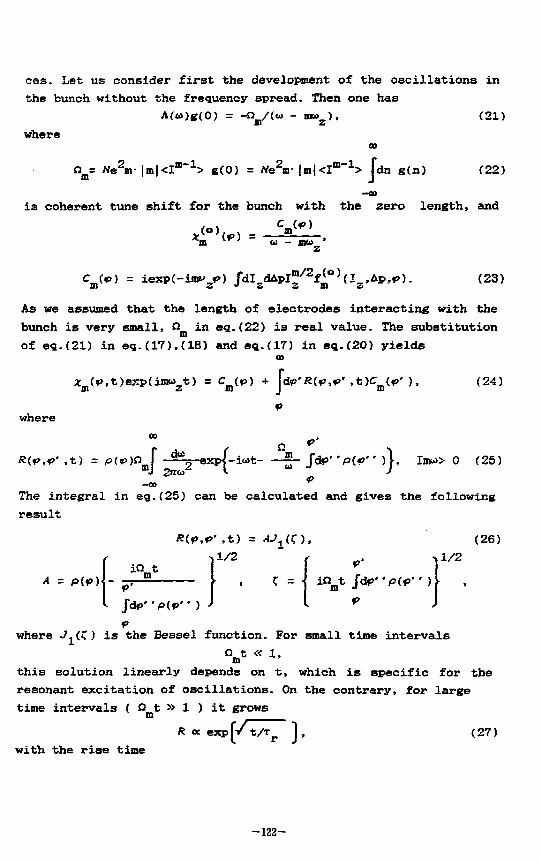
ces. Let us consider first the development of the oscillations in the bunch without the frequency spread. Then one has

A(«)g(0) = -a m/(« - n*>z), (21) where

CO

Om= Ate2m- Iml-cl 1 1 1 "^ g ( 0 ) = W e 2 m - | m | < I m _ 1 > fdn g ( n ) (22 )

-OB is coherent tune shift for the bunch with the zero length, and

C («>) = iexp(-imf jo) fdI_dApl"/2f<0)(I Ap,*>). m z •* z z m z

(23)

As we assumed that the length of electrodes interacting with the bunch is very small, Q_ in eg.(22) is real value. The substitution

m of eg.(21) in eg.(17),(IB) and eg.(17) in eg.(20) yields

CD *(*>,t)ej:p(in*>..t) = C («>) + de*«(*>,*>' ,t)C <*>' ),

m J< (24)

where

ff(^,p' ,t) = P(*>)nf d t e2 gxpl-i^t S_ Jd*>"P(«»" )|, Imu» 0 (25)

-co ^ The integral in eg. (25) can be calculated and gives the following result

R{<p,V ,t) = AJAZ), (26)

P(*>) m ^1/2

C = *>'

m t Jdp*'p(?>" ) 1/2

*>* Jdp'' P(P'' ) <p

where JAK) is the Bessel function. For small time intervals Cl t « 1, ID

this solution linearly depends on t, which is specific for the resonant excitation of oscillations. On the contrary, for large time intervals ( D t » 1 ) it grows m

R <x exp with the rise time

(/^T), (27)

-122-

1/T = \a\ [df>- V(*>" ),

depending on the relative position of particles inside the bund This asymptotic of the solution is caused by the screening < tail-on particles from head-on ones due to collective reaction < the bunch.

3. Let us now discuss the damping of considered instabilit; Once the amplitudes of the oscillations grow nonexponentiall: they can be damped by either the beam cooling, or bunch frequent spreads, or by the detuning of head-on and tail-on particles. Tl last method was initially suggested to damp oscillations in line* colliders [53 and is called now as BNS-method.

As more specific for storage rings let us consider first tl action on fast coherent oscillations of the beam cooling and t the Landau damping. If. for instance, the oscillations of indiv: dual particle are damped with the cooling decrement- >-, which exct eds significantly the frequensy spread in the beam

X. » |mdu|, the modification of the solution in eq.(24) will be described I the substitution u_-» ui^- iX_. Hence, the unstable oscillatior ea.(27) will start decay after the time

t > t c = % . (2

Of course, the condition (t <•> « 1 ) , or o c jmjxs » 2(a> cA r) 1 / 2= - f — / I T T (2 r

should be valid. Due to initial assumption « T « 1 condition (29 c r

generaly does not requires the surpass of the cooling decremen over the instability increment.

The influence of Landau damping due to frequency spreads i the bunch on the oscillations can be described in the followin way. When the frequency spread is taken into account, the mai: contribution into time dependence of the resolvent kernel (25 yields the vicinity of the point, where the phase

*(«o) = -iut - O [ds J { s \ (3< m ** Go — *;

is stationary. Here /(«) is the the frequency distribution in th< beam and

-123-

aip- m¥» = n f d*»"p(*>'*)-m m •»

P The stationarity condition d*/d« = 0 leads to the "dispersion equation"

1 = i—SL_ 1 _ J d* — — ^ , i. « > o . (31)

If Ato is the frequency spread, for smooth distributions f{£) in the region

|fim(*>',*>)| » (mA»)2t eq.(31) has the roots

*»(*>* ,*>,t) = ± / iO/t , (32) which correspond to initial blow-up of oscillations. On the contrary, if the condition similar to (28) becomes valid

t » t 0 = |fim|/(m&»)2, (33) the roots of eq.(31) will be close to u s -ijmA«|, which corres­ponds to asymptotic damping of the beam oscillation by the fre­quency spread.

4. Let us discuss now the BNS damping. It sufficiently uses the resonant nature of the instability and assumes its suppression by the introduction of the deviation of particles oscillation fre­quences along the bunch. Practicaly this can be done using the en­ergy deviation along the beam and the chromaticity of the lattice. That is why this method seems to be less specific for storage rings. Nevertheless, such conditions can be realized in storage rings, say, after the injection of intense bunch from linac.

The simple calculations of BNS-damping can be done for speci­al case, when particles betatron frequncies linearly depends on <p

wz(*») = " z

+ **> and the linear density in the bunch is described by the step functuon

• { . V2*> b , |P| < Pb;

P<*>) = •{ (34) • M > *>b •

The results of calculations generally depends on the shape of the distribution -if initial displacement of particles along the bunch. If, for instance, x_ }(<p) " S(p - *>•.), the asymptotical dependence

-124-

of the solution on time has the form (see in Ref.[4] for more de­tails )

a —a X (t) * A t " + B t m , |m6wjt » 1, (35)

6ui = 2**v ,ct = £i /(iwSu) , D m m A and B are non increasing functions of the time. In fact this so­lution is always unstable, though the instability can be done very slow, provided |« | « 1- Quite different result can be calculated for the uniform distribution of the displacement along the bunch £4]:

-a a -1 , , -imu t X (t) ~ A t m + B t m + xl Je z , jmowlt » 1. (36) m m • •

This solution will not grow provided the BNS-criterion [5] is valid:

Q 0 S S_ < x. (37)

REFERENCES

1. W.K.H.Panofsky and M.Bander. Rev. Sci. Instrum. v.39, 206, 1968. 2. D.V.Pestrikcv. Proc. of the 13-th Intern. Conf. on High Energy Ace. Novosibirsk 1986, v.2, 142, 3.0. Nauka 1987: A.V.Eurov, N.S.Dikansky, D.V.Pestrikov. ibid, p. 145. 3. R.D.Ruth, Z.M.Wang. IEEE Trans, on Nucl. Science, NS-28, 2405, 1981. 4. N.S.Dikansky, D.V.Pestrikov. Physics of Intense Beams in Storage Rings. S.O. Nauka 1989. 5. V.E.Balakin, A.V.Novokhatsky. V.P.Smirnov. Proc of the 12-th Intern. Conf. on High Energy Ace. FNAL, Batavia (111), 119, 1983.

-125-

Beam Dynamic Issues at Fermilab

King-Yuen Ng

Fermi National Accelerator Laboratory,' P.O. Bos 500, Batmwia, JL 60510

Some beam-dynamic studies have been performed recently at Fermilab. Here, we are going to present, in Sect. II the result of a beam transfer function experiment on the Tevatron, and in Sect. Ill some progress on transition crossing.

I. BEAM TRANSFER FUNCTION We would like to measure the longitudinal impedance of the Tevatron by the method

of beam transfer function.1 A special cavity was installed. The Tevatron beam at 150 GeV was debunched by lowering the rf adiabatically. The momentum spread was monitored by Schottky scans through a wall-resistive monitor and a spectrum analyser (HP8568B) having a resolution bandwidth of 10 Hz. Such a scan is shown in Fig. 1. The beam was then kicked longitudinally at a certain harmonic The response was picked up by a wall-resistive monitor and swept by a network analyser (HP3577A of resolution bandwidth 1 Hz) around that harmonic. The sweeping time was so chosen that the upward and downward scans produced the same structure. A typical scan is shown in Fig. 2. Unlike our past experience of the same experiment on the Accumulator, the transfer function was not smooth; it exhibit many notches (deficiency in amplitude). These structures were highly reproducible and appeared also in the transfer functions corresponding the lacks at other harmonics.

Due to the signal-to-noise consideration, Schottky scans had been performed at low frequencies. Any notches in the scan contributing to the transfer function would not show up due to the 10 Hz resolution of the HP8568B. In order to understand the source of notches, a spectrum analyser (HP3588A) with a resolution of 0.088 Ex was used in a later study run. This time we saw also notches in the Schottky scan (Fig. 3). The corresponding transfer function was shown in Fig. 4. We next tried to debnnch the beam by turning off the rf suddenly. The notches in the Schottky disappeared and the frequency spread was larger. We were not able to measure the transfer function of this coasting beam (with a wider momentum spread), because the beam intensity was too low at that time. We can draw the conclusion that these notches were the result of some collective instability which was damped by a wider momentum spread of the beam. However, we have not been able to explain the source of this instability by the existing known impedances of the Tevatron vacuum chamber.

If we look at the time evolution of the response of the kick at different frequen­cies. The HP8566B spectrum analyser was set to full frequency span of 1 MHz, so that roughly two revolution harmonics per division would be visible. The resolution and video bandwidths were kept between 10 kHz and 30 kHz so that the sweep time remained near 30 ms. With the spectrum analyser in mwirnnm hold mode, the peak power per bin of all sweeps was constantly displayed, we saw firstly the excitation of the harmonic of the kick, which is to be expected. Very soon, we also saw the exci­tation of the individual harmonics below the kicked harmonic However, we did not

* Operated by the Univenities Beseatch Aaodatioa, Inc., aader contract with the D.S. Departneat of Eaetgy.

- 1 2 6 -

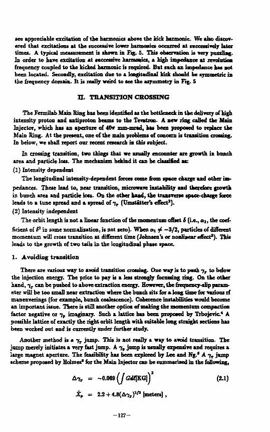
tee appreciable excitation of the harmonics above the Jack harmonic We alto discov­ered that excitations at the successive lower harmonics occurred at successively later timet. A typical measurement it shown in Fig. 5. This observation it very puzzling. In order to have excitation at successive harmonics, a high impedance at revolution frequency coupled to the kicked harmonic it required. But such an impedance has not been located. Secondly, excitation due to a longitudinal kick should be symmetric in the frequency domain. It it really weird to see the asymmetry in Fig. 5

H. TRANSITION CROSSING

The Fermilab Main Ring has been identified at the bottleneck in the delivery of high intensity proton and antiproton beams to the Tevatron. A new ring called the Main Injector, which has an aperture of 40* mm-mrad, hat been proposed to replace the Main Ring. At the present, one of the main problems of concern is transition crossing. In below, we shall report our recent research in tins subject.

In crossing transition, two things that we usually encounter are growth in bunch area and particle loss. The mechanism behind it can be classified as: (1) Intensity dependent

The longitudinal intensity-dependent forces come from space charge and other im­pedances. These lead to, near transition, microwave instability and therefore growth in bunch area and particle loss. On the other hand, the transverse space-charge force leads to a tune spread and a spread of 7 r (TJmstitter't effect'). (2) Intensity independent

The orbit length it not a linear function of the momentum onset 6 (i.e., a i , the coef­ficient of P in some normalization, it not zero). When a.\ g£ —3/2, particles of different momentum will cross transition at different time (Johnten't or nonlinear effect*). This leads to the growth of two tails in the longitudinal phase space.

1. Avoiding transition

There are various way to avoid transition crossing. One way is to push ->T to below the injection energy. The price to pay is a lest strongly focussing ring. On the other hand, tT can be pushed to above extraction energy. However, the frequency-slip param­eter will be too small near extraction where the bunch sits for a long time for various rf maneuverings (for example, bunch coalescence). Coherence instabilities would become an important issue. There is still another option of making the momentum compaction factor negative or fT imaginary. Such a lattice has been proposed by Trbojevic4 A possible lattice of exactly the right orbit length with suitable long straight sections has been worked out and is currently under further study.

Another method is a fT jump. This is not really a way to avoid transition. The jump merely initiates a very fast jump. A i t jnmp is usually expensive and requires a large magnet aperture. The feasibility has been explored by Lee and Ng.* A tT jump scheme proposed by Holmes* for the Main Injector can be summarized in the following,

A7]. = -Q.m(jG4qKG]\ (2.1)

X, = 2.2 + 4.8(A7 T ) 1 / 2 [meters],

- 1 2 7 -

whew G is the field gradient of the qnadrupole responsible for the jump and Xr is the maximum momentum dispersion. The corresponding rms momentum width is

where 5 is the bunch area, and V* is the rf voltage at transition. With A*jrr = 1, the TieBTimum dispersion is 7 m. Thus the required momentum aperture is about 40 mm.

The minimum transition energy jump is A7T > max(2Trc,3'rna)) where r e = 1.96 ms is the nominal nonadiabatic time and TML = 2.1 ms (QI ~ 1), while 7 is the rate of increase of 7. The maximum AfT is determined by the dynamical aperture limitation, which corresponds to maximum X, = 8.5 m. These two conditions give us 1.72 > A7T > 1.3 . The minimum number of turns N„ for the 7 r jump which minimises transverse phase space area growth is given byT

^•<rt<Ag, (2.3)

where Ag is the rms betatron amplitude at maximum beta 0 = 57 m. One expects, for A7T = 1 and normalised 95% transverse omittance of 20s- nun-mi, the minimum number of turns should be about 39 or the minimum jumping time should be about 0.43 ms which gives 1% nonadiabatic change in transverse phase space. Thus one obtains j T > 2340 sec - 1 , which is about 14 times larger than the nominal 7. Numerical simulation* shows that a jump of

/ S \ 1 / 2

in 1 ms is sufficient to maintain the bunch area. Here 6 = y/E vs. Thus the nonlinear effect dictates longitudinal beam dynamics at the transition energy crossing.

2. Crossing transition

If we do not want to avoid transition, we would like to know which of the two above mentioned mechanisms dominates at transition. As a function of initial bunch area, we expect the fractional growth of bunch area and particle loss for two different rf voltages but at the same acceleration rate to behave as depicted in Fig. 6. An experiment was performed on the Fenmlab Main Ring by Konrbanis, Heisner, and Ng.* The results shown in Fig. 7 agree with the domination of nonlinearity. For the future Main Injector, we believe that the impedance per harmonic can be controlled to some reasonably small value. Therefore, we expect nonlinearity to dominate also. In fact, this conjecture has been verified by simulations.10

One possible cure of nonlinearity is to control ai by adding a third set of sextapoles. If these sextupoles ate placed in between the quadrupoks, an unreasonably high sex-tnpole strength will be required. Bogacs and Peggs11 introduce a dispersion wave in the lattice by modulating the strength of the quadrupoles. In this way, the 3 sets of sextupoles can be made orthogonal. Preliminary calculation indicates that sextupoles of reasonable strengths can indeed reduce aj to —3/2.

Griffin13 recently proposed a new scheme of transition crossing. Near transition, a second- or third- harmonic is added to the present rf so that a flat plateau-like voltage

-128-

is obtained. As a result, all particles in a bunch mil be accelerated at exactly the same rate regardless of their momenta. This prevents the formation of tails. Therefore, we should anticipate no growth of bunch area and particle loss. Approaching transition, the bunch tends to tilt because of the absence of the synchrotron oscillation restoring force (Fig. 8a). After the higher-energy particles have crossed transition, the top of the bunch starts to drift backward. The lower portion of the bunch, being still below transition, continue the drift in the same direction (Fig. 8b). After all the particles have crossed transition, the bunch shape will be of the form as shown in Fig. 8c. At this time the higher-harmonic if is turned off and the bunch is recaptured into an accelerating bucket. In order to minimise the width of the if plateau, a. lowering of the rf (duck under) before transition is desired so that the bunch drift or tilt will be smaller. Simulations by MacLachlan13 show that this scheme is indeed feasible in the Main Injector when the bunch has an intensity of 1 x 10" and a bunch area of 1.7 eV-sec. An impedance of Z/n = 5 $1 and an aj ~ 1 were assumed.

It would be nice if this idea could be tested on the Main Ring. There, it would require about 1 MV (27%) of 106 MHz rf to produce the if plateau. However, if the third harmonic were used, only ~ 300 kV (12%) at 159 MHz would be needed, although the plateau would be shorter.

REFERENCES

1. An experiment performed by A. Bogacz, P. Colestock, F. Harfoash, G. Jackson, X. Lu, K.Y. Ng, and X.Q. Wang, 1990. 2. A. S0renssen, Particle Accelerators 6,141 (1975). 3. K. Johnsen, Proc. of CERN Symposium on High Energy Accelerators and Pion Physics, Geneva, 1956, Vol. 1, p.106. 4. D. Trbojevic, D. Finley, R. Gerig, and S. Holmes, Design Method for High Energy Accelerator without Transition Energy, to be published in Proc. of Second European Particle Accelerator Conference, Nice, France, June 12-16,1990. 5. S. Y. Lee, Summary Report on the Transition Crossing for the Main injector, Proc. of the Fermilab IH Instabilities Workshop, Fermilab, June 25-29,1990, Fermilab Re­port TM-1696. 6. S. Holmes, Main INjector Transition Jump, Fermilab Internal Report MI-0008, 1989. 7. S. Peggs, Betatron Adiabaiicity During a tT Jump, K.Y. Ng, Transverse Emittance Growth During 7T Jump, Proc. of the Fermilab HI Instabilities Workshop, Fermilab, June 25-29, 1990, Fermilab Report TM-1696. 8. J. Wei, Transition Crossing m the Main Injector, ibib 9. I. Kourbanis, K. Meisner, and K.Y. Ng, Experimental Study of the Main Ring Tran­sition Crossing, Fermilab Report TM-1693, 1990. 10. A. Bogacz, Transition Crossing in the Mam Injector ESME Simulation, Proc. of the Fermilab III Instabilities Workshop, Fermilab, June 25-29,1990, Fermilab Report TM-1696. 11. A. Bogacz and S. Peggs, private communications. 12. J. Griffin, talk given at Fermilab. 13. J. MacLachlan, talk given at Fermilab.

- 1 2 9 -

MIDDLE SPECTRUM. T : I K A U s 4 . U C I 2 . OOOS PRCAMP E—•» ROOM 0 3 / 0 S / 9 0 130S A HPSS66B SS 98 RCr - « S dbm ATTEN O 4b S db /d lv AVES 3 2 / 32

1 u^ Kit

j V, \ J V ^

<lWty « f l ^ V*W V ' "X ****w „fcM 1 , CENTER 24.667237 MHz RES BW t o Hz VIO

SPAN O.OO0SO0 MHz 3 0 Hz SWP 15.000 »•£

Figure 1: Longitudinal Schottky scan in the Tevatron at revolution harmonic 517 using spectrum analyser HP8568B with resolution bandwidth 10 Hz. No notches or spikes were observed.

1KMZ 3*.-tOOaM«»»M*«eM.teMZBW. SSCC. U* M M M C— a *fc/«w f a u n a * . <—)

Figure 2: Longitudinal beam transfer function at revolution harmonic 1100 in the Tevatron swept by network analyser HP3577A with resolution bandwidth 1 Hz. Note the notches or spikes in the beam response.

-130-

Rang*: -2Q dBm 13-Ju1 — 1000 7, 28 Rm»t B0 mHz Zoom* H * gh» Accuracy M*a« T l «••• 40. OS Sac Ai NARROW BAND ZOOM MKi- 524 030.00 Hi -118.76 dB-

- l O O dSm

A /V L o g H a g

S d 8 r v ir "Vv A Xef* v Ai V4L v *»w^

V r 1 / JVi\ i H/ l - AA ^ „ . . / »

lA/V y*"*'!!

- I S O

TAKING DATA S24 B30. S H z

AVGi IB Spans 9. 6

Figure 3: Longitudinal Schottky scan in the Tevatron at revolution harmonic 11, us­ing spectrum analyser HP8568B with a resolution bandwidth of 88 mHz. Note the appearance of notches in the momentum distribution.

C-4« ••Oil «7StS/*«

- 4 * s m*/*t* MMMim <«*) SSI

- 4 * 1 1

--- C\ - i \ i / T * * \ - I / \

^ S I J ^\.~ V 1

i •

a - a ^ , , ,s i n\\ ] MPM77AT

A 1 1

1 1

1

CCMTCfU U. IA14M MHc

Figure 4: Longitudinal beam transfer function measured in a later study period when Figure 3 was taken. Note that the notches match those of the Schottky scan in Figure 3.

-131-

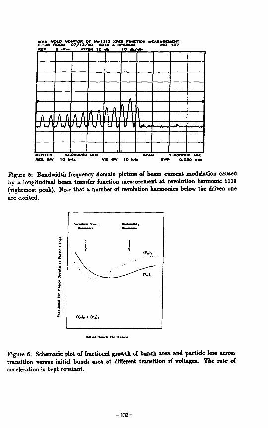
MAX HOLD U O M T M OF Matt 113 XFER FUNCTION MEASUREMENT e—*a R O O M 0 7 / i 3 / * o o o i a A Hrssaaa 2»7 137 REF O dbnr» ATTCN I P «b I P «%/«*»

1

«

A /I W U A A A A A AAA mstt jL /uwwuuiy i **-v—W

^ u -CENTER SS.OOOOOO MHz SRAN 1 .000000 MHz RES BW 10 kHz V10 «W 10 kHz SWf 0 .030 »«c

Figure 5: Bandwidth frequency domain picture of beam current modulation caused by a longitudinal beam transfer function measurement at revolution harmonic 1113 (rightmost peak). Note that a number of revolution harmonics below the driven one are excited.

C«), > {v j ,

laiUal Bunch Emittance

Figure 6: Schematic plot of fractional growth of bunch area and particle loss across transition versus initial bunch area at different transition if voltages. The rate of acceleration is kept constant.

-132-

tang. «mit. blowup for 2 6 turn* ( , I * - M C

* 9

O Va««itie» »e»«ii 2.0 MV

o.os cols ~ a i 0 . 1 2 s a i s o.«s 0.2 022s a » Partid>lanfar2Skm fcrt-nc

Figure 7: Experimental results showing fractional growth of bunch area and particle loss across transition versus initial bunch area for 2-booster-turn injection. The rate of acceleration was kept constant.

- 1 3 3 -

^ ^ ^

(a) approaching (b) top of bunch has (c) all particles transition passed transition have passed

but not the bottom transition

Figure 8: Bunch motion across transition in Griffin's scheme. The rf plateau is shown above the bunch.

- 1 3 4 -

High Frequency Behavior of the Coupling Impedance for a Large Number of Obstacles

2 R.L. Gluckstern and Rui Li University of Maryland College Park, MD 20742

3 In a recent paper the longitudinal coupling impedance for N

identical obstacles was calculated analytically at high frequency for N » 1. In particular, the impedance, which oscillates rapidly at high

frequency, is locally averaged over the oscillations. The result for the reciprocal of the averaged impedance per obstacle was

, -1 a

N Z Y„(k) 2 Z Y, (k) + a V N - 1 tan , (1) o N o 1 2 ^

where (1 + j) a V5k

a. - , (2)

and where Z Y (k) is the averaged admittance for a single obstacle, given

for kg » 1 by (1 + j) *a Vik

Z Y. (k) - . (3) ° X ^

This particularly simple result can be evaluated in two limits. The first is for N -» eo, where

Work supported by the U.S. Department of Energy. 2 Present address: CEBAF, Newport News, VA 23606. 3 R.L. Gluckstern, "High Frequency Dependence of the Coupling Impedance for a Large Number of Obstacles", Proceedings of the Particle Accelerator Conference, Chicago, IL, March 1989, p. 1157.

-135-

<1 + j» xa Vik j n k a 2

Lim N Z o y N , k ) + , (4,

-3/2 leading to the k dependence for the real part of the impedance at

high frequency. The second is for k -> en for finite but large N, in which

case (1 + j> ita

Lim N Z Y„(k) -O N k + « ^

VgN 1 +

2vT (5)

which exhibits the V N behavior of the impedance for large N suggested by 4 Palmer . Of particular interest is the fact that the admittance in

Eq. (1) consists of the .am of one term containing the information

involving the single obstacle and a second term involving only the

separation of the obstacles.

Figures 1 and 2 show the quantities

R e Z N I m 2 N N Re Z ' N im Z '

computed from numerical codes involving decomposition into axial wave

components and averaged over frequency, as functions of rfca. The smooth

curves are those predicted by Eq. (1) for N « 1, 10, 20, co.

As a result of discussions at the KEK workshop (September 1990)

attention is now being focussed on the high frequency behavior of the

coupling impedance for H cavities, each consisting of N cells in a

parameter range intermediate between the limits in Eqs. (4) and (5).

4 R.B. Palmer, "A Qualitative Study of Hakefields for Very Short Bunches", SLAC Report SIAC-PUB-4433, October 1987.

-136-

ReZ(n=20) KeZ(nslO) —RcZ(nsl) RcZ(N=20) UoZf N= 101

ReZ(N*o°)—ReZ(N=l)

2 4 6 8 10 12 14 16 IS 20 SqrL(ka)

-fi. » — __ a« —• a 8 * a 6

t-1.2

—ImZtn=20) IraZ(n=10) —lmZ(n=l} -•-ImZ(N»20J ImZ(N=10J

ftnZ(Ngoa)-—tmZ(N=l)

0 2 4 6 8 10 12 14 16 18 20 Sqrt(ka)

a"8 • 1*6 ' I" 1' 2

-137-

Measurement of the Asymptotic Behovior of the High Frequency Impedance

A.Hofmann, T.Risselada, B.Zotter

Abstract

A new evaluation of old measurements of the parasitic mode loss in the ISR shows that the asymptotic frequency dependence is very close to the inverse square root which has been found analytically for single cavities.

- 1 3 8 -

1 Discussion Measurement of the slow decrease of orbit radius of an unbundled beam in the ISR over many hours was made many years ago, and has permitted a determination of the parasitic mode loss factor at several frequencies after a small correction for the energy loss due to synchrotron radiation(l)..

In a smooth coasting beam, there should be no energy loss due to interaction with the chamber walls (the real part of all wall impedances must vanish for DC). It has further been shown that the energy loss due to (coherent) density fluctuations averages to zero[2]. The parasitic mode loss is therefore due only to the fact that the beam consists of single protons which interact individually with the wall impedances. The interaction frequency cfa is then determined by the width of the cone of field lines at the chamber wall of a point charge on the axis (see Fig.l)

"tt (1 )

where a is the chamber radius. For high energies (hf » 1, the width is quite small, and thus corresponds to rather high frequencies (over 60 GHz at the highest energy of 31.4 GeV).

Measurement have been made at 3 different energies, which thus yield thus loss factors for 3 different frequencies. The decrease of orbit radius with time is shown in Fig.3: a) for 3.6 GeV, b) for 15.4 GcV, c) and d) for 31.4 GeV. The last two figures show that the decrease is the same for beams with almost five orders of magnitude difference in current (4 mA and 32 A), justifying the assumption that single protons cause the energy loss.

Table 1 shows the calculated energy loss per turn, the loss factors and the corresponding frequencies for the 3 energies for which measurements had been made. The loss factor is plotted against frequency on logarithmic scales in Fig.4, and is seen to depend on frequency approximately as an inverse square root. A least mean square fit has been made and gave the value -0.533. The impedance is obtained from the average over 2 adajcent lossfactors, and also depends approximately on the inverse square root of frequency. This is in excellent agreement with the calculations for the energy loss of single cavities[3j, and not with the asymptotic loss factor of periodic cavities ("Optical resonator model")[4].

To our knowledge, this is the first experimental result for the asymptotic, high-frequency behavior of the wall impedance in particle accelerators or storage rings, which has been possible by using individual protons for the measurement.

References

[1] A. Hofmann, T. Risselada,IEEE-NS 30 (1983) p.2400 [2] Panofski - Philips: Electromagnetism (1957) [3] J. Lawson, Rutherford Report RHEL/M 144 (1968) [4] D. Brandt, B. Zotter, CERN Report/TH92-12 (1982) [5] K. Bane, M. Sands, SLAC Pub 4441 (1987)

- 1 3 9 -

Fig. 1: Field lines of a single charge (velocity pc) in cylindrical chamber

3UG**

^ v ^ s ^ *

<0 10 HNinl

Fig.2 : Distribution of induced current Fig 3: Change of average Orbit Radius vs. time in the wall fro 2 energies *) 3.6 GeV, 27 mA

b) 15.4 GeV, 4 mA c) 31.4 GeV, 4 mA d) 31.4 GeV, 32.2 A

T

3000

300

T — i — r

31.4 GeV/c

15.3 GeV/c

5 6 7 B 910

3.6 GeV/c -

p s 2 0 a 30 40

Fig 4: Measured Loss factor as function of bunchlength

Sept. 1990

SHORT-RANGE IMPEDANCE1

Kaoru Yokoya

National Laboratory for High Energy Physics,

Oho, Tsukuba, Ibaraki, 305, Japan

Abstract

Short-range wake functions are usually obtained using time-domain computer pro­grams. We demonstrate that frequency domain methods can also be usefully applied to this end. In addition, we show that the speed and ease of the required computations can be greatly improved if the calculations are performed at complex, rather than at real, frequencies.

Time-Domain and Frequency-Domain When charged particles pass through a structure in accelerators, electro-magnetic

fields are excited. The effect of these fields back on the particles themselves can be expressed in terms of the wake function and/or its Fourier transform, the impedance, if the effect within the structure is small. The Methods of computing the wake func­tion/impedance can be classified into two categories, time-domain methods and fre­quency domain methods. The calculations iu the time-domain are usually performed numerically, using computer programs such as TBCI[1]. These calculations are best suited for finding the short-range wake field within a bunch. When long range forces, such as the interaction between bunches, are needed we usually employ frequency do­main methods. In these cases the wake function is expressed by a few parameters such as the resonant frequencies, shunt impedances, etc. Frequency-domain calculations are also useful for finding approximate formulas of impedances and the limiting behavior at short distances but these are mostly analytic and are limited to structures of special shapes.

When one is interested in the wake function within a bunch in structures of general shape, time-domain methods has been preferred. However, when the bunch is very short, the obstacle on the wall is small, or the structure is very long, a fine integration mesh is needed and the computing memory and time requirements can be very large. In this note we discuss the possibility of computing the short-range wake function using the frequency domain. One such attempt is the work by Bane and Wilson[2]. They

'Talk at ICFA Beam Dynamics Workshop, Sep. 19-24, 1990, KEK, Tsukuba.

- 1 4 2 -

computed the short range wake function for infinitely periodic rectangular cavities by summing many resonant modes and then extrapolating to infinitely high frequencies using the optical resonator model. Kheifets[3] developed a computer code for structures with a smooth periodic shape by the Fourier transformation of the wall shape. Another example is the field matching method for finite structures attached to uniform beam pipes[4,5]. These programs compute the impedance for a given frequency. If the short-range wake function is needed, one needs first to compute the impedance over a large frequency range and then to calculate the Fourier transform.

Disadvantages of the Frequency Domain The frequency-domain computation of the short range wake function, however, has

the following disadvantages: (A) Program codes available so far are limited to special structures such as rectan­

gular cavities, sinusoidally varying walls, etc. (B) At each frequency step, a large matrix equation needs to be solved. If we are

interested in structures with special shapes, we may be able tc employ the field matching methods. With these methods we expand the fields in terms of orthogonal functions and then construct a matrix equation using the expansion coefficients as unknowns. The matrix obtained in this way is usually dense and, at high frequencies, large. The computing time needed to solve a dense matrix is proportional to the dimension cubed. If we are interested in structures of general shapes, the situation is essentially the same. In this cae we cannot use the field matching technique because suitable orthogonal functions cannot be found. However, one method for solving such problems is the boundary element method[6]. In this method the wall of the structure is approximated by line segments and the wall currents/charges (or the fields on the wall) are used as the unknowns. In this case, too, the matrix is dense. If the length of the structure is L and the mesh size is A, the number of unknowns is ~ L/A so that the computing time of the impedance at one frequency is ~ (L/A)3. On the other hand, in the time-domain computation, if one needs a wake function up to a distance S from the source particle and if the typical radius of the structure is R, the total computing time is proportional to (R/A)(S/A)(L/A). This product is normally much smaller than (L/A)3.

(C) The impedance at many frequency points is needed for obtaining the short-range wake function. One problem is that 'short-range' is not equivalent to 'high frequency'. The high frequency behavior of the impedance does not contain enough information to compute the short range wake. If, for example, the structure is infinitely periodic, the limiting behavior of SZ(w) is ~ u~3/2 [7]. Therefore, the dominant contribution to the short range wake W(t) (t —* 0) comes from the integral of Z(LJ) over the whole range of u). Even when the structure is of finite length so that Z(u) at high frequencies varies as u> - 1/ 2, as long as the bunch is not extremely short the low frequency impedance can contribute significantly to the short-range wake.

On the other hand, the high frequency impedance contains a great deal of informa­tion which is not needed for computing the short range wake. As is seen in Fig.3(a), Z(w) is normally a rapidly oscillating function of u>. This behavior is basically due

- 1 4 3 -

to multiple reflections on the structure walls. These reflections do not contribute to the short range wake function because of the time delay. Nevertheless, because of its oscillatory behavior, we need to compute Z[w) at many frequency points in order to be able to accurately calculate the Fourier transform. The number of frequency points Nu is typically >1000.

From the points (B) and (C) we see that the total computing time of the frequency domain methods is proportional to (L/A)3NU This computing time is normally much larger than the required computing time of the time domain method which, as we saw above, is proportional to LSR/A3.

Calculations at Complex Frequencies In order to overcome difficulties (B) and (C), we propose calculating the impedance

at complex frequencies. Because of causality the wake W(t) is zero ahead of the charge, for t < 0 (we assume

the particles travel at the speed of light). The impedance Z(w) is therefore regular in the upper half plane of complex w; all the singularities are in the lower half plane. Consequently, we expect Z(u) to be smoother in the upper half plane. If we carry out the Fourier transformation + w

W(t) = ^- I" Z(w)e-*"da;

along the line of constant Sto = uj (see Fig.l), we obtain

&TT J—oo

Fig. 1. Complex a-Plane

The contributions from the right and left edges are zero. The above expression is exact. As we move the integration path further upward, the integrand continues to become smoother, and the numerical integration becomes easier. However, if we go too far, we will need to extract a rapidly oscillating'component from a smooth function and then to multiply it by a large factor e?''. This will result in a loss of numerical accuracy.

The best choice of the path offset is to take wj/c ~ 1/5, where c is the velocity of light and S is the maximum distance needed for the wake function W. Since the oscillatory behavior of Z(ui) comes from the multiple reflections, Z(UR + WJ) is smooth if w//c>l// , where / is the typical dimension of the structure. Therefore, if S<1, we can reduce Nu considerably. (However, we lose nothing by going to complex w even if S>L)

Thus, we can say that SHORT-RANGE = LARGE w,.

As an example, in order to demonstrate the advantages of this method, we have com­puted the impedance for the structure in Fig. 2 by Henke's field matching method[5] but at complex, rather than at real, frequencies. The field in the tube region (dotted

- 1 4 4 -

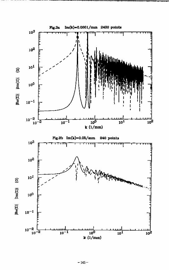
Fig.3a lm(k)=0.000l/mm 2400 points 10B

10 2

10*

P 1 1 I I I I I I !

N

I io°

& 1 0 - 1

10" lo-

• i i i i i i i n i l 1—i n u n 10 -1 10°

k (1/mm)

i i 111 i i 10 J 10*

1Q3

10 2

10>

Fig.ab Im(k)=0.05/mm 240 points T — I I I I I I I I I—I I I I I I I 1 1—I I I I I I I 1 1 — | I | I I t

I 1 0 °

IS

I 10-1

10 —2 I 1—i i i i m l i i • • • »••! • 10 - 2 10 - 1 10°

k (1/nun)

I l i n n 1—i i i i i n 10* 10 2

- 1 4 5 -

10 3

Fig.Sc lm(k)=0.6/mm 80 pointa 10 3

1 1 M

ill

i I I I I I I I I i I I I I I I I I i I I I I I I I I i i i

i n

un

10 2

J_ lin

n i i

10 2

J_ lin

n i i

1

10*

10°

r

r

- !

t? t- -10-1

- i i

inul

,

i i - 1 1 1 i n i i i 1 1 m l 1—i i 1 1 1 n l 1—i—i_i i 11 n

10

60

- 2 10 - 1 10u 10' 10*= k (1/mm)

Fig. 4. Point Charge Wake for JLC Single Cell

i—i i i i i i—i i i i i—i i I i — I I I I I I I I — i i i i i T T Im(lc) (l/mn)

0.0001 0.05 0.5

a(mro)

-146-

area) is expanded in a form such as

&* = JdkzF(k,)Jm{y/k* - *2r)e*-

and that in the cavity region (shaded area) as

*"+««-?&{ fe}{;} IVKZ

9 Fig. 2. Cavity Structure used as an Example

Here, £ ' 5 ' and E^ are the source and the radiated field, respectively, and k = uijc. The coefficients are found by matching the fields at the boundary between the two regions, and by requiring that the wave propagates to the left(right) in the left(right) end pipe. The dimensions used in our example calculation are a=3.672mm, 6=10.6mm, #=6.746mm and <f=8.746mrn. Pig. 3 displays the longitudinal impedance for one single cell as a function of fcfl = « R / C . The imaginary part of the frequency is fcj = w//c = 0.0001/mm, 0.05/mm and 0.5/mm for Figs. 3a, 3b and 3c, respectively. The solid (dashed) lines are \^tZ\ ( |SZ|). As one can see, the impedance is a very compli­cated function on the (almost) real axis but it is surprisingly smooth for complex frequencies. In Fig. 3c one can easily see that the asymptotic high frequency behav­ior of the impedance is Z ~ k~1^2. By fitting the high frequency part to the form Z(k) — const, x (kji + iki)~1^2 and then performing the Fourier transform, we obtain the point charge wake function shown in Fig. 4. The dotted, dashed and solid lines in the plot give the wake computed from Figs. 3a, 3b and 3c, respectively. (The number of computed frequency points is 2400, 240 and 80, respectively.) Although the three impedance functions are very different, the wake functions computed from them are almost identical. Thus we see that the information contained in the smooth graph of Fig. 3c is in fact sufficient to compute the wake function up to ~0.5mm.

Calculating the impedance at complex frequencies can also alleviate disadvantage (B). To see why this is so, let us consider the boundary element method of calculating the fields. Suppose there is a source point on the wall at longitudinal coordinate z\ and a field point at z-i. (Let a larger value of z signify a more forward position.) The kernel between these points is given by

e«Ml eikRR-k,R G = R R

where R is the distance between the points. This kernel is exponentially small for large distances if w/ > 0. This does not, however, mean that the effect of the source cannot reach far. The impedance is computed by a formula such as

•O Ek{z)e-ik*dz,

where e~xkz can be exponentially large for complex frequencies. What matters is not

- 1 4 7 -

^^^^^f^mmmmmmmmmmmmmmmmmmmmmmmMm

I

Fig.5. SIC UulU-cell Im(k)=0.5/mm 1 to 32 ceils 10* c 1—i i i i mi 1—i—i m m 1—i i i i m i 1—r—r-rrrra

10'

10^

10" - 1 I _ • i I , i i i i i ii 11_ 1—i i i I nil, 1—i i i i in 10 - 2 10 - 1 10°

k (1/mm) 10 1 10"=

Fig.6. Gaussian Bunch Yake az= 60/na 1 to 32 cells

o \

o

2 5 r — i — i — i — 1 — i — i — i — i i i — i — i — i — I — i — i — i — i — I — i — i — r

20

15

10

J — i i i_ 0 0.1

s(nun) 0.3

- 1 4 8 -

the field E but E = Ee~'k*. The corresponding kernel for E is given by

eik(R-Z2+zi)

which is exponentially small if z 2 < zj but contains a long tail for z 2 > zj, i.e., if the field point is ahead of the source point. Thus, the interaction is almost only in one direction if the distance between the two points is large. This fact is due to causality. Therefore, if one writes a matrix equation using the fields on the walls as the unknowns, the matrix is nearly triangular, i.e. the components in the upper triangle are exponentially small. Such a matrix equation can easily be solved by iteration. Thus, the computing time is proportional to (L/A) 2 x (number of iteration) instead of to (£/A) 3 .

The same feature is found with the field matching method. For example, if kjd 3> 1, the matrix for the many-cell structure depicted in Fig. 2 is also nearly (block-wise) triangular. Therefore, one can compute the multi-cell impedance within a reasonable computing time. In Fig.5 we plot \%tZ\ per cell for a structure with 1, 2, 4, 8, 16 and 32 cells (fc;=0.5/mm). One can clearly see the transition from the k'1^3 to the k~3^2

behavior of the impedance. (The computing time was a few seconds for the single cell to ~20 minutes for 32 cells.) The wake functions for a Gaussian bunch (r. m. s. bunch length of 60/im) computed from these impedances are plotted in Fig. 6 in solid lines. The dashed lines are those computed by the time-domain method (like TBCI) with a mesh size of 6/tm. The dotdashed line is the wake function per cell for an infinite number of cells. It was computed by field matching and by imposing periodic boundary conditions. (For this case the impedance was calculated at many frequency points on the real axis. At the moment the computer program for infinite cells using complex frequencies is not yet finished). The dotted curve in the plot represents the charge distribution.

We note that the solid lines approach the dotdashed line in the limit of infinite cells. However, the time-domain computations, for the cases of 16 and 32 cells, do not approach the asymptotic limit. We believe that this disagreement is due to a numerical problem of the time-domain method. For this example, it seems that the mesh size needs to be reduced if the number of cells is ^16.

Conclusions We have described a poweful method of computing the wake functions of very short

bunches. In this method we first compute the impedance at complex frequencies, and then Fourier transform this function to obtain the wake. The advantages of finding the impedance at complex, rather than at real, frequencies are twofold.

(1) Because the impedance at complex frequencies is smoother, the number of fre­quency points at which the impedance needs to be calculated is fewer.

(2) For complex frequencies the matrix that needs to be solved to find the impedance is nearly triangular. Therefore, at each frequency point the calculation of the impedance is much quicker at complex than at real frequencies.

- 1 4 9 -

On the other hand, the difficulty (A), namely, that the frequency-domain compu­tation is limited so far to structures of particular shapes, has not yet been solved. For this, we would like to develop a computer program using the boundary-element method in the near future.

Acknowledgement The author would like to thank K. Bane for helpful comments and correcting English.

References [1] T. Weiland, Nucl. Inst. Meth. 212,13 (1983).

[2] K. Bane and P. B. Wilson, Proc. of the 11th Int. Conf. on High Energy Ace. CERN (Birkhauser Verlag, Basel, 1980), p592.

[3] S. A. Kheifets and P. M. Gygi, Proc. of 1985 Part. Ace. Conf., May 1985, Vancou­ver, Canada. (CERN LEP-TH/85-9, May 1985).

[4] S. A. Kheifets, SLAC-PUB-4133, Oct.1986. S. A. Kheifets, K. L. F. Bane and H. Bizek, Proc. 1987 Part. Ace. Conf, Washington D.C., March 1987. (SLAC-PUB-4097, Mar.1987).

[5] H. Henke, Proc. First Europian Part. Ace .Conf, Rome, June 1988. (CERN-LEP-RF/88-31, June 1988).

[6] For example, see C. A. Brebbia, The Boundary Element Method for Engineers, Pentech Press Limited, Graham Road, London, 1978.

[7] For a review, see J. J. Bisognano, proc. 1988 Linear Ace. Conf., Oct.3-7,1988 (CEBAF-report-89-001, June 1989), page 261.

- 1 5 0 -

Shielded Coherent Synchrotron Radiation and Its Effect on Very Short Bunches*

Robert L. Warnock Stanford Linear Accelerator Center, Stanford University, Stanford, California 94309

Abstract

Shielded coherent synchrotron radiation is discussed for two cases: (1) a beam following a circular path midway between two parallel con­ducting plates, and (2) a beam circulating in a toroidal chamber. Wake fields and the energy radiated are computed for both cases. Under condi­tions like those of the high-energy bunch compressor of the Next Linear Collider (NLC), in which bunches as short as 40 microns are contem­plated, the shielded coherent radiated power is estimated to be small compared to the incoherent power, but can still amount to a few hun­dred KeV over the compressor arc.

1. Introduction

Particles in a bunch following a curved path may radiate coherently at a wave­length comparable to the size of the bunch. The radiated power is proportional to the square of the current, hence proportional in this event to N2, where N is the number of particles in the bunch. The power of incoherent radiation will vary only as N, since each particle contributes a power proportional to its own squared current. In typical conditions in electron storage rings, most of the radiation is incoherent, peaking at frequencies far beyond the microwave region. In an experiment using short bunches from a linac, Nakazato et al.,1 observed coherent radiation, with a clear indication of a transition from N to N2 dependence.

Fortunately for the operation of electron rings, shielding provided by metallic walls of the vacuum chamber greatly reduces the amount of coherent radiation. This effect was recognized in the early days of circular electron accelerators and has been studied theoretically from time to time ever since. In a simple, but relevant model first studied by Schwinger2 and Nodvick and Saxon,3 one considers a beam following a circular trajectory in a plane midway between two infinite, parallel, conducting planes, separated by a distance h = 2g. According to work of Fattens and Laslett* the real part of the longitudinal coupling impedance for this situation should satisfy roughly the condition

maxf — — ^ 1 = 3 0 0 | . ohms , (1.1) n l n J R

* Work supported by Department of Energy contract DE-AC03-76SF00515.

- 1 5 1 -

where n is the azimuthal mode number, R is the trajectory radius, and ui0 = fic/R is the revolution frequency. As we shall see presently, ReZ/n is negligible below a certain threshold, then rises rather sharply to this maximum, and henceforth falls slowly. The threshold can be estimated as

n = x(R/k)3'2 . (1.2)

In terms of the frequency w = w0n, or normalized wavelength A = A/2JT, the same criterion is

wk/c = *0(R/h)1'2 , X=(k/R)1'2h/T . (1.3)

For typical R/k, with h being the transverse dimension of the vacuum chamber, this threshold is at a much higher frequency than the "waveguide cutoff" for propagation parallel to the plates, which lies near wA/c = 1.

The radiated power is determined by the impedance and the Fourier spectrum of the bunch. If the bunch is rigid (i.e., maintains a constant form in a rest frame) and the particles radiate coherently, then the energy change per radian on the circular path is

dU/d6 = -q2w0 Y, |A»|2ReZ(n,nw„) , (1.4) «=—00

where q is the total charge in the bunch and A„ is the Fourier transform of the longi­tudinal charge distribution A(0),

2x

\n = ±j<TMmd9. (1.5) 0

If the bunch has significant Fourier components near the maximum (1.1) of the impedance, the radiated power is quite large, as the following discussion will show. This situation usually does not occur in storage rings, since the bunch is long com­pared to the wavelength at the maximum impedance. Oa the other hand, in the last stages of bunch compression in the NLC, the bunches are sufficiently short to pro­duce appreciable coherent radiation, provided that the impedance resembles that of the parallel plate model.

Section 2 gives definitions and formulas for the impedance, and derivations of expressions for the energy loss and wake field. The impedance for the toroidal chamber is taken from Ref. 5; that for the parallel plates is obtained by taking a limit of a formula in the same paper. Numerical examples are presented in Section 3 for parameters appropriate to four different designs of the NLC bunch compressor.

The notation and point of view will be the same as in Ref. 5. The reader may refer to that paper for details of technique not discussed here, in particular, for the numerical treatment of high-order Bessel functions.

- 1 5 2 -

2. Impedance , Wake Field, and Energy Loss

We work in cylindrical coordinates (r,0,z), and suppose that the centroid of the bunch follows an orbit in the plane z = 0. For the present discussion, the orbit is cir­cular; slightly different ideas may be required for single-pass orbits. It is convenient to make a Fourier analysis of the longitudinal electric field with respect to 0 and the time t:

Es(r,0,z,t) = I dwe-*"* £ J* E*JLr,*,u) . (2.1) -Joo "—«»

Since we are interested primarily in longitudinal effects, we consider the average of this field over r and z, weighted with the transverse charge distribution of the beam. Spe­cializing to the case of a rigid bunch, we suppose that the charge and current densities have the form

p(r,0,z,t) = q\(0 -w0t)f{r,z) , J9(r,0,z,t) = u0rp(r,&,z,t) , (2.2)

where

f\(0)d0 = l , frdr fdzf(r,z) = l . (2.3) o

Here and in the following, the (r, z) integrals extend over the support of / . The field written without arguments (r, z) will be understood as the transverse average,

Ee{0,t) = jrdrfdzf{r,z)Eg{r,e,z,t) . (2.4)

The Fourier transform of \(0—uot), defined in analogy to (2.1), is A„ 6(u —w0n). The corresponding transform of the current is

Ig(n,u) = I dr J dzJe(r,n,z,u) =u„qXnS(u—u/0n) . (2.5)

If the environment of the beam has no longitudinal inhomogeneity, as in the models treated below, then there exists a complex function Z(n,u), the longitudinal coupling impedance, such that

-2)riJ£j(n,w) = Z(n,w)/j(n,w) . (2.6)

If the environment is inhomogeneous, perhaps because of cavities in the vacuum cham­ber, this single impedance function is replaced by a matrix, Z(n,n',u>), since many harmonics of the current contribute to the excitation of one harmonic of the field.

The use of the weighted average (2.4) in the definition of the impedance is not conventional; usually, the simple average or merely the value of the field at the center of the beam is used. The weighted average seems quite natural, however, and we shall see that it leads to a cleaner derivation of the formula for energy loss than would otherwise be possible. If /(r , z) = W(r)H(z), where rW{r) and H(z) are rectangular

- 1 5 3 -

step functions or delta functions, then the simple average coincides with (2.4). In Ref. 5, / had such a form and the impedance was denned with the simple average; consequently, the impedance obtained in Ref. 5 can be used in our present formulas.

The wake field Eg(ut0(t + r),t) is defined as the field on the trajectory at an angular distance u0r in front of the bunch center. Taking the weighted average of (2.1) over r and z, and introducing (2.6) and (2.5), we see that the wake field is given by the Fourier transform of the impedance, weighted by the transform of the bunch:

oo V{w,T) = -2TRE8(u>0(t + T),t)=u0q J2 tima"r\nZ(n,nu0) . (2.7)

«=-oo

The function V is sometimes called the wake potential. It is the "wake voltage per turn"; a positive value of V(U)0T) means energy loss by particles at a distance U)0T from the center of the bunch.

If the beam environment is not homogeneous, the formula replacing (2.7) is oo oo

V(«,r, * )=« .« £ e™'T £ Z(n,n',Uon')Xn.ei^-'t>'t . (2.8) »=-oo n'=—oo

average over one period T = 2ir/u0 is given by formula (2.7), since the averaging sets n = n'.

Let us now compute the radiated power. The change in energy in time dt is the work done by the field Eg,

dU = / / / E9(T, 9, z, t) [p(r, 0, z, t)rdrdOdz] [w0rdt]

r r t , ( 2 9 )

= qu, I I r2drdzf(r,z)Et(r,$,z,t)X($ -u>ot)d0dt . For the integration over r, we note that r 2 varies almost linearly over the extent of the beam, which is tiny compared to R. Thus, r 2 a Rr and the average (2.4) appears. The power is

dU/dt = qcj0R Id6E0{&,t)\(O -u0t) r f (2.10)

= qu0R dO due-™1 £ tintE,(n, w) £ j*'V-*AA„. .

If we now substitute (2.6), and carry out the 9 and w integrals we obtain 00

dU/dt=-(qu0)2 ^ |A„|2ite Z{n,nu0) • (2.11) »=—oo

We have used the properties A_„ = AJ and Z(—n,—nu0) = Z(n,nu0)*. Notice that the latter follows directly from the definition (2.6) and the corresponding reflection property of E$(n,ui) and I(n,u). For a delta function bunch, A» = l/2x and

- 1 5 4 -

dU/dt=-I2 J2 XeZ(n,nw0) , (2.12) »=—oo

possible impedances, "connected in series."

It remains to give formulas for the coupling impedance for the two models to be explored. In the first model we have infinite, parallel, perfectly conducting plates, separated by a distance k = 2g; the beam circulates in the median plane between the plates. As in Ref. 5, the boundary conditions on the plates are enforced by expanding the fields in Fourier series in z; for instance,

oo £ f l(r,n,z,w) = 53sina,(z+0)£#(r,n,p,w) ' ( 2 J 3 )

p=l

where ap = icp/h. Correspondingly, the ̂ -dependence of charge and current densities must be represented by Fourier series. The r-dependence of fields is expressed in terms of Bessel functions of order n.

In order to obtain the impedance in a convenient analytic form, we choose a simple form for the transverse beam profile:

f{r,z) = W(r)H(z) , W(r) = 6{r - R)/R . (2.14)

With a little numerical work, one could accomodate a function W(r) with a finite width. The impedance comes out in terms of the Fourier transform of H(z). Again, to get a simple formula, we take H{z) to be a rectangular step mnction, symmetrical about z = 0, but any other choice could be treated easily.

With the beam profile as stated, the impedance for the parallel-plate problem is given by

Zi^J^R E A , » W ) ( ( / s M ) + i l , M ) )

P(odd)>i L ( 2 . 1 5 )

+ (^fMipR^MfpR) + iYndpR))] , Tp J

where

7 2 = ( w / c ) 2 - a 2 , A, = (sin x/x)2 , x = xp6h/2k , (2.16)

the vertical size of the beam being Sh. The impedance is in ohms with Z0 = 120 x ft. In the second model the vacuum chamber is a torus of rectangular cross section.

The cross section has height h = 1g and width w. The inner and outer torus radii

- 1 5 5 -

are a and 6, respectively. The radial wave functions are expressed in terms of cross products of Bessel functions, defined as follows:

Pn{x,y) = Jn(x)Yn(y)-Yn(x)Jn(y) ,

*.(*,») = JL(*)yi(*)-yl(*)£(9) • For perfectly conducting walls, the impedance of the torus is given by

Z(n,u) 2ix2Z„R y* A ?0u>R su{tPb,^R^fpR,-,pa) n & k ri**)>i '•• n C s*ilph>1pa)

+ r <*r x2 P»(7»6,7y-ft)P»(7>fl,Ty») 1

(2.17)

(2.18)

The expression (2.18) has poles corresponding to the resonances of the closed, perfectly conducting structure, and is imaginary wherever it is finite. When wall resistance is introduced, the function acquires a real part and the poles are replaced by sharp peaks in the real part. Our calculations include wall resistance, following the theory given in Ref. 5.

The formula (2.15) for parallel plates can be derived immediately from a result of Ref. 5; namely, the formula for impedance of a beam circulating in a cylindrical pillbox of radius b. One merely takes the limit for 6 —» oo. This is best done using the form appropriate to the low-frequency region, in which Bessel functions are replaced by modified Bessel functions [see Eq. (4.3) of Ref. 5]. The latter have simple exponential behavior in the relevant limit. Analytic continuation through the upper half u plane produces the high-frequency form (2.15).

To close this section we recall the well known formula for the total power from incoherent synchrotron radiation.6 For a single electron,

dU 1 2e2/?V dt 4TC ZR2 (2.19)

3. Numerical Examples of Wake Field and Energy Loss

For calculations, we take a Gaussian bunch with length a:

m = V27 7 °*[-2(-) J • A« - 27 ^ h ( T ) J • <31> A wave moving with phase velocity equal to the particle velocity at r = R, i.e., with frequency w = u0n, has wavelength 2xJ?/n. The relevant length for our discussion is wavelength over 2x,

* = R/n . (3.2)

- 1 5 6 -

Table I: Energy losses for four versions of the NLC bunch compressor. The values of energy loss AU are for a bunch containing JV = 2 • 10 J O electrons.

Version V.1 V.2 V.3 V.4

R(m) 84.218 213.6 149.5 106.8 A0(degrees) 10.89 180 180 180

a, (microns) 460 460 460 460

o-f (microns) 37 86 61 44

Atf(plates) MeV 0.176 0.164 0.827 2.08

AU (torus) MeV 0.123 0.0121 0.337 1.30

A£/(incoherent) MeV 2.19 14.2 20.4 28.5

In terms of A the spectral density of the bunch that appears in in the power formula (2.11) is

w^^^Ri) 2 ] • <«> We illustrate with values of <r and R from four different conceptual designs for

the NLC high-energy (16.2 GeV) bunch compressor [7]. Since the expected beam pipe radius is about 1 cm, the plate separation or torus height h will be 2 cm, and the torus width w also 2 cm. The beam height Sh, not a significant parameter, will be 1 mm. Table I shows the compressor parameters, including the initial and final bunch lengths, tj{ and <Tf, and the total deflection angle A0 of the compressor arc.

Figure 1 shows a typical graph of the real part of Z(n, nu)0)/n, for the parallel-plate model including only the p = 1 term in Eq. (2.15); the parameters are R = 149.5 m and h = 2 cm, for Version 3 of Table I. At the frequencies of the plot, the higher axial modes p = 3,5, • • • make a negligible contribution. The Fattens-Laslett estimate (1.1) of the peak value is confirmed. According to the estimate (1.2), ReZ/ra should first have significant magnitude around n = 2 • 106. Indeed, it first reaches half-maximum at about that point. Figure 2 shows ReZ plotted as a function of A. From the graph and (2.11), (3.3), we see that significant power will be radiated only for bunch lengths less than 90 (i or so with R and A as in Version 3. For longer bunches the relevant impedance is too low.

Figure 3 shows ReZ/n for an aluminum toroidal chamber with parameters for Version 3. The beam is centered in the chamber. The threshold at which the impedance

- 1 5 7 -

0.020 r — 60.000 cs #40,000 -

20.000 -

100 200 K (microns)

Figure 1: ReZ(n,nw0)/n versus n for the parallel-plate model, R = 149.5m, h = 2cm

Figure 2: ReZ(n,nu0)/n versus X for the parallel-plate model, R = 149.5m, /i = 2cm.

is first appreciable is a bit higher than in the parallel-plate model, but the maximum occurs at about the same point. The resistive wall theory is somewhat defective, in that ReZ is negative at some distance from either resonance peak. In the calculation, we put ReZ = 0 wherever the theory gives negative values.

To estimate the total energy loss in the arc, we assume that the energy loss per unit angle of deflection at a particular bunch length is the same as in our steady state model running at the same (fixed) bunch length. Repeating the steady state calculation for many bunch lengths, we find a curve for dU/d9 versus a. Since a decreases in the compressor almost linearly with 8, this is equivalent to knowing dUfdO as a function of 9. Integration with respect to $ produces the figures for total energy loss shown in Table I. The values are in MeV per particle, supposing that the bunch contains N = 2 • 10 1 0 electrons. The conductivity of aluminum is used for the toroidal chamber, whereas the parallel plates are perfectly conducting. For comparison, values for incoherent radiant energy are listed. For that, we assume that the energy radiated per unit angle is (l/w„) dU/dt, with dU/dt given by Eq. (2.19).

The curve of dU/dO for Version 3 of the compressor is shown in Figure 4, for the parallel-plate model. In all four versions the energy loss is sharply concentrated near the end of the arc, since elsewhere the impedance is too small at wavelengths within the bunch spectrum |A n | 2. The corresponding curve for the resistive toroidal chamber has a similar form, but is concentrated still closer to the end of the arc, due to the higher threshold of the impedance. The high-threshold effect is especially pronoun~«d in Version 2 of the compressor, which has relatively large values of R and oy.

For a given final bunch length oj, one can reduce the coherent radiation by making R as large as possible and the transverse dimensions of the chamber as small as possible. This raises the threshold (2.2) for the onset of a large impedance, and allows the bunch spectrum (3.3) to cut off the radiation.

- 1 5 8 -

- 1 1 1 1 1 1 i 1 -

_ 0.08 -« -

0.06 -c

a 0 0 4 -= -•S 0.02 1 V -ISI y \ / • I 0 — ^ — J -

-0 02 ! 1 I 1 l _ ..!_ l 1 I . L -

yooe i 1 r -1 i | -r -

I -• 1 o> / | 0.08 -> / . a / 5 0.04 / -CD / -•D / 5 0.02 / -•o /

n i i ,J, ' 4 6

n (106) S

C7C7A7

Figure 3: ReZ(n, nu0)/n versus n for aluminum toroidal chamber, R = 149.5m, k = w = 2cm.

0 50 100 150 •i» 6 (degrees) m „

Figure 4: dU/dO for the parallel-plate model in Version 3 of the bunch com­pressor.

In Figure 5 we show the wake voltage per turn, as defined by (2.7), for the parallel-plate problem and Version 3 of the compressor. Particles within one a of the bunch center lose energy, whereas those around two o on either side gain energy. The peak wake voltage per unit length is comparable to typical wakes in the SLAC linac structure, which amount to a few volts per picocoulomb over a 3.5 cm cell.

Corresponding results for the toroidal model are displayed in Figure 6. Within two a of the center the behavior is similar, although the voltage is somewhat lower due to the higher threshold of the torus impedance. The persistent oscillations well beyond the bunch length can be understood if we refer to the limiting case of infinite conductivity. As that limit is approached, the peak of ReZ(n, nu0) narrows to a delta function, and the wake field has the form exp(inm0r) with essentially a single value of n. In fact, the oscillations in Figure 6 have almost exactly the period of such a single exponential, if we choose n to have the value at the peak of the impedance; (in units of bunch length, the wavelength of the oscillation should be lirRfna, which in the present example is about five). If we increase the Q of the system by increasing the conductivity, we find numerically that the wake indeed approaches the expected single oscillatory exponential. In Figure 6 the oscillations before and after the bunch die off relatively quickly, because a band of n values is involved. In Ref. 5, Section 7, it was shown that the band width is given approximately as

n w Q The result (3.4) arises from the peculiar nature of the dispersion relation w(n)

of the resonances of this structure. In the (w, n)-plane, the dispersion curve is almost parallel to the synchronism line w = ui0n at the point where the two cross. This means that a rather broad range of n-values can be simultaneously synchronous and resonant when the system has resistive walls.

- 1 5 9 -

40

1 i '

| r- -r "| i

\ £ 20 : ~ o $ o a ^ - 2 0 H • o $ o a ^ - 2 0 H V > r 1 -40 r V

1 1 1 . M M C7C7A4

-10 0 10 Distance from Center, Units of o

F 5: Wake voltage per turn for the pcjrallel-plate model, R = 149.5m, h = 2cm, bunch length a = 61pm.

r - r - l 1 1 1 1 -40 A O

~ 20 :\ A ! \ :

o

• — -20 M V y ^ ^ : > - v 1/ -40 v v

- 1. .1 1 1 < -

tl-M -10 0 10 Distance from Center, Units of a

Figure 6: Wake voltage per turn for the toroidal chamber, R = 149.5 m, h = w = 2 cm, bunch length a = 61/tm.

Acknowledgment

I am grateful to Ron Ruth for encouraging this stud}, and for several good sug­gestions. Conversations with S. Kheifets, S. Heifets, J. Bisognano, and R. Gluckstern were also very helpful.

References

1. T. Nakazato, M. Oyamada, N. Niimura, S. Urasawa, 0 . Konno, A. Kagaya, R. Kato, T. Kamiyama, Y. Torizuka, T. Nanba, Y. Kondo, Y. Shibata, K. Ishi, T. Ohsaka, and M. Ikezawa, Phys. Rev. Lett. 63 (1989) 1245.

2. J. Schwinger, On Radiation by Electrons in a Betatron, unpublished report (1945). 3. J. S. Nodvick and D. S. Saxon, Phys. Rev. 96 (1954) 180. 4. A. Faltens and L. J. Laslett, Part. AcceL 4 (1973) 152; Brookhaven National Labo­

ratory Report BNL-20550 (1975); V. Brady, A. Faltens, and L. J. Laslett, Lawrence Berkeley Laboratory Report LBID-536 (1981).

5. R. L. Warnock and P. Morton, Part. Accel. 25 (1990) 113. 6. J. D. Jackson, Classical Electrodynamics, (Wiley, New York, 1962). 7. S. A. Kheifets, R. D. Ruth, and T. H. Fieguth, Proc. Int. Conf. High-Energy Accel­

erators, Tsukuba, Japan, August 22-26,1989; available as SLAC-PUB-5034 (1989).

- 1 6 0 -

Impedance Scaling and Synchrotron Radiation Intercept Weiren Chou

SSC Laboratory* 2550 Beckleymeade Ave, Dallas, TX 75237, USA

ABSTRACT

This paper presents several scalings in 2-D and 3-D impedance calculations. Most of the scalings are empirical and are found by using the boundary perturbation method and numerical simulations. As an application of these scalings, it is calcu­lated, the impedance of one type of the synchrotron radiation intercept. The results are then compared with that of several other types of intercept designs.

1. INTRODUCTION

The beam-environment coupling impedances are important parameters in the design of modern large accelerators. The calculations of the impedances are usually quite involved. In order to reduce the amount of computational work and to obtain quick estimations, it is desirable to have certain scalings, even approximate ones. In Section 2, several methods are compared, that are commonly used in impedance calculations. They are in general agreement. In Section 3, consideration is given for several parametric scalings in 2-D cases. Two geometric scalings in 3-D are discussed in Section 4. The next section introduces the so-called synchrotron radiation inter­cept. It is really a 3-D structure and has to be computed using 3-D codes such as MAFIA [1]. The scalings have greatly simplified the computations of this structure. The results of several different designs of intercepts are compared.

2. COMPARISON OF DIFFERENT METHODS

In the past years, several impedance computation methods have been developed. These include the field matching, boundary perturbation, transmission line and nu­merical simulations, etc. A comparison of the results obtained from these methods have been made and found that they are in general agreement.

(a) Field matching vs. TBCI [2]: Henke calculates the impedance of a small pillbox with beampipes (Fig­ure 1) using the field matching method. [3] Figure 2 are the spectra that he got. TBCI is run in order to compute the wake potentials of the same struc­ture. The wakes are then Fourier transformed to obtain the impedance as shown in Figure 3. They compare to each other reasonably well, except some spurious peaks as shown in Figure 3 remains to be understood.

' Operated by the Universities Research Association, for the U.S. Department of Energy under Contract No. DE-AC02-89ER40486.

- 1 6 1 -

_.l . Figure 1 . A small pillbox with beampipes. (b = 10 cm, 2g = O.OSb, 2e = 0.1b.)

ReZ,(a)

Figure 2. Henke's impedance spectra of the pillbox in Figure 1.

a ImZ,((l)

di (b)

"

t /» 0 1 3 3 * S C 7 * 9 1 O l l t a 0 1 2 3 4 « C 7 * « 1 0 l l l *

Figure 3. Impedance spectra obtained from TBCI and Fourier transform. The dashed line in 3(b) is the result given by the transmission line method.

(b) TBCI vs. transmission line method: The simple structure shown in Figure 1 can be approximated by a trans­mission line, in which the longitudinal impedance at low frequencies is purely inductive and can be roughly estimated by the formula

* - * . • £ • * « » • ( i )

in which fio = 4ir x 10~ 7 H/m. This is a straight line with a slope equal to (/* 0/2x) • (4ge/b), as shown by the dashed line in Figure 3(b). It agrees with the TBCI results up to the cutoff of the beampipe.

- 1 6 2 -

(c) TBCI vs. boundary perturbation (BP): The boundary perturbation technique is basically an analytic tool. Unlike the field matching method, this tool can be applied to various types of geometries provided that the perturbation is not too large. For details of this method, refer to Refs. 4-6. As an example, Figure 4 shows a peri­odic structure which is typical in the beampipe of the storage ring of the synchrotron radiation sources (e.g. ALS, APS, ESRF and SPring-8). The longitudinal and transverse wake potentials of a Gaussian bunch of rms length a traversing this structure are, respectively,

WJiW—°(V/K?) = -1.8xf>|2c, | 2

P = i

l * - * ^ " ^ - * 7 & • (2» 360* W±(sr=l(V/pC-m) = - - £ - £ , , 1 2 *

o p = i

• » i J r~ri--.V2*,.../Mn?:

in which

.2e_ sin(p^) _1_

= 0 otherwise,

°v = -J-=u s» 3 / o r p = ± l , ± 3 , . . . (4) TTb0 -f p '

and

*mn ~ L + 4 T P 5 g ' l 5 J

*mn - T + l^" ' ( 6 )

xmn and x'mn are the nth root of the Bessel functions Jm and J'm, respec­tively, and w is the complex error function. All the lengths on the r.h.s. of Eqs. (2)-(6) are in centimeters. Figure 5 is a reproduction from Ref. 5. It is seen that in the range [-5a, 2a], BP and TBCI give almost identical wakes. The discrepencies near the bunch tail may be attributed to accumulation of numerical errors in TBCI. Another possible cause is different boundary conditions used — BP assumes periodic boundary, whereas TBCI assumes open boundaries.

- 1 6 3 -

h ZJZ&-J—\i

Figure 4. A periodic structure used to demonstrate the boundary perturbation method.

Wj ( V / j O

• bunch ^ , x 7 \ \

f N

BP

TBCI

BP

TBCI b o a d u A / ^ \ V

: v TBCI

>/<r »/» Figure 5. The wakefieids of a Gaussian bunch calculated by BP (solid line) and by

TBCI (dashed line). The left side is the bunch head. (cf. Ref. 5)

Figure 6. An exhibit of scaling I. (cf. Ref. 6)

3. PARAMETRIC SCALINGS IN 2-D

Assuming a rotationally symmetric obstacle in an otherwise smooth beampipe, the basic parameters that would determine the impedance of this discontinuity are the average radius, the depth and the width of the obstacle, and the slope of its edges. When these parameters vary, the changes of the impedance obey (approximately) certain power laws.1 Use the obstacle in Figure 4 as an illustration. A typical set of parameters are &o = 1.8 cm, e = 0.2 cm, 8 = 1/2 (in unit of ir/2) and L = 8 cm.

1The width of obstacle plays a somewhat different role, which will not be discussed here.

- 1 6 4 -

• Scaling I: k± = B8a (a = 0.7 ±0.1) . (7)

The transverse loss k± varies with the taper angle 8 by the power law described by Eq. (7), in which B and a. are constants. [7] The value of a. is close to 0.7. There is a small variation (±0.1) according to different bunch lengths a and parameters b0 and e. Figure 6 demonstrates the usage of this scaling. For given a, bo and e, first calculate k± for 8 = 1 (i.e. ir/2), which gives B. Then from the loss for 8 = 1/2 (i.e. ir/4), obtain a. These two constants determine the solid curve in Figure 6. When TBCI is used to compute the losses for other values of 8, they just sit on this curve as shown in Figure 6. This greatly simplifies the work, in particular, for small 8. Because it is known that TBCI has troubles to treat the long tapered structures. [8] It should be pointed out, though, that this scaling may not be very accurate when the bunch length becomes too small.

• Scaling II: fc~^ (1 .5</3<2) . (8)

When the obstacle depth 6 varies, both the longitudinal and the transverse losses k vary as described by Eq. (8). Here one may distinguish two cases. If the angle 8 varies with e such that the taper length g keeps a constant, 0 exactly equals to 2. This can be seen immediately in Eqs. (2)-(4). If, on the other hand, 8 is fixed while e and g vary, the value of 0 is between 1.5 and 2. See figure 7.

e (em) e (cm)

Figure 7. An exhibit of scaling II. When both e and 8 vary while g keeps a constant, 0 is exactly 2 (solid curve). For fixed 8, 0 is between 1.5 and 2 (dashed line).

• Scaling III: k±~bl ( - 3 < 7 < - 2 . 3 ) . (9)

When the average radius 6o varies, the transverse loss is inversely proportional to the second to third power of 6Q. This is seen in Figure 8.

- 1 6 5 -

10

10

I t 0 ° r

i i l l | l I

V ( - 3 < i r < -2-3)

10' - I—I 1 1 1 1 10-' 10° 10'

b„ (cm) Figure 8. An exhibit of scaling III.

logk

Figure 9. Summary of scaling I, II and III.

The results are summarized in Figure 9. Various derivations can be obtained by combining these scalings. For example, in the design of the undulators, one needs to know the dependance of k± on the undulator aperture b (= bg— e) when the beam chamber radius a (= bo+e) and the taper angle 6 are fixed. It can be readily shown that the scaling of this variation is

^~(^r)M^y o + 62 a — bo (10)

in which ox and 62 are two values of b. This scaling has been used in the design of the 7-GeV Advanced Photon Source (APS) at ANL, in which the transverse impedance is dominated by the undulator aperture.

-166-

4. GEOMETRIC SCALINGS IN 3-D

When the obstacles are real 3-D structures, the impedance calculations usually have to invoke 3-D codes. However, for certain 3-D geometry, there are two simple scalings which can provide us with quick estimates from 2-D results. Assume a flag type 3-D structure as in Figure 10(a), and its 2-D counterpart, which has a rotational symmetry, in Figure 10(b).

(a)

Figure 10. (a) A flag type 3-D structure, (b) The 2-D counterpart which has a rota­tional symmetry.

Scaling IV:

2-D vs. 3-D ~ area ratio

~ 1

The longitudinal loss is roughly proportional to the cross-section area of the obstacle, which is conceivable. The transverse one along the direction towards the obstacle, however, is not sensitive to the area. 2 It is basically determined by the depth of the obstacle (the distance from the beampipe axis).

• Scaling V:

One-sided vs. Symmetric (about x-z plane)

2.0 0.5 2.0

Figure 11(a) is a 3-D view of one flag. Figure 11(b) shows two flags symmetric about the x-z plane. Due to the symmetry, it is understandable that, when there exist two flags, both the x and z components of the wakefields would be doubled, while the y component would be reduced. It is not clear, though, why it should be reduced by a factor of 2, which is a numerical output.

2The transverse loss along another direction is insignificant.

-167-

Figure 11. (a) A 3-D view of the flag type intercept, (b) Two symmetric flags.

5. SYNCHROTRON RADIATION INTERCEPT AND ITS IMPEDANCE

Now employ the scalings discussed in the previous sections to study a specific structure - the synchrotron radiation intercept. It is a crucial component in upgrad­ing the luminosity of huge hadron colliders, such as the SSC and LHC. One main limitation of the luminosity of both machines comes from the synchrotron radiation of the protons, which needs to be absorbed at very low temperatures. In order to get higher Carnot efficiency in the cryogenic system, it is suggested to design an in­tercept to absorb the radiation and to keep it at a temperature that is considerably higher than that of the superconducting magnets. There are several different types of intercepts, for example, the flag type (Figure 11), the dog-ear type (Figure 12), and the liner (Figure 13).

Figure 12. The dog-ear type intercept with three little posts.

- 1 6 8 -

© © -£ "Vf Vf

M m

Figure 13. The inner tube is a liner. Figure 14. Five variations of the flag type intercept.

OS OJ 2e (on)

Figure 15. Losses vs. flag depth. For small e. the curves tend to be quadratic (/? « 2).

One concern about the intercept is how much additional impedance it would bring with it. We have used the scalings to analyze various designs of the flag type intercept. Figure 14 exhibits five variations. Their relative impedances are listed in Table 1. Furthermore, when the depth of the flag shrinks, its impedance is reduced as the scaling II, and is shown in Figure 15. Meanwhile, the number of the flags is increased in a linear way. It is thus concluded that the total impedance would be lower if the flags are smaller, symmetric and tapered on both sides.

Table 1. Comparison of Various Designs of the Flag Type Intercept

Taper angle

a b c d e

Taper angle 1-flag

90° + 90° 2-flag

90° + 90° 1-flag

90° + 5° 1-flag

30° + 5° 1-flag

15° + 5°

Ky

1 unit 1 unit

2 0.5

0.6 0.7

0.26 0.42

0.2 0.36

- 1 6 9 -

As another comparison, Table 2 lists the impedance of three different types of intercept relative to that of the bellows. Because of the simplicity and the small impedance of the liner and some other reasons, it has been given serious consideration.

Table 2. Comparison of Various Types of Intercept

Bellows Flag Ear Ear + Posts Liner + 1 Slot Dielectric Metallic i mm 2 mm 3 mm

1 unit 1 unit

0.15 0.0014 0.0026 0.0026 0.0004 0.003 0.01 1.7 0.06 0.02 n/a 0.004 0.04 0.15

Note that a comparison of different materials for the posts (dielectric and metallic) has been made and also different sizes for the slot (1, 2 and 3 mm).

6. CONCLUSIONS

Five impedance scalings have been demonstrated. They have been used in the design of two large accelerator facihties — the APS at ANL and the SSC. From our experience, they usually give quite good quick estimates without the need of sophis­ticated computations. The study of the flag type intercept gives one such example. However, except a few cases, most of them are empirical. A further analytical study by means of, say, the boundary perturbation method, will be useful in order to get more insight into these scalings.

References [1] MA.FIA is a group of time and spectral domain simulation codes developed by

T. Weiland and his group in collaboration with several laboratories.

[2] TBCI is a time domain simulation code written by T. Weiland.

[3] H. Henke, CERN-LEP-RF/85-41 (1985).

[4] M. Chatard-Moulin and A. Papiernik, Proc. Particle Accelerator Conference, San Francisco, 1979, IEEE Traus Nucl. Sci. V 26, p 3523 (1979).

[5] R. K. Cooper, S. Krinsky and P. L. Morton, Particle Accelerators, V 12, p 1 (1982).

[6] W. Chou, Argonne National Laboratory, Light Source Note LS-149, 1990.

[7] H. Bizek and W. Chou, Argonne National Laboratory, Light Source Note LS-150, 1990.

[8] W. Chou and H. Bizek, Proc. of Impedance and Bunch Instabilities Workshop, ANL, 1989, p. 7, ANL/APS/TM-5 (April, 1990).

- 1 7 0 -

Coherent Synchrotron Radiation

T. Nakazato and Coherent Synchrotron Radiation Group* Laboratory of Nuclear Science, Tohoku University 1-2-1 Mikamine, Taihaku-ku Seniai, 982, JAPAN

Abstract

The complete spectrum of coherent synchrotron radiation were measured at wave­lengths from 0.16 to 3.5 mm. A bunch shape was estimated by the Fourier analysis for this spectrum. This result agrees with that of simulation for the bunching process in the injector of the accelerator. The interferential effects between radiation which were emitted by the different bunches were observed by an interferometer. It was shown that every radiation had the same phase when it was emitted by a bunch.

1 Introduction in the early study of a synchrotron, coherence and shielding effects of synchrotron radiation (SR) was discussed theoretically by Schiff[l], Nodvick and Saxon[2]. In 1982 an astronomer pointed out the possibility of intense coherent submillimeter radiation in electron storage rings on the analogy of radiation from pulsars[3]. According to these theories, the intensity of SR is expected to be enhanced due to the coherent effects, in case

l)the radiation wavelength under consideration is longer than the longitudinal bunch length, 2)the suppression of radiation due to the shielding effect by the metallic boundaries is negligible.

The enhancement factor should be equal to N, where N is the number of electrons in a bunch. As the existing electron storage rings have about 101 0 electrons in a bunch, we might be able to obtain extremely strong photon flux with a continuous spectrum at mill-/submillimeter wavelengths.

A positive sign of the presence of the coherent SR was reported by Yarwood et al.[4] in 1984 at the SRS, Daresbury. However, the coherent SR from a storage ring has not been conclusively confirmed. Schweizer et al.[5] were unable to detect any enhancement at the wavelengths A = 1 ~ 667 pm with the bunch length of about 3 cm at the BESSY, Berlin. Williams et al.[6] could observe no enhancement at A = 30 ~ 400 (xm with the bunch length of 30 cm using the NSLS, BNL. In these experiments the observed wavelengths were much shorter than the bunch lengths.

In January, 1989 the coherence effects in SR were observed for the first time from short bunches accelerated by an electron linac[7]. It had a continuous spectrum and its intensity was more than 106 times as strong as that of ordinary SR at A = 0.33

'This research has been a collaborative effort by the Lab. of Nuclear Science, the Research Institute for Scientific Measurements and the Dept. of Applied Physics, all Tohoku University. Participants are M. Oyarnada, N. Niimura, S. Urasawa, Y. Shibasald, R. Kato, S. Niwano (LNS), M. Ikezawa T. Ohsaka, Y. Shibata, K. Ishi, T. Tsaiaya, T. Takahashi, H. Mishiro, F. Arai (RISM) and Y. Kondo (DAP)

- 1 7 1 -

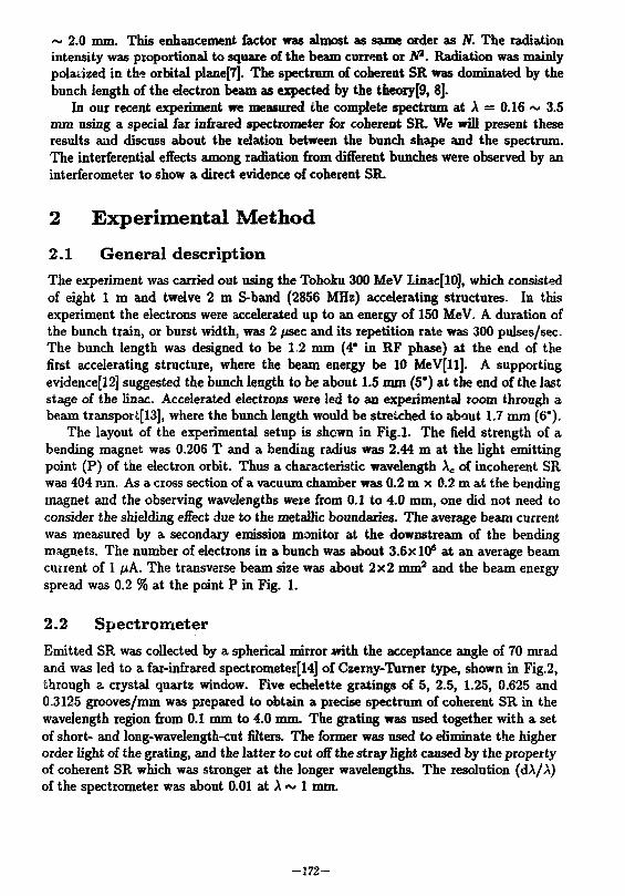
~ 2.0 mm. This enhancement factor was almost as same order as N. The radiation intensity was proportional to square of the beam current or N2. Radiation was mainly polarized in ths orbital plane[7]. The spectrum of coherent SR was dominated by the bunch length of the electron beam as expected by the theory[9, 8].

In our recent experiment we measured the complete spectrum at A = 0.16 ~ 3.5 mm using a special far infrared spectrometer for coherent SR. We will present these results and discuss about the relation between the bunch shape and the spectrum. The interferential effects among radiation from different bunches were observed by an interferometer to show a direct evidence of coherent SR.

2 Experimental Method

2.1 General description The experiment was carried out using the Tohoku 300 MeV Linac[10], which consisted of eight 1 m and twelve 2 m S-band (2856 MHz) accelerating structures. In this experiment the electrons were accelerated up to an energy of 150 MeV. A duration of the bunch train, or burst width, was 2 psec and its repetition rate was 300 pulses/sec. The bunch length was designed to be 1.2 mm (4* in RF phase) at the end of the first accelerating structure, where the beam energy be 10 MeV[ll]. A supporting evidence[12] suggested the bunch length to be about 1.5 mm (5*) at the end of the last stage of the linac. Accelerated electrons were led to an experimental room through a beam transpott[13], where the bunch length would be stretched to about 1.7 mm (6*).

The layout of the experimental setup is shewn in Fig.l. The field strength of a bending magnet was 0.206 T and a bending radius was 2.44 m at the light emitting point (P) of the electron orbit. Thus a characteristic wavelength Ac of incoherent SR was 404 nm. As a cross section of a vacuum chamber was 0.2 m x 0.2 m at the bending magnet and the observing wavelengths were from 0.1 to 4.0 mm, one did not need to consider the shielding effect due to the metallic boundaries. The average beam current was measured by a secondary emission monitor at the downstream of the bending magnets. The number of electrons in a bunch was about 3.6x 10s at an average beam cunent of 1 nA. The transverse beam size was about 2x2 mm2 and the beam energy spread was 0.2 % at the point P in Fig. 1.

2.2 Spectrometer Emitted SR was collected by a spherical mirror with the acceptance angle of 70 mrad and was led to a far-infrared spectrometer[14] of Czerny-Turner type, shown in Fig.2, through a crystal quartz window. Five echelette gratings of 5, 2.5, 1.25, 0.625 and 0.3125 grooves/mm was prepared to obtain a precise spectrum of coherent SR in the wavelength region from 0.1 mm to 4.0 mm. The grating was used together with a set of short- and long-wavelength-cut filters. The former was used to eliminate the higher order light of the grating, and the latter to cut off the stray light caused by the property of coherent SR which was stronger at the longer wavelengths. The resolution (dA/A) of the spectrometer was about 0.01 at A ~ 1 mm.

- 1 7 2 -

The intensity of SR was detected by a LHe-cooled silicon bolometer Ds with three long-wavelength-pass filters and its signal was transmitted to an amplifier which was phase-locked to a 10 Hz chopper mirror Ch. Radiation reflected by the chopper was converged onto a monitor bolometer Dj*, which was used to correct the SR inten­sity fluctuation caused by the drift of the electron beam intensity. The radioactive background noise into the detectors was measured to be negligible. All the optical components were set in a vacuum chamber to eliminate the absorption loss due to the water vapor.

The absolute sensitivity of the measuring system was calibrated[14] by a blackbody radiator, which was a graphite cavity and was located at the emission point of SR. The temperature of the black body was kept at 1500 ± 1 K during the calibration. The accuracy of the absolute intensity measurement of coherent SR was estimated to be within a factor of 1.5 after this correction.

2.3 Interferometer An interference experiment was carried out to clarify the emission mechanism of coher­ent SR. An interferogram of pulsed SR from the successive bunches was measured by a polarizing interferometer[15]. The schematic layout of the interferometer is shown in Fig.3. Radiation which tras emitted by a bunch was delayed by AX, the optical path difference between two arms, and interfered with another radiation which was emitted by the next bunch. The distance between the successive bunches Lg was 104.97 mm, which corresponded to the wavelength of the accelerating RF. As the variable range of AZ was from -9 to 110 mm, it covered the bunch distance LB. Two wire grid polariz­ers, WGl and WG2, had the wire spacing of 25 pm. The wire direction of WG1 was placed at an angle of 45* to the electron orbital plane, and that of WG2 was at 0*. Radiation was detected by two LHe-cooled Silicon bolometers; one was used to observe the interfeiogram and the other was used to monitor the intensity of SR.

3 Experimental Results

3.1 Spectrum of Coherent SR As is shown in Fig.4, the complete SR spectrum was obtained in the wavelength region of 0.16 ~ 3.5 mm. Radiation intensity is normalized for an average beam current of 1 fnA, which corresponds to N = 3.6 xlO 6. The spectrum is continuous in these wavelengths and shows a broad peak at A ~ 1.5 mm. The intensity decreases rapidly for A < 0.5 mm. As the calculated intensity of incoherent SR (see Eq.(l)) is 6 xlO 6

[photons/sec/mrad/1% BW] at 1 /xA and A = 1 mm, the enhancement factor at this wavelength is obtained to be 3.3 x10 s, which is almost as same value as N.

3.2 Estimation of the bunch length The spectral intensity of incoherent SR was derived by Schwinger[16]. For a bunch which has N electrons in it, the spectral intensity of incoherent SR at an angular

- 1 7 3 -

frequency OJ is given by

where p is the bending radius, 7 is the beam energy in units of the electron rest energy, u0 = c/p is the revolution frequency, wc = (3/2)w 07 3 is the characteristic frequency of SR and Jfi(f) is the modified Bessel function. According to the classical electromagnetic theory[2, 6], the intensity of coherent SR /a*(w) is given by

/«*(") = Iincok{<*){l + (N- 1)F(W)} (2)

F(w) = I / e>unrlcS(r)dif (3)

where S(r) is the density distribution of electrons in a bunch, n is a unit vector toward the observing point and F(u) is a bunch form factor defined by the Fourier transform of S(r). The value of the bunch form factor varies from zero at wavelengths A <£ aL

(incoherent limit) to unity at A 2> 07, (coherent limit), where ox, is the longitudinal bunch size.

Assuming that the bunch shape S(r) is an even function of r, we can estimate the bunch shape by using the Fourier transform from the observed SR spectrum. Estimated bunch shape is shown in Fig.5. The bunch shape resembles a Gaussian function with a sharp peak. The longitudinal bunch length is about 0.25 mm at full width of a half maximum, which is much shorter than the bunch length of 1.7 mm estimated from the characteristics of the linac.

According to the asymptotic property of Eq.(3), the bunch form factor for A > 1.6 mm should increase monotonically to unity, as the wavelength increases. On the contrary, the observed bunch form factor decreases towards longer wavelength. Two cases may be considered for this decrease. One is due to the bunch structure. The longitudinal bunch shape from the linac has some sharp spikes in it (see Fig.7). The other is the shielding effect by the electron beam vacuum chamber. Coherent SR might be suppressed by a metallic boundary condition.

3.3 Polarization of Coherent SR The degree of polarization P is denned as

P=ih-Ix)/{h + Is.) (4)

where I\\ and I± are the SR intensities which have electrical vectors parallel and per­pendicular to the orbital plane, respectively. The polarization of SR was measured to be P = 0.73 and 0.92 at A = 0.4 and 1.5 mm. Radiation is mainly polarized in the orbital plane. For comparison the calculated P's for incoherent SR for the same optical aperture are 0.64 and 0.77 at A = 0.4 and 1.5 mm. Diffraction correction must be done to compare these values with observed P's.

- 1 7 4 -

3.4 Interference of SR The observed interferogram is shown in Fig.6. It is clear that the interference modu­lation at around the optical pass difference A L=0 mm is repeated at around AZ = £ f l=105 mm. The first modulation at around A £=0 mm shows the interference of SR from a bunch with itself, and the second one at around A£ = 105 mm corresponds to the mutual interference with radiation from the next neighbor bunch. These two interference modulation patterns are congruous with each other within the accuracy of the experiment. That is, the first radiation emitted by a bunch has the same amplitude and phase as the second one by the next bunch. This is a direct evidence that observed radiation is coherent.

4 Simulation of the bunching process In order to examine a possibility of the sharp structure of the electron distribution in the bunch, the bunching process was simulated by tracking the longitudinal motion of the electrons. The bunches are produced in the injector section of the linac, which consists of an electron gun of 80 kV, a re-entrant type prebuncher of ±10 kV, a traveling wave type buncher of 2.6 MV/m, the first accelerating structure of 10 MV/m and drift spaces. The calculation was carried out according to the formulae[17, 18]

d ? e E • A az mo<r

and ^ = *L(± _ i_, ( . dz V A . & w

where y = 1/(1 — P?)1*2 is the total electron energy in units of the rest energy m^c2, <f> is the phase relative to an accelerating wave with phase ve!o. . t.y cfiv, E is the electric field gradient, A0 is the free space wavelength of the a> srating RF and z is an independent variable along the beam axis. As the energy ot the electron is about 10 MeV (pe = 0.9987) at the end of the first accelerating structure, and /?„ = 1.00 for the regular section of the linac, the right side of Eq.(6) can be regarded as zero at the downstream of the injector, i.e. the bunch shape is determined in the injector.

The bunch shape depends strongly on the relative phase of the RF supplied to the prebuncher, buncher and the first accelerating structure. One of the result of this simulation is shown in Fig.7. The main body of the bunch is 1.3 mm in longitudinal length and it has three spikes, which are about 0.1 mm. This result is not an exact but similar shape as our experimental condition, and is consistent with the result of Fig.5. The effects of the beam loading and the space charge are not taken into account in the above simulation. To consider these effects, a rough calculation was done by the one-dimensional disk model[19]. The beam intensity was so small that the results was almost same as Fig.7.

5 Conclusion There are two additional important results were obtained by the recent experiments.

- 1 7 5 -

1) The bunch length which is calculated by Fourier analysis of the radiation spectrum is consistent with the simulated result of the bunching process in the injector of the linac. 2)The coherent property of radiation was directly observed by the interfero­meter. In Tohoku 300 MeV Linac we are now preparing the equipments for the routine

application experiments. For example, a physical experiment to measure the reflectance of the superionic conductors has been started. In order to generate coherent SR in the far infrared region, we are developing a bunch compressor with a beam chopper to obtain a short bunch in the order of micrometers.

We thank the staff in the Laboratory of Nuclear Science for their technical support and assistance. We also express our thanks to Dr. M. Takahashi for his technical guidance on the blackbody radiation source, and Prof. I. Sato in KEK for his offering the program code of the one dimensional disk model.

References [1] L. I. Schiff, Rev. Sci. Instr. 17, (1946) 6.

[2] J. S. Nodvick and D. S. Saxon, Phys. Rev. 96, (1954) 180.

[3] F. C. Michel, Phys. Rev. Lett. 48, (1982) 580.

[4] J. Yarwood, T. Shuttleworth, J. B. Hasted and T. Nanba, Nature 312, (1984) 742.

[5] E. Schweizer, J. Nagel, W. Braun, E. Lippert and A. M. Bradshaw, Nucl. Instrum. & Methods, A239, (1985) 630.

[6] G. P. Williams, C. J. Hirschmugl, E. M. Kneedler, P. Z. Takacs, M. Shleifer, Y. J. Chabal and F. M. Hoffmann, Phys. Rev. Lett. 62, (1989) 261.

[7] T. Nakazato, M. Oyamada, N. Niimura, S. Urasawa, O. Konno, A. Kagaya, R. Kato, T. Kamiyama, Y. Torizuka, T. Nanba, Y. Kondo, Y. Shibata, K. Ishi, T. Ohsaka and M. Ikezawa, Phys. Rev. Lett. 63, (1989) 1245.

[8] T. Nakazato, M. Oyamada, N. Niimura, S. Urasawa, R. Kato, Y. Shibata, K. Ishi, T. Ohsaka, T. Takahashi, H. Mishiro, M. Ikezawa, Y. Kondo, T. Nanba and Y. Torizuka, Particle Accelerators, 33, (1990) 141.

[9] Y. Shibata, K. Ishi, T. Ohsaka, H. Mishiro, T. Takahashi, M. Ikezawa, Y. Kondo, T. Nakazato, M. Oyamada, N. Niimura, S. Urasawa, R, Kato and Y. Torizuka, Research Report of Laboratory of Nuclear Science, Tohoku University, 22 (10!*9) 151. (unpublished)

[10] Mitsubishi Denki Giho 42, (1968) 271-354 (special issue for Tohoku 300 MeV Linac, Mitsubishi Electric Co.).

- 1 7 6 -

[11] T. Toda, K. Irie and I. Uetomi, Mitsubishi Denki Laboratory Report 9, (1968) 117.

[12] M. Sugawara, T. Icbinohe, S. Urasawa, M. Oyamada, T. Kubota, A. Kurihara, 0 . Konno, Y. Shibasaki, T. Terasawa, K. Nakahara, S. Nemoto, M. Mutoh, K. Shoda and Y. Torizuka, Nucl. lustrum. & Methods 153, (1978) 343.

[13] M. Gotoh and T. Akiba, Mitsubishi Denki Laboratory Report 9, (1968) 175.

[14] K. Ishi, Y. Shibata, T. Takahashi, H. Mishiro, T. Tsutaya, T. Ohsaka, M. Ikezawa, Y. Kondo, M. Oyamada, N. Niimura, S. Urasawa, T. Nakazato and R. Kato, Research Report of Laboratory of Nuclear Science, Tohoku University, 23 (1990) 131. (unpublished)

[15] D. H. Martin and E. Puplett, Infrared Phys. 10, (1969) 105.

[16] J. Schwinger, Phys. Rev. 75 (1949) 1912.

[17] R. H. Miller, in The Stanford Two-Mile Accelerator, edited by R. B. Neal (W. A. Benjamin, New York, 1968)

[18] R. H. Helm, R. Miller, P. Brunet and X. Buffet, in Linear Accelerators, edited by P. M. Lapostolle and A. L. Septier (North-Holland, Amsterdam, 1970).

[19] S. Takeda, K. Tsumori, N. Kimura, T. Yamamoto, T. Hori, T. Sawai, J. Ohkuma, S. Takamuku, T. Okada, K. Hayashi and M. Kawanishi, IEEE Trans. Nucl. Sci. NS-32, No.5, (1985) 3219.

- 1 7 7 -

Fig.l. The experimental setup. P: light emitting point of SR, Ms: bending magnet, Mo: dumping magnet, SEM: secondary emission monitor, M t: collecting mirror, G: gratings, D s and Du: LHe-cooled detectors for signal and SR monitor, and CB-concrete blocks for radiation shield. Trajectory of bunched electron beam is shown by a chain line.

Fig.2. The optical layout of the spectrometer. M], M», Ms, M6, Ms, Ms, Mio and M13: plane mirrors, M3: spherical mirror, M<: scatter plate, M7: collimator mirror for monitor, Mn: collimator mirror, Mu: telescope mirror, L: high pressure mercury arc lamp, Ch: chopper mirror, P: polarizer/shutter, F: filter set, Si and S3: entrance and exit slits, Gj, G2 and G3: gratings, Gu- grating for monitor, LP: light pipe, T: turntable, V: vacuum tank and SR: synchrotron radiation.

- 1 7 8 -

MM WG2

Fig.3. Interferometer to measure the interference effect between the bunches. Ml, M3, M5 and M7-. plane mirrors, M2, M4 and M6: collimators, WG1 and WG2: wire grids, FM: fixed mirror, MM: moving mirror, DS : detector for signal and DM: detector for monitor.

1 0 ' 10" 10 WAVELENGTH (mm)

Fig.4. The observed spectrum of coherent SR.

-1 .0 -0 .5 0.0 0.5 1.0

BUNCH LENGTH r [mm]

Fig.5. The electron distribution function in the bunch obtained from the observed spectrum.

Optical path difference AL(vta)

J W/v^^J W-

& -V -i • i i 1 i 'A A & i> ti A * A tk -Optical path difference AL(.mm)

Fig.6. Interferogram of coherent SR. (a) Full picture. (b) Enlarged detail at around AL = 0 and 105 mm.

- 1 7 9 -

- 2 - 1 0 I 2 3

BUNCH LENGTH [ m m ]

Fig.7. One of the bunch shape calculated by the simulation of the bunching process in the injector of the linac.

- 1 8 0 -

Coherent Synchrotron Radiation in LEP

L. RlVKIN [PSI], A. HOFMANN AND B. ZOTTER [CERN] PSI, Villigen, Switzerland CERN, Geneva, Switzerland

1 I n t r o d u c t i o n

The fact that a bunch of accelerated charges will radiate coherently at waivelengths compa­rable or longer than the bunch length has been pointed out a long time ago [1]. The reason why this effect has not played a significant role in the past and present storage rings has also been explained, it is due to the presence of the conducting vacuum chamber that provides shielding [1, 2].

It turns out that at some of the proposed high luminosity e +-e~ colliders [3], where the bunch length required is rather short and the vacuum chamber apertures tend to be rather large, this effect may lead to a substantial increase in the RF power required to compensate for the radiation losses, and thus may become a limiting factor in the design.

Given the approximate nature of the estimates of the shielding effects due to the beam surroundings, it is of interest to try to observe the coherent emission of synchrotron radiation in an existing storage ring to help to improve the estimates.

2 Rev iew of t h e basic resu l t s

The ratio of the coherent radiation power to the incoherent one, emitted by a bunch that con­tains Nf, particles and has an rms bunch length of a, (gaussian distribution), is approximately [1,4]

where a is the half height of the vacuum chamber and p is the bending radius. Since the incoherent power itself is proportional to y* the above expression indicates that the coherent power is independent of the energy, as expected for the low frequency part of the synchrotron radiation spectrum. The vacuum chamber was modeled by two infinite conducting plates placed at a distance a above and below the beam. For comparison, if the shielding effect is neglected, this ratio becomes

"incoh *{£T$ «° - 5 f" ZX (2)

- 1 8 1 -

Table 1: Some LEP parameters at injection energy

Energy 20 GeV Average radius 4242.9 m Bending radius (dipoles) 3102 m Harmonic number 31320 Energy spread 3.1 • 10"« Momentum compaction 3.9 • 10" 4

Vacuum chamber half height 31 mm

We can rewrite the expression for the coherent power in terms of the average current per bunch It = efoNi,

2/3 5±.~_*.(±y(py * M °incoh ~ 224 \<rj \<T,J E[GeV]4 *incoh

where R is the average machine radius, and in terms of peak current I

PineoH~ SJ3 E[GeV]* (3)

where

'-^(S*-VB Ht

3 Turbulent bunch lengthening threshold

To estimate the amount of coherent radiation power we expect in LEP at injection energy (see Table 1) we first take note of the following fact. Above the threshold of the microwave instability, given by the so-called "localized Keil-Schnell"[8] or "Boussard" [9] criterion

7 = 2* EaS2

(4)

and as the average current increases beyond the threshold, both the bunch length a, and the relative energy spread 6 increase as a cube root of the bunch current

IT, <xl. 1/3 6x1, 1/3 /oc / i •2/3" (above threshold)

Thus above threshold the ratio of the coherent to incoherent power is roughly constant and it suffices to evaluate it at the threshold. To simplify things, we will use the "zero current" value of bunch lengt i below the threshold for the estimates. This simplification may not be correct for some machines where there is significant potential well bunch lengthening (e. g. in the SLC damping rings[5]), but the measurements of bunch length in LEP [7]. are consistent with either no bunch lengthening below the turbulence threshold, or even with some bunch shortening.

- 1 8 2 -

4 Effective impedance for short bunches

In the condition for the microwave instability threshold the MH is usually a constant, cor­responding to the case of long bunches. As the bunches become shorter, it is the effective impedance seen by the bunch, that has to be taken into account in Eqn. 4.

Here we are using a broad band resonator impedance model for LEP, with the resonator frequency fr = 2 GHz, taking the quality factor of the resonator Q — 1. Bunches are considered short when

WrffJa « 1 <TT =

and the effective impedance to be used in the calculations of the threshold current becomes

W e / y 2 (wwr T O ) 2 | - | (5)

This model has worked well in describing the threshold and bunch lengthening data obtained recently at LEP at the injection energy[6], resulting in the effective impedance of LEP, de­termined from this model of only

W e / / 20 mil while — as 0.25ft

n

The impedance model for very short bunches will almost certainly have to be modified to reflect the correct behaviour of the impedance at high frequencies. The scaling of the effective impedance with bunch length can be checked at LEP since at injection energy we can shorten the bunches by both applying the extra RF voltage available at present (up to 400 MV) and by using the 90° phase advance per cell lattice (reducing the momentum compaction factor a by a factor of 2). With 400 MV RF voltage, we can make tr, = 2.5 mm, resulting in

W e / / :6mn

and with the 90° lattice we can further reduce the bunch length to tr, — 1.8 mm, reaching

i4mfi \nJeff

These values for the effective impedance approach the estimate for the so-called "free-space" or radiation impedance[10] for LEP

(-) = 300-1 = 2mQ ' Tad

5 C o h e r e n t power e s t ima te s for LEP

Taking into account the change in the effective impedance with bunch length, we can write down the threshold current as

^ = vfNTT^* 1 0" 3^ ( 6 )

v R (w>7wor

- 1 8 3 -

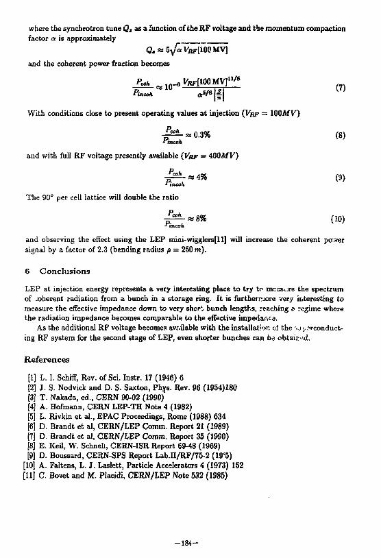
where the synchrotron tune Q,asa function of the RF voltage and the momentum compaction factor a is approximately

Q,«5yoVBF[100MV]

and the coherent power fraction becomes

Pes . . i n - 6 ^ [ 1 0 0 M V ] " / 6 . . .

With conditions close to present operating values at injection (VftF = lOOAf V)

•p^- « 0.3% (8) * I I M O A

and with full RF voltage presently available (VRF = 400MV)

*incaK

The 90° per cell lattice will double the ratio Pcoh _

4% (9)

*incoA (10)

and observing the effect using the LEP mini-wigglers[ll] will increase the coherent po-.ver signal by a factor of 2.3 (bending radius p = 250 m).

6 Conclus ions

LEP at injection energy represents a very interesting place to try to measure the spectrum of coherent radiation from a bunch in a storage ring. It is furthermore very interesting to measure the effective impedance down to very short bunch lengths, reaching a regime where the radiation impedance becomes comparable to the effective impedance.

As the additional RF voltage becomes available with the installation of the :.J ^conduct ­ing RF system for the second stage of LEP, even shorter bunches can be obtain-.'.d.

References

[1] L. I. Schiff, Rev. of Sci. Instr. 17 (1946) 6 [2] J. S. Nodvick and D. S. Saxton, Phys. Rev. 96 (1954)180 [3] T. Nafcada, ed., CERN 90-02 (1990) [4] A. Hofmann, CERN LEP-TH Note 4 (1982) [5] L. Rivkin et al., EPAC Proceedings, Rome (1988) 634 [6] D. Brandt et al, CERN/LEP Comm. Report 21 (1989) [7] D. Brandt et al, CERN/LEP Comm. Report 35 (1990) [8] E. Keil, W. Schneli, CERN-ISR Report 69-48 (1969) [9] D. Boussard, CERN-SPS Report Lab.II/RF/75-2 (19*5)

[10] A. Faltens, L. J. Laslett, Particle Accelerators 4 (1973) 152 [11] C. Bovet and M. Placidi, CERN/LEP Note 532 (1985)

- 1 8 4 -

Coherent Radiation in an Undulator*

Yong Ho Chin

Exploratory Studies Group Accelerator 8 Fusion Research Division

Laurence Berkeley Laboratory, Berkeley, CA 94720

Abstract

This paper is concerned with the synchrotron radiation from an undulating electron beam in a rectangular waveguide. The analysis is based on the dyadic Green's function approach to solve Maxwell's equations in terms of the vector potential. It is shown analytically and numerically that the radiated energy spectrum may differ significantly from the free space result when the undulator length divided by the Lorentz factor of the electron beam is larger than the transverse size of the waveguide. Then, the appearance of the spectrum is changed into a small number of sharp peaks, each corresponding to an excited waveguide mode. The undulator radiation is identified with the wake field in beam instabilities. The concepts of wake function and impedance are introduced to formulate the present problem in the same manner as the beam instability problem, so that the accumulated techniques of the latter can be applied. It is shown that the obtained impedances satisfy the Panofsky-Wenzel theorem and other properties inevitable for wake fields.

Introduction

An (plane) undulator is a device to produce high-flux quasi-monochromatic radia­tion in a narrow angular cone in the forward direction. A relativistic charged particle travelling in the undulator undergoes transverse oscillations and emits multipole radi­ation. Interference effects between the radiation fields from different poles compress the spectrum to sharp peaks. Most works on the undulator refer to radiation in free space. In reality, however, undulators are surrounded by metallic boundaries, such as a vacuum chamber. Then, the first question arises:

(1) How will the properties of the undulator radiation be changed when the bound­aries are taken into account?

The radiation fields in the waveguide are modified when they reach the boundaries because they must satisfy the boundary conditions. When their wave properties match those of waveguide modes, they can survive and propagate in the waveguide. The radiated energy is redistributed among such waveguide modes. In consequence, the energy spectrum tends to change from a monotonously increasing function to discrete sharp peaks, each corresponding to an excited waveguide mode. This change is particularly of interest in the low frequency region, where the waveguide modes are

* This work was supported by the Director, Office of Energy Research, Office of Basic Energy Sciences, Materials Sciences Division, the VS. Department of Energy under Contract No. DE-AC03-76SF00098.

- 1 8 5 -

well separated. The redistribution of the radiated energy into these few modes will enhance their power significantly. If the wavelength of a waveguide mode is larger than the bunch size, the whole bunch is reinforced to move collectively by the waveguide fields. This may cause a new type of collective instability.

So far, only a few studies have been done on the influence of metallic boundaries on the radiation.1,2* Motz and Nakamura1) gave the first discussion on the subject by means of the Herzt vector approach to solve Maxwell's equations for an infinitely long undulator. In this paper, we present a general method to calculate the radiation fields from an undulator with finite length in the presence of a rectangular waveguide. The method is actually a generalization of Motz-Nakamura's Hertz vector method.

Once the radiation fields are calculated, the next question arises:

(2) How will the radiation fields disturb the motion of particles in a beam?

In this question, both the high and the low frequency parts of the radiation play important roles. The high frequency part will contribute to the bunching of particles on a microscopic scale, which induces coherent radiation from particles in the same bunch. This is the stimulated emission process in FEL's. The low frequency part, if it contains significant energy, will drive collective motion of the whole bunch. In both cases, the particles and the radiation fields create a coupled system. Our ultimate purpose is to solve this particle-radiation system in a self-consistent way. To this end, it is necessary first to formulate the action of the undulator radiation fields on particles. We have a similar situation in beam instability problems.3' A charged particle interacts with its environment to create a wake field. This field acts back on the beam and disturbs the particle motion. This particle-environment system may be identified with the present particle-radiation system. With this in mind, we introduce the concepts of wake functions and their Fourier transforms, impedances.

Vector Potential

Any solutions of Maxwell's equations may be expressed in terms of the scalar poten­tial $ and the vector potential A. Under the Lorentz condition, Maxwell's equations are equivalent to the two inhomogeneous wave equations for • and A:

V ' A 4 l £ " ~* <» where c is the speed of light, p is the charge density, J is the convective current 'density, e is the dielectric constant, and p is the permeability. Since the scalar potential $ can be calculated from A using the Lorentz condition, our task is to seek a solution for the vector potential only. To solve Eq. (2), it is useful to find a Green's function G which is defined as a solution of the following equation with appropriate boundary conditions:

a'GMIr'.O - l ^ 6 - - -M(r-iO«(«-0, (3)

- 1 8 6 -

where G is a 3 x 3 matrix, the so-called dyadic Green's function, 4' and I is the unit dyadic. A solution of Eq. (2) is calculated from

A(r,r) = pjj G(r,t\r\t')3[r',l!)d*i>dt>. (4)

In rectangular coordinates x,y and z, the solution G of Eq. (3) has only diagonal terms. The geometry of concern may be that part of a considerably longer waveguide that is sandwiched by the undulator of finite length. We assume that the walls have infinite conductivity. We denote the inside region of the waveguide by 0 < x < a and 0 < y < b. Then the solution is written as4)

G(r,<ir',o=̂ E E u. r +r d^^Tr^^'-'^^, 4 x m,«>0 »«.».* J-°° J-°° r-0>i/C+cZtm

(5) where , _ (H^\2 , / n y \ 2

Here i„(i/ = x, y, z) is the unit vector, rj. is the transverse component of r, and i„i„ is an operator such that (i„i„) • a = (i v • a)i„ for any vector a. The functions <f>mny(r±) are the eigenfunctions of waveguide modes with real eigenvalues.4)

The integration over p in Eq. (5) can be done readily using the residue theorem. The result is

G(r,*|r',0 = - ^ - E U , r d b ^ = = ^ ^ = = ^ e ^ - « ' ) e - i * - - l * - * ' l , " x m.iw/ J-o° *Pwm

(7)

where /U = ^/l-£)***,,. (8)

Let us consider a single electron moving in the x — z plane. It enters the undulator at x = xo, y = Jfo, z = zo at time t =* 0. The undulator has length L. We assume that the particle's motion is described by

x = siawot + Xo, (9) 7«<*>

y = 9b, (io) z = vt + zo, (11)

where K = ^ j - , B is the undulator field, w&(= *?•) is the undulator frequency, 7 is the Lorentz factor of the electron, m is the electron rest mass, and v is the initial longitudinal velocity of the electron. In Eqs. (9)- ( l l ) , we have kept only the lowest order terms in powers of fc/7, assuming ic/7 < 1 (weak field approximation). The longitudinal velocity modulation term of second order in * is neglected in the RHS of Eq. (11). It contributes mainly to higher order harmonics.

If we insert Eq. (7) and the current densities corresponding to the undulating motion, Eqs. (9)-( l l ) , into Eq. (4) and carry out the integration over volume r*x and time t' (0 < t' < L/v), we have for A(r, t)

1 roo /*_,'Wp-A»»H' 1\ A(r,0 = ^ " E E W ~ ~ ( r x ) W / <**L, J^-aW*-*.),

2 ™ £Z,V _o6<?Coo J - o a 2€Pmn[P, - Pmn) (12)

- 1 8 7 -

where

and the explicit forms of ImKty are given by

^ = w _ p u ^ ; p = : integer ( i 3 )

/»» , . - euo^Fmn» (14)

/«»» = 0, (15) = evFmmp, (16)

where

and J p (z) is a Bessel function. The harmonic number p emerges due to the expansion

of

(ct) [—•(•~ sinuif)t+xo)] by the Fourier series about ugt. In obtaining Eq. (12),

we have neglected the contribution from the backward radiation in the laboratory frame, i.e., the z < z1 case. This radiation covers only the tiny part of the Doppler down-shifted frequency range between pwb/2 and pwo-

Radiated Energy The power flow P along the waveguide is given by integrating the Poynting vector

over the waveguide cross section at the exit: P{t) = [' [\E x H) • udxdy, (18)

Jo Jo where E and B are the electromagnetic fields calculated from the vector potential A(r, t) given by Eq. (12) with XQ and yo set to the values at the center of the waveguide. The total radiated energy U is the time integral of P(t):

U= I" P(t)dt. (19) J-oo

This can be expressed by the Fourier transforms E(w) and H(w) of E(t) and H(t), respectively, as

U = 2x / " /* 1°* (E(w) x H » ) • \,dwdxdy. (20) JO JO J -oo

After tedious calculation, we have

<*- E E ^%r«M^. (2D m,n>0 — eo<p<oo °°

where

4e 2 , 2x

i 2 - 2/«*wa,™* as . f cos 2 (—) for p = odd — sm 2(—)J?( x . rfa (22) a6 fc ' v a TWO sin2( ) for p = even

-188-

?(£>/, , \ _ 1 t/u^ii i /F^W a \i\ (ft i ***»̂ 21 »fa8(& ~ Pm»)L/2 *•>») ~ W^ [ ( 7> ( 1 + (V } <5?> } " W - + Tn((ft-fcJW ( 2 3 )

where we have neglected the cross terms between different harmonics p. They drop out if the undulator is sufficiently long. The quantity Aj£^ depends on the particle orbit and provides the selection rule about mode number: n =odd, m + p =odd. On the other hand, the quantity Z^p(u) has the dimensions of impedance, and indeed can be identified as an impedance, as will be confirmed later. The product A!^pZj^r(u) represents the energy flow of the radiation of the p-th harmonic from the undulating electron into the waveguide mode specified by (m,n). Note that Zj£}p(w) is always positive and is an even function of w, being accompanied rrith a change in sign of p.

Now let us take a close look at Zj$p(u). The sink function 1ffif&^£/|jr represents phase matching condition. The straight line 0 = 0P = ™~™ expresses the resonance condition between the particle and the radiation field of the p-th harmonic. The curved line 0 = 0mn = 7^1 — (^)2o*„, or 02 = (*f)2 — o^ represents the dispersion relation of the structure for the waveguide mode (ro,n). The factor ^ f ^ ^ f ^ r is peaked at the frequencies where the two lines cross. The two intersections correspond to the excited waveguide modes which move together with the electron having the same speed, so that they can interact over a prolonged period of time. The peak frequencies are obtained by solving 0P = pmn for u. The result is

v I c* w = w± = 72[pwo ± - y (pwo)2 - ^a&J. (24)

The signs + and — correspond to the Doppler up- and down-shifted frequencies of the radiation fields emitted in the forward and the backward directions, respectively, in the electron rest frame.

Figure 1 shows an example of the energy spectrum. The parameters used, 7 = 5.9, A0 = the undulator wavelength = 2.77 cm, a = 13.34 cm, 4 — 1.9 cm, and N — L/Xo = 258, are relevant to those of the University of California at Santa Barbara (UCSB) FEL. The peak frequency corresponds to the wavelength of 0.4 mm. The free space spectrum denoted by the broken line is drawn for comparison. One can recognize that the interference effects due to the boundary change the spectrum significantly from the free space result.

A criterion for the transverse size of the waveguide for which the boundary effects may be neglected (we assume always a>b)

b>Lh (25)

can be derived from the following physical consideration. In the electron rest frame, the length of the undulator is Z/7. If the radiation emitted at the entrance of the undulator cannot, after bouncing at the boundary, come back to the electron by the time when the electron gets out of the undulator, the electron cannot know the existence of the boundary. In other words, since the information about the boundary does not reach the electron, the boundary effects cannot influence the interaction properties between the electron and the radiation fields. The fastest information may be brought back by the fields radiated into the purely vertical direction. It takes time b/c. This value has to be larger than L/{ic).

- 1 8 9 -

0.30E+01

dU <?NK2

du/{ 4ec '

0.15E+01 -

O.OOE+00 0.OOE+00 0.50E+00

w/(2w»72) 0.10E+01

Figure 1: Radiated energy spectrum of UCSB FEL. The free space result is denoted by the broken line.

Wake Function and Impedance

We here would like to study the action of the radiation on particles in a beam. If we are allowed to neglect the perturbation in particle motions due to the radiation fields while particles go through the undulator, we can apply the concepts of wake function ar •'. its Fourier transform, impedance.3) Suppose a charged particle travelling through an undulator, emitting the radiation. We call it the driving particle. Imagine another particle (test particle) which moves together with the driving particle keeping the fixed distance Z = Tv. The wake function is defined by the total Lorenzt force exerted on the test particle over the structure from the radiation fields. The test particle may go either ahead of or behind the driving particle. This is the peculiar point of the present problem different from the beam instability case where we consider only the test particle following the driving particle since there is no fields ahead of the driving particle. The wake function contains the longitudinal and the transverse components. They may be written explicitly as

Jfrf^dtp-iEt-v,!},),

J d*r J " dtp(Ev + vzBz - vz%),

WX(T)

Wy(T)

WAT) = -Jd^rJ^dtpfE.+v^), rT+i

(26)

(27)

(28)

- 1 9 0 -

where p is the charge density of the test particle. Note the minus sign in the definition of the longitudinal wake function. This follows the convention of the beam instability formalism where WZ(T) is always negative, i.e., the test particle is decelerated, in the vicinity of the driving particle. If the test particle is the same particle as the driving one (T = 0), the longitudinal wake function gives the energy loss of the particle due to deceleration by its own fields. This energy loss is nothing but the total radiated energy, namely,

Wx(0) = U. (29) The wake function generalizes the concept of the radiated energy to the case where the particle that creates the radiation fields and the particle that feels them are different.

Carrying out the integration in Eqs. (26)-(28), we obtain,

m,n>0 —oo<r<oo Mtfv "mnpv(-l ) (30)

with

where

twco= 1 /°° - T

— I ZmnfV(u)e du for v = x or y

/ Zmnpv(u)e?*Tdu for v = z > J—oo

(31)

M = mx a

mx v c c c v & v 2ewfl sm*(/3p-0mn)L/2

X ( ( A , - / ? m I . ) I / 2 ) ' ' (32)

J mnpy M = 6 a tfU.puo.2 ( a • Pu°\ . v2WT*m2{0,-0m*)L/2 tlJZ—YZ.tt—Z.Y — (ft j . r~v\ j . _ _ l 2^mn

X{mx) v( c } {Pm» + v } + <? v'Ofi, - 0mn)L/2)* '

Jmnpz («) = 5-%-{(—r/w—)2- 2

puo 2 1 a> - pup, sin2(fl, - ftmn)L/2 r-

(33)

(34)

and we have neglected the cross terms between different harmonics p. As in the previous section, we call ZmHpv(w) the impedance. The explicit forms of An*^ are as follows:

e 2 4 L 2 ,7TIX . . .JBX . . .TIT . . .TIT » ¥ 2 / f O T CK . , —-^ix»{-—x0)s^{-—x1)sm{-^)sm{-ryi)3l{ ) forp = odd IT ao a a o o r a -ywo e2 4L2 . ,mx . ,IOT . . .nx . ,n* » , 2 / m * c»c . , 7-sm( ar0)cos( xi)sm(—jfo)sin(-7-yi)J;( ) forp = even, ST ao a a o o a "J/WQ

*mnj>x •

(35)

Amnm — '

e 2 AL1 ,mr . ,mi . . .nx . .nx «¥o,tnx at . , 7- cos(—-io) cos(—-x,)sin(-T-y 0)<™(^Vi)Ji(——) » P = odd

2x ao a a o o r a fuo e 4£ . ,tnx . . ,mx . . ,nx . , B T l r f , n i T c« . . r 7- sin( x0) sm( i i ) sm(—yo) cos(-7-j&)Jf ( ) for p = even, AT ao a a o o r a fuo

(36) ,rnx ,mx . . ,nx . .nx . »,7nx CK . r ,.

cos( x0)cos( *i)sin(-j-y0)sin(-7-yi)J'( ) for p = odd

e ^ 4 ^ 2x ai a 7fa\>

mx cic c- 4If* . ,n>T . .m- , . .»IT . nx , l 2 / n w CK . r s , n ( *o)s"H *iissnv-r-yo)»n(-r-yiW;( ) forp = even.

2x ab a a t> o ' a "JJVQ (37)

- 1 0 1 -

Some conclusions may be drawn from inspection of Eqs. (30) to (37). (1) The transverse impedances are odd functions of frequency w in connection with

the change in sign of p:

ZmKrv(w) = ~.Zm»,_^(-w) > 0 forv = xory , (38)

while the longitudinal impedance is an even function of w:

Zmnpx(u) = £™,-„(-w) > 0. (39)

This implies that Wrm«^(0)=0 for i/ = x or y (40)

which means that a particle receives no net transverse force from its own radiation. (2) If we take the limit of infinitely long waveguide, i.e., L —» oo, we find that the

following relationships hold between the transverse and the longitudinal impedances for the same set of (m,n,p)

Zmn^(w) = HL^*(JL)Znn„(u), (41)

iw(«) - ,^T±^)z'-^uy («) V IMF

The above relationships are quite similar to the Panofsky-Wenzel theorem3' except for the factor (u — puo)/v instead of utfv. The appearance of B» might originate from the characteristics of the undulating orbit of the particle.

(3) From Eqs. (35)-(37) and (30), we notice that

Wx(T) = 0 if * 0 = * i « | , (43)

W,(T) = 0 iflto = Jfc = f. (44)

This is obvious from the geometrical symmetry of the particle trajectory and the wave guide.

In carrying out the integration in Eq. (31), it is necessary to separate the frequency range of the integration in impedance according to the sign of T. Namely, the test particle lagging behind or going ahead of the driving particle sees a different frequency range of the impedance. There is the following physical reason for this case distinction. For simplicity, let us consider the radiation in free space. In the electron rest frame, Power flow to the radiation must be the same in the forward and backward directions for symmetry. Most of the backward radiation in the electron rest frame is turned around into the forward direction in the laboratory frame by the Lorentz transformation. The plane z' = 0 perpendicular to the z'-axis in the electron rest frame now forms a narrow cone about the z-axis with the angle 8 = 1/7. This cone sets the border that separates the two kinds of the forward radiation having different origins. The radiation inside and outside of the cone correspond to the forward and the backward radiations in the electron rest frame, respectively. The test particle lagging behind the driving particle in the laboratory frame is also sitting behind it in the electron rest frame. Therefore it can feel only the backward radiation in the rest frame. It sees the forward radiation

- 1 9 2 -

outside of the cone and the backward radiation in the laboratory frame. The test particle going ahead of the driving particle sees the forward radiation in the electron rest frame and the corresponding forward radiation inside of the cone in the laboratory frame.

The frequency of the radiation fields emitted along the cone can be easily calculated from the Lorentz transformation: that is i^amc — PWBT2 which is just half the peak frequency 2pu>of2. The backward radiation in the laboratory frame covers only the very low frequency region from pufe/2 to jwo. Its total power is about T 2 times smaller than that of the forward radiation. Thus, the backward radiation may be neglected for ultra-relativistic particles. From the above arguments, we can conclude that for T > (<)0, i.e, when the test particle lags behind (goes ahead of) the driving particle, the integral in Eq. (31) should be done over the frequency range from 0 (puof2) to puo-y2 (oo).

Figure 2 shows an example of the longitudinal wake function. Again, the parameters are taken from those of the UCSB FEL. One can see that the wake function is significant only in the close vicinity of the driving particle (AT ~ 2T/(U*J7 2)). This is due to the rapidly oscillating phase factor e*"7 in the integrand for large T. The broken line denotes the wake function from free space radiation. Even for a small value of the transverse size, no large differences in the wake functions are recognizable, although the energy spectra are quite different (see Fig. 1). This suggests that the free space radiation result for the wake function may be used as a good approximation to any structure.

If we compare Eqs. (21)-(23) with Eqs. (30)-(37) and neglect the quantities smaller than the leading term by a factor f2, we can conclude that

\(WI(0+) + Wt(0-)) = U=W,(0)- (45)

This approximation is consistent with having ignored the longitudinal velocity modu­lation term in Eq. (11) and the backward radiation in the Green's function. In fact, the relationship(45) is a physical consequence of energy conservation and can be de­rived from the following thought experiment. Suppose that the test particle follows the driving particle at an infinitesimal distance and that they have opposite unit charges. Here the test particle is a real particle, i.e., it also emits radiation. Both particles lose energy U by radiation, while the test and the driving particles gain an energy W,(0_) and W,(0+), respectively, from the fields radiated by the other particle. When they are put together, the charges will be neutralized and the radiation is suppressed. In order for the total energy to be conserved, we need

W,(0+) + W,(0_) = 2tf ( 4 6 )

which agrees with Eq. (45). The above relationship is a modified form of the funda­mental theorem of beam loading.3)

- 1 9 3 -

0 . 1 2 E + 0 1 A- 2 8 . 0 B - 4 . 0 GAMMA- 5 . 9 N P - 2 5 8

- . 1 0 E + 0 2

2W072

Figure 2: Longitudinal wake function of the UCSB FEL.

Conclusions

The identification of the undulator radiation with the wake field in beam instabilities seems to be proper. The difference is only that the wake function is significant mostly ahead of the driving particle in the case of undulator radiation, while it is non-zero only behind the driving particle in usual wake fields. The longitudinal wake function includes necessary information on how particles will be accelerated or decelerated by the radiation fields. From this, one can calculate the bunching of particles and eventually explain the stimulated emission process. In the analyses of FEL behavior so far, the bunching has been estimated by picking up only the radiation field emitted on axis in the forward direction. As a result, the wake function becomes a periodic function of the. distance from the driving particle, and one needs to impose an arbitrary upper limit on the distance that the force can reach. The present analysis removes such arbitrariness. Future study will be aimed towards solving the particle-radiation system in a self-consistent way in order to clarify the coherent radiation mechanism.

References

1. H. Motz and M. Nakamura, Ann. Phys., 7, 84(1959). 2. Y. H. Chin, in Proc. of the 1989 IEEE Particle Accelerator Conference, (Chicago,

IL, March, 1989), pp. S09-S11. 3. A. W. Chao, SLAC Report, SLAC-PUB-2946, June, 1982. 4. R. E. Collin, Field Theory of Guided Waves (McGraw-Hill, New York, 1960).

- 1 9 4 -

List of Participants

Jiunn-Ming Wang Brookhaven National Laboratory

AlessandroG. Ruggiero Brookhaven National Laboratory

Joseph John Bisognano CEBAF

EberhardKeil CERN

Bruno Zotter CERN

Roberto Cappi CERN

Fritz Caspers CERN

Klaus Balewski DESY

Takeshi Nakamura Electrotechnical Laboratory

Laurent Farvacque European Synchrotron Radiation FacMty

King Yuen Ng Fermilab

AkiraNoda INS, Univ. of Tokyo

Chihiro Ohmori INS. Univ. of Tokyo

Hiromi Ofcamofo Inst. Chemical Res., Kyoto Univ.

Elena N. Shaposhnikova Institute for Nuclear Research

Alexander A. Mikhailichenko

Institute of Nuclear Physics

Nikolay Sergey Dikansky Institute of Nuclear Physics

Dmitri Pestrikov Institute of Nuclear Physics

James A. Holt KEK

Kohtarou Satoh KEK

H. Sugawara KEK

S. Suwa KEK

H. Hirabayashi KEK

Yoshtharu Mori KEK

Y.Kirnura KEK

Kohji Hirata KEK

Susumu Kamada KEK

Eiji Kikutani KEK

Shin-tehi Kurokawa KEK

Shinji Machida KEK Norio Nakamura KEK

Katsurobu Otde KEK

Tetsuo ShRJara KEK Toshto Suzuki KEK

Takanori Toyomasu KEK

- 1 9 5 -

List of Participants

Junjt Urakawa KEK

isaoYamane KEK

KaoruYokoya KEK

Masakazu Yoshioka KEK

HaruyoKoiso KEK

Shyogo Sakanaka KEK

Ryukou Kato Lab. of Nuclear Science, Tohoku University

Satoshi Niwano Lab. of Nuclear Science, Tohoku University

Takeshi Eguchi Lab. of Nuclear Science, Tohoku University

Toshihaiu Nakazato Lab. of Nuclear Science, Tohoku University

Tsutomu Taniuchi Lab. of Nuclear Science, Tohoku University

Michael Gerard Bflfing Lab. of Nuclear Studies, Cornell University

Marie Paule Level Lab. LURE ORSAY

Yong Ho Chin Lawrence Berkeley Laboratory

Tai-Sen F. Wang Los Alarms National Laboratory

Masao Takanaka NFDD. Mitsubishi Electric Corporation

ShuichiOkuda Osaka University

Leonid Z. Rivkin Paul Scherrer Institute.

Ainosuke Ando RCNP, Osaka University

Robert Wamock SLAC

Samuel A. Heifets SLAC

Ronald 0. Ruth SLAC

Karl Bane SLAC/KEK

Shkjeki Sasaki SRF.Insttute of Physical & Chemical Research

WeirsnChou SSC Laboratory

Alexander W. Chao SSC Laboratory

Chen Shiung Hsue Synchrotron Radiation Research Center

Richard Abram Baartman TRIUMF

Robert L. Gluckstem University of Maryland

- 1 9 6 -