Superpositions of multifractals: Generators of phase transitions in the generalized thermodynamic...

$: Superpositions of multifractals: Generators of phase transitions in the generalized thermodynamic formalism$
Journal of Statistical Physics. Iiol. 82, Nos. 3/4, 1996

Superpositions of Multifractals: Generators of Phase Transitions in the Generalized Thermodynamic Formalism

Giinter Radons ~ and Ruedi Stoop 2

Received February 28, 1995

We investigate the superposition of multifractals in the generalized thermodynamic formalism. It is shown analytically that phase transitions of first and second order are obtained and that the topology of the corresponding critical lines endows bicritical behavior. We demonstrate that these phase transitions can be observed in the spectrum of fractal dimensions and in the spectra of related quantities. Therefore, the obtained results are of importance for the interpretation of experimental systems.

KEY WORDS: Multifractals; generalized thermodynamic formalism; projections of fractal measures; phase transitions.

1. I N T R O D U C T I O N

In many exper imental s i tuat ions it is impossible to observe the full mult i - fractal s tructure of the object of interest since the desired informat ion is only accessible in the form of projections. Examples are the observat ion of clouds, images of fractal structures in the universe, or, quite generally, of fractal s tructures with d imension larger than that of the image. F o r a mult i - fractal analysis, to derive the consequences of such a s i tuat ion consti tutes a nontr ivial theoret ical problem. Correspondingly there exist only very few general results for this problem, cl-3~ A related but simpler s i tuat ion is obta ined if one considers the superposi t ion of two or more independent multifractals with measure. Such sums of mult ifractal measures, which can

t lnstitut f'tir Theoretische Physik, Universit/it Kiel, D-24118 Kiel, Germany. E-mail: [email protected].

2 lnstitut fiir Theoretische Physik, Universit/it Ziirich-Irchel, CH-8057 Ziirich-Irchel, CH-8057 Ziirich, Switzerland. E-mail: [email protected].

1063

0022-4715/96/0209-1063109.50/0 �9 1996 Plenum Publishing Corporation

1064 Radons and Stoop

be regarded as a special case of the projection problem, give rise to nontrivial behavior even in the simplest case: In ref. 4 it is shown that sums of multifractal measures supported by the same equal-scale Cantor set lead to first- and unexpected second-order phase transitions ~5-8~ in the thermodynamics of multifractals. ~9-14~ Here we extend these results to the case of multiscale Cantor supports. The appropr ia te tool for the investigation of this more general case is the generalized or bivariate thermodynamic formalism as elaborated in refs. 15 and 16 and reviewed, e.g., in refs. 17 and 18.

2. RESULTS

In the following we consider sums of multifractal sources where all of the sources are complete, self-similar two-scale multifractals with multiplicative measures. One of these multifractals is then determined by the probabilities P,,P2 and the associated length scales Ii, 12 (see, e.g., refs. 19 and 20). The hierarchical structure of this multiplicative process is captured in the generalized parti t ion sum ~j ~' ~4-241

Z,(q, fl, N ) = ,r,-,t"q/•+ (pq2l~) g (1)

where N denotes the level of the construct ion hierarchy. The probabili t ies are normalized: Pl +P2 = 1. In order to label the M independent com- ponents we use the index v. Accordingly, the system is characterized by the set of quantities pi(v), li(v), where i = 1, 2 and v = 1 ..... M. In the following we investigate the case of the superposit ion /t of M = 2 multifractal measures/1( 1 ) and ll(2), i.e., It = ~z( 1 ) ll( 1 ) + ~(2)/l(2), where the parameters 7~(v) are the weights of the contributions of the involved multifractals [n( 1 ) + n(2) = 1 ]. A further simplification is obtained if the supports of the two measures are the same. This implies t h a t / i ( 1 ) = / , ( 2 ) = 1~ for all i. The parti t ion sum of such a superposit ion then has the form

Z(q, fl, N)= ~ [x(1)pl(l)Jp2(1)N-J+rc(2)p,(2)Jp2(2)g-J]q j=O

x (/J IN-J)/ ' (2)

In the following we assign without loss of generality the index v = 1 to the system with the larger value of p~, i.e., p~( 1 ) > pt(2). In order to evaluate the parti t ion sum of Eq. (2) in the limit of large N, we introduce the ratio

=j/N and write Z as an integral

f2 Z(q, fl, N) ~ e -Ng(~''q'/') d~ (3)

Superpositions of Multifractals 1065

For n( 1 ), n(2) ~ 0 the function g is composed of two contributions:

g(~, q, fl) = g,(~, q, fl) 0(~ - ~o) + gz(~, q, fl) 0(~o - ~)

with

(4)

g,,(~, q, fl) -- ~ In ~ + (1 - ~ ) ln(1 - ~ )

- ~ [ q l n p t ( v ) + f l l n l l ] - ( 1 - ~ ) [ q l n p 2 ( v ) + f l l n 12] (5)

where O(x) denotes the step function and G0 has the value

~0 = { 1 + ln[pl(2)/pl(1)]/ln[p2(1)/p2(2)] } - i (6)

This value is derived from the condition that the contributions from sources 1 and 2 to the partition sum are of the same order in the thermodynamic limit. With the saddle point approach the generalized free energy

r(q, fl) = - lim ln[Z(q, fl, N)] /N (7) N ~ r

can be written as

r(q, fl) = g( ~( q, fl), q, fl) (8)

where ~(q, fl) maximizes the integrand in Eq. (3) by minimizing the function g for given q and ft. Because of the simplicity of the model, it is straightforward to investigate the analyticity properties of the system. Quite surprisingly, nontrivial phase transition scenarios are detected. This is demonstrated in Fig. 1 where we show two typical phase diagrams in the q-fl plane. It can be observed that there are three different domains in both situations. In each domain, r(q, fl) is analytic. The separation is by critical lines of first order (full lines in Fig. 1) or of critical lines of second order (dashed lines). At the intersection point B where two second-order phase boundaries merge into a first-order boundary, bicritical behavior 125"26~ is obtained, and B is called the bicritical point. In the following let us demonstrate these observations analytically. First, note that the value ~(q, fl) which "minimizes g determines r(q, fl) [cf. Eq. (8)]. We therefore concentrate on the location of the minimum of g. Since, according to Eq. (4), the function g is composed of two functions gl and g2, we end up with three distinct cases: In the first case the minimum of g is provided by the minimum of gl. Then r(q, fl) is equal to

rv(q, fl) = - ln [p l ( v ) q 1~ + P2(V) q l~] (9)


4 2

0

-2

-4

-6

-8

-i0

-12

phase 2 Y

phase 0/s" phase_.l s

i J

-4 -2 0 2 4

q

(a)

12

i0

8

6

2 0

-2 -4

phase_2

-- phase 0 ph2 is~ 1

(b)

-4 -2 0 2 4

q

Fig. 1. Two typical phase diagrams for the superposition of two multifractal measures p( 1 ) and/ t (2) [parameters: (a) pj( 1 ) = 0.9, p~(2) = 0.7, (b) Pt( 1 ) = 0.7, pl (2) = 0.1 ]. Generically, there exist three phases which are separated by critical lines of first (full lines) and second order (dashed lines). Their intersection point B is a bicritical point. Note that the phase diagrams do not depend on I I and 12 if p is measured in units of ln(Ijll) [ see Eqs. (11) and (12)]. Therefore, these units were used also in the following Figs. 2-7.

where v = 1. Note that this expression is just the free energy of the isolated first source. The second case arises analogously , with v = 2 . There is, however, a third case, which occurs if the m i n i m u m is found at ~ = Go [Eq. (6)] . In this case, the locat ion of the min imum is found at the intersection of the two branches g~ and g2; the corresponding r0(q, fl) is given by

r0(q, fl) = g(~)[~=r (10)

All three cases are obtained in Fig. l a if, for instance, the parameter q is held fixed at q = - 1 and fl assumes the values fl = - 2 , 1, and 4, respectively. F i g u r e 2 s h o w s th e c o r r e s p o n d i n g p i c t u r e s o f the free e n e r g y


g(r 2.2 2 1.8

1.6

1.4

0.2 0.4 0,6 0.8

(a)

g(~)

-6

-6.5

-7

-7.5

-8

j/ 0 .2 0.4 0,6 0.8

(b)

- t . 5 () -1.75

-2

c - 2 . 5

-2.75

-3

0 0.2 0.4 0.6 0.8

Fig. 2. The free energy functional giG, q, P), gq. (4), for each of the three phases on the line q = -1 . (a) p = -2 : A minimum on the right of the vertical line (located at Go = 0.3608... [ see Eq.(6)] means that the system is in phase_l corresponding to multifractal measure p(1) (b) p=4: The minimum is left of ~0, meaning that the system is in phase_2 where measure p(2) dominates. (c) A new phase_O appears if the minimum is at ~0, e.g., for p -- 1 (parameters as in Fig. lb with l l . = 1/3, / 2 = 1/9).

funct ionals g. In the f o l l o w i n g w e derive where the phase transit ions occur as a funct ion o f the variables q, fl and w e w o r k out the order o f the transitions. By a c o n t i n u o u s var iat ion of parameter fl we arrive at the s i tuat ions s h o w n in Fig. 3. T h e y are characterist ic for the transi t ion be tween phase_l and phase_O and b e tween phase_O and phase_2, respectively. It is n o w


Fig. 3.

0.25

0

-0.25

-0.5

-0.75

-i \

0 O. .4 0.6 0.8 1

(a)

3 // g(~) - ' (b)

-5.."

-6

0 0.2 0.4 0.6 0.8 1

Same as Fig. 2, with p chosen to hit second-order critical lines. (a) p =Pol: the minimum of gl(~, q, P) coincides with '~u; (b) p =Po2: arg min~ g_,(~, q, p) = ~o.

-i

-1.2

-1.4

-1.6

-1.8

~2nd order

-4 -2 0 2 4

Fig. 4. The first derivative of the generalized free energy at(q, fl)/afllq=_, is continuous at the critical points flo~(q= - 1 ) and flo2(q = - 1 ) , but discontinuous in the second derivative. This shows that here the phase transitions are of second order [parameters pi(v), li as in Fig. 2].


important to note that the phase boundaries flv~(q) between the phases v and 9 are obtained from the conditions rv(q, f l )= r~(q,/~). From this it is easily found that

flo,,,(q) = - ( I n ln[p~(1)/p~(2)] +q in p,(v)'~ /, Ii ln[p2(2)/p2(1)] p - - ~ . ) / m ~ (11)

where v = 1, 2. The order of the phase transitions is determined by the derivates of the free energy r(q, p). In Fig. 4, we again keep q fixed at the

i.i

1

0.9

0.8

0.7

, . . ~ , . ,

0 0.2 .4 0.6 0.8 1

(a)

g(r

0

-0.2

-0.4

-0,6

-0.8

0 0.2 .4 0.6 0.8 1

(b)

0.35

0.3

0.25

0.2

0.15

0.I

0.05

0

0.2 0.4 0.6 0.8

(c)

Fig. 5. Same as Fig. 2, but for q= l and (a) fl=-0.5, (b) fl=0.5, and (c) p=pu=0 . Obviously the "order parameter" Cmi. jumps at the transition from (a) to (b) via (c). This first-order behavior is verified in Fig. 6.


value q = - I and plot the analytically derived first derivative of r with respect to fl as we cross the phase border upon variation of ft. The con- tinuity of the first derivative and the apparent jump in the second derivative clearly identify a second-order phase transition. The very same situation holds for the whole left half-plane q < 0.

On the right half-plane, however, a direct transition between phase_l and phase~2 is found. The corresponding phase boundary is given by

[lnP,(1)q--P,(2)~h/ln 11 f l " - ' ( q ) = - - \ p,_(2)q--p,_(1) J~ 12 (12)

In Fig. 5 we show the free energy functional g below, above, and at the critical line flj. ,_(q). Again, the minimum of g determines the free energy z. From the plots it is clear that the location of the minimum (which plays the role of the order parameter) jumps as the critical line is crossed. This typical first-order behavior is accordingly verified in Fig. 6, where one finds that the first derivative of z with respect to fl jumps upon variation of fl as we cross the phase boundary along the line q-- 1.

Clearly, phase transitions are important features by themselves. They gain, however, even more importance if they can be connected with observations from experiments. In experiments, usually the generalized dimen- sionstlO. 27)Dq or the spectrum of dimensions I~ll f(c~) is measured. Dq can be obtained from the zeros of the generalized free energy r(q, fl(q))=0 as Dq = -fl(q)/(q-1 ).c~71 The function --fl(q) is usually denoted by r(q) and its Legendre transform is the spectrum of dimensions f(c0. The point of interest is whether the phase transition detected above have an effect on these functions. We therefore concentrate on the level line r(q, f l )=0. In

II

-i

-1.2

-1.4

-1.6

-1.8

-2

~ i rder

-4 -2 0 2

Fig. 6. S a m e as Fig. 4, bu t o n the l ine q = 1.


the c o n t o u r plots of Fig. 7, this l ine can easily be identified. In bo th pic- tures, the zero-level line crosses the f i rs t-order phase b o u n d a r y at the po in t

(qlst, fllst) = ( l , 0). This is t rue in general, since tr ivially r(q) = ( q - 1) Dq is zero for q = 1, a n d f rom Eq. (12), fl~. 2(q = 1 ) = 0. Therefore, the f irs t-order phase t r ans i t ion is a lways detected in exper iments to which ou r theoret ical set t ing applies. In cont ras t , the presence of the second-order phase

Fig. 7. Contour lines (z/r = 2) of the generalized free energy r(q, ,8) for the cases of Fig. 1 and for / t = 1/3, 12 = 1/9. The zero-level line (full line) is the well-known free energy r(q) of ref. 11. The first- and second-order phase transitions show up in the latter curves as crossings with the critical lines (dashed, same as in Fig. 1): (a) (PI(1) =0.9, p 1(2)=0.7) yields a first-order transition only, (b) (pt(l) = 0.7, p t(2) = 0.1) yields a first- and a second-order phase transition in r(q).


transition may or may not be observable in r(q), depending on the system parameters. This is clearly seen in Fig. 8, where the first derivative ar(q)/Oq is depicted for the two cases shown in Fig. 7.

In the following we derive analytically the critical q value q2nd where the second derivative of r(q) is discontinuous. From this result we will be able to find the parameter regime where the second-order phase transition is observable. In order to calculate the critical value q2nd, we observe that this value can determined from the crossing of the phase boundary flo,,(q) for v = 1 or v = 2 by the zero-level line f l = - r v ( q ) of rv(q, fl). Although there is in general no explicit analytical expression for the solution of the equation r~(q, f l )=0 , the defining equation rv(q, fl=flov(q))=O can be solved for q, which yields the desired solution q2,d provided that q ~< 0. Proceeding in this way, one obtains that

0.5

0.4

0.3

0.2

0.i

-4 -2 0 2 4

q

(a)

0.5

0.4

0.3

~ q q 0.2

0.1

0

2nd order

1st order

-4 -2 0 2 4

q

(b)

Fig. 8. For the two cases of Fig. 7 we show plots of the analytic results for the derivative ar(q)/c3q. In both cases a jump is observable. The discontinuity in the second derivative, however, appears only in the case corresponding to Fig. 7b.


where

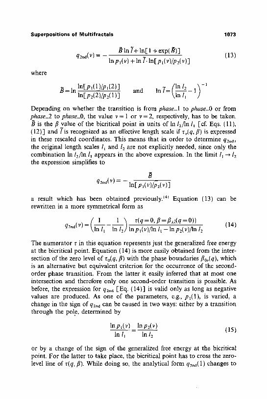
B In 7+ In[ 1 + exp(B)] q2,d(v) = (13)

lnpl(v) + In T. ln[pt(v)/p2(v)]

ln[p,(1)/p,(2)] (In l, = In and in T= \----=ln/l - 1 ln[ pz( 2 )/p,_(1) ] J

--1

Depending on whether the transition is from phase_l to phase_O or from phase_2 to phase_O, the value v = 1 or v = 2, respectively, has to be taken.

is the fl value of the bicritical point in units of In 12/ln l~ [cf. Eqs. (I1), (12)] and Tis recognized as an effective length scale if rv(q, fl) is expressed in these rescaled coordinates. This means that in order to determine q2nd, the original length scales l~ and 12 are not explicitly needed, since only the combination In 12fln Ii appears in the above expression. In the limit Ii --* 12 the expression simplifies to

q2,o(v) = __ ln[pl(v)/p,_(v)]

a result which has been obtained previously. 14~ Equation (13) can be rewritten in a more symmetrical form as

1 1 ) r(q=O, fl=fl).~(q=O)) q'-"d(V)= i-~1 l n ~ lnp,(v)/ln lt--lnp2(v)/ln 12

(14)

The numerator r in this equation represents just the generalized free energy at the bicritical point. Equation (14) is more easily obtained from the intersection of the zero level of to(q, fl) with the phase boundaries flo,.(q), which is an alternative but equivalent criterion for the occurrence of the second- order phase transition. From the latter it easily inferred that at most one intersection and therefore only one second-order transition is possible. As before, the expression for q2nd [Eq. (14)] is valid only as long as negative values are produced. As one of the parameters, e.g., pl(1), is varied, a change in the sign of q_,nd can be caused in two ways: either by a transition through the pole, determined by

lnpl(v) In pz(v)

In/l In l_, (15)

or by a change of the sign of the generalized free energy at the bicritical point. For the latter to take place, the bicritical point has to cross the zero- level line of r(q, fl). While doing so, the analytical form q_,,d(1) changes to


q2n,~(2). These scenarios are illustrated in Fig. 9a, where p~(1) is varied in the interval [0, 1 ] for fixed p1(2)= 0.4 and 12 =/~. As a simple consequence of this scenario, we may conclude that the boundaries which determine the onset of the occurrence of the second-order phase transition in the parameter space are simply given by Eq. (15) with v = 1 and v = 2. Note that this equation can also be expressed as D ~ ( v ) = D~{v), where D+ o~(v) are the asymptotic slopes of the functions rv(q). (lt~ These conditions are best understood in connection with the results for the fl0~) spectra discussed

Fig. 9. (a) The q value at which r,,{q) and the corresponding critical line flo,,(q) intersect is plotted as a function ofpz( l ) for v= 1 (full line) and v = 2 (dashed line). In the parameter region (gray shaded) where the intersection occurs at negative q values, q is identical with the critical value qana. (b) In the symmetry-reduced pt( l ) -pl(2) parameter regime (dashed triangle) there exists a rectangle R, Eq.(16), where the second-order phase transition is observable (gray shaded). On the solid line the numerator of Eq. (13) vanishes. It separates the parameter regimes where the expressions for q2,,a{ 1 ) and q2,a{2) are valid, respectively.


below. For given 1~ and 12, Eq. (15) is a transcendental equation for p~(v) [since p2(v)= 1 -p t (v ) ] . Denoting the larger of the solutions by p*, one obtains as the parameter regime for the existence of the second-order phase transition the rectangle

R = [p* ~ pl(1) ~ 1] x [0 ~<p~(2) ~<p*] (16)

[remember that by symmetry we may restrict ourselves to p~(1)>~p,(2)]. Thus, for any combination of length scales 1~, 12, there exists a regime in the p,(1)-p~(2) plane where a second-order transition occurs. For 12 = l i (which has been used in the previous figures) one obtains p* = (x//-5 - 1 )/2. This region, together with the line where the analytic form for q2nd changes from q2,d(1) to q2.d(2), is depicted in Fig. 9b.

The effect of these phase transitions is more drastically exhibited in the function f(ct), the Legendre transform of r(q) I1.), which will allow us to gain a deeper insight into the mechanisms leading to the phase transitions. Figure 10 shows the f(00 curves corresponding to the cases of Fig. 7. Whereas the first-order phase transition is detected in both figures as a straight-line segment, t28) the second-order phase transition (present only in Fig. 7b) is observed as a stopping point in the f(~) curve with finite left- hand derivative. Note that the stopping point at 0~ = ~max is identical with the intersection point of the curves f 1(00 and f2(~) which correspond to the isolated measures/~(1 ) and/t(2), respectively. This fact is characteristic for the observed second-order phase transition. In order to make this point clear we consider the scaling behavior of the isolated measures/~( 1 ),/a(2), respectively. Let us denote by ~v(~) the scaling exponent (H61der exponent) of the measure p(v) restricted to the fractal subset S(~) of the support S of p, where ( is some real number in the interval [0, 1 ] (recall that [cf. Eqs. (2), (3)] j = ~N is the number of digits one in the binary addresses of the fractal elementsJ ~9~ For the two-scale Cantor measure, ev(() is given byll*l

lnpl(v) + (1 - ~) In p2(v) ~v(~) = (17)

In Ii + (1 - ~ ) In 12

The fractal dimension (Hausdorff dimension) of S(~) is given by

In ~ + (1 -~ ) ln (1 - ~ ) f(~) - (18)

In ll + (1 - ~ ) In 12

822/82/3.-4-30

1076

f(a)

0.5

0.4

0.3

0.2

0.i

0

~, ... .....

~5." .

0.I 0.2 0.3 0.4 0.5

Ol

Radons and Stoop

0.6

f(o~)

0.5

0.4

0.3 0.2 0.1 . / /

0 0

..-~ .............. ," ::" .........- i .....

, ."'

, , :~ ' i ' : / .~ .

0.i 0.2 0.3 0.4 0.5 0.6

(b)

Fig. 10. The Legendre transforms f(ct) (full line) of the functions r(q) of Fig. 7 are known analytically. The first-order transition appears as a straight-line segment (dashed) on the bisectrix f(~x)=cx [in (a) and (b)]. The second-order transition is recognized as a stopping point off(et) with a finite slope at 0q.ax case (b)]. The stopping point is identical with the intersection point of the curves ft(ct) and fz(ct) (dotted lines) corresponding to the separate measures lt( 1 ) and/t(2).

The curves f,.(~) are then obtained by solving Eq. (17) for ~ and inserting this expression into Eq. (18), which yields

lnp2(v) --ct n l 2 ) f,,(Ct) = f ~ -- l n [ p 2 ( v ) / p l ( v ) ] --o~ ln(12/l~)

(19)

Now remember that the phase_O is characterized by the unique value = Go, Eq. (6), where the two contributions in Eq. (2) are asymptotically

of the same order. The latter condition can also be written as ctt(~ o) = ct2(~o), and to(q), the zero-level line of to(q, fl) of Eq. (10), can be expressed as to(q)=q.0cv(~o)-f(~o). This shows that at the transition to


phase_O, the scaling exponents ct o = Oro(q)/Oq = cq(~o) = ~z(~o) = ~m~x coin- cide. Also the fractal dimensions are identical and equal to f(~o). We emphasize, however, that the intersecting of the 'unperturbed' curves f , (~) is not a sufficient condition for the occurrence of the second-order phase transition [the f (~) curves of the isolated measures p(v) intersect also in the case of Fig. 10a, but no second-order transition is observed]. In addition, the parameters have to lie in the rectangle R of Eq. (16). The latter condition basically expresses a geometrical relationship between the measures p ( l ) and p(2). In order to see this we show in Fig. 11 the functions ~v((), v = l , 2 , of Eq. (17) for case (a) where only a first-order transition is present, and for case (b) where in addition the second-order

f(~)

. 6 . . . . .

0.5

0.4 ,-- '" . . . . . . -,

0.3 ," ' "

0

o \

0 0.2 0.4 0.6 0.8 1

r

(a)

0 . 6 �84

0 .5

f ( ~ ) 0.3 (b) 0.2

0 .1

0 . . . .

0 0.2 0.4 0.6 0.8 1

Fig. 11. The functions ct,.(~), v = 1, 2, are shown as full lines, together withf(~) from Eq. (18) (dashed). The singularity exponent ct(~)=min,. ~t,.(~) is monotonous in case (a), whereas in case (b) it exhibits a maximum at the intersection point C0. The latter fact is the reason for the second-order phase transition. For a given value of a [in the range ofa(r the va luef(a) is found by taking the preimage ~ of ct under the mapping ct(~) and reading off the corresponding valuef(~). If there are two preimages [possible only in case (b)], the value with the larger f ( ( ) has to be taken. However, this construction is not valid in the ~t range between the two tangencies of ct(~) with f(~), since f (c t )= a in this region (first-order phase transition).


transition is observable. First note that 0c,(~) is always a monotonous function of ~, since

aoc~(~) In l~.ln 12 . fflnp,(v) Inpz(v ) '~ O~ = [ ~ l n / ] + ( 1 - ~ ) l n l 2 ] 2 \ ~n~ ln/2 ,/ (20)

is either positive or negative, depending on the sign of the second factor in Eq. (20). Taking into account the results of Fig. 11, this means that in case (a) the measures are superimposed such that the strongest singularities minr of both measures/~(v), v= 1, 2, lie on the same set S(~ = 1) and also the weakest singularities maxr add up on the same set S(~ = 0). In contrast, for case (b) the superposition is such that minr and maxr are combined on S(~= 1), and maxr is combined with minr on the set S(~ = 0). In order to see that this argument actually explains the f (a ) spectra of Fig. 10 and therefore the phase transitions encountered, one has to compute the singularity exponents 0c(~) of the combined measure/t( 1 )+/~(2). By the same reasoning that leads to Eq. (2), one finds

0c(~:) = lira In[n(1 )P](1 )r (1)(1 -ON+ n(2) pl (2)eNp,_(2) (I --~)N'] N-- ~ ln(l~Nl~t --r

= min ~v(~) (21)

This equation is the key for explaining the form of the f(0t) curves in our model. It implies that in case (a) possible ~ values are restricted to the interval [~(~= 1),0c(~=0)]. In case (b), however, they are confined to the interval [0c(~ = 0), 0c(~ = ~o)], since here the maximum is attained at the cusp at ~ = ~o. This means that the fractal dimension which corresponds to this point is f (~o )> 0, as can be read off in Fig. 11 from the function f ( ( ) (dashed line). This is in contrast to case (a), which yields the usual result f (~ = 0) = f ( ~ = I ) = 0. This explains exactly the behavior of the f(o:) spectra shown in Fig. 10.

With this improved understanding of the phase transition behavior we may now formulate a necessary and sufficient condition for the occurence of a transition of second order. This transition occurs iff the function 0c(~) attains its maximum on the open interval (0, 1), which is only possible if one of the functions 0cv is decreasing while the other is increasing. With the aid of Eq. (20), this can be stated as

!npl(1) In p,(1)'~(In p,(2) In , I ]-nn-]~ / \ i-nn~ lnl~/(2))~<O (22)


This, of course, defines the same rectangle R [and its equivalent mirror image for p~(1)<pl (2) ] as is given by Eq. (16). Noting that Eq. (22) can also be written as [ el(0) - ~ 2(0) ] [ ~ ( I ) - e,_( 1 ) ] ~< 0, one observes that at the boundaries of R, one of the multifractal measures p(v) actually degenerates to a simple fractal measure, characterized by a single singularity exponent 0~ = D_o~(v)= D o~(v) and a single fractal dimension.

In conclusion we mention that the inverse Legendre transform offv(e) of Eq. (19) yields a parametrical representation of r,,(q), the zero level of rv(q, fl) of Eq. (9). It is given by rv(oc)=~Ofv(o~)/O~-f~(~) and q~(0~)= Of,,(e)/O~ [for the choice of parameters 12 = 12 used in the figures there exists also an explicit formula for r~(q)]. Thus, with the results presented above, we have obtained a full analytical solution for the problem of the superposition of two two-scale Cantor measures and the resulting phase transition scenarios.

3. D I S C U S S I O N

The basic nature of the system investigated suggests that this kind of phase transition behavior can also be observed in experiments. It is well possible that in the light of our results the unexpected behavior of some experimental systems can be explained in a novel and very natural way. Although we have restricted our presentation to the superposition of two two-scale multiplicative measures, the discussed phenomena are more general. In ref. 4, for instance, it has been shown that the inclusion of memory in the construction hierarchy (Markovian instead of multiplicative measures) leads to the same type of phase transitions. In the equal-scale situation treated there one also has an interpretation of the observed phase transitions in terms of a simple one-dimensional Ising system with long- range interactions. From our discussion of the f(00 curves it follows that an extension to more than two measures and more than two scales yields similar results. In particular, the possibility for second-order transitions to new thermodynamic phases exists also in these very general cases. Finally, from a theoretical point of view, it is interesting to note that the treatment presented here provides us with one of the few known mechanisms (for alternatives see ref. 29) for second-order phase transitions in the thermodynamics of m~ltifractals.

A C K N O W L E D G M E N T S

R.S. acknowledges the generous support by D. Wyler and the Swiss National Science Foundation. We are indebted to one of the referees for bringing ref. 5 to our attention.


REFERENCES

1. P. Mattila, Ann. Acad. Sci. Fenn. A 1 1:227 (1975). 2. G. Radons, Physica A 191:532 (1992). 3. G. Radons, J. Stat. Phys. 72:227 (1993). 4. G. Radons, Phys. Rev. Lett. 75:2518 (1995). 5. O. E. Lanford, in Statistical Mechanics and Mathematical Problems, A. Lenard, ed.

(Springer, Berlin, 1973). 6. D. Katzen and I. Procaccia, Phys. Rev. Lett. 58:1169 (1986). 7. P. Grassberger, in Proceedings Workshop on Dynamics ol1 Fractals and Hierarchies of

Critical Exponents ( Orsay, 1986). 8. P. Cvitanovi6, in XVth International Colloquium on Group Theoretical Methods #i Physics,

R. Gilmore, ed. (World Scientific, Singapore, 1987). 9. D. Ruelle, Thermodynamic Formalism (Addison-Wesley, Reading, Massachusetts, 1978).

10. H. G. E. Hentschel and I. Procaccia, Physica 8D:435 (1983). 11. T. C. Halsey, M. H. Jensen, L. P. Kadanoff, I. Procaccia, and B. Shraiman, Phys. Rev. A

33:1141 (1986). 12. J. P. Eckmann and I. Procaccia, Phys. Rev. A 34:659 (1986). 13. H. G. Schuster, Deterministic Chaos, 2nd ed. (VCH, Weinheim, 1989). 14. T. T6I, Z. Naturforsch. 43a:1154 (1988). 15. R. Stoop, Z. Naturforsch 46a:1117 (1991). 16. Z. Kov~ics and T. T~I, Phys. Rev. A 45:2270 (1992). 17. J. Peinke, J. Parisi, O. E. Roessler, and R. Stoop, Encounter with Chaos (Springer, Berlin,

1992). 18. Ch. Beck and F. Sch6gl, Thermodynamics of Chaotic Systems (Cambridge University

Press, Cambridge, 1993). 19. J. Feder, Fractals (Plenum Press, New York, 1988). 20. K. Falconer, Fractal Geometry (Wiley, Chichester, 1990). 21. M. Kohmoto, Phys. Rev. A 37:1345 (1988). 22. R. Stoop and J. Parisi, Phys. Rev. A 43:1802 (1991). 23. R. Stoop, J. Parisi, and H. Brauchli, Z. Natulforsch 46a:642 (1991). 24. R. Stoop and J. Parisi, Phys. Lett. A 161:67 (1991). 25. M. E. Fisher and D. R. Nelson, Phys. Rev. Lett. 32:1350 (1975). 26. W. Gebhardt and U. Krey, Phasenfiberghnge und kritische Phhnomene (Vieweg,

Braunschweig, 1980). 27. P. Grassberger and I. Procaccia, Phys. Rev. Lett. 50:346 (1983). 28. E. Ott, C. Grebogi, and J. A. Yorke, Phys. Lett. A 135:343 (1989). 29. G. Radons, Z. Naturforsch 49a:1219 (1994).

Superpositions of multifractals: Generators of phase transitions in the generalized thermodynamic...

Documents

Transcript of Superpositions of multifractals: Generators of phase transitions in the generalized thermodynamic...