
Study on the Antecedent Runoff Condition in Seolma Cheon Stream
73
공학석사학위 청구논문 工學碩士學位論文 Study on the Antecedent Runoff Condition in Seolma Cheon Stream 2014년 2월 인하대학교 대학원 사회기반시스템공학부(토목공학전공) 이씨든
Transcript of Study on the Antecedent Runoff Condition in Seolma Cheon Stream

공학석사학위 청구논문
工學碩士學位論文
Study on the Antecedent Runoff Condition in Seolma Cheon
Stream
2014년 2월
인하대학교 대학원
사회기반시스템공학부(토목공학전공)
이씨든
공학석사학위 청구논문
Study on the Antecedent Runoff Condition in Seolma Cheon
River Watershed
2014년 2월
지도교수 김 형 수
이 논문을 석사학위 논문으로 제출함
인하대학교 대학원
사회기반시스템공학부(토목공학전공)
이씨든
이 論文을 申鉉釋의
碩士學位 論文으로 認定함
2014년 2월
主番 983339
副番 983339
委員 983339
ABSTRACT
Curve number (CN) originally developed compiled by The Natural Resources Conservation
Service (NRCS)lsquo and has been widely used throughout the world However there is the
uncertainty of CN derived from the use of antecedent moisture condition (AMC)Antecedent
Runoff Condition (ARC) As in Korea where nearly 70 covered by mountainous area it is
still not sufficient handbook precedent to guide or support the estimation of AMCARC The
failure to develop formal criteria of applying AMC ARC will be a gaping profession and
results not only in uncertainty of CN estimation in particular but also in designing appropriate
structures in Korea as a whole This paper is aiming at presenting a critical review of
AMCARC and deriving a procedure to deal more realistically with event rainfall-runoff over
wider variety of initial conditions Proposed methods have been developed It is based on
modifying estimated runoff to observed runoff with coefficient of determination and then
applying different algebraic expression with the verification of AMC by antecedent rainfall
table of NEH-1964 Clearly indicated from 12 years period analysis and 2 years period of
verification normalized root mean square error RE and E are best described by the
application of algebraic expression by Arnold et al at the value of 08950 09460 and 00244
respectively for AMC condition and 13799 09642 and -00197 respectively for ARC
condition Therefore Arnold et al algebraic equation is the best representation criteria of
AMC and ARC This algebraic expression might be applied properly considering South Korea
condition
TABLE OF CONTENTS
Chapter I Introduction 1
11 Research Background 1
12 Literature Review 4
13 Outline of the Thesis 6
Chapter II Methodology 9
21 The Curve Number Method 9
211 SCS-CN based hydrological Models 12
22 Evaluation of the Curve Number Method 13
221 Procedures for determining the curve number 13
222 Asymptotic Method 15
223 Accuracy of procedures for determining the curve number 18
224 Seasonal variations of curve numbers 20
23 Antecedent Moisture Condition (AMC) and Antecedent Runoff Condition Review 21
23 1 Antecedent Moisture Condition (AMC)Antecedent Runoff Condition
application 23
232 ARC and AMC in continuous model (Soil Moisture Modeling) 25
24 Web-based Hydrograph Analysis Tool (WHAT) 28
241 Evaluation of the WHAT (Base flow Separation Method) 31
Chapter III Estimation of Antecedent Runoff ondition criteria for the Estimation of Curve
Number 32
31 Study basin 32
32 Analysis of hydrologic observation data 33
321 Limitation of data 33
322 Rainfall and runoff datasets used 34
3221 Base flow separation 36
33 Evaluation of curve number procedures 39
34 Reliability of Curve number method on Gauged Basins 47
35 Estimation of Thresholds for AMCARC 49
Chapter 4 Conclusions 61
REFERENCES 633
LIST OF FIGURES
Figure 1 1 Outline of the study 8
Figure 2 1 Standard Watershed response (from Hawkins 1993) 17
Figure 2 2 Violent Watershed response (from Hawkins 1993) 17
Figure 2 3 Procedure for the asymptotic determinationhelliphelliphelliphelliphelliphelliphelliphelliphelliphelliphelliphelliphelliphellip18
Figure 3 1 Seolma Cheon Examination Watershed 33
Figure 3 2 Rainfall during summer from June to September Plot annually from 2000 to 2011
36
Figure 3 3 Rainfall versus Direct Runoff Plot annually from 2000 to 2011 38
Figure 3 4 Rainfall versus Direct Runoff Plot from 2000 to 2011 39
Figure 3 5 Schematic of Cure Number Estimation procedure 40
Figure 3 6 Curve number versus Rainfall plot amp Asymptotic Fitting Curve plot and Residual
plot for asymptotic curve number fits for Seolma Cheon River Watershed 44
Figure 3 7 Plot of the comparison of measure runoff to the estimated runoff for each
procedure 45
Figure 38 Plot of the comparison of measure runoff to the estimated runoff for all procedure
45
Figure 3 9 Coefficient of determination of each CN estimation procedures 48
Figure 3 10 Antecedent Moisture Condition (AMC)Antecedent Run off Condition proposed
Methodology 50
Figure 3 11 Schematic representation of AMCARC estimation criteria 51
Figure 3 12 Verification of AMCARC condition (using algebraic expression by Sobhani
1975) 52
Figure 3 13 Verification of AMCARC condition (using algebraic expression by Hawkins et
al 1985) 54
Figure 3 14 Verification of AMCARC condition (using algebraic expression by chow et al
1988) 56
Figure 3 15 Verification of AMCARC condition (using algebraic expression by Arnold et al
1988) 57
LIST OF TABLES
Table 2 1 Seasonal rainfall limits for AMC (Source NEH-4 1964)helliphelliphelliphelliphelliphelliphelliphelliphellip 24
Table 3 1 CN of examination basin 34
Table 3 2 Curve number estimation from the selected rainfall from 2000 to 2011 in summer
40
Table 3 3 Watershed Curve Number by all procedures from 2000 to 2011 46
Table 3 4 Overall Watershed Curve Number by all Procedures 46
Table 3 5 Coefficient of determination and Goodness of fit of AMC ARC and Regression
Equation in respect Sobhanilsquos algebraic expression 53
Table 3 6 Coefficient of determination and Goodness of fit of AMC ARC and Regression
Equation in respect to Hawkins et allsquos algebraic expression 54
Table 3 7 Coefficient of determination and Goodness of fit of AMC ARC and Regression
Equation in respect to chow et allsquos algebraic expression 56
Table 3 8 Coefficient of determination and Goodness of fit of AMC ARC and Regression
Equation in respect to Arnold et allsquos algebraic expression 58
Table 3 9 Result of all coefficient of determination 59
CHAPTER I INTRODUCTION
11 Research Background
The hydrologic methods developed by the Natural Resources Conservation Service (NRCS
formerly the Soil Conservation Service (SCS) were originally developed as agency
procedures and did not undergo journal review procedures (Ponce and Hawkins 1996) The
only official source documentation is the NRCSlsquos National Engineering Handbook Section 4
(NEH-4) Unfortunately NEH-4 has gone through several revisions (1956 1964 1965 1969
1972 1985 and 1993) since first being published in 1954 The numerous revisions have
resulted in confusion by people who use the methods (Hjelmfelt 1991)
The accuracy of the Curve Number Method has not been thoroughly determined (Ponce and
Hawkins 1996 McCutcheon et al 2006) and empirical evidence suggests that with the current
NRCS (2001) curve number table hydrologic infrastructure is being over-designed by billions
of dollars annually (Schneider and McCuen 2005) Furthermore SCS-CN main weak points
are including it does not consider the impact of rainfall intensity and its temporal distribution
it does not address the effects of spatial scale it is highly sensitive to changes in values of its
sole parameter and it does not address clearly the effect of adjacent moisture condition
(Hawkins 1993 Ponce and Hawkins 1996 Michel et al 2005) In addition to that use of
the Curve Number Method to simulate runoff volume from forested watersheds would likely
result in an inaccurate estimate of runoff volume from a given volume of rainfall (Ponce and
Hawkins 1996 McCutcheon 2003 Garen and Moore 2005 Schneider and McCuen 2005
Michel et al 2005 McCutcheon et al 2006)
The methodlsquos credibility and acceptance has suffered however due to its origin as agency
methodology which effectively isolated from the rigors of peer review Other than the
information contained in NEH-4 which was not intended to be exhaustive (Rallison and
Cronshey 1979) no complete account of methodlsquos foundations is available to date despite
some recent noteworthy attempts (Rallison 1980 Chen 1982 Miller and Cronshey 1989)
In the four decade that has elapsed since the methodlsquos inception the increased availability of
computers has led to the use of complex hydrologic models many of which incorporate the
curve number method Thus the questions naturally arise what is the status of the curve
number method in a postulated hierarchy of hydrologic abstraction models (Miller and
Cronshey 1989 Rallison and Miller 1982)
In practice hydraulic engineer frequently use the curve number procedure of the US Soil
Conservation Service (SCS) to compute in these small to medium-sized ungagged basins
probably due to its apparent simplicity Runoff estimates are based upon the soil types land-
use practices within a basin and the influence of the antecedent soil moisture conditions for a
specific storm
An effective overhaul of the method would require a clearer understanding of its properties
than is currently available (Woodward 1991 Woodward and Gburek 1992)
Far too many water resource professionals have accepted the CN methods without
independently reviewing extensive real hydrologic data One example is the concept of the
Antecedent Moisture Condition (AMC) When the CN was originally developed it was well
known that soil moisture played a significant role on the infiltration capacity of a soil
Therefore instead of trying to determine or predict soil moisture the NRCS decided to
account for the soil moisture using the amount of rainfall received in the five days preceding
the storm event of interest The NRCS defined this 5-day measurement as the antecedent
moisture condition (AMC) (now called the antecedent runoff condition (ARC)) However
Hope and Schulze (1982) noted in a personal communication with N Miller that the use of a
5-day index for ARC was not based on physical reality but rather on subjective judgment
As one can observe even for these larger rainfall and runoff events the AMC exhibits a large
degree of scatter Additionally researchers have been unable to validate the NRCS 5-day
index method Nonetheless the concept still is frequently used by researchers and practitioners
However many leading researchers consider the AMC to represent the variation in runoff
volume (Q) from all sources such as model and data error intensity seasonal cover and site
moisture In this context the AMC and ARC represents nothing more than error bands
The rainfall runoff transformation is a nonlinear process The most important cause of non-
linearity represented by the effect of antecedent conditions consequently the runoff
coefficient depends on the initial conditions It is well known that soil moisture is a major
control on the catchment response antecedent moisture conditions have been used to
represent variability of the CN in the SCS method for predicting direct runoff (eg Rallison
and Miller 1981) But soil moisture measurements are usually not widely available and a lot
of point measurements are needed to get either an average or an antecedent catchment state
Antecedent moisture conditions can be simulated using models (either lumped or distributed)
provided standard climate data are available Alternatively some other easily measured
hydrological variable that are even if only approximately related to soil moisture conditions
may be considered
One of the several problems (Ponce and Hawkins 1996 King et al 1999) is that the Method
does not contain any expression for time and as a result ignores the
impact of rainfall intensity as well as antecedent runoff condition So far there is no
concrete guidebook for estimating the antecedent runoff conditions More importantly the
procedure to identify the ARC has been applied within the US soil condition and for decades
for mountainous topographical area like South Korea there will be encountered the variation
and bias Misestimating the runoff depth will lead to the failure in design structure
consequently there will dramatically damage ranging from capital loss to human loss Also
driving force of economic development will be getting down unavoidable
It is apparent that the CN-variability is primarily attributed to the antecedent moisture and it
has led to statistical and stochastic considerations of the curve number undermining the
physical basis of the SCS-CN methodology Furthermore incorporation of the antecedent
moisture in the existing SCS-CN method in the terms of the three AMC levels allows
unreasonable sudden jumps in the CN variation Therefore the determination of the
antecedent moisture condition plays an important role in selecting the appropriate CN value
The practical application of this procedure should be simple and direct It replies on the
determination curve numbers which are widely documented in the literature for various land
uses and soil types (NEH-4 1964 Chow et al 1988 Pigrim amp Cordery 1993) Nevertheless
in spite of its apparent simplicity the application of the curve number procedure lead to
diversity of the interpretation and confusion due to ignorance about limitations because the
existing documentation of how it was developed is severely limited (Hawkins 1979 Boznay
1989 Hjelmfelt 1991 Pilgrim amp Cordery 1993) Difficulties in its application are mainly
related to the classification of soils outside the USA into the four hydrological soil group A B
C D and the determination of antecedent moisture condition (AMC) which is an index of
basin wetness Care is required in its application and verification against measured of flood
data in each region where the method is applied is necessary
This objective of this paper is to present a critical review of antecedent runoff condition ARC
and derive a procedure to deal more realistically with event rainfall-runoff over wider variety
of initial conditions
12 Literature Review
It is well known that soil moisture is a major control on catchment response antecedent soil
moisture conditions have been used to represent variability of the CN in the SCS method for
predicting direct runoff (eg Rallison and Miller 1981) But soil moisture measurements are
usually not widely available and a lot of point measurements are needed to get either an
average or an antecedent catchment state Antecedent soil moisture conditions can be
simulated using models (either lumped or distributed) provided standard climate data are
available
The practical application of this procedure should be simple and direct It replies on the
determination curve numbers which are widely documented in the literature for various land
uses and soil types (NEH-4 1964 Chow et al 1988 Pigrim amp Cordery 1993) Nevertheless
in spite of its apparent simplicity the application of the curve number procedure lead to
diversity of the interpretation and confusion due to ignorance about limitations because the
existing documentation of how it was developed is severely limited (Hawkins 1979 Boznay
1989 Hjelmfelt 1991 Pilgrim amp Cordery 1993) Difficulties in its application are mainly
related to the classification of soils outside the USA into the four hydrological soil group A B
C D and the determination of antecedent moisture condition (AMC) which is an index of
basin wetness Care is required in its application and verification against measured of flood
data in each region where the method is applied is necessary
The NRCS (2001) Curve Number Method is widely used for estimating watershed runoff
from rainfall in engineering design (Jacobs et al 2003) The extensive use of the curve
number technique follows from the simplicity that lumps the complexity of runoff generation
into a single watershed parameter the maximum potential retention S that is easily converted
mathematically to a curve number CN (Nachabe and Morel-Seytoux 2005) However the
simplicity of a single lumped parameter introduces great uncertainty to estimates of runoff
Ponce and Hawkins (1996) attribute the ambiguity of the Method to several characteristics
including (Jacobs et al 2003) Use of arbitrarily limited measures of watershed
characteristics lumped into the single parameter the maximum potential retention S Lack of
peer reviewed justification and explanation of the simplified procedures necessary to
consistently determine runoff for engineering design and significant agency support
manifested as publication in the National Engineering Handbook (NRCS 2001)
Despite the limitations the NRCS (2001) Curve Number Method is used to (1) estimate
runoff from ungaged watersheds (2) evaluate the effect of changes in land use and treatment
on direct runoff and (3) parameterize rainfall-runoff relationships in watershed simulation
models
Proper CN estimates are needed to accurately evaluate water availability and close the water
budget of agriculture fields Careful measurements of runoff volume are needed to
systematically evaluate the role of key variables such as rainfall intensity soil moisture
condition tillage practice and land cover on CN values (SUDAS 2004)
13 Outline of the Thesis
This thesis consists of 4 chapters
Chapter 1 it will present the general introduction and significance of study briefly but
concisely about the antecedent runoff conditions which is practically applied in South Korea
as a case of study
Chapter 2 present an overview of previous work related to the study topic that serve as the
necessity of background for the purpose of this research Relevant and previous literature
reviews prevail the SCS curve number and general assumptions Also present the
methodology and some practical tactics to determine AMC and its critical thinking of this
application and figure out effective practice for further usage in South Korea in particular
Chapter 3 demonstrate the results and discuss the finding
Chapter 4 Conclusion
The figure 11 indicates the process of research Firstly direct runoff is necessary to be
separated from total runoff By applying base flow separation known as Web Based
Hydrograph Tools (WHAT) the base flow and direct runoff can be separated The data are
derived from the examinational rainfall station After identifying direct runoff from total
runoff curve number estimation can be calculated from equation 7 by knowing daily rainfall
and matched direct runoff However further consideration is necessary to take into account
That is to test the accuracy of curve number To test the accuracy of curve number
determination curve numbers are computed depending upon four different procedures
including arithmetic mean median geometric mean and asymptotic fit Except for the
asymptotic method unranked paired rainfall and runoff volumes from the maximum peal flow
event each year of record were used to compute the calibrated curve number After the curve
number is estimated the next step is to simulate antecedent moisture condition by applying all
the proposed algebraic expression of NEH4 with the consideration of 5 day prior to rainfall
(definition of AMC using antecedent rainfall table) Next is to validate and calibrate among
the proposed procedure to figure out the estimator of antecedent moisture condition criteria
Check evaluation of curve
number procedures
(NRMSE RE R2 NSE)
1st Proposed Method 2nd Proposed Method
Algebraic expression of NEH4
( developed Sobhani (1975) Chow
et al (1988) Hawkins et al (1985)
Arnold et al (1988)
Making AMCARC Estimation
Criteria
Data collection (Rainfall and
Runoff data)
Derive direct runoff ( by Web
Based Hydrograph Tools
WHAT)
Curve Number Estimation
Calibration amp Validation
( NRMSE RENSE R2)
Determination of AMCARC
estimation criteria
Definition of AMCARC
(NEH-4 1964)
Average conditions (NEH-4
1964)
Median curve number
(NEH-4 1964)
Antecedent rainfall table
(NEH-4 1964)
Comparison within
definitions
Determination of
AMCARC estimation
criteria
Comparison of AMCARC
Result of AMCARC
estimation criteria
Figure 1 1 Outline of the study
CHAPTER II METHODOLOGY
In this chapter we are going to cover the review of literature regarding to Curve number
hydrology methodology critical thinking on antecedent runoff condition and applicable
methodology to define antecedent runoff condition Base flow separation technique known as
Web based Hydrograph Analysis Tools (WHAT) and further discussion how it integrates base
flow separation to define standard of antecedent conditions
21 The Curve Number Method
The curve number procedure of US the soil Conservation Service is a widely used method for
estimating runoff depth direct runoff from the rainfall on small to medium-sized ungagged
basin The basic reference is the National Engineering Handbook Section 4 Hydrology
(1964) hereafter referred to as ―NEH-4
The SCS-CN (original) method is a procedure for estimating the depth of runoff from depth of
precipitation in given soil textural classification land useland cover and an estimate of
watershed wetness The method combines the watershed parameters and climatic factors in
one entity called the curve number which varies with cumulative rainfall soil cover land use
and initial water content
Originally this technique was originally derived from the examination of annual flood event
data Implicit in the reasoning of Mockus (1949) and Andrews (1954) the curve number
runoff equation can be derived from a watershed water balance for a storm event written as
(1)aP I F Q
where P is the storm event rainfall Ia is the initial abstraction (includes interception
depression storage and infiltration losses prior to ponding and the commencement of
overland flow) F is the cumulative watershed retention of water and Q is the total runoff
from the rain event
Victor Mockus (Ponce 1996) hypothesized that the ratio of actual runoff to the maximum
potential runoff (expressed as rainfall P minus initial abstraction Ia added later by the SCS
over the objections of Mockus) is equal to the ratio of the actual retention of water during a
rainstorm to maximum potential retention S in a catchment (Ponce and Hawkins 1996) or
runoff
2a
Q F
P I S
To reduce the number of unknown parameters (3) in Equations (1) and (2) the SCS
hypothesized that
3aI S
Where λ is the initial abstraction ratio or coefficient a relation between the initial abstraction
Ia and maximum potential retention S has not been defined theoretically or conceptually
As the Method is currently practiced runoff can be computed using the tabulated curve
numbers based on the land use and condition hydrologic soil group and the rainfall depth
from combining Equations (1) and (2) as
2
4a
a
P IQ
P I S
Equation (4) is valid for precipitation P gt Ia For P lt Ia Q = 0 such that no runoff occurs
when the rainfall depth is less than or equal to the initial abstraction Ia With initial
abstraction included in Equation (4) the actual retention F= P ndash Q asymptotically approaches
a constant value of S + Ia as the rainfall increases
Using the value of λ = 02 Equation (4) becomes
202
0208
0 02 5
P SQ for P S
P S
Q for P S
Equation (5) contains only one parameter (maximum potential retention S) which varies
conceptually between 0 and infin For convenience in practical applications maximum potential
retention S is defined in terms of a dimensionless parameter CN (curve number) that varies
over the more restricted range of 0 lt CN lt 100
1000 1000
10 610
S CN aCN S
25400 25400
254 6254
S CN bCN S
The CN ranges from 0 to 100 and is a transformation of S which varies between 0 S A
value of S can be calculated from P and Q if 02 (Hawkins 1993)
2
2
5 2 4 5 254 ( )
5 2 4 5 10 ( ) 7
S P Q Q PQ metricunits or
S P Q Q PQ inchunits
The numbers 1000 and 10 (in inches) as expressed in Equation (6a) or 25400 and 254 (in
millimeters) as expressed in Equation (6b) are arbitrarily chosen constants having the same
units as the maximum potential retention S
Watershed curve numbers are estimated by cross referencing land use hydrologic condition
and hydrologic soil group for ungagged watersheds in standard tables (NRCS 2001) or
calculated for gaged watersheds by algebraic rearrangement of Equations (5) (6) and (7) as
2
10008
5 2 4 5 10CN a
P Q Q PQ
2
254008
5 2 4 5 254CN b
P Q Q PQ
Measured pairs of rainfall volume P and runoff volume Q from an individual storm event are
or
or
used with Equation (7) to determine the watershed curve number CN The measured rainfall
and runoff are expressed in inches or millimeters for Equations (8a) and (8b) respectively
The CN value for representative land uses soil types and hydrological conditions along with
a conversion table AMC for three AMC conditions AMC I (dry) AMC II (normal) AMC III
( wet) which statistically correspond to 90 50 and 10 cumulative probability of exceedance
of runoff depth for a given rainfall respectively [42] are given in NEH-4 table [1] The higher
the antecedent moisture or rainfall amount the higher is the CN and therefore the high
runoff potential of the watershed and vice versa
If the watershed includes segments with several types of soil and soil cover complex
appreciate CNs are assigned to each segment and a weighted CN can be estimated for the
entire watershed using the equation
1 1 2 2 9n n
W
CN A CN A CN ACN
A
Where nCN and nA are the CN and area respectively for the thn watershed n is the total
number of segments in the watershed and A is the total area of the watershed
211 SCS-CN based hydrological Models
This paper provides a recent documentation on the subject with their limitations and
advantages and computer models developed over the year The empirical methods are
Williams and LaSeur Hawkins Pandit and Gopalakrishnan Mishra et al Mishra and Singh
Developed in 1976 by Williams and LaSeur is a continuous simulation model by relating the
SCS-CN parameter (S) with the soil moisture (M) for computation of direct surface runoff
They accounted antecedent moisture (M) which depleted continuously between storms by
evapotranspiration and deep storage M is assumed to vary with the lake evaporation as given
2
0
a
a
a
a
P IQ if P I
P I S
Q I S
absM S S and
1
10
1t T
c tt
MM
b M E
Where absS absolute potential maximum retention equal to 20 t-time
cb -depletion
coefficient M-soil moisture index at the beginning of the first storm t
M -soil moisture
index at any time t t
E -average monthly lake evaporation for day t and T-number of days
between storms
The advantages of this model are that it eliminates sudden quantum jumps in the CN values
when changing from one AMC level to other However the downside is that it utilizes an
arbitrarily assigned value of 20 inches for absolute potential maximum retention and assumes
physically unrealizable decay of soil moisture with Lake Evapotranspiration which is false
assumption
Mishra and Singh (1998) proposed used a linear regression approach similar to the unit
hydrograph scheme to transform rainfall excess into direct runoff They described the AMC
based on the NEH-4 table and varied CN with time t using the following equation
22 Evaluation of the Curve Number Method
221 Procedures for determining the curve number
Measured rainfall and runoff volumes for the event with annual peak flow were used to
determine a curve number for each year of record on watersheds Representative watershed
curve numbers for gaged watersheds were selected from a set of curve numbers determined
using the (1) arithmetic mean (2) median (3) geometric mean (4) asymptotic value and (5) a
nonlinear least squares fit procedures To access the accuracy of NRCS (2001) Curve Number
Method these calibrated values were compared to the NRCS (2001) tabulated curve numbers
for the specific hydrologic soil group (Group A B C or D) cover-complex (land use
treatment or practice) and hydrologic condition (poor fair or good) on each gaged
watershed The detailed procedures for each technique follow
Arithmetic curve number The curve number for each year of record for a particular
watershed is averaged to determine the representative curve number
Median curve number The median was originally determined for the NRCS (2001) curve
number tables using the Graphical Method The direct runoff was plotted versus the rainfall
volume to determine the curve that divides the plotted points into two equal groups The curve
number for that curve is the median curve number
Geometric mean curve number The NRCS (2001) Statistical Method determines the
geometric mean curve number (Yuan 1939) from a lognormal distribution of annual
watershed curve numbers about the median (Hjelmfelt et al 1982 Hauser and Jones 1991
Hjelmfelt 1991) The procedure is
The maximum potential retention S is computed from each pair of annual runoff
volume Q and rainfall volume P as Equation (8)
The mean micro and standard deviation δ of the logarithms of the annual maximum
potential retention S was determined as
log
2
log
log
log13
log14
1
S
S
S
S
N
S
N
where N is the number of years in the watershed rainfall-runoff record The mean of the
transformed values the mean (log S) is the median of the series of the maximum potential
retention if the distribution is lognormal
The geometric mean (GM) of the maximum potential retention S is the antilogarithm
of the mean (log S) in base 10 logarithms
log10 15S
GMS
Finally the geometric mean curve number for rainfall and runoff volumes expressed in
inches is
1000 25400
( ) 1610 254
GM GM
GM GM
CN inch units CN metricunitsS S
Nonlinear Least Squares Fit For a record of N observed rainfall P and observed runoff Qo
the optimal value of the maximum potential retention S for the watershed is that which
minimizes the objective function
2
1
17N
oi pi
i
f Obj Q Q
where Qp is the runoff computed from the NRCS (2001) runoff Equation (5) The square root
of the minimum objective function divided by N (number of observations) is the standard
error The measure of variance reduction R2 is similar to the correlation coefficient r2
2
2 1 18
o
e
Q
SR
S
where oQS is the standard deviation of the observed runoff values and se is the standard error
222 Asymptotic Method
Handbook table values of CN give guidance in the absence of better information but
incorporate only limited land uses and conditions and are often untested With increasing user
sophistication coupled with the awareness that the runoff Calculation is more sensitive to CN
than to rainfall interest in determining local CNs from local rainfall-runoff data has grown
Three methods of analyzing local event rainfall and runoff for CN are outlined here
In this method the Hawkinslsquos method CN calculated using Equation (6) and (7) are plotted
against the respective P values and the asymptotic value at high rainfalls is taken as the final
CN The analysis can be done on ordered or unordered data and we have plotted ordered data
to increase the clarity of the figure The actual analysis used unordered data as this should
give more accurate result (Hawkins et al 2009) In some cases however the CN does not
reach an asymptotic value but keeps declining and the CN cannot be calculated (Figure 2b)
This is called complacent behavior (Hawkins 1993) and is possibly due to insufficient data in
the series The opposite is violent behavior in which the CN values suddenly increase after an
initial decline Hawkins 1993) We again used nonlinear least squares (nls) in R (R
Development Core Team 2010) to calculate the asymptotic S1 related to CN1 values by
inserting Equation (6) into the suggested empirical equations (Hawkins 1993) to fit standard
behavior
25400 25400
100 exp 11254 254
CN P kPS S
Or violent behavior depending on the data
25400
1 exp 12254
CN P kPS
In these equations k is a fitting constant that describes the slope of the log (CN)-log (P)
relationship The non-least square function maximizes the log-Likelihood therefore
separation between standard and violent behavior was based on which Equation ((11) or (12))
gave the highest log-likelihood Additionally if the asymptotic S value was greater than the
maximum calculated S value based on Equation (6) we assumed complacent behavior
(Hawkins 1993)
Figure 2 1 Standard Watershed response (from Hawkins 1993)
Figure 2 2 Violent Watershed response (from Hawkins 1993)
The procedure for the asymptotic determination of observed watershed curve
1 Rank the rainfall and mnoff depths independently
2 Calculate curve numbers for each ordered pair
3 Plot the resulting curve numbers with respect to the
conesponding precipitations
4 Define the curve number from the asymptofic behavior as
standard violent or complacent
Figure 2 3 Procedure for the asymptotic determination
223 Accuracy of procedures for determining the curve number
The relative accuracy of the four methods for determining the watershed curve
number from the series of measured runoff depth and the rainfall depth has not
been fully explored and defined Therefore the accuracy of all four procedures for
calibrating curve numbers to estimate runoff volumes was assessed by using coefficient of
determination R square Relative Error (RE) Nash-Sutcliffe efficiency E and error statistic
based on the Normalized root mean square error NRMSE The coefficient of determination is
expressed as following
R square (2R )
2
( ) ( )2 1
22
( ) ( )
1 1
19
n
obs i obs est i est
i
n n
obs i obs est i est
i i
Q Q Q Q
R
Q Q Q Q
Relative Error
( ) ( ) ( ) 100 20est i obs i obs iRE Q Q Q
Nash-Sutcliffe efficiency
2 2
1 1
2
1
12 21
n n
obs obs obs est
i i
n
obs obs
i
Q Q Q Q
E i n
Q Q
Normal Root Mean Square Error
2
1
1
22
N
obs comp ii
obs
N Q Q
NRMSEQ
where i is the number of each event from 1 to N (the total number of rainfall-runoff events)
Qest is the computed runoff volume Qobs is the observed event runoff volume and est obsQ Q
are the mean of the estimated and observed runoff volumes respectively
R square (2R ) can be also be expressed as the squared ratio between the covariance and the
multiplied standard deviations of the observed and predicted values Therefore it estimates
the combined dispersion against the single dispersion of the observed and predicted values
The range of 2R lies between 0 and 1 which describes how much of the observed of the
observed dispersion is explained by the prediction A value of zero means that the dispersion
of the prediction is equal to that of the observation The fact that only the dispersion is
quantified is one of the major drawbacks of 2R if it is considered alone A model which
systematically over or under predict all the time will still result in good 2R values close to 10
even if all prediction were wrong
Relative Error Relative error gives an indication of how good a measurement is relative to
the size of the thing being measured
Nash and Sutcliffe Efficiency (E) The efficiency of E is proposed by Nash and Sutcliffe
(1970) The normalization of the variance of the observation series results in relatively higher
value of E in catchments with higher dynamics and lower values of E in catchments with
lower dynamics To obtain comparable values of E in a catchment with lower dynamics and
prediction has to be better than in a basin high dynamics The range of E lies between 10
(perfect fit) and infinity An efficiency of E lower than zero indicates that the mean value of
observed time series would have been a better predictor than the model
The normalized root-mean-square deviation or error (NRMSE) is a frequently used
measure of the differences between values predicted by a model or an estimator and the
values actually observed NRMSE is a good measure of accuracy but only to compare
forecasting errors of different models for a particular variable and not between variables as it
is scale-dependent The larger the NRMSE the poorer is the estimated curve number and
vice-a-versa
224 Seasonal variations of curve numbers
Jacobs and Srinivasan (2005) and Paik et al (2005) showed that the watershed curve number
seems to vary from season to season And this seasonality of curve numbers seems to occur
for some North Georgia forested watersheds However a physical justification for these
variations has not been developed (Tedela et al 2007) For this report the working hypothesis
is that seasonal differences in recharge and evapotranspiration may affect watershed
maximum potential retention by raising or lowering water tables and by adding or depleting
soil moisture Furthermore the dropping of and seasonal regrowth of deciduous leaves may
affect the initial abstraction
To investigate the seasonal variation of curve numbers the observed rainfall and runoff
volume data were divided according to the two seasons and analyzed separately The
watershed curve number for each season was computed using measured rainfall and runoff
volumes in Equation (8) Tedela et al (2007) discovered that inclusion of storm events during
the transitions between seasons obscured some of the observed differences in curve numbers
determined for the growing and dormant seasons Transitional hydrologic conditions are
evidently affected by a combination of tree growth and dormancy Therefore the rainfall and
runoff volumes from the months of October and November and March and April were not
included in computing the record of seasonal curve numbers To test the arbitrary exclusion of
what seems to be transition months this study investigated the effect of seasonal variation
with or without the transitions
23 Antecedent Moisture Condition (AMC) and Antecedent Runoff Condition
Review
The original NEH4 exposition of the CN contained the AMC motion in two forms both
seemingly independent First as a climatic definition presented in the since discontinued
NEH4 Table 42 or based on discontinued NEH4 Table 42 indicating AMC status (III and
III) based on 5-day prior rainfall depths and season Second as an undocumented table (Table
101 in NEH4) that gave the I II and III equivalents This was linked to explaining that
observed variation in direct runoff between events
Prior 5-day rainfall depths The cumulative 5-day rainfall depth is a characterizing climatic
description of a site A number of subsequent papers (Including Gray et al 1982 Hawkins
1983) examined this and found that for most stations ndashand using the Table 42 criteria ndashthe
apparent dominant rainfall-defined status was in AMC I This invited local interpretations and
selection of AMC I CN from soils and cover data with consequent reduction in design peaks
and volumes From this realization in 1993 the SCS dropped the Table 42 definitions from
update NEH4 (Shaw 1993) Furthermore CN at AMC II status was defined as the reference
CN as that occurring with the annual floods and as the basis find continued application
usually in continuous daily time-step models a topic covered elsewhere in this report
AMC conversion values The correspondence between CN at three AMC status levels was
stated in NEH4 Table 101 without explanatory background or hydrologic reference the
original data sources and the deviation technique have not been located However in attempts
to formulate the relationships the table offerings have been re-expressed algebraically as
shown in Table 15 The first three of these equations are essentially identical Reduces very
nearly to 49 and 50 upon simplification Equation 23 and 24 are known to arise from simple
linear fits on the storage term ―S of the CNs offered in NEH4 Table 101 Specifically 23a
and 23b are fit to 45 points from CN = 50 to CN = 95 giving (Hawkins et al 1985)
2
2
( ) 2281 ( ) 0999 0206
( ) 0427 ( ) 0994 0088
S I S II r Se in
S II S II r Se in
It should be note that the coefficient in the above are very nearly reciprocals or
0427 1 2281
Sobhani
(1975)
( ) ( ) [2334 001334 ( )] 24
( ) ( ) [04036 00059 ( ) 24
CN I CN II CN II a
CN III CN II CN II b
Hawkins
et al
(1985)
( ) ( ) [2281 001381 ( )] 25
( ) ( ) [0427 000573 ( ) 25
CN I CN II CN II a
CN III CN II CN II b
Chow et
al (1988)
( ) 42 ( ) 10 0058 ( ) 26
( ) 23 ( ) 23 ( ) 10 013 ( ) 26
CN I CN II CN II a
CN III CN III CN II CN II b
Arnold et
al (1988)
( ) ( ) ( ( )) 27
( ) ( )exp[000673(100 ( )] 27
CN I CN II F CN II a
CN III CN II CN II b
( ( ) 20(100 ( ) [100 ( ) exp(2533 00636(100 ( )]F CN II CN II CN II CN II
(23a)
(23b)
Double
Normal
1
1
( ) 100( ( 100) 051 28
( ) 100( ( 100) 051 28
II
II
CN I F CN a
CN III F CN b
Table 21 Algebraic expression of NEH4 Table 101 (Source NEH4 Table 101)
Double normal plotting the ultimate practical fitting of the Table 101 AMC relations can be
found by plotting CN I II and III on the Y-axis on double normal-probability paper against
CNII (X -axis) with the CNs shown as ―probability in percent This pragmatic exercise
leads to three equally spaced and tightly-fitting parallel straight lines This is consistent with
the reciprocal coefficients mentioned above and suggests a smoothing procedure on limited
data to create the original relationship Fit to the ―data in NEH4630 Table 101 the
expressions are shown as Equation 28 below
1
1
100( ( 100) 051) 027
100( ( 100) 051) 028
I II
II II
CN F CN Se CN
CN F CN Se CN
Where F Normal probability integral and 1F inverse of F
AMC and ARC as ―error band The ―AMC concept was converted to an ―error bands
concept via findings by Hjemfelt et al (1982) of error probabilities associated with the table
value of AMC I and AMC III AMC III was shown to approximate the direct runoff for a
given rainfall for which 90 percent of runoffs were less while AMC I approximated the direct
runoff for the same rainfall for which 10 percent of the runoff were less Further research by
Grabau et al (2008) further affirms with concept but refines AMC I and III probabilities as
about 12 and 88 percent respectively leading to about 75 percent of the runoff event falling
between ARC I and ARC III
23 1 Antecedent Moisture Condition (AMC)Antecedent Runoff
Condition application
However determination of antecedent moisture condition content and classification into the
antecedent moisture classes AMC I AMC II and AMC III representing dry average and wet
(28)
conditions is an essential matter for the application of the SCS curve number procedure that
is without a clear answer yet The definition of antecedent moisture condition AMC II is the
basis from which adjustments to the corresponding curve numbers for dry soils (AMC I) and
wet soils (AMC III) are made Nevertheless Hjelmfelt (1991) noted that the SCS gives three
definitions for AMC II
Average conditions (NEH-4 1964) The SCS defines the antecedent moisture
condition as an index of basin wetness In particular AMC II is defined as ―the average
condition However Hjelmfelt (1991) pointed out that it is not clear if this is to be
quantitative or qualitative definition and if quantitative
Median curve number (NEH-4 1964) The curve number that divides the plotting of
the relationship between direct runoff and the corresponding rainstorm into two equal
numbers of points (the median) is associated with AMC II AMC I and AMC II are
defined by envelope curve
Antecedent rainfall table (NEH-4 1964) The appropriate moisture group AMC I
AMC II AMC III is based on a five-day antecedent rainfall amount and season
category (dormant and growing seasons)
Table 2 1 Seasonal rainfall limits for AMC (Source NEH-4 1964)
Common practice makes the method dependent on the antecedent precipitation index a
simple indicator derived from rainfall depth which can be used to determine antecedent
moisture condition of the soil
Furthermore Morel-Seytoux amp Verdin (1981) noted that examination of the SCS curve
number procedure also shows that the infiltration rate implied in the SCS procedure fluctuates
with the rainfall intensity which disagree with field and laboratory measurements and
physical infiltration theory The SCS infiltration rate only produces a monotonic decreasing
infiltration curve for constant rainfall intensity Morel-Seytoux amp Verdin (1981) extended the
SCS curve number procedure using infiltration theory and established a table relating the
curve number (CN) to the hydraulic conductivity of the soil under conditions of natural
saturation (K) and the storage suction factor (Sf) This table allows the use of infiltration
equations to estimate rainfall excess for any ungagged basin assuming that the curve number
can be determined from knowledge of soil types and land use
232 ARC and AMC in continuous model (Soil Moisture Modeling)
The curve number event runoff equation and the ARC-CN relationships offered in NEH4
Table 101 have found application as a hydrologic interpretation of soil profile and site
characteristics in ecologic models Insofar as this is a major extension of the method not
covered in the original formulation in NEH4 there is a lack of hand book authority or
precedent to guide or support it
Continuous models with the CN method as a soil moisture manager are sometimes used to
determine watershed yield it is also popular as the hydrology underpinning for upland water
quality models Such approaches also find wide application in continuous hydrologic
simulation usually in planning agricultural or wild land management This application is
widespread but only defining and cursory coverage is given here A full critical review is
needed but is well beyond the scope of this report
Abbreviated and selected listing of such continuous model include SWAT (Arnold et al
1994) SWRRB (Arnold et al 1990 Williams et al 1985) EPIC (Williams et al 1984)
GLEAMS (Leonard et al 1987) CREAMS (Knisel 1980 ) NLEAP (Shaffer et al 1991)
AGNPS (Young et al 1989) Cronshey and Theurer 1998) ARDBSN (Stone et al 1986)
SPUR (Carlson et al 1995) PRZM (Carsel et al 1984) ACRU(Schulze 1992) RUSLE2
(Foster et al 2003) SPAW (Saxton 1993) and TVAHYSIM (Betson et al 1980)
Essentially all of the current works are technical descendent of the pioneering paper by
Williams and LaSeur (1976) Later addition by Arnold et al (1990) provided the essentials
found in many contemporary versions The most popular module appears to be the one
incorporated in SWAT (Nietsch et al 2002) A more recent procedure along similar lines with
successful application is given by Mishra and Singh (2004) An alternative with some
enhancements was given shortly following the Williams and LaSeur (1976) paper by Hawkins
(1977 1978) It was applied to the continuous daily model ACRU (Schulze 1982 1992) in
South Africa (which uses IaS = 010 however)
A critique of both of these approaches ndash based on mass conservation consideration ndashis given
by Mishra and Singh (2004) who suggest the corrected and improved method Their approach
incorporated in a river basin model applied to condition in India Michel et al (2005)
present a criteria review of these procedure and highlight several inconsistencies when used in
continuous models and derive a procedure to deal more realistically with event rainfall-runoff
over a wider variety of method is as follow
The soil water balance modeling strategy spring from the notion that CNndashand thus S (or 12S)
ndashis a continuous function of soil moisture with time Thus it gives physical meaning to S as
the maximum possible post ndashIa different between rainfall and runoff and is a time-variable
measure for site water storage potential While variation in details abound a basic
representation of the general method is as follows
1 CN values ndash assumed to be condition II ndashare selected from handbook tables or charts
from handbook tables or charts for the soil and land use conditions under study
2 From this conditions I and III are established using the handbook relationships in
NEH4 Table 101 In some versions the storage indices (S) corresponding to ARC I
and ARC III may be taken to be site wilting point and fieldslsquo capacity respectively
3 Direct runoff (Q) is generated from the daily rainfall P and the daily CN the latter
defined by allocating the soil moisture with condition I and III as the limiting cases
4 Total losses of runoff (P-Q) are counted as additions to moisture Site moisture losses
from evapotranspiration and drainagepercolation are calculated by various sub
process models
5 The CN for the next day is calculated from the residual soil moisture content
following the above accounting limited by the wilting point (or ARC I) and by a
special case under very wet conditions in excess of field capacity
Within this general structure the CN status may be either continuous (a range of soil water
contents between AMC I and III) or discrete (I II and III) Variants also exist in time step
selection parameter identification association processes GIS application and accounting
intervals
While these models use the CN runoff equation as a central core much of the subsequent
model operation and logic are beyond the scope of this report In some cases the primary role
of the CN logic is in managing soil moisture coupled with other processes such as snowmelt
and very little (or no) direct surface runoff is generated (See Ahl etal 2006 Ahl and Woods
2006)
It is worth nothing that the curve number relationships that began as humble annual peak flow
data plots are now interpreted as measures of soil physics Condition I and III originally seen
as extremes of rainfall-runoff response are asserted to be the profilelsquos wilting point and field
capacity
Soil moisture effects on direct runoff The above begs the question of actual effects of prior
rain or start-of-storm soil on event runoff either in the P-Q or CN context Hawkins and Cate
(1998) were able to how consistent positive effect of prior 5-day rainfall in only 11 of 25
cases for small rain-fed agricultural watershed and very mixed effects from intensity and
storm distribution factors A later study (Hawkins and Verweire 2005) with a larger sample
(43watersheds) reaffirms the above general findings and point out the complex role of storm
intensity which seems to be less important than prior rainfall
CN and direct runoff variation the above leads naturally into the independent quantification
of natural observed variation of Q given P Such would promote the opportunity of natural
observed variation of Q given P Such would promote the opportunity to generate large
samples of random data and evaluate the probability of extreme natural event Insofar as
variation in Q is variation in CN this problem directs attention to CN scatter around CN (II)
24 Web-based Hydrograph Analysis Tool (WHAT)
For accurate model calibration and validation the direct runoff and base flow components
from stream flow have to be first separated
The process of separating the base flow component from the varying stream flow hydrograph
is called ―hydrograph analysis The shape of the hydrograph varies depending on physical
and meteorological conditions in a watershed (Bendient and Huber 2002) thereby
complicating hydrograph analysis There are numerous methods called hydrograph analysis
or ―base flow separation available to separate base flow from measured stream flow
hydrographs The traditional hydrograph analysis methods are not very efficient because these
subjective techniques do not provide consistent results Thus the US Geological Survey
(USGS) has developed and distributed an automated hydrograph analysis program called
HYSEP (Sloto and Crouse 1996) Digital filtering methods have also been used in base flow
separation because they are easy to use and provide consistent results (Lyne and Hollick
1979 Chapman 1987 Nathan and McMahon 1990 Arnold et al 1995 Arnold and Allen
1999 Eckhardt 2005) The BFLOW (Lyne and Hollick 1979 Arnold and Allen 1999) and
the Eckhardt (Eckhardt 2005) digital filters are widely used for hydrograph analysis
Although a new parameter was introduced in the Eckhardt digital filter to reflect local
hydrogeological situations (BFImax) and representative values were proposed for various
aquifers the use of a BFImax value specific to local conditions is strongly recommended
instead of using the proposed representative BFImax values
Lim et al (2005) developed the Web GIS-based Hydrograph Analysis Tool (WHAT)
(httpsengineeringpurdueedu~what) to provide fully automated functions for base flow
separation Lim et al (2005) compared the filtered base flow for 50 gaging stations in Indiana
USA using the Eckhardt filter with a default BFImax value of 080 and the BFLOW filter The
Nash-Sutcliffe coefficient values were 091 for 50 Indiana gaging stations However the use
of the default BFImax value of 080 for 50 Indiana gaging stations is not recommended
because the filtered base flow data were compared with the results from the BFLOW digital
filter which did not reflect the physical characteristics in the aquifer and watershed
The Web Based Hydrograph Analysis Tool (WHAT) (httpsengineergpurdueedu~what) wa
s developed (Lim et al 2005) to provide a Web GIS interface for the 48 continental states in
the USA for base flow separation using a local minimum method the BFLOW digital filter
method and the Eckhardt filter method The Web Geographic Information System (GIS)
version of the WHAT system accesses and uses US Geological Survey (USGS) daily stream
flow data from the USGS web server To evaluate WHAT performance the filtered results
using the Eckhardt digital filter with default BFImax value of 080 were compared with the
results from the BFLOW filter method that was previously validated (Lim et al 2005) The
Nash-Sutcliffe coefficient values were 091 and the R2 values were over 098 for 50 Indiana
gaging stations However the use of the default BFImax value of 080 for 50 Indiana gaging
stations is not recommended because the filtered base flow data were compared with the
results from the BFLOW digital filter which did not reflect physical characteristics in the
aquifer and watershed Although the WHAT system cannot consider server release and
snowmelt that can affect stream hydrographs the fully automated WHAT system can play an
important role for sustainable ground water and surface water exploitation
The digital filter method has been used in signal analysis and processing to separate high
frequency signal from low frequency signal (Lyne and Hollick 1979) This method has been
used in base flow separation because high frequency waves can be associated with the direct
runoff and low frequency waves can be associated with the base flow (Eckhardt 2005) Thus
filtering direct runoff from base flow is similar to signal analysis and processing (Eckhardt
2005) Equation shows the digital filter used for base flow separation (Lyne and Hollick
1979 Nathan and McMahon 1990 Arnold and Allen 1999 Arnold et al 2000)
For validation of hydrology components of models direct runoff and base flow components
of the stream flow hydrograph typically need to be separated because direct runoff and base
flow are usually simulated separately in the computer models
Equation below shows the digital filter used for base flow separation (Lyne and Hollick
1979 Nathan and McMahon 1990 Arnold and Allen 1999 Arnold et al 2000)
1 1
129
2t t t tq q Q Q
where tq is the filtered direct runoff at the t time step (m3s) 1tq is the filtered direct
runoff at the t-1 time step (m3s) α is the filter parameter tQ is the total stream flow at the t
time step (m3s) and 1tQ is the total stream flow at the t-1 time step (m
3s)
The Eckhardt filter separates the base flow from stream flow with Equation as shown below
1 1
1
3 1 130
3 3
131
2 2
t t t t
t t t
b b Q Q
b b Q
where tb is the filtered base flow at the t time step 1tb is the filtered base flow at the t-1
time step α is the filter parameter tQ is the total stream flow at the t time step (m3s) and
1tQ is the total stream flow at the t-1 time step (m
3s)
max 1 max
max
1 132
1
t t
t
BFI b BFI Qb
BFI
Where tb is the filtered base flow at the t time step 1tb is the filtered base flow at the t-1
time step BFImax is the maximum value of long-term ratio of base flow to total stream flow
α is the filter parameter and Qt is the total stream flow at the t time step
241 Evaluation of the WHAT (Base flow Separation Method)
Nash-Sutcliffe efficiency
2 2
1 1
2
1
12 21
n n
obs obs obs est
i i
n
obs obs
i
Q Q Q Q
E i n
Q Q
The range of E lies between 10 (perfect fit) and infinity An efficiency of E lower than zero
indicates that the mean value of observed time series would have been a better predictor than
the model
CHAPTER III ESTIMATION OF ANTECEDENT RUNOFF ONDITION
CRITERIA FOR THE ESTIMATION OF CURVE NUMBER
31 Study basin
The Seolma Cheon River Watershed is selected for this study The watershed were
selected because it is a test delta managed by a South Korean construction technology
researcher fellow who is situated at the Kyonggido Paju city Juksungmyun which is about
46km upstream from the Imjin river estuary Seolma River is arborization form to the
Imjin Riverlsquos first tributary and has a river channel length of 113km and basin area of
185km2 Rainfall-runoff data of the Seolma river basin elected as the examination basin
was selected as the recorded data of that operation of the examination basin in 2001 and
hydrologic characteristics were investigated
The topography characteristics of the basin were investigated by each sub watershed at the
inundation level observatory It is better to use a large scale map for various topography
factors of the basin because the whole basin area is only 850km2 The calculated
topography factors are sub watershed area channel length basin average range shape
factor and basins center etc
Figure 3 1 Seolma Cheon Examination Watershed
32 Analysis of hydrologic observation data
321 Limitation of data
There are some limitations to the data as most of the detailed management records related to
these studies are difficult to access In our study rainfall (P) data was explicitly matched to
the runoff (Q) data Unreasonable and clearly wrongly recorded data were removed manually
such as Q data with missing P data In addition the daily Q data was manually matched to
runoff generating storms in the P data To account for possible differences in season the data
was split in summer season and dry season data to represent different land uses
322 Rainfall and runoff datasets used
The one watershed records of rainfall and runoff volumes used for this study were obtained
from the daily record at the experiment area to get precisely and accurate measured result
(Appendix A) The number of select rainfall-runoff data is 12 records year and 10 second
interval time then convert to daily rainfall-runoff record A number of estimated runoff
volumes were generated for using the curve number procedure
Table 3 1 CN of examination basin
According to Dinaple (1965) the direct runoff was computed by separating the base flow
from the total flow by using Web based Hydrograph Tools (WHAT)
For comparison to measured values runoff volumes Q are computed using
2000 2001
2002 2003
2005 2004
Figure 3 2 Rainfall during summer from June to September Plot annually from 2000 to 2011
3221 Base flow separation
Firstly direct runoff is necessary to be separated from total runoff By applying base flow
separation known as Web Based Hydrograph Tools (WHAT) the base flow and direct runoff
2006 2007
2008 2009
2010 2011
can be separated The data are derived from the Juksungmyun examinational rainfall station
from 2000 to 2011 By applying base flow separation known as Web Based Hydrograph Tools
(WHAT) the base flow and direct runoff can be derived from the analysis The data is derived
from the Juksungmyun experimental rainfall station from 2000 to 2011
2000 2001
2002 2003
2004 2005
Figure 3 3 Rainfall versus Direct Runoff Plot annually from 2000 to 2011
(Where Direct Runoffs are derived from Web based Hydrograph Tools WHAT)
2006 2007
2008 2009
2010 2011
Figure 3 4 Rainfall versus Direct Runoff Plot from 2000 to 2011
33 Evaluation of curve number procedures
After identifying direct runoff from total runoff curve number estimation can be calculated
from equation (7) by knowing daily rainfall and matched direct runoff However further
consideration is necessary to take into account That is to test the accuracy of curve number
To test the accuracy of curve number determination curve numbers are computed depending
upon four different procedures including arithmetic mean median geometric mean and
asymptotic fit Except for the asymptotic method unranked paired rainfall and runoff volumes
from the maximum peal flow event each year of record were used to compute the calibrated
curve number
To test the accuracy of curve number determination curve numbers are computed depending
upon the arithmetic mean median geometric mean and asymptotic fit as shown the Table
below Except for the asymptotic method unranked paired rainfall and runoff volumes from
the maximum peal flow event each year of record were used to compute the calibrated curve
number
Asymptotic FitGeometric MeanMedianArithmetic
Mean
Data Analysis and Data Management ( Rainfall and runoff datasets are being used to derive direct runoff by the application of Web Based
Hydrograph Tools)
Evaluation of curve number procedures
Matlab Program is used to encode the following procedures
Coefficient of Determination and Goodness of Fit ( NRMSE RE Rsquare)
Curve Number Estimation
Figure 3 5 Schematic of Cure Number Estimation procedure
The table 32 indicates the curve number estimation generated from rainfall events throughout
the entire year from 2000 to 2011 during summer season (from June to September)
Table 3 2 Curve number estimation from the selected rainfall from 2000 to 2011 in summer
No P (mm) Q (m3s) S (mm) CN No P (mm) Q (m3s) S (mm) CN
1 1500 000 7500 7720 124 6700 3048 4974 8362
2 050 000 250 9903 125 1450 1404 039 9985
3 1000 047 3001 8943 126 050 000 250 9903
4 800 098 1700 9373 127 250 000 1250 9531
5 1450 096 3930 8660 128 2650 000 13250 6572
6 4150 080 15058 6278 129 1150 000 5750 8154
7 450 063 895 9660 130 150 000 750 9713
8 600 564 031 9988 131 800 000 4000 8639
9 4700 751 8703 7448 132 150 000 750 9713
10 600 258 480 9814 133 250 000 1250 9531
11 150 000 750 9713 134 050 000 250 9903
12 2750 228 6888 7867 135 050 000 250 9903
13 800 091 1759 9352 136 600 102 1072 9595
14 4500 041 18090 5840 137 1300 099 3359 8832
15 500 000 2500 9104 138 1400 395 1745 9357
16 7000 333 20939 5481 139 1600 1152 465 9820
17 9200 1268 18443 5793 140 100 000 500 9807
18 150 066 117 9954 141 1650 463 2067 9248
19 350 000 1750 9355 142 200 000 1000 9621
20 200 000 1000 9621 143 1250 556 957 9637
21 7650 165 27231 4826 144 1250 663 733 9720
22 050 000 250 9903 145 8050 3188 7136 7807
23 100 000 500 9807 146 4600 000 23000 5248
24 650 000 3250 8866 147 650 046 1723 9365
25 300 000 1500 9442 148 5750 4578 1139 9571
26 900 000 4500 8495 149 1800 1561 219 9914
27 150 000 750 9713 150 200 028 398 9846
28 600 044 1571 9418 151 2250 534 3222 8874
29 65 035 1878 9312 152 100 045 075 9970
30 05 009 086 9966 153 1400 214 2657 9053
31 36 058 13438 654 154 050 000 250 9903
32 35 121 36 986 155 500 065 1032 9609
33 05 0 25 9903 156 100 042 083 9968
34 30 934 3424 8812 157 2850 376 5841 8130
35 1005 9138 811 969 158 1750 490 2196 9204
36 2 0 10 9621 159 680 049 1791 9341
37 05 0 25 9903 160 080 000 400 9845
38 15 0 75 9713 161 660 000 3300 8850
39 13 0 65 7962 162 080 000 400 9845
40 05 0 25 9903 163 450 000 2250 9186
41 415 2334 2191 9206 164 450 000 2250 9186
42 15 0 75 9713 165 750 000 3750 8714
43 15 85 781 9702 166 200 140 063 9975
44 25 105 206 9919 167 1450 196 2936 8964
45 2 022 446 9827 168 050 030 023 9991
46 2200 036 8193 7561 169 1600 1330 255 9901
47 2100 009 9050 7373 170 1550 360 2255 9184
48 700 005 2887 8979 171 050 000 250 9903
49 500 000 2500 9104 172 050 000 250 9903
50 1750 032 6405 7986 173 3100 2587 483 9813
51 600 004 2491 9107 174 150 116 034 9987
52 5450 1274 7893 7629 175 050 000 250 9903
53 6100 349 17308 5947 176 4850 4154 645 9753
54 250 111 192 9925 177 700 048 1875 9313
55 050 038 012 9995 178 450 022 1336 9500
56 850 000 4250 8567 179 050 000 250 9903
57 600 000 3000 8944 180 3800 1976 2304 9168
58 050 000 250 9903 181 9600 000 48000 3460
59 150 131 017 9993 182 100 000 500 9807
60 5700 132 20033 5591 183 1450 000 7250 7779
61 3650 1820 2368 9147 184 600 000 3000 8944
62 4750 121 16398 6077 185 800 230 981 9628
63 23550 3490 45451 3585 186 700 067 1658 9387
64 12250 569 36879 4078 187 2420 462 4028 8631
65 650 000 3250 8866 188 040 000 200 9922
66 100 000 500 9807 189 100 000 500 9807
67 850 000 4250 8567 190 040 000 200 9922
68 750 000 3750 8714 191 2740 988 2699 9039
69 1700 000 8500 7493 192 720 483 257 9900
70 3000 000 15000 6287 193 950 000 4750 8425
71 3700 000 18500 5786 194 500 000 2500 9104
72 3400 000 17000 5991 195 050 000 250 9903
73 3550 023 14777 6322 196 100 034 105 9959
74 050 000 250 9903 197 250 000 1250 9531
75 350 000 1750 9355 198 350 140 307 9881
76 650 000 3250 8866 199 350 134 323 9875
77 450 000 2250 9186 200 17150 8010 12268 6743
78 300 000 1500 9442 201 1800 1109 789 9699
79 1250 000 6250 8025 202 250 000 1250 9531
80 600 005 2436 9125 203 800 097 1708 9370
81 400 126 452 9825 204 1450 254 2545 9089
82 300 208 098 9962 205 100 007 266 9896
83 550 071 1139 9571 206 050 000 250 9903
84 950 564 451 9826 207 1850 531 2272 9179
85 2300 407 4012 8636 208 600 199 644 9753
86 150 000 750 9713 209 1340 000 6700 7913
87 700 000 3500 8789 210 660 000 3300 8850
88 050 000 250 9903 211 340 000 1700 9373
89 150 000 750 9713 212 300 000 1500 9442
90 100 000 500 9807 213 640 067 1460 9456
91 100 000 500 9807 214 4280 000 21400 5427
92 350 000 1750 9355 215 020 000 100 9961
93 050 000 250 9903 216 020 000 100 9961
94 600 000 3000 8944 217 340 000 1700 9373
95 600 000 3000 8944 218 1220 377 1402 9477
96 100 000 500 9807 219 8160 3882 5683 8172
97 050 000 250 9903 220 020 000 100 9961
98 150 000 750 9713 221 280 000 1400 9478
99 150 000 750 9713 222 10080 9274 711 9728
100 350 070 565 9782 223 1300 043 4252 8566
101 050 000 250 9903 224 020 000 100 9961
102 150 000 750 9713 225 2360 000 11800 6828
103 1100 214 1809 9335 226 1220 000 6100 8063
104 800 616 183 9929 227 100 000 500 9807
105 250 127 157 9938 228 020 000 100 9961
106 500 271 282 9890 229 2540 1108 1996 9272
107 1050 000 5250 8287 230 1250 402 1383 9484
108 050 000 250 9903 231 300 189 125 9951
109 550 000 2750 9023 232 250 023 602 9769
110 100 000 500 9807 233 7650 4767 3271 8859
111 1250 000 6250 8025 234 3550 1231 3644 8745
112 100 000 500 9807 235 1750 1020 862 9672
113 3350 1894 1751 9355 236 4150 2876 1353 9494
114 950 433 703 9731 237 100 000 500 9807
115 1350 187 2699 9039 238 250 000 1250 9531
116 1350 073 3895 8670 239 400 000 2000 9270
117 3800 2147 1989 9274 240 750 597 149 9942
118 050 000 250 9903 241 400 000 2000 9270
119 6750 4115 3030 8934 242 2300 811 2320 9163
120 100 063 042 9984 243 050 003 140 9945
121 1450 178 3078 8919 244 300 087 365 9858
122 350 035 814 9689 245 2350 539 3451 8804
123 150 013 369 9857
Figure 3 6 Curve number versus Rainfall plot amp Asymptotic Fitting Curve plot and Residual
plot for asymptotic curve number fits for Seolma Cheon River Watershed
Based on the graphic representation on figure 36 asymptotic curve number is 7857 with
regression equation
005697857 (100 7857) pCN e
005697857 (100 7857) pCN e
Runoff estimated by Arithmetic Mean Runoff estimated by Median
Figure 3 7 Plot of the comparison of measure runoff to the estimated runoff for each
procedure
Figure 38 Plot of the comparison of measure runoff to the estimated runoff for all procedure
From the figure 37 the geometric mean curve numbers of all year were greater than the curve
numbers based on the other calculation procedures However the geometric mean and median
curve numbers do not seem to be significantly different as expected if the watershed curve
number distribution are logarithmic In addition the arithmetic mean curve numbers generally
are close in magnitude to median curve number The mean median and geometric mean
Runoff estimated by Geometry Runoff estimated by Asymptotic CN
derived curve number do not seem to be significantly different
The asymptotic curve numbers were smaller than the curve number based on the other
procedures and some of them are not available due to the fitting points of rainfall and
estimated curve number by equation 7 It is remarkable that asymptotic curve numbers are
expected to be smaller because set of curve number that are not too scattered are associated
with the largest numbers rainfall volume observed or infinitely large volumes Remarkable is
that the asymptotic fit is biased to smaller curve number with very low frequencies of
occurrence
Table 3 3 Watershed Curve Number by all procedures from 2000 to 2011
Year Arithmetic Mean Median Geometric Mean Asymptotic Fit
200 9380 9773 9750 7100
2001 9385 9713 9697 8586
2002 8085 8790 8955 NA
2003 9585 9748 9729 8688
2004 9397 9713 9674 8954
2005 9225 9689 9628 7819
2006 9190 9595 9560 7107
2007 9433 9475 9719 8955
2008 9025 9564 9590 NA
2009 9380 9699 9683 6654
2010 9078 9449 9568 7931
2011 9473 9513 9654 9021
Table 3 4 Overall Watershed Curve Number by all Procedures
Arithmetic Mean Median Geometric Mean Asymptotic Fit
9314 9615 9652 7857
Also included in table 34 are the NRCS (2001) curve number derived from table The
geometric mean curve numbers of all year were greater than the curve number based on the
other calculation However the geometric mean and median curve numbers do not seem to be
significantly different as expected if the watershed curve number distributions are logarithmic
In addition the arithmetic mean curve number generally fall or are close in magnitude to one
of the values
The asymptotic curve numbers was smaller than the curve numbers based on the other
procedure The asymptotic curve numbers are expected to be smaller because these values are
associated with the largest rainfall volumes observed or infinitely large volume
34 Reliability of Curve number method on Gauged Basins
To assess the reliability of the handbook CN method the runoff depth were estimated from
the theoretical CN and compared with the measure runoff depth The theoretical CN was
computed as the basin mean value derived from the asymptotic method to take into account 5-
day antecedent rainfall and season differentiation To evaluate model performance two
additional indexes were computed to assess the agreement of estimated runoff and measured
runoff There are the Normal root-mean-square error (NRMSE) R2 RE and Nash and
Sutcliffe (1970) efficiency (E)
Arithmetic Mean Procedure R2 = 07233 Median Procedure R
2 = 07315
Figure 3 9 Coefficient of determination of each CN estimation procedures
Procedure of CN
estimation CN R
2 RE NRMSE E
Arithmetic Mean 9314 07233 06274 00653 04054
Median 9615 07315 07240 00722 01864
Geometric Mean 9652 07320 07357 00733 01496
Asymptotic Fit 7857 06376 01809 00738 0601
Table 26 Reliability of Curve number method
The relative accuracy and correlation of rainfall-runoff derived curve numbers based on four
procedures are determined from coefficient of determination and goodness of fit such as
Normalized Root Mean Square Error (NRMSE) Relative Error (RE) R-Square (R2) and
Nash Sutcliffe coefficient (E)
Based on the tests shown in table 36 the asymptotic procedure is the best for curve number
estimation In addition to that the curve number derived by the three procedures known as
arithmetic mean median and geometric mean are in general not very different these finding
only serve to highlight that one highlight that one procedure is as similar as another Hence
curve number derived from asymptotic method is used for further analysis Asymptotic curve
Geometry Procedure R2 = 07320 Asymptotic CN Procedure R
2 = 06376
number is 7857 with regression equation 005697857 (100 7857) pCN e
After the curve number is estimated the next step is to simulate antecedent moisture
condition by applying all the proposed algebraic expression of NEH4 with the consideration
of 5 day prior to rainfall (definition of AMC using antecedent rainfall table) Next is to
validate and calibrate among the proposed procedure to figure out the estimator of antecedent
moisture condition criteria
35 Estimation of Thresholds for AMCARC
To reduce uncertainties in the CN method new rainfall thresholds for the definition of the
AMC class where computed The new thresholds have been evaluated for each of the basin as
the precipitation of the antecedent 5-day time span which minimizes the difference between
measured and estimated runoff The optimization procedure was based on a simple manual
trial-and-error approach The differentiation between growth and dormant seasons was not
considered in this analysis
Figure 3 10 Antecedent Moisture Condition (AMC)Antecedent Run off Condition
proposed Methodology
Algebraic expression of
NEH4 ( developed Sobhani
(1975) Chow et al (1988)
Hawkins et al (1985)
Arnold et al (1988)
Data collection (Rainfall
and Runoff data)
Derive direct runoff ( by
Web Based Hydrograph
Tools WHAT)
Calibration amp Validation
( NRMSE RENSE R2)
Determination of AMCARC
estimation criteria
Asymptotic FitGeometric MeanMedianArithmetic
Mean
Accuracy of curve number procedures
Matlab Program is used to encode the following procedures
Coefficient of Determination and Goodness of Fit ( NRMSE RE Rsquare)
Curve Number Estimation
Hawkins
et al (1985)
Sobhani
(1975)Chow et al
(1988)
Algebraic expression of NEH4
Arnold et al
(1988)
Once curve number has been estimated proposed algebraic equation can be used to determine
the criteria for choosing ARCAMC
Curve Number
estimation by
all procedures
Hawkins
et al (1985)
Sobhani
(1975)Chow et al
(1988)
ARCAMC criteria
determination
Algebraic expression of NEH4
Arnold et al
(1988)
Calibrated Validated by Coefficient of Determination
and Goodness of Fit ( NRMSE RE Rsquare)
Determination of AMCARC estimation criteria
Compare among Coefficient of Determination and Goodness of Fit
Figure 3 11 Schematic representation of AMCARC estimation criteria
Once algebraic expressions are computed comparison among coefficient of determination
and Goodness of fit is necessary to follow up Finally AMCARC criteria are identified
Second step of the proposed procedure is to determine AMCARC criteria estimation using
algebraic Expression developed by Sobhani (1975) Hawkins et al (1985) Chow et al 1988
and Arnold et al (1990)
Algebraic Expression of NEH4 developed by Sobhani 1975
Figure 3 12 Verification of AMCARC condition (using algebraic expression by Sobhani
1975)
AMC R2 RE NRMSE E
2000-2011 0327801474 094605433 0896495482 0024430041
2011 0918578445 094605433 1733367342 0059823241
2010 0348851642 096495701 3596402064 -0030357167
ARC R2 RE NRMSE E
2000-2011 0369420822 096416947 1379920476 -0019679303
2011 093839593 096416947 267172036 0014620395
2010 0380569445 098809233 1086921876 -0086673899
2010 2011
Table 3 5 Coefficient of determination and Goodness of fit of AMC ARC and Regression
Equation in respect Sobhanilsquos algebraic expression
Fig 312 shows about the plot of rainfall direct runoff and AMCARC versus time in
different time period That is 12 year of daily record and the below graph are the plot of daily
record in 2011 and 2010 respectively from June to September In other words they are plotted
during summer season
With the value of R-square 03278 for AMC condition and 03694 for ARC condition it is
denoted that it poorly explains the observed direct runoff Also with RE equal to 0946 it is
indicated that model overestimate observed data (direct runoff) by 946 However model
performance is fairly fit among validated value across the year 2011 and 2010
Regarding to validation and calibration of the estimated model (direct runoff estimation) in
2011 it fairly well describes the observed direct runoff with R-square equal to 09185 for
AMC condition and 09383 for ARC condition yet it model overestimate observed data by
9460 percent In 2010 it shows the value close to the estimation of 12 years period ranging
from 2000 to 2011
Algebraic Expression of NEH4 developed by Hawkins et al 1985
2010 2011
Figure 3 13 Verification of AMCARC condition (using algebraic expression by Hawkins et
al 1985)
AMC R2 RE NRMSE E
2000-2011 0333680999 0946660232 0907297388 0023098886
2011 0928099542 0946660232 1754467056 0058310338
2010 0350696295 09660276 3714648349 -0033086936
ARC R2 RE NRMSE E
2000-2011 0369420822 096416947 1379920476 -0019679303
2011 093839593 096416947 267172036 0014620395
2010 0380569445 098809233 1086921876 -0086673899
Table 3 6 Coefficient of determination and Goodness of fit of AMC ARC and Regression
Equation in respect to Hawkins et allsquos algebraic expression
Fig 313 and Table 36 present about the plot of rainfall direct runoff and AMC versus time
in different time period by the application of Hawkin et al 1985 That is 12 year of daily
record and the below graph are the plot of daily record in 2011 and 2010 respectively from
June to September in summer
With the value of R-square 03336 for AMC condition and 03694 for ARC condition it is
denoted that it poorly explains the observed Also with RE equal to 09466 and 09461 for
AMC and ARC respectively it is indicated that model overestimate observed data (direct
runoff) by 9466 and 9441 in respect to AMC and ARC condition However model
performance is fairly fit among validated value across the year 2011 and 2010
Regarding to validation and calibration of the estimated model (direct runoff estimation) in
2011 it fairly well describes the observed direct runoff yet it model overestimate observed
runoff
Overall algebraic equations by Hawkins at el seem to be more reliable than by Sobhani
Remarkable is that the two proposed equations are very close to one another in term of
reliability
Algebraic Expression of NEH4 developed by Chow et al 1988
2010 2011
Figure 3 14 Verification of AMCARC condition (using algebraic expression by chow et al
1988)
AMC R2 RE NRMSE E
2000-2011 0330815816 0946759955 0909419272 0022190703
2011 0924871529 0946759955 1758274536 0057751809
20100350433876 0966201253 373475769 -0033653731
ARC R2 RE NRMSE E
2000-2011 0369420822 096416947 1379920476 -0019679303
2011 093839593 096416947 267172036 0014620395
2010 0380569445 098809233 1086921876 -0086673899
Table 3 7 Coefficient of determination and Goodness of fit of AMC ARC and Regression
Equation in respect to chow et allsquos algebraic expression
Graphic representation in figure 314 indicates the rainfall direct runoff and AMC and ARC
versus time relationship different time period by the application of Chow et al 1988 That is
12 year of daily record and the below graph are the plot of daily record in 2011 and 2010
respectively in summer
With the same consideration as in previous description overall the simulated direct runoff
with algebraic equation represented CN I and CN III by Chow et al 1988 is closely similar to
the two other proposed equation Closely look into the coefficient of determination
simulation of direct runoff is somewhere in between the two proposed methods It is
noticeably that also overestimate the observed direct runoff by 9467 and 9641 in regard
to AMC and ARC condition
Algebraic Expression of NEH4 developed by Arnold et al 1990
Figure 3 15 Verification of AMCARC condition (using algebraic expression by Arnold et al
1990)
2010 2011
AMC R2 RE NRMSE E
2000-2011 0308655367 0945964916 0895016283 0024420732
2011 090537271 0945964916 1729746927 0060640334
2010 0348083522 0964796732 3576773151 -0028484523
ARC R2 RE NRMSE E
2000-2011 0369420822 096416947 1379920476 -0019679303
2011 093839593 096416947 267172036 0014620395
2010 093839593 096416947 267172036 0014620395
Table 3 8 Coefficient of determination and Goodness of fit of AMC ARC and Regression
Equation in respect to Arnold et allsquos algebraic expression
Figure 315 represents plot of rainfall direct runoff and simulated direct runoff by AMC
taking into account of algebraic equation developed by Arnold et al 1990
With the value of R-square 03086 for AMC condition and 03694 for ARC condition it is
denoted that it poorly explains the observed direct runoff Also with RE equal to 09459 for
AMC condition and 09641 for ARC condition it is indicated that model overestimate
observed data (direct runoff) by 9459 and 9641 respectively However model performance
is fairly fit among validated value across the year 2011 and 2010
Regarding to validation and calibration of the estimated model (direct runoff estimation) in
2011 it fairly describes the observed direct runoff yet it model overestimate observed data
Third step to compare among Coefficient of Determination and Goodness of Fit
Sobhani Hawkins et al Chow et al Arnold et al
R2 03278 03337 03308 03087
RE 09461 09467 09468 09460
NRMSE 08965 09073 09094 08950
E 00244 00231 00222 00244
R2 09186 09281 09249 09054
RE 09461 09467 09468 09460
NRMSE 17334 17545 17583 17297
E 00598 00583 00578 00606
R2 03489 03507 03504 03481
RE 09650 09660 09662 09648
NRMSE 35964 37146 37348 35768
E -00304 -00331 -00337 -00285
Algebraic Expression
2000-2011
2011
2010
AMCCoefficient of
Determination
Sobhani Hawkins et al Chow et al Arnold et al
R2 03694 03694 03694 03694
RE 09642 09642 09642 09642
NRMSE 13799 13799 13799 13799
E -00197 -00197 -00197 -00197
R2 09384 09384 09384 09384
RE 09642 09642 09642 09642
NRMSE 26717 26717 26717 26717
E 00146 00146 00146 00146
R2 03806 03806 03806 09384
RE 09881 09881 09881 09642
NRMSE 108692 108692 108692 26717
E -00867 -00867 -00867 00146
2000-2011
2011
2010
Algebraic ExpressionARC
Coefficient of
Determination
Table 3 9 Result of all coefficient of determination
Table 39 present results of coefficient of determination of AMC from the four different
proposed equations
Clearly indicated in the table 39 for 12 years period analysis normalized root mean square
error RE and E are best described by the application of algebraic expression by Arnold et al
at the value of 08950 09460 and 00244 for AMC condition In addition for all the
coefficient of determination in regard to ARC condition Arnold et al algebraic equation is the
best representation criteria However overall calculated coefficients of determination
among proposed method are very close to each other In the other words it remarkably
indicates the least residual variance
In addition to that for all the application of algebraic equation in determining AMC and ARC
criteria it overestimates the actual runoff by over 90 However in terms of estimation
performance proposed expression by Arnold et al fairly explains the observed direct runoff
more reliable than others proposed expressions With regarding to R-square proposed method
by Hawkins et al is the most reliable for AMC condition
For the verification observed and estimated runoff data from 2010 and 2011 have been
conducted As results from the comparison of coefficient of determination Arnold et al is the
most favorable estimation of antecedent moisture condition criteria as well as antecedent
runoff condition criteria
Proposed methods are overall is very close to one and another it is implied that all the
application of proposed method can be used to describe the antecedent moisture condition
criteria and as antecedent runoff condition criteria Also the antecedent rainfall table from
NEH report
CHAPTER 4 CONCLUSIONS
WHAT is the acronym of Web Based Hydrograph Analysis Tool which is the useful internet
based application that allows the user to get the results of base flow from different digital
filters by just simple click and then get the preferable results In accordance to its simplicity it
might be recommended for further study to determine base flow
Application of curve number procedures and evaluation of each procedure by the coefficient
of determination
The relative accuracy and correlation of rainfall-runoff derived curve numbers based on four
procedures determined from coefficient of determination and goodness of fit show that the
asymptotic procedure is the best for curve number estimation It is found that asymptotic CN
number is the most appropriate procedure in Seolma Cheon River watershed with the value of
7857 It is noticeably that the curve number derived by the three procedures known as
arithmetic mean median and geometric mean are in general not very different these finding
only serve to highlight that one highlight that one procedure is as similar as another
Proposed methods are developed by modifying estimated runoff to observed runoff with
coefficient of determination and then applying different algebraic expression developed In
addition by choosing precipitation from antecedent moisture condition due to the 5 prior to
rainfall (NEH-1964 AMC definition) it is indicated that the overall results of estimated runoff
is nearly double to the observed runoff The reason is originated from the selection of
precipitation according antecedent rainfall table
Clearly indicated from 12 years period analysis and 2 years period of verification normalized
root mean square error RE and E are best described by the application of algebraic expression
by Arnold et al at the value of 08950 09460 and 00244 respectively for AMC condition
and 13799 09642 and -00197 respectively for ARC condition Furthermore for all the
coefficient of determination with the respect to ARC condition Arnold et al algebraic
equation is the best representation criteria Therefore Arnold et al is the most appropriate for
antecedent moisture condition criteria as well as for antecedent runoff condition Therefore
this algebraic expression might be used in South Korea condition properly Since calculated
coefficients of determination among proposed method are very close to each other it
remarkably indicates the least residual variance
From results and the validation of AMCARC it is implied that the determination of AMC has
some inconsistency from one to another Thus for long time period of time determination of
AMC might be accepted for further usage
For further study it is recommended to compare the Base flow Separation and CN Estimation
Method for determining ARC and AMC as well as to figure out the best practices for
identifying ARC and AMC By applying different base flow digital filter the research might
find out the better results of ARC and AMC in turn it might be useful to get better
understanding about ARC and AMC as well as the optimization value of AMC and ARC with
regards to Korea condition
REFERENCES
Andrews RG (1954) The use of relative infiltration indices in computing runoff in Rainfall-runoff
relationship Singh VP Water Resources Publications
Arnold JG Williams JR Nicks AD and Sammons NB (1990) SWRRB A basin scale simulation model for
soil and water resources management Texas AampM University Press pp 142
Babu PS and Mishra SK (2011) An improved SCS- CN inspired model J of Hydrological
Engineering ASCE 17(11) pp 1164-1172
Chow VT Maidment DR and Mays LW (1988) Applied Hydrology Mc-Graw-Hill New
York pp 572
Eckhardt K (2005) How to construct recursive digital filters for baseflow separation Hydrological Process
19(2) pp 337-349
Elhakeem M and Papanicolaou AN (2009) Estimation of the runoff curve number via direct rainfall
simulator measurements in the state of Iowa USA Water Resources Management 23(12) pp 2455ndash2473
Garen DC and Moore DS (2005a) Curve number hydrology in water quality modeling uses abuses and
future direction J of the American Water Resources Association 412 (April 2005) Paper 03127 pp 377-
388
Garen DC and Moore DS (2005b) Reply to discussion of curve number hydrology in water quality
modeling uses abuses and future directions by MT Walter and SB Shaw J of the American Water
Resources Association 416 (December 2005) pp 1493-1494
Grabau MR Hawkins RH VerWeire KE and Slack DC (2008 in review) Curve numbers as random
variables empirical observations and implication for design and modeling J of American Society of
Agricultural and Biological Engineering [in Review]
Hawkins RH (1993) Asymptotic determination of runoff curve numbers from data J of Irrigation and
Drainage Engineering ASCE 119(2) pp 334-345
Hawkins RH Hjelmfelt Jr AT and Zevenbergen AW (1985) Runoff probability storm depth and curve
numbers J of Irrigation and Drainage Division ASCE 111(4) pp 330-340
Hawkins RH (1996) Discussion of SCS runoff equation revisited for variable source runoff areas by TS
Steenhuis M Mitchell JRossing and MFWalter J of Irrigation and Drainage Engineering ASCE
122(5) pp 319
Hawkins RH Ward TJ Woodward DE and Van Mullen JA (2009) Curve number hydrology State of the
practice American Society of Civil Engineers ASCE USA
Hjelmfelt Jr AT and Kramer LA (1983) Discussion of antecedent moisture condition probability by D D
Gray et al J of Irrigation and Drainage Engineering ASCE 109 p300
Hjelmfelt Jr AT (1991) Investigation of curve number procedure J of Hydraulic Engineering Division
Amer Soc Civ Eng 117(6) pp 725-737
Jain MK Mishra SK Singh VP (2006) Evaluation of AMC dependent SCS-CN based models using
watershed characteristics J of Water Resources Management 20( 4) pp 531-552
Kim NW and Lee JW (2008) Temporally weighted average curve number method for daily runoff
simulation J of Hydrological Processes 22(25) pp 4936-4948
King KW Arnold JG and Bingner RL (1999) Comparison of Green ndashAmpt and curve number methods on
Goodwin Creek using SWAT Transaction of the American Society of Agricultural Engineers 42(4) pp
919-925
Kwak JW Kim SJ Yin SH and KIM HS (2010) direct runoff simulation using CN regression equation for
Bocheong Stream J of Korean Society on Water Quality 26(4) pp 590-597 [Korean Literature]
Michel C Vazken A and Charles P (2005) Soil conservation service curve number method
how to mend among soil moisture accounting procedure Water Resources Research 41(2)
pp 1-6
Miliani F Ravazzani G and Manicini M (2011) Adaptation of precipitation index for the estimation of
antecedent moisture condition in large mountainous basin J of Hydrological Engineering 16(3) pp 218-227
Mishra SK Jain MK and Singh VP (2004) Evaluation of SCS-CN based models incorporating antecedent
moisture J of Water Resources Management 18(6) pp 567-589
Mishra SK Jain MK Pandey RP and Singh VP (2005) Catchment area-based evaluation of the AMC-
dependent SCS-CN-based rainfall-runoff models J of Hydrological Processes 19 pp 2701ndash2718
Mishra SK Pandey RP Jain MK and Singh VP (2008) A rain duration and modified AMC dependent
SCS- CN procedure for long duration rainfall- runoff events Water Resources Management 22(7) pp
861-876
Mockus V (1949) Estimation of total (peak rates of) surface runoff for individual storms Exhibit A of
Appendix B Interim Survey Rep Grand (Neosho) River Watershed USDA Washington DC
Pandit A and Gopalakrishnan G (1996) Estimation of annual storm runoff coefficients by continuous
simulation J of Irrigation and Drainage Engineers ASCE 122(4) pp 211-220
Ponce VM and Hawkins RH (1996) Runoff curve number has it reached maturity J of Hydrologic
Engineering ASCE 1(1) pp 11-19
Rallison RE (1980) Origin and evolution of the SCS runoff equationrdquo Proceedings of Symposium on
Watershed Management 1980 American Society of Civil Engineering New York pp 921-924
Rallison RE and Cronshey RG (1979) Discussion of runoff curve numbers with varying site moisture Proc
Amer Soc Civ Eng 105(IR4) pp 439-441
Sahu RK Mishra SK Eldho TI and Jain MK (2007) An advanced soil moisture accounting procedure for
SCS curve number method Hydrological Processes 21(21) pp 2827-2881
Sahu RK Mishra SK and Eldho TI (2010) An improved AMC-coupled runoff curve number model
Hydrological Processes 24(20) pp 2834-2839
Schneider LE and McCuen RH (2005) Statistical guideline for curve number generation J of Irrigation and
Drainage Engineering 131(3) 282-290
Silveira L Charbonnier F and Genta JL (2000) The antecedent soil moisture condition of the curve number
procedure J of Hydrological Sciences 45(1)
Van Mullem JA (1992) Soil moisture and runoffmdashanother look ASCE Water Forum 92 Proceedings of the
Irrigation and Drainage Session Baltimore MD
Williams JR and LaSeur V (1976) Water yield model using SCS curve numbers J of Hydraulic Engineers
102( 9) pp 1241-1253

2
0
a
a
a
a
P IQ if P I
P I S
Q I S
absM S S and
1
10
1t T
c tt
MM
b M E
Where absS absolute potential maximum retention equal to 20 t-time
cb -depletion
coefficient M-soil moisture index at the beginning of the first storm t
M -soil moisture
index at any time t t
E -average monthly lake evaporation for day t and T-number of days
between storms
The advantages of this model are that it eliminates sudden quantum jumps in the CN values
when changing from one AMC level to other However the downside is that it utilizes an
arbitrarily assigned value of 20 inches for absolute potential maximum retention and assumes
physically unrealizable decay of soil moisture with Lake Evapotranspiration which is false
assumption
Mishra and Singh (1998) proposed used a linear regression approach similar to the unit
hydrograph scheme to transform rainfall excess into direct runoff They described the AMC
based on the NEH-4 table and varied CN with time t using the following equation
22 Evaluation of the Curve Number Method
221 Procedures for determining the curve number
Measured rainfall and runoff volumes for the event with annual peak flow were used to
determine a curve number for each year of record on watersheds Representative watershed
curve numbers for gaged watersheds were selected from a set of curve numbers determined
using the (1) arithmetic mean (2) median (3) geometric mean (4) asymptotic value and (5) a
nonlinear least squares fit procedures To access the accuracy of NRCS (2001) Curve Number
Method these calibrated values were compared to the NRCS (2001) tabulated curve numbers
for the specific hydrologic soil group (Group A B C or D) cover-complex (land use
treatment or practice) and hydrologic condition (poor fair or good) on each gaged
watershed The detailed procedures for each technique follow
Arithmetic curve number The curve number for each year of record for a particular
watershed is averaged to determine the representative curve number
Median curve number The median was originally determined for the NRCS (2001) curve
number tables using the Graphical Method The direct runoff was plotted versus the rainfall
volume to determine the curve that divides the plotted points into two equal groups The curve
number for that curve is the median curve number
Geometric mean curve number The NRCS (2001) Statistical Method determines the
geometric mean curve number (Yuan 1939) from a lognormal distribution of annual
watershed curve numbers about the median (Hjelmfelt et al 1982 Hauser and Jones 1991
Hjelmfelt 1991) The procedure is
The maximum potential retention S is computed from each pair of annual runoff
volume Q and rainfall volume P as Equation (8)
The mean micro and standard deviation δ of the logarithms of the annual maximum
potential retention S was determined as
log
2
log
log
log13
log14
1
S
S
S
S
N
S
N
where N is the number of years in the watershed rainfall-runoff record The mean of the
transformed values the mean (log S) is the median of the series of the maximum potential
retention if the distribution is lognormal
The geometric mean (GM) of the maximum potential retention S is the antilogarithm
of the mean (log S) in base 10 logarithms
log10 15S
GMS
Finally the geometric mean curve number for rainfall and runoff volumes expressed in
inches is
1000 25400
( ) 1610 254
GM GM
GM GM
CN inch units CN metricunitsS S
Nonlinear Least Squares Fit For a record of N observed rainfall P and observed runoff Qo
the optimal value of the maximum potential retention S for the watershed is that which
minimizes the objective function
2
1
17N
oi pi
i
f Obj Q Q
where Qp is the runoff computed from the NRCS (2001) runoff Equation (5) The square root
of the minimum objective function divided by N (number of observations) is the standard
error The measure of variance reduction R2 is similar to the correlation coefficient r2
2
2 1 18
o
e
Q
SR
S
where oQS is the standard deviation of the observed runoff values and se is the standard error
222 Asymptotic Method
Handbook table values of CN give guidance in the absence of better information but
incorporate only limited land uses and conditions and are often untested With increasing user
sophistication coupled with the awareness that the runoff Calculation is more sensitive to CN
than to rainfall interest in determining local CNs from local rainfall-runoff data has grown
Three methods of analyzing local event rainfall and runoff for CN are outlined here
In this method the Hawkinslsquos method CN calculated using Equation (6) and (7) are plotted
against the respective P values and the asymptotic value at high rainfalls is taken as the final
CN The analysis can be done on ordered or unordered data and we have plotted ordered data
to increase the clarity of the figure The actual analysis used unordered data as this should
give more accurate result (Hawkins et al 2009) In some cases however the CN does not
reach an asymptotic value but keeps declining and the CN cannot be calculated (Figure 2b)
This is called complacent behavior (Hawkins 1993) and is possibly due to insufficient data in
the series The opposite is violent behavior in which the CN values suddenly increase after an
initial decline Hawkins 1993) We again used nonlinear least squares (nls) in R (R
Development Core Team 2010) to calculate the asymptotic S1 related to CN1 values by
inserting Equation (6) into the suggested empirical equations (Hawkins 1993) to fit standard
behavior
25400 25400
100 exp 11254 254
CN P kPS S
Or violent behavior depending on the data
25400
1 exp 12254
CN P kPS
In these equations k is a fitting constant that describes the slope of the log (CN)-log (P)
relationship The non-least square function maximizes the log-Likelihood therefore
separation between standard and violent behavior was based on which Equation ((11) or (12))
gave the highest log-likelihood Additionally if the asymptotic S value was greater than the
maximum calculated S value based on Equation (6) we assumed complacent behavior
(Hawkins 1993)
Figure 2 1 Standard Watershed response (from Hawkins 1993)
Figure 2 2 Violent Watershed response (from Hawkins 1993)
The procedure for the asymptotic determination of observed watershed curve
1 Rank the rainfall and mnoff depths independently
2 Calculate curve numbers for each ordered pair
3 Plot the resulting curve numbers with respect to the
conesponding precipitations
4 Define the curve number from the asymptofic behavior as
standard violent or complacent
Figure 2 3 Procedure for the asymptotic determination
223 Accuracy of procedures for determining the curve number
The relative accuracy of the four methods for determining the watershed curve
number from the series of measured runoff depth and the rainfall depth has not
been fully explored and defined Therefore the accuracy of all four procedures for
calibrating curve numbers to estimate runoff volumes was assessed by using coefficient of
determination R square Relative Error (RE) Nash-Sutcliffe efficiency E and error statistic
based on the Normalized root mean square error NRMSE The coefficient of determination is
expressed as following
R square (2R )
2
( ) ( )2 1
22
( ) ( )
1 1
19
n
obs i obs est i est
i
n n
obs i obs est i est
i i
Q Q Q Q
R
Q Q Q Q
Relative Error
( ) ( ) ( ) 100 20est i obs i obs iRE Q Q Q
Nash-Sutcliffe efficiency
2 2
1 1
2
1
12 21
n n
obs obs obs est
i i
n
obs obs
i
Q Q Q Q
E i n
Q Q
Normal Root Mean Square Error
2
1
1
22
N
obs comp ii
obs
N Q Q
NRMSEQ
where i is the number of each event from 1 to N (the total number of rainfall-runoff events)
Qest is the computed runoff volume Qobs is the observed event runoff volume and est obsQ Q
are the mean of the estimated and observed runoff volumes respectively
R square (2R ) can be also be expressed as the squared ratio between the covariance and the
multiplied standard deviations of the observed and predicted values Therefore it estimates
the combined dispersion against the single dispersion of the observed and predicted values
The range of 2R lies between 0 and 1 which describes how much of the observed of the
observed dispersion is explained by the prediction A value of zero means that the dispersion
of the prediction is equal to that of the observation The fact that only the dispersion is
quantified is one of the major drawbacks of 2R if it is considered alone A model which
systematically over or under predict all the time will still result in good 2R values close to 10
even if all prediction were wrong
Relative Error Relative error gives an indication of how good a measurement is relative to
the size of the thing being measured
Nash and Sutcliffe Efficiency (E) The efficiency of E is proposed by Nash and Sutcliffe
(1970) The normalization of the variance of the observation series results in relatively higher
value of E in catchments with higher dynamics and lower values of E in catchments with
lower dynamics To obtain comparable values of E in a catchment with lower dynamics and
prediction has to be better than in a basin high dynamics The range of E lies between 10
(perfect fit) and infinity An efficiency of E lower than zero indicates that the mean value of
observed time series would have been a better predictor than the model
The normalized root-mean-square deviation or error (NRMSE) is a frequently used
measure of the differences between values predicted by a model or an estimator and the
values actually observed NRMSE is a good measure of accuracy but only to compare
forecasting errors of different models for a particular variable and not between variables as it
is scale-dependent The larger the NRMSE the poorer is the estimated curve number and
vice-a-versa
224 Seasonal variations of curve numbers
Jacobs and Srinivasan (2005) and Paik et al (2005) showed that the watershed curve number
seems to vary from season to season And this seasonality of curve numbers seems to occur
for some North Georgia forested watersheds However a physical justification for these
variations has not been developed (Tedela et al 2007) For this report the working hypothesis
is that seasonal differences in recharge and evapotranspiration may affect watershed
maximum potential retention by raising or lowering water tables and by adding or depleting
soil moisture Furthermore the dropping of and seasonal regrowth of deciduous leaves may
affect the initial abstraction
To investigate the seasonal variation of curve numbers the observed rainfall and runoff
volume data were divided according to the two seasons and analyzed separately The
watershed curve number for each season was computed using measured rainfall and runoff
volumes in Equation (8) Tedela et al (2007) discovered that inclusion of storm events during
the transitions between seasons obscured some of the observed differences in curve numbers
determined for the growing and dormant seasons Transitional hydrologic conditions are
evidently affected by a combination of tree growth and dormancy Therefore the rainfall and
runoff volumes from the months of October and November and March and April were not
included in computing the record of seasonal curve numbers To test the arbitrary exclusion of
what seems to be transition months this study investigated the effect of seasonal variation
with or without the transitions
23 Antecedent Moisture Condition (AMC) and Antecedent Runoff Condition
Review
The original NEH4 exposition of the CN contained the AMC motion in two forms both
seemingly independent First as a climatic definition presented in the since discontinued
NEH4 Table 42 or based on discontinued NEH4 Table 42 indicating AMC status (III and
III) based on 5-day prior rainfall depths and season Second as an undocumented table (Table
101 in NEH4) that gave the I II and III equivalents This was linked to explaining that
observed variation in direct runoff between events
Prior 5-day rainfall depths The cumulative 5-day rainfall depth is a characterizing climatic
description of a site A number of subsequent papers (Including Gray et al 1982 Hawkins
1983) examined this and found that for most stations ndashand using the Table 42 criteria ndashthe
apparent dominant rainfall-defined status was in AMC I This invited local interpretations and
selection of AMC I CN from soils and cover data with consequent reduction in design peaks
and volumes From this realization in 1993 the SCS dropped the Table 42 definitions from
update NEH4 (Shaw 1993) Furthermore CN at AMC II status was defined as the reference
CN as that occurring with the annual floods and as the basis find continued application
usually in continuous daily time-step models a topic covered elsewhere in this report
AMC conversion values The correspondence between CN at three AMC status levels was
stated in NEH4 Table 101 without explanatory background or hydrologic reference the
original data sources and the deviation technique have not been located However in attempts
to formulate the relationships the table offerings have been re-expressed algebraically as
shown in Table 15 The first three of these equations are essentially identical Reduces very
nearly to 49 and 50 upon simplification Equation 23 and 24 are known to arise from simple
linear fits on the storage term ―S of the CNs offered in NEH4 Table 101 Specifically 23a
and 23b are fit to 45 points from CN = 50 to CN = 95 giving (Hawkins et al 1985)
2
2
( ) 2281 ( ) 0999 0206
( ) 0427 ( ) 0994 0088
S I S II r Se in
S II S II r Se in
It should be note that the coefficient in the above are very nearly reciprocals or
0427 1 2281
Sobhani
(1975)
( ) ( ) [2334 001334 ( )] 24
( ) ( ) [04036 00059 ( ) 24
CN I CN II CN II a
CN III CN II CN II b
Hawkins
et al
(1985)
( ) ( ) [2281 001381 ( )] 25
( ) ( ) [0427 000573 ( ) 25
CN I CN II CN II a
CN III CN II CN II b
Chow et
al (1988)
( ) 42 ( ) 10 0058 ( ) 26
( ) 23 ( ) 23 ( ) 10 013 ( ) 26
CN I CN II CN II a
CN III CN III CN II CN II b
Arnold et
al (1988)
( ) ( ) ( ( )) 27
( ) ( )exp[000673(100 ( )] 27
CN I CN II F CN II a
CN III CN II CN II b
( ( ) 20(100 ( ) [100 ( ) exp(2533 00636(100 ( )]F CN II CN II CN II CN II
(23a)
(23b)
Double
Normal
1
1
( ) 100( ( 100) 051 28
( ) 100( ( 100) 051 28
II
II
CN I F CN a
CN III F CN b
Table 21 Algebraic expression of NEH4 Table 101 (Source NEH4 Table 101)
Double normal plotting the ultimate practical fitting of the Table 101 AMC relations can be
found by plotting CN I II and III on the Y-axis on double normal-probability paper against
CNII (X -axis) with the CNs shown as ―probability in percent This pragmatic exercise
leads to three equally spaced and tightly-fitting parallel straight lines This is consistent with
the reciprocal coefficients mentioned above and suggests a smoothing procedure on limited
data to create the original relationship Fit to the ―data in NEH4630 Table 101 the
expressions are shown as Equation 28 below
1
1
100( ( 100) 051) 027
100( ( 100) 051) 028
I II
II II
CN F CN Se CN
CN F CN Se CN
Where F Normal probability integral and 1F inverse of F
AMC and ARC as ―error band The ―AMC concept was converted to an ―error bands
concept via findings by Hjemfelt et al (1982) of error probabilities associated with the table
value of AMC I and AMC III AMC III was shown to approximate the direct runoff for a
given rainfall for which 90 percent of runoffs were less while AMC I approximated the direct
runoff for the same rainfall for which 10 percent of the runoff were less Further research by
Grabau et al (2008) further affirms with concept but refines AMC I and III probabilities as
about 12 and 88 percent respectively leading to about 75 percent of the runoff event falling
between ARC I and ARC III
23 1 Antecedent Moisture Condition (AMC)Antecedent Runoff
Condition application
However determination of antecedent moisture condition content and classification into the
antecedent moisture classes AMC I AMC II and AMC III representing dry average and wet
(28)
conditions is an essential matter for the application of the SCS curve number procedure that
is without a clear answer yet The definition of antecedent moisture condition AMC II is the
basis from which adjustments to the corresponding curve numbers for dry soils (AMC I) and
wet soils (AMC III) are made Nevertheless Hjelmfelt (1991) noted that the SCS gives three
definitions for AMC II
Average conditions (NEH-4 1964) The SCS defines the antecedent moisture
condition as an index of basin wetness In particular AMC II is defined as ―the average
condition However Hjelmfelt (1991) pointed out that it is not clear if this is to be
quantitative or qualitative definition and if quantitative
Median curve number (NEH-4 1964) The curve number that divides the plotting of
the relationship between direct runoff and the corresponding rainstorm into two equal
numbers of points (the median) is associated with AMC II AMC I and AMC II are
defined by envelope curve
Antecedent rainfall table (NEH-4 1964) The appropriate moisture group AMC I
AMC II AMC III is based on a five-day antecedent rainfall amount and season
category (dormant and growing seasons)
Table 2 1 Seasonal rainfall limits for AMC (Source NEH-4 1964)
Common practice makes the method dependent on the antecedent precipitation index a
simple indicator derived from rainfall depth which can be used to determine antecedent
moisture condition of the soil
Furthermore Morel-Seytoux amp Verdin (1981) noted that examination of the SCS curve
number procedure also shows that the infiltration rate implied in the SCS procedure fluctuates
with the rainfall intensity which disagree with field and laboratory measurements and
physical infiltration theory The SCS infiltration rate only produces a monotonic decreasing
infiltration curve for constant rainfall intensity Morel-Seytoux amp Verdin (1981) extended the
SCS curve number procedure using infiltration theory and established a table relating the
curve number (CN) to the hydraulic conductivity of the soil under conditions of natural
saturation (K) and the storage suction factor (Sf) This table allows the use of infiltration
equations to estimate rainfall excess for any ungagged basin assuming that the curve number
can be determined from knowledge of soil types and land use
232 ARC and AMC in continuous model (Soil Moisture Modeling)
The curve number event runoff equation and the ARC-CN relationships offered in NEH4
Table 101 have found application as a hydrologic interpretation of soil profile and site
characteristics in ecologic models Insofar as this is a major extension of the method not
covered in the original formulation in NEH4 there is a lack of hand book authority or
precedent to guide or support it
Continuous models with the CN method as a soil moisture manager are sometimes used to
determine watershed yield it is also popular as the hydrology underpinning for upland water
quality models Such approaches also find wide application in continuous hydrologic
simulation usually in planning agricultural or wild land management This application is
widespread but only defining and cursory coverage is given here A full critical review is
needed but is well beyond the scope of this report
Abbreviated and selected listing of such continuous model include SWAT (Arnold et al
1994) SWRRB (Arnold et al 1990 Williams et al 1985) EPIC (Williams et al 1984)
GLEAMS (Leonard et al 1987) CREAMS (Knisel 1980 ) NLEAP (Shaffer et al 1991)
AGNPS (Young et al 1989) Cronshey and Theurer 1998) ARDBSN (Stone et al 1986)
SPUR (Carlson et al 1995) PRZM (Carsel et al 1984) ACRU(Schulze 1992) RUSLE2
(Foster et al 2003) SPAW (Saxton 1993) and TVAHYSIM (Betson et al 1980)
Essentially all of the current works are technical descendent of the pioneering paper by
Williams and LaSeur (1976) Later addition by Arnold et al (1990) provided the essentials
found in many contemporary versions The most popular module appears to be the one
incorporated in SWAT (Nietsch et al 2002) A more recent procedure along similar lines with
successful application is given by Mishra and Singh (2004) An alternative with some
enhancements was given shortly following the Williams and LaSeur (1976) paper by Hawkins
(1977 1978) It was applied to the continuous daily model ACRU (Schulze 1982 1992) in
South Africa (which uses IaS = 010 however)
A critique of both of these approaches ndash based on mass conservation consideration ndashis given
by Mishra and Singh (2004) who suggest the corrected and improved method Their approach
incorporated in a river basin model applied to condition in India Michel et al (2005)
present a criteria review of these procedure and highlight several inconsistencies when used in
continuous models and derive a procedure to deal more realistically with event rainfall-runoff
over a wider variety of method is as follow
The soil water balance modeling strategy spring from the notion that CNndashand thus S (or 12S)
ndashis a continuous function of soil moisture with time Thus it gives physical meaning to S as
the maximum possible post ndashIa different between rainfall and runoff and is a time-variable
measure for site water storage potential While variation in details abound a basic
representation of the general method is as follows
1 CN values ndash assumed to be condition II ndashare selected from handbook tables or charts
from handbook tables or charts for the soil and land use conditions under study
2 From this conditions I and III are established using the handbook relationships in
NEH4 Table 101 In some versions the storage indices (S) corresponding to ARC I
and ARC III may be taken to be site wilting point and fieldslsquo capacity respectively
3 Direct runoff (Q) is generated from the daily rainfall P and the daily CN the latter
defined by allocating the soil moisture with condition I and III as the limiting cases
4 Total losses of runoff (P-Q) are counted as additions to moisture Site moisture losses
from evapotranspiration and drainagepercolation are calculated by various sub
process models
5 The CN for the next day is calculated from the residual soil moisture content
following the above accounting limited by the wilting point (or ARC I) and by a
special case under very wet conditions in excess of field capacity
Within this general structure the CN status may be either continuous (a range of soil water
contents between AMC I and III) or discrete (I II and III) Variants also exist in time step
selection parameter identification association processes GIS application and accounting
intervals
While these models use the CN runoff equation as a central core much of the subsequent
model operation and logic are beyond the scope of this report In some cases the primary role
of the CN logic is in managing soil moisture coupled with other processes such as snowmelt
and very little (or no) direct surface runoff is generated (See Ahl etal 2006 Ahl and Woods
2006)
It is worth nothing that the curve number relationships that began as humble annual peak flow
data plots are now interpreted as measures of soil physics Condition I and III originally seen
as extremes of rainfall-runoff response are asserted to be the profilelsquos wilting point and field
capacity
Soil moisture effects on direct runoff The above begs the question of actual effects of prior
rain or start-of-storm soil on event runoff either in the P-Q or CN context Hawkins and Cate
(1998) were able to how consistent positive effect of prior 5-day rainfall in only 11 of 25
cases for small rain-fed agricultural watershed and very mixed effects from intensity and
storm distribution factors A later study (Hawkins and Verweire 2005) with a larger sample
(43watersheds) reaffirms the above general findings and point out the complex role of storm
intensity which seems to be less important than prior rainfall
CN and direct runoff variation the above leads naturally into the independent quantification
of natural observed variation of Q given P Such would promote the opportunity of natural
observed variation of Q given P Such would promote the opportunity to generate large
samples of random data and evaluate the probability of extreme natural event Insofar as
variation in Q is variation in CN this problem directs attention to CN scatter around CN (II)
24 Web-based Hydrograph Analysis Tool (WHAT)
For accurate model calibration and validation the direct runoff and base flow components
from stream flow have to be first separated
The process of separating the base flow component from the varying stream flow hydrograph
is called ―hydrograph analysis The shape of the hydrograph varies depending on physical
and meteorological conditions in a watershed (Bendient and Huber 2002) thereby
complicating hydrograph analysis There are numerous methods called hydrograph analysis
or ―base flow separation available to separate base flow from measured stream flow
hydrographs The traditional hydrograph analysis methods are not very efficient because these
subjective techniques do not provide consistent results Thus the US Geological Survey
(USGS) has developed and distributed an automated hydrograph analysis program called
HYSEP (Sloto and Crouse 1996) Digital filtering methods have also been used in base flow
separation because they are easy to use and provide consistent results (Lyne and Hollick
1979 Chapman 1987 Nathan and McMahon 1990 Arnold et al 1995 Arnold and Allen
1999 Eckhardt 2005) The BFLOW (Lyne and Hollick 1979 Arnold and Allen 1999) and
the Eckhardt (Eckhardt 2005) digital filters are widely used for hydrograph analysis
Although a new parameter was introduced in the Eckhardt digital filter to reflect local
hydrogeological situations (BFImax) and representative values were proposed for various
aquifers the use of a BFImax value specific to local conditions is strongly recommended
instead of using the proposed representative BFImax values
Lim et al (2005) developed the Web GIS-based Hydrograph Analysis Tool (WHAT)
(httpsengineeringpurdueedu~what) to provide fully automated functions for base flow
separation Lim et al (2005) compared the filtered base flow for 50 gaging stations in Indiana
USA using the Eckhardt filter with a default BFImax value of 080 and the BFLOW filter The
Nash-Sutcliffe coefficient values were 091 for 50 Indiana gaging stations However the use
of the default BFImax value of 080 for 50 Indiana gaging stations is not recommended
because the filtered base flow data were compared with the results from the BFLOW digital
filter which did not reflect the physical characteristics in the aquifer and watershed
The Web Based Hydrograph Analysis Tool (WHAT) (httpsengineergpurdueedu~what) wa
s developed (Lim et al 2005) to provide a Web GIS interface for the 48 continental states in
the USA for base flow separation using a local minimum method the BFLOW digital filter
method and the Eckhardt filter method The Web Geographic Information System (GIS)
version of the WHAT system accesses and uses US Geological Survey (USGS) daily stream
flow data from the USGS web server To evaluate WHAT performance the filtered results
using the Eckhardt digital filter with default BFImax value of 080 were compared with the
results from the BFLOW filter method that was previously validated (Lim et al 2005) The
Nash-Sutcliffe coefficient values were 091 and the R2 values were over 098 for 50 Indiana
gaging stations However the use of the default BFImax value of 080 for 50 Indiana gaging
stations is not recommended because the filtered base flow data were compared with the
results from the BFLOW digital filter which did not reflect physical characteristics in the
aquifer and watershed Although the WHAT system cannot consider server release and
snowmelt that can affect stream hydrographs the fully automated WHAT system can play an
important role for sustainable ground water and surface water exploitation
The digital filter method has been used in signal analysis and processing to separate high
frequency signal from low frequency signal (Lyne and Hollick 1979) This method has been
used in base flow separation because high frequency waves can be associated with the direct
runoff and low frequency waves can be associated with the base flow (Eckhardt 2005) Thus
filtering direct runoff from base flow is similar to signal analysis and processing (Eckhardt
2005) Equation shows the digital filter used for base flow separation (Lyne and Hollick
1979 Nathan and McMahon 1990 Arnold and Allen 1999 Arnold et al 2000)
For validation of hydrology components of models direct runoff and base flow components
of the stream flow hydrograph typically need to be separated because direct runoff and base
flow are usually simulated separately in the computer models
Equation below shows the digital filter used for base flow separation (Lyne and Hollick
1979 Nathan and McMahon 1990 Arnold and Allen 1999 Arnold et al 2000)
1 1
129
2t t t tq q Q Q
where tq is the filtered direct runoff at the t time step (m3s) 1tq is the filtered direct
runoff at the t-1 time step (m3s) α is the filter parameter tQ is the total stream flow at the t
time step (m3s) and 1tQ is the total stream flow at the t-1 time step (m
3s)
The Eckhardt filter separates the base flow from stream flow with Equation as shown below
1 1
1
3 1 130
3 3
131
2 2
t t t t
t t t
b b Q Q
b b Q
where tb is the filtered base flow at the t time step 1tb is the filtered base flow at the t-1
time step α is the filter parameter tQ is the total stream flow at the t time step (m3s) and
1tQ is the total stream flow at the t-1 time step (m
3s)
max 1 max
max
1 132
1
t t
t
BFI b BFI Qb
BFI
Where tb is the filtered base flow at the t time step 1tb is the filtered base flow at the t-1
time step BFImax is the maximum value of long-term ratio of base flow to total stream flow
α is the filter parameter and Qt is the total stream flow at the t time step
241 Evaluation of the WHAT (Base flow Separation Method)
Nash-Sutcliffe efficiency
2 2
1 1
2
1
12 21
n n
obs obs obs est
i i
n
obs obs
i
Q Q Q Q
E i n
Q Q
The range of E lies between 10 (perfect fit) and infinity An efficiency of E lower than zero
indicates that the mean value of observed time series would have been a better predictor than
the model
CHAPTER III ESTIMATION OF ANTECEDENT RUNOFF ONDITION
CRITERIA FOR THE ESTIMATION OF CURVE NUMBER
31 Study basin
The Seolma Cheon River Watershed is selected for this study The watershed were
selected because it is a test delta managed by a South Korean construction technology
researcher fellow who is situated at the Kyonggido Paju city Juksungmyun which is about
46km upstream from the Imjin river estuary Seolma River is arborization form to the
Imjin Riverlsquos first tributary and has a river channel length of 113km and basin area of
185km2 Rainfall-runoff data of the Seolma river basin elected as the examination basin
was selected as the recorded data of that operation of the examination basin in 2001 and
hydrologic characteristics were investigated
The topography characteristics of the basin were investigated by each sub watershed at the
inundation level observatory It is better to use a large scale map for various topography
factors of the basin because the whole basin area is only 850km2 The calculated
topography factors are sub watershed area channel length basin average range shape
factor and basins center etc
Figure 3 1 Seolma Cheon Examination Watershed
32 Analysis of hydrologic observation data
321 Limitation of data
There are some limitations to the data as most of the detailed management records related to
these studies are difficult to access In our study rainfall (P) data was explicitly matched to
the runoff (Q) data Unreasonable and clearly wrongly recorded data were removed manually
such as Q data with missing P data In addition the daily Q data was manually matched to
runoff generating storms in the P data To account for possible differences in season the data
was split in summer season and dry season data to represent different land uses
322 Rainfall and runoff datasets used
The one watershed records of rainfall and runoff volumes used for this study were obtained
from the daily record at the experiment area to get precisely and accurate measured result
(Appendix A) The number of select rainfall-runoff data is 12 records year and 10 second
interval time then convert to daily rainfall-runoff record A number of estimated runoff
volumes were generated for using the curve number procedure
Table 3 1 CN of examination basin
According to Dinaple (1965) the direct runoff was computed by separating the base flow
from the total flow by using Web based Hydrograph Tools (WHAT)
For comparison to measured values runoff volumes Q are computed using
2000 2001
2002 2003
2005 2004
Figure 3 2 Rainfall during summer from June to September Plot annually from 2000 to 2011
3221 Base flow separation
Firstly direct runoff is necessary to be separated from total runoff By applying base flow
separation known as Web Based Hydrograph Tools (WHAT) the base flow and direct runoff
2006 2007
2008 2009
2010 2011
can be separated The data are derived from the Juksungmyun examinational rainfall station
from 2000 to 2011 By applying base flow separation known as Web Based Hydrograph Tools
(WHAT) the base flow and direct runoff can be derived from the analysis The data is derived
from the Juksungmyun experimental rainfall station from 2000 to 2011
2000 2001
2002 2003
2004 2005
Figure 3 3 Rainfall versus Direct Runoff Plot annually from 2000 to 2011
(Where Direct Runoffs are derived from Web based Hydrograph Tools WHAT)
2006 2007
2008 2009
2010 2011
Figure 3 4 Rainfall versus Direct Runoff Plot from 2000 to 2011
33 Evaluation of curve number procedures
After identifying direct runoff from total runoff curve number estimation can be calculated
from equation (7) by knowing daily rainfall and matched direct runoff However further
consideration is necessary to take into account That is to test the accuracy of curve number
To test the accuracy of curve number determination curve numbers are computed depending
upon four different procedures including arithmetic mean median geometric mean and
asymptotic fit Except for the asymptotic method unranked paired rainfall and runoff volumes
from the maximum peal flow event each year of record were used to compute the calibrated
curve number
To test the accuracy of curve number determination curve numbers are computed depending
upon the arithmetic mean median geometric mean and asymptotic fit as shown the Table
below Except for the asymptotic method unranked paired rainfall and runoff volumes from
the maximum peal flow event each year of record were used to compute the calibrated curve
number
Asymptotic FitGeometric MeanMedianArithmetic
Mean
Data Analysis and Data Management ( Rainfall and runoff datasets are being used to derive direct runoff by the application of Web Based
Hydrograph Tools)
Evaluation of curve number procedures
Matlab Program is used to encode the following procedures
Coefficient of Determination and Goodness of Fit ( NRMSE RE Rsquare)
Curve Number Estimation
Figure 3 5 Schematic of Cure Number Estimation procedure
The table 32 indicates the curve number estimation generated from rainfall events throughout
the entire year from 2000 to 2011 during summer season (from June to September)
Table 3 2 Curve number estimation from the selected rainfall from 2000 to 2011 in summer
No P (mm) Q (m3s) S (mm) CN No P (mm) Q (m3s) S (mm) CN
1 1500 000 7500 7720 124 6700 3048 4974 8362
2 050 000 250 9903 125 1450 1404 039 9985
3 1000 047 3001 8943 126 050 000 250 9903
4 800 098 1700 9373 127 250 000 1250 9531
5 1450 096 3930 8660 128 2650 000 13250 6572
6 4150 080 15058 6278 129 1150 000 5750 8154
7 450 063 895 9660 130 150 000 750 9713
8 600 564 031 9988 131 800 000 4000 8639
9 4700 751 8703 7448 132 150 000 750 9713
10 600 258 480 9814 133 250 000 1250 9531
11 150 000 750 9713 134 050 000 250 9903
12 2750 228 6888 7867 135 050 000 250 9903
13 800 091 1759 9352 136 600 102 1072 9595
14 4500 041 18090 5840 137 1300 099 3359 8832
15 500 000 2500 9104 138 1400 395 1745 9357
16 7000 333 20939 5481 139 1600 1152 465 9820
17 9200 1268 18443 5793 140 100 000 500 9807
18 150 066 117 9954 141 1650 463 2067 9248
19 350 000 1750 9355 142 200 000 1000 9621
20 200 000 1000 9621 143 1250 556 957 9637
21 7650 165 27231 4826 144 1250 663 733 9720
22 050 000 250 9903 145 8050 3188 7136 7807
23 100 000 500 9807 146 4600 000 23000 5248
24 650 000 3250 8866 147 650 046 1723 9365
25 300 000 1500 9442 148 5750 4578 1139 9571
26 900 000 4500 8495 149 1800 1561 219 9914
27 150 000 750 9713 150 200 028 398 9846
28 600 044 1571 9418 151 2250 534 3222 8874
29 65 035 1878 9312 152 100 045 075 9970
30 05 009 086 9966 153 1400 214 2657 9053
31 36 058 13438 654 154 050 000 250 9903
32 35 121 36 986 155 500 065 1032 9609
33 05 0 25 9903 156 100 042 083 9968
34 30 934 3424 8812 157 2850 376 5841 8130
35 1005 9138 811 969 158 1750 490 2196 9204
36 2 0 10 9621 159 680 049 1791 9341
37 05 0 25 9903 160 080 000 400 9845
38 15 0 75 9713 161 660 000 3300 8850
39 13 0 65 7962 162 080 000 400 9845
40 05 0 25 9903 163 450 000 2250 9186
41 415 2334 2191 9206 164 450 000 2250 9186
42 15 0 75 9713 165 750 000 3750 8714
43 15 85 781 9702 166 200 140 063 9975
44 25 105 206 9919 167 1450 196 2936 8964
45 2 022 446 9827 168 050 030 023 9991
46 2200 036 8193 7561 169 1600 1330 255 9901
47 2100 009 9050 7373 170 1550 360 2255 9184
48 700 005 2887 8979 171 050 000 250 9903
49 500 000 2500 9104 172 050 000 250 9903
50 1750 032 6405 7986 173 3100 2587 483 9813
51 600 004 2491 9107 174 150 116 034 9987
52 5450 1274 7893 7629 175 050 000 250 9903
53 6100 349 17308 5947 176 4850 4154 645 9753
54 250 111 192 9925 177 700 048 1875 9313
55 050 038 012 9995 178 450 022 1336 9500
56 850 000 4250 8567 179 050 000 250 9903
57 600 000 3000 8944 180 3800 1976 2304 9168
58 050 000 250 9903 181 9600 000 48000 3460
59 150 131 017 9993 182 100 000 500 9807
60 5700 132 20033 5591 183 1450 000 7250 7779
61 3650 1820 2368 9147 184 600 000 3000 8944
62 4750 121 16398 6077 185 800 230 981 9628
63 23550 3490 45451 3585 186 700 067 1658 9387
64 12250 569 36879 4078 187 2420 462 4028 8631
65 650 000 3250 8866 188 040 000 200 9922
66 100 000 500 9807 189 100 000 500 9807
67 850 000 4250 8567 190 040 000 200 9922
68 750 000 3750 8714 191 2740 988 2699 9039
69 1700 000 8500 7493 192 720 483 257 9900
70 3000 000 15000 6287 193 950 000 4750 8425
71 3700 000 18500 5786 194 500 000 2500 9104
72 3400 000 17000 5991 195 050 000 250 9903
73 3550 023 14777 6322 196 100 034 105 9959
74 050 000 250 9903 197 250 000 1250 9531
75 350 000 1750 9355 198 350 140 307 9881
76 650 000 3250 8866 199 350 134 323 9875
77 450 000 2250 9186 200 17150 8010 12268 6743
78 300 000 1500 9442 201 1800 1109 789 9699
79 1250 000 6250 8025 202 250 000 1250 9531
80 600 005 2436 9125 203 800 097 1708 9370
81 400 126 452 9825 204 1450 254 2545 9089
82 300 208 098 9962 205 100 007 266 9896
83 550 071 1139 9571 206 050 000 250 9903
84 950 564 451 9826 207 1850 531 2272 9179
85 2300 407 4012 8636 208 600 199 644 9753
86 150 000 750 9713 209 1340 000 6700 7913
87 700 000 3500 8789 210 660 000 3300 8850
88 050 000 250 9903 211 340 000 1700 9373
89 150 000 750 9713 212 300 000 1500 9442
90 100 000 500 9807 213 640 067 1460 9456
91 100 000 500 9807 214 4280 000 21400 5427
92 350 000 1750 9355 215 020 000 100 9961
93 050 000 250 9903 216 020 000 100 9961
94 600 000 3000 8944 217 340 000 1700 9373
95 600 000 3000 8944 218 1220 377 1402 9477
96 100 000 500 9807 219 8160 3882 5683 8172
97 050 000 250 9903 220 020 000 100 9961
98 150 000 750 9713 221 280 000 1400 9478
99 150 000 750 9713 222 10080 9274 711 9728
100 350 070 565 9782 223 1300 043 4252 8566
101 050 000 250 9903 224 020 000 100 9961
102 150 000 750 9713 225 2360 000 11800 6828
103 1100 214 1809 9335 226 1220 000 6100 8063
104 800 616 183 9929 227 100 000 500 9807
105 250 127 157 9938 228 020 000 100 9961
106 500 271 282 9890 229 2540 1108 1996 9272
107 1050 000 5250 8287 230 1250 402 1383 9484
108 050 000 250 9903 231 300 189 125 9951
109 550 000 2750 9023 232 250 023 602 9769
110 100 000 500 9807 233 7650 4767 3271 8859
111 1250 000 6250 8025 234 3550 1231 3644 8745
112 100 000 500 9807 235 1750 1020 862 9672
113 3350 1894 1751 9355 236 4150 2876 1353 9494
114 950 433 703 9731 237 100 000 500 9807
115 1350 187 2699 9039 238 250 000 1250 9531
116 1350 073 3895 8670 239 400 000 2000 9270
117 3800 2147 1989 9274 240 750 597 149 9942
118 050 000 250 9903 241 400 000 2000 9270
119 6750 4115 3030 8934 242 2300 811 2320 9163
120 100 063 042 9984 243 050 003 140 9945
121 1450 178 3078 8919 244 300 087 365 9858
122 350 035 814 9689 245 2350 539 3451 8804
123 150 013 369 9857
Figure 3 6 Curve number versus Rainfall plot amp Asymptotic Fitting Curve plot and Residual
plot for asymptotic curve number fits for Seolma Cheon River Watershed
Based on the graphic representation on figure 36 asymptotic curve number is 7857 with
regression equation
005697857 (100 7857) pCN e
005697857 (100 7857) pCN e
Runoff estimated by Arithmetic Mean Runoff estimated by Median
Figure 3 7 Plot of the comparison of measure runoff to the estimated runoff for each
procedure
Figure 38 Plot of the comparison of measure runoff to the estimated runoff for all procedure
From the figure 37 the geometric mean curve numbers of all year were greater than the curve
numbers based on the other calculation procedures However the geometric mean and median
curve numbers do not seem to be significantly different as expected if the watershed curve
number distribution are logarithmic In addition the arithmetic mean curve numbers generally
are close in magnitude to median curve number The mean median and geometric mean
Runoff estimated by Geometry Runoff estimated by Asymptotic CN
derived curve number do not seem to be significantly different
The asymptotic curve numbers were smaller than the curve number based on the other
procedures and some of them are not available due to the fitting points of rainfall and
estimated curve number by equation 7 It is remarkable that asymptotic curve numbers are
expected to be smaller because set of curve number that are not too scattered are associated
with the largest numbers rainfall volume observed or infinitely large volumes Remarkable is
that the asymptotic fit is biased to smaller curve number with very low frequencies of
occurrence
Table 3 3 Watershed Curve Number by all procedures from 2000 to 2011
Year Arithmetic Mean Median Geometric Mean Asymptotic Fit
200 9380 9773 9750 7100
2001 9385 9713 9697 8586
2002 8085 8790 8955 NA
2003 9585 9748 9729 8688
2004 9397 9713 9674 8954
2005 9225 9689 9628 7819
2006 9190 9595 9560 7107
2007 9433 9475 9719 8955
2008 9025 9564 9590 NA
2009 9380 9699 9683 6654
2010 9078 9449 9568 7931
2011 9473 9513 9654 9021
Table 3 4 Overall Watershed Curve Number by all Procedures
Arithmetic Mean Median Geometric Mean Asymptotic Fit
9314 9615 9652 7857
Also included in table 34 are the NRCS (2001) curve number derived from table The
geometric mean curve numbers of all year were greater than the curve number based on the
other calculation However the geometric mean and median curve numbers do not seem to be
significantly different as expected if the watershed curve number distributions are logarithmic
In addition the arithmetic mean curve number generally fall or are close in magnitude to one
of the values
The asymptotic curve numbers was smaller than the curve numbers based on the other
procedure The asymptotic curve numbers are expected to be smaller because these values are
associated with the largest rainfall volumes observed or infinitely large volume
34 Reliability of Curve number method on Gauged Basins
To assess the reliability of the handbook CN method the runoff depth were estimated from
the theoretical CN and compared with the measure runoff depth The theoretical CN was
computed as the basin mean value derived from the asymptotic method to take into account 5-
day antecedent rainfall and season differentiation To evaluate model performance two
additional indexes were computed to assess the agreement of estimated runoff and measured
runoff There are the Normal root-mean-square error (NRMSE) R2 RE and Nash and
Sutcliffe (1970) efficiency (E)
Arithmetic Mean Procedure R2 = 07233 Median Procedure R
2 = 07315
Figure 3 9 Coefficient of determination of each CN estimation procedures
Procedure of CN
estimation CN R
2 RE NRMSE E
Arithmetic Mean 9314 07233 06274 00653 04054
Median 9615 07315 07240 00722 01864
Geometric Mean 9652 07320 07357 00733 01496
Asymptotic Fit 7857 06376 01809 00738 0601
Table 26 Reliability of Curve number method
The relative accuracy and correlation of rainfall-runoff derived curve numbers based on four
procedures are determined from coefficient of determination and goodness of fit such as
Normalized Root Mean Square Error (NRMSE) Relative Error (RE) R-Square (R2) and
Nash Sutcliffe coefficient (E)
Based on the tests shown in table 36 the asymptotic procedure is the best for curve number
estimation In addition to that the curve number derived by the three procedures known as
arithmetic mean median and geometric mean are in general not very different these finding
only serve to highlight that one highlight that one procedure is as similar as another Hence
curve number derived from asymptotic method is used for further analysis Asymptotic curve
Geometry Procedure R2 = 07320 Asymptotic CN Procedure R
2 = 06376
number is 7857 with regression equation 005697857 (100 7857) pCN e
After the curve number is estimated the next step is to simulate antecedent moisture
condition by applying all the proposed algebraic expression of NEH4 with the consideration
of 5 day prior to rainfall (definition of AMC using antecedent rainfall table) Next is to
validate and calibrate among the proposed procedure to figure out the estimator of antecedent
moisture condition criteria
35 Estimation of Thresholds for AMCARC
To reduce uncertainties in the CN method new rainfall thresholds for the definition of the
AMC class where computed The new thresholds have been evaluated for each of the basin as
the precipitation of the antecedent 5-day time span which minimizes the difference between
measured and estimated runoff The optimization procedure was based on a simple manual
trial-and-error approach The differentiation between growth and dormant seasons was not
considered in this analysis
Figure 3 10 Antecedent Moisture Condition (AMC)Antecedent Run off Condition
proposed Methodology
Algebraic expression of
NEH4 ( developed Sobhani
(1975) Chow et al (1988)
Hawkins et al (1985)
Arnold et al (1988)
Data collection (Rainfall
and Runoff data)
Derive direct runoff ( by
Web Based Hydrograph
Tools WHAT)
Calibration amp Validation
( NRMSE RENSE R2)
Determination of AMCARC
estimation criteria
Asymptotic FitGeometric MeanMedianArithmetic
Mean
Accuracy of curve number procedures
Matlab Program is used to encode the following procedures
Coefficient of Determination and Goodness of Fit ( NRMSE RE Rsquare)
Curve Number Estimation
Hawkins
et al (1985)
Sobhani
(1975)Chow et al
(1988)
Algebraic expression of NEH4
Arnold et al
(1988)
Once curve number has been estimated proposed algebraic equation can be used to determine
the criteria for choosing ARCAMC
Curve Number
estimation by
all procedures
Hawkins
et al (1985)
Sobhani
(1975)Chow et al
(1988)
ARCAMC criteria
determination
Algebraic expression of NEH4
Arnold et al
(1988)
Calibrated Validated by Coefficient of Determination
and Goodness of Fit ( NRMSE RE Rsquare)
Determination of AMCARC estimation criteria
Compare among Coefficient of Determination and Goodness of Fit
Figure 3 11 Schematic representation of AMCARC estimation criteria
Once algebraic expressions are computed comparison among coefficient of determination
and Goodness of fit is necessary to follow up Finally AMCARC criteria are identified
Second step of the proposed procedure is to determine AMCARC criteria estimation using
algebraic Expression developed by Sobhani (1975) Hawkins et al (1985) Chow et al 1988
and Arnold et al (1990)
Algebraic Expression of NEH4 developed by Sobhani 1975
Figure 3 12 Verification of AMCARC condition (using algebraic expression by Sobhani
1975)
AMC R2 RE NRMSE E
2000-2011 0327801474 094605433 0896495482 0024430041
2011 0918578445 094605433 1733367342 0059823241
2010 0348851642 096495701 3596402064 -0030357167
ARC R2 RE NRMSE E
2000-2011 0369420822 096416947 1379920476 -0019679303
2011 093839593 096416947 267172036 0014620395
2010 0380569445 098809233 1086921876 -0086673899
2010 2011
Table 3 5 Coefficient of determination and Goodness of fit of AMC ARC and Regression
Equation in respect Sobhanilsquos algebraic expression
Fig 312 shows about the plot of rainfall direct runoff and AMCARC versus time in
different time period That is 12 year of daily record and the below graph are the plot of daily
record in 2011 and 2010 respectively from June to September In other words they are plotted
during summer season
With the value of R-square 03278 for AMC condition and 03694 for ARC condition it is
denoted that it poorly explains the observed direct runoff Also with RE equal to 0946 it is
indicated that model overestimate observed data (direct runoff) by 946 However model
performance is fairly fit among validated value across the year 2011 and 2010
Regarding to validation and calibration of the estimated model (direct runoff estimation) in
2011 it fairly well describes the observed direct runoff with R-square equal to 09185 for
AMC condition and 09383 for ARC condition yet it model overestimate observed data by
9460 percent In 2010 it shows the value close to the estimation of 12 years period ranging
from 2000 to 2011
Algebraic Expression of NEH4 developed by Hawkins et al 1985
2010 2011
Figure 3 13 Verification of AMCARC condition (using algebraic expression by Hawkins et
al 1985)
AMC R2 RE NRMSE E
2000-2011 0333680999 0946660232 0907297388 0023098886
2011 0928099542 0946660232 1754467056 0058310338
2010 0350696295 09660276 3714648349 -0033086936
ARC R2 RE NRMSE E
2000-2011 0369420822 096416947 1379920476 -0019679303
2011 093839593 096416947 267172036 0014620395
2010 0380569445 098809233 1086921876 -0086673899
Table 3 6 Coefficient of determination and Goodness of fit of AMC ARC and Regression
Equation in respect to Hawkins et allsquos algebraic expression
Fig 313 and Table 36 present about the plot of rainfall direct runoff and AMC versus time
in different time period by the application of Hawkin et al 1985 That is 12 year of daily
record and the below graph are the plot of daily record in 2011 and 2010 respectively from
June to September in summer
With the value of R-square 03336 for AMC condition and 03694 for ARC condition it is
denoted that it poorly explains the observed Also with RE equal to 09466 and 09461 for
AMC and ARC respectively it is indicated that model overestimate observed data (direct
runoff) by 9466 and 9441 in respect to AMC and ARC condition However model
performance is fairly fit among validated value across the year 2011 and 2010
Regarding to validation and calibration of the estimated model (direct runoff estimation) in
2011 it fairly well describes the observed direct runoff yet it model overestimate observed
runoff
Overall algebraic equations by Hawkins at el seem to be more reliable than by Sobhani
Remarkable is that the two proposed equations are very close to one another in term of
reliability
Algebraic Expression of NEH4 developed by Chow et al 1988
2010 2011
Figure 3 14 Verification of AMCARC condition (using algebraic expression by chow et al
1988)
AMC R2 RE NRMSE E
2000-2011 0330815816 0946759955 0909419272 0022190703
2011 0924871529 0946759955 1758274536 0057751809
20100350433876 0966201253 373475769 -0033653731
ARC R2 RE NRMSE E
2000-2011 0369420822 096416947 1379920476 -0019679303
2011 093839593 096416947 267172036 0014620395
2010 0380569445 098809233 1086921876 -0086673899
Table 3 7 Coefficient of determination and Goodness of fit of AMC ARC and Regression
Equation in respect to chow et allsquos algebraic expression
Graphic representation in figure 314 indicates the rainfall direct runoff and AMC and ARC
versus time relationship different time period by the application of Chow et al 1988 That is
12 year of daily record and the below graph are the plot of daily record in 2011 and 2010
respectively in summer
With the same consideration as in previous description overall the simulated direct runoff
with algebraic equation represented CN I and CN III by Chow et al 1988 is closely similar to
the two other proposed equation Closely look into the coefficient of determination
simulation of direct runoff is somewhere in between the two proposed methods It is
noticeably that also overestimate the observed direct runoff by 9467 and 9641 in regard
to AMC and ARC condition
Algebraic Expression of NEH4 developed by Arnold et al 1990
Figure 3 15 Verification of AMCARC condition (using algebraic expression by Arnold et al
1990)
2010 2011
AMC R2 RE NRMSE E
2000-2011 0308655367 0945964916 0895016283 0024420732
2011 090537271 0945964916 1729746927 0060640334
2010 0348083522 0964796732 3576773151 -0028484523
ARC R2 RE NRMSE E
2000-2011 0369420822 096416947 1379920476 -0019679303
2011 093839593 096416947 267172036 0014620395
2010 093839593 096416947 267172036 0014620395
Table 3 8 Coefficient of determination and Goodness of fit of AMC ARC and Regression
Equation in respect to Arnold et allsquos algebraic expression
Figure 315 represents plot of rainfall direct runoff and simulated direct runoff by AMC
taking into account of algebraic equation developed by Arnold et al 1990
With the value of R-square 03086 for AMC condition and 03694 for ARC condition it is
denoted that it poorly explains the observed direct runoff Also with RE equal to 09459 for
AMC condition and 09641 for ARC condition it is indicated that model overestimate
observed data (direct runoff) by 9459 and 9641 respectively However model performance
is fairly fit among validated value across the year 2011 and 2010
Regarding to validation and calibration of the estimated model (direct runoff estimation) in
2011 it fairly describes the observed direct runoff yet it model overestimate observed data
Third step to compare among Coefficient of Determination and Goodness of Fit
Sobhani Hawkins et al Chow et al Arnold et al
R2 03278 03337 03308 03087
RE 09461 09467 09468 09460
NRMSE 08965 09073 09094 08950
E 00244 00231 00222 00244
R2 09186 09281 09249 09054
RE 09461 09467 09468 09460
NRMSE 17334 17545 17583 17297
E 00598 00583 00578 00606
R2 03489 03507 03504 03481
RE 09650 09660 09662 09648
NRMSE 35964 37146 37348 35768
E -00304 -00331 -00337 -00285
Algebraic Expression
2000-2011
2011
2010
AMCCoefficient of
Determination
Sobhani Hawkins et al Chow et al Arnold et al
R2 03694 03694 03694 03694
RE 09642 09642 09642 09642
NRMSE 13799 13799 13799 13799
E -00197 -00197 -00197 -00197
R2 09384 09384 09384 09384
RE 09642 09642 09642 09642
NRMSE 26717 26717 26717 26717
E 00146 00146 00146 00146
R2 03806 03806 03806 09384
RE 09881 09881 09881 09642
NRMSE 108692 108692 108692 26717
E -00867 -00867 -00867 00146
2000-2011
2011
2010
Algebraic ExpressionARC
Coefficient of
Determination
Table 3 9 Result of all coefficient of determination
Table 39 present results of coefficient of determination of AMC from the four different
proposed equations
Clearly indicated in the table 39 for 12 years period analysis normalized root mean square
error RE and E are best described by the application of algebraic expression by Arnold et al
at the value of 08950 09460 and 00244 for AMC condition In addition for all the
coefficient of determination in regard to ARC condition Arnold et al algebraic equation is the
best representation criteria However overall calculated coefficients of determination
among proposed method are very close to each other In the other words it remarkably
indicates the least residual variance
In addition to that for all the application of algebraic equation in determining AMC and ARC
criteria it overestimates the actual runoff by over 90 However in terms of estimation
performance proposed expression by Arnold et al fairly explains the observed direct runoff
more reliable than others proposed expressions With regarding to R-square proposed method
by Hawkins et al is the most reliable for AMC condition
For the verification observed and estimated runoff data from 2010 and 2011 have been
conducted As results from the comparison of coefficient of determination Arnold et al is the
most favorable estimation of antecedent moisture condition criteria as well as antecedent
runoff condition criteria
Proposed methods are overall is very close to one and another it is implied that all the
application of proposed method can be used to describe the antecedent moisture condition
criteria and as antecedent runoff condition criteria Also the antecedent rainfall table from
NEH report
CHAPTER 4 CONCLUSIONS
WHAT is the acronym of Web Based Hydrograph Analysis Tool which is the useful internet
based application that allows the user to get the results of base flow from different digital
filters by just simple click and then get the preferable results In accordance to its simplicity it
might be recommended for further study to determine base flow
Application of curve number procedures and evaluation of each procedure by the coefficient
of determination
The relative accuracy and correlation of rainfall-runoff derived curve numbers based on four
procedures determined from coefficient of determination and goodness of fit show that the
asymptotic procedure is the best for curve number estimation It is found that asymptotic CN
number is the most appropriate procedure in Seolma Cheon River watershed with the value of
7857 It is noticeably that the curve number derived by the three procedures known as
arithmetic mean median and geometric mean are in general not very different these finding
only serve to highlight that one highlight that one procedure is as similar as another
Proposed methods are developed by modifying estimated runoff to observed runoff with
coefficient of determination and then applying different algebraic expression developed In
addition by choosing precipitation from antecedent moisture condition due to the 5 prior to
rainfall (NEH-1964 AMC definition) it is indicated that the overall results of estimated runoff
is nearly double to the observed runoff The reason is originated from the selection of
precipitation according antecedent rainfall table
Clearly indicated from 12 years period analysis and 2 years period of verification normalized
root mean square error RE and E are best described by the application of algebraic expression
by Arnold et al at the value of 08950 09460 and 00244 respectively for AMC condition
and 13799 09642 and -00197 respectively for ARC condition Furthermore for all the
coefficient of determination with the respect to ARC condition Arnold et al algebraic
equation is the best representation criteria Therefore Arnold et al is the most appropriate for
antecedent moisture condition criteria as well as for antecedent runoff condition Therefore
this algebraic expression might be used in South Korea condition properly Since calculated
coefficients of determination among proposed method are very close to each other it
remarkably indicates the least residual variance
From results and the validation of AMCARC it is implied that the determination of AMC has
some inconsistency from one to another Thus for long time period of time determination of
AMC might be accepted for further usage
For further study it is recommended to compare the Base flow Separation and CN Estimation
Method for determining ARC and AMC as well as to figure out the best practices for
identifying ARC and AMC By applying different base flow digital filter the research might
find out the better results of ARC and AMC in turn it might be useful to get better
understanding about ARC and AMC as well as the optimization value of AMC and ARC with
regards to Korea condition
REFERENCES
Andrews RG (1954) The use of relative infiltration indices in computing runoff in Rainfall-runoff
relationship Singh VP Water Resources Publications
Arnold JG Williams JR Nicks AD and Sammons NB (1990) SWRRB A basin scale simulation model for
soil and water resources management Texas AampM University Press pp 142
Babu PS and Mishra SK (2011) An improved SCS- CN inspired model J of Hydrological
Engineering ASCE 17(11) pp 1164-1172
Chow VT Maidment DR and Mays LW (1988) Applied Hydrology Mc-Graw-Hill New
York pp 572
Eckhardt K (2005) How to construct recursive digital filters for baseflow separation Hydrological Process
19(2) pp 337-349
Elhakeem M and Papanicolaou AN (2009) Estimation of the runoff curve number via direct rainfall
simulator measurements in the state of Iowa USA Water Resources Management 23(12) pp 2455ndash2473
Garen DC and Moore DS (2005a) Curve number hydrology in water quality modeling uses abuses and
future direction J of the American Water Resources Association 412 (April 2005) Paper 03127 pp 377-
388
Garen DC and Moore DS (2005b) Reply to discussion of curve number hydrology in water quality
modeling uses abuses and future directions by MT Walter and SB Shaw J of the American Water
Resources Association 416 (December 2005) pp 1493-1494
Grabau MR Hawkins RH VerWeire KE and Slack DC (2008 in review) Curve numbers as random
variables empirical observations and implication for design and modeling J of American Society of
Agricultural and Biological Engineering [in Review]
Hawkins RH (1993) Asymptotic determination of runoff curve numbers from data J of Irrigation and
Drainage Engineering ASCE 119(2) pp 334-345
Hawkins RH Hjelmfelt Jr AT and Zevenbergen AW (1985) Runoff probability storm depth and curve
numbers J of Irrigation and Drainage Division ASCE 111(4) pp 330-340
Hawkins RH (1996) Discussion of SCS runoff equation revisited for variable source runoff areas by TS
Steenhuis M Mitchell JRossing and MFWalter J of Irrigation and Drainage Engineering ASCE
122(5) pp 319
Hawkins RH Ward TJ Woodward DE and Van Mullen JA (2009) Curve number hydrology State of the
practice American Society of Civil Engineers ASCE USA
Hjelmfelt Jr AT and Kramer LA (1983) Discussion of antecedent moisture condition probability by D D
Gray et al J of Irrigation and Drainage Engineering ASCE 109 p300
Hjelmfelt Jr AT (1991) Investigation of curve number procedure J of Hydraulic Engineering Division
Amer Soc Civ Eng 117(6) pp 725-737
Jain MK Mishra SK Singh VP (2006) Evaluation of AMC dependent SCS-CN based models using
watershed characteristics J of Water Resources Management 20( 4) pp 531-552
Kim NW and Lee JW (2008) Temporally weighted average curve number method for daily runoff
simulation J of Hydrological Processes 22(25) pp 4936-4948
King KW Arnold JG and Bingner RL (1999) Comparison of Green ndashAmpt and curve number methods on
Goodwin Creek using SWAT Transaction of the American Society of Agricultural Engineers 42(4) pp
919-925
Kwak JW Kim SJ Yin SH and KIM HS (2010) direct runoff simulation using CN regression equation for
Bocheong Stream J of Korean Society on Water Quality 26(4) pp 590-597 [Korean Literature]
Michel C Vazken A and Charles P (2005) Soil conservation service curve number method
how to mend among soil moisture accounting procedure Water Resources Research 41(2)
pp 1-6
Miliani F Ravazzani G and Manicini M (2011) Adaptation of precipitation index for the estimation of
antecedent moisture condition in large mountainous basin J of Hydrological Engineering 16(3) pp 218-227
Mishra SK Jain MK and Singh VP (2004) Evaluation of SCS-CN based models incorporating antecedent
moisture J of Water Resources Management 18(6) pp 567-589
Mishra SK Jain MK Pandey RP and Singh VP (2005) Catchment area-based evaluation of the AMC-
dependent SCS-CN-based rainfall-runoff models J of Hydrological Processes 19 pp 2701ndash2718
Mishra SK Pandey RP Jain MK and Singh VP (2008) A rain duration and modified AMC dependent
SCS- CN procedure for long duration rainfall- runoff events Water Resources Management 22(7) pp
861-876
Mockus V (1949) Estimation of total (peak rates of) surface runoff for individual storms Exhibit A of
Appendix B Interim Survey Rep Grand (Neosho) River Watershed USDA Washington DC
Pandit A and Gopalakrishnan G (1996) Estimation of annual storm runoff coefficients by continuous
simulation J of Irrigation and Drainage Engineers ASCE 122(4) pp 211-220
Ponce VM and Hawkins RH (1996) Runoff curve number has it reached maturity J of Hydrologic
Engineering ASCE 1(1) pp 11-19
Rallison RE (1980) Origin and evolution of the SCS runoff equationrdquo Proceedings of Symposium on
Watershed Management 1980 American Society of Civil Engineering New York pp 921-924
Rallison RE and Cronshey RG (1979) Discussion of runoff curve numbers with varying site moisture Proc
Amer Soc Civ Eng 105(IR4) pp 439-441
Sahu RK Mishra SK Eldho TI and Jain MK (2007) An advanced soil moisture accounting procedure for
SCS curve number method Hydrological Processes 21(21) pp 2827-2881
Sahu RK Mishra SK and Eldho TI (2010) An improved AMC-coupled runoff curve number model
Hydrological Processes 24(20) pp 2834-2839
Schneider LE and McCuen RH (2005) Statistical guideline for curve number generation J of Irrigation and
Drainage Engineering 131(3) 282-290
Silveira L Charbonnier F and Genta JL (2000) The antecedent soil moisture condition of the curve number
procedure J of Hydrological Sciences 45(1)
Van Mullem JA (1992) Soil moisture and runoffmdashanother look ASCE Water Forum 92 Proceedings of the
Irrigation and Drainage Session Baltimore MD
Williams JR and LaSeur V (1976) Water yield model using SCS curve numbers J of Hydraulic Engineers
102( 9) pp 1241-1253
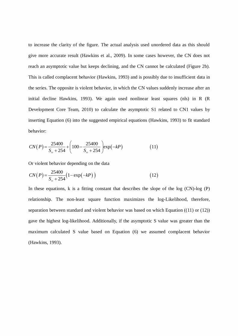

2000 2001
2002 2003
2005 2004
Figure 3 2 Rainfall during summer from June to September Plot annually from 2000 to 2011
3221 Base flow separation
Firstly direct runoff is necessary to be separated from total runoff By applying base flow
separation known as Web Based Hydrograph Tools (WHAT) the base flow and direct runoff
2006 2007
2008 2009
2010 2011
can be separated The data are derived from the Juksungmyun examinational rainfall station
from 2000 to 2011 By applying base flow separation known as Web Based Hydrograph Tools
(WHAT) the base flow and direct runoff can be derived from the analysis The data is derived
from the Juksungmyun experimental rainfall station from 2000 to 2011
2000 2001
2002 2003
2004 2005
Figure 3 3 Rainfall versus Direct Runoff Plot annually from 2000 to 2011
(Where Direct Runoffs are derived from Web based Hydrograph Tools WHAT)
2006 2007
2008 2009
2010 2011
Figure 3 4 Rainfall versus Direct Runoff Plot from 2000 to 2011
33 Evaluation of curve number procedures
After identifying direct runoff from total runoff curve number estimation can be calculated
from equation (7) by knowing daily rainfall and matched direct runoff However further
consideration is necessary to take into account That is to test the accuracy of curve number
To test the accuracy of curve number determination curve numbers are computed depending
upon four different procedures including arithmetic mean median geometric mean and
asymptotic fit Except for the asymptotic method unranked paired rainfall and runoff volumes
from the maximum peal flow event each year of record were used to compute the calibrated
curve number
To test the accuracy of curve number determination curve numbers are computed depending
upon the arithmetic mean median geometric mean and asymptotic fit as shown the Table
below Except for the asymptotic method unranked paired rainfall and runoff volumes from
the maximum peal flow event each year of record were used to compute the calibrated curve
number
Asymptotic FitGeometric MeanMedianArithmetic
Mean
Data Analysis and Data Management ( Rainfall and runoff datasets are being used to derive direct runoff by the application of Web Based
Hydrograph Tools)
Evaluation of curve number procedures
Matlab Program is used to encode the following procedures
Coefficient of Determination and Goodness of Fit ( NRMSE RE Rsquare)
Curve Number Estimation
Figure 3 5 Schematic of Cure Number Estimation procedure
The table 32 indicates the curve number estimation generated from rainfall events throughout
the entire year from 2000 to 2011 during summer season (from June to September)
Table 3 2 Curve number estimation from the selected rainfall from 2000 to 2011 in summer
No P (mm) Q (m3s) S (mm) CN No P (mm) Q (m3s) S (mm) CN
1 1500 000 7500 7720 124 6700 3048 4974 8362
2 050 000 250 9903 125 1450 1404 039 9985
3 1000 047 3001 8943 126 050 000 250 9903
4 800 098 1700 9373 127 250 000 1250 9531
5 1450 096 3930 8660 128 2650 000 13250 6572
6 4150 080 15058 6278 129 1150 000 5750 8154
7 450 063 895 9660 130 150 000 750 9713
8 600 564 031 9988 131 800 000 4000 8639
9 4700 751 8703 7448 132 150 000 750 9713
10 600 258 480 9814 133 250 000 1250 9531
11 150 000 750 9713 134 050 000 250 9903
12 2750 228 6888 7867 135 050 000 250 9903
13 800 091 1759 9352 136 600 102 1072 9595
14 4500 041 18090 5840 137 1300 099 3359 8832
15 500 000 2500 9104 138 1400 395 1745 9357
16 7000 333 20939 5481 139 1600 1152 465 9820
17 9200 1268 18443 5793 140 100 000 500 9807
18 150 066 117 9954 141 1650 463 2067 9248
19 350 000 1750 9355 142 200 000 1000 9621
20 200 000 1000 9621 143 1250 556 957 9637
21 7650 165 27231 4826 144 1250 663 733 9720
22 050 000 250 9903 145 8050 3188 7136 7807
23 100 000 500 9807 146 4600 000 23000 5248
24 650 000 3250 8866 147 650 046 1723 9365
25 300 000 1500 9442 148 5750 4578 1139 9571
26 900 000 4500 8495 149 1800 1561 219 9914
27 150 000 750 9713 150 200 028 398 9846
28 600 044 1571 9418 151 2250 534 3222 8874
29 65 035 1878 9312 152 100 045 075 9970
30 05 009 086 9966 153 1400 214 2657 9053
31 36 058 13438 654 154 050 000 250 9903
32 35 121 36 986 155 500 065 1032 9609
33 05 0 25 9903 156 100 042 083 9968
34 30 934 3424 8812 157 2850 376 5841 8130
35 1005 9138 811 969 158 1750 490 2196 9204
36 2 0 10 9621 159 680 049 1791 9341
37 05 0 25 9903 160 080 000 400 9845
38 15 0 75 9713 161 660 000 3300 8850
39 13 0 65 7962 162 080 000 400 9845
40 05 0 25 9903 163 450 000 2250 9186
41 415 2334 2191 9206 164 450 000 2250 9186
42 15 0 75 9713 165 750 000 3750 8714
43 15 85 781 9702 166 200 140 063 9975
44 25 105 206 9919 167 1450 196 2936 8964
45 2 022 446 9827 168 050 030 023 9991
46 2200 036 8193 7561 169 1600 1330 255 9901
47 2100 009 9050 7373 170 1550 360 2255 9184
48 700 005 2887 8979 171 050 000 250 9903
49 500 000 2500 9104 172 050 000 250 9903
50 1750 032 6405 7986 173 3100 2587 483 9813
51 600 004 2491 9107 174 150 116 034 9987
52 5450 1274 7893 7629 175 050 000 250 9903
53 6100 349 17308 5947 176 4850 4154 645 9753
54 250 111 192 9925 177 700 048 1875 9313
55 050 038 012 9995 178 450 022 1336 9500
56 850 000 4250 8567 179 050 000 250 9903
57 600 000 3000 8944 180 3800 1976 2304 9168
58 050 000 250 9903 181 9600 000 48000 3460
59 150 131 017 9993 182 100 000 500 9807
60 5700 132 20033 5591 183 1450 000 7250 7779
61 3650 1820 2368 9147 184 600 000 3000 8944
62 4750 121 16398 6077 185 800 230 981 9628
63 23550 3490 45451 3585 186 700 067 1658 9387
64 12250 569 36879 4078 187 2420 462 4028 8631
65 650 000 3250 8866 188 040 000 200 9922
66 100 000 500 9807 189 100 000 500 9807
67 850 000 4250 8567 190 040 000 200 9922
68 750 000 3750 8714 191 2740 988 2699 9039
69 1700 000 8500 7493 192 720 483 257 9900
70 3000 000 15000 6287 193 950 000 4750 8425
71 3700 000 18500 5786 194 500 000 2500 9104
72 3400 000 17000 5991 195 050 000 250 9903
73 3550 023 14777 6322 196 100 034 105 9959
74 050 000 250 9903 197 250 000 1250 9531
75 350 000 1750 9355 198 350 140 307 9881
76 650 000 3250 8866 199 350 134 323 9875
77 450 000 2250 9186 200 17150 8010 12268 6743
78 300 000 1500 9442 201 1800 1109 789 9699
79 1250 000 6250 8025 202 250 000 1250 9531
80 600 005 2436 9125 203 800 097 1708 9370
81 400 126 452 9825 204 1450 254 2545 9089
82 300 208 098 9962 205 100 007 266 9896
83 550 071 1139 9571 206 050 000 250 9903
84 950 564 451 9826 207 1850 531 2272 9179
85 2300 407 4012 8636 208 600 199 644 9753
86 150 000 750 9713 209 1340 000 6700 7913
87 700 000 3500 8789 210 660 000 3300 8850
88 050 000 250 9903 211 340 000 1700 9373
89 150 000 750 9713 212 300 000 1500 9442
90 100 000 500 9807 213 640 067 1460 9456
91 100 000 500 9807 214 4280 000 21400 5427
92 350 000 1750 9355 215 020 000 100 9961
93 050 000 250 9903 216 020 000 100 9961
94 600 000 3000 8944 217 340 000 1700 9373
95 600 000 3000 8944 218 1220 377 1402 9477
96 100 000 500 9807 219 8160 3882 5683 8172
97 050 000 250 9903 220 020 000 100 9961
98 150 000 750 9713 221 280 000 1400 9478
99 150 000 750 9713 222 10080 9274 711 9728
100 350 070 565 9782 223 1300 043 4252 8566
101 050 000 250 9903 224 020 000 100 9961
102 150 000 750 9713 225 2360 000 11800 6828
103 1100 214 1809 9335 226 1220 000 6100 8063
104 800 616 183 9929 227 100 000 500 9807
105 250 127 157 9938 228 020 000 100 9961
106 500 271 282 9890 229 2540 1108 1996 9272
107 1050 000 5250 8287 230 1250 402 1383 9484
108 050 000 250 9903 231 300 189 125 9951
109 550 000 2750 9023 232 250 023 602 9769
110 100 000 500 9807 233 7650 4767 3271 8859
111 1250 000 6250 8025 234 3550 1231 3644 8745
112 100 000 500 9807 235 1750 1020 862 9672
113 3350 1894 1751 9355 236 4150 2876 1353 9494
114 950 433 703 9731 237 100 000 500 9807
115 1350 187 2699 9039 238 250 000 1250 9531
116 1350 073 3895 8670 239 400 000 2000 9270
117 3800 2147 1989 9274 240 750 597 149 9942
118 050 000 250 9903 241 400 000 2000 9270
119 6750 4115 3030 8934 242 2300 811 2320 9163
120 100 063 042 9984 243 050 003 140 9945
121 1450 178 3078 8919 244 300 087 365 9858
122 350 035 814 9689 245 2350 539 3451 8804
123 150 013 369 9857
Figure 3 6 Curve number versus Rainfall plot amp Asymptotic Fitting Curve plot and Residual
plot for asymptotic curve number fits for Seolma Cheon River Watershed
Based on the graphic representation on figure 36 asymptotic curve number is 7857 with
regression equation
005697857 (100 7857) pCN e
005697857 (100 7857) pCN e
Runoff estimated by Arithmetic Mean Runoff estimated by Median
Figure 3 7 Plot of the comparison of measure runoff to the estimated runoff for each
procedure
Figure 38 Plot of the comparison of measure runoff to the estimated runoff for all procedure
From the figure 37 the geometric mean curve numbers of all year were greater than the curve
numbers based on the other calculation procedures However the geometric mean and median
curve numbers do not seem to be significantly different as expected if the watershed curve
number distribution are logarithmic In addition the arithmetic mean curve numbers generally
are close in magnitude to median curve number The mean median and geometric mean
Runoff estimated by Geometry Runoff estimated by Asymptotic CN
derived curve number do not seem to be significantly different
The asymptotic curve numbers were smaller than the curve number based on the other
procedures and some of them are not available due to the fitting points of rainfall and
estimated curve number by equation 7 It is remarkable that asymptotic curve numbers are
expected to be smaller because set of curve number that are not too scattered are associated
with the largest numbers rainfall volume observed or infinitely large volumes Remarkable is
that the asymptotic fit is biased to smaller curve number with very low frequencies of
occurrence
Table 3 3 Watershed Curve Number by all procedures from 2000 to 2011
Year Arithmetic Mean Median Geometric Mean Asymptotic Fit
200 9380 9773 9750 7100
2001 9385 9713 9697 8586
2002 8085 8790 8955 NA
2003 9585 9748 9729 8688
2004 9397 9713 9674 8954
2005 9225 9689 9628 7819
2006 9190 9595 9560 7107
2007 9433 9475 9719 8955
2008 9025 9564 9590 NA
2009 9380 9699 9683 6654
2010 9078 9449 9568 7931
2011 9473 9513 9654 9021
Table 3 4 Overall Watershed Curve Number by all Procedures
Arithmetic Mean Median Geometric Mean Asymptotic Fit
9314 9615 9652 7857
Also included in table 34 are the NRCS (2001) curve number derived from table The
geometric mean curve numbers of all year were greater than the curve number based on the
other calculation However the geometric mean and median curve numbers do not seem to be
significantly different as expected if the watershed curve number distributions are logarithmic
In addition the arithmetic mean curve number generally fall or are close in magnitude to one
of the values
The asymptotic curve numbers was smaller than the curve numbers based on the other
procedure The asymptotic curve numbers are expected to be smaller because these values are
associated with the largest rainfall volumes observed or infinitely large volume
34 Reliability of Curve number method on Gauged Basins
To assess the reliability of the handbook CN method the runoff depth were estimated from
the theoretical CN and compared with the measure runoff depth The theoretical CN was
computed as the basin mean value derived from the asymptotic method to take into account 5-
day antecedent rainfall and season differentiation To evaluate model performance two
additional indexes were computed to assess the agreement of estimated runoff and measured
runoff There are the Normal root-mean-square error (NRMSE) R2 RE and Nash and
Sutcliffe (1970) efficiency (E)
Arithmetic Mean Procedure R2 = 07233 Median Procedure R
2 = 07315
Figure 3 9 Coefficient of determination of each CN estimation procedures
Procedure of CN
estimation CN R
2 RE NRMSE E
Arithmetic Mean 9314 07233 06274 00653 04054
Median 9615 07315 07240 00722 01864
Geometric Mean 9652 07320 07357 00733 01496
Asymptotic Fit 7857 06376 01809 00738 0601
Table 26 Reliability of Curve number method
The relative accuracy and correlation of rainfall-runoff derived curve numbers based on four
procedures are determined from coefficient of determination and goodness of fit such as
Normalized Root Mean Square Error (NRMSE) Relative Error (RE) R-Square (R2) and
Nash Sutcliffe coefficient (E)
Based on the tests shown in table 36 the asymptotic procedure is the best for curve number
estimation In addition to that the curve number derived by the three procedures known as
arithmetic mean median and geometric mean are in general not very different these finding
only serve to highlight that one highlight that one procedure is as similar as another Hence
curve number derived from asymptotic method is used for further analysis Asymptotic curve
Geometry Procedure R2 = 07320 Asymptotic CN Procedure R
2 = 06376
number is 7857 with regression equation 005697857 (100 7857) pCN e
After the curve number is estimated the next step is to simulate antecedent moisture
condition by applying all the proposed algebraic expression of NEH4 with the consideration
of 5 day prior to rainfall (definition of AMC using antecedent rainfall table) Next is to
validate and calibrate among the proposed procedure to figure out the estimator of antecedent
moisture condition criteria
35 Estimation of Thresholds for AMCARC
To reduce uncertainties in the CN method new rainfall thresholds for the definition of the
AMC class where computed The new thresholds have been evaluated for each of the basin as
the precipitation of the antecedent 5-day time span which minimizes the difference between
measured and estimated runoff The optimization procedure was based on a simple manual
trial-and-error approach The differentiation between growth and dormant seasons was not
considered in this analysis
Figure 3 10 Antecedent Moisture Condition (AMC)Antecedent Run off Condition
proposed Methodology
Algebraic expression of
NEH4 ( developed Sobhani
(1975) Chow et al (1988)
Hawkins et al (1985)
Arnold et al (1988)
Data collection (Rainfall
and Runoff data)
Derive direct runoff ( by
Web Based Hydrograph
Tools WHAT)
Calibration amp Validation
( NRMSE RENSE R2)
Determination of AMCARC
estimation criteria
Asymptotic FitGeometric MeanMedianArithmetic
Mean
Accuracy of curve number procedures
Matlab Program is used to encode the following procedures
Coefficient of Determination and Goodness of Fit ( NRMSE RE Rsquare)
Curve Number Estimation
Hawkins
et al (1985)
Sobhani
(1975)Chow et al
(1988)
Algebraic expression of NEH4
Arnold et al
(1988)
Once curve number has been estimated proposed algebraic equation can be used to determine
the criteria for choosing ARCAMC
Curve Number
estimation by
all procedures
Hawkins
et al (1985)
Sobhani
(1975)Chow et al
(1988)
ARCAMC criteria
determination
Algebraic expression of NEH4
Arnold et al
(1988)
Calibrated Validated by Coefficient of Determination
and Goodness of Fit ( NRMSE RE Rsquare)
Determination of AMCARC estimation criteria
Compare among Coefficient of Determination and Goodness of Fit
Figure 3 11 Schematic representation of AMCARC estimation criteria
Once algebraic expressions are computed comparison among coefficient of determination
and Goodness of fit is necessary to follow up Finally AMCARC criteria are identified
Second step of the proposed procedure is to determine AMCARC criteria estimation using
algebraic Expression developed by Sobhani (1975) Hawkins et al (1985) Chow et al 1988
and Arnold et al (1990)
Algebraic Expression of NEH4 developed by Sobhani 1975
Figure 3 12 Verification of AMCARC condition (using algebraic expression by Sobhani
1975)
AMC R2 RE NRMSE E
2000-2011 0327801474 094605433 0896495482 0024430041
2011 0918578445 094605433 1733367342 0059823241
2010 0348851642 096495701 3596402064 -0030357167
ARC R2 RE NRMSE E
2000-2011 0369420822 096416947 1379920476 -0019679303
2011 093839593 096416947 267172036 0014620395
2010 0380569445 098809233 1086921876 -0086673899
2010 2011
Table 3 5 Coefficient of determination and Goodness of fit of AMC ARC and Regression
Equation in respect Sobhanilsquos algebraic expression
Fig 312 shows about the plot of rainfall direct runoff and AMCARC versus time in
different time period That is 12 year of daily record and the below graph are the plot of daily
record in 2011 and 2010 respectively from June to September In other words they are plotted
during summer season
With the value of R-square 03278 for AMC condition and 03694 for ARC condition it is
denoted that it poorly explains the observed direct runoff Also with RE equal to 0946 it is
indicated that model overestimate observed data (direct runoff) by 946 However model
performance is fairly fit among validated value across the year 2011 and 2010
Regarding to validation and calibration of the estimated model (direct runoff estimation) in
2011 it fairly well describes the observed direct runoff with R-square equal to 09185 for
AMC condition and 09383 for ARC condition yet it model overestimate observed data by
9460 percent In 2010 it shows the value close to the estimation of 12 years period ranging
from 2000 to 2011
Algebraic Expression of NEH4 developed by Hawkins et al 1985
2010 2011
Figure 3 13 Verification of AMCARC condition (using algebraic expression by Hawkins et
al 1985)
AMC R2 RE NRMSE E
2000-2011 0333680999 0946660232 0907297388 0023098886
2011 0928099542 0946660232 1754467056 0058310338
2010 0350696295 09660276 3714648349 -0033086936
ARC R2 RE NRMSE E
2000-2011 0369420822 096416947 1379920476 -0019679303
2011 093839593 096416947 267172036 0014620395
2010 0380569445 098809233 1086921876 -0086673899
Table 3 6 Coefficient of determination and Goodness of fit of AMC ARC and Regression
Equation in respect to Hawkins et allsquos algebraic expression
Fig 313 and Table 36 present about the plot of rainfall direct runoff and AMC versus time
in different time period by the application of Hawkin et al 1985 That is 12 year of daily
record and the below graph are the plot of daily record in 2011 and 2010 respectively from
June to September in summer
With the value of R-square 03336 for AMC condition and 03694 for ARC condition it is
denoted that it poorly explains the observed Also with RE equal to 09466 and 09461 for
AMC and ARC respectively it is indicated that model overestimate observed data (direct
runoff) by 9466 and 9441 in respect to AMC and ARC condition However model
performance is fairly fit among validated value across the year 2011 and 2010
Regarding to validation and calibration of the estimated model (direct runoff estimation) in
2011 it fairly well describes the observed direct runoff yet it model overestimate observed
runoff
Overall algebraic equations by Hawkins at el seem to be more reliable than by Sobhani
Remarkable is that the two proposed equations are very close to one another in term of
reliability
Algebraic Expression of NEH4 developed by Chow et al 1988
2010 2011
Figure 3 14 Verification of AMCARC condition (using algebraic expression by chow et al
1988)
AMC R2 RE NRMSE E
2000-2011 0330815816 0946759955 0909419272 0022190703
2011 0924871529 0946759955 1758274536 0057751809
20100350433876 0966201253 373475769 -0033653731
ARC R2 RE NRMSE E
2000-2011 0369420822 096416947 1379920476 -0019679303
2011 093839593 096416947 267172036 0014620395
2010 0380569445 098809233 1086921876 -0086673899
Table 3 7 Coefficient of determination and Goodness of fit of AMC ARC and Regression
Equation in respect to chow et allsquos algebraic expression
Graphic representation in figure 314 indicates the rainfall direct runoff and AMC and ARC
versus time relationship different time period by the application of Chow et al 1988 That is
12 year of daily record and the below graph are the plot of daily record in 2011 and 2010
respectively in summer
With the same consideration as in previous description overall the simulated direct runoff
with algebraic equation represented CN I and CN III by Chow et al 1988 is closely similar to
the two other proposed equation Closely look into the coefficient of determination
simulation of direct runoff is somewhere in between the two proposed methods It is
noticeably that also overestimate the observed direct runoff by 9467 and 9641 in regard
to AMC and ARC condition
Algebraic Expression of NEH4 developed by Arnold et al 1990
Figure 3 15 Verification of AMCARC condition (using algebraic expression by Arnold et al
1990)
2010 2011
AMC R2 RE NRMSE E
2000-2011 0308655367 0945964916 0895016283 0024420732
2011 090537271 0945964916 1729746927 0060640334
2010 0348083522 0964796732 3576773151 -0028484523
ARC R2 RE NRMSE E
2000-2011 0369420822 096416947 1379920476 -0019679303
2011 093839593 096416947 267172036 0014620395
2010 093839593 096416947 267172036 0014620395
Table 3 8 Coefficient of determination and Goodness of fit of AMC ARC and Regression
Equation in respect to Arnold et allsquos algebraic expression
Figure 315 represents plot of rainfall direct runoff and simulated direct runoff by AMC
taking into account of algebraic equation developed by Arnold et al 1990
With the value of R-square 03086 for AMC condition and 03694 for ARC condition it is
denoted that it poorly explains the observed direct runoff Also with RE equal to 09459 for
AMC condition and 09641 for ARC condition it is indicated that model overestimate
observed data (direct runoff) by 9459 and 9641 respectively However model performance
is fairly fit among validated value across the year 2011 and 2010
Regarding to validation and calibration of the estimated model (direct runoff estimation) in
2011 it fairly describes the observed direct runoff yet it model overestimate observed data
Third step to compare among Coefficient of Determination and Goodness of Fit
Sobhani Hawkins et al Chow et al Arnold et al
R2 03278 03337 03308 03087
RE 09461 09467 09468 09460
NRMSE 08965 09073 09094 08950
E 00244 00231 00222 00244
R2 09186 09281 09249 09054
RE 09461 09467 09468 09460
NRMSE 17334 17545 17583 17297
E 00598 00583 00578 00606
R2 03489 03507 03504 03481
RE 09650 09660 09662 09648
NRMSE 35964 37146 37348 35768
E -00304 -00331 -00337 -00285
Algebraic Expression
2000-2011
2011
2010
AMCCoefficient of
Determination
Sobhani Hawkins et al Chow et al Arnold et al
R2 03694 03694 03694 03694
RE 09642 09642 09642 09642
NRMSE 13799 13799 13799 13799
E -00197 -00197 -00197 -00197
R2 09384 09384 09384 09384
RE 09642 09642 09642 09642
NRMSE 26717 26717 26717 26717
E 00146 00146 00146 00146
R2 03806 03806 03806 09384
RE 09881 09881 09881 09642
NRMSE 108692 108692 108692 26717
E -00867 -00867 -00867 00146
2000-2011
2011
2010
Algebraic ExpressionARC
Coefficient of
Determination
Table 3 9 Result of all coefficient of determination
Table 39 present results of coefficient of determination of AMC from the four different
proposed equations
Clearly indicated in the table 39 for 12 years period analysis normalized root mean square
error RE and E are best described by the application of algebraic expression by Arnold et al
at the value of 08950 09460 and 00244 for AMC condition In addition for all the
coefficient of determination in regard to ARC condition Arnold et al algebraic equation is the
best representation criteria However overall calculated coefficients of determination
among proposed method are very close to each other In the other words it remarkably
indicates the least residual variance
In addition to that for all the application of algebraic equation in determining AMC and ARC
criteria it overestimates the actual runoff by over 90 However in terms of estimation
performance proposed expression by Arnold et al fairly explains the observed direct runoff
more reliable than others proposed expressions With regarding to R-square proposed method
by Hawkins et al is the most reliable for AMC condition
For the verification observed and estimated runoff data from 2010 and 2011 have been
conducted As results from the comparison of coefficient of determination Arnold et al is the
most favorable estimation of antecedent moisture condition criteria as well as antecedent
runoff condition criteria
Proposed methods are overall is very close to one and another it is implied that all the
application of proposed method can be used to describe the antecedent moisture condition
criteria and as antecedent runoff condition criteria Also the antecedent rainfall table from
NEH report
CHAPTER 4 CONCLUSIONS
WHAT is the acronym of Web Based Hydrograph Analysis Tool which is the useful internet
based application that allows the user to get the results of base flow from different digital
filters by just simple click and then get the preferable results In accordance to its simplicity it
might be recommended for further study to determine base flow
Application of curve number procedures and evaluation of each procedure by the coefficient
of determination
The relative accuracy and correlation of rainfall-runoff derived curve numbers based on four
procedures determined from coefficient of determination and goodness of fit show that the
asymptotic procedure is the best for curve number estimation It is found that asymptotic CN
number is the most appropriate procedure in Seolma Cheon River watershed with the value of
7857 It is noticeably that the curve number derived by the three procedures known as
arithmetic mean median and geometric mean are in general not very different these finding
only serve to highlight that one highlight that one procedure is as similar as another
Proposed methods are developed by modifying estimated runoff to observed runoff with
coefficient of determination and then applying different algebraic expression developed In
addition by choosing precipitation from antecedent moisture condition due to the 5 prior to
rainfall (NEH-1964 AMC definition) it is indicated that the overall results of estimated runoff
is nearly double to the observed runoff The reason is originated from the selection of
precipitation according antecedent rainfall table
Clearly indicated from 12 years period analysis and 2 years period of verification normalized
root mean square error RE and E are best described by the application of algebraic expression
by Arnold et al at the value of 08950 09460 and 00244 respectively for AMC condition
and 13799 09642 and -00197 respectively for ARC condition Furthermore for all the
coefficient of determination with the respect to ARC condition Arnold et al algebraic
equation is the best representation criteria Therefore Arnold et al is the most appropriate for
antecedent moisture condition criteria as well as for antecedent runoff condition Therefore
this algebraic expression might be used in South Korea condition properly Since calculated
coefficients of determination among proposed method are very close to each other it
remarkably indicates the least residual variance
From results and the validation of AMCARC it is implied that the determination of AMC has
some inconsistency from one to another Thus for long time period of time determination of
AMC might be accepted for further usage
For further study it is recommended to compare the Base flow Separation and CN Estimation
Method for determining ARC and AMC as well as to figure out the best practices for
identifying ARC and AMC By applying different base flow digital filter the research might
find out the better results of ARC and AMC in turn it might be useful to get better
understanding about ARC and AMC as well as the optimization value of AMC and ARC with
regards to Korea condition
REFERENCES
Andrews RG (1954) The use of relative infiltration indices in computing runoff in Rainfall-runoff
relationship Singh VP Water Resources Publications
Arnold JG Williams JR Nicks AD and Sammons NB (1990) SWRRB A basin scale simulation model for
soil and water resources management Texas AampM University Press pp 142
Babu PS and Mishra SK (2011) An improved SCS- CN inspired model J of Hydrological
Engineering ASCE 17(11) pp 1164-1172
Chow VT Maidment DR and Mays LW (1988) Applied Hydrology Mc-Graw-Hill New
York pp 572
Eckhardt K (2005) How to construct recursive digital filters for baseflow separation Hydrological Process
19(2) pp 337-349
Elhakeem M and Papanicolaou AN (2009) Estimation of the runoff curve number via direct rainfall
simulator measurements in the state of Iowa USA Water Resources Management 23(12) pp 2455ndash2473
Garen DC and Moore DS (2005a) Curve number hydrology in water quality modeling uses abuses and
future direction J of the American Water Resources Association 412 (April 2005) Paper 03127 pp 377-
388
Garen DC and Moore DS (2005b) Reply to discussion of curve number hydrology in water quality
modeling uses abuses and future directions by MT Walter and SB Shaw J of the American Water
Resources Association 416 (December 2005) pp 1493-1494
Grabau MR Hawkins RH VerWeire KE and Slack DC (2008 in review) Curve numbers as random
variables empirical observations and implication for design and modeling J of American Society of
Agricultural and Biological Engineering [in Review]
Hawkins RH (1993) Asymptotic determination of runoff curve numbers from data J of Irrigation and
Drainage Engineering ASCE 119(2) pp 334-345
Hawkins RH Hjelmfelt Jr AT and Zevenbergen AW (1985) Runoff probability storm depth and curve
numbers J of Irrigation and Drainage Division ASCE 111(4) pp 330-340
Hawkins RH (1996) Discussion of SCS runoff equation revisited for variable source runoff areas by TS
Steenhuis M Mitchell JRossing and MFWalter J of Irrigation and Drainage Engineering ASCE
122(5) pp 319
Hawkins RH Ward TJ Woodward DE and Van Mullen JA (2009) Curve number hydrology State of the
practice American Society of Civil Engineers ASCE USA
Hjelmfelt Jr AT and Kramer LA (1983) Discussion of antecedent moisture condition probability by D D
Gray et al J of Irrigation and Drainage Engineering ASCE 109 p300
Hjelmfelt Jr AT (1991) Investigation of curve number procedure J of Hydraulic Engineering Division
Amer Soc Civ Eng 117(6) pp 725-737
Jain MK Mishra SK Singh VP (2006) Evaluation of AMC dependent SCS-CN based models using
watershed characteristics J of Water Resources Management 20( 4) pp 531-552
Kim NW and Lee JW (2008) Temporally weighted average curve number method for daily runoff
simulation J of Hydrological Processes 22(25) pp 4936-4948
King KW Arnold JG and Bingner RL (1999) Comparison of Green ndashAmpt and curve number methods on
Goodwin Creek using SWAT Transaction of the American Society of Agricultural Engineers 42(4) pp
919-925
Kwak JW Kim SJ Yin SH and KIM HS (2010) direct runoff simulation using CN regression equation for
Bocheong Stream J of Korean Society on Water Quality 26(4) pp 590-597 [Korean Literature]
Michel C Vazken A and Charles P (2005) Soil conservation service curve number method
how to mend among soil moisture accounting procedure Water Resources Research 41(2)
pp 1-6
Miliani F Ravazzani G and Manicini M (2011) Adaptation of precipitation index for the estimation of
antecedent moisture condition in large mountainous basin J of Hydrological Engineering 16(3) pp 218-227
Mishra SK Jain MK and Singh VP (2004) Evaluation of SCS-CN based models incorporating antecedent
moisture J of Water Resources Management 18(6) pp 567-589
Mishra SK Jain MK Pandey RP and Singh VP (2005) Catchment area-based evaluation of the AMC-
dependent SCS-CN-based rainfall-runoff models J of Hydrological Processes 19 pp 2701ndash2718
Mishra SK Pandey RP Jain MK and Singh VP (2008) A rain duration and modified AMC dependent
SCS- CN procedure for long duration rainfall- runoff events Water Resources Management 22(7) pp
861-876
Mockus V (1949) Estimation of total (peak rates of) surface runoff for individual storms Exhibit A of
Appendix B Interim Survey Rep Grand (Neosho) River Watershed USDA Washington DC
Pandit A and Gopalakrishnan G (1996) Estimation of annual storm runoff coefficients by continuous
simulation J of Irrigation and Drainage Engineers ASCE 122(4) pp 211-220
Ponce VM and Hawkins RH (1996) Runoff curve number has it reached maturity J of Hydrologic
Engineering ASCE 1(1) pp 11-19
Rallison RE (1980) Origin and evolution of the SCS runoff equationrdquo Proceedings of Symposium on
Watershed Management 1980 American Society of Civil Engineering New York pp 921-924
Rallison RE and Cronshey RG (1979) Discussion of runoff curve numbers with varying site moisture Proc
Amer Soc Civ Eng 105(IR4) pp 439-441
Sahu RK Mishra SK Eldho TI and Jain MK (2007) An advanced soil moisture accounting procedure for
SCS curve number method Hydrological Processes 21(21) pp 2827-2881
Sahu RK Mishra SK and Eldho TI (2010) An improved AMC-coupled runoff curve number model
Hydrological Processes 24(20) pp 2834-2839
Schneider LE and McCuen RH (2005) Statistical guideline for curve number generation J of Irrigation and
Drainage Engineering 131(3) 282-290
Silveira L Charbonnier F and Genta JL (2000) The antecedent soil moisture condition of the curve number
procedure J of Hydrological Sciences 45(1)
Van Mullem JA (1992) Soil moisture and runoffmdashanother look ASCE Water Forum 92 Proceedings of the
Irrigation and Drainage Session Baltimore MD
Williams JR and LaSeur V (1976) Water yield model using SCS curve numbers J of Hydraulic Engineers
102( 9) pp 1241-1253
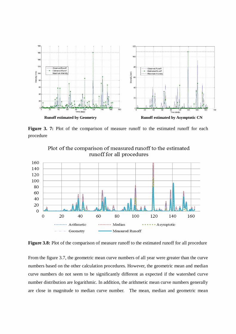
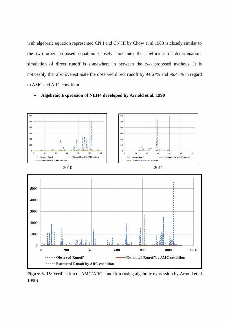

Sobhani Hawkins et al Chow et al Arnold et al
R2 03278 03337 03308 03087
RE 09461 09467 09468 09460
NRMSE 08965 09073 09094 08950
E 00244 00231 00222 00244
R2 09186 09281 09249 09054
RE 09461 09467 09468 09460
NRMSE 17334 17545 17583 17297
E 00598 00583 00578 00606
R2 03489 03507 03504 03481
RE 09650 09660 09662 09648
NRMSE 35964 37146 37348 35768
E -00304 -00331 -00337 -00285
Algebraic Expression
2000-2011
2011
2010
AMCCoefficient of
Determination
Sobhani Hawkins et al Chow et al Arnold et al
R2 03694 03694 03694 03694
RE 09642 09642 09642 09642
NRMSE 13799 13799 13799 13799
E -00197 -00197 -00197 -00197
R2 09384 09384 09384 09384
RE 09642 09642 09642 09642
NRMSE 26717 26717 26717 26717
E 00146 00146 00146 00146
R2 03806 03806 03806 09384
RE 09881 09881 09881 09642
NRMSE 108692 108692 108692 26717
E -00867 -00867 -00867 00146
2000-2011
2011
2010
Algebraic ExpressionARC
Coefficient of
Determination
Table 3 9 Result of all coefficient of determination
Table 39 present results of coefficient of determination of AMC from the four different
proposed equations
Clearly indicated in the table 39 for 12 years period analysis normalized root mean square
error RE and E are best described by the application of algebraic expression by Arnold et al
at the value of 08950 09460 and 00244 for AMC condition In addition for all the
coefficient of determination in regard to ARC condition Arnold et al algebraic equation is the
best representation criteria However overall calculated coefficients of determination
among proposed method are very close to each other In the other words it remarkably
indicates the least residual variance
In addition to that for all the application of algebraic equation in determining AMC and ARC
criteria it overestimates the actual runoff by over 90 However in terms of estimation
performance proposed expression by Arnold et al fairly explains the observed direct runoff
more reliable than others proposed expressions With regarding to R-square proposed method
by Hawkins et al is the most reliable for AMC condition
For the verification observed and estimated runoff data from 2010 and 2011 have been
conducted As results from the comparison of coefficient of determination Arnold et al is the
most favorable estimation of antecedent moisture condition criteria as well as antecedent
runoff condition criteria
Proposed methods are overall is very close to one and another it is implied that all the
application of proposed method can be used to describe the antecedent moisture condition
criteria and as antecedent runoff condition criteria Also the antecedent rainfall table from
NEH report
CHAPTER 4 CONCLUSIONS
WHAT is the acronym of Web Based Hydrograph Analysis Tool which is the useful internet
based application that allows the user to get the results of base flow from different digital
filters by just simple click and then get the preferable results In accordance to its simplicity it
might be recommended for further study to determine base flow
Application of curve number procedures and evaluation of each procedure by the coefficient
of determination
The relative accuracy and correlation of rainfall-runoff derived curve numbers based on four
procedures determined from coefficient of determination and goodness of fit show that the
asymptotic procedure is the best for curve number estimation It is found that asymptotic CN
number is the most appropriate procedure in Seolma Cheon River watershed with the value of
7857 It is noticeably that the curve number derived by the three procedures known as
arithmetic mean median and geometric mean are in general not very different these finding
only serve to highlight that one highlight that one procedure is as similar as another
Proposed methods are developed by modifying estimated runoff to observed runoff with
coefficient of determination and then applying different algebraic expression developed In
addition by choosing precipitation from antecedent moisture condition due to the 5 prior to
rainfall (NEH-1964 AMC definition) it is indicated that the overall results of estimated runoff
is nearly double to the observed runoff The reason is originated from the selection of
precipitation according antecedent rainfall table
Clearly indicated from 12 years period analysis and 2 years period of verification normalized
root mean square error RE and E are best described by the application of algebraic expression
by Arnold et al at the value of 08950 09460 and 00244 respectively for AMC condition
and 13799 09642 and -00197 respectively for ARC condition Furthermore for all the
coefficient of determination with the respect to ARC condition Arnold et al algebraic
equation is the best representation criteria Therefore Arnold et al is the most appropriate for
antecedent moisture condition criteria as well as for antecedent runoff condition Therefore
this algebraic expression might be used in South Korea condition properly Since calculated
coefficients of determination among proposed method are very close to each other it
remarkably indicates the least residual variance
From results and the validation of AMCARC it is implied that the determination of AMC has
some inconsistency from one to another Thus for long time period of time determination of
AMC might be accepted for further usage
For further study it is recommended to compare the Base flow Separation and CN Estimation
Method for determining ARC and AMC as well as to figure out the best practices for
identifying ARC and AMC By applying different base flow digital filter the research might
find out the better results of ARC and AMC in turn it might be useful to get better
understanding about ARC and AMC as well as the optimization value of AMC and ARC with
regards to Korea condition
REFERENCES
Andrews RG (1954) The use of relative infiltration indices in computing runoff in Rainfall-runoff
relationship Singh VP Water Resources Publications
Arnold JG Williams JR Nicks AD and Sammons NB (1990) SWRRB A basin scale simulation model for
soil and water resources management Texas AampM University Press pp 142
Babu PS and Mishra SK (2011) An improved SCS- CN inspired model J of Hydrological
Engineering ASCE 17(11) pp 1164-1172
Chow VT Maidment DR and Mays LW (1988) Applied Hydrology Mc-Graw-Hill New
York pp 572
Eckhardt K (2005) How to construct recursive digital filters for baseflow separation Hydrological Process
19(2) pp 337-349
Elhakeem M and Papanicolaou AN (2009) Estimation of the runoff curve number via direct rainfall
simulator measurements in the state of Iowa USA Water Resources Management 23(12) pp 2455ndash2473
Garen DC and Moore DS (2005a) Curve number hydrology in water quality modeling uses abuses and
future direction J of the American Water Resources Association 412 (April 2005) Paper 03127 pp 377-
388
Garen DC and Moore DS (2005b) Reply to discussion of curve number hydrology in water quality
modeling uses abuses and future directions by MT Walter and SB Shaw J of the American Water
Resources Association 416 (December 2005) pp 1493-1494
Grabau MR Hawkins RH VerWeire KE and Slack DC (2008 in review) Curve numbers as random
variables empirical observations and implication for design and modeling J of American Society of
Agricultural and Biological Engineering [in Review]
Hawkins RH (1993) Asymptotic determination of runoff curve numbers from data J of Irrigation and
Drainage Engineering ASCE 119(2) pp 334-345
Hawkins RH Hjelmfelt Jr AT and Zevenbergen AW (1985) Runoff probability storm depth and curve
numbers J of Irrigation and Drainage Division ASCE 111(4) pp 330-340
Hawkins RH (1996) Discussion of SCS runoff equation revisited for variable source runoff areas by TS
Steenhuis M Mitchell JRossing and MFWalter J of Irrigation and Drainage Engineering ASCE
122(5) pp 319
Hawkins RH Ward TJ Woodward DE and Van Mullen JA (2009) Curve number hydrology State of the
practice American Society of Civil Engineers ASCE USA
Hjelmfelt Jr AT and Kramer LA (1983) Discussion of antecedent moisture condition probability by D D
Gray et al J of Irrigation and Drainage Engineering ASCE 109 p300
Hjelmfelt Jr AT (1991) Investigation of curve number procedure J of Hydraulic Engineering Division
Amer Soc Civ Eng 117(6) pp 725-737
Jain MK Mishra SK Singh VP (2006) Evaluation of AMC dependent SCS-CN based models using
watershed characteristics J of Water Resources Management 20( 4) pp 531-552
Kim NW and Lee JW (2008) Temporally weighted average curve number method for daily runoff
simulation J of Hydrological Processes 22(25) pp 4936-4948
King KW Arnold JG and Bingner RL (1999) Comparison of Green ndashAmpt and curve number methods on
Goodwin Creek using SWAT Transaction of the American Society of Agricultural Engineers 42(4) pp
919-925
Kwak JW Kim SJ Yin SH and KIM HS (2010) direct runoff simulation using CN regression equation for
Bocheong Stream J of Korean Society on Water Quality 26(4) pp 590-597 [Korean Literature]
Michel C Vazken A and Charles P (2005) Soil conservation service curve number method
how to mend among soil moisture accounting procedure Water Resources Research 41(2)
pp 1-6
Miliani F Ravazzani G and Manicini M (2011) Adaptation of precipitation index for the estimation of
antecedent moisture condition in large mountainous basin J of Hydrological Engineering 16(3) pp 218-227
Mishra SK Jain MK and Singh VP (2004) Evaluation of SCS-CN based models incorporating antecedent
moisture J of Water Resources Management 18(6) pp 567-589
Mishra SK Jain MK Pandey RP and Singh VP (2005) Catchment area-based evaluation of the AMC-
dependent SCS-CN-based rainfall-runoff models J of Hydrological Processes 19 pp 2701ndash2718
Mishra SK Pandey RP Jain MK and Singh VP (2008) A rain duration and modified AMC dependent
SCS- CN procedure for long duration rainfall- runoff events Water Resources Management 22(7) pp
861-876
Mockus V (1949) Estimation of total (peak rates of) surface runoff for individual storms Exhibit A of
Appendix B Interim Survey Rep Grand (Neosho) River Watershed USDA Washington DC
Pandit A and Gopalakrishnan G (1996) Estimation of annual storm runoff coefficients by continuous
simulation J of Irrigation and Drainage Engineers ASCE 122(4) pp 211-220
Ponce VM and Hawkins RH (1996) Runoff curve number has it reached maturity J of Hydrologic
Engineering ASCE 1(1) pp 11-19
Rallison RE (1980) Origin and evolution of the SCS runoff equationrdquo Proceedings of Symposium on
Watershed Management 1980 American Society of Civil Engineering New York pp 921-924
Rallison RE and Cronshey RG (1979) Discussion of runoff curve numbers with varying site moisture Proc
Amer Soc Civ Eng 105(IR4) pp 439-441
Sahu RK Mishra SK Eldho TI and Jain MK (2007) An advanced soil moisture accounting procedure for
SCS curve number method Hydrological Processes 21(21) pp 2827-2881
Sahu RK Mishra SK and Eldho TI (2010) An improved AMC-coupled runoff curve number model
Hydrological Processes 24(20) pp 2834-2839
Schneider LE and McCuen RH (2005) Statistical guideline for curve number generation J of Irrigation and
Drainage Engineering 131(3) 282-290
Silveira L Charbonnier F and Genta JL (2000) The antecedent soil moisture condition of the curve number
procedure J of Hydrological Sciences 45(1)
Van Mullem JA (1992) Soil moisture and runoffmdashanother look ASCE Water Forum 92 Proceedings of the
Irrigation and Drainage Session Baltimore MD
Williams JR and LaSeur V (1976) Water yield model using SCS curve numbers J of Hydraulic Engineers
102( 9) pp 1241-1253