
Study on biomass supply chain planning and inventory control ...
185
Thèse de doctorat de l’UTT Duc Huy NGUYEN Study on Biomass Supply Chain Planning and Inventory Control of Perishable Products Champ disciplinaire : Sciences pour l’Ingénieur 2019TROY0005 Année 2019
-
Upload
khangminh22 -
Category
Documents
-
view
0 -
download
0
Transcript of Study on biomass supply chain planning and inventory control ...

Thèse de doctorat
de l’UTT
Duc Huy NGUYEN
Study on Biomass Supply Chain Planning and Inventory Control
of Perishable Products
Champ disciplinaire : Sciences pour l’Ingénieur
2019TROY0005 Année 2019

THESE
pour l’obtention du grade de
DOCTEUR
de l’UNIVERSITE DE TECHNOLOGIE DE TROYES
EN SCIENCES POUR L’INGENIEUR
Spécialité : OPTIMISATION ET SURETE DES SYSTEMES
présentée et soutenue par
Duc Huy NGUYEN
le 23 janvier 2019
Study on Biomass Supply Chain Planning and Inventory Control of Perishable Products
JURY
M. C. PRINS PROFESSEUR DES UNIVERSITES Président
M. S. DAUZÈRE-PÉRÈS PROFESSEUR Rapporteur
M. A. MOUKRIM PROFESSEUR DES UNIVERSITES Rapporteur
Mme E. SAHIN PROFESSEURE DES UNIVERSITES Examinatrice
M. Z. WANG PROFESSOR Examinateur
M. H. CHEN PROFESSEUR DES UNIVERSITES Directeur de thèse

Acknowledgments
The research work presented in this Ph.D. thesis is realized in the Laboratory of Indus-
trial Systems Optimization (LOSI) at the University of Technology of Troyes, France. This
work has been accomplished under the supervision of M. Haoxun CHEN. I would like to
thank the people who have helped me to complete the work contained in this manuscript.
First of all, I would like to express my deepest gratitude to my advisor, Prof. Haoxun
CHEN, for his restless guidance, his excellent scientific support throughout my studies. I
feel very honored and lucky to have him as an advisor, and I admire him for his knowledge,
patience, excellent cooperation and care.
Secondly, I would like to express my special thanks to M. Stéphane DAUZERE-PERES
and M. Aziz MOUKRIM for accepting to review my Ph.D. thesis. I would also like to thank
Mme Evren SAHIN, M. Christian PRINS and M. Zheng WANG for agreeing to examine this
thesis. Their valuable remarks and constructive comments have helped us to improve the
presentation and the quality of this manuscript.
At the same time, I would like to thank the members of ROSAS for the friendly and
adorable environment which they have offered me since I joint the department. More-
over, I would also like to acknowledge my friends at UTT and LOSI, for their help.
Last of all, but not least, I also want to express gratitude and love for my family, espe-
cially my loving and understanding wife Cam Tu VU, for their love and endless support. I
thank my parents and my little sister for the foundations you all provided for me. I dedi-
cate my thesis to them.
1

2

Abstract
In the last decades, the use of renewable energy sources reduced the effect of global
warming. Biomass is a promising energy resource to produce heat, electricity, and biofuel.
An efficient supply chain design and optimal inventory management could contribute to
reduce biofuel prices significantly and improve competitiveness with fossil fuel.
This thesis addresses two crucial problems: biomass supply chain optimization and
inventory control for a perishable product (biomass). The former is devoted to an issue
of supplier selection and operation planning in biomass supply chains under uncertainty.
This problem is formulated as a deterministic (MILP) model and a two-stage stochastic
programming model. The deterministic model is solved by using a MIP solver GUROBI.
An enhanced L-shaped decomposition method is developed to find an optimal solution
for the stochastic model.
The second deals with a stochastic inventory problem of a perishable product with
uncertainty in both supply and demand. After demonstrating its optimal inventory pol-
icy is an order-to-level policy, a Lagrangian relaxation based algorithm is developed to
quickly find a near-optimal solution of the problem. The stochastic inventory problem
is, then, extended to a product with a fixed lifetime. The Conditional scenario method is
developed to solve approximately this problem.
Keywords: Operations research, Combinatorial Optimization, Business logistics, Biomass,
Inventory Control, Stochastic Programming, Uncertainty, Heuristic.
3

4

Résumé
Au cours des dernières décennies, l’utilisation de sources d’énergie renouvelables a
réduit les effets du réchauffement climatique. La biomasse est une ressource énergétique
prometteuse pour la production de la chaleur, de l’électricité et des biocarburants. Une
conception efficace de la chaîne d’approvisionnement et une gestion optimale des stocks
permettent à réduire significativement les prix des biocarburants et à améliorer la com-
pétitivité contre des combustibles fossiles.
Cette thèse aborde deux problèmes cruciaux : l’optimisation d’une chaîne logistique
et la gestion des stocks périssables (biomasse). Le premier problème est consacré à la
sélection des fournisseurs et la planification des opérations dans une chaîne logistique
en biomasse. Ce problème est formulé sous forme de modèle déterministe (MILP) et de
modèle stochastique à deux étapes. Le premier modèle est résolu de manière optimale
par le solveur GUROBI. Une méthode de décomposition « L-shaped » est développée pour
traiter le deuxième modèle.
Le second problème consiste à la gestion des stocks d’un produit périssable sous in-
certitudes d’approvisionnement et de demande. Après avoir démontré que sa politique de
gestion des stocks est une politique "order-up-to level", un algorithme basé sur la relaxa-
tion lagrangienne est développé pour trouver rapidement une solution quasi-optimale
du problème. Ensuite, ce problème est étendu pour un produit à durée de vie fixe. La
méthode « Conditional scenario » est développée pour résoudre approximativement ce
problème.
Mots-clés : Recherche opérationnelle, Optimisation combinatoire, Logistique, Biomasse,
Gestion des stocks, Programmation stochastique, Incertitude, Heuristique.
5

6

Contents
Acknowledgments 1
Contents 7
List of Figures 11
List of Tables 13
1 Introduction 15
1.1 Context . . . . . . . . . . . . . . . . . . . . . . . . . . . . . . . . . . . . . . . . . 16
1.2 The problems studied in this thesis . . . . . . . . . . . . . . . . . . . . . . . . 17
1.3 The contributions of the thesis . . . . . . . . . . . . . . . . . . . . . . . . . . . 18
1.4 Structure of the thesis . . . . . . . . . . . . . . . . . . . . . . . . . . . . . . . . 19
2 State of the art 21
2.1 Introduction . . . . . . . . . . . . . . . . . . . . . . . . . . . . . . . . . . . . . . 22
2.2 Biomass supply chains management . . . . . . . . . . . . . . . . . . . . . . . 22
2.2.1 Biomass supply chains . . . . . . . . . . . . . . . . . . . . . . . . . . . . 22
2.2.2 Structure, activities and challenges of biomass supply chains . . . . . 23
2.2.3 Optimization models for biomass supply chain management . . . . . 25
2.3 Perishable inventory management . . . . . . . . . . . . . . . . . . . . . . . . . 34
2.3.1 Characteristics of perishable inventory problems . . . . . . . . . . . . 34
2.3.2 Classification of perishable inventory models . . . . . . . . . . . . . . 36
2.3.3 Modeling approaches for perishable inventory problems . . . . . . . 43
2.4 Modeling and solution approaches for stochastic optimization . . . . . . . . 44
2.4.1 Two-stage stochastic optimization approach . . . . . . . . . . . . . . 45
2.4.2 Decomposition methods . . . . . . . . . . . . . . . . . . . . . . . . . . 47
2.5 Conclusion . . . . . . . . . . . . . . . . . . . . . . . . . . . . . . . . . . . . . . . 49
3 Modeling and optimization of biomass supply chain with two types of feedstock
suppliers 51
3.1 Introduction . . . . . . . . . . . . . . . . . . . . . . . . . . . . . . . . . . . . . . 52
3.2 Problem description and model formulation . . . . . . . . . . . . . . . . . . . 52
3.2.1 Problem description . . . . . . . . . . . . . . . . . . . . . . . . . . . . . 52
7

CONTENTS
3.2.2 Model formulation . . . . . . . . . . . . . . . . . . . . . . . . . . . . . . 53
3.3 Numerical study . . . . . . . . . . . . . . . . . . . . . . . . . . . . . . . . . . . . 57
3.3.1 Data generation . . . . . . . . . . . . . . . . . . . . . . . . . . . . . . . . 57
3.3.2 Analysis of the solution . . . . . . . . . . . . . . . . . . . . . . . . . . . 59
3.3.3 Sensitivity analysis . . . . . . . . . . . . . . . . . . . . . . . . . . . . . . 59
3.4 Conclusion . . . . . . . . . . . . . . . . . . . . . . . . . . . . . . . . . . . . . . . 62
4 Supplier selection and Operation planning in biomass supply chain with supply
uncertainty 65
4.1 Introduction . . . . . . . . . . . . . . . . . . . . . . . . . . . . . . . . . . . . . . 66
4.2 Problem description and model formulation . . . . . . . . . . . . . . . . . . . 67
4.2.1 Problem description . . . . . . . . . . . . . . . . . . . . . . . . . . . . . 67
4.2.2 Mathematical formulation . . . . . . . . . . . . . . . . . . . . . . . . . 68
4.3 Solution approach . . . . . . . . . . . . . . . . . . . . . . . . . . . . . . . . . . 72
4.3.1 Scenario-based approach and deterministic equivalent model . . . . 73
4.3.2 Multi-cut L-shaped algorithm . . . . . . . . . . . . . . . . . . . . . . . 73
4.3.3 Enhanced and regularized decomposition approach . . . . . . . . . . 76
4.3.4 Determination of the number of scenarios by Monte Carlo Sampling 78
4.4 Numerical study . . . . . . . . . . . . . . . . . . . . . . . . . . . . . . . . . . . . 79
4.4.1 Data generation . . . . . . . . . . . . . . . . . . . . . . . . . . . . . . . . 79
4.4.2 Performance evaluation of the solution algorithm . . . . . . . . . . . . 81
4.4.3 Analysis of the solution . . . . . . . . . . . . . . . . . . . . . . . . . . . 82
4.4.4 Value of the stochastic solution . . . . . . . . . . . . . . . . . . . . . . . 84
4.4.5 Sensitivity analysis . . . . . . . . . . . . . . . . . . . . . . . . . . . . . . 85
4.5 Conclusions . . . . . . . . . . . . . . . . . . . . . . . . . . . . . . . . . . . . . . 88
5 Optimal policy and algorithm for a perishable inventory system with uncertainty
in both Demand and Supply 89
5.1 Introduction . . . . . . . . . . . . . . . . . . . . . . . . . . . . . . . . . . . . . . 91
5.2 Problem description and model formulation . . . . . . . . . . . . . . . . . . . 92
5.2.1 Problem description . . . . . . . . . . . . . . . . . . . . . . . . . . . . . 92
5.2.2 Dynamic programming model . . . . . . . . . . . . . . . . . . . . . . . 94
5.3 Properties of the model . . . . . . . . . . . . . . . . . . . . . . . . . . . . . . . 94
5.3.1 Single period total cost . . . . . . . . . . . . . . . . . . . . . . . . . . . . 94
5.3.2 Multi-period expected cost . . . . . . . . . . . . . . . . . . . . . . . . . 95
5.4 Solution approach . . . . . . . . . . . . . . . . . . . . . . . . . . . . . . . . . . 99
5.4.1 Deterministic equivalent model . . . . . . . . . . . . . . . . . . . . . . 99
5.4.2 Lagrangian relaxation approach . . . . . . . . . . . . . . . . . . . . . . 100
5.5 Numerical study . . . . . . . . . . . . . . . . . . . . . . . . . . . . . . . . . . . . 103
5.5.1 Parameters setting . . . . . . . . . . . . . . . . . . . . . . . . . . . . . . 103
5.5.2 Performance evaluation of the solution algorithm . . . . . . . . . . . . 104
8

CONTENTS
5.6 Conclusion . . . . . . . . . . . . . . . . . . . . . . . . . . . . . . . . . . . . . . . 107
6 Modeling and optimization for an inventory problem of a fixed lifetime product
under uncertainties 109
6.1 Introduction . . . . . . . . . . . . . . . . . . . . . . . . . . . . . . . . . . . . . . 110
6.2 Problem description and model formulation . . . . . . . . . . . . . . . . . . . 110
6.2.1 Problem description . . . . . . . . . . . . . . . . . . . . . . . . . . . . . 110
6.2.2 Model formulation . . . . . . . . . . . . . . . . . . . . . . . . . . . . . . 111
6.3 Solution approach . . . . . . . . . . . . . . . . . . . . . . . . . . . . . . . . . . 113
6.3.1 Scenario-based approach and deterministic equivalent model . . . . 113
6.3.2 Conditional scenarios approach . . . . . . . . . . . . . . . . . . . . . . 116
6.4 Solution evaluation . . . . . . . . . . . . . . . . . . . . . . . . . . . . . . . . . . 117
6.4.1 Sample Average Approximation . . . . . . . . . . . . . . . . . . . . . . 118
6.4.2 Latin hypercube sampling . . . . . . . . . . . . . . . . . . . . . . . . . . 119
6.5 Numerical study . . . . . . . . . . . . . . . . . . . . . . . . . . . . . . . . . . . . 119
6.5.1 Data generation . . . . . . . . . . . . . . . . . . . . . . . . . . . . . . . . 120
6.5.2 Performance evaluation of the solution algorithms . . . . . . . . . . . 120
6.5.3 Analysis of the solution . . . . . . . . . . . . . . . . . . . . . . . . . . . 121
6.5.4 Sensitivity analysis . . . . . . . . . . . . . . . . . . . . . . . . . . . . . . 122
6.6 Conclusion . . . . . . . . . . . . . . . . . . . . . . . . . . . . . . . . . . . . . . . 124
Conclusions and Perspectives 125
A Résumé étendu en francais 129
A.1 Introduction . . . . . . . . . . . . . . . . . . . . . . . . . . . . . . . . . . . . . . 131
A.1.1 Contexte . . . . . . . . . . . . . . . . . . . . . . . . . . . . . . . . . . . . 131
A.1.2 Problèmatique . . . . . . . . . . . . . . . . . . . . . . . . . . . . . . . . 131
A.1.3 Contributions . . . . . . . . . . . . . . . . . . . . . . . . . . . . . . . . . 132
A.1.4 Organisation . . . . . . . . . . . . . . . . . . . . . . . . . . . . . . . . . . 132
A.2 Etat de l’art . . . . . . . . . . . . . . . . . . . . . . . . . . . . . . . . . . . . . . . 134
A.2.1 Chaîne d’approvisionnement en biomasse . . . . . . . . . . . . . . . 134
A.2.2 Gestion des stocks périssables . . . . . . . . . . . . . . . . . . . . . . . 136
A.2.3 Modélisation et méthode de résolution . . . . . . . . . . . . . . . . . . 138
A.2.4 Conclusions . . . . . . . . . . . . . . . . . . . . . . . . . . . . . . . . . . 139
A.3 Modélisation et optimisation de la chaîne d’approvisionnement en biomasse
avec deux types de fournisseurs de matières premières . . . . . . . . . . . . . 140
A.3.1 Description du problème . . . . . . . . . . . . . . . . . . . . . . . . . . 140
A.3.2 Modèle mathématique . . . . . . . . . . . . . . . . . . . . . . . . . . . 140
A.3.3 Étude numérique . . . . . . . . . . . . . . . . . . . . . . . . . . . . . . . 142
A.4 Sélection des fournisseurs et planification dans la chaîne d’approvisionne-
ment en biomasse sous incertitude . . . . . . . . . . . . . . . . . . . . . . . . 144
9

CONTENTS
A.4.1 Mathematical formulation of the problem . . . . . . . . . . . . . . . . 144
A.4.2 Approches de résolution . . . . . . . . . . . . . . . . . . . . . . . . . . . 147
A.4.3 Étude numérique . . . . . . . . . . . . . . . . . . . . . . . . . . . . . . . 149
A.5 Gestion de stocks périssables sous incertitudes : Politique optimal et algo-
rithme . . . . . . . . . . . . . . . . . . . . . . . . . . . . . . . . . . . . . . . . . 151
A.5.1 Description du problème et formulation du modèle . . . . . . . . . . 151
A.5.2 Approche de résolution . . . . . . . . . . . . . . . . . . . . . . . . . . . 153
A.5.3 Expériences numériques . . . . . . . . . . . . . . . . . . . . . . . . . . 155
A.6 Modélisation et optimisation de la gestion des stocks d’un produit à durée
de vie fixe sous incertitudes . . . . . . . . . . . . . . . . . . . . . . . . . . . . . 157
A.6.1 Description du problème et formulation du modèle . . . . . . . . . . 157
A.6.2 Approache de résolution . . . . . . . . . . . . . . . . . . . . . . . . . . . 159
A.6.3 Etude numérique . . . . . . . . . . . . . . . . . . . . . . . . . . . . . . . 161
A.7 Conclusions et Perspectives . . . . . . . . . . . . . . . . . . . . . . . . . . . . 163
B Benders decomposition Principle 165
10

List of Figures
1.1 Share of renewable energy in global energy consumption, 2016 . . . . . . . . 16
2.1 Biomass feedstock in each biofuel generation . . . . . . . . . . . . . . . . . . 23
2.2 Examples of a bioenergy supply chain . . . . . . . . . . . . . . . . . . . . . . . 24
2.3 Decision levels in biomass supply chains . . . . . . . . . . . . . . . . . . . . . 26
3.1 A biomass supply chain . . . . . . . . . . . . . . . . . . . . . . . . . . . . . . . 53
3.2 Distribution of cost in supply chain . . . . . . . . . . . . . . . . . . . . . . . . 59
3.3 Distribution of cost in supply chain . . . . . . . . . . . . . . . . . . . . . . . . 61
3.4 Distribution of cost in supply chain . . . . . . . . . . . . . . . . . . . . . . . . 61
3.5 Distribution of cost in supply chain . . . . . . . . . . . . . . . . . . . . . . . . 62
4.1 A two stage stochastic programming model with recourse for a biomass sup-
ply chain . . . . . . . . . . . . . . . . . . . . . . . . . . . . . . . . . . . . . . . . 67
4.2 Cost distribution for the entire supply chain . . . . . . . . . . . . . . . . . . . 84
4.3 Evolution of biomass inventory level at biorefinery . . . . . . . . . . . . . . . 85
4.4 Impact of unit purchase price of biomass from market . . . . . . . . . . . . . 86
4.5 Impact of minimum contracted quantity of biomass . . . . . . . . . . . . . . 86
4.6 Impact of fixed cost for establish contracts . . . . . . . . . . . . . . . . . . . . 87
5.1 Quasi convex function . . . . . . . . . . . . . . . . . . . . . . . . . . . . . . . . 95
6.1 Solution approach . . . . . . . . . . . . . . . . . . . . . . . . . . . . . . . . . . 114
6.2 Analysis of the solution . . . . . . . . . . . . . . . . . . . . . . . . . . . . . . . . 123
11

LIST OF FIGURES
12

List of Tables
2.1 Stochastic optimization models for biomass supply chains . . . . . . . . . . 32
3.1 List of parameters and variables . . . . . . . . . . . . . . . . . . . . . . . . . . 54
3.2 Data of model parameters . . . . . . . . . . . . . . . . . . . . . . . . . . . . . . 58
3.3 Problem size and solution performance . . . . . . . . . . . . . . . . . . . . . . 60
4.1 List of parameters and variables . . . . . . . . . . . . . . . . . . . . . . . . . . 69
4.2 Data of model parameters . . . . . . . . . . . . . . . . . . . . . . . . . . . . . . 81
4.3 Problem size of the deterministic equivalent model . . . . . . . . . . . . . . . 81
4.4 Comparison of solution approaches . . . . . . . . . . . . . . . . . . . . . . . . 83
4.5 Comparison of results from stochastic program . . . . . . . . . . . . . . . . . 85
5.1 Parameter values for the numerical study . . . . . . . . . . . . . . . . . . . . . 104
5.2 Performance of the LR algorithm in case a . . . . . . . . . . . . . . . . . . . . 105
5.3 Performance of the LR algorithm in case b . . . . . . . . . . . . . . . . . . . . 106
5.4 Performance of the LR algorithm in case c . . . . . . . . . . . . . . . . . . . . 106
6.1 Parameter values for the simulation experiment . . . . . . . . . . . . . . . . . 120
6.2 Performance of the solution algorithm in case of M = 2 . . . . . . . . . . . . . 122
6.3 Performance of the solution algorithm in case of M = 3 . . . . . . . . . . . . . 123
13

LIST OF TABLES
Abbreviations
LP Linear Programming
IP Integer Programming
MILP Mixed Integer Linear Programming
DEP Deterministic Equivalent Programming
SP Stochastic Programming
DP Dynamic Programming
FIFO First In First Out
LIFO Last In First Out
MLS Multi-cut L-Shaped method
ERD Enhanced and Regularized decomposition L-shaped method
RD Regularized Decomposition method
VSS Value of the Stochastic Solution
LR Lagrangian Relaxation
CS Conditional Scenarios method
SAA Sample Average Approximation method
GIS Geographic Information System
EOQ Economic Order Quantity
EPQ Economic Production Quantity
14

Chapter 1
Introduction
15

CHAPTER 1. INTRODUCTION
1.1 Context
For many centuries, the global economy has relied mainly on fossil energy including
coal, oil and natural gas to provide goods and services. Nevertheless, these sources are
unsustainable and likely to exhaust in the next several decades. In addition, the adop-
tion of fossil fuel causes greenhouse emission, which is one of the major causes of global
warming severely affecting human life and increasing natural disasters (Shafiee and Topal
[2009]). Therefore, renewable energy would play a significant role in the energy transition
and appear to be a very promising solution to sustainable development.
According to the report Ren21 [2018], renewable energy accounts for 20.5% of global
energy consumption in 2016 and allows to create an additional 10.3 million of jobs in
this field. As depicted in Figure 1.1, traditional biomass provides 7.8% of global energy
consumption whereas modern renewables generate 10.4%. As for the total renewable
sources, 0.9% arises from biofuels, 4.1% from heat energy, and 1.7% from wind, solar,
geothermal, biomass and ocean power. In 2017, global bioelectricity generation increases
at a rate of 11%, to 555 TWh and global biofuels production increases at around 2% to 143
billion liters.
Figure 1.1: Share of renewable energy in global energy consumption, 2016
Bioenergy could be generated from various sources such as wood, agricultural prod-
ucts, animal and plant wastes. In contrast to wind and solar power, biomass can be stored
in existing infrastructures in response to various demand according to Kaut et al. [2015].
Although biomass is a relatively low-cost raw material, costs associated with logistic ac-
tivities might lead to a significant increase in total cost. The study of Eksioglu et al. [2009]
pointed out that issues related to low energy density, high harvest, and transportation
costs of biomass could have a substantial impact on the final production price. A num-
ber of studies affirmed that an efficient supply chain design and management could con-
tribute to lowering the biofuel price significantly. Nowadays, many efforts have been de-
voted to deal with challenges in design and management of biomass supply chains to
16

CHAPTER 1. INTRODUCTION
improve competitiveness and increase the bioenergy segment in total global energy con-
sumption. In other words, the success or failure of a bioenergy project mainly depends
on the management of logistics costs as well as the design of logistics networks.
The sustainability of a biomass supply chain also depends on the uncertainty man-
agement considering feedstock supply, bioenergy demand, and price. Several researchers
confirm that biomass storage facilities in a biorefinery site could reduce the dependency
of feedstock seasonality e.g. Andersson et al. [2002]. In practice, biomass supply and de-
mand are unlikely matching due to feedstock seasonality and demand variation. Conse-
quently, storage of biomass becomes urgent at certain intermediate facilities. Such stor-
age facilities allow collecting enough biomass feedstock during low demand periods to
meet the peak demand. An alternative is to increase biofuel production during low-cost
periods as a buffer storage for peak demand periods.
1.2 The problems studied in this thesis
The biomass supply chain is quite complex and faces uncertainty in several aspects
such as supply, biomass quality, production yield and demand. The reliability of feed-
stock supply considerably affects the efficiency of a biomass supply chain, so building a
stable relationship with biomass suppliers is highly important to assure a steady supply
of high-quality biomass at low prices. The partnership established with suppliers should
be integrated with tactical planning to cope with uncertain environments.
Besides, one of the top priorities in biomass supply chain management at the tactical
level is to determine the optimal inventory policy. An effective inventory policy noticeably
contributes to reducing system costs. Unlike conventional products, biomass is charac-
terized by degradation during storage. Therefore, optimization of inventory policy for
each stock in a biomass supply chain should consider perishable nature of biomass.
In this thesis, we focus on the management of a biomass supply chain against the
variations of feedstock supply at strategic and tactical levels. We aim to address issues
related to the following questions:
• How to select suppliers to stabilize the feedstock supply and design an optimal op-
eration plan for biomass transportation and biofuel production? Could we deter-
mine an optimal solution integrating the two mentioned objectives?
• How to find an optimal inventory policy in a biomass supply chain taking account
of the degradation of biomass under environmental uncertainty?
The primary objective is to develop optimization models and algorithms to find an
optimal solution for the stated problems. The study should take the degradable nature
of biomass and all constraints related to biomass logistics activities into consideration.
For the first problem, optimization models are required to evaluate the economic impact
17
CHAPTER 1. INTRODUCTION
of the feedstock supply and operation plan on a biomass supply chain at the strategic
and tactical levels. For the second problem, a model needs to be proposed to capture
the entire characteristics and constraints of biomass at the tactical level. Additionally, an
effective algorithm should be developed to find an optimal/near-optimal solution in a
reasonable computational time.
1.3 The contributions of the thesis
The objective of this thesis is to address the inventory management challenges in a
biomass supply chain. In particular, the biomass supply chain management and per-
ishable inventory control problems are examined, taking into account the uncertainty in
different aspects. The contributions of this study are summarized as follows:
Firstly, we study a mixed integer linear programming model for a biomass supply
chain management. This model has a flexible structure which allows capturing most lo-
gistic activities in transportation, operation planning and supplier selection decision in a
biomass supply chain. A numerical study is conducted to evaluate the economic impact
of the supplier selection and operation planning in a biomass supply chain.
Secondly, we propose a two-stage stochastic programming model for biomass supply
chain planning. As a stochastic optimization problem, it is difficult to solve the model
optimally due to large number of integer variables. Therefore, we develop an enhanced
and regularized L-shaped decomposition method for solving our model optimally in a
reasonable time. The algorithm based on Bender decomposition. The numerical results
show that the algorithm can find an optimal solution in a reasonable computation time
while a commercial solver cannot for large instances. Besides, we also evaluate some
critical factors that affect the total system cost and the structure of supplier selection to
better understand the system behaviors. This study can be used as a decision support
tool for both supplier selection and operations planning of a biomass supply chain under
uncertainty.
Thirdly, we propose two stochastic inventory models for a perishable product under
uncertainty in both demand and supply. The study is relevant to inventory management
of each stock in a biomass supply chain.
For a product with a constant deterioration rate, we discover several fundamental
properties of the proposed model and demonstrate that the optimal inventory policy is
an order-up-to level. Nevertheless, a considerable computational effort is required to find
the optimal solution. For this reason, an algorithm for finding the near-optimal solution
of the model is developed. The solution approach is based on the scenario optimization
and the Lagrangian Relaxation. A numerical study shows that the proposed solution ap-
proach could find near-optimal inventory policies with the expected total cost less than
1% of deviation from the optimal expected total cost on average. Besides, several impor-
tant factors are also evaluated through sensibility analysis to provide a better understand-
18

CHAPTER 1. INTRODUCTION
ing of the system.
For a product with a fixed lifetime, we propose a stochastic model that could be ap-
plied to determine the timing and quantity of order in each period. For solving the model,
we adopt the two approaches, the Conditional scenarios (CS) and the Sample Average Ap-
proximation (SAA). The results show that the CS approach could provide a better solution
in a shorter computational time than the SAA approach.
The results of the research work of this thesis have been published in international
journals or proceedings of international conferences as given below.
Journal articles
1. Duc Huy Nguyen, Haoxun Chen (2018). "Supplier selection and operation planning
in biomass supply chains with supply uncertainty", Computers & Chemical Engi-
neering, Jul 2018, DOI: 10.1016/j.compchemeng.2018.07.012
2. Duc Huy Nguyen, Haoxun Chen, "Inventory Control of Perishable Product with Un-
certain Demand and Supply: Optimal policy and Algorithm", 2018 (under review).
3. Duc Huy Nguyen, Haoxun Chen. "Optimization of a perishable inventory system
with both stochastic demand and supply: Comparison of two scenario approaches",
2018 (under review).
Conference papers
1. Duc Huy Nguyen, Haoxun Chen, and Nengmin Wang. "Modeling and optimization
of biomass supply chain with two types of feedstock suppliers". In Proceedings of the
7th International Conference on Industrial Engineering and Systems Management
IESM 2017, pages 610–615, Oct 2017, Saarbrücken, Germany.
2. Duc Huy Nguyen, Haoxun Chen. "Optimization of a perishable inventory system
with both stochastic demand and supply: Comparison of two scenario approaches",
the 17th International Conference on Operational Research KOI2018, Sep 2018, Zadar,
Croatia
1.4 Structure of the thesis
The rest of this thesis is organized as follows. Chapter 2 provides a general review of
the literature considered in this work. We introduce some key concepts and focus on sup-
ply chain planning models and inventory models available in the literature. The chapter
motives the need of considering the integration of supplier selection into the framework
of operational and transportation planning for biomass supply chain management. In
addition, this literature review also indicates the requirement of considering perishable
inventory model with uncertainty in both demand and supply.
19

CHAPTER 1. INTRODUCTION
Chapter 3 presents an optimization model for biomass supply chains. We consider
the problem of selecting suppliers under specific constraints. Supplier selection has an
important impact on the stability of biomass supply chain, minimizing shortage costs and
satisfying biofuel demand for end-use. Besides, the integration of supplier selection into
the framework of operational and transportation planning helps to enhance the relevance
of selection.
Chapter 4 extends the previous biomass supply chain model by considering environ-
mental uncertainty. A two-stage stochastic programming model for biomass supply chain
planning is proposed. An enhanced and regularized L-shaped decomposition method is
developed for solving the model optimally in a reasonable time. The effectiveness of the
solution method is proved by a numerical study.
Due to the degradable nature of biomass, it can be considered as a perishable product
with a constant deterioration rate per unit time. Chapter 5 presents a stochastic perish-
able inventory model for a product with a constant deterioration rate. In this model, the
demand and supply are both stochastic. An algorithm based on Lagrangian relaxation is
developed to find a near-optimal solution.
In Chapter 6, this previous perishable inventory model is extended for a product with
fixed lifetime and uncertainty under both supply and demand. We also develop a scenario-
based optimization approach based on Conditional Scenarios (CS) approach to solve this
challenging problem.
Finally, the last chapter summarizes the work of this thesis and draws some conclu-
sions based on the results obtained. Besides, research perspectives are provided in this
chapter.
20

Chapter 2
State of the art
“ “Life throws challenges and every
challenge comes with rainbows
and lights to conquer it.” ”
Amit Ray, World Peace: The Voice
of a Mountain Bird
Contents
1.1 Context . . . . . . . . . . . . . . . . . . . . . . . . . . . . . . . . . . . . . . . 16
1.2 The problems studied in this thesis . . . . . . . . . . . . . . . . . . . . . . 17
1.3 The contributions of the thesis . . . . . . . . . . . . . . . . . . . . . . . . . 18
1.4 Structure of the thesis . . . . . . . . . . . . . . . . . . . . . . . . . . . . . . 19
21

CHAPTER 2. STATE OF THE ART
2.1 Introduction
In this chapter, we first address characteristics and challenging issues related to biomass
supply chain management and perishable inventory management. Then, we attempt to
identify supply chain models and inventory models available in the literature and related
to our research topics in this thesis. This analysis shows the abundance of models and
approaches to deal with various decision-making problems in the two research domains.
After identifying the research gaps in the existing works, we propose some research direc-
tions to bridge these gaps.
2.2 Biomass supply chains management
In this subsection, a brief overview of biomass supply chains is provided, but a more
detailed explanation can be found in Ba et al. [2016]; Melis et al. [2018]; Shabani et al.
[2013]; Zandi Atashbar et al. [2017].
This subsection is organized as follows: Subsection 2.2.1 describes the main char-
acteristics of biomass supply chains. Subsection 2.2.2 presents the structure, activities
and challenges of biomass supply chains. A literature review on optimization models of
biomass supply chain is given in Subsection 2.2.3.
2.2.1 Biomass supply chains
Biomass is any biological material produced on the planet through the process of pho-
tosynthesis. Biofuels refer to the fuels produced from biomass and bioenergy is the energy
generated from biofuels [Allen et al., 1998; Ba et al., 2016; Zandi Atashbar et al., 2017]. As
an extensive resource, biofuels/bioenergy could be produced from forestry and agricul-
tural resources, animal excrement, industrial and municipal biodegradable waste accord-
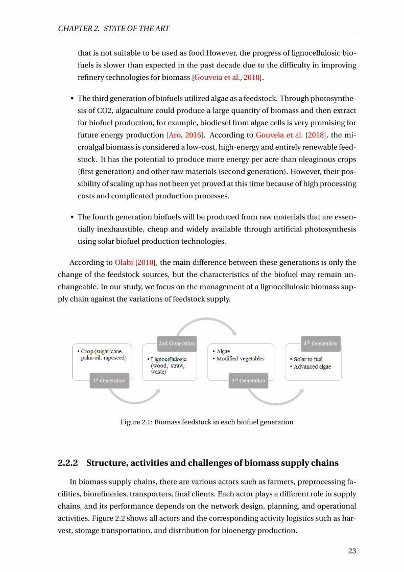
ing to An et al. [2011]. The research of Gouveia et al. [2018]; Pérez et al. [2017] classified
the feedstock, biofuels and the related production processes into four generations. Figure
2.1 shows the main type of biomass feedstock in each biofuel generation.
• In first-generation, biofuels are produced from food crops (corn, sugarcane, or sweet
sorghum) through conventional technologies such as abstracting oils and fermen-
tation. Up to now, only the first generation of biofuels has reached the industrial
stage. However, the main issue with the first generation biofuels is their competi-
tion with the global food security that raised the debate about their actual benefit
over the last two decades.
• The second generation biofuels are in the industrial take-off phase. They use lig-
nocellulosic biomass such as wood, organic waste, food crop waste and specific
biomass crops. Unlike the first generation, they can eliminate the principal prob-
lem of the production of the first generation biofuels because they use the biomass
22
CHAPTER 2. STATE OF THE ART
that is not suitable to be used as food.However, the progress of lignocellulosic bio-
fuels is slower than expected in the past decade due to the difficulty in improving
refinery technologies for biomass [Gouveia et al., 2018].
• The third generation of biofuels utilized algae as a feedstock. Through photosynthe-
sis of CO2, algaculture could produce a large quantity of biomass and then extract
for biofuel production, for example, biodiesel from algae cells is very promising for
future energy production [Aro, 2016]. According to Gouveia et al. [2018], the mi-
croalgal biomass is considered a low-cost, high-energy and entirely renewable feed-
stock. It has the potential to produce more energy per acre than oleaginous crops
(first generation) and other raw materials (second generation). However, their pos-
sibility of scaling up has not been yet proved at this time because of high processing
costs and complicated production processes.
• The fourth generation biofuels will be produced from raw materials that are essen-
tially inexhaustible, cheap and widely available through artificial photosynthesis
using solar biofuel production technologies.
According to Olabi [2010], the main difference between these generations is only the
change of the feedstock sources, but the characteristics of the biofuel may remain un-
changeable. In our study, we focus on the management of a lignocellulosic biomass sup-
ply chain against the variations of feedstock supply.
Figure 2.1: Biomass feedstock in each biofuel generation
2.2.2 Structure, activities and challenges of biomass supply chains
In biomass supply chains, there are various actors such as farmers, preprocessing fa-
cilities, biorefineries, transporters, final clients. Each actor plays a different role in supply
chains, and its performance depends on the network design, planning, and operational
activities. Figure 2.2 shows all actors and the corresponding activity logistics such as har-
vest, storage transportation, and distribution for bioenergy production.
23

CHAPTER 2. STATE OF THE ART
Figure 2.2: Examples of a bioenergy supply chain
In comparison with industrial supply chains, biomass supply chains have many dif-
ferent features regarding their structures and characteristics. Their structures could be
naturally classified according to logistics activities required by supplying biomass from
farmers to production sites and delivering biofuel from the production sites to service
stations (gas stations). These activities include ground preparation and plantation, cul-
tivation, harvesting, handling, storage, conversion, transportation and utilization of the
biofuel at service stations according to Ba et al. [2016]. The characteristics of these activi-
ties in biomass supply chains are underlined as follows:
i) Harvesting activities usually occur in fields on a limited time window with a mate-
rial loss of 10-20%. A limited group of machines such as combine harvesters is employed
when the crop is ready. Sambra et al. [2008] distinguished three modes of harvest: multi-
pass, single-pass, and whole-crop harvesting. A combine harvester is used for harvesting
wheat, corn, and rapeseed in a multi-pass method. Grain, straw, and chaff are separated
and stored in different places. In single-pass harvesting, grain and straw are harvested
at the same time. Compared to a multi-pass collection, this mode is faster but requires
more powerful and expensive equipment. In the latter one, the whole crop is cut and col-
lected without separating its different components. There are four ways (baling, loafing,
dry chop, wet chop) to collect biomass before storage and transportation to a biorefin-
ery [Forsberg, 2000]. The appropriate method for biomass collection also depends on the
nature of biomass and the desired moisture level.
ii) Storage is necessary to synchronize the biomass production calendar with the bio-
fuel production plan. Storage can occur in the fields, in the farms, in centralized storage
sites, or before the processes in a biorefinery. It is important to note that storage is a buffer
between the harvesting windows of the different crops and their consumptions by the
biorefineries. Suitable storage could reduce dry matter loss and protect biomass against
the indoor/outdoor condition. Ebadian et al. [2013] affirmed that the total storage capac-
ity required in a biomass supply chain should be much larger than in the traditional one
to meet the same biofuel demand all over the year. Unlike fossil energy, biomass decays
during storage, at a rate estimated to be 1-2% of the material stocked per month under
the ambient storage, according to Rentizelas et al. [2009].
24

CHAPTER 2. STATE OF THE ART
iii) Preprocessing, also called pretreatment allows to improve the quality of preserva-
tion and handling and to reduce transportation costs by increasing density and reducing
degradations. There are many type of pretreatments such as ensilaging, pelletisation, tor-
refaction, pyrolysis. These pretreatments aim to reduce moisture, stabilize products and
increase its calorific value and yield solid uniform products.
iv) Several transport modes can be used to deliver biomass feedstock such as road,
rail transportation. However, road transport is often the best solution if fields have limited
accessibility. Railways can be used if distances are large enough [Rentizelas et al., 2009].
Different types of uncertainty present in almost all logistics activities of a biomass sup-
ply chain, not only arise from external environments, but also from the supply chain itself
Bot et al. [2015]. Firstly, the feedstock supply is always seasonal and depends on weather
conditions and harvest time. In addition, a plant’s location has a significant impact on
the sustainability of feedstock supply thanks to geographical dispersion. Due to the het-
erogeneous and low-density characteristics, pretreatment operations are essential to ho-
mogenize and increase biomass density that may help us to reduce transportation costs
of biomass significantly. Moreover, the fluctuation of purchase price and biofuel demand
affects the efficiency of a supply chain network eventually. In some cases, it is hard to find
an optimal network design because of uncertainty (fluctuation) in price and demand. The
efficiency of a biomass supply chain is also affected by long-term contracts with suppliers,
transportation and local distribution infrastructure, conversion technology and policies
of the government according to Ba et al. [2016]; Gold and Seuring [2011].
2.2.3 Optimization models for biomass supply chain management
Mathematical programming and optimization techniques have been employed to de-
sign and manage biomass supply chains considering their different components and var-
ious decisions. Iakovou et al. [2010]; Mula et al. [2010]; Shabani et al. [2013] categorized
decision-making in supply chain management into three levels according to the degree
of importance and the planning horizon such as strategic, tactical and operational deci-
sions. Figure 2.3 illustrates three decision levels for a biomass supply chain.
Strategic decision models
Most part of the considered publication focused on the design and management of
biomass supply chains at the strategic level (55.8% according to the overview in Melis
et al. [2018]). The decision-making at this level involves long-term decisions such as se-
lecting production technologies, biomass preprocessing techniques, determining the fa-
cilities’capacity and location, the optimal configuration of logistics network, establishing
long-term contracts with suppliers.
Samsatli et al. [2015] proposed a biomass supply chain model to evaluate the eco-
nomic and environmental impacts under different scenarios and constraints concerning
25

CHAPTER 2. STATE OF THE ART
Figure 2.3: Decision levels in biomass supply chains
optimal resources and technologies selected. In Hombach et al. [2016], a mixed-integer
linear programming (MILP) model was proposed to design a second generation biofuel
supply chain in a German region under European biofuel regulations. Woo et al. [2016]
proposed a MILP model for designing a supply chain network against fluctuations of
biomass availability and hydrogen demand. The impact of biomass quality-related costs
on operational costs in a biofuel supply chain was investigated in Castillo-Villar et al.
[2016].
In the research of Woo et al. [2016], the authors proposed a mixed integer linear pro-
gramming (MILP) model which can be used to design the optimal supply chain network
to manage logistics operations against fluctuations of biomass availability and hydrogen
demand. The research of Samsatli et al. [2015] developed a MILP model called Biomass
Value Chain Model (BVCM) which takes account of the economic and environmental im-
pacts associated such as: optimal use of land, biomass resources and technologies with
respect to different objectives, scenarios and constraints. Castillo-Villar et al. [2016] pro-
posed a bioefuel supply chain model that minimizes operational costs and the biomass
quality-related costs. A MILP model in Rudi et al. [2017] aimed to identify location, tech-
nology, and capacity investment in a biomass supply chain by considering the compro-
mise between economic scale and technology range. A case study is presented for a
biomass value chain design in the Upper Rhine Region.
Geographic information system (GIS) is a powerful visualization tool that allows cap-
ture, store, manipulate, analyze, manage, and present spatial or geographic data. In biomass
supply chain management, it could support decision-makers to estimate biomass feed-
stock availability, transportation cost and evaluate land use and natural obstacles. Re-
cently, Zareei [2018] developed a GIS-based model to evaluate biogas production from
livestock manure and rural household waste in Iran. Similarly, Zyadin et al. [2018] used
26

CHAPTER 2. STATE OF THE ART
mapping and survey data from farmers to assess the potental exploitation of biomass in
central Poland. Using a remote sensing high resolution data and GIS tools, Setyawidati
et al. [2018] confirmed the high possibility to exploit brown seaweeds in Ekas Bay (Indone-
sia) as a biomass feedstock. Based on open source GIS and DBMS (Database Management
System) applications, Tommasi et al. [2018] analyzed the technical, economic and envi-
ronmental aspects and identified the optimal power plant location in Friuli Venezia Giulia
Region, Italia. It is possible to compute the optimal objective function in the GIS-based
models through a classical programming language or in the GIS script language such as
Zhang et al. [2011].
Tactical decision models
The tactical decisions level in biomass supply chain are those related to medium-term
decisions such as production planning, logistics planning (number of vehicles and work-
ers), transportation mode and definition of safety stock level. Few studies integrated ac-
tivities in a biomass supply chain at the tactical decision level such as Atashbar et al.
[2018]; Ba et al. [2015]; Marques et al. [2018]; Morales-Chávez et al. [2016]; Sosa et al.
[2015].
Ba et al. [2015] studied a biomass supply chain with multi-feedstock supply with the
objective of minimizing the total logistic cost of the system on a regional basis. The
MILP model could determines the optimal number of harvesting machine, the fleet size
of trucks for transportation and the amount of each type of biomass harvested. Morales-
Chávez et al. [2016] proposed a mixed-integer linear programming model to minimize the
total system costs including costs of resources for harvesting and loading, shortage cost
and transportation cost. The model determines the quantity of machines and workers to
meet the biofuel plant requirements. Sosa et al. [2015] designed a linear programming
tool to manage production planning for a wood biomass supply chain in Ireland. The
study focus on the impact of moisture content and truck configurations on logistic plan-
ning. The results indicate that using 6-axle trucks could reduce 14.8% of truckloads and a
12.3% of haulage costs in comparison to using 5-axle trucks.
Marques et al. [2018] studied a tactical biomass supply planning problem with syn-
chronization between chipping and transportation at the roadside. The authors also con-
sider the constraints related to the variation of moisture content in storage. The numer-
ical study shows that efficient management of the variation of moisture content in stor-
age could improve until 20% of the supplier’s profit. A MILP model in Atashbar et al.
[2018] was developed to optimize a multi-period and multi-biomass supply chain with
several biorefineries at tactical level. Han et al. [2018] aimed to optimize biomass extrac-
tion, transportation, conversion and product production by considering a multi-period,
multi-commodity, multi-echelon supply chain problem. The MLIP model is solved by
using a genetic algorithm.
27

CHAPTER 2. STATE OF THE ART
Operational decision models
The operational level corresponds to short-term decisions, weekly and daily, which
can be considered as a decomposed activities from tactical level. In biomass supply chain
management, the operation levels include logistics operations (harvesting, collection and
handling) in a given days, and biomass transportation (vehicle routing problems). There
are few mathematical models for biomass supply chains management at operational level.
Bochtis et al. [2013] studied the planning of the biomass collection operations with the
objective of minimizing the total completion time of the whole activities in all fields. The
case study in Thessaly, Greece involved the collection (baling–loading) of cotton residues
from dispersed fields for the production of bioenergy. The numerical research shows the
optimal schedule could reduce 9.8% of the total operations time in comparison with the
one planned from experience of operations manager. Orfanou et al. [2013] continued the
work presented in Bochtis et al. [2013] by considering a large number of machines per task
type and introducing an economic objective. The meta-heuristic approach that based on
the greedy heuristic and the "Tabu search" is proposed to solve the model.
Gracia et al. [2014] studied a mixed integer programming model for the biomass col-
lection problem. The model is formulated as an application of the classical vehicle routing
problem with the objective to minimize the total traveled distance in the field. A hybrid
approach based on genetic algorithms and local search methods is presented to solve a
real case study. Torjai and Kruzslicz [2016] proposed a mixed integer programming model
for the truck scheduling problem in a real-life herbaceous biomass supply chain around
Pécs, Hungary. In Li et al. [2017], a new concept, called "distance potential" was proposed,
which could be used to optimize biomass logistics networks. Matindi et al. [2018] studied
the harvesting and transport operations in a lignocellulosic supply chain and proposed
the constraint programming model to optimize the delivery and collection times in the
transportation network. An adapted Limited Discrepancy Search (LDS) was introduced
to find the near optimal solution of the proposed model.
Some authors applied the GIS-based model to find the optimal operational plan such
as Hoefnagels et al. [2014]; Montgomery et al. [2016]. A geo-spatial based model was de-
veloped by Montgomery et al. [2016] to generate an operational work plan that can be
used on industrial timberlands. Based on the GIS framework, Hoefnagels et al. [2014]
assessed lignocellulosic feedstock supply systems at the operational level such as the im-
pact of overseas shipping routes and inter-modal transportation on the delivered costs
and greenhouse gas emissions.
Some authors adopted a statistical method to optimize the bale collection activities.
Igathinathane et al. [2016]; Subhashree et al. [2017] developed a statistical-based approach
to find a better management of bale collection logistics and evaluate the field parameters
on logistics activities. The study concludes that the "field middle" (that followed the best
geometric median method) was an easy and practical method for locating field stacks.
28

CHAPTER 2. STATE OF THE ART
Most studies at operational level do not consider uncertainty and environmental as-
pects in their mathematical models. A review paper of Malladi and Sowlati [2017] sug-
gested that the future researches should take into account the environmental impact in
the objective function or uncertainties in truck routing and scheduling models.
In addition, these mathematical models can be classified into two categories: deter-
ministic and stochastic. Most studies ignored uncertainty by only considering determin-
istic models. A bibliographic analysis in Pérez et al. [2017] shows that 75% of studies which
focus on economic and environmental criteria adopt deterministic models. We present
in this following sections the deterministic and stochastic models.
Deterministic optimization models
Deterministic optimization models have a considerable majority of application in biomass
supply chains. It is useful for "what-if" scenarios where decision-makers can observe the
outcomes of their decisions in different inputs/conditions. With “what-if ” analysis, the
sensitivity of optimal solutions can be easy to estimate as the value of the key parame-
ters varies from their original values. In most studies, the critical parameters could be the
prices, demands, production capacity and product availabilities.
In deterministic optimization models for biomass supply chains, the simplest way is to
apply linear programming to simulate logistics activities (e.g., harvest, purchase, produc-
tion, and transportation) by continuous variables. All constraints and objective function
are linear. Besides, as pointed by Ba et al. [2016], mixed integer linear programming mod-
els are broadly used for supply chain network design or biomass logistics planning (e.g.,
number of vehicles, facility location, and selection of production capacity). In the pre-
vious decades, the development of the commercial solvers allows for solving many com-
plex problems in a reasonable time. Most authors use a commercial solver (e.g., CPLEX,
AIMMS, AMPL, GORUBI, LINGO, and XPRESS) to solve MILP models thanks to its power-
ful capabilities.
In some cases, it is hard to find an optimal solution by commercial solvers because
the CPU time overgrows as a function of model size and a number of integer variables.
That is why researchers have developed their algorithms based on Lagrangian relaxation,
genetic, and metaheuristic approaches. However, metaheuristic has rarely appeared in
several applications.
Stochastic optimization models
Based only on the expected value, deterministic models are not able to well capture
events in the tails of the distributions of random variables. This disadvantage could lead
to a negative impact on the performance of the models. For example, some scenarios with
a low probability of occurrence might have a high impact on the total cost/profit of a sys-
tem. So, stochastic models may be more appropriate. According to Shabani and Sowlati
29

CHAPTER 2. STATE OF THE ART
[2016], this approach is adequate and useful when the probability distribution of uncer-
tain parameter can be assessed and then decomposed into a set of scenarios. However,
stochastic models are not conventional in biomass supply chain management because
they are tough to be solved optimally and to guarantee constraint feasibility for all con-
sidered scenarios. According to Sahinidis [2004], there are three principal approaches
to cope with uncertainty: stochastic programming (recourse models, robust stochastic
programming, and probabilistic models), fuzzy programming (flexible and possibilistic
programming), and stochastic dynamic programming.
An the literature for biomass supply chains, most mathematical models are determin-
istic and only few stochastic models exist. As reported in Table 2.1, these stochastic mod-
els are usually based on two-stage stochastic programming with recourse to design supply
chains at the strategic level (selecting production technologies, determining the location
and capacity of each facility). Awudu and Zhang [2013] studied a biofuel supply chain for
biorefineries already placed and producing biofuels under demand and price uncertain-
ties in North Dakota. They applied Bender decomposition algorithm and Monte Carlo
method to approximate the value of second-stage based on a set of scenarios. Osmani
and Zhang [2013] consider a similar problem but with objective to determine a location of
biorefineries under more uncertainties (supply, demand, and prices). The solution tech-
nique is identical to those previously mentioned.
Kim et al. [2011] also study a similar problem but with objective to determine location
and size of two types of conversion facilities with the high level of uncertainty in sup-
ply amounts, market demands, market prices, and processing technologies. This model
is implemented on the commercial software GAMS and uses the CPLEX solver. Chen
and Fan [2012] studied the same problem but consider separately two major sources
of uncertainties, feedstock supply and fuel demand. They applied Progressive hedging
algorithm to solve this model optimize a biomass supply chain under uncertainties in
biofuel demand and feedstock supply. Dal-Mas et al. [2011] investigated economic per-
formances and risk on investment of the entire biomass-based ethanol supply chain in
Northern Italy. The authors proposed a multi-echelon mixed Integer Linear Program
(MILP) modeling framework and solved the model by using a solver CPLEX. Similar to
Osmani and Zhang [2013],Kaut et al. [2015] want to determine the location of facility and
flow of biomass in a supply chain with uncertainty in demand, supply and prices. They
proposed a hybrid stochastic programming-robust optimization model and solved this
MLIP model by using FICO™ Xpress Optimizer.
With similar objective as Kim et al. [2011], a two-stage chance-constrained stochastic
programming model for a biofuel supply chain network was presented in Quddus et al.
[2018]. This study considered the uncertainties due to feedstock seasonality due to sud-
den fluctuation or total unavailability in biomass supply arises. Besides, a joint chance-
constraint related to a percentage of biomass supply from municipal solid waste at a cer-
tain probability was introduced. A Sample Average Approximation algorithm was devel-
30

CHAPTER 2. STATE OF THE ART
oped to solve the mathematical model.
Most works only consider road transportation, except for the study of Marufuzza-
man et al. [2014] focused on selecting transportation mode (rented truck, facility-owned
trucks, and pipelines) and facility location of a biodiesel supply chain with uncertainties
in feedstock and technology development. They investigate the impact of carbon regu-
latory mechanisms on the design and management of a supply chain. They proposed an
algorithm combining Lagrangian relaxation and L-shaped method to solve this model.
Most researchers study supply chains for biofuel production whereas Shabani and
Sowlati [2016] investigate a forest-based biomass supply chain for a power-plant with
uncertainty in biomass quality and biomass availability. This model is solved using the
AIMMS software and CPLEX solver. Almost works mentioned above consider biomass
supply chains at only one period such as Awudu and Zhang [2013]; Chen and Fan [2012];
Kim et al. [2011]; Marufuzzaman et al. [2014].
There exist different methods to solve a two-stage stochastic programming model
such as L-shaped algorithm in Awudu and Zhang [2013]; Marufuzzaman et al. [2014], Pro-
gressive Hedging algorithm in Chen and Fan [2012], Genetic algorithm in Mirkouei et al.
[2017]. Some authors used a commercial solver to find an optimal solution of a determin-
istic equivalent linear program model such as Kaut et al. [2015]; Kim et al. [2011]; Osmani
and Zhang [2013]; Shabani and Sowlati [2016]; Shabani et al. [2014].
31

CHAPTER 2. STATE OF THE ART
Tab
le2.
1:St
och
asti
co
pti
miz
atio
nm
od
els
for
bio
mas
ssu
pp
lych
ain
s
Ref
Un
cert
ain
tyD
ecis
ion
vari
able
Dec
isio
n
leve
l
Ob
ject
ive
Mo
del
&So
luti
on
met
ho
d
Kim
etal
.[20
11]
Bio
mas
sp
rice
,yi
eld
s
and
un
itp
rod
uct
ion
cost
,dem
and
s
Net
wo
rkfl
ows,
Qti
esu
sed
top
rod
uce
ener
gyin
CU
,fac
ilit
ylo
cati
on
s(b
inar
y)
SM
axto
talp
rofi
t2-
stag
est
och
asti
cM
IP,
GA
MS-
CP
LEX
,
Scen
ario
-bas
edM
on
teC
arlo
met
ho
d
Ch
enan
dFa
n
[201
2]
Feed
sto
cksu
pp
ly
and
fuel
dem
and
Net
wo
rkfl
ows,
Bio
refi
ner
iean
dte
rmi-
nal
loca
tio
ns
(bin
ary)
SM
into
tal
exp
ecte
d
syst
emco
st
2-st
age
sto
chas
tic
MIP
,Pro
gres
sive
hed
gin
gal
-
gori
thm
Osm
ani
and
Zh
ang
[201
3]
Bio
mas
sav
aila
bil
ity,
pri
cean
dd
eman
ds
Net
wo
rkfl
ows,
BR
loca
tio
ns
(bin
ary)
SM
axex
pec
ted
pro
fit
2-st
age
sto
chas
tic
MIP
,A
ggre
gate
dsc
enar
ios,
GA
MS-
XP
RE
SS
Dal
-Mas
etal
.
[201
1]
Co
rnco
st,
eth
ano
l
sale
pri
ce
Net
wo
rkfl
ows,
Co
rnco
st,e
than
ols
ell-
ing
pri
ce,
Tran
spo
rtm
od
ese
lect
ion
(bin
ary)
,BR
loca
tio
n,s
ize
and
tech
no
l-
ogy
cho
ice
(bin
ary)
SM
axex
pec
ted
NP
VSt
och
asti
cM
IP,
Agg
rega
ted
scen
ario
s,G
AM
S+
CP
LEX
Kau
teta
l.[2
015]
Dem
and
,su
pp
lyan
d
pri
ces
Loca
tio
no
ffac
ility
(bin
ary)
and
flow
of
bio
mas
s
S+
TM
axov
eral
lpro
fit
Hyb
rid
sto
chas
tic
pro
gram
min
g-ro
bu
sto
pti
-
miz
atio
nm
od
el,F
ICO
™X
pre
ssO
pti
miz
er
Qu
dd
us
etal
.
[201
8]
Feed
sto
cksu
pp
lyFa
cili
tylo
cati
on
dec
isio
ns
(bin
ary)
and
flow
ofb
iom
ass
SM
into
tal
exp
ecte
d
syst
emco
st
2-st
age
chan
ce-c
on
stra
ined
sto
chas
tic
pro
-
gram
min
gm
od
el,
Co
mb
ined
Sam
ple
Ave
rage
Ap
pro
xim
atio
n
Mar
ufu
zzam
an
etal
.[20
14]
Bio
mas
ssu
pp
lyan
d
tech
no
logy
Loca
tio
n(b
inar
y)an
dtr
ansp
ort
atio
n
dec
isio
ns
SM
inim
ize
cost
san
d
GH
Gem
issi
on
s
2-st
age
sto
chas
tic
pro
gram
min
gm
od
el,
La-
gran
gian
rela
xati
on
and
L-sh
aped
met
ho
d
Shab
ani
and
Sow
lati
[201
6]
Bio
mas
sq
ual
ity
and
bio
mas
sav
aila
bil
ity
Am
ou
nt
of
bio
mas
sto
pu
rch
ase,
sto
re
and
con
sum
efr
om
each
sup
plie
rin
each
mo
nth
,an
dw
het
her
or
no
tto
gen
erat
eth
esu
rplu
slo
ad
TM
axto
talp
rofi
tH
ybri
dm
ult
i-st
age
sto
chas
tic,
pro
gram
min
g-
rob
ust
mo
del
,AIM
MS-
CP
LEX
Shab
ani
etal
.
[201
4]
Bio
mas
sav
aila
bil
ity
Am
ou
nt
of
bio
mas
sto
be
pu
rch
ased
,
sto
red
and
con
sum
edfr
om
each
sup
-
pli
er
TM
axto
talp
rofi
t2-
stag
est
och
asti
co
pti
miz
atio
nm
od
el,
AIM
MS-
CP
LEX
Mir
kou
eiet
al.
[201
7]
bio
mas
sq
ual
ity
and
acce
ssib
ilit
yra
tes
Net
wo
rkfl
ows
(am
ou
nt
of
bio
mas
s
and
bio
fuel
tob
etr
ansp
ort
ed)
TM
into
tala
nn
ual
cost
Sto
chas
tic
mo
del
wit
hm
ult
i-cr
iter
iad
ecis
ion
mak
ing
fram
ewo
rk,
Sup
po
rtve
cto
rm
ach
ine
(SV
M),
Gen
etic
algo
rith
man
dli
fecy
cle
asse
ss-
men
t
(*)
S:St
rate
gic,
T:T
acti
cal,
O:O
per
atio
nal
,NP
V:N
etP
rofi
tVal
ue
32

CHAPTER 2. STATE OF THE ART
Multi-objective models
In the biomass supply chain optimization, most of the research focuses on minimiz-
ing the total cost or maximizing the profit of the whole system. In the last decades, the
trend of integrating environmental and social objectives into the mathematical model is
gradually becoming more popular. This approach has received much attention from the
scientific community as it is suitable for the sustainable development of renewable energy
in general and biofuels in particular.
Due to the ability to deal with different and competitive objectives (aspects), the multi-
objective programming approach has been applied widely in the natural resources man-
agement. For example, the design of a biomass supply chain network may consider simul-
taneously multiple criteria related to energy sufficiency, environmental effects, and socio-
economic impacts. This approach is usually applied for multi-products, single period
models with several objectives such as maximizing job creation, reducing greenhouse gas
emissions, and minimizing total system cost. Dealing with the conflicts between objec-
tives, most works often use Pareto-optimality to provide several compromise solutions. As
an example, Grigoroudis et al. [2014] proposed a multi-objective programming model to
find the optimal design of a biomass supply chain network with objective of maximizing
efficiency and minimizing the total costs. A RDEA (Recursive Data Envelopment Analysis)
algorithm have been developed to provide the optimal solution with high convergence
speed. Similarly, Liu et al. [2014] proposed a MILP model for biofuel supply chains with
multiple production pathways with economic, energy, and environmental objectives. The
model was solved using the ε-constraint method.
Many works use the ε-constraint method to solve multi-objective models and provide
a set of Pareto-optimal solutions. In the ε-constraint method, the problem is reformulated
as a single objective problem by keeping one selecting objective and transforming other
objectives into additional constraints by using a specified ε scalar values. As an example,
Cambero and Sowlati [2016] focused on maximizing the social benefit, net present value
and minimizing greenhouse gas emission of a forest based biorefinery supply chain. The
authors formulated a multi-objective MILP model and developed a improve ε-constraint
method to solve this model. Roni et al. [2017] attempted to minimize total system costs
and total emissions CO2 in the supply chain while maximizing social objective (number
of created jobs). The MILP model is solved by the augmented ε-constraint method us-
ing CPLEX in C++. A case study is conducted with data from the Midwest region of the
USA. Recently, Wheeler et al. [2018] studied the multi-objective design of biomass supply
chains for bioethanol from sugar cane production in Argentina. The authors combined
the mixed-integer programming with multi-attribute decision-making tools to identify a
unique Pareto solution of the multi-objective problem. Wang et al. [2018] studied a reli-
able multi-period supply chain model against feedstock seasonality and time-varying dis-
ruption risks. A case study in Hubei, China was studied to validate the model and solved
33

CHAPTER 2. STATE OF THE ART
by using Knitro Solver in AMPL.
There are very few studies developed a mathematical model under uncertainty to find
the trade-off between conflicting objectives such as social, economic, and environmen-
tal aspect. Mirkouei et al. [2017] proposed a multi-criteria decision-making framework
to assess the economic and environmental aspects of a mixed biomass supply chain. The
model considers uncertainties in biomass quality and accessibility rates. The authors em-
ployed a support vector machine technique to predict the pattern of uncertainty param-
eters. Then, a stochastic optimization model incorporated with uncertainties are formu-
lated and solved by a genetic algorithm. By applying fuzzy multi-objective programming,
Tsao et al. [2018] studied the supply chain networks design under uncertain environments
(e.g., demand, capacity, and costs). Three objective functions are considered in the model
such as the minimization of total costs, environmental impact, and maximization of so-
cial benefits. They proposed an interactive fuzzy approach to provide solutions with the
compromise of the objective functions for decision-makers.
2.3 Perishable inventory management
As mentioned in the previous subsection, biomass deteriorates with a constant rate
estimated at 1% of the material stocked per month under the ambient storage Rentize-
las et al. [2009]. Thus, biomass can be considered a perishable product. In fact, perish-
able product refers to an item which loses its value over time until it eventually becomes
worthless. Typical examples of perishable products include fresh products, blood cells,
chemicals, photographic films, drugs and other pharmaceutical products.
Effective inventory management allows companies to respond quickly to the change
in market demand and develop a flexible production system to improve their compet-
itiveness. Multi-echelon models are usually adopted for inventory management when
considering a system with multi locations and multi-facilities. However, for perishable
products, single-echelon models remain essential and could provide a primary princi-
ple to make multi-echelon models more realistic and relevant according to Duong et al.
[2018].
The goal of this subsection is to provide and analyze the perishable inventory mod-
els in various dimensions such as its evolution, scope, demand, shelf life, replenishment
policy, modeling techniques, and research gaps. We focus not only on the mathematical
details but also on the assumption and feature of perishable inventory models (Subsec-
tions 2.3.1- 2.3.2). An overview of the solution approaches is outlined in subsection 2.3.3.
2.3.1 Characteristics of perishable inventory problems
According to Silver [2008], there are many possible objectives should be taken into
considerations in inventory management such as cost minimization, profit maximiza-
34

CHAPTER 2. STATE OF THE ART
tion, maximization of return rate on stock investment, improving flexibility to cope with
an uncertain, minimizing political conflicts regarding the competing interests within the
organization... Most studies have focused on only the first and second objective. There are
various possible constraints including supplier constraints (minimum order sizes, maxi-
mum order quantities, restrictions on replenishment times), customer service levels and
internal constraints (storage, budget, workforce and workload limitations). Generally,
decision-makers who seek to satisfy customer demand at the minimal cost must consider
two fundamental decisions: the size and timing of each inventory replenishment order.
In most inventory models, it is assumed that products can be stored indefinitely to meet
future demands. However, the effects of perishability cannot be ignored for certain types
of products, which may become partially or completely unsuitable for consumption as
time passes.
Different from that of a product with unlimited shelf life, the structure of the optimal
replenishment policy for a perishable product is usually more complex: the replenish-
ment quantity depends on the shelf life categories of the current inventories, as well as
on all outstanding orders, uncertain demand, supply, and price. Directly speaking, in-
ventory policies consist of determining time and quantity for replenishment. According
to Duong et al. [2018], many characteristics such as demand distribution, stock issuing,
product lifetime, replenishment lead time, and shortage situations should be accounted
into the models for dealing with different business situations. The fundamental inventory
policies are given as follows:
• (s, S) is a minimum/maximum inventory policy., when the inventory falls to a min-
imum level s, an order is placed to bring the inventory back to the maximum level
S. The order size is quantity (S – s). This model provides significant flexibility.
• (s, nQ) or (r, nQ) whenever the inventory falls below the level s or r, an order quantity
n times a predetermined Q (order quantity) is placed where n is a multiple equal to
or greater than 1. This policy is suitable for ordering in batches.
• (S – 1, S), an order is placed immediately whenever a demand occurs for one or more
units of an item. This model is preferred when lead times are zero and ordering cost
is low.
• (T, S) is the periodic review order up to level policy. In each period, the decision-
maker will request a replenishment quantity that will restore the on-hand inventory
to a target, S. The order size is quantity (S – the on-hand inventory). This policy is
simple for real world practices.
Due to the limited lifetime of products, the stock issuing policy is essential and has a
significant impact not only on the system cost but also on the satisfaction of customers.
In perishable inventory management, there are two most commonly used stock issuing
35

CHAPTER 2. STATE OF THE ART
policies: First-In-First-Out (FIFO) and Last-In-Fist-Out (LIFO). In FIFO, the product ar-
rives in warehouse first will be delivered to customers early in the order of arrival; in LIFO,
the product that has mostly come in the warehouse will be given to customers first. In
reality, customers prefer LIFO to FIFO policies regarding the freshest products. According
to Parlar et al. [2011], the FIFO is better than the LIFO when considering the combina-
tion of all operational costs. However, the situation is reversed when the holding cost is
high, or the purchase cost is low. Most research uses the FIFO policy because this policy
is suitable for reducing the waste of the expiration products logically.
In addition, an inventory problem with fixed lifetime is more complicated than the
one with stochastic lifetime due to the high-dimension problem and inability to apply
the Markovian property to describe the stock on-hand [Olsson and Tydesjö, 2010].
2.3.2 Classification of perishable inventory models
To reflect the real-life issues, many researchers integrated several related factors into
the inventory models such as credit and different payment problems; inflation and time
value for money; investment, promotion and budget constraint; customer satisfaction...In
this subsection, we discuss some essential modeling elements that are popular in perish-
able inventory management.
Many companies offer customer deteriorated items at a discount price to boost sales
and increase profit. Moreover, the relevant discount price policy could allow companies
to reduce the loss due to deterioration items by enhancing sales. Such policy is applicable
for some products in supermarkets, e.g., milk, yogurt, and bread are always sold at a dis-
count price when they are very close to their expiration date. Such price discounts and or-
der policy are presented in the works of Banerjee and Agrawal [2017]; Chung et al. [2015];
Pal [2016]. In recent years, many studies focused on the investment of preservation tech-
nology to improve the storage condition for deteriorated products such as Mishra et al.
[2017, 2018]; Pal et al. [2017]; Singh et al. [2016a]; Tayal et al. [2016]; Yang et al. [2015].
Since the inflation crises in the 1970s and early 80s, many authors realize the impor-
tance of taking consideration inflation into account, to make the models more realistic.
A model in Buzacott [1975] is the first model with inflation. Until now, various models
have explored different aspects from inflation. The readers can find the recent models in
Chakrabarty et al. [2017]; Shah and Vaghela [2018]; Tayal et al. [2016].
To increase the partnership, it is common that suppliers usually offer a retailer a per-
missible delay period. During this period, there would be no interest charged if the full
payment is made. The period is so-called, the permissible delay period. The first EOQ
(Economic Order Quantity) model with a permissible delay period is provided by Goyal
[1985]. Recently, Mishra et al. [2018] determined the optimal joint ordering, pricing, and
preservation technology investment policies for the inventory model with deteriorated
items under the permissible delay in payments. Chan and Hsu [2018] provided an EOQ
36

CHAPTER 2. STATE OF THE ART
model under payment conditions that combinate the good-faith prepayment, the cash
payment, and the delayed credit payment. The impact of inflation, perishability and trade
credit policy is taken into consideration in the study of Tiwari et al. [2016]. Mohanty et al.
[2018] study the joint effect of preservation technology investment and trade-credit policy
on a stochastic perishable inventory.
Service level constraint is one of the most useful techniques for integrating customer
satisfaction into the inventory models. There are several studies focus on finding the or-
der policy under service level constraints. Such problem are addressed in the works of
Belo-Filho et al. [2015]; Hendrix et al. [2012, 2015, 2018]; Pauls-Worm et al. [2015, 2016].
These authors proposed approximation approaches to find the near-optimal solution for
stochastic inventory models. By considering the service requirement under random yield
and uncertain demand, Belo-Filho et al. [2015] proposed a perishable inventory model of
coordination with revenue sharing contract. However, that paper only characterizes the
optimal policy of one-period inventory model.
In the following, perishable inventory models are classified according to the product
life time, demand and supply characteristics. A more detailed classification can be found
in Bakker et al. [2012]; Chaudhary et al. [2018]; Duong et al. [2018]; Janssen et al. [2016];
Karaesmen et al. [2011]; Nahmias [1982].
Product lifetime
According to Bakker et al. [2012]; Janssen et al. [2016], the limited shelf life products
are classified into two categories: deterministic lifetime products and random lifetime
products which may have a probabilistic distributed lifetime (e.g., Weibull), constant,
known or unknown deterioration rate. In case of fixed lifetime, a product becomes un-
usable and must be discarded when its lifetime are achieved. In case of random lifetime
products, one cannot know exactly the lifetime of items in advance. As an example, veg-
etables and fruits could be considered as stochastic lifetime products because they have
an unknown lifetime and their deterioration rate depend on the external environmental
condition such as temperature, storage condition.
Evidently, an inventory model applying to products with limited lifetime is more com-
plicated than one applying to products with unlimited lifetime. This is due to the fact that
dimension and state of inventory grows up as a function of a lifetime and number of pe-
riods. As mentioned by Schmidt and Nahmias [1985], the perishable inventory problem
under either continuous or periodic review systems is challenging to find an optimal pol-
icy when the lifetime is more than two periods. Many researchers turned their attention
to developing heuristic approaches.
Kouki et al. [2013] focused on verifying the effectiveness of existing (r, Q) inventory
systems, in which products have fixed lifetime and positive order lead time. A periodic
review inventory model of fixed lifetime product with deterministic demand and supply
37

CHAPTER 2. STATE OF THE ART
disruptions over an infinite horizon is studied in Atan and Rousseau [2016]. Chen et al.
[2014] generalized an inventory model for a perishable product with fixed time life and
positive lead time over a finite horizon to allow coordinated pricing, inventory control
and disposal decisions. A study of Dobson et al. [2017] is focused on an inventory model
of a perishable product with age-dependent demand rate and introduces a simple EOQ
to calculate approximately the optimal order cycle. Lately, Kouki et al. [2018] studied an
inventory model with dual-sourcing and the perishable items have a fixed or exponential
lifetime. They recommend that the dual-sourcing could reduce substantial cost and the
percentage of cost reduction is dependent on the lifetime distribution, e.g, the shorter the
mean lifetime is, the higher the cost reduction.
According to Goyal and Giri [2001], it is likely that an inventory model for a perish-
able product with a random lifetime is more difficult than the one with a fixed lifetime.
The random lifetime problem attracts a lot of attention in the last decades. Particularly,
Liu et al. [2018] studied the purchase and inventory policy for a perishable seasonal agri-
cultural product. They formulated this problem as a multi-period dynamic program-
ming model. The optimal purchase and inventory retrieval policy are characterized based
on the sell-down-to policy and the corresponding minimal storage level. The optimal
inventory period, cycle length and investment amount in preservation techniques are
studied in the work of Pal et al. [2017]. They formulated an inventory model for non-
instantaneously deteriorating items with constant demand, and the deterioration rate
could be reduced by investing in preservation technology. The optimum order quantity
and reorder intervals for a periodic review inventory model with non-instantaneous dete-
riorating items are provided by Pal and Samanta [2018]. In this model, the pre-deterioration
period is a random variable and the uniform demand rate during the pre-deterioration
period is greater than that in the post-deterioration period.
Inventory models become extremely complex when considering a positive order lead
time. By way of illustration, Baron et al. [2017] investigated a continuous review (s, S)
model of perishable products under stochastic in both lead times and demand. They
developed a heuristic approach to finding the optimal re-order level, s, and order-up-to
level, S to minimize the total cost. Chao et al. [2017] proposed an approximation algo-
rithm for perishable inventory systems with positive lead times and limited ordering ca-
pacities. A novel transient unit-matching mechanism is provided to find the dynamical
match between the supply and demand units.
Demand
Customer demand plays a vital role in an inventory management because the better
demand planning, the more profit companies can reach. According to Duong et al. [2018];
Goyal and Giri [2001]; Janssen et al. [2016], there are two categories: deterministic and
stochastic demand.
38

CHAPTER 2. STATE OF THE ART
Deterministic demand
In deterministic problems, demand is known with certainty. The assumption of de-
terministic demand could simplify the problem and allows to provide optimal ordering
policies such as EOQ (Economic Order Quantity) and EPQ (Economic Production Quan-
tity) [Pahl and Voß, 2014]. However, this could not reflect customer demand accurately
in practice. The deterministic demand can be also divided into sub-categories as fol-
lows: uniform demand, time-vary demand, stock-dependent demand, price-dependent
demand,freshness dependent demand.
In inventory models with stock-dependent demand, the assumption is based on the
observation that customer attention arises from a large stock of products in the super-
market. This problem becomes more complex in case of perishable products [Goyal and
Giri, 2001]. As an example, Singh et al. [2016b] developed a perishable inventory model
with stock-dependent and seasonal pattern demand over finite time horizon. The study
illustrated that the customer demand decreases when the product is close to the end of
the season and the stock level is lower. In the same year, Singh et al. [2016a] provided
an optimal economic order quantity for perishable inventory model in consideration of
stock-dependent demand with trade credit period and preservation technology.
In reality, many products have fluctuation in the demand rate such as electronic goods,
fashionable clothes, etc. In the growth stage, the customers demand increases rapidly and
continuously remain at the maturity phase then it will gradually decrease after the emer-
gence of competitive products which affects consumer’s preference. Another possibility
that could be considered in this sub-category is that the age of production may have some
impact on the customer demand. In fact, the customer always prefers a fresh product
to the old one. For these products, inventory models with time/age-dependent demand
may be plausible and relevant such as the works of Chowdhury et al. [2016]; Demirag et al.
[2017]; Dobson et al. [2017]; Tayal et al. [2016]. Lately, Demirag et al. [2017] proposed an
adaptive EOQ solution for managing a perishable inventory with remaining lifetime de-
pendent demand. They show that by integrating the freshness-dependent demand into
ordering decision, retailers may improve their total profit significantly. Chowdhury et al.
[2016] introduced a perishable inventory model with time-quadratic demand and par-
tial backlogging. Based on this model, the authors also investigate the effect of inflation
and time value of money. Tayal et al. [2016] study an integrated perishable inventory pol-
icy in a two-echelon supply chain, comprising a vendor and a retailer. In this model, set
up costs and ordering costs are considered to be time dependent; trade credit period is
allowed and preservation technology can be invested with the objective of reducing the
deterioration rate of a product.
Other sub-category of deterministic demand is based on the inter-dependent between
price and demand. In the market, almost all items are price sensitive because the selling
price affects demand directly. There are many studies explore this feature of inventory
management. Recently, Lu et al. [2016] studied a continuous-review inventory model for
39

CHAPTER 2. STATE OF THE ART
perishable items with inventory-level-dependent demand. The authors developed the
optimal joint dynamic pricing and replenishment policy based on Pontryagin’s maximum
principle to maximize the total profit. Cheng et al. [2017] proposed a joint pricing and
inventory model for perishable products with price-dependent demand and the return
of a product after purchasing. This study focus on finding the optimal sales period and
selling price to maximizing total profit. The numerical study suggests that by reducing
the order cancel rate, a retailer could improve sales and profits simultaneously.
In recent times, many researchers combine different types of demand patterns in their
studies. The combination allows to improve the relevant of demand pattern in real situ-
ation such as the works of Banerjee and Agrawal [2017]; Chen et al. [2016]; Mishra et al.
[2017]; Shah et al. [2018]. In practice, the retail always offers a discount to boost sales for
the items which begin to deteriorate because the lower freshness could lead to the lower
demand at the same price. By considering the effect of freshness and selling price on the
customer demand, Banerjee and Agrawal [2017] proposed an optimal discounting and or-
dering policies to maximize the total profit. They suggested that decision-makers should
offer more discount when selling price rises, but they could still experience a small loss in
their benefit.
For the fresh product, Chen et al. [2016] noted that the customer demand depends on
the freshness and displayed volume of the product on the shelf space. The author pro-
posed an economic order quantity model with freshness-and-stock dependent demand
to maximize the total annual profit. The decision variables related to the optimal level of
shelf space size, replenishment cycle time, and ending inventory level. With the similar
ideal, Mishra et al. [2017] investigated the impact of the preservation technology invest-
ment on a perishable inventory model. In this model, the demand rate depends on the
stock level and selling price. They focus on determining the optimal selling price, order-
ing frequency and storage technology investment to maximize the total profit. An inven-
tory model for returned/reworked items with price-sensitive as well as stock-dependent
demand is proposed by Shah et al. [2018]. The authors suggested an optimal economic
production quantity for maximizing the total profit with respect to production rate, cycle
time and retail price.
Stochastic demand
In many real situations, the demand for perishable products not only depends on ex-
ternal factors such as trends, technology, customer’s preference but also internal factors
pricing, marketing, etc. So the demand should not be considered as deterministic be-
cause it is far from many realistic situations. Stochastic models are useful when demand
pattern is uncertain or unknown. In many studies, demand function is assumed to fol-
low a probability distribution such as normal, random log-normal exponential, etc. For
example, Kouki et al. [2015] studied an (r, Q) inventory system for perishable products un-
der stochastic demand, constant lifetime and constant lead time. In this model, demand
is assumed to follow the Gamma or Gaussian distribution. They developed an approxi-
40

CHAPTER 2. STATE OF THE ART
mation algorithm to estimate the parameters r and Q that minimize the total system cost.
Most research uses the Poisson distribution to depict the stochastic demand. As an
example, Alizadeh et al. [2014] proposed an inventory system with Poisson demand, pos-
itive lead time and an (S – 1, S) ordering policy. The authors developed an enumeration
algorithm to find an optimal solution. Baron et al. [2017] studied an inventory model with
two cases of demand distribution (Poisson and compound Poisson with general demand
sizes) and positive lead time.
A renewal process is a generalization of the Poisson process that has an interesting
mathematical structure and can be used to make the inventory model more realistic.
Therefore, demand arrival could be modeled as a renewal process where the times be-
tween two successive demands are independent and identically distributed such as Gür-
ler and Özkaya [2008]. Lately, Boxma et al. [2016] extended the classical EOQ model by
taking into account a random environment and perishability. Demand is alternated be-
tween two random state (high and low demand period) according to a continuous-time
semi-Markov process. The high and low demand period are both represented by com-
pound Poisson processes with different parameters. The study of Haijema and Minner
[2015] dealt with the case of double stochastic Poisson demands, positive lead time, par-
tial backorder, perishable items, and emergency replenishment. They demonstrate the
stationary distributions of the age of items is unique.
A lot of studies applied the rolling horizon approach in the literature of inventory
management. Hendrix et al. [2012] study an inventory control problem for a perishable
product with a non-stationary random demand and a service level constraint. Recently,
Janssen et al. [2018] investigated the impact of closing days constraint on waste quantity
and total costs. They formulated a stochastic perishable inventory model for multi-items
with a fixed lifetime includes total stock capacity constraints, a positive lead time, a peri-
odic inventory control, a target customer service level and mixed FIFO and LIFO issuing
policies under a non-stationary random demand. The study shows that closing days con-
straint could reduce on average 1.77% of the outdating quantity and 0.29% of total costs
in grocery stores. Ferreira et al. [2018] developed a inventory model of perishable goods
with stochastic demand and stochastic donations for long term humanitarian operations,
using Markov Decision Process.
The companies are likely to deal with a stochastic non-stationary demand when prod-
ucts have a short lifetime and demand depends on the season and customer buying pat-
tern. So, the non-stationary stochastic demand should be taken into account because it
could make the model more realistic [Chaudhary et al., 2018]. In these models, demand is
modeled as a random variable following a probability distribution and statistical param-
eters changes from one period to the other. A number of research developed a stochastic
programming inventory model for a perishable product with non-stationary stochastic
demand and a service level constraint such as [Alcoba et al., 2015; Hendrix et al., 2012,
2015; Pauls-Worm et al., 2015]. The study in Gutierrez-Alcoba et al. [2016] is focused on
41

CHAPTER 2. STATE OF THE ART
an inventory model of a perishable product with non-stationary stochastic demand and
introduces two heuristics extending Silver’s one to solve the model quickly. A randomized
proportional-balancing policy (RPB) for a stochastic inventory model of a fixed-lifetime
product with setup costs is introduced in Zhang et al. [2016].
To better represent the real-life situation, Chaudhary et al. [2018] recommended that
the researchers should focus sharply on the stochastic perishable inventory and multi-
item approaches because these approaches would be a valuable contribution to theory
and practice.
Supply
According to Tajbakhsh et al. [2007], one of the top inventory management challenges
that need more attention is the supply uncertainty. Such uncertainty can be found in
three aspects as follows:
• Supply lead time
• Supply quantity
• Purchase price.
Uncertainty in supply quantity can be classified into three categories: random yield
(the quality ordered and the amount received are not the same), random supply availabil-
ity and random supply capacity (supplier’s capacity is variable).
The importance of the research on perishable inventory management with capacity
constraints is emphasized in Bakker et al. [2012]; Janssen et al. [2016]. However, models
with limited capacity impose real challenges in practice and require innovative heuristic
policies. The study in Belo-Filho et al. [2015] analyzes a perishable inventory model of
coordination with revenue sharing contract and service requirement under random yield
and uncertain demand. However, that paper only characterizes the optimal policy of one-
period inventory model. A periodic review inventory model of fixed lifetime product with
deterministic demand and supply disruptions over an infinite horizon is studied in Atan
and Rousseau [2016]. By using a base-stock policy, they concluded that companies should
focus on reducing the duration of supply disruptions instead of trying to prevent them.
One of the top inventory management challenges that needs more attention is supply
uncertainty. Such uncertainty can be found in three aspects: uncertainty in supply lead
time (Janakiraman et al. [2013]; Muthuraman et al. [2014]), uncertainty in supply quantity
(Ciarallo et al. [1994]; Jakšic [2016]; Wang and Gerchak [1996]) and uncertainty in pur-
chase price (Chen et al. [2015]; Gaur et al. [2015]; Tajbakhsh et al. [2007]). Uncertainty
in supply quantity can be classified into three categories: random yield (the quantity or-
dered and the quantity received are not the same), random supplier availability and ran-
dom capacity (supplier’s capacity is variable). The first inventory model for a single prod-
42

CHAPTER 2. STATE OF THE ART
uct with random demand and random supply in multi-period or infinite-horizon was in-
troduced in Ciarallo et al. [1994]. An inventory model of single product with random yield,
random capacity and uncertain demand is studied in Wang and Gerchak [1996], whereas
inventory models of single product with stochastic supply capacity and stochastic de-
mand are studied in Jakšic [2016].
2.3.3 Modeling approaches for perishable inventory problems
In the literature for perishable inventory models, various mathematical programming
models are applied to analyze the whole system under different realistic constraints. The
conventional modeling techniques can be used such as dynamic programming, mixed
integer nonlinear/linear programming, fuzzy programming, Markov decision process...
Since the 70s, many works used the Markovian process to formulate perishable inven-
tory models. The early works are the inventory models of Brodheim et al. [1975]; Chazan
and Gal [1977]; Schmidt and Nahmias [1985]. Some studies considered different types of
demand to adapt the models close to the real-life situation such as Baron et al. [2017];
Boxma et al. [2016]; Gürler and Özkaya [2008]; Haijema and Minner [2015]. In recent
times, Ferreira et al. [2018] studied an inventory management model for perishable items
with stochastic demand and stochastic donations. The products have deterministic dete-
rioration rates. The objective function is to to minimize the average operational costs for
a continuous aid operation in a humanitarian crisis environment. Soujanya et al. [2015]
considered a perishable inventory model with service interruptions, retrial demands, and
negative customers, using the (s, S) policy. Demands are simulated by the Poisson process
and the life time is assumed to be exponential. By definition, a positive customer joins
the system whereas a negative customer could hinder other’s coming into the system. Be-
sides, negative customers could be viruses or commands that delete some transaction in a
computer network or a database. Amirthakodi et al. [2015] studied a perishable inventory
system with service facility and feedback customers.
When the customer demand is stochastic, dynamic programming can be useful. In
the article of Smith [2000], the application of dynamic programming for inventory man-
agement problems has been highlighted. It is evident that dynamic programming has
suitable properties for modeling the recurrent relationship in inventory problem and al-
lows to prove that there may exist an optimal control policy for the inventory manage-
ment. Some authors have used this ideal for infinite-horizon or infinite horizon models
with a discount factor such as Belo-Filho et al. [2015]; Haijema et al. [2017]; Hendrix et al.
[2012, 2015, 2018]; Pauls-Worm et al. [2015]. However, it is difficult to solve the recursive
equations in many instances, due to the “curse of dimensionality” or the complexity of
the model. That is why many researchers develop and evaluate heuristics for inventory
management. Some researchers used stochastic dynamic programming for blood man-
agement at blood banks such as Haijema et al. [2017]. The authors suggested that an SDP
43

CHAPTER 2. STATE OF THE ART
approach could be most useful in combination with simulation techniques. Similarly,
Hendrix et al. [2018] compared different order policies for an inventory control problem
for a perishable product with a maximum fixed shelf life. The system is reviewed peri-
odically under non-stationary demand, fixed ordering cost and a service level (chance)
constraint.
Some mixed integer linear programming models could be found in Claassen et al.
[2016]; Dillon et al. [2017]; Gunpinar and Centeno [2015]; Pauls-Worm et al. [2015]. Gun-
pinar and Centeno [2015] presented a stochastic integer programming models to mini-
mize the total cost, shortage and wastage levels of blood inventory. In their models, the
uncertainties related to demand and a crossmatch-to-transfusion ratio. Claassen et al.
[2016] used mixed integer linear programming to solve a planning problem in the food
processing industry. They noted that optimal production schedules change significantly
when product decay is considered. Based on two-stage stochastic programming, Dillon
et al. [2017] studied the blood inventory under uncertainty in demand. In this model, they
consider multiple types of blood, perishability, lead times, and periodic review policy.
Many researchers have studied inventory under fuzzy circumstances such as Chen
and Ouyang [2006]; Halim et al. [2008]; Hsiao et al. [2017]; Katagiri and Ishii [2002]; Shaikh
et al. [2018]. As an example, Hsiao et al. [2017] developed a perishable inventory model
for ready-to-eat food under fuzzy environment by combining the traditional deteriora-
tion model and quality prediction model. The storage temperature fluctuation of prod-
ucts is simulated by fuzzy temperature. Lately, Shaikh et al. [2018] proposed a Quantum-
behaved particle swarm optimization algorithm to solve a fuzzy inventory model for a
deteriorating item with the permissible delay in payments. In this paper, the demand
depends on selling price and the advertisement frequency.
In recent decades, machine learning has become a popular approach and also widely
used in many fields. Among the machine learning methods, reinforcement learning is
considered appropriate to solve sequential decision-making problems in the changing
environment. Reinforcement learning allows the use of the past knowledge to make fu-
ture choices. Recently, reinforcement learning has been employed to solve different prob-
lems in inventory management. This method has been implemented to find near-optimal
ordering policies in an inventory system. The study in Kara and Dogan [2017] proposes
a reinforcement learning method to deal with a perishable inventory system under the
random demand and deterministic lead time.
2.4 Modeling and solution approaches for stochastic opti-
mization
This subsection presents relevant approaches used to cope with optimization under
uncertainty such as stochastic dynamic programming and stochastic programming ap-
44

CHAPTER 2. STATE OF THE ART
proaches. In this thesis, these approaches are mainly applied to solve biomass supply
chain and inventory control/management problems with stochastic supply and demand.
The two-stage stochastic programming model with recourse is presented in the following
subsection and decomposition methods are explained in Section 2.4.2.
2.4.1 Two-stage stochastic optimization approach
In a two-stage stochastic programming model with recourse, the decision variables
are divided into those of two different stages. In the first stage, the decision maker chooses
decisions x associated with a cost cTx before knowing the actual realization of random
parameters ω. In the second stage, an action associated with vector y (recourse action)
can be taken to correct the adverse effects that result from the first stage decision x. The
joint objective function of two-stage recourse model is to minimize the first stage cost and
the expected cost of the second stage.
In most applications, the first stage is often related to strategic decisions such as fa-
cilities’ capacities and locations whereas the second stage usually refers to operational or
tactical decisions such as production schedule, inventory control, transportation plan-
ning.
The conventional formulation of a two-stage stochastic linear program with fixed re-
course is given as follows:
min cTx +Eω[Q(x,ω)]
s.t Ax = b, x ≥ 0 (2.1)
where:
Q(x,ω) = miny
qTs y
s.t Wy = hω−Tωx
y ≥ 0
and
• ω is the random vector defined on Ω
• x ∈Rn1 is the first stage decision variable. This means that decision x must be made
before observing outcome (”here and now”).
• c ∈Rn1 is fixed cost associated with decision x.
• A ∈ Rm1×n1 , b ∈ Rm1 are fixed matrix and vector that related to restrictions con-
straints on x at the first stage.
45

CHAPTER 2. STATE OF THE ART
• y ∈ Rn2 is the second stage decision variable. Decision y is made after event occurs
and was observed. Obviously, decisions y depend on x.
• qω ∈Rn2 is the cost associated with the second stage decision y .
• Tω ∈Rm2×n1 is called technology matrix, is given ∀s ∈ S
• Q(x,ω) be the objective function value of the second stage problem
• hω ∈Rm2 is the right hand-side in y restriction constraints for all ωi nΩ
• W ∈Rm2×n2 is the recourse matrix. We assume here that W is fixed (fixed recourse)
Let S denotes the set of all realization of the random variable ω, called scenarios. Let
s = 1,2, . . . , | S | index of all possible scenarios. Each scenario s is associated with a prob-
ability of occurrence ps and the sum of the probabilities for all scenarios equal to 1. Let
ys be the second-stage decision variables for each scenario s. Ts is the matrix related to
the first stage decision variables x. Ws is a recourse matrix, qs and hs are two vectors as-
sociated with scenario s in the second stage model. The objective of this problem is to
minimize the cost of the first stage (cTx) and the expected cost over all scenarios of the
second stage∑
s∈Sps qT
s ys .
The general model (2.1) can be expanded as a deterministic equivalent model.
min cTx+ p1qT1 y1+ p2qT
2 y2+ ·· ·+ ps qTs ys
s.t Ax = b → first-stage problem
T1x+ W1 y1 = h1
T2x+ W2 y2 = h2
.... . .
...
Scenario subproblem
Ts x+ Ws ys = hs
x ≥ 0, ys ≥ 0 ∀s ∈ S
(2.2)
If the number of scenarios considered is small, the deterministic equivalent model could
be solved by any commercial solver. The number of scenarios is determined by using a
statistical method Linderoth et al. [2006]; Shapiro [2000] to obtain solutions within spe-
cific confidence intervals for a desired level of accuracy. This method is very effective for
scenario reduction, particularly for large-scale problems. Besides, the two-stage problem
2.2 has a desirable structure which can be exploited in the Benders’ framework to solve
these problems. For any further and detailed information of the Benders’ Principle, the
interested reader can easily refer to Appendix B. By extending this decomposition method
46

CHAPTER 2. STATE OF THE ART
in stochastic programming, Birge and Louveaux [1988]; Van Slyke and Wets [1969] intro-
duced the L-shaped algorithm that decompose the model 2.2 into a first-stage problem
and a number of scenarios sub-problem.
2.4.2 Decomposition methods
L-shaped algorithm
Special block (L-shaped) structure of two-stage stochastic linear program with fixed
recourse allows to apply L-shaped algorithm to find a solution Van Slyke and Wets [1969].
This is a popular method for solving stochastic programming models. Similar to Bender
decomposition, the basic idea of L-shaped method is to first solve the model with those
constraints that do not include the second stage variables to obtain the values of first stage
decisions. Then solving all the scenario sub-problems with first stage decisions found in
the previous step to obtain the optimal values of the second stage decisions. In addition,
the L-shaped method allows to construct convex estimation of the recourse function and
the optimality Bender cuts can be added to the first-stage problem in each iteration.
The master problem (or the first stage problem) is given by:
minx,θ
cTx +θ
s.t θ≥ Dk x +d k k = 1,2...K
0 ≥ Ek x +ek k = 1,2...K
Ax = b, x ∈ X (2.3)
where k denotes the k th iteration, K is the number of iterations so far. The first and second
constraints in the master problem refer to the optimality and feasibility cuts, respectively.
The subproblem for each scenario s is given as follows and is solved with the values x
given by the solution of the first-stage problem:
minys
qTs ys
s.t Wys = hs −Ts x
ys ≥ 0 (2.4)
In each iteration, the first-stage problem and the subproblem for each scenario s are
linked through optimality cuts. These optimality cuts are generated from the dual of the
subproblem. The coefficients Dk and d k of the optimality cut are given as follows:
Dk = ∑s∈S
psπTk,sTs ∀s ∈ S, k = 1,2...K
d k = ∑s∈S
psπTk,shs ∀s ∈ S, k = 1,2...K (2.5)
47
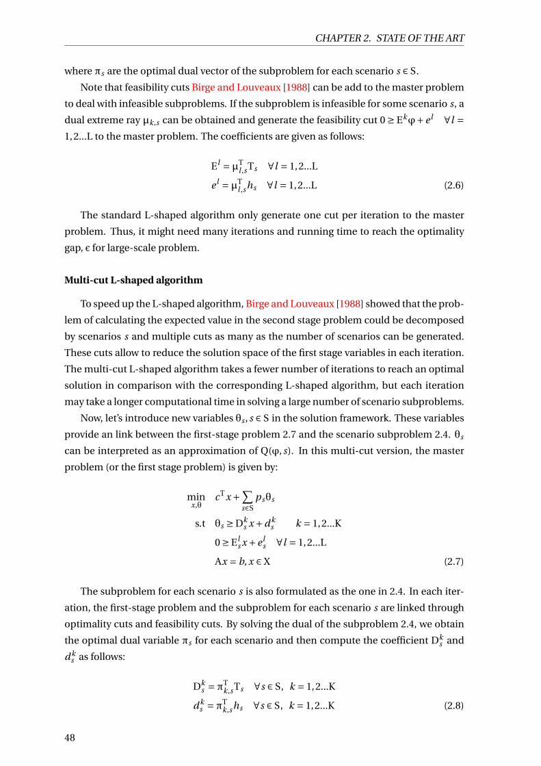
CHAPTER 2. STATE OF THE ART
where πs are the optimal dual vector of the subproblem for each scenario s ∈ S.
Note that feasibility cuts Birge and Louveaux [1988] can be add to the master problem
to deal with infeasible subproblems. If the subproblem is infeasible for some scenario s, a
dual extreme ray µk,s can be obtained and generate the feasibility cut 0 ≥ Ekϕ+ e l ∀l =1,2...L to the master problem. The coefficients are given as follows:
El =µTl ,sTs ∀l = 1,2...L
e l =µTl ,shs ∀l = 1,2...L (2.6)
The standard L-shaped algorithm only generate one cut per iteration to the master
problem. Thus, it might need many iterations and running time to reach the optimality
gap, ε for large-scale problem.
Multi-cut L-shaped algorithm
To speed up the L-shaped algorithm, Birge and Louveaux [1988] showed that the prob-
lem of calculating the expected value in the second stage problem could be decomposed
by scenarios s and multiple cuts as many as the number of scenarios can be generated.
These cuts allow to reduce the solution space of the first stage variables in each iteration.
The multi-cut L-shaped algorithm takes a fewer number of iterations to reach an optimal
solution in comparison with the corresponding L-shaped algorithm, but each iteration
may take a longer computational time in solving a large number of scenario subproblems.
Now, let’s introduce new variables θs , s ∈ S in the solution framework. These variables
provide an link between the first-stage problem 2.7 and the scenario subproblem 2.4. θs
can be interpreted as an approximation of Q(ϕ, s). In this multi-cut version, the master
problem (or the first stage problem) is given by:
minx,θ
cTx +∑s∈S
psθs
s.t θs ≥ Dks x +d k
s k = 1,2...K
0 ≥ Els x +e l
s ∀l = 1,2...L
Ax = b, x ∈ X (2.7)
The subproblem for each scenario s is also formulated as the one in 2.4. In each iter-
ation, the first-stage problem and the subproblem for each scenario s are linked through
optimality cuts and feasibility cuts. By solving the dual of the subproblem 2.4, we obtain
the optimal dual variable πs for each scenario and then compute the coefficient Dks and
d ks as follows:
Dks =πT
k,sTs ∀s ∈ S, k = 1,2...K
d ks =πT
k,shs ∀s ∈ S, k = 1,2...K (2.8)
48

CHAPTER 2. STATE OF THE ART
If there is at least one infeasible subproblem under scenario s, a dual extreme ray µl ,s
can be obtained and generate the feasibility cut 0 ≥ Ekϕ+ ek ∀l = 1,2...L and add to the
master problem. The coefficients Els and e l
s of a feasibility cut are given as follows:
El =µTl ,sTs ∀l = 1,2...l
e l =µTl ,shs ∀l = 1,2...L (2.9)
The framework for the multi-cut L-shaped algorithm is very similar to the standard
one. It is outlined as follows:
(i) In each iteration, the first-stage problem is solved and the dual of subproblem 2.4 is
solved as many times as the number of scenarios s ∈ S
(ii) By solving the first-stage problem, the values of the first stage decision variables ϕ
are determined and the value of function Q(x, s) at each scenario s in the second
stage is approximated by θs .
(iii) By solving the dual of subproblem 2.4, the expected value of the second stage prob-
lem for all scenarios can be found for the given value of the first stage variables
found in the previous step.
(iv) In each iteration, after solving the dual of the scenario subproblem, multiple cuts of
type with the number equal to that of scenarios are added to the first-stage problem.
2.5 Conclusion
From the analysis of recent literature on biomass supply chain management, we ob-
serve that many models are used to formulate problems at different decision levels at
different objectives to meet various decision-making requirements. Almost all works are
based on deterministic models, whereas the use of stochastic approach is quite rare al-
though it can reflect better real-life situations than the previous one. To find an optimal
solution of the models, most authors used a commercial solver such as CPLEX, GUROBI,
GAMS, and XPRESS while the rest developed their algorithms such as Lagrangian relax-
ation, Bender decomposition. In addition, we discover that no previous work addresses
the issue of supplier selection for better stabilizing feedstock supply in biomass supply
chains. In fact, stabilizing feedstock supply would contribute to the sustainability of a
biomass supply chain and allows to improve competitiveness with fossil energy.
Thus, in Chapters 3 and 4, we address the supplier selection and operation planning
problem in biomass supply chains. These two issues are analyzed by considering two ap-
proaches: deterministic and stochastic. The first approach is suitable for the "what-if"
analysis where decision-makers already know the inputs and want to evaluate the out-
come of their decisions. This model is then extended to consider under environmental
49

CHAPTER 2. STATE OF THE ART
uncertainty by applying a two-stage stochastic programming approach in Chapter 4. An
improved L-shaped algorithm is developed to solve the stochastic model.
An overview of perishable inventory management has identified the important factors
such as demand, supply, uncertainty, price, deterioration rate, shelf life, replenishment
policy, etc. It is clear that the scientific community did not consider all of these factors
at the same time. For example, uncertainty in both supply and demand can be easily
found in the real world, but only few works considered this kind of uncertainty. Most of
models proposed to combinate stochastic demand with one or more specific factors such
as discount price, credit, and different payment problems; inflation and time value for
money; investment, promotion and budget constraint; customer satisfaction to represent
real-life issues. From the analysis, we discover that the study of inventory models for
perishable products under both stochastic demand and stochastic supply is essential for
the inventory management of biomass supply chains. In such inventory management,
some available information may be not precise due to environmental uncertainty. So it is
logical to develop appropriate methods such as fuzzy, stochastic and dynamic approaches
to capture uncertainty in a perishable inventory problem.
Thus, a perishable inventory model under both stochastic demand and supply will
be presented in Chapter 5 based on dynamic programming. In Chapter 5, the product
considered is assumed to have a constant deterioration rate. We then develop a solution
method based on the scenario optimization approach and Lagrangian relaxation to find a
near-optimal solution. In the last chapter, we extend this model to a product with a fixed
lifetime.
50

Chapter 3
Modeling and optimization of biomass
supply chain with two types of feedstock
suppliers
“ Knowledge is an unending
adventure at the edge of
uncertainty. ”
Jacob Bronowski
Contents
2.1 Introduction . . . . . . . . . . . . . . . . . . . . . . . . . . . . . . . . . . . . 22
2.2 Biomass supply chains management . . . . . . . . . . . . . . . . . . . . . 22
2.2.1 Biomass supply chains . . . . . . . . . . . . . . . . . . . . . . . . . . . 22
2.2.2 Structure, activities and challenges of biomass supply chains . . . . 23
2.2.3 Optimization models for biomass supply chain management . . . . 25
2.3 Perishable inventory management . . . . . . . . . . . . . . . . . . . . . . 34
2.3.1 Characteristics of perishable inventory problems . . . . . . . . . . . 34
2.3.2 Classification of perishable inventory models . . . . . . . . . . . . . 36
2.3.3 Modeling approaches for perishable inventory problems . . . . . . 43
2.4 Modeling and solution approaches for stochastic optimization . . . . . . 44
2.4.1 Two-stage stochastic optimization approach . . . . . . . . . . . . . 45
2.4.2 Decomposition methods . . . . . . . . . . . . . . . . . . . . . . . . . 47
2.5 Conclusion . . . . . . . . . . . . . . . . . . . . . . . . . . . . . . . . . . . . . 49
51

CHAPTER 3. MODELING AND OPTIMIZATION OF BIOMASS SUPPLY CHAIN WITHTWO TYPES OF FEEDSTOCK SUPPLIERS
3.1 Introduction
This chapter presents a mixed-integer linear approach for a lignocellulosic biomass
supply chain planning including different logistics activities such as: feedstock supply,
preprocessing, storage, transportation and biofuel production.
According to Li et al. [2011], lignocellulosic biomass such as corn, wheat and switch-
grass can be used as feedstock and is interchangeable with minimal effect on biorefinery
production costs and bioethanol yields. The multi-biomass approach could be a potential
solution, which uses a mix of feedstock (corn, wheat and switchgrass) harvested/collected
in different time period. Stabilization of feedstock has a critical impact on the sustainabil-
ity of a biomass supply chain. To stabilize the feedstock supply, it is essential to integrate
supplier selection decision with operational planning. In other words, the better under-
standing of the operational plan, the better supplier selection decision in this problem.
To the best of our knowledge, none of these studies present a multi-period supply
chain model to cope with the supplier selection and the design of operation planning. For
this reason, we present a multi-period mixed integer programming model that can be ap-
plied to capture most activities and supplier selection decision in biomass supply chain.
Our model has a flexible structure which allows for the modeling of value chains sup-
plier selection and different logistic activities (transportation and operation planning).
We also evaluated the economic impact of the supplier selection and operation planning
on a biomass supply chain.
This chapter is organized as follows: In Section 3.2, the problem and its model are
introduced. A numerical study is presented and its results are analyzed in Section 3.3.
Section 3.4 concludes this chapter with some remarks.
3.2 Problem description and model formulation
3.2.1 Problem description
In this chapter, we study a biomass supply chain as shown in Figure 3.1 and develop
a deterministic mixed integer linear programming (MILP) model to support decision-
makers to observe the outcomes of their decisions in different inputs/conditions. Our
study focused on how to select feedstock suppliers and establish a mid/long-term con-
tract with them to ensure the stabilization of feedstock supply. Moreover, numerous con-
straints should be respected such as feedstock availability, biomass degradations, resource
capacities, and refinery demands.
In the model, the production infrastructure such as pretreatment facilities and biore-
fineries have been located. We assume that biofuel producers seek to establish a long-
term relationship with certain local/regional suppliers in order to stabilize the feedstock
supply. The unit purchase price and the minimum delivery quantity are fixed under a
52

CHAPTER 3. MODELING AND OPTIMIZATION OF BIOMASS SUPPLY CHAIN WITHTWO TYPES OF FEEDSTOCK SUPPLIERS
Figure 3.1: A biomass supply chain
long-term contract during a planning horizon. The unit transportation cost per trip from
local/regional suppliers to biorefineries is pre-computed based on their distances and
fixed costs associated with trucks.
The logistics activities occurred in each period are presented as follows:
• In each period, biomass is transported from contracted suppliers to preprocessing
facilities, then to biorefineries.
• In each conversion facility, the supplied biomass feedstock is pre-processed and
then converted into biofuel or be kept as inventory at the biorefinery.
• Biomass can be bought from international/national markets to meet part of biofuel
demand only at a reasonable price of biomass.
• After satisfying the biofuel demand in each period, any excess volume of biofuel is
kept as inventory. A shortage cost is charged for any unit of unmet biofuel demand.
• Biomass preprocessed/biofuel produced is limited by biomass preprocessing/processing
capacity and also by storage capacity in each facility.
• Many lignocellulosic crops can be used lignocellulosic biomass (corn, wheat, and
switchgrass...) can be used as feedstock and is interchangeable in biofuel produc-
tion because their compositions are very similar according to Li et al. [2011].
3.2.2 Model formulation
In the following, we formulate a MILP model that considers the suppliers selection
with a mid/long-term contract, inventory management and transportation planning. We
consider a planning horizon of T periods, each period could be a week, a month or a
53

CHAPTER 3. MODELING AND OPTIMIZATION OF BIOMASS SUPPLY CHAIN WITHTWO TYPES OF FEEDSTOCK SUPPLIERS
Table 3.1: List of parameters and variables
SetT Set of periods tI Set of suppliers iP Set of preprocessing facilities pB Set of biorefineries bA Set of all arcs in the biomass supply chain A = (I×P)∩ (P×B)∩ (M×B)Parametersavai l I(i , t ) Amount of biomass (tons) available at supplier i in period tcost AI(i ) Unit purchase cost of biomass from supplier i ($/ton)Qmi n(i ) Minimum supply quantity (tons) under contract with supplier i during planning horizon
Tmcost (i ) Fixed cost for establishing a contract with supplier i
International/national marketavai l M(m, t ) Amount of biomass (tons) available at market m in period tcost AM(m) Unit purchase cost of biomass from market m ($/ton)
Preprocessing siteΓmax
p (p) Maximum amount of biomass (tons) that could be preprocessed at preprocessing facilityp
Γmi np (p) Minimum amount of biomass (tons) that could be preprocessed at preprocessing facility
pWmax (p) Maximum biomass storage capacity (tons) at preprocessing facility p in each periodWmi n(p) Minimum biomass storage capacity (tons) at preprocessing facility p in each periodhcostP(p) Biomass inventory holding cost at preprocessing facility p ($/ton)tcostP(p) Biomass preprocessing cost of preprocessing facility p ($/ton)λP(p) Ratio of biomass storage loss at preprocessing facility p in each periodηP(p) Preprocessing rate at preprocessing facility p in each period
Biorefinery site:Γmax
b (b) Maximum amount of biomass (tons) could be processed by biorefinery b in each periodΓmi n
b (b) Minimum amount of biomass (tons) could be processed by biorefinery b in each periodVmax
av (b) Maximum biomass storage capacity (tons) of biorefinery b in each periodVmmi n
av (b) Minimum biomass storage capacity(tons)of biorefinery b in each periodVmax
ap (b) Maximum biofuel storage capacity(litres) of biorefinery b in each periodVmmi n
ap (b) Minimum biofuel storage capacity (litres) of biorefinery b in each periodpcost (b) Unit penalty cost for unmet biofuel demand at biorefinery b ($/tons)tcostB(b) Biofuel production cost at biorefinery b ($/tons)hcostBav (b) Unit inventory holding cost of biomass at biorefinery site b in each period ($ / ton)hcost B
ap (b) Unit inventory holding cost of biofuel at biorefinery b in each period ($/ ton)ηB(b) Biofuel yield rate of lignocellulosic biomass for biorefinery b (litre/ton)λB(b) Ratio of biomass storage loss at biorefinery b in each perioddemand(b, t ) Demand of biofuel(litre) at biorefinery b in period t
Transportation:CapV(i , j ) Transportation capacity from node i to node j (tons/truck)Vcost (i , j ) Unit transportation cost of each trip of a truck from node i to node j ($ /trip)
Decision variablesContinuous variables
x(i , j , t ) Amount of biomass transported from node i to node j in each period tW(p, t ) Biomass inventory level (tons) at preprocessing facility p in period tVB
av (b, t ) Inventory level of biomass at biorefinery b in period tVB
ap (b, t ) Inventory level of biofuel at biorefinery b in period tQP(p, t ) Amount of biomass preprocessed (tons) at preprocessing facility p in period tz(b, t ) Amount of biomass required (tons) to produce biofuel at refinery b in period tshor t (b, t ) Shortage of biofuel (liters) at biorefinery b in period t
Integer variablesnbr T(i , j , t ) Number of truck trips from node i to node j in period t
Binary variablesϕ(i ) Equal to 1 if a contract between refinery b and supplier i is established, 0 otherwise
trimester. Let I be a set of biomass suppliers, P be a set of pretraitement facilities and B be
a set of biorefineries.
Let ϕ = ϕ(i ), i ∈ I be the decision variables related to mid/longterm contracts be-
tween the biorefineries and suppliers, ϕ(i ) = 1 if a long term contract is established with
54

CHAPTER 3. MODELING AND OPTIMIZATION OF BIOMASS SUPPLY CHAIN WITHTWO TYPES OF FEEDSTOCK SUPPLIERS
supplier i , 0 otherwise. The vector mcost = mcost (i ), i ∈ I includes fixed cost mcost (i )
for establishing a contract with supplier i .
Denote x(i , j , t , s) as the flow of biomass on arc (i , j ) ∈ A in period t . Such an arc (i , j )
could be arc (i , p) or (p,b) that refers to an arc from supplier i ∈ I to preprocessing facility
p ∈ P or from preprocessing facility p ∈ P to biorefinery b. Let pr e(n), suc(n) denote, re-
spectively, the set of predecessor and the set of successors of a given node n. For example,
suc(i ), i ∈ I indicates a set of pretreatment facilities to which biomass feedstock is deliv-
ered from farm i ; pr e(p), p ∈ P indicates a set of farms that supply biomass feedstock to
pretreatment facility p; suc(p), p ∈ P indicates a set of biorefineries to which biomass is
delivered from pretreatment facility p.
Let cost AI(i ), cost AM(m) be unit purchase price of biomass from supplier i and from
market m, respectively; tcostP(p) be unit biomass preprocessing cost at pretreatment
facility p; hcostBav (b), hcost Bap (b) be unit inventory holding costs of biomass and biofuel
at biorefinery site b in each period, respectively; ηB(b) be the biofuel yield rate and λB(b)
be the ratio of biomass storage loss at biorefinery b in each period.
For convenience, all notations used in the model formulation are summarized in Table
3.1. All continuous decision variables are non-negative. The minimization of the different
costs of the biomass supply chain can be modeled by the mixed linear program detailed
as follows:
Objective function:
min z =∑t∈T
∑(i , j )∈A
nbr T(i , j , t )∗Vcost (i , j )
+ ∑t∈T
∑p∈P
ηPQP(p, t )tcostP(p)
+ ∑t∈T
∑b∈B
shor t (b, t )pcostB(b)
+ ∑t∈T
∑b∈B
ηBz(b, t )costB(B)
+ ∑t∈T
∑p∈P
hcost P(p)W(p, t )
+ ∑t∈T
∑b∈B
hcost Bav (b)Vav (b, t )
+ ∑t∈T
∑b∈B
hcost Bap (b)Vap
+ ∑t∈T
∑i∈I
QI(i , t )∗ cost AI(i )
+ ∑t∈T
∑m∈M
∑b∈B
x(m,b, t )∗ cost AM(m)
+∑i∈Iφ(i )∗mcost (i ) (3.1)
The objective function (3.1) is to minimize the total cost, composed of nine costs:
transportation costs (1st term), pre-traitement costs (2nd term), shortage costs (3rd term),
55

CHAPTER 3. MODELING AND OPTIMIZATION OF BIOMASS SUPPLY CHAIN WITHTWO TYPES OF FEEDSTOCK SUPPLIERS
biofuel conversion costs (4th terms) holding costs(5-7th terms), purchase costs from sup-
pliers and markets (8-9th terms) and fixed cost for establishing a contract with suppliers
(last term).
Constraints on suppliers
QI(i , t ) = ∑p∈suc(i )
x(i , p, t ) ∀t ∈ T, i ∈ I (3.2)
QI(i , t ) ≤ avai l I(i , t ).ϕ(i ) ∀t ∈ T, i ∈ I (3.3)
Qmi n(i )ϕ(i ) ≤ ∑t∈T
QI(i , t ) ∀i ∈ I (3.4)
Equation (3.2) defines the total amount of feedstock is transported from supplier i to
pretreatment facilities in each period. Note that the decision variable QI(i , t ) is redundant
but it is introduced for improving the readability of the model.
Inequality (3.3) states that there is no feedstock supply unless there is a mid/long-
term contract between supplier i and biorefinery b. This inequality also ensures that the
total purchase amount must not exceed the available amount in each period. Inequality
(3.4) ensures the minimum supply quantity under a contract between a supplier i and the
biorefinery b during planning horizon T.
Constraints on market
∑b∈B
x(m,b, t ) ≤ avai l M(m, t ) ∀t ∈ T,m ∈ M (3.5)
Inequality (3.5) shows that the purchase amount of biomass is also limited by the mar-
ket’s supply availability.
Constraints on preprocessing sites
QP(p, t ) = ∑(i )∈pr e(p)
x(i , p, t ) ∀t ∈ T, p ∈ P (3.6)
W(p, t ) = λP(p)W(p, t −1)+ηPQP(p, t )− ∑(b)∈suc(p)
x(p,b, t ) ∀t ∈ T, p ∈ P (3.7)
Γmi np (p) ≤ QP(p, t ) ≤ Γmax
p (p) ∀t ∈ T, p ∈ P (3.8)
Wmi n(p) ≤ W(p, t ) ≤ Wmax(p) ∀t ∈ T, p ∈ P (3.9)
Equation (3.6) defines the total amount of biomass is transported from pretreatment
facility p to refineries in each period. Note that the decision variable QP(p, t ) is redundant
but it is introduced for improving the readability of the model. Constraint (3.7) is the
inventory balance constraints for biomass storage at preprocessing facility. Constraint
(3.8) ensures the capacity production of each pre-processing plant.
56

CHAPTER 3. MODELING AND OPTIMIZATION OF BIOMASS SUPPLY CHAIN WITHTWO TYPES OF FEEDSTOCK SUPPLIERS
Constrains on refinery sites
Vav (b, t ) = λB(b)Vav (b, t −1)+ ∑(p)∈pr e(b)
x(p,b, t )
+ ∑m∈M
x(m,b, t )− z(b, t ) ∀t ∈ T,b ∈ B (3.10)
Vap (b, t ) = Vap (b, t −1)+ηBz(b, t )
+ shor t (b, t )−demand(b, t ) ∀t ∈ T,b ∈ B (3.11)
Γmaxb (b) ≤ z(b, t ) ≤ Γmax
b (b) ∀t ∈ T,b ∈ B (3.12)
Vmi nav (b) ≤ VB
av (b, t ) ≤ Vmaxav (b) ∀t ∈ T,b ∈ B (3.13)
Vmi nap (b) ≤ VB
ap (b, t ) ≤ Vmaxap (b) ∀t ∈ T,b ∈ B (3.14)
Constraints (3.10) and (3.11) are the inventory balance constraints for biomass and
biofuel storage at biorefinery, respectively. These constraints ensure that no more biomass
or biofuel is delivered or processed at a location than available amount in stock. Con-
straint (3.11) ensures that biofuel demand is satisfied as much as possible, and unsatisfied
demand is lost. Shortage cost is incurred for any unit lost.
The capacity production of each refinery plant is respected via constraint (3.12). Con-
straints (3.13) and (3.14) show inventory capacity for biomass and biofuel at refinery site,
respectively.
Constraints on transportation
x(i , j , t ) ≤ nbr T(i , j , t )∗CapV(i , j ) (3.15)
Constraint (3.15) shows the number of trips required for transporting a given amount
of biomass from node i to node j in each period. The total flows should not be greater
than the required number of vehicles in anytime period.
This model allows the user to formulate complex biomass supply chains by adding a
new nodes (suppliers, preprocessing/refinery plants) and arcs linking these nodes.
3.3 Numerical study
In this section, a numerical study is conducted to evaluate the economic aspect and
some critical factors of the biomass supply chain. This model is implemented in Python
3.5 on a HP computer with Intel Core i5-4210M CPU 2.66 GHz and 8.0 GB RAM. All MILP
problems were solved by a solver GUROBI 6.5 with default parameters.
3.3.1 Data generation
To demonstrate the use of the biomass supply chain model, a simple case study is
carried out. In the baseline case, we consider a biomass supply chain with one refinery,
57

CHAPTER 3. MODELING AND OPTIMIZATION OF BIOMASS SUPPLY CHAIN WITHTWO TYPES OF FEEDSTOCK SUPPLIERS
two pretreatment site, 100 supplier candidates over 12 periods. Each period in this study
corresponds to one month. The biofuel producer seeks to sign a contract with several
local feedstock suppliers.
Concerning suppliers, amount of biomass available in each supplier can be estimated
from a land area for cultivation and biomass yield. We also use parameter data from Os-
mani and Zhang [2013] and other sources such as literature reviews and research articles
to validate our model.Contracts with suppliers are characterized by fixed cost, purchase
price and minimum quantity to supply. Purchase price varies from 35 to 37 $/ton. The
minimum supply quantity varies from 20 000 to 100 000 tons. Fixed cost for establishing
a contract varies from $20 000 to $30 000. We precomputed transportation cost per trip
based on distances, variable transportation cost, and fixed cost.
All 100 candidates of supplier selection are located within 50 km radius of the biorefin-
ery. The amount of biomass available in each supplier is estimated from land availability
according to Osmani and Zhang [2013, 2014]. For each supplier, biomass yield is gen-
erated from uniform distribution U[3.5,4.5]. A ratio of biomass storage loss varies from
1 to 3% per month (worst case). The biorefinery plant has a production capacity of 190
MLPY with a unit production cost of 0.2$/ liter. The bioethanol yield rate of lignocel-
lulosic biomass is about 313 liters/ton. The unit biofuel storage cost and unit biomass
storage cost at biorefinery is 0.227 $/liter and 0.9 $/ ton, respectively. The unit shortage
cost is 1.06 $/liter.
The dataset is summarized in Table 3.2. Based on historical data (19981-2005) in
Osmani and Zhang [2013], we generate annual biofuel demand randomly from Normal
probability distribution N(2133,4138) and truncated on the interval [2006,2280]. The
model size increases when the numbers of periods, suppliers, pretraitement facilities and
biorefineries increase. For testing the model with different instances, we adjust biofuel
demand according to the scalability of feedstock suppliers.
Table 3.2: Data of model parameters
Input parameters ValueBioethanol yield rate (litre/tonne) 313.00Penalty cost for unmet bioethanol demand ($/liter) 1.06Bioethanol production cost ($/liter) 0.20Maximum annual production capacity of biorefinery(MLPY) 380.00Minimum annual production capacity of biorefinery(MLPY) 190.00Preprocessing cost at preprocessing facility ($/ton) 13.39Inventory cost for biomass in time period t ($/ton) 0.90Ratio of biomass storage loss in time period 0.01Ratio of biomass storage loss in time period (%) 1-3 %Maximum annual pretraitement capacity (tons) 2 000 000.00Maximum biomass storage capacity (tons) of biorefinery 3 500 000.00Maximum biomass storage capacity (tons) of pretraitement facility 3 500 000.00Yield biomass feedstocks (tons/hecta) Uniform[3.5, 4.5]Unit biomass purchase price from suppliers ($/ton) 35-37
58

CHAPTER 3. MODELING AND OPTIMIZATION OF BIOMASS SUPPLY CHAIN WITHTWO TYPES OF FEEDSTOCK SUPPLIERS
3.3.2 Analysis of the solution
In this section, we analyze our numerical results. The optimal value of total cost in
the supply chain is $181 281 119 when a biomass supply chain includes one refinery, two
pretreatment site and 100 supplier candidates over 12 time periods. For this instance, the
whole model has in fact 3 808 constraints, 2 532 continuous variables and 1 324 integer
variables. The running time is reasonable: an optimal solution is obtained in less than 5
seconds (1.78 seconds).
Fig 3.2 represents the distribution of costs in the biomass supply chain over planning
horizon T= 12. It is evident that transportation costs play an essential role in the biomass
supply chain with approximatively 25% of total system costs. This result shows the impor-
tance of transportation operation in biomass supply chains. Holding costs is only 2.3%
because in this study the amount of biomass available for biofuel production is higher
than the demand, so the storage of a significant amount of biomass at biorefinery seems
to be not critical.
Figure 3.2: Distribution of cost in supply chain
One important aspect of the model is the running time which depends on the num-
ber of periods, suppliers, pretreatment facilities and biorefineries. We further tested this
model for different instances when I= 10, 20, 50, 100, 150, 200, 250, 300, 350, 400; P= 1, 2,
5 and T= 12. The problem size and execution time of these instances are summarized in
Table 3.3. The results illustrate that this model can be solved quickly and exactly with a
commercial solver.
3.3.3 Sensitivity analysis
We then study the impacts of some critical parameters (purchase price from a market,
minimum supply quantity and fixed contracted cost) on the total system cost. As these
59

CHAPTER 3. MODELING AND OPTIMIZATION OF BIOMASS SUPPLY CHAIN WITHTWO TYPES OF FEEDSTOCK SUPPLIERS
Table 3.3: Problem size and solution performance
Problem sizeN° I P B T Integer Continous Constraint CPU(s)
1 10 1 1 12 142 336 442 0.042 20 1 1 12 272 576 812 0.143 50 1 1 12 662 1296 1922 0.154 100 1 1 12 1312 2496 3772 0.525 200 1 1 12 2612 4896 7472 3.266 10 2 1 12 154 372 478 0.037 20 2 1 12 284 612 848 0.078 50 2 1 12 674 1332 1958 0.859 100 2 1 12 1324 2532 3808 1.78
10 200 2 1 12 2624 4932 7508 5.4411 10 5 1 12 190 480 586 0.0512 20 5 1 12 320 720 956 0.0713 50 5 1 12 710 1440 2066 0.1314 100 5 1 12 1360 2640 3916 0.3715 150 5 1 12 2010 3840 5766 0.8016 200 5 1 12 2660 5040 7616 0.8417 250 5 2 12 3310 6240 9466 1.4618 300 5 2 12 3960 7440 11316 2.0119 350 5 2 12 4610 8640 13166 9.5820 400 5 2 12 5260 9840 15016 12.84
parameters have significant impacts on feedstock supply, it is essential to learn how they
affect the optimal expected total cost of biomass supply chain and the total number of
contracted suppliers.
Effect of purchase price
Figure 3.3 shows the total system cost and the number of contracted suppliers under
different values of the purchase price that varies between 90% and 130 % of its base value.
The horizontal axis represents the various purchase price of biomass from an interna-
tional or regional market. The bar graphs with the height measured by the vertical axis
on the left correspond to the total costs of this supply chain under different values of the
purchase price. The dotted line with the value of each point measured by the vertical axis
on the right indicates the number of contracted suppliers at each possible value of the
purchase price considered.
We observe that the total system cost is less sensitive to the variation of the market
price. In fact, the optimal total system cost increases slightly from $ 179 828 032 to $ 181
281 119 (less than 1%) when the market price varies from 90% to 100% of its base value.
Then, it remains nearly constant when the market price is set from 100% to 130% of its
basic level. This relationship confirms that when the market price increases too high,
decision-makers have less interest in purchasing an additional quantity of biomass from
markets to meet biofuel demand. In this case, they would intend to establish more long-
60

CHAPTER 3. MODELING AND OPTIMIZATION OF BIOMASS SUPPLY CHAIN WITHTWO TYPES OF FEEDSTOCK SUPPLIERS
Figure 3.3: Distribution of cost in supply chain
term supply contracts to ensure the stability of feedstock supply. This explains why the
number of contracted suppliers increases when the market price grows.
Effect of fixed cost
Figure 3.4 shows the effect of fixed cost on the biomass supply chain in term of the
total system cost and the number of contracted suppliers. The horizontal axis represents
the fixed cost varying from 50% to 400% in comparison to its base value. The bar graphs
with the height measured by the vertical axis on the left hand present the total expected
system costs under different values of the fixed cost. The dotted line with the value of each
point measured by the vertical axis on the right hand indicates the number of contracted
suppliers at each possible value of the fixed cost.
Figure 3.4: Distribution of cost in supply chain
This figure shows that the increase in fixed cost may lead to higher total system cost
and might hinder the establishment of long-term contracts. However, it is a slight effect
on the overall system cost and the total number of contracted suppliers.
61

CHAPTER 3. MODELING AND OPTIMIZATION OF BIOMASS SUPPLY CHAIN WITHTWO TYPES OF FEEDSTOCK SUPPLIERS
Effect of the minimum supply quantity of suppliers
Figure 3.5 presents the impacts of a contracted supply quantity on the total system
cost of biomass supply chain and the number of contracted suppliers. The horizontal axis
represents the various contracted quantity delivered from 60% to 180% in comparison
with its base value. The bar graphs with the height measured by the vertical axis on the left
hand show the total expected system costs under different values of the minimum supply
quantity. The dotted line with the value of each point measured by the vertical axis on
the right hand indicates the number of contracted suppliers at each possible value of the
minimum supply quantity.
Figure 3.5: Distribution of cost in supply chain
The figure shows that the minimum supply quantity and the total system cost are pro-
portional to each other; however, the increase of minimum supply quantity is not as much
as the one of total system cost. Besides, the total number of contracted suppliers de-
creases as the supply quantity increases. In this case, decision-maker would require ad-
ditional quantity from market to satisfy the final demand but only at a reasonable market
price.
3.4 Conclusion
This chapter presents a mixed integer linear programming (MILP) model for minimiz-
ing the total system costs in a biomass supply chain. The model integrates all supply chain
logistics such as transportation plan, purchase activities, inventory control, and produc-
tion to provide an optimal solution. The case presented has been solved optimally with
different instances in reasonable computation time. Moreover, we have analyzed the im-
pacts of some critical parameters on the optimal expected cost of the system and supplier
selection.
62

CHAPTER 3. MODELING AND OPTIMIZATION OF BIOMASS SUPPLY CHAIN WITHTWO TYPES OF FEEDSTOCK SUPPLIERS
This chapter could provide a decision-making support tool for biomass supply chain
management for a "what-if" scenarios where decision markers want to evaluate the out-
comes from their decisions with different inputs. In the next chapter, we extended our
model into stochastic environments.
The work in this chapter was presented at the 7th International Conference on Indus-
trial Engineering and Systems Management in Saarbrücken, Germany [Duc-Huy et al.,
2017].
63

CHAPTER 3. MODELING AND OPTIMIZATION OF BIOMASS SUPPLY CHAIN WITHTWO TYPES OF FEEDSTOCK SUPPLIERS
64

Chapter 4
Supplier selection and Operation
planning in biomass supply chain with
supply uncertainty
Contents
3.1 Introduction . . . . . . . . . . . . . . . . . . . . . . . . . . . . . . . . . . . . 52
3.2 Problem description and model formulation . . . . . . . . . . . . . . . . 52
3.2.1 Problem description . . . . . . . . . . . . . . . . . . . . . . . . . . . . 52
3.2.2 Model formulation . . . . . . . . . . . . . . . . . . . . . . . . . . . . . 53
3.3 Numerical study . . . . . . . . . . . . . . . . . . . . . . . . . . . . . . . . . . 57
3.3.1 Data generation . . . . . . . . . . . . . . . . . . . . . . . . . . . . . . . 57
3.3.2 Analysis of the solution . . . . . . . . . . . . . . . . . . . . . . . . . . 59
3.3.3 Sensitivity analysis . . . . . . . . . . . . . . . . . . . . . . . . . . . . . 59
3.4 Conclusion . . . . . . . . . . . . . . . . . . . . . . . . . . . . . . . . . . . . . 62
65

CHAPTER 4. SUPPLIER SELECTION AND OPERATION PLANNING IN BIOMASSSUPPLY CHAIN WITH SUPPLY UNCERTAINTY
4.1 Introduction
In the previous chapter, we have developed a deterministic model to provide the sup-
plier selection and operation planning decisions in a biomass supply chain. This deter-
ministic approach is only appropriate when all parameters are precise. In real-life situ-
ations, we often encounter the presence of uncertainty in biomass feedstock supply be-
cause its availability and yield depend on seasonality (weather condition, temperature)
and harvest time. Therefore, this uncertainty is a critical factor that must be accounted
for because it has a substantial impact on the sustainability of a biomass supply chain.
To the best of our knowledge, the study of supplier selection in a biomass supply chain
was rare in the literature. There is no work considering strategical supplier selection along
with tactical planning under uncertain environments although the two types de decisions
are interdependent. For this reason, we present a stochastic programming model that
can be used to capture most activities in a biomass supply chain and the uncertainty in
feedstock supply. The main contributions of this chapter include:
Firstly, we propose a two-stage stochastic programming model for biomass supply
chain management. In the model, the first stage decision is to select suppliers who pro-
vide long/mid term feedstock supply. The second-stage decisions determine the amount
of biomass to purchase, to transport, to pre-process and the volume of bioethanol to pro-
duce in each period.
Secondly, we develop an enhanced and regularized L-shaped decomposition method
to solve the stochastic programming model with a given number of scenarios. The Monte
Carlo sampling approach is used to find the required number of scenarios for ensuring
that the exact value of an output of the model is located within a confidence interval with
a given probability.
Thirdly, we conduct a numerical study to evaluate the performance of the proposed
algorithm. The numerical results show that the algorithm can find an optimal solution
in a reasonable computation time while a commercial solver cannot for large instances.
Sensitivity analysis is performed to investigate the effect of some critical parameters on
the optimal expected cost and suppliers selection.
This chapter is organized as follows: Section 4.2 describes the problem studied and
its model are introduced. We describe the solution method for the model in Section 4.3.
A numerical study is presented, and its results are analyzed in Section 4.4. Section 4.5
concludes this chapter with some remarks for future research.
66

CHAPTER 4. SUPPLIER SELECTION AND OPERATION PLANNING IN BIOMASSSUPPLY CHAIN WITH SUPPLY UNCERTAINTY
Figure 4.1: A two stage stochastic programming model with recourse for a biomass supply chain
4.2 Problem description and model formulation
4.2.1 Problem description
This chapter studies a biomass supply chain under uncertainty in supply as shown
in Figure 4.1. Biorefineries seek to establish a long-term relationship with certain lo-
cal/regional suppliers to stabilize its feedstock supply. Under a mid/long-term contract,
the unit purchase price and the minimum supply quantity are predetermined. The logis-
tics activities occurred in each period are presented as follows:
• Biorefineries can buy biomass from international/national markets (if available) to
meet part of biofuel demand only at a reasonable price of biomass.
• In each period, biomass is transported from contracted suppliers to preprocessing
facilities, then to biorefineries. In each conversion facility, the supplied biomass
feedstock is pre-processed and then converted into biofuel or be kept as inventory
at the biorefinery.
• After satisfying the biofuel demand in each period, any excess volume of biofuel
is kept as inventory. In case of shortfall in biofuel requirement, a relatively high
shortage cost is charged for any unmet biofuel demand.
• Biomass preprocessed/biofuel produced is limited by biomass preprocessing/processing
capacity and also by storage capacity in each facility. During storage, biomass has a
ratio of loss about 1-2% per month.
We assume that the production infrastructure such as pretreatment facilities and biore-
fineries have been located. The unit transportation costs from local/regional suppliers to
biorefineries are pre-calculated based on their distances and fixed costs are associated.
67

CHAPTER 4. SUPPLIER SELECTION AND OPERATION PLANNING IN BIOMASSSUPPLY CHAIN WITH SUPPLY UNCERTAINTY
In the following, we introduce a two-stage stochastic programming model to tackle
the supplier selection and operation planning in a biomass supply chain. The general
framework of the two-stage stochastic programming model is given in the next subsec-
tion.
4.2.2 Mathematical formulation
In this section, we formulate a two-stage stochastic programming model that con-
siders the selection of suppliers with a mid/long-term contract, inventory management
and transportation planning in a biomass supply chain. The first-stage decision variables
include only binary variables which determine the choice of suppliers with long/mid-
term contracts. The second-stage variables include the amount of biomass to be pur-
chased from suppliers, the amount of biomass feedstock to be transported to biorefinery,
the amount of biomass to be used to transform into bioethanol, the volume of unmet
bioethanol, the inventory of biomass and bioethanol in each period (Figure 4.1).
We consider a planning horizon of T periods, each period corresponds to a month.
Let I be a set of biomass suppliers, P be a set of pretreatment facilities, B be a set of biore-
fineries, S be a set of stochastic scenarios and A be the set of arcs in the biomass supply
chain A. An arc (i , j ) ∈ A stands for a path with biomass flow from node i to node j in
the supply chain network considered. A node may be a supplier, a pretreatment facility or
a biorefinery. Let pr e(n), suc(n) denote, respectively, the set of predecessor and the set
of successors of a given node n. For example, suc(i ), i ∈ I indicates a set of pretreatment
facilities to which biomass feedstock is delivered from farm i ; pr e(p), p ∈ P indicates a set
of farms that supply biomass feedstock to pretreatment facility p; suc(p), p ∈ P indicates
a set of biorefineries to which biomass is delivered from pretreatment facility p.
The first-stage and second stage model are presented as follows:
(SP): minϕ
mcost Tϕ+∑
s∈SpsQ(ϕ, s) |ϕ ∈ 0,1
(4.1)
where: Q(ϕ, s) = minys
f (ϕ, s, ys) | subject to (4.4)− (4.19)
(4.2)
where ϕ = ϕ(i ), i ∈ I are the first stage decision variables related to mid/longterm con-
tracts between the biorefineries and suppliers, ϕ(i ) = 1 if a long term contract is estab-
lished with supplier i , 0 otherwise. The vector mcost = mcost (i ), i ∈ I includes fixed
cost mcost (i ) for establishing a contract with supplier i , which is independent of sce-
nario s. The function Q(ϕ, s) refers to the cost function of the second stage problem for
each scenario s, in which the first stage decisions, ϕ are already made.
For convenience, all notations used in the model formulation are summarized in Table
4.1. All continuous decision variables are non-negative. The constraints (4.4 - 4.19) will be
presented in the next part of this section. The different components of the second stage
total cost f (ϕ, s, ys) under scenario s are given below; where ys contains all second-stage
68

CHAPTER 4. SUPPLIER SELECTION AND OPERATION PLANNING IN BIOMASSSUPPLY CHAIN WITH SUPPLY UNCERTAINTY
Table 4.1: List of parameters and variables
SetT Set of periods tI Set of suppliers iP Set of preprocessing facilities pB Set of biorefineries bM Set of markets mA Set of all arcs in the biomass supply chain A = (I×P)∩ (P×B)∩ (M×B)S Set of scenarios s
Deterministic parametersLocal/Regional suppliers
mcost (i ) Fixed cost for establishing a contract with supplier icost AI(i ) Unit purchase price of biomass from supplier i ($/ton)qmi n (i ) Minimum supply quantity of biomass (tons) under contract with supplier i during planning horizon
T
International/national marketavai l M(m, t ) Amount of biomass (tons) available at market m in period tcost AM(m) Unit purchase price of biomass from market m ($/ton)
Preprocessing siteγmax
p (p) Maximum amount of biomass (tons) that could be preprocessed at preprocessing facility p
γmi np (p) Minimum amount of biomass (tons) that could be preprocessed at preprocessing facility p
wmax (p) Maximum biomass storage capacity (tons) at preprocessing facility p in each periodwmi n (p) Minimum biomass storage capacity (tons) at preprocessing facility p in each periodw i ni t (p) Initial stock of biomass (tons) at preprocessing facility phcostP(p) Unit holding cost at preprocessing facility p ($/ton)tcostP(p) Unit biomass preprocessing cost of preprocessing facility p ($/ton)λP(p) Ratio of biomass storage loss at preprocessing facility p in each periodηP(p) Preprocessing rate at preprocessing facility p in each period
Biorefinery siteγmax
b (b) Maximum amount of biomass (tons) that could be processed by biorefinery b in each period
γmi nb (b) Minimum amount of biomass (tons) that could be processed by biorefinery b in each period
Vi ni tav (b) Initial stock of biomass (tons) of biorefinery b
Vmaxav (b) Maximum biomass storage capacity (tons) of biorefinery b in each period
Vmi nav (b) Minimum biomass storage capacity(tons)of biorefinery b in each period
Vi ni tap (b) Initial stock of biofuel (litres) of biorefinery b
Vmaxap (b) Maximum biofuel storage capacity(litres) of biorefinery b in each period
Vmi nap (b) Minimum biofuel storage capacity (litres) of biorefinery b in each period
pcost (b) Unit shortage cost for unmet biofuel demand at biorefinery b ($/tons)tcostB(b) Unit biofuel production cost at biorefinery b ($/tons)hcostBav (b) Unit inventory holding cost of biomass at biorefinery site b in each period ($ / ton)hcost B
ap (b) Unit inventory holding cost of biofuel at biorefinery b in each period ($/ ton)
ηB(b) Biofuel yield rate of biomass for biorefinery b (litre/ton)λB(b) Ratio of biomass storage loss at biorefinery b in each perioddemand(b, t ) Demand of biofuel(litre) at biorefinery b in period t
Transportation:Vcost (i , j ) Unit transportation cost from node i to node j ($ /tons)
Stochastic parametersavai l I(i , t , s) Amount of biomass (tons) available at supplier i in period t under scenario s
Decision variables Continuous variablesx(i , j , t , s) A flow of biomass on arc (i , j ) ∈ A in period t under scenario s, originally from node i to node jw(p, t , s) Biomass inventory level (tons) at preprocessing facility p in period t under scenario sVav (b, t , s) Inventory level of biomass at biorefinery b in period t under scenario sVap (b, t , s) Inventory level of biofuel at biorefinery b in period t under scenario sqI(i , t , s) Total amount of biomass transported from supplier i in period t under scenario sqP(p, t , s) Total amount of biomass transported to preprocessing facility p in period t under scenario sz(b, t , s) Amount of biomass required (tons) to produce biofuel at refinery b in period t under scenario sshor t (b, t , s) Shortage of biofuel (litres) at biorefinery b in period t under scenario s
Binary variablesϕ(i ) Equal to 1 if a mid/long-term contract between the biorefineries and supplier i is established, 0
otherwise
Dual variablesπ(.) Dual variables associated with the constraints (5)-(20) for problem (P2). For readability, each dual
variable is written in bracket at the right hand of the corresponding constraint in model (P2)
69

CHAPTER 4. SUPPLIER SELECTION AND OPERATION PLANNING IN BIOMASSSUPPLY CHAIN WITH SUPPLY UNCERTAINTY
decision variables, ys = (x, w,Vav ,Vap , qP, z, shor t ).
f (ϕ, s, ys) =∑t∈T
∑(i , j )∈A
x(i , j , t , s)∗Vcost (i , j )
+∑t∈T
∑p∈P
ηP ∗qP(p, t , s)∗ tcostP(p)
+∑t∈T
∑b∈B
shor t (b, t , s)∗pcost (b)
+∑t∈T
∑b∈B
ηB ∗ z(b, t , s)∗ tcostB(B)
+∑t∈T
∑p∈P
hcost P(p)w(p, t , s)
+∑t∈T
∑b∈B
hcost Bav (b)Vav (b, t , s)
+∑t∈T
∑b∈B
hcost Bap (b)Vap (b, t , s)
+∑t∈T
∑i∈I
q I(i , t , s)∗ cost AI(i )
+∑t∈T
∑m∈M
∑b∈B
x(m,b, t , s)∗ cost AM(m) (4.3)
where x(i , j , t , s) is the flow of biomass on arc (i , j ) ∈ A in period t under scenario s. Such
an arc (i , j ) could be arc (i , p) or (p,b) that refers to an arc from supplier i ∈ I to prepro-
cessing facility p ∈ P or from preprocessing facility p ∈ P to biorefinery b. w(p, t , s) is the
inventory level at preprocessing facility p in period t under scenario s.
The variables Vav (b, t , s), Vap (b, t , s) are the inventory level of biomass and the inven-
tory level of biofuel at biorefinery b in period t under scenario s, respectively. z(b, t , s),
shor t (b, t , s) are the amount of biomass used to produce biofuel and the shortage of
biofuel at biorefinery b in period t under scenario s, respectively. q I(i , t , s) is the total
amount of biomass transported from supplier i to the pretreatment facilities in period
t under scenario s. qP(p, t , s) is the total amount of biomass transported to pretreat-
ment facility p in period t under scenario s. Note that the decision variables q I(i , t , s)
and qP(p, t , s) are redundant but they are introduced for the readability of the model.
cost AI(i ), cost AM(m) are unit purchase price of biomass from supplier i and from market
m, respectively; tcostP(p) is unit biomass preprocessing cost at pretreatment facility p;
hcostBav (b), hcost Bap (b) are unit inventory holding costs of biomass and biofuel at biore-
finery site b in each period, respectively; ηB(b) is the biofuel yield rate and λB(b) is the
ratio of biomass storage loss at biorefinery b in each period.
The objective function is to minimize the total cost of the supply chain which includes
the first stage costs and the expected second-stage costs. The first stage costs comprise
the total costs for establishing contracts with local/regional suppliers. Equation (4.3) gives
the second stage costs Q(ϕ, s) for each scenario s, which comprise nine costs: transporta-
tion costs (1st term), pretreatment costs (2nd term), shortage costs (3rd term), biofuel
70

CHAPTER 4. SUPPLIER SELECTION AND OPERATION PLANNING IN BIOMASSSUPPLY CHAIN WITH SUPPLY UNCERTAINTY
conversion costs (4th term ), holding costs (5th-7th terms), and purchase costs (9th-10th
terms).
Constraints on suppliers
q I(i , t , s) = ∑p∈suc(i )
x(i , p, t , s) ∀t ∈ T, i ∈ I, s ∈ S [π1i ,t ,s] (4.4)
q I(i , t , s) ≤ avai l I(i , t , s).ϕ(i ) ∀t ∈ T, i ∈ I, s ∈ S [π2i ,t ,s] (4.5)∑
t∈Tq I(i , t , s) ≥ qmi n(i ).ϕ(i ) ∀i ∈ I, s ∈ S [π3
i ,s] (4.6)
Equation (4.4) defines the total amount of feedstock transported from supplier i to the
pretreatment facilities in each period under scenario s.
Inequality (4.5) states that there is no feedstock supply from supplier i unless there is a
mid/long-term contract between the supplier and biorefinery b. This inequality also en-
sures that the total purchase amount does not exceed the available amount of the supplier
in each period under scenario s.
Inequality (4.6) specifies the minimum supply quantity under a contract between a
supplier i and the biorefinery b during planning horizon T.
Constraints on market
∑b∈B
x(m,b, t , s) ≤ avai l M(m, t ) ∀t ∈ T,m ∈ M [π4m,t ,s] (4.7)
Inequality (4.7) ensures that the purchase quantity of biomass is also limited by the
market’s supply availability in each scenario.
Constraints on preprocessing sites
qP(p, t , s) = ∑i∈pr e(p)
x(i , p, t , s) ∀t ∈ T, p ∈ P, s ∈ S [π5p,t ,s] (4.8)
w(p, t , s) = (1−λP(p))w(p, t −1, s)+ηPqP(p, t , s)
− ∑b∈suc(p)
x(p,b, t , s) ∀t ≥ 2, p ∈ P, s ∈ S [π6p,t ,s] (4.9)
w(p,1, s) = (1−λP(p))w i ni t (p)+ηPqP(p,1, s)
− ∑b∈suc(p)
x(p,b,1, s) ∀p ∈ P, s ∈ S [π7p,s] (4.10)
γmi np (p) ≤ qP(p, t , s) ≤ γmax
p (p) ∀t ∈ T, p ∈ P, s ∈ S [π8a/bp,t ,s ] (4.11)
w mi n(p) ≤ w(p, t , s) ≤ w max(p) ∀t ∈ T, p ∈ P, s ∈ S [π9a/bp,t ,s ] (4.12)
Equation (4.8) defines the total amount of biomass transported from suppliers to pre-
treatment facility p in each period under scenario s. Equation (4.9) and (4.10) ensure the
inventory balance for each stock at preprocessing facility under scenario s. These con-
straints ensure that no more biomass is delivered from or processed at a location than its
available amount in stock. The capacity of each preprocessing facility and its inventory
71

CHAPTER 4. SUPPLIER SELECTION AND OPERATION PLANNING IN BIOMASSSUPPLY CHAIN WITH SUPPLY UNCERTAINTY
capacity are given by constraints (4.11) and (4.12), respectively.
Constrains on refinery sites
Vav (b, t , s) = (1−λB(b))Vav (b, t −1, s)− z(b, t , s)
+ ∑p∈pr e(b)
x(p,b, t , s)+ ∑m∈M
x(m,b, t , s) ∀t ≥ 2,b ∈ B, s ∈ S [π10b,t ,s] (4.13)
Vav (b,1, s) = (1−λB(b))Vi ni tav (b)− z(b,1, s)
+ ∑p∈pr e(b)
x(p,b,1, s)+ ∑m∈M
x(m,b,1, s) ∀b ∈ B, s ∈ S [π11b,s] (4.14)
Vap (b, t , s) = Vap (b, t −1, s)+ηBz(b, t , s)
−demand(b, t )+ shor t (b, t , s) ∀t ≥ 2,b ∈ B, s ∈ S [π12b,t ,s] (4.15)
Vap (b,1, s) = Vi ni tap (b)+ηBz(b,1, s)
−demand(b,1)+ shor t (b,1, s) ∀b ∈ B, s ∈ S [π13b,s] (4.16)
γmi nb (b) ≤ z(b, t , s) ≤ γmax
b (b) ∀t ∈ T,b ∈ B, s ∈ S [π14a/bb,t ,s ] (4.17)
Vmi nav (b) ≤ Vav (b, t , s) ≤ Vmax
av (b) ∀t ∈ T,b ∈ B, s ∈ S [π15a/bb,t ,s ] (4.18)
Vmi nap (b) ≤ Vap (b, t , s) ≤ Vmax
ap (b) ∀t ∈ T,b ∈ B, s ∈ S [π16a/bb,t ,s ] (4.19)
Equations (4.13 -4.16) are the inventory balance constraints for each biomass or bio-
fuel stock at biorefinery b, respectively. These constraints ensure that no more biomass
or biofuel is delivered from or processed at a location than its available amount in stock.
They also ensure that biofuel demand is satisfied as much as possible, and any unsatisfied
demand is lost. The shortage cost is charged for any unit lost.
Equation (4.18) and (4.19) are inventory capacity constraints for biomass and biofuel
stock at biorefinery b. The conversion capacity of each refinery facility is given by con-
straints (4.17).
4.3 Solution approach
In this section, the stochastic programming model (SP) is transformed into a deter-
ministic equivalent model (DEP) by applying the scenario approach. The second model
can be solved by a commercial solver like CPLEX ou GUROBI. However, if the number of
scenarios is large, the resolution of the model requires an enormous memory and com-
putational effort. Therefore, we propose in this section an enhanced and regularized de-
composition (ERD) method for the model to overcome the computational difficulties.
72

CHAPTER 4. SUPPLIER SELECTION AND OPERATION PLANNING IN BIOMASSSUPPLY CHAIN WITH SUPPLY UNCERTAINTY
4.3.1 Scenario-based approach and deterministic equivalent model
We reformulate the model (SP) as a deterministic mixed integer linear programming
(MILP) model as follows:
(DEP) minx,ys
(mcost Tϕ+∑
s∈Sps f (ϕ, s, ys)
)s.t . ϕ(i ) ∈ 0,1 ∀i ∈ I
ys subject to constraints (4.4)-(4.19)
This (DEP) model could be solved by a commercial solver like CPLEX or GUROBI.
However, for an instance considering a large number of scenarios, the size of the model
is too large to be solved by such a solver due to the memory requirement of a computer.
For example, in case of an instance with I = 60, P = 6, T = 12 and S = 1000 scenarios, the
coefficient matrix of the DEP model has 1.680.000 rows and 1.716.060 columns. A com-
puter uses 12 bytes to store each non-zero element of this matrix. Thus, it requires at least
1.716.060x1.680.000×12/109 ≈ 240 GB to store the matrix. So, to solve this instance, the
PC should have at least 240GB of RAM. Such high memory requirement could not be met
by most PCs. For this reason, we develop a stochastic decomposition method to solve the
model in a reasonable time with much less memory requirement.
4.3.2 Multi-cut L-shaped algorithm
The scenario-based stochastic programming approach allows to capture the uncer-
tainty in an approximate way with the precision depending on the number of scenarios
considered. The size of the model can grow dramatically due to the consideration of a
large number of scenarios. By extended a Bender decomposition in stochastic program-
ming, Van Slyke and Wets [1969] introduced an iterative method, namely the L-shaped
algorithm. To speed up this algorithm, Birge and Louveaux [1988] showed that the prob-
lem of calculating the expected value in the second stage problem could be decomposed
by scenarios s and multiple cuts as many as the number of scenarios can be generated.
These cuts allow to reduce the solution space of the first stage variables in each iteration.
The multi-cut L-shaped algorithm takes a fewer number of iterations to reach an optimal
solution in comparison with the corresponding L-shaped algorithm, but each iteration
may take a longer computational time in solving a large number of scenario subproblems.
We now introduce a new variable vector θ = (θs , s ∈ S) that provides an link between
the first-stage problem (P1) and the scenario subproblem (P2). θs can be interpreted as
73

CHAPTER 4. SUPPLIER SELECTION AND OPERATION PLANNING IN BIOMASSSUPPLY CHAIN WITH SUPPLY UNCERTAINTY
an approximation of Q(ϕ, s). The first-stage problem (P1) is thus given by:
(P1) minϕ,θ
mcost Tϕ+∑s∈S
psθs
s.t . θs ≥ d ks ϕ+ek
s ∀s ∈ S, k = 1,2...K (4.20)
ϕ(i ) ∈ 0,1 ∀i ∈ I
where k denotes the k th iteration, K is the number of iterations so far. In the first iteration,
the first-stage problem is solved without considering the second stage variables and their
constraints. Then, the subproblem for each scenario s ∈ S is formulated as follows and is
solved with the values of the first-stage variables,ϕ given by the solution of the first-stage
problem (P1).
(P2) minys
f (ϕ, s, ys)
s.t . constraints (4.4)− (4.19)
In each iteration, the first-stage problem and the subproblem for each scenario s are
linked through optimality cuts. These cuts (4.20) are generated from the dual of the sub-
problem (P2). The coefficients d ks and ek
s of the optimality cut are given as follows:
d ks =πT
k,sTs ∀s ∈ S, k = 1,2...K
eks =πT
k,shs ∀s ∈ S, k = 1,2...K (4.21)
where πs = πis (∀i = 1...16) is the optimal dual vector of the subproblem (P2) for
each scenario s ∈ S. hs is the vector associated with scenario s and Ts is the matrix related
to the first stage decision variables ϕ in the corresponding model (2.1).
By solving the dual of the subproblem (P2), we obtain the optimal dual variable πs for
74

CHAPTER 4. SUPPLIER SELECTION AND OPERATION PLANNING IN BIOMASSSUPPLY CHAIN WITH SUPPLY UNCERTAINTY
each scenario and then compute the coefficient d ks and ek
s as follows:
d ks = ∑
t∈T
∑i∈I
avai l I(i , t , s)π2i ,t ,s +
∑i∈I
qmi n(i )π3i ,s
eks = ∑
t∈T
∑m∈M
avai l M(m, t , s)π4m,t ,s +
∑p∈P
(1−λP(p))w i ni t (p)π7p,s
+ ∑t∈T
∑p∈P
γmaxp (p)π8a
p,t ,s +∑t∈T
∑p∈P
γmi np (p)π8b
p,t ,s
+ ∑t∈T
∑p∈P
w max(p)π9ap,t ,s +
∑t∈T
∑p∈P
w mi n(p)π9bp,t ,s
+ ∑b∈B
(1−λB(b))Vi ni tav (B)π11
b,s −∑
t≥2∈T
∑b∈B
demand(b, t )π12b,t ,s
+ ∑b∈B
[Vi ni t
ap (B)−demand(b,1)]π13
b,s +∑t∈T
∑b∈B
γmaxb (b)π14a
b,t ,s
+ ∑t∈T
∑b∈B
γmi nb (b)π14b
b,t ,s +∑t∈T
∑b∈B
Vmaxav (b)π15a
b,t ,s
+ ∑t∈T
∑b∈B
Vmi nav (b)π15b
b,t ,s +∑t∈T
∑b∈B
Vmaxap (b)π16a
b,t ,s
+ ∑t∈T
∑b∈B
Vmi nap (b)π16b
b,t ,s
Algorithm 4.1: : Multi-cut L-shaped algorithm
Initialization: Set k = 1, LB =−∞, UB =∞.Step 1: In each iteration k, solve the first stage problem (P1) with all the optimalitycuts generated at all previous iterations. Denote the optimal objective value of theproblem as αk and the optimal solution of the first stage decision variables ϕ as ϕk .
If αk ≥ LB, set LB = αk
Step 2: Solve all the dual of subproblems of (P2) with the values of first stage decisionvariables fixed as ϕ=ϕk and obtain the optimal dual vector for each scenario s ∈ Sand .
Set βk = ∑i∈Iϕk (i )∗mcost (i )+ ∑
s∈Spsθs .
If βk ≤ UB then update UB = βk
Step 3: If (UB−LB)/UB ≤ ε, stop and get an optimal solution. Otherwise, go to Step 4.Step 4: Add the optimality cuts to the first-stage problem. Set k = k +1, and go to Step1.
This multi-cut L-shaped algorithm is presented in pseudo-code in Algorithm 4.1. It is
outlined as follows:
(i) In each iteration, the first-stage problem is solved and the dual of subproblem (P2)
is solved as many times as the number of scenarios s ∈ S
(ii) By solving the first-stage problem, the values of the first stage decision variables ϕ
are determined and the value of function Q(ϕ, s) at each scenario s in the second
stage is approximated by θs .
75

CHAPTER 4. SUPPLIER SELECTION AND OPERATION PLANNING IN BIOMASSSUPPLY CHAIN WITH SUPPLY UNCERTAINTY
(iii) By solving the dual of subproblem (P2), the expected value of the second stage
problem for all scenarios can be found for the given value of the first stage variables
found in the previous step.
(iv) In each iteration, after solving the dual of the scenario subproblem, multiple cuts
of type (4.20) with the number equal to that of scenarios are added to the first-stage
problem.
4.3.3 Enhanced and regularized decomposition approach
Regularized decomposition
In general, the classical L-shaped method has two drawbacks: (1) At initial iterations;
cuts are often inefficient; (2) At final iterations, cuts become degenerately. To avoid these
drawbacks, Ruszczynski and Swietanowski [1997] introduced a regularized decomposi-
tion method that combines a multi-cut approach with adding a quadratic regularized
term in the objective function. We have adapted this approach to our problem. The regu-
larized decomposition approach is given in Algorithm 4.2.
In addition, we have also applied several acceleration techniques to improve the con-
vergence of the regularized decomposition algorithm. The valid inequalities are added to
the regularized first-stage problem (RD) involved. These valid inequalities are described
in the next section.
Algorithm 4.2: : Regularized decomposition algorithm
Initialization: Set k = 0, LB =−∞ and UB =∞. Select a1 as a feasible solution.Step 1: Set k = k +1. Solve the regularized first-stage problem
(RD) minϕ,θ
mcost Tϕ+∑s∈S
psθs + 1
2‖ϕ−ak‖2
s.t . θs ≥ eks ϕ+d k
s ∀s ∈ S, k = 1,2...K
ϕ(i ) ∈ 0,1 ∀i ∈ I
Let (ϕk ,θk ) be an optimal solution of the (RD) problem at iteration k, whereϕk = (ϕk (i ), i ∈ T) is a vector of ϕ.
If (UB−LB)/UB ≤ ε, stop and get an optimal solution. Otherwise, go to Step 2Step 2: Solve the dual of subproblem (P2) for all s ∈ S. Compute an optimality cut(4.20) as before.Step 3: If mcost Tϕk +∑
s∈S psQ(ϕ, s) ≤ mcost Tak +∑s∈S psQ(ak , s)
then update UB = mcost Tϕk +∑s∈S psQ(ϕ, s) and set ak+1 =ϕk , go to Step 1.
Else, ak+1 = ak , go to Step 1.
76

CHAPTER 4. SUPPLIER SELECTION AND OPERATION PLANNING IN BIOMASSSUPPLY CHAIN WITH SUPPLY UNCERTAINTY
Valid inequalities
The first-stage problem only includes the binary constraints of ϕ and a few cuts. In
some initial iteration, that may lead to the fact that very few suppliers are selected and
that correspond to a small objective function value (lower bound). In addition, for such
small number of suppliers selected, there is a little demand can be met in the scenario
sub-problems. Consequently, it causes high shortage costs and leads to a high value of
upper bound.
To avoid these inefficiencies in the initial iterations, it is necessary to integrate more
information obtained from subproblems into the first stage problem to improve more
significantly the quality of lower and upper bound in each iteration. From the nature
of the biomass supply chain problem, valid inequalities may be added to the first-stage
problem to improve the convergence rate and produce high-quality solutions.
From inequalities (4.4), (4.6) and (4.11), we obtain the following valid inequalities:
∑i∈I
qmi n(i )ϕ(i ) ≤ ∑t∈T
∑i∈I
q I(i , t , s) = ∑t∈T
∑p∈P
qP(p, t , s) ≤ ∑t∈T
∑p∈P
γmaxp (p)
=⇒∑i∈I
qmi n(i )ϕ(i ) ≤ T∑p∈P
γmaxp (p) ∀s ∈ S (4.22)
These valid inequalities (4.22) ensure the total minimum supply quantity from suppli-
ers selected that are not surpassed a maximal amount biomass processed at preprocess-
ing facility.
We also have:
∑t∈T
∑i∈I
avai l I(i , t , s)ϕ(i ) ≥ ∑t∈T
∑i∈I
q I(i , t , s) ≥ ∑t∈T
∑p∈P
γmaxp (p) ≥ ∑
t∈T
∑p∈P
γmi np (p)
=⇒∑t∈T
∑i∈I
avai l I(i , t , s)ϕ(i ) ≥ T∑p∈P
γmi np (p) ∀s ∈ S (4.23)
These valid inequalities (4.23) ensure that the suppliers selected are capable of satis-
fying at least a minimum amount biomass processed at preprocessing facility.
Besides, adding these valid inequalities (4.22) and (4.23) not only reduce the feasible
region of the first-stage problem but also avoids the infeasibility of the scenario subprob-
lems in each iteration.
77

CHAPTER 4. SUPPLIER SELECTION AND OPERATION PLANNING IN BIOMASSSUPPLY CHAIN WITH SUPPLY UNCERTAINTY
Knapsack inequalities
Let UB be the current upper bound in the iteration considered. By combining the
optimal cut: θs ≥ eks ϕ+d k
s and UB ≥ mcost Tϕ+∑p∈P psθs , we have:
UB ≥ mcost Tϕ+ ∑p∈P
psθs ≥ mcost Tϕ+∑s∈S
ps(eks ϕ+d k
s )
=⇒(mcost +∑
s∈Spsek
s
)Tϕ≤ UB−∑
s∈Spsd k
s
Asϕ are binary variables, we can rounded down two sides of the above inequality and
obtain a following valid inequality follows:
b(mcost +∑s∈S
pseks
)Tcϕ≤ bUB−∑s∈S
psd ks c (4.24)
Where bac is a number rounded down from a given number a. When an upper bound
ubs is available, adding a knapsack inequality (4.24) along with the optimality cut (4.20)
could tighten the first-stage problem and lead to a good quality solution in each iteration.
Specific optimality cut
Laporte and Louveaux [1993] defined an optimality cut for the general L-shaped al-
gorithm with the binary first-stage decision variable. This specific optimality cut can be
added to accelerate the L-shaped algorithm when the first-stage variables are binary vari-
ables. We reformulated the specific optimality cut for the multi-cut L-shaped algorithm
as follows:
∑s∈S
psθs ≥ (qs −L)(∑
i∈τϕ(i )−∑
i∉τϕ(i )− | τ | +1
)+L (4.25)
where: qs =∑s∈S psQ(ϕ, s) is the corresponding recourse function value in each iteration.
L is a lower bound satisfying: L ≤ mi nϕ∑
s∈S psQ(ϕ, s) ∀ϕ. The set τ is defined as the set
of all selected suppliers i : τ= i | ϕ(i ) = 1
and | τ | denote the cardinality of set τ.
4.3.4 Determination of the number of scenarios by Monte Carlo Sam-
pling
To approximate the distribution of a random event, we use a Monte Carlo sampling
approach to generate the scenarios which allow to reduce the model size according to
Linderoth et al. [2006]; Shapiro [2000]. Each scenario is assigned with the same probabil-
ity, and the sum of the probabilities of all scenarios is equal to 1. Using a statistical method
in Shapiro and Homem-de Mello [1998], we are able to determine the minimum number
of scenarios required to obtain a solution within a confidence interval for a given level of
confidence α. The idea of this approach is based on the theory of probability to find a
78

CHAPTER 4. SUPPLIER SELECTION AND OPERATION PLANNING IN BIOMASSSUPPLY CHAIN WITH SUPPLY UNCERTAINTY
relationship between reducing the number of scenarios and the reliability of the obtained
solution. This method is based on the measure of the confidence interval of the expected
total cost. The Monte Carlo sampling variance estimator σ(n) is given as follows:
σ(n) =√∑n
s=1(E[tot alcost ]− tot alcosts)2
n −1(4.26)
where n is the number of scenarios used to estimate the Monte Carlo sampling variance,
and tot alcosts is the total system cost under scenario s. The minimum number of sce-
narios N required can be calculated by:
N =(zα/2σ(n)
H
)2(4.27)
where H is a given confidence interval and α is a given level of confidence. The value zα/2
is determined by Pr (z ≤ zα/2) = 1−α/2, where z ∼ N(0,1). In summary, the procedure for
determining the minimum number of scenarios is given as follows:
(i) Solve the stochastic programming model with a small number of scenarios n (E.g
n= 10-100).
(ii) Estimate the value of sampling estimator σ(n).
(iii) Determine the number of scenarios N required for a given confidence interval H
and level of confidence α.
4.4 Numerical study
In this section, numerical studies are conducted to evaluate the performance of the
proposed algorithm and demonstrate the effectiveness of our approach. The algorithm is
implemented in Python 3.5 on an HP computer with Intel Core i5-4210M CPU 2.66 GHz
and 8.0 GB RAM. All linear programming (LP) problems are solved by using commercial
solver GUROBI 6.5. According to the Benchmarks of Optimization Software [Mittelmann,
2018], GUROBI performs better than CPLEX on the MIPLIB2010 benchmark set. That is
why we chose GUROBI as MILP solver in our numerical study.
4.4.1 Data generation
In the numerical study, we use data from Osmani and Zhang [2013, 2014]; Zhang et al.
[2012] to make our tested instances more realistic. The dataset is summarized in Table
4.2. We consider a biomass supply chain over one year-horizon divided into 12 periods.
Miscanthus is used as biomass raw material, and it is harvested from March to April. In
our study, the first period, t = 1 corresponds to March. The model data assumptions are
presented as follows:
79

CHAPTER 4. SUPPLIER SELECTION AND OPERATION PLANNING IN BIOMASSSUPPLY CHAIN WITH SUPPLY UNCERTAINTY
1. One period in this study corresponds to one month. The biorefinery seeks to sign
a contract with several local feedstock suppliers. The initial inventory quantity re-
quired to commence operations is 25 000 tons of biomass for a biofuel facility.
2. The installed biorefinery has a production capacity of 190 MLPY with a unit pro-
duction cost of 0.2$/ liter. The bioethanol yield rate of lignocellulosic biomass is
about 313 liters/ton. The unit biofuel storage cost and unit biomass storage cost at
biorefinery are 0.227 $/liter and 0.9 $/ton , respectively. The unit shortage cost is
1.06 $/liter.
3. All 50 potential suppliers are located within 100km radius of the biorefinery.
4. The amount of biomass available in each supplier is estimated from land availabil-
ity Osmani and Zhang [2013, 2014] and miscanthus yield (from 10 to 14 ton/hecta
according to Clifton-Brown et al. [2007]). For each supplier, its miscanthus yield is
generated from uniform distribution U[10,14].
5. The pretreatment facility has a production capacity of 2 Mton/year with unit pro-
duction cost of 13.94 $/ton and its transformation yield rate is 0.75. Unit biomass
storage cost at pretreatment facility is 1.125 $/ton.
6. The ratio of biomass storage loss at pretreatment and at biorefinery are 3% and 1%
respectively.
7. Biofuel demand is generated from Normal probability distribution N(2133,4138)
and truncated in the interval [2006,2280] based on historical data (1981-2005) in
Osmani and Zhang [2013]. The monthly biofuel demand is also adjusted to the pro-
duction capacity of the biorefinery.
8. Contracts with suppliers are characterized by fixed cost, purchase price and mini-
mum quantity to supply. Purchase price varies from 42 to 45 $/ton. The minimum
supply quantity varies from 20 000 to 30 000 tons. Fixed cost for establishing a con-
tract varies from $20 000 to $30 000.
9. Biomass in market has a purchase price 55 $/ton. However, the distance from a
market to the biorefinery varies from 150 to 200km.
The objective of this section is to study the impact of uncertain supply on the strategic
decision made. This uncertainty is incorporated into the model by considering a set of
possible scenarios. The number of scenarios should be large enough to capture the entire
range of the probability distribution of feedstock supply.
80

CHAPTER 4. SUPPLIER SELECTION AND OPERATION PLANNING IN BIOMASSSUPPLY CHAIN WITH SUPPLY UNCERTAINTY
Table 4.2: Data of model parameters
Input parameters ValueBioethanol yield (litre/tonne) 313Unit shortage cost for ummet bioethanol demand ($/litre) 1.06Unit bioethanol production cost ($/litre) 0,200Unit biomass storage cost at biorefinery ($/litre) 0.9Unit biofuel storage cost ($/ton ) 0.228Annual production capacity of biorefinery(MLPY) 190Unit preprocessing cost at preprocessing facility ($/tonne) 13.94Unit biomass storage cost at pretreatment facility ($/tonne) 1.125Transformation yield rate at pretreatment facility i 75Ratio of biomass storage loss in time period (%) 1-3%Annual production capacity of pretraitement facility (Mton) 2.00Unit biomass purchase price from market ($/ton) 55Unit biomass purchase price from suppliers ($/ton) 42-45Minimum quantitity to supply from each supplier (tons/year) 20 000-30 000Fixed cost for establishing a contract ($) 20 000-30 000Demand of biofuel (MLPY) N(2133,4138) on [2016,2280]Yield biomass feedstocks (tons/hecta) Uniform[10, 14]
Table 4.3: Problem size of the deterministic equivalent model
I P B TNo. Of
scenarios
No. Ofbinary
variables
No. Ofcontinuous
variables40 4 1 12 50 50 58 20040 4 1 12 100 100 116 40040 4 1 12 1000 100 1 164 00050 5 1 12 50 50 72 00050 5 1 12 100 100 144 00050 5 1 12 1000 100 1 440 00060 6 1 12 50 50 85 80060 6 1 12 100 100 171 60060 6 1 12 1000 100 1 716 000
4.4.2 Performance evaluation of the solution algorithm
In this section, we describe our computational experiments on the algorithm pro-
posed in the previous section when solving instances of different sizes. The computation
time for solving the model depends on the number of periods, suppliers, preprocessing
facilities, biorefineries, and scenarios. We tested this model for instances with I = 40, 50,
60; P = 4, 5, 6; T = 12 and number of scenarios S = 50, 100, 1000. The dimension of the
deterministic equivalent problem for these instances is presented in Table 4.3. It shows
that the size of the stochastic programming model increases rapidly as a function of the
number of scenarios, suppliers and pretreatment sites.
Table 4.4 summarizes the size, the number of scenarios and the execution time of
the solver GUROBI, the multi-cut L-Shaped method (MLS) and the enhanced and reg-
ularized decomposition L-shaped method (ERD) for these instances. We fixed the stop-
81

CHAPTER 4. SUPPLIER SELECTION AND OPERATION PLANNING IN BIOMASSSUPPLY CHAIN WITH SUPPLY UNCERTAINTY
ping condition of the algorithm as follows: the optimality gap ε ≤ 0.01(%) or CPU time
≥ t i memax=1800s or the number of iterations ≥ i ter ati onmax = 1000, where the opti-
mality gap is calculated by: ε(%) = 100∗ (UB−LB/UB). We also generated 10 samples of
biofuel demand for each instance, denoted by di (∀i = 1...10). As the experimental re-
sults indicate, the (ERD) method and GUROBI constantly outperforms by a factor of 2 the
standard multi-cut L-Shaped method (MLS). On average, the (ERD) method is 1.01, 1.21,
1.16, 1.20, 1.20 and 1.32 times faster than GUROBI for all instances studied, respectively
(6 sub-tables in the 1st and 2nd lines of Table 4.4). Therefore, the (ERD) method can be
used to solve the considered problem because it can find an optimal solution in a shorter
computational time.
For large instances, the size of the model is too large to be solved by solver GUROBI
due to the limited memory of our PC. Three sub-tables in the third line of Table 4.4 show
that the (ERD) algorithm still performed well for large instances because the second stage
problem is decomposed into multiple subproblems with reasonable size.
By comparing the last two columns, we observe that the added valid inequalities allow
improving the convergence speed of the solution method significantly. In fact, adding the
valid inequalities presented in Section 4.3.2- 4.3.4 could reduce 8.8-30.3% of the computa-
tion time in comparison with the RD method (the classic regularization approach without
adding valid inequalities). This result proves the relevance of adding these inequalities in
the solution method.
4.4.3 Analysis of the solution
This section analyzes our numerical results. Figure 4.2 shows the cost distribution of
the base case for the biomass supply chain over planning horizon T= 12. The optimal
value of the total expected cost of the supply chain is $114 271 335 when the biomass
supply chain includes 1 biorefinery, 1 pretreatment site, 50 suppliers over 12 time periods.
The biofuel production cost and feedstock purchase cost are the primary cost drivers
that account for nearly 39.5 % and 34.8% of the total system costs respectively. The trans-
portation cost has an essential role in the biomass supply chain with approximatively
14.7% of total system cost. This result shows the importance of transportation operation
in biomass supply chains. The holding cost is only 2.9%, so in this case, the storage of a
significant amount of biomass at biorefinery seems not critical.
82

CHAPTER 4. SUPPLIER SELECTION AND OPERATION PLANNING IN BIOMASSSUPPLY CHAIN WITH SUPPLY UNCERTAINTY
Tab
le4.
4:C
om
par
iso
no
fso
luti
on
app
roac
hes
Pro
ble
msi
zeC
PU
tim
eP
rob
lem
size
CP
Uti
me
Pro
ble
msi
zeC
PU
tim
eI
PB
TS
DG
uro
bi
ML
SR
DE
RD
IP
BT
SD
Gu
rob
iM
LS
RD
ER
DI
PB
TS
DG
uro
bi
ML
SR
DE
RD
404
112
50d
12.
244.
472.
462.
0950
51
1250
d1
2.99
7.18
3.52
2.83
606
112
50d
13.
779.
963.
943.
3240
41
1250
d2
2.29
5.53
4.38
3.51
505
112
50d
23.
047.
755.
084.
1160
61
1250
d2
3.86
6.45
3.68
3.27
404
112
50d
32.
274.
352.
562.
2150
51
1250
d3
3.18
7.67
5.66
4.17
606
112
50d
33.
829.
524.
223.
5540
41
1250
d4
2.32
4.38
2.49
2.07
505
112
50d
43.
215.
193.
242.
2960
61
1250
d4
3.87
6.53
3.46
2.90
404
112
50d
52.
426.
164.
383.
6150
51
1250
d5
3.22
5.22
2.71
2.49
606
112
50d
53.
936.
513.
913.
2240
41
1250
d6
2.31
4.36
2.26
1.79
505
112
50d
63.
297.
782.
682.
2760
61
1250
d6
3.85
6.55
3.83
3.30
404
112
50d
72.
434.
372.
271.
8550
51
1250
d7
2.97
5.24
2.77
2.29
606
112
50d
73.
806.
663.
573.
0540
41
1250
d8
2.44
4.39
2.43
2.01
505
112
50d
83.
085.
132.
742.
1660
61
1250
d8
3.77
6.48
3.90
3.23
404
112
50d
92.
306.
672.
342.
0750
51
1250
d9
3.11
5.10
2.63
2.10
606
112
50d
93.
756.
633.
602.
9640
41
1250
d10
2.31
4.83
2.27
1.88
505
112
50d
103.
155.
132.
652.
1160
61
1250
d10
3.74
6.53
3.44
2.90
Ave
rage
2.33
4.95
2.78
2.31
Ave
rage
3.12
6.14
3.37
2.68
Ave
rage
3.82
7.18
3.76
3.17
IP
BT
SD
Gu
rob
iM
LS
RD
ER
DI
PB
TS
DG
uro
bi
ML
SR
DE
RD
IP
BT
SD
Gu
rob
iM
LS
RD
ER
D40
41
1210
0d
14.
758.
824.
754.
0550
51
1210
0d
16.
5615
.58
9.76
7.56
606
112
100
d1
7.86
13.0
47.
166.
0940
41
1210
0d
24.
848.
844.
924.
4350
51
1210
0d
26.
5710
.20
5.11
4.13
606
112
100
d2
7.97
13.0
57.
876.
3640
41
1210
0d
34.
918.
864.
523.
7950
51
1210
0d
36.
8815
.66
6.19
5.03
606
112
100
d3
8.20
12.8
87.
136.
0340
41
1210
0d
45.
108.
764.
614.
2450
51
1210
0d
46.
6410
.43
5.47
4.50
606
112
100
d4
8.12
12.8
36.
755.
4440
41
1210
0d
54.
898.
824.
633.
8850
51
1210
0d
56.
4215
.38
9.93
8.17
606
112
100
d5
8.09
13.0
66.
835.
9740
41
1210
0d
64.
998.
854.
523.
9050
51
1210
0d
66.
5810
.38
5.21
4.27
606
112
100
d6
8.17
13.0
46.
525.
4940
41
1210
0d
74.
868.
774.
574.
1150
51
1210
0d
76.
5315
.44
9.85
8.06
606
112
100
d7
7.98
13.0
76.
705.
6040
41
1210
0d
84.
768.
934.
723.
9450
51
1210
0d
86.
7010
.40
5.24
4.39
606
112
100
d8
8.17
13.0
510
.48
8.47
404
112
100
d9
4.82
8.81
4.50
3.83
505
112
100
d9
6.66
10.2
45.
134.
3260
61
1210
0d
97.
9720
.10
6.63
5.91
404
112
100
d10
5.08
9.03
5.02
4.35
505
112
100
d10
6.27
10.3
45.
354.
4460
61
1210
0d
108.
1412
.94
6.77
5.74
Ave
rage
4.90
8.85
4.68
4.05
Ave
rage
6.58
12.4
16.
725.
49A
vera
ge8.
0713
.71
7.28
6.11
IP
BT
SD
Gu
rob
iM
LS
RD
ER
DI
PB
TS
DG
uro
bi
ML
SR
DE
RD
IP
BT
SD
Gu
rob
iM
LS
RD
ER
D40
41
1210
00d
1O
OM
88.3
451
.23
50.2
150
51
1210
00d
1O
OM
126.
9765
.53
62.8
160
61
1210
00d
1O
OM
227.
0815
0.31
111.
6840
41
1210
00d
2O
OM
90.6
654
.76
48.4
650
51
1210
00d
2O
OM
190.
5877
.51
77.3
060
61
1210
00d
2O
OM
229.
6515
9.33
110.
6540
41
1210
00d
3O
OM
89.2
460
.40
43.2
750
51
1210
00d
3O
OM
189.
9611
8.39
103.
3460
61
1210
00d
3O
OM
231.
5610
9.85
95.9
440
41
1210
00d
4O
OM
152.
3267
.64
51.2
850
51
1210
00d
4O
OM
183.
6472
.89
69.5
860
61
1210
00d
4O
OM
322.
0320
0.92
123.
3940
41
1210
00d
5O
OM
103.
2454
.74
67.2
450
51
1210
00d
5O
OM
126.
6172
.30
68.5
760
61
1210
00d
5O
OM
243.
8716
2.12
123.
6740
41
1210
00d
6O
OM
102.
4757
.34
55.6
950
51
1210
00d
6O
OM
191.
8386
.76
72.6
360
61
1210
00d
6O
OM
240.
0416
2.35
116.
2140
41
1210
00d
7O
OM
104.
4754
.90
45.5
850
51
1210
00d
7O
OM
190.
0311
6.46
108.
2760
61
1210
00d
7O
OM
231.
4516
1.97
126.
0140
41
1210
00d
8O
OM
98.1
753
.38
48.4
850
51
1210
00d
8O
OM
188.
7311
5.86
110.
9060
61
1210
00d
8O
OM
323.
2016
8.89
127.
8540
41
1210
00d
9O
OM
93.8
160
.51
44.5
550
51
1210
00d
9O
OM
190.
8067
.58
55.7
360
61
1210
00d
9O
OM
247.
6080
.47
84.9
540
41
1210
00d
10
OO
M90
.04
53.1
946
.48
505
112
1000
d10
OO
M12
8.39
70.1
864
.31
606
112
1000
d10
OO
M22
7.30
89.1
988
.38
Ave
rage
101.
2856
.81
50.1
2A
vera
ge17
0.75
86.3
579
.34
Ave
rage
252.
3814
4.54
110.
87
(*)O
OM
:ou
tofm
emo
ry
83

CHAPTER 4. SUPPLIER SELECTION AND OPERATION PLANNING IN BIOMASSSUPPLY CHAIN WITH SUPPLY UNCERTAINTY
Feedstock procurement
34.8%
Storage cost
2.9%
Transportation cost
14.7%Shortage cost
0.0%
Biofuel production cost
39.5%
Contract cost
0.6%
Pretreatement cost
7.4%
Figure 4.2: Cost distribution for the entire supply chain
Figure 4.3 shows the vital role of biomass storage facility in a biorefinery site. Due to
seasonality and short harvest time of biomass, we must collect enough biomass feedstock
during the harvest season and store it later in order to cope with supply variability and to
satisfy biofuel demand over the whole planning horizon. That explains why the inventory
level of biomass during the harvest season (period t = 1,2,3) is higher than that in other
periods. The biomass storage facility provides a buffer for the biomass supply chain to
protect against the fluctuations of supply and demand.
4.4.4 Value of the stochastic solution
In a deterministic approach, the decision-maker may assume expected supply avail-
ability based on average yield (12 tons/hectare) and seek for optimal contracts with sup-
pliers (farmer) according to these supply availability. In other words, we formulate a de-
terministic model by using expected values of biomass supply availability. Based on the
solution of the model found, we fix the values of the first-stage variables in formulation
(SP) and then solve the model.
This approach represents the expected value solution as we mentioned before, but it
might lead to unfavorable consequences. Here, as shown in Table 4.5, using the expected
value solution could provide in the planning horizon the annual total cost of $ 124 088 777.
This total cost is 7.9% higher than the one resulting from the corresponding stochastic
programming model, $ 114 271 335. The choice of suppliers would affect the expected
total cost strongly under the stochastic environments. We can consider that the value,
VSS = 124088777−114271335 = $9817442, represents the possible gain by taking account
of the random variations of biomass supply. This value is called the value of the stochastic
solution (VSS) according to Birge and Louveaux [2011].
84

CHAPTER 4. SUPPLIER SELECTION AND OPERATION PLANNING IN BIOMASSSUPPLY CHAIN WITH SUPPLY UNCERTAINTY
Figure 4.3: Evolution of biomass inventory level at biorefinery
Table 4.5: Comparison of results from stochastic program
Solution Total costs ($)Deterministic 124 088 777Stochastic 114 271 335VSS 9 817 442VSS (%) 7.9%
4.4.5 Sensitivity analysis
We investigated the impacts of some critical parameters such as purchase price from
a market, minimum supply quantity and fixed contracted cost on the expected total sys-
tem cost since they have significant impacts on feedstock supply. A sensitivity analysis
is conducted to learn how purchase price, minimum quantity to supply and fixed con-
tracted cost impact the optimal expected total cost of biomass supply chain and the total
number of contracted suppliers.
Effect of purchase price
Figure 4.4 shows the total system cost and the number of contracted suppliers under
different values of the purchase price which ranges between 70% and 140 % of its base
value. The horizontal axis represents the various purchase price of biomass from an in-
ternational/regional market. The bar graphs with the height measured by the vertical axis
on the left correspond to the total costs of this supply chain under different values of the
purchase price. The dotted line with the value of each point measured by the vertical
axis on the right indicates the number of contracted suppliers at each possible value of
the purchase price considered. As the market price increases, the optimal total system
cost increases slightly from $ 112 685 030 to $ 114 410 480 (less than 2%), and then it
remains constant at $ 114 435 526 when the market price is set at 120% or higher than
its basic level. This confirms that when the market price increases too high, decision-
85

CHAPTER 4. SUPPLIER SELECTION AND OPERATION PLANNING IN BIOMASSSUPPLY CHAIN WITH SUPPLY UNCERTAINTY
60 70 80 90 100 110 120 130 140 150% costAM
1.06
1.08
1.10
1.12
1.14
1.16
1.18
1.20
Total system cost
1e8
Total cost
N° suppliers
10
12
14
16
18
20
22
24
Total number of supplie
rs
Figure 4.4: Impact of unit purchase price of biomass from market
40 60 80 100 120 140 160 180 200 220% Q_min
1.05
1.10
1.15
1.20
1.25
Total system cost
1e8
Total cost
N° suppliers
10
11
12
13
14
15
16
17
18
19
Total number of suppliers
Figure 4.5: Impact of minimum contracted quantity of biomass
makers have less interest in purchasing an additional quantity of biomass from markets
to meet biofuel demand. In this case, they would intend to establish more long-term sup-
ply contracts to ensure the stability of feedstock supply. This explains why the number of
contracted suppliers increases when the market price grows. This result suggests that to
achieve the overall system efficiency, a balance between purchase price under long-term
contracts and the one from market supply need to be considered. In the long term, the
quantity and price of biomass supplied from suppliers would be guaranteed by long-term
contracts whereas the price and availability of biomass from markets vary highly due to
external conditions such as weather.
86

CHAPTER 4. SUPPLIER SELECTION AND OPERATION PLANNING IN BIOMASSSUPPLY CHAIN WITH SUPPLY UNCERTAINTY
0 50 100 150 200 250 300 350 400 450% mcost
1.05
1.10
1.15
1.20
1.25
Total system cost
1e8
Total cost
N° suppliers
12
13
14
15
16
17
18
19
20
Total number of supplie
rs
Figure 4.6: Impact of fixed cost for establish contracts
Effect of fixed cost
Factors such as volatile market price, uncertain yield and limited land availability
would contribute the difficulty in estimating a fixed purchase price and the minimum
supply quantity in long-term contracts. This explains the motivation we conduct a study
of the effect of fixed cost on the biomass supply chain. In Figure 4.6, the horizontal axis
represents the fixed cost varying from 50% to 400% in comparison to its base value. The
bar graphs with the height measured by the vertical axis on the left hand present the total
expected system costs under different values of the fixed cost. The dotted line with the
value of each point measured by the vertical axis on the right hand indicates the num-
ber of contracted suppliers at each possible value of the fixed cost. The result indicates
that the increase of fixed cost slightly affects the total system cost and the total number of
contracted suppliers. This also reveals the fact that the increase in fixed cost could lead to
higher total system cost and might hinder the establishment of long-term contracts.
Effect of the minimum supply quantity of suppliers
Figure 4.5 presents the impacts of a contracted supply quantity on the total system
cost of biomass supply chain and the number of contracted suppliers. The horizontal
axis represents the various contracted quantity delivered from 60% to 200% in compari-
son with its base value. The bar graphs with the height measured by the vertical axis on
the left hand show the total expected system costs under different values of the minimum
supply quantity. The dotted line with the value of each point measured by the vertical axis
on the right hand indicates the number of contracted suppliers at each possible value of
the minimum supply quantity. This result shows that with the increase in minimum sup-
ply quantity, the total system cost will increase; however, this increase is not as significant
as the increase in supply quantity. On the other hand, the total number of contracted
87

CHAPTER 4. SUPPLIER SELECTION AND OPERATION PLANNING IN BIOMASSSUPPLY CHAIN WITH SUPPLY UNCERTAINTY
suppliers decreases as the supply quantity increases. In this case, decision-maker would
require additional quantity from market to satisfy the final demand but only at a reason-
able market price.
4.5 Conclusions
This chapter proposes a mathematical model to tackle the supplier selection and op-
eration planning problem in biomass supply chains to support decision-makers facing
uncertainty of biomass feedstock supply. The objective is to minimize the total system
cost of a biomass supply chain. The approach is based on the two-stage stochastic pro-
gramming model that is able to capture uncertainty in biomass availability. An enhanced
and regularized L-shaped method is proposed to solve the stochastic model. This tech-
nique allows us to decompose a high dimensional stochastic model into subproblems of
reasonable size. These sub-problems could be solved on a personal computer with lim-
ited memory. Moreover, our proposed method could find an optimal solution faster than
the standard L-shaped decomposition method and commercial MILP solver Gurobi. Be-
sides, we have analyzed the impacts of critical parameters on the optimal expected cost
of the system and supplier selection.
These works in this chapter have been presented in the following publication:
Duc Huy Nguyen, Haoxun Chen (2018). "Supplier selection and operation planning
in biomass supply chains with supply uncertainty", Computers & Chemical Engineering
88

Chapter 5
Optimal policy and algorithm for a
perishable inventory system with
uncertainty in both Demand and Supply
“ Knowledge is an unending
adventure at the edge of
uncertainty. ”
Jacob Bronowski
Contents
4.1 Introduction . . . . . . . . . . . . . . . . . . . . . . . . . . . . . . . . . . . . 66
4.2 Problem description and model formulation . . . . . . . . . . . . . . . . 67
4.2.1 Problem description . . . . . . . . . . . . . . . . . . . . . . . . . . . . 67
4.2.2 Mathematical formulation . . . . . . . . . . . . . . . . . . . . . . . . 68
4.3 Solution approach . . . . . . . . . . . . . . . . . . . . . . . . . . . . . . . . 72
4.3.1 Scenario-based approach and deterministic equivalent model . . . 73
4.3.2 Multi-cut L-shaped algorithm . . . . . . . . . . . . . . . . . . . . . . 73
4.3.3 Enhanced and regularized decomposition approach . . . . . . . . . 76
4.3.4 Determination of the number of scenarios by Monte Carlo Sampling 78
4.4 Numerical study . . . . . . . . . . . . . . . . . . . . . . . . . . . . . . . . . . 79
4.4.1 Data generation . . . . . . . . . . . . . . . . . . . . . . . . . . . . . . . 79
4.4.2 Performance evaluation of the solution algorithm . . . . . . . . . . . 81
4.4.3 Analysis of the solution . . . . . . . . . . . . . . . . . . . . . . . . . . 82
4.4.4 Value of the stochastic solution . . . . . . . . . . . . . . . . . . . . . . 84
4.4.5 Sensitivity analysis . . . . . . . . . . . . . . . . . . . . . . . . . . . . . 85
89

CHAPTER 5. OPTIMAL POLICY AND ALGORITHM FOR A PERISHABLE INVENTORYSYSTEM WITH UNCERTAINTY IN BOTH DEMAND AND SUPPLY
4.5 Conclusions . . . . . . . . . . . . . . . . . . . . . . . . . . . . . . . . . . . . 88
90

CHAPTER 5. OPTIMAL POLICY AND ALGORITHM FOR A PERISHABLE INVENTORYSYSTEM WITH UNCERTAINTY IN BOTH DEMAND AND SUPPLY
5.1 Introduction
This chapter presents an inventory model for perishable products under both stochas-
tic demand and stochastic supply. Such problem appears in biomass supply chains. As
mentioned before, the ratio of biomass degradation during storage approximate 1-2% per
month under the ambient storage Rentizelas et al. [2009]. Besides, feedstock supply is
uncertain due to weather condition, insect population. So, it is essential to study a per-
ishable inventory model under two types of uncertainty: demand uncertainty and supply
uncertainty.
In this chapter, we propose a stochastic inventory model which can be considered
an extension of two inventory models: a model with perishable inventory and infinite
supply capacity Shah and Jaiswal [1977], and a model with non-perishable inventory and
uncertain supply capacity Ciarallo et al. [1994], by combining the two features "inventory
perishability" and "supply uncertainty". Also, we consider inventory holding, backorder
costs and purchase costs whereas Ciarallo et al. [1994] only considers inventory holding
costs and backorder costs. For the two models in Ciarallo et al. [1994]; Shah and Jaiswal
[1977], their optimal inventory policies have been proven to be order-up-to policies or
base-stock policies. However, perishability may destroy the simple base-stock structure
of optimal policies for discrete review models without fixed ordering costs in the absence of
perishability according to Karaesmen et al. [2011]. In fact, we tried to transform our model
into a model without decay but failed. Therefore, it is necessary to study the structure of
optimal inventory policy of this extended model.
To the best of our knowledge, only few articles dealing with perishable product, stochas-
tic demand, and stochastic supply were published. For this reason, we study a periodic
review perishable inventory model with multi-periods under both stochastic demand and
stochastic supply.
The stochastic inventory model is quite complicated. Although the optimal inven-
tory policy of the model can be found by a dynamic programming algorithm, it is very
time-consuming. For this reason, instead of finding the optimal inventory policy, we try
to find a high-quality near-optimal policy quickly. Birge and Louveaux [2011] suggests
a solution approach, called a scenario-based stochastic framework. A scenario is a real-
ization for the stochastic variables. By constructing a large number of scenarios, we can
transform conventional stochastic programming model into a mixed integer linear pro-
gramming (MILP) model by replacing the stochastic parameters by the values taken in the
corresponding scenario. One advantage of this approach is that we can use a commercial
solver to solve the MILP model if the number of scenarios is small. However, to well ap-
proximate the stochastic model, the number of scenarios should be taken large enough,
which leads to a MILP model of very large size whose resolution by using a commercial
solver requires a lot of memory and is very time-consuming.
Lagrangian relaxation is a very popular approach not only for linear optimization but
91

CHAPTER 5. OPTIMAL POLICY AND ALGORITHM FOR A PERISHABLE INVENTORYSYSTEM WITH UNCERTAINTY IN BOTH DEMAND AND SUPPLY
also for nonlinear optimization such as the research of Barahona and Anbil [2000]; Lemaréchal
[1989, 2001]; Shor [2012], this method is useful when a problem can be solved easily if few
complicated constraints are relaxed. By solving the so-called Lagrangian dual, the optimal
solution or a near-optimal solution of the original problem may be found under certain
conditions. For these two reasons, we combine the scenario-based optimization and La-
grangian relaxation to find a near-optimal solution of the stochastic inventory problem
considered in this chapter.
The main contributions of this chapter include:
(i) Introduce a periodic review perishable inventory model with uncertainty in both
demand and supply where a part of inventory is degraded/deteriorated at a constant rate
from one period to the next;
(ii) Understanding some crucial properties of the model and demonstrate that its op-
timal inventory policy is an order-up-to level policy;
(iii) Develop a solution method that combines scenario-based optimization and La-
grangian relaxation to find a near-optimal solution (order-up-to levels) for the original
problem. The proposed method is applicable to problems with a large number of scenar-
ios;
(iv) Conduct a numerical study which shows that the proposed solution approach can
find near-optimal inventory policies with the expected total cost less than 1% of deviation
from the optimal expected total cost on average;
This chapter is organized as follows. In Section 5.2, the problem and its model are
introduced. The properties of the model and its optimal inventory policy are then pre-
sented in Section 5.3. Lagrangian relaxation based algorithm for finding optimal inven-
tory polices and a numerical study are then presented in Section 5.4 and 5.5. Section 5.6
concludes this chapter with some remarks for future research.
5.2 Problem description and model formulation
5.2.1 Problem description
In this section, we present an inventory model with a single item, single-stock and a
time horizon of n-periods. The product we consider is perishable, and its deterioration
rate is constant, denoted by (1−λ), where λ is a parameter between 0 and 1. Let st be the
inventory level at the beginning of period t and before eventual placement of an order of
quantity qt in this period. The stochastic demand in each period occurs independently.
The demand in period t is represented by a non negative random variable Dt with known
probability density function ft and cumulative distribution function Ft .
The supply of the stock is also stochastic. The stochastic supply capacities in n-periods,
which are independent and distributed random variables. The supply in period t is de-
noted by yt , which has probability density function g t and cumulative distribution func-
92

CHAPTER 5. OPTIMAL POLICY AND ALGORITHM FOR A PERISHABLE INVENTORYSYSTEM WITH UNCERTAINTY IN BOTH DEMAND AND SUPPLY
tion Gt . We assume that the lead time of the stock is zero, unsatisfied demand is back-
logged, and the inventory level is reviewed periodically. The objective of this problem is
to minimize the total expected (discounted) cost which includes three types of costs: in-
ventory holding costs, backorder costs and purchasing costs over the planning horizon of
n periods.
The order of occurred events in each period is assumed as follows. At the beginning of
the period, the inventory level is reviewed considering the product deterioration that oc-
curred in the previous period. Based on the inventory policy used, an order is then placed
if necessary. After that, the demand and the supply in this period are observed and cus-
tomer demand is satisfied as much as possible, and unsatisfied demand is back-ordered.
In the end, holding costs are charged according to the remaining inventory which will be
carried over from the current period to the next. At the same time, backorder costs are
incurred in case of negative inventory level. The holding and backorder costs are deter-
mined by the inventory level at the end of the period which depends on both customer
demand and supply capacity.
The stochastic perishable inventory model is presented as follows:
(SP) minqt
T∑t=1
αtφt (st , qt ) (5.1)
s.t st+1 = λs+t − s−t +mi n(qt , yt )−Dt (5.2)
s+t = max(0, st ) (5.3)
s−t = max(0,−st ) (5.4)
where the function φt (st , qt ) is the expected single period cost which includes the ex-
pected inventory holding, backorder and purchasing cost, given as follows. Let c, p, h be
purchasing cost, backorder cost and holding cost per unit in each period, respectively. Let
α represents the discount factor per period (0 < α< 1).
φt (st , qt ) = E(Dt ,yt )
[c(minqt , yt )+h(λs+t − s−t +min(qt , yt )−Dt )+
+p(Dt −minqt , yt −λs+t + s−t )+]
(5.5)
Equation 5.3 illustrates the relationship between the inventory level at the beginning
of period t and that at the beginning of period t+1 under product perishability effect.
Since we assume that unsatisfied demand is backlogged, the inventory level st may be
negative when there is a backlogged demand. In this case, st < 0, the on-hand inventory
is zero, and only −s−t = st is carried over to the next period. In case of positive inventory
level st , the on-hand inventory is also st , part of it, i.e., λst , is carried out over to the next
period after removing (1−λ)st , the quantity perished during the period t .
93

CHAPTER 5. OPTIMAL POLICY AND ALGORITHM FOR A PERISHABLE INVENTORYSYSTEM WITH UNCERTAINTY IN BOTH DEMAND AND SUPPLY
5.2.2 Dynamic programming model
In this section, we formulate a stochastic dynamic programming model that considers
uncertainty in both supply and demand. Let V∗t ,n(st ) denote the optimal total expected
(discounted) cost from period t to n using the optimal policy, given the inventory level st
in period t . The optimal cost V∗t ,n(st ) can be calculated recursively by:
V∗t ,n(st ) = min
qtVt ,n(st , qt ) (5.6)
where Vt ,n(st , qt ) =φt (st , qt )+ αE(Dt ,yt )
V∗t+1,n(st+1)
In the equation above, Vt ,n(st , qt ) corresponds to the total expected (discounted) cost
from period t to n, obtained by using the optimal policy for period t +1 through n, when
the starting inventory level is st and the order quantity is qt in period t . By definition,
Vn+1,n(.) ≡ 0. The functionφt (st , qt ) is a function of the starting inventory st , as well as qt .
From Equation (5), it can be rewritten in the following form:
φ(st , qt ) =((1−Gt (qt ))∫ +∞
λs+t −s−t +qt
[(c −p)qt +p(D−λst + s−t )
]ft (D)dD
+((1−Gt (qt ))∫ λs+t −s−t +qt
0
[(c +h)qt +h(λst − s−t −D)
]ft (D)dD
+∫ qt
0
∫ +∞
λs+t −s−t +y
[(c −p)y +p(D−λst + s−t )
]ft (D)g t (y)dDd y
+∫ qt
0
∫ λs+t −s−t +y
0
[(c +h)y +h(λst − s−t −D)
]ft (D)g t (y)dDd y (5.7)
5.3 Properties of the model
In this section, we study the model’s proprieties and demonstrate the function Vt ,n(st , qt )
is quasi-convex. As a result, the optimal inventory policy of the model is an order-up-to
level policy.
5.3.1 Single period total cost
The first derivative of φ(sn , qn), with respect to the order quantity qn , is as follows
∂φ(sn , qn)
∂qn= [
1−Gn(qn)][
c −p + (h +p)Fn(λs+n − s−n +qn)]
(5.8)
and the second derivative:
∂2φ(sn , qn)
∂q2n
= ((1−Gn(qn))(h +p) f[λs+n − s−n +qn
]− gn(qn)
((h +p)Fn(λs+n − s−n +qn)−p + c
)(5.9)
94

CHAPTER 5. OPTIMAL POLICY AND ALGORITHM FOR A PERISHABLE INVENTORYSYSTEM WITH UNCERTAINTY IN BOTH DEMAND AND SUPPLY
∂φ(sn , qn)
∂qn= 0 ⇔ q∗
n = F−1n (
p − c
h +p)−λs+n + s−n (5.10)
When qn ≤ q∗n , we have:
qn ≤ F−1n (
p − c
h +p)−λs+n + s−n
⇒((h +p)Fn(−λs+n + s−n +qn)−p + c
)≤ 0
In this case, the first right-hand term of Equation (5.9) is always non-negative and its
second term is negative. Thus, ∂2
∂q2nφ(sn , qn) ≥ 0 then the function φ(sn , qn) is convex in
[0, q∗n ].
When qn > q∗n , we have:
((h +p)F(−λs+n + s−n +qn)−p +c
)> 0. Thus, the right hand of
Equation (5.8) is positive, then the function φ(sn , qn) is increasing in (q∗n ,+∞).
So, the function φ(sn , qn) has a global minimum at qn = q∗n . Graphically, the function
φ(sn , qn) has a quasi-convex form as shown in Figure 5.1. For the single-period case, it is
clear that the order quantity only depends on customer demand, the deterioration rate,
and the initial stock level.
0 20 4070
95
Figure 5.1: Quasi convex function
5.3.2 Multi-period expected cost
Now, we consider the n-periods model. The total expected (discounted) cost from
periods t to n when the initial stock level is st in period t and the optimal policy is applied
95

CHAPTER 5. OPTIMAL POLICY AND ALGORITHM FOR A PERISHABLE INVENTORYSYSTEM WITH UNCERTAINTY IN BOTH DEMAND AND SUPPLY
from period t+1 to n, is given as follows:
Vt ,n(st , qt ) =φ(st , qt )+α∫ qt
0
∫ +∞
0V∗
t+1,n(λs+t − s−t + y −D) ft (D)g t (y)dDd y
+α((1−Gt (qt ))∫ +∞
0V∗
t+1,n(λs+t − s−t +qt −D) ft (D)dD (5.11)
The following expressions give the first and second partial derivatives of total expected
cost Vt ,n(st , qt ), with respect to the order quantity qt :
∂Vt ,n(st , qt )
∂qt= [
1−Gt (qt )]ϕt ,n(st , qt ),Ψt ,n(st , qt ) (5.12)
where ϕt ,n(st , qt ), α
∫ +∞
0
∂
∂qtV∗
t+1,n(λs+t − s−t +qt −D) ft (D)dD
+ c −p + (h +p)Ft (λs+t − s−t +qt ) (5.13)
Note that qt = q∗t is a solution of the equation: Ψt ,n(st , qt ) = 0, which implies:
Ψt ,n(st , q∗t ) = 0 ⇔ ∂Vt ,n(st , qt )
∂qt|qt=q∗
t= 0 ⇔ϕt ,n(st , q∗
t ) = 0 (5.14)
Proposition 1 ∂2
∂s2t
Vt ,n(st , q∗t ) ≥ 0 ∀st
Proof: The following expressions give the first and second partial derivatives of total ex-
pected cost Vt ,n(st , qt ), with respect to the inventory level st :
∂Vt ,n(st , qt )
∂st=
∂∂stφ(st , qt )+α ∂
∂st
∫ qt0
∫ +∞0 V∗
t+1,n(λst + y −D) ft (D)g t (y)dDd y
+α((1−Gt (qt )) ∂∂st
∫ +∞0 V∗
t+1,n(λst +qt −D) ft (D)dD, if st ≥ 0
∂∂stφ(st , qt )+α ∂
∂st
∫ qt0
∫ +∞0 V∗
t+1,n(st + y −D) ft (D)g t (y)dDd y
+α((1−Gt (qt )) ∂∂st
∫ +∞0 V∗
t+1,n(st +qt −D) ft (D)dD, if st < 0
(5.15)
∂2Vt ,n(st , q∗t )
∂s2t
=
λ2(h +p)∫ q∗
t0 ft (λst + y)g t (y)d(y)
+α∫ +∞0
∫ q∗t
0∂2
∂s2t
V∗t+1,n(λst + y −D) ft (D)dDg t (y)d y, if st ≥ 0
(h +p)∫ q∗
t0 ft (st + y)g t (y)d(y)
+α∫ +∞0
∫ q∗t
0∂2
∂s2t
V∗t+1,n(st + y −D) ft (D)dDg t (y)d y, if st < 0
(5.16)
96

CHAPTER 5. OPTIMAL POLICY AND ALGORITHM FOR A PERISHABLE INVENTORYSYSTEM WITH UNCERTAINTY IN BOTH DEMAND AND SUPPLY
The proposition can be proved by induction. For t = n, the equation above can be written
as follows:
∂2Vn,n(sn , q∗n )
∂s2n
=λ
2(h +p)∫ q∗
n0 ft (λsn + y)g t (y)d y ≥ 0, if sn ≥ 0
(h +p)∫ q∗
n0 ft (sn + y)g t (y)d y ≥ 0, if sn < 0
(5.17)
Note that Vn+1,n(.) = 0. Thus, Proposition 1 is true when t = n. Suppose that Proposi-
tion 1 is true for every period from t+1 to n. We can prove that Proposition 1 is also true
for period t as follows:
∂2Vt ,n(st , q∗t )
∂s2t
=
λ2 ∂2
∂s2t+1
V∗t+1,n(st+1, q∗
t+1) ≥ 0, if st ≥ 0
∂2
∂s2t+1
V∗t+1,n(st+1, q∗
t+1) ≥ 0, if st < 0
From the assumption of the induction, we obtain ∂2
∂s2t+1
V∗t+1,n(st+1, q∗
t+1) ≥ 0. So, ∂2
∂s2t+1
Vt+1,n(st+1)
is non negative for any t. Therefore, the second term of Equation (5.16) is also non neg-
ative. As a result, we obtain ∂2
∂s2t
Vt ,n(st , q∗t ) ≥ 0. Then, this proposition is true for every
period t.
Proposition 2 ϕt ,n(st , qt ) is an increasing function in qt .
Proof: In Equation (5.13), we can see that Ft (λs+t − s−t + qt ) is an increasing function, so
it remains to demonstrate ∂∂qt
V∗t+1,n(λs+t − s−t + qt −D) is also an increasing function. To
simplify the notation, let Ω2(st , qt ) = λs+t − s−t +qt −D = st+1. Thanks to partial derivative
properties, we obtain the following equation:
∂
∂qtV∗
t+1,n(λs+t − s−t +qt −D) = ∂
∂qtV∗
t+1,n(Ω2(st , qt ))
=∂V∗
t+1,n(Ω2(st , qt ))
∂Ω2(st , qt )
∂Ω2(st , qt )
∂qt=∂V∗
t+1,n(Ω2(st , qt ))
∂Ω2(st , qt )(5.18)
The right hand side of Equation (5.18) is equal to ∂∂st+1
V∗t+1,n(st+1). Then the left hand side
of Equation (5.18) is an increasing function in qt because ∂∂st+1
V∗t+1,n(st+1) is increasing
due to Proposition 1. Note that: Vt+1,n(st+1, q∗t+1) = V∗
t+1,n(st+1).
Proposition 3 Vt ,n(st , qt ) has a global minimum at qt = q∗t
Proof: The second derivative Vt ,n(st , q∗t ) with respect to the order quality qt is given as
follows:
∂2Vt ,n(st , qt )
∂qt= ∂Ψ(st , qt )
∂qt
= [1−Gt (qt )
]θt ,n(st , qt )− g t (qt )ϕt ,n(st , qt ) (5.19)
97

CHAPTER 5. OPTIMAL POLICY AND ALGORITHM FOR A PERISHABLE INVENTORYSYSTEM WITH UNCERTAINTY IN BOTH DEMAND AND SUPPLY
Let : θt ,n(st , qt ),∂ϕt ,n(st , qt )
∂qt
= α∫ +∞
0
∂2
∂q2t
V∗t+1,n(λs+t − s−t +qt −D) ft (D)dD
+ (h +p) ft (λs+t − s−t +qt ) (5.20)
When qt ≤ q∗t , the function θt ,n(st , qt ) is always no negative and ϕt ,n(st , qt ) is an in-
creasing function (Proposition 2), thusϕt ,n(st , qt )6ϕt ,n(st , q∗t ) = 0. Therefore, ∂2
∂q2t
Vt ,n(st , qt )
is non negative when qt ≤ q∗t . In other words, V(st , qt ) is convex in (−∞, q∗
t ].
When qt ≥ q∗t , Equation (5.12) is non negative because 1−Gt (qt ) ≥ 0 and ϕt ,n(st , qt )
is an increasing function, thus ϕt ,n(st , qt ) ≥ ϕt ,n(st , q∗t ) = 0. In other words, Vt (st , qt )
is increasing in [q∗t ,+∞). So the function Vt ,n(st , qt ) has a global minimum at qt = q∗
t .
Graphically, the function Vt ,n(st , qt ) has a quasi-convex form. Note that q∗t is a solution
of equation Ψt ,n(st , qt ) = 0.
Proposition 4 The optimal policy for the n-periods model is an order-up-to level policy.
Proof: Differentiating Ψt ,n(st , q∗t ) with respect to the inventory level, st , and applying
Equation (5.15), we have the following equation:
dΨt ,n(st , q∗t )
d st=
(λ+ d q∗t
d st)[1−Gt (q∗
t )](α
∫ +∞0
∂2
∂q2t
V∗t+1,n(λst +qt −D) ft (D)dD+λ(h +p) ft (λst +qt )
)−d q∗
td st
g t (q∗t )ϕt ,n(st , q∗
t ), if st ≥ 0
(1+ d q∗t
d st)[1−Gt (q∗
t )](α
∫ +∞0
∂2
∂q2t
V∗t+1,n(st +qt −D) ft (D)dD+ (h +p) ft (st +qt )
)−d q∗
td st
g t (q∗t )ϕt ,n(st , q∗
t ), if st < 0
(5.21)
In Equation (5.21), we observe that: 1−Gt (q∗t ) > 0 and the next term, (α
∫(.) ft (D)dD+
λ(h + p) ft (.)) is nonnegative due to Proposition 1. The second term of Equation (5.21)
is zero at q∗t because ϕt ,n(st , q∗
t ) = 0, according to the first-order condition provided by
Equation (5.14).
As a result, Equation (5.21) is zero if:(λ+ d qtd st
)|qt=q∗t= 0 =⇒ q∗
t +λst = consant , if st ≥ 0
(1+ d qtd st
)|qt=q∗t= 0 =⇒ q∗
t + st = const ant , if st < 0(5.22)
In both cases, the order-up-to level (the inventory level after placing an order) does
not depend on st , so the optimal inventory policy is an order-up-to level policy.
98

CHAPTER 5. OPTIMAL POLICY AND ALGORITHM FOR A PERISHABLE INVENTORYSYSTEM WITH UNCERTAINTY IN BOTH DEMAND AND SUPPLY
5.4 Solution approach
Dynamic programming is a useful tool which supports multi-stage decision-making
processes, but its drawback is the curse of dimensionality. For the studied problem with
high dimension, it is hard to apply this approach directly. That is why we develop a new
solution approach to overcome the curse of dimensionality in the inventory model of the
problem.
In this section, we first introduce scenario-based stochastic optimization approach
and then transform the (SP) model into a deterministic equivalent model (DEP). The
scenario-based stochastic programming approach allows to capture the uncertainty ap-
proximately, but its drawback is computational burden related to high dimensional data.
The size of the model can grow dramatically due to the consideration of a large number of
scenarios. To reduce computational burden, we proposed a Lagrangian relaxation based
algorithm to find a near-optimal solution.
5.4.1 Deterministic equivalent model
Based on scenario approach, we reformulate the stochastic model in Section 5.2.1 as
a mixed integer linear programming (MILP) model. Let Ω be a set of scenarios, ω ∈Ω be
the index of a scenario (a possible realization of random variables) and its probability of
occurrence is denoted by pω. The index ω is added to decision variables related to the
considered scenario ω. The mathematic expectation E(.) in the objective function (5.1) is
replaced by∑ωpω(.)
Let st ,ω be the inventory level at the beginning of period t under scenario ω. Denote
Lt as an order-up to level in period t . Our objective is to find this level, Lt , by solving the
following (DEP) model. Thanks to Equation (5.22), the order quantity, qt ,ω, in each period
t under scenario ω is defined by:
qt ,ω = minLt −λs+t ,ω+ s−t ,ω, yt ,ω (5.23)
We introduce auxiliary variable, βt ,ω as follows:
βt ,ω =1 if Lt −λs+t ,ω+ s−t ,ω ≤ yt ,ω
0 otherwise
99

CHAPTER 5. OPTIMAL POLICY AND ALGORITHM FOR A PERISHABLE INVENTORYSYSTEM WITH UNCERTAINTY IN BOTH DEMAND AND SUPPLY
The deterministic equivalent (DEP) model is given as follows:
(DEP) min∑t∈T
αt( ∑ω∈Ω
pω(cqt ,ω+hs+t ,ω+ps−t ,ω))
(5.24)
s.t Lt −λs+t ,ω+ s−t ,ω− (1−βt ,ω)M ≤ qt ,ω ≤ Lt −λs+t ,ω+ s−t ,ω (5.25)
yt ,ω−βt ,ωM ≤ qt ,ω ≤ yt ,ω (5.26)
st+1,ω = λs+t ,ω− s−t ,ω+qt ,ω−Dt ,ω (5.27)
st ,ω = s+t ,ω− s−t ,ω (5.28)
s+t ,ω ≥ st ,ω (5.29)
s−t ,ω ≥−st ,ω (5.30)
βt ,ω ∈ 0,1, st ,ω ∈R, s+t ,ω ≥ 0, s−t ,ω ≥ 0, qt ,ω ≥ 0,Lt ≥ 0 (5.31)
M: a big number
Equation (5.27) ensures the inventory balance constraint as Equation (5.2) in the orig-
inal model. Equations (5.3)-(5.4) are linearized by constraints (5.28)-(5.30). Equation
(5.23) is linearized by constraints (5.25-5.26). That can be explained as follows:
• If βt ,ω = 1, we have qt ,ω = Lt −λs+t ,ω+ s−t ,ω and qt ,ω ≤ yt ,ω due to (5.25-5.26).
• If βt ,ω = 0, we have qt ,ω ≤ Lt −λs+t ,ω+ s−t ,ω and qt ,ω = yt ,ω due to (5.25-5.26).
The two cases of βt ,ω imply that the constraint (5.23) is well ensured by the constraints
(5.25-5.26) in the deterministic equivalent model.
5.4.2 Lagrangian relaxation approach
The (DEP) model could be solved by a commercial solver like CPLEX or GUROBI. How-
ever, it is too time consuming for the solvers to solve optimally large instances of the
model. For this reason, we develop a Lagrangian relaxation based-method to find a near-
optimal solution in a reasonable time. Lagrangian relaxation was introduced by Held and
Karp [1970, 1971]; Held et al. [1974] and then this method has been widely used in combi-
natorial optimization. The Lagrangian relaxation is one of the techniques for generating
lower bounds for solving combinatorial problems.
In this section, we propose a Lagrangian relaxation based algorithm for solving the
(DEP) model. We decomposes the DEP model across scenarios and partitions the model
into manageable sub-models. Our method used the volume algorithm of Barahona and
Anbil [2000] for dual optimization. The volume method is an extension of the sub-gradient
algorithm and very similar to the bundle method [Lemaréchal, 1989] but it could avoid the
extra computational cost for solving a quadratic problem in each iteration. Solving the
scenario sub-models defined for all ω ∈Ω will give us different order-quantity, qt ,ω which
depend on the order-up-to levels Lt and the scenario corresponding corresponded. To
100

CHAPTER 5. OPTIMAL POLICY AND ALGORITHM FOR A PERISHABLE INVENTORYSYSTEM WITH UNCERTAINTY IN BOTH DEMAND AND SUPPLY
combine the scenario-dependent solutions of the sub-models to an implementable so-
lution of the original problem in Lagrangian relaxation framework, we replace Lt by Lt ,ω
and introduce the following condition:
Lt ,ω = Lt ,ω′ ∀ω,ω′ ∈Ω andω 6=ω′ (5.32)
We then use Lagrange multipliers to relax the above equalities. Let π= (πt ,ω) ∀t ∈ T,ω ∈Ωbe a vector of Lagrange multipliers associated with the constraint (5.32). For the read-
ability of the solution approach, we introduce an intermediate variable, δt ,ω which can be
interpreted as the violation of the constraint (5.32).
δt ,ω = Lt ,ω−Lt ,ω′ ∀ω,ω′ ∈Ω andω 6=ω′ (5.33)
Therefore, the Lagrangian relaxed program (LRP) can be formulated as follows. It could
provide a lower bound on the optimal objective value to the deterministic equivalent
(DEP) model.
(LRP) min∑t∈T
αt( ∑ω∈Ω
pω(cqt ,ω+hs+t ,ω+ps−t ,ω))+ ∑
t∈T
∑ω∈Ω
πt ,ωδt ,ω (5.34)
s.t Lt ,ω−λs+t ,ω+ s−t ,ω− (1−βt ,ω)M ≤ qt ,ω ≤ Lt ,ω−λs+t ,ω+ s−t ,ω (5.35)
constraint(5.26)− (5.31)
From the solution Lt ,ω found by solving the LRP, we can transform it into a feasible solu-
tion, Lt for the original problem by scenarios aggregation as follows. This feasible solution
can provide an upper bound of the optimal objective value of the (DEP) model.
Lt =∑ω∈Ω
pωLt ,ω ∀t ∈ T (5.36)
It is important to find the values for the Lagrange multipliers,π that give the maximum
lower bound. In other words, we need to find a lower bound that is as close as possible
to the optimal objective value of the (DEP) model. This leads to the following Lagrangian
dual problem:
maxπ∈R
LRP(π)
=maxπ∈R
min
∑t∈Tα
t(∑
ω∈Ωpω(cqt ,ω+hs+t ,ω+ps−t ,ω))+∑
t∈T∑ω∈Ωπt ,ωδt ,ω
s.t
Lt ,ω−λs+t ,ω+ s−t ,ω− (1−βt ,ω)M ≤ qt ,ω ≤ Lt ,ω−λs+t ,ω+ s−t ,ω
constraint (5.26)-(5.31)
The sub-gradient method is often used to solve a Lagrangian dual problem. Accord-
ing to Barahona and Anbil [2000], this method has a low computational burden, but it
101
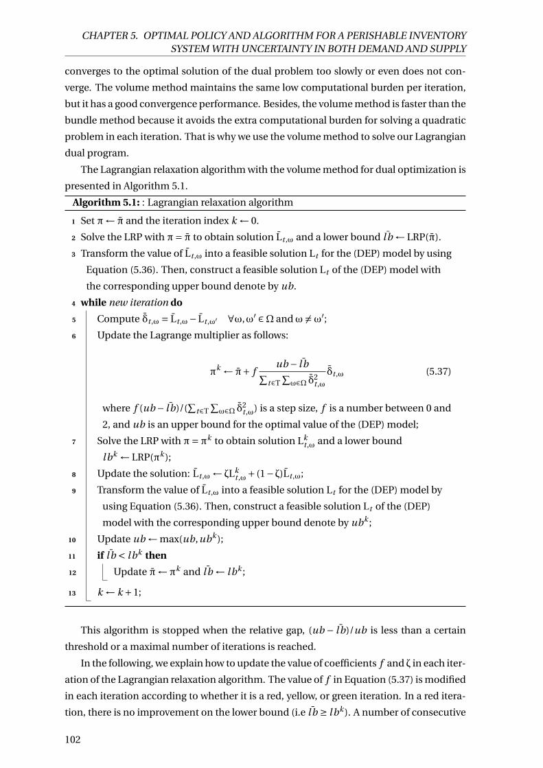
CHAPTER 5. OPTIMAL POLICY AND ALGORITHM FOR A PERISHABLE INVENTORYSYSTEM WITH UNCERTAINTY IN BOTH DEMAND AND SUPPLY
converges to the optimal solution of the dual problem too slowly or even does not con-
verge. The volume method maintains the same low computational burden per iteration,
but it has a good convergence performance. Besides, the volume method is faster than the
bundle method because it avoids the extra computational burden for solving a quadratic
problem in each iteration. That is why we use the volume method to solve our Lagrangian
dual program.
The Lagrangian relaxation algorithm with the volume method for dual optimization is
presented in Algorithm 5.1.
Algorithm 5.1: : Lagrangian relaxation algorithm
1 Set π← π and the iteration index k ← 0.
2 Solve the LRP with π= π to obtain solution Lt ,ω and a lower bound ¯l b ← LRP(π).
3 Transform the value of Lt ,ω into a feasible solution Lt for the (DEP) model by using
Equation (5.36). Then, construct a feasible solution Lt of the (DEP) model with
the corresponding upper bound denote by ub.
4 while new iteration do
5 Compute δt ,ω = Lt ,ω− Lt ,ω′ ∀ω,ω′ ∈Ω andω 6=ω′;6 Update the Lagrange multiplier as follows:
πk ← π+ fub − ¯l b∑
t∈T∑ω∈Ω δ2
t ,ω
δt ,ω (5.37)
where f (ub − ¯lb)/(∑
t∈T∑ω∈Ω δ2
t ,ω) is a step size, f is a number between 0 and
2, and ub is an upper bound for the optimal value of the (DEP) model;
7 Solve the LRP with π=πk to obtain solution Lkt ,ω and a lower bound
lbk ← LRP(πk );
8 Update the solution: Lt ,ω← ζLkt ,ω+ (1−ζ)Lt ,ω;
9 Transform the value of Lt ,ω into a feasible solution Lt for the (DEP) model by
using Equation (5.36). Then, construct a feasible solution Lt of the (DEP)
model with the corresponding upper bound denote by ubk ;
10 Update ub ← max(ub,ubk );
11 if ¯l b < l bk then
12 Update π←πk and ¯l b ← lbk ;
13 k ← k +1;
This algorithm is stopped when the relative gap, (ub − ¯lb)/ub is less than a certain
threshold or a maximal number of iterations is reached.
In the following, we explain how to update the value of coefficients f and ζ in each iter-
ation of the Lagrangian relaxation algorithm. The value of f in Equation (5.37) is modified
in each iteration according to whether it is a red, yellow, or green iteration. In a red itera-
tion, there is no improvement on the lower bound (i.e ¯lb ≥ lbk ). A number of consecutive
102

CHAPTER 5. OPTIMAL POLICY AND ALGORITHM FOR A PERISHABLE INVENTORYSYSTEM WITH UNCERTAINTY IN BOTH DEMAND AND SUPPLY
red iterations suggests the need for a smaller step-size, i.e the value of f should be reduced
(multiplied by a positive number less than 1). Otherwise, d = ∑ω∈Ω
∑t∈T δt ,ωδ
kt ,ω is com-
puted. The value d ≤ 0 means that a longer step in the direction of δ= (δt ,ω) ∀t ∈ T,ω ∈Ωwould give a smaller value for LRP(πk ). A yellow iteration is defined as an iteration with
no improvement on lower bound and the value d ≤ 0. If d ≥ 0, we have a green iteration
which suggests the requirement of a larger step-size, i.e., the value of f should be multi-
plied by a positive number greater than 1). In our numerical study, the value f is updated
as follows.
f k =
1.1 f if k-th iteration is green iteration
0.66 f after 5 consecutive red iterations
f k−1 Otherwise
According to Barahona and Anbil [2000], ζ is set in each iteration as the value that
minimizes√∑
ω∈Ω∑
t∈T[ζδkt ,ω+ (1−ζ)δt ,ω]2 where ζ ∈ [ζmi n ,ζmax]. Therefore, the value of
ζ is given by:
ζ=
ζmi n if ζopt ≤ ζmi n
ζopt if ζopt ∈ [ζmi n ,ζmax]
ζmax if ζopt ≥ ζmax
where ζopt =∑
t∈T∑ω∈Ω δt ,ω(δt ,ω−δk
t ,ω)∑t∈T
∑ω∈Ω(δt ,ω−δk
t ,ω)2
5.5 Numerical study
In this section, a numerical study is conducted to evaluate the performance and demon-
strate the effectiveness of our Lagrangian relaxation algorithm. This approach is imple-
mented in Python 3.5 on a HP computer with Intel Core i5-4210M CPU 2.66 GHz and 8.0
GB RAM. All MILP problems were solved by a solver GUROBI 6.5 with default parameters.
According to the Benchmarks of Optimization Software of Mittelmann [2018], GUROBI
performs better than CPLEX on the MIPLIB2010 benchmark set. That is why we chose
GUROBI as MILP solver in our numerical study.
5.5.1 Parameters setting
In the numerical study, we use the data from Broekmeulen and Van Donselaar [2009];
Pauls-Worm et al. [2015] for average demand, coefficient of variation (CV =σ/µ), number
of time periods. The holding cost h is set to 5. The unit purchase cost c is varied from 30
to 40. The unit backorder cost p is determined from the ratio p/(p +h), which is varied
between 95% and 97.5%. The number of periods and scenarios are T = 7 and |Ω| = 200. By
applying a statistical method in Shapiro [2000], we observed that the stochastic program-
103

CHAPTER 5. OPTIMAL POLICY AND ALGORITHM FOR A PERISHABLE INVENTORYSYSTEM WITH UNCERTAINTY IN BOTH DEMAND AND SUPPLY
ming model requires 200 scenarios for an instance with 7 periods to achieve an approxi-
matively optimal solution with probability 95% within 1% deviation from the true optimal
solution.
According to Rentizelas et al. [2009], the degradation of biomass is estimated about
1% on average under the ambient storage condition. Therefore, we vary the deterioration
rate (1−λ) from 1% to 3% (extreme case). All parameter values are given in Table 5.1. We
also consider three cases of demand and supply distribution as follows:
(i) The mean demand in each period is computed by µDt = ft .µD where the demand
pattern in each period is ft = 0.12,0.13,0.13,0.16,0.18,0.18,0.10, and the value of
mean demand over 7 periods µD is taken as [12,13,13,16,18,18,10]. The stochastic
supply follows a stationary normal distribution with µSt = 16 and σSt = 0.2µSt for
all t = 1...7.
(ii) Demand and supply follow a stationary normal distribution with µDt = 13, σDt =3.5, µSt = 15 and σSt = 0.2µSt for all t = 1...7.
(iii) Demand and supply follow a stationary normal distribution with µDt = 14, σDt =0.25µDt , µSt = 15 and σSt = 0.2µSt for all t = 1...7.
The parameters setting of the LR algorithm is given as follows. We fix the optimal-
ity gap as ε ≤ 0.01%, maximal number of iterations as i ter ati onmax = 500 and maximal
CPU time as t i memax = 3600s. The algorithm also stops if the upper bound cannot be
improved after 50 consecutive iterations. In each green iteration, the coefficient f is mul-
tiplied by 1.1. After a sequence of 5 consecutive red iterations, f will be multiplied by 0.66.
We set ζmi n = 0.3 and ζmax = 0.8.
Table 5.1: Parameter values for the numerical study
Input parameters RangeCoefficient of variation CVD =σD/µD [0.20 , 0.25]Coefficient of variation CVS =σS/µS 0.20Backorder cost ratio p/(p +h) [0.95, 0.975]Holding cost h [5]Purchase cost, c [30, 40]Deterioration rate, (1−λ) [1%, 3%]Discount factor, α [0.96, 0.98]
5.5.2 Performance evaluation of the solution algorithm
To compare the performance of our solution approach, we also ran a dynamic pro-
gramming (DP) algorithm ([Bellmam, 1957, Chapter III.3]) to find the optimal order-up-
to level policy for the multi-period perishable inventory model. One issue that may affect
the accuracy of the results of the DP algorithm needs to be addressed. In each period, the
104

CHAPTER 5. OPTIMAL POLICY AND ALGORITHM FOR A PERISHABLE INVENTORYSYSTEM WITH UNCERTAINTY IN BOTH DEMAND AND SUPPLY
Table 5.2: Performance of the LR algorithm in case a
LR method DP methodc p h α λ CPU(s) E-LR CPU(s) DP Gap
40 100 5 0.96 0.97 166.31 3792.24 5463.00 3787.15 0.13%40 100 5 0.98 0.97 201.50 4023.11 5228.27 4012.88 0.25%40 100 5 0.96 0.99 199.17 3734.97 5301.20 3729.39 0.15%40 100 5 0.98 0.99 215.42 3958.55 5149.86 3948.82 0.25%40 200 5 0.96 0.97 195.36 4065.29 5155.27 3990.89 1.86%40 200 5 0.98 0.97 234.94 4273.45 5182.28 4220.89 1.25%40 200 5 0.96 0.99 388.29 3939.26 5146.70 3910.90 0.73%40 200 5 0.98 0.99 217.81 4177.95 5157.06 4133.24 1.08%50 100 5 0.96 0.97 197.71 4624.92 5159.33 4592.93 0.70%50 100 5 0.98 0.97 203.13 4879.23 5136.91 4868.01 0.23%50 100 5 0.96 0.99 201.45 4544.56 5139.81 4525.84 0.41%50 100 5 0.98 0.99 207.78 4809.46 5139.49 4792.93 0.34%50 200 5 0.96 0.97 181.45 4955.46 5134.46 4821.47 2.78%50 200 5 0.98 0.97 225.10 5146.83 5130.03 5098.38 0.95%50 200 5 0.96 0.99 211.12 4748.26 5130.63 4728.81 0.41%50 200 5 0.98 0.99 208.01 5034.91 5138.43 4996.62 0.77%
Average 215.91 5180.80 0.77%
expected total cost E(Dt ,yt )
V∗t+1,n(st+1) is calculated using a numerical integration method.
However, the numerical integration may introduce some error in the cost. To make the
integration accurate enough, its step size should be taken as small as possible, i.e., the in-
terval of integration must be small enough. In our implementation of the algorithm, the
problem is solved at different levels of discretization,i.e., using different step sizes from
large to small for the numerical integration, until no significant change in the cost can be
observed.
To evaluate the quality of the solutions obtained by the LR algorithm, we compute
the E-LR which is the expected objective value of the stochastic inventory model at the
solution obtained by our Lagrangian relaxation approach. Note that for each instance,
the (DEP) model includes 3 807 continuous, 1400 binary variables, and 7 007 constraints.
Table 5.2, 5.3 and 5.4 give the computational time and the expected objective value
of the solution obtained by LR and DP algorithm, respectively. The last column shows
the relative gap between the two solution approaches (E-LR and DP). As we can see, the
LR algorithm has a much shorter CPU time than DP algorithm on average (215.91s vs
5180.80s in case a, 187.83s vs 5476.63s in case b and 172.59s vs 5399.91s in case c). In
terms of expected cost, the average gap of the LR solution from the DP solution is only
0.77% , 0.70% and 0.50% in three cases, respectively. The numerical study demonstrates
that the LR approach can be obtain a high-quality near-optimal solution in a reasonable
time and thus more practical than the DP approach.
105

CHAPTER 5. OPTIMAL POLICY AND ALGORITHM FOR A PERISHABLE INVENTORYSYSTEM WITH UNCERTAINTY IN BOTH DEMAND AND SUPPLY
Table 5.3: Performance of the LR algorithm in case b
LR method DP methodc p h α λ CPU(s) E-LR CPU(s) DP Gap
40 100 5 0.96 0.97 162.27 3331.37 5463.00 3316.79 0.44%40 100 5 0.98 0.97 181.42 3527.55 5472.82 3517.36 0.29%40 100 5 0.96 0.99 186.09 3297.49 5480.86 3277.14 0.62%40 100 5 0.98 0.99 191.07 3485.77 5474.70 3473.88 0.34%40 200 5 0.96 0.97 177.89 3525.09 5476.79 3477.96 1.35%40 200 5 0.98 0.97 189.15 3745.13 5470.18 3683.81 1.66%40 200 5 0.96 0.99 189.78 3437.06 5476.65 3426.16 0.32%40 200 5 0.98 0.99 201.63 3667.29 5481.99 3627.36 1.10%50 100 5 0.96 0.97 178.00 4057.46 5489.69 4037.91 0.48%50 100 5 0.98 0.97 185.39 4294.05 5477.86 4282.11 0.28%50 100 5 0.96 0.99 191.71 4022.92 5472.96 3990.68 0.81%50 100 5 0.98 0.99 203.08 4249.43 5486.43 4230.02 0.46%50 200 5 0.96 0.97 179.80 4244.37 5478.14 4223.15 0.50%50 200 5 0.98 0.97 189.87 4526.88 5473.96 4472.82 1.21%50 200 5 0.96 0.99 190.09 4178.69 5477.39 4161.80 0.41%50 200 5 0.98 0.99 207.98 4443.27 5472.69 4405.73 0.85%
Average 187.83 5476.63 0.70%
Table 5.4: Performance of the LR algorithm in case c
LR method DP methodc p h α λ CPU(s) E-LR CPU(s) DP Gap
40 100 5 0.96 0.97 144.86 3666.22 5413.41 3651.44 0.40%40 100 5 0.98 0.97 159.23 3878.07 5400.99 3871.24 0.18%40 100 5 0.96 0.99 166.72 3613.40 5397.55 3604.50 0.25%40 100 5 0.98 0.99 178.00 3822.41 5401.94 3819.79 0.07%40 200 5 0.96 0.97 159.76 3933.00 5394.93 3898.08 0.90%40 200 5 0.98 0.97 177.87 4164.19 5397.44 4133.60 0.74%40 200 5 0.96 0.99 176.09 3843.55 5402.22 3831.49 0.31%40 200 5 0.98 0.99 182.61 4090.81 5398.43 4060.84 0.74%50 100 5 0.96 0.97 165.11 4442.42 5402.30 4432.73 0.22%50 100 5 0.98 0.97 173.30 4709.94 5397.96 4698.94 0.23%50 100 5 0.96 0.99 180.34 4391.54 5400.17 4377.90 0.31%50 100 5 0.98 0.99 188.62 4659.73 5393.06 4638.59 0.46%50 200 5 0.96 0.97 163.72 4719.05 5390.70 4701.33 0.38%50 200 5 0.98 0.97 177.95 5089.67 5399.97 4983.42 2.13%50 200 5 0.96 0.99 182.22 4635.81 5403.49 4625.36 0.23%50 200 5 0.98 0.99 185.02 4924.90 5403.99 4900.30 0.50%
Average 172.59 5399.91 0.50%
106

CHAPTER 5. OPTIMAL POLICY AND ALGORITHM FOR A PERISHABLE INVENTORYSYSTEM WITH UNCERTAINTY IN BOTH DEMAND AND SUPPLY
5.6 Conclusion
In this chapter, we proposed a stochastic inventory model for a perishable product un-
der stochastic environments and developed an algorithm that combines scenario-based
optimization and Lagrangian relaxation to solve approximatively the model. A compu-
tational study was conducted with data from the literature to evaluate the near-optimal
solution obtained by the algorithm by comparing it to the optimal solution found by dy-
namic programming. Our results indicated that the LR solution is usually very close to the
optimal solution. The relevance of our solution approach is thus proved. Our proposed
solution approach can assist managers to make ordering decisions under fluctuation in
demand and supply.
107
CHAPTER 5. OPTIMAL POLICY AND ALGORITHM FOR A PERISHABLE INVENTORYSYSTEM WITH UNCERTAINTY IN BOTH DEMAND AND SUPPLY
108

Chapter 6
Modeling and optimization for an
inventory problem of a fixed lifetime
product under uncertainties
“ “Il n’est pas certain que tout soit
incertain. ”
— Blaise Pascal, Pascal’s Pensees
Contents
5.1 Introduction . . . . . . . . . . . . . . . . . . . . . . . . . . . . . . . . . . . . 91
5.2 Problem description and model formulation . . . . . . . . . . . . . . . . 92
5.2.1 Problem description . . . . . . . . . . . . . . . . . . . . . . . . . . . . 92
5.2.2 Dynamic programming model . . . . . . . . . . . . . . . . . . . . . . 94
5.3 Properties of the model . . . . . . . . . . . . . . . . . . . . . . . . . . . . . 94
5.3.1 Single period total cost . . . . . . . . . . . . . . . . . . . . . . . . . . . 94
5.3.2 Multi-period expected cost . . . . . . . . . . . . . . . . . . . . . . . . 95
5.4 Solution approach . . . . . . . . . . . . . . . . . . . . . . . . . . . . . . . . 99
5.4.1 Deterministic equivalent model . . . . . . . . . . . . . . . . . . . . . 99
5.4.2 Lagrangian relaxation approach . . . . . . . . . . . . . . . . . . . . . 100
5.5 Numerical study . . . . . . . . . . . . . . . . . . . . . . . . . . . . . . . . . . 103
5.5.1 Parameters setting . . . . . . . . . . . . . . . . . . . . . . . . . . . . . 103
5.5.2 Performance evaluation of the solution algorithm . . . . . . . . . . . 104
5.6 Conclusion . . . . . . . . . . . . . . . . . . . . . . . . . . . . . . . . . . . . . 107
109

CHAPTER 6. MODELING AND OPTIMIZATION FOR AN INVENTORY PROBLEM OF AFIXED LIFETIME PRODUCT UNDER UNCERTAINTIES
6.1 Introduction
In the previous chapter, we have studied an inventory problem for a product with
constant deterioration rate under uncertainty in both supply and demand. As highlighted
in Chapter 2, some perishable products continuously deteriorate whereas the others have
fixed lifetime. To the best of our knowledge, very few works study the inventory control
problem for a product with a fixed lifetime under uncertainty in both supply and demand.
Therefore, the mentioned problem should be taken into account.
In this chapter, we extend a previous model to a perishable product with a fixed life-
time under both stochastic demand and stochastic supply. Based on the product’s re-
maining lifetime and some useful historical information related to demand and supply,
we develop a practical approach to help retail managers generating an effective inventory
replenishment plan. The essential characteristics of the inventory model are perishabil-
ity, stochastic demand, stochastic supply, and multi-period. The main contributions of
this chapter include:
Firstly, we propose a stochastic programming model for a perishable inventory sys-
tem with fixed life shelf under both stochastic demand and stochastic supply in a rolling
horizon framework.
Secondly, we formulate a mixed integer linear programming (MILP) model equivalent
to the original problem using the Conditional Scenarios (CS) approach.
Thirdly, we conduct a numerical study to evaluate the performance of the proposed
algorithm. The results show that these approaches can find a high-quality solutions with
statistical performance guaranteed in a reasonable computation time. Sensitivity analysis
is conducted to examine the effect of some critical parameters on the total system cost.
This remainder of this chapter is organized as follows: in Section 6.2, the problem and
its model are introduced. Then, we introduce the solution approaches and solution eval-
uation in Sections 6.3 and 6.4. A numerical study is performed, and its results are analyzed
in Section 6.5. Section 6.6 concludes this chapter with a brief resume and perspectives.
6.2 Problem description and model formulation
6.2.1 Problem description
In this chapter, we consider a multi-period inventory problem for a perishable prod-
uct with fixed shelf life. For simplicity, we assume that company uses the first in first out
(FIFO) withdraw policy. In this paper, the order of events occurred in each period is given
as follows:
(i) Fresh items arrive at the beginning of each period. Then, the inventory level of each
age is updated. The expired items are discarded.
110

CHAPTER 6. MODELING AND OPTIMIZATION FOR AN INVENTORY PROBLEM OF AFIXED LIFETIME PRODUCT UNDER UNCERTAINTIES
(ii) Based on the inventory policy used, an order then placed if necessary. After that, the
demand and supply in this period are observed, and customer demand is satisfied
as much as possible, and unsatisfied demand is lost (lost sale).
(iii) At the end of each period, holding costs or shortage costs are charged based on the
remaining inventory which will be carried over from the current period to the next.
The out-dating costs are also charged for expired items.
6.2.2 Model formulation
In the following, we formulate a stochastic programming model for the inventory op-
timization problem of perishable product considered. The product is perishable, and its
age is denoted by i ∈ 1, ...,M. Let Iit denote the inventory level of the product which has
age i at the end of period t ∈ 1, ...,T. It is convenient to denote I1t as fresh items of the
product in stock at the end of period t ∈ 1, ...,T. In the first stage, the decision variable
includes the timing of ordering yt and the ordering quantity Ot in each period t ∈ 1, ...,T.
The second-stage variables include the supply quantity received qt , inventory level Iit ,ω for
each age i , lost sales Bt and outdated items IMt at the end of period t . In the second stage,
the recourse actions are made to correct the negative effects due to the first stage decision
(the timing of ordering). In the model, all continuous decision variables are non-negative.
It is assumed that demand Dt and supply St in each period t are multi-normally dis-
tributed random variables with known distribution N(µ,Σ) where µ is a vector of mean
of Dt ,St and Σ is a covariance matrix which gives the correlation between the supply St
and the demand Dt .
For convenience, all notations used in the model formulation are summarized as fol-
lows.
Indices:
• i : Age index, i ∈ 1, ...,M with M being the fixed shelf life
• t : Period index t ∈ 1, ...,T with T being the time horizon
Deterministic Parameters
• a: Ordering cost for each order placed
• v : Purchasing cost for each unit of product
• h: Holding cost for each unit of product and each period in stock
• p: Shortage cost charged for each unit of unmet demand at the end of period t
• w : Waste/out-dating cost for each unit of products expired
• Ii0 : Initial inventory, for all age i = 1...M
111

CHAPTER 6. MODELING AND OPTIMIZATION FOR AN INVENTORY PROBLEM OF AFIXED LIFETIME PRODUCT UNDER UNCERTAINTIES
Stochastic Parameters
• Dt : Random demand in period t
• St : Random supply capacity in period t
Decision variables:
• Iit : Inventory level of age i ∈ 1, ...,M at the end of period t . Note that I1
t refers to
fresh items in stock and IMt refers to wasted/outdated items at the end of period t .
• qt : Supply quantity received in period t
• yt : Timing of ordering in period t (binary variable), yt = 1 if an order is placed in
period t and yt = 0 otherwise.
• Ot : Order quantity in period t
• Bt : Unsatisfied demand (lost sales) in period t
The stochastic programming model for an inventory of perishable product is given as
follows:
(SP) minT∑
t=1EDt ,St
[ayt +uqt +h(
M−1∑i=1
Iit )+pBt +wIM
t
](6.1)
s.t
yt =1, i f Ot > 0
0, other wi set = 1, ...T (6.2)
Yit = (Dt −
M−1∑j=i
I jt−1)+ i = 1...M, t = 1, ...T (6.3)
Iit = (Ii−1
t−1 −Yit )+, t = 1, ...T, i = 2...M (6.4)
I1t = (qt −Y1
t )+, t = 1, ...T (6.5)
Bt =M−1∑i=1
Iit−1 −
M∑i=1
Iit +qt −Dt , t = 1, ...T (6.6)
qt = mi nSt ,Ot , t = 1, ...T (6.7)
Iit ≥ 0, i = 1...M, t = 1, ...T (6.8)
qt ,Bt ≥ 0, t = 1, ...T (6.9)
yt ∈ 0,1, t = 1, ...T (6.10)
where: x+ = max0, x
The objective (6.1) is to minimize the total expected cost which includes five types
of costs: ordering, purchasing, inventory holding, lost sales and out-dating cost over the
planning horizon of T periods.
112

CHAPTER 6. MODELING AND OPTIMIZATION FOR AN INVENTORY PROBLEM OF AFIXED LIFETIME PRODUCT UNDER UNCERTAINTIES
In Equation (6.2), the binary variable yt = 1 only if there is an order quantity Ot in pe-
riod t . Equation (6.3) shows the variable Yit , as the remaining demand after withdrawing
all products having ages from i to M using FIFO withdraw policy. Note that the deci-
sion variables Yit , are redundant, but they are introduced for the readability of the model.
Equation (6.4) and (6.5) give the transition of inventory from the actual period to the next.
In Equations (6.3) and (6.4), we implicitly assume that for the first period, t = 1, the vari-
ables Iit−1 are replaced by the predetermined parameters Ii
0 (initial inventory). Equation
(6.6) shows the inventory balance constraints between period t and t +1. This equation
also determines that lost sale, Bt , which only occurs when the supply quantity received,
qt , and the inventory of all age i cannot meet demand, Dt . Equation (6.7) ensures that the
quantity received is always limited by the supply St .
6.3 Solution approach
The stochastic programming model is quite complicated, and it requires an enormous
memory and computational effort to find the optimal solution. For this reason, we try to
provide a high-quality solution quickly instead of finding the optimal solution because
solving. By applying a scenario-based stochastic framework Birge and Louveaux [2011],
we can transform a stochastic programming model into a mixed integer linear program-
ming (MILP) model by replacing the stochastic parameters by the values taken in the cor-
responding scenario. However, the number of scenarios should be considered significant
enough to approximate the stochastic model well. So, it could lead to a MILP model hav-
ing enormous size whose resolution requires a lot of memory and is very time-consuming.
The Sample Average Approximation (SAA) method is a conventional approach for stochas-
tic optimization such as the research of Kim et al. [2015]; Kleywegt et al. [2002]; Pagnon-
celli et al. [2009]. This method allows to reduce the number of scenarios considered and
find the near-optimal solution. Based on conditional expectation discretization, Beltran-
Royo [2017] proves that Conditional Scenarios (CS) method might provide a better solu-
tion than SAA method. That is why we develop a scenario-based optimization approach
for solving our model based on Conditional Scenarios (CS) approach.
In this section, the original model (SP) is transformed into an equivalent MILP model
by applying the scenario approach. This solution approach is outlined in Figure 6.1. The
Conditional Scenarios method allows to generate a set of scenarios from given continuous
random vector by applying a conditional expectation discretization. The CS approach will
be compared with the Sample Average Approximation (SAA) method in the next section.
6.3.1 Scenario-based approach and deterministic equivalent model
Based on the scenario-based stochastic programming approach, we reformulate the
model (SP) into a mixed integer linear programming (MILP) model. This approach allows
113

CHAPTER 6. MODELING AND OPTIMIZATION FOR AN INVENTORY PROBLEM OF AFIXED LIFETIME PRODUCT UNDER UNCERTAINTIES
Figure 6.1: Solution approach
to capture the uncertainty in an approximate way with the precision depending on the
number of scenarios considered.
Let ω ∈Ω be the index of a scenario (a possible realization of random variables) and
its probability of occurrence is pω. Note that the index pair for conditional scenario r,e
and its corresponding probability are replaced by scenario ω and pω in this section. The
mathematic expectation E(.) in the objective function (6.1) can be replaced by∑ωpω[.].
Then, the nonlinear objective function (6.1 is transformed into the deterministic objective
function (6.11). The deterministic equivalent MILP model is given as follows:
minT∑
t=1ayt +
∑ω∈Ω
T∑t=1
pω[
uqt ,ω+h(M−1∑i=1
Iit ,ω)+pBt ,ω+wIM
t ,ω
](6.11)
s.t . Constraints (6.12)− (6.21)
The index ω is added to each two-stage decision variables related to the scenario ω
except for the ordering quantity Ot . The notation of the first-stage decision variables yt
remains as before. The ordering quantity Ot does not appear explicitly in the objective
function but implicitly through the realization of random variables such demand Dt ,ω
and supply St ,ω.
In the following subsections, we linearize the nonlinear constraints (6.2)-(6.6) of the
original problem (SP). Note that H is a big number.
Ordering constraints
Constraint (6.2) can be linearized as follows:
0 ≤ Ot ≤ Hyt t = 1, ...T (6.12)
Constraints on Yit ,ω
Equation (6.3) can be linearized as follows:
Dt ,ω−M−1∑j=i
I jt−1,ω ≤ Yi
t ,ω ≤ (Dt ,ω−M−1∑j=i
I jt−1,ω)+ (1−αi
t ,ω)H (6.13)
0 ≤ Yit ,ω ≤ αi
t ,ωH (6.14)
αit ,ω ∈ 0,1 (6.15)
114

CHAPTER 6. MODELING AND OPTIMIZATION FOR AN INVENTORY PROBLEM OF AFIXED LIFETIME PRODUCT UNDER UNCERTAINTIES
That can be explained as follows:
• Ifαit ,ω = 1, we have Yi
t ,ω = (Dt ,ω−∑M−1j=i I j
t−1,ω) ≥ 0 due to constraints (6.13) and (6.14).
• If αit ,ω = 0, we have Yi
t ,ω = 0 and (Dt ,ω−∑M−1j=i I j
t−1,ω) ≤ 0 due to constraints (6.13) and
(6.14).
The two cases of αit ,ω imply that the constraint (3) can be replaced by the constraints (6.13
- 6.15) in the deterministic equivalent model.
FIFO constraints
Now, the constraints (6.4) and (6.5) can be linearized as follows:
Iit ,ω ≥ (Ii−1
t−1,ω−Yit ,ω) ∀t = 1, ...T, i = 2...M (6.16)
I1t ,ω ≥ (qt ,ω−Y1
t ,ω) ∀t = 1, ...T (6.17)
Since the coefficients related to Iit ,ωi = 1, ...M in the objective function (6.1) to mini-
mize are positive.
Unsatisfied demand
Constraint (6.6) ensure the inventory balance between period t and t + 1. Lost sale,
Bt ,ω, occurs when the demand Dt ,ω can not be satisfied in period t under scenarioω. The
constraints are given by:
Bt ,ω =M−1∑i=1
Iit−1,ω−
M∑i=1
Iit ,ω+qt ,ω−Dt ,ω, t = 1, ...T (6.18)
Random supply capacity
Constraint (6.7) specifies that the quantity received qt ,ω is the minimum between or-
der quantity Ot and a realization of supply capacity St ,ω in period t under scenario ω.
That constraint can be linearized as follows:
St ,ω− (1−γt ,ω)H ≤ qt ,ω ≤ St ,ω (6.19)
Ot −γt ,ωH ≤ qt ,ω ≤ Ot (6.20)
γt ,ω ∈ 0,1 (6.21)
H: a big number
That can be explained as follows:
• If γt ,ω = 1, we have qt ,ω = St ,ω because St ,ω is not only an upper bound but also a
lower bound of qt ,ω due to Constraint(6.19). We then have qt ,ω = St ,ω ≤ Ot due to
Constraint (6.20). Then qt ,ω = mi nSt ,ω,Ot .
115
CHAPTER 6. MODELING AND OPTIMIZATION FOR AN INVENTORY PROBLEM OF AFIXED LIFETIME PRODUCT UNDER UNCERTAINTIES
• If γt ,ω = 0. we have qt ,ω = Ot due to Constraint (6.20) and qt ,ω = Ot ≤ St ,ω due to
Constraint (6.19). So, qt ,ω = mi nSt ,ω,Ot
Then in both cases, we have qt ,ω = minSt ,ω,Ot .
6.3.2 Conditional scenarios approach
Since the computational complexity for solving the stochastic programming problem
increases with the number of scenarios, some techniques to reduce the number of repre-
sentative scenarios that should be considered: moment matching methods, the Sample
Average Approximation (SAA) method, approaches based on probability metrics among
others. According to Beltran-Royo [2017], the Conditional Scenarios (CS) problem allows
to deal with uncertainty in shorter computational time, and it could yield a better solu-
tion. Also, the CS approach can be seen as an aggregation method, in which, aggregation
weights are given by conditional probability function of the random parameters. It is also
possible to compute conditional scenarios directly from a given continuous random vec-
tor by applying a conditional expectation discretization. The notation for the conditional
scenarios method is given as follows:
Indices:
• E: number of discrete realizations of random variable considered
• e: index of realization of random variables, e = 1...E
• r : Component index of random vectors, r = 1...R
• r,e: Index pair for conditional scenarios
Random vectors:
• ξ: random vectors including R components (ξ1, ...ξR)T
• ξr : r th component of random vector ξ
• ξr,e : realization of random variable ξr with e = 1, ...E
• pr,e : the corresponding probability of the realization ξr,e
• ξr,e : Conditional scenario or realization given at the end of the CS procedure.
• pr,e : the corresponding probability of realization ξr,e
We summarize the conditional scenarios method Beltran-Royo [2017] in the following
procedure:
116

CHAPTER 6. MODELING AND OPTIMIZATION FOR AN INVENTORY PROBLEM OF AFIXED LIFETIME PRODUCT UNDER UNCERTAINTIES
1. Given a vector of random variables ξ = (ξ1, ...ξR)T with the index r = 1...R and ξ ∼NR(µ,Σ). For each random variable ξr defined in a given interval Lr , we discretize
it and obtain finite realizations ξr,e , e = 1, ...Er with the corresponding probabilities
pr,e . Er is the number of discrete realizations in the given interval Lr = [ar ,br ]. For
example, Lr = [µr −4σr ,µr +4σr ].
(i) Divide the interval Lr into Er sub-intervals of equal length Lr,e = [ar,e ,br,e ]
(ii) For each Lr,e , compute the discrete realizations, ξr,e and their corresponding
probabilities, pr,e as follows:
ξr,e = E[ξr | ξr ∈ Lr,e ] =µr +σrpd f (αr,e )−pd f (βr,e )
cd f (αr,e )− cd f (βr,e )
pr,e =P(ξr ∈ Lr,e ) = cd f (αr,e )− cd f (βr,e )
where αr,e = (ar,e −µr )/σr and βr,e = (br,e −µr )/σr . pd f and cd f are the prob-
ability density function and the cumulative distribution function, respectively,
of a standard normal variable. µr and σr are the mean and the standard devi-
ation of the random variable ξr
2. We compute the conditional scenarios ξr,e and the corresponding probabilities pr,e
by using the discrete realizations, ξr,e found in step 1 as follows:
ξr,e = E[ξ | ξr,e ] =µ+ ξr,e −µr
σ2r
Σr
pr,e = pr,e
The total number of conditional scenarios is:∑R
r=1 Er where Er is the number dis-
crete realizations of ξr into ξr .
The above procedure can be summarized by the following procedure: ξ → ξr,e →ξr,e . With this method, we can formulate the MILP problem with its conditional expec-
tation scenarios.
6.4 Solution evaluation
To evaluate the solution quality, we compare our approach with the most common
approach, Sample Average Approximation (SAA) method. In this technique, the expected
objective function of the stochastic problem is approximated by an average sample esti-
mate derived from a random sample. The main differences between SAA and CS approach
are the ways to approximate the random vector ξ and their associated probabilities (equal
probability versus conditional probability). Besides, only one sampling is made in CS ap-
117

CHAPTER 6. MODELING AND OPTIMIZATION FOR AN INVENTORY PROBLEM OF AFIXED LIFETIME PRODUCT UNDER UNCERTAINTIES
proach, but a large number of samplings is necessary to ensure the quality of solution in
SAA approach.
Some reduction techniques such as Latin hypercube sampling [Diwekar and David,
2015; McKay et al., 1979] has been proposed to increase the efficiency of the SAA method.
According to Diwekar and David [2015], Latin Hypercube Sampling can estimate more
precisely the distribution function and improve computational efficiency.
6.4.1 Sample Average Approximation
The sample average approximation (SAA) method Kleywegt et al. [2002] is an approach
for solving stochastic optimization problems by using Monte Carlo simulation. In this
technique, the expected objective function of the stochastic problem is approximated by
an average sample estimate derived from a random sample. In the SAA algorithm, a sam-
ple set ξ1,ξ2, ....ξR of R scenarios is randomly generated from Ω total scenarios. In other
words, this sample set is a subset of Ω whole scenarios. Each scenario occurs with equal
probability pξ = 1/R. The expected value of the objective function E(.)) is approximated
by a set of scenarios considered. Then, the general two-stage stochastic programming
model can be rewritten as follows:
Mi n
cx + 1
R
R∑r=1
Q(x,ξr )
(6.22)
s.t
Ax = b, x ≥ 0 (6.23)
Tr x +Wr yr = hr (6.24)
yr ≥ 0, r = 1...R
Where the vector x is the first-stage decision variables and yr is the second-stage de-
cision variables for each scenario r . The objective is to minimize the cost of the first stage
(cTx) and the expected cost over all scenarios in the second stage 1R
∑Rr=1 Q(x,ξr ). Ts is the
matrix related to the first stage decision variables x. Wr is a recourse matrix, qr and hr are
two vectors associated with scenario r in the model of the second stage.
The SAA method then generates A independent sample tests, each containing R sce-
narios, solving the associated problems, and obtain objective values z1R; z2
R; ...; zAR and can-
didate solutions x1; x2; ...; xA are obtained. The average of the A optimal values of the
problems is given by:
zR = 1
R
A∑a=1
zaR (6.25)
It is well known that E(zR) ≤ z∗, where z∗ is the optimal objective value of the original
problem. Thus, we can obtain a lower bound, z∗ by estimating E(zR) according to the
118

CHAPTER 6. MODELING AND OPTIMIZATION FOR AN INVENTORY PROBLEM OF AFIXED LIFETIME PRODUCT UNDER UNCERTAINTIES
formulation in (6.25). This estimation (6.25) is an unbiased of E(zR) and therefore is a
statistical lower bound to z∗.
For any feasible solution x ∈ X, the upper bound of z can be obtained by using total
scenarios Ω:
zΩ(x) = cx + 1
Ω
Ω∑a=1
Q(x,ξa) (6.26)
Note that the above procedure produces up to A different candidate solutions. It is
natural to take x∗ as one of the optimal solutions x1; x2; ...; xA of the A problems which has
the smallest estimated objective value, that is,
x∗ ∈ ar g mi n
zΩ(x) | x ∈ [x1; x2; ...; xA]
(6.27)
The above procedure is stopped when the relative gap, (| zΩ(x∗)− zR |/zR) or the vari-
ance of the expected solution Var(zΩ(x)) is less than a certain threshold or a maximal
number of iterations is reached.
6.4.2 Latin hypercube sampling
According to Diwekar and David [2015], Latin Hypercube Sampling (LHS) can esti-
mate more precisely the distribution function and improve computational efficiency. In
LHS method, the range of each uncertain parameter is subdivided into non-overlapping
intervals of equal probability. One value from each interval is selected randomly with the
probability distribution in the interval. Iman and Conover [1982]; Pebesma and Heuvelink
[1999]; Zhang and Pinder [2003] show that Latin hypercube sampling (LHS) combined
with Cholesky decomposition method allows to cover better the distributions of random
input variables and obtain the desired correlations between different input random vari-
ables via covariance matrix. For this reason, we applied this technique to generate the
whole scenarios in the SAA method.
6.5 Numerical study
In this section, numerical studies are conducted to evaluate the performance of the
proposed algorithm and demonstrate the effectiveness of our approach. All MILP prob-
lems related to CS and SAA approach were solved by Gurobi 6.5 [Gurobi Optimization,
2016] with default parameters on a HP computer with Intel Core i5-4210M CPU 2.66 GHz
and 8.0 GB RAM. According to the Benchmarks of Optimization Software [Mittelmann,
2018], GUROBI performs better than CPLEX on the MIPLIB2010 benchmark set. That is
why we chose GUROBI as MILP solver in our numerical study.
119

CHAPTER 6. MODELING AND OPTIMIZATION FOR AN INVENTORY PROBLEM OF AFIXED LIFETIME PRODUCT UNDER UNCERTAINTIES
Table 6.1: Parameter values for the simulation experiment
Input parameters LevelProduct lifetime M [2, 3]Mean week demand µD [200]Coefficient of variation CVD =σD/µD 0.25Coefficient of variation CVS =σS/µS 0.20Correlation between random variables [0.5]Out-dating cost ratio w/v [0.5, 1.0]Lost sales cost ratio p/(v +p +h) [0.90, 0.95, 0.99]Holding cost ratio h/v [0.002, 0,004]Ordering cost for each order placed, a [250v , 500v]
6.5.1 Data generation
In the numerical study, we use the data from Broekmeulen and Van Donselaar [2009];
Pauls-Worm et al. [2016] for the fixed maximum shelf life, average demand, coefficient
of variation (CV = σ/µ), length of time period. All parameter values are given in Table
6.1. Following Broekmeulen and Van Donselaar [2009], we normalize all cost parame-
ters on the purchasing cost v , which is set to 1. The unit holding cost ratio h/v is varied
from 0.02 to 0.04. The unit lost sales cost p is determined from the lost sales cost ra-
tio p/(v + p +h), which is varied between 90% and 99%. The unit out-dating cost ratio,
w/v is varied between 0 and 1. The fixed ordering cost for each order placed is varies
from 250v to 500v . The maximum shelf life is M= 2 or 3. The number of periods is T =7.
The mean demand for each day is computed by µDt = ft .µD where demand pattern is
ft = 0.12,0.13,0.13,0.16,0.18,0.18,0.10, and the value of mean demand in each periods
,µDt = [240,260,260,320,360,360,200]. Supply follows a stationary normal distribution
with µSt = 320 and σSt = 0.2µSt for all t = 1...7.
The main focus of our work is to study the performance of the proposed approaches
and the impacts of some key parameters of the studied model on its optimal cost. This
uncertainty is incorporated into the model by considering a set of possible scenarios. The
number of scenarios should be large enough to capture the entire range of the probability
distribution of supply and demand.
6.5.2 Performance evaluation of the solution algorithms
In this section, we present our computational experiments on the algorithms pro-
posed in the previous section for solving instances. To formulate the CS problem, we
apply Section 4.1 to calculate the conditional scenarios that approximate the normal ran-
dom vector which includes µ = µDt ,µSt and σ = σDt ,σSt . For T=7, we have R=14 ran-
dom parameters, E=12 discretization points and Lr = [µr −4σr ,µr +4σr ]. The choice of
E=12 can be explained as follows: we considered the (MILP) problem with different dis-
cretization level such as E= 5,6,7..100. We observe that the scenarios optimal solution has
very similar quality compared with others for the discretization with E ≥ 12.
120

CHAPTER 6. MODELING AND OPTIMIZATION FOR AN INVENTORY PROBLEM OF AFIXED LIFETIME PRODUCT UNDER UNCERTAINTIES
In fact, the SAA and CS approaches try to solve the original problem approximately
with an intention to reduce the computational burden. However, it is hard to assess the
quality of the optimal SAA and CS solutions by using the optimality gap because we can
not find the optimal solution of the original problem. In this case, we assess the E-SAA and
E-CS value which are the expected value of the objective function of the original problem
obtained at the SAA solution and CS solution, respectively. To calculate the E-SAA, E-CS,
we generated 1000 000 scenarios randomly sampled from a multivariate normal distribu-
tion of ξ= Dt ,St , t = 1...T to estimate approximately the value of E-SAA and E-CS.
Table 6.2 and 6.3 present the computational time and solution obtained by CS and SAA
approach. All instances include 4 368 continuous variables, 3 192 binary variables, and 16
471 constraints. The last column shows the relative gap between the two solutions found
by CS and SAA approach (E-CS and E-SAA). Based on the inferential statistical analysis,
the obtained solutions, E-SAA, could achieve an approximatively optimal solution with
probability 95% within 0.1% deviation from the true optimal solution. As we can see, we
can see that the CS approach performed efficiently for instances of different sizes because
the E-CS value is always less than the E-SAA value with 0.07% and 0.09% in average for
M=2 and 3 respectively. Besides, the CS approach has much shorter CPU times (35.37s
versus 284.91s and 35.41s versus 317.08s respectively). The numerical study suggests that
the CS approach has a good balance between the solution quality and the computational
time.
6.5.3 Analysis of the solution
Figure 6.2a shows the cost distribution of the base case for the perishable inventory
system over planning horizon T= 5. We consider a perishable product with the fixed shelf
life M=2. The ordering cost is $30. The unit holding cost, unit shortage cost, and unit
wastage cost are $2, $15, $3 respectively. In this study, we assume demand and supply are
normal variables. Their parameters over T periods are presented as follows:
The optimal value of the total expected cost of CS problem is $41 740,98. As we can see,
the purchase cost and shortage cost are the primary cost drivers that account for nearly
71% and 27% of the total system costs respectively. The holding cost is only 1%, so in this
case, the storage of a significant amount of product seems not critical. This result shows
how the most important of inventory policy on the total system cost because it affects the
purchased quantity and unmet demand strongly.
µD = [860,810,760,570,620]
µS = [520,550,860,940,760]
σ2D = [29584,26244,23104,12996,15376]
σ2S = [10816,12100,29584,35344,23104]
121

CHAPTER 6. MODELING AND OPTIMIZATION FOR AN INVENTORY PROBLEM OF AFIXED LIFETIME PRODUCT UNDER UNCERTAINTIES
Table 6.2: Performance of the solution algorithm in case of M = 2
CS approach SAA approachInstances M a h p w CPUs E-CS CPUs E-SAA %1 2 250 0.02 10 0.5 41.70 4 292.30 412.22 4 296.62 0.10%2 2 250 0.02 10 1.0 46.02 4 314.66 416.08 4 320.61 0.14%3 2 250 0.02 20 0.5 37.08 4 624.11 277.45 4 627.32 0.07%4 2 250 0.02 20 1.0 42.38 4 650.57 278.18 4 651.37 0.02%5 2 250 0.02 100 0.5 21.74 7 168.08 124.52 7 165.30 0.04%6 2 250 0.02 100 1.0 22.70 7 187.49 124.44 7 189.40 0.03%7 2 250 0.04 10 0.5 50.63 4 310.32 402.67 4 316.87 0.15%8 2 250 0.04 10 1.0 50.46 4 335.91 404.42 4 340.85 0.11%9 2 250 0.04 20 0.5 44.42 4 643.95 284.44 4 648.22 0.09%10 2 250 0.04 20 1.0 37.32 4 672.40 284.28 4 672.30 0.00%11 2 250 0.04 100 0.5 20.13 7 190.01 131.28 7 187.21 0.04%12 2 250 0.04 100 1.0 21.31 7 208.03 137.75 7 211.31 0.05%13 2 500 0.02 10 0.5 40.72 6 045.13 493.51 6 046.23 0.02%14 2 500 0.02 10 1.0 45.74 6 065.13 471.14 6 070.21 0.08%15 2 500 0.02 20 0.5 35.96 6 376.24 281.32 6 376.38 0.00%16 2 500 0.02 20 1.0 40.82 6 398.31 281.08 6 400.45 0.03%17 2 500 0.02 100 0.5 23.83 8 917.29 125.89 8 917.31 0.00%18 2 500 0.02 100 1.0 18.01 8 959.10 126.31 8 941.42 0.20%19 2 500 0.04 10 0.5 44.07 6 061.58 472.26 6 066.87 0.09%20 2 500 0.04 10 1.0 50.49 6 084.54 478.42 6 090.85 0.10%21 2 500 0.04 20 0.5 35.37 6 396.94 284.28 6 398.14 0.02%22 2 500 0.04 20 1.0 35.50 6 420.17 283.06 6 422.20 0.03%23 2 500 0.04 100 0.5 21.37 8 929.61 131.20 8 939.28 0.11%24 2 500 0.04 100 1.0 21.18 8 951.67 131.63 8 963.38 0.13%
Mean 35.37 284.91 0.07%
6.5.4 Sensitivity analysis
We investigated the impacts of some critical parameters such as purchase price, unit
set up cost, unit shortage cost on the expected total system cost.
Figure 6.2b presents the effect of the unit purchase price on the total cost of perishable
inventory. The horizontal axis represents the various unit purchase price from 80% to
130% in comparison with its base value. The vertical axis shows the total expected system
costs under different values of the unit purchase price. This result indicates that with the
increase in purchase price, the total system cost will increase rapidly. This confirms the
fact that buying cost plays the most crucial role in this system with 72% of total cost.
Whereas total system cost also grows up slightly as the function of setup cost (Figure
6.2c), however, this increases is not as significant as the increase in setup cost (from 80%
to 130% in comparison with its base value).
Due to uncertainties in demand and supply, the total system cost seems to be sensitive
due to unit shortage cost. Figure 6.2d shows of the unit purchase price on the total cost of
perishable inventory. The horizontal axis represents the various unit shortage cost from
80% to 130% in comparison with its base value. The vertical axis shows the total expected
system costs under different values of unit shortage cost.
122

CHAPTER 6. MODELING AND OPTIMIZATION FOR AN INVENTORY PROBLEM OF AFIXED LIFETIME PRODUCT UNDER UNCERTAINTIES
Table 6.3: Performance of the solution algorithm in case of M = 3
CS approach SAA approachInstances M a h p w CPUs E-CS CPUs E-SAA %25 3 250 0.02 10 0.5 55.84 4 266.77 445.58 4 273.36 0.15%26 3 250 0.02 10 1.0 54.97 4 267.57 444.91 4 274.58 0.16%27 3 250 0.02 20 0.5 47.55 4 604.56 292.38 4 602.29 0.05%28 3 250 0.02 20 1.0 51.79 4 598.56 292.78 4 603.51 0.11%29 3 250 0.02 100 0.5 22.27 7 118.65 159.28 7 115.32 0.05%30 3 250 0.02 100 1.0 23.20 7 114.27 159.04 7 116.54 0.03%31 3 250 0.04 10 0.5 45.14 4 289.65 451.54 4 297.92 0.19%32 3 250 0.04 10 1.0 46.21 4 292.36 453.91 4 299.14 0.16%33 3 250 0.04 20 0.5 32.27 4 623.46 322.44 4 622.92 0.01%34 3 250 0.04 20 1.0 31.60 4 624.95 320.81 4 624.14 0.02%35 3 250 0.04 100 0.5 19.76 7 141.74 161.24 7 139.52 0.03%36 3 250 0.04 100 1.0 20.74 7 143.25 162.05 7 140.74 0.04%37 3 500 0.02 10 0.5 48.60 6 017.28 491.71 6 023.72 0.11%38 3 500 0.02 10 1.0 42.23 6 018.43 490.53 6 024.94 0.11%39 3 500 0.02 20 0.5 32.26 6 349.65 315.73 6 349.74 0.00%40 3 500 0.02 20 1.0 34.53 6 348.71 313.72 6 350.96 0.04%41 3 500 0.02 100 0.5 23.70 8 874.10 161.54 8 867.33 0.08%42 3 500 0.02 100 1.0 18.09 8 843.12 161.43 8 868.56 0.29%43 3 500 0.04 10 0.5 43.59 6 041.52 514.15 6 046.52 0.08%44 3 500 0.04 10 1.0 46.65 6 042.33 516.14 6 047.75 0.09%45 3 500 0.04 20 0.5 34.15 6 371.62 324.92 6 378.35 0.11%46 3 500 0.04 20 1.0 35.77 6 378.56 324.59 6 379.57 0.02%47 3 500 0.04 100 0.5 19.39 8 881.60 165.02 8 891.59 0.11%48 3 500 0.04 100 1.0 19.65 8 871.92 164.53 8 892.81 0.23%
Mean 35.41 317.08 0.09%
0.4%1.3%
71.2%
0.0%
27.1%
ordering cost
Holding cost
Purchase cost
Wastage cost
Shortage cost
(a) Cost distribution of inventory
70 80 90 100 110 120 130 140% Unit purchase cost
3.0
3.5
4.0
4.5
5.0
Total system cost
1e4
(b) Impact of unit purchase price
70 80 90 100 110 120 130 140% set up cost
4.14
4.15
4.16
4.17
4.18
4.19
4.20
Total system cost
1e4
(c) Impact of unit ordering cost
70 80 90 100 110 120 130 140% Unit shortage cost
3.6
3.8
4.0
4.2
4.4
4.6
Total system cost
1e4
(d) Impact of unit shortage cost
Figure 6.2: Analysis of the solution
123

CHAPTER 6. MODELING AND OPTIMIZATION FOR AN INVENTORY PROBLEM OF AFIXED LIFETIME PRODUCT UNDER UNCERTAINTIES
6.6 Conclusion
In this chapter, we proposed a stochastic model for minimizing the total system cost
of a perishable inventory under stochastic environments. We proposed a CS method to
solve approximatively the stochastic programming model. The CS approach appears a
better choice in comparison with the SAA approach since the former can provide a better
quality solution in a shorter computation time. The CS approach seems practical since
the computation of the conditional scenarios is comprehensible and straightforward. It
requires only a set of samplings generated from conditional expectations of random pa-
rameters.
The work in this chapter has been submitted to the Croatian Operational Research
Review (CRORR) journal.
124

Conclusions and Perspectives
The transition from traditional fuel to biofuel has raised a number of management
challenges in biomass supply chains. The efficient design and management of the supply
chain could enhance competitiveness and promote the biofuel to become more common
in real life. In recent decades, the field of biomass supply chain management has attracted
the interest of several researchers in response to the grave threat from the global climate
change and the global warming.
The primary objective of this thesis is to propose optimization models and solution
methods for biomass supply chain management and biomass inventory management
with different hierarchical decision levels.
State of the art in Section 2.2 shows that there has not been any work on biomass
supply chain management at strategic level considering the supplier selection along with
tactical planning under uncertain environments although the two types of decisions are
interdependent. At tactical level, biomass inventory management could be considered
as a perishable inventory problem. A literature review in Section 2.3 affirms that very
few works study perishable inventory system with both stochastic supply and stochas-
tic demand. Therefore, we propose mathematical models to solve problems at different
management decision levels. In this thesis, the biomass supply chain management is
approached by different directions, depending on the different decision levels and math-
ematical model.
The biomass supply chain models with integrated supplier selection and production
planning are presented in Chapters 3 and 4. In Chapter 3, the deterministic model is used
to support decision-makers when the input is predetermined. In the next chapter, the
biomass supply chain model is extended in the stochastic environment, which makes the
solution more robust compared to the deterministic approach in Chapter 3. According to
the numerical study in Section 4.4.4, this stochastic approach could provide an optimal
solution which allows reducing 7.9% of the expected total cost in comparison with the
corresponding deterministic programming model. The choice of suppliers would highly
affect the expected total cost under the stochastic environments.
In chapter 3, we present a mixed integer linear programming (MILP) model for min-
imizing the total system cost in a biomass supply chain. The decision variables in this
model are related to the supplier selection and logistics activities (transportation plan,
purchase activities, inventory control, and production). The case study shows that the
125

CHAPTER 6. MODELING AND OPTIMIZATION FOR AN INVENTORY PROBLEM OF AFIXED LIFETIME PRODUCT UNDER UNCERTAINTIES
model can be solved optimally with different instances in reasonable computation time.
Moreover, the impacts of several parameters on the expected optimal cost of the system
and supplier selection are presented. The deterministic approach presented in this chap-
ter is appropriate when decision markers want to evaluate the outcomes from their deci-
sions with different inputs.
In Chapter 4, we propose a two-stage stochastic programming model for biomass sup-
ply chain management under uncertain supply. To solve the stochastic model, a commer-
cial solver requires a large memory (RAM), which could not be met by most PCs. For this
reason, we develop an improved version of L-shaped decomposition method to solve the
model in a reasonable time with much less memory requirement. The Monte Carlo sam-
pling approach is applied to find the required number of scenarios for ensuring that the
exact value of an output of the model is located within a confidence interval with a given
probability. The numerical results show the effectiveness of the proposed algorithm.
Perishable inventory problems are discussed in Chapters 5 and 6. Both models ad-
dress the central problem in the context of stochastic supply and stochastic demand. The
only difference between the two models is related to the nature of a product. Chapter 5 is
devoted to an inventory problem for a product having similar characteristics as biomass
(deterioration rate in each period is a constant). Chapter 6 solves an inventory problem
for a product with a fixed lifetime. Due to the different characteristics of the products, the
corresponding algorithms have been developed to provide near-optimal solutions that
can be applied in many real-life situations.
In Chapter 5, we propose a periodic review perishable inventory model with uncer-
tainty in both demand and supply. A part of inventory is degraded/deteriorated at a con-
stant rate from one period to the next. We also delivery several crucial properties of the
model and demonstrate that its optimal inventory policy is an order-up-to level policy. A
solution method that is based on a combination of scenario-based optimization and La-
grangian relaxation is developed. The Lagrangian relaxation algorithm with the volume
method for dual optimization could provide a near-optimal solution with high-quality. A
numerical study shows that the proposed method is applicable to problems with a large
number of scenarios because it can find near-optimal inventory policies with less than
1% of deviation from the optimal expected total cost in reasonable computational time
In Chapter 6, we propose a stochastic programming model for a perishable inven-
tory system with fixed life shelf under both stochastic demand and stochastic supply in a
rolling horizon framework. In our solution method, the original model is transformed into
an equivalent MILP model by applying the scenario approach based on Conditional Sce-
narios method. This method allows generating a set of scenarios from given continuous
random vector by applying a conditional expectation discretization. The CS approach is
compared with the Sample Average Approximation (SAA) method in the numerical study.
The results suggest that the CS approach could be a good choice in comparison with the
SAA approach in term of quality solution and CPU time. Sensitivity analysis is conducted
126

CHAPTER 6. MODELING AND OPTIMIZATION FOR AN INVENTORY PROBLEM OF AFIXED LIFETIME PRODUCT UNDER UNCERTAINTIES
to evaluate the effect of several parameters on the total system cost.
Overall, all works in this thesis are original but our research still has some inevitable
limitations as follows: 1) In the stochastic programming model for biomass supply chain,
biofuel demand is assumed to be constant, but it is actually stochastic in the real-life situ-
ation; 2) In the perishable inventory control model, lead-time is supposed to be zero, but
it can be positive (non-negligible).
The work achieved during this thesis opens several perspectives for future research
by following the two axes: biomass supply chain management and perishable inventory
control.
First, stochastic biofuel demand and several options for setting up contracts with sup-
pliers should be considered in a biomass supply chain model. This integration would
allow the model to become more realistic. Considerable terms for setting up contracts
between suppliers and biorefinery could include: quality requirements (water content,
contamination. . . ), agreements on minimum delivery volumes, indemnification from de-
livery promise in case of adverse weather and crop condition, regulations for future price
changes, payment condition. These options also enhance the flexibility of biofuel pro-
duction and improve the stability of biomass feedstock supply. Therefore, the mentioned
problem may be more complicated because of a large number of integer variables which,
as a result, is necessary to develop an effective algorithm to find an optimal solution.
Besides, another possibility for future research is to integrate the environmental and
social impact into the objective function. A multi-objective model should be developed
to find the trade-off between the conflict objectives: maximization of profit/reduction of
total supply chain costs, minimization of greenhouse gas emissions, and maximization of
jobs creation.
Second, the future study of the perishable inventory control should include a positive
lead-time. It may be interested to consider the joint of several key topics and the environ-
mental uncertainty (price, quality) in a perishable inventory problem. The key topic for
future research could be as follows: credit and different payment problems; inflation and
time value for money; investment, promotion and budget constraint; customer satisfac-
tion.
On the other hand, we also could integrate risk criteria (Value-at-risk, Conditional
value-at-risk, Mean absolute deviation) into the actual perishable inventory model. This
integration could improve the robustness of the solution and help the model be more
realistic.
127

CHAPTER 6. MODELING AND OPTIMIZATION FOR AN INVENTORY PROBLEM OF AFIXED LIFETIME PRODUCT UNDER UNCERTAINTIES
128

Annexe A
Résumé étendu en francais
Contents
A.1 Introduction . . . . . . . . . . . . . . . . . . . . . . . . . . . . . . . . . . . . 131
A.1.1 Contexte . . . . . . . . . . . . . . . . . . . . . . . . . . . . . . . . . . . 131
A.1.2 Problèmatique . . . . . . . . . . . . . . . . . . . . . . . . . . . . . . . 131
A.1.3 Contributions . . . . . . . . . . . . . . . . . . . . . . . . . . . . . . . . 132
A.1.4 Organisation . . . . . . . . . . . . . . . . . . . . . . . . . . . . . . . . . 132
A.2 Etat de l’art . . . . . . . . . . . . . . . . . . . . . . . . . . . . . . . . . . . . . 134
A.2.1 Chaîne d’approvisionnement en biomasse . . . . . . . . . . . . . . 134
A.2.2 Gestion des stocks périssables . . . . . . . . . . . . . . . . . . . . . . 136
A.2.3 Modélisation et méthode de résolution . . . . . . . . . . . . . . . . . 138
A.2.4 Conclusions . . . . . . . . . . . . . . . . . . . . . . . . . . . . . . . . . 139
A.3 Modélisation et optimisation de la chaîne d’approvisionnement en bio-
masse avec deux types de fournisseurs de matières premières . . . . . . 140
A.3.1 Description du problème . . . . . . . . . . . . . . . . . . . . . . . . . 140
A.3.2 Modèle mathématique . . . . . . . . . . . . . . . . . . . . . . . . . . 140
A.3.3 Étude numérique . . . . . . . . . . . . . . . . . . . . . . . . . . . . . . 142
A.4 Sélection des fournisseurs et planification dans la chaîne d’approvision-
nement en biomasse sous incertitude . . . . . . . . . . . . . . . . . . . . . 144
A.4.1 Mathematical formulation of the problem . . . . . . . . . . . . . . . 144
A.4.2 Approches de résolution . . . . . . . . . . . . . . . . . . . . . . . . . . 147
A.4.3 Étude numérique . . . . . . . . . . . . . . . . . . . . . . . . . . . . . . 149
A.5 Gestion de stocks périssables sous incertitudes : Politique optimal et al-
gorithme . . . . . . . . . . . . . . . . . . . . . . . . . . . . . . . . . . . . . . 151
A.5.1 Description du problème et formulation du modèle . . . . . . . . . 151
A.5.2 Approche de résolution . . . . . . . . . . . . . . . . . . . . . . . . . . 153
129

ANNEXE A. RÉSUMÉ ÉTENDU EN FRANCAIS
A.5.3 Expériences numériques . . . . . . . . . . . . . . . . . . . . . . . . . 155
A.6 Modélisation et optimisation de la gestion des stocks d’un produit à du-
rée de vie fixe sous incertitudes . . . . . . . . . . . . . . . . . . . . . . . . . 157
A.6.1 Description du problème et formulation du modèle . . . . . . . . . 157
A.6.2 Approache de résolution . . . . . . . . . . . . . . . . . . . . . . . . . . 159
A.6.3 Etude numérique . . . . . . . . . . . . . . . . . . . . . . . . . . . . . . 161
A.7 Conclusions et Perspectives . . . . . . . . . . . . . . . . . . . . . . . . . . 163
130

ANNEXE A. RÉSUMÉ ÉTENDU EN FRANCAIS
A.1 Introduction
A.1.1 Contexte
L’émission des gaz à effet de serre représente une part des principales causes du ré-
chauffement de la planète qui affecte gravement à la vie humaine et l’augmentation des
catastrophes naturelles (Shafiee and Topal [2009]). Par conséquent, les énergies renouve-
lables joueraient un rôle important dans la transition énergétique et seraient une solution
très prometteuse au développement durable.
La bioénergie pourrait être générée à partir de la matière organique telle que le bois,
les produits agricoles, les déchets animaux et végétaux. Ils sont des matières premières
moins chères, mais les coûts élevés associés aux activités logistiques pourraient entraîner
une augmentation significative du prix de biocarburant. Le succès ou l’échec d’un projet
de bioénergie dépend notamment de la gestion des activités logistiques ainsi que de la
conception du système.
La durabilité d’une chaîne d’approvisionnement en biomasse dépend également de
la gestion des incertitudes en tenant compte de l’approvisionnement en matières pre-
mières, de la demande en bioénergie et du prix. Dans la pratique, le déséquilibre entre
l’approvisionnement et la demande sont inévitables à cause de la saisonnalité de bio-
masse et de la variation de la demande. Par conséquent, le stockage de grandes quantités
de biomasse est essentielle afin de mitiger ce déséquilibre.
A.1.2 Problèmatique
La gestion d’une chaîne d’approvisionnement en biomasse est assez complexe à cause
de la présence des incertitudes d’approvisionnement, de qualité de la biomasse, de ren-
dement de la production et de demande. La fiabilité de l’approvisionnement en matières
premières affecte considérablement l’efficacité d’une chaîne d’approvisionnement en bio-
masse. Au niveau stratégique, une relation fiable avec les fournisseurs est essentielle pour
maintenir un flux d’approvisionnement constant en biomasse de bonne qualité. Cette re-
lation devrait être intégrée à la planification de production à long terme pour mitiger des
défis dans l’environnement incertain.
Au niveau tactique, la gestion d’une chaîne logistique en biomasse nécessite une poli-
tique de gestion des stocks efficaces pour réduire les coûts du système entier de manière
significative. Contrairement aux produits conventionnels, la biomasse est détériorée par
un taux constant pendant sa période de stockage. Par conséquent, l’identification d’une
politique de gestion des stocks optimales est essentielle pour répondre aux besoins des
clients et améliorer la compétitivité de cette source d’énergie.
Dans cette thèse, nous nous intéressons à la gestion d’une chaîne d’approvisionne-
ment de biomasse aux niveaux stratégiques et tactiques.
131

ANNEXE A. RÉSUMÉ ÉTENDU EN FRANCAIS
A.1.3 Contributions
Le but de cette thèse est de développer des modèles d’optimisation et des méthodes
de résolution pour trouver des solutions optimales aux problèmes considérés. Les mo-
dèles d’optimisation devraient prendre en compte toutes les caractéristiques de biomasse
et les contraintes liées aux activités de logistique de biomasse.
Concernant la gestion d’une chaîne logistique en biomasse, nous développons un mo-
dèle flexible pour capturer la plupart des activités logistiques et la sélection des fournis-
seurs dans une chaîne logistique en biomasse.
Ensuite, nous étendons le modèle précédant en considérant des incertitudes dans
le système d’approvisionnement. Un modèle de programmation stochastique en deux
étages est proposée. Une méthode de résolution est développée en se basant sur la mé-
thode de décomposition de L-shaped. Cette méthode permet de résoudre de manière op-
timale les grandes instances du problème dans un temps de calcul raisonnable.
Concernant la gestion des stocks d’un produit périssable (biomasse), nous proposons
deux modèles de gestion des stocks de produits périssables avec demandes et capacité
d’approvisionnement aléatoires. L’étude est pertinente pour la gestion des stocks dans
une chaîne d’approvisionnement en biomasse.
Pour un produit périssable avec un taux de détérioration constant, nous découvrons
les propriétés fondamentales du modèle proposé et démontrons que la politique opti-
male est « Order-up to level ». Une approche basée sur la méthode de scénarios et la mé-
thode de relaxation lagrangienne est développée. Cette approche nous permet de trouver
une solution approchée de bonne qualité du problème étudié. Une expérimentation nu-
mérique montre que notre approche permet de trouver une solution très proche de l’op-
timum avec l’écart de 1% en termes de l’espérance du coût total par rapport à la solution
optimale.
Pour un produit à durée de vie fixe, nous proposons un modèle stochastique dont
la résolution est basée sur les approches, Conditional scenarios (CS) et Sample Average
Approximation (SAA). Une étude numérique montre que l’intérêt de l’approche CS à la
fois en terme de la qualité des solutions et des temps de calcul.
A.1.4 Organisation
Dans ce premier chapitre, nous soulignons la motivation et le contexte de la thèse. Le
chapitre 2 présente une revue de la littérature générale concernant la gestion d’une chaîne
logistique en biomasse et la gestion des stocks périssables. Nous examinons les travaux
existants et identifions la manque de recherches clés pour positionner notre recherche.
Le chapitre 3 présente le modèle d’optimisation proposé pour une chaîne d’approvi-
sionnement en biomasse. Nous considérons le problème de l’intégration de la sélection
des fournisseurs dans le cadre de la planification des opérations. La sélection des four-
nisseurs est essentielle pour influer de manière significative sur la stabilité de la chaîne
132

ANNEXE A. RÉSUMÉ ÉTENDU EN FRANCAIS
d’approvisionnement, en minimisant les coûts de rupture et en satisfaisant la demande
de biocarburant.
Dans le chapitre 4, nous étendons le modèle précédent à l’incertitude d’approvision-
nement. Un modèle de programmation stochastique en deux étapes pour la gestion d’une
chaîne logistique en biomasse. Le reste du chapitre présente une approche de résolution
basée sur la méthode de décomposition de L-shaped. Cette approche nous permet de
résoudre ce problème de manière optimale dans un temps de calcul raisonnable. Notre
méthode de résolution est testée numériquement pour montrer son efficacité.
Le chapitre 5 présente un modèle de gestion des stocks d’un produit périssable dont
le taux de détérioration est constant (par exemple : biomasse). Dans ce modèle, l’ap-
provisionnement et la demande sont stochastiques. Une approche de résolution basée
sur la méthode de relaxation lagrangienne est développée. Une étude numérique montre
que notre approche permet de trouver une solution approchée de bonne qualité dans un
temps de calcule raisonnable.
Dans le chapitre 6, nous étendons le modèle précédent pour un produit à durée de vie
fixe avec demandes et capacité d’approvisionnement aléatoires à la fois. Nous dévelop-
pons une approche de résolution basée sur les approches CS (Conditional Scenarios) et
SAA (Sample Average Approximation).
Enfin, la dernière partie résume les résultats de nos travaux et tire ainsi des conclu-
sions. De plus, la perspective et les travaux futurs sont exposés dans cette partie.
133

ANNEXE A. RÉSUMÉ ÉTENDU EN FRANCAIS
A.2 Etat de l’art
Dans ce chapitre, nous abordons des défis, des caractéristiques et des problèmes liés
à la gestion d’une chaîne logistique en biomasse et à la gestion des stocks périssables.
Ensuite, nous avons cherché à identifier le manque de recherches clés pour positionner
notre recherche.
A.2.1 Chaîne d’approvisionnement en biomasse
La biomasse représente l’ensemble de la matière organique d’origine végétale ou ani-
male. Le biocarburant et la bioénergie pourraient être générés à partir de la biomasse.
Dans les chaînes d’approvisionnement de la biomasse, il existe différents acteurs tels que
les agriculteurs, les installations de prétraitement, les bioraffineries, les transporteurs et
les clients finaux. Chaque acteur joue un rôle différent dans les chaînes d’approvision-
nement et ses performances dépendent de la conception du système, de la planification
opérationnelle.
En effet, des chaînes d’approvisionnement en biomasse procèdent un nombre des
caractéristiques différentes concernant leurs structures et leurs caractéristiques. Leurs
structures pourraient être classées naturellement en fonction des activités logistiques re-
quises. Ces activités comprennent la préparation du sol et la plantation, la culture, la ré-
colte, la manutention, le stockage, la conversion, le transport et l’utilisation du biocarbu-
rant dans les stations-service, selon Ba et al. [2016].
De plus, l’incertitude se trouve dans plupart activités logistiques d’une chaîne d’ap-
provisionnement en biomasse. L’approvisionnement en biomasse est toujours saisonnier
et dépend de condition météorologique et de la période de récolte. En outre, la fluctuation
du prix d’achat et de la demande affecte l’efficacité d’une chaîne d’approvisionnement.
L’efficacité d’une chaîne d’approvisionnement en biomasse est également affectée par la
fluctuation du prix d’achat et de la demande, des contrats à long terme avec fournisseurs,
l’infrastructure et réseaux de distribution locale, la technologie de conversion et la poli-
tique du gouvernement, selon Ba et al. [2016]; Gold and Seuring [2011].
Modèles d’optimisation de la gestion d’une chaîne d’approvisionnement en biomasse
Des modèles de programmation mathématique pour la gestion d’une chaîne logis-
tique en biomasse peuvent être classées en deux catégories : déterministes et stochas-
tiques. Une analyse bibliographique de Pérez et al. [2017] montre que 75% des études
sont basées sur l’approche déterministe.
Modèles d’optimisation déterministe :
Le modèle de programmation linéaire à nombres entiers mixtes est largement uti-
lisé pour déterminer la conception optimale d’une chaîne d’approvisionnement consi-
dérée. Un solveur commercial (CPLEX, AIMMS, AMPL, GORUBI, LINGO et XPRESS) peut
134

ANNEXE A. RÉSUMÉ ÉTENDU EN FRANCAIS
être utilisé pour résoudre le modèle MILP. Certains chercheurs ont développé des algo-
rithmes basés sur la méthode de relaxation lagrangienne, la méthode génétique et méta-
heuristique. Cependant, la méta-heuristique est rarement apparue dans plusieurs appli-
cations.
Selon Melis et al. [2018], 55,8% de publications concentrent sur la conception d’une
chaîne logistique en biomasse au niveau stratégique. La décision à ce niveau concerne la
sélection de technologie de production, la technique de prétraitement, la capacité et de
l’emplacement des installations, la configuration optimale du réseau logistique, l’établis-
sement des contrats avec fournisseurs, par exemple Castillo-Villar et al. [2016]; Hombach
et al. [2016]; Samsatli et al. [2015]; Woo et al. [2016].
Au niveau tactique, la décision est liée à la planification des opérations, la planification
logistique (nombre de véhicules et de travailleurs), le mode de transport et l’identification
du niveau de stock de sécurité. Il n’y a pas beaucoup d’études effectuées à ce niveau tel
que les travaux de Atashbar et al. [2018]; Ba et al. [2015]; Marques et al. [2018]; Morales-
Chávez et al. [2016]; Sosa et al. [2015].
Le niveau opérationnel comprend les opérations logistiques (récolte, collecte et ma-
nutention) et le transport de la biomasse (problèmes d’acheminement des véhicules) au
cours d’une journée. Il existe très peu de modèles mathématiques à ce niveau. Au niveau
opérationnel, la plupart des études néglige souvent des incertitudes et des aspects envi-
ronnementaux dans leurs modèles, selon Malladi and Sowlati [2017].
Modèles d’optimisation stochastique
Le modèle stochastique peut être plus approprié dans le cas des événements aléa-
toires survenue. Il existe trois approches principales pour faire face à l’incertitude : la
programmation stochastique (modèles de recours, programmation stochastique robuste
et modèles probabilistes), la programmation floue et la programmation dynamique sto-
chastique.
Grace à cette analyse de la littérature, on peut trouver quelques modèles stochastiques
existant qui sont basées sur la programmation stochastique en deux étages pour trouver
une conception optimale de la chaîne logistique considérée au niveau stratégique, par
exemple [Awudu and Zhang, 2013; Chen and Fan, 2012; Dal-Mas et al., 2011; Kaut et al.,
2015; Kim et al., 2011; Osmani and Zhang, 2013; Quddus et al., 2018].
Pour résoudre ces modèles stochastiques, plusieurs techniques sont proposées telles
que la méthode de L-shaped [Awudu and Zhang, 2013; Marufuzzaman et al., 2014], la
méthode de Progressive Hedging [Chen and Fan, 2012], l’algorithme génétique [Mirkouei
et al., 2017]. Les autres utilisent un solveur commercial pour résoudre un modèle linéaire
équivalent déterministe [Kaut et al., 2015; Kim et al., 2011; Osmani and Zhang, 2013; Sha-
bani and Sowlati, 2016; Shabani et al., 2014].
Modèle multi-objectif
Dans dernières décennies, la programmation multi-objectif a été largement appliquée
dans la gestion d’une chaîne d’approvisionnement en biomasse en intégrant des aspects
135

ANNEXE A. RÉSUMÉ ÉTENDU EN FRANCAIS
environnementaux et sociaux (la création d’emplois, la réduction des émissions de gaz à
effet de serre et la réduction du coût total du système). La plupart des travaux utilisent la
méthode ε-contrainte pour déterminer la frontière d’efficacité de Pareto [Cambero and
Sowlati, 2016; Grigoroudis et al., 2014; Liu et al., 2014; Roni et al., 2017; Wang et al., 2018;
Wheeler et al., 2018]. Très peu d’études considèrent des objectifs contradictoires sous in-
certitudes, par exemple des travaux dans [Mirkouei et al., 2017; Tsao et al., 2018].
A.2.2 Gestion des stocks périssables
La biomasse peut être considérée comme un produit périssable à un taux de détério-
ration constant. Le produit périssable est un article qui perd sa valeur au fil du temps jus-
qu’à ce qu’il devienne sans valeur, par exemple des produits frais, des produits sanguins,
des produits chimiques et autres produits pharmaceutiques.
Caractéristiques de la gestion des stocks périssables
Contrairement à un produit conventionnel, la gestion des stocks d’un produit péris-
sable est généralement plus complexe parce que la quantité de réapprovisionnement dé-
pend des stocks physiques, de la commande en cours, de l’incertaine de demande, d’ap-
provisionnement et de prix.
Il existe deux politiques d’extrait les plus utilisées : le premier entré, le premier sorti
(FIFO) et le dernier entré, le dernier sorti (LIFO). Selon Parlar et al. [2011], le FIFO est
meilleur que le LIFO pour la combinaison de tous les coûts opérationnels. Cependant,
la situation est inversée lorsque le coût de stockage est élevé ou que le coût d’achat est
faible. La plupart des recherches utilisent la politique FIFO, car elle est appropriée pour
réduire le gaspillage des produits d’expiration.
Selon Olsson and Tydesjö [2010], la gestion des stocks d’un produit à durée de vie
fixe est plus compliqué que celui à durée de vie stochastique à cause de la dimension
élevée et de l’impossibilité d’appliquer la propriété markovienne pour modéliser le stock
disponible.
Classification des modèles de gestion des stocks périssables
Des modèles de gestion des stocks périssables peuvent être classés par la durée de vie
d’un produit, la caractéristique de la demande et de l’approvisionnement.
Durée de vie : Des produits périssables peuvent être classés en deux catégories : les
produits à durée de vie déterministe et les produits à durée de vie aléatoire. Selon Schmidt
and Nahmias [1985], le problème de gestion des stocks est difficile de trouver une poli-
tique optimale pour un produit dont la durée de vie est supérieure à deux périodes. C’est
la raison pour laquelle plusieurs chercheurs se sont concentrés de développer des mé-
thodes heuristiques, par example Atan and Rousseau [2016]; Chen et al. [2014]; Dobson
136

ANNEXE A. RÉSUMÉ ÉTENDU EN FRANCAIS
et al. [2017]; Kouki et al. [2018, 2013]. Le problème de la durée de vie aléatoire attire beau-
coup d’attention au cours des dernières décennies Liu et al. [2018]; Pal et al. [2017]; Pal
and Samanta [2018]. Le problème de gestion des stocks périssables devient extrêmement
complexes en considérant un délai de commande positif.
Demande : L’hypothèse de la demande déterministe pourrait simplifier le problème
et permettre de trouver une politique optimale telles que la quantité d’ordre économique
(EOQ) et la quantité de production économique (EPQ) [Pahl and Voß, 2014]. La demande
déterministe peut également être divisée en sous-catégories : demande uniforme, de-
mande variable dans le temps, demande dépendante du niveau de stock, demande dé-
pendante du prix, demande dépendante de la fraîcheur.
Le modèle stochastique est très utile lorsque la demande est incertaine. Dans plu-
sieurs études, la demande suit une distribution de probabilité (normale, exponentielle
log-normale aléatoire, etc). La plupart des recherches utilisent la distribution de Poisson
pour décrire la demande stochastique [Alizadeh et al., 2014; Baron et al., 2017]. L’arrivée
de la demande pourrait être modélisée comme un processus de renouvellement où les
délais entre deux demandes successives sont indépendants et distribués de manière iden-
tique, tels que [Boxma et al., 2016; Gürler and Özkaya, 2008; Haijema and Minner, 2015].
Certain recherches ont développé un modèle stochastique pour la gestion des stocks d’un
produit périssable avec demande stochastique non stationnaire et une contrainte de ni-
veau de service, par exemple [Alcoba et al., 2015; Hendrix et al., 2012, 2015; Pauls-Worm
et al., 2015].
Supply : L’incertitude d’approvisionnement est l’un des défis dans la gestion des stocks
périssables. Cette incertitude peut être trouvée sous trois aspects : le délai d’approvision-
nement [Janakiraman et al., 2013; Muthuraman et al., 2014], la quantité d’approvisionne-
ment [Chen et al., 2015; Gaur et al., 2015]) et le prix d’achat [Chen et al., 2015; Gaur et al.,
2015; Tajbakhsh et al., 2007]. L’incertitude de la quantité d’approvisionnement peut être
classée en trois catégories : le rendement aléatoire, la disponibilité aléatoire et la capacité
aléatoire.
Sujets clés : Un nombreux chercheurs considèrent des différents sujets dans les mo-
dèles des stocks périssables, tels que le crédit et les différents problèmes de paiement,
l’inflation et le rapport qualité-prix, l’investissement, la promotion et la contrainte bud-
gétaire, la satisfaction du client...
Lorsque la date d’expiration est proche, une réduction de prix d’un produit périssable
permet de stimuler la vente et d’augmenter le bénéfice de société. De plus, cette politique
de tarification pourrait permettre aux sociétés de réduire les pertes dues à la détériora-
tion. Ce type de problème est présenté dans les travaux de Banerjee and Agrawal [2017];
Chung et al. [2015]; Pal [2016]. Ces dernières années, le problème d’investissement de
technologies de préservation est attiré l’attention de plusieurs rechercher comme Mishra
et al. [2017, 2018]; Singh et al. [2016a]; Tayal et al. [2016]; Yang et al. [2015]. De plus, l’in-
flation peut être considérée pour rendre le modèle de gestion des stocks plus réaliste, par
137

ANNEXE A. RÉSUMÉ ÉTENDU EN FRANCAIS
example Chakrabarty et al. [2017]; Shah and Vaghela [2018]; Tayal et al. [2016].
Les autres travaux se portent sur le délai autorisé de paiement dans la gestion des
stocks périssables. Récemment, Mishra et al. [2018] détermine une politique optimale
conjointe pour l’investissement de technologie de préservation, la tarification et la com-
mande dans un délai de paiement autorisés. L’intégration du niveau de service est très
utile pour traiter la satisfaction du client dans la gestion des stocks périssables, par exemple
les travaux de Belo-Filho et al. [2015]; Hendrix et al. [2012, 2015, 2018]; Pauls-Worm et al.
[2015, 2016].
Modélisation et méthode de résolution dans la gestion des stocks périssables
En passant en revue la littérature de gestion des stocks périssables, nous constatons
qu’il y a différents modèles mathématiques utilisés pour analyser le système considéré
sous différentes contraintes réalistes telles que la programmation dynamique, la pro-
grammation non linéaire/linéaire mixte en nombres entiers, la programmation floue, le
processus de décision de Markovienne.
Depuis les années 70, il y a beaucoup de travaux basés sur le processus de Markov
pour formuler des modèles de gestion des stocks périssables Baron et al. [2017]; Boxma
et al. [2016]; Gürler and Özkaya [2008]; Haijema and Minner [2015]. La programmation
dynamique possède des propriétés appropriées pour modéliser la relation récurrente de
niveau de stock par exemple Belo-Filho et al. [2015]; Haijema et al. [2017]; Hendrix et al.
[2015, 2018]; Pauls-Worm et al. [2015]. Donc, la méthode heuristique est développée afin
de résoudre les équations récursives à cause de la complexité et de la dimension élévée
du problème.
Certains modèles de programmation linéaire en nombres entiers mixtes peuvent être
trouvés dans les travaux de Claassen et al. [2016]; Dillon et al. [2017]; Gunpinar and Cen-
teno [2015]; Pauls-Worm et al. [2015]. Cetains chercheurs utilisent la programmation floues
comme les travaux de Chen and Ouyang [2006]; Halim et al. [2008]; Hsiao et al. [2017]; Ka-
tagiri and Ishii [2002]; Shaikh et al. [2018]. Certain travaux ont utilisé la méthode de ma-
chine learning pour gérer un stock périssable sous la demande aléatoire et le délai positif,
par example Kara and Dogan [2017].
A.2.3 Modélisation et méthode de résolution
Dans cette sous-section, nous présentons le principal de la programmation stochas-
tique à deux étapes et sa méthode de résolution commune.
Dans un modèle de programmation stochastique à deux étapes avec recours, les va-
riables de décision sont divisées en deux étapes différentes. Les décisions dans la pre-
mière étape ont pris avant de connaître la réalisation réelle des paramètres aléatoires.
Dans la deuxième étape, une action de recours peut être effectuée pour corriger les effets
négatifs en provenant des décisions dans la première étape. La fonction objectif consiste à
138

ANNEXE A. RÉSUMÉ ÉTENDU EN FRANCAIS
minimiser le coût de la première étape et l’espérance du coût de la deuxième étape. Dans
la plupart des applications, la première étape est souvent liée aux décisions stratégiques
telles que la capacité et l’emplacement des installations, tandis que la deuxième étape
concerne généralement les décisions opérationnelles et tactiques (plan de production,
gestion des stocks, planification des transports).
Si le nombre de scénarios considéré est faible, le modèle équivalent déterministe pour-
rait être résolu par un solveur commercial. Le nombre de scénarios peut être déterminé
en utilisant une méthode statistique Linderoth et al. [2006]; Shapiro [2000] afin d’obtenir
des solutions approchées dans un intervalle de confiance avec une tolérance considérée.
Cette méthode est très efficace pour réduire la taille des problèmes considérés.
La structure en blocs spéciaux du modèle de programmation stochastique en deux
étages permet d’appliquer un algorithme de L-shaped pour trouver une solution opti-
male Van Slyke and Wets [1969]. Comme la décomposition de Bender, son idée consiste à
résoudre d’abord le modèle avec les contraintes qui n’incluent pas les variables dans le 2e
étage pour obtenir les valeurs des décisions de premier étage. Ensuite, les sous-problèmes
du deuxième étage sont résolus sachant qu’on connait les décisions de premier étage
grâce à l’étape précédente.
De plus, la méthode de L-shaped permet de construire une estimation convexe de
la fonction de recours et les coupes d’optimalité peuvent être ajoutées au problème de
premier étage à chaque itération. À chaque itération, le problème de première étape et
le sous-problème de deuxième étage sont reliés par des coupes d’optimalité. Ces coupes
sont générées à partir de problème dual des sous-problèmes. Notez que les coupes de fai-
sabilité Birge and Louveaux [1988] peuvent être ajoutées au problème de première étape
pour éviter des sous-problèmes infaisable. L’algorithme standard ne génère qu’une seule
coupe par itération dans le problème de première étape. Pour accélérer cet algorithme,
Birge and Louveaux [1988] a montré que le problème de deuxième étage pourrait être
décomposé par scénarios et de multiples coupes peuvent être générés.
A.2.4 Conclusions
Dans cette section, nous avons passé une revue de littérature pour la gestion de la
chaîne logistique en biomasse ainsi que la gestion des stocks périssables. Grace à cette
analyse, nous avons pu noter deux orientations majeures dans notre recherche.
La première orientation est l’intégration de la sélection des fournisseurs à la planifi-
cation des opérations dans une chaîne logistique en biomasse. De plus, la présence de
l’incertitude doit être prise en compte pour rendre notre modèle plus réaliste.
La seconde orientation est dévouée à la gestion des stocks d’un produit périssable
sous incertitudes d’approvisionnement et de demande. Cette étude est essentielle pour la
gestion d’un stock dans la chaîne d’approvisionnement en biomasse.
139

ANNEXE A. RÉSUMÉ ÉTENDU EN FRANCAIS
A.3 Modélisation et optimisation de la chaîne d’approvision-
nement en biomasse avec deux types de fournisseurs
de matières premières
Cette section présente une programmation linéaire mixte en nombres entiers (MILP)
pour la résolution d’un problème de gestion de la chaîne d’approvisionnement en bio-
masse. Nous nous intéressons à la sélection des fournisseurs et à l’établissement du contrat
avec eux pour assurer la stabilisation de l’approvisionnement en biomasse. Selon l’état de
l’art, aucune étude ne considère la sélection des fournisseurs et la planification simulta-
nément dans la gestion d’une chaîne d’approvisionnement en biomasse.
A.3.1 Description du problème
Nous considérons une chaîne logistique en biomasse comme celle présentée dans le
Figure 3.1. On suppose que les infrastructures de production telles que les installations
de prétraitement et les bioraffineries ont été localisées. Les producteurs de biocarburants
cherchent à établir une relation à long terme avec certains fournisseurs locaux/régionaux
afin de stabiliser l’approvisionnement en biomasse. Le prix d’achat unitaire et la quantité
minimum de livraison sont fixés dans le cadre d’un contrat au cours d’un horizon de pla-
nification. Le coût de transport unitaire par trajet est calculé au préalable en fonction des
distances et des coûts fixes associés aux camions.
Les activités logistiques sont les suivants. À chaque période, la biomasse est transpor-
tée des fournisseurs sous contrat aux installations de prétraitement, puis aux bioraffine-
ries. Dans chaque installation de conversion, la biomasse est prétraitée, puis transformée
en biocarburant ou conservée en stock à la bioraffinerie. De plus, la biomasse peut être
achetée sur les marchés internationaux ou nationaux pour satifaire une partie de la de-
mande de biocarburant à un prix raisonnable de la biomasse. Après avoir satisfait à la
demande de biocarburant, le reste de biocarburant est conservé en stock. Un coût en
rupture s’est chargé pour la partie de la demande non satisfaite. Le prétraitement de la
biomasse et la production de biocarburant sont limitées par la capacité de prétraitement
/ production et par la capacité de stockage de chaque installation.
A.3.2 Modèle mathématique
Soit T l’ensemble des périodes de l’horizon de planification T dont chaque période est
un mois. Soit I un ensemble de fournisseurs de biomasse, P un ensemble d’installations
de prétraitement et B un ensemble de bioraffineries. Soit x(i , j , t , s) flux de biomasse sur
l’arc (i , j ) ∈ A à la période t . Un tel arc (i , j ) pourrait être un arc (i , p) ou (p,b) qui repré-
sente un arc du fournisseur i enI à la facilité de prétraitement p ∈ P ou de l’installation de
prétraitement p ∈ P à la bioraffinerie b. Soit pr e(n), suc(n), respectivement, l’ensemble
140
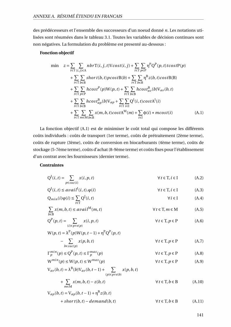
ANNEXE A. RÉSUMÉ ÉTENDU EN FRANCAIS
des prédécesseurs et l’ensemble des successeurs d’un noeud donné n. Les notations uti-
lisées sont résumées dans le tableau 3.1. Toutes les variables de décision continues sont
non négatives. La formulation du problème est presenté au-dessous :
Fonction objectif
min z =∑t∈T
∑(i , j )∈A
nbr T(i , j , t )Vcost (i , j )+ ∑t∈T
∑p∈P
ηPQP(p, t )tcostP(p)
+ ∑t∈T
∑b∈B
shor t (b, t )pcostB(b)+ ∑t∈T
∑b∈B
ηBz(b, t )costB(B)
+ ∑t∈T
∑p∈P
hcost P(p)W(p, t )+ ∑t∈T
∑b∈B
hcost Bav (b)Vav (b, t )
+ ∑t∈T
∑b∈B
hcost Bap (b)Vap + ∑
t∈T
∑i∈I
QI(i , t )cost AI(i )
+ ∑t∈T
∑m∈M
∑b∈B
x(m,b, t )cost AM(m)+∑i∈Iφ(i )∗mcost (i ) (A.1)
La fonction objectif (A.1) est de minimiser le coût total qui compose les différents
coûts individuels : coûts de transport (1er terme), coûts de prétraitement (2ème terme),
coûts de rupture (3ème), coûts de conversion en biocarburants (4ème terme), coûts de
stockage (5-7ème terme), coûts d’achat (8-9ème terme) et coûts fixes pour l’établissement
d’un contrat avec les fournisseurs (dernier terme).
Contraintes
QI(i , t ) = ∑p∈suc(i )
x(i , p, t ) ∀t ∈ T, i ∈ I (A.2)
QI(i , t ) ≤ avai l I(i , t ).ϕ(i ) ∀t ∈ T, i ∈ I (A.3)
Qmi n(i )ϕ(i ) ≤ ∑t∈T
QI(i , t ) ∀i ∈ I (A.4)∑b∈B
x(m,b, t ) ≤ avai l M(m, t ) ∀t ∈ T,m ∈ M (A.5)
QP(p, t ) = ∑(i )∈pr e(p)
x(i , p, t ) ∀t ∈ T, p ∈ P (A.6)
W(p, t ) = λP(p)W(p, t −1)+ηPQP(p, t )
− ∑b∈suc(p)
x(p,b, t ) ∀t ∈ T, p ∈ P (A.7)
Γmi np (p) ≤ QP(p, t ) ≤ Γmax
p (p) ∀t ∈ T, p ∈ P (A.8)
Wmi n(p) ≤ W(p, t ) ≤ Wmax(p) ∀t ∈ T, p ∈ P (A.9)
Vav (b, t ) = λB(b)Vav (b, t −1)+ ∑(p)∈pr e(b)
x(p,b, t )
+ ∑m∈M
x(m,b, t )− z(b, t ) ∀t ∈ T,b ∈ B (A.10)
Vap (b, t ) = Vap (b, t −1)+ηBz(b, t )
+ shor t (b, t )−demand(b, t ) ∀t ∈ T,b ∈ B (A.11)
141

ANNEXE A. RÉSUMÉ ÉTENDU EN FRANCAIS
Γmaxb (b) ≤ z(b, t ) ≤ Γmax
b (b) ∀t ∈ T,b ∈ B (A.12)
Vmi nav (b) ≤ VB
av (b, t ) ≤ Vmaxav (b) ∀t ∈ T,b ∈ B (A.13)
Vmi nap (b) ≤ VB
ap (b, t ) ≤ Vmaxap (b) ∀t ∈ T,b ∈ B (A.14)
x(i , j , t ) ≤ nbr T(i , j , t )∗CapV(i , j ) (A.15)
L’équation (A.2) définit la quantité totale de matières premières acheminées du four-
nisseur i aux installations de prétraitement. L’inégalité (A.3) indique qu’il n’y a pas d’ap-
provisionnement de biomasse sauf s’il existe un contrat entre le fournisseur i et le bio-
raffinerie b. La quantité minimale de livraison selon le contrat d’approvisionnement est
exprimée par la contrainte (A.4).
La contrainte (A.5) exprime que la quantité d’achat de biomasse est également limi-
tée par la disponibilité de marché. L’équation (A.6) définit la quantité totale de biomasse
acheminée des installations de prétraitement p aux bioraffineries à chaque période. La
contrainte (A.7) assure l’équilibre des flux d’entrée et des flux de sortie dans les installa-
tions de prétraitement.
La capacité de production de l’installation de prétraitement et de bioraffinerie est res-
pectée via les contraintes (A.8 - A.12). Les contraintes (A.10) et (A.11) représentent l’équi-
libre des stocks en biomasse et en biocarburant dans chaque bioraffinerie. La contrainte
(A.11) assure que la demande en biocarburant est satisfaite autant que possible. Les contraintes
(A.13) et (A.14) indiquent respectivement la capacité de stockage en biomasse et en bio-
carburant dans chaque bioraffinerie. La contrainte (A.15) représente le nombre de tourné
requis pour la livraison de biomasse à chaque période. Le total des flux ne doit pas dépas-
ser le nombre de véhicules requis.
A.3.3 Étude numérique
Ce modèle est implémenté en langue de programmation Python 3.5 sur un ordinateur
HP Intel Core i5-4210M de 8,0 Gb RAM. Tous les problèmes MILP ont été résolus par le
solveur GUROBI 6.5 avec les paramètres par défaut.
Génération de données d’entrée
Une étude numérique est effectuée pour évaluer l’aspect économique et certains fac-
teurs critiques de la chaîne d’approvisionnement en biomasse. Dans le cas de référence,
nous considérons une chaîne d’approvisionnement en biomasse avec une raffinerie, deux
sites de prétraitement, les 100 fournisseurs potentiels sur 12 périodes. Chaque période de
cette étude correspond à un mois. Le producteur de biocarburants cherche à signer un
contrat avec plusieurs fournisseurs locaux de matières premières. La quantité disponible
de biomasse de chaque fournisseur peut être estimée en fonction de sa surface cultivée
et son rendement de récolte.
142

ANNEXE A. RÉSUMÉ ÉTENDU EN FRANCAIS
Nous utilisons les données de Osmani and Zhang [2013] pour valider notre modèle.
Un contrat avec fournisseur se caractérise par un coût fixe, un prix d’achat unitaire et une
quantité minimale d’approvisionnement en biomasse à fournir. Le prix d’achat varie de
35 à 37 $/tonne. La quantité minimum d’approvisionnement varie entre 20 000 et 100 000
tonne. Le coût fixe pour l’établissement d’un contrat varie entre 20 000 et 30 000 dollar.
Le coût unitaire de transport par trajet est calculé en fonction des distances, des coûts
variables et des coûts fixes liées au transport. Les 100 candidats de fournisseurs se situent
dans un rayon de 50 km de la bioraffinerie. La quantité disponible de biomasse est es-
timée en fonction de la disponibilité des terres selon Osmani and Zhang [2013, 2014] et
le rendement de la biomasse en suivant la distribution uniforme U[3,5,4,5]. Un ratio de
perte pour la biomasse en stockage varie de 1 à 3% par mois (dans le pire des cas).
La capacité de production de bioraffinerie est de 190 MLPY. Le coût de production
unitaire est de 0,2 $/litre. Le taux de transformation en bioéthanol à partir de la biomasse
est 313 litres/tonne. Le coût unitaire de stockage des biocarburants et celui de la biomasse
dans la bioraffinerie sont respectivement de 0,227 $/litre et 0,9 $/tonne. Le coût unitaire
de rupture est de 1,06$/litre. Grâce à la base de données historiques (19981-2005) de Os-
mani and Zhang [2013], la demande est modélisée aléatoirement à l’aide de la distribution
normale N(2133,4138) et tronquée dans l’intervalle [2006,2280] .
Résultats numériques
Dans le cas de référence, la solution optimale du coût total est de $ 181 281 119. Pour
cette instance, le modèle contient 3 808 contraintes, 2 532 variables continues et 1 324
variables entières. Le temps de calcul est moins de 5 secondes (1,78 secondes). La figure
3.2 représente la répartition des coûts dans la chaîne d’approvisionnement de la biomasse
sur l’horizon de planification T = 12. Il est évident que les coûts de transport jouent un
rôle essentiel dans la chaîne d’approvisionnement en biomasse avec environ 25% du coût
total du système.
Nous avons également testé ce modèle pour différentes instances lorsque I = 10, 20,
50, 100, 150, 200, 250, 300, 350, 400 ; P = 1, 2, 5 et T = 12. La taille du problème et la durée
d’exécution de ces instances sont résumées dans le tableau 3.3. Ces résultats montrent
que ce modèle peut être résolu rapidement et exactement avec un solveur commercial.
Analyse de sensibilité
Certains paramètres tels que prix d’achat sur un marché, quantité minimum d’appro-
visionnement et coût contractuel fixe ont un impact significativement sur le coût total
optimal du système et le nombre total de fournisseurs sous contrat.
La figure 3.3 représente le coût total du système est moins sensible à la variation du
prix du marché, qui varie entre 90 % et 130 % de sa valeur de base. Lorsque le prix du
marché devient trop cher, e décideur hésite à acheter une quantité supplémentaire de
143
ANNEXE A. RÉSUMÉ ÉTENDU EN FRANCAIS
biomasse sur les marchés pour satisfaire la totalité de la demande de biocarburants. Dans
ce cas, il préfère établir plus de contrats d’approvisionnement. Cela explique pourquoi le
nombre de fournisseurs sous contrat augmente lorsque le prix du marché augmente.
La figure 3.4 montre qu’une augmentation des coûts fixes de l’établissement de contrats
entraînerai un coût total du système très élevé et entraverai l’établissement de contrats à
long terme. Cependant, il s’agit d’un léger effet sur le coût global du système et le nombre
total de fournisseurs sous contrat.
La figure 3.5 indique la proportionne faible entre la quantité minimum d’approvi-
sionnement et le coût total du système. Cependant, le nombre total de fournisseurs sous
contrat diminue à mesure que la quantité d’approvisionnement augmente. Dans ce cas,
on a besoin d’une quantité supplémentaire en provenant du marché pour satisfaire la
demande finale si et seulement si le prix d’achat est raisonnable.
A.4 Sélection des fournisseurs et planification dans la chaîne
d’approvisionnement en biomasse sous incertitude
Dans cette section, nous étendons le problème précédent en considérant l’incerti-
tude d’approvisionnement. Nous présentons au-dessous un modèle de programmation
stochastique en deux étages pour aborder la sélection des fournisseurs et la planification
des opérations dans une chaîne logistique en biomasse.
A.4.1 Mathematical formulation of the problem
Dans cette section, nous formulons un modèle de programmation stochastique en
deux étages en prenant en compte la sélection des fournisseurs et la planification des opé-
rations de façon simultanée. Les variables de décision de la première étape comprennent
uniquement les variables binaires qui déterminent le choix des fournisseurs ayant des
contrats à long ou moyen terme. Les variables de la deuxième étape comprennent la
quantité de biomasse à acheter auprès des fournisseurs, la quantité de biomasse à trans-
porter à la bioraffinerie, la quantité de biomasse à utiliser pour la transformation en bioé-
thanol, le volume de bioéthanol non satisfait, le niveau de stock en biomasse et bioétha-
nol à chaque période. Le modèle mathématique est présenté au-dessous :
(SP) : minϕ
mcost Tϕ+∑
s∈SpsQ(ϕ, s) |ϕ ∈ 0,1
(A.16)
where : Q(ϕ, s) = minys
f (ϕ, s, ys) | subject to (A.19)− (A.34)
(A.17)
oùϕ= ϕ(i ), i ∈ I sont les variables de décision de la première étape relatives aux contrats
entre les bioraffineries et les fournisseurs, ϕ(i ) = 1 si le contrat est établi avec le four-
nisseur i , 0 sinon. Le vecteur mcost = mcost (i ), i ∈ I inclut le coût fixe mcost (i ) pour
144

ANNEXE A. RÉSUMÉ ÉTENDU EN FRANCAIS
établir un contrat avec le fournisseur i . La fonction Q(ϕ, s) est la fonction de coût de sous-
problème de deuxième étape pour chaque scénario s, dans lequel les décisions de la pre-
mière étape, ϕ, ont déjà été prises.
Toutes les notations utilisées sont résumées dans le tableau 4.1. Toutes les variables
de décision continues sont non négatives. Les différentes composantes du coût total de
la deuxième étape f (ϕ, s, ys) pour chaque scénario s sont indiquées ci-dessous; où ys
contient toutes les variables de décision de seconde étape, ys = (x, w,Vav ,Vap , qP, z, shor t ).
f (ϕ, s, ys) =∑t∈T
∑(i , j )∈A
x(i , j , t , s)∗Vcost (i , j )+ ∑t∈T
∑p∈P
ηP ∗qP(p, t , s)∗ tcostP(p)
+∑t∈T
∑b∈B
shor t (b, t , s)∗pcost (b)+ ∑t∈T
∑b∈B
ηB ∗ z(b, t , s)∗ tcostB(B)
+∑t∈T
∑p∈P
hcost P(p)w(p, t , s)+ ∑t∈T
∑b∈B
hcost Bav (b)Vav (b, t , s)
+∑t∈T
∑b∈B
hcost Bap (b)Vap (b, t , s)+ ∑
t∈T
∑i∈I
q I(i , t , s)∗ cost AI(i )
+∑t∈T
∑m∈M
∑b∈B
x(m,b, t , s)∗ cost AM(m) (A.18)
où x(i , j , t , s) est le flux de biomasse sur l’arc (i , j ) ∈ A à la période t dans le scénario s. Un
tel arc (i , j ) pourrait être un arc (i , p) ou (p,b) qui fait référence à un arc du fournisseur
i ∈ I à la facilité de prétraitement p ∈ P ou de l’installation de prétraitement p ∈ P à la
bio-raffinerie b.
La fonction objectif est de minimiser le coût total de la chaîne d’approvisionnement,
qui comprend les coûts de la première étape et l’espérance des coûts de deuxième étape.
Les coûts de la première étape comprennent les coûts totaux liés à l’établissement de
contrats avec fournisseurs. L’équation (A.18) présente les coûts de la deuxième étape Q(ϕ, s)
pour chaque scénario s, qui comprend neuf coûts : coûts de transport (1er terme), coûts
de prétraitement (2ème terme), coûts de rupture (3ème terme), coûts de conversion en
biocarburant (4ème terme), coûts de stockage (5ème-7ème termes) et coûts d’achat (9ème-
10ème termes).
Constraints on suppliers
q I(i , t , s) = ∑p∈suc(i )
x(i , p, t , s) ∀t ∈ T, i ∈ I, s ∈ S [π1i ,t ,s] (A.19)
q I(i , t , s) ≤ avai l I(i , t , s).ϕ(i ) ∀t ∈ T, i ∈ I, s ∈ S [π2i ,t ,s] (A.20)∑
t∈Tq I(i , t , s) ≥ qmi n(i ).ϕ(i ) ∀i ∈ I, s ∈ S [π3
i ,s] (A.21)
L’équation (4.4) définit la quantité totale de matières premières transportées du four-
nisseur i aux installations de prétraitement dans chaque période du scénario s. L’inégalité
(A.20) indique qu’il n’y a pas d’approvisionnement en biomasse en provenant du fournis-
seur i sauf s’il existe un contrat avec fournisseur i . L’inégalité (A.21) assure que la quantité
145

ANNEXE A. RÉSUMÉ ÉTENDU EN FRANCAIS
minimum d’approvisionnement dans un contrat entre un fournisseur i et la bioraffinerie
b est respecté.
Constraints on market
∑b∈B
x(m,b, t , s) ≤ avai l M(m, t ) ∀t ∈ T,m ∈ M [π4m,t ,s] (A.22)
L’inégalité (A.22) assure que la quantité d’achat en biomasse est limitée par la dispo-
nibilité de biomasse sur le marché dans chaque scénario.
Constraints on preprocessing sites
qP(p, t , s) = ∑i∈pr e(p)
x(i , p, t , s) ∀t ∈ T, p ∈ P, s ∈ S [π5p,t ,s] (A.23)
w(p, t , s) = (1−λP(p))w(p, t −1, s)+ηPqP(p, t , s)
− ∑b∈suc(p)
x(p,b, t , s) ∀t ≥ 2, p ∈ P, s ∈ S [π6p,t ,s] (A.24)
w(p,1, s) = (1−λP(p))w i ni t (p)+ηPqP(p,1, s)
− ∑b∈suc(p)
x(p,b,1, s) ∀p ∈ P, s ∈ S [π7p,s] (A.25)
γmi np (p) ≤ qP(p, t , s) ≤ γmax
p (p) ∀t ∈ T, p ∈ P, s ∈ S [π8a/bp,t ,s ] (A.26)
w mi n(p) ≤ w(p, t , s) ≤ w max(p) ∀t ∈ T, p ∈ P, s ∈ S [π9a/bp,t ,s ] (A.27)
L’équation (A.23) présente la quantité totale de biomasse transportée des fournisseurs
aux installations de prétraitement p à chaque période dans le scénario s. L’équation (A.24)
et (A.25) sont la contrainte de balance de chaque stock dans l’installation de prétraite-
ment dans le scénario s. La capacité de prétraitement et sa capacité de stockage sont pré-
sentées par des contraintes (A.26) et (A.27), respectivement.
Constrains on refinery sites
Vav (b, t , s) = (1−λB(b))Vav (b, t −1, s)− z(b, t , s)
+ ∑p∈pr e(b)
x(p,b, t , s)+ ∑m∈M
x(m,b, t , s) ∀t ≥ 2,b ∈ B, s ∈ S [π10b,t ,s] (A.28)
Vav (b,1, s) = (1−λB(b))Vi ni tav (b)− z(b,1, s)
+ ∑p∈pr e(b)
x(p,b,1, s)+ ∑m∈M
x(m,b,1, s) ∀b ∈ B, s ∈ S [π11b,s] (A.29)
Vap (b, t , s) = Vap (b, t −1, s)+ηBz(b, t , s)
−demand(b, t )+ shor t (b, t , s) ∀t ≥ 2,b ∈ B, s ∈ S [π12b,t ,s] (A.30)
Vap (b,1, s) = Vi ni tap (b)+ηBz(b,1, s)
−demand(b,1)+ shor t (b,1, s) ∀b ∈ B, s ∈ S [π13b,s] (A.31)
146

ANNEXE A. RÉSUMÉ ÉTENDU EN FRANCAIS
γmi nb (b) ≤ z(b, t , s) ≤ γmax
b (b) ∀t ∈ T,b ∈ B, s ∈ S [π14a/bb,t ,s ] (A.32)
Vmi nav (b) ≤ Vav (b, t , s) ≤ Vmax
av (b) ∀t ∈ T,b ∈ B, s ∈ S [π15a/bb,t ,s ] (A.33)
Vmi nap (b) ≤ Vap (b, t , s) ≤ Vmax
ap (b) ∀t ∈ T,b ∈ B, s ∈ S [π16a/bb,t ,s ] (A.34)
Les équations (A.28 -A.31) sont les contraintes de balance des stocks en biomasse et
en biocarburant à la bio-raffinerie b, respectivement. Les équations (A.33) and (A.34) sont
des contraintes de capacité de stockage en biomasse et en biocarburant à la bioraffine-
rie b. La capacité de conversion de chaque bio-raffinerie est donnée par des contraintes
(A.32).
A.4.2 Approches de résolution
Dans cette section, le modèle de programmation stochastique (SP) est transformé en
un modèle équivalent déterministe (DEP) en appliquant l’approche de scénarios. Le se-
cond modèle peut être résolu par un solveur commercial comme CPLEX ou GUROBI.
Cependant, si le nombre de scénarios est élevé, la résolution du modèle nécessite une
énorme quantité de mémoire et d’effort de calcul. Par conséquent, nous proposons dans
cette sous-section une méthode de décomposition (ERD) pour surmonter les difficultés
de calcul.
Modèle déterministe équivalent
Nous transformons le modèle original en un modèle déterministe de programmation
linéaire en nombres entiers (MILP) au dessous :
(DEP) minx,ys
(mcost Tϕ+∑
s∈Sps f (ϕ, s, ys)
)s.t . ϕ(i ) ∈ 0,1 ∀i ∈ I
ys subject to constraints (A.19)-(A.34)
Méthode de résolution
En général, la méthode de L-shaped ont deux inconvénients : (1) lors d’itérations ini-
tiales ; les coupures sont souvent inefficaces ; (2) Lors des dernières itérations, les coupes
deviennent dégénérés. Ruszczynski and Swietanowski [1997] propose une méthode de
décomposition régularisée pour éviter les deux inconvénients de la méthode de L-shaped.
Le concept de cette méthode est similaire à celui de la méthode de L-shaped multi-coupes
mais on ajoute un terme régularisé quadratique dans la fonction objectif . Nous avons
adapté cette approche à notre problème.
Dans notre algorithme (ERD), nous ajoutons des coupes dans le problème de premier
étage pour accélérer la vitesse de convergence de l’algorithme. Ils permettent de réduire
147

ANNEXE A. RÉSUMÉ ÉTENDU EN FRANCAIS
la région faisable du problème de premier étage et évite l’infaisabilité des sous-problèmes
de deuxième étage dans chaque itération. Les coupes sont présentées au-dessous :
∑i∈I
qmi n(i )ϕ(i ) ≤ ∑t∈T
∑i∈I
q I(i , t , s) = ∑t∈T
∑p∈P
qP(p, t , s) ≤ ∑t∈T
∑p∈P
γmaxp (p)
=⇒∑i∈I
qmi n(i )ϕ(i ) ≤ T∑p∈P
γmaxp (p) ∀s ∈ S (A.35)
Ces inégalités au-dessus assurent que la quantité totale minimale fournie par les four-
nisseurs sélectionnés ne dépasse pas la quantité maximale de biomasse traitée dans les
installations de prétraitement.
∑t∈T
∑i∈I
avai l I(i , t , s)ϕ(i ) ≥ ∑t∈T
∑i∈I
q I(i , t , s) ≥ ∑t∈T
∑p∈P
γmaxp (p) ≥ ∑
t∈T
∑p∈P
γmi np (p)
=⇒∑t∈T
∑i∈I
avai l I(i , t , s)ϕ(i ) ≥ T∑p∈P
γmi np (p) ∀s ∈ S (A.36)
Les coupes au-dessus garantissent que les fournisseurs sélectionnés sont capables de
satisfaire au moins une quantité minimale de biomasse traitée dans une installation de
prétraitement.
Coupes de Knapsack : Soit UB la borne supérieure actuelle dans l’itération considé-
rée. En combinant la coupe d’optimalité : θs ≥ eks ϕ+d k
s et UB ≥ mcost Tϕ+∑p∈P psθs , on
obtient :
UB ≥ mcost Tϕ+ ∑p∈P
psθs ≥ mcost Tϕ+∑s∈S
ps(eks ϕ+d k
s )
=⇒(mcost +∑
s∈Spsek
s
)Tϕ≤ UB−∑
s∈Spsd k
s
Comme ϕ sont des variables binaires, nous pouvons arrondir les deux côtés de l’inégalité
ci-dessus et obtenir une inégalité valide suivante :
b(mcost +∑s∈S
pseks
)Tcϕ≤ bUB−∑s∈S
psd ks c (A.37)
Où bac est un nombre arrondi d’un nombre donné a. Quand une limite supérieure ubs
est disponible, on peut ajouter une coupe (A.37) pour resserrer l’espace de solution du
problème de la première étape.
Coupes d’optimalité spécifique : Selon Laporte and Louveaux [1993], une coupe d’op-
timalité spécifique permet d’accélérer notre algorithme lorsque les variables du premier
étage sont des variables binaires. Nous avons reformulé cette coupe pour notre algo-
148

ANNEXE A. RÉSUMÉ ÉTENDU EN FRANCAIS
rithme comme suit :
∑s∈S
psθs ≥ (qs −L)(∑
i∈τϕ(i )−∑
i∉τϕ(i )− | τ | +1
)+L (A.38)
Où qs =∑s∈S psQ(ϕ, s) est la valeur de la fonction de recours correspondante à chaque ité-
ration. L est une borne inférieure satisfaisant :L ≤ mi nϕ∑
s∈S psQ(ϕ, s) ∀ϕ. L’ensemble τ
est un ensemble des fournisseurs sélectionnées i : τ= i | ϕ(i ) = 1
et | τ | est la cardina-
lité de l’ensemble τ.
A.4.3 Étude numérique
Dans l’étude numérique, nous utilisons des données de Osmani and Zhang [2013,
2014]; Zhang et al. [2012] pour rendre nos instances testées plus réalistes. Les données
sont résumées dans le tableau 4.2.
Evaluation des performances de méthode de résolution
Le tableau 4.4 résume la taille, le nombre de scénarios et le temps d’exécution du sol-
veur GUROBI, de la version "multi-coupes" de L-shaped (MLS) et de la méthode ERD
pour instances différentes. Nous observons que la méthode (ERD) et GUROBI sont deux
fois plus rapide que la méthode MLS. En moyenne, la méthode (ERD) est respectivement
1,01, 1,21, 1,16, 1,20, 1,20 et 1,32 fois plus rapide que GUROBI pour toutes les instances.
Par conséquent, la méthode ERD peut être utilisée pour résoudre le problème considéré,
car elle permet de trouver une solution optimale en un temps de calcul plus court.
Les trois sous-tables de la troisième ligne de la table 4.5 montrent que l’algorithme
(ERD) fonctionne toujours bien pour les grandes instances. Le solveur GUROBI ne peut
pas résoudre ces grandes tailles du modèle en raison de la mémoire limitée de notre PC.
De plus, les deux dernières colonnes prouvent la pertinence d’ajouter ces inégalités dans
la méthode de résolution. Les coupes permettent d’améliorer considérablement la vitesse
de convergence de la méthode de résolution. En fait, l’ajout des coupes pourrait réduire
de 8,8 à 30,3% du temps de calcul par rapport à la méthode classique RD (sans ajouter des
coupes).
Analyse de la solution
La figure 4.2 montre la répartition des coûts du scénario de base pour une chaîne d’ap-
provisionnement en biomasse sur l’horizon de planification T = 12. La valeur optimale du
coût total attendu de la chaîne d’approvisionnement est de $114 271 335. Le coût de pro-
duction des biocarburants et le coût d’achat des matières premières sont les principaux
facteurs de coût qui représentent respectivement près de 39,5% et 34,8% du coût total du
système. Le coût du transport joue un rôle essentiel dans la chaîne d’approvisionnement
149

ANNEXE A. RÉSUMÉ ÉTENDU EN FRANCAIS
de la biomasse, avec environ 14,7% du coût total du système. Ce résultat montre l’impor-
tance des opérations de transport dans les chaînes d’approvisionnement en biomasse. Le
coût de possession n’est que de 2,9%, de sorte que dans ce cas, le stockage d’une quantité
importante de biomasse à la bioraffinerie ne semble pas critique.
Valeur de la solution stochastique
En réalité, la disponibilité de biomasse peut être estimée par le rendement moyen (12
tonnes/hectare) et puis chercher à identifier des contrats avec les fournisseurs. Cette ap-
proche est une approche déterministe qui base sur la valeur moyenne de la disponibilité
de biomasse mais elle pourrait avoir des conséquences défavorables. Le tableau 4.5 in-
dique que l’approche stochastique permet de réduire de 7,9% l’espérance du coût total
annuel en comparaison de celle obtenue par l’approche déterministe. On peut considé-
rer que la valeur VSS = 124088777−114271335 = $9817442 représente le gain possible en
tenant compte de l’incertitude d’approvisionnement en biomasse. Cette valeur s’appelle
la valeur de la solution stochastique (VSS).
Analyse de sensibilité
Dans cette sous-section, nous avons examiné les impacts de certains paramètres cri-
tiques sur l’espérance du coût total du système.
Effet du prix d’achat : Selon la figure 4.4, lorsque le prix du marché augmente trop, les
décideurs ont moins intérêt à acheter une quantité supplémentaire de biomasse sur les
marchés pour répondre à la demande de biocarburants. Dans ce cas, ils auraient l’inten-
tion d’établir des contrats d’approvisionnement à plus long terme pour assurer la stabi-
lité de l’approvisionnement en matières premières. Cela explique pourquoi le nombre de
fournisseurs sous contrat augmente lorsque le prix du marché augmente. Ce résultat sug-
gère que pour atteindre l’efficacité globale du système, il convient d’établir un équilibre
entre le prix d’achat dans le cadre de contrats à long terme et celui du marché.
Effet du coût fixe : Nous effectuons une étude de l’effet du coût fixe sur la chaîne d’ap-
provisionnement de la biomasse. Dans la figure 4.6, le résultat indique que l’augmenta-
tion du coût fixe affecte légèrement le coût total du système et le nombre total de four-
nisseurs sous contrat. Cela montre également que l’augmentation des coûts fixes pour-
rait entraîner une augmentation du coût total du système et entraver l’établissement de
contrats à long terme.
Effet de la quantité minimum d’approvisionnement des fournisseurs : Figure 4.5
montre que l’augmentation de la quantité minimum d’approvisionnement entraine une
augmentation légèrement du coût total du système. En outre, le nombre total de fournis-
seurs sous contrat diminue quand la quantité d’approvisionnement augmente. Dans ce
cas, le décideur exigerait une quantité supplémentaire du marché pour satisfaire la de-
mande finale, mais uniquement à un prix raisonnable du marché.
150

ANNEXE A. RÉSUMÉ ÉTENDU EN FRANCAIS
A.5 Gestion de stocks périssables sous incertitudes : Poli-
tique optimal et algorithme
Ce chapitre présente un modèle stochastique de gestion des stocks pour un produit
périssable sous incertitudes. Une partie des stocks est dégradée à un constant taux dune
période à l’autre. Ce problème apparaît dans les chaînes d’approvisionnement en bio-
masse. En fait, le taux de dégradation de biomasse en stockage est d’environ 1 à 2% par
mois Rentizelas et al. [2009].
A.5.1 Description du problème et formulation du modèle
Description du problème
Considérons un modèle de gestion des stocks pour un seul produit, un seul stock à
l’horizon de planification de n -périodes. Ce produit est périssable et son taux de dété-
rioration est constant, noté (1−λ), où 0 < λ < 1. Soit st le niveau de stock au début de la
période t et avant de lancer une quantité commandée qt dans cette période.
La demande dans la période t est représentée par la variable aléatoire non négative Dt
dont la fonction de densité de probabilité ft et la fonction de distribution cumulative Ft
sont connues. Les demandes dans toutes les périodes sont indépendantes.
Les capacités d’approvisionnement dans n -périodes, qui sont des variables aléatoires
et indépendantes, notée par yt , dont la fonction de densité de probabilité g t et la fonction
de distribution cumulative Gt sont connues. Supposons que le délai de livraison est nul, la
demande non satisfaite est mise en attente et le niveau de stock est revu périodiquement.
L’objectif de ce problème est de minimiser l’espérance mathématique du coût total,
qui comprend trois types de coûts : coûts de stockage, coûts de rupture et coûts d’achat
sur l’horizon de planification de n périodes.
L’ordre des événements survenus dans chaque période est supposé comme suit.
• Au début de la période, le niveau de stock est examiné en tenant compte de la dété-
rioration du produit survenue dans la période précédente.
• Selon la politique de gestion des stocks choisies, une commande est alors placée
si nécessaire. Ensuite, la demande de client est satisfaite autant que possible et la
demande non satisfaite est mise en attente.
• Un coût de stockage est chargé en fonction du stock disponible à la fin de cette
période. Un coût de rupture est chargé en cas de niveau de stock négatif à la fin de
chaque période.
Le modèle de gestion des stocks périssables est présenté sous la forme suivante :
151

ANNEXE A. RÉSUMÉ ÉTENDU EN FRANCAIS
(SP) minqt
T∑t=1
αtφt (st , qt ) (A.39)
s.t st+1 = λs+t − s−t +mi n(qt , yt )−Dt (A.40)
s+t = max(0, st ) (A.41)
s−t = max(0,−st ) (A.42)
où la fonction φt (st , qt ) est l’espérance mathématique du coût pour une seul période
qui inclut l’espérance mathématique du coût de stockage, du coût de rupture et du coût
d’achat. Soit c, p, textit h le coût d’achat, celui de rupture et celui de stockage par unité,
respectivement. Soit α le facteur de discount (0 < al pha < 1).
φt (st , qt ) = E(Dt ,yt )
[c(minqt , yt )+h(λs+t − s−t +min(qt , yt )−Dt )+
+p(Dt −minqt , yt −λs+t + s−t )+]
(A.43)
L’équation A.41 représente la relation entre le niveau de stocks au début de la période
t et celle au début de la période t+1 en considérant la périssabilité du produit.
Le niveau de stock st peut être négatif en cas où la demande est en attente. Dans ce
cas, st < 0, le stock disponible est zéro, et seul −s−t = st est reporté à la période suivante.
Au cas d’un niveau de stocks positif st , le stock disponible est égal à st . Donc, une partie
de stocks disponible (1−λ)st , aura péri pendant la période t .
Modèle de programmation dynamique et propriétés du modèle
Dans cette section, nous formulons un modèle de programmation dynamique sto-
chastique tenant en compte l’incertitude à la fois dans l’approvisionnement et la de-
mande. Soit V∗t ,n(st ) la valeur optimale de l’espérance mathématique du coût total de la
période t à n en utilisant la politique optimale sachant que le niveau de stock st à la pé-
riode t est connu. Le coût optimal V∗t ,n(st ) peut être calculé de manière récursive comme
suit :
V∗t ,n(st ) = min
qtVt ,n(st , qt ) (A.44)
where Vt ,n(st , qt ) =φt (st , qt )+ αE(Dt ,yt )
V∗t+1,n(st+1)
Dans l’équation au-dessus, Vt ,n(st , qt ) correspond à la valeur du coût total cumulée
entre la période t et n, obtenu en utilisant la politique optimale pour les périodes t + 1
à n, sachant que le niveau de stock st et la quantité de commande qt sont connus. Par
définition, Vn+1,n(.) ≡ 0. La fonction φt (st , qt ) est une fonction du stock initial st , ainsi
que la quantité de commande qt .
152

ANNEXE A. RÉSUMÉ ÉTENDU EN FRANCAIS
Les propriétés du modèle se présentent comme suit :
1. ∂2
∂s2t
Vt ,n(st , q∗t ) ≥ 0 ∀st
2. ϕt ,n(st , qt ) est une function croissante en qt .
3. Vt ,n(st , qt ) a un minimum global en qt = q∗t
4. Le politique optimal est une politique « order-up-to level ».
A.5.2 Approche de résolution
Pour trouver les niveaux de recomplètement optimaux, nous constatons qu‘il est dif-
ficile d’appliquer directement l’approche de programmation dynamique due à la grand
dimension du problème. C’est pourquoi nous développons une approche de résolution
qui est une combinaison entre l’approche de scénarios et la méthode de relaxation lagran-
gienne. L’approche de scénarios permet de capturer l’incertitude de manière approxima-
tive, mais la taille du modèle peut augmenter considérablement en fonction du nombre
de scénarios considérée. Pour surmonter ce défi, nous développons un algorithme basé
sur la relaxation lagrangienne pour trouver une solution approchée de bonne qualité.
Modèle équivalent déterministe
Dans cette sous-section, nous transformons le modèle stochastique (A.39) au modèle
de programmation linéaire à nombres entiers mixtes (MILP) en utilisant de l’approche
basée sur scenarios. Soit Ω un ensemble de scénarios, ω ∈Ω l’indice d’un scénario et sa
probabilité d’occurrence est notée par pω. L’index ω est ajouté aux variables de décision
liées au scénario considéré ω. L’espérance mathématique E(.) dans la fonction objectif (
ref modèle original) est remplacée par∑ωpω(.)
Soit st ,ω le niveau de stock au début de la période textit t dans le scénario ω. Soit Lt le
niveau de recomplètement dans la période t . Notre objectif est de trouver ce niveau, Lt ,
en résolvant le modèle suivant (DEP). La quantité de commande, qt ,ω, est définie par :
qt ,ω = minLt −λs+t ,ω+ s−t ,ω, yt ,ω (A.45)
La variable auxiliaire βt ,ω est définie comme suit :
βt ,ω =1 if Lt −λs+t ,ω+ s−t ,ω ≤ yt ,ω
0 otherwise
153

ANNEXE A. RÉSUMÉ ÉTENDU EN FRANCAIS
Le modèle équivalent déterministe (DEP) est le suivant :
(DEP) min∑t∈T
αt( ∑ω∈Ω
pω(cqt ,ω+hs+t ,ω+ps−t ,ω))
(A.46)
s.t
Lt −λs+t ,ω+ s−t ,ω− (1−βt ,ω)M ≤ qt ,ω ≤ Lt −λs+t ,ω+ s−t ,ω (A.47)
yt ,ω−βt ,ωM ≤ qt ,ω ≤ yt ,ω (A.48)
st+1,ω = λs+t ,ω− s−t ,ω+qt ,ω−Dt ,ω (A.49)
st ,ω = s+t ,ω− s−t ,ω (A.50)
s+t ,ω ≥ st ,ω (A.51)
s−t ,ω ≥−st ,ω (A.52)
βt ,ω ∈ 0,1 (A.53)
st ,ω ∈R, s+t ,ω ≥ 0, s−t ,ω ≥ 0, qt ,ω ≥ 0,Lt ≥ 0 (A.54)
L’équation (A.49) représente l’équilibre des stocks, similaire à l’équation (A.40) dans le
modèle d’origine.
Les équations (A.41) - (A.42) sont linéarisées par des contraintes (A.50) - (A.52).
L’équation (A.45) est linéarisée par des contraintes (A.47 - A.48). Notez que M est un
grand nombre.
Relaxation Lagrangienne
Le modèle (DEP) pourrait être résolu par un solveur commercial mais son temp de
calcul devient plus important pour les instances de grande taille. Dans cette sous-section,
nous proposons un algorithme basé sur la méthode de relaxation lagrangienne.
Nous relaxons Lt par Lt ,ω en introduisant la contrainte suivante :
Lt ,ω = Lt ,ω′ ∀ω,ω′ ∈Ω andω 6=ω′ (A.55)
Nous définissons une variable intermédiaire, δt ,ω comme la violation de la contrainte
(A.55). Soit π= (πt ,ω) ∀t ∈ T,ω ∈Ω un vecteur de multiplicateurs de Lagrange associé à la
contrainte (A.55).
δt ,ω = Lt ,ω−Lt ,ω′ ∀ω,ω′ ∈Ω andω 6=ω′ (A.56)
Donc, la programmation de relaxation lagrangien (LRP) est présentée au-dessous. Elle
154

ANNEXE A. RÉSUMÉ ÉTENDU EN FRANCAIS
permet de trouver une borne inférieure pour le modèle (DEP).
(LRP) min∑t∈T
αt( ∑ω∈Ω
pω(cqt ,ω+hs+t ,ω+ps−t ,ω))+ ∑
t∈T
∑ω∈Ω
πt ,ωδt ,ω (A.57)
s.t
Lt ,ω−λs+t ,ω+ s−t ,ω− (1−βt ,ω)M ≤ qt ,ω ≤ Lt ,ω−λs+t ,ω+ s−t ,ω (A.58)
constraint (A.48)− (A.54)
À partir des solutions Lt ,ω,ω ∈Ω obtenue par la résolution du problème de relaxation
lagrangien (LRP), nous pouvons la transformer en une solution réalisable, Lt pour le pro-
blème originale par une agrégation de scénarios au-dessous. Cette solution faisable Lt
permet de fournir une borne supérieure de la valeur objective optimale du modèle (DEP).
Lt =∑ω∈Ω
pωLt ,ω ∀t ∈ T (A.59)
Il est nécessaire de déterminer les multiplicateurs de Lagrange, π qui maximisent la
borne inférieure. Autrement dit, nous devons chercher une borne inférieure aussi proche
que possible de la valeur objective optimale du modèle (DEP). Cela conduit au problème
dual lagrangien suivant :
maxπ∈R
LRP(π)
=maxπ∈R
min
∑t∈Tα
t(∑
ω∈Ωpω(cqt ,ω+hs+t ,ω+ps−t ,ω))+∑
t∈T∑ω∈Ωπt ,ωδt ,ω
s.t
Lt ,ω−λs+t ,ω+ s−t ,ω− (1−βt ,ω)M ≤ qt ,ω ≤ Lt ,ω−λs+t ,ω+ s−t ,ω
constraint (5.26)-(5.31)
La méthode du sous-gradient est souvent utilisée pour résoudre le problème dual la-
grangien mais elle converge très lente ou même ne converge pas. Nous utilisons la mé-
thode de volume pour la résolution du problème dual lagrangien. Selon Barahona and
Anbil [2000], la méthode de volume est une extension de l’algorithme de sous-gradient
et très similaire à la méthode de bundle [Lemaréchal, 1989] mais son temps de calcul est
moins important que les autres méthodes. C’est pourquoi nous utilisons la méthode du
volume pour résoudre le problème dual lagrangien. Notre algorithme est détaillé dans
l’Algorithme 5.1
A.5.3 Expériences numériques
Dans cette sous-section, nous effectuons une étude numérique pour évaluer la per-
formance et démontrer l’efficacité de notre algorithme. Cet algorithme est implémenté
en Python 3.5 sur un ordinateur HP Intel Core i5-4210M de 8 Gb RAM.
155

ANNEXE A. RÉSUMÉ ÉTENDU EN FRANCAIS
Paramétrage
Dans l’étude numérique, nous utilisons les données présentées dans Broekmeulen
and Van Donselaar [2009]; Pauls-Worm et al. [2015] telles que la demande moyenne, le
coefficient de variation (CV =σ/µ) et le nombre de périodes. Le coût de stockage unitaire
h est fixé à 5. Le coût d’achat unitaire c varie de 30 à 40. Le coût de rupture par unité p est
déterminé à partir du ratio p/(p+h). Le nombre de périodes et celui de scénarios sont res-
pectivement T = 7 et |Ω| = 200. Basant sur la méthode statistique de Shapiro [2000], nous
estimons que l’instance inclut 200 scénarios permet d’obtenir une solution très proche
de l’optimum avec l’écart de 1% dans l’intervalle de confiance à 95% par rapport à la so-
lution optimale. Toutes les valeurs de paramètre sont présentées dans le tableau 5.1. Les
trois cas concernant la lois de distribution de la demande et de l’approvisionnement sont
les suivantes :
a) La demande suit une distribution normale non-stationnaire avec µDt = ft .µD où
ft = 0.12,0.13,0.13,0.16,0.18,0.18,0.10, etµD est pris dans la liste [12,13,13,16,18,18,10].
L’approvisionnement suit une distribution normale stationnaire avec µSt = 16 et σSt =0.2µSt∀t = 1...7.
b) La demande et l’approvisionnement suivent une distribution normale stationnaire
avec les paramètres suivante µDt = 13, σDt = 3.5, µSt = 15 et σSt = 0.2µSt∀t = 1...7.
c) La demande et l’approvisionnement suivent une distribution normale stationnaire
avec les paramètres suivante µDt = 14, σDt = 0.25µDt , µSt = 15 et σSt = 0.2µSt∀t = 1...7.
Concernant, le paramétrage de l’algorithme LR, nous fixons le seuil d’optimalité ε ≤0.01%, le nombre d’itérations maximal i ter ati onmax = 500 et le temps de calcul maximal
t i memax = 3600s. L’algorithme s’arrête également lorsque la borne supérieure ne peut
pas être améliorée après 50 itérations consécutives.
Evaluation des performances de l’algorithme
Dans cette sous-section, nous comparons la performance de notre solution avec avec
l’approche de programmation dynamique ([Bellmam, 1957, Chapter III.3]). Les tables 5.2,
5.3 et 5.4 représentent le temps de calcul et l’écart relatif entre les deux approches (E-
LR et DP). En fait, E-LR est la valeur objective attendue du modèle stochastique obtenue
en utilisant la solution de l’approche de relaxation lagrangienne. Pour chaque instance,
le modèle (DEP) comprend 3 807 variables continues, 1400 variables binaires et 7 007
contraintes.
Nous observons que le temps de calcul de l’algorithme LR est plus court que celui
de l’algorithme DP (215,91s vs 5180,80s dans le cas a, 187,83s vs 5476,63s dans le cas b et
172,59s vs 5399,91s dans le cas c). De plus, l’écart moyen entre la solution LR et celle de DP
n’est que de 0,77 %, 0,70 % et 0,50 % respectivement dans les trois cas considérés. L’étude
numérique montre que l’approche LR permet de trouver une solution de haute qualité en
temps de calcul raisonnable et donc il est convient pour une application pratique.
156

ANNEXE A. RÉSUMÉ ÉTENDU EN FRANCAIS
A.6 Modélisation et optimisation de la gestion des stocks
d’un produit à durée de vie fixe sous incertitudes
La réduction du gaspillage provenant de la périssabilité des produits, est l’une des
défies majeures de plusieurs secteurs industriels concernant les produits frais, les pro-
duits sanguins, la viande, les produits chimiques, les matériaux composites et les pro-
duits pharmaceutiques. À notre connaissance, il y a très peu d’études de recherche por-
tées sur la gestion des stocks d’un produit périssable, avec l’approvisionnement aléatoire
et la demande aléatoire dans un horizon de planification glissant. Pour cette raison, nous
étudions un modèle de gestion des stocks d’un produit périssable à durée de vie fixe. Les
caractéristiques essentielles de ce modèle sont : périssabilité, la demande aléatoire, l’ap-
provisionnement aléatoire et multi-périodes.
A.6.1 Description du problème et formulation du modèle
Description du problème
Dans cette sous-section, nous considérons un problème multi-périodes de gestion
des stocks d’un produit périssable à durée de vie fixe dans un horizon de planification
glissant. Pour simplifier, nous supposons que la méthode du premier entré, premier sorti
(FIFO) est employée pour la méthode de rangement. Supposons que l’ordre des événe-
ments survenus au cours de chaque période est le suivant :
i) Les articles frais arrivent au début de chaque période. Ensuite, le niveau de stock est
mis à jour selon la durée de vie restant de chaque article. Les articles expirés sont rejetés.
ii) Selon la politique de gestion des stocks utilisée, une commande est alors lancée si
nécessaire. Puis, la demande des clients est satisfaite autant que possible et la demande
non satisfaite est perdue ; iii) À la fin de chaque période, le coût de stockage et le coût de
rupture sont chargés en fonction du stock disponible. Le coût de gaspillage est également
estimé pour tous les articles expirés.
Formulation du modèle
Dans cette sous-section, nous formulons un modèle de programmation stochastique
pour le problème de gestion des stocks d’un produit périssable considéré. Le produit est
périssable et son âge est noté par l’indice i ∈ 1, ...,M. Soit Iit le niveau de stocks concer-
nant des articles ayant l’âge i à la fin de la période t ∈ 1, ...,T. Il convient de noter I1t
comme le niveau de stocks pour des articles frais à la fin de la période t ∈ 1, ...,T.
La première temps consistes la décision de lancement d’un commande au période t .
La variable binaire yt est égal à 1 si la quantité de commande Ot est lancé à la période
t ∈ 1, ...,T, sinon 0. Les variables de la deuxième étape comprennent la quantité d’ap-
provisionnement reçue qt , le niveau de stock Iit ,ω pour chaque âge i , la demande perdue
157

ANNEXE A. RÉSUMÉ ÉTENDU EN FRANCAIS
Bt et des articles expirées IMt . Dans un deuxième temps, les recours sont prises pour at-
ténuer les effets négatifs de la décision prise en première temps. Toutes les variables de
décision continues sont non négatives.
Supposons que Dt et St sont des variables aléatoires qui suivent une distribution nor-
mal multidimensionnelle connue N(µ,Σ) où µ est un vecteur de moyenne de Dt ,St et Σ
est une matrice de covariance qui donne la corrélation entre l’offre St et la demande Dt .
Notons que x+ = max0, x.
Le modèle de programmation stochastique pour la gestion des stocks d’un produit
périssable est le suivant :
(SP) minT∑
t=1EDt ,St
[ayt +uqt +h(
M−1∑i=1
Iit )+pBt +wIM
t
](A.60)
s.t
yt =1, if Ot > 0
0, sinont = 1, ...T (A.61)
Yit = (Dt −
M−1∑j=i
I jt−1)+ i = 1...M, t = 1, ...T (A.62)
Iit = (Ii−1
t−1 −Yit )+, t = 1, ...T, i = 2...M (A.63)
I1t = (qt −Y1
t )+, t = 1, ...T (A.64)
Bt =M−1∑i=1
Iit−1 −
M∑i=1
Iit +qt −Dt , t = 1, ...T (A.65)
qt = minSt ,Ot
, t = 1, ...T (A.66)
Iit ≥ 0, i = 1...M, t = 1, ...T (A.67)
qt ,Bt ≥ 0, yt ∈ 0,1 t = 1, ...T (A.68)
L’objectif (A.60) est de minimiser l’espérance mathématique du coût total, qui com-
prend cinq types de coûts : coût de passasion de commande, coût d’achat, coût de sto-
ckage, coût de rupture et coût de gaspillage sur l’horizon de planification de T.
Equation (A.61) indique que la variable binaire yt = 1 seulement s’il y a une quantité de
commande Ot est lancé à la période t , sinon 0. L’équation (A.62) représente que la variable
Yit , est la demande restante après avoir retiré tous articles ayant l’âge compris entre i et
M en utilisant la méthode de FIFO. L’équation ( ref 5.Equaton 4A) et (A.64) présentent la
transition du stocks de la période actuelle à la période suivante. Concernant les équations
(A.62) et (A.63), nous supposons implicitement que pour la période, t = 1, les variables
Iit−1 sont remplacés par les paramètres prédéterminés Ii
0 (stocks initial).
L’équation (A.65) montre les contraintes de balance des stocks entre période t et t +1.
Cette équation détermine également la demande perdue, Bt , dans le cas où la quantité de
commande reçue, qt , et le stock de tous les âges i ne peuvent pas satisfaire la demande,
158

ANNEXE A. RÉSUMÉ ÉTENDU EN FRANCAIS
Dt . L’équation (A.66) assure que la quantité de commande reçue ne dépasse pas la capa-
cité d’approvisionnement St .
A.6.2 Approache de résolution
Dans cette sous-section, le modèle original (SP) est transformé en un modèle MILP
équivalent en appliquant l’approche de scénario. La méthode d’approximation de la moyenne
de l’échantillon (SAA) est une méthode conventionnelle pour l’optimisation stochastique.
L’étude de Beltran-Royo [2017] montre que la méthode des scénarios conditionnels (CS)
peut trouver une meilleure solution que cela obtenue par la méthode SAA. C’est pourquoi
nous développons une approche de résolution en basant sur la méthode de scénarios
conditionnels.
Deterministic equivalent model
Dans cette sous-section, nous reformulons le modèle (SP) en un modèle de program-
mation linéaire à nombres entiers mixtes (MILP). Cette approche permet de capturer l’in-
certitude de manière approximative avec la précision en fonction du nombre de scénarios
considérés. Soit ω ∈ Ω l’index d’un scénario et sa probabilité d’occurrence est p omeg a .
L’espérance mathématique E(.) peut être remplacée par∑ωpω[.]. Ensuite, la fonction ob-
jective non linéaire (A.60) se transforme en fonction objectif déterministe (A.69).
La fonction objectif du modèle MILP équivalent déterministe est donné comme suit :
minT∑
t=1ayt +
∑ω∈Ω
T∑t=1
pω[
uqt ,ω+h(M−1∑i=1
Iit ,ω)+pBt ,ω+wIM
t ,ω
](A.69)
s.t . Constraints (A.70)− (A.79)
L’index ω est ajouté à chaque variable de décision en deux étapes liée au scénario
ω sauf la variable Ot et yt . La quantité d’ordre Ot n’apparaît pas explicitement dans la
fonction objectif mais implicitement à travers la réalisation de variables aléatoires Dt ,ω et
St ,ω. En suite, nous linéarisons les contraintes (A.61) - (A.65) du problème original (SP).
Soit H est un grand nombre. Les contraintes du problème déterministe équivalent sont
présentées au-dessous :
0 ≤ Ot ≤ Hyt t = 1, ...T (A.70)
Dt ,ω−M−1∑j=i
I jt−1,ω ≤ Yi
t ,ω ≤ (Dt ,ω−M−1∑j=i
I jt−1,ω)+ (1−αi
t ,ω)H (A.71)
0 ≤ Yit ,ω ≤ αi
t ,ωH (A.72)
αit ,ω ∈ 0,1 (A.73)
Iit ,ω ≥ (Ii−1
t−1,ω−Yit ,ω) ∀t = 1, ...T, i = 2...M (A.74)
159
ANNEXE A. RÉSUMÉ ÉTENDU EN FRANCAIS
I1t ,ω ≥ (qt ,ω−Y1
t ,ω) ∀t = 1, ...T (A.75)
Bt ,ω =M−1∑i=1
Iit−1,ω−
M∑i=1
Iit ,ω+qt ,ω−Dt ,ω, t = 1, ...T (A.76)
St ,ω− (1−γt ,ω)H ≤ qt ,ω ≤ St ,ω (A.77)
Ot −γt ,ωH ≤ qt ,ω ≤ Ot (A.78)
γt ,ω ∈ 0,1 (A.79)
Conditional scenarios approach
Afin de réduire la complexité du problème de programmation, nous considérons cer-
taines techniques telles que la méthode de « moment matching », la méthode d’approxi-
mation de la moyenne de l’échantillon (SAA) et les autres basées sur métriques de proba-
bilité.
Selon Beltran-Royo [2017], la méthode de scénarios conditionnels (CS) permet de gé-
rer l’incertitude dans un temps de calcul plus court et pourrait apporter une meilleure
solution. De plus, cette méthode peut être considérée comme une méthode d’agrégation
dans laquelle les poids correspondants sont calculés en fonction de la probabilité condi-
tionnelle des paramètres aléatoires. Il est également possible de calculer des scénarios
conditionnels directement à partir d’un vecteur aléatoire continu donné en appliquant
une discrétisation conditionnelle.
Evaluation des solutions
Pour évaluer la qualité de la solution, nous comparons notre méthode de résolution
avec la méthode de l’approximation de la moyenne de l’échantillon (Sample Average Ap-
proximation). Dans la méthode de SAA, la fonction objectif attendue du problème sto-
chastique est approximée par une estimation d’échantillon moyenne tirée à partir d’un
échantillon aléatoire.
La différence principale entre les approches SAA et CS concerne la manière d’approxi-
mer le vecteur aléatoire et leurs probabilités associées (probabilité égaux versus probabi-
lité conditionnelle). En outre, un seul échantillonnage est utilisé dans la méthode de CS,
mais un grand nombre d’échantillonnages est nécessaire pour garantir la qualité de solu-
tion dans la méthode SAA.
De plus, l’utilisation de techniques de réduction telles que l’échantillonnage en hy-
percube latin Diwekar and David [2015]; McKay et al. [1979] pourrait accroître l’efficacité
de la méthode SAA. Pour cette raison, nous avons appliqué cette technique pour générer
l’ensemble des échantillons dans la méthode SAA.
160

ANNEXE A. RÉSUMÉ ÉTENDU EN FRANCAIS
A.6.3 Etude numérique
Dans cette sous-section, nous effectuons l’étude numérique dans laquelle les pro-
blèmes MILP liés à la méthode CS et SAA ont été résolus par le solveur Gurobi 6.5 avec
des paramètres par défaut sur un ordinateur HP Intel Core i5-4210M 8GB RAM.
Paramétrage
Dans l’étude numérique, nous utilisons les données de Broekmeulen and Van Don-
selaar [2009]; Pauls-Worm et al. [2016] telles que la durée de vie maximale, la demande
moyenne, le coefficient de variation (CV = σ/µ), le nombre de période. Les paramètres
de coût sont normalisé par rapport au coût d’achat unitaire v , qui est fixé à 1. Le ra-
tio de coût de stockage unitaire h/v varie de 0,02 à 0,04. Le coût de rupture unitaire p
est déterminé à partir du ratio p/(v + p + h), qui varie entre 90 % et 99 %. Le ratio de
coût de gaspillage unitaire, w/v , varie entre 0 et 1. Le coût fixe de commande varie de
250v à 500v . La durée de vie maximale est de M = 2 ou 3. Le nombre de périodes est
de T = 7. La demande moyenne est calculée par µDt = ft .µD où coefficient saisonner est
ft = 0.12,0.13,0.13,0.16,0.18,0.18,0.10 et la demande moyenne µDt est pris dans la liste
[240,260,260,320,360,360,200]. L’approvisionnement suit une distribution normale sta-
tionnaire avec µSt = 320 et σSt = 0.2µSt pour tous t = 1...7.
Evaluation de la performance de l’approche de résolution
Pour évaluer la performance des solutions, nous comparons notre méthode avec la
méthode SAA en terme de la valeur attendue et du temps de calcule. Les valeurs E-SAA et
E-CS sont des valeurs attendues de la fonction objectif du problème d’origine obtenues
respectivement en utilisant la solution obtenue par la méthode SAA et celle de CS. Nous
générons de manière aléatoire 1000 000 scénarios à partir de la distribution normale mul-
tivariée du vecteur aléatoire ξ= Dt ,St , t = 1...T pour estimer la valeur de E-SAA et E-CS.
Le tableau 6.2 présente le temps de calcul et la solution obtenue par l’approche CS et
SAA. Toutes les instances comprennent 4 368 variables continues, 3 192 variables binaires
et 16 471 contraintes. La dernière colonne montre l’écart relatif entre E-CS et E-SAA. Par
une analyse statistique, la méthode de SAA peut obtenir une solution très proche de l’op-
timum dans un intervalle de confiance de 95% avec un écart de 0,1% en termes de l’espé-
rance du coût total par rapport à la solution optimale.
Nous constatons que la qualité de solution des deux méthodes sont similaire, car
l’écart rélatif entre eux est très petit (0,07 % et 0,09 % en moyenne dans le case M = 2 et
3, respectivement). De plus, notre approche CS possède le temps de calcul moins impor-
tant que la méthode SAA (35,37s contre 284,91s et 35,41s contre 317,08s respectivement).
L’étude numérique suggère que l’approche CS présente un bon équilibre entre la qualité
de solution et le temps de calcul.
161
ANNEXE A. RÉSUMÉ ÉTENDU EN FRANCAIS
Analyse de la solution
Dans cette sous-section, nous considérons un produit périssable avec la durée de vie
fixe M = 2 sur l’horizon de planification T = 5. Le coût fixe de commande est de $ 30. Le
coût de stockage unitaire, le coût de rupture unitaire et le coût de gaspillage unitaire sont
respectivement de $ 2, $ 15, $ 3. Supposons que la capcité d’approvisionnement et la de-
mande sont des variables normales. Leurs paramètres sur des périodes T sont présentés
comme suit :
µD = [860,810,760,570,620] ;
µS = [520,550,860,940,760] ;
σ2D = [29584,26244,23104,12996,15376] ;
σ2S = [10816,12100,29584,35344,23104].
La figure 6.2a présente la distribution des coûts taux du système. La valeur optimale du
coût total attendu obtenue par la méthode de CS est de 41 740,98 dollars. Nous observons
que le coût d’achat et le coût de rupture représentent respectivement de 71% et 27% du
coût total du système. Le coût de stockage est d’environ 1%. Dans ce cas, le stockage d’une
quantité importante de produit ne semble pas critique.
Ensuite, nous étudions les impacts de certains paramètres critiques sur le coût total du
système. La figure 6.2b présente l’effet du prix d’achat unitaire sur le coût total. Ce résultat
indique qu’avec l’augmentation du prix d’achat, le coût total du système augmentera ra-
pidement. Cela confirme le fait que le coût d’achat unitaire joue le rôle le plus important
dans ce système avec 72% du coût total.
Le coût total du système augmente légèrement en fonction du coût fixe (Figure 6.2c),
cette augmentation est moins importante par rapport à l’augmentation du coût fixe (de
80% à 130%). La figure 6.2d montre le changement du coût total des stocks lorsqu’on va-
rie le coût unitaire de rupture. A cause de la présence des incertitudes, le coût total du
système semble être sensible au changement du coût unitaire de rupture .
162

ANNEXE A. RÉSUMÉ ÉTENDU EN FRANCAIS
A.7 Conclusions et Perspectives
La transition du carburant traditionnel au biocarburant a soulevé un certain nombre
de problèmes de gestion dans les chaînes d’approvisionnement de la biomasse. La concep-
tion optimale et la gestion efficaces de la chaîne d’approvisionnement pourraient renfor-
cer la compétitivité et promouvoir le biocarburant pour qu’il devienne plus courant dans
la vie quotidienne.
L’objectif principal de cette thèse est de proposer des modèles d’optimisation et des
méthodes de résolution pour la gestion de la chaîne d’approvisionnement en biomasse et
la gestion des stocks en biomasse.
Tout d’abord, l’état de l’art a souligné le manque de recherche sur un problème de
gestion d’une chaîne d’approvisionnement et des stocks périssables. Par cette analyse,
nous pouvons positionner notre recherche dans cette thèse en considérant des différents
aspects du problème.
En premier lieu, nous avons étudié la gestion d’une chaîne d’approvisionnement en
biomasse. Dans la section 3, nous avons présenté un modèle (MILP) pour minimiser le
coût total d’une chaîne d’approvisionnement de la biomasse. Dans ce modèle, les va-
riables de décision sont liées à la sélection des fournisseurs et aux activités logistiques.
L’étude de cas montre que ce modèle peut être résolu de manière optimale dans un temps
de calcul raisonnable par un solveur commercial.
Ensuite, dans la section 4, nous avons étendu le problème précèdent sous incertitudes
en formulant un modèle de programmation stochastique à deux étapes. A la recherche
d’une méthode de résolution plus rapide, une méthode de la famille de décomposition
de L-shaped a été développée. Le résultat numérique prouve une excellente performance
de notre méthode par rapport au solveur commercial Gurobi. De plus, la sous-section
4.4.4 indique que l’approche stochastique pourrait constituer une solution optimale per-
mettant de réduire de 7,9% du coût total par rapport à l’approche déterministe. Il montre
que le choix des fournisseurs affecterait fortement le coût total attendu dans les environ-
nements stochastiques
En second lieu, nous avons cherché à identifier la politique optimale de la gestion des
stocks d’un produit périssable. Nous avons proposé deux modèles dans les chapitres 5 et
6. Une seule différence entre les deux modèles concerne la nature d’un produit considéré.
Le chapitre 5 est destinée à la gestion des stocks pour un produit ayant des caractéris-
tiques similaires à la biomasse (le taux constant de détérioration). Le chapitre 6 adresse
au produit ayant une durée de vie fixée.
Dans le chapitre 5, nous proposons un modèle stochastique de gestion des stocks pé-
rissables avec demande et capacité d’approvisionnement aléatoires. Ce produit considéré
s’est dégradé par un taux constant. Nous avons démontré que la politique optimale est
une politique « Oder-up-to-level ». Puis, nous avons développé un algorithme basant sur
la relaxation lagrangienne permettant de trouver une solution approchée de bonne qua-
163

ANNEXE A. RÉSUMÉ ÉTENDU EN FRANCAIS
lité. L’étude numérique montre que notre méthode est capable de résoudre les problèmes
de grande taille avec un écart de l’espérance du coût total plus petite (<1%).
Le chapitre 6 présente un modèle stochastique de la gestion des stocks d’un produit à
durée de vie fixe sur un horizon glissant. La demande et la capacité d’approvisionnement
sont aléatoires. Nous avons développé une méthode de résolution en basant l’approche
par scénario et la méthode des scénarios conditionnels (CS). L’étude numérique montre
que l’approche CS est plus performant que la méthode SAA en termes de la qualité de so-
lution et du temps de calcule. Une analyse de sensibilité est effectuée pour évaluer l’im-
pact de certains paramètres sur le coût total du système.
Avant de terminer cette thèse, nous présentons certaines orientations des recherches
selon chaque contribution.
Dans la gestion d’une chaine d’approvisionnement en biomasse, nous pouvons consi-
dérer la demande stochastique de biocarburants et certaines options au contrat d’appro-
visionnent telles que la qualité requise (teneur en eau, contamination. . . ), les volumes de
livraison minimaux, l’indemnisation contre la promesse de livraison en cas d’intempé-
ries et de conditions de récolte, les réglementations pour les changements de prix futurs,
la condition de paiement. Cette intégration permet de rendre le modèle plus réaliste
Autre possibilité est d’intégrer l’aspect environnemental et social dans la fonction ob-
jectif. Puis, un modèle multi-objectif pourrait être développé pour trouver le compromis
entre les objectifs contradictoires : maximisation du profit / réduction des coûts totaux,
minimisation des émissions de gaz à effet de serre et maximisation de la création d’em-
plois.
Il nous faut encore poursuivre l’étude sur la gestion des stocks périssables avec le dé-
lai positif. De plus, il est intéressant d’envisager d’autres incertitudes comme le prix, la
qualité. Les sujets de recherche futurs pourraient être les suivants : le crédit et le mode de
paiement, l’inflation, l’investissement, la promotion et la contrainte budgétaire, la satis-
faction du client.
Nous pouvons également intégrer un des critères de risque ( la valeur à risque, la va-
leur à risque conditionnelle, l’écart absolu moyen) afin d’améliorer la robustesse de la
solution obtenue et de rendre notre modèle plus réaliste.
164

Annexe B
Benders decomposition Principle
Benders decomposition technique is a popular method for solving certain large-scale
linear optimization problems. Consider the following problem :
minx,y
cTx + f T y
s.t Ax +Dy ≥ b
y ∈ Y, x ≥ 0 (B.1)
Suppose that the problem becomes easy to solve if the "complicating" variables y are
fixed. The idea of Benders’ decomposition is to partition the problem into two problems,
one called the master problem which contains the complicating variables y , the second
called the subproblem that contains the variables x. For a fixed value of y in the original
problem B.1, the resulting model to solve is given by :
minx,y
cTx
s.t Ax ≥ b −Dy
x ≥ 0 (B.2)
The problem B.1 can be reformulated as :
miny∈Y
[f T y +min
x≥0cTx | Ax ≥ b −Dy
](B.3)
Let u be the dual variable associated with Ax ≥ b−Dy . The dual of the subproblem B.2
165

ANNEXE B. BENDERS DECOMPOSITION PRINCIPLE
is given by :
maxu
(b −Dy)Tu
s.t ATu ≤ c
u ≥ 0 (B.4)
The feasible region of the dual problem B.4 does not depend on y . Assuming that
this feasible region in the problem B.4 is non-empty, we can find all extreme points u j
and directions ul based on the fixed y that maximizes the value of objective function
(b −Dy)Tu j . Let z = max
(b −Dy)Tu j , j = 1, . . . ,Q
. The dual subproblem B.4 can be re-
formulated as follows :
miny
z
s.t z ≥ (b −Dy)Tu j , j = 1, . . . ,Q
0 ≥ (b −Dy)Tul , l = 1, . . . ,L (B.5)
The reformulation of the original problem B.1 in term of z and y-variables can be ob-
tained by replaced cTx with z. Thus the master problem which has the form :
(MP)min f T y + z
s.t z ≥ (b −Dy)Tu j , j = 1, . . . ,Q (B.6)
0 ≥ (b −Dy)Tul , l = 1, . . . ,L (B.7)
y ∈ Y, z unrestricted (B.8)
The Benders Decomposition algorithm is given as follows :
Algorithm B.1: : Bender decomposition algorithm
1 Initialization : Set y initial feasible solution, LB =−∞, UB =∞.
2 while UB−LB)/UB ≥ ε do
3 Solve subproblem with fixed variable y , maxu
(b −Dy)Tu | ATu ≤ c,u ≥ 0
4 if Unbounded then
5 Get unbounded ray u
6 Add cut (b −Dy)Tu ≤ 0 to master problem (MP)
else
7 Get extreme point u and add cut z ≥ (b −Dy)Tu to master problem (MP)
8 Update upper bound, UB = min
UB, f T y + (b −Dy])u
9 Solve master problem (MP), miny,z
f T y + z | cuts, y ∈ Y, z unrestricted
and
get y and a lower bound LB = f T y + z
166

ANNEXE B. BENDERS DECOMPOSITION PRINCIPLE
Bibliography
Alcoba, A. G., Hendrix, E. M., García, I., Ortega, G., Pauls-Worm, K. G., and Haijema,
R. (2015). On computing order quantities for perishable inventory control with non-
stationary demand. In International Conference on Computational Science and Its Ap-
plications, pages 429–444. Springer. 41, 137
Alizadeh, M., Eskandari, H., and Sajadifar, S. (2014). A modified (s- 1, s) inventory system
for deteriorating items with poisson demand and non-zero lead time. Applied Mathe-
matical Modelling, 38(2):699–711. 41, 137
Allen, J., Browne, M., Hunter, A., Boyd, J., and Palmer, H. (1998). Logistics management
and costs of biomass fuel supply. International Journal of Physical Distribution & Lo-
gistics Management, 28(6):463–477. 22
Amirthakodi, M., Radhamani, V., and Sivakumar, B. (2015). A perishable inventory system
with service facility and feedback customers. Annals of Operations Research, 233(1):25–
55. 43
An, H., Wilhelm, W. E., and Searcy, S. W. (2011). Biofuel and petroleum-based fuel supply
chain research: a literature review. Biomass and Bioenergy, 35(9):3763–3774. 22
Andersson, G., Asikainen, A., Björheden, R., Hall, P., Hudson, J., Jirjis, R., Mead, D., Nurmi,
J., and Weetman, G. (2002). Production of forest energy. Bioenergy from Sustainable
Forestry, pages 49–123. 17
Aro, E.-M. (2016). From first generation biofuels to advanced solar biofuels. Ambio,
45(1):24–31. 23
Atan, Z. and Rousseau, M. (2016). Inventory optimization for perishables subject to sup-
ply disruptions. Optimization Letters, 10(1):89–108. 38, 42, 136
Atashbar, N. Z., Labadie, N., and Prins, C. (2018). A model to locate and supply bio-
refineries in large-scale multi-biomass supply chains. In Operations Research Proceed-
ings 2016, pages 357–363. Springer. 27, 135
Awudu, I. and Zhang, J. (2013). Stochastic production planning for a biofuel supply chain
under demand and price uncertainties. Applied Energy, 103:189–196. 30, 31, 135
Ba, B. H., , C., and Prodhon, C. (2016). Models for optimization and performance evalua-
tion of biomass supply chains: An operations research perspective. Renewable Energy,
87:977–989. 22, 24, 25, 29, 134
Ba, B. H., Prins, C., and Prodhon, C. (2015). A new tactical optimization model for bioen-
ergy supply chain. In International Conference on Applied Mathematics and OR, vol-
ume 2. 27, 135
167

ANNEXE B. BENDERS DECOMPOSITION PRINCIPLE
Bakker, M., Riezebos, J., and Teunter, R. H. (2012). Review of inventory systems with de-
terioration since 2001. European Journal of Operational Research, 221(2):275–284. 37,
42
Banerjee, S. and Agrawal, S. (2017). Inventory model for deteriorating items with fresh-
ness and price dependent demand: optimal discounting and ordering policies. Applied
Mathematical Modelling, 52:53–64. 36, 40, 137
Barahona, F. and Anbil, R. (2000). The volume algorithm: producing primal solutions with
a subgradient method. Mathematical Programming, 87(3):385–399. 92, 100, 101, 103,
155
Baron, O., Berman, O., and Perry, D. (2017). Continuous review inventory models for per-
ishable items with leadtimes. Probability in the Engineering and Informational Sci-
ences, pages 1–26. 38, 41, 43, 137, 138
Bellmam, R. (1957). Dynamic programming princeton university press. 104, 156
Belo-Filho, M., Amorim, P., and Almada-Lobo, B. (2015). An adaptive large neighbourhood
search for the operational integrated production and distribution problem of perish-
able products. International Journal of Production Research, 53(20):6040–6058. 37, 42,
43, 138
Beltran-Royo, C. (2017). Two-stage stochastic mixed-integer linear programming: The
conditional scenario approach. Omega, 70:31–42. 113, 116, 159, 160
Birge, J. R. and Louveaux, F. (2011). Introduction to stochastic programming. Springer
Science & Business Media. 84, 91, 113
Birge, J. R. and Louveaux, F. V. (1988). A multicut algorithm for two-stage stochastic linear
programs. European Journal of Operational Research, 34(3):384–392. 47, 48, 73, 139
Bochtis, D., Dogoulis, P., Busato, P., Sørensen, C., Berruto, R., and Gemtos, T. (2013). A
flow-shop problem formulation of biomass handling operations scheduling. Comput-
ers and electronics in agriculture, 91:49–56. 28
Bot, P., van Donk, D. P., Pennink, B., and Simatupang, T. M. (2015). Uncertainties in the
bidirectional biodiesel supply chain. Journal of Cleaner Production, 95:174–183. 25
Boxma, O., Perry, D., Stadje, W., and Zacks, S. (2016). A compound poisson eoq model for
perishable items with intermittent high and low demand periods. Annals of Operations
Research, pages 1–21. 41, 43, 137, 138
Brodheim, E., Derman, C., and Prastacos, G. (1975). On the evaluation of a class of inven-
tory policies for perishable products such as blood. Management Science, 21(11):1320–
1325. 43
168

ANNEXE B. BENDERS DECOMPOSITION PRINCIPLE
Broekmeulen, R. A. and Van Donselaar, K. H. (2009). A heuristic to manage perishable
inventory with batch ordering, positive lead-times, and time-varying demand. Com-
puters & Operations Research, 36(11):3013–3018. 103, 120, 156, 161
Buzacott, J. (1975). Economic order quantities with inflation. Journal of the Operational
Research Society, 26(3):553–558. 36
Cambero, C. and Sowlati, T. (2016). Incorporating social benefits in multi-objective opti-
mization of forest-based bioenergy and biofuel supply chains. Applied Energy, 178:721–
735. 33, 136
Castillo-Villar, K. K., Minor-Popocatl, H., and Webb, E. (2016). Quantifying the impact of
feedstock quality on the design of bioenergy supply chain networks. Energies, 9(3):203.
26, 135
Chakrabarty, R., Roy, T., and Chaudhuri, K. (2017). A production: inventory model for
defective items with shortages incorporating inflation and time value of money. Inter-
national Journal of Applied and Computational Mathematics, 3(1):195–212. 36, 138
Chan, Y.-L. and Hsu, S.-M. (2018). An inventory policy for perishable products with per-
missible delay in payment. In International Conference on Innovative Mobile and Inter-
net Services in Ubiquitous Computing, pages 888–902. Springer. 36
Chao, X., Gong, X., Shi, C., Yang, C., Zhang, H., and Zhou, S. X. (2017). Approximation
algorithms for capacitated perishable inventory systems with positive lead times. Man-
agement Science. 38
Chaudhary, V., Kulshrestha, R., and Routroy, S. (2018). State-of-the-art literature review
on inventory models for perishable products. Journal of Advances in Management Re-
search. 37, 41, 42
Chazan, D. and Gal, S. (1977). A markovian model for a perishable product inventory.
Management Science, 23(5):512–521. 43
Chen, C.-W. and Fan, Y. (2012). Bioethanol supply chain system planning under supply
and demand uncertainties. Transportation Research Part E: Logistics and Transporta-
tion Review, 48(1):150–164. 30, 31, 32, 135
Chen, L.-H. and Ouyang, L.-Y. (2006). Fuzzy inventory model for deteriorating items with
permissible delay in payment. Applied Mathematics and Computation, 182(1):711–726.
44, 138
Chen, S.-C., Min, J., Teng, J.-T., and Li, F. (2016). Inventory and shelf-space optimization
for fresh produce with expiration date under freshness-and-stock-dependent demand
rate. Journal of the Operational Research Society, 67(6):884–896. 40
169

ANNEXE B. BENDERS DECOMPOSITION PRINCIPLE
Chen, W., Feng, Q., and Seshadri, S. (2015). Inventory-based dynamic pricing with costly
price adjustment. Production and Operations Management, 24(5):732–749. 42, 137
Chen, X., Pang, Z., and Pan, L. (2014). Coordinating inventory control and pricing strate-
gies for perishable products. Operations Research, 62(2):284–300. 38, 136
Cheng, M.-C., Hsieh, T.-P., Lee, H.-M., and Ouyang, L.-Y. (2017). Optimal ordering policies
for deteriorating items with a return period and price-dependent demand under two-
phase advance sales. Operational Research, pages 1–20. 40
Chowdhury, R. R., Ghosh, S., and Chaudhuri, K. (2016). An optimal inventory replenish-
ment policy for a perishable item with time quadratic demand and partial backlogging
with shortages in all cycles. International Journal of Applied and Computational Math-
ematics, pages 1–17. 39
Chung, W., Talluri, S., and Narasimhan, R. (2015). Optimal pricing and inventory strate-
gies with multiple price markdowns over time. European Journal of Operational Re-
search, 243(1):130–141. 36, 137
Ciarallo, F. W., Akella, R., and Morton, T. E. (1994). A periodic review, production planning
model with uncertain capacity and uncertain demand—optimality of extended myopic
policies. Management Science, 40(3):320–332. 42, 43, 91
Claassen, G., Gerdessen, J., Hendrix, E. M., and van der Vorst, J. G. (2016). On production
planning and scheduling in food processing industry: Modelling non-triangular setups
andproduct decay. Computers & Operations Research, 76:147–154. 44, 138
Clifton-Brown, J. C., Breuer, J., and Jones, M. B. (2007). Carbon mitigation by the energy
crop, miscanthus. Global Change Biology, 13(11):2296–2307. 80
Dal-Mas, M., Giarola, S., Zamboni, A., and Bezzo, F. (2011). Strategic design and invest-
ment capacity planning of the ethanol supply chain under price uncertainty. Biomass
and bioenergy, 35(5):2059–2071. 30, 32, 135
Demirag, O. C., Kumar, S., and Rao, K. M. (2017). A note on inventory policies for products
with residual-life-dependent demand. Applied Mathematical Modelling, 43:647–658.
39
Dillon, M., Oliveira, F., and Abbasi, B. (2017). A two-stage stochastic programming model
for inventory management in the blood supply chain. International Journal of Produc-
tion Economics, 187:27–41. 44, 138
Diwekar, U. and David, A. (2015). BONUS Algorithm for Large Scale Stochastic Nonlinear
Programming Problems. Springer. 118, 119, 160
170

ANNEXE B. BENDERS DECOMPOSITION PRINCIPLE
Dobson, G., Pinker, E. J., and Yildiz, O. (2017). An eoq model for perishable goods with
age-dependent demand rate. European Journal of Operational Research, 257(1):84–88.
38, 39, 136
Duc-Huy, N., Haoxun, C., and Nengmin, W. (2017). Modeling and optimization of biomass
supply chain with two types of feedstock suppliers. In Proceedings of IESM 2017 7th In-
ternational Conference on Industrial Engineering and Systems Management, pages 610–
615, Saarbrücken, Germany. 63
Duong, L. N. K., Wood, L. C., and Wang, W. Y. (2018). A review and reflection on inventory
management of perishable products in a single-echelon model. International Journal
of Operational Research, 31(3):313–329. 34, 35, 37, 38
Ebadian, M., Sowlati, T., Sokhansanj, S., Townley-Smith, L., and Stumborg, M. (2013).
Modeling and analysing storage systems in agricultural biomass supply chain for cellu-
losic ethanol production. Applied energy, 102:840–849. 24
Eksioglu, S. D., Acharya, A., Leightley, L. E., and Arora, S. (2009). Analyzing the design
and management of biomass-to-biorefinery supply chain. Computers & Industrial En-
gineering, 57(4):1342–1352. 16
Ferreira, G. O., Arruda, E. F., and Marujo, L. G. (2018). Inventory management of per-
ishable items in long-term humanitarian operations using markov decision processes.
International Journal of Disaster Risk Reduction, 31:460–469. 41, 43
Forsberg, G. (2000). Biomass energy transport: analysis of bioenergy transport chains
using life cycle inventory method. Biomass and Bioenergy, 19(1):17–30. 24
Gaur, V., Osadchiy, N., Seshadri, S., and Subrahmanyam, M. G. (2015). Optimal timing of
inventory decisions with price uncertainty. 42, 137
Gold, S. and Seuring, S. (2011). Supply chain and logistics issues of bio-energy production.
Journal of Cleaner Production, 19(1):32–42. 25, 134
Gouveia, L., Oliveira, A., Congestri, R., Bruno, L., Soares, A., Menezes, R., Tzovenis, I., et al.
(2018). Biodiesel from microalgae. In Microalgae-Based Biofuels and Bioproducts, pages
235–258. Elsevier. 22, 23
Goyal, S. and Giri, B. C. (2001). Recent trends in modeling of deteriorating inventory.
European Journal of operational research, 134(1):1–16. 38, 39
Goyal, S. K. (1985). Economic order quantity under conditions of permissible delay in
payments. Journal of the operational research society, 36(4):335–338. 36
Gracia, C., Velazquez-Marti, B., and Estornell, J. (2014). An application of the vehicle rout-
ing problem to biomass transportation. Biosystems engineering, 124:40–52. 28
171
ANNEXE B. BENDERS DECOMPOSITION PRINCIPLE
Grigoroudis, E., Petridis, K., and Arabatzis, G. (2014). Rdea: A recursive dea based al-
gorithm for the optimal design of biomass supply chain networks. Renewable Energy,
71:113–122. 33, 136
Gunpinar, S. and Centeno, G. (2015). Stochastic integer programming models for reduc-
ing wastages and shortages of blood products at hospitals. Computers & Operations
Research, 54:129–141. 44, 138
Gürler, Ü. and Özkaya, B. Y. (2008). Analysis of the (s, s) policy for perishables with a
random shelf life. IIe Transactions, 40(8):759–781. 41, 43, 137, 138
Gurobi Optimization, I. (2016). Gurobi optimizer reference manual. 119
Gutierrez-Alcoba, A., Rossi, R., Martin-Barragan, B., and Hendrix, E. M. (2016). A sim-
ple heuristic for perishable item inventory control under non-stationary stochastic de-
mand. International Journal of Production Research, pages 1–13. 41
Haijema, R. and Minner, S. (2015). Stock-level dependent ordering of perishables: A com-
parison of hybrid base-stock and constant order policies. International Journal of Pro-
duction Economics. 41, 43, 137, 138
Haijema, R., van Dijk, N. M., and van der Wal, J. (2017). Blood platelet inventory manage-
ment. In Markov Decision Processes in Practice, pages 293–317. Springer. 43, 138
Halim, K., Giri, B., and Chaudhuri, K. (2008). Fuzzy economic order quantity model for
perishable items with stochastic demand, partial backlogging and fuzzy deterioration
rate. International Journal of Operational Research, 3(1-2):77–96. 44, 138
Han, H.-S., Jacobson, A., Bilek, E. T., and Sessions, J. (2018). Waste to wisdom: Utilizing
forest residues for the production of bioenergy and biobased products. 27
Held, M. and Karp, R. M. (1970). The traveling-salesman problem and minimum spanning
trees. Operations Research, 18(6):1138–1162. 100
Held, M. and Karp, R. M. (1971). The traveling-salesman problem and minimum spanning
trees: Part ii. Mathematical programming, 1(1):6–25. 100
Held, M., Wolfe, P., and Crowder, H. P. (1974). Validation of subgradient optimization.
Mathematical programming, 6(1):62–88. 100
Hendrix, E. M., Haijema, R., Rossi, R., and Pauls-Worm, K. G. (2012). On solving a stochas-
tic programming model for perishable inventory control. In International Conference
on Computational Science and Its Applications, pages 45–56. Springer. 37, 41, 43, 137,
138
172
ANNEXE B. BENDERS DECOMPOSITION PRINCIPLE
Hendrix, E. M., Pauls-Worm, K. G., Rossi, R., Alcoba, A. G., and Haijema, R. (2015).
A sample-based method for perishable good inventory control with a service level
constraint. In International Conference on Computational Logistics, pages 526–540.
Springer. 37, 41, 43, 137, 138
Hendrix, E. M. T., Pauls-Worm, K. G., et al. (2018). Inventory control for a non-stationary
demand perishable product: comparing policies and solution methods. 37, 43, 44, 138
Hoefnagels, R., Searcy, E., Cafferty, K., Cornelissen, T., Junginger, M., Jacobson, J., and
Faaij, A. (2014). Lignocellulosic feedstock supply systems with intermodal and overseas
transportation. Biofuels, Bioproducts and Biorefining, 8(6):794–818. 28
Hombach, L. E., Cambero, C., Sowlati, T., and Walther, G. (2016). Optimal design of sup-
ply chains for second generation biofuels incorporating european biofuel regulations.
Journal of Cleaner Production, 133:565–575. 26, 135
Hsiao, H.-I., Tu, M., Yang, M.-F., and Tseng, W.-C. (2017). Deteriorating inventory model
for ready-to-eat food under fuzzy environment. International Journal of Logistics Re-
search and Applications, 20(6):560–580. 44, 138
Iakovou, E., Karagiannidis, A., Vlachos, D., Toka, A., and Malamakis, A. (2010). Waste
biomass-to-energy supply chain management: a critical synthesis. Waste management,
30(10):1860–1870. 25
Igathinathane, C., Tumuluru, J., Keshwani, D., Schmer, M., Archer, D., Liebig, M., Halvor-
son, J., Hendrickson, J., and Kronberg, S. (2016). Biomass bale stack and field outlet
locations assessment for efficient infield logistics. Biomass and bioenergy, 91:217–226.
28
Iman, R. L. and Conover, W.-J. (1982). A distribution-free approach to inducing rank cor-
relation among input variables. Communications in Statistics-Simulation and Compu-
tation, 11(3):311–334. 119
Jakšic, M. (2016). Inventory models with uncertain supply. 42, 43
Janakiraman, G., Park, S. J., Seshadri, S., and Wu, Q. (2013). New results on the newsven-
dor model and the multi-period inventory model with backordering. Operations Re-
search Letters, 41(4):373–376. 42, 137
Janssen, L., Claus, T., and Sauer, J. (2016). Literature review of deteriorating inventory
models by key topics from 2012 to 2015. International Journal of Production Economics.
37, 38, 42
Janssen, L., Sauer, J., Claus, T., and Nehls, U. (2018). Development and simulation anal-
ysis of a new perishable inventory model with a closing days constraint under non-
stationary stochastic demand. Computers & Industrial Engineering, 118:9–22. 41
173

ANNEXE B. BENDERS DECOMPOSITION PRINCIPLE
Kara, A. and Dogan, I. (2017). Reinforcement learning approaches for specifying ordering
policies of perishable inventory systems. Expert Systems with Applications. 44, 138
Karaesmen, I. Z., Scheller-Wolf, A., and Deniz, B. (2011). Managing perishable and aging
inventories: review and future research directions. In Planning production and inven-
tories in the extended enterprise, pages 393–436. Springer. 37, 91
Katagiri, H. and Ishii, H. (2002). Fuzzy inventory problems for perishable commodities.
European Journal of Operational Research, 138(3):545–553. 44, 138
Kaut, M., Egging, R., Flatberg, T., and Uggen, K. T. (2015). Blomst—an optimization model
for the bioenergy supply chain. In Handbook of Bioenergy, pages 37–66. Springer. 16,
30, 31, 32, 135
Kim, J., Realff, M. J., and Lee, J. H. (2011). Optimal design and global sensitivity analysis of
biomass supply chain networks for biofuels under uncertainty. Computers & Chemical
Engineering, 35(9):1738–1751. 30, 31, 32, 135
Kim, S., Pasupathy, R., and Henderson, S. G. (2015). A guide to sample average approxi-
mation. In Handbook of simulation optimization, pages 207–243. Springer. 113
Kleywegt, A. J., Shapiro, A., and Homem-de Mello, T. (2002). The sample average approx-
imation method for stochastic discrete optimization. SIAM Journal on Optimization,
12(2):479–502. 113, 118
Kouki, C., Babai, M. Z., and Minner, S. (2018). On the benefits of emergency orders in
perishable inventory systems. International Journal of Production Economics. 38, 137
Kouki, C., Jemaï, Z., and Minner, S. (2015). A lost sales (r, q) inventory control model
for perishables with fixed lifetime and lead time. International Journal of Production
Economics, 168:143–157. 40
Kouki, C., Jemai, Z., Sahin, E., and Dallery, Y. (2013). Comparison between continuous
review inventory control systems for perishables with deterministic lifetime and lead
time. In Modeling, Simulation and Applied Optimization (ICMSAO), 2013 5th Interna-
tional Conference on, pages 1–6. IEEE. 37, 137
Laporte, G. and Louveaux, F. V. (1993). The integer l-shaped method for stochastic integer
programs with complete recourse. Operations research letters, 13(3):133–142. 78, 148
Lemaréchal, C. (1989). Chapter vii nondifferentiable optimization. Handbooks in opera-
tions research and management science, 1:529–572. 92, 100, 155
Lemaréchal, C. (2001). Lagrangian relaxation. In Computational combinatorial optimiza-
tion, pages 112–156. Springer. 92
174

ANNEXE B. BENDERS DECOMPOSITION PRINCIPLE
Li, J.-M., Li, A.-H., Varbanov, P. S., and Liu, Z.-Y. (2017). Distance potential concept and
its applications to the design of regional biomass supply chains and solving vehicle
routing problems. Journal of Cleaner Production. 28
Li, Z., Liu, Y., Liao, W., Chen, S., and Zemetra, R. S. (2011). Bioethanol production us-
ing genetically modified and mutant wheat and barley straws. biomass and bioenergy,
35(1):542–548. 52, 53
Linderoth, J., Shapiro, A., and Wright, S. (2006). The empirical behavior of sampling meth-
ods for stochastic programming. Annals of Operations Research, 142(1):215–241. 46, 78,
139
Liu, H., Zhang, J., Zhou, C., and Ru, Y. (2018). Optimal purchase and inventory retrieval
policies for perishable seasonal agricultural products. Omega, 79:133–145. 38, 137
Liu, Z., Qiu, T., and Chen, B. (2014). A study of the lca based biofuel supply chain multi-
objective optimization model with multi-conversion paths in china. Applied Energy,
126:221–234. 33, 136
Lu, L., Zhang, J., and Tang, W. (2016). Optimal dynamic pricing and replenishment policy
for perishable items with inventory-level-dependent demand. International Journal of
Systems Science, 47(6):1480–1494. 39
Malladi, K. T. and Sowlati, T. (2017). Optimization of operational level transportation plan-
ning in forestry: a review. International Journal of Forest Engineering, 28(3):198–210. 29,
135
Marques, A., Rasinmäki, J., Soares, R., and Amorim, P. (2018). Planning woody biomass
supply in hot systems under variable chips energy content. Biomass and Bioenergy,
108:265–277. 27, 135
Marufuzzaman, M., Eksioglu, S. D., and Huang, Y. E. (2014). Two-stage stochastic pro-
gramming supply chain model for biodiesel production via wastewater treatment.
Computers & Operations Research, 49:1–17. 31, 32, 135
Matindi, R., Masoud, M., Hobson, P., Kent, G., and Liu, S. (2018). Harvesting and trans-
port operations to optimise biomass supply chain and industrial biorefinery processes.
International Journal of Industrial Engineering Computations, 9(3):265–288. 28
McKay, M. D., Beckman, R. J., and Conover, W. J. (1979). Comparison of three methods
for selecting values of input variables in the analysis of output from a computer code.
Technometrics, 21(2):239–245. 118, 160
Melis, E., Vincis, A., and Orrù, P. F. (2018). An overview of current models and approaches
to biomass supply chain design and management. Current Sustainable/Renewable En-
ergy Reports, pages 1–12. 22, 25, 135
175

ANNEXE B. BENDERS DECOMPOSITION PRINCIPLE
Mirkouei, A., Haapala, K. R., Sessions, J., and Murthy, G. S. (2017). A mixed biomass-
based energy supply chain for enhancing economic and environmental sustainability
benefits: A multi-criteria decision making framework. Applied Energy, 206:1088–1101.
31, 32, 34, 135, 136
Mishra, U., Cárdenas-Barrón, L. E., Tiwari, S., Shaikh, A. A., and Treviño-Garza, G. (2017).
An inventory model under price and stock dependent demand for controllable deteri-
oration rate with shortages and preservation technology investment. Annals of opera-
tions research, 254(1-2):165–190. 36, 40, 137
Mishra, U., Tijerina-Aguilera, J., Tiwari, S., and Cárdenas-Barrón, L. E. (2018). Retailer’s
joint ordering, pricing, and preservation technology investment policies for a deterio-
rating item under permissible delay in payments. Mathematical Problems in Engineer-
ing, 2018. 36, 137, 138
Mittelmann, H. (2018). Benchmarks for optimization software. Available as http:
//plato.la.asu.edu/bench.html. 79, 103, 119
Mohanty, D. J., Kumar, R. S., and Goswami, A. (2018). Trade-credit modeling for deteri-
orating item inventory system with preservation technology under random planning
horizon. Sadhana, 43(3):45. 37
Montgomery, T. D., Han, H.-S., and Kizha, A. R. (2016). Modeling work plan logistics for
centralized biomass recovery operations in mountainous terrain. Biomass and Bioen-
ergy, 85:262–270. 28
Morales-Chávez, M. M., José A, S.-M., and William, A. S. (2016). A mixed-integer linear
programming model for harvesting, loading and transporting sugarcane. a case study
in peru. DYNA, 83(195):173–179. 27, 135
Mula, J., Peidro, D., Díaz-Madroñero, M., and Vicens, E. (2010). Mathematical program-
ming models for supply chain production and transport planning. European Journal of
Operational Research, 204(3):377–390. 25
Muthuraman, K., Seshadri, S., and Wu, Q. (2014). Inventory management with stochastic
lead times. Mathematics of Operations Research, 40(2):302–327. 42, 137
Nahmias, S. (1982). Perishable inventory theory: A review. Operations research, 30(4):680–
708. 37
Olabi, A. G. (2010). The 3rd international conference on sustainable energy and environ-
mental protection seep 2009–guest editor’s introduction. 23
Olsson, F. and Tydesjö, P. (2010). Inventory problems with perishable items: Fixed life-
times and backlogging. European Journal of Operational Research, 202(1):131–137. 36,
136
176

ANNEXE B. BENDERS DECOMPOSITION PRINCIPLE
Orfanou, A., Busato, P., Bochtis, D., Edwards, G., Pavlou, D., Sørensen, C. G., and Berruto,
R. (2013). Scheduling for machinery fleets in biomass multiple-field operations. Com-
puters and Electronics in Agriculture, 94:12–19. 28
Osmani, A. and Zhang, J. (2013). Stochastic optimization of a multi-feedstock
lignocellulosic-based bioethanol supply chain under multiple uncertainties. Energy,
59:157–172. 30, 31, 32, 58, 79, 80, 135, 143, 149
Osmani, A. and Zhang, J. (2014). Economic and environmental optimization of a large
scale sustainable dual feedstock lignocellulosic-based bioethanol supply chain in a
stochastic environment. Applied Energy, 114:572–587. 58, 79, 80, 143, 149
Pagnoncelli, B., Ahmed, S., and Shapiro, A. (2009). Sample average approximation method
for chance constrained programming: theory and applications. Journal of optimization
theory and applications, 142(2):399–416. 113
Pahl, J. and Voß, S. (2014). Integrating deterioration and lifetime constraints in produc-
tion and supply chain planning: A survey. European Journal of Operational Research,
238(3):654–674. 39, 137
Pal, H., Bardhan, S., and Giri, B. (2017). Optimal replenishment policy for non-
instantaneously perishable items with preservation technology and random deterio-
ration start time. International Journal of Management Science and Engineering Man-
agement, pages 1–12. 36, 38, 137
Pal, M. (2016). A periodic review inventory model with stock dependent demand, permis-
sible delay in payment and price discount on backorders. Yugoslav Journal of Opera-
tions Research, 24(1). 36, 137
Pal, M. and Samanta, A. (2018). Inventory model for non-instantaneous deteriorating
item with random pre-deterioration period. International Journal of Inventory Re-
search, 5(1):3–12. 38, 137
Parlar, M., Perry, D., and Stadje, W. (2011). Fifo versus lifo issuing policies for stochas-
tic perishable inventory systems. Methodology and Computing in Applied Probability,
13(2):405–417. 36, 136
Pauls-Worm, K. G., Hendrix, E. M., Alcoba, A. G., and Haijema, R. (2015). Order quantities
for perishable inventory control with non-stationary demand and a fill rate constraint.
International Journal of Production Economics. 37, 41, 43, 44, 103, 137, 138, 156
Pauls-Worm, K. G. J., Hendrix, E. M. T., Alcoba, A. G., and Haijema, R. (2016). Order quan-
tities for perishable inventory control with non-stationary demand and a fill rate con-
straint. 181:238–246. 37, 120, 138, 161
177

ANNEXE B. BENDERS DECOMPOSITION PRINCIPLE
Pebesma, E. J. and Heuvelink, G. B. (1999). Latin hypercube sampling of gaussian random
fields. Technometrics, 41(4):303–312. 119
Pérez, A. T. E., Camargo, M., Rincón, P. C. N., and Marchant, M. A. (2017). Key chal-
lenges and requirements for sustainable and industrialized biorefinery supply chain
design and management: A bibliographic analysis. Renewable and Sustainable Energy
Reviews, 69:350–359. 22, 29, 134
Quddus, M. A., Chowdhury, S., Marufuzzaman, M., Yu, F., and Bian, L. (2018). A two-
stage chance-constrained stochastic programming model for a bio-fuel supply chain
network. International Journal of Production Economics, 195:27–44. 30, 32, 135
Ren21 (2018). Renewables Global Status: Advancing the global renewable energy tran-
sition. http://www.ren21.net/status-of-renewables/global-status-report/.
Online. 16
Rentizelas, A. A., Tolis, A. J., and Tatsiopoulos, I. P. (2009). Logistics issues of biomass:
the storage problem and the multi-biomass supply chain. Renewable and Sustainable
Energy Reviews, 13(4):887–894. 24, 25, 34, 91, 104, 151
Roni, M. S., Eksioglu, S. D., Cafferty, K. G., and Jacobson, J. J. (2017). A multi-objective,
hub-and-spoke model to design and manage biofuel supply chains. Annals of Opera-
tions Research, 249(1-2):351–380. 33, 136
Rudi, A., Müller, A.-K., Fröhling, M., and Schultmann, F. (2017). Biomass value chain de-
sign: a case study of the upper rhine region. Waste and Biomass Valorization, 8(7):2313–
2327. 26
Ruszczynski, A. and Swietanowski, A. (1997). Accelerating the regularized decomposition
method for two stage stochastic linear problems. European Journal of Operational Re-
search, 101(2):328–342. 76, 147
Sahinidis, N. V. (2004). Optimization under uncertainty: state-of-the-art and opportuni-
ties. Computers & Chemical Engineering, 28(6-7):971–983. 30
Sambra, A., Sørensen, C. A. G., and Kristensen, E. F. (2008). Optimized harvest and lo-
gistics for biomass supply chain. In Proceedings of European Biomass Conference and
Exhibition, Valencia, Spain.(DVD), ISBN-10, volume 299472989. 24
Samsatli, S., Samsatli, N. J., and Shah, N. (2015). Bvcm: a comprehensive and flexible
toolkit for whole system biomass value chain analysis and optimisation–mathematical
formulation. Applied Energy, 147:131–160. 25, 26, 135
Schmidt, C. P. and Nahmias, S. (1985). (s- 1, s) policies for perishable inventory. Manage-
ment Science, 31(6):719–728. 37, 43, 136
178

ANNEXE B. BENDERS DECOMPOSITION PRINCIPLE
Setyawidati, N. A. R., Puspita, M., Kaimuddin, A. H., Widowati, I., Deslandes, E., Bour-
gougnon, N., and Stiger-Pouvreau, V. (2018). Seasonal biomass and alginate stock as-
sessment of three abundant genera of brown macroalgae using multispectral high res-
olution satellite remote sensing: A case study at ekas bay (lombok, indonesia). Marine
pollution bulletin. 27
Shabani, N., Akhtari, S., and Sowlati, T. (2013). Value chain optimization of forest biomass
for bioenergy production: a review. Renewable and Sustainable Energy Reviews, 23:299–
311. 22, 25
Shabani, N. and Sowlati, T. (2016). A hybrid multi-stage stochastic programming-robust
optimization model for maximizing the supply chain of a forest-based biomass power
plant considering uncertainties. Journal of Cleaner Production, 112:3285–3293. 29, 31,
32, 135
Shabani, N., Sowlati, T., Ouhimmou, M., and Rönnqvist, M. (2014). Tactical supply chain
planning for a forest biomass power plant under supply uncertainty. Energy, 78:346–
355. 31, 32, 135
Shafiee, S. and Topal, E. (2009). When will fossil fuel reserves be diminished? Energy
policy, 37(1):181–189. 16, 131
Shah, N. H., Patel, D. G., and Shah, D. B. (2018). Epq model for returned/reworked in-
ventories during imperfect production process under price-sensitive stock-dependent
demand. Operational Research, 18(2):343–359. 40
Shah, N. H. and Vaghela, C. R. (2018). Imperfect production inventory model for time
and effort dependent demand under inflation and maximum reliability. International
Journal of Systems Science: Operations & Logistics, 5(1):60–68. 36, 138
Shah, Y. and Jaiswal, M. (1977). A periodic review inventory model for items that deterio-
rate continuously in time. International Journal of Production Research, 15(2):179–190.
91
Shaikh, A. A., Bhunia, A. K., Cárdenas-Barrón, L. E., Sahoo, L., and Tiwari, S. (2018). A
fuzzy inventory model for a deteriorating item with variable demand, permissible de-
lay in payments and partial backlogging with shortage follows inventory (sfi) policy.
International Journal of Fuzzy Systems, 20(5):1606–1623. 44, 138
Shapiro, A. (2000). Stochastic programming by monte carlo simulation methods. 46, 78,
103, 139, 156
Shapiro, A. and Homem-de Mello, T. (1998). A simulation-based approach to two-stage
stochastic programming with recourse. Mathematical Programming, 81(3):301–325. 78
179

ANNEXE B. BENDERS DECOMPOSITION PRINCIPLE
Shor, N. Z. (2012). Minimization methods for non-differentiable functions, volume 3.
Springer Science & Business Media. 92
Silver, E. A. (2008). Inventory management: An overview, canadian publications, practi-
cal applications and suggestions for future research. INFOR: Information Systems and
Operational Research, 46(1):15–27. 34
Singh, S., Khurana, D., and Tayal, S. (2016a). An economic order quantity model for deteri-
orating products having stock dependent demand with trade credit period and preser-
vation technology. Uncertain Supply Chain Management, 4(1):29–42. 36, 39, 137
Singh, S., Rastogi, M., and Tayal, S. (2016b). An inventory model for deteriorating items
having seasonal and stock-dependent demand with allowable shortages. In Proceed-
ings of Fifth International Conference on Soft Computing for Problem Solving, pages
501–513. Springer. 39
Smith, D. K. (2000). Dynamic programming and inventory management: What has been
learnt in the last generation. 43
Sosa, A., Acuna, M., McDonnell, K., and Devlin, G. (2015). Controlling moisture content
and truck configurations to model and optimise biomass supply chain logistics in ire-
land. Applied Energy, 137:338–351. 27, 135
Soujanya, M. et al. (2015). Perishable inventory system with service interruptions, retrial
demands and negative customers. Applied Mathematics and Computation, 262:102–
110. 43
Subhashree, S. N., Igathinathane, C., Bora, G. C., Ripplinger, D., and Backer, L. (2017).
Optimized location of biomass bales stack for efficient logistics. Biomass and Bioenergy,
96:130–141. 28
Tajbakhsh, M. M., Zolfaghari, S., and Lee, C.-G. (2007). Supply uncertainty and diversifi-
cation: a review. In Trends in Supply Chain Design and Management, pages 345–368.
Springer. 42, 137
Tayal, S., Singh, S., and Sharma, R. (2016). An integrated production inventory model for
perishable products with trade credit period and investment in preservation technol-
ogy. International Journal of Mathematics in Operational Research, 8(2):137–163. 36,
39, 137, 138
Tiwari, S., Cárdenas-Barrón, L. E., Khanna, A., and Jaggi, C. K. (2016). Impact of trade
credit and inflation on retailer’s ordering policies for non-instantaneous deteriorat-
ing items in a two-warehouse environment. International Journal of Production Eco-
nomics, 176:154–169. 37
180

ANNEXE B. BENDERS DECOMPOSITION PRINCIPLE
Tommasi, A., Cefalo, R., Grazioli, A., Pozzetto, D., Serrano, Y. M. A., and Zuliani, M. (2018).
Optimization of a co-generative biomass plant location using open source gis tech-
niques. technical, economical and environmental validation methodology. In New Ad-
vanced GNSS and 3D Spatial Techniques, pages 217–227. Springer. 27
Torjai, L. and Kruzslicz, F. (2016). Mixed integer programming formulations for the
biomass truck scheduling problem. Central European Journal of Operations Research,
24(3):731–745. 28
Tsao, Y.-C., Thanh, V.-V., Lu, J.-C., and Yu, V. (2018). Designing sustainable supply chain
networks under uncertain environments: fuzzy multi-objective programming. Journal
of Cleaner Production, 174:1550–1565. 34, 136
Van Slyke, R. M. and Wets, R. (1969). L-shaped linear programs with applications to op-
timal control and stochastic programming. SIAM Journal on Applied Mathematics,
17(4):638–663. 47, 73, 139
Wang, S., Liu, Z., and Ouyang, Y. (2018). Reliable biomass supply chain design under
feedstock seasonality. Technical report. 33, 136
Wang, Y. and Gerchak, Y. (1996). Periodic review production models with variable capac-
ity, random yield, and uncertain demand. Management science, 42(1):130–137. 42, 43
Wheeler, J., Páez, M., Guillén-Gosálbez, G., and Mele, F. (2018). Combining multi-attribute
decision-making methods with multi-objective optimization in the design of biomass
supply chains. Computers & Chemical Engineering, 113:11–31. 33, 136
Woo, Y.-b., Cho, S., Kim, J., and Kim, B. S. (2016). Optimization-based approach for strate-
gic design and operation of a biomass-to-hydrogen supply chain. International Journal
of Hydrogen Energy, 41(12):5405–5418. 26, 135
Yang, C.-T., Dye, C.-Y., and Ding, J.-F. (2015). Optimal dynamic trade credit and preserva-
tion technology allocation for a deteriorating inventory model. Computers & Industrial
Engineering, 87:356–369. 36, 137
Zandi Atashbar, N., Labadie, N., and Prins, C. (2017). Modelling and optimisation of
biomass supply chains: a review. International Journal of Production Research, pages
1–25. 22
Zareei, S. (2018). Evaluation of biogas potential from livestock manures and rural wastes
using gis in iran. Renewable Energy, 118:351–356. 26
Zhang, F., Johnson, D. M., and Johnson, M. A. (2012). Development of a simulation model
of biomass supply chain for biofuel production. Renewable Energy, 44:380–391. 79, 149
181

ANNEXE B. BENDERS DECOMPOSITION PRINCIPLE
Zhang, F., Johnson, D. M., and Sutherland, J. W. (2011). A gis-based method for identifying
the optimal location for a facility to convert forest biomass to biofuel. Biomass and
Bioenergy, 35(9):3951–3961. 27
Zhang, H., Shi, C., and Chao, X. (2016). Technical note—approximation algorithms for
perishable inventory systems with setup costs. Operations Research, 64(2):432–440. 42
Zhang, Y. and Pinder, G. (2003). Latin hypercube lattice sample selection strategy for cor-
related random hydraulic conductivity fields. Water Resources Research, 39(8). 119
Zyadin, A., Natarajan, K., Latva-Käyrä, P., Iglinski, B., Iglinska, A., Trishkin, M., Pelko-
nen, P., and Pappinen, A. (2018). Estimation of surplus biomass potential in southern
and central poland using gis applications. Renewable and Sustainable Energy Reviews,
89:204–215. 26
182

Étude sur la planification de la chaîne logistique en biomasse et la gestion des stocks de produits périssables Au cours des dernières décennies, l’utilisation de sources d’énergie renouvelables a réduit les effets du réchauffement climatique. La biomasse est une ressource énergétique prometteuse pour la production de la chaleur, de l’électricité et des biocarburants. Une conception efficace de la chaîne d’approvisionnement et une gestion optimale des stocks permettent à réduire significativement les prix des biocarburants et à améliorer la compétitivité contre des combustibles fossiles. Cette thèse aborde deux problèmes cruciaux : l’optimisation d’une chaîne logistique et la gestion des stocks périssables (biomasse). Le premier problème est consacré à la sélection des fournisseurs et la planification des opérations dans une chaîne logistique en biomasse. Ce problème est formulé sous forme de modèle déterministe (MILP) et de modèle stochastique à deux étapes. Le premier modèle est résolu de manière optimale par le solveur GUROBI. Une méthode de décomposition « L-shaped » est développée pour traiter le deuxième modèle. Le second problème consiste à la gestion des stocks d'un produit périssable sous incertitudes d’approvisionnement et de demande. Après avoir démontré que sa politique de gestion des stocks est une politique "order-up-to level", un algorithme basé sur la relaxation lagrangienne est développé pour trouver rapidement une solution quasi-optimale du problème. Ensuite, ce problème est étendu pour un produit à durée de vie fixe. La méthode « Conditional scenario » est développée pour résoudre approximativement ce problème. Mots clés : recherche opérationnelle – optimisation combinatoire – logistique (organisation) – gestion des stocks – programmation stochastique – incerti-tude – biomasse.
Duc Huy NGUYEN Doctorat : Optimisation et Sûreté des Systèmes
Année 2019
Study on Biomass Supply Chain Plan-ning and Inventory Control of Perishable Products In the last decades, the use of renewable energy sources reduced the effect of global warming. Biomass is a promising energy resource to produce heat, electricity, and biofuel. An efficient supply chain design and optimal inventory management could contribute to reduce biofuel prices significantly and improve competitiveness with fossil fuel. This thesis addresses two crucial problems: biomass supply chain optimization and inventory control for a perishable product (biomass). The former is devoted to an issue of supplier selection and operation planning in biomass supply chains under uncertainty. This problem is formulated as a deterministic (MILP) model and a two-stage stochastic programming model. The deterministic model is solved by using a MIP solver GUROBI. An enhanced L-shaped decomposition method is developed to find an optimal solution for the stochastic model. The second deals with a stochastic inventory problem of a perishable product with uncertainty in both supply and demand. After demonstrating its optimal inventory policy is an order-to-level policy, a Lagrangian relaxation based algorithm is developed to quickly find a near-optimal solution of the problem. The stochastic inventory problem is, then, extended to a product with a fixed lifetime. The Conditional scenario method is developed to solve approximately this problem. Keywords: operations research – combinatorial optimization – business logistics – inventory control – stochastic programming – uncertainty – biomass.
Ecole Doctorale "Sciences pour l’Ingénieur"