Airborne high spectral resolution lidar for measuring aerosol ...
Upload
independentCategory
view
2download
0
Remote Sens. 2015, 7, 229-255; doi:10.3390/rs70100229
remote sensing ISSN 2072-4292
www.mdpi.com/journal/remotesensing
Article
Modeling Forest Aboveground Biomass and Volume Using Airborne LiDAR Metrics and Forest Inventory and Analysis Data in the Pacific Northwest
Ryan D. Sheridan 1,*, Sorin C. Popescu 1, Demetrios Gatziolis 2, Cristine L. S. Morgan 3
and Nian-Wei Ku 1
1 LiDAR Applications for the Study of Ecosystems with Remote Sensing (LASERS) Laboratory,
Department of Ecosystem Science and Management, Texas A&M University, 1500 Research
Parkway Suite B 217, College Station, TX 77843, USA; E-Mails: [email protected] (S.C.P.);
[email protected] (N.-W.K.) 2 Pacific Northwest Research Station, United States Forest Service, 620 SW Main Street Suite 400,
Portland, OR 97205, USA; E-Mail: [email protected] 3 Department of Soil and Crop Sciences, Texas A&M University, 545 Heep Center, College Station,
TX 77843, USA; E-Mail: [email protected]
* Author to whom correspondence should be addressed; E-Mail: [email protected];
Tel.: +1-208-521-1748.
Academic Editors: Nicolas Baghdadi and Prasad S. Thenkabail
Received: 29 July 2014 / Accepted: 15 December 2014 / Published: 24 December 2014
Abstract: The United States Forest Service Forest Inventory and Analysis (FIA) Program
provides a diverse selection of data used to assess the status of the nation’s forests using
sample locations dispersed throughout the country. Airborne laser scanning (ALS) systems
are capable of producing accurate measurements of individual tree dimensions and also
possess the ability to characterize forest structure in three dimensions. This study
investigates the potential of discrete return ALS data for modeling forest aboveground
biomass (AGBM) and gross volume (gV) at FIA plot locations in the Malheur National
Forest, eastern Oregon utilizing three analysis levels: (1) individual subplot (r = 7.32 m);
(2) plot, comprising four clustered subplots; and (3) hectare plot (r = 56.42 m). A
methodology for the creation of three point cloud-based airborne LiDAR metric sets is
presented. Models for estimating AGBM and gV based on LiDAR-derived height metrics
were built and validated utilizing FIA estimates of AGBM and gV derived using regional
allometric equations. Simple linear regression models based on the plot-level analysis out
OPEN ACCESS

Remote Sens. 2015, 7 230
performed subplot-level and hectare-level models, producing R2 values of 0.83 and 0.81 for
AGBM and gV, utilizing mean height and the 90th height percentile as predictors,
respectively. Similar results were found for multiple regression models, where plot-level
analysis produced models with R2 values of 0.87 and 0.88 for AGBM and gV, utilizing
multiple height percentile metrics as predictor variables. Results suggest that the current FIA
plot design can be used with dense airborne LiDAR data to produce area-based estimates of
AGBM and gV, and that the increased spatial scale of hectare plots may be inappropriate for
modeling AGBM of gV unless exhaustive tree tallies are available. Overall, this study
demonstrates that ALS data can be used to create models that describe the AGBM and gV
of Pacific Northwest FIA plots and highlights the potential of estimates derived from ALS
data to augment current FIA data collection procedures by providing a temporary
intermediate estimation of AGBM and gV for plots with outdated field measurements.
Keywords: LiDAR; forestry; modeling; Monitoring; inventory
1. Introduction
Light detection and ranging (LiDAR) is a laser-based, active remote sensing system, which collects
ranging data utilizing the speed of light and information about the flight time of a laser pulse [1]. In this
context, flight time refers to the time it takes for a given laser pulse to travel from a system, backscatter
from an object, and return back to the system. A wide variety of LiDAR systems currently exist, and
data have been successfully collected utilizing systems mounted to space-borne, aerial, and terrestrial
(tripod or vehicle-based) platforms.
Over the past several decades the use of LiDAR remote sensing data in forestry has seen steady
growth. The increased use of LiDAR systems to acquire data over forested areas can be attributed to
their ability to cover extents of local or regional scales and accurately quantify the three-dimensional
structure of the forest. Previous studies have demonstrated the usefulness of LiDAR for: (1) Forest
measurements [2–11]; (2) habitat analysis [12–14]; (3) estimation of forest biophysical parameters [15–27];
(4) change detection [23,28,29]; and (5) estimation of wild land fire parameters [30–32].
It should be noted that the ability to acquire three-dimensional data is not unique to LiDAR remote
sensing systems. This type of data can also be obtained by radar systems (another active remote sensing
system) or through the use of photogrammetric techniques in conjunction with stereoscopic image pairs
collected by airborne or satellite systems. A variety of studies have provided comparisons of LiDAR and
radar forest measurements to ground measurements. For example, Sexton et al. [33] used linear
regression to examine LiDAR canopy height measurements and radar canopy height measurements and
concluded that LiDAR provided more precise results (R2 = 0.83). Hyde et al. [34] used LiDAR, synthetic
aperture radar (SAR), and interferometric synthetic aperture radar (InSAR) to individually and
synergistically predict AGBM for a southwestern ponderosa pine forest, and found, through individual
comparison, that LiDAR predicted AGBM best, accounting for almost 84% of the variability.
Airborne laser scanners (ALS) can be broadly grouped into two categories: discrete return and full
waveform digitizers. These categories can be further specified by the type of system (profiling or
Remote Sens. 2015, 7 231
scanning), laser footprint size, and the number of recorded returns for each laser pulse. Previous ALS
studies have demonstrated that both large-footprint waveform and small-footprint discrete return ALS
data, can be used to derive measurements (e.g., tree height, crown dimensions, tree location) at the stand
level [5,25,30,35] and plot level [8,19,36,37]. Additionally, small-footprint LiDAR is also capable of
deriving measurements at the individual tree level [10,11,21,22,28,38–44]. These direct ALS
measurements can then be used in conjunction with known allometric relationships or statistical analysis
procedures to estimate parameters such as diameter at breast height (DBH), AGBM, or gross volume (gV).
LiDAR research for forestry applications has largely focused on the development of methodologies
to employ LiDAR data as a surrogate for various ground measurements. ALS data can be collected over
larger areas with a reduced amount of effort compared to traditional field measurements. However, the
high level of complexity present within many forests (e.g., large number of species and variable canopy
densities) can complicate the retrieval of such measurements. In Norway, researchers have developed
and implemented methods to produce measurements of interest for stand-based forest inventories, and
were able to account for 84% to 89% of the variance when predicting stand volume [45]. A summary of
stand-based variables of interest, study characteristics, and results from investigations by Scandinavian
researchers are listed in [45].
Since ALS systems collect data looking down on the forest, forest measurements other than tree
height or crown dimensions (e.g., diameter at breast height, biomass) are typically indirectly estimated.
Popescu [21], used regression analysis to estimate the DBH of individual trees, using the
LiDAR-derived height and crown diameter measurements provided by TreeVaW (an individual tree
detection software package) as independent variables in a regression analysis. Individual tree detection
algorithms implemented in TreeVaW are described in Popescu and Wynne [46]. In traditional forestry,
biomass estimation requires destructive sampling, or the use of species-specific [47], regional, or
national [48] allometric equations. Allometric equations can also be applied to LiDAR data, if the
required information is available. Popescu [21] outlined a method for obtaining individual tree AGBM
estimates using allometric equations and estimates of individual tree DBH from ALS data. Examples of
other studies that have also predicted AGBM using LiDAR data include [17,20,34,49].
The United States Forest Service (USFS) Forest Inventory and Analysis (FIA) program provides
forest inventory measurements used to assess the status of the nation’s forests. Forest resource managers
and researchers commonly use these measurements to estimate forest biophysical parameters such as,
gV, AGBM, or Carbon stocks (C) at local, regional, and national scales. This direct link between data
provider and end user makes the FIA Program the primary information provider for many of the gV
estimates, AGBM budgets, and C budgets created in the United States.
The collection of forest inventory data at a national level is a challenging and complex undertaking.
Models relating ALS data to FIA parameters hold great potential to contribute to this task, by:
(1) supplementing ground-based FIA measurements or biophysical parameter estimates with estimates
produced from ALS data, especially in recently disturbed areas; (2) providing an increased amount of
data for areas of interest that contain only a small number of FIA sample locations; or (3) aiding data
collection in remote areas where challenging environmental or terrain conditions make ground-based
measurements exceedingly dangerous, time consuming, and costly.
The overall objective of this study is to model forest AGBM and gV utilizing LiDAR metrics from
individual subplots, four clustered subplots (hereafter referred to as a plot), and hectare plots using
Remote Sens. 2015, 7 232
AGBM and gV estimates for individual subplots and plots calculated from ground-based FIA
measurement data and regional allometric equations and subsequently compared to LiDAR-derived
height percentile, height bin, and density bin metrics calculated for individual subplots, plots, and hectare
plots. Plot AGBM and gV estimates were compared to plot and hectare plot LiDAR metrics as exhaustive
tree tallies were not collected for the hectare plots. Since the data collected by ALS systems are capable
of describing the three dimensional structure of the forest, they can be used to estimate forest biophysical
parameters of interest such as AGBM and gV. Specific study objectives include: (1) development of a
methodology to derive area-based airborne LiDAR metrics related to forest biophysical parameters for
FIA subplots, plots, and hectare plots; (2) identification of relationships between the LiDAR metric sets
and FIA subplot and plot estimates of forest AGBM and gV calculated using regional allometric
equations; (3) investigation of the effectiveness of individual and multiple point cloud metrics to predict
AGBM and gV within the context of the FIA plot design; and (4) identification of the most appropriate
LiDAR metrics and analysis level for estimating AGBM and gV in the conditions present in the western
forests in the US. While the remote sensing literature abounds with forestry LiDAR studies, our study
brings novel elements that include: (1) development of an ALS-based methodology for estimating
AGBM and gV utilizing the national forest inventory in the US, the USFS FIA plot design and ground
measurements; (2) investigation of the effectiveness of previously developed point cloud metrics within
the context of the FIA plot design; and (3) comparison of AGBM and gV estimates over three analysis
scales: individual subplots (r = 7.32 m), plots (n = 4 subplots, each with r = 7.32 m), and hectare plots
(r = 56.42 m).
2. Materials and Methods
2.1. Study Area
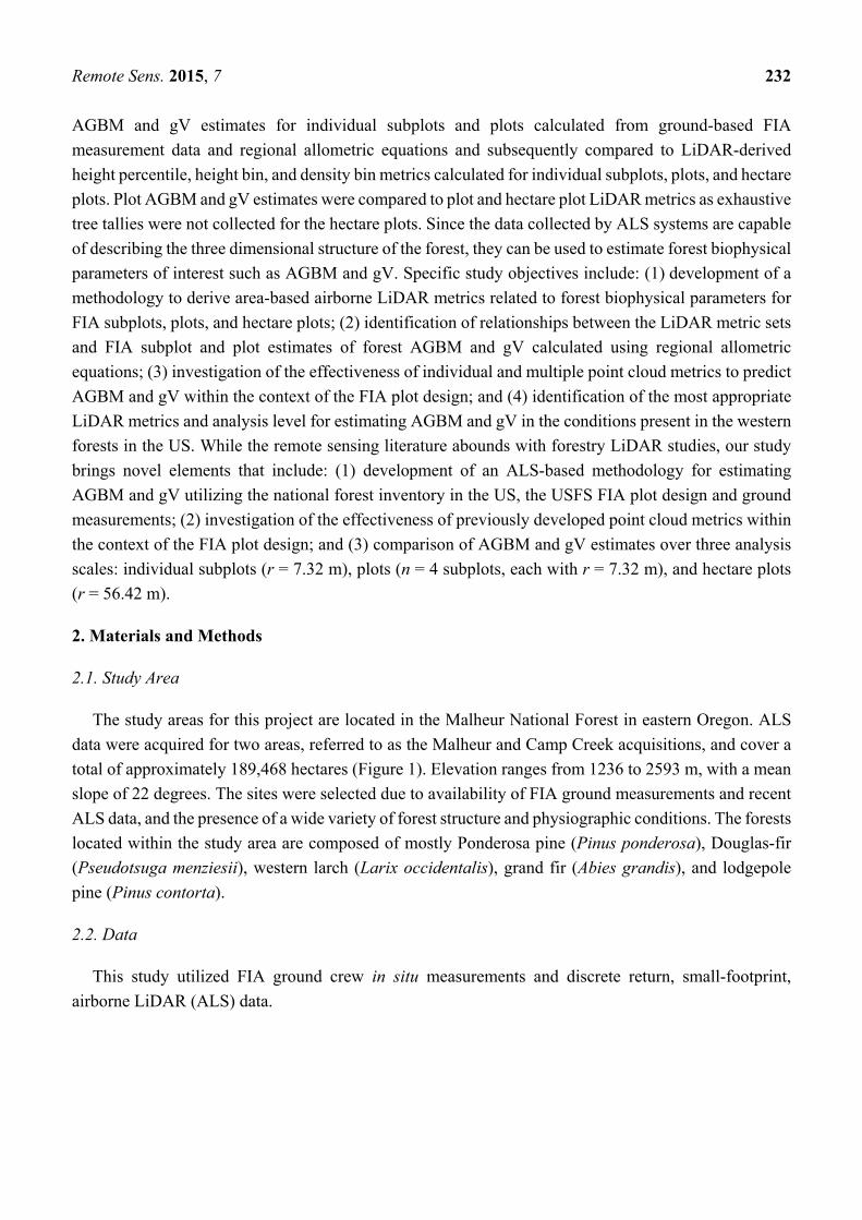
The study areas for this project are located in the Malheur National Forest in eastern Oregon. ALS
data were acquired for two areas, referred to as the Malheur and Camp Creek acquisitions, and cover a
total of approximately 189,468 hectares (Figure 1). Elevation ranges from 1236 to 2593 m, with a mean
slope of 22 degrees. The sites were selected due to availability of FIA ground measurements and recent
ALS data, and the presence of a wide variety of forest structure and physiographic conditions. The forests
located within the study area are composed of mostly Ponderosa pine (Pinus ponderosa), Douglas-fir
(Pseudotsuga menziesii), western larch (Larix occidentalis), grand fir (Abies grandis), and lodgepole
pine (Pinus contorta).
2.2. Data
This study utilized FIA ground crew in situ measurements and discrete return, small-footprint,
airborne LiDAR (ALS) data.
Remote Sens. 2015, 7 233
Figure 1. Malheur National Forest study area in eastern Oregon with slope depicted in
degrees. Black squares represent locations of selected Forest Inventory and Analysis plots
field-visited between 2007 and 2009. Actual plot locations have been obscured due to
confidentiality constraints.
2.2.1. Forest Inventory and Analysis Data
The USFS provided FIA data for all FIA plots within the study area (177 plots, 708 subplots, and
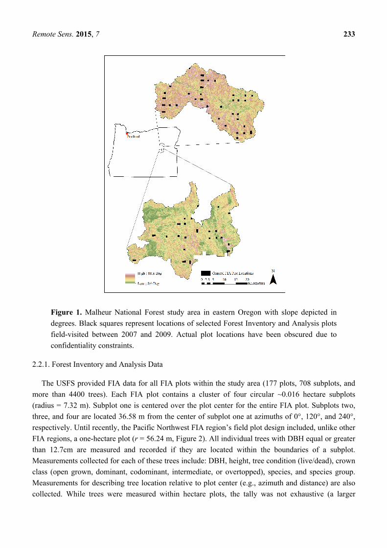
more than 4400 trees). Each FIA plot contains a cluster of four circular ~0.016 hectare subplots
(radius = 7.32 m). Subplot one is centered over the plot center for the entire FIA plot. Subplots two,
three, and four are located 36.58 m from the center of subplot one at azimuths of 0°, 120°, and 240°,
respectively. Until recently, the Pacific Northwest FIA region’s field plot design included, unlike other
FIA regions, a one-hectare plot (r = 56.24 m, Figure 2). All individual trees with DBH equal or greater
than 12.7cm are measured and recorded if they are located within the boundaries of a subplot.
Measurements collected for each of these trees include: DBH, height, tree condition (live/dead), crown
class (open grown, dominant, codominant, intermediate, or overtopped), species, and species group.
Measurements for describing tree location relative to plot center (e.g., azimuth and distance) are also
collected. While trees were measured within hectare plots, the tally was not exhaustive (a larger
Remote Sens. 2015, 7 234
minimum DBH threshold was employed). Tree measurements from hectare plots were not utilized in
this study.
Figure 2. The location and dimensions of the subplots (r = 7.32 m) and one-hectare
(r = 56.42 m) plot used by the Pacific Northwest Forest Inventory and Analysis region.
Figure not drawn to scale.
The regional equations used to calculate individual tree AGBM and gV estimates are discussed in
detail in [50]. AGBM estimates can be derived from gV estimates by simple linear scaling, where the
scaling factor is the mean specific gravity for a particular species. Thus, estimates of AGBM and gV
produced with regional equations tend to be highly correlated.
Subplot-level estimates of total AGBM and gV were calculated by summing the AGBM and gV
estimates for all live trees (meeting FIA measurement requirements) within each subplot. Total subplot
AGBM and gV were then scaled to a per hectare estimates. Plot and hectare plot estimates for total
AGBM and gV were calculated using the total AGBM and gV for all subplots within each hectare plot.
Total AGBM and gV were then scaled to a per hectare estimate. In essence, the area from the four
subplots is scaled up to one hectare. It is important to note that the same estimates of field-based AGBM
and gV are utilized for the plots and hectare plots, as field data for all of the trees within hectare plots
were not available.
The FIA ground crew data utilized in this study (collected in 2007, 2008, and 2009) contained a total
of 232 subplots and 58 hectare plots (Table 1). Temporal disparities between FIA ground data and the
Subplot 1
Subplot 3Subplot 4
36.58 m
r = 7.32 m
Subplot 2
N
r = 56.42 m
Hectare plot
Remote Sens. 2015, 7 235
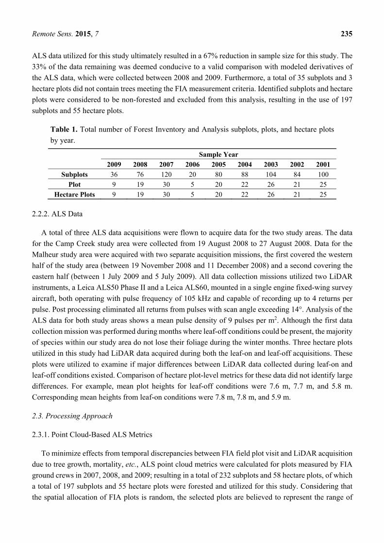
ALS data utilized for this study ultimately resulted in a 67% reduction in sample size for this study. The
33% of the data remaining was deemed conducive to a valid comparison with modeled derivatives of
the ALS data, which were collected between 2008 and 2009. Furthermore, a total of 35 subplots and 3
hectare plots did not contain trees meeting the FIA measurement criteria. Identified subplots and hectare
plots were considered to be non-forested and excluded from this analysis, resulting in the use of 197
subplots and 55 hectare plots.
Table 1. Total number of Forest Inventory and Analysis subplots, plots, and hectare plots
by year.
Sample Year
2009 2008 2007 2006 2005 2004 2003 2002 2001
Subplots 36 76 120 20 80 88 104 84 100
Plot 9 19 30 5 20 22 26 21 25
Hectare Plots 9 19 30 5 20 22 26 21 25
2.2.2. ALS Data
A total of three ALS data acquisitions were flown to acquire data for the two study areas. The data
for the Camp Creek study area were collected from 19 August 2008 to 27 August 2008. Data for the
Malheur study area were acquired with two separate acquisition missions, the first covered the western
half of the study area (between 19 November 2008 and 11 December 2008) and a second covering the
eastern half (between 1 July 2009 and 5 July 2009). All data collection missions utilized two LiDAR
instruments, a Leica ALS50 Phase II and a Leica ALS60, mounted in a single engine fixed-wing survey
aircraft, both operating with pulse frequency of 105 kHz and capable of recording up to 4 returns per
pulse. Post processing eliminated all returns from pulses with scan angle exceeding 14°. Analysis of the
ALS data for both study areas shows a mean pulse density of 9 pulses per m2. Although the first data
collection mission was performed during months where leaf-off conditions could be present, the majority
of species within our study area do not lose their foliage during the winter months. Three hectare plots
utilized in this study had LiDAR data acquired during both the leaf-on and leaf-off acquisitions. These
plots were utilized to examine if major differences between LiDAR data collected during leaf-on and
leaf-off conditions existed. Comparison of hectare plot-level metrics for these data did not identify large
differences. For example, mean plot heights for leaf-off conditions were 7.6 m, 7.7 m, and 5.8 m.
Corresponding mean heights from leaf-on conditions were 7.8 m, 7.8 m, and 5.9 m.
2.3. Processing Approach
2.3.1. Point Cloud-Based ALS Metrics
To minimize effects from temporal discrepancies between FIA field plot visit and LiDAR acquisition
due to tree growth, mortality, etc., ALS point cloud metrics were calculated for plots measured by FIA
ground crews in 2007, 2008, and 2009; resulting in a total of 232 subplots and 58 hectare plots, of which
a total of 197 subplots and 55 hectare plots were forested and utilized for this study. Considering that
the spatial allocation of FIA plots is random, the selected plots are believed to represent the range of

Remote Sens. 2015, 7 236
slopes and forest conditions present in the Malheur National Forest. Tables 1 and 2 provide summaries
of the data collection year for each subplot and the frequency of tree species in each crown class.
Descriptive statistics for FIA measured DBH and tree height, as well as subplot and hectare plot mean
AGBM and gV are presented in Tables 3 and 4.
Table 2. Tree species crown class frequencies.
Crown Class
Species n a Og b D c CD d I e OT f
Abies concolor 34 0 6 19 6 3 Abies grandis 331 1 52 111 121 46 Juniperus occidentalis 24 0 3 12 7 2 Larix occidentalis 79 0 23 32 23 1 Picea engelmannii 5 0 0 3 2 0 Pinus contorta 250 0 28 125 84 13 Pinus monticola 1 0 1 0 0 0 Pinus ponderosa 411 4 125 178 95 9 Pseudotsuga menziesii 217 0 45 73 76 23 Cercocarpus ledifolius 45 0 0 24 20 1
a Number of trees; b Open grown crown class; c Dominant crown class; d Codominant crown class; e Intermediate crown class; and f Overtopped crown class.
2.3.2. Extraction of Subplot and Hectare Plot Point Clouds
Global positioning system (GPS) coordinates for all subplot center locations were obtained by using
a real time differential, wide area augmentation system enabled survey-grade GPS receiver and
post-processed with information from a base station. Plot coordinates were furnished with estimates of
precision known to correspond to the 95th percentile three-dimensional distance threshold around the
plot center location (Table 5). The resulting geolocation precision of plots used in this study is likely
superior to the coordinates obtained during the 2007–2009 regular FIA field visits, when FIA field crews
were utilizing recreational-grade GPS receivers.
Circular plot buffers for subplots (r = 7.32 m) and hectare plots (r = 56.42 m) were generated using
subplot center coordinates and plot center coordinates, respectively. The buffers for each cluster of four
individual subplot comprising a plot were also merged into one file. Individual subplots, plots, and
hectare plot point clouds were subsequently extracted from the vendor-provided LiDAR tiles utilizing
FUSION [51] (version 3.30, Figure 3), a LiDAR viewing and analysis software suite developed by the
USFS. Previous studies have shown that geolocation error can increase variation in ALS metrics as well
as biophysical parameter estimates based on these metrics [52]. Frazer et al. [53] found that plot size
could amplify or reduce the severity of geolocation error. Increased robustness of larger area plots to
geolocation error is a direct result of the increased amount of overlap between ground and ALS data, the
ability to capture more variability from ground measurements, and the reduction of the perimeter of the
plot with respect to the area within the plot. The conclusions presented in these studies evidence the
possible need to use hectare plot-level point cloud metrics (as opposed to subplot-level point cloud
metrics) since the larger plot area should mitigate and negative effects stemming from geolocation errors.
Remote Sens. 2015, 7 237
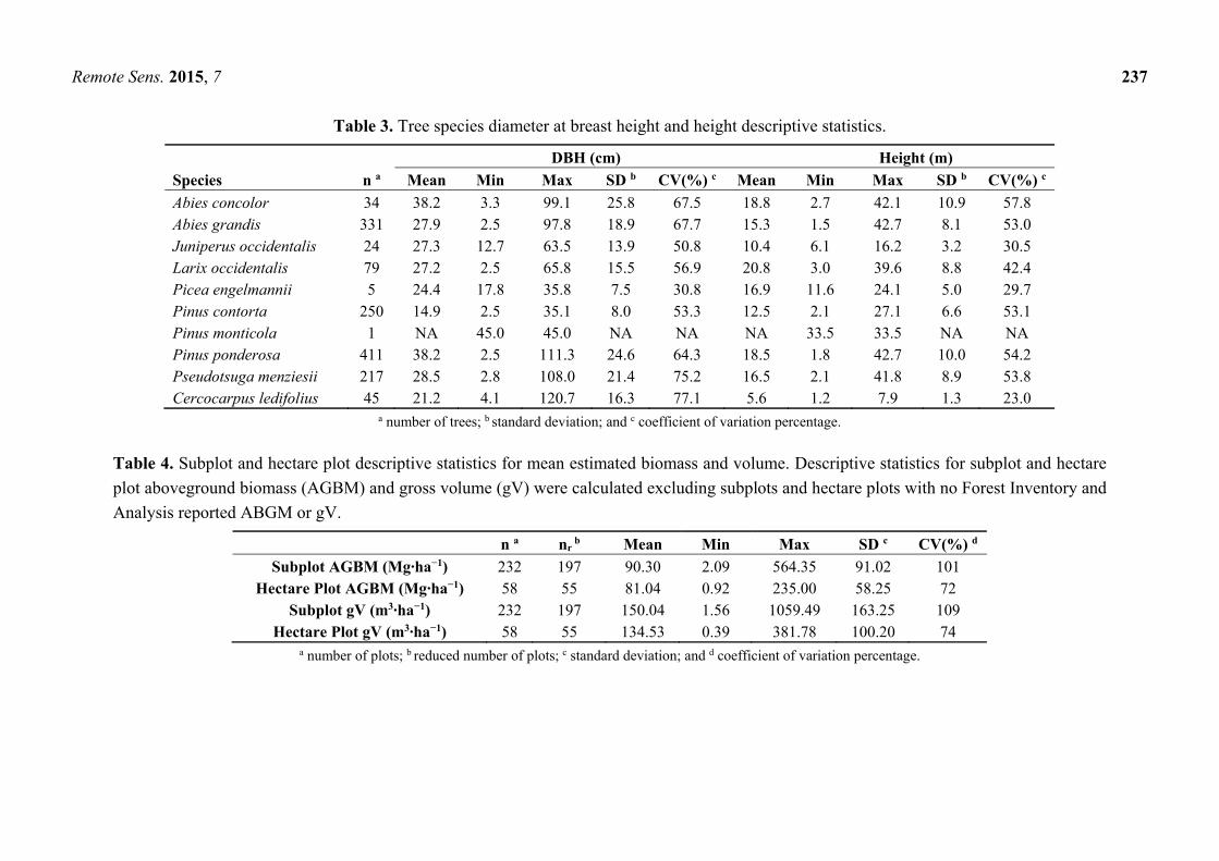
Table 3. Tree species diameter at breast height and height descriptive statistics.
DBH (cm) Height (m)
Species n a Mean Min Max SD b CV(%) c Mean Min Max SD b CV(%) c
Abies concolor 34 38.2 3.3 99.1 25.8 67.5 18.8 2.7 42.1 10.9 57.8 Abies grandis 331 27.9 2.5 97.8 18.9 67.7 15.3 1.5 42.7 8.1 53.0 Juniperus occidentalis 24 27.3 12.7 63.5 13.9 50.8 10.4 6.1 16.2 3.2 30.5 Larix occidentalis 79 27.2 2.5 65.8 15.5 56.9 20.8 3.0 39.6 8.8 42.4 Picea engelmannii 5 24.4 17.8 35.8 7.5 30.8 16.9 11.6 24.1 5.0 29.7 Pinus contorta 250 14.9 2.5 35.1 8.0 53.3 12.5 2.1 27.1 6.6 53.1 Pinus monticola 1 NA 45.0 45.0 NA NA NA 33.5 33.5 NA NA Pinus ponderosa 411 38.2 2.5 111.3 24.6 64.3 18.5 1.8 42.7 10.0 54.2 Pseudotsuga menziesii 217 28.5 2.8 108.0 21.4 75.2 16.5 2.1 41.8 8.9 53.8 Cercocarpus ledifolius 45 21.2 4.1 120.7 16.3 77.1 5.6 1.2 7.9 1.3 23.0
a number of trees; b standard deviation; and c coefficient of variation percentage.
Table 4. Subplot and hectare plot descriptive statistics for mean estimated biomass and volume. Descriptive statistics for subplot and hectare
plot aboveground biomass (AGBM) and gross volume (gV) were calculated excluding subplots and hectare plots with no Forest Inventory and
Analysis reported ABGM or gV.
n a nr b Mean Min Max SD c CV(%) d
Subplot AGBM (Mg·ha−1) 232 197 90.30 2.09 564.35 91.02 101 Hectare Plot AGBM (Mg·ha−1) 58 55 81.04 0.92 235.00 58.25 72
Subplot gV (m3·ha−1) 232 197 150.04 1.56 1059.49 163.25 109 Hectare Plot gV (m3·ha−1) 58 55 134.53 0.39 381.78 100.20 74
a number of plots; b reduced number of plots; c standard deviation; and d coefficient of variation percentage.
Remote Sens. 2015, 7 238
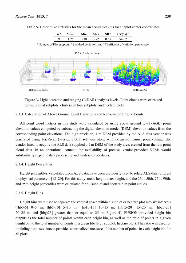
Table 5. Descriptive statistics for the mean accuracies (m) for subplot center coordinates.
n a Mean Min Max SD b CV(%) c
197 1.25 0.38 3.72 0.67 54.02 a Number of FIA subplots; b Standard deviation; and c Coefficient of variation percentage.
Figure 3. Light detection and ranging (LiDAR) analysis levels. Point clouds were extracted
for individual subplots, clusters of four subplots, and hectare plots.
2.3.3. Calculation of Above Ground Level Elevations and Removal of Ground Points
All point cloud metrics in this study were calculated by using above ground level (AGL) point
elevation values computed by subtracting the digital elevation model (DEM) elevation values from the
corresponding point elevations. The high precision, 1 m DEM provided by the ALS data vendor was
generated using TerraScan (version 8.001) software along with extensive manual point editing. The
vendor hired to acquire the ALS data supplied a 1 m DEM of the study area, created from the raw point
cloud data. In an operational context, the availability of precise, vendor-provided DEMs would
substantially expedite data processing and analysis procedures.
2.3.4. Height Percentiles
Height percentiles, calculated from ALS data, have been previously used to relate ALS data to forest
biophysical parameters [18–20]. For this study, mean height, max height, and the 25th, 50th, 75th, 90th,
and 95th height percentiles were calculated for all subplot and hectare plot point clouds.
2.3.5. Height Bins
Height bins were used to separate the vertical space within a subplot or hectare plot into six intervals
([hb0-5] 0–5 m; [hb5-10] 5–10 m; [hb10-15] 10–15 m; [hb15-20] 15–20 m; [hb20-25]
20–25 m; and [hbgt25] greater than or equal to 25 m; Figure 4). FUSION provided height bin
outputs as the total number of points within each height bin, as well as the ratio of points in a given
height bin to the total number of points in a given file (e.g., subplot, hectare plot). The ratio was used for
modeling purposes since it provides a normalized measure of the number of points in each height bin for
all plots.
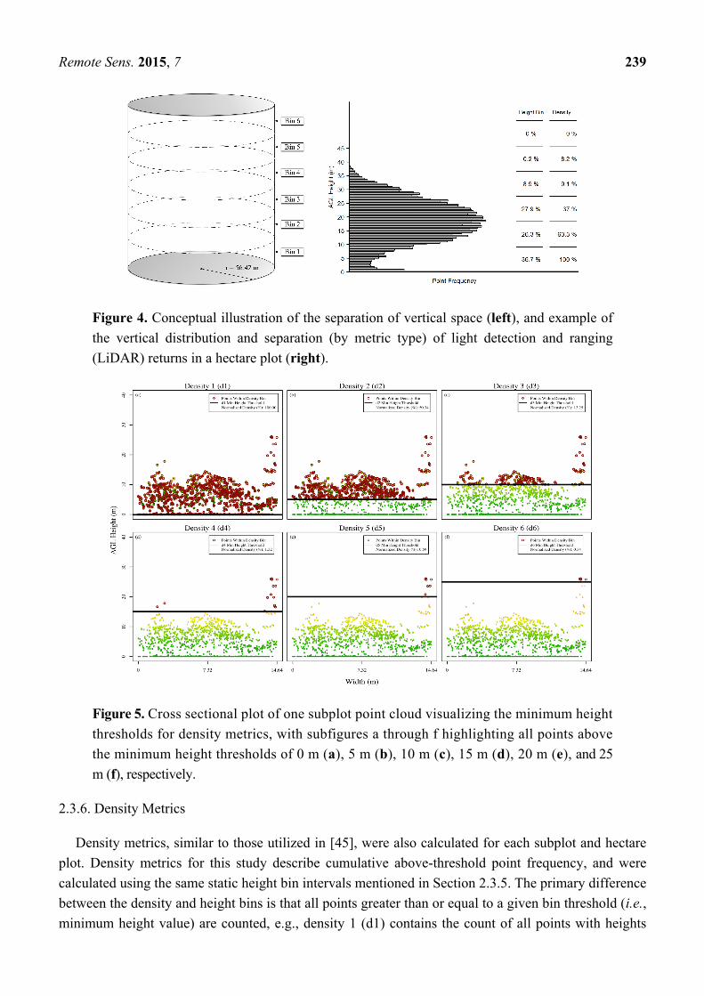
Remote Sens. 2015, 7 239
Figure 4. Conceptual illustration of the separation of vertical space (left), and example of
the vertical distribution and separation (by metric type) of light detection and ranging
(LiDAR) returns in a hectare plot (right).
Figure 5. Cross sectional plot of one subplot point cloud visualizing the minimum height
thresholds for density metrics, with subfigures a through f highlighting all points above
the minimum height thresholds of 0 m (a), 5 m (b), 10 m (c), 15 m (d), 20 m (e), and 25
m (f), respectively.
2.3.6. Density Metrics
Density metrics, similar to those utilized in [45], were also calculated for each subplot and hectare
plot. Density metrics for this study describe cumulative above-threshold point frequency, and were
calculated using the same static height bin intervals mentioned in Section 2.3.5. The primary difference
between the density and height bins is that all points greater than or equal to a given bin threshold (i.e.,
minimum height value) are counted, e.g., density 1 (d1) contains the count of all points with heights
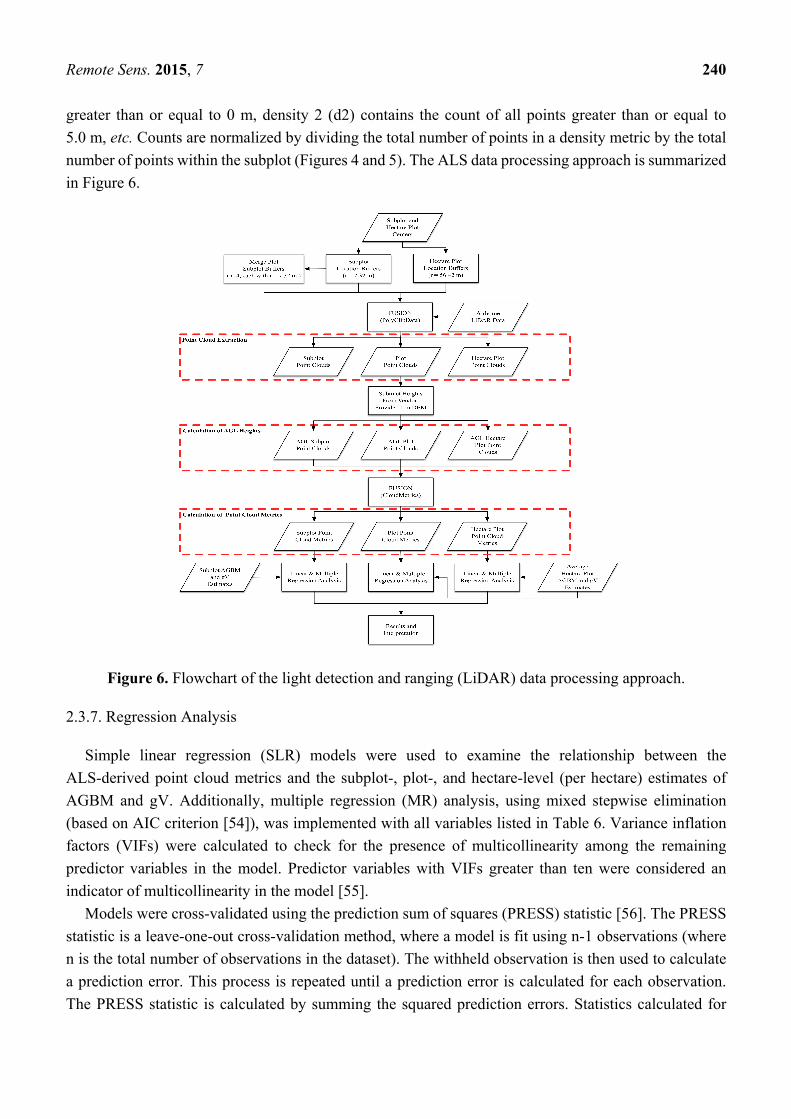
Remote Sens. 2015, 7 240
greater than or equal to 0 m, density 2 (d2) contains the count of all points greater than or equal to
5.0 m, etc. Counts are normalized by dividing the total number of points in a density metric by the total
number of points within the subplot (Figures 4 and 5). The ALS data processing approach is summarized
in Figure 6.
Figure 6. Flowchart of the light detection and ranging (LiDAR) data processing approach.
2.3.7. Regression Analysis
Simple linear regression (SLR) models were used to examine the relationship between the
ALS-derived point cloud metrics and the subplot-, plot-, and hectare-level (per hectare) estimates of
AGBM and gV. Additionally, multiple regression (MR) analysis, using mixed stepwise elimination
(based on AIC criterion [54]), was implemented with all variables listed in Table 6. Variance inflation
factors (VIFs) were calculated to check for the presence of multicollinearity among the remaining
predictor variables in the model. Predictor variables with VIFs greater than ten were considered an
indicator of multicollinearity in the model [55].
Models were cross-validated using the prediction sum of squares (PRESS) statistic [56]. The PRESS
statistic is a leave-one-out cross-validation method, where a model is fit using n-1 observations (where
n is the total number of observations in the dataset). The withheld observation is then used to calculate
a prediction error. This process is repeated until a prediction error is calculated for each observation.
The PRESS statistic is calculated by summing the squared prediction errors. Statistics calculated for
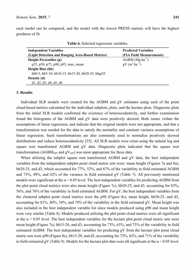
Remote Sens. 2015, 7 241
each model can be compared, and the model with the lowest PRESS statistic will have the highest
goodness of fit.
Table 6. Selected regression variables.
Independent Variables (Light Detection and Ranging Area-Based Metrics)
Predicted Variables (FIA Field Measurements)
Height Percentiles (p) AGBM (Mg·ha−1) p25, p50, p75, p90, p95, max, mean gV (m3·ha−1)
Height Bins (hb) hb0-5, hb5-10, hb10-15, hb15-20, hb20-25, hbgt25
Density (d) d1, d2, d3, d4, d5, d6
3. Results
Individual SLR models were created for the AGBM and gV estimates using each of the point
cloud-based metrics calculated for the individual subplots, plots, and the hectare plots. Diagnostic plots
from the initial SLR models confirmed the existence of heteroscedasticity, and further examination
found the histograms of the AGBM and gV data were positively skewed. Both issues violate the
assumptions of linear regression, and indicate that the original models were not appropriate, and that a
transformation was needed for the data to satisfy the normality and constant variance assumptions of
linear regression. Such transformations are also commonly used to normalize positively skewed
distributions and reduce heteroscedasticity [55]. All SLR models were rerun using the natural log and
square root transformed AGBM and gV data. Diagnostic plots indicated that the square root
transformation (AGBMsqrt and gVsqrt) was most appropriate for these data.
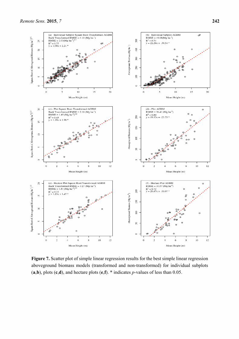
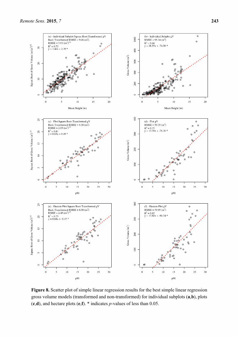
When utilizing the subplot square root transformed AGBM and gV data, the best independent
variables from the independent subplot point cloud metric sets were: mean height (Figures 7a and 8a),
hb20-25, and d3, which accounted for 77%, 52%, and 67% of the variability in field estimated AGBM
and 73%, 49%, and 62% of the variance in field estimated gV (Table 7). All previously mentioned
models were significant at the α = 0.05 level. The best independent variables for predicting AGBM from
the plot point cloud metrics were also mean height (Figure 7c), hb20-25, and d3, accounting for 83%,
56%, and 76% of the variability in field estimated AGBM. For gV, the best independent variables from
the clustered subplot point cloud metrics were the p90 (Figure 8c), mean height, hb20-25, and d3,
accounting for 81%, 80%, 54%, and 74% of the variability in the field estimated gV. Mean height was
also included in the best independent variable list since models produced using p90 and mean height
were very similar (Table 8). Models produced utilizing the plot point cloud metrics were all significant
at the α = 0.05 level. The best independent variables for the hectare plot point cloud metric sets were
mean height (Figure 7e), hb15-20, and d3, accounting for 73%, 63%, and 73% of the variability in field
estimated AGBM. The best independent variables for predicting gV from the hectare plot point cloud
metric sets were p90 (Figure 8e), hb15-20, and d3, accounting for 73%, 62%, and 71% of the variability
in field estimated gV (Table 9). Models for the hectare plot data were all significant at the α = 0.05 level.
Remote Sens. 2015, 7 242
Figure 7. Scatter plot of simple linear regression results for the best simple linear regression
aboveground biomass models (transformed and non-transformed) for individual subplots
(a,b), plots (c,d), and hectare plots (e,f). * indicates p-values of less than 0.05.
Remote Sens. 2015, 7 243
Figure 8. Scatter plot of simple linear regression results for the best simple linear regression
gross volume models (transformed and non-transformed) for individual subplots (a,b), plots
(c,d), and hectare plots (e,f). * indicates p-values of less than 0.05.
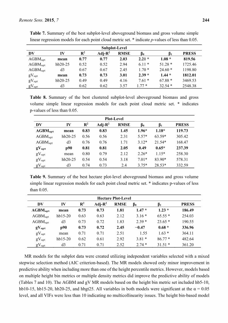
Remote Sens. 2015, 7 244
Table 7. Summary of the best subplot-level aboveground biomass and gross volume simple
linear regression models for each point cloud metric set. * indicate p-values of less than 0.05.
Subplot-Level DV IV R2 Adj-R2 RMSE β0 β1 PRESS AGBMsqrt mean 0.77 0.77 2.03 2.21 * 1.08 * 819.56 AGBMsqrt hb20-25 0.52 0.52 2.94 6.11 * 51.28 * 1725.46 AGBMsqrt d3 0.67 0.67 2.45 1.70 * 24.60 * 1198.80 gVsqrt mean 0.73 0.73 3.01 2.39 * 1.44 * 1812.01 gVsqrt hb20-25 0.49 0.49 4.16 7.61 * 67.88 * 3469.53 gVsqrt d3 0.62 0.62 3.57 1.77 * 32.54 * 2548.38
Table 8. Summary of the best clustered subplot-level aboveground biomass and gross
volume simple linear regression models for each point cloud metric set. * indicates
p-values of less than 0.05.
Plot-Level
DV IV R2 Adj-R2 RMSE β0 β1 PRESS
AGBMsqrt mean 0.83 0.83 1.45 1.96* 1.18* 119.73 AGBMsqrt hb20-25 0.56 0.56 2.31 5.57* 63.59* 305.42 AGBMsqrt d3 0.76 0.76 1.71 3.12* 21.54* 168.47 gVsqrt p90 0.81 0.81 2.05 0.49 0.65* 237.39 gVsqrt mean 0.80 0.79 2.12 2.26* 1.15* 258.30 gVsqrt hb20-25 0.54 0.54 3.18 7.01* 83.90* 578.31 gVsqrt d3 0.74 0.73 2.4 3.75* 28.53* 332.59
Table 9. Summary of the best hectare plot-level aboveground biomass and gross volume
simple linear regression models for each point cloud metric set. * indicates p-values of less
than 0.05.
Hectare Plot-Level
DV IV R2 Adj-R2 RMSE β0 β1 PRESS
AGBMsqrt mean 0.73 0.73 1.81 1.47 * 1.23 * 186.49 AGBMsqrt hb15-20 0.63 0.63 2.12 3.16 * 65.55 * 254.03 AGBMsqrt d3 0.73 0.72 1.83 2.39 * 23.65 * 190.55
gVsqrt p90 0.73 0.72 2.45 −0.47 0.68 * 336.96 gVsqrt mean 0.71 0.71 2.51 1.55 1.63 * 364.11 gVsqrt hb15-20 0.62 0.61 2.92 3.81 * 86.77 * 482.64 gVsqrt d3 0.71 0.71 2.52 2.74 * 31.51 * 361.20
MR models for the subplot data were created utilizing independent variables selected with a mixed
stepwise selection method (AIC criterion-based). The MR models showed only minor improvement in
predictive ability when including more than one of the height percentile metrics. However, models based
on multiple height bin metrics or multiple density metrics did improve the predictive ability of models
(Tables 7 and 10). The AGBM and gV MR models based on the height bin metric set included hb5-10,
hb10-15, hb15-20, hb20-25, and hbgt25. All variables in both models were significant at the α = 0.05
level, and all VIFs were less than 10 indicating no multicollinearity issues. The height bin-based model
Remote Sens. 2015, 7 245
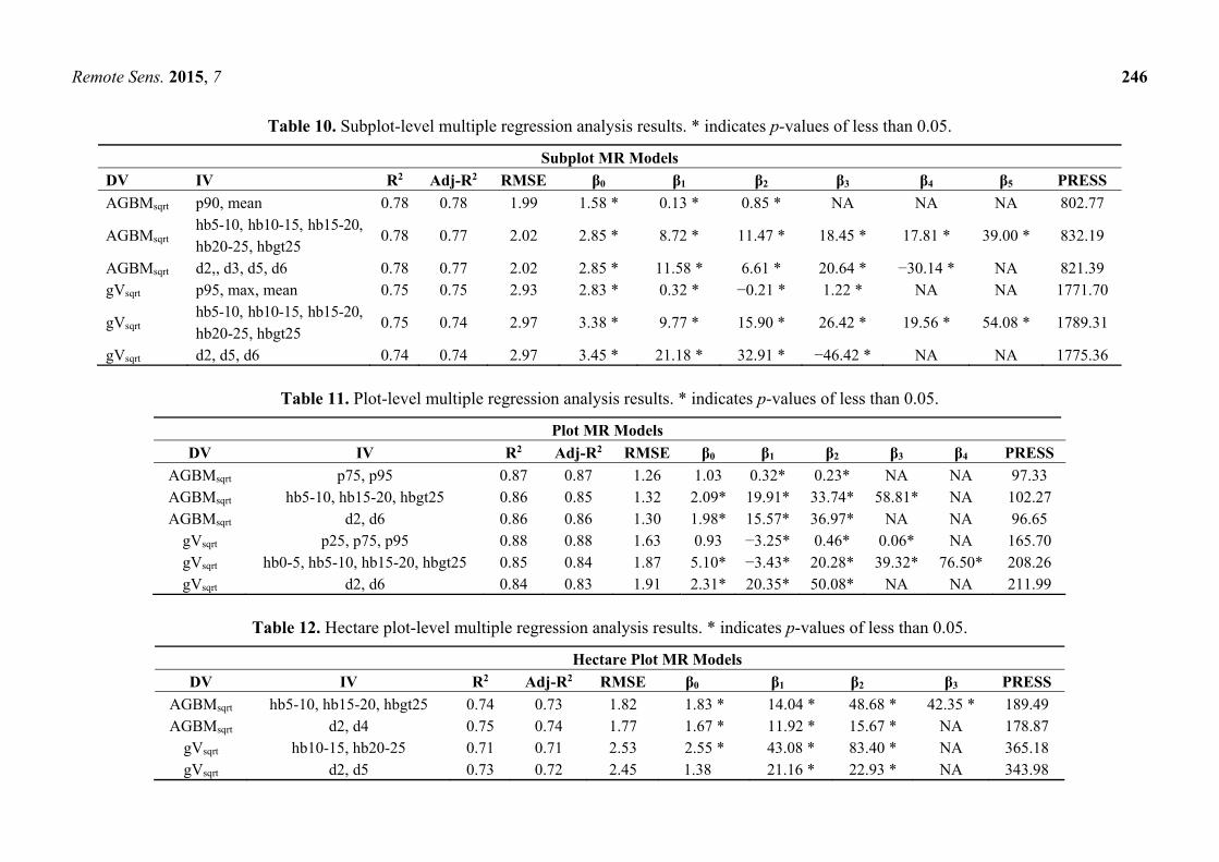
was able to explain 78% of the variability in field estimated AGBM at the subplot-level. The height bin
based gV MR model was able to explain 75% of the variability in gV. The MR model for predicting
subplot AGBM from density metrics utilized d2, d3, d5, and d6, while the MR model for predicting
subplot gV from density metrics utilized d2, d5, and d6. All model variables were significant at the
α = 0.05 level, and VIFs were below 10. The MR models were able to explain 78% and 74% of the
variance in field estimated AGBM and gV, respectively.
For MR models based on plot metric sets (Table 11), the addition of multiple independent variables
improved models for every metric set. Models utilizing percentile metrics as independent variables were
able to account for the greatest variability in the field estimated AGBM and gV, 87% and 88%,
respectively. The most notable improvement was seen in models utilizing height bin metrics, where the
use of multiple height bin metrics allowed height bin-based models of AGBM and gV to account for
86% and 85% of the variability in the field estimated AGBM and gV, as compared to SLR models
(utilizing hb20-25) which accounted for 56% and 54% of the variability in field estimated AGBM and
gV. AGBM and gV models employing density metrics both utilized two density bins (d2 and d6), and
were able to account for 86% and 84% of the variability in the field estimated AGBM and gV. All models
reported in Table 11 were significant at the α = 0.05 level, and showed no multicollinearity issues (all
VIFs were lower than 10).
For MR models based on hectare plot metric sets, the addition of multiple independent variables only
improved models based on height bin metrics or density metrics. The percentile-based MR models (for
ABGM and gV) identified several independent variables (mean height and p90 for AGBM and mean
height p90, and p25 for gV), but not all of the selected variables were significant at the α = 0.05 level,
and had VIFs larger than 10 (indicating multicollinearity). The resulting model had a lower R2 value and
higher RMSE than the SLR models developed for AGBM and gV SLR. The initial height bin-based MR
model for AGBM (utilizing the square root transformation) utilized hb5-10, hb10-15, and hb15-20 as
independent variables. This model showed no multicollinearity issues (VIFs below 10). All independent
variables utilized were significant at the α = 0.05 level. The height bin-based model for gV (utilizing the
square root transformation) employed hb10-15 and hb20-25, and showed no indication of
multicollinearity (VIFs below 10). All independent variables were significant at the α = 0.05 level. The
height bin-based MR models for AGBM and gV accounted for 74% and 73% of the variability in field
estimated AGBM and gV, respectively. Analysis of the VIFs for the initial density-based MR models
for the square root transformed AGBM and square root transformed gV did not indicate multicollinearity
issues. All selected independent variables (d2 and d4 for AGBM and d2 and d5 for gV) were significant
at the α = 0.05 level. Density-based MR models for AGBM and gV accounted for 75% and 73% of the
variability in the field estimated AGBM and gV, respectively.
Modeling results presented above show that model R2 values improved from models based on
individual subplots to models based on plots. When the scale of the analysis level is increased to the
hectare plot-level, a decrease in model R2 values was observed. This pattern was visible in both SLR
models and MR models (Tables 7–9 and 10–12, respectively). Overall, the best R2 values were obtained
when using plot-level analysis.
Remote Sens. 2015, 7 246
Table 10. Subplot-level multiple regression analysis results. * indicates p-values of less than 0.05.
Subplot MR Models
DV IV R2 Adj-R2 RMSE β0 β1 β2 β3 β4 β5 PRESS
AGBMsqrt p90, mean 0.78 0.78 1.99 1.58 * 0.13 * 0.85 * NA NA NA 802.77
AGBMsqrt hb5-10, hb10-15, hb15-20, hb20-25, hbgt25
0.78 0.77 2.02 2.85 * 8.72 * 11.47 * 18.45 * 17.81 * 39.00 * 832.19
AGBMsqrt d2,, d3, d5, d6 0.78 0.77 2.02 2.85 * 11.58 * 6.61 * 20.64 * −30.14 * NA 821.39 gVsqrt p95, max, mean 0.75 0.75 2.93 2.83 * 0.32 * −0.21 * 1.22 * NA NA 1771.70
gVsqrt hb5-10, hb10-15, hb15-20, hb20-25, hbgt25
0.75 0.74 2.97 3.38 * 9.77 * 15.90 * 26.42 * 19.56 * 54.08 * 1789.31
gVsqrt d2, d5, d6 0.74 0.74 2.97 3.45 * 21.18 * 32.91 * −46.42 * NA NA 1775.36
Table 11. Plot-level multiple regression analysis results. * indicates p-values of less than 0.05.
Plot MR Models
DV IV R2 Adj-R2 RMSE β0 β1 β2 β3 β4 PRESS
AGBMsqrt p75, p95 0.87 0.87 1.26 1.03 0.32* 0.23* NA NA 97.33 AGBMsqrt hb5-10, hb15-20, hbgt25 0.86 0.85 1.32 2.09* 19.91* 33.74* 58.81* NA 102.27 AGBMsqrt d2, d6 0.86 0.86 1.30 1.98* 15.57* 36.97* NA NA 96.65
gVsqrt p25, p75, p95 0.88 0.88 1.63 0.93 −3.25* 0.46* 0.06* NA 165.70 gVsqrt hb0-5, hb5-10, hb15-20, hbgt25 0.85 0.84 1.87 5.10* −3.43* 20.28* 39.32* 76.50* 208.26 gVsqrt d2, d6 0.84 0.83 1.91 2.31* 20.35* 50.08* NA NA 211.99
Table 12. Hectare plot-level multiple regression analysis results. * indicates p-values of less than 0.05.
Hectare Plot MR Models
DV IV R2 Adj-R2 RMSE β0 β1 β2 β3 PRESS
AGBMsqrt hb5-10, hb15-20, hbgt25 0.74 0.73 1.82 1.83 * 14.04 * 48.68 * 42.35 * 189.49 AGBMsqrt d2, d4 0.75 0.74 1.77 1.67 * 11.92 * 15.67 * NA 178.87
gVsqrt hb10-15, hb20-25 0.71 0.71 2.53 2.55 * 43.08 * 83.40 * NA 365.18 gVsqrt d2, d5 0.73 0.72 2.45 1.38 21.16 * 22.93 * NA 343.98
Remote Sens. 2015, 7 247
4. Discussion
Previous studies have found that ALS-derived variables describing the height of trees can produce
accurate AGBM, gV, and other forest biophysical parameter predictions [15–27]. To our knowledge,
few studies have compared the ability of height percentile, height bin, and density LiDAR metrics to
estimate AGBM and gV for the same dataset. In one such study, Næsset and Gobakken [57] compare
similar LiDAR metrics, but focused on forest growth using mean tree height, basal area, and volume
under different forest conditions than those present in the Malheur National Forest. Our study is also
unique in its analysis utilizing point cloud metrics from individual subplots, plots comprising a cluster
of 4 subplots, and hectare plots to determine which dataset would best estimate AGBM and gV. Hectare
plots were also utilized due to concern regarding geolocation and edge effect errors commonly associated
with small area plots [51,52]. Table 5 provides descriptive statistics for the subplot center coordinates
used to extract plot-level LiDAR data. Plot center GPS data utilized for this study exhibit superior
geolocation precision when compared to the recreational-grade GPS receivers usually employed by FIA
field crews.
After our analyses, it can be inferred that geolocation and edge effect errors did not have noticeable
effect on the ability of subplot point cloud metrics to estimate AGBM and gV within our study area.
However, future research efforts will attempt to quantify how geolocation and edge effect errors affected
our AGBM and gV estimates. The best predictors of AGBM and gV at the individual
subplot-level were mean height, hb20-25, and d3. Individual subplot SLR models based on hb20-25
exhibited a moderate relationship to AGBM and gV, while models based on d3 and mean height
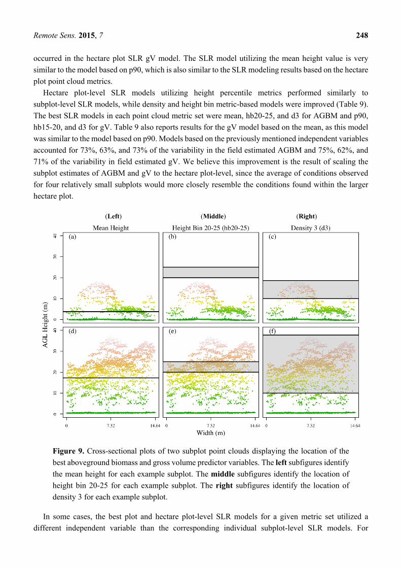
exhibited a stronger relationship. A visual examination of a subset of subplot point clouds identified that
subplot-level mean height is commonly located near a high density cluster of LiDAR returns in the
vertical distribution (as expected), while d3 typically covers a majority of the points within the upper
forest canopy (Figure 9). This suggests that mean height is an accurate predictor of AGBM and gV
because it accurately describes tree height for the majority of trees on a plot. The d3 metric typically
provides information on the taller trees within a plot, although in the presence of mostly short trees it
may fail to capture such information (Figure 9c,f). One possible reason for poor performance of SLR
models based on subplot hb20-25 is the limited number of returns occurring within the 20–25 m. Thus,
when larger trees are present within a plot this metric provides information useful for describing subplot-
level AGBM or gV (since these trees will typically contain a large portion of the AGBM or gV within a
subplot). However, when subplots contain trees less than 20 m tall, this metric essentially reports that no
vegetation layers are present within a plot (Figure 9b). This suggests that multiple height bin metrics
might be required to correctly model AGBM and gV for forests with conditions similar to those exhibited
in the Malheur National Forest. Our subplot MR models utilizing height bin-based independent variables
(Table 9) provide evidence for this finding, with the final model utilizing multiple height bin metrics,
exhibiting no multicollinearity issues, and accounting for a similar amount of variance in field estimated
AGBM and gV as the best subplot SLR models.
Overall, the plot SLR and MR models were able to account for the largest amounts of variability in
the field estimate AGBM and gV (Table 8). LiDAR-derived independent variables for the clustered
subplot SLR models were mostly the same as those identified for the individual subplot models (mean,
hb20-25, and d3). However, the best SLR model for gV utilized the percentile metric p90. This also
Remote Sens. 2015, 7 248
occurred in the hectare plot SLR gV model. The SLR model utilizing the mean height value is very
similar to the model based on p90, which is also similar to the SLR modeling results based on the hectare
plot point cloud metrics.
Hectare plot-level SLR models utilizing height percentile metrics performed similarly to
subplot-level SLR models, while density and height bin metric-based models were improved (Table 9).
The best SLR models in each point cloud metric set were mean, hb20-25, and d3 for AGBM and p90,
hb15-20, and d3 for gV. Table 9 also reports results for the gV model based on the mean, as this model
was similar to the model based on p90. Models based on the previously mentioned independent variables
accounted for 73%, 63%, and 73% of the variability in the field estimated AGBM and 75%, 62%, and
71% of the variability in field estimated gV. We believe this improvement is the result of scaling the
subplot estimates of AGBM and gV to the hectare plot-level, since the average of conditions observed
for four relatively small subplots would more closely resemble the conditions found within the larger
hectare plot.
(Left) (Middle) (Right)
Figure 9. Cross-sectional plots of two subplot point clouds displaying the location of the
best aboveground biomass and gross volume predictor variables. The left subfigures identify
the mean height for each example subplot. The middle subfigures identify the location of
height bin 20-25 for each example subplot. The right subfigures identify the location of
density 3 for each example subplot.
In some cases, the best plot and hectare plot-level SLR models for a given metric set utilized a
different independent variable than the corresponding individual subplot-level SLR models. For
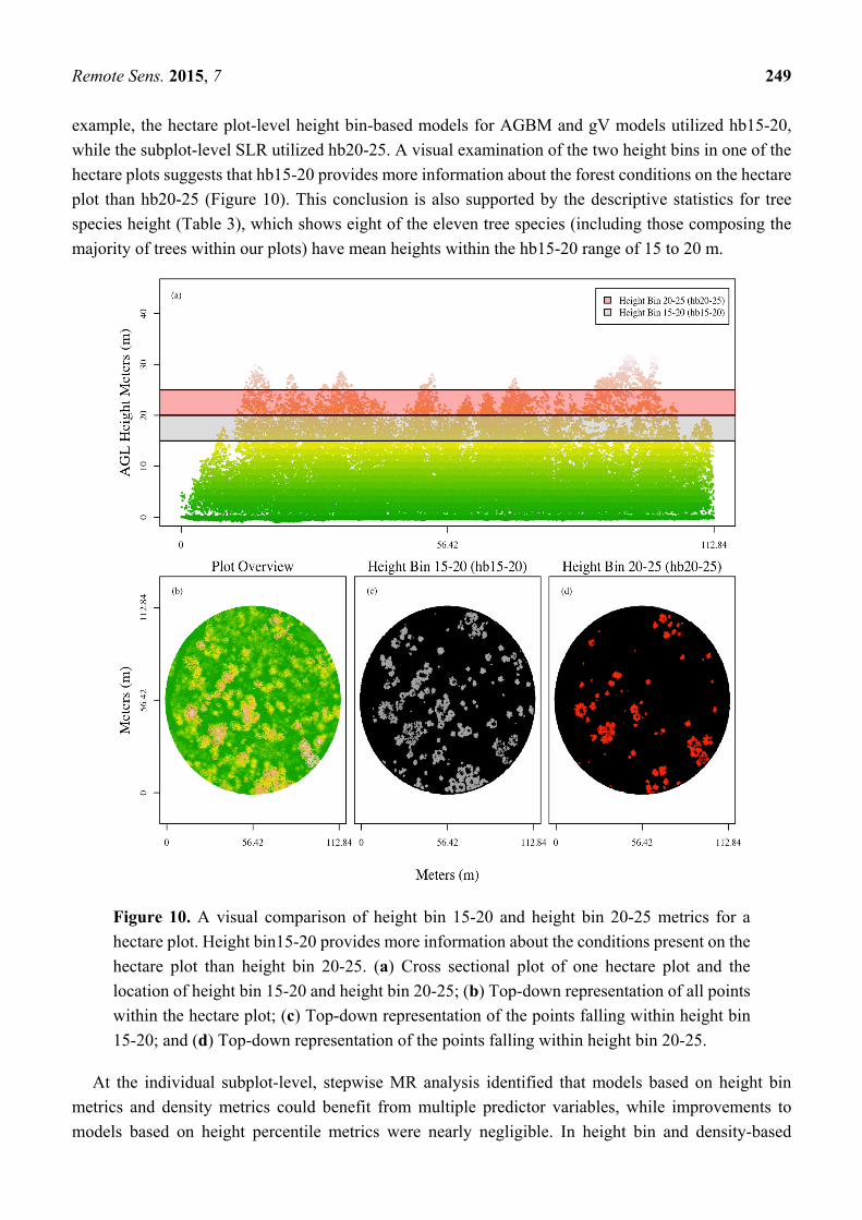
Remote Sens. 2015, 7 249
example, the hectare plot-level height bin-based models for AGBM and gV models utilized hb15-20,
while the subplot-level SLR utilized hb20-25. A visual examination of the two height bins in one of the
hectare plots suggests that hb15-20 provides more information about the forest conditions on the hectare
plot than hb20-25 (Figure 10). This conclusion is also supported by the descriptive statistics for tree
species height (Table 3), which shows eight of the eleven tree species (including those composing the
majority of trees within our plots) have mean heights within the hb15-20 range of 15 to 20 m.
Figure 10. A visual comparison of height bin 15-20 and height bin 20-25 metrics for a
hectare plot. Height bin15-20 provides more information about the conditions present on the
hectare plot than height bin 20-25. (a) Cross sectional plot of one hectare plot and the
location of height bin 15-20 and height bin 20-25; (b) Top-down representation of all points
within the hectare plot; (c) Top-down representation of the points falling within height bin
15-20; and (d) Top-down representation of the points falling within height bin 20-25.
At the individual subplot-level, stepwise MR analysis identified that models based on height bin
metrics and density metrics could benefit from multiple predictor variables, while improvements to
models based on height percentile metrics were nearly negligible. In height bin and density-based
Remote Sens. 2015, 7 250
models, the inclusion of multiple predictors increased the predictive ability of the models to a level
similar to the mean height-based SLR model, with R2 values ranging from 0.74 to 0.78. AGBM and gV
models utilizing height bin metrics always required more predictor variables than models utilizing
density metrics, in part due to the compartmentalized nature of height bin metrics. Density metrics
exhibit strong spatial correlation, and as such the inclusion of a large number of density bins leads to
multicollinearity issues.
At the plot analysis level, stepwise MR analysis identified that models for each metric set could
benefit from multiple predictor variables. While multiple independent variables were utilized in models
for each metric set, a decrease in the number of variables in the height bin and density based models is
observed. At the hectare plot-level, stepwise MR analysis identified that models utilizing height bin or
density metrics would benefit from multiple predictor variables, while no additional predictor variables
were identified for models based on height percentiles. However, it should be noted that density metric
based models received only a minor improvement when a second predictor variable was added.
Results for the MR analyses show that point cloud metrics derived from the clustered subplots were
able to account for the most variability in field estimated AGBM and gV, followed by models based on
individual subplot metrics, and models based on hectare plot metrics. We hypothesize that the extent of
hectare plot point cloud metrics was too large to adequately describe the average conditions present in
the four subplots contained within each hectare plot. Future studies will investigate if a more appropriate
plot size for LiDAR data covering the four subplots exists.
While subplot-level and hectare plot-level analyses produced adequate SLR and MR models, the best
SLR and MR models were produced with the plot-level analysis. We believe there are several reasons
why the plot level analysis produced the best results. When moving from subplot- to plot-level, the
sample size is increased three-fold. If AGBM or gV is spatially distributed as a uniform
random process, where tree locations approximating a Poisson simple point pattern and tree sizes
approximating a distribution skewed to the right (considered to be the usual case) we expect estimation
accuracy to increase rapidly with initial increases in sample size. However, when the spatial extent of
the analysis is increased from the plot-level to the hectare plot-level we are forced to assume that the
population is distributed identically within the hectare as within the subplots. This assumption might not
be valid for all hectare plots utilizing the current field data, which was collected for each of the subplots.
Thus, reductions in model R2 values are a result of the discrepancies in the population distribution
between hectare plots and plots. Such discrepancies would not be an issue if exhaustive tree tallies were
available for the hectare plots. Overall, this finding provides evidence that the current FIA plot design
can be used with dense airborne LiDAR data to produce area-based estimates of AGBM and gV.
5. Conclusions
This study represents an initial attempt to model biophysical parameters of interest to the FIA
program utilizing the standard FIA plot design, data from FIA ground crews, and ALS data.
As previously mentioned, other studies have successfully modeled similar forest parameters with ALS
data [15–27,34,46,49,55]. However, to our knowledge none have done so for multiple analysis level
(i.e., subplot, plot, and hectare plot) comparing the performance of percentile, height bin, and density
metrics, and specifically focused on modeling AGBM and gV for FIA purposes. Models based on
Remote Sens. 2015, 7 251
subplot point cloud metrics, for AGBM and gV provided results similar to those presented in the
literature and cited throughout this study.
Overall results from this study show that ALS can be used to create models that describe the AGBM
and gV of Pacific Northwest FIA subplots with results comparable in accuracy to those of other
published studies. Point cloud metrics based on PNW FIA hectare plots or individual subplots were not
able to describe AGBM and gV as well as those based on plot point cloud metrics. The ability of ALS
to collect data over large areas coupled with these results demonstrates the potential of ALS systems to
augment current FIA data collection procedures by providing a temporary intermediate estimation of
AGBM and gV for plots with outdated field measurements. We hypothesize that these intermediate
estimates could prove beneficial for increasing the accuracy of forest C budgets by reducing
variance caused by temporal measurement discrepancies in the currently available FIA measurements.
However, more work must be done to quantify the amount of variance that would be reduced due to
temporal measurement discrepancies, as well as the contribution of ALS-based estimates to this variance.
Future research identified by this study, includes: (1) utilization of regional species-specific growth
and yield models to mitigate error caused by out-of-date tree measurements, while increasing the number
of samples available for use in modeling efforts; and (2) investigations of how GPS accuracy and ALS
data can be utilized to identify plots to be withheld from future modeling exercises.
Acknowledgments
We would like to thank the United States Forest Service Pacific Northwest Research station for their
support through the LiDAR Assisted Forest Inventory and Analysis Measurements Grant, the NASA
New Investigator Program Grant (A Multi-scale Approach using LiDAR and MODIS Products for
Assessing Forest Carbon), and Edward Uebler, Forest Analyst with the Malheur National Forest, for
help with logistics and his diligence with plot geolocation.
Author Contributions
Ryan Sheridan collected and analyzed data, interpreted results, prepared the manuscript, and
coordinated revisions of the manuscript. Sorin Popescu secured funding for the project, assisted in data
collection, assisted in the overall design of the study, assisted with interpretation of the results, and
reviewed the manuscript. Demetrios Gatziolis contributed to project funding, assisted in data collection,
provided access to and compilation of Pacific Northwest FIA data and LiDAR data, and reviewed the
manuscript. Cristine Morgan assisted in reviewing the analysis methods and the manuscript.
Nian-Wei Ku assisted with data collection.
Conflicts of Interest
The authors declare no conflict of interest.
References
1. Lim, K.; Treitz, P.; Wulder, M.; St-Onge, B.; Flood, M. LiDAR remote sensing of forest structure.
Prog. Phys. Geog. 2003, 27, 88–106.
Remote Sens. 2015, 7 252
2. Nilsson, M. Estimation of tree heights and stand volume using an airborne LiDAR system. Remote
Sens. Environ. 1996, 56, 1–7.
3. Naesset, E. Estimating timber volume of forest stands using airborne laser scanner data. Remote
Sens. Environ. 1997, 61, 246–253.
4. Naesset, E. Determination of mean tree height of forest stands using airborne laser scanner data.
ISPRS J. Photogramm. Remote Sens. 1997, 52, 49–56.
5. Naesset, E.; Bjerknes, K. Estimating tree heights and number of stems in young forest stands using
airborne laser scanner data. Remote Sens. Environ. 2001, 78, 328–340.
6. Naesset, E.; Okland, T. Estimating tree height and tree crown properties using airborne scanning
laser in a boreal nature reserve. Remote Sens. Environ. 2002, 79, 105–115.
7. Popescu S.; Wynne, R.; Nelson, R. Estimating plot-level tree heights with LiDAR: Local filtering
with a canopy-height based variable window size. Comput. Electron. Agric. 2002, 37, 71–95.
8. Holmgren, J.; Nilsson, M.; Olsson, H. Estimation of tree height and stem volume on plots-using
airborne laser scanning. For. Sci. 2003, 49, 419–428.
9. Zhao, K.; Popescu, S.; Meng, X.; Pang, Y.; Agca, M. Characterizing forest canopy structure with
LiDAR composite metrics and machine learning. Remote Sens. Environ. 2011, 115, 1978–1996.
10. Dalponte, M.; Ørka, H.O.; Ene, L.T.; Gobakken, T. Tree crown delineation and tree species
classification in boreal forests using hyperspectral and ALS data. Remote Sens. Environ. 2014, 140,
306–317.
11. Packalén, P.; Vauhkonen, J.; Kallio, E.; Peuhkurinen, J.; Pitkänen, J.; Pippuri, I.; Strunk, J.;
Maltamo, M. Predicting the spatial pattern of trees by airborne laser scanning. Int. J. Remote Sens.
2013, 34, 5154–5165.
12. Hyde, P.; Dubayah, R.; Peterson, B.; Blair, J.; Hofton, M.; Hunsaker, C.; Knox, R.; Walker, W.
Mapping forest structure for wildlife habitat analysis using waveform LiDAR: Validation of
montane ecosystems. Remote Sens. Environ. 2005, 96, 427–437.
13. Vierling, K.T.; Vierling, L.A.; Gould, W.A.; Martinuzzi, S.; Clawges, R.M. LiDAR: Shedding new
light on habitat characterization and modeling. Front. Ecol. Environ. 2008, 6, 90–98.
14. Palminteri, S.; Powell, G.V.N.; Asner, G.P.; Peres, C.A. LiDAR measurements of canopy structure
predict spatial distribution of a tropical mature forest primate. Remote Sens. Environ. 2012, 127,
98–105.
15. Cannell, M. Woody biomass of forest stands. For. Ecol. Manag. 1984, 8, 299–312.
16. Nelson, R.; Krabill, W.; Tonelli, J. Estimating forest biomass and volume using airborne laser data.
Remote Sens. Environ. 1988, 24, 247–267.
17. Lefsky, M.A.; Cohen, W.B.; Acker, S.A.; Parker, G.; Spies, T.; Harding, D. LiDAR remote sensing
of the canopy structure and biophysical properties of Douglas-fir western hemlock forests. Remote
Sens. Environ. 1999, 70, 339–361.
18. Holmgren, J. Prediction of tree height, basal area and stem volume in forest stands using airborne
laser scanning. Scand. J. For. Res. 2004, 19, 543–553.
19. Lim, K.S.; Treitz, P.M. Estimation of above ground forest biomass from airborne discrete return
laser scanner data using canopy-based quantile estimators. Scand. J. For. Res. 2004, 19, 558–570.
20. Patenaude, G.; Hill, R.; Milne, R.; Gaveau, D.; Briggs, B.; Dawson, T. Quantifying forest above
ground carbon content using LiDAR remote sensing. Remote Sens. Environ. 2004, 93, 368–380.

Remote Sens. 2015, 7 253
21. Popescu, S. Estimating biomass of individual pine trees using airborne LiDAR. Biomass Bioenergy
2007, 31, 646–655.
22. Popescu, S.; Zhao, K.; Neuenschwander, A. Satellite LiDAR vs. small footprint airborne LiDAR:
Comparing the accuracy of aboveground biomass estimates and forest structure metrics at footprint
level. Remote Sens. Environ. 2011, 115, 2786–2797.
23. Hudak, A.; Strand, E.; Vierling, L.; Byrne, J. Quantifying aboveground forest carbon pools and
fluxes from repeat LiDAR surveys. Remote Sens. Environ. 2012, 123, 25–40.
24. Nyström, M.; Holmgren, J.; Olsson, H. Prediction of tree biomass in the forest–tundra ecotone using
airborne laser scanning. Remote Sens. Environ. 2012, 123, 1–9.
25. Watt, P.; Watt, M.S. Development of a national model of Pinus radiata stand volume from LiDAR
metrics for New Zealand. Int. J. Remote Sens. 2013, 34, 5892–5904.
26. Ahmed, R.; Siqueira, P.; Hensley, S. A study of forest biomass estimates from LiDAR in the
northern temperate forests of New England. Remote Sens. Environ. 2013, 130, 121–135.
27. Naesset, E.; Bollandsås, O.M.; Gobakken, T. Model-assisted estimation of change in forest biomass
over an 11year period in a sample survey supported by airborne LiDAR: A case study with post-
stratification to provide “activity data”. Remote Sens. Environ. 2013, 128, 299-314.
28. Yu, X.; Hyyppä, J.; Kaartinen, H.; Maltamo, M. Automatic detection of harvested trees and
determination of forest growth using airborne laser scanning. Remote Sens. Environ. 2004, 90,
451–462.
29. Teo, T.-A.; Shih, T.-Y. LiDAR-based change detection and change-type determination in urban
areas. Int. J. Remote Sens. 2013, 34, 968–981.
30. Hall, S.; Burke, I.; Box, D.; Kaufmann, M.; Stoker, J. Estimating stand structure using
discrete-return LiDAR: An example from low density, fire prone ponderosa pine forests. Forest
Ecol. Manag. 2005, 208, 189–209.
31. Mutlu, M.; Popescu, S.; Zhao, K. Sensitivity analysis of fire behavior modeling with
LIDAR-derived surface fuel maps. For. Ecol. Manag. 2008, 256, 289–294.
32. Mutlu, M.; Popescu, S.; Stripling, C.; Spencer, T. Mapping surface fuel models using LiDAR and
multispectral data fusion for fire behavior. Remote Sens. Environ. 2008, 112, 274–285.
33. Sexton, J.O.; Bax, T.; Siqueira, P.; Swenson, J.J.; Hensley, S. A comparison of LiDAR, radar, and
field measurements of canopy height in pine and hardwood forests of southeastern North America.
For. Ecol. Manag. 2009, 257, 1136–1147.
34. Hyde, P.; Nelson, R.; Kimes, D.; Levine, E. Exploring LiDAR–RaDAR synergy—predicting
aboveground biomass in a southwestern ponderosa pine forest using LiDAR, SAR and InSAR.
Remote Sens. Environ. 2007, 106, 28–38.
35. Racine, E.B.; Coops, N.C.; St-Onge, B.; Bégin, J. Estimating forest stand age from
LiDAR-derived predictors and nearest neighbor imputation. Forest. Sci. 2014, 60, 128–136.
36. Popescu, S.C.; Wynne, R.; Scrivani, J. Fusion of small-footprint LiDAR and multispectral data to
estimate plot-level volume and biomass in deciduous and pine forests in Virginia, USA. For. Sci.
2004, 50, 551–565.
37. Wulder, M.A.; White, J.C.; Bater, C.W.; Coops, N.C.; Hopkinson, C.; Chen, G. LiDAR plots—A
new large-area data collection option: Context, concepts, and case study. Can. J. Remote Sens. 2012,
38, 1–19.
Remote Sens. 2015, 7 254
38. Popescu, S.C.; Wynne, R.; Nelson, R. Measuring individual tree crown diameter with LiDAR and
assessing its influence on estimating forest volume and biomass. Can. J. Remote Sens. 2003, 29,
564–577.
39. Coops, N.; Wulder, M.; Culvenor, D.; St-Onge, B. Comparison of forest attributes extracted from
fine spatial resolution multispectral and LiDAR data. Can. J. Remote Sens. 2004, 30, 855–866.
40. Holmgren, J.; Persson, Å. Identifying species of individual trees using airborne laser scanner.
Remote Sens. Environ. 2004, 90, 415–423.
41. Roberts, S.; Dean, T.; Evans, D.; Mccombs, J.; Harrington, R.; Glass, P. Estimating individual tree
leaf area in loblolly pine plantations using LiDAR-derived measurements of height and crown
dimensions. For. Ecol. Manag. 2005, 213, 54–70.
42. Falkowski, M.J.; Smith, A.M.S.; Hudak, A.T.; Gessler, P.E.; Vierling, L.A.; Crookston, N.L.
Automated estimation of individual conifer tree height and crown diameter via two-dimensional
spatial wavelet analysis of LiDAR data. Can. J. Remote Sens. 2006, 32, 153–161.
43. Edson, C.; Wing, M.G. Airborne Light Detection and Ranging (LiDAR) for individual tree stem
location, height, and biomass measurements. Remote Sens. 2011, 3, 2494–2528.
44. Kaartinen, H.; Hyyppa, J.; Yu, X.; Vastaranta, M.; Hyyppä, H.; Kukko, A.; Holopainen, M.; Heipke,
C.; Hirschmugl, M.; Morsdorf, F.; et al. An international comparison of individual tree detection
and extraction using airborne laser scanning. Remote Sens. 2012, 4, 950–974.
45. Næsset, E. Airborne laser scanning as a method in operational forest inventory: Status of accuracy
assessments accomplished in Scandinavia. Scand. J. For. Res. 2007, 22, 433–442.
46. Popescu, S.C.; Wynne, R.H. Seeing the trees in the forest: Using LiDAR and multispectral data
fusion with local filtering and variable window size for estimating tree height. Photogramm. Eng.
Remote Sens. 2004, 70, 589–604.
47. TerMikaelian, M.; Korzukhin, M. Biomass equations for sixty-five North American tree species.
For. Ecol. Manag. 1997, 97, 1–24.
48. Jenkins, J.; Chojnacky, D.; Heath, L.; Birdsey, R. National-scale biomass estimators for United
States tree species. For. Sci. 2003, 49, 12–35.
49. Zhao, K.; Popescu, S.; Nelson, R. LiDAR remote sensing of forest biomass: A scale-invariant
estimation approach using airborne lasers. Remote Sens. Environ. 2009, 113, 182–196.
50. Zhou, X.; Hemstrom, M.A. Timber Volume and Aboveground Live Tree Biomass Estimations for
Landscape Analyses in the Pacific Northwest. Available online: http://www.fs.fed.us/
pnw/pubs/pnw_gtr819.pdf (accessed on 17 December 2014).
51. McGaughey, R.J. FUSION/LDV: Software for LIDAR Data Analysis and Visualization;
US Department of Agriculture, Forest Service, Pacific Northwest Research Station: Seattle, WA,
USA, 2014; p. 179.
52. Gobakken, T.; Næsset, E. Assessing effects of laser point density, ground sampling intensity, and
field sample plot size on biophysical stand properties derived from airborne laser scanner data. Can.
J. For. Res. 2008, 38, 1095–1109.
53. Frazer, G.W.; Magnussen, S.; Wulder, M.A.; Niemann, K.O. Simulated impact of sample plot size
and co-registration error on the accuracy and uncertainty of LiDAR-derived estimates of forest stand
biomass. Remote Sens. Environ. 2011, 115, 636–649.

Remote Sens. 2015, 7 255
54. Akaike, H. A new look at the statistical model identification. IEEE Trans. Autom. Control 1974,
19, 716–723.
55. Sheskin, D.J. Handbook of Parametric and Nonparametric Statistical Procedures, 4th ed.;
Chapman & Hall/CRC: Boca Raton, FL, USA, 2007.
56. Myers, R.H. Classical and Modern Regression with Applications; The Duxbury Advanced Seriese
in Statistics and Decision Sciences; PWS-Kent: Boston, MA, USA, 1990.
57. Nasset, E.; Gobakken, T. Estimating forest growth using canopy metrics derived from airborne laser
scanner data. Remote Sens. Environ. 2005, 96, 453–465.
© 2014 by the authors; licensee MDPI, Basel, Switzerland. This article is an open access article
distributed under the terms and conditions of the Creative Commons Attribution license
(http://creativecommons.org/licenses/by/4.0/).
Copyright © 2022 FDOKUMEN