TÉKHNE - Review of Applied Management Studies (2017) 15, 124---142

www.elsevier.pt/tekhne

ARTICLE

Two layers green supply chain imperfect production

inventory model under bi-level credit period

A.K. Manna a, B. Dasb, J.K. Dey c,∗, S.K. Mondal a

a Department of Applied Mathematics with Oceanology and Computer Programming, Vidyasagar University, Midnapore, Indiab Department of Mathematics, Sidho-Kanho-Birsha University, Purulia, Indiac Department of Mathematics, Mahishadal Raj College, Mahishadal, India

Received 7 September 2016; accepted 10 October 2017Available online 20 November 2017

JEL

CLASSIFICATION

D24;D81

KEYWORDS

Supply chain;Imperfectproduction;Inventory;Randomcarbon-emission;Bi-level credit period

Abstract This article focuses on an integrated production inventory model with rework of theimperfect units and stock dependent demands of the customer from several retailers. There isan opportunity to build a model to measure the amount of carbon emissions during the timeof production and the corresponding rate of carbon emission parameters are random whichfollows Beta distribution. Here, the rate of imperfectness is assumed to be a function of timeand production rate. In this paper, a manufacturer---retailer---customer chain system is developedin which the retailer gets an upstream trade credit period from the manufacturer and retailersoffer a downstream trade credit period to customers to stimulate demand as well as sales andreduce inventory. The model has been developed as a profit maximization problem with respectto the manufacturer and retailers. Finally, several numerical examples and sensitivity analysisare provided to illustrate the model.© 2017 Instituto Politecnico do Cavado e do Ave (IPCA). Published by Elsevier Espana, S.L.U. Allrights reserved.

1. Introduction

In the past few decades, the classical economic production quantity (EPQ) model assumes that the production systemis failures free and that all time produced are perfect quality items (Silver & Peterson, 1985). In a real situation, theproduction process starts in an in-control state and it may become out-of-control by producing defective items. Porteus(1986) was one of the first to consider the situation where the production process may shift from an ‘in-control’ state to an

∗ Corresponding author.E-mail addresses: dey jaykum@yahoo.com, akmannal1987@gmail.com (J.K. Dey).

https://doi.org/10.1016/j.tekhne.2017.10.0011645-9911/© 2017 Instituto Politecnico do Cavado e do Ave (IPCA). Published by Elsevier Espana, S.L.U. All rights reserved.

Two layers green supply chain imperfect production inventory model 125

‘out-of-control’ state with a given probability each time it produces an item and as a consequence it begins to produce acertain percentage of defective items. Khouja and Mehrez (1994) considered a classical economic production lotsize (EPL)model where the elapsed time for the production process shift to imperfect production is assumed to be an exponentialdistribution. Salameh and Jaber (2000) proposed a modified production inventory model which accounted for imperfectquality items. Goyal and Cárdenas-Barrón (2002) extended the idea of Salameh and Jaber’s (2000) model and proposed apractical approach to determine EPQ for items with imperfect quality. Goyal and Cárdenas-Barrón (2002) have reworkedthe paper of Salameh and Jaber (2000) and presented a practical approach to find out the optimal lotsize. Chiu (2003) hasextended Hayek and Salameh’s (2001) model by assuming a portion of the defective items are reworked to make them goodquality items instead of reworking on all of the defective items and the remaining items are sold at a price. Annadurai andUthayakumar (2010) developed an EPQ model with random defective rate with beta distribution. The inspection processmonitors the production process which in turn reduces the number of imperfect quality products. Sana (2010) developedtwo inventory models in an imperfect production system and showed that the inferior quality items could be reworked ata cost where overall production inventory costs could be reduced significantly. Sana (2011) extended the idea of imperfectproduction process in three layer supply chain management system. Panda and Modak (2015) introduced an inventory modelfor random replenishment interval and imperfect quality items under demand fluctuation. Modak, Panda, and Sana (2015)presented a complete review over optimal just-in-time buffer inventory for preventive maintenance with imperfect qualityitems. Recently, researchers have studied the imperfect production inventory problems with different policies. Manna, Das,Dey, and Mondal (2016) investigated a production-inventory model for an imperfect production system with repairable itemsand promotional demand. Later, Manna, Dey, and Mondal (2017) introduced a lot-sizing problem for a defective manufacturingsystem with advertisement dependent demand and manufacturing rate dependent of defective rate.

In today’s highly competitive business world, the Supply Chain Management (SCM) is a vital issue for manufacturers,retailers, and customers. It is an improvement methodology to improve the business performance. As a result, SCM are inthe form to enhance the revenue and reduced operational costs, improved flow of supplies, reduction in delays of productionand increased customer satisfaction. Researchers as well as practitioners in manufacturing industries have given importanceto develop inventory control problems in supply chain management. In his pioneer work, Khouja (2003) addressed optimizinginventory decisions in a multistage multi customer supply chain. Modak, Panda, and Sana (2016) developed a three-echelonsupply chain coordination considering duopolistic retailers with perfect quality products. Manna, Dey, and Mondal (2014)investigated a three-layer supply chain in an imperfect production inventory model with two storage facilities under fuzzyrough environment. Panda, Modak, and Basu (2014) derived a disposal cost sharing and bargaining for coordination andprofit division in a three-echelon supply chain. Later, Panda and Modak (2016) explored the effects of social responsibilityon coordination and profit division in a supply chain. Further, Panda, Modak, and Cárdenas-Barrón (2017) dealt with aproblem of coordinating a socially responsible closed-loop supply chain with product recycling. Recent reviews on supplychain management are provided by Chaharsooghi, Heydari, and Zegordi (2008), Munson and Rosenblatt (2001), Wang, Wee,and Tsao (2010), and Yao, Evers, and Dresner (2007).

In present business culture, usually suppliers offer a permissible delay in payments to manufacturer, manufacturer offersa permissible delay in payments to retailer, and retailer offers a permissible delay in payments to customers, known astrade credit period, in paying for purchasing cost, which is a very common business practice. Suppliers often offer tradecredit as a marketing strategy to increase sales and reduce on hand stock level. Once a trade credit has been offered,the amount of period that the retailer’s capital tied up in stock is reduced, and that leads to a reduction in the retailer’sholding cost of finance. In addition, during trade credit period, the retailer can accumulate revenues by selling items and byearning interests. As a matter of fact, retailers, especially small businesses which tend to have a limited number of financingopportunities, rely on trade credit as a source of short-term funds. In this research field, Goyal and Cárdenas-Barrón (2002)establish a classical economic order quantity (EOQ) model with a constant demand rate under the condition of permissibledelay in payments. Chung and Liao (2009) studied a lot-sizing problem under a supplier’s trade credit depending on theretailer’s order quantity. Abad and Jaggi (2003) developed a seller---buyer model under permissible delay in payments bygame theory to determine the optimal unit price with trade credit period considering that the demand rate is a functionof the retail price. Recently, Das, Das, and Mondal (2015) developed an integrated model under trade credit policy. Thedetailed comparative statement of the proposed model with the existing literature is presented in Table 1.

The basic well known EOQ model was first introduced by Harris (1915). The model is based on the assumption of constantdemand without any deterioration function. However, in reality, the demand may increase or fall in the course of time.According to Levin, Mclaughlin, Lamone, and Kottas (1972), the presence of inventory has a motivational effect on the peoplearound it. Now-a-days, with the advent of multi-nationals in the developing countries, there is a stiff competition amongstthe multi-nationals to capture the market. Thus, in the recent competitive market, the inventory/stock is decorativelyexhibited and colorably displayed through electronic media to attract the customers and thus to boost the sale. For thisreason, Datta and Pal (1990) consider linear form of stock dependent demand.

In recent years, the green house effect and global warming have gained much attention due to strong and more frequentextreme weather events. In developing countries, there is a scope of measuring and maintaining such carbon-emission.Benjaafar, Li, and Daskin (2013) first presented a series of model formulations that illustrate how carbon emission consider-ations can be incorporated in to decision-making problem. Dye and Yang (2015) study a deteriorating inventory system undervarious carbon emissions policies.

Uncertainty of the parameters in decision making is a well established phenomenon in recent years. Estimation of suchparameters in the objective functions using traditional econometric methods is not always possible due to the insufficient

126 A.K. Manna et al.

Table 1 Summary of related literature for supply chain models.

Author(s) EOQ/EPQ Defective rate Demandrate dependon

Environment Credit period Retailer/Agent

Abad and Jaggi (2003) EOQ --- Pricesensitive

Crisp Decisionvariables

Single

Annadurai andUthayakumar (2010)

EOQ Random Stochasticlead-time

Stochastic --- Single

Chaharsooghi et al.(2008)

EPQ --- Stochasticlead-time

Stochastic Crisp (fixed) Multiple

Chang et al. (2006) EOQ --- Fuzzyrandom-leadtime

Fuzzy-stochastic

--- Single

Chung and Liao (2009) EOQ Constant Constant Crisp Crisp (fixed) SingleDas et al. (2015) EPQ Constant Constant Fuzzy Crisp and fuzzy MultipleDatta and Pal (1990) EOQ --- Stock level Crisp --- SingleDey et al. (2005) EOQ --- Dynamic Fuzzy --- SingleJaber, Zanoni, andZavanella (2014)

EOQ Random Constant Stochastic --- Single

Khouja (2003) EPQ --- Constant Crisp --- MultipleManna et al. (2014) EPQ Constant Stock level Fuzzy --- SinglePanda and Maiti (2009) EPQ --- Price

dependentFuzzy --- Single

Yang and Wee (2001) EPQ --- Constant Stochastic --- MultiplePresent paper EPQ Production rate

& timedependent

Stock andcreditlinked

Fuzzy-stochastic

Bi-level withfuzzy & crisp

Multiple

historical data, especially for newly launched products. Generally, nature of uncertainties can be classified into three majorgroups --- random (stochastic), fuzzy (imprecise), and rough (approximation). Several research works on fuzzy inventoryproblem (Chang, Yao, & Ouyang, 2006; Dey, Kar, & Maiti, 2005) have been presented in the literature. Panda and Maiti(2009) extended the single period inventory problem in a multi-product manufacturing system under chance and impreciseconstraints. Chang (2004) has developed an EOQ model with fuzzy defective rate and demand. More recently, Das et al.(2015) and Manna et al. (2014) considered different imprecise parameters in their supply chain models.

This paper considers a manufacturer---retailer---customer supply chain model involving bi-level trade credit and randomcarbon emission. In this paper, a two-echelon supply chain system with several markets is considered. By taking the imperfectproduction process into consideration, we establish a bi-level trade credit model to enhance the demand of the customers,which actually is a Stackelberg model with the customer’s satisfaction and whole system being the leader in the management.Here, we introduce an integrated production-inventory model with rework policy. The manufacturer offers trade credit periodto retailer and retailer offers trade credit to the customers. Both the credit periods are fuzzy in nature and defuzzified usingthe expression of expectation. The demand of the customers is considered stock dependent.

The remainder of this paper is organized as follows. In Section 2, we present the notations and assumptions employedthroughout this paper. Section 3 develops an economic production inventory model for the optimization of production timeand expected profit. Section 4 contains basic concepts on fuzzy sets and develops different cases of the proposed model formanufacturer credit period (M), retailers’ credit period (N1, N2). Section 5 presents a solution methodology and algorithm toobtain optimal solutions of fuzzy stochastic problem. Several numerical examples and managerial insights of the illustratemodel are presented in Section 6. Then, we perform a sensitivity analysis in Section 7. Finally, Section 8 contains a summaryof the paper and some concluding remarks with future research directions.

2. Notations and assumptions

To develop the model, the following notations and assumptions have been used.

Two layers green supply chain imperfect production inventory model 127

2.1. Notations

qm(t) : Inventory level of the manufacturer at any time t of perfect quality items.qi

r(t) : Inventory level of the ith retailer at any time t of perfect quality items.n : Number of retailers.P : Production rate in units, P > D.� : Rate of produced defective item that depends on time and production rate.�ε : Rate of carbon emissions associated per unit produce item, a random variable.� : Rate of carbon emissions associated per unit rework item, a random variable.�� : Rate of carbon emissions associated per unit disposal item, a random variable.g(�) : The probability density function of �, � ∈ [0, 1).ı : Percentage of rework of defective units per unit time.di

r : Demand rate of perfect quality items of the ith retailer.di

c : Demand rate of perfect quality items of the customers from ith retailer.D : Selling rate of perfect quality items of the manufacturer, where D =

∑n

i=1dir.

t1 : Production run-time in one period.t2 : Manufacturer business period.Ti : Time at which the selling season ends for ith retailer.M : Imprecise credit period offered by the manufacturer to the retailers.Ni : Credit period offered by the ith retailer to the customers, 0 < Ni < M.Iem : Rate of interest per year earned manufacturer from retailer.Ier : Rate of interest per year earned retailer from customer.sc : Screening cost per unit item.Am : Set up cost of manufacturer, Am = Am0 + Am1Pk, k > 0.hm : Holding cost per unit for per unit time for perfect item in manufacturer.hi

r : Holding cost per unit for per unit time of perfect quality items of the ith retailer.rcm : Reworking cost per unit for manufacturer.cp : Production cost per unit.ec : Cost per unit carbon emission.cd : Disposal cost per unit.sm : Selling price per unit of perfect quality items for manufacturer.Ai

r : Set up cost of the ith retailer.si

r : Selling price per unit of perfect quality items of the ith retailer sir ∈ [smin, smax].

2.2. Assumptions

1) Manufacturer produces a mixture of perfect and imperfect quality items. Some portion of imperfect items are reworkedand transformed into perfect quality items.

2) The defective rate is not constant, it increased with time and production rate. So, the defective rate depends on time andproduction rate. It is defined as follows: � = + �P + �t, where ˇ, � and � are positive constants as well as taken suitablevalues.

3) The demand rate of the customers depend on displayed stock/inventory of the item and the credit period offered, i.e.,di

c = dic0 + di

c1e�Ni+ di

1qir(t), di

c0 > 0, dic1 > 0, di

1 > 0, � > 04) The production-project might involve rolling out clean energy technologies or soaking up carbon emission from the

production that need to be included in a production problem as a carbon emission cost.5) Set up cost of manufacturer has been considered as production rate dependent.6) It is assumed that the fuzzy credit period (M) offered by supplier must be within replenishment period (T), i.e., M < T.7) The ith retailer provides a down-stream credit period (Ni) to his/her customers, where Ni < M.

3. Mathematical formulation of the model

We consider a manufacturing system which produces both perfect and imperfect items in each production run at rates (1 − �)Pand �P respectively. Among the imperfect items, few are repaired at a rate ı�P portion. We consider a manufacturing systemwhich produces the lot size Q in each production run, with constant production and demand rates denoted by p and d,respectively. In this process of production, screening and repaired unavoidable carbons are emited at rates �ε, �� and �

respectively. The fresh units are transported to several markets with their individual demand along with an imprecise tradecredit M. The retailers sold the units in their respective markets as per customers demand di

c(t) = dic0 + di

c1e�iNi+ di

1qir(t).

Here it necessary to mention that the demand depends on the displayed stock of the retailer and the credit period Ni offeredto the customers. Such a supply chain inventory model is derived to formulate different cost expression (Fig. 1).

128 A.K. Manna et al.

Carbon

Emission

η

η

η

∋

P

P

P

P

P

PP

(1− ) P (1−

δ

δ

θ

θ

θ

γ

)Disposal

stock

Manufacturing

centre

Screening

centre

Repairable

stock

Serviceable

stock

Customers

d1

d1

d2

dn

dn

d2

r

c

c

c

r

r

Retailer 1

Retailer 1

Retailer 1

ρ

δ θ

Figure 1 The flow of the produce items of the integrated model.

3.1. Mathematical formulation of the manufacturer

The rate of change of inventory level of manufacturer for perfect quality items can be represented by the followingdifferential equations:

dqm

dt=

{

P − D − (1 − ı)(ˇ + �P + �t)P, 0 ≤ t ≤ t1

−D, t1 ≤ t ≤ t2

with boundary conditions qm(0) = 0, qm(t2) = 0.The solution of above differential equations are given by

qm(t) =

⎧

⎨

⎩

{P − D − (1 − ı)(ˇ + �P)P}t − (1 − ı)�

2Pt2, 0 ≤ t ≤ t1

−D(t − t2), t1 ≤ t ≤ t2

Lemma 1. The manufacturer’s production time length (t1) and production rate (P) must satisfy the condition t2 = 1D{P −

(1 − ı)(ˇ + �P)P}t1 − (1 − ı) �P

2Dt2

1.

Proof: From the continuity conditions of qm(t) at t = t1, the following is obtained,

{P − D − (1 − ı)(ˇ + �P)P}t1 − (1 − ı)�

2Pt2

1 = −D(t1 − t2)

⇒ Pt1 − (1 − ı)(ˇ + �P)Pt1 − (1 − ı)�

2Pt2

1 = Dt2

⇒ t2 =1D

{P − (1 − ı)(ˇ + �P)P}t1 − (1 − ı)�P

2Dt2

1

Inventory holding cost for perfect items is

HCM = hm[

∫ t1

0

qm(t)dt +

∫ t2

t1

qm(t) dt]

= hm[

∫ t1

0

{{

P − D − (1 − ı)(ˇ + �P)P}t − (1 − ı)�

2Pt2

}

dt +

∫ t2

t1

{−D(t − t2)

}

dt

=hm

2[{P − D − (1 − ı)(ˇ + �P)P}t2

1 − (1 − ı)�

3Pt3

1 + D(t1 − t2)2]

Production cost for the manufacturer = cpPt1.Inspection cost = scPt1.Reworking cost for manufacture = rcm

∫ t1

0ı(ˇ + �P + �t)Pdt = rcmı

(

ˇ + �P +�

2 t1

)

Pt1

Set up cost of the manufacturer = Am.Revenue of perfect quality items for the manufacturer = smdrt2.Disposal cost during (0, t2) = cd(1 − ı)

(

+ �P +�

2 t1

)

Pt1

Two layers green supply chain imperfect production inventory model 129

The total amount of carbon emissions during the production run time can be calculated as follows:

CE(t1) = �ε

∫ t1

0

P dt + �

∫ t1

0

ı( + �P + �t)P dt + ��

∫ t1

0

(1 − ı)(ˇ + �P + �t)P dt

= �εPt1 + {� ı + ��(1 − ı)}

(

ˇ + �P +�

2t1

)

Pt1

The expected carbon emission cost during the production run time is given by:

E[CE(t1; �)] = ec[E[�ε]Pt1 + {E[� ]ı + E[��](1 − ı)}

(

+ �P +�

2t1

)

Pt1]

Expected total profit ˘m(t1) of manufacturer during the period (0, T) is given by:

E[˘m(t1; �)] = smDt2 − (cp + sc + ecE[�ε])Pt1 − (rcm + ecE[� ])ı

(

ˇ + �P +�

2t1

)

Pt1

−

(

cd + ecE[��])(1 − ı)(ˇ + �P +�

2t1

)

Pt1

−hm

2

[

{P − D − (1 − ı)(ˇ + �P)P}t21 − (1 − ı)

�

3Pt3

1 + D(t1 − t2)2

]

− Am

3.2. Formulation of the ith retailer

The ith retailer receives his/her required quantity per unit time dir from the manufacturer and fulfils the customers’ demand

rate dic. Those retailers start their business on or before the production run time t1, pay r portion of the price amount payable

initially and the remaining (1 − r) portion is paid at the end of his/her business period. But those retailers arrive after theproduction run time t1, pay the total amount at their business starting time. They pay the initial amount by getting loansfrom banks at the rate of interest of Ip per year. Every retailer earns interest at the rate of Ie by depositing sales revenuecontinuously. The inventory level qi

r(t) for the ith retailer is governed by the following differential equation:

dqir(t)

dt=

{

(dir − di

c), 0 ≤ t ≤ t2

−dic, t2 ≤ t ≤ T i

with boundary conditions qir(0) = 0 and qi

r(Ti) = 0.

The customer demand is dic(t) = di

c0 + dic1e�iNi

+ di1qi

r(t) = di0 + di

1qir(t), where di

0 = dic0 + di

c1e�Ni.

Therefore the solutions of above differential equations are given by:

qir(t) =

⎧

⎪

⎪

⎨

⎪

⎪

⎩

(dir − di

0)

di1

(1 − e−di1t), 0 ≤ t ≤ t2

−di

0

di1

[1 − e−di1(t−T i)], t2 ≤ t ≤ T i

Lemma 2. The retailer time length of inventory (Ti) is given by:

T i = t2 +1

di1

log

{

1 +(di

r − di0)

di0

(1 − e−di1t2 )

}

Proof: From the continuity conditions of qir(t) at t = t2, we have

(dir − di

0)

di1

(1 − e−di1t2 ) = −

di0

d1{1 − e−d1(t2−T i)} ⇒ (di

r − di0)(1 − e−di

1ti2 ) = −di

0{1 − e−di1(ti

2−T i)

}

⇒ e−di1(t2−T i)

= 1 +(di

r − di0)

di0

(1 − e−di1t2 )

130 A.K. Manna et al.

⇒ T i = t2 +1

di1

log

{

1 +(di

r − di0)

di0

(1 − e−di1t2 )

}

Holding cost of the ith retailer is given by

HCRi = hir

[

∫ t2

0

qir(t) dt +

∫ T i

t2

qir(t) dt

]

= hir

[

(dir − di

0)

di1

{

t2 +1

di1

(e−di1t2 − 1)

}

−di

0

di1

{

(T i − t2) +1

di1

{1 − e−di1(t2−T i)

}

}]

Holding cost (HCR) for all retailers’ is given by

HCR =

n∑

i=1

hir

[

(dir − di

0)

di1

{

t2 +1

di1

(e−di1t2 − 1)

}

−di

0

di1

{

(T i − t2) +1

di1

{1 − e−di1(t2−T i)

}

}]

Sales revenue from perfect quality items of the ith retailer is given by

SRRi = sir

[∫ t2

0

(di0 + di

1qir(t)) dt +

∫ T

t2

(di0 + di

1qir(t)) dt

]

= sir

[

di0T i + (di

r − di0){t2 +

1

di1

(e−di1t2 − 1)} − di

0{(Ti − t2) +

1

di1

{1 − e−di1(t2−T i)

}}

]

= sir

[

dirt2 +

(dir − di

0)

di1

(e−di1t2 − 1) −

di0

di1

{1 − e−di1(t2−T i)

}

]

All retailers’ total sales revenue (SRR) is given by:

SRR =

n∑

i=1

sir

[

dirt2 +

(dir − di

0)

di1

(e−di1t2 − 1) −

di0

di1

{1 − e−di1(t2−T i)

}

]

All retailers’ total purchase cost (PCR) is given by: PCR =

n∑

i=1

smdirt2

Here it is assumed that the retailer’s trade credit period offered by the manufacturer is M and that of customer’s offeredby the retailer is Ni (where Ni < M). The retailer is charged by the manufacturer an interest rate of Ip per year per unit forthe unpaid amount after the delay period and can earn an interest at the rate of Ie (Ie > Ip) per year per unit for the amountsold during the period (Ni,M) respectively. Depending on the cycle times of the retailer and offering as well as receivingcredit periods, three different cases may arise, which have been discussed separately.

Case 1: Ni < M < t2 < Ti

Interest paid by the ith retailer (IPi1) is (Fig. 2):

IPi1 = smIp

∫ T i

M

qir(t) dt = smIp

[

∫ t2

M

qir(t) dt +

∫ T i

t2

qir(t) dt

]

= smIp

[

(dir − di

0)

di1

{

(t2 − M) +1

di1

(e−di1t2 − e−di

1M)

}

−di

0

di1

{(T i − t2) +1

di1

{1 − e−di1(t2−T i)

}}

]

Two layers green supply chain imperfect production inventory model 131

Inventory

Interest earn Interest paid

QM

QR

t1 t2Ni TiM Time

Figure 2 Graphical representation of total interest earned and paid when Ni < M < t2 < Ti.

Interest earned by the ith retailer (IE i1) is:

IE i1 = si

r Ie

[

(T i − Ni)

∫ Ni

0

dic(t) dt + (T i − M)

∫ M

Ni

(M − t)dic(t) dt

+(T i − t2)

∫ t2

M

(t2 − t)dic(t) dt +

∫ T i

t2

(T i − t)dic(t) dt

]

= sir Ie

[

(T i − Ni)

{

di0Ni + (di

r − d0)

{

N +1

di1

(e−di1Ni

− 1)

}}

+ (T i − M)

{

dir

2(M − Ni)

2

−(M − Ni)e−di

1Ni

di1

+1

(di1)

2(e−di

1Ni

− e−di1M)

}

+ (T i − t2)

{

dir

2(M − t2)2

− (t2 − M)e−di

1M

di1

+1

(di1)

2(e−di

1M

− e−di1t2 )

}

+di

0

di1

(T i − t2)e−di1(t2−T i)

+di

0

(di1)

2{1 − e−di

1(t2−T i)

}

]

All retailers’ total interest payable (IP1) is expressed as:

IP1 =

n∑

i=1

smIp

[

(dir − di

0)

di1

{

(t2 − M) +1

di1

(e−di1t2 − e−di

1M)

}

−di

0

di1

{

(T i − t2) +1

di1

{1 − e−di1(t2−T i)

}

}]

All retailers’ total interest earned (IE1) is obtained as:

IE1 =

n∑

i=1

sir Ie

[

(T i − Ni)

{

di0Ni + (di

r − d0)

{

N +1

di1

(e−di1Ni

− 1)

}}

+ (T i − M)

{

dir

2(M − Ni)

2

−(M − Ni)e−di

1Ni

di1

+1

(di1)

2(e−di

1Ni

− e−di1M)

}

+ (T i − t2)

{

dir

2(M − t2)2

− (t2 − M)e−di

1M

di1

+1

(di1)

2(e−di

1M

− e−di1t2 )

}

+di

0

di1

(T i − t2)e−di1(t2−T i)

+di

0

(di1)

2{1 − e−di

1(t2−T i)

}

]

Therefore, all retailers’ total profit is given by:

˘ (1)r (t1) = SRR − PCR − HCR − IP1 + IE1 −

n∑

i=1

Air

The total profit (ITP) for this case of the integrated system is written as:E[ITP1(t1; �)] = E[˘(t1; �)] + ˘

(1)r (t1)

132 A.K. Manna et al.

Inventory

Interest earn Interest paid

QM

QR

Timet1 t2Ni TiM

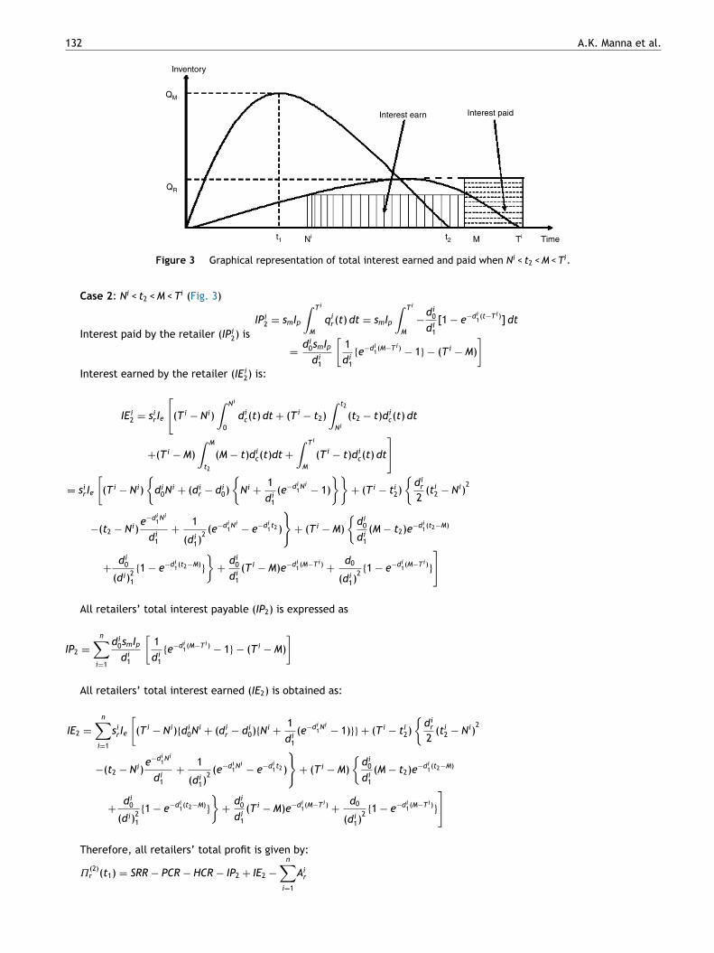
Figure 3 Graphical representation of total interest earned and paid when Ni < t2 < M < Ti.

Case 2: Ni < t2 < M < Ti (Fig. 3)

Interest paid by the retailer (IPi2) is

IPi2 = smIp

∫ T i

M

qir(t) dt = smIp

∫ T i

M

−di

0

di1

[1 − e−di1(t−T i)] dt

=di

0smIp

di1

[

1

di1

{e−di1(M−T i)

− 1} − (T i − M)

]

Interest earned by the retailer (IE i2) is:

IE i2 = si

r Ie

[

(T i − Ni)

∫ Ni

0

dic(t) dt + (T i − t2)

∫ t2

Ni

(t2 − t)dic(t) dt

+(T i − M)

∫ M

t2

(M − t)dic(t)dt +

∫ T i

M

(T i − t)dic(t) dt

]

= sir Ie

[

(T i − Ni)

{

di0Ni + (di

r − di0)

{

Ni +1

di1

(e−di1Ni

− 1)

}}

+ (T i − ti2)

{

dir

2(ti

2 − Ni)2

−(t2 − Ni)e−di

1Ni

di1

+1

(di1)

2(e−di

1Ni

− e−di1t2 )

}

+ (T i − M)

{

di0

di1

(M − t2)e−di1(t2−M)

+di

0

(di)21

{1 − e−di1(t2−M)

}

}

+di

0

di1

(T i − M)e−di1(M−T i)

+d0

(di1)

2{1 − e−di

1(M−T i)

}

]

All retailers’ total interest payable (IP2) is expressed as

IP2 =

n∑

i=1

di0smIp

di1

[

1

di1

{e−di1(M−T i)

− 1} − (T i − M)

]

All retailers’ total interest earned (IE2) is obtained as:

IE2 =

n∑

i=1

sir Ie

[

(T i − Ni){di0Ni + (di

r − di0){Ni +

1

di1

(e−di1Ni

− 1)}} + (T i − ti2)

{

dir

2(ti

2 − Ni)2

−(t2 − Ni)e−di

1Ni

di1

+1

(di1)

2(e−di

1Ni

− e−di1t2 )

}

+ (T i − M)

{

di0

di1

(M − t2)e−di1(t2−M)

+di

0

(di)21

{1 − e−di1(t2−M)

}

}

+di

0

di1

(T i − M)e−di1(M−T i)

+d0

(di1)

2{1 − e−di

1(M−T i)

}

]

Therefore, all retailers’ total profit is given by:

˘(2)r (t1) = SRR − PCR − HCR − IP2 + IE2 −

n∑

i=1

Air

Two layers green supply chain imperfect production inventory model 133

Inventory

QM

QR

Interest earnInterest paid

t1 t2 Ni M Ti Time

Figure 4 Graphical representation of total interest earned and paid when t2 < Ni < M < Ti.

The total profit (ITP) for this case of the integrated system is written as:E[ITP2(t1; �)] = E[˘(t1; �)] + ˘

(2)r (t1)

Case 3: t2 < Ni < M < Ti

Interest paid by the retailer (IPi3) is (Fig. 4):

IPi3 = smIp

∫ T i

M

qir(t) dt = smIp

∫ T i

M

−di

0

di1

[1 − e−di1(t−T i)] dt

=d0smIp

di1

[

1

di1

{e−di1(M−T i)

− 1} − (T i − M)

]

Interest earned by the retailer (IE i3) is:

IE i3 = si

r Ie[(T i − Ni){

∫ t2

0

dic(t) dt +

∫ Ni

t2

dic(t) dt} +

∫ T i

Ni

(T i − t)dic(t) dt]

= sir Ie[(T i − Ni){

∫ t2

0

{di0 + di

1qir(t)} dt +

∫ Ni

t2

{di0 + di

1qir(t)} dt} +

∫ T

Ni

(T i − t){di0 + di

1qir(t)} dt]

= sir Ie

[

(T i − Ni){di0Ni + (di

r − di0){t2 +

1

di1

(e−di1t2 − 1)} − di

0{(Ni − t2) +

1

di1

{1 − e−di1(t2−Ni)

}}}

+di

0

di1

(T i − Ni)e−di1(Ni−T i)

+di

0

(di1)

2{1 − e−di

1(Ni−T i)

}

]

All retailers’ total interest payable (IP3) is expressed as:

IP3 =

n∑

i=1

d0smIp

di1

[

1di

1

{e−di1(M−T i)

− 1} − (T i − M)]

All retailers’ total interest earned (IE3) is obtained as:

IE3 =

n∑

i=1

sir Ie

[

(T i − Ni)

{

di0Ni + (di

r − di0)

{

t2 +1

di1

(e−di1t2 − 1)

}

− di0

{

(Ni − t2) +1

di1

{1 − e−di1(t2−Ni)

}

}}

+di

0

di1

(T i − Ni)e−di1(Ni−T i)

+di

0

(di1)

2{1 − e−di

1(Ni−T i)

}

]

Therefore, all retailers’ total profit is given by:

˘ (3)r (t1) = SRR − PCR − HCR − IP3 + IE3 −

n∑

i=1

Air

So, the total profit (ITP) for this case of the integrated system is written as:E[ITP3(t1; �)] = E[˘(t1; �)] + ˘

(3)r (t1)

134 A.K. Manna et al.

1

0a1 a2 a3 a4 x

µÃ(x)

Figure 5 Membership function of a general fuzzy number A = (a1, a2, a3, a4).

When manufacturer and retailers’ have decided to share resources to undertake mutually beneficial coop-eration, the joint total profit which is a function of t1 can be obtained by maximized E[ITP(t1; �)] and isgiven by:

Maximize E[ITP(t1; �)] =

⎧

⎪

⎪

⎨

⎪

⎪

⎩

E[ITP1(t1; �)] = E[˘m(t1; �)] + ˘(1)r (t1), if Ni < M < t2 < T i

E[ITP2(t1; �)] = E[˘m(t1; �)] + ˘(2)r (t1), if Ni < t2 < M < T i

E[ITP3(t1; �)] = E[˘m(t1; �)] + ˘(3)r (t1), if t2 < Ni < M < T i

4. Basic concepts on fuzzy sets

The fuzzy set theory was developed to define and solve the complex system with sources of uncertainty or imprecision whichare non-statistical in nature. The fuzzy set theory is a theory of graded concept (a matter of degree) but different from atheory of chance or probability. The term fuzzy was proposed by Zadeh (1965). A short delineation of the fuzzy set theoryis given below.

Fuzzy set: A fuzzy set is a class of objects in which there is no sharp boundary between those objects that belong to theclass and those that do not. Let X be a collection of objects and x be an element of X, then a fuzzy set à in X is a set ofordered pairs A = {(x, �A(x))/x ∈ X}

where �A(x) is called the membership function or grade of membership of x in A which maps X to the membership spaceM which is considered as the closed interval [0,1].

Note: When M consists of only two points 0 and 1, Ã becomes a non-fuzzy set (or Crisp set) and �A(x) reduces to thecharacteristic function of the non-fuzzy set (or crisp set).

Fuzzy number: A fuzzy number is a special class of a fuzzy sets. Different definitions and properties of fuzzy numbers areencountered in the literature but they all agree on that a fuzzy number represents the conception of a set of real numbersclose to a, where a is the number being fuzzyfied.

A fuzzy number is a fuzzy set in the universe of discourse ℜ whose membership function �A(x) is

i. a continuous mapping from ℜ to the closed interval [0,1],ii. constant on (−∞, a1] : �A(x) = 0, ∀x ∈ (−∞, a1],

iii. strictly increasing on [a1, a2]: e.g., �A(x) = f(x), ∀x ∈ [a1, a2] where f(x) is a strictly increasing function of x,iv. constant on [a2, a3]: e.g., �A(x) = 1, ∀x ∈ [a2, a3],v. strictly decreasing on [a3, a4], e.g., �A(x) = g(x), ∀x ∈ [a3, a4] where g(x) is a strictly decreasing function of x,

vi. constant on [a4, ∞): e.g., �A(x) = 0, ∀x ∈ [a4, ∞).

A general shape of a fuzzy number following the above definition may be shown pictorially as in Fig. 5. Here, a1, a2, a3

and a4 are real numbers. A fuzzy number à in ℜ is said to be discrete or continuous according as its membership function�A(x) is discrete or continuous.

Two layers green supply chain imperfect production inventory model 135

Note 1: When the membership function are linear and increasing from a1 to a2, and decreasing from a2 to a3 such fuzzynumber is known as triangular fuzzy number (TFN).

Note 2: When the membership function are linear and increasing from a1 to a2, constant between a2 to a3 and decreasingfrom a3 to a4 such fuzzy number is known as trapezoidal fuzzy number (TrFN).

Zadeh’s extension principle: One of the basic concepts of fuzzy set theory which is used to generalize crisp mathematicalconcepts to fuzzy sets is the extension principle. Let X and Y be two universes and f: X → Y be a crisp function. The extensionprinciple tells us how to induce a mapping f: P(X) → P(Y), where P(X) and P(Y) are the power sets of X and Y respectively.

Following Zadeh (1978) we define the fuzzy extension principle as follows:We have the mapping f: X → Y, y = f(x) which induce a function f: A → B such that B = f(A) = {((y, �B(y))|y = f(x), x ∈ X)},

where

�B(y) =

⎧

⎪

⎨

⎪

⎩

sup �A(x) if f−1(y) /= ˚,

x ∈ f−1(y)

0 otherwise

Centroid of the fuzzy number: The centroid value of a fuzzy function �M is given by

C[�M] =

∫ ∞

−∞y��

M(y) dy

∫ ∞

−∞��

M(y) dy

For a triangular fuzzy number (TFN) A = (a − �1, a, a + �2), where 0 < �1 < a and 0 < �2, �1, �2 are determined by thedecision makers. Then the centroid value, C[A] = a + 1

3 (�1 + �2)

4.1. Model with fuzzy credit period

We assume that the manufacturer gives an opportunity to all the retailers by offering a fuzzy credit period (M). Here, thecredit period M is represented in form of triangular fuzzy number. So due to fuzzy credit period (M), the optimum value ofintegrated profit function ITP(t1) will be different for various values of M with some degree of belongingness. Therefore, insuch a situation, the profit function will be fuzzy in nature and is denoted by ˜ITP(t1; M, �), where:

E[

˜ITP(t1; M, �)]

=

⎧

⎪

⎪

⎪

⎪

⎨

⎪

⎪

⎪

⎪

⎩

E

[

˜ITP(1)

(t1; M, �) = E[∏

m(t1; �)

]

]

+∏(1)

r(t1; M), if Ni < M < t2 < T i

E

[

˜ITP(2)

(t1; M, �) = E[∏

m(t1; �)

]

]

+∏(2)

r(t1; M), if Ni < M < t2 < T i

E

[

˜ITP(3)

(t1; M, �) = E[∏

m(t1; �)

]

]

+∏(3)

r(t1; M), if Ni < M < t2 < T i

136 A.K. Manna et al.

The imprecise expressions of E

[

˜ITP(1)

(t1; M, �)]

, E

[

˜ITP(2)

(t1; M, �)]

and E

[

˜ITP(3)

(t1; M, �)]

are given below:

E

[

˜ITP(1)

(t1; M, �)]

= sm

n∑

i=1

dirt2 − (cp + sc + ecE[�ε])Pt1 − (rcm + ecE[� ])ı

(

ˇ + �P +�

2t1

)

Pt1

−(cd + ecE[��])(1 − ı)

(

+ �P +�

2t1

)

Pt1

−hm

2

[{

P −

n∑

i=1

dir − (1 − ı)(ˇ + �P)P}t2

1 − (1 − ı)�

3Pt3

1 +

n∑

i=1

dir(t1 − t2)2] − Am

+

n∑

i=1

sir

[

dirt2 +

(dir − di

0)

di1

(e−di1t2 − 1) −

di0

di1

{1 − e−di1(t2−T i)

}

]

−

n∑

i=1

smdirt2

−

n∑

i=1

hir

[

(dir − di

0)

di1

{

t2 +1

di1

(e−di1t2 − 1)

}

−di

0

di1

{

(T i − t2) +1

di1

{1 − e−di1(t2−T i)

}

}]

−

n∑

i=1

smIp

[

(dir − di

0)

di1

{

(t2 − M) +1

di1

(e−di1t2 − e−di

1M)

}

−di

0

di1

{

(T i − t2) +1

di1

{1

−e−di1(t2−T i)

}}]

+

n∑

i=1

sir Ie

[

(T i − Ni){di0Ni + (di

r − d0){N +1

di1

(e−di1Ni

− 1)}}

+(T i − M)

{

dir

2(M − Ni)

2− (M − Ni)

e−di1Ni

di1

+1

(di1)

2(e−di

1Ni

− e−di1M)

}

+(T i − t2)

{

dir

2(M − t2)

2− (t2 − M)

e−di1M

di1

+1

(di1)

2(e−di

1M

− e−di1t2 )

}

+di

0

di1

(T i − t2)e−di1(t2−T i)

+di

0

(di1)

2{1 − e−di

1(t2−T i)

}

]

−

n∑

i=1

Air .

E

[

˜ITP(2)

(t1; M, �)]

= sm

n∑

i=1

dirt2 − (cp + sc + ecE[�ε])Pt1 − (rcm + ecE[� ])ı

(

ˇ + �P +�

2t1

)

Pt1

−(cd + ecE[��])(1 − ı)

(

+ �P +�

2t1

)

Pt1

−hm

2

[

{P −

n∑

i=1

dir − (1 − ı)(ˇ + �P)P}t2

1 − (1 − ı)�

3Pt3

1 +

n∑

i=1

dir(t1 − t2)2] − Am

+

n∑

i=1

sir[d

irt2 +

(dir − di

0)

di1

(e−di1t2 − 1) −

di0

di1

{1 − e−di1(t2−T i)

}

]

−

n∑

i=1

smdirt2

−

n∑

i=1

hir

[

(dir − di

0)

di1

{

t2 +1

di1

(e−di1t2 − 1)

}

−di

0

di1

{(T i − t2) +1

di1

{1 − e−di1(t2−T i)

}}

]

−

n∑

i=1

di0smIp

di1

[

1

di1

{e−di1(M−T i)

− 1} − (T i − M)

]

+

n∑

i=1

sir Ie

[

(T i − Ni){

di0Ni

+(dir − di

0){Ni +1

di1

(e−di1Ni

− 1)}

}

+ (T i − ti2)

{

dir

2(ti

2 − Ni)2− (t2 − Ni)

e−di1Ni

di1

+1

(di1)

2(e−di

1Ni

− e−di1t2 )

}

+ (T i − M)

{

di0

di1

(M − t2)e−di1(t2−M)

+di

0

(di)21

{1

−e−di1(t2−M)

}}

+di

0

di1

(T i − M)e−di1(M−T i)

+d0

(di1)

2{1 − e−di

1(M−T i)

}] −

n∑

i=1

Air

Two layers green supply chain imperfect production inventory model 137

and

E

[

˜ITP(2)

(t1; M, �)]

= sm

n∑

i=1

dirt2 − (cp + sc + ecE[�ε])Pt1 − (rcm + ecE[� ])ı

(

ˇ + �P +�

2t1

)

Pt1

−(cd + ecE[��])(1 − ı)

(

ˇ + �P +�

2t1

)

Pt1

−hm

2[{P −

n∑

i=1

dir − (1 − ı)(ˇ + �P)P}t2

1 − (1 − ı)�

3Pt3

1 +

n∑

i=1

dir(t1 − t2)2] − Am

+

n∑

i=1

sir[d

irt2 +

(dir − di

0)

di1

(e−di1t2 − 1) −

di0

di1

{1 − e−di1(t2−T i)

}] −

n∑

i=1

smdirt2

−

n∑

i=1

hir

[

(dir − di

0)

di1

{

t2 +1

di1

(e−di1t2 − 1)

}

−di

0

di1

{

(T i − t2) +1

di1

{1 − e−di1(t2−T i)

}

}]

−

n∑

i=1

d0smIp

di1

[

1

di1

{e−di1(M−T i)

− 1} − (T i − M)

]

+

n∑

i=1

sir Ie

[

(T i − Ni){

di0Ni

+(dir − di

0)

{

t2 +1

di1

(e−di1t2 − 1)

}

− di0{(N

i − t2) +1

di1

{1 − e−di1(t2−Ni)

}}}

+di

0

di1

(T i − Ni)e−di1(Ni−T i)

+di

0

(di1)

2{1 − e−di

1(Ni−T i)

}

]

−

n∑

i=1

Air .

5. Solution methodology

The proposed non-linear problem of model are solved by a gradient based non-linear optimization method --- GeneralizedReduced Gradient Method using LINGO Solver 12.0 for particular input data.

5.1. Algorithm to get the optimum values

The optimum values production time (t1) and expected total profit for the fuzzy stochastic model are obtained throughalgorithm.

Step 1: For the random variable ′�′ with p.d.f ‘g(�)’ evaluate the expected value of integrated total profit ˜ITP(1)

(t1; M, �),˜ITP

(2)(t1; M, �) and ˜ITP

(3)(t1; M, �) using the definition E

[

˜ITP(1)

(t1; M, �)]

=∫ ∞

−∞˜ITP

(1)(t1; M, �)g(�)d(�), similarly obtained

E

[

˜ITP(2)

(t1; M, �)]

and E

[

˜ITP(3)

(t1; M, �)]

Step 2: For a given triangular fuzzy number (TFN) M = (M − �1, M, M + �2), the fuzzy expressions of EITP(1)M

= E

[

˜ITP(1)

]

=

(EITP(1)l , EITP

(1)m , EITP

(1)r ), EITP

(2)M

= E

[

˜ITP(2)

]

= (EITP(2)l , EITP

(2)m , EITP

(2)r ) and EITP

(3)M

= E

[

˜ITP(3)

]

= (EITP(3)l , EITP

(3)m , EITP

(3)r )

are obtained using fuzzy extension principal.

Step 3: Then from the fuzzy expressions E

[

˜ITP(1)

(t1; M, �)]

, E

[

˜ITP(2)

(t1; M, �)]

and E

[

˜ITP(3)

(t1; M, �)]

obtained the centroid

values CEITP(1) = C

[

EITP(1)M

]

, CEITP(2) = C

[

EITP(2)M

]

and CEITP(3) = C

[

EITP(3)M

]

respectively, using the definition presents in

Section 4, which is the process of defuzzification.Step 4: Finally, maximized each CEITP(1)(t1), CEITP(2)(t1) and CEITP(3)(t1) with respect to the decision variable t1 by usingLINGO Solver 12.0 for particular input data.

6. Numerical analysis

Example 1. We consider a production-inventory supply chain model with the following characteristics: P=42 units, ˇ1 = 0.10,� = 0.001, � = 0.02, �1 = 0.01, �2 = 0.02, ı = 0.70, cp = $32 per unit, csr = $2 per unit, rcm = $10 per unit, cd = $5 per unit, hm = $4per unit per unit time, h

(1)r = $4.5 per unit per unit time, h

(2)r = $4.8 per unit per unit time, A

(m0)r = $140, A

(m1)r = $130,

A(1)r = $140, A

(2)r = $130, sm = $140 per unit, s

(1)r = $260 per unit, s

(2)r = $250 per unit, ec = $2.5 per unit, smin = $220, smax = $280,

d(1)r = 17 unit, d

(2)r = 18 unit, d

(1)c0 = 9.84 unit, d

(2)c0 = 9.54 unit, d

(1)c1 = 1.8, d

(2)c1 = 3, d

(1)1 = 7, d

(2)1 = 6, �(1) = 7, �(2) = 6.

138 A.K. Manna et al.

Table 2 Optimal results of different cases when � = ˇ + �P + �t.

Cases Retailers’credit period(N1, N2)

Manufacturercredit period(M)

Production time t1 Period of manufacturer Period ofretailers’

Expected profit

Case 1 (0.12, 0.10) (0.19, 0.20,0.22)

0.528 0.605 (0.734,0 .730) 4178.54

Case 2 (0.12, 0.10) (0.69, 0.70,0.72)

0.531 0.610 (0.739, 0.732) 3512.53

Case 3 (0.65, 0.62) (0.69, 0.70,0.72)

0.538 0.618 (0.726, 0.720) 4128.05

Table 3 Optimal results of different cases when � = ˇ + �P.

Cases Retailers’credit period(N1, N2)

Manufacturercredit period(M)

Productiontime (t1)

Period ofmanufacturer(t2)

Period ofretailers’(T1, T2)

Expected profit

Case 1 (0.10, 0.12) (0.19,0.20,0.22)

0.543 0.622 (0.763,0.750)

4370.80

Case 2 (0.12, 0.10) (0.69, 0.70,0.72)

0.548 0.637 (0.767,0.761)

3872.79

Case 3 (0.65, 0.62) (0.69, 0.70,0.72)

0.558 0.642 (0.755,0.748)

4327.61

The respective carbon-emission rates �ε, � and �� for production process, rework process and disposal units followed aBeta distribution g(�) with parameters v, w i.e., the p.d.f. of � is:

g(�) =

⎧

⎨

⎩

�v−1(1 − �)w−1

ˇ(v, w), 0 ≤ � ≤ 1

0, otherwise

For ε = 1, = 2 and � = 3, we have:E[�ε] = v

v+w, E[� ] =

v(v+1)(v+w)(v+w+1) and � = ˇ + �P

Applying the proposed computational algorithm yields the results shown in Table 2 for different cases.In manager’s point of view, case 2 gives minimum profit. Since in that case manufacturer lost maximum opportunity of

credit period, where as the customers receive maximum benefit from the management system. The first and last cases arenearly same in terms of profit since in the first case both the members offer lower credit period and in the last case boththe members offer higher credit periods. More over, in the third case, as retailer offers higher credit period, the demandof the customers becomes high but the quantity transferred from manufacturer to retailer is the same, therefore, period ofconsumptions of the retailer is reduced. As the demand of the customers are linked with the credit period offered by theretailer, high demand of the customers reduced the time period of the retailers.

Example 2. Evaluate the optimal policy of the decision maker when the defective rate of produce item depends onproduction rate only (i.e., � = 0) and the remain parameters of the system are unalter.

Table 3 shows the optimum policies of the decision maker when the defective rate of the produced item is of the form� = + �P.

In comparison of the cases, Example 2 reveals the same decisions as Example 1. Moreover, when defective rate does notdepend on time, the defective units are quite less, i.e., fresh units are more than that of Example 1. So, business periodsare larger than the Example 1, which also yield more profit than Example 1 for each cases.

Example 3. Find the optimal policies of the decision maker when the defective rate of produce item depend on time only(i.e., � = 0) and the remain parameters of the system are unaltered.

When the defective rate of produce item does not depend on production rate but depends on time only, i.e., � = + �t,then the optimum results are shown in the following Table 4.

If defective rate does not depend on the production rate, then production time is much larger. So manufacturer producesmore quantity of items. For this reason, the periods of manufacturer and retailers are more than the scenarios when� = + �P + �t or � = ˇ + �P. So the optimum profit is more than the other two scenarios, as expected.

Example 4. When the defective rate of produce item is constant (i.e., � = 0 and � = 0) then evaluate the optimal profit ofthe decision maker (the remain parameter of the system remain unalter).

Two layers green supply chain imperfect production inventory model 139

Table 4 Optimal results of different cases when � = + �t.

Cases Retailers’credit period(N1, N2)

Manufacturercreditperiod (M)

Productiontime (t1)

Period ofmanufacturer(t2)

Period of retailers’(T1, T2)

Expectedprofit

Case 1 (0.10, 0.12) (0.19, 0.20,0.22)

0.728 0.848 (1.020, 1.010) 6074.09

Case 2 (0.12, 0.10) (0.69, 0.70,0.72)

0.731 0.851 (1.023, 1.013) 6833.38

Case 3 (0.65, 0.62) (0.69, 0.70,0.72)

0.739 0.858 (0.998, 0.991) 6095.70

Table 5 Optimal results of different cases when � = ˇ.

Cases Retailers’creditperiod (N1,N2)

Manufacturercreditperiod (M)

Productiontime (t1)

Period ofmanufacturer(t2)

Period ofretailers’(T1, T2)

Expectedprofit

Case 1 (0.10, 0.12) (0.19, 0.20,0.22)

0.783 0.913 (1.080,1.081)

6593.89

Case 2 (0.12, 0.10) (0.69, 0.70,0.72)

0.787 0.918 (1.098,1.090)

7664.13

Case 3 (0.65, 0.62) (0.69, 0.70,0.72)

0.794 0.924 (1.033,1.045)

6638.49

Table 6 Sensitivity analysis on different values of trade credit period M and N’s case 2.

�1 �2 ManufacturercreditperiodM = (M −

�1, M, M +

�2)

Retailers’creditperiod (N1,N2)

Interestearned by theretailers (IE2)

Interest paid bythe retailers(IP2)

Expected profit

(0.09,0.07) 294.92 895.84 3488.150.008 0.020 (0.688,

0.700,0.720)

(0.12,0.10) 315.52 895.84 3508.76

(0.15,0.13) 333.76 895.84 3526.99

(0.09, 0.07) 298.70 895.87 3491.930.010 0.020 (0.690,

0.700,0.720)

(0.12, 0.10) 319.31 895.87 3512.53

(0.15, 0.13) 337.54 895.87 3530.77

(0.09, 0.07) 302.49 895.89 3495.700.012 0.020 (0.692,

0.700,0.720)

(0.12, 0.10) 323.09 895.89 3516.31

(0.15, 0.13) 341.34 895.89 3534.55

(0.09, 0.07) 302.27 896.48 3496.120.010 0.018 (0.690,

0.700,0.718)

(0.12, 0.10) 322.88 896.48 3516.72

(0.15, 0.13) 341.12 896.48 3534.96

(0.09, 0.07) 295.13 897.64 3487.740.010 0.022 (0.690,

0.700,0.722)

(0.12, 0.10) 315.74 897.64 3508.35

(0.15, 0.13) 333.98 897.64 3526.58

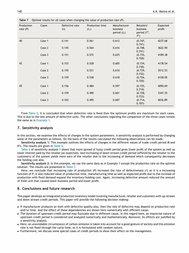
140 A.K. Manna et al.

Table 7 Optimal results for all cases when changing the value of production rate (P).

Productionrate (P)

Cases Defective rate(�)

Production time(t1)

Manufacturerbusinessperiod (t2)

Retailers’businessperiod (T1,T2)

Expectedprofit

40 Case 1 0.141 0.561 0.612 (0.747,0.741)

4237.68

Case 2 0.145 0.564 0.616 (0.748,0.741)

3622.90

Case 3 0.151 0.572 0.625 (0.735,0.728)

4189.38

42 Case 1 0.153 0.528 0.605 (0.734,0.730)

4178.54

Case 2 0.155 0.531 0.610 (0.739,0.732)

3512.53

Case 3 0.159 0.538 0.618 (0.726,0.720)

4128.05

45 Case 1 0.156 0.484 0.597 (0.725,0.719)

4090.69

Case 2 0.159 0.490 0.601 (0.728,0.723)

3347.35

Case 3 0.165 0.495 0.607 (0.714,0.707)

4036.89

From Table 5, it is concluded that when defective rate is fixed then the optimum profits are maximum for each cases.This is due to the less amount of defective units. The other conclusions regarding the comparison of the three cases remainthe same as in Example 1.

7. Sensitivity analysis

In this section, we examine the effects of changes in the system parameters. A sensitivity analysis is performed by changingsome of the parameters as follows. On the basis of the results calculated the following observations can be made.

Sensitivity analysis 1: This example outlines the effects of changes in the different values of trade credit period M andN’s. The results are given in Table 6.

Table 6 of sensitivity analysis 1 shows that more spread of fuzzy credit period gives lower profit of the system as well aslower interest paid by the retailer (as expected). And increasing of down stream credit period (offered by the retailer to thecustomers) of the system yields more earn of the retailer due to the increasing of demand which consequently decreasesthe holding cost also.

Sensitivity analysis 2: In this example, we use the same data as in Example 1 except the production rate on the optimalsolution. The results are presented in Table 7.

Here, we conclude that increasing rate of production (P) increases the rate of defectiveness (�) as it is a increasingfunction of P, it also reduced value of production time, manufacturing time as well as expected profit due to the increase ofproduction with fixed demand expand the inventory/holding cost. Again, increasing defective amount reduced the amountof fresh unit that caused lower business period and lower profit.

8. Conclusions and future research

This paper develops an integrated production inventory model involving manufacturer, retailer and customers with up-streamand down stream credit periods. This paper will provide the following decision making:

• If manufacturer produces an item with defective quality also, then the rate of defective may depend on production-rateand/or time. And the effect of these dependencies are shown here numerically with efficient cause.

• The duration of upstream credit period may fluctuate due to different cause, in this regard here, an imprecise nature ofupstream credit period is considered and analyzed numerically and mathematically. Moreover, its effects are justified bya sensitivity analysis.

• Here, an unavoidable circumstance of carbon-emission is taken into account for a good gesture of society and this emissionrate is not fixed through the cycle time, so it is formulated with random nature.

• Furthermore, we discuss some special cases of credit periods to show their effect on the management.

Two layers green supply chain imperfect production inventory model 141

• Finally, we run several numerical examples and sensitivity analysis to illustrate the problem and provide some managerialinsights.

We suggest several possible directions for future research. First, one may extend our considered EPQ model to joint opti-mization of expected total profit and carbon emission (i.e., maximize expected total profit and minimize carbon emission).Second, one immediate possible extension could be allowable shortages, cash discounts, etc. Finally, one can extend thefully trade credit policy to the partial trade credit policy in which a seller requests its credit-risk customers to pay a fractionof the purchase amount at the time of placing an order as a collateral deposit, and then grants a permissible delay on therest of the purchase amount.

References

Abad, P. L., & Jaggi, C. K. (2003). A joint approach for setting unit price and the length of the credit period for a seller when end demandis price sensitive. International Journal of Production Economics, 83(2), 115---122.

Annadurai, K., & Uthayakumar, R. (2010). Controlling setup cost in (Q, r, L) inventory model with defective items. Applied Mathematical

Modelling, 34(6), 1418---1427.Benjaafar, S., Li, Y., & Daskin, M. (2013). Carbon foot print and the management of supply chains: Insights from simple models. IEEE

Transactions on Automation Science and Engineering, 10(1), 99---116.Chaharsooghi, S. K., Heydari, J., & Zegordi, S. H. (2008). A reinforcement learning model for supply chain ordering management: An

application to the beer game. Decision Support Systems, 45(4), 949---959.Chang, H. C. (2004). An application of fuzzy sets theory to the EOQ model with imperfect quality items. Computers and Operations Research,

31(12), 2079---2092.Chang, H. C., Yao, J. S., & Ouyang, L. Y. (2006). Fuzzy mixture inventory model involving fuzzy random variable lead time demand and

fuzzy total demand. European Journal of Operational Research, 169(1), 65---80.Chiu, Y. P. (2003). Determining the optimal lot size for the finite production model with random defective rate, the rework process, and

backlogging. Engineering Optimization, 35(4), 427---437.Chung, K. J., & Liao, J. J. (2009). The optimal ordering policy of the EOQ model under trade credit depending on the ordering quantity

from the DCF approach. European Journal of Operational Research, 196(2), 563---568.Das, B. C., Das, B., & Mondal, S. K. (2015). An integrated production inventory model under interactive fuzzy credit period for deteriorating

item with several markets. Applied Soft Computing, 28, 453---465.Datta, T. K., & Pal, A. K. (1990). A note on inventory model with inventory-level-dependent demand rate. Journal of Operational Research

Society, 41(10), 971---975.Dey, J. K., Kar, S., & Maiti, M. (2005). An interactive method for inventory control with fuzzy lead-time and dynamic demand. European

Journal of Operational Research, 167(2), 381---397.Dye, C. Y., & Yang, C. T. (2015). Sustainable trade credit and replenishment decisions with credit-linked demand under carbone mission

constraints. European Journal of Operational Research, 244(1), 187---200.Goyal, S. K., & Cárdenas-Barrón, L. E. (2002). Note on: Economic production quantity model for items with imperfect quality --- A practical

approach. International Journal of Production Economics, 77(1), 85---87.Harris, F. (1915). Operations and cost (Factory Management Series). Chicago: A. W. Shaw Co.Hayek, P. A., & Salameh, M. K. (2001). Production lot sizing with the reworking of imperfect quality items produced. Production Planning

and Control, 12(6), 584---590.Jaber, M. Y., Zanoni, S., & Zavanella, L. E. (2014). Economic order quantity models for imperfect items with buy and repair options.

International Journal of Production Economics, 155, 126---131.Khouja, M. (2003). Optimizing inventory decisions in a multistage multi customer supply chain. Transportation Research Part E: Logistics

and Transportation Review, 39(3), 193---208.Khouja, M., & Mehrez, A. (1994). An economic production lot size model with imperfect quality and variable production rate. Journal of

the Operational Research Society, 45(12), 1405---1417.Levin, R. I., Mclaughlin, C. P., Lamone, R. P., & Kottas, J. F. (1972). Production/operations management: Contemporary policy for managing

operating systems. New York: McGraw-Hill.Manna, A. K., Das, B., Dey, J. K., & Mondal, S. K. (2016). An EPQ model with promotional demand in random planning horizon: Population

varying genetic algorithm approach. Journal of Intelligent Manufacturing, 27(1), 1---19.Manna, A. K., Dey, J. K., & Mondal, S. K. (2014). Three-layer supply chain in an imperfect production inventory model with two storage

facilities under fuzzy rough environment. Journal of Uncertainty Analysis and Applications, 2(1), 1---31.Manna, A. K., Dey, J. K., & Mondal, S. K. (2017). Imperfect production inventory model with production rate dependent defective rate and

advertisement dependent demand. Computers & Industrial Engineering, 104, 9---22.Modak, N. M., Panda, S., & Sana, S. S. (2015). Optimal just-in-time buffer inventory for preventive maintenance with imperfect quality

items. Tékhne, 13(2), 135---144.Modak, N. M., Panda, S., & Sana, S. S. (2016). Three-echelon supply chain coordination considering duopolistic retailers with perfect quality

products. International Journal of Production Economics, 182, 564---578.Munson, L. C., & Rosenblatt, J. M. (2001). Coordinating a three level supply chain with quantity discounts. IIE Transactions, 33(5), 371---384.Panda, D., & Maiti, M. (2009). Multi-item inventory models with price dependent demand under flexibility and reliability consideration and

imprecise space constraint: A geometric programming approach. Mathematical and Computer Modeling, 49(9/10), 1733---1749.Panda, S., & Modak, N. M. (2015). An inventory model for random replenishment interval and imperfect quality items under demand

fluctuation. International Journal of Supply Chain and Inventory Management, 1(4), 269---285.Panda, S., & Modak, N. M. (2016). Exploring the effects of social responsibility on coordination and profit division in a supply chain. Journal

of Cleaner Production, 139, 25---40.

142 A.K. Manna et al.

Panda, S., Modak, N. M., & Basu, M. (2014). Disposal cost sharing and bargaining for coordination and profit division in a three-echelonsupply chain. International Journal of Management Science and Engineering Management, 9(4), 276---285.

Panda, S., Modak, N. M., & Cárdenas-Barrón, L. E. (2017). Coordinating a socially responsible closed-loop supply chain with product recycling.International Journal of Production Economics, 188, 11---21.

Porteus, E. L. (1986). Optimal lotsizing, process quality improvement and setup cost reduction. Operations Research, 34(1), 137---144.Salameh, M. K., & Jaber, M. Y. (2000). Economic production quantity model for items with imperfect quality. International Journal of

Production Economics, 64(1/3), 59---64.Sana, S. S. (2010). An economic production lot size model in an imperfect production system. European Journal of Operational Research,

201(1), 158---170.Sana, S. S. (2011). A production-inventory model of imperfect quality products in a three-layer supply chain. Decision Support Systems,

50(2), 539---547.Silver, E. A., & Peterson, R. (1985). Decision systems for inventory management and production planning. New York: John Wiley.Wang, W. T., Wee, H. M., & Tsao, H. S. J. (2010). Revisiting the note on supply chain integration in vendor-managed inventory. Decision

Support Systems, 48(2), 419---420.Yang, C. P., & Wee, M. H. (2001). An arborescent inventory model in a supply chain system. Production Planning and Control, 12(8), 728---735.Yao, Y., Evers, P. T., & Dresner, M. E. (2007). Supply chain integration in vendor-managed inventory. Decision Support Systems, 43(2),

663---674.Zadeh, L. A. (1965). Fuzzy sets. Information and Control, 8(3), 338---356.Zadeh, L. A. (1978). Fuzzy sets as a basis for a theory of possibility. Fuzzy Sets and Systems, 100(1), 3---28.