Vertigo: Comparing structural models of imperfect behavior in experimental games

GAMES AND ECONOMIC BEHAVIOR 8, 3 2 2 - 3 4 8 (1995)

Vertigo: Comparing Structural Models of Imperfect Behavior in Experimental Games

MAHMOU D A . E L - G A M A L AND THOMAS R. PALFREY*

Division of the Humanities and Social Sciences, Caltech, Pasadena, California 91125

Received July 9, 1992

We introduce the game of Vertigo to study learning in experimental games with one-sided incomplete information. Our models allow players to make errors when choosing their actions. We compare six models where the players are modeled as sophisticated (taking errors in action into account when constructing strategies) or unsophisticated on one dimension, and employ Bayes' rule, a faster updating rule, or no updating at all on the second. Using a fully Bayesian structural econometric approach, we find that unsophisticated models perform better than sophisticated models, and models with no (or slower) updating perform better than models with faster updating. Journal of Economic Literature Classification Numbers: 026, 211,215. © 1995 Academic Press. Inc.

1. INTRODUCTION

This paper investigates learning in multistage games with one-sided incomplete information using laboratory data. We focus on two issues related to possible deviations from behavior predicted by game theoretic models focused on perfectly rational behavior by Bayesian players. The first issue is imperfect choice behavior, and employs a model that generates an error structure that permits rigorous statistical analysis of the data. The second issue is imperfect learning behavior; agents' updating may be too fast or too slow.

* We acknowledge the financial support from NSF grants SES9011828 and SBR-9223701 to the California Institute of Technology and from the JPL-Caltech Supercomputing project. We have benefited from many discussions with Richard McKelvey. We thank an associate editor and an anonymous referee for useful suggestions. Marty Hahm wrote the computer programs for the experiment.

322 0899-8256/95 $6.00 Copyright © 1995 by Academic Press, Inc. All rights of reproduction in any form reserved.

VERTIGO 323

Recently, it has become increasingly clear that models of game behavior demanding perfect rationality of the players seem to perform poorly under the scrutiny of careful statistical analysis of data from simple finite game experiments. This is true whether the games are strictly competitive (Brown and Rosenthal (1990)), have clear gains to cooperative behavior (Camerer and Weigelt (1988), McKelvey and Palfrey (1992)), or lie in some intermediate territory (Banks et al. (1994), Brandts and Holt (1992), Palfrey and Rosenthal (1991), and Palfrey and Rosenthal (1994)). One reason for the existence of these problems is that most equilibrium concepts are essentially static and fail to address basic issues of learning dynamics, information, and the cognitive limitations of the players. A second, related, reason is that these equilibrium concepts typically place overly strong restrictions on the data. In fact, for most of the games that have been experimentally investigated, the equilibrium predicts the use of pure strategies. More to the point, equilibrium models frequently predict that certain strategies will never be observed. In these cases, both classical and Bayes- ian statistical methods lead to outright rejection of strictly rational models.

The predictions that certain strategies should never be observed may arise from a number of different scenarios ranging from the availability of dominant actions under certain circumstances, to very sophisticated updating rules resulting in full revelation of certain states of nature, and requiring particular'pure strategies to be played (e.g. Cooper et al. (1990), and E1-Gamal et al. (1993)). The end result is that certain actions cannot be observed at certain points in time during the experiment. If those "infinitely unlikely" events are observed in experimental data (e.g., players choosing a dominated action in Cooper et al. (1990)), one is faced with what we call the zero l ikel ihood prob lem. A common, but statistically unsatisfactory way to deal with this problem is to ignore the zero-likelihood data points, treating them as missing data. Other popular procedures involve descriptive data analyses and the application ofad hoc measures of association or fit to compare the relative performance of several competing models.

Several recent attempts have been made to endow the strict rationality models with an extra feature that allows all observations to occur with positive probability. This paper follows this approach, and evaluates and compares several different specific ways to do this in the context of a multistage game of incomplete information. The players are assumed to follow the theory as long as they do not "tremble", and they tremble with some probability 0 < e < 1. When players tremble, they are assumed to choose their action in an arbitrary way which allows all possible actions to be chosen with some positive probability.l The first question explored

I There are alternative ways to introduce imperfect choice behavior. Besides this "trembling" model, we have stochastic utility models (Logit, Probit, etc.), imperfectly

324 EL-GAMAL AND PALFREY

along this approach was what value of e to use. In Boylan and El-Gamal's (1993) study of disequilibrium dynamics, the model comparison was done at all possible e's in [0, l], and in their case, the results held for almost all e (excluding those values arbitrarily close to 1). In McKelvey and Palfrey (1992), and Harless and Camerer (1992), a value of e was estimated by its maximum likelihood estimator under the relevant model(s). In El- Gamai et al. (1993), the parameter e was viewed as a nuisance parameter, and hence, a prior was induced on e together with all other nuisance parameters of the models they studied, and this prior on e was updated as experimental data was collected. In this paper, we follow this fully Bayesian procedure, by specifying a model with nuisance parameters, and integrating out these nuisance parameters with respect to our beliefs, which are updated as more data are observed.

The second issue that the introduction of the trembles poses is how players take it into account. In EI-Gamai et al. (1993), and McKelvey and Palfrey (1992), the trembles were assumed to come from a common knowledge distribution which the players incorporated in making their decisions. In this sense, the players were assumed to be very sophisticated in dealing with the fact that their opponents, as well as themselves, may tremble at any point in the game. They incorporated these probabilities of trembles in their strategies (mappings from beliefs to actions) as well as updating rules (mappings from beliefs and observed actions to beliefs). This very high degree of sophistication would seem to put an incredible computational burden on the players. In order to solve for the full sequential equilibrium of a three-move centipede game played with two opponents, E1-Gamal et al. (1993) required 120 CPU hours of a fast supercom- puter (a Cray Y-MP2E/116). It might seem odd to deviate from perfect rationality by introducing the trembles, and then require such a high level of rationality in dealing with the trembles to make it almost impossible to solve for the equilibrium behavior. Lower degrees of sophistication in dealing with the trembles may be more reasonable.

This paper considers two levels of sophistication in the players' strategies. The sophisticated model lets the agents take into account the fact that they, as well as their opponents, can tremble at any time, and adjust for that fact when deciding on their strategies. The unsophisticated model does not have the agents take account of the tremble probabilities when formulating their best responses, i.e., they decide on their actions as if no one ever trembles.

A second source of deviation from behavior predicted by Bayesian

controlled preference models (Palfrey and Rosenthal (1991)), evolutionary models with mutation, and imperfect equilibrium models (Beja (1992)). This paper focuses only on a simple version of the model with trembles.

VERTIGO 325

equilibrium, besides errors in actions, derives from errors in updating. The players may, to varying degrees, use available information in ways that are inconsistent with Bayes's rule. We consider three alternative updating models. The first model (which we label the undampened or fast updating model) lets the agents update from the observed moves of their opponents via the Bayes updating map, not taking into account the fact that their opponents may have trembled. The second model (which we label the dampened updating model) lets the agents update from the observed moves taking into account the fact that they may have resulted from a tremble. The last model of updating we consider is the no updating model, where the players do not use the observed actions to adjust their beliefs. Combining the two models of sophistication with the three models of updating generates a total of six alternative models.

We compare these models using a simple game of one-sided incomplete information, which we call the game of Vertigo. The informed player may be one of two-types, corresponding to two possible payoff tables of a bimatrix game, called Game I and Game II. The games are equivalent, up to a relabeling of the players, so one may think of the private information being that the informed player knows whether he is the row player or the column player, but the uninformed player does not. 2 The probability distribution of the informed player's type is common knowledge. No player has a domilaant strategy in either Game I or Game II. There is a unique mixed-strategy equilibrium in each component game.

The game of incomplete information also has a unique equilibrium, which depends on the common knowledge prior over the types. One type mixes, and the other type adopts a pure strategy. Which type mixes depends on the prior.

In the experiment, each uninformed player plays a sequence of informed players, all of whom are the same type. The experimental procedures are organized in a manner that eliminates signaling possibilities by the informed (row) players. The next section will analyze the equilibrium of the game and describe the details of the experimental design and procedures. Section 3 lays out the six models embodying varying degrees of sophistication on the part of the players when accounting for the tremble probabilities in their strategies and updating rules. Section 4 presents the experimental results and our methods of data analysis, and discusses our ranking of the models that we consider. Section 5 concludes the paper.

2 In the experiment, the two players know their labels, and the payoff entries for game two are the same as the payoff entries for game one, except that they have been rotated counterclockwise by one cell in the table. Hence the name "V~rtigo." This is equivalent to relabeling the players.

326 E L - G A M A L A N D P A L F R E Y

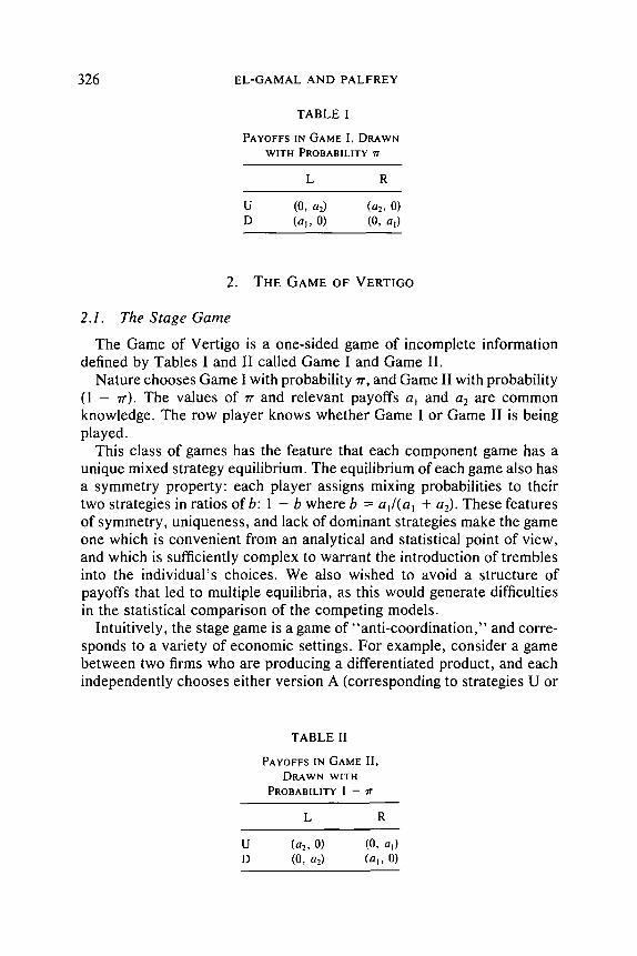
TABLE I

PAYOFFS IN GAME I, DRAWN

WITH PROBABILITY ~"

L R

U (0, a2) (az, 0) D (al, 0) (0, at)

2. THE GAME OF VERTIGO

2.1. The Stage Game

The Game of Vertigo is a one-sided game of incomplete information defined by Tables I and II called Game I and Game II.

Nature chooses Game I with probability or, and Game II with probability (1 - or). The values of or and relevant payoffs a I and a 2 are common knowledge. The row player knows whether Game I or Game II is being played.

This class of games has the feature that each component game has a unique mixed strategy equilibrium. The equilibrium of each game also has a symmetry property: each player assigns mixing probabilities to their two strategies in ratios of b: 1 - b where b = at/(a ~ + a2). These features of symmetry, uniqueness, and lack of dominant strategies make the game one which is convenient from an analytical and statistical point of view, and which is sufficiently complex to warrant the introduction of trembles into the individual's choices. We also wished to avoid a structure of payoffs that led to multiple equilibria, as this would generate difficulties in the statistical comparison of the competing models.

Intuitively, the stage game is a game of "ant i -coordinat ion," and corresponds to a variety of economic settings. For example, consider a game between two firms who are producing a differentiated product, and each independently chooses either version A (corresponding to strategies U or

TABLE II

PAYOFFS IN GAME II ,

DRAWN WITH

PROBABILITY I --

L R

U (az, O) (0, al) D (0, az) (a I, O)

VERTIGO 327

L) or version B (corresponding to strategies D or R). One of the firms is "bet ter" (say, superior quality control) than the other firm, and this is private information to firm 1. The better firm is best off if both firms choose the same version and compete head to head. The worse firm is best off if both firms choose different versions. Both firms are (weakly) better off when the worse firm chooses version A, conditional either on competing head-to-head (choosing the same version) or on choosing different versions. Game I corresponds to the column firm being better, and Game II corresponds to the row firm being better.

2.2 The Experimental Design

We study a 2n-person (n -> 5) five-stage repeated game based on the vertigo stage game defined above. There are n row players and n column players, who are seated at computer terminals which are separated by partitions. One payoffgame is drawn according to the probability zr before the beginning of stage 1. All row players in the room are informed of the outcome of this random draw. In stages I-5 each participant in the experiment plays the stage game against a sequence of five different opponents, always usi0g the same payoff game that was drawn initially.

The matching sequence is constructed using the technique of McKelvey and Palfrey (1992), which guarantees within the five stage game that it is logically impossible for a player's current move to have an effect on how that player's future opponents make choices in the later stages of the game. This is done by first labeling the players row player 1, row player 2 . . . . . row player n; column player 1, column player 2 . . . . . column player n. In stage 1, row player i is matched with column player i, and in stage j , row player i is matched with column player (i + j - 1) (mod n). Notice that, to avoid repetition, at least I0 players are needed. This matching sequence is announced to all subjects, and they are informed that the labels (e.g., row player i) are assigned randomly so that they cannot identify any of the players by their labels.

The information structure is controlled in a special way. In each stage players make their choices simultaneously. After everyone has moved, the row and column players are told what move their opponents at that stage chose. However, only the row players are told their payoff for that stage (they can infer it anyway from their knowledge of the drawn game). Since the column players were initially uninformed, and do not see their payoff they cannot infer directly which game was played. Play then proceeds to the next stage. After being rematched, each row player is informed of the history of the moves of other row players when they had previously played his current column player opponent. Thus for each pair, in each stage, the column player's past observations of row player moves is common knowledge to both players. The row player is not informed of the

328 E L - G A M A L AND PALFREY

current column player's past moves, nor is the column player informed of the current row player's past moves. This information structure permits the row player to (in principle) infer the current column player opponent's updated belief of whether the actual game being played uses payoff Game I or II, under the maintained hypothesis that earlier games followed Bayes- ian equilibrium play.

After the last stage (5) game is over, the payoff table is revealed to the column players and all subjects record their earnings. Subjects are then randomly reassigned player number labels (but row players remain row players, and column players remain column players). A second 5-stage game is then played in exactly the same manner as the previous one. A new payoff table is drawn according to the probability rr, independently from the past draws. The matching sequence is done in the same manner (but anonymously, since labels have been randomly shuffled), and so on. Over the course of each experimental session, we conduct a total of 10 5-stage games in exactly this manner. After the 10th 5-stage game, subjects are paid in private, one at a time, in a separate room.

All of the above information is publicly announced to the subjects, by reading the instructions aloud at the beginning of the session. Following the instruction periods, subjects were led step-by-step through a series of exercises to assure that they understood the information structure, the matching rule, how they would be paid, and the keyboard and record- keeping tasks. See Appendix A for all the details. The sessions were conducted on a network of computer terminals at the Caitech Laboratory of Experimental Economics and Political Science, using Caltech under- graduate students. No subject participated in more than one session. A total of two sessions were conducted using 26 different subjects.

The first session had 16 subjects. Therefore, we had 8 column subjects playing 10 rounds each, with each round consisting of 5 stages. Hence, we had 800 data points (400 column moves, and 400 row moves) from that first session. The second session had 10 subjects, i.e., 5 column subjects, and hence generated 500 data points. The first experimental session was conducted with ~- = 1/6, and payoffs a~ = $0.25, and a2 = $1.00. The second experimental session was conducted with rr = 0.2, and payoffs al = $0.50, and az = $0.75.

2.3. Equilibrium Strategies and Beliefs

The Bayesian equilibrium of the 5-stage repeated game can be calculated by separately computing the equilibrium of an arbitrary stage s, depending on the prior ~'s of a column player at stage s. The reason each stage can be treated independently (after accounting for the updating of the beliefs ~r s) is that our rotation and information structure isolates the strategic calculations of each stage. There is no role for signalling equilibria and

VERTIGO 3 2 9

reputational phenomena. Thus, for stage s, we index the strategies by the prior of the column player, say 7r s that Game I is currently being played. Denote:

q(Trs) = column player's mixed strategy [prob(L)].

p](Tr s) = row player 's mixed strategy [prob(U)] if Game I.

p2(~" s) = row player's mixed strategy [prob(U)] if Game II.

Finally, let 7rs+ I = 23(rr s, As) define the Bayes updating rule for a column player who started period s with prior ~'s, and observed the matched row opponent make move A s. Of course, rr~ = ~', the common knowledge probability announced in the instructions.

Thus to compute the equilibrium at stage s if the current prior on game I is rrs, we simply compute the (unique) one-shot Bayesian equilibrium given 7 L, and then at stage (s + I), we perform a similar derivation, except that we use the posterior 7L+ E = ~(Trs, D) or 7"/'s+ 1 = ~( 'n 's , U), depending on the row player's realized move at stage s.

Notice that in the laboratory sessions, several games are played simultaneously, so (except for stage 1) different pairs of players matched in stage s may have different common knowledge priors of the column player that they are playing Game I, depending on a column player's observations of moves by earlier row players. Recall that the design calls for row players to be told their current column opponent 's past observations of moves by other row players, which (in theory) preserves common knowledge of the current belief.

The actual derivation of equilibrium proceeds by establishing three facts, each of which may be verified by the reader. First denote b = a~/ (a~ + a2), and assume that b :~ rr. 3 The three facts are:

1. There is no pure strategy equilibrium.

2. For all values of rr, the column player is mixing.

3. For all values of zr, exactly one row type mixes.

From these facts, it is easy to compute the unique equilibrium of the game, and compute the updating rule, 7rs+ ~ = ~(rr~, A.~). One first shows that for any value zr ~ b, pure strategy equilibria cannot exist, the column player must be mixing, and the row player cannot be mixing in both games. It is then easy to show that there is a semi-pooling equilibrium where the row player mixes in Game I if and only if b < ~r, and the row player mixes in Game II if and only if b > 7r The non-mixing type chooses " U " . The column player 's mixing probability only depends on which type of row player is mixing. This is summarized below.

If b = ~', the equilibrium is indeterminate.


ifTr, E [0, b)

ifTr, ~ (b, 1]

q(Trs) = b

pl('rrs) = 1

1 - b P2(~'s) - I - 7r

7T ~ t a a 7Ts+ 1 "~¢rs"~sJ - I - b + 7r

7rs+l = ~(7r,, As) = 0

q(Tr s) = 1 - b

b pl(rrs) = --

77"

p2(Trs) = 1

if As = U

if As = D

b if As = U 7r,+j = 2~(~-s, As) - 1 + b - rr

7rs+t = ~(Trs, As) = 1 i fA s = D.

There are several notewor thy features of the equilibrium and the updating rule. First, the uninformed player acts " a s i f" he were informed. That is, if ~r s is sufficiently large (~- > b), his s trategy is exactly the same as if 7r = 1 was c o m m o n knowledge. I f 7r is sufficiently low, the reverse is true. Second, only hybrid equilibria (one type mixes, the other does not) can arise. This has two interesting implications. First, it implies a zero likelihood problem: some moves are predicted to never be played by some types of row players. Second, beliefs are updated sharply following some moves , since the mixing type is using a strategy that the non-mixing type never uses. When rr s is low, a choice of D reveals that it is Game II , and when 7r s is high, a choice of D reveals that it is Game I. Both of these implications point to the overly strong restrictions implied by Bayesian equilibrium. The first has to do with overly strong restrictions on actions, while the second has to do with overly strong restrictions on beliefs. What we propose below are some alternative models for coming to grips with these problems.

3. M O D E L I N G IMPERFECT B E H A V I O R

3.1. Errors in Actions

The maintained model is that at each move, an individual may t remble (with probabil i ty e) and randomly choose (with equal probability) a move f rom the menu of moves available to him/her. We write the strategies and

VERTIGO 331

updating rules as a function of e. It is convenient to define:

E = e(1 - 2b) 2 - 2 e

Model S, the sophis t ica ted model . The first model we introduce is the "perfect ly rational" extension of the previous model where the agents take into consideration that both their opponents and they themselves may tremble at any move with probability e, and incorporate that into their strategies. Straightforward analysis yields the following equilibrium strategies.

i fe < 2b andTr s < b - E f t

i fe < 2b and rr~

~ q(Trs)= 1

ife > 2b ~ ~pl(~'s) = 1 l

Lp2(Trs) = 1

"q(rr s) = b - E

pl(Tr~) = 1

l + E - b pz('n'~) - 1 - ~'~

(q(cr s) = l - b + E I

kp2(rr ,) = I.

Notice that if e is sufficiently large relative to b, there is a pure strategy pooling equilibrium at (U, L) which does not permit the uninformed players to update.

Mode l U: the unsophis t ica ted model . This model does not allow the players to take the e into account when constructing their strategies. The resulting strategies are:

['q(~'~) = b

~ p l ( ~ ) = I ifzrs ~ [0' b) ~ ~p2(Trs) = ~ - b

7/"

f q(Trs) = 1 ~ b

if~r s E (b, I] ::~ pl(Trs) =

kp2('/rs) = I.


The unsophis t ica ted model has the same equil ibrium as e = 0, since errors are not taken into a c c oun t when formulat ing strategies. Neve r the - less, different pat ters o f play are predic ted under the unsophis t ica ted model if e > 0, since obseroed mixing probabili t ies will be c loser to .5.

3.2. Errors in Beliefs

Model F, fas t (undampened) updating. This model uses the Bayes updat ing map to update f rom obse rved row player moves under the as- sumpt ion that t rembles canno t occur . For models SF (i.e. sophis t ica ted strategies, fast updat ing) and U F (i.e., unsophis t ica ted strategies, fast updating) the updat ing rule is:

f if~'s E [0, b] ~ ~ ~rs+t / (. 'B's + 1

i .

ifzrs ~ [b, 1] z~ ~ ' s + i / I- "B's + I

7r i fA s = U = ~3(~" s, A,.) - I - b + zr

= ~(Tr s, A s) = 0 i fA s = D

b = , . - i fA s = U ~ ( r r s A,,) I + b - 7r

= ~ ( r r s, As) = 1 i fA s = D

Not ice , that model F is only cor rec t when e = 0.

Model D, dampened updating. This model uses the Bayes updat ing map taking into cons idera t ion the fact that the obse rved row player moves may have resul ted f rom trembles . This updat ing rule will be different for models S and U. Fo r model SD (i.e., sophis t ica ted strategies, d a m p e n e d updating), the updat ing rule is:

i fe > 2b ~ {Trs+ I = ~(Trs, As) = ~'s

if e-< 2 b a n d 7r s-< b - E ~

• rs(1 - e/2) if A+. --- U 7rs+t = ~(Trs' As) = (1 - e)(l + ~'~ - b + E) + e/2

~r+e/2 i'rrs+~ ~ ( T r s ' a ' J (I e ) ( b ~ - ~ s - b S ) ~ - - e ~ i f a s = D

if e -< 2 b and ~'s -< b - E

= 1rs((l - e)(b - E)I~'~ + el2)

VERTIGO 333

if zrs ~ [0, b]

lrs(l - e/2)

f zrs+ t = ~(¢r~, A s) = (1 - e)(1 - b + 7r s) + e/2 i fA s = U

_ zr~e/2 ifA~ = D kTr~+, = ~(r rs , As) (1 - 8)(b - rr~) + 8/2

if~'s E [b, I] b ( l - 8) + ~r88/2

I zrs+ I = ~(¢r~, As) = (1 - 8)(I + b - rr s) + 8/2 i fA s = U

(Tr s - b)(1 - 8) + ~-88/2 LTr~+ I ~3(7r~, A s) (1 - 8)(7r s - b) + 8/2 i fA s = D

Not i ce that mode l D is " c o r r e c t " upda t ing for all va lues of 8.

Model N, no updating. The final mode l o f updat ing that we cons ide r is the c o m p l e t e l y m y o p i c one whe re the p layers do not learn f rom obse rva - t ions and main ta in their initial be l ief rr~ = ¢r th roughou t the s tages s = 1, . . . . 5. The updat ing rule for the two mode l s SN (i.e. sophis t ica ted s t rate- gies, no updat ing) , and U N (i.e. unsoph i s t i ca t ed s t ra tegies , no updating) is s imply:

~'s+1 = ~( r rs , U) = ~(Tr s, D) = rr s = zr

Mode l N is co r rec t with unsoph i s t i ca t ed s t ra tegies only if e = 1, and with soph is t i ca ted s t ra tegies only if e > 2b.

4. EXPERIMENTAL RESULTS

4.1. Bayesian Econometric Method

We have a total o f six mode l s which we have labeled SN, U N , SD, UD, SF, UF . The first le ter (S or U) refers to whe the r the model a s s u m e s that agents i nco rpo ra t e the t r emble probabi l i t ies in fo rming their s t ra tegies (deno ted by S for sophis t ica ted) , or ignore t hem (denoted U for unsophis t i - cated) . T h e second le t ter (N, D, or F) refers to w h e t h e r the mode l a s s u m e s that agents do no updat ing at all (deno ted N for no updat ing) , use B a y e s updat ing but d a m p e n e d by the t r emble probabi l i t ies (denoted D for d a m p ened updat ing) , or use B a y e s updat ing under the a s s u m p t i o n that no t r embles can o c c u r (deno ted F for fast updat ing) . 4

T h e e c o n o m e t r i c mode l we use to c o m p a r e the six theore t ica l mode l s is der ived di rec t ly f rom the stat ist ical s t ruc ture implied jo in t ly by the

4 The SD and SN models correspond to the "sequential" and "nonsequential" models of EI-Gamal et al. (1993), respectively.


predicted strategies and the "errors in actions" assumption. In our model, we allow the errors to vary across time, in order to capture any learning- by-doing that may occur. We parameterize this by assuming that et = eo e-~t, where e0 E [0, 1] is the initial error rate and a -> 0 is the learning- by-doing parameter.

We adopt a Bayesian econometric procedure. Since some readers may not be familiar with this approach, we briefly explain the procedure below. Loosely speaking, the data analysis can be divided into two steps, roughly corresponding to the traditional components of estimation and testing. We begin the first part of the analysis by assessing our priors over the possible values of the two nuisance parameters, e0 and a. 5 After each observation of a data point, we update our priors over these two parameters using Bayes' rule, using the likelihood functions from each of the six competing models. This gives us six beliefs (one for each of the six models), in the form of posterior distributions on the parameter space. At this point, the only departure from standard Maximum Likelihood procedures is that MLEs take the form of point estimates (corresponding to the mode of our posterior, since we use uniform priors) ignoring the rest of the information in our posterior. Given these posterior distributions, the second part of the statistical procedure (roughly corresponding to "testing") begins by assessing our prior odds for the six models. We assume equal (uninformative) prior odds of 1/6 for each model. After updating our beliefs about the nuisance parameters, we compute the posterior odds of each model, which, given our assumption of equal prior odds, is simply the relative likelihood of observing that data set under each model. These posterior odds are normalized to sum to 1 across the six models.

The likelihood functions under each of the six models are derived as follows. As in Subsection 2.3 above, the equilibrium strategic behavior under all the models can be indexed by the beliefs of the column (uninformed players) at time s that Game I is being played (which we label ¢rs, being updated over the five stages of the game using the appropriate updating rule N, D, or F). For each column player, we observe that player's five moves, and the moves of his 5 row opponent (a total of 10 data points) for each round. Notice that again by our discussion of Subsec- tion 2.3 above, once we condition on the belief ors of each column player at each stage s (which is directly computable since we know ¢r~ = 7r, and the sequence of row-opponent moves that he observes), all 1300 data

s We first decided on the suppor ts of e0 ~ [0, 1] and c~ ~ [0, 0.3] (corresponds to a = 0.3 and el0 = e0/20). We then cons t ruc ted uninformative (uniform) priors on those supports . It is well known that as our data sample gets large, the likelihood function dominates the prior, and hence only the supports of the prior are o f real concern. Our choice of the upper limit of the support of ct reflects our belief that the rate of errors after l0 rounds would not be less than 5% of e0.

V E R T I G O 3 3 5

points that we have can be treated as independent draws 6 from the appropriate q(Tr s) and either pl(zrs) or p2(zr s) depending on whether Game I or II was being played.

For each model IJ (I = S, U; and J = N, D, F), denote the strategies of the players under that model by qU(zrs), p~(rrs), and p~J(zrs), and denote the updating rule by ~tJ(Tr s, As). Then, given data for n column players, we compute the likelihood under model IJ of the data generated in all n x 50 games (n players times 5 stages times 10 rounds) by

I~I 10 5 Like tJ (zr)= f0' f0 °'3 1--[ I-[ [(1 _,o0~,~-ar~Dr,-,klJl~eolumn./l"vt-' I-t~rs , 7rrs } .at_ e0e-,~/2]

player= 1 r= 1 s= 1

[(1 - - a r l J row eoe )Prob {ars zr~s } + eoe-~r/2]prior(deo, dct), x

where r indexes the rounds 1 . . . . . 10; s indexes the stages 1 . . . . . 5; the tremble probability in round r is the same for all players and defined by the learning by doing model er = e0e-'~r; A~ °W is (U or D) the appropriate row player 's action in round r and stage s; and aCrs °lumn is (L o r R) the appropriate row player 's action in round r and stage s. ~'~s is the appropriate column player 's belief in stage s of round r, which is set at each stage 1 at 7rrl = zr, and then updated using Try.s+ l = ~H(Zrrs, ar°w). All variables are of course indexed by the column players 1 . . . . . n but that dependence has been suppressed in the above equation since no confusion can arise. The probabilities ProbtS{.} are computed using the Bayes -Nash strategies under model IJ. For instance ProbeS{U; 7rrs } = p~J(zrs) if Game I was played and p~J(Trs) if Game II was played; ProbH{R; 7 r J = I - qIJ(rr,), and so o n .

After evaluating the likelihoods of our six models Like tJ, for I = U, S, and J = N, D, F, we can compare each of the models to the other five by computing the posterior odds ratio. The posterior odds for model IJ are simply Like~J/'Zi=u.s~=N,o. F Like °. This measures the relative likelihood of model IJ within the collection of models that we consider.

4.2. Results

Table III displays the likelihood for all six models that we study using all 1300 data points. The results were very similar for the first and second sessions, and hence we only report the aggregate results from both sessions.

6 This also embodies an implicit assumption of homogeneity of initial error rates (e0) and learning rates (c0 across subjects. Each additional nuisance parameter increases computation time between 10- and 100-fold, depending on how fine a grid is used for the numerical integration. Making the model more heterogeneous (for instance with different error rates for informed and uninformed players) would add parameters to the model.

336 E L - G A M A L AND PALFREY

T A B L E III

LIKELIHOODS OF THE OBSERVED DATA UNDER

OUR SIX MODELS

N D F

U 8.8 × 10 -355 2 × 10 -355 1 x 10 -358

S 4.8 x 10 -373 4.1 x 10 -373 1.9 x 10 -377

Table IV shows the posterior odds discussed in the previous subsection. Notice that the pure randomness model (where all players mix with probability 0.5) is nested in all six models (via e0 -- 1, a = 0). Hence, all six models will perform better than the pure randomness model. The likelihood under the pure randomness model is 0.5 ~3°° = 4.6 × 10 -392, which is many orders of magnitude lower than the worst performing of our six models. Even though our conclusion is that the unsophisticated models are very strongly favoured over the sophisticated models, we should also state that even the sophisticated models explain the data much better than pure randomness.

It is clear that only unsophisticated models have credibility within the class of six models that we analyze. Moreover, model UN (which assumes the least sophistication in updating) seems to be about 4.4 times as likely as model UD, suggesting that models can be ranked according to their degree of sophistication. While UF significantly outperforms all of the sophisticated models, it performs poorly within the class of unsophisticated models. Indeed, a quick look at Tables III and IV shows that models can be monotonically ranked with less sophistication always being better than more (U uniformly beats S), and with slower or no updating always dominating fast updating (N uniformly beats D which in turn uniformly beats F).

Appendix B contains six figures depicting the joint posterior on (e0, a) under each of the models. Since we started with uniform priors on those nuisance parameters, those posteriors are simply the likelihood function at each (e0, a) under each of the models normalized to integrate to 1. It is clear from the pictures that all the models concentrate our posterior

T A B L E IV

THE POSTERIOR ODDS ON OUR SIX MODELS

N D F

U 0.815 0.185 9.3 x 10 -5 S 4.4 x 10 -19 3.7 x I0 -19 1.8 x 10 -23

VERTIGO 337

belief on e0, the initial rate of trembling, around 0.7, with the exception of model SF which has the posterior concentrated at a value of e0 above 0.8. The striking difference between the models in terms of posterior beliefs on the nuisance parameters is between the unsophisticated (U) models on the one hand, and the sophisticated (S) models on the other. All the sophisticated models concentrate our beliefs on a, the exponential rate of learning by doing, at zero. This means that the rate of trembling does not decline over time. This will typically happen when the strategic model fails to explain the behavior of the subjects, and it becomes easier to explain their behavior by trembles. For the unsophisticated models, our posterior belief on et is concentrated around 0.1. This means that the subjects start the session trembling around 70% of the time, and end up trembling around 26% of the time by the 10th round.

Appendix C contains the raw data. While the main point of this paper is not to provide an informal description of subject behavior, some aggregate descriptive features of the data are useful for explaining why the UN model performs better than the other five models. First, there are clear time trends in the data that correspond to the predictions of the U-model if there is learning-by-doing (a > 0). In this case, the U-model makes several qualitative predictions about time trends in the aggregate frequencies of row choices and column choices, including the following.

I. The frequency of " L " by the column player should decline over the course of the experiment, for both experimental parameter sets.

2. The " L " frequency should be greater in the second parameter set than in the first parameter set.

3. The decline i n " L " frequency should be greater in the first parameter set (b = 1/5, rr = I/6) than in the second parameter set (b = 2/5, 1r--- 1/5).

4. The observed frequencies o f " U " should increase over the course of an experimental session, for both Game I and Game II, and for both parameter sets.

The S-model makes a different prediction. In particular, for large e the S-model predicts that column player strategy is to choose " L " in both parameter sets. The effect of learning for the range of e that we estimate imply the opposite of prediction 1 (if there is learning by doing): " L " frequencies should decline over time. All four of the above qualitative features appear in the data. This is captured in the parameter estimates of the probit equations reported in Table V, and in the aggregate move frequencies reported in Tables VI and VII. This gives some indication of why the S-model is outperformed by the U-model.

Of the three U-models, the fast updating model (F) is clearly the worst. We believe the reason for this is that F predicts a strong history depen-


TABLE V

PROBIT ESTIMATES OF TIME TRENDS

Parameter set 1 Parameter 2

Col. move Row move Col. move Row move

Constant 0.164 0.453 0.131 0.168 (1.21) (3.02) (0.76) (0.95)

Round coeff. -0.047 0.074 -0.007 0.073 (2.14) (2.88) (0.26) (2.47)

n 120 280 75 175

Note. Dependent variable for "column move" estimates takes on a value of 1 if " L " and 0 if " R " . Dependent variable for "row move" takes on value 1 if " U " and 0 if " D " . Asymptotic t-values in parentheses, n is the number of data points for each probit equation.

dence in the moves by the row player if his current column opponent has ever observed a "D", since in equilibrium "D" is a revealing move in the F-model, informing column players that game two has been drawn. In both games and in both parameter sets, this should lead to a decrease in the frequency of column players choosing "U" following any history where a "D" has been observed. In fact, we observe exactly the opposite. Table VIII displays the effect on row player behavior of histories that include at least one "D" observation by the column player.

TABLE VI

FREQUENCY OF COLUMN PLAYER MOVES FOR ALL ROUNDS, EARLY ROUNDS~ AND LATE ROUNDS

Parameter set 1 Parameter set 2

Game I Game II Game I Game II

Frequency of " R " 0.58 0.52 0.45 0.47 All rounds (69) (146) (34) (82)

Frequency of " L " 0.42 0.48 0.55 0.53 All rounds (51 ) (134) (41) (93)

Frequency of " 'R" - - 0.49 0.52 0.44 Rounds 1-5 (--) (97) (26) (33)

Frequency of " L " - - 0.51 0.48 0.56 Rounds 1-5 (--) (103) (24) (42)

Frequency of " R " 0.58 0.61 0.32 0.49 Rounds 6-10 (69) (49) (8) (49)

Frequency of " L " 0.42 0.39 0.68 0.51 Rounds 6-10 (51) (31) (17) (51)

Note. The number of observations in each cell is shown in parentheses.

VERTIGO

TABLE VII

FREQUENCY OF ROW PLAYER MOVES FOR ALL ROUNDS, EARLY ROUNDS, AND LATE ROUNDS

339


Game I Game II Game I Game lI

Frequency of " U " 0,90 0.76 0.67 0.73 All rounds (108) (212) (50) (128)

Frequency of " D " 0,10 0.24 0.33 0.27 All rounds (12) (68) (25) (47)

Frequency of " U " - 0.76 0.68 0.65 Rounds I-5 (-) (152) (34) (49)

Frequency of " D " - 0.24 0.32 0.35 Rounds 1-5 (-) (48) (16) (26)

Frequency of " U " 0.90 0.75 0.64 0.79 Rounds 6-10 (108) (60) (16) (79)

Frequency of " D " 0.10 0.25 0.36 0.21 Rounds 6-10 (12) (20) (9) (21)


TABLE VIII

FREQUENCY OF " U " BY ROW PLAYER, DEPENDING ON WHETHER COLUMN PLAYER HAS OBSERVED AT LEAST ONE " D " ( " D " HISTORY) OR NO " D " (No " D " HISTORY), FOR

ALL ROUNDS, EARLY ROUNDS (I--5) AND LATE ROUNDS (6--10)


Game I Game II Game I Game II

" D " hist. 0.952 0.766 0.718 0.792 All rounds (21) (107) (39) (77)

No " D " hist 0.889 0.751 0.611 0.684 All rounds (99) (1"13) (36) (98)

" D " hist. - - 0.76 0.77 0.69 Rounds I-5 (--) (76) (30) (35)

No " D " hist - - 0.76 0.55 0.63 Rounds 1-5 (--) (124) (20) (40)

" D " hist. 0,95 0.77 0.56 0.88 Rounds 6-10 (21) (31) (9) (42)

No " D " hist 0,89 0.73 0.69 0.72 Rounds 6-10 (99) (49) (16) (58)

Total n 120 280 75 175



The dampened updating model (D) does better than the F model because it does not make as sharp a prediction about the updating. In fact, for large values of e, its predictions coincide with the predictions of the N model. With the estimated value of c~, the predictions of the D model go in the wrong direction in the last few rounds, when e has declined due to learning-by-doing. Because the N model assumes no history dependence at all, it does the best of all three updating models.

Finally, observe that task experience (rounds 6-10 vs rounds 1-5) does not lead to many changes in behavior, according to Tables VI and VII. The only apparent change of any magnitude is in parameter set 2 (see also Table VIII). There we find an increase in " U " play in Game II, which is consistent with c~ > 0 in the U model. Also consistent with task learning (c~ > 0) is the observation (Table 6) that in Game I, experienced column players choose " L " more frequently than inexperienced column players, while the reverse is true in Game II. In fact, inexperienced players in parameter set 2 choose " L " with higher frequency in Game II than in Game I, while this reverses (as predicted) for experienced subjects. In parameter set 1, there were no draws of Game I for inexperienced subjects, but experienced subjects (as predicted) play " L " more frequently in Game I than in Game II.

5. CONCLUDING REMARKS

We introduced a simple repeated game with one-sided incomplete information to study models which allow for deviations from perfect rationality. We introduced the probability of players making errors in actions, and studied deviations from Bayes-Nash behavior in two dimensions. On the first dimension, we developed two models where players take or do not take into account the errors in actions when formulating their optimal responses. On the second dimension, we developed three models where players use Bayes updating ignoring the errors in actions, use Bayes updating taking account of the errors in actions, and do not use any updating. The results from the experimental data show that on both dimensions, less sophisticated models perform better than the more sophisticated ones. This ranking is particularly strong along the dimension of optimal response formulation (where the computational cost of incorporat- ing the errors in actions is more pronounced), the unsophisticated model very impressively outperforms the sophisticated.

As usual with all experimental work, the results may be limited to the class of games that we looked at. It would be interesting to investigate if similar results obtain in different environments. In fact some of the findings here are probably true for a very wide class of experimental games. For

VERTIGO 341

example, the estimate of ct > 0, reflecting learning-by-doing, was also recovered in McKelvey and Palfrey (1992) and EI-Gamal et al. (1993), and is supported widely in informal data analysis of most game experiments.

Proceeding cautiously, we hope the reader is left with two strong mes- sages from our results. The first is methodological, and states that appar- ently small differences in the way that imperfect behavior in experimental games is introduced can have substantially different implications. Never- theless, rigorous statistical analysis of the data is both feasible and worth doing. Clearly more investigation of alternative ways to statistically model these imperfections is an important job for future theoretical and experimental research. The second is theoretical, and states that it is unreason- able to assume too much rationality on the part of players. This is true not only because of the unreasonably strong statistical restrictions implied by full rationality, but for substantive reasons as well. Further synthesis of experimental and modeling techniques to uncover useful and theoretically sound ways to incorporate limited rationality seems to be a useful direction to proceed.

A P P E N D I X A : INSTRUCTIONS FOR EXPERIMENTAL PARTICIPANTS

This is an experiment in human decision making under uncertainty. As you entered the room, you were randomly assigned a seat. If your seat is on the middle isle of the room, you are an " A " participant and will be one for the duration of this experiment. If your seat is on one of the outside aisles of the room, you are a " B " participant and will be one for the duration of this experiment. The instructions are slightly different for A participants and B participants. You should make sure that you understand the instructions for both A and B participants since your payoff will depend on your actions, and the actions of participants of the other type. The experiment will have 10 rounds, each round consisting of 5 periods.

Feel free to raise your hand and ask questions at any point. Make sure that you understand the instructions before the experiment begins. If you have any questions during the experiment, feel free to raise your hand and ask the experimenter who will be present throughout the experiment, and will answer your question privately.

At no point during the instructions period or during the experiment are you allowed to communicate in any way with other participants.

In each period of each round, each A participant will be matched with a different B participant. A participants will be asked to choose either left (L) or right (R). B participants will be asked to choose either up (U) or down (D). The two moves of the A and the B participants determine their payoffs for that period of that round according to one of the following two payoff tables: (show transparency I)

I Two out of ten chance: PAYOFF TABLE I ]

A participant chooses L A participant chooses R B participant A gets $0.75 A gets $0.00

chooses U B gets $0.00 B gets $0.75 B participant A gets $0.00 A gets $0.50

chooses D B gets $0.50 B gets $0.00


eight out of ten chance: PAYOFF TABLE II [

A participant chooses L A participant chooses R B participant A gets $0.00

chooses U B gets $0.75 B participant A gets $0.75

chooses D B gets $0.00

A gets $0.50 B gets $0.00 A gets $0.00 B gets $0.50

For example, if the relevant payoff table turns out to be Table I, and if you are participant A3, matched with participant B2, and if you choose L, and B2 chooses D, then you get $0.00, and participant B2 gets $0.50. For a second example, if the relevant payoff table turns out to be Table II, and if you are participant B5, matched with participant AI, and if you choose U, and participant AI chooses L, then you get $0.75, and AI gets $0.00.

At the beginning of each round, one of the two payoff tables will be chosen at random by rolling a fair 10-sided die. If the outcome is 0 or 1, the first payoff table will be used for that round, otherwise, (if the outcome is 2, 3, 4, 5, 6, 7, 8, or 9) the second payoff table will be used for that round. All B participants will then be informed of the relevant payoff table for the round as soon as the die is rolled. The die will be rolled so one of the B participants can verify the outcome. The A participants will not be informed of the relevant payoff table until the end of the round.

At the beginning of each round, new identity numbers will be randomly assigned to both A and B participants. For the duration of that round, you will be referred to by your type (A or B), and your number. For instance, if you are an A participant, you may be AI, A2, . . . . etc. If you are a B participant, you may be B l, B2 . . . . . etc. (Remember that your letters (A or B) remains the same all the time, but your number may be different from round to round.) Each A participant is assigned one white sheet, one red sheet, and five green slips. The white sheet contains the following table to be filled by each A participant (show transparency 2):

WHITE SHEET FOR Name ID:A--

ROUND 1 MY MY MOVE PERIODS MATCH L or R

TOTAL PAYOFF THIS ROUND IS:

MATCH's PAYOFF U or D in $

The red sheet contains the following table to be filled by the B participants with whom our A participant is matched at each period:

RED SHEET FOR A - - [

PERIODS 1 2 3 4 5

My B's MATCH Moves

VERTIGO 343

The green slips each contains one cell, and they are to be filled by the A participant.

GREEN SLIP FOR PARTICIPANT A-- ]

To each B player is assigned a white sheet to be filled out by the B participants:

WHITE SHEET FOR NAME ID: B--

ROUND I MY PERIODS MATCH

I 2 3 4 5

TOTAL PAYOFF THIS ROUND IS:

MY MOVE MATCH's PAYOFF U or D L or R in $

Since participants are randomly assigned new identity numbers in each round, you will never know the participant with whom you are matched.

In each round, the following sequence of events occurs:

I. The round begins.

2. Participant identity numbers are randomly drawn. Everyone is informed of their own identity number but no one else's.

3. The relevant payoff matrix is randomly determined by rolling a 6-sided die, the B participants are informed of the relevant payoff table (it is the table with the highlighted background) for that round.

4. The first period begins. During that period: (a) The A participants enter their move (L or R) at the flashing sign on their green

slip (the green slip disappears from the A participant's screen). (b) The revelant A participant's red sheet appears on each B participant's screen.

The B participants enter their move (U or D) at the flashing sign on the red sheet of the relevant A participants.

(c) After all participants have made their moves, all moves are automatically re- corded on the white sheets of A and B participants.

(d) The B participants will see their payoffs after each period whereas the A participants will only be informed of their payoffs at the very end of the round when the relevant payoff table is revealed.

(e) The first period ends.

5. The second period begins. The same procedure is followed.

6. The third period begins. The same procedure is followed.

7. The fourth period begins. The same procedure is followed.

8. The fifth period begins. The same procedure is followed.

9. The round ends.

10. The relevant payoff table for this round is revealed. The white sheets now show your total payoff for this round as well as your payoff for each period. Copy your total payoff for this round onto the record sheet.


There will be 10 such rounds. Now, instruct participants to turn on their computers, and follow instructions. First we

shall walk you through a practice round, you will not be paid for this practice round. The practice round will be conducted both on the computers and using actual paper sheets and slips. Follow the instructions of the experimenter and do not write anything on the sheets or the computers until instructed to do so. During the practice round, the experimenter will tell you what choices to make, make exactly those choices.

First period: DR, second period: UL, third period: UR, fourth period: DL, fifth period: DR.

The practice round is over, check payoffs, etc. Get ready for starting the actual experiments. Remember that the experiment will have 10 rounds like the one you just witnessed. You will be paid what you earn for all 10 rounds. In the actual experiment, you will use the computers only (no sheets of paper will be used).

Outcomes of practice round if the first table is drawn (show transparency 3). Outcomes of practice round if the second table is drawn (show transparency 4).

VERTIGO 345

A P P E N D I X B: POSTERIORS ON (e0, or) UNDER THE SIX MODELS

1500 !

IOOC

50,

Fro. 1. Posterior under Model SN.

LI500

1000

~00

.3

Flo. 2. Posterior under Model SD.

L1500

1000

;00

3

FIG. 3. Posterior under Model SF.

346 E L - G A M A L A N D P AL F REY

30-~

20

11

FIG. 4. Posterior under Model UN.

0

) iff

FIG. 5. Posterior under Model UD.

~30

2O

/t/ 0

3

FIG. 6. Posterior under Model UF.

V E R T I G O 3 4 7

APPENDIX C: RAW DATA

R A W DATA, BOTH SESSIONS, FIRST 5 ROUNDS [

I I U SEsS,ON X II SESSION 2 Rd St Dr C1 C2 C3 C4 C5 C6 C7 C8 Dr C9 CI0 C11 C12 C13

I i 2 LU LU RU LU LU LD LU RU 1 RU LD RU LU LD

I 2 2 LU LU RU LU LD LU RD RU I RD LU LD RU RD

I 3 2 RU LD RU LD LU RU RU LD I RU LU LU RD LU

1 4 2 LU RU RD LU LD LU LD RD 1 LD RU LU RD RD

1 5 2 LU LD LU LD LU LU LD LU 1 RU LD LU LD LU

2 I 2 RU RU RU LU LU RU LU LU 2 RU RU RD RU RU

2 2 2 RU LU LU RU LU RU LU LU 2 RU LD RD RD RU

2 3 2 LU LU RU RU LD RU LU RD 2 RD LU RU LD RU

2 4 2 RU LU RD LU LU LU LD RU 2 LD RD LU LD LU

2 5 2 LU LD RU RU LU RU LD RU 2 RU LU LU RU LD

3 I 2 RU RU RU RU LU RD RU RD 2 RU LD LD LU RD

3 2 2 RU RD RU RU RU RU LD RU 2 RU LU LD LU RU

3 3 2 LD RD LD RU LD RU RU RU 2 LD LU LU RU LD

3 4 2 RD LU LU RU RU RU LU LD 2 RD RU LU RU LU

3 5 2 LU LU LU RU LD RU LU RU 2 LU LD LU LD LU

4 I 2 RU RD RU RU LU RD RU RD I LU LU RD RU RD

4 2 2 RD LU RU RU RU RU LU RD I RD RU RU RD LU

4 3 2 RD LU LU RU LD RU LU LU 1 RU LU RU LD RU

4 4 2 LU LD LU RU LU RU LU LU 1 RU RU RU LU RU

4 5 2 RU LU LU RD LU RD LU LU I LU LU RU LU LU

5 1 2 RU LD RU RU LU LD RU LD 2" LU LU RD RU LU

5 2 2 LU LU RU RU RD LU LU LU 2 RU RU LU LD LU

5 3 2 RU LU LU RU LU RU RU RU 2 LD LU RU LD LU

5 4 2 RU LD LU RD RD RD RU RU 2 LU RU RU RU LU

5 5 2 LU RU LU LU LU RU LU LU 2 LD LD RU LU RD

[ RAW DATA, BOTH SESSIONS, LAST 5 ROUNDS J

I i il SEsSiON i Ii SESSION 2 Rd St Dr Cl C2 C3 C4 C5 C6 C7 C8 Dr C9 CI0 CII C12 C13

6 I 2 LU LD RU RU RU LU RU RU 2 RU LU LU RU RD

6 2 2 RU LU RD RD LU LU RU RU 2 RD RD LU RU RU

6 3 2 RD LD RU RU RD LU RU RD 2 RU LU LD LU LU

6 4 2 LU LU RU RD LU LD RU RU 2 RU RU LU RD LU

6 5 2 RU LD RU LU RU RD RU RU 2 LU LD RD LU RU

7 I 2 RU LU RD RU RU LU RU LU 1 RU LU LU RU LU

7 2 2 RU LD RU RD RU RU RU RU 1 LU LU LU RD RU

7 3 2 RU LD RU LU LD LU RU RD I RU RU LD LD LD

7 4 2 RU RU RU RU LU LU RU LU 1 LD LD LU LD LU

7 5 2 LU LU RU LD LD LD RU LU I RU RD LU LU LD

8 I 1 RU LU RU LU RU LU RU RU 2 RU RU LU RD LU

8 2 I RD LU RU RD LU RU RU RU 2 RU LD LD LU RU

8 3 I RU LU RU RU RD RU RU LU 2 LU LU LU LU LD

8 4 I RU LU RU LU RU LU RU RU 2 LU RU LU LU LU

8 5 I LU LU RD LU LU LU RU RU 2 LU LU LU LD LU

348

I

EL-GAMAL AND PALFREY

RAW DATA, BOTH SESSIONS, LAST 5 ROUNDS

I I II 9 1 l RU

9 2 l LU

9 3 I RU

9 4 1 RU

9 5 1 RU

I0 l I RU

10 2 I RU

10 3 1 RU

I0 4 I LU

10 5 I RU

SESSION

LU RU RU RU LU

LU RU RD LU RU

LU RU RU RD RU

LU RU LU LU LD

LU RU LD LU RU

LU RU RU RU LU

LU LU RU LU RU

LU RU LU RD RU

LU RU RU LU LU

LU RU RU LU LU

II SESSION 2

RU RU 2 RU LU LU LU RU LU LU 2 RU RU LU RU LU RU RU 2 RU LU LD LU RU RD RU 2 LU LU RU RD RU LU LU 2 RU RD RU LU LU RU LU 2 RU RU RU RD RD

LU RD 2 LD RD RU LU LU

RU LU 2 RU LU RU LU RU

RD LU 2" RU RU RU RD RU

LU RU 2 RU LD RU LU LU

Note. Rd is the round, St the stage being played by column (uninformed) player Ci. There were a total of 13 column players in both sessions. Dr is the draw of the game which is either I or 2. In session I, game 1 was drawn with probability rr = 1/6, and payoffs a~ = $0.25, and a 2 = $1.00. Session 2 was conducted with p = 0.2, and payoffs a~ = $0.50, and a2 = $0.75. The two letters in each cell represent the moves of the column player (L or R) followed by the moves of the row player (U or D). The identities of the row players being matched with the column player in each round was different for each stage within a round.

REFERENCES

BANKS, J., CAMERER, C., AND PORTER, D. (1994). "An Experimental Analysis of Nash Refinements in Signaling Games," Games Econ. Behav. 6, 1-31.

BEJA, A. (1992). "Imperfect Equilibrium," Games Econ. Behav. 4, 18-36.

BOYLAN, R., AND EL-GAMAL, M. (1993) "Fictitious Play: A Statistical Study of Multiple Economic Experiments," Games Econ. Behav. 5, 205-222.

BP, ANDTS, J., AND HOLT, C. (1992). "An Experimental Test of Equilibrium Dominance in Signaling Games. Amer. Econ. Rev. 82, 1350-1365.

BROWN, J., AND ROSENTHAL, R. (1990). "Testing the Minimax Hypothesis: A Re-Examina- tion of O'Neill 's Game Experiment," Econometrica 58, 1065-1081.

CAMERER, C., AND WEIGELT, K. (1988). "Experimental tests of a sequential equilibrium reputation model," Econometrica 56, 1-36.

COOPER, R., DEJONG, D., FORSYTHE, R., AND ROSS, T. (1990). Selection criteria in coordination games. American Economic Review 80, 218-233.

EL-GAMAL, M., MCKELVEY, R., AND PALFREY, T. (1993). "A Bayesian Sequential Experi- mental Study of Learning in Games," J. Amer. Statist. Assoc. 88, 428-435.

HARLESS, D., AND CAMERER, C. (1992). The predictive utility of generalized expected utility theories, mimeo, University of Chicago.

MCKELVEY, R. D., AND PALFREY, T. (1992). "'An Experimental Study of the Centipede Game," Econometrica 60, 803-836.

PALFREY, T., AND ROSENTHAL, R. (1991). "Testing Game-Theoretic Models of Free Riding: New Evidence on Probability Bias and Learning," in Laboratory Research in Political Economy (T. Palfrey, Ed.), 239-268. Univ. Michigan Press, Ann Arbor.

PALFREY, T. AND ROSENTHAL, R. (1992). Repeated play, cooperation and coordination: An experimental study, SSWP 785, California Institute of Technology.

Vertigo: Comparing structural models of imperfect behavior in experimental games

Documents

Transcript of Vertigo: Comparing structural models of imperfect behavior in experimental games