1

Exp Fluids (2011) 50:233–246, DOI 10.1007/s00348-010-0919-8

STUDY OF MASS AND MOMENTUM

TRANSFER IN DIESEL SPRAYS BASED ON X-

RAY MASS DISTRIBUTION MEASUREMENTS

AND ON A THEORETICAL DERIVATION.

J.M. Desantes, F.J. Salvador (*), J.J. López, J. De la Morena.

CMT-Motores Térmicos, Universidad Politécnica de Valencia, Camino de Vera

s/n, E-46022 Valencia, Spain

(*) Corresponding author:

Dr. Francisco Javier Salvador

Telephone: +34-963879658

FAX: +34-963877659

fsalvado@mot.upv.es

In this paper a research aimed at quantifying mass and momentum transfer in the near-nozzle field

of diesel sprays injected into stagnant ambient air is reported. The study combines x-ray

measurements for two different nozzles and axial positions, which provide mass distributions in

the spray, with a theoretical model based on momentum flux conservation which was previously

validated. This investigation has allowed the validation of Gaussian profiles for local fuel

concentration and velocity near the nozzle exit, as well as the determination of Schmidt number at

realistic diesel spray conditions. This information could be very useful for those who are interested

in spray modelling, especially at high pressure injection conditions.

Keywords: Diesel sprays, near field, Schmidt number, concentration, modelling,

x-ray

2

List of symbols

A Outlet hole section.

C (x,r) Local spray mass concentration.

Cv (x,r) Local spray volume concentration.

Caxis (x) Concentration at a determined axial position of the

spray.

D Mass diffusivity.

I X-ray beam intensity after passing through the spray.

I0 X-ray beam incident intensity.

i Counter of Taylor’s series.

j Counter used in the determination of the Mean Squared

Deviation (MSD) between PDPA data and prediction by

radial profiles.

k Constant used in fitted Gaussian profiles.

M’ Projected mass obtained from x-ray measurements.

o

.

M Momentum flux at the nozzle orifice outlet.

am Air mass.

fm Fuel mass.

f

.

m Fuel mass flow rate.

MSD Mean Squared Deviation between PDPA experiments

and theoretical radial profiles.

p, q Counters in the numerical procedure for determining the

optimal Schmidt number.

N Number of terms in the Taylor series.

nr Number of measuring points in the radial direction.

nx Number of measuring points in the axial direction.

nex Number of measurements from PDPA.

Pback Backpressure.

Pin Injection pressure.

3

r Radial coordinate.

r1 Radial position of the x-ray beam at the central plane of

the spray.

r1/2 Radial position at which local spray velocity decreases

until a value of 0.5·Uaxis.

R Radius of the spray defined from velocity profile.

Rm Radius of the spray defined from concentration profile.

S Spray tip penetration.

Sc Schmidt Number.

t Time from the start of injection.

Uaxis (x) Velocity at the spray’s axis.

Uo Orifice outlet velocity.

U(x, r) Local spray velocity.

Uex (xj,rj) Experimental local velocity value from PDPA

measurements at experiment j.

Umo (xj,rj) Local velocity value estimated form a theoretical radial

profile at experiment j.

Va Local volume occupied by air.

Vf Local volume occupied by fuel.

x Axial coordinate.

z Axial perpendicular coordinate used in the experimental

x-ray measurements.

Greek symbols:

Coefficient of the Gaussian radial profile for the axial

velocity.

ε Mean deviation in the prediction of M’.

eq Equivalent diameter.

o Outlet diameter of the nozzle’s orifice.

Local spray density defined as a f

a f

m m

V V

.

4

L Local fuel density defined as fL

a f

m

V V

.

a Ambient density.

f Fuel density.

Kinematic viscosity.

Pi number.

m Spray cone angle defined from mass distribution.

u Spray cone angle defined from velocity distribution.

5

1. Introduction

Despite being used in many industrial applications, the study of sprays has always

been difficult due to the complex phenomena involved: atomization, mixing,

coalescence, transfer of mass and momentum and evaporation (Lefèbvre 1989,

Dumouchel 2008). This complexity is accentuated when studying sprays in direct

injection diesel engines because of the high frequency transient operation and the

small characteristic injection time and length (~1 ms and 25 mm). In such adverse

conditions from the point of view of experimentation, the spray characteristics

that can be measured are quite limited, especially in the densest part of the spray

(near-nozzle region). The most typical characteristics are spray tip penetration and

spray cone angle (Hiroyasu and Arai 1990; Naber and Siebers 1996; Way 1997;

Roisman et al. 2007), which are macroscopic characteristics, and droplet velocity

and droplet diameter, which are microscopic features (Wu et al. 1986; Jawad et al.

1992; Roisman and Tropea 2001; Subramaniam 2001). Nevertheless, in the

studies available in the literature, the microscopic features are normally measured

for axial positions far from the nozzle orifice, where local density in the spray has

decreased due to air entrainment. This is especially true when the characterization

is made by means of Phase Doppler Particle Analyzer systems (PDPA), which

cannot work properly if droplet concentration is higher than a given threshold. In

the last years, new and original techniques have been developed, helping to get

further information about spray structure. As an example, x-ray measurements

have shown to be useful in order to obtain information about mass distribution in

the dense primary break-up (Leick et al. 2007; Tanner et al. 2006; Ramirez et al.

2009). As a consequence, in some cases, microscopic measurements are becoming

as reliable as macroscopic ones, so that the relationship existing between them can

be properly studied.

One of the key parameters that relate microscopic and macroscopic characteristics

of the spray is momentum flux. It is considered by several authors as one of the

most important parameters governing the spray dynamics (Way 1997; Cossali

2001, Payri, F. et al. 2004; Desantes et al. 2006a). Momentum flux is a direct

function of effective flux velocity at the orifice outlet, fuel density and effective

diameter of the nozzle orifice and it can be properly measured using a suitable

methodology (Payri, R. et al. 2005).

6

As evidence of the importance of momentum flux on spray dynamics, Ricou and

Spalding (1961) found out that different gas jets behave in a similar way if both

momentum flux and exit velocity are the same. Additionally, and as a result of a

theoretical approach based on momentum flux conservation along the spray axis,

a mathematical model was derived by Desantes et al. (2007) in which the

momentum flux was related with the axial profiles of velocity and concentration.

The main contribution of the model with respect to previous work in the literature

(Dent 1971; Naber and Siebers 1996; Correas 1998) was the consideration of local

density variations and the deduction of the model for a generic Schmidt number.

Despite the relevance of the Schmidt number, which represents the relative rate of

momentum and mass transfer in the spray, contributions about its value are quite

scarce in sprays specialized literature on sprays. Only Prasad and Kar (1976) gave

a range of value of 0.7-0.8, using an injection pressure of 10-20 MPa and nozzle

diameters between 0.4 and 0.57 mm. These values seemed to be dependent on

injection pressure since a lower value was obtained at an injection pressure of 20

MPa. Nevertheless, injection parameters were quite far from current diesel

injection conditions, both in terms of injection pressures and nozzle diameters.

Despite having shown theoretically that the influence of Schmidt number on

concentration and velocity profiles is mainly important in the near nozzle field,

the model proposed by Desantes et al. (2007) has only been validated in the past

by means of velocity measurements using a PDPA system and for axial distances

no smaller than 25 mm, due to requirements of measurement principle. Thus,

although the experimental characterization was useful to provide reliability to the

model derived, nothing could be concluded about actual values of the Schmidt

number in real high pressure applications. In this paper, thanks to an innovative

technique based on x-ray radiography developed at Argonne National

Laboratories (Leick et al. 2007, Tanner et al. 2006), valuable information has

been obtained and processed with the aim of consolidating the validity of the

model and, furthermore, in order to obtain an estimated value for the Schmidt

number.

As far as the structure of the paper is concerned, the article is divided in 4 parts. In

section 2, the basis of the model is summarized accompanied by an example of

the complete validation against PDPA measurements that was made in the past

and published in Desantes et al. (2007) and Payri, R. et al. (2008). In section 3,

7

raw measurements provided from x-ray technique are given, as well as the way

they have been processed and combined with the model in order to obtain the

maximum possible information. Analysis of results of two different nozzles is

performed in this section where, as a main result of the investigation, an

approximation of the Schmidt number value under typical diesel sprays conditions

is given. Finally, in section 4, the most important conclusions of the work are

drawn.

2. Spray dynamics

2.1. Background

The structure of diesel sprays has been widely studied over the last decades. The

atomization process in a spray is a complex phenomenon, which is strongly

affected by different aspects such as cavitation or turbulence inside the nozzle

(Reitz and Bracco 1982; Payri, F. et al. 2004; Dumouchel 2008). Traditionally,

the internal structure of the steady zone of the spray has been divided into two

regions: the initial region, located near the orifice of the nozzle, where fuel

concentration along the spray axis can be considered as equal to the unity, and the

local velocity is still the same as the exit velocity, and the main or fully developed

region, where the fuel in the whole section of the spray includes a significant air

fraction (Hiroyasu and Arai 1990). A schematic view of these two regions is

presented in Fig 1. More recently, other studies (Yue et al. 2001) have pointed out

that spray could be actually disrupted immediately after leaving the nozzle due to

the characteristics of internal nozzle flow. Nevertheless, the present theoretical

development will focus on the main steady region of the spray, once primary

break-up has been undergone.

Many advances have been made in the fluid mechanics of single-phase jets in the

past, and the quantitative and qualitative basis established for the jet theory can be

conveniently utilized for the spray phenomenon as well. Adler and Lyn (1969)

proposed a study of sprays using a continuous model of a gas jet, stating that this

was justified due to the similarity between gas jets and sprays from the point of

view of basic mechanisms. Since then, many other researchers have followed this

path, as for example Rife and Heywood (1974), who developed a model to predict

spray behaviour based on the gas jet equation, or Prasad and Kar (1976), who

8

performed an investigation in order to analyse the processes of diffusion of mass

and velocity, obtaining quantitative data for treating the diesel spray as a turbulent

jet. These and many other investigations imply that many results from the

literature concerning gas jets can be directly applicable to sprays. The main

difference between a turbulent gas jet and a spray is that, for a given nozzle

geometry, the jet has a constant cone angle (Spalding 1979) which depends

neither on injection pressure nor on ambient density, whilst the diesel spray has a

cone angle that depends on the operating conditions (Wu et al. 1984; Coghe and

Cossali 1994; Way 1997; Payri, R. et al. 2005) or indirectly on the presence or not

of cavitation (Payri, F. et al. 2004; Sou et al. 2007). In this statement, the cone

angle is assumed to be the one corresponding to the main region of the jet or spray

(see Figure 1). An additional important feature concerning the radial evolution of

axial velocity and fuel concentration is self-similarity. Rajaratnam (1976), among

others (Abramovich 1963; Hinze 1975; Sinnamon et al. 1980; Lefèbvre 1989;

Desantes et al. 2006b), found that, for any section in the fully developed region of

the spray, if the velocity at any radial position is divided by the centreline velocity

and plotted versus the normalized radius (r/R), where r is the radial coordinate and

R the spray radius defined from the velocity angle θu (see figure 1), it has a single

evolution.

This result can be expressed as:

, ,0 /U x r U x f r R (1)

where f is a radial profile for the variable U. The same result is obtained if fuel

concentration is considered:

, ,0 /Sc

C x r C x f r R (2)

where Sc is the effective Schmidt number.

The Schmidt number is the ratio of effective momentum diffusivity to effective

mass diffusivity and represents the relative rate of momentum and mass transfer,

including both molecular and turbulent contributions. It is defined as:

ScD

(3)

with the kinematic viscosity, and D the mass diffusivity.

9

An immediate consequence of self-similarity is that a significant simplification

can be made when presenting results: only centreline axial velocity and fuel

concentration are required, as values for any other point can be deduced from

centreline values.

2.2. Theoretical derivation

In order to rigorously impose momentum flux conservation in a free gas jet or a

diesel spray, it is necessary to take into account the radial evolution of both axial

velocity and fuel concentration. For any section perpendicular to the spray axis in

the steady region of the gas jet or diesel spray, momentum flux is conservative,

and thus equal to that existing at the nozzle exit (Payri, R. et al. 2005).

Consequently, the following equation can be written:

. .

( )oM M x (4)

where o

.

M and .

M( x ) are the momentum flux through a spray cross section at the

orifice outlet and at a distance x, respectively. It can be assumed that the radial

profile of the velocity at the nozzle exit is flat, and thus. .

o f oM m U , where f

.

m is

the mass flux, and Uo the orifice outlet velocity. Influences of a non-flat profile

have been studied by Post et al. (2000). They show that, if the mass and axial

momentum fluxes are the same, the influence of the profile shape is confined to

the initial region. In the main jet region, the distribution of axial velocity is

identical at any axial position.

In order to develop expression (4), momentum must be integrated over the whole

section, assuming cylindrical symmetry of the spray or jet:

. .

2

o

0

M M x 2πρ x,r rU x,r dr

(5)

where the x-coordinate coincides with the spray axis, and the r-coordinate is the

radial position (perpendicular to the spray axis). In this expression, U (x,r) is the

local spray velocity and (x,r) is the local density in the gas jet or diesel spray

defined as:

10

,a f

a f

m mx r

V V

(6)

being mf and Vf the local mass and volume of fuel, and ma and Va the local mass

and volume of air.

The density at an internal point of the spray, taking into account the local

concentration, can be written in terms of spray local concentration as follows

(complete derivation can be seen in Appendix A):

1,

, 1

ff f

a a

x r

C x r

(7)

with f the fuel density, a the air density and C(x,r) the local (mass-based) fuel

concentration, defined as:

f

a f

mC( x,r )

m m

(8)

whose value can be significantly different from the local volume concentration,

which is also frequently used in sprays studies (more details can be seen in the

Appendix A).

For the developed region in the spray, fuel concentration and axial velocity can be

considered to follow a Gaussian radial profile:

2

( , ) ( )expaxisrU x r U xR

(9)

2

( , ) ( )expaxisrC x r C x ScR

(10)

with Sc the Schmidt number, and the shape factor of the Gaussian distribution.

At this point it is necessary to point out that radial distributions of axial velocity

are not well known in sprays. Some authors use gas jet distributions as a first

approximation. Experimental similarities between them have been always

remarked by other researchers (Adler and Lyn 1969; Prasad and Kar 1976;

Sinnamon et al. 1980; Correas 1998; Desantes et al. 2006a). Different expressions

for radial profiles can be found in the literature (Abramovich 1963; Hinze 1975;

Schlichting 1978; Spalding 1979; Sinnamon et al. 1980). Correas (1998) made a

11

comparative study of all of them, and proposed a modification of the expressions

by Hinze (1975), which has often been considered as the profile that best fits the

available experimental data in the literature. This profile was also assumed by the

authors of this paper in more recent studies (Desantes et al. 2006a, Desantes et al.

2007; Payri, R. et al. 2008). Even though it is included here as an assumption,

results obtained with a PDPA (Phase Doppler Particle Analyzer) system will be

presented in the next sub-section as a summary of those presented in Desantes et

al. (2007); Payri, R. et al. (2008), which will show that the Gaussian profile is a

proper approach for the type of sprays within the scope of the present work.

Additionally, Yue et al. (2001) have verified that the Gaussian distributions can

reproduce results obtained via x-ray radiography rather accurately.

Substituting Eqs. (7), (9) and (10) in Eq. (5), the momentum in any section of the

spray can be expressed as:

2

2

20

exp 2.

2

1 exp

o f axisf f

axisa a

rrR

M U drrC ScR

(11)

Integrating Eq. (11) and taking into account that the radius of the spray R can be

expressed with respect to the spray velocity angle as:

tan2uθR x (12)

the following expression is obtained (details of the steps followed in integration

can be found in Desantes et al. 2007):

.. 2 2 2

0

1tan2 2 1

2

i

f auo a axis axis

fi

M x U CSci

(13)

In this expression, spray velocity angle θu is defined as the angle at which velocity

reaches 1% of its value at spray axis which is assumed to be constant along the

spray axis, and i is the index for the summation which approximates the solution

of the integration seen in Equation (11). The previous equation is very interesting

because it relates momentum flux with velocity on the axis for a given position,

density in the chamber, spray cone angle and Sc number. For this model, the

following assumptions are explicitly made:

12

Cylindrical symmetry and Gaussian profiles are assumed for spray

microscopic characteristics.

The environment is quiescent and so no axis deflection exists.

Air density in the injection chamber is constant during the whole injection

process.

Momentum and thus injection velocity and mass flow rate are constant

during the whole injection process.

Slip between gas and liquid phases is negligible.

The authors found in Desantes et al. (2007) that, for a given set of

conditions, Schmidt number variations between 0.6 and 1.4 did not have any

significant influence on the calculated on-axis velocities for the spray region

beyond approximately 20ϕeq (with eq o f a/ ), ϕeq being the equivalent

diameter and ϕo the outlet diameter of the nozzle. Nevertheless, the influence of

Schmidt number becomes very important in the near-nozzle field as it will be seen

in section 4 where some measurements of mass distribution are performed. The

consequence is that when Sc is not known, which is normally the case, a

simplified equation for Sc=1 can be expected to give very good estimations far

from the nozzle exit, as it will be demonstrated in next section. This hypothesis

implies that the diffusion rates of these two parameters are the same, and so, mass

concentration and velocity profiles have the same radial profile (according to eqs.

1 and 2).

Another possible simplification refers to the consideration of a constant density in

the chamber (and thus, inside the spray) equal to the air density in the chamber in

the injection chamber. This assumption can only be made far from the nozzle exit,

where droplets are dispersed, so that the mass and volume occupied by fuel can be

considered negligible with respect to the entrained air. According to Desantes et

al. (2007), assuming that the density is constant inside the spray and equal to the

ambient one, Equation (13) can be further simplified. In fact, if aρx,rρ , the

integration of Equation (5) simplifies and leads to Equation (14):

13

1/2

tan2 2

oaxis

ua

MU

x

(14)

The authors (Desantes et al. 2007) compared the velocity in the axis calculated

from Equation (14) (constant density) with that obtained from Equation (13)

(local density variations with Sc=1) and they found that the main differences

occur very close to the orifice because in this initial part of the spray, the local

density is far from constant. Nevertheless, beyond 30ϕeq the differences are less

than 3%. This is due to the fact that the constant density assumption starts

becoming valid as the jet develops and spreads apart.

2.3. Experimental support and validation using momentum flux

measurements and PDPA measurements

The spray momentum can be measured experimentally with good reliability and

precision by simply employing a sensor that measures the impact force of the

spray on a plate perpendicular to its axis (Payri, R. et al. 2005)

From the theoretical point of view and considering Equation (13), apart from the

spray momentum, the half spray cone angle is also needed for the model

predictions. This parameter can be obtained from a fitting of the exponential

function to the normalized profiles of axial velocity. Velocity fields measured

with the PDPA system can be used for that purpose.

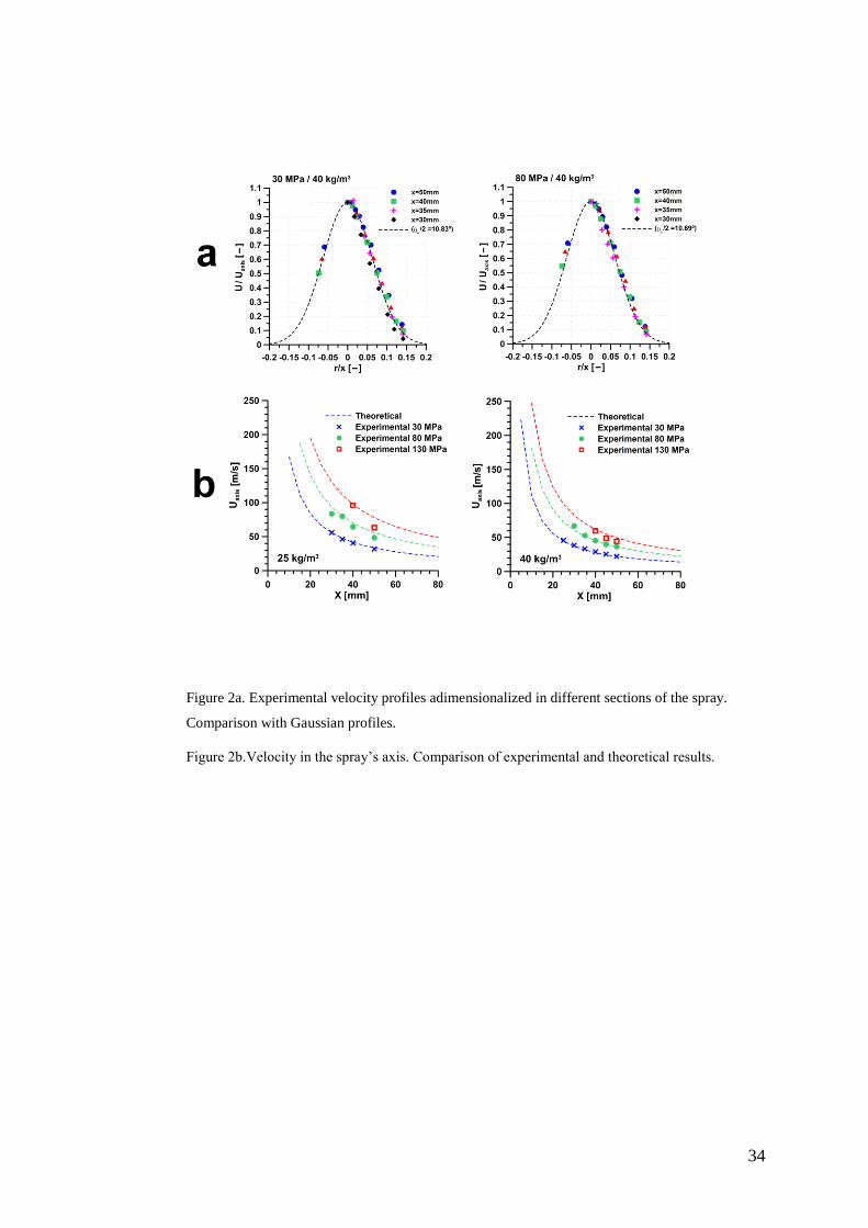
As an example, in Figure 2a, the velocity values normalized by the spray axis

velocity are plotted in terms of normalized coordinates (r/x) for a tapered nozzle

with 126 micrometers of nozzle diameter and for two different injection pressures:

30 MPa and 80 MPa. The density in the chamber was 40 kg/m3 at room

temperature. The accuracy of the PDPA technique at these conditions has been

estimated as ±5%. From these experimental points, a fit has been performed to the

function exp(k(r/x)2) which is also plotted as a dotted line in Figure 2a. The

constant k coming from the previous fitting of the velocity measurements can be

compared to the expression of the Gaussian profile seen in Equation (9). Thus,

spray velocity angle can be obtained from the following expression:

14

2tan

2u

k

(15)

with the shape factor of the Gaussian distribution equal to 4.6 according to

Desantes et al. (2007) and Payri, R. et al. (2008). The figure clearly demonstrates

the suitability of the Gaussian profiles for the velocity fields. The same conclusion

was obtained in Payri, R. et al. (2008) involving three different nozzles and

injection conditions. Furthermore, a comparison of different radial profiles

available in the literature is made in Appendix B, showing that Gaussian profiles

proposed in Equation (9) give the most accurate estimation for spray velocity

radial distribution.

On the other hand, in Figure 2b the results of spray droplet velocity measured in

the spray axis at different axial positions for the same nozzle, but in this case at

three different injection pressures (30 MPa, 80 MPa and 130 MPa) and two

different ambient densities (25 kg/m3 and 40 kg/m

3), are presented. As stated

before, at this distance, variations due to Schmidt number or local density

variations are already negligible, and so, the simplified Equation (14) is enough in

order to compare theoretical results with those obtained experimentally. In this

case, and taking into account Equation (14), the information needed is the spray

momentum flux and the velocity cone angle previously determined. As far as the

momentum flux is concerned, the values obtained for this nozzle at 30 MPa, 80

MPa and 130 MPa of injection pressure were 0.62 N, 1.61 N and 3.05 N for full

needle lift conditions. As it can be seen from the figure, the agreement between

the model and the experimental data is fairly good. As for the radial profiles,

further conditions and nozzles are evaluated in Payri, R. et al. (2008).

3. Analysis of x-ray mass distribution

measurements

Up to this point, the experimental data available have allowed a validation in the

main region of the spray but not quite in the initial region (see Figure 1). From

now on, a fruitful combination of the model and x-ray measurements near the

initial region of the spray will allow extracting information about mass and

momentum transfer in the nozzle vicinity.

15

3.1. Measurement basis

Quantification of spray characteristics such as fuel concentration, velocity or

droplet size has been the aim of numerous studies. In order to carry out non-

intrusive measurements, several optical techniques have been used for this

purpose. Nevertheless, most of these techniques are limited to the edge of the

spray, where fuel concentrations are low.

On the contrary, the x-ray absorption technique developed by Argonne National

Laboratories has recently shown to be helpful to understand spray behaviour in

the dense core of the spray (Leick et al. 2007; Tanner et al. 2006; Ramirez et al.

2009). Visible light is highly scattered by fuel parcels, so the intensity is rapidly

attenuated. Instead of this, x-ray beams are mainly absorbed by fuel, but the

intensity remaining after the passage through the dense core region remains high

enough to be accurately measured. The intensity loss of monochromatic x-ray

beams inside the spray is related with the fuel mass present in the beam path:

0

exp( ')mI MI

(16)

I being the x-ray beam intensity measured after the spray by a photodiode, I0 the

incident x-ray intensity, and μm the absorption constant. M’ is the projected fuel

mass per unit area along the x-ray beam path, which can be defined as:

' ( )LM z dz (17)

where ρL is the local fuel density, defined as f

La f

m

V V

, and z is the axis that

defines x-ray beam direction, perpendicular to the spray. The definition of local

fuel density differs from the local spray density seen before (ρ), as it only

contemplates the fuel mass, due to the fact that x-ray absorption by the air

entrained into the jet is negligible. A scheme of the experimental setup is shown

in Figure 3a.

Equation (17) gives the relationship between the experimental parameter M’ and

local spray characteristics in terms of density. It can be demonstrated that local

fuel density can be expressed as a function of local concentration (more details

can be seen in Appendix A):

16

( , )11

( , )

fL

f f

a a

x r

C x r

(18)

As it was stated in Equation (10), C(x,r) can be expressed as

2

( , ) ( )expaxisrC x r C x ScR

(19)

In this expression, R is the spray radius at axial position x, defined

as tan 2uR x . This radius can be calculated in terms of mass angle instead of

velocity angle (see Figure 1) using the following relationship:

tan tan2 2u mSc

(20)

So that local concentration can be calculated as:

2

( )exptan 2

axism

rC(x,r)= C xx

(21)

Introducing this expression of C(x,r) into Equation (18), and defining

tan 2m mR x , local fuel density can be expressed as:

2

( , )11

( )exp

fL

f f

a a

axism

x r

rC xR

(22)

where spray mass angle θm is defined as the angle at which concentration reaches

1% of its value at spray axis at any axial position.

In order to be related with experimental M’ values, and so to extract as much

information as possible, local fuel density must be expressed in terms of the

position in path direction z instead of in terms of radial position r. For this

purpose, and as depicted in Figure 3b, the following change of variable is needed:

1

2 2 2

1r r z (23)

where r1 is the radial position of the x-ray beam at the z = 0 plane.

Taking into account Equations (22) and (23), Equation (17) can be transformed

into:

17

2 2

12

'11

( )exp

f

f f

a a

axis

m

M dz

r zC x

R

(24)

This equation is very useful because it enables to relate the variable M’,

determined experimentally by the x-ray technique, to other more important

parameters such as local fuel concentration or spray radius (and, consequently,

spray cone angle). Additionally, this reasoning can be followed to analyze x-ray

results at any axial position or experimental setup, with the only assumption that

spray characteristics can be described using Gaussian profiles, as stated in

Equation (19).

3.2. Analysis of radial profiles

In previous studies developed at Argonne National Laboratories (Leick et al.

2007; Tanner et al. 2006; Ramirez et al. 2009), information about M’ values was

obtained for two different nozzles at several radial positions r1. These results

concerned two different experimental setups (including different nozzles, injection

and discharge pressure conditions and also different axial positions for the x-ray

beam), giving a total amount of 25 measurements.

The first set of measurements chosen for the current analysis (Test 1) is reported

in Leick et al.’s study (2007). In this paper, a 3-hole tapered VCO nozzle with an

outlet diameter of 0.145 mm and a k-factor of 1.5 is mounted on a Bosch common

rail injector. X-ray measurements are performed in a constant volume vessel;

injection pressure is 80 MPa and the chamber is filled with nitrogen at a density of

21.7 kg/m3. The same methodology has been used in Tanner et al. (2006), using a

single-hole nozzle with a diameter of 0.180 mm, an injection pressure of 50 MPa

and a chamber pressure of 0.5 MPa, leading to a chamber density of 5.65 kg/m3

(Test 2). A diesel fuel/cerium blend (ρf = 890 kg/m3) has been used for the two

tests. All the experimental tests were carried out at room temperature. A summary

of these two experimental setups, as well as the experimental data available, are

shown in Figure 4.

These experimental results can be analyzed with the aid of Equation (24) in order

to extract physical information about fuel concentration inside a diesel spray, as

well as to validate Gaussian radial profiles proposed in Equations (9) and (10) in

18

the near-nozzle field. Nevertheless, Equation (24) does not have an analytical

solution and, moreover, it involves two unknown parameters: axial concentration

and mass angle (involved in Rm definition). For this reason, a numerical procedure

has been defined in order to determine these parameters. A scheme of this

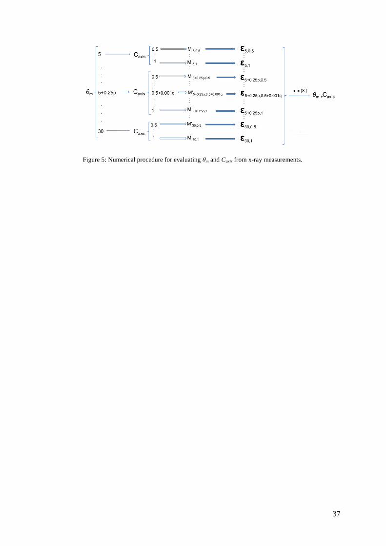
procedure is shown in Figure 5.

As it can be seen, a wide range of θm is tested (from 5 to 30º, with an angle step of

0.25º). For each of these values, also a range for Caxis is used (from 0.5 to 1, with a

concentration step of 0.001), giving a total number of 50601 combinations of

these two parameters. Each combination of θm and Caxis, together with the

experimental conditions described in Figure 4, allows the calculation of M’ at

each one of the nr radial measuring positions, giving a radial distribution of M’.

This distribution can be compared with the experimental data using the following

expression:

1

2

, 1 10

,

' ( ) ' ( )R

C exm axisr

Cm axisr

M r M r

n

(25)

where εθm,Caxis is the mean deviation obtained between the predicted and

experimental values of the whole radial M’ distribution at a fixed θm and Caxis

combination, M’θm,Caxis(r1) and M’ex(r1) are the predicted and the experimental

values at each radial position and nr is the total amount of radial positions

measured.

A minimization of the deviation parameter defined in Equation (25) can be

developed in order to obtain the θm and Caxis combination that best fits with the

experimental results. A 3-D surface plot of the average deviation in terms of the

two parameters considered for the predictions (θm and Caxis) for Test 1 conditions

is shown in Figure 6. As it can be seen, average deviation function has a global

minimum at θm = 20.25 degrees and Caxis =0.933. Thus, it can be established that

this combination produces the optimal estimation of the experimental results for

these conditions, with a maximum uncertainty equal to the step value considered

for each parameter (0.25 for spray angle and 0.001 for axial concentration).

Similar behaviour is obtained for Test 2 conditions, arriving to values of θm = 14

degrees and Caxis =0.954. The results of the optimization are summarized in Table

1 for the test conditions already described.

19

As it can be seen, the mean deviation obtained for these two predictions is low

enough to assure that these parameters reproduce properly the experimental

results (lower than 5% of the centre line value). To corroborate the quality of this

approach, comparison of experimental and predicted radial M’ profiles are

represented in Figure 7. It can be seen that the estimated values reproduce

experimental data with a high degree of confidence. This way, Gaussian profiles

introduced in section 2 are shown to be adequate to reproduce spray

characteristics even in the near-nozzle field.

3.3. Evolution along the spray axis

As it has been shown in section 2.2, the Schmidt number determines not only the

radial distribution of local concentration and velocity, but also the evolution of

these parameters along the spray axis. Thus, M’ axial evolution could be used to

characterize the Sc in diesel sprays. This kind of information was also available

for the same nozzle and conditions of Test 1 radial analysis already described

(Leick et al. 2007).

With the aim of evaluating the Schmidt number in these conditions, the first step

has consisted in calculating the concentration Caxis(x) at every axial position at

which M’ has been measured.

As it was seen in the previous radial analysis, Equation (24) relates M’ and axial

concentration (Caxis) at a given position x. Introducing the value of spray mass

angle calculated in the previous section, Equation (24) can be used to obtain

directly the evolution of Caxis. Again, this equation does not have an analytical

solution, so a numerical procedure must be followed. Caxis between 0.5 and 1 has

been tested at each axial position, giving a numerical value M’Caxis, and so

deviation between experimental and predicted values can be calculated as:

2' ( ) ' ( )

( )' ( )

C exaxisCaxis

ex

M x M xx

M x

(26)

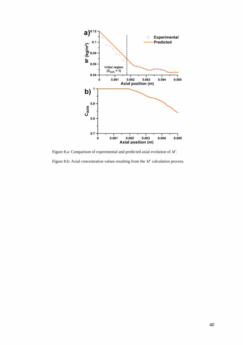
which has been minimized. Optimal M’ values obtained following this procedure

are plotted together with experimental values in Figure 8.a. Additionally, the

values of axial concentration obtained from the optimization process performed at

each axial position are represented in Figure 8.b. As it can be seen, experimental

and predicted M’ values are almost equal except in the initial region of the spray.

20

This result can be due to the fact that some hypotheses used in the theoretical

derivation (as the Gaussian profiles) cannot be applicable in the initial region of

the spray, where axial concentration is equal to the unity.

In order to gain knowledge about the influence of Sc on the axial evolution of

spray concentration, the values of Caxis which minimized the error in the M’

prediction can be compared to the behaviour predicted by the theoretical model

already described in section 2.

In this model, as seen in Equation (13), axial spray behaviour is described in terms

of momentum flux, outlet velocity and axial concentration. Momentum flux at the

nozzle exit can also be calculated as:

· 2

o f oM AU (27)

where A is the section of the outlet hole of the nozzle. So that Equation (13) can

then be easily transformed into:

.2

2 2

0

1tan2 2 1

2

iN

f au axisf a axis

o fi

UA x C

U Sci

(28)

where N is the number of terms for the truncation of the series defined in Equation

(13), necessary for the numerical calculation of the series value. Previous analyses

have shown that axial concentration and velocity can be related with the aid of the

Schmidt number (Desantes et al. 2006b). In particular, the following expression

has shown to perform properly in the near-nozzle field:

Scaxisaxis

o

UC

U

(29)

If this definition is introduced in Equation (13), an implicit equation for the Sc in

terms of Caxis can be stated:

22 2

0

1 11 tan2 2 1

2

iNSc f aa u

axis axisf fi

x C CA Sci

(30)

Finally, Equation (20) can be used to express Equation (30) in terms of mass

angle:

21

22 2

0

1 11 tan2 2 1

2

iNSc f aa m

axis axisf fi

Sc x C CA Sci

(31)

where θm is the spray mass angle at an axial position of 4 mm (section 3.2, test 1

conditions). This value is assumed to be constant for any axial position.

This expression cannot be solved analytically, but numerical methods can be

applied in order to have a solution in terms of Caxis for the different axial

positions. Although previous analysis have pointed out that the solution given by

this model is independent of N for values higher than 7-9 (Desantes et al. 2006a),

the current calculation has been developed for N = 11, in order to assure a high

degree of accuracy. In particular, the truncation error of the series would represent

around 1.5-2% for typical values of Sc and Caxis, so that it can be concluded that

the resolution with 11 terms is adequate. Using this expression, a comparison of

experimental and theoretical axial evolution of Caxis can be obtained and shown in

Figure 9. In this figure, theoretical axial profiles of Caxis are evaluated at different

Schmidt numbers using Equation (31), together with Caxis values obtained from

experimental M’ data.

As it can be seen, there are three different zones attending to the behaviour of Caxis

in terms of Sc. The first zone corresponds to the initial region of the spray, where

axial concentration is equal to one. The length of this zone is better reproduced as

the Sc chosen for calculation gets higher. The final zone (beyond ~3.5 mm) shows

a good agreement with the results given by the theoretical model for a Sc value

near 0.5. This value is lower than those observed by Prasad and Kar (1976), but it

must be considered that their study was developed under quite different conditions

(Pin < 20 MPa, ϕo > 0.4 mm, Pback = 0.1 MPa). Furthermore, they found that Sc

decreased as injection pressure got higher, which would imply that values lower

than 0.7 could be expected under modern engine conditions, as it has been

obtained in the current study.

In the transitional region (from 2 to 3.5 mm), the behaviour of Caxis(x) does not

correspond with any theoretical curve. This could be due to different reasons:

- The Schmidt number could not be constant along the spray axis. In fact, as

it has been explained, high Sc values would reproduce more properly spray

parameters as the length at which Caxis =1. An evolution of Sc from values

22

near unity to the fully developed value of 0.5 could explain the

experimental evolution of Caxis.

- Spray cone angle has been supposed to be constant along the whole spray.

Nevertheless, recent investigation works based on visualization techniques

have pointed out that spray angle near the nozzle exit is significantly

different from the expected cone angle defined at higher axial positions

(Linne et al. 2006, Saliba et al. 2004, Heimgärtner and Leipertz 2000).

- The proposed model uses the gaseous jet analogy. For this reason, this

model can only be useful to characterize spray behaviour at positions at

which atomization has already taken place and fuel has been decomposed

in droplets small enough to behave in a similar way to a gas jet.

3.4. Application of previous results

The previous analyses based on x-ray measurements have allowed the

determination of spray cone angle for two different nozzles and pressure

conditions, as well as an estimation of the Schmidt number from axial

measurements for one of them. The importance of these parameters is based on

the possibility of predicting spray behaviour by means of the theoretical model

described in section 2 once these parameters are known. In this sense, Figure 10

shows local velocity and concentration contours for the two experimental setups

analyzed in this paper. For this purpose, although the Schmidt number estimation

has been developed only for Test 1 conditions, the same value has been assumed

for the Test 2, where only the value of the spray mass angle has been adapted.

These contours summarize the air-fuel mixing process in the first 15 millimetres

of the spray. It can be seen that the mixing process is more effective for Test 1

conditions, mainly due to the higher chamber density, which is known to have a

decisive influence. Thus, it is appreciable that spray concentration drops faster

along the axial direction for Test 1 conditions, and that spray widening is more

pronounced. The black zone in these contour maps can be immediately related

with the length of the initial region of the spray. This length, defined as the

position at which axial concentration reaches unity, is an important parameter in

order to analyze air-fuel mixing process. Again, it is seen that higher density

induces a shorter length of the Caxis = 1 region (~3.2 mm) with respect to Test 2

conditions (~9 mm). Remembering Figure 9, the simplified model overestimated

23

the length of the region at which Caxis = 1, due to the inaccuracies of the model in

this region. For this reason, shorter lengths should be expected in reality.

Another noticeable aspect is the strong difference between local velocity and

concentration contours. Paying attention to the edge of the spray in these contour

maps (defined as 1% of the maximum concentration or velocity), it can be seen

that the concentration contour is much wider than the velocity one. This is due to

the fact that the Schmidt number, defined as the ratio between viscosity and mass

diffusivity, is considerably smaller than 1, which indicates that momentum

transfer is less effective than mass transfer. In particular, Equation (19) indicates

that tan(θu/2)=0.75tan(θm/2) for a Sc of 0.5. This relationship explains the

differences seen between velocity and concentration contours.

4. Conclusions

A theoretical analysis combined with experimental measurements of momentum

flux, droplet velocity (using a Phase Doppler Particle Analyzer) and mass

distribution with x-ray radiography has been used in this research, which has

made it possible to better understand the behaviour of diesel spray dynamics.

The theoretical development is based on physical considerations and on empirical

evidence.

From this work, the following conclusions can be drawn:

As a result of a theoretical reasoning based on momentum flux

conservation in the axis direction of the diesel spray, a mathematical

model has been obtained which relates the momentum flux with the

profiles of velocity and concentration, local density and spray cone angle.

Some experimental results of droplet velocity measured with the PDPA

technique have been used to validate the model obtaining acceptable

agreement between experimental measurements and the theoretical model.

X-ray projected mass distribution measurements have shown to be useful

in order to characterize spray behaviour in the near-nozzle field, where the

influence of Schmidt number is more severe. Information from two

different nozzles, experimental setups and axial positions were available.

The analysis of the x-ray measurements has led to the conclusion that the

Gaussian profiles proposed reproduce properly experimental data available

from the near-nozzle region.

24

When analyzing axial distribution of M’, the best fit for experimental

measurements is obtained for a Schmidt number around 0.5 for axial

positions higher than 3.5 mm. Nevertheless, for x < 3.5 mm, there is no

value of Sc that reproduces the axial distribution of Caxis. Furthermore, it

can be seen that the initial region length (position at which Caxis is 1) is

better reproduced as Sc is increased. This could indicate that the Schmidt

number is varying in the first millimeters of the spray until it arrives at its

full-developed value. Also variation of spray angle during this transitional

region could explain this phenomenon.

Once the Schmidt number and the spray cone angle are known for a set of

experimental conditions, the theoretical approach already described allows

the complete characterization of spray behaviour in terms of velocity and

local concentration. In this sense, contour plots of these parameters for the

two nozzles analyzed in this paper have been developed and analyzed.

Appendix A

Local density ρ can be defined as the ratio between the total mass and volume at a

given location of the spray:

( , )a f

a f

m mx r

V V

(32)

being mf and Vf the local mass and volume of fuel, and ma and Va the local mass

and volume of air.

Together with this local density, local volume and mass concentrations can be

defined as:

( , )f

va f

VC x r

V V

; ( , )

f

a f

mC x r

m m

(33)

Using these definitions, local density can be rewritten as:

( , )( , )

( , )

fa f v

ffa f

v

mm m C x rCx r

VV V C x rC

(34)

Dividing local mass and volume concentrations:

25

( , )

( , )

f a f f a a f f

v a f f a f f f

m V V m m mC x r

C x r m m V m m m

1 1(1 ( , )) ( , )

f faf

a a f f a f a

mmC x r C x r

m m m m

(35)

Introducing this expression into the local density definition, it can be seen that:

( , )( , )

( , )1 ( , ) ( , ) ( , ) 1

f fvf

f f f

a a a

C x rx r

C x rC x r C x r C x r

(36)

Additionally, local fuel density can be defined as:

( , )f

La f

mx r

V V

(37)

This definition is useful for the analysis of x-ray measurements, as the absorption

by the air mass is almost negligible. It can be seen that there is a direct

relationship between local fuel density ρL and local density ρ:

( , ) ( , ) ( , )a f f f

La f a f a f

m m m mx r C x r x r

V V m m V V

(38)

So that local fuel density can be expressed in terms of local concentration as:

( , )( , )

1( , ) 1 1( , )

f fL

f f f f

a a a a

C x rx r

C x rC x r

(39)

Appendix B

A summary of some of the most relevant radial profiles available in the literature

for the characterization of spray velocity is made in Table 2. In these expressions,

spray width must be adjusted by experimental results. For this purpose, two

parameters can be defined:

- Spray radius (R), which can be calculated in terms of spray velocity angle

as:

tan2uθR x (40)

26

- r1/2, which is defined as the radial position at which spray velocity reaches

50% of its maximum value.

These profiles can be used to approach experimental data of spray velocity

obtained from a Phase Doppler Particle Analyzer (PDPA), presented in section

2.3. The reproduction of the experimental data by each of these expressions is

seen in Figure 11.a.

As it can be seen, experimental data is properly reproduced for all the expressions,

with the only exception of the one proposed by Spalding (1979). Nevertheless, in

order to quantify the capability of each one of these radial profiles to reproduce

the experimental data, mean squared deviation between predictions and

experiments (MSD) is calculated as:

2

1

( , ) ( , )nex

mo j j ex j jj

ex

U x r U x r

MSDn

(41)

Uex(xj,rj) being the velocity values obtained in the PDPA measurements at the

experiment j, Umo(xj,rj) the predicted value given by each model at the same

operating conditions, xj and rj the measuring position for experiment j, and nex the

total number of measurements available from PDPA system.

As it can be seen in Figure 11.b, Gaussian fit proposed by the authors shows the

lowest MSD values for both injection pressure values considered in the analysis.

Radial profile proposed by Schlichting (1978) gives results with similar accuracy,

while the other two profiles are considerably less accurate in their prediction.

Considering these results, Gaussian profiles described in Equations (8) and (9)

would be the best option for the spray analysis performed afterwards in terms of

MSD. Nevertheless, the differences between the radial profiles tested are slight, so

that any of them would be acceptable to reproduce the experimental results.

Acknowledgement

This work was partly sponsored by “Vicerrectorado de Investigación, Desarrollo e Innovación” of

the “Universidad Politécnica de Valencia” in the frame of the project “Estudio del flujo en el

interior de toberas de inyección Diesel”, reference Nº 3150 and by “Generalitat Valenciana” in the

frame of the project with the same title and reference GV/2009/031.

27

This support is gratefully acknowledged by the authors.

References

Abramovich GN (1963) The theory of turbulent jets. MIT Press.

Adler D, Lyn WT (1969) The evaporation and mixing of a liquid fuel spray in a Diesel air swirl.

Proc. Instn. Mech. Engrs. 184: 171-180.

Coghe A, Cossali GE (1994) Phase Doppler characterisation of a Diesel spray injected into a high

density gas under vaporisation regimes. 7th Int. Symp. On Appl. Of Laser Tech. To Fluid Mech.,

Lisbon.

Correas D (1998) Theoretical and experimental study of isothermal Diesel free sprays (In

Spanish). PhD Thesis, Universidad Politécnica de Valencia.

Cossali GE (2001) An integral model for gas entrainment into full cone sprays. J. Fluid Mech.

439: 353-366.

Dent JC (1971) A basis for the comparison of various experimental methods for studying spray

penetration. SAE Paper 710571.

Desantes JM, Payri R, Salvador FJ, Gil A (2006a) Deduction and validation of a theoretical model

for a free Diesel Spray. Fuel 85: 910-917.

Desantes JM, Arrègle J, López JJ, Cronhjort A (2006b) Scaling laws for free turbulent gas jets and

Diesel-like sprays. Atomization Spray 16: 443-473.

Desantes JM, Payri R, García JM, Salvador FJ (2007) A contribution to the understanding of

isothermal diesel spray dynamics. Fuel 86: 1093-1101.

Dumouchel C (2008) On the experimental investigation on primary atomization of liquid streams.

Exp. Fluids 45: 371:422.

Heimgärtner C, Leipertz A (2000) of the primary spray break-up close to the nozzle of a common-

rail high pressure Diesel injection system. SAE Paper 2000-01-1799.

Hinze JO (1975) Turbulence. McGraw-Hill.

Hiroyasu H, Arai M (1990) Structures of fuel sprays in Diesel engines. SAE Paper 900475.

Jawad B, Gulari E, Henein NA (1992) Characteristics of intermittent fuel sprays. Combust. flame

88: 384-396.

Lefèbvre AH (1989) Atomization and Sprays. Hemisphere Publishing Corporation.

Leick P, Riedel T, Bittlinger G, Powell CF, Kastengren AL, Wang J (2007) X-Ray Measurements

of the Mass Distribution in the Dense Primary Break-Up Region of the Spray from a Standard

Multi-Hole Common-Rail Diesel Injection System. Proc. 21st ILASS (Europe).

Linne M, Paciaroni M, Hall T, Parker T (2006) Ballistic imaging of the near field in a diesel spray.

Exp. Fluids 40: 836-846.

Naber J, Siebers DL (1996) Effects of gas density and vaporisation on penetration and dispersion

of Diesel sprays. SAE Paper 960034.

Payri F, Bermúdez V, Payri R, Salvador FJ (2004) The influence of cavitation on the internal flow

and the Spray characteristics in diesel injection nozzles. Fuel 83: 419-431.

28

Payri R, García JM, Salvador FJ, Gimeno J (2005) Using spray momentum flux measurements to

understand the influence of Diesel nozzle geometry on spray characteristics. Fuel 84: 551-561.

Payri R, Tormos B, Salvador FJ, Araneo L (2008) Spray droplet velocity characterization for

convergent nozzles with three different diameters. Fuel 87: 3176- 3182.

Post S, Iyer V, Abraham J (2000) A study of near-field entrainment in gas jets and sprays under

diesel conditions. ASME J. Fluids Eng. 122: 385-395.

Prasad CMV, Kar S (1976) An investigation on the diffusion of momentum and mass of fuel in a

Diesel fuel spray. ASME J. Eng. Power 76-DGP-1: 1-11.

Ramirez AI, Som S, Aggarwal SK, Kastengren AL, El-Hannouny EM, Longman DE, Powell CF

(2009) Quantitative X-ray measurements of high-pressure fuel sprays from a production heavy

duty diesel injector, Exp. Fluids 47:119–134

Rajaratnam N (1976) Turbulent jets. Elsevier Scientific Publishing Company.

Reitz RD, Bracco FV (1982) Mechanism of atomisation of a liquid jet. Phys. Fluids 25 (10): 1730-

1742.

Ricou FP, Spalding DB (1961) Measurements of entrainment by axisymmetrical turbulent jets. J.

Fluid Mech. 11: 21-32.

Rife J, Heywood JB (1974) Photographic and performance studies of Diesel combustion with a

rapid compression machine. SAE Paper 740948.

Roisman IV, Araneo L, Tropea C (2007) Effect of ambient pressure on penetration of a diesel

spray. Int. J. Multiphase Flow 33 (8): 904-920.

Roisman IV, Tropea C (2001) Flux measurements in sprays using phase doppler techniques.

Atomization spray 11: 667-699.

Saliba R, Baz I, Champoussin JC, Lance M, Marié JL (2004) Cavitation effect on the near nozzle

spray development in high-pressure diesel injection. Proc. 19th ILASS (Europe).

Schlichting H (1978) Boundary layer theory. McGraw-Hill.

Sinnamon JF, Lancaster DR, Stiener JC (1980) An experimental and analytical study of engine

fuel spray trajectories. SAE Paper 800135.

Spalding DB (1979) Combustion and mass transfer. Pergamon press.

Sou A, Hosokawa S, Tomiyama A (2007) Effects of cavitation in a nozzle on liquid jet

atomization. Int. J. Heat Mass Tran. 50 (17-18): 3575-3582.

Subramaniam S (2001) Statistical modelling of a spray as using the droplet distribution function.

Phys. Fluids 13 (3): 624-642.

Tanner FX, Feigl A, Ciatti SA, Powell CF, Cheong S-K, Liu J, Wang J (2006) Structure of high-

velocity dense sprays in the near-nozzle region. Atomization Spray 16: 579-597.

Way RJB (1977) Investigation of interaction between swirl and jets in direct injection Diesel

engines using a water model. SAE Paper 770412.

Wu KJ, Reitz RD, Bracco FV (1986) Measurements of drop size at the spray edge near the nozzle

in atomising liquid jets. Phys. Fluids 29 (4): 941-951.

Wu KJ, Santavicca DA, Bracco FV (1984) LDV measurements of drop velocity in Diesel-type

sprays. AAIA J. 22 (9): 1263-1270.

29

Yue Y, Powell CF, Poola R, Wang J, Schaller JK (2001). Quantitative measurements of diesel fuel

spray characteristics in the near-nozzle region using X-ray absorption. Atomization Spray 11 (4):

471-490.

30

FIGURE CAPTIONS

Figure 1. Initial and Main Region in a jet.

Figure 2a. Experimental velocity profiles adimensionalized in different sections of the spray.

Comparison with Gaussian profiles.

Figure 2b.Velocity in the spray’s axis. Comparison of experimental and theoretical results.

Figure 3.a. Scheme of x-ray measuring technique.

Figure 3.b. Description of integration for calculating M’.

Figure 4.a,b. Summary of experimental conditions and measuring positions in the x-ray tests.

Figure 4.c,d. X-ray experimental data from radial measurements.

Figure 5: Numerical procedure for evaluating θm and Caxis from x-ray measurements.

Figure 6: Evolution of the deviation between experimental and predicted M’ in terms of θm and

Caxis.

Figure 7: Experimental vs. predicted M’ radial profiles.

Figure 8.a: Comparison of experimental and predicted axial evolution of M’.

Figure 8.b: Axial concentration values resulting from the M’ calculation process.

Figure 9: Comparison of axial concentration obtained from experimental results and model

predictions for different Schmidt numbers.

Figure 10: Local velocity and concentration contour maps for Test 1 and Test 2 conditions.

Figure 11: Comparison of different radial profiles available in the literature.

31

TABLES

Table 1: Summary of results from M’ radial profiles optimization process

Test 1 Test 2

Axial position (mm) 4 10

Chamber density (kg/m3) 21.7 5.65

Axial concentration 0.933 0.954

Mass angle (º) 20.25 14

Average deviation (kg/m2) 0.0021 0.0026

32

Table 2: Expressions for radial profiles in the literature

Reference Expression

Gaussian fit

(current study)

2

( , ) ( )expaxisrU x r U xR

Sinnamon et al. 1980 2

1.5

( , ) ( ) 1axisrU x r U xR

Schlichting 1978

21.5

1 2

( , ) ( ) 1 0.293axisrU x r U x

r

Spalding 1979

22

1 2

( , ) ( ) 1 0.414axisrU x r U x

r

33

FIGURES

Figure 1. Initial and Main Region in a jet.

34

Figure 2a. Experimental velocity profiles adimensionalized in different sections of the spray.

Comparison with Gaussian profiles.

Figure 2b.Velocity in the spray’s axis. Comparison of experimental and theoretical results.

35

Figure 3.a. Scheme of x-ray measuring technique.

Figure 3.b. Description of integration for calculating M’.

36

Figure 4.a,b. Summary of experimental conditions and measuring positions in the x-ray tests.

Figure 4.c,d. X-ray experimental data from radial measurements.

37

Figure 5: Numerical procedure for evaluating θm and Caxis from x-ray measurements.

38

Figure 6: Evolution of the deviation between experimental and predicted M’ in terms of θm and

Caxis.

39

Figure 7: Experimental vs. predicted M’ radial profiles.

40

Figure 8.a: Comparison of experimental and predicted axial evolution of M’.

Figure 8.b: Axial concentration values resulting from the M’ calculation process.

41

Figure 9: Comparison of axial concentration obtained from experimental results and model

predictions for different Schmidt numbers.

42

Figure 10: Local velocity and concentration contour maps for Test 1 and Test 2 conditions.

43

Figure 11: Comparison of different radial profiles available in the literature.