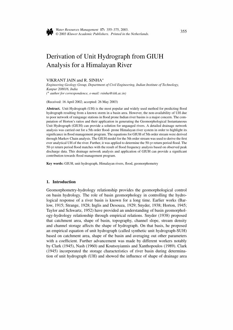
Water Resources Management 17: 355–375, 2003.© 2003 Kluwer Academic Publishers. Printed in the Netherlands.

355

Derivation of Unit Hydrograph from GIUHAnalysis for a Himalayan River

VIKRANT JAIN and R. SINHA∗Engineering Geology Group, Department of Civil Engineering, Indian Institute of Technology,Kanpur 208016, India(∗ author for correspondence, e-mail: rsinha@iitk.ac.in)

(Received: 16 April 2002; accepted: 26 May 2003)

Abstract. Unit Hydrograph (UH) is the most popular and widely used method for predicting floodhydrograph resulting from a known storm in a basin area. However, the non-availability of UH dueto poor network of raingauge stations in flood prone Indian river basins is a major concern. The com-putation of Horton’s ratios and their application in generating the Geomorphological InstantaneousUnit Hydrograph (GIUH) can provide a solution for ungauged rivers. A detailed drainage networkanalysis was carried out for a 5th order flood- prone Himalayan river system in order to highlight itssignificance in flood management program. The equations for GIUH of 5th order stream were derivedthrough Markov Chain analysis. The GIUH model for the 5th order stream was used to derive the firstever analytical UH of the river. Further, it was applied to determine the 50-yr return period flood. The50-yr return period flood matches with the result of flood frequency analysis based on observed peakdischarge data. This drainage network analysis and application of GIUH can provide a significantcontribution towards flood management program.

Key words: GIUH, unit hydrograph, Himalayan rivers, flood, geomorphometry

1. Introduction

Geomorphometry-hydrology relationship provides the geomorphological controlon basin hydrology. The role of basin geomorphology in controlling the hydro-logical response of a river basin is known for a long time. Earlier works (Bar-low, 1915; Strange, 1928; Inglis and Desouza, 1929; Snyder, 1938; Horton, 1945;Taylor and Schwartz, 1952) have provided an understanding of basin geomorphol-ogy-hydrology relationship through empirical relations. Snyder (1938) proposedthat catchment area, shape of basin, topography, channel slope, stream densityand channel storage affects the shape of hydrograph. On that basis, he proposedan empirical equation of unit hydrograph (called synthetic unit hydrograph-SUH)based on catchment area, shape of the basin and averaging out other parameterswith a coefficient. Further advancement was made by different workers notablyby Clark (1945), Nash (1960) and Koutsoyiannis and Xanthopoulos (1989). Clark(1945) incorporated the storage characteristics of river basin during determina-tion of unit hydrograph (UH) and showed the influence of shape of drainage area

356 V. JAIN AND R. SINHA

upon the shape of the hydrograph. Nash (1960) correlated the Instantaneous UnitHydrograph (IUH) with seven different topographical characteristics (viz. basinarea, length of longest stream to the catchment boundary, two different measure ofthe main channel slope, overland slope, variation in the overland slope and meanstream intervals) for 90 stations in 23 river basins in Britain based on regressionanalysis and derived a general equation for IUH. Koutsoyiannis and Xanthopoulos(1989) highlighted the advantage of parametric approaches for derivation of unithydrograph in order to establish a relationship between the UH and catchmentcharacteristics. However, these relationships are characterised by some constants,which represent the ‘ensemble average’ of geomorphological control on the riverdischarge. Significant progress has been made in the recent years towards the‘quantitative assessment’ of geomorphologic control on the basin hydrology not-ably after Rodriguez-Iturbe and Valdes’s (1979) theoretical model of Geomorpho-logical Instantaneous Unit Hydrograph (GIUH), through which a river hydrographcan be determined from the input of Horton’s morphometric parameters and aver-age channel velocity. Rodriguez-Iturbe and Valdes (1979) provided a set of basicequations for a 3rd order basin. This quantitative understanding opened a newdimension in the hydrological analysis, specially for the ungauged river basin. ThisGIUH model has been used successfully for rainfall-runoff analysis of some riverbasins in Venezuela and Puerto-Rico (Valdes et al., 1979; Rodriguez-Iturbe et al.,1979).

The Himalayan river basins are one of the worst flood affected regions in theworld (Agarwal and Narain, 1996). The flood management in these basins throughconventional methods such as hydrograph analysis or runoff models is difficultdue to absence of adequate number of raingauge stations. The application of theGIUH to derive the unit hydrograph of river basin can therefore provide a suitableapproach. Further, the GIUH provides the hydrological response of a river basin onthe basis of its physical characteristics defined by Horton’s morphometric ratios.This approach has an advantage over traditional methods in that the effects of themorphometric characteristics on basin hydrology are well-understood. Further, thehydrological response of smaller sub-basins can also be obtained using the GIUHapproach, and hence, the contribution of different tributaries to flood hazard inriver basin can be analysed. Again, the comparison of GIUH for two different riverbasins would provide a better comparison between hydrological responses of thebasins having distinctive morphometric characteristics. On the other hand, SUHsare based on coefficients, which are region specific, and hence, it is difficult tocompare two river basins on the basis of SUH only.

Recently, some workers have used the functional relationship of the GIUHdeveloped by Rodriguez-Iturbe and Valdes (1979) to estimate the values of hy-drograph peak (qp) and time to peak (tp) of UH for the rivers in western Indian(Bhaskar and Devulapalli, 1991; Jain et al., 2000). The morphometric paramet-ers were computed using the ARCINFO GIS software and taken as input for theestimation of qp and tp. These hydrograph parameters were further used for the

DERIVATION OF UNIT HYDROGRAPH FROM GIUH ANALYSIS 357

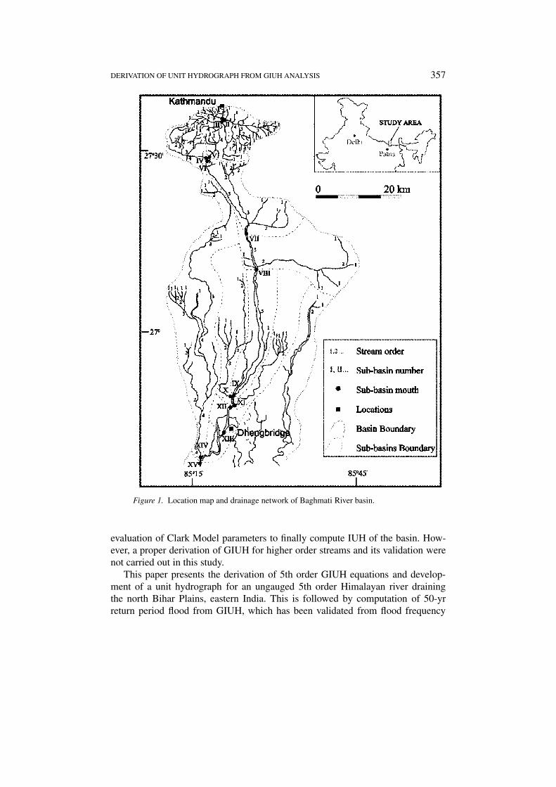
Figure 1. Location map and drainage network of Baghmati River basin.

evaluation of Clark Model parameters to finally compute IUH of the basin. How-ever, a proper derivation of GIUH for higher order streams and its validation werenot carried out in this study.

This paper presents the derivation of 5th order GIUH equations and develop-ment of a unit hydrograph for an ungauged 5th order Himalayan river drainingthe north Bihar Plains, eastern India. This is followed by computation of 50-yrreturn period flood from GIUH, which has been validated from flood frequency

358 V. JAIN AND R. SINHA

analysis. The plains of north Bihar in eastern India are severely affected by regularand extensive floods (Kale, 1997; Sinha and Jain, 1998). Considering this fact, ariver draining the north Bihar plains, namely, the Baghmati River has been chosenfor the present study (Fig. 1). The Baghmati River causes havoc due to severityof floods every year. The total damage during a period of 20 years (1971–1990) isof the order of a whopping Rs. 600 million. In the absence of raingauge stationsin the upstream mountainous basin area lying in Nepal, it is difficult to derive theunit hydrograph for Baghmati River for any site in the plains (GFCC, 1991). ASynthetic Unit Hydrograph (SUH) is normally used by the Ganga Flood ControlCommission, the parameters for which are based from neighbouring river basinsi.e. Son basin, Middle Gangetic plains, Lower Gangetic plains and Mahanadi Basin(GFCC, 1991). The existing SUH therefore does not provide good estimate of theflood discharge. This poses a great difficulty in designing of hydraulic structureson the river and/or development of flood forecasting and warning systems based onrainfall. Keeping this in view, the GIUH model for the Baghmati River presentedin this paper should serve as a significant contribution.

2. The Baghmati River: Hydrology and Flood Characteristics

The Baghmati River is a foothills-fed river (Sinha and Friend, 1994), originatingfrom the Nepal Himalaya at an elevation of 1500 m and draining around 8440 km2

area. Out of this, 4720 km2 of area (about 56% of the total area) lies in Nepal andrest in north Bihar. The average annual rainfall in the river basin is about 1250 mmand almost 85% of the rainfall occurs in the monsoon season (June-September)itself (GFCC, 1991). Because of this sudden increase in rainfall, the channels ofBaghmati River system receive exceptionally high discharge during the monsoonseason. Figure 2 shows a plot of peak discharge values for the upstream (Dheng-bridge, 1970–89) and downstream (Hayaghat, 1956–89) stations (see Fig. 1 forlocation). The available data suggest that the peak discharges at both the stationsare quite variable and unpredictable. Table I summarizes the flood hydrology of theBaghmati River at Dhengbridge and Hayaghat stations. The most probable flood,mean annual flood and 50-yr, 100-yr return period flood were computed throughflood frequency analysis using Gumbel’s probability distribution. Further detailson morphology, hydrology and fluvial dynamics of the Baghmati river are availablefrom GFCC (1991), Sinha and Friend (1994), Sinha (1998), Sinha and Jain (1998)and Jain and Sinha (2003, in press-a).

3. Data Used and Approach for Present Work

Hydrological data was obtained from various agencies in India viz. Central Wa-ter Commission (CWC), Ganga Flood Control Commission (GFCC), Patna, andCenter for Water Resource Station (CWRS), Patna to study the hydrological char-acteristics of the Baghmati river. For morphometric analysis, a detailed drainage

DERIVATION OF UNIT HYDROGRAPH FROM GIUH ANALYSIS 359

Figure 2. Peak discharge variation in Baghmati River at Dhengbridge and Hayaghat.

Table I. Hydrological characteristics of the Baghmati River

Parameter Dhengbridge (u/s) Hayaghat (d/s)

(m3/sec) (m3/sec)

Average Annual Discharge (Qm) 156 189

Bankfull discharge (Qb) 1100 870

Max. Observed Discharge (Qobs) 3033 2617

Most probable flood (Qmp) (T= 1.58 yrs.) 1155 834

Mean annual flood (Qma) (T=2.33 yrs.) 1473 1076

Flood Discharge (T=50 years) 3298 2606

Flood Discharge (T=100 years) 3681 2927

map was prepared using the Survey of India topographic sheets of 1:50,000 scaleand it was sub-divided into different sub-basins for morphometric analysis (Fig.1). Morphometric analysis involved the computation of stream number, averagestream length and average stream area of different sub-basins of the Baghmatibasin following Strahler’s ordering (1956) scheme. These parameters were usedto determine the Horton’s Raito (Table II). The results of morphometric analysis(Table III) were used to develop the Geomorphologic Instantaneous Unit Hydro-graph (GIUH) for the Baghmati basin. The results of the GIUH analysis were

360 V. JAIN AND R. SINHA

Table II. Morphometric parameters (after Horton, 1971)

Parameter Definition Relationships

Bifurcation Ratio (RB) Ratio of number of streams RB = Nu−1 / Nu

Nu = no. of streams of order u

Length Ratio (RL ) Ratio of average length of RL = Lu / Lu−1

streams Lu = Avg. length of streams of order u

Area Ratio (RA ) Ratio of average area of RA = Au / Au−1

streams Au = Avg. basin area of streams of order u

Table III. Geomorphometric parameters of the Baghmati River Basin

Sub-basin Equivalent to Bifurcation ratio Length ratio Area ratio

I – 3.000 1.655 3.510

II – 3.292 1.442 3.788

III I+II 3.417 1.501 3.863

IV III+. . . 4.207 1.979 5.051

V – 2.767 1.396 3.334

VI IV+V 3.122 1.729 3.684

VII VI+. . . 3.272 2.102 3.803

VIII VII+. . . 3.330 2.001 4.472

IX VIII+. . . 3.356 2.684 4.781

X – 2.833 2.677 5.277

XI – 2.250 3.734 3.420

XII IX+X+XI 3.531 3.073 5.336

XIII XII+. . . 3.531 3.681 5.411

XIV – 3.536 2.727 4.754

XV XIII+XIV+. . . 3.506 2.767 5.102

used in computing the Unit Hydrograph (UH) of the Baghmati River at Dheng-bridge station (Figure 1). A 50-yr return period flood was calculated from this UH.This 50-yr return period flood was compared with the results of flood frequencyanalysis, carried out with the observed peak discharge data from 1956 to 1990.

4. Derivation of GIUH for Baghmati River

The Geomorphologic Instantaneous Unit Hydrograph (GIUH) is defined as theprobability density function for the time of arrival of a randomly chosen drop tothe trapping state (Rodriguez-Iturbe and Valdes, 1979). The general equation ofGIUH is a function of Horton’s numbers i.e. Bifurcation Ratio (RB ), Area Ratio

DERIVATION OF UNIT HYDROGRAPH FROM GIUH ANALYSIS 361

(RA), Length Ratio (RL), Length of highest order stream (L�) and mean velocityof streamflow (v) (Table II). In order to understand the geomorphometrical controlon river hydrology and to develop the Unit Hydrograph (UH) of Baghmati River,the GIUH was derived for the Baghmati River. In deriving the GIUH of a riverbasin, it is assumed that excess rainfall of unit volume is uniformly distributedover the basin and is instantaneously imposed upon it.

The general equation of GIUH for an Nth order stream will be expressed as(after Rodriguez-Iturbe and Valdes, 1979),

dθN+2(t)

dt=

N∑i=1

θi(0)dφi(N+2)(t)

dt(1)

where:θN(t) State probability, defined as probability that the process (drop) is

found in state (N+2) at time interval ‘t’.

θi(0) Initial state probability, defined as probability that the process startsat state ‘i’

φi(N+2)(t) Interval transition probability from state ‘i’ to state N+2, defined asprobability that process (drop) entered state ‘i’ at time ‘t’.

The final stage is taken as N+2 for stream of order N because of exponentialdistribution of mean waiting time. The general equations of GIUH are based onSemi Markov process (Rodriguez-Iturbe and Valdes, 1979). In a Semi Markovprocess, mean waiting time is assumed to be governed by exponential distribution.However, for highest order stream, the exponential distribution does not apply well,as its origin shifts from zero value. Therefore, the highest order stream (�=N)is divided into two parts (�a and �b) where �a (=N) receive all discharge fromlower order stream and �b (=N+1) receives all discharge from �a and finally thesevolume of water is collected at the trapping state (=N+2) at the outlet of the basin

From geomorphometric analysis, the Baghmati River works out to be a 5th orderstream (see Fig. 1). For the 5th order stream, the GIUH equation for the BaghmatiRiver will be expressed from equation 1 as,

dθ7(t)

dt= θ1(0).

dφ17(t)

dt+ θ2(0).

dφ27(t)

dt+ θ3(0).

dφ37(t)

dt+ θ4(0).

dφ47(t)

dt+ θ5(0).

dφ57(t)

dt

(2)

Solving the above equation would involve determination of transition state prob-ability (φiN ) and initial state probability (θN(0)). The derivation of these paramet-ers was initiated with the generation of probability matrices for the Baghmati River.The following sections discuss the computation of these parameters.

362 V. JAIN AND R. SINHA

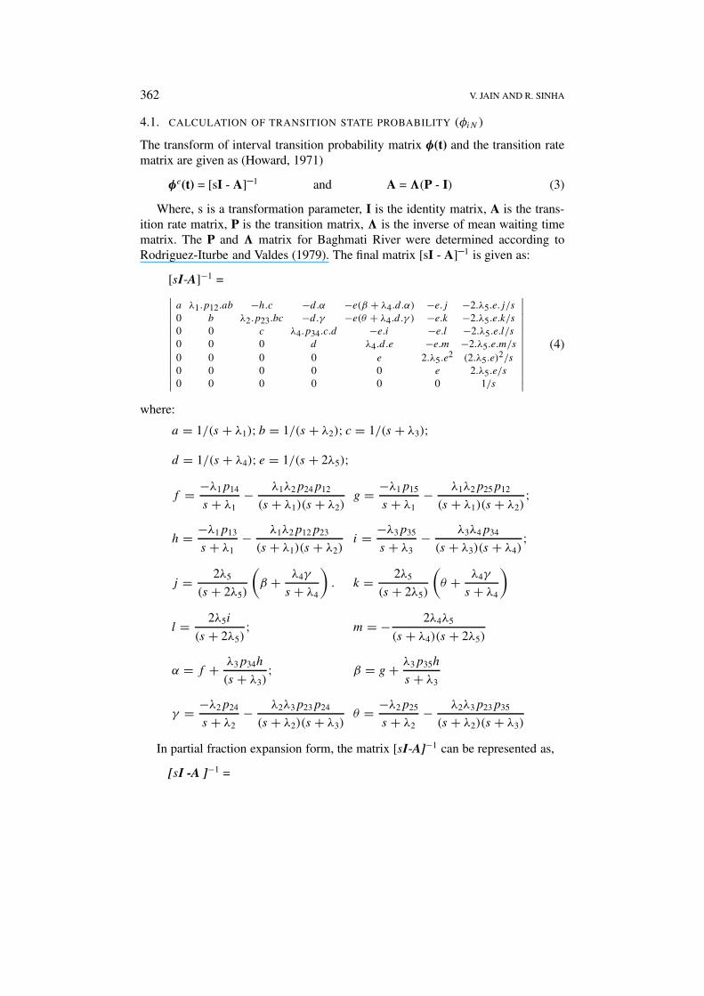
4.1. CALCULATION OF TRANSITION STATE PROBABILITY (φiN )

The transform of interval transition probability matrix φ(t) and the transition ratematrix are given as (Howard, 1971)

φe(t) = [sI - A]–1 and A = �(P - I) (3)

Where, s is a transformation parameter, I is the identity matrix, A is the trans-ition rate matrix, P is the transition matrix, � is the inverse of mean waiting timematrix. The P and � matrix for Baghmati River were determined according toRodriguez-Iturbe and Valdes (1979). The final matrix [sI - A]–1 is given as:

[sI-A]−1 =∣∣∣∣∣∣∣∣∣∣∣∣

a λ1.p12.ab −h.c −d.α −e(β + λ4.d.α) −e.j −2.λ5.e.j/s

0 b λ2.p23.bc −d.γ −e(θ + λ4.d.γ ) −e.k −2.λ5.e.k/s

0 0 c λ4.p34.c.d −e.i −e.l −2.λ5.e.l/s

0 0 0 d λ4.d.e −e.m −2.λ5.e.m/s

0 0 0 0 e 2.λ5.e2 (2.λ5.e)2/s

0 0 0 0 0 e 2.λ5.e/s

0 0 0 0 0 0 1/s

∣∣∣∣∣∣∣∣∣∣∣∣(4)

where:

a = 1/(s + λ1); b = 1/(s + λ2); c = 1/(s + λ3);d = 1/(s + λ4); e = 1/(s + 2λ5);

f = −λ1p14

s + λ1− λ1λ2p24p12

(s + λ1)(s + λ2)g = −λ1p15

s + λ1− λ1λ2p25p12

(s + λ1)(s + λ2);

h = −λ1p13

s + λ1− λ1λ2p12p23

(s + λ1)(s + λ2)i = −λ3p35

s + λ3− λ3λ4p34

(s + λ3)(s + λ4);

j = 2λ5

(s + 2λ5)

(β + λ4γ

s + λ4

). k = 2λ5

(s + 2λ5)

(θ + λ4γ

s + λ4

)

l = 2λ5i

(s + 2λ5); m = − 2λ4λ5

(s + λ4)(s + 2λ5)

α = f + λ3p34h

(s + λ3); β = g + λ3p35h

s + λ3

γ = −λ2p24

s + λ2− λ2λ3p23p24

(s + λ2)(s + λ3)θ = −λ2p25

s + λ2− λ2λ3p23p35

(s + λ2)(s + λ3)

In partial fraction expansion form, the matrix [sI-A]−1 can be represented as,

[sI -A ]−1 =

DERIVATION OF UNIT HYDROGRAPH FROM GIUH ANALYSIS 363

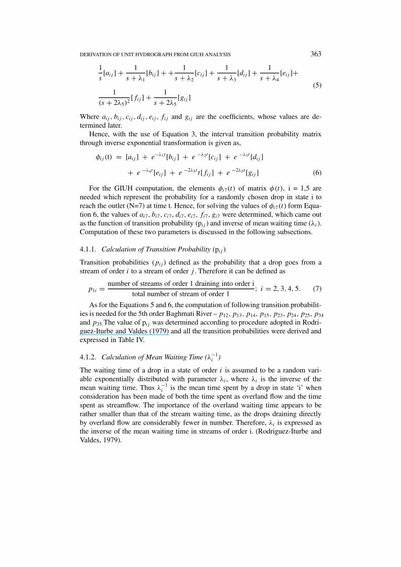
1

s[aij ] + 1

s + λ1[bij ] + + 1

s + λ2[cij ] + 1

s + λ3[dij ] + 1

s + λ4[eij ]+

1

(s + 2λ5)2[fij ] + 1

s + 2λ5[gij ]

(5)

Where aij , bij , cij , dij , eij , fij and gij are the coefficients, whose values are de-termined later.

Hence, with the use of Equation 3, the interval transition probability matrixthrough inverse exponential transformation is given as,

φij (t) = [aij ] + e−λ1t [bij ] + e −λ2t [cij ] + e −λ3t [dij ]+ e −λ4t [eij ] + e −2λ5t t[fij ] + e −2λ5t [gij ] (6)

For the GIUH computation, the elements φi7(t) of matrix φ(t), i = 1,5 areneeded which represent the probability for a randomly chosen drop in state i toreach the outlet (N=7) at time t. Hence, for solving the values of φi7(t) form Equa-tion 6, the values of ai7, bi7, ci7, di7, ei7, fi7, gi7 were determined, which came outas the function of transition probability (pij ) and inverse of mean waiting time (λi).Computation of these two parameters is discussed in the following subsections.

4.1.1. Calculation of Transition Probability (pij )

Transition probabilities (pij ) defined as the probability that a drop goes from astream of order i to a stream of order j . Therefore it can be defined as

p1i = number of streams of order 1 draining into order i

total number of stream of order 1; i = 2, 3, 4, 5. (7)

As for the Equations 5 and 6, the computation of following transition probabilit-ies is needed for the 5th order Baghmati River – p12, p13, p14, p15, p23, p24, p25, p34

and p35.The value of pij was determined according to procedure adopted in Rodri-guez-Iturbe and Valdes (1979) and all the transition probabilities were derived andexpressed in Table IV.

4.1.2. Calculation of Mean Waiting Time (λ−1i )

The waiting time of a drop in a state of order i is assumed to be a random vari-able exponentially distributed with parameter λi , where λi is the inverse of themean waiting time. Thus λ−1

i is the mean time spent by a drop in state ‘i’ whenconsideration has been made of both the time spent as overland flow and the timespent as streamflow. The importance of the overland waiting time appears to berather smaller than that of the stream waiting time, as the drops draining directlyby overland flow are considerably fewer in number. Therefore, λi is expressed asthe inverse of the mean waiting time in streams of order i. (Rodriguez-Iturbe andValdes, 1979).

364 V. JAIN AND R. SINHA

Table IV. Transition probabilites (pij ) for the Baghmati River

p12 =4R7

B+ 6R6

B− 6R5

B− 3R4

B− 6R3

B+ 4R2

B+ 4RB − 2

8R7B − 4R6

B − 4R5B − 2R4

B + 2R3B + 2R2

B − RB

p13 =2R6

B − 5R5B + 2R4

B − 2R3B + 5R2

B − 2RB

8R6B

− 4R5B

− 4R4B

− 2R3B

+ 2R2B

+ 2RB − 1

p14 =R6

B − 2R5B − R4

B + R3B + 2R2

B + RB − 2

8R6B

− 4R5B

− 4R4B

− 2R3B

+ 2R2B

+ 2RB − 1

p15 =R7

B− 3R6

B+ R5

B+ 2R4

B+ R3

B− R2

B− 3RB + 2

8R7B − 4R6

B − 4R5B − 2R4

B + 2R3B + 2R2

B − RB

p23 =R3

B+ 2R2

B− 2

2R3B − RB

p24 =R3

B − 2R2B − RB + 2

4R3B

− 2R2B

− 2RB + 1

p25 =RB − 3R3

B+ R2

B+ 3RB − 2

4R4B

− 2R3B

− 2R2B

+ RB

p34 =R2

B + 2RB − 2

2R2B

− RB

p35 =R2

B− 3RB + 2

2R2B − RB

λi can be determined as a function of either L1 or L�.. As the measurement oflength of first order stream (L1) is more dependent on the scale, the percentage oferror remains higher for first order streams. Hence, λi has been taken as a functionof L�. For the analysis of the Baghmati River, the mathematical expression of λ5

will be given as,

λ5 = ν/L�(=5) (8)

where v is the average velocity in the basin area and L� is the length of 5th orderstream in Baghmati River basin.

The mean waiting time for lower order streams can thus be expressed as,

λ4 = ν

L4= ν

L5∗ L5

L4; or λ4 = λ5.RL; (9)

Similarly, λ3 = λ5.R2L; λ2 = λ5.R

3L; and λ1 = λ5.R

4L (10)

where RL is the Length Ratio (see Table II for definition).

DERIVATION OF UNIT HYDROGRAPH FROM GIUH ANALYSIS 365

The expression of mean waiting time assumes that for a given rainfall-runoffevent, the velocity at any moment is approximately the same throughout the wholedrainage network (Rodriguez-Iturbe and Valdes, 1979). The assumption is basedon the pioneer work of Leopold (1953) and Leopold and Maddock (1953) and hasbeen experimentally validated by many workers (Langbein, 1964; Carlston, 1969;Calkins and Dunne, 1970; Pilgrim, 1966, 1976, 1977).

4.2. COMPUTATION OF INITIAL STATE PROBABILITY [θi (0)]

Initial state probability is defined as the probability that the drop starts its travel ina stream of order i. For 5th order Baghmati River, the initial state probability willbe given as,

θi(0) = A∗i

AT

(11)

where A∗i (i = 1,2,3,4,5) represents the sub-basin area for order i draining directly

into a stream of order i and AT is the total basin area.Initial state probability is determined through the calculation for all orders. For

first order sub-basin, total area draining directly into stream of order 1 will be givenas,

A∗1 = N1A1 (12)

Where N1 is the number of 1st order streams and A1 is average area of 1st ordersub-basins.

However, for θ2(0), θ3(0), θ4(0) and θ5(0) different procedure will be adopted.Basin area of streams of order 1 draining directly into stream of order 2 will begiven as, N1p12

Further, number of streams is expressed as bifurcation ratio as,

N1 = N1

N2.N2

N3.N3

N4.

N4

N5(= 1)= R4

B

Similarly, N2 = R3B,N3 = R2

B,N4 = RB

Therefore,

N1p12 = R4B(p12) (13)

Thus, the area draining directly into second order streams will be given by,

A∗2 = N2A2 − A1(R

4Bp12) = R3

BA2 − A1(R4Bp12) (14)

Where, A2 average area of 2nd order sub-basins.Similarly, A∗

i , i = 3, 4, 5 were determined, and finally the values of initial stateprobability are given in the Table V.

366 V. JAIN AND R. SINHA

Table V. Initial state probabilities [θi (0)] for the Baghmati River

θ1(0) = N1A1

A5

θ2(0) =(

RB

RA

)3−

(RB

RA

)4p12

θ3(0) =(

RB

RA

)2−

(RB

RA

)3p23 −

(RB

RA

)4p13

θ4(0) =(

RB

RA

)−

(RB

RA

)2p34 −

(RB

RA

)3p24 −

(RB

RA

)4p14

θ5(0) = 1 −(

RB

RA

)−

(RB

RA

)2p35 −

(RB

RA

)3p25 −

(RB

RA

)4p15

4.3. FINAL GIUH EQUATION FOR THE BAGHMATI RIVER

From the general GIUH equation of Baghmati River (Eq. 2), it follows that theGIUH is a function of initial state probability [θ i(0)] and transitional state probab-ility (φij ) i.e.

GIUH = f {θi(0), φij }It follows from the equations of φij (equation 6) and θ i(0) (Table V), that

θi(0) = f {RB,RA, pij } (15)

φij = f {RB, pij , λi} (16)

Where from Table IV, pij = f {RB}and from equation 9 and 10, λi = f {v, L�(=5), RL}

Hence,

GIUH = f {RA,RB,RL, ν, L5} (17)

It follows, therefore, that the GIUH is essentially a function of geomorphomet-ric parameters of the basin and its stream velocity.

The GIUH at Dhengbridge station of Baghmati River was computed through acomputer program, the code for which was written in C. The morphometric valuesat Dhengbridge site were obtained from the geomorphometric analysis (Table III).Rodriguez-Iturbe et al. (1979) suggested that constant velocity corresponding topeak discharge (maximum stage) value provides right value of hydrograph peak(qp) and time to peak (tp) of GIUH, as most of the flow remains concentratedaround peak velocity in a histogram of the velocity distribution of whole periodof outflow. Hence, the average stream velocity at maximum stage of 71 meter

DERIVATION OF UNIT HYDROGRAPH FROM GIUH ANALYSIS 367

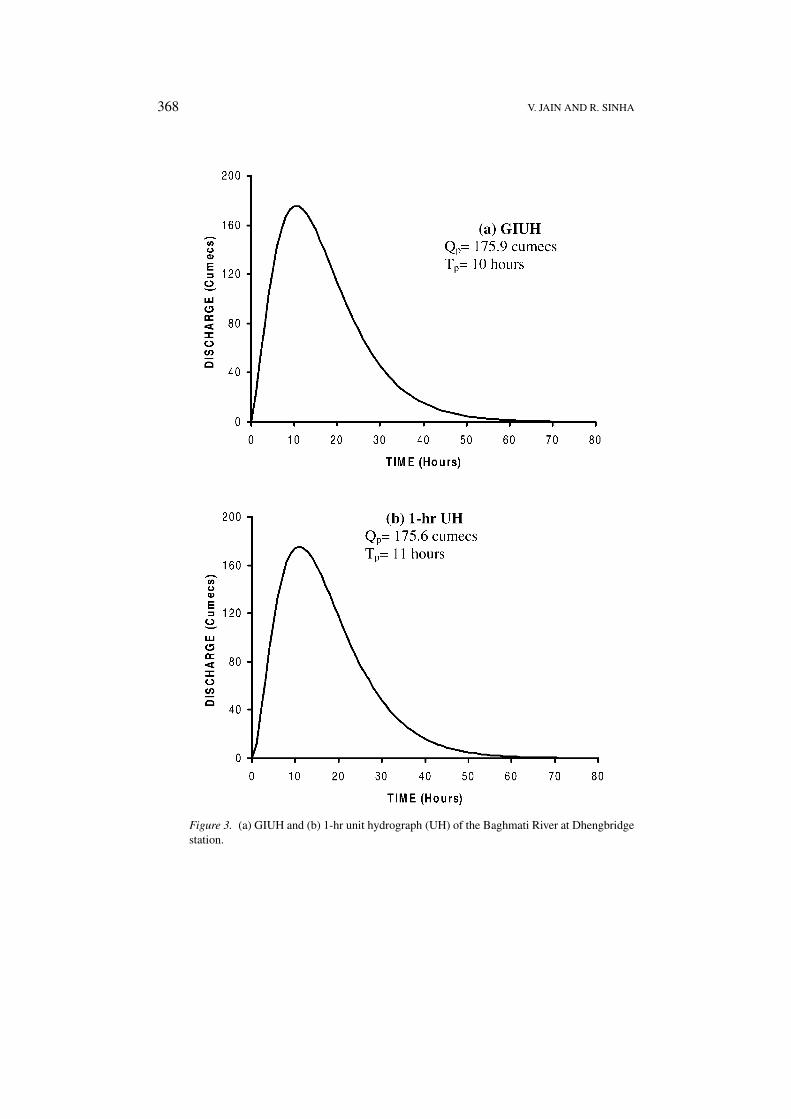
from the available 1988 data at Dhengbridge was taken as 1.63 m/sec (5.87 km/hr)(from stage-velocity, stage-discharge curves, CWC, Patna). This maximum stagewas corresponding to discharge of 1256 cumecs with a return period of 1.9 years,which is in between the values of most probable flood (1155 cumecs, T=1.58 yrs)and mean annual flood (1473 cumecs, T=2.33 years) (Table I). The ordinate valuesof GIUH were obtained at different time intervals, through the GIUH equations.These values were plotted to obtain the GIUH of the river at Dhengbridge. Thepeak discharge and time to peak of the geomorphic IUH were obtained as 175. 86cumecs and 10 hrs respectively (Fig. 3a). It was noted that functional relationshipobtained through regression analysis after Rodriguez-Iturbe and Valdes (1979)provides approximately same value of qp and tp, these function relationship areexpressed as:

qp = 1.31.L−1� .R0.43

L .ν (18)

tp = 0.44.L�.R0.55B .R−0.55

A .R−0.38L .ν−1 (19)

After substituting the values of Horton’s morphometric ratio, length of max-imum order channel (80.75 km) and average channel velocity (1.63 m/sec), thevalue of qp and tp was obtained as 175.44 cumecs and 10.5 hrs respectively. How-ever, further hydrologic analysis and its validation can not be carried out withthese functional relationships alone. The 1-hr unit hydrograph (UH) was generatedfrom GIUH from 1-hr time lag method for further hydrological analysis . The peakdischarge and time to peak of the 1-hr UH were computed as 175.67 cumecs and11 hours respectively (Fig. 3b).

5. Validation of GIUH Approach and Further Applications

The real validation of any hydrograph model should normally be done with the ob-served storm data. Unfortunately, no storm data is available from upstream reachesof the Baghmati River basin falling in Nepal (56% of the basin area), and therefore,such validation of GIUH was not possible. The approach followed in the presentstudy was to calculate 50-yr return period flood through GIUH of Baghmati Riverfor the Dhengbridge station and compare it with the 50-yr return period flood ob-tained through flood frequency data that is based on observed peak discharge data.The 50-yr return period flood from geomorphologic UH was computed through amethodology developed by Centre Water Commission (CWC, 1985).

5.1. COMPUTATION OF 50-YR RETURN PERIOD FLOOD FROM THE

GEOMORPHOLOGIC UH

The estimation of the 50-yr flood from the geomorphologic UH as per the methodadopted by Center Water Commission (CWC) for the middle Ganga plain (CWC,1985) includes different steps.

368 V. JAIN AND R. SINHA

Figure 3. (a) GIUH and (b) 1-hr unit hydrograph (UH) of the Baghmati River at Dhengbridgestation.

DERIVATION OF UNIT HYDROGRAPH FROM GIUH ANALYSIS 369

Step 1: Estimation of Design Storm Duration (TD):

The value of TD was determined for specific time to peak (tp) value using standardtable for Indian river basins (CWC, 1985).

For tp = 11 hours, TD = 18 hours.

Step 2: Estimation of Point Rainfall and Areal Rainfall

The 50-yr 24-h point rainfall for Baghmati River system is 34.6 cm (GFCC, 1991).As the design storm duration comes out to be 18-h, the 50-yr 18-h rainfall forBaghmati River system was deduced using conversion factors from standard tables(CWC, 1985).

50-yr 18-h point rainfall = 0.94 * 34.6 cm = 32.5 cm

50-yr 18-h areal rainfall = 0.72*32.5 cm = 23.4 cm

(0.94 is the ratio of 24-h point rainfall to 18-h point rainfall for the middle Gangaplain. The factor 0.72 is the areal reduction factor corresponding to the basin areamore than 2200 (the river basin upto Dhengbridge station is 3790 km2) for TD =18 hours.)

Step 3: Time Distribution of Areal Rainfall and Estimation of Effective Rainfall

The 50-yr 18-h areal rainfall of 23.4 cm was distributed using the distributioncoefficients (CWC, 1985). In this process, the 1-h rainfall increments and effectiverainfall units were determined (Table VI) using a design loss rate of 0.3 cm/hr (afterGFCC, 1991; CWC, 1988). Distribution coefficient in the table indicates that about39% of 18 hour rainfall (corresponding to a return of 50 years) of 23.4 cm occursduring first 1 hours, 52% during the next 1 hours and so on.

Step 4: Estimation of Base Flow

Base flow in the region was taken as 0.05 cumecs km−2 (GFCC, 1991). Taking thebasin area upto Dhengbridge as 3790 km2, the total base flow for the basin workedout to be 189.5 (0.05*3790) cumecs or 190 cumecs.

Step 5: Estimation of 50-yr Flood

For the estimation of the peak discharge, the effective rainfall units were rearrangedagainst the ordinates such that the maximum effective rainfall was placed againstthe maximum 1-h UH ordinate, the next lower value of effective rainfall againstthe next lower value of 1-h UH ordinate and so on (Table VI). Summation of theproduct of 1-h UH ordinate and the rainfall gives the total direct runoff in whichthe base flow is added to obtain the value of 50-yr design flood (Table VI). The

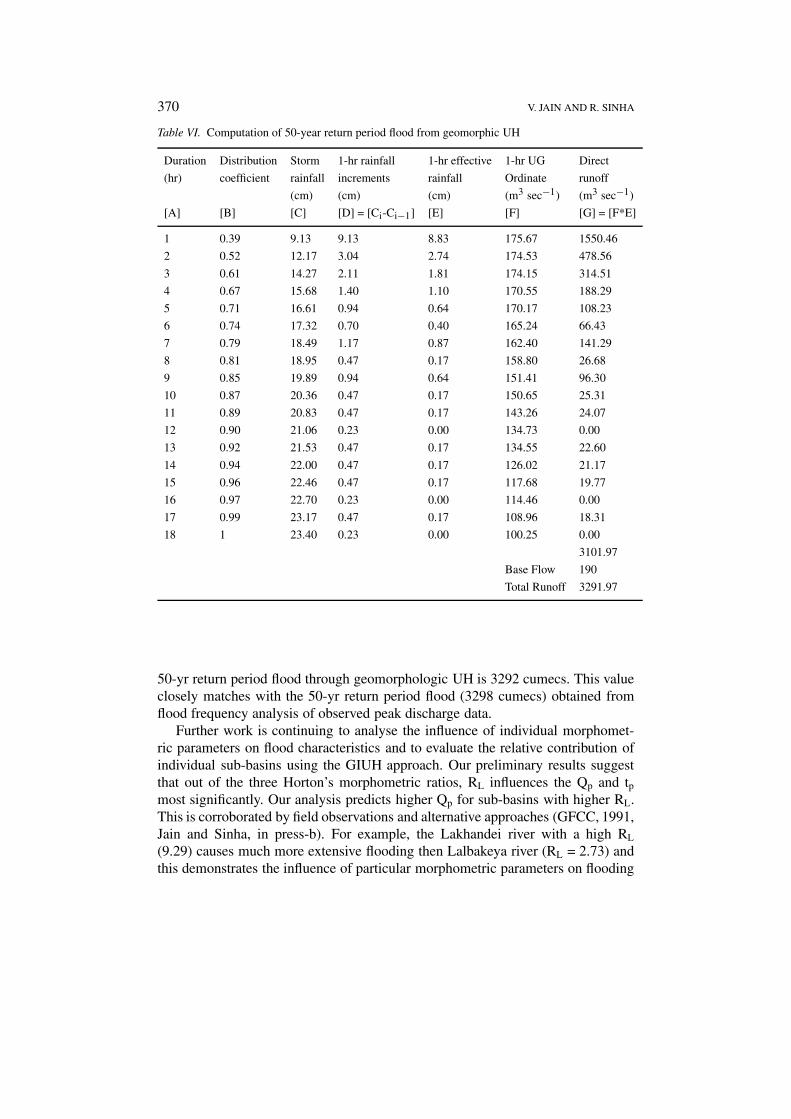
370 V. JAIN AND R. SINHA

Table VI. Computation of 50-year return period flood from geomorphic UH

Duration Distribution Storm 1-hr rainfall 1-hr effective 1-hr UG Direct

(hr) coefficient rainfall increments rainfall Ordinate runoff

(cm) (cm) (cm) (m3 sec−1) (m3 sec−1)

[A] [B] [C] [D] = [Ci-Ci−1] [E] [F] [G] = [F*E]

1 0.39 9.13 9.13 8.83 175.67 1550.46

2 0.52 12.17 3.04 2.74 174.53 478.56

3 0.61 14.27 2.11 1.81 174.15 314.51

4 0.67 15.68 1.40 1.10 170.55 188.29

5 0.71 16.61 0.94 0.64 170.17 108.23

6 0.74 17.32 0.70 0.40 165.24 66.43

7 0.79 18.49 1.17 0.87 162.40 141.29

8 0.81 18.95 0.47 0.17 158.80 26.68

9 0.85 19.89 0.94 0.64 151.41 96.30

10 0.87 20.36 0.47 0.17 150.65 25.31

11 0.89 20.83 0.47 0.17 143.26 24.07

12 0.90 21.06 0.23 0.00 134.73 0.00

13 0.92 21.53 0.47 0.17 134.55 22.60

14 0.94 22.00 0.47 0.17 126.02 21.17

15 0.96 22.46 0.47 0.17 117.68 19.77

16 0.97 22.70 0.23 0.00 114.46 0.00

17 0.99 23.17 0.47 0.17 108.96 18.31

18 1 23.40 0.23 0.00 100.25 0.00

3101.97

Base Flow 190

Total Runoff 3291.97

50-yr return period flood through geomorphologic UH is 3292 cumecs. This valueclosely matches with the 50-yr return period flood (3298 cumecs) obtained fromflood frequency analysis of observed peak discharge data.

Further work is continuing to analyse the influence of individual morphomet-ric parameters on flood characteristics and to evaluate the relative contribution ofindividual sub-basins using the GIUH approach. Our preliminary results suggestthat out of the three Horton’s morphometric ratios, RL influences the Qp and tpmost significantly. Our analysis predicts higher Qp for sub-basins with higher RL.This is corroborated by field observations and alternative approaches (GFCC, 1991,Jain and Sinha, in press-b). For example, the Lakhandei river with a high RL

(9.29) causes much more extensive flooding then Lalbakeya river (RL = 2.73) andthis demonstrates the influence of particular morphometric parameters on flooding

DERIVATION OF UNIT HYDROGRAPH FROM GIUH ANALYSIS 371

Figure 4. GIUH at different values of average channel velocity.

behaviour of individual sub-basins. The details of this work are being presentedelsewhere.

5.2. EFFECT OF VELOCITY PARAMETER ON THE GIUH

The stage-velocity curve shows variation in average channel velocity from 0.5(during lean period) to 1.63 (during peak discharge time) m sec−1. Thus, in orderto analyse the effect of average channel velocity on GIUH, four graphs were gener-ated for the velocity of 0.5, 1.0, 1.5 and 2.0 m sec−1, while keeping the geomorphicparameters fixed (Fig 4). Lower velocity values are corresponding to low stageindicating the lean period. Higher velocity values indicate higher stage period.Variation in GIUH parameters with respect to velocity reflects the dynamic beha-viour of hydrological response of Baghmati river basin in different periods. Figure4 shows that increase in average channel velocity causes significant increase in thepeak of hydrograph (qp) with less time to peak (tp). Thus, even though the generalform of GIUH is expressed by average channel velocity at peak discharge, Figure4 provides a complete dynamic hydrologic response of Baghmati river system.

5.3. COMPARISON WITH EXISTING SUH

The presently available UH, i.e. SUH for this site generated by GFCC is based onthree physiographic parameters, namely area (A), length of the longest stream and

372 V. JAIN AND R. SINHA

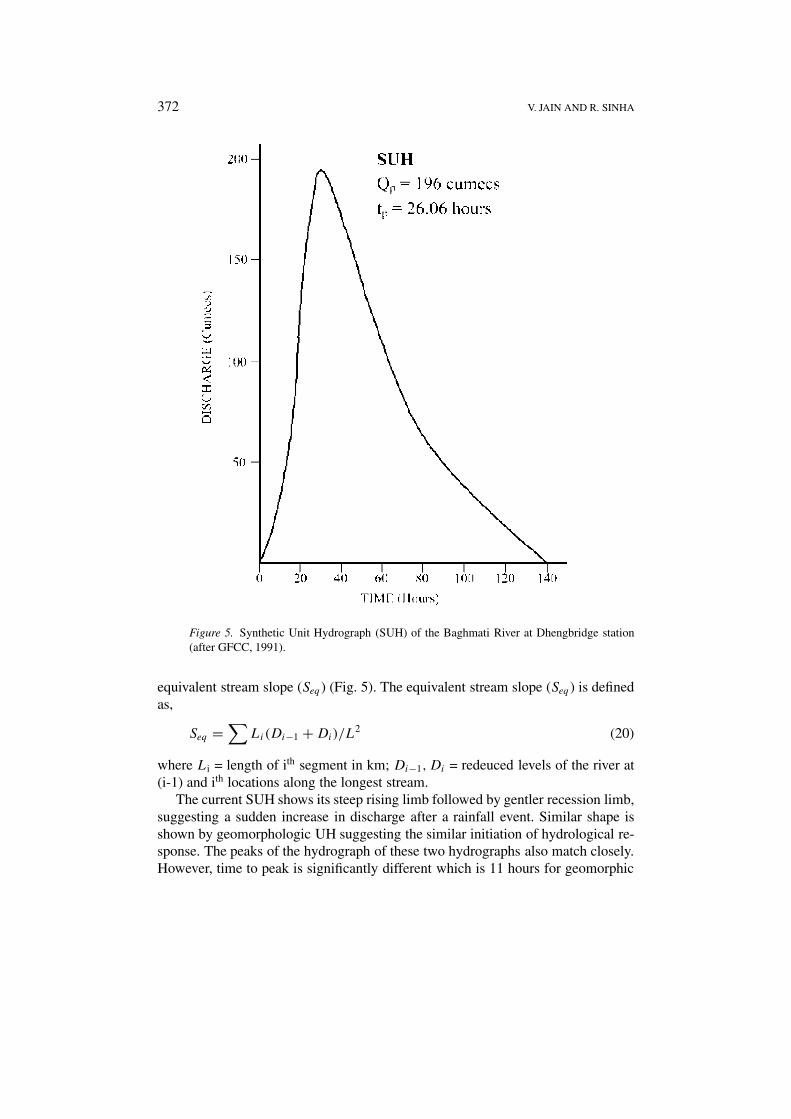
Figure 5. Synthetic Unit Hydrograph (SUH) of the Baghmati River at Dhengbridge station(after GFCC, 1991).

equivalent stream slope (Seq ) (Fig. 5). The equivalent stream slope (Seq ) is definedas,

Seq =∑

Li(Di−1 + Di)/L2 (20)

where Li = length of ith segment in km; Di−1,Di = redeuced levels of the river at(i-1) and ith locations along the longest stream.

The current SUH shows its steep rising limb followed by gentler recession limb,suggesting a sudden increase in discharge after a rainfall event. Similar shape isshown by geomorphologic UH suggesting the similar initiation of hydrological re-sponse. The peaks of the hydrograph of these two hydrographs also match closely.However, time to peak is significantly different which is 11 hours for geomorphic

DERIVATION OF UNIT HYDROGRAPH FROM GIUH ANALYSIS 373

IUH and 26 hours for SUH. The parameters of the SUH i.e. qp and tp are notdirectly validated with any data. Only validation is through computation of 50 yrreturn period flood (after GFCC, 1991), which show significant departure from theobserved data, whereas a similar validation of geomorphic UH indicates a bettermatch. The 50-year flood obtained from SUH comes out to be much higher (3779cumecs, after GFCC, 1991) than the 50-year flood from the observed data (3298cumecs after flood frequency analysis, see Table I). Though, no explanation isavailable for this large difference, the present SUH is the only available UH forthis river basin. On the other hand, the 50-yr flood derived from GIUH analysis(3292 cumecs) closely matches with the 50-yr flood from the observed data. Theanalysis indicates the validity of GIUH model in Baghmati River basin.

Further, velocity analysis on GIUH shows that same UH can not be consideredfor the different time period. It is noted that qp and tp of geomorphologic UH variesfrom 215 to 54 cumecs and 9 to 34 hours in the case of high velocity (peak dis-charge period) to low velocity during (lean period) (see Fig 4). It agrees well withthe observation of Rodriguez-Iturbe et al. (1979) that different unit hydrographscan be obtained in the same basin when performing the estimation to differentrainfall and their corresponding hydrographs. Thus, the dynamic nature of the geo-morphic IUH represents the variation in hydrologic response of the Baghmati riverbasin for different time period.

6. Conclusions

The geomorphic UH of the 5th order Baghmati river basin presented in this paperis the first analytically determined UH of any Himalayan river. An empiricallygenerated SUH based on coefficients from neighbouring river basin has been in usein the region. Our study demonstrates that the GIUH provide a better estimationof qp and tp compared to empirically derived SUH. Our results are validated bycomparison with the results of flood frequency analysis based on observed data.

The geomorphic UH of the Baghmati river utilizes the morphometric para-meters and stream velocity as the input parameters and it provides a quantitativeunderstanding of geomorphological influence on the river hydrology. Apart from itsutility for ungauged stations, the GIUH approach provides additional informationabout the effect of individual morphometric parameter on flood discharge. Further,the effect of velocity on GIUH reflects the dynamics of hydrological response ofa basin. Thus, apart from getting the better estimation of hydrological response ofriver basin, the GIUH provides an understanding of the hydrological response andits variability in space and time. The successful application of GIUH approach hasopened the possibility to derive the unit hydrograph of often ungauged Himalayanrivers and offers a sound approach for flood management in the region.

374 V. JAIN AND R. SINHA

References

Agarwal, A. and Narain, S.: 1996, Floods, Floodplains and Environmental Myths, State of India’sEnvironment: A Citizen Report, Centre for Science and Environment, New Delhi.

Barlow, 1915 (cited in Subramanya, K, 1994).Bhaskar, N. R. and Devulapalli, R. S.: 1991, ‘Run-off Modelling Geomorphological Instantaneous

Unit Hydrograph and ARC/INFO Geographical Information system’, D. B. Stafford (ed.), Proc.Civil Engineering applications of remote sensing and GIS, Published by ASCE.

Calkins, D. and Dunne, T.: 1970, ‘A salt tracing method for measuring channel velocities in smallmountain streams’, J. Hydrol. 11, 379–392.

Carlston, C. W., 1969, ‘Downstream variations in the hydraulic geometry of streams: Specialemphasis on mean velocity’, Amer. J. Sci. 267, 499–509.

Clark, C. O.: 1945, ‘Storage and the Unit Hydrograph’, Trans. Am. Soc. Civil Eng. 110, 1419–1488.CWC: 1985, Flood Estimation Report for Middle Ganga Plains (sub zone-1f), Central Water

Commission Report Number GP\10\1984, New Delhi.CWC: 1988, Workshop for Application of Reports on Sone Basin, Middle Gangetic Plains, Lower

Gangetic Plains and Mahanadi Basin for Design Flood Estimation for Small and MediumCatchments in Bihar 1988, Central Water Commission Publication No. 32/88.

GFCC: 1991, Comprehensive Plan of Flood Management for the Ganga Sub-Basin, Part II/9 – TheBaghmati River System, (Unpublished), Ganga Flood Control Commission, Ministry of WaterResources, Government of India.

Horton, R. E.: 1945, ‘Erosional development of streams and their drainage basins: Hydrophysicalapproach to quantitative morphology, Bull. Geol. Soc. Amer. 56, 275–370.

Howard, R. A.: 1971, Dynamic Probability Systems, John Wiley and Sons, Inc., New-York.Inglis and Desouza: 1929, (cited in Subramanya, K, 1994).Jain, S. K., Singh, R. D. and Seth, S. M.: 2000, ‘Design flood estimation using GIS supported GIUH

approach’, Water Res. Manage. 14, 369–376.Jain, V. and Sinha, R.: 2003, ‘Hyperavulsive-anabranching Baghmati river system, north Bihar plains,

eastern India’, Zeitschrift für Geomorphologie 47(1), 101–116.Jain, V. and Sinha, R.: ‘Fluvial dynamics of an anabranching river system in Himalayan foreland

basin, north Bihar Plains, India’, Geomorphology (in press-a).Jain, V. and Sinha, R.: ‘Geomorphological manifestation of the flood hazard’, Geocarto Interna-

tional, (in press-b).Koutsoyiannis, D. and Xanthopoulos, T.: 1989, ‘On the parametric approach to Unit Hydrograph

identification’, Water Res. Manage. 3, 107–128.Kale, V.S.: 1997, ‘Flood studies in India: A brief review’, J. Geolog. Soc. India 49, 359–370.Langbein, W. B.: 1964, ‘Geometry of river channels’, J. Hydr. Div., Amer. Soc. Civil Engin. HY2,

301–311.Leopold, L. B.: 1953, ‘Downstream change of velocity in rivers’, Amer. J. Sci. 251, 606–624.Leopold, L. B. and Maddock, T.: 1953, ‘The hydraulic geometry of stream channels and some

physiographic implications’, United States Geological Survey Professional Paper 252, 1–57.Nash, J. E.: 1960, ‘A Unit Hydrograph study, with particular reference to British catchments’, Proc.

Inst. Civil Engg. 17, 249–282.Pilgrim, D. H.: 1966, ‘Radioactive tracing of storm runoff on a small catchment’, J. Hydrol. 4,

289–305.Pilgrim, D. H.: 1976, ‘Travel time and nonlinearity of flood runoff from tracer measurements on a

small watershed’, Water Res. Res. 12(3), 487–496.Pilgrim, D. H.: 1977, ‘Isochrones of travel time and distribution of flood storage from a tracer study

on a small watershed’, Water Res. Res. 13(3), 587–595.Rodriguez-Iturbe, I. and Valdes, J. B.: 1979, ‘The geomorphologic structure of hydrologic response’,

Water Res. Res. 15(6), 1409–1420.

DERIVATION OF UNIT HYDROGRAPH FROM GIUH ANALYSIS 375

Rodriguez-Iturbe, I., Devoto, G. and Valdes, J. B.: 1979, ‘Discharge response analysis and hydrologicsimilarity: The interrelation between the geomorphologic IUH and the storm characteristics’,Water Res. Res. 15(6), 1435–1444.

Sinha, R.: 1998, ‘On the Controls of Fluvial Hazards in the North Bihar Plains, Eastern India’, inMaund, J. G. and Eddleston, M. (eds), Geohazards in Engineering Geology, Geological SocietyLondon, Engineering Geology Sp. Pub., 15, 35–40.

Sinha, R. and Friend, P. F.: 1994, ‘River systems and their sediment flux, Indo-Gangetic plains,northern Bihar, India’, Sedimentology 41, 825–845.

Sinha, R. and Jain, V.: 1998, ‘Flood Hazards of North Bihar Rivers, Indo-Gangetic Plains’, in V. S.Kale (ed.), Flood Studies in India, Geological Society of India, 41, 27–52.

Strahler, A. N.: 1956, ‘Quantitative slope analysis’, Bull. Geol. Soc. Amer. 67, 571–596.Strange: 1928, (cited in Subramanya, K., 1994).Snyder, F. F.: 1938, ‘Synthetic Unitgraphs’, Transactions of American Geophysics Union, 19th

Annual Meeting, Part 2, p. 447.Taylor, A. B. and Schwartz, H. E.: 1952, ‘Unit-hydrograph lag and peak flow related to basin

characteristics’, Transact. Amer. Geophys. Union 33, 235–246.Valdes, J. B., Fiallo, Y. and Rodriguez-Iturbe, I.: 1979, ‘A rainfall-runoff analysis of the geomorpho-

logic IUH’, Water Res. Res. 15(6), 1421–1434.