arX

iv:h

ep-p

h/96

1131

3v1

12

Nov

199

6

McGill/96-41

Derivation of the Lamb Shiftusing an Effective Field Theory

Patrick Labelle 1

Department of Physics, Bishop’s University

Lennoxville, Quebec, Canada J1M 1Z7

and

S. Mohammad Zebarjad2

Department of Physics, McGill University

Montreal, Quebec, Canada H3A 2T8

Abstract

We rederive the O(α5) shift of the hydrogen levels in the non-recoil limit (me/mP →0) using Nonrelativistic QED (NRQED), an effective field theory developed by Caswelland Lepage (Phys. Lett.167B, 437 (1986)). Our result contains the Lamb shift as aspecial case. Our calculation is far simpler than traditional approaches and has theadvantage of being systematic. It also clearly illustrates the need to renormalize (or“match”) the coefficients of the effective theory beyond tree level.

1labelle@hep.physics.mcgill.ca2zebarjad@hep.physics.mcgill.ca

1 Introduction

The Lamb shift, the shift between the hydrogen 2S1/2 and 2P1/2 states, is without anydoubt the most well-known bound state application of radiative corrections. It has the formmeα

5( lnα+ finite) where the finite piece contains the Bethe logarithm, a state dependentterm that must be evaluated numerically. The log term is relatively easy to extract and itscalculation is presented in many quantum mechanics textbooks. The finite contributionis much more difficult to evaluate because it requires the application of QED to a boundstate. In this paper, we rederive the complete O(α5) corrections in the non-recoil limit1

(me/mP = 0) using NRQED, an effective field theory developed by Caswell and Lepage[1], as extended by Labelle [2] to study retardation effects.

To construct NRQED, one writes down the most general Lagrangian consistent withthe low energy symmetries of QED such as parity and gauge invariance, etc. The first fewterms of this Lagrangian are given by (we follow the notation of [7])

L2−Fermi = ψ†iDt +D2

2m+ δR

D4

8m3+ δF

qσ · B2m

+ δDq(D · E −E · D)

8m2

+δSiqσ · (D ×E − E× D)

8m2+ . . .ψe

+ same terms with ψe → ψp + photon terms, (1)

where ψe and ψp are two component fields associated with the electron and proton, respec-tively. There are of course many other interactions, including four-fermion interactions,however, as we will discuss below, those are not relevant at O(α5). For the photon, we usethe Coulomb gauge which is the most efficient gauge to study nonrelativistic bound statessince it permits to isolate the Coulomb interaction (which must be treated nonperturba-tively) from all other interactions (which can be treated as perturbations). In that gauge,the photon terms in Eq.(1) are

− 1

4FµνF

µν + δV Pα

15πA0(k)

k4

m2A0(k) − δV P

α

15πAi(k)

k4

m2Aj(k) (δij −

kikj

k2) + . . . (2)

Using D = i(p− qA) and Dt = ∂t + iqA0, the NRQED hamiltonian can be written as

H = ψ′†

[

p2

2m+ qA0 −

p4

8m3− q

2m(p′ + p) · A +

q2

2mA · A

−δFiq

2mσ · (k × A) − δD

q

8m2k2A0 + δS

iq

4m2σ · (p′ × p)A0

+δSiq

8m2k0

σ · (p′ + p) × A − δSiq

4m2σ · (k1 × A(k1))A

0(k2) + . . .]

ψ,

(3)

1In the literature, these corrections are also referred to as the Lamb shift. We will also adopt thisnotation in the rest of the paper.

1

and the photon hamiltonian can be written as

Hphoton =1

2(E2 + B2) − δV P

α

15πA0(k)

k4

m2A0(k) + δV P

α

15πAi(k)

k4

m2Ai(k)(δij −

kikj

k2) + . . .

(4)

The Feynman rules of Eqs.(3) and (4) are given in Fig.[1].The photon propagator requires a special treatment. We use time-ordered perturbation

theory (in which all particles are on-shell but energy is not conserved at the vertices) and,as mentioned above, we work in the Coulomb gauge. In a time-ordered diagram, Coulombphotons propagate instantaneously (i.e. along vertical lines in our diagrams since we choosethe time axis to point to the right) and transverse photon propagate in the time direction.The corresponding Feynman rules are given in Figs.[2] and [3].

As is shown in [2], the power of NRQED is enhanced if one separates “soft” transversephotons (having energies of order γ ≡ Zµα ) from the “ultra-oft” photons (with E ≃ γ2/µ)because the counting rules differ for the two types of photons. In that reference, it is alsoshown that the multipole expansion can be applied to the vertices containing ultra-softphotons. The distinction between soft and ultra-soft photons is particularly important inthis work because the Lamb shift involves both types of contributions. We have there-fore separated the general photon propagator of Fig.[4] into a contribution correspondingto a soft photon, Fig.[4(a)], and the contribution corresponding to an ultra-soft photon,Fig.[(4b)].

Finally, in NRQED loop diagrams, all internal momenta must be integrated over, witha measure d3p/(2π)3.

The unknown coefficients δR, δF . . . can be found by imposing that NRQED is equiva-lent to QED for nonrelativistic scattering processes, i.e. by imposing

NRQED scatteringamplitudes

= QED scattering amplitudesexpanded in powers of p/m.

This is the so-called matching procedure. Notice that no bound state physics enters at thisstage of the calculation.

The coefficients appearing in (3) can be fixed by considering the scattering of an electronoff an external field Aµ. This is illustrated, at tree level, in Fig.[5]. We have chosen thenormalization of the interactions of Eq.(3) in such a way that the tree level matching givesδ = 1 for all the coefficients appearing in (3). The first non-zero contribution to δV P comesfrom the one-loop QED vacuum polarization diagram, as illustrated in Fig.[6 ] and, again,our normalization is such that δV P = 1, to one loop [7]. We will still refer to this as “treelevel matching” because only tree level NRQED diagrams are involved (similarly, n-loopsmatching will refer to the number of loops “n” the NRQED diagrams). The one-loopmatching will bring O(α) corrections to the coefficients δ′s.

We are now in position to proceed with the calculation. All NRQED calculations canbe divided into three steps. The first one consists in using the counting rules to identify the

2

diagrams which will contribute to the order of interest. This first step not only permits toidentify the relevant diagrams but it also fixes the order (in the number of loops) at whichthe coefficients must be matched. The second step consists in matching the coefficients tothe order required and the last step corresponds to finally evaluating the NRQED boundstate diagrams.

In our case, we first need to isolate the NRQED diagrams contributing to order α5

in the non-recoil limit i.e. we neglect corrections suppressed by powers of me/mp. As asimpler example, we will first isolate the diagrams contributing to order α4 in the non-recoillimit (the full NRQED calculation of the O(α4) energy shift for arbitrary masses will bepresented in Ref.[8]). In that limit, the only relevant diagrams are shown in Fig.[7]. Thiscan easily be checked by using the NRQED counting rules derived in Ref.[2]. Since softand ultra-soft photons obey different counting rules, we consider their contribution in turn.Soft photons contribute to order :

µκ+ρ+1

mκem

ρpZηαζ ≈ mρ+1

e

mρpαζ, (5)

where µ is the reduced mass and ρ and κ are, respectively, the total number of inversepowers of mp and me appearing in the NRQED vertices. In (5), we approximated µ ≈ me

which is exact in the non-recoil limit. The coefficient ζ is defined by

ζ = 1 + κ + ρ−NTOP +∑

i

ni, (6)

where NTOP is the number of intermediate state time-ordered propagators (see Ref.[2] formore details) and last term is the sum of factors of α contained in the vertices (includingpossible factors coming from the δ’s). Now, to obtain the correction of order meα

4, weneed to have ρ = 0 and ζ = 4 (see Eq.(5)). The only way to have ρ = 0 is to either havea Coulomb interaction on the nucleus line or no interaction at all. This already reducesgreatly the possible diagrams. Turning now to the condition ζ = 4, we obtain from Eq.(6)

κ−NTOP +∑

i

ni = 3. (7)

Since in first order of perturbation theory Ntop = 0, we are left with the conditionκ+

∑

i ni = 3. One possibility is κ = 3 and∑

ni = 0 which corresponds to the relativistickinetic energy vertex on the electron line. Another possibility is κ = 2 and

∑

ai = 1 whichcan be fulfilled with the Coulomb vertex on the proton line and either the Darwin or theSpin-Orbit interaction on the electron line. There are no Coulomb interaction with onlyone inverse mass so the condition κ = 1 and

∑

ni = 2 cannot be satisfied. The threepossible diagrams are illustrated in Fig.[7].

To order α5, and still in first order of perturbation theory, we must either increase κ or∑

ni by one. It is not possible to increase the number of inverse electron masses κ by one,but there are two ways to increase

∑

ni by one. One is to include the one-loop correctionsto the coefficients δ’s of the vertices in Fig.[7], so we will have to match these interactions

3

to one loop. The other possibility for κ = 2 and∑

ni = 2 is to consider the new interactioncorresponding to the vacuum polarization correction to the Coulomb propagator which isdepicted in Fig.[8].

We now turn to diagrams in second order of perturbation theory, in which case NTOP =1. It can easily be verified that ζ , Eq.(6), cannot then be made equal to 5. We have nowuncovered all the diagrams containing only soft photons which contribute to order α5. Theonly remaining possibility is to consider diagrams with ultra-soft photons which lead to acontribution of the form given by Eq.(5) but now with (see Ref.[2]):

ζ =∑

i

ni + 1 + ρ+ κ−Ntop + 2Nγ +∑

i

Mi, (8)

where Nγ is the number of ultra-soft photons in the diagram and Mi is the order, in themultipole expansion, of the ith vertex and the sum is over the vertices connected to ultra-soft photons only. As before, we set ζ = 5 and ρ = 0 to obtain non-recoil corrections oforder α5. For diagrams containing ultra-soft photons, the minimum value of NTOP is 1,because these photons propagate in the time direction (we again refer the reader to Ref.[2]for more details). Working at the zeroth order of the multipole expansion (Mi = 0) andconsidering only one ultra-soft photon (Nγ = 1), we then have the condition κ+

∑

ni = 3.Since the ultra-soft photon is necessarily transverse and transverse vertices contain at leastone power of inverse mass (see Fig.[1]), κ is bigger or equal to 2. In addition,

∑

ni is atleast equal to one (i.e. there at least a total number of one factor of α in the vertices).We therefore already fulfill the condition κ +

∑

ni = 3 with the simplest diagram whichcorresponds to an ultra-soft photon connected to two p · A vertices, as represented inFig.[9].

We have now identified all diagrams contributing to the order of interest. We now turnto the matching. From the above discussion, we see that we need to match to one loop thecoefficients of the interactions contributing to order α4.

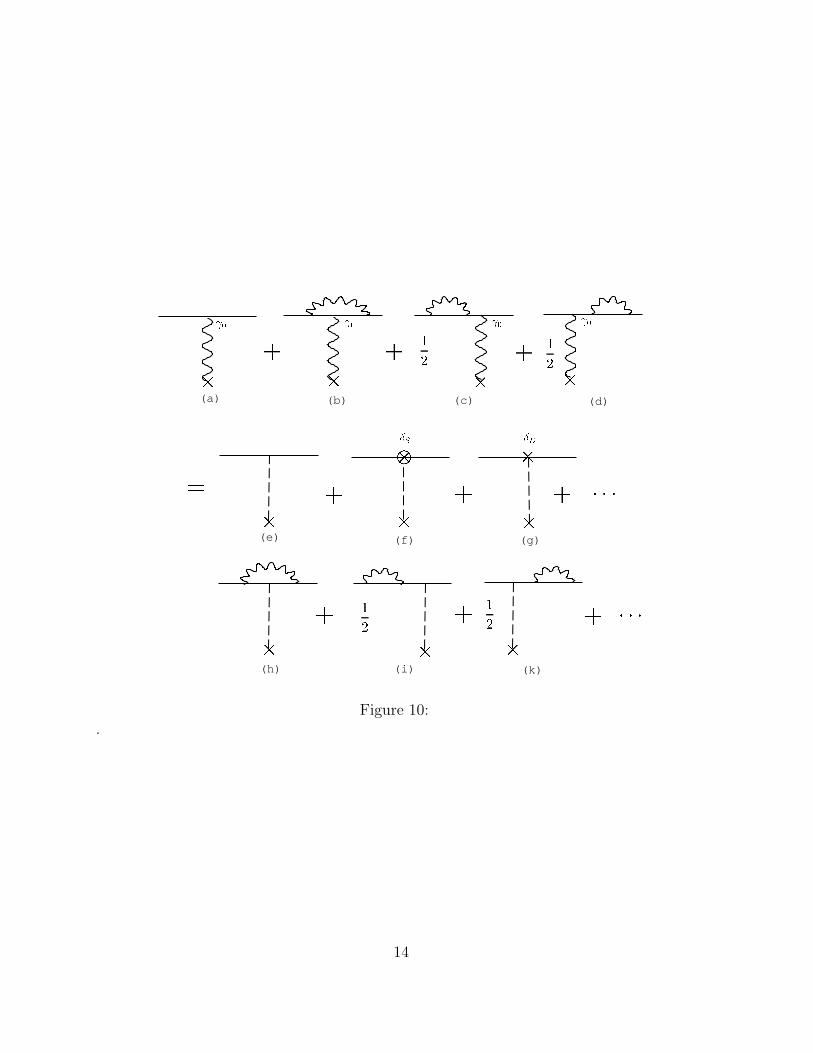
To make NRQED agree with QED at the one loop order, we impose the relation illus-trated in Fig.[10]. This matching was performed in [7] but, even though our final result is ofcourse the same, our derivation differs sufficiently to be presented it here. The QED scat-tering amplitude (the left hand side of Fig.[10]) can be expressed in terms of the usual formfactors F1(Q

2) and F2(Q2) in the following way (to be consistent, we use a nonrelativistic

normalization for the Dirac spinors):

−eu(p′, s′)√

2E ′

[

γ0A0(Q)F1(Q

2) − i

2mσ0j A0(Q) Qj F2(Q

2)]

u(p, s)√2E

=

F1(Q2)ξ

′†

[

− eA0 +e

8m2Q 2A0 − ie

4m2σ · (p ′ × p)A0 + . . .

]

ξ +

F2(Q2)ξ

′†

[

e

4m2Q 2A0 − ie

2m2σ · (p ′ × p)A0 + . . .

]

ξ, (9)

where Q = p′ − p, s and s′ are the initial and final spin of the electron, respectively, andξ, ξ′ are the corresponding initial and final two component Pauli spinors normalized to

4

unity. We choose the convention that e is positive so that the charge of the electron is −e.In (9), as in the rest of the paper, we use m to represent the mass of the electron. Noticethat the matching involves a double expansion. One expansion is in the coupling constantα and the other is the nonrelativistic expansion in Q/m which leads to renormalization ofdifferent NRQED operators. The nonrelativistic expansions of the form factors are [7]

F1(Q2) = 1 − α

3π

[

Q 2

m2

(

ln(m

λ) − 3

8

)]

+ . . .

F2(Q2) = ae −

α

π

Q 2

12m2+ . . . . (10)

where ae is the electron anomalous magnetic moment which, to the order of interest, canbe taken to be α/(2π). In the above Eqs., since Q0 is of order of v2 and |Q| is of order v,we have ignored Q0 respect to Q.

If we substitute (10) in (9) we obtain

ξ′† (−eA0) ξ +

e

8m2ξ′† Q2A0ξ

[

1 +8α

3π

(

ln(m

λ) − 3

8

)

+ 2ae + . . .]

− ie

4m2ξ′†

σ · (p′ × p)A0 ξ[

1 + 2ae + . . .]

+ O(Q4/m4). (11)

We must now compute the right-hand side of Fig.[10] to complete the calculation of theone-loop renormalized NRQED coefficients. Since we are dealing with ultra-soft photonsin Figs. [10(h)], [10(i)] and [10(k)], we use the special Feynman rules derived in Ref.[2].Working at the zeroth order of the multipole expansion, Fig.[10(h)] corresponds to

ξ′†(

2epi

2m)(

2ep′j2m

)∫

d3k

(2π)3

δij − kikj

k2+λ2

2√

k2 + λ2

1

−√

k2 + λ2(−eA0)

1p2

2m− p′2

2m−√

k2 + λ2ξ

≈ ξ′†(−eA0)ξ (

e

m)2 p′ · p

3

∫ dk k2

2π2

2k2 + 3λ3

k2 + λ2

1

2√

k2 + λ2

1

k2 + λ2

= −8α

3π

[

ln(2Λ

λ) − 5

6

]

ξ′†eA0ξ

p · p′

4m2(12)

where, in the second line, we have used the fact that the integral is already proportional top ·p′ to approximate p2 ≈ p′2 ≈ 0 in the propagators. The corrections to these expressionswill lead to higher order operators.

Notice that we are only working with scattering diagrams when performing the match-ing, no bound state physics enters this stage of the calculation. To compute the amplitudesin Figs.[10(i)] and [10(k)], we just need to evaluate the first one and then obtain the secondone by replacing p by p ′. For Fig.[10(i)], we can write

1

2ξ′†(

2epi

2m)(

2epj

2m)∫ d3k

(2π)3

δij − kikj

k2+λ2

2√

k2 + λ2

1

E − p2

2m−√

k2 + λ2

1

E − p2

2m

(−eA0) ξ.

(13)

5

Here, E represents the on-shell energy p2/2m. Of course, in that limit, the propagator1/(E−p2/2m) is divergent, which signals the need for a mass renormalization. In NRQED,we perform mass renormalization exactly as in QED, i.e. we start by keeping E 6= p2/2mand subtract the mass counter-term:

− 1

2ξ′†eA0(

e

m)2 p2

3

∫

dk k2

2π2

2k2 + 3λ3

k2 + λ2

1

2√

k2 + λ2

(

1

E − p2

2m−

√k2 + λ2

− 1

−√

k2 + λ2

)

1

E − p2

2m

ξ. (14)

Expanding the term in the parenthesis around E− p2

2m, we get a series which, by construc-

tion, starts at order (E−p2/2m)1, which cancels the propagator 1/(E−p2/2m) in Eq.(13).One can then finally take the limit E → p2/2m with for result, for the sum of Figs.[10(i)]and [10(k)],

− 1

2ξ′† eA0

α

3πm2(p2 + p′2)

∫

dkk22k2 + 3λ2

k2 + λ2

1√k2 + λ2

−1

k2 + λ2ξ

= −8α

3π

[

ln(2Λ

λ) − 5

6

](− ξ′†eA0ξ

8m2(p2 + p′2)

)

. (15)

Putting everything together, the complete right-hand side of Fig.[10] is equal to the sumof Eqs.(12) and (15):

ξ′† (−eA0) ξ +

e

8m2ξ′† Q2A0ξ

[

δD +8α

3π

(

ln(2Λ

λ) − 5

6

)]

− δSie

4m2ξ′†

σ · (p ′ × p)A0 ξ (16)

Now, by equating (11) and (16), we can evaluate δD and δS:

δD = 1 +α

π

8

3

[

ln(m

2Λ) +

11

24

]

+ 2ae + O(α2) (17)

δS = 1 + 2ae + O(α2). (18)

Notice that, since the relativistic kinetic vertex does not enter the matching, we alsofind2

δR = 1 + O(α2). (19)

We are now ready for the third and last step of the calculation, the computation of thebound state diagrams per se. Since only δD and δS receive an O(α) correction, but not

2One might expect that δR be equal to one to all orders, since this interaction comes from Taylorexpanding the relativistic expression for the energy, but this might not be so if the regulator (as is the casein this calculation) breaks Lorentz invariance.

6

δR, only Figs.[7(b)] and [7(c)] are needed for the O(α5) calculation. Let us now start withFig.[7(b)].

∆E7(b) = δS−iZe24m2

∫

d3p′d3p

(2π)6Ψ∗(p)

(

σ · p ′ × p

(p ′ − p)2

)

Ψ(p ′)

= δSZα

2m2<

s · Lr3

>

= δSm(Zα)4

4n3(l + 1/2)

(

δ(j − (l + 1/2))

(l + 1)− δ(j − (l − 1/2))

l

)

(1 − δl,0),

(20)

where Ψ(p) is the Schrodinger wavefunction (including the electron spin3 corresponding tothe quantum numbers n, j and l.

In Eq.(20) we used

∫

d3p′

(2π)3eip ′·r ′ σ · p × p ′

p′2= i

σ · p× r ′

4πr′3. (21)

For the diagram of Fig.[7(c)], we find

∆E7(c) =∫

d3p′d3p

(2π)6Ψ∗(p ′)

(

δDe(p ′ − p)2

8m2a

Ze1

(p ′ − p)2

)

Ψ(p)

=∫

d3p′d3p

(2π)6Ψ∗(p ′)Ψ(p)

= δDZe2

8m2|Ψ(0)|2 = δD

m(Zα)4

2n3δl,0. (22)

Using the counting rules, we also found that the diagram depicted in Fig.[8] wouldcontribute to O(mα5). This diagram corresponds to the well-known Uehling potential andis found to be

∆E8 =∫

d3p′d3p

(2π)3Ψ∗(p ′)

(

− e1

(p ′ − p)2δV P

−(p ′ − p)4α

15πm2

1

(p ′ − p)2Ze

)

Ψ(p)

= −δV PZe2 α

15π

1

m2|Ψ(0)|2 = −δV P

4α

15π

m(Zα)4

n3δl,0. (23)

We finally turn our attention to the only remaining diagram, which is represented inFig.[10]. The corresponding integral is (as shown in Ref.[2], in zeroth order of the multipoleexpansion we set p ′ = p on the vertices):

∆E8 =∫

d3kd3p

(2π)6Ψ∗(p)

2epi

2m

2epj

2m

1

2k

1

En − p2

2m− k

(δij −kikj

k2) Ψ(p)

3 In the non-recoil limit, the spin of the proton completely decouples from the problem.

7

=e2

2m2(2π)3

∫ d3p

(2π)3Ψ∗(p)

∫

dk kdΩ(p2 − (p·k)2

k2 )

En − p2

2m− k

Ψ(p)

=2α

3π

∫

d3p

(2π)3

∫

dk k Ψ∗(p) (p2/m2

En − p2

2m− k

) Ψ(p). (24)

In a bound state, beyond tree level one must include an infinite number of Coulomb linesin the intermediate state. This can easily be seen from the counting rules, Eq.(8). Indeed,adding a Coulomb line will not change ζ because this increases both Ntop and

∑

i ni by one,which has no overall effect. Because of this, one must use the Coulomb Green’s functionfor the intermediate state. Using the bra and ket notation, Eq.(24) must then be replacedby the well-known expression:

2α

3π

∑

n′

∫

dk k< n|vop|n′ >< n′|vop|n >

En − En′ − k. (25)

This part of the calculation is well known and is carried out in many texbooks (see forexample Ref.[5]). The result is

∆E = m4α

3π

(Zα)4

n3

ln Λ<En>

if l = 0

ln Z2mα2

2<En>if l 6= 0,

(26)

where < En > is the Bethe logarithm which can be evaluated numerically [9]. Now, usingEqs.(17) and (18), we add the α5 contributions from Eqs.(20) and(22) to Eqs.(23) and (26)to obtain

∆E = m4α

3π

(Zα)4

n3

ln m2<En,0>

+ 1930

if l = 0

ln Z2mα2

2<En,l>+ 3

8(2l+1)( δ(j−(l+1/2))

(l+1)− δ(j−(l−1/2))

l) if l 6= 0,

(27)

which is the well-known Lamb shift.

2 Conclusion

We have calculated the complete O(mα5) non-recoil corrections to the hydrogen energylevels, also referred to as the Lamb shift. The superiority of NRQED over the traditionalapproaches is twofold. Firstly, the calculation of the bound state diagrams is greatly sim-plified because the use of an effective field theory permits to disentangle the contributionsfrom low and high momenta and only QED scattering diagrams need to be evaluated. Sec-ondly, the NRQED calculation is systematic in the sense that simple counting rules can beused to isolate the diagrams contributing to a given order in α, which is not possible intraditional approaches.

8

O~p

~p

~p~p

Coulomb Vertex

Dipole Vertex

Spin-Orbit Vertex

Fermi Vertex

O~p~p

Darwin Vertex

~p

Relativistic Kinetic Vertex

~p 0~p 0~p 0~p 0~p 0~p 0~p 0

q2m(~p 0 + ~p)D q8m2(~p ~p 0)2

F iq2m(~p 0 ~p) ~

~p 48m3(2)33(~p 0 ~p)q2 ij2m

q

S iq4m2(~p 0 ~p) ~Seagull Vertex

Figure 1: NRQED Vertices

9

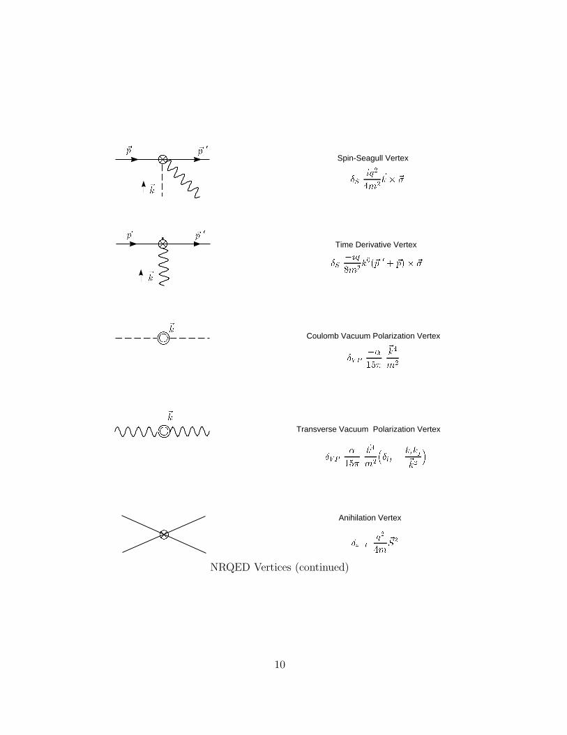
O~k ~p 0~p S iq24m2~k ~Spin-Seagull Vertex

O~k~p ~p 0 S iq8m2k0(~p 0 + ~p) ~Time Derivative Vertex

~kCoulomb Vacuum Polarization VertexV P 15 ~k4m2

~k Transverse Vacuum Polarization VertexV P 15 ~k4m2ij kikj~k2 O Anihilation Vertex4F q24m~S2

NRQED Vertices (continued)

10

Coulomb Photon

~k1~k2 + 2~k

Fermion Propagator

Transverse Photon Propagator

1E0 Eintermediate = 1E0 ~p22m~p 12q~k2 + 2 ij kikj~k2+2E0 Eintermediate = 12q~k2 + 2 ij kikj~k2+2E0 q~k2 + 2

Figure 2: NRQED Propagator. m1m2m1m2

Fermion-Fermion Propagator

Transverse Photon + Fermion-Fermion propagator~k~p2~p1~p1~p2 1Ei ~p212m1 ~p222m2 12q~k2 + 2 ij kikj~k2+2E0 ~p212m1 ~p222m2 q~k2 + 2

Figure 3: Time-ordered propagators for two fermions plus one transverse photon.. = +

(a) (b)

Figure 4:.

11

==

OO+ +

+ + + 0 i : : :

: : :Figure 5:

. ~k ~k== 0 0 i j : : :: : :++Figure 6:

. O

mM MM

mm~p

~p 0 ~p 0~p 0

~p ~p

~p 0~p 0~p 0~p

~p~p

(a) (b)

(c)

Figure 7:.

12

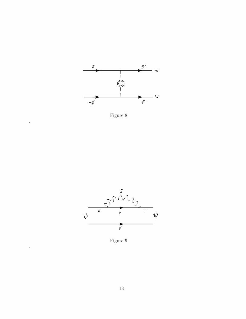
mM ~p ~p 0~p 0~pFigure 8:

.

~p ~p~p ~k~p

Figure 9:.

13

=

+ ++ O + ++ ++ +

12 12

1212

(a) (b) (c) (d)

(e) (f) (g)

(h) (i) (k)

0 0 0 0

: : :: : :S D

Figure 10:.

14

References

[1] W.E. Caswell and G.P. Lepage, Phys. Rev. A20, 36 (1979).

[2] P. Labelle, hep-ph/9608491.

[3] P. Labelle, G. P. Lepage, and U. Magnea, Phys. Rev. Lett. 72, 2006 (1994).

[4] P. Labelle, Ph.D. Thesis, Cornell University, January (1994).

[5] C.Itzykson and Zuber, Quantum Field Theory, McGraw-Hill,1980.

[6] P. Labelle, “NRQED in bound states: applying renormalization to an effective fieldtheory”, proceedings of the fourteenth MRST Meeting, P.J. O’Donnell ed., Universityof Toronto, 1992, hep-ph/9209266.

[7] T. Kinoshita, M. Nio, Phys. Rev. D53, 4909, 1996.

[8] P.Labelle, S M Zebarjad, work in preparation.

[9] J.R. Sapirstein and D.R. Yennie in Quantum Electrodynamics, ed. by T. Kinoshita(World Scientific, Singapore, 1990).

15