arX

iv:n

ucl-

th/0

1060

71v3

3 J

ul 2

003

Microscopic derivation of pion-nucleon and

pion-Delta scattering lengths

P. Bicudo 1 , M. Faria, G. M. Marques 2 and J. E. Ribeiro 3

Centro de Fısica das Interaccoes Fundamentais (CFIF),Departamento de Fısica, Instituto Superior Tecnico,

Av. Rovisco Pais, 1049-001 Lisboa, Portugal

Abstract

A general expression for the π − N and π − ∆ scattering lengths is derived inthe framework of a microscopic calculation. Annihilation, negative energy wave-functions and spontaneous chiral symmetry are included consistently. The point-likelimit is used to calculate the scattering lengths.

Key words:preprint FISIST/18-2002/CFIFPACS: 11.30.Rd, 12.39.Jh, 13.75.Gx

1 Introduction

In the last decade a global picture for low energy hadronic physics has slowlyemerged. Although the theory of hadronic reactions, which one expects to bea consequence of QCD, remains as challenging as ever, we possess a naturalsymmetry (chiral symmetry) which acts, so to speak, as a filter for the stilllargely unknown low energy details of strong interactions. Indeed it is remark-able that although intermediate theoretical concepts like gluon propagators,quark effective masses and so on, might vary (in fact they are not gauge invari-ant and hence they are not physical observables), chiral symmetry contrivesfor the final physical results, e.g. hadronic masses and scattering lengths, to belargely insensitive to the above mentioned theoretical uncertainties. The pionmass furnishes the ultimate example. For massless quarks, the pion mass is

1 bicudo@ist.utl.pt2 gmarques@cfif.ist.utl.pt3 emilio@netcabo.pt

Preprint submitted to Elsevier Science 1 August 2013

bound to be zero, regardless of the form of the effective quark interaction pro-

vided it supports the mechanism of spontaneous breakdown of chiral symmetry(SχSB).

π − π elastic scattering [1,2,3,4] provides another example of this insensitiv-ity to the form of the quark microscopic interaction. The incorporation ofchiral symmetry in quark models has, in the history of hadronic physics, along standing, starting with the attempts at restoring chiral symmetry tothe MIT bag model [5,6,7,8]. Those models can be considered as realizationsof a more general class of microscopic models, known as extended Nambu–Jonas-Lasinio [9] models(eNJL) [10,11,12,13,14,15] , which in turn could beformally deduced from QCD through cumulant expansion [16] if we were toknow all the gluon correlators. However, for practical applications, the set ofall gluon correlators gets reduced to the Gaussian approximation (two gluoncorrelators). It simply turns out that chiral symmetry alleviates us from theburden of knowing in detail even this correlator. In fact, SχSB forces thequark-quark, quark-antiquark, antiquark-antiquark potentials together withthe annihilation and creation interactions to originate from the same singlechiral invariant Bethe-Salpeter kernel. Then it turns out, in what concernsπ−hadron scattering lengths, that even this dependence is not explicit so thatsuch scattering lengths are purely given in terms of hadronic masses and nor-malizations. Of course the implicit dependence on a given kernel is ensured bythe actual values of those masses and normalizations for that kernel. But whatis important to stress is that the formulae for the scattering lengths will notexplicitly depend on such kernels and will therefore remain formally invariantfor arbitrary kernels. The initial studies within eNJL models were aimed atstudying the interplay between confinement and dynamical chiral symmetrybreaking (DχSB), and concentrated on critical couplings [10] for DχSB andlight-meson spectroscopy [11]. Those NJL like models have been extended tostudy the pion beyond BCS level and meson resonant decays in the contextof a generalized [14,17,18,19,20,21] resonating group method (RGM) [22].

In this paper we will derive the scattering lengths for the π −B system, withB standing for either N or ∆. This notation will be used throughout thispaper. The effects of quark-antiquark annihilation, of the relativistic negativeenergy component of the pion, and of the hadron exchange interaction will beconsistently computed in the framework of the SχSB. This will also improvethe state of the art [23,24] of the RGM.

This paper is organized as follows: in Section 2 we present the Hamiltonianand some useful definitions; in Section 3 we determine the RGM diagramswhich contribute for the contact effective pion-hadron potential; Section 4 isdevoted to the the study of the Salpeter amplitudes of mesons and baryons; inSection 5 we compute the various contributions to ORGM

π−B and explain how toassemble them together; the computation of the one hadron exchange effective

2

potential can be avoided in the point-like limit; in Section 6 the full effectivepotential is computed just with the contact term; we conclude in Section 7.The technical details involving flavor and spin traces are left for Appendix A.

2 The Hamiltonian

The eNJL class of models correspond to the Gaussian approximation of QCDin the cumulant expansion in terms of gluon correlators,

H =∫

d3x q†(x)(−iα · ∇ +mβ)q(x)

− i

2

∫

d3x∫

d3y q(x)γµT aq(x)q(y)γνT bq(y)〈〈gAaµ(x)gA

bν(y)〉〉, (1)

The Gaussian correlator 〈〈gAaµ(x)gA

bν(y)〉〉 turns out to be identical to the

vacuum expectation of K(x, y) = 〈gAaµ(x)gA

bν(y)〉. Translation invariance,

K(x, y) = K(x − y) is assumed throughout this paper. In Eq. (1) the T a

stands for the Gell-Mann generator λa/2 and the quark field q(x) is given by

q(x) =∑

s

∫

d3k

(2π)3

[

us(k)bk s + vs(k)d†−k s

]

eik·x , (2)

with

us(k) =

√

1 + S(k)

2+

√

1 − S(k)

2k · α

us(0) ,

vs(k) =

√

1 + S(k)

2−

√

1 − S(k)

2k · α

vs(0) .

(3)

For the quark spinors u↑(0) = (1, 0, 0, 0), u↓(0) = (0, 1, 0, 0), v↑(0) = (0, 0, 0, 1)and v↓(0) = (0, 0,−1, 0). In Eq. (3) S(k) is a shorthand notation for sinφ(k)the solution of the SχSB mass gap equation. For details on the solution of themass gap equation see Ref. [10,12,13,25]. Following this reference we arriveat the set of possible quark-quark, quark-antiquark and antiquark-antiquarkvertices, which are defined in Table 1, with the convention of representing thequark with a single line and the antiquark with a double line. For completenesswe also represent in the last entry the single-quark (antiquark) energy E(p),as a function of the modulus of the momentum p.

The set of all diagrams which can be built from the basic vertices of Table 1fall into two disjoint classes:

3

Table 1The microscopic vertices for the coupling of the potential rung with the quark andantiquark lines.

Quark vertex Γqq u†s(k)βγµus′(k

′) q

Antiquark vertex Γqq −v†s(k)βγµvs′(k

′) r

Creation vertex Γqq u†s(k)βγµvs′(k

′) ❍✟✟

r

Annihilation vertex Γqq v†s(k)βγµus′(k

′) ✟❍❍r

Kinetic energy Tp s

+ + + + ...

...

...

...

...

N N

φαπ φβ

π

+ + + ...

Fig. 1. Example of a diagram with intermediate hadrons

• Diagrams in which no intermediate hadron propagator can be cut. As anexample of diagrams belonging to this class see Fig. 2. We call the diagramsbelonging to this class contact diagrams.

• The complementary class of diagrams having an intermediate hadron. SeeFig. 1 for an example.

In the remainder of his paper we will derive the π−Baryon (π−B) scatteringlengths, aπ−B.

3 The Resonating Group Method evaluation of aπ−B

To compute the Tπ−B transition matrix we follow the RGM to obtain theeffective π −B potential ORGM

π−B. To see how to derive the RGM formalism foreNJL Hamiltonians see ref. [14,17,18,19,20,21], where it was shown that the

4

〈E〉 = E×

φ✚✚

❩❩

ψ✜✜✜

❭❭❭

φ❩❩

✚✚

ψ❭❭❭

✜✜✜

☛✡❄p

☛✡❄k

☛✡❄p

✟✠✻p

✟✠✻k

✟✠✻p

✄✄✄✄✄✄✄❈

❈❈❈❈❈❈

〈T1〉 =

Tp

φ✚✚

❩❩

ψ✜✜✜

❭❭❭

φ❩❩

✚✚

ψ❭❭❭

✜✜✜

t

✄✄✄✄✄✄✄❈

❈❈❈❈❈❈

〈T2〉 =

φ✚✚

❩❩

ψ✜✜✜

❭❭❭

φ❩❩

✚✚

ψ❭❭❭

✜✜✜

t

✄✄✄✄✄✄✄❈

❈❈❈❈❈❈

〈T5〉 =

φ✚✚

❩❩

ψ✜✜✜

❭❭❭

φ❩❩

✚✚

ψ❭❭❭

✜✜✜

t

✄✄✄✄✄✄✄❈

❈❈❈❈❈❈

〈V14〉 =

Γqq(p′, p)

Γqq(p, p′)

V (p−p′)

φ✚✚

❩❩

ψ✜✜✜

❭❭❭

φ❩❩

✚✚

ψ❭❭❭

✜✜✜

☛✡❄p

′

☛✡❄k

☛✡❄p

✟✠✻p′

✟✠✻k

✟✠✻p

q

q

✄✄✄✄✄✄✄❈

❈❈❈❈❈❈

〈V25〉 =

φ✚✚

❩❩

ψ✜✜✜

❭❭❭

φ❩❩

✚✚

ψ❭❭❭

✜✜✜

r

q

✄✄✄✄✄✄✄❈

❈❈❈❈❈❈

〈V23〉 =

φ✚✚

❩❩

ψ✜✜✜

❭❭❭

φ❩❩

✚✚

ψ❭❭❭

✜✜✜q

q

✄✄✄✄✄✄✄❈

❈❈❈❈❈❈

〈A15〉 =

φ✚✚

❩❩

ψ✜✜✜

❭❭❭

φ❩❩

✚✚

ψ❭❭❭

✜✜✜

✄✄✄✄

✄✄✄✄

❉❉❉❉❉❉

❈❈❈❈

❈❈❈❈

☎☎☎☎☎☎r r

Fig. 2. Energy, kinetic and potential overlaps contributing to meson-hadron scat-tering. The dot corresponds to the insertion of a kinetic operator.

RGM equations for hadronic scattering, being dynamical equations for coupledchannels of boundstates and resonances scattering, are simply obtained byreplacing in the S matrix Dyson equations the correspondent solutions of theBethe-Salpeter equations for each of the intervening hadrons. We get

ORGM

π−B = 〈3E − 6T1 − 6T2 − 3T5 − 3V23 + 3V14 + 6V25 + 3A15〉 , (4)

where the factors 3 and 6 are there to account for all the possible permutationsin the exchange of quarks and the minus signs are produced by the Pauli

5

principle. The existence of negative energy spin amplitudes for the mesonscomplicates considerably the RGM calculations. In order to take into accountthis degree of freedom we will proceed in two steps. First we will only considerthose diagrams containing positive energy amplitudes and later we extend thisset of diagrams to those containing the negative energy amplitudes. For themoment let us consider only the positive energy amplitudes.

The different terms of Eq. (4) are represented by the diagrams in Fig. 2. Forinstance diagrams 〈E〉 and 〈V14〉 correspond to the integrals

〈E〉=∑

si

∫

d3p

(2π)3

d3k

(2π)3Ψ†

s1,s2,s3(p,k) Ψs4,s2,s3

(p,k) φ†s1,s5

(p) φs4,s5(p) ,(5)

〈V14〉=∑

si

∫

d3p

(2π)3

d3p′

(2π)3

d3k

(2π)3Ψ†

s1,s2,s3(p,k) Ψs7,s2,s3

(p,k)

Γqqs1,s6

(p,p′) V (p − p′) Γqqs4,s7

(p′,p) φ†s4,s5

(p′) φs6,s5(p′) , (6)

where V (p − p′) represents the Fourier transform of a generic quark kernelK(x− y) which we do not need to know. In Eq. (6) φ and Ψ are the Salpeteramplitudes for pions and baryons respectively.

Fig. 2 includes all topologically possible diagrams, except for diagrams whichinteraction can be included from the onset in the energy of the external boundstates. All diagrams, except for 〈A15〉, include a quark exchange because a

simple kernel insertion (which goes with~λ2· ~λ

2in color space) has zero matrix

element between color singlets.

The diagrams 〈V14〉 and 〈V25〉 are the usual RGM diagrams yielding for mostreactions a repulsive force. This is the case of Nucleon-Nucleon elastic scatter-ing where they are shown to provide a substantial repulsion [22,26]. The samehappens with exotic meson-meson reactions. Retrospectively we can say thatthe success of the present calculation constitutes an extension of these results.

The diagram 〈A15〉 contains quark-antiquark annihilation amplitudes and formost cases it provides for attraction [27].

Then aπ−B is given by

aπ−B = −µredORGM

π−B/(2π + 2µredORGM

π−BN2/3). (7)

In Eq. (7) µred is the reduced mass of the system π − B,

µred = Mπ −M2π/MB + · · · , (8)

and the simple Born approximation already provides the leading order in Mπ

aπ−B = −MπORGM

π−B/(2π) . (9)

6

[E − 2Tp]× φ+❩❩

✚✚

✟✠✻p =

Γqq(p, p′)

Γqq(p, p′)

V (p−p′) φ+❩❩

✚✚r

q

+

φ−✚✚

❩❩

✟✠✻p

☛✡❄p

′� �

��

��

�

❅❅ ❅❅

❅

r r

[−E − 2Tp]× φ−✚✚

❩❩

☛✡❄p =

❅❅❅

❅

❅❅

❅

����

�

rrφ+❩❩

✚✚

Γqq ΓqqV

+φ−✚✚

❩❩ r

q☛✡❄p

′☛✡❄p

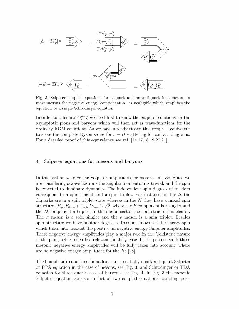
Fig. 3. Salpeter coupled equations for a quark and an antiquark in a meson. Inmost mesons the negative energy component φ− is negligible which simplifies theequation to a single Schrodinger equation

In order to calculate ORGM

π−B we need first to know the Salpeter solutions for theasymptotic pions and baryons which will then act as wave-functions for theordinary RGM equations. As we have already stated this recipe is equivalentto solve the complete Dyson series for π −B scattering for contact diagrams.For a detailed proof of this equivalence see ref. [14,17,18,19,20,21].

4 Salpeter equations for mesons and baryons

In this section we give the Salpeter amplitudes for mesons and Bs. Since weare considering s-wave hadrons the angular momentum is trivial, and the spinis expected to dominate dynamics. The independent spin degrees of freedomcorrespond to a spin singlet and a spin triplet. For instance, in the ∆ thediquarks are in a spin triplet state whereas in the N they have a mixed spinstructure (FspinFflavor +DspinDflavor)/

√2, where the F component is a singlet and

the D component a triplet. In the meson sector the spin structure is clearer.The π meson is a spin singlet and the ρ meson is a spin triplet. Besidesspin structure we have another degree of freedom known as the energy-spinwhich takes into account the positive ad negative energy Salpeter amplitudes.These negative energy amplitudes play a major role in the Goldstone natureof the pion, being much less relevant for the ρ case. In the present work thesemesonic negative energy amplitudes will be fully taken into account. Thereare no negative energy amplitudes for the Bs [28].

The bound state equations for hadrons are essentially quark-antiquark Salpeteror RPA equation in the case of mesons, see Fig. 3, and Schrodinger or TDAequation for three quarks case of baryons, see Fig. 4. In Fig. 3 the mesonicSalpeter equation consists in fact of two coupled equations, coupling posi-

7

[E − Tp

−Tk−p − Tk]✟✠✻k

✟✠✻p ψ❭❭❭

✜✜✜

=Γqq(k−p,k−p′)V (p−p′)

Γqq(p, p′)

q

q

ψ❭❭❭

✜✜✜

+

q

q ✟✠✻k′

✟✠✻k

✟✠✻p ψ❭❭❭

✜✜✜

+

q

q

ψ❭❭❭

✜✜✜

Fig. 4. Schrodinger equation for 3 quarks in a baryon

tive to negative energy amplitudes. As an example, we can use the verticesdefinitions of Table 1 to write one of these equations (the topmost) as

Hφ+s1,s2

(p) = [Tp + T−p]φ+s1,s2

(p)+

+∑

s3,s4

∫ d3p′

(2π)3Γqq

s1,s3(p,p′)V (p − p′)Γqq

s2,s4(p′,p)φ+

s3,s4(p′)+

+∑

s3,s4

∫

d3p′

(2π)3Γqq

s1,s3(p,p′)V (p − p′)Γqq

s2,s4(p′,p)φ−

s3,s4(p′)

= Eφ+s1,s2

(p) .

(10)

In particular Eq. (10) reduces to the Schrodinger equation for mesons whenthe coupling to the negative energy φ− wave-function is negligible.

The next step consists in working out the spin×flavour×colour traces. Thesetraces are worked out in appendix A. Doing this will lead us, in the case ofmesons, to the following two coupled channel equations,

Hm(p)

|φ+m〉

|φ−m〉

=∫

d3q

(2π)3H(p, q)

|φ+m〉

|φ−m〉

= Mmσ3

|φ+m〉

|φ−m〉

, (11)

with

H(p, q) =

2Tp δ(p − q) + V ++m (p, q) V +−

m (p, q)

V −+m (p, q) 2Tp δ(p − q) + V −−

m (p, q)

, (12)

where V ++m , V +−

m , V −+m and V −−

m contain the aforementioned spin traces.

8

4.1 The pion case

First we work out the spin traces for the pion case. We have,

V ++π (p,p′) =

4

3Tr{Σπ · Γqq

p,p′ · Σπ† · Γqqp′,p}V (p − p′)

= −2

3Tr{Γqq

p,p′Γqqp′,p}V (p − p′) ,

V +−π (p,p′) =

4

3Tr{Σπ · Γqq

p,p′ · Σπ · Γqqp′,p}V (p − p′)

= −2

3Tr{Γqq

p,p′Γqqp′,p}V (p − p′) .

(13)

where Σπ stands for the pion spin wave function defined in Appendix A alongwith spin wave functions for other relevant hadrons. Notice that V +−

π acts asa potential coupling the negative energy wave-function φ− with the positiveenergy wave-function φ+. V ++

π stands as the usual potential binding the quarkand the antiquark in the positive energy wave-function φ+. The color factor4/3 is included in the V ’s definition for simplicity. The relations

Γqq = (iσ2)Γqq(iσ2) , Γqq = −(iσ2)Γ

qq(iσ2) , (14)

were used. They hold for both the Dirac vertices γ0 and ~γ.

The pion occupies a singular position, insofar it is the only bound state whereφ−

π is not negligible. In particular |φ−π | is just slightly smaller than |φ+

π | becausethe π is nearly a Goldstone boson. The Salpeter pion wave functions are

φ±(k) =S(k)

a± a ξ(k) with a =

√

2Mπ

3fπ , (15)

where fπ is the well known pion decay constant, S(k) determines the extentof dynamical chiral symmetry breaking and ξ(k) is related to normalizationof the wave function. The Salpeter wave functions are normalized as follows,

[

〈φ+| 〈φ−|]

σ3

|φ+〉|φ−〉

=∫ d3k

(2π)3(φ+(k)2 − φ−(k)2) =

= 4∫

d3k

(2π)3S(k)ξ(k) =

2

a

∫

d3k

(2π)3S(k)(φ+(k) − φ+(k)) = 1 .

(16)

9

4.2 The rho case

For the ρ we can follow exactly the same steps as in the pion case to get

V ++ρ (p,p′) = −2

9Tr{σkΓqq

p,p′σkΓqq

p′,p}δss′V (p − p′) . (17)

To obtain Eq. (17) the following identity

∫ d3p

(2π)3

d3p′

(2π)3Tr{σiΓqq

p,p′σjΓqq

p′,p} =∫ d3p

(2π)3

d3p′

(2π)3

1

3Tr{σkΓqq

p,p′σkΓqq

p′,p}δij ,

(18)must be used.

The potential V +−ρ (p,p′) can also be computed and it turns out that it is

exactly equal to −1/3 of V +−π (p,p′). It provides a negligible coupling of φ−

ρ

to φ+ρ and this is the technical reason why the ρ is essentially a Schrodinger

bound state.

4.3 The baryon case

In the case of the baryons we have no negative energy amplitude (there is noway with a two body kernel of simultaneously reversing three quark lines) andwe need only to consider the V ++

B . Following the same steps used in derivingEqs. (13) and (17) we get,

V ++

NF (p,p′) = 32

3Tr{ΣNF

s · Γqqp−k,p′−k · ΣNF

s′† · Γqq

p,p′} V (p − p′)

= −21

2Tr{Γqq

p′−k,p−kΓqqp,p′} δss′V (p − p′)

= −Tr{Γqqp′−k,p−kΓ

qqp,p′} δss′V (p − p′),

(19)

V ++

ND (p,p′) = 32

3Tr{ΣND

s · Γqqp−k,p′−k · ΣND

s′† · Γqq

p,p′} V (p − p′)

= −21

6Tr{σiΓqq

p′−k,p−kσjΓqq

p,p′} σiscσ

jcs′V (p − p′)

= −1

3Tr{σkΓqq

p′−k,p−kσkΓqq

p,p′} δss′V (p − p′),

(20)

10

V ++∆ (p,p′) = 3

2

3Tr{Σ∆

s · Γqqp−k,p′−k · Σ∆

s′† · Γqq

p,p′} V (p − p′)

= −31

3Tr{σiΓqq

p′−k,p−kσjΓqq

p,p′} wisc

†wj

cs′V (p − p′)

= −1

3Tr{σkΓqq

p′−k,p−kσkΓqq

p,p′}δss′V (p − p′).

(21)

Along with the color factors we include the factor three that accounts for thenumber of diagrams. We checked numerically, for various microscopic kernels(like for example the r2 harmonic kernel) that, under integration in k, V ++

NF ,V ++

ND and V ++∆ are, to a good approximation, given by,

V ++

NF (p,p′) ≃ 3

2V ++

π (p,p′)δss′,

V ++

ND (p,p′) ≃ 3

2V ++

ρ (p,p′)δss′,

V ++∆ (p,p′) ≃ 3

2V ++

ρ (p,p′)δss′,

(22)

For the various quark kernels, the errors for the N and ∆ masses when usingEqs. (22) instead of Eqs. (19), (20) and (21), were always below 7%.

Having the spin×flavor nucleon structure in mind – see Appendix A – we get,

V ++N =

3

4(V ++

π + V ++ρ )δss′ ,

V ++∆ =

3

2V ++

ρ δss′ . (23)

In this case the baryon Salpeter amplitude will depend only on the diquarkinner momentum and the baryon Salpeter amplitude is given by,

Ψ(p) ≃ S(p)/N (24)

where N is the baryon wave function normalization which is essentially thesame for both N and ∆.

11

4.4 Summary

The results of the previous subsections can be summarized as follows,

Hπ

|φ+π 〉

|φ−π 〉

=∫

d3q

(2π)3Hπ(p, q)

|φ+π 〉

|φ−π 〉

= Mπσ3

|φ+π 〉

|φ−π 〉

;

Hρ|φρ〉 =∫

d3q

(2π)3Hρ(p, q)|φρ〉 = Mρ|φρ〉;

Hρ(p, q) =[

2Tp δ(p − q) + V ++ρ (p, q)

]

;

HN |ΨN〉 =∫

d3q

(2π)3HN(p, q)|ΨN〉 = MN |ΨN〉;

HN(p, q) =3

2

[

2Tp δ(p − q) +V ++

π (p, q) + V ++ρ (p, q)

2

]

;

H∆|Ψ∆〉 =∫

d3q

(2π)3H∆(p, q)|Ψ∆〉 = M∆|Ψ∆〉;

H∆(p, q) =3

2

[

2Tp δ(p − q) + V ++ρ (p, q)

]

.

(25)

Eq. (25) predicts that M∆ = (3/2)Mρ. This is a natural relation in the quarkmodel and it is experimentally correct within 7% discrepancy. This suggeststhat neglecting both the negative energy wave-function φ−

ρ and the diquarkrecoil in the baryons are not unreasonable approximations for low energy scat-tering (scattering lengths).

5 Assembling the π − B RGM overlaps ORGM

π−B

Before computing the flavor contribution to the RGM overlaps of Fig. 2, wehave to extend the class of diagrams in Fig. 2 including the diagrams thatcouple to the negative energy wave function φ−

π of the external pions. Thenegative energy wave function is defined in Fig. 3 and in Eqs. (10) and (15).

For simplicity the negative energy wave function φ−π was not included in the

set of diagrams of Fig. 2. As we said, only φ+π were included. There an incoming

meson is a Dirac bra that couples to the right side of the RGM diagrams andan outgoing meson is a Dirac ket that couples to the left side of the RGMdiagrams. To obtain the full set of the RGM overlaps, containing both φ+

π andφ−

π it is sufficient to notice that negative energy wave functions φ−π must couple

as Dirac bras to the right side of the diagram when they are outgoing and asDirac kets to the left side when they are incoming and that they can onlycome in pairs either of two φ+

π s or two φ−π s. The only possible topologies are

12

φ+out ✚✚

❩❩

ψout ✜✜✜

❭❭❭

φ+ in❩❩

✚✚

ψ in❭❭❭

✜✜✜

���������������������

�

+

φ−in ✚✚

❩❩

ψout ✜✜✜

❭❭❭

φ− out❩❩

✚✚

ψ in❭❭❭

✜✜✜

���������������������

�

Fig. 5. Including the negative energy wave functions φ−π in the RGM overlaps.

depicted in Fig. 5. Including φ−π s amounts to double the number of diagrams

of Fig.2. This has been studied in detail in Refs. [2,14,18].

In general 〈ORGM

π−B〉 = 〈ORGM

π−B〉colour〈ORGM

π−B〉spin×flavour×momentum. Therefore weneed to disentangle the various contributions for ORGM

π−B in the spin×flavour×mo-mentum space. To achieve this it is enough to notice two things: 1 - In thecase of the nucleon, B = N , the spin gets mixed with flavour due to thefact that the spin×flavour nucleon wave function is given by (FspinFflavour +DspinDflavour)/

√2. There is no such mixing in the case of the ∆. Therefore in

order to disentangle the spin×flavour is enough to work separately for the Fand D spin components. 2 - The flavour gets mixed with momentum due tothe presence of negative energy amplitudes. This is a curious effect deservingsome explanation. ¿From the discussion in the introduction of this section wecan have either two φ+s or two φ−s. When going from φ+ to φ− what was aket state becomes a bra state and vice versa. That is, the position of the twoφs in the trace get interchanged when we go from φ+ to φ−. In general this isenough to make the flavour traces to distinguish between the two cases. Thesame effect would have occurred in the spin case would it not be for the factthe pion has no total spin. Again, in order to disentangle flavour×momentumit is enough to give the flavour results discriminated in φ+φ+ and φ−φ−.

Having the above considerations in mind we now proceed to the separateevaluation of colour, spin, flavour and momentum contributions to ORGM

π−B.

5.1 Spin and colour contributions to ORGM

π−B

The spin and colour contributions to RGM are independent of the energy-spin degree of freedom and therefore can be evaluated for the diagrams ofFig. 2. The colour contributions to ORGM

π−B are given in Table 2. As for thespin, we give in Table 3 the results for ORGM

π−B discriminated by F and D spincomponents for the nucleon case. Notice that this overlaps are given in termsof the Salpeter V ++

π , V +−π , V ++

ρ , VNF, VND

and V∆ discussed in Section 4. Forinstance, the annihilation overlap 〈A15〉 is proportional to the V +−

π that couples

13

Table 2Color contributions.

〈E〉 , 〈Ti〉 〈V14〉 〈V25〉 〈V23〉 〈A15〉13

49

−29

−29

49

Table 3Spin contributions

Nπ ∆π

F D

〈E〉 , 〈Ti〉 12δss′

12δss′

12δss′

〈V14〉 −38V ++

π (p,q)δss′ −38V ++

π (p,q)δss′ −38V ++

π (p,q)δss′

〈V25〉 −1

4VNF (p,q) −1

4VND(p,q) −1

4V∆(p,q)

〈V23〉 14VNF

(p,q) 14VND

(p,q) 14V∆(p,q)

〈A15〉 −3

8V +−

π (p,q)δss′ −3

8V +−

π (p,q)δss′ −3

8V +−

π (p,q)δss′

the positive energy component of the π to its negative energy component. Thequark exchange overlaps 〈V14〉, 〈V25〉 and 〈V23〉, include a linear combinationof the spin singlet V ++

π and of the spin triplet V ++ρ .

5.2 Flavour contributions

Table 4Flavor contributions. τN , τπ are, respectively, the isospin generators acting in I=1/2 and 1 isospin wave functions. The I represents the identity operator in flavorspace

F D

φ+φ+ φ−φ− φ+φ+ φ−φ−

〈E〉 , 〈Ti〉 12I 1

2I 1

2I + 2

3τN · τπ

12I − 2

3τN · τπ

〈V14〉 12I 1

2I 1

2I + 2

3τN · τπ

12I − 2

3τN · τπ

〈V25〉 1

2I 1

2I 1

2I + 2

3τN · τπ

1

2I − 2

3τN · τπ

〈V23〉 12I + τN · τπ

12I − τN · τπ

12I − 1

3τN · τπ

12I + 1

3τN · τπ

〈A15〉 1

2I 1

2I 1

2I − 2

3τN · τπ

1

2I + 2

3τN · τπ

In the case of the flavour diagrams with different energy-spin asymptotic statesfor the mesons contribute differently. As we have said the existence of negative

14

Table 5Flavor contributions. τπ and τ∆ are, respectively, the isospin generators acting inI= 1 and 3/2 isospin wave functions. The I represents the identity operator in flavorspace

∆π

φ+φ+ φ−φ−

〈E〉 , 〈Ti〉 12I + 1

3τ∆ · τπ

12I − 1

3τ∆ · τπ

〈V14〉 12I + 1

3τ∆ · τπ

12I − 1

3τ∆ · τπ

〈V25〉 1

2I + 1

3τ∆ · τπ

1

2I − 1

3τ∆ · τπ

〈V23〉 12I + 1

3τ∆ · τπ

12I − 1

3τ∆ · τπ

〈A15〉 1

2I − 1

3τ∆ · τπ

1

2I + 1

3τ∆ · τπ

Table 6Nucleon Total Contribution. The upper (lower) sum/subtraction signs are associ-ated with φ+ ⊗ φ+ (φ− ⊗ φ−). E± = EB ± Eπ, with EB and Eπ being the energyof the incoming baryon and pion

〈E〉 , 〈Ti〉 14(I ± 2

3τN · τπ)(2T1 + 2T2 + T5 − E±)

〈V14〉 −14(I ± 2

3τN · τπ)V ++

π (p,q)

〈V25〉 −18I V ++

π (p,q) − 18(I ± 4

3τN · τπ)V ++

ρ (p,q)

〈V23〉 116

(I ± 2τN · τπ)V ++π (p,q) + 1

16(I ∓ 2

3τN · τπ)V ++

ρ (p,q)

〈A15〉 1

4(I ∓ 2

3τN · τπ)V +−

π (p,q)

energy-spin φ− amounts to the doubling of diagrams of Fig. 2 each of themgiving rise to two diagrams, one with φ+φ+ mesonic asymptotic states andanother with φ−φ− mesonic asymptotic states. No diagrams with φ+φ− areallowed.

We give the isospin traces in Tables 4 and 5 for Nπ and ∆π in terms of theφ± content of the diagrams 〈E〉, 〈Ti〉, 〈V14〉, 〈V23〉 and 〈A15〉. As in the spincase we must distinguish between the F and D flavour components becausethe nucleon wave function mixes this components with the correspondent Fand D spin. So the net result of considering negative energy amplitudes forthe mesons is to double the entries in Table 4 for each of the flavours F andD. In this respect the ∆π case is simpler and we can give final flavour resultsfor φ+φ+ and φ−φ−.

Next we can assemble the results of Tables 2, 3, 4 and 5 to obtain the finalπ−B results for colour×spin×flavour×momentum presented in Tables 6 and7.

15

Table 7Delta Total Contribution. The upper (lower) sum/subtraction signs are associatedwith φ+ ⊗ φ+ (φ− ⊗ φ−).

〈E〉 , 〈Ti〉 14(I ± 2

3τ∆ · τπ)(2T1 + 2T2 + T5 − E±)

〈V14〉 −14(I ± 2

3τ∆ · τπ)V ++

π (p,q)

〈V25〉 −14(I ± 2

3τ∆ · τπ)V ++

ρ (p,q)

〈V23〉 18(I ± 2

3τ∆ · τπ)V ++

ρ (p,q)

〈A15〉 14(I ∓ 2

3τ∆ · τπ)V +−

π (p,q)

Finally integrating in the internal momenta p, q and k we get for ORGM

π−N

ORGM

π−N =∫ d3p

(2π)3

d3q

(2π)3

d3k

(2π)3

{

Ψ(p, k)φ+(p)1

4A1(2T1 + 2T2 + T5 −E+)Ψ(p, k)φ+(p) δ3(p − q)+

+ Ψ(p, k)Ψ(p, k)1

4

(

A1V++π + A−1V

+−π

)

φ+(q)φ+(q)+

+ Ψ(p, k)φ+(p)1

8

(

I V ++π + A2V

++ρ

)

Ψ(q, k)φ+(q)+

+ Ψ(p, k)φ+(k)1

16

(

A3V++π + A−1V

++ρ

)

Ψ(q, k)φ+(k)+

+ Ψ(p, k)φ−(p)1

4A−1(2T1 + 2T2 + T5 −E−)Ψ(p, k)φ−(p) δ3(p − q)+

+ Ψ(p, k)Ψ(p, k)1

4

(

A−1V++π + A1V

+−π

)

φ−(q)φ−(q)+

+ Ψ(p, k)φ−(p)1

8

(

I V ++π + A−2V

++ρ

)

Ψ(q, k)φ−(q)+

+Ψ(p, k)φ−(k)1

16

(

A−3V++π + A1V

++ρ

)

Ψ(q, k)φ−(k)}

,

(26)

with An = I + 2

3nτN · τπ.

16

Similarly for the π∆ − π∆ overlaps we get

ORGM

π−∆ =∫

d3p

(2π)3

d3q

(2π)3

d3k

(2π)3

{

Ψ∆(p, k)φ+(p)1

4A1(2T1 + 2T2 + T5 − E+)Ψ∆(p, k)φ+(p) δ3(p − q)+

+ Ψ∆(p, k)Ψ∆(p, k)(

1

4A1V

++π +

1

4A−1V

+−π

)

φ+(q)φ+(q)+

+ Ψ∆(p, k)φ+(p)(

1

4A1V

++ρ

)

Ψ∆(q, k)φ+(q)+

+ Ψ∆(p, k)φ+(k)(

1

8A1V

++ρ

)

Ψ∆(q, k)φ+(k)+

+ Ψ∆(p, k)φ−(p)1

4A−1(2T1 + 2T2 + T5 −E−)Ψ∆(p, k)φ−(p) δ3(p − q)+

+ Ψ∆(p, k)Ψ∆(p, k)(

1

4A−1V

++π +

1

4A1V

+−π

)

φ−(q)φ−(q)+

+ Ψ∆(p, k)φ−(p)(

1

4A−1V

++ρ

)

Ψ∆(q, k)φ−(q)+

+Ψ∆(p, k)φ−(k)(

1

8A−1V

++ρ

)

Ψ∆(q, k)φ−(k)}

.

(27)

It is a matter of a simple calculation, to rewrite Eqs. (26) and (27) in orderto bring forward the explicit dependence on the matrix elements Hπ, HN andH∆.

As an example let us consider the π − N case. We use the following generalidentity

∫ d3p

(2π)3

∫ d3p′

(2π)3χ(p)(2T + V ++

π (p,p′) + V +−π (p,p′))ζ(p′) =

=1

2

∫

d3p

(2π)3

∫

d3p′

(2π)3

[

χ(p), χ(p)

]

Hπ

ζ(p′)

ζ(p′)

,(28)

17

with χ and ξ being arbitrary functions, together with the definition of HN

and H∆ (see Eqs. (25)), to cast Eq. (26) as

ORGM

π−N =∑

α=±

∫

d3p

(2π)3

d3q

(2π)3

d3k

(2π)3

{

−Ψ(p, k)φα(p)Eα

4

(

I + α2

3τN · τπ

)

Ψ(p, k)φα(p) δ3(p − q)+

+1

8

[

Ψ(p, k)Ψ(p, k), Ψ(p, k)Ψ(p, k)

]

Hπ

(

I − α2

3τN · τπ

)

φα(q)φα(q)

φα(q)φα(q)

+

+ Ψ(p, k)Ψ(p, k)1

3(2HN −H∆)α

2

3τN · τπ φα(q)φα(q)+

+ Ψ(p, k)φα(p)1

6

(

HNI + H∆α2

3τN · τπ

)

Ψ(q, k)φα(q)+

+Ψ(p, k)φα(k)1

12

(

HNI + (3HN − 2H∆)α2

3τN · τπ

)

Ψ(q, k)φα(k)}

.

(29)

Finally we use the spectral decomposition of Hπ, HN and H∆,

Hπ =∑

π∗

σ3

|φ+π∗〉

|φ−π∗〉

Mπ∗

[

〈φ+π∗| 〈φ−

π∗|]

σ3+

+ σ3

|φ−π∗〉

|φ+π∗〉

Mπ∗

[

〈φ−π∗| 〈φ+

π∗|]

σ3 ,

HN =∑

N∗

|ψN∗〉MN∗〈ψN∗ | ,

H∆ =∑

∆∗

|ψ∆∗〉M∆∗〈ψ∆∗| ,

(30)

which are a direct consequence of Eq. (25), to obtain for ORGM

π−B

ORGM

π−N =∑

α=±

{

−Iα0

Eα

4

(

I + α2

3τN · τπ

)

+1

8I4Mπ

(

I − α2

3τN · τπ

)

Iα5 +

+1

3I1 (2MN −M∆)α

2

3τN · τπIα

2 +1

6Iα3

(

MNI +M∆α2

3τN · τπ

)

Iα3 +

+1

12I6

(

MNI + (3MN − 2M∆)α2

3τN · τπ

)

I6

}

,

(31)

18

N

��

N

+

N

��

N

�

+

N

��

N

N

�

Fig. 6. Classes of diagrams in π − B scattering

Zq = ��

��

❅��r r

φ+❩❩

✚✚

Γqq ΓqqV+

φ−✚✚

❩❩

�❅❅

❅❅

❅❅

r rΓqq ΓqqV

Fig. 7. Zq annihilation of a meson in a quark line

with

I±0 =∫ d3p

(2π)3ΨB(p)ΨB(p)φ±(p)φ±(p),

I1 =∫

d3p

(2π)3ΨB(p)ΨB(p)ΨB′(p), I±2 =

∫

d3p

(2π)3φ±(p)φ±(p)ΨB′(p),

I±3 =∫ d3p

(2π)3ΨB(p)φ±(p)ΨB′ , I4 =

∫ d3p

(2π)3ΨB(p)ΨB(p)(φ+(p) − φ−(p)),

I±5 =∫ d3p

(2π)3φ±(p)φ±(p)(φ+(p) − φ−(p)), I6 =

√

3

f 2πmπ

∫ d3p

(2π)3ΨB(p)ΨB′(p).

(32)

We can deal with π − ∆ along similar lines. Here we only quote the result:

ORGM

π−∆ =∑

α=±

{

−Iα0

Eα

4

(

I + α2

3τ∆ · τπ

)

+1

8I4Mπ

(

I − α2

3τ∆ · τπ

)

Iα5 +

+1

3I1 (2MN −M∆)α

2

3τ∆ · τπIα

2 +1

6Iα3 M∆

(

I + α2

3τ∆ · τπ

)

Iα3 +

+1

12I6M∆

(

I + α2

3τ∆ · τπ

)

I6

}

.

(33)

We have succeeded in writing ORGM

π−B in terms of hadron masses and geometricoverlaps only. Any explicit dependence on the microscopic quark kernel K asdisappeared. The above formulas (31) and (33) are kernel independent. In thenext section we are going to evaluate the geometrical overlaps I’s of Eq. (32)in the point-like limit approximation.

19

6 The point like limit

In this paper we follow closely the work done in the π − π case [2]. There itwas shown, for any microscopic model complying with chiral symmetry, thatin order to calculate π − π scattering lengths it is sufficient to consider thepoint-like limit,

S(k) −→ 1 . (34)

In this limit only contact diagrams contribute to π−π T matrix. This is clearlyseen if we compute [14,17,18] the coupling of a meson to a single quark linewith the Zq annihilation diagrams depicted in Fig. 7. In this limit, the verticespresent in Fig. 7, which represent the integral

Zqs1,s2

(p) =∑

s3,s4

∫ d3p′

(2π)3Γqq

s1,s3(p, p′)V (p− p′)Γqq

s2,s4(p′, p)φ+

s3,s4(p′)+

+∑

s3,s4

∫

d3p′

(2π)3Γqq

s1,s3(p, p′)V (p− p′)Γqq

s2,s4(p′, p)φ−

s3,s4(p′) ,

(35)

vanish. Assumption (34) implies the vanishing of the products of vertices,

ΓqqΓqq → 0 , ΓqqΓqq → 0 ,

ΓqqΓqq → 0 , ΓqqΓqq → 0 .(36)

In the class of models embodied by Eq. (1) Zq (and Z q) are the microscopicsources of intermediate hadronic exchange so that, in this limit, diagramswhich do not belong to the class of contact diagrams vanish. When leavingthis limit both classes of diagrams contribute to Tπ−π matrix, but then chiralsymmetry forces cancellations among diagrams belonging to each of these twodifferent classes, so that the Tπ−π transition matrix remains formally invari-ant. This cancellation is clearly seen in the sigma model calculation of π − πscattering [29] where the X shaped diagram of the contact four π coupling andthe H shaped diagram of the sigma meson exchange miraculously cancel andthis provides the small physical result. This result is encoded by the existenceof the Adler zeroes [30] which are present whenever a low energy pion couplesto hadrons. In references [2,3] we have shown this cancellation for microscopicmodels defined for the class of Hamiltonians of Eq. (1). As a byproduct itwas also shown that the transition matrix Tπ−π is formally independent of thequark microscopic kernel K. In fact Tπ−π was shown to depend explicitly onlyon physical masses mπ and wave-function normalizations fπ. So that any de-pendence on the quark kernel K is buried into the masses and normalizationconstants dependence on K. Therefore we were allowed, in order to find theTπ−π formula in terms of mπ and fπ to choose a kernel consistent to S(k) → 1.In this paper we follow the prescription of S(k) → 1 and therefore we will onlyconsider contact diagrams.

20

The integrals I of Eq. (32) are particularly simple to do in the point like limit.In Eqs. (31) and (33), the only relevant combinations of I’s we need to beconcerned with, have, up to the first order in ξ = (φ+ − φ−)/2a, the followingpoint like limits

I+0 + I−0 =

∫ d3p

(2π)3ΨBΨBφ

+φ+ +∫ d3p

(2π)3ΨBΨBφ

−φ−

=3

f 2πMπ

∫

d3p

(2π)3ΨBΨBS

2 +4

3f 2

πMπ

∫

d3p

(2π)3ΨBΨBξ

2

S→1−→ 3

f 2πMπ

∫ d3p

(2π)3ΨBΨB =

3

f 2πMπ

I+0 − I−0 =

∫

d3p

(2π)3ΨBΨBφ

+φ+ −∫

d3p

(2π)3ΨBΨBφ

−φ−

= 4∫ d3p

(2π)3ΨBΨBS

1

2a(φ+ − φ−)

S→1−→ 1

N 24

∫

d3p

(2π)3S

1

2a(φ+ − φ−) =

1

N 2

{I1I+2 + I1I

−2 , I1I

+2 − I1I

−2 }

S→1−→ { 3

f 2πMπ

,1

N 2}

{I+3 I

+3 + I−3 I

−3 , I

+3 I

+3 − I−3 I

−3 } S→1−→ { 3

f 2πMπ

,1

N 2}

{I6I6 + I6I6, I6I6 − I6I6} S→1−→ { 3

f 2πMπ

, 0}

{I4I+5 + I4I

−5 , I4I

+5 − I4I

−5 }

S→1−→ {O(Mπ),O(Mπ)}

(37)

In order to derive the limits of Eq. (37), Eqs. (15), (16) and (24) were used.The last entry of Eq. (37) presents combinations of the I’s which are of theorder Mπ. Because we are interested in scattering lengths evaluated to orderzero in Mπ these combinations will not be considered.

Using Eq. (37) we can further simplify ORGM

π−B noticing that due to energyconservation E±

πB = MB ±Mπ, the following combination

3 I−E+

πB − E−πB + 2MB

8f 2πMπ

= O(Mπ) . (38)

is of order Mπ. Therefore it will be discarded for the same reasons as before.

To zero order in Mπ, only the τB ·τπ terms survive, and the total overlap kernelORGM

π−B turns out to be quite simple,

ORGM

π−B =4MN − 2M∆

9N 2τB · τπ + O(Mπ) . (39)

21

We finally get the desired scattering lengths, see Eq. (9), in a compact notation,

aπB = −Mπ

2π

4MN − 2M∆

9N 2τB · τπ + O(M2

π) . (40)

The scattering lengths vanish in the chiral limit of a vanishing quark massMπ → 0, and this complies with the Adler zero [29,30] .

7 Numerical results and Conclusion

We have a free parameter, the N and ∆ normalization that N needs to befixed. To this effect we can use the experimental value for the aπN{I = 1/2}scattering length,

aexpπN{I = 1/2} = (0.171 ± 0.005)M−1

π , (41)

to fix N . We obtain N = 1580MeV −3/2, corresponding to a nucleon size of0.4 fm. Equipped with this value we predict the following values for

aπN{I = 3/2} = −0.086M−1π [aexp

πN{I = 3/2} = −(0.088 ± 0.004)M−1π ] ,

aπ∆{I = 1/2} = 0.429M−1π ,

aπ∆{I = 3/2} = 0.172M−1π ,

aπ∆{I = 5/2} = −0.258M−1π .

(42)

Although it is difficult o measure directly the π−∆ scattering lengths becausethe ∆ is quite unstable, the π − ∆ coupling may be determined indirectly inthe same way as the N − ∆ scattering lengths are determined in Ref. [31].We stress that the QM provides the correct framework to derive the π − ∆scattering lengths. For instance it would be hard to derive the π−∆ scatteringlengths in the framework of effective hadronic models.

In particular we predict that the different scattering lengths of the π in s-wavebaryons are exactly proportional with remarkable integer factors,

aπN,I= 12

: aπN,I= 32

: aπ∆,I= 12

: aπ∆,I= 32

: aπ∆,I= 52

= 2 : −1 : 5 : 2 : −3 . (43)

The work of G. M. Marques is supported by Fundacao para a Ciencia e aTecnologia under the grant SFRH/BD/984/2000.

22

A Traces

In this appendix the computation of the color, spin and flavor traces aredetailed. There are different equivalent methods to compute these standardtraces.

A.1 color

The color traces are the most straightforward to calculate. The baryon colorwave-function is a simple ǫabc/

√6 and the meson a δab/

√3. The interaction

has the well known structure λab/2. For instance the pion Bethe-Salpeter colorfactor 4/3 of Eq. (13) is calculated in the following way

δij√3

λaik

2

δkl√3

λbjl

2=

1

12Tr{λ · λ} =

4

3. (A.1)

For the baryons the color factor -2/3 of Eqs. (19), (20) and (21) comes from

ǫijk√6

λail

2

ǫlmk√6

λbjm

2=

1

24(Tr{λ} · Tr{λ} − Tr{λ · λ}) = −2

3(A.2)

In Table 2 we present the results for the diagrams of Fig. 2.

A.2 spin

For the spin our method relies on the Pauli matrices σi.

The spin structures of π, N and ∆ wave functions, together with the spinvector structure ρ, later needed in the calculations, can be written as

Σπ =(

iσ2/√

2)

ab; Σρ

s=

[

σiσ2/√

2]

ab· vs; Σ∆

s=

[

σiσ2/√

2]

ab· wcs;

ΣNF

s=

(

iσ2/√

2)

abδcs; ΣND

s= (1/

√3)

[

σiσ2/√

2]

ab· σcs

(A.3)

where a, b and c stand for the quarks individual spin, whereas s stands for thetotal spin of the meson or baryon under consideration. For example, we have

[

↑ ↓]

Σπ

↑↓

=1√2(↑↓ − ↓↑). (A.4)

23

The vectors vs and wcs, are given by,

v1 =(

−1/√

2,−i/√

2, 0)

, v0 = (0, 0,−1) , v−1 =(

1/√

2,−i/√

2, 0)

,

wc 32

= v1 δc 12, wc 1

2= 1/

√3 v1 σ

−

c 12

+√

2/3 v0 δc 12, (A.5)

wc− 12

= 1/√

3 v−1 σ+

c− 12

+√

2/3 v0 δc− 12, wc− 3

2= v−1 δc− 1

2.

They have the following properties,

vis†vj

s′ = δijδss′ − (J jJ i)ss′,

wisc

†wj

cs′ =3

4δijδss′ −

1

3(J iJ j)ss′ +

i

2ǫijkJk

ss′.(A.6)

where the J ’s are the spin 1 SU(2) generating matrices in the case of the v’srelation and the spin 3/2 SU(2) generating matrices in the case of the w’srelation. When we contract i with j we have simply

vis†vi

s′ = wisc

†wi

cs′ = δss′. (A.7)

The importance of the above spin functions lies in the fact that they mapthe quark spin content of a given bound state to the total spin of that boundstate. Once this map is achieved it is a matter of straightforward calculationsto obtain the diagrammatic traces. The results are presented in table A.1.For instance for the spin traces which contribute to the RGM 〈E〉 and 〈V24〉overlap diagrams the computation is

〈E〉spin = Tr{ΣBs · ΣB

s′† · Σπ · Σπ†} =

= −1

2δss′ ,

(A.8)

〈V24〉spin = Tr{ΣBs · ΣB

s′† · Γqq · Σπ · Σπ† · Γqq}V (p − p′) =

=1

2Tr{ΣB

s · ΣBs′† · Γqq · Γqq}V (p − p′) =

= −3

8V ++

π (p,p′)δss′ .

(A.9)

where the super-index B stands for the corresponding baryon which may bethe F component of the nucleon, the D component of the nucleon or the Delta.

A.3 flavor

In the isospin case we use τi as the Pauli matrices.

24

Table A.1Spin contributions

〈E〉 , 〈Ti〉 Tr{ΣBs · ΣB

s′† · Σπ · Σπ†}

〈V14〉 Tr{ΣBs · ΣB

s′† · Γqq · Σπ · Σπ† · Γqq}V (p − q)

〈V25〉 Tr{ΣBs · Γqq · ΣB

s′† · Σπ · Γqq · Σπ†}V (p − q)

〈V23〉 12Tr{ΣB

s · Γqq · ΣBs′† · Γqq}V (p − q)

〈A15〉 Tr{ΣBs · ΣB

s′† · Γqq · Σπ† · Σπ · Γqq}V (p − q)

For π −N we have the cases of isospin 3/2 and 1/2.

(I = 3/2) : pπ+,1√3(nπ+ +

√2pπ0) ,

1√3(√

2nπ0 + pπ−), nπ−

(I = 1/2) :1√3(√

2nπ+ − pπ0),1√3(nπ0 −

√2pπ−) (A.10)

The isospin contribution of any diagram must be a linear combination of theidentity and τN · τπ, where

τN · τπ =1

2((τπ + τN)2 − τ 2

π − τ 2N ) =

1

2(I(I + 1) − 2 − 3

4). (A.11)

The computation of these contributions was done for each diagram and eachmultiplet element. The results are presented in Table A.2.

In the same way for ∆ − π we have isospin 5/2, 3/2 and 1/2.

(I = 5/2) :

∆++π+,1√5(√

2∆++π0 +√

3∆+π+),1√10

(∆++π− +√

6∆+π0 +√

3∆0π+)

1√10

(√

3∆+π− +√

6∆0π0 + ∆−π+),1√5(√

3∆0π− +√

2∆−π0), ∆−π−

(I = 3/2) :1√5(√

3∆++π0 −√

2∆+π+),1√15

(√

2∆++π− + ∆+π0 −√

8∆0π+),

1√15

(√

8∆+π− − ∆0π0 −√

2∆−π+),1√5(√

2∆0π− −√

3∆−π0)

(I = 1/2) :1√6(√

3∆++π− −√

2∆+π0 + ∆0π+),1√6(∆+π− −

√2∆0π0 +

√3∆−π+)

(A.12)

In this case the isospin contributions must be a linear combination of the

25

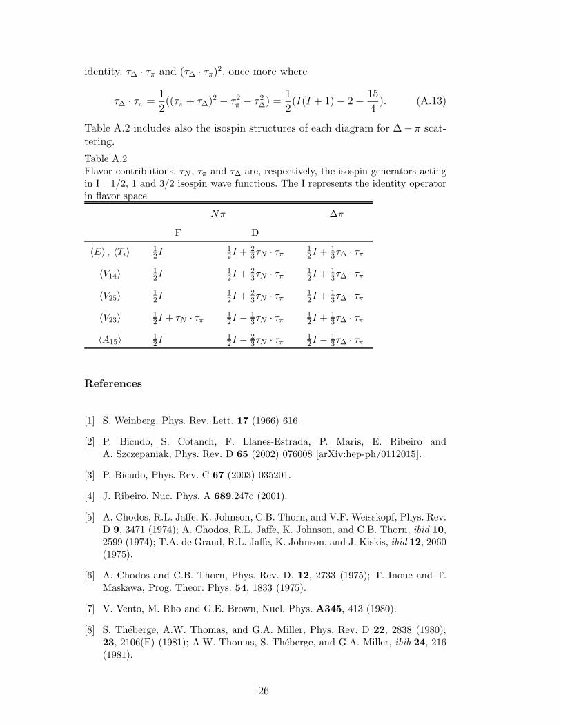
identity, τ∆ · τπ and (τ∆ · τπ)2, once more where

τ∆ · τπ =1

2((τπ + τ∆)2 − τ 2

π − τ 2∆) =

1

2(I(I + 1) − 2 − 15

4). (A.13)

Table A.2 includes also the isospin structures of each diagram for ∆− π scat-tering.

Table A.2Flavor contributions. τN , τπ and τ∆ are, respectively, the isospin generators actingin I= 1/2, 1 and 3/2 isospin wave functions. The I represents the identity operatorin flavor space

Nπ ∆π

F D

〈E〉 , 〈Ti〉 12I 1

2I + 2

3τN · τπ

12I + 1

3τ∆ · τπ

〈V14〉 12I 1

2I + 2

3τN · τπ

12I + 1

3τ∆ · τπ

〈V25〉 12I 1

2I + 2

3τN · τπ

12I + 1

3τ∆ · τπ

〈V23〉 1

2I + τN · τπ

1

2I − 1

3τN · τπ

1

2I + 1

3τ∆ · τπ

〈A15〉 12I 1

2I − 2

3τN · τπ

12I − 1

3τ∆ · τπ

References

[1] S. Weinberg, Phys. Rev. Lett. 17 (1966) 616.

[2] P. Bicudo, S. Cotanch, F. Llanes-Estrada, P. Maris, E. Ribeiro andA. Szczepaniak, Phys. Rev. D 65 (2002) 076008 [arXiv:hep-ph/0112015].

[3] P. Bicudo, Phys. Rev. C 67 (2003) 035201.

[4] J. Ribeiro, Nuc. Phys. A 689,247c (2001).

[5] A. Chodos, R.L. Jaffe, K. Johnson, C.B. Thorn, and V.F. Weisskopf, Phys. Rev.D 9, 3471 (1974); A. Chodos, R.L. Jaffe, K. Johnson, and C.B. Thorn, ibid 10,2599 (1974); T.A. de Grand, R.L. Jaffe, K. Johnson, and J. Kiskis, ibid 12, 2060(1975).

[6] A. Chodos and C.B. Thorn, Phys. Rev. D. 12, 2733 (1975); T. Inoue and T.Maskawa, Prog. Theor. Phys. 54, 1833 (1975).

[7] V. Vento, M. Rho and G.E. Brown, Nucl. Phys. A345, 413 (1980).

[8] S. Theberge, A.W. Thomas, and G.A. Miller, Phys. Rev. D 22, 2838 (1980);23, 2106(E) (1981); A.W. Thomas, S. Theberge, and G.A. Miller, ibib 24, 216(1981).

26

[9] Y. Nambu and J. Jona-Lasinio, Phys. Rev. 124, 246 (1961); Phys. Rev. 122,345 (1961).

[10] A. Le Yaouanc, L. Oliver, O. Pene, and J.-C. Raynal, Phys. Rev. D 29, 1233(1984).

[11] A. Le Yaouanc, L. Oliver, O. Pene, and J.-C. Raynal, Phys. Rev. D 31, 137(1985).

[12] S. Adler and A. Davis, Nucl. Phys. B 244, 469 (1984).

[13] P. J. Bicudo and J. E. Ribeiro, Phys. Rev. D 42 (1990) 1611.

[14] P. J. Bicudo and J. E. Ribeiro, Phys. Rev. D 42 (1990) 1625; 42 (1990) 1635.

[15] F. Llanes-Estrada and S. Cotanch, Phys. Rev. Lett. 84, 1102 (2000).

[16] H.G. Dosch Phys. Lett. B 190, 177 (1987); H.G. Dosch and Yu A. SimonovPhys. Lett. B 205, 339 (1988).

[17] P. J. Bicudo, Phys. Rev. C 60 (1999) 035209.

[18] P. Bicudo and J. Ribeiro, Phys. Rev. C 55 (1997) 834 [arXiv:nucl-th/9703027].

[19] P. Bicudo, G. Krein and J. Ribeiro, Phys. Rev. C 64, 025202 (2001).

[20] P. Bicudo, J. Ribeiro and J. Rodrigues Phys. Rev. C 52, 2144 (1995).

[21] P. Bicudo, L.Ferreira, C. Placido and J. Ribeiro, Phys. Rev. C 56, 670 (1997).

[22] J. E. Ribeiro, Z. Phys. C 5 (1980) 27.

[23] S. Lemaire, J. Labarsouque and B. Silvestre-Brac, Nucl. Phys. A714, 265,(2003).

[24] R. Ceuleneer, C. Semay and B. Silvestre-Brac, J. Phys. G 22, 1395 (1996).

[25] P. Bicudo, J. E. Ribeiro and A. Nefediev, Phys. Rev. D65 :085026 (2002).

[26] J. E. Ribeiro, Phys. Rev. D 25, 2406 (1982); E. van Beveren, Zeit. Phys. C 17,135 (1982).

[27] J. Dias de Deus and J. Ribeiro Phys. Rev. D 21, 1251 (1980).

[28] P. Bicudo, G. Krein, E. Ribeiro and J. Villate, Phys. Rev. D 45, 1673 (1992).

[29] V. De Alfaro, S. Fubini, G. Furlan, C. Rosseti, “Currents in Hadron Physics” ,Amsterdam, North-Holland, (1973).

[30] S. L. Adler, Phys. Rev. 137 (1965) B1022.

[31] H. Garcilazo, P. Sauer, T. Mizutani and M. Pena, Phys. Rev. C 42 2315 (1990).

27