Nuclear Structure based on Correlated RealisticNucleon-Nucleon Potentials

R. Roth a, T. Neff b, H. Hergert a, and H. Feldmeier b

aInstitut fur Kernphysik, Technische Universitat Darmstadt, 64289 Darmstadt, GermanybGesellschaft fur Schwerionenforschung, Planckstr. 1, 64291 Darmstadt, Germany

Abstract

We present a novel scheme for nuclear structure calculations based on realistic nucleon-nucleon potentials. The essential ingredient is the explicit treatment of the dominant inter-action-induced correlations by means of the Unitary Correlation Operator Method (UCOM).Short-range central and tensor correlations are imprinted into simple, uncorrelated many-body states through a state-independent unitary transformation. Applying the unitary trans-formation to the realistic Hamiltonian leads to a correlated, low-momentum interaction,well suited for all kinds of many-body models, e.g., Hartree-Fock or shell-model. We em-ploy the correlated interaction, supplemented by a phenomenological correction to accountfor genuine three-body forces, in the framework of variational calculations with antisym-metrised Gaussian trial states (Fermionic Molecular Dynamics). Ground state propertiesof nuclei up to mass numbers A . 60 are discussed. Binding energies, charge radii, andcharge distributions are in good agreement with experimental data. We perform angularmomentum projections of the intrinsically deformed variational states to extract rotationalspectra.

Key words: Nuclear Structure; Hartree-Fock; Effective Interactions; Short-RangeCorrelations; Unitary Correlation Operator Method; Fermionic Molecular DynamicsPACS: 21.30.Fe, 21.60.-n, 13.75.Cs

Preprint submitted to Elsevier Science 8 June 2004

1 Introduction

The advent of realistic nucleon-nucleon (NN) potentials has created a supremechallenge and opportunity for nuclear structure theory: the ab initio description ofnuclei. Several families of realistic or modern NN potentials have been developedover the past three decades — among others the Argonne, Bonn, and Nijmegenpotentials [1–4]. The latest members of these families reproduce the NN-scatteringdata and the deuteron properties with high precision. All realistic potentials exhibita quite complicated operator structure with substantial contributions from non-central terms, most notably the tensor and spin-orbit interaction. Besides these,explicit momentum dependent terms or quadratic orbital angular momentum andspin-orbit operators enter. The most recent potentials also employ charge-symmetryand charge-independence breaking terms to further improve the agreement with theexperimental phase-shifts.

Given a realistic NN-potential we are faced with the difficult task of solving thenuclear many-body problem. Ideally, one would like to treat the (non-relativistic)quantum many-body problem ab initio, i.e., without introducing further approx-imations. So far, ab initio solutions utilising realistic potentials are restricted tolight nuclei with A . 12. Extensive studies on ground state properties and excita-tion spectra in this mass range have been performed using, e.g., Green’s FunctionMonte Carlo methods [5,6] and the no-core shell model [7,8].

The results of these ab initio calculations clearly show that in addition to therealistic NN-potential a three-nucleon force is inevitable to reproduce the experi-mental data on light nuclei. The Argonne group has constructed a series of phe-nomenological three-nucleon potentials [9] to fit the binding energies and spectraof light nuclei to experiment. In this way the results for ground states and low-lying excitations are in good agreement with the experimental findings in the wholeaccessible mass range. Recent developments in chiral effective field theories [10]provide a framework for a consistent derivation of two-, three- and multi-nucleonforces from more fundamental grounds.

Our aim is to describe the structure of larger nuclei on the basis of realis-tic nucleon-nucleon interactions while staying as close as possible to an ab initiotreatment of the many-body problem. The step towards larger particle numbers re-quires a truncation of the full many-body Hilbert space to a simplified subspaceof tractable size. In the simplest approach, the many-body state is described by asingle Slater determinant, as, e.g., in the Hartree-Fock approximation. More elab-orate approximations, the multi-configuration shell-model for example, allow formany-body states which are represented as a superposition of several Slater de-terminants. When combining realistic nucleon-nucleon interactions with simplemany-body states composed of single or few Slater determinants a fundamentalproblem arises. Those states do not allow for an adequate description of the strongshort-range correlations induced by the realistic NN-potential [11,12].

Already in the deuteron, structure and origin of these correlations are appar-ent. We consider the spin-projected two-body density matrix ρ(2)

S=1,MS(r) as function

of the relative coordinate r = x1 − x2 of the two particles, resulting from an ex-

2

Fig. 1. Spin-projected two-body density ρ(2)1,MS

(r) of the deuteron calculated with the AV18potential. Shown is the iso-density surface for 0.005 fm−3.

0 0.5 1 1.5 2 2.5 3r [fm]

-100

0

100

200

300

.

V01(r

)[M

eV]

(a)

0 0.5 1 1.5 2 2.5 3r [fm]

0

0.1

0.2

0.3

.

ρ(2

)01(r

)[fm−

3]

(b)

Fig. 2. (a) Central part of the AV18 potential in the (S ,T ) = (0, 1) channel. (b) Two-bodydensity distribution ρ

(2)S=0,T=1(r) for 4He resulting from an ansatz wave function using

a Slater determinant of Gaussian single-particle states ( ) compared to a realistictwo-body density including the interaction-induced central correlations ( ).

act calculation with the Argonne V18 potential (AV18) [1,13,12]. Figure 1 depictsiso-density cuts of the two-body density for MS = 0 and MS = ±1, respectively,which corresponds to parallel and antiparallel alignment of the two nucleon spins.Two dominant structural features appear: (i) At small particle distances |r| the two-body density is fully suppressed, i.e., the probability of finding two nucleons closerthan r ∼ 0.5 fm is practically zero. (ii) The angular structure of ρ(2)

S=1,MS(r) de-

pends strongly on the spin orientation. For parallel spins the probability density isconcentrated along the quantisation axis (“dumbbell”), for antiparallel spins it isconstricted around the plane perpendicular to the spin direction (“doughnut”).

These structures are the manifestation of two types of interaction-induced cor-relations which govern the nuclear many-body problem: (i) short-range central cor-relations and (ii) tensor correlations.

The central correlations are induced by the strong repulsive core of the centralpart of the interaction. Figure 2 shows the radial dependence of the central partof the AV18 potential in a specific spin-isospin channel. Due to the short-rangerepulsion the two-body density, shown for 4He, is completely suppressed withinthe region of the repulsive core. A typical ansatz for the many-body wave function

3

2.1.56

0.5

-0.56

-1.

-0.56

0.5

1.562.

-2.-1.56

-0.5

0.56

1.

0.56

-0.5

-1.56-2.

(a)

σ2 σ1

r

(b)

σ2 σ1

r

Fig. 3. Dependence of the tensor interaction energy on the spatial orientation of the twospins for fixed antiparallel (a) and parallel spins (b), respectively. The numbers indicate thevalues of VT for each of the configurations.

using a Slater determinant of Gaussian (or any other) single-particle states is notcapable of describing this correlation hole. The dashed line in Fig. 2(b) shows thatthe Slater determinant ansatz leads to a significant probability of finding the nu-cleons within the core. Even with a superposition of a moderate number of Slaterdeterminants one is not able to describe the strong short-range central correlationscaused by realistic potentials.

The origin of the tensor correlations is the long-range tensor interaction, partic-ularly in the (S ,T ) = (1, 0) channel. As seen in Fig. 1, the tensor correlations arerevealed through the dependence of the two-body density on the spatial orientationof the two nucleons with respect to their spins. This can be understood from thestructure of the tensor operator S12 =

3r2 (σ1 · r)(σ2 · r) − (σ1 · σ2). For illustration

we consider the interaction energy VT = −[ 3r2 (σ1 · r)(σ2 · r) − (σ1 · σ2)], where the

minus sign was introduced to account for the sign of the radial dependence of thetensor interaction. Spin vectors and relative coordinate enter in the same way as forthe magnetic dipole-dipole interaction. Figure 3 gives the values of VT for differ-ent spatial orientations of two fixed antiparallel and parallel spins, respectively. Forantiparallel spins, those configuration with r perpendicular to the spin direction areenergetically favoured. Contrariwise, for parallel spins a fully aligned arrangementof spins and relative coordinate is preferred. This explains the structure of the two-body density shown in Fig. 1. It is clear that these tensor correlations between thetwo spins and the relative coordinate cannot be described adequately by a singleSlater determinant.

The aim of this paper is to devise and apply a method to include central andtensor correlations explicitly into simple model spaces. We discuss this approach,the Unitary Correlation Operator Method (UCOM), in Sec. 2. The structure of thecorrelated realistic interaction is presented in Sec. 3 with application to the AV18potential. Section 4 introduces a simple yet powerful variational model for thetreatment of the nuclear many-body problem based on the Slater determinant ofGaussian wave packets used in Fermionic Molecular Dynamics (FMD). Ground

4

state calculations up to mass numbers A . 60 are performed, and binding ener-gies, charge radii, and charge distributions are compared to experiment. Finally,Sec. 5 discusses the projection onto angular momentum eigenstates of the intrinsi-cally deformed variational states and compares the resulting rotational spectra withexperiment.

2 Unitary Correlation Operator Method (UCOM)

2.1 Concept

The basic idea of the Unitary Correlation Operator Method (UCOM) is thefollowing: Introduce the dominant short-range central and tensor correlations intoa simple many-body state by means of a state-independent unitary transformation.The unitary operator C describing this transformation applied to an uncorrelatedmany-body state |Ψ〉 leads to a correlated state |Ψ〉 1 ,

|Ψ〉 = C |Ψ〉 . (1)

In the simplest case, the uncorrelated state is a Slater determinant. The correlatedstate |Ψ〉, however, is no longer a Slater determinant. Due to the complex short-range correlations introduced by the correlation operator C, any expansion of |Ψ〉in a basis of Slater determinants will require a huge number of basis states.

The representation of short-range correlations in terms of a unitary state-inde-pendent operator is technically very advantageous. Calculating a matrix element〈Ψ|O |Ψ′〉 of an operator O with correlated states is equivalent to calculating thematrix element 〈Ψ| O |Ψ′〉 of the correlated operator

O = C†O C (2)

using uncorrelated states. For the treatment of the many-body problem it is gener-ally more convenient to correlate all operators of interest and to evaluate expecta-tion values or matrix elements with the uncorrelated states.

In accord with the two types of correlations discussed above, we decomposethe correlation operator into separate unitary operators CΩ and Cr for tensor andcentral correlations, respectively,

C = CΩCr = exp[

− i∑

i< j

gΩ,i j

]

exp[

− i∑

i< j

gr,i j

]

. (3)

Each of the correlation operators can be written as an exponential involving a Her-mitian generator. Since the correlations considered here are induced by a two-bodypotential, the generators are also assumed to be two-body operators. The detailedform of the two-body generators gr and gΩ reflects the structure of the central and

1 Throughout the paper, hats identify correlated quantities; upright symbols indicate oper-ators.

5

tensor correlations, as discussed in the Sec. 1. We will construct these generators inthe following sections.

2.2 Central Correlations

The short-range repulsion in the central part of the NN-interaction prevents thenucleons in a many-body system from approaching each other closer than the extentof the repulsive core, i.e., the two-body density matrix exhibits a correlation holeat small interparticle distances. One way to incorporate these correlations into asimple many-body state is by shifting each pair of nucleons apart from each other.The shift has to be distance-dependent since it should only affect nucleon pairswhich are closer than the core radius.

Using this picture, we can construct the following ansatz for the Hermitian gen-erator of the corresponding unitary transformation (3): radial shifts are generatedby the component of the relative momentum q = 1

2 [p1 − p2] along the distancevector r = x1 − x2 of two particles:

qr =12

[q · rr +

rr · q] . (4)

To describe the dependence of the shift on the particle distance we introduce afunction s(r) and define the following Hermitian generator for the central correla-tion operator Cr [11]:

gr =12

[s(r)qr + qr s(r)] . (5)

To illustrate the effect of the correlation operator cr = exp[−igr] in two-bodyspace 2 , we apply it to a two-body state |ψ〉 = |Φcm〉 ⊗ |φ〉. The correlation oper-ator does not act on the centre of mass component |Φcm〉 by construction. For thecorrelated relative part |φ〉 we obtain in coordinate representation [11]:

〈r|φ〉 = 〈r| cr |φ〉 =R−(r)

r

√

R′−(r) 〈R−(r) rr |φ〉 . (6)

Hence, the application of the correlation operator corresponds to a norm conservingcoordinate transformation r 7→ R−(r) r

r with respect to the relative coordinate. Thefunction R−(r) and its inverse R+(r) are connected to the shift function s(r) by theintegral equation

∫ R±(r)

r

dξs(ξ)= ±1 , R±[R∓(r)] = r . (7)

For slowly varying shift functions s(r), the correlation functions are approximatelygiven by R±(r) ≈ r ± s(r). The R±(r) are determined by an energy minimisation inthe two-body system, as discussed in Sec. 3.5.

2 c stands for the correlation operator in two-body space, whereas C indicates the generalcorrelation operator in many-body space. In general, small symbols are used for k-bodyoperators in k-body space, capital symbols for operators in many-body space.

6

Since the NN-interaction depends strongly on the spin S and isospin T of theinteracting nucleon pair, we decompose the two-body generators gr into a sum ofdifferent generators gS T

r for each of the four different (S ,T ) channels

gr =

∑

S ,T

gS Tr ΠS T , (8)

where ΠS T is a projection operator onto the spin S and isospin T subspace. Thecorrelation operator in two-body space decomposes into a sum of independent cor-relation operator for the different channels

cr = exp[

− i∑

S ,T

gS Tr ΠS T

]

=

∑

S ,T

exp[−igS Tr ] ΠS T =

∑

S ,T

cS Tr ΠS T . (9)

This form is very convenient, since it allows us to treat the (S ,T ) channels sepa-rately. For the sake of a concise formulation, we will not write out this spin-isospindependence in the following, but add it when needed.

2.3 Tensor Correlations

The strong tensor part of the NN-interaction induces subtle correlations be-tween the spin of a nucleon pair and their relative spatial orientation. In order todescribe these correlations, we need to generate a spatial shift perpendicular to theradial direction. This is done by the “orbital momentum” operator

qΩ= q − r

r qr =1

2r2 [ l × r − r × l ] , (10)

where l is the relative orbital angular momentum operator. Radial momentum rr qr

and the orbital momentum qΩ

constitute a special decomposition of the relativemomentum operator q and generate shifts orthogonal to each other. The complexdependence of the shift on the spin orientation is encapsulated in the followingansatz for the generator gΩ [12]:

gΩ =32ϑ(r)[

(σ1 · qΩ)(σ2 · r) + (σ1 · r)(σ2 · qΩ)]

= ϑ(r) s12(r,qΩ

) , (11)

where s12(r,qΩ

) = 32[(σ1 · qΩ)(σ2 · r) + (σ1 · r)(σ2 · qΩ)]. The two spin operators

and the relative coordinate r enter in a similar manner like in the tensor operators12, however, one of the coordinate operators is replaced by the orbital momentumqΩ

, which generates the transverse shift. The size and the distance-dependence ofthe transverse shift is given by the function ϑ(r) — the counterpart to s(r) for thecentral correlator. The isospin dependence of the tensor correlator is implementedin analogy to the spin-isospin dependence of the central correlator (9) through pro-jection operators.

Again we illustrate the effect of the correlation operator cΩ = exp[−igΩ] by ap-plying it to a two-body wave function in coordinate representation. For simplicity

7

0 1 2 3 4 5 6r [fm]

0 1 2 3 4 5 6r [fm]

0

0.05

0.1

0.15

.

[fm

−3/2]

0

0.05

0.1

0.15

.

[fm

−3/2]

0

0.05

0.1

0.15

.

[fm

−3/2]

0

0.02

0.04

0.06

0.08

0

0.05

0.1

0.15

0.2

.

[fm

](c)

(b)

(a)

(e)

(d)

⟨

r

∣

∣ cΩcr

∣

∣φ⟩

L = 0

L = 2

⟨

r

∣

∣ cr

∣

∣φ⟩

L = 0

⟨

r

∣

∣φ⟩

L = 0

R+(r) − r ≈ s(r)

ϑ(r)

Fig. 4. Construction of the deuteron wave function for the AV18 potential starting froman uncorrelated wave function shown in panel (a). Application of the central correlatorwith a correlation function R+(r) shown in (d) leads to the central correlated wave function(b). Application of the tensor correlator with ϑ(r) shown in panel (e) produces a D-waveadmixture and leads to a realistic deuteron wave function depicted in (c).

we use LS -coupled two-body states |φ; (LS )J〉. Starting from a pure L = 0 un-correlated wave function with S = 1, T = 0, and J = 1, for example, the tensorcorrelator generates a superposition of an L = 0 and an L = 2 state

〈r| cΩ |φ; (01)1〉 = cos(3√

2 ϑ(r)) 〈r|φ; (01)1〉+ sin(3

√2 ϑ(r)) 〈r|φ; (21)1〉 .

(12)

The tensor correlation function ϑ(r) determines the amplitude and the radial depen-dence of the D-wave admixture.

To further illustrate the effect of the central and the tensor correlation operatoron a two-body state, Fig. 4 details the steps from a simplistic ansatz to the exactdeuteron wave function for the AV18 potential. We start with an uncorrelated L = 0wave function, shown in panel (a), which correctly describes the long-range be-

8

haviour but does not contain a correlation hole or a D-wave admixture. Applying,in a first step, the central correlation operator with the correlation function R+(r)depicted in panel (d) leads to the correlated wave function shown in Fig. 4(b). Theamplitude is shifted out of the core region towards particle distances where the po-tential is attractive. To this end, the shift function s(r) ≈ R+(r) − r has to be largewithin the core radius, but has to decrease rapidly outside the core region. In asecond step, we apply the tensor correlator for a correlation function ϑ(r) given inFig. 4(e). As seen from Eq. (12) this generates a D-wave admixture and leads toa fully correlated wave function depicted in panel (c), which is in nice agreementwith the exact deuteron solution. Note that the shape of the D-wave component isdetermined by the correlation function ϑ(r) — a long-range L = 2 wave functionrequires a tensor correlation function ϑ(r) of long range.

2.4 Correlated Operators and Cluster Expansion

The explicit formulation of correlated wave functions for the many-body prob-lem becomes technically increasingly complicated, and the equivalent notion ofcorrelated operators proves more convenient. The similarity transformation (2) ofan operator O leads to a correlated operator which contains irreducible contribu-tions to all particle numbers. We can formulate a cluster expansion of the correlatedoperator

O = C†OC = O[1]+ O[2]

+ O[3]+ · · · , (13)

where O[n] denotes the irreducible n-body part [11]. When starting with a k-bodyoperator, all irreducible contributions O[n] with n < k vanish. Hence, the unitarytransformation of a two-body operator — the NN-interaction for example — yieldsa correlated operator containing a two-body contribution, a three-body term, etc.

The significance of the higher order terms depends on the range of the cen-tral and tensor correlations [11,12,14]. If the range of the correlation functions issmall compared to the mean interparticle distance, then three-body and higher-order terms of the cluster expansion are negligible. Discarding these higher-ordercontributions leads to the two-body approximation

OC2= O[1]

+ O[2] . (14)

Already the example discussed in connection with Fig. 4 shows that for thecentral correlations the two-body approximation is well justified. The range of theshift function s(r) ≈ R+(r) − r is smaller than the mean interparticle distance atsaturation density which is about 1.8 fm. One can show by an explicit evaluation[14] that higher order contributions due to central correlations are indeed small forthe nuclear many-body problem.

The situation is different for tensor correlations. The tensor correlation functionϑ(r) needed to generate the D-wave component of the deuteron wave function isnecessarily long-ranged (see Fig. 4(e)). In a many-nucleon system, however, thetensor correlations between two nucleons will not be established up to the samelarge distances as in the deuteron. The other nucleons interfere and inhibit the for-

9

mation of long-range tensor correlations and thus lead to an effective screeningof the long-range tensor correlations. If we were to use the long-range tensor cor-relator suitable for the deuteron also in the many-body problem, this screeningeffect would emerge through substantial higher-order contributions of the clusterexpansion. Since an explicit calculation of the higher-order tensor contributions tothe cluster expansion is presently not feasible, we will anticipate the screening ofthe long-range tensor correlations by restricting the range of the tensor correlationfunction [12]. In this way, we can improve upon the quality of the computationallysimple two-body approximation. Possible residual long-range tensor correlationsthat are not represented in the short-range tensor correlator have to be described bythe many-body states of the model space. We will come back to the construction ofthe optimal correlation functions for a given NN-potential in Sec. 3.5.

3 Correlated Realistic Interactions

3.1 Nuclear Hamiltonian

We are now applying the formalism of the Unitary Correlation Operator Methoddiscussed in Sec. 2 to construct the correlated nuclear Hamiltonian in two-bodyapproximation. The starting point is an uncorrelated Hamiltonian for the A-bodysystem

H = T + V =A∑

i=1

12mN

p2i +

A∑

i> j=1

vi j , (15)

consisting of the kinetic energy operator T and a two-body potential V. For thelatter, we employ realistic NN-potentials from the Bonn or Argonne family of in-teractions. Those are given in a closed operator representation facilitating the usewithin the UCOM framework. The Argonne V14 [15] and the charge independentterms of the Argonne V18 interaction [1] have the following operator structure

vArgonne =

∑

S ,T

[

vcS T (r) + vl2

S T (r) l 2]ΠS T

+

∑

T

[

vtT (r) s12 + vls

T (r) (l · s) + vls2T (r) (l · s)2]

Π1T ,(16)

where ΠS T denotes the projection operator onto spin S and isospin T . In the fol-lowing, operators ΠS with a single index always refer to a projection in spin-spaceonly. The quadratic spin-orbit term can be rewritten

(l · s)2=

23 l 2Π1 − 1

2 (l · s) + 16s12(l, l) , (17)

where

s12(l, l) = 3(σ1 · l)(σ2 · l) − (σ1 · σ2) l 2 . (18)

10

The non-relativistic configuration space versions of the Bonn potentials [2] areparametrised using a different set of operators

vBonn =

∑

S ,T

[

vcS T (r) + 1

2 q2vq2

S T (r) + vq2S T (r) q2

]

ΠS T

+

∑

T

[

vtT (r) s12 + vls

T (r) (l · s)]

Π1T .(19)

Instead of the l 2 and (l · s)2 terms in (16), the Bonn potentials employ a non-localmomentum-dependent term involving q2. For the following considerations it is con-venient to rephrase this contribution in terms of the radial momentum qr and theangular momentum l

12 q

2vq2(r) + vq2(r) q2 = 12 q

2r vq2(r) + vq2(r) q2

r +vq2(r)

r2 l 2 . (20)

3.2 Tensor Correlated Hamiltonian

The first step to construct the correlated Hamiltonian in two-body approxima-tion is the application of the tensor correlation operator cΩ = exp(−igΩ) in two-body space. A general way to evaluate the similarity transformation is by utilisingthe Baker-Campbell-Hausdorff expansion

c†Ω

O cΩ = exp(igΩ)O exp(−igΩ)

= O + i [gΩ,O] +i2

2[gΩ, [gΩ,O]] + · · ·

=

∞∑

n=0

1n!

LnΩ

O = exp(LΩ) O .

(21)

In the last line we have introduced a compact notation of the iterated commutatorsin terms of powers of the super-operator LΩ = i[gΩ, ] with the generator gΩ givenby Eq. (11). Summing up the full expansion formally leads to the exponential ofthe super-operator.

First we study the transformation of the various terms of the realistic NN-potentials (16) and (19). A minimal set of operators we have to consider in order toformulate the tensor correlated interaction is r, q2

r , l 2, (l · s), s12, s12(l, l). The dis-tance operator r commutes with the generator gΩ, i.e., it is invariant under tensorcorrelations

c†Ω

r cΩ = r . (22)For the radial momentum q2

r , the Baker-Campbell-Hausdorff expansion terminatesafter the second order and we obtain a closed expression for the tensor correlatedoperator [12],

c†Ω

q2r cΩ = q2

r − [ϑ′(r) qr + qrϑ′(r)] s12(r,q

Ω) + [ϑ′(r) s12(r,q

Ω)]2 , (23)

which can be further simplified using the identity s12(r,qΩ

)2= 9[s2

+3(l ·s)+(l ·s)2].All other basic operators require the evaluation of the full commutator expansion

11

(21). At first order, the following commutators appear [16]:

[gΩ, s12] = iϑ(r)[−24Π1 − 18 (l · s) + 3 s12][gΩ, (l · s)] = iϑ(r)[−s12(q

Ω,qΩ

)][gΩ, l 2] = iϑ(r)[2 s12(q

Ω,qΩ

)][gΩ, s12(l, l)] = iϑ(r)[7 s12(q

Ω,qΩ

)] ,

(24)

where we have used the short-hand notation

s12(qΩ,qΩ

) = 2r2s12(qΩ,qΩ

) + s12(l, l) − 12 s12 . (25)

In addition to the original set of operators, a new tensor containing two orbitalmomentum operators is generated

s12(qΩ,qΩ

) = 3(σ1 · qΩ)(σ2 · qΩ) − (σ1 · σ2) q2Ω. (26)

For the calculation of the second order of the expansion (21), the commutator of gΩand s12(q

Ω,qΩ

) is required:

[gΩ, s12(qΩ,qΩ

)] = iϑ(r)[(108 + 96l 2)Π1 + (153 + 36l 2)(l · s) + 15s12(l, l)] . (27)

Again a new operator, l 2(l·s), emerges, whose commutator with the generator entersinto the third order of the Baker-Campbell-Hausdorff expansion:

[gΩ, l 2(l · s)] = iϑ(r)[−3 s12(qΩ,qΩ

) − l 2s12(qΩ,qΩ

)H] . (28)

This in turn leads to the new operator l 2s12(qΩ,qΩ

)H = 12(l 2s12(q

Ω,qΩ

)+s12(qΩ,qΩ

)l 2),whose commutator appears in the fourth order of the expansion:

[gΩ, l 2s12(qΩ,qΩ

)H] =iϑ(r)[324Π1 + 477(l · s) + 600l 2+ 51s12(l, l)

+ 477l 2(l · s) + 144l 4+ 27l 2s12(l, l) + 36l 4(l · s)] .

(29)

Evidently, with increasing order in the Baker-Campbell-Hausdorff expansion, op-erators containing successively higher powers of the angular momentum l are gen-erated. The last three terms of (29) are of fourth order in l already. In the following,we will neglect the contributions beyond the third order in angular momentum.Thus we achieve a closure of the operator set contributing to the Baker-Campbell-Hausdorff expansion:

r, q2r ,l

2, (l · s), s12, s12(l, l),s12(q

Ω,qΩ

), qrs12(r,qΩ

), l 2s12(qΩ,qΩ

)H, l 2(l · s) .(30)

We can represent the super-operator LΩ defined in (21) as a matrix acting on thevector (30) of operators. The summation of the full Baker-Campbell-Hausdorff ex-pansion is then reduced to calculating a matrix exponential for the super-operator.In this way a closed operator representation of the tensor correlated potential isconstructed.

12

0 1 2 3r [fm]

0 1 2 3r [fm]

0 1 2 3 4r [fm]

-40

-20

0

20

40

.

[MeV

fm2]

(a) (b) (c)

r2v

t

0(r)

r2v

t

0(r) r

2v

c

10(r) r

2v

ls

0(r)

Fig. 5. Radial dependency of the tensor part of the AV18 potential ( ) and the radialdependencies ( ) of the tensor (a), central (b), and spin-orbit contribution (c) thatresult from applying the tensor correlator to the isolated tensor part of the interaction. Allpotentials are for the (S ,T ) = (1, 0) channel, and the appropriate tensor correlation functionis given in Sec. 3.5 (α-correlators).

The set (30) already contains the operators relevant for the transformation ofthe kinetic energy. We can decompose the kinetic energy T in two-body space intoa relative, trel, and a centre of mass contribution, tcm. The latter is not affected bythe correlations. The relative contribution is further decomposed into a radial andan angular term

T = tcm + trel = tcm +1

mN

(

q2r +

l 2

r2

)

. (31)

Thus the transformation of the kinetic energy can be inferred from the transforma-tion properties of the first three operators in the set (30).

The effect of the tensor correlator on the tensor part of the interaction is illus-trated in Fig. 5. For this example we take the isolated tensor part of the AV18 poten-tial in the (S ,T ) = (1, 0) channel and apply the tensor correlation operator. Throughthe correlation procedure, i.e., the application of the matrix exponential accordingto (21), contributions to the other operator channels (30) are generated. Most no-tably, additional central and spin-orbit contributions emerge, which are depicted inpanels (b) and (c) of Fig. 5. Both, the induced central and spin-orbit contributionsare attractive at intermediate ranges. Hence, through the correlation procedure, partof the tensor attraction is transfered to other operator channels, where it can beexploited using simple uncorrelated many-body states. The marginal repulsion atshort ranges will be completely removed by the central correlation operator as dis-cussed in the following.

3.3 Central and Tensor Correlated Hamiltonian

The subsequent application of the central correlator to the tensor correlatedterms of Hamiltonian is technically simpler. In Section 2.2 we have shown that thecentral correlator acts like a norm conserving coordinate transformation when ap-plied to a relative two-body wave function (6). Using the transformation propertiesof the wave function in coordinate representation we can immediately derive ex-

13

pressions for the central-correlated operators in two-body approximation [11]. Theevaluation of the Baker-Campbell-Hausdorff expansion for the central correlationsis therefore not required.

The application of the central correlation operator cr to the distance operator rconfirms the picture of a coordinate transformation

c†r r cr = R+(r) , (32)

where R+(r) is the correlation function introduced in Sec. 2.2. Wherever the dis-tance operator r appears in the Hamiltonian, it has to be replaced by a transformeddistance operator R+(r). This affects, most notably, all radial dependencies of thedifferent contributions of the interaction

c†r v(r) cr = v(

R+(r))

. (33)

The components of the relative momentum operator q are also influenced by thecentral correlations. Using the correlated two-body wave function (6), one can showthat

c†r qrcr =1

√

R′+(r)qr

1√

R′+(r), c†r q

Ωcr =

rR+(r)

qΩ. (34)

For the quadratic radial momentum q2r , which appears in the tensor correlated po-

tential as well as in the kinetic energy (31), one obtains

c†r q2r cr =

12

1[R′+(r)]2 q2

r + q2r

1[R′+(r)]2

+7[R′′

+(r)]2

4[R′+(r)]4 −R′′′+

(r)2[R′+(r)]3 . (35)

Notice that the transformation of q2r generates a local potential in addition to the

momentum-dependent term.All basic operators that act only on the angular part of the two-body wave func-

tion, are invariant under central correlations, e.g.,

c†r l cr = l , c†rrrcr =

rr. (36)

Utilising the unitarity of the correlation operator, one can easily deduce from thesebasic identities the correlated expressions for the composite tensor and spin orbitoperators contained in the operator set (30). One finds that l 2, (l · s), s12, s12(l, l),s12(q

Ω,qΩ

), l 2s12(qΩ,qΩ

)H, and l 2(l · s) are invariant under similarity transforma-tion with the central correlation operator.

3.4 Properties of the Correlated Interaction VUCOM

Combining the different central and tensor correlated operators discussed inthe previous sections, we can formulate the correlated many-body Hamiltonian intwo-body approximation

HC2= T[1]

+ T[2]+ V[2]

= T + VUCOM . (37)

14

Its one-body contribution is just the uncorrelated kinetic energy T[1]= T. Two-

body contributions arise from the correlated kinetic energy T[2] and the correlatedpotential V[2]. Together they constitute the correlated interaction VUCOM, which isthe basis for the following nuclear structure studies.

The generic operator structure of the correlated interaction VUCOM is more com-plicated than that of the bare potentials

vUCOM =

∑

S ,T

[

vcS T (r) + vqr2

S T (r) q2r H + vl2

S T (r) l 2]ΠS T

+

∑

T

[

vlsT (r) (l · s) + vt

T (r) s12 + vtllT (r) s12(l, l)

+ vtqqT (r) s12(q

Ω,qΩ

) + vl2tqqT (r) l 2s12(q

Ω,qΩ

)H

+ vqr2trqT (r) q2

r s12(r,qΩ

)H + vl2lsT (r) l 2(l · s)

]

Π1T ,

(38)

where we use the short-hand notation · · ·H to indicate explicit Hermitisation. Thenew radial dependencies v ···S T (r) result from the correlation procedure, i.e., from thematrix exponential for the tensor correlator and the coordinate transformation forthe central correlator. They depend on the radial dependencies of the bare potentialand on the correlation functions. The structure of the different radial dependencieswas discussed in Refs. [11,12]. In summary, the two prime effects of the unitarytransformation are: (i) The short-range repulsive core of the central interaction isremoved by the central correlator and an effective repulsion in the momentum-dependent terms is generated. (ii) Additional attractive central and spin-orbit con-tributions as well as new tensorial terms are created by the tensor correlator out ofthe bare tensor interaction.

Before entering into concrete many-body calculations, we summarise a few keyproperties of the correlated interaction VUCOM. First, the correlated interaction isphase-shift equivalent to the uncorrelated potential by construction. This is a directconsequence of the finite range of the correlation functions. The asymptotics of ascattering wave function is not altered by the correlation operators and the phaseshifts are preserved. Hence, the unitary correlation operator provides a tool to gen-erate an infinite manifold of phase-shift equivalent NN-potentials originating froma single realistic interaction. In addition to the two-body potential the correlationoperator generates a three-body (and higher-order) interaction which, of course,depends on the particular correlation functions used.

Furthermore, there is an interesting connection to the low-momentum interac-tion Vlow−k determined by means of renormalisation group techniques [17]. Themomentum space matrix elements of VUCOM are in very good agreement with theVlow−k matrix elements [12]. Although both approaches are formally quite differ-ent, the underlying physics is the same: the high-momentum components of theinteraction are treated explicitly — by the unitary correlation operator or throughthe renormalisation group procedure — leaving an effective interaction adaptedto low-momentum model spaces. One major practical advantage of the correlatedinteraction VUCOM is that it is given in a closed operator representation (38). De-

15

pending on the particular application, one can easily compute the relevant matrixelements, e.g., in a plane wave, oscillator, or non-orthogonal Gaussian basis. Therenormalisation group method just provides numerical values for the momentum-space matrix elements.

3.5 Optimal Correlation Functions

A crucial step is the construction of optimal correlation functions for the usein many-body calculations. These correlation functions depend, of course, on thebare potential, but they should not depend on the nucleus under consideration. Theaim is to fix a set of optimal state-independent correlation functions which definea fixed correlated interaction VUCOM. When constructing the correlation functionsone, therefore, has to disentangle state-dependent properties and state-independentfeatures.

This is an issue in particular for the tensor correlations in the (S ,T ) = (1, 0)channel. The long-range tensor correlation function ϑ(r), which was used in Fig.4(e) to reproduce the D-wave admixture of the exact deuteron solution, is certainlynot appropriate for a many-body system. As already discussed in Sec. 2.4, long-range tensor correlations of a pair of nucleons are screened through tensor interac-tions with other nucleons. One way to isolate the essential state-independent con-tributions is to restrict the tensor correlation functions to short ranges. Long-rangetensor correlations, which are not accounted for explicitly by the short-range corre-lator, have to be described through the degrees of freedom of the many-body states.For the central correlations this restriction to short ranges emerges automatically,since the strong repulsive core and the induced correlation hole are short-rangedthemselves.

Another motivation to consider only correlation functions of short range is thevalidity of the two-body approximation. The two-body approximation is appropri-ate as long as the correlation range is small compared to the mean interparticledistance. In this case, the probability of finding three nucleons within the range ofthe correlator is sufficiently small to neglect three-body and higher-order contribu-tions to the cluster expansion.

Different methods for the construction of optimal correlation functions werediscussed in detail in Refs. [11,12]. Here we employ an energy minimisation inthe two-body system using simple parametrisations for the central and tensor cor-relation functions. For the correlation functions R+(r) in the four possible (S ,T )channels we will use one of the following forms:

RA+(r) = r + α (r/β)η exp[− exp(r/β)] ,

RB+(r) = r + α (1 − exp[−(r/γ)η]) exp[− exp(r/β)] .

(39)

The tensor correlations functions ϑ(r) for the two S = 1 channels are parametrised

16

Table 1Parameters of the optimal central and tensor correlation functions for the AV18 potential asdetermined in Ref. [12].

Central correlation functions R+(r)(S ,T ) Param. α [fm] β [fm] γ [fm] η

(0, 1) A 1.379 0.8854 — 0.3723(1, 0) A 1.296 0.8488 — 0.4187(0, 0) B 0.76554 1.272 0.4243 1(1, 1) B 0.57947 1.3736 0.1868 1

Tensor correlation functions ϑ(r)(S ,T ) Param. α β [fm] γ [fm] η

(1, 0)α A 530.38 1.298 1000 1(1, 0)γ A 0.383555 2.665 0.4879 1(1, 1) B -0.023686 1.685 0.8648 1

by

ϑA(r) = α (1 − exp[−(r/γ)η]) exp[− exp(r/β)] ,ϑB(r) = α (1 − exp[−(r/γ)η]) exp[−r/β] .

(40)

The uncorrelated two-body wave functions are the free zero-energy solutions of thetwo-body Schrodinger equation with the lowest orbital angular momentum consis-tent with antisymmetry for given (S ,T ). The energy minimisation is performed foreach (S ,T ) channel separately. The range of the tensor correlation function in the(S ,T ) = (1, 0) channel is controlled by using the following integral constraint forthe variation

∫

dr r2ϑ(r) =

0.1 fm3 ;α-correlator0.5 fm3 ; γ-correlator

. (41)

Depending on this constraint on the (S ,T ) = (1, 0) tensor correlation functions, wewill refer to the resulting sets of correlators as α- and γ-correlators, respectively.The parameters of the correlation functions resulting from the energy minimisationfor the AV18 potential are summarised in Table 1. The details of their determinationand the corresponding correlation functions for the Bonn A potential can be foundin Ref. [12].

Plots of the optimal correlation functions for the AV18 potential are shownin Fig. 6. All central correlation functions R+(r) − r are of similar short range.Beyond r ≈ 1.5 fm for the even channels and r ≈ 2 fm for the odd channels theshift R+(r) − r vanishes and the unitary correlation operator acts like the identityoperator. In general, the maximum shift is smaller for the odd channels, since theuncorrelated L = 1 wave functions are already depleted at small r by the centrifugalbarrier. The tensor correlation function ϑ(r) in the (S ,T ) = (1, 1) channel is veryweak and does not lead to significant effects. For the dominant (S ,T ) = (1, 0)channel, the optimal tensor correlators for the two different values of the constraint(41) are depicted. Only the α-correlator can be considered short-ranged. The γ-

17

0 1 2 3 4r [fm]

0

0.05

0.1

0.15

0.2

0.25

.

RS

T+

(r)−r

[fm

](a)

0 1 2 3 4r [fm]

0

0.02

0.04

0.06

0.08

0.1

.

ϑS

T(r

)

(b)

γ

α

Fig. 6. Optimal central (a) and tensor correlation functions (b) for the AV18 potential. Thedifferent lines correspond to the different (S ,T ) channels: (0, 1) ( ), (1, 0) ( ),(0, 0) ( ), (1, 1) ( ).

correlator has sizable contributions beyond 3 fm and one has to expect significantthree-body contributions to the cluster expansion.

An indirect estimate for higher-order contributions to the cluster expansion canbe obtained by comparing the exact solution of a few-body problem using the cor-related Hamiltonian in two-body approximation with the solution based on the bareinteraction. This has been done in the no-core shell model [8] for 4He [18]. It turnsout that for the α-correlators the three- and four-body contributions to the correlatedHamiltonian are roughly 4 MeV. For the longer ranged γ-correlators this contribu-tion grows significantly.

4 Variational Ground State Calculations

The correlated realistic interaction VUCOM provides a robust starting point fordifferent approaches to tackle the many-body problem. The dominant short-rangecorrelations are included explicitly though the unitary correlation operator so thatsimple low-momentum many-body spaces — not able to represent the short-rangecorrelations themselves — suffice for a realistic description.

4.1 Variational Model — FMD States

Here we will employ a variational model based on an extremely versatile para-metrisation for the many-body states which was developed in the framework of theFermionic Molecular Dynamics (FMD) model [19–22]. The many-body trial state|Q〉 is given by a Slater determinant of single-particle states |qi〉

|Q〉 = A( |q1〉 ⊗ |q2〉 ⊗ · · · ⊗ |qA〉) . (42)

The single-particle states |q〉 are parametrised by Gaussian wave packets with vari-able spin orientation and fixed isospin. In general a superposition of several wave

18

0

20

40

60

.

E/A

[MeV

]

4He

16O

40Ca

48Ca

Cr

CΩ

y

y

Fig. 7. Energy expectation value for different nuclei calculated with the uncorrelated Hamil-tonian (left), the central-correlated Hamiltonian (centre) and the fully correlated Hamilto-nian (right) in two-body approximation using the α-correlators.

packets can be used to represent the single-nucleon state

|q〉 =n∑

ν=1

cν |aν, bν〉 ⊗ |χν〉 ⊗ |mt〉 . (43)

The Gaussian wave packet in configuration space is parametrised in terms of acomplex width parameter aν and a complex vector bν = ρν + iaνπν, where ρν is themean position and πν the mean momentum of the wave packet,

〈x|aν, bν〉 = exp[

− (x − bν)2

2aν

]

. (44)

In the simplest case each single particle-state contains 10 independent variationalparameters. These are determined by a large-scale numerical minimisation of theexpectation value of the correlated Hamiltonian

E =〈Q| HC2 − Tcm |Q〉

〈Q|Q〉→ min. (45)

The operator Tcm of the centre of mass kinetic energy is explicitly subtracted toeliminate the centre of mass contribution to the energy.

The antisymmetrised Gaussian trial states are extremely flexible and allow fora multitude of intrinsic structures. Shell-model type states as well as states withstrong α-clustering can be described on the same footing. One should stress that inthe following calculations none of these structures is put in by hand, but that theyemerge naturally from the energy minimisation. A tremendous technical advantageis that all necessary matrix elements, e.g., for the various terms of the correlatedinteraction, can be calculated analytically. This makes large-scale variational cal-culations up to mass numbers A ≈ 60 possible. Details on the matrix elements andthe implementation are given in Ref. [23].

We use this variational model to illustrate the effect of the central and tensorcorrelations on the ground-state energy of different nuclei. To this end we per-form the energy minimisation with the fully correlated interaction (38) using the

19

α-correlators. With the resulting states we then compute the expectation values ofthe central-correlated Hamiltonian (without tensor correlations) and of the uncor-related Hamiltonian. The results for 4He, 16O, 40Ca, and 48Ca are summarised inFig. 7. The energy expectation value calculated with the uncorrelated Hamiltonianis large and positive, i.e., the system is not bound. As discussed in Sec. 1 the Slaterdeterminant (42) is not capable of describing short-range central and tensor cor-relations. This entails that the repulsive core of the central interaction generates alarge positive energy contribution and that the expectation value of the tensor partis practically zero.

The proper inclusion of the short-range central correlations lowers the energysignificantly, but still does not lead to bound nuclei since the attractive contribu-tion of the tensor interaction is missing. This is a striking demonstration of theimportance of the tensor interaction and the associated correlations. Only after theinclusion of both, central and tensor correlation operators, we obtain bound ground-states.

We point out that in general all tensor components of the correlated interactionVUCOM detailed in (38) yield negligible expectation values with a single Slater de-terminant and can be omitted in the following. The tensor interaction enters onlythough the central, the l 2, and the (l·s) terms generated by the correlation procedure(cf. Sec. 3.2). For the sake of simplicity, the l 2(l · s) contribution in (38) is replacedby 2(l ·s) and added to the conventional (l ·s) term. Thus two-body states with L = 0and L = 1 are treated correctly and contributions from L ≥ 2 components, whichare suppressed due to the centrifugal barrier, are approximated.

4.2 Long-Range Correlations and Three-Body Interactions

In the framework of the FMD variational model we calculate the ground stateenergies and the charge radii for a few nuclei using the correlated AV18 potentialwith the short-ranged α-correlators. Table 2 summarises the results and comparesthem to experimental data. The magnitude of the binding energies and the chargeradii for larger nuclei are significantly smaller than the experimental values. Thereare two major reasons for these systematic deviations: long-range correlations andgenuine three-body forces.

Table 2Variational ground state energies and charge radii for the correlated AV18 potential withthe α- and γ-correlators in comparison with experiment.

AV18α AV18γ ExperimentNucleus E/A [MeV] rch [fm] E/A [MeV] rch [fm] E/A [MeV] rch [fm]

4He -4.18 1.57 -6.99 1.51 -7.07 1.6816O -4.07 2.33 -7.40 2.25 -7.98 2.7128Si -3.45 2.72 -6.68 2.66 -8.45 3.1240Ca -5.22 2.87 -8.19 2.89 -8.55 3.4848Ca -5.14 2.87 -7.87 2.93 -8.67 3.47

20

Long-range correlations. Due to the restriction of the range of the tensor cor-relator in the (S ,T ) = (1, 0) channel, long-range tensor correlations are not ad-equately described by the correlator. Remember, the range constraint is used inorder to ensure the validity of the two-body approximation (cf. Sec. 3.5). Ideally,the missing long-range correlations would have to be accounted for by the model-space. However, in the case of the simple variational model, the single Slater de-terminant is not capable of describing long-range tensor correlations. In principleone could enlarge the model-space such that the long-range attraction provided bythe tensor interaction can be exploited. This would lead to an increase in bindingenergy and radius but is presently not feasible, at least for larger nuclei.

Alternatively one could resort to long-range tensor correlators at the price ofincluding contributions of higher orders of the cluster expansion. A step into thisdirection is the use of the longer-ranged γ-correlator in the (S ,T ) = (1, 0) channel.The binding energies and charge radii resulting in two-body approximation arealso given in Tab. 2. The binding energy increases significantly compared to theα-correlators. Part of this increase is an artifact of the two-body approximation:The three-body contributions, which are neglected here, would provide an effectiverepulsion and compensate most of the gain in binding energy. Hence, a treatment oflong-range tensor correlations by the Unitary Correlations Operator necessitates aconsistent inclusion of higher-order cluster contributions — a technically extremelychallenging task.

Genuine three-body forces. As quasi-exact Green’s function Monte Carlo cal-culations for small systems show [5], realistic two-body potentials alone do notgenerate sufficient binding to reproduce experimental data. This can be remediedby introducing a phenomenological three-nucleon force which is adjusted to groundstates and low-lying excitations [9]. Promising developments in effective field the-ories [10] might lead to realistic three-body forces which go beyond the ratherphenomenological three-body terms considered so far in ab initio calculations.

4.3 Phenomenological Correction

The inclusion of three body terms, a genuine three-body force or three-bodycontributions of the cluster expansion, poses an enormous computational challenge.At the moment this is not feasible for the full range of particle numbers envisioned.We, therefore, resort to a pragmatic approach and employ a momentum-dependenttwo-body force to simulate the missing three-body terms and long-range correla-tions. The generic contribution of a momentum-dependent two-body interaction tothe energy per particle in nuclear matter is similar to a local three-body force.

The structure of the phenomenological correction should be as simple as possi-ble. For the single Slater determinant employed so far, only the local and momentum-dependent central terms and the spin-orbit term have sizable contributions. There-fore, a sensible ansatz for the correction is a sum of these three terms

∆v = ∆vc(r) + q∆vqq(r) q + ∆vls(r) (l · s) . (46)

21

The symmetric form of the momentum-dependent part is chosen for convenienceand can easily be transformed to the form appearing in (38) or (19). In order to keepthe correction simple we consider only spin-isospin independent, i.e., Wigner-type,forces. Each of the radial dependencies ∆v(r) is given by a single Gauss function

∆v(r) = γ exp[−r2/(2κ)] (47)

with strength γ and range parameter κ. The adjustment of the parameters of thethree radial dependencies is done in two steps: First, the strengths and ranges ofthe central corrections are adjusted such that binding energies and charge radii ofthe doubly magic nuclei 4He, 16O, and 40Ca are in agreement with experiment.Notice that there are only four parameters available to fit six quantities. Second, theparameters of the attractive spin-orbit correction are chosen such that the bindingenergies of 24O and 48Ca are consistent with experiment. The resulting correctionparameters for the correlated AV18 potential with the short-ranged α-correlatorsare

∆vc(r) : γ = −7.261 MeV, κ = 2.75 fm2 ,

∆vqq(r) : γ = +14.05 MeV fm2, κ = 2.5 fm2 ,

∆vls(r) : γ = −2.7 MeV, κ = 3.0 fm2 .

(48)

It turns out that each of the three terms of the correction plays a different andphysically quite intuitive role. The repulsive momentum-dependent term is respon-sible for the reduction of the central densities and the increase of the charge radii.The attractive local term provides the bulk of the missing binding energy. The at-tractive spin-orbit term gives additional binding especially for nuclei far off stabil-ity. Hence, (46) can be considered the simplest possible form of correction capableof generating all the necessary effects.

One of the effects which is absorbed in the phenomenological correction isthe lack of long-range tensor correlations. From this it is already clear that thecorrection depends on the available model space. For an extended model space,which is capable of describing part of the missing correlations by itself, the phe-nomenological correction will be different. The parameter set (48) is adapted toa model space of states consisting of a single Slater determinant as used in ourvariational approach or in Hartree-Fock calculations. If one allows for superposi-tions of Slater determinants, e.g., in the framework of variation after projection ormulti-configuration calculations, the correction has to be readjusted.

4.4 Binding Energies and Charge Radii

Using the α-correlated AV18 potential with the phenomenological correction(46) we perform variational ground state calculations in the mass region A . 60.Figure 8 depicts the part of the nuclear chart accessible to the variational modelbased on the FMD trial state (42). The shadings indicate the deviation of the energyexpectation value (45) from the experimental binding energy per nucleon [24]. Themain chart was obtained using a single Gaussian wave packet to describe the single-particle states. The agreement with experiment of the absolute binding energies

22

H2 H3

He3 He4 He5 He6 He7 He8

Li5 Li6 Li7 Li8 Li9 Li10 Li11

Be7 Be8 Be9 Be10Be11Be12Be13Be14

B8 B9 B10 B11 B12 B13 B14 B15 B16 B17

C9 C10 C11 C12 C13 C14 C15 C16 C17 C18 C19 C20

N12 N13 N14 N15 N16 N17 N18 N19 N20 N21 N22

O13 O14 O15 O16 O17 O18 O19 O20 O21 O22 O23 O24

F16 F17 F18 F19 F20 F21 F22 F23 F24 F25 F26

Ne17Ne18Ne19Ne20Ne21Ne22Ne23Ne24Ne25Ne26Ne27Ne28

Na20Na21Na22Na23Na24Na25Na26Na27Na28Na29Na30Na31

Mg20Mg21Mg22Mg23Mg24Mg25Mg26Mg27Mg28Mg29Mg30Mg31Mg32Mg33Mg34

Al24 Al25 Al26 Al27 Al28 Al29 Al30 Al31 Al32 Al33 Al34 Al35 Al36

Si22 Si24 Si25 Si26 Si27 Si28 Si29 Si30 Si31 Si32 Si33 Si34 Si35 Si36 Si37 Si38 Si39

P27 P28 P29 P30 P31 P32 P33 P34 P35 P36 P37 P38 P39 P40 P41

S29 S30 S31 S32 S33 S34 S35 S36 S37 S38 S39 S40 S41 S42 S43 S44

Cl31 Cl32 Cl33 Cl34 Cl35 Cl36 Cl37 Cl38 Cl39 Cl40 Cl41 Cl42 Cl43 Cl44 Cl45

Ar32 Ar33 Ar34 Ar35 Ar36 Ar37 Ar38 Ar39 Ar40 Ar41 Ar42 Ar43 Ar44 Ar45 Ar46 Ar47

K35 K36 K37 K38 K39 K40 K41 K42 K43 K44 K45 K46 K47 K48 K49 K50

Ca36Ca37Ca38Ca39Ca40Ca41Ca42Ca43Ca44Ca45Ca46Ca47Ca48Ca49Ca50Ca51Ca52Ca53Ca54

Sc39Sc40Sc41Sc42Sc43Sc44Sc45Sc46Sc47Sc48Sc49Sc50Sc51Sc52Sc53Sc54

Ti41 Ti42 Ti43 Ti44 Ti45 Ti46 Ti47 Ti48 Ti49 Ti50 Ti51 Ti52 Ti53 Ti54 Ti55

V45 V46 V47 V48 V49 V50 V51 V52 V53 V54 V55 V56

Cr46 Cr47 Cr48 Cr49 Cr50 Cr51 Cr52 Cr53 Cr54 Cr55 Cr56 Cr57

Mn49Mn50Mn51Mn52Mn53Mn54Mn55Mn56Mn57Mn58

Fe50Fe51Fe52Fe53Fe54Fe55Fe56Fe57Fe58Fe59

Co53Co54Co55Co56Co57Co58Co59Co60

Ni48 Ni54 Ni55 Ni56 Ni57 Ni58 Ni59 Ni60 Ni61

H2 H3

He3 He4 He5 He6 He7 He8

Li5 Li6 Li7 Li8 Li9 Li10 Li11

Be7 Be8 Be9 Be10 Be11 Be12 Be13 Be14

B8 B9 B10 B11 B12 B13 B14 B15 B16 B17

C9 C10 C11 C12 C13 C14 C15 C16 C17 C18 C19 C20

N12 N13 N14 N15 N16 N17 N18 N19 N20 N21 N22

O13 O14 O15 O16 O17 O18 O19 O20 O21 O22 O23 O24

F16 F17 F18 F19 F20 F21 F22 F23 F24 F25

Ne17Ne18Ne19Ne20Ne21Ne22Ne23Ne24Ne25Ne26

Na20Na21Na22Na23Na24Na25Na26Na27

Mg20Mg21Mg22Mg23Mg24Mg25Mg26Mg27Mg28

2 4 6 8 10 12 14 16 18 20 22 24 26 28 30 32 34

N

2

4

6

8

10

12

14

16

18

20

22

24

26

28

.

Z

0 0.5 1 1.5 2(E − Eexp)/A [MeV]

(a)

(b)

Fig. 8. Chart of nuclei accessible to the variational model. The shading shows the differ-ence between the variational and the experimental binding energy. The main chart (a) wasobtained using a single Gaussian wave packet per nucleon. The inset (b) shows results withtwo Gaussians per nucleon.

around the magic numbers and for larger nuclei is quite good (bright shades). Thelargest deviations appear for p- and sd-shell nuclei away from the shell closures.One reason for these deviations is the insufficient flexibility of the single-particletrial states to simulate, e.g., the long-range behaviour of the states especially forlight nuclei. Enhancing the flexibility by using a superposition of two Gaussiansto parametrise the single-particle states leads to a significant improvement, as thesmall chart in Fig. 8 demonstrates.

A more quantitative view is given in Fig. 9, where the binding energy devia-tions (E − Eexp)/A and the charge radii rch are shown for selected stable isotopes.The calculated charge radii are in excellent agreement with the experimental data[25] throughout the whole mass range. The binding energies are in nice agreementwith experiment in the vicinity of the magic nuclei but start to deviate in betweenthe shell closures, especially for p-shell nuclei. As already mentioned, part of thisdeviation is due to an insufficient flexibility of the single-particle trial states. A re-

23

3He4He

7Li9Be

10B12C

14N16O

20Ne23Na

24Mg27Al

28Si32S

36Ar40Ca

48Ca50Ti

56Fe60Ni

2

3

4

.

r ch

[fm

]

0

0.5

1

1.5

. (E−E

exp)/

A[M

eV]

Fig. 9. Difference between variational and experimental binding energy per nucleon (up-per panel) and charge radius (lower panel) for selected stable isotopes. All calculationsare performed using the α-correlated AV18 potential plus phenomenological correction(46). Shown are results obtained with one ( ) and with two Gaussian wave-packets( ) for each single-particle trial state.

36Ca37Ca

38Ca39Ca

40Ca41Ca

42Ca43Ca

44Ca45Ca

46Ca47Ca

48Ca49Ca

50Ca51Ca

52Ca54Ca

3.3

3.4

3.5

3.6

3.7

.

r ch

[fm

]

-0.2

0

0.2

0.4

0.6

0.8

. (E−E

exp)/

A[M

eV]

Fig. 10. Binding energy difference and charge radius for Calcium isotopes (cf. Fig. 9). De-picted are results based on the α-correlated AV18 potential with the full phenomenologicalcorrection ( ) and with the central terms of the correction only ( ).

finement of the trial states by using a superposition of two Gaussian wave-packets(dashed line) instead of one (solid line) leads to a noticeable improvement of theenergies. The remaining discrepancy can be reduced further by angular momentumprojection as discussed in Sec. 5.

For larger nuclei, the trial state with one Gaussian per nucleon provides a gooddescription. The binding energy differences and charge radii for the Calcium iso-

24

topes are depicted in Fig. 10. The binding energies are in very good agreement withexperiment, the charge radii are slightly overestimated for the heavier isotopes butare generally in agreement with experiment. Figure 10 also illustrates the effect ofthe spin-orbit contribution in the phenomenological correction. The gray symbolsshow results of a calculation using the α-correlated AV18 potential with centralcorrection but without the spin-orbit term. The spin-orbit term provides additionalattraction for the N , Z isotopes and reduces the charge radii at the same time. Theclosed-shell N = Z nuclei are not affected.

4.5 Intrinsic Single-Particle Density Distributions

Since the variational calculation provides us with the full many-body wavefunction we can easily compute other physical quantities, e.g., the intrinsic single-particle density distribution

ρ(x) =∑

ms,mt

〈Q|Ψ†ms,mt(x)Ψms,mt(x) |Q〉 . (49)

Unlike for the two-particle density distribution, the short-range central and tensorcorrelations have only marginal influence on the diagonal elements of the one-particle density matrix [11,14]. Therefore, we restrict ourselves to the uncorrelatedone-body densities for simplicity.

Figure 11 shows three-dimensional illustrations of the intrinsic density distribu-tions for selected nuclei. Depicted is the iso-density surface for ρ(x) = ρ0/2, whereρ0 = 0.17 fm−3 is the nuclear matter saturation density. In addition one octant isremoved to visualise the interior density distribution. For the doubly magic nuclei16O, 40Ca, and 48Ca the variational calculation leads to spherical symmetric densitydistributions in accord with shell-model-type states. For the p- and sd-shell nuclei7Li, 9Be, 12C, 20Ne, and 26Mg the one-body density distributions exhibit pronouncedintrinsic deformations. The density distribution of 9Be reveals a clear two-α sub-structure; 20Ne shows a toroidal belt similar to a 12C nucleus supplemented with twoα-clusters forming end-caps. For 26Mg only remnants of α-clustering are visible inthe rather smooth density distribution with a multipolar deformation.

These plots showcase the flexibility of the FMD states. A Slater determinant ofGaussian single-particle states is capable of describing shell-model wave functionsas well as states with strong α-clustering. We should stress that the structures shownin Fig. 11 are generated by a subtle interplay between the different terms of therealistic potential. They are not imposed through constraining the trial state like inα-cluster models.

In many cases, strong intrinsic deformations and α-clusters present in a N ≈ Znucleus dissolve gradually when neutrons are added (or removed). An example arethe Neon isotopes depicted in Fig. 12. Starting from 20Ne with its characteristicintrinsic deformation, the addition of neutrons washes out the α-clusters and even-tually leads to an almost spherical, shell-model-type density distribution for 26Ne.

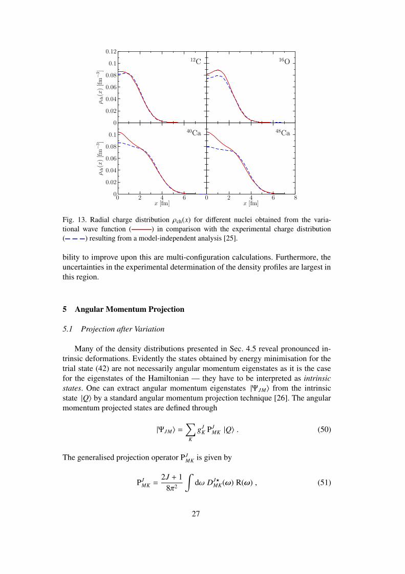
Finally, in Fig. 13 we compare the radial charge density distributions for 12C,

25

Fig. 11. Intrinsic total density distributions of several stable nuclei. Shown is the iso-densitysurface for ρ(x) = ρ0/2 with one octant cut away to reveal the density distribution in thecentre. The colour coding on the section gives the density according to the colour bar at theright. The background grid has a mesh size of 1 fm × 1 fm.

Fig. 12. Intrinsic single-particle density distribution ρ(x) for different Neon isotopes (cf.Fig. 11).16O, 40Ca, and 48Ca with a model-independent analysis of electron scattering data[25]. For this comparison, the exact centre of mass correction and the proton andneutron form factors are included in the theoretical curves. The calculated densityprofiles are in good agreement with the experimental analysis. The surface struc-ture is reproduced extremely well. In the interior the modulations of the calculateddensity distribution are slightly more pronounced. This behaviour is common tomost models based on a single Slater determinant for the ground state; one possi-

26

0 2 4 6x [fm]

0 2 4 6 8x [fm]

0

0.02

0.04

0.06

0.08

0.1

.

ρch(x

)[fm

−3]

0

0.02

0.04

0.06

0.08

0.1

0.12

.

ρch(x

)[fm

−3]

12C 16O

40Ca 48Ca

Fig. 13. Radial charge distribution ρch(x) for different nuclei obtained from the varia-tional wave function ( ) in comparison with the experimental charge distribution( ) resulting from a model-independent analysis [25].

bility to improve upon this are multi-configuration calculations. Furthermore, theuncertainties in the experimental determination of the density profiles are largest inthis region.

5 Angular Momentum Projection

5.1 Projection after Variation

Many of the density distributions presented in Sec. 4.5 reveal pronounced in-trinsic deformations. Evidently the states obtained by energy minimisation for thetrial state (42) are not necessarily angular momentum eigenstates as it is the casefor the eigenstates of the Hamiltonian — they have to be interpreted as intrinsicstates. One can extract angular momentum eigenstates |ΨJM〉 from the intrinsicstate |Q〉 by a standard angular momentum projection technique [26]. The angularmomentum projected states are defined through

|ΨJM〉 =∑

K

gJK PJ

MK |Q〉 . (50)

The generalised projection operator PJMK is given by

PJMK =

2J + 18π2

∫

dω DJ?MK(ω) R(ω) , (51)

27

where DJMK(ω) are the Wigner D-functions and R(ω) is the unitary rotation operator

expressed in terms of the three Euler angles ω = (α, β, γ):

R(ω) = exp(−iαJz) exp(−iβJy) exp(−iγJz) . (52)

The coefficients gJK are formally determined by minimising the energy expectation

value in the projected state |ΨJM〉

EJ =〈ΨJM |H − Tcm |ΨJM〉〈ΨJM |ΨJM〉

=

∑

KK′ gJ?K gJ

K′hJKK′

∑

KK′ gJ?K gJ

K′nJKK′

, (53)

where hJKK′ = 〈Q| (H − Tcm)PJ

KK′ |Q〉 and nJKK′ = 〈Q|PJ

KK′ |Q〉. This leads to a gener-alised eigenvalue problem for the energies EJ of the projected states and the coef-ficients gJ

K:∑

K′hJ

KK′ gJK′ = EJ

∑

K′nJ

KK′ gJK′ . (54)

In this paper we employ the angular momentum projection in the frameworkof a projection after variation (PAV) calculation, i.e., we use the intrinsic state |Q〉obtained by minimising the energy expectation value (45) and subsequently projectit onto angular momentum eigenstates (50).

This scheme is different from a variation after projection (VAP) calculationwhich is based on a minimisation of the energy expectation value (53) calculatedwith the projected states. The presence of strong intrinsic deformations is associ-ated with a kinetic energy contribution that makes such states unfavourable whenminimising the intrinsic energy. This energy contribution, however, is removed bythe projection procedure. Therefore, clustering and intrinsic deformation are gen-erally more pronounced in a VAP framework, where the projected energy is min-imised. In terms of the available model-space, a VAP calculation goes beyond thevariation with a single Slater determinant. The VAP trial state is a specific super-position of rotated Slater determinants. As discussed in Sec. 4.3 this, in general,necessitates a readjustment of the phenomenological correction. First results ofa variation after parity projection calculation are available. A full variation afterangular momentum projection is computationally extremely involved and will bediscussed elsewhere.

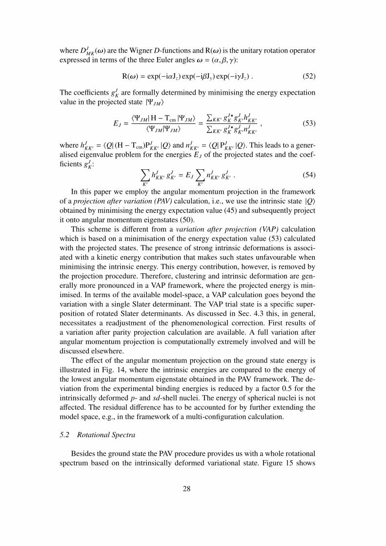
The effect of the angular momentum projection on the ground state energy isillustrated in Fig. 14, where the intrinsic energies are compared to the energy ofthe lowest angular momentum eigenstate obtained in the PAV framework. The de-viation from the experimental binding energies is reduced by a factor 0.5 for theintrinsically deformed p- and sd-shell nuclei. The energy of spherical nuclei is notaffected. The residual difference has to be accounted for by further extending themodel space, e.g., in the framework of a multi-configuration calculation.

5.2 Rotational Spectra

Besides the ground state the PAV procedure provides us with a whole rotationalspectrum based on the intrinsically deformed variational state. Figure 15 shows

28

3He4He

7Li9Be

10B12C

14N16O

20Ne23Na

24Mg27Al

28Si32S

36Ar40Ca

48Ca50Ti

56Fe60Ni

0

0.5

1

1.5

. (E−E

exp)/

A[M

eV]

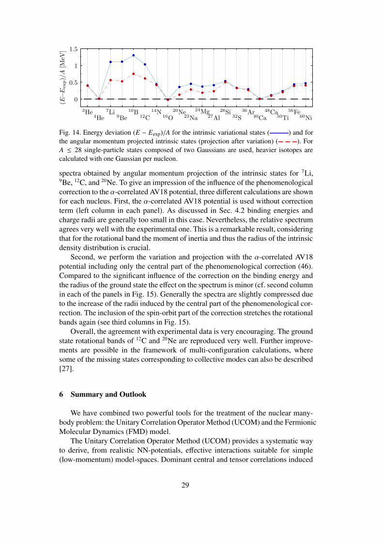
Fig. 14. Energy deviation (E − Eexp)/A for the intrinsic variational states ( ) and forthe angular momentum projected intrinsic states (projection after variation) ( ). ForA ≤ 28 single-particle states composed of two Gaussians are used, heavier isotopes arecalculated with one Gaussian per nucleon.

spectra obtained by angular momentum projection of the intrinsic states for 7Li,9Be, 12C, and 20Ne. To give an impression of the influence of the phenomenologicalcorrection to the α-correlated AV18 potential, three different calculations are shownfor each nucleus. First, the α-correlated AV18 potential is used without correctionterm (left column in each panel). As discussed in Sec. 4.2 binding energies andcharge radii are generally too small in this case. Nevertheless, the relative spectrumagrees very well with the experimental one. This is a remarkable result, consideringthat for the rotational band the moment of inertia and thus the radius of the intrinsicdensity distribution is crucial.

Second, we perform the variation and projection with the α-correlated AV18potential including only the central part of the phenomenological correction (46).Compared to the significant influence of the correction on the binding energy andthe radius of the ground state the effect on the spectrum is minor (cf. second columnin each of the panels in Fig. 15). Generally the spectra are slightly compressed dueto the increase of the radii induced by the central part of the phenomenological cor-rection. The inclusion of the spin-orbit part of the correction stretches the rotationalbands again (see third columns in Fig. 15).

Overall, the agreement with experimental data is very encouraging. The groundstate rotational bands of 12C and 20Ne are reproduced very well. Further improve-ments are possible in the framework of multi-configuration calculations, wheresome of the missing states corresponding to collective modes can also be described[27].

6 Summary and Outlook

We have combined two powerful tools for the treatment of the nuclear many-body problem: the Unitary Correlation Operator Method (UCOM) and the FermionicMolecular Dynamics (FMD) model.

The Unitary Correlation Operator Method (UCOM) provides a systematic wayto derive, from realistic NN-potentials, effective interactions suitable for simple(low-momentum) model-spaces. Dominant central and tensor correlations induced

29

AV18α + ∆Vc + ∆Vls Exp.

0

2

4

6

8

.

E?[MeV]

7Li

1/2−

3/2−

5/2−

7/2−

1/2−

3/2−

5/2−

7/2−

1/2−

3/2−

5/2−

7/2−

3/2−1/2−

7/2−

5/2−

5/2−

[−12.65] [−34.53] [−35.35] [−39.24]

AV18α + ∆Vc + ∆Vls Exp.

0

2

4

6

8

.

E?[MeV] 9

Be

3/2−

5/2−

7/2−

3/2−

5/2−

7/2−

3/2−

5/2−

7/2−

3/2−

1/2+

5/2−1/2−5/2+

(3/2)+

7/2−

(1/2−)

[−22.21] [−51.56] [−53.50] [−58.16]

AV18α + ∆Vc + ∆Vls Exp.

0

5

10

15

.

E?[MeV]

12C

0+

2+

4+

0+

2+

4+

0+

2+

4+

0+

2+

0+

3−(0+)

1−(2+)2−

1+(2−)

4+

[−38.23] [−80.61] [−84.81] [−92.16]

AV18α + ∆Vc + ∆Vls Exp.

0

2

4

6

.

E?[MeV]

20Ne

0+

2+

4+

0+

2+

4+

0+

2+

4+

0+

2+

4+

2−

3−1−

[−76.45] [−151.8] [−153.9] [−160.6]

Fig. 15. Energy spectra resulting from the angular momentum projection of the variationalground states for 7Li, 9Be, 12C, and 20Ne. Shown are the excitation energies obtained usingthe α-correlated AV18 potential without correction (first column), with central correctiononly (second column), with central and spin-orbit correction (third column) in comparisonto the experimental spectra (fourth column). The numbers given beneath the lowest levelare the absolute ground state energies in [MeV].

by the NN-potential are described explicitly by an unitary transformation. By ap-plying the unitary correlation operator to a simple many-body state, e.g., a Slaterdeterminant, the short-range correlations are imprinted into the state. Alternativelythe Hamiltonian (and all other operators) can be transformed. The resulting corre-lated interaction VUCOM possesses a closed operator representation, is phase-shiftequivalent to the original potential, and leads to momentum-space matrix elementsin accord with the Vlow−k matrix elements [12]. It provides a robust starting point formany-body methods relying on model spaces not capable of describing short-rangecorrelations themselves, e.g., variational models with simple trial states, Hartree-Fock calculations, and multi-configuration shell-model.

We have employed the correlated interaction VUCOM in the variational frame-work of the Fermionic Molecular Dynamics (FMD) model. The many-body trialstate is a Slater determinant of Gaussian single-particle states which prove to beextremely flexible. On the same footing, it allows for the description of spheri-cal shell-model-type wave functions as well as states with intrinsic deformationsand α-clustering. At the same time, the approach is computationally quite efficientso that a treatment of nuclei up to mass number A . 60 is possible for realistic

30

two-body interactions with complex operator structure. The inclusion of three-bodyforces would substantially increase the computational cost and thus reduce the ac-cessible region of the nuclear chart. At the present stage, three-body interactionsand long-range correlations are, therefore, simulated by a phenomenological two-body correction. Charge radii and charge distributions are in nice agreement withexperiment. Around the magic numbers the variational energies agree well withthe experimental binding energies. Away from the shell closures the intrinsic den-sity distributions exhibit strong deformations and α-clustering, which necessitatesprojection of the intrinsic states onto angular momentum eigenstates. Within a pro-jection after variation (PAV) framework we have achieved very promising resultsfor ground state energies and rotational spectra.

Natural next steps are variation after projection (VAP) and multi-configurationcalculations. First results along these lines have been obtained using a GeneratorCoordinate Method to implement an approximate VAP scheme. Constraints on themultipole moments are used to generate different intrinsic states which serve asinput for variation after projection (w.r.t. the generator coordinates, i.e., the mul-tipole moments) and multi-configuration calculations. VAP calculations for 16Oshow, e.g., that a tetrahedron of α-clusters is energetically more favourable thanthe spherical shell-model-type state resulting from the unprojected variation [27].Detailed results of these investigations will be discussed in a forthcoming publica-tion.

Other future applications of the correlated realistic interaction VUCOM are Hartree-Fock and RPA calculations. This provides a consistent scheme to perform nuclearstructure calculations based on realistic NN-potentials also for large nuclei.

Acknowledgements

This work is supported by the Deutsche Forschungsgemeinschaft through con-tract SFB 634.

References

[1] R. B. Wiringa, V. G. J. Stoks, R. Schiavilla, Phys. Rev. C 51 (1995) 38.

[2] R. Machleidt, Adv. Nucl. Phys. 19 (1989) 189.

[3] R. Machleidt, Phys. Rev. C 63 (2001) 024001.

[4] V. G. J. Stoks, R. A. M. Klomp, C. P. F. Terheggen, J. J. de Swart, Phys. Rev. C 49(1993) 2950.

[5] S. C. Pieper, K. Varga, R. B. Wiringa, Phys. Rev. C 66 (2002) 044310.

[6] B. S. Pudliner, V. R. Pandharipande, J. Carlson, S. C. Pieper, R. B. Wiringa, Phys. Rev.C 56 (1997) 1720.

[7] E. Caurier, P. Navratil, W. E. Ormand, J. P. Vary, Phys. Rev. C 66 (2002) 024314.

31

[8] P. Navratil, J. P. Vary, B. R. Barrett, Phys. Rev. C 62 (2000) 054311.

[9] S. C. Pieper, V. R. Pandharipande, R. B. Wiringa, Phys. Rev. C 64 (2001) 014001.

[10] D. R. Entem, R. Machleidt, Phys. Rev C. 68 (2003) 041001.

[11] H. Feldmeier, T. Neff, R. Roth, J. Schnack, Nucl. Phys. A632 (1998) 61.

[12] T. Neff, H. Feldmeier, Nucl. Phys. A714 (2003) 311.

[13] J. L. Forest, V. R. Pandharipande, S. C. Pieper, R. B. Wiringa, R. Schiavilla,A. Arriaga, Phys. Rev. C 54 (1996) 646.

[14] R. Roth, Ph.D. thesis, Technische Universitat Darmstadt (2000),http://crunch.ikp.physik.tu-darmstadt.de/tnp/.

[15] R. Wiringa, R. Smith, T. Ainsworth, Phys. Rev. C 29 (1984) 1207.

[16] T. Neff, Ph.D. thesis, Technische Universitat Darmstadt (2002),http://theory.gsi.de/˜tneff/.

[17] S. K. Bogner, T. T. S. Kuo, A. Schwenk, Phys. Rep. 386 (2003) 1.

[18] T. Neff, H. Feldmeier, Proc. of the International Workshop XXXI on Gross Propertiesof Nuclei and Nuclear Excitations, Hirschegg, Austria, (2003) 56.

[19] H. Feldmeier, Nucl. Phys. A515 (1990) 147.

[20] H. Feldmeier, J. Schnack, Prog. Part. Nucl. Phys. 39 (1997) 393.

[21] H. Feldmeier, K. Bieler, J. Schnack, Nucl. Phys. A586 (1995) 493.

[22] H. Feldmeier, J. Schnack, Rev. Mod. Phys. 72 (2000) 655.

[23] T. Neff, Master’s thesis, Technische Universitat Darmstadt (1998),http://theory.gsi.de/˜tneff/.

[24] G. Audi, A. Wapstra, Nucl. Phys. A595 (1995) 409.

[25] H. d. Vries, C. W. d. Jager, C. d. Vries, At. Data Nucl. Data Tables 36 (1987) 495.

[26] P. Ring, P. Schuck, The Nuclear Many-Body Problem, Springer Verlag, New York,1980.

[27] T. Neff, H. Feldmeier, Nucl. Phys. A738c (2004) 357.

32