Stochastic Strategies for a Swarm Robotic Assembly System

Loıc Matthey, Spring Berman and Vijay Kumar

Abstract— We present a decentralized, scalable approachto assembling a group of heterogeneous parts into differentproducts using a swarm of robots. While the assembly plansare predetermined, the exact sequence of assembly of partsand the allocation of subassembly tasks to robots are deter-mined by the interactions between robots in a decentralizedfashion in real time. Our approach is based on developing acontinuous abstraction of the system derived from models ofchemical reactions and formulating the strategy as a problemof selecting rates of assembly and disassembly. These rates aremapped onto probabilities that determine stochastic controlpolicies for individual robots, which then produce the desiredaggregate behavior. This top-down approach to determiningrobot controllers also allows us to optimize the rates at theabstract level to achieve fast convergence to the specifiedtarget numbers of products. Because the method incorporatesprograms for assembly and disassembly, changes in demandcan lead to reconfiguration in a seamless fashion. We illustratethe methodology using a physics-based simulator with examplesinvolving 15 robots and two types of final products.

I. INTRODUCTION

We develop an approach to designing a reconfigurablemanufacturing system in which a swarm of homogeneousrobots assembles static, heterogeneous parts into differenttypes of products. The system must respond quickly toproduce desired amounts of products from any initial set ofparts. We employ a decentralized strategy in which robotsoperate autonomously and both robots and parts use localcommunication. The strategy can be readily implemented onresource-constrained robots, and it is scalable in the numberof robots and parts and robust to changes in robot population.

We specify that robots move randomly inside a closedarena and pick up randomly scattered parts. The system canbe modeled as being spatially homogeneous, and the robot-part and robot-robot interactions are analogous to chemicalreactions between molecules. This allows us to model thesystem using the extensively studied Chemical ReactionNetwork (CRN) framework [1].

In the taxonomy [2] of macroscopic self-assembly sys-tems, our objective and approach are most similar to thoseof [3], which considers a set of modules that bind throughrandom collisions and detach into different parts according to

L. Matthey is with the DISAL Laboratory, Ecole PolytechniqueFederale de Lausanne, Station 14, 1015 Lausanne, Switzerland,loic.matthey@epfl.ch

S. Berman and V. Kumar are with the GRASP Laboratory, Univer-sity of Pennsylvania, 3330 Walnut Street, Philadelphia, PA 19104, USA,{spring, kumar}@grasp.upenn.edu

We gratefully acknowledge partial support from NSF grants CSR-CPS0720801, IIS-0427313, NSF IIP-0742304, and IIS-0413138, ARO grantW911NF-05-1-0219, and ONR grant N00014-07-1-0829.

programmed probabilities. The system in [3] is also modeledas a CRN, as is the one in [4], which predicts the yield ofcomplete assemblies from passive, vertically stirred modules.In [3], an optimization problem is formulated to computethe detachment probabilities that maximize the yield of aparticular assembly at equilibrium. The optimization is basedon a Markov process model of the system and requires theenumeration of all reachable states, which does not scale wellwith the number of parts. Our use of robots to transport andjoin passive parts according to decentralized rules is similarto the setup in [5], which derives rules for building a singledesired structure out of blocks.

In this paper, we use a “top-down” design methodologysimilar to [6], [7] to synthesize stochastic control policiesfor robots that cause them to produce target amounts ofproducts as quickly as possible. Fig. 1 illustrates our method-ology. As in recent work on modeling robot swarms [8]–[10], we develop an accurate macroscopic model of thephysical system. We generate the continuous dynamics ofindividual robots using a realistic 3D physics simulation,the micro-continuous model. Since the system is spatiallyhomogeneous, it can be represented by the Chemical MasterEquation [11]. We call this the complete macro-discretemodel because it describes a continuous-time Markov pro-cess whose states are the discrete populations of parts androbots. When these populations are large, the system can beabstracted to an ordinary differential equation (ODE) model,the complete macro-continuous model, whose state variablesare continuous amounts of parts and robots. We compute rateconstants in this model from geometrical properties of therobots and environment and check that the model predictsthe behavior of the micro-continuous model. We simplifythis abstraction to a more easily analyzable reduced macro-continuous model with the same rates.

Our novel contribution to prior work on swarm modelingis our control synthesis methodology, which provides theo-retical guarantees on system performance. Using an approachsimilar to [7], we optimize the rates in the reduced macro-continuous model to minimize system convergence timewhile enforcing target quantities of all parts at equilibrium.The optimization problem is independent of the number ofparts, scaling only with the number of rates. We then map therates onto probabilities of assembly and disassembly whichare used as robot control policies in the micro-continuousmodel. The trends in the evolution of part populations inthis simulation are predicted by the designed behavior ofthe continuous model, including the faster convergence thatresults from using optimized versus non-optimal rates.

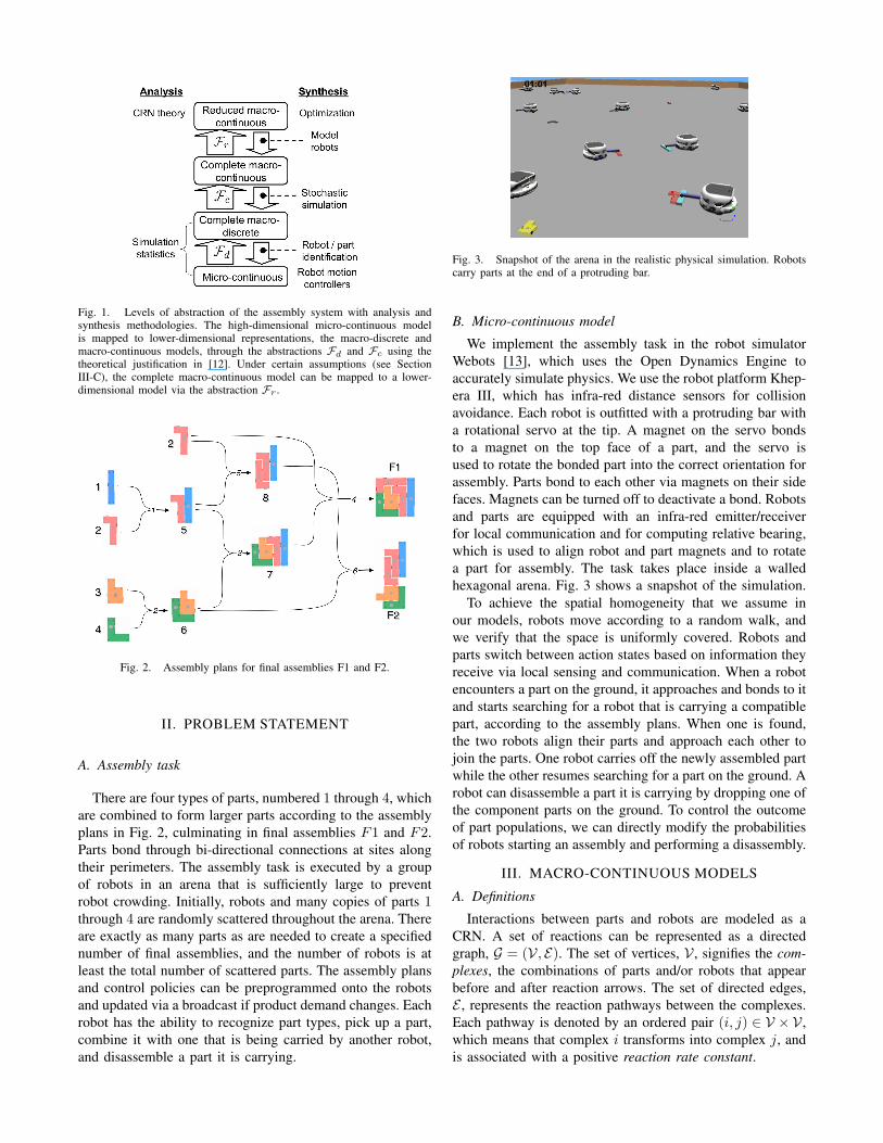
Fig. 1. Levels of abstraction of the assembly system with analysis andsynthesis methodologies. The high-dimensional micro-continuous modelis mapped to lower-dimensional representations, the macro-discrete andmacro-continuous models, through the abstractions Fd and Fc using thetheoretical justification in [12]. Under certain assumptions (see SectionIII-C), the complete macro-continuous model can be mapped to a lower-dimensional model via the abstraction Fr .

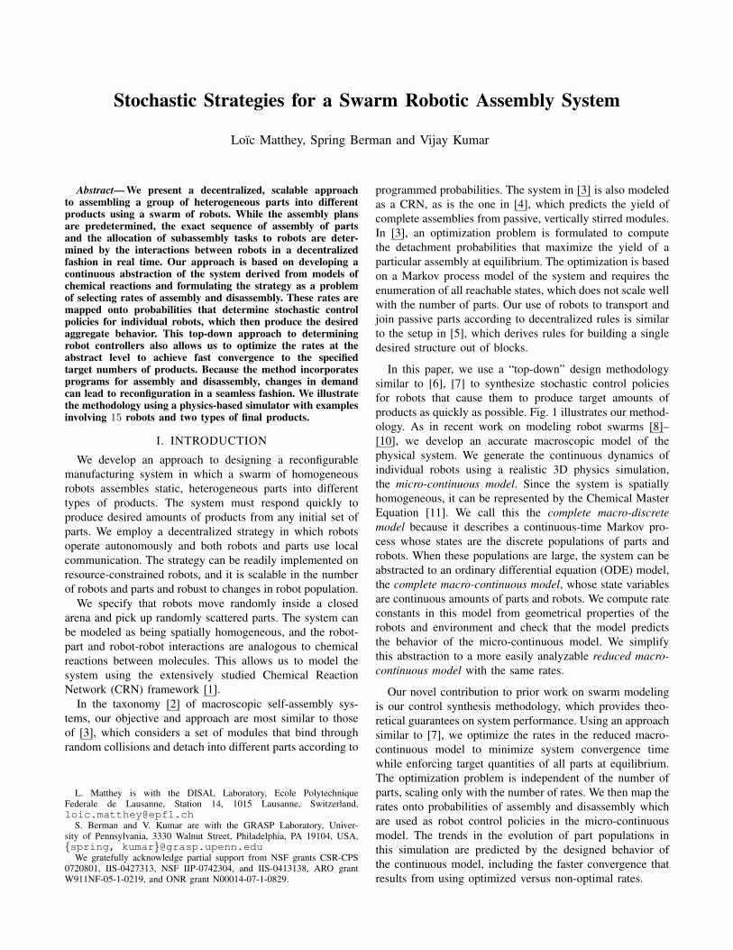
Fig. 2. Assembly plans for final assemblies F1 and F2.

II. PROBLEM STATEMENT

A. Assembly task

There are four types of parts, numbered 1 through 4, whichare combined to form larger parts according to the assemblyplans in Fig. 2, culminating in final assemblies F1 and F2.Parts bond through bi-directional connections at sites alongtheir perimeters. The assembly task is executed by a groupof robots in an arena that is sufficiently large to preventrobot crowding. Initially, robots and many copies of parts 1through 4 are randomly scattered throughout the arena. Thereare exactly as many parts as are needed to create a specifiednumber of final assemblies, and the number of robots is atleast the total number of scattered parts. The assembly plansand control policies can be preprogrammed onto the robotsand updated via a broadcast if product demand changes. Eachrobot has the ability to recognize part types, pick up a part,combine it with one that is being carried by another robot,and disassemble a part it is carrying.

Fig. 3. Snapshot of the arena in the realistic physical simulation. Robotscarry parts at the end of a protruding bar.

B. Micro-continuous model

We implement the assembly task in the robot simulatorWebots [13], which uses the Open Dynamics Engine toaccurately simulate physics. We use the robot platform Khep-era III, which has infra-red distance sensors for collisionavoidance. Each robot is outfitted with a protruding bar witha rotational servo at the tip. A magnet on the servo bondsto a magnet on the top face of a part, and the servo isused to rotate the bonded part into the correct orientation forassembly. Parts bond to each other via magnets on their sidefaces. Magnets can be turned off to deactivate a bond. Robotsand parts are equipped with an infra-red emitter/receiverfor local communication and for computing relative bearing,which is used to align robot and part magnets and to rotatea part for assembly. The task takes place inside a walledhexagonal arena. Fig. 3 shows a snapshot of the simulation.

To achieve the spatial homogeneity that we assume inour models, robots move according to a random walk, andwe verify that the space is uniformly covered. Robots andparts switch between action states based on information theyreceive via local sensing and communication. When a robotencounters a part on the ground, it approaches and bonds to itand starts searching for a robot that is carrying a compatiblepart, according to the assembly plans. When one is found,the two robots align their parts and approach each other tojoin the parts. One robot carries off the newly assembled partwhile the other resumes searching for a part on the ground. Arobot can disassemble a part it is carrying by dropping one ofthe component parts on the ground. To control the outcomeof part populations, we can directly modify the probabilitiesof robots starting an assembly and performing a disassembly.

III. MACRO-CONTINUOUS MODELS

A. Definitions

Interactions between parts and robots are modeled as aCRN. A set of reactions can be represented as a directedgraph, G = (V, E). The set of vertices, V , signifies the com-plexes, the combinations of parts and/or robots that appearbefore and after reaction arrows. The set of directed edges,E , represents the reaction pathways between the complexes.Each pathway is denoted by an ordered pair (i, j) ∈ V × V ,which means that complex i transforms into complex j, andis associated with a positive reaction rate constant.

Each part of type i in Fig. 2 is symbolized by Xi, and arobot is symbolized by XR. Xi may be further classified asXui , an unclaimed part on the ground, or as Xc

i , a claimedpart i and the robot that is carrying it. Let M be the numberof these variables, or species, in a model of the system. Thenx(t) ∈ RM is the vector of the species populations, whichare represented as continuous functions of time t.

B. Complete macro-continuous model

We define a CRN that represents each possible action inthe micro-continuous model of the assembly system:

XR +Xui

ei−→ Xci , i = 1, ..., 8

Xc1 +Xc

2

k+1−−→ Xc

5 +XR Xc2 +Xc

7

k+4−−→ Xc

F1 +XR

Xc3 +Xc

4

k+2−−→ Xc

6 +XR Xc2 +Xc

5

k+5−−→ Xc

8 +XR

Xc5 +Xc

6

k+3−−→ Xc

7 +XR Xc6 +Xc

8

k+6−−→ Xc

F2 +XR

Xc5

k−1−−→ Xc1 +Xu

2 XcF1

k−4−−→ Xc7 +Xu

2

Xc6

k−2−−→ Xc3 +Xu

4 Xc8

k−5−−→ Xc5 +Xu

2

Xc7

k−3−−→ Xc6 +Xu

5 XcF2

k−6−−→ Xc8 +Xu

6 (1)

In this CRN, ei is the rate at which a robot encounters apart of type i, k+

i is the rate of assembly process i, and k−i isthe rate of disassembly process i. We theoretically estimatethese rates as functions of the following probabilities:

ei = pe , k+i = pe · pai · p+

i , k−i = p−i . (2)

pe is the probability that a robot encounters a part oranother robot. Since our arena size yields a low robot density,this probability is modeled as being independent of the robotpopulation. The property that robots and parts are distributeduniformly throughout the arena allows us to calculate pe

from the geometrical approach that is used to computeprobabilities of molecular collisions [9], [11]: pe ≈ vTw/A,where v is the average robot speed, T is a timestep, A is thearea of the arena, and w is twice a robot’s communicationradius, since this is the range within which a robot detects apart or robot and initiates an assembly process.pai is the probability of two robots successfully completing

assembly process i; it depends on the part geometries.p+i is the probability of two robots starting assembly

process i, and p−i is the probability per unit time of a robotperforming disassembly process i. These are the tunableparameters of the system.

We compute pai and the parameters for pe using mea-surements from the micro-continuous model (Webots simu-lations): A = 23.4 m2 (hexagon of radius 3 m), w = 1.2 m,v = 0.128 m/s from an average over 50 runs, and pa =[0.9777 0.9074 0.9636 0.9737 0.8330 1.0] (entries follow thenumbering of the associated reactions) from averages over100 runs. We set T = 1 s.

In the thermodynamic limit, which includes the conditionthat populations approach infinity, the physical system repre-sented by (1) can be abstracted to an ODE model [12]. Thisis illustrated in the next section. We numerically integrate

0 200 400 600 800 10000

0.5

1

1.5

2

2.5

3

3.5

4

Time [s]

Part

popu

latio

ns

xF 1

xF 2

(a)

0 200 400 600 800 10000

0.5

1

1.5

2

2.5

3

3.5

Time [s]

Part

popu

latio

ns

Macro−continuous Macro−discrete Micro−continuous

xF 2

xF 1

(b)

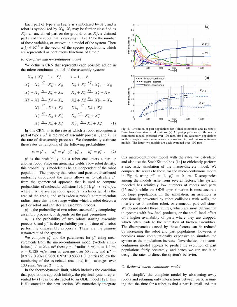
Fig. 4. Evolution of part populations for 3 final assemblies and 15 robots.Error bars show standard deviations. (a) All part populations in the micro-continuous model, averaged over 100 runs. (b) Final assembly populationsin the complete macro-continuous, macro-discrete, and micro-continuousmodels. The latter two models are each averaged over 100 runs.

this macro-continuous model with the rates we calculatedand also use the StochKit toolbox [14] to efficiently performa stochastic simulation of the macro-discrete model. Wecompare the results to those for the micro-continuous modelin Fig. 4, using p+

i = 1, p−i = 0 ∀i. Discrepanciesamong the models arise from several factors. The systemmodeled has relatively low numbers of robots and parts(15 each), while the ODE approximation is most accuratefor large populations. In the simulation, an assembly isoccasionally prevented by robot collisions with walls, theinterference of another robot, or erroneous part collisions.We do not model these failures, which are most detrimentalto systems with few final products, or the small local effectof a higher availability of parts where they are dropped,which often leads to the recreation of broken assemblies.The discrepancies caused by these factors can be reducedby increasing the robot and part populations; however, itbecomes more computationally expensive to simulate thesystem as the populations increase. Nevertheless, the macro-continuous model appears to predict the evolution of partpopulations fairly accurately, and hence we can use it todesign the rates to direct the system’s behavior.

C. Reduced macro-continuous model

We simplify the complete model by abstracting awayrobots and retaining only interactions between parts, assum-ing that the time for a robot to find a part is small and that

there are at least as many robot as parts:

X1 +X2

k+1

k−1

X5 X3 +X4

k+2

k−2

X6 X5 +X6

k+3

k−3

X7

X2 +X7

k+4

k−4

XF1 X2 +X5

k+5

k−5

X8 X6 +X8

k+6

k−6

XF2 (3)

The rates are also defined by equation (2).We define a vector y(x) ∈ R12 in which entry yi is the

part or product of parts in complex i:

y(x) = [x1x2 x5 x3x4 x6 x2x7 xF1

x5x6 x7 x2x5 x8 x6x8 xF2]T . (4)

We also define a matrix M ∈ R10×12 in which each entryMji, j = 1, ..., 10, of column mi is the coefficient ofpart type j in complex i (0 if absent). We relabel the rateassociated with reaction (i, j) ∈ E as kij and define a matrixK ∈ R12×12 with entries

Kij =

kji if i 6= j , (j, i) ∈ E ,0 if i 6= j , (j, i) /∈ E ,−∑

(i,l)∈E kil if i = j .(5)

Then our ODE abstraction of the system can be written inthe following form [15]:

x = MKy(x) . (6)

One set of linearly independent conservation constraintson the part quantities is:

x3 − x4 = N1

x1 + x5 + x7 + x8 + xF1 + xF2 = N2

x2 + x5 + x7 + 2(x8 + xF1 + xF2) = N3

x3 + x6 + x7 + xF1 + xF2 = N4

(7)

where Ni, i = 1, ..., 4, are computed from the initial partquantities.

Theorem 1: System (6) subject to (7) has a unique, stableequilibrium x > 0.

Proof: Each equilibrium of the system,{x | MKy(x) = 0}, can be classified as either apositive equilibrium x > 0 or a boundary equilibriumin which xi = 0 for some i, which can be found bysolving y(x) = 0 [15]. From definition (4) of y(x), itcan be concluded that in each boundary equilibrium, allxi = 0 except for one of the four combinations of variables(x1, x3), (x1, x4), (x2, x3), (x2, x4). Since we only considersystems that can produce xF1 and xF2, it is not possiblefor the system to reach any of these equilibria; each onelacks two part types needed for the final assemblies.

The deficiency δ of a reaction network is the number ofcomplexes minus the number of linkage classes, each ofwhich is a set of complexes connected by reactions, minusthe network rank, which is the rank of the matrix with rowsmi −mj , (i, j) ∈ E [1]. Network (3) has 12 complexes, 6linkage classes, and rank 6; hence, δ = 0. Also, the networkis weakly reversible because whenever there is a directedarrow pathway from complex i to complex j, there is onefrom j to i. Because the network has deficiency 0, is weakly

reversible, and does not admit any boundary equilibria, it hasa unique, globally asymptotically stable positive equilibriumaccording to Theorem 4.1 of [16].

IV. RATE OPTIMIZATION

We consider the problem of designing the system de-scribed by model (6) subject to (7) to produce desiredquantities of parts as quickly as possible. The objective willbe posed as the design of optimal probabilities p+

i , p−i , i =

1, ..., 6, that minimize the convergence time of the systemto a vector of target part quantities, xd. We formulate anoptimization problem in which these probabilities are writtenin terms of the rates k+

i , k−i , i = 1, ..., 6, using equation (2).

Although only the amounts of the final assemblies F1 andF2 may need to be specified in practice, our optimizationproblem requires that target quantities of all parts be defined.

We first specify xd1, xd2, x

d3, x

d5, x

d8 and a parameter

α ≡ xdF1/(xdF1 + xdF2) . (8)

Then we compute the dependent variables xd4, xd6, x

d7, and

xdF1+xdF2 from the conservation equations (7) and definition(8) and check that they are positive to ensure a valid xd. Inthis way, we can keep xdF1+xdF2 and the target non-final partquantities constant while adjusting the ratio between xF1 andxF2 using α. Theorem 1 shows that we can achieve xd fromany initial distribution x0 by specifying that x = xd throughthe following constraint on K,

MKy(xd) = 0 . (9)

We quantify the time to converge to xd in terms ofthe system relaxation times τi, i = 1, ..., 6, the times inwhich different modes (dynamically independent variables)of the system converge to a stable equilibrium after pertur-bation [17], [18]. Various measures of the average relaxationtime of a CRN have been defined, but they are applicableonly under certain conditions, such as a linear reactionsequence [19] [20]. To estimate the τi, we reformulate thesystem in terms of new variables. Define vi, i = 1, ..., 6,as the difference between the forward and reverse fluxesassociated with reaction i in system (3). For example, v1 =k1x1x2 − k2x5. Let v(x) = [v1 ... v6]T and let S ∈ R6×10

denote the stoichiometric matrix of the system, which isdefined such that model (6) can be written as [17]:

x = Sv(x) . (10)

The dynamical properties of a CRN are often analyzedby linearizing the ODE model of the system about anequilibrium and studying the properties of the associatedJacobian matrix J = SG, where the entries of G areGij = dvi/dxj [18]. Denoting the eigenvalues of J by λi,a common measure of relaxation time is τi = 1/|Re(λi)|.Since the λi are negative at a stable equilibrium, one wayto yield fast convergence is to choose rates that minimizethe largest λi. However, in our system it is very difficult tofind analytical expressions for the λi. We use an alternative

estimate of relaxation time that is also derived by linearizingthe system around its equilibrium xd [17],

τj =

(10∑i=1

(−Sij)dvjdxi

)−1

x=xd

. (11)

Each reaction j in system (3) is of the form Xk +

Xl k+

j

k−jXm. Thus, vj = k+

j xkxl−k−j xm, and the entries

of column j in S are all 0 except for Skj = Slj = −1 andSmj = 1. Then according to equation (11), the relaxationtime for each reaction is

τj = (k+j (xdk + xdl ) + k−j )−1 . (12)

Define k ∈ R12 as the vector of all k+i , k

−i and p ∈ R12 as

the vector of all p+i , p

−i . Note that according to equation (2),

k = k(p). We define the objective function as the averageτ−1j , which should be maximized to produce fast convergence

to xd. The optimization problem can now be posed as:

[P] maximize 16

∑6j=1 τ

−1j

subject to MK(p)y(xd) = 0, 0 ≤ p ≤ 1 .

Problem P is a linear program, which can be solvedefficiently. For comparison, we also implemented a MonteCarlo method to find the k(p) that directly minimizes theconvergence time. We measure the degree of convergenceto xd by ∆(x) = ||x − xd||2 and say that one systemconverges faster than another if it takes less time tβ for∆(x) to decrease to some small fraction β, here defined as0.1, of its initial value. At each iteration, k(p) is perturbedby a random vector and projected onto the null space oflinearly independent rows of a matrix N defined such thatNk = MKy(xd) = 0. Once k(p) also satisfies 0 ≤ p ≤ 1,it is used to simulate model (6), and a Newton scheme is usedto compute the exact time t0.1 when ∆(x) = 0.1∆(x0).

V. RESULTS

A. Optimization of rates k(p)To investigate the effect of rate optimization on the

convergence time of model (6), we generated non-optimalrates, which satisfy constraint (9) and 0 ≤ p ≤ 1 butare not optimized for some objective, and computed ratesusing Problem P and the Monte Carlo method. The non-optimal and Problem P rates were calculated for α ∈{0.01, 0.02, . . . , 0.99}, and the Monte Carlo rates for α ∈{0.1, 0.2, . . . , 0.9}. We set x0 = [60 120 60 60 0]T andxd = [0.5 2.5 1 1 0.5 1 1 1 57α 57(1 − α)]T . Problem Pproduced the same rates for each α (for instance, p+

i = 1∀i) except for the rates of disassembly processes 4 and 6,which vary with α. This shows that the system is flexibleenough to yield any α when only the rates of breaking apartthe final assemblies are modified.

Fig. 5 compares the system convergence time t0.1 for thesedifferent sets of rates. The Monte Carlo rates consistentlyyield the fastest convergence but are time-consuming tocompute: on a standard 2 GHz laptop, it takes about 10hours for t0.1 to decrease slowly enough with each program

0 0.1 0.2 0.3 0.4 0.5 0.6 0.7 0.8 0.9 1101

102

103

104

105

!

t 0.1

Monte CarloProblem PNon!opt Ave

Fig. 5. Time for model (6) to converge to 0.1∆(x0) vs. α for optimizedand non-optimal k. “Non-opt Ave” is the average of 100 t0.1 correspondingto different random feasible k for each α.

100 101 102 103 104 105 106 1070

0.2

0.4

0.6

0.8

1

Time

x F1/(x

F1d+x

F2d)

and

x F2

/(xF1d

+xF2d

)

! = 0.1

100 101 102 103 104 105 1060

0.2

0.4

0.6

0.8

1

Time

x F1/(x

F1d+x

F2d)

and

x F2

/(xF1d

+xF2d

)! = 0.5

100 101 102 103 104 105 1060

0.2

0.4

0.6

0.8

1

Time

x F1/(x

F1d+x

F2d)

and

x F2

/(xF1d

+xF2d

)

! = 0.9

Fig. 6. Evolution of final assembly ratios in model (6) for α = 0.1, 0.5, 0.9using non-optimal rates (light solid lines) and rates optimized by the MonteCarlo method (dark solid lines) and Problem P (dashed lines).

iteration for k to be considered close enough to optimal. Therates from Program P, which for each α are computed in lessthan a second, yield t0.1 that dip close to the Monte Carlotimes for α = 0.2 − 0.5 but increase up to two orders ofmagnitude outside this range. However, these t0.1 are stillmuch lower than the average t0.1 (over 100 values) of thesystem using non-optimal rates.

We numerically integrated model (6) for α = 0.1, 0.5, 0.9using both optimized and non-optimal rates. The evolutionof the model for each set of rates is shown in Fig. 6. Foreach α, the optimized models converge faster to the targetassembly ratios than the non-optimal model.

B. Mapping rates onto the micro-continuous model

For α = 0.1, 0.5, 0.9, we mapped the optimized andnon-optimal rates onto the micro-continuous model to see

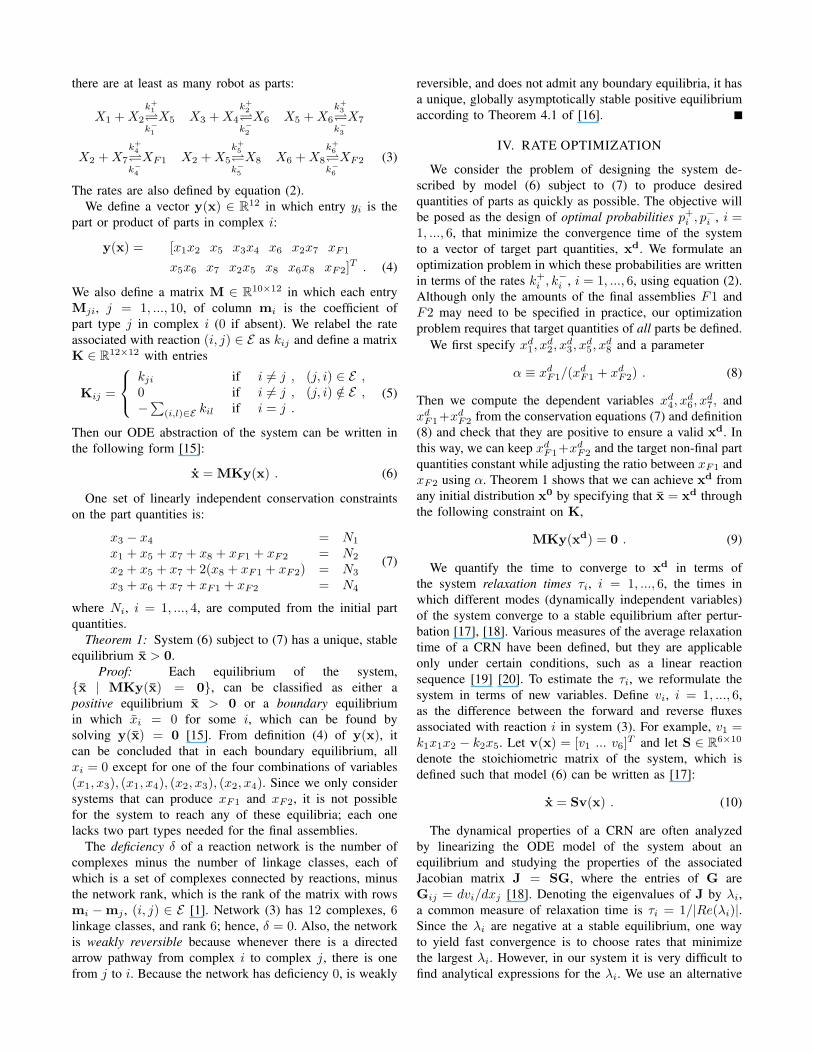
Fig. 7. Evolution of final assembly ratios in the micro-continuous modelfor α = 0.1, 0.5, 0.9 using rates optimized by the Monte Carlo method(top row) and Problem P (center row) and non-optimal rates (bottom row).xd

F1 + xdF2 was computed as the equilibrium xF1 + xF2 of model (6)

with x0 = [3 6 3 3 0]T .

whether the physical system would behave similarly to thereduced continuous model. We did this in the following way.Let R be a uniformly distributed random number between0 and 1 and let ∆t be the simulation timestep (32 ms). Arobot carrying a part that can be disassembled according toprocess i computes R at each timestep and disassembles thepart if R < p−i ∆t. A robot about to begin assembly processi computes R and executes the assembly if R < p+

i ∆t.Fig. 7 shows the time evolution of the micro-continuousmodel averaged over 30 runs for all sets of rates, using 15robots and 15 parts (3 final assemblies).

Since the simulations are time-consuming to run, theywere stopped well before the ODE models’ end times in Fig.6. This is why they do not attain full convergence. However,their qualitative behavior follows the same trends as Fig. 6.The runs using the Monte Carlo rates make the most progresstoward the target ratios, the runs using the non-optimal ratesmake very little progress, and the runs using the Problem Prates display intermediate performance. Thus, in this realisticsystem model, the rates that are optimized in a much simplermodel do indeed produce faster convergence than the non-optimal rates. Interestingly, Fig. 6 also predicts the crossingbetween final assembly amounts that occurs in the ProblemP, α = 0.9 run. Discrepancies between the simulations andmodel (6) are due to the factors described in Section III-B.

VI. CONCLUSIONS AND FUTURE WORK

We have presented a method to systematically derivedecentralized, stochastic control policies for a swarm ofrobots to quickly manufacture different products in responseto varying demand. The collective behavior of the systemis abstracted to an ODE model whose parameters, the rateconstants of assembly and disassembly, govern the controlpolicies running on individual robots for executing the as-sembly task. By tuning these rates, we tune the performanceof the system. This optimization relies on global stabilityproperties of a specific class of CRN to which the ODE

model belongs, and it is independent of the number of partsand robots. We map the rates onto probabilities of assemblyand disassembly followed by the robots and find that thebehavior of the resulting system is qualitatively predictedby the ODE model; it is expected that performance closerto the model would be observed for larger robot and partpopulations. One avenue of future work is to investigate thesynthesis of the discrete assembly plans and incorporate feed-back into the process. This direction draws inspiration frombio-molecular pathways in which intermediate subassembliesor molecules can promote or inhibit chemical reactions. Wewould like to be able to optimize the discrete assembly planby constructing feedback loops to improve the yield rate.

REFERENCES

[1] M. Feinberg, “The existence and uniqueness of steady states for aclass of chemical reaction networks,” Archive for Rational Mechanicsand Analysis, vol. 132, pp. 311–370, 1995.

[2] R. Groß and M. Dorigo, “Self-assembly at the macroscopic scale,”Proceedings of the IEEE, vol. 96, no. 9, pp. 1490–1508, 2008.

[3] E. Klavins, S. Burden, and N. Napp, “Optimal rules for programmedstochastic self-assembly,” Proc. Robotics: Science and Systems II, pp.9–16, 2007.

[4] K. Hosokawa, I. Shimoyama, and H. Miura, “Dynamics of self-assembling systems: Analogy with chemical kinetics,” Artificial Life,vol. 1, no. 4, pp. 413–427, 1994.

[5] J. Werfel and R. Nagpal, “Three-dimensional construction with mobilerobots and modular blocks,” Int’l. J. Robotics Research, vol. 27, no.3-4, pp. 463–479, 2008.

[6] A. Halasz, M. A. Hsieh, S. Berman, and V. Kumar, “Dynamicredistribution of a swarm of robots among multiple sites,” Proc. Int’l.Conf. on Intelligent Robots and Systems (IROS), pp. 2320–2325, 2007.

[7] S. Berman, A. Halasz, M. A. Hsieh, and V. Kumar, “Optimizedstochastic policies for task allocation in swarms of robots,” IEEETrans. on Robotics, 2009, accepted.

[8] A. Martinoli, K. Easton, and W. Agassounon, “Modeling swarmrobotic systems: A case study in collaborative distributed manipula-tion,” Int’l. J. Robotics Research, vol. 23, no. 4, pp. 415–436, 2004.

[9] N. Correll and A. Martinoli, “Modeling self-organized aggregation ina swarm of miniature robots,” in Proc. Int’l. Conf. on Robotics andAutomation (ICRA), Workshop on Collective Behaviors inspired byBiological and Biochemical Systems, 2007.

[10] H. Hamann and H. Worn, “A framework of space-time continuousmodels for algorithm design in swarm robotics,” Swarm Intelligence,vol. 2, no. 2-4, pp. 209–239, 2008.

[11] D. Gillespie, “A rigorous derivation of the chemical master equation,”Physica A, vol. 188, no. 1-3, pp. 404–425, 1992.

[12] ——, “Stochastic simulation of chemical kinetics,” Annual Review ofPhysical Chemistry, vol. 58, pp. 35–55, 2007.

[13] O. Michel, “Webots: Professional mobile robot simulation,” Int’l. J.Advanced Robotic Systems, vol. 1, no. 1, pp. 39–42, 2004.

[14] H. Li, Y. Cao, and L. Petzold, “StochKit: A stochastic simulationtoolkit,” http://cs.ucsb.edu, Dept. of Computer Science, Univ. of Cal-ifornia, Santa Barbara.

[15] M. Chaves, E. D. Sontag, and R. J. Dinerstein, “Steady-states ofreceptor-ligand dynamics: a theoretical framework,” J. TheoreticalBiology, vol. 227, no. 3, pp. 413–28, 2004.

[16] D. Siegel and D. MacLean, “Global stability of complex balancedmechanisms,” J. Mathematical Chemistry, vol. 27, pp. 89–110, 2000.

[17] R. Heinrich and S. Schuster, The Regulation of Cellular Systems. NewYork, NY: Chapman & Hall, 1996.

[18] N. Jamshidi and B. O. Palsson, “Formulating genome-scale kineticmodels in the post-genome era,” Molecular Systems Biology, vol. 4,no. 171, pp. 1–10, 2008.

[19] R. Heinrich, S. Schuster, and H.-G. Holzhutter, “Mathematical analysisof enzymic reaction systems using optimization principles,” Eur. J.Biochem., vol. 201, pp. 1–21, 1991.

[20] S. Schuster and R. Heinrich, “Time hierarchy in enzymatic reactionchains resulting from optimality principles,” J. Theoretical Biology,vol. 129, no. 2, pp. 189–209, 1987.