Stochastic Model Predictive Control for Robust ... - idUS
125
ESCUELA T ´ ECNICA SUPERIOR DE INGENIER ´ IA DEPARTAMENTO DE INEGNIER ´ IA DE SISTEMAS Y AUTOM ´ ATICA DOCTORAL THESIS Stochastic Model Predictive Control for Robust Operation of Distribution Systems Pablo Velarde Rueda Supervisors: Dr. Jos´ e M. Maestre Dr. Carlos Bordons Seville, 2017
-
Upload
khangminh22 -
Category
Documents
-
view
1 -
download
0
Transcript of Stochastic Model Predictive Control for Robust ... - idUS

ESCUELA TECNICA SUPERIOR DE INGENIERIA
DEPARTAMENTO DE INEGNIERIA DE SISTEMAS Y AUTOMATICA
DOCTORAL THESIS
Stochastic Model Predictive Control for RobustOperation of Distribution Systems
Pablo Velarde Rueda
Supervisors:Dr. Jose M. MaestreDr. Carlos Bordons
Seville, 2017


Acknowledgments
First, I would like to thank my family. In particular, my mom who has been there withme in spite of the distance. This dream is possible, and I am sure that my father is gladfor this moment.
I would like to express my special appreciation and thanks to Dr. Jose M. Maestrefor his unconditional help, friendship, and dedication along these years. I also want tothank Dr. Carlos Bordons for his time spent reviewing my works. Your advice was animportant part of my studies.
I would especially like to thank Dr. Carlos Ocampo-Martinez for his comments,suggestions, and his patience. Besides, my admiration and acknowledgment to every-body who collaborated and taught me how is a realistic academic life.
Moreover, I can not forget of my friends from Spain and Ecuador; I want to saythem thank you for their real friendship. Thanks, in particular, to Jesus and Mario.
At last, but not least. I want to acknowledge to “Secretaria Nacional de EducacinSuperior, Ciencia y Tecnologıa” (Senescyt) from Ecuador for its economic support ofmy doctoral studies.
3

4

Abstract
There are many systems in which uncertainties are present in their model, either inthe same system description or as disturbances. Among many random variables wecan mention the electrical demand of a generation network, the amount of rainfall inan irrigation system, the number of people occupying a room in a system of heating.Among others, they are examples of stochastic systems, in which the idea of scenarioscan be considered for their solution. Specifically, the stochastic model predictive con-trol seeks to generate a solution for several scenarios that can be established under aprobabilistic condition. In this work is carried out an analysis and comparison regard-ing performance among the three well-known stochastic MPC approaches, namely,multi-scenario, tree-based, and chance-constrained model predictive control. The pos-sibility of application in several distribution sectors is also analyzed. Moreover, someimprovements are proposed in terms of robustness. To this end, the stochastic MPCcontrollers are designed and implemented in a real renewable-hydrogen-based micro-grid as well as to the drinking water network of Barcelona via simulation. Finally,an application of CC-MPC to inventory management in a hospital pharmacy, is alsopresented.
Stochastic MPC controllers are applied in a hierarchical and distributed fashion. Inthis sense, a scenario-based hierarchical and distributed MPC is applied for water re-sources management by considering dynamical uncertainty. In addition, a multicriteriaoptimal operation of a microgrid considering risk analysis and MPC is shown. For allapplications, their design has considered the important role that uncertainty plays inthese kind of systems.
Finally, in order to analyze different types of the so-called insider attacks in aDMPC scheme is presented. In particular, the situation where one of the local con-trollers sends false information to others is considered to manipulate costs for its ownadvantage. Then, some mechanisms based on stochastic MPC techniques are proposedto protect or, at least, relieve the consequences of the attack in a typical DMPC negoti-ation procedure is addressed along this work.
5

6
Contents
Acknowledgments 3
Abstract 5
1 Introduction 91.1 Objectives of the thesis . . . . . . . . . . . . . . . . . . . . . . . . . 121.2 Thesis outline . . . . . . . . . . . . . . . . . . . . . . . . . . . . . . 12
2 Centralized Stochastic Model Predictive Control 152.1 Model Predictive Control (MPC) . . . . . . . . . . . . . . . . . . . . 15
2.1.1 Multiple-scenarios MPC approach (MS-MPC) . . . . . . . . 162.1.2 Tree-based MPC (TB-MPC) . . . . . . . . . . . . . . . . . . 182.1.3 Chance-Constrained MPC (CC-MPC) . . . . . . . . . . . . . 20
2.2 Case Study: A Hydrogen-based Microgrid . . . . . . . . . . . . . . 222.2.1 Hydrogen-based Microgrid Description . . . . . . . . . . . . 222.2.2 Results and Discussion . . . . . . . . . . . . . . . . . . . . . 27
2.3 Case study: Drinking Water Network . . . . . . . . . . . . . . . . . . 362.3.1 DWN Control Problem Statement . . . . . . . . . . . . . . . 402.3.2 Results . . . . . . . . . . . . . . . . . . . . . . . . . . . . . 42
2.4 Case Study: Stock management in a hospital pharmacy . . . . . . . . 472.4.1 Pharmacy Inventory Management . . . . . . . . . . . . . . . 482.4.2 MPC Setup . . . . . . . . . . . . . . . . . . . . . . . . . . . 532.4.3 Results . . . . . . . . . . . . . . . . . . . . . . . . . . . . . 57
3 Hierarchical Stochastic MPC 613.1 Multicriteria Optimal Operation of a Microgrid . . . . . . . . . . . . 61
3.1.1 A Risk-based control approach in power generation systems . 62
7

8 CONTENTS
3.1.2 Risk management on the HyLab plant . . . . . . . . . . . . . 643.1.3 Results . . . . . . . . . . . . . . . . . . . . . . . . . . . . . 66
3.2 Tree based HD-MPC for WRM . . . . . . . . . . . . . . . . . . . . . 703.2.1 Two-level hierarchy TB-MPC . . . . . . . . . . . . . . . . . 743.2.2 Simulations and results . . . . . . . . . . . . . . . . . . . . . 79
4 Stochastic MPC to Deal with Vulnerabilities in Distributed Schemes 874.1 Dual Decomposition based DMPC . . . . . . . . . . . . . . . . . . . 884.2 Attacks in a DMPC scheme . . . . . . . . . . . . . . . . . . . . . . . 92
4.2.1 Fake reference . . . . . . . . . . . . . . . . . . . . . . . . . 924.2.2 Fake constraints . . . . . . . . . . . . . . . . . . . . . . . . 934.2.3 “Liar” controller . . . . . . . . . . . . . . . . . . . . . . . . 934.2.4 Selfish attack . . . . . . . . . . . . . . . . . . . . . . . . . . 94
4.3 Secure Scenario-based DMPC . . . . . . . . . . . . . . . . . . . . . 944.3.1 Scenario Generation . . . . . . . . . . . . . . . . . . . . . . 944.3.2 Multi-scenario DMPC (MS-DMPC) . . . . . . . . . . . . . . 954.3.3 Tree-based DMPC (TB-DMPC) . . . . . . . . . . . . . . . . 96
4.4 Secure dual decomposition based DMPC . . . . . . . . . . . . . . . 974.5 Case Study and Results . . . . . . . . . . . . . . . . . . . . . . . . . 97
4.5.1 Description . . . . . . . . . . . . . . . . . . . . . . . . . . . 1004.5.2 Standard Dual Decomposition DMPC . . . . . . . . . . . . . 1014.5.3 Attacks in the Control Network . . . . . . . . . . . . . . . . 1024.5.4 Robustifying . . . . . . . . . . . . . . . . . . . . . . . . . . 103
5 Conclusions and Future Researches 1095.1 Conclusions . . . . . . . . . . . . . . . . . . . . . . . . . . . . . . . 1105.2 Future Researches . . . . . . . . . . . . . . . . . . . . . . . . . . . . 1125.3 Publications from this work . . . . . . . . . . . . . . . . . . . . . . . 113
Chapter 1
Introduction
Model Predictive Control (MPC) is a control strategy widely used in the industry com-pared with other control techniques. MPC provides a control framework capable ofdealing with delays, nonlinearities, constraints on the states as well as on the inputvariables, moreover, it can be easily extended to multi-variable systems, to name a fewadvantages of this technique [1, 2]. The main idea of MPC is to obtain a control signalby solving, at each time step, a finite-horizon optimization problem (FHOP) that takesinto account a model of the system to predict its evolution and to steer it in accordanceto given objectives. The first component of the obtained control sequence is appliedto the system at the current time step and the problem is solved again at the next timestep, following a receding horizon strategy [3].
However, the classical formulation of MPC does not allow considering systemswith uncertainties, although some MPC schemes have been proposed to ensure stabilityand compliance with constraints in the presence of disturbances [4]. As summarizedin [5], alternative approaches of MPC for stochastic systems are based on min-maxMPC, tube-based MPC, and stochastic MPC (SMPC). The first two approaches areoriented to ensure worst-case robustness and consequently are conservative, while thethird approach relies on stochastic programming (SP) techniques to offer a probabilis-tic constraint fulfillment [6]. Since some violations are allowed with some stochasticapproaches, the solutions obtained are less conservative and hence the performance isbetter in terms of cost from the objective function. In this way, disturbances are mod-eled as random variables, and the control problem is stated by using the expected valueof the system variables, i.e., states and control inputs. A less conservative approach isthe stochastic one, which is based on the design of predictive controllers for dynamicalsystems subject to disturbances and/or uncertainty in terms of the probability that a
9

10 CHAPTER 1. INTRODUCTION
certain solution is feasible [7], mainly because it is not strictly possible to speak aboutguaranteed feasibility in this context.
Nevertheless, there exist other MPC schemes reported in the literature that aim toensure robust stability and compliance with constraints in the presence of stochasticdisturbances, see e.g., [4, 5].
The stochastic approach is a mature theory in the field of optimization [8], butrenewed attention has been given to it due to its great potential in control applications,see e.g., [9] and references therein. From the wide range of SMPC methods, this workis focused on three specific techniques, namely: multiple-scenario MPC (MS-MPC),also called Multiple MPC in [10], tree-based MPC (TB-MPC), and chance-constrainedMPC (CC-MPC).
MS-MPC consists in calculating a single control sequence that takes into accountdifferent possible evolutions of the process disturbances. Hence, the control sequencecalculated has a certain degree of robustness against the potential realizations of theuncertainties. This approach is used for example in [10] for water systems and in[11,12] within the context of the control of smart grids. One of its advantages is that itis possible to calculate bounds on the probability of constraint violation as a functionof the number of scenarios considered [13].
An alternative to model the uncertainty that is faced by this type of systems isto use rooted trees. The rationale behind this approach is that uncertainty spreads withtime, i.e., it is possible to predict –more accurately– both the energy demand and energyproduction by a renewable source in a short horizon than in a large one. For this reason,the possible evolutions of the disturbances can be confined to a tree. In the tree, thereis a bifurcation point whenever the disturbances branch into two possible trajectories.Consequently, the outcome, the so-called TB-MPC, is a rooted tree of control actions.This approach is used for example in [14] for a semi-batch reactor example, in [15] forthe energy management of a renewable hydrogen-based microgrid, and in [16] in thecontext of water systems.
CC-MPC uses an explicit probabilistic modeling of the system disturbances to cal-culate explicit bounds on the system constraint satisfaction. For instance, [17] presentsa chance-constrained two-stage stochastic program for unit commitment with uncer-tain wind power output and [18] shows an autoregressive-moving-average (ARMA)type prediction model for the underlying uncertainties (load/generation) into chance-constrained finite-horizon optimal control. An application of this technique in the con-text of the drinking water network of the city of Barcelona is reported in [19]. Inaddition, [20] shows a comparison between TB-MPC and CC-MPC approaches ap-plied to drinking water systems. Further, this subject has drawn significant interest; astochastic optimization model implemented in the context of the control of microgridscan be seen in [21–24] and references therein.
11
An important aspect here is the way the control can be implemented from a decen-tralized viewpoint. Some systems – e.g., power dispatch system, water and navigationsystem, logistic systems, among others– often spread over large-scale areas. The wholesystem may be divided into smaller ones that can be governed by different local enti-ties. If the local controllers do not communicate at all, the control architecture is saidto be decentralized. By other side, when all the controllers are equally important andshare information to find the most appropriate control actions from a global perspec-tive, it is using a distributed control scheme, see e.g., [25, 26]. Moreover, a possibilityis to use a hierarchical structure where an upper control layer provides instructions tothe lower control layers, the latter are in charge of the regulation of smaller regionscontrolled by local agents. In this way, coordination is attained [27–29].
Since the uncertainties and disturbances can be presented on different geographi-cally disperse subsystems, their structures are different and need to be reviewed in thehierarchy for sending reliable information to multi-subsystem. At this point, this workshows a scenario based Hierarchical and Distributed MPC (HD-MPC) in one of itschapters. The overall control architecture is composed of two layers. On the one hand,the top layer collects global forecast information and sends to the local agents a set ofdifferent scenarios one per each subsystem to deal with the uncertainty. On the otherhand, the bottom layer solves the optimal control problem in a distributed fashion byusing a distributed scheme, where the role played by the uncertainties is carried out bymulti-subsystem scenario based MPC.
Moreover, many approaches for DMPC schemes have been developed in recentyears, as described in [30]. A topic that deserves attention is the regular exchange ofinformation during the negotiation process among the controllers. In this sense, DMPCschemes have been carried out by considering a coordinated negotiation process whereall controllers work in a reliable way. However, a malicious controller could exploit thevulnerabilities of the network by sharing false information with other controllers, pro-ducing an undesirable behavior in the optimization process. At this point, it is possibleto speak about cyber-security in the context of DMPC. At this point, cyber-securityissues have not been considered in the DMPC literature. Hence, in this work it is an-alyzed one of the most popular schemes, Lagrange based DMPC. In particular, it isshown how a malicious controller in the network can take advantage of the vulnera-bilities of the scheme to increase its own benefit at the cost of other controllers. Also,these issues are addressed by considering some stochastic based MPC techniques toensure robustness within the DMPC network.
12 CHAPTER 1. INTRODUCTION
1.1 Objectives of the thesisThe main objective of this thesis is to carry out an analysis and comparison regard-ing performance among the three stochastic MPC approaches, namely, multi-scenario,tree-based, and chance-constrained model predictive control. The possibility of appli-cation in several distribution sectors has been also analyzed. Finally, some improve-ments have been proposed in terms of robustness. To this end, the stochastic MPCcontrollers have been designed and implemented in first place in a real renewable-hydrogen-based microgrid. Moreover, on the comparison of these stochastic tech-niques is applied to the drinking water network of Barcelona. Finally, an application ofCC-MPC to inventory management in hospitalary pharmacy, is also presented.
As a second objective in this work is to apply stochastic MPC controllers in ahierarchical and distributed fashion. In this sense, a scenario-based hierarchical anddistributed MPC is applied for water resources management by considering dynamicaluncertainty. In addition, a multicriteria optimal operation of a microgrid consideringrisk analysis and MPC is shown. For all applications, their design has considered theimportant role that uncertainty plays in these kind of systems.
To analyze different types of the so-called insider attacks in a DMPC scheme ispresented as the last objective of this thesis. In particular, the situation where one ofthe local controllers sends false information to others is considered to manipulate costsfor its own advantage. Then, some mechanisms based on stochastic MPC techniqueare proposed to protect or, at least, relieve the consequences of the attack in a typicalDMPC negotiation procedure is addressed along this work.
1.2 Thesis outlineThe remainder of this thesis is organized as follows. To cope with uncertainty presentin the most kind of distribution systems, the use of three stochastic MPC approachesis proposed: multiple-scenario MPC, tree-based MPC, and chance-constrained MPC.A comparative assessment of these approaches is performed when they are applied toreal case studies, specifically, a hydrogen based microgrid situated at the Universityof Seville, a sector and an aggregate version of the Barcelona drinking water network,and the stock management in a hospital pharmacy using chance-constrained modelpredictive control, are shown in the Chapter 2.
Chapter 3 is focused on the hierarchical stochastic MPC. On the one hand, the op-timal power dispatch taking into account risk management and renewable resources inthe real laboratory-scale plant is addressed. To this end, identification of potential riskshas been performed and two MPCs are designed: one for risk mitigation and another

1.2. THESIS OUTLINE 13
for the optimal control of the microgrid. The proposed algorithm considers an externalloop where information about risk evaluation is updated. The risk mitigation policymay change setting points and constraints as well as execute actions. Results showimprovements in terms of costs and demand satisfaction. On the other hand, a treebased hierarchical and distributed Model Predictive Control (HD-MPC) is applied todeal with operational water management problems under dynamical uncertainty. A twolayer-hierarchical structure is proposed, the higher layer collects and coordinates fore-cast information for sending different scenarios that take into account the uncertaintiesto the local agents. The lower layer, comprised of local agents, solves an optimizationproblem in a distributed fashion. The HD-MPC method is tested on a real-world case,the North Sea Canal system. At this point, results show the benefits of the proposedmethod regarding control performance of large-scale systems.
Chapter 4 provides an analysis of the vulnerability of a distributed model predic-tive control scheme in the context of cyber-security. A distributed system can be easilyattacked by a malicious agent that modifies the reliable information exchange. Weconsider different types of so-called insider attacks. In particular, it is analyzed a con-troller that is part of the control architecture that sends false information to othersto manipulate costs for its own advantage. In addition, mechanisms to protect or, atleast, relieve the consequences of attack in a typical DMPC negotiation procedure isproposed. More specifically, a consensus approach that dismisses the extreme controlactions is presented as a way to protect the distributed system from potential threats.In this sense, secure dual decomposition techniques based on stochastic MPC is de-veloped to mitigate the impact that an attacker can cause to the other controllers. Adistributed local electricity grid of households is considered as case study to illustrateboth the consequences of the attacks and the defense mechanisms.
Finally, conclusions are drawn in Chapter 5.

14 CHAPTER 1. INTRODUCTION
Chapter 2
Centralized Stochastic ModelPredictive Control
In this chapter, three popular stochastic MPC techniques (MS-MPC, TB-MPC, andCC-MPC) are briefly introduced. Moreover, these stochastic approaches have been ap-plied on the framework of centralized distribution applications. In first place, stochasticMPC controllers have been designed to power dispatch in a real hydrogen-based mi-crogrid. Moreover, a comparison among these controllers is carried out on a secondcase study, the Barcelona drinking water network. Finally, CC-MPC is applied to stockmanagement in a hospital pharmacy. These three applications have been presentedpreviously in [31–33], respectively.
2.1 Model Predictive Control (MPC)
MPC is a strategy based on the explicit use of a dynamical model of the plant to pre-dict the state/output evolution of the process in future time instants along a predictionhorizon Np [2]. The set of future control signals is calculated by the optimization of acriterion or objective function. Only the control signal calculated for the time instant kis applied to the process, whereas the others are withdrawn. One of the advantages ofMPC over other control methods includes the easy extension to the multivariable case.
15

16 STOCHASTIC MPC
The optimization problem to be solved at each time instant k is formulated as
min{u(k),...,u(k+Np−1)}
Np−1∑i=0
J(x(k + i), u(k + i)), (2.1)
subject to
x(i+ 1) = Ax(i) +Bu(i) +Dω(i), (2.2a)x(0) = x(k), (2.2b)x(i+ 1) ∈ X , (2.2c)
u(i) ∈ U , ∀i ∈ ZNp−10 , (2.2d)
where x ∈ Rnx , u ∈ Rnu , and ω ∈ Rnd represent the state vector of the system,the manipulated variables, and the system disturbances, respectively. Moreover, A ∈Rnx×nx , B ∈ Rnx×nu , and D ∈ Rnx×nd are the matrices that defines the lineardynamic system. The sequence of inputs that must be applied to the system alongthe horizon is denoted by {u(k), ..., u(k + Np − 1)}. Note that only u(k) is actuallyapplied.
A common approach used to cope with perturbed systems is to rely on the so-called certainty equivalence property [34], which in the MPC framework leads to aperturbed nominal deterministic MPC strategy, also named certainty-equivalent MPC(CE-MPC) in [35]. This strategy addresses perturbed systems by considering nominalmodels that do not include the uncertainty. Hence, the expected value of system inputswill lead to an average performing system. In the case of linear systems with uniformlydistributed scenarios, the certainty equivalence property holds [36] and this strategy isoptimal. Nevertheless, this may not be the case due to factors such as the presence ofnonlinearities. Hence, the CE-MPC is usually complemented with a (de)tuning of thecontroller. Although, in one hand, a frequent violation of soft constraints can occur, onthe other hand, infeasible solutions would result if the constraints were hard due to theignored effects of future uncertainty.
Next, the description of the stochastic MPC techniques designed and implementedis presented.
2.1.1 Multiple-scenarios MPC approach (MS-MPC)The optimization based on scenarios provides an intuitive way to approximate the so-lution to the stochastic optimization problem. In order to design the MS-MPC, it isrequired to know several scenarios with possible evolutions of the energy demand and
2.1. MODEL PREDICTIVE CONTROL (MPC) 17
generation. The scenario forecasts can be obtained either from historical data or byintroducing a random scenario generation. The idea behind this approach is that ageneral control sequence that optimizes all the considered scenarios is calculated, ob-taining in this way a certain robustness against the different possible evolutions of thedisturbances. The scenario-based approach is computationally efficient since its solu-tion is based on a deterministic convex optimization, even when the original problem isnot [37]. One advantage of this approach is that it does not assume a prior knowledgeof the statistical properties that characterize the uncertainty (e.g., a certain probabilityfunction) as generally required in stochastic optimization.
The main idea for optimization with a finite number of scenarios is to consider thesame system for each one of the known disturbance realizations. The problem consistsin solving
min{u(k),...,u(k+Np−1)}
Ns∑j=1
Np−1∑i=0
J(xj(k + i), u(k + i))
, (2.3)
subject to
xj(i+ 1) = Axj(i) +Bu(i) +Dωj(i), (2.4a)xj(0) = x(k), (2.4b)ωj(i) = ωj(i), (2.4c)xj(i+ 1) ∈ X , (2.4d)
u(i) ∈ U ∀i ∈ ZNp−10 , ∀j ∈ ZNs
1 , (2.4e)
where Ns ∈ Z+ is the finite number of scenarios considered and ωj(k) is the distur-bance forecast for scenarioj ∈ ZNs
1 .Due to the stochastic nature of the disturbances, the number of scenarios considered
Ns deserves special attention to ensure compliance with the state constraints with acertain confidence degree, i.e.,
P [xj(i+ 1) ∈ X ] > 1− δx,
where P[·] denotes the probability operator and δx ∈ (0, 1) is the risk acceptabilitylevel of constraint violation for the states. The number of scenarios needed to achievethis goal can be calculated as a function of δx, the number of variables in the opti-mization problem (z), and a quite small confidence level (β ≤ 10−6), as indicated

18 STOCHASTIC MPC
in [38]
Ns ≥z + 1 + ln( 1β ) +
√2(z + 1) ln( 1β )
δx. (2.5)
Furthermore, the sample scenarios must meet the following assumptions, as pointedout in [37]:
1. The uncertainties ωj ; ∀j ∈ ZNs1 are independent and identically distributed (IID)
random variables on a probability space.
2. A “sufficient number” of IID samples of ωj can be obtained, either empiricallyor by a random-number generator.
In this manner, a control sequence is optimized for the system given by (2.4a),which includes different possible evolutions of the original one. The calculation ofthe controller will result in a unique robust control action that satisfies all the potentialrealizations of the disturbances with a certain probability.
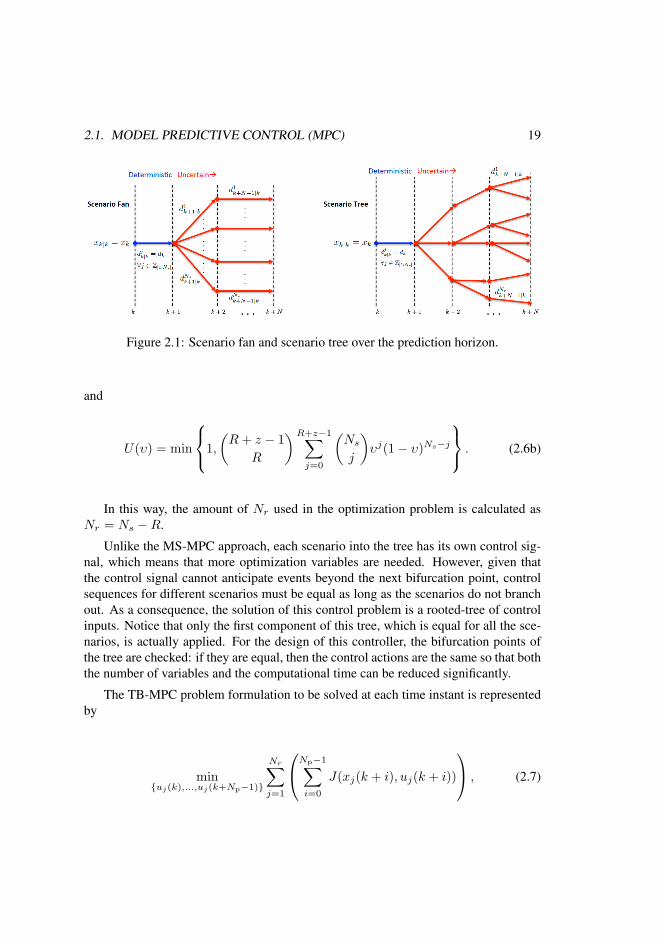
2.1.2 Tree-based MPC (TB-MPC)This technique consists of transforming the different possible evolutions of the distur-bances into a rooted tree that, through its evolution, diverges and generates a reducednumber of scenarios. The points of divergence are called bifurcations and they repre-sent moments in time in which the potential evolution of the disturbances is uncertainenough to consider more than one trajectory, as shown in Figure 2.1. The formula-tion of the control problem involves making tree-based optimization scenarios, whereonly the most relevant disturbance patterns are modeled, starting with a common rootthat corresponds to the current disturbance at each time instant. It must be noted thatTB-MPC formulates the optimization problem by means of Multistage Stochastic Pro-gramming [39, 40]. The number of scenarios used to build the tree should be coherentwith the computational capability of the controller and the risk probability, δx.
Being a scenario-based approach, it is possible to determine δx by taking into ac-count the number of discarded scenarios R from the initial Ns scenarios for any viola-tion level υ ∈ [0, 1], as seen in [37]. The probability of satisfying the state constraintsis given by
P[xi+1 ∈ X ] ≥ 1− δx,
where
δx =
∫ 1
0
U(υ)dυ, (2.6a)
2.1. MODEL PREDICTIVE CONTROL (MPC) 19
Figure 2.1: Scenario fan and scenario tree over the prediction horizon.
and
U(υ) = min
1,
(R+ z − 1
R
)R+z−1∑j=0
(Ns
j
)υj(1− υ)Ns−j
. (2.6b)
In this way, the amount of Nr used in the optimization problem is calculated asNr = Ns −R.
Unlike the MS-MPC approach, each scenario into the tree has its own control sig-nal, which means that more optimization variables are needed. However, given thatthe control signal cannot anticipate events beyond the next bifurcation point, controlsequences for different scenarios must be equal as long as the scenarios do not branchout. As a consequence, the solution of this control problem is a rooted-tree of controlinputs. Notice that only the first component of this tree, which is equal for all the sce-narios, is actually applied. For the design of this controller, the bifurcation points ofthe tree are checked: if they are equal, then the control actions are the same so that boththe number of variables and the computational time can be reduced significantly.
The TB-MPC problem formulation to be solved at each time instant is representedby
min{uj(k),...,uj(k+Np−1)}
Nr∑j=1
Np−1∑i=0
J(xj(k + i), uj(k + i))
, (2.7)

20 STOCHASTIC MPC
subject to
xj(i+ 1) = Axj(i) +Buj(i) +Dωj(i), (2.8a)xj(0) = x(k), (2.8b)ωj(i) = ωj(i), (2.8c)
xj(i+ 1) ∈ X , ∀i ∈ ZNp−10 , (2.8d)
uj(i) ∈ U , ∀j ∈ ZNr1 . (2.8e)
In addition, it is necessary to introduce non-anticipative constraints to force the con-troller to compute the control inputs only considering the observed uncertainty beforethe bifurcation points [40]. These constraints are given by
ui(k) = uj(k) if ωi(k) = ωj(k); ∀ i = j. (2.8f)
One way to satisfy (2.8f) is to introduce equality constraints into the optimizationproblem and solving it with a number of optimization variables defined as z = Np ×Nr × nu. Nevertheless, constraints in (4.19e) can be used to reduce the number ofoptimization variables by removing the redundancy to lower the computational burden.
As said before, a control sequence is optimized for the extended system with adisturbance tree, and only the first component of the input tree is applied to the system.The problem is repeated at each time instant k ∈ Z+.
2.1.3 Chance-Constrained MPC (CC-MPC)Given that disturbances are stochastic, another way of addressing this problem is us-ing CC-MPC. The stochastic behavior from the disturbances can be addressed by for-mulating hard constraints into probabilistic constraints related to a risk of constraintviolation that determines the degree of the conservatism when computing the controlinputs. Also, the cost function is expressed as its expected value in the formulation ofthe optimization problem. A major advantage of this approach is that the computationalburden is not increased as in the scenario-based techniques.
Given that the disturbances in the dynamic model (2.45) are stochastic, the stateconstraints (2.19) must be formulated in a probabilistic manner, i.e.,
P[x(i+ 1) ∈ X | Gx ≤ g] > 1− δx. (2.9)
Here, G ∈ Rnr×nx and g ∈ Rnr . The probabilistic constraints (2.9), also called chanceconstraints, can be written in two different manners [19]:

2.1. MODEL PREDICTIVE CONTROL (MPC) 21
• Individual chance constraints that express a probabilistic equivalent for eachconstraint. They are formulated as
P[G(m)x < g(m)] > 1− δx,m, ∀m ∈ Znx1 , (2.10)
where G(m) and g(m) are the mth row of G and g, respectively. Each mth rowsatisfies its respective δx,m.
• Joint chance constraints, which take into account an unique risk of constraintviolation for all stochastic constraints. They are written as
P[G(m)x < g(m), ∀m ∈ Znx1 ] > 1− δx. (2.11)
All rows jointly satisfy the unique δx.
The application of (2.11) along Np is necessary to implement the controller. To thisend, it is assumed that the disturbances behave as Gaussian random variables, with aknown cumulative distribution function. The deterministic equivalent of these chanceconstraints can be formulated as follows:
P[G(m)x(k + 1) < g(m)] > 1− δx
⇔ FG(m)Dω(k)(g(m) −G(m)(Ax(k) +Bu(k))) > 1− δx
⇔ G(m)(Ax(k) +Bu(k)) < g(m) − F−1G(m)Dω(k)(1− δx). (2.12)
Here, FG(m)Dω(k)(·) represents the cumulative distribution function of the randomvariable G(m)Dω(k), and F−1
G(m)Dω(k)(·) is its inverse cumulative distribution function.Note that the expression (2.12) is the deterministic equivalent of the chance con-
straints and is built based on historical data.The optimization problem formulation related to the design of the CC-MPC con-
troller is stated as
min{u(k),...,u(k+Np−1)}
Np−1∑i=0
E[J(x(k + i), u(k + i))], (2.13)
subject to
x(i+ 1) = Ax(i) +Bu(i) +Dω(i), (2.14a)x(0) = x(k), (2.14b)ω(i) = ω(i), (2.14c)
G(m)(Ax(k) +Bu(k)) < g(m) − F−1G(m)Dω(k)(1− δx), (2.14d)
u(i) ∈ U , ∀i ∈ ZNp−11 , (2.14e)
22 STOCHASTIC MPC
where E[·] denotes the expected value of the cost function.
2.2 Case Study: A Hydrogen-based MicrogridA microgrid is a network of electric generators that may take advantage of several re-newable energy sources: solar panels, wind mini-generators, micro-turbines, fuel cells,among others, to meet the consumer demand by working together with the centralizedgrid or autonomously [41]. In a microgrid, the energy is generated only at certain times,being necessary to provide continuous service to meet the demand at any time of theday. Challenges arise from the natural intermittency of renewable energy sources andthe requirements to satisfy the user energy demand [42]. Thereby, storage devices be-come very important in the operation of this type of systems. Among well-establishedenergy storage technologies, there are batteries, super-capacitors, conventional capaci-tors, etc. In this case study, the use of hydrogen as an energy vector for energy storageis focussed. Hydrogen, combined with other renewable energy sources, is a safe andviable option to mitigate the problems associated with hydrocarbon combustion be-cause the entire system can be developed as an efficient, clean, and sustainable energysource, as mentioned in [43]. The hydrogen is converted into electrical energy by usingfuel cells; the reverse process, i.e., the transformation of electric energy into hydrogen,is conducted by electrolysis [44], or ethanol reforming [45], among other techniques.
The control problem in a microgrid is to satisfy the electricity demand under eco-nomical and optimal conditions despite the uncertainties and disturbances that mightappear in the processes. Taking into account that there are mathematical models avail-able that represent the main dynamics and the load of these systems [46], and that thecontrol problem here requires the simultaneous handling of constraints, delays, anddisturbances, model predictive control (MPC) emerges as a solution to this problem. Inthis, sense, uncertainty in the load and generation profiles has been mainly addressedindirectly in the dispatch problem by using the MPC approach [47].
2.2.1 Hydrogen-based Microgrid Description
The microgrid under study is the lab-scale microgrid called HyLab [48]. The microgridtest bench used in this study is an experimental platform specifically designed for test-ing control strategies. HyLab is composed of a modular system equipped with variouscomponents that allow experimentation and simulation of several types of renewableenergy sources. In the Figure 2.2, a picture of the experimental Hylab platform isshown.
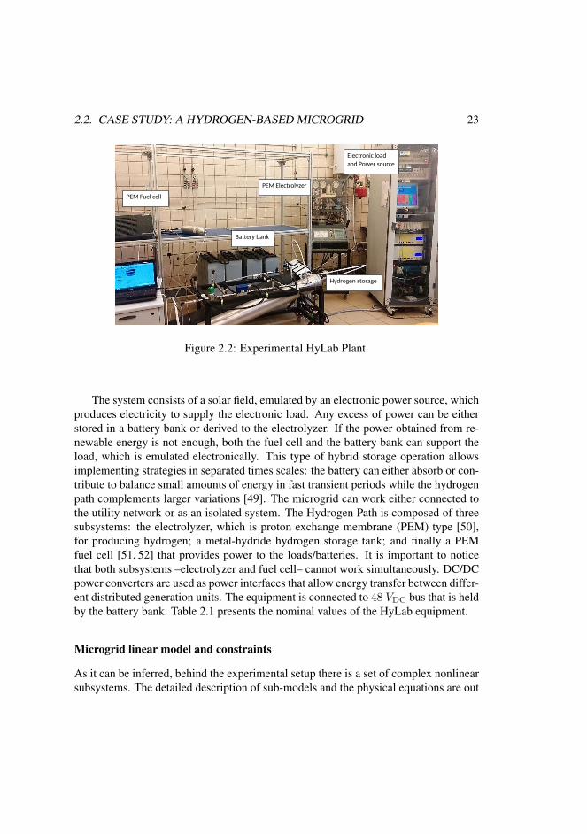
2.2. CASE STUDY: A HYDROGEN-BASED MICROGRID 23
PEM Electrolyzer
PEM Fuel cell
Battery bank
Hydrogen storage
Electronic load
and Power source
Figure 2.2: Experimental HyLab Plant.
The system consists of a solar field, emulated by an electronic power source, whichproduces electricity to supply the electronic load. Any excess of power can be eitherstored in a battery bank or derived to the electrolyzer. If the power obtained from re-newable energy is not enough, both the fuel cell and the battery bank can support theload, which is emulated electronically. This type of hybrid storage operation allowsimplementing strategies in separated times scales: the battery can either absorb or con-tribute to balance small amounts of energy in fast transient periods while the hydrogenpath complements larger variations [49]. The microgrid can work either connected tothe utility network or as an isolated system. The Hydrogen Path is composed of threesubsystems: the electrolyzer, which is proton exchange membrane (PEM) type [50],for producing hydrogen; a metal-hydride hydrogen storage tank; and finally a PEMfuel cell [51, 52] that provides power to the loads/batteries. It is important to noticethat both subsystems –electrolyzer and fuel cell– cannot work simultaneously. DC/DCpower converters are used as power interfaces that allow energy transfer between differ-ent distributed generation units. The equipment is connected to 48 VDC bus that is heldby the battery bank. Table 2.1 presents the nominal values of the HyLab equipment.
Microgrid linear model and constraints
As it can be inferred, behind the experimental setup there is a set of complex nonlinearsubsystems. The detailed description of sub-models and the physical equations are out

24 STOCHASTIC MPC
Table 2.1: HyLab equipment.
Equipment Nominal Value
Electronic power source 6 kWElectronic load source 2.5 kWPEM fuel cell 1.2 kWPEM electrolyzer 0.23Nm3h−1 @5barg
1 kWMetal hydrides tank 7Nm3
5 barBattery bank C120 = 367AhDC/DC converters 1.5 kW, 1 kW
of the scope of this work. The complete non-linear model of the plant, its simulation,and validation are presented in [53].
Remark 1 To apply linear MPC techniques is required to find a linear model of thesystem around a working point (x∗, u∗). The identification process for obtaining thelinear model of the plant is developed in [54]. The continuous linear system was dis-cretized using Tustin’s method with a sampling time of 30 s. Also, the working point isgiven by u∗ = [0 kW, 1.75 kW]T and x∗ = [50%, 50%]T .
The linear discrete-time model of the plant consists of two input variables, PH2(k)
and Pgrid(k), which are measured in kilowatts (kW). Here, PH2(k) represents thepower of the electrolyzer and the power of the fuel cell: when it is greater than zero, thePEM fuel cell is working (Pfc(k)), and when PH2(k) is negative, it indicates that theelectrolyzer is operating (Pez(k)). Both the electronic load and the electronic powersource can either deliver or absorb power from the utility power grid (UPG). The con-nection with the electric network is “virtual”, since it is emulated by the source andelectronic load. Moreover, Pgrid(k) represents the power of UPG, which is positivewhen the power is imported by the microgrid from the UPG, and it is negative whenexporting power to the UPG. The system is subject to uncertainties from the powerproduced by a renewable energy source; in this case, it is the power from the solarfield, (Pres(k)) and the power demanded by the consumers (Pdem(k)); the differencebetween them can be considered as disturbances (Pnet(k)) to the system. Moreover,the plant counts with an additional variable, the power of the batteries (Pbatt), which is
2.2. CASE STUDY: A HYDROGEN-BASED MICROGRID 25
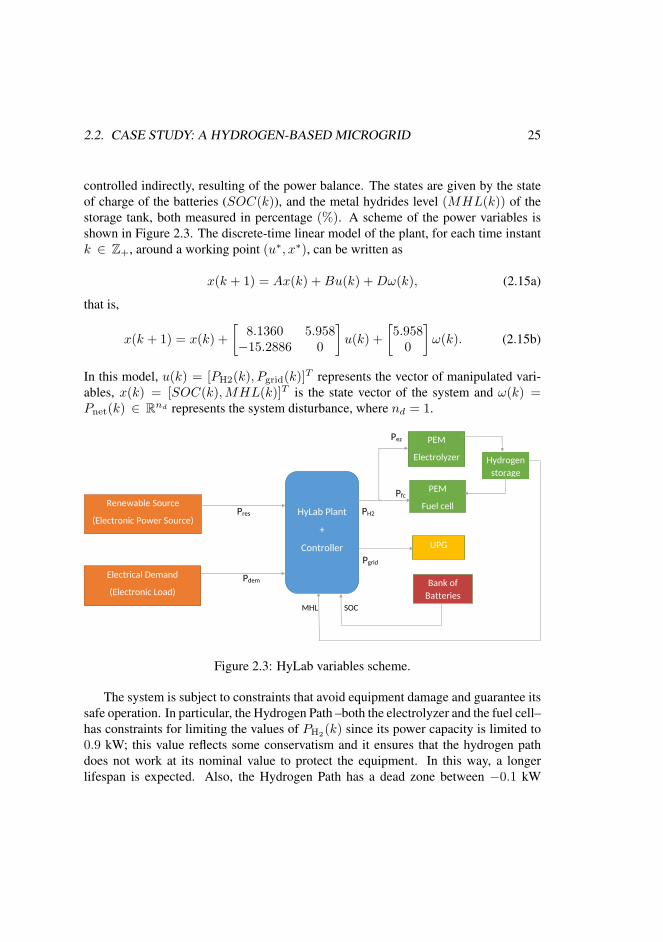
controlled indirectly, resulting of the power balance. The states are given by the stateof charge of the batteries (SOC(k)), and the metal hydrides level (MHL(k)) of thestorage tank, both measured in percentage (%). A scheme of the power variables isshown in Figure 2.3. The discrete-time linear model of the plant, for each time instantk ∈ Z+, around a working point (u∗, x∗), can be written as
x(k + 1) = Ax(k) +Bu(k) +Dω(k), (2.15a)
that is,
x(k + 1) = x(k) +
[8.1360 5.958
−15.2886 0
]u(k) +
[5.9580
]ω(k). (2.15b)
In this model, u(k) = [PH2(k), Pgrid(k)]T represents the vector of manipulated vari-
ables, x(k) = [SOC(k),MHL(k)]T is the state vector of the system and ω(k) =Pnet(k) ∈ Rnd represents the system disturbance, where nd = 1.
Pez
Pfc
Pres PH2
Pgrid
Pdem
MHL SOC
HyLab Plant
+
Controller
Renewable Source
(Electronic Power Source)
Electrical Demand
(Electronic Load)
PEM
Electrolyzer
PEM
Fuel cell
Hydrogen
storage
UPG
Bank of
Batteries
Figure 2.3: HyLab variables scheme.
The system is subject to constraints that avoid equipment damage and guarantee itssafe operation. In particular, the Hydrogen Path –both the electrolyzer and the fuel cell–has constraints for limiting the values of PH2(k) since its power capacity is limited to0.9 kW; this value reflects some conservatism and it ensures that the hydrogen pathdoes not work at its nominal value to protect the equipment. In this way, a longerlifespan is expected. Also, the Hydrogen Path has a dead zone between −0.1 kW

26 STOCHASTIC MPC
and 0.1 kW that ensures a minimum production of power from both the electrolyzerand the fuel cell. The constraints for Pgrid(k) correspond to physical limitations of theelectronic units. Furthermore, it is necessary to include constraints on their incrementalsignals ∆PH2(k) and ∆Pgrid(k), to guarantee the physical safety of the equipment.These constraints are mathematically expressed as follows:
− 0.9 kW ≤ PH2(k) ≤ 0.9 kW, (2.16a)− 2.5 kW ≤ Pgrid(k) ≤ 2 kW, (2.16b)
− 20Ws−1 ≤ ∆PH2(k) ≤ 20Ws−1, (2.16c)
− 2.5 kWs−1 ≤ ∆Pgrid(k) ≤ 2 kWs−1. (2.16d)
Overall constraints have to be considered as hard constraints, since the equipmentlifespan could be drastically reduced. Both the battery bank and the metal hydridesstorage tank have limited capacity to prevent any plant damage by overcharge or un-dercharge. Constraints on SOC(k) guarantee suitable voltage levels in the 48 VDC
bus. Also, they protect the battery bank of strong load voltage variations. These stateconstraints are written as
40% ≤ SOC(k) ≤ 90%, (2.17a)10% ≤ MHL(k) ≤ 90%. (2.17b)
The input constraints given by (2.16) can be properly rewritten as
u(k) ∈ U ⊆ Rnu , (2.18)
with nu = 2, while the state constraints defined by (2.17) are expressed as
x(k) ∈ X ⊆ Rnx , (2.19)
with nx = 2. Furthermore, the total power delivered to the load, in order to satisfy theconsumer demand, must satisfy the energy balance
Pdem(k) = PH2(k)− Pbatt(k) + Pgrid(k) + Pres(k). (2.20)
The multi-objective cost function to be minimized is given by
J(x(k), u(k)) = a1(SOC(k)− SOCref)2
+ a2(MHL(k)−MHLref)2 (2.21)
+ b1P2H2
(k) + b2P2grid(k).
2.2. CASE STUDY: A HYDROGEN-BASED MICROGRID 27
Here, SOCref = 65% and MHLref = 40% are the references given for the stateof charge of the batteries and the metal hydride level, respectively. The tuning ofthe cost function weights seeks for a soft tracking of the output variables towards thegiven references and an efficient use of the energy. More specifically, the controller isdesigned such that the batteries are the first way of energy storage. If there exists a bigdifference between the demanded energy and the produced energy by the renewablesources, it proceeds to the production of hydrogen. These prioritization weights ai, bihave been adjusted by trial and error approach carried out on simulation tests reportedin previous works with this plant, see, e.g. [44, 54, 55]. In this sense, they have beenestablished as a1 = a2 = 10, b1 = 5000, and b2 = 8000. As can be seen, the weightassociated with the hydrogen production is lower than the weight related to the powerof the grid in order to minimize the power interchange with the UPG. The weightsassociated with the outputs take low values compared with the others to give flexibilityto the smart grid. However, these values can be modified in the multi-objective function(4.4) for tracking the reference. In this work, the energy management is the mainobjective, therefore the weights associated with the hydrogen path and the grid arehigher than those associated with the outputs of the system.
2.2.2 Results and Discussion
The experiments were conducted in the microgrid described in Section 2.2.1 during atrial period of eight hours for each experiment. The controller receives the measuredvariables SOC(k) and MHL(k), which are used to compute the optimal control sig-nals PH2(k) and Pgrid(k)) by means of Simulink Real-Time workshop toolbox. Thecontrol signals are sent to the SCADA via the OPC Matlab Library and finally the PLCcarries out these control actions.
The prediction horizon was Np = 5 and the sampling time was 30 s. The selectedweather and load profiles for verifying the performance of the three proposed con-trollers were the scaled difference between the real solar generation and the demandregistered by the Spanish National Electricity Network (SNEN)1 on May 23, 2014.These values were sampled each 3 s and scaled for the microgrid allowable power val-ues, which are shown in Figure 2.4(a). The initial conditions for all experiments wereSOC(0) = 70% and MHL(0) = 50%.
An issue that deserves particular attention is the amount of scenarios to be con-sidered into the optimization problem. This number should be selected by taking intoaccount a trade-off between robustness and computational burden. In this sense, it ispossible to establish the number of scenarios that guarantees a particular risk level,
1SNEN demand data can be obtained at: https://demanda.ree.es/movil/peninsula/demanda/total
28 STOCHASTIC MPC
according to (2.5), as shown Table 2.2.
Table 2.2: Number of scenarios (Ns) that fulfills an specific risk level (δx).
δx 0.20 0.15 0.10 0.05 0.01Ns 152 203 316 611 3005
MS-MPC was performed by using the electricity demand and the solar generationregistered during Ns = 316 different days of one year from historical data, obtainedfrom the SNEN. For these scenarios, it is expected a risk of violation of constraintsless than δx ≤ 10%. This number of scenarios offers an acceptable risk and ensuresa reasonable computational burden when solving the optimization problem. Further-more, this set of scenarios considers days with enough solar energy generation as wellas cloudy days, which makes the controllers more robust and somehow relieves theneed for increasing the number of scenarios used. TB-MPC was performed by usingan original number of Ns = 316 scenarios, which were reduced to Nr = 250 scenariosforming a tree using GAMS [56]. This reduction tried to replicate the main dynamicsof all original disturbances considered in a small disturbance tree. This reduction in-troduces a boundary that guarantees δx ≤ 10%, according to (2.6). Finally, CC-MPCapproach was performed considering the failure probability δx = 10%. The distur-bances were considered as a random function with a cumulative distribution function(cdf), which were obtained from the historical daily data registered in 2014.
The scheme of the microgrid operation, from a general point of view, follows simi-lar patterns for the three proposed controllers. At this point, given that the energy fromthe renewable source is not sufficient to meet the energy demand, the fuel cell turns on,the battery SOC and the MHL decrease gradually without going below their forbid-den levels. Also, energy is imported from the grid to meet the load beyond demand.When the energy from the renewable source greatly exceeds demand, the electrolyzeris switched on, the batteries are fully charged, and the excess of energy is stored in thehydrogen tank, and the remaining power that cannot be stored in the form of hydro-gen is exported to the grid. However, each stochastic MPC approach shows particulardifferences, as reported below, which are highlighted to offer a suitable comparisonamong them.
In order to compare all the considered strategies, Figure 2.4(b) shows the batterypower for the three aforementioned stochastic predictive controllers. As can be noticed,CC-MPC controller performs a deep cycle using the batteries. It strives for using thefull capacity, reaching the upper and lower levels. In contrast, TB-MPC controller,

2.2. CASE STUDY: A HYDROGEN-BASED MICROGRID 29
although partly discharges and recharges the batteries, it does in a softer way. Thisimplies that the excess of energy must be balanced through either the electrolyzer or thegrid. It is observed that MS-MPC technique behaves between the two other approaches.Therefore, MS-MPC controller achieves a trade-off between using the full capacity ofthe batteries and the energy derived either to the electrolyzer or the grid.
Figure 2.4(c) presents the fuel cell and electrolyzer power along the test duration.The fuel cell performance signals obtained are similar for all the three controllers, ex-cept for CC-MPC controller, which shows a peak between the first and second hour, tosatisfy an increase in the energy demand at that time. When there is an excess of energyfrom the renewable source, the electrolyzer starts its operation. Results show a cleardifference in the electrolyzer operation. On the one hand, with CC-MPC technique, theelectrolyzer presents a larger use of the power, as expected. On the contrary, the elec-trolyzer utilization is restricted quite more with TB-MPC approach, reaching only apeak of 200 W, while CC-MPC controller sets the electrolyzer power to nearly 600 W.Regarding TB-MPC approach, it also shows a small ripple; this is explained becausethe controller seeks to primary satisfy the demand and compensate any power unbal-ance in the system. As it has been shown through experimental tests, there are cleardifferences in the way each controller manages the power signals of the electrolyzerand the fuel cell.
Figure 2.4(d) shows the grid power signal generated by applying the stochasticMPC controllers. From the point of view of the network operators (DSO2/TSO3), theuse of the UPG is minimized with the CC-MPC approach. In this manner, the impactin the electrical system generated by the renewable sources present in the microgrid isreduced. On the other hand, for the consumer point of view, it might be convenient notto force the equipment to a deep duty cycle and take advantage of the grid to smooththe power profiles.
Figure 2.4(e) shows the evolution of the SOC and MHL for each proposed con-trollers along the test period. In general, for all the implemented controllers, the bat-teries are discharged until the fuel cell turns off at the first time, and then they raisetheir charge level lower than 85% for MS-MPC and CC-MPC controllers. RegardingTB-MPC controller, it holds a charge level around 75% for a longer period comparedwith the other ones. Then, the SOC starts to decrease again for all controllers understudy. The MHL presents a minor variation, and it reduces its level below 40% untilthe renewable source can contribute with power to the load. After this, the MHL seeksto track its reference.
2DSO: Distributed System Operator3TSO: Transmission System Operator

30 STOCHASTIC MPC
(a) Energy generated by solar panels Pres, demand of energy
Pden, and Pnet corresponding to May 23, 2014.
(b) Battery power.
(c) Fuel cell power and Electrolyzer power. (d) Grid power.
(e) Battery SOC and MHL. (f) Electric power provided by the microgrid compared with the
consumer demand.
Figure 2.4: Experimental results applying the proposed stochastic MPC approaches.
Figure 2.4(f) shows the comparison among the different powers delivered to theload by applying the controllers. As seen, the demand is satisfied by the power fromthe microgrid for all the controllers as imposed in their design. Notice that, in somesituations, using the “elasticity” of the consumer; it might be possible to momentarily

2.2. CASE STUDY: A HYDROGEN-BASED MICROGRID 31
unbalance the power demand to satisfy other microgrid objectives [57]. Nevertheless,demand response is out of the scope of this work.
In order to quantitatively assess the performances of these three stochastic ap-proaches that have been implemented in the HyLab microgrid laboratory, several KPIshave been defined as follows:
• KPI1 defines the final cumulative cost given by (4.4) (in cost units).
• KPI2 is the computational time to solve the optimization problem (in s).
• KPI3 counts the average unmet demand with respect to the overall power demand(in %).
• KPI4 is the time that the fuel cell is operating (in hours).
• KPI5 is the time that the electrolyzer is operating (in hours).
• KPI6 indicates the final value of SOC (in %).
• KPI7 indicates the final value of MHL (in %).
Table 3 summarizes the numerical results of the KPIs. As it can be seen the highestvalue for KPI1 is obtained when using MS-MPC. The rationale behind this value isthat the controller optimizes a sequence of control actions valid for the most favorablescenarios as well as the least favorable ones. In this sense, an over-conservative controlaction is carried out. This issue can be relaxed by calculating a tree of control actionsthat is subject to non-anticipatory equality constraints. In this way, the control actionsare calculated in a closed-loop fashion, i.e., the controller can adapt the future controlactions to the evolution of the disturbances. As can be seen, TB-MPC reduces its cumu-lative cost by increasing the number of control variables involved into the optimizationproblem. Hence, its computational time is the biggest within this comparative study.Regarding CC-MPC, it has the lowest cumulative cost without increasing the numberof control variables. For reference purposes, the final cumulative cost for an MPC witha perfect forecast (PF-MPC), obtained via simulation, is 2.05 × 10¹². The computa-tional time comparison is provided by KPI2.
The three tested controllers are able to meet the overall demand in a satisfactoryway, as indicated by the performance comparison given by KPI3. At this point, wemust remark that the three tested controllers solve their optimization problems fasterthan the sampling time. Therefore, it is possible to select the approach that has the bestperformance in terms of the demand satisfaction and the use of the hydrogen path.

32 STOCHASTIC MPC
Table 2.3: Comparison of the MS-MPC, TB-MPC, and CC-MPC controllers appliedto HyLab microgrid by means of KPIi, i = 1, ..., 7.
Controller KPI1 KPI2 KPI3 KPI4 KPI5 KPI6 KPI7(cost units) (s) (%) (hours) (hours) (%) (%)
MS-MPC 3.89× 10¹² 7.76 0.12 3.26 2.90 63.53 42.91TB-MPC 2.75× 10¹² 18.15 0.11 2.63 2.45 62.51 41.58CC-MPC 2.44× 10¹² 1.04 0 3.70 2.97 63.71 43.85
The comparisons between the proposed controllers regarding the time when boththe fuel cell and the electrolyzer are operating are given by KPI4 and KPI5, respectively.In this sense, TB-MPC shows the lowest time for the fuel cell and the electrolyzer. Itoffers a larger conservatism when working with the hydrogen path, which is obtainedat the expense of a higher computational time since TB-MPC meets the current demandand reformulates its disturbance tree at each time step. Notice that the main differenceis at the time that the hydrogen path is working.
The final values of SOC and MHL, which present similar values for the threecontrollers, are around 63% and 42%, respectively. These values are provided by KPI6and KPI7.
Table 2.4 presents a comparison among the total energy produced by the fuel cell(Efc), the electrolyzer (Eez), the batteries (Ebatt), and the grid (Egrid) during the testperiod. The negative sign in Egrid indicates that the amount of energy sold to UPGis greater than the energy purchased. The total energy of the batteries indicates thedifference between the stored energy and the delivered energy to the load: the negativevalue means that the stored energy predominates over the delivered energy.
Table 2.4: Energy produced by the fuel cell, electrolyzer, batteries, and grid during thetest period by applying the proposed stochastic MPC controllers.
Controller Efc Eez Ebatt Egrid
(Wh) (Wh) (Wh) (Wh)MS-MPC 302 481 −62.2 −418TB-MPC 261 217 −110.23 −661CC-MPC 348 642 −43.09 −268
2.2. CASE STUDY: A HYDROGEN-BASED MICROGRID 33
Notice that the absolute value of the energy amounts are taken to achieve a reliablecomparison in terms of energy consumption for each component of the system. Inthis sense, CC-MPC has better performance regarding energy efficiency. CC-MPCachieves less exchange with UPG, and the batteries provide enough power to supplythe load. Also, both the fuel cell and electrolyzer use energy in a wider range whencompared to the MS-MPC and TB-MPC approaches. Note also that TB-MPC and MS-MPC handled more cautiously hydrogen energy from the path while performing moreexchanges with the UPG, specially TB-MPC.
Another KPI to compare the performance of the controllers for energy managementin a smartgrid is the number of start-ups for both equipment, the fuel cell and theelectrolyzer. From the results obtained from the experimental setup, the number ofstart-ups is the same for all the controllers. However, it is a major factor that couldreduce the lifespan of the hydrogen path.
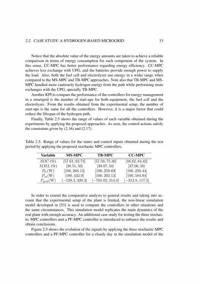
Finally, Table 2.5 shows the range of values of each variable obtained during theexperiments by applying the proposed approaches. As seen, the control actions satisfythe constraints given by (2.16) and (2.17).
Table 2.5: Range of values for the states and control inputs obtained during the testperiod by applying the proposed stochastic MPC controllers.
Variable MS-MPC TB-MPC CC-MPCSOC (%) [57.61, 83.73] [57.59, 75.30] [48.82, 84.42]MHL (%) [38.51, 50] [39.07, 50] [37.06, 50]Pfc(W) [100, 268.13] [100, 259.69] [100, 250.44]Pez(W) [100, 432.9] [100, 202.13] [100, 584.94]Pgrid(W) [−529.4, 320.3] [−705.02, 314.0] [−312.8, 117.5]
In order to extend the comparative analysis to general results and taking into ac-count that the experimental setup of the plant is limited, the non-linear simulationmodel developed in [53] is used to compare the controllers in other situations andthe same circumstances. This simulation model replicates the main dynamics of thereal plant with enough accuracy. An additional case study for testing the three stochas-tic MPC controllers and a PF-MPC controller is introduced to enhance the results andobtain conclusions.
Figure 2.5 shows the evolution of the signals by applying the three stochastic MPCcontrollers and a PF-MPC controller for a cloudy day in the simulation model of the

34 STOCHASTIC MPC
HyLab microgrid. All controllers present the same evolution to satisfy the demand.The fuel cells are turned on when the power from the renewable sources is not enoughto meet the electric demand. Hence, SOC and MHL decrease gradually to supplypower to the load. For this particular day, the microgrid imports energy power fromthe UPG. Given that the excess of renewable energy production over the demand is notenough, the batteries are charged, and the electrolyzer stays off.
To compare the behavior of these MPC controllers, Table 2.6 shows the results fromaforementioned KPIs. The results obtained from the comparison are similar to the pre-vious experimental case study. As expected, the lowest value of KPI1 is presented bystandard MPC controller with perfect information; this value gives a target for the com-parison. In this sense, CC-MPC controller results in a lower cumulative cost as well asthe computational time compared with MS-MPC and TB-MPC controllers. The elec-trical demand is satisfied by all controllers. Regarding KPI3, MS-MPC controller usesthe hydrogen path longer than the other two approaches. Finally, KPI6 shows very sim-ilar values for all controllers, the battery SOC is reduced until its lower constrainedlevel. The lowest value of KPI7 is presented by CC-MPC controller because this con-troller delivers a bigger amount of energy from the fuel cell. Finally, the electrolyzerstays off over the simulation period; therefore KPI5 is zero for all controllers.
Table 2.6: Comparison of the MS-MPC, TB-MPC, CC-MPC, and PF-MPC controllersapplied to the simulation model of HyLab microgrid for a cloudy day by means ofKPIi, i = 1, ..., 7.
Controller KPI1 KPI2 KPI3 KPI4 KPI6 KPI7(cost units) (s) (%) (hours) (%) (%)
MS-MPC 6.24× 10¹² 7.76 0.10 6.00 40.56 20.43TB-MPC 5.33× 10¹² 18.20 0.11 5.67 40.64 23.46CC-MPC 4.22× 10¹² 1.04 0.10 5.68 40.46 14.08PF-MPC 4.05× 10¹² 0.98 0 5.90 40.01 19.77
Table 2.7 compares the stochastic MPC controllers regarding energy for a cloudyday via simulation. The CC-MPC controller results in higher energy consumption fromthe fuel cell. The energy from the renewable sources is not enough at the time to turnon the electrolyzer for storing energy as hydrogen. The batteries are used to provideenergy to the load; both, MS-MPC and TB-MPC controllers, show a similar use of theenergy of the batteries. A remarkable difference is shown in the energy exchanged with
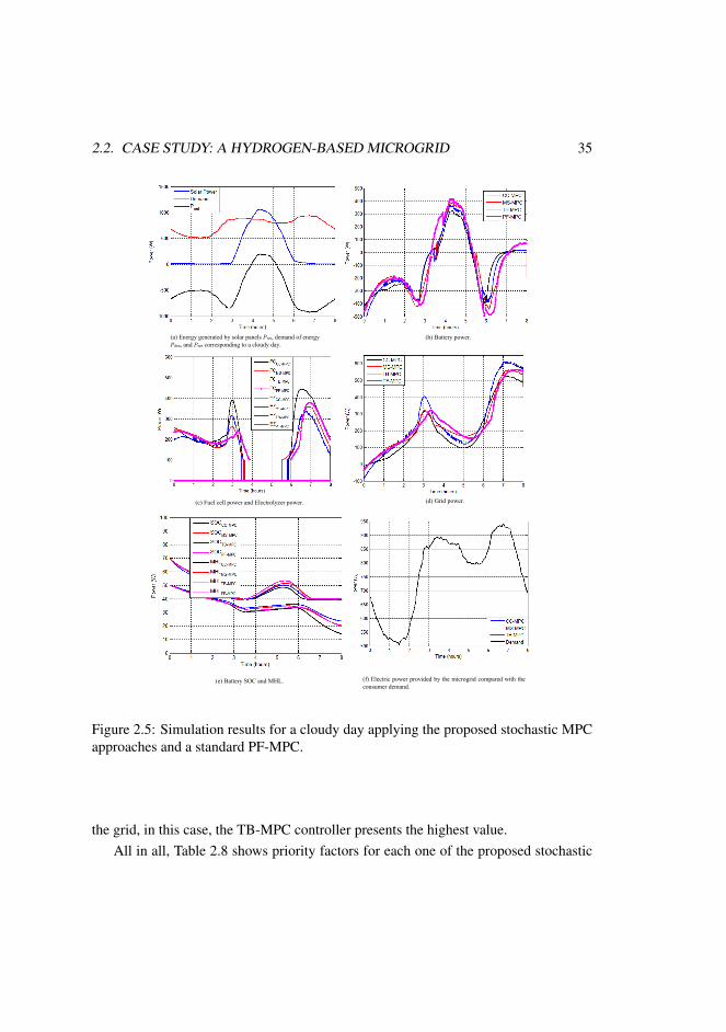
2.2. CASE STUDY: A HYDROGEN-BASED MICROGRID 35
(a) Energy generated by solar panels Pres, demand of energy
Pden, and Pnet corresponding to a cloudy day.
(b) Battery power.
(c) Fuel cell power and Electrolyzer power.
(e) Battery SOC and MHL. (f) Electric power provided by the microgrid compared with the
consumer demand.
(d) Grid power.
Figure 2.5: Simulation results for a cloudy day applying the proposed stochastic MPCapproaches and a standard PF-MPC.
the grid, in this case, the TB-MPC controller presents the highest value.All in all, Table 2.8 shows priority factors for each one of the proposed stochastic

36 STOCHASTIC MPC
Table 2.7: Energy produced by the fuel cell, electrolyzer, batteries, and grid duringthe test period for the simulation model by applying the proposed stochastic MPCcontrollers.
Controller Efc Eez Ebatt Egrid
(Wh) (Wh) (Wh) (Wh)MS-MPC 472 0 −285 688TB-MPC 437 0 −287 721CC-MPC 547 0 −295 604
Table 2.8: Priority factors for selecting one of the proposed stochastic MPC controllers.
Priority MS-MPC TB-MPC CC-MPCMaximization of hydrogen path lifespan XMinimization of energy exchanged with the UPG XCumulative cost XComputational burden XDemand satisfaction X X XAvailability of historical data X X
MPC controllers based on the overall analysis at the time of selecting one of them.Other factors that are important to take into account are the initial conditions for
SOC and MHL. These values will determine the evolution of the variables. Besides,the final value of these variables will take an additional meaning of comparison after alonger time of use of the plant. However, they have been employed in a smaller periodto show how they finish after the experiments.
These results have been published in [31].
2.3 Case study: Drinking Water NetworkDrinking water networks (DWNs) transport water from sources to consumers ensur-ing the quality of service [58]. Nevertheless, limited water sources, conservation andsustainability policies, as well as the infrastructure complexity for meeting consumerdemands with appropriate flow pressure and quality levels make water management achallenging problem [1]. Water demand forecasting based on historical data is com-

2.3. CASE STUDY: DRINKING WATER NETWORK 37
monly used for the operational control of water supply along a given prediction horizon.However, the optimality of such scheduling is affected by the one associated to waterdemand forecasts. Therefore, the scheduling of control inputs must be continuouslyadjusted. This leads to consider the DWNs as dynamical systems and their operationas optimal control problems, with the objective of satisfying water demands in an op-timal manner despite the presence of disturbances and uncertainties, and consideringadditionally issues such as constraints on the manipulated and output variables andmultiple conflicting control goals.
The MPC approaches presented in this work are assessed with two representativecase studies based on the Barcelona DWN.
A DWN must satisfy water demands and guarantee service reliability by makingoptimal use of water sources and network components in order to minimize economiccosts. The water network operates as a full-interconnected system driven by endoge-nous and exogenous flow demands. In the Barcelona DWN, water is taken from bothsuperficial and underground sources. Flows coming from sources are regulated bypumps or valves. After being extracted from sources, water is purified up to levelssuitable for human consumption in four water treatment plants (WTP). The water flowfrom any of the sources is limited and has costs associated to the extraction and thetreatment required. The DWN is divided in two management layers: the transport net-work, which links the water treatment plants with the reservoirs located all over the city,and the distribution network, which is sectored in sub-networks, linking reservoirs di-rectly to consumers. In this work, each sector of the distribution network is consideredas a pooled demand to be satisfied by the transport network.
The two systems under study have been extracted from the Barcelona transportnetwork. The first case study consists in a sector model and the second one is anaggregate model of the whole network. They differ mainly in the size of the networkflow problems and the number of constitutive elements:
• The sector network considers only a small-scale subsystem related to a portionof the overall DWN (see Fig. 2.6). This case study considers 2 water sources, 3tanks, 6 flows controlled by valves and pumps, 4 demand nodes and 2 intersec-tion nodes.
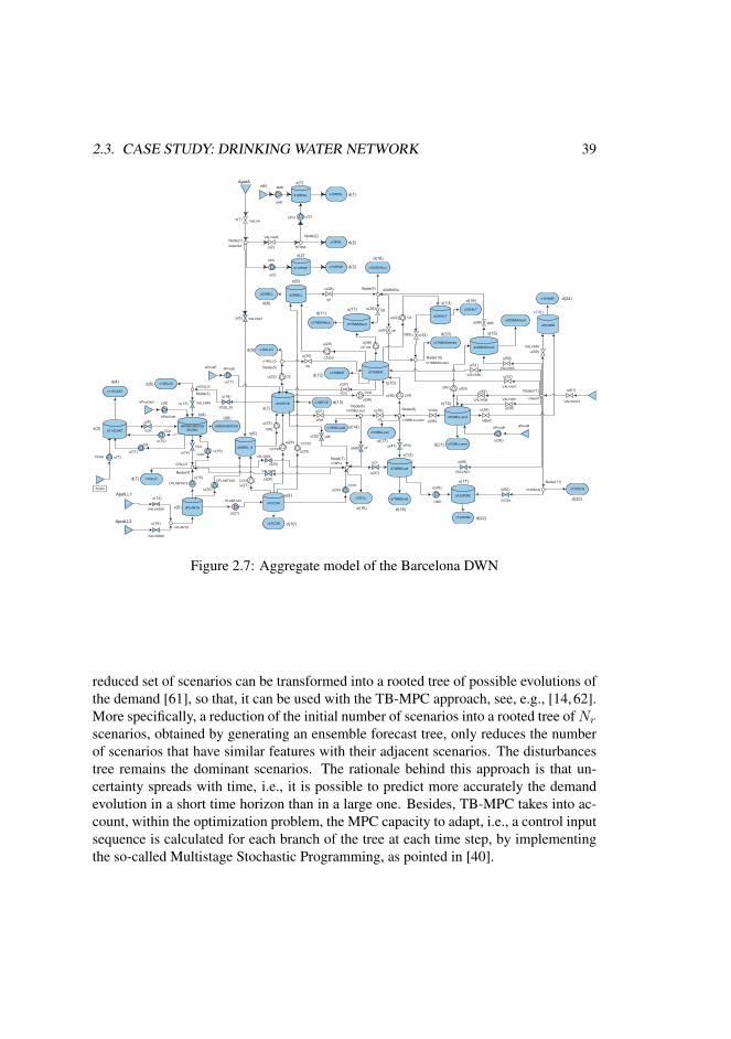
• The aggregate network represents a simplification from the original DWN, wheresets of elements are aggregated in a single element in order to reduce the size ofthe original model (see Fig. 2.7). It consists of 9 water sources, 17 tanks, 61flows controlled by valves and pumps, 25 demand nodes and 11 intersectionnodes.

38 STOCHASTIC MPC
Figure 2.6: Sector diagram of the Barcelona DWN
Demand Modelling and Scenario Generation
In DWNs, the uncertainty is generally introduced by the stochastic behavior of waterconsumers. Therefore, a proper demand modeling is required to achieve an acceptablewater supply service level. For the case studies of this work, time series forecastingbased on auto-regressive integrated moving average (ARIMA) models are used due toits ability to capture complex linear dynamics from historical data [59]. In this way,it is possible to generate artificial scenarios with similar statistical properties to thoseobtained from historical data.
A correct sampling of scenarios is essential for developing the proposed SMPCapproaches. For the CC-MPC approach, ARIMA models are used to generate a largenumber of possible demand scenarios by Monte Carlo sampling for a given time hori-zon Np ∈ Z+; the mean demand is then used for the controller design. For theMS-MPC approach, a set of Ns ∈ Z+ water demand scenarios is generated and used.Increasing the number of scenarios allows the controller to gain robustness but at theexpense of additional computational effort and economic performance losses. MS-MPC is generally over-conservative, because it does not consider the controller capac-ity to adapt to the new observations of the uncertainty and reformulate its controllerstructure at each time instant. To cope with this drawback, a representative subset ofscenarios might be chosen using scenario reduction algorithms [39, 60]. Moreover, the
2.3. CASE STUDY: DRINKING WATER NETWORK 39
Figure 2.7: Aggregate model of the Barcelona DWN
reduced set of scenarios can be transformed into a rooted tree of possible evolutions ofthe demand [61], so that, it can be used with the TB-MPC approach, see, e.g., [14,62].More specifically, a reduction of the initial number of scenarios into a rooted tree of Nr
scenarios, obtained by generating an ensemble forecast tree, only reduces the numberof scenarios that have similar features with their adjacent scenarios. The disturbancestree remains the dominant scenarios. The rationale behind this approach is that un-certainty spreads with time, i.e., it is possible to predict more accurately the demandevolution in a short time horizon than in a large one. Besides, TB-MPC takes into ac-count, within the optimization problem, the MPC capacity to adapt, i.e., a control inputsequence is calculated for each branch of the tree at each time step, by implementingthe so-called Multistage Stochastic Programming, as pointed in [40].

40 STOCHASTIC MPC
2.3.1 DWN Control Problem StatementThis section introduces the CE-MPC formulation, including the system defined bytime-invariant state-space linear model in discrete time, its goals and constraints.
Control-oriented Model
The system model may be described considering the volume of water in tanks as thestate variables x ∈ Rn, the flow through the actuators as the manipulated inputs u ∈Rm, and the demanded flows as additive measured disturbances d ∈ Rp. The control-oriented model of the network is described by the following equations for all timeinstant k ∈ Z+:
xk+1 = Axk +Buk +Bpdk, (2.22a)0 = Euuk + Eddk, (2.22b)
where (2.22a) and (2.22b) describe the mass balance equations for storage tanks and in-tersection nodes, respectively. Moreover, A ∈ Rnx×nx , B ∈ Rnx×nu , Bp ∈ Rnx×nd ,Eu ∈ Rnq×nu and Ed ∈ Rnq×nd , are time-invariant matrices dictated by the networktopology.
Assumption 1 The states in x and the demands in d are measured at any time instantk ∈ Z+.
Assumption 2 The pair (A,B) is controllable and (2.22b) is reachable4, providedthat nq ≤ nu with rank(Eu) = nq .
Assumption 3 The realization of disturbances at the current time instant k may bedecomposed as
dk = dk + ek, (2.23)
where dk ∈ Rne is the vector of expected disturbances, and ek ∈ Rne is the vectorof forecasting errors with non-stationary uncertainty and a known (or approximated)quasi-concave probability distribution D. Therefore, the stochastic nature of each jth
row of dk is described by d(j),k ∼ Di(d(j),k,Σ(e(j),k)), where d(j),k denotes its mean,and Σ(e(j),k) its variance.
Assumption 4 The demands are bounded, i.e., dk ∈ D, for all k ∈ Z+, and input-disturbance dominance constraints hold, i.e., BdD ⊆ −BU and EdD ⊆ −EuU.
4If nq < nu, then multiple solutions exist, so uk should be selected by means of an optimizationproblem. Equation (2.22b) implies the possible existence of uncontrollable flows dk at the junction nodes.Therefore, a subset of the control inputs will be restricted by the domain of some flow demands.

2.3. CASE STUDY: DRINKING WATER NETWORK 41
The system is subject to storage and flow capacity hard constraints considered herein the form of convex polyhedra defined as
xk ∈ X , {x ∈ Rnx | Gx ≤ g}, (2.24a)
uk ∈ U , {u ∈ Rnu | Hu ≤ h}, (2.24b)
for all k, where G ∈ Rrx×nx , g ∈ Rrx , H ∈ Rru×nu , h ∈ Rru , being rx ∈ Z+ andru ∈ Z+ the number of state and input constraints, respectively.
Note that in (2.22b) a subset of controlled flows are directly related with a subsetof uncontrolled flows. Hence, u does not take values in Rnu but in a linear variety.This latter observation, in addition to Assumption 2, can be exploited to develop anaffine parametrization of control variables in terms of a minimum set of disturbancesas shown in [19, Appendix A], mapping control problems to a space with a smaller de-cision vector and with less computational burden due to the elimination of the equalityconstraints. Thus, the system (2.32) can be rewritten as
xk+1 = Axk + Buk + Bddk, (2.25)
and the input constraint (2.24b) replaced with a time-varying restricted set defined as
Uk , {u ∈ Rnu−nq |HP1u ≤ h−HP2dk} ∀k ∈ Z+, (2.26)
where B ∈ Rnx×(nu−nq), Bd ∈ Rnx×nd , P1 ∈ Rnu×(nu−nq) and P2 ∈ Rnu×nd , areselection and permutation matrices (see [19, Appendix A] for details). The sets Uk arenon-empty for all k due to Assumption 4.
Control Problem Statement
The goal is to design a control law that minimises a (possibly multi-objective) convexstage cost ℓ(k, x, u) : Z+ × X × Uk → R+, which bears a functional relationship tothe economics of the system operation. Let xk ∈ X be the current state and let dk ={dk+i|k}i∈Z[0,Np−1]
be the sequence of disturbances over a given prediction horizonNp ∈ Z≥1. The first element of this sequence is measured, i.e., dk|k = dk, while therest of the elements are estimates of future disturbances computed by an exogenoussystem and are available at each time step k ∈ Z+. Hence, the MPC controller designis based on the solution of the following finite-horizon optimization problem:
minuk
Np−1∑i=0
ℓ(k + i, xk+i|k, uk+i|k), (2.27a)

42 STOCHASTIC MPC
subject to:
xk+i+1|k = Axk+i|k + Buk+i|k + Bddk+i|k, ∀i ∈ Z[0,Np−1] (2.27b)xk+i|k ∈ X, ∀i ∈ Z[1,Np] (2.27c)
uk+i|k ∈ Uk+i, ∀i ∈ Z[0,Np−1] (2.27d)xk|k = xk. (2.27e)
Assuming that (2.27) is feasible, i.e., there exists a non-empty control input sequenceuk = {uk+i|k}i∈Z[0,Np−1]
, then the receding horizon philosophy and the model back-transformation commands to apply the control input
uk = κN (k, xk,dk) = P1u∗k|k + P2dk. (2.28)
This procedure is repeated at each time instant k, using the current measurements ofstates and disturbances and the most recent forecast of these latter over the next futurehorizon.
2.3.2 ResultsThe formulation of the SMPC problems for the case studies considered in this workaddresses the design of a control law that (i) minimizes the economic operational cost,(ii) guarantees the availability of enough water to satisfy the demand and (iii) operatesthe network with smooth variations of the flow through actuators. These objectives canbe expressed quantitatively by the following performance indicators5 for all time stepsk ∈ Z+:
ℓE(xk, uk; cu,k) , c⊤u,kWe uk∆t, (2.29a)
ℓS(xk; sk) ,{(xk − sk)
⊤Ws(xk − sk) if xk ≤ sk
0 otherwise,(2.29b)
ℓ∆(∆uk) , ∆u⊤k W∆u ∆uk. (2.29c)
The first objective, ℓE(xk, uk; cu,k) ∈ R≥0, represents the economic cost of networkoperation at time step k, which depends on a time-of-use pricing scheme driven by atime-varying price of the flow through the actuators cu,k , (c1 + c2,k) ∈ Rnu−nq
+ ,which in this application takes into account a fixed water production cost c1 ∈ Rnu
+
5The performance indicators considered in this work may vary or be generalized with the correspondingmanipulation to include other control objectives.

2.3. CASE STUDY: DRINKING WATER NETWORK 43
and a water pumping cost c2,k ∈ Rnu+ that changes according to the electricity tariff
(assumed periodically time-varying). All prices are given in economic units per cubicmeter (e.u./m3). The second objective, ℓS(xk; sk) ∈ R≥0 for all k, is a performanceindex that penalizes the amount of water volume going below a given safety thresholdsk ∈ Rnx in m3, which is desired to be stored in tanks and satisfies the conditionxmin ≤ sk ≤ xmax. Note that this safety objective is a piecewise continuous function,but it can be redefined as ℓS(ξk;xk, sk) , ξ⊤k Ws ξk, accompanied with two additionalconvex constraints, i.e., xk ≥ sk − ξk and ξk ∈ Rnx
+ , for all k, being ξk a slackvariable. The minimal volume of water required in a tank is given by its net demand,hence, sk = −Bpdk for all k. The last objective, ℓ∆(∆uk) ∈ R≥0, represents thepenalization of control signal variations ∆uk , uk−uk−1 ∈ Rnu−nq . The inclusion ofthis latter objective aims to extend actuator’s life and assure a smooth operation of thedynamic network flows. Furthermore, We ∈ Snu−nq
++ , Ws ∈ Snx++ and W∆u ∈ Snu−nq
++
are matrices that weight each decision variable in their corresponding cost function.To achieve the control task, the above predefined objectives are aggregated in a
multi-objective stage cost function, which depends explicitly on time due to the time-varying parameters of the involved individual objectives. The overall stage cost isdefined for all k ∈ Z+ as
ℓ(k, xk, uk, ξk) , λ1ℓE(xk, uk; cu,k) + λ2ℓ∆(∆uk) + λ3ℓS(ξk;xk, sk), (2.30)
where λ1, λ2, λ3 ∈ R+ are scalar weights that allow to prioritize the impact of each ob-jective involved in the overall performance of the network. These weights are assumedto be fixed by the managers of the DWN.
Numerical results of applying the three different SMPC approaches (CC-MPC, TB-MPC and MS-MPC) to the Barcelona DWN case studies are summarized in Tables 2.9,2.10 and 2.11.
Simulations have been carried out over a time horizon of eight days, i.e., ns =192 hours, with a sampling time of one hour. The patterns of the water demand inthis work were synthesized from real values measured in the considered demand ofthe Barcelona DWN between July 23th and July 27th, 2007. Initial conditions, i.e.,source capacities, initial volume of water at tanks and starting demands, are set a pri-ori according to real data. The weights of the cost function (2.30) are λ1 = 100,λ2 = 10, and λ3 = 1; these values allow to prioritize the impact of each objectiveinvolved in the overall performance of the network. The prediction horizon is selectedas Np = 24 hours, due to the periodicity of disturbances. The formulation of theoptimization problems and the closed-loop simulations have been carried out usingMATLAB R2012a (64 bits) and CPLEX solver, running in a PC Core i7 at 3.2 GHzwith 16 GB of RAM.

44 STOCHASTIC MPC
The key performance indicators used to assess the aforementioned controllers aredefined as follows:
Φ1 , 24
ns
ns∑k=1
ℓk, (2.31a)
Φ2 , |{k ∈ Z[1,ns] | xk < −Bpdk
}|, (2.31b)
Φ3 ,ns∑k=1
nx∑i=1
max{0,−Bp(i)dk − xk(i)}, (2.31c)
Φ4 , 1
ns
ns∑k=1
tk, (2.31d)
where Φ1 is the average daily multi-objective cost with ℓk given by (2.30), Φ2 is thenumber of time instants where water demands are not satisfied, Φ3 is the accumulatedvolume of water demand that was not satisfied over the simulation horizon ns, and Φ4
is the average time in seconds required to solve the MPC problem at each time instantk ∈ Z[1,ns].
The effect of considering different levels of joint risk acceptability was analyzedfor the CC-MPC approach using δ = {0.3, 0.2, 0.1}. In the same way, the size ofthe set of scenarios selected for the MS-MPC is established by using (2.6) to guaran-tee the same risk levels of the CC-MPC approach. In this way, the total number ofscenarios that represents the evolution of the water demand in the considered sim-ulation time for the MS-MPC was Ns = 192. Likewise, the TB-MPC approachwas applied considering different sizes for the set of reduced scenarios, i.e., Nr ={5, 10, 19, 38, 75, 107, 129, 149}. The last three Nr scenarios allow to compare thebehavior between MS-MPC and TB-MPC, while the remaining scenarios were used toanalyze the performance with respect to a small number of scenarios.
Table 2.9 summarizes the results of applying the SMPC approaches to the sectormodel of the Barcelona DWN presented in Fig. 2.6. The different values of δ in theCC-MPC approach highlight that both reliability and control performance are conflict-ing objectives, i.e., the inclusion of safety mechanisms in the controller increases thereliability of the DWN in terms of demand satisfaction, but also the cost of its opera-tion. The main advantage of the CC-MPC is its formal methodology, which leads toobtain optimal safety constraints that tackle uncertainties and allow to achieve a spec-ified global service level in the DWN. Moreover, the CC-MPC robustness is achievedwith a low computational burden given that the only extra load is the computation ofthe stochastic characteristics of disturbances propagated along the prediction horizon

2.3. CASE STUDY: DRINKING WATER NETWORK 45
Table 2.9: Comparison of the CC-MPC, TB-MPC and MS-MPC applied to the sectormodel of the DWN.
CC-MPC TB-MPC MS-MPC
δ Φ1 Φ2 Φ3 Φ4 Φ1 Φ2 Φ3 Φ4 Nr Φ1 Φ2 Φ3 Φ4 Ns δ
0.3 58535.80 0 0 0.091958397.14 0 0 1.2548 5
60831.33 0 0 16.1547 107 0.358515.40 1 0.4813 1.9701 1058589.15 1 4.155 3.0145 14
0.2 58541.19 0 0 0.70758515.37 0 0 3.2218 19
69342.48 0 0 17.2401 129 0.258678.12 2 0.7443 7.5362 3858647.27 4 4.0329 27.0914 75
0.1 58558.29 0 0 0.71658705.28 1 0.2136 35.6572 107
66011.29 0 0 21.7521 149 0.158713.15 0 0 42.7024 12958761.98 0 0 54.4587 149
Np. In this way, the CC-MPC approach is suitable for real-time control of large-scaleDWNs.
Regarding the TB-MPC and MS-MPC approaches, numerical results show thatconsidering a large number of scenarios, increments (in average) the stage cost whilereducing the volume of unsatisfied water demand. This might be influenced by thequality of the information that remains after the reduction algorithms, consequently, itaffects the robustness of the approach being subject of further research.
Results show that all the proposed methods take less than 1 minute to solve theoptimization problem in each case, being much shorter than the sampling time of 1hour. Hence, it is possible to select an approach that may show the best performance interms of demand satisfaction (in practice).
The main drawback of the TB-MPC approach is the solution average time and thecomputational burden. The implementation for all cases taking scenarios greater thanNr = 149 was not possible due to memory issues. Hence, some simplification assump-tions as those used in [63] or parallel computing techniques might be useful. Anotherway to address the problem generated by the computer effort is to use a MS-MPC basedon the three-scenarios approach. At this point, the best, the worst and the average dis-turbance scenarios were obtained by generating 100 different possible evolutions ofthe disturbance, then they were lumped and averaged the 10 lowest, 10 highest, and 80middle, respectively. It means that the occurrence probabilities were established as 0.1,0.1, and 0.8 for the best, the worst, and the average disturbance scenario, respectively,as proposed in [10].
Additionally, Table 2.10 summarizes the simulation results of applying the stud-ied SMPC approaches again to the sector model DWN. The configuration of the con-trollers in this case is as follows: the CC-MPC with a probability of risk of 5%, theTB-MPC reducing to Nr = 3 branched disturbances, the MS-MPC based on the three

46 STOCHASTIC MPC
scenarios approach (i.e., best, worst and average), and the CE-MPC with an averagedisturbance. On the one hand, the CE-MPC approach presents the lower cost but onthe other hand it has problems with the demand satisfaction. The TB-MPC approachpresents a lower accumulated volume of unsatisfied water demand compared with re-spect to the CE-MPC approach. The MS-MPC and CC-MPC approaches are able tosatisfy the water demand required by the consumers. The CC-MPC approach presentsa better performance regarding cost and computational time compared to the MS-MPCapproach.
Table 2.10: Comparison of the MS-MPC, TB-MPC, CC-MPC and CE-MPC applied tothe sector model DWN.
Controller Φ1 Φ2 Φ3 Φ4
CC-MPC 585401.16 0 0 0.1069TB-MPC 58425.59 1 1.2229 1.4235MS-MPC 60567.62 1 0.6965 0.5314CE-MPC 58327.55 1 0.7411 0.1041
As for the second case study, Table 2.11 presents the results obtained after the ap-plication of the SMPC approaches to the aggregate model DWN, as a way to show thestrengths and weaknesses of each of the aforementioned approaches applied to a largersystem. For this reason, TB-MPC and MS-MPC with a large number of scenarios,could not be applied due to memory issues. TB-MPC was implemented with a reduc-tion to Nr = 3 branched scenarios. MS-MPC has been designed considering the threescenarios (minimum, average and maximum) as explained in the previous case study.CC-MPC is applied to this system with a risk probability of 5%. As it can be seen fromthe results, the TB-MPC approach does not offer benefits in terms of satisfaction of wa-ter demand and computational time with this limited amount of scenarios for the DWNaggregate model. MS-MPC presents encouraging results regarding demand satisfac-tion and computational time well below that TB-MPC. MS-MPC approach presents ahigher average daily multi-objective cost and a computational time required to solvethe FHOP around three times more regarding CC-MPC. Furthermore, MS-MPC andCC-MPC, have a good performance with respect to water demand satisfaction. Basedon the obtained results, the CC-MPC approach offers better performance in terms ofdemand satisfaction, computational time and, it presents the best behavior with respectto the average daily multi-objective cost (ϕ1) compared with the same indicator ob-tained with TB-MPC and MS-MPC approaches.

2.4. CASE STUDY: STOCK MANAGEMENT IN A HOSPITAL PHARMACY 47
Table 2.11: Comparison of the MS-MPC, TB-MPC, CC-MPC and CE-MPC applied tothe DWN case study for the aggregate DWN model.
Controller Φ1 Φ2 Φ3 Φ4
CC-MPC 1.4064 · 104 0 0 0.9056TB-MPC 1.4497 · 104 20 18.81 8.48MS-MPC 1.5267 · 104 0 0 3.24CE-MPC 1.2038 · 104 23 5.211 0.8442
As expected, the SMPC approaches have a better performance indicators with re-spect to CE-MPC approach, which does not take into account the stochastic nature ofwater demand in the formulation of FHOP.
Simulation results show that all the considered methods require less than 1 minto solve the optimization problem in each case, much shorter than the sampling timeof 1 h. Hence, it is possible to choose an approach that shows the best performancein terms of demand satisfaction, which is given by the number of time instants wherewater demands were not satisfied and by the cumulated volume of non-satisfied waterdemand. In this sense, the results in this work show that CC-MPC is more appropriatewhen requiring a low probability of constraint violation because the use of TB-MPCand MS-MPC implies the inclusion of a higher number of scenarios, which hindersthe application of these control strategies to large DWNs. However, the use of thesescenario-based approaches may be very demanding in terms of computational time.
These results have been published in [32].
2.4 Case Study: Stock management in a hospital phar-macy
Stock management is a common problem that is present in almost all the companiesand organizations. The solution for this problem is given by a policy that determineshow and when the orders should be placed. However, there are different difficultiesassociated to the problem. In the first place, there are uncertainties in the demandand delays in the deliveries, which make the problem not deterministic and require adegree of conservatism to avoid stockouts. It is needless to say that the lack of certaindrugs in a hospital may endanger the life of the inpatients and, in the worst case, mayhave catastrophic consequences in the form of human losses. In order to avoid thissituation, it is preferred to increase stock levels, but this is not always possible due

48 STOCHASTIC MPC
to economical constraints. Actually, the pharmacy is a major source of expenses inhospitals. In [64], it is estimated that about 35% of the total budget of a public hospitalcomes from the pharmacy department. In a wider sense, the limitations imposed bythe budget are also translated into the human resources in the pharmacy and the roomavailable for storing drugs, which introduce additional constraints for the management.Hence, it may not be possible to place and receive orders too often due to the lack ofpharmacists. Moreover, space constraints are important for example in drugs that mustbe stored in a fridge. Therefore, there is a need to develop advanced cost-efficient safepolicies for stock management in hospitals capable of dealing with many different typeof constraints.
In general, the typical method used to solve inventory control problems is simple.An usual policy is a point of reorder one (s, S), that is, whenever the stock is belowthe level s, an order is placed to increase the stock up to the value S. Another op-tion is to fix a size for the orders, Q, and submit an order once the stock is at level s.Other related policies about how to solve this problem are given in [65] and [66]. Themajor drawback with these techniques is that they are not able to take into account allthe factors involved in the decision problem. For example, [67] presents an analyti-cal model for the coordination of inventory and transportation in supply-chain systemsconsidering a vendor realizing a sequence of random demands. Also in [68], a supplychain network model consisting of manufacturers and retailers, where the demand israndom, is developed. More strategies are presented in [69], where a competitive andcooperative selection of inventory policies in a supply chain with stochastic demandare studied. On the other hand, [70] develops a model to design a supply chain net-work with deterministic demand. In this sense, CC-MPC is applied to cope with theuncertainty that involves the drug demand in a hospital pharmacy.
2.4.1 Pharmacy Inventory Management
In this section, the mathematical background needed to build the optimization problemto be solved by the CC-MPC is presented.
System Definition
In general, it will be assumed that there are Ni different drugs in the pharmacy inven-tory. The stock level of each one follows an evolution depending on the orders and onthe demand. This evolution is represented by a discrete linear model, which for the

2.4. CASE STUDY: STOCK MANAGEMENT IN A HOSPITAL PHARMACY 49
Pharmacy Inventory Demands
Risk information
Stock levels
Orders (units and time)
Optimized costs
Constraints
Figure 2.8: Block System
particular case of drug i is
si(t+ 1) = si(t) +
npi∑j=1
oji (t− τ ji )− di(t), (2.32)
where si ∈ Z is the stock of drug i, oji ∈ Z is the number of ordered items to the j-thof the npi providers of the drug i, τ ji is its corresponding transport delay, and di(t)represents the aggregate demand of drug i.
The number of ordered items can be modeled as oji = δji (t− τ ji )oji (t− τ ji ), where
δji (t) is a Boolean variable, that is, δji (t) = 1 if an order of drug i to provider j is placedduring time t, otherwise δji (t) = 0, and oji ∈ Z represents the number of ordered itemsof drug i to provider j, only in those cases where δji (t) = 1.
Single Hospital Optimization Problem
The system can be represented according to Figure 2.8. In this figure, the inputs rep-resent the information that the pharmacy managers have available in order to make thedecisions about the order placement. The information consists of the estimated drugdemands, the information about the disturbances and the constraints. The outputs arethe optimal stock levels, minimum costs and data about when and how many ordersshould be placed.
Every time an order is placed, the following costs are associated to it:
50 STOCHASTIC MPC
• pji , the j-th provider offers this price for drug i. It is supposed in this paper thatit does not depend on the number of ordered items.
• Cjsh,i, asking drug i to provider j has associated this shipping cost.
• Cop,i is the cost of ordering drug i.
• Cos,i is the cost associated with having less stock of drug i in the pharmacythan the minimum stock level allowed for drug i. This situation is particularlydangerous since there is a high risk for the hospital of running out of drug i andnot satisfy the clinical needs of the patients. In this case, it would be possible toask the drugs to other hospitals, but these kind of loans may have a high cost.
• Cs,i is the cost of storage of drug i.
• Co,i is the opportunity cost of having drug i in the pharmacy storage.
Note that both stock levels and costs are direct consequence of the orders placed.Finally, the goals that the managers reach are the following: i) the demand has to besatisfied; ii) the fixed assets must be reduced; and iii) the number of orders placed has tobe minimized. This goals are considered in the optimization problem. In particular, theperformance index considered in this work involves a multicriteria weighted functionwhere demand satisfaction, expenses and number of orders are included, i.e.,
mino
J := β1J1(o, t) + β2J2(o, t) + β3J3(o, t), (2.33)
where J1, J2 and J3 are the terms associated to demand satisfaction, costs and orders,respectively. Weights βi prioritize the different terms, being the solution of the problemstrongly dependable on them.
The terms in the objective function (2.33) are described next in decreasing priority:
1. J1: Demand satisfaction. The main objective is the minimization of stockoutprobability. The main issue here is that the demand is not known in advance,i.e., it is stochastic. There may also be uncertainty in the transport delays. Forthis reason, it is usual in practice to set a safety stock to mitigate the impactof uncertainty. There are two possibilities in the way the safety stock is set: itcan be either fixed or variable. The former proposes that the minimum stocklevel is introduced as a fixed parameter in the optimization problem. The lattertreats the safety stock as an optimization variable. The mathematical conditionis expressed as
minδji ,o
ji ∀i,j
N∑k=0
Ni∑i=1
Cos,iλistockout, (2.34)

2.4. CASE STUDY: STOCK MANAGEMENT IN A HOSPITAL PHARMACY 51
with
λistockout =
{1 if si(t+ k) < Simin,
0 if si(t+ k) > Simin,(2.35)
where λistockout is a variable that tells whether or not the safety stock has been vi-
olated, Simin is the minimum stock level allowed for the drug i, N is the length ofthe time horizon in which the condition has to be satisfied and Ni is the numberof different drugs.
2. J2: Expenses. This term of the objective function (2.33) deals with the min-imization of the expenses in the orders of drugs and the inventory levels, i.e.,
minδji ,o
ji ∀i,j
N∑k=0
Ni∑i=1
npi∑j=1
δji (t+ k)(pjioji (t+ k) + Cj
sh,i)
+N∑
k=0
Ni∑i=1
Cs,isi(t+ k) +N∑
k=0
Ni∑i=1
Co,isi(t+ k).
(2.36)
3. J3: Orders. With the inclusion of this term in the objective function, the numberof placed orders is trying to be minimized. That is useful because each orderhas associated certain costs. For example, in a hospital such as Reina Sofıa(Cordoba, Spain) more than twelve thousand orders are placed during a year.This condition can be written as the following minimization problem:
minδ
N∑k=0
Ni∑i=1
npi∑j=1
Cop,iδji (t+ k). (2.37)
Furthermore, the problem considers the following constraints:
• Storage constraints. As explained before, the level of the stock of drug i hasto be greater than a safety stock Simin, to reduced the probability of running outof the drug. Furthermore, the space restrictions in the storage room must also beconsidered, which limits the maximum number of drugs that can be stored in thepharmacy. Therefore,
si ∈ [Simin,Simax]. (2.38)
• Order constraints. In order to formulate these constraints, two type of variablesare going to be used. The first one is a Boolean variable δji (t) ∈ [0, 1], wherethe value 1 means that an order of drug i has been placed to provider j duringtime t, and the value 0 means that no order has been placed. In case of placing an
52 STOCHASTIC MPC
order (δji (t) = 1), the other variable, that represents the ordered number of items,is used. This variable should be bounded by both a minimum and a maximumvalues, i.e.,
oji ∈ [minoji,maxoji
]. (2.39)
There are also some considerations about the minimum number of items to order:
– There is a minimum of items to order at each time, minitemji. That is
because the distributors do not work if the number of items is too small.Hence, there is a threshold for the number of items to order.
– The pharmaceutical laboratories do not provide the drugs unless a mini-mum quantity of money is spent. That is translated into a minimum ordersize, minlabj
i. Taking into account these quantities,
minoji= max(minitemj
i,minlabj
i).
– There is also another consideration to take into account related to the non-working days of the laboratory (e.g., Sundays, holidays). The controllerwill have to be synthesized in such a way this constraint is considered.That leads into the following constraint:
δji (t) = 0, ∀t /∈ {working days}. (2.40)
• Operational constraints. These constraints take into account the limited capac-ity of the pharmacy for placing orders and receiving shipments. This fact limitsthe number of orders placed along a time horizon of length N , i.e.,
N∑k=0
npi∑j=1
δji (t+ k) ≤ ∆i, (2.41)
where ∆i is the maximum number of orders of drug i that can be placed alongN .
• Economical constraints. The money spent during the time horizon N has tobe also limited, being max$ the maximum amount. Therefore, the mathematicalconstraint is expressed as
N∑k=0
Ni∑i=1
npi∑j=1
δji (t+ k)(pjioji (t+ k) + Cj
sh,i + Cop,i) ≤ max$. (2.42)

2.4. CASE STUDY: STOCK MANAGEMENT IN A HOSPITAL PHARMACY 53
Multiple-hospitals Extension
In order to reduce the minimal stock of drugs required in a hospital pharmacy, differ-ent hospitals could collaborate between them, e.g., if they are close to each other andthe consumption of certain drugs is uncorrelated between them. Consequently, the ex-penses derived from loans between them are getting lower or can even be neglected.This way, the hospitals can focus on the joint stockout probability instead of the indi-vidual one, which should be higher, resulting in lower safety and average stock levels.In the simplest case, each hospital would keep its original optimization problem onlywith different constraints. Likewise, it could also be possible to pose this problem asa distributed control one, where the hospitals are agents that have to reach a consensuson the safety levels. The optimization problem is
mino
H∑h=1
Jh, (2.43)
where Jh stands for the cost of each hospital and H is the number of collaboratinghospitals. The overal objective function taking into account all considered hospitals isgiven by
Jh =3∑
i=1
H∑j=1
βi,jJi,j(o, t),
where the demand, expenses and orders terms are like in (2.34)-(2.37). The differencehere is that, in the demand term, the probability Pr(shi (t+ k) < 0) can be greater.
The constraints are, like in the previous case, (2.38)-(2.42), and:
shi (t+ 1) = shi (t) +
npi∑j=1
oj,hi (t− τ ji )− dhi (t), ∀h ∈ {1, ..., H}. (2.44)
2.4.2 MPC SetupThe implementation of the control problem will be detailed, adding some considerationto make it easier. The objective is the minimization of the objective function, whichwill minimize the number of orders. Consider the system defined by
s(t+ 1) = s(t) + o(t− τ)− d(t), (2.45)
where s(t) = [s1(t), ..., sNi(t)], d(t) = [d1(t), ..., dNi(t)] and o(t − τ) =npi∑j=1
δji (t −
τ ji )uji (t − τ ji ) represent the total number of items ordered. Note that system (2.45) is
equivalent to (2.32).

54 STOCHASTIC MPC
The control variables taken into account in this problem are δji (t) and oji (t), bothcomponents of the control variable o(t). Solving the optimization problem by usingdirectly the control variable o(t) (i.e., δji (t) and oji (t) together) is a difficult task, sincethey have different nature because δji (t) is a Boolean variable. The way to proceedwill be the use of an exhaustive search algorithm, which will solve the problem asmany times as possible scenarios depending on the value of {δji (t), ..., δ
ji (t + Np)},
i.e., 2npi×Ni(Np+1) times. In that way, the optimization problem can be solved withrespect to the variable oji (t).
It is straightforward to see that if δji (t+k) = 0, for k ∈ {0, 1, ..., Np}, the quantityof ordered items is oji (t + k) = 0. Furthermore, the variable oji (t) can be consideredas a real one, in order to simplify the problem, since the obtained solution is an integerone because of the problem features. Besides, that fact also accelerates the problemresolution. Moreover, the vector of control variables {oji (t), ..., o
ji (t+Np)} is reduced
by eliminating the components oji (t+ k) that are equal to zero. Hence,
∀δji (t+ k) = 0, k ∈ {0, 1, ..., Np},
then
oji (t)...
oji (t+ k)...
oji (t+Np)
︸ ︷︷ ︸
oji(t)
→
oji (t)...
oji (t+ k − 1)
oji (t+ k + 1)...
oji (t+ Np)
︸ ︷︷ ︸
oji(t)
,
where oji(t) ∈ RNp+1 and oj
i(t) ∈ RNp+1 is a reduced vector of non-zero orders,where
Np = Np −Np∑k=0
(1− δji (t+ k)
),
is the number of non-zero orders.The vector reduction from oj
i(t) to oji(t) can be represented by the following
change of variable:oji (t) = M oj
i(t),
where M ∈ R(Np+1)×(Np+1).
2.4. CASE STUDY: STOCK MANAGEMENT IN A HOSPITAL PHARMACY 55
Matrix M is used to reduce the dimension of the order vector oji (t) depending onthe value of δji (t). Therefore, M is defined as
M(i, j) =
{1 if δji (t) = 1 ∧ i = j,
0 if δji (t) = 0 ∨ i = j.(2.46)
As direct consequence, oji(t) contains only non-null components, i.e., the orders
that are non-zero.As it was explained before, this optimization problem will be solved as many times
as many possible combinations with the values of {δji (t), ..., δji (t + Np)}. This way,
this variable can be avoided in the optimization and then the same number of valuesof the objective function will be obtained. Of course, the optimal solution correspondswith the combination of the values of {δji (t), ..., δ
ji (t+Np)} that provides the minimal
value of the objective function.Taking into account the integer nature of the variable δji (t), the resulting optimiza-
tion problem is a mixed integer one (MIP). There are different techniques to solve themlike branch and bound [71], genetic algorithms [72] or the cutting-plane method [73].
Remark 2 It is necessary to pay special attention to the constraints while solving thisproblem. It is not possible to impose the whole matrix of constraints to the reducedvector oj
i(t), so it is necessary to also apply the change matrix M to the matrix ofconstraints to impose them only to the considered control components.
CC-MPC
The aggregate demand d(t) in (2.45) includes a stochastic disturbance component givenits uncertain nature. Due to the presence of these uncertainties, the constraints have astochastic nature, i.e., they can not be written as deterministic ones. Therefore, theconstraints can be expressed as
P (s(t+ k) ≥ Smin) ≥ 1− δs, ∀k ∈ {1, .., Np},
where δs is the probability of having less stock than Smin. This expression can bedeveloped along Np and obtain the mean and standard deviation of the state.
Remark 3 It is also possible to assume that the behavior of the disturbances can beadjusted as a function of a certain probability distribution. In [74], a normal distribu-tion is used to characterize the behavior of the perturbations, with mean µ and standarddeviation σ, i.e., d(t) = N (µ, σ). This assumption could be extended to other patternsor even work directly with historical data, like in this case.

56 STOCHASTIC MPC
For the first time instant along N (i.e., k = 1), it yields
P (s(t+ 0) + o(t+ 0)− d(t+ 0) ≥ Smin) ≥ 1− δs,
P (−d(t+ 0) ≥ Smin − s(t+ 0)− o(t+ 0)) ≥ 1− δs,
P (d(t+ 0)︸ ︷︷ ︸Random
≤ −Smin + s(t+ 0) + o(t+ 0)︸ ︷︷ ︸Deterministic
) ≥ 1− δs,
which can be rewritten as
ϕ0(−Smin + s(t+ 0) + o(t+ 0)) ≥ 1− δs,
where ϕ0(·) is the cumulative distribution function (cdf) of the random variable d(t+0).The deterministic equivalent for this chance constraint is
−Smin + s(t+ 0) + o(t+ 0) ≥ ϕ0−1(1− δs),
−o(t+ 0) ≤ −Smin + s(t+ 0)− ϕ0−1(1− δs).
For the next time instant along N (i.e., k = 2), it yields
P (s(t+ 2) ≥ Smin) ≥ 1− δsP (s(t+ 1) + o(t+ 1)− d(t+ 1) ≥ Smin) ≥ 1− δsP ((s(t+ 0) + o(t+ 0)− d(t+ 0)) + o(t+ 1)− d(t+ 1) ≥ Smin) ≥ 1− δsP (−d(t+ 0)− d(t+ 1)) ≥ Smin − s(t+ 0)− o(t+ 0)− o(t+ 1)) ≥ 1− δs,P (d(t+ 0) + d(t+ 1) ≤ −Smin + s(t+ 0) + o(t+ 0) + o(t+ 1)) ≥ 1− δs.
Defining ϕ1(·) as the cumulative distribution function of the variable d(t+0)+d(t+1)yields
ϕ1(−Smin + s(t+ 0) + o(t+ 0) + o(t+ 1)) ≥ 1− δs,
−Smin + s(t+ 0) + o(t+ 0) + o(t+ 1) ≥ ϕ1−1(1− δs),
o(t+ 0) + o(t+ 1) ≥ Smin − s(t+ 0) + ϕ1−1(1− δs),
−o(t+ 0)− o(t+ 1) ≤ −Smin + s(t+ 0)− ϕ1−1(1− δs).
Iteratively (e.g., k = 3) and according to the previous development, it can written as
−o(t+ 0)− o(t+ 1)− o(t+ 2) ≤ −Smin + s(t+ 0)− ϕ2−1(1− δs),
where ϕ2(·) denotes the cumulative distribution function of the variable d(t + 0) +d(t+ 1) + d(t+ 2). Generalizing for a prediction horizon Np,
−
1 0 0 · · · 01 1 0 · · · 01 1 1 · · · 0...
...1 1 · · · 1
o(t+ 0)o(t+ 1)o(t+ 2)
...o(t+Np − 1)
≤
1 11 11 1...
...1 1
[s(t+ 0)−Smin
]−
ϕ0
−1(1− δs)
ϕ1−1(1− δs)
ϕ2−1(1− δs)
...ϕNp−1
−1(1− δs)
,

2.4. CASE STUDY: STOCK MANAGEMENT IN A HOSPITAL PHARMACY 57
where ϕ−1Np−1(1 − δs) is the cumulative distribution function of the random variable
d(t+ 0) + d(t+ 1) + d(t+ 2) + · · ·+ d(t+Np − 1).
2.4.3 ResultsDue to CC-MPC offers a significant advantage regarding computational burden, ro-bustness, and performance; moreover, taking into account that it is possible to obtain acumulative distribution function from historical data of demand from particular drugs,CC-MPC is going to be applied to manage the orders of two drugs available in thehospitals San Juan de Dios and Universitario Reina Sofıa (both located at Cordoba,Spain). These drugs are not only expensive because of their prices but also becauseof their maintenance costs, since they must be stored in a fridge. Due to this fact, thereduction of their stock levels is a priority.
Regarding the controller, a prediction horizon Np=8 days has been considered.The evolution of the stock is modeled by using the discrete-time linear model in (2.45).The orders of these drugs have a minimum amount of 4 units and the maximum hasbeen set to 1000. The prices of the drugs are respectively 227 and 298 euros per unit,respectively, and each order placed implies an additional cost of 2 euros. The deliveriesof these drugs usually have a delay of 2 days with respect to the moment in which theorder was placed. The initial values of the stock levels are 500 and 1520, respectively.Finally, the demand term of (2.45) is non deterministic. A probabilistic characterizationof their behavior has been calculated for these drugs based on historical data.
For simplicity, neither storage cost nor storage limits have been considered at thisstage of the proposed work. The only implemented constraint with respect to the stockis that the probability of stockout event has to be lower than 0.001 (i.e., it is requesteda reliability level of 99.999 %).
The 360-days simulation scenario considered here is shown in Figures 2.9 and 2.10for each drug. In blue, the evolution of the stocks using CC-MPC is shown. In red,the real evolution of the stock according to the hospital data is shown. Tables 2.4.3 and2.4.3 show a comparison of the behavior of these two drugs applying CC-MPC with theresults register by the hospitals in this period, considering the average level, standarddeviation and the number of orders. In this period the hospitals placed 9 orders for thedrug 1 and 14 for the second one.
These results clearly show that the CC-MPC policy provides better results than thepolicy that is currently implemented in the hospital pharmacies. For the first drug, morethan 1000 euros on average could be used for purposes other than having stock at thepharmacy with the same clinical results. In the case of drug 2 this amount is 27118
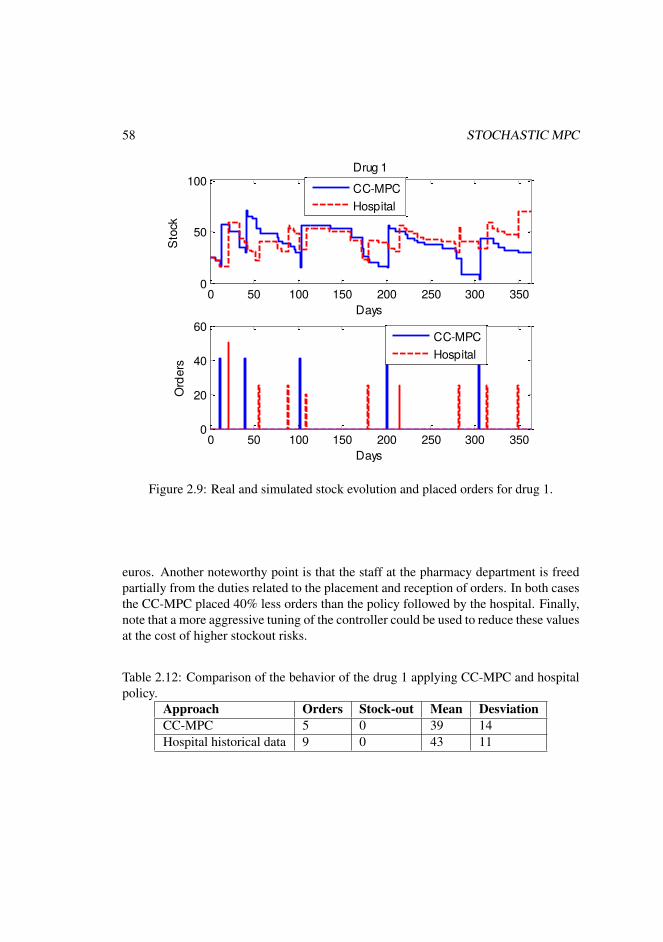
58 STOCHASTIC MPC
0 50 100 150 200 250 300 3500
50
100S
tock
Days
Drug 1
CC-MPC
Hospital
0 50 100 150 200 250 300 3500
20
40
60
Days
Ord
ers
CC-MPC
Hospital
Figure 2.9: Real and simulated stock evolution and placed orders for drug 1.
euros. Another noteworthy point is that the staff at the pharmacy department is freedpartially from the duties related to the placement and reception of orders. In both casesthe CC-MPC placed 40% less orders than the policy followed by the hospital. Finally,note that a more aggressive tuning of the controller could be used to reduce these valuesat the cost of higher stockout risks.
Table 2.12: Comparison of the behavior of the drug 1 applying CC-MPC and hospitalpolicy.
Approach Orders Stock-out Mean DesviationCC-MPC 5 0 39 14Hospital historical data 9 0 43 11
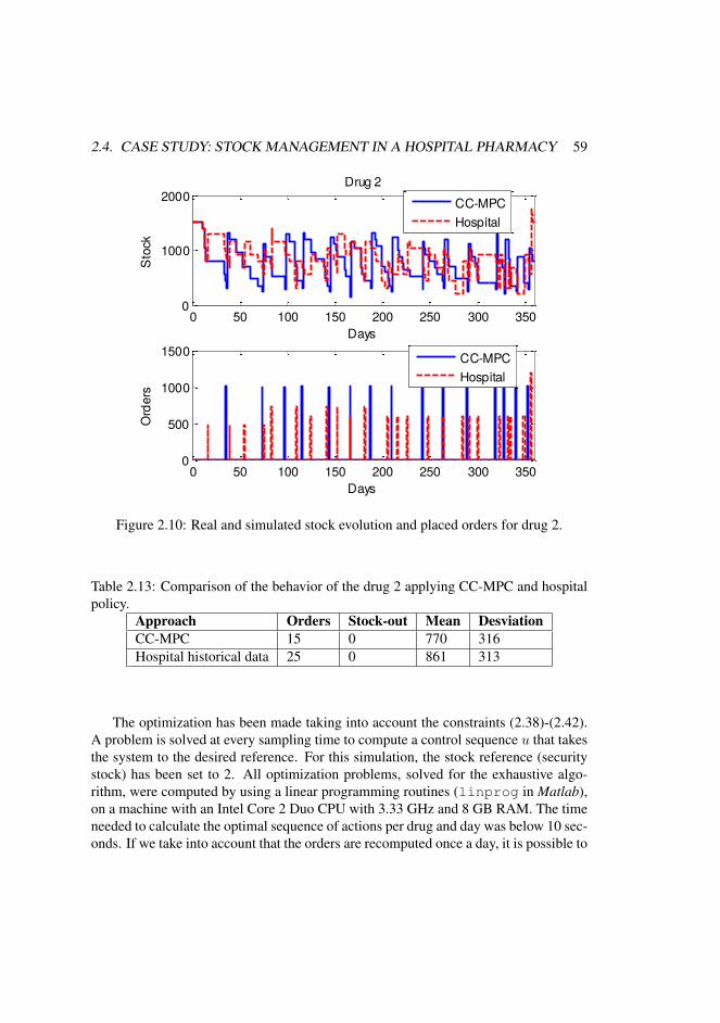
2.4. CASE STUDY: STOCK MANAGEMENT IN A HOSPITAL PHARMACY 59
0 50 100 150 200 250 300 3500
1000
2000
Sto
ck
Days
Drug 2
CC-MPC
Hospital
0 50 100 150 200 250 300 3500
500
1000
1500
Days
Ord
ers
CC-MPC
Hospital
Figure 2.10: Real and simulated stock evolution and placed orders for drug 2.
Table 2.13: Comparison of the behavior of the drug 2 applying CC-MPC and hospitalpolicy.
Approach Orders Stock-out Mean DesviationCC-MPC 15 0 770 316Hospital historical data 25 0 861 313
The optimization has been made taking into account the constraints (2.38)-(2.42).A problem is solved at every sampling time to compute a control sequence u that takesthe system to the desired reference. For this simulation, the stock reference (securitystock) has been set to 2. All optimization problems, solved for the exhaustive algo-rithm, were computed by using a linear programming routines (linprog in Matlab),on a machine with an Intel Core 2 Duo CPU with 3.33 GHz and 8 GB RAM. The timeneeded to calculate the optimal sequence of actions per drug and day was below 10 sec-onds. If we take into account that the orders are recomputed once a day, it is possible to

60 STOCHASTIC MPC
calculate optimal control actions for 8640 drugs a day with the current configuration,many more than those used in the hospitals.
These results have been published in [33].

Chapter 3
Hierarchical Stochastic MPC
A possibility to deal with the risks and uncertainties that affect to the distributed sys-tems, e.g., energy management and water resources management (WRM) systems, isto use a hierarchical structure where an upper control layer provides instructions to thelower control layers, the latter are in charge of the regulation of smaller regions con-trolled by local agents. In this way, coordination is attained [27–29]. Next, two casestudies are presented in this Chapter. First, a multicriteria optimal operation of a mi-crogrid considering risk analysis, renewable resources and a centralized MPC, whereidentification of potential risks has been performed and two MPCs are designed: onefor risk mitigation and another for the optimal control of the microgrid. The proposedalgorithm considers an external loop where information about risk evaluation is up-dated. The risk mitigation policy may change setting points and constraints as wellas execute actions. On the other hand, as a second case study, tree-based hierarchi-cal and distributed MPC (HD-MPC) for WRM is addressed by two layer-hierarchicalstructure, the higher layer collects and coordinates forecast information for sendingdifferent scenarios that take into account the uncertainties to the local agents. Thelower layer, comprised of local agents, solves an optimization problem in a distributedfashion. The HD-MPC method is tested on a real-world case, the North Sea Canalsystem.
3.1 Multicriteria Optimal Operation of a Microgrid
Renewable energies promote competition in the generation of electricity, ensuring en-vironmental protection. They are easily accessible and inexhaustible, unlike fossil fu-
61

62 HS-MPC
els. The investment in their development ensures a sustainable future for our planet.The objective from this Section is to undertake assessment and mitigation actions inoptimal power dispatch. An external loop controls the risk factors and can change pa-rameters on operation of the microgrid. An MPC is used at this level to reach optimalrisk avoiding, as seen below.
3.1.1 A Risk-based control approach in power generation systemsRisk management is a process that includes three basic elements [75]:
1. Goal settings.
2. Risk Identification: information gathering and interpretation. Risk identifica-tion involves ensuring all key topics are considered, and lessons learnt from pastrisk experience are incorporated. In order to protect the microgrid and obtain anoptimal dispatch of the energy, the possible faults detected in the main grid aswell as the microgrid should de considered. In the first case, actions to be takenshould be aimed to isolate the microgrid from the main grid as soon as possible.In the case of presenting an internal failure of the microgrid, we should definea sequence of steps to replace or repair the subsystem where the error occurred.Hazard and Operativity Analysis (HAZOP), cause/effect diagrams, brainstorm-ing sessions, among others, can be tools to help in the identification.
Risk can be defined with this expression:
Risk = Probability ∗ Impact
Probability, is the likelihood that risk occurs and it may depend on the time. Afunction Pr(t) is defined for each risk Rr. Impacts can be evaluated on variousparameters, i.e. cost, time, efficiency, etc.
So, we can define the total Risk Exposure of a risk r like the sum of the ncpotential impacts that would result:
REr(t) = Pr(t)nc∑c=1
IIrc, (3.1)
where Pr(t) is the probability of risk Rr at instant t and IIrc denotes the initialimpact of risk Rr affecting parameter Zc; both of these can be time dependent.
Note that all components of the microgrid (e.g., sources, transformers, and elec-tric lines) are susceptible to present risks affecting parameters like cost, timedelay, etc.
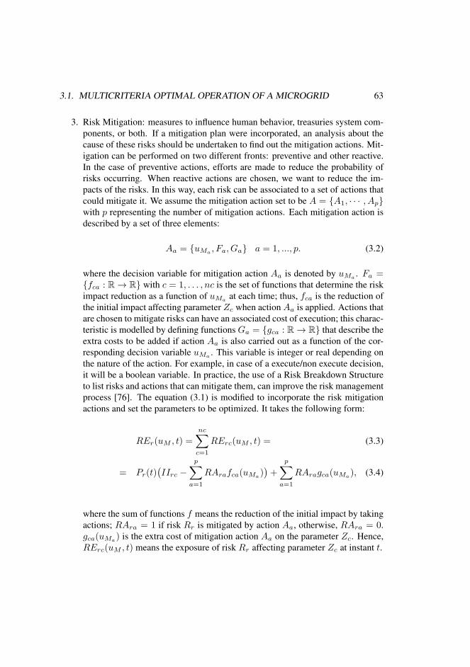
3.1. MULTICRITERIA OPTIMAL OPERATION OF A MICROGRID 63
3. Risk Mitigation: measures to influence human behavior, treasuries system com-ponents, or both. If a mitigation plan were incorporated, an analysis about thecause of these risks should be undertaken to find out the mitigation actions. Mit-igation can be performed on two different fronts: preventive and other reactive.In the case of preventive actions, efforts are made to reduce the probability ofrisks occurring. When reactive actions are chosen, we want to reduce the im-pacts of the risks. In this way, each risk can be associated to a set of actions thatcould mitigate it. We assume the mitigation action set to be A = {A1, · · · , Ap}with p representing the number of mitigation actions. Each mitigation action isdescribed by a set of three elements:
Aa = {uMa , Fa, Ga} a = 1, ..., p. (3.2)
where the decision variable for mitigation action Aa is denoted by uMa . Fa ={fca : R → R} with c = 1, . . . , nc is the set of functions that determine the riskimpact reduction as a function of uMa at each time; thus, fca is the reduction ofthe initial impact affecting parameter Zc when action Aa is applied. Actions thatare chosen to mitigate risks can have an associated cost of execution; this charac-teristic is modelled by defining functions Ga = {gca : R → R} that describe theextra costs to be added if action Aa is also carried out as a function of the cor-responding decision variable uMa . This variable is integer or real depending onthe nature of the action. For example, in case of a execute/non execute decision,it will be a boolean variable. In practice, the use of a Risk Breakdown Structureto list risks and actions that can mitigate them, can improve the risk managementprocess [76]. The equation (3.1) is modified to incorporate the risk mitigationactions and set the parameters to be optimized. It takes the following form:
REr(uM , t) =
nc∑c=1
RErc(uM , t) = (3.3)
= Pr(t)(IIrc −
p∑a=1
RArafca(uMa))+
p∑a=1
RAragca(uMa), (3.4)
where the sum of functions f means the reduction of the initial impact by takingactions; RAra = 1 if risk Rr is mitigated by action Aa, otherwise, RAra = 0.gca(uMa) is the extra cost of mitigation action Aa on the parameter Zc. Hence,RErc(uM , t) means the exposure of risk Rr affecting parameter Zc at instant t.

64 HS-MPC
Optimal risk mitigation
The control goal is expressed by a multicriteria weighted index performance functionwhere parameters to optimize are included:
minuM ,t
J =∑
βiJi(uM , t). (3.5)
Terms Ji are defined as:
Ji(uM , t) =N∑
k=1
(Yic(t+ k|t)− wc(t+ k))2, (3.6)
where Yic is the predicted output on parameter ZC at instant (t + j) on the class ofrisk i. wc is the reference to follow for parameter Zc. Note that wc corresponds to thereference to follow in the MPC. In this study, usually term wc is 0, because we want tooptimize the parameters. Yic is calculated as
Yic =m∑r=1
RErc(u, t+ k), (3.7)
where m denotes the total number of risks and N the prediction horizon.The risk analysis procedure can be described as follow:
• Step 1: Initialize/update the parameters of all the elements of the microgrid, i.e.load curve, simulation step, risks, impacts, probabilities and actions.
• Step 2: Evaluate expression 3.5 with MPC and execute actions estimated to doat time t.
• Step 3: Set changes in the microgrid (if proceed).
• Step 4: Wait for the next simulation step k = k + 1.
• Step 5: Loop back to Step 1 if simulation period is not finished.
3.1.2 Risk management on the HyLab plantNext, an identification about potential risks in the real microgrid is undertaken.

3.1. MULTICRITERIA OPTIMAL OPERATION OF A MICROGRID 65
Photovoltaic plant
The following risks have been identified:
• R1: Production capacity of panel.
• R2: Difficulty in maintenance on rugged terrain.
• R3: Long time to start supplying energy to the grid.
• R4: Failure of mechanical parts.
• R5: Increased need for maintenance due to dirt build up on the panel.
• R6: Efficiency loss due to tracking failure.
• R7: Lifetime of panel (degrading in harsh conditions).
• R8: High maintenance costs.
• R9: Fluctuations in supply to and hence electricity price on grid (potential over-capacity during daytime).
• R10: Material durability (given high temperatures involved).
• R11: On cloudy days supply to the grid could be inefficient.
• R12: During low demand periods could occur an overcapacity of stored energy.
Fuel Cell
In many situations the major hazards associated with a fuel cell installation may be putinto the following items:
• R13: Dangerous substances.
• R14: Fire and explosion.
• R15: Harmful effects of exposure.
• R16: Electric shock.
• R17: General safety hazards, for example manual handling.

66 HS-MPC
Batteries
• R18: Contactor fails closed.
• R19: Loss of HV continuity.
• R20: Electrical short-circuit.
• R21: Overcharge.
• R22: Fire or elevated temperature.
• R23: Low efficiency in batteries, producing not estimated SOC.
Weather conditions
The power generation by renewable sources such as solar panels or wind turbines canchange due to weather conditions. Also, weather conditions can change the estimateddemand for a specific period. For example, if weather conditions change apprecia-bly, this will result in an increase/decrease in global electricity demand. This can betransferred to the following risks:
• R24: Significant changes in power demand.
• R25: Significant changes in solar generation capacity.
Remark 4 The internal loop steers the microgrid satisfying the electric demand curve.An MPC, as described in Section 2.1, is also used in the internal loop, but with adifferent model and objective functions discussed previously in Section 2.2. Note thatthe frequency at the internal loop is higher that in the external loop.
3.1.3 ResultsThe simulations were carried out by using a non-linear model as replacement of thereal plant [54]. The initial conditions for SOC and MHL were 50% for each one. Theresults are presented over a simulation time of 93 days. The sampling time step was30s for the internal loop and 1 day for the risk loop. The prediction horizon is 5 days.
Table 3.1 shows the risks that have been considered for the example and the mitiga-tion actions that can reduce them. Initial impacts (II) are expressed on the parametersZ = {Z1, Z2, Z3, }, with Z1 being the cost (euros/day), Z2 the estimated power de-mand, and Z3 the estimated power generation by the solar panels. Table 3.2 describes

3.1. MULTICRITERIA OPTIMAL OPERATION OF A MICROGRID 67
Table 3.1: Risk identification and mitigation
Ri Impact Pi Ai
SolarR5 II31 = 50, II22 = 0, II23 = 0 P3(t) A1
R11 II11,1 = 300, II11,2 = 0, II11,3 = 0.55 ∗ SG P11(t) = N (0.9, 0.3), {25− 34} A2
Fuel CellR13 −R17 II13,1 = 1000, II13,2 = 0, II13,3 = 0 P13(t) A3, A4
BatteriesR23 II23,1 = 90, II23,2 = 0, II23,3 = 0 P23(t) = 0.6{10− 20} A5
WeatherR24 II24,1 = 0,II24,2 = 0.32 ∗ PD, II24,3 = 0 P24(t) = 1{50, 74} A6
the actions and their reductions. Last column means if control variable is boolean (B) orreal (R). Note that actions A1 to A5 involve boolean variables. Therefore, the CPLEXcommercial package has been used for the simulations. More specifically:
Table 3.2: Mitigation actions description.
Ac Description f1i, g1i on Z1(cost) ui
A1 Periodic cleaning of mirrors f11 = 0.95II1u1, g11 = 250u1 BA2 Modify the solar generation load shape f12 = 0.99II1u2, f32 = II1u2, g12 = 45u2 BA3 Properly maintenance of fuel cell f13 = 0.95II13u3, g13 = 300u3 BA4 Training for personnel f14 = 0.70II14u4, g14 = 600u4 BA5 Change upper limit of SOC in battery f15 = 150u5, g15 = u5 BA6 Change Power Demand curve as request f16 = 0, f26 = II2u6, g16 = u6 ∗ p R
• Risk R5 considers how clean panels are. The probability rises with the time anddecrease if action A1 is selected. This is done when the probability exceeds athreshold.
• Risk R11 represents the 50% decrease on solar generation estimation used forthe prediction and control when there is a cloudy day. Probability of the solargeneration between days 25 to 34 is modeled as a normal distribution with mean0.9 and deviation 0.3. Action A2 modifies the solar generation estimation valuein the simulation.
• All the identified risks in fuel cells are grouped and the proposed action is the

68 HS-MPC
skilled periodic maintenance (A3) and training for the personnel on time at thebeginning (A4). Probability takes the same form that R5.
• Risk R23 set the loss of efficiency in batteries. A change in the upper limit ofbattery SOC (from 90% to 70%) is proposed to mitigate it. In order to illustratethis event, probability between days 10 to 20 is set to 0.6. The unexpected chang-ing power demand is described in risk R24. To show the effects, the probabilityin days 50 and 74 is set to 1. Action A6 changes the power demand with theincreased value.
Figure 3.1 shows the modified power demand and solar generation curves accordingto risk mitigation. These data are sent to the microgrid controller. The cost function (ineuros) is shown in Figure 3.2. It can be observed that a reduction of 10000 euros, bycomputing Z1, is reached in 93 days if mitigation is done. Mitigation actions and thedays when are running are described in Figure 3.3. Note that actions A1 and A3 areperformed monthly and A4 every 90 days.
Figure 3.1: Estimations on power demand and solar generation.
Figure 3.4 shows the evolution of the variables that compose the experimental mi-crogrid. The microgrid follows a general scheme of operation to satisfy the demand.
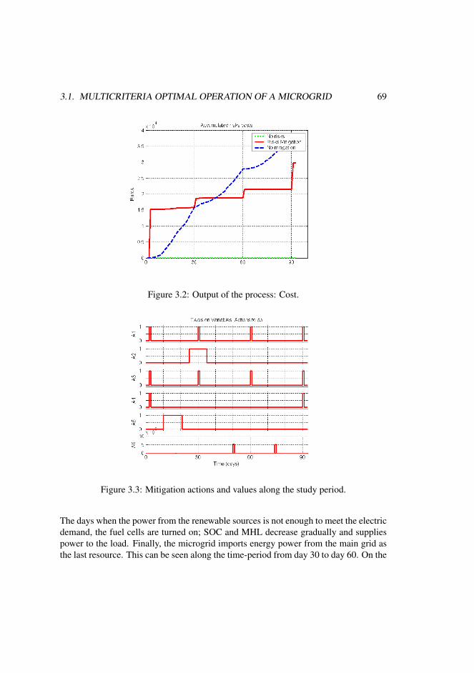
3.1. MULTICRITERIA OPTIMAL OPERATION OF A MICROGRID 69
Figure 3.2: Output of the process: Cost.
Figure 3.3: Mitigation actions and values along the study period.
The days when the power from the renewable sources is not enough to meet the electricdemand, the fuel cells are turned on; SOC and MHL decrease gradually and suppliespower to the load. Finally, the microgrid imports energy power from the main grid asthe last resource. This can be seen along the time-period from day 30 to day 60. On the

70 HS-MPC
contrary, when there exists excess of renewable energy production and the user demandhas been satisfied, the electrolyzer is active, and energy is stored as metallic hydrides,batteries are charged, and power is sold to the external grid.
Figure 3.4: Control signals, states, and disturbances by applying multicriteria optimalpower dispatch in the HyLab plant.
Figure 3.5 shows in solid line the batteries SOC by considering the risks mitiga-tion over them. The dashed line represents the batteries SOC without a risk analysis.When the renewable power is enough, the batteries are fully charged, which could com-promise their lifespan. Therefore, by implementing a risk analysis, the constraints onSOC are readjusted toward acceptable levels, in this case to a maximum level of 70%.
3.2 Tree based HD-MPC for WRMSubstantial uncertainties affect the water systems, e.g., human disturbances (channelmodification, drainage, land use, etc.), climatic change and demographic changes,which cause alterations in rainfall and evaporation, changes in sea levels, meltingglaciers, etc. [77]. In addition, given that the human dependence on water resources,social, economic, and technological changes are also influencing the behavior of users

3.2. TREE BASED HD-MPC FOR WRM 71
Figure 3.5: Batteries SOC by considering risk analysis and no mitigation actions.
on the demand supplies [78–80]. For these reasons, it is necessary to consider stochas-tic models and approaches to cope with different types of uncertainties. In this way itis possible to take into account flexible, adaptive, and robust plans, which can respondto predictable and unpredictable environmental changes [81, 82].
For the sake of representation in a control problem, meteorological and hydrolog-ical forecasts are usually expressed in the form of an ensemble forecast(EF), whichis a collection of trajectories, standing for all the possible evolution along the timeof the disturbances, in other words, the uncertainty is modeled by considering its dy-namic behavior. Raso [83] pointed out that using EFs in MPC is both beneficial andrisky. Prediction makes the control proactive and better at accommodating potentialupcoming extreme events. On the other hand, jeopardized robustness may hinder theapplicability of MPC. In order to enhance the robustness of MPC when consideringEFs, a scenario-based approach is able to address this issue. In this sense, a tree-basedapproach can be introduced to transfer EFs into a computationally acceptable structurein the control problem [39]. The idea of using a tree-shaped structure is that when tra-jectories have the same or very similar information of forecasts, a branch of a tree canbe used to represent these trajectories. Once the trajectories start to diverge, the branchbegins to bifurcate and to spilt up into two or more branches. The resulting MPC con-troller is known as tree-based MPC (TB-MPC), and greatly improves the robustness ofthe controller. Regarding TB-MPC applied to WRM, some works have been presented,which deal with the uncertainties and disturbances through a set of possible scenarios

72 HS-MPC
modeled as a branched tree structure.TB-MPC has been applied in a centralized water system [20] as well as in a dis-
tributed drainage water system [84] with a single EF for all subsystems. However, sinceEFs are presented on different geographically disperse subsystem, their structures aredifferent and need to be modified in the hierarchy to be sending to multi-subsystem. Atthis point, a scenario based Hierarchical and Distributed MPC (HD-MPC) is developedfor deal with the uncertainty in WRM.
The generic MPC formulation and its application have been widely discussed inthe literature [2, 3]. Below, it is briefly presented the standard framework of MPC andthen explain how to apply it to a general WRM problem. For a water system that needsto be managed to meet several targets in real-time, such as flood defense and coastalmanagement, one accepted way to model the system dynamics and its constraints is ofthe form [85, 86]:
s(x(k), u(k)) = x(k + 1) = Ax(k) +Buu(k) +Bdd(k), (3.8)
g(x(k), u(k)) =[x(k); −x(k); u(k); −u(k)
]T, (3.9)
b =[xmax; −xmin; umax(k); −umin(k)
]T. (3.10)
The control performance can be measured by:
f(x(k + 1), u(k)) = (3.11)[x(k + 1)− r(k)]TQ[x(k + 1)− r(k)] + uT (k)Ru(k),
where the state x(k) = [h(k), q(k), hg(k)]T consists of the water level h(k) of the
open channel, the flow q(k) via the pump and the height hg(k) of the gate, the controlvariable u(k) = [∆q(k),∆hg(k)]
T consists of the change of the pump flow ∆q(k) andthe change of the gate height ∆hg(k), d(k) ∈ Rn is the system disturbance, r(k) ∈Rn is the reference vector, Q ∈ Rn×n, R ∈ Rm×m, xmin ∈ Rn and xmax ∈ Rn
are the minimum and maximum allowed values on the state x, which are either thesafety level or the maximum pump capacity or the highest and lowest gate positions,umin(k) ∈ Rm and umax(k) ∈ Rm are the minimum and maximum allowed changesof pump flows or gate positions cite. A ∈ Rn×n, Bu ∈ Rn×m and Bd ∈ Rn×l arerelevant coefficients derived from the linearized De Saint-Venant equations as well asthe physical parameters of the considered water system [87, 88].
Remark 5 This study uses the formulation of A, Bu and Bd given in the Appendix Bof [88].

3.2. TREE BASED HD-MPC FOR WRM 73
Remark 6 Q is semi-definite and R is definite, and both are diagonal matrices, whichguarantee the cost function (3.11) is convex. This implies that: (a) The terminationof the optimization can be guaranteed [3]; (b) The problem can be solved by efficientalgorithms, such as the interior-point method or the active-set method.
Remark 7 As known the physical parameters of the system, in this study, the controlof the gate height is made by flow, as a way to conserve the linearly of the system.
Standard MPC structure has the form:
minu(0),...,u(Np−1)
J(k) =
Np−1∑k=0
f(x(k + 1), u(k)), (3.12)
subject to
x(k + 1) = s(x(k), u(k), d(k)), k = 0, 1, ..., Np − 1, (3.13)g(x(k + 1), u(k)) ≤ b(k), k = 0, 1, ..., Np − 1, (3.14)
where Np ∈ N+ is the length of the prediction horizon, x(k) ∈ Rn is the systemstate at time step k, u(k) ∈ Rm is the control variable at time step k, d(k) ∈ Rn
is the system disturbance at time step k, f : Rn+m → R is the stage cost function(linear or non-linear), s : Rn+m → Rn is the function describing the system dynamics,g : R(n+m)×l → Rl is the constraint function, and b(k) ∈ Rl in the constraint vector.The idea is to use the system model to predict its behavior along a certain horizon. Thecost function is optimized to calculate the best sequence of inputs that can be appliedto the system, penalizing the deviations of the inputs and the state of the system withrespect to the desired behavior. The sequence of inputs is also designed to satisfy theconstrains of the problem.
The tree-based approach can contribute to a control problem when considering en-semble forecasts (EFs). Taking Nr possible scenarios into account as a tree, the formu-
74 HS-MPC
lation of TB-MPC for WRM can be expressed as following:
minu[1](0), ..., u[1](Np − 1)
...u[Nr](0), ..., u[Nr](Np − 1)
J(k) =
Nr∑i=1
p[i]
Np−1∑k=0
f(x[i](k + 1), u[i](k))
,
(3.15)subject to
x[i](k + 1) = s(x[i](k), u[i](k)), k = 0, 1, ..., Np − 1, i = 1, ..., Nr, (3.16)g(x[i](k + 1), u[i](k)) ≤ b[i](k), k = 0, 1, ..., Np − 1, i = 1, ..., Nr, (3.17)u[i1](k) = u[i2](k), if section i1 overlaps section i2 at step k, (3.18)d[i1](k)) = d[i2](k), if section i1 overlaps section i2 at step k. (3.19)
Remark 8 We define p(·) as the probability of an event. As a result, for all the scenariosections between time steps k and k + 1, they satisfy:
Nr∑i=1
p(d[i](k)) = 1, (3.20)
and over the prediction horizon Np, they satisfy:
Np∏k=0
p(d[i](k)) = p[i], (3.21)
Nr∑i=1
p[i] = 1. (3.22)
3.2.1 Two-level hierarchy TB-MPCA water system, especially a large-scale one, usually consists of a number of canalsand reservoirs. In practical water management problems, the whole water system isoften managed in a distributed way. The system is comprised of several subsystems,each of which has its own system prediction (with uncertainties) and objectives. Forexample, a long river may be separately managed by the countries and regions it flowsthrough. Another example is the Dutch water system. The whole system is dividedinto 27 non-intersecting areas, each of which is managed by a local Water Board with

3.2. TREE BASED HD-MPC FOR WRM 75
local and national management targets. Such a system is manipulated in a distributedway, which means each subsystem is municipal yet has influence on (and is influencedby) its adjacent neighbors. Consequently, the control problem cannot be solved onlyby a central controller.
There are two ways to exchange information between the local agents and the cen-tral unit. Either a top-down manner or a bottom-up one. In the top-down manner, thecentral unit gathers the complete information of the whole system and delivers it toall the subsystems. This type of information usually comes from processed satellitedata. In the bottom-up manner, the subsystem with a gauge station gives its disperseinformation to the central unit. Then the central unit reckons other subsystems withoutgauge stations, for example, using the Kalman filter or the neural network algorithm.While, if the information is delivered from down to top, each subsystem has its ownforecast or its forecast is calculated from forecasts of its gauged neighbors. The globalscenario is obtained by combining the local EFs.
Top-down
The optimization problem can be addressed by two layers composed of a central EFin the top one, and the bottom layer compromises of local MPC problems with EFscenarios for each subsystem. Assume the system comprises Nb subsystems. We usethe subscript {j} to denote a variable that is corresponding to subsystem j (j=1,...,Nb).A centralized objective function (3.15) can be distributed as follows:
min J(k) =
Nb∑j=1
J{j}(k) (3.23)
=
Nb∑j=1
Nr,{j}∑i=1
p{j},[i]J{j},[i](k), (3.24)
where the J{j}(k) in (3.23) implies the cost of the objective function of subsystem j.The subsystem j may also have Nr,{j} scenarios derived from the centralized EF so thatJ{j}(k) is the sum of all p{j},[i]J{j},[i](k)’s, which is shown in (3.24). The optimiza-tion should also subject to the constraints corresponding to (3.16)-(3.17) within eachsubsystem. Note that (3.15) shows the central information of the whole system. Whendistributing the system, there occur coupled variables. For example, the outflow ofthe upstream catchment is the right inflow of the downstream catchment, which meansthey are coupled variables linking these two catchments. These coupled variables areimportant to be considered for system distribution.

76 HS-MPC
Remark 9 The prerequisite that a system can be managed in a distributed way is thatthe local information of each subsystem must be known. Note that, in this study, onesubsystem actually stands for a certain area which has its own control targets as wellas connections with its neighbors.
It is assumed that all the local agents at the lower level obtain information from thecentral unit at the higher level. In other words, the prediction of all the scenarios hasthe same structure of the EF tree.
Figure 3.6 shows an idea of how a centralized tree can be distributed to the sub-systems. We assume the system comprises two subsystems. Scenarios 1 and 2 mayhappen in the subsystem. Therefore, Scenario 3 does not need to be considered in sub-system 1 and the corresponding branch can be left out. So is Scenario 1 for subsystem2. The modified EF trees only carry useful information for control. Though subsystemshave different EF tree structures, they are connected with their neighbors by coupledoutputs.
Figure 3.6: A centralized disturbances tree is distributed into the subsystems in a top-down approach.

3.2. TREE BASED HD-MPC FOR WRM 77
Bottom-up
In this case, the bottom level usually solves a set of problems locally, which means anysubsystem j has its objective function J{j}(k) to solve. Adjacent subsystems are linkedby their coupled variables. A button-top scheme can be carried out, as shown Figure3.7. The idea behind this approach is that all targets are merged in a single objectivefunction at the upper level by taking into account the probability of occurrence of eachscenario inside the local disturbance tree.
Figure 3.7: A centralized EF is built with the local EFs in a bottom-up fashion.
Remark 10 The tree structure of any subsystem has the same (homologous) bifurcat-

78 HS-MPC
ing points and branches as the tree of the whole system. This is owing to the fact thatwhen building the tree of the whole system based on the information of subsystems(Remark 9), all pieces of information are kept and determine where branches shouldbifurcate in the whole system, (the algorithm results in that when branches of a subsys-tem bifurcate at a certain time step k, the corresponding branches in the whole systembifurcate accordingly at time step k as well). Therefore, It is necessary to compensatesome virtual branches in trees of subsystems whose probability p is made zero for themissing branches between a subsystem and the whole system.
At the bottom layer, local controllers or agents take decision, under their own EF,and share their objective, states and inputs with each others, in a reliable exchange ofinformation in order to coordinate their actions by meaning coupled variables. A dis-tributed fashion can be able to address these kind of problems maintaining the advan-tages of an MPC, see, e.g., [30]. All in all, the formulation of the tree based HD-MPCcan be expressed as follows
for ∀k ∈ [0, 1, ..., Np − 1], ∀i ∈ [1, ..., Nr,{j}],∀j ∈ [1, ..., Nb] :
minall u{j},[i](k)
Nb∑j=1
Nr,{j}∑i=1
p{j},[i]J{j},[i](k), (3.25)
subject to
x{j},[i](k + 1) = s(x{j}.[i](k), u{j},[i](k)), (3.26)g(x{j},[i](k + 1), u{j},[i](k)) ≤ b{j},[i](k), (3.27)u{j},[i1](k) = u{j},[i2](k), if [i1] overlaps [i2] in{j}, (3.28)d{j},[i1](k) = d{j},[i2](k), if [i1] overlaps [i2] in{j}, (3.29)u{j1}(k) = u{j2}(k) if they are coupled between {j1} and {j2}. (3.30)
The above formulation only shows an idea of how all targets are merged in a singleobjective function at the upper level. When solving the optimization, it is possible tocarry out algorithms for distributing them, such as dual decomposition, see, e.g., [89].It implies to introduce Lagrangian multipliers many as coupling constraints the opti-mization problem presents. In this case, each subsystem solves its own optimizationconstrained by the coupled variables with a exchange information process, as following

3.2. TREE BASED HD-MPC FOR WRM 79
Figure 3.8: Schematic diagram of the North Dutch catchment.
maxall λ{j1,j2}(k)
minall u{j},[i](k)
Nb∑j=1
Nr,{j}∑i=1
p{j},[i]J{j},[i](k) (3.31)
+λ{j1,j2}(k)(u{j1}(k)− u{j2}(k)),
subject to
x{j},[i](k + 1) = s(x{j}.[i](k), u{j},[i](k)), (3.32)g(x{j},[i](k + 1), u{j},[i](k)) ≤ b{j},[i](k), (3.33)u{j},[i1](k) = u{j},[i2](k), if [i1] overlaps [i2] in {j}, (3.34)d{j},[i1](k) = d{j},[i2](k) if [i1] overlaps [i2] in {j}. (3.35)
Where λ{j1,j2} are the Lagrange multipliers associated with coupling constraints.
3.2.2 Simulations and resultsWe test the proposed controller in a North Dutch catchment, which consists of LakeIJsselmeer and Markermeer (subsystem 1) and the North Sea Canal (subsystem 2).For simplification, we use a simplified model, in which gates and pumps are regardedas a single structure if they work in a synchronized way. For example, there are twolarge sluice gate sets between Lake Ijsselmeer and the North Sea, which are 108 and 54meters wide respectively. In this case, they are treated as a single 1611 meter wide gate.The North Sea is the boundary condition to be considered. Though Lake IJsselmeer

80 HS-MPC
Table 3.3: Simulation parameters.Parameters ValueStorage capacity of Lake IJsselmeer and Markermeer 7.4e8 m3
Storage capacity of North Sea Canal 3.1e7 m3
Length of time step 1 hPrediction horizon 24 hSimulation time 30 daysSetpoint of the water level -0.4 mQuadratic penalty on the setpoint 4000Quadratic penalty on ∆q via the Houtrib Gate 1/3000Quadratic penalty on ∆q via the Schellingwoude Gate 1/200Quadratic penalty on ∆q via the IJmuiden pumps 1/260
and Markermeer may have differences in water levels, they are connected via two sluicegates by gravity flows. In this study, they are combined and regarded as one reservoirfor simplification. Finally, the model can be depicted as in Figure 3.8. The Lakeand the Canal are linked by a locked gate (Schellingwoude Gate), which is the coupledvariable that shows the water exchanged between subsystems 1 and 2. The lake, and thecanal, discharge into the sea via the Houtrib Gate and the Schellingwoude Gate. Bothsubsystem carry out a water exchange via IJmuiden pumps. The subsystems’ outflowsare denoted as q1 and q2, respectively. The maximum capacity for the outflow via theHoutrib Gate, the Schellingwoude Gate, and the IJmuiden pumps are constrained to1000 m3/s, 260 m3/s, and 50 m3/s, respectively. The parameters used for simulationare listed in Table 3.3.
Both subsystems, the Lake and the Canal, have inflows as disturbance d(k) thatcome from the Rhine River and rainfall. Stochastic inflows have been obtained bysampling historical data from a Dutch live web service operated by Rijkswaterstaat1.Twenty scenarios with a Gaussian distribution, which mean value is the historical se-quence and standard deviation is 250 m3/s. These scenarios are used to evaluate theperformance of the whole system at the top layer. Figure 3.9 shows the maximum,mean, and minimum values from the EF during the simulation horizon. Therefore, thedisturbances fall between these maximum and minimum values. It is possible to notethat the disturbances present an increased level due to rainfall from day 6 to day 12,where the maximum value of the EFs is around 1400 m3/s. Moreover, remaining time

3.2. TREE BASED HD-MPC FOR WRM 81
0 5 10 15 20 25 300
200
400
600
800
1000
1200
1400
Time (days)
Inflow
(m
3/s
)
Disturbances
max
mean
max
Figure 3.9: Inflow scenarios generated at the top layer.
shows a regular input for two subsystems,The hierarchy of the system is given as follows: the top level deals with the dis-
tribution of the system, in which the system and disturbance are distributed into thetwo subsystems as mentioned earlier. The top layer delivers two different EF trees,which are composed of the most likely Ns scenarios, for subsystem 1 and subsystem2, respectively, which may be mainly due to different precipitation in different areasor different water demand for various purposes, i.e., different hydrological conditions.Figure 3.10 shows two different disturbance trees, one for each subsystem, for the firstinstant of the simulation time over five hours. These disturbance trees collect the mostrelevant probabilistic patterns that each local controller will use to solve the optimiza-tion problem dealing with its proper uncertainty at each time instant. While, the bottomlayer focuses on the local subsystem, in which local controllers are designed by takingaccount of multiple scenarios given by the top layer.
In order to show the advantages of the implemented control strategy, we carriedout the simulation along 30 days, with a prediction horizon of 24 hours. At each timeinstant, a new disturbance tree is generated and delivered from the top layer to localcontrollers. Each tree starts with its measured value as the root of the tree, and theirNs branches result from the EF at the top level for the prediction horizon. The treeconstruction algorithm is carried out by GAMS [56].
1http://live.waterbase.nl

82 HS-MPC
0 1 2 3 4 50
100
200
300
400
500
600
700
800
Time(hours)
Tre
e 1
0 1 2 3 4 560
80
100
120
140
160
180
200
220
Time(hours)
Tre
e 2
Figure 3.10: Inflows of the local subsystems.
The constraints for the local controllers are given as follows: the maximum capaci-ties for the outflows are set as 1000 m3/s for subsystem 1, and 260 m3/s for subsystem2. The water exchange is constrained between 0 and 50 m3/s. The water level for bothsubsystems is bounded between -5 m and 5 m.
The control inputs result from a tree composed of Ns control actions, where onlythe first component of the sequence is implemented, which corresponds to the controlaction for the current measured disturbance in each subsystem. The pumps actuate overthe outflows; these variables represent the control action carried out by these actuators.Figure 3.11 shows the behavior of the pumps for both subsystems. The pumps turn onfor dealing with rainfall. The pumps reach their first peaks; these are 334 m3/s and255 m3/s, respectively.
The pump via the Houtrib Gate, which corresponds to subsystem 1, gets its maxi-mum level, 552 m3/s, at the time instant which corresponds to the maximum inflows atday 10, approximately. It increases its capacity to give free space in the catchment andmaintain the water level. After this period the outflow from pump 1 decreases graduallyduring 13 days. The inflows present an augmented value, while the discharge increasesagain to prevent an overflow. On the other hand, the pump 2, via the SchellingwoudeGate, enhances its capacity until it gets its peak value since this subsystem receives thewater from the subsystem 1 as well as the rainfall input. Then the outflow, which is op-erated by pump 2, works between 50 and 143 m3/s during 15 days. After this period,the inflow increases its value. Therefore the outflow from pump 2 must increase too.

3.2. TREE BASED HD-MPC FOR WRM 83
0 5 10 15 20 25 300
100
200
300
400
500
600
Time (days)
q (
m3/s
)
Outflow
q1
q2
Figure 3.11: Outflows of the local subsystems.
The behavior of the water exchange via the IJmuiden pumps is shown in Figure3.12. The water exchange is carried out from the sea to the canal. It displays a peak atthree times by getting its maximum capacity until the highest rainfall input is over; outof these periods, the water exchanged is reduced remarkably due to the disturbancesdecrease and it is necessary to keep the water into the reference values.
The water level for both subsystems remains around the reference despite the pres-ence of disturbances. The reference level for the Lake is shown in Figure 3.13. Thisreference level has a mean value of −0.3967m and a standard deviation of 0.025. Re-garding subsystem 2, the water level has a mean level of −0.3984m with a standarddeviation that corresponds to 0.034. The water level for the Canal system is shown inFigure 3.14. It is possible to note that both reference levels do not violate the estab-lished constraints, at any time instant.

84 HS-MPC
0 5 10 15 20 25 300
5
10
15
20
25
30
35
40
45
50
Time (days)
qex(m
3/s
)
Water Exchange
Figure 3.12: Water exchange between the local subsystems.
0 5 10 15 20 25 30-0.46
-0.44
-0.42
-0.4
-0.38
-0.36
-0.34
-0.32
Time (days)
h1
(m)
Water Level
Figure 3.13: Water level of the Lake IJsselmeer and Markermeer.
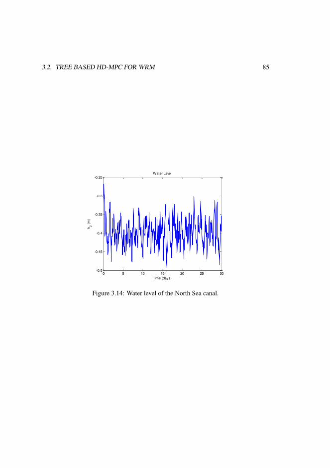
3.2. TREE BASED HD-MPC FOR WRM 85
0 5 10 15 20 25 30-0.5
-0.45
-0.4
-0.35
-0.3
-0.25
Time (days)
h2
(m)
Water Level
Figure 3.14: Water level of the North Sea canal.

86 HS-MPC

Chapter 4
Stochastic MPC to Deal withVulnerabilities in DistributedSchemes
There are several geographically disperse systems such as road-traffic, logistics, trans-portation, water, electrical networks, etc., where it is not possible to apply a centralizedMPC due to computational burden, issues with centralized modeling, data collection,etc., as reported in [90]. An alternative to deal with this kind of problems is to di-vide the whole system into subsystems, each one governed by an MPC controller (oragent) that takes decisions and exchanges information with the other controllers undera negotiation process to obtain an optimal global solution. This control scheme is theso-called distributed MPC (DMPC). Ease of implementation, low computational effortin comparison with centralized MPC, modularity of the system, among others are thepotential advantages that DMPC offers, as discussed in [30].
Many approaches for DMPC schemes have been developed in recent years, as de-scribed in [30]. A topic that deserves attention is the regular exchange of informationduring the negotiation process among the controllers. In this sense, DMPC schemeshave been carried out by considering a coordinated negotiation process where all con-trollers work in a reliable way. However, a malicious controller could exploit the vul-nerabilities of the network by sharing false information with other controllers, produc-ing an undesirable behavior in the optimization process. At this point, it is possible tospeak about cyber-security in the context of DMPC.
Cyber-security can be defined as the activities for protecting cyber-space from in-
87
88 STOCHASTIC MPC AND VULNERABILITIES
fringements, and for defending its technology infrastructure, the services provided andthe information, i.e., the set of methods and tools for protecting systems against threats.Cyber-security goals are confidentiality, availability, and integrity of information [91].Some general applications have been developed in this context. Application areas forwhich cyber-security needs to be considered are protection systems [92], Internet homeusers [93], logistics [94–96], and power systems [97, 98]. Control systems are not ex-empt from possible cyber-attacks, as reported in [99,100]; the consequences of a cyberattack within a control system can go from performance loss to instability. In par-ticular, [101] presents cyber-security risk assessment for supervisory control and dataacquisition (SCADA) and distributed control system networks. So far, cyber-securityissues have not been considered in the DMPC literature. Hence, one of the most popu-lar schemes is analyzed, Lagrange based DMPC. In particular, it is shown how a mali-cious controller in the network can take advantage of the vulnerabilities of the schemeto increase its own benefit at the cost of other controllers. These issues are addressedby considering two well known scenario-based techniques to ensure robustness withinthe DMPC network, as well as a secure dual decomposition based DMPC which is aheuristic defense inspired by [102]. In this sense, it is possible to robustify the controlnetwork against possible malicious controllers.
On the one hand, both types of scenario-based MPC, MS-MPC and TB-MPC, pro-vide robustness by considering several possible scenarios in the optimization prob-lem [32]. On the other hand, the secure dual decomposition based DMPC based on aconsensus approach that dismisses the extreme control actions is presented as a way toprotect the distributed system from potential threats.
In this work, these approaches are applied toward distributed systems to cope withinternal threats and mitigate the effects of the attacks from malicious controllers. Basedon this background, and to deal with the internal threats from the distributed network,these approaches are incorporated in the DMPC formulation as a way to secure dualdecomposition DMPC. Also, in order to illustrate the proposed defense methods, thecontrol of a local grid of households is presented as a case study [103].
4.1 Dual Decomposition based DMPCThis section presents a commonly used distributed optimization algorithm based ondual decomposition [89, 104]. Let us consider a distributed system composed of Nb
subsystems defined by discrete-time linear time-invariant models. The dynamics ofsubsystem i are given by
xi(k + 1) = Aixi(k) +Biui(k), (4.1)

4.1. DUAL DECOMPOSITION BASED DMPC 89
where xi ∈ Rnx,i and ui ∈ Rnu,i denote the states and input of the system, respec-tively. Ai ∈ Rnx,i×nx,i is the state matrix and Bi ∈ Rnx,i×nu,i represents the inputmatrix. The variables nx,i and nu,i represent the number of states and the number ofinputs of the subsystem i, respectively. Each subsystem is subject to convex state andinput constraints:
xi(k) ∈ Xi, ∀k ∈ Z+, (4.2a)ui(k) ∈ Ui, ∀k ∈ Z+, (4.2b)
where Z+ denotes the set of non-negative integer numbers. Let the aggregated vectorsof states and inputs be x(k) =
[x1(k)
T · · ·xNb(k)T
]T, and u(k) =
[u1(k)
T · · ·uNb(k)T
]T,
where x ∈ Rnx , nx =∑Nb
i=1 nx,i, u ∈ Rnu , and nu =∑Nb
i=1 nu,i.The Nb subsystems are also subject to constraints coupling the inputs:
Cu(k) =
Nb∑i=1
Ciui(k) ≤ c, (4.3)
where C ∈ Rnc×nu , Ci ∈ Rnc×nui and c ∈ Rnc .
Remark 11 This formulation is used for simplicity and it can be easily extended toother types of coupling constraints in the dynamics, e.g., coupling in the states.
It is assumed that a convex stage cost function for each subsystem is given by
ℓi(xi(k + 1), ui(k)). (4.4)
This cost has to be minimized by the controller i.Each subsystem i is controlled by a local MPC controller. The main idea of (cen-
tralized and distributed) MPC is to obtain a control signal by solving, at each time step,a finite-horizon optimization problem (FHOP) that takes into account the predictionmodel of each subsystem. In particular, (4.1) is used to predict the evolution of thesystem along a given horizon Np as a function of the sequence of inputs provided. Inthis way, it is possible to calculate a control sequence u∗
i [k : k+Np−1] that optimizes(4.4) along the horizon. The first component of the control sequence is implemented atthe current time step, and the problem is solved at the next time step following a reced-ing horizon strategy. The optimization problem over a fixed time prediction horizonNp ∈ Z+ can be written as
u∗i [k : k +Np − 1] = arg min
ui[k:k+Np−1]
k+Np−1∑j=k
ℓi(xi(j + 1), ui(j)), (4.5)

90 STOCHASTIC MPC AND VULNERABILITIES
subject to (4.1)-(4.3), assuming that the predicted control actions and states of the restof the subsystems are known.
From an overall perspective, the stage cost function is
ℓ(x(k), u(k)) =
Nb∑i=1
ℓi(xi(k), ui(k)). (4.6)
In this way, the optimization problem, from a global point of view, is given by
minu[k:k+Np−1]
k+Np−1∑j=k
ℓ(x(j + 1), u(j)), (4.7)
subject to (4.1)-(4.3).Due to the coupling in (4.3), controllers have to share information. It is necessary
to consider the role played by coupling variables explicitly. Hence, the controllers haveto coordinate their actions using a negotiation process.
The dual decomposition approach consists of decomposing the coupled variablesin local versions with additional constraints to guarantee that they have a coordinatedvalue. The constraints are relaxed by introducing associated Lagrange multipliers. Inthis sense, the optimization problem is formulated by minimizing
L(η(k),Λ(k)) =
k+Np−1∑j=k
(ℓ(x(j + 1), u(j)) + λ(j)T(Cu(j)− c)), (4.8)
where η(k) =[x[k + 1 : k +Np]
T, u[k : k +Np − 1]T]T is defined as the vector
composed of the states and inputs along the horizon Np, λ(j) ∈ Rnc are the mul-tipliers associated with the coupling constraints (4.3), and Λ(k) = λ[k : k + Np − 1]is the sequence of the Lagrange multipliers along the horizon.
Remark 12 Each coupling constraint is associated with a Lagrange multiplier, whichcan be interpreted as a price. These prices are used to coordinate the subsystems torespect collectively the coupling constraints [89].
The optimal value of the problem is defined as
g(Λ(k)) = minu[k:k+Np−1]
k+Np−1∑j=k
(ℓ(x(j + 1), u(j)) (4.9)
+ λ(j)T(Cu(j)− c)),

4.1. DUAL DECOMPOSITION BASED DMPC 91
subject to (4.1) and (4.2).The optimization problem (4.7) can be solved in a distributed manner by solving
its dual problem
maximize g(Λ(k)), (4.10)subject to Λ(k) ≽ 0,
by using a distributed gradient search, where ≽ represents componentwise inequality.The distributed control problem solved by dual decomposition is summarized in
Algorithm 1 [89].
Algorithm 1 Dual decomposition based DMPC.1: Each controller initializes its prices (Lagrange multipliers) Λ[k] ≽ 0.2: repeat3: Each controller solves its local optimization problem with the current value of
Λ(k), i.e.,
minui[k:k+Np−1]
k+Np−1∑j=k
(ℓi(xi(j + 1), ui(j)) + λ(j)TCiui(j)), (4.11a)
subject to
xi(j + 1) = Aixi(j) +Biui(j), ∀j ∈ Z+, (4.11b)xi(j) ∈ Xi, ∀j ∈ Z+, (4.11c)ui(j) ∈ Ui, ∀j ∈ Z+. (4.11d)
The solution of the optimization problem is denoted as x∗i [k + 1 : k +Np], u∗
i [k :k +Np − 1]. Then these values are exchanged with other controllers.
4: Each controller i determines the violations of the coupling constraints s(k) ,∑Ni=1 Ciu
∗i (k)− c, S(k) = s[k : k +Np − 1] ∈ RNp×nc and calculates the new
prices along the horizon Λ(k) := max[0,Λ(k) + γS(k)], where γ is the step size.5: until max(S(k)) < ϵ, where ϵ is a prespecified threshold, or the maximum number
of iterations reached.6: Each subsystem implements at the current time step the first component of the
control sequence u∗i [k : k +Np − 1].
7: Let k = k + 1 and return to step 1.

92 STOCHASTIC MPC AND VULNERABILITIES
Dual decomposition has been used in several applications, e.g., [105] shows a dis-tributed predictive control approach for building temperature regulation; in [106], aDMPC based on dual decomposition is applied to a network of households; in [107]and [108] is used DMPC for ships and logistics, respectively.
4.2 Attacks in a DMPC schemeAlgorithm 1 works in a reliable information exchange setting. If one of the controllersis malicious, the whole system can fail. In particular, we consider that one of thecontrollers is an attacker that shares false information with others. The attacker canlie about its information: states, control variables, constraints, and goals. This kindof information is typically exchanged among the controllers. However, some of themcould be manipulated and produce a potential failure of the control system or at leastloss of optimality/performance. Four different ways in which an attacker can takeadvantage by exchanging false information with other controllers of the subsystemsare presented.
4.2.1 Fake referenceAt this point, the whole system is composed of Nb subsystems, where the controllerm ∈ N = {1, ..., Nb} attacks the remaining controllers by using a false reference(xm
∗ref ) to bias the negotiation. Therefore, the stage cost function optimized by con-
troller m is given by
ℓ∗m(xm(k + 1), um(k)) (4.12)= ℓm(xm(k + 1)− xm
∗ref , um(k)).
The optimization problem for controller m can be written as
minum[k:k+Np−1]
k+Np−1∑j=k
(ℓ∗m(xm(j + 1), um(j))+ (4.13a)
λ(j)TCmum(j)),
subject to
xm(j + 1) = Amx(j) +Bmum(j), ∀j ∈ Z+, (4.13b)xm(j) ∈ Xm, ∀j ∈ Z+, (4.13c)um(j) ∈ Um, ∀j ∈ Z+. (4.13d)
4.2. ATTACKS IN A DMPC SCHEME 93
The use of a fake reference could steer the negotiation process towards a result thatis more beneficial for the attacker. In this sense, there is no incentive for the controllersto be honest regarding their real preferences because they can be better off in this wayfrom a local perspective.
4.2.2 Fake constraints
Another way in which the attacking controller m can take advantage from the wholesystem is by carrying out the optimization problem using fake constraints, i.e., theremaining subsystems optimize their objective functions by considering their originalconstraints while the attacker uses constraints that steer the negotiation process by re-ducing its own cost function. The cost function optimized by the attacker is
minum[k:k+Np−1]
k+Np−1∑j=k
(ℓm(xm(j + 1), um(j))+ (4.14a)
λ(j)TCmum(j)),
subject to
xm(j + 1) = Amx(j) +Bmum(j), ∀j ∈ Z+, (4.14b)xm(j) ∈ X ∗
m, ∀j ∈ Z+, (4.14c)um(j) ∈ U∗
m, ∀j ∈ Z+, (4.14d)
where X ∗m and U∗
m are the sets of false constraints that have been modified to takeadvantage of the other controllers.
4.2.3 “Liar” controller
The third way to manipulate other controllers is to carry out the standard negotiationprocess given by Algorithm 1, but implementing a different action at the end. Oncethe control signal has been negotiated, the malicious controller has more informationregarding the shared variables and can change the value of those under its control, thatis, it implements a control signal that only optimizes its own cost function. In otherwords, the controller m recalculates its control signal in a selfish manner for example,with λ[k] = 0 in its objective function given by (4.22).
94 STOCHASTIC MPC AND VULNERABILITIES
4.2.4 Selfish attackThe attacker seeks to optimize only its own cost function, which depends on its ownstates and input variables and on those of its neighbors. In other words, the agentmay calculate the control actions to make the coordination process more beneficial forits own interest. To cheat the system, the attacker may share false information withothers to steer the negotiation process. The other controllers will compute a sequenceof control actions with the information received and hence the overall optimization willbe manipulated by the attacker.
To obtain a better result, agent m can modify its cost function by including a newcoefficient denoted as α. In this manner, the subsystem m optimizes
minum[k:k+Np−1]
k+Np−1∑j=k
[α (ℓm(xm(j + 1), um(j))) + λ(j)TCmum(j)]
with α > 1. This is equivalent to solving the overall optimization problem expressedas minimizing
ℓ(x(k), u(k)) = αℓm(xm(k), um(k)) +∑i =m
ℓi(xi(k), ui(k)), (4.15)
subject to (4.1), (4.2), and (4.3).In this way, the solution is biased towards the interests of agent m.
4.3 Secure Scenario-based DMPCAs seen in the previous section, the negotiation process can be manipulated. It isnecessary to carry out a method that relieves the potential effects of an intentionalattack whenever this situation is presumed. In this sense, we propose two scenario-based approaches to robustify the control network against malicious controllers.
Given that the attacker is able to manipulate the costs and negotiates consideringits own benefit, trustworthy price information based on historical data will be used togenerate scenarios. All in all, the price information is accessible for all controllers.
4.3.1 Scenario GenerationThe scenario generation is necessary to relieve the effects of an attacker inside thenetwork, and might be performed in a empirical manner or by using a stochastic model[109].

4.3. SECURE SCENARIO-BASED DMPC 95
In order to generate different scenario evolutions, noise was added to the con-trollers’ states xi[k] at each time step considered in the experiments, i.e.,
xi(k) = xi(k) +N (µ, σ), (4.16)
where xi[k] represents the measurement of each state containing noise N (µ, σ), whichis a normal distribution function with mean µ and standard deviation σ. In this way,several experiments are repeated, and the price information λi(k) is collected as ascenario. It is important to note that the collected information has to be reliable, i.e.,any abnormal behavior has to be discarded.
The set of price scenarios of each controller i is expressed as follows
Λi(k) = {λ1i (k), λ
2i (k), · · · , λ
Nsi (k)}. (4.17)
Here, Ns is the number of scenarios. A higher number of scenarios increases thecomputational burden of each subsystem.
4.3.2 Multi-scenario DMPC (MS-DMPC)MS-DMPC provides robustness to the subsystems in a distributed fashion. It describesthe dynamics of each subsystem by considering its evolution in all the scenarios con-sidered. The idea behind this scheme is to compute a unique input control that ensuresthe satisfaction of the constraints for all the potential trajectories determined by theset of scenarios. One issue that deserves special attention is the number of scenarios(Ns) that guarantees the robustness of the whole system. A higher number of scenariosresults in an over conservative control input and may compromise the computationalburden.
The problem formulation of MS-DMPC for each controller i ∈ ZNb1 at each time
instant k is expressed as
minui[k:k+Np−1]
Ns∑l=1
ρli
k+Np−1∑j=k
(ℓi(xli(j + 1), ui(j))+ (4.18a)
λl(j)TCiui(j)),
subject to
xli(j + 1) = Al
ixli(j) +Bl
iui(j), (4.18b)
xli(j) ∈ Xi, ∀j ∈ Z+, ∀l ∈ ZNs
1 , (4.18c)
uli(j) ∈ Ui, ∀j ∈ Z+, ∀l ∈ ZNs
1 , (4.18d)

96 STOCHASTIC MPC AND VULNERABILITIES
where ρl is the probability of occurrence of each scenario l.
Remark 13 The first scenario λ1i (k) results from the actualization of the prices at each
iteration by carrying out the dual decomposition DMPC, while the remaining scenariosdo not update their values over the current time k.
4.3.3 Tree-based DMPC (TB-DMPC)TB-DMPC requires transforming the different price evolutions into a scenarios treethat, through its evolution over the prediction horizon, diverges at the bifurcation pointswhen the evolution of the prices cannot be confined in one branch of a tree. Theformulation of the control problem involves making tree-based scenarios where onlythe main price patterns are modeled.
Each scenario in the tree has its own control signal, which means that the over con-servativeness of MS-DMPC can be reduced. However, more optimization variables areneeded: given that the control signal cannot anticipate events beyond the next bifur-cation point, control sequences for different scenarios have to be equal as long as thescenarios do not branch out, i.e., non-anticipate constraints have to be introduced. Thesolution of the optimization problem results in a rooted-tree of control actions. Also,only the first component of this tree, which is equal for all the scenarios, is applied atthe current time.
The TB-DMPC problem formulation to be solved for each controller i ∈ ZNb1 at
each time instant is represented by
minuli[k:k+Np−1]
Ns∑l=1
ρli
k+Np−1∑j=k
(ℓi(xli(j + 1), ul
i(j))+ (4.19a)
λl(j)TCiuli(j)),
subject to
xli(j + 1) = Al
ixli(j) +Bl
iuli(j), (4.19b)
xli(j) ∈ Xi, ∀j ∈ Z+, ∀l ∈ ZNs
1 , (4.19c)
uli(j) ∈ Ui, ∀j ∈ Z+, ∀l ∈ ZNs
1 , (4.19d)
and the non-anticipate constraints given by
uli(j) = ur
i (j) if λli(j) = λr
i (j); ∀ l = r. (4.19e)

4.4. SECURE DUAL DECOMPOSITION BASED DMPC 97
4.4 Secure dual decomposition based DMPC
The idea behind this third defense approach is that each agent optimizes its own ob-jective function, given by (4.22), in a regular manner before the negotiation process,described by Algorithm 1, starts. During the inner iteration, i.e., the negotiation onthe coupled variables (4.3), the largest and smallest optimal control signals and theirrespective local controllers are ignored. Hence, the consensus process is performedwithout taking into account of two agents, because one of them could be an attackerthat pretends to steer the value of the coupled variables away from the social consen-sus. The optimal control action for each agent is calculated by carrying out Algorithm1 without considering the two potential attackers. Then this process is repeated at eachtime instant k.
This scheme tries to avoid that a malicious agent can increase the costs of the restof the subsystems looking for its benefit. As a consequence, the attacker is ignored bythe remainder of the agents during the negotiation process.
With this modification, the algorithm carried out by each local controller i ∈ N isgiven by Algorithm 2.
Remark 14 The secure dual decomposition based DMPC algorithm is motivated byresilient techniques for multi-agent consensus studied in [102], whose root can befound in fault tolerant distributed algorithms, e.g., [110]. There, a consensus prob-lem is considered where up to f agents can be malicious/faulty and may confuse theremaining normal agents by sending arbitrary signals.
In the simple case where the agent network forms a complete graph, the normalagents can achieve consensus under the following conditions: (i) The normal agentsupdate their states by ignoring the f smallest and f largest values received from theirneighbors. (ii) The number f of malicious agents satisfies f ≤ (⌈n/2⌉ − 1)/2, where⌈·⌉ is a ceiling function.
For example, in a five-agent system, to satisfy (ii), up to one agent can be malicious.
4.5 Case Study and Results
This section presents a local grid composed of five households that must satisfy theoverall electric demand by producing collective power, which is a modification of thatin [103]. The case study is carried out by a standard dual decomposition DMPC andthe aforementioned scenario based approaches to robustify the control network.
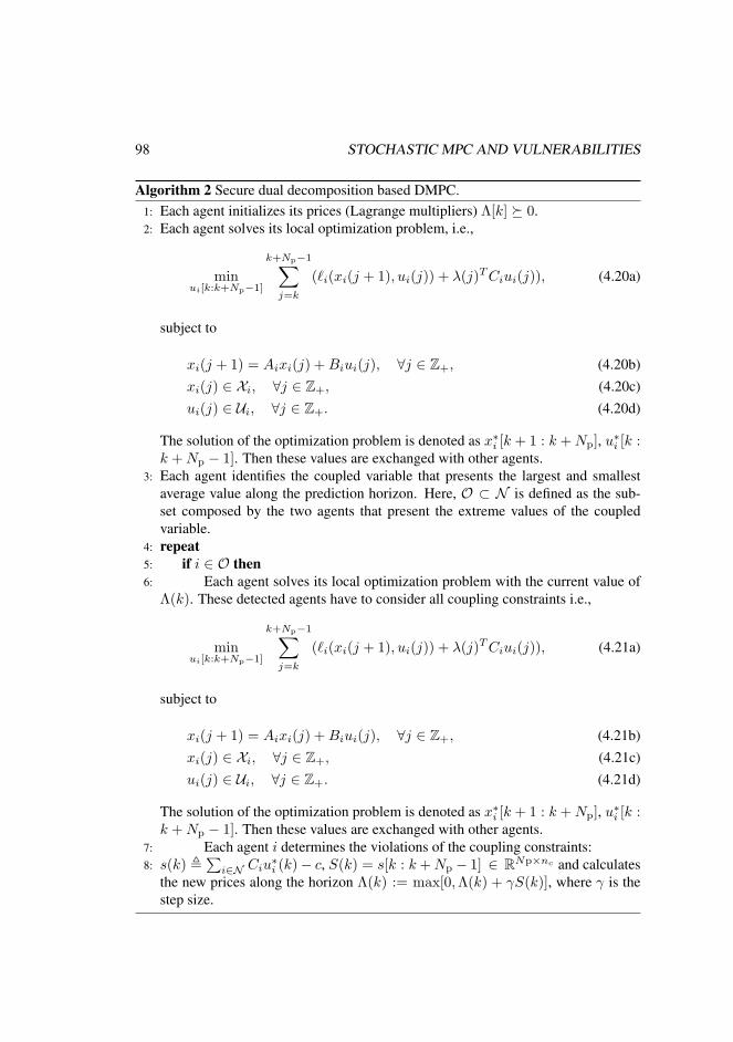
98 STOCHASTIC MPC AND VULNERABILITIES
Algorithm 2 Secure dual decomposition based DMPC.1: Each agent initializes its prices (Lagrange multipliers) Λ[k] ≽ 0.2: Each agent solves its local optimization problem, i.e.,
minui[k:k+Np−1]
k+Np−1∑j=k
(ℓi(xi(j + 1), ui(j)) + λ(j)TCiui(j)), (4.20a)
subject to
xi(j + 1) = Aixi(j) +Biui(j), ∀j ∈ Z+, (4.20b)xi(j) ∈ Xi, ∀j ∈ Z+, (4.20c)ui(j) ∈ Ui, ∀j ∈ Z+. (4.20d)
The solution of the optimization problem is denoted as x∗i [k + 1 : k +Np], u∗
i [k :k +Np − 1]. Then these values are exchanged with other agents.
3: Each agent identifies the coupled variable that presents the largest and smallestaverage value along the prediction horizon. Here, O ⊂ N is defined as the sub-set composed by the two agents that present the extreme values of the coupledvariable.
4: repeat5: if i ∈ O then6: Each agent solves its local optimization problem with the current value of
Λ(k). These detected agents have to consider all coupling constraints i.e.,
minui[k:k+Np−1]
k+Np−1∑j=k
(ℓi(xi(j + 1), ui(j)) + λ(j)TCiui(j)), (4.21a)
subject to
xi(j + 1) = Aixi(j) +Biui(j), ∀j ∈ Z+, (4.21b)xi(j) ∈ Xi, ∀j ∈ Z+, (4.21c)ui(j) ∈ Ui, ∀j ∈ Z+. (4.21d)
The solution of the optimization problem is denoted as x∗i [k + 1 : k +Np], u∗
i [k :k +Np − 1]. Then these values are exchanged with other agents.
7: Each agent i determines the violations of the coupling constraints:8: s(k) ,
∑i∈N Ciu
∗i (k)− c, S(k) = s[k : k+Np − 1] ∈ RNp×nc and calculates
the new prices along the horizon Λ(k) := max[0,Λ(k) + γS(k)], where γ is thestep size.

4.5. CASE STUDY AND RESULTS 99
9: else10: The remaining agents will ignore the coupling constraints provided by
these potential attackers during the consensus process, with the current value ofΛ(k), i.e.,
minui[k:k+Np−1]
k+Np−1∑j=k
(ℓi(xi(j + 1), ui(j)) + λ(j)TCiui(j)), (4.22a)
subject to
xi(j + 1) = Aixi(j) +Biui(j), ∀j ∈ Z+, (4.22b)xi(j) ∈ Xi, ∀j ∈ Z+, (4.22c)ui(j) ∈ Ui, ∀j ∈ Z+. (4.22d)
The solution of the optimization problem x∗i [k + 1 : k +Np], u∗
i [k : k +Np − 1]are exchanged with other agents.
11: Each agent i determines the violations of the coupling constraints:12: s(k) ,
∑i∈N\O Ciu
∗i (k)−c, S[k] = s[k : k+Np−1] ∈ RNp×nc and calculates
the new prices along the horizon Λ(k) := max[0,Λ(k) + γS(k)].13: end if14: until max(S(k)) < ϵ, where ϵ is a prespecified threshold, or the maximum number
of iterations reached.15: Each subsystem implements at the current time step the first component of the
control sequence u∗i [k : k +Np − 1].
16: Let k = k + 1 and return to step 1.
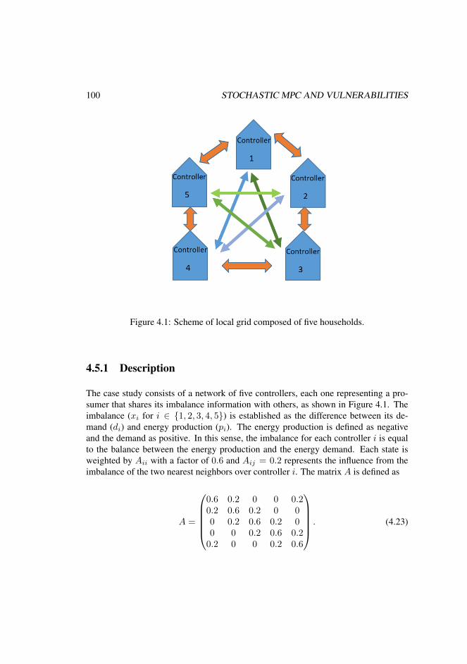
100 STOCHASTIC MPC AND VULNERABILITIES
Figure 4.1: Scheme of local grid composed of five households.
4.5.1 Description
The case study consists of a network of five controllers, each one representing a pro-sumer that shares its imbalance information with others, as shown in Figure 4.1. Theimbalance (xi for i ∈ {1, 2, 3, 4, 5}) is established as the difference between its de-mand (di) and energy production (pi). The energy production is defined as negativeand the demand as positive. In this sense, the imbalance for each controller i is equalto the balance between the energy production and the energy demand. Each state isweighted by Aii with a factor of 0.6 and Aij = 0.2 represents the influence from theimbalance of the two nearest neighbors over controller i. The matrix A is defined as
A =
0.6 0.2 0 0 0.20.2 0.6 0.2 0 00 0.2 0.6 0.2 00 0 0.2 0.6 0.20.2 0 0 0.2 0.6
. (4.23)

4.5. CASE STUDY AND RESULTS 101
At this point, the system model is described as
xi(k + 1) = Aiixi(k) +∑Nb
j=1 Aijxj(k) + ui(k) + ωi(k)
∀i ∈ {1, 2, 3, 4, 5}, j = i, (4.24a)
andxi(k) = di(k) + pi(k),∀k ≥ 0, (4.24b)
where, the control input ui(k) = pi(k) − pi(k − 1) is the increase in the energyproduction. The disturbance ωi(k) = di(k) − di(k − 1) represents the change in theenergy demand.
Also, the systems are coupled by its imbalance, i.e.,
Ajixi(k + 1) = Aijxj(k + 1), ∀i ∈ {1, 2, 3, 4, 5} ∧ j = i. (4.25)
The control system uses DMPC to steer the controllers’ imbalance to zero by pro-ducing energy from the generators. The optimization problem over a prediction horizonNp is given by
Ji = minui[k:k+Np−1]
k+Np∑i=k
[xi[k + 1]TQxi(k + 1)
+ui(k)TRui(k) + λi(k)(Aijxj(k + 1)−Ajixi(k + 1))
],
∀i ∈ {1, 2, 3, 4, 5} ∧ j = i,
(4.26)
subject to (4.24),
pmin < pi(k) < pmax, (4.27a)xi(0) = di(0) + pi(0), (4.27b)
where pmin = 0 kW and pmax = 1 kW. Q and R are the weights of the cost function(4.26). Also, λi is the Lagrangian multiplier described in Section 4.1. Finally, allvalues are given in cost per unit.
4.5.2 Standard Dual Decomposition DMPCThe simulations were carried out with a prediction horizon Np = 8 with a time steplength and simulation time of 1 and 20 minutes, respectively. The demand is consideredconstant for controller 1 and is equal to 0.25 and the remaining controllers have ademand of 0.5. Controller 3 was chosen as the attacker.
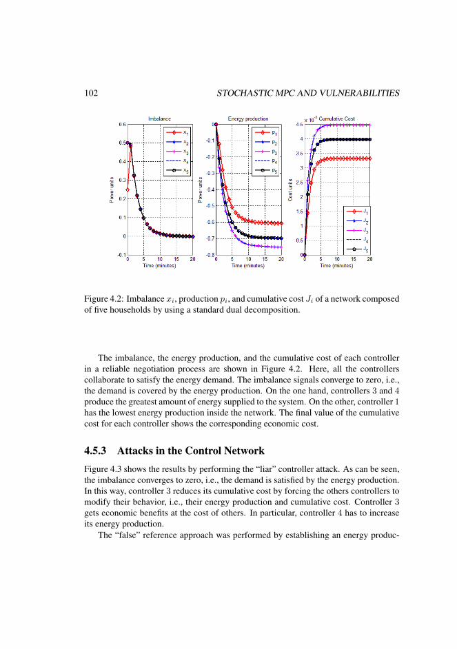
102 STOCHASTIC MPC AND VULNERABILITIES
Figure 4.2: Imbalance xi, production pi, and cumulative cost Ji of a network composedof five households by using a standard dual decomposition.
The imbalance, the energy production, and the cumulative cost of each controllerin a reliable negotiation process are shown in Figure 4.2. Here, all the controllerscollaborate to satisfy the energy demand. The imbalance signals converge to zero, i.e.,the demand is covered by the energy production. On the one hand, controllers 3 and 4produce the greatest amount of energy supplied to the system. On the other, controller 1has the lowest energy production inside the network. The final value of the cumulativecost for each controller shows the corresponding economic cost.
4.5.3 Attacks in the Control NetworkFigure 4.3 shows the results by performing the “liar” controller attack. As can be seen,the imbalance converges to zero, i.e., the demand is satisfied by the energy production.In this way, controller 3 reduces its cumulative cost by forcing the others controllers tomodify their behavior, i.e., their energy production and cumulative cost. Controller 3gets economic benefits at the cost of others. In particular, controller 4 has to increaseits energy production.
The “false” reference approach was performed by establishing an energy produc-

4.5. CASE STUDY AND RESULTS 103
Figure 4.3: Imbalance xi, production pi, and cumulative cost Ji of a network composedof five households by using a “liar” controller approach.
tion reference of x3∗ref = 0.1 for controller 3. Figure 4.4 shows the imbalance, energy
production, and the cumulative cost for the aforementioned network. It is possible tonote that controller 3 reduces the amount of energy production significantly.
Figure 4.5 shows the imbalance, the energy production, and the cumulative costs ofall controllers by using the third attack approach by setting “false” constraints for theenergy production of the controller 3, i.e., 0 < x3[k] < 1. In this way, the controllerreduces its imbalance bounds. It is possible to note that the attacker decreases its energyproduction; conversely, controllers 2 and 4 increase their energy production to steer theimbalance to zero. The final cumulative cost for all agents is increased because theattacker reduces its energy production and the imbalance has to be regulated to zero.
4.5.4 RobustifyingTo ensure certain robustness, we apply scenario-based approaches, as described in Sec-tion 4.3. The price scenarios were obtained by adding a white noise N (0, 0.1), asdescribed in Subsection 4.3.1. The number of scenarios used in both approaches (MS-DMPC and TB-DMPC) was Ns = 10.

104 STOCHASTIC MPC AND VULNERABILITIES
Figure 4.4: Imbalance xi, production pi, and cumulative cost Ji of a network composedof five households by using a “false reference” approach.
Figures 4.6 and 4.7 show the behavior of each controller after applying MS-DMPCand TB-DMPC with a false reference approach. Each one achieves the goal of avoidingthat the malicious controller cheats the others. Notice that the cumulative costs fromMS-DMPC are higher than TB-DMPC.
Table 4.1 shows the cumulative cost by using standard DMPC, the three describedattack approaches, and the cumulative cost resulting from using MS-DMPC and TB-DMPC to the attack schemes for each controller. As can be seen, both scenario-basedDMPC are able to reduce the effects that a malicious controller causes. MS-DMPC pro-duces a single control input valid for all scenarios, resulting in an expensive cumulativecost. TB-DMPC relaxes this over conservativeness by computing as many control se-quences as scenarios are considered by increasing its computational burden. Therefore,the cumulative costs are reduced with TB-DMPC compared with MS-DMPC.
It is important to remark that these scenario-based schemes give certain robustness.However, they increase the cumulative costs for the whole system, i.e., there is a lossof performance of the only system. In this sense, these schemes could be carried outwhen the system is under a potential attack and also has sufficient resources.
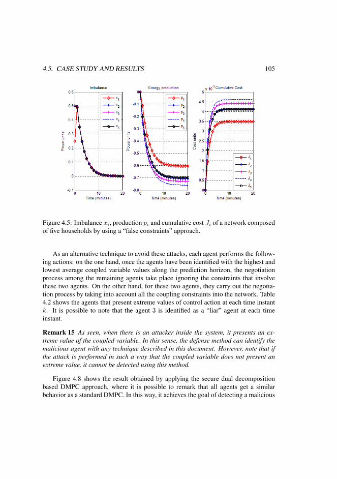
4.5. CASE STUDY AND RESULTS 105
Figure 4.5: Imbalance xi, production pi and cumulative cost Ji of a network composedof five households by using a “false constraints” approach.
As an alternative technique to avoid these attacks, each agent performs the follow-ing actions: on the one hand, once the agents have been identified with the highest andlowest average coupled variable values along the prediction horizon, the negotiationprocess among the remaining agents take place ignoring the constraints that involvethese two agents. On the other hand, for these two agents, they carry out the negotia-tion process by taking into account all the coupling constraints into the network. Table4.2 shows the agents that present extreme values of control action at each time instantk. It is possible to note that the agent 3 is identified as a “liar” agent at each timeinstant.
Remark 15 As seen, when there is an attacker inside the system, it presents an ex-treme value of the coupled variable. In this sense, the defense method can identify themalicious agent with any technique described in this document. However, note that ifthe attack is performed in such a way that the coupled variable does not present anextreme value, it cannot be detected using this method.
Figure 4.8 shows the result obtained by applying the secure dual decompositionbased DMPC approach, where it is possible to remark that all agents get a similarbehavior as a standard DMPC. In this way, it achieves the goal of detecting a malicious

106 STOCHASTIC MPC AND VULNERABILITIES
Figure 4.6: Imbalance xi, production pi, and cumulative cost Ji of a network composedof five households by using a “false reference” approach and MS-DMPC.
agent within the distributed controllers network, forcing all agents to negotiate in arelatively honest way, although there is a chance that an innocent agent is punished andignored.
One disadvantage of this defense approach is that an innocent agent can be penal-ized for presenting an extreme value in the information exchanged. The resulting lossof performance is the price to pay in order to gain robustness against potential attack-ers. In any case it becomes clear in this work that DMPC schemes should introducemechanisms that discourage or limit the consequences derived from potential attacks.Likewise, it is important to remark that the violation of some of the constraints could bederived from the attacks or even from a wrong implementation of this defense policy.Hence, its application must be carefully designed to avoid this type of issues. More-over, it is necessary to think carefully about the role of the constraints in this context,especially since fake constraints could be used to take advantage of the DMPC scheme.In case that the fulfillment of the constraints is essential for the application considered,a supervisory layer could be included to ensure that the control actions taken do notpush the system beyond its limits.
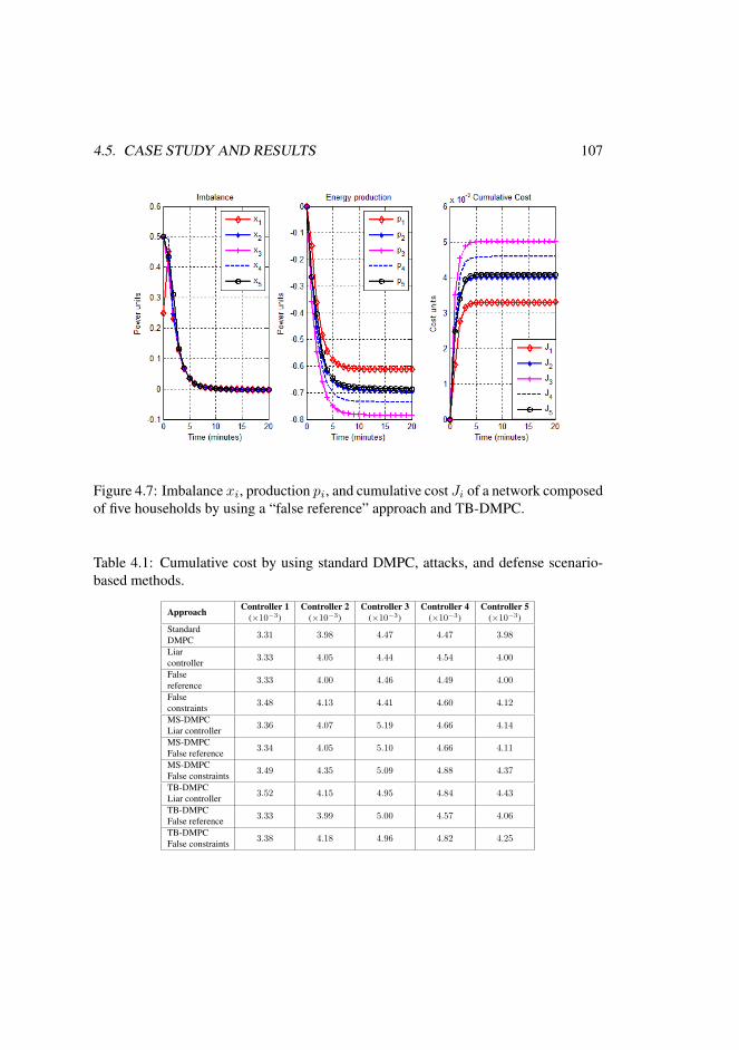
4.5. CASE STUDY AND RESULTS 107
Figure 4.7: Imbalance xi, production pi, and cumulative cost Ji of a network composedof five households by using a “false reference” approach and TB-DMPC.
Table 4.1: Cumulative cost by using standard DMPC, attacks, and defense scenario-based methods.
Approach Controller 1 Controller 2 Controller 3 Controller 4 Controller 5(×10−3) (×10−3) (×10−3) (×10−3) (×10−3)
Standard3.31 3.98 4.47 4.47 3.98DMPC
Liar3.33 4.05 4.44 4.54 4.00controller
False3.33 4.00 4.46 4.49 4.00reference
False3.48 4.13 4.41 4.60 4.12constraints
MS-DMPC3.36 4.07 5.19 4.66 4.14Liar controller
MS-DMPC3.34 4.05 5.10 4.66 4.11False reference
MS-DMPC3.49 4.35 5.09 4.88 4.37False constraints
TB-DMPC3.52 4.15 4.95 4.84 4.43Liar controller
TB-DMPC3.33 3.99 5.00 4.57 4.06False reference
TB-DMPC3.38 4.18 4.96 4.82 4.25False constraints
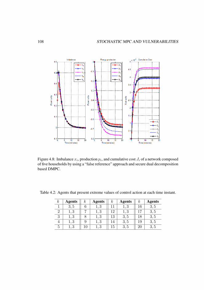
108 STOCHASTIC MPC AND VULNERABILITIES
Figure 4.8: Imbalance xi, production pi, and cumulative cost Ji of a network composedof five households by using a “false reference” approach and secure dual decompositionbased DMPC.
Table 4.2: Agents that present extreme values of control action at each time instant.
k Agents k Agents k Agents k Agents1 3, 5 6 1, 3 11 1, 3 16 3, 52 1, 3 7 1, 3 12 1, 3 17 3, 53 1, 3 8 1, 3 13 3, 5 18 3, 54 1, 3 9 1, 3 14 3, 5 19 3, 55 1, 3 10 1, 3 15 3, 5 20 3, 5

Chapter 5
Conclusions and FutureResearches
Several control approaches cope with the operational management of distribution sys-tems as a hierarchical control given by layers of planning, management, and regulationof the nonlinear system. However, those techniques, in spite of the inherent robustnessof optimization-based controllers, do not guarantee the proper disturbance rejectionrelated to the uncertainties of the whole system.
The novelty of this work consists in the design and assessment of three stochasticcontrollers applied to the operational management of distribution systems, in this case,energy dispatch systems and water resource management. These stochastic controllersare designed to deal with internal and external uncertainties with different configura-tions, i.e., centralized, hierarchical, and distributed fashion. The common advantage ofall the proposed approaches relies, apart of the robustness features, on the compromisebetween profits, reliability, and computational burden. Moreover, this thesis offers adeep discussion about the tractability and performance of the closed loops based on theproposed approaches.
During the last years, distributed model predictive control (DMPC) has becomea very active optimal control field where many algorithms and strategies have beenproposed to ease the coordination in multi-agent systems where there are coupled dy-namics. This work raises an important issue in the field of DMPC. In particular, DMPCschemes rely on the assumption that the information shared across the network is trust-worthy. A malicious controller could send false information to the rest of the con-trollers to steer the negotiation process, which may result in a loss of performance or
109

110 CHAPTER 5. CONCLUSIONS AND FUTURE RESEARCHES
even in the instability of the closed loop system. To illustrate and raise awareness of thisproblem, this work has presented the vulnerabilities of a very popular distributed modelpredictive control scheme. More specifically, it has shown how a malicious agent inthe network could exploit the information exchange to steer the negotiation processarbitrarily. Also, stochastic based MPCs and a heuristic technique have been proposedas alternatives to give some robustness the DMPC scheme against this problem.
5.1 ConclusionsBelow, the main conclusions of each chapter of this thesis are provided.
• Centralized Stochastic Model Predictive Control
In Chapter 2, stochastic MPC schemes have been designed and applied to ensurerobustness against external disturbances in the context of distribution systems,more specifically, a real microgrid, the drinking water network of Barcelona,and the stock management of a hospital pharmacy. In this context, it is possi-ble to conclude that MS-MPC controller is over-conservative because it does notconsider the controller capacity to adapt. It calculates a control series valid toall possible scenarios by means an open-loop formulation. However, it is pos-sible to solve the optimization problem by using a control tree and increasingthe number of optimization variables and the computational time. Regardingthe control point of view, TB-MPC controller works in a closed-loop fashion toadapt the control actions to the expected evolution of the disturbances. Finally,CC-MPC controller formulates the optimization problem by taking into accountthe statistical features of the uncertainty without increasing the number of vari-ables. The results obtained with the three presented versions of stochastic MPCcontrollers show their effectiveness in energy management and drinking waternetwork under economic and optimal criteria. According to the results obtainedand the evaluation of the case studies, it can be said that CC-MPC controllerrelaxes the constraints of the optimization problem by assuming a risk to offerbetter performance, resulting in a lower cost, less energy exchange with the net-work and a lower number of constraints violation for energy management anddrinking water networks compared MS-MPC and TB-MPC controllers. This isalso the approach with the lowest computational burden. The downside of thisapproach is that it requires a statistical characterization of the disturbances.
Also, a solution for the problem of stock management in a hospital pharmacy hasbeen proposed. A control methodology has been described to deal with the dif-ferent and contradictory objectives of the problem. The proposed control strategy
5.1. CONCLUSIONS 111
is a based on MPC, which allows the fulfillment of the management objectiveswhile imposing different operational constraints. In that way, it has been possi-ble to guarantee, with a high probability, that the drugs will be available for thepatients, knowing explicitly the allowed risk level. In addition, we have shownthat several hospitals could collaborate to reduce their stock levels. Finally, somesimulations have been carried out to show the performance of the proposed man-agement approach. It has been seen how the average level of stocked drugs hasbeen reduced, which reduces the economical costs for the hospital, and how thework burden in the pharmacy was also reduced while guaranteeing the needs ofthe patients.
• Hierarchical Stochastic MPC
In Chapter 3, this work has shown a risk assessment methodology applied tomicrogrids. Although many risks have been identified, only a reduced set ofthem has been used in the example for illustrating the method. Two differentmodel predictive controllers have been used. One for the external loop in orderto evaluate risks and determine the optimal mitigation actions and another for thecontrol of the plant. Results show that the benefits that can be obtained are verypositive.
By another site, it has been considered a water resource management system,which is subject to dynamical uncertainty. The system is distributed into subsys-tems at the bottom, but the overall performance is checked for the whole systemat the top layer. The final goal was to decompose the overall problem into differ-ent regions and under different hydrological conditions. In this sense, a scenariobased Hierarchical and Distributed Model Predictive Control have been used toaddress the disturbances and uncertainties, which commonly affect this kind ofsystems. For the uncertainty, the tree based approach based on scenarios hasbeen widely applied principally in the field of centralized water systems due toits adaptability at the moment to generate the disturbances tree. A drawback thatpresents this approach is its higher computational burden, this problem was ad-dressed by the hierarchical controller, which collects the whole information andsends only the most likely scenarios to be taken into account by the distributedcontrollers at the time to solve the local optimization problem. Results show theeffectiveness of this method to ensure the water level into the desired referencedespite the presence of uncertainties for a large scale system.
• Stochastic MPC to Deal with Vulnerabilities in Distributed Schemes
In Chapter 4, cyber-security issues in DMPC have been considered. An anal-ysis of the vulnerability of a popular Lagrange-based DMPC scheme has been

112 CHAPTER 5. CONCLUSIONS AND FUTURE RESEARCHES
presented. By using a relevant case study involving a power network, we haveillustrated the potential of this mechanism, and how a controller can attack thesystem to obtain benefits. It has been addressed the problem of providing ro-bustness to DMPC for defending it from a malicious controller by carrying outscenario-based mechanisms. We have also proposed a heuristic mechanism todefend the attacked agents, that is, to identify false information and perform thenegotiation process among agents regardless of the actions of the attacker. Ahighly relevant case study involving a power network illustrates the potential ofthis mechanism.
5.2 Future ResearchesThe research of stochastic MPC techniques applied to distribution systems has been amajor issue in recent years. However, some important issues fall out of the scope ofthis thesis and can be studied in the future. Next, several research lines are pointed outfor their study and analysis.
• On the one hand, centralized stochastic MPCs have been analyzed and imple-mented via simulation and experimental setup, describing their advantages anddrawbacks. However, in this work the bounds for violating constraints were as-sumed in the same way for MS-MPC and TB-MPC, this assumption may bemodified, and a further study for TB-MPC may be developed. Moreover, somealgorithms for obtaining three disturbances deserve particular attention for im-proving the computational burden. Regarding CC-MPC, the formulation of de-terministic constraints to replace the stochastic ones by considering other well-known probability distribution functions instead of normal distribution functionsor historical data, as been discussed, may be an accurate bullet for being devel-oped.
• On the other hand, regarding hierarchical and distributed MPC, it is importantto remark the possibility to design, implement, and compare the assessment andperformance of other stochastic MPC at the lower level to deal with the uncer-tainty that the distribution system present. Furthermore, some results have beencarried out by simulation and show the benefit of these approaches described inthis document; however, an aggregated value will apport an experimental setupin real case studies.
• Cyber-security issues is a very relevant and critical topic that has not been ex-plicitly considered in the DMPC literature in a structured way. In this thesis,

5.3. PUBLICATIONS FROM THIS WORK 113
one of the most popular distributed MPC schemes has been considered. How-ever, other kinds of attacks will be discussed in different distributed algorithms.In this sense, there are many important issues in the context of distribution sys-tems related to the reliable information exchange that can be exploited, such asuncertainty in the demand patterns will be considered as a manner to robustifythe system against possible internal attackers. Moreover, the use of the quality ofservice (QoS) as an index of trustworthiness of each agent will be investigated. Itwill also address cyber security issues in DMPC from other points of view, e.g.,by considering other stochastic MPC methods or by developing new approachesto identify and isolate the attackers from the whole distributed system. In thismanner, it is possible to mitigate losses and the impact from malicious agents inthe performance of the system.
5.3 Publications from this workSeveral publications have taken place as peer-reviewed articles and conference papers.The list of scientific articles is enumerated as follows:
• Jurado, I., Maestre, J. M., Velarde, P., Ocampo-Martinez, C., Fernndez, I., Tejera,B. I., del Prado, J. R. (2016). Stock management in hospital pharmacy us-ing chance-constrained model predictive control. Computers in biology andmedicine, 72, 248-255.
• Grosso, J. M., Velarde, P., Ocampo-Martinez, C., Maestre, J. M., Puig, V. (2016).Stochastic model predictive control approaches applied to drinking water net-works. Optimal Control Applications and Methods. DOI:10.1002/oca.2269.
• Velarde, P., Valverde, L., Maestre, J. M., Ocampo-Martinez, C., Bordons, C.(2017). On the comparison of stochastic model predictive control strategies ap-plied to a hydrogen-based microgrid, Journal of Power Sources, 343, 161-173.
• Velarde, P., Maestre, J. M., Ishii, H., Negenborn, R. R., (2017). Vulnerabilitiesin Lagrange-based Distributed Model Predictive Control. Submitted to OptimalControl Applications and Methods.
• Maestre, J. M., Velarde, P., Jurado, I., Ocampo-Martnez, C., Fernandez, I.,Tejera, B. I., del Prado, J. R. (2014, December). An application of chance-constrained model predictive control to inventory management in hospitalarypharmacy. In 53rd IEEE Conference on Decision and Control (pp. 5901-5906).IEEE.

114 CHAPTER 5. CONCLUSIONS AND FUTURE RESEARCHES
• Velarde, P., Maestre, J. M., Jurado, I., Fernandez, I., Tejera, B. I., del Prado,J. R. (2014, September). Application of robust model predictive control to in-ventory management in hospitalary pharmacy. In Proceedings of the 2014 IEEEEmerging Technology and Factory Automation (ETFA) (pp. 1-6). IEEE.
• Velarde, P., Maestre, J. M., Ocampo-Martinez, C., Bordons, C. (2016, June).Application of robust model predictive control to a renewable hydrogen-basedmicrogrid. In Proceedings of the 2016 European Control Conference (ECC),Aalborg, Denmark, 2016, pp. 1209-1214.
• Velarde, P., Maestre, J. M., Ishii, H., Negenborn, R. R., Vulnerabilities in Lagrange-based DMPC in the Context of Cyber-Security. Submitted to The 20th WorldCongress of the International Federation of Automatic Control (IFAC).
• Velarde, P., Maestre, J. M., Ishii, H., Negenborn, R. R., Scenario Based DefenseMechanism for Distributed Model Predictive Control. Submitted to The 20thWorld Congress of the International Federation of Automatic Control (IFAC).
• Zafra-Cabeza, A., Velarde, P., Maestre, J. M., Multicriteria Optimal Operationof a Microgrid considering Risk Analysis, Renewable Resources and MPC. Sub-mitted to The 20th World Congress of the International Federation of AutomaticControl (IFAC).
• Maestre, J. M., Velarde, P., Muros, F. J., An Application of the LogarithmicMean Divisia Index Method to Distributed and Coalitional Control. Submittedto The 20th World Congress of the International Federation of Automatic Control(IFAC).

Bibliography
[1] C. Ocampo-Martinez, V. Puig, G. Cembrano, J. Quevedo, Application of pre-dictive control strategies to the management of complex networks in the urbanwater cycle, Control Systems, IEEE 33 (1) (2013) 15–41.
[2] E. F. Camacho, C. Bordons, Model Predictive Control. Second Edition,Springer-Verlag, London, England, 2004.
[3] J. Maciejowski, Predictive control with constraints, Prentice Hall, Essex, Eng-land, 2002.
[4] D. Bernardini, A. Bemporad, Scenario-based model predictive control ofstochastic constrained linear systems, Joint 48th IEEE Conference on Decisionand Control and 28th Chinese Control Conference, Shanghai, P.R. China (2009)6333–6338.
[5] M. Cannon, P. Couchman, B. Kouvaritakis, MPC for stochastic systems, in:R. Findeisen, F. Allgower, L. Biegler (Eds.), Assessment and Future Directionsof Nonlinear Model Predictive Control, Vol. 358 of Lecture Notes in Controland Information Sciences, Springer Berlin Heidelberg, 2007, pp. 255–268.
[6] D. Munoz de la Pena, A. Bemporad, T. Alamo, Stochastic programming appliedto model predictive control, in: Proceedings of 44th IEEE Conference on Deci-sion and Control and European Control Conference (CDC-ECC), Seville, 2005,pp. 1361 – 1366.
[7] D. Munoz de la Pena, A. Bemporad, T. Alamo, Stochastic programming appliedto model predictive control, in: Proceedings of the 44th IEEE Conference onDecision and Control, and European Control Conference (CDC-ECC), Seville,Spain, 2005, pp. 1361–1366.
115
116 BIBLIOGRAPHY
[8] G. Calafiore, F. Dabbene, Probabilistic and randomized methods for design un-der uncertainty, Springer, London, England, 2006.
[9] G. Calafiore, F. Dabbene, R. Tempo, Research on probabilistic methods for con-trol system design, Automatica 47 (7) (2011) 1279 – 1293.
[10] P. J. van Overloop, S. Weijs, S. Dijkstra, Multiple model predictive control on adrainage canal system, Control Engineering Practice 16 (5) (2008) 531–540.
[11] D. E. Olivares, J. D. Lara, C. A. Canizares, M. Kazerani, Stochastic-predictiveenergy management system for isolated microgrids, IEEE Transactions on SmartGrid 6 (6) (2015) 2681–2693.
[12] T. Niknam, R. Azizipanah-Abarghooee, M. R. Narimani, An efficient scenario-based stochastic programming framework for multi-objective optimal micro-grid operation, Applied Energy 99 (2012) 455 – 470.
[13] G. Calafiore, M. Campi, The scenario approach to robust control design, IEEETransactions on Automatic Control 51 (5) (2006) 742–753.
[14] S. Lucia, T. Finkler, D. Basak, S. Engell, A new robust NMPC scheme andits application to a semi-batch reactor example., In Proc. of the InternationalSymposium on Advanced Control of Chemical Processes, Singapore (2012) 69–74.
[15] M. Petrollese, L. Valverde, D. Cocco, G. Cau, J. Guerra, Real-time integrationof optimal generation scheduling with MPC for the energy management of arenewable hydrogen-based microgrid, Applied Energy 166 (2016) 96–106.
[16] J. M. Maestre, L. Raso, P. J. Van Overloop, B. De Schutter, Distributed tree-based model predictive control on an open water system, in: Proceedings of theAmerican Control Conference (ACC), Montreal, Canada, 2012, pp. 1985–1990.
[17] Q. Wang, Y. Guan, J. Wang, A chance-constrained two-stage stochastic programfor unit commitment with uncertain wind power output, IEEE Transactions onPower Systems 27 (1) (2012) 206–215.
[18] M. Ono, U. Topcu, M. Yo, S. Adachi, Risk-limiting power grid control with anarma-based prediction model, in: Proceedings of the 52nd IEEE Annual Con-ference on Decision and Control (CDC), Florence, Italy, 2013, pp. 4949–4956.

BIBLIOGRAPHY 117
[19] J. Grosso, C. Ocampo-Martinez, V. Puig, B. Joseph, Chance-constrained modelpredictive control for drinking water networks, Journal of Process Control 24 (5)(2014) 504–516.
[20] J. Grosso, J. Maestre, C. Ocampo-Martinez, V. Puig, On the assessment of tree-based and chance-constrained predictive control aproaches applied to drinkingwater networks, 19th IFAC World Congress, Cape Town, South Africa (2014)6240–6245.
[21] A. Hooshmand, B. Asghari, R. Sharma, A novel cost-aware multi-objective en-ergy management method for microgrids, in: Proceedings of the InnovativeSmart Grid Technologies (ISGT), IEEE PES, Washington, DC, USA, 2013, pp.1–6.
[22] Z. Yu, L. McLaughlin, L. J., M. Murphy-Hoye, A. Pratt, L. T., Modeling andstochastic control for home energy management, in: Proceedings of the IEEEPower and Energy Society General Meeting, San Diego, California, USA, 2012,pp. 1–9.
[23] P. Meibom, R. Barth, B. Hasche, H. Brand, C. Weber, M. O’Malley, Stochasticoptimization model to study the operational impacts of high wind penetrationsin Ireland, IEEE Transactions on Power Systems 26 (3) (2011) 1367–1379.
[24] T. Hovgaard, L. Larsen, J. Jorgensen, Robust economic MPC for a power man-agement scenario with uncertainties, in: Proceedings of the 50th IEEE Confer-ence on Decision and Control and European Control Conference (CDC-ECC),Orlando, Florida, 2011, pp. 1515–1520.
[25] X. Tian, J. Maestre, P. van Overloop, R. Negenborn, Distributed model predic-tive control for multi-objective water system management, in: Proceedings of10th Int. Conf. hydroinformatics, Hamburg, Germany, 2012, p. 175.
[26] R. R. Negenborn, P.-J. van Overloop, T. Keviczky, B. De Schutter, Distributedmodel predictive control of irrigation canals., NHM 4 (2) (2009) 359–380.
[27] A. Zafra-Cabeza, J. Maestre, M. A. Ridao, E. F. Camacho, L. Sanchez, A hierar-chical distributed model predictive control approach to irrigation canals: A riskmitigation perspective, Journal of Process Control 21 (5) (2011) 787–799.
[28] A. Sadowska, P. Overloop, C. Burt, B. Schutter, Hierarchical operation of wa-ter level controllers: Formal analysis and application on a large scale irrigationcanal, Water Resources Management 28 (14) (2014) 4999–5019.
118 BIBLIOGRAPHY
[29] A. Sadowska, B. De Schutter, P.-J. van Overloop, Delivery-oriented hierarchi-cal predictive control of an irrigation canal: event-driven versus time-drivenapproaches, IEEE Transactions on Control Systems Technology 23 (5) (2015)1701–1716.
[30] J. M. Maestre, R. R. Negenborn, Distributed Model Predictive Control MadeEasy, Springer, 2014.
[31] P. Velarde, L. Valverde, J. M. Maestre, C. Ocampo-Martinez, C. Bordons, Onthe comparison of stochastic model predictive control strategies applied to ahydrogen-based microgrid, Journal of Power Sources 343 (2017) 161–173.
[32] J. M. Grosso, P. Velarde, C. Ocampo-Martinez, J. M. Maestre, V. Puig,Stochastic model predictive control approaches applied to drinking wa-ter networks, Optimal Control Applications and Methods In Press.doi:10.1002/oca.2269.
[33] I. Jurado, J. Maestre, P. Velarde, C. Ocampo-Martinez, I. Fernandez, B. I. Tejera,J. del Prado, Stock management in hospital pharmacy using chance-constrainedmodel predictive control, Computers in biology and medicine 72 (2016) 248–255.
[34] H. van de Water, J. Willems, The certainty equivalence property in stochasticcontrol theory, IEEE Transactions on Automatic Control 26 (5) (1981) 1080 –1087.
[35] J. M. Grosso, On model predictive control for economic and robust operationof generalised flow-based networks, Ph.D. thesis, Universitat Politecnica deCatalunya, Barcelona, Spain (2015).
[36] H. van de Water, J. Willems, The certainty equivalence property in stochasticcontrol theory, IEEE Transactions on Automatic Control 26 (5) (2002) 1080–1087.
[37] G. Schildbach, L. Fagiano, C. Frei, M. Morari, The scenario approach forstochastic model predictive control with bounds on closed-loop constraint vi-olations, Automatica 50 (12) (2014) 3009–3018.
[38] L. Giulioni, Stochastic model predictive control with application to distributedcontrol systems, Ph.D. thesis, Politecnico di Milano (2015).

BIBLIOGRAPHY 119
[39] L. Raso, N. Giesen, P. Stive, D. Schwanenberg, P. Overloop, Tree structure gen-eration from ensemble forecasts for real time control, Hydrological Processes27 (1) (2013) 75–82.
[40] L. Raso, D. Schwanenberg, N. van de Giesen, P. van Overloop, Short-term op-timal operation of water systems using ensemble forecasts, Advances in WaterResources 71 (2014) 200 – 208.
[41] J. P. Lopes, C. Moreira, A. Madureira, Defining control strategies for microgridsislanded operation, IEEE Transactions on Power Systems 21 (2) (2006) 916–924.
[42] L. Valverde, C. Bordons, F. Rosa, Integration of fuel cell technologies inrenewable-energy-based microgrids optimizing operational costs and durability,IEEE Transactions on Industrial Electronics 63 (1) (2016) 167–177.
[43] C. Kunusch, C. Ocampo-Martinez, M. Valla, Modeling, diagnosis, and controlof fuel-cell-based technologies and their integration in smart grids and automo-tive systems, IEEE Transactions on Industrial Electronics 62 (8) (2015) 5143–5145.
[44] L. Valverde, F. Rosa, C. Bordons, Design, planning and management of ahydrogen-based microgrid, IEEE Transactions on Industrial Informatics 9 (3)(2013) 1398–1404.
[45] D. Recio, C. Ocampo-Martinez, M. Serra, Design of linear predictive controllersapplied to ethanol steam reformers for hydrogen production, International Jour-nal of Hydrogen Energy 37(15) (2012) 11141–11156.
[46] T. Dragicevic, J. Guerrero, J. Vasquez, A distributed control strategy for coordi-nation of an autonomous LVDC microgrid based on power-line signaling, IEEETransactions on Industrial Electronics 61 (7) (2014) 3313–3326.
[47] D. E. Olivares, A. Mehrizi-Sani, A. H. Etemadi, C. A. Canizares, R. Iravani,M. Kazerani, A. H. Hajimiragha, O. Gomis-Bellmunt, M. Saeedifard, R. Palma-Behnke, G. Jimenez-Estevez, N. Hatziargyriou, Trends in microgrid control,IEEE Transactions on Smart Grid 5 (4) (2014) 1905–1919.
[48] L. Valverde, F. Rosa, A. del Real, A. Arce, C. Bordons, Modeling, simulationand experimental set-up of a renewable hydrogen-based domestic microgrid,International Journal of Hydrogen Energy 38 (2013) 11672–11684.

120 BIBLIOGRAPHY
[49] C. Bordons, F. Garcıa-Torres, L. Valverde, Gestion optima de la energıa en mi-crorredes con generacion renovable, Revista Iberoamericana de Automatica eInformatica Industrial RIAI 12 (2) (2015) 117–132.
[50] B. S. Lee, H. Y. Park, I. Choi, M. K. Cho, H. J. Kim, S. J. Yoo, D. Henkensmeier,J. Y. Kim, S. W. Nam, S. Park, et al., Polarization characteristics of a low catalystloading pem water electrolyzer operating at elevated temperature, Journal ofPower Sources 309 (2016) 127–134.
[51] A. J. Del Real, A. Arce, C. Bordons, Development and experimental validationof a pem fuel cell dynamic model, Journal of Power Sources 173 (1) (2007)310–324.
[52] M. Tanrioven, M. Alam, Reliability modeling and assessment of grid-connectedpem fuel cell power plants, Journal of Power Sources 142 (1) (2005) 264–278.
[53] L. Valverde, F. Rosa, A. del Real, A. Arce, C. Bordons, Modeling, simulationand experimental set-up of a renewable hydrogen-based domestic microgrid,International Journal of Hydrogen Energy 38 (27) (2013) 11672–11684.
[54] M. Pereira, D. Limon, D. Munoz de la Pena, L. Valverde, T. Alamo, Periodiceconomic control of a nonisolated microgrid, IEEE Transactions on IndustrialElectronics 62 (8) (2015) 5247–5255.
[55] F. Garcia-Torres, C. Bordons, Optimal economical schedule of hydrogen-basedmicrogrids with hybrid storage using model predictive control, IEEE Transac-tions on Industrial Electronics 62 (8) (2015) 5195–5207.
[56] A. Brooke, D. Kendrick, A. Meeraus, R. Raman, General algebraic modelingsystem (GAMS): A users guide, Boyd & Fraser publishing company, Danvers,Massachusetts.
[57] E. Karfopoulos, L. Tena, A. Torres, P. Salas, J. G. Jorda, A. Dimeas, N. Hatziar-gyriou, A multi-agent system providing demand response services from residen-tial consumers, Electric Power Systems Research 120 (2015) 163 – 176.
[58] H. Alegre, J. Baptista, E. Cabrera, F. Cubillo, Performance Indicators for WaterSupply Services, Manuals of Best Practice Series, IWA Publishing, 2006.
[59] G. E. P. Box, G. M. Jenkins, G. C. Reisnel, Time Series Analysis, Forecastingand Control, 3rd Edition, Prentice-Hall International, Inc., New Jersey, U.S.A,1994.
BIBLIOGRAPHY 121
[60] G. Schildbach, L. Fagiano, C. Frei, M. Morari, The scenario approach forstochastic model predictive control with bounds on closed-loop constraint vi-olations, Automatica 50 (12) (2014) 3009–3018.
[61] H. Heitsch, W. Romisch, Scenario tree modeling for multistage stochastic pro-grams, Mathematical Programming 118 (2) (2009) 371–406.
[62] L. Raso, D. Schwanenberg, N. van der Giesen, P.-J. van Overloop, Tree-scenariobased model predictive control, in: Proceedings of EGU General Assembly Con-ference Abstracts, Vol. 12, 2010, p. 3178.
[63] S. Lucia, S. Subramanian, S. Engell, Non-conservative robust nonlinear modelpredictive control via scenario decomposition, in: Proceedings of IEEE Multi-Conference on Systems and Control (MSC), Hyderabad, India, 2013, pp. 586–591.
[64] T. Bermejo, B. Cuna, V. Napal, E. Valverde, The hospitalary pharmacy specialisthandbook (in Spanish), Spanish Society of Hospitalary Pharmacy, 1999.
[65] S. Tayur, R. Ganeshan, M. Magazine, Quantitative models for supply chain man-agement, Kluwer Academic Publisher, 1999.
[66] A. M. Brewer, K. J. Button, D. A. Hensher, Handbook of logistics and supply-chain management, Pergamon, 2001.
[67] S. Cetinkaya, C. Lee, Stock replenishment and shipment scheduling for vendor-managed inventory systems, Management Science 46 (2) (2000) 217–232.
[68] J. Dong, D. Zhang, A. Nagurney, A supply chain network equilibrium modelwith random demands, European Journal of Operational Research 156 (1)(2004) 194–212.
[69] G. Cachon, Stock wars: Inventory competition in a two-echelon supply chainwith multiple retailers, Operations Research 49 (5) (2001) 658–674.
[70] S. Rezapour, R. Farahani, Strategic design of competing centralized supplychain networks for markets with deterministic demands, Advances in Engineer-ing Software 41 (5) (2010) 810822.
[71] E. Lawler, D. Wood, Branch-and-bound methods: A survey, Operations Re-search 14 (4) (1966) 699–719.

122 BIBLIOGRAPHY
[72] V. Summanwara, V. Jayaramana, B. Kulkarnia, H. Kusumakarb, K. Guptab,J. Rajesh, Solution of constrained optimization problems by multi-objective ge-netic algorithm, Computers & Chemical Engineering 26 (10) (2002) 1481–1492.
[73] W. Cook, R. Kannan, A. Schrijver, Chvatal closures for mixed integer program-ming problems, Mathematical Programming 47 (1) (1990) 155–174.
[74] J. Maestre Torreblanca, P. Velarde, I. Jurado, C. Ocampo-Martinez, I. Fernandez,B. Isla Tejera, J. del Prado Llergo, An application of chance-constrained modelpredictive control to inventory management in hospitalary pharmacy, in: 53rdIEEE Conference on Decision and Control, CDC 2014, Los Angeles, CA, USA,December 15-17, 2014, pp. 5901–5906.
[75] C. Hood, D. K. C. Jones, Accident And Design: Contemporary Debates On RiskManagement, Taylor & Francis, 2003.
[76] A. Zafra-Cabeza, M. Ridao, E. Camacho, A mixed integer quadratic program-ming formulation of risk management for reverse osmosis plants, Desalination268.
[77] P. C. D. Milly, J. Betancourt, M. Falkenmark, R. M. Hirsch, Z. W. Kundzewicz,D. P. Lettenmaier, R. J. Stouffer, Stationarity Is Dead: Whither Water Manage-ment?, Science 319 (5863) (2008) 573–574.
[78] M. Spiller, J. H. Vreeburg, I. Leusbrock, G. Zeeman, Flexible design in waterand wastewater engineering Definitions, literature and decision guide, Journalof Environmental Management 149 (2015) 271–281.
[79] M. Haasnoot, J. H. Kwakkel, W. E. Walker, Dynamic adaptive policy pathways: A method for crafting robust decisions for a deeply uncertain world, GlobalEnvironmental Change 23 (2) (2013) 485–498.
[80] G. W. Characklis, B. R. Kirsch, J. Ramsey, K. E. M. Dillard, C. T. Kelley, De-veloping portfolios of water supply transfers, Water Resources Research 42 (5).
[81] E. H. Y. Beh, H. R. Maier, G. C. Dandy, Adaptive, multiobjective optimal se-quencing approach for urban water supply augmentation under deep uncertainty,Water Resources Research 51 (3) (2015) 1529–1551.
[82] W. Walker, M. Haasnoot, J. Kwakkel, Adapt or Perish: A Review of PlanningApproaches for Adaptation under Deep Uncertainty, Sustainability 5 (3) (2013)955–979.

BIBLIOGRAPHY 123
[83] L. Raso, D. Schwanenberg, N. van de Giesen, P. van Overloop, Short-term op-timal operation of water systems using ensemble forecasts, Advances in WaterResources 71 (2014) 200–208.
[84] J. Maestre, L. Raso, P. V. Overloop, B. De Schutter, Distributed tree-basedmodel predictive control on a drainage water system, Journal of Hydroinfor-matics 15 (2) (2013) 335–347.
[85] P. J. van Overloop, Model predictive control on open water systems, Ph.D. the-sis, Delft University of Technology (2006).
[86] X. Tian, P.-J. van Overloop, R. R. Negenborn, N. van de Giesen, Operationalflood control of a low-lying delta system using large time step model predictivecontrol, Advances in Water Resources 75 (2015) 1 – 13.
[87] M. Xu, Real-time control of combined water quantity & quality in open chan-nels, TU Delft, Delft University of Technology, 2013.
[88] M. Xu, P. J. van Overloop, N. van de Giesen, Model reduction in model predic-tive control of combined water quantity and quality in open channels, Environ-mental Modelling & Software 42 (2013) 72 – 87.
[89] B. Biegel, J. Stoustrup, P. Andersen, Distributed MPC via dual decomposition,in: Distributed Model Predictive Control Made Easy, Springer, 2014, pp. 179–192.
[90] R. R. Negenborn, J. M. Maestre, Distributed model predictive control: Anoverview and roadmap of future research opportunities, IEEE Control Systems34 (4) (2014) 87–97.
[91] R. Radvanovsky, J. Brodsky, Handbook of SCADA/control systems security,CRC Press, 2016.
[92] S. Sheng, W. Chan, K. Li, D. Xianzhong, Z. Xiangjun, Context information-based cyber security defense of protection system, IEEE Transactions on PowerDelivery 22 (3) (2007) 1477–1481.
[93] E. Kritzinger, S. Von Solms, Cyber security for home users: A new way ofprotection through awareness enforcement, Computers & Security 29 (8) (2010)840 – 847.

124 BIBLIOGRAPHY
[94] L. Li, R. R. Negenborn, B. De Schutter, Intermodal freight transport planning areceding horizon control approach, Transportation Research Part C: EmergingTechnologies 60 (2015) 77 – 95.
[95] J. L. Nabais, R. R. Negenborn, R. B. Carmona, M. Ayala, Achieving transportmodal split targets at intermodal freight hubs using a model predictive approach,Transportation Research Part C: Emerging Technologies 60 (2015) 278 – 297.
[96] B. van Riessen, R. R. Negenborn, G. Lodewijks, R. Dekker, Impact and rele-vance of transit disturbances on planning in intermodal container networks usingdisturbance cost analysis, Maritime Economics & Logistics 17 (2015) 440–463.
[97] Y. Chakhchoukh, H. Ishii, Coordinated cyber-attacks on the measurement func-tion in hybrid state estimation, IEEE Transactions on Power Systems 30 (5)(2015) 2487–2497.
[98] C. Barreto, J. Giraldo, A. A. Cardenas, E. Mojica-Nava, N. Quijano, Controlsystems for the power grid and their resiliency to attacks, IEEE Security & Pri-vacy 12 (6) (2014) 15–23.
[99] A. Teixeira, K. C. Sou, H. Sandberg, K. H. Johansson, Secure control systems:A quantitative risk management approach, IEEE Control Systems 35 (1) (2015)24–45.
[100] Q. Zhu, T. Basar, Game-theoretic methods for robustness, security, and re-silience of cyberphysical control systems: games-in-games principle for opti-mal cross-layer resilient control systems, IEEE Control Systems 35 (1) (2015)46–65.
[101] R. Dhal, S. Roy, Vulnerability of continuous-time network synchronization pro-cesses: A minimum energy perspective, in: Proceedings of the 52nd IEEE Con-ference on Decision and Control, Florence, Italy, 2013, pp. 823–828.
[102] S. Dibaji, H. Ishii, Consensus of second-order multi-agent systems in the pres-ence of locally bounded faults, Systems & Control Letters 79 (2015) 23 – 29.
[103] G. Larsen, N. van Foreest, J. Scherpen, A price mechanism for supply demandmatching in local grid of households with micro-CHP, in: Proceedings of theEPJ Web of Conferences, Vol. 33, EDP Sciences, 2012, p. 01011.
[104] P. Giselsson, A. Rantzer, Generalized accelerated gradient methods for dis-tributed MPC based on dual decomposition, in: Distributed Model PredictiveControl Made Easy, Springer, 2014, Ch. 11, pp. 309–325.

BIBLIOGRAPHY 125
[105] L. Yushen, L. Shuai, L. Xie, K. Johansson, A scenario-based distributed stochas-tic MPC for building temperature regulation, in: Proceedings of the 2014 IEEEInternational Conference on Automation Science and Engineering, New Taipei,Taiwan, 2014, pp. 1091–1096.
[106] G. Larsen, N. Van Foreest, J. Scherpen, Distributed MPC applied to a networkof households with micro-CHP and heat storage, IEEE Transactions on SmartGrids, 5 (4) (2014) 2106–2114.
[107] H. Zheng, R. R. Negenborn, G. Lodewijks, Closed-loop schedulingand control of waterborne AGVs for energy-efficient inter terminaltransport, Transportation Research Part E: Logistics and TransportationReviewdoi:http://dx.doi.org/10.1016/j.tre.2016.07.010.
[108] L. Li, R. R. Negenborn, B. De Schutter, Distributed model pre-dictive control for cooperative synchromodal freight transport,Transportation Research Part E: Logistics and TransportationReviewdoi:http://dx.doi.org/10.1016/j.tre.2016.08.006.
[109] G. Schildbach, M. Morari, Scenario mpc for linear time-varying systems withindividual chance constraints, in: American Control Conference, IEEE, 2015,pp. 415–421.
[110] N. A. Lynch, Distributed algorithms, Morgan Kaufmann, 1996.