STOCHASTIC APPROACH FOR FINE SEDIMENT EROSION PREDICTION

By

FAEZEH BEHZADNEJAD

A dissertation submitted to the

Graduate School-New Brunswick

Rutgers, The State University of New Jersey

In partial fulfillment of the requirements

For the degree of

Doctor of Philosophy

Graduate Program in Civil and Environmental Engineering

Written under the direction of

Professor Ali Maher

And approved by

New Brunswick, New Jersey

October, 2015

ii

ABSTRACT OF THE DISSERTATION

Stochastic Approach for Fine Sediment Erosion Prediction

By FAEZEH BEHZADNEJAD

Dissertation Director:

Dr. Ali Maher

This study aimed to characterize the erosion behavior of cohesive sediments in the Newark Bay,

at flow velocities below 1

based on their index properties. The experimental methodology and

data interpretation scheme of this research were devised based on the critical analysis of previous

literature and aimed to reduce uncertainty, subjectivity, and arbitrariness. A comparison of

erosion measurements obtained in this study with the results of some in-situ experiments

conducted by other researchers revealed a strong consistency between these studies. The fact that

this ex-situ study has been as successful as in-situ studies is quite an achievement. The success of

the devised experimental methodology was also highlighted when the results were compared to

similar ex-situ studies because the range of erosion rates measured in this study was well beyond

the capability of those methods.

This research contributes to the literature on cohesive sediment erosion by offering new insights

into three primary areas: regression, stochastic, and probabilistic analysis of erosion test results.

iii

First, this study employed the regression technique to obtain the best linear unbiased estimator of

erosion rates based on sediment index properties. The analysis resulted in the development of two

fairly valid models for both fine- and coarse-grained sediments of the Newark Bay: (1) Newark

Bay Fine Model (NBFM) and (2) Newark Bay Coarse Model (NBCM). These models were

evaluated through cross-validation and cross-model comparison, as well as validation against a

new dataset.

Second, a new methodology was developed for a stochastic analysis of erosion data by applying

the Monte Carlo simulation technique. To the best of the author’s knowledge, this technique had

not been previously used in sediment erosion studies. This robust stochastic method enabled the

researcher to investigate erosion over many artificially generated samples, in lieu of measured

data, and make more realistic predictions. The confidence interval provided by stochastic

simulations has a significant application in sediment erosion risk analysis.

Third, the framework developed for the probabilistic analysis of erosion data offers a

standardized methodology for data analysis that paves the way for the comparison of different

studies that use inconsistent methodologies.

iv

ACKNOWLEDGEMENTS

I would like to convey my heartfelt gratitude to my PhD advisor Professor Ali Maher, Director of

Center for Advanced Infrastructure and Transportation at Rutgers University. Without his

unconditional support, guidance, and encouragement, this research would not have been possible.

I have definitely learned the most from his visionary thinking and inspiring courage to tackle

challenges.

I am also very grateful to the New Jersey Department of Transportation, particularly Mr. Scott

Douglas for patiently providing strong support to this research. My thanks to Mr. Richard N.

Weeks, the President of Weeks Marine Inc., as well for his major contribution to this research

through his generous donations for establishment of the Weeks Soil and Sediment Management

Laboratory.

I am indebted to Mr. Ryan Miller, the manager of Weeks Soil and Sediment Management

Laboratory, whose contribution was integral to the establishment of the laboratory as well as

timely completion of this research project. He always offered a helping hand when I encountered

technical difficulties in my research. I would also like to convey my appreciation for the efforts of

Mr. Dane Brosseau, our dedicated laboratory technician, as well as our laboratory interns Mr.

Peter Katz, Mr. Cory Karinja, Mr. Brian Bersch, and Mr. Emre Imamoglu.

My warmest thanks go to Professor Nenad Gucunski, Chairman of Rutgers Department of Civil

and Environmental Engineering, who provided me constant support and guidance since my first

day at Rutgers. I am also thankful to my other committee members, Professor Mohsen Jafari,

Chairman of Rutgers Department of Industrial and Systems Engineering, as well as Professor

Trefor Williams, who kindly accepted the request to be my committee members despite their

v

busy schedules. Special thanks go to Professor Robert Miskewitz for his constructive feedback

that improved my dissertation.

My gratitude too to the research team at J. Sterling Jones Hydraulics Research Laboratory of

the Turner-Fairbank Highway Research Center, especially Dr. Kornel Kerenyi and Mr. Andreas

Wagner, for their time and collaboration. I also owe many thanks to Professor Doyle Knight,

Director of the Centre for Computational Design at Rutgers Department of Mechanical &

Aerospace Engineering, for his support and advice throughout this study.

My thanks also to Ms. Azam Kalantari, the Administrative Coordinator of Center for Advanced

Infrastructure and Transportation, not only because of her great assistance with my administrative

needs, but also because she made me feel at home.

I have also been very fortunate to have the strong support of my advisors at the George

Washington University School of Business, Professor Kristin Lamoureux and Professor Don

Hawkins, in the past year. The completion of my thesis would not have been possible without the

steadfast support of my mentor and supervisor at the World Bank, Dr. Hannah Messerli. Her

encouragement and absolute support during the final stages were the catalysts for me to complete

my thesis.

I owe all my success and achievements to my parents who fostered my creativity and self-

confidence and gave me the courage to think big, aim high, and try hard. I would like to thank

them as well as my best friend, sister, and role model, Fatemeh, for being my strongest supporters

for longer than I remember.

Lastly, I would like to convey my sincere appreciation and gratitude to all my friends who have

helped and inspired me during my doctoral study: Ms. Mehrnaz Tavan, Ms. Beheshteh Abdi, Mr.

Alireza Aghasi, Ms. Sogol Fallah Moshfeghi, Mr. Farhad Fetrat, Ms. Nikoo Ghaffari , Mr. Amir

Ghafoori, Ms. Soudeh Ghorbani , Mr. Munir Haggag , Ms. Donya Hajializadeh, Mr. Masoud

vi

Janbaz, Ms. Golnaz Javaheri, Ms. Dominika Kanakova, Ms Tara K. Looie, Ms. Yuanrui Li, Ms.

Niloufar Mirhosseini, Ms. Dharini Natarajan, Ms. Tina Nikou, Mr. Hooman Parvardeh, Ms.

Maryam Salehi, Ms. Faranak Salman Nouri, Ms. Farahnaz Soleimani, Ms. Elaheh Taghaddos.

vii

DEDICATION

This dissertation is dedicated to:

My parents, Mina and Mohammad

And my grandparents, especially my dearest Ziba and Iran

viii

TABLE OF CONTENTS

ABSTRACT OF THE DISSERTATION ........................................................................................ ii

ACKNOWLEDGEMENTS ............................................................................................................ iv

DEDICATION ............................................................................................................................... vii

LIST OF TABLES ........................................................................................................................ xiii

LIST OF FIGURES ....................................................................................................................... xv

LIST OF ABBREVIATIONS ..................................................................................................... xxiv

LIST OF SYMBOLS .................................................................................................................. xxvi

1. INTRODUCTION ....................................................................................................................... 1

2. LITERATURE REVIEW ............................................................................................................ 8

2.1. Definition of Cohesive Sediment .......................................................................................... 8

2.2. Processes of Cohesive Sediments ....................................................................................... 10

2.2.1. Flocculation .................................................................................................................. 10

2.2.2. Adsorption.................................................................................................................... 13

2.2.3. Sediment Transport ...................................................................................................... 13

2.2.4. Deposition .................................................................................................................... 15

2.2.5. Consolidation ............................................................................................................... 18

2.2.6. Sediment Transfer ........................................................................................................ 19

2.3. Erosion ................................................................................................................................ 25

2.3.1. Definition of Erosion ................................................................................................... 25

2.3.2. Critical Shear Stress for Erosion .................................................................................. 31

ix

2.3.3. Erosive Capacity of Water ........................................................................................... 35

2.3.4. Erosion Resistive Forces and Mechanisms .................................................................. 40

2.3.5. Erosion Studies of Cohesive Sediments ....................................................................... 40

2.3.6. Erosion Models for Cohesive Sediments ..................................................................... 44

2.3.6.1. Empirical Models .................................................................................................. 44

2.3.6.2. Theoretical Models ............................................................................................... 45

2.3.6.3. Stochastic Models ................................................................................................. 47

2.4. Other Factors Contributing to Erosion ................................................................................ 48

2.4.1. Biological Factors ........................................................................................................ 48

2.4.2. Sediment Structure ....................................................................................................... 55

2.4.3. Extreme Events ............................................................................................................ 57

2.5. The Concept of Scale in Sediment Erosion ........................................................................ 58

2.5.1. Introduction .................................................................................................................. 58

2.5.2. Process Scale ................................................................................................................ 62

2.5.2.1. Temporal Variation ............................................................................................... 63

2.5.2.1.1. Hydrodynamics .............................................................................................. 64

2.5.2.1.2. Tidal Cycle ..................................................................................................... 66

2.5.2.1.3. Waves ............................................................................................................. 67

2.5.2.1.4. Seasonal Variation ......................................................................................... 70

2.5.2.1.5. Suspended Solids ........................................................................................... 72

2.5.2.1.6. Basin Geology and Geomorphology .............................................................. 72

x

2.5.3. Observational Scale ..................................................................................................... 73

2.5.4. Modeling Scale ............................................................................................................ 78

2.5.5. Conclusion ................................................................................................................... 86

3. METHODOLOGY..................................................................................................................... 87

3.1. Sample Collection ............................................................................................................... 87

3.2. Sample Transportation & Preservation ............................................................................... 89

3.3. Sample Preparation ............................................................................................................. 90

3.4. Index Properties .................................................................................................................. 93

3.4.1. Bulk Density ................................................................................................................ 96

3.4.2. Water Content .............................................................................................................. 99

3.4.3. Organic Content ......................................................................................................... 100

3.4.4. Atterberg Limits ......................................................................................................... 100

3.4.5. Particle Size Analysis ................................................................................................ 100

3.4.6 Specific Gravity .......................................................................................................... 100

3.5. Erosion Tests ..................................................................................................................... 101

3.5.1. Ex-Situ Erosion Testing Machine (ESETM) ............................................................. 101

3.5.1.1. Weight sensor assessment ................................................................................... 105

3.5.1.2. Shear Stress Sensor Assessment ......................................................................... 108

3.5.1.3. Belt Assessment .................................................................................................. 120

3.5.2. Probabilistic Analysis ................................................................................................ 121

3.5.2.1. Introduction ......................................................................................................... 122

xi

3.5.2.2. Analysis Framework ........................................................................................... 123

3.5.2.3. Algorithm ............................................................................................................ 125

3.5.2.4. Results ................................................................................................................. 126

3.5.2.5. Conclusion and Discussion ................................................................................. 131

3.5.3. Erosion Testing Methodology .................................................................................... 132

4. TEST RESULTS ...................................................................................................................... 137

4.1. Index Properties ................................................................................................................ 137

4.2. Erosion Tests ..................................................................................................................... 141

5. DATA ANALYSIS .................................................................................................................. 146

5.1. Introduction ....................................................................................................................... 146

5.2. Regression Analysis .......................................................................................................... 147

5.2.1. Introduction ................................................................................................................ 147

5.2.2. Clustering the Dataset ................................................................................................ 147

5.2.3. Model Development ................................................................................................... 150

5.2.4. Model Validation ....................................................................................................... 160

5.2.5. Comparative Analysis ................................................................................................ 170

5.2.5.1. Comparison with Other Experimental Flume Studies ........................................ 170

5.2.5.2. Comparison with Other Empirical Models ......................................................... 179

5.2.6. Conclusion and Discussion ........................................................................................ 182

5.3. Stochastic Analysis ........................................................................................................... 185

5.3.1. Introduction ................................................................................................................ 185

xii

5.3.2. Analysis...................................................................................................................... 187

5.3.3. Model Evaluation ....................................................................................................... 192

5.3.4. Discussion .................................................................................................................. 193

6. CONCLUSION ........................................................................................................................ 195

APPENDIX A. ............................................................................................................................. 203

APPENDIX B .............................................................................................................................. 231

BIBLIOGRAPHY ........................................................................................................................ 285

xiii

LIST OF TABLES

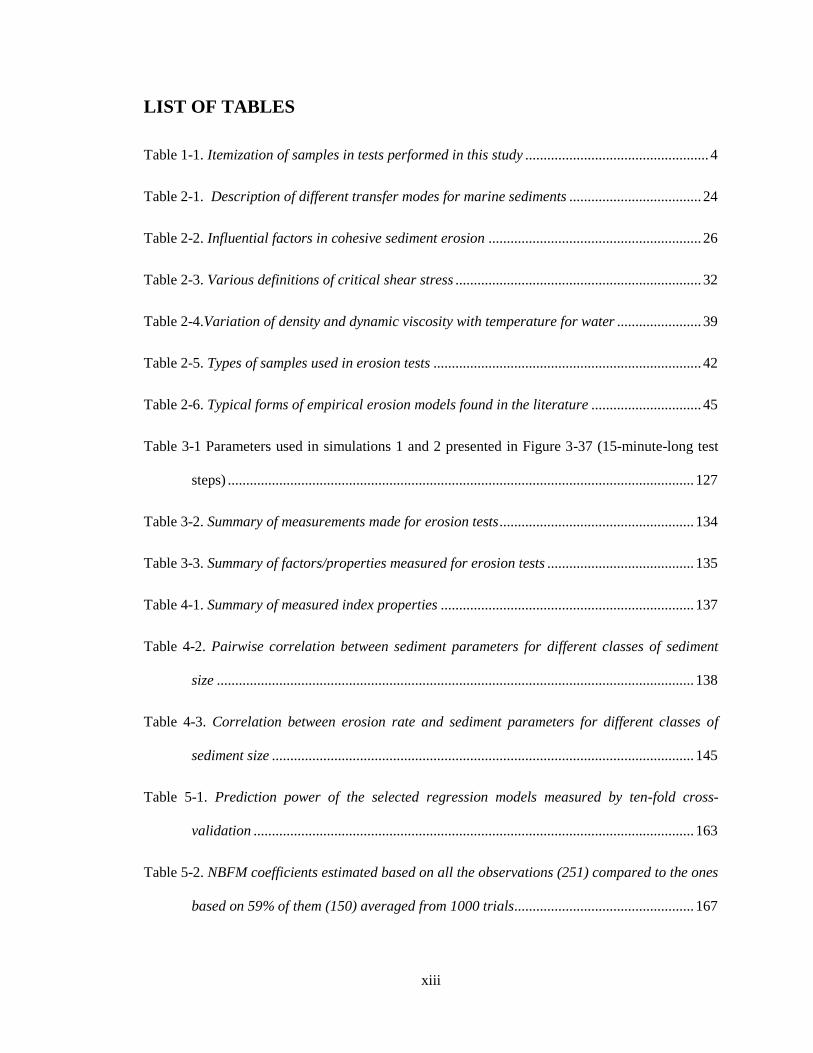
Table 1-1. Itemization of samples in tests performed in this study .................................................. 4

Table 2-1. Description of different transfer modes for marine sediments .................................... 24

Table 2-2. Influential factors in cohesive sediment erosion .......................................................... 26

Table 2-3. Various definitions of critical shear stress ................................................................... 32

Table 2-4.Variation of density and dynamic viscosity with temperature for water ....................... 39

Table 2-5. Types of samples used in erosion tests ......................................................................... 42

Table 2-6. Typical forms of empirical erosion models found in the literature .............................. 45

Table 3-1 Parameters used in simulations 1 and 2 presented in Figure 3-37 (15-minute-long test

steps) ............................................................................................................................... 127

Table 3-2. Summary of measurements made for erosion tests ..................................................... 134

Table 3-3. Summary of factors/properties measured for erosion tests ........................................ 135

Table 4-1. Summary of measured index properties ..................................................................... 137

Table 4-2. Pairwise correlation between sediment parameters for different classes of sediment

size .................................................................................................................................. 138

Table 4-3. Correlation between erosion rate and sediment parameters for different classes of

sediment size ................................................................................................................... 145

Table 5-1. Prediction power of the selected regression models measured by ten-fold cross-

validation ........................................................................................................................ 163

Table 5-2. NBFM coefficients estimated based on all the observations (251) compared to the ones

based on 59% of them (150) averaged from 1000 trials ................................................. 167

xiv

Table 5-3. NBCM coefficients estimated based on all the observations for coarse sediments (44)

compared to the ones based on 56% of them (25) - averaged from 1000 trials ............. 169

Table 5-4. Key information on the studies compared in Section 5.2.5.1 ..................................... 172

Table 5-5. Comparison of average shear stresses of erosion tests in this study with those used in

the Sedflume study conducted by Borrowman et al., 2006 ............................................. 175

xv

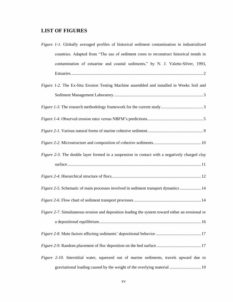
LIST OF FIGURES

Figure 1-1. Globally averaged profiles of historical sediment contamination in industrialized

countries. Adapted from “The use of sediment cores to reconstruct historical trends in

contamination of estuarine and coastal sediments,” by N. J. Valette-Silver, 1993,

Estuaries. ............................................................................................................................. 2

Figure 1-2. The Ex-Situ Erosion Testing Machine assembled and installed in Weeks Soil and

Sediment Management Laboratory ..................................................................................... 3

Figure 1-3. The research methodology framework for the current study ........................................ 3

Figure 1-4. Observed erosion rates versus NBFM’s predictions ..................................................... 5

Figure 2-1. Various natural forms of marine cohesive sediment ..................................................... 9

Figure 2-2. Microstructure and composition of cohesive sediments ............................................. 10

Figure 2-3. The double layer formed in a suspension in contact with a negatively charged clay

surface ............................................................................................................................... 11

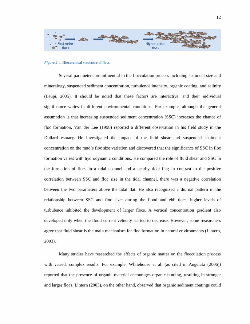
Figure 2-4. Hierarchical structure of flocs ..................................................................................... 12

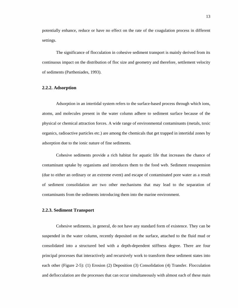
Figure 2-5. Schematic of main processes involved in sediment transport dynamics .................... 14

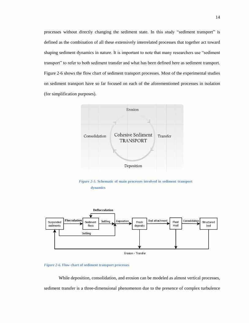
Figure 2-6. Flow chart of sediment transport processes ................................................................ 14

Figure 2-7. Simultaneous erosion and deposition leading the system toward either an erosional or

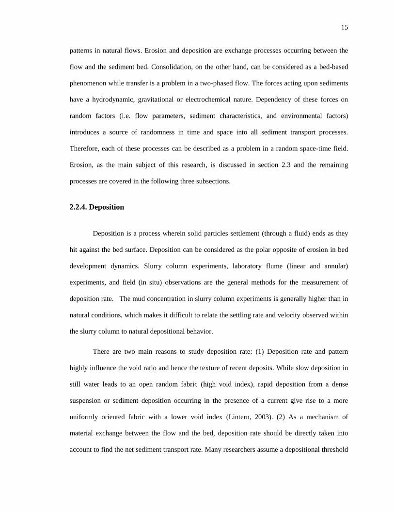
a depositional equilibrium................................................................................................. 16

Figure 2-8. Main factors affecting sediments’ depositional behavior ........................................... 17

Figure 2-9. Random placement of floc deposition on the bed surface .......................................... 17

Figure 2-10. Interstitial water, squeezed out of marine sediments, travels upward due to

gravitational loading caused by the weight of the overlying material .............................. 19

xvi

Figure 2-11. Hjulstrom curve (source: unknown) ......................................................................... 20

Figure 2-12. Shields diagram modified by Rouse ......................................................................... 22

Figure 2-13. Effect of the level of intensity and size of eddies on a suspended particle’s trajectory

.......................................................................................................................................... 24

Figure 2-14. Repetitive cycles of resuspension, transfer, and resettlement in cohesive sediments

.......................................................................................................................................... 24

Figure 2-15. Three major modes of erosion: entrainment, floc erosion, and mass erosion ........... 26

Figure 2-16. Flat flakes of three clay minerals (source: unknown) ............................................... 29

Figure 2-17. Topographic structure of a cohesive bed at a micron scale ...................................... 30

Figure 2-18. Two possible erosion alternatives for a flaky chunk of cohesive sediment .............. 30

Figure 2-19. Variation of theoretical shear stress with velocity at different temperatures ............ 40

Figure 2-20. Typical pattern of data generally observed in erosion experiments.......................... 43

Figure 2-21. Life cycle of biofilm ................................................................................................. 50

Figure 2-22. A fresh layer of biofilm peeled off from the surface ................................................ 53

Figure 2-23. Temporal scales associated with cohesive sediment processes ................................ 59

Figure 2-24. Spatial scales associated with cohesive sediment processes ..................................... 59

Figure 2-25. The circular cause-and-consequence relationship between flow hydrodynamics, bed

morphology, and sediment transport patterns ................................................................... 65

Figure 2-26. Transfer of model components between two scales ................................................. 82

Figure 3-1. Sampling sites in the Newark Bay, New Jersey ......................................................... 88

Figure 3-2. The bottom corer used in this study ............................................................................ 89

xvii

Figure 3-3. Undisturbed surface of a sample extracted from the bay ............................................ 89

Figure 3-4. A sediment core obtained from the Newark Bay on 06/19/2012 ................................ 91

Figure 3-5. Extension ring and cutter used to trim a section of sediment ..................................... 92

Figure 3-6. A sample obtained from a trimmed section of the original sediment core ................. 92

Figure 3-7. Parameters influencing erosion of cohesive sediments .............................................. 95

Figure 3-8. Comparison of bulk density measurements of this study with theoretical values

calculated based on three assumptions for specific gravity (2.5, 2.7, and 2.9) – The

samples are assumed to be saturated ................................................................................. 97

Figure 3-9. Comparison of bulk density measurements of this study with theoretical values

calculated based on the specific gravity and water content measurements made in this

study – The samples are assumed to be saturated ............................................................. 99

Figure 3-10. Samples of granular (left) and cohesive (right) sediments prepared for the specific

gravity test....................................................................................................................... 101

Figure 3-11. Side view of ESETM .............................................................................................. 102

Figure 3-12. Top view of ESETM ............................................................................................... 103

Figure 3-13. Top and side views of the Ex-Situ Erosion Testing Machine (ESETM) testing duct

........................................................................................................................................ 103

Figure 3-14. The internal structure of ESTEM’s force measurement sensors ............................ 104

Figure 3-15. The ring and sliding bottom plate designed to confine the sediment sample ......... 105

Figure 3-16. Map of sample locations for spatial sensitivity analysis of ESETM ...................... 106

Figure 3-17. Weight sensor measurements for a 10-gram weight located at different points on the

sensor .............................................................................................................................. 106

xviii

Figure 3-18. Typical drift observed in the signals generated by the weight sensor .................... 107

Figure 3-19. Histogram of all the measured weight losses .......................................................... 107

Figure 3-20. Weight measurements for a typical erosion test on a manufactured sample .......... 108

Figure 3-21. The flat aluminum disk used to create a smooth surface for device assessment .... 109

Figure 3-22. Comparison of shear stress measurements obtained from three methods: (1) indirect

measurements in Erosion Function Apparatus (Briaud et al. , 2001); (2) direct

measurements in ESETM; (3) calculated based on Prandtl’s universal law of friction .. 110

Figure 3-23. A typical drift observed in the signals generated by the shear stress sensor .......... 111

Figure 3-24. Results of two typical erosion tests performed on manufactured kaolinite samples in

which negative shear stress values were observed .......................................................... 112

Figure 3-25. Vertical cross-section of a sample surrounded by the aperture ring. Non-uniform

erosion around the edges of the sample disturbs the flow and creates forces in the

direction opposite to the flow ......................................................................................... 112

Figure 3-26. Top view and vertical cross-section of the sample probe surrounded by the aperture

ring .................................................................................................................................. 113

Figure 3-27. Reliability analysis of the shear stress sensor using the aluminum disk tested at

different elevations (0.00 is the bed level) ...................................................................... 114

Figure 3-28. Velocity profile in ESETM’s testing channel at the section passing through the

center of the sample probe. The average velocity in the channel is 1 m/s. Calculations are

based on computational fluid dynamic analysis conducted by Anderson and Knight

(2012). Adapted from (Anderson and Knight, 2012). .................................................... 115

Figure 3-29. Comparison of CFD computations with five experiments (each replicated twice)

conducted on the aluminum disk leveled with the bed (0.00 mm protrusion) ................ 116

xix

Figure 3-30. Measured shear stresses for the aluminum disk leveled with the channel’s bed

(replications of the same test) ......................................................................................... 117

Figure 3-31. Measured shear stress values on the aluminum disk extruded by 1.00 mm into the

flow (replications of the same test) ................................................................................. 118

Figure 3-32. Comparison of shear stress values measured by the sensor with theoretical values

calculated based on average velocity .............................................................................. 119

Figure 3-33. The Couette flow created by the belt can be combined with the pipe flow profile to

create a more realistic velocity profile ............................................................................ 120

Figure 3-34. Velocity profile in ESETM’s testing duct measured through 2-dimensional particle

image velocimetry in the J. Sterling Jones Hydraulics Research Laboratory at the Turner-

Fairbank Highway Research Center (used with permission). ......................................... 120

Figure 3-35. Impact of the roughness of channel cover on the measured shear stress values for the

aluminum disk (smooth surface) at different levels of protrusion .................................. 121

Figure 3-36. Surface sediment partitioned into clusters with similar erosion behavior .............. 123

Figure 3-37. Comparison of data from Zerik, Krishnappan, Germaine, and Madsen, (1998) with

data predicted by the model ............................................................................................ 127

Figure 3-38. Breakup of erosion observed by Zerik et al. (1998) into different clusters at shear

stress levels 1-4 ............................................................................................................... 128

Figure 3-39. Comparison of data observed by Zreik et al. (1998) with predictions of models

calibrated based on data presented in Figure 3-37 .......................................................... 129

Figure 3-40. Comparison of data observed by Parchure and Mehta (1984) with the model

predictions ....................................................................................................................... 130

xx

Figure 3-41. Comparison of data observed by Sanford and Maa (2001) with the probabilistic

model predictions ............................................................................................................ 131

Figure 3-42. Two Newark Bay samples after the erosion test .................................................... 133

Figure 4-1. Scatterplot matrix of sediment properties - PF 60 ................................................ 139

Figure 4-2. Scatterplot matrix of sediment properties - PF 40 ................................................ 140

Figure 4-3. Specific gravity versus percent fines for all samples ................................................ 140

Figure 4-4. Bulk density versus percent fines for all samples ..................................................... 141

Figure 4-5. Observed erosion rates for different classes of sediment size .................................. 142

Figure 4-6. Average velocities used for testing different classes of sediment size ..................... 142

Figure 4-7. Average velocities used for testing different classes of sediment size ..................... 143

Figure 4-8. Theoretical shear stresses used for testing different classes of sediment size .......... 143

Figure 4-9. Observed erosion rates at different shear stress levels .............................................. 144

Figure 4-10. Erosion rates observed for testing different classes of sediment size ..................... 145

Figure 5-1. The research methodology framework for the current study .................................... 146

Figure 5-2. Bulk density versus percentage of fines for all the samples ..................................... 148

Figure 5-3. Organic content versus percentage of fines for all the samples ................................ 149

Figure 5-4. Water content versus percentage of fines for all the samples ................................... 149

Figure 5-5. Organic content versus water content for different classes of sediment size ............ 150

Figure 5-6. Multiple distributions fitted erosion rate measurements - PF ≥ 60 ........................... 151

Figure 5-7. Analysis of residuals for NBFM ............................................................................... 153

Figure 5-8. Cook’s distances for NBFM ..................................................................................... 154

xxi

Figure 5-9. Frequency distribution of standardized residuals for NBFM.................................... 154

Figure 5-10. Plots of standardized residuals versus: fitted values (top left), Average Velocity (top

tight), Bulk Density (bottom left), and Water Content (bottom right) - .............. 155

Figure 5-11. Predicted versus observed erosion rates for NBFM ............................................... 156

Figure 5-12. Multiple distributions fitted to the erosion rate data ............................................... 157

Figure 5-13. Frequency distribution of the natural logarithm of observed erosion rates ............ 157

Figure 5-14. Analysis of residuals for NBCM ............................................................................ 158

Figure 5-15. Predicted versus observed erosion rates for NBCM ............................................... 159

Figure 5-16. Results of the ten-fold cross-validation analysis for NBCM .................................. 161

Figure 5-17. Results of the ten-fold cross-validation analysis for NBCM .................................. 162

Figure 5-18. Distribution of regression model parameters estimated based on samples of different

sizes (derived from original observations)–NBFM ........................................................ 164

Figure 5-19. Distribution of coefficients of distribution estimated based on samples of different

sizes (derived from observations) –NBFM ..................................................................... 166

Figure 5-20. Distribution of regression model parameters estimated based on samples of different

sizes (derived from observations) –NBCM .................................................................... 168

Figure 5-21. Distribution of coefficients of distribution estimated based on samples of different

sizes (derived from observations) – NBCM ................................................................... 169

Figure 5-22. A typical erosion rate graph republished from “Erodibility Study Of Passaic River

Sediments Using USACE Sedflume” by T. D. Borrowman et al. (2006) ...................... 174

xxii

Figure 5-23. Observed erosion rates for different classes of sediment size (ESETM). The

minimum erosion rate value reported in the Sedflume study by Borrowman et al., (2006)

is marked by the red arrow.............................................................................................. 175

Figure 5-24. East-west velocity measurements at mooring 2, Lower Passaic River, New Jersey,

December 5, 2005. Republished from “Results of Cross-Channel Monitoring During the

Lower Passaic River Environmental Dredging Pilot Program on the Lower Passaic River,

December 1 to 12” by T. P. Wilson (2006) .................................................................... 176

Figure 5-25. Erosion rates measured by Witt and Westrich (2003) for manually homogenized

sediment cores tested at shear stress levels in the range of 2-4 Pa. Republished from

“Quantification of erosion rates for undisturbed contaminated cohesive sediment cores by

image analysis” by O. Witt and B. Westrich (2003) ....................................................... 177

Figure 5-26. Erosion rate as a function of bulk density for samples made of 14.8-micron quartz

particles and tested under different shear stresses. Republished from "Effects of particle

size and bulk density on erosion of quartz particles" by J. Robert et al. (1998) ............. 178

Figure 5-27. Erosion rates measured by (Ravens, 1997) in the Boston Harbor through six flume

experiments in 1995. Republished from “Sediment resuspension in Boston Harbor” by T.

M. Ravens (1997). Massachusetts Institute of Technology ............................................ 179

Figure 5-28. Density distribution of observed and predicted erosion rates .................. 186

Figure 5-29. Density distribution of observed and predicted erosion rates (NBCM)................. 186

Figure 5-30. Steps involved in stochastic simulation of erosion ................................................. 188

Figure 5-31. Cumulative frequency distribution of erosion rates simulated for different velocities

using the original (observed) sediment parameters and four velocity levels– Simulations

are based on NBFM ........................................................................................................ 190

xxiii

Figure 5-32. Empirical cumulative frequency distribution of the observed, predicted and

simulated data – Simulations are based on NBFM ......................................................... 190

Figure 5-33. Cumulative frequency distribution of erosion rates simulated for different velocities

using the observed sediment parameters (at four velocity levels) – Simulations are based

on NBCM ........................................................................................................................ 191

Figure 5-34. Empirical Cumulative frequency distribution of the observed, predicted and

simulated data - Simulations are based on NBCM ......................................................... 191

Figure 5-35. Empirical cumulative frequency distribution of new observations compared with

simulated data. The erosion rate values and average velocity values used to generate this

graph (238 points) were not used for training the regression model and hence can be

considered as a new validation set. However, as index properties were not determined for

this validation set, it has been assumed that all the samples contained more than 60% of

fines and artificial bulk density and water content values were used based on the rest of

the tests. .......................................................................................................................... 193

xxiv

LIST OF ABBREVIATIONS

ANOVA Analysis of Variance

cm centimeter

EFA Erosion Function Apparatus

EPS Extracellular Polymeric Substance

ESETM Ex-Situ Erosion Testing Machine

CFD Computational Fluid Dynamics

Cov Covariance

CV Cross-Validation

d Hydraulic diameter, Particle diameter

D Depth of sediment (in the bed)

FHWA Federal Highway Administration

gr gram

K Von Kármán constant

constant

kg kilogram

LL Liquid Limit

m meter

mm millimeter

MSE Mean Squared Error

NBFM Newark Bay Fine Model

NBCM Newark Bay Coarse Model

P Rose Number

Pa Pascal

PF Percent Fines

PI Plasticity Index

PL Plastic Limit

SD Standard deviation

xxv

SE Standard error

SS Sample size

v Volume of the sample

V Average Velocity (

)

xxvi

LIST OF SYMBOLS

Shear viscosity of the fluid

Micrometer

Pearson correlation

Bulk density

Water density

hear stress

Theoretical shear stress

Kinetic viscosity (

)

Friction factor

Initial weight

1

1. INTRODUCTION

Statement of the Problem

Knowledge of cohesive sediment transport has found applications in many disciplines

like geology and geography, as well as mechanical, geotechnical and environmental engineering.

Waterways management and contaminant transport are two major interdisciplinary fields

motivating exclusive research on cohesive sediment transport to address their challenges. In

waterways management, maintenance and capital dredging are inevitable operations for

maintaining competitive global networks. The fact that over 80 percent of the volume of global

trade is handled by maritime transport indicates a high traffic concentration imposed on large

ports (Rodrigue, Slack, & Notteboom, N.D.). Manufacturing of the giant post-Panamax

generation of containerships is also an influential trend, obligating the creation of deeper and

wider navigation channels. Hence, there is no surprise that dredging schemes and waterfront

development projects are most in need of research on sediment transport.

Contaminant transport is the second field that emphasizes research on cohesive sediment

transport. In only a few decades of industrial progress, a huge volume of toxic and hazardous

chemicals has been accidently or deliberately released into the aquatic environment. As cohesive

sediments can absorb a wide range of these pollutants, their accumulation in low energy

environments, e.g. estuaries and coastal waterfronts, has produced hazardous contaminant

repositories close to many developed areas. This explains why many of the studies on sediment

transport are triggered by human health and ecological concerns, and aim to model contaminant

2

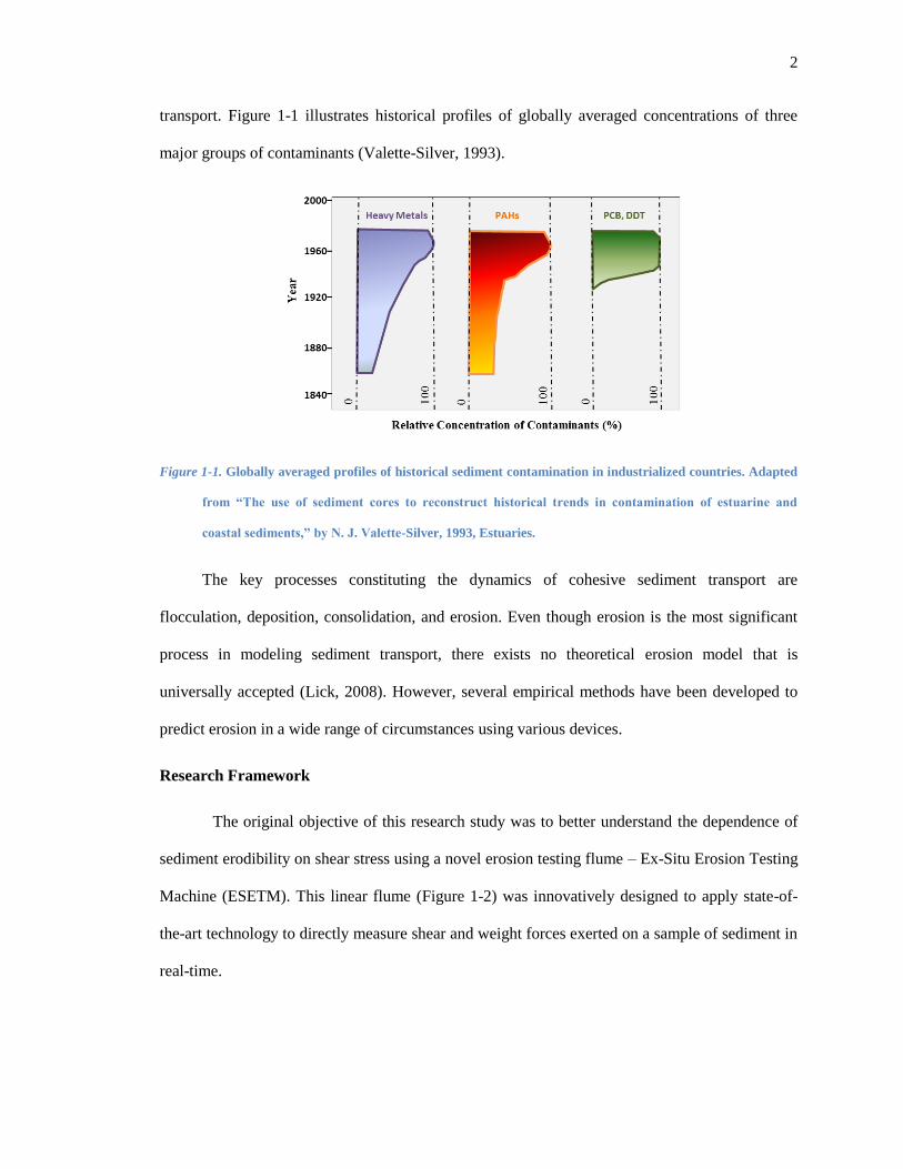
transport. Figure 1-1 illustrates historical profiles of globally averaged concentrations of three

major groups of contaminants (Valette-Silver, 1993).

Figure 1-1. Globally averaged profiles of historical sediment contamination in industrialized countries. Adapted

from “The use of sediment cores to reconstruct historical trends in contamination of estuarine and

coastal sediments,” by N. J. Valette-Silver, 1993, Estuaries.

The key processes constituting the dynamics of cohesive sediment transport are

flocculation, deposition, consolidation, and erosion. Even though erosion is the most significant

process in modeling sediment transport, there exists no theoretical erosion model that is

universally accepted (Lick, 2008). However, several empirical methods have been developed to

predict erosion in a wide range of circumstances using various devices.

Research Framework

The original objective of this research study was to better understand the dependence of

sediment erodibility on shear stress using a novel erosion testing flume – Ex-Situ Erosion Testing

Machine (ESETM). This linear flume (Figure 1-2) was innovatively designed to apply state-of-

the-art technology to directly measure shear and weight forces exerted on a sample of sediment in

real-time.

3

Figure 1-2. The Ex-Situ Erosion Testing Machine assembled and installed in Weeks Soil and Sediment

Management Laboratory

The research framework used in this study consists of the four following main

components: (1) device assessment, (2) experimental tests, (3) regression analysis of the

experimental data, and (4) stochastic analysis. Figure 1-3 shows the flow chart of the main

research activities accomplished in this study.

Figure 1-3. The research methodology framework for the current study

Regression Analysis

Stochastic Analysis

Design of Experiments

ESETM Assessment

Erosion Tests

Index Properties

ESETM Calibration

ESETM Modification

ESETM Installation

Sample Collection

Literature Review

4

1- Device assessment: After the Ex-Situ Erosion Testing Machine was assembled, installed, and

calibrated, extensive research was conducted to evaluate its performance. Significant effort

was made in implementing a scientific methodology to identify the strengths and weaknesses

of ESETM and evaluate the accuracy and reliability of its measurements. Due to the results of

this assessment, the research objective was transformed into “characterization of the

behavior of cohesive sediments in the Newark Bay, at flow velocities below 1

, based on

their index properties.”

2- Experimental tests: In this study, 755 erosion rate tests were conducted on 142 fairly

undisturbed samples taken from 24 cores extracted from the Newark Bay. Table 1-1 lists all

the samples taken for various tests within this study.

Table 1-1. Itemization of samples in tests

performed in this study

Test Count of samples

Erosion 142

Water content 74

Organic content 68

Bulk density 77

Specific gravity 16

Percentage of fines 18

Atterberg limits 14

5

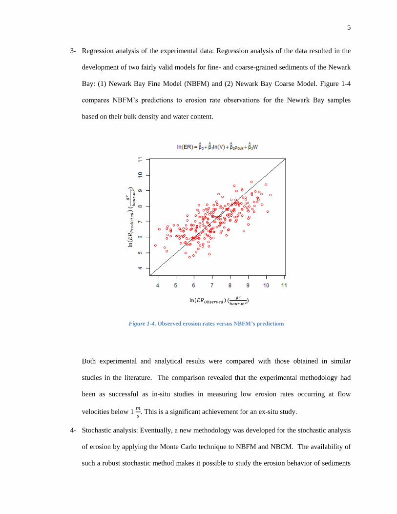
3- Regression analysis of the experimental data: Regression analysis of the data resulted in the

development of two fairly valid models for fine- and coarse-grained sediments of the Newark

Bay: (1) Newark Bay Fine Model (NBFM) and (2) Newark Bay Coarse Model. Figure 1-4

compares NBFM’s predictions to erosion rate observations for the Newark Bay samples

based on their bulk density and water content.

Figure 1-4. Observed erosion rates versus NBFM’s predictions

Both experimental and analytical results were compared with those obtained in similar

studies in the literature. The comparison revealed that the experimental methodology had

been as successful as in-situ studies in measuring low erosion rates occurring at flow

velocities below 1

. This is a significant achievement for an ex-situ study.

4- Stochastic analysis: Eventually, a new methodology was developed for the stochastic analysis

of erosion by applying the Monte Carlo technique to NBFM and NBCM. The availability of

such a robust stochastic method makes it possible to study the erosion behavior of sediments

)

𝐸𝑅𝑃𝑟𝑒𝑑𝑖𝑐𝑡𝑒𝑑

𝑔𝑟

𝑜𝑢𝑟 𝑚

)

6

over many artificially generated samples (in lieu of measured data), resulting in higher levels

of confidence in predictions.

Organization of Thesis

This thesis is organized into six chapters as follows:

Chapter 1 (current chapter): This chapter introduces the research and outlines its objectives.

Chapter 2: This chapter reviews the literature on cohesive sediment erosion. It explains the

essential concepts and serves as a background to understanding the remaining chapters. The first

four sections of this chapter are on sediments and sediment transport dynamics and concepts. The

review of the literature revealed the lack of sufficient attention to the issue of scale. Despite its

significance, this concept had generally been used in an unclear or inaccurate manner in the field

of sediment transport. The final section of the literature review is devoted to a comprehensive and

insightful discussion of the concept of scale in cohesive sediment erosion.

Chapter 3: This chapter provides a thorough explanation of the methodology used in this study

for sample collection, preservation, and preparation, as well as the experimental methodology for

index property and erosion tests.

One of the main conclusions from the literature review was the strong dependence of the results

of the erosion rate tests on the experimental design (selected levels of shear stress, duration of

each step) as well as the interpretation method. This makes the interpretation of the experimental

results very subjective and hinders the comparison of data from different experiments. In order to

mitigate the above concerns, it was decided to explore this practical problem and investigate its

consequences in more detail prior to designing the erosion experiments for the current study.

Therefore, a methodology was developed for the analytical interpretation of the erosion test

results. This method, which is based on the probabilistic modeling of erosion, applies an

optimization technique to solve for the model’s parameters probabilistically.

7

Chapter 4: In this chapter, the results of both erosion and geotechnical tests are presented.

Chapter 5: Chapter 5 addresses data analysis and explains the analytical methodology used in

this research in two sections: regression analysis and stochastic analysis. The second section

describes the regression analysis used to develop two models for erosion rate of both fine and

coarse sediments in the Newark Bay. The third section describes the methodology developed to

build upon these models and conduct stochastic simulations for cohesive sediment erosion. The

main conclusions are discussed at the end of each section.

Chapter 6: This chapter concludes and addresses the main results of the thesis.

Appendix A: Appendix A includes the additional graphs, tables, and boxes that can be referred to

for more details.

Appendix B: The scope of erosion rate experiments is presented completely in Appendix B.

8

2. LITERATURE REVIEW

This chapter serves as a background to understanding the remaining chapters. Section 2.1

defines cohesive sediments and followed by the definition of sediment flocculation, adsorption,

transport, deposition, consolidation, and transport in section 2.2. Sections 2.3 and 2.4 are

dedicated to erosion and the concepts relevant to it. Section 2.5 focuses on the concept of scale in

cohesive sediment erosion. It investigates the causes and consequences of temporal and spatial

variations in the erosion behavior of cohesive sediments and aims to shed light on the

significance of the issue of scale.

2.1. Definition of Cohesive Sediment

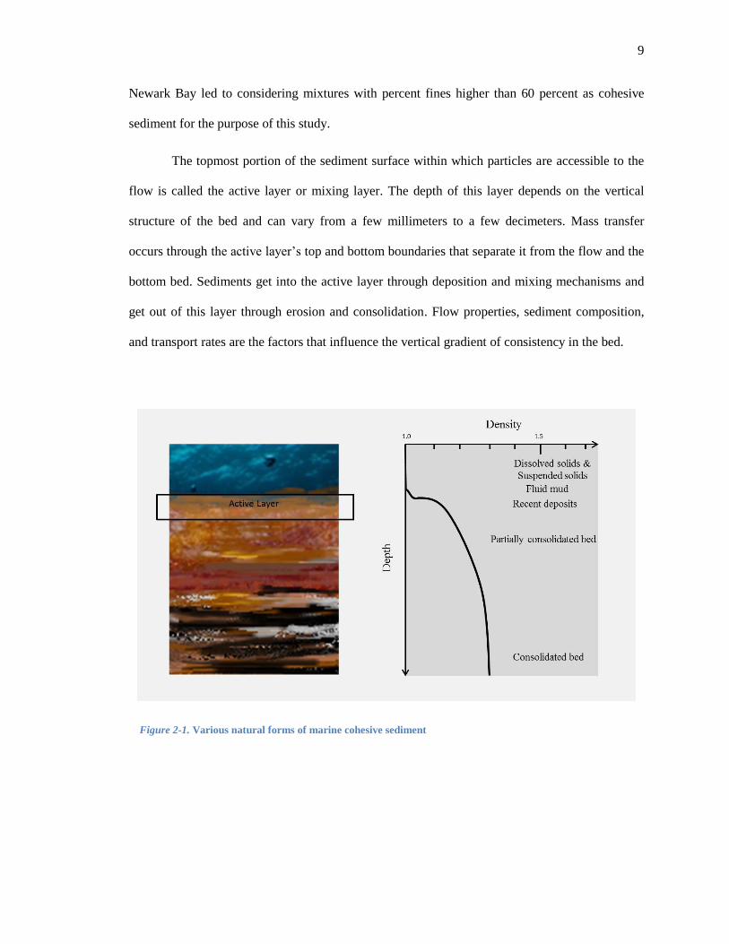
Natural cohesive sediment is a heterogeneous and porous material containing all three

phases of solid, liquid and gas (Winterwerp & Van Kesteren, 2004) with a form varying from

suspended sediments to highly consolidated bed structures (Figure 2-1). The weight and volume

proportions of the solid, liquid, and gas phases and the particle size distribution can be extremely

variable in natural sediments as illustrated in Figure 2-2. In soil mechanics, particles smaller than

63 (including silt and clay) are generally considered as fine particles and mixtures with

percentage of fines higher than 50% are generally categorized as cohesive (versus granular for

mixtures with less than 50 percent of fines). However, Whitehouse et al. (2009) believe that only

about 10% dry mass by weight of fines is required to convert a sandy bed into one exhibiting

cohesive properties. Moreover, mineralogical composition of particles also has an important

effect on sediment behavior. Particle size analysis and cluster analysis of samples taken from the

9

Newark Bay led to considering mixtures with percent fines higher than 60 percent as cohesive

sediment for the purpose of this study.

The topmost portion of the sediment surface within which particles are accessible to the

flow is called the active layer or mixing layer. The depth of this layer depends on the vertical

structure of the bed and can vary from a few millimeters to a few decimeters. Mass transfer

occurs through the active layer’s top and bottom boundaries that separate it from the flow and the

bottom bed. Sediments get into the active layer through deposition and mixing mechanisms and

get out of this layer through erosion and consolidation. Flow properties, sediment composition,

and transport rates are the factors that influence the vertical gradient of consistency in the bed.

Figure 2-1. Various natural forms of marine cohesive sediment

10

Figure 2-2. Microstructure and composition of cohesive sediments

2.2. Processes of Cohesive Sediments

This section describes the main processes of cohesive sediments including flocculation,

adsorption, deposition, consolidation, and transfer. Erosion is discussed in detail in section 2.3.

2.2.1. Flocculation

Flocculation is the most characteristic property of cohesive sediments; when these

sediments are brought in contact with a fluid, e.g. water, particle clusters (including enclosed

water) named flocs, will be formed as a result of electrostatic aggregation (Winterwerp & Van

Kesteren, 2004). Flocculation is the phenomenon that differentiates the behavior of granular and

cohesive sediments. It is because of this process that sediment mineralogy and structure have a

higher influence on the behavior of fine sediments compared to particle size distribution. In

coastal regions, the dominant mode for deposition of fine cohesive material is flocculation

(Lintern, 2003). However, “The mechanism of flocculation considerably complicates the task of

modeling the transport of cohesive fine sediments, such as the ones found in estuaries” (Leupi,

2005). In certain environments similar to estuary heads, where salt and fresh water are mixed,

11

flocculation occurs more often and thus becomes a particularly important process to consider

(Angelaki, 2006).

Clay particles have negatively charged external and interlayer surfaces. When these

particles are in contact with an electrolyte, the charged surface absorbs polar water molecules and

ions to form an ionic structure named the “double layer” referring to the two parallel layers of

charge adsorbed to the surface. Figure 2-3 is a schematic of some clay particles surrounded by a

double layer.

Figure 2-3. The double layer formed in a suspension in contact with a negatively charged

clay surface

Sediment flocs have an open structure with several hierarchical orders of aggregation as

displayed in Figure 2-4. First-order flocs consist of primary particles while higher-order flocs are

made of lower-order aggregates and generally have lower strength (Partheniades, 1993). The low

strength of larger flocs makes it difficult to measure floc size distribution from fluid samples as

even sample extraction could lead to a disaggregation of the flocs (Angelaki, 2006).

Although the gravity force increases as a result of flocculation, floc’ density generally decreases

because of the open structure of the skeleton of the flocs formed in suspension. However, Lintern

(2003) observed that the field settling velocity increases as a net result of these contracting

actions. The floc settling velocity also depends on suspended solids concentration as it can be

influenced by the interaction of other flocs present in the medium. For example, smaller particles

can get trapped in a cluster of larger particles and settle at similar velocities (Been, 1980).

12

Figure 2-4. Hierarchical structure of flocs

Several parameters are influential in the flocculation process including sediment size and

mineralogy, suspended sediment concentration, turbulence intensity, organic coating, and salinity

(Leupi, 2005). It should be noted that these factors are interactive, and their individual

significance varies in different environmental conditions. For example, although the general

assumption is that increasing suspended sediment concentration (SSC) increases the chance of

floc formation, Van der Lee (1998) reported a different observation in his field study in the

Dollard estuary. He investigated the impact of the fluid shear and suspended sediment

concentration on the mud’s floc size variation and discovered that the significance of SSC in floc

formation varies with hydrodynamic conditions. He compared the role of fluid shear and SSC in

the formation of flocs in a tidal channel and a nearby tidal flat; in contrast to the positive

correlation between SSC and floc size in the tidal channel, there was a negative correlation

between the two parameters above the tidal flat. He also recognized a diurnal pattern in the

relationship between SSC and floc size: during the flood and ebb tides, higher levels of

turbulence inhibited the development of larger flocs. A vertical concentration gradient also

developed only when the flood current velocity started to decrease. However, some researchers

agree that fluid shear is the main mechanism for floc formation in natural environments (Lintern,

2003).

Many studies have researched the effects of organic matter on the flocculation process

with varied, complex results. For example, Whitehouse et al. (as cited in Angelaki (2006))

reported that the presence of organic material encourages organic binding, resulting in stronger

and larger flocs. Lintern (2003), on the other hand, observed that organic sediment coatings could

13

potentially enhance, reduce or have no effect on the rate of the coagulation process in different

settings.

The significance of flocculation in cohesive sediment transport is mainly derived from its

continuous impact on the distribution of floc size and geometry and therefore, settlement velocity

of sediments (Partheniades, 1993).

2.2.2. Adsorption

Adsorption in an intertidal system refers to the surface-based process through which ions,

atoms, and molecules present in the water column adhere to sediment surface because of the

physical or chemical attraction forces. A wide range of environmental contaminants (metals, toxic

organics, radioactive particles etc.) are among the chemicals that get trapped in intertidal zones by

adsorption due to the ionic nature of fine sediments.

Cohesive sediments provide a rich habitat for aquatic life that increases the chance of

contaminant uptake by organisms and introduces them to the food web. Sediment resuspension

(due to either an ordinary or an extreme event) and escape of contaminated pore water as a result

of sediment consolidation are two other mechanisms that may lead to the separation of

contaminants from the sediments introducing them into the marine environment.

2.2.3. Sediment Transport

Cohesive sediments, in general, do not have any standard form of existence. They can be

suspended in the water column, recently deposited on the surface, attached to the fluid mud or

consolidated into a structured bed with a depth-dependent stiffness degree. There are four

principal processes that interactively and recursively work to transform these sediment states into

each other (Figure 2-5): (1) Erosion (2) Deposition (3) Consolidation (4) Transfer. Flocculation

and deflocculation are the processes that can occur simultaneously with almost each of these main

14

processes without directly changing the sediment state. In this study “sediment transport” is

defined as the combination of all these extensively interrelated processes that together act toward

shaping sediment dynamics in nature. It is important to note that many researchers use “sediment

transport” to refer to both sediment transfer and what has been defined here as sediment transport.

Figure 2-6 shows the flow chart of sediment transport processes. Most of the experimental studies

on sediment transport have so far focused on each of the aforementioned processes in isolation

(for simplification purposes).

Figure 2-5. Schematic of main processes involved in sediment transport

dynamics

Figure 2-6. Flow chart of sediment transport processes

While deposition, consolidation, and erosion can be modeled as almost vertical processes,

sediment transfer is a three-dimensional phenomenon due to the presence of complex turbulence

Deflocculation

Flocculation

15

patterns in natural flows. Erosion and deposition are exchange processes occurring between the

flow and the sediment bed. Consolidation, on the other hand, can be considered as a bed-based

phenomenon while transfer is a problem in a two-phased flow. The forces acting upon sediments

have a hydrodynamic, gravitational or electrochemical nature. Dependency of these forces on

random factors (i.e. flow parameters, sediment characteristics, and environmental factors)

introduces a source of randomness in time and space into all sediment transport processes.

Therefore, each of these processes can be described as a problem in a random space-time field.

Erosion, as the main subject of this research, is discussed in section 2.3 and the remaining

processes are covered in the following three subsections.

2.2.4. Deposition

Deposition is a process wherein solid particles settlement (through a fluid) ends as they

hit against the bed surface. Deposition can be considered as the polar opposite of erosion in bed

development dynamics. Slurry column experiments, laboratory flume (linear and annular)

experiments, and field (in situ) observations are the general methods for the measurement of

deposition rate. The mud concentration in slurry column experiments is generally higher than in

natural conditions, which makes it difficult to relate the settling rate and velocity observed within

the slurry column to natural depositional behavior.

There are two main reasons to study deposition rate: (1) Deposition rate and pattern

highly influence the void ratio and hence the texture of recent deposits. While slow deposition in

still water leads to an open random fabric (high void index), rapid deposition from a dense

suspension or sediment deposition occurring in the presence of a current give rise to a more

uniformly oriented fabric with a lower void index (Lintern, 2003). (2) As a mechanism of

material exchange between the flow and the bed, deposition rate should be directly taken into

account to find the net sediment transport rate. Many researchers assume a depositional threshold

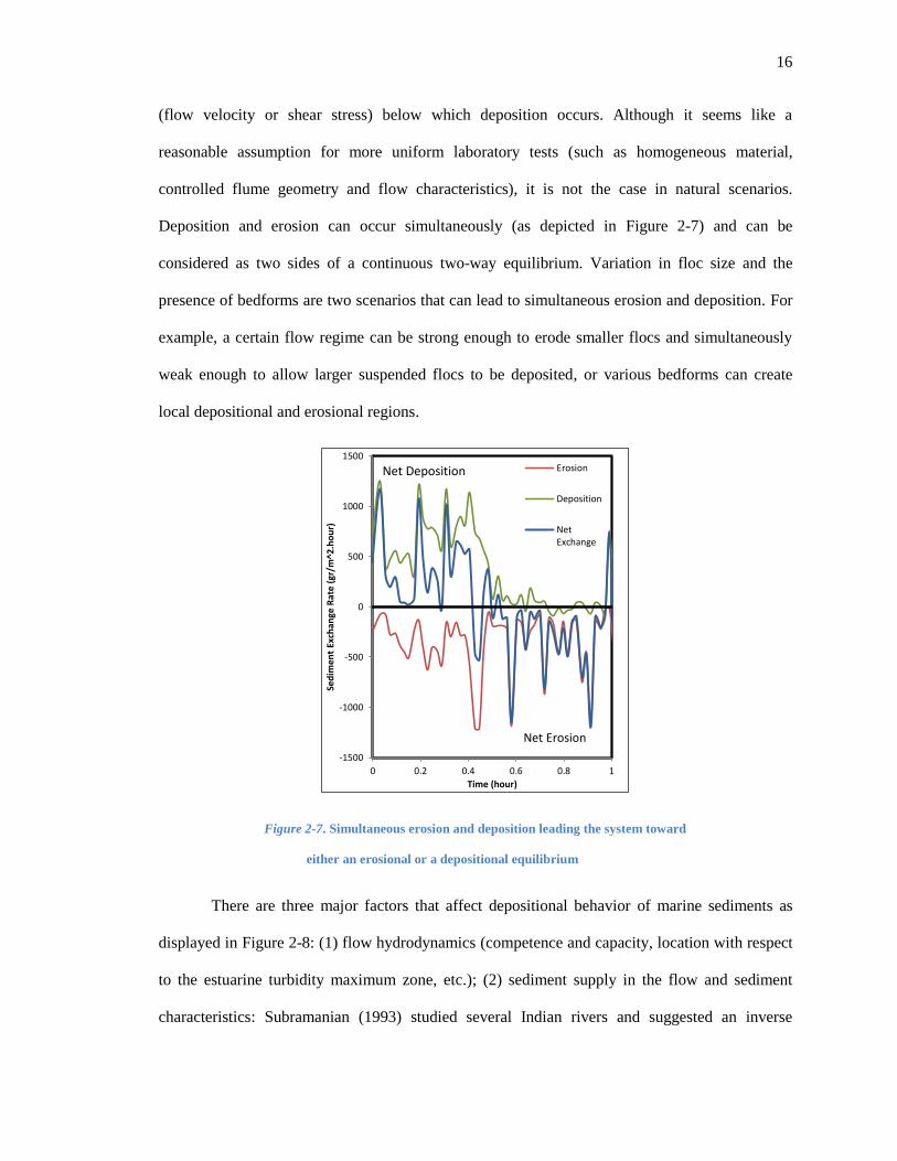
16

(flow velocity or shear stress) below which deposition occurs. Although it seems like a

reasonable assumption for more uniform laboratory tests (such as homogeneous material,

controlled flume geometry and flow characteristics), it is not the case in natural scenarios.

Deposition and erosion can occur simultaneously (as depicted in Figure 2-7) and can be

considered as two sides of a continuous two-way equilibrium. Variation in floc size and the

presence of bedforms are two scenarios that can lead to simultaneous erosion and deposition. For

example, a certain flow regime can be strong enough to erode smaller flocs and simultaneously

weak enough to allow larger suspended flocs to be deposited, or various bedforms can create

local depositional and erosional regions.

Figure 2-7. Simultaneous erosion and deposition leading the system toward

either an erosional or a depositional equilibrium

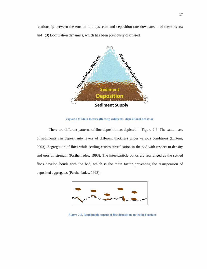
There are three major factors that affect depositional behavior of marine sediments as

displayed in Figure 2-8: (1) flow hydrodynamics (competence and capacity, location with respect

to the estuarine turbidity maximum zone, etc.); (2) sediment supply in the flow and sediment

characteristics: Subramanian (1993) studied several Indian rivers and suggested an inverse

-1500

-1000

-500

0

500

1000

1500

0 0.2 0.4 0.6 0.8 1

Sed

imen

t Ex

chan

ge R

ate

(gr/

m^2

.ho

ur)

Time (hour)

Erosion

Deposition

NetExchange

Net Deposition

Net Erosion

17

relationship between the erosion rate upstream and deposition rate downstream of these rivers;

and (3) flocculation dynamics, which has been previously discussed.

Figure 2-8. Main factors affecting sediments’ depositional behavior

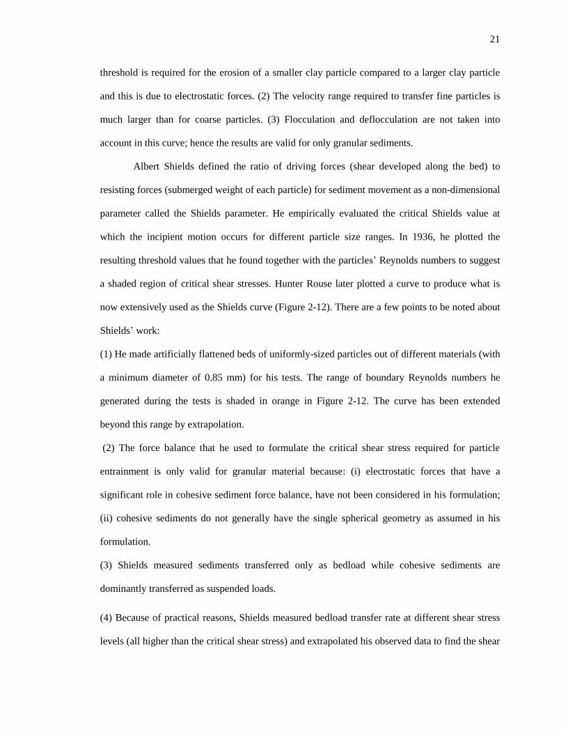
There are different patterns of floc deposition as depicted in Figure 2-9. The same mass

of sediments can deposit into layers of different thickness under various conditions (Lintern,

2003). Segregation of flocs while settling causes stratification in the bed with respect to density

and erosion strength (Partheniades, 1993). The inter-particle bonds are rearranged as the settled

flocs develop bonds with the bed, which is the main factor preventing the resuspension of

deposited aggregates (Partheniades, 1993).

Figure 2-9. Random placement of floc deposition on the bed surface

18

2.2.5. Consolidation

Karl Von Terzaghi, defines consolidation as any process that involves a decrease in water content

of saturated soil without replacement of water by air. As new sediments overlay the bed surface,

their submerged weight would be applied to the underneath layers as a static load. This

gravitational loading causes an increase in the interstitial pore pressure, and as cohesive

sediments have low permeability, the excess pressure can only be gradually transferred to solid

particles through the expulsion of the fluid phase. This process will result in a reduction in the

void ratio and hence a reorganization of sediment structure toward a more compacted state. The

essential difference between the settling suspension and structured sediment matrix is an effective

stress that develops during a transition phase (Been, 1980).

Although the driving force for consolidation (gravitational force from the overlying sediments) is

mainly a physical force depending on the rate of deposition (Figure 2-10), there are also some

chemical and biological factors that affect the soil permeability leading to complications in the

consolidation process. Bioturbation (reworking of sediments by plants or animals) and gas

production caused by decomposition of organic material are examples of such biochemical

factors. Several investigations of consolidation have been conducted so far (although the

presence of gas has been ignored in most cases); however, the effects of all the factors, especially

the interaction between them, have not been considered (Lick, 2008).

Considering the factors affecting consolidation, different time scales should be involved when

modeling this process in marine environments. In a self-weigh consolidation process, which

normally occurs in natural environments, deposition and erosion rates and any time scale

associated with them will influence the overburden pressure and hence consolidation. Deposition

rate also influences the strength of fresh deposits by impacting the void ratio as more quickly

deposited beds do not have time to strengthen before being bombarded and loaded by additional

19

flocs (Lintern, 2003). Biological activities, specifically gas formation (and gas movement within

the matrix of flocs and aggregates) are additional time-dependent factors with rates varying in

different environmental conditions.

In classic soil consolidation models, the rate of settlement on the surface is initially high,

followed by lower rates, which is explained by the reduction in permeability. However, the

presence, production, and movement of gas pockets in natural environments can create short-term

and long-term irregularities in this pattern.

Figure 2-10. Interstitial water, squeezed out of marine sediments, travels upward due to

gravitational loading caused by the weight of the overlying material

2.2.6. Sediment Transfer

Marine sediment transfer (often referred to as sediment transport in the literature) is the

movement of sediment particles or flocs by the flow. Flows carrying cohesive sediments in

natural environments delineate a very complex problem in fluid mechanics not only because of

the effect of solid particles in the turbulence structure, but also due to the strong interaction

between the dynamic and movable sediment bed and the flow condition. Variations in the bed

20

geometry, bed roughness, and flow viscosity are examples of factors that are influenced by the

flow and simultaneously affect the shear stress distribution at the boundary and hence the flow

parameters in the near-bed region. “Description of sediment-laden flow becomes further

complicated as suspended sediment includes smaller or larger vertical density gradients that can

affect the efficiency of sweeps and ejections considerably” (Winterwerp & Van Kesteren, 2004).

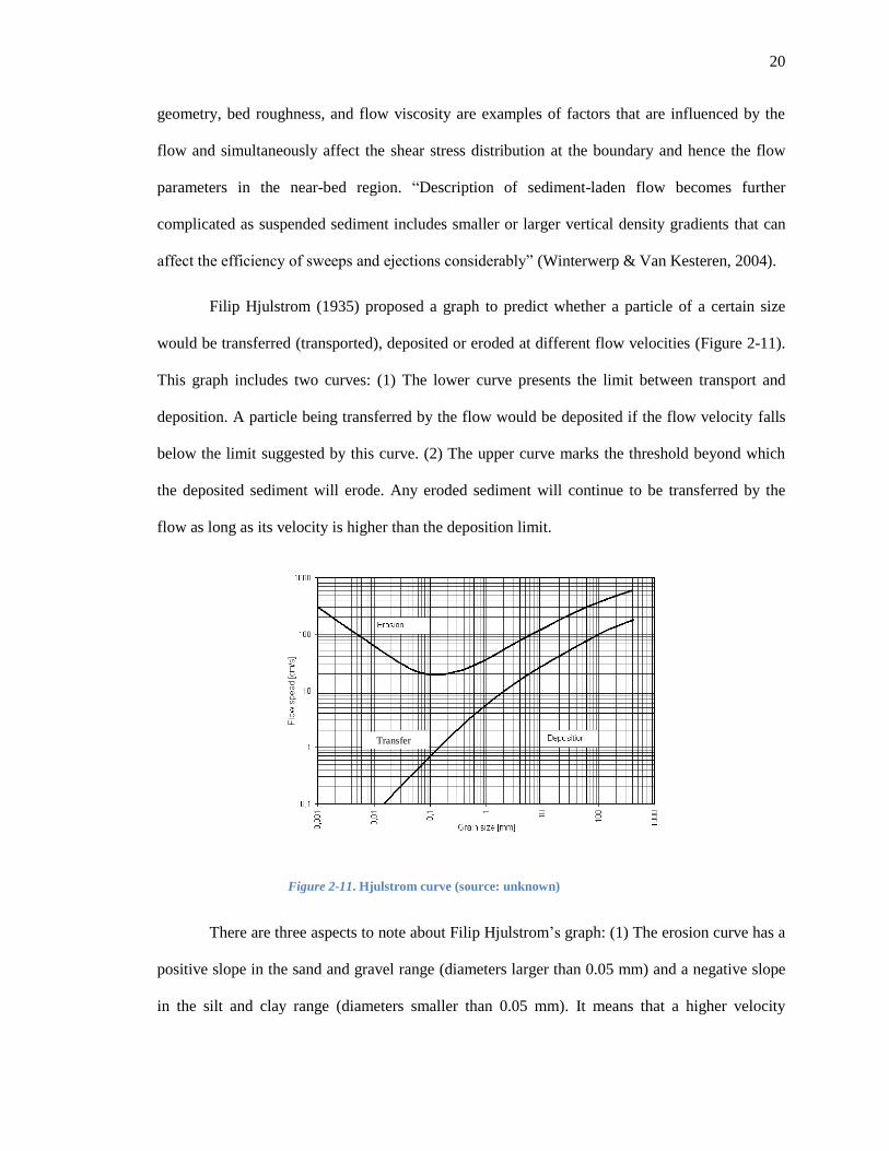
Filip Hjulstrom (1935) proposed a graph to predict whether a particle of a certain size

would be transferred (transported), deposited or eroded at different flow velocities (Figure 2-11).

This graph includes two curves: (1) The lower curve presents the limit between transport and

deposition. A particle being transferred by the flow would be deposited if the flow velocity falls

below the limit suggested by this curve. (2) The upper curve marks the threshold beyond which

the deposited sediment will erode. Any eroded sediment will continue to be transferred by the

flow as long as its velocity is higher than the deposition limit.

Figure 2-11. Hjulstrom curve (source: unknown)

There are three aspects to note about Filip Hjulstrom’s graph: (1) The erosion curve has a

positive slope in the sand and gravel range (diameters larger than 0.05 mm) and a negative slope

in the silt and clay range (diameters smaller than 0.05 mm). It means that a higher velocity

Transfer

21

threshold is required for the erosion of a smaller clay particle compared to a larger clay particle

and this is due to electrostatic forces. (2) The velocity range required to transfer fine particles is

much larger than for coarse particles. (3) Flocculation and deflocculation are not taken into

account in this curve; hence the results are valid for only granular sediments.

Albert Shields defined the ratio of driving forces (shear developed along the bed) to

resisting forces (submerged weight of each particle) for sediment movement as a non-dimensional

parameter called the Shields parameter. He empirically evaluated the critical Shields value at

which the incipient motion occurs for different particle size ranges. In 1936, he plotted the

resulting threshold values that he found together with the particles’ Reynolds numbers to suggest

a shaded region of critical shear stresses. Hunter Rouse later plotted a curve to produce what is

now extensively used as the Shields curve (Figure 2-12). There are a few points to be noted about

Shields’ work:

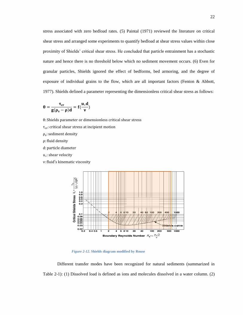
(1) He made artificially flattened beds of uniformly-sized particles out of different materials (with

a minimum diameter of 0.85 mm) for his tests. The range of boundary Reynolds numbers he

generated during the tests is shaded in orange in Figure 2-12. The curve has been extended

beyond this range by extrapolation.

(2) The force balance that he used to formulate the critical shear stress required for particle

entrainment is only valid for granular material because: (i) electrostatic forces that have a

significant role in cohesive sediment force balance, have not been considered in his formulation;

(ii) cohesive sediments do not generally have the single spherical geometry as assumed in his

formulation.

(3) Shields measured sediments transferred only as bedload while cohesive sediments are

dominantly transferred as suspended loads.

(4) Because of practical reasons, Shields measured bedload transfer rate at different shear stress

levels (all higher than the critical shear stress) and extrapolated his observed data to find the shear

22

stress associated with zero bedload rates. (5) Paintal (1971) reviewed the literature on critical

shear stress and arranged some experiments to quantify bedload at shear stress values within close

proximity of Shields’ critical shear stress. He concluded that particle entrainment has a stochastic

nature and hence there is no threshold below which no sediment movement occurs. (6) Even for

granular particles, Shields ignored the effect of bedforms, bed armoring, and the degree of

exposure of individual grains to the flow, which are all important factors (Fenton & Abbott,

1977). Shields defined a parameter representing the dimensionless critical shear stress as follows:

Figure 2-12. Shields diagram modified by Rouse

Different transfer modes have been recognized for natural sediments (summarized in

Table 2-1): (1) Dissolved load is defined as ions and molecules dissolved in a water column. (2)

23

Suspended load includes particles and flocs kept in suspension by turbulent diffusive forces. (3)

Wash load is the portion of suspended solids that are very tiny in size (clay range) and are kept in

suspension by Brownian motion. (4) Bedload includes particles and flocs that move (roll, slide,

saltate) while partially or completely supported by the bed.

Hickin (1995) collected data on various major rivers in all continents to compare the

mean dissolved load to the mean suspended load and found ratios between 2% and 80% in these

rivers (Hickin, 1995). Even though the high volume of wash load has a huge significance for land

erosion studies at the watershed level, it does not directly affect river/estuarine morphology

because the solute remains within the flow unless it is saturated. However, the wash load can

have an indirect effect on erosion/deposition by altering the water column chemistry.

In order to predict the transfer mode for a particle of a certain size, we need to consider

its vertical force balance. Figure 2-13 compares a floc of sediment with a certain settlement

velocity (in static water) at three different turbulence levels. At lower velocities, eddies are

smaller than the floc which causes smaller flow velocity fluctuations around the particle

compared to the average settlement velocity. At higher velocities, on the other hand, larger eddies

create bigger velocity fluctuations compared to the average fall velocity causing greater

distortions in the particle’s trajectory.

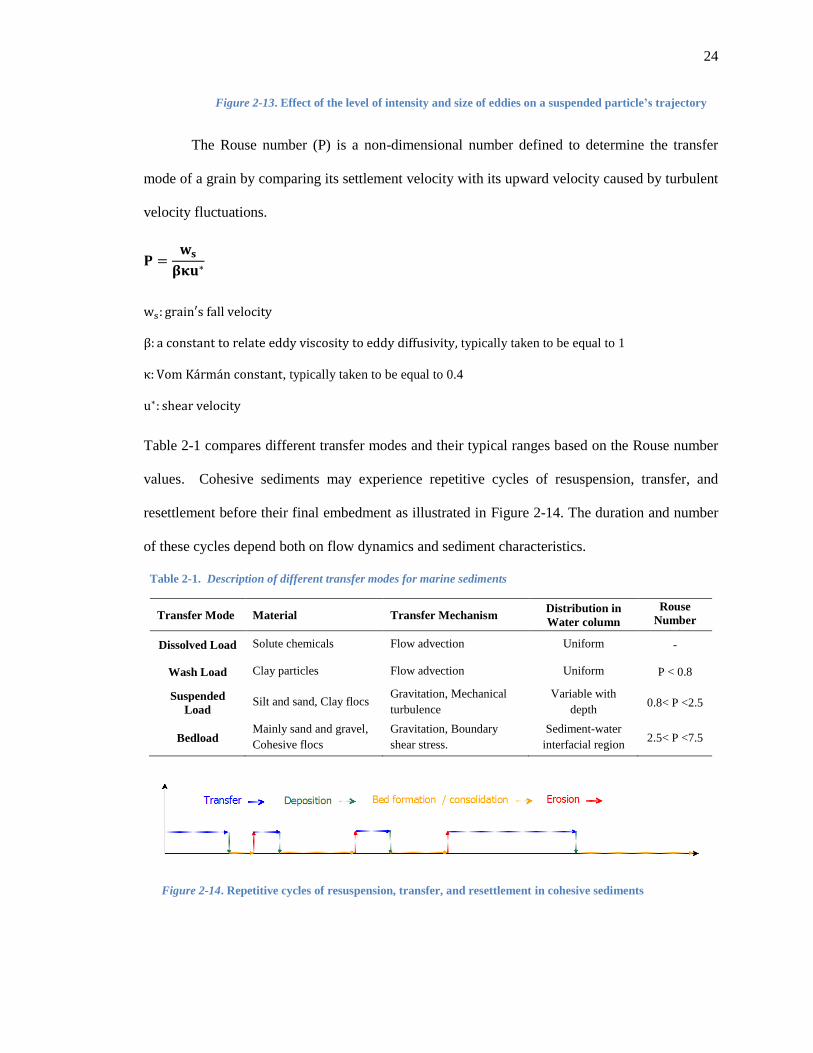
24

Figure 2-13. Effect of the level of intensity and size of eddies on a suspended particle’s trajectory

The Rouse number (P) is a non-dimensional number defined to determine the transfer

mode of a grain by comparing its settlement velocity with its upward velocity caused by turbulent

velocity fluctuations.

typically taken to be equal to 1

, typically taken to be equal to 0.4

Table 2-1 compares different transfer modes and their typical ranges based on the Rouse number

values. Cohesive sediments may experience repetitive cycles of resuspension, transfer, and

resettlement before their final embedment as illustrated in Figure 2-14. The duration and number

of these cycles depend both on flow dynamics and sediment characteristics.

Table 2-1. Description of different transfer modes for marine sediments

Transfer Mode Material Transfer Mechanism Distribution in

Water column

Rouse

Number

(P) Dissolved Load Solute chemicals Flow advection Uniform -

Wash Load Clay particles Flow advection Uniform P < 0.8

Suspended

Load Silt and sand, Clay flocs

Gravitation, Mechanical

turbulence

Variable with

depth 0.8< P <2.5

Bedload Mainly sand and gravel,

Cohesive flocs

Gravitation, Boundary

shear stress.

Sediment-water

interfacial region 2.5< P <7.5

Figure 2-14. Repetitive cycles of resuspension, transfer, and resettlement in cohesive sediments

25

2.3. Erosion

Section 3 is dedicated to the study of literature on the subject of erosion. The definition of

erosion, critical shear stress for erosion, erosive capacity of water, and erosion resistive forces

and mechanism are reviewed in sections 2.3.1-2.3.4 and section 2.3.5 describes different types of

erosion models developed for cohesive sediments.

2.3.1. Definition of Erosion

Erosion in marine environments (also referred to as incipient motion, entrainment or

resuspension) can be defined as the detachment of particles, flocs, or mud clusters from the bed

by flow. In granular materials, grain size distribution and grain density are the main factors

affecting erosion behavior. Table 2-2 provides a list of influential factors for the erosion of

cohesive sediments and categorizes them into intrinsic and extrinsic properties. Moreover, in

cohesive sediments, particles are not identified individually, and both their properties and

behavior are generally defined for bulk samples. Annandale (2005) highlights this characteristic

by modeling cohesive sediments as chemical gels consisting of elements in occupied spaces that

are connected to each other by fixed bonds. He then analogizes the erosion process to the failure

mechanism of these chemical bonds, arguing that the energy required to separate a particle from

the matrix of cohesive sediments follows the same pattern as the typical energy required for

chemical reactions.

26

Table 2-2. Influential factors in cohesive sediment erosion

Type Influential factors in cohesive sediment erosion

Intrinsic

properties Specific density, Mineralogy, Particle size distribution

Extrinsic

properties

Sediment Composition: (organic content, gas content, water content), Void ratio, Permeability,

Bioturbation and other biogenic influences e.g. biofilm , Maturation period, Consolidation time,

Deposition rate, Aerial exposure, Shear stress history, Pore water composition (salinity, PH)

Mehta (Mehta, 1988) identified three different modes of erosion depending on sediment

structure and bed shear stress magnitude (Figure 2-15): (1) floc erosion, (2) mass erosion, and (3)

re-entrainment of fluid mud (a high density suspension). Winterwerp and Van Kesteren (2004)

considered a fourth mode as well-surface erosion.

Figure 2-15. Three major modes of erosion: entrainment,

floc erosion, and mass erosion

27

Individual disruption of flocs/particles from the bed is defined as floc erosion. When a

floc reaches a bed of consolidating soil, it may immediately be broken up into smaller pieces or

may maintain its original structure. Fresh deposits are surrounded by a boundary layer of water

(double layer) and before they can come into close contact with other flocs to create a frictional

resistance, they should overcome repulsive forces and expel some excess trapped water. This

explains the presence of a density gradient (density increases with depth) in the top few

centimeters of the bed. It also explains why the morphology of such sediments is easily disturbed

by environmental factors and reshaped into new forms. In floc erosion, the fluid forces exceed

either the internal strength of a floc or the overall adhesion to the bed. As a result, the surface

material is washed away particle by particle. This mode does not normally have large magnitudes

of erosion but as a continuous process, it can be a major contributor to the total erosion rates.

Recognition of this erosion mode and detection of its threshold (if it exists) is not simple.

Mass erosion (sometimes referred to as bulk erosion) occurs when erosive forces are large enough

to detach chunks/clods of sediment from the bed. The failure process can be either instantaneous

(brittle fracture) or continuous (fatigue). While the former requires the forces to exceed the

fracture resistance instantaneously, the latter involves cyclic (fluctuating) loading applied for a

long enough period. Natural surface imperfections, local strength deficiencies, and bioturbation

are among the factors that can enhance the formation and growth of ruptures. Surface

irregularities can also create stress concentrations leading to the removal of a piece of the bed.

Although this erosion type is poorly understood, some researchers relate it to flow-induced

pressures and believe that it occurs when the mean flow and/or wave induced stagnation pressures

are much larger than the critical shear stress (Winterwerp & Van Kesteren, 2004).

Lick (2008) used particle size to explain different modes of erosion. For particles smaller

than 200 microns (in diameter), he suggested that as cohesive effects become significant, particles

start to erode in the form of chunks. Critical shear stress in this situation becomes a function of

28

both bulk density and particle diameter. He mentions that as sediment diameter decreases even

further, cohesive forces become more dominant which results in the frequent occurrence of chunk

erosion and a simultaneous increase in both bulk density and size of chunks.

As suspended sediments settle toward the bed they may experience a transition state in

which they can neither form a structure to develop effective stresses nor can they still be

considered as suspended particles. This static, high density, viscous fluid mud can be formed

when rapid sedimentation occurs or as a result of bed liquefaction. Fluid mud can be considered

as a thick liquid with some behavior like a soft solid. For example, there is a shear stress that if

exceeded, will cause a permanent displacement of sediment particles resulting in the flow of the

structured fluid (yield stress). When a turbulent flow applies shear stresses higher than the yield

stress to a layer of fluid mud, it will be entrained, and the particles/flocs within it will be

resuspended back into the flow. This mode of erosion is called entrainment.

Two general modes of erosion have been recognized by many researchers: Type I erosion

(depth limited) and Type II erosion (steady state or unlimited). In the depth limited erosion,

within each shear stress level, the erosion rate exponentially decays with time (Sanford & Maa,

2001). This type of erosion is observed in the upper portion of natural sediments where the degree

of consolidation is very depth-dependent. Unlimited erosion (type II) occurs in uniform beds

when the time scale of sediment depletion is longer than that of shear stress change. This type of

erosion is generally observed in more consolidated sediments where the bed shear strength does

not have a vertical gradient. However, a mixture of these two behaviors is what is observed most

frequently. With any increase in flow strength, the erosion rate increases initially and then

reduces to reach zero if the test duration is long enough. It can be concluded that a combination

of two factors determines the erosion mode: (1) sensitivity of sediment strength to depth (due to

factors like sediment properties, deposition history and consolidation history); (2) experiment

design (duration and organization of different test steps).

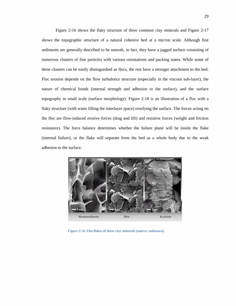
29

Figure 2-16 shows the flaky structure of three common clay minerals and Figure 2-17

shows the topographic structure of a natural cohesive bed at a micron scale. Although fine

sediments are generally described to be smooth, in fact, they have a jagged surface consisting of

numerous clusters of fine particles with various orientations and packing states. While some of

these clusters can be easily distinguished as flocs, the rest have a stronger attachment to the bed.

Floc erosion depends on the flow turbulence structure (especially in the viscous sub-layer), the

nature of chemical bonds (internal strength and adhesion to the surface), and the surface

topography in small scale (surface morphology). Figure 2-18 is an illustration of a floc with a

flaky structure (with water filling the interlayer space) overlying the surface. The forces acting on

the floc are flow-induced erosive forces (drag and lift) and resistive forces (weight and friction

resistance). The force balance determines whether the failure plane will be inside the flake

(internal failure), or the flake will separate from the bed as a whole body due to the weak

adhesion to the surface.

Figure 2-16. Flat flakes of three clay minerals (source: unknown)

Kaolinite Illite Montmorillonite

𝟏𝝁𝒎 𝟏𝝁𝒎

𝟏𝝁𝒎

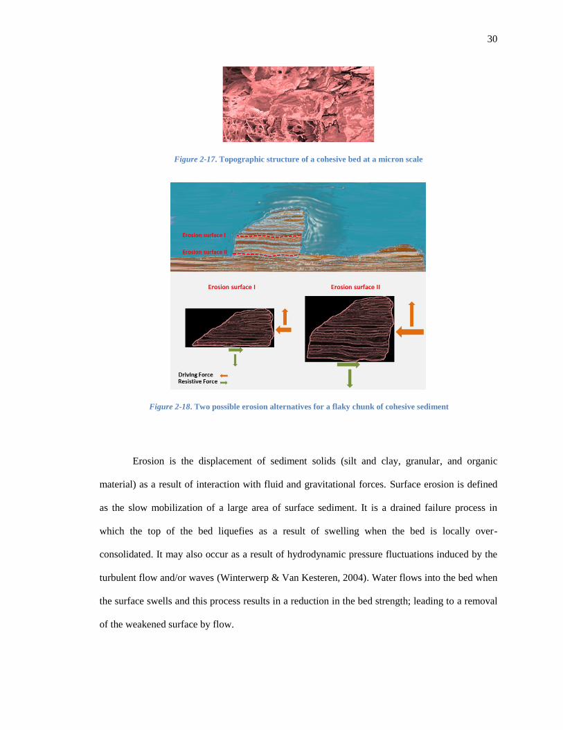
30

Figure 2-17. Topographic structure of a cohesive bed at a micron scale

Figure 2-18. Two possible erosion alternatives for a flaky chunk of cohesive sediment

Erosion is the displacement of sediment solids (silt and clay, granular, and organic

material) as a result of interaction with fluid and gravitational forces. Surface erosion is defined

as the slow mobilization of a large area of surface sediment. It is a drained failure process in

which the top of the bed liquefies as a result of swelling when the bed is locally over-

consolidated. It may also occur as a result of hydrodynamic pressure fluctuations induced by the

turbulent flow and/or waves (Winterwerp & Van Kesteren, 2004). Water flows into the bed when

the surface swells and this process results in a reduction in the bed strength; leading to a removal

of the weakened surface by flow.

31

Sediment transport in regimes with low shear stresses is very poorly understood. Pintal

(1971) studied bedload transport for granular particles (with diameters in the range of 2-22 mm)

in the proximity of the sediment critical shear stress and could not find a threshold for the

movement of particles. He observed that incipient motion was possible at any shear stress level if

the sediment was exposed for a long enough period to initiate the particles’ motion. This is

consistent with the lower probability of movement at lower shear stress levels. While bedload rate

was found to be proportional to the 2.5th power of (dimensionless) bed shear stress in relatively

higher shear stresses by different researchers and confirmed by Paintal (1971), he found a 16th

power correlation in very low shear stress levels. This means that sensitivity to shear stress is

very high in low shear stress regimes. In contrast to the mindset that assumes erosion has a

threshold, some researchers consider erosion to be a continuous process that is influential in

creating the balance between deposition and entrainment. However, there is not much data in

support of this hypothesis (Wiltshire et al., 1998).

2.3.2. Critical Shear Stress for Erosion

It can be concluded from the above discussion that there is no universal definition of the

onset of sediment erosion. Sutherland et al. (1998) reported the following incompatible

observational definitions that they found in the literature for the entrainment of non-cohesive

sediments: (1) “simultaneous movement of ten or more inorganic grains”; (2) “simultaneous

movement of both organic and inorganic grains”; (3) occurrence of erosion “at four distinct

stages”; and (4) “a reduction (>30%) in" light transmission.” The definition of a threshold gets

even more complicated for cohesive marine sediments because of the impossibility of studying

individual particles, variability in the size of flocs, existence of different modes of erosion, and

complexities caused by surface topography among other reasons. Table 2-3 presents some

common definitions of critical shear stress in fine sediments.

32

Table 2-3. Various definitions of critical shear stress

Critical Shear Stress Definition

1 The stress at which initiation of particle motion first occurs

2 The stress at which significant erosion first occurs

3 The intercept of erosion rate versus stress data

4 An entire depth sequence of increasing critical shear stress

5 An empirical function of soil physical parameters

Source of items1-4: (Sanford & Maa, 2001)

Definitions 1 and 2 in Table 2-3 are very sensitive to the visual recognition of the onset

of erosion. Among the three major modes of erosion (floc erosion, mass erosion and re-

entrainment of fluid mud), only mass erosion can be easily recognized through observation. This

mode of erosion generally occurs at shear stresses which are much larger than the critical shear

stress. Sutherland et al. (1998) also mention that the movement of larger particles can cause bias

in the detection of motion and introduce an element of subjectivity in critical shear stress

determination. All efforts to provide clear definitions of the onset of erosion (like number of

grains eroded within a certain period for larger granular particles) have not gained much success

for cohesive sediments. The onset of floc erosion and re-entrainment cannot be easily detected

and involves a high degree of the observer’s personal judgment. The results of field studies on

natural sediments (or laboratory studies in which deposition is allowed) are also very dependent

on the deposition history of the surface. Almost all methods to determine the critical shear stress

rely on the behavior of the most erodible surface particles. Some experiments suggest that erosion

commences almost simultaneously with the initiation of any flow over the cohesive sediment

surface (Annandale, 2005). This is probably due to the re-entrainment of recently deposited

particles and is evidence for the presence of hysteresis (history affects measured critical shear

stress). Definition 3 reduces the role of personal judgment by providing a less subjective

guideline to be followed. However, the methodology used for erosion measurements results in

significant variation in the shape and intercept of the erosion rate-versus-stress curve. Even for a

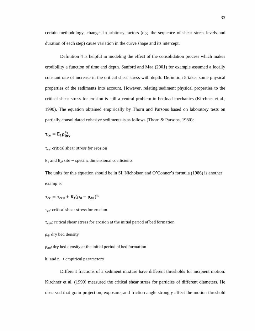
33

certain methodology, changes in arbitrary factors (e.g. the sequence of shear stress levels and

duration of each step) cause variation in the curve shape and its intercept.

Definition 4 is helpful in modeling the effect of the consolidation process which makes

erodibility a function of time and depth. Sanford and Maa (2001) for example assumed a locally

constant rate of increase in the critical shear stress with depth. Definition 5 takes some physical

properties of the sediments into account. However, relating sediment physical properties to the

critical shear stress for erosion is still a central problem in bedload mechanics (Kirchner et al.,

1990). The equation obtained empirically by Thorn and Parsons based on laboratory tests on

partially consolidated cohesive sediments is as follows (Thorn & Parsons, 1980):

The units for this equation should be in SI. Nicholson and O’Conner’s formula (1986) is another

example:

Different fractions of a sediment mixture have different thresholds for incipient motion.

Kirchner et al. (1990) measured the critical shear stress for particles of different diameters. He

observed that grain projection, exposure, and friction angle strongly affect the motion threshold

34

of single-sized particles. The distribution of erosion probability that he assigned to each particle

size became broader with the decrease in the size of particles. Estimation of critical shear stress

becomes more complex when considering the interaction of fractions of different sizes due to the

protective influence of larger particles/flocs on smaller ones.

It can be concluded from the above discussions that even for a single grain size, there is

no determinant and single threshold shear stress value for erosion. Winterwerp and Van Kestern

(2004) suggest that as the onset of sediment movement is governed by the peaks in the bed shear

stress, the measured shear stress underestimates the true values and hence should be called the

“apparent critical shear stress”. Hickin (1995) believes that the fluctuation about the mean value

is more important than the mean velocity (shear stress) in initiating sediment motion. Considering

the stochastic nature of both resisting and driving forces active in sediment incipient motion, it

seems that a comparison of probability frequency distribution of these forces can offer a

promising solution. However, the measurement and prediction of turbulent forces in the field

conditions is still not feasible.

Another aspect worth mentioning is the dependency of observed values of critical shear

stress on the choice of experimental time frame and sample size. As stated by Sutherland et al.

(1998) “Given an extended observation period or working area, the probability of particle

movement would increase.” This can be explained by the stochastic nature of hydrodynamic

forces and the high levels of non-homogeneity in natural sediments.

Despite all the aforementioned ambiguities, critical shear stress – the shear stress associated with

the onset of erosion – is a factor typically present in most erosion models (e.g. models 3, 4, 6 in

Table 2-6). The definition of this concept is also very qualitative, and there is no universally

accepted method for its quantification (Paintal, 1971). The presence of different definitions of

critical shear stress (presented in Table 2-3) has led to considerable inconsistencies in the

experimental results reported in the literature (Sutherland et al., 1998). This is why the direct

35

comparison of different studies (using different criteria or methods for determination of critical

shear stress) is generally not possible.

2.3.3. Erosive Capacity of Water

The most influential part of the flow regarding sediment erosion is the bottom boundary

layer. The fluid energy can be dissipated through two mechanisms when in contact with a

boundary: skin friction and form drag. Skin friction is caused by the shear stress induced at the

bed by the flow. It has for long been considered as the main factor determining the erosive

capacity of water. Different methods have been developed for the estimation of the boundary

shear stress depending on the technical constraints of the measurement methods. Almost all of

these methods are obtained for particle-free, hydraulically smooth flows over impermeable and

rigid beds. Although flows over cohesive sediments are typically considered as hydraulically

smooth, factors like bed permeability and elasticity, surface irregularities and bedform creation,

and the presence of suspended solids in the flow make natural field conditions sophisticatedly

different from the theoretical assumptions behind these methods. For example, previous studies

have proved that a low concentration of suspended clay

reduces the skin friction

significantly and results in higher erosion thresholds (because of the increase in mixture

viscosity). On the other hand, a higher concentration of suspended clay can make a fluid diverge

from the Newtonian response toward a Bingham-like behavior (Angelaki, 2006).

Regarding laboratory studies, Heuvelink and Webster (2001) compared the shear stress

distribution in various erosion testing devices and found differences between them and the field

condition. Presently, no theory exists for the prediction of the actual shape of the bed shear stress

probability density function (Winterwerp & Van Kesteren, 2004).

Form drag is caused by stochastic turbulent ejections and sweeps along the boundary

layer. Even though the form drag is a major contributor to the total forces on the bed, only skin

36

friction is assumed to be relevant to the erosion of single grains by many researchers. Partitioning

the shear stress into form drag and skin friction is largely motivated by this hypothesis (Garcaia,

2008). However, if each particle/floc is studied individually, a form drag can be associated with

its geometry that generates pressure fluctuations. Pressure fluctuation has also been proved to

affect erosion (Lopez & Garcia, 2001) and has even been considered as the prime driver of

incipient motion by some researchers (Annandale, 2005). It has been argued that such pressure

forces are also correlated with shear stress, but there is no strong evidence to prove the presence

of adequate correlation between them (Hickin, 1995).

Presently there is no unique way of quantifying erosion capacity of water because bed

instability processes are not sufficiently understood. The indicator parameters that are generally

used for the estimation of flow erosion capacity are average velocity, shear stress, and stream

power (Annandale, 2005).

A vertical velocity gradient in the near-bed region – through which the fluid velocity

reduces down to zero – forms the flow structure named the “boundary layer”. This layer consists

of three regions in smooth-turbulent flows (which is the type of flow expected in natural flows

over hydraulically smooth surfaces): (1) Viscous sub-layer, (2) Buffer zone, and (3) Logarithmic

turbulent zone.

Viscous sub-layer is a thin layer within which viscous effects are dominant. This layer

lies in direct contact with the boundary, and the velocity gradient is almost constant within this

layer. If roughness elements exceed the thickness of the viscous sub-layer, this layer diminishes,

and the flow will be considered as a rough-turbulent flow. The bottom shear stress in smooth-

turbulent flows can be calculated by the gradient method based on Newton’s viscous stress

equation:

37

shear stress in the fluid

shear viscosity of the fluid

The flow in the viscous sub-layer is non-turbulent. The slender longitudinal vortices

advected at low velocities within this layer become unstable at specific moments and form hairpin

or horseshoe vortices that are ejected into the boundary layer (Winterwerp & Van Kesteren,

2004). The transition between viscous and logarithmic sub-layers occurs, is called buffer zone.

Within this zone, the momentum is comparably transferred via both viscosity and turbulence and

the linear relationship between velocity and depth in the viscous sub-layer merges to the

logarithmic velocity profile.

Logarithmic turbulent zone is the sub-layer within which the momentum is transferred

mainly through turbulence. The average flow velocity in this region can be calculated based on

the law of the wall which relates the average velocity to the logarithm of the distance from the

boundary as follows:

√

K: Von Korman constant

Y: distance from the wall

: distance from the wall at which velocity reduces to zero

The net force applied to each particle/floc is generally resolved into a vertical component

(lift) and a horizontal component (drag). The term drag used here is an effective force on

individual sediments and should not be confused with “form drag” which is a source of hydraulic

resistance resulting from pressure distribution over an entire bedform. Incipient motion occurs

38

when the combination of lift and drag forces applied to a floc/particle exceeds the resistive forces.

The relative importance of drag and lift forces is highly variable with the degree of exposure and

the impact of neighboring flocs/particles. It means that even for a single particle size, no single

force (either lift or drag) can be determined as the erosion threshold.

Lift forces can originate from three sources: (1) Buoyancy: Buoyancy force is

understood well and easily estimated for granular particles. However, as this force is dependent

on the volume of the particles, estimation of its magnitude is not very straight forward for

cohesive material with all its structural complexities. Connectivity of the fluid trapped within the

internal voids to the flow can also affect the buoyancy force. (2) Upward turbulence forces:

Diffusion of eddies within the flow superimposes some random velocity fluctuation on the flow

average velocity (in all directions including the vertical direction). Eddy creation can be

intensified by the presence of local bedforms and an increase in roughness. (3) Vertical velocity

gradient: Fluid velocity reaches zero at any solid boundary to match the boundary velocity.

According to Bernoulli’s principle, any decrease in the flow speed is simultaneous with an

increase in fluid pressure. It can be concluded that a vertical pressure gradient also exists in the

boundary layer with higher pressure values occurring closer to the bed. As a consequence, an

upward lift force is applied to particles in this region, thus facilitating motion initiation. The

direct measurement of lift and drag forces has been the focus of several experimental

investigations; however, almost all of them concentrate on granular particles.

Researchers have studied turbulent flow through pipes extensively and developed some empirical

functions that relate the mean flow rate to the wall shear stress. An implicit formula relating the

wall shear stress to the mean flow in a smooth pipe of arbitrary cross section can be obtained

from Prandtl’s universal law of friction and expressed as (Schlichting, 1979):

√ [

√

]

39

V: average velocity

: kinetic viscosity (

)

friction factor

d: hydraulic diameter

W: duct width (m)

: density of water

theoretical shear stress at the wall (Pa)

As water density and kinetic viscosity are temperature-dependent as presented in Table

2-4, a sensitivity analysis was conducted to see the effect of temperature on theoretical shear

stress. As illustrated in Figure 2-19, temperature has a significant effect on shear stress, so

temperature measurements were taken into account by using the values in Table 2-4 and

interpolation. The temperature was assumed to be for those tests missing temperature

measurements.

Table 2-4.Variation of density and dynamic viscosity

with temperature for water

Temperature

(

Kinematic viscosity

Density

0 1.787e-6 999.8

10 1.307e-6 999.7

20 1.004e-6 998.2

30 0.801e-6 995.7

40 0.658e-6 992.2

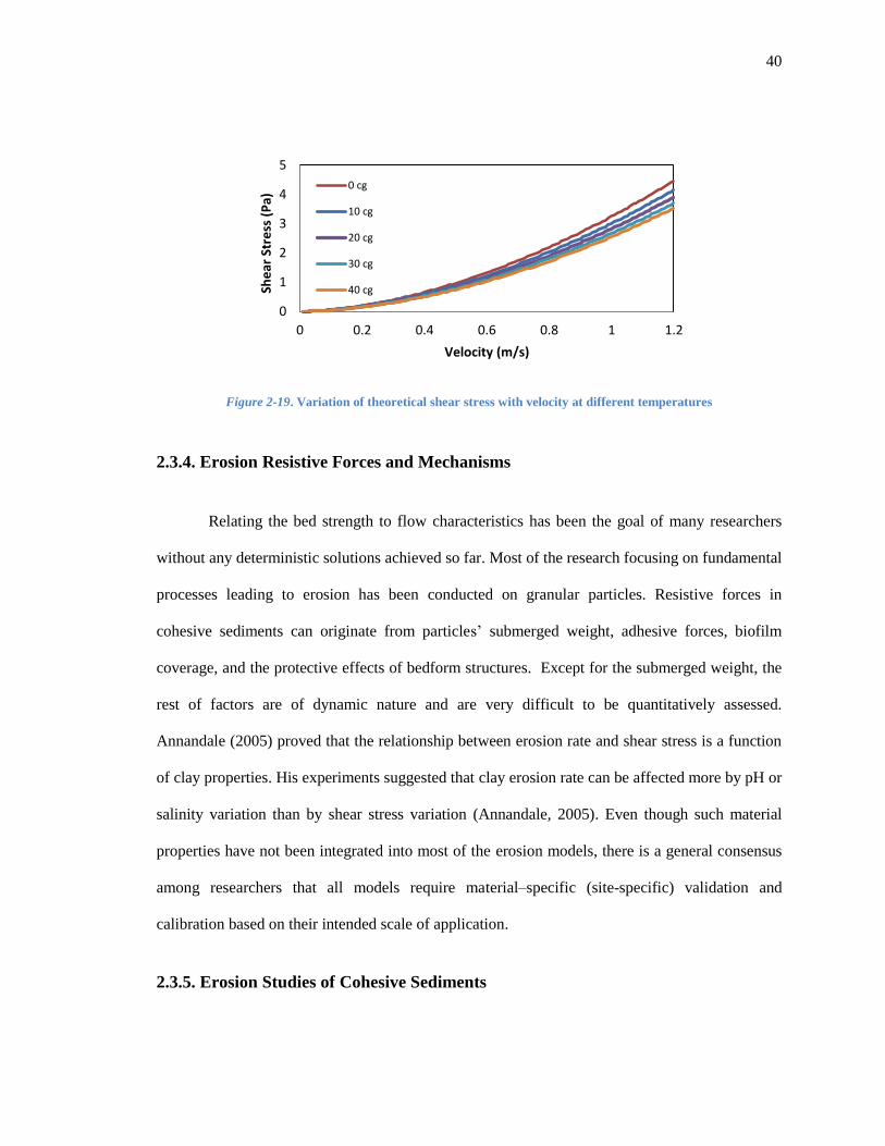
40

Figure 2-19. Variation of theoretical shear stress with velocity at different temperatures

2.3.4. Erosion Resistive Forces and Mechanisms

Relating the bed strength to flow characteristics has been the goal of many researchers

without any deterministic solutions achieved so far. Most of the research focusing on fundamental

processes leading to erosion has been conducted on granular particles. Resistive forces in

cohesive sediments can originate from particles’ submerged weight, adhesive forces, biofilm

coverage, and the protective effects of bedform structures. Except for the submerged weight, the

rest of factors are of dynamic nature and are very difficult to be quantitatively assessed.

Annandale (2005) proved that the relationship between erosion rate and shear stress is a function

of clay properties. His experiments suggested that clay erosion rate can be affected more by pH or

salinity variation than by shear stress variation (Annandale, 2005). Even though such material

properties have not been integrated into most of the erosion models, there is a general consensus

among researchers that all models require material–specific (site-specific) validation and

calibration based on their intended scale of application.

2.3.5. Erosion Studies of Cohesive Sediments

0

1

2

3

4

5

0 0.2 0.4 0.6 0.8 1 1.2

She

ar S

tre

ss (

Pa)

Velocity (m/s)

0 cg

10 cg

20 cg

30 cg

40 cg

41

Erosion quantification of cohesive sediments has been studied intensely since 1960.

Researchers have made numerous simplifying assumptions, developed various experimental set-

ups, and applied approximate analytical methods to overcome the inadequacy of a basic

understanding of this type of erosion and mitigate the high variability in sediment properties. The

variability in both experimental protocols and data analysis procedures has also been considered

as important factors contributing to uncertainty in these studies (Sanford, 2006). Researchers have

used a wide range of devices for the quantification of erosion. These devices employ different

methods for flow generation such as use of a pump, rotating disk or cylinder, water jet, oscillating

grid, and rotating propeller. In both laboratory and field tests, flow has generally been formed in

either flumes (straight or annular) or cylindrical chambers. Lee and Mehta (1994) have provided

a comprehensive review of the devices and assemblies used for cohesive sediment erosion tests.

None of these devices guarantee that the pressure gradients (or turbulent intensity spectrum)

generated in the sediment interface will have a structure similar to those created by natural flows,

and this presents a major barrier toward scientifically valid experimental protocols.

Additionally, different types of samples have been used in erosion testing devices as

summarized in Table 2-5. The mutual interaction between the deformable sediment boundary and

the sediment-carrying flow makes the measurement of the shear stress and quantification of

erosion difficult. Various experimental methodologies have been used by researchers for the

quantification of erosion. They can be categorized as: (1) total suspended solids measurement

(densimetric, acoustic, and optical methods) (2) volume loss estimation (visual, total suspended

solids, image analysis) (3) weight loss estimation. Several shear stress evaluation methods can

also be found in the literature including (1) empirical equations, (2) direct shear stress

measurement, (3) pressure differential, and (4) velocity profile in the laminar layer.

42

Table 2-5. Types of samples used in erosion tests

Sample type Description

Natural bed In-situ tests

Placed bed Natural sediment is mixed and placed on bed or remolded

Deposited bed A dilute suspension of natural sediment settles to forms a consolidated bed

Undisturbed samples Undisturbed cores of sediment

Most of the erosion experiments were designed to simulate layer-by-layer erosion under

different shear stress levels. The duration of each test step, shear stress at each step, and the order

of successive steps were arbitrarily chosen by researchers. The simultaneous occurrence of each

of the aforementioned factors made the comparison of different studies very challenging and

sometimes impossible. Thus, it is no surprise that there is no consistency in the way the critical

erosion values have been reported in the literature. For example, some studies report the critical

erosion values in terms of flow velocity at a specific height above the bed, or revolution speed (of

a propeller, duct cover or concentric cylinders) while others use the pressure of a vertical jet, or a

spatial and time-averaged bed shear stress among other ways (Sutherland et al., 1998).

As erosion is a time-dependent process (except for type II erosion occurring in uniform

beds) the duration of exposure to each shear stress level affects the quantity of material eroded at

that step in a non-linear fashion. Figure 2-20 illustrates a typical erosion rate-versus-time graph

for a test with four successively increasing shear stress levels. The shear stress levels were

applied to the sediment sample for 20-minute intervals.

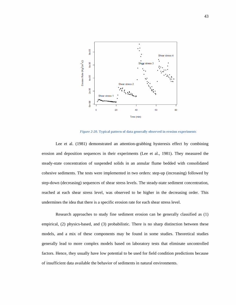
43

Figure 2-20. Typical pattern of data generally observed in erosion experiments

Lee et al. (1981) demonstrated an attention-grabbing hysteresis effect by combining

erosion and deposition sequences in their experiments (Lee et al., 1981). They measured the

steady-state concentration of suspended solids in an annular flume bedded with consolidated

cohesive sediments. The tests were implemented in two orders: step-up (increasing) followed by

step-down (decreasing) sequences of shear stress levels. The steady-state sediment concentration,

reached at each shear stress level, was observed to be higher in the decreasing order. This

undermines the idea that there is a specific erosion rate for each shear stress level.

Research approaches to study fine sediment erosion can be generally classified as (1)

empirical, (2) physics-based, and (3) probabilistic. There is no sharp distinction between these

models, and a mix of these components may be found in some studies. Theoretical studies

generally lead to more complex models based on laboratory tests that eliminate uncontrolled

factors. Hence, they usually have low potential to be used for field condition predictions because

of insufficient data available the behavior of sediments in natural environments.

44

2.3.6. Erosion Models for Cohesive Sediments

The three major types of erosion models found in the literature – empirical, theoretical,

and stochastic – are presented in the following sections.

2.3.6.1. Empirical Models

Empirical models are the most simplistic type of models that are generally developed

under the assumptions of stationarity and homogeneity and have the least computational

complexities among other models. It is a common approach in erosion studies to create empirical

models based on observed data (either in the laboratory or field). Generally, a simple form of an

equation relating selected causal variables to the response variable is assumed, and the

characteristic coefficients are determined experimentally for each site based on observations.

Many different devices and testing protocols have been used to estimate cohesive sediments’

erosion rate, but there is no unique standard procedure and guideline on how to sample and test

cohesive sediments for this purpose. Even with one specific device and a standard material and

test protocol, it is still possible to generate different incompatible results due to the over-

dependency of experimental results on the operator’s subjective assessment. Some popular forms

of the empirical models developed in the literature are listed in Table 2-6. The characterizing

parameters obtained by different researchers reflect a wide range in the values’ orders of

magnitude. Even for a specific mud sample, it is possible to obtain coefficients that vary within

one order of magnitude (Kronvang et al., 2006). Despite the shortcomings of empirical models,

one main advantage is their capability to cope with limited measurements.

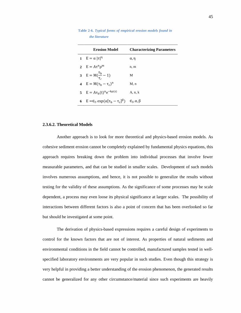
45

Table 2-6. Typical forms of empirical erosion models found in

the literature

Erosion Model Characterizing Parameters

1

2 n, m

3

M

4 M, n

5 A, n, k

6 [ ]

2.3.6.2. Theoretical Models

Another approach is to look for more theoretical and physics-based erosion models. As

cohesive sediment erosion cannot be completely explained by fundamental physics equations, this

approach requires breaking down the problem into individual processes that involve fewer

measurable parameters, and that can be studied in smaller scales. Development of such models

involves numerous assumptions, and hence, it is not possible to generalize the results without

testing for the validity of these assumptions. As the significance of some processes may be scale

dependent, a process may even loose its physical significance at larger scales. The possibility of

interactions between different factors is also a point of concern that has been overlooked so far

but should be investigated at some point.

The derivation of physics-based expressions requires a careful design of experiments to

control for the known factors that are not of interest. As properties of natural sediments and

environmental conditions in the field cannot be controlled, manufactured samples tested in well-

specified laboratory environments are very popular in such studies. Even though this strategy is

very helpful in providing a better understanding of the erosion phenomenon, the generated results

cannot be generalized for any other circumstance/material since such experiments are heavily

46

simplified. More surprisingly, it is common in erosion literature to see similar studies with

contrasting results. For example, increasing the fluid’s PH has been proven to both increase and

decrease erosion resistance in different studies. Such a complex behavior can be explained by the

dependence of chemical forces between clay particles on the temperature, salinity, and PH of the

ambient and interstitial water (Annandale, 2005). Not only does this reasoning justify the

observation of contrasting results, but it also gives rise to a serious question: Even if we assume

to know the erosion behavior of all natural minerals deterministically, is it practical or reasonable

to include details at a mineralogical level in erosion prediction models? The answer may be “yes”

if we are interested in the erosion behavior of a certain material with uniform chemical properties;

but what about natural sediments with all their complexities? The large scale of typical erosion

problems and sparsity of available data impose severe limitations on the applicability of models

developed at small scales.

Although most of the factors in Figure 3-7 have been extensively studied and their

significance in erosion has been proved, we are still far from understanding the true physics

behind erosion. As a result, there is no physical formulation for fine sediment erosion and most

of the proposed forms originate from empirical studies. Many physics-based models are

developed based on small-scale tests and under very controlled conditions while their application

is generally at higher scales and under different (and variable) conditions. Although many such

models have been proven to match the experimental results well, the numerous assumptions

involved do not guarantee the functionality of the model in predicting erosion behavior under new

conditions and for larger scales of variability in data. Moreover, the physics-based models fall

short as the results they provide are deterministic in nature as compared to the stochastic

character of erosion.

47

2.3.6.3. Stochastic Models

It can be concluded from the previous discussions that random processes have a

significant role in sediment transport. Even though a deterministic approach is not sufficient for

modeling and predicting such processes, they are still frequently conceptualized deterministically.

This is mainly because of “lack of enough experimental and / or field information to perform

stochastic analysis” (Lopez & Garcia, 2001), which is a common practice in other research areas.

A popular approach in stochastic erosion modeling efforts found in the literature is to

assign a probability distribution function to either erosive forces or erosion strength (or both).

Van Prooijen and Winterwerp (2010) analyzed sediment erosion by using stochastic bed strength

and shear forcing in a linear erosion formulation. They used a formulation suggested by other

researchers to calculate the probability density distribution based on the mean bed shear stress.

Their analytical method could reproduce the time-varying erosion rates reported in two other

studies. Winterwerp et al. (2012) also assumed a probability density function for both the eroding

shear stress and bed strength and validated their results against a limited set of experimental data.

They derived the average bed strength from soil mechanics theory.

Another approach for stochastic modeling of erosion is to assign a probability density

function to the flow-induced shear stresses and to compare that with the distribution of sediments’

critical shear stress. For example Zanke (1990 as cited in (Lopez & Garcia, 2001)) used the

erosion risk concept defined as the risk for a particle to be eroded and estimated as:

∫

[∫

]

48

2.4. Other Factors Contributing to Erosion

Three major factors that impact erosion are investigated in this section: biological factors,

sediment structure, and extreme events.

2.4.1. Biological Factors

Studies prove that an intense two-way interaction exists between biological and

geomorphological processes in intertidal mudflats (Herman et al., 2001). Even though this review

mainly focuses on the effect of biological activities on sediment transport, it should be noted that

sediment transport can also affect the biological nature of sediments by changing the bed

composition and flow characteristics. Estuarine ecosystems are extremely dynamic areas

combining marine, fluvial and terrestrial ecosystems to create a highly productive environment.

Salinity gradient, the hydrodynamic interaction of tidal and non-tidal flows, and partial exposure

to air and the sun are some major factors creating a wide variety of local ecosystems in coastal

estuaries.

Remarkable variations in habitats and species occur over very short distances in intertidal

environments (Meadows et al., 1998). Population and composition dynamics of the biota can

influence cohesive sediment dynamics through various mechanisms (toward both stabilization

and destabilization (Riethmüller et al., 1998)) and over a wide range of spatial and temporal

scales. Although many researchers have studied this influence at small scales, the large-scale

effects of small-scale biological activities have very rarely been quantified (Borsje et al., 2008).

Even at a small scale, there still remain many uncertainties about the interaction of organisms and

flow. As stated by Paterson and Black (1999), living organisms are not simply affected by the

49

flow since they also shape and mediate the flow in a manner that generally enhances their

survival chances.

In order to have a dynamic interaction, processes should act on the same temporal and

spatial scales, otherwise they will be considered as either noise or boundary conditions (Borsje et

al., 2008). For example, Ruddy et al. (1998) compared the potential erosion and deposition depths

with the photosynthesis depth and as they both occurred in the order of a few hundred microns,

they suggested that ecological and sediment dynamics occur at a similar physical scale (Ruddy et

al., 1998).

A bed of natural cohesive sediments is often densely colonized by assemblages of

bacteria and microphytobenthos (Wiltshire et al., 1998). The top few (~10) centimeters of the

cohesive sediments are exposed to aerobic conditions while the deeper zones are anaerobic

(Winterwerp & Van Kesteren, 2004). Only the top few hundred microns (300-3000 microns

according to (Ruddy et al., 1998)) of sediment surface in the intertidal zone are euphotic. Thus,

photosynthesizing microorganisms accumulate in this region only (Wiltshire et al., 1998).

There are various dynamic mechanisms through which biological activities affect

sediments’ physical properties: (1) Organic compounds decrease the sediment bulk and dry

density because their density is almost 60 percent that of natural minerals. (2) The organic content

of deeper sediments (also known as carbon storage) is mainly a result of the burial of the highly

dynamic uppermost layer (Ruddy et al., 1998)). (3) Reworking and restructuring of sediments by

living organisms (also called bioturbation) affects sediment porosity and texture. Specifically,

bioturbation can keep a (generally thin) layer of surface sediments from becoming a part of the

bed (Luettich et al., 1990). The bottom shear stress required to resuspend the material in this layer

is generally small due to the low consistency caused by mixing the liquid (flow) and solid phases.

(4) The degradation of organic matter under aerobic or anaerobic conditions produces gases,

mainly methane and carbon dioxide. The amount of gas produced in many natural types of

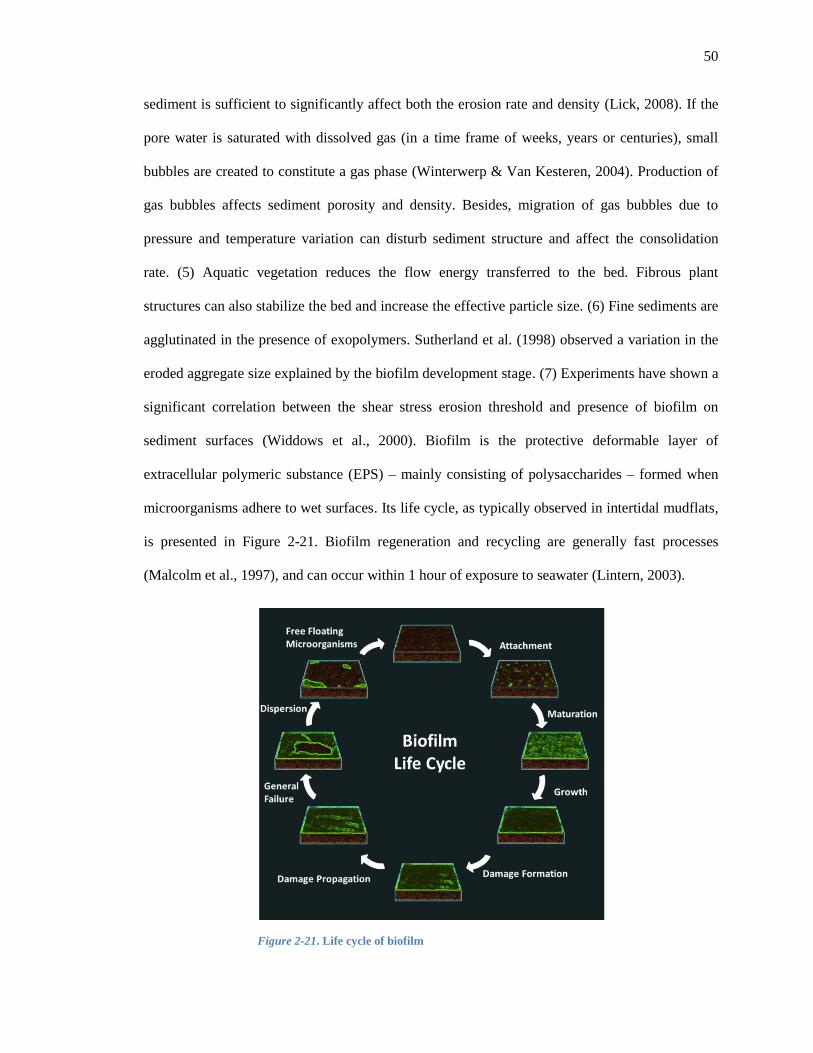
50

sediment is sufficient to significantly affect both the erosion rate and density (Lick, 2008). If the

pore water is saturated with dissolved gas (in a time frame of weeks, years or centuries), small

bubbles are created to constitute a gas phase (Winterwerp & Van Kesteren, 2004). Production of

gas bubbles affects sediment porosity and density. Besides, migration of gas bubbles due to

pressure and temperature variation can disturb sediment structure and affect the consolidation

rate. (5) Aquatic vegetation reduces the flow energy transferred to the bed. Fibrous plant

structures can also stabilize the bed and increase the effective particle size. (6) Fine sediments are

agglutinated in the presence of exopolymers. Sutherland et al. (1998) observed a variation in the

eroded aggregate size explained by the biofilm development stage. (7) Experiments have shown a

significant correlation between the shear stress erosion threshold and presence of biofilm on

sediment surfaces (Widdows et al., 2000). Biofilm is the protective deformable layer of

extracellular polymeric substance (EPS) – mainly consisting of polysaccharides – formed when

microorganisms adhere to wet surfaces. Its life cycle, as typically observed in intertidal mudflats,

is presented in Figure 2-21. Biofilm regeneration and recycling are generally fast processes

(Malcolm et al., 1997), and can occur within 1 hour of exposure to seawater (Lintern, 2003).

Figure 2-21. Life cycle of biofilm

51

A biofilm-covered sediment surface can be considered as a thin film in contact with a less

deformable sediment structure. Different failure mechanisms can be recognized in this system:

(1) Hydrodynamic forces or biological activities can cause local damages in the biofilm matrix.

Fluid forces help the biofilm skin to be peeled off the surface near the damaged zone. The

continuous nature of such forces widens the crack and finally releases the patch of biofilm

surrounded by the developed cracks. (2) The variation in the environmental conditions (e.g.

temperature, light, nutrients concentration, biota composition, etc.) may lead the system toward a

new equilibrium in which EPS secretion is stopped, and available polysaccharides are consumed

as a food source by microorganisms. (3) Wiltshire et al. (1998) reported the presence of loose

pieces of biofilm on top of its structure which suspend into the flow easily. Sutherland et al.

(1998) also found that the biofilm’s strength has a stratified structure with respect to depth

(increasing downward). These observations suggest a continuing mode of failure associated with

the gradually increasing fluid forces that dissolve looser parts of the biofilm matrix layer by layer.

(4) Freund and Suresh (2003) suggested that the biofilm may buckle and separate from the

sediment interface where the compressive stresses are large enough (Freund & Suresh, 2003).

An intact and mature layer of biofilm acts as a force absorbent and controls the exposure

of the underlying sediments to the fluid forces. Not only does this prevent the resuspension of

freshly deposited sediments, but it also provides a chance for such particles to establish bonds

with the surface and enhances the consolidation of the top sections of sediment. If fluid forces

cannot penetrate through the biofilm layer to break it up, erosion will not initiate regardless of the

sediment’s strength (Hickin, 1995). Wiltshire et al. (1998) also measured the pigments derived

from the biofilm in the water column during erosion tests and concluded that the general failure

of the bed occurs after biofilm separation, confirming the strong dependence of the sediment

erosion threshold on biological factors.

52

Some researchers have compared the erosion threshold of sediments in the presence and

absence of biogenic influences. The ratio of these values is called the stabilization coefficient

(Sutherland et al., 1998). For example, Neumann et al. (1975) observed a stabilization coefficient

equal to 5 in their study. Kornman and De Deckere (1998) studied the temporal variation of

biofilm effects on sediment erodibility in the Dollard Estuary, England in 1996. They found

erosion thresholds of 0.2, 0.5, 0.6, 0.1 and 0.1 Pa, in March, April, May, June, and July

respectively. As they could not explain this variation by observed differences in grain size, water

content and density of samples, they concluded that the presence of biofilm caused the strong

increases and decreases in the erosion threshold (that could take place within a period of two

weeks).

Some undisturbed samples taken from the Newark Bay mudflats during the period of this

study were covered by a layer of intact and elastic biofilm easily observed by the naked eye. This

layer could be separated and peeled off from the surface using tweezers because of its consistent

structure as seen in Figure 2-22. However, it is not always as easy to detect biofilm. Wiltshire et

al. (1998) used electron microscopy to observe and measure the thickness of a biofilm layer to be

less than 10 microns.

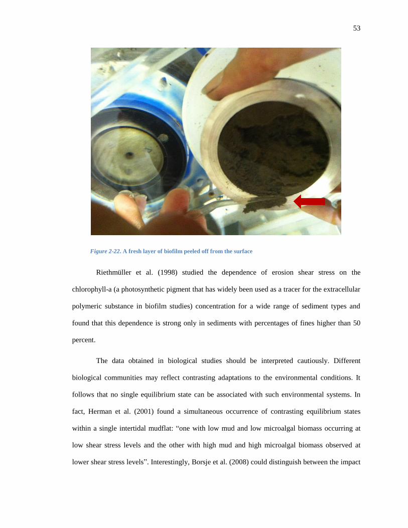
53

Figure 2-22. A fresh layer of biofilm peeled off from the surface

Riethmüller et al. (1998) studied the dependence of erosion shear stress on the

chlorophyll-a (a photosynthetic pigment that has widely been used as a tracer for the extracellular

polymeric substance in biofilm studies) concentration for a wide range of sediment types and

found that this dependence is strong only in sediments with percentages of fines higher than 50

percent.

The data obtained in biological studies should be interpreted cautiously. Different

biological communities may reflect contrasting adaptations to the environmental conditions. It

follows that no single equilibrium state can be associated with such environmental systems. In

fact, Herman et al. (2001) found a simultaneous occurrence of contrasting equilibrium states

within a single intertidal mudflat: “one with low mud and low microalgal biomass occurring at

low shear stress levels and the other with high mud and high microalgal biomass observed at

lower shear stress levels”. Interestingly, Borsje et al. (2008) could distinguish between the impact

54

of stabilizing and destabilizing organisms. The stabilizing organisms were found to be mainly

responsible for seasonal variation in the suspended sediment concentration while the destabilizing

organisms were the primary cause of spatial variation in the fine sediments present in the bed.

The overall conclusion is that the results obtained at a certain spatial or temporal scale and under

a specific environmental setup, should not be generalized or extrapolated to other situations

without additional experiments.

Borsje et al. (2008) made research endeavors to understand the large-scale effects of

small-scale biological activities in the North Sea. They hypothesized that if the biological

parameters were well-documented and averaged over small support units, their basin-wide effects

on sediment dynamics could be sufficiently estimated. Given all the difficulties in modeling the

biological activities, they concluded that even though not all the biological and transport

parameters could be prescribed for the entire study area, trends and orders of magnitude of

biological influence on sediment transport could be estimated (Borsje et al., 2008).

Even though it has been proven that abiotic conditions are not representative of natural

environments for erosion studies (Sutherland et al., 1998), many laboratory studies completely

eliminate biota from the system to control for unknown factors. Biological cycles are also very

sensitive to seasonal, tidal, and diurnal variations. For example, Malcolm et al. (1997) found a

dramatic change in the system’s balance between summer (when benthic production of organic

material is dominant) and winter (when the organic material is being degraded). Despite all the

difficulties in simulating estuarine natural processes in the laboratory, many successful cross-

disciplinary studies have investigated the interaction between geotechnical variables and

biological factors. However, innovative methods for the measurement of biological and

geotechnical parameters with high accuracy are still missing (Meadows et al., 1998).

55

2.4.2. Sediment Structure

Bed evolution is a rather slow and intermittent process that can be highly impacted by

intense events. There is no direct pathway for the transformation of the loose discrete elements

recently deposited on the surface to deeper sediments possessing an established structural

strength. Sediment particles/flocs may experience repetitive cycles of deposition and erosion

before being buried downward. Current- and wave-induced forces, biological influences (limited

to the upper bed layer), exposure to air and light, and gas production and migration are among the

active processes that can either enhance or diminish the bed formation trends. Therefore, water-

worked sediment deposits are the result of a complex chain of events, and their future behavior

depends on the conditions at the time as well as past events.

It is not possible to study the long-term development of sediment deposits through direct

observation. A very valuable source of information specially for understanding the chronological

evolution and long-term patterns in sediment transport is geochemical analysis performed by

high- resolution absolute and relative dating (such as Pb1 and Cs

2 dating) techniques. Herman et

al. (2001) used radionuclides’ profiles for estimation of both long- and short-term sedimentation

rates. Additionally, Cundy et al. (1998) proved that palaeoecological and geochemical analysis

can be combined to reconstruct environmental changes that previously occurred in the fluvial and

estuarine wetland settings. While these methods are very informative of sediment accumulation

rate, they provide no clue of erosion rates because of their exclusive dependence on the available

particles.

1 lead

2 caesium

56

Halonen (2011) performed a historical bathymetric analysis for the Newark Bay and

realized that between 1934 and 2008, significant changes had occurred in the hydraulic geometry

of the Newark Bay. During this period, most of the flats (except known areas of human

disturbance) had experienced a net deposition of less than 1 meter with annual deposition rates

less than 1.2 cm/year. He also found the accumulation patterns to be complicated and correlated

to the channel deepening activities.

Meadows et al. (1998) analyzed the small-scale differences in sediment properties

(particle size, organic content, load resistance and in-situ shear strength) by taking replicate cores

from four adjacent sites on the Clyde Estuary in Scotland. Their cluster analysis revealed a break

in the data at a depth between 40 and 70 mm (Meadows et al., 1998). They explained it to be due

to either biological activity within the sediment, the impact of the water column across the

sediment-water interface, or the influence of deeper sediments.

The sediment structure has a direct relevance to its physical properties e.g. water content

and bulk density. Penetration of fluid into the surface material is also very dependent on the level

of interconnectedness of void spaces which is a function of particle arrangement. Fluid

penetration through the surface boundary can be influential in two ways: (1) exerting physical

forces through shear stress and pressure fluctuation; or (2) changing the chemistry of interstitial

water. This change can either strengthen or weaken the chemical bonds in sediments depending

on the chemical properties of the water (Annandale, 2005). The level of dissolved oxygen in the

interstitial water can also affect biological activities.

As cohesive sediments have low permeability, pressure pulses caused by flow are not

dissipated immediately; hence gradients are established in the pore water. This makes the

estimation of internal forces within the upper bed layer very complicated. Furthermore, cohesive

sediments constitute an elastic porous medium, which has a mutual interaction with the flow, thus

presenting an additional complication. As the boundary, the sediment surface shapes the near-bed

57

flow, and the flow-induced shear, in turn, deforms the bed surface and modifies the hydraulic

roughness. For example, erosion of sediments in spots of surface imperfection increases the

surface roughness which causes higher turbulence levels followed by a progressive erosion.

As discussed above, there are various factors that affect sediment structure during bed

formation and evolution. It is not possible to quantify the relationship between sediment structure

and its erosion behavior without obtaining samples with uniform and similar structures. As

natural samples cannot be controlled for their structure, many researchers manufacture replicate

samples for this purpose. However, most artificial samples are not prepared by the action of

flowing water which eliminates many complexities naturally present in water-worked sediments.

2.4.3. Extreme Events

Rare meteorological events (e.g. severe storms, extreme floods, tsunamis, and hurricanes)

are processes highly compressed in time that are responsible for significant amounts of sediment

transport. Lack of data on the effects of such extreme events on local and global sediment flux is

a fundamental problem (Syvitski, 2003). Small and shallow waterways are highly susceptible to

the impacts of these events as deposits of several years can be disturbed and relocated within few

minutes of wave activities intensified by extreme events.

In order to reflect the intense sediment transport patterns and increase the model’s

responsiveness to extraordinary forces, some event-based models were developed to increase the

temporal resolution of data analysis during extreme events. Even though the ongoing

improvements in computation power has made it possible to move toward more continuous

simulations of reality (Merritt et al., 2003), the data collection techniques have not improved as

much. For example, most tests used to determine sediment index properties still require

laboratory investigation of samples obtained from the field. The extreme post-event conditions

pose a practical barrier against performing such site studies immediately after the events. Even

58

the use of automated sampling devices, as suggested by Quinton (2005) is a viable solution only

for some factors e.g. flow velocity and depth.

The global climate trend toward more frequent extreme weather events and a more

vigorous hydrologic cycle (Amore et al., 2004), indicates a growing significance for studying the

effects of intense nonstationarities caused by such events. It can be concluded that the

contribution of episodic events to the total sediment transport is very sensitive to the length of

time series, data frequency, and number of events recorded. For instance, Subramanian (1993)

measured 12% of the annual sediment load of the Godavari River occurring in a single day.

Calculation of the mean annual load based on this measurement overestimates the Godavari’s

annual sediment load fortyfold. This is true even for longer records: a yearlong study will result

in very different results based on the occurrence or absence of extreme events during the study

period.

2.5. The Concept of Scale in Sediment Erosion

Section 2.5 focuses on the concept of scale in cohesive sediment erosion. It investigates

the causes and consequences of temporal and spatial variations in the erosion behavior of

cohesive sediments and aims to shed light on the significance of the issue of scale. In this context,

the term “scale” refers not to any specific number, but to a rough indication of the order of

magnitude (Blöschl & Sivapalan, 1995). Scale in cohesive sediment transport is classified into

three categories: process, observational, and modeling scales, which are discussed in sections

2.5.2, 2.5.3, and 2.5.4, respectively.

2.5.1. Introduction

Scale is considered one of the most fundamental aspects in almost all research endeavors

and simultaneously one of the most ambiguous ones (Goodchild et al., 1997). However, the

concept of scale in the sediment transport field, if not completely ignored, has generally been

59

used in an unclear or inaccurate manner. For example, the temporal and spatial scales are often

not distinguished from each other and are both referred to as scale.

Sediment transport occurs in a wide range of temporal (Figure 2-23) and spatial (Figure

2-24) scales. Nano-scale inter-particle forces, micro-scale turbulence structures, mezzo-scale tidal

currents, and macro-scale regional and global climate patterns are examples of processes within

that range. While moving from small scales to large scales, the contribution of individual

processes to erosion behavior may either increase or decrease. This could be due to the

introduction of new processes to the system and/or the presence of scale-sensitive processes e.g.

reciprocal cyclic forces.

Figure 2-23. Temporal scales associated with cohesive sediment processes

Figure 2-24. Spatial scales associated with cohesive sediment processes

Scale has numerous definitions and in the sediment transport context it may refer to any

of the following concepts (applicable to both temporal and spatial aspects): (1) Support: Support

is a measure of the finest level of spatial or temporal data resolution (McBratney, 1998). Support

60

is sometimes also referred to as “grain”. Within each support unit, the measured or predicted

variable is assumed to be homogeneous (in space) or time-invariant (in time). (2) Extent: Extent

refers to the domain of study in either space (area/volume) or time (duration) delineated by the

boundaries imposed by the rest of reality. If the study extent is thought of as the target population

from a statistics viewpoint, support will be the sub-unit of the population selected for observation.

As typical with statistical studies, only a sub-set of support units are observed in each study.

Coverage is defined as the ratio of observed support units (area, volume or duration) to all

possible non-overlapping units within the study extent. In most environmental studies, the

support size is much smaller than the project extent, resulting in very small coverage ratios; thus,

coverage is sometimes reported as the number of observations per a certain area or duration

(Bierkens et al., 2000). (3) To scale (as a verb): Scale may also be used as a verb to refer to the

act of transferring information across different support units (to scale up or down). In this study,

to avoid any confusion due to the inconsistent use of the term “scale”, the terms “support” and

“extent” are used when possible.

Progress in the sediment transport field requires simultaneous advancements in three

distinct yet conceptually sequential phases: (1) process identification and phenomenological

investigation; (2) observation and evaluation; and (3) modeling and prediction. The three major

interrelated constraints that are associated with almost any approach to cohesive sediment erosion

modeling can also be related to this classification: (1) In the process phase, the complex

spatiotemporal variation of sediment and flow properties in a wide range of scales necessitates

extensive field studies making the interpolation of parameters between the sampling points

inevitable. (2) Data scarcity is still a critical concern in sediment erosion studies especially at the

regional or global levels. Despite all the advancements in the remote sensing technologies (which

seem to be the solution for collecting high-resolution data in heterogeneous fields), they still

cannot measure many sediment parameters successfully, especially below the surface. Sampling

61

and testing sediments in the laboratory are still necessities for quantifying some parameters even

though it may reduce the accuracy of results due to sample disturbance. (3) The resolution of the

input data, the extent of the study site, relative dominance of different processes and variability of

input parameters at different scales, are some factors affecting model uncertainty. As sediment

erosion is considered to be a local phenomenon (both erosive forces and resistive forces are

highly dependent on local factors), most models developed so far have been obtained and

calibrated under laboratory conditions or based on field data obtained at small temporal and

spatial scales. Model predictions, however, are generally required and used at larger scales.

Although system behavior at larger scales is to a great extent the outcome of processes taking

place at smaller scales, the scale of study can still seriously affect a model’s predictions

(Heuvelink, 1998).

Scale can be defined and used at three levels corresponding to the aforementioned

phases: (1) process scales are the scales of different phenomena operating within the study area;

(2) observational scales include all the scales associated with experimental measurements and

observations; and (3) modeling scales or working scales are the scales over which the model is

assumed to represent reality. The process scales are controlled by the nature and intensity of

environmental forces. Observational and modeling scales are generally imposed by the study’s

technical and financial resource constraints. The modeling scales, constrained by computational

limitations, should be compatible with the process and observational scales.

It is interesting to note that the process scale is considered as an abstract idea rather than a

physical reality by some researchers e.g. Bierkens (2000). They believe that no clear distinction

can be made between the process and modeling scales because our understanding of reality can

only be presented through some form of a model. In this study, however, process scales are

studied with a focus on models’ inputs and state variables while the modeling scale mainly

focuses on the process of modeling erosion. Another type of scale that is defined and used by

62

some researchers is the “policy scale” or “operational scale”. This is the scale of information

required by policy makers to make decisions (Karstens, 2009) and (Bierkens et al., 2000). It is

worth mentioning that operational scale is sometimes used in lieu of process scale (Zhang et al.,

2005).

2.5.2. Process Scale

The process scale (sometimes referred to as operational scale) is the characteristic time

(or length) at which processes occur in the system (environment). For example, a seasonal flow

pattern operates at a larger scale than tidal fluctuations. While natural process scales are generally

beyond the researcher's control (with the exception of controllable factors in laboratory or field

experiments), understanding these scales seems to be helpful when designing the experiments and

interpreting the results. However, environmental systems consist of numerous interlinked

processes such that the processes operating at small (fast) scales are constrained by the ones

operating at large (slow) scales (Zhang et al., 2005), making it impossible to recognize and

understand all the operation scales.

As previously discussed, the key processes in cohesive sediment transport are

flocculation, deposition, consolidation, erosion, and transport by flow. Even though these

processes are linked together extensively, most of the experimental studies on erosion have so far

primarily focused on a single process in isolation Another fundamental issue is that cohesive

sediments, in general, do not have a standard form of existence. One other issue to be noted is

that the forces acting upon sediments can be hydrodynamic (frictional or form drag), gravitational

or electrochemical in nature. The dependence of these forces on flow parameters, sediment

characteristics, and environmental factors, among others, introduces a source of randomness into

all sediment transport processes. Variation in the medium’s properties in space is generally

referred to as “heterogeneity” while the term “variability” is often used for variation with time

(Blöschl & Sivapalan, 1995).

63

The relationship between spatial and temporal scales is ambiguous. Bloschl (1995) argues

that there is a direct relationship between the length and time scales of a certain process, meaning

that large time scales are associated with large length scales (similarly for small scales).

However, this statement might not always be true. For example, a long-term climate variation

may affect transport processes in small as well as large dimensional scales. The emphasis in the

following subsection is to explore the variability of different factors (influencing erosion) with

time and space as found in the literature.

2.5.2.1. Temporal Variation

Variability of sediment transport processes with time occurs at a very wide range of time

scales – from fractions of a second to years – with a spectral gap in between (referred to as

separation of scales). “The influence of temporal variability (including tides as well as lower-

frequency processes) on the time-averaged estuarine regime is one of the most important topics in

estuarine physics” (Geyer, 2010). The ratio of the time period of the recorded data to the forecast

period strongly affects the reliability of the predictions (De Vriend, 1991) due to superposition of

components with different frequencies. Another challenge in the detection and tracking of

different temporal scales is caused by the time lag between input variations and the response of

some processes.

Temporal variations can be classified into the following three categories based on their

nature of variation: cyclic, pulsed, and ramped. Cyclic variations are periodical fluctuations with

certain frequencies such as the variability caused by tidal and seasonal trends. The characteristic

time scale of such variables is generally the period of the cycle. When intense variations occur in

a short period of time, for example in floods, tsunamis and storms, they are considered to be

pulsed variations and can be modeled as a point phenomenon in long-term modeling. Although

the characteristic time-scale of such events is generally their recurrence interval (or return

period), the duration of these events can also be taken into account for a more detailed analysis.

64

Ramped variations (e.g. climatic change) occur continuously and often gradually throughout

time and are usually considered as integrating processes.

Reaction and relaxation time are two additional concepts relevant to temporal variations

that must be defined when observing process scales are reaction time and relaxation time. (1)

Reaction time is defined as the amount of time between an external stimulation to a system and

its corresponding response. (2) Relaxation time is defined as the time required for a system to

return to its original state or to adjust toward new equilibrium state post stimulation.

2.5.2.1.1. Hydrodynamics

The variation of hydrodynamic forces in tidal estuaries covers a wide range of time

scales. The random velocity fluctuations occurring in fractions of a second mark the minimum in

this range while long-term climate patterns affecting global hydrological cycle and sea level for

instance represent the largest scales. Tidal and seasonal cycles fall somewhere in the middle of

this range.

There exists a circular cause-and-consequence relationship between flow hydrodynamics,

bed morphology, and sediment transport patterns (erosion and deposition) as illustrated in Figure

2-25. This relationship can be illustrated using the example of a deeply dredged shipping channel.

In such a channel, a bathymetric discontinuity leads to a complicated hydrodynamic behavior

(Burke at al., 2002), which results in a complex sediment transport pattern. Incorporating this

relationship in sediment transport models is challenging specifically because of the dependence of

the bottom shear stress on the surface roughness. For example, in low-shear-stress regimes, a

muddy environment generally dominates, and the deposition of fine particles creates a

hydrodynamically smooth muddy surface (Herman et al., 2001). The continuous deposition of

sediments in such regimes can eventually alter the bed’s morphology to reach a new equilibrium

between the bed elevation and the flow condition by imposing higher velocities (as a result of

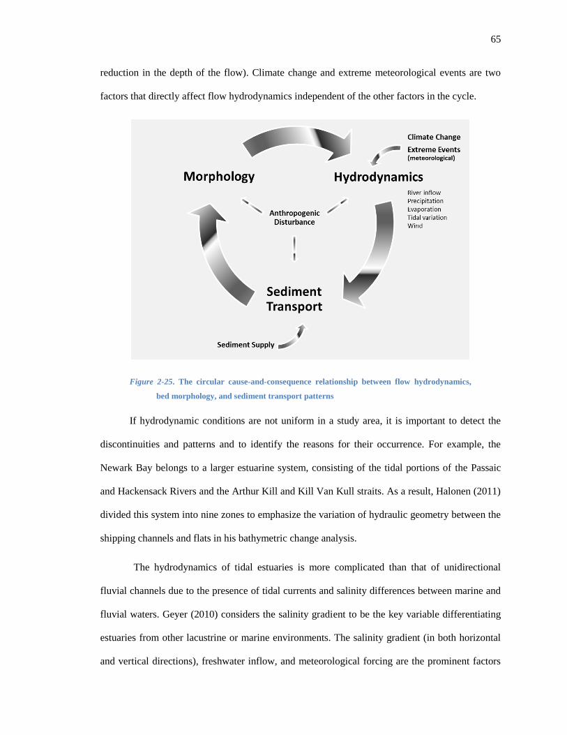
65

reduction in the depth of the flow). Climate change and extreme meteorological events are two

factors that directly affect flow hydrodynamics independent of the other factors in the cycle.

Figure 2-25. The circular cause-and-consequence relationship between flow hydrodynamics,

bed morphology, and sediment transport patterns

If hydrodynamic conditions are not uniform in a study area, it is important to detect the

discontinuities and patterns and to identify the reasons for their occurrence. For example, the

Newark Bay belongs to a larger estuarine system, consisting of the tidal portions of the Passaic

and Hackensack Rivers and the Arthur Kill and Kill Van Kull straits. As a result, Halonen (2011)

divided this system into nine zones to emphasize the variation of hydraulic geometry between the

shipping channels and flats in his bathymetric change analysis.

The hydrodynamics of tidal estuaries is more complicated than that of unidirectional

fluvial channels due to the presence of tidal currents and salinity differences between marine and

fluvial waters. Geyer (2010) considers the salinity gradient to be the key variable differentiating

estuaries from other lacustrine or marine environments. The salinity gradient (in both horizontal

and vertical directions), freshwater inflow, and meteorological forcing are the prominent factors

66

that shape the circulation regime in estuaries. The regime is influenced mainly through the tidal

propagation pattern and the location of the estuarine turbidity maximum (ETM). In a recent

hydrodynamic study in the Newark Bay, Kill Van Kull strait, and southern part of the Arthur Kill

strait, the seaward surface currents and landward bottom currents (primarily restricted to shipping

channels) were observed to form a classic gravitational circulation (Chant, 2005).

2.5.2.1.2. Tidal Cycle

Recently deposited sediments are very susceptible to erosion until they get a chance to

gain some strength as a result of self-consolidation, biostabilization, and evaporation (in air-

exposed areas in intertidal zones). Variation of water depth during tidal cycles also affects the

significance of wave climate as an erosive force. Whitehouse and Mitchener (1998) observed that

a large portion of the change in the bed level occurred at the initial and final stages of the tide

cycle when the shallow depth of water (<0.5m) and wave actions could exert a strong controlling

influence on the sediment surface. The reversing of direction in tidal currents can also complicate

the behavior of fine sediments during each tidal cycle. Consequently, a certain particle can be

resuspended and repeatedly resettled before it either becomes part of the bed or exits the estuary.

Burke et al. (2002) performed a frequency analysis on the flow data from the Newark

Bay and distinguished the semidiurnal tide to be the dominant force exerted by the current (Burke

at al., 2002). They also observed in their study channel that the predominant bed suspension

occurred twice per month during spring tides. Van (1998) studied the floc size of mud in the

Dollard Estuary in October 1995 and found strong variations in floc size during the tidal cycle.

The observed floc size correlated positively with the suspended solids concentration and

negatively with the current velocity. He also detected a vertical concentration gradient during

periods of lower velocity that occurred due to the settling of larger flocs (Van der Lee, 1998).

The detailed measurements of waves, suspended sediment concentrations (SSC), and

boundary-layer currents made by Green et al. (1997) in an estuary in New Zealand revealed an

67

interesting tide-dependent trend in the origin of suspended sediments (Green et al., 1997). During

ebb tides, a majority of sediments were derived from upstream but during the flood tides, most of

the particles originated from the local seabed. Whitehouse and Mitchener (1998) reported a

similar phenomenon during the fortnightly tidal cycle. They studied bed level variations in an

intertidal mudflat (in the Severn Estuary, England) during 31 tidal immersions (15 days) in the

winter of 1995. During the spring tides, the soft mud supplied to the intertidal zone they studied

was easily resuspended, whereas during the neap tides, the data reflected the behavior of a more

consolidated bed. It can be concluded that the stage of the tidal cycle should be taken into account

when analyzing the current velocity and SSC data. On a tide-by-tide basis, the range of variations

in the bed level was between 10 and 20mm. Whitehouse and Mitchener (1998) found the bed

level to be generally 10mm higher during the spring tide compared to the preceding and

following neap tides. They also observed a net increase of at least 3mm in the bed level over all

31 tides. On an annual timescale, the bed level variation was found to be in the order of 100mm.

However, they emphasized that the phasing of the spring-neap cycle and the tidal elevation with

periods of low- or high-wave activity has a strong control on tidal and fortnightly trends. The

surface wave activity, which is a tide-independent factor, can also influence the bed elevation

data.

Mariotti et al. (2013) explored the long-term behavior of cohesive sediments under

intermittent and moderate-energy disturbances e.g. tidal currents (and winds). They subjected a

placed bed of montmorillonite to consecutive cycles of erosion and deposition for an 80-day

period and found patterns of temporal variation for sediment resuspension occurring on scales of

weeks to months (Mariotti et al., 2013).

2.5.2.1.3. Waves

Although steady currents play the main role in the horizontal transport of sediments, the

main causes of sediment suspension in shallow estuarine flats are intermittent processes such as

68

wind waves (Burke at al., 2002). Wave-induced sediment transport has very rarely been studied

analytically (Xiao, 2009). Both local and distant winds can create surface waves in estuaries.

Short, sharp-crested waves originate from local winds while slow, gently rolling waves (called

swell) have a distant source (Beer, 1996). Although the effect of waves on the marine sediments

in shallow water has been studied extensively in the past decades (Jeng et al., 2000) wave-

induced erosion is not understood well yet (Winterwerp & Van Kesteren, 2004). Waves may

simultaneously influence the estuarine sediment transport through several mechanisms, including

but not limited to the following.

(1) Increasing bed shear stress and causing pressure fluctuations at the sediment-flow

interface: Wave-induced shear stresses in the bed surface can easily exceed flow-induced shear

stresses by an order of magnitude because of the non-linear nature of the interaction between

currents and waves (Winterwerp & Van Kesteren, 2004). Subtidal waves can also cause pressure

fluctuations at the sediment surface (Meysman et al., 2003).

(2) Affecting the salinity structure and estuarine circulation by enhancing the mixing

throughout the water column: A sufficiently strong wind can totally mix the water column from

top to bottom, inducing a windward flow on top and a reverse flow underneath (Beer, 1996).

(3) Generating a seepage flux into and out of the sediment bed: The sediment bed is a three-

phase porous medium and waves passing over it can induce a seepage flux into and out of this

medium (Jeng et al., 2000). The micro-scale velocity variations within the top portion of the bed

depend on the compressibility, permeability, and saturation level of the bed.

(4) Affecting the size and strength of suspended flocs: Waves can influence the flow’s capacity

to entrain cohesive sediments and its competence to keep the flocs/particles of a certain size

suspended. The large turbulence intensity caused by waves can also inhibit the development of

large flocs (Van der Lee, 1998)

69

Currents and waves have different temporal scales; hence, in order to take both current-

and wind-induced shear stresses into account, combined shear stress is generally defined. Natural

surface waves, however, are composed of a whole spectrum of waves originating from different

sources rather than a simple train of waves (Beer, 1996). Although one option to overcome this

complexity is to replace the whole spectrum with an average value, Winterwerp and Van

Kesteren (2004) found that the mean bed shear stress may not be the parameter describing the

surface sediment dynamics most accurately. Therefore, they proposed the peak values as a more

suitable parameter for sediment transport analysis. There are also some phase-resolved models

that compute the details of wave propagation and its effects on current (and sediment transport) at

each phase of the cycle (Wu & Wang, n.d.). Such models, however, require extensive

computational resources.

Sediment transport rates in the presence and absence of intermittent waves have been

compared in both laboratory and field studies. In field studies, as the level of control over

sediment sources is very low, care should be given to distinguish between the wave-induced local

suspension and sediments of non-local origins. Green et al. (1997) suggested examining

concentrations of suspended sediments at different elevations above the bed for this purpose.

Laboratory studies also have pitfalls as a result of limitations associated with scaling down the

field conditions.

The ratio of the magnitude of wave-induced velocities to current velocities is an

important factor contributing to the observed spatial variation morphology and sediment

composition in tidal flats of Strangford Loch (Ireland) (Ryan & Cooper, 1998). This ratio also

varies with time (following the wave cycle pattern) causing temporal variations in the turbulence

structure. The relative contribution of currents and waves to the total sediment transport is such a

significant factor that it can be used to classify the cross-shore profiles of mud flats (Kirby, 2000).

Erosional flats dominated by wind waves fall at one end of this classification range while tidally

70

dominated flats lie at the other end (Pritchard et al.). Whitehouse (2009) suggested that the depth

of the water column, shallow enough to let waves create oscillatory velocity at the bed level, is

approximately , where is the significant wave height.

2.5.2.1.4. Seasonal Variation

Seasonal trends affect sediment transport in a variety of ways. The fresh water discharge

rate has an obvious seasonal trend, which impacts the tidal propagation pattern, average salinity,

and salinity intrusion length. The phasing of the air exposure period, that is when sediments in

intertidal zones are exposed to air, with daylight hours also has a seasonal pattern, which affects

the subaerial self-consolidation (hardening) and biological activities in sediments (Whitehouse &

Mitchener, 1998).

Herman et al. (2001) report an interesting example of a seasonal cycle which does not

leave any long-term trace. They observed fine sediment accumulation up to 10 cm in an intertidal

flat in the Westerschelde Estuary (The Netherlands), between the months of March and June in

1997 (Herman et al., 2001). However, radionuclide profiles could only detect long-term sand

deposition in that area. They deduced that the mud deposition in that region was a temporary

phase being reversed (washed away) during the winter probably due to storms. Another seasonal

study in the Oues Estuary (England) also revealed a seasonal cycle of (sand-sized) sediment

redistribution operating between summer and winter (due to variations in the discharge) in both

the subtidal and intertidal zones (Uncles et al., 1998). In this study, up-channel banks, which were

covered by fine sand during the summer and autumn, were eroded back to a stronger, cohesive

bed over the winter.

Subramanian (1993) studied sediment load in India’s peninsular rivers, looking for

temporal trends. He observed that 95% of the annual sediment loads were delivered to the mouth

of the rivers during the monsoon months coinciding with peak discharges. This implies that

71

during the remaining seasons, rivers generally deposited sediments at extremely low rates. He

also discovered a negative correlation between the upstream erosion rate and the downstream

deposition rate in different Indian rivers. When he compared the variation of annual sediment

load of these rivers across different years, he found loads differing by factors as large as 20 over a

period of 5 years in the Godavari river, and 12 over a 10-year period in the Mahandi river

(Subramanian, 1993).

Whitehouse et al. (1998) compared the bed elevation measured in the tidal and annual

time scales at the Severn Estuary (England). They concluded that the annual trends in the data

could be explained by integrating the tide-by-tide behavior and superposing the impacts of

seasonal variations on the biological activity, climate, and storminess.

The volume of sediments delivered to an estuary by rivers depends on the availability of

sediments, the erosive power of flow, and the capacity of flow to carry sediments of different

sizes along the river. The last two factors are strongly related to the river’s discharge rate which is

a season-dependent variable. However, it is worth noting that a higher availability of particles in

the water column does not necessarily result in a higher siltation rate. Herman et al. (2001)

suggested that research be conducted at the estuarine level to determine if there is a causal link

between the total availability of mud in an estuary and the siltation rate.

Whitehouse and Mitchener (1998) did an extensive survey of bed levels in an intertidal

mudflat at the Severn Estuary (England) over a period of 22 months. They observed a seasonal

pattern for the reworking and redistribution of sediments, which reached a peak between August

and October, and was followed by an erosion period caused by waves during the winter.

The sediment structure can be divided into microstructure and macrostructure. While

sediments’ microstructure strongly depends on their depositional and stress history; their

macrostructure is also dependent on the biological activities of the ecosystem’s flora and fauna,

which is also a season-dependent factor.

72

2.5.2.1.5. Suspended Solids

In mudflats, more than 98 percent of the sediment flux (to the bed) can potentially be

resuspended (Ruddy et al., 1998). Measuring suspended solids concentrations is relatively easier

and cheaper than measuring other physical properties of sediments. This is why SSC time series

are generally long and have high frequencies. However, even the acquisition of accurate SSC data

can be problematic in environments with multiple sediment sources and variable grain sizes and

compositions (Green et al., 1997). It is also important to note that the size distribution of

suspended sediments is different from that of the bed sediments at the same location (Lick, 2008).

This is because the suspended sediments’ measurements do not exclusively reflect the local and

immediate conditions as they are highly influenced by sediments suspended in other locations and

transferred in the system through advection (Mikkelsen & Pejrup, 1998).

2.5.2.1.6. Basin Geology and Geomorphology

The geological formation of each basin and its contributing watershed plays the dominant

role in determining the available sediment supply that could potentially be transported by the

flow. The spatial variation of a fluvial basin’s lithology evidently impacts the sediment load in

large rivers (Subramanian, 1993).

Bedforms, as small-scale topographic structures, can also create spatial and temporal

variations in the system. In cohesive beds, bedforms can be caused by factors such as fluid forces,

bioturbation, and collision of hard objects (shells, pieces of wood, etc.) with the surface.

Bedforms control the relative projection of flocs above the average bed level and hence their

degree of exposure to the fluid and the surface roughness. They can also modify the local flow

field and turbulence level. Additionally, large-scale geologic formations can create

inhomogeneities and erosion trends as well (Wood et al., 1988).

73

Analysis of bathymetric change and sediment geochronology are two useful methods for

the investigation of long-term morphological changes and recognition of net sediment transport

patterns (Halonen, 2011). Variability of sediment characteristics with depth is a strong indicator

of long-term trends and patterns in sediment transport.

The volume, timing, and composition of sediments carried by a river are to some extent a

function of flow hydrodynamics. They are also highly influenced by the soil erosion in the

subaerial zones of the watershed. The amount and size of sediments available for transport is

referred to as sediment supply, which can be a limiting factor for sediment transport capacity

when the supply of sediments of a certain size are limited (Hickin, 1995). Many researchers have

studied soil erosion using the Universal Soil Loss Equation, which is the most popular

mathematical model for the estimation of long-term average annual soil loss due to an overland

flow. This model has been developed based on empirical studies and is not event-responsive.

R: rainfall erosivity factor

K: soil erodibility factor

L and S: topographic factors

C and P: cropping management factors

Each of the factors in the Universal Soil Loss Equation introduces a new source of

temporal or spatial variation into the cycle represented in Figure 2-25 by directly affecting the

sediment supply (independent of hydrodynamic and morphological factors).

2.5.3. Observational Scale

Observation is a fundamental step in environmental sciences that includes both direct

observations (primary research) and historical data obtained from other sources (secondary

research). Karstens (2009) defines observation scale as the scale at which humans choose to study

74

natural phenomena. Bierkens et al. (2000) defined it as the scale for which an observation

provides an average value. Observational scale in this study refers to both the resolution and

extent of observed data (spatial or temporal). Choosing the scale of measurements is a matter of

personal judgment. Researchers should choose the observational scale based on their prior

knowledge and the purpose of study while also considering the logistic and technical

measurement constraints and the nature of processes they study. Ideally, the observational scale

should be similar to the process scale because the process scales larger than the observational

scale appear as trends in the data and those smaller appear as noise (Blöschl & Sivapalan, 1995).

However, the simultaneous operation of multiple processes at different scales and the infeasibility

of making continuous, direct observations at large scales make researchers choose observational

scales that are practical but not ideal.

Most studies in the field of sediment transport provide an Eulerian description of

variables by collecting data from fixed points. This is why the spatial resolution of collected data

is generally poorer than its temporal resolution. Some additional issues specific to studying

sediment properties are lack of access to subsurface material, difficulty in estimation of sediment

properties with depth, and necessity of destructive sampling in determining some properties

including grain size distribution and density.

Determining the proper observational scale that provides sufficient detail for a new site is

a difficult task due to the lack of prior knowledge about significant scales. The impact of

changing observational scales on the interpretation of sediment transport data and development of

models has very rarely been studied. Erosion and deposition thresholds are very significant

parameters in most sediment transport models. The methods that measure these parameters in a

certain location (sample) have strong stochastic components. For a sample of fixed area A,

examined under a specific flow level, the longer the duration of observation, the more likely it is

that the threshold is exceeded within the testing period. The same argument is valid regarding the

75

sample’s area. For an observation of a fixed duration, as the sample area is enlarged, the

sediments are more likely to reach the erosion threshold during the test. This can be explained by

the stochastic nature of flow turbulence, probabilistic sediment characteristics (size and

composition), and dependence of measurement techniques on the volume of sediments tested

compared to the flow discharge rate. Another concern when choosing the observation duration for

studying natural sediments’ behavior is the dynamic processes occurring at the time scales similar

to the observation period. A perfect example in this context is the dependence of sediment

erodibility on the stage of the biofilm development in a mudflat resulting in unstable thresholds

for observations of short duration. Another example is the multi-scale variability caused by waves

and currents. The oft used coastal process models either compute the wave propagation details at

each phase (phase-resolved) or only take the average effect of waves on current and sediment

transport into account (phase-averaged) (Wu & Wang, n.d.).

A crucial question that can be raised is whether we can find a “Threshold Observation

Scale” that leads to an acceptably realistic representation of a site. This threshold should

definitely be set for the combination of support and coverage. Inspired by the concept of

“Representative Elementary Volume” used in the porous media literature, Wood et al. (1998)

introduced the concept of “Representative Elementary Area” for hydrologic models. They defined

it as the smallest discernible point that is representative of the continuum. This seems to be

analogous to the following assumption, previously used in the definition of support: the predicted

variable is assumed to be homogeneous (if spatial) or time-invariant (if temporal) within each

support unit. For each study, the minimum required size of the support unit depends on the

technical methodology for making the measurements as well as the scale of variability of the

measured parameters. The average value of the parameters measured for each support unit should

not vary significantly with increasing the sample size. Even after finding the minimum support

size, we need to understand the proper coverage (i.e. number of samples) that informs us about

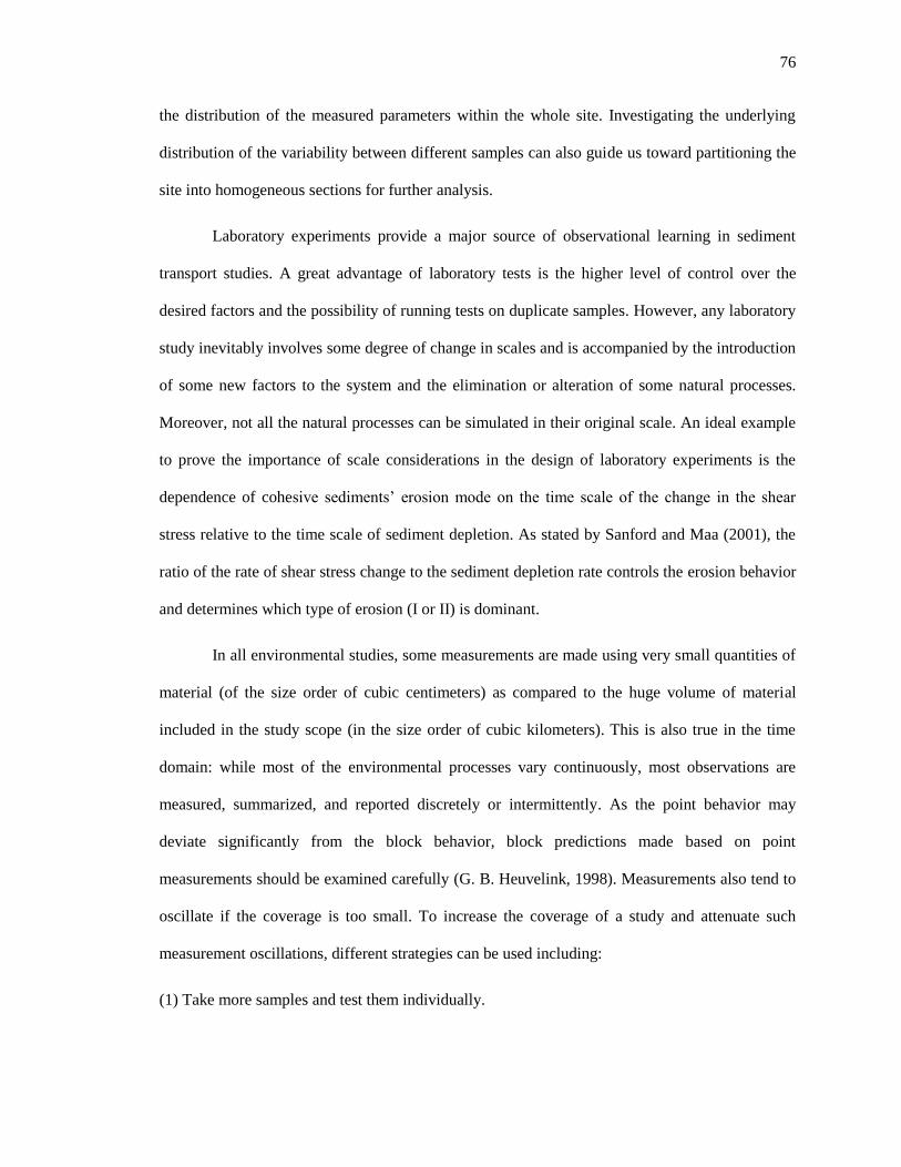
76

the distribution of the measured parameters within the whole site. Investigating the underlying

distribution of the variability between different samples can also guide us toward partitioning the

site into homogeneous sections for further analysis.

Laboratory experiments provide a major source of observational learning in sediment

transport studies. A great advantage of laboratory tests is the higher level of control over the

desired factors and the possibility of running tests on duplicate samples. However, any laboratory

study inevitably involves some degree of change in scales and is accompanied by the introduction

of some new factors to the system and the elimination or alteration of some natural processes.

Moreover, not all the natural processes can be simulated in their original scale. An ideal example

to prove the importance of scale considerations in the design of laboratory experiments is the

dependence of cohesive sediments’ erosion mode on the time scale of the change in the shear

stress relative to the time scale of sediment depletion. As stated by Sanford and Maa (2001), the

ratio of the rate of shear stress change to the sediment depletion rate controls the erosion behavior

and determines which type of erosion (I or II) is dominant.

In all environmental studies, some measurements are made using very small quantities of

material (of the size order of cubic centimeters) as compared to the huge volume of material

included in the study scope (in the size order of cubic kilometers). This is also true in the time

domain: while most of the environmental processes vary continuously, most observations are

measured, summarized, and reported discretely or intermittently. As the point behavior may

deviate significantly from the block behavior, block predictions made based on point

measurements should be examined carefully (G. B. Heuvelink, 1998). Measurements also tend to

oscillate if the coverage is too small. To increase the coverage of a study and attenuate such

measurement oscillations, different strategies can be used including:

(1) Take more samples and test them individually.

77

(2) Mix several samples and create a single composite sample on which the tests are conducted.

This method requires sample disturbance and only measures an average value for all samples

without any estimate of the variability between the samples.

(3) Find auxiliary variables, which are correlated with the parameter of interest (at the scale of

interest) and more easily measurable. Using optical remote sensing methods to measure the

surface chlorophyll-a concentration in exposed mudflats as an indicator of surface stability

(because of its correlation with the biofilm concentration) is an example of this approach

(Murphy at al., 2004).

Point samples are generally widely separated apart by distances which are larger than the

sample’s dimensions by several orders of magnitude. Observational experiments should be

designed to reflect the environment and maximize our understanding of the variability in

sediment properties given all the technical and financial limitations. The selection of sampling

locations can be a random, systematic, or judgment-based process or may include a combination

of these methods. Random sampling requires the least design effort as it follows the procedures

for simple random sampling. It gives all possible points the same chance of being tested.

Systematic sampling involves a systematic randomization technique e.g. presenting a geometric

configuration for the points to be sampled. To ensure that estimates are unbiased, an element of

randomization that provides a probabilistic basis for the inference should be applied (Webster &

Oliver, 2007). Partitioning the study area into fairly homogeneous grid cells is often a necessary

step in studies of large scope including those examining different sediment types. A single value

is generally assigned for each of the grids to be used within the models.

In order to deal with complexities at very small scales, a fundamental question is if there

exists a threshold scale that attenuates the small-scale, undefinable complexities in sediment

heterogeneities without losing a realistic perspective of the variations. In practice, however, the

number of samples and the sample size are generally determined based on the measurement

78

techniques and sampling methods used, site conditions, study purposes, and other technical

considerations.

2.5.4. Modeling Scale

Modeling (working) scale is the scale of predictions made by the model outputs. For

instance, an estuarine annual sediment transport model provides the average annual sediment

transport for that estuary. What some researchers categorize as policy scale is also treated as a

modeling scale in this study. The modeling scale should be determined based on both the model

applications and the observation scales. The typical temporal modeling scales for sediment

transport are long-term, annual, seasonal, monthly, weekly, daily and event-based. Similarly, the

spatial scales of data can vary from pore-scale to local, regional, and global scales. In

environmental studies, it is typically easier to increase the support and extent of a study in the

temporal dimension compared to the spatial dimension; this explains why spatial data is often

widely dispersed. The modeling scale is generally much larger or smaller than the observation

scale; therefore, the data needs to be scaled to bridge this gap (Blöschl & Sivapalan, 1995).

Models representing a process at different scales are unlikely to be linearly related and thus, the

data will carry different information at various scales. For example, a model developed at the

pore scale is not applicable at the regional scale without adjustment.

The following factors cause considerable differences between models at different scales:

(1) The significance and dominance of processes vary at different scales. The relationships

derived at one scale may not be valid at other scales. For instance, tidal and seasonal variations in

suspended solids, which are significant factors in short-term transport rates may have no effect on

annual transport rates.

(2) The heterogeneity and variation of model inputs in space and time make them scale-invariant

and adds a source of nonlinearity to all processes including linear ones.

79

(3) The temporal and spatial scales of most observations are much smaller than the scales at

which predictions are required for the system. This necessitates aggregating small-scale

observations to represent larger-scale processes. However, Goodchild et al. (1997) believe that

when data are aggregated, new properties may emerge. The quality and quantity of data available

for doing large-scale analysis is generally poor and insufficient, which makes the use of simpler

models with fewer parameters inevitable. For a fixed experimental design, the coverage (ratio of

observed support units to the study extent) varies based on the extent for which the model is used.

This ratio significantly affects the reliability of the model at different scales.

(4) Most of the models used for sediment transport analysis have a strong empirical nature

because of a lack of understanding of the physics of the processes. The model coefficients and

constants as well as the form of the statistical models heavily depend on the set of measurements

over which the model is developed and calibrated.

(5) Some properties of the system may be correlated only at certain scales (Webster & Oliver,

2007). Consequently, if a model depends on such correlations, it cannot simply be transferred

across different scales.

The development and modification of models for different scales are not straight- forward

tasks. The advent in technology (both computational and observational) has made it possible to

concentrate on fine-scale erosion processes (with the aim of understanding the physics behind

them). The general improvement in observation scales in recent years makes it even more critical

to clarify the relationship between larger and smaller scales. There are two extreme viewpoints

regarding this relationship. The first one assumes that the significance of each process is limited

only to the scale at which it operates and that there is no transfer of influence across scales. The

second thinks of larger-scale processes as being shaped by and extended from processes

occurring at smaller scales. In reality, each of these views partly explains the relationship between

the scales, and the contribution of each process to the overall sediment transport is generally a

80

scale-dependent variable. The fact that flocculation occurs at fine scales never undermines its

significance at larger scales while some processes occurring during the course of a tidal cycle

may not remain as contributory in models operating on large scales.

The inherent relationship between the process scales and observation scales on one hand

and the observation scales and modeling scales on the other hand, makes it important to design

experiments bearing these relationships and the end use(s) of the results in mind. Future studies

and additional measurements can also be improved based on the model requirements and

previous measurements.

Bierkens et al. (2000) divided the scale transfer operations into three categories. A

combination of these methods is generally used to transfer data between the observation and

modeling scales.

(1) Change of extent (extrapolation versus singling out): when the extent of the observations and

the model do not match, the data should be either extrapolated (to increase the extent) or singled

out (to decrease the extent) should be performed.

(2) Change of support (upscaling versus downscaling): An Examples of upscaling include

calculating the annual sediment transport rate based on the measured daily rate or measuring

erodibility in a single location and assuming that it applies to the surrounding area. On the other

hand, an example of downscaling is estimating the net sediment deposition in a section of a

channel based on suspended sediment concentration measurements made at the input and output

points for the entire channel. Another example is when a monthly sediment transport rate is

derived from an annual record.

(3) Change of coverage (interpolation versus sampling): For instance, while sediment organic

content is determined for a few small samples taken from the basin, an erosion model may require

the organic content value for each of the model grids. This necessitates increasing the coverage of

81

the input data by interpolation. If a model requires fewer data points than the collected

measurements, sampling should be performed to reduce the coverage of input values to be used in

the model.

It may be necessary to partition a site into smaller areas and model them as interacting

adjacent systems. The suitable scale for analysis of the observed data, in this case, is the scale that

tolerably lowers the response variability between various sufficiently large areas. Zhang et al.

(2005) suggested the following methods for determining a relevant homogeneous size to be used

as the optimal scale in environmental models.

(1) Analysis of the variogram change with variation in spatial resolution

(2) Estimation of the average local variance from a moving window for different measurement

scales and finding the scale at which the variation is maximized

(3) Plotting the semi-variance at a lag of one pixel versus different spatial resolutions

(4) Using the dispersion variance of a variable within a specific region that is defined on a spatial

scale

These techniques along with prior knowledge of the site can also be used for site

partitioning. The process for selecting the optimum analysis scale – as discussed above – is

independent of the scale of the model outputs required by decision makers. This problem is

viewed as a discrepancy between the observed data, the analysis efforts, and the required outputs

in the literature. In order to align the model output with the scale of the environmental measures

decision makers need to know, a scale transfer mechanism should also be built into the model.

One approach to reduce the scaling complexities is to break different model components apart.

Bierkens et al. (2000) defined model components as follows: Inputs are the measured variables

that are fed into the model. State variables are all the variables that are necessary to describe the

system. They should be known along with the input variables to describe the system’s response

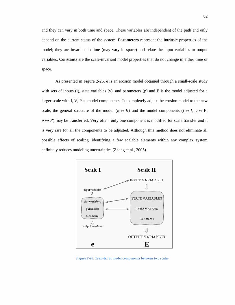
82

and they can vary in both time and space. These variables are independent of the path and only

depend on the current status of the system. Parameters represent the intrinsic properties of the

model; they are invariant in time (may vary in space) and relate the input variables to output

variables. Constants are the scale-invariant model properties that do not change in either time or

space.

As presented in Figure 2-26, e is an erosion model obtained through a small-scale study

with sets of inputs (i), state variables (v), and parameters (p) and E is the model adjusted for a

larger scale with I, V, P as model components. To completely adjust the erosion model to the new

scale, the general structure of the model and the model components ( , ,

) may be transferred. Very often, only one component is modified for scale transfer and it

is very rare for all the components to be adjusted. Although this method does not eliminate all

possible effects of scaling, identifying a few scalable elements within any complex system

definitely reduces modeling uncertainties (Zhang et al., 2005).

Figure 2-26. Transfer of model components between two scales

E e

83

Adjusting the general structure of a model across scales involves using statistical

techniques and background knowledge (mostly empirical), to develop a new model structure that

is more suitable for the new scale (often a larger scale). The state variable is the model

component that appears to be neglected the most in sediment transport studies. To the best of the

author’s knowledge, no model in the literature has explicitly included this component so far. This

variable represents those elements of the system that cause different responses to identical inputs.

The modification of model parameters across different scales can be considered as a special type

of model structure adjustment in which the form of the model does not change, and only the

parameters are modified.

A large body of literature has been developed on scale transfer methods in the past three

decades (Bierkens et al,, 2000) providing guidance for linking the observation and modeling

efforts across different scales. Some of these methods are presented here:

(I) Calibration: This technique finds empirical relationships between available fine-scale and

large-scale data (generally using regression techniques). It can be applied to any of the model

components (inputs, parameters, state variables) or used to form a new model structure at the

modified scale. Despite its computational simplicity, this method postulates that sufficient data is

available for calibration which is rarely the case. The model’s reliability should also be validated

in different conditions to ensure the validity of the statistical assumptions.

(II) Estimation Interpolation: There are a wide range of interpolation techniques available for

generating new data based on available information for the surrounding points. An interpolation

technique that is widely used in geostatistics to estimate a single realization of a random field is

Kriging or Gaussian process regression. Under suitable assumptions, Kriging results in the best

linear unbiased estimator of a variable at an unmeasured location based on point observations at

other locations. Similar to other interpolation algorithms, Kriging calculates the weighted sum of

the surrounding data points. The main difference between this technique and other interpolation

84

methods (splines, inverse distance squared, etc.) is that instead of using an arbitrary function, the

weight assignment procedure for Kriging is data-driven and weights are assigned based on the

level of spatial continuity in the data. However, creating a model that describes the spatial

dependence of the data, still involves an arbitrary selection of a mathematical form and values of

the associated parameters. Another difference between Kriging and other linear estimation

methods is that it minimizes the error variance and gives an estimation of the variable along with

approximate values of the estimation error (Kriging variance). There are different types of

Kriging: (1) Simple Kriging: The whole dataset is assumed to have a constant mean. (2) Ordinary

Kriging: This is the most widely used type of Kriging in which the mean is assumed to be

constant only in the local neighborhood of each estimation point. (3) Universal Kriging: It is very

similar to ordinary Kriging with the only difference that it fits a trend to estimate the mean value

at each point. (4) Cokriging: This is a multivariate Kriging that uses the correlation between

variables (as a function of lag) to improve predictions. It is considered as a reliable framework to

incorporate auxiliary information into predictions (Zhang et al., 2005).

The spatial continuity in a dataset can be estimated and modeled using any of the following

methods:

(a) Correlogrom: This graph depicts the auto correlation of the dataset at varying time lags or

distance lags. If there is no spatial or temporal dependence between different points, the

autocorrelation will be approximately zero for all lags.

(b) Covariance function: This function is defined as:

: The correlation between any two points separated by lag h

(c) Semi-variogram: The semi-variance between points i and j is defined as

[ ]

85

If the semi-variance between all the pairs of data is plotted against the distance that

separates the two locations, a semi-variogram cloud is created which generally consists of many

points. If the data has spatial dependence, closer points will have lower semi-variance. In order to

make it easier to interpret the data, the distance range is divided into lag classes [

represented by the mid-range value h. The semi-variance values between all n pairs of data

separated by a lag h are averaged as follows to obtain the variogram:

∑

Models fitted to variograms can have different forms (spherical, exponential, etc.) but the

following parameters are common to all of them: Nugget : the semi-variance at extremely

small separation distances (or times). Theoretically, this value should be zero but because of

short-scale variations and measurement errors it is possible to have different observations at very

close locations, creating a discontinuity at the origin of the curve. Range: the lag at which the

semi-variogram reaches its plateau. Sill : the maximum semi-variogram value which is

the semi-variance between any two points with separation lags larger than the range value.

(III) Stochastic simulation: Stochastic simulation has been previously discussed in Section 2.5.3.

While the main goal in estimation is optimizing the local estimates (for example, Kriging

minimizes the local error variance), stochastic simulation focuses mainly on the global statistics

to better reproduce the spatial variability. This is why simulation, in general, is a much better

method (compared to estimation) to preserve statistics such as variance, the shape of the

histogram, and the spatial continuity of the variogram. Despite resulting in larger mean prediction

errors, simulated values better represent the spatial variations in the field because estimation

methods like Kriging reflect a smoothed representation of the reality.

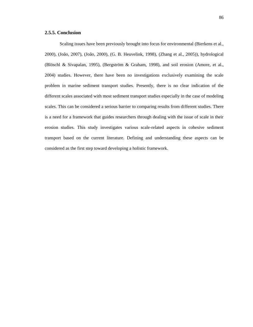
86

2.5.5. Conclusion

Scaling issues have been previously brought into focus for environmental (Bierkens et al.,

2000), (João, 2007), (João, 2000), (G. B. Heuvelink, 1998), (Zhang et al., 2005)), hydrological

(Blöschl & Sivapalan, 1995), (Bergström & Graham, 1998), and soil erosion (Amore, et al.,

2004) studies. However, there have been no investigations exclusively examining the scale

problem in marine sediment transport studies. Presently, there is no clear indication of the

different scales associated with most sediment transport studies especially in the case of modeling

scales. This can be considered a serious barrier to comparing results from different studies. There

is a need for a framework that guides researchers through dealing with the issue of scale in their

erosion studies. This study investigates various scale-related aspects in cohesive sediment

transport based on the current literature. Defining and understanding these aspects can be

considered as the first step toward developing a holistic framework.

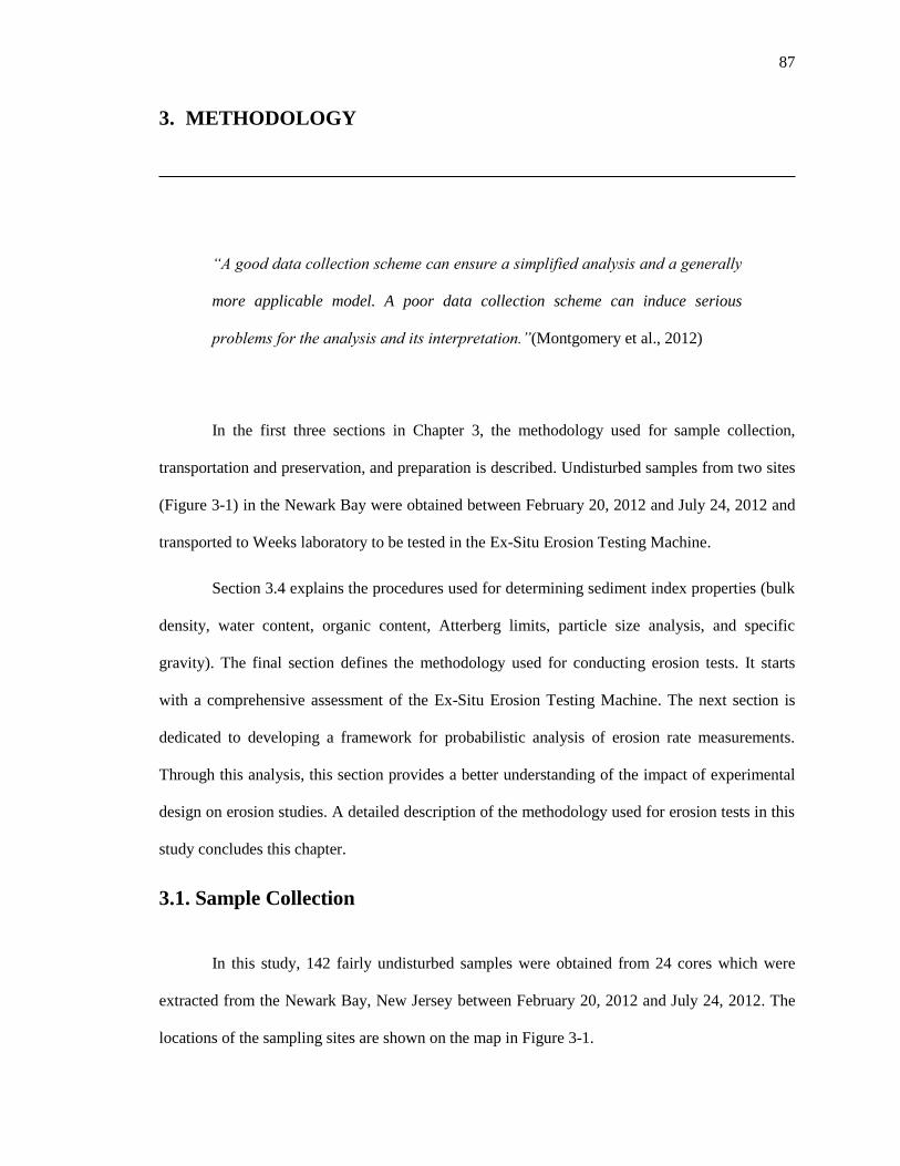
87

3. METHODOLOGY

“A good data collection scheme can ensure a simplified analysis and a generally

more applicable model. A poor data collection scheme can induce serious

problems for the analysis and its interpretation.”(Montgomery et al., 2012)

In the first three sections in Chapter 3, the methodology used for sample collection,

transportation and preservation, and preparation is described. Undisturbed samples from two sites

(Figure 3-1) in the Newark Bay were obtained between February 20, 2012 and July 24, 2012 and

transported to Weeks laboratory to be tested in the Ex-Situ Erosion Testing Machine.

Section 3.4 explains the procedures used for determining sediment index properties (bulk

density, water content, organic content, Atterberg limits, particle size analysis, and specific

gravity). The final section defines the methodology used for conducting erosion tests. It starts

with a comprehensive assessment of the Ex-Situ Erosion Testing Machine. The next section is

dedicated to developing a framework for probabilistic analysis of erosion rate measurements.

Through this analysis, this section provides a better understanding of the impact of experimental

design on erosion studies. A detailed description of the methodology used for erosion tests in this

study concludes this chapter.

3.1. Sample Collection

In this study, 142 fairly undisturbed samples were obtained from 24 cores which were

extracted from the Newark Bay, New Jersey between February 20, 2012 and July 24, 2012. The

locations of the sampling sites are shown on the map in Figure 3-1.

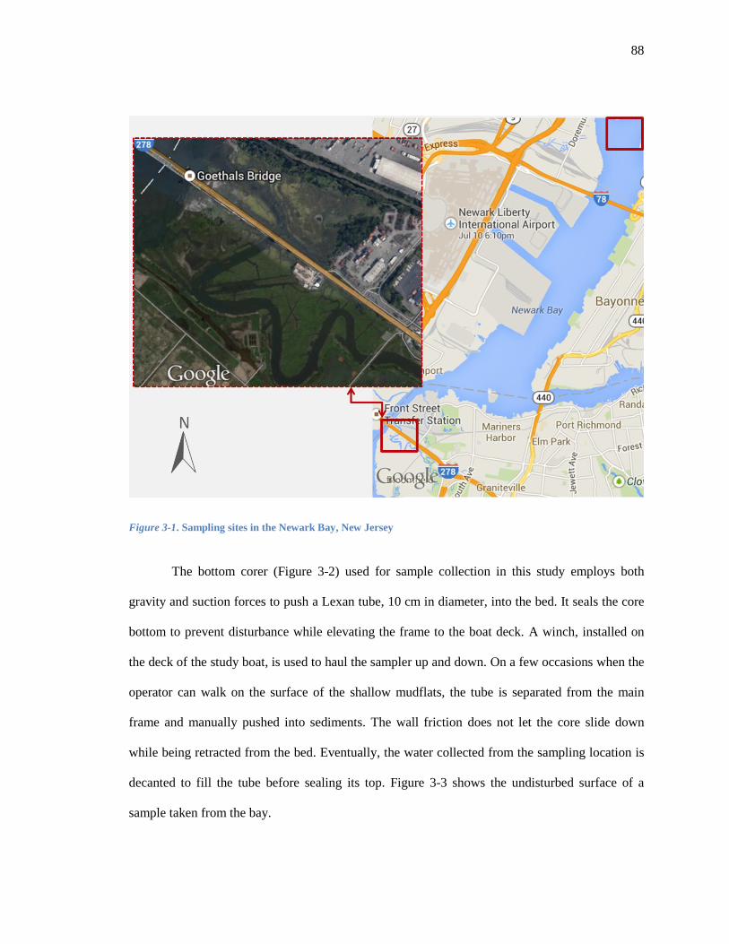
88

Figure 3-1. Sampling sites in the Newark Bay, New Jersey

The bottom corer (Figure 3-2) used for sample collection in this study employs both

gravity and suction forces to push a Lexan tube, 10 cm in diameter, into the bed. It seals the core

bottom to prevent disturbance while elevating the frame to the boat deck. A winch, installed on

the deck of the study boat, is used to haul the sampler up and down. On a few occasions when the

operator can walk on the surface of the shallow mudflats, the tube is separated from the main

frame and manually pushed into sediments. The wall friction does not let the core slide down

while being retracted from the bed. Eventually, the water collected from the sampling location is

decanted to fill the tube before sealing its top. Figure 3-3 shows the undisturbed surface of a

sample taken from the bay.

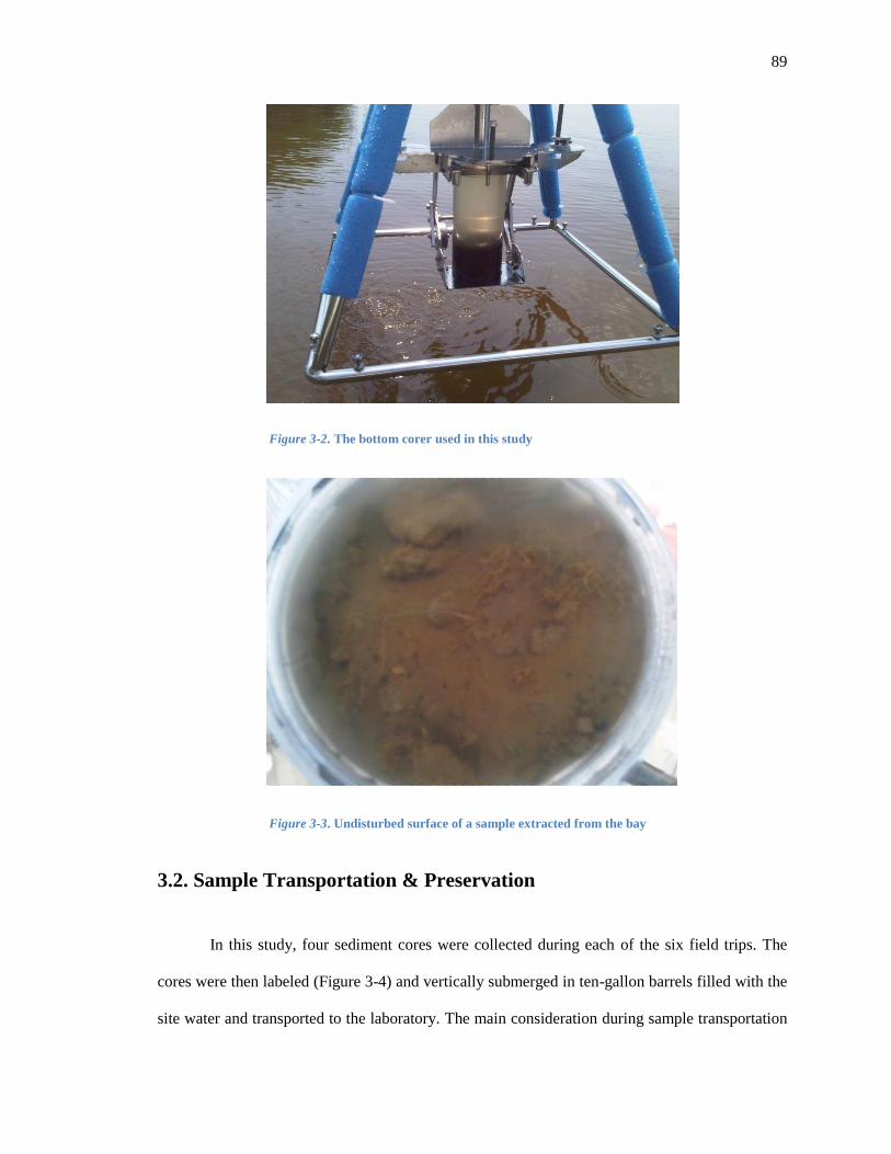
89

Figure 3-2. The bottom corer used in this study

Figure 3-3. Undisturbed surface of a sample extracted from the bay

3.2. Sample Transportation & Preservation

In this study, four sediment cores were collected during each of the six field trips. The

cores were then labeled (Figure 3-4) and vertically submerged in ten-gallon barrels filled with the

site water and transported to the laboratory. The main consideration during sample transportation

90

and preservation was to minimize physical disturbance and maintain the system’s natural balance.

The cores were transported to the laboratory within a three-hour time frame. Upon arrival at the

laboratory, the distance between the bottom and top of each core was recorded as the thickness

before submerging the tube into a cool chamber filled with the site water. The cool environment

reduces the biological activity and helps the cores to maintain their integrity for a longer period.

The biofilm layer that was originally visible on the surface of some of the samples lost much of

its strength (consistency) in the first few hours after being removed from the site. There was no

visible biofilm on top of the samples after 24 hours. This was consistent with the observations of

Sutherland et al. (1998). Their biostabilization studies proved that sediment stability is affected

by the physiological state of the biofilm and its composition (influenced by nutrient status and

growth phase). They also found a correlation between the biofilm’s age and eroded particles’

shape and size. The storage chamber was aerated with an air pump, and a light source was added

to the system to simulate natural daylight.

3.3. Sample Preparation

Sample preparation is an essential part of performing reliable erosion tests. After

removing the top and bottom lids, the tube was placed on a sample ejector and a 2.5-cm-thick

extension ring (Figure 3-5) was placed and pushed tightly over that. The ejection piston was then

pushed upward to slide the sediment core outward into the extension ring. When a sufficient

amount of sediment was pushed into the ring, it was detached from the rest of the core using a

thin cutter plate (Figure 3-6). A smaller cutter (a metal ring with an external diameter of 61 mm)

was then used to obtain up to 2 sub-samples from this sediment section as shown in Figure 3-6.

Ejection, cutting, and trimming of the sample tend to disturb the sediment structure, especially at

the periphery of the sample and along the cutting surfaces when roots are present. Hence, care

was taken to minimize sediment disturbance as much as possible. The disturbance potential was

the highest on the surface where the sample had its lowest consistency. The final samples were

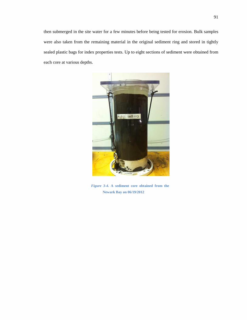
91

then submerged in the site water for a few minutes before being tested for erosion. Bulk samples

were also taken from the remaining material in the original sediment ring and stored in tightly

sealed plastic bags for index properties tests. Up to eight sections of sediment were obtained from

each core at various depths.

Figure 3-4. A sediment core obtained from the

Newark Bay on 06/19/2012

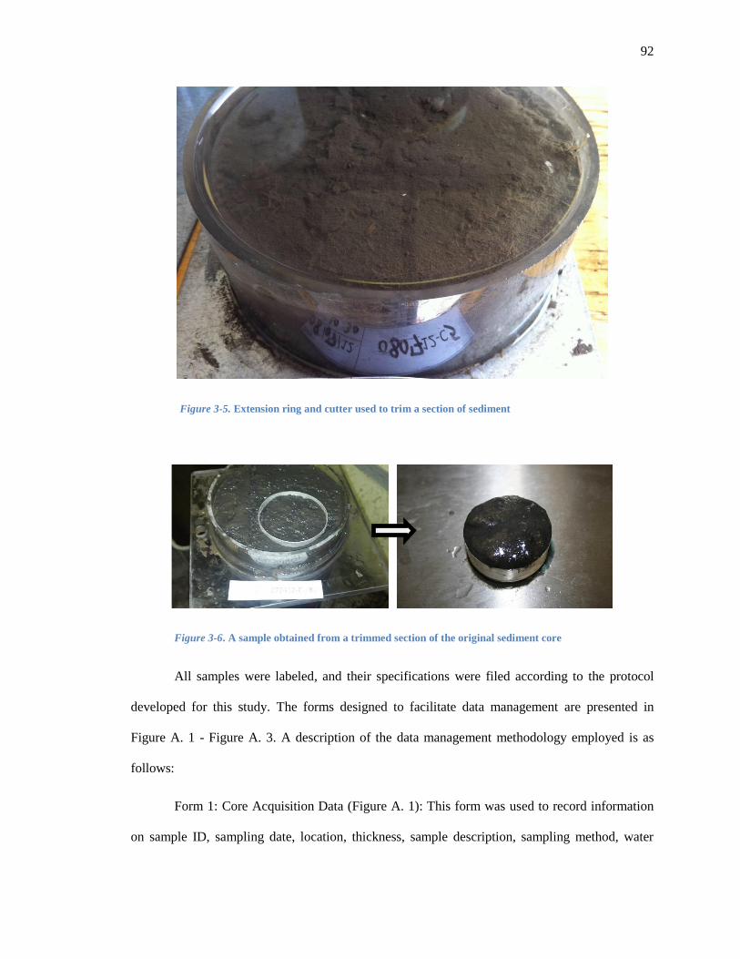
92

Figure 3-5. Extension ring and cutter used to trim a section of sediment

Figure 3-6. A sample obtained from a trimmed section of the original sediment core

All samples were labeled, and their specifications were filed according to the protocol

developed for this study. The forms designed to facilitate data management are presented in

Figure A. 1 - Figure A. 3. A description of the data management methodology employed is as

follows:

Form 1: Core Acquisition Data (Figure A. 1): This form was used to record information

on sample ID, sampling date, location, thickness, sample description, sampling method, water

93

depth, and the names of image files. It was filled out during sample preparation. The format for

the sample ID (example: 020112-C1 ) was “date of sampling-C Core Number” where the prefix

“C” denoted “core” and the Core Number was a number from 01 to 04 that distinguished between

the four cores collected on that date.

Form 2: Ring Identification Data (Figure A. 2): This form was designed to keep track of

each sample’s depth with respect to the bed level. As previously explained, each core was divided

into various sections (rings). The sections derived from each core were numbered according to

their depth starting from 1 for the uppermost section. The thickness of each section and its

extraction date were recorded in form 2.

Form 3: Undisturbed Sample Identification Data (Figure A. 3): This form included the

sample ID and the top and bottom depths of the sample. The format for the sample ID (example:

022412-C03-R07-S2) was “date of sampling-C Core Number-R Ring Number-S Sample Number.

The age of the sample (indicating the time lag between the coring and sampling procedures

measured in days, and the time between the sampling and testing steps indicated in hours) were

also recorded in this form.

3.4. Index Properties

Many parameters have been proven to affect the erosion behavior of cohesive sediments

so far. Many researchers including Winterwerp and Van Kesteren (2004), Whitehouse et al.

(2009), and Grabowski et al. (2011) have provided comprehensive lists of factors influencing

erosion. These researchers often classified the contributing factors into physical, chemical, or

biological categories.

A summary of the most important parameters studied more or less extensively in the

literature is presented in Figure 3-7. They are classified according to their domain: fluid;

interface; and sediment. Lick (2008) and Whitehouse et al. (2009) are good references that

94

discuss many of these parameters in detail. Climatic and hydrological variations, biological

activities, physical processes, and chemical reactions are the main driving forces that cause

variations in these parameters both interactively and independently. While a few of these

parameters can be measured in the field (e.g. flow properties and interface specifications), most

of them require laboratory measurements. This means that field tests alone cannot measure such

parameters without complementary laboratory tests.

It is neither possible nor useful to measure all sediment properties known to influence

erosion behavior simultaneously. Considering the Ex-Situ Erosion Testing Machine’s

requirements for sediment testing including specifications for experiment configuration, sample

size, fluid characteristics, and sample preservation methods, the following tests were conducted in

this study as complementary laboratory tests: (1) bulk density; (2) water content; (3) organic

content; (4) Atterberg limits; (5) particle size analysis; and (6) specific gravity. Given the quantity

of material required for each of these tests as compared to the material available within each ring,

the last three tests were performed on homogenized samples obtained from the whole core. While

the bulk density was measured for individual samples, water and organic content were measured

for each sediment ring. These tests will be discussed in sections 3.4.1 through 3.4.6.

95

Figure 3-7. Parameters influencing erosion of cohesive sediments

Biological processes: Biostabilisation Bioturbation Biodestabilization

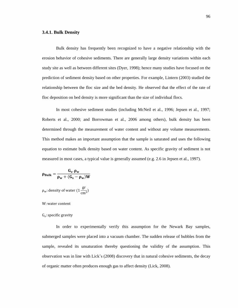
96

3.4.1. Bulk Density

Bulk density has frequently been recognized to have a negative relationship with the

erosion behavior of cohesive sediments. There are generally large density variations within each

study site as well as between different sites (Dyer, 1998); hence many studies have focused on the

prediction of sediment density based on other properties. For example, Lintern (2003) studied the

relationship between the floc size and the bed density. He observed that the effect of the rate of

floc deposition on bed density is more significant than the size of individual flocs.

In most cohesive sediment studies (including McNeil et al., 1996; Jepsen et al., 1997;

Roberts et al., 2000; and Borrowman et al., 2006 among others), bulk density has been

determined through the measurement of water content and without any volume measurements.

This method makes an important assumption that the sample is saturated and uses the following

equation to estimate bulk density based on water content. As specific gravity of sediment is not

measured in most cases, a typical value is generally assumed (e.g. 2.6 in Jepsen et al., 1997).

In order to experimentally verify this assumption for the Newark Bay samples,

submerged samples were placed into a vacuum chamber. The sudden release of bubbles from the

sample, revealed its unsaturation thereby questioning the validity of the assumption. This

observation was in line with Lick’s (2008) discovery that in natural cohesive sediments, the decay

of organic matter often produces enough gas to affect density (Lick, 2008).

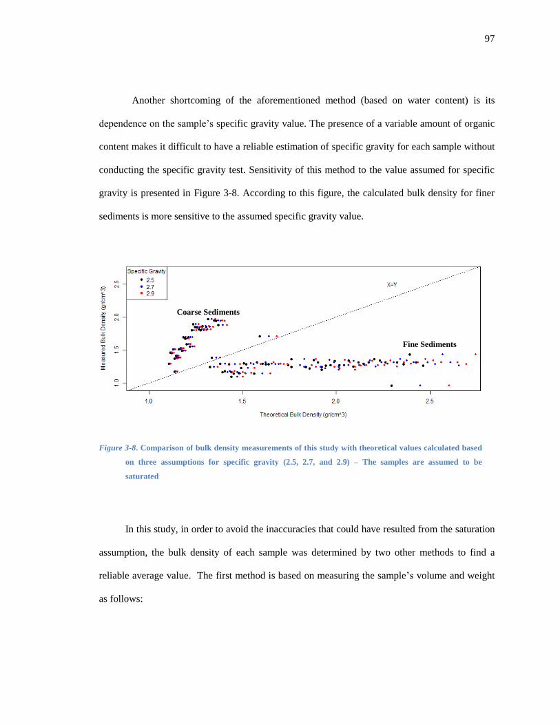
97

Another shortcoming of the aforementioned method (based on water content) is its

dependence on the sample’s specific gravity value. The presence of a variable amount of organic

content makes it difficult to have a reliable estimation of specific gravity for each sample without

conducting the specific gravity test. Sensitivity of this method to the value assumed for specific

gravity is presented in Figure 3-8. According to this figure, the calculated bulk density for finer

sediments is more sensitive to the assumed specific gravity value.

Figure 3-8. Comparison of bulk density measurements of this study with theoretical values calculated based

on three assumptions for specific gravity (2.5, 2.7, and 2.9) – The samples are assumed to be

saturated

In this study, in order to avoid the inaccuracies that could have resulted from the saturation

assumption, the bulk density of each sample was determined by two other methods to find a

reliable average value. The first method is based on measuring the sample’s volume and weight

as follows:

Fine Sediments

Coarse Sediments

98

volume of the sample

The second method calculates the bulk density based on the difference between the submerged

and non-submerged weights of the sample as presented here:

(

)

(

)

(

)

The results of the bulk density measurements in this study are presented in Figure 4-4.

Figure 3-9 compares the bulk density measurements of this study with theoretical values

calculated based on specific gravity measurements with the assumption that the samples are

saturated. According to this figure, the theoretical method significantly underestimates the bulk

density of fine sediments and overestimates the bulk density of coarse sediments.

99

Figure 3-9. Comparison of bulk density measurements of this study with

theoretical values calculated based on the specific gravity and

water content measurements made in this study – The samples

are assumed to be saturated

3.4.2. Water Content

ASTM D-2216 was the test procedure used for the determination of the water content in

this study. The samples obtained for water content tests were taken from each of the rings and

dried for 24 hours at a temperature of The same water content value was used for both

samples if two erosion samples were obtained from one ring.

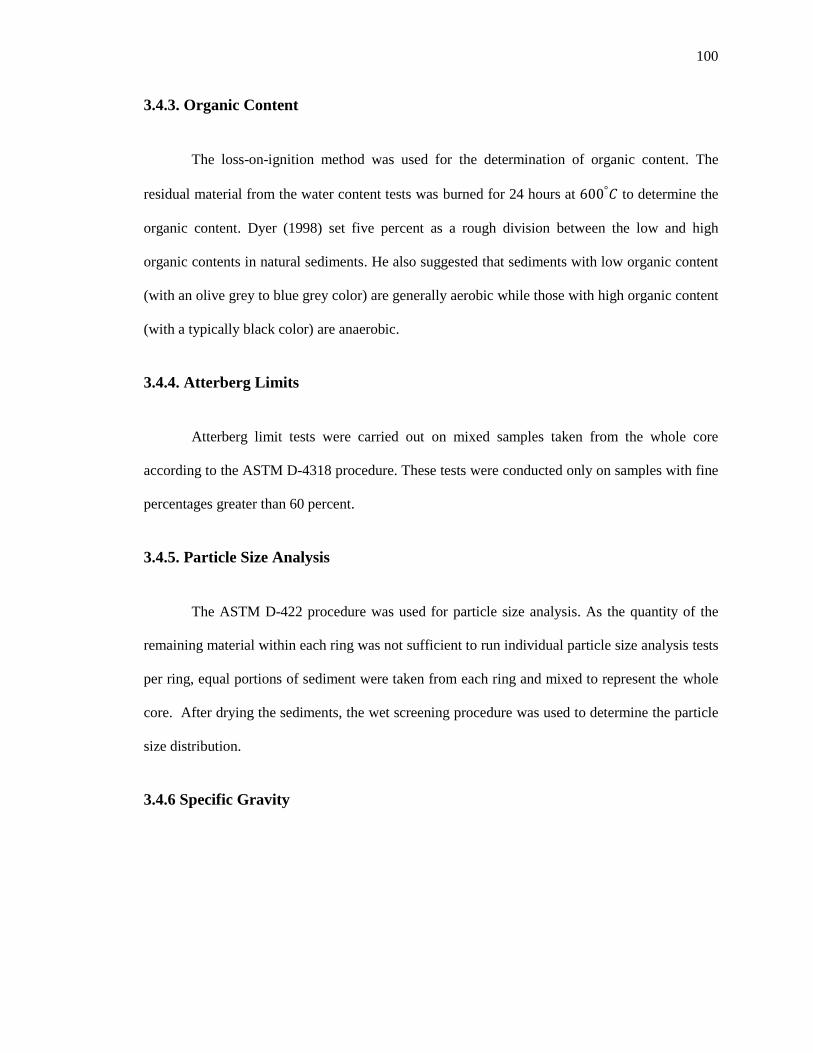
100

3.4.3. Organic Content

The loss-on-ignition method was used for the determination of organic content. The

residual material from the water content tests was burned for 24 hours at to determine the

organic content. Dyer (1998) set five percent as a rough division between the low and high

organic contents in natural sediments. He also suggested that sediments with low organic content

(with an olive grey to blue grey color) are generally aerobic while those with high organic content

(with a typically black color) are anaerobic.

3.4.4. Atterberg Limits

Atterberg limit tests were carried out on mixed samples taken from the whole core

according to the ASTM D-4318 procedure. These tests were conducted only on samples with fine

percentages greater than 60 percent.

3.4.5. Particle Size Analysis

The ASTM D-422 procedure was used for particle size analysis. As the quantity of the

remaining material within each ring was not sufficient to run individual particle size analysis tests

per ring, equal portions of sediment were taken from each ring and mixed to represent the whole

core. After drying the sediments, the wet screening procedure was used to determine the particle

size distribution.

3.4.6 Specific Gravity

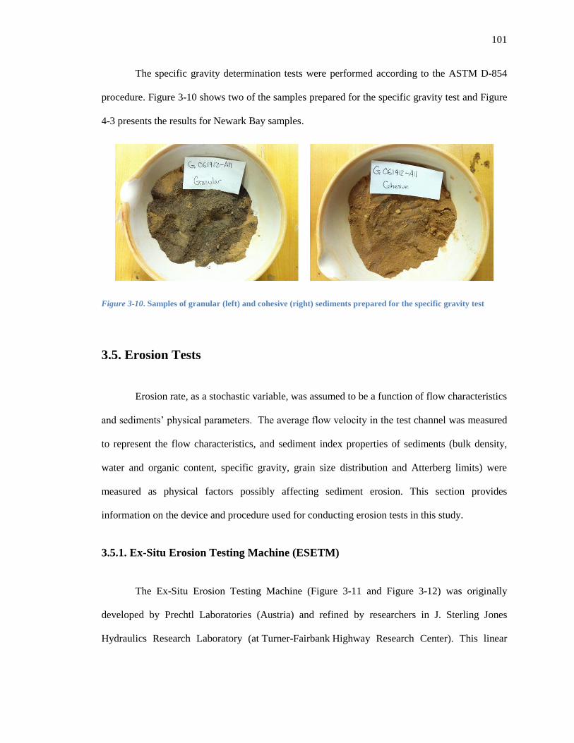
101

The specific gravity determination tests were performed according to the ASTM D-854

procedure. Figure 3-10 shows two of the samples prepared for the specific gravity test and Figure

4-3 presents the results for Newark Bay samples.

Figure 3-10. Samples of granular (left) and cohesive (right) sediments prepared for the specific gravity test

3.5. Erosion Tests

Erosion rate, as a stochastic variable, was assumed to be a function of flow characteristics

and sediments’ physical parameters. The average flow velocity in the test channel was measured

to represent the flow characteristics, and sediment index properties of sediments (bulk density,

water and organic content, specific gravity, grain size distribution and Atterberg limits) were

measured as physical factors possibly affecting sediment erosion. This section provides

information on the device and procedure used for conducting erosion tests in this study.

3.5.1. Ex-Situ Erosion Testing Machine (ESETM)

The Ex-Situ Erosion Testing Machine (Figure 3-11 and Figure 3-12) was originally

developed by Prechtl Laboratories (Austria) and refined by researchers in J. Sterling Jones

Hydraulics Research Laboratory (at Turner-Fairbank Highway Research Center). This linear

102

flume was innovatively designed to apply state-of-the-art technology to directly measure shear

and weight forces exerted on a sample of sediment in real time as well as to enhance the flow

velocity profile in erosion tests. Compared to most other flumes and devices used for sediment

erosion studies, ESETM was considered a major innovation that could help push the boundaries

in experimental erosion studies.

As indicated in Figure 3-13, the dimensions of the test channel are 110x800x21

mm the sediment probe has an internal diameter of 61 mm. The sample probe’s elevation can

be set by an internal elevator that has a full 30 mm range of vertical movement (Figure 3-14). The

force sensor can measure shear stresses of up to 100 Pa. Vertical forces in the range of 0-1N can

also be measured by the weight sensor, which is shown in (Figure 3-14).

Figure 3-11. Side view of ESETM

Belt

Test Channel

Sample Probe

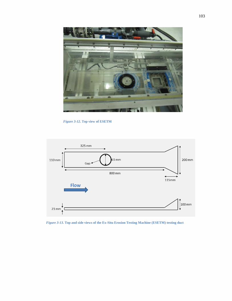
103

Figure 3-12. Top view of ESETM

Figure 3-13. Top and side views of the Ex-Situ Erosion Testing Machine (ESETM) testing duct

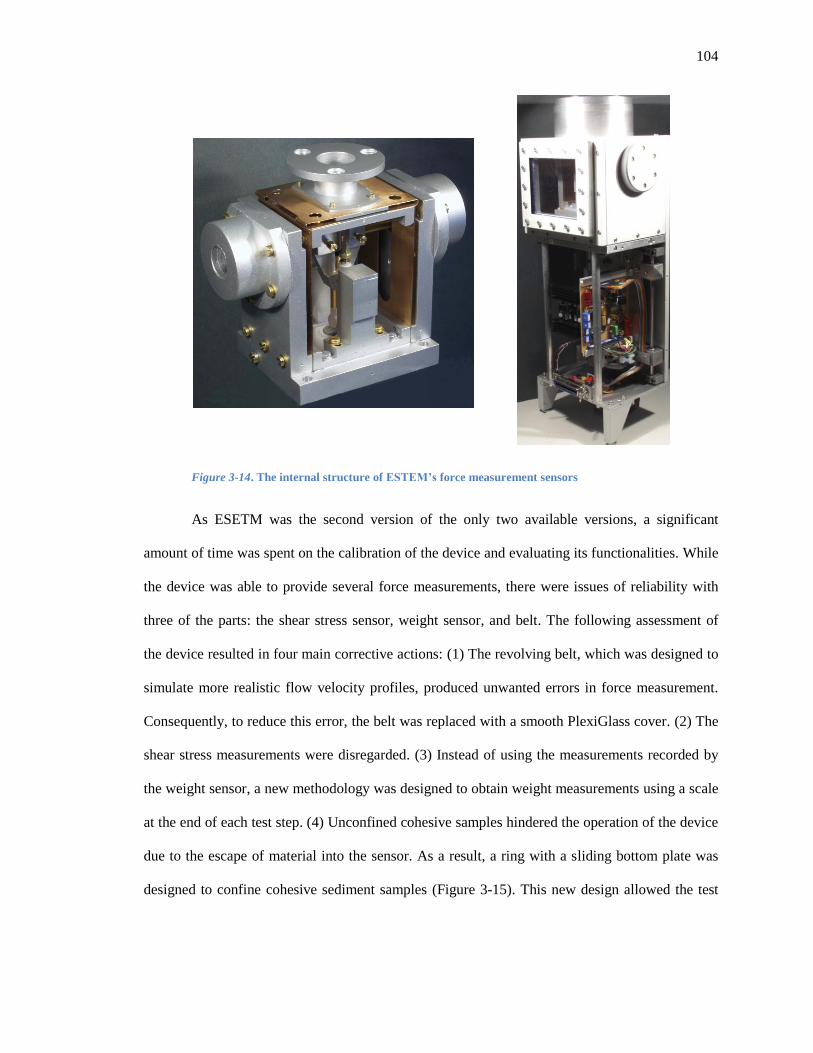
104

Figure 3-14. The internal structure of ESTEM’s force measurement sensors

As ESETM was the second version of the only two available versions, a significant

amount of time was spent on the calibration of the device and evaluating its functionalities. While

the device was able to provide several force measurements, there were issues of reliability with

three of the parts: the shear stress sensor, weight sensor, and belt. The following assessment of

the device resulted in four main corrective actions: (1) The revolving belt, which was designed to

simulate more realistic flow velocity profiles, produced unwanted errors in force measurement.

Consequently, to reduce this error, the belt was replaced with a smooth PlexiGlass cover. (2) The

shear stress measurements were disregarded. (3) Instead of using the measurements recorded by

the weight sensor, a new methodology was designed to obtain weight measurements using a scale

at the end of each test step. (4) Unconfined cohesive samples hindered the operation of the device

due to the escape of material into the sensor. As a result, a ring with a sliding bottom plate was

designed to confine cohesive sediment samples (Figure 3-15). This new design allowed the test

105

instructor to maintain the sediment surface level with the bed as much as possible. A brief

explanation of the methodology used for the device assessment in addition to some major

findings are presented in sections 3.5.1.1-3.5.1.3.

Figure 3-15. The ring and sliding bottom plate designed to

confine the sediment sample

3.5.1.1. Weight sensor assessment

Two tests were conducted to evaluate the accuracy and reliability of weight sensor

measurements. In the first test, a standard ten-gram weight was placed on the plate attached to the

weight sensor 24 times at predetermined spots as displayed in Figure 3-16. The entire procedure

was repeated three times with the plate set at different elevations. The results presented in Figure

3-17 show a large spatial variance in the accuracy of the measured weight. The measured values

ranged between 5 and 17 grams in this test and between 75 and 120 grams for the same test using

a 100-gram weight. This could be explained by the torque created due to non-uniform loading on

the plate that caused a swing in the central rod and the magnet attached to it. In conclusion, the

high variation in weight measurements negatively impacts the ability to estimate the weight of

sediments being eroded as samples do not erode uniformly during erosion tests.

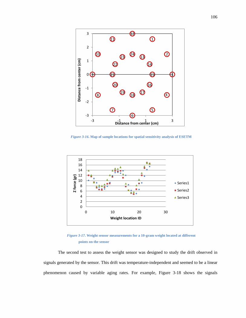
106

Figure 3-16. Map of sample locations for spatial sensitivity analysis of ESETM

Figure 3-17. Weight sensor measurements for a 10-gram weight located at different

points on the sensor

The second test to assess the weight sensor was designed to study the drift observed in

signals generated by the sensor. This drift was temperature-independent and seemed to be a linear

phenomenon caused by variable aging rates. For example, Figure 3-18 shows the signals

12

1

2

3

4

5

6

7

8

9

10

11

24 13

14

15

16

17 18

19

20

21

22

23

-3

-2

-1

0

1

2

3

-3 -1 1 3

Dis

tan

ce f

rom

ce

nte

r (c

m)

Distance from center (cm)

0

2

4

6

8

10

12

14

16

18

0 10 20 30

Z fo

rce

(gr

)

Weight location ID

Series1

Series2

Series3

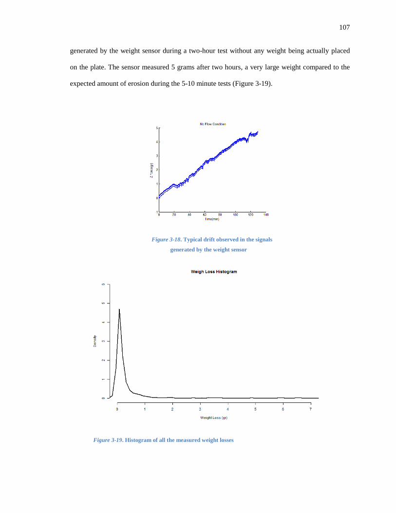
107

generated by the weight sensor during a two-hour test without any weight being actually placed

on the plate. The sensor measured 5 grams after two hours, a very large weight compared to the

expected amount of erosion during the 5-10 minute tests (Figure 3-19).

Figure 3-18. Typical drift observed in the signals

generated by the weight sensor

Figure 3-19. Histogram of all the measured weight losses

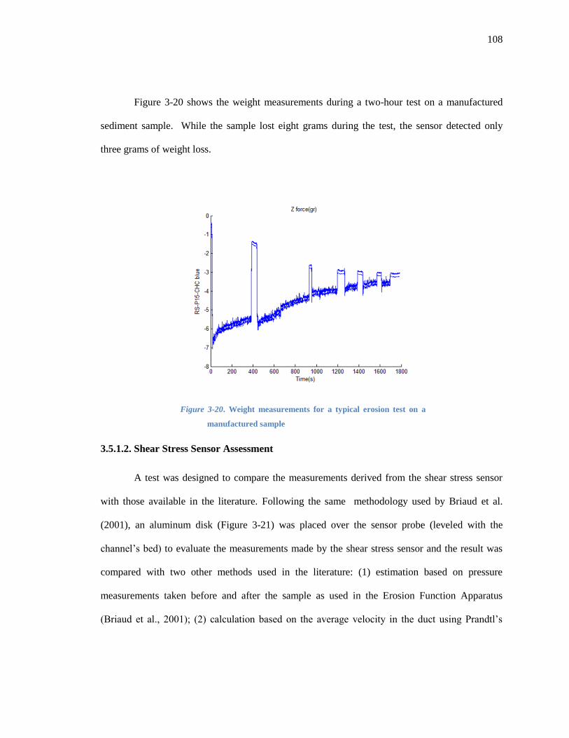
108

Figure 3-20 shows the weight measurements during a two-hour test on a manufactured

sediment sample. While the sample lost eight grams during the test, the sensor detected only

three grams of weight loss.

Figure 3-20. Weight measurements for a typical erosion test on a

manufactured sample

3.5.1.2. Shear Stress Sensor Assessment

A test was designed to compare the measurements derived from the shear stress sensor

with those available in the literature. Following the same methodology used by Briaud et al.

(2001), an aluminum disk (Figure 3-21) was placed over the sensor probe (leveled with the

channel’s bed) to evaluate the measurements made by the shear stress sensor and the result was

compared with two other methods used in the literature: (1) estimation based on pressure

measurements taken before and after the sample as used in the Erosion Function Apparatus

(Briaud et al., 2001); (2) calculation based on the average velocity in the duct using Prandtl’s

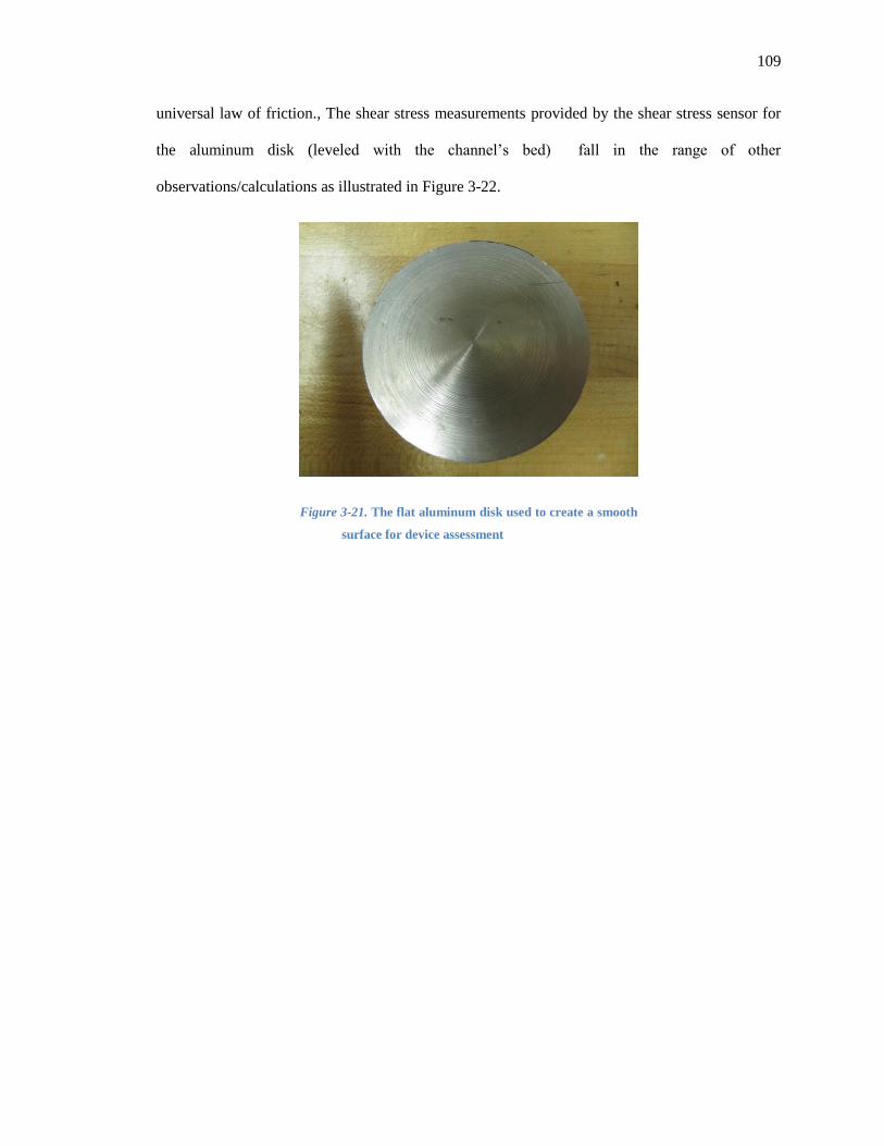
109

universal law of friction., The shear stress measurements provided by the shear stress sensor for

the aluminum disk (leveled with the channel’s bed) fall in the range of other

observations/calculations as illustrated in Figure 3-22.

Figure 3-21. The flat aluminum disk used to create a smooth

surface for device assessment

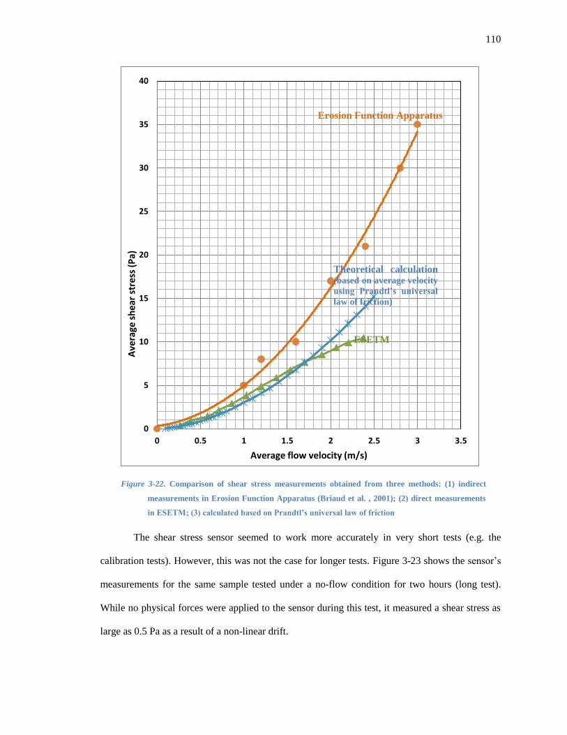
110

Figure 3-22. Comparison of shear stress measurements obtained from three methods: (1) indirect

measurements in Erosion Function Apparatus (Briaud et al. , 2001); (2) direct measurements

in ESETM; (3) calculated based on Prandtl’s universal law of friction

The shear stress sensor seemed to work more accurately in very short tests (e.g. the

calibration tests). However, this was not the case for longer tests. Figure 3-23 shows the sensor’s

measurements for the same sample tested under a no-flow condition for two hours (long test).

While no physical forces were applied to the sensor during this test, it measured a shear stress as

large as 0.5 Pa as a result of a non-linear drift.

0

5

10

15

20

25

30

35

40

0 0.5 1 1.5 2 2.5 3 3.5

Ave

rage

sh

ear

stre

ss (

Pa)

Average flow velocity (m/s)

Erosion Function Apparatus

Theoretical calculation (based on average velocity

using Prandtl’s universal

law of friction)

ESETM

111

Figure 3-23. A typical drift observed in the signals

generated by the shear stress sensor

Another anomaly observed in the shear stress data was the presence of negative shear

stress measurements, (Figure 3-24) which suggested the presence of a force in the direction

opposite to the flow. Further investigation revealed that uneven erosion (more erosion occurring

at the edges of unconfined manufactured samples) might let the flow face into the aperture ring

and cause this negative force as shown in Figure 3-25.

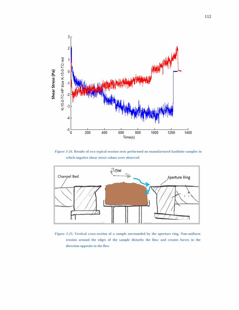
112

Figure 3-24. Results of two typical erosion tests performed on manufactured kaolinite samples in

which negative shear stress values were observed

Figure 3-25. Vertical cross-section of a sample surrounded by the aperture ring. Non-uniform

erosion around the edges of the sample disturbs the flow and creates forces in the

direction opposite to the flow

Shea

r St

ress

(P

a)

113

One other point of concern regarding the accuracy of shear stress measurements is the

shear forces caused by the form drag exerted on the walls of the sample when it is mildly

extended into the flow as shown in Figure 3-26.

Figure 3-26. Top view and vertical cross-section of the

sample probe surrounded by the aperture ring

To further study the effect of sample protrusion on shear stress measurements, a series of

tests were conducted on the aluminum disk, the results of which are provided in Figure 3-27. In

these tests, a rigid Plexiglas strip tool was used to level the disk with respect to the bottom of the

channel very carefully. The elevator was then used to extrude the disk by different amounts to

measure shear stress values for different flow velocities. As shown in Figure 3-28, protrusions

smaller than 1 mm can create high variations in the shear stress values. This high variation occurs

not only because of the sensor error but also because the shear stress sensor is measuring skin

friction and form drag simultaneously.

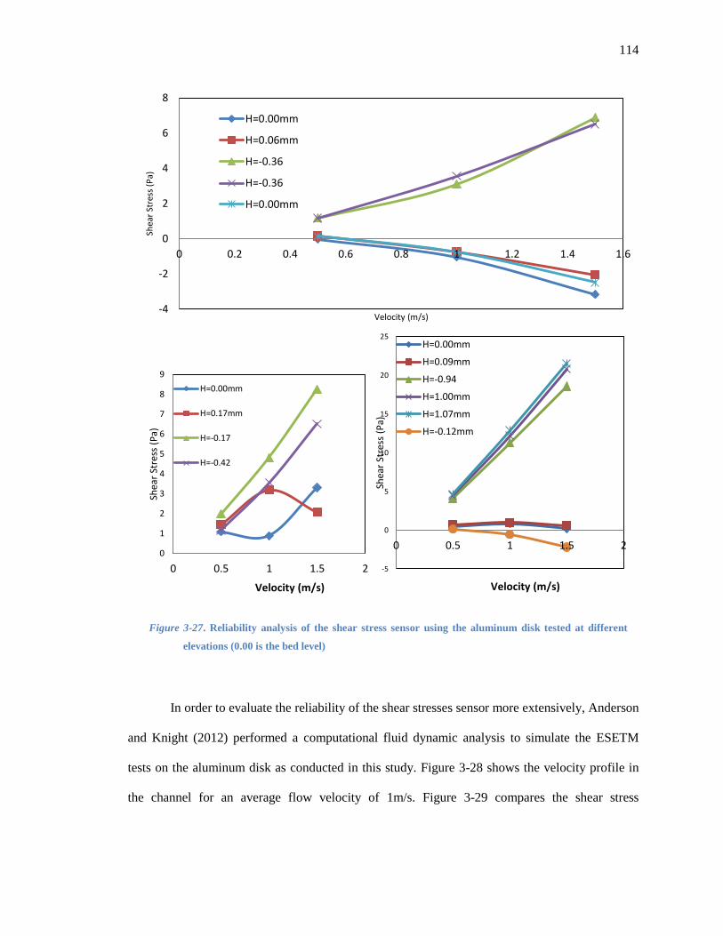
114

Figure 3-27. Reliability analysis of the shear stress sensor using the aluminum disk tested at different

elevations (0.00 is the bed level)

In order to evaluate the reliability of the shear stresses sensor more extensively, Anderson

and Knight (2012) performed a computational fluid dynamic analysis to simulate the ESETM

tests on the aluminum disk as conducted in this study. Figure 3-28 shows the velocity profile in

the channel for an average flow velocity of 1m/s. Figure 3-29 compares the shear stress

-4

-2

0

2

4

6

8

0 0.2 0.4 0.6 0.8 1 1.2 1.4 1.6

Shea

r St

ress

(P

a)

Velocity (m/s)

H=0.00mm

H=0.06mm

H=-0.36

H=-0.36

H=0.00mm

0

1

2

3

4

5

6

7

8

9

0 0.5 1 1.5 2

Shea

r St

ress

(P

a)

Velocity (m/s)

H=0.00mm

H=0.17mm

H=-0.17

H=-0.42

-5

0

5

10

15

20

25

0 0.5 1 1.5 2

Shea

r St

ress

(P

a)

Velocity (m/s)

H=0.00mm

H=0.09mm

H=-0.94

H=1.00mm

H=1.07mm

H=-0.12mm

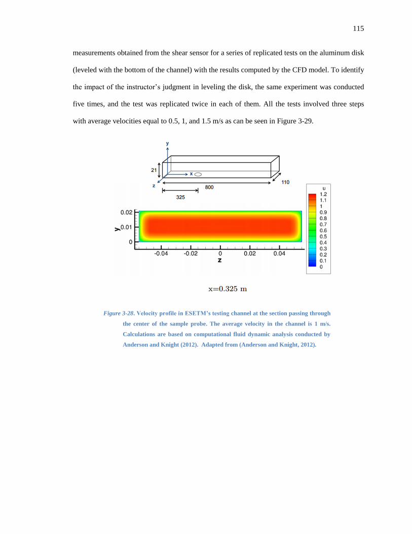
115

measurements obtained from the shear sensor for a series of replicated tests on the aluminum disk

(leveled with the bottom of the channel) with the results computed by the CFD model. To identify

the impact of the instructor’s judgment in leveling the disk, the same experiment was conducted

five times, and the test was replicated twice in each of them. All the tests involved three steps

with average velocities equal to 0.5, 1, and 1.5 m/s as can be seen in Figure 3-29.

Figure 3-28. Velocity profile in ESETM’s testing channel at the section passing through

the center of the sample probe. The average velocity in the channel is 1 m/s.

Calculations are based on computational fluid dynamic analysis conducted by

Anderson and Knight (2012). Adapted from (Anderson and Knight, 2012).

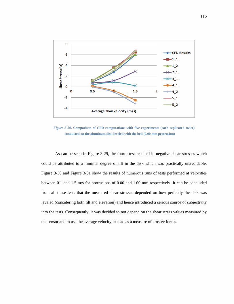
116

Figure 3-29. Comparison of CFD computations with five experiments (each replicated twice)

conducted on the aluminum disk leveled with the bed (0.00 mm protrusion)

As can be seen in Figure 3-29, the fourth test resulted in negative shear stresses which

could be attributed to a minimal degree of tilt in the disk which was practically unavoidable.

Figure 3-30 and Figure 3-31 show the results of numerous runs of tests performed at velocities

between 0.1 and 1.5 m/s for protrusions of 0.00 and 1.00 mm respectively. It can be concluded

from all these tests that the measured shear stresses depended on how perfectly the disk was

leveled (considering both tilt and elevation) and hence introduced a serious source of subjectivity

into the tests. Consequently, it was decided to not depend on the shear stress values measured by

the sensor and to use the average velocity instead as a measure of erosive forces.

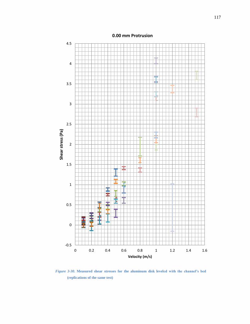
117

Figure 3-30. Measured shear stresses for the aluminum disk leveled with the channel’s bed

(replications of the same test)

-0.5

0

0.5

1

1.5

2

2.5

3

3.5

4

4.5

0 0.2 0.4 0.6 0.8 1 1.2 1.4 1.6

She

ar s

tre

ss (

Pa)

Velocity (m/s)

0.00 mm Protrusion

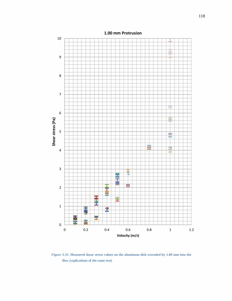
118

Figure 3-31. Measured shear stress values on the aluminum disk extruded by 1.00 mm into the

flow (replications of the same test)

0

1

2

3

4

5

6

7

8

9

10

0 0.2 0.4 0.6 0.8 1 1.2

She

ar s

tre

ss (

Pa)

Velocity (m/s)

1.00 mm Protrusion

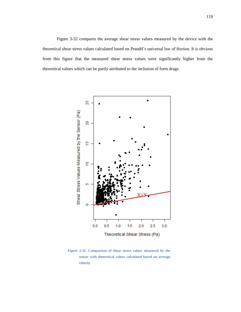
119

Figure 3-32 compares the average shear stress values measured by the device with the

theoretical shear stress values calculated based on Prandtl’s universal law of friction. It is obvious

from this figure that the measured shear stress values were significantly higher from the

theoretical values which can be partly attributed to the inclusion of form drags.

Figure 3-32. Comparison of shear stress values measured by the

sensor with theoretical values calculated based on average

velocity

120

3.5.1.3. Belt Assessment

The revolving belt (Figure 3-11) was originally designed to innovatively modify the

velocity profile in the testing channel (Figure 3-28) to make it more similar to natural flows

(Figure 3-33).

Figure 3-34 shows the velocity profile measured in the channel through 2-dimensional

particle image velocimetry (PIV).

Figure 3-33. The Couette flow created by the belt can be combined with the pipe flow profile to create a more

realistic velocity profile

Belt

H V(h) V +

Couette flow Pipe flow

Boundary

Log law layer =

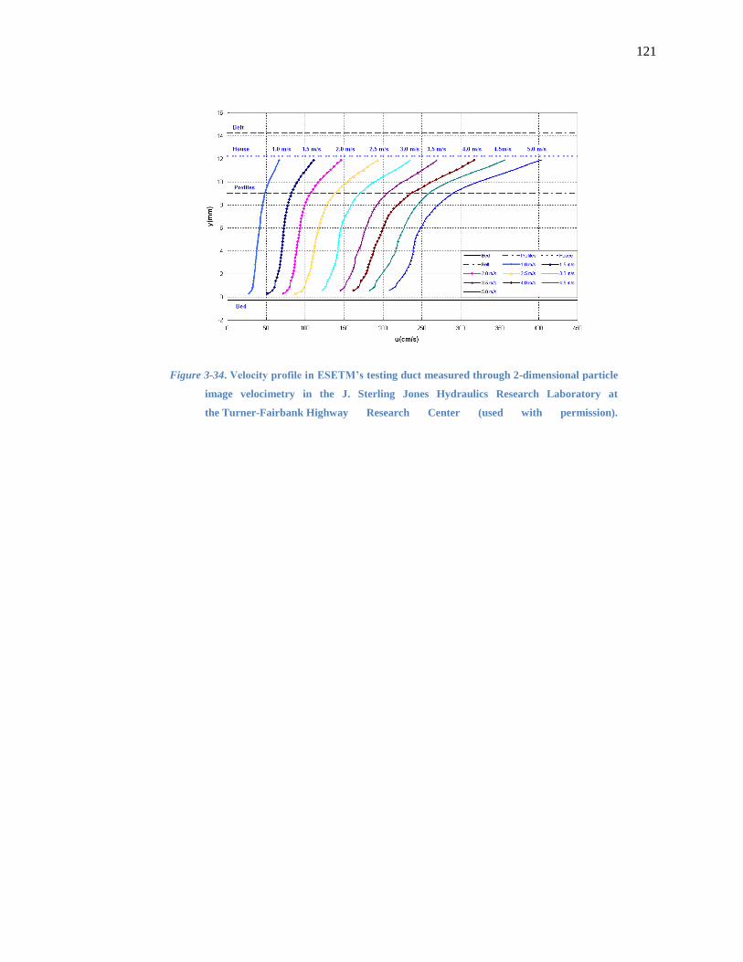
121

Figure 3-34. Velocity profile in ESETM’s testing duct measured through 2-dimensional particle

image velocimetry in the J. Sterling Jones Hydraulics Research Laboratory at

the Turner-Fairbank Highway Research Center (used with permission).

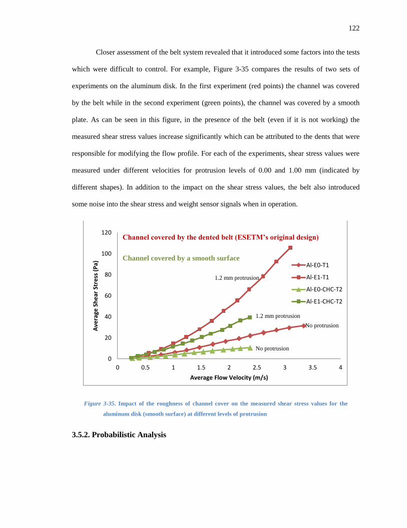
122

Closer assessment of the belt system revealed that it introduced some factors into the tests

which were difficult to control. For example, Figure 3-35 compares the results of two sets of

experiments on the aluminum disk. In the first experiment (red points) the channel was covered

by the belt while in the second experiment (green points), the channel was covered by a smooth

plate. As can be seen in this figure, in the presence of the belt (even if it is not working) the

measured shear stress values increase significantly which can be attributed to the dents that were

responsible for modifying the flow profile. For each of the experiments, shear stress values were

measured under different velocities for protrusion levels of 0.00 and 1.00 mm (indicated by

different shapes). In addition to the impact on the shear stress values, the belt also introduced

some noise into the shear stress and weight sensor signals when in operation.

Figure 3-35. Impact of the roughness of channel cover on the measured shear stress values for the

aluminum disk (smooth surface) at different levels of protrusion

3.5.2. Probabilistic Analysis

0

20

40

60

80

100

120

0 0.5 1 1.5 2 2.5 3 3.5 4

Ave

rage

Sh

ear

Str

ess

(P

a)

Average Flow Velocity (m/s)

Al-E0-T1

Al-E1-T1

Al-E0-CHC-T2

Al-E1-CHC-T2

Channel covered by the dented belt (ESETM’s original design)

Channel covered by a smooth surface

1.2 mm protrusion

1.2 mm protrusion

No protrusion

No protrusion

123

3.5.2.1. Introduction

One of the main conclusions of the literature review for this study was that the results of

erosion rate tests are highly dependent on the design of the experiment (sequence or arrangement3

of the shear stress levels applied to the sediment, and duration4 of each step) as well as the

interpretation method.

Aberle et al. (2004) categorized the various interpretation approaches for the evaluation of

erosion rates in the literature as: (1) the initial peak erosion rate after application of a new bed

shear stress, (2) the rate of erosion after some initial response has passed, (3) the average erosion

rate over the entire test interval, and (4) the inclusion of a time factor in the erosion rate

prediction equations. These sources of uncertainty and their consequences have made it very

difficult to compare different studies.

In order to mitigate the above concerns, it was decided to define this practical problem

and explore its consequences prior to designing the erosion experiments for the current study.

Therefore, a methodology was developed (section 3.5.2.2) for analytical interpretation of erosion

test results. This method, which is based on the probabilistic modeling of erosion, applies an

optimization technique to solve for the model’s parameters probabilistically. The algorithm

developed for this method is presented in section 3.5.2.3 and is followed by the results and

conclusions in sections 2.5.2.3 and 2.5.2.4 respectively.

3 For example, in Figure 2-20, if the third step of the test has a shear stress level that is very close to the

stress level in the second step (or even equal to it), the observations in the third step will follow the pattern

of points in the second step, resulting in a lower average erosion rate for the same shear stress level.

4 For example, in Figure 2-20, If the third step of the test continues for longer than 20 minutes, a smaller

peak value will be observed for the erosion rate at the beginning of the fourth step because less material

will be available to erode at this stage.

124

3.5.2.2. Analysis Framework

In this section, an analysis framework has been developed and used to reanalyze the

datasets published by different researchers. This approach is proved to be capable of generating

results that are comparable to empirical data from different studies.

Van Prooijen and Winterwerp (2010) classified a bed of sediment according to critical

shear stress to take the time dependency of erosion rate into account. Similarly in this study, the

portion of cohesive sediment eroded during each erosion test (the top layer of sediment with

thickness h) was assumed to consist of an array of n different material clusters (Figure 3-36).

However, particles or flocs in each cluster are taken to have similar erosion behavior. An average

probability of erosion is assigned to each of these clusters for all stress (or velocity) levels to

which the sediment is exposed for a specific duration.

Figure 3-36. Surface sediment partitioned into clusters with similar erosion behavior

The probability matrix is defined as

[

]

125

where is the probability of a particle in cluster being eroded during the step of the test. If

any two test steps and b in this matrix have similar shear stress or velocity levels, then rows

and b in this matrix will be equivalent.

The vector consists of velocity or shear stress levels at the step of the test such that

[

]

For example, if the sediment is eroded under shear stress (or velocity) levels (1, 2, 3) for

(20,10,30) minutes successively, and the probabilities in matrix are set for a 5-minute long

exposure, then [ ]. The length of matrix is assumed to be .

The ratio matrix consists of entities equal to the proportion of particles in cluster at

the beginning of step of the test. Hence, the sum of the entities in each row is equal to 1. The

first row of this matrix includes the initial weight proportion of particles in each of the available n

clusters and should be provided as an input to the code. The values in the remaining rows are

unknown and are calculated within the suggested framework.

[

]

Available material vector, , is a vector of length with entities equal to the

material available for erosion at the beginning of the step of the test. represents the total

material eroded during the whole test and should be provided as an input to the program.

[

]

Cluster erosion matrix, , consists of entities equal to the material eroded from

cluster during step All the first-row entities are equal to zero.

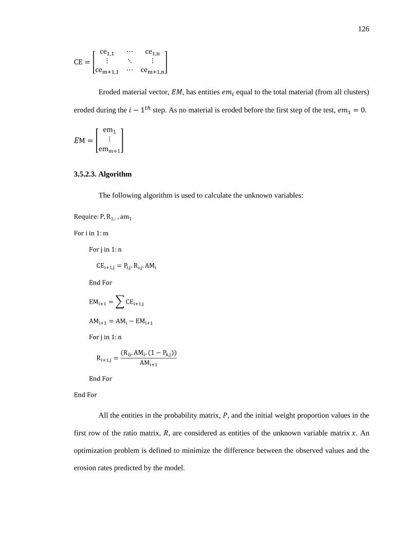
126

[

]

Eroded material vector, has entities equal to the total material (from all clusters)

eroded during the step. As no material is eroded before the first step of the test,

[

]

3.5.2.3. Algorithm

The following algorithm is used to calculate the unknown variables:

∑

All the entities in the probability matrix, and the initial weight proportion values in the

first row of the ratio matrix, are considered as entities of the unknown variable matrix . An

optimization problem is defined to minimize the difference between the observed values and the

erosion rates predicted by the model.

127

(

)

The minimization is subjected to the following constraints:

1. All the variables in the vector should be in the [ ] range as they are either probability or

weight ratio values.

2. [ ] [ ]

3. If the shear stress level in step is larger than in step then [ ]

4. ∑

{

3.5.2.4. Results

The proposed methodology was applied to data published by Zerik, Krishnappan,

Germaine, and Madsen (1998), Parchure and Mehta (1985), and Sanford and Maa (2001). Figure

3-37 depicts the results obtained by the proposed probabilistic framework compared to the data

observed by Zerik et al., (1998). The set of parameters used for simulation 1 are presented in

Table 3-1. Simulation 2 uses the same parameters but applies a different arrangement of shear

stress levels starting at the highest level. It is interesting to note that the weight of material eroded

in the first step in simulation 2 is greater than the weight of the total material eroded in all nine

steps with the same shear stress level (level 4) in simulation 1. This can be attributed to the fact

that in the first simulation, the original weight proportion of clusters with different erosion

resistances is altered through 16 testing steps at shear stress levels 1 to 3 before reaching shear

stress level 4. This example proves that simple parameterization of erosion behavior (regardless

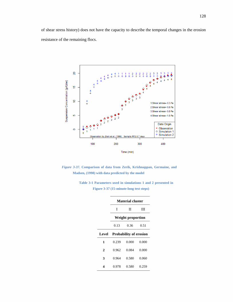
128

of shear stress history) does not have the capacity to describe the temporal changes in the erosion

resistance of the remaining flocs.

Figure 3-37. Comparison of data from Zerik, Krishnappan, Germaine, and

Madsen, (1998) with data predicted by the model

Table 3-1 Parameters used in simulations 1 and 2 presented in

Figure 3-37 (15-minute-long test steps)

Level

Material cluster

I II III

Weight proportion

0.13 0.36 0.51

Level Probability of erosion

1 0.239 0.000 0.000

2 0.962 0.084 0.000

3 0.964 0.580 0.060

4 0.978 0.580 0.259

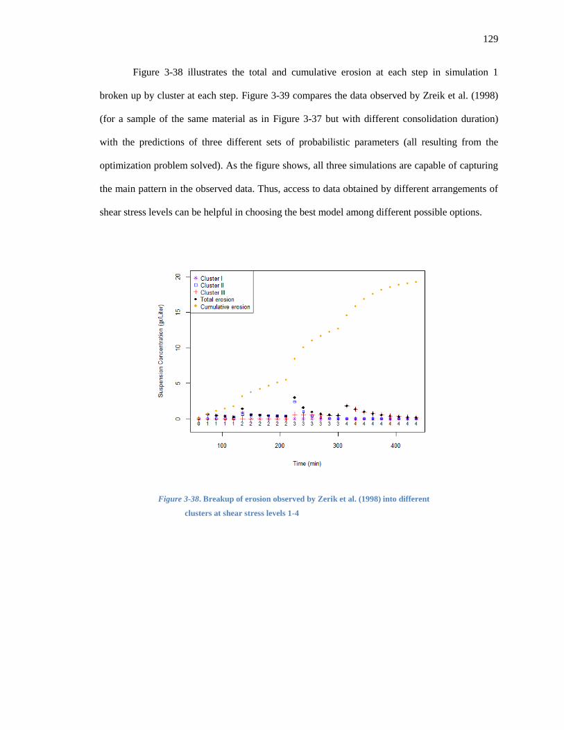
129

Figure 3-38 illustrates the total and cumulative erosion at each step in simulation 1

broken up by cluster at each step. Figure 3-39 compares the data observed by Zreik et al. (1998)

(for a sample of the same material as in Figure 3-37 but with different consolidation duration)

with the predictions of three different sets of probabilistic parameters (all resulting from the

optimization problem solved). As the figure shows, all three simulations are capable of capturing

the main pattern in the observed data. Thus, access to data obtained by different arrangements of

shear stress levels can be helpful in choosing the best model among different possible options.

Figure 3-38. Breakup of erosion observed by Zerik et al. (1998) into different

clusters at shear stress levels 1-4

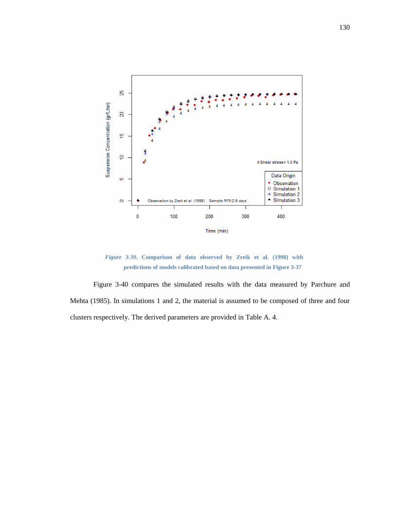
130

Figure 3-39. Comparison of data observed by Zreik et al. (1998) with

predictions of models calibrated based on data presented in Figure 3-37

Figure 3-40 compares the simulated results with the data measured by Parchure and

Mehta (1985). In simulations 1 and 2, the material is assumed to be composed of three and four

clusters respectively. The derived parameters are provided in Table A. 4.

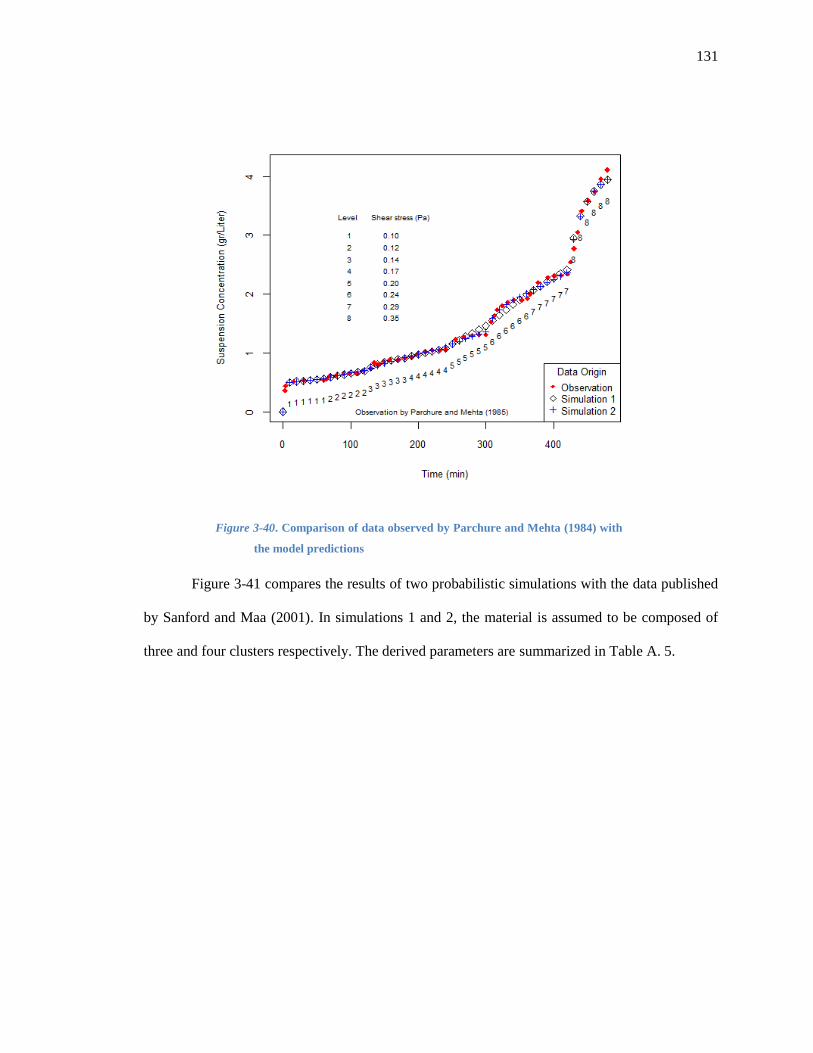
131

Figure 3-40. Comparison of data observed by Parchure and Mehta (1984) with

the model predictions

Figure 3-41 compares the results of two probabilistic simulations with the data published

by Sanford and Maa (2001). In simulations 1 and 2, the material is assumed to be composed of

three and four clusters respectively. The derived parameters are summarized in Table A. 5.

132

Figure 3-41. Comparison of data observed by Sanford and Maa (2001) with the

probabilistic model predictions

3.5.2.5. Conclusion and Discussion

1. The analysis framework developed in section 3.5.2.2 solved an inverse problem to

convert erosion rate data to information about erosion probability of different material

clusters assumed to constitute the studied sediment. This problem is ill-posed, as typical

for inverse problems and has no unique optimal solution.

2. The great advantage of this approach is that the results obtained by this methodology are

not dependent on any particular testing arrangement and can be used to make predictions

for new arrangements of flow levels to which the material is exposed.

3. This framework also offers the opportunity to compare the results obtained by different

devices by standardizing the analysis methodology.

133

4. The probabilistic analysis conducted in this section clearly indicated the significant

impact of the design of erosion experiments – specifically the length and order of

different shear stress levels applied to sediments – on experimental outcomes.

5. Ideally, it is best to run only one test on each sediment sample. However, as only one

erosion rate per sample does not reveal much about the overall behavior of sediment at

different shear stress levels, testing a sample under different shear stress levels is

inevitable. The main conclusion of this section for the purpose of this study is that if

the sample is tested for shorter periods at each shear stress level, the effect of shear stress

history on the observed erosion rates will be lower. This is because less sediment will be

eroded during each step, and hence the sediment will retain its original composition.

6. The probabilistic analysis clearly demonstrated that the validity of measurements

decrease as more tests are conducted on one sample because of the impact of shear

history. It can be concluded that for the purpose of this study, the number of shear stress

steps to which a sample is exposed to should be limited to avoid unrealistic results.

3.5.3. Erosion Testing Methodology

The erosion tests conducted in this study exposed the samples to a sequence of increasing

flow velocities, each of which were followed by a stage of no-flow for a few minutes. The tests

were designed based on the conclusions derived in section 3.5.2.5.

In order to minimize the effect of sudden flow generation at the beginning of each test step, the

pump power was programmed to increase at a low rate. The samples’ submerged weights were

measured during the no-flow intervals to determine the weight loss occurring in the preceding

stage. The operator set the elevation of each sample (to be flushed with the channel bottom) at the

beginning of each test cycle using the device’s elevation control feature. Each test step lasted for

5, 10, or 15 minutes depending on the rate and extent of the observed surface disturbance. All the

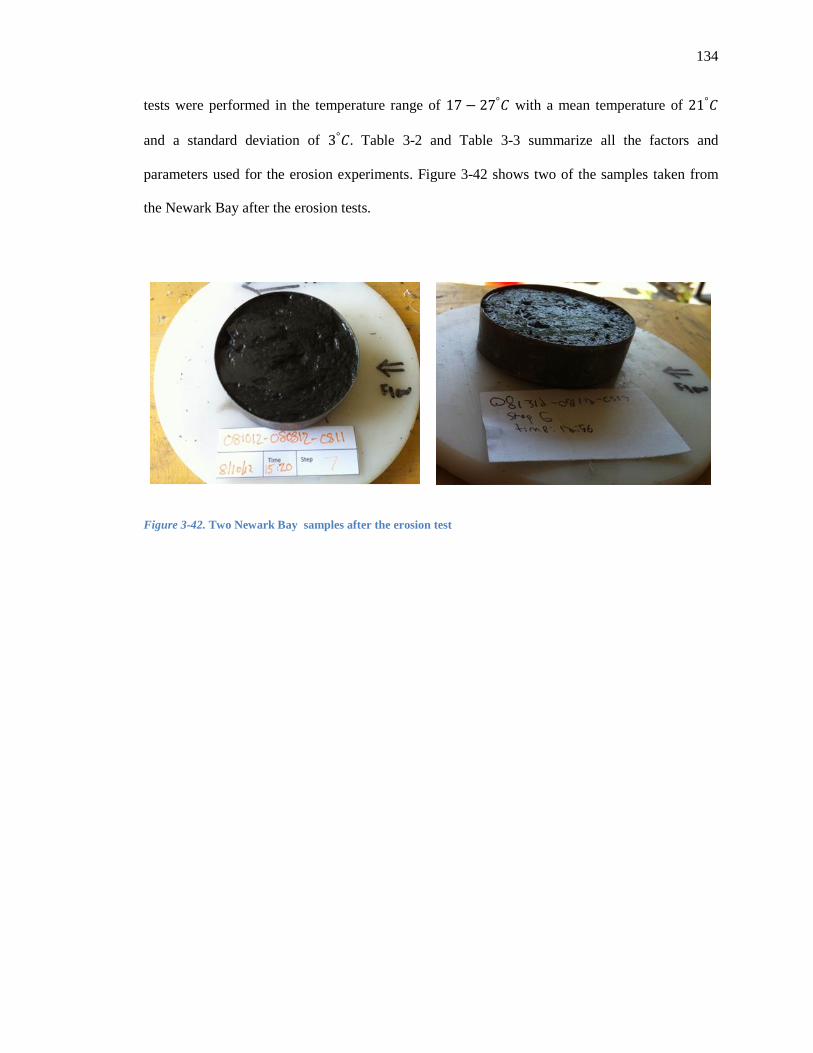
134

tests were performed in the temperature range of with a mean temperature of

and a standard deviation of Table 3-2 and Table 3-3 summarize all the factors and

parameters used for the erosion experiments. Figure 3-42 shows two of the samples taken from

the Newark Bay after the erosion tests.

Figure 3-42. Two Newark Bay samples after the erosion test

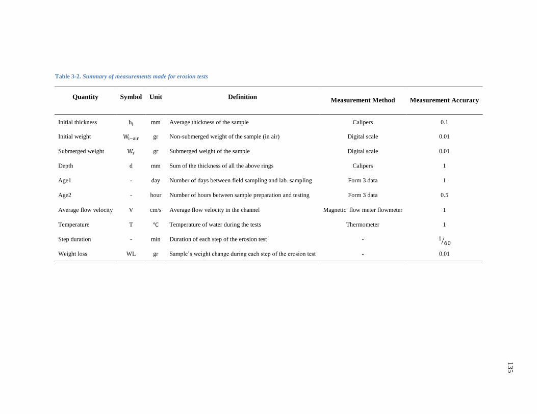
13

5

Table 3-2. Summary of measurements made for erosion tests

Quantity Symbol Unit Definition Measurement Method Measurement Accuracy

Initial thickness mm Average thickness of the sample Calipers 0.1

Initial weight gr Non-submerged weight of the sample (in air) Digital scale 0.01

Submerged weight gr Submerged weight of the sample Digital scale 0.01

Depth d mm Sum of the thickness of all the above rings Calipers 1

Age1 - day Number of days between field sampling and lab. sampling Form 3 data 1

Age2 - hour Number of hours between sample preparation and testing Form 3 data 0.5

Average flow velocity V cm/s Average flow velocity in the channel Magnetic flow meter flowmeter 1

Temperature T Temperature of water during the tests Thermometer 1

Step duration - min Duration of each step of the erosion test - ⁄

Weight loss WL gr Sample’s weight change during each step of the erosion test - 0.01

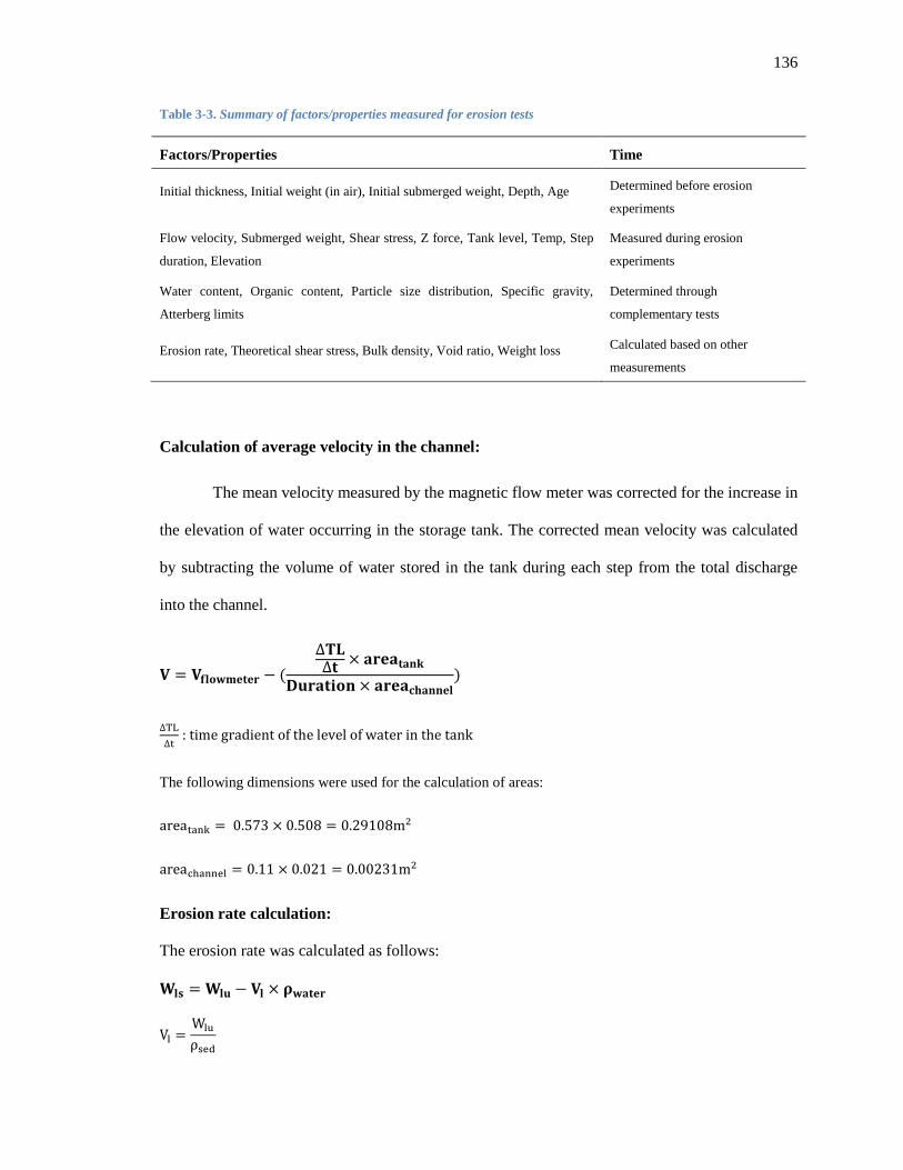
136

Table 3-3. Summary of factors/properties measured for erosion tests

Factors/Properties Time

Initial thickness, Initial weight (in air), Initial submerged weight, Depth, Age Determined before erosion

experiments

Flow velocity, Submerged weight, Shear stress, Z force, Tank level, Temp, Step

duration, Elevation

Measured during erosion

experiments

Water content, Organic content, Particle size distribution, Specific gravity,

Atterberg limits

Determined through

complementary tests

Erosion rate, Theoretical shear stress, Bulk density, Void ratio, Weight loss Calculated based on other

measurements

Calculation of average velocity in the channel:

The mean velocity measured by the magnetic flow meter was corrected for the increase in

the elevation of water occurring in the storage tank. The corrected mean velocity was calculated

by subtracting the volume of water stored in the tank during each step from the total discharge

into the channel.

: time gradient of the level of water in the tank

The following dimensions were used for the calculation of areas:

Erosion rate calculation:

The erosion rate was calculated as follows:

137

The non-submerged weight loss during each test step was used to calculate the erosion

rate for that step which is defined as the mass of sediments (including liquid and solid phases)

eroded from a surface of one square meter per hour.

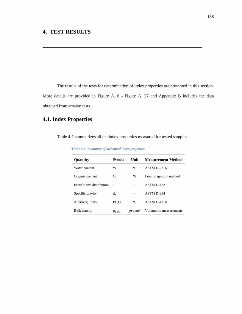
138

4. TEST RESULTS

The results of the tests for determination of index properties are presented in this section.

More details are provided in Figure A. 6 - Figure A. 27 and Appendix B includes the data

obtained from erosion tests.

4.1. Index Properties

Table 4-1 summarizes all the index properties measured for tested samples.

Table 4-1. Summary of measured index properties

Quantity Symbol Unit Measurement Method

Water content W % ASTM D-2216

Organic content O % Loss on ignition method

Particle size distribution - - ASTM D-422

Specific gravity - ASTM D-854

Atterberg limits PL,LL % ASTM D-4318

Bulk density Volumetric measurements

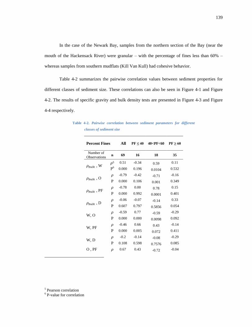
139

In the case of the Newark Bay, samples from the northern section of the Bay (near the

mouth of the Hackensack River) were granular – with the percentage of fines less than 60% –

whereas samples from southern mudflats (Kill Van Kull) had cohesive behavior.

Table 4-2 summarizes the pairwise correlation values between sediment properties for

different classes of sediment size. These correlations can also be seen in Figure 4-1 and Figure

4-2. The results of specific gravity and bulk density tests are presented in Figure 4-3 and Figure

4-4 respectively.

Table 4-2. Pairwise correlation between sediment parameters for different

classes of sediment size

Percent Fines

All PF ≤ 40 40<PF<60 PF ≥ 60

Number of

Observations n 69 16 18 35

, W 5 0.51 -0.34 0.59 0.11

P6 0.000 0.196 0.0104 0.532

, O -0.79 -0.42 -0.71 -0.16

P 0.000 0.106 0.001 0.349

, PF -0.78 0.00 0.78 0.15

P 0.000 0.992 0.0001 0.401

, D -0.06 -0.07 -0.14 0.33

P 0.607 0.797 0.5856 0.054

W, O -0.59 0.77 -0.59 -0.29

P 0.000 0.000 0.0098 0.092

W, PF -0.46 0.66 0.43 -0.14

P 0.000 0.005 0.072 0.411

W, D -0.2 -0.14 -0.08 -0.29

P 0.108 0.598 0.7576 0.085

O , PF 0.67 0.43 -0.72 -0.04

5 Pearson correlation

6 P-value for correlation

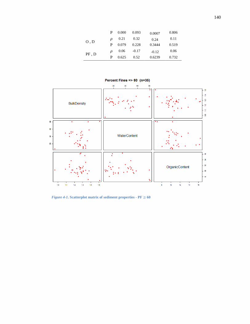
140

P 0.000 0.093 0.0007 0.806

O , D 0.21 0.32 0.24 0.11

P 0.079 0.228 0.3444 0.519

PF , D 0.06 -0.17 -0.12 0.06

P 0.625 0.52 0.6239 0.732

Figure 4-1. Scatterplot matrix of sediment properties - PF 60

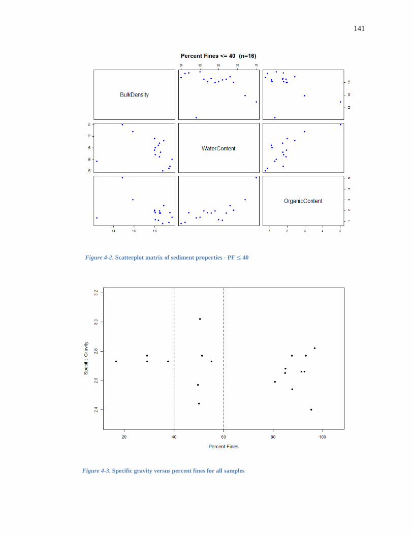
141

Figure 4-2. Scatterplot matrix of sediment properties - PF 40

Figure 4-3. Specific gravity versus percent fines for all samples

142

Figure 4-4. Bulk density versus percent fines for all samples

4.2. Erosion Tests

Figure 4-5 and Figure 4-6 show the box plots of observed erosion rates and average

velocities for different classes of sediment size, respectively. Figure 4-7 and Figure 4-8 display

the distribution of average velocities and theoretical shear stresses used in the tests. The erosion

rate measurements are plotted against theoretical shear stress values in Figure 4-9 and Figure 4-10

shows the frequency distribution of erosion rates. Table 4-3 includes correlation values between

erosion rate and sediment parameters for different classes of sediment size.

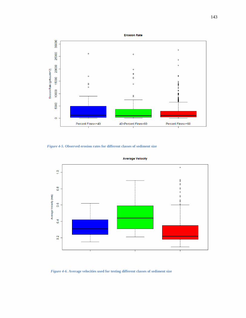
143

Figure 4-5. Observed erosion rates for different classes of sediment size

Figure 4-6. Average velocities used for testing different classes of sediment size

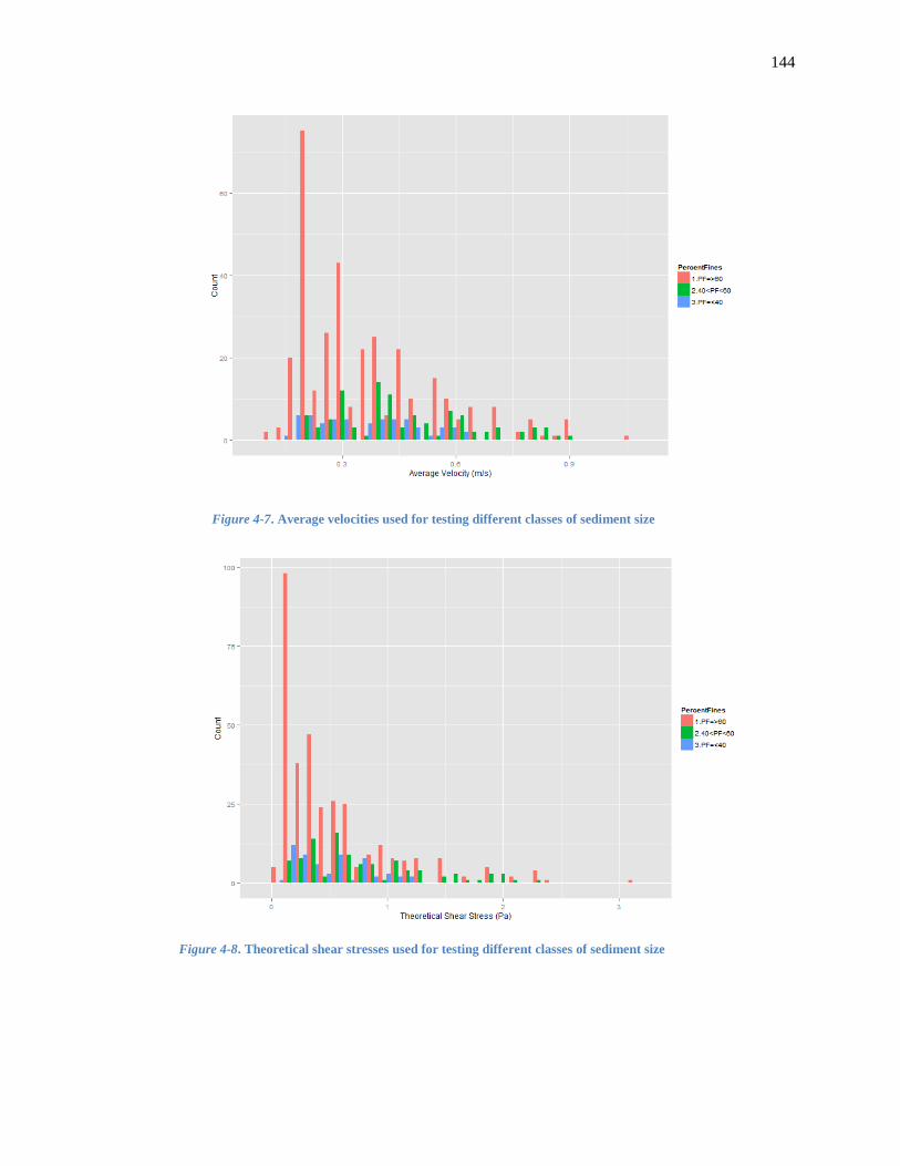
144

Figure 4-7. Average velocities used for testing different classes of sediment size

Figure 4-8. Theoretical shear stresses used for testing different classes of sediment size

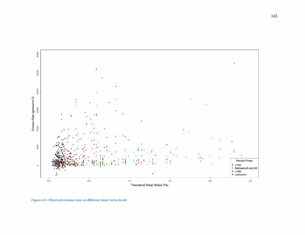
145

Figure 4-9. Observed erosion rates at different shear stress levels

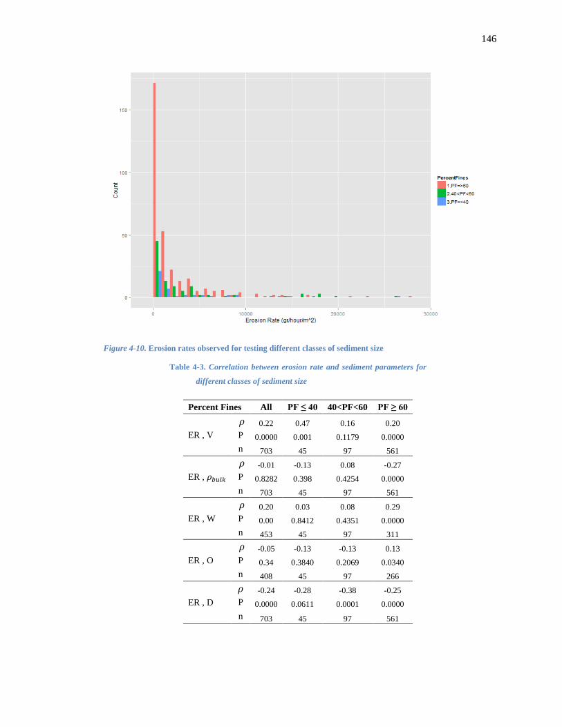
146

Figure 4-10. Erosion rates observed for testing different classes of sediment size

Table 4-3. Correlation between erosion rate and sediment parameters for

different classes of sediment size

Percent Fines All PF ≤ 40 40<PF<60 PF ≥ 60

ER , V

0.22 0.47 0.16 0.20

P 0.0000 0.001 0.1179 0.0000

n 703 45 97 561

ER ,

-0.01 -0.13 0.08 -0.27

P 0.8282 0.398 0.4254 0.0000

n 703 45 97 561

ER , W

0.20 0.03 0.08 0.29

P 0.00 0.8412 0.4351 0.0000

n 453 45 97 311

ER , O

-0.05 -0.13 -0.13 0.13

P 0.34 0.3840 0.2069 0.0340

n 408 45 97 266

ER , D

-0.24 -0.28 -0.38 -0.25

P 0.0000 0.0611 0.0001 0.0000

n 703 45 97 561

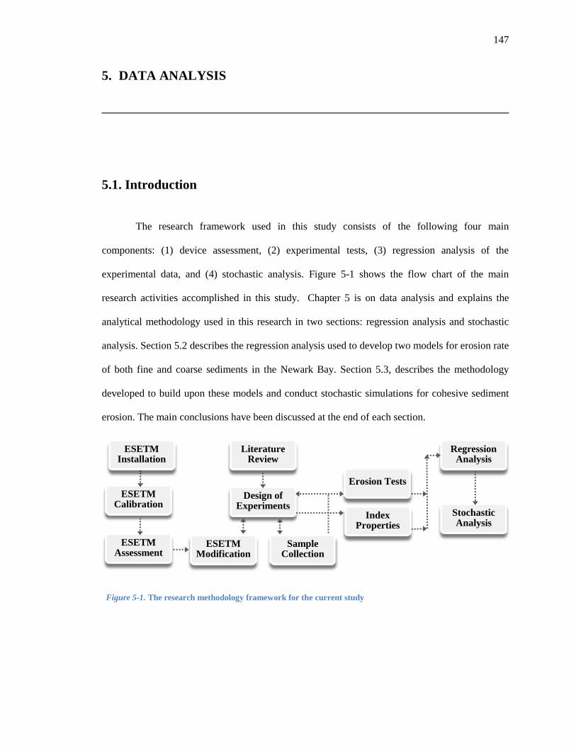
147

5. DATA ANALYSIS

5.1. Introduction

The research framework used in this study consists of the following four main

components: (1) device assessment, (2) experimental tests, (3) regression analysis of the

experimental data, and (4) stochastic analysis. Figure 5-1 shows the flow chart of the main

research activities accomplished in this study. Chapter 5 is on data analysis and explains the

analytical methodology used in this research in two sections: regression analysis and stochastic

analysis. Section 5.2 describes the regression analysis used to develop two models for erosion rate

of both fine and coarse sediments in the Newark Bay. Section 5.3, describes the methodology

developed to build upon these models and conduct stochastic simulations for cohesive sediment

erosion. The main conclusions have been discussed at the end of each section.

Figure 5-1. The research methodology framework for the current study

Regression Analysis

Stochastic Analysis

Design of Experiments

ESETM Assessment

Erosion Tests

Index Properties

ESETM Calibration

ESETM Modification

ESETM Installation

Sample Collection

Literature Review

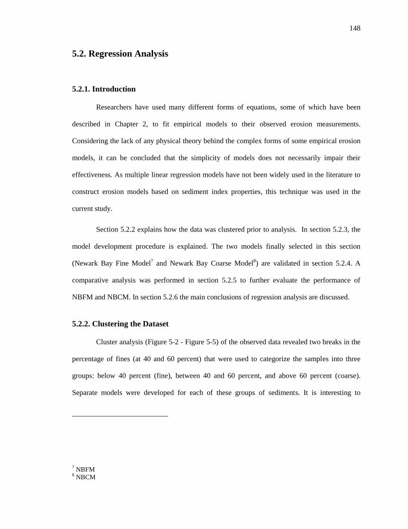
148

5.2. Regression Analysis

5.2.1. Introduction

Researchers have used many different forms of equations, some of which have been

described in Chapter 2, to fit empirical models to their observed erosion measurements.

Considering the lack of any physical theory behind the complex forms of some empirical erosion

models, it can be concluded that the simplicity of models does not necessarily impair their

effectiveness. As multiple linear regression models have not been widely used in the literature to

construct erosion models based on sediment index properties, this technique was used in the

current study.

Section 5.2.2 explains how the data was clustered prior to analysis. In section 5.2.3, the

model development procedure is explained. The two models finally selected in this section

(Newark Bay Fine Model7 and Newark Bay Coarse Model

8) are validated in section 5.2.4. A

comparative analysis was performed in section 5.2.5 to further evaluate the performance of

NBFM and NBCM. In section 5.2.6 the main conclusions of regression analysis are discussed.

5.2.2. Clustering the Dataset

Cluster analysis (Figure 5-2 - Figure 5-5) of the observed data revealed two breaks in the

percentage of fines (at 40 and 60 percent) that were used to categorize the samples into three

groups: below 40 percent (fine), between 40 and 60 percent, and above 60 percent (coarse).

Separate models were developed for each of these groups of sediments. It is interesting to

7 NBFM

8 NBCM

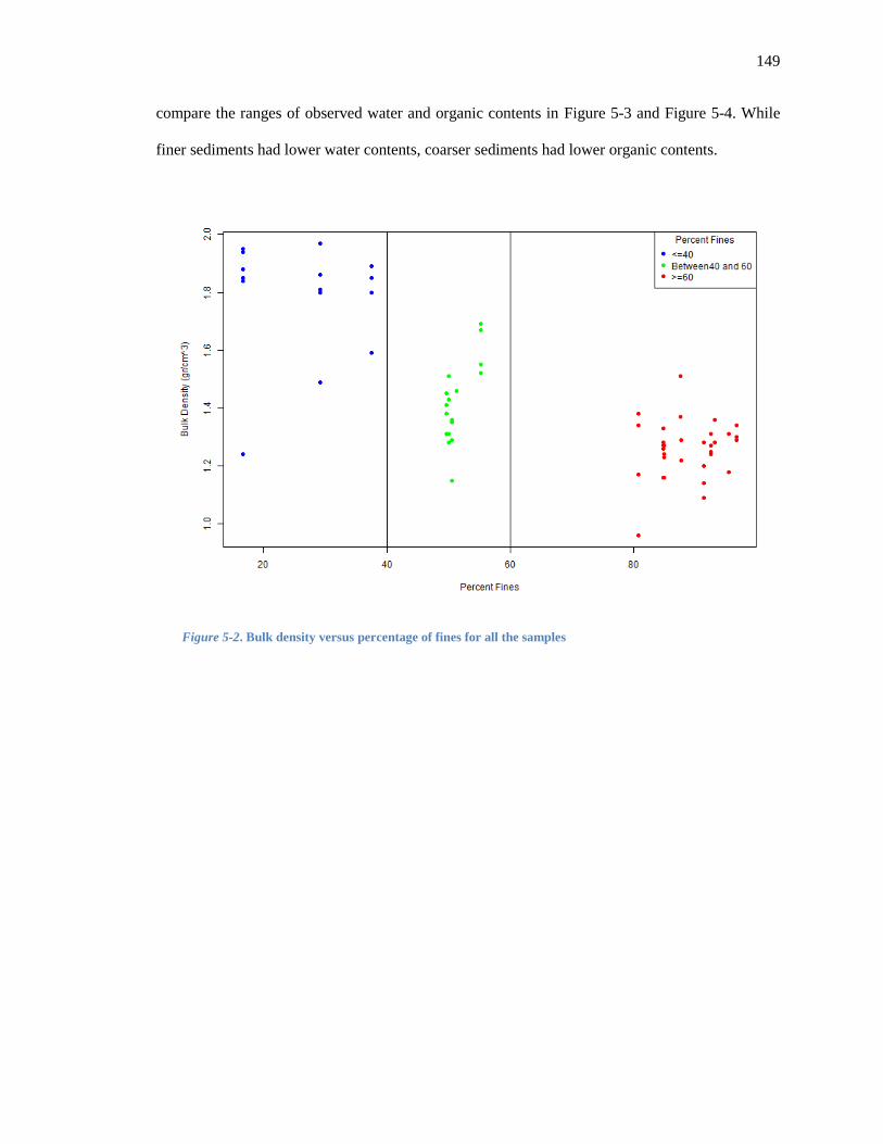
149

compare the ranges of observed water and organic contents in Figure 5-3 and Figure 5-4. While

finer sediments had lower water contents, coarser sediments had lower organic contents.

Figure 5-2. Bulk density versus percentage of fines for all the samples

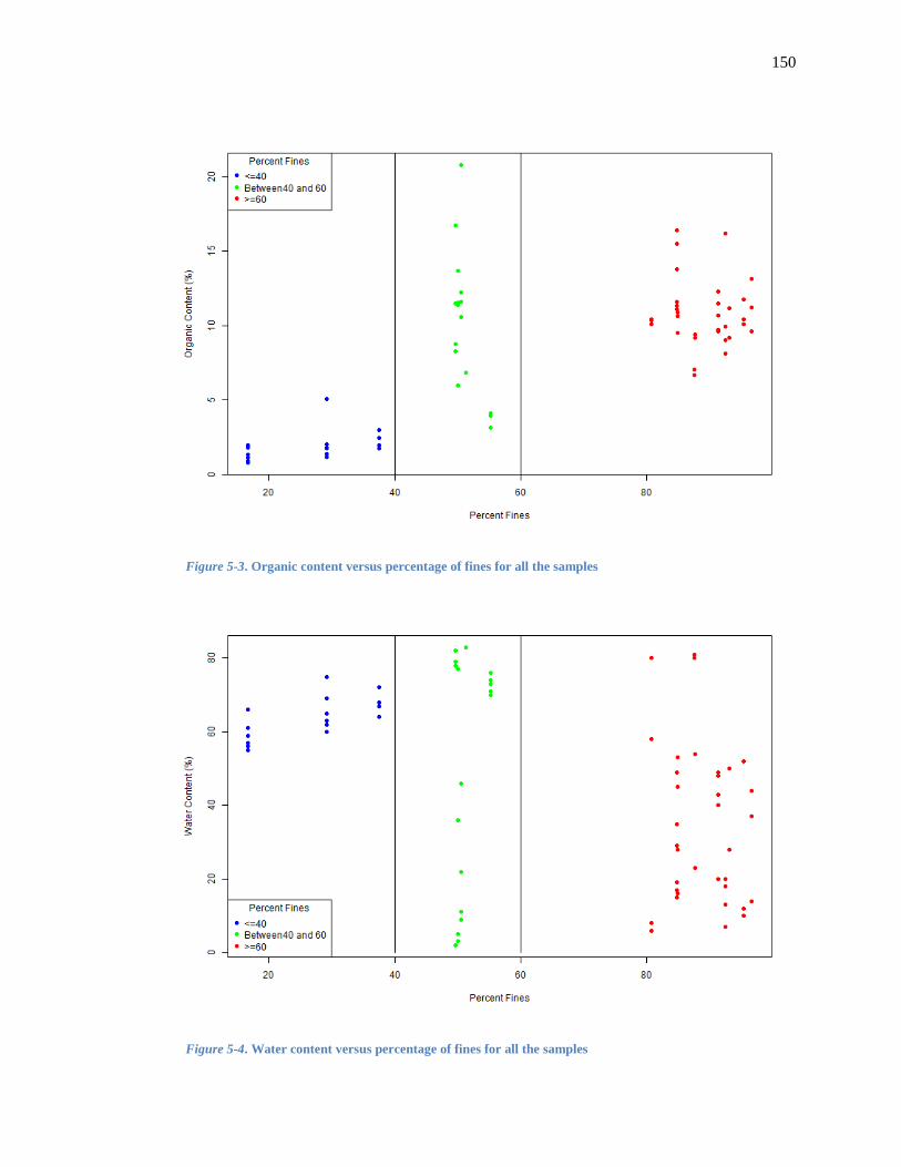
150

Figure 5-3. Organic content versus percentage of fines for all the samples

Figure 5-4. Water content versus percentage of fines for all the samples

151

Figure 5-5. Organic content versus water content for different classes of sediment size

5.2.3. Model Development

A full simple linear regression model was initially fitted to the data including all the

measured index properties (bulk density, water content, organic content, and depth), as well as the

average velocity. Both forward selection and backward elimination methods were applied to

select the best fit among all possible models, resulting in the selection of the following (full)

model. This model was not adequate according to Box A. 28 and Figure A. 29.

The observed residuals’ patterns in Figure A. 29 revealed obvious problems with this

model and suggested applying a transformation on the response values for an improved model.

Several transformation options were considered to linearize the model and stabilize its residuals’

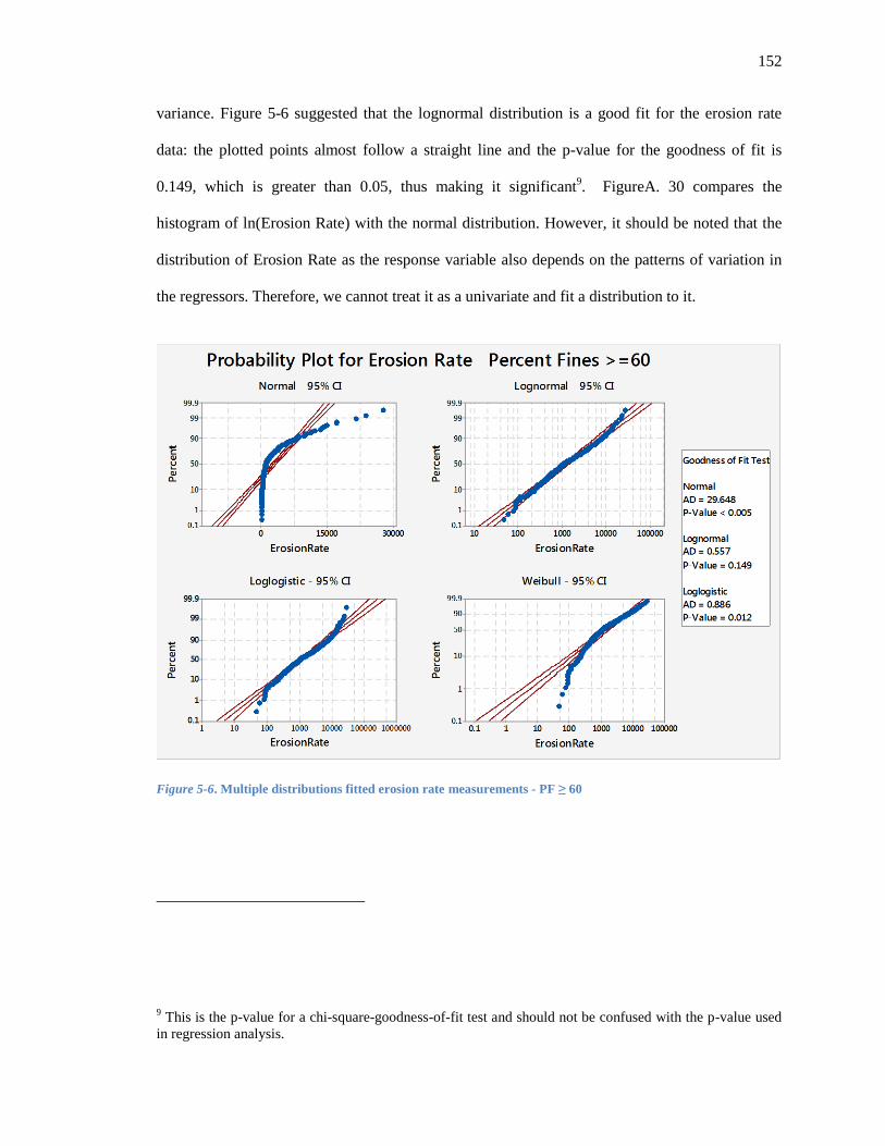
152

variance. Figure 5-6 suggested that the lognormal distribution is a good fit for the erosion rate

data: the plotted points almost follow a straight line and the p-value for the goodness of fit is

0.149, which is greater than 0.05, thus making it significant9. FigureA. 30 compares the

histogram of ln(Erosion Rate) with the normal distribution. However, it should be noted that the

distribution of Erosion Rate as the response variable also depends on the patterns of variation in

the regressors. Therefore, we cannot treat it as a univariate and fit a distribution to it.

Figure 5-6. Multiple distributions fitted erosion rate measurements - PF ≥ 60

9 This is the p-value for a chi-square-goodness-of-fit test and should not be confused with the p-value used

in regression analysis.

153

A logarithmic transformation on the average velocity proved to be helpful as well. The

forward selection and backward elimination methods were applied again, which resulted in the

selection of the following model. This model is to be called the Newark Bay Fine Model

(NBFM).

NBFM

(%)

Box 5-1. Model summary for: - PF 60

In order to check the model adequacy, different plots of residuals were investigated as

shown in Figure 5-7. The plots of the model’s least-squared residuals versus the corresponding

Lm(ln (Erosion Rate) ~ ln(AverageVelocity)+Bulk Density+Water Content)

Residuals:

Min 1Q Median 3Q Max

-2.4317 -0.6565 0.0756 0.6222 2.4221

Coefficients:

Estimate Std. Error t value Pr (>|t|)

(Intercept) 7.99318 1.21117 6.60 0.00000000024968 ***

ln(V) 1.94370 0.14123 13.76 < 0.0000000000000002 ***

-7.10538 0.87328 -8.14 0.00000000000002 ***

W 0.03173 0.00358 8.85 < 0.0000000000000002 ***

---

Signif. codes: 0 ‘***’ 0.001 ‘**’ 0.01 ‘*’ 0.05 ‘.’ 0.1 ‘ ’ 1

Residual standard error: 0.92 on 247 degrees of freedom

Multiple R-squared: 0.533, Adjusted R-squared: 0.527

F-statistic: 93.9 on 3 and 247 DF, p-value: <0.0000000000000002

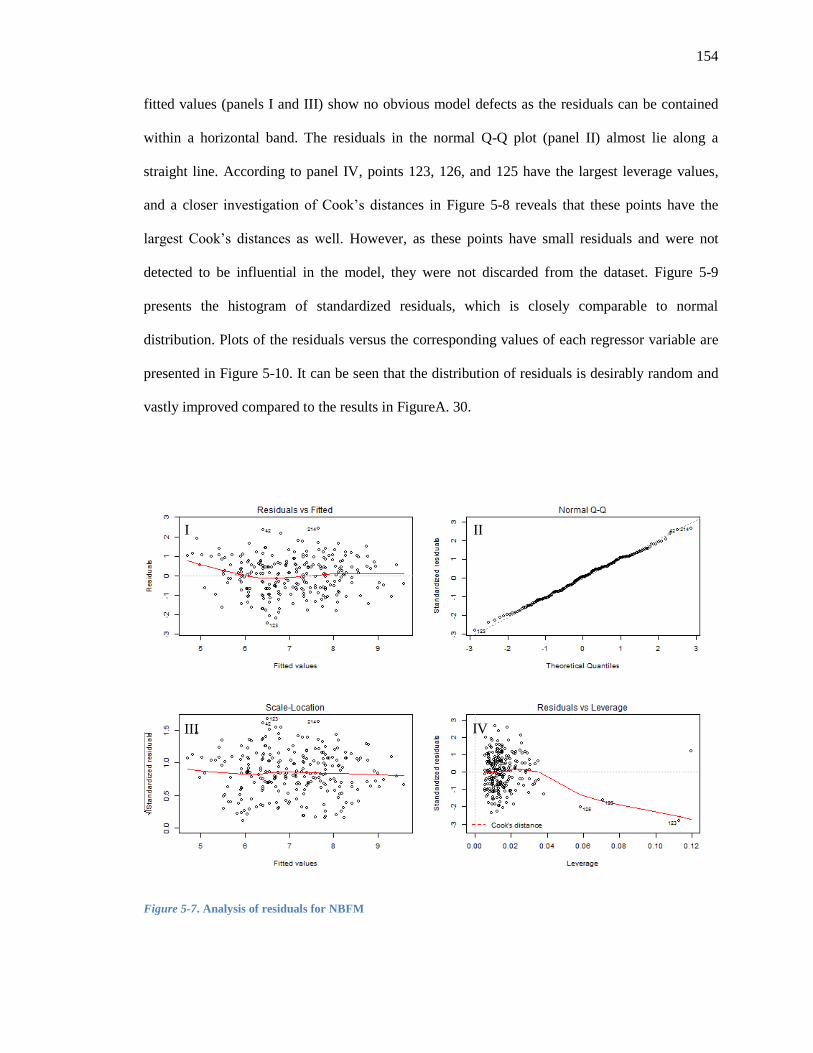
154

fitted values (panels I and III) show no obvious model defects as the residuals can be contained

within a horizontal band. The residuals in the normal Q-Q plot (panel II) almost lie along a

straight line. According to panel IV, points 123, 126, and 125 have the largest leverage values,

and a closer investigation of Cook’s distances in Figure 5-8 reveals that these points have the

largest Cook’s distances as well. However, as these points have small residuals and were not

detected to be influential in the model, they were not discarded from the dataset. Figure 5-9

presents the histogram of standardized residuals, which is closely comparable to normal

distribution. Plots of the residuals versus the corresponding values of each regressor variable are

presented in Figure 5-10. It can be seen that the distribution of residuals is desirably random and

vastly improved compared to the results in FigureA. 30.

Figure 5-7. Analysis of residuals for NBFM

I II

III IV

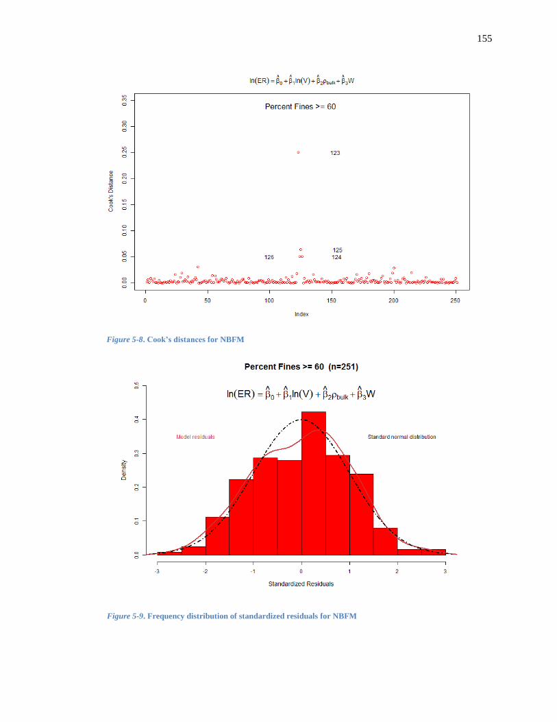
155

Figure 5-8. Cook’s distances for NBFM

Figure 5-9. Frequency distribution of standardized residuals for NBFM

156

Figure 5-10. Plots of standardized residuals versus: fitted values (top left), Average Velocity (top tight), Bulk

Density (bottom left), and Water Content (bottom right) -

Figure 5-11 presents a plot of values predicted by this model versus the natural logarithm

of observed erosion rates.

157

Figure 5-11. Predicted versus observed erosion rates for NBFM

In order to check the presence of multicollinearity, the regressors used in the model were

investigated for possible correlations. According to Table 4-2 and Figure 4-1, there is no

significant correlation between bulk density and water content in fine sediments.

Analysis of data with percent fines less than 40 percent (44 data points) resulted in the following

model with an R-squared of 62 percent (Box 5-2 and Figure 5-12 - Figure 5-15). This model is to

be called the Newark Bay Coarse Model (NBCM).

Percent Fines 40 NBCM

(%)

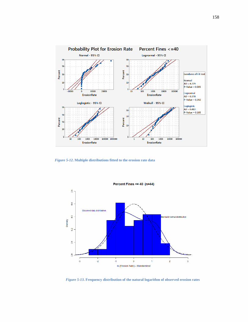
158

Figure 5-12. Multiple distributions fitted to the erosion rate data

Figure 5-13. Frequency distribution of the natural logarithm of observed erosion rates

159

Box 5-2. Model summary for: NBCM - PF 40

Figure 5-14. Analysis of residuals for NBCM

Lm (ln (Erosion Rate) ~ Average Velocity+Bulk Density+Organic Content

Residuals:

Min 1Q Median 3Q Max

-2.3669 -0.7214 0.0003 0.6353 2.1384

Coefficients:

Estimate Std. Error t value Pr(>|t|)

(Intercept) 9.9089 2.0885 4.74 0.000026625 ***

V 0.0987 0.0133 7.41 0.000000005 ***

-2.3583 1.0330 -2.28 0.028 *

O -0.9102 0.1878 -4.85 0.000019211 ***

---

Signif. codes: 0 ‘***’ 0.001 ‘**’ 0.01 ‘*’ 0.05 ‘.’ 0.1 ‘ ’ 1

Residual standard error: 1.02 on 40 degrees of freedom

Multiple R-squared: 0.622, Adjusted R-squared: 0.594

F-statistic: 22 on 3 and 40 DF, p-value: 0.0000000145

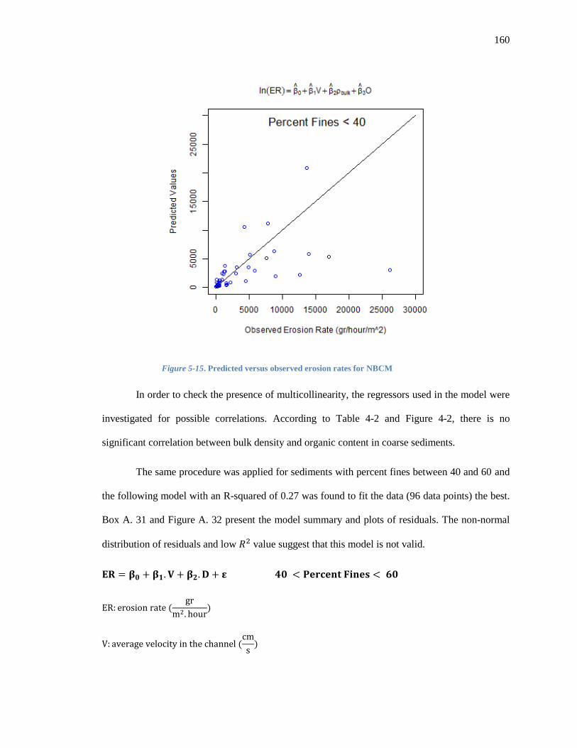
160

Figure 5-15. Predicted versus observed erosion rates for NBCM

In order to check the presence of multicollinearity, the regressors used in the model were

investigated for possible correlations. According to Table 4-2 and Figure 4-2, there is no

significant correlation between bulk density and organic content in coarse sediments.

The same procedure was applied for sediments with percent fines between 40 and 60 and

the following model with an R-squared of 0.27 was found to fit the data (96 data points) the best.

Box A. 31 and Figure A. 32 present the model summary and plots of residuals. The non-normal

distribution of residuals and low value suggest that this model is not valid.

161

5.2.4. Model Validation

One of the techniques widely used for model validation is cross-validation (Mosteller and

Tukey, 1968). In order to protect a model against overfitting, this method evaluates the

performance of a model for independent measurements without requiring the collection of new

data. The available data is randomly split into K folds, one of which is removed as the test set; the

remaining folds are used to refit a model to the data. The common division ratio of 90% train

(10% test) was used in this study which corresponds to a ten-fold cross validation. Figure 5-16

and Figure 5-17 display the results of cross-validation for NBFM and NBCM respectively and

Box A. 33 and BoxA. 34 provide the corresponding ANOVA tables.

The fitted lines (each representing one fold of data) in Figure 5-16 are almost on top of

each other and indicate that outliers are not very influential in the model. Larger points are actual

observations for each fold of data and smaller ones (plotted on the line) are the values predicted

by the model when each fold of data is deleted. The distance between the large points and their

corresponding small points is a measure of the model’s prediction accuracy. It can be concluded

that despite having a lower R-squared value, NBFM is more stable than NBCM in general.

However, the difference in the size of the datasets used for developing each of these models

should not be ignored.

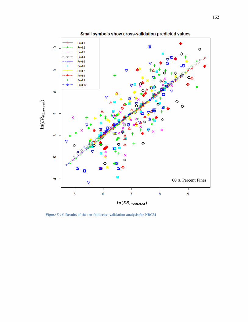
162

Figure 5-16. Results of the ten-fold cross-validation analysis for NBCM

60 Percent Fines

163

Figure 5-17. Results of the ten-fold cross-validation analysis for NBCM

In order to estimate the prediction power of NBFM and NBCM, R-squared was

calculated for the models’ predictions (for the test dataset) using PRESS statistic as defined

below. According to Table 5-1, NBFM’s prediction power reduced by three percentage points

(from 0.53 to 0.50) when it is used for a new dataset. The corresponding decrease for NBCM was

five percentage points (from 0.62 to 0.57). These low reductions in the two models’ power

indicate that none of the models are overfitted.

Percent Fines 40

ln (

)

164

∑[ ]

∑

Table 5-1. Prediction power of the selected regression models measured by ten-fold cross-validation

Model

Overall MSE

(CV) PF

NBFM

0.533 0.506 0.879

NBCM

0.622 0.578 1.050

Another set of numerical experiments were conducted to study the effect of sample size.

In each of these experiments random samples of different sizes were drawn from the observations

for 1000 times and NBFM and NBCM was fitted to them. Figure 5-18 and Figure 5-19 show the

distribution of model coefficients in these experiments. Figure 5-20 and Figure 5-21 Show the

results of the same experiments for coarse sediments of the Newark Bay.

16

5

Figure 5-18. Distribution of regression model parameters estimated based on samples of different sizes (derived from original

observations)–NBFM

166

Figure 5-19. Distribution of coefficients of distribution estimated based on samples of

different sizes (derived from observations) –NBFM

Table 5-2 compares the mean and standard deviation of model coefficients obtained from

this experiment (for 150-point data sets) to the coefficients obtained from the complete dataset.

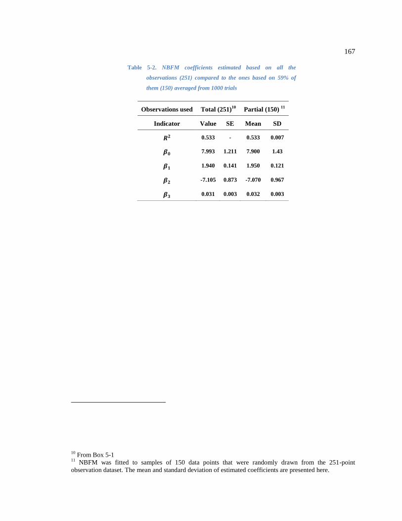
167

Table 5-2. NBFM coefficients estimated based on all the

observations (251) compared to the ones based on 59% of

them (150) averaged from 1000 trials

10 From Box 5-1

11 NBFM was fitted to samples of 150 data points that were randomly drawn from the 251-point

observation dataset. The mean and standard deviation of estimated coefficients are presented here.

Observations used Total (251)10

Partial (150) 11

Indicator Value SE Mean SD

0.533 - 0.533 0.007

7.993 1.211 7.900 1.43

1.940 0.141 1.950 0.121

-7.105 0.873 -7.070 0.967

0.031 0.003 0.032 0.003

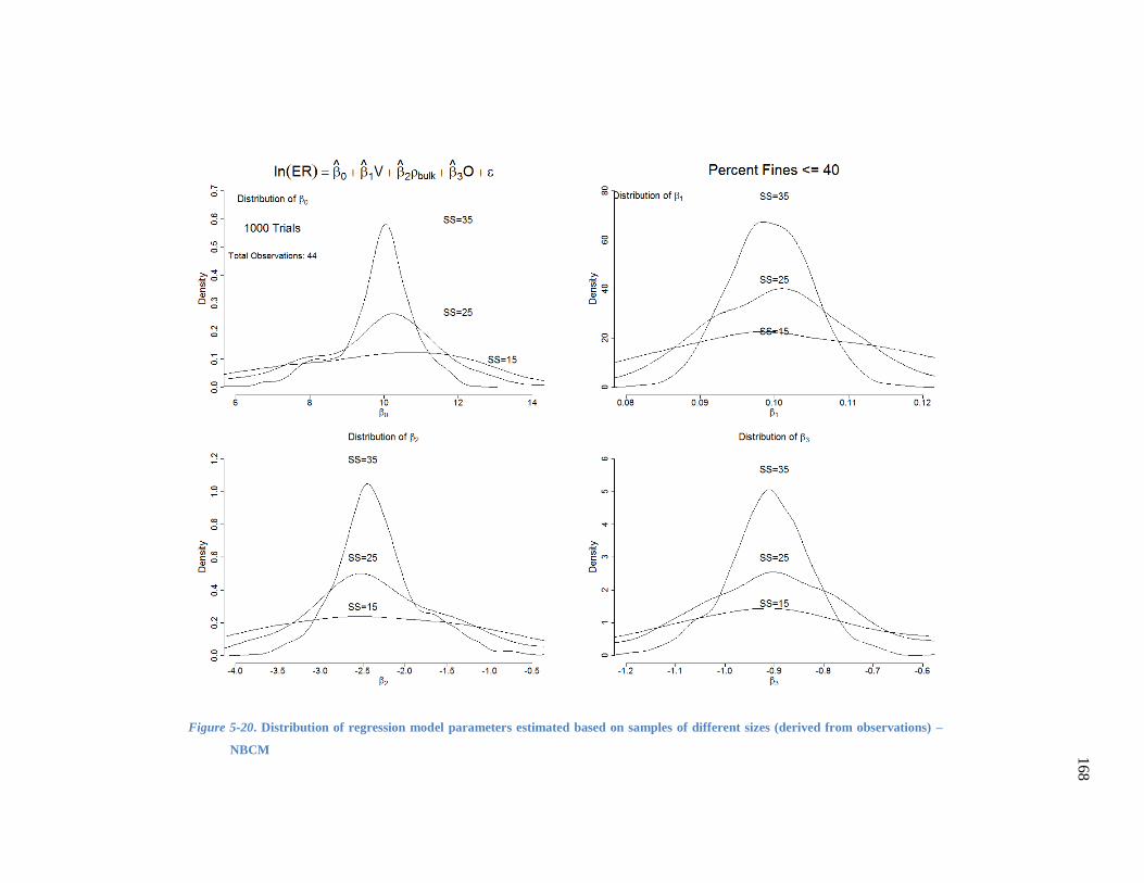
168

Figure 5-20. Distribution of regression model parameters estimated based on samples of different sizes (derived from observations) –

NBCM

169

Figure 5-21. Distribution of coefficients of distribution estimated based on

samples of different sizes (derived from observations) – NBCM

Table 5-3 compares the mean and standard deviation of model coefficients obtained from

this experiment (for 25-point data sets) to the coefficients obtained from the complete dataset.

Table 5-3. NBCM coefficients estimated based on all the

observations for coarse sediments (44) compared to

the ones based on 56% of them (25) - averaged from

1000 trials

Observations used Total (44)12

Partial (25) 13

Indicator Value SE Mean SD

12 Box 5-2

13 NBCM was fitted to samples of 25 data points that were randomly drawn from the 44-point observation

dataset. The mean and standard deviation of estimated coefficients are presented here.

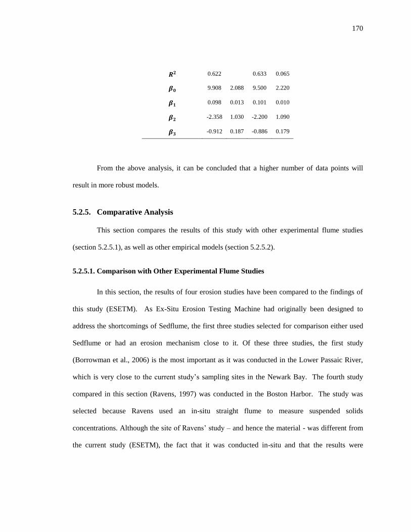
170

0.622 0.633 0.065

9.908 2.088 9.500 2.220

0.098 0.013 0.101 0.010

-2.358 1.030 -2.200 1.090

-0.912 0.187 -0.886 0.179

From the above analysis, it can be concluded that a higher number of data points will

result in more robust models.

5.2.5. Comparative Analysis

This section compares the results of this study with other experimental flume studies

(section 5.2.5.1), as well as other empirical models (section 5.2.5.2).

5.2.5.1. Comparison with Other Experimental Flume Studies

In this section, the results of four erosion studies have been compared to the findings of

this study (ESETM). As Ex-Situ Erosion Testing Machine had originally been designed to

address the shortcomings of Sedflume, the first three studies selected for comparison either used

Sedflume or had an erosion mechanism close to it. Of these three studies, the first study

(Borrowman et al., 2006) is the most important as it was conducted in the Lower Passaic River,

which is very close to the current study’s sampling sites in the Newark Bay. The fourth study

compared in this section (Ravens, 1997) was conducted in the Boston Harbor. The study was

selected because Ravens used an in-situ straight flume to measure suspended solids

concentrations. Although the site of Ravens’ study – and hence the material - was different from

the current study (ESETM), the fact that it was conducted in-situ and that the results were

171

independent of the instructor’s subjective decision (for extruding the samples), made it a good

candidate for comparison. Table 5-4 summarizes the key information about the studies compared

in this section.

17

2

Table 5-4. Key information on the studies compared in Section 5.2.5.1

Study Device Study Site Sample Type Erosion measurement

Range of ER

measurements

Current study ESETM Newark Bay Undisturbed samples Weight loss (direct

measurement)

0- 30,000

1 (Borrowman et al., 2006) Sedflume14 Lower Passaic Undisturbed cores The core’s extrusion rate 4,680-4,680,000

2 (Witt & Westrich, 2003) SETEG15 Marckolsheim Reservoir,

Germany

Homogenized and

manufactured cores

Volume loss (laser

measurements)

42,000-220,000

3 (Robert et al., 1998) Sedflume Quartz particles Manufactured Core’s upward movement 1,800-3,200,000

4 Ravens (1997) In-situ flume Boston Harbor In-situ Measurement of SSC 0-6,000

14 Sedflume was designed by McNeil et al. (1996) to measure sediment erosion with depth under high shear stresses.

15 SETEG was designed by Witt and Westrich (2003) based on Sedflume.

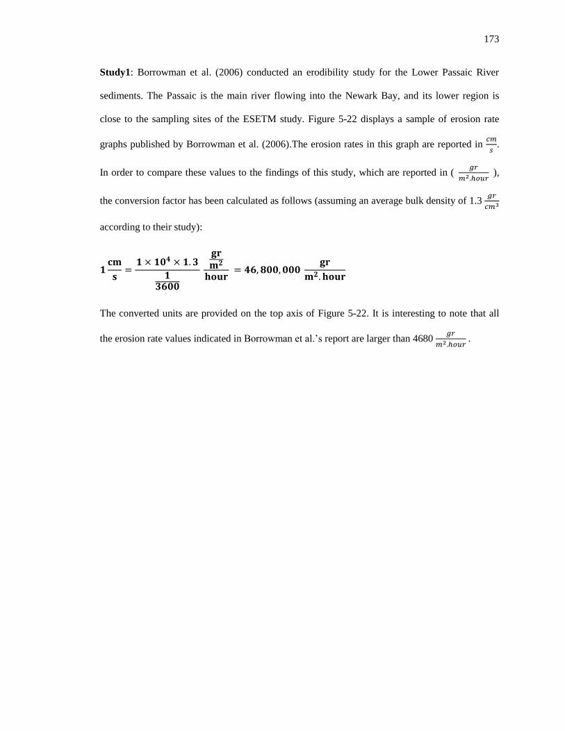
173

Study1: Borrowman et al. (2006) conducted an erodibility study for the Lower Passaic River

sediments. The Passaic is the main river flowing into the Newark Bay, and its lower region is

close to the sampling sites of the ESETM study. Figure 5-22 displays a sample of erosion rate

graphs published by Borrowman et al. (2006).The erosion rates in this graph are reported in

.

In order to compare these values to the findings of this study, which are reported in (

),

the conversion factor has been calculated as follows (assuming an average bulk density of 1.3

according to their study):

The converted units are provided on the top axis of Figure 5-22. It is interesting to note that all

the erosion rate values indicated in Borrowman et al.’s report are larger than 4680

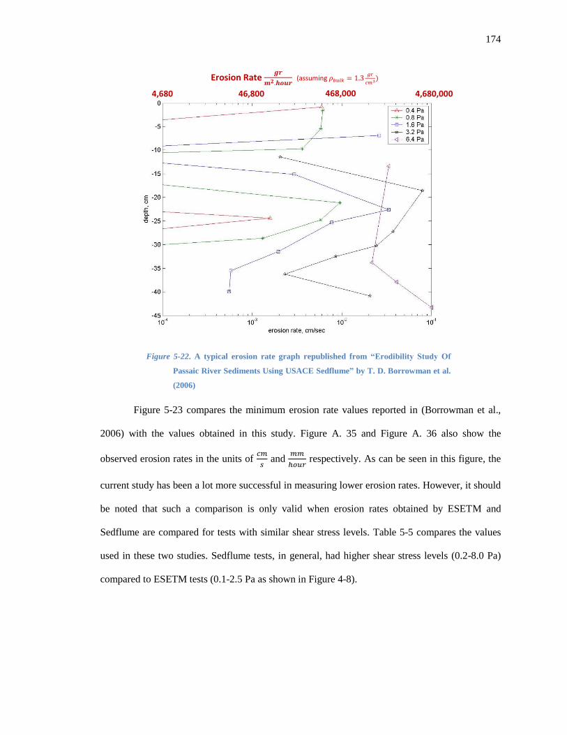
174

Figure 5-22. A typical erosion rate graph republished from “Erodibility Study Of

Passaic River Sediments Using USACE Sedflume” by T. D. Borrowman et al.

(2006)

Figure 5-23 compares the minimum erosion rate values reported in (Borrowman et al.,

2006) with the values obtained in this study. Figure A. 35 and Figure A. 36 also show the

observed erosion rates in the units of

and

respectively. As can be seen in this figure, the

current study has been a lot more successful in measuring lower erosion rates. However, it should

be noted that such a comparison is only valid when erosion rates obtained by ESETM and

Sedflume are compared for tests with similar shear stress levels. Table 5-5 compares the values

used in these two studies. Sedflume tests, in general, had higher shear stress levels (0.2-8.0 Pa)

compared to ESETM tests (0.1-2.5 Pa as shown in Figure 4-8).

Erosion Rate 𝒈𝒓

𝒎𝟐 𝒉𝒐𝒖𝒓 (assuming 𝜌𝑏𝑢𝑙𝑘

𝑔𝑟

𝑐𝑚

4,680 46,800 4,680,000 468,000

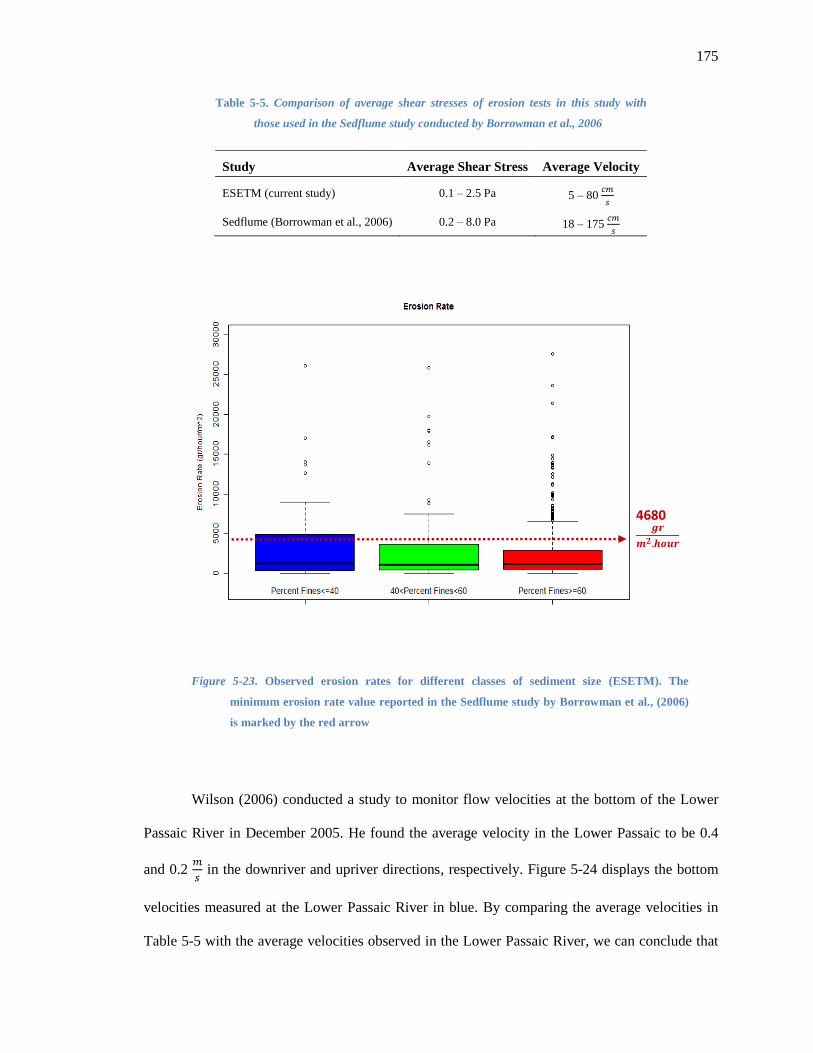
175

Table 5-5. Comparison of average shear stresses of erosion tests in this study with

those used in the Sedflume study conducted by Borrowman et al., 2006

Study Average Shear Stress Average Velocity

ESETM (current study) 0.1 – 2.5 Pa 5 – 80

Sedflume (Borrowman et al., 2006) 0.2 – 8.0 Pa 18 – 175

Figure 5-23. Observed erosion rates for different classes of sediment size (ESETM). The

minimum erosion rate value reported in the Sedflume study by Borrowman et al., (2006)

is marked by the red arrow

Wilson (2006) conducted a study to monitor flow velocities at the bottom of the Lower

Passaic River in December 2005. He found the average velocity in the Lower Passaic to be 0.4

and 0.2

in the downriver and upriver directions, respectively. Figure 5-24 displays the bottom

velocities measured at the Lower Passaic River in blue. By comparing the average velocities in

Table 5-5 with the average velocities observed in the Lower Passaic River, we can conclude that

4680 𝒈𝒓

𝒎𝟐 𝒉𝒐𝒖𝒓

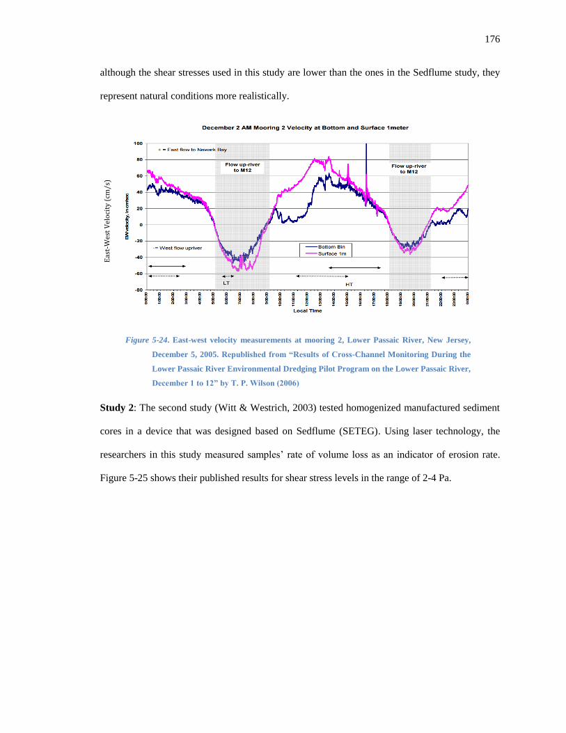
176

although the shear stresses used in this study are lower than the ones in the Sedflume study, they

represent natural conditions more realistically.

Figure 5-24. East-west velocity measurements at mooring 2, Lower Passaic River, New Jersey,

December 5, 2005. Republished from “Results of Cross-Channel Monitoring During the

Lower Passaic River Environmental Dredging Pilot Program on the Lower Passaic River,

December 1 to 12” by T. P. Wilson (2006)

Study 2: The second study (Witt & Westrich, 2003) tested homogenized manufactured sediment

cores in a device that was designed based on Sedflume (SETEG). Using laser technology, the

researchers in this study measured samples’ rate of volume loss as an indicator of erosion rate.

Figure 5-25 shows their published results for shear stress levels in the range of 2-4 Pa.

Eas

t-W

est

Vel

oci

ty (

cm/s

)

177

Figure 5-25. Erosion rates measured by Witt and Westrich (2003) for manually homogenized sediment

cores tested at shear stress levels in the range of 2-4 Pa. Republished from “Quantification of

erosion rates for undisturbed contaminated cohesive sediment cores by image analysis” by O. Witt

and B. Westrich (2003)

Study 3: Robert et al., (1998) also used Sedflume to study the erosion of manufactured samples

made of fine quartz particles. Figure 5-26 shows one of their published graphs.

Erosio

n R

ate

𝒈𝒓

𝒎𝟐 𝒉𝒐𝒖𝒓

72,000

144,000

0

216,000

288,000

Time (s) 300 0

178

Figure 5-26. Erosion rate as a function of bulk density for samples made of 14.8-micron

quartz particles and tested under different shear stresses. Republished from

"Effects of particle size and bulk density on erosion of quartz particles" by J.

Robert et al. (1998)

Study 4: Ravens (1997) conducted in-situ flume experiments to study the resuspension of

sediments in the Boston Harbor. He evaluated the shear stress at the bottom of the Harbor

comprehensively by taking current, low frequency waves, ocean swell, local wind waves, and

boat waves into account. He evaluated the maximum shear stress values to be 0.071, 0.093, 0.092,

and 0.17 Pa for low frequency, middle frequency, wind, and boat waves, respectively and his

measured shear stresses were in the ranges of and at the

two study sites. In order to evaluate the erosion rate, he measured the concentration of suspended

solids. Figure 5-27 shows the measured erosion rates at one of these sites. Comparison of his

6,480

648

64

64,800

648,000

6,480,000

64,800,000

Erosio

n R

ate*

𝒈𝒓

𝒎𝟐 𝒉𝒐𝒖𝒓

*(Calculated for 𝝆𝒃𝒖𝒍𝒌 𝟏 𝟖𝒈𝒓

𝒄𝒎𝟑

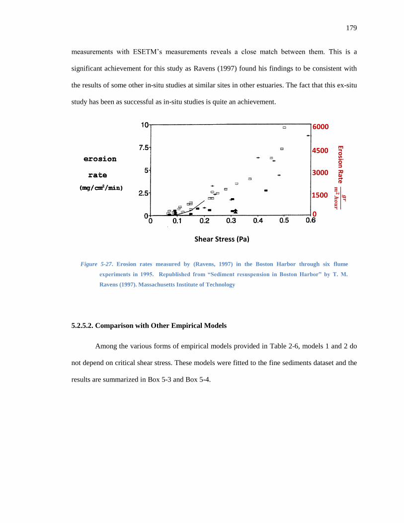
179

measurements with ESETM’s measurements reveals a close match between them. This is a

significant achievement for this study as Ravens (1997) found his findings to be consistent with

the results of some other in-situ studies at similar sites in other estuaries. The fact that this ex-situ

study has been as successful as in-situ studies is quite an achievement.

Figure 5-27. Erosion rates measured by (Ravens, 1997) in the Boston Harbor through six flume

experiments in 1995. Republished from “Sediment resuspension in Boston Harbor” by T. M.

Ravens (1997). Massachusetts Institute of Technology

5.2.5.2. Comparison with Other Empirical Models

Among the various forms of empirical models provided in Table 2-6, models 1 and 2 do

not depend on critical shear stress. These models were fitted to the fine sediments dataset and the

results are summarized in Box 5-3 and Box 5-4.

Shear Stress (Pa)

Erosio

n R

ate 𝒈𝒓

𝒎𝟐 𝒉𝒐𝒖𝒓

0

1500

3000

4500

6000

180

Model 1 (Table 2-6):

16

(

)

The model obtained based on this power law equation has an R-squared of 0.17 (Box 5-3)

which is much lower than NBFM.

Box 5-3. Model summary for: - PF ≥ 60

Model 2 (Table 2-6):

17

16 (Lavelle et al., 1984) and others

lm(formula = ln (Erosion Rate) ~ ln ( ))

Residuals:

Min 1Q Median 3Q Max

-2.895 -0.866 -0.167 0.888 2.817

Coefficients:

Estimate Std. Error t value Pr (>|t|)

(Intercept) 7.6988 0.1181 65.18 < 0.0000000000000002 ***

ln ( 0.7105 0.0978 7.27 0.0000000000048 ***

---

Signif. codes: 0 ‘***’ 0.001 ‘**’ 0.01 ‘*’ 0.05 ‘.’ 0.1 ‘ ’ 1

Residual standard error: 1.22 on 249 degrees of freedom

Multiple R-squared: 0.175, Adjusted R-squared: 0.172

F-statistic: 52.8 on 1 and 249 DF, p-value: 0.00000000000478

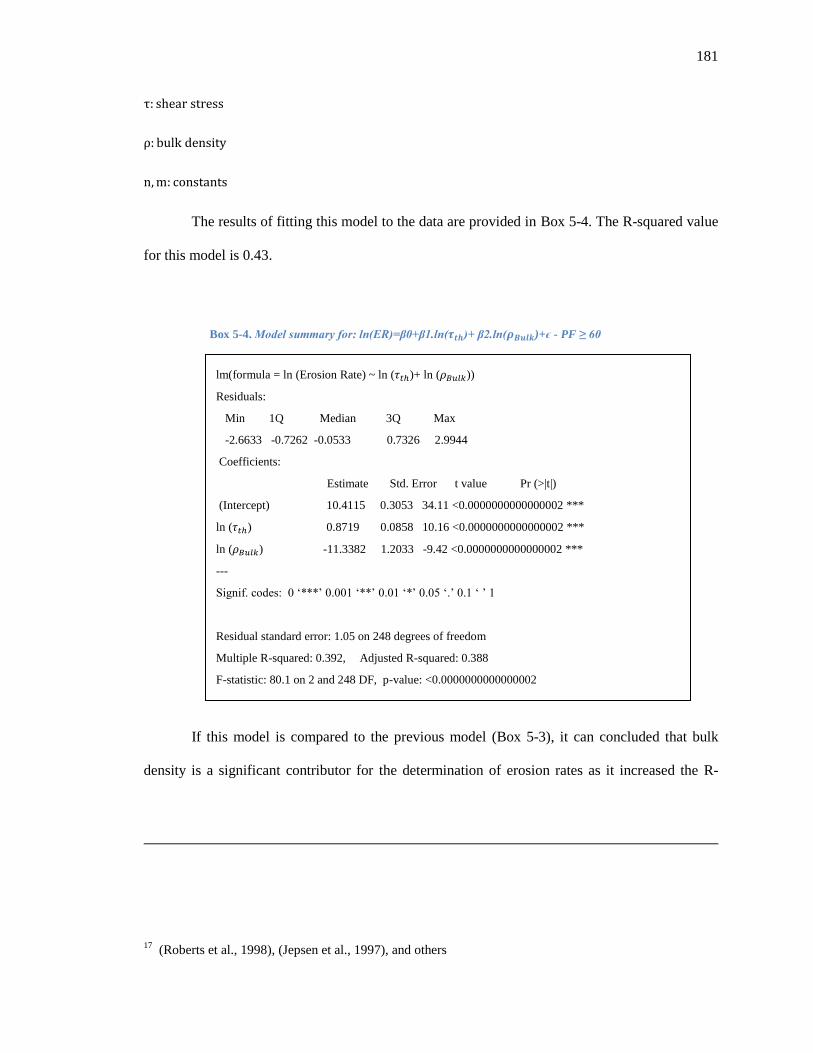
181

The results of fitting this model to the data are provided in Box 5-4. The R-squared value

for this model is 0.43.

Box 5-4. Model summary for: ln(ER)=β0+β1.ln( )+ β2.ln( )+ϵ - PF ≥ 60

If this model is compared to the previous model (Box 5-3), it can concluded that bulk

density is a significant contributor for the determination of erosion rates as it increased the R-

17 (Roberts et al., 1998), (Jepsen et al., 1997), and others

lm(formula = ln (Erosion Rate) ~ ln ( )+ ln ( ))

Residuals:

Min 1Q Median 3Q Max

-2.6633 -0.7262 -0.0533 0.7326 2.9944

Coefficients:

Estimate Std. Error t value Pr (>|t|)

(Intercept) 10.4115 0.3053 34.11 <0.0000000000000002 ***

ln ( ) 0.8719 0.0858 10.16 <0.0000000000000002 ***

ln ( ) -11.3382 1.2033 -9.42 <0.0000000000000002 ***

---

Signif. codes: 0 ‘***’ 0.001 ‘**’ 0.01 ‘*’ 0.05 ‘.’ 0.1 ‘ ’ 1

Residual standard error: 1.05 on 248 degrees of freedom

Multiple R-squared: 0.392, Adjusted R-squared: 0.388

F-statistic: 80.1 on 2 and 248 DF, p-value: <0.0000000000000002

182

squared from 0.17 to 0.43. Comparison of this model with NBFM reveals that adding water

content to regressors also increased the R-squared (from 0.43 to 0.53).

5.2.6. Conclusion and Discussion

Earlier in this chapter, NBFM and NBCM (models) were developed (5.2.3) and validated

(5.2.4) and their performance was evaluated and compared with models developed by other

researchers (5.2.5). The data used for developing these models was obtained from erosion tests on

undisturbed samples (taken from the Newark Bay, NJ in 2012) using the Ex-Situ Erosion Testing

Machine (ESETM).

(1) Newark Bay Fine Model (NBFM) based on 251 observations -

(2) Newark Bay Coarse Model (NBCM) based on 44 observations - PF 40

The main points regarding this analysis are as follows:

1- Both NBFM and NBCM were valid models with significant P-values. Their R-squared

values were 0.53 and 0.63 respectively. Since R-squared values for experimental erosion

studies are not frequently reported in the literature, it is difficult to compare the

prediction power of different tests. One of the very few studies that measured R-squared

was conducted by Hamilton and Mitchell (1996). They reported R-squared values

ranging from 0.47-0.73 for their empirical model developed based on samples taken from

seven lakes in New Zealand.

183

2- Even though this study focused mainly on the erosion behavior of cohesive sediments, a

model was also developed for non-cohesive samples. Thus, the linear regression

approach adds further value to research on sediment erosion by providing a practical and

robust framework that can be used to study both fine and granular sediments. However,

no sufficient linear model could be created for samples with the percentage of fines

between 40 and 60. This could be caused by an inherently different erosion behavior for

mixtures of fine and coarse sediments or could be attributed to inaccuracies in the

measurements of percentages of fines for the samples. It is critical to note that in this

study, percentages-of-fines tests were performed on a mixture of subsamples taken from

all the tested subsections of each core. Consequently, it is hypothesized that the cores

with percentages of fines between 40 and 60 were actually composed of both cohesive

and granular subsections. In order to avoid such inaccuracies in the future, measurements

should be taken from each section of the core to obtain more representative percentage-

of-fines values for individual samples.

3- One of the main conclusions drawn from the literature review was that erosion of natural

sediments has not been well studied at low shear stress levels. This is in part because

most of the techniques used for the measurement of erosion rates are incapable of

detecting low rates of erosion. Prevalent use of the poorly defined concept of critical

shear stress is also a major contributor to the present confusion in erosion behavior of

cohesive sediments at low shear stresses. Another factor hindering erosion tests at low

shear stresses is the limitations of some of the shear stress measurement techniques. The

current study has successfully addressed this shortcoming in the literature by providing

empirical insight into the behavior of cohesive sediments at low shear stresses.

4- The considerable size of the dataset used for fine sediments (251) gives this research an

advantage when compared to similar studies with relatively small sizes of the datasets.

For example, the sample size used by Hamilton and Mitchell (1996) – one of the only

184

studies that had reported R-squared values – was in the range of 13-55 for each of the

lakes they studied.

5- It should be noted that the datasets corresponding to fine and coarse sediments did not

have comparable sizes. While the fine dataset included 251 observations, there were only

44 observations in the coarse dataset.

6- The form of the relationship between erosion rate and flow velocity varies between

NBCM and NBFM. While average velocity is one of the regressors in the former, its

natural logarithm is among the regressors in the latter. Some other studies in the

literature (including (Roberts et al., 2000) and (Jepsen et al., 1997)) also found the same

type of relationship for cohesive sediments.

7- Both NBFM and NBCM indicate the presence of a negative correlation between bulk

density and erodibility. In addition to flow velocity and bulk density, NBFM and NBCM

depended on water content and organic content respectively. While the water-content

parameter is 0.03 in NBFM, the organic-content parameter is -0.91 in NBCM. This

indicates that in coarse sediments of the Newark Bay, a higher organic content will result

in a lower erodibility. This might be in part explained by the correlation between bulk

density and organic content.

8- Although many researchers have studied the impact of depth on erosion, this study did

not find any significant relationship between depth and erosion rate in either NBFM or

NBCM.

9- Negative weight losses were measured in almost 8% of erosion tests (67 out of 755)

indicating that the sample actually gained weight during the erosion test. Given the high

level of confidence in the accuracy of weight measurements, this phenomenon is

attributed to the presence of gas in the samples. Flow of water into air voids can replace

the gas, which results in negative weight losses. This hypothesis was validated by the fact

185

that most negative values were observed in the initial test steps when the sample had just

been exposed to air for preparation.

In order to mitigate this problem, all the observations with negative values (67 out of

755) were removed from the dataset. However, this did not completely address the

possibility of such an error in the remaining measurements. Thirteen observations that

had erosion rates larger than 30,000

were considered as outliers and removed

before fitting the models.

10- All the techniques and methods used for measuring average velocity, bulk density, weight

loss, and water and organic content were very accurate and reliable, especially when

compared to most other erosion studies. Consequently, the observed error can be mainly

attributed to model prediction. However, the observed negative weight losses increase the

uncertainty in weight loss measurements not because of the measurement technique but

because they added a physical factor that could not be controlled or measured.

5.3. Stochastic Analysis

This section introduction is devoted to stochastic analysis of the results and includes four

sections on introduction, analysis, model evaluation, and discussion.

5.3.1. Introduction

In Section 5.2.3, two linear regression models were developed for the Newark Bay

samples tested in ESETM and it was concluded that both models have acceptable prediction

power. Figure 5-28 and Figure 5-29 compare the density distribution of observed erosion rates

with predicted rates for NBFM and NBCM respectively. However, it should be noted that the

distributions displayed in these two figures completely depend on the experimental design of the

186

study. This means that if more tests were conducted at higher velocities, higher erosion rates

would push the curves upward.

Figure 5-28. Density distribution of observed and predicted erosion rates

Figure 5-29. Density distribution of observed and predicted erosion rates (NBCM)

Percent Fines 40

Percent Fines ≥ 60

187

In such cases, stochastic simulation can be used to simulate random natural scenarios and

build confidence intervals for predictions. Although stochastic analysis has been previously used

for sediment erosion (Section 2.3.6.3), to the best of the author’s knowledge, the approach used in

this study has not been previously used in any cohesive sediment erosion studies. Section 5.3.2

explains the analysis process and provides the results. In Section 5.3.3, the Newark Bay Fine

Model was interestingly evaluated using an independent dataset that was not used for developing

the model. The main conclusions from the stochastic analysis are provided in section 5.3.4.

5.3.2. Analysis

Stochastic simulation is the use of stochastic processes to generate various realizations of

a variable with statistical characteristics similar to those of the observed data. On one hand, the

complexity of sediment transport processes precludes the application of purely analytical

methods. On the other hand, limited access to experimental data makes it challenging to take

randomness into account, apply a model to different situations (combinations of input values),

and compare model predictions for different scenarios. As simulation techniques provide a

potential solution to these challenges, the Monte Carlo simulation method was applied in this

study. This method simulates multiple experiments by using sets of artificially generated input

188

variables, resulting in the distribution of possible model predictions.

Figure 5-30 presents the main idea involved in applying the Monte Carlo method to the

results of this erosion study.

Figure 5-30. Steps involved in stochastic simulation of erosion

189

In this study, pseudo-populations of input factors were created by drawing random

samples from the observed dataset. The model’s output is the Monte Carlo estimate of the

sampling distribution of the weight of eroded material per hour and per unit area of the surface

when exposed to the assumed velocity distribution.

Figure 5-31 shows the cumulative frequency distribution of erosion rates simulated for

different velocities using the original (observed) sediment parameters and velocities of 10, 20, 30,

and 40

and Figure 5-32 compares the empirical cumulative frequency distribution of the

observed, predicted and simulated data. Both these figures are based on NBFM and the

corresponding results for NBCM are presented in Figure 5-33 and Figure 5-34.

The information gained with the help of stochastic analysis provides a deep insight on

erosion risk analysis. This is very helpful for both researchers and policy makers to predict and

decide more realistically. Another advantage of stochastic models is that they provide a feasible

platform for the comparison of the confidence interval of predictions made by different models

for any specific scenario.

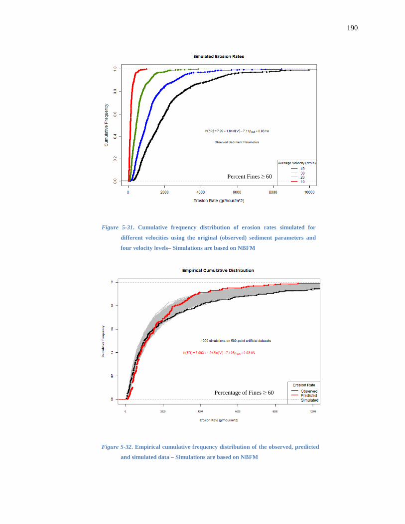
190

Figure 5-31. Cumulative frequency distribution of erosion rates simulated for

different velocities using the original (observed) sediment parameters and

four velocity levels– Simulations are based on NBFM

Figure 5-32. Empirical cumulative frequency distribution of the observed, predicted

and simulated data – Simulations are based on NBFM

Percent Fines ≥ 60

Percentage of Fines ≥ 60

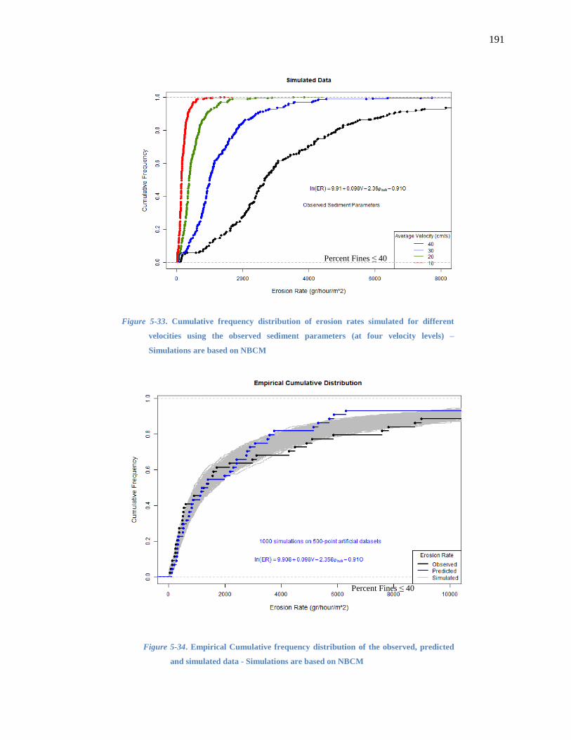
191

Figure 5-33. Cumulative frequency distribution of erosion rates simulated for different

velocities using the observed sediment parameters (at four velocity levels) –

Simulations are based on NBCM

Figure 5-34. Empirical Cumulative frequency distribution of the observed, predicted

and simulated data - Simulations are based on NBCM

Percent Fines ≤ 40

Percent Fines ≤ 40

192

5.3.3. Model Evaluation

Finally, the stochastic analysis methodology developed in Section 5.3.2 was validated

using a set of partially new data that was not used for model development (training). This data

came from samples obtained from the Newark Bay in the first two days of sample collection.

Two hundred and sixty-three erosion tests were conducted on thirty-one samples taken from eight

cores. Only erosion rate (ER) and average velocity (V) were measured in these tests and hence,

index properties were not available. Figure 5-35 shows the cumulative frequency distribution of

erosion rates measured in these tests. The gray curves represent the results of 1000 simulations

using the average velocities used for the actual tests combined with bulk density and water

content values simulated based on the measurements obtained from other samples. Although data

was not available on the percentage of fines for these samples, it was assumed that all the samples

had more than 60% of fines and hence NBFM was used for them.

According to Figure 5-35, the stochastic approach is fairly successful in predicting the

erosion rates for an independent dataset. The stochastic simulation results overestimate the

erosion rates in the range below 4000

. However, it is much more successful in higher

erosion rates.

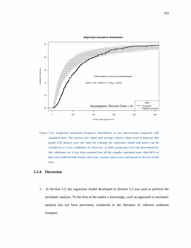
193

Figure 5-35. Empirical cumulative frequency distribution of new observations compared with

simulated data. The erosion rate values and average velocity values used to generate this

graph (238 points) were not used for training the regression model and hence can be

considered as a new validation set. However, as index properties were not determined for

this validation set, it has been assumed that all the samples contained more than 60% of

fines and artificial bulk density and water content values were used based on the rest of the

tests.

5.3.4. Discussion

1- In Section 5.3, the regression model developed in Section 5.2 was used to perform the

stochastic analysis. To the best of the author’s knowledge, such an approach to stochastic

analysis has not been previously conducted in the literature of cohesive sediment

transport.

Assumption: Percent Fines ≥ 60

194

2- The information gained with the help of stochastic analysis provides a deep insight on

erosion risk analysis. This is very helpful for both researchers and policy makers to

predict and decide more realistically. Another advantage of stochastic models is that they

offer a feasible platform for the comparison of the confidence interval of the predictions

made by different models for any specific scenario.

3- The Monte Carlo simulation method was applied to the selected regression models to

stochastically predict erosion rates for synthetically generated input parameters. To the

best of the author’s knowledge, this technique has not been used previously in the study

of sediment erosion.

4- A partially new dataset (including erosion rate and average velocity measurements only)

which was not used for model development was used to validate the stochastic analysis

methodology and it was concluded that the stochastic analysis conducted in Section 5.3 is

meaningful and helpful.

195

6. CONCLUSION

“The eventual goal of understanding and predicting fine sediment erodibility on the

basis of more readily measured sediment properties remains a very important one.”18

This study aimed to predict the erosion behavior of cohesive sediments at flow velocities

below 1

based on their index properties. In summary, the main outcomes of this study are as

follows: (1) Two fairly valid erosion models were developed for fine- and coarse-grained

sediments of the Newark Bay. (2) A framework was developed for stochastic analysis of erosion

test results. (3) An experimental methodology was designed for comparatively less subjective

measurement of erosion rates at low shear stress levels. (4) A probabilistic modeling platform

was developed to explore the impact of experimental design on interpretation of erosion test

results. (5) A comprehensive review of the literature on scale-related issues in cohesive sediment

transport was conducted. (6) A novel erosion testing flume – Ex-Situ Erosion Testing Machine

(ESETM) – was assessed for its potential to be used in sediment erosion studies. (7) A

comprehensive literature review was conducted on cohesive sediment transport with emphasis on

erosion.

The discussion of the major results and contributions of this study is organized into three

parts: (1) literature review, (2) methodology, and (3) analysis.

18 Larry Sanford (Sanford, 2006)

196

Literature Review

1- A main conclusion drawn from the literature review is that erosion of natural sediments has

not been well studied at low shear stress levels. This is in part because most of the techniques

used for the measurement of erosion rates are incapable of detecting low rates of erosion.

Prevalent use of the poorly defined concept of critical shear stress is also a major contributor

to the present confusion in the erosion behavior of cohesive sediments at low shear stress

levels.

2- The experimental methodology and data interpretation scheme in this research were devised

based on the critical analysis of previous literature and aimed to reduce uncertainty,

subjectivity, and arbitrariness.

3- In conducting empirical studies on erosion, spatial heterogeneity and temporal variation in

properties of natural cohesive sediments, together with the lack of physical modeling of

erosion pose significant challenges to predict sediment erosion.

4- Physics-based models might fit a limited set of experimental data well but are only applicable

to the particular material tested and under conditions similar to the testing conditions. This is

due to both the complex nature of sediment erosion and the extensive input parameters

required by such models. Contrarily, a purely empirical erosion model that concentrates on

the most significant factors can be generalized to a wider variety of materials and conditions.

There is a great need for such models, as complex physics-based models demand extensive

accurate inputs that cannot be realistically measured in large-scale real-world situations.

5- Another important aspect explored in this study is the concept of scale. The concept of scale

in the sediment transport field, if not completely ignored, has generally been used in an

unclear or inaccurate manner. Presently, there is no clear indication of the different scales

associated with most sediment transport studies especially in the case of modeling scales.

This is a serious barrier to comparing the results from different studies. There is a need for a

197

framework that guides researchers through dealing with the issue of scale in their erosion

studies. This study investigates various scale-related aspects in cohesive sediment transport

based on the current literature, and is the first step toward developing a holistic framework.

6- A final point worth mentioning is that researchers in the field of cohesive sediment erosion

should weigh a model’s complexity and comprehensiveness on one hand with its accuracy

and reliability on the other hand. A legitimate question that arose in this context is: which

model is better? A more complex model with poorly measured input variables (e.g. critical

shear stress) or a simpler model with fewer well-defined parameters measured more

accurately and less subjectively?

Methodology

1- In this study, 755 erosion rate tests were conducted on 142 fairly undisturbed samples taken

from 24 cores extracted from the Newark Bay. The considerable size of the dataset used for

fine sediments (251) gives this research an advantage when compared to similar studies with

relatively small sizes of the datasets.

2- Comparison of erosion measurements made in this study with the results of some in-situ

studies reveals a strong consistency between them. The fact that this ex-situ study has been as

successful as in-situ studies is quite an achievement.

3- The success of the devised experimental methodology is also highlighted when the results are

compared to similar ex-situ studies as the range of erosion rates measured in this study are

well beyond the capability of many other methods.

4- After the Ex-Situ Erosion Testing Machine was assembled, installed, and calibrated,

extensive research was conducted to evaluate its performance. Significant effort was made in

implementing a scientific methodology to identify the strengths and weaknesses of ESETM

and evaluate the accuracy and reliability of its measurements. Subsequently, the research

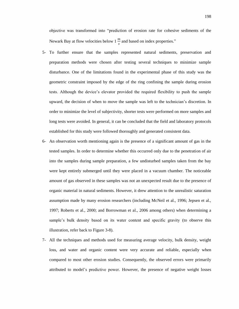
198

objective was transformed into “prediction of erosion rate for cohesive sediments of the

Newark Bay at flow velocities below 1

and based on index properties.”

5- To further ensure that the samples represented natural sediments, preservation and

preparation methods were chosen after testing several techniques to minimize sample

disturbance. One of the limitations found in the experimental phase of this study was the

geometric constraint imposed by the edge of the ring confining the sample during erosion

tests. Although the device’s elevator provided the required flexibility to push the sample

upward, the decision of when to move the sample was left to the technician’s discretion. In

order to minimize the level of subjectivity, shorter tests were performed on more samples and

long tests were avoided. In general, it can be concluded that the field and laboratory protocols

established for this study were followed thoroughly and generated consistent data.

6- An observation worth mentioning again is the presence of a significant amount of gas in the

tested samples. In order to determine whether this occurred only due to the penetration of air

into the samples during sample preparation, a few undisturbed samples taken from the bay

were kept entirely submerged until they were placed in a vacuum chamber. The noticeable

amount of gas observed in these samples was not an unexpected result due to the presence of

organic material in natural sediments. However, it drew attention to the unrealistic saturation

assumption made by many erosion researchers (including McNeil et al., 1996; Jepsen et al.,

1997; Roberts et al., 2000; and Borrowman et al., 2006 among others) when determining a

sample’s bulk density based on its water content and specific gravity (to observe this

illustration, refer back to Figure 3-8).

7- All the techniques and methods used for measuring average velocity, bulk density, weight

loss, and water and organic content were very accurate and reliable, especially when

compared to most other erosion studies. Consequently, the observed errors were primarily

attributed to model’s predictive power. However, the presence of negative weight losses

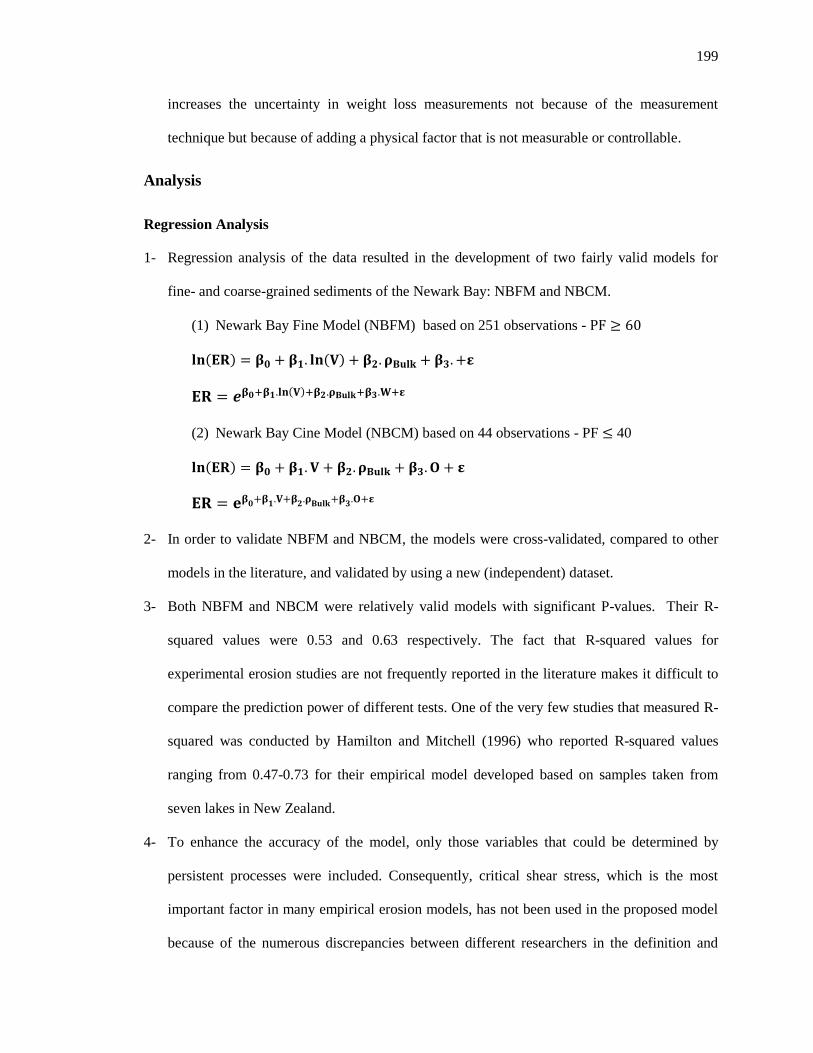
199

increases the uncertainty in weight loss measurements not because of the measurement

technique but because of adding a physical factor that is not measurable or controllable.

Analysis

Regression Analysis

1- Regression analysis of the data resulted in the development of two fairly valid models for

fine- and coarse-grained sediments of the Newark Bay: NBFM and NBCM.

(1) Newark Bay Fine Model (NBFM) based on 251 observations -

(2) Newark Bay Cine Model (NBCM) based on 44 observations - PF 40

2- In order to validate NBFM and NBCM, the models were cross-validated, compared to other

models in the literature, and validated by using a new (independent) dataset.

3- Both NBFM and NBCM were relatively valid models with significant P-values. Their R-

squared values were 0.53 and 0.63 respectively. The fact that R-squared values for

experimental erosion studies are not frequently reported in the literature makes it difficult to

compare the prediction power of different tests. One of the very few studies that measured R-

squared was conducted by Hamilton and Mitchell (1996) who reported R-squared values

ranging from 0.47-0.73 for their empirical model developed based on samples taken from

seven lakes in New Zealand.

4- To enhance the accuracy of the model, only those variables that could be determined by

persistent processes were included. Consequently, critical shear stress, which is the most

important factor in many empirical erosion models, has not been used in the proposed model

because of the numerous discrepancies between different researchers in the definition and

200

measurement of this factor. Additionally, the literature reveals that there is a high chance of

erosion even at shear stress levels well below the average critical shear stress (Lopez &

Garcia, 2001), thus calling into question the very validity of this concept. Another source of

discrepancy in the findings of different studies is the methodology used for the estimation of

shear stress giving rise to inconsistent shear stress values. Since there is no universal method

to obtain shear stress values, the proposed model avoided the inclusion of this factor. Instead,

this model includes flow velocity, which is a commonly used indicator of shear stress.

5- The suggested modeling framework avoids dependency on too many parameters. This might

yield a poorer fit to the observed data (than more complex models) in the calibration phase

but eliminates over-parameterization, which can result in a more robust performance in the

verification phase (Merritt et al., 2003). Given the high spatial variability of the factors used

in erosion models, complicated models that include numerous factors or suggest complex

forms cannot be generalized to any domain other than the ones for which they have been

obtained. With a simpler model on the other hand, the level of uncertainty can be reduced

through the acquisition of more samples representing the domain.

6- Even though this study focused mainly on the erosion behavior of cohesive sediments, a

model was also developed for non-cohesive samples. Thus, the linear regression approach

adds further value to the research on sediment erosion by providing a practical and robust

framework that can be used to study both fine and granular sediments. However, no

sufficient linear model could be created for samples with percentage of fines between 40 and

60. This could be caused by an inherently different erosion behavior for mixtures of fine and

coarse sediments, or otherwise attributed to inaccuracies in determination of percentage of

fines. It is critical to note that in this study, percentage of fines tests were performed on a

mixture of subsamples taken from all the tested subsections of each core. Consequently, it

can be hypothesized that the cores with percentages of fines between 40 and 60 were actually

composed of both cohesive and granular subsections. In order to avoid such inaccuracies in

201

the future, measurements should be taken from each section of the core to get percentage of

fines values that are more representative of individual samples.

It should be noted that the datasets corresponding to fine and coarse sediments did not have

similar sizes. While the fine dataset included 251 observations, there were only 44 coarse

data points available.

Stochastic Analysis

1- A new methodology was developed for the stochastic analysis of erosion by applying the

Monte Carlo simulation technique to NBFM and NBCM. To the best of the author’s

knowledge, this technique has not been used previously in the study of sediment erosion. The

availability of such a robust stochastic process makes it possible to study the erosion behavior

of sediments over many artificially generated samples (in lieu of measured data), resulting in

higher levels of confidence in predictions.

2- The information gained with the help of stochastic analysis provides a deep insight on erosion

risk analysis. This is very helpful for both researchers and policy makers to predict and

decide more realistically.

3- A partially new dataset (including erosion rate and average velocity measurements only),

which was not used for model development, was used to validate the stochastic analysis

methodology and it was concluded that the stochastic analysis conducted in Section 5.3 is

meaningful and helpful.

Probabilistic Analysis

1- The framework developed in section 3.5.2 for the probabilistic analysis of erosion data offers

a standardized methodology for data analysis that paves the way for the comparison of

different studies. The main takeaways from this analysis are: (1) Classification of sediments

to uniform clusters, which was initially conducted by Van Prooijen and Winterwerp (2010), is

an effective method to capture the time-dependent erosion behavior of sediments. (2) As

202

clearly indicated in Figure 3-37, design of the experiment has a significant role in the results

of erosion tests and this should be considered in the analysis and interpretation phases. (3)

The results obtained by this new methodology are not dependent on any particular testing

arrangement. (4) This framework can be considered as an initial step toward comparing the

results obtained in different studies. (5) Although the optimization problem is ill-posed (as is

typical for inverse problems) and has no unique optimal solution, modifications in the design

of experiments can help select the most interpretable result from the set of possible solutions.

2- The probabilistic analysis conducted in this study clearly indicated the significant impact of

the design of erosion experiments – specifically the length and order of different shear stress

levels applied to sediments – on experimental outcomes.

3- The probabilistic analysis clearly demonstrated that the validity of measurements decreases as

more tests are conducted on one sample because of the impact of shear history. It can be

concluded that for the purpose of this study, the number of shear stress steps to which a

sample is exposed should be limited to avoid unrealistic results.

Future Research

1- The erosion behavior of sediments with percent fines between 40 and 60 needs more

research.

2- The predictions made by the Newark Bay Corse Model can be compared with available

models for prediction of granular sediments.

3- If models similar to NBFM and NBCM are further validated, the next important step will be

to develop practical techniques for extensive measurement of the index properties required by

these models (bulk density, percent fines, and water and organic content).

4- The probabilistic framework developed in this study for the analysis of erosion rate data is

independent of the experimental design, which opens the way for the comparison of different

studies.

203

APPENDIX A.

Other graphs, tables and boxes

20

4

Figure A. 1. Core Acquisition Data (Form 1)

20

5

Figure A. 2. Ring Identification Data (Form 2)

20

6

Figure A. 3. Undisturbed Sample Identification Form (Form 3)

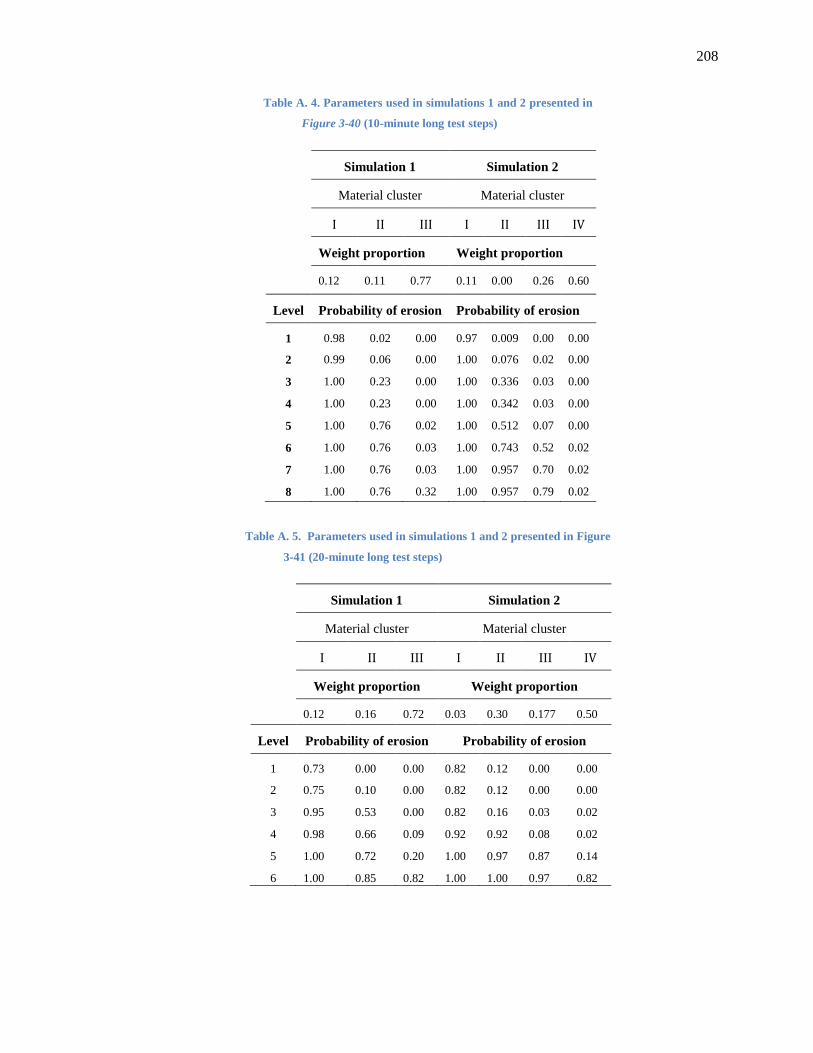
208

Table A. 4. Parameters used in simulations 1 and 2 presented in

Figure 3-40 (10-minute long test steps)

Table A. 5. Parameters used in simulations 1 and 2 presented in Figure

3-41 (20-minute long test steps)

Simulation 1 Simulation 2

Material cluster Material cluster

Weight proportion Weight proportion

0.12 0.16 0.72 0.03 0.30 0.177 0.50

Level Probability of erosion Probability of erosion

1 0.73 0.00 0.00 0.82 0.12 0.00 0.00

2 0.75 0.10 0.00 0.82 0.12 0.00 0.00

3 0.95 0.53 0.00 0.82 0.16 0.03 0.02

4 0.98 0.66 0.09 0.92 0.92 0.08 0.02

5 1.00 0.72 0.20 1.00 0.97 0.87 0.14

6 1.00 0.85 0.82 1.00 1.00 0.97 0.82

Simulation 1 Simulation 2

Material cluster Material cluster

Weight proportion Weight proportion

0.12 0.11 0.77 0.11 0.00 0.26 0.60

Level Probability of erosion Probability of erosion

1 0.98 0.02 0.00 0.97 0.009 0.00 0.00

2 0.99 0.06 0.00 1.00 0.076 0.02 0.00

3 1.00 0.23 0.00 1.00 0.336 0.03 0.00

4 1.00 0.23 0.00 1.00 0.342 0.03 0.00

5 1.00 0.76 0.02 1.00 0.512 0.07 0.00

6 1.00 0.76 0.03 1.00 0.743 0.52 0.02

7 1.00 0.76 0.03 1.00 0.957 0.70 0.02

8 1.00 0.76 0.32 1.00 0.957 0.79 0.02

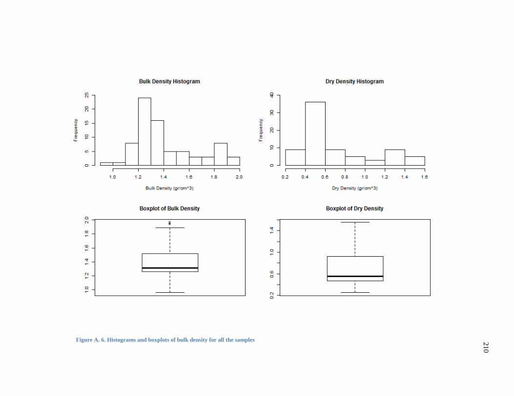
21

0

Figure A. 6. Histograms and boxplots of bulk density for all the samples

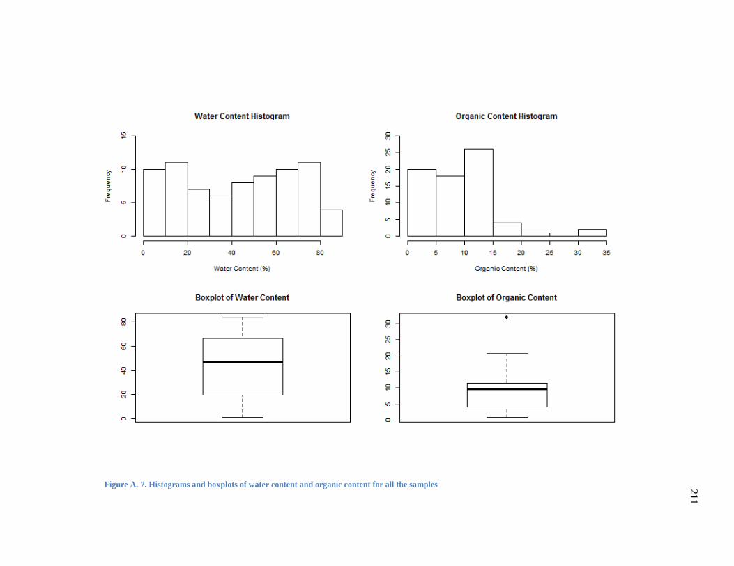
21

1

Figure A. 7. Histograms and boxplots of water content and organic content for all the samples

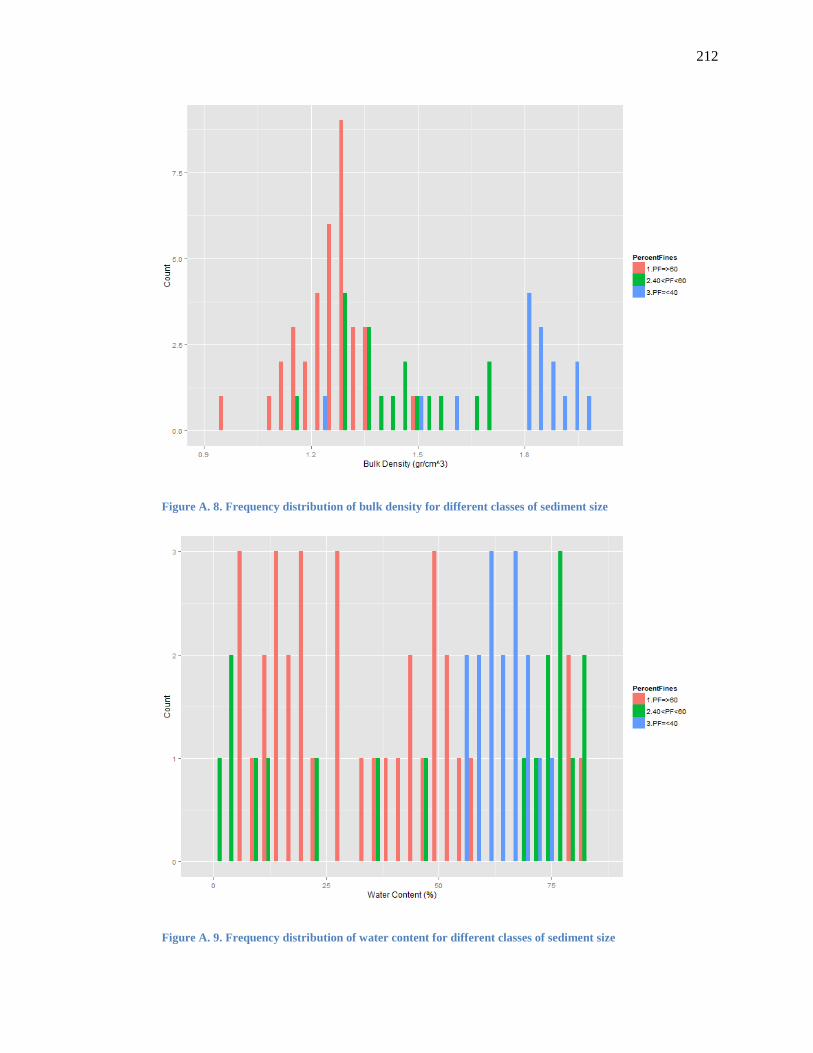
212

Figure A. 8. Frequency distribution of bulk density for different classes of sediment size

Figure A. 9. Frequency distribution of water content for different classes of sediment size

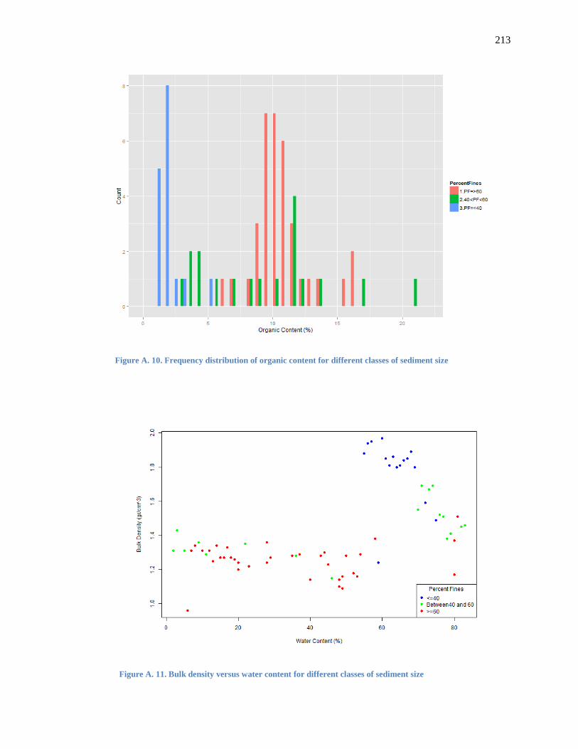
213

Figure A. 10. Frequency distribution of organic content for different classes of sediment size

Figure A. 11. Bulk density versus water content for different classes of sediment size

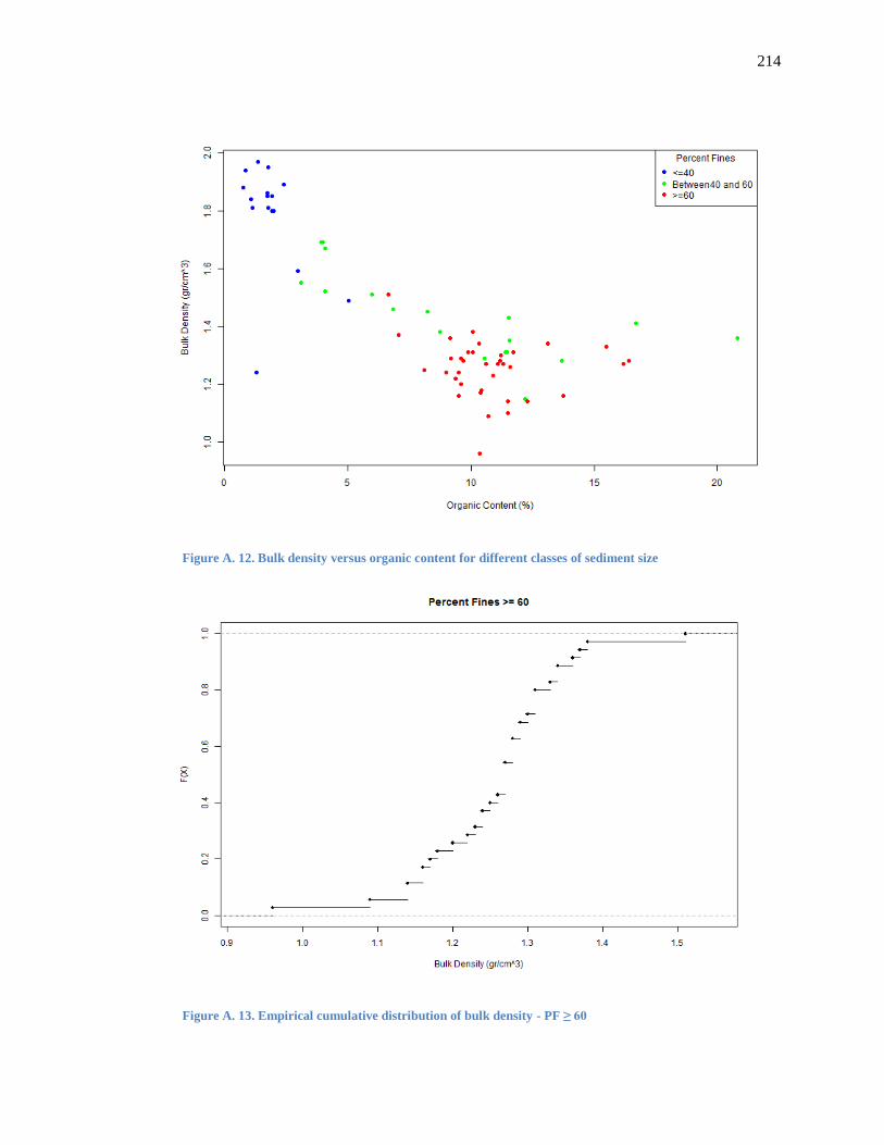
214

Figure A. 12. Bulk density versus organic content for different classes of sediment size

Figure A. 13. Empirical cumulative distribution of bulk density - PF ≥ 60

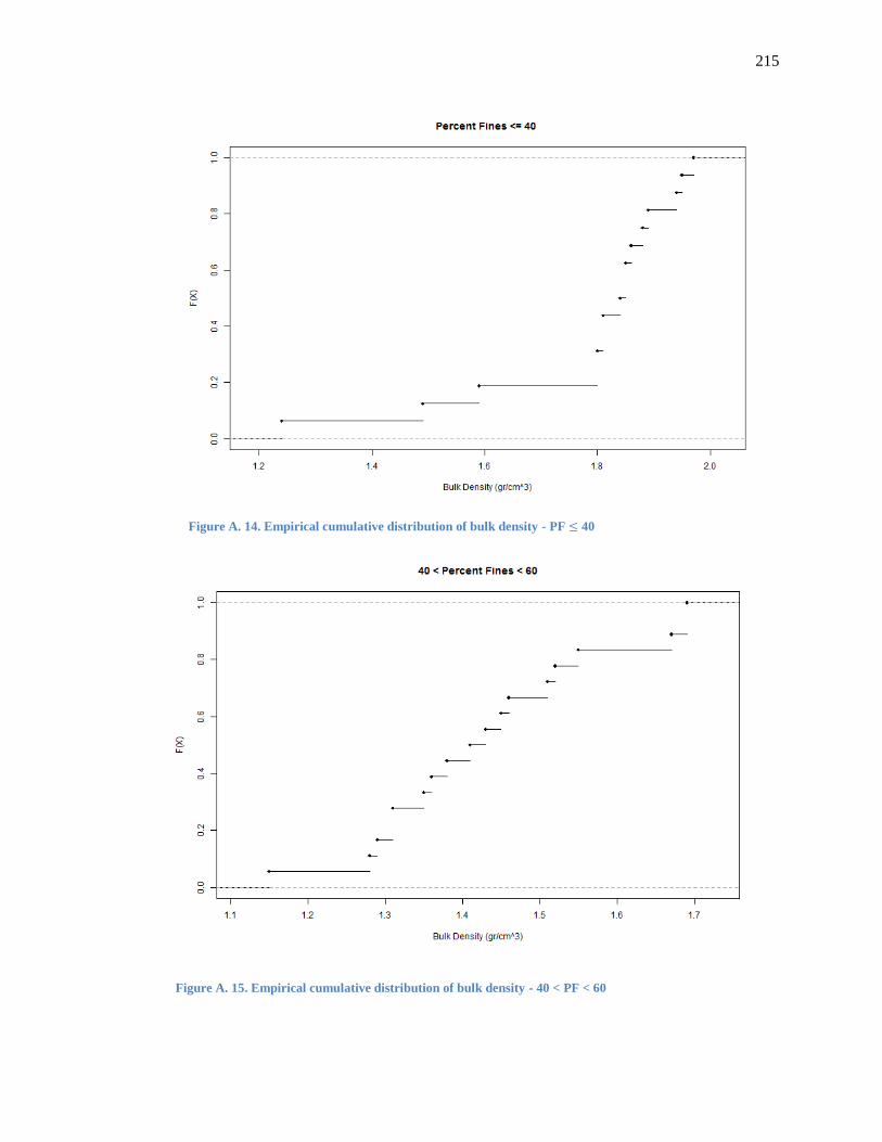
215

Figure A. 14. Empirical cumulative distribution of bulk density - PF 40

Figure A. 15. Empirical cumulative distribution of bulk density - 40 < PF < 60

216

Figure A. 16. Empirical cumulative distribution of organic content - PF ≥ 60

Figure A. 17. Empirical cumulative distribution of organic content - PF ≤ 40

217

Figure A. 18. Empirical cumulative distribution of organic content - 40 < PF < 60

Figure A. 19. Empirical cumulative distribution of water content - PF ≥ 60

218

Figure A. 20. Empirical cumulative distribution of water content - PF ≤ 40

Figure A. 21. Empirical cumulative distribution of water content - 40 < PF < 60

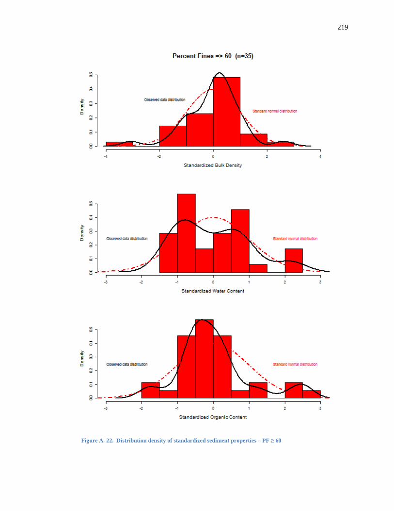
219

Figure A. 22. Distribution density of standardized sediment properties – PF ≥ 60

220

Figure A. 23. Distribution density of standardized sediment properties – PF ≤ 40

221

Figure A. 24. Distribution density of standardized sediment properties – 40 < PF < 60

222

Figure A. 25. Q-Q plot of sediment properties – PF ≥ 60

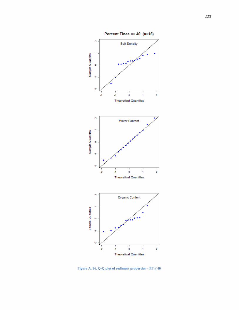
223

Figure A. 26. Q-Q plot of sediment properties – PF ≤ 40

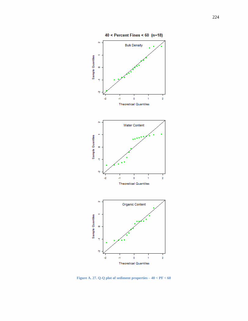
224

Figure A. 27. Q-Q plot of sediment properties – 40 < PF < 60

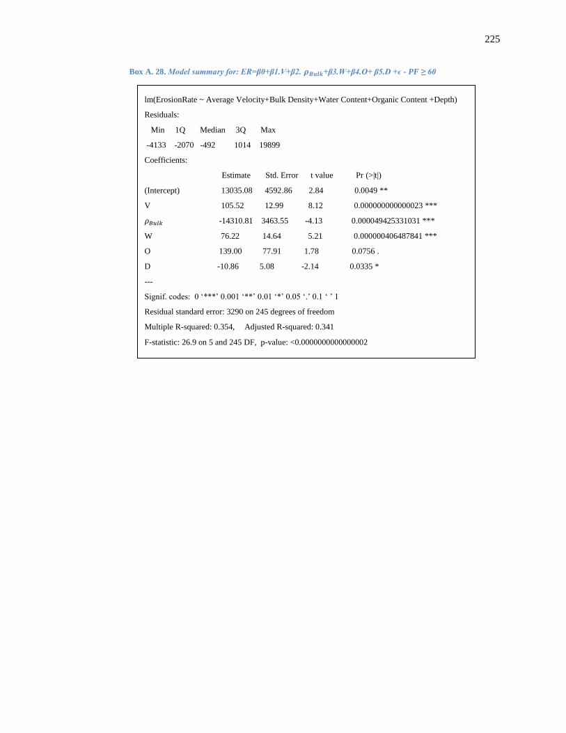
225

Box A. 28. Model summary for: ER=β0+β1.V+β2. +β3.W+β4.O+ β5.D +ϵ - PF ≥ 60

lm(ErosionRate ~ Average Velocity+Bulk Density+Water Content+Organic Content +Depth)

Residuals:

Min 1Q Median 3Q Max

-4133 -2070 -492 1014 19899

Coefficients:

Estimate Std. Error t value Pr (>|t|)

(Intercept) 13035.08 4592.86 2.84 0.0049 **

V 105.52 12.99 8.12 0.000000000000023 ***

-14310.81 3463.55 -4.13 0.000049425331031 ***

W 76.22 14.64 5.21 0.000000406487841 ***

O 139.00 77.91 1.78 0.0756 .

D -10.86 5.08 -2.14 0.0335 *

---

Signif. codes: 0 ‘***’ 0.001 ‘**’ 0.01 ‘*’ 0.05 ‘.’ 0.1 ‘ ’ 1

Residual standard error: 3290 on 245 degrees of freedom

Multiple R-squared: 0.354, Adjusted R-squared: 0.341

F-statistic: 26.9 on 5 and 245 DF, p-value: <0.0000000000000002

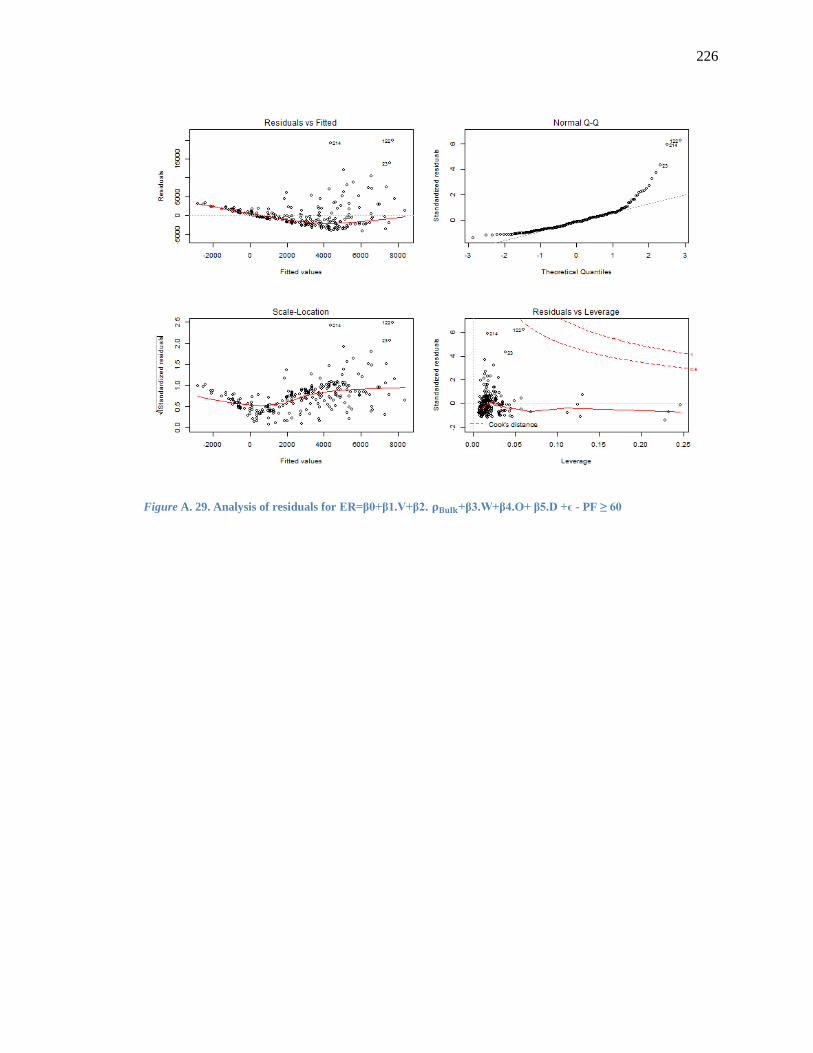
226

Figure A. 29. Analysis of residuals for ER=β0+β1.V+β2. +β3.W+β4.O+ β5.D +ϵ - PF ≥ 60

227

FigureA. 30. Frequency distribution of the predicted erosion rates with log-normal distribution for:

ER=β0+β1.V+β2. +β3.W+β4.O+ β5.D +ϵ - PF ≥ 60

Box A. 31. Model summary for: - 40 < PF < 60

lm(Erosion Rate ~ AverageVelocity+Depth)

Residuals:

Min 1Q Median 3Q Max

-5416 -2781 -1447 1612 19068

Coefficients:

Estimate Std. Error t value Pr (>|t|)

(Intercept) 1965.72 1314.12 1.50 0.14

V 118.70 28.83 4.12 0.00008299 ***

D -45.39 7.99 -5.68 0.00000015 ***

---

Signif. codes: 0 ‘***’ 0.001 ‘**’ 0.01 ‘*’ 0.05 ‘.’ 0.1 ‘ ’ 1

Residual standard error: 4490 on 93 degrees of freedom

Multiple R-squared: 0.275, Adjusted R-squared: 0.26

F-statistic: 17.7 on 2 and 93 DF, p-value: 0.000000316

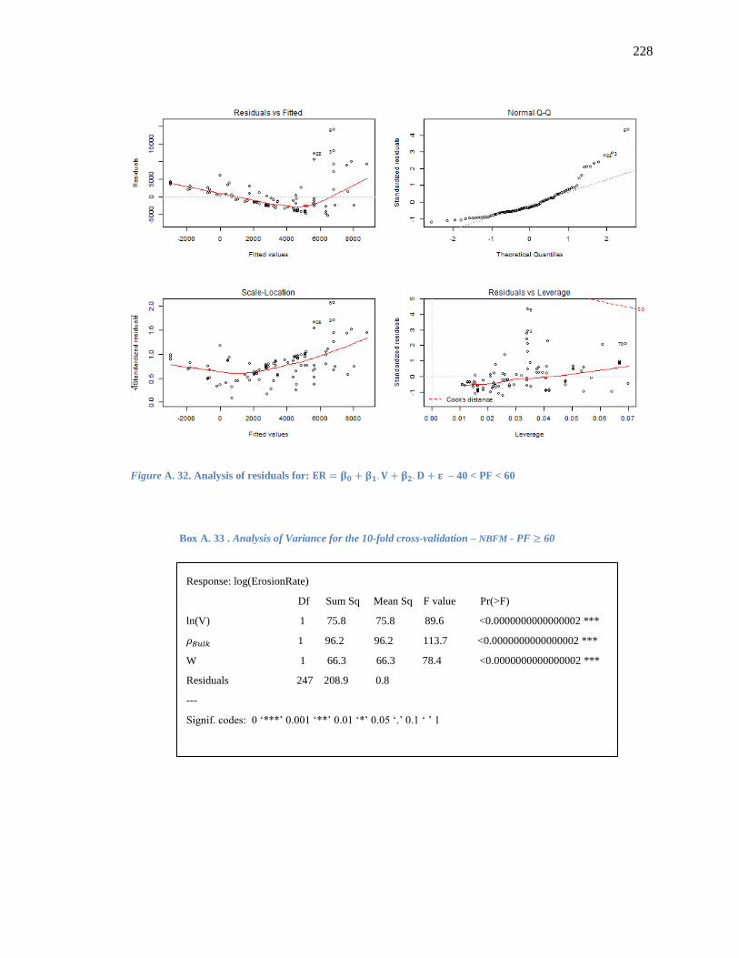
228

Figure A. 32. Analysis of residuals for: – 40 < PF < 60

Box A. 33 . Analysis of Variance for the 10-fold cross-validation – NBFM - PF 60

Response: log(ErosionRate)

Df Sum Sq Mean Sq F value Pr(>F)

ln(V) 1 75.8 75.8 89.6 <0.0000000000000002 ***

1 96.2 96.2 113.7 <0.0000000000000002 ***

W 1 66.3 66.3 78.4 <0.0000000000000002 ***

Residuals 247 208.9 0.8

---

Signif. codes: 0 ‘***’ 0.001 ‘**’ 0.01 ‘*’ 0.05 ‘.’ 0.1 ‘ ’ 1

229

BoxA. 34. Analysis of Variance for the 10-fold cross-validation - - PF 40

Figure A. 35. Observed erosion rates (cm/s) for different classes of sediment size

(ESETM). The minimum erosion rate values reported by Borrowman et al. (2006)

Response: log(ErosionRate)

Df Sum Sq Mean Sq F value Pr(>F)

V 1 43.9 43.9 42.3 0.000000093 ***

1 0.1 0.1 0.1 0.76

O 1 24.4 24.4 23.5 0.000019211 ***

Residuals 40 41.5 1.0

---

Signif. codes: 0 ‘***’ 0.001 ‘**’ 0.01 ‘*’ 0.05 ‘.’ 0.1 ‘ ’ 1

230

Figure A. 36. Frequency distribution of Erosion Rate (mm/hour) for different classes of sediment size

Erosion Rate (mm/hour)

231

APPENDIX B

Test results

232

Test Specifications Erosion Test Results Properties

# D

a

y Core Test Test ID Step

V

Duration (min)

WL

(gr)

ER

Depth

(mm)

(

W

(%)

O

(%)

(Pa) Gs

%

Fines

LL

(%)

PL

(%) PI

1 1 1 1 021612-020112-C1-R1-S1 1 16.74 5 0.08 2057 0 1.19 NA NA 0.12 NA NA NA NA NA

2 1 1 1 021612-020112-C1-R1-S1 2 16.42 5 0.13 3236 0 1.19 NA NA 0.12 NA NA NA NA NA

3 1 1 1 021612-020112-C1-R1-S1 3 16.40 10 0.05 622 0 1.19 NA NA 0.12 NA NA NA NA NA

4 1 1 2 021612-020112-C1-R1-S2 1 16.39 5 0.1 2385 0 1.2 NA NA 0.12 NA NA NA NA NA

5 1 1 2 021612-020112-C1-R1-S2 2 16.59 5 0.09 2146 0 1.2 NA NA 0.12 NA NA NA NA NA

6 1 1 2 021612-020112-C1-R1-S2 3 16.56 10 0.306 3649 0 1.2 NA NA 0.12 NA NA NA NA NA

7 1 1 2 021612-020112-C1-R1-S2 4 16.29 10 0.07 835 0 1.2 NA NA 0.12 NA NA NA NA NA

8 1 1 2 021612-020112-C1-R1-S2 5 19.33 10 0.37 4412 0 1.2 NA NA 0.16 NA NA NA NA NA

9 1 1 2 021612-020112-C1-R1-S2 6 19.65 10 0.35 4173 0 1.2 NA NA 0.16 NA NA NA NA NA

10 1 1 2 021612-020112-C1-R1-S2 7 19.59 10 0.13 1550 0 1.2 NA NA 0.16 NA NA NA NA NA

11 1 1 3 021712-020112-C1-R2-S1 1 16.41 5 0.2 5471 18 1.17 NA NA 0.12 NA NA NA NA NA

12 1 1 3 021712-020112-C1-R2-S1 2 16.38 5 0.13 3556 18 1.17 NA NA 0.12 NA NA NA NA NA

13 1 1 3 021712-020112-C1-R2-S1 3 16.10 10 0.09 1231 18 1.17 NA NA 0.12 NA NA NA NA NA

14 1 1 4 021712-020112-C1-R2-S2 1 16.28 5 0.06 2073 18 1.13 NA NA 0.12 NA NA NA NA NA

15 1 1 4 021712-020112-C1-R2-S2 2 16.09 5 0.04 1382 18 1.13 NA NA 0.12 NA NA NA NA NA

16 1 1 4 021712-020112-C1-R2-S2 3 15.90 10 0.04 691 18 1.13 NA NA 0.1 NA NA NA NA NA

17 1 1 5 022012-020112-C1-R3-S1 1 15.88 5 0.16 3983 38 1.19 NA NA 0.11 NA NA NA NA NA

18 1 1 5 022012-020112-C1-R3-S1 2 15.90 5 0.01 249 38 1.19 NA NA 0.11 NA NA NA NA NA

19 1 1 5 022012-020112-C1-R3-S1 3 15.86 10 0.02 249 38 1.19 NA NA 0.11 NA NA NA NA NA

20 1 1 5 022012-020112-C1-R3-S1 4 21.20 5 0.39 9709 38 1.19 NA NA 0.19 NA NA NA NA NA

21 1 1 5 022012-020112-C1-R3-S1 5 21.31 5 0.16 3983 38 1.19 NA NA 0.19 NA NA NA NA NA

22 1 1 5 022012-020112-C1-R3-S1 6 21.18 5 0.21 5228 38 1.19 NA NA 0.19 NA NA NA NA NA

23 1 1 6 022012-020112-C1-R4-S1 1 15.96 5 0.11 2425 55 1.22 NA NA 0.11 NA NA NA NA NA

24 1 1 6 022012-020112-C1-R4-S1 2 15.89 5 0.1 2204 55 1.22 NA NA 0.11 NA NA NA NA NA

25 1 1 6 022012-020112-C1-R4-S1 3 15.61 10 -0.05 -551 55 1.22 NA NA 0.11 NA NA NA NA NA

26 1 1 6 022012-020112-C1-R4-S1 4 21.21 5 0.22 4849 55 1.22 NA NA 0.19 NA NA NA NA NA

27 1 1 6 022012-020112-C1-R4-S1 5 21.39 5 0.12 2645 55 1.22 NA NA 0.19 NA NA NA NA NA

28 1 1 6 022012-020112-C1-R4-S1 6 21.43 10 0.15 1653 55 1.22 NA NA 0.19 NA NA NA NA NA

29 1 1 7 022112-020112-C1-R4-S2 1 15.68 5 -0.08 -1992 55 1.19 NA NA 0.1 NA NA NA NA NA

30 1 1 7 022112-020112-C1-R4-S2 2 15.72 5 0.22 5477 55 1.19 NA NA 0.1 NA NA NA NA NA

233

Test Specifications Erosion Test Results Properties

# D

a

y Core Test Test ID Step

V

Duration (min)

WL

(gr)

ER

Depth

(mm)

(

W

(%)

O

(%)

(Pa) Gs

%

Fines

LL

(%)

PL

(%) PI

31 1 1 7 022112-020112-C1-R4-S2 3 15.46 10 0.04 498 55 1.19 NA NA 0.1 NA NA NA NA NA

32 1 1 7 022112-020112-C1-R4-S2 4 21.34 5 0.23 5726 55 1.19 NA NA 0.18 NA NA NA NA NA

33 1 1 7 022112-020112-C1-R4-S2 5 21.14 5 0.03 747 55 1.19 NA NA 0.18 NA NA NA NA NA

34 1 1 7 022112-020112-C1-R4-S2 6 21.01 10 0.24 2987 55 1.19 NA NA 0.18 NA NA NA NA NA

35 1 1 8 022112-020112-C1-R5-S1 1 15.54 5 0.06 1156 119 1.26 NA NA 0.1 NA NA NA NA NA

36 1 1 8 022112-020112-C1-R5-S1 2 15.28 5 0.07 1348 119 1.26 NA NA 0.1 NA NA NA NA NA

37 1 1 8 022112-020112-C1-R5-S1 3 15.33 10 0.15 1445 119 1.26 NA NA 0.1 NA NA NA NA NA

38 1 1 8 022112-020112-C1-R5-S1 4 20.47 5 0.318 6125 119 1.26 NA NA 0.17 NA NA NA NA NA

39 1 1 8 022112-020112-C1-R5-S1 5 21.09 5 0.03 578 119 1.26 NA NA 0.18 NA NA NA NA NA

40 1 1 8 022112-020112-C1-R5-S1 6 20.88 10 0.18 1734 119 1.26 NA NA 0.17 NA NA NA NA NA

41 1 1 9 022112-020112-C1-R6-S1 1 14.99 5 0.02 547 188 1.17 NA NA 0.09 NA NA NA NA NA

42 1 1 9 022112-020112-C1-R6-S1 2 15.18 5 -0.01 -274 188 1.17 NA NA 0.1 NA NA NA NA NA

43 1 1 9 022112-020112-C1-R6-S1 3 15.04 10 0 0 188 1.17 NA NA 0.1 NA NA NA NA NA

44 1 1 9 022112-020112-C1-R6-S1 4 20.41 5 0.05 1368 188 1.17 NA NA 0.17 NA NA NA NA NA

45 1 1 9 022112-020112-C1-R6-S1 5 20.56 5 0.03 821 188 1.17 NA NA 0.17 NA NA NA NA NA

46 1 1 9 022112-020112-C1-R6-S1 6 20.65 10 -0.01 -137 188 1.17 NA NA 0.17 NA NA NA NA NA

47 1 2 1 022212-020112-C2-R1-S1 1 14.74 5 0.16 5528 0 1.13 NA NA 0.09 NA NA NA NA NA

48 1 2 1 022212-020112-C2-R1-S1 2 15.00 5 -0.02 -691 0 1.13 NA NA 0.1 NA NA NA NA NA

49 1 2 1 022212-020112-C2-R1-S1 3 14.48 10 0.04 691 0 1.13 NA NA 0.09 NA NA NA NA NA

50 1 2 1 022212-020112-C2-R1-S1 4 20.17 5 0.16 5528 0 1.13 NA NA 0.17 NA NA NA NA NA

51 1 2 1 022212-020112-C2-R1-S1 5 20.14 5 0.07 2418 0 1.13 NA NA 0.17 NA NA NA NA NA

52 1 2 1 022212-020112-C2-R1-S1 6 20.28 10 0.11 1900 0 1.13 NA NA 0.17 NA NA NA NA NA

53 1 2 2 022212-020112-C2-R1-S2 1 14.57 5 0.1 3237 0 1.14 NA NA 0.09 NA NA NA NA NA

54 1 2 2 022212-020112-C2-R1-S2 2 14.68 5 0.1 3237 0 1.14 NA NA 0.09 NA NA NA NA NA

55 1 2 2 022212-020112-C2-R1-S2 3 14.32 10 0.07 1133 0 1.14 NA NA 0.09 NA NA NA NA NA

56 1 2 2 022212-020112-C2-R1-S2 4 19.80 5 0.43 13917 0 1.14 NA NA 0.16 NA NA NA NA NA

57 1 2 2 022212-020112-C2-R1-S2 5 19.99 5 0.12 3884 0 1.14 NA NA 0.16 NA NA NA NA NA

58 1 2 2 022212-020112-C2-R1-S2 6 20.16 10 0.2 3237 0 1.14 NA NA 0.17 NA NA NA NA NA

59 1 2 2 022212-020112-C2-R1-S2 7 20.13 10 0.08 1295 0 1.14 NA NA 0.17 NA NA NA NA NA

60 1 2 2 022212-020112-C2-R1-S2 8 22.93 10 -1.56 -25245 0 1.14 NA NA 0.2 NA NA NA NA NA

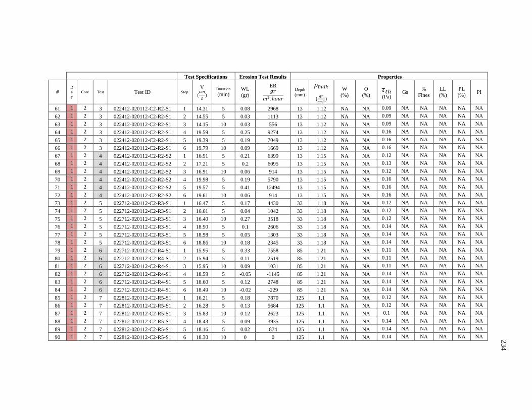
234

Test Specifications Erosion Test Results Properties

# D

a

y Core Test Test ID Step

V

Duration (min)

WL

(gr)

ER

Depth

(mm)

(

W

(%)

O

(%)

(Pa) Gs

%

Fines

LL

(%)

PL

(%) PI

61 1 2 3 022412-020112-C2-R2-S1 1 14.31 5 0.08 2968 13 1.12 NA NA 0.09 NA NA NA NA NA

62 1 2 3 022412-020112-C2-R2-S1 2 14.55 5 0.03 1113 13 1.12 NA NA 0.09 NA NA NA NA NA

63 1 2 3 022412-020112-C2-R2-S1 3 14.15 10 0.03 556 13 1.12 NA NA 0.09 NA NA NA NA NA

64 1 2 3 022412-020112-C2-R2-S1 4 19.59 5 0.25 9274 13 1.12 NA NA 0.16 NA NA NA NA NA

65 1 2 3 022412-020112-C2-R2-S1 5 19.39 5 0.19 7049 13 1.12 NA NA 0.16 NA NA NA NA NA

66 1 2 3 022412-020112-C2-R2-S1 6 19.79 10 0.09 1669 13 1.12 NA NA 0.16 NA NA NA NA NA

67 1 2 4 022412-020112-C2-R2-S2 1 16.91 5 0.21 6399 13 1.15 NA NA 0.12 NA NA NA NA NA

68 1 2 4 022412-020112-C2-R2-S2 2 17.21 5 0.2 6095 13 1.15 NA NA 0.13 NA NA NA NA NA

69 1 2 4 022412-020112-C2-R2-S2 3 16.91 10 0.06 914 13 1.15 NA NA 0.12 NA NA NA NA NA

70 1 2 4 022412-020112-C2-R2-S2 4 19.98 5 0.19 5790 13 1.15 NA NA 0.16 NA NA NA NA NA

71 1 2 4 022412-020112-C2-R2-S2 5 19.57 5 0.41 12494 13 1.15 NA NA 0.16 NA NA NA NA NA

72 1 2 4 022412-020112-C2-R2-S2 6 19.61 10 0.06 914 13 1.15 NA NA 0.16 NA NA NA NA NA

73 1 2 5 022712-020112-C2-R3-S1 1 16.47 5 0.17 4430 33 1.18 NA NA 0.12 NA NA NA NA NA

74 1 2 5 022712-020112-C2-R3-S1 2 16.61 5 0.04 1042 33 1.18 NA NA 0.12 NA NA NA NA NA

75 1 2 5 022712-020112-C2-R3-S1 3 16.40 10 0.27 3518 33 1.18 NA NA 0.12 NA NA NA NA NA

76 1 2 5 022712-020112-C2-R3-S1 4 18.90 5 0.1 2606 33 1.18 NA NA 0.14 NA NA NA NA NA

77 1 2 5 022712-020112-C2-R3-S1 5 18.98 5 0.05 1303 33 1.18 NA NA 0.14 NA NA NA NA NA

78 1 2 5 022712-020112-C2-R3-S1 6 18.86 10 0.18 2345 33 1.18 NA NA 0.14 NA NA NA NA NA

79 1 2 6 022712-020112-C2-R4-S1 1 15.95 5 0.33 7558 85 1.21 NA NA 0.11 NA NA NA NA NA

80 1 2 6 022712-020112-C2-R4-S1 2 15.94 5 0.11 2519 85 1.21 NA NA 0.11 NA NA NA NA NA

81 1 2 6 022712-020112-C2-R4-S1 3 15.95 10 0.09 1031 85 1.21 NA NA 0.11 NA NA NA NA NA

82 1 2 6 022712-020112-C2-R4-S1 4 18.59 5 -0.05 -1145 85 1.21 NA NA 0.14 NA NA NA NA NA

83 1 2 6 022712-020112-C2-R4-S1 5 18.60 5 0.12 2748 85 1.21 NA NA 0.14 NA NA NA NA NA

84 1 2 6 022712-020112-C2-R4-S1 6 18.49 10 -0.02 -229 85 1.21 NA NA 0.14 NA NA NA NA NA

85 1 2 7 022812-020112-C2-R5-S1 1 16.21 5 0.18 7870 125 1.1 NA NA 0.12 NA NA NA NA NA

86 1 2 7 022812-020112-C2-R5-S1 2 16.28 5 0.13 5684 125 1.1 NA NA 0.12 NA NA NA NA NA

87 1 2 7 022812-020112-C2-R5-S1 3 15.83 10 0.12 2623 125 1.1 NA NA 0.1 NA NA NA NA NA

88 1 2 7 022812-020112-C2-R5-S1 4 18.43 5 0.09 3935 125 1.1 NA NA 0.14 NA NA NA NA NA

89 1 2 7 022812-020112-C2-R5-S1 5 18.16 5 0.02 874 125 1.1 NA NA 0.14 NA NA NA NA NA

90 1 2 7 022812-020112-C2-R5-S1 6 18.30 10 0 0 125 1.1 NA NA 0.14 NA NA NA NA NA

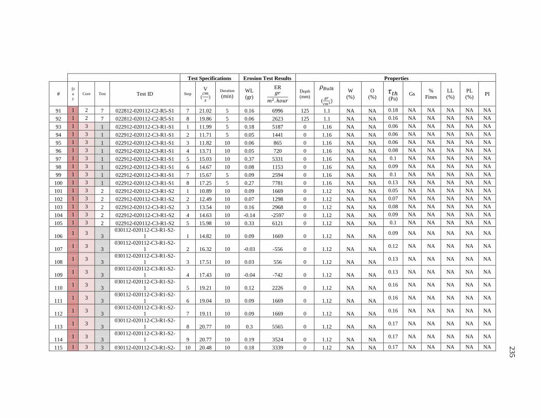
235

Test Specifications Erosion Test Results Properties

# D

a

y Core Test Test ID Step

V

Duration (min)

WL

(gr)

ER

Depth

(mm)

(

W

(%)

O

(%)

(Pa) Gs

%

Fines

LL

(%)

PL

(%) PI

91 1 2 7 022812-020112-C2-R5-S1 7 21.02 5 0.16 6996 125 1.1 NA NA 0.18 NA NA NA NA NA

92 1 2 7 022812-020112-C2-R5-S1 8 19.86 5 0.06 2623 125 1.1 NA NA 0.16 NA NA NA NA NA

93 1 3 1 022912-020112-C3-R1-S1 1 11.99 5 0.18 5187 0 1.16 NA NA 0.06 NA NA NA NA NA

94 1 3 1 022912-020112-C3-R1-S1 2 11.71 5 0.05 1441 0 1.16 NA NA 0.06 NA NA NA NA NA

95 1 3 1 022912-020112-C3-R1-S1 3 11.82 10 0.06 865 0 1.16 NA NA 0.06 NA NA NA NA NA

96 1 3 1 022912-020112-C3-R1-S1 4 13.71 10 0.05 720 0 1.16 NA NA 0.08 NA NA NA NA NA

97 1 3 1 022912-020112-C3-R1-S1 5 15.03 10 0.37 5331 0 1.16 NA NA 0.1 NA NA NA NA NA

98 1 3 1 022912-020112-C3-R1-S1 6 14.67 10 0.08 1153 0 1.16 NA NA 0.09 NA NA NA NA NA

99 1 3 1 022912-020112-C3-R1-S1 7 15.67 5 0.09 2594 0 1.16 NA NA 0.1 NA NA NA NA NA

100 1 3 1 022912-020112-C3-R1-S1 8 17.25 5 0.27 7781 0 1.16 NA NA 0.13 NA NA NA NA NA

101 1 3 2 022912-020112-C3-R1-S2 1 10.89 10 0.09 1669 0 1.12 NA NA 0.05 NA NA NA NA NA

102 1 3 2 022912-020112-C3-R1-S2 2 12.49 10 0.07 1298 0 1.12 NA NA 0.07 NA NA NA NA NA

103 1 3 2 022912-020112-C3-R1-S2 3 13.54 10 0.16 2968 0 1.12 NA NA 0.08 NA NA NA NA NA

104 1 3 2 022912-020112-C3-R1-S2 4 14.63 10 -0.14 -2597 0 1.12 NA NA 0.09 NA NA NA NA NA

105 1 3 2 022912-020112-C3-R1-S2 5 15.98 10 0.33 6121 0 1.12 NA NA 0.1 NA NA NA NA NA

106 1 3

3 030112-020112-C3-R1-S2-

1 1 14.82 10 0.09 1669 0 1.12 NA NA 0.09 NA NA NA NA NA

107 1 3

3

030112-020112-C3-R1-S2-

1 2 16.32 10 -0.03 -556 0 1.12 NA NA 0.12 NA NA NA NA NA

108 1 3

3

030112-020112-C3-R1-S2-

1 3 17.51 10 0.03 556 0 1.12 NA NA 0.13 NA NA NA NA NA

109 1 3

3

030112-020112-C3-R1-S2-

1 4 17.43 10 -0.04 -742 0 1.12 NA NA 0.13 NA NA NA NA NA

110 1 3

3 030112-020112-C3-R1-S2-

1 5 19.21 10 0.12 2226 0 1.12 NA NA 0.16 NA NA NA NA NA

111 1 3

3

030112-020112-C3-R1-S2-

1 6 19.04 10 0.09 1669 0 1.12 NA NA 0.16 NA NA NA NA NA

112 1 3

3 030112-020112-C3-R1-S2-

1 7 19.11 10 0.09 1669 0 1.12 NA NA 0.16 NA NA NA NA NA

113 1 3

3

030112-020112-C3-R1-S2-

1 8 20.77 10 0.3 5565 0 1.12 NA NA 0.17 NA NA NA NA NA

114 1 3

3

030112-020112-C3-R1-S2-

1 9 20.77 10 0.19 3524 0 1.12 NA NA 0.17 NA NA NA NA NA

115 1 3 3 030112-020112-C3-R1-S2- 10 20.48 10 0.18 3339 0 1.12 NA NA 0.17 NA NA NA NA NA

236

Test Specifications Erosion Test Results Properties

# D

a

y Core Test Test ID Step

V

Duration (min)

WL

(gr)

ER

Depth

(mm)

(

W

(%)

O

(%)

(Pa) Gs

%

Fines

LL

(%)

PL

(%) PI

1

116 1 3

3

030112-020112-C3-R1-S2-

1 11 20.31 10 0.07 1298 0 1.12 NA NA 0.17 NA NA NA NA NA

117 1 3

3

030112-020112-C3-R1-S2-

1 12 21.46 10 0.13 2411 0 1.12 NA NA 0.19 NA NA NA NA NA

118 1 3

4

0305012-020112-C3-R1-

S2-2 1 15.52 10 0.1 3511 0 1.06 NA NA 0.11 NA NA NA NA NA

119 1 3

4

0305012-020112-C3-R1-

S2-2 2 18.17 10 0.06 2107 0 1.06 NA NA 0.14 NA NA NA NA NA

120 1 3

4

0305012-020112-C3-R1-

S2-2 3 21.44 10 0.03 1053 0 1.06 NA NA 0.19 NA NA NA NA NA

121 1 3

4

0305012-020112-C3-R1-

S2-2 4 24.07 10 0.28 9831 0 1.06 NA NA 0.24 NA NA NA NA NA

122 1 3

4 0305012-020112-C3-R1-

S2-2 5 24.21 10 0.11 3862 0 1.06 NA NA 0.24 NA NA NA NA NA

123 1 3

4

0305012-020112-C3-R1-

S2-2 6 25.35 10 0.07 2458 0 1.06 NA NA 0.25 NA NA NA NA NA

124 1 3 5 0305012-020112-C3-R2-S1 1 10.34 10 0.07 1009 10 1.16 NA NA 0.05 NA NA NA NA NA

125 1 3 5 0305012-020112-C3-R2-S1 2 10.41 10 0.03 432 10 1.16 NA NA 0.05 NA NA NA NA NA

126 1 3 5 0305012-020112-C3-R2-S1 3 12.50 10 -0.05 -720 10 1.16 NA NA 0.07 NA NA NA NA NA

127 1 3 5 0305012-020112-C3-R2-S1 4 13.45 10 0.09 1297 10 1.16 NA NA 0.08 NA NA NA NA NA

128 1 3 5 0305012-020112-C3-R2-S1 5 14.14 10 0.37 5331 10 1.16 NA NA 0.09 NA NA NA NA NA

129 1 3 5 0305012-020112-C3-R2-S1 6 15.28 10 0.09 1297 10 1.16 NA NA 0.11 NA NA NA NA NA

130 1 3 5 0305012-020112-C3-R2-S1 7 16.22 10 0.2 2882 10 1.16 NA NA 0.12 NA NA NA NA NA

131 1 3 5 0305012-020112-C3-R2-S1 8 16.61 10 0.11 1585 10 1.16 NA NA 0.12 NA NA NA NA NA

132 1 3 6 030612-020112-C3-R3-S1 1 10.11 10 0.1 1145 25 1.21 NA NA 0.05 NA NA NA NA NA

133 1 3 6 030612-020112-C3-R3-S1 2 11.69 10 0 0 25 1.21 NA NA 0.06 NA NA NA NA NA

134 1 3 6 030612-020112-C3-R3-S1 3 12.75 10 0.01 115 25 1.21 NA NA 0.07 NA NA NA NA NA

135 1 3 6 030612-020112-C3-R3-S1 4 13.48 10 0 0 25 1.21 NA NA 0.08 NA NA NA NA NA

136 1 3 6 030612-020112-C3-R3-S1 5 14.71 10 0.15 1718 25 1.21 NA NA 0.09 NA NA NA NA NA

137 1 3 6 030612-020112-C3-R3-S1 6 16.21 10 0.07 802 25 1.21 NA NA 0.12 NA NA NA NA NA

138 1 3 6 030612-020112-C3-R3-S1 7 17.39 10 0.2 2290 25 1.21 NA NA 0.13 NA NA NA NA NA

139 1 3 6 030612-020112-C3-R3-S1 8 18.82 10 0.07 802 25 1.21 NA NA 0.15 NA NA NA NA NA

237

Test Specifications Erosion Test Results Properties

# D

a

y Core Test Test ID Step

V

Duration (min)

WL

(gr)

ER

Depth

(mm)

(

W

(%)

O

(%)

(Pa) Gs

%

Fines

LL

(%)

PL

(%) PI

140 1 3 6 030612-020112-C3-R3-S1 9 19.73 10 0.06 687 25 1.21 NA NA 0.16 NA NA NA NA NA

141 1 3 6 030612-020112-C3-R3-S1 10 19.84 10 0.16 1832 25 1.21 NA NA 0.16 NA NA NA NA NA

142 1 3 7 030612-020112-C3-R3-S2 1 11.94 10 0.04 425 25 1.23 NA NA 0.06 NA NA NA NA NA

143 1 3 7 030612-020112-C3-R3-S2 2 12.73 10 0.1 1063 25 1.23 NA NA 0.07 NA NA NA NA NA

144 1 3 7 030612-020112-C3-R3-S2 3 14.30 10 0.26 2763 25 1.23 NA NA 0.09 NA NA NA NA NA

145 1 3 7 030612-020112-C3-R3-S2 4 15.36 10 0.05 531 25 1.23 NA NA 0.11 NA NA NA NA NA

146 1 3 7 030612-020112-C3-R3-S2 5 16.66 10 0.27 2870 25 1.23 NA NA 0.12 NA NA NA NA NA

147 1 3 8 030712-020112-C3-R4-S1 1 9.13 10 0.11 1093 55 1.25 NA NA 0.04 NA NA NA NA NA

148 1 3 8 030712-020112-C3-R4-S1 2 11.58 10 0.1 994 55 1.25 NA NA 0.06 NA NA NA NA NA

149 1 3 8 030712-020112-C3-R4-S1 3 13.85 10 0.02 199 55 1.25 NA NA 0.08 NA NA NA NA NA

150 1 3 8 030712-020112-C3-R4-S1 4 15.11 10 0.16 1590 55 1.25 NA NA 0.11 NA NA NA NA NA

151 1 3 8 030712-020112-C3-R4-S1 5 16.59 10 0.2 1987 55 1.25 NA NA 0.12 NA NA NA NA NA

152 1 3 8 030712-020112-C3-R4-S1 6 17.91 10 0.27 2683 55 1.25 NA NA 0.13 NA NA NA NA NA

153 1 3 8 030712-020112-C3-R4-S1 7 18.93 10 0.16 1590 55 1.25 NA NA 0.15 NA NA NA NA NA

154 1 3 8 030712-020112-C3-R4-S1 8 19.86 10 0.11 1093 55 1.25 NA NA 0.16 NA NA NA NA NA

155 1 3 8 030712-020112-C3-R4-S1 9 21.87 10 0.22 2186 55 1.25 NA NA 0.19 NA NA NA NA NA

156 1 3 9 030712-020112-C3-R5-S1 2 10.75 10 -0.01 -103 87 1.24 NA NA 0.05 NA NA NA NA NA

157 1 3 9 030712-020112-C3-R5-S1 3 13.23 10 -0.02 -205 87 1.24 NA NA 0.08 NA NA NA NA NA

158 1 3 9 030712-020112-C3-R5-S1 4 14.22 10 0.06 616 87 1.24 NA NA 0.09 NA NA NA NA NA

159 1 3 9 030712-020112-C3-R5-S1 5 15.72 10 0.08 821 87 1.24 NA NA 0.11 NA NA NA NA NA

160 1 3 9 030712-020112-C3-R5-S1 6 17.13 10 -0.03 -308 87 1.24 NA NA 0.13 NA NA NA NA NA

161 1 3 9 030712-020112-C3-R5-S1 7 19.51 10 0.11 1129 87 1.24 NA NA 0.16 NA NA NA NA NA

162 1 3 9 030712-020112-C3-R5-S1 8 20.17 10 0.07 719 87 1.24 NA NA 0.17 NA NA NA NA NA

163 1 3 9 030712-020112-C3-R5-S1 9 22.52 10 0.1 1027 87 1.24 NA NA 0.2 NA NA NA NA NA

164 2 1 1 032012-031912-C1-R1-S1 1 15.17 10 0.36 3697 0 1.24 NA NA 0.1 NA NA NA NA NA

165 2 1 1 032012-031912-C1-R1-S1 2 15.52 10 -0.09 -924 0 1.24 NA NA 0.1 NA NA NA NA NA

166 2 1 1 032012-031912-C1-R1-S1 3 16.70 10 0.32 3286 0 1.24 NA NA 0.11 NA NA NA NA NA

167 2 1 1 032012-031912-C1-R1-S1 4 17.64 10 0.1 1027 0 1.24 NA NA 0.13 NA NA NA NA NA

168 2 1 1 032012-031912-C1-R1-S1 5 19.18 10 0.09 924 0 1.24 NA NA 0.15 NA NA NA NA NA

169 2 1 1 032012-031912-C1-R1-S1 6 20.28 10 0.08 821 0 1.24 NA NA 0.17 NA NA NA NA NA

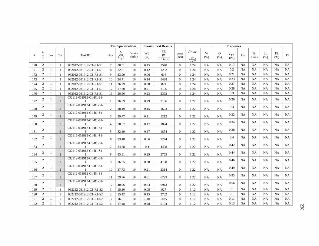
238

Test Specifications Erosion Test Results Properties

# D

a

y Core Test Test ID Step

V

Duration (min)

WL

(gr)

ER

Depth

(mm)

(

W

(%)

O

(%)

(Pa) Gs

%

Fines

LL

(%)

PL

(%) PI

170 2 1 1 032012-031912-C1-R1-S1 7 20.51 10 0.15 1540 0 1.24 NA NA 0.17 NA NA NA NA NA

171 2 1 1 032012-031912-C1-R1-S1 8 22.81 10 0.12 1232 0 1.24 NA NA 0.2 NA NA NA NA NA

172 2 1 1 032012-031912-C1-R1-S1 9 23.90 10 0.06 616 0 1.24 NA NA 0.21 NA NA NA NA NA

173 2 1 1 032012-031912-C1-R1-S1 10 24.71 10 0.14 1438 0 1.24 NA NA 0.23 NA NA NA NA NA

174 2 1 1 032012-031912-C1-R1-S1 11 26.29 10 0.08 821 0 1.24 NA NA 0.27 NA NA NA NA NA

175 2 1 1 032012-031912-C1-R1-S1 12 27.70 10 0.21 2156 0 1.24 NA NA 0.28 NA NA NA NA NA

176 2 1 1 032012-031912-C1-R1-S1 13 28.66 10 0.23 2362 0 1.24 NA NA 0.3 NA NA NA NA NA

177 2 1

2

032112-031912-C1-R1-S1-

1 1 26.89 10 0.29 3196 0 1.22 NA NA 0.26 NA NA NA NA NA

178 2 1

2

032112-031912-C1-R1-S1-

1 2 28.19 10 0.15 1653 0 1.22 NA NA 0.3 NA NA NA NA NA

179 2 1

2

032112-031912-C1-R1-S1-

1 3 29.47 10 0.11 1212 0 1.22 NA NA 0.32 NA NA NA NA NA

180 2 1

2

032112-031912-C1-R1-S1-

1 4 30.57 10 0.17 1874 0 1.22 NA NA 0.34 NA NA NA NA NA

181 2 1

2

032112-031912-C1-R1-S1-

1 5 32.19 10 0.17 1874 0 1.22 NA NA 0.38 NA NA NA NA NA

182 2 1

2

032112-031912-C1-R1-S1-

1 6 33.48 10 0.66 7274 0 1.22 NA NA 0.4 NA NA NA NA NA

183 2 1

2

032112-031912-C1-R1-S1-

1 7 34.78 10 0.4 4408 0 1.22 NA NA 0.42 NA NA NA NA NA

184 2 1

2

032112-031912-C1-R1-S1-

1 8 35.31 10 0.25 2755 0 1.22 NA NA 0.44 NA NA NA NA NA

185 2 1

2

032112-031912-C1-R1-S1-

1 9 36.35 10 0.38 4188 0 1.22 NA NA 0.46 NA NA NA NA NA

186 2 1

2 032112-031912-C1-R1-S1-

1 10 37.73 10 0.21 2314 0 1.22 NA NA 0.49 NA NA NA NA NA

187 2 1

2

032112-031912-C1-R1-S1-

1 11 39.76 10 0.61 6723 0 1.22 NA NA 0.53 NA NA NA NA NA

188 2 1

2 032112-031912-C1-R1-S1-

1 12 40.96 10 0.63 6943 0 1.22 NA NA 0.56 NA NA NA NA NA

189 2 1 3 032212-031912-C1-R1-S2 1 15.10 10 0.05 927 0 1.12 NA NA 0.1 NA NA NA NA NA

190 2 1 3 032212-031912-C1-R1-S2 2 15.42 10 0.15 2782 0 1.12 NA NA 0.1 NA NA NA NA NA

191 2 1 3 032212-031912-C1-R1-S2 3 16.61 10 -0.01 -185 0 1.12 NA NA 0.11 NA NA NA NA NA

192 2 1 3 032212-031912-C1-R1-S2 4 17.48 10 0.28 5194 0 1.12 NA NA 0.13 NA NA NA NA NA

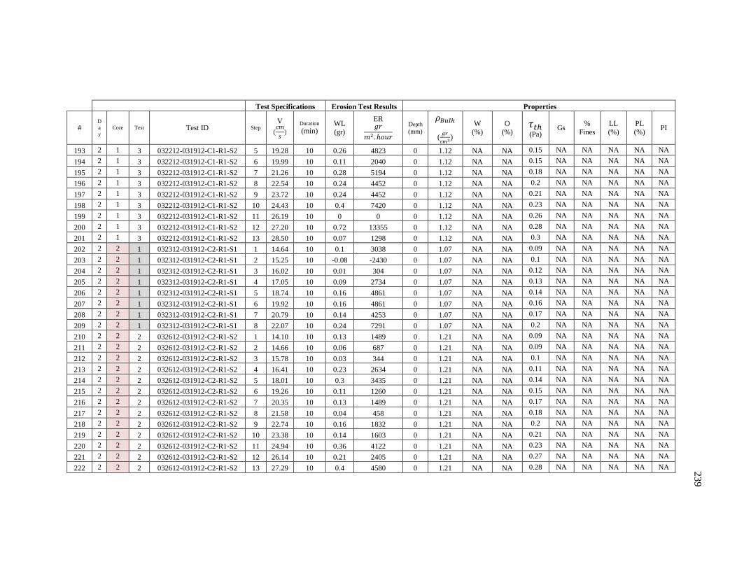
239

Test Specifications Erosion Test Results Properties

# D

a

y Core Test Test ID Step

V

Duration (min)

WL

(gr)

ER

Depth

(mm)

(

W

(%)

O

(%)

(Pa) Gs

%

Fines

LL

(%)

PL

(%) PI

193 2 1 3 032212-031912-C1-R1-S2 5 19.28 10 0.26 4823 0 1.12 NA NA 0.15 NA NA NA NA NA

194 2 1 3 032212-031912-C1-R1-S2 6 19.99 10 0.11 2040 0 1.12 NA NA 0.15 NA NA NA NA NA

195 2 1 3 032212-031912-C1-R1-S2 7 21.26 10 0.28 5194 0 1.12 NA NA 0.18 NA NA NA NA NA

196 2 1 3 032212-031912-C1-R1-S2 8 22.54 10 0.24 4452 0 1.12 NA NA 0.2 NA NA NA NA NA

197 2 1 3 032212-031912-C1-R1-S2 9 23.72 10 0.24 4452 0 1.12 NA NA 0.21 NA NA NA NA NA

198 2 1 3 032212-031912-C1-R1-S2 10 24.43 10 0.4 7420 0 1.12 NA NA 0.23 NA NA NA NA NA

199 2 1 3 032212-031912-C1-R1-S2 11 26.19 10 0 0 0 1.12 NA NA 0.26 NA NA NA NA NA

200 2 1 3 032212-031912-C1-R1-S2 12 27.20 10 0.72 13355 0 1.12 NA NA 0.28 NA NA NA NA NA

201 2 1 3 032212-031912-C1-R1-S2 13 28.50 10 0.07 1298 0 1.12 NA NA 0.3 NA NA NA NA NA

202 2 2 1 032312-031912-C2-R1-S1 1 14.64 10 0.1 3038 0 1.07 NA NA 0.09 NA NA NA NA NA

203 2 2 1 032312-031912-C2-R1-S1 2 15.25 10 -0.08 -2430 0 1.07 NA NA 0.1 NA NA NA NA NA

204 2 2 1 032312-031912-C2-R1-S1 3 16.02 10 0.01 304 0 1.07 NA NA 0.12 NA NA NA NA NA

205 2 2 1 032312-031912-C2-R1-S1 4 17.05 10 0.09 2734 0 1.07 NA NA 0.13 NA NA NA NA NA

206 2 2 1 032312-031912-C2-R1-S1 5 18.74 10 0.16 4861 0 1.07 NA NA 0.14 NA NA NA NA NA

207 2 2 1 032312-031912-C2-R1-S1 6 19.92 10 0.16 4861 0 1.07 NA NA 0.16 NA NA NA NA NA

208 2 2 1 032312-031912-C2-R1-S1 7 20.79 10 0.14 4253 0 1.07 NA NA 0.17 NA NA NA NA NA

209 2 2 1 032312-031912-C2-R1-S1 8 22.07 10 0.24 7291 0 1.07 NA NA 0.2 NA NA NA NA NA

210 2 2 2 032612-031912-C2-R1-S2 1 14.10 10 0.13 1489 0 1.21 NA NA 0.09 NA NA NA NA NA

211 2 2 2 032612-031912-C2-R1-S2 2 14.66 10 0.06 687 0 1.21 NA NA 0.09 NA NA NA NA NA

212 2 2 2 032612-031912-C2-R1-S2 3 15.78 10 0.03 344 0 1.21 NA NA 0.1 NA NA NA NA NA

213 2 2 2 032612-031912-C2-R1-S2 4 16.41 10 0.23 2634 0 1.21 NA NA 0.11 NA NA NA NA NA

214 2 2 2 032612-031912-C2-R1-S2 5 18.01 10 0.3 3435 0 1.21 NA NA 0.14 NA NA NA NA NA

215 2 2 2 032612-031912-C2-R1-S2 6 19.26 10 0.11 1260 0 1.21 NA NA 0.15 NA NA NA NA NA

216 2 2 2 032612-031912-C2-R1-S2 7 20.35 10 0.13 1489 0 1.21 NA NA 0.17 NA NA NA NA NA

217 2 2 2 032612-031912-C2-R1-S2 8 21.58 10 0.04 458 0 1.21 NA NA 0.18 NA NA NA NA NA

218 2 2 2 032612-031912-C2-R1-S2 9 22.74 10 0.16 1832 0 1.21 NA NA 0.2 NA NA NA NA NA

219 2 2 2 032612-031912-C2-R1-S2 10 23.38 10 0.14 1603 0 1.21 NA NA 0.21 NA NA NA NA NA

220 2 2 2 032612-031912-C2-R1-S2 11 24.94 10 0.36 4122 0 1.21 NA NA 0.23 NA NA NA NA NA

221 2 2 2 032612-031912-C2-R1-S2 12 26.14 10 0.21 2405 0 1.21 NA NA 0.27 NA NA NA NA NA

222 2 2 2 032612-031912-C2-R1-S2 13 27.29 10 0.4 4580 0 1.21 NA NA 0.28 NA NA NA NA NA

240

Test Specifications Erosion Test Results Properties

# D

a

y Core Test Test ID Step

V

Duration (min)

WL

(gr)

ER

Depth

(mm)

(

W

(%)

O

(%)

(Pa) Gs

%

Fines

LL

(%)

PL

(%) PI

223 2 3 1 032712-031912-C3-R1-S1 1 14.09 10 0.15 1491 0 1.25 NA NA 0.09 NA NA NA NA NA

224 2 3 1 032712-031912-C3-R1-S1 2 14.38 10 0.09 894 0 1.25 NA NA 0.09 NA NA NA NA NA

225 2 3 1 032712-031912-C3-R1-S1 3 15.61 10 0.02 199 0 1.25 NA NA 0.1 NA NA NA NA NA

226 2 3 1 032712-031912-C3-R1-S1 4 16.30 10 0.05 497 0 1.25 NA NA 0.11 NA NA NA NA NA

227 2 3 1 032712-031912-C3-R1-S1 5 17.97 10 0.04 397 0 1.25 NA NA 0.13 NA NA NA NA NA

228 2 3 1 032712-031912-C3-R1-S1 6 19.06 10 0.1 994 0 1.25 NA NA 0.15 NA NA NA NA NA

229 2 3 1 032712-031912-C3-R1-S1 7 20.20 10 0.07 696 0 1.25 NA NA 0.17 NA NA NA NA NA

230 2 3 1 032712-031912-C3-R1-S1 8 21.42 10 0.11 1093 0 1.25 NA NA 0.18 NA NA NA NA NA

231 2 3 1 032712-031912-C3-R1-S1 9 22.49 10 0.19 1888 0 1.25 NA NA 0.2 NA NA NA NA NA

232 2 3 1 032712-031912-C3-R1-S1 10 22.70 10 0.08 795 0 1.25 NA NA 0.2 NA NA NA NA NA

233 2 3 1 032712-031912-C3-R1-S1 11 24.62 10 0.31 3080 0 1.25 NA NA 0.23 NA NA NA NA NA

234 2 3 1 032712-031912-C3-R1-S1 12 25.95 10 0.23 2285 0 1.25 NA NA 0.25 NA NA NA NA NA

235 2 3 1 032712-031912-C3-R1-S1 13 26.97 10 0.19 1888 0 1.25 NA NA 0.27 NA NA NA NA NA

236 2 3 2 032812-031912-C3-R1-S2 1 13.67 10 0 0 0 1.22 NA NA 0.08 NA NA NA NA NA

237 2 3 2 032812-031912-C3-R1-S2 2 14.03 10 0.08 882 0 1.22 NA NA 0.09 NA NA NA NA NA

238 2 3 2 032812-031912-C3-R1-S2 3 15.10 10 -0.02 -220 0 1.22 NA NA 0.1 NA NA NA NA NA

239 2 3 2 032812-031912-C3-R1-S2 4 15.91 10 0.13 1433 0 1.22 NA NA 0.1 NA NA NA NA NA

240 2 3 2 032812-031912-C3-R1-S2 5 17.70 10 0.19 2094 0 1.22 NA NA 0.13 NA NA NA NA NA

241 2 3 2 032812-031912-C3-R1-S2 6 18.70 10 0.09 992 0 1.22 NA NA 0.14 NA NA NA NA NA

242 2 3 2 032812-031912-C3-R1-S2 7 20.04 10 0.15 1653 0 1.22 NA NA 0.17 NA NA NA NA NA

243 2 3 2 032812-031912-C3-R1-S2 8 21.08 10 0.02 220 0 1.22 NA NA 0.18 NA NA NA NA NA

244 2 3 2 032812-031912-C3-R1-S2 9 22.20 10 0.17 1874 0 1.22 NA NA 0.2 NA NA NA NA NA

245 2 3 2 032812-031912-C3-R1-S2 10 22.69 10 0.12 1323 0 1.22 NA NA 0.2 NA NA NA NA NA

246 2 3 2 032812-031912-C3-R1-S2 11 24.49 10 0.17 1874 0 1.22 NA NA 0.23 NA NA NA NA NA

247 2 3 2 032812-031912-C3-R1-S2 12 25.84 10 0.17 1874 0 1.22 NA NA 0.24 NA NA NA NA NA

248 2 3 2 032812-031912-C3-R1-S2 13 26.58 10 0.23 2535 0 1.22 NA NA 0.26 NA NA NA NA NA

249 2 4 1 032912-031912-C4-R1-S1 1 13.00 10 0.05 684 0 1.17 NA NA 0.08 NA NA NA NA NA

250 2 4 1 032912-031912-C4-R1-S1 2 13.11 10 0.07 957 0 1.17 NA NA 0.08 NA NA NA NA NA

251 2 4 1 032912-031912-C4-R1-S1 3 14.42 10 0.07 957 0 1.17 NA NA 0.09 NA NA NA NA NA

252 2 4 1 032912-031912-C4-R1-S1 4 15.37 10 0.18 2462 0 1.17 NA NA 0.1 NA NA NA NA NA

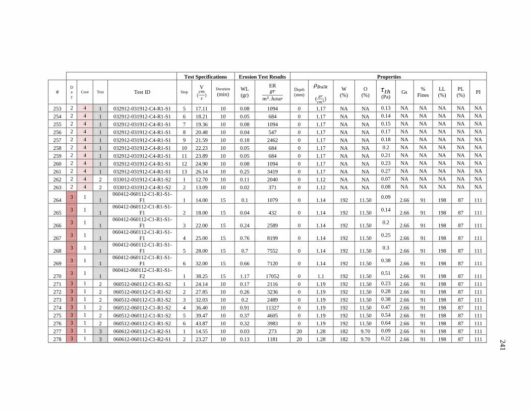
241

Test Specifications Erosion Test Results Properties

# D

a

y Core Test Test ID Step

V

Duration (min)

WL

(gr)

ER

Depth

(mm)

(

W

(%)

O

(%)

(Pa) Gs

%

Fines

LL

(%)

PL

(%) PI

253 2 4 1 032912-031912-C4-R1-S1 5 17.11 10 0.08 1094 0 1.17 NA NA 0.13 NA NA NA NA NA

254 2 4 1 032912-031912-C4-R1-S1 6 18.21 10 0.05 684 0 1.17 NA NA 0.14 NA NA NA NA NA

255 2 4 1 032912-031912-C4-R1-S1 7 19.36 10 0.08 1094 0 1.17 NA NA 0.15 NA NA NA NA NA

256 2 4 1 032912-031912-C4-R1-S1 8 20.48 10 0.04 547 0 1.17 NA NA 0.17 NA NA NA NA NA

257 2 4 1 032912-031912-C4-R1-S1 9 21.59 10 0.18 2462 0 1.17 NA NA 0.18 NA NA NA NA NA

258 2 4 1 032912-031912-C4-R1-S1 10 22.23 10 0.05 684 0 1.17 NA NA 0.2 NA NA NA NA NA

259 2 4 1 032912-031912-C4-R1-S1 11 23.89 10 0.05 684 0 1.17 NA NA 0.21 NA NA NA NA NA

260 2 4 1 032912-031912-C4-R1-S1 12 24.90 10 0.08 1094 0 1.17 NA NA 0.23 NA NA NA NA NA

261 2 4 1 032912-031912-C4-R1-S1 13 26.14 10 0.25 3419 0 1.17 NA NA 0.27 NA NA NA NA NA

262 2 4 2 033012-031912-C4-R1-S2 1 12.70 10 0.11 2040 0 1.12 NA NA 0.07 NA NA NA NA NA

263 2 4 2 033012-031912-C4-R1-S2 2 13.09 10 0.02 371 0 1.12 NA NA 0.08 NA NA NA NA NA

264 3 1

1

060412-060112-C1-R1-S1-

F1 1 14.00 15 0.1 1079 0 1.14 192 11.50 0.09

2.66 91 198 87 111

265 3 1

1 060412-060112-C1-R1-S1-

F1 2 18.00 15 0.04 432 0 1.14 192 11.50 0.14

2.66 91 198 87 111

266 3 1

1

060412-060112-C1-R1-S1-

F1 3 22.00 15 0.24 2589 0 1.14 192 11.50 0.2

2.66 91 198 87 111

267 3 1

1 060412-060112-C1-R1-S1-

F1 4 25.00 15 0.76 8199 0 1.14 192 11.50 0.25

2.66 91 198 87 111

268 3 1

1

060412-060112-C1-R1-S1-

F1 5 28.00 15 0.7 7552 0 1.14 192 11.50 0.3

2.66 91 198 87 111

269 3 1

1 060412-060112-C1-R1-S1-

F1 6 32.00 15 0.66 7120 0 1.14 192 11.50 0.38

2.66 91 198 87 111

270 3 1

1

060412-060112-C1-R1-S1-

F2 1 38.25 15 1.17 17052 0 1.1 192 11.50 0.51

2.66 91 198 87 111

271 3 1 2 060512-060112-C1-R1-S2 1 24.14 10 0.17 2116 0 1.19 192 11.50 0.23 2.66 91 198 87 111

272 3 1 2 060512-060112-C1-R1-S2 2 27.85 10 0.26 3236 0 1.19 192 11.50 0.28 2.66 91 198 87 111

273 3 1 2 060512-060112-C1-R1-S2 3 32.03 10 0.2 2489 0 1.19 192 11.50 0.38 2.66 91 198 87 111

274 3 1 2 060512-060112-C1-R1-S2 4 36.40 10 0.91 11327 0 1.19 192 11.50 0.47 2.66 91 198 87 111

275 3 1 2 060512-060112-C1-R1-S2 5 39.47 10 0.37 4605 0 1.19 192 11.50 0.54 2.66 91 198 87 111

276 3 1 2 060512-060112-C1-R1-S2 6 43.87 10 0.32 3983 0 1.19 192 11.50 0.64 2.66 91 198 87 111

277 3 1 3 060612-060112-C1-R2-S1 1 14.55 10 0.03 273 20 1.28 182 9.70 0.09 2.66 91 198 87 111

278 3 1 3 060612-060112-C1-R2-S1 2 23.27 10 0.13 1181 20 1.28 182 9.70 0.22 2.66 91 198 87 111

242

Test Specifications Erosion Test Results Properties

# D

a

y Core Test Test ID Step

V

Duration (min)

WL

(gr)

ER

Depth

(mm)

(

W

(%)

O

(%)

(Pa) Gs

%

Fines

LL

(%)

PL

(%) PI

279 3 1 3 060612-060112-C1-R2-S1 3 33.83 10 0.33 2998 20 1.28 182 9.70 0.4 2.66 91 198 87 111

280 3 1

4

060812-060112-C1-R2-S1-

1 1 22.52 10 0.09 775 20 1.3 182 9.70 0.19

2.66 91 198 87 111

281 3 1

4

060812-060112-C1-R2-S1-

1 2 31.06 10 0.04 344 20 1.3 182 9.70 0.35

2.66 91 198 87 111

282 3 1

4

060812-060112-C1-R2-S1-

1 3 41.21 10 0.13 1120 20 1.3 182 9.70 0.57

2.66 91 198 87 111

283 3 1 5 061212-060112-C1-R3-S1 1 22.07 10 0.05 1203 36 1.09 203 10.70 0.2 2.66 91 198 87 111

284 3 1 5 061212-060112-C1-R3-S1 2 30.41 10 0.13 3129 36 1.09 203 10.70 0.34 2.66 91 198 87 111

285 3 1 5 061212-060112-C1-R3-S1 3 40.70 10 0.24 5777 36 1.09 203 10.70 0.56 2.66 91 198 87 111

286 3 1 5 061212-060112-C1-R3-S1 4 50.03 10 0.89 21422 36 1.09 203 10.70 0.83 2.66 91 198 87 111

287 3 1 6 061212-060112-C1-R4-S1 1 22.10 10 0.2 2385 56 1.2 162 9.60 0.19 2.66 91 198 87 111

288 3 1 6 061212-060112-C1-R4-S1 2 30.45 10 0.06 715 56 1.2 162 9.60 0.33 2.66 91 198 87 111

289 3 1 6 061212-060112-C1-R4-S1 3 40.91 10 0.06 715 56 1.2 162 9.60 0.55 2.66 91 198 87 111

290 3 1 6 061212-060112-C1-R4-S1 4 50.06 10 0.1 1192 56 1.2 162 9.60 0.81 2.66 91 198 87 111

291 3 1 6 061212-060112-C1-R4-S1 5 60.84 10 0.07 835 56 1.2 162 9.60 1.12 2.66 91 198 87 111

292 3 1 7 061212-060112-C1-R5-S1 1 22.01 10 -0.11 -1260 75 1.21 NA NA 0.2 2.66 91 198 87 111

293 3 1 7 061212-060112-C1-R5-S1 2 22.33 10 -0.04 -458 75 1.21 NA NA 0.2 2.66 91 198 87 111

294 3 1

8

061312-060112-C1-R5-S1-

1 1 17.75 10 -0.05 -651 75 1.18 NA NA 0.12

2.66 91 198 87 111

295 3 1

8

061312-060112-C1-R5-S1-

1 2 22.35 10 0.05 651 75 1.18 NA NA 0.19

2.66 91 198 87 111

296 3 1

8

061312-060112-C1-R5-S1-

1 3 26.18 10 0.02 261 75 1.18 NA NA 0.26

2.66 91 198 87 111

297 3 1

8

061312-060112-C1-R5-S1-

1 4 30.66 10 0.01 130 75 1.18 NA NA 0.33 2.66 91 198 87 111

298

3 1

8

061312-060112-C1-R5-S1-

1 5 35.80 10 0.08 1042 75 1.18 NA NA

0.43

2.66 91 198 87 111

299

3 1

8 061312-060112-C1-R5-S1-

1 6 40.77 10 0.05 651 75 1.18 NA NA

0.54

2.66 91 198 87 111

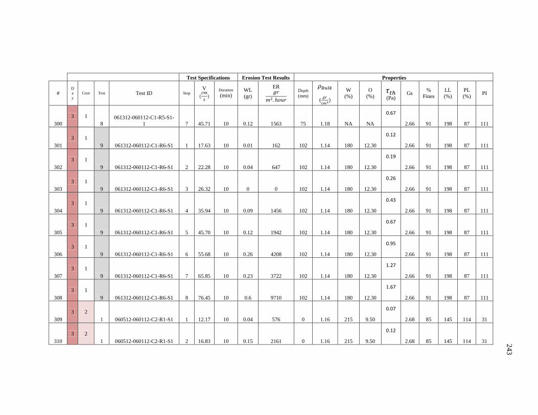
243

Test Specifications Erosion Test Results Properties

# D

a

y Core Test Test ID Step

V

Duration (min)

WL

(gr)

ER

Depth

(mm)

(

W

(%)

O

(%)

(Pa) Gs

%

Fines

LL

(%)

PL

(%) PI

300

3 1

8

061312-060112-C1-R5-S1-

1 7 45.71 10 0.12 1563 75 1.18 NA NA

0.67

2.66 91 198 87 111

301

3 1

9 061312-060112-C1-R6-S1 1 17.63 10 0.01 162 102 1.14 180 12.30

0.12

2.66 91 198 87 111

302

3 1

9 061312-060112-C1-R6-S1 2 22.28 10 0.04 647 102 1.14 180 12.30

0.19

2.66 91 198 87 111

303

3 1

9 061312-060112-C1-R6-S1 3 26.32 10 0 0 102 1.14 180 12.30

0.26

2.66 91 198 87 111

304

3 1

9 061312-060112-C1-R6-S1 4 35.94 10 0.09 1456 102 1.14 180 12.30

0.43

2.66 91 198 87 111

305

3 1

9 061312-060112-C1-R6-S1 5 45.70 10 0.12 1942 102 1.14 180 12.30

0.67

2.66 91 198 87 111

306

3 1

9 061312-060112-C1-R6-S1 6 55.68 10 0.26 4208 102 1.14 180 12.30

0.95

2.66 91 198 87 111

307

3 1

9 061312-060112-C1-R6-S1 7 65.85 10 0.23 3722 102 1.14 180 12.30

1.27

2.66 91 198 87 111

308

3 1

9 061312-060112-C1-R6-S1 8 76.45 10 0.6 9710 102 1.14 180 12.30

1.67

2.66 91 198 87 111

309

3 2

1 060512-060112-C2-R1-S1 1 12.17 10 0.04 576 0 1.16 215 9.50

0.07

2.68 85 145 114 31

310

3 2

1 060512-060112-C2-R1-S1 2 16.83 10 0.15 2161 0 1.16 215 9.50

0.12

2.68 85 145 114 31

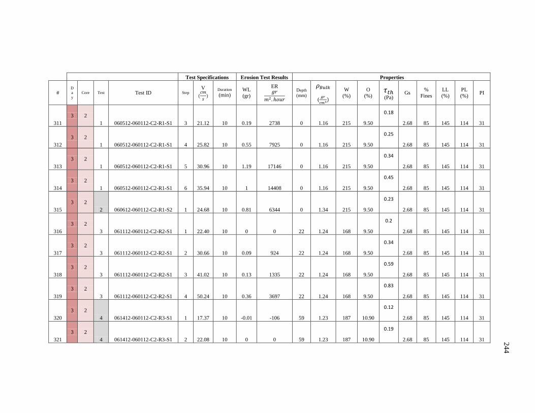
244

Test Specifications Erosion Test Results Properties

# D

a

y Core Test Test ID Step

V

Duration (min)

WL

(gr)

ER

Depth

(mm)

(

W

(%)

O

(%)

(Pa) Gs

%

Fines

LL

(%)

PL

(%) PI

311

3 2

1 060512-060112-C2-R1-S1 3 21.12 10 0.19 2738 0 1.16 215 9.50

0.18

2.68 85 145 114 31

312

3 2

1 060512-060112-C2-R1-S1 4 25.82 10 0.55 7925 0 1.16 215 9.50

0.25

2.68 85 145 114 31

313

3 2

1 060512-060112-C2-R1-S1 5 30.96 10 1.19 17146 0 1.16 215 9.50

0.34

2.68 85 145 114 31

314

3 2

1 060512-060112-C2-R1-S1 6 35.94 10 1 14408 0 1.16 215 9.50

0.45

2.68 85 145 114 31

315

3 2

2 060612-060112-C2-R1-S2 1 24.68 10 0.81 6344 0 1.34 215 9.50

0.23

2.68 85 145 114 31

316

3 2

3 061112-060112-C2-R2-S1 1 22.40 10 0 0 22 1.24 168 9.50

0.2

2.68 85 145 114 31

317

3 2

3 061112-060112-C2-R2-S1 2 30.66 10 0.09 924 22 1.24 168 9.50

0.34

2.68 85 145 114 31

318

3 2

3 061112-060112-C2-R2-S1 3 41.02 10 0.13 1335 22 1.24 168 9.50

0.59

2.68 85 145 114 31

319

3 2

3 061112-060112-C2-R2-S1 4 50.24 10 0.36 3697 22 1.24 168 9.50

0.83

2.68 85 145 114 31

320

3 2

4 061412-060112-C2-R3-S1 1 17.37 10 -0.01 -106 59 1.23 187 10.90

0.12

2.68 85 145 114 31

321

3 2

4 061412-060112-C2-R3-S1 2 22.08 10 0 0 59 1.23 187 10.90

0.19

2.68 85 145 114 31

245

Test Specifications Erosion Test Results Properties

# D

a

y Core Test Test ID Step

V

Duration (min)

WL

(gr)

ER

Depth

(mm)

(

W

(%)

O

(%)

(Pa) Gs

%

Fines

LL

(%)

PL

(%) PI

322

3 2

4 061412-060112-C2-R3-S1 3 35.93 10 0.08 850 59 1.23 187 10.90

0.43

2.68 85 145 114 31

323

3 2

4 061412-060112-C2-R3-S1 4 50.10 10 0.13 1382 59 1.23 187 10.90

0.81

2.68 85 145 114 31

324

3 2

5 061412-060112-C2-R4-S1 1 22.10 10 0.06 561 74 1.27 157 10.60

0.19

2.68 85 145 114 31

325

3 2

5 061412-060112-C2-R4-S1 2 30.43 10 -0.02 -187 74 1.27 157 10.60

0.33

2.68 85 145 114 31

326

3 2

5 061412-060112-C2-R4-S1 3 40.92 10 0.06 561 74 1.27 157 10.60

0.54

2.68 85 145 114 31

327

3 2

5 061412-060112-C2-R4-S1 4 49.92 10 0.07 654 74 1.27 157 10.60

0.78

2.68 85 145 114 31

328

3 2

5 061412-060112-C2-R4-S1 5 60.69 10 0.08 748 74 1.27 157 10.60

1.11

2.68 85 145 114 31

329

3 2

5 061412-060112-C2-R4-S1 6 70.88 10 0.09 841 74 1.27 157 10.60

1.46

2.68 85 145 114 31

330

3 2

5 061412-060112-C2-R4-S1 7 81.46 10 0.24 2244 74 1.27 157 10.60

1.88

2.68 85 145 114 31

331

3 2

6 061412-060112-C2-R4-S1-

1 1 22.16 20 0.01 47 74 1.27 157 10.60

0.2

2.68 85 145 114 31

332

3 2

6 061412-060112-C2-R4-S1-

1 2 30.58 10 0.06 561 74 1.27 157 10.60

0.34

2.68 85 145 114 31

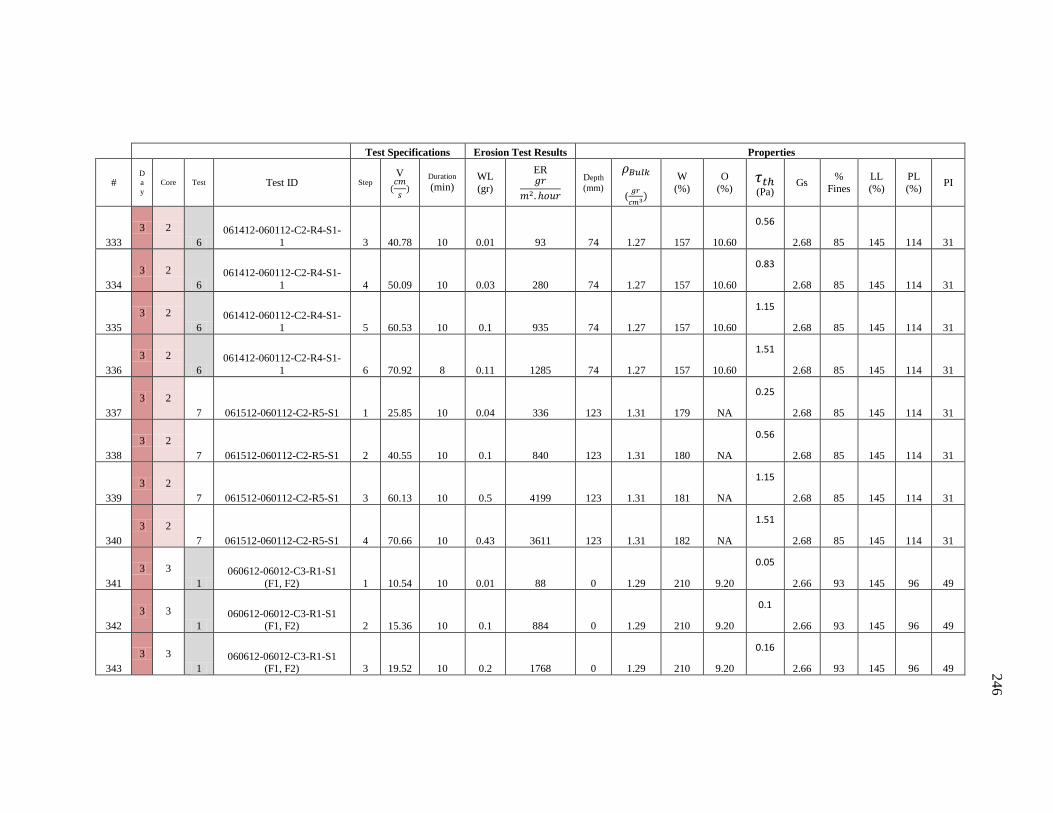
246

Test Specifications Erosion Test Results Properties

# D

a

y Core Test Test ID Step

V

Duration (min)

WL

(gr)

ER

Depth

(mm)

(

W

(%)

O

(%)

(Pa) Gs

%

Fines

LL

(%)

PL

(%) PI

333

3 2

6

061412-060112-C2-R4-S1-

1 3 40.78 10 0.01 93 74 1.27 157 10.60

0.56

2.68 85 145 114 31

334

3 2

6

061412-060112-C2-R4-S1-

1 4 50.09 10 0.03 280 74 1.27 157 10.60

0.83

2.68 85 145 114 31

335

3 2

6

061412-060112-C2-R4-S1-

1 5 60.53 10 0.1 935 74 1.27 157 10.60

1.15

2.68 85 145 114 31

336

3 2

6

061412-060112-C2-R4-S1-

1 6 70.92 8 0.11 1285 74 1.27 157 10.60

1.51

2.68 85 145 114 31

337

3 2

7 061512-060112-C2-R5-S1 1 25.85 10 0.04 336 123 1.31 179 NA

0.25

2.68 85 145 114 31

338

3 2

7 061512-060112-C2-R5-S1 2 40.55 10 0.1 840 123 1.31 180 NA

0.56

2.68 85 145 114 31

339

3 2

7 061512-060112-C2-R5-S1 3 60.13 10 0.5 4199 123 1.31 181 NA

1.15

2.68 85 145 114 31

340

3 2

7 061512-060112-C2-R5-S1 4 70.66 10 0.43 3611 123 1.31 182 NA

1.51

2.68 85 145 114 31

341

3 3

1

060612-06012-C3-R1-S1

(F1, F2) 1 10.54 10 0.01 88 0 1.29 210 9.20

0.05

2.66 93 145 96 49

342

3 3

1 060612-06012-C3-R1-S1

(F1, F2) 2 15.36 10 0.1 884 0 1.29 210 9.20

0.1

2.66 93 145 96 49

343

3 3

1 060612-06012-C3-R1-S1

(F1, F2) 3 19.52 10 0.2 1768 0 1.29 210 9.20

0.16

2.66 93 145 96 49

247

Test Specifications Erosion Test Results Properties

# D

a

y Core Test Test ID Step

V

Duration (min)

WL

(gr)

ER

Depth

(mm)

(

W

(%)

O

(%)

(Pa) Gs

%

Fines

LL

(%)

PL

(%) PI

344

3 3

1

060612-06012-C3-R1-S1

(F1, F2) 4 23.88 10 0.24 2122 0 1.29 210 9.20

0.22

2.66 93 145 96 49

345

3 3

1

060612-06012-C3-R1-S1

(F1, F2) 5 29.46 10 0.46 4067 0 1.29 210 9.20

0.32

2.66 93 145 96 49

346

3 3

1

060612-06012-C3-R1-S1

(F1, F2) 6 34.36 10 0.97 8575 0 1.29 210 9.20

0.43

2.66 93 145 96 49

347

3 3

2 060712-06012-C3-R1-S2 1 17.86 10 0.04 547 0 1.17 210 9.20

0.13

2.66 93 145 96 49

348

3 3

2 060712-06012-C3-R1-S2 2 22.68 10 0.13 1778 0 1.17 210 9.20

0.2

2.66 93 145 96 49

349

3 3

2 060712-06012-C3-R1-S2 3 26.63 10 0.26 3556 0 1.17 210 9.20

0.27

2.66 93 145 96 49

350

3 3

2 060712-06012-C3-R1-S2 4 31.14 10 0.48 6565 0 1.17 210 9.20

0.36

2.66 93 145 96 49

351

3 3

2 060712-06012-C3-R1-S2 5 36.35 10 0.97 13267 0 1.17 210 9.20

0.47

2.66 93 145 96 49

352

3 3

3 061512-06012-C3-R3-S1 1 25.77 10 0.08 821 65 1.24 162 9.00

0.25

2.66 93 145 96 49

353

3 3

3 061512-06012-C3-R3-S1 2 40.48 10 0.12 1232 65 1.24 162 9.00

0.56

2.66 93 145 96 49

354

3 3

3 061512-06012-C3-R3-S1 3 60.18 10 0.26 2670 65 1.24 162 9.00

1.15

2.66 93 145 96 49

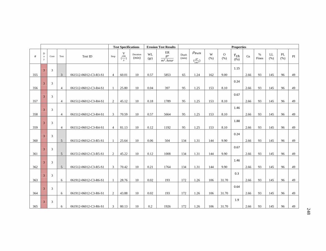
248

Test Specifications Erosion Test Results Properties

# D

a

y Core Test Test ID Step

V

Duration (min)

WL

(gr)

ER

Depth

(mm)

(

W

(%)

O

(%)

(Pa) Gs

%

Fines

LL

(%)

PL

(%) PI

355

3 3

3 061512-06012-C3-R3-S1 4 60.01 10 0.57 5853 65 1.24 162 9.00

1.15

2.66 93 145 96 49

356

3 3

4 061512-06012-C3-R4-S1 1 25.80 10 0.04 397 95 1.25 153 8.10

0.24

2.66 93 145 96 49

357

3 3

4 061512-06012-C3-R4-S1 2 45.12 10 0.18 1789 95 1.25 153 8.10

0.67

2.66 93 145 96 49

358

3 3

4 061512-06012-C3-R4-S1 3 70.59 10 0.57 5664 95 1.25 153 8.10

1.46

2.66 93 145 96 49

359

3 3

4 061512-06012-C3-R4-S1 4 81.13 10 0.12 1192 95 1.25 153 8.10

1.88

2.66 93 145 96 49

360

3 3

5 061512-06012-C3-R5-S1 1 25.64 10 0.06 504 134 1.31 144 9.90

0.24

2.66 93 145 96 49

361

3 3

5 061512-06012-C3-R5-S1 2 45.22 10 0.12 1008 134 1.31 144 9.90

0.67

2.66 93 145 96 49

362

3 3

5 061512-06012-C3-R5-S1 3 70.42 10 0.21 1764 134 1.31 144 9.90

1.46

2.66 93 145 96 49

363

3 3

6 061912-06012-C3-R6-S1 1 28.76 10 0.02 193 172 1.26 106 31.70

0.3

2.66 93 145 96 49

364

3 3

6 061912-06012-C3-R6-S1 2 43.88 10 0.02 193 172 1.26 106 31.70

0.64

2.66 93 145 96 49

365

3 3

6 061912-06012-C3-R6-S1 3 80.13 10 0.2 1926 172 1.26 106 31.70

1.9

2.66 93 145 96 49

249

Test Specifications Erosion Test Results Properties

# D

a

y Core Test Test ID Step

V

Duration (min)

WL

(gr)

ER

Depth

(mm)

(

W

(%)

O

(%)

(Pa) Gs

%

Fines

LL

(%)

PL

(%) PI

366

3 3

7 061912-06012-C3-R7-S1 1 28.74 10 0.02 187 189 1.27 159 16.20

0.3

2.66 93 145 96 49

367

3 3

7 061912-06012-C3-R7-S1 2 43.86 10 0.07 654 189 1.27 159 16.20

0.64

2.66 93 145 96 49

368

3 3

7 061912-06012-C3-R7-S1 3 79.98 10 0.35 3272 189 1.27 159 16.20

1.86

2.66 93 145 96 49

369

3 3

8 061912-06012-C3-R8-S1 1 28.90 10 0.06 530 211 1.29 N/A NA

0.29

2.66 93 145 96 49

370

3 3

8 061912-06012-C3-R8-S1 2 59.33 10 0.04 354 211 1.29 N/A NA

1.08

2.66 93 145 96 49

371

3 3

8 061912-06012-C3-R8-S1 3 90.18 10 0.74 6542 211 1.29 N/A NA

2.27

2.66 93 145 96 49

372

3 4

1 060812-06012-C4-R1-S1 1 17.99 10 0.06 865 0 1.16 203 13.76

0.13

2.65 85 134 78 56

373

3 4

1 060812-06012-C4-R1-S1 2 22.69 10 0.22 3170 0 1.16 203 13.76

0.2

2.65 85 134 78 56

374

3 4

1 060812-06012-C4-R1-S1 3 26.65 10 0.22 3170 0 1.16 203 13.76

0.27

2.65 85 134 78 56

375

3 4

1 060812-06012-C4-R1-S1 4 31.08 10 0.59 8501 0 1.16 203 13.76

0.36

2.65 85 134 78 56

376

3 4

1 060812-06012-C4-R1-S1 5 36.35 10 0.77 11094 0 1.16 203 13.76

0.47

2.65 85 134 78 56

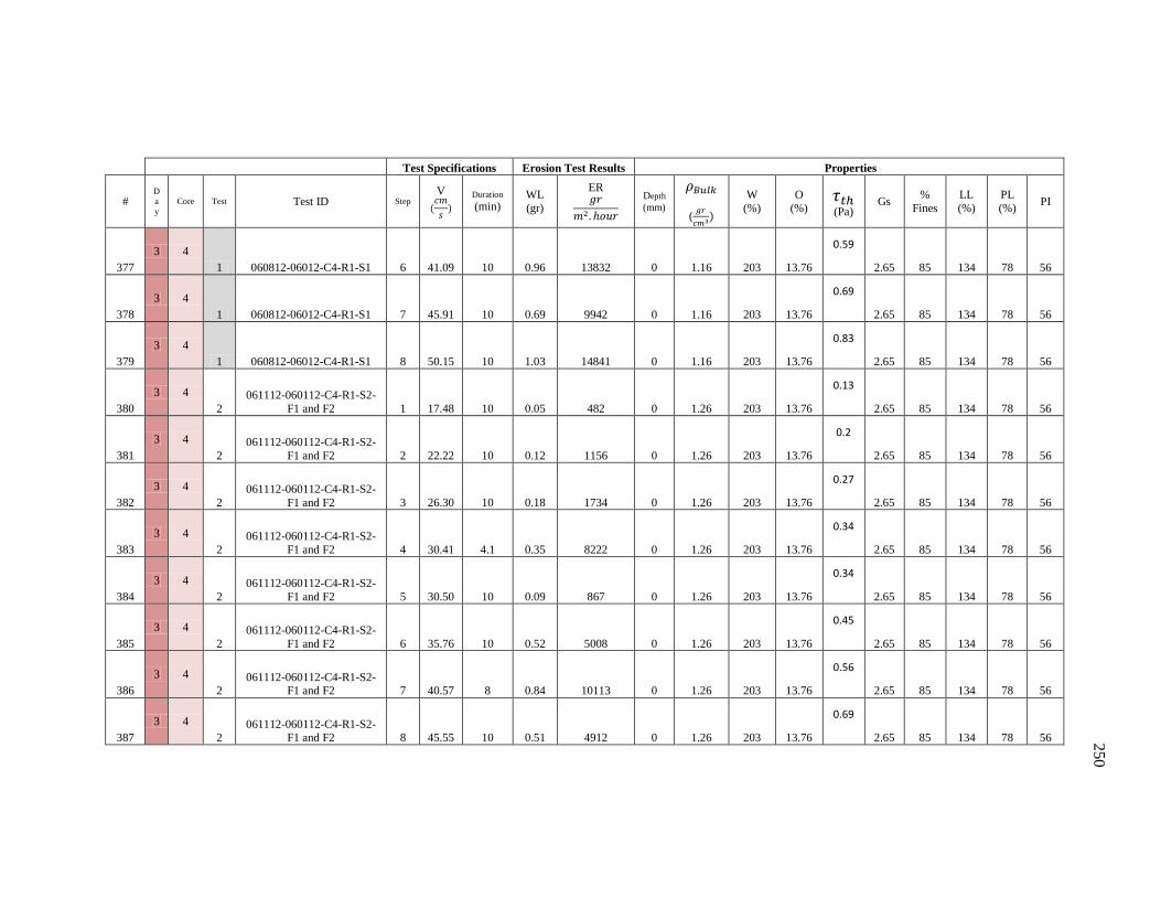
250

Test Specifications Erosion Test Results Properties

# D

a

y Core Test Test ID Step

V

Duration (min)

WL

(gr)

ER

Depth

(mm)

(

W

(%)

O

(%)

(Pa) Gs

%

Fines

LL

(%)

PL

(%) PI

377

3 4

1 060812-06012-C4-R1-S1 6 41.09 10 0.96 13832 0 1.16 203 13.76

0.59

2.65 85 134 78 56

378

3 4

1 060812-06012-C4-R1-S1 7 45.91 10 0.69 9942 0 1.16 203 13.76

0.69

2.65 85 134 78 56

379

3 4

1 060812-06012-C4-R1-S1 8 50.15 10 1.03 14841 0 1.16 203 13.76

0.83

2.65 85 134 78 56

380

3 4

2

061112-060112-C4-R1-S2-

F1 and F2 1 17.48 10 0.05 482 0 1.26 203 13.76

0.13

2.65 85 134 78 56

381

3 4

2

061112-060112-C4-R1-S2-

F1 and F2 2 22.22 10 0.12 1156 0 1.26 203 13.76

0.2

2.65 85 134 78 56

382

3 4

2

061112-060112-C4-R1-S2-

F1 and F2 3 26.30 10 0.18 1734 0 1.26 203 13.76

0.27

2.65 85 134 78 56

383

3 4

2

061112-060112-C4-R1-S2-

F1 and F2 4 30.41 4.1 0.35 8222 0 1.26 203 13.76

0.34

2.65 85 134 78 56

384

3 4

2

061112-060112-C4-R1-S2-

F1 and F2 5 30.50 10 0.09 867 0 1.26 203 13.76

0.34

2.65 85 134 78 56

385

3 4

2

061112-060112-C4-R1-S2-

F1 and F2 6 35.76 10 0.52 5008 0 1.26 203 13.76

0.45

2.65 85 134 78 56

386

3 4

2 061112-060112-C4-R1-S2-

F1 and F2 7 40.57 8 0.84 10113 0 1.26 203 13.76

0.56

2.65 85 134 78 56

387

3 4

2 061112-060112-C4-R1-S2-

F1 and F2 8 45.55 10 0.51 4912 0 1.26 203 13.76

0.69

2.65 85 134 78 56

251

Test Specifications Erosion Test Results Properties

# D

a

y Core Test Test ID Step

V

Duration (min)

WL

(gr)

ER

Depth

(mm)

(

W

(%)

O

(%)

(Pa) Gs

%

Fines

LL

(%)

PL

(%) PI

388

3 4

2

061112-060112-C4-R1-S2-

F1 and F2 9 50.14 10 0.82 7897 0 1.26 203 13.76

0.83

2.65 85 134 78 56

389

3 4

2

061112-060112-C4-R1-S2-

F1 and F2 10 55.59 10 0.73 7031 0 1.26 203 13.76

0.99

2.65 85 134 78 56

390

3 4

3

061112-060112-C4-R1-S2-

1 1 60.60 10 1.06 12138 0 1.21 203 13.76

1.15

2.65 85 134 78 56

391

3 4

3

061112-060112-C4-R1-S2-

1 2 50.16 10 0.53 6069 0 1.21 203 13.76

0.83

2.65 85 134 78 56

392

3 4

3

061112-060112-C4-R1-S2-

1 3 40.97 10 0.29 3321 0 1.21 203 13.76

0.56

2.65 85 134 78 56

393

3 4

4 061812-060112-C4-R2-S1 1 24.78 10 0.01 93 36 1.27 168 11.10

0.23

2.65 85 134 78 56

394

3 4

4 061812-060112-C4-R2-S1 2 44.73 10 0.08 748 36 1.27 168 11.10

0.67

2.65 85 134 78 56

395

3 4

4 061812-060112-C4-R2-S1 3 64.68 10 0.19 1776 36 1.27 168 11.10

1.29

2.65 85 134 78 56

396

3 4

4 061812-060112-C4-R2-S1 4 85.60 10 0.75 7011 36 1.27 168 11.10

2.12

2.65 85 134 78 56

397

3 4

5 061812-060112-C4-R3-S1 1 64.57 10 0.05 482 50 1.26 159 11.60

1.29

2.65 85 134 78 56

398

3 4

5 061812-060112-C4-R3-S1 2 85.34 10 0.47 4527 50 1.26 159 11.60

2.12

2.65 85 134 78 56

252

Test Specifications Erosion Test Results Properties

# D

a

y Core Test Test ID Step

V

Duration (min)

WL

(gr)

ER

Depth

(mm)

(

W

(%)

O

(%)

(Pa) Gs

%

Fines

LL

(%)

PL

(%) PI

399

3 4

5 061812-060112-C4-R3-S1 3 64.49 10 0.07 674 50 1.26 159 11.60

1.29

2.65 85 134 78 56

400

3 4

5 061812-060112-C4-R3-S1 4 25.00 10 0.03 289 50 1.26 159 11.60

0.25

2.65 85 134 78 56

401

3 4

6 061812-060112-C4-R4-S1 1 90.77 10 0.43 4020 84 1.27 156 11.30

2.29

2.65 85 134 78 56

402

3 4

6 061812-060112-C4-R4-S1 2 59.55 10 0.03 280 84 1.27 156 11.30

1.09

2.65 85 134 78 56

403

3 4

6 061812-060112-C4-R4-S1 3 29.18 10 0.04 374 84 1.27 156 11.30

0.31

2.65 85 134 78 56

404

3 4

7 061812-060112-C4-R5-S1 1 29.09 10 0.03 240 123 1.33 158 15.50

0.31

2.65 85 134 78 56

405

3 4

7 061812-060112-C4-R5-S1 2 59.33 10 0.16 1282 123 1.33 158 15.50

1.09

2.65 85 134 78 56

406

3 4

7 061812-060112-C4-R6-S1 1 89.37 2.5 0.76 27619 123 1.28 174 16.40

2.3

2.65 85 134 78 56

407

4 1

1 062012-061912-C1-R1-S1 1 19.25 10 0.08 358 0 1.8 45 2.00

0.16 2.73

29 74 55 18

408

4 1

1 062012-061912-C1-R1-S1 2 27.96 10 0.35 1565 0 1.8 45 2.00

0.28 2.73

29 74 55 18

409

4 1

1 062012-061912-C1-R1-S1 3 38.11 10 2.01 8988 0 1.8 45 2.00

0.52 2.73

29 74 55 18

253

Test Specifications Erosion Test Results Properties

# D

a

y Core Test Test ID Step

V

Duration (min)

WL

(gr)

ER

Depth

(mm)

(

W

(%)

O

(%)

(Pa) Gs

%

Fines

LL

(%)

PL

(%) PI

410

4 1

1 062012-061912-C1-R1-S1 4 47.81 10 8.01 35817 0 1.8 45 2.00

0.75 2.73

29 74 55 18

411

4 1

2 062012-061912-C1-R1-S2 1 19.20 10 0.11 506 0 1.76 45 2.00

0.16 2.73

29 74 55 18

412

4 1

2 062012-061912-C1-R1-S2 2 27.66 10 0.47 2163 0 1.76 45 2.00

0.28 2.73

29 74 55 18

413

4 1

2 062012-061912-C1-R1-S2 3 38.19 10 2.74 12610 0 1.76 45 2.00

0.52 2.73

29 74 55 18

414

4 1

2 062012-061912-C1-R1-S2 4 47.29 10 3.7 17029 0 1.76 45 2.00

0.75 2.73

29 74 55 18

415

4 1

3 062012-061912-C1-R2-S1 1 18.64 10 0.37 1590 15 1.86 35 1.76

0.14 2.73

29 74 55 18

416

4 1

3 062012-061912-C1-R2-S1 2 27.23 10 0.06 258 15 1.86 35 1.76

0.28 2.73

29 74 55 18

417

4 1

3 062012-061912-C1-R2-S1 3 42.59 10 1.14 4900 15 1.86 35 1.76

0.61 2.73

29 74 55 18

418

4 1

3 062012-061912-C1-R2-S1 4 57.80 10 8.79 37782 15 1.86 35 1.76

1.05 2.73

29 74 55 18

419

4 1

4 062112-061912-C1-R3-S1 1 21.86 10 0.11 488 52 1.81 37 1.14

0.18 2.73

29 74 55 18

420

4 1

4 062112-061912-C1-R3-S1 2 42.05 10 1.97 8749 52 1.81 37 1.14

0.6 2.73

29 74 55 18

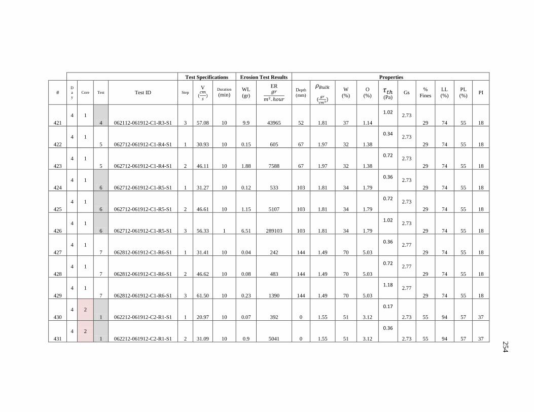
254

Test Specifications Erosion Test Results Properties

# D

a

y Core Test Test ID Step

V

Duration (min)

WL

(gr)

ER

Depth

(mm)

(

W

(%)

O

(%)

(Pa) Gs

%

Fines

LL

(%)

PL

(%) PI

421

4 1

4 062112-061912-C1-R3-S1 3 57.08 10 9.9 43965 52 1.81 37 1.14

1.02 2.73

29 74 55 18

422

4 1

5 062712-061912-C1-R4-S1 1 30.93 10 0.15 605 67 1.97 32 1.38

0.34 2.73

29 74 55 18

423

4 1

5 062712-061912-C1-R4-S1 2 46.11 10 1.88 7588 67 1.97 32 1.38

0.72 2.73

29 74 55 18

424

4 1

6 062712-061912-C1-R5-S1 1 31.27 10 0.12 533 103 1.81 34 1.79

0.36 2.73

29 74 55 18

425

4 1

6 062712-061912-C1-R5-S1 2 46.61 10 1.15 5107 103 1.81 34 1.79

0.72 2.73

29 74 55 18

426

4 1

6 062712-061912-C1-R5-S1 3 56.33 1 6.51 289103 103 1.81 34 1.79

1.02 2.73

29 74 55 18

427

4 1

7 062812-061912-C1-R6-S1 1 31.41 10 0.04 242 144 1.49 70 5.03

0.36 2.77

29 74 55 18

428

4 1

7 062812-061912-C1-R6-S1 2 46.62 10 0.08 483 144 1.49 70 5.03

0.72 2.77

29 74 55 18

429

4 1

7 062812-061912-C1-R6-S1 3 61.50 10 0.23 1390 144 1.49 70 5.03

1.18 2.77

29 74 55 18

430

4 2

1 062212-061912-C2-R1-S1 1 20.97 10 0.07 392 0 1.55 51 3.12

0.17

2.73 55 94 57 37

431

4 2

1 062212-061912-C2-R1-S1 2 31.09 10 0.9 5041 0 1.55 51 3.12

0.36

2.73 55 94 57 37

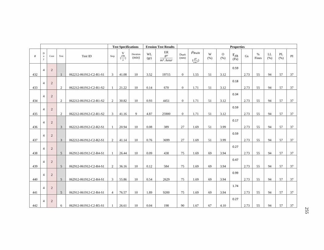
255

Test Specifications Erosion Test Results Properties

# D

a

y Core Test Test ID Step

V

Duration (min)

WL

(gr)

ER

Depth

(mm)

(

W

(%)

O

(%)

(Pa) Gs

%

Fines

LL

(%)

PL

(%) PI

432

4 2

1 062212-061912-C2-R1-S1 3 41.08 10 3.52 19715 0 1.55 51 3.12

0.59

2.73 55 94 57 37

433

4 2

2 062212-061912-C2-R1-S2 1 21.22 10 0.14 670 0 1.71 51 3.12

0.18

2.73 55 94 57 37

434

4 2

2 062212-061912-C2-R1-S2 2 30.82 10 0.93 4451 0 1.71 51 3.12

0.34

2.73 55 94 57 37

435

4 2

2 062212-061912-C2-R1-S2 3 41.16 9 4.87 25900 0 1.71 51 3.12

0.59

2.73 55 94 57 37

436

4 2

3 062212-061912-C2-R2-S1 1 20.94 10 0.08 389 27 1.69 51 3.99

0.17

2.73 55 94 57 37

437

4 2

3 062212-061912-C2-R2-S1 2 41.14 10 0.76 3699 27 1.69 51 3.99

0.59

2.73 55 94 57 37

438

4 2

5 062912-061912-C2-R4-S1 1 26.44 10 0.09 438 75 1.69 69 3.94

0.27

2.73 55 94 57 37

439

4 2

5 062912-061912-C2-R4-S1 2 36.16 10 0.12 584 75 1.69 69 3.94

0.47

2.73 55 94 57 37

440

4 2

5 062912-061912-C2-R4-S1 3 55.86 10 0.54 2629 75 1.69 69 3.94

0.99

2.73 55 94 57 37

441

4 2

5 062912-061912-C2-R4-S1 4 76.57 10 1.89 9200 75 1.69 69 3.94

1.74

2.73 55 94 57 37

442

4 2

6 062912-061912-C2-R5-S1 1 26.61 10 0.04 198 90 1.67 67 4.10

0.27

2.73 55 94 57 37

256

Test Specifications Erosion Test Results Properties

# D

a

y Core Test Test ID Step

V

Duration (min)

WL

(gr)

ER

Depth

(mm)

(

W

(%)

O

(%)

(Pa) Gs

%

Fines

LL

(%)

PL

(%) PI

443

4 2

6 062912-061912-C2-R5-S1 2 41.38 10 0.01 50 90 1.67 67 4.10

0.59

2.73 55 94 57 37

444

4 2

6 062912-061912-C2-R5-S1 3 61.18 10 0.22 1090 90 1.67 67 4.10

1.18

2.73 55 94 57 37

445

4 2

6 062912-061912-C2-R5-S1 4 81.66 10 3.34 16545 90 1.67 67 4.10

1.95

2.73 55 94 57 37

446

4 2

7 062912-061912-C2-R6-S1 1 26.70 10 0.05 290 130 1.52 73 4.09

0.26

2.73 55 94 57 37

447

4 2

7 062912-061912-C2-R6-S1 2 46.23 10 0.01 58 130 1.52 73 4.09

0.7

2.73 55 94 57 37

448

4 2

7 062912-061912-C2-R6-S1 3 66.06 10 0.08 465 130 1.52 73 4.09

1.32

2.73 55 94 57 37

449

4 2

7 062912-061912-C2-R6-S1 4 86.87 10 0.37 2149 130 1.52 73 4.09

2.11

2.73 55 94 57 37

450

4 2

8 070212-061912-C2-R7-S1 1 30.68 10 0.02 126 167 1.46 94 6.84

0.34

2.77 51 94 57 37

451

4 2

8 070212-061912-C2-R7-S1 2 50.32 10 0.17 1072 167 1.46 94 6.84

0.83

2.77 51 94 57 37

452

4 2

8 070212-061912-C2-R7-S1 3 71.04 10 0.47 2965 167 1.46 94 6.84

1.54

2.77 51 94 57 37

453

4 3

1 062112-061912-C3-R1-S1 1 17.87 10 -0.01 -44 0 1.84 38 1.09

0.13

2.73 17 0

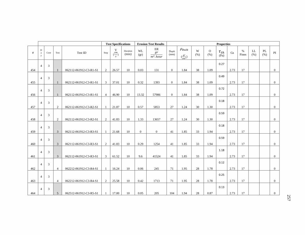
257

Test Specifications Erosion Test Results Properties

# D

a

y Core Test Test ID Step

V

Duration (min)

WL

(gr)

ER

Depth

(mm)

(

W

(%)

O

(%)

(Pa) Gs

%

Fines

LL

(%)

PL

(%) PI

454

4 3

1 062112-061912-C3-R1-S1 2 26.57 10 0.03 131 0 1.84 38 1.09

0.27

2.73 17 0

455

4 3

1 062112-061912-C3-R1-S1 3 37.01 10 0.32 1393 0 1.84 38 1.09

0.49

2.73 17 0

456

4 3

1 062112-061912-C3-R1-S1 4 46.90 10 13.32 57986 0 1.84 38 1.09

0.72

2.73 17 0

457

4 3

2 062112-061912-C3-R2-S1 1 21.87 10 0.57 5853 27 1.24 30 1.30

0.18

2.73 17 0

458

4 3

2 062112-061912-C3-R2-S1 2 41.83 10 1.33 13657 27 1.24 30 1.30

0.59

2.73 17 0

459

4 3

3 062112-061912-C3-R3-S1 1 21.68 10 0 0 41 1.85 33 1.94

0.18

2.73 17 0

460

4 3

3 062112-061912-C3-R3-S1 2 41.83 10 0.29 1254 41 1.85 33 1.94

0.59

2.73 17 0

461

4 3

3 062112-061912-C3-R3-S1 3 61.52 10 9.6 41524 41 1.85 33 1.94

1.18

2.73 17 0

462

4 3

4 062212-061912-C3-R4-S1 1 16.24 10 0.06 245 71 1.95 28 1.78

0.12

2.73 17 0

463

4 3

4 062212-061912-C3-R4-S1 2 25.58 10 0.42 1713 71 1.95 28 1.78

0.25

2.73 17 0

464

4 3

5 062512-061912-C3-R5-S1 1 17.00 10 0.05 205 104 1.94 28 0.87

0.13

2.73 17 0

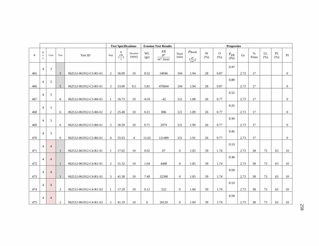
258

Test Specifications Erosion Test Results Properties

# D

a

y Core Test Test ID Step

V

Duration (min)

WL

(gr)

ER

Depth

(mm)

(

W

(%)

O

(%)

(Pa) Gs

%

Fines

LL

(%)

PL

(%) PI

465

4 3

5 062512-061912-C3-R5-S1 2 36.09 10 8.52 34946 104 1.94 28 0.87

0.47

2.73 17 0

466

4 3

5 062512-061912-C3-R5-S1 3 53.00 0.5 5.81 476604 104 1.94 28 0.87

0.89

2.73 17 0

467

4 3

6 062512-061912-C3-R6-S1 1 16.73 10 -0.01 -42 121 1.88 26 0.77

0.12

2.73 17 0

468

4 3

6 062512-061912-C3-R6-S1 2 25.48 10 0.21 886 121 1.89 26 0.77

0.25

2.73 17 0

469

4 3

6 062512-061912-C3-R6-S1 3 30.59 10 0.71 2979 121 1.90 26 0.77

0.34

2.73 17 0

470

4 3

6 062512-061912-C3-R6-S1 4 35.63 4 11.65 121489 121 1.91 26 0.77

0.45

2.73 17 0

471

4 4

1 062512-061912-C4-R1-S1 1 17.65 10 0.02 87 0 1.85 39 1.74

0.13

2.73 38 73 63 10

472

4 4

1 062512-061912-C4-R1-S1 2 31.32 10 1.04 4498 0 1.85 39 1.74

0.36

2.73 38 73 63 10

473

4 4

1 062512-061912-C4-R1-S1 3 41.38 10 7.49 32398 0 1.85 39 1.74

0.59

2.73 38 73 63 10

474

4 4

2 062512-061912-C4-R1-S2 1 17.29 10 0.12 522 0 1.84 39 1.74

0.13

2.73 38 73 63 10

475

4 4

2 062512-061912-C4-R1-S2 2 41.19 10 6 26120 0 1.84 39 1.74

0.59

2.73 38 73 63 10

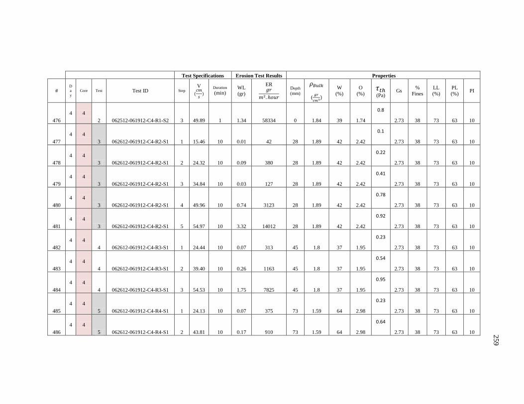
259

Test Specifications Erosion Test Results Properties

# D

a

y Core Test Test ID Step

V

Duration (min)

WL

(gr)

ER

Depth

(mm)

(

W

(%)

O

(%)

(Pa) Gs

%

Fines

LL

(%)

PL

(%) PI

476

4 4

2 062512-061912-C4-R1-S2 3 49.89 1 1.34 58334 0 1.84 39 1.74

0.8

2.73 38 73 63 10

477

4 4

3 062612-061912-C4-R2-S1 1 15.46 10 0.01 42 28 1.89 42 2.42

0.1

2.73 38 73 63 10

478

4 4

3 062612-061912-C4-R2-S1 2 24.32 10 0.09 380 28 1.89 42 2.42

0.22

2.73 38 73 63 10

479

4 4

3 062612-061912-C4-R2-S1 3 34.84 10 0.03 127 28 1.89 42 2.42

0.41

2.73 38 73 63 10

480

4 4

3 062612-061912-C4-R2-S1 4 49.96 10 0.74 3123 28 1.89 42 2.42

0.78

2.73 38 73 63 10

481

4 4

3 062612-061912-C4-R2-S1 5 54.97 10 3.32 14012 28 1.89 42 2.42

0.92

2.73 38 73 63 10

482

4 4

4 062612-061912-C4-R3-S1 1 24.44 10 0.07 313 45 1.8 37 1.95

0.23

2.73 38 73 63 10

483

4 4

4 062612-061912-C4-R3-S1 2 39.40 10 0.26 1163 45 1.8 37 1.95

0.54

2.73 38 73 63 10

484

4 4

4 062612-061912-C4-R3-S1 3 54.53 10 1.75 7825 45 1.8 37 1.95

0.95

2.73 38 73 63 10

485

4 4

5 062612-061912-C4-R4-S1 1 24.13 10 0.07 375 73 1.59 64 2.98

0.23

2.73 38 73 63 10

486

4 4

5 062612-061912-C4-R4-S1 2 43.81 10 0.17 910 73 1.59 64 2.98

0.64

2.73 38 73 63 10

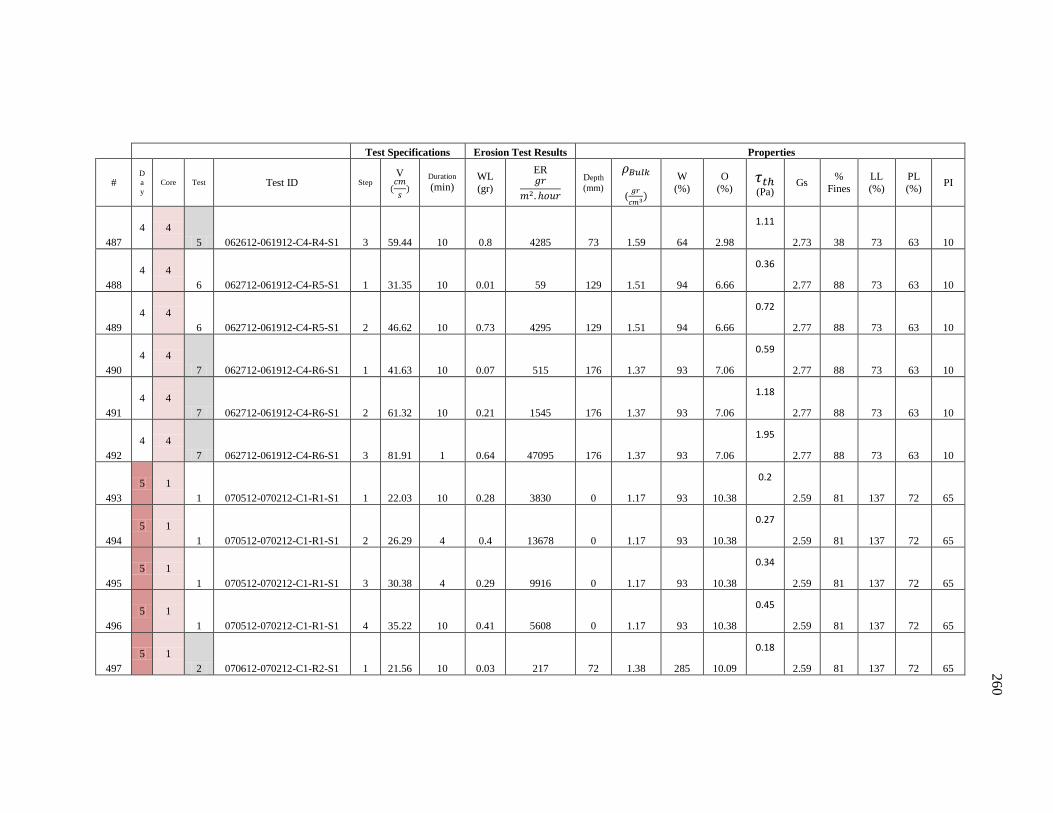
260

Test Specifications Erosion Test Results Properties

# D

a

y Core Test Test ID Step

V

Duration (min)

WL

(gr)

ER

Depth

(mm)

(

W

(%)

O

(%)

(Pa) Gs

%

Fines

LL

(%)

PL

(%) PI

487

4 4

5 062612-061912-C4-R4-S1 3 59.44 10 0.8 4285 73 1.59 64 2.98

1.11

2.73 38 73 63 10

488

4 4

6 062712-061912-C4-R5-S1 1 31.35 10 0.01 59 129 1.51 94 6.66

0.36

2.77 88 73 63 10

489

4 4

6 062712-061912-C4-R5-S1 2 46.62 10 0.73 4295 129 1.51 94 6.66

0.72

2.77 88 73 63 10

490

4 4

7 062712-061912-C4-R6-S1 1 41.63 10 0.07 515 176 1.37 93 7.06

0.59

2.77 88 73 63 10

491

4 4

7 062712-061912-C4-R6-S1 2 61.32 10 0.21 1545 176 1.37 93 7.06

1.18

2.77 88 73 63 10

492

4 4

7 062712-061912-C4-R6-S1 3 81.91 1 0.64 47095 176 1.37 93 7.06

1.95

2.77 88 73 63 10

493

5 1

1 070512-070212-C1-R1-S1 1 22.03 10 0.28 3830 0 1.17 93 10.38

0.2

2.59 81 137 72 65

494

5 1

1 070512-070212-C1-R1-S1 2 26.29 4 0.4 13678 0 1.17 93 10.38

0.27

2.59 81 137 72 65

495

5 1

1 070512-070212-C1-R1-S1 3 30.38 4 0.29 9916 0 1.17 93 10.38

0.34

2.59 81 137 72 65

496

5 1

1 070512-070212-C1-R1-S1 4 35.22 10 0.41 5608 0 1.17 93 10.38

0.45

2.59 81 137 72 65

497

5 1

2 070612-070212-C1-R2-S1 1 21.56 10 0.03 217 72 1.38 285 10.09

0.18

2.59 81 137 72 65

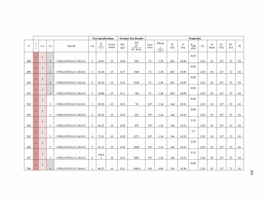
261

Test Specifications Erosion Test Results Properties

# D

a

y Core Test Test ID Step

V

Duration (min)

WL

(gr)

ER

Depth

(mm)

(

W

(%)

O

(%)

(Pa) Gs

%

Fines

LL

(%)

PL

(%) PI

498

5 1

2 070612-070212-C1-R2-S1 2 25.87 10 0.09 650 72 1.38 285 10.09

0.25

2.59 81 137 72 65

499

5 1

2 070612-070212-C1-R2-S1 3 35.30 10 0.27 1949 72 1.38 285 10.09

0.45

2.59 81 137 72 65

500

5 1

2 070612-070212-C1-R2-S1 4 45.16 10 0.35 2526 72 1.38 285 10.09

0.69

2.59 81 137 72 65

501

5 1

2 070612-070212-C1-R2-S1 5 54.88 10 0.11 794 72 1.38 285 10.09

0.95

2.59 81 137 72 65

502

5 1

3 070612-070212-C1-R3-S1 1 30.33 10 0.01 78 107 1.34 144 10.33

0.34

2.59 81 137 72 65

503

5 1

3 070612-070212-C1-R3-S1 2 45.35 10 0.03 235 107 1.34 144 10.33

0.69

2.59 81 137 72 65

504

5 1

3 070612-070212-C1-R3-S1 3 60.25 10 0.06 470 107 1.34 144 10.33

1.15

2.59 81 137 72 65

505

5 1

3 070612-070212-C1-R3-S1 4 75.51 10 0.29 2271 107 1.34 144 10.33

1.7

2.59 81 137 72 65

506

5 1

3 070612-070212-C1-R3-S1 5 91.13 10 0.36 2820 107 1.34 144 10.33

2.39

2.59 81 137 72 65

507

5 1

3 070612-070212-C1-R3-S1 6 106.4

3 10 0.47 3681 107 1.34 144 10.33

3.13

2.59 81 137 72 65

508

5 1

4 070612-070212-C1-R4-S1 1 40.37 10 0.21 -10016 145 0.96 139 10.36

0.56

2.59 81 137 72 65

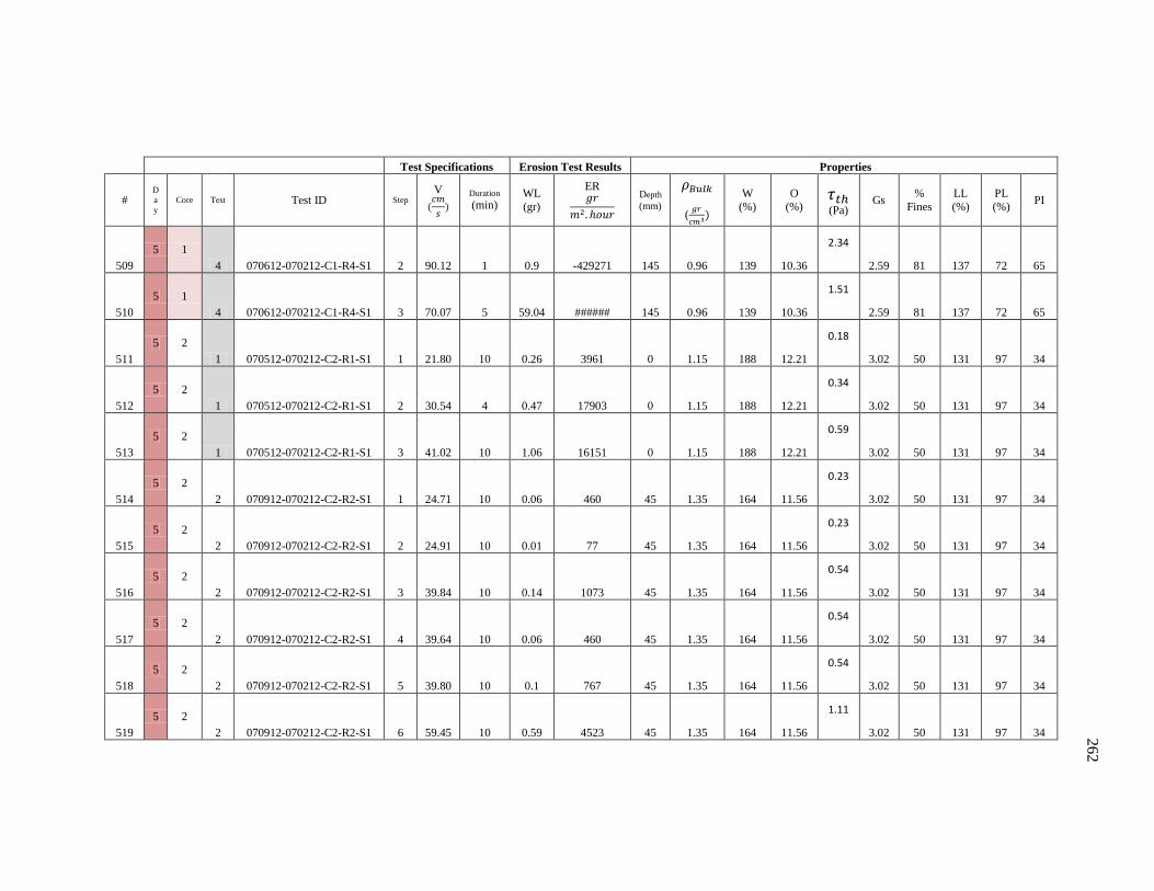
262

Test Specifications Erosion Test Results Properties

# D

a

y Core Test Test ID Step

V

Duration (min)

WL

(gr)

ER

Depth

(mm)

(

W

(%)

O

(%)

(Pa) Gs

%

Fines

LL

(%)

PL

(%) PI

509

5 1

4 070612-070212-C1-R4-S1 2 90.12 1 0.9 -429271 145 0.96 139 10.36

2.34

2.59 81 137 72 65

510

5 1

4 070612-070212-C1-R4-S1 3 70.07 5 59.04 ###### 145 0.96 139 10.36

1.51

2.59 81 137 72 65

511

5 2

1 070512-070212-C2-R1-S1 1 21.80 10 0.26 3961 0 1.15 188 12.21

0.18

3.02 50 131 97 34

512

5 2

1 070512-070212-C2-R1-S1 2 30.54 4 0.47 17903 0 1.15 188 12.21

0.34

3.02 50 131 97 34

513

5 2

1 070512-070212-C2-R1-S1 3 41.02 10 1.06 16151 0 1.15 188 12.21

0.59

3.02 50 131 97 34

514

5 2

2 070912-070212-C2-R2-S1 1 24.71 10 0.06 460 45 1.35 164 11.56

0.23

3.02 50 131 97 34

515

5 2

2 070912-070212-C2-R2-S1 2 24.91 10 0.01 77 45 1.35 164 11.56

0.23

3.02 50 131 97 34

516

5 2

2 070912-070212-C2-R2-S1 3 39.84 10 0.14 1073 45 1.35 164 11.56

0.54

3.02 50 131 97 34

517

5 2

2 070912-070212-C2-R2-S1 4 39.64 10 0.06 460 45 1.35 164 11.56

0.54

3.02 50 131 97 34

518

5 2

2 070912-070212-C2-R2-S1 5 39.80 10 0.1 767 45 1.35 164 11.56

0.54

3.02 50 131 97 34

519

5 2

2 070912-070212-C2-R2-S1 6 59.45 10 0.59 4523 45 1.35 164 11.56

1.11

3.02 50 131 97 34

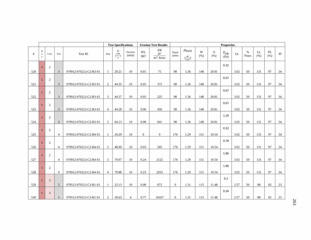
263

Test Specifications Erosion Test Results Properties

# D

a

y Core Test Test ID Step

V

Duration (min)

WL

(gr)

ER

Depth

(mm)

(

W

(%)

O

(%)

(Pa) Gs

%

Fines

LL

(%)

PL

(%) PI

520

5 2

3 070912-070212-C2-R3-S1 1 29.21 10 0.01 75 98 1.36 148 20.81

0.32

3.02 50 131 97 34

521

5 2

3 070912-070212-C2-R3-S1 2 44.35 10 0.05 375 98 1.36 148 20.81

0.67

3.02 50 131 97 34

522

5 2

3 070912-070212-C2-R3-S1 3 44.37 10 0.03 225 98 1.36 148 20.81

0.67

3.02 50 131 97 34

523

5 2

3 070912-070212-C2-R3-S1 4 44.28 10 0.06 450 98 1.36 148 20.81

0.67

3.02 50 131 97 34

524

5 2

3 070912-070212-C2-R3-S1 5 64.13 10 0.08 601 98 1.36 148 20.81

1.29

3.02 50 131 97 34

525

5 2

4 070912-070212-C2-R4-S1 1 29.29 10 0 0 176 1.29 151 10.54

0.32

3.02 50 131 97 34

526

5 2

4 070912-070212-C2-R4-S1 2 48.99 10 0.03 265 176 1.29 151 10.54

0.78

3.02 50 131 97 34

527

5 2

4 070912-070212-C2-R4-S1 3 79.97 10 0.24 2122 176 1.29 151 10.54

1.86

3.02 50 131 97 34

528

5 2

4 070912-070212-C2-R4-S1 4 79.88 10 0.23 2033 176 1.29 151 10.54

1.86

3.02 50 131 97 34

529

5 3

5 070512-070212-C3-R1-S1 1 22.13 10 0.08 672 0 1.31 115 11.48

0.2

2.57 50 88 65 23

530

5 3

5 070512-070212-C3-R1-S1 2 30.63 4 0.77 16167 0 1.31 115 11.48

0.34

2.57 50 88 65 23

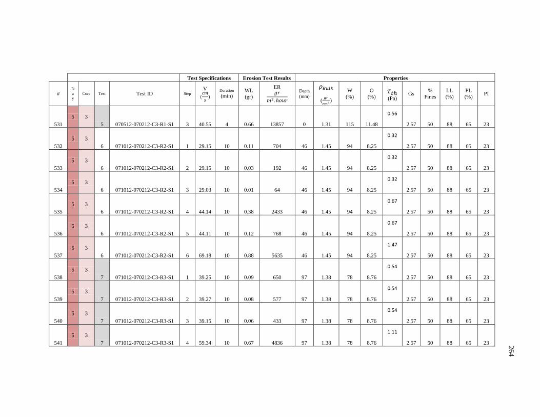
264

Test Specifications Erosion Test Results Properties

# D

a

y Core Test Test ID Step

V

Duration (min)

WL

(gr)

ER

Depth

(mm)

(

W

(%)

O

(%)

(Pa) Gs

%

Fines

LL

(%)

PL

(%) PI

531

5 3

5 070512-070212-C3-R1-S1 3 40.55 4 0.66 13857 0 1.31 115 11.48

0.56

2.57 50 88 65 23

532

5 3

6 071012-070212-C3-R2-S1 1 29.15 10 0.11 704 46 1.45 94 8.25

0.32

2.57 50 88 65 23

533

5 3

6 071012-070212-C3-R2-S1 2 29.15 10 0.03 192 46 1.45 94 8.25

0.32

2.57 50 88 65 23

534

5 3

6 071012-070212-C3-R2-S1 3 29.03 10 0.01 64 46 1.45 94 8.25

0.32

2.57 50 88 65 23

535

5 3

6 071012-070212-C3-R2-S1 4 44.14 10 0.38 2433 46 1.45 94 8.25

0.67

2.57 50 88 65 23

536

5 3

6 071012-070212-C3-R2-S1 5 44.11 10 0.12 768 46 1.45 94 8.25

0.67

2.57 50 88 65 23

537

5 3

6 071012-070212-C3-R2-S1 6 69.18 10 0.88 5635 46 1.45 94 8.25

1.47

2.57 50 88 65 23

538

5 3

7 071012-070212-C3-R3-S1 1 39.25 10 0.09 650 97 1.38 78 8.76

0.54

2.57 50 88 65 23

539

5 3

7 071012-070212-C3-R3-S1 2 39.27 10 0.08 577 97 1.38 78 8.76

0.54

2.57 50 88 65 23

540

5 3

7 071012-070212-C3-R3-S1 3 39.15 10 0.06 433 97 1.38 78 8.76

0.54

2.57 50 88 65 23

541

5 3

7 071012-070212-C3-R3-S1 4 59.34 10 0.67 4836 97 1.38 78 8.76

1.11

2.57 50 88 65 23

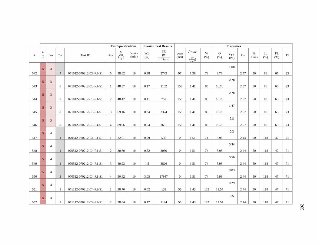
265

Test Specifications Erosion Test Results Properties

# D

a

y Core Test Test ID Step

V

Duration (min)

WL

(gr)

ER

Depth

(mm)

(

W

(%)

O

(%)

(Pa) Gs

%

Fines

LL

(%)

PL

(%) PI

542

5 3

7 071012-070212-C3-R3-S1 5 58.62 10 0.38 2743 97 1.38 78 8.76

1.08

2.57 50 88 65 23

543

5 3

8 071012-070212-C3-R4-S1 1 48.37 10 0.17 1162 153 1.41 85 16.70

0.78

2.57 50 88 65 23

544

5 3

8 071012-070212-C3-R4-S1 2 48.42 10 0.11 752 153 1.41 85 16.70

0.78

2.57 50 88 65 23

545

5 3

8 071012-070212-C3-R4-S1 3 69.16 10 0.34 2324 153 1.41 85 16.70

1.47

2.57 50 88 65 23

546

5 3

8 071012-070212-C3-R4-S1 4 89.96 10 0.54 3691 153 1.41 85 16.70

2.3

2.57 50 88 65 23

547

5 4

1 070512-070212-C4-R1-S1 1 22.01 10 0.09 530 0 1.51 74 5.98

0.2

2.44 50 118 47 71

548

5 4

1 070512-070212-C4-R1-S1 2 30.60 10 0.52 3060 0 1.51 74 5.98

0.34

2.44 50 118 47 71

549

5 4

1 070512-070212-C4-R1-S1 3 40.93 10 1.5 8826 0 1.51 74 5.98

0.56

2.44 50 118 47 71

550

5 4

1 070512-070212-C4-R1-S1 4 50.42 10 3.05 17947 0 1.51 74 5.98

0.83

2.44 50 118 47 71

551

5 4

2 071112-070212-C4-R2-S1 1 28.70 10 0.02 132 55 1.43 122 11.54

0.29

2.44 50 118 47 71

552

5 4

2 071112-070212-C4-R2-S1 2 38.84 10 0.17 1124 55 1.43 122 11.54

0.5

2.44 50 118 47 71

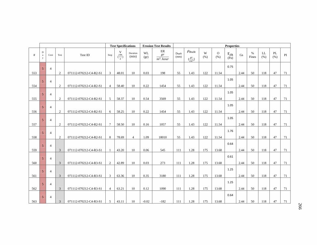
266

Test Specifications Erosion Test Results Properties

# D

a

y Core Test Test ID Step

V

Duration (min)

WL

(gr)

ER

Depth

(mm)

(

W

(%)

O

(%)

(Pa) Gs

%

Fines

LL

(%)

PL

(%) PI

553

5 4

2 071112-070212-C4-R2-S1 3 48.01 10 0.03 198 55 1.43 122 11.54

0.75

2.44 50 118 47 71

554

5 4

2 071112-070212-C4-R2-S1 4 58.40 10 0.22 1454 55 1.43 122 11.54

1.05

2.44 50 118 47 71

555

5 4

2 071112-070212-C4-R2-S1 5 58.37 10 0.54 3569 55 1.43 122 11.54

1.05

2.44 50 118 47 71

556

5 4

2 071112-070212-C4-R2-S1 6 58.25 10 0.22 1454 55 1.43 122 11.54

1.05

2.44 50 118 47 71

557

5 4

2 071112-070212-C4-R2-S1 7 58.50 10 0.16 1057 55 1.43 122 11.54

1.05

2.44 50 118 47 71

558

5 4

2 071112-070212-C4-R2-S1 8 78.69 4 1.09 18010 55 1.43 122 11.54

1.76

2.44 50 118 47 71

559

5 4

3 071112-070212-C4-R3-S1 1 43.20 10 0.06 545 111 1.28 175 13.68

0.64

2.44 50 118 47 71

560

5 4

3 071112-070212-C4-R3-S1 2 42.89 10 0.03 273 111 1.28 175 13.68

0.61

2.44 50 118 47 71

561

5 4

3 071112-070212-C4-R3-S1 3 63.36 10 0.35 3180 111 1.28 175 13.68

1.25

2.44 50 118 47 71

562

5 4

3 071112-070212-C4-R3-S1 4 63.21 10 0.12 1090 111 1.28 175 13.68

1.25

2.44 50 118 47 71

563

5 4

3 071112-070212-C4-R3-S1 5 43.11 10 -0.02 -182 111 1.28 175 13.68

0.64

2.44 50 118 47 71

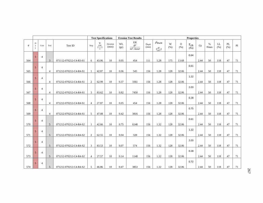
267

Test Specifications Erosion Test Results Properties

# D

a

y Core Test Test ID Step

V

Duration (min)

WL

(gr)

ER

Depth

(mm)

(

W

(%)

O

(%)

(Pa) Gs

%

Fines

LL

(%)

PL

(%) PI

564

5 4

3 071112-070212-C4-R3-S1 6 43.06 10 0.05 454 111 1.28 175 13.68

0.64

2.44 50 118 47 71

565

5 4

4 071212-070212-C4-R4-S1 1 42.87 10 0.06 545 156 1.28 128 32.06

0.61

2.44 50 118 47 71

566

5 4

4 071212-070212-C4-R4-S1 2 62.99 10 0.37 3361 156 1.28 128 32.06

1.22

2.44 50 118 47 71

567

5 4

4 071212-070212-C4-R4-S1 3 83.62 10 0.82 7450 156 1.28 128 32.06

2.03

2.44 50 118 47 71

568

5 4

4 071212-070212-C4-R4-S1 4 27.87 10 0.05 454 156 1.28 128 32.06

0.28

2.44 50 118 47 71

569

5 4

4 071212-070212-C4-R4-S1 5 47.08 10 0.42 3816 156 1.28 128 32.06

0.75

2.44 50 118 47 71

570

5 4

5 071212-070212-C4-R4-S2 1 42.66 10 0.75 6148 156 1.32 128 32.06

0.61

2.44 50 118 47 71

571

5 4

5 071212-070212-C4-R4-S2 2 62.55 10 0.04 328 156 1.32 128 32.06

1.22

2.44 50 118 47 71

572

5 4

5 071212-070212-C4-R4-S2 3 83.53 10 0.07 574 156 1.32 128 32.06

2.03

2.44 50 118 47 71

573

5 4

5 071212-070212-C4-R4-S2 4 27.57 10 0.14 1148 156 1.32 128 32.06

0.28

2.44 50 118 47 71

574

5 4

5 071212-070212-C4-R4-S2 5 46.86 10 0.47 3853 156 1.32 128 32.06

0.72

2.44 50 118 47 71

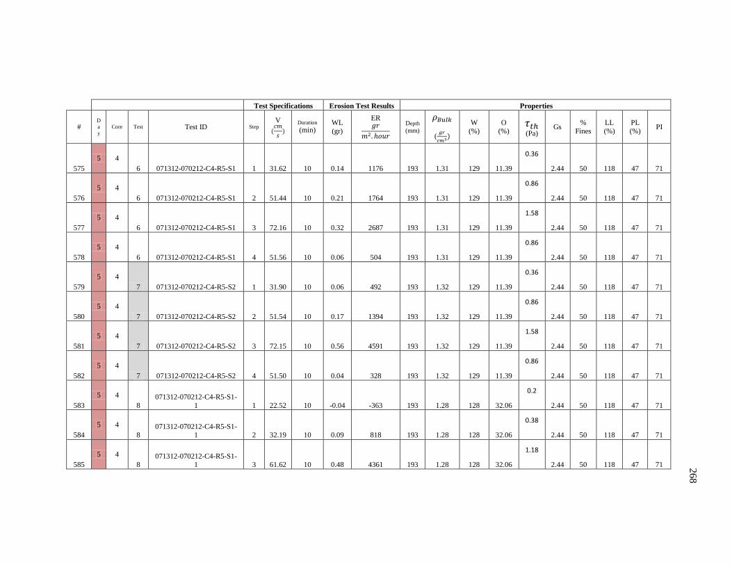
268

Test Specifications Erosion Test Results Properties

# D

a

y Core Test Test ID Step

V

Duration (min)

WL

(gr)

ER

Depth

(mm)

(

W

(%)

O

(%)

(Pa) Gs

%

Fines

LL

(%)

PL

(%) PI

575

5 4

6 071312-070212-C4-R5-S1 1 31.62 10 0.14 1176 193 1.31 129 11.39

0.36

2.44 50 118 47 71

576

5 4

6 071312-070212-C4-R5-S1 2 51.44 10 0.21 1764 193 1.31 129 11.39

0.86

2.44 50 118 47 71

577

5 4

6 071312-070212-C4-R5-S1 3 72.16 10 0.32 2687 193 1.31 129 11.39

1.58

2.44 50 118 47 71

578

5 4

6 071312-070212-C4-R5-S1 4 51.56 10 0.06 504 193 1.31 129 11.39

0.86

2.44 50 118 47 71

579

5 4

7 071312-070212-C4-R5-S2 1 31.90 10 0.06 492 193 1.32 129 11.39

0.36

2.44 50 118 47 71

580

5 4

7 071312-070212-C4-R5-S2 2 51.54 10 0.17 1394 193 1.32 129 11.39

0.86

2.44 50 118 47 71

581

5 4

7 071312-070212-C4-R5-S2 3 72.15 10 0.56 4591 193 1.32 129 11.39

1.58

2.44 50 118 47 71

582

5 4

7 071312-070212-C4-R5-S2 4 51.50 10 0.04 328 193 1.32 129 11.39

0.86

2.44 50 118 47 71

583

5 4

8

071312-070212-C4-R5-S1-

1 1 22.52 10 -0.04 -363 193 1.28 128 32.06

0.2

2.44 50 118 47 71

584

5 4

8 071312-070212-C4-R5-S1-

1 2 32.19 10 0.09 818 193 1.28 128 32.06

0.38

2.44 50 118 47 71

585

5 4

8 071312-070212-C4-R5-S1-

1 3 61.62 10 0.48 4361 193 1.28 128 32.06

1.18

2.44 50 118 47 71

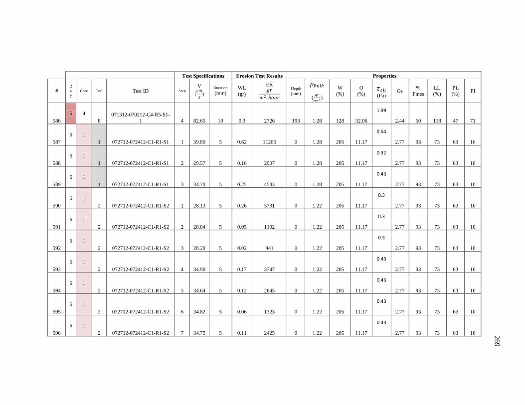
269

Test Specifications Erosion Test Results Properties

# D

a

y Core Test Test ID Step

V

Duration (min)

WL

(gr)

ER

Depth

(mm)

(

W

(%)

O

(%)

(Pa) Gs

%

Fines

LL

(%)

PL

(%) PI

586

5 4

8

071312-070212-C4-R5-S1-

1 4 82.65 10 0.3 2726 193 1.28 128 32.06

1.99

2.44 50 118 47 71

587

6 1

1 072712-072412-C1-R1-S1 1 39.80 5 0.62 11266 0 1.28 205 11.17

0.54

2.77 93 73 63 10

588

6 1

1 072712-072412-C1-R1-S1 2 29.57 5 0.16 2907 0 1.28 205 11.17

0.32

2.77 93 73 63 10

589

6 1

1 072712-072412-C1-R1-S1 3 34.70 5 0.25 4543 0 1.28 205 11.17

0.43

2.77 93 73 63 10

590

6 1

2 072712-072412-C1-R1-S2 1 28.13 5 0.26 5731 0 1.22 205 11.17

0.3

2.77 93 73 63 10

591

6 1

2 072712-072412-C1-R1-S2 2 28.04 5 0.05 1102 0 1.22 205 11.17

0.3

2.77 93 73 63 10

592

6 1

2 072712-072412-C1-R1-S2 3 28.20 5 0.02 441 0 1.22 205 11.17

0.3

2.77 93 73 63 10

593

6 1

2 072712-072412-C1-R1-S2 4 34.90 5 0.17 3747 0 1.22 205 11.17

0.43

2.77 93 73 63 10

594

6 1

2 072712-072412-C1-R1-S2 5 34.64 5 0.12 2645 0 1.22 205 11.17

0.43

2.77 93 73 63 10

595

6 1

2 072712-072412-C1-R1-S2 6 34.82 5 0.06 1323 0 1.22 205 11.17

0.43

2.77 93 73 63 10

596

6 1

2 072712-072412-C1-R1-S2 7 34.75 5 0.11 2425 0 1.22 205 11.17

0.43

2.77 93 73 63 10

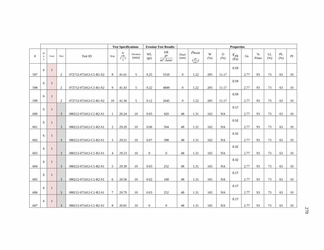
270

Test Specifications Erosion Test Results Properties

# D

a

y Core Test Test ID Step

V

Duration (min)

WL

(gr)

ER

Depth

(mm)

(

W

(%)

O

(%)

(Pa) Gs

%

Fines

LL

(%)

PL

(%) PI

597

6 1

2 072712-072412-C1-R1-S2 8 41.61 5 0.25 5510 0 1.22 205 11.17

0.59

2.77 93 73 63 10

598

6 1

2 072712-072412-C1-R1-S2 9 41.43 5 0.22 4849 0 1.22 205 11.17

0.59

2.77 93 73 63 10

599

6 1

2 072712-072412-C1-R1-S2 10 41.36 5 0.12 2645 0 1.22 205 11.17

0.59

2.77 93 73 63 10

600

6 1

3 080212-072412-C1-R2-S1 1 20.24 10 0.05 420 48 1.31 162 NA

0.17

2.77 93 73 63 10

601

6 1

3 080212-072412-C1-R2-S1 2 29.20 10 0.06 504 48 1.31 162 NA

0.32

2.77 93 73 63 10

602

6 1

3 080212-072412-C1-R2-S1 3 29.21 10 0.07 588 48 1.31 162 NA

0.32

2.77 93 73 63 10

603

6 1

3 080212-072412-C1-R2-S1 4 29.23 10 0 0 48 1.31 165 NA

0.32

2.77 93 73 63 10

604

6 1

3 080212-072412-C1-R2-S1 5 29.30 10 0.03 252 48 1.31 165 NA

0.32

2.77 93 73 63 10

605

6 1

3 080212-072412-C1-R2-S1 6 20.56 10 0.02 168 48 1.31 165 NA

0.17

2.77 93 73 63 10

606

6 1

3 080212-072412-C1-R2-S1 7 20.79 10 0.03 252 48 1.31 165 NA

0.17

2.77 93 73 63 10

607

6 1

3 080212-072412-C1-R2-S1 8 20.81 10 0 0 48 1.31 165 NA

0.17

2.77 93 73 63 10

271

Test Specifications Erosion Test Results Properties

# D

a

y Core Test Test ID Step

V

Duration (min)

WL

(gr)

ER

Depth

(mm)

(

W

(%)

O

(%)

(Pa) Gs

%

Fines

LL

(%)

PL

(%) PI

608

6 1

3 080212-072412-C1-R2-S1 9 20.91 10 0 0 48 1.31 165 NA

0.17

2.77 93 73 63 10

609

6 1

3 080212-072412-C1-R2-S1 10 29.34 10 0.05 420 48 1.31 165 NA

0.32

2.77 93 73 63 10

610

6 1

3 080212-072412-C1-R2-S1 11 20.76 10 0.03 252 48 1.31 165 NA

0.17

2.77 93 73 63 10

611

6 1

4 080212-072412-C1-R2-S2 1 20.70 10 0.02 153 48 1.35 165 NA

0.17

2.77 93 73 63 10

612

6 1

4 080212-072412-C1-R2-S2 2 29.21 10 0 0 48 1.35 165 NA

0.32

2.77 93 73 63 10

613

6 1

4 080212-072412-C1-R2-S2 3 29.34 10 0.01 77 48 1.35 165 NA

0.32

2.77 93 73 63 10

614

6 1

5 080312-072412-C1-R3-S1 1 19.95 10 -0.05 -375 99 1.36 168 9.15

0.16

2.77 93 73 63 10

615

6 1

5 080312-072412-C1-R3-S1 2 33.64 10 0.03 225 99 1.36 168 9.15

0.4

2.77 93 73 63 10

616

6 1

5 080312-072412-C1-R3-S1 3 33.83 10 0.02 150 99 1.36 168 9.15

0.4

2.77 93 73 63 10

617

6 1

5 080312-072412-C1-R3-S1 4 44.15 10 0.03 225 99 1.36 168 9.15

0.67

2.77 93 73 63 10

618

6 1

5 080312-072412-C1-R3-S1 5 53.56 10 0.11 826 99 1.36 168 9.15

0.92

2.77 93 73 63 10

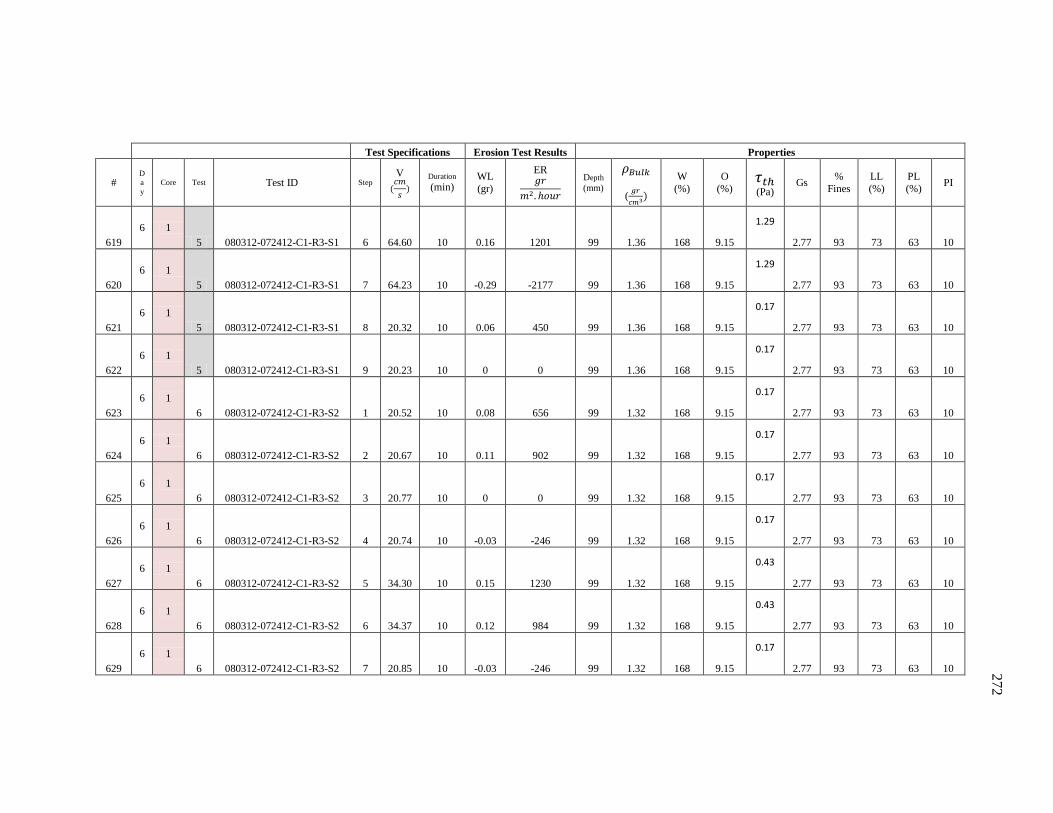
272

Test Specifications Erosion Test Results Properties

# D

a

y Core Test Test ID Step

V

Duration (min)

WL

(gr)

ER

Depth

(mm)

(

W

(%)

O

(%)

(Pa) Gs

%

Fines

LL

(%)

PL

(%) PI

619

6 1

5 080312-072412-C1-R3-S1 6 64.60 10 0.16 1201 99 1.36 168 9.15

1.29

2.77 93 73 63 10

620

6 1

5 080312-072412-C1-R3-S1 7 64.23 10 -0.29 -2177 99 1.36 168 9.15

1.29

2.77 93 73 63 10

621

6 1

5 080312-072412-C1-R3-S1 8 20.32 10 0.06 450 99 1.36 168 9.15

0.17

2.77 93 73 63 10

622

6 1

5 080312-072412-C1-R3-S1 9 20.23 10 0 0 99 1.36 168 9.15

0.17

2.77 93 73 63 10

623

6 1

6 080312-072412-C1-R3-S2 1 20.52 10 0.08 656 99 1.32 168 9.15

0.17

2.77 93 73 63 10

624

6 1

6 080312-072412-C1-R3-S2 2 20.67 10 0.11 902 99 1.32 168 9.15

0.17

2.77 93 73 63 10

625

6 1

6 080312-072412-C1-R3-S2 3 20.77 10 0 0 99 1.32 168 9.15

0.17

2.77 93 73 63 10

626

6 1

6 080312-072412-C1-R3-S2 4 20.74 10 -0.03 -246 99 1.32 168 9.15

0.17

2.77 93 73 63 10

627

6 1

6 080312-072412-C1-R3-S2 5 34.30 10 0.15 1230 99 1.32 168 9.15

0.43

2.77 93 73 63 10

628

6 1

6 080312-072412-C1-R3-S2 6 34.37 10 0.12 984 99 1.32 168 9.15

0.43

2.77 93 73 63 10

629

6 1

6 080312-072412-C1-R3-S2 7 20.85 10 -0.03 -246 99 1.32 168 9.15

0.17

2.77 93 73 63 10

273

Test Specifications Erosion Test Results Properties

# D

a

y Core Test Test ID Step

V

Duration (min)

WL

(gr)

ER

Depth

(mm)

(

W

(%)

O

(%)

(Pa) Gs

%

Fines

LL

(%)

PL

(%) PI

630

6 1

7 080312-072412-C1-R4-S1 1 20.71 10 0.05 239 138 1.71 178 NA

0.17

2.77 93 73 63 10

631

6 1

7 080312-072412-C1-R4-S1 2 20.64 10 0.02 96 138 1.71 178 NA

0.17

2.77 93 73 63 10

632

6 1

7 080312-072412-C1-R4-S1 3 20.95 10 0 0 138 1.71 178 NA

0.17

2.77 93 73 63 10

633

6 1

7 080312-072412-C1-R4-S1 4 29.17 10 0.02 96 138 1.71 178 NA

0.32

2.77 93 73 63 10

634

6 1

7 080312-072412-C1-R4-S1 5 29.22 10 0.04 191 138 1.71 178 NA

0.32

2.77 93 73 63 10

635

6 1

7 080312-072412-C1-R4-S1 6 29.12 10 0.01 48 138 1.71 178 NA

0.32

2.77 93 73 63 10

636

6 1

7 080312-072412-C1-R4-S1 7 48.81 10 0.1 479 138 1.71 178 NA

0.78

2.77 93 73 63 10

637

6 2

1 072512-072412-C2-R1-S1 1 16.58 10 -0.03 -265 0 1.29 219 9.19

0.12

2.54 88 175 76 98

638

6 2

1 072512-072412-C2-R1-S1 2 16.82 10 0.05 442 0 1.29 219 9.19

0.12

2.54 88 175 76 98

639

6 2

1 072512-072412-C2-R1-S1 3 21.77 10 0.05 442 0 1.29 219 9.19

0.18

2.54 88 175 76 98

640

6 2

1 072512-072412-C2-R1-S1 4 21.95 10 0.09 796 0 1.29 219 9.19

0.18

2.54 88 175 76 98

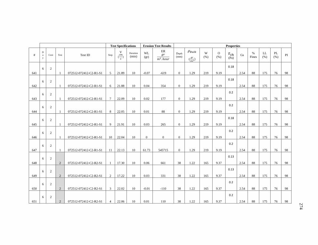
274

Test Specifications Erosion Test Results Properties

# D

a

y Core Test Test ID Step

V

Duration (min)

WL

(gr)

ER

Depth

(mm)

(

W

(%)

O

(%)

(Pa) Gs

%

Fines

LL

(%)

PL

(%) PI

641

6 2

1 072512-072412-C2-R1-S1 5 21.89 10 -0.07 -619 0 1.29 219 9.19

0.18

2.54 88 175 76 98

642

6 2

1 072512-072412-C2-R1-S1 6 21.88 10 0.04 354 0 1.29 219 9.19

0.18

2.54 88 175 76 98

643

6 2

1 072512-072412-C2-R1-S1 7 22.09 10 0.02 177 0 1.29 219 9.19

0.2

2.54 88 175 76 98

644

6 2

1 072512-072412-C2-R1-S1 8 22.05 10 0.01 88 0 1.29 219 9.19

0.2

2.54 88 175 76 98

645

6 2

1 072512-072412-C2-R1-S1 9 21.91 10 0.03 265 0 1.29 219 9.19

0.18

2.54 88 175 76 98

646

6 2

1 072512-072412-C2-R1-S1 10 22.04 10 0 0 0 1.29 219 9.19

0.2

2.54 88 175 76 98

647

6 2

1 072512-072412-C2-R1-S1 11 22.13 10 61.73 545715 0 1.29 219 9.19

0.2

2.54 88 175 76 98

648

6 2

2 072512-072412-C2-R2-S1 1 17.30 10 0.06 661 38 1.22 165 9.37

0.13

2.54 88 175 76 98

649

6 2

2 072512-072412-C2-R2-S1 2 17.22 10 0.03 331 38 1.22 165 9.37

0.13

2.54 88 175 76 98

650

6 2

2 072512-072412-C2-R2-S1 3 22.02 10 -0.01 -110 38 1.22 165 9.37

0.2

2.54 88 175 76 98

651

6 2

2 072512-072412-C2-R2-S1 4 22.06 10 0.01 110 38 1.22 165 9.37

0.2

2.54 88 175 76 98

275

Test Specifications Erosion Test Results Properties

# D

a

y Core Test Test ID Step

V

Duration (min)

WL

(gr)

ER

Depth

(mm)

(

W

(%)

O

(%)

(Pa) Gs

%

Fines

LL

(%)

PL

(%) PI

652

6 2

2 072512-072412-C2-R2-S1 5 22.06 10 0.02 220 38 1.22 165 9.37

0.2

2.54 88 175 76 98

653

6 2

2 072512-072412-C2-R2-S1 6 26.01 10 0.04 441 38 1.22 165 9.37

0.27

2.54 88 175 76 98

654

6 2

2 072512-072412-C2-R2-S1 7 26.03 10 0.02 220 38 1.22 165 9.37

0.27

2.54 88 175 76 98

655

6 2

2 072512-072412-C2-R2-S1 8 26.11 10 0.01 110 38 1.22 165 9.37

0.27

2.54 88 175 76 98

656

6 3

1 072612-072412-C3-R1-S1 1 16.65 10 0.05 651 0 1.18 212 10.41

0.12

2.4 95 208 110 98

657

6 3

1 072612-072412-C3-R1-S1 2 16.74 10 0.01 130 0 1.18 212 10.41

0.12

2.4 95 208 110 98

658

6 3

1 072612-072412-C3-R1-S1 3 16.87 10 0 0 0 1.18 212 10.41

0.12

2.4 95 208 110 98

659

6 3

1 072612-072412-C3-R1-S1 4 16.94 10 0.03 391 0 1.18 212 10.41

0.12

2.4 95 208 110 98

660

6 3

1 072612-072412-C3-R1-S1 5 25.81 10 0.08 1042 0 1.18 212 10.41

0.25

2.4 95 208 110 98

661

6 3

1 072612-072412-C3-R1-S1 6 25.80 10 0.04 521 0 1.18 212 10.41

0.25

2.4 95 208 110 98

662

6 3

1 072612-072412-C3-R1-S1 7 25.82 10 0.04 521 0 1.18 212 10.41

0.25

2.4 95 208 110 98

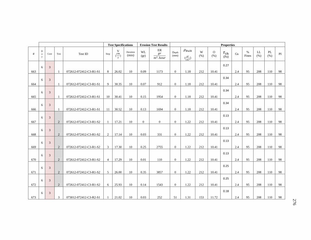
276

Test Specifications Erosion Test Results Properties

# D

a

y Core Test Test ID Step

V

Duration (min)

WL

(gr)

ER

Depth

(mm)

(

W

(%)

O

(%)

(Pa) Gs

%

Fines

LL

(%)

PL

(%) PI

663

6 3

1 072612-072412-C3-R1-S1 8 26.02 10 0.09 1173 0 1.18 212 10.41

0.27

2.4 95 208 110 98

664

6 3

1 072612-072412-C3-R1-S1 9 30.35 10 0.07 912 0 1.18 212 10.41

0.34

2.4 95 208 110 98

665

6 3

1 072612-072412-C3-R1-S1 10 30.41 10 0.15 1954 0 1.18 212 10.41

0.34

2.4 95 208 110 98

666

6 3

1 072612-072412-C3-R1-S1 11 30.52 10 0.13 1694 0 1.18 212 10.41

0.34

2.4 95 208 110 98

667

6 3

2 072612-072412-C3-R1-S2 1 17.21 10 0 0 0 1.22 212 10.41

0.13

2.4 95 208 110 98

668

6 3

2 072612-072412-C3-R1-S2 2 17.14 10 0.03 331 0 1.22 212 10.41

0.13

2.4 95 208 110 98

669

6 3

2 072612-072412-C3-R1-S2 3 17.30 10 0.25 2755 0 1.22 212 10.41

0.13

2.4 95 208 110 98

670

6 3

2 072612-072412-C3-R1-S2 4 17.29 10 0.01 110 0 1.22 212 10.41

0.13

2.4 95 208 110 98

671

6 3

2 072612-072412-C3-R1-S2 5 26.00 10 0.35 3857 0 1.22 212 10.41

0.25

2.4 95 208 110 98

672

6 3

2 072612-072412-C3-R1-S2 6 25.93 10 0.14 1543 0 1.22 212 10.41

0.25

2.4 95 208 110 98

673

6 3

3 073012-072412-C3-R2-S1 1 21.02 10 0.03 252 51 1.31 153 11.72

0.18

2.4 95 208 110 98

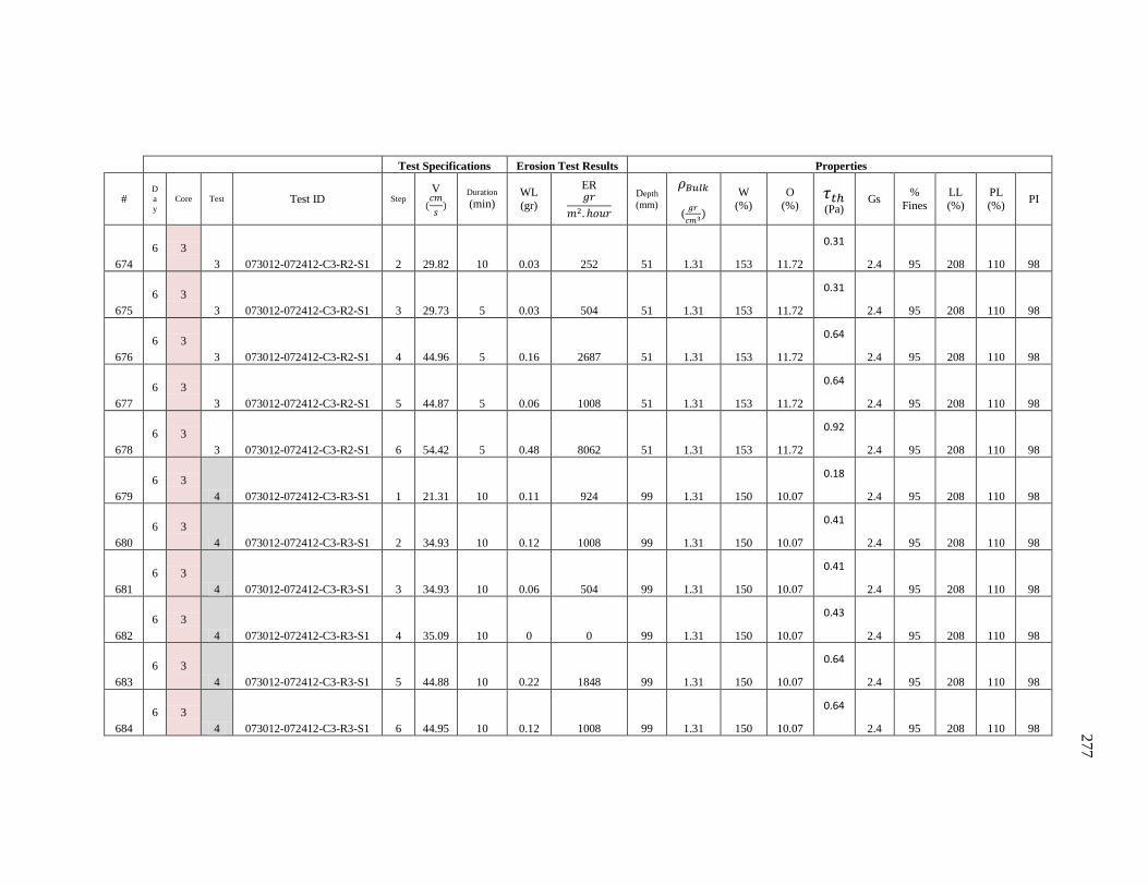
277

Test Specifications Erosion Test Results Properties

# D

a

y Core Test Test ID Step

V

Duration (min)

WL

(gr)

ER

Depth

(mm)

(

W

(%)

O

(%)

(Pa) Gs

%

Fines

LL

(%)

PL

(%) PI

674

6 3

3 073012-072412-C3-R2-S1 2 29.82 10 0.03 252 51 1.31 153 11.72

0.31

2.4 95 208 110 98

675

6 3

3 073012-072412-C3-R2-S1 3 29.73 5 0.03 504 51 1.31 153 11.72

0.31

2.4 95 208 110 98

676

6 3

3 073012-072412-C3-R2-S1 4 44.96 5 0.16 2687 51 1.31 153 11.72

0.64

2.4 95 208 110 98

677

6 3

3 073012-072412-C3-R2-S1 5 44.87 5 0.06 1008 51 1.31 153 11.72

0.64

2.4 95 208 110 98

678

6 3

3 073012-072412-C3-R2-S1 6 54.42 5 0.48 8062 51 1.31 153 11.72

0.92

2.4 95 208 110 98

679

6 3

4 073012-072412-C3-R3-S1 1 21.31 10 0.11 924 99 1.31 150 10.07

0.18

2.4 95 208 110 98

680

6 3

4 073012-072412-C3-R3-S1 2 34.93 10 0.12 1008 99 1.31 150 10.07

0.41

2.4 95 208 110 98

681

6 3

4 073012-072412-C3-R3-S1 3 34.93 10 0.06 504 99 1.31 150 10.07

0.41

2.4 95 208 110 98

682

6 3

4 073012-072412-C3-R3-S1 4 35.09 10 0 0 99 1.31 150 10.07

0.43

2.4 95 208 110 98

683

6 3

4 073012-072412-C3-R3-S1 5 44.88 10 0.22 1848 99 1.31 150 10.07

0.64

2.4 95 208 110 98

684

6 3

4 073012-072412-C3-R3-S1 6 44.95 10 0.12 1008 99 1.31 150 10.07

0.64

2.4 95 208 110 98

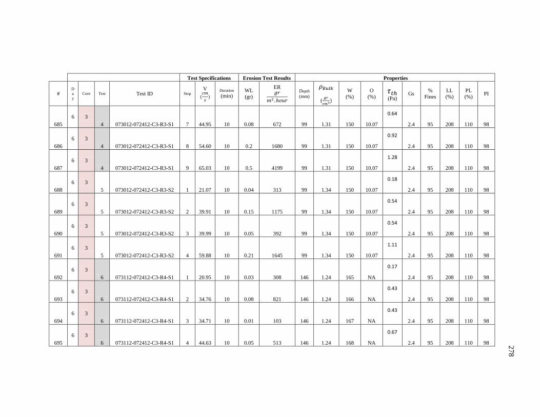
278

Test Specifications Erosion Test Results Properties

# D

a

y Core Test Test ID Step

V

Duration (min)

WL

(gr)

ER

Depth

(mm)

(

W

(%)

O

(%)

(Pa) Gs

%

Fines

LL

(%)

PL

(%) PI

685

6 3

4 073012-072412-C3-R3-S1 7 44.95 10 0.08 672 99 1.31 150 10.07

0.64

2.4 95 208 110 98

686

6 3

4 073012-072412-C3-R3-S1 8 54.60 10 0.2 1680 99 1.31 150 10.07

0.92

2.4 95 208 110 98

687

6 3

4 073012-072412-C3-R3-S1 9 65.03 10 0.5 4199 99 1.31 150 10.07

1.28

2.4 95 208 110 98

688

6 3

5 073012-072412-C3-R3-S2 1 21.07 10 0.04 313 99 1.34 150 10.07

0.18

2.4 95 208 110 98

689

6 3

5 073012-072412-C3-R3-S2 2 39.91 10 0.15 1175 99 1.34 150 10.07

0.54

2.4 95 208 110 98

690

6 3

5 073012-072412-C3-R3-S2 3 39.99 10 0.05 392 99 1.34 150 10.07

0.54

2.4 95 208 110 98

691

6 3

5 073012-072412-C3-R3-S2 4 59.88 10 0.21 1645 99 1.34 150 10.07

1.11

2.4 95 208 110 98

692

6 3

6 073112-072412-C3-R4-S1 1 20.95 10 0.03 308 146 1.24 165 NA

0.17

2.4 95 208 110 98

693

6 3

6 073112-072412-C3-R4-S1 2 34.76 10 0.08 821 146 1.24 166 NA

0.43

2.4 95 208 110 98

694

6 3

6 073112-072412-C3-R4-S1 3 34.71 10 0.01 103 146 1.24 167 NA

0.43

2.4 95 208 110 98

695

6 3

6 073112-072412-C3-R4-S1 4 44.63 10 0.05 513 146 1.24 168 NA

0.67

2.4 95 208 110 98

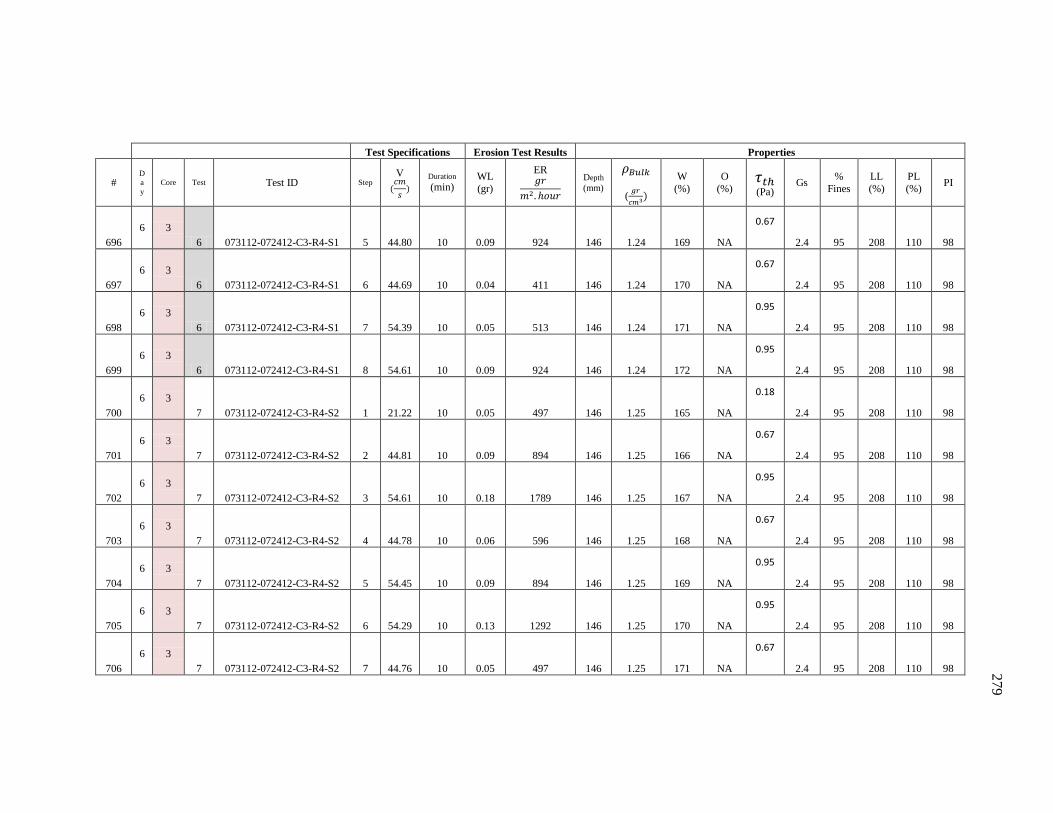
279

Test Specifications Erosion Test Results Properties

# D

a

y Core Test Test ID Step

V

Duration (min)

WL

(gr)

ER

Depth

(mm)

(

W

(%)

O

(%)

(Pa) Gs

%

Fines

LL

(%)

PL

(%) PI

696

6 3

6 073112-072412-C3-R4-S1 5 44.80 10 0.09 924 146 1.24 169 NA

0.67

2.4 95 208 110 98

697

6 3

6 073112-072412-C3-R4-S1 6 44.69 10 0.04 411 146 1.24 170 NA

0.67

2.4 95 208 110 98

698

6 3

6 073112-072412-C3-R4-S1 7 54.39 10 0.05 513 146 1.24 171 NA

0.95

2.4 95 208 110 98

699

6 3

6 073112-072412-C3-R4-S1 8 54.61 10 0.09 924 146 1.24 172 NA

0.95

2.4 95 208 110 98

700

6 3

7 073112-072412-C3-R4-S2 1 21.22 10 0.05 497 146 1.25 165 NA

0.18

2.4 95 208 110 98

701

6 3

7 073112-072412-C3-R4-S2 2 44.81 10 0.09 894 146 1.25 166 NA

0.67

2.4 95 208 110 98

702

6 3

7 073112-072412-C3-R4-S2 3 54.61 10 0.18 1789 146 1.25 167 NA

0.95

2.4 95 208 110 98

703

6 3

7 073112-072412-C3-R4-S2 4 44.78 10 0.06 596 146 1.25 168 NA

0.67

2.4 95 208 110 98

704

6 3

7 073112-072412-C3-R4-S2 5 54.45 10 0.09 894 146 1.25 169 NA

0.95

2.4 95 208 110 98

705

6 3

7 073112-072412-C3-R4-S2 6 54.29 10 0.13 1292 146 1.25 170 NA

0.95

2.4 95 208 110 98

706

6 3

7 073112-072412-C3-R4-S2 7 44.76 10 0.05 497 146 1.25 171 NA

0.67

2.4 95 208 110 98

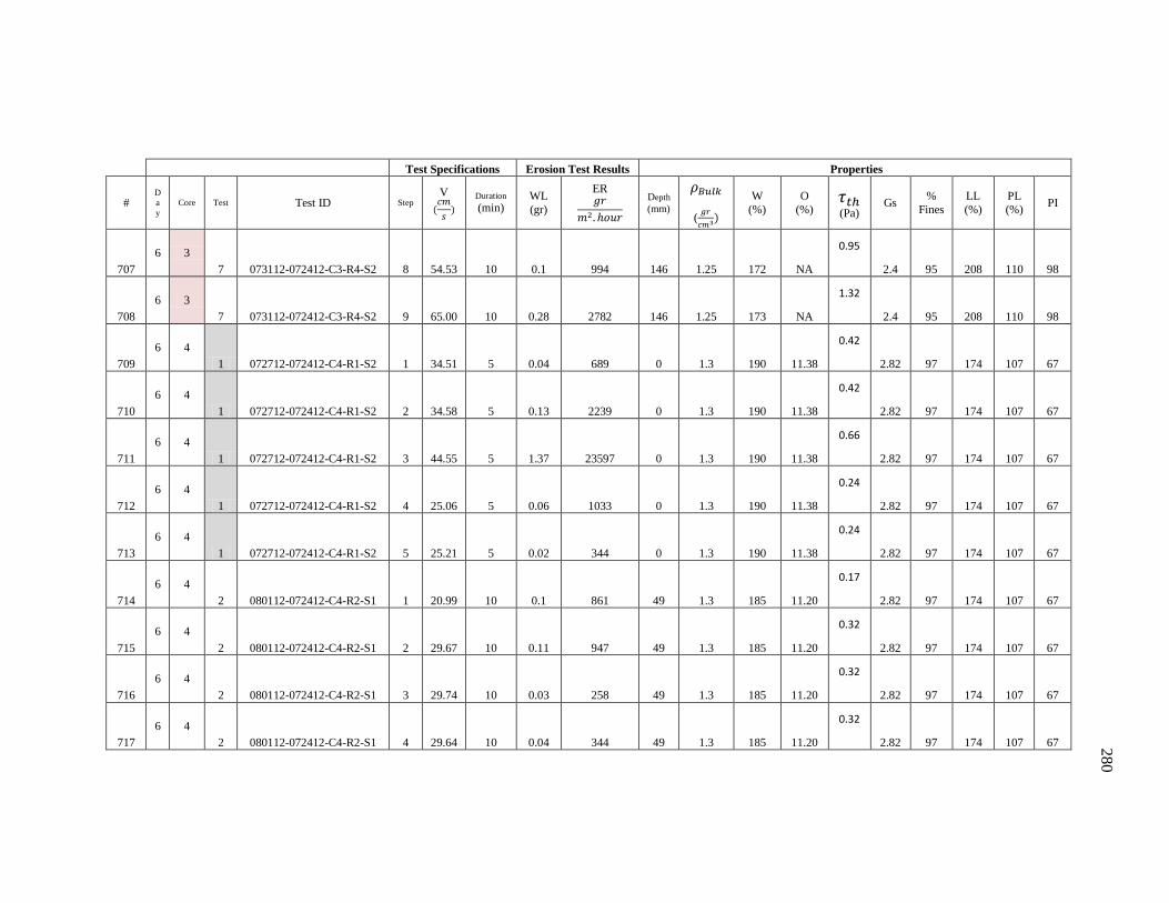
280

Test Specifications Erosion Test Results Properties

# D

a

y Core Test Test ID Step

V

Duration (min)

WL

(gr)

ER

Depth

(mm)

(

W

(%)

O

(%)

(Pa) Gs

%

Fines

LL

(%)

PL

(%) PI

707

6 3

7 073112-072412-C3-R4-S2 8 54.53 10 0.1 994 146 1.25 172 NA

0.95

2.4 95 208 110 98

708

6 3

7 073112-072412-C3-R4-S2 9 65.00 10 0.28 2782 146 1.25 173 NA

1.32

2.4 95 208 110 98

709

6 4

1 072712-072412-C4-R1-S2 1 34.51 5 0.04 689 0 1.3 190 11.38

0.42

2.82 97 174 107 67

710

6 4

1 072712-072412-C4-R1-S2 2 34.58 5 0.13 2239 0 1.3 190 11.38

0.42

2.82 97 174 107 67

711

6 4

1 072712-072412-C4-R1-S2 3 44.55 5 1.37 23597 0 1.3 190 11.38

0.66

2.82 97 174 107 67

712

6 4

1 072712-072412-C4-R1-S2 4 25.06 5 0.06 1033 0 1.3 190 11.38

0.24

2.82 97 174 107 67

713

6 4

1 072712-072412-C4-R1-S2 5 25.21 5 0.02 344 0 1.3 190 11.38

0.24

2.82 97 174 107 67

714

6 4

2 080112-072412-C4-R2-S1 1 20.99 10 0.1 861 49 1.3 185 11.20

0.17

2.82 97 174 107 67

715

6 4

2 080112-072412-C4-R2-S1 2 29.67 10 0.11 947 49 1.3 185 11.20

0.32

2.82 97 174 107 67

716

6 4

2 080112-072412-C4-R2-S1 3 29.74 10 0.03 258 49 1.3 185 11.20

0.32

2.82 97 174 107 67

717

6 4

2 080112-072412-C4-R2-S1 4 29.64 10 0.04 344 49 1.3 185 11.20

0.32

2.82 97 174 107 67

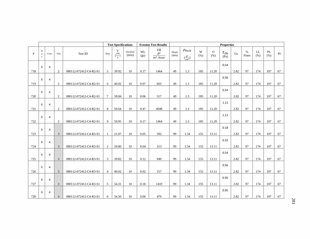
281

Test Specifications Erosion Test Results Properties

# D

a

y Core Test Test ID Step

V

Duration (min)

WL

(gr)

ER

Depth

(mm)

(

W

(%)

O

(%)

(Pa) Gs

%

Fines

LL

(%)

PL

(%) PI

718

6 4

2 080112-072412-C4-R2-S1 5 39.92 10 0.17 1464 49 1.3 185 11.20

0.54

2.82 97 174 107 67

719

6 4

2 080112-072412-C4-R2-S1 6 40.02 10 0.07 603 49 1.3 185 11.20

0.56

2.82 97 174 107 67

720

6 4

2 080112-072412-C4-R2-S1 7 39.84 10 0.06 517 49 1.3 185 11.20

0.54

2.82 97 174 107 67

721

6 4

2 080112-072412-C4-R2-S1 8 59.64 10 0.47 4048 49 1.3 185 11.20

1.11

2.82 97 174 107 67

722

6 4

2 080112-072412-C4-R2-S1 9 59.95 10 0.17 1464 49 1.3 185 11.20

1.11

2.82 97 174 107 67

723

6 4

3 080112-072412-C4-R3-S1 1 21.07 10 0.05 392 99 1.34 155 13.11

0.18

2.82 97 174 107 67

724

6 4

3 080112-072412-C4-R3-S1 2 29.80 10 0.04 313 99 1.34 155 13.11

0.32

2.82 97 174 107 67

725

6 4

3 080112-072412-C4-R3-S1 3 39.82 10 0.12 940 99 1.34 155 13.11

0.54

2.82 97 174 107 67

726

6 4

3 080112-072412-C4-R3-S1 4 40.02 10 0.02 157 99 1.34 155 13.11

0.56

2.82 97 174 107 67

727

6 4

3 080112-072412-C4-R3-S1 5 54.31 10 0.18 1410 99 1.34 155 13.11

0.95

2.82 97 174 107 67

728

6 4

3 080112-072412-C4-R3-S1 6 54.50 10 0.06 470 99 1.34 155 13.11

0.95

2.82 97 174 107 67

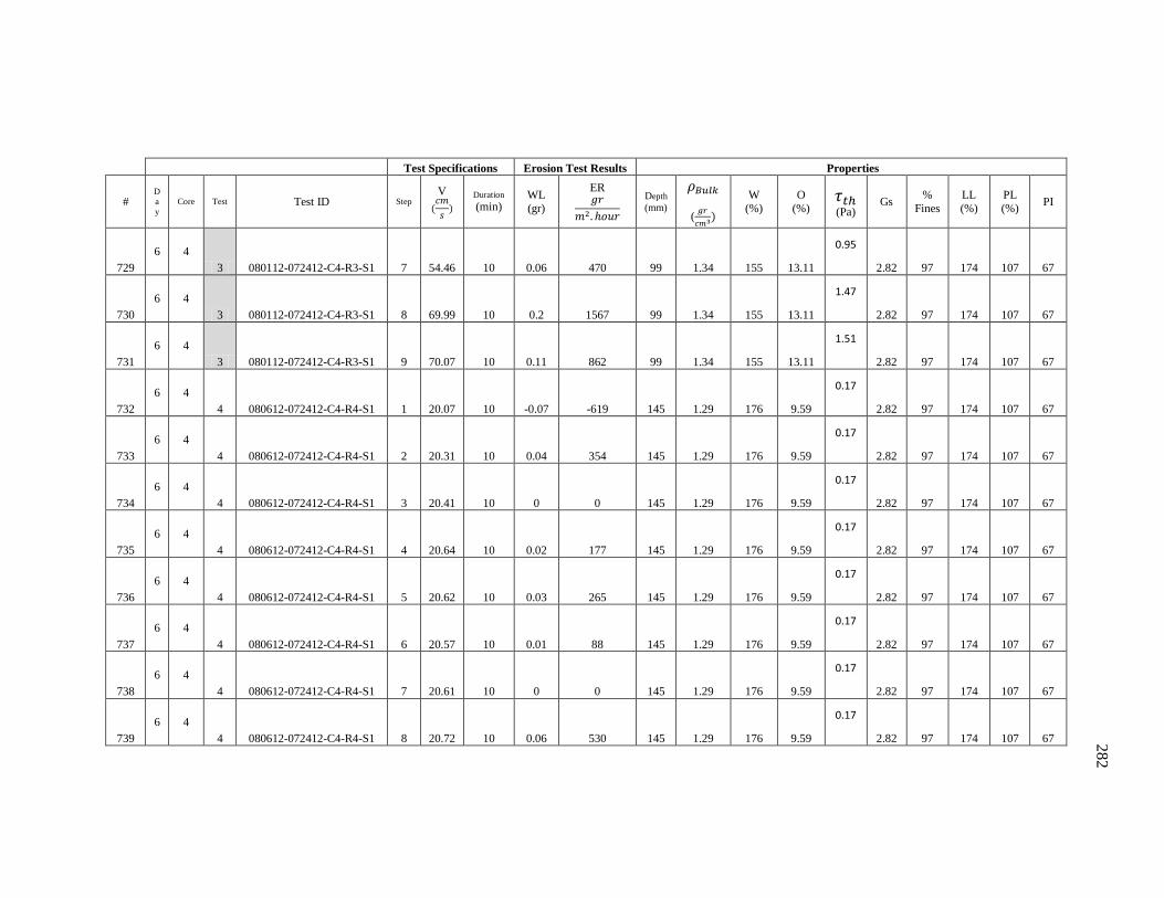
282

Test Specifications Erosion Test Results Properties

# D

a

y Core Test Test ID Step

V

Duration (min)

WL

(gr)

ER

Depth

(mm)

(

W

(%)

O

(%)

(Pa) Gs

%

Fines

LL

(%)

PL

(%) PI

729

6 4

3 080112-072412-C4-R3-S1 7 54.46 10 0.06 470 99 1.34 155 13.11

0.95

2.82 97 174 107 67

730

6 4

3 080112-072412-C4-R3-S1 8 69.99 10 0.2 1567 99 1.34 155 13.11

1.47

2.82 97 174 107 67

731

6 4

3 080112-072412-C4-R3-S1 9 70.07 10 0.11 862 99 1.34 155 13.11

1.51

2.82 97 174 107 67

732

6 4

4 080612-072412-C4-R4-S1 1 20.07 10 -0.07 -619 145 1.29 176 9.59

0.17

2.82 97 174 107 67

733

6 4

4 080612-072412-C4-R4-S1 2 20.31 10 0.04 354 145 1.29 176 9.59

0.17

2.82 97 174 107 67

734

6 4

4 080612-072412-C4-R4-S1 3 20.41 10 0 0 145 1.29 176 9.59

0.17

2.82 97 174 107 67

735

6 4

4 080612-072412-C4-R4-S1 4 20.64 10 0.02 177 145 1.29 176 9.59

0.17

2.82 97 174 107 67

736

6 4

4 080612-072412-C4-R4-S1 5 20.62 10 0.03 265 145 1.29 176 9.59

0.17

2.82 97 174 107 67

737

6 4

4 080612-072412-C4-R4-S1 6 20.57 10 0.01 88 145 1.29 176 9.59

0.17

2.82 97 174 107 67

738

6 4

4 080612-072412-C4-R4-S1 7 20.61 10 0 0 145 1.29 176 9.59

0.17

2.82 97 174 107 67

739

6 4

4 080612-072412-C4-R4-S1 8 20.72 10 0.06 530 145 1.29 176 9.59

0.17

2.82 97 174 107 67

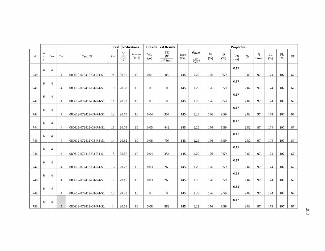
283

Test Specifications Erosion Test Results Properties

# D

a

y Core Test Test ID Step

V

Duration (min)

WL

(gr)

ER

Depth

(mm)

(

W

(%)

O

(%)

(Pa) Gs

%

Fines

LL

(%)

PL

(%) PI

740

6 4

4 080612-072412-C4-R4-S1 9 20.57 10 0.01 88 145 1.29 176 9.59

0.17

2.82 97 174 107 67

741

6 4

4 080612-072412-C4-R4-S1 10 20.58 10 0 0 145 1.29 176 9.59

0.17

2.82 97 174 107 67

742

6 4

4 080612-072412-C4-R4-S1 11 20.80 10 0 0 145 1.29 176 9.59

0.17

2.82 97 174 107 67

743

6 4

4 080612-072412-C4-R4-S1 12 20.70 10 0.04 354 145 1.29 176 9.59

0.17

2.82 97 174 107 67

744

6 4

4 080612-072412-C4-R4-S1 13 20.78 10 0.05 442 145 1.29 176 9.59

0.17

2.82 97 174 107 67

745

6 4

4 080612-072412-C4-R4-S1 14 20.82 10 0.08 707 145 1.29 176 9.59

0.17

2.82 97 174 107 67

746

6 4

4 080612-072412-C4-R4-S1 15 20.67 10 0.04 354 145 1.29 176 9.59

0.17

2.82 97 174 107 67

747

6 4

4 080612-072412-C4-R4-S1 16 20.72 10 0.03 265 145 1.29 176 9.59

0.17

2.82 97 174 107 67

748

6 4

4 080612-072412-C4-R4-S1 17 29.16 10 0.03 265 145 1.29 176 9.59

0.32

2.82 97 174 107 67

749

6 4

4 080612-072412-C4-R4-S1 18 29.20 10 0 0 145 1.29 176 9.59

0.32

2.82 97 174 107 67

750

6 4

5 080612-072412-C4-R4-S2 1 20.53 10 0.08 882 145 1.22 176 9.59

0.17

2.82 97 174 107 67

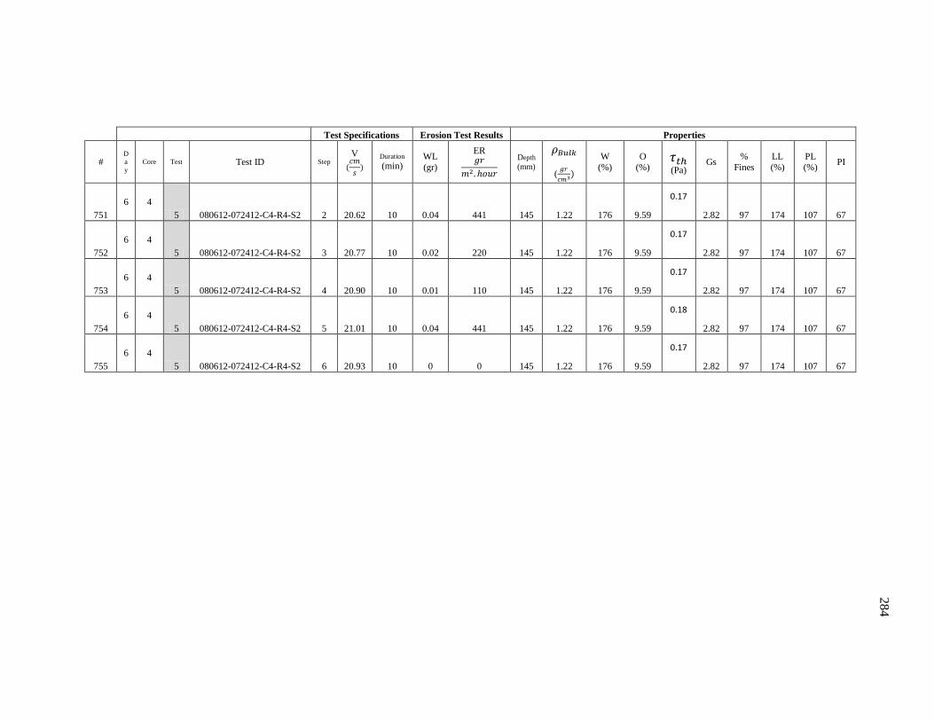
284

Test Specifications Erosion Test Results Properties

# D

a

y Core Test Test ID Step

V

Duration (min)

WL

(gr)

ER

Depth

(mm)

(

W

(%)

O

(%)

(Pa) Gs

%

Fines

LL

(%)

PL

(%) PI

751

6 4

5 080612-072412-C4-R4-S2 2 20.62 10 0.04 441 145 1.22 176 9.59

0.17

2.82 97 174 107 67

752

6 4

5 080612-072412-C4-R4-S2 3 20.77 10 0.02 220 145 1.22 176 9.59

0.17

2.82 97 174 107 67

753

6 4

5 080612-072412-C4-R4-S2 4 20.90 10 0.01 110 145 1.22 176 9.59

0.17

2.82 97 174 107 67

754

6 4

5 080612-072412-C4-R4-S2 5 21.01 10 0.04 441 145 1.22 176 9.59

0.18

2.82 97 174 107 67

755

6 4

5 080612-072412-C4-R4-S2 6 20.93 10 0 0 145 1.22 176 9.59

0.17

2.82 97 174 107 67

285

BIBLIOGRAPHY

Aberle, J., Nikora, V., & Walters, R. (2004). Effects of bed material properties on cohesive

sediment erosion. Marine Geology, 207 (1), 83–93.

Aberle, J., Nikora, V., & Walters, R. (2006). Data interpretation for in situ measurements of

cohesive sediment erosion. Journal of Hydraulic Engineering, 132 (6), 581–588.

Amore, E., Modica, C., Nearing, M. A., & Santoro, V. C. (2004). Scale effect in USLE and

WEPP application for soil erosion computation from three Sicilian basins. Journal of

Hydrology, 293 (1), 100–114.

Anderson, K. and Knight, D., (2012) “”CAIT Channel Calculation”,” Technical Report, Rutgers

University, Center for Computational Design.

Angelaki, M. (2006). Evaluation of bed shear stress under turbid flows through measures of flow

deceleration (Unpublished doctoral dissertation). University of Southampton.

Annandale, G. W. (2005). Scour technology: mechanics and engineering practice. McGraw Hill

Professional.

Been, K. (1980). Stress strain behaviour of a cohesive soil deposited under water. (Unpublished

doctoral dissertation). University of Oxford.

Beer, T. (1996). Environmental oceanography (Vol. 11). CRC Press.

Bergström, S. (1991). Principles and confidence in hydrological modelling. Nord. Hydrol., 22 (2),

123–136.

Bergström, S., & Graham, L. (1998). On the scale problem in hydrological modelling. Journal of

Hydrology, 211 (1), 253–265.

Bierkens, M. F., Finke, P. A., & Willigen, P. d. (2000). Upscaling and downscaling methods for

environmental research.

Blöschl, G., & Sivapalan, M. (1995). Scale issues in hydrological modelling: a review.

Hydrological processes, 9 (3-4), 251–290.

Borrowman, T. D., Smith, E. R., Gailani, J. Z., & Caviness, L. (2006).Erodibility Study Of

Passaic River Sediments Using USACE Sedflume (No. ERDC-TR-06-7). ENGINEER

RESEARCH AND DEVELOPMENT CENTER VICKSBURG MS

ENVIRONMENTAL LAB.

Borsje, B. W., de Vries, M. B., Hulscher, S. J., & de Boer, G. J. (2008). Modeling large-scale

cohesive sediment transport affected by small-scale biological activity. Estuarine,

Coastal and Shelf Science, 78 (3), 468–480.

Briaud, J. L., Ting, F. C. K., Chen, H. C., Cao, Y., Han, S. W., & Kwak, K. W. (2001). Erosion

function apparatus for scour rate predictions. Journal of geotechnical and

geoenvironmental engineering.

Burke, P., Bruno, M., Rankin, K., & Herrington, T. (2002). Sediment transport between deep

navigation channels and shallow side banks under variable tidal and meteorological

forcing. In AGU Fall meeting abstracts (Vol. 1, p. 0258).

Burt, N., Parker, R., & Watts, J. H. (1997). Cohesive sediments. John Wiley.

Chant, R. J. (2005). Hydrodynamics of the Newark Bay/Kills system (Tech.Rep.). New Jersey

Department of Environmental Protection.

Cundy, A. B., Collins, P. E., Turner, S. D., Croudace, I. W., & Horne, D. (1998). 100 years of

environmental change in a coastal wetland, Augusta Bay, southeast Sicily: evidence from

geochemical and palaeoecological studies. Geological Society, London, Special

Publications, 139 (1), 243–254.

De Vriend, H. J. (1991a). Mathematical modelling and large-scale coastal behaviour: Part 2:

Predictive models. Journal of Hydraulic Research, 29 (6), 741–753.

286

De Vriend, H. J. (1991b). Mathematical modelling and large-scale coastal behaviour: Part 2:

Predictive models. Journal of Hydraulic Research, 29 (6), 741–753.

Dyer, K. (1998). Sedimentary processes in the intertidal zone. In K. S. Black,D. M. Paterson, &

A. Cramp (Eds.), (p. 11-24). Geological Society of London.

Fenton, J., & Abbott, J. (1977). Initial movement of grains on a stream bed: The effect of relative

protrusion. Proceedings of the Royal Society of London. A. Mathematical and Physical

Sciences, 352 (1671), 523–537.

Freund, L. B., & Suresh, S. (2003). Thin film materials: stress, defect formation and surface

evolution. Cambridge University Press.

Garcaia, M. H. (2008). Sedimentation engineering: processes, measurements, modeling, and

practice (No. 110). ASCE Publications.

Geyer, W. R. (2010). Contemporary issues in estuarine physics. In A. ValleLevinson (Ed.), (p.

12-26). Cambridge University Press.

Goodchild, M. F., et al. (1997). Scale in remote sensing and GIS. CRC Press.

Grabowski, R. C., Droppo, I. G., & Wharton, G. (2011). Erodibility of cohesive sediment: The

importance of sediment properties. Earth-Science Reviews, 105 (3), 101–120.

Green, M. O., Black, K. P., & Amos, C. L. (1997). Control of estuarine sediment dynamics by

interactions between currents and waves at several scales. Marine Geology, 144 (1), 97–

116.

Hamilton, D. P., & Mitchell, S. F. (1996). An empirical model for sediment resuspension in

shallow lakes. Hydrobiologia, 317(3), 209-220.

Halonen, J. (2011). Effects of historical morphologic change on sediment accumulation in

Newark Bay, New Jersey (Unpublished doctoral dissertation). University of Delaware.

Herman, P. M., Middelburg, J. J., & Heip, C. H. (2001). Benthic community structure and

sediment processes on an intertidal flat: results from the ECOFLAT project. Continental

Shelf Research, 21 (18), 2055–2071.

Heuvelink, G., & Webster, R. (2001). Modelling soil variation: past, present, and future.

Geoderma, 100 (3), 269–301.

Heuvelink, G. B. (1998). Uncertainty analysis in environmental modelling under a change of

spatial scale. Nutrient Cycling in Agroecosystems, 50 (1-3), 255–264.

Hickin, E. J. (1995). River geomorphology. John Wiley & Sons.

Jeng, D. S., Barry, D., & Li, L. (2000). Water wave-driven seepage in marine sediments.

Advances in water resources, 24 (1), 1–10.

Jepsen, R., Roberts, J., & Lick, W. (1997). Effects of bulk density on sediment erosion

rates. Water, Air, and Soil Pollution, 99(1-4), 21-31.

João, E. (2007). A research agenda for data and scale issues in strategic environmental

assessment (SEA). Environmental Impact Assessment Review, 27 (5), 479–491.

João, E. M. (2000). The importance of scale issues in environmental impact assessment and the

need for scale guidelines.

Karstens, S. (2009). Bridging boundaries: Making scale choices in multi-actor policy analysis on

water management (Vol. 4). IOS Press.

Kirby, R. (2000). Practical implications of tidal flat shape. Continental Shelf Research, 20 , 1061

- 1077.

Kirchner, J. W., Dietrich, W. E., Iseya, F., & Ikeda, H. (1990). The variability of critical shear

stress, friction angle, and grain protrusion in water-worked sediments. Sedimentology, 37

(4), 647–672.

Kornman, B. A., & De Deckere, E. M. (1998). Temporal variation in sediment erodibility and

suspended sediment dynamics in the Dollard estuary. Geological Society, London,

Special Publications, 139 (1), 231–241.

287

Kronvang, B., Faganeli, J., & Ogrinc, N. (2006). The interactions between sediments and water.

Springer.

Lavelle, J. W., Mofjeld, H. O., & Baker, E. T. (1984). An in situ erosion rate for a fine‐grained

marine sediment. Journal of Geophysical Research: Oceans (1978–2012), 89(C4), 6543-

6552.

Lee, D.-Y., Lick, W., & Kang, S. W. (1981). The entrainment and deposition of fine-grained

sediments in Lake Erie. Journal of Great Lakes Research, 7 (3), 224–233.

Lee, S. C., & Mehta, A. J. (1994). Cohesive sediment erosion. Final report prepared for Dept. of

the Army, U.S. Army Corps of Engineers.

Leupi, C. (2005). Numerical modeling of cohesive sediment transport and bed morphology in

estuaries (Unpublished doctoral dissertation). ÉCOLE POLYTECHNIQUE FÉDÉRALE

DE LAUSANNE.

Lick, W. (2008). Sediment and contaminant transport in surface waters. CRC Press.

Lintern, D. G. (2003). Influences of flocculation on bed properties for fine-grained cohesive

sediment (Unpublished doctoral dissertation). University of Oxford.

Lopez, F., & Garcia, M. H. (2001). Risk of sediment erosion and suspension in turbulent flows.

Journal of Hydraulic Engineering, 127 (3), 231–235.

Luettich, R. A., Harleman, D. R., & Somlyody, L. (1990). Dynamic behavior of suspended

sediment concentrations in a shallow lake perturbed by episodic wind events. Limnology

and Oceanography, 35 (5), 1050–1067.

Lund-Hansen, L. C., Christiansen, C., Jensen, O., & Laima, M. (1999). The LABEREX chamber

for studying the critical shear stress for fine-grained sediment. Geografisk Tidsskrift-

Danish Journal of Geography, 99 (1), 1–7.

Malcolm, D. B., S. J.; Sivyer. (1997). Biogeochemistry of intertidal sediments. In J. E. Jickells T.

D.; Rae (Ed.), (p. 84-98). Cambridge University Press.

Mariotti, G., Valentine, K., & Fagherazzi, S. (2013). Time-dependent behavior of a placed bed of

cohesive sediment subjected to erosion and deposition cycles. Ocean Dynamics, 1–8.

McBratney, A. B. (1998). Some considerations on methods for spatially aggregating and

disaggregating soil information. In Soil and water quality at different scales (pp. 51–62).

Springer.

McNeil, J., Taylor, C., & Lick, W. (1996). Measurements of erosion of undisturbed bottom

sediments with depth. Journal of Hydraulic Engineering, 122 (6), 316–324.

Meadows, A., Meadows, P. S., & McLaughlin, P. (1998). Spatial heterogeneity in an intertidal

sedimentary environment and its macrobenthic community. Geological Society, London,

Special Publications, 139 (1), 367–388.

Meadows, P. S., Murray, J. M., Meadows, A., Wood, D. M., & West, F. J. (1998). Microscale

biogeotechnical differences in intertidal sedimentary ecosystems. Geological Society,

London, Special Publications, 139 (1), 349–366.

Mehta, A. (1988). Laboratory studies on cohesive sediment deposition and erosion. In Physical

processes in estuaries (pp. 427–445). Springer.

Merritt, W. S., Letcher, R. A., & Jakeman, A. J. (2003). A review of erosion and sediment

transport models. Environmental Modelling & Software, 18 (8), 761–799.

Meysman, F. J., Middelburg, J. J., Herman, P. M., & Heip, C. H. (2003). Reactive transport in

surface sediments. II. media: an object-oriented problem-solving environment for early

diagenesis. Computers & Geosciences, 29 , 301 - 318.

Mikkelsen, O., & Pejrup, M. (1998). Comparison of flocculated and dispersed suspended

sediment in the Dollard estuary. Geological Society, London, Special Publications, 139

(1), 199–209.

Mosteller, F., & Tukey, J. W. (1968). Data analysis, including statistics.

288

Murphy, R., Tolhurst, T., Chapman, M., & Underwood, A. (2004). Estimation of surface

chlorophyll on an exposed mudflat using digital colour-infrared (CIR) photography.

Estuarine, Coastal and Shelf Science, 59 (4), 625–638.

Neumann, A. C., & Land, L. S. (1975). Lime mud deposition and calcareous algae in the Bight of

Abaco, Bahamas: a budget. Journal of Sedimentary Research, 45 (4).

Nicholson, J., & O'Connor, B. A. (1986). Cohesive sediment transport model. Journal of

Hydraulic Engineering, 112(7), 621-640.

Paintal, A. (1971). Concept of critical shear stress in loose boundary open channels. Journal of

Hydraulic Research, 9 (1), 91–113.

Parchure, T. M., & Mehta, A. J. (1985). Erosion of soft cohesive sediment deposits. Journal of

Hydraulic Engineering, 111 (10), 1308–1326.

Partheniades, E. (1993). Turbulence, flocculation and cohesive sediment dynamics. Nearshore

and estuarine cohesive sediment transport, 40–59.

Paterson, D., & Black, K. (1999). Water flow, sediment dynamics and benthic biology. Advances

in Ecological Research, 29, 155–194.

Pritchard, D., Hogg, A., & Roberts, W. (2002). Morphological modelling of intertidal mudflats:

the role of cross-shore tidal currents. Continental Shelf Research, 22 (11), 1887–1895.

Quinton, J. N. (2005). Environmental modelling: Finding simplicity in complexity. In J.

Wainwright & M. Mulligan (Eds.), (p. 187-196). John Wiley & Sons.

Ravens, T. M. (1997). Sediment resuspension in Boston Harbor (Unpublished doctoral

dissertation). Massachusetts Institute of Technology.

Ravens, T. M. (2007). Comparison of two techniques to measure sediment erodibility in the Fox

River, Wisconsin. Journal of Hydraulic Engineering, 133 (1), 111–115.

Ravens, T. M., & Gschwend, P. M. (1999). Flume measurements of sediment erodibility in

Boston Harbor. Journal of Hydraulic Engineering, 125 (10), 998–1005.

Riethmüller, R., Hakvoort, J., Heineke, M., Heymann, K., Kuehl, H., & Witte, G. (1998).

Relating erosion shear stress to tidal flat surface colour. Geological Society, London,

Special Publications, 139 (1), 283–293.

Roberts, J., Jepsen, R., Bryan, C., and Chapin, M., 2000. Boston Harbor Sediment Study, Report

Submitted to the U.S. Army Corps of Engineers, New England District.

Roberts, J., Jepsen, R., Gotthard, D., & Lick, W. (1998). Effects of particle size and bulk density

on erosion of quartz particles. Journal of Hydraulic Engineering.

Rodrigue, J., Slack, B., & Notteboom, T. (n.d.). The Geogrophy of Transport Systems: Port

Terminals. Retrieved May 15, 2014, fro

http://people.hofstra.edu/geotrans/eng/ch4en/conc4en/ch4c3en.html

Ruddy, G., Turley, C., & Jones, T. (1998). Ecological interaction and sediment transport on an

intertidal mudflat I. Evidence for a biologically mediated sediment-water interface.

Geological Society, London, Special Publications, 139 (1), 135–148.

Ryan, N., & Cooper, J. (1998). Spatial variability of tidal flats in response to wave exposure:

examples from Strangford lough, Co. Down, Northern Ireland. Geological Society,

London, Special Publications, 139 (1), 221–230.

Sanford, L. P. (2006). Uncertainties in sediment erodibility estimates due to a lack of standards

for experimental protocols and data interpretation. Integrated environmental assessment

and management, 2 (1), 29–34.

Sanford, L. P., & Maa, J. P.-Y. (2001). A unified erosion formulation for fine sediments. Marine

Geology, 179 (1), 9–23.

Schlichting, H. (n.d.). 1979, boundary layer theory, mcgraw-hill. New York.

Stein, A., Riley, J., & Halberg, N. (2001). Issues of scale for environmental indicators.

Agriculture, Ecosystems & Environment, 87 (2), 215–232.

289

Subramanian, V. (1993). Sediment load of Indian rivers. CURRENT SCIENCE-BANGALORE-,

CURRENT SCIENCE ASSOC/INDIAN ACADEMY OF SCIENCES, 64, 928–928.

Sutherland, T., Amos, C. L., & Grant, J. (1998). The erosion threshold of biotic sediments: a

comparison of methods. Geological Society, London, Special Publications, 139 (1), 295–

307.

Syvitski, J. P. (2003). Supply and flux of sediment along hydrological pathways: research for the

21st century. Global and Planetary Change, 39 (1), 1–11.

Uncles, R., Stephens, J., & Harris, C. (1998). Seasonal variability of subtidal and intertidal

sediment distributions in a muddy, macrotidal estuary: the Humber-Ouse, UK.

Geological Society, London, Special Publications, 139 (1), 211–219.

Unknown. (2003). Collection and preparation of bottom sediment samples for analysis of

radionuclides and trace elements (Tech. Rep.). International Atomic Energy Agency.

Valette-Silver, N. J. (1993). The use of sediment cores to reconstruct historical trends in

contamination of estuarine and coastal sediments. Estuaries, 16 (3), 577–588.

Van der Lee, W. (1998). The impact of fluid shear and the suspended sediment concentration on

the mud floc size variation in the Dollard estuary, The Netherlands. Geological Society,

London, Special Publications, 139 (1), 187–198.

Van Prooijen, B., & Winterwerp, J. (2010). A stochastic formulation for erosion of cohesive

sediments. Journal of Geophysical Research: Oceans (1978–2012), 115 (C1).

Webster, R., & Oliver, M. A. (2007). Geostatistics for environmental scientists. John Wiley &

Whitehouse, R., Soulsby, R., Roberts, W., & Mitchener, H. (2009). Dynamics of estuarine muds.

Institution of Civil Engineers.

Whitehouse, R. J., & Mitchener, H. J. (1998). Observations of the morphodynamic behaviour of

an intertidal mudflat at different timescales. Geological Society, London, Special

Publications, 139 (1), 255–271.

Widdows, J., Brown, S., Brinsley, M., Salkeld, P., & Elliott, M. (2000). Temporal changes in

intertidal sediment erodability: influence of biological and climatic factors. Continental

Shelf Research, 20 (10), 1275–1289.

Wilson, T. P. (2006). Results of Cross-Channel Monitoring During the Lower Passaic River

Environmental Dredging Pilot Program on the Lower Passaic River, December 1 to 12,

2005. USGS Report, West Trenton, New Jersey Page intentionally left blank.

Wiltshire, K. H., Tolhurst, T., Paterson, D., Davidson, I., & Gust, G. (1998). Pigment fingerprints

as markers of erosion and changes in cohesive sediment surface properties in simulated

and natural erosion events. Geological Society, London, Special Publications, 139 (1),

99–114.

Winterwerp, J., Kesteren, W., Prooijen, B., & Jacobs, W. (2012). A conceptual framework for

shear flow–induced erosion of soft cohesive sediment beds. Journal of Geophysical

Research: Oceans (1978–2012), 117 (C10).

Winterwerp, J. C., & Van Kesteren, W. G. (2004). Introduction to the physics of cohesive

sediment dynamics in the marine environment (Vol. 56). Elsevier Science.

Witt, O., & Westrich, B. (2003). Quantification of erosion rates for undisturbed contaminated

cohesive sediment cores by image analysis. In The Interactions between Sediments and

Water (pp. 271-276). Springer Netherlands.

Wood, E. F., Sivapalan, M., Beven, K., & Band, L. (1988). Effects of spatial variability and scale

with implications to hydrologic modeling. Journal of Hydrology, 102 (1), 29–47.

Wu, W., & Wang, S. S. (n.d.). An introduction to latest developments in soil erosion and

sediment transport modeling.

Xiao, H. (2009). Experimental and numerical modeling of wave-induced sediment transport and

soil responses. Princeton University.

290

ZHANG, X., DRAKE, N. A., & WAINWRIGHT, J. (2005). Environmental modelling: Finding

simplicity in complexity. In J. Wainwright & M. Mulligan(Eds.), (p. 319-334). John

Wiley & Sons.

Zreik, D. A., Krishnappan, B. G., Germaine, J. T., Madsen, O. S., & Ladd, C. C. (1998).

Erosional and mechanical strengths of deposited cohesive sediments. Journal of

Hydraulic Engineering, 124 (11), 1076–1085.