
Steady Two-Dimensional Heat Conduction in L-Bars
11
Project 1 Heat Transfer Dr. Mohammed Almeshaal Steady Two-Dimensional Heat Conduction in L-Bars Consider steady heat transfer in an L-shaped solid body whose cross section is given in Figure 5–26. Heat transfer in the direction normal to the plane of the paper is negligible, and thus heat transfer in the body is two- dimensional. The thermal conductivity of the body is k 15 W/m · °C, and heat is generated in the body at a rate of g · 2 106 W/m3. The left surface of the body is insulated, and the bottom surface is maintained at a uniform temperature of 90°C. The entire top surface is subjected to convection to ambient air at T 25°C with a convection coefficient of h 80 W/m2 · °C, and the right surface is subjected to heat flux at a uniform rate of q · R 5000 W/m2. The nodal network of the problem consists of 15 equally spaced nodes with x y 1.2 cm, as shown in the figure. Five of the nodes are at the bottom surface, and thus their temperatures are known. Obtain the finite difference equations at the remaining nine nodes and determine the nodal temperatures by solving them.
Transcript of Steady Two-Dimensional Heat Conduction in L-Bars

Project 1 Heat Transfer Dr. Mohammed Almeshaal
Steady Two-Dimensional Heat Conduction in L-Bars
Consider steady heat transfer in an L-shaped solid body whose cross section is given in Figure 5–26. Heat transfer in the direction normal to the plane of the paper is negligible, and thus heat transfer in the body is two-dimensional. The thermal conductivity of the body is k 15 W/m · °C, and heat is generated in the body at a rate of g · 2 106 W/m3. The left surface of the body is insulated, and the bottom surface is maintained at a uniform temperature of 90°C. The entire top surface is subjected to convection to ambient air at T25°C with a convection coefficient of h 80 W/m2 · °C, and the right surface is subjected to heat flux at a uniform rate of q · R 5000 W/m2. The nodal network of the problem consists of 15 equally spaced nodes with x y 1.2 cm, as shown in the figure. Five of the nodes are at the bottom surface, and thus their temperatures are known. Obtain the finite difference equations atthe remaining nine nodes and determine the nodal temperatures by solving them.

Project 1 Heat Transfer Dr. Mohammed Almeshaal
Node 1: with∆x=∆y=l
0+h ∆x2 (T∞−T1)+k
∆y2 (T2−T1
∆x )+k ∆y2 (T4−T1
∆x )+e ∆x2 ∆y2
=0
h2 (T∞−T1 )+k2 (T2−T1l )+k2 (T4−T1
l )+e l4=0
h2 (T∞−T1 )+ k
2l (T2−T1+T4−T1 )+e l4=0
hlk (T∞−T1 )+(T2−T1+T4−T1 )+e l2
2k=0
−hlk T1−2T1+T2+T4=−e l2
2k−hlk T∞
−(80) (0.012)
(15)T1−2T1+T2+T4=−(2x10⁶) (0.012 )2
30−
(80) (0.012 )15
(25)
−0.064T1−2T1+T2+T4=−9.6−1.6
−2.064T1+T2+T4=−11.2 (1)
Node 2: with∆x=∆y=l

Project 1 Heat Transfer Dr. Mohammed Almeshaal
h∆x (T∞−T2)+k∆y2 (T1−T2
∆x )+k ∆y2 (T3−T2
∆x )+k∆x(T5−T2
∆y )+e∆x ∆y2 =0
h (T∞−T2 )+k2 (T1−T2
l )+k2 (T3−T2
l )+k(T5−T2
l )+e l2=0
hl (T∞−T2 )+k2 (T1−T2+T3−T2+2T5−2T2 )+e l2
2=0
2hlk T
∞−2hlk T2+T1+T3−2T2−2T2+2T5+e
l2k =0
−2hlk T2−2T2−2T2+T1+T3+2T5=−e l
2
k −2hlk T
∞
−2 (80) (0.012)
15T2−2T2−2T2+T1+T3+2T5=−(2x10⁶)
0.012215
−2 (80) (0.012 )
15(25)
−0.128T2−4T2+T1+T3+2T5=−19.2−3.2
T1−4.14T2+T3+2T5=−22.4 (2)
Node 3: with∆x=∆y=l
h(∆x2
+∆y2
)(T∞−T3 )+k ∆y2 (T2−T3
∆x )+k ∆y2 (T6−T3∆x )+e ∆x2 ∆y
2=0
h (T∞−T3 )+k2 (T2−T3
l )+k2 (T6−T3
l )+ e l4=0
h (T∞−T3 )+ k2l (T2−T3+T6−T3)+e
l4=0
2hlk (T∞−T3 )+T2−T3+T6−T3+e
l22k=0

Project 1 Heat Transfer Dr. Mohammed Almeshaal
−2hlk T3−2T3+T2+T6=−e l2
2k−2hlk T∞
−(2) (80) (0.012)
15T3−2T3+T2+T6=−(2x10⁶) (0.012)2
30−
(2) (80) (0.012)
15(25)
−0.0128T3−2T3+T2+T6=−9.6−3.2
T2−2.0128T3+T6=−12.8 (3)
Node 4: with∆x=∆y=l
0+k ∆x2 (T1−T4
∆y )+k∆y(T5−T4∆x )+k ∆x2 (T10−T4
∆y )+e ∆x∆y2=0
k2 (T1−T4 )+k (T5−T4 )+k2 (T10−T4 )+e l
2
2=0
k (T1−T4+2T5−2T4+T10−T4 )+el2=0
T5+T1+T5+T10−4T4+ el2
k =0
T1−4T4+2T5=−T10−el2
k
T1−4T4+2T5=−90−(2x10⁶)(0.012)2
15
T1−4T4+2T5=−90−19.2
T1−4T4+2T5=−109.2 (4)
Node 5: Using interior node formula
Project 1 Heat Transfer Dr. Mohammed Almeshaal
T4+T2+T6+T11−4T5+ el2
k =0
T4+T2+T6−4T5=−T11−el2
k
T4+T2+T6−4T5=−90−(2x10⁶) (0.012)2
15
T2+T4−4T5+T6=−109.2 (5)
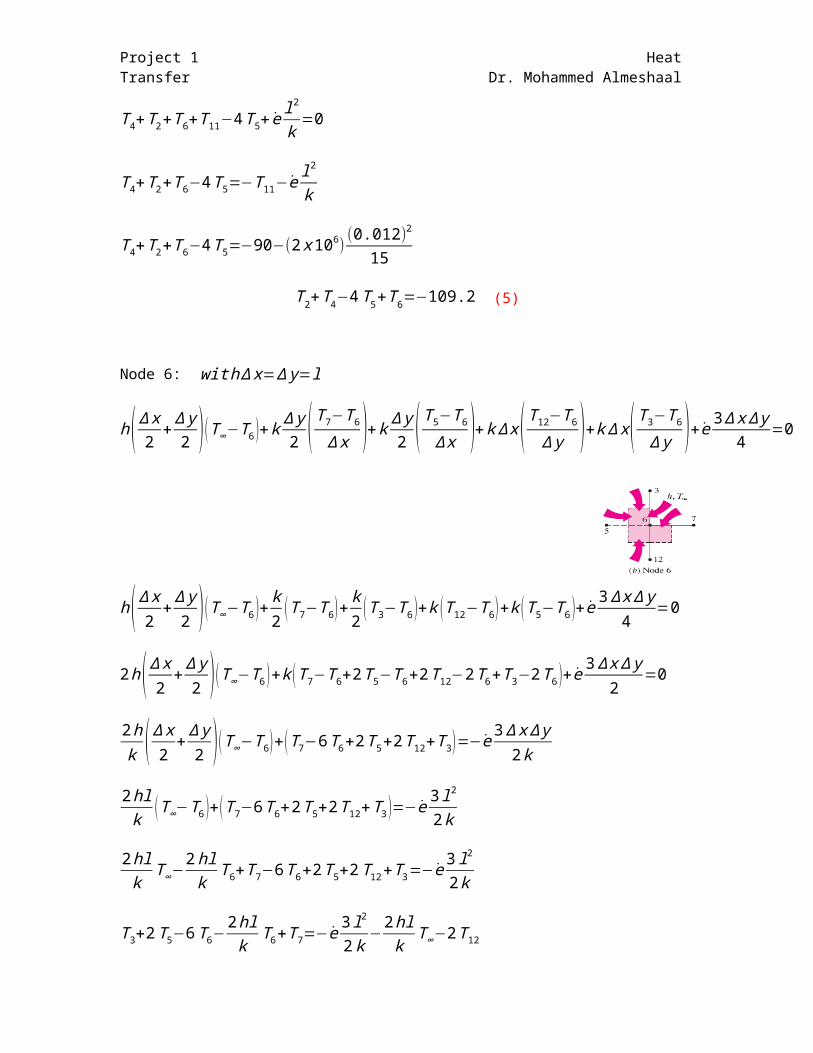
Node 6: with∆x=∆y=l
h(∆x2 +∆y2 )(T∞−T6 )+k ∆y2 (T7−T6
∆x )+k ∆y2 (T5−T6
∆x )+k∆x(T12−T6
∆y )+k∆x(T3−T6
∆y )+e 3∆x∆y4=0
h(∆x2 +∆y2 )(T∞−T6 )+k2 (T7−T6)+
k2 (T3−T6 )+k (T12−T6)+k (T5−T6 )+e 3∆x∆y4
=0
2h(∆x2 +∆y2 )(T∞−T6 )+k (T7−T6+2T5−T6+2T12−2T6+T3−2T6 )+e 3 ∆x∆y2
=0
2hk (∆x2 +
∆y2 )(T∞−T6)+(T7−6T6+2T5+2T12+T3)=−e 3∆x∆y
2k
2hlk (T∞−T6 )+(T7−6T6+2T5+2T12+T3 )=−e 3l
2
2k
2hlk T∞−
2hlk T6+T7−6T6+2T5+2T12+T3=−e 3l
2
2k
T3+2T5−6T6−2hlk T6+T7=−e 3l
2
2k −2hlk T∞−2T12

Project 1 Heat Transfer Dr. Mohammed Almeshaal
T3+2T5−6T6−2 (80)(0.012)
15T6+T7=−(2x10⁶)
3(0.012)2
30−
(2) (80 )(0.012)
15(25)−180
T3+2T5−6T6−0.128T6+T7=−28.8−3.2−180
T3+2T5−6.128T6+T7=−212 (6)
Node 7: with∆x=∆y=l
h∆x (T∞−T7)+k∆y2 (T8−T7
∆x )+k ∆y2 (T6−T7
∆x )+k∆x(T13−T7
∆y )+ e∆x ∆y2 =0
h (T∞−T7 )+k2 (T8−T7
l )+k2 (T6−T7
l )+k(T13−T7
l )+ e l2=0
hl (T∞−T7 )+k2 (T8−T7+T6−T7+2T13−2T7 )+e l2
2=0
2hlk T
∞−2hlk T7+T8+T6−2T7−2T7+2T13+ e
l2
k =0
+T6−2hlk T7−2T7−2T7+T8=−2T13−e
l2
k −2hlk T
∞
+T6−2 (80)(0.012)
15T7−4T7+T8=−180−(2x10⁶)
(0.012)2
15−
(2)(80 )(0.012)
15(25)
+T6−4.128T7+T8=−202.4 (7)
Node 8: with∆x=∆y=l
h∆x (T∞−T8)+k∆y2 (T9−T8
∆x )+k ∆y2 (T7−T8
∆x )+k∆x(T14−T8
∆y )+ e∆x ∆y2 =0

Project 1 Heat Transfer Dr. Mohammed Almeshaal
h (T∞−T8 )+k2 (T9−T8
l )+k2 (T7−T8
l )+k(T14−T8
l )+ e l2=0
hl (T∞−T8 )+k2 (T9−T8+T7−T8+2T14−2T8 )+e l2
2=0
2hlk T
∞−2hlk T8+T9+T7−2T8−2T8+2T14+ e
l2
k =0
+T7−2hlk T8−2T8−2T8+T9=−2T14−e
l2
k −2hlk T
∞
+T7−2 (80)(0.012)
15T8−4T8+T9=−180−(2x10⁶)
(0.012)2
15−
(2)(80 )(0.012)
15(25)
+T7−4.128T8+T9=−202.4 (8)
Node 9: with∆x=∆y=l
h ∆x2 (T∞−T9 )+k ∆y2 (T15−T9
∆x )+k ∆y2 (T8−T9
∆x )+q ∆y2 +e ∆x2
∆y2
=0
2hl (T∞−T9 )+2k (T15−T9+T8−T9 )+ql+e l2
2=0
−hlk T
9−2T9+T8=−T15−
hlk T∞−
qlk −e l2
2k
−(80)(0.012)
15T9−2T9+T8=−90− (80) (0.012 )
15(25)−
(5000 )(0.012)
15−(2x10⁶)
(0.012)2
30
T8−2.064T9=−105.2 (9)

Project 1 Heat Transfer Dr. Mohammed AlmeshaalCollecting all the functions:
−2.064T1+T2+T4=−11.2 (1)
T1−4.128T2+T3+2T5=−22.4 (2)
T2−2.0128T3+T6=−12.8 (3)
T1−4T4+2T5=−109.2 (4)
T2+T4−4T5+T6=−109.2 (5)
T3+2T5−6.128T6+T7=−212 (6)
T6−4.128T7+T8=−202.4 (7)
T7−4.128T8+T9=−202.4 (8)
T8−2.064T9=−105.2 (9)
Solving the equations using gauss seidel iterative method in matlab:
a=[-2.064 1 0 1 0 0 0 0 0; 1 -4.128 1 0 2 0 0 0 0 ;0 1 -2.128 0 0 1 0 0 0;1 0 0 -4 2 0 0 0 0 ;0 1 0 1 -4 1 0 0 0 ;0 0 1 0 2 -6.128 1 0 0 ;0 0 0 0 0 1 -4.128 1 0 ;0 0 0 0 0 0 1 -4.128 1 ;0 0 0 0 0 0 0 1 -2.064];b=[-11.2 -22.4 -12.8 -109.2 -109.2 -212 -202.4 -202.4 -105.2]; k=1; e=1;disp(' T1 T2 T3 T4 T5 T6 T7 T8 T9')

Project 1 Heat Transfer Dr. Mohammed AlmeshaalT0=[57 57 57 57 57 57 57 57 57];out=[T0];disp(out)tol=10^-10;n=9;while e>tol for i=1:n sum1=0;sum2=0; for j=1:i-1; sum1=sum1+a(i,j)*T(j); end for j=i+1:n; sum2=sum2+a(i,j)*T0(j); end T(i)=(b(i)-sum1-sum2)/a(i,i); end e=max(abs(T-T0)); if e>tol T0=T; if k<8 k=k+1; end if k>=8 format short out=[T]; disp(out) format long out=[e]; disp(out) k=1; end endend

Project 1 Heat Transfer Dr. Mohammed Almeshaal
And we get the answer
T1 T2 T3 T4 T5 T6 T7 T8 T9 E 57 57 57 57 57 57 57 57 57 105.9033 106.0586 103.2338 105.7923 105.4685 101.6433 96.9254 96.1331 97.5451 3.294257146724476 111.7979 110.5544 106.3908 109.2163 108.0040 103.0853 97.3187 96.2497 97.6016 0.163905593399932 112.0873 110.7747 106.5454 109.3842 108.1282 103.1559 97.3380 96.2554 97.6044 0.008028177770782 112.1014 110.7855 106.5530 109.3924 108.1343 103.1593 97.3389 96.2557 97.6045 0.000393222564539 112.1021 110.7860 106.5533 109.3928 108.1346 103.1595 97.3389 96.2557 97.6045 0.000019260159589 112.1022 110.7860 106.5534 109.3928 108.1346 103.1595 97.3390 96.2557 97.6045 0.000000943368419 112.1022 110.7860 106.5534 109.3928 108.1346 103.1595 97.3390 96.2557 97.6045 0.000000046206480 112.1022 110.7860 106.5534 109.3928 108.1346 103.1595 97.3390 96.2557 97.6045 0.000000002263206 T1 T2 T3 T4 T5 T6 T7 T8 T9 E 112.1022 110.7860 106.5534 109.3928 108.1346 103.1595 97.3390 96.2557 97.6045 0.000000000110844
0 0.02 0.04 0.06 0.08 0.1 0.12859095100105110115
Temperature distribution
T path
X m
Temp
C
Project 1 Heat Transfer Dr. Mohammed Almeshaal
Conclusion: in this body the temperature decrease with thedistance and that the effect of the surroundingtemperature by convection heat transfer. From thegraph we can see diverges in temperature path atnode 3 and that because it the most node exposed tothe surrounding temperature. Also in the end of thetemperature path we can see the last node is higherthan that before it and that because the effect ofthe heat flux that considering to node 9.