SPEED LIMIT RECOMMENDATION IN VICINITY OF ...

University of Nebraska - LincolnDigitalCommons@University of Nebraska - LincolnFinal Reports & Technical Briefs from Mid-AmericaTransportation Center Mid-America Transportation Center

2012

SPEED LIMIT RECOMMENDATION INVICINITY OF SIGNALIZED, HIGH-SPEEDINTERSECTIONAnuj Sharma Ph.D.University of Nebraska at Lincoln, [email protected]

Laurence Rilett Ph.D.University of Nebraska-Lincoln, [email protected]

Zifeng Wu M.S.University of Nebraska–Lincoln

Shefang WangUniversity of Nebraska-Lincoln, [email protected]

Follow this and additional works at: http://digitalcommons.unl.edu/matcreports

Part of the Civil Engineering Commons

This Article is brought to you for free and open access by the Mid-America Transportation Center at DigitalCommons@University of Nebraska -Lincoln. It has been accepted for inclusion in Final Reports & Technical Briefs from Mid-America Transportation Center by an authorizedadministrator of DigitalCommons@University of Nebraska - Lincoln.

Sharma, Anuj Ph.D.; Rilett, Laurence Ph.D.; Wu, Zifeng M.S.; and Wang, Shefang, "SPEED LIMIT RECOMMENDATION INVICINITY OF SIGNALIZED, HIGH-SPEED INTERSECTION" (2012). Final Reports & Technical Briefs from Mid-AmericaTransportation Center. 37.http://digitalcommons.unl.edu/matcreports/37

http://digitalcommons.unl.edu?utm_source=digitalcommons.unl.edu%2Fmatcreports%2F37&utm_medium=PDF&utm_campaign=PDFCoverPages

http://digitalcommons.unl.edu/matcreports?utm_source=digitalcommons.unl.edu%2Fmatcreports%2F37&utm_medium=PDF&utm_campaign=PDFCoverPages


http://digitalcommons.unl.edu/matc?utm_source=digitalcommons.unl.edu%2Fmatcreports%2F37&utm_medium=PDF&utm_campaign=PDFCoverPages


http://network.bepress.com/hgg/discipline/252?utm_source=digitalcommons.unl.edu%2Fmatcreports%2F37&utm_medium=PDF&utm_campaign=PDFCoverPages

http://digitalcommons.unl.edu/matcreports/37?utm_source=digitalcommons.unl.edu%2Fmatcreports%2F37&utm_medium=PDF&utm_campaign=PDFCoverPages

Nebraska Transportation Center

Report # UNL: SPR-P1 (11) M307 Final Report

SPEED LIMIT RECOMMENDATION IN VICINITY OF SIGNALIZED, HIGH-SPEED INTERSECTION

Anuj Sharma, Ph.D. Assistant ProfessorDepartment of Civil EngineeringUniversity of Nebraska-Lincoln

“This report was funded in part through grant[s] from the Federal Highway Administration [and Federal Transit Administration], U.S. Department of Transportation. The views and opinions of the authors [or agency] expressed herein do not necessarily state or reflect those of the U. S. Department of Transportation.”

Nebraska Transportation Center262 WHIT2200 Vine StreetLincoln, NE 68583-0851(402) 472-1975

Zifeng Wu, M.S.Shefang Wang

WBS:26-1121-0009-001

Laurence Rilett, Ph.D.ProfessorDepartment of Civil EngineeringUniversity of Nebraska Lincoln

Speed Limit Recommendation in Vicinity of Signalized, High-Speed Intersection

Anuj Sharma, Ph.D. Zifeng Wu

Assistant Professor Graduate Research Assistant

Department of Civil Engineering Department of Civil Engineering

University of Nebraska-Lincoln University of Nebraska-Lincoln

Shefang Wang Laurence R. Rilett, Ph.D., P.E.

Graduate Research Assistant Keith Klaasmeyer Chair in Engineering and Technology

Department of Civil Engineering Director

University of Nebraska-Lincoln Nebraska Transportation Center

Professor

University of Nebraska-Lincoln

A Report on Research Sponsored by

Nebraska Transportation Center

University of Nebraska-Lincoln

Nebraska Department of Roads

Federal Highway Administration

April 2012

ii

Technical Report Documentation Page

1. Report No.

SPR-P1 (11) M307

2. Government Accession No.

3. Recipient's Catalog No.

4. Title and Subtitle

Speed Limit Recommendation in Vicinity of Signalized, High-Speed

Intersection

5. Report Date

April 2012

6. Performing Organization Code

7. Author(s)

Anuj Sharma, Zifeng Wu, Shefang Wang, and Laurence R. Rilett

8. Performing Organization Report No.

SPR-P1 (11) M307

9. Performing Organization Name and Address

Nebraska Transportation center

2200 Vine St.

PO Box 830851

Lincoln, NE 68583-0851

10. Work Unit No. (TRAIS)

11. Contract or Grant No.

12. Sponsoring Agency Name and Address

Nebraska Department of Roads

1500 Hwy. 2

Lincoln, NE 68502

Federal Highway Administration

1200 New Jersey Avenue, SE

Washington, DC 20590

13. Type of Report and Period Covered

Final Report

14. Sponsoring Agency Code

TRB RiP No. 28908

15. Supplementary Notes

16. Abstract

We evaluated the traffic operations and safety effects of 5 mph and 10 mph speed limit reductions in the vicinity of high-

speed, signalized intersections with advance warning flashers (AWF). Traffic operational effects of the reduced speed

limits were analyzed for seven high-speed, signalized intersections with AWF using the Quantile regression model and

Seemingly Unrelated Regression Estimation (SURE). Change of speed limit from 60 mph to 55 mph did not lead to any

statistically significant reduction in 15th

, 50th

, or 85th percentile. The reduction from 65 mph to 55 mph hour led to a 4.6

mph reduction in 85th

percentile speed; also, the speed dispersion based on inter-percentile range between 15th

and 85th

percentiles was reduced by 1.8 mph. About the mean and standard deviation of speed estimated by SURE, the only

statistically significant impact is from the speed limit reduction of 10 mph from 65 mph, which reduced the mean speed of

vehicles by 3.8 mph at the significance level of 95%. In the safety effect study, a crash analysis based on 56 approaches

from 28 intersections was performed. The 10 mph speed limit reduction from 65 to 55 mph was found to reduce, on an

average, 0.4 crashes per approach per year with 90% percent level of confidence while the 5 mph reductions in the dataset

was found to reduce, on an average, 0.6 crashes per approach per year with 95% significance level. Also, the studied

approaches with 10 mph reduction were found to have a lower probability of possible injury crashes and a higher

probability of property damage crashes with a 90% level of confidence. The 5 mph reductions in this dataset did not show

any significant effect on reducing crash severity. It was also found that lower speed limits in vicinity of the signalized

intersection reduced the probability of fatal and injury crashes.

17. Key Words

18. Distribution Statement

19. Security Classif. (of this report)

Unclassified

20. Security Classif. (of this page)

Unclassified

21. No. of Pages

112

22. Price

iii

Table of Contents

Acknowledgements vii

Disclaimer viii

Abstract ix

Chapter 1 Introduction 1 1.1 Background Information 1

1.2 Research Objectives 2

1.3 Organization of the Report 3

Chapter 2 Literature Review 5

2.1 Standards of Speed Limit 5 2.1.1 Studies of Driver Compliance 6

2.1.2 Studies of Crashes and Safety 7 2.2 Advisory Speed for Transition Speed Zone 7

2.2.1 Variable Speed Limit 8 2.2.2 Dynamic Message Sign 9 2.2.3 Speed Limit Sign 9

2.3 Survey of Practices in the Field 11

Chapter 3 Data Collection and Reduction 15 3.1 Trailer Setup 15

3.2 Sensor Performance Evaluation 19

3.3 Site Selection 20

3.4 Data Collection 23

3.5 Data Classification 24

Chapter 4 Speed Data Analysis 29

4.1 Sample Size 29

4.2 Speed Cumulative Distribution Plot 30

4.3 Quantile Regression Model 36

4.4 Seemingly Unrelated Equation Models 39 4.4.1 Data Preparation 39 4.4.2 Variable Selection and Data Preparation 40 4.4.3 Seemingly Unrelated Regression Estimation (SURE) 42 4.4.4 Results 44

4.5 Summary 47 Chapter 5 Crash Analysis 49

5.1 Data Preparation 50

5.2 Overview of Crash Data 51

5.3 Crash Frequency Model 52 5.3.1 Literature Review 52 5.3.2 Poisson Model and NB Model 53 5.3.3 Zero-Altered Probability Processes 54 5.3.4 Random Parameter Count Model 56 5.3.5 Interpretation of Count Models 57 5.3.6 Data Preparation and Model Development 58 5.3.7 Interpretation of Results 61

5.4 Crash Severity Model 64 5.4.1 Literature Review 64

iv

5.4.2 Multinomial Logit Model (MNL) 65

5.4.3 Mixed Logit Model 66 5.4.4 Data Preparation and Model Development 67 5.4.5 Interpretation of Results 70

5.5 Summary 71

Chpater 6 Conclusions 73 References 76

Appendix A Information on the Intersections 80

Appendix B Intersection Information of Crash Analysis 87

Appendix C Statistics of Variables in Accident Frequency Model 89

Appendix D Statistics of Variables in Accident Severity Model 90

Appendix E Survey Emails 91

v

List of Figures

Figure 2.1 Comparison of speed limit change and actual change based on

literature review 11

Figure 2.2 Standards to determine speed limits (TxDOT) ............................................................ 14

Figure 3.1 Figures of equipment for data collection ..................................................................... 16

Figure 3.2 Trailer setup of data collection .................................................................................... 17

Figure 3.3 Mobile trailer data collection environment ................................................................. 18

Figure 3.4 Data in MATLAB........................................................................................................ 18

Figure 3.5 Wavetronix’s performance ..................................................................................... 19-20

Figure 3.6 Trailer layout at test site US-77 and Saltillo Rd. ......................................................... 22

Figure 3.7 Diff_range & sample points with QDA....................................................................... 27

Figure 4.1 CDF plots of speed for each intersection ............................................................... 33-35

Figure 4.2 CDF of mean speed based on quantile regression for 10 mph reduction .................... 38

Figure 4.3 Distribution of hourly volume in the seven intersections ............................................ 40

Figure 5.1 Distribution of crash frequency and rate by accident type and speed limit reduction

....................................................................................................................................................... 52

Figure 5.2 Box plots for various groups ....................................................................................... 64

vi

List of Tables

Table 2.1 Summary of previous research ..................................................................................... 10

Table 2.2 Survey results pertaining to application of speed limit reduction ................................ 13

Table 3.1 Information on study sites............................................................................................. 21

Table 3.2 Wavetronix raw data sample ......................................................................................... 23

Table 3.3 Data collection information .......................................................................................... 24

Table 3.4 Classifier’s accuracy on training set ............................................................................. 27

Table 3.5 Classifier's accuracy ...................................................................................................... 28

Table 4.1 Sample size and speed tolerance ................................................................................... 30

Table 4.2 Speed characteristics for each site (mph) ..................................................................... 36

Table 4.3 Comparison of quantile regression for each intersection group ................................... 37

Table 4.4 List of variables tested in seemingly unrelated equation model ................................... 41

Table 4.5 Comparison of the SURE models for speed limit reduction ........................................ 45

Table 4.6 Summary of the impact from speed limit reduction on downstream speed statistics (in

mph) compared with upstream at a 95% significant level ............................................................ 48

Table 5.1 Guideline of model selection ........................................................................................ 55

Table 5.2 Variables selection ........................................................................................................ 59

Table 5.3 Coefficient estimation of RPNB model ........................................................................ 60

Table 5.4 Maringal effects of NB model with random effects ..................................................... 61

Table 5.5 Variable explanation ..................................................................................................... 69

Table 5.6 Coefficient estimation of Mixed Logit Model of significant variables ........................ 69

Table 5.7 Elasticity analysis of Mixed Logit Model..................................................................... 72

Table 5.8 Summary of the safety effects of speed limit reduction ............................................... 72

vii

List of Abbreviations

Advance Warning Flashers (AWF)

Average Daily Traffic (ADT)

Dynamic Message Signs (DMS)

Federal Highway Administration (FHWA)

Generalized Least Squares Method (GLS)

Intelligent Transportation Systems (ITS)

Inter-Percentile Range (IPR)

Linear Discriminant Analysis (LDA)

Manual of Uniform Control Devices (MUCTD)

Multinomial Logit Model (MNL)

National Maximum Speed Limit (NMSL)

Nebraska Department of Roads (NDOR)

Negative Binomial (NB)

Ordinary Least Squares Method (OLS)

Property Damage Only (PDO)

Quadratic Discriminant Analysis (QDA)

Seemingly Unrelated Regression Estimation (SURE)

Variable Speed Limit (VSL)

Wide Area Detector (WAD)

Zero-Inflated NB Model (ZINB)

Zero-Inflated Poisson Model (ZIP)

viii

Acknowledgements

This project was sponsored by the Traffic, Safety, and Planning Division of Nebraska

Department of Roads (NDOR). The authors wish to thank TAC members for their valuable

advice. The authors also wish to thank Matt Neemann, Ryan Huff, Sean Owings, Rick

Ernstmeyer, and Bob Simard from the Nebraska Department of Roads, who provided the crash

history data and other information regarding the intersections, which was utilized in this study.

ix

Disclaimer

The contents of this report reflect the views of the authors, who are responsible for the

facts and accuracy of the information presented herein. This document is disseminated under the

sponsorship of the Department of Transportation University Transportation Centers Program, in

the interest of information exchange. The U.S. Government assumes no liability for the contents

or use thereof.

x

Abstract

This report presents the results of Nebraska Department of Roads (NDOR) research

project SPR-P1 (11) M307, which evaluated the traffic operations and safety effects of 5 mph

and 10 mph speed limit reductions in the vicinity of high-speed, signalized intersections with

advance warning flashers (AWF).

The methodology involved two studies: 1) field study of the impact of speed limit

reduction at seven high-speed intersections, 2) crash analysis using the 10-year history from 28

high-speed intersections.

In the field study, traffic operational effects of the reduced speed limits were analyzed for

seven high-speed, signalized intersections with AWF, using the Quantile regression model and

Seemingly Unrelated Regression Estimation (SURE). The Quantile regression models indicated

that reduction of speed limit from 60 mph to 55 mph did not lead to any statistically significant

reduction in the 15th

, 50th

, or 85th

percentiles. It was found that a speed limit reduction from 65

mph to 55 mph led to a 4.6 mph reduction in 85th

percentile speed. Also, the speed dispersion

based on an inter-percentile range between 15th

and 85th

percentiles was reduced by 1.4 mph in

the vicinity of the intersection. SURE was used to estimate the mean and standard deviation of

grouped average speeds simultaneously. The SURE model was chosen to account for any

potential correlations between the mean and standard deviation of speed. It was found that a

speed limit reduction of 10 mph, when the upstream speed limit was 65 mph, reduced the mean

speed of vehicles by 3.8 mph, or by six percent. This result was statistically significant at the

95% percent level of confidence. It was also found that reducing the speed limit by 5 mph when

the speed limit was 60 mph did not produce any statistically significant reduction in mean speed.

xi

In addition, the standard deviation of the speeds downstream of the speed limit sign was not

statistically significantly different from the upstream for either 10 mph or 5 mph reductions.

In the second study, a crash analysis based on 56 approaches from 28 intersections was

performed to study the safety effects of speed limit reductions. The dataset included four

approaches of 10 mph reduction from 65 mph to 55 mph, seven approaches of 5 mph reduction

from 60 mph to 55 mph, two approaches of 5 mph reduction from 55 mph to 50 mph, and 43

approaches with no limit reduction (i.e., the control group). The 10 mph speed reduction from 65

to 55 mph was found to reduce, on average, 0.4 crashes per approach per year with a 90% level

of confidence. Also, the studied approaches with 10 mph reduction were found to have a lower

probability of possible injury crashes and a higher probability of possible damage crashes with a

90% level of confidence. The 5 mph reductions from 60 mph to 55 mph and from 55 mph to 50

mph were found to reduce 0.6 crashes per approach per year at a 95% significance level. It was

also found that lower speed limits in the vicinity of signalized intersections reduced the

probability of fatal and injury crashes.

The conclusions of this study, however, are limited by the low number of intersections

with speed limit reductions. For example, only two intersections with 10 mph reduction were

available for the study, where the speed limit was reduced from 65 mph to 55 mph. Based on this

dataset, for a highway with speed limit at 65 mph, the reduction to 55 mph at intersections with

AWF has been found to reduce mean speed and crash frequency, and alleviate possible crashes

in comparison to the intersections with only AWF. It is recommended that future research

include other speed limit combinations, such as a 5 mph reduction from 65 mph to 60 mph, and

utilize larger datasets to provide better generalizability and transferability of results. A before-

xii

and-after study could also provide partially controlled conditions to isolate the impacts of speed

limit reduction.

1

Chapter 1 Introduction

1.1 Background Information

The National Safety Council reports motor vehicle crashes as the leading cause of

unintentional injury deaths in the United States. The cost of motor vehicle collisions in 2006

totaled nearly $230.6 billion. Intersection crashes constitute 30% of all vehicle crashes, and they

account for an average of 9,000 fatalities and 1.5 million injuries annually. Furthermore, among

all intersection and intersection-related crashes in the United States in 2009, signalized

intersections accounted for 52.3% (1). The safety concerns involving signalized intersections

become critical for rural and suburban highways, since high-speed aggravates the severity of

crashes.

The Nebraska Department of Roads (NDOR) is responsible for the operation of a large

number of traffic signals on rural and suburban expressways throughout Nebraska. However,

there is no documented policy on assigning speed limits on expressways in the vicinity of the

traffic signals. The undocumented strategy generally adopted is that on some sections there are

speed limit reductions in the vicinity of signalized intersections at highways with speed limit

higher than 60 mph. For example, on certain sections of Highway 75 the speed limit decreases

from 65 mph to 55 mph in the vicinity of signalized intersections. However, on Highway 34,

west of Lincoln, the standard speed limit is 60 mph, with no speed limit reduction at the

intersections of NW 48th Street and Highway 79. The effects of speed limit reduction on

operation and safety are not adequately studied, and no documented guidelines are available. A

compounding issue is that most of the intersections are equipped with advanced warning flashers

(AWF) and a dilemma protection algorithm; therefore, there may be less need for speed

reductions in these situations.

2

1.2 Research Objectives

The Manual of Uniform Control Devices (MUCTD) states that "Advance warning signs

and other traffic control devices to attract the motorist’s attention to a signalized intersection are

usually more effective than a reduced speed limit zone" (3). However, the MUTCD is silent

regarding recommendations of speed limit reduction in conjunction with AWF. For the past

several years NDOR has used AWF at high-speed rural intersections that meet their criteria. The

speed limit may or may not be reduced at these intersections, and this decision is made on

engineering-based judgments. The current research aims to verify the effectiveness of speed

limit reduction at rural, high-speed intersections equipped with the NDOR AWF system. This

objective can be broken into two important issues:

1. How does a transitional speed limit influence safety at signalized, high-speed intersections

with AWF?

The purpose of a transitional speed limit is to increase road safety. Speed limits can

increase road users’ safety in two ways: by a limiting function; and by a coordinating function.

The limiting function is to set up a maximum speed along the road, which can reduce the chance

and severity of collisions. For the coordinating function, a maximum speed limit can reduce the

variance of speeds along the road, which can make the speed more uniform and increase road

safety (4). For example, suppose the speed limit for the transition zone is reduced at a high-speed

intersection, one possible consequence is that it separates drivers into two subsets: those who

drive accordingly with lower speeds, and those who choose their own speeds, which are probably

higher than the reduced limit. The resulting variance of driving speeds could be a potential trap

for highway safety.

2. What is the recommended drop in the speed limit for transitional speed zones?

3

Given that the use of a transitional zone does result in increased safety for the traveling

public, a second issue pertains to the appropriate level of speed limit reduction. Based on

previous research, “speed limits should be evidence-led, self-explaining and seek to reinforce

people’s assessment of what is a safe speed to travel” (2); otherwise, there would be little change

in the mean or 85th

percentile speed as a result of raising or lowering the posted speed limit on

urban and rural non-limited access highways. Thus, an engineering study in accordance with

traffic engineering practices should be performed to establish speed zones (3). The analyses

conducted in this study included an examination of the current speed distribution of free-flowing

vehicles. This study compared the speed distribution of free-flow vehicles approaching

intersections with different speed limit reductions to justify the effectiveness of advisory speed

zone.

The objectives of this study were to identify the necessity and effectiveness of

transitional speed zones on signalized, high-speed intersections with AWF on Nebraska

highways, as well as to clarify their influence on safety through crash analysis. The goal would

be to develop guidelines for a transitional speed limit policy based on the effects of speed limit

reductions on vehicle speeds and safety concerns at signalized, high-speed intersections.

1.3 Organization of the Report

There are six chapters in this report. Chapter 1 contains an introduction of the problem

and the objectives of the current project. Chapter 2 provides a summary of the literature review

of speed limit studies, and a survey about current practices at signalized, high-speed intersections

in neighbor states (KS, IA, MO, SD, WY, CO, and CA). Chapter 3 details the data collection

process and the validation of the sensors, while introducing data pre-processing. Chapter 4

presents the analytical results of the speed data and provides conclusions on the efficiency of

speed limit reductions used in advisory speed zone. Chapter 5 analyzes the crash data at

4

signalized intersections with different speed limit reductions and discusses the safety issues

related to transition speed zone at signalized, high-speed intersections with AWF. Chapter 6

summarizes the findings and provides recommendations in developing guidelines for the

application of speed limit reduction at signalized, high-speed intersections with AWF.

5

Chapter 2 Literature Review

2.1 Standards of Speed Limit

There are two kinds of speed limits: general speed limits and speed limits in altered speed

zones. General speed limits should obey the statewide law or even nationwide law. The speed

limit in altered speed zones is based on a thorough engineering study, and applied to a specific

section of road.

Throughout U.S. history, the government has imposed two statutory national speed limits.

The first federal speed limit, established during World War II, was 35 mph. The second national

speed limit was known as the National Maximum Speed Limit (NMSL), with a maximum speed

of 55 mph. The purpose of these two statutory speed limits was based upon reducing energy

consumption, rather than transportation cost (4). NMSL has changed several times throughout

the years. In 1974, NMSL was set at a maximum of 55 mph. In 1987, Congress allowed the

increase of NMSL to 65 mph on some qualified sections of Interstate highways in rural areas.

Finally, in 1995, NMSL was repealed to allow each state and local jurisdictions to set their own

speed limits. Subsequently, nearly all states increased their speed limits (5). State statutory limits

may restrict the maximum speed limit that can be established on a particular road regardless of

what an engineering study might indicate, while altered speed zones should be based on

engineering studies. For altered speed zones, the advisory speed plaque, used to supplement any

warning sign to indicate the advisory speed for a condition (e.g., horizontal curve), should be

determined by an engineering study (3). Different states may have different policies regarding

speed limits based on the Manual on Uniform Traffic Control Devices (MUTCD) standards. For

example, Michigan has regulatory speed limits categorized as statutory or modified speed limits,

in addition to the advisory speed limits to alert drivers of the maximum recommended safe

6

driving speeds through a curve or for other special roadways conditions. Or, for instance, Texas

classifies speed limits in two groups: statewide statutory speed limits, and a regulatory speed

zone which may include an advisory speed section if needed. Despite the variety of speed limits

in different states, performing engineering studies is the most common procedure for establishing

all but statutory speed limits. One task of engineering studies is to extract the 85th

percentile

speed from free flow speed in a specific location. The 85th

percentile speed has been

demonstrated to be beneficial in lowering the possibility of a crash and to promote driver

compliance (21). Arbitrary lowering or raising the speed limit has little impact on driver

behavior.

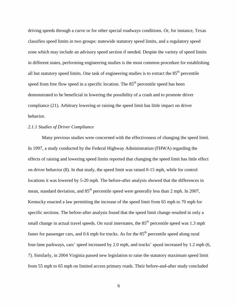
2.1.1 Studies of Driver Compliance

Many previous studies were concerned with the effectiveness of changing the speed limit.

In 1997, a study conducted by the Federal Highway Administration (FHWA) regarding the

effects of raising and lowering speed limits reported that changing the speed limit has little effect

on driver behavior (8). In that study, the speed limit was raised 0-15 mph, while for control

locations it was lowered by 5-20 mph. The before-after analysis showed that the differences in

mean, standard deviation, and 85th

percentile speed were generally less than 2 mph. In 2007,

Kentucky enacted a law permitting the increase of the speed limit from 65 mph to 70 mph for

specific sections. The before-after analysis found that the speed limit change resulted in only a

small change in actual travel speeds. On rural interstates, the 85th

percentile speed was 1.3 mph

faster for passenger cars, and 0.6 mph for trucks. As for the 85th

percentile speed along rural

four-lane parkways, cars’ speed increased by 2.0 mph, and trucks’ speed increased by 1.2 mph (6,

7). Similarly, in 2004 Virginia passed new legislation to raise the statutory maximum speed limit

from 55 mph to 65 mph on limited access primary roads. Their before-and-after study concluded

7

that average speed increased only 1.7-4.3 mph for all the test sites. However, speed limit

compliance decreased from over 80% to approximately 50%. Also, the variance in traffic speed

remained fairly constant (9). The consistent conclusion drawn from these studies is that no

matter the speed limit posted, drivers mainly choose their own comfortable speed according to

road conditions, and not on the basis of posted speed limit signs.

2.1.2 Studies of Crashes and Safety

One common misconception regarding the speed limit is that “lowering speed limit will

increase the road users’ safety and reduce the crashes rate, and vice versa” (4). Researchers have

indicated that the variance of speeds, rather than the absolute magnitude, poses a threat to safety.

As the FHWA publication states, “the potential of being involved in a crash is highest when

traveling at a speed much lower or much higher than the majority of motorists” (8). The U-

shaped relationship between motorist speeds and the chance of being in a crash invalidates the

idea that lowering speed limits would increase safety (12). In general, the lowest risk of being

involved in a crash occurs at approximately the 85th

percentile speed.

2.2 Advisory Speed for Transition Speed Zone

Special road conditions, such as a high-speed intersection, may favor an advisory speed

limit different from, and probably lower than, that of other highway segments. However, prior to

the current study, there were few studies to support any standard on how to set advisory speed

limits for high-speed intersections, while studies do exist for horizontal curves. In order to avoid

obtaining skewed results for the 85th

percentile speed, MUTCD requires that speed studies for

signalized intersection approaches be undertaken outside the influence area of the traffic control

signal, which is generally considered to be approximately 1/2 mile (3). However, this 85th

percentile speed does not represent the road condition in the vicinity of signalized intersections.

A reduced speed limit specific to the signalized intersection could reduce the crash severity

8

resulted from high speed on highways; however, an arbitrary reduction may result in violating

drivers’ expectations, and lead to lower compliance. Consequently, the increased variety of

driving speeds will increase the probability of crashes. Thus, the establishment of a reduced

transitional speed limit in advisory speed zones, such as at high-speed intersection, requires

special engineering studies to demonstrate its effectiveness. There are several means to display

reduced advisory speeds to alert drivers of the recommended speed for special road condition.

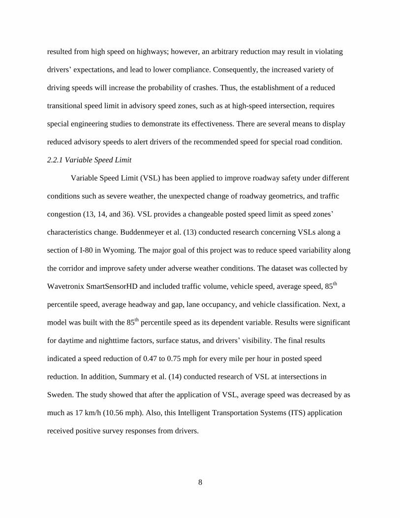
2.2.1 Variable Speed Limit

Variable Speed Limit (VSL) has been applied to improve roadway safety under different

conditions such as severe weather, the unexpected change of roadway geometrics, and traffic

congestion (13, 14, and 36). VSL provides a changeable posted speed limit as speed zones’

characteristics change. Buddenmeyer et al. (13) conducted research concerning VSLs along a

section of I-80 in Wyoming. The major goal of this project was to reduce speed variability along

the corridor and improve safety under adverse weather conditions. The dataset was collected by

Wavetronix SmartSensorHD and included traffic volume, vehicle speed, average speed, 85th

percentile speed, average headway and gap, lane occupancy, and vehicle classification. Next, a

model was built with the 85th

percentile speed as its dependent variable. Results were significant

for daytime and nighttime factors, surface status, and drivers’ visibility. The final results

indicated a speed reduction of 0.47 to 0.75 mph for every mile per hour in posted speed

reduction. In addition, Summary et al. (14) conducted research of VSL at intersections in

Sweden. The study showed that after the application of VSL, average speed was decreased by as

much as 17 km/h (10.56 mph). Also, this Intelligent Transportation Systems (ITS) application

received positive survey responses from drivers.

9

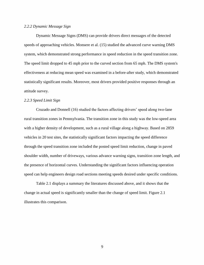
2.2.2 Dynamic Message Sign

Dynamic Message Signs (DMS) can provide drivers direct messages of the detected

speeds of approaching vehicles. Monsere et al. (15) studied the advanced curve warning DMS

system, which demonstrated strong performance in speed reduction in the speed transition zone.

The speed limit dropped to 45 mph prior to the curved section from 65 mph. The DMS system's

effectiveness at reducing mean speed was examined in a before-after study, which demonstrated

statistically significant results. Moreover, most drivers provided positive responses through an

attitude survey.

2.2.3 Speed Limit Sign

Cruzado and Donnell (16) studied the factors affecting drivers’ speed along two-lane

rural transition zones in Pennsylvania. The transition zone in this study was the low-speed area

with a higher density of development, such as a rural village along a highway. Based on 2859

vehicles in 20 test sites, the statistically significant factors impacting the speed difference

through the speed transition zone included the posted speed limit reduction, change in paved

shoulder width, number of driveways, various advance warning signs, transition zone length, and

the presence of horizontal curves. Understanding the significant factors influencing operation

speed can help engineers design road sections meeting speeds desired under specific conditions.

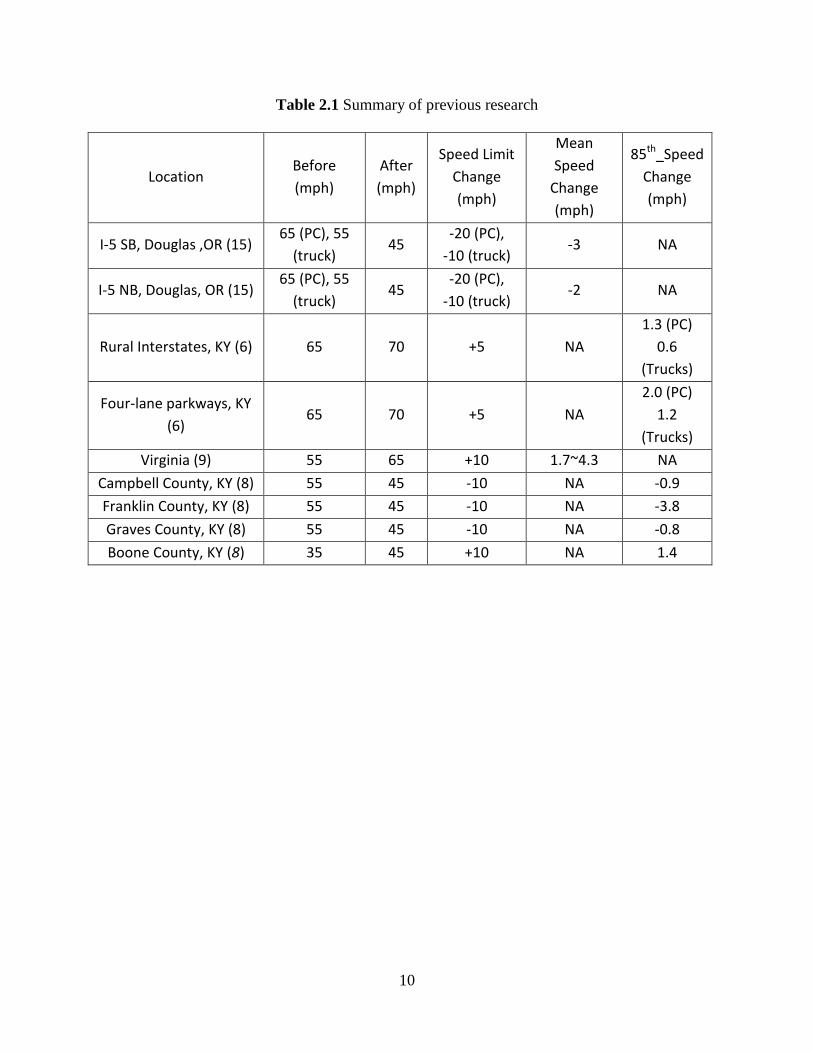
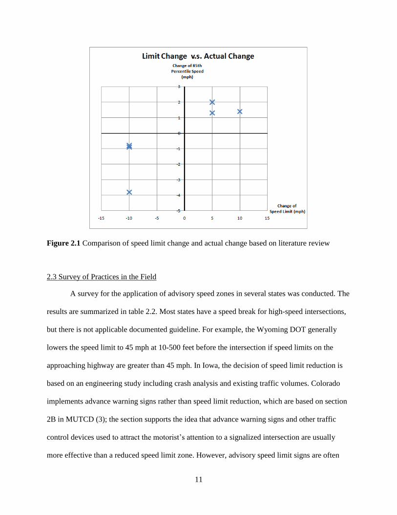
Table 2.1 displays a summary the literatures discussed above, and it shows that the

change in actual speed is significantly smaller than the change of speed limit. Figure 2.1

illustrates this comparison.

10

Table 2.1 Summary of previous research

Location Before

(mph)

After

(mph)

Speed Limit

Change

(mph)

Mean

Speed

Change

(mph)

85th_Speed

Change

(mph)

I-5 SB, Douglas ,OR (15) 65 (PC), 55

(truck) 45

-20 (PC),

-10 (truck) -3 NA

I-5 NB, Douglas, OR (15) 65 (PC), 55

(truck) 45

-20 (PC),

-10 (truck) -2 NA

Rural Interstates, KY (6) 65 70 +5 NA

1.3 (PC)

0.6

(Trucks)

Four-lane parkways, KY

(6) 65 70 +5 NA

2.0 (PC)

1.2

(Trucks)

Virginia (9) 55 65 +10 1.7~4.3 NA

Campbell County, KY (8) 55 45 -10 NA -0.9

Franklin County, KY (8) 55 45 -10 NA -3.8

Graves County, KY (8) 55 45 -10 NA -0.8

Boone County, KY (8) 35 45 +10 NA 1.4

11

Figure 2.1 Comparison of speed limit change and actual change based on literature review

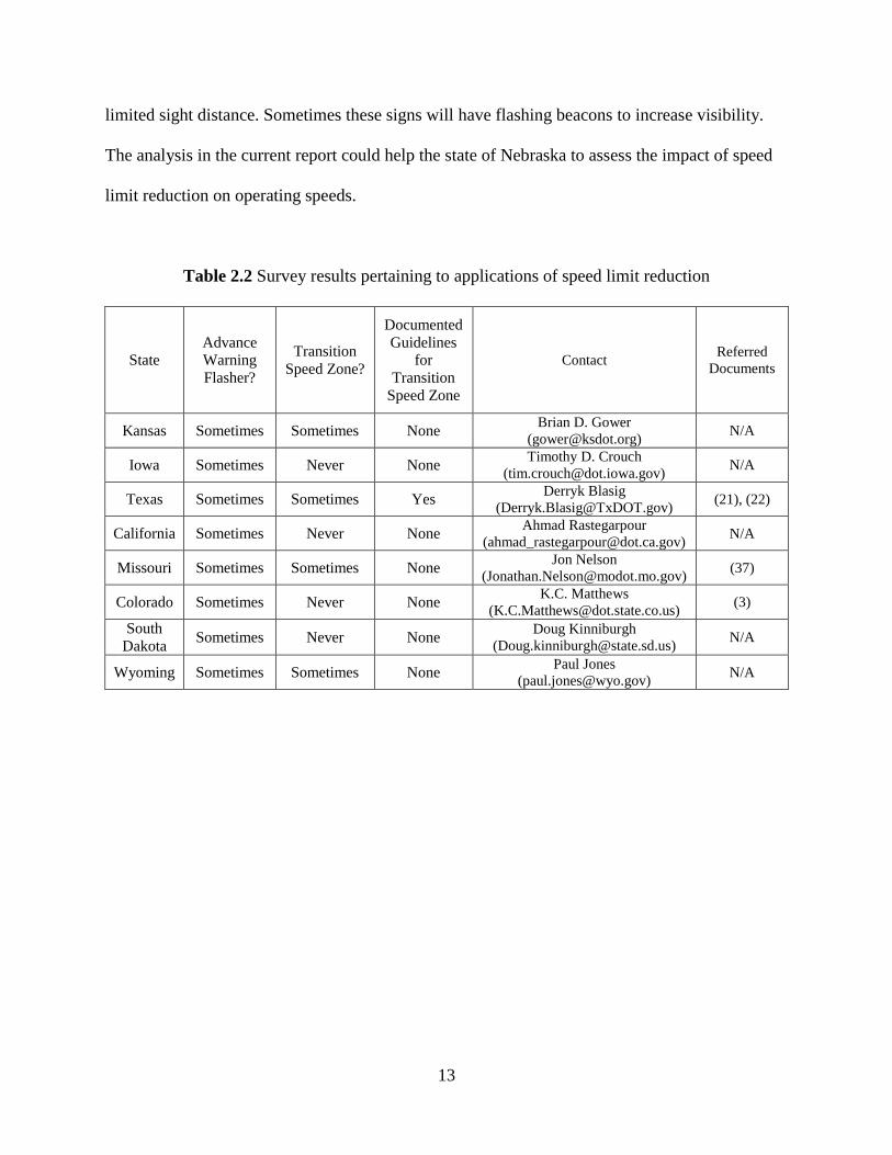
2.3 Survey of Practices in the Field

A survey for the application of advisory speed zones in several states was conducted. The

results are summarized in table 2.2. Most states have a speed break for high-speed intersections,

but there is not applicable documented guideline. For example, the Wyoming DOT generally

lowers the speed limit to 45 mph at 10-500 feet before the intersection if speed limits on the

approaching highway are greater than 45 mph. In Iowa, the decision of speed limit reduction is

based on an engineering study including crash analysis and existing traffic volumes. Colorado

implements advance warning signs rather than speed limit reduction, which are based on section

2B in MUTCD (3); the section supports the idea that advance warning signs and other traffic

control devices used to attract the motorist’s attention to a signalized intersection are usually

more effective than a reduced speed limit zone. However, advisory speed limit signs are often

12

implemented together with advance warning signs to indicate the advisory speed for a condition.

To some extent, advisory speed limit signs fortify advance warning signs. The Missouri DOT

typically installs advance warning signs with a dynamic flasher, which are timed with the signal

and start to flash if approaching vehicles are expected to arrive at the intersection during a red

light. Most other states, however, apply advance warning signs with or without flashing beacons

and only install the dynamic flasher at certain locations. Furthermore, advance warning signs,

speed limit reduction, and dilemma-zone protection algorithms are also widely applied for

isolated high-speed signals.

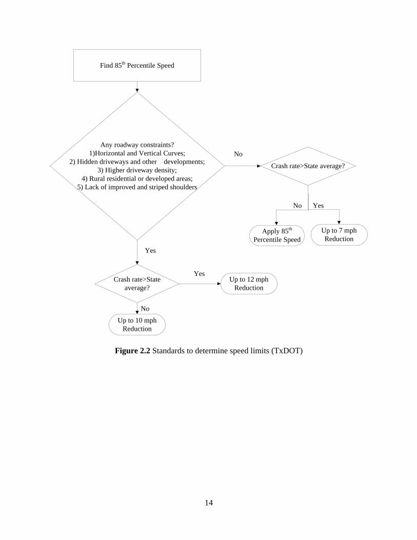
Texas has one documented guideline that outlines the procedure for establishing speed

zones. It advises that advisory zones be posted at intersections where roundabouts which are

designed for an operating speed less than the speed of the approaches or intersections with

restricted sight distances that require a reduction in speed for safe operation. A flow chart based

on this document was developed and is presented in figure 2.2. This procedure enables TxDOT

to lower speed limits on roadways by as much as 10 mph (12 mph if the traffic crash rate is

above the statewide average) below the 85th

percentile speed while considering factors such as

pavement width, curves, number of driveways, crash history at a given location, rural, residential

or developed areas, and a lack of improved and striped shoulders (21). These procedures were

developed as a result of comments received at speed limit town meetings. TxDOT and cities

must use these procedures when establishing speed zones on state highways. As shown in

Chapter 3, section 2 in (15), TxDOT typically performs a speed study midway between signals—

or 0.2 miles from any signal, whichever is less—to ensure an accurate representation of speed

patterns. In addition, TxDOT uses advanced warning signs for signalized intersections. These are

typically used when there is a crash history at a certain location, or where vertical curves cause

13

limited sight distance. Sometimes these signs will have flashing beacons to increase visibility.

The analysis in the current report could help the state of Nebraska to assess the impact of speed

limit reduction on operating speeds.

Table 2.2 Survey results pertaining to applications of speed limit reduction

State

Advance

Warning

Flasher?

Transition

Speed Zone?

Documented

Guidelines

for

Transition

Speed Zone

Contact Referred

Documents

Kansas Sometimes Sometimes None Brian D. Gower

([email protected]) N/A

Iowa Sometimes Never None Timothy D. Crouch


Texas Sometimes Sometimes Yes Derryk Blasig

([email protected]) (21), (22)

California Sometimes Never None Ahmad Rastegarpour


Missouri Sometimes Sometimes None Jon Nelson

([email protected]) (37)

Colorado Sometimes Never None K.C. Matthews

([email protected])

(3)

South

Dakota Sometimes Never None

Doug Kinniburgh


Wyoming Sometimes Sometimes None Paul Jones


mailto:[email protected]

mailto:[email protected]

14

Find 85th Percentile Speed

Any roadway constraints?

1)Horizontal and Vertical Curves;

2) Hidden driveways and other developments;

3) Higher driveway density;

4) Rural residential or developed areas;

5) Lack of improved and striped shoulders

Crash rate>State average?

No

Yes

Crash rate>State

average?

No

Yes

Up to 7 mph

ReductionApply 85th

Percentile Speed

Up to 12 mph

Reduction

Up to 10 mph

Reduction

No

Yes

Figure 2.2 Standards to determine speed limits (TxDOT)

15

Chapter 3 Data Collection and Reduction

3.1 Trailer Setup

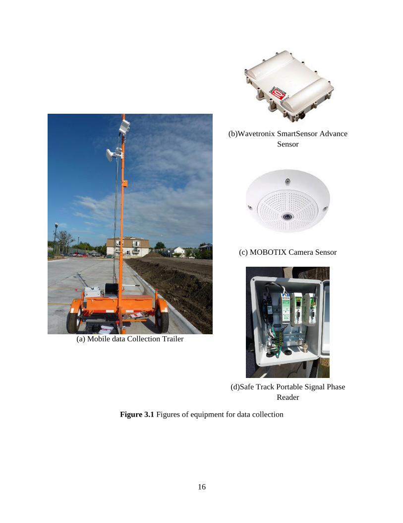
A portable trailer, as shown below in figure 3.1a, is utilized in data collection. Data was

collected on days having no precipitation and with wind gusts lower than 10 mph. The data

collection trailer was equipped with a Wavetronix sensor (WAD) (fig. 3.1b) and a MOBOTIX

fisheye camera (fig. 3.1c). The SmartSensor Advance WAD installed on the research pole

utilizes digital wave radar technology to track the vehicles upstream of the pole and record their

distance, speed, lane, and vehicle length up to a distance of 500 ft. The video was used to

identify vehicle types and lane occupation, and also to eliminate false calls.

The signal phase reader (shown in fig. 3.1d) communicates the signal phase status via

radio to the portable sensor pole cabinet. There is one Click! 200 in the cabinet to collect data

from the detector and send it to the Click! 500; thus, the Click! 500 in the pole cabinet receives

data from the signal and Wavetronix detectors.

Time synchronization with the portable system is maintained with reference to the

trailer’s Click! 500 real-time clock. The phase-reading Click! 500 receives updates from trailer’s

Click! 500 via the wireless link. When both of these systems are properly synced, drift is less

than 70 ms. The entire system has a time resolution accuracy of at least 0.1 sec. The data is

pushed from the Click! 500 using the device’s serial port and a serial to USB converter that

connects to a laptop. MATLAB opens the serial port and saves the data in both .DAT and .txt

files.

16

(a) Mobile data Collection Trailer

(b)Wavetronix SmartSensor Advance

Sensor

(c) MOBOTIX Camera Sensor

(d)Safe Track Portable Signal Phase

Reader

Figure 3.1 Figures of equipment for data collection

17

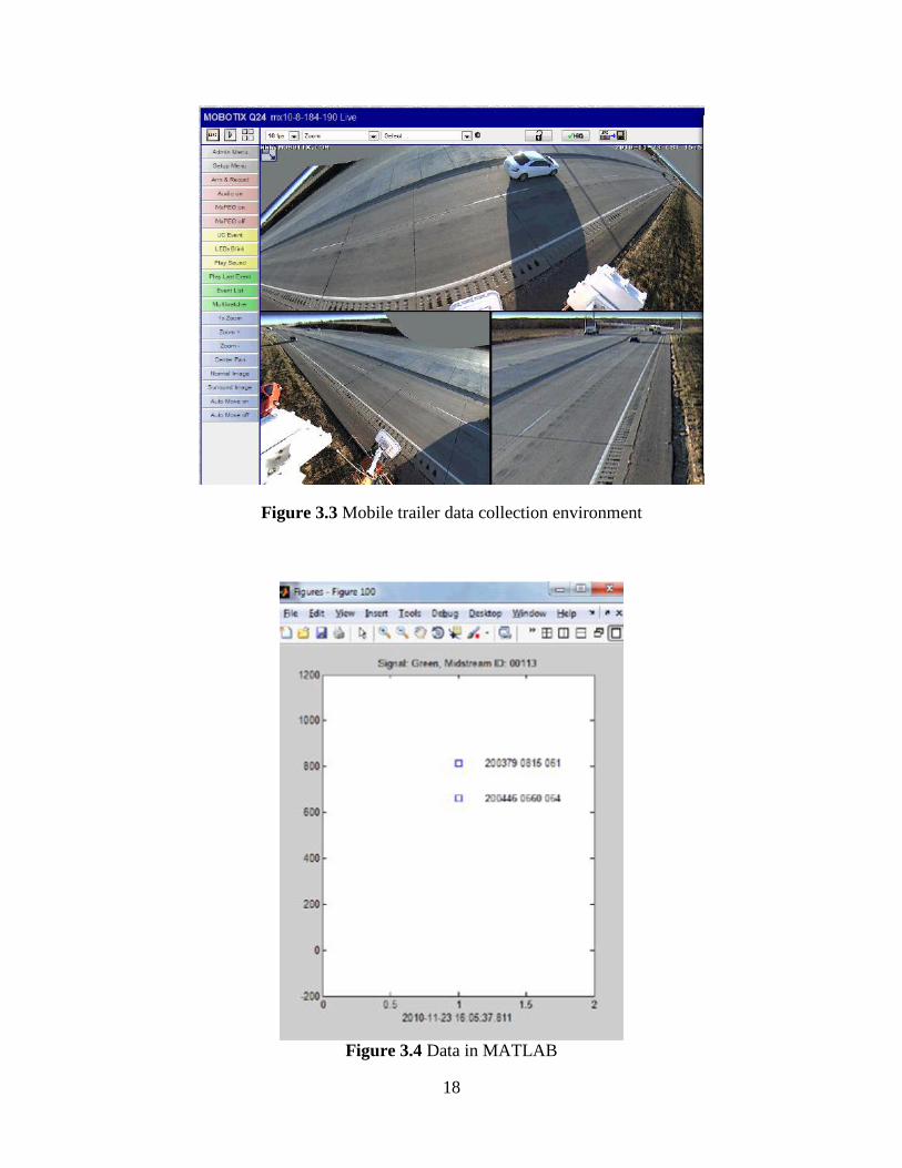
The overall data collection schematic is shown below in figure 3.1; the MOBOTIX

camera on the top (A2 in fig. 3.2) can record the live traffic with a field of vision covering up to

180 . Figure 3.3 displays the view from the camera. The data collected by Wavetronix Sensor, as

show in figure 3.4, includes date, time, ID, range, and speed.

A. Sensor Trailer

A1. Radar Sensors

A2. Video Camera

A3. Laptop

B. Detection Zone

C. Signal cabinet

B

A

A1

A2

A3

C

Figure 3.2 Trailer setup of data collection

18

Figure 3.3 Mobile trailer data collection environment

Figure 3.4 Data in MATLAB

19

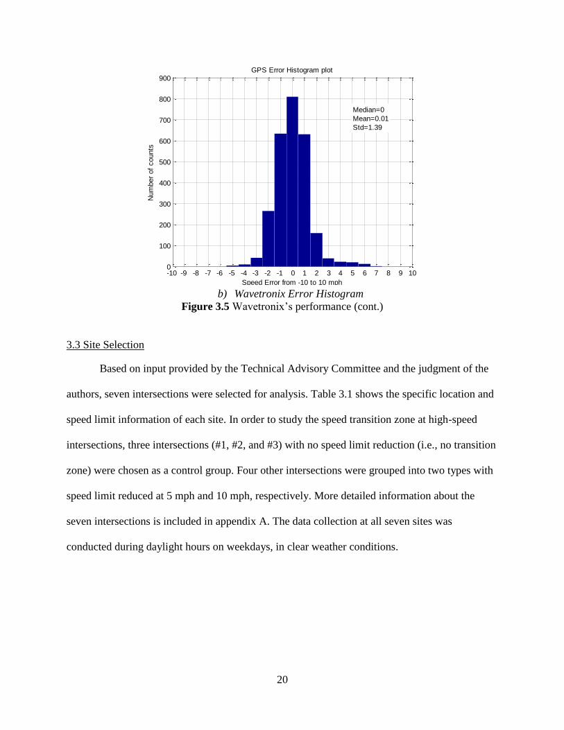
3.2 Sensor Performance Evaluation

GPS was used to validate the accuracy of Wavetronix in this study. Researchers

performed 55 test runs with portable GPS to record the speed and distance data. Figure 3.5a

shows a comparison of data recorded by GPS and Wavetronix for one test run. The difference

between the two trajectories is the error of the Wavetronix, and represents a measurement of

accuracy. Figure 3.5b shows the error histogram for all 55 runs. The error is distributed with the

mean close to 0.01 mph and the standard deviation at 1.39 mph, which indicates acceptable

performance of the Wavetronix sensor.

500 550 600 650 700 750 800 850 900 950 10000

10

20

30

40

50

60

70

Distance(ft)

Speed(m

ph)

GPS VS Wavetronix

GPS

Wavetronix

a) GPS vs. Wavetronix

Figure 3.5 Wavetronix’s performance

20

-10 -9 -8 -7 -6 -5 -4 -3 -2 -1 0 1 2 3 4 5 6 7 8 9 100

100

200

300

400

500

600

700

800

900

Median=0

Mean=0.01

Std=1.39

Speed Error from -10 to 10 mph

Num

ber

of

counts

GPS Error Histogram plot

b) Wavetronix Error Histogram

Figure 3.5 Wavetronix’s performance (cont.)

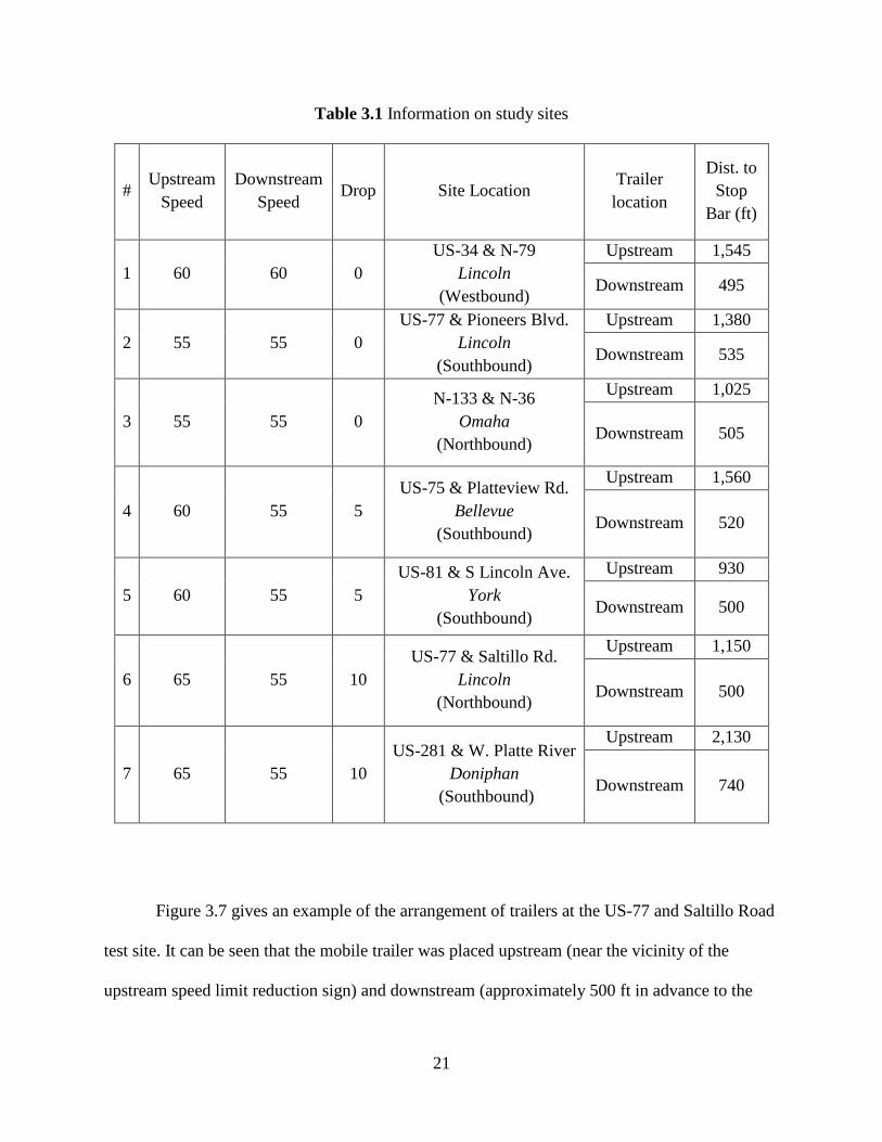
3.3 Site Selection

Based on input provided by the Technical Advisory Committee and the judgment of the

authors, seven intersections were selected for analysis. Table 3.1 shows the specific location and

speed limit information of each site. In order to study the speed transition zone at high-speed

intersections, three intersections (#1, #2, and #3) with no speed limit reduction (i.e., no transition

zone) were chosen as a control group. Four other intersections were grouped into two types with

speed limit reduced at 5 mph and 10 mph, respectively. More detailed information about the

seven intersections is included in appendix A. The data collection at all seven sites was

conducted during daylight hours on weekdays, in clear weather conditions.

21

Table 3.1 Information on study sites

# Upstream

Speed

Downstream

Speed Drop Site Location

Trailer

location

Dist. to

Stop

Bar (ft)

1 60 60 0

US-34 & N-79

Lincoln

(Westbound)

Upstream 1,545

Downstream 495

2 55 55 0

US-77 & Pioneers Blvd.

Lincoln

(Southbound)

Upstream 1,380

Downstream 535

3 55 55 0

N-133 & N-36

Omaha

(Northbound)

Upstream 1,025

Downstream 505

4 60 55 5

US-75 & Platteview Rd.

Bellevue

(Southbound)

Upstream 1,560

Downstream 520

5 60 55 5

US-81 & S Lincoln Ave.

York

(Southbound)

Upstream 930

Downstream 500

6 65 55 10

US-77 & Saltillo Rd.

Lincoln

(Northbound)

Upstream 1,150

Downstream 500

7 65 55 10

US-281 & W. Platte River

Doniphan

(Southbound)

Upstream 2,130

Downstream 740

Figure 3.7 gives an example of the arrangement of trailers at the US-77 and Saltillo Road

test site. It can be seen that the mobile trailer was placed upstream (near the vicinity of the

upstream speed limit reduction sign) and downstream (approximately 500 ft in advance to the

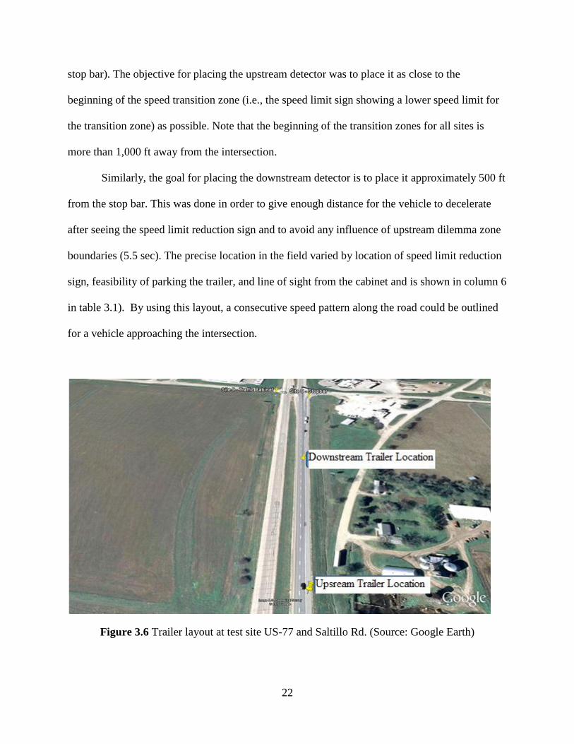
22

stop bar). The objective for placing the upstream detector was to place it as close to the

beginning of the speed transition zone (i.e., the speed limit sign showing a lower speed limit for

the transition zone) as possible. Note that the beginning of the transition zones for all sites is

more than 1,000 ft away from the intersection.

Similarly, the goal for placing the downstream detector is to place it approximately 500 ft

from the stop bar. This was done in order to give enough distance for the vehicle to decelerate

after seeing the speed limit reduction sign and to avoid any influence of upstream dilemma zone

boundaries (5.5 sec). The precise location in the field varied by location of speed limit reduction

sign, feasibility of parking the trailer, and line of sight from the cabinet and is shown in column 6

in table 3.1). By using this layout, a consecutive speed pattern along the road could be outlined

for a vehicle approaching the intersection.

Figure 3.6 Trailer layout at test site US-77 and Saltillo Rd. (Source: Google Earth)

23

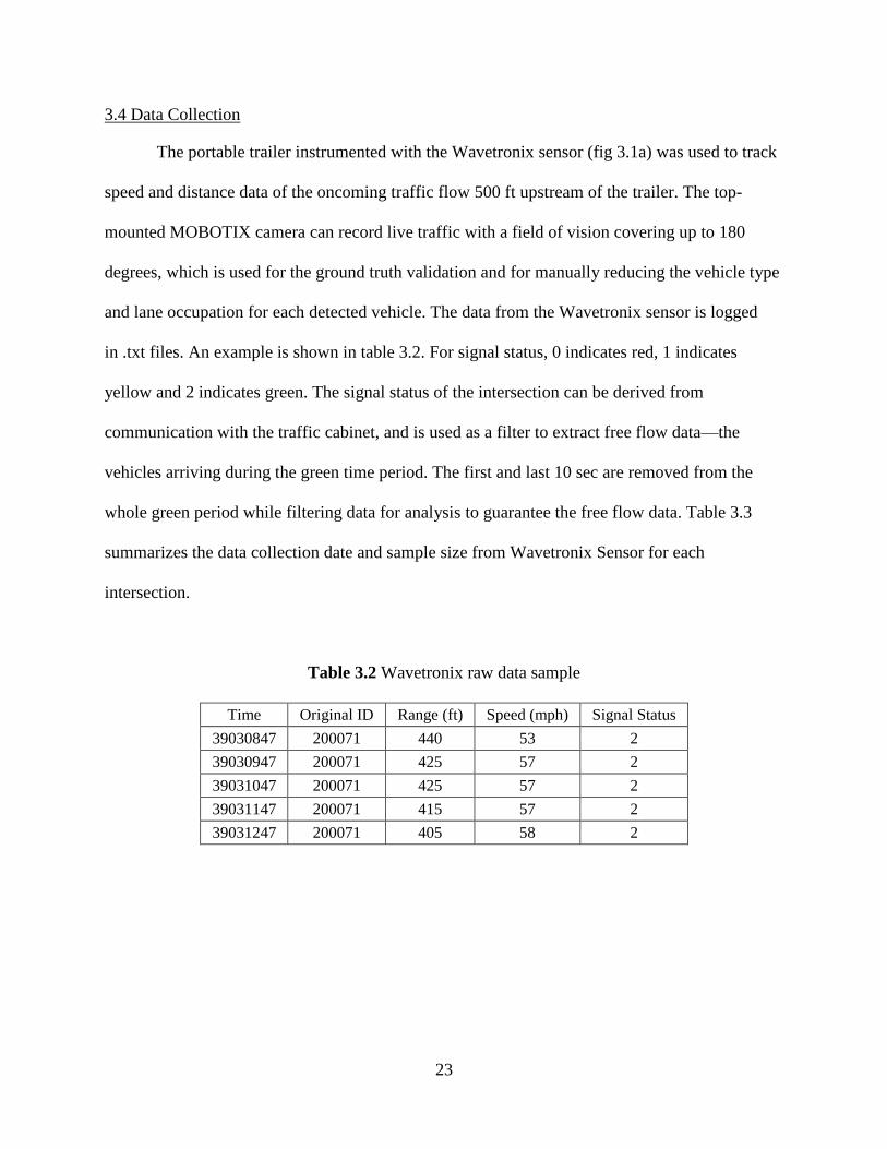
3.4 Data Collection

The portable trailer instrumented with the Wavetronix sensor (fig 3.1a) was used to track

speed and distance data of the oncoming traffic flow 500 ft upstream of the trailer. The top-

mounted MOBOTIX camera can record live traffic with a field of vision covering up to 180

degrees, which is used for the ground truth validation and for manually reducing the vehicle type

and lane occupation for each detected vehicle. The data from the Wavetronix sensor is logged

in .txt files. An example is shown in table 3.2. For signal status, 0 indicates red, 1 indicates

yellow and 2 indicates green. The signal status of the intersection can be derived from

communication with the traffic cabinet, and is used as a filter to extract free flow data—the

vehicles arriving during the green time period. The first and last 10 sec are removed from the

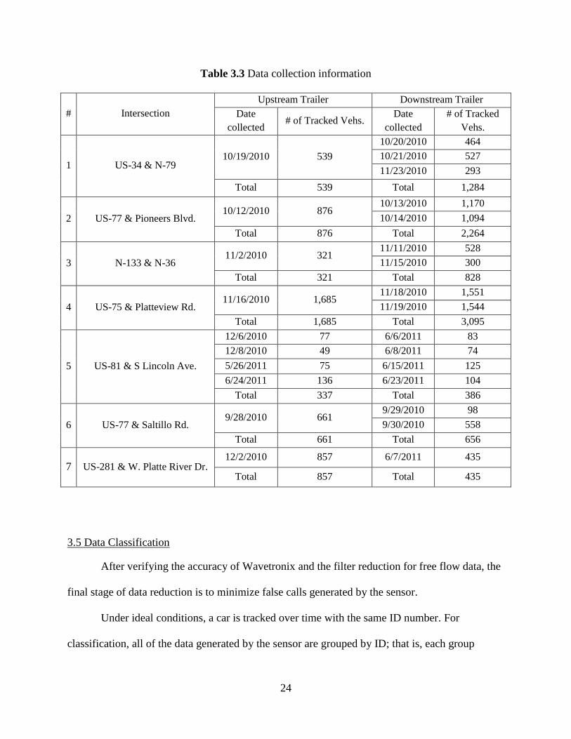
whole green period while filtering data for analysis to guarantee the free flow data. Table 3.3

summarizes the data collection date and sample size from Wavetronix Sensor for each

intersection.

Table 3.2 Wavetronix raw data sample

Time Original ID Range (ft) Speed (mph) Signal Status

39030847 200071 440 53 2

39030947 200071 425 57 2

39031047 200071 425 57 2

39031147 200071 415 57 2

39031247 200071 405 58 2

24

Table 3.3 Data collection information

# Intersection

Upstream Trailer Downstream Trailer

Date

collected # of Tracked Vehs.

Date

collected

# of Tracked

Vehs.

1 US-34 & N-79 10/19/2010 539

10/20/2010 464

10/21/2010 527

11/23/2010 293

Total 539 Total 1,284

2 US-77 & Pioneers Blvd. 10/12/2010 876

10/13/2010 1,170

10/14/2010 1,094

Total 876 Total 2,264

3 N-133 & N-36 11/2/2010 321

11/11/2010 528

11/15/2010 300

Total 321 Total 828

4 US-75 & Platteview Rd. 11/16/2010 1,685

11/18/2010 1,551

11/19/2010 1,544

Total 1,685 Total 3,095

5 US-81 & S Lincoln Ave.

12/6/2010 77 6/6/2011 83

12/8/2010 49 6/8/2011 74

5/26/2011 75 6/15/2011 125

6/24/2011 136 6/23/2011 104

Total 337 Total 386

6 US-77 & Saltillo Rd. 9/28/2010 661

9/29/2010 98

9/30/2010 558

Total 661 Total 656

7 US-281 & W. Platte River Dr. 12/2/2010 857 6/7/2011 435

Total 857 Total 435

3.5 Data Classification

After verifying the accuracy of Wavetronix and the filter reduction for free flow data, the

final stage of data reduction is to minimize false calls generated by the sensor.

Under ideal conditions, a car is tracked over time with the same ID number. For

classification, all of the data generated by the sensor are grouped by ID; that is, each group

25

represents only one vehicle. Classification analysis is used to classify the good calls from the

false call. Several variables could be used to classify groups:

Diff_Range: Diff_Range is defined as the distance between the range where the

vehicle first triggers the sensor and the range where the sensor last detects the

vehicle. Since the Wavetronix sensor is able to track a vehicle continuously within

500 ft, a well-detected vehicle should have a Diff_Range around 550 ft That is, a

well-detected vehicle would keep the sensor turned on over a relatively long

distance within the 500 ft range, while false calls will have a lower Diff_Range.

The false call might stay in the same point with the same range value and trigger

multiple calls, or, generate a short track. For both cases, the Diff_Range is

relatively small compared to that of good calls. Thus, Diff_Range can be an

efficient criterion to discriminate between good and false calls.

Sample points: Ideally, Wavetronix tracks a vehicle every 5 ft after it first hits the

detection area. Thus, a false call is highly possible when the vehicle has

unreasonably fewer points. The number of points in an ID group could be used as

a variable to distinguish groups.

Mean speed and speed variance: for each vehicle, they have been detected with

different speeds at different points in its group as it is passing the detection area.

Hence, the mean speed and variance could be calculated for each group.

In the current study, a binary classification system was used where each vehicle ID

generated by Wavetronix was classified as belonging to either a false or true ID group. In order

to get a clean and valid dataset to analyze speed characteristics, it is necessary to find the most

significant variable(s) among those variables listed above that can discriminate the false groups

26

in the collection. The discriminant analysis technique is used for the binary classification (19).

Discriminate function analysis includes Linear Discriminant Analysis (LDA) and Quadratic

Discriminant Analysis (QDA). A linear classifier is based on the value of a linear combination of

the variables, while the quadratic classifier will separate measurements of two classes by a

quadric surface. The functions for these two classifiers comprise equations 3.1 and 3.2 (20):

(3.1)

(3.2)

where

K: Constant term of the boundary equation

L: Linear coefficients of the boundary equation.

Q: Quadratic coefficient matrix of the boundary equation.

x: Group characteristic variables.

Based on a training dataset composing 549 groups manually reduced from the US-77 &

Saltillo Rd. intersections, classify command in MATLAB was used to select the most significant

variable combinations that could divide the data efficiently into two target groups. Different

combinations of the four variables (i.e., Diff_Range, sample_points, mean speed, and speed

variance) are tested in terms of their ability to accurately classify the groups. Figure 3.6 shows

the best classifier from Quadratic Discriminant Analysis based on the combination of

Diff_Range and sample points.

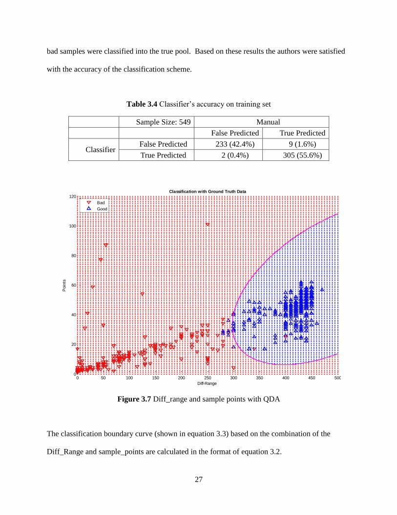
The accuracy of this classifier on training set is summarized in table 3.4. It may be seen

that the classification accuracy was 98% (538 of 549). True data are well classified, and only two

27

bad samples were classified into the true pool. Based on these results the authors were satisfied

with the accuracy of the classification scheme.

Table 3.4 Classifier’s accuracy on training set

Sample Size: 549 Manual

False Predicted True Predicted

Classifier False Predicted 233 (42.4%) 9 (1.6%)

True Predicted 2 (0.4%) 305 (55.6%)

0 50 100 150 200 250 300 350 400 450 5000

20

40

60

80

100

120

Diff-Range

Poin

ts

Classification with Ground Truth Data

Bad

Good

Figure 3.7 Diff_range and sample points with QDA

The classification boundary curve (shown in equation 3.3) based on the combination of the

Diff_Range and sample_points are calculated in the format of equation 3.2.

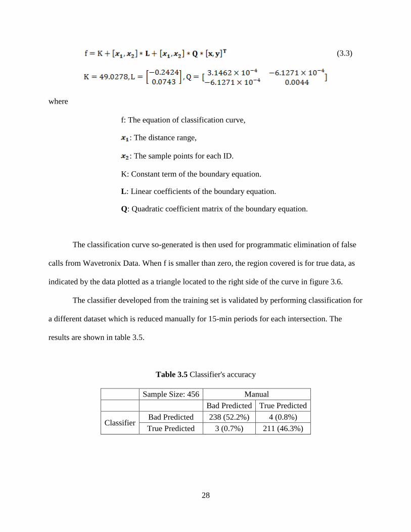
28

(3.3)

where

f: The equation of classification curve,

: The distance range,

: The sample points for each ID.

K: Constant term of the boundary equation.

L: Linear coefficients of the boundary equation.

Q: Quadratic coefficient matrix of the boundary equation.

The classification curve so-generated is then used for programmatic elimination of false

calls from Wavetronix Data. When f is smaller than zero, the region covered is for true data, as

indicated by the data plotted as a triangle located to the right side of the curve in figure 3.6.

The classifier developed from the training set is validated by performing classification for

a different dataset which is reduced manually for 15-min periods for each intersection. The

results are shown in table 3.5.

Table 3.5 Classifier's accuracy

Sample Size: 456 Manual

Bad Predicted True Predicted

Classifier Bad Predicted 238 (52.2%) 4 (0.8%)

True Predicted 3 (0.7%) 211 (46.3%)

29

Chapter 4 Speed Data Analysis

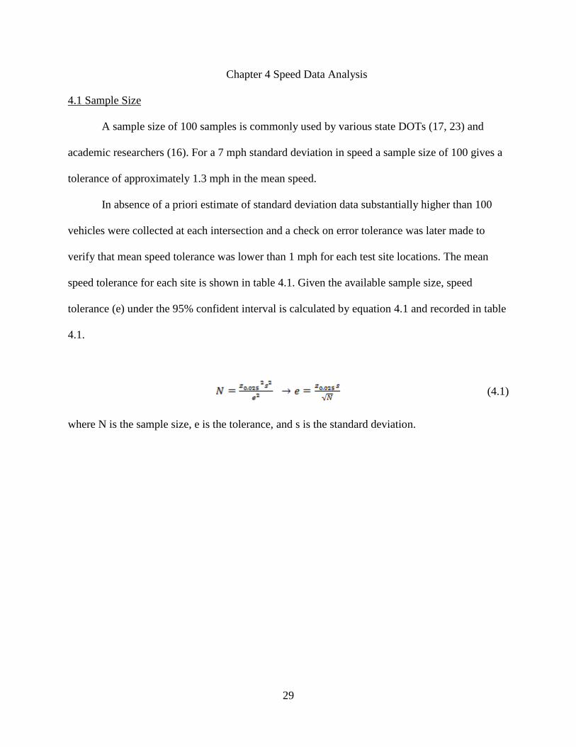
4.1 Sample Size

A sample size of 100 samples is commonly used by various state DOTs (17, 23) and

academic researchers (16). For a 7 mph standard deviation in speed a sample size of 100 gives a

tolerance of approximately 1.3 mph in the mean speed.

In absence of a priori estimate of standard deviation data substantially higher than 100

vehicles were collected at each intersection and a check on error tolerance was later made to

verify that mean speed tolerance was lower than 1 mph for each test site locations. The mean

speed tolerance for each site is shown in table 4.1. Given the available sample size, speed

tolerance (e) under the 95% confident interval is calculated by equation 4.1 and recorded in table

4.1.

(4.1)

where N is the sample size, e is the tolerance, and s is the standard deviation.

30

Table 4.1 Sample size and speed tolerance

# Site Name Standard Deviation Sample Size Tolerance (mph)

Upstream Downstream Upstream Downstream Upstream Downstream

1 US-34 &

N-79 5.85 6.20 539 1284 0.49 0.34

2 US-77 &

Pioneers

Blvd.

4.66 5.93 876 2264 0.31 0.24

3 N-133 &

N-36 5.44 6.94 321 828 0.60 0.47

4 US-75 &

Platteview

Rd.

5.80 5.87 1685 3095 0.28 0.21

5 US-81 &

S. Lincoln

Ave.

6.94 7.16 337 386 0.74 0.71

6 US-77 &

Saltillo

Rd.

6.29 8.04 661 656 0.48 0.62

7 US-281 &

W. Platte

River

6.22 5.45 857 435 0.42 0.51

4.2 Speed Cumulative Distribution Plot

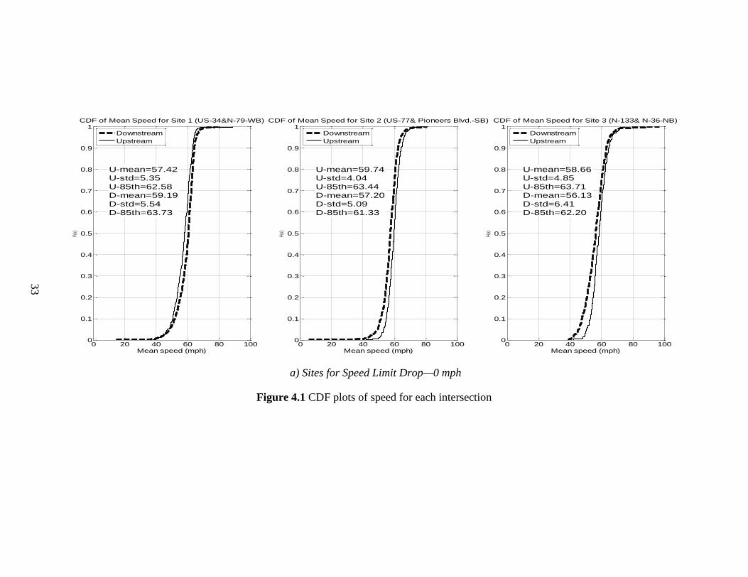
Figure 4.1 plots the cumulative speed distribution for upstream and downstream

locations at each test site. The plots are grouped by speed limit drop. For example, figure 4.1a

shows plots of three test sites where there was no speed limit reduction at the vicinity of the

intersection. The x-axis represents speed in mph and the y-axis represents cumulative percentage.

The description of site and approach is provided in the title of each subplot. For example, the left

most subplot shows upstream and downstream cumulative speed distribution as measured at the

west bound approach of the intersection at US-34 & N-79. The dotted line is the cumulative

speed profile for the downstream section and the solid line is the cumulative speed profile for the

upstream section. Important cumulative speed distribution statistics are listed as text within the

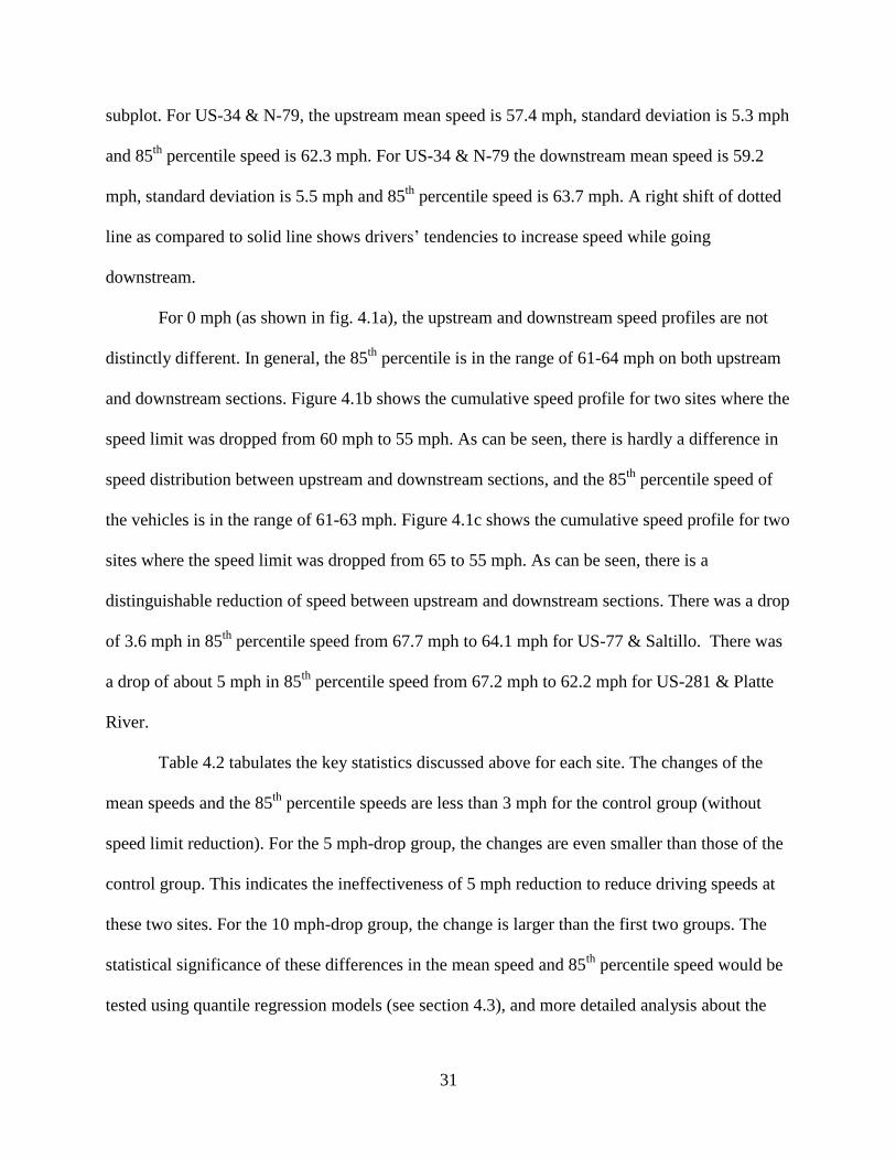
31

subplot. For US-34 & N-79, the upstream mean speed is 57.4 mph, standard deviation is 5.3 mph

and 85th

percentile speed is 62.3 mph. For US-34 & N-79 the downstream mean speed is 59.2

mph, standard deviation is 5.5 mph and 85th

percentile speed is 63.7 mph. A right shift of dotted

line as compared to solid line shows drivers’ tendencies to increase speed while going

downstream.

For 0 mph (as shown in fig. 4.1a), the upstream and downstream speed profiles are not

distinctly different. In general, the 85th

percentile is in the range of 61-64 mph on both upstream

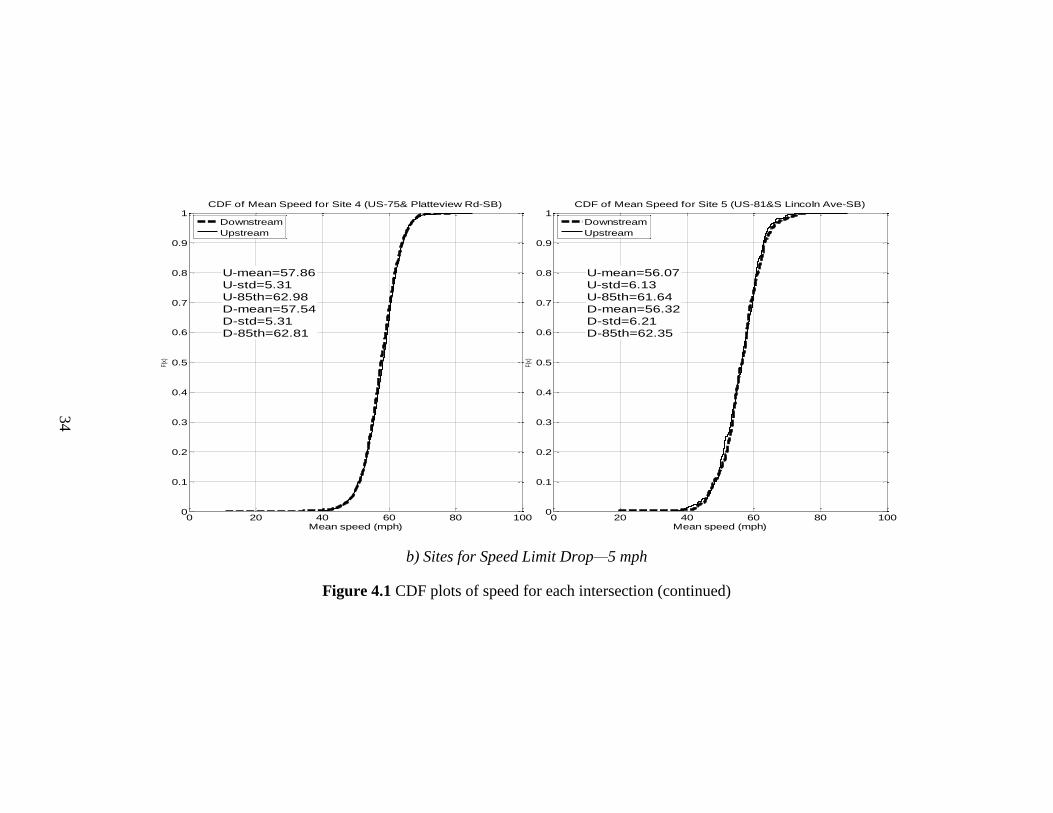
and downstream sections. Figure 4.1b shows the cumulative speed profile for two sites where the

speed limit was dropped from 60 mph to 55 mph. As can be seen, there is hardly a difference in

speed distribution between upstream and downstream sections, and the 85th

percentile speed of

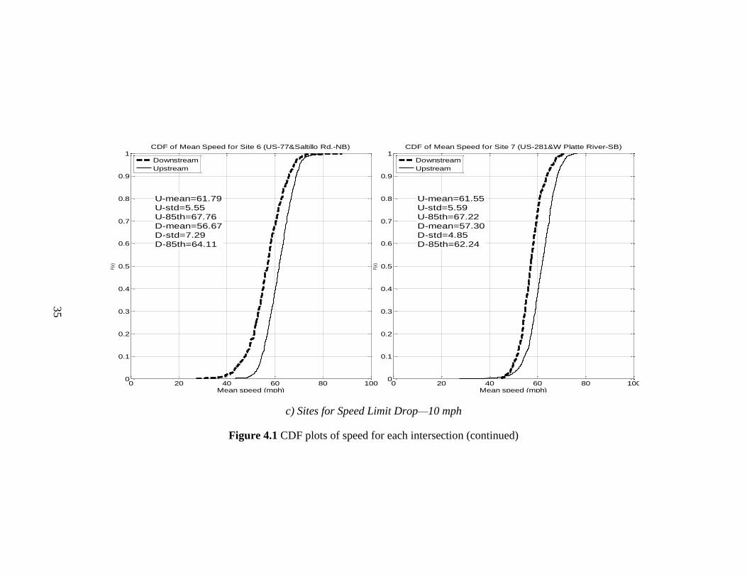
the vehicles is in the range of 61-63 mph. Figure 4.1c shows the cumulative speed profile for two

sites where the speed limit was dropped from 65 to 55 mph. As can be seen, there is a

distinguishable reduction of speed between upstream and downstream sections. There was a drop

of 3.6 mph in 85th

percentile speed from 67.7 mph to 64.1 mph for US-77 & Saltillo. There was

a drop of about 5 mph in 85th

percentile speed from 67.2 mph to 62.2 mph for US-281 & Platte

River.

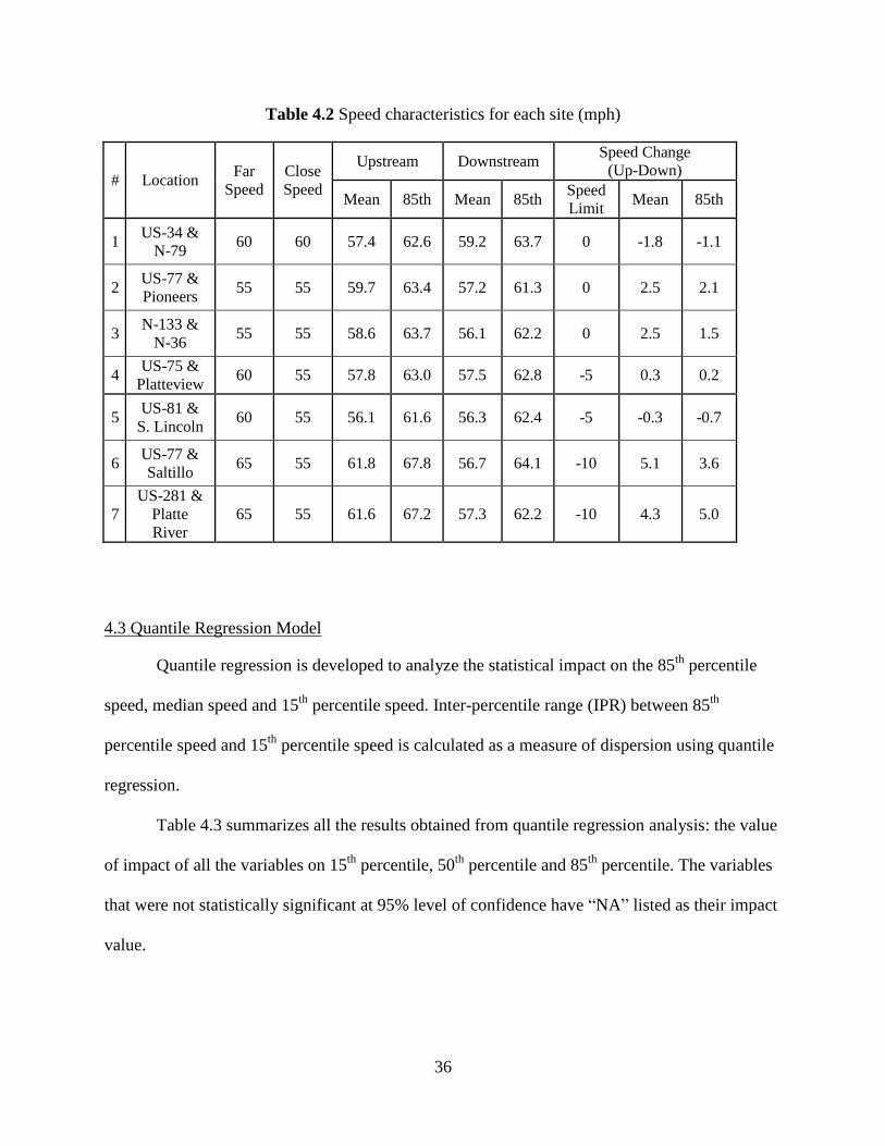
Table 4.2 tabulates the key statistics discussed above for each site. The changes of the

mean speeds and the 85th

percentile speeds are less than 3 mph for the control group (without

speed limit reduction). For the 5 mph-drop group, the changes are even smaller than those of the

control group. This indicates the ineffectiveness of 5 mph reduction to reduce driving speeds at

these two sites. For the 10 mph-drop group, the change is larger than the first two groups. The

statistical significance of these differences in the mean speed and 85th

percentile speed would be

tested using quantile regression models (see section 4.3), and more detailed analysis about the

32

impact of reduced signal speed limit on the average and standard deviation of the speeds will be

explored by SURE in section 4.4.

0 20 40 60 80 1000

0.1

0.2

0.3

0.4

0.5

0.6

0.7

0.8

0.9

1

Mean speed (mph)

F(x)

CDF of Mean Speed for Site 1 (US-34&N-79-WB)

U-mean=57.42

U-std=5.35

U-85th=62.58

D-mean=59.19

D-std=5.54

D-85th=63.73

Downstream

Upstream

0 20 40 60 80 1000

0.1

0.2

0.3

0.4

0.5

0.6

0.7

0.8

0.9

1

Mean speed (mph)

F(x)

CDF of Mean Speed for Site 2 (US-77& Pioneers Blvd.-SB)

U-mean=59.74

U-std=4.04

U-85th=63.44

D-mean=57.20

D-std=5.09

D-85th=61.33

Downstream

Upstream

0 20 40 60 80 1000

0.1

0.2

0.3

0.4

0.5

0.6

0.7

0.8

0.9

1

Mean speed (mph)

F(x)

CDF of Mean Speed for Site 3 (N-133& N-36-NB)

U-mean=58.66

U-std=4.85

U-85th=63.71

D-mean=56.13

D-std=6.41

D-85th=62.20

Downstream

Upstream

a) Sites for Speed Limit Drop—0 mph

Figure 4.1 CDF plots of speed for each intersection

33

0 20 40 60 80 1000

0.1

0.2

0.3

0.4

0.5

0.6

0.7

0.8

0.9

1

Mean speed (mph)

F(x)

CDF of Mean Speed for Site 4 (US-75& Platteview Rd-SB)

U-mean=57.86

U-std=5.31

U-85th=62.98

D-mean=57.54

D-std=5.31

D-85th=62.81

Downstream

Upstream

0 20 40 60 80 1000

0.1

0.2

0.3

0.4

0.5

0.6

0.7

0.8

0.9

1

Mean speed (mph)F(

x)

CDF of Mean Speed for Site 5 (US-81&S Lincoln Ave-SB)

U-mean=56.07

U-std=6.13

U-85th=61.64

D-mean=56.32

D-std=6.21

D-85th=62.35

Downstream

Upstream

b) Sites for Speed Limit Drop—5 mph

Figure 4.1 CDF plots of speed for each intersection (continued)

34

0 20 40 60 80 1000

0.1

0.2

0.3

0.4

0.5

0.6

0.7

0.8

0.9

1

Mean speed (mph)

F(x)

CDF of Mean Speed for Site 6 (US-77&Saltillo Rd.-NB)

U-mean=61.79

U-std=5.55

U-85th=67.76

D-mean=56.67

D-std=7.29

D-85th=64.11

Downstream

Upstream

0 20 40 60 80 1000

0.1

0.2

0.3

0.4

0.5

0.6

0.7

0.8

0.9

1

Mean speed (mph)

F(x)

CDF of Mean Speed for Site 7 (US-281&W Platte River-SB)

U-mean=61.55

U-std=5.59

U-85th=67.22

D-mean=57.30

D-std=4.85

D-85th=62.24

Downstream

Upstream

c) Sites for Speed Limit Drop—10 mph

Figure 4.1 CDF plots of speed for each intersection (continued)

35

36

Table 4.2 Speed characteristics for each site (mph)

# Location Far

Speed Close

Speed

Upstream Downstream Speed Change

(Up-Down)

Mean 85th Mean 85th Speed

Limit Mean 85th

1 US-34 &

N-79 60 60 57.4 62.6 59.2 63.7 0 -1.8 -1.1

2 US-77 & Pioneers

55 55 59.7 63.4 57.2 61.3 0 2.5 2.1

3 N-133 &

N-36 55 55 58.6 63.7 56.1 62.2 0 2.5 1.5

4 US-75 &

Platteview 60 55 57.8 63.0 57.5 62.8 -5 0.3 0.2

5 US-81 &

S. Lincoln 60 55 56.1 61.6 56.3 62.4 -5 -0.3 -0.7

6 US-77 & Saltillo

65 55 61.8 67.8 56.7 64.1 -10 5.1 3.6

7 US-281 &

Platte

River 65 55 61.6 67.2 57.3 62.2 -10 4.3 5.0

4.3 Quantile Regression Model

Quantile regression is developed to analyze the statistical impact on the 85th

percentile

speed, median speed and 15th

percentile speed. Inter-percentile range (IPR) between 85th

percentile speed and 15th

percentile speed is calculated as a measure of dispersion using quantile

regression.

Table 4.3 summarizes all the results obtained from quantile regression analysis: the value

of impact of all the variables on 15th

percentile, 50th

percentile and 85th

percentile. The variables

that were not statistically significant at 95% level of confidence have “NA” listed as their impact

value.

37

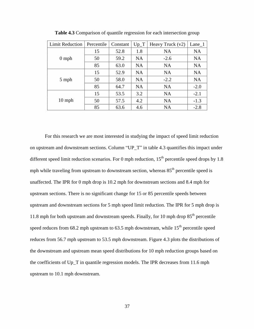
Table 4.3 Comparison of quantile regression for each intersection group

Limit Reduction Percentile Constant Up_T Heavy Truck (v2) Lane_1

0 mph

15 52.8 1.8 NA NA

50 59.2 NA -2.6 NA

85 63.0 NA NA NA

5 mph

15 52.9 NA NA NA

50 58.0 NA -2.2 NA

85 64.7 NA NA -2.0

10 mph

15 53.5 3.2 NA -2.1

50 57.5 4.2 NA -1.3

85 63.6 4.6 NA -2.8

For this research we are most interested in studying the impact of speed limit reduction

on upstream and downstream sections. Column “UP_T” in table 4.3 quantifies this impact under

different speed limit reduction scenarios. For 0 mph reduction, 15th

percentile speed drops by 1.8

mph while traveling from upstream to downstream section, whereas 85th

percentile speed is

unaffected. The IPR for 0 mph drop is 10.2 mph for downstream sections and 8.4 mph for

upstream sections. There is no significant change for 15 or 85 percentile speeds between

upstream and downstream sections for 5 mph speed limit reduction. The IPR for 5 mph drop is

11.8 mph for both upstream and downstream speeds. Finally, for 10 mph drop 85th

percentile

speed reduces from 68.2 mph upstream to 63.5 mph downstream, while 15th

percentile speed

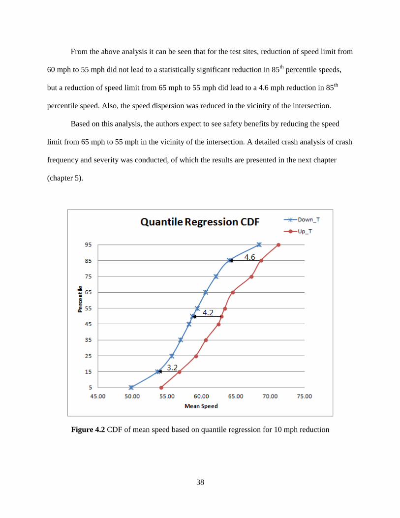
reduces from 56.7 mph upstream to 53.5 mph downstream. Figure 4.3 plots the distributions of

the downstream and upstream mean speed distributions for 10 mph reduction groups based on

the coefficients of Up_T in quantile regression models. The IPR decreases from 11.6 mph

upstream to 10.1 mph downstream.

38

From the above analysis it can be seen that for the test sites, reduction of speed limit from

60 mph to 55 mph did not lead to a statistically significant reduction in 85th

percentile speeds,

but a reduction of speed limit from 65 mph to 55 mph did lead to a 4.6 mph reduction in 85th

percentile speed. Also, the speed dispersion was reduced in the vicinity of the intersection.

Based on this analysis, the authors expect to see safety benefits by reducing the speed

limit from 65 mph to 55 mph in the vicinity of the intersection. A detailed crash analysis of crash

frequency and severity was conducted, of which the results are presented in the next chapter

(chapter 5).

Figure 4.2 CDF of mean speed based on quantile regression for 10 mph reduction

39

4.4 Seemingly Unrelated Equation Models

The 10 mph reduction of transitional speed limit has shown more impact on reducing

driving speed from previous analyses. The seemingly unrelated equation model developed in this

section will test the statistical significance of the impact on both the mean and the standard

deviation of the average speeds simultaneously, which takes consideration of the indirect

interaction between the mean and standard deviation. Besides, the model can account for factors

other than speed limit reduction impacting the change in driver speed and speed variance. The

analysis of standard deviation will yield a stronger conclusion in terms of the safety impact from

speed limit reduction since it’s well established that high variance in traffic flow speeds is

potentially unsafe.

4.4.1 Data preparation

Hourly volume.

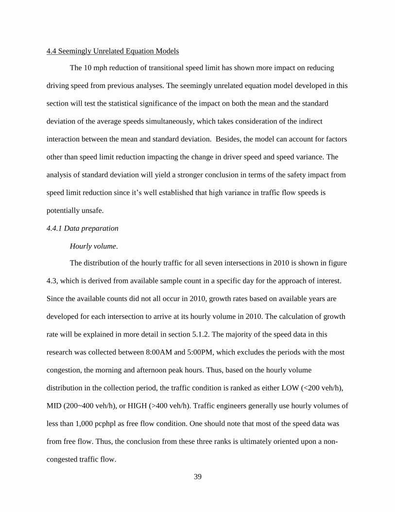
The distribution of the hourly traffic for all seven intersections in 2010 is shown in figure

4.3, which is derived from available sample count in a specific day for the approach of interest.

Since the available counts did not all occur in 2010, growth rates based on available years are

developed for each intersection to arrive at its hourly volume in 2010. The calculation of growth

rate will be explained in more detail in section 5.1.2. The majority of the speed data in this

research was collected between 8:00AM and 5:00PM, which excludes the periods with the most

congestion, the morning and afternoon peak hours. Thus, based on the hourly volume

distribution in the collection period, the traffic condition is ranked as either LOW (<200 veh/h),

MID (200~400 veh/h), or HIGH (>400 veh/h). Traffic engineers generally use hourly volumes of

less than 1,000 pcphpl as free flow condition. One should note that most of the speed data was

from free flow. Thus, the conclusion from these three ranks is ultimately oriented upon a non-

congested traffic flow.

40

Figure 4.3 Distribution of hourly volume in the seven intersections

Grouping.

As in the quantile analysis, the average speed for each vehicle was calculated by

averaging all the spot speeds detected continuously within 500 ft by wide area detector. With the

help of the MOBOTIX camera and Wavetronix sensor, the lane occupation and vehicle type are

reduced manually for each location. The reduced data includes 1,393 samples with

approximately 100 samples for each location (i.e., upstream or downstream) of each intersection.

To apply SURE, these average speeds are further grouped based on time of day and hourly

traffic volume into groups with a size of approximately 10. The mean and standard deviation of

speeds in each group are the dependent variables of SURE models.

4.4.2 Variable Selection and Data Preparation

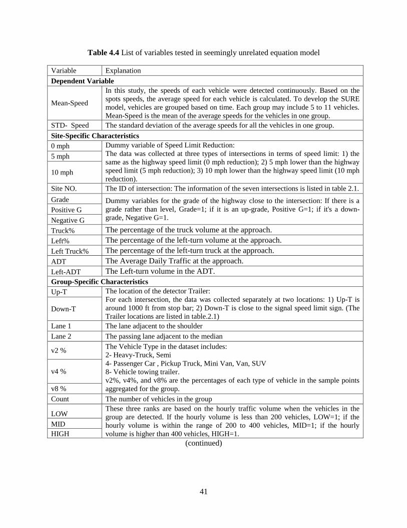
Table 4.4 lists the explanation of all the variables tested.

41

Table 4.4 List of variables tested in seemingly unrelated equation model

Variable Explanation

Dependent Variable

Mean-Speed

In this study, the speeds of each vehicle were detected continuously. Based on the

spots speeds, the average speed for each vehicle is calculated. To develop the SURE

model, vehicles are grouped based on time. Each group may include 5 to 11 vehicles.

Mean-Speed is the mean of the average speeds for the vehicles in one group.

STD- Speed The standard deviation of the average speeds for all the vehicles in one group.

Site-Specific Characteristics

0 mph Dummy variable of Speed Limit Reduction: The data was collected at three types of intersections in terms of speed limit: 1) the

same as the highway speed limit (0 mph reduction); 2) 5 mph lower than the highway

speed limit (5 mph reduction); 3) 10 mph lower than the highway speed limit (10 mph

reduction).

5 mph

10 mph

Site NO. The ID of intersection: The information of the seven intersections is listed in table 2.1.

Grade Dummy variables for the grade of the highway close to the intersection: If there is a

grade rather than level, Grade=1; if it is an up-grade, Positive G=1; if it's a down-

grade, Negative G=1. Positive G

Negative G

Truck% The percentage of the truck volume at the approach.

Left% The percentage of the left-turn volume at the approach.

Left Truck% The percentage of the left-turn truck at the approach.

ADT The Average Daily Traffic at the approach.

Left-ADT The Left-turn volume in the ADT.

Group-Specific Characteristics

Up-T The location of the detector Trailer: For each intersection, the data was collected separately at two locations: 1) Up-T is

around 1000 ft from stop bar; 2) Down-T is close to the signal speed limit sign. (The

Trailer locations are listed in table.2.1) Down-T

Lane 1 The lane adjacent to the shoulder

Lane 2 The passing lane adjacent to the median

v2 % The Vehicle Type in the dataset includes: 2- Heavy-Truck, Semi 4- Passenger Car , Pickup Truck, Mini Van, Van, SUV 8- Vehicle towing trailer. v2%, v4%, and v8% are the percentages of each type of vehicle in the sample points

aggregated for the group.

v4 %

v8 %

Count The number of vehicles in the group

LOW These three ranks are based on the hourly traffic volume when the vehicles in the

group are detected. If the hourly volume is less than 200 vehicles, LOW=1; if the

hourly volume is within the range of 200 to 400 vehicles, MID=1; if the hourly

volume is higher than 400 vehicles, HIGH=1.

MID

HIGH

(continued)

42

Table 4.4 (continued)

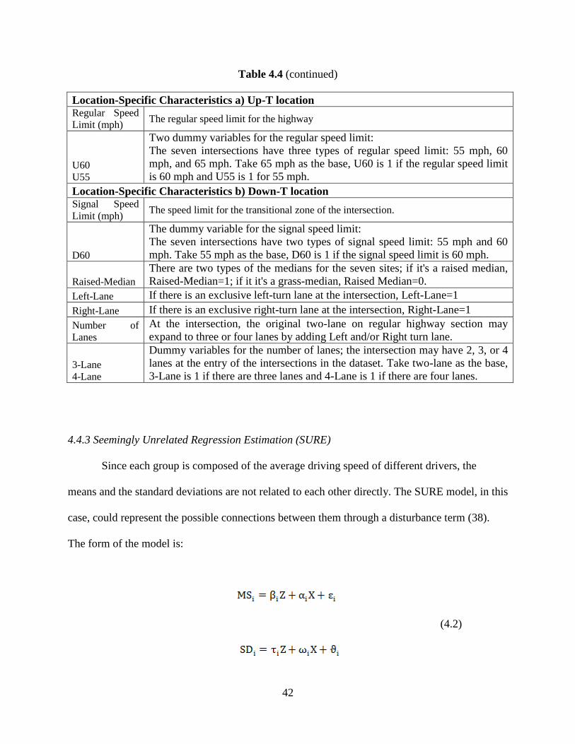
Location-Specific Characteristics a) Up-T location Regular Speed

Limit (mph) The regular speed limit for the highway

U60 U55

Two dummy variables for the regular speed limit:

The seven intersections have three types of regular speed limit: 55 mph, 60

mph, and 65 mph. Take 65 mph as the base, U60 is 1 if the regular speed limit

is 60 mph and U55 is 1 for 55 mph.

Location-Specific Characteristics b) Down-T location Signal Speed

Limit (mph) The speed limit for the transitional zone of the intersection.

D60

The dummy variable for the signal speed limit:

The seven intersections have two types of signal speed limit: 55 mph and 60

mph. Take 55 mph as the base, D60 is 1 if the signal speed limit is 60 mph.

Raised-Median

There are two types of the medians for the seven sites; if it's a raised median,

Raised-Median=1; if it it's a grass-median, Raised Median=0.

Left-Lane If there is an exclusive left-turn lane at the intersection, Left-Lane=1

Right-Lane If there is an exclusive right-turn lane at the intersection, Right-Lane=1

Number of

Lanes

At the intersection, the original two-lane on regular highway section may

expand to three or four lanes by adding Left and/or Right turn lane.

3-Lane 4-Lane

Dummy variables for the number of lanes; the intersection may have 2, 3, or 4

lanes at the entry of the intersections in the dataset. Take two-lane as the base,

3-Lane is 1 if there are three lanes and 4-Lane is 1 if there are four lanes.

4.4.3 Seemingly Unrelated Regression Estimation (SURE)

Since each group is composed of the average driving speed of different drivers, the

means and the standard deviations are not related to each other directly. The SURE model, in this

case, could represent the possible connections between them through a disturbance term (38).

The form of the model is:

(4.2)

43

where

=Mean of the mean speeds in sub-sample i;

= standard deviation of the mean speeds in sub-sample i;

=vector of site-specific characteristics (e.g., limit reduction, signal/regular speed limit,

ADT, etc.);

=vector of group-specific characteristics (e.g., vehicle type percentage, lane occupation,

etc.).

= group ID.

Each group, as shown in the group-specific characteristics, consists of speed values

obtained from same lane and detector location with an identical traffic condition rank; however,

it is reasonable to assume they are impacted by some unobserved factors. Generalized least

squares method (GLS) is applied to estimate the coefficients for both equations jointly. This

relaxes the assumptions of the ordinary least squares (OLS). OLS estimates the two equations

separately, and will yield inefficient estimations not considering the correlation of the

disturbances term resulting from unobserved factors.

OLS will estimate the parameters by:

(4.3)

where

is a column vector and p is the number of coefficients;

is a matrix of data and n is the number of observations;

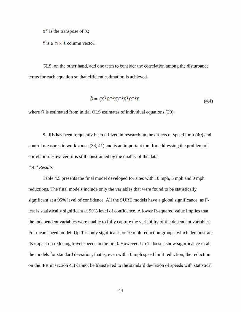
44

is the transpose of X;

is a column vector.

GLS, on the other hand, add one term to consider the correlation among the disturbance

terms for each equation so that efficient estimation is achieved.

(4.4)

where is estimated from initial OLS estimates of individual equations (39).

SURE has been frequently been utilized in research on the effects of speed limit (40) and

control measures in work zones (38, 41) and is an important tool for addressing the problem of

correlation. However, it is still constrained by the quality of the data.

4.4.4 Results

Table 4.5 presents the final model developed for sites with 10 mph, 5 mph and 0 mph

reductions. The final models include only the variables that were found to be statistically

significant at a 95% level of confidence. All the SURE models have a global significance, as F-

test is statistically significant at 90% level of confidence. A lower R-squared value implies that

the independent variables were unable to fully capture the variability of the dependent variables.

For mean speed model, Up-T is only significant for 10 mph reduction groups, which demonstrate

its impact on reducing travel speeds in the field. However, Up-T doesn't show significance in all

the models for standard deviation; that is, even with 10 mph speed limit reduction, the reduction

on the IPR in section 4.3 cannot be transferred to the standard deviation of speeds with statistical

45

significance. Detailed conclusions related to each variable are listed in the comments column in

table 4.5.

Table 4.5 Comparison of the SURE models for speed limit reduction

a) SURE for 10 mph reduction intersections

Parameter Estimation for Mean-Speed of 10 mph reduction Sites Adjusted R-squared=0.47 Chi-sq[2] (prob)=32.86 (.0000) Number of Observations=44

Variable

Parameter (Std. Err)

P Value

(t stat) Comments

Constant 58.37 (0.63)

.0000

(91.95)

The mean speed of vehicles travelling through the sensor close to

signal speed limit is 58.37 mph on the passing lane of the 10 mph

reduction sites (i.e., S6 and S7).

Up-T 3.81 (0.65)

.0000

(5.85)

The mean speed collected by Up-T is 3.81 mph higher than that at

Down-T. This demonstrates the significant effect of 10 mph

reduction on reducing speed in the field.

Lane 1 -1.96 (0.68)

.0042

(-2.86) Compared to the passing lane adjacent to the median, vehicles on

Lane1 travels with a mean speed 1.96 mph slower.

Parameter Estimation for STD-Speed of 10 mph reduction sites Adjusted R-squared=0.24 Chi-sq[1] (prob)=14.91 (.0001) Number of Observations=44

Variable Parameter (Std. Err) P Value Comments

Constant 4.16 (0.27)

.0000

(15.58)

The standard deviation of Site #7 (S7) is 4.16 mph. Note: There is no significant difference for the flow at Up-T and

the flow close to the signal speed limit.

S6 1.46 (0.38)

.0001

(3.87)

The STD-Speed is significantly higher at Site #6 than Site #7 by

1.46 mph. This may be from the higher grade for #6 close to the

intersection. The grade at #6 is 2.99% while the grade at #7 is

0.04%.

46

b) SURE for 5 mph reduction intersections


Variable

Parameter (Std. Err)

P Value

(t stat) Comments

Constant 58.39 (0.43)

.0000

(136.45)

The mean speed of vehicles travelling on the passing lane of 5

mph reduction sites (i.e., S4 and S5) is 58.39 mph, which does not

vary significantly from site to site. Note: There was no significant difference for the flow at Up-T and

the flow close to the signal speed limit. This shows a weak impact

of 5 mph reduction at signal speed limit on reducing speeds of

operation.

Lane1 -1.42 (0.56)

.0112

(-2.53) Compared to the passing lane adjacent to the median, vehicles on

Lane 1 travel at a 1.42 mph slower mean speed.

Parameter Estimation for STD-Speed of 5 mph reduction Sites Adjusted R-squared=0.06 Chi-sq[1] (prob)=5.73 (.0167) Number of Observations=43



.0000

(19.36)

The standard deviation of the two 5 mph reduction sites on passing

lane is 4.16 mph. This value is not significantly different from site

to site. Note: There is no significant difference for the flow at Up-T and


Lane1 -0.71 (0.36)

.0498

(-1.96)

Compared to the passing lane adjacent to the median, vehicles on

Lane1 travel with a standard deviation of speed that is 0.71 mph

slower.

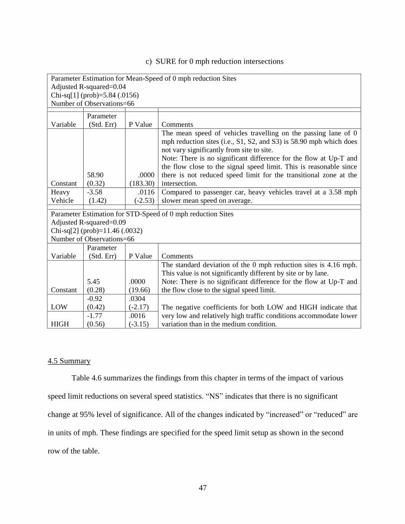
47

c) SURE for 0 mph reduction intersections


Variable

Parameter (Std. Err) P Value Comments

Constant 58.90 (0.32)

.0000

(183.30)

The mean speed of vehicles travelling on the passing lane of 0

mph reduction sites (i.e., S1, S2, and S3) is 58.90 mph which does

not vary significantly from site to site. Note: There is no significant difference for the flow at Up-T and

the flow close to the signal speed limit. This is reasonable since

there is not reduced speed limit for the transitional zone at the

intersection. Heavy

Vehicle -3.58 (1.42)

.0116

(-2.53) Compared to passenger car, heavy vehicles travel at a 3.58 mph

slower mean speed on average.

Parameter Estimation for STD-Speed of 0 mph reduction Sites Adjusted R-squared=0.09 Chi-sq[2] (prob)=11.46 (.0032) Number of Observations=66



.0000

(19.66)

The standard deviation of the 0 mph reduction sites is 4.16 mph.

This value is not significantly different by site or by lane. Note: There is no significant difference for the flow at Up-T and


LOW -0.92 (0.42)

.0304

(-2.17) The negative coefficients for both LOW and HIGH indicate that

very low and relatively high traffic conditions accommodate lower

variation than in the medium condition. HIGH -1.77 (0.56)

.0016

(-3.15)

4.5 Summary

Table 4.6 summarizes the findings from this chapter in terms of the impact of various

speed limit reductions on several speed statistics. “NS” indicates that there is no significant

change at 95% level of significance. All of the changes indicated by “increased” or “reduced” are

in units of mph. These findings are specified for the speed limit setup as shown in the second

row of the table.

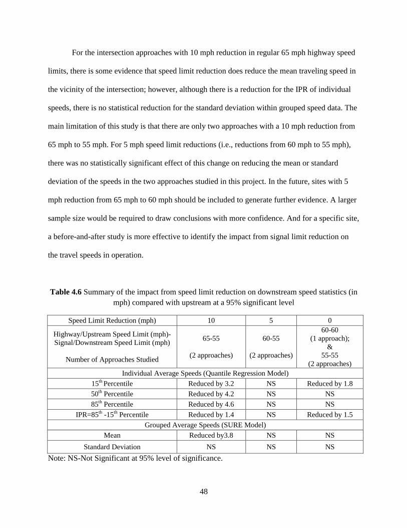
48

For the intersection approaches with 10 mph reduction in regular 65 mph highway speed

limits, there is some evidence that speed limit reduction does reduce the mean traveling speed in

the vicinity of the intersection; however, although there is a reduction for the IPR of individual

speeds, there is no statistical reduction for the standard deviation within grouped speed data. The

main limitation of this study is that there are only two approaches with a 10 mph reduction from

65 mph to 55 mph. For 5 mph speed limit reductions (i.e., reductions from 60 mph to 55 mph),

there was no statistically significant effect of this change on reducing the mean or standard

deviation of the speeds in the two approaches studied in this project. In the future, sites with 5

mph reduction from 65 mph to 60 mph should be included to generate further evidence. A larger

sample size would be required to draw conclusions with more confidence. And for a specific site,

a before-and-after study is more effective to identify the impact from signal limit reduction on

the travel speeds in operation.

Table 4.6 Summary of the impact from speed limit reduction on downstream speed statistics (in

mph) compared with upstream at a 95% significant level

Speed Limit Reduction (mph) 10 5 0

Highway/Upstream Speed Limit (mph)-

Signal/Downstream Speed Limit (mph)

Number of Approaches Studied

65-55

(2 approaches)

60-55

(2 approaches)

60-60

(1 approach);

&

55-55

(2 approaches)

Individual Average Speeds (Quantile Regression Model)

15th

Percentile Reduced by 3.2 NS Reduced by 1.8

50th Percentile Reduced by 4.2 NS NS

85th Percentile Reduced by 4.6 NS NS

IPR=85th -15

th Percentile Reduced by 1.4 NS Reduced by 1.5

Grouped Average Speeds (SURE Model)

Mean Reduced by3.8 NS NS

Standard Deviation NS NS NS

Note: NS-Not Significant at 95% level of significance.

49

Chapter 5 Crash Analysis

Based on the analysis conducted in last chapter, safety benefits are expected upon

reducing the speed limit from 65 mph to 55 mph in the vicinity of signalized high-speed

intersections. This chapter presents a detailed crash analysis to better understand the safety

impact of speed limit reduction.

A list of 28 intersections was compiled under the guidance of Matt Neemann from

NDOR to identify high-speed intersections managed by NDOR. Ten years of detailed crash data

(January 2001 to December 2010) was obtained for 28 intersections. The crash data is further

reduced for each approach of the main street of each intersection; resulting in56 approaches total

approaches. In the 56 approaches, 43 approaches have the constant speed limit without reduced

signal speed limit, 9 approaches have a 5 mph speed limit drop, and 4 approaches have a 10 mph

speed limit drop. The uneven numbers of approaches for 0 mph reduction and 5 mph reduction

come from the main street (N133) of the rest one intersection (N133 & N36), which has one

approach (Northbound) with a 0 mph reduction and another approach (Southbound) with a 5

mph reduction. Appendix B shows the detailed information for these 28 intersections. After

being separated by approach, the accident dataset is further categorized by year. Thus, there were

originally 560 data points (28 intersections * 2 approaches * 10 years) for the accident frequency

model. However, two intersections have a history of stop-control prior to implementing

signalized control. Excluding these points, there were 536 observations for the accident

frequency model. On the other hand, accidents in the ten years at the 56 approaches totaled 635.

Thus, there were 635 observations for the accident severity model.

Statistical models were developed to test the impacts of speed limit reduction and

downstream speed limits on crash frequency and severity.

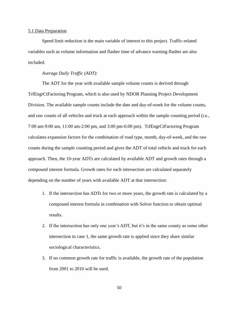
50

5.1 Data Preparation

Speed limit reduction is the main variable of interest to this project. Traffic-related

variables such as volume information and flasher time of advance warning flasher are also

included.

Average Daily Traffic (ADT):

The ADT for the year with available sample volume counts is derived through

TrfEngrCtFactoring Program, which is also used by NDOR Planning Project Development

Division. The available sample counts include the date and day-of-week for the volume counts,

and raw counts of all vehicles and truck at each approach within the sample counting period (i.e.,

7:00 am-9:00 am, 11:00 am-2:00 pm, and 3:00 pm-6:00 pm). TrfEngrCtFactoring Program

calculates expansion factors for the combination of road type, month, day-of-week, and the raw

counts during the sample counting period and gives the ADT of total vehicle and truck for each

approach. Then, the 10-year ADTs are calculated by available ADT and growth rates through a

compound interest formula. Growth rates for each intersection are calculated separately

depending on the number of years with available ADT at that intersection:

1. If the intersection has ADTs for two or more years, the growth rate is calculated by a

compound interest formula in combination with Solver function to obtain optimal

results.

2. If the intersection has only one year’s ADT, but it’s in the same county as some other

intersection in case 1, the same growth rate is applied since they share similar

sociological characteristics.

3. If no common growth rate for traffic is available, the growth rate of the population

from 2001 to 2010 will be used.

51

4. A similar calculation is used for truck volume and left-turn volume.

Flasher-Dummy.

The flasher-dummy is created to study the impact of the flasher time of AWF in the field.

This variable is based on the fact that whether the flasher time is greater than the time required

for the drivers at signal speed limit traveling from the flasher to the stop bar, which is calculated

by equation 5.1.

(5.1a)

(5.1b)

5.2 Overview of Crash Data

Figure 5.1 shows the accident frequency and annual rate distribution by accident type and

speed limit reduction. The x-axis consists of three speed limit reduction: 0 mph, 5 mph, and 10

mph. The y-axis for the left column is crash frequency in terms of total accident frequency, angle

accident frequency, and rear-end accident frequency. The y-axis for the right column is the

frequency rate for each type of accident. This annual rate is calculated by the annual frequency at

each approach divided by the corresponding ADT for the approach, as seen in equation 5.2.

There are 536 observations in all; the 0mph-box includes 406 observations; the 5 mph-box

includes 90 points; and the 10mph-box includes 40 points at each plot.

(5.2)

52

0

2

4

6

8

10

0 5 10Speed Limit Reduction(MPH)

Total Frequency

Num

ber

of

cra

shes

0

2

4

6

8

10

0 5 10Speed Limit Reduction(MPH)

Total Rate

Rate

(Num

ber

of

cra

shes/A

AD

T)

Size=406Size=406 Size=90 Size=40 Size=90 Size=40

Figure 5.1 Distribution of crash frequency and rate by accident type and speed limit reduction

5.3 Crash Frequency Model

5.3.1 Literature Review

Numerous studies have been conducted to investigate the effects of traffic characteristics

and traffic on crash frequency (27, 28, 29, 32, 33, 34). Due to the discrete response variable, the

Poisson model is appropriate to apply when the mean and the variance are approximately equal.

Whenever the equality does not hold, the parameter vector of the Poisson model would be biased.

If the data is over-dispersed (i.e., the variance is significantly greater than the mean) for what is

common in crash frequency data, a negative binomial (NB) regression model fits better.

53

However, neither the Poisson nor the NB model considers the possibility that crash frequency

likelihood may be affected by two or more underlying processes. For example, if the observation

of reported crashes for a one-year period is zero, there are two possible states for this observation.

One is a normal count-process state in which zero crashes is one outcome of all the possible

outcomes of the Poisson or NB distribution; the other one is zero-state, in which this observation

comes from a road section that is inherently safe and the occurrence of crash on it is so extremely

rare that it will be zero most of the time. Trying to model a dual-state system as a single state

system would provide erroneous conclusion; for example, an NB model is chosen while a

Poisson distribution is correct. Shanker et al. compared a zero-inflated Poisson Model (ZIP) and

a zero-inflated NB model (ZINB) with the NB model on studying crash frequency for non-

intersection roadway sections (29). The results showed that different variants of the ZIP and

ZINB Models are plausible for road sections in different functional classification.

5.3.2 Poisson Model and NB Model

Poisson regression models define the probability of intersection i having crashes in the

observed period as:

(5.3)

where : is the Poisson parameter for intersection i and equal to the expected number of crashes

per five years at intersection i. And is estimated by and is a vector of the

explanatory variables such as signal speed limit. will be estimated by standard maximum

likelihood methods using Limdep.

54

However, Poisson distribution requires equality of the mean and variance. In actual

studies, the main variables influencing the crash frequency may not be included in the available

data; this will lead to over-dispersed data, which violates the assumption of the Poisson

regression model. In this case, an NB regression model is the alternative to a Poisson model. The

in an NB regression model is calculated by

(5.4)

where is a gamma-distributed error with mean 1 and variance . The added

error term would release the restrains of Poisson and accommodate the data with a variance

different from the mean. The model choice will be based on the dispersion parameter.

5.3.3 Zero-Altered Probability Processes

In reality, crashes do not happen very frequently; therefore, there could be a zero count

for an intersection or approach in a given year. A zero count could result from two cases: 1) the

intersection is safe enough that no accident will ever happen there, or 2) the zero is one

observation from a regular count process (29). Case 1 violates the assumption of the Poisson

regression model and negative binominal model since it is not from a regular count process.

Zero-altered probability processes such as the ZIP and ZINB distributions relax this assumption,

and are more flexible to model the accident dataset with a significant number of zero.

ZIP assumes events Y= (y1, y2, y3...yn) are independent. The model is as presented below.

(5.5a)

(5.5b)

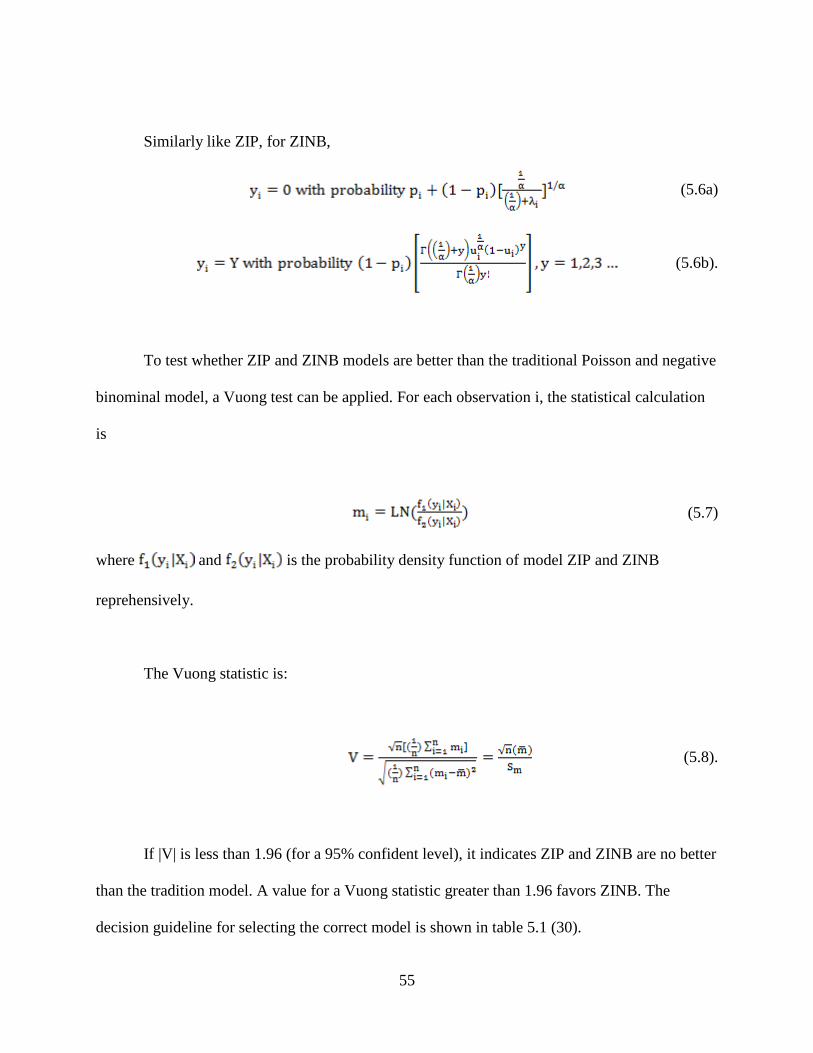
55

Similarly like ZIP, for ZINB,

(5.6a)

(5.6b).

To test whether ZIP and ZINB models are better than the traditional Poisson and negative

binominal model, a Vuong test can be applied. For each observation i, the statistical calculation

is

(5.7)

where and is the probability density function of model ZIP and ZINB

reprehensively.

The Vuong statistic is:

(5.8).

If |V| is less than 1.96 (for a 95% confident level), it indicates ZIP and ZINB are no better

than the tradition model. A value for a Vuong statistic greater than 1.96 favors ZINB. The

decision guideline for selecting the correct model is shown in table 5.1 (30).

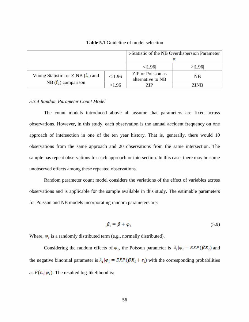
56

Table 5.1 Guideline of model selection

t-Statistic of the NB Overdispersion Parameter

<|1.96| >|1.96|

Vuong Statistic for ZINB ( ) and

NB ( ) comparison

<-1.96 ZIP or Poisson as

alternative to NB NB

>1.96 ZIP ZINB

5.3.4 Random Parameter Count Model

The count models introduced above all assume that parameters are fixed across

observations. However, in this study, each observation is the annual accident frequency on one

approach of intersection in one of the ten year history. That is, generally, there would 10

observations from the same approach and 20 observations from the same intersection. The

sample has repeat observations for each approach or intersection. In this case, there may be some

unobserved effects among these repeated observations.

Random parameter count model considers the variations of the effect of variables across

observations and is applicable for the sample available in this study. The estimable parameters

for Poisson and NB models incorporating random parameters are:

(5.9)

Where, is a randomly distributed term (e.g., normally distributed).

Considering the random effects of , the Poisson parameter is and

the negative binomial parameter is with the corresponding probabilities

as . The resulted log-likelihood is:

57

(5.10)

where g( ) is the probability density function of the .

Due to the numerical integration of the Poisson or NB function over the distribution of

the random parameters in equation 5.10, the random-parameter count model is computationally

demanding. Thus, a simulation-based maximum likelihood method is commonly used by

applying Halton draws.

5.3.5 Interpretation of Count Models

For all the count models above, it is difficult to make inferences directly from the

parameter estimation. Elasticities are computed to determine the marginal effects of 1% change

in independent variables on the expected crash frequency. For continuous variables (e.g.,

AADT), the elasticity of frequency is calculated as:

(5.11)

where

: is the elasticity;

: is the value of k-th independent variable for i-th intersection;

: is the estimated parameter for

For indicator variables (e.g., 10 mph reduction) with values only as 0 or 1, a pseudo-

elasticity provides an inference about the incremental change of the number of crashes from the

indicator variable. This is also referred to as marginal effect. The calculation is:

58

(5.12)

5.3.6 Data Preparation and Model Development

The independent variables tested during model development are summarized in table 5.2.

The statistics of all variables are collected in appendix C. Random Parameter NB (RPNB)

model is applied to analyze the impact of speed limit reduction on accident frequency. NB is

selected due to the over-dispersion of the data. The outputs of coefficient estimation and

marginal effects are shown in table 5.3 and 5.4, respectively.

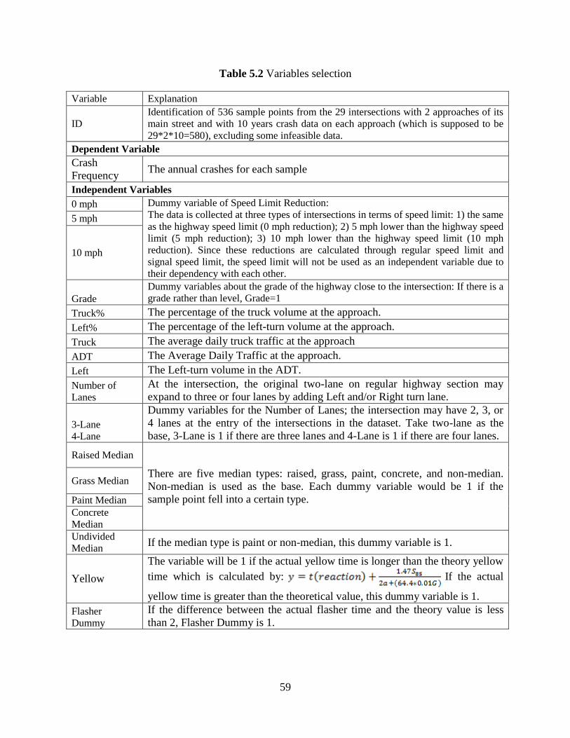
59

Table 5.2 Variables selection


ID

Identification of 536 sample points from the 29 intersections with 2 approaches of its

main street and with 10 years crash data on each approach (which is supposed to be

29*2*10=580), excluding some infeasible data.

Dependent Variable

Crash

Frequency The annual crashes for each sample

Independent Variables

0 mph Dummy variable of Speed Limit Reduction: The data is collected at three types of intersections in terms of speed limit: 1) the same

as the highway speed limit (0 mph reduction); 2) 5 mph lower than the highway speed

limit (5 mph reduction); 3) 10 mph lower than the highway speed limit (10 mph

reduction). Since these reductions are calculated through regular speed limit and

signal speed limit, the speed limit will not be used as an independent variable due to

their dependency with each other.

5 mph

10 mph

Grade Dummy variables about the grade of the highway close to the intersection: If there is a

grade rather than level, Grade=1

Truck% The percentage of the truck volume at the approach.

Left% The percentage of the left-turn volume at the approach.

Truck The average daily truck traffic at the approach

ADT The Average Daily Traffic at the approach.

Left The Left-turn volume in the ADT.

Number of

Lanes

At the intersection, the original two-lane on regular highway section may

expand to three or four lanes by adding Left and/or Right turn lane.

3-Lane 4-Lane

Dummy variables for the Number of Lanes; the intersection may have 2, 3, or

4 lanes at the entry of the intersections in the dataset. Take two-lane as the

base, 3-Lane is 1 if there are three lanes and 4-Lane is 1 if there are four lanes.

Raised Median

There are five median types: raised, grass, paint, concrete, and non-median.

Non-median is used as the base. Each dummy variable would be 1 if the

sample point fell into a certain type.

Grass Median

Paint Median

Concrete

Median

Undivided

Median If the median type is paint or non-median, this dummy variable is 1.

Yellow

The variable will be 1 if the actual yellow time is longer than the theory yellow

time which is calculated by: If the actual

yellow time is greater than the theoretical value, this dummy variable is 1.

Flasher

Dummy

If the difference between the actual flasher time and the theory value is less

than 2, Flasher Dummy is 1.

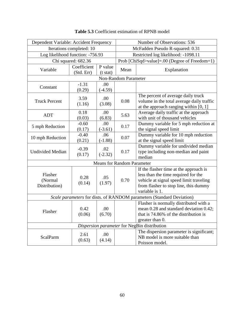
60

Table 5.3 Coefficient estimation of RPNB model

Dependent Variable: Accident Frequency Number of Observations: 536

Iterations completed: 10 McFadden Pseudo R-squared: 0.31

Log likelihood function: -756.93 Restricted log likelihood: -1098.11

Chi squared: 682.36 Prob [ChiSqd>value]=.00 (Degree of Freedom=1)

Variable Coefficient

(Std. Err)

P value

(t stat) Mean Explanation

Non-Random Parameter

Constant -1.31

(0.29)

.00

(-4.59)

Truck Percent 3.59

(1.16)

.00

(3.08) 0.08

The percent of average daily truck

volume in the total average daily traffic

at the approach ranging within [0, 1]

ADT 0.18

(0.03)

.00

(6.83) 5.63

Average daily traffic at the approach

with unit of thousand vehicles

5 mph Reduction -0.60

(0.17)

.00

(-3.61) 0.17

Dummy variable for 5 mph reduction at

the signal speed limit


(0.21)

.06

(-1.88) 0.07

Dummy variable for 10 mph reduction

at the signal speed limit

Undivided Median -0.39

(0.17)

.02

(-2.32) 0.17

Dummy variable for undivided median

type including non-median and paint

median

Means for Random Parameter

Flasher

(Normal

Distribution)

0.28

(0.14)

.05

(1.97) 0.70

If the flasher time at the approach is

less than the time required for the

vehicle at signal speed limit traveling

from flasher to stop line, this dummy

variable is 1.

Scale parameters for dists. of RANDOM parameters (Standard Deviation)

Flasher 0.42

(0.06)

.00

(6.70)

Flasher is normally distributed with a

mean 0.28 and standard deviation 0.42;

that is 74.86% of the distribution is

greater than 0.

Dispersion parameter for NegBin distribution

ScalParm 2.61

(0.63)

.00

(4.14)

The dispersion parameter is significant;

NB model is more suitable than

Poisson model.

61

Table 5.4 Marginal effects of NB model with random effects


(Std. Err)

P value

(t stat) Explanation

Truck Percent 3.48

(1.36)

.01

(2.56)

An approach with all-truck traffic will get about 3.5

more accidents per year, compared with non-truck

traffic.

ADT 0.17

(0.03)

.00

(4.97)

An increase of 10,000 vehicles will increase about

1.7 accidents per approach per year on average.


(0.16)

.00

(-3.60)

On average, an approach with a 5 mph reduction for

signal speed limit has 0.6 less accidents than the

approach with no speed limit reduction.


(0.21)

.07

(-1.79)

On average, an approach with 10 mph reduction for

signal speed limit has 0.4 less accidents per year

than the approach with no speed limit reduction at

the significance level of 90%.

Undivided Median -0.38

(0.16)

.02

(-2.33)

The approach with no or paint median has less

accident than that with divided median; this may be

from the fact that intersections do not need median

(e.g., with less traffic demand) are generally safer

than those who do.

Flasher 0.27

(0.17)

.10

(1.65)

If the flasher time is less than the time needed for

the vehicle at signal speed limit traveling from

flasher to stop bar, the approach will have generally

0.27 more accidents per year at the significance

level of 90%. However, the effect varies across

observations.

5.3.7 Interpretation of Results

1) Traffic volume also impacts crash frequency at 95 % level of significance. 1% increase

in the average daily traffic (1,000 vehicles) of one approach will increase total accidents by

0.17%; a 1% increase in truck composition of traffic flow will increase total accidents by 3.48%.

2) Approaches with undivided median have 0.38 less crashes per year compared with

approaches with other type of median. This seems opposite to common expectation that divided

median should improve safety by reducing number of accidents. One explanation is that, using

divided median is one measure to address unsafe sites; the approaches with 'undivided median'

62

are the sites with less or no safety concerns and less crashes. Also, although the divided median

did not show reducing impact on crash frequency, it shows the impact to reduce possibility of

PDO crashes in the severity analysis at section 5.4.

3) Flasher is one random parameter with normal distribution with a mean 0.28 and

standard deviation 0.42; that is 74.86% of the distribution is greater than 0. In most of time

(74.86%), if a flasher time is less than the required time for drivers traveling from flasher to stop

bar at speed according to signal speed limit, the approach will have more accident. However, the

effect varies across observations since there is still 25.14% percent of time when its distribution

is greater than 0 and increase crash frequency would be resulted.

4) Annually, on average, 10 mph reduction approaches have 0.4 fewer crashes than

approaches with 0 mph reduction at a 90% level of significance. That is, 10 mph drop in the

speed limit in the vicinity of an intersection on a facility designed to serve traffic at 65 mph leads

to a significant reduction in crash count. 5 mph reduction approaches, on average, have 0.6 few

annual crashes than approaches with 0 mph reduction at a 95% level of significance.

It is notable that 5 mph reduction did not have any impact on average speed or speed

standard deviation based on the speed analysis in chapter 4 while it has significant impact on

reducing accident frequency. There could be many reasons for this seeming inconsistency.

Besides travel speed, there are many other factors that would lead to traffic accidents, especially

human factors. Although based on the speed data collected in this research, 5 mph reduction did

not show significant impact on reducing travel speeds. The signal speed limit sign with reduced

limit may still be able to keep drivers aware and vigilant of the possible braking and other

maneuvers in the vicinity of intersections. Also, the speed data in this research is collected within

limited range; there is no way to understand a speed change beyond this range. Furthermore, the

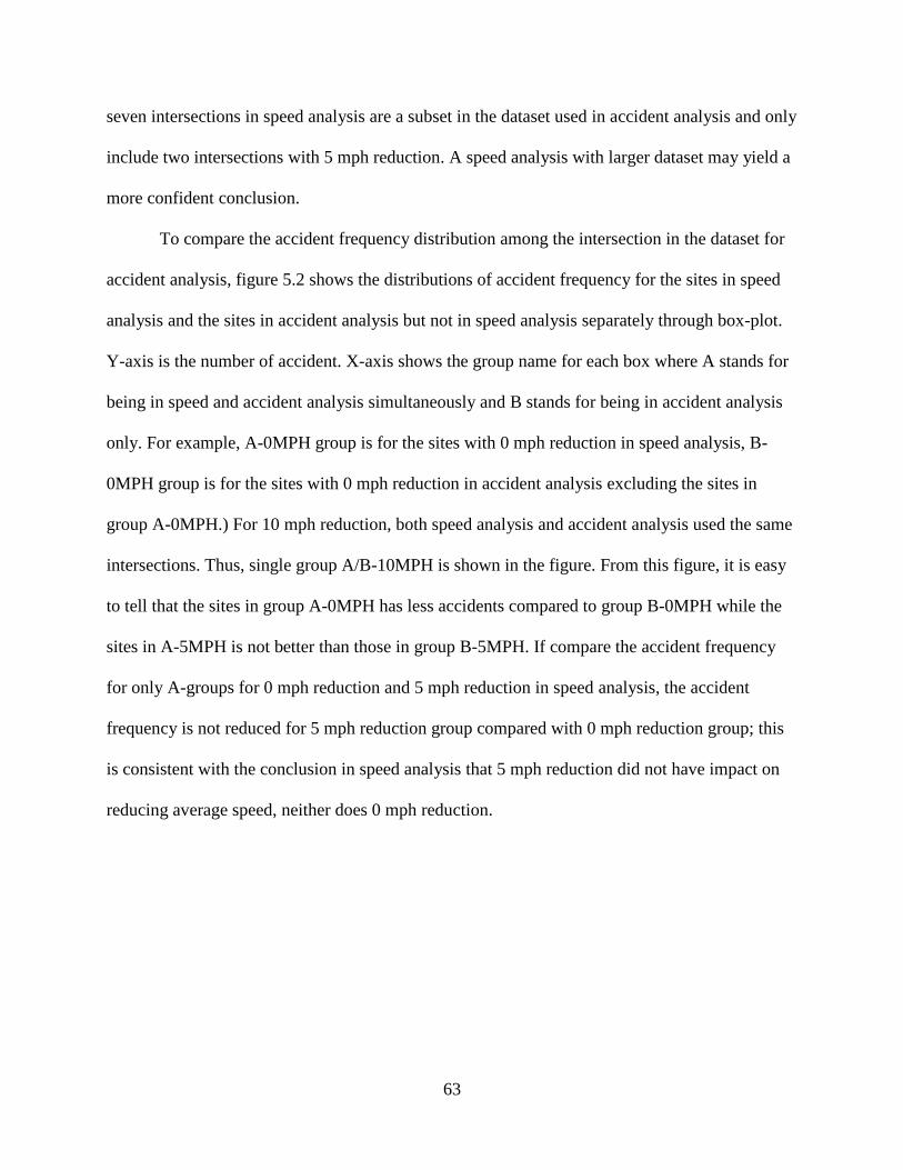
63

seven intersections in speed analysis are a subset in the dataset used in accident analysis and only

include two intersections with 5 mph reduction. A speed analysis with larger dataset may yield a

more confident conclusion.

To compare the accident frequency distribution among the intersection in the dataset for

accident analysis, figure 5.2 shows the distributions of accident frequency for the sites in speed

analysis and the sites in accident analysis but not in speed analysis separately through box-plot.

Y-axis is the number of accident. X-axis shows the group name for each box where A stands for

being in speed and accident analysis simultaneously and B stands for being in accident analysis

only. For example, A-0MPH group is for the sites with 0 mph reduction in speed analysis, B-

0MPH group is for the sites with 0 mph reduction in accident analysis excluding the sites in

group A-0MPH.) For 10 mph reduction, both speed analysis and accident analysis used the same

intersections. Thus, single group A/B-10MPH is shown in the figure. From this figure, it is easy

to tell that the sites in group A-0MPH has less accidents compared to group B-0MPH while the

sites in A-5MPH is not better than those in group B-5MPH. If compare the accident frequency

for only A-groups for 0 mph reduction and 5 mph reduction in speed analysis, the accident

frequency is not reduced for 5 mph reduction group compared with 0 mph reduction group; this

is consistent with the conclusion in speed analysis that 5 mph reduction did not have impact on

reducing average speed, neither does 0 mph reduction.

64

Figure 5.2 Box plots for various groups

5.4 Crash Severity Model

5.4.1 Literature Review

Studies of the effects of traffic characteristics as well as driver characteristics on crash

severity are widely studied for various kinds of crashes. Johansson applied time series count data

regression models (i.e., Poisson Model, Negative Binomial Model, Zeger Model, and Structure

Approach Model) for each severity level of crashes (27). Due to the ordinal scale of the

dependent variable, level of severity, an ordered discrete model could be applied. O’Donnell and

Connor identified risk factors that increase the probabilities of serious injury and fatalities with

the ordered Logit model and ordered Probit models (35). Jin et al. applied an ordered Logit

model to study the factors significantly contributing to the severity of right-angle crashes (31).

The results showed that factors such as whether the person was ejected, alcohol and/or drug use,

65

the driver's age, point of impact, and standardized yellow time have significant impacts on the

average severity of crashes. However, traditionally ordered probability models are susceptible to

underreporting of crash-injury data; also, the shift in thresholds is constrained to move in the

same direction (42). These two drawbacks make it improper to use ordered probability models in

accident severity analysis. In the current research, a Multinomial Logit model (MNL) was used

to study the critical factors for accident severity. MNL has been applied widely in this area. Lee

and Mannering studied the relationship between observable characteristics such as season,

weekday, daylight, and other roadway factors through developing an MNL model (33). Shankar

and Mannering used an MNL model specification to estimating the severity of motorcycle rider

crash severity given that a crash has occurred (43). Carson and Mannering developed MNL

models to identify the effect of warning signs on ice-related crash severities on interstates,

principal arterials, and minor arterial state highways (44). Sriniva et al. applied MNL to predict

the proportion of crashes by manner of collision.

5.4.2 Multinomial Logit Model (MNL)

Let be a linear function that determines discrete the severity i for observation n as

(5.13)

where,

is a vector of estimable parameters of discrete severity level i; and is a vector of

the observable characteristics which determine discrete outcomes for observation n. is a

disturbance term which can account for the unobserved effects. Under the assumption that the

disturbance term is independently and identically distributed, extreme value Type I distributed,

the standard multinomial logit formulation can be built as

66

(5.14)

Maximum likelihood can estimate the parameter beta. The log maximum likelihood

function is

(5.15)

where,

I is the total number of outcomes and is defined as being equal to 1 if the observed

discrete outcome for observation n is i and 0 otherwise (30).

5.4.3 Mixed Logit Model

The Mixed Logit Model is also referred to as the Random Parameter Logit (RPL) or

Mixed Multinomial Logit Model (MMNL), as shown in equation 5.16. The MNL mode has three

assumptions: 1) the data is case specific (i.e., each independent variable has a single value for

each case; 2) colinearity of independent variables is relatively low, high correlation makes it

difficult to differentiate the impacts of different variables; 3) independence of irrelevant

alternatives. Mixed Logit Model obviates these three assumptions since it allows for random

parameters which are varied across observations. The βi in equation 5.13 could be randomly

distributed according to normal, lognormal, triangle, uniform and other distribution

(i.e.,βi~f(β

i|θ)

).

67

𝑃𝑛 𝑖 = 𝐸𝑋𝑃(𝜷𝑖𝑿𝑖𝑛)

𝐸𝑋𝑃(𝜷𝐼𝑿𝐼𝑛)∀𝐼f(𝛃|θ)d𝛃

(5.16)

5.4.4 Data Preparation and Model Development

Most of the variables in previous studies, such as one-way, light condition, weather

condition, curve and slope, concrete or asphalt pavement, and functional classification do not

have enough variability in terms of intersection accidents; and are not included in this study. The

analysis of severity based on identical traffic-related characteristics for accident frequency

studies is listed in table 5.2. A summary of the statistics of all the variables in accident severity

model is given in appendix D. Besides. Accident-related variables are also considered and listed

in table 5.5.

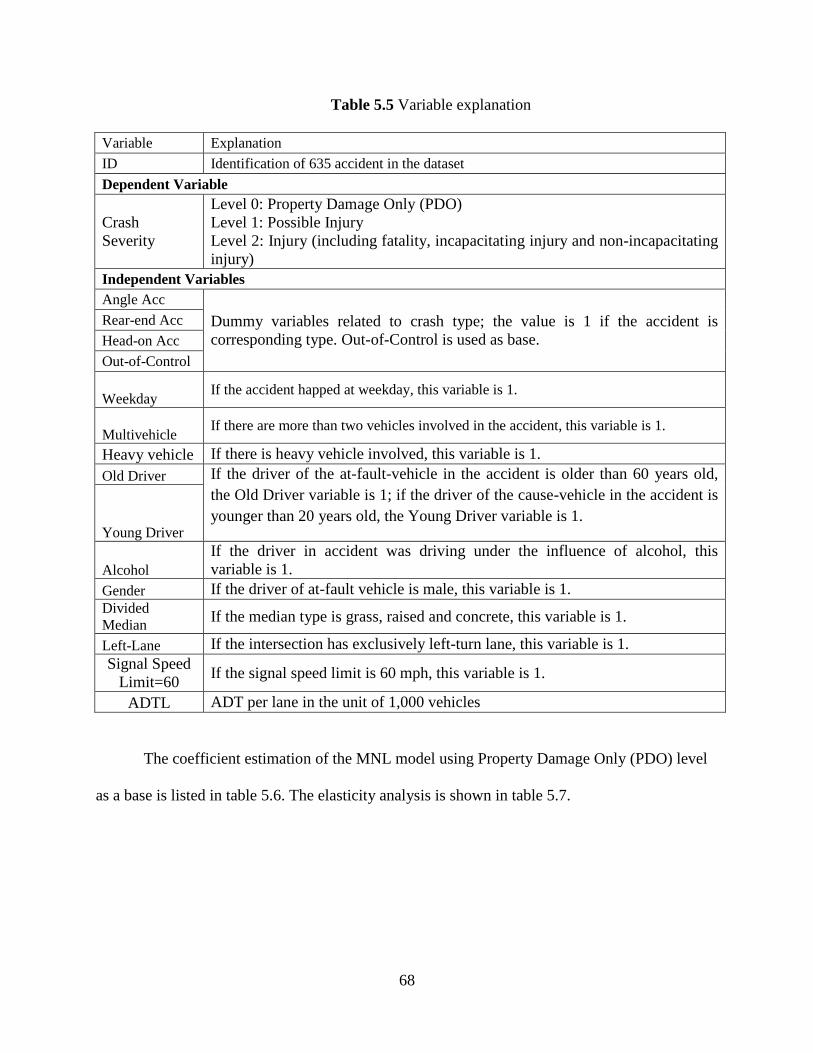
68

Table 5.5 Variable explanation


ID Identification of 635 accident in the dataset

Dependent Variable

Crash

Severity

Level 0: Property Damage Only (PDO)

Level 1: Possible Injury

Level 2: Injury (including fatality, incapacitating injury and non-incapacitating

injury)

Independent Variables

Angle Acc

Dummy variables related to crash type; the value is 1 if the accident is

corresponding type. Out-of-Control is used as base.

Rear-end Acc

Head-on Acc

Out-of-Control

Weekday If the accident happed at weekday, this variable is 1.

Multivehicle If there are more than two vehicles involved in the accident, this variable is 1.

Heavy vehicle If there is heavy vehicle involved, this variable is 1.

Old Driver If the driver of the at-fault-vehicle in the accident is older than 60 years old,

the Old Driver variable is 1; if the driver of the cause-vehicle in the accident is

younger than 20 years old, the Young Driver variable is 1. Young Driver

Alcohol

If the driver in accident was driving under the influence of alcohol, this

variable is 1.

Gender If the driver of at-fault vehicle is male, this variable is 1.

Divided

Median If the median type is grass, raised and concrete, this variable is 1.

Left-Lane If the intersection has exclusively left-turn lane, this variable is 1.

Signal Speed

Limit=60 If the signal speed limit is 60 mph, this variable is 1.

ADTL ADT per lane in the unit of 1,000 vehicles

The coefficient estimation of the MNL model using Property Damage Only (PDO) level

as a base is listed in table 5.6. The elasticity analysis is shown in table 5.7.

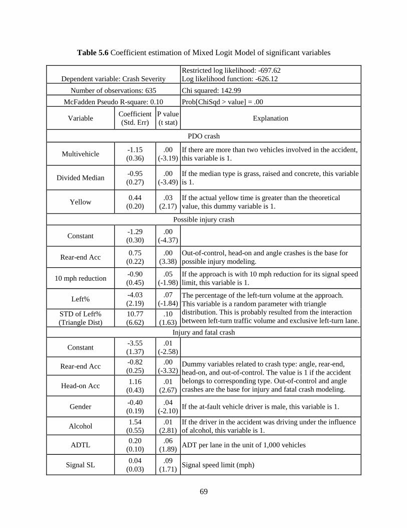
69

Table 5.6 Coefficient estimation of Mixed Logit Model of significant variables

Dependent variable: Crash Severity

Restricted log likelihood: -697.62

Log likelihood function: -626.12

Number of observations: 635 Chi squared: 142.99

McFadden Pseudo R-square: 0.10 Prob[ChiSqd > value] = .00


(Std. Err)

P value

(t stat) Explanation

PDO crash

Multivehicle -1.15

(0.36)

.00

(-3.19)

If there are more than two vehicles involved in the accident,

this variable is 1.

Divided Median -0.95

(0.27)

.00

(-3.49)

If the median type is grass, raised and concrete, this variable

is 1.

Yellow 0.44

(0.20)

.03

(2.17)

If the actual yellow time is greater than the theoretical

value, this dummy variable is 1.

Possible injury crash

Constant -1.29

(0.30)

.00

(-4.37)

Rear-end Acc 0.75

(0.22)

.00

(3.38)

Out-of-control, head-on and angle crashes is the base for

possible injury modeling.

10 mph reduction -0.90

(0.45)

.05

(-1.98)

If the approach is with 10 mph reduction for its signal speed

limit, this variable is 1.

Left% -4.03

(2.19)

.07

(-1.84) The percentage of the left-turn volume at the approach.

This variable is a random parameter with triangle

distribution. This is probably resulted from the interaction

between left-turn traffic volume and exclusive left-turn lane. STD of Left%

(Triangle Dist)

10.77

(6.62)

.10

(1.63)

Injury and fatal crash

Constant -3.55

(1.37)

.01

(-2.58)

Rear-end Acc -0.82

(0.25)

.00

(-3.32) Dummy variables related to crash type: angle, rear-end,

head-on, and out-of-control. The value is 1 if the accident

belongs to corresponding type. Out-of-control and angle

crashes are the base for injury and fatal crash modeling. Head-on Acc

1.16

(0.43)

.01

(2.67)

Gender -0.40

(0.19)

.04

(-2.10) If the at-fault vehicle driver is male, this variable is 1.

Alcohol 1.54

(0.55)

.01

(2.81)

If the driver in the accident was driving under the influence

of alcohol, this variable is 1.

ADTL 0.20

(0.10)

.06

(1.89) ADT per lane in the unit of 1,000 vehicles

Signal SL 0.04

(0.03)

.09

(1.71) Signal speed limit (mph)

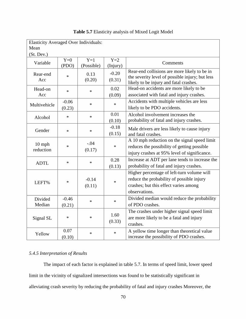
70

Table 5.7 Elasticity analysis of Mixed Logit Model

Elasticity Averaged Over Individuals:

Mean

(St. Dev.)

Variable Y=0

(PDO)

Y=1

(Possible)

Y=2

(Injury) Comments

Rear-end

Acc *

0.13

(0.20)

-0.20

(0.31)

Rear-end collisions are more likely to be in

the severity level of possible injury; but less

likely to be injury and fatal crashes.

Head-on

Acc * *

0.02

(0.09)

Head-on accidents are more likely to be

associated with fatal and injury crashes.

Multivehicle -0.06

(0.23) * *

Accidents with multiple vehicles are less

likely to be PDO accidents.

Alcohol * * 0.01

(0.10)

Alcohol involvement increases the


Gender * * -0.18

(0.15) Male drivers are less likely to cause injury

and fatal crashes.

10 mph

reduction *

-.04

(0.17) *

A 10 mph reduction on the signal speed limit

reduces the possibility of getting possible

injury crashes at 95% level of significance.

ADTL * * 0.28

(0.13)

Increase at ADT per lane tends to increase the


LEFT% * -0.14

(0.11) *

Higher percentage of left-turn volume will

reduce the probability of possible injury

crashes; but this effect varies among

observations.

Divided

Median

-0.46

(0.21) * *

Divided median would reduce the probability

of PDO crashes.

Signal SL * * 1.60

(0.33)

The crashes under higher signal speed limit

are more likely to be a fatal and injury

crashes.

Yellow 0.07

(0.10) * *

A yellow time longer than theoretical value

increase the possibility of PDO crashes.

5.4.5 Interpretation of Results

The impact of each factor is explained in table 5.7. In terms of speed limit, lower speed

limit in the vicinity of signalized intersections was found to be statistically significant in

alleviating crash severity by reducing the probability of fatal and injury crashes Moreover, the

71

dummy variable of 10 mph reduction at signal speed limit reduces the probability of possible

injury accidents at a 95% level of significance. To sum up, for a high-speed signalized

intersection on a highway with a regular speed limit of 65 mph, a 10 mph reduction will reduce

possible injury accidents, and the resulting signal speed limit (i.e., 55 mph) will reduce the

probability of injury and fatal accidents significantly.

Compared to angle accidents and out-of-control accidents, rear-end accidents are more

likely to result in possible injury, while head-on accident are more likely to result in injury or

fatality. Head-on accidents therefore are often the most severe accidents, and require case-by-

case study to determine if there are potential factors related to the traffic system that cause this

type of accident. Further, accidents involving multiple vehicles are less likely to be PDO

accidents in comparison to two-vehicle accidents. However, this reduction of probability on PDO

crashes will probably be accompanied with increase of probability on severe crashes although

this is not significant in this model. Another risk factor for fatal and injury accidents is alcohol.

Education and policy implementation are required to improve this problem. Also, female drivers

are more likely to cause injury and fatal accidents.

Moreover, traffic conditions like ADT per lane would increase the probability of fatal and

injury crashes. Increased percentage of left-turn volume reduces the chance of possible injury;

this impact, however, varies across observation and is triangularly distributed. Yellow time

longer than theoretical value and divided median both reduce the probability of PDO crashes.

5.5 Summary

Table 5.8 summarizes this chapter in terms of the impact of various speed limit

reductions on accident frequency and severity. “NS” indicates no significant effect. These

findings are specified for the speed limit setup, shown in the second row of table 5.8. For the

studied intersection approaches with 10 mph reduction from the regular highway speed limits of

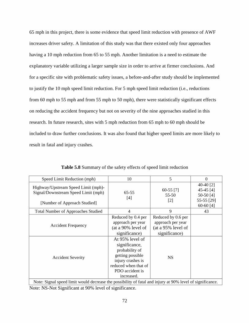
72

65 mph in this project, there is some evidence that speed limit reduction with presence of AWF

increases driver safety. A limitation of this study was that there existed only four approaches

having a 10 mph reduction from 65 to 55 mph. Another limitation is a need to estimate the

explanatory variable utilizing a larger sample size in order to arrive at firmer conclusions. And

for a specific site with problematic safety issues, a before-and-after study should be implemented

to justify the 10 mph speed limit reduction. For 5 mph speed limit reduction (i.e., reductions

from 60 mph to 55 mph and from 55 mph to 50 mph), there were statistically significant effects

on reducing the accident frequency but not on severity of the nine approaches studied in this

research. In future research, sites with 5 mph reduction from 65 mph to 60 mph should be

included to draw further conclusions. It was also found that higher speed limits are more likely to

result in fatal and injury crashes.

Table 5.8 Summary of the safety effects of speed limit reduction

Speed Limit Reduction (mph) 10 5 0

Highway/Upstream Speed Limit (mph)-

Signal/Downstream Speed Limit (mph)

[Number of Approach Studied]

65-55

[4]

60-55 [7]

55-50

[2]

40-40 [2]

45-45 [4]

50-50 [4]

55-55 [29]

60-60 [4]

Total Number of Approaches Studied 4 9 43

Accident Frequency

Reduced by 0.4 per

approach per year

(at a 90% level of

significance)

Reduced by 0.6 per

approach per year

(at a 95% level of

significance)

Accident Severity

At 95% level of

significance,

probability of

getting possible

injury crashes is

reduced when that of

PDO accident is

increased.

NS

Note: Signal speed limit would decrease the possibility of fatal and injury at 90% level of significance.

Note: NS-Not Significant at 90% level of significance.

73

Chapter 6 Conclusions

This study provides empirical analysis of the effect of reduced transitional speed limits in

the vicinity of high-speed, signalized intersections with AWF on speed distribution and crash

frequency and severity. AWF is recommended by MUTCD, and commonly used at high-speed

intersections in Nebraska, where around 60 advance warning beacons are installed on roads

having a speed limit of 50 mph or higher. For intersections already equipped with AWF, the

necessity and effectiveness of speed limit reduction has not been thoroughly studied in previous

research. In Nebraska, typically speed limits in the vicinity of high-speed signals are not greater

than 55 mph. That is, the speed limit is usually reduced to 55 mph for signals if the highway

speed limit is higher than 55 mph. However, there is no official document to guide AWF

implementation in terms of the magnitude of limit reduction and its effect. In the procedures that

establish speed zone in Texas, a speed limit could be lowered by up to 10 mph in lieu of limited

field of vision near the intersection. If the intersection crash rate is higher than the state average,

the speed limit could be lowered by as much as 12 mph. However, there is no specific

recommendation in terms of high-speed intersections installed with other safety measures. This

study provides several helpful observations in terms of the advantages of reduced transitional

speed limits at high-speed intersections with AWF over intersections only having AWF.

First, the effect of speed limit reduction on reducing speed in the field was tested with

speed data collected from seven intersections having AWF. The seven intersections were

grouped into 0 mph reduction, 5 mph reduction (from 60 mph to 55 mph) and 10 mph reduction

(from 65 mph to 55 mph) intersections. Wavetronix sensor was used to collect vehicle speed and

corresponding distance. By collecting speed data for two separate locations—one close to the

signal speed limit sign and the other approximately 600 ft from the stop bar—the question of

74

whether there is significant difference among the mean speeds at these two locations was studied

using quantile regression models and SURE models. Quantile regressions for the individual

average speeds at 10 mph reduction showed that 10 mph reductions from 65 mph to 55 mph

incurred a more uniformly distributed speed distribution in the vicinity of signals. The quantile

regression of 85th

, 50th

, and 15th

percentile speeds indicated a 4.6 mph, 4.2 mph, and 3.2 mph

reduction, respectively. By further reducing the fast traffic, the 10 mph reduction reduced the

dispersion of speed distribution at the vicinity of high-speed intersections in terms of an inter-

percentile range between the 85th

and 15th

percentiles. Reduced speed limit variability has, in the

past, been found to correlate positively with improved safety. However, the seemingly unrelated

equation models did not show any significant negative impact of 10 mph limit reduction on the

standard deviation of grouped individual average speeds. On the other hand, this proves that

there is no increase in the standard deviation of speeds by 10 mph limit reduction. SURE models

estimate the variables for both the mean and the standard deviation collectively, and take into

consideration the possibility of unobserved factors impacting both mean and standard deviation.

The results indicated a significant, 3.8 mph reduction in mean speed for the 10 mph reduction

intersections and no significant reduction for the 5 mph reduction intersections. This result

coincides with a study conducted in Virginia, in which increases of 1.7 mph and 4.3 mph in

mean speeds were observed from a 10 mph increase on speed limits (9).

Aside from the effect of reducing driving speeds in the field, the intent of this research

also included providing a methodological study of the effect of the implementation of a

transitional speed zone at signalized, high-speed intersection with AWF on increasing driver

safety. A crash analysis was performed to identify the effects of speed limit reductions on crash

severity and frequency. The accident dataset included four approaches with 10 mph speed limit

75

reduction from 65 mph to 55 mph and nine 5 mph-speed-limit reduction approaches, seven of

which were from 60 mph to 55 mph and two of which were from 55 mph to 50 mph. Based on

the available information from 28 intersections in Nebraska State, both 5 mph and 10 mph

reduction demonstrate a significant effect on reducing crash frequency based on a RPNB model

with a dependent variable of annual crash count for each approach. This conclusion supports the

Texas procedure which recommends as much as 12 mph reduction in speed limit whenever the

crash rate of an intersection is higher than the state average. A Mixed Logit model was

developed to study the impact of speed limit reduction on crash severity; 10mph reduction

showed significant effects on reducing the probability of possible injury crashes at a at 95% level

of significance. It was also found that the higher the signal speed limit is, the more likely the

occurrence of fatal and injury crashes.

The study shows that even with AWF facility, reduction on speed limit in the vicinity of

high-speed signalized intersection still improves the safety condition in comparison with those

without speed limit reduction. The conclusions of this study, however, are limited by the small

sample size, especially for the approaches with 10 mph speed limit reduction from 65 mph to 55

mph. Also, for the approaches with 5 mph reduction, most were from 60 mph to 55 mph. Future

research should include more varieties of limit reduction sets, as well as larger sample size. For a

specific site of interest, a before-and-after study is strongly recommended to identify the impact

of a specific speed limit reduction.

76

References

1. National Highway Traffic Safety Administration. 2009. “Traffic Safety Facts” Retrieved from

http://www-nrd.nhtsa.dot.gov/pubs/811402ee.pdf.

2. Department for Transport. “Setting Local Speed Limits: Guidance for Local Authorities:

ETLLD Circular 1/2006. Retrieved from http://www2.dftgov.uk/pgr/roadsafety/

speedmanagement/dftcircular106/dftcircular106.pdf.

3. Federal Highway Administration. 2009. “Manual on Uniform Traffic Control Devices for

Streets and Highways.” FHWA and U.S. Department of Transportation. Retrieved form

mucd.fhwa.gov.

4. “Special Report 254 Managing Speed—Review of Current Practice for Setting and Enforcing

Speed Limit.” Transportation Research Board, National Research Council, Washington,

D.C.

5. Coleman, J. A. and Morford, G. 1980. “Speed Management Program in FHWA and NHTSA

Institute of Transportation Engineers.” ITE Journal, Vol. 68, No. 7.

6. K.R. Agent. 2008. “Evaluation of 70 mph Speed Limit in Kentucky.” Kentucky

Transportation Center. Retrieved from www.ktc.edu

7. K.R. Agent, J. G. Pigman, and J. M. Weber. 1997. “Evaluation of Speed Limits in Kentucky.”

Annual Report, Kentucky Transportation Center, Kentucky Transportation Cabinet,

Commonwealth of Kentucky, and FHWA.

8. U.S. Department of Transportation. 1997. “Effects of Raising and Lowering Speed Limits on

Selected Roadway Sections.” U.D Department of Transportation Publication FHWA-RD-

97-084.

9. Hojun S, M. D. Fontaine, and B. Park. 2009.” Long-term speed compliance and safety impacts

of rational speed limits.” Journal of Transportation Engineering, 135: 536-545.

10. Austin Texas State Department of High and Public Transportation.1990. "Speed Zoning on

Texas Highways."

11. Office of Highway Safety. "Establishing Realistic Speed Limit". Michigan State. Accessed

Nov 15, 2011 from www.livingstonroads.org/pdf_docs/StatePD_Speedlimits

_Booklet.pdf.

12. State Department of Highways and Public Transportation. 1990. “Speed Zoning on Texas

Highways.” Austin, Texas.

77

13. Buddemeyer, J., R. K. Young, and B. Dorsey. 2010. “Rural Variable Speed Limit System for

Southeast Wyoming.” Transportation Research Record: Journal of the Transportation

Research Board, 2189: 37-44.

14. Mohsen Towliat, Helena Svensson, Gunnar Lind, et al. "Variable Speed Limits at

Intersections-Effects and Experience", European Transportation Conference 2006.

15. Monsere, C. M., C. Nolan, R. L. Bertini, E. L. Anderson, and T. A. El-Seoud. 2005.

“Measuring the Impacts of Speed Reduction Technologies: A Dynamic Advanced Curve

Warning System Evaluation.” 84th Annual Meeting of the Transportation Research

Board, Washington, D.C.

16. Cruzado, I. and E. T. Donnell. 2010. “Factors affecting driver speed choice along two-lane

rural highway transition zones.” Journal of Transportation Engineering, 136, no. 8: 755-

764.

17. California Department of Transportation. 1998. “Realistic Speed Zoning, Why & How.”

Retrieved from www.ca.gov.

18. Sharma, A., D. Bullock, and S. Peeta. 2010. “Estimating dilemma zone hazard function at

high-speed isolated intersections.” Transportation Research Part C: Emerging

Technologies, 19, no. 3: 400-412.

19. Online textbook. Discriminant Function Analysis. Accessed on Nov 15, 2011 from

www.statsoftcom/textbook/discriminant-function-analysis/.

20. MATLAB online resource. Accessed on Nov 15, 2011 from

http://www.mathworks.com/help/toolbox/stats/classify.html.

21. Texas Department of Transportation. 2011. “Procedures for Establishing Speed Zones.”

Accessed on Nov 16 from http://onlinemanuals.TxDOT.gov/TxDOTmanuals/szn/szn.pdf.

22. Texas Department of Transportation. 2011. “Manual on Uniform Traffic Control Devices

(TMUTCD).” Accessed Nov 16. 2011 from

http://www.TxDOT.gov/TxDOT_library/publications/tmutcd.htm.

23. Kansas Department of Transportation. “Establishing speed limits. A case of "majority rule."

Retrieved from

http://www.ksdot.org/burTrafficSaf/brochures/EstablishingSpeedLimits.asp.

24. Srinivasan, R., Parker M., Harkey, D., Tharpe, D., and Sumner, R. 2006. “An Expert System

for Recommending Speed Limits in Speed Zones.” National Cooperative Highway

Research Program, Transportation Research Board, National Research Council.

Retrieved from www.trb.org

http://www.statsoft.com/textbook/discriminant-function-analysis/

http://www.statsoft.com/textbook/discriminant-function-analysis/

http://www.mathworks.com/help/toolbox/stats/classify.html

http://onlinemanuals.txdot.gov/txdotmanuals/szn/szn.pdf

http://www.txdot.gov/txdot_library/publications/tmutcd.htm

http://www.ksdot.org/burTrafficSaf/brochures/EstablishingSpeedLimits.asp

78

25. Hakim, S. D. Shefer, A. S.Hakkert, I. A. Hocherman. 1991. “Critical review of macro models

for road crashes.” Accident Analysis and Prevention, 23: 379-440.

26. Forester, T. H., R. F. McNown, and L. D. Singell. 1984. “A cost-benefit analysis of the 55

mph speed limit.” Southern Economic Journal, 50: 631-641.

27. P. Johansson. “Speed limitation and Motorway Casualties: A time Series Count Data

Regression Approach.” Accident Analysis and Prevention, 28, no.1: 73-87.

28. Milton, J.C and F.L. Mannering. 1996. “The Relationship between Highway Geometrics,

Traffic Related Elements and Motor Vehicle Crashes.” Final Research Report. WA-RD

403.1, Washington State Department of Transportation.

29. Shankar, V., J. Milton and F. Mannering. 1997. “Modeling crash frequencies as zero-altered

probability processes: An empirical inquiry. Accident Analysis and Prevention, 29, no. 6:

829-837.

30. Washington, S. P., M. G. Karlaftis, and F.L. Mannering. 2003. “Statistical and Econometric

Methods for Transportation Data Analysis.” Chapman and Hall/CRC.

31. Jin, Y., X. Wang, and X. Chen. 2011. “Right-angle Crash Injury Severity Analysis Using

Ordered Probability Models.” 2011 International Conference on Intelligent Computation

Technology and Automation.

32. Shanker, V. R. B. Albin, J. C. Milton, and F.L. Mannering. 1998. “Evaluating Median

Crossover Likelihoods with Clustered Crash Counts: An Empirical Inquiry Using the

Random Effects Negative Binomial Modal.” Transportation Research Record, 1635: 44-

48.

33. Lee, J. and F. Mannering. 1999. “Analysis of Roadside Crash Frequency and Severity and

Roadside Safety Management.” Research Project T9903, Task 97 Report. Accessed Nov

15, 2011 from http://www.wsdot.wa.gov/research/reports/fullreports/475.1.pdf.

34. Strathman, J.G., K. J. Dueker, J. Zhang, and T. Williams. 2001. “Analysis of Design

Attributes and Crashes on the Oregon Highway System.” Research Project FHWA-

OR0RD-02-01.

35. O’Donnell, C. J. and D. H. Connor. 1996. “Predicting the severity of motor vehicle crash

injuries using models of ordered multiple choice.” Analysis and Prevention, 28, no. 6:

739-753.

36. van den Hoogen, E. and S. Smulders. “Control by Variable Speed Signs: Results of the

Dutch Experiment.” Road Traffic Monitoring and Control, Seventh International

Conference, 26-28 Apr 1994.

http://www.wsdot.wa.gov/research/reports/fullreports/475.1.pdf

http://ieeexplore.ieee.org/xpl/mostRecentIssue.jsp?punumber=3097

http://ieeexplore.ieee.org/xpl/mostRecentIssue.jsp?punumber=3097

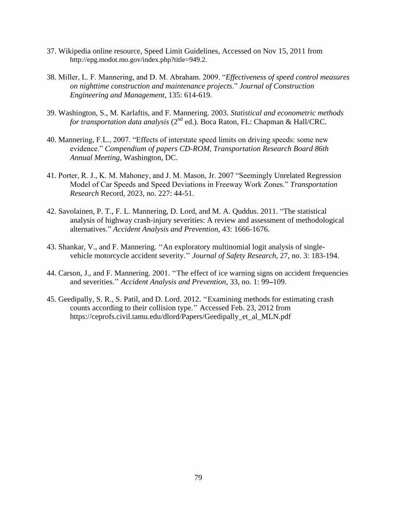
79

37. Wikipedia online resource, Speed Limit Guidelines, Accessed on Nov 15, 2011 from http://epg.modot.mo.gov/index.php?title=949.2.

38. Miller, L. F. Mannering, and D. M. Abraham. 2009. “Effectiveness of speed control measures

on nighttime construction and maintenance projects.” Journal of Construction

Engineering and Management, 135: 614-619.

39. Washington, S., M. Karlaftis, and F. Mannering. 2003. Statistical and econometric methods

for transportation data analysis (2nd

ed.). Boca Raton, FL: Chapman & Hall/CRC.

40. Mannering, F.L., 2007. “Effects of interstate speed limits on driving speeds: some new

evidence.” Compendium of papers CD-ROM, Transportation Research Board 86th

Annual Meeting, Washington, DC.

41. Porter, R. J., K. M. Mahoney, and J. M. Mason, Jr. 2007 “Seemingly Unrelated Regression

Model of Car Speeds and Speed Deviations in Freeway Work Zones.” Transportation

Research Record, 2023, no. 227: 44-51.

42. Savolainen, P. T., F. L. Mannering, D. Lord, and M. A. Quddus. 2011. “The statistical

analysis of highway crash-injury severities: A review and assessment of methodological

alternatives.” Accident Analysis and Prevention, 43: 1666-1676.

43. Shankar, V., and F. Mannering. ‘‘An exploratory multinomial logit analysis of single-

vehicle motorcycle accident severity.’’ Journal of Safety Research, 27, no. 3: 183-194. 44. Carson, J., and F. Mannering. 2001. ‘‘The effect of ice warning signs on accident frequencies

and severities.’’ Accident Analysis and Prevention, 33, no. 1: 99---109. 45. Geedipally, S. R., S. Patil, and D. Lord. 2012. ‘‘Examining methods for estimating crash

counts according to their collision type.’’ Accessed Feb. 23, 2012 from https://ceprofs.civil.tamu.edu/dlord/Papers/Geedipally_et_al_MLN.pdf

http://www.ncbi.nlm.nih.gov/pubmed/9370019

https://ceprofs.civil.tamu.edu/dlord/Papers/Geedipally_et_al_MLN.pdf

Appendix A Information on the Intersections

#1 – US-34 and N-79 (Westbound Approach)

Speed limit

through

signal (mph)

Speed limit

prior to

signal (mph)

Number of

lanes

Nearest

intersection

Area type Road

curvature

Comments:

Westbound Approach Selected

Good feasibility for communicating with the traffic cabinet

and parking the trailer along US-34 60 60 2 WB 1 NB 0.7 mi East Rural No

80

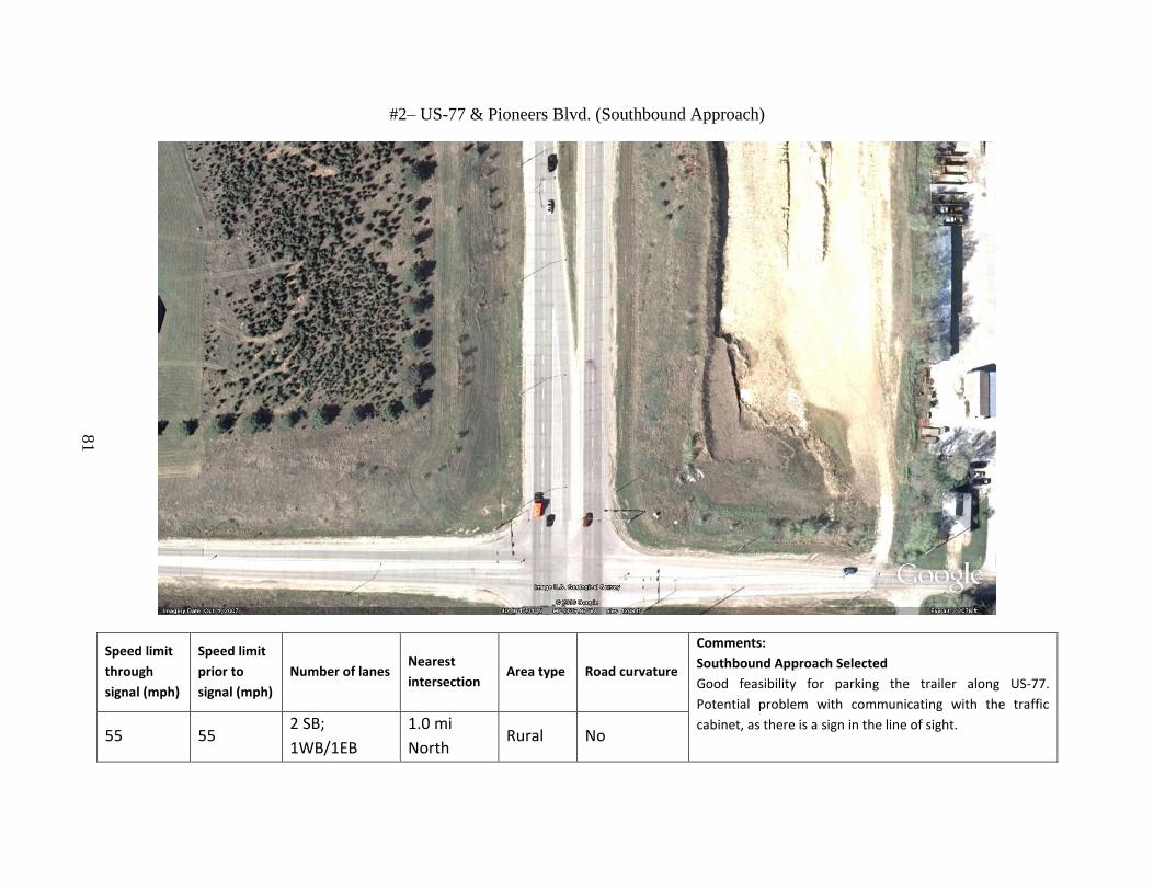
#2– US-77 & Pioneers Blvd. (Southbound Approach)

Speed limit

through

signal (mph)

Speed limit

prior to

signal (mph)

Number of lanes Nearest

intersection Area type Road curvature

Comments:

Southbound Approach Selected

Good feasibility for parking the trailer along US-77.

Potential problem with communicating with the traffic

cabinet, as there is a sign in the line of sight. 55 55

2 SB;

1WB/1EB

1.0 mi

North Rural No

81

#3 – N-133 and N-36 (Northbound Approach)

Speed limit

through

signal (mph)

Speed limit

prior to

signal (mph)

Number of

lanes

Nearest

intersection Area type

Road

curvature

Comments:

Northbound Approach Selected

Speed limit sign was only 1,000 ft from the intersection. End

of curve approx. 2,000 ft from intersection 55 55 2 NB & 1EB/WB 1.1 mi South Rural No

82

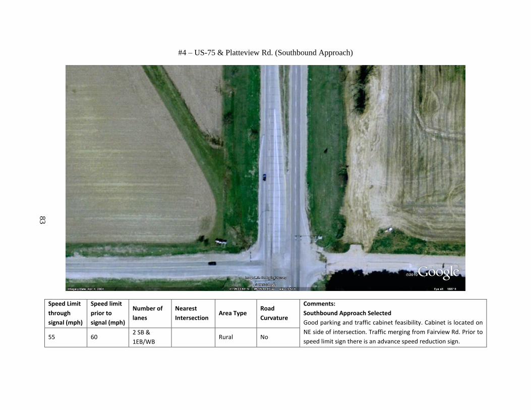
#4 – US-75 & Platteview Rd. (Southbound Approach)

Speed Limit

through

signal (mph)

Speed limit

prior to

signal (mph)

Number of

lanes

Nearest

Intersection Area Type

Road

Curvature

Comments:


Good parking and traffic cabinet feasibility. Cabinet is located on

NE side of intersection. Traffic merging from Fairview Rd. Prior to

speed limit sign there is an advance speed reduction sign. 55 60

2 SB &

1EB/WB Rural No

83

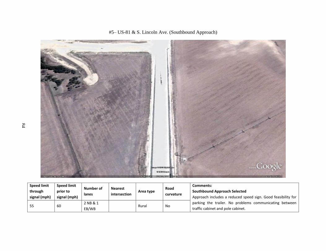
#5– US-81 & S. Lincoln Ave. (Southbound Approach)

Speed limit

through

signal (mph)

Speed limit

prior to

signal (mph)

Number of

lanes

Nearest


Road

curvature

Comments:


Approach includes a reduced speed sign. Good feasibility for

parking the trailer. No problems communicating between

traffic cabinet and pole cabinet. 55 60

2 NB & 1

EB/WB Rural No

84

#6 – US-77 & Saltillo Rd. (Northbound Approach)

Speed limit

through

signal (mph)

Speed limit

prior to

signal (mph)

Number of

lanes

Nearest

intersection

Area type Road curvature Comments:

Northbound Approach Selected

Northbound approach has a slight grade, still able to

communicate 55 65 2 SB & 1

WB/1EB

1.0 mi North Rural No

85

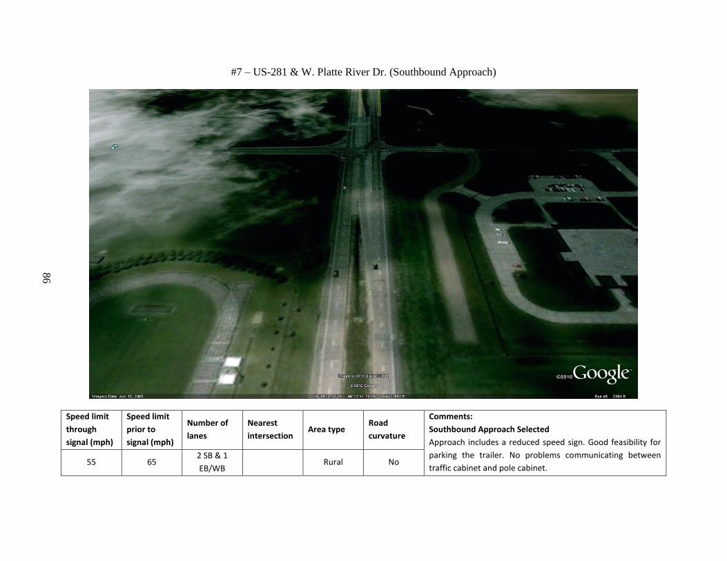
#7 – US-281 & W. Platte River Dr. (Southbound Approach)

Speed limit

through

signal (mph)

Speed limit

prior to

signal (mph)

Number of

lanes

Nearest


Road

curvature

Comments:


Approach includes a reduced speed sign. Good feasibility for

parking the trailer. No problems communicating between

traffic cabinet and pole cabinet. 55 65

2 SB & 1

EB/WB Rural No

86

Appendix B Intersection Information of Crash Analysis

No.

Highway Cross Street

Highway Speed Limit

Signal Speed Limit

Speed Limit Reduction

Number of Approaches Approaching Lanes

Median Type

Distance to

AWF Yellow Time

Flasher Time

1 US-30 30th Ave. 40 40 0 2 2+L Raised 650 4.5 10

2 US-83 J St. 45 45 0 2 2+L Concrete 650 4.5 8

3

US-75

N-2 (S. Jct.

Bypass) 45 45 0 2 2+L+R (WB) & 2+L (EB) Grass 650 4.5 10

4 US-275 N-24 50 50 0 2 2+L Raised 650 4.5 9

5 US-81

Ta-Ha-Zouka 50 50 0 2 2+L Raised 650 4.5 9

6 US-30

US-81 (S. Jct.) 55 55 0 2

2+L+R (SB) & 2T+L (NB) Raised 650 4.5 8

7 US-30 29th Ave. E. 55 55 0 2 2+L Raised 650 4.5 9

8 N-36 N-133 55 (NB) 55 (NB) 0 1 2+L Raised 650 4.5 8

9 US-6 Q ST. 55 55 0 2 1+L Raised 650 4.5 8

10 US-34 US-281 55 55 0 2 2+L+R Grass 650 5 8

11

US-77

Old Cheney

Rd. 55 55 0 2 2+L Grass 650 5 7

12 US-77 Pioneers 55 55 0 2 2+L Grass 650 5 8

13 US-6

Wal-Mart/ Wedgwood 55 55 0 2 1+L+R (W) None 650 4.5 10

14 N-370 108th St. 55 55 0 2

2T+R (W) & 2+2L (E) Grass 650 4 8

15 US-75 N-66 55 55 0 2 1+L None 650 4.5 9

16 US-75 Ave. B 55 55 0 2 1+L None 650 4.5 8

17 N-370 168th St. 55 55 0 2

1+L (W) & 2+L (E) None 650 4.5 8

18 N-370 132nd St. 55 55 0 2 2+L+R Grass 650 4.5 8

(continued)

87

19 US-6 I-80 ramp 55 55 0 2

2 (W) & 2+L (E) Raised 650 4.5 8

20 US-34 N-79 60 60 0 2

2T+L (W) & 2T (W) Raised 650 4.5 7

21 US-34 NW 48th St. 60 60 0 2

2+L+R (W) & 2+L (E) Raised 650 4.5 7

22 N-36 N-133

60 (SB) 55 (SB) 5 1 2+L Raised 650 4.5 8

22 N-36 72nd St.

55 (NB)

55 (NB) 0 2 2+L Painted 650 4.5 8

23 L17J

Old Post Rd. 55 50 5 2 2+L+R Raised 650 4.5 8

24 US-75 LaPlatte Rd. 60 55 5 2 2+L Grass 480 4.5 6

25 US-75

Platteview Rd. 60 55 5 2 2+L+R Grass 480 4.5 6

26 US-81

Lincoln Ave. 60 55 5 2

2+L (N) & 2 (S) Raised 650 4.5 7

27 US-34 Pine St. 65 55 10 2 2+L Raised 650 4.5 7

28 US-77

Saltillo Rd. 65 55 10 2

2+L (N) & 2+L+R (S) Grass 650 4.5 7

88

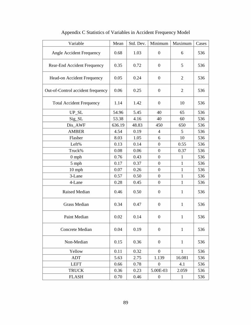
89

Appendix C Statistics of Variables in Accident Frequency Model

Variable Mean Std. Dev. Minimum Maximum Cases

Angle Accident Frequency 0.68 1.03 0 6 536

Rear-End Accident Frequency 0.35 0.72 0 5 536

Head-on Accident Frequency 0.05 0.24 0 2 536

Out-of-Control accident frequency 0.06 0.25 0 2 536

Total Accident Frequency 1.14 1.42 0 10 536

UP_SL 54.96 5.45 40 65 536

Sig_SL 53.38 4.16 40 60 536

Dis_AWF 636.19 48.83 450 650 536

AMBER 4.54 0.19 4 5 536

Flasher 8.03 1.05 6 10 536

Left% 0.13 0.14 0 0.55 536

Truck% 0.08 0.06 0 0.37 536

0 mph 0.76 0.43 0 1 536

5 mph 0.17 0.37 0 1 536

10 mph 0.07 0.26 0 1 536

3-Lane 0.57 0.50 0 1 536

4-Lane 0.28 0.45 0 1 536

Raised Median 0.46 0.50 0 1 536

Grass Median 0.34 0.47 0 1 536

Paint Median 0.02 0.14 0 1 536

Concrete Median 0.04 0.19 0 1 536

Non-Median 0.15 0.36 0 1 536

Yellow 0.11 0.32 0 1 536

ADT 5.63 2.75 1.139 16.081 536

LEFT 0.66 0.78 0 4.1 536

TRUCK 0.36 0.23 5.00E-03 2.059 536

FLASH 0.70 0.46 0 1 536

90

Appendix D Statistics of Variables in Accident Severity Model

Variable Mean Std. Dev. Minimum Maximum Cases

Crash Severity 0.845669 0.854452 0 2 635

Weekday 0.76063 0.427035 0 1 635

Angle Acc 0.607874 0.488609 0 1 635

Rear-end Acc 0.300787 0.458962 0 1 635

Head-on Acc 3.94E-02 0.194627 0 1 635

Out-of-Control 5.20E-02 0.222138 0 1 635

Old Driver 0.177953 0.382774 0 1 635

Gender 0.63937 0.480562 0 1 635

Alcohol 2.52E-02 0.156846 0 1 635

2-Lane 0.137008 0.344127 0 1 635

3-Lane 0.511811 0.500255 0 1 635

4-Lane 0.351181 0.477716 0 1 635

Left Lane 0.944882 0.228391 0 1 635

Divided Median 0.87874 0.326686 0 1 635

0 mph 0.801575 0.399128 0 1 635

5 mph 0.138583 0.345783 0 1 635

10 mph 5.98E-02 0.237382 0 1 635

TRUCK% 7.42E-02 6.41E-02 4.46E-03 0.372731 635

LEFT% 0.111372 0.119984 0 0.484754 635

Young Driver 0.146457 0.353842 0 1 635

Hwy. Speed Limit 54.7795 5.44098 40 65 635

Signal Speed Limit 53.4882 4.31392 40 60 635

Flasher Dummy 0.267717 0.443118 0 1 635

Multivehicle 7.56E-02 0.26455 0 1 635

Heavy Vehicle 0.103937 0.305419 0 1 635

ADT 6.3165 2.70927 1.512 15.612 635

TRUCK 0.399699 0.270933 7.00E-03 2.059 635

LEFT 0.639367 0.774102 0 4.1 635

Signal Speed Limit=60 5.98E-02 0.237382 0 1 635

91

Appendix E Survey Emails

In the following pages is the email correspondence between the researchers and survey

respondents. The respondents include representatives from California, Colorado, Iowa, Kansas,

Missouri, South Dakota, Texas, and Wyoming (respectively).

Subject: Fw: Questions ...supplement

From: Ahmad Rastegarpour ([email protected])

To: [email protected];

Cc: [email protected]; [email protected];

Date: Friday, November 18, 2011 11:09 AM

Hi Zifeng,

I am responding to your question below:

Question:

And for the advance warning devices, do you use advance warning flasherwhich can be timed with the signal and begin to flash when the car isexpected to arrive the intersection at red?

Answer:

We do use advance warning flashing beacon, but they are not timed to theoperation of traffic signal.

Thanks,

Ahmad Rastegarpour, P.E.Division of Traffic OperationsCalifornia Department of Transportation916.651.6128----- Forwarded by Ahmad Rastegarpour/HQ/Caltrans/CAGov on 11/18/2011 09:03AM ----- Roberta McLaughlin/HQ/Cal trans/CAGov To Shaila 11/17/2011 01:59 Chowdhury/HQ/Caltrans/CAGov@DOT PM cc Ahmad Rastegarpour/HQ/Caltrans/CAGov@DOT Subject Re: Fw: Questions ...supplement (Document link: Ahmad Rastegarpour)

Print http://us.mg6.mail.yahoo.com/neo/launch?.rand=0gukpnup26b3b

1 of 6 11/27/2011 11:01 PM

That question is best answered by Ahmad is the signal section.

Roberta L. McLaughlin, PE, TE, PTOEOffice of Signs, Markings and CA MUTCDDivision of Traffic OperationsCalifornia Department of TransportationPHONE: 916-651-1248

Shaila Chowdhury/HQ/Calt rans/CAGov To Roberta 11/17/2011 01:43 McLaughlin/HQ/Caltrans/CAGov@DOT PM cc Subject Fw: Questions ...supplement

Please see the new inquiry from Zifeng.

Thanks,Shaila Chowdhury, P.E.Executive Engineering AssistantDivision of Traffic OperationsCalifornia Department of TransportationPh: (916) 651 9377Cell: (916) 969 6186----- Forwarded by Shaila Chowdhury/HQ/Caltrans/CAGov on 11/17/2011 01:37PM ----- Zifeng Wu <zifengwu2008@yah oo.com> To Shaila Chowdhury 11/17/2011 01:36 <[email protected]> PM cc Subject Please respond to Re: Questions ...supplement Zifeng Wu <zifengwu2008@yah oo.com>


2 of 6 11/27/2011 11:01 PM

Yes, I saw them! I was looking for blue thing; so didn't pay attentionthere.And for the advance warning devices, do you use advance warning flasherwhich can be timed with the signal and begin to flash when the car isexpected to arrive the intersection at red?ZifengFrom: Shaila Chowdhury <[email protected]>To: Zifeng Wu <[email protected]>Sent: Thursday, November 17, 2011 2:52 PMSubject: Re: Questions ... I cannot find the answer

Hi Zifeng,I see them under your questions but they are in black. Please call me ifyou are still not able to see.

Thanks,Shaila Chowdhury, P.E.Executive Engineering AssistantDivision of Traffic OperationsCalifornia Department of TransportationPh: (916) 651 9377Cell: (916) 969 6186

Zifeng Wu <zifengwu2008@yah oo.com> To Shaila Chowdhury 11/17/2011 12:42 <[email protected]> PM cc

Subject Please respond to Re: Questions ... I cannot find the Zifeng Wu answer <zifengwu2008@yah oo.com>

Hello, Shaila:I am not sure what do you mean by "blue". I can't find the answer except


3 of 6 11/27/2011 11:01 PM

one small picture.... Maybe there are some mistake during the delivery.Could you send me again?Thank you very much for your help!ZifengFrom: Shaila Chowdhury <[email protected]>To:Cc: Robert Copp <[email protected]>; Wayne Henley<[email protected]>; Janice Benton <[email protected]>;Roberta McLaughlin <[email protected]>Sent: Thursday, November 17, 2011 12:32 PMSubject: Fw: Questions about the policy regarding speed limit at signalizedhigh-speed intersection

Hi Zifeng,Our responses are shown in blue below.

Thanks,Shaila Chowdhury, P.E.Executive Engineering AssistantDivision of Traffic OperationsCalifornia Department of TransportationPh: (916) 651 9377Cell: (916) 969 6186----- Forwarded by Shaila Chowdhury/HQ/Caltrans/CAGov on 11/17/2011 10:21AM -----

Robert Copp/HQ/Caltrans/ CAGov To Shaila 11/14/2011 02:19 Chowdhury/HQ/Caltrans/CAGov@DOT PM cc [email protected] Subject Fw: Questions about the policy regarding speed limit at signalized high-speed intersection

This could be Wayne and Janice. Please coordinate.

-------------------------------------------------------------------------------------------------------

Robert Copp


4 of 6 11/27/2011 11:01 PM

Chief, Division of Traffic OperationsCalifornia Department of Transportation1120 ' N' Street, MS #36Sacramento, CA 95814Phone: 916-654-2352Fax: 916-653-6080Cell Phone: 916-952-6436----- Forwarded by Robert Copp/HQ/Caltrans/CAGov on 11/14/2011 02:18 PM-----

Zifeng Wu <zifengwu2008@yah oo.com> To "[email protected]" 11/14/2011 01:02 <[email protected]> PM cc

Subject Please respond to Questions about the policy Zifeng Wu regarding speed limit at signalized <zifengwu2008@yah high-speed intersection oo.com>

Mr. Copp:Hello!

This is Zifeng Wu, from Nebraska Transportation Center at University ofNebraska-Lincoln.Currently, we are conducting a research about speed limit in the vicinityof rural signalized high-speed intersections. As a part of a survey aboutwhat are other states doing in this area, we need the information about thepolicy of speed limit at high-speed intersections in California state. Hereare some questions,1.2. Do you have some safety issues around the rural signalizedhigh-speed intersections?We continuously monitor the safety performance at rural signalizedhigh-speed intersections to identify potential safety concerns. These mayinclude visibility, sight distance or other items that can be addressedthru infrastructure improvements, including signing. Other concernsinclude those from the driver behavior aspect such as drivers that areinattentive, drowsy, or under the influence.

3. When it approaches the signalized, high speed intersections, doyou have any advanced warning devices?We have used the following sign as advanced warning.


5 of 6 11/27/2011 11:01 PM

(Embedded image moved to file: pic10867.jpg)4. When it approaches the intersection, does the speed limit remainsame or reduced? Is there any documented policy? If not, what are yougenerally do?In general, we do not reduce the speed limit on the approach to asignalized intersection.

We really appreciate your help. If you are not familiar about this area,could you forward this Email to the one who is responsible for this area?Thank you again!

Zifeng


6 of 6 11/27/2011 11:01 PM

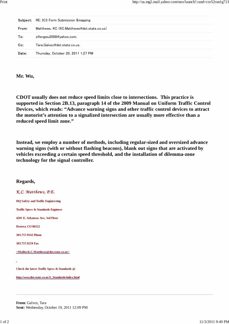
Subject: RE: IC3 Form Submission $mapping

From: Matthews, KC ([email protected])


Cc: [email protected];

Date: Thursday, October 20, 2011 1:27 PM

Mr. Wu,

CDOT usually does not reduce speed limits close to intersections. This practice issupported in Section 2B.13, paragraph 14 of the 2009 Manual on Uniform Traffic ControlDevices, which reads: “Advance warning signs and other traffic control devices to attractthe motorist’s attention to a signalized intersection are usually more effective than areduced speed limit zone.”

Instead, we employ a number of methods, including regular-sized and oversized advancewarning signs (with or without flashing beacons), blank out signs that are activated byvehicles exceeding a certain speed threshold, and the installation of dilemma-zonetechnology for the signal controller.

Regards,

K.C. Matthews, P.E.

HQ Safety and Traffic Engineering

Traffic Specs & Standards Engineer

4201 E. Arkansas Ave, 3rd Floor

Denver, CO 80222

303.757.9543 Phone

303.757.9219 Fax

<Mailto:[email protected]>

Check the latest Traffic Specs & Standards @

http://www.dot.state.co.us/S_Standards/index.html

From: Galvez, TaraSent: Wednesday, October 19, 2011 12:09 PM

Print http://us.mg2.mail.yahoo.com/neo/launch?.rand=cre52run1g713

1 of 2 11/3/2011 9:40 PM

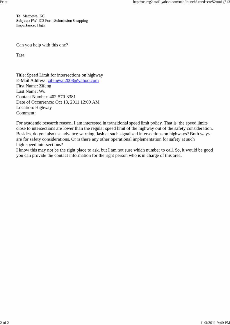
To: Matthews, KCSubject: FW: IC3 Form Submission $mappingImportance: High

Can you help with this one?

Tara

Title: Speed Limit for intersections on highwayE-Mail Address: [email protected] Name: ZifengLast Name: WuContact Number: 402-570-3381Date of Occurrence: Oct 18, 2011 12:00 AMLocation: HighwayComment:

For academic research reason, I am interested in transitional speed limit policy. That is: the speed limitsclose to intersections are lower than the regular speed limit of the highway out of the safety consideration.Besides, do you also use advance warning flash at such signalized intersections on highways? Both waysare for safety considerations. Or is there any other operational implementation for safety at suchhigh-speed intersections?I know this may not be the right place to ask, but I am not sure which number to call. So, it would be goodyou can provide the contact information for the right person who is in charge of this area.


2 of 2 11/3/2011 9:40 PM

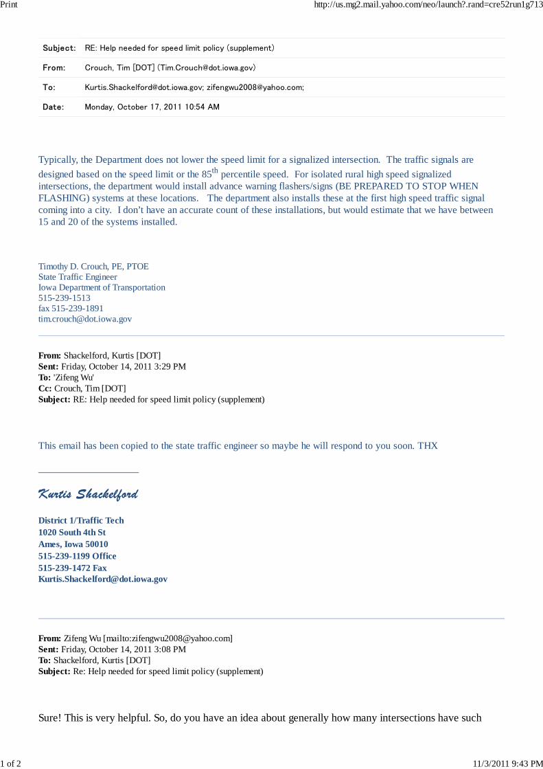
Subject: RE: Help needed for speed limit policy (supplement)

From: Crouch, Tim [DOT] ([email protected])

To: [email protected]; [email protected];

Date: Monday, October 17, 2011 10:54 AM

Typically, the Department does not lower the speed limit for a signalized intersection. The traffic signals are

designed based on the speed limit or the 85th percentile speed. For isolated rural high speed signalizedintersections, the department would install advance warning flashers/signs (BE PREPARED TO STOP WHENFLASHING) systems at these locations. The department also installs these at the first high speed traffic signalcoming into a city. I don’t have an accurate count of these installations, but would estimate that we have between15 and 20 of the systems installed.

Timothy D. Crouch, PE, PTOEState Traffic EngineerIowa Department of Transportation515-239-1513fax [email protected]

From: Shackelford, Kurtis [DOT]Sent: Friday, October 14, 2011 3:29 PMTo: 'Zifeng Wu'Cc: Crouch, Tim [DOT]Subject: RE: Help needed for speed limit policy (supplement)

This email has been copied to the state traffic engineer so maybe he will respond to you soon. THX

______________________

District 1/Traffic Tech1020 South 4th StAmes, Iowa 50010515-239-1199 Office515-239-1472 [email protected]

From: Zifeng Wu [mailto:[email protected]]Sent: Friday, October 14, 2011 3:08 PMTo: Shackelford, Kurtis [DOT]Subject: Re: Help needed for speed limit policy (supplement)

Sure! This is very helpful. So, do you have an idea about generally how many intersections have such


1 of 2 11/3/2011 9:43 PM

lower-transitional-speed limit (or percentage)? Besides, do you also use advance warning flash at suchsignalized intersections on highways? Either way is for safety considerations. Or is there any otheroperational implementation for safety reason at such high-speed intersections?

Again, thank you very much for the help.

Sincerely

Zifeng

From: "Shackelford, Kurtis [DOT]" <[email protected]>To: 'Zifeng Wu' <[email protected]>Sent: Friday, October 14, 2011 7:09 AMSubject: RE: Help needed for speed limit policy

Normally we would try to have a speed study done, run crash history and check volumes before consideringlowering the speed limit at a particular location. Each intersection would be a case by case basis. Does this help?______________________

District 1/Traffic Tech1020 South 4th StAmes, Iowa 50010515-239-1199 Office515-239-1472 [email protected]

From: Zifeng Wu [mailto:[email protected]]Sent: Tuesday, October 11, 2011 11:00 AMTo: Shackelford, Kurtis [DOT]Subject: Help needed for speed limit policy Good morning, Mr.Shackelford :I am a research assistant in the University of Nebraska Lincoln majoring in transportation engineering. Weare doing one research about Transitional Speed Limit for signalized, high-speed intersections. That is: thespeed limits close to intersections are lower than the regular speed limit of the highway out of the safetyconsideration. We are collecting the information about this kind of policy in neighbor states. Do you haveany formal or informal special speed limit policy for the signalized intersection on highways in yourstate? If possible, the related policy documents would help a lot. Otherwise, you can just explain what youdo in simple sentence. Whatever the information is, I appreciate that very much.I found your Email address online and know that you are in charge of District one of Iowa. Do you haveany idea that what other districts do? If you are not familiar about this part, could you provide the contactinformation for the right person who is in charge of traffic operation and policy to me?Thanks very much for your attention and help!Sincerely.Zifeng Wu


2 of 2 11/3/2011 9:43 PM

Subject: FW: Help needed for ttransitional speed limit policy

From: Brian Gower ([email protected])


Cc: [email protected]; [email protected]; [email protected]; [email protected]; [email protected]; [email protected];

Date: Monday, October 17, 2011 2:00 PM

ZW:

My name is Brian D. Gower. I work for Kansas DOT in the Traffic Engineering Unit.

Speed Limits

The state has no policy on setting speeds around traffic signals. Ideally, we would like the speed limit to be thesame through the intersection (ie US-75 north/south – both legs have the same speed limit) but that is not always thecase. In some instances, the speed break is at the intersection which is signalized.

Advanced Warning

Typically on high speed approaches, we have a warning sign scheme of {signal ahead ½ mile with flashing beaconsand be prepared to stop ¼ mile}. Most locations beacons are not tied to the signal system. Some locations thebeacons are tied into the signal system but they are few. Some locations do not have beacons at all. So I supposethere is really no policy other than installing the actual signs themselves.

If a high speed corridor has signals at every intersection, we will have advanced warning sign scheme listed aboveprior to the first signal encountered but for signals in the middle, we may only have the signal ahead sign.

If you need to contact me, my info is below.

Thx.

Brian D. Gower (BDG)

785 296 1181

[email protected]


1 of 2 11/3/2011 9:42 PM

From: Jeff StewartSent: Monday, October 17, 2011 10:00 AMTo: Brian GowerSubject: FW: Help needed for ttransitional speed limit policy

Should this go to you? If not, any suggestions?

From: Zifeng Wu [mailto:[email protected]]Sent: Thursday, October 13, 2011 6:18 PMTo: Randy West; Jeff Stewart; Mike Stringer; Robert Cook; Larry ThompsonSubject: Help needed for ttransitional speed limit policy

Hello!

I am a research assistant in the University of Nebraska Lincoln majoring in transportation engineering. Weare doing one research about Transitional Speed Limit for signalized, high-speed intersections. That is: thespeed limits close to intersections are lower than the regular speed limit of the highway out of the safetyconsideration. We are collecting the information about this kind of policy in neighbor states. Do you haveany formal or informal special speed limit policy for the signalized intersection on highways in yourdistrict? If possible, the related policy documents would help a lot. Otherwise, you can just explain whatyou generally do in simple sentences. Whatever the information is, I appreciate that very much.Besides, do you also use advance warning flash at such signalized intersections on highways? Both waysare for safety considerations. Or is there any other operational implementations for safety at suchhigh-speed intersections?

I found your Email address online and know that you are in charge of the District in Kansas. If you are notfamiliar about this part, could you provide the contact information for the right person who is in charge ofthis kind of traffic operation and policy to me?

Thanks very much for your attention!

Sincerely.

Zifeng Wu


2 of 2 11/3/2011 9:42 PM

Print

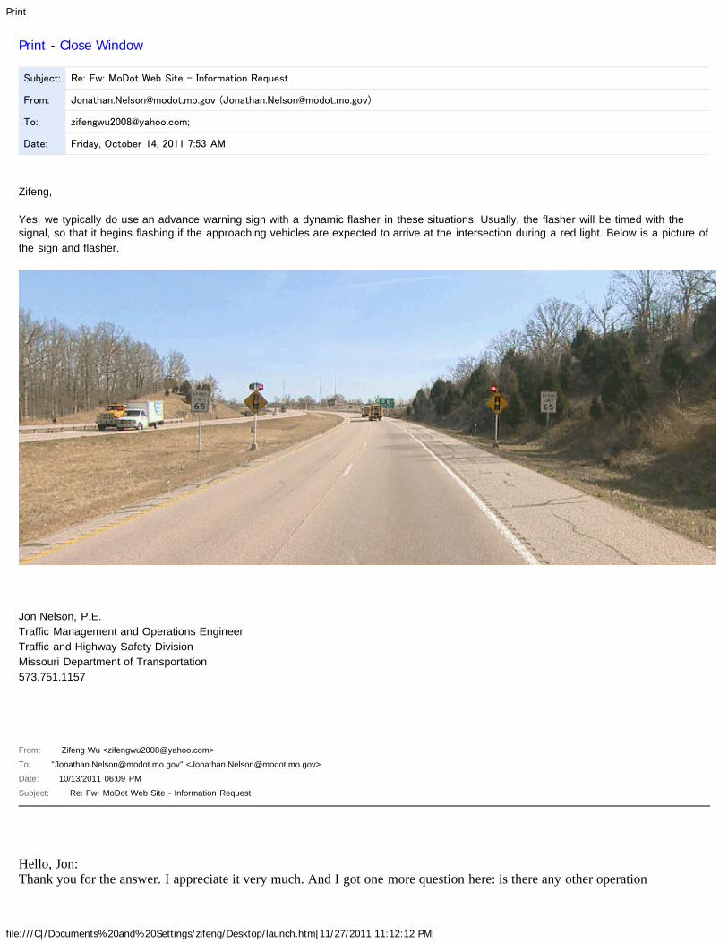
file:///C|/Documents%20and%20Settings/zifeng/Desktop/launch.htm[11/27/2011 11:12:12 PM]

Print - Close Window

Subject: Re: Fw: MoDot Web Site - Information Request

From: [email protected] ([email protected])


Date: Friday, October 14, 2011 7:53 AM

Zifeng,

Yes, we typically do use an advance warning sign with a dynamic flasher in these situations. Usually, the flasher will be timed with the

signal, so that it begins flashing if the approaching vehicles are expected to arrive at the intersection during a red light. Below is a picture of

the sign and flasher.

Jon Nelson, P.E. Traffic Management and Operations Engineer Traffic and Highway Safety Division Missouri Department of Transportation 573.751.1157

From: Zifeng Wu <[email protected]> To: "[email protected]" <[email protected]> Date: 10/13/2011 06:09 PM Subject: Re: Fw: MoDot Web Site - Information Request

Hello, Jon: Thank you for the answer. I appreciate it very much. And I got one more question here: is there any other operation

javascript:window.print()

javascript:window.close()

Print


implementation for safety close to the intersections on highway? For example, advance warning flash... There exists someopinions like no need for both advance warning flash and transitional speed limit in Lincoln. Best regards. Zifeng

From: "[email protected]" <[email protected]>

To: [email protected]

Cc: [email protected]

Sent: Tuesday, October 11, 2011 12:21 PM

Subject: Re: Fw: MoDot Web Site - Information Request

Zifeng,

We do not have any policy specifically dictating what the speed limit should be in transition zones leading up to signalized intersections at

high-speed locations. In general, the speed limit is reduced prior to the signal, but we do not have specific guidelines in place that govern

such reductions. Speed limits in Missouri are determined based on a number of factors. The link below will provide you with some

information as to how that's accomplished.

http://epg.modot.mo.gov/index.php?title=949.2_Speed_Limit_Guidelines

If you have any more questions, feel free to contact me.

Thanks.

Jon Nelson, P.E. Traffic Management and Operations Engineer Traffic and Highway Safety Division Missouri Department of Transportation 573.751.1157

From: Charlett T Scott/D5/MODOT To: Jonathan A Nelson/SC/MODOT@MODOT Date: 10/11/2011 11:16 AM Subject: Fw: MoDot Web Site - Information Request

Good Morning, Can you please help the customer below. Thanks!

Charlett Scott

Senior Customer Service Representative

MoDOT Central Missouri District - Customer Relations -Jefferson City 573-522-8472

1-888-ASK-MODOT (275-6636) www.modot.org/central ----- Forwarded by Charlett T Scott/D5/MODOT on 10/11/2011 11:13 AM -----

From: To: [email protected] Date: 10/10/2011 05:14 PM Subject: MoDot Web Site - Information Request

http://epg.modot.mo.gov/index.php?title=949.2_Speed_Limit_Guidelines

Print


Contact Information:

Zifeng Wu

NE

[email protected]

Requested Item: 1. see my comments below

Comments: Hello! I am a research assistant in the University of Nebraska Lincoln. We are doing one research about Transitional Speed Limit for signalized,high-speed intersections. That is: the speed limits close to intersections are lower than the rest segments of the highway due to the safety consideration. Weare collecting the information about this kind of policy in neighbor states. Do you have special speed limit policy for the signalized intersection on highwaysin Missouri? Maybe this is not the right place I should ask. But I was not able to find other contact information. If you could provide the right person who isin charge of traffic operation and policy, I would appreciate that very much. Thanks very much for your attention and help!

129.93.64.56129.93.64.56

Subject: Re: One Question about speed limit policy on highway ---supplement

From: [email protected] ([email protected])


Cc: [email protected];

Date: Friday, October 14, 2011 9:03 AM

We do have one location where we have advance warning signs with flashing lights connected to a traffic signal towarn motorists that the signal is about to change. It is in a rural location on a 65mph roadway at an intersection withentrance road to a major traffic generator (Crazy Horse Memorial). Aside from this one location, our standard ofpractice is to utilize dilemma zone detection at all isolated signals (non-coordinated) on roadways with speedsgreater then or equal to 45mph. We also have coordinated systems that are coordinated with time of day programsand run free during non-peak hours that also utilize advance detection and volume-density based timing to findadequate safe gaps to change phases.

Doug From: Zifeng Wu [mailto:[email protected]]Sent: Thursday, October 13, 2011 04:38 PMTo: Kinniburgh, Doug (DOT)Subject: Re: One Question about speed limit policy on highway ---supplement Mr. Kinniburgh:Thank you for the answer. I appreciate it very much. And I got one more question here: is there any otheroperation implementation for safety close to the intersections on highway? For example, advance warningflash... There exists some opinions like no need for both advance warning flash and transitional speed limitin Lincoln. Best regards.Zifeng

From: "[email protected]" <[email protected]>To: [email protected]: [email protected]; [email protected]: Thursday, October 13, 2011 12:01 PMSubject: RE: One Question about speed limit policy on highway ---supplement

Mr. Wu, The State of South Dakota does not have a policy specifically in addressing lowering speed limits close tointersections. Aside from state statute, which designates maximum speeds (and minimum on interstate), our policyon setting speed limits is simply to follow recommend practice as set forth in the Manual on Uniform Traffic ControlDevices.

Traffic Safety Engineer

Office of Project Development

700 East Broadway

Pierre, SD [email protected]

-----Original Message-----From: Zifeng Wu [mailto:[email protected]]Sent: Monday, October 10, 2011 5:27 PM


1 of 2 11/3/2011 9:44 PM

To: Seaman, Todd (DOT)Subject: Re: One Question about speed limit policy on highway ---supplement

I realized that I mentioned Missouri in last email. I am very sorry for that mistake. I am askingseveral states one by one, and didn't notice that mistake. I am really sorry and I also need theinformation about related speed limit policy on the highways in Rapid City or in South Dakota. Hope you don't mind my mistake...Thanks.Zifeng

From: Zifeng Wu <[email protected]>To: "[email protected]" <[email protected]>Sent: Monday, October 10, 2011 6:11 PMSubject: One Question about speed limit policy on highway

Hello, Todd:I am a research assistant in the University of Nebraska Lincoln. We are doing one research aboutTransitional Speed Limit for signalized, high-speed intersections. By transitional speed limit, wemean the speed limits close to intersections may (or may not be) lower than the rest segments ofthe highway due to the safety consideration. We are collecting the information about this kind ofpolicy in neighbor states. Do you have special speed limit policy for the signalized intersection onhighways in Missouri? If yes, is it OK to offer me related document? Or just some informalstandards? Maybe this is not the right place for this question... If you could provide the rightperson who is in charge of traffic operation and policy, I would appreciate that very much.Thanks very much for your attention and help!Best regards.Zifeng Wu


2 of 2 11/3/2011 9:44 PM

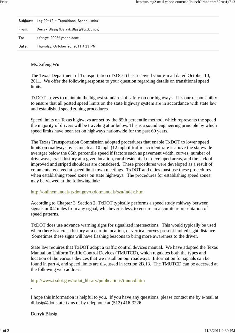
Subject: Log 90-12 - Transitional Speed Limits

From: Derryk Blasig ([email protected])


Date: Thursday, October 20, 2011 4:23 PM

Ms. Zifeng Wu The Texas Department of Transportation (TxDOT) has received your e-mail dated October 10,2011. We offer the following response to your question regarding details on transitional speedlimits. TxDOT strives to maintain the highest standards of safety on our highways. It is our responsibilityto ensure that all posted speed limits on the state highway system are in accordance with state lawand established speed zoning procedures. Speed limits on Texas highways are set by the 85th percentile method, which represents the speedthe majority of drivers will be traveling at or below. This is a sound engineering principle by whichspeed limits have been set on highways nationwide for the past 60 years. The Texas Transportation Commission adopted procedures that enable TxDOT to lower speedlimits on roadways by as much as 10 mph (12 mph if traffic accident rate is above the statewideaverage) below the 85th percentile speed if factors such as pavement width, curves, number ofdriveways, crash history at a given location, rural residential or developed areas, and the lack ofimproved and striped shoulders are considered. These procedures were developed as a result ofcomments received at speed limit town meetings. TxDOT and cities must use these procedureswhen establishing speed zones on state highways. The procedures for establishing speed zonesmay be viewed at the following link: http://onlinemanuals.txdot.gov/txdotmanuals/szn/index.htm According to Chapter 3, Section 2, TxDOT typically performs a speed study midway betweensignals or 0.2 miles from any signal, whichever is less, to ensure an accurate representation ofspeed patterns. TxDOT does use advance warning signs for signalized intersections. This would typically be usedwhen there is a crash history at a certain location, or vertical curves present limited sight distance. Sometimes these signs will have flashing beacons to bring more awareness to the driver. State law requires that TxDOT adopt a traffic control devices manual. We have adopted the TexasManual on Uniform Traffic Control Devices (TMUTCD), which regulates both the types andlocation of the various devices that we install on our roadways. Information for signals can befound in part 4, and speed limits are discussed in section 2B.13. The TMUTCD can be accessed atthe following web address: http://www.txdot.gov/txdot_library/publications/tmutcd.htm I hope this information is helpful to you. If you have any questions, please contact me by e-mail [email protected] or by telephone at (512) 416-3226. Derryk Blasig


1 of 2 11/3/2011 9:39 PM

Traffic Operations DivisionTexas Department of Transportation

==========================Texas Transportation ForumFor more information on registration and program details visitwww.texastransportationforum.com


2 of 2 11/3/2011 9:39 PM

Subject: Re: Fwd: Transitional speed limit policy

From: Paul Jones ([email protected])


Date: Monday, October 24, 2011 3:30 PM

We may install advanced warning such as a flashing beacon only if crash data indicates that a problemexists.

On Thu, Oct 13, 2011 at 5:08 PM, Zifeng Wu <[email protected]> wrote:Hello, Paul:Thank you for the answer. I appreciate it very much. And I got one more question here: is there anyother operation implementation, due to safety consideration, close to the intersections on highway? Forexample, advance warning flash... There exists some opinions like no need for both advance warningflash and transitional speed limit in Lincoln. Best regards.Zifeng

From: Paul Jones <[email protected]>To: Zifeng Wu <[email protected]>Sent: Tuesday, October 11, 2011 4:27 PMSubject: Fwd: Transitional speed limit policy

Zifeng Wu, When entering signalized intersections on roads with speed limits greater than 45 mph, Wydot generallylowers the speed limit to 45 mph10 feet to 1500 feet before the intersection. If the road is to maintain ahigher speed limit, it is raised after the intersection. Paul Jones

---------- Forwarded message ----------From: DOT Public Affairs <[email protected]>Date: Tue, Oct 11, 2011 at 1:31 PMSubject: Transitional speed limit policyTo: Paul Jones <[email protected]>

---------- Forwarded message ----------From: Zifeng Wu <[email protected]>Date: Tue, Oct 11, 2011 at 1:28 PMSubject: Other - Select One If Available

Hello! I am a research assistant in the University of Nebraska Lincoln. We are doing one research aboutTransitional Speed Limit for signalized, high-speed intersections. That is: the speed limits close tointersections are lower than the rest segments of the highway due to the safety consideration. We arecollecting the information about this kind of policy in neighbor states. Do you have special speed limitpolicy for the signalized intersection on highways in Wyoming? Maybe this is not the right place Ishould ask. But I was not able to find other contact information. If you could provide the right personwho is in charge of traffic operation and policy, I would appreciate that very much. Thanks very muchfor your attention and help!


1 of 2 11/3/2011 9:30 PM

E-Mail to and from me, in connection with the transaction of public business,is subject to the Wyoming Public Records Act and may be disclosed to third parties.


2 of 2 11/3/2011 9:30 PM

SPEED LIMIT RECOMMENDATION IN VICINITY OF ...

Documents

Transcript of SPEED LIMIT RECOMMENDATION IN VICINITY OF ...